Université de ParisÉcole Doctorale de Sciences Mathématiques de Paris Centre

(ED 386)Institut de Mathématiques de Jussieu - Paris Rive Gauche

(UMR 7586)

Scuola Internazionale Superiore di StudiAvanzati

Weyl group actions on the cohomology ofcharacter and quiver varieties

Par Mathieu Ballandras

Thèse de doctorat de mathématiques

Dirigée par Emmanuel Letellieret par Fernando Rodriguez-Villegas

Institut de Mathématiques deJussieu-Paris Rive Gauche(CNRS – UMR 7586)Université Paris Diderot (Paris 7)Bâtiment Sophie Germain - BoîteCourrier 70128, place Aurélie Nemours75205 Paris Cedex 13France

École Doctorale de SciencesMathématiques de Paris CentreBoîte Courrier 2904, place Jussieu75252 Paris Cedex 05France

2

Résumé

Nous étudions la cohomologie de certaines variétés de caractères et de leurs analoguesadditifs, les variétés de carquois en forme de comète. Ces variétés de caractères clas-sifient les représentations du groupe fondamental d’une surface de Riemann épointéeavec monodromie prescrite autour des points. Le polynôme de Poincaré pour la co-homologie d’intersection à support compact est calculé. Des actions de groupes deWeyl sur les escpaces de cohomologie sont également étudiées. Des traces de ces ac-tions apparaissent comme certain coefficients de structure d’une algèbre engendréepar les polynômes de Kostka modifiés.

Mots-clefs : Variétés de caractères, variétés de carquois, groupe de Weyl, co-homologie d’intersection.

Abstract

We study the cohomology of some character varieties and their additive analogous,comet-shaped quiver varieties. Those character varieties classify representationsof the fundamental group of a punctured Riemann surface with prescribed mon-odromies around the punctures. The Poincaré polynomial for compactly supportedintersection cohomology is computed. Weyl group actions on the cohomology spacesare also studied. Some traces of those actions are related to particular structure co-efficients of an algebra spanned by modified Kostka polynomials.

Keywords: Character varieties, quiver varieties, Weyl group, intersection coho-mology.

3

Remerciements

Tout d’abord je tiens à remercier mes directeurs Emmanuel Letellier et FernandoRodriguez Villegas. Ils ont su trouver un sujet de thèse qui me passionne et m’ontappris énormément. Ils m’ont soutenu tout au long de ce travail, pour les mathé-matiques comme pour le reste. Pour cela, je leur en suis très reconnaissant.

Throughout the thesis I was lucky to receive help from great mathematicians.First much of this work rely on previous results from Anton Mellit. I am very

grateful to him for interesting discussions and for suggesting the starting point ofChapter 5.

I want to thank Philip Boalch, a fundamental idea in this work was hinted byhim. He explained me why non-Abelian Hodge theory could be useful and pointedout the relevant references.

I am very grateful to Hiraku Nakajima for his very useful comments and sug-gestions on Chapter 2 and for clarifying many historical facts. I want to thankMichèle Vergne for interesting discussions about the same chapter. The motivationof this work originated in discussions with Andrea Maffei. I want to thank FlorentSchaffhauser and Andrea Maffei for their support and their very detailed and helpfulproofreading.

I am thankful to François Bergeron for interesting comments about the combi-natorics of modified Kostka polynomials.

I want to thank Oscar García-Prada and Carlos Simpson for pointing out relevantreferences.

4

Contents

1 Introduction 81.1 Cohomology of character varieties: state of the art . . . . . . . . . . . 8

1.1.1 One puncture with a central monodromy . . . . . . . . . . . . 81.1.2 Any number of punctures and arbitrary monodromies . . . . . 10

1.2 Intersection cohomology of character varieties . . . . . . . . . . . . . 111.2.1 Poincaré polynomial . . . . . . . . . . . . . . . . . . . . . . . 111.2.2 Springer theory and resolution of character varieties . . . . . . 111.2.3 Weyl group action on the cohomology of character varieties . . 14

1.3 Additive version of character varieties . . . . . . . . . . . . . . . . . . 151.3.1 Comet-shaped quiver varieties . . . . . . . . . . . . . . . . . . 151.3.2 Combinatorics of the Weyl group action on the cohomology of

comet-shaped quiver varieties . . . . . . . . . . . . . . . . . . 161.4 Plan of the thesis . . . . . . . . . . . . . . . . . . . . . . . . . . . . . 17

2 Trivializations of moment maps 182.1 Introduction . . . . . . . . . . . . . . . . . . . . . . . . . . . . . . . . 18

2.1.1 Symplectic quotients and GIT quotients of affine varieties . . . 182.1.2 Real moment map for the action of a reductive group on an

affine variety . . . . . . . . . . . . . . . . . . . . . . . . . . . 192.1.3 Nakajima’s quiver varieties and hyperkähler moment map . . . 21

2.2 Kempf-Ness theory for affine varieties . . . . . . . . . . . . . . . . . . 232.2.1 Characterization of semistability from a differential geometry

point of view . . . . . . . . . . . . . . . . . . . . . . . . . . . 232.2.2 Correspondence between linear characters and elements in the

center of the Lie algebra of H . . . . . . . . . . . . . . . . . . 242.2.3 Correspondence between symplectic quotient and GIT quotient 252.2.4 Hilbert-Mumford criterion for stability . . . . . . . . . . . . . 272.2.5 Regular locus . . . . . . . . . . . . . . . . . . . . . . . . . . . 312.2.6 Trivialization of the real moment map over the regular locus . 34

2.3 Quiver varieties and stability . . . . . . . . . . . . . . . . . . . . . . . 362.3.1 Generalities about quiver varieties . . . . . . . . . . . . . . . . 362.3.2 King’s characterization of stability of quiver representations . 39

2.4 Nakajima’s quiver varieties as hyperkähler quotients and trivializationof the hyperkähler moment map . . . . . . . . . . . . . . . . . . . . . 422.4.1 Hyperkähler structure on the space of representations of an

extended quiver . . . . . . . . . . . . . . . . . . . . . . . . . . 422.4.2 Hyperkähler structure and moment maps . . . . . . . . . . . . 442.4.3 Trivialization of the hyperkähler moment map . . . . . . . . . 45

5

3 Geometric and combinatoric background 513.1 Perverse sheaves and intersection cohomology . . . . . . . . . . . . . 51

3.1.1 Perverse sheaves . . . . . . . . . . . . . . . . . . . . . . . . . 513.1.2 Intersection cohomology . . . . . . . . . . . . . . . . . . . . . 53

3.2 Symmetric functions . . . . . . . . . . . . . . . . . . . . . . . . . . . 543.2.1 Lambda ring and symmetric functions . . . . . . . . . . . . . 543.2.2 Characters of the symmetric group and symmetric functions . 593.2.3 Orthogonality and Macdonald polynomials . . . . . . . . . . . 623.2.4 A result of Garsia-Haiman . . . . . . . . . . . . . . . . . . . . 65

3.3 Conjugacy classes and adjoint orbits for general linear group . . . . . 683.3.1 Notations for adjoint orbits and conjugacy classes . . . . . . . 683.3.2 Types and conjugacy classes over finite fields . . . . . . . . . . 693.3.3 Resolutions of Zariski closure of conjugacy classes and adjoint

orbits . . . . . . . . . . . . . . . . . . . . . . . . . . . . . . . 703.4 Resolution of conjugacy classes and Weyl group actions . . . . . . . . 71

3.4.1 Borho-MacPherson approach to Springer theory . . . . . . . . 713.4.2 Parabolic induction . . . . . . . . . . . . . . . . . . . . . . . . 733.4.3 Relative Weyl group actions on multiplicity spaces . . . . . . . 753.4.4 Relative Weyl group actions and Springer theory . . . . . . . 77

3.5 Character varieties and their additive counterpart . . . . . . . . . . . 803.5.1 Character varieties . . . . . . . . . . . . . . . . . . . . . . . . 803.5.2 Additive analogous of Character varieties . . . . . . . . . . . . 833.5.3 Resolutions of character varieties . . . . . . . . . . . . . . . . 843.5.4 Relative Weyl group actions . . . . . . . . . . . . . . . . . . . 87

3.6 Cohomology of character varieties: some results and conjectures . . . 883.6.1 Conjectural formula for the mixed-Hodge polynomial . . . . . 883.6.2 Poincaré polynomial of character varieties with semisimple

conjugacy classes at punctures . . . . . . . . . . . . . . . . . . 893.6.3 Weyl group actions on the cohomology . . . . . . . . . . . . . 91

4 Weyl group actions on the cohomology of comet-shaped quiver va-rieties and combinatorics 934.1 Introduction . . . . . . . . . . . . . . . . . . . . . . . . . . . . . . . . 934.2 Nakajima’s quiver varieties . . . . . . . . . . . . . . . . . . . . . . . . 94

4.2.1 Resolution of Zariski closure of adjoint orbits as Nakajima’sframed quiver varieties . . . . . . . . . . . . . . . . . . . . . . 94

4.2.2 Comet-shaped quiver varieties . . . . . . . . . . . . . . . . . . 964.2.3 Family of comet-shaped quiver varieties . . . . . . . . . . . . . 98

4.3 Weyl group action . . . . . . . . . . . . . . . . . . . . . . . . . . . . . 1004.3.1 Decomposition of the family QL,P . . . . . . . . . . . . . . . . 1004.3.2 Construction of a Weyl group action on the cohomology of the

quiver varieties in the family QL,P . . . . . . . . . . . . . . . 1014.3.3 Frobenius morphism and monodromic action . . . . . . . . . . 104

4.4 Combinatorial interpretation in the algebra spanned by Kostka poly-nomials . . . . . . . . . . . . . . . . . . . . . . . . . . . . . . . . . . 1074.4.1 Description of the algebra . . . . . . . . . . . . . . . . . . . . 1074.4.2 Interpretation of coefficients as traces of Weyl group action on

the cohomology of quiver varieties . . . . . . . . . . . . . . . . 112

6

4.4.3 Cohomological interpretation in the multiplicative case . . . . 113

5 Intersection cohomology of character varieties with k−1 semisimplemonodromies 1155.1 Introduction . . . . . . . . . . . . . . . . . . . . . . . . . . . . . . . . 1155.2 Resolutions of regular conjugacy classes and

parabolic induction . . . . . . . . . . . . . . . . . . . . . . . . . . . . 1165.3 Resolution of the k-th conjugacy of character variety . . . . . . . . . 1185.4 Family of character varieties . . . . . . . . . . . . . . . . . . . . . . . 119

5.4.1 Springer action . . . . . . . . . . . . . . . . . . . . . . . . . . 1205.4.2 Monodromic action . . . . . . . . . . . . . . . . . . . . . . . . 1215.4.3 Comparison of monodromic action and Springer action . . . . 121

5.5 Poincaré polynomial for intersection cohomology of character varietieswith k − 1 semisimple monodromies . . . . . . . . . . . . . . . . . . . 123

6 Intersection cohomology of character varieties through non-AbelianHodge theory 1266.1 Introduction . . . . . . . . . . . . . . . . . . . . . . . . . . . . . . . . 126

6.1.1 Intersection cohomology of character varieties and Weyl groupactions . . . . . . . . . . . . . . . . . . . . . . . . . . . . . . . 126

6.1.2 Diffeomorphism between a resolution ML,P ,σ and a charactervariety with semisimple monodromiesMS . . . . . . . . . . . 127

6.2 Poincaré polynomial and twisted Poincaré polynomial . . . . . . . . . 1296.2.1 Computation of the Poincaré polynomial . . . . . . . . . . . . 1296.2.2 Weyl group action and twisted Poincaré polynomial . . . . . . 130

6.3 Example of the sphere with four punctures and rank 2 . . . . . . . . 1326.3.1 Fricke relation . . . . . . . . . . . . . . . . . . . . . . . . . . . 1326.3.2 Projective cubic surfaces . . . . . . . . . . . . . . . . . . . . . 1346.3.3 Lines on cubic surfaces . . . . . . . . . . . . . . . . . . . . . . 137

6.4 Moduli spaces . . . . . . . . . . . . . . . . . . . . . . . . . . . . . . . 1406.4.1 de Rham moduli space . . . . . . . . . . . . . . . . . . . . . . 1406.4.2 Filtered local systems and resolutions of character varieties . . 1416.4.3 Dolbeault moduli space . . . . . . . . . . . . . . . . . . . . . . 1426.4.4 Various steps of the diffeomorphism . . . . . . . . . . . . . . . 142

6.5 Local model . . . . . . . . . . . . . . . . . . . . . . . . . . . . . . . . 1436.5.1 Local model for Riemann-Hilbert correspondence . . . . . . . 1436.5.2 Metric and parabolic structure . . . . . . . . . . . . . . . . . . 1446.5.3 Local beahaviour for non-Abelian Hodge theory . . . . . . . . 1456.5.4 Local description of weighted Sobolev spaces . . . . . . . . . . 1466.5.5 Variation of the stability parameters and the metric . . . . . . 147

6.6 Diffeomorphism between moduli spaces . . . . . . . . . . . . . . . . . 1486.6.1 Analytic construction of the moduli spaces . . . . . . . . . . . 1486.6.2 Construction of the diffeomorphisms . . . . . . . . . . . . . . 151

7

Chapter 1

Introduction

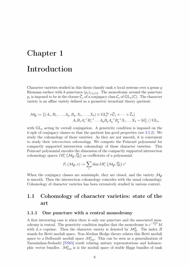
Character varieties studied in this thesis classify rank n local systems over a genus gRiemann surface with k-punctures (pj)1≤j≤k. The monodromy around the puncturepj is imposed to be in the closure Cj of a conjugacy class Cj of GLn(C). The charactervariety is an affine variety defined as a geometric invaritant theory quotient:

MC :=

(A1, B1, . . . , Ag, Bg, X1, . . . , Xk) ∈ GL2gn ×C1 × · · · × Ck

∣∣A1B1A

−11 B−1

1 . . . AgBgA−1g B−1

g X1 . . . Xk = Id//GLn

with GLn acting by overall conjugation. A genericity condition is imposed on thek-uple of conjugacy classes so that the quotient has good properties (see 3.5.2). Westudy the cohomology of those varieties. As they are not smooth, it is convenientto study their intersection cohomology. We compute the Poincaré polynomial forcompactly supported intersection cohomology of those character varieties. ThisPoincaré polynomial encodes the dimension of the compactly supported intersectioncohomology spaces IHr

c

(MC,Ql

)as coefficients of a polynomial:

Pc (MC, v) :=∑r

dim IHrc

(MC,Ql

)vr

When the conjugacy classes are semisimple, they are closed, and the variety MCis smooth. Then the intersection cohomology coincides with the usual cohomology.Cohomology of character varieties has been extensively studied in various context.

1.1 Cohomology of character varieties: state of theart

1.1.1 One puncture with a central monodromy

A first interesting case is when there is only one puncture and the associated mon-odromy is central. The genericity condition implies that the monodromy is e−

2iπdn Id

with d, n coprime. Then the character variety is denoted by MdB. The index B

stands for Betti moduli space. Non-Abelian Hodge theory relates this Betti modulispace to a Dolbeault moduli space Md

Dol. This can be seen as a generalization ofNarasimhan-Seshadri [NS65] result relating unitary representations and holomor-phic vector bundles. Md

Dol is is the moduli space of stable Higgs bundles of rank

8

n and degree d. Non-Abelian Hodge correspondence was proved in rank n = 2by Hitchin [Hit87] and Donaldson [Don87]. It was generalized to higher ranks andhigher dimensions by Corlette [Cor88] and Simpson [Sim88] see also [Sim92]. Thecorrespondence is obtained as a homeomorphism between moduli spaces by Simpson[Sim94a; Sim94b].

Many computations of the cohomology are performed from the Dolbeault side.First Hitchin [Hit87] computed the Poincaré polynomial in rank n = 2. Gothen[Got94] extended the computation to rank n = 3. Hausel-Thaddeus [HT03b; HT04]computed the cohomology ring in rank n = 2. García-Prada, Heinloth, Schmitt[GHS11] gave a recursive algorithm to compute the motive of the Dolbeault modulispace. They computed an explicit expression in rank n = 4. García-Prada, Heinloth[GH13] obtained an explicit formula for y-genus in any rank.

As in the last examples, there exist more precise cohomological information thanthe Poincaré polynomial. The character varieties are affine, by Deligne [Del71], theircohomology carries a mixed-Hodge structure. The non-Abelian Hodge theory doesnot preserve this mixed-Hodge structure. Indeed the cohomology of the Dolbeaultmoduli space is pure contrarily to the cohomology of the affine character variety.De Cataldo-Hausel-Migliorini [CHM12] conjectured that under non-Abelian Hodgecorrespondence, the weight filtration coincides with a perverse filtration induced byHitchin fibration. This is known as the P = W conjecture, they proved it in rankn = 2. Recently, de Cataldo-Maulik-Shen [CMS19] proved the conjecture for genusg = 2 and any rank.

Another interesting aspect of those moduli spaces is the mirror symmetry. Hausel-Thaddeus [HT01; HT03a] conjectured that the moduli space of PGLn-Higgs bundlesand the moduli space of SLn-Higgs bundles are related by mirror symmetry, see also[Hau04]. This conjecture was proved by Groechenig-Wyss-Ziegler [GWZ17] and amotivic version by Loeser-Wyss [LW21]. Mirror symmetry was also studied in theparabolic case by Biswas-Dey [BD12]. Gothen-Oliveira [GO17] proved a parabolicversion of the conjecture, for particular ranks.

An efficient approach to compute cohomological invariant is to count points of al-gebraic varieties over finite fields. On the Betti side, Hausel and Rodriguez-Villegas[HR08] gave a conjectural formula for the mixed-Hodge polynomial of charactervarieties with one puncture and a central generic monodromy. They proved theE-polynomial specialization of the conjecture by counting points over finite fields.With a similar approach, Mereb [Mer15] computed the E-polynomial of SLn char-acter varieties. Hausel [Hau04] also proposed a conjectural formula for the Hodgepolynomial of the associated Dolbeault moduli space. Mozgovoy [Moz11] extendedthis conjecture to the motives of the Dolbeault moduli space.

Schiffmann [Sch16] computed the Poincaré polynomial of the Dolbeault modulispace by counting Higgs bundles over finite fields. In following articles [MS14; MS20]Mozgovoy-Schiffmann extended this counting to twisted Higgs bundles. Chaudouard-Laumon [CL16] counted Higgs bundles using automorphic forms.

Mellit [Mel17b] proved that the formula obtained by Schiffmann [Sch16] is equiv-alent to the Poincaré polynomial specialization of the conjecture of Hausel and Ro-driguez Villegas [HR08].

Fedorov-Soibelman-Soibelman [FSS17] computed the motivic class of the modulistack of semistable Higgs bundles.

9

1.1.2 Any number of punctures and arbitrary monodromies

Logares-Muñoz-Newstead [LMN12] computed the E-polynomial of character vari-eties for SL2 and small genus g = 1, 2. They consider one puncture with anyconjugacy class, without the genericity assumption. They also obtained the Hodgenumbers in genus g = 1. Logares-Muñoz [LM13] extended those results to genusg = 1 and two punctures. They computed the E-polynomials and some Hodgenumbers. Martínez-Muñoz [MM14a; MM14b] computed the E-polynomial of SL2-character varieties for any genus and any conjugacy class at the puncture. Martínez[Mar17] then treated the case of PGL2-character varieties.

Simpson [Sim90] generalized non-Abelian Hodge theory to character varietieswith punctures and arbitrary conjugacy classes. The generalization is even larger asit concerns filtered local systems. They correspond to parabolic Higgs bundles onthe Dolbeault side. The moduli space of stable parabolic Higgs bundles was con-structed algebraically by Yokogawa [Yok93]. The moduli spaces were constructedanalytically by Konno [Kon93] for Higgs fields with nilpotent residues and by Naka-jima [Nak96]. Those analytic constructions provide the non-Abelian Hodge theory asa diffeomorphism. Biquard-Boalch [BB04] proved a more general wild non-AbelianHodge theory and constructed the associated moduli spaces. Biquard, García-Pradaand Mundet i Riera [BGM15] generalized filtered non-Abelian Hodge theory to alarge family of groups.

On the Dolbeault side of this correspondence, Boden-Yokogawa [BY96] computedthe Poincaré polynomial of the moduli space of parabolic Higgs bundles, in rankn = 2, using Morse theory. García-Prada, Gothen, Muñoz [GGM07] computed thePoincaré polynomial in rank n = 3.

Hausel, Letellier and Rodriguez-Villegas [HLR11] made a conjecture for themixed-Hodge polynomial of character varieties with generic semisimple conjugacyclasses at punctures. Counting points of the character variety over finite fieldthey proved the E-polynomial specialization. Chuang-Diaconescu-Pan [CDP14] andChuang-Diaconescu-Donagi-Pantev [Chu+15] proposed a string theoretic interpre-tation of the conjecture. This string theoretic approach was also applied to wildcharacter varieties by Diaconescu [Dia17] and Diaconescu-Donagi-Pantev [DDP18].Another approach uses recursive relations for various genus. It is used by Moz-govoy [Moz11], Carlsson and Rodriguez-Villegas [CR18]. Similarly to this recursiveapproach, González-Prieto [Gon18] developped a topological quantum field theoryassociated to character varieties.

Mellit [Mel17a] proved the Poincaré polynomial specialization of the conjecturefrom [HLR11] by counting parabolic Higgs bundles over finite fields. This result is ofthe utmost importance for this thesis. This is the starting point of the computationof intersection cohomology of the character variety with the closure of any genericconjugacy classes at punctures. Fedorov-Soibelman-Soibelman [FSS20] computedthe motivic class of the moduli stack of semistable parabolic Higgs bundles.

10

1.2 Intersection cohomology of character varieties

1.2.1 Poincaré polynomial

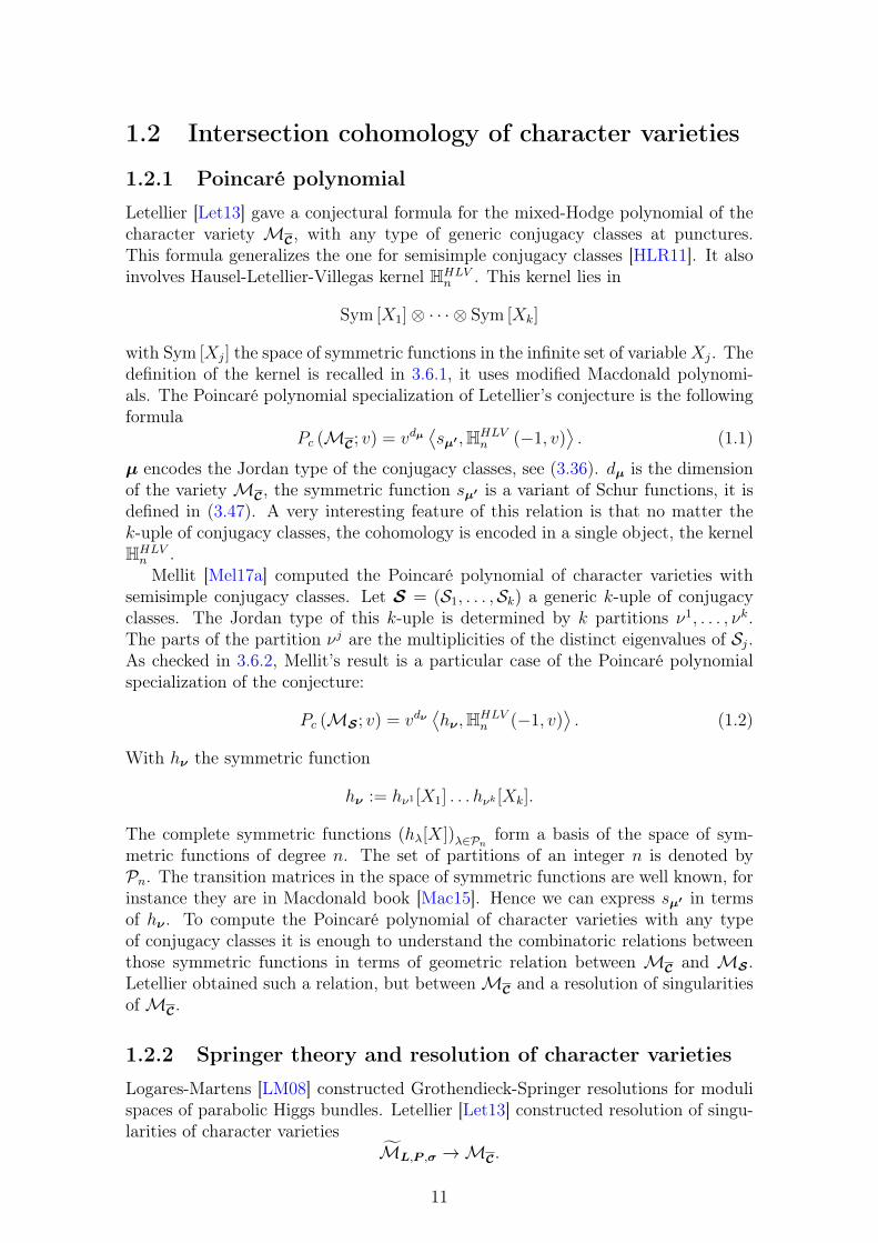
Letellier [Let13] gave a conjectural formula for the mixed-Hodge polynomial of thecharacter variety MC, with any type of generic conjugacy classes at punctures.This formula generalizes the one for semisimple conjugacy classes [HLR11]. It alsoinvolves Hausel-Letellier-Villegas kernel HHLV

n . This kernel lies in

Sym [X1]⊗ · · · ⊗ Sym [Xk]

with Sym [Xj] the space of symmetric functions in the infinite set of variableXj. Thedefinition of the kernel is recalled in 3.6.1, it uses modified Macdonald polynomi-als. The Poincaré polynomial specialization of Letellier’s conjecture is the followingformula

Pc (MC; v) = vdµ⟨sµ′ ,HHLV

n (−1, v)⟩. (1.1)

µ encodes the Jordan type of the conjugacy classes, see (3.36). dµ is the dimensionof the varietyMC, the symmetric function sµ′ is a variant of Schur functions, it isdefined in (3.47). A very interesting feature of this relation is that no matter thek-uple of conjugacy classes, the cohomology is encoded in a single object, the kernelHHLVn .Mellit [Mel17a] computed the Poincaré polynomial of character varieties with

semisimple conjugacy classes. Let S = (S1, . . . ,Sk) a generic k-uple of conjugacyclasses. The Jordan type of this k-uple is determined by k partitions ν1, . . . , νk.The parts of the partition νj are the multiplicities of the distinct eigenvalues of Sj.As checked in 3.6.2, Mellit’s result is a particular case of the Poincaré polynomialspecialization of the conjecture:

Pc (MS ; v) = vdν⟨hν ,HHLV

n (−1, v)⟩. (1.2)

With hν the symmetric function

hν := hν1 [X1] . . . hνk [Xk].

The complete symmetric functions (hλ[X])λ∈Pn form a basis of the space of sym-metric functions of degree n. The set of partitions of an integer n is denoted byPn. The transition matrices in the space of symmetric functions are well known, forinstance they are in Macdonald book [Mac15]. Hence we can express sµ′ in termsof hν . To compute the Poincaré polynomial of character varieties with any typeof conjugacy classes it is enough to understand the combinatoric relations betweenthose symmetric functions in terms of geometric relation between MC and MS .Letellier obtained such a relation, but betweenMC and a resolution of singularitiesofMC.

1.2.2 Springer theory and resolution of character varieties

Logares-Martens [LM08] constructed Grothendieck-Springer resolutions for modulispaces of parabolic Higgs bundles. Letellier [Let13] constructed resolution of singu-larities of character varieties

ML,P ,σ →MC.

11

Symplectic resolutions of character varieties were also studied in details by Schedler-Tirelli [ST19]. The construction of ML,P ,σ is recalled in 3.5.11, it relies on Springertheory. This theory closely intertwines the geometry of reductive groups with therepresentation theory of their Weyl groups. A first step in this direction comes fromGreen [Gre55] who computed the characters of general linear groups over finite fieldsin terms of symmetric functions. Then Springer [Spr76] proved a correspondencebetween unipotent conjugacy classes and representations of Weyl groups for anyconnected reductive group. Following work of Lusztig [Lus81] for the general lineargroup, Borho-MacPherson [BM83] obtained Springer correspondence in terms ofintersection cohomology.

Let us briefly recall their result for the Springer resolution of the unipotent locusin GLn. Let B the subgroup of upper triangular matrices, U the subgroup of B with1 on the diagonal. T is the subgroup of diagonal matrices so that B = TU . Let Uthe set of unipotent elements in GLn, i.e. the set of matrices with all eigenvaluesequal to 1. Then U is stratified by conjugacy classes (Cλ)λ∈Pn with λ the partitionof n with parts specifying the size of the Jordan blocks. Let

U = (X, gB) ∈ U ×GLn /B∣∣g−1Xg ∈ U

the projection to the first factor U → U is a resolution of singularities. Borho-Macpherson approach to Springer theory provides the following relation betweencohomology of the resolution U and intersection cohomology of the closure of thestrata of U

Hr+dim Uc

(U ,Ql

)∼=⊕λ∈Pn

Vλ ⊗ IHr+dim Cλc

(Cλ,Ql

).

Vλ is the irreducible representation of the symmetric group indexed by the partitionλ. The indexing is as in Macdonald’s book [Mac15], so that V(n) is the trivialrepresentation and V(1n) the sign. In terms of Poincaré polynomial previous relationbecomes

v− dim UPc

(U , v

)=∑λ∈Pn

(dimVλ) v− dim CλPc

(Cλ, v

).

Interestingly, this relation between v− dim UPc

(U , v

)and v− dim CλPc

(Cλ, v

)is exactly

the base change relation expressing the symmetric function h1n in terms of Schurfunctions (sλ)λ∈Pn

h1n =∑λ∈Pn

(dimVλ) sλ.

In this simple example, a base change relation between complete symmetric functionsand Schur functions has a geometrical interpretation in terms of Springer resolutions.

For character varieties the idea is similar but a more general theory is necessary.It is provided by Lusztig parabolic induction [Lus84; Lus85; Lus86]. Letellier appliedthis theory to obtain relations between cohomology of the resolution ML,P ,σ andintersection cohomology of character varieties MCρ,σ (see 3.36 and 3.3.1 for thedefinition of the k-uple of conjugacy classes Cρ,σ). This relation is used to provethat various formulations of the conjecture are equivalent [Let11, Proposition 5.7].In terms of Poincaré polynomial the relation reads

v−dµPc

(ML,P ,σ, t

)=∑ρµ

(dimAµ′,ρ) v−dρPc

(MCρ,σ , v

). (1.3)

12

This geometric relation is discussed in details in 6.2, it is exactly a combinatoricrelation between various basis of symmetric functions:

hµ′ =∑ρµ

(dimAµ′,ρ) sρ. (1.4)

It will appear that the Poincaré polynomial of resolution the ML,P ,σ is equal tothe Poincaré polynomial of a character variety with semisimple monodromie MS .Together with Mellit’s result (1.2), this implies

v−dµPc

(ML,P ,σ, v

)= v−dµPc (MS , v) =

⟨hµ′ ,HHLV

n (−1, v)⟩

Relations (1.3) (1.4) can be inverted so that the Poincaré polynomial of a charactervariety with any type of monodromies can be expressed as Poincaré polynomial ofcharacter varieties with semisimple monodromies. This is exactly what is necessaryto obtain the general formula 1.1 fromMellit’s result for semisimple conjugacy classes1.2.

To summarize, computing the Poincaré polynomial for intersection cohomologyof character varieties requires three elements:

• Mellit’s result for character varieties with semisimple monodromies (1.2).

• Letellier’s relation (1.3) between cohomology of the resolution ML,P ,σ andintersection cohomology of character varietiesMC.

• Relation between cohomology of the resolution ML,P ,σ and cohomology of acharacter variety with semisimple monodromiesMS .

The last point is studied in Chapter 6 where a diffeomorphism between the resolutionML,P ,σ and a character variety with semisimple monodromies MS is detailed sothat the Poincaré polynomial coincide. First the particular case of the sphere withfour punctures is studied. Then the character varieties are cubic surfaces given byan explicit equation, the Fricke relation [FK97]. The geometry of cubic surfaces iswell-known since Cayley [Cay69], see also Bruce-Wall [BW79] and Manin [Man86].Smooth projective cubic surfaces in P3 are obtained as P2 blow-up in six points. Thisdescription gives a direct prove, on the Betti side, that the resolution is diffeomorphicto a character variety with semisimple monodromies.

Constructing the diffeomorphism in the general case requires analytical tech-nics. They are detailed in 6.6.1, they rely on the filtered version of non-AbelianHodge theory and Riemann-Hilbert correspondence. Those correspondences aredue to Simpson [Sim90]. The moduli spaces providing non-Abelian Hodge theoryas a diffeomorphism were constructed by Konno [Kon93], Nakajima [Nak96] andBiquard-Boalch [BB04] in the more general setting of wild non-Abelian Hodge the-ory. Filtered version of Riemann-Hilbert correspondence is described as a diffeomor-phism by Yamakawa [Yam08]. A filtered version of non-Abelian Hodge theory wasalso developped for a large family of groups by Biquard, García-Prada and Mundeti Riera [BGM15]. In Chapter 6 this is used to construct a diffeomorphism betweenML,P ,σ andMS , see Theorem 6.1.3. Finally it is used in 6.2 to prove the Poincarépolynomial specialization of Letellier’s conjecture:

13

Theorem 1.2.1. Consider a generic k-uple of conjugacy classes Cµ,σ (notations areintroduced in (3.36)). the Poincaré polynomial for compactly supported intersectioncohomology of the character varietyMCµ,σ is

Pc

(MCµ,σ , v

)= vdµ

⟨sµ′ ,HHLV

n (−1, v)⟩.

In addition to provide a combinatorial relation between Poincaré polynomials, afundamental aspect of Springer theory and Lusztig parabolic induction is the actionof Weyl group on cohomology spaces.

1.2.3 Weyl group action on the cohomology of character va-rieties

The construction of resolutions of character varieties relies on Springer resolutionsand Lusztig parabolic induction. Therefore there is a Weyl group action on the co-homology of resolutions of character varieties (see Letellier [Let13]). It is interestingto notice that the Weyl group only acts on the cohomology and not on the varietyitsel. Another Weyl group action on the cohomology of character varieties and theirresolutions is constructed by Mellit [Mel19]. He constructed a family containing res-olutions of character varieties and character varieties with semisimple monodromies.Different fibers of the family have different conjugacy classes prescribed at the k-thpuncture, the k − 1 first conjugacy classes being fixed and semisimple. With thisfamily, Mellit constructed a monodromic Weyl group action on the cohomology ofsome character varieties. This action is unified with the Springer action on the co-homology of some resolutions. Both appear as various fibers of an equivariant localsystem. It is actually difficult to construct this local system. To obtain it, Mellitused subtle cell decomposition of character varieties.

In Chapter 5, following a suggestion of Mellit, we use this family and the Weylgroup action to compute the Poincaré polynomial of character varieties with k − 1semisimple monodromies and any conjugacy class prescribed at the last puncture.This result is less general than Chapter 6 where any k-uple of generic conjugacyclasses is considered. However, the advantage of this approach is that it remainson the Betti side and avoids the analytic technicality of non-Abelian Hodge theory.Except for Mellit’s result about the Poincaré polynomial of character varieties whichwas obtained from the Dolbeault side.

As explained in previous section, in order to compute the intersection cohomol-ogy of character varieties for any conjugacy classes, we construct a diffeomorphismbetween a resolution ML,P ,σ and a character variety with semisimple monodromiesMS . This diffeomorphism allows to move the Springer-like Weyl group action onthe cohomology of the resolution, to a Weyl group action on the cohomology of thecharacter varieties with semisimple monodromiesMS . This action is enough for ourpurpose of computation of the Poincaré polynomial. Moreover, it also provides theη-twisted Poincaré polynomials, i.e. the trace of any elements of the Weyl groupon the cohomology spaces, see Definition 3.6.6. Considering a k-uple of genericsemisimple conjugacy classes S = (S1, . . . ,Sk), the relative Weyl group is the grouppermuting eigenvalues with the same multiplicity in a given class Sj. Next theoremis proved in 6.2.2.

14

Theorem 1.2.2. For any η conjugacy class in the relative Weyl group, the η-twistedPoincaré polynomial of the character varietyMS is

P ηc (MS , v) :=∑r

tr(η, Hr

c (MS ,Ql))vr = (−1)r(η)vdµ

⟨hη,HHLV

n (−1, v)⟩.

The symmetric functions hη and r(η) are defined in 3.5.18.

However a more satisfying approach would be to directly construct a monodromicWeyl group action on the cohomology of character varieties with semisimple mon-odromies. Like the one constructed by Mellit for the k-th monodromy.

1.3 Additive version of character varieties

1.3.1 Comet-shaped quiver varieties

There is an additive version of character varieties. Let O = (O1, . . . ,Ok) a k-upleof adjoint orbits in gln the Lie algebra of GLn. The additive analogous of charactervariety is defined as the following GIT quotient

QO :=

(A1, B1, . . . , Ag, Bg, X1, . . . , Xk) ∈ gl2gn ×O1 × · · · × Ok∣∣

g∑i=1

[Ai, Bi] +k∑j=1

Xj = 0

//GLn

with [Ai, Bi] := AiBi−BiAi the Lie bracket and GLn acting by overall conjugation.Like in the multiplicative case, a genericity condition is imposed to the eigenvaluesof the adjoint orbits (Definition 3.5.8). This condition allows to have a well behavedquotient. Such varieties were studied by Crawley-Boevey [Cra03b; Cra06] in genusg = 0, in particular he proved a criteria for non-emptiness. For any genus andsemisimple adjoint orbits, they were studied by Letellier, Hausel and Rodriguez-Villegas [HLR11]. Letellier [Let11] generalized to any type of conjugacy classes.Interestingly, the geometry of those varieties is closely related to representationtheory of the general linear group over a finite field GLn(Fq) see [Let12].

Many things are easier to study on the additive versions than on the charac-ter varieties. For instance the cohomology of those varieties is pure. Therefore,by counting points, Letellier, Hausel and Rodriguez-Villegas [HLR11] and Letellier[Let11] obtained the Poincaré polynomial. This is different to the character varietywhere only the E-polynomial is obtained by this method.

A fundamental aspect of this additive analogous is the interpretation in termsof Nakajima’s quiver varieties introduced in [Nak94]. Because of this interpretation,the varieties QO are referred to as comet-shaped quiver varieties [HLR11] or crab-shaped quiver varieties for instance by Schedler-Tirelli [ST19].

Weyl group action on the cohomology of Nakajima’s quiver varieties were studiedby Nakajima [Nak94; Nak00], Lusztig [Lus00] and Maffei [Maf02]. They were used toprove Kac conjecture by Letellier, Hausel, Rodriguez-Villegas [HLR13] and to studyunipotent character of GLn(Fq) by Letellier [Let12]. A construction of Weyl groupaction relies on the hyperkähler structure of Nakajima’s quiver varieties. Thosevarieties can be constructed as hyperkähler quotients as introduced by Hitchin-Karlhede-Lindström-Roček [Hit+87]. The quotients are obtained considering the

15

action of a compact group on a fiber of the hyperkähler moment map. Such momentmap is useful as it allows to construct a family containing both resolutions QL,P ,σand the varietiesQO. Then the hyperkähler moment map is a locally trivial fibrationover a regular locus. This is the property missing so far for character varieties andwhich could allow to construct a monodromic Weyl group action in general. Thisproperty of the hyperkähler moment map for quiver varieties was known and used byexperts such as Nakajima and Maffei. Chapter 2 is devoted to its proof as we couldnot locate one in the literature. Then in Chapter 4 it is applied to comet shapedquiver varieties in order to have a coherent description of the Springer-like actionsand the monodromic action. The combinatorics of the action obtained appears tobe rich.

1.3.2 Combinatorics of the Weyl group action on the coho-mology of comet-shaped quiver varieties

We study combinatorics aspect of the cohomology of character varieties and theiradditive analogous. Modified Macdonald polynomial appearing in Hausel-Letellier-Villegas kernel HHLV

n were introduced by Garsia-Haiman [GH96] as a deformationof Macdonald polynomials [Mac15]. The transition matrix between the modifiedMacdonald polynomials and the Schur function is formed by the so-called modifiedKostka polynomial

(Kλ,µ(q, t)

)λ,µ∈Pn

. The fact that they are polynomials in q, t

with integer coefficients is far from trivial. It is known as Macdonald conjecture, itis a consequence of the n! conjecture of Garsia-Haiman [GH93], this last conjecturewas proved by Haiman [Hai01].

In unpublished notes, Rodriguez-Villegas studied an algebra spanned by modifiedKostka polynomial. The structure coefficients cλµ,ν (q, t) of this algebra are definedby

Kµ,ρKν,ρ =∑ν

cλµ,νKλ,ρ for all ρ ∈ Pn.

Rodriguez-Villegas conjectured that the coefficients cλµ,ν are actually polynomi-als in q, t with integer coefficients. Moreover he noticed that they are related tothe Hausel-Letellier-Villegas kernel. He studied in particular the coefficients c1n

µ,ν ,they appear as a generalization of the (q, t)-Catalan sequence from Garsia-Haiman[GH96]. Rodriguez-Villegas proved that the coefficient c1n

µ,ν has an expression simi-lar to the conjecture concerning the mixed Hodge polynomial of character varieties(with genus g = 0)

c1n

µ,ν (q, t) = (−1)n−1⟨sµ[X1]sν [X2]pn[X3]h(n−1,1)[X4],HHLV

n

(q

12 , t

12

)⟩.

In Chapter 4 we prove that a specialization of this formula indeed relates the co-efficients c1n

µ,ν to traces of Weyl group actions on the cohomology of comet-shapedquiver varieties.

Theorem 1.3.1. Consider a generic 4-uple of adjoint orbits of the following type:

• O1 has one eigenvalue with Jordan type µ′ ∈ Pn .

• O2 has one eigenvalue with Jordan type ν ′ ∈ Pn.

16

• O3 is semisimple regular i.e. it has n distinct eigenvalues.

• O4 is semisimple with one eigenvalue of multiplicity n − 1 and the other ofmultiplicity 1.

Then the Weyl group with respect to O3 is the symmetric group Sn and it acts onthe cohomology of QO. Let w a n-cycle in this Weyl group then

c1n

µ,ν (0, t) = t− dimQO

2

∑r

tr(w, IH2r

c

(QO,Ql

))tr.

The coefficient c1n

µ,ν (0, t) thus appears as a Poincaré polynomial twisted by an n-cycle.

A similar result (Theorem 6.2.7) relates the coefficients c1n

µ,ν(1, t) to a twistedPoincaré polynomial of character varieties. Conjecturaly c1n

µ,ν(q, t) is related to atwisted mixed-Hodge polynomial of resolutions of character varieties 4.4.3.

It would be interesting to also find a geometric interpretation of the others coef-ficients cλµ,ν .

1.4 Plan of the thesisThe second chapter can be read independently of the others. We study the locallytrivial property of the hyperkähler moment map for quiver varieties over a regularlocus. This result was known and used by expert such as Nakajima [Nak94] andMaffei [Maf02]. We detail the prove here as we could not locate one in the literature.This result is used in Chapter 4.

The third chapter contains reminder of the geometric and combinatoric back-ground behind character varieties and comet-shaped quiver varieties. Most of thenotations relative to conjugacy classes, resolutions and Weyl groups are also intro-duced in this chapter.

In Chapter 4 we study a family of comet-shaped quiver varieties and their reso-lutions. It relies on the local triviality of the hyperkähler moment map recalled inChapter 2. As usual in the theory of quiver varieties, this local triviality allows toconstruct a monodromic Weyl group action on the cohomology of the comet-shapedquiver varieties. We check that the representations obtained in this family are iso-morphic to the Springer-like actions. Then those actions are related to particularcoefficients of the algebra spanned by Kostka polynomials and Theorem 1.3.1 isproved.

Chapter 5 is devoted to the study of the family of character varieties constructedby Mellit [Mel19]. Following his suggestion, we use the monodromic Weyl groupaction to compute the Poincaré polynomial for intersection cohomology of charactervarieties with k − 1 monodromies semisimple and any conjugacy class at the lastpuncture. This is a particular case of Theorem 1.2.1. Except for Mellit’s resultabout the Poincaré polynomial of character varieties with semisimple monodromies,this chapter remains on the Betti side and uses only algebraic tools.

In the last chapter the Poincaré polynomial of character varieties with any generick-uple of conjugacy classes at punctures is computed, thus proving Theorem 1.2.1.Contrarily to previous chapter, the computation requires analytic methods such asnon-Abelian Hodge theory. As a by-product we obtain a Weyl group action onthe cohomology of character varieties and an expression for the η-twisted Poincarépolynomials: Theorem 1.2.2.

17

Chapter 2

Trivializations of moment maps

We study various trivializations of moment maps. First in the general framework ofa reductive group G acting on a smooth affine variety. We prove that the momentmap is a locally trivial fibration over a regular locus of the center of the Lie algebraof H a maximal compact subgroup of G. The construction relies on Kempf-Nesstheory [KN79] and Morse theory of the square norm of the moment map studiedby Kirwan [Kir84], Ness-Mumford [NM84] and Sjamaar [Sja98]. Then we apply ittogether with ideas from Nakajima [Nak94] and Kronheimer [Kro89] to trivialize thehyperkähler moment map for Nakajima’s quiver varieties. Notice this trivializationresult about quiver varieties was known and used by experts such as Nakajima andMaffei but we could not locate a proof in the literature.

2.1 Introduction

2.1.1 Symplectic quotients and GIT quotients of affine vari-eties

Consider a reductive group G acting on a complex smooth affine variety X. Forχθ ∈ X ∗(G) a linear character, Xθ-ss is the θ-semistable locus and Xθ-s the θ-stablelocus. Mumford’s geometric invariant theory [MF82] provides a quotient

Xθ-ss → Xθ-ss//G.

The affine variety X can be embedded in an hermitian vector spaceW such that theG-action is linear and restricts to a unitary action of a maximal compact subgroupH ⊂ G. The hermitian norm on W is denoted by || . . . ||. We study the associatedreal moment map

µ : X → h

with h the Lie algebra of H. Its definition relies on the choice of a non degeneratescalar product 〈. . . , . . . 〉 on h invariant under the adjoint action of H. The realmoment map satisfies for all Y ∈ h

〈µ(x), Y 〉 =1

2

d

dt|| exp(itY ).x||2

∣∣∣∣t=0

(2.1)

Thanks to the invariant scalar product, to a linear character χθ is associated anelement θ in Z(h), the center of the Lie algebra h, such that for all Y ∈ h

〈θ, Y 〉 = idχθId(Y ).

18

For a pair (χθ, θ), Kempf-Ness theory [KN79] relates the symplectic quotient (definedby Meyer [Mey73] and Marsden-Weinstein [MW74]) to the GIT quotient, it givesan homeomorphism

µ−1(θ)/H∼−→ Xθ-ss//G.

We study trivialization of the moment map over a regular locus in the centerof the Lie algebra h. First, in Section 2.2, we study the general framework of aunitary action of a compact group on a smooth affine variety. After a reminder ofMigliorini’s version of Kempf-Ness theory [Mig96], a regular locus in Z(h) is defined.Over this locus the moment map is proved to be a locally trivial fibration. The caseof a torus action was treated by Kac-Peterson [KP84]. The construction of theregular locus uses the negative gradient flow of square norm of the moment mapstudied by Kirwan [Kir84], Ness-Mumford [NM84], Sjamaar [Sja98], Harada-Wilkin[HW08] and Hoskins [Hos13].

Nakajima’s quiver varieties introduced in [Nak94] are particular instances of thesymplectic quotients studied in Section 2.2. Moreover they are hyperkähler quo-tients as defined by Hitchin-Karlhede-Lindström-Roček [Hit+87], the constructionof those varieties is recalled in Section 2.3. In Section 2.4, the idea of Kronheimer[Kro89] and Nakajima [Nak94] of consecutive use of different complex structures areapplied together with techniques from previous sections to prove that the hyper-kähler moment map is a locally trivial fibration. This implies in particular that thecohomology of the fibers forms a local system. This later result is used by Nakajimain [Nak94, Section 9] to construct a Weyl group action on the cohomology of quivervarieties. Maffei pursued this construction in [Maf02]. I was informed by Nakajimathat the property of the cohomology of the fibers can also be obtained by general-izing Slodowy argument from [Slo80] to quiver varieties. Similar results concerningcohomology of the fibers also exist in the framework of deformations of symplec-tic quotient singularities in Ginzburg-Kaledin [GK04]. Finally Crawley-Boevey andVan den Bergh [CV04] trivialize the hyperkähler moment map for Nakajima’s quivervarieties over complex lines. Nakajima explained to us how to extend their result toquaternionic lines minus a point thanks to the theory of twistor spaces see Theorem2.4.15.

In the remaining of the introduction the results are stated and the various stepsof the constructions are outlined.

2.1.2 Real moment map for the action of a reductive groupon an affine variety

In Section 2.2, H ⊂ G is a maximal compact subgroup acting unitarily on a smoothaffine variety X embedded in an hermitian vector space. The differential geometrypoint of view from Kempf-Ness theory allows to extend the definition of θ-stabilityfor elements χθ ∈ X ∗(G)R := X ∗(G)⊗ZR. The correspondence between linear char-acters and elements in the center of the Lie algebra h thus extends to an isomorphismof R-vector spaces between X ∗(G)R and Z(h).

In 2.2.4 we prove a Lie group variant of Hilbert-Mumford criterion for θ-stability.It is adapted to the differential geometric point of view of Kempf-Ness theory andthe use of real parameters θ ∈ X ∗(G)R. Similar criteria are discussed by Georgoulas,Robbin and Salamon in [GRS13].

19

Theorem 2.1.1 (Hilbert-Mumford criterion for stability). Let θ ∈ X ∗(G)R andx ∈ X. The following statements are equivalent

(i) x is θ-stable.

(ii) For all Y ∈ h, different from zero, such that limt→+∞ exp(itY ).x exists then〈θ, Y 〉 < 0.

This theorem is applied in 2.3.2 to generalize a result of King [Kin94] characterizingθ-stability for quiver representations.

The regular locus Breg is introduced in 2.2.5. Its construction relies on thestudy of the negative gradient flow of the square norm of the moment map fromKirwan [Kir84], Ness-Mumford [NM84], Sjamaar [Sja98], Harada-Wilkin [HW08]and Hoskins [Hos13]. Breg is an open subset of Z(h) such that for θ ∈ Breg, one hasXθ-ss = Xθ-s 6= ∅ and for all x ∈ Xθ-s the stabilizer of x is trivial. Over the regularlocus, the moment map is a locally trivial fibration. A similar fibration when G is atorus follows from a result of Kac-Peterson [KP84]. Let us also mention that withthe flow of the norm square in the hermitian space W , Sjamaar [Sja98] constructeda retraction of the 0-stable locus to the fiber over 0 of the moment map.

Theorem 2.1.2. Let θ0 in Breg, and Uθ0 the connected component of Breg containingθ0. There is a diffeomorphism f such that the following diagram commutes

Uθ0 × µ−1 (θ0) µ−1(Uθ0)

Uθ0

f

∼

µ

Moreover f is H equivariant so that the diagram goes down to quotient

Uθ0 × µ−1 (θ0) /H µ−1(Uθ0)/H

Uθ0

∼

To prove this theorem, first we prove that for any θ ∈ Uθ0 and x ∈ Xθ0-s thereexists a unique Y (θ, x) ∈ h such that exp(iY (θ, x)).x ∈ µ−1(θ). This is achievedthanks to Migliorini’s version of Kempf-Ness theory [Mig96] which applies to affinevarieties and real parameters χθ ∈ X ∗(G)R. Then the map f is defined by

f(θ, x) := exp (iY (θ, x)) .x

and similarly for its inverse

f−1(x) = (µ(x), exp (iY (θ0, x)) .x) .

The smoothness of f and its inverse is proved in 2.2.6 with the implicit functiontheorem.

20

2.1.3 Nakajima’s quiver varieties and hyperkähler momentmap

The quiver varieties considered in this thesis were introduced by Nakajima [Nak94].Let Γ be an extended quiver with vertices Ω0 and edges Ω, fix a dimension vectorv ∈ NΩ0 . The space of representations of Γ with dimension vector v is

Rep(

Γ, v)

=⊕γ∈Ω

MatC(vh(γ), vt(γ)).

with h(γ) ∈ Ω0 the head of the edge γ and t(γ) ∈ Ω0 its tail. This space is actedupon by the group

Gv∼=

(gj)j∈Ω0 ∈

∏j∈Ω0

GLvj

∣∣∣∣∣ ∏j∈Ω0

det(gj) = 1

.

This action is described in 2.3.1, it restricts to a unitary action of the maximalcompact subgroup

Uv =

(gj)j∈Ω0 ∈

∏j∈Ω0

Uvj

∣∣∣∣∣ ∏j∈Ω0

det(gj) = 1

with Uvj the group of unitary matrices of size vj. Denote by uv the Lie algebra ofUv. This is a particular instance of the general situation of Section 2.2: a unitaryaction of a compact group on a smooth complex affine variety. Let θ ∈ ZΩ0 suchthat

∑j vjθj = 0. Define χθ a linear character of Gv by

χθ ((gj)j∈Ω0) :=∏j∈Ω0

det(gj)−θj . (2.2)

For quiver representations, the correspondence between linear characters and ele-ments in the center of uv is easily described: to the character χθ is associated theelement (−iθj Idvj)j∈Ω0 ∈ Z(uv). This element is still denoted by θ, and Z(uv) isidentified in this way with a subspace of RΩ0 .

A well-known theorem from King [Kin94] gives a characterization of θ-stabilityfor quiver representations. In 2.3.2 this result is generalized to real parameterscorresponding to elements χθ ∈ X ∗(G)R.

Theorem 2.1.3. For θ ∈ RΩ0 such that∑

j∈Ω0θjvj = 0 and associated element

χθ ∈ X ∗(Gv)R. A quiver respresentation (V, φ) is θ-stable if and only if for all

subrepresentation W ⊂ V ∑j∈Ω0

θj dimWj < 0.

unless W = V or W = 0.

The space Rep(

Γ, v)admits three complex structures denoted by I, J and K,

they are detailed in 2.4.1. There is a real moment map for each one of this complexstructure, they are denoted by µI , µJ and µK . They are defined as in equation (2.1),for instance

〈µI(x), Y 〉 =1

2

d

dt|| exp(t.I.Y ).x||2

∣∣∣∣t=0

21

and〈µJ(x), Y 〉 =

1

2

d

dt|| exp(t.J.Y ).x||2

∣∣∣∣t=0

.

Together they form the hyperkähler moment map µH = (µI , µJ , µK), it takes valuesin u⊕3

v .Nakajima’s quiver varieties are constructed for (θI , θJ , θK) ∈ Z(uv)

⊕3 as quotientsof fibers of the hyperkähler moment map.

mv(θI , θJ , θK) = µ−1H (θI , θJ , θK)/Uv.

The hyperkähler regular locus in Z(uv)⊕3 is defined by:

Definition 2.1.4 (Hyperkähler regular locus). For w ∈ NΩ0 a dimension vector

Hw :=

(θI , θJ , θK) ∈

(RΩ0

)3

∣∣∣∣∣∑j

wjθI,j =∑j

wjθJ,j =∑j

wjθK,j = 0

.

The regular locus isHregv = Hv \

⋃w<v

Hw (2.3)

the union is over dimension vector w 6= v such that 0 ≤ wi ≤ vi.

In 2.4.3 various trivializations of the hyperkähler moment map are discussed. Weprove that the hyperkähler moment map is a locally trivial fibration by consecutiveuse of constructions of Theorem 2.1.2 for each complex structure and associatedmoment map. The idea of consecutive use of different complex structures comesfrom Kronheimer [Kro89] and Nakajima [Nak94].

Theorem 2.1.5 (Local triviality of the hyperkähler moment map). Over the regularlocus Hreg

v , the hyperkähler moment map µH is a locally trivial fibration compatiblewith the Uv-action:

Any (θI , θJ , θK) ∈ Hregv admits an open neighborhood V , and a diffeomorphism

f such that the following diagram commutes

V × µ−1H (θI , θJ , θK) µ−1

H (V )

V

f

∼

µH

Moreover f is compatible with the Uv-action so that the diagram goes down to quo-tient

V × µ−1H (θI , θJ , θK)/Uv µ−1

H (V )/Uv

V

∼

p

A similar trivialization of the hyperkähler moment map over lines is describedin [CV04, Lemma 2.3.3]. In Theorem 2.4.15 we provide an extension of their resultusing twistor spaces as suggested by Nakajima.

22

Denote by π the map obtained by taking quotient of the hyperkähler momentmap over the regular locus

µ−1H (Hreg

v )/Uvπ−→ Hreg

v .

ConsiderHiπ∗Ql, the cohomology sheaves of the derived pushforward of the constantsheaf. As a direct corollary of the local triviality of the hyperkähler moment map,those sheaves are locally constant. Moreover as Hreg

v is simply connected, thosesheaves are constant. They provide the local system of the cohomology of the fibers.

2.2 Kempf-Ness theory for affine varietiesKempf-Ness [KN79] relate geometric invariant theory quotients to symplectic quo-tients. In this section we recall Migliorini’s version of this theory [Mig96] whichapplies to affine varieties and real parameter χθ ∈ X ∗(G)R. Then we prove that thereal moment map is a locally trivial fibration over a regular locus.

G is a connected reductive group acting on a smooth affine variety X. The actionis assumed to have a trivial kernel.

2.2.1 Characterization of semistability from a differential ge-ometry point of view

For χθ ∈ X ∗(G) a linear character of G, a regular function f ∈ C [X] is θ-equivariantif there exists a strictly positive integer r such that f(g.x) = χθ(g)rf(x) for all x ∈ X.

Definition 2.2.1. A point x ∈ X is θ-semistable if there exists a θ-equivariantregular function f such that f(x) 6= 0. The set of θ-semistable points is denoted byXθ-ss.

A point x ∈ X is θ-stable if it is θ-semistable and if its orbit G.x is closed inXθ-ss and its stabilizer is finite. The set of θ-stable points is denoted by Xθ-s.

The GIT quotient as defined by Mumford [MF82] is denoted byXθ-ss → Xθ-ss//G.A point of this quotient represents a closed G-orbit in Xθ-ss. When working over thefield of complex numbers, such quotients are related to symplectic quotients. Theaffine variety X can be embedded as a closed subvariety of an hermitian space Wwith hermitian pairing denoted by p(. . . , . . . ). The embedding can be chosen so thatthe action of G on X comes from a linear action on W and the action of a maximalcompact subgroup H ⊂ G preserves the hermitian pairing, p(h.u, h.v) = p(u, v) forall h ∈ H and u, v ∈ W . Then G can be identified with a subgroup of GL(W ). Thehermitian pairing induces a symplectic form on the underlying real space

ω(. . . , . . . ) := Re p(i . . . , . . . ) (2.4)

with i a square root of −1 and Re the real part. The hermitian pairing on theambient space induces an hermitian metric on X. As X is a smooth subvariety ofW , its tangent space is stable under multiplication by i, hence the non-degeneracy ofthe hermitian metric implies the non degeneracy of the restriction of the symplecticform ω to the tangent space of X and the symplectic form on W restricts to asymplectic form on X. Then the action of G on X induces a symplectic action ofH on X.

23

For x ∈ X introduce the Kempf-Ness map

φθ,x : G → Rg 7→ ||g.x||2 − log

(|χθ(g)|2

)with || . . . || the hermitian norm.

Theorem 2.2.2 ([Mig96] Theorem A.4 ). A point x0 ∈ X is θ-semistable if andonly if there exists in the closure of its orbit a point x ∈ G.x0 such that φθ,x has aminimum at the identity.

Remark 2.2.3. Let X ∗(G)R := X ∗(G)⊗Z R, the definiton of φθ,x makes sense notonly for linear characters but for any χθ ∈ X ∗(G)R. It provides the following gener-alization of the definition of θ-semistability and θ-stability for any χθ ∈ X ∗(G)R.

Definition 2.2.4 (Semistable points). Let χθ ∈ X ∗(G)R, a point x0 is θ-semistableif there exists x ∈ G.x0 such that φθ,x has a minimum at the identity.

A point x0 is θ-stable if it is θ-semistable, its orbit is closed in Xθ-ss and itsstabilizer is finite.

In the following of this chapter, θ-stability and θ-semistability as well as thenotations Xθ-s and Xθ-ss always refer to this definition.

2.2.2 Correspondence between linear characters and elementsin the center of the Lie algebra of H

The Lie algebra of G is denoted by g and the real Lie algebra of H is h. Fix anon-degenerate scalar product 〈. . . , . . . 〉 on h invariant under the adjoint action.

Proposition 2.2.5 (Polar decomposition). For all g ∈ G there exists a unique(h, Y ) ∈ H × h such that g = h exp(iY ) such an expression is called a polar decom-position. This implies for the Lie algebra g = h⊕ ih.

Proof. It follows from [OVG94] Theorem 6.6.

The first step in Kempf-Ness theory is to associate to a character χθ ∈ X ∗(G) anelement in the center Z(h) of the Lie algebra h. As H is compact, its image undera complex character lies in the unit circle. Consider the differential of the characterat the identity, it is a C-linear map dχθId : g→ C. The inclusion χθ(H) ⊂ S1 impliesfor the Lie algebra dχθId(h) ⊂ iR. By C-linearity, dχθId(ih) ⊂ R and the followingmap is R-linear

dχθId(i . . . ) : h → RY 7→ dχθId(iY )

. (2.5)

The invariant scalar product on h identifies this linear form with an element of hdenoted by θ satisfying for all Y ∈ h

〈θ, Y 〉 = idχθId(Y ).

Moreover, as the scalar product is invariant for the adjoint action and so is thecharacter χθ, the element θ lies in the center of h. This construction is Z-linear sothat it extends to an R-linear map

ι : X ∗(G)R → Z(h)χθ 7→ θ

24

Proposition 2.2.6. The R-linear map ι is an isomorphism from X ∗(G)R to Z(h).

Proof. As G is a complex reductive group G = Z(G)D(G) with Z(G) its center andD(G) its derived subgroup. Then X ∗(G) identifies with the set of linear charactersof the torus Z(G). Hence X ∗(G) is a Z-module of rank the complex dimension ofZ(G) so that dimRX ∗(G)R = dimR Z(h). It remains to prove that ι is injective.Let χθ a linear character such that dχθId(iY ) = 0 for all Y ∈ h. By C-linearity andpolar decomposition dχθId = 0. Hence for any g ∈ G the differential at g is also zerodχθg = 0. As G is connected, χθ is the trivial character.

Remark 2.2.7. This isomorphism justifies the notation χθ for elements in X ∗(G)R,such elements are uniquely determined by a choice of θ ∈ Z(h), moreover

χθχθ′= χθ+θ

′.

2.2.3 Correspondence between symplectic quotient and GITquotient

Definition 2.2.8 (Real moment map). The real moment map µ : X → h is definedthanks to the invariant scalar product 〈. . . , . . . 〉 by

〈µ(x), Y 〉 =1

2

d

dt|| exp(itY ).x||2

∣∣∣∣t=0

for all Y ∈ h and x ∈ X. In this section the real moment map is just called themoment map. Later on complex and hyperkähler moment maps are also considered.

Example 2.2.9. Assume the compact group H is a torus T . The ambient spacedecomposes as an orthogonal direct sum W =

⊕χαWχα with χα linear characters of

T andWχα = x ∈ W |t.x = χα(t)w for all t ∈ T

Similarly to 2.2.2, a character χα is uniquely determined by an element α in t theLie algebra of T such that

idχαId(Y ) = 〈α, Y 〉 .

Let A the finite subset of elements α ∈ t such that Wχα 6= 0. Let us compute µTthe moment map for the torus action. Let x =

∑α∈A xχα in W , for Y in t the Lie

algebra of T

〈µT (x), Y 〉 =1

2

d

dt|| exp(itY ).x||2

∣∣∣∣t=0

=∑α∈A

idχαId(Y ) ||xχα||2

=

⟨∑χ∈A

||xχα ||2 α, Y

⟩

Therefore the non-degeneracy of the scalar product implies µT (x) =∑

χ∈A ||xχα||2 α.

In particular the image of µT is the cone C(A) ⊂ t spanned by positive coefficientscombinations of elements α ∈ A. This example proves to be useful later on.

25

Proposition 2.2.10 (Guillemin-Sternberg [GS82]). dxµ the differential of the mo-ment map at x is surjective if and only if the stabilizer of x in H is finite.

Proof. A computation using the definition of the moment map and the symplecticform gives for v ∈ TxX a tangent vector at x and Y ∈ h

〈dxµ(v), Y 〉 = ω

(d

dtexp(tY ).x

∣∣∣∣t=0

, v

).

This relation is often taken as a definition of the moment map. By non degeneracyof the symplectic form ω it implies that Y is orthogonal to the image of dxµ if andonly if the stabilizer of x contains exp(tY ) for all t ∈ R. Hence the differential ofthe moment map is surjective if and only if the stabilizer of x is finite.

Lemma 2.2.11. Let χθ ∈ X ∗(G)R and x ∈ X, then φθ,x has a minimum at theidentity if and only if µ(x) = θ.

Moreover if φθ,x has a minimun at the identity and at a point h exp(iY ) withh ∈ H and Y ∈ h, then exp(iY ).x = x.

Proof. Up to a shift in the definition of the moment map, this result is [Mig96,Corollary A.7]. The proof is recalled as it is useful for next proposition.

For all h ∈ H and g ∈ Gφθ,x(hg) = φθ,x(g)

so that the differential of φθ,x at the identity vanishes on h. For Y ′ + iY ∈ h ⊕ ihthis differential is

dφθ,xId (Y ′ + iY ) = dφθ,xId (iY ) =d

dt|| exp(itY ).x||2

∣∣∣∣t=0

− dχθId(iY )− dχθId(iY )

= 2 〈µ(x), Y 〉 − 2 〈θ, Y 〉 .

last equality follows from the definition of the moment map µ and the discussion in2.2.2 defining θ and proving the reality of dχθId(iY ).

So far we proved that φθ,x has a critical point at the identity if and only ifµ(x) = θ, it remains to prove that this critical point is necessarily a minimum. Letφθ,x be critical a the identity and g ∈ G written in polar form g = h exp(iY ). Theaction of iY is hermitian so that it can be diagonalized in an orthonormal basis (ej)such that iY.ej = λjej with λj ∈ R.

φθ,x(h exp(iY ))− φθ,x(Id) = φθ,x(exp(iY ))− φθ,x(Id)

=∑

j |exp(λj)p(ej, x)|2 − log

(∏j

exp(2rjλj)

)−∑j

|p(ej, x)|2

with rj real parameters determined by χθ ∈ X ∗(G)R. As φθ,x is critical at theidentity:

0 =d

dtφθ,x (exp(itY ))

∣∣∣∣t=0

=∑j

(2λj |p(ej, x)|2 − 2rjλj

).

26

Combining the two previous equations

φθ,x(h exp(iY ))− φθ,x(Id) =∑j

(exp(2λj)− 2λj − 1) |p(ej, x)|2 .

So that φθ,x(h exp(iY )) − φθ,x(Id) ≥ 0 with equality if and only if exp(iY ).x = x.Hence when φθ,x has a critical point at the identity, it is necessarily a minimum.

Proposition 2.2.12. Let χθ ∈ X ∗(G)R then µ−1(θ) ⊂ Xθ-ss. Moreover, a point x0

is θ-stable if and only if the orbit G.x0 intersects µ−1(θ) exactly in a H-orbit.

Proof. First statement follows from definition of stability 2.2.4 and Lemma 2.2.11.Assume x0 is θ-stable, then its orbit is closed in Xθ-ss and G.x0 ∩ µ−1(θ) is not

empty. Let x lies in this intersection, then φθ,x has a minimum at the identity. Forall g, g′ ∈ G

φθ,g.x(g′) = φθ,x(g′g) + log(∣∣χθ(g)

∣∣2)Hence φθ,g.x(g′) is minimum for g′ = g−1. Now if g ∈ G verifies g.x ∈ µ−1(θ)by Lemma 2.2.11, φθ,g.x(g′) has a minimum not only at g′ = g−1 but also at theidentity. By the second statement of previous lemma, g−1 = h exp(iY ) with h ∈ Hand exp(iY ).x = x. As x is stable, its stabilizer is finite so that exp(iY ) = Id andg−1 ∈ H. Moreover for any h ∈ H, the map φθ,h.x has a minimum at identity henceh.x ∈ µ−1(θ) so that G.x0 ∩ µ−1(θ) = H.x.

Conversely suppose G.x0∩µ−1(θ) = H.x. First x0 is θ-semistable. By Migliorini[Mig96, Proposition A.9], the orbit G.x0 is closed in Xθ-ss. It remains to provethat the stabilizer of x0 is finite. By Lemma 2.2.11 the map φθ,x is minimum at theidentity. Let Y ∈ h such that exp(iY ) is in the stabilizer of x. Then

∣∣χθ (exp(iY ))∣∣ =

1, otherwise either φθ,x (exp(iY )) < φθ,x(Id) or φθ,x (exp(−iY )) < φθ,x(Id). Henceφθ,x(exp(iY )) = φθ,x(Id) and exp(iY ) ∈ H so that Y = 0 and the stabilizer of x isfinite.

Remark 2.2.13. For χθ ∈ X ∗(G) such that θ-stability and θ-semistability coincide.Last proposition implies that the inclusion µ−1(θ) ⊂ Xθ-ss goes down to a continuousbijective map

µ−1(θ)/H∼−→ Xθ-ss//G.

This result is a particular instance of Kempf-Ness theory, it gives a natural bijectionbetween a symplectic quotient and a GIT quotient. Hoskins [Hos13] proved that thismap is actually an homeomorphism.

2.2.4 Hilbert-Mumford criterion for stability

Next theorem is a variant of the usual Hilbert-Mumford criterion for stability. Itapplies to real parameters χθ ∈ X ∗(G)R not only to to linear characters. Instead ofalgebraic one-parameter subgroups it relies on one-parameter real Lie groups definedfor Y ∈ h by

R → Gt 7→ exp(itY )

Many variants of Hilbert-Mumford criterion for one-parameter real Lie groups aregiven in [GRS13]. Before proving the criterion, two classical technical lemmas arenecessary.

27

Lemma 2.2.14. Let χθ ∈ X ∗(G)R and Y ∈ h, for t ∈ R

log∣∣χθ (exp(itY ))

∣∣2 = 2 〈θ, Y 〉 t.

Proof. We prove it for χθ ∈ X ∗(G) and deduce for elements in X ∗(G)R by R-linearity.

d

dt

∣∣∣∣t=s

log∣∣χθ (exp(itY ))

∣∣2 =1

|χθ (exp(isY ))|2d

dt

∣∣∣∣t=s

∣∣χθ (exp(itY ))∣∣2

=d

dt

∣∣∣∣t=s

∣∣χθ (exp(i(t− s)Y ))∣∣2

=d

dt

∣∣∣∣t=0

∣∣χθ (exp(itY ))∣∣2

= 2dχθId(iY )

By the construction of the element θ ∈ Z(h) from 2.2.2 we conclude that

d

dt

∣∣∣∣t=s

log∣∣χθ (exp(itY ))

∣∣2 = 2 〈θ, Y 〉

andlog∣∣χθ (exp(itY ))

∣∣2 = 2 〈θ, Y 〉 t.

Lemma 2.2.15. Let x0 ∈ Xθ-s such that φθ,x0 is minimum at the identity. LetZ ∈ h and decompose x0 in a basis of eigenvectors of the hermitian endomorphismiZ

x0 =∑λ

x0λ

withexp(iZ)x0

λ = exp(λ)x0λ.

Then either 〈θ, Z〉 < 0 or there exists λ > 0 with x0λ 6= 0.

Proof. By Lemma 2.2.11 and Proposition 2.2.12, as x0 is θ-stable, the Kempf-Nessmap φθ,x0 reaches its minimum exactly on H. For Z ∈ h consider the map fZ definedfor t real by

fZ(t) = φθ,x0 (exp(iZt)) .

fZ reaches its minimum only at t = 0. We can compute fZ(t) using the decomposi-tion of x0 in eigenvectors of iZ and Lemma 2.2.14

fZ(t) =∑λ

exp(2tλ)∣∣∣∣x0

λ

∣∣∣∣2 − 2 〈θ, Z〉 t. (2.6)

Its second derivative is

f ′′Z(t) =∑λ

4λ2 exp(2tλ)∣∣∣∣x0

λ

∣∣∣∣2 .Then fZ is convex, moreover it reaches its minimum only at t = 0 so that

limt→+∞

fZ(t) = +∞.

Looking at equation (2.6) this implies either 〈θ, Z〉 < 0 or there exists λ > 0 withx0λ 6= 0.

28

Theorem 2.2.16 (Hilbert-Mumford criterion for stability). Let θ ∈ X ∗(G)R andx ∈ X. The following statements are equivalent

(i) x is θ-stable.

(ii) For all Y ∈ h, different from zero, such that limt→+∞ exp(itY ).x exists then〈θ, Y 〉 < 0.

Proof. not (i) implies not (ii)

Let x ∈ X \Xθ-s. Then if φθ,x admits a minimum, the stabilizer of x is not finiteand this minimum is reached on an unbounded subset of G. Thus there exists anunbounded minimizing sequence for φθ,x. By polar decomposition and H invariancewe can assume it has the following form (exp iYn)n∈N with (Yn)n∈N ∈ hN unbounded.The hermitian space W admits an orthonormal basis Bn = (en1 , . . . , e

nd) made of

eigenvectors of iYn with associated eigenvalues λn1 , . . . , λnd .

exp(iYn).enk = exp(λnk)enk .

This basis allows to compute:

φθ,x (exp iYn) =d∑

k=1

exp (2λnk) ||xnk ||2 − 2 〈θ, Yn〉

with xnk = p(x, enk)enk the components of x in the basis Bn. By compactness of theset of orthonormal frames, we can assume the sequence of basis (Bn)n∈N convergesto an orthonormal basis B = (e1, . . . , ek). Let xk = p(x, ek)ek the components of xin the basis B. Then limn→+∞ x

nk = xk. Let

Σn =d∑

k=1

|λnk |

As (Yn)n∈N is unbounded, up to an extraction of a subsequence, we can assume thatlimn→+∞Σn = +∞ and that the following limit exist and are finite:

Y := limn→+∞

YnΣn

andλk := lim

n→+∞

λnkΣn

.

Now one can bound from bellow the values φθ,x (exp iYn) of the minimizing sequence

φθ,x (exp iYn) ≥∑

k|xk 6=0

exp (2λnk) ||xnk ||2 − 2 〈θ, Yn〉 .

≥∑

k|xk 6=0

exp (2 (λk + o(1)) Σn)(||xk||2 + o(1)

)−2 (〈θ, Y 〉+ o(1)) Σn

with o(1) some sequences going to zero when n goes to infinity. As the left-hand sideis the value of a minimizing sequence, it cannot go to plus infinity. Hence 〈θ, Y 〉 ≥ 0,

29

moreover if xk 6= 0 Then λk ≤ 0. We conclude as Y satisfies limt→+∞ exp(itY ).xexists and 〈θ, Y 〉 ≥ 0.

(i) implies (ii)

Let x ∈ Xθ-s, by Lemma 2.2.11 and Proposition 2.2.12 there exists g0 ∈ G suchthat for x0 = g0.x, the Kempf-Ness map φθ,x0 reaches its minimum exactly on H.Now let Y ∈ h such that limt→+∞ exp(itY ).x exists then limn→+∞ exp(inY ).x exists.For all n ∈ N polar decomposition provides unique hn ∈ H and Zn ∈ h such that

exp(inY ) = hn exp(iZn)g0.

Then Zn is unbounded. Proceed as in the first part of the proof, iZn is an hermitianendomorphism denote by λn1 , . . . , λnd its eigenvalues and let

Σn =d∑

k=1

|λnk | .

We can assume that limn→+∞Σn = +∞ and that the following limits exist and arefinite:

Z := limn→+∞

ZnΣn

andλk := lim

n→+∞

λnkΣn

.

Then denoting by x0k the components of x0 in an orthonormal basis of eigenvectors

of iZ

φθ,x (exp(iZn)g0) ≥∑

k|xk 6=0

exp (2 (λk + o(1)) Σn)(||xk||2 + o(1)

)−2 (〈θ, Z〉+ o(1)) Σn + log

∣∣χθ(g0)∣∣2

By Lemma 2.2.15 either 〈θ, Z〉 < 0 or there exists λk > 0 with x0k 6= 0. In any case

limn→+∞

φθ,x (exp(iZn)g0) = +∞.

Then the relation (2.2.4) defining Zn implies

limn→+∞

φθ,x(exp(inY )) = +∞. (2.7)

Decompose x in a basis of eigenvectors of the hermitian endomorphism iY

x =∑λ

xλ

thenφθ,x(exp(inY )) =

∑λ

exp(2nλ) ||xλ||2 − 2 〈θ, Y 〉n.

As the limit limn→+∞ exp(inY ).x is assumed to exist, λ ≤ 0 if xλ 6= 0. Then thecondition (2.7) implies 〈θ, Y 〉 < 0.

30

2.2.5 Regular locus

In this subsection the closed subvariety X is not relevant, the action of G and H onthe ambient hermitian vector space W is studied. First note that the moment mapcan be defined not only on X but on the whole space W . Let T ⊂ H a maximaltorus. As in Example 2.2.9 the ambient spaceW decomposes as an orthogonal directsum W =

⊕Wχα with χα characters of T and

Wχα = x ∈ W |t.x = χα(t)x for all t ∈ T .

Denote by A the finite subset of elements α ∈ t such that for the character χα thespace Wχα is not zero then

W =⊕α∈A

Wχα .

As before the link between linear characters and elements in t is through the invariantpairing 〈. . . , . . . 〉

idχαId(β) = 〈α, β〉 .Hence if β is orthogonal to the R vector space spanned by A

χα(exp tβ) = 1

for all α ∈ A so that exp tβ is in the kernel of the action of H on W . From thebeginning this kernel is assumed to be trivial, hence the vector space spanned by Ais t. As in Example 2.2.9, the image of µT , the moment map relative to the T -action,is the cone spanned by positive combinations of A. For any A′ finite subset of t thecone spanned by positive combinations of A′ is:

C(A′) :=

∑α∈A′

aαα | aα ≥ 0 for all α ∈ A′.

For any β ∈ t

〈µ(x), β〉 =d

dt||exp(itβ).x||2

∣∣t=0

= 〈µT (x), β〉 .

Hence, as noted by Kirwan [Kir84], if µ(x) ∈ t then µ(x) = µT (x). For A′ a finitesubset of t we denote by dimA′ the dimension of the vector space spanned by A′.

Lemma 2.2.17. Let x ∈ W such that for all A′ ⊂ A with dimA′ < dim t, the valueof the moment map µT (x) does not lie in C(A′). Then the stabilizer of x is finite.

Proof. Decompose x according to its weight x =∑

α∈A xα then

µT (x) =∑||xα||2 α.

Denote by Ax the set of elements α such that xα 6= 0. The hypothesis about µT (x)implies that dimAx = dim t. Now for β ∈ t

exp(βt).x =∑α∈Ax

χα(exp βt)xα.

Hence if exp βt is in the stabilizer of x, for all α ∈ Ax the pairing with β vanishes〈α, β〉 = 0. As Ax spans t this implies that β = 0 and the stabilizer of x in T isfinite.

31

Previous lemma justifies the introduction of the following nonempty open subsetof t

C(A)reg := C(A) \⋂A′⊂A

dimA′<dim t

C(A′).

As all maximal torus of H are conjugated, the set C(A)reg ∩Z(h) is independent ofa choice of maximal torus T .

Proposition 2.2.18. For θ ∈ C(A)reg∩Z(h), every θ-semistable points are θ-stable,W θ-ss = W θ-s and in particular Xθ-ss = Xθ-s.

Proof. Let x ∈ W θ-ss, then G.x meets µ−1(θ). But G.x \G.x is a union of G-orbitsof dimension strictly smaller than G.x, points in those orbits has stabilizer withdimension greater than one. By previous lemma every point in µ−1(θ) has a finitestabilizer. Thus G.x ∩ µ−1(θ) 6= ∅ and the stabilizer of x is finite so that x isθ-stable.

Kirwan [Kir84], Ness-Mumford [NM84], Sjamaar [Sja98], Harada-Wilkin [HW08]and Hoskins [Hos13] studied a stratification of W . It relies on the Morse theory ofthe following map. For θ ∈ Z(h)

hθ : W → Rx 7→ |µ(x)− θ|2

with |. . . | the norm defined by the invariant pairing 〈. . . , . . . 〉 on h. A critical pointof a smooth map f is a point x where the differential vanishes dxf = 0. A criticalvalue of f is the image f(x) of a critical point x. The gradient of hθ is the vectorfield defined thanks to the hermitian pairing p(. . . , . . . ) for x ∈ W and v ∈ TxW by

p (gradx hθ, v) = dxhθ.v

For x ∈ W the negative gradient flow relative to hθ is the map

γθx : R≥0 → Wt 7→ γθx(t)

uniquely determined by the condition

dγθx(s)

ds

∣∣∣∣s=t

= − gradγθx(t) hθ.

and γθx(0) = x. By [Sja98] and [HW08] it is well defined and for any x the limitlimt→+∞ γ

θx(t) exists and is a critical point of hθ. Sθ is the set of point x ∈ W with

negative gradient flow for hθ converging to a point where hθ reaches its minimalvalue 0:

Sθ :=

x ∈ W

∣∣∣∣ limt→+∞

γθx(t) ∈ µ−1(θ)

.

This is the open strata of the stratification, Sjamaar called it the set of analiticallysemistable points. When the stability parameter is a true character i.e. χθ ∈ X ∗(G),Hoskins [Hos13] proved that this strata coincides with the θ-semistable locus. Herewe want to consider any χθ ∈ X ∗(G)R, the proof of the inclusion Sθ ⊂ W θ-ss is thesame and it is enough for our purpose.

32

Proposition 2.2.19. Sθ is a subset of W θ-ss.

Proof. The flow γx(t) belongs to the orbitG.x hence limt→+∞ γx(t) ⊂ G.x. Thereforeif x ∈ Sθ then G.x ∩ µ−1(θ) 6= ∅.

An important feature of the map hθ is that its critical points lie in a finite union⋃A′⊂A µ

−1 (H.β(A′, θ)) indexed by the subsets of the finite set A. With β(A′, θ)the projection of θ to the closed convex C(A′) and H.β(A′, θ) the adjoint orbit ofβ(A′, θ).

Lemma 2.2.20. By definition of the projection to a closed convex in an euclidianspace |β(A′, θ)− θ| is the distance between θ and the cone C(A′), define

dθ = infA′⊂A

β(A′,θ)6=θ

|β(A′, θ)− θ|2 (2.8)

then dθ > 0 and hθ−1 [0, dθ[ ⊂ Sθ.

Proof. For any h ∈ H by invariance of the scalar product under the adjoint actionand as θ ∈ Z(h)

|h.β(A′, θ)− θ|2 = |β(θ, A′)− θ|2 .

Hence if x is a critical point of hθ not in µ−1(θ), then x ∈ µ−1(H.β(A′, θ)) for someβ(A′, θ) different from θ and

|µ(x)− θ|2 = |β(θ, A′)− θ|2 > dθ.

So that the only critical value of hθ0 in the intervalle [0, dθ[ is 0.Now for any x ∈ W , the map t 7→ hθ

(γθx(t)

)can only decrease, and it converges

to a critical value. Therefore if x ∈ h−1θ [0, dθ[ the negative gradient flow converges

necessarily to a point limt→+∞ γθx(t) which belongs to h−1

θ (0) = µ−1(θ) so that x ∈Sθ.

Theorem 2.2.21. Let θ0 ∈ C(A)reg ∩ Z(h), there is an open neighborhood Vθ0 ofθ0 in C(A)reg ∩ Z(h) such that for all θ ∈ Vθ0, θ-stability and θ0-stability coincideW θ0-ss = W θ-ss.

Proof. Let ε > 0 such that B(θ0, ε) the ball of center θ0 and radius ε in t is includedin C(A)reg. Then when θ varies in B(θ0, ε) it does not meet any frontier of a coneC(A′) with A′ ⊂ A. So that for θ ∈ B(θ0, ε), for all A′ ⊂ A, β(θ, A′) 6= 0 if and onlyif β(θ0, A

′) 6= 0. Thus the subset indexing the infima defining dθ and dθ0 in (2.8) areidentical. As the projection to closed convex is a continuous map, the map θ 7→ dθis continuous on B(θ0, ε). Therefore one can chose ε′ > 0 such that

• dθ >dθ02

for all θ ∈ B(θ0, ε′).

Moreover ε′ can be chosen to satisfy the following conditions

• B(θ0, ε′) ⊂ C(A)reg

• ε′2 <dθ02

33

Let θ in B(θ0, ε′) ∩ Z(h), we shall see that W θ-ss = W θ0-ss. First note that θ ∈

C(A)reg ∩ Z(h) and Proposition 2.2.18 implies W θ-ss = W θ-s.For x ∈ W θ-ss = W θ-s, by Proposition 2.2.12 there exists g ∈ G such that

g.x ∈ µ−1(θ). Then |µ(g.x)− θ0|<dθ02

and g.x ∈ h−1θ0

[0, dθ0 [. By Lemma 2.2.20,g.x ∈ Sθ0 and by Proposition 2.2.19 g.x is θ0-semistable so that x ∈ W θ0-ss.

Similarly for x ∈ W θ0-ss, there exists g ∈ G such that g.x ∈ µ−1(θ0). Then|µ(g.x)− θ|2 < dθ0

2and as dθ0

2< dθ, the point g.x lies in h−1

θ [0, dθ[ therefore x isθ-stable.

Considering again the closed subvariety X ⊂ W one defines the regular locus:

Definition 2.2.22 (Regular locus). The regular locus Breg is the set of elementsθ ∈ C(A)reg ∩ Z(h) such that for all x ∈ Xθ-ss the stabilizer of x in G is trivial andXθ-ss 6= ∅.

Proposition 2.2.23. The regular locus Breg is the union of some connected com-ponents of C(A)reg ∩ Z(h).

Proof. By Theorem 2.2.21, if θ and θ′ are in the same connected component ofC(A)reg ∩Z(h) then W θ-ss = W θ′-ss. Hence if θ ∈ C(A)reg ∩Z(h) is such that for allx ∈ Xθ-ss the stabilizer of x in G is trivial and Xθ-ss 6= ∅, the same holds for θ′ inthe same connected component of C(A)reg ∩ Z(h).

Remark 2.2.24. Note that the regular locus Breg can be empty, for instance if thecenter Z(h) is a subset of a cone C(A′) with dimA′ < dim t. Fortunately it isnon-empty for the application to Nakajima’s quiver varieties of next sections.

In next subsection we prove that the real moment map is a locally trivial fibrationover the regular locus Breg.

2.2.6 Trivialization of the real moment map over the regularlocus

Next construction follows ideas from Hitchin-Karlhede-Lindström-Roček and is il-lustrated in [Hit+87, Figure 3 p.348].

Proposition 2.2.25. For χθ ∈ X ∗(G)R and x a θ-stable point with trivial stabilizer,there exists a unique Y θ,x ∈ h such that exp

(iY θ,x

).x ∈ µ−1(θ). Moreover for h ∈ H

the adjoint action of h on Y θ,x satisfies

h.Y θ,x = Y θ,h.x. (2.9)

Let θ′ = µ(x) and x′ = exp(iY θ,x

).x, then

Y θ′,x′ = −Y θ,x. (2.10)

.

Proof. As x is θ-stable, by Proposition 2.2.12 the orbit G.x intersects µ−1(θ) exactlyon aH-orbit. There exists g ∈ G such that g.x ∈ µ−1(θ). Apply polar decompositionto this element g = h0 exp

(iY θ,x

)with h0 ∈ H and Y θ,x ∈ h. Then

µ−1(θ) ∩G.x = H. exp(iY θ,x

).x

34

Take Y ′ such that exp (iY ′) .x ∈ µ−1(θ) then

exp(iY ′).x = h exp(iY θ,x).x

for some h in H. By triviality of the stabilizer of x and uniqueness of polar decom-position Y ′ = Y θ,x hence Y θ,x is uniquely determined. Let us check H-equivariance,for h ∈ H

µ−1(θ) 3 h exp(iY θ,x).x = exp(ih.Y θ,x

).h.x

by uniqueness Y θ,h.x = h.Y θ,x. Equation (2.10) is clear.

Remark 2.2.26. The assumption that x has a trivial stabilizer can be relaxed. Thenthere exists Y x,θ ∈ h such that

Y ∈ h | exp(iY ).x ∈ µ−1(θ)

= (StabH x) .Y θ,x

The right-hand side is the orbit of Y θ,x under the adjoint action of the stabilizer ofx in H. For applications to quiver varieties we only need to consider the case of atrivial stabilizer.

Lemma 2.2.27. Let θ ∈ Z(h) and x0 a θ-stable point with trivial stabilizer. Thereexists an open neighborhood Uθ,x0 of (θ, x0) in h×X and a smooth map

Y : Uθ,x0 → h(θ′, x′) 7→ Y (θ′, x′)

such that µ (exp (iY (θ′, x′)) .x′) = θ′.

Proof. Note that when θ ∈ Z(h) necessarily Y (θ, x) is equal to the Y θ,x introduced inprevious proposition. Let Y θ,x0 such that x := exp

(iY θ,x0

).x0 is in the intersection

G.x0 ∩ µ−1(θ). Consider the map

f : h× h×X → h(Y ′, θ′, x′) 7→ µ (exp(iY ′).x′)− θ′

in order to use the implicit function theorem on a neighborhood of(Y θ,x0 , θ, x0

)we

first prove that the differential of f with respect to Y ′ at (Y θ,x0 , θ, x0) is invertible. Asx has a finite stabilizer, the embedding of tangent spaces TxH.x −→ TxG.x identifieswith the embedding

h ∼= TIdH −→ TIdG ∼= h⊕ ih. (2.11)

By Proposition 2.2.10, dµ is surjective so that µ−1(θ) is a smooth manifold andker dµx = Txµ

−1(θ). Proposition 2.2.12 implies µ−1(θ) ∩G.x = H.x Restricting dxµto the tangent space of the G-orbit we obtain the following short exact sequence

0 −→ TxH.x −→ TxG.xdxµ|TxG.x−−−−−−→ h −→ 0.

the surjectivity follows from dimension counting and the identification of the tangentspaces with (2.11). Thus we obtain the expected invertibility of the differentialwith respect to Y ′ of f at (Y θ,x0 , θ, x0), the map dY ′f(Y θ,x0 ,θ,x0), identifies with aninvertible map ih→ h. The implicit function theorem applies and gives the existenceof Uθ,x0 ⊂ h × X an open neighborhood of (θ, x0) and the expected smooth mapY (. . . , . . . ).

35

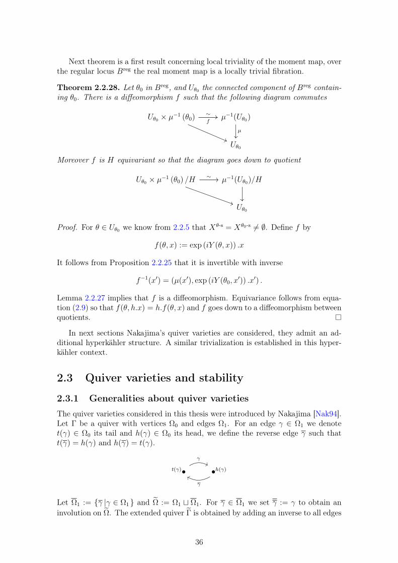
Next theorem is a first result concerning local triviality of the moment map, overthe regular locus Breg the real moment map is a locally trivial fibration.

Theorem 2.2.28. Let θ0 in Breg, and Uθ0 the connected component of Breg contain-ing θ0. There is a diffeomorphism f such that the following diagram commutes

Uθ0 × µ−1 (θ0) µ−1(Uθ0)

Uθ0

f

∼

µ

Moreover f is H equivariant so that the diagram goes down to quotient

Uθ0 × µ−1 (θ0) /H µ−1(Uθ0)/H

Uθ0

∼

Proof. For θ ∈ Uθ0 we know from 2.2.5 that Xθ-s = Xθ0-s 6= ∅. Define f by

f(θ, x) := exp (iY (θ, x)) .x

It follows from Proposition 2.2.25 that it is invertible with inverse

f−1(x′) = (µ(x′), exp (iY (θ0, x′)) .x′) .

Lemma 2.2.27 implies that f is a diffeomorphism. Equivariance follows from equa-tion (2.9) so that f(θ, h.x) = h.f(θ, x) and f goes down to a diffeomorphism betweenquotients.

In next sections Nakajima’s quiver varieties are considered, they admit an ad-ditional hyperkähler structure. A similar trivialization is established in this hyper-kähler context.

2.3 Quiver varieties and stability

2.3.1 Generalities about quiver varieties

The quiver varieties considered in this thesis were introduced by Nakajima [Nak94].Let Γ be a quiver with vertices Ω0 and edges Ω1. For an edge γ ∈ Ω1 we denotet(γ) ∈ Ω0 its tail and h(γ) ∈ Ω0 its head, we define the reverse edge γ such thatt(γ) = h(γ) and h(γ) = t(γ).

t(γ)• •h(γ)

γ

γ

Let Ω1 := γ |γ ∈ Ω1 and Ω := Ω1 t Ω1. For γ ∈ Ω1 we set γ := γ to obtain aninvolution on Ω. The extended quiver Γ is obtained by adding an inverse to all edges

36

in Ω1, its set of vertices is Ω0 and its set of edges is Ω. Let ε : Ω → −1, 1 be themap

ε(γ) = 1 if γ ∈ Ω1

ε(γ) = −1 if γ ∈ Ω1

We fix a dimension vector v ∈ NΩ0 . A representation of the quiver Γ with dimensionvector v is a pair (V, φ) with V =

⊕j∈Ω0

Vj a graded vector space with dimVj = vjand φ = (φγ)γ∈Ω1 a collection of linear maps φγ : Vt(γ) → Vh(γ). A subrepresentationis a subspace W ⊂ V with a compatible Ω0-grading and preserved by φ. The set ofquiver representations with dimension vector v is identified with

Rep (Γ, v) :=⊕γ∈Ω1

MatC(vh(γ), vt(γ)).

For construction of quiver varieties it is interesting to consider representations ofthe extended quiver Γ

Rep(

Γ, v)

:=⊕γ∈Ω

MatC(vh(γ), vt(γ)).

It is a complex vector space, the complex structure considered in this section is

I.(φγ)γ∈Ω = (iφγ)γ∈Ω

The group GLv :=∏

i∈Ω0GLvi(C) acts linearly on Rep(Γ, v)

g. (φγ)γ∈Ω :=(gh(γ)φγg

−1t(γ)

)γ∈Ω

.

The diagonal embedding of C∗ in GLv acts trivially so that the action goes down toan action of the group

Gv := GLv /C∗,which identifies with

Gv∼=

(gj)j∈Ω0 ∈ GLv|

∏j∈Ω0

det(gj) = 1

.

Note that Gv is isomorphic to a product of a special linear group and a finite numberof general linear groups so that it is a reductive group. The Lie algebra of GLv,respectively Gv is glv =

⊕j∈Ω0

glvj(C) respectively.

gv =

(xj)j∈Ω0 ∈ glv

∣∣∣∣∣∑j∈Ω0

trxj = 0

The center of gv is

Z(gv) =

(ξj Idvj)j∈Ω0

∣∣∣∣∣(ξj)j∈Ω0 ∈ (C)Ω0 with∑j∈Ω0

vjξj = 0

.

Let θ ∈ ZΩ0 such that∑

j∈Ω0vjθj = 0, define χθ a character of Gv by

χθ ((gj)j∈Ω0) =∏j∈Ω0

det(gj)−θj . (2.12)

The θ-semistable locus, respectively θ-stable locus in the sense of Mumford’s Geo-metric Invariant Theory [MF82], are denoted by Rep(Γ, v)θ-ss, respectively Rep(Γ, v)θ-s.

37

Definition 2.3.1 (Complex moment map). The complex moment map is defined by

µC : Rep(Γ, v) → gv(φγ)γ∈Ω 7→

∑γ∈Ω ε(γ)φγφγ

it is Gv-equivariant for the adjoint action on gv.

This complex moment map will be related to the real moment map of Definition2.2.8 in next section.

Definition 2.3.2 (Nakajima’s quiver variety). For ξ ∈ Z(gv), the set µ−1C (ξ) is an

affine variety in Rep(Γ, v), it inherits a Gv action. Nakajima’s quiver varieties aredefined as GIT quotients:

Mθv(ξ) := µ−1

C (ξ) ∩ Rep(Γ, v)θ-ss//Gv.

Those varieties are interesting from the differential geometry point of view andhave an hyperkähler structure. We are interested in the family formed by thosevarieties when the parameters ξ and θ are varying. Before studying those family, weintroduce another kind of variety: Nakajima’s framed quiver variety.

Fix another dimension vector w ∈ NΩ0 and denote

Rep (v, w) :=⊕j∈Ω0

MatK(vi, wi)

Rep (w, v) :=⊕j∈Ω0

MatK(wi, vi)

An element g ∈ GLv acts on a = (aj)j∈Ω0 ∈ Rep (v, w) by

g.a := (ajg−1j )j∈Ω0

and on b = (bj)j∈Ω0 ∈ Rep (v, w) by

g.b := (gjbj)j∈Ω0

Introduce framed quiver representations

Rep(

Γ, v, w)

:= Rep (v, w)⊕ Rep (w, v)⊕ Rep(

Γ, v)

and extend the moment map

µ′ : Rep(Γ, v, w) → glv(a, b, φ) 7→ (µ(φ)j − bjaj)j∈Ω0

.

Definition 2.3.1. Let θ ∈ RΩ0, a representation (a, b, φ) ∈ Rep(Γ, v, w) is θ-semistable if for any φ-invariant subspace S ⊂ V such that Sj ∈ aj the followinginequality holds ∑

j∈Ω0

θj dimSj ≤ 0

and for any φ-invariant subspace T ⊂ V such that Im bj ⊂ Tj∑j∈Ω0

θj dimTj ≤∑j∈Ω0

θjvj.

It is stable if the inequality are strict unless S = 0 and T = V .

38

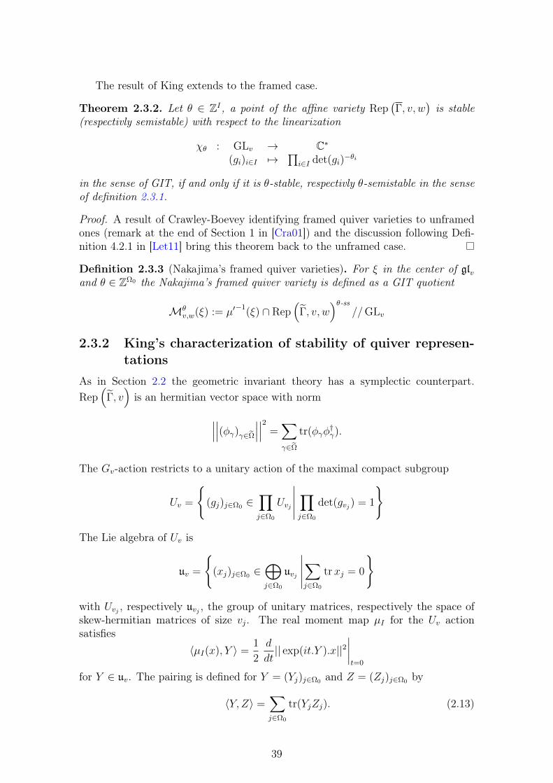
The result of King extends to the framed case.

Theorem 2.3.2. Let θ ∈ ZI , a point of the affine variety Rep(Γ, v, w

)is stable

(respectivly semistable) with respect to the linearization

χθ : GLv → C∗(gi)i∈I 7→

∏i∈I det(gi)

−θi

in the sense of GIT, if and only if it is θ-stable, respectivly θ-semistable in the senseof definition 2.3.1.

Proof. A result of Crawley-Boevey identifying framed quiver varieties to unframedones (remark at the end of Section 1 in [Cra01]) and the discussion following Defi-nition 4.2.1 in [Let11] bring this theorem back to the unframed case.

Definition 2.3.3 (Nakajima’s framed quiver varieties). For ξ in the center of glvand θ ∈ ZΩ0 the Nakajima’s framed quiver variety is defined as a GIT quotient

Mθv,w(ξ) := µ′

−1(ξ) ∩ Rep

(Γ, v, w

)θ-ss//GLv

2.3.2 King’s characterization of stability of quiver represen-tations

As in Section 2.2 the geometric invariant theory has a symplectic counterpart.Rep

(Γ, v)is an hermitian vector space with norm

∣∣∣∣∣∣(φγ)γ∈Ω

∣∣∣∣∣∣2 =∑γ∈Ω

tr(φγφ†γ).

The Gv-action restricts to a unitary action of the maximal compact subgroup

Uv =

(gj)j∈Ω0 ∈

∏j∈Ω0

Uvj

∣∣∣∣∣ ∏j∈Ω0

det(gvj) = 1

The Lie algebra of Uv is

uv =

(xj)j∈Ω0 ∈

⊕j∈Ω0

uvj

∣∣∣∣∣∑j∈Ω0

trxj = 0

with Uvj , respectively uvj , the group of unitary matrices, respectively the space ofskew-hermitian matrices of size vj. The real moment map µI for the Uv actionsatisfies

〈µI(x), Y 〉 =1

2

d

dt|| exp(it.Y ).x||2

∣∣∣∣t=0

for Y ∈ uv. The pairing is defined for Y = (Yj)j∈Ω0 and Z = (Zj)j∈Ω0 by

〈Y, Z〉 =∑j∈Ω0

tr(YjZj). (2.13)

39

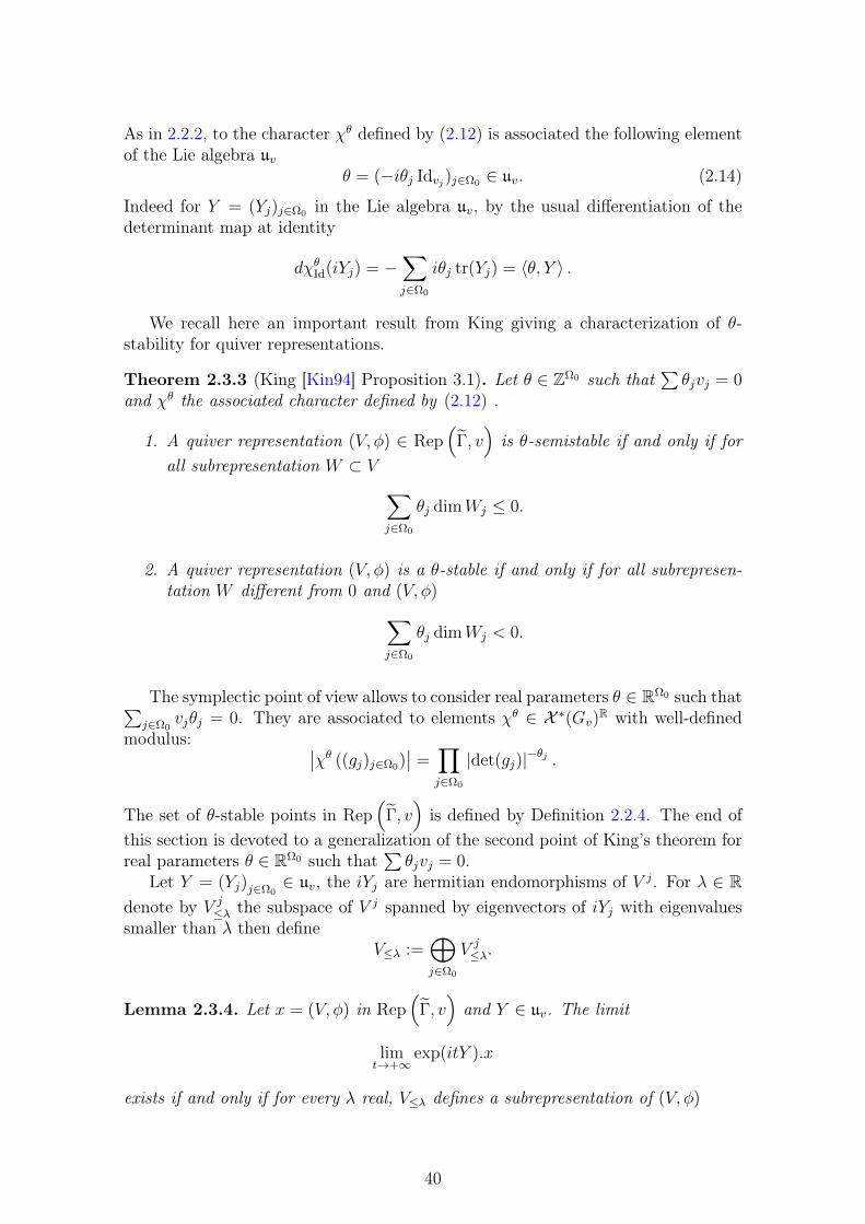
As in 2.2.2, to the character χθ defined by (2.12) is associated the following elementof the Lie algebra uv

θ = (−iθj Idvj)j∈Ω0 ∈ uv. (2.14)

Indeed for Y = (Yj)j∈Ω0 in the Lie algebra uv, by the usual differentiation of thedeterminant map at identity

dχθId(iYj) = −∑j∈Ω0

iθj tr(Yj) = 〈θ, Y 〉 .

We recall here an important result from King giving a characterization of θ-stability for quiver representations.

Theorem 2.3.3 (King [Kin94] Proposition 3.1). Let θ ∈ ZΩ0 such that∑θjvj = 0

and χθ the associated character defined by (2.12) .

1. A quiver representation (V, φ) ∈ Rep(

Γ, v)is θ-semistable if and only if for

all subrepresentation W ⊂ V ∑j∈Ω0

θj dimWj ≤ 0.

2. A quiver representation (V, φ) is a θ-stable if and only if for all subrepresen-tation W different from 0 and (V, φ)∑

j∈Ω0

θj dimWj < 0.

The symplectic point of view allows to consider real parameters θ ∈ RΩ0 such that∑j∈Ω0

vjθj = 0. They are associated to elements χθ ∈ X ∗(Gv)R with well-defined

modulus: ∣∣χθ ((gj)j∈Ω0)∣∣ =

∏j∈Ω0

|det(gj)|−θj .

The set of θ-stable points in Rep(

Γ, v)is defined by Definition 2.2.4. The end of

this section is devoted to a generalization of the second point of King’s theorem forreal parameters θ ∈ RΩ0 such that

∑θjvj = 0.

Let Y = (Yj)j∈Ω0∈ uv, the iYj are hermitian endomorphisms of V j. For λ ∈ R

denote by V j≤λ the subspace of V j spanned by eigenvectors of iYj with eigenvalues

smaller than λ then defineV≤λ :=

⊕j∈Ω0

V j≤λ.

Lemma 2.3.4. Let x = (V, φ) in Rep(

Γ, v)and Y ∈ uv. The limit

limt→+∞

exp(itY ).x

exists if and only if for every λ real, V≤λ defines a subrepresentation of (V, φ)

40

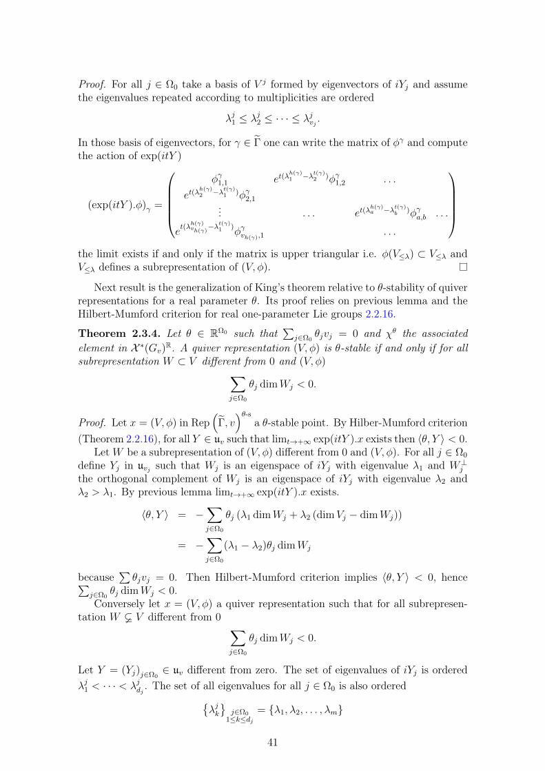
Proof. For all j ∈ Ω0 take a basis of V j formed by eigenvectors of iYj and assumethe eigenvalues repeated according to multiplicities are ordered

λj1 ≤ λj2 ≤ · · · ≤ λjvj .

In those basis of eigenvectors, for γ ∈ Γ one can write the matrix of φγ and computethe action of exp(itY )

(exp(itY ).φ)γ =

φγ1,1 et(λ

h(γ)1 −λt(γ)2 )φγ1,2 . . .

et(λh(γ)2 −λt(γ)1 )φγ2,1

... . . . et(λh(γ)a −λt(γ)b )φγa,b . . .

et(λ

h(γ)vh(γ)

−λt(γ)1 )φγvh(γ),1 . . .

the limit exists if and only if the matrix is upper triangular i.e. φ(V≤λ) ⊂ V≤λ andV≤λ defines a subrepresentation of (V, φ).

Next result is the generalization of King’s theorem relative to θ-stability of quiverrepresentations for a real parameter θ. Its proof relies on previous lemma and theHilbert-Mumford criterion for real one-parameter Lie groups 2.2.16.

Theorem 2.3.4. Let θ ∈ RΩ0 such that∑

j∈Ω0θjvj = 0 and χθ the associated

element in X ∗(Gv)R. A quiver representation (V, φ) is θ-stable if and only if for all

subrepresentation W ⊂ V different from 0 and (V, φ)∑j∈Ω0

θj dimWj < 0.

Proof. Let x = (V, φ) in Rep(

Γ, v)θ-s

a θ-stable point. By Hilber-Mumford criterion(Theorem 2.2.16), for all Y ∈ uv such that limt→+∞ exp(itY ).x exists then 〈θ, Y 〉 < 0.

LetW be a subrepresentation of (V, φ) different from 0 and (V, φ). For all j ∈ Ω0

define Yj in uvj such that Wj is an eigenspace of iYj with eigenvalue λ1 and W⊥j

the orthogonal complement of Wj is an eigenspace of iYj with eigenvalue λ2 andλ2 > λ1. By previous lemma limt→+∞ exp(itY ).x exists.

〈θ, Y 〉 = −∑j∈Ω0

θj (λ1 dimWj + λ2 (dimVj − dimWj))

= −∑j∈Ω0

(λ1 − λ2)θj dimWj

because∑θjvj = 0. Then Hilbert-Mumford criterion implies 〈θ, Y 〉 < 0, hence∑

j∈Ω0θj dimWj < 0.

Conversely let x = (V, φ) a quiver representation such that for all subrepresen-tation W V different from 0 ∑

j∈Ω0

θj dimWj < 0.

Let Y = (Yj)j∈Ω0∈ uv different from zero. The set of eigenvalues of iYj is ordered

λj1 < · · · < λjdj . The set of all eigenvalues for all j ∈ Ω0 is also orderedλjk

j∈Ω01≤k≤dj

= λ1, λ2, . . . , λm

41

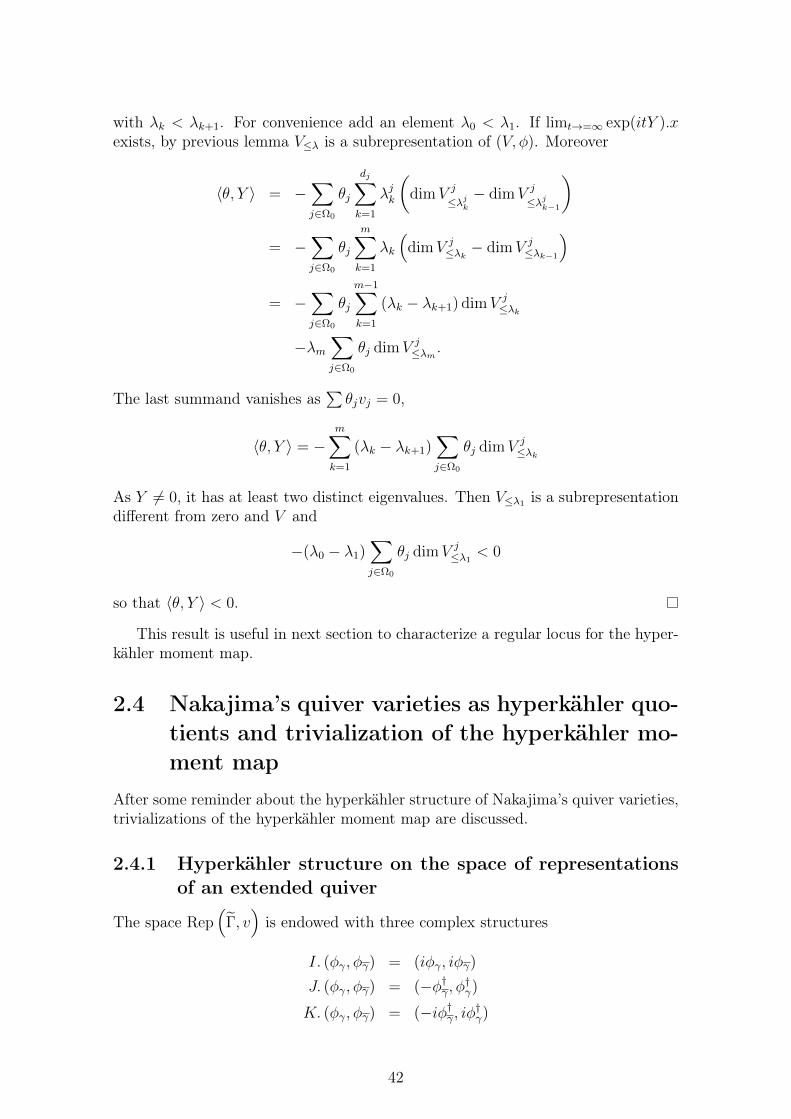
with λk < λk+1. For convenience add an element λ0 < λ1. If limt→=∞ exp(itY ).xexists, by previous lemma V≤λ is a subrepresentation of (V, φ). Moreover

〈θ, Y 〉 = −∑j∈Ω0

θj

dj∑k=1

λjk

(dimV j

≤λjk− dimV j

≤λjk−1

)

= −∑j∈Ω0

θj

m∑k=1

λk

(dimV j

≤λk − dimV j≤λk−1

)= −

∑j∈Ω0

θj

m−1∑k=1

(λk − λk+1) dimV j≤λk

−λm∑j∈Ω0

θj dimV j≤λm .

The last summand vanishes as∑θjvj = 0,

〈θ, Y 〉 = −m∑k=1

(λk − λk+1)∑j∈Ω0

θj dimV j≤λk

As Y 6= 0, it has at least two distinct eigenvalues. Then V≤λ1 is a subrepresentationdifferent from zero and V and

−(λ0 − λ1)∑j∈Ω0

θj dimV j≤λ1 < 0

so that 〈θ, Y 〉 < 0.

This result is useful in next section to characterize a regular locus for the hyper-kähler moment map.

2.4 Nakajima’s quiver varieties as hyperkähler quo-tients and trivialization of the hyperkähler mo-ment map

After some reminder about the hyperkähler structure of Nakajima’s quiver varieties,trivializations of the hyperkähler moment map are discussed.

2.4.1 Hyperkähler structure on the space of representationsof an extended quiver

The space Rep(

Γ, v)is endowed with three complex structures

I. (φγ, φγ) = (iφγ, iφγ)

J. (φγ, φγ) = (−φ†γ, φ†γ)K. (φγ, φγ) = (−iφ†γ, iφ†γ)

42

satisfying quaternionic relations

I2 = J2 = K2 = IJK = −1 (2.15)

and a norm ∣∣∣∣∣∣(φγ)γ∈Ω

∣∣∣∣∣∣2 =∑γ∈Ω

tr(φγφ

†γ

).

For each complex structure, polarisation identity defines an hermitian pairing com-patible with || . . . ||. For example the hermitian pairing compatible with the complexstructure I used in previous section is

pI (u, v) =1

4

(||u+ v||2 − ||u− v||2 + i||u+ I.v||2 − i||u− I.v||2

)pJ(. . . , . . . ) and pK(. . . , . . . ) are similarly defined. One expression is particularlysimple

pI

((φγ)γ∈Ω, (ψγ)γ∈Ω

)=∑γ∈Ω

tr(φγψ†γ).

Remark 2.4.1. Even if the hermitian metric relies on the choice of complex struc-ture, by the polarisation identity the real part remains the same, it is the hyperkählermetric

g(. . . , . . . ) := Re pI(. . . , . . . ) = Re pJ(. . . , . . . ) = Re pK(. . . , . . . ).

Definition 2.4.2 (Real symplectic forms). As in equation (2.4) we define a realsymplectic form for each complex structure

ωI(. . . , . . . ) := g(I . . . , . . . )

ωJ(. . . , . . . ) := g(J . . . , . . . )

ωK(. . . , . . . ) := g(K . . . , . . . )

Notations 2.4.3. I-linear means C-linear with respect to the complex structure Iand similarly for J-linear and K-linear.

Proposition 2.4.4 (Permutation of complex structures). Consider the map

Ψ : Rep(

Γ, v)→ Rep

(Γ, v)

x 7→ 12

(1 + I + J +K) .x

It is an isomorphism from the hermitian vector space Rep(

Γ, v)with the complex

structure I and hermitian pairing pI to the hermitian vector space Rep(

Γ, v)with

the complex structure J and pairing pJ .More generally it cyclically permutes the three complex structure I, J,K

Ψ(I.x) = J.Ψ(x)Ψ(J.x) = K.Ψ(x)Ψ(K.x) = I.Ψ(x).

(2.16)

Such a map is sometimes called an hyperkähler rotation.

43

Proof. Relations (2.16) follow from a computation with the quaternionic relations(2.15). To prove the compatibility with the hermitian structures it is enough tocheck that ||Ψ(x)|| = ||x||.

||(1 + I + J +K).x||2 = g ((1 + I + J +K).x, (1 + I + J +K).x) .

The expected result is obtain after cancellations from the identity g(I.u, u) = 0,similar relations for the other complex structures and quaternionic relations (2.15).

In 2.3.1 an I-linear action of Gv is described. The hyperkähler rotation Ψ pro-vides the following construction for J-linear andK-linear actions. This three actionscoincide when restricted to the compact subgroup Uv.

Definition 2.4.5 (Complexification of the action). Thanks to polar decomposition,to define a linear action of Gv compatible with the complex structure J it is enoughto define the action of exp(i.Y ) for Y ∈ uv. To highlight the complex structure used,this action is written exp(J.Y ) . . . and defined by

exp(J.Y ).x := Ψ(exp(i.Y ).Ψ−1(x)

)with the element exp(i.Y ) of Gv acting by the natural I-linear action previouslydescribed. Similarly

exp(K.Y ).x := Ψ−1 (exp(i.Y ).Ψ(x)) .

Remark 2.4.6. A point x is θ-(semi)stable with respect to the I-linear action if andonly if Ψ(x) is θ-(semi)stable with respect to the J-linear action.

2.4.2 Hyperkähler structure and moment maps

By Proposition 2.4.4 the various Gv-actions previously described are compatiblewith the hermitian metrics so that the constructions of section 2.2 apply. Theyprovide a moment map for each complex structure.

〈µI(x), Y 〉 =1

2

d

dt|| exp(t.I.Y ).x||2

∣∣∣∣t=0

〈µJ(x), Y 〉 =1

2

d

dt|| exp(t.J.Y ).x||2

∣∣∣∣t=0

〈µK(x), Y 〉 =1

2

d

dt|| exp(t.K.Y ).x||2

∣∣∣∣t=0

.

The pairing is defined by (2.13).

Definition 2.4.7 (Hyperkähler moment map). Those three real moment maps fittogether in an hyperkähler moment map µH : Rep

(Γ, v)→ uv ⊕ uv ⊕ uv defined by

µH = (µI , µJ , µK).

The moment map µC defined in 2.3.1 by

µC

((φγ)γ∈Ω

):=∑γ∈Ω

ε(γ)φγφγ. (2.17)

44

can be expressed from the real moment maps

µC := µJ + iµK .

it is a polynomial map with respect to the complex structure I.

Remark 2.4.8. By cyclic permutation of the complex structure, µK + iµI is polyno-mial with respect to the complex structure J and µI + iµJ is polynomial with respectto the complex structure K.

Take (θJ,j)j∈Ω0 and (θK,j)j∈Ω0 in RΩ0 such that∑

j vjθJ,j =∑

j vjθK,j = 0. Asso-ciate to each of them an element in the center of the Lie algebra uv

θJ :=(−iθJ,j Idvj

)j∈Ω0

θK :=(−iθK,j Idvj

)j∈Ω0

.

Then θJ + iθK defines an element in the center of gv = uv ⊕ iuv. Hence µ−1J (θJ) ∩

µ−1K (θK) = µ−1

C (θJ+iθK) is an affine variety embedded in the vector space Rep(

Γ, v)

endowed with the complex structure I and stable under the Gv-action. Section 2.2does not apply directly to this situation as µ−1

C (θJ+iθK) might be singular. Howeverit applies to the action of Gv on the ambiant space Rep

(Γ, v). For θI ∈ RΩ0 such

that∑

j∈Ω0vjθI,j = 0 consider the associated element χθI ∈ X ∗(Gv)

R.

Definition 2.4.9 (Hyperkähler regular locus). For w ∈ NΩ0 a dimension vector

Hw :=

(θI , θJ , θK) ∈

(RΩ0

)3

∣∣∣∣∣∑j

wjθI,j =∑j

wjθJ,j =∑j

wjθK,j = 0

.

The regular locus isHregv = Hv \

⋃w<v

Hw (2.18)

the union is over dimension vector w 6= v such that 0 ≤ wi ≤ vi.

Remark 2.4.10. This regular locus is empty unless the dimension vector v is indi-visible, then Hreg

v is the complementary of a finite union of codimension 3 real vectorspace.

Thanks to Kempf-Ness theory, Nakajima’s quiver varieties can be constructed ashyperkähler quotients. The underlying manifold of the varietyMθI

v (θJ + iθK) (seedefinition 2.3.2) is :

mv(θI , θJ , θK) = µ−1H (θI , θJ , θK)/Uv

2.4.3 Trivialization of the hyperkähler moment map

We study the family of Nakajima’s quiver varieties when the parameters (θI , θJ , θK)are varying. Nakajima proved by consecutive uses of different complex structuresthat for θ and θ′ in Hreg

v the manifolds mv(θI , θJ , θK) and mv(θ′I , θ′J , θ′K) are diffeo-

morphic [Nak94, Corollary 4.2]. We use this idea of consecutive uses of differentcomplex structures to prove that those manifolds fit in a locally trivial family overthe regular locus Hreg

v . First let us highlight relevant facts about the regular locus.

45

Lemma 2.4.11. Let (θI , θJ , θK) ∈ Hregv and x ∈ µ−1

J (θJ) ∩ µ−1K (θK). Then x is

θI-stable if and only if it is θI-semistable.

Proof. If x0 ∈ µ−1H (θI , θJ , θK) its stabilizer in Gv is trivial. Indeed Maffei proved

that the differential of the moment map at x0 is surjective [Maf02, Lemma 48], thenProposition 2.2.10 implies the triviality of the stabilizer of x0.

Let x ∈ µ−1J (θJ) ∩ µ−1

K (θK) a θI-semistable point. Then Gv.x ∩ µ−1I (θI) is not

empty. As µ−1J (θJ) ∩ µ−1

K (θK) = µ−1C (θJ + iθK) is Gv stable, the closure of the

orbit Gv.x meets µ−1H (θI , θJ , θK) at a point x0. This point necessarily has a trivial

stabilizer, hence x0 ∈ Gv.x and x is θI-stable.

Let (θI , θJ , θK) ∈ Hregv and consider first the complex structure I. By previous

lemma and King’s characterisation of stability (Theorem 2.3.4), for θ′I in an openneighborhood of θI , stability with respect to θ′I is the same as stability with respectto θI .

Now consider the complex structure J . Thanks to Remark 2.4.6 on the affinevariety µ−1

K (θK) ∩ µ−1I (θI) all θJ -semistable points are θJ -stable. Moreover for θ′J in

an open neighborhood of θJ , stability with respect to θ′J is the same as stability withrespect to θJ . Similarly for the complex structure K.

Assume that the dimension vector v is a root of the quiver so that the momentmap is surjective, see [Cra06, Theorem 2]. Consider the diagram

µ−1H (Hreg

v ) Rep(

Γ, v)

Hregv uv ⊕ uv ⊕ uv

µH.

.

Theorem 2.4.12 (Local triviality of the hyperkähler moment map). Over the regu-lar locus Hreg

v , the hyperkähler moment map µH is a locally trivial fibration compatiblewith the Uv-action:

Any (θI , θJ , θK) ∈ Hregv admits an open neighborhood V , and a diffeomorphism

f such that the following diagram commutes

V × µ−1H (θI , θJ , θK) µ−1

H (V )

V

f

∼

µH

Moreover f is compatible with the Uv-action so that the diagram goes down to quo-tient

V ×mv(θI , θJ , θK) µ−1H (V )/Uv

V

∼

Proof. The method is similar to the proof of Theorem 2.2.28 applied consecutivelyto the three complex structures. The idea of using different complex structurescomes from [Nak94] and [Kro89]. Take (θI , θJ , θK) ∈ Hreg

v and a connected open

46

neighborhood UI × UJ × UK such that for θ′I ∈ UI , any x ∈ µ−1J (UJ) ∩ µ−1

K (UK) isθ′I-semistable if and only if it is θI-stable. Similarly for UJ and UK . For any x withµH(x) = (θ′I , θ

′J , θ′K) ∈ UI × UJ × UK , by Proposition 2.2.25 applied to the I-linear

action of Gv on Rep(

Γ, v), there exists a unique YI(θI , x) ∈ uv such that

exp (I.YI(θI , x)) .x ∈ µ−1H (θI , θ

′J , θ′K).

Then by exchanging the three complex structures with hyperkähler rotations, thereexists unique YJ(θJ , x) and YK(θK , x) such that

exp (J.YJ(θJ , x)) exp (I.YI(θI , x)) .x ∈ µ−1H (θI , θJ , θ

′K)

and

exp (K.YK(θK , x)) exp (J.YJ(θJ , x)) exp (I.YI(θI , x)) .x ∈ µ−1H (θI , θJ , θK).

This defines the map f−1

f−1(x) := ((θ′I , θ′J , θ′K), exp (K.YK(θJ , x)) exp (J.YJ(θJ , x)) exp (I.YI(θI , x)) .x) .

Lemma 2.2.27 implies the smoothness of f−1. This map induces a diffeomorphism,indeed exchanging θ and θ′ in previous construction produces the expected inverse

f (x, (θ′I , θ′J , θ′K)) := exp (I.YI(θ

′I , x)) exp (J.YJ(θ′J , x)) exp (K.YK(θ′K , x)) .x

It follows from equation (2.10) that the maps are inverse of each others. The ex-change in the order of appearance of the complex structures I, J and K in thedefinition of f and f−1 are necessary as the exponentials do not necessarily com-mute. The Uv-equivariance follows from equation (2.9).

Similarly one can consider the complex moment map µC = µJ + iµK instead ofµH. The complex regular locus is Creg

v := Cv \⋃w<v Cw with

Cw =

ξ ∈ CΩ0

∣∣∣∣∣∑j∈Ω0

wjξj = 0

Theorem 2.4.13. The complex moment map is a locally trivial fibration over Cregv .

Any ξ ∈ Cregv admits an open neighborhood V , and a diffeomorphism f such that the

following diagram commutes

V × µ−1C (ξ) µ−1

C (V )

V

f

∼

µC

Proof. The proof is similar to the hyperkähler situation.

Denote π : µ−1H (Hreg

v )/Uv → Hregv the map obtained taking the quotient of µH.

Consider the cohomology sheaves Hiπ∗Ql of the derived pushforward of the con-stant sheaf and the cohomology sheaves Hiπ!Ql of the derived compactly supportedpushforward of the constant sheaf.

47

Corollary 2.4.14. The sheaves Hiπ∗Ql and Hiπ!Ql are constant sheaves over Hregv .

Proof. By Theorem 2.4.12 those sheaves are locally constant. Hregv is a comple-

mentary of a finite union of codimension 3 real vector spaces, hence it is simplyconnected so that the locally constant sheaves are constant.

Nakajima explained to us that this corollary can also be obtained by generalizingSlodowy’s construction [Slo80] to quiver varieties.

Finally we extend the trivialization of the hyperkähler moment map over linesconstructed by Crawley-Boevey and Van den Bergh [CV04] using twistor spaces astold to us by Nakajima.

Denote by H, respectively H0, the set of quaternions, respectively the set ofpurely imaginary quaternions and H∗0 = H0 \ 0. The space u⊕3

v is identified withH0 ⊗R uv. Then the hyperkähler moment map reads

µH = I ⊗ µI + J ⊗ µJ +K ⊗ µK .

Once an orthonormal basis of R3 is fixed, the triple of complex structures I, J andK is fixed and we write µR = µI , µC = µJ + iµK . The hyperkähler moment mapis assumed to be surjective and the dimension vector indivisible. Then Hreg

v is theopen subset of generic parameters in H0⊗RZ(uv). For θ ∈ Hreg

v a generic parameterand S a contractible subset of H∗0, Crawley-Boevey and Van den Bergh constructeda trivialization of the hyperkähler moment map over S ⊗ θ, see [CV04] proof ofLemma 2.3.3 (in the statement of this lemma S is chosen to be a complex line). Theassumption contractible is relaxed in next theorem. It relies on the theory of twistorspaces developped by Penrose [Pen76], Atiyah-Hitchin-Singer [AHS78] and Salamon[Sal82][Sal86]. The main point is the compatibility between hyperkähler quotientsand twistor spaces from Hitchin-Karlhede-Lindström-Roček [Hit+87] p.560, see alsoHitchin [Hit92]. The following Theorem as well as its proof was told to us byNakajima.

Theorem 2.4.15. For θ generic in H0 ⊗R Z(uv) define

H∗0.θ = h⊗ θ |h ∈ H∗0 .

There exists a diffeomorphism f such that the following diagram commutes

µ−1H (H∗0.θ)/Uv µ−1

H (θ)/Uv ×H∗0.θ

H∗0.θ

f

µH

the vertical arrow is the projection to H∗0.θ.

Proof. Consider the quaternionic vector space Rep(

Γ, v)and the projection

Rep(

Γ, v)× S2 → S2.

With S2 the 2-sphere of imaginary quaternions with unit norm

S2 =aI + bJ + cK

∣∣a2 + b2 + c2 = 1.

48

S2 is given the usual complex structure of the projective line. The twistor spaceassociated to Rep

(Γ, v)is the manifold Rep

(Γ, v)× S2 endowed with a complex

structure such that the fiber over Iu ∈ S2 is Rep(

Γ, v)seen as a vector space with

complex structure Iu.As detailed in [CV04], the group of quaternion of unit norm, identified with

SU(2), acts on H0 ⊗ Z(uv) by

h. (h′ ⊗ θ) = hh′h⊗ θ.

with aI + bJ + cK + d = −aI − bJ − cK + d. Let θ a generic parameter, up to thechoice of orthonormal basis of R3 we can assume θ = I ⊗ θI . The SU(2) orbit of θthus identifies with S2 as

SU(2).θ =Iu ⊗ θ

∣∣Iu ∈ S2. (2.19)

The twistor space of the hyperkähler manifold µ−1H (θ)/Uv is a complex manifold T

with an holomorphic map p to S2

T S2.p

The underlying differential manifold of the twistor space is just a product and p theprojection to the second factor

µ−1H (θ)/Uv × S2 S2.

The twistor spaces construction is compatible with hyperkähler quotients as ex-plained in [Hit+87] p.560. Thus the fiber of p over Iu is µ−1

H (θ)/Uv endowed with thecomplex structure inherited from the complex structure Iu on Rep

(Γ, v). Namely

if Iu ⊗ θ = (θ′I , θ′J , θ′K) then the fiber of the twistor space over Iu is the complex

manifoldp−1(Iu) = µ−1

C (θ′J + iθ′K) ∩ µ−1R (θ′I)/Uv

Thus fibers of p are exactly fibers of µH and the twistor space provides trivializationof the hyperkähler moment map over the orbit SU(2).θ:

µ−1H (SU(2).θ)/Uv T µ−1

H (θ)/Uv × S2

SU(2).θ S2

µH

β

p

γ

∼α

α is defined thanks to (2.19), the map β is the identity on the fibers and γ forgets thecomplex structure. This diagram traduces the equivalence between, on the right,varying complex structure on a fixed fiber µ−1

H (θ)/Uv and on the left varying thefiber for a fixed complex structure I.

The construction is similar to Crawley-Boevey and Van den Bergh’s constructionexcept that the twistor space formalism allows to obtain a trivialization over thenon-contractible space SU(2).θ.

49

As in [CV04], the trivialization can be extended thanks to the R>0 action. Notethat for t a positive real number µH(tx) = t2µH(x). Then identifying S2×R>0 withH∗0 we obtain the trivialization

µ−1H (H∗0.θ)/Uv µ−1

H (θ)/Uv ×H∗0

H∗0.θ H∗0

The SU(2)-action on the base of this trivialization traduces the variation of complexstructure on the hyperkähler manifold µ−1

H (θ)/Uv whereas the R>0 action traducesthe rescaling of the metric.

50

Chapter 3

Geometric and combinatoricbackground

This chapter recalls the geometric and combinatoric tools necessary to study char-acter varieties and their cohomology. The base field K is either C or an algebraicclosure Fq of a finite field Fq. Section 3.1 introduces the notations for perversesheaves and intersection cohomology.

In Section 3.2 some properties of symmetric functions are recalled. They areused to define Hausel-Letellier-Villegas kernel HHLV

n . This kernel is fundamental inthe description of cohomology of character varieties. Moreover symmetric functionsformalism is useful to study representation of Weyl groups. They are also necessaryto define the algebra spanned by Kostka polynomials mentioned in the introduc-tion 1.3.2. In order to relate this algebra with cohomology of quiver varieties, animportant result of Garsia-Haiman [GH96] is recalled in 3.2.4.

Section 3.3 contains various notations for conjugacy classes and their Jordantype, they will be used throughout the thesis.

In 3.4, Springer theory [Spr76; BM83], Lusztig parabolic induction [Lus84; Lus85;Lus86] and the associated resolutions of closure of conjugacy classes are recalled.

Construction and basic properties of character varieties are given in 3.5. More-over construction of resolutions from 3.4 are extended to character varieties, follow-ing Letellier [Let11; Let13].

Finally some conjecture and theorems relating the cohomology of character va-rieties with the kernel HHLV

n are stated in 3.6.

3.1 Perverse sheaves and intersection cohomology

3.1.1 Perverse sheaves

In this section classical results about perverse sheaves and intersection cohomologyare stated. The constructions come from Beilinson, Bernstein, Deligne and Gabber[Bei+18].K is either C or an algebraic closure Fq of a finite field Fq with q elements. X is

an algebraic variety over K. Let l be a prime different from the characteristic anddenote by κX the constant l-adic sheaf on X with coefficients in Ql.

Notations 3.1.1. The category of κ-constructible sheaves on X is denoted by Dbc (X).Its objects are represented by complexes of sheaves K such that the cohomology

51

sheaves HiK are κ-constructible sheaves on X and finitely many of them are non-zero. For Y a variety over K and f : X → Y a morphism one has the usualfunctors

f ∗, f ! : Dbc (Y )→ Dbc (X)

f∗, f! : Dbc (X)→ Dbc (Y )

For m an integer K[m] is the shifted complex such that HiK[m] = Hi+mK. For x apoint in X, the stalk at x of the i-th cohomology sheave of the complex K is denotedby Hi

xK . The structural morphism of X is p : X → SpecK. The k-th cohomologyspace of X with coefficients in κ is

Hk(X, κ) := Hkp∗κX

and the k-th compactly supported intersection cohomology space of X is

Hkc (X, κ) := Hkp!κX .

The Verdier dual operator is denoted by DX : Dbc (X)→ Dbc (X).

Theorem 3.1.2 (Base change). Consider K ∈ Dbc (Y ′) and a cartesian square

X ′ Y ′

X Y

g

b a

f

(3.1)

then the natural morphism f ∗a!K → b!g∗K is an isomorphism.

Remark 3.1.3. Let α → X a geometric point of X and β its image by f . Considerthe fibers of the vertical arrows:

Xα := X ′ ×X α, Yβ := Y ′ ×Y β

In the following diagram h is an isomorphism

Xα Yβ

α β

h

The base change isomorphism for this diagram identifies with the stalk at β of thebase change isomorphism of Diagram (3.1):

f ∗a!Kα → b!g∗Kα

which is nothing but the morphism obtained by functoriality of the compactly sup-ported cohomology

H•

c(Yβ, K)h∗−→ H

•

c(Xα, h∗K).

52

Definition 3.1.4. Let W a finite group acting from the left on a variety X. Forall w ∈ W there is a morphism w : X → X. An action of W on an elementK ∈ Dbc (X) is the data of morphisms φw : w∗K ∼= K satisfying the followingrelation for all w,w′ ∈ W

φw′w = φww∗(φw′) (3.2)

and such that φ1 = Id. Then we say that the complex K is W -equivariant.

Remark 3.1.5. When the action of W on X is trivial, an action of W on K ∈Dbc (X) is just a group morphism from the opposite group W op to the group of auto-morphism Aut(K).

Proposition 3.1.6. Let f : X → Y a W -equivariant morphism between varietieswith left W -action. Let W act on K by morphisms φw : w∗K ∼= K. Then W actson f!K.

Proof. The action is defined for w ∈ W the following way. Base change formulaprovides an isomorphism w∗f!K → f!w

∗K. Compose this isomorphism with f!φwto obtain an isomorphism φw : w∗f!K → f!K. The compatibility (3.2) follows fromfunctoriality of base change.

Definition 3.1.7 (Perverse sheave). A perverse sheave is an object K in Dbc (X)such that for all i ∈ N

dim(SuppHiK

)≤ −i

dim(SuppHiDXK

)≤ −i.

The category of perverse sheaves on X is denoted byM(X), it is an abelian category.

3.1.2 Intersection cohomology

Definition 3.1.8 (Intersection complex). Let Y → X a closed embedding and j :U → Y an open embedding. Assume U is smooth, irreducible and U = Y . Let ξ bea local system on U . IC•Y,ξ is the unique perverse sheave K on Y characterized by

HiK = 0 if i < − dimY (3.3)H− dimYK|U = ξ (3.4)

dim(SuppHiK

)< −i if i > − dimY (3.5)

dim(SuppHiDYK

)< −i if i > − dimY. (3.6)

We also denote IC•Y,ξ its extension j∗IC•Y,ξ. The intersection complex defined byGoresky-MacPherson [GM83] and Deligne is obtained by shifting this perverse sheaf

IC•Y,ξ := IC•Y,ξ [− dimY ] .

Remark 3.1.9 (Continuation principle). The intersection complex of ξ can also bedefined as the intermediate extension IC•Y,ξ = j!∗ξ. Moreover the functor j!∗ is fullyfaithful (see Kiehl-Weissauer [KW01, III - Corollary 5.11]).

Remark 3.1.10. The intersection complex does not depend on the choice of smoothopen subset in Y . When the local system ξ is not specified, it is chosen to be theconstant sheaf κX and IC•X := IC•X,κU .

53

Definition 3.1.11 (Intersection cohomology). Let p : X → SpecK the structuralmorphism and k an integer. The k-th intersection cohomology space of X is

IHk(X, κ) := Hkp∗IC•X

and the k-th compactly supported intersection cohomology space of X is

IHkc (X, κ) := Hkp!IC•X .

For K = C, Saito [Sai86] proved that the intersection cohomology spaces carrya mixed-Hodge structure. Thus there exists on IHk

c (X,Q) an increasing finite fil-tration called the weight filtration and denoted by W k

• such that the complexifiedquotient C ⊗Q W k

r /Wkr−1 carries a pure Hodge structure of weight r. The Hodge

numbers of this structure are denoted hi,j,kc (X) and satisfy i+ j = r.

Definition 3.1.12. The mixed-Hodge structure is encoded in the mixed-Hodge poly-nomial:

IHc (X;x, y, v) :=∑i,j,k

hi,j,kc (X)xiyjvk. (3.7)

This polynomial has two important specialisations, the Poincaré polynomial

Pc(X; t) := IHc (X; 1, 1, v) =∑k

dim IHkc (X, κ)vk (3.8)

and the E-polynomial

Ec(X;x, y) := IHc (X;x, y,−1) . (3.9)

Remark 3.1.13. For X a smooth variety the intersection cohomology is the usuall-adic cohomology

IH i(X, κ) = H i(X, κ)

IH ic(X, κ) = H i

c(X, κ).

3.2 Symmetric functions

3.2.1 Lambda ring and symmetric functions

In this section the combinatorics involved in the cohomology of character varietiesis recalled.

Notations 3.2.1. A partition of an integer n ∈ N is a decreasing sequence of non-negative integers

λ = (λ1, λ2, . . . , λl(λ)) with |λ| := λ1 + λ2 + · · ·+ λl(λ) = n.

The length of λ is the number l(λ) of non-zero terms. The set of partitions of n isdenoted by Pn and

P∗ :=⋃

n∈N>0

Pn and P =⋃n∈N

Pn

54

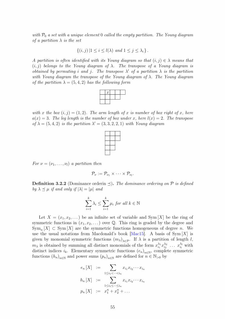
with P0 a set with a unique element 0 called the empty partition. The Young diagramof a partition λ is the set

(i, j) |1 ≤ i ≤ l(λ) and 1 ≤ j ≤ λi .

A partition is often identified with its Young diagram so that (i, j) ∈ λ means that(i, j) belongs to the Young diagram of λ. The transpose of a Young diagram isobtained by permuting i and j. The transpose λ′ of a partition λ is the partitionwith Young diagram the transpose of the Young diagram of λ. The Young diagramof the partition λ = (5, 4, 2) has the following form

x

with x the box (i, j) = (1, 2). The arm length of x is number of box right of x, herea(x) = 3. The leg length is the number of box under x, here l(x) = 2. The transposeof λ = (5, 4, 2) is the partition λ′ = (3, 3, 2, 2, 1) with Young diagram

For ν = (ν1, . . . , νl) a partition then

Pν := Pν1 × · · · × Pνl .

Definition 3.2.2 (Dominance orderin ). The dominance ordering on P is definedby λ µ if and only if |λ| = |µ| and

k∑i=1

λi ≤k∑i=1

µi for all k ∈ N

Let X = (x1, x2, . . . ) be an infinite set of variable and Sym [X] be the ring ofsymmetric functions in (x1, x2, . . . ) over Q. This ring is graded by the degree andSymn [X] ⊂ Sym [X] are the symmetric functions homogeneous of degree n. Weuse the usual notations from Macdonald’s book [Mac15]. A basis of Sym [X] isgiven by monomial symmetric functions (mλ)λ∈P . If λ is a partition of length l,mλ is obtained by summing all distinct monomials of the form xλ1i1 x

λ2i2

. . . xλlil withdistinct indices ik. Elementary symmetric functions (en)n∈N, complete symmetricfunctions (hn)n∈N and power sums (pn)n∈N are defined for n ∈ N>0 by

en [X] :=∑

1≤i1<···<in

xi1xi2· · · xin

hn [X] :=∑

1≤i1≤···≤in

xi1xi2· · · xin

pn [X] := xn1 + xn2 + . . .

55

and e0 := h0 := p0 := 1. Each one of this family freely generates the ring Sym [X].We introduce the corresponding basis labelled by partitions λ ∈ P

eλ := eλ1eλ2· · · eλlhλ := hλ1hλ2· · ·hλlpλ := pλ1pλ2· · · pλl

When talking about symmetric functions, if we do not need to specify the set ofvariable we write just F instead of F [X], we can think of F as an element in theQ-algebra freely generated by (en)n∈N. A convenient formalism to study symmetricfunctions is provided by lambda rings. The following reminder on this topic comesfrom Mellit [Mel17a; Mel18].

Definition 3.2.3 (Lambda ring). A lambda ring over Q is a commutative andunitary Q-algebra Λ endowed, for n ∈ N>0, with ring morphisms

pn : Λ → Λa 7→ pn[a]

such that pn pm = pnm for n,m ∈ N>0. The pn are called the Adams operators.We use square brackets instead of parenthesis for evaluation of Adams operators.

Example 3.2.4 (Symmetric functions over Q). The ring of symmetric functionsSym [X] is freely generated, as a Q-algebra by the power sums pn[X]. Adams oper-ators on Sym [X] can be defined by their values on the power sums

pm [pn[X]] := pmn[X] for m ∈ N>0 and n ∈ N.

This gives Sym [X] a lambda ring structure.

Remark 3.2.5. Note that for all n ∈ N>0, pn[X] = pn[p1[X]] then let X := p1[X].All the power sums pn[X] with n > 0 are obtained applying Adams operator to X.The notations used for the power sums agree with the one resulting of applicationsof Adams operators to X.

Example 3.2.6. Q(q, t) is endowed with the Adams operator defined by pn[f(q, t)] =f(qn, tn) for any f(q, t) ∈ Q(q, t).

Example 3.2.7 (Symmetric functions over Q(q, t)). The ring of symmetric func-tions over Q(q, t) is still denoted Sym [X]. It is a lambda ring, the Adams operatorsact by pn [f(q, t)F [X]] = f(qn, tn)pn [F [X]].

Example 3.2.8 (Multivariate symmetric functions).

Sym[X1, . . . , Xk] := Sym[X1]⊗ Sym[X2]⊗ · · · ⊗ Sym[Xk]

is the ring of functions in k sequences of variables Xi = (xi,1, xi,2, . . . ) symmetricin each sequence. The Adams operators are defined by

pn [F1[X1]⊗ . . . ⊗ Fk[Xk]] = pn [F1[X1]]⊗ . . . ⊗ pn [Fk[Xk]]

56

Notations 3.2.9 (Conventions for variable in ring of symmetric functions). Whenconsidering symmetric functions, uppercase characters such as X, Y, Z,Xi will beinfinite set of variable so that (pn[X])n∈N are algebraically free. Lowercase characterssuch as q, r, s, t, u, v, w, z will be single variables and Adams operator act on them aspn[u] = un.

Definition 3.2.10 (Plethystic action). Let α ∈ Λ be an element in a lambda ringand F [X] ∈ Sym [X]. As the power sums freely generate the ring of symmetricfunctions there exists a unique polynomial f such that F [X] = f(p1[X], p2[X], . . . ).To compute the plethystic action of F on α we evaluate the polynomial f on theAdams operator F [α] := f(p1, p2, . . . )[α]. It defines a ring morphism from Sym [X]to Λ. It is also called plethystic substitution of X by α.

Remark 3.2.11. Once again, denoting by X the element p1[X] ∈ Sym [X], nota-tions are compatible. pn[X] is both the evaluation of the Adams operator pn on theelement X and the plethystic action of the symmetric function pn on the elementX. Plethystic action can be thought of as evaluation of a symmetric function F onan element of a lambda ring.

For Λ a lambda ring, Λ[[s]] is the ring of power series in s with coefficients inΛ. It is endowed with a lambda ring structure such that pn[s] = sn. Elements ofSym[X][[s]] such that the symmetric function in front of sn is of degree n can bethought of as elements in Sym[[X]] the completion of Sym [X] with respect to theideal Sym [X]+ of symmetric functions without constant terms.

Definition 3.2.12 (Plethystic exponential and logarithm). Let Λ be a lambda ringand sΛ[[s]] the formal series in s with coefficient in Λ without terms in s0. ForG ∈ sΛ[[s]] the plethystic exponential is defined by

Exp[G] :=+∞∑n=0

hn[G] = exp

(+∞∑n=1

pn[G]

n

)and the plethystic logarithm

Log[1 +G] :=+∞∑n=1

µ(n)

npn [log(1 +G)] .

with µ the usual Mobius function. Contrarily to the ordinary ones, the plethysticexponential and logarithm start with an uppercase character.

Remark 3.2.13. As the Adams operators are ring morphism

Exp[F +G] = Exp[F ] Exp[G]

Log[(1 + F )(1 +G)] = Log[1 + F ] + Log[1 +G]

Remark 3.2.14. As expected, the plethystic logarithm is the inverse of the plethysticexponential

Log[Exp[G]] =∑n,m≥1

µ(n)

nmpnm[G]

=∑n≥1

∑d|n

µ(d)

npn[G]

= G

57

This computation follows from the characterisation of Mobius function and the factthat p1 acts as identity.

Proposition 3.2.15. Let F ∈ Λ[[s]], write the expansion of its logarithm andplethystic logarithm

log(F ) =∑n

Unnsn

Log[F ] =∑n

Vnsn.

Then the coefficients of those expansions are related by

Vn =1

n

∑d|n

µ(d)pd[Und

].

Proof.

Log[F ] =∑d,n

µ(d)

dpd

[Ummsm]

=∑d,n

µ(d)

d

pd[Um]

msmd

As pd is a ring morphism and pd[sm] = smd. Conclusion follows by taking the

coefficient in front of sn.

Remark 3.2.16. There is natural way to embed Sym [X] in Sym [X] [[s]], we canadd a variable s to keep track of the degree. For F ∈ Sym [X] written in the basisof power sums as

F [X] =∑λ∈P

cλpλ[X]

we denote also by F the element in Sym [X] [[s]]

F =∑λ∈P

cλpλ[X]s|λ|

with cλ the coordinate of F in the basis (pλ)λ∈P .

Proposition 3.2.17 ([HLR13] proof of proposition 3.1). Plethystic logarithm andplethystic substitution commute. Namely for any α ∈ Λ and F symmetric functionwithout constant term

Log [1 + F [α]] = Log[1 + F ][α]

where F [α] ∈ Λ[[s]] and Log[1 + F ][α] means plethystic substitution in each coeffi-cients of the power series in s.

Proof. Use notations from Proposition 3.2.15 and Remark 3.2.16. First the Un[X]are obtained from the cλpλ[X] by additions and multiplications. Then the Vn[X]are obtained from the Un[X] by additions, multiplications and Adams operator.Conclusion follows as plethystic action is a ring morphism commuting with Adamsoperator.

58

This section ends with the introduction of Hall pairing. Other related pairingswill be discussed in 3.2.3.

Definition 3.2.18 (Hall pairing). The Hall pairing is a symmetric bilinear pairingon Sym [X] such that the power sums form an orthogonal basis

〈pλ, pµ〉 = δλ,µzλ (3.10)

δλ,µ is 1 if λ = µ and 0 otherwise. zλ is the order of a the stabilizer of a partitionof cycle type λ. Namely

zλ =k∏l=1

imll ml!

for a partition λ = (i1, . . . i1︸ ︷︷ ︸m1

, . . . , ik, . . . ik︸ ︷︷ ︸mk

) .

3.2.2 Characters of the symmetric group and symmetric func-tions

Well-known results relating symmetric functions and representation theory of thesymmetric group are recalled, see [Mac15] for more details. A class function on afinite group W is a Q-valued function constant over conjugacy classes. Importantexamples of class functions are given by characters of finite dimensional representa-tions of the groupW . The space of class functions is actually spanned by irreduciblecharacters. It is endowed with a scalar product defined by

〈f, g〉W =1

|W |∑σ∈W

f(σ)g(σ−1).

Irreducible characters then form an orthonormal basis of the space of class functions.

Remark 3.2.19. For χ and η two characters of a finite group W and Vχ, Vη theassociated representations

dim HomW (Vχ, Vη) = 〈χ, η〉W

Definition 3.2.20. Let R = ⊕n∈NRn with Rn, n > 0 the space of class function onthe symmetric group Sn and R0 := Q. It is endowed with a non-degenerate pairing〈. . . , . . . 〉 and a product :

• 〈f, g〉 = 〈f, g〉Sn for f, g ∈ Rn and Rn is orthogonal to Rm if n 6= m.

• Let f ∈ Rn and g ∈ Rm then f × g defines a class function on Sn ×Sm. Fixan embedding Sn ×Sm ⊂ Sn+m so that class functions can be induced fromSn×Sm to Sn+m and define the product f.g := Ind

Sm+n

Sn×Sm f ×g. This productis sometime called external tensor product.

Definition 3.2.21 (Characteristic map). Conjugacy classes in Sn are indexed bypartitions of n specifying the cycle type. For a class function f ∈ Rn define

ch(f) = 〈f,Ψn〉Sn

59

whereΨn : Sn → Sym [X]

σ 7→ pcyc(σ)

with cyc(σ) the partition giving the cycle type of the permutation σ. The map chextends by linearity to give the characteristic map ch : R → Sym [X]. R0 is sent toconstants by ch.

Remark 3.2.22. It is convenient to express ch with partitions rather than permu-tations. For a class function f ∈ Rn with value fλ on the conjugacy class of cycletype λ

ch(f) =1

|Sn|∑σ∈Sn

f(σ)pcyc(σ) (3.11)

=∑|λ|=n

z−1λ fλpλ (3.12)

In last line the sum over elements of the symmetric group is turned into a sumover partitions indexing conjugacy classes of the symmetric group. We used that|Cλ||Sn| = z−1

λ where Cλ is the conjugacy class of cycle type λ.

Proposition 3.2.23. The characteristic map ch is an isomorphism between R andSym [X] compatible with the products and the pairings (Sym [X] being endowed theHall pairing 3.2.18).

Proof. First let us check that 〈ch(f), ch(g)〉 = 〈f, g〉, by linearity we just have tocheck it for f, g ∈ Rn. Orthogonality properties of the power sums (Definition3.2.18) and (3.12) give

〈ch(f), ch(g)〉 =∑|λ|=n

z−1λ fλgλ = 〈f, g〉Sn

last equality comes from the previous trick used to go from a sum over the symmet-ric group to a sum over partitions in Remark 3.2.22.

To check that it is a ring morphism take f ∈ Rn and g ∈ Rm. By adjunctionbetween induction and restriction of representations:

ch(f.g) = 〈f.g,Ψ〉Sm+n= 〈f × g,Ψ〉Sm×Sn

last term splits into a product of sum overs Sm and Sn

1

|Sm ×Sn|∑

(σ,τ)∈Sm×Sn

f(σ)g(τ)pσpτ = 〈f,Ψ〉Sm 〈g,Ψ〉Sn

so thatch(f.g) = ch(f) ch(g).

Let 1λ the map 1λ(σ) = 1 if σ is of cycle type λ and 1λ(σ) = 0 otherwise. (1λ)λ∈Pis a basis of R. It is sent to

(z−1λ pλ

)λ∈P by ch. Hence the characteristic map send a

basis to a basis, it is an isomorphism.

60

Remark 3.2.24. Under the characteristic map ch, the symmetric function hn issent to the constant class function with value 1. The symmetric function en is sentto the sign.

Irreducible characters of Sn are indexed by partitions of n as in [Mac15] insuch a way that χ(n) corresponds to the trivial representation and χ(1n) to the signrepresentation.

Definition 3.2.25. The Schur functions are the images of the irreducible charactersof the symmetric group under the characteristic map. For λ ∈ Pn

sλ[X] := ch(χλ) =∑|µ|=|λ|

χλµpµ[X]

zµ(3.13)

where χλµ is the value of the character of type λ evaluated on a conjugacy class ofcycle type µ.

Proposition 3.2.26. Schur functions (sλ)λ∈P form an orthonormal basis with re-spect to the Hall pairing and equation (3.13) might be inverted to express the powersums from the Schur functions

pλ[X] =∑|µ|=|λ|

χµλsµ[X]. (3.14)

Proof. The family of Schur functions is the image under the characteristic map ofan orthonormal basis of R. Equation (3.14) follows from (3.13) and orthogonalityof characters of the symmetric group.

Remark 3.2.27. Let χV ∈ Rn the class function defined as the character of arepresentation V of Sn. The Schur functions and the power sums have the followingrepresentation theoretic interpretation:

• 〈sλ, ch(χV )〉 is the multiplicity of the irreducible representation Vλ in the rep-resentation V .

• 〈pµ, ch(χV )〉 is the trace of an element in Sn with cycle type µ on the repre-sentation V .

Lemma 3.2.28. For ν a partition of n let εν the sign representation of Sν =Sν1 × · · · × Sνl. A choice of inclusion Sν ⊂ Sn allows to induce εν. Then forλ ∈ Pn

dim HomSn

(IndSn

Sνεν , Vλ

)= 〈eν , sλ〉 = 〈hν , sλ′〉 .

Proof. dim HomSn

(IndSn

Sνεν , Vλ

)is the multiplicity of the irreducible representation

Vλ in IndSnSνεν . For m ∈ N>0 the symmetric function em is the characteristic of

the sign representation of Sm. Thanks to the compatibility between induction andproduct, eν is the characteristic of IndSn

Sνεν . First equality now follows from Remark

3.2.27. To obtain the second equality, notice that Vλ′ is the representation Vλ twistedby the sign.

61

Definition 3.2.29 (Frobenius characteristic). We extend the characteristic map chto bigraded representations of Sn by adding variable q and t to keep track of thedegree. To a bigraded representation of the symmetric group V =

⊕(i,j)∈N2 Vi,j is

associated a symmetric function over Z(q, t) given by

ch(V ) =∑λ∈Pn

∑(i,j)∈N2

〈Vi,j, χλ〉 qitjsλ (3.15)

where the representation Vi,j is identified with its character so that 〈Vi,j, χλ〉 is themultiplicity of the irreducible representation of type λ in Vi,j. The symmetric func-tion ch(V ) is called the Frobenius characteristic of the bigraded representation V .

Example 3.2.30. For any µ ∈ Pn the Macdonald polynomial Hµ[X; q, t] is obtainedin this way from a bigraded representations of the symmetric group. This is thefamous n!-conjecture of Garsia-Haiman [GH93], proved by Haiman [Hai01].

3.2.3 Orthogonality and Macdonald polynomials

In this section Mellit [Mel17a; Mel18] characterisation of modified Macdonald poly-nomials is recalled.

Generalities about scalar products on Sym [X]

A scalar product on Sym [X] is a Q(q, t)-bilinear form

(. . . , . . . )S : Sym [X]× Sym [X] → Q(q, t)F,G 7→ (F [X], G[X])S

which is non-degenerate. It can be extended to multivariate symmetric functions byspecifying the variable acted upon in index

(. . . , . . . )SX : Sym[X, Y1,· · · , Yk]× Sym[X,Z1,· · · , Zl] → Sym[Y1,· · · , Yk, Z1,· · · , Zl]

on pure tensors it reads

(F [X]⊗F ′[Y1,· · · , Yk], G[X]⊗G′[Z1,· · · , Zl])SX := (F [X], G[X])SG′[Z1,· · · , Zl]F ′[Y1,· · · , Yk]

and it extends by linearity.

Assumption 3.2.31 (Homogeneity). When considering families of symmetric func-tions indexed by partitions such as (uλ)λ∈P , the symmetric function uλ is alwaysassumed to be homogeneous of degree |λ|.

Definition 3.2.32. Let (uλ)λ∈P , (vµ)µ∈P two basis dual with respect to a scalarproduct (. . . , . . . )S. Then the element KS[X, Y ] ∈ Sym[X, Y ] defined by

KS[X, Y ] :=∑λ∈P

uλ[X]vλ[Y ]

is called the reproducing kernel of the scalar product (. . . , . . . )S. It depends only onthe scalar product but not on the choice of dual basis as detailed in next proposition.

62

Proposition 3.2.33. With the notations of previous definition, two families of sym-metric functions (aλ)λ∈P , (bµ)µ∈P are dual basis with respect to (. . . , . . . )S if and onlyif

KS[X, Y ] =∑λ∈P

aλ[X]bλ[Y ] (3.16)

Proof. Express aλ and bν in the basis (uλ)λ∈P and (vλ)λ∈P

aλ[X] =∑|µ|=|λ|

cµλuµ[X] (3.17)

bν [Y ] =∑|ρ|=|ν|

dρνvρ[Y ]. (3.18)

Equation (3.16) now reads∑µ,ρ

cµλdρλuµ[X]vρ[Y ] =

∑λ∈P

uλ[X]vλ[Y ].

As the family (uλ[X]vµ[Y ])λ,µ∈P is free in Sym[X, Y ] this last equation is equivalentto ∑

|λ|=|µ|

cµλdρλ = δµ,ρ. (3.19)

Now (aµ)µ∈P and (bρ)ρ∈P are dual with respect to (. . . , . . . )S if and only if

(aµ, bρ)S = δµ,ρ.

Using expansions (3.17), (3.18) and duality of (uλ)λ∈P , (vµ)µ∈P this is equivalent to∑|λ|=|µ|

cλµdλρ = δµ,ρ. (3.20)

Two last equations can be written with matrices with columns and rows indexed bypartitions of a given integer then Equation (3.19) reads CtD = Id which is clearlyequivalent to (3.20) : CDt = Id.

Remark 3.2.34. The name reproducing kernel comes from the notion of kernel ofan operator see [Mel18]. KS is the kernel of the identity operator with respect to thepairing (. . . , . . . )S, indeed for any F [X] ∈ Sym [X]

(KS[X, Y ], F [X])SX = F [Y ].

Hall pairing and (q, t)-deformations

The Hall pairing was defined in 3.2.18, it satisfies

〈pλ, pµ〉 = δλ,µzλ

Remark 3.2.35. (pλ)λ∈P and(z−1µ pµ

)µ∈P form dual basis with respect to the Hall

pairing so that the kernel of Hall pairing is

Exp[XY ] =∑λ∈P

pλ[X]pλ[Y ]

zλ=∑n

hn[XY ].

63

Before introducing deformations of the Hall pairing we need the following lemma.

Lemma 3.2.36. For F,G ∈ Sym [X] and S ∈ Q(q, t)

〈F [X], G[SX]〉 = 〈F [SX], G[X]〉 (3.21)

Proof. It follows from successive applications of remark 3.2.34

〈F [X], G[SX]〉X = 〈F [X], 〈Exp[XSY ], G[Y ]〉Y 〉X= 〈〈F [X],Exp[XSY ]〉X , G[Y ]〉Y= 〈F [SY ], G[Y ]〉Y .

Definition 3.2.37 (deformations of Hall pairing). The (q, t)-deformation of the Hallpairing is defined by

(F [X], G[X])q,t := 〈F [X], G[(q − 1)(1− t)X]〉 .

Previous lemma implies that (. . . , . . . )q,t defines scalar products on Sym [X].

Remark 3.2.38. The reproducing kernel of the (q, t) Hall pairing is

Exp

[XY

(q − 1)(1− t)

].

Definition 3.2.39 (Modified Macdonald polynomials). Mλ is the subspace ofSym [X] spanned by monomials symmetric functions mµ[X] with µ λ. Macdonaldpolynomials

(Hλ[X; q, t]

)λ∈P

are uniquely determined by

• Hλ[X(t− 1); q, t] ∈Mλ

• Hλ[X(q − 1); q, t] ∈Mλ′

• normalization H[1; q, t] = 1.

Proposition 3.2.40. An equivalent characterization of MacDonald polynomials is

• Orthogonality (Hλ[X; q, t], Hµ[X; q, t])q,t = 0 if λ 6= µ

• One of the triangularity condition Hλ[X(t−1)] ∈Mλ or Hλ[X(q−1)] ∈Mλ′

• Normalization H[1; q, t] = 1

Moreover

aλ(q, t) :=(Hλ[X; q, t], Hλ[X; q, t]

)q,t=∏x∈λ

(qa(x)+1 − tl(x))(qa(x) − tl(x)+1). (3.22)

the product is over the Young diagram of λ and a(x) is the arm length and l(x) theleg length (see Notations 3.2.1).

Proof. [Mel17a] corollary 2.8.

64

Definition 3.2.41 (Modified Kostka polynomials). The modified Kostka polynomi-als(Kλ,ρ(q, t)

)λ,ρ∈Pn

are defined as the coefficients of the transition matrix between

the basis of Schur functions and the basis of modified Macdonald polynomials:

Hρ[X; q, t] =∑λ∈Pn

Kλ,ρ(q, t)sλ.

Notations 3.2.42. The variables (q, t) will often be omitted and the modified Kostkapolynomial denoted by Kλ,ρ and the modified Macdonald polynomial by Hλ[X].

The Macdonald polynomials Hλ [X; q, t] where first introduced by Garsia-Haiman[GH96] as a deformation of polynomials defined by Macdonald [Mac15]. The defi-nition recalled here comes from [Mel17a].

The remaining of this combinatoric background section is devoted to the presen-tation of a result of Garsia-Haiman [GH96, Theorem 3.4]. This result will be usedin 4.4 when discussing a combinatoric interpretation of traces of Weyl group actionson cohomology of quiver and character varieties.

3.2.4 A result of Garsia-Haiman

Proposition 3.2.43. Define an operator ∆1 by

∆1F [X] := F [X]− F[X +

(1− q)(1− t)z

]Exp [−zX] |z0

Where |z0 means take the coefficient in front of z0. Then

∆1Hλ [X; q, t] = (1− t)(1− q)∑

(i,j)∈λ

qj−1ti−1Hλ [X; q, t]

MoreoverHλ [1− u; q, t] =

∏(i,j)∈λ

(1− uqj−1ti−1

)(3.23)

Proof. [GH96] Corollary 3.1 and theorem 3.2

Lemma 3.2.44. At first order in u

Hλ [1 + u; q, t] = 1 + u∑

(i,j)∈λ

qj−1ti−1 +O(u2) (3.24)

Proof. One should be careful with plethystic substitution, to compute left hand sideof (3.24) one cannot just substitute −u for u in (3.23). Indeed pn[1 − u] = 1 − unand pn[1 + u] = 1 + un so that substituting −u for u in the latter gives back theformer only when n is odd. Denote by dλ,µ the coefficient of pµ in the power sumexpansion of Hλ then

Hλ [1− u; q, t] =∑|µ|=|λ|

dλ,µ∏i

(1− uµi)

Hλ [1 + u; q, t] =∑|µ|=|λ|

dλ,µ∏i

(1 + uµi).

We conclude by comparing the coefficient in front of u and using (3.23).

65

Lemma 3.2.45. Let F ∈ Symn [X] be a symmetric function of degree n ≥ 2. Thenthe coefficient in front of u in F [1 + u] is given by the Hall pairing with a completesymmetric function

F [1 + u]|u =⟨h(n−1,1)[X], F [X]

⟩Proof. The coefficient of mλ in the monomial expansion of F is denoted by cλ.The plethystic substitution F [1 +u] corresponds to the evaluation of the symmetricfunction F on the set of variables (1, u, 0, . . . ).

F [1 + u] =∑|λ|=n

cλmλ[1 + u]

Hence the only mλ contributing are the one with λ of length at most two, and thecoefficient in front of u is c(n−1,1). Conclusion follow as complete symmetric functionsand monomial symmetric functions are dual with respect to the Hall pairing.

Lemma 3.2.46. Let F ∈ Symn [X] be a symmetric function of degree n then

F [1− u]

1− u

∣∣∣∣u=1

= 〈F [X], pn[X]〉 .

Proof. Let dλ be the coefficient in front of pλ in the power sum expansion of F .

F [1− u] =∑|λ|=n

dλpλ[1− u]

=∑|λ|=n

dλ∏i

(1− uλi).

When dividing by (1 − u) and setting u = 1 all terms coming from partitions oflength at least two will vanish as (1− u)2 divides them

F [1− u]

1− u

∣∣∣∣u=1

= d(n)1− un

1− u

∣∣∣∣u=1

= nd(n).

The size of the centralizer of an n-cycle in Sn is z(n) = n, conclusion follows byorthogonality of power sums (3.10).

Let us recall an important combinatorics theorem that will be related later tocohomology of character and quiver varieties.

Theorem 3.2.47 (Garsia, Haiman [GH96] theorem 3.4). We denote by∏′

(i,j)∈λ aproduct over the young diagram of a partition λ omitting the top left corner with(i, j) = (1, 1).

(−1)n−1s(1n)[X] = (q − 1)(1− t)∑|λ|=n

∑(i,j)∈λ q

j−1ti−1∏′

(i,j)∈λ(1− qj−1ti−1)Hλ[X]

aλ(q, t)

(3.25)

Proof. The reproducing kernel of the (q, t)-Hall pairing was given in Remark 3.2.38.The n-degree term of Exp[Z] is hn[Z]. The basis

(Hλ[X]

)λ∈P

and(Hλ[X]aλ

)λ∈P

are

66

dual with respect to this scalar product. Following Proposition 3.2.33, the degree nterm of the reproducing kernel of the (q, t)-Hall pairing is

hn

[XY

(q − 1)(1− t)

]=∑|λ|=n

Hλ[X]Hλ[Y ]

aλ.

Now expand hn in the basis of power sums, proceed to plethystic substitution Y =1− u and apply (3.23)

∑|µ|=n

z−1µ pµ

[X(1− u)

(q − 1)(1− t)

]=∑|λ|=n

Hλ[X]∏

(i,j)∈λ (1− uqj−1ti−1)

aλ.

Now divide by (1 − u) and set u = 1. Apply lemma 3.2.46 to left hand side andcompute explicitly the right hand side

∑|µ|=n

z−1µ

(pµ

[XY

(q − 1)(1− t)

], p(n)[Y ]

)Y

=∑|λ|=n

Hλ[X]∏′

(i,j)∈λ (1− qj−1ti−1)

aλ

as Adams operator are ring morphisms

pµ

[XY

(q − 1)(1− t)

]= pµ

[X

(q − 1)(1− t)

]pµ[Y ]

and using orthogonality of power sums (3.10)

p(n)

[X

(q − 1)(1− t)

]=∑|λ|=n

Hλ[X]∏′

(i,j)∈λ (1− qj−1ti−1)

aλ. (3.26)

. We apply the operator ∆1 to (3.26). According to Proposition 3.2.43, ∆1 isdiagonal in the basis of Macdonal polynomials and we obtain, up to a sign, the righthand side of (3.25). Let us compute the left hand side

∆1p(n)

[X

(q−1)(1−t)

]= p(n)

[X

(q−1)(1−t)

]− p(n)

[X

(q−1)(1−t) −1z

]Exp[−zX] |z0

= p(n)

[X

(q−1)(1−t)

]− p(n)

[X

(q−1)(1−t)

]Exp[−zX] |z0 + p(n)

[1z

]Exp[−zX] |z0

= 1zn

Exp[−zX] |z0 .

In second line we used that Adam operator pn is a ring morphism and in the lastline that it acts on z as raising to power n. Now Exp[−zX] is the inverse of Exp[zX]so that if X = (x1 + x2 + . . . )

Exp[−zX] =∏i

(1− zxi)

the coefficient in front of zn is (−1)nen[X] so that

(−1)nen[X] = −(q − 1)(1− t)∑|λ|=n

∑(i,j)∈λ q

j−1ti−1∏′

(i,j)∈λ(1− qj−1ti−1)Hλ[X]

aλ.

Conclusion follows as en = s(1n).

67

3.3 Conjugacy classes and adjoint orbits for generallinear group

K is either C or an algebraic closure Fq of the finite field with q elements Fq.

3.3.1 Notations for adjoint orbits and conjugacy classes

For r an integer and z ∈ K, denote by Jr(z) the Jordan block of size r with eigen-value z

Jr(z) :=

z 1

z. . .. . . 1

z 1z

∈ glr .

Let µ = (µ1, µ2, . . . , µs) a partition of an integer m and let z ∈ C. Denote by Jµ(z)the matrix with eigenvalue z and Jordan blocks of size µj.

Jµ(z) :=

Jµ1(z)

Jµ2(z). . .

Jµs(z)

∈ glm .

Let ν = (ν1, . . . , νl) ∈ Pn a partition of n, introduce the following notation

Pν := Pν1 × Pν2 × · · · × Pνl .

Consider a diagonal matrix σ

σ =

σ1 Idν1

σ2 Idν2. . .

σl Idνl

(3.27)

with σi 6= σj for i 6= j, so that νi is the multiplicity of the eigenvalue σi. Letµ =

(µ1, . . . , µl

)∈ Pν .

Notations 3.3.1. Denote by Oµ,σ the adjoint orbit of the matrix:

Jµ,σ :=

Jµ1(σ1)

Jµ2(σ2). . .

Jµl(σl).

If all the eigenvalue are non-zero, this adjoint orbit is also a conjugacy class in GLn,it is then denoted by Cµ,σ.

We recall a well-known proposition.

68

Proposition 3.3.2. The Zariski closure of the adjoint orbit Oµ,σ is

Oµ,σ =⋃ρµ

Oρ,σ

the union is over l-uple ρ =(ρ1, . . . , ρl

)with ρj µj for all 1 ≤ j ≤ l. The

dominance order on partition was recalled in Definition 3.2.2 .

Proof.

Oµ,σ =⋂

1≤j≤l

X ∈ gln

∣∣∣∣∣dim ker(X − ζj)k =∑

1≤i≤k

µji′for all k ∈ N

with µj ′ the transpose of the partition µj so that µji′

= card r ∈ N |µjr ≤ i. TheZariski closure is

Oµ,σ =⋂

1≤j≤l

X ∈ gln

∣∣∣∣∣dim ker(X − ζj)k ≥∑

1≤i≤k

µji′for all k ∈ N

.

Indeed the inequality on the dimension of the kernel is a close condition, it corre-sponds to the vanishing of all minors of (X − ζj)k of size νj + 1−

∑1≤i≤k µ

ji

′. Then

Oρ,σ ⊂ Oµ,σ if and only if ρj ′ µj′ which is equivalent to ρj µj.

3.3.2 Types and conjugacy classes over finite fields

ix a total order on N>0 × P∗.

Definition 3.3.3 (Type). A type is a non-increasing sequence ω = (d1, ω1) . . . (dl, ω

l)with (di, ω

i) ∈ N>0 × P∗. Denote by Tn the set of type ω with∑di|ωi| = n and

T =⋃n∈N>0

Tn.

Definition 3.3.4 (Type of a GLn(Fq) conjugacy class or of a gln(Fq) adjoint orbit).Let C be a conjugacy class in GLn(Fq), its characteristic polynomial has its coeffi-cients in Fq so that its eigenvalues, which live in Fq, are permuted by the Frobenius.The spectrum of C, with multiplicity, reads(γ1, . . . , γ

qd1−1

1

), . . . ,

(γ1, . . . , γ

qd1−1

1

)︸ ︷︷ ︸

m1

, . . . ,(γl, . . . , γ

qdl−1

l

), . . . ,

(γl, . . . , γ

qdl−1

l

)︸ ︷︷ ︸

ml

with γi ∈ F

∗q such that γq

di−1

i 6= γi, γqdi

i = γi and γi 6= γj for i 6= j. Then theconjugacy class C determines partitions ωi ∈ Pmi giving the size of the Jordan blocksof the Frobenius orbit of eigenvalues

(γi, . . . , γ

qdi−1

i

). After reordering it defines a

type ω ∈ T n given by ω = (d1, ω1) . . . (dl, ωl). The same description holds for adjointorbits instead of conjugacy classes.

Notations 3.3.5. For any family of symmetric functions (uλ)λ∈P indexed by parti-tions and any type ω = (d1, ω

1) . . . (dl, ωl) introduce the following notation

uω :=l∏

i=1

pdi [uωi ] =l∏

i=1

uωi [Xdi ]

69

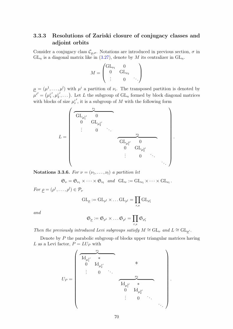
3.3.3 Resolutions of Zariski closure of conjugacy classes andadjoint orbits

Consider a conjugacy class Cµ,σ. Notations are introduced in previous section, σ inGLn is a diagonal matrix like in (3.27), denote by M its centralizer in GLn.

M =

GLν1 00 GLν2... 0

. . .

µ = (µ1, . . . , µl) with µi a partition of νi. The transposed partition is denoted byµi′=(µi1′, µi2

′, . . .

). Let L the subgroup of GLn formed by block diagonal matrices

with blocks of size µir′, it is a subgroup of M with the following form

L =

ν1︷ ︸︸ ︷GLµ11

′ 0

0 GLµ12′

... 0. . .

ν2︷ ︸︸ ︷GLµ21

′ 0

0 GLµ22′

... 0. . .

. . .

.

Notations 3.3.6. For ν = (ν1, . . . , νl) a partition let

Sν = Sν1 × · · · ×Sνl and GLν := GLν1 × · · · ×GLνl .

For ρ = (ρ1, . . . , ρl) ∈ Pν

GLρ := GLρ1 × . . .GLρl =∏r,s

GLρrs

andSρ := Sρ1 × . . .Sρl =

∏r,s

Sρrs

Then the previously introduced Levi subgroups satisfy M ∼= GLν and L ∼= GLµ′.

Denote by P the parabolic subgroup of blocks upper triangular matrices havingL as a Levi factor, P = LUP with

UP =

ν1︷ ︸︸ ︷Idµ11

′ ∗0 Idµ12

′

... 0. . .

*

ν2︷ ︸︸ ︷Idµ21

′ ∗0 Idµ22

′

... 0. . .

. . .

.

70

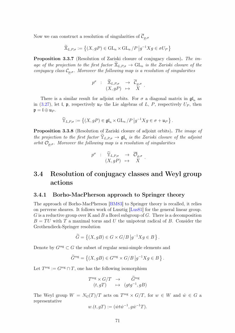
Now we can construct a resolution of singularities of Cµ,σ

XL,P,σ :=

(X, gP ) ∈ GLn×GLn /P∣∣g−1Xg ∈ σUP

Proposition 3.3.7 (Resolution of Zariski closure of conjugacy classes). The im-age of the projection to the first factor XL,P,σ → GLn is the Zariski closure of theconjugacy class Cµ,σ. Moreover the following map is a resolution of singularities

pσ : XL,P,σ → Cµ,σ(X, gP ) 7→ X

.

There is a similar result for adjoint orbits. For σ a diagonal matrix in gln asin (3.27), let l, p, respectively uP the Lie algebras of L, P , respectively UP , thenp = l⊕ uP .

YL,P,σ :=

(X, gP ) ∈ gln×GLn /P∣∣g−1Xg ∈ σ + uP

.

Proposition 3.3.8 (Resolution of Zariski closure of adjoint orbits). The image ofthe projection to the first factor YL,P,σ → gln is the Zariski closure of the adjointorbit Oµ,σ. Moreover the following map is a resolution of singularities

pσ : YL,P,σ → Oµ,σ(X, gP ) 7→ X

.

3.4 Resolution of conjugacy classes and Weyl groupactions

3.4.1 Borho-MacPherson approach to Springer theory

The approach of Borho-MacPherson [BM83] to Springer theory is recalled, it relieson perverse sheaves. It follows work of Lusztig [Lus81] for the general linear group.G is a reductive group overK and B a Borel subgroup ofG. There is a decompositionB = TU with T a maximal torus and U the unipotent radical of B. Consider theGrothendieck-Springer resolution

G =

(X, gB) ∈ G×G/B∣∣g−1Xg ∈ B

.

Denote by Greg ⊂ G the subset of regular semi-simple elements and

Greg =

(X, gB) ∈ Greg ×G/B∣∣g−1Xg ∈ B

.

Let T reg := Greg ∩ T , one has the following isomorphism

T reg ×G/T → Greg

(t, gT ) 7→ (gtg−1, gB)

The Weyl group W = NG(T )/T acts on T reg × G/T , for w ∈ W and w ∈ G arepresentative

w.(t, gT ) := (wtw−1, gw−1T ).

71

Thus W acts on Greg by

w.(X, gB) = (X, gw−1B).

Consider the following map

pG : G → G(X, gB) 7→ X

.

Denote by preg its restriction to Greg. Then preg is a Galois cover with group W .Denote by U ⊂ G the subset of unipotent elements and

U =

(X, gB) ∈ U ×G/B∣∣g−1Xg ∈ U

.

Consider the following diagram, both squares are cartesian

U G Greg

U G Greg.

pU pG

i

preg

i

Proposition 3.4.1 (Borho-MacPherson [BM83], 2.6). The Weyl group W acts onpG! κG and on pU! κU .

Proof. Let κGreg ∈ Dbc(Greg

)be the constant sheaf concentrated in degree 0. It

is W -equivariant with φw : w∗κGreg → κGreg a morphism which is the identity onstalks. preg is equivariant for the trivial action of W on Greg so that by Proposition3.1.6, W acts on preg

! κGreg and there is a group morphism W op → Aut(p!κGreg). Thismorphism is composed with inversion in order to obtain a left action.

This rather formal construction will be relevant later to compare various actions.In the present situation the action can be easily described without the formalism ofW -equivariant complexes. The complex preg

! κGreg is concentrated in degree 0, its stalkis isomorphic to the group algebra of W , the group W acts by right multiplication.

Springer theory extends this action to the derived pushforward pG! κG. FirstpG is small, and by base change i∗pG! κG ∼= preg

! i∗κGreg . Therefore pG! κG[dim G] =

IC•preg! κGreg

. Then Aut(preg! κGreg) ∼= Aut

(IC•preg! κ

Greg

)so that W acts on pG! κG. To

conclude, by base change pU! κU is isomorphic to the restriction of pG! κG to U .

To study characters varieties, this construction is used when G is either GLn ora Levi subgroup of a parabolic subgroup of GLn.

Example 3.4.2. When G = GLn, the Weyl group is isomorphic to a symmetricgroup Sn. The irreducible representations of the symmetric group Sn are indexedby partitions of n. For λ ∈ Pn the associated irreducible representation is Vλ. Thetrivial representation is V(n) and V(1n) is the signature. Then there is a nice descrip-tion of the left W -action on pU! κU

pU! κU

[dim U

]=⊕λ∈Pn

Vλ ⊗ IC •Cλ .

With Cλ the unipotent class with Jordan type λ. With notations from previous sectionCλ = Cλ,1.

72

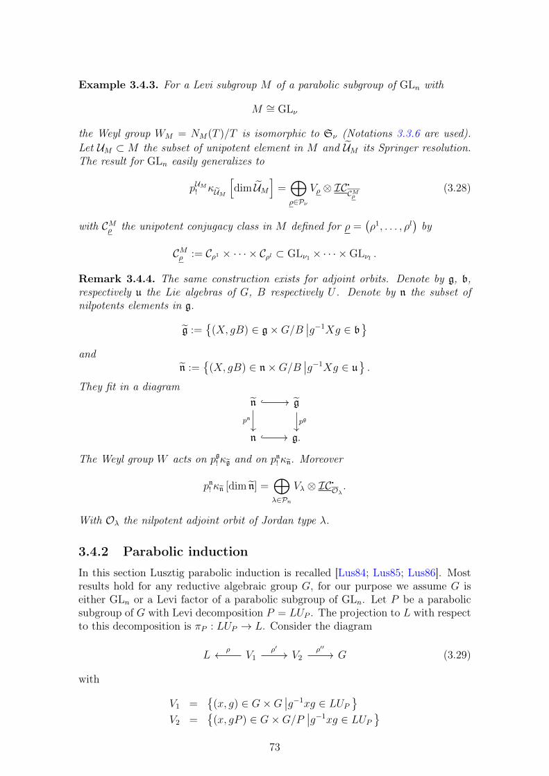
Example 3.4.3. For a Levi subgroup M of a parabolic subgroup of GLn with

M ∼= GLν

the Weyl group WM = NM(T )/T is isomorphic to Sν (Notations 3.3.6 are used).Let UM ⊂M the subset of unipotent element in M and UM its Springer resolution.The result for GLn easily generalizes to

pUM! κUM

[dim UM

]=⊕ρ∈Pν

Vρ ⊗ IC •CMρ (3.28)

with CMρ the unipotent conjugacy class in M defined for ρ =(ρ1, . . . , ρl

)by

CMρ := Cρ1 × · · · × Cρl ⊂ GLν1 × · · · ×GLνl .

Remark 3.4.4. The same construction exists for adjoint orbits. Denote by g, b,respectively u the Lie algebras of G, B respectively U . Denote by n the subset ofnilpotents elements in g.

g :=

(X, gB) ∈ g×G/B∣∣g−1Xg ∈ b

and

n :=

(X, gB) ∈ n×G/B∣∣g−1Xg ∈ u

.

They fit in a diagramn g

n g.

pn pg

The Weyl group W acts on pg! κg and on pn! κn. Moreover

pn! κn [dim n] =⊕λ∈Pn

Vλ ⊗ IC •Oλ .

With Oλ the nilpotent adjoint orbit of Jordan type λ.

3.4.2 Parabolic induction

In this section Lusztig parabolic induction is recalled [Lus84; Lus85; Lus86]. Mostresults hold for any reductive algebraic group G, for our purpose we assume G iseither GLn or a Levi factor of a parabolic subgroup of GLn. Let P be a parabolicsubgroup of G with Levi decomposition P = LUP . The projection to L with respectto this decomposition is πP : LUP → L. Consider the diagram

L V1 V2 Gρ ρ′ ρ′′ (3.29)

with

V1 =

(x, g) ∈ G×G∣∣g−1xg ∈ LUP

V2 =

(x, gP ) ∈ G×G/P

∣∣g−1xg ∈ LUP

73

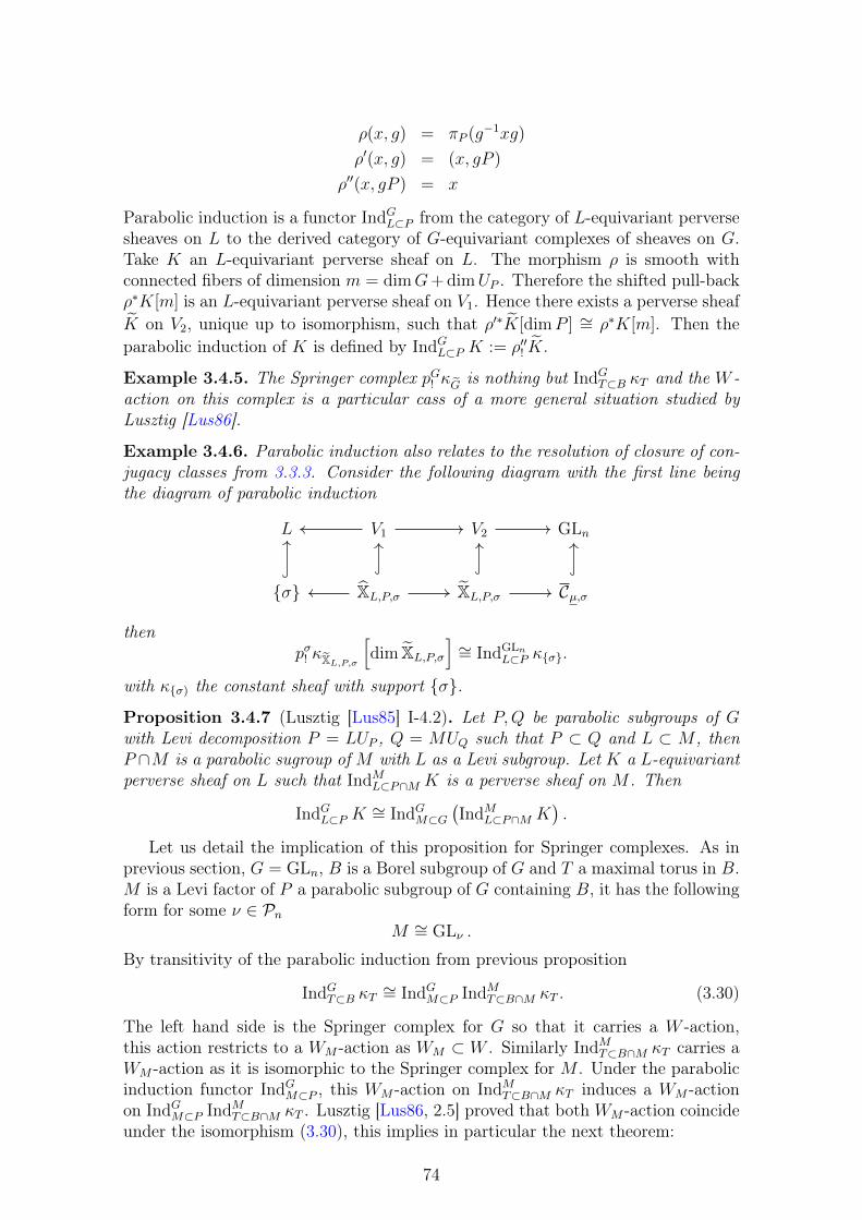
ρ(x, g) = πP (g−1xg)

ρ′(x, g) = (x, gP )

ρ′′(x, gP ) = x

Parabolic induction is a functor IndGL⊂P from the category of L-equivariant perversesheaves on L to the derived category of G-equivariant complexes of sheaves on G.Take K an L-equivariant perverse sheaf on L. The morphism ρ is smooth withconnected fibers of dimension m = dimG+ dimUP . Therefore the shifted pull-backρ∗K[m] is an L-equivariant perverse sheaf on V1. Hence there exists a perverse sheafK on V2, unique up to isomorphism, such that ρ′∗K[dimP ] ∼= ρ∗K[m]. Then theparabolic induction of K is defined by IndGL⊂P K := ρ′′! K.

Example 3.4.5. The Springer complex pG! κG is nothing but IndGT⊂B κT and the W -action on this complex is a particular cass of a more general situation studied byLusztig [Lus86].

Example 3.4.6. Parabolic induction also relates to the resolution of closure of con-jugacy classes from 3.3.3. Consider the following diagram with the first line beingthe diagram of parabolic induction

L V1 V2 GLn

σ XL,P,σ XL,P,σ Cµ,σ

thenpσ! κXL,P,σ

[dim XL,P,σ

]∼= IndGLn

L⊂P κσ.

with κσ) the constant sheaf with support σ.

Proposition 3.4.7 (Lusztig [Lus85] I-4.2). Let P,Q be parabolic subgroups of Gwith Levi decomposition P = LUP , Q = MUQ such that P ⊂ Q and L ⊂ M , thenP ∩M is a parabolic sugroup of M with L as a Levi subgroup. Let K a L-equivariantperverse sheaf on L such that IndML⊂P∩M K is a perverse sheaf on M . Then

IndGL⊂P K∼= IndGM⊂G

(IndML⊂P∩M K

).

Let us detail the implication of this proposition for Springer complexes. As inprevious section, G = GLn, B is a Borel subgroup of G and T a maximal torus in B.M is a Levi factor of P a parabolic subgroup of G containing B, it has the followingform for some ν ∈ Pn

M ∼= GLν .

By transitivity of the parabolic induction from previous proposition

IndGT⊂B κT∼= IndGM⊂P IndMT⊂B∩M κT . (3.30)

The left hand side is the Springer complex for G so that it carries a W -action,this action restricts to a WM -action as WM ⊂ W . Similarly IndMT⊂B∩M κT carries aWM -action as it is isomorphic to the Springer complex for M . Under the parabolicinduction functor IndGM⊂P , this WM -action on IndMT⊂B∩M κT induces a WM -actionon IndGM⊂P IndMT⊂B∩M κT . Lusztig [Lus86, 2.5] proved that both WM -action coincideunder the isomorphism (3.30), this implies in particular the next theorem:

74

Theorem 3.4.8. Let σ ∈ Z(L) and κσ the constant sheaf with support σ. LetM = ZGLn(σ), assume M ∼= GLν

IndGLnL⊂P κσ

∼=⊕ρ∈Pν

HomWM

(IndWM

WLε, Vρ

)⊗ IC•Cρ,σ

with ε the sign representation of WL.

Remark 3.4.9. The same constructions exist for Lie algebras, see for instance[Let05]. Previous theorem then becomes:

Indglnl⊂p κσ

∼=⊕ρ∈Pν

HomWM

(IndWM

WLε, Vρ

)⊗ IC•Oρ,σ

3.4.3 Relative Weyl group actions on multiplicity spaces

An interesting feature of the multiplicity spaces HomWM

(IndWM

WLε, Vρ

)is that they

carry a relative Weyl group action. Before describing this action, we recall a generalresult about symmetric group, see Letellier [Let11, 6.1, 6.2].

Consider a type ω = (d1, ω1) . . . (dl, ω

l) ∈ Tn (the set of types was defined in3.3.3). The associated Schur function is

sω = sω1

[Xd1

]. . . sωl

[Xdl]

and

r(ω) :=l∑

i=1

(di − 1)|ωi|. (3.31)

Definition 3.4.10 (Twisted Littlewood-Richardson coefficients). As the usual Schurfuntions (sρ)ρ∈Pn form a basis of Symn[X], there exist coefficients cρω such that

sω =∑ρ∈Pn

cρωsρ.

Coefficients cρω are called the twisted Littlewood-Richardson coefficients.

Lemma 3.4.11. Let ω′ the transpose of ω, i.e ω′ =(d1, ω

1′) . . .(dl, ωl′). Then

cρ′

ω′ = (−1)r(ω)cρω.

with r(ω) defined in (3.31).

Proof. This follows from a computation in the ring of symmetric functions using thebasis of power sums, see Letellier [Let11, 6.2.4].

Let us recall their interpretation in terms of representations of symmetric group.The type ω defines an irreducible representation Vω of the groupSω :=

∏li=1 S

di|ωi|.

Vω := ⊗li=1V⊗diωi

75

with Vωi the representation of S|ωi| indexed by the partition ωi. Denote by fω themorphism Sω → GL(Vω) induced by the representation Vω. Introduce the relativeWeyl group

WSn (Sω, Vω) =n ∈ NSn(Sω)

∣∣fω(n−1 . . . n) = fω(. . . )/Sω

This is the group of permutations of the blocks of Sω corresponding to the samerepresentation Vωi .

Proposition 3.4.12 (Letellier [Let11] Proposition 6.2.5). For ρ ∈ Pn and Vρ theassociated representation of Sn. For ω ∈ Tn a type. The relative Weyl groupWSn (Sω, Vω) acts on

HomSn

(IndSn

SωVω, Vρ

).

Let w ∈ WSn (Sω, Vω) acting by cyclic permutation of the di blocks with representa-tion Vωi for 1 ≤ i ≤ l. Then

tr(w,HomSn

(IndSn

SωVω, Vρ

))= cρω.

Remark 3.4.13. Assume the type ω has the following form

ω = (λ1, (1)) . . . (λl, (1)) with λ = (λ1, . . . , λl) ∈ Pn.

Then sω = pλ and by (3.14), for ρ ∈ Pn

cρω = χρλ

Notice that WSn (Sn, Vω) ∼= Sn and the element w associated to ω has cycle type λ.Therefore the proposition implies that as a WSn (Sn, Vω) representation

HomSn

(IndSn

SωVω, Vρ

) ∼= Vρ.

With this general result about symmetric group, we go back to the Weyl groupsrelative to resolution of conjugacy classes.

Definition 3.4.14 (Relative Weyl group). For L a Levi subgroup ofM , The relativeWeyl group is

WM(L) := NM(L)/L.

Take L and M similarly to Section 3.3.3. Denote by (mi1, . . . ,m

iki

) the multiplic-ity of the parts of µi′ so that it has the following form

µi′=

ai1, . . . , ai1︸ ︷︷ ︸mi1

, ai2, . . . , ai2︸ ︷︷ ︸

mi2

, . . . , aiki , . . . , aiki︸ ︷︷ ︸

miki

.

Then with notations 3.3.6 L ∼= GLµ′ and the relative Weyl group is

WM(L) ∼=∏

1≤i≤l1≤r≤ki

Smir.

When M = GLn then the relative Weyl group is the group of permutations ofsame-sized blocks of L.

76

Notations 3.4.15. Conjugacy classes in WM(L) are indexed by elements

η = (ηi,r) 1≤i≤l1≤r≤ki

∈∏

1≤i≤l1≤r≤ki

Pmir .

A conjugacy class then determined l distinct types ωηi with parts(ηi,rs , (1

air))

1≤r≤ki1≤s≤l(ηi,r)

.

Note that

sω′ηi

=

ki∏r=1

l(ηi,r)∏s=1

hair

[Xηi,rs

]Following notations will be convenient to compute Weyl group actions on the coho-mology of character varieties.

hη :=l∏

i=1

sω′ηi

and

r(η) :=l∑

i=1

r(ωηi).

with r(ωηi) defined by (3.31).

Those data describe the WM(L) action on the multiplicity spaces, Proposition3.4.12 implies:

Theorem 3.4.16. Let εµ′ the sign representation of WL and ρ ∈ Pν. The relative

Weyl group WM(L) acts on HomWM

(IndWM

WLεµ′ , Vρ

). The trace of the action of an

element with conjugacy class indexed by η ∈∏

1≤i≤lj1≤r≤ki

Pmir is

tr(η,HomWM

(IndWM

WLεµ′ , Vρ

))=

l∏i=1

cρi

wηi.

3.4.4 Relative Weyl group actions and Springer theory

There is another construction of relative Weyl group action using another variantof Springer theory. It will be useful to construct relative Weyl group actions whenconsidering family of comet-shaped quiver varieties.

Let P be a parabolic subgroup of GLn and L a Levi factor of P . L is isomorphicto a group of blocks diagonal matrices GLc1 × · · · × GLcr . The Lie algebra of L,respectivly UP are denoted l respectivly uP . At the level of the Lie algebras the Levidecomposition becomes p = l⊕ uP . The center of this Lie algebra l is denoted Z(l)and its regular locus is

Z(l)reg = x ∈ Z(l) |ZG(x) = L .

DefineYregL,P =

(x, gL) ∈ gln×GLn /L

∣∣g−1xg ∈ Z(l)reg

Consider the projection on the first factor preg : YregL,P → gln, denote Y

regL,P its im-

age. This image consists of semisimple elements with r distinct eigenvalues with

77

multiplicities c1, . . . , cr. Consider the relative Weyl group WGLn(L) = NGLn(L)/L,and for each w ∈ WGLn(L) chose a representative w ∈ NGLn(L). This relative Weylgroup acts on Z(l) by

w.σ := wσw−1.

Consider the fiber product

Z(l)reg YregL,P ×Z(l)reg/WGLn (L) Z(l)reg

Z(l)reg/WGLn(L) YregL,Pχ

with χ the characteristic polynomial. Note that the following map is an isomorphism

YregL,P → Yreg

L,P ×Z(l)reg/WGLn (L) Z(l)reg

(x, gL) 7→ (x, g−1xg)(3.32)

Therefore the WGLn(L) action on Z(l)reg induces an action on YregL,P . It is given

explicitly byw.(x, gL) = (x, gw−1L).

ThenYregL,P

preg−−→ YregL,P

is a Galois cover with group WGLn(L). This relative Weyl group acts on the pushforward of the constant sheaf preg

∗ κ. Define

YL,P =

(x, gP ) ∈ gln×GLn /P∣∣g−1xg ∈ Z(l)⊕ uP

Remark 3.4.17. An element gP ∈ GLn /P identifies with a partial flag

0 = Er ⊂ Er−1 ⊂ · · · ⊂ E1 ⊂ Kn

such that dimEi−1/Ei = ci for all 1 ≤ i ≤ r. Indeed GLn acts transitively onsuch flags and the stabilizer is P . Then a point (x, gP ) in YL,P consists of anendomorphism x ∈ gln and a partial flag gP preserved by x such that x acts as ascalar on Ei−1/Ei for all 1 ≤ i ≤ r.

Denote YL,P the image of the projection to the first factor p : YL,P → gln.Note that the map p is proper. The following theorem is a particular case of[Lus84, Lemma 4.3 and Proposition 4.5]. It can be seen as a generalization ofBorho-MacPherson result.

Theorem 3.4.18. YregL,P is an open, dense, smooth subset of YL,P and the following

square is cartesian

YregL,P YL,P

YregL,P YL,P

i

preg p (3.33)

with i the map (x, gL)→ (x, gP ). Moreover p!κ = IC• (YL,P , preg! κ) so thatWGLn(L)

acts on p∗κ.

78

Remark 3.4.19. preg is a Galois cover and i an open embedding so that the dimen-sions can be easily computed:

dimYL,P = dim YL,P = dim YregL,P = dim GLn− dimL+ dimZ(L). (3.34)

Let us describe the relation with the resolution of closure of adjoint orbits in-troduced in 3.3.8. Let σ ∈ Z(l) and M := ZGLn(σ). Then use the same notationsas in 3.3.3 so that M ∼= GLν for ν a partition of n. Moreover L ⊂ M and theintegers (c1, c2, . . . , cr) are relabelled (µ1

1′, µ1

2′, . . . ) so that µi′ is a partition of νi.

The inclusion L ⊂M comes from inclusions

GLµi1′ × · · · ×GLµili

′ ⊂ GLνi .

The resolution of the closure of Oµ,σ fits in the following diagram

YL,P YL,P,σ

YL,P Oµ,σ =⊔ρµOρ,σ

p pσ (3.35)

The decomposition Oµ,σ =⊔ρµOρ,σ actualy comes from a decomposition of

YL,P . DefineYM,ρ

L,P :=⊔

σ′∈Z(m)reg

Oρ,σ′ .

This decomposition is similar to the one introduced by Shoji [Sho88].

Proposition 3.4.20. YM,ρ

L,P is smooth of dimension

dimYM,ρ

L,P = dimOρ,σ + dimZ(m).

Then YL,P admits the following decomposition

YL,P =⊔M

⊔ρµ

YM,ρ

L,P .

The first union is over the set of centralizer of elements σ ∈ Z(l). In the secondunion, µ depends on M as previously described. The unique part indexed by M = Lis Yreg

L,P .

Proof. Denote by Zρ the centralizer in GLn of the element Jρ,σ in Oρ,σ (see Notations3.3.1). Then there is a natural finite cover

Z(m)reg ×GLn /Zρ → YM,ρ

L,P(σ′, gZρ

)7→ gJρ,σ′g

−1

Therefore YM,ρ

L,P is smooth and

dimYM,ρ

L,P = dimOρ,σ + dimZ(m).

79

3.5 Character varieties and their additive counter-part

In this section the main objects studied in this thesis are introduced.

3.5.1 Character varieties

Let Σ be a compact Riemann surface of genus g. Consider the punctured Riemannsurface Σ = Σ\p1, . . . , pk where pj are distinct points on Σ called punctures. Thefield K is either C or an algebraic closure Fq of a finite field Fq with q elements. Fixa non negative integer n. We are concerned by n-dimensional K-representations ofthe fundamental group of Σ with prescribed monodromy around the punctures.

For each puncture, specify a conjugacy class Cµj ,σj . The notations are the sameas in previous section, with the addition of an upper index 1 ≤ j ≤ k labelling thepunctures. σj is a diagonal matrix with diagonal coefficients

(σj1, . . . , σj1︸ ︷︷ ︸

νj1

, . . . , σjlj , . . . , σjlj︸ ︷︷ ︸

νjlj

)

and σjr 6= σjs for r 6= s. Moreover, µj =(µj,1, . . . , µj,lj

)with µj,r ∈ Pνjr the partition

giving the size of the Jordan blocks of the eigenvalue σjr .A bold symbol is used to represent k-uple:

µ :=(µ1, . . . , µk

)σ :=

(σ1, . . . , σk

)Cµ,σ :=

(Cµ1,σ1 , . . . , Cµk,σk

) (3.36)

The representations of the fundamental group of Σ with monodromy around pjin the closure Cµj ,σj form the following affine variety

RCµ,σ :=

(A1, B1, . . . , Ag, Bg, X1, . . . , Xk) ∈ GL2gn ×Cµ1,σ1 × · · · × Cµk,σk

∣∣∣A1B1A

−11 B−1

1 . . . AgBgA−1g B−1

g X1 . . . Xk = Id.

The group GLn acts by simultaneous conjugation on RCµ,σ

g. (A1, . . . , Bg, X1, . . . , Xk) =(gA1g

−1, . . . , gBgg−1, gX1g

−1, . . . , gXkg−1).

The center of GLn acts trivially so this action factors through an action of PGLn.

Definition 3.5.1 (Character variety). The character variety we are interested in isthe following GIT quotient

MCµ,σ := RCµ,σ//PGLn := SpecK[RCµ,σ

]PGLn.

It is an affine variety with regular functions the PGLn-invariants functions on RCµ,σ .

Under some generecity assumptions, the PGLn action is free.

80

Definition 3.5.2 (Generic conjugacy classes). Denote ∆(σj) the multiset of eigen-values of σj repeated according to multiplicities. σjr appears exactly νjr times in themultiset ∆(σj). The k-uple of conjugacy classes Cµ,σ is generic if and only if itsatisfy the two following conditions

1.k∏j=1

∏α∈∆(σj)

α = 1

2. For any r ≤ n− 1, for all (R1, . . . , Rk) with Rj ⊂ ∆(σj) of size r

k∏j=1

∏α∈Rj

α 6= 1

Throughout the thesis, every character varieties considered are assumed to havegeneric conjugacy classes at the punctures.

Remark 3.5.3. If the k-uple of conjugacy classes Cµ,σ is generic and V is a non-zero subspace of Kn stable by some elements Xj ∈ Cµj ,σj such that

k∏j=1

det(Xj |V ) = 1

then V = Kn.

Definition 3.5.4. Let RCµ,σ := RCµ,σ ∩(

GLn(K)2g ×∏k

j=1 Cµj ,σj)and MCµ,σ the

image of RCµ,σ in RCµ,σ .

Proposition 3.5.5. If Cµ,σ is generic then points of RCµ,σ correspond to irreduciblerepresentations of the fundamental group of the punctured Riemann surface Σ.

Proof. Let V be a subrepresentation of (A1, B1, . . . , Ag, Bg, X1, . . . , Xk) ∈ RCµ,σ .Then V is stable by thoses matrices and the equation defining RCµ,σ restricts to

(A1|V , B1|V ) . . . (Ag |V , Bg |V )X1|V . . . Xk |V = IdV .

Taking determinant, the genericity implies V = 0 or V = Kn.

We recall a proposition from [Let13], and [HLR11] for the semisimple case.

Proposition 3.5.6. If Cµ,σ is generic then RCµ,σ is non-singular, when non-emptyits dimension is

dimRCµ,σ = 2gn2 − n2 + 1 +k∑j=1

dim Cµj ,σj .

Proof. The proof combines the one of theorem 2.2.5 in [HR08] and proposition 5.2.8in [EOR04].RC = µ−1(In) where µ is the map

81

µ : GLn(K)2g ×∏k

i=1 Ci → SLn(K)(A1, B1, . . . , Ag, Bg, X1, . . . , Xk) 7→ (A1, B1) . . . (Ag, Bg)X1 . . . Xk.

It is enough to check that the differential dµz of this map at a point

z = (A1, B1, . . . , Ag, Bg, X1, . . . , Xk) ∈ RCis a surjective map between tangent space. The tangent space of SLn(K) is the Liealgebra sln(K). The tangent space of Ci at Xi is made of Lie brackets [ri, Xi] forri ∈ gln(K). Hence an element of the tangent space at z reads

v = (h1, l1, . . . , hg, lg, [r1, X1], . . . , [rk, Xk])

for ri, hj, lj ∈ gln(K). First we compute the differential with respect to Aj of thecommutator Aj 7→ AjBjA

−1j B−1

j

dj(hj) := hjBjA−1j B−1

j − AjBjA−1j hjA

−1j B−1

j

similarly with respect to Bj

d′j(lj) := AjljA−1j B−1

j − AjBjA−1j B−1

j ljB−1j .

We use the usual rule to differentiate a product of matrix

dµz(v) =k∑i=1

(A1, B1) . . . (Ag, Bg)X1 . . . Xi−1[ri, Xi]Xi+1 . . . Xk

+

g∑j=1

(A1, B1) . . . (Aj−1, Bj−1)dj(hj)(Aj+1, Bj+1) . . . (Ag, Bg)X1 . . . Xk

+

g∑j=1

(A1, B1) . . . (Aj−1, Bj−1)d′j(lj)(Aj+1, Bj+1) . . . (Ag, Bg)X1 . . . Xk

the first, respectively second and third lines correspond to differenciation with re-spect to Xi respectively Aj and Bj. Now we use that z satisfies the equation definingRC

dµz(v) =k∑i=1

(Xi . . . Xk)−1[ri, Xi]Xi+1 . . . Xk

+

g∑j=1

(A1, B1) . . . (Aj−1, Bj−1)dj(hj) ((A1, B1) . . . (Aj−1, Bj−1)(Aj, Bj))−1

+

g∑j=1

(A1, B1) . . . (Aj−1, Bj−1)d′j(lj) ((A1, B1) . . . (Aj−1, Bj−1)(Aj, Bj))−1

We rewrite to exhibit some conjugation

dµz(v) =k∑i=1

(Xi+1 . . . Xk)−1X−1

i [ri, Xi]Xi+1 . . . Xk

+

g∑j=1

(A1, B1) . . . (Aj−1, Bj−1)dj(hj)(Aj, Bj)−1 ((A1, B1) . . . (Aj−1, Bj−1))−1

+

g∑j=1

(A1, B1) . . . (Aj−1, Bj−1)d′j(lj)(Aj, Bj)−1 ((A1, B1) . . . (Aj−1, Bj−1))−1

82

. To prove that this differential is surjective we take u ∈ sln(K) such that for any vtangent to z we have tr(dµz(v)u) = 0 and show that u = 0. For any ri ∈ gln(K) wemust have

tr((Xi+1 . . . Xk)−1X−1

i [ri, Xi]Xi+1 . . . Xku) = 0 (3.37)Let us prove by recursion that u commutes with Xi for all 1 ≤ i ≤ k.When i = k

0 = tr(X−1k [rk, Xk]u) = tr(X−1

k rkXku)− tr(rku) = tr(rkXkuX−1k − rku)

in last equality we use the cyclicity of the trace. This must be true for any rk sothat u = XkuX

−1k . Now let us assume that u commutes with Xm for any i < m ≤ k,

(3.37) impliestr(X−1

i [ri, Xi]u) = 0

so that u commutes with Xi. Similarly u commutes with Aj and Bj. By genericityand Schur lemma this implies that u is a scalar matrix, as it is in sln(K) it must bezero which achieves the proof.

Proposition 3.5.7 (Stratification of MCµ,σ , [Let13] Corollary 3.6 ). We assumeCµ,σ is generic. The stratification of Zariski closure of conjugacy classes induces astratification of the character variety:

MCµ,σ =⊔ρµ

MCρ,σ .

The union is over ρ =(ρ1, . . . , ρk

)with ρj =

(ρj,1, . . . , ρj,lj

)such that

ρj,i µj,i, for all 1 ≤ j ≤ k, 1 ≤ i ≤ lj

with the dominance order on Pνji .Moreover ifMCµ,σ is non empty, thenMCµ,σ is also non empty. Therefore when

MCµ,σ is non empty, its dimension is

dimMCµ,σ = dµ := n2(2g − 2) + 2 +k∑j=1

dim Cµj ,σj . (3.38)

3.5.2 Additive analogous of Character varieties

Instead of the multiplicative equation in GLn defining RCµ,σ , one can consider ad-ditive equation in gln. This is called the additive Deligne-Simpson problem. It wasstudied by Crawley-Boevey [Cra03b], [Cra06] in the case g = 0, by Hausel, Letel-lier and Rodriguez-Villegas [HLR11] for semisimple adjoint orbits and by Letellier[Let11] in general.

As before, notation from 3.3.1 are used, and a k-uple of adjoint orbits in gln isintroduced:

Oµ,σ :=(Oµ1,σ1 , . . . ,Oµk,σk

).

Consider the affine variety

VOµ,σ :=

(A1, B1, . . . , Ag, Bg, X1, . . . , Xk) ∈ gl2gn ×Oµ1,σ1 × · · · × Oµk,σk∣∣∣

g∑i=1

[Ai, Bi] +k∑j=1

Xj = 0

.

83

This is an affine variety acted upon by GLn by coordinate-wise adjoint action. Thecenter of GLn acts trivialy so that the action factors through a PGLn action. Con-sider the GIT quotient

QOµ,σ := VOµ,σ//

PGLn = Spec

(K[VOµ,σ

]GLn). (3.39)

Definition 3.5.8 (Generic adjoint orbits). Denote ∆(σj) the multiset of eigenvaluesof σj repeated according to multiplicities. σjr appears exactly νjr times in the multiset∆(σj). The k-uple of adjoint orbits Oµ,σ is generic if and only if it satisfy the twofollowing conditions

1.k∑j=1

∑α∈∆(σj)

α = 0

2. For any r ≤ n− 1, for all (R1, . . . , Rk) with Rj ⊂ ∆(σj) of size r

k∑j=1

∑α∈Rj

α 6= 0

.

Remark 3.5.9. Contrarily to the multiplicative case, generic k-uple of adjoint orbitsdo not exist for every multiplicities (ν1, . . . , νk). In particular if an integer d > 1divides all νj for 1 ≤ j ≤ k.

Character varieties and their additive analogous share many properties in com-mon. They have the same dimension and similar stratifications. Let

UOµ,σ := UOµ,σ ∩ gl2gn ×Oµ1,σ1 × · · · × Oµk,σk

and QOµ,σ the image of UOµ,σ in QOµ,σ .

Proposition 3.5.10 (Stratification of QOµ,σ). Assume Oµ,σ is generic, then

QOµ,σ =⊔ρµ

QOρ,σ

is a stratification of QOµ,σ . Moreover

dimQOµ,σ = dµ = n2(2g − 2) + 2 +k∑j=1

dimOµj ,σj .

3.5.3 Resolutions of character varieties

The resolutions of conjugacy classes introduced in 3.3.3 induce resolutions of char-acter variety. As before we consider a generic k-uple of conjugacy classes

Cµ,σ =(Cµ1,σ1 , . . . , Cµk,σk

)84

and upper indices 1 ≤ j ≤ k label the puncture. As usual σj is a diagonal matrixwith diagonal coefficients

(σj1, . . . , σj1︸ ︷︷ ︸

νj1

, . . . , σjlj , . . . , σjlj︸ ︷︷ ︸

νjlj

).

Let M j := ZGLn(σj) then with Notation 3.3.6

M j ∼= GLνj

As usual µj,i ∈ Pνji is the Jordan type of σji . Denote by µj,i′ =(µj,i1

′, µj,i2

′, . . .

)the

transposed partition. Let Lj ⊂M j the subgroup of diagonal matrices as in 3.3.3

Lj ∼= GLµj,11

′ ×GLµj,12

′ × . . .︸ ︷︷ ︸⊂GL

νj1

× · · · ×GLµj,lj1

′ ×GLµj,lj2

′ × . . .︸ ︷︷ ︸⊂GL

νjlj

.

Let XLj ,P j ,σj a resolution of Cµj ,σj as constructed in 3.3.3. Let

XL,P ,σ :=∏

1≤j≤k

XLj ,P j ,σj .

Letellier [Let13] constructed resolutions of singularities for character varieties.

Definition 3.5.11 (Resolutions of character variety). Define

ML,P ,σ :=

(Ai, Bi)1≤i≤g, (Xj, gjPj)1≤j≤k ∈ GL2g

n ×XL,P ,σ∣∣A1B1A−11 B−1

1 . . . B−1g X1 . . . Xk = Id

//PGLn . (3.40)

The maps pσj : XLj ,P j ,σj → Cµj ,σj induce a map

pσ : ML,P ,σ →MCµ,σ

this map is a resolution of singularity.

Next theorem is a particular case of a result of Letellier [Let13, Theorem 5.4]

Theorem 3.5.12.pσ! κ[dµ] ∼=

⊕ρµ

Aµ′,ρ ⊗ IC•MCσ,ρ

and in terms of cohomology:

H i+dµc

(ML,P ,σ, κ

)∼=⊕ρµ

Aµ′,ρ ⊗ IH i+dρc

(MCσ,ρ , κ

). (3.41)

The multiplicity space Aµ′,ρ will be described in the remaining of the section.

85

Like the resolutions of closure of conjugacy classes, the resolution of charactervarieties come with a Weyl group action à la Springer. First we present the Weylgroups involved. The Weyl group of M j is WMj = NMj(T )/T then

WMj∼= Sνj .

For ρj =(ρj,1, . . . , ρj,lj

)∈ Pνj and Vρj,i the irreducible representation of Sνji

indexedby ρj,i let

Vρj :=

lj⊗i=1

Vρj,i

it is an irreducible representation of WMj .The Weyl group of Lj is WLj = NLj(T )/T , it is a subgroup of WMj

WLj∼= S

µj,11

′ ×Sµj,12

′ × . . .︸ ︷︷ ︸⊂S

νj1

× · · · ×Sµj,lj1

′ ×Sµj,lj2

′ × . . .︸ ︷︷ ︸⊂S

νjlj

.

The sign representation for this Weyl group is

εµj ′ :=

lj⊗i=1

⊗r

εµj,ir′ .

It was previously denoted only by ε, the index is now added to remind the form ofthe Weyl group WLj

∼= Sµj ′ .

Definition 3.5.13. The multiplicity space relative to the j-th puncture is

Aµj ′,ρj = HomWMj

(Ind

WMj

WLjεµj ′ , Vρj

).

Remark 3.5.14. The expression is particularly simple when Lj is a torus T . Thenthe multiplicity space is just Vρj .

Define WM :=∏k

j=1 WMj and similarly WL :=∏k

j=1WLj . The parameter ρ =

(ρ1, . . . , ρk) ∈ Pν1 × · · · × Pνk indexes irreducible representations of

WM∼=

k∏j=1

lj∏i=1

Sνji.

Vρ is the following irreducible representation of∏k

j=1

∏lji=1 Sνji

Vρ =k⊗j=1

lj⊗i=1

Vρj,i . (3.42)

Now εµ′ is the sign representation of WL, namely

εµ′ :=k⊗j=1

εµj ′

The description of the multiplicity space for resolutions of closure of conjugacyclasses (Theorem 3.4.8) extends to Aµ′,ρ:

86

Notations 3.5.15. The multiplicity space Aµ′,ρ is

Aµ′,ρ = HomWM

(IndWMWL εµ′ , Vρ

)=

k⊗j=1

Aµj ′,ρj

Everything in this section also apply to the additive case.

Definition 3.5.16. For Oµ,σ a generic k-uple of adjoint orbits, define

QL,P ,σ :=

(Ai, Bi)1≤i≤g, (Xj, gjPj)1≤j≤k ∈ GL2g

n ×YL,P ,σ∣∣∣∣∣g∑i=1

[Ai, Bi] +k∑j=1

Xj = 0

//PGLn . (3.43)

The maps pσj : YLj ,P j ,σj → Oµj ,σj induce a resolution of singularities:

pσ : QL,P ,σ → QOµ,σ .

Theorem 3.5.17.pσ! κ[dµ] ∼=

⊕ρµ

Aµ′,ρ ⊗ IC•QOρ,σ

and in terms of cohomology:

H i+dµc

(QL,P ,σ, κ

)∼=⊕ρµ

Aµ′,ρ ⊗ IH i+dρc

(MOρ,σ , κ

). (3.44)

3.5.4 Relative Weyl group actions

An interesting feature of the multiplicity spaces Aµ′,ρ is that they carry a relativeWeyl group action. It is constructed by Letellier [Let11, 6.1, 6.2]. The relative Weylgroup is

WM (L) :=k∏j=1

WMj(Lj)

with WMj(Lj) the relative Weyl groups described in 3.4.3. Their action on themultiplicity spaces provide a WM (L)-action on Aµ′,ρ. As usual an index 1 ≤ j ≤ kis added to label the puncture. Conjugacy classes inWM (L) are labelled by elements

η = (ηj)1≤j≤k

with ηj ∈∏

1≤i≤lj1≤r≤kj,i

Pmj,ir as in 3.4.3 with an additional index j for the puncture.

ηj = (ηj,i,r) 1≤i≤lj1≤r≤kj,i

∈∏

1≤i≤lj1≤r≤kj,i

Pmj,ir .

Notations 3.4.15 extend to k-uple:

87

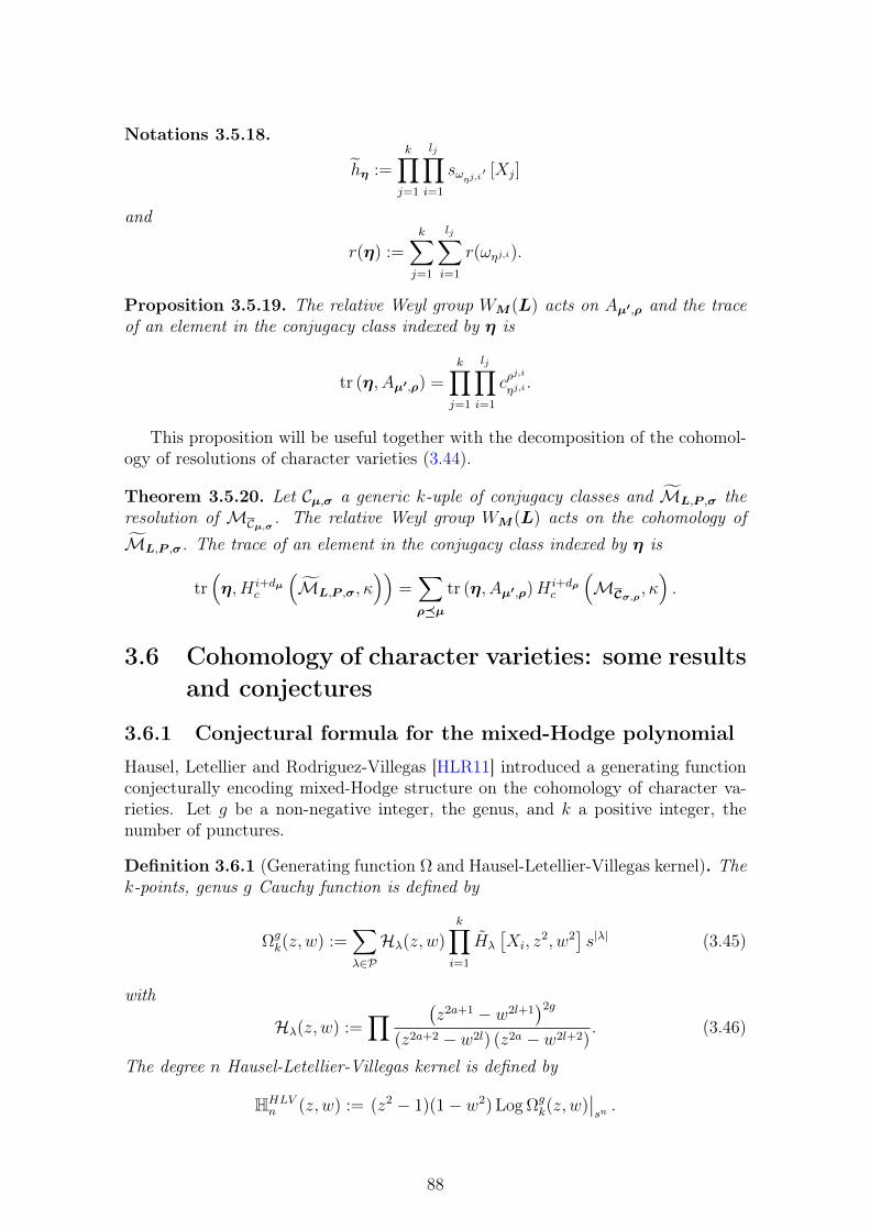
Notations 3.5.18.

hη :=k∏j=1

lj∏i=1

sωηj,i′ [Xj]

and

r(η) :=k∑j=1

lj∑i=1

r(ωηj,i).

Proposition 3.5.19. The relative Weyl group WM (L) acts on Aµ′,ρ and the traceof an element in the conjugacy class indexed by η is

tr (η, Aµ′,ρ) =k∏j=1

lj∏i=1

cρj,i

ηj,i.

This proposition will be useful together with the decomposition of the cohomol-ogy of resolutions of character varieties (3.44).

Theorem 3.5.20. Let Cµ,σ a generic k-uple of conjugacy classes and ML,P ,σ theresolution of MCµ,σ . The relative Weyl group WM (L) acts on the cohomology ofML,P ,σ. The trace of an element in the conjugacy class indexed by η is

tr(η, H i+dµ

c

(ML,P ,σ, κ

))=∑ρµ

tr (η, Aµ′,ρ)Hi+dρc

(MCσ,ρ , κ

).

3.6 Cohomology of character varieties: some resultsand conjectures

3.6.1 Conjectural formula for the mixed-Hodge polynomial

Hausel, Letellier and Rodriguez-Villegas [HLR11] introduced a generating functionconjecturally encoding mixed-Hodge structure on the cohomology of character va-rieties. Let g be a non-negative integer, the genus, and k a positive integer, thenumber of punctures.

Definition 3.6.1 (Generating function Ω and Hausel-Letellier-Villegas kernel). Thek-points, genus g Cauchy function is defined by

Ωgk(z, w) :=

∑λ∈P

Hλ(z, w)k∏i=1

Hλ

[Xi, z

2, w2]s|λ| (3.45)

with

Hλ(z, w) :=∏ (

z2a+1 − w2l+1)2g

(z2a+2 − w2l) (z2a − w2l+2). (3.46)

The degree n Hausel-Letellier-Villegas kernel is defined by

HHLVn (z, w) := (z2 − 1)(1− w2) Log Ωg

k(z, w)∣∣sn.

88

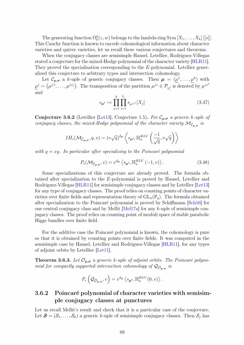
The generating function Ωgk(z, w) belongs to the lambda ring Sym [X1, . . . , Xk] [[s]].

This Cauchy function is known to encode cohomological information about charactervarieties and quiver varieties, let us recall these various conjectures and theorems.

When the conjugacy classes are semisimple Hausel, Letellier, Rodriguez-Villegasstated a conjecture for the mixed-Hodge polynomial of the character variety [HLR11].They proved the specialisation corresponding to the E-polynomial. Letellier gener-alized this conjecture to arbitrary types and intersection cohomology.

Let Cµ,σ a k-uple of generic conjugacy classes. Then µ = (µ1, . . . , µk) withµj =

(µj,1, . . . , µj,lj

). The transposition of the partition µj,i ∈ Pνji is denoted by µj,i′

and

sµ′ :=k∏j=1

lj∏i=1

sµj,i′ [Xj] (3.47)

Conjecture 3.6.2 (Letellier [Let13], Conjecture 1.5). For Cµ,σ a generic k-uple ofconjugacy classes, the mixed-Hodge polynomial of the character varietyMCµ,σ is

IHc(MCµ,σ , q, v) = (v√q)dµ

⟨sµ′ ,HHLV

n

(−1√q, v√q

)⟩with q = xy. In particular after specializing to the Poincaré polynomial

Pc(MCµ,σ , v) = vdµ⟨sµ′ ,HHLV

n (−1, v)⟩. (3.48)

Some specializations of this conjecture are already proved. The formula ob-tained after specialization to the E-polynomial is proved by Hausel, Letellier andRodriguez-Villegas [HLR11] for semisimple conjugacy classes and by Letellier [Let13]for any type of conjugacy classes. The proof relies on counting points of character va-rieties over finite fields and representation theory of GLn(Fq). The formula obtainedafter specialization to the Poincaré polynomial is proved by Schiffmann [Sch16] forone central conjugacy class and by Mellit [Mel17a] for any k-uple of semisimple con-jugacy classes. The proof relies on counting point of moduli space of stable parabolicHiggs bundles over finite field.

For the additive case the Poincaré polynomial is known, the cohomology is pureso that it is obtained by counting points over finite fields. It was computed in thesemisimple case by Hausel, Letellier and Rodriguez-Villegas [HLR11], for any typesof adjoint orbits by Letellier [Let11].

Theorem 3.6.3. Let Oµ,σ a generic k-uple of adjoint orbits. The Poincaré polyno-mial for compactly supported intersection cohomology of QOµ,σ is

Pc

(QOµ,σ , v

)= vdµ

⟨sµ′ ,HHLV

n (0, v)⟩.

3.6.2 Poincaré polynomial of character varieties with semisim-ple conjugacy classes at punctures

Let us recall Mellit’s result and check that it is a particular case of the conjecture.Let S = (S1, . . . ,Sk) a generic k-uple of semisimple conjugacy classes. Then Sj has

89

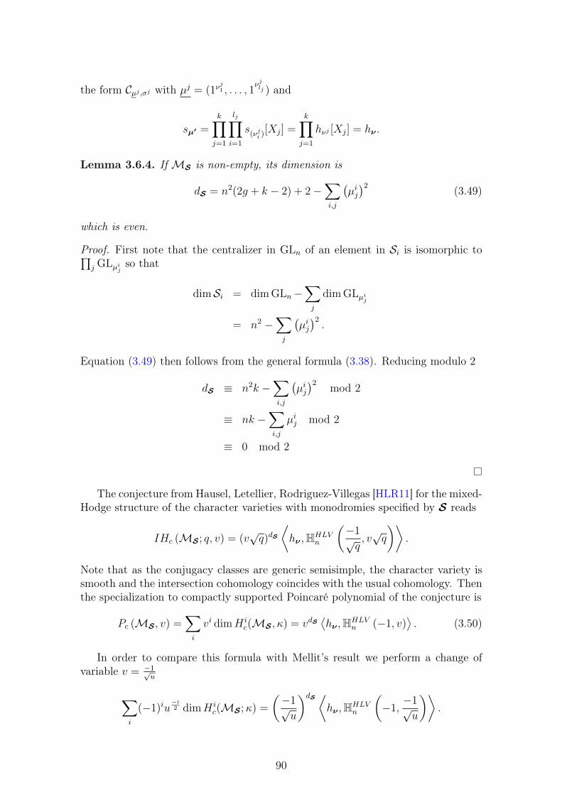
the form Cµj ,σj with µj = (1νj1 , . . . , 1

νjlj ) and

sµ′ =k∏j=1

lj∏i=1

s(νji )[Xj] =k∏j=1

hνj [Xj] = hν .

Lemma 3.6.4. IfMS is non-empty, its dimension is

dS = n2(2g + k − 2) + 2−∑i,j

(µij)2 (3.49)

which is even.

Proof. First note that the centralizer in GLn of an element in Si is isomorphic to∏j GLµij so that

dimSi = dim GLn−∑j

dim GLµij

= n2 −∑j

(µij)2.

Equation (3.49) then follows from the general formula (3.38). Reducing modulo 2

dS ≡ n2k −∑i,j

(µij)2

mod 2

≡ nk −∑i,j

µij mod 2

≡ 0 mod 2

The conjecture from Hausel, Letellier, Rodriguez-Villegas [HLR11] for the mixed-Hodge structure of the character varieties with monodromies specified by S reads

IHc (MS ; q, v) = (v√q)dS

⟨hν ,HHLV

n

(−1√q, v√q

)⟩.

Note that as the conjugacy classes are generic semisimple, the character variety issmooth and the intersection cohomology coincides with the usual cohomology. Thenthe specialization to compactly supported Poincaré polynomial of the conjecture is

Pc (MS , v) =∑i

vi dimH ic(MS , κ) = vdS

⟨hν ,HHLV

n (−1, v)⟩. (3.50)

In order to compare this formula with Mellit’s result we perform a change ofvariable v = −1√

u

∑i

(−1)iu−i2 dimH i

c(MS ;κ) =

(−1√u

)dS ⟨hν ,HHLV

n

(−1,−1√u

)⟩.

90

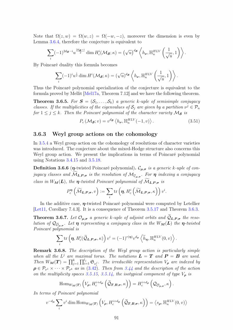
Note that Ω(z, w) = Ω(w, z) = Ω(−w,−z), moreover the dimension is even byLemma 3.6.4, therefore the conjecture is equivalent to∑

i

(−1)2dS−iu2dS−i

2 dimH ic(MS ;κ) =

(√u)dS ⟨hν ,HHLV

n

(1√u, 1

)⟩.

By Poincaré duality this formula becomes∑i

(−1)iui2 dimH i(MS ;κ) = (

√u)dS

⟨hν ,HHLV

n

(1√u, 1

)⟩.

Thus the Poincaré polynomial specialization of the conjecture is equivalent to theformula proved by Mellit [Mel17a, Theorem 7.12] and we have the following theorem.

Theorem 3.6.5. For S = (S1, . . . ,Sk) a generic k-uple of semisimple conjugacyclasses. If the multiplicities of the eigenvalues of Sj are given by a partition νj ∈ Pnfor 1 ≤ j ≤ k. Then the Poincaré polynomial of the character varietyMS is

Pc (MS ; v) = vdS⟨hν ,HHLV

n (−1, v)⟩. (3.51)

3.6.3 Weyl group actions on the cohomology

In 3.5.4 a Weyl group action on the cohomology of resolutions of character varietieswas introduced. The conjecture about the mixed-Hodge structure also concerns thisWeyl group action. We present the implications in terms of Poincaré polynomialusing Notations 3.4.15 and 3.5.18.

Definition 3.6.6 (η-twisted Poincaré polynomial). Cµ,σ is a generic k-uple of con-jugacy classes and ML,P ,σ is the resolution of MCµ,σ . For η indexing a conjugacyclass in WM (L), the η-twisted Poincaré polynomial of ML,P ,σ is

P ηc

(ML,P ,σ, v

):=∑i

tr(η, H i

c

(ML,P ,σ, κ

))vi.

In the additive case, η-twisted Poincaré polynomial were computed by Letellier[Let11, Corollary 7.4.3]. It is a consequence of Theorem 3.5.17 and Theorem 3.6.3.

Theorem 3.6.7. Let Oµ,σ a generic k-uple of adjoint orbits and QL,P ,σ the reso-lution of QOµ,σ . Let η representing a conjugacy class in the WM (L) the η-twistedPoincaré polynomial is∑

i

tr(η, H i

c(QL,P ,σ, κ))vi = (−1)r(η)vdµ

⟨hη,HHLV

n (0, v)⟩.

Remark 3.6.8. The description of the Weyl group action is particularly simplewhen all the Lj are maximal torus. The notations L = T and P = B are used.Then WM (T ) =

∏kj=1

∏lji=1 Sνji

. The irreducible representation Vρ are indexed byρ ∈ Pν1 × · · · × Pνk as in (3.42). Then from 3.44 and the description of the actionon the multiplicity spaces 3.5.15, 3.5.14, the isotypical component of type Vρ is

HomWM (T )

(Vρ, H

i+dµc

(QT ,B,σ, κ

))= H i+dρ

c

(QOρ,σ , κ

).

In terms of Poincaré polynomial

v−dµ∑i

vi dim HomWM (T )

(Vρ, H

i+dµc

(QT ,B,σ, κ

))=⟨sρ,HHLV

n (0, v)⟩

91

Remark 3.6.9. It is also interesting to study the action of a Weyl group relative toa particuar puncture, for instance the first puncture. This will be used in 4.4.2 todescribe some structure coefficients of an algebra spanned by Kostka polynomial. Aparticularly interesting case is when L1 is a maximal torus and M1 = GLn. Thenthe component of the Weyl group relative to the first puncture is WM1(L1) ∼= Sn and

WM (L) ∼= Sn ×k∏j=2

WMj(Lj).

According to this decomposition consider an element (w, 1, . . . , 1) ∈ WM (L) withw ∈ Sn an element of cycle type λ ∈ Pn. Then

hη = pλ[X1]hµ′2 [X2] . . . hµ′k [Xk]

and (−1)r(η) = ε(λ) the sign of the permutation w with cycle type λ. Previoustheorem reads

P ηc

(QL,P ,σ, v

)= vdµε(λ)

⟨pλ[X1]hµ′2 [X2] . . . hµ′k [Xk],HHLV

n (0, v)⟩.

This can be understood in terms of Frobenius characteristic, see Definition 3.2.29.Consider the representation of Sn on the cohomology of QL,P ,σ twisted by the sign:H•(QL,P ,σ, κ)⊗ ε. Its graded Frobenius characteristic is given by the following sym-metric function in X1

vdµ⟨hµ′2 [X2] . . . hµ′k [Xk],HHLV

n (0, v)⟩X2,...,Xk

.

Notice that Vρ ⊗ ε ∼= Vρ′, by Remark 3.2.27, the multiplicity of the irreducible com-ponent Vρ in H•(QL,P ,σ, κ) is given by

vdµ⟨sρ′ [X1]hµ′2 [X2] . . . hµ′k [Xk],HHLV

n (0, v)⟩.

Letellier proved that the Weyl group action on the cohomology of the resolutionML,P ,σ preserves the weight filtration. Therefore similarly to the η-twisted Poincarépolynomial one can defined the η-twisted mixed-Hodge polynomial IHη

c

(ML,P ,σ, q, v

).

Conjecture 3.6.10 (Letellier [Let13] Conjecture 1.8). Let Cµ,σ a generic k-uple ofconjugacy classes. For ML,P ,σ the resolution of a character varietyMCµ,σ and η aconjugacy class in WM (L), the η-twisted Poincaré polynomial is

IHηc

(ML,P ,σ, q, v

)= (−1)r(η)(v

√q)dµ

⟨hη,HHLV

n

(−1√q, v√q

)⟩.

92

Chapter 4

Weyl group actions on thecohomology of comet-shaped quivervarieties and combinatorics

4.1 IntroductionIn this chapter the construction of the varieties QOµ,σ and their resolutions QL,P ,σas comet-shaped quiver varieties is recalled. The base field K is either C or analgebraic closure Fq of a finite field Fq. We consider QL,P the family formed byresolutions QL,P ,σ when σ is varying. In terms of comet-shaped quiver varietiesthis family is induced by the moment map. Weyl group actions on the cohomologyof quiver varieties have been studied by Nakajima [Nak94; Nak98], Lusztig [Lus00]and Maffei [Maf02]. With those methods we construct a monodromic Weyl groupaction on the cohomology of fibers of the family QL,P . The construction of thisaction relies on the moment map being locally trivial. The local triviality of suchmoment was recalled in Chapter 2. Similar Weyl group action were used by Hausel,Letellier and Rodriguez-Villegas [HLR13] to prove Kac conjecture. Moreover theycomputed traces of those actions thanks to Grothendieck trace formula. The samemethod is applied in this chapter.

Notice that Theorem 3.5.17 also provides a relative Weyl group action, à laSpringer, on the cohomology of resolutions QL,P ,σ. Letellier [Let11] computed thetrace of the action by counting points over finite fields. In this chapter we checkthat the monodromic and the Springer action are isomorphic.

Some combinatoric interpretation are given for those Weyl group actions. Sur-prisingly, some traces of those actions are related to some structure coefficients of analgebra spanned by modified Kostka polynomials

(Kλ,ρ

)λ,ρ∈Pn

. The structure co-

efficents(cλµ,ν)λ,µ,ν∈Pn

were introduces by Rodriguez-Villegas in unpublished notes,they are defined by

Kµ,ρKν,ρ =∑λ∈Pn

cλµ,νKλ,ρ.

We prove that the specialization c1n

µ,ν(0, t) of the coefficients has an interpretation interms of Weyl group action on the cohomology of comet-shaped quiver varieties.Theorem 4.1.1. Consider a generic 4-uple of adjoint orbits of the following type:

93

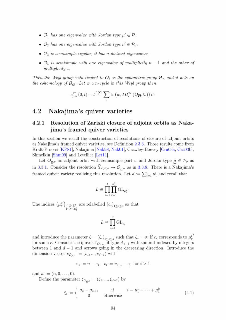
• O1 has one eigenvalue with Jordan type µ′ ∈ Pn

• O2 has one eigenvalue with Jordan type ν ′ ∈ Pn.

• O3 is semisimple regular, it has n distinct eigenvalues.

• O4 is semisimple with one eigenvalue of multiplicity n − 1 and the other ofmultiplicity 1.

Then the Weyl group with respect to O3 is the symmetric group Sn and it acts onthe cohomology of QO. Let w a n-cycle in this Weyl group then

c1n

µ,ν (0, t) = t−dO

2

∑r

tr(w, IH2r

c (QO,C))tr.

4.2 Nakajima’s quiver varieties

4.2.1 Resolution of Zariski closure of adjoint orbits as Naka-jima’s framed quiver varieties

In this section we recall the construction of resolutions of closure of adjoint orbitsas Nakajima’s framed quiver varieties, see Definition 2.3.3. Those results come fromKraft-Procesi [KP81], Nakajima [Nak98; Nak01], Crawley-Boevey [Cra03a; Cra03b],Shmelkin [Shm09] and Letellier [Let11].

Let Oµ,σ an adjoint orbit with semisimple part σ and Jordan type µ ∈ Pν asin 3.3.1. Consider the resolution YL,P,σ → Oµ,σ as in 3.3.8. There is a Nakajima’sframed quiver variety realizing this resolution. Let d :=

∑li=1 µ

i1 and recall that

L ∼=l∏

i=1

µi1∏r=1

GLµir ′ .

The indices(µir′)

1≤i≤l1≤r≤µi1

are relabelled (cs)1≤s≤d so that

L ∼=d∏s=1

GLcs

and introduce the parameter ζ = (ζs)1≤s≤d such that ζs = σi if cs corresponds to µir′

for some r. Consider the quiver ΓOµ,σ of type Ad−1 with summit indexed by integersbetween 1 and d − 1 and arrows going in the decreasing direction. Introduce thedimension vector vOµ,σ := (v1, ..., vd−1) with

v1 := n− c1, vi := vi−1 − ci for i > 1

and w := (n, 0, . . . , 0).Define the parameter ξOµ,σ = (ξ1, ..., ξd−1) by

ξi :=

σk − σk+1 if i = µ1

1 + · · ·+ µk10 otherwise (4.1)

94

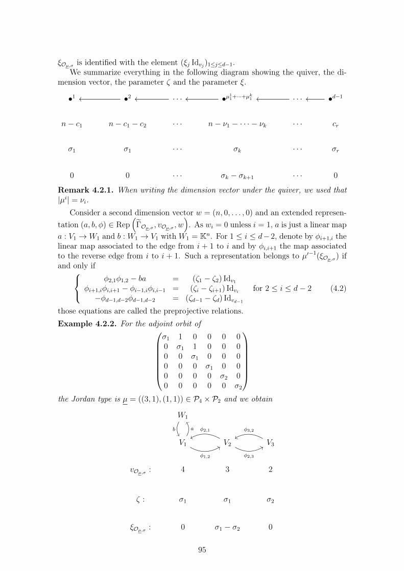
ξOµ,σ is identified with the element (ξj Idvj)1≤j≤d−1.We summarize everything in the following diagram showing the quiver, the di-

mension vector, the parameter ζ and the parameter ξ.

•1 •2 · · · •µ11+···+µk1 · · · •d−1

n− c1 n− c1 − c2 · · · n− ν1 − · · · − νk · · · cr

σ1 σ1 · · · σk · · · σr

0 0 · · · σk − σk+1 · · · 0

Remark 4.2.1. When writing the dimension vector under the quiver, we used that|µi| = νi.

Consider a second dimension vector w = (n, 0, . . . , 0) and an extended represen-tation (a, b, φ) ∈ Rep

(ΓOµ,σ , vOµ,σ , w

). As wi = 0 unless i = 1, a is just a linear map

a : V1 → W1 and b : W1 → V1 with W1 = Kn. For 1 ≤ i ≤ d−2, denote by φi+1,i thelinear map associated to the edge from i + 1 to i and by φi,i+1 the map associatedto the reverse edge from i to i + 1. Such a representation belongs to µ′−1(ξOµ,σ) ifand only if

φ2,1φ1,2 − ba = (ζ1 − ζ2) Idv1φi+1,iφi,i+1 − φi−1,iφi,i−1 = (ζi − ζi+1) Idvi for 2 ≤ i ≤ d− 2−φd−1,d−2φd−1,d−2 = (ζd−1 − ζd) Idvd−1

(4.2)

those equations are called the preprojective relations.Example 4.2.2. For the adjoint orbit of

σ1 1 0 0 0 00 σ1 1 0 0 00 0 σ1 0 0 00 0 0 σ1 0 00 0 0 0 σ2 00 0 0 0 0 σ2

the Jordan type is µ = ((3, 1), (1, 1)) ∈ P4 × P2 and we obtain

W1

V1 V2 V3

vOµ,σ : 4 3 2

ζ : σ1 σ1 σ2

ξOµ,σ : 0 σ1 − σ2 0

b a

φ1,2

φ2,1

φ2,3

φ3,2

95

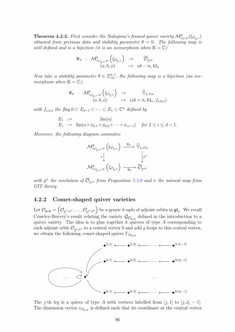
Theorem 4.2.3. First consider the Nakajima’s framed quiver varietyM0vO,w

(ξOµ,σ)obtained from previous data and stability parameter θ = 0. The following map iswell defined and is a bijection (it is an isomorphism when K = C)

Ψ0 : M0vOµ,σ ,w

(ξOµ,σ

)→ Oµ,σ

(a, b, φ) 7→ ab− σ1 Idn

Now take a stability parameter θ ∈ Zd−1>0 , the following map is a bijection (an iso-

morphism when K = C).

Ψθ : MθvOµ,σ ,w

(ξOµ,σ

)→ YL,P,σ

(a, b, φ) 7→ (ab+ σ1 Idn, fa,b,φ)

with fa,b,φ the flag 0 ⊂ Ed−1 ⊂ · · · ⊂ E1 ⊂ Cn defined by

E1 := Im(a)Ei := Im(a φ2,1 φ3,2 · · · φi,i−1) for 2 ≤ i ≤ d− 1.

Moreover, the following diagram commutes

MθvOµ,σ ,w

(ξOµ,σ

)YL,P,σ

M0vOµ,σ ,w

(ξOµ,σ

)Oµ,σ

Ψθ

π pσ

Ψ0

with pσ the resolution of Oµ,σ from Proposition 3.3.8 and π the natural map fromGIT theory.

4.2.2 Comet-shaped quiver varieties

Let Oµ,σ =(Oµ1,σ1 , . . . ,Oµk,σk

)be a genric k-uple of adjoint orbits in gln. We recall

Crawley-Boevey’s result relating the variety QOµ,σ defined in the introduction to aquiver variety. The idea is to glue together k quivers of type A corresponding toeach adjoint orbit Oµj ,σj to a central vertex 0 and add g loops to this central vertex,we obtain the following comet-shaped quiver ΓOµ,σ

•[1,1] •[1,2] · · · •[1,d1−1]

•[2,1] •[2,2] · · · •[2,d2−1]

. . . •0 . . .

•[k,1] •[k,2] · · · •[k,dk−1]

The j-th leg is a quiver of type A with vertices labelled from [j, 1] to [j, dj − 1].The dimension vector vOµ,σ is defined such that its coordinate at the central vertex

96

is n and its coordinates on the j-th leg coincide with the dimension vector vOµj,σj

described in previous section. Similarly the parameter ξOµ,σ is defined such that itscoordinates on the j-th leg coincide with the parameter ξO

µj,σj. The component at

the central vertex ξOµ,σ ,0 is defined such that vOµ,σ .ξOµ,σ = 0 hence

nξOµ,σ ,0 = −k∑j=1

dj−1∑i=1

vOµ,σ ,[j,i]ξOµ,σ ,[j,i].

Consider a representation of the extended quiver φ ∈ Rep(

ΓOµ,σ , vOµ,σ

).

• Denote by φ[j,i] the linear map associated to the arrow with tail [j, i] and φ[j,i]

the linear map associated to the reversed arrow with head [j, i].

• For 1 ≤ i ≤ g the map associated to the i-th loop is denoted φi and the oneassociated to the reverse loop is denoted φi.

As usual µ is the moment map and ξOµ,σ is identified with an element in the centerof the Lie algebra gvOµ,σ . Let

Xj := φ[j,1]φ[j,1] − ζ[j,1]

If φ belongs to µ−1(ξOµ,σ) then Xj ∈ Oµj ,σj . Indeed it follows from previous de-scription of closure of adjoint orbits as framed quiver varieties and identification,for each legs, of the vector space at the central vertex with the framing vector spaceW1 from previous section.

Now if Ai is the linear map associated to the i-th loop of the quiver and Bi themap associated to the reversed loop, the preprojective relation at the central vertexis exactly the equation defining VO. Hence the following map is well defined

ΨOµ,σ : µ−1(ξOµ,σ) → VOµ,σφ 7→ (A1, B1, . . . , Ag, Bg, X1, . . . , Xk)

Theorem 4.2.4. In the following diagram where the vertical arrows are quotientmaps, the application ΨOµ,σ goes down to the quotient to a bijective morphism ΦOµ,σ

(when K = C it is an isomorphism).

µ−1(ξOµ,σ) VOµ,σ

M0vOµ,σ

(ξOµ,σ) QOµ,σ

ΨOµ,σ

ΦOµ,σ

Proof. It is proved by Crawley-Boevey [Cra01; Cra03b], see also Letellier [Let11,Proposition 5.2.2] for any genus.

QL,P ,σ, the resolution of QOµ,σ introduced in 3.5.16, is also interpreted as Naka-jima’s quiver variety for the quiver ΓOµ,σ .

97

Theorem 4.2.5. Consider a stability parameter θ associated to the quiver QOµ,σsuch that θ[j,i] > 0 for all vertices [j, i]. There is a bijective morphism ΦOµ,σ ,θ :

MθvOµ,σ

(ξOµ,σ) → QL,P ,σ which is an isomorphism when K = C and the followingdiagram commutes

MθvOµ,σ

(ξOµ,σ) QL,P ,σ

M0vOµ,σ

(ξOµ,σ) QOµ,σ

ΦOµ,σ ,θ

π pσ

ΦOµ,σ

with π the natural projection from GIT theory.

Proof. It follows from Letellier’s article [Let11], where the construction of the mapΦOµ,σ ,θ is given in Section 5.3. This map is induced by the map Ψθ of Theorem4.2.3. Contrarily to Letellier’s article, we do not consider partial resolution so thatour parameter θ has non-zero components. Therefore the dimension vector for thequiver variety Mθ

vOµ,σ(ξOµ,σ) describing the resolution QL,P ,σ is the same as the

dimension vector of the quiver variety describing QOµ,σ .

The quiver variety point of view gives a criteria for non-emptiness. The questionof emptiness of QOµ,σ andMCµ,σ is known as the Deligne-Simpson problem. Kostov[Kos04] gave a survey about this problem. For a different approach see Soibelman[Soi16]. The additive version was answered by Crawley-Boevey in terms of rootsof the quiver [Cra03b]. The multiplicative case (for generic conjugacy classes andgenus g = 0) is solved by Crawley-Boevey [Cra03a, Theorem 8.3]. For any genus, theresult follows from Hausel, Letellier, Rodriguez-Villegas [HLR11, 5.2] and Letellier[Let11, Corollary 3.15]. Those results are summarized in the following theorem:

Theorem 4.2.6. Let Oµ,σ a generic k-uple of adjoint orbit. The variety QOµ,σ isnot empty if and only QOµ,σ is not empty. This happens if and only if the dimensionvector vOµ,σ is a root of the quiver ΓOµ,σ . This is always the case for g > 0.

Let Cµ,σ′ a generic k-uple of conjugacy classes. The varietyMCµ,σ′ is not empty

if and only if MCµ,σ′ is not empty. This happens if and only if the the dimension

vector vOµ,σ′ is a root of the quiver ΓO

µ,σ′ . This is always the case for g > 0.

4.2.3 Family of comet-shaped quiver varieties

When the eigenvalues σ are varying, one obtains a family of varieties.

Notations 4.2.7. From now on the pair L,P is fixed. For short, let

Z(l) := Z(l1)× · · · × Z(lk).

Denote by B the subset of elements σ ∈ Z(l) such that the k-uple of adjoint orbitsOµ,σ is generic. Note that the genericity condition depends only the semisimple partσ and not on the type µ. The set B is a Zariski open subset of a codimension onesubspace of Z(l) given by the vanishing of the sum of the traces. Identifying Z(l)with an affine space, B is either empty or the complementary of a finite union ofhyperplanes in the codimension one subspace.

98

Definition 4.2.8 (Family of varieties QL,P ,σ). Define

VL,P :=(σ, (Ai, Bi)1≤i≤g, (Xj, gjP

j)1≤j≤k) ∣∣

σ ∈ B, and (Ai, Bi)1≤i≤g, (Xj, gjPj)1≤j≤k ∈ VL,P,σ

QL,P := VL,P //GLn

and denote η the map η : QL,P → B. Thus the varieties QL,P ,σ = η−1(σ) fit in afamily QL,P .

The choice of L determine a unique quiver ΓOµ,σ and a unique dimension vectorvOµ,σ independent of a choice of σ. Assume that the dimension vector is indivisibleso that B is not empty. Then we can make the following assumption

Assumption 4.2.9 (Genericity of the stability parameter θ). θ is a generic stabilityparameter, i.e. a stability parameter for the quiver ΓOµ,σ with dimension vector vOµ,σsuch that (θ, 0, 0) ∈ Hreg

vOµ,σwith notations from 2.1.4.

The construction of Theorem 3.5.17 extends to this family. It provides the fol-lowing commutative diagram (the left vertical arrows is induced by the moment mapµ)

µ−1(zgenvOµ,σ

)θ-ss//GvOµ,σQL,P

zgenvOµ,σ

B

Φ

η (4.3)

θ is a fixed generic stability parameter. zgenvOµ,σ

is the subset of the center of theLie algebra gvOµ,σ corresponding to the subset B under the correspondence betweenparameters ξOµ,σ and eigenvalues σ. Note that the correspondence between param-eters of the quiver variety ξOµ,σ ∈ Z(gvOµ,σ ) and Z(l) is not bijective. Thus theprevious diagram relies on a choice of k − 1 eigenvalues. To σ ∈ Z(l) associate theelement (ξOµ,σ , σ

11, . . . , σ

k−11 ) in Z(gvOµ,σ )×Kk−1 this defines a bijective map

h : Z(l)∼−→ zvOµ,σ ×K

k−1. (4.4)

Note that for a given parameter ξOµ,σ the genericity conditions is independant ofthe choice of the k− 1 eigenvalues, namely h−1(ξOµ,σ , σ

11, . . . , σ

k−11 ) is generic if and

only if h−1(ξOµ,σ , 0, . . . , 0) is generic. Therefore Diagram (4.3) can be modified toaccount for various choices of eigenvalues, then the horizontal arrows are bijectionsand isomorphism when K = C.

Kk−1 × µ−1(zgenvOµ,σ

)θ-ss//GvOµ,σQL,P

Kk−1 × zgenvOµ,σ

B

Φ

Id×µ η (4.5)

Theorem 4.2.10. If K = C, or if the characteristic is large enough, the cohomologysheaves Hiη!κ are constant sheaves.

Proof. When K = C, this is a consequence of Chapter 2 Corollary 2.4.14 and dia-gram (4.5). As θ is generic, To prove the result for K = Fq we can change charac-teristic as in [HLR13] proof of Theorem 2.3. This imply the result in large enoughcharacteristic.

99

4.3 Weyl group action

4.3.1 Decomposition of the family QL,PNotations 4.3.1. First we recall notations from 3.4.4 in this context. For 1 ≤ j ≤ k

YLj ,P j :=

(X, gjPj) ∈ gln×GLn /P

j∣∣g−1j Xgj ∈ Z(lj)⊕ uP j

and define

YL,P := YL1,P 1 × · · · × YLk,Pk .Then YL,P is the image in glkn of the map forgetting the partial flags gjP j:

p : YL,P → glkn(Xj, gjP

j)1≤j≤k 7→ (Xj)1≤j≤k.

Similarly VL,P , respectively QL,P , is obtained from VL,P , respectively QL,P , by for-getting the partial flags.

In this section a decomposition of the family QL,P is deduced from the decom-position Oµ,σ =

⊔ρµOρ,σ and the decomposition introduced in Proposition 3.4.20:

YL,P =⊔M

⊔ρµ

YM,ρ

L,P .

The decomposition is used in next section (Lemma 4.3.4) in order to define a Weylgroup action.

Let YBL,P the subset of elements in YL,P with semisimple part generic, i.e. in B.The dimension of YBL,P is computed similarly to dimYL,P in Remark 3.4.19:

dimYBL,P = kn2 + dimB −k∑j=0

dimLj.

The decomposition YL,P =⊔M

⊔ρµY

M,ρ

L,P induces a similar decomposition for YBL,P

YBL,P =⊔M

⊔ρµ

YB,M ,ρL,P

With M = (M1, . . . ,M l) and YB,M ,ρL,P the subset of elements in

YB,M1,ρ1

L1,P 1 × · · · × YB,Mk,ρk

Lk,Pk

with generic semisimple parts. From the computation of the dimension of YM,ρ

L,P inProposition 3.4.20, we deduce that when Z(m) ∩ B is not empty

dimYB,M ,ρL,P =

n∑j=1

dimOρj ,σj + dimZ(m) ∩ B. (4.6)

Now the decomposition of YBL,P induces a decomposition of the family of quivervarieties QL,P . Let

QM ,ρL,P :=

(VL,P ×YL,P Y

B,M ,ρL,P

)//PGLn .

We have the following proposition:

100

Proposition 4.3.2.QL,P =

⊔M

⊔ρµ

QM ,ρL,P .

When non-empty, the dimension of a part is

dimQM ,ρL,P = n2(2g − 2) + 2 + dimZ(m) ∩ B +

k∑j=1

dimOρj ,σj . (4.7)

Proof. The dimension of QM ,ρL,P can be computed just like the dimension of QOµ,σ

(see Proposition 3.5.6 for the case of character varieties). The computation relieson the smoothness of YB,M ,ρ

L,P which follows from the smoothness of YB,Mj ,ρj

Lj ,P j. Then

from the dimension of YB,M ,ρL,P given by (4.6) we obtain

dimQM ,ρL,P = n2(2g − 2) + 2 + dimZ(m) ∩ B +

k∑j=1

dimOρj ,σj .

4.3.2 Construction of a Weyl group action on the cohomologyof the quiver varieties in the family QL,P

The family QL,P → B is used to construct a Weyl group action on the cohomologyof the varieties QL,P ,σ for σ ∈ B. The Weyl group considered in this section is

W := WGLn(L1)× · · · ×WGLn(Lk).

Each WGLn(Lj) is isomorphic to a symmetric group and acts on Z(lj) by permut-ing the eigenvalues with same multiplicities. Therefore W acts on B, for w =(w1, . . . , wk) ∈ W and σ =

(σ1, . . . , σk

)∈ B

w.σ :=(w1σ

1w−11 , . . . , wkσ

kw−1k

)with wj a representative in GLn of wj ∈ WGLn(Lj). Consider the diagram:

B QL,P

B/W QL,P

π0

η

p

χ

(4.8)

Thanks to the quiver variety point of view, the cohomology sheaves Hiη!κ are con-stant (Theorem 4.2.10). In this section a W -equivariant structure on those coho-mology sheaves is constructed. The method comes from Lusztig (see [Let05, Proofof Proposition 5.5.3]), it is also used by Laumon-Letellier [LL19, Section 5.2].

Before proving this result, let us define the regular locus. Denote by Breg thesubset of regular elements, i.e. elements

(σ1, . . . , σk

)∈ B such that ZGLn(σj) = Lj.

101

It is the locus of B where the W -action is free. Diagram (4.8) is pulled back to theregular locus

Breg QregL,P

Breg/W QregL,P

πreg

ηreg

preg

χreg

(4.9)

Similarly to 3.32, notice that

QregL,P ×Breg/W B

reg ∼= QregL,P . (4.10)

Theorem 4.3.3. The cohomology sheaves Hiη!κ admit a W -equivariant structureover B.

Proof. Consider the diagram:

QL,P

B QL,P ×B/W B

B/W QL,P

η

p

c

π0

a

b

χ

(4.11)

W acts on QL,P ×B/W B and the morphism a is W -equivariant. QregL,P ×Breg/W Breg is

smooth, dense and open in QL,P ×B/W B. The constant sheaf κ over QL,P ×B/W Bis W -equivariant. Indeed for w ∈ W we can define a morphism

φw : w∗κ→ κ

which is the identity on the stalks. It satisfies the conditions of definitions 3.1.4.Applying the continuation principle from Remark 3.1.9, thisW -equivariant structureextends to a W -equivariant structure on IC•QL,P×B/WB. Notice that η!κ ∼= a!c!κ. Weshall see in Lemma 4.3.4 that

c!κ ∼= IC•QL,P×B/WB.

Then the W -equivariant structure on c!κ induces a W -equivariant structure on η!κ.Up to the isomorphism c!κ ∼= IC•QL,P×B/WB, the theorem is proved.

It remains to prove the lemma:

Lemma 4.3.4. There is an isomorphism c!κ ∼= IC•QL,P×B/WB.

Proof. Because of the isomorphism (4.10), the restriction of c!κ to the smooth locusQregL,P ×Breg/W Breg is the constant sheaf κ. In order to verify the hypothesis of

Definition 3.1.8 it remains to prove that the map c is small, i.e. that it satisfies thefollowing inequality

dimx ∈ QL,P ×B/W B

∣∣dim c−1(x) ≥ d≤ dimQL,P ×B/W B − 2d for all d > 0.

It relies on dimension estimates from Lusztig [Lus84, 1.2], see also [Sho88, The-orem 1.4]. In the Lie algebra gln the estimate becomes, for X in O an adjointorbit

dimgP ∈ GLn /P

∣∣g−1Xg ∈ σ + uP≤ 1

2

(n2 − dimL− dimO

). (4.12)

102

The proof is then standard in Springer theory. Let d > 0 and x such that

dim c−1(x) ≥ d.

x belongs to some QOρ,σ for σ ∈ B and some adjoint orbits Oρ1,σ1 , . . . ,Oρk,σk . Thedimension estimate (4.12) implies

d ≤ 1

2

(kn2 −

k∑j=1

dimLj − dimOρj ,σj)

so thatk∑j=1

dimOρj ,σj ≤ kn2 −k∑j=1

dimLj − 2d.

Using the decomposition from Proposition 4.3.2, x ∈ QB,M ,ρL,P . Previous inequality

and the expression (4.7) for the dimension of QB,M ,ρL,P give

dimQB,M ,ρL,P ≤ n2(2g − 2) + 2 + dimZ(m) ∩ B + kn2 −

k∑j=1

dimLj − 2d. (4.13)

MoreoverdimQB,M ,ρ

L,P ×B/W B = dimQB,M ,ρL,P (4.14)

and

dimQL,P ×B/W B = dimQL,P = n2(2g− 2) + 2 + dimB+ kn2−k∑j=1

dimLj. (4.15)

Combining (4.13)(4.14) and (4.15):

dimQB,M ,ρL,P ×B/W B ≤ dimQL,P ×B/W B + 2d+ dimZ(m) ∩ B − dimB. (4.16)

As d is assumed to be strictly positive, necessarily the inclusion L ( M is strict,hence

dimZ(m) ∩ B < dimB. (4.17)

Now (4.16) and (4.17) provide the estimate

dimQB,M ,ρL,P ×B/W B < dimQL,P ×B/W B − 2d. (4.18)

To conclude, the setx ∈ QL,P ×B/W B |dim c−1(x) ≥ d

is a finite union of varieties

QB,M ,ρL,P ×B/W B with dimension satisfying previous estimate (4.18).

Remark 4.3.5. Let us study the restriction of the W -equivariant sheaves Hiη!κ tothe regular locus. Recall that Qreg

L,P ×Breg/W Breg ∼= QregL,P , then for σ ∈ Breg

Hiση!κ ∼= H i

c(QL,P ,σ, κ).

For w ∈ W , theW -equivariant structure is given by the functoriality of the compactlysupported cohomology (see Proposition 3.1.6 and Remark 3.1.3)

w∗ : H ic

(QL,P ,w.σ, κ

)→ H i

c

(QL,P ,σ, κ

).

This is called the monodromic action.

103

4.3.3 Frobenius morphism and monodromic action

The techniques in this section come from Hausel, Letellier and Rodriguez-Villegas[HLR13], though we do no consider regular semisimple values of the moment map.Instead each component of the moment map is central and each leg of the comet-shaped quiver corresponds to a particular adjoint orbit. Comet-shaped quiver vari-eties were also studied in this context by Letellier [Let12]. A slightly more generalsituation is considered here, as a leg can represents any adjoint orbit and not onlya semisimple regular.

We proved in 4.2.10 that the cohomology sheaves Hiη!κ are constant sheavesover B. Note that the fiber over σ of this constant sheaf is H i

c(QL,P ,σ;κ). Thus forany σ, τ ∈ B, there is an isomorphism

fσ,τ : H ic(QL,P ,σ;κ)→ H i

c(QL,P,τ ;κ).

such that for any ω ∈ Bfσ,τ = fω,τ fσ,ω.

The W -equivariance of the local system Hiη!κ implies the following theorem. It canalso be proved directly, without referring to equivariance of the local system (seeMaffei [Maf02, Section 5]).

Theorem 4.3.6. Let σ, τ ∈ B, the following diagram commutes

H ic(QL,P ,σ;κ) H i

c(QL,P,w−1.σ;κ)

H ic(QL,P,τ ;κ) H i

c(QL,P,w−1.τ ;κ)

w∗

fσ,τ fw−1.σ,w−1.τ

w∗

Remark 4.3.7. Note that if σ ∈ B is not regular, then the map

w∗ : H ic

(QL,P ,σ, κ

)→ H i

c

(QL,P ,w−1.σ

)is only the map coming from theW -equivariant structure of the constant sheaf Hiη!κ.It does not come by functoriality from a morphism a variety. At the level of variety,W only acts on Qreg

L,P .

This theorem allows to define a W -action on the compactly supported cohomol-ogy space H i

c(QL,P ,σ;κ).

Proposition 4.3.8. For w ∈ W introduce the morphism

ρi(w) = fw.σ,σ (w−1)∗

This defines an action of W on H ic(QL,P ,σ;κ).

Proof. Let w1, w2 in W , the following diagram commutes by Theorem 4.3.6.

H ic(QL,P ,σ;κ) H i

c(QL,P,w2.σ;κ) H ic(QL,P,w1w2.σ;κ)

H ic(QL,P ,σ;κ) H i

c(QL,P,w1.σ;κ)

H ic(QL,P ,σ;κ)

(w−12 )∗

(w−11 )∗

fw2.σ,σ fw1w2.σ,w1.σ

(w−11 )∗

fw1.σ,σ

104

Going from top left corner to bottom right corner by top right corner is ρ(w1w2).Going by the middle gives ρ(w1) ρ(w2). Therefore ρ(w1w2) = ρ(w1) ρ(w2).

The representation obtained when K = C is isomorphic to the representationobtained for K = Fq and large enough characteristic. Indeed this can be provedby base change exactly like in [HLR13, Theorem 2.5]. Therefore from now on weassume:

Assumption 4.3.9. K = Fq and the characteristic is large enough.

This assumption is very convenient as it allows to introduce Frobenius endo-morphism and use Grothendiek’s trace formula to compute the traces of the actionobtained.

F is the Frobenius endomorphism on gln raising coefficients to the power q sothat its set of fixed point if gln(Fq) and similarly for the group GLn. Assume thatthe Lj are subgroups of bock diagonal matrices, and P j subgroup of block uppertriangular matrices, so that they are F -stable. F induces a Frobenius endomorphismon Qreg

L,P and on Breg also denoted by F

F(σ, (Ai, Bi)1≤i≤g , (Xj, gjLj)1≤j≤k

)=(F (σ), (F (Ai), F (Bi))1≤i≤g , (F (Xj), F (gj)Lj)1≤j≤k

)This Frobenius can be twisted by an element w = (w1, . . . , wk) in the Weyl groupW . For σ ∈ Breg, define

wF (σ1, . . . ,σk) = (w1.F (σ1), . . . , wk.F (σk)) .

(Breg)wF is the set of points fixed by wF . Similarly the w-twisted Frobenius on QregL,P

iswF := w F.

They are compatible preg wF = wF preg so that for σ, τ ∈ Breg the followingdiagram commutes

H ic(QL,P,σ;κ) H i

c(QL,P,F−1(σ);κ)

H ic(QL,P,τ ;κ) H i

c(QL,P,F−1(τ );κ)

F ∗

fσ,τ fF−1(σ),F−1(τ)

F ∗

Theorem 4.3.10. Let τ ∈ (Breg)F and σ ∈ (Breg)wF . The cardinal of the set ofwF fixed points of QL,P ,σ is

]QwFL,P ,σ =∑i

tr(ρ2i(w), H2i

c (QL,P,τ ;κ))qi

Proof. Consider the commutative diagram:

H ic(QL,P,τ ;κ) H i

c(QL,P,w−1.τ ;κ)

H ic(QL,P,τ ;κ) H i

c(QL,P,τ ;κ)

H ic(QL,P,σ;κ) H i

c(QL,P,F (σ);κ) H ic(QL,P,σ;κ)

w∗

ρ(w−1)fw−1.τ ,τ

F ∗fσ,τ

w∗

fF (σ),τ

F ∗

fσ,τ

105

Apply Grothendieck trace formula to wF

]QwFL,P ,σ =∑i

(−1)i tr(

(wF )∗, H ic(QL,P ,σ;κ)

)=

∑i

(−1)i tr(F ∗ ρi(w−1), H i

c(QL,P,τ ;κ))

The varieties QL,P,τ are pure and polynomial count and ρ(w−1) commutes with Fso that

]QwFL,P ,σ =∑i

tr(F ∗ ρ2i(w−1), H2i

c (QL,P,τ ;κ))

=∑i

tr(ρ2i(w−1), H2i

c (QL,P,τ ;κ))qi

Now as W is isomorphic to a product of symmetric group, w is conjugated to itsinverse w−1 and

]QwFL,P ,σ =∑i

tr(ρ2i(w), H2i

c (QL,P,τ ;κ))qi

The Levi subgroup has the following form

Lj ∼= GLcj1× · · · ×GLcj1︸ ︷︷ ︸

mj1

× · · · ×GLcjkj× · · · ×GLcjkj︸ ︷︷ ︸mjkj

with cjr 6= cjs for r 6= s. Then the relative Weyl group is

WGLn(Lj) ∼= Smj1× · · · ×Smjkj

The symmetric group Smjracts by permuting the blocks of size cjr. Notations are

similar to 3.5.4 except that the index i disappears as M j = GLn. A conjugacy classin this Weyl group is determined by a kj-uple (ηj,1, . . . , ηj,kj) with ηj,r ∈ Pmjr . Hencethe conjugacy class of w ∈ W determines a k-uple of n-types ω = (ω1, . . . , ωk) with

ωj =(ηj,11 , 1c

j1

). . .(ηj,1l(ηj,1)

, 1cj1

). . .

(ηj,kj1 , 1

cjkj

). . .

(ηj,kj

l(ηj,kj ), 1

cjkj

)(4.19)

Let Oω = (Oω1 , . . . ,Oωk) be the k-uple of F -stable adjoint orbits such that the F -fixed points (OFω1

, . . . ,OFωk) is of type ω (the type of adjoint orbit in gln(Fq) is definedin 3.3.4). Then the natural map QL,P ,σ → QOω is an isomorphism commuting withthe Frobenius so that

]QwFL,P ,σ = ]QFOω (4.20)

Letellier [Let11] computed the number of points of QFOω .

Theorem 4.3.11. The cardinal of QFOω is given by

]QFOω = (−1)r(η)qdµ2

⟨hη,HHLV

n (0, q12 )⟩

106

Proof. As the orbits Oωj are semisimple, the variety QOω is smooth so that thecharacteristic function of the intersection complex is constant with value 1. Theresult follows from Letellier [Let11, Theorem 6.9.1, Theorem 7.4.1 and Corollary7.4.3].

Corollary 4.3.12. For σ ∈ B and η representing a conjugacy class in the Weylgroup as described in (4.19), the η-twisted Poincaré polynomial of QL,P ,σ is∑

i

tr(η, H i

c(QL,P ,σ, κ))vi = (−1)r(η)vdµ

⟨hη,HHLV

n (0, v)⟩.

Proof. The action comes from the W -equivariant structure of the constant sheavesHiη!κ. Therefore up to isomorphism the action does not depend on the choice ofσ ∈ B so that the twisted Poincaré polynomial can be computed for τ ∈ (Breg)F .Then from Theorem 4.3.10 and (4.20)∑

i

tr(ρ2i(η), H2i

c

(QL,P ,τ , κ

))qi = (−1)r(η)q

dµ2

⟨hη,HHLV

n (0, q12 )⟩.

This equality remains true after substituting qn for q for n > 0. Thus it is an equalitybetween two polynomials and the corollary is proved.

It is interesting to notice that Letellier [Let11, Corollary 7.4.3] obtained exactlythe same formula for twisted Poincaré polynomials with a different construction ofthe action. His construction is the one recalled in Theorem 3.5.20 for the charactervarieties setting. Notice that it does not necessarily involve the whole group Wbut only the subgroup of elements w ∈ W such that w.σ = σ. Interestingly forsuch w the action from 4.3.8 is simply given by ρi(w) = (w−1)

∗. In the particularcase where the Levi subgroup is a torus, in the character variety setting, we shallsee in Chapter 5 that both action coincide. Except in that particular case, we donot have a direct prove that both action coincide. However as the twisted Poincarépolynomial coincide they are necessarily isomorphic.

It is also interesting to consider this action as an action on the cohomology ofa quiver variety with semisimple adjoint orbits at punctures. Indeed notice thatfor σ ∈ Breg the map pσ : QL,P ,σ → QS from 3.5.16 is an isomorphism. LetS = (S1, . . . ,Sk) a generic k-uple of semisimple adjoint orbit, Sj is the adjoint orbitof σj. The Weyl group WGLn(Lj) is the group of permutation of the eigenvalues ofSj with the same multiplicities. We have another formulation of previous corollary

Corollary 4.3.13. For η representing a conjugacy class in the Weyl group as de-scribed in (4.19), the η-twisted Poincaré polynomial of QS is∑

i

tr(η, H i

c(QS , κ))vi = (−1)r(η)vdη

⟨hη′ ,HHLV

n (0, v)⟩.

4.4 Combinatorial interpretation in the algebra spannedby Kostka polynomials

4.4.1 Description of the algebra

In this section an algebra spanned by Kostka polynomials is studied and some struc-ture coefficients are related to traces of Weyl group action on the cohomology of

107

quiver varieties. Define a linear map ∆# : Sym[X] → Sym[X, Y ] such that on thebasis of modified Macdonald polynomials

∆#(Hλ[X]

):= Hλ[X]Hλ[Y ] for λ ∈ P .

As in 3.2.42, the variable (q, t) are implicit. Now as the Hall pairing is non-degeneratethere is a uniquely determined bilinear map . . .# . . . such that for all F,G and Hin Sym[X]:

〈F [X]#G[X], H[X]〉 =⟨F [X]G[Y ],∆# (H[X])

⟩The product # defines an associative and commutative algebra structure on Sym[X].

Definition 4.4.1. For a k-uplet of partitions µ =(µ1, . . . , µk

)∈ Pkn and λ ∈ Pn

we denote by cλµ the structure coefficients of the product # in the basis of Schurfunctions

sµ1#sµ2 . . .#sµk =∑|µ|=n

cλµsλ. (4.21)

Remark 4.4.2. For µ = (µ, ν), the coefficient cλµ,ν coincides with the one introducedin the introduction, i.e. the following relation is satisfied

Kµ,ρKν,ρ =∑λ

cλµ,νKλ,ρ. (4.22)

Proof. First let(Lη,λ

)λ,η∈Pn

the inverse of the matrix of Kostka polynomials(Kη,λ

)λ,η∈Pn

(see Definition 3.2.41)sλ =

∑η∈Pn

Lη,λHη[X].

Now the coefficient cλµ,ν is defined by

cλµ,ν = 〈sµ#sν , sλ〉

=

⟨sµ#sν ,

∑η∈Pn

Lη,λHη[X]

⟩.

Then by definition of the product # and the coproduct ∆#:

cλµ,ν =∑η∈Pn

Lη,λ

⟨sµ[X]sν [Y ], Hη[X]Hη[Y ]

⟩cλµ,ν =

∑η∈Pn

Lη,λKµ,ηKν,η

Multiply last equation by Kλ,ρ and sum over λ ∈ Pn:

Kµ,ρKν,ρ =∑λ

cλµ,νKλ,ρ.

Which is the relation used in introduction to define the coefficients cλµ,ν .

108

Example 4.4.3. We computed some coefficients with Sage

c(2,1,1)(2,2),(2,1,1) = −q3t− q2t2 − qt3 − q2t− t2q + q2 + qt+ t2

c(1,1,1,1)(2,2),(2,1,1) = q3 + q2t+ qt2 + t3 + q2 + 2qt+ t2 + q + t

Next conjecture comes from unpublished notes by Fernando Rodriguez Villegas.

Conjecture 4.4.4. The structure coefficients cλµ lie in Z[q, t].

Some evidences supporting this conjecture will be provided. Following definitionand remark were suggested by François Bergeron.

Definition 4.4.5. Let F be a symmetric function, consider the operator

F# . . . : Sym [X] → Sym [X]G 7→ F#G.

We denote ψF its adjoint with respect to the Hall pairing so that for any G,H ∈Sym [X]

〈F#G,H〉 = 〈G,ψF (H)〉 (4.23)

Those operators are diagonal in the basis of modified Macdonald polynomials

ψF (Hλ[X; q, t]) =⟨F, Hλ[X; q, t]

⟩Hλ[X; q, t]. (4.24)

Remark 4.4.6. Applying (4.24) with en

ψen

(Hλ[X; q, t]

)= qn(λ′)tn(λ)Hλ[X; q, t]

we recognize the usual expression of the operator ∇ introduced by Bergeron-Garsia[BG98]. The higher (q, t)-Catalan sequence from Garsia-Haiman [GH96] (see alsoHaiman [Hai02, p.95]) is defined by

C(m)n (q, t) = 〈en,∇men〉

∇ = ψen is the adjoint of en# . . . , moreover s1n = en so that

C(m)n (q, t) = c1n

1n, . . . , 1n︸ ︷︷ ︸m+1

.

The higher (q, t)-Catalan sequence are particular cases of the coefficients c1n

µ .

We recall an important theorem which was first conjectured by Garsia-Haiman[GH96].

Theorem 4.4.7 ([Hai02] theorem 4.2.5). The symmetric function ∇(en) is obtainedas the Frobenius characteristic (see definition 3.2.29) of a bigraded representationof Sn, the so-called diagonal harmonics. In particular

〈∇(en), sλ〉 ∈ N[q, t].

109

Corollary 4.4.8. For any µ ∈ Pn the structure coefficients c1n

1n,µ gives the multiplic-ity of the irreducible representation of type µ in the bigraded representation of Sn

on diagonal harmonics. In particular are c1n

1n,µ(q, t) ∈ N[q, t] so that the conjecture4.4.4 is true for those particular coefficients.

Proof. According to remark 4.4.6 and adjonction relation (4.23)

〈sµ,∇(en)〉 = 〈en#sµ, en〉 (4.25)

. By definition of the structure coefficients cλµ,ν and as en = s1n

en#sµ =∑λ∈Pn

cλ1nµsλ

substituting in (4.25) we obtain

c1n

1n,µ(q, t) = 〈sµ,∇(en)〉

we conclude by the interpretation of ∇(en) as a Frobenius characteristic from The-orem 4.4.7.

Next theorem and corollary come from unpublished notes by Rodriguez-Villegas.The particular structure coefficients c1n

µ are related to the kernel HHLVn .

Consider the generating function from Definition 3.6.1 for genus g = 0, k + 2punctures and with variable z = q

12 , w = t

12 . It is given by

Ω0k+2 :=

∑λ∈P

∏k+2i=1 Hλ [Xi; q, t]

aλ(q, t)s|λ|

with aλ(q, t) =(Hλ[X; q, t], Hλ[X; q, t]

)q,tas in 3.2.40.

Theorem 4.4.9. We have the following relation:

⟨p(n)[Xk+1]h(n−1,1)[Xk+2],Log

[Ωgk+2

]⟩Xk+1,Xk+2

=∑|λ|=n

φλΠ′λ

aλ

k∏i=1

Hλ[Xi]s|λ|

with

φλ =∑i,j∈λ

qj−1ti−1

Π′λ =∏

i,j∈λ\(1,1)

(1− qj−1ti−1)

Proof. According to Lemma 3.2.45, take the Hall pairing with h(n−1,1)[Xk+2] is equiv-alent to do plethystic substitution Xk+2 = 1 + u and take the degree n coefficient infront of u. As plethystic substitution and plethystic logarithm commute according toProposition 3.2.17, we can perform this substitution inside the plethystic logarithm.

110

We consider terms of order 1 in u using (3.24)

Log[Ω0k+2

]= Log

[Ω0k+1 + u

∑λ∈P∗

φλaλ

k+1∏i=1

Hλ[Xi]s|λ| +O(u2)

]

= Log

[Ω0k+1

(1 + u

1

Ω0k+1

∑λ∈P∗

φλaλ

k+1∏i=1

Hλ[Xi]s|λ| +O(u2)

)]

= Log[Ω0k+1

]+ Log

[1 + u

1

Ω0k+1

∑λ∈P∗

φλaλ

k+1∏i=1

Hλ[Xi]s|λ| +O(u2)

]We used that plethystic logarithm turns product into sum. From the definition ofthe plethystic logarithm, as pn[u] = un, we easily see the coefficient in front of u inprevious expression

Log[Ω0k+2

]∣∣u

=1

Ω0k+1

∑λ∈P∗

φλaλ

k+1∏i=1

Hλ[Xi]s|λ|.

Keeping the terms of degree n we obtain

⟨h(n−1,1)[Xk+2],Log

[Ω0k+2

]⟩Xk+2

=1

Ω0k+1

∑λ∈P∗

φλaλ

k+1∏i=1

Hλ[Xi]s|λ|

∣∣∣∣∣sn

.

Inverting Ω0k+1 is licit, it is defined by

1

Ω0k+1

=1

1 +(Ω0k+1 − 1

) =∑k

(1− Ω0

k+1

)k.

Now we just have to take Hall pairing with the power sum p(n) [Xk+1]. It is equivalentto take the coefficient in front of n−1p(n) [Xk+1]. But p(n) cannot be written as theproduct of two symmetric functions of degree strictly smaller than n so that thecontribution of Ω0

k+1 in the denominator is irrelevant for the coefficient in front ofn−1p(n) [Xk+1] so that

(p(n)[Xk+1]h(n−1,1)[Xk+2],Log

[Ω0k+2

])Xk+1,Xk+2

=

(p(n)[Xk+1],

∑λ∈P∗

φλaλ

k+1∏i=1

Hλ[Xi]s|λ|

)Xk+1

We conclude with Lemma 3.2.46 and (3.23).

Corollary 4.4.10. With the notations of previous theorem and definition 4.4.1

(−1)n−1c(1n)µ = (q−1)(1−t)

(k∏j=1

sµj [Xj]p(n)[Xk+1]h(n−1,1)[Xk+2],Log[Ω0k+2

])X1,...,Xk+2

(4.26)

Proof. We apply Theorem 4.4.9 to express the right hand side of (4.26) as

(q − 1)(1− t)

sµ1 [X1] . . . sµk [Xk],∑|λ|=n

φλΠ′λ

aλ

k∏i=1

Hλ[Xi]

X1,...,Xk

.

111

By definition of the product #:

(q − 1)(1− t)

sµ1# . . .#sµk [X],∑|λ|=n

φλΠ′

aλHλ[X]

X

.

Here we recognize the expression of Theorem 3.2.47(sµ1# . . .#sµk [X], (−1)n−1s(1n)

)X

so that if we writesµ1# . . .#sµk [X] =

∑λ

cλµsλ[X]

the result follows from orthonormality of Schur functions.

4.4.2 Interpretation of coefficients as traces of Weyl groupaction on the cohomology of quiver varieties

In this section a cohomological interpretation is given for the coefficients cλµ. Inorder to lighten the notations the description is only given for the coefficient cλµ,ν .The generalization to any µ is straightforward.

First let us detail the data to describe the relevant variety QL,P ,σ. The Levisubgroups are torus of diagonal matrices Lj = T for 1 ≤ j ≤ 4. The semisimplepart σ = (σ1, . . . , σ4) is such that:

• σ1 = ζ1 Id is central.

• σ2 = ζ2 Id is central.

• σ3 =

α1

α2

. . .αn

with αr 6= αs for r 6= s.

• σ4 =

β

γ. . .

γ

has two eigenvalues β 6= γ. The multiplicity of α is one

and the multiplicity of β is n− 1.

Notice that such a choice can be made in the regular locus σ ∈ Breg.First we consider Letellier’s construction of the action in order to compute iso-

typical component. LetM = M1 × · · · ×M4 with M j the centralizer in GLn of σj.Then WM (L) ∼= S2

n. Letellier’s construction provide an action of WM (L) on thecohomology of QL,P ,σ. Moreover

HomWM (L)

(Vµ′ ⊗ Vν′ , H

i+dQL,P ,σc

(QL,P ,σ, κ

))= H

i+dQOc (QO, κ) (4.27)

With O = (O1, . . . ,O4) the 4-uple of generic adjoint orbits defined by:

112

• O1 has Jordan type µ′ and eigenvalue ζ1.

• O2 has Jordan type ν ′ and eigenvalue ζ2.

• O3 is the orbit of σ3.

• O4 is the orbit of σ4.

Now with the construction from previous section, there is an action of the wholegroup W ∼= S4

n on the cohomology of QL,P ,σ. The restriction of this W -actionto WM (L) ∼= S2

n is isomorphic to the Springer action. First take the Vµ′ ⊗ Vν′isotypical component with respect to the S2

n-action. There remains an action of theWeyl group S2

n relative to the puncture 3 and 4 on the cohomology IH i+dOc (QO, κ).

Theorem 4.4.11. Let w an n-cycle in the Weyl group relative to the third puncture.The coefficient c1n

µ,ν, after specialization q = 0, is given by the w-twisted Poincarépolynomial of QO, namely

c1n

µ,ν(0, t) = t−dO2

∑i

tr(w, IH2i

c (QO, κ))ti

Proof. Combining (4.27), Theorem 3.6.7 and Remark 3.6.9∑i

tr(w, IH i

c (QO, κ))vi = (−1)n−1vdO

⟨sµ[X1]sν [X2]p(n)[X3]h(n−1,1)[X4],HHLV

n (0, v)⟩.

The theorem follows from Corollary 4.4.10.

4.4.3 Cohomological interpretation in the multiplicative case

Let us mention a conjectural similar interpretation in the multiplicative case. Firstintroduce the relevant parameters. The Levi subgroups are tori of diagonal matricesLj = T for 1 ≤ j ≤ 4. The semisimple par σ = (σ1, . . . , σ4) is such that:

• σ1 = ζ1 Id is central.

• σ2 = ζ2 Id is central.

• σ3 = ζ3 Id is central.

• σ4 =

β

γ. . .

γ

has two eigenvalues β 6= γ. The multiplicity of α is one

and the multiplicity of β is n− 1.

Moreover this 4-uple can be chosen in the regular locus. Note that the same notationsfor the parameter are the same as in previous section, however objects are differentas we now consider resolutions of character varieties. For instance the eigenvaluesare now necessarily non zero and the genericity condition is the multiplicative one.The relative Weyl group is WM (L) ∼= S3

n. Now consider the following conjugacyclasses

113

• C1 has Jordan type µ′ and eigenvalue ζ1.

• C2 has Jordan type ν ′ and eigenvalue ζ2.

• C3 has Jordan type (n) and eigenvalue ζ3.

• C4 is the conjugacy class of σ4.

Then ML,P ,σ is the resolution of MC with C = (C1, . . . , C4). An intermediatebetween ML,P ,σ andMC is given by the variety

Mµ′,ν′ =

(X1, . . . , X4) ∈ C1 × · · · × C4, gB ∈ GLn /B∣∣g−1X3g ∈ ζ3U

X1 . . . X4 = Id //PGLn .

Then the resolution ML,P ,σ →MC factors throughMµ,ν . This is a particular caseof the partial resolutions of character varieties studied by Letellier [Let13]. As inthe additive case, first take the Vµ′ ⊗ Vν′ isotypical component of the cohomologyH•c

(ML,P ,σ,

)then take the trace of an n-cycle with respect to the third puncture.

Just like Theorem 4.4.11 is derived from Theorem 3.6.7; next conjecture followsfrom Conjecture 3.6.10 for the twisted mixed-Hodge polynomial a resolution ML,P ,σ.

Conjecture 4.4.12. Let w an n-cycle in the Weyl group relative to the third punc-ture. The coefficient c1n

µ,ν relates to the w-twisted mixed Hodge polynomial ofMµ′,ν′:

c1n

µ,ν(q, t) = tdimMµ′,ν′

2 IHwc

(Mµ′,ν′ ,

1

q,√qt

).

In 6.2.2, the Poincaré polynomial specialization of this conjecture is proved.

114

Chapter 5

Intersection cohomology of charactervarieties with k − 1 semisimplemonodromies

5.1 IntroductionIn this chapter the base field is C and we study character varieties with one mon-odromy of any type and the k − 1 others semisimple. With this assumption, thePoincaré polynomial for intersection cohomology can be computed using only alge-braic tools. In next chapter the hypothesis k − 1 monodromies are semisimple isrelaxed, then analytic tools are necessary.

Mellit computed the Poincaré polynomial of character varieties with semisimpleconjugacy classes at each punctures [Mel17a]. He also constructed a family M ofcharacter varieties with their resolutions [Mel19]. This chapter relies on both results.In the family M, the k − 1 first conjugacy classes are fixed and are semisimple.

• The family’s generic fiber is a character variety with a regular semisimpleconjugacy class at the k-th puncture.

• Particular fibers are resolutions of character varieties with the closure of aregular conjugacy class at the k-th puncture.

This family comes with various Weyl group actions. There is a monodromic Weylgroup action on the cohomology of the generic fibers (a character variety with regularsemisimple conjugacy class at the k-th puncture). There is a Springer action on thecohomology of the particular fibers, it coincides with the action from 3.5.4. Mellitunified those actions on a local system equivariant for the action of the Weyl groupW . This construction was a motivation for the construction of the Weyl groupaction on the cohomology of comet-shaped quiver varieties in 4.3.

Those constructions and the combinatoric relations between cohomology of res-olutions and intersection cohomology of character varieties allow to compute thePoincaré polynomial. The idea Mellit suggested us, is to study the restriction ofthe W -action to subgroup WM . Then the fiber of the W -equivariant local systemover a point fixed by WM carries a WM -action. The isotypical component corre-sponding to the sign representation of WM is the cohomology of a character varietywith semisimple conjugacy classes at each punctures. The Poincaré polynomial of

115

those character varieties is known. Considering various subgroup WM , the relationcan be inverted. This proves the Poincaré polynomial specialization of Letellier’sconjecture [Let13] when k − 1 conjugacy classes at punctures are semisimple.

Theorem 5.1.1. S1, . . . ,Sk−1 are k−1 semisimple conjugacy classes, the multiplici-ties of their eigenvalues is determined by α = (α1, . . . , αk−1) ∈ Pk−1

n . The conjugacyclass Cµ,σ is such that (S1, . . . ,Sk−1, Cµ,σ) is generic. Then the Poincaré polynomialfor compactly supported intersection cohomology of the character variety MS,Cµ,σwith k−1 monodromies in the semisimple conjugacy classes Sj and one monodromyin Cµ,σ is

Pc

(MS,Cµ,σ , t

)= tdα,µ

⟨hαsµ′ ,HHLV

n (−1, t)⟩.

Wherehαsµ′ = hα1 [X1] . . . hαk−1 [Xk−1]sµ′ [Xk]

and dα,µ := dimMS,Cµ,σ

First in 5.2 we check compatibility between W -action on the restriction of theSpringer complex and WM -action from parabolic induction for regular conjugacyclasses. Then it is applied to character varieties 5.3. In section 5.4, Mellit’s con-struction of family of character varieties is detailed. Finally, in 5.5, combinatoricrelations are inverted and the Poincaré polynomial for intersection cohomology iscomputed.

5.2 Resolutions of regular conjugacy classes andparabolic induction

In 3.3.3, resolutions of closure of conjugacy classes were discussed. Those resolutionscome with Weyl group actions. In this section we focus on resolution of regularconjugacy classes. We check that the Weyl group action coming from such resolutionis compatible with the action coming from restriction of the Springer complex.

Let σ ∈ T and M = ZG(σ) the centralizer of σ in G. The Weyl group WM is thestabilizer of σ in W . Let Creg

σ the closure of the regular conjugacy class in G withsemisimple part σ. Consider the Cartesian square

G⊔w∈W/WM

XT,B,w.σ

G Cregσ

pG⊔w∈W/WM

pw.σ

iσ

with w.σ := wσw−1 for w a representative of w in G. Base change gives an isomor-phism

i∗σpG! κ∼=

⊕w∈W/WM

pw.σ! κ.

Springer theory recalled in 3.4.1 provides an action of the Weyl group W on pG! κtherefore on

⊕w∈W/WM

pw.σ! κ. Next theorem is a direct application of Lusztigparabolic induction.

116

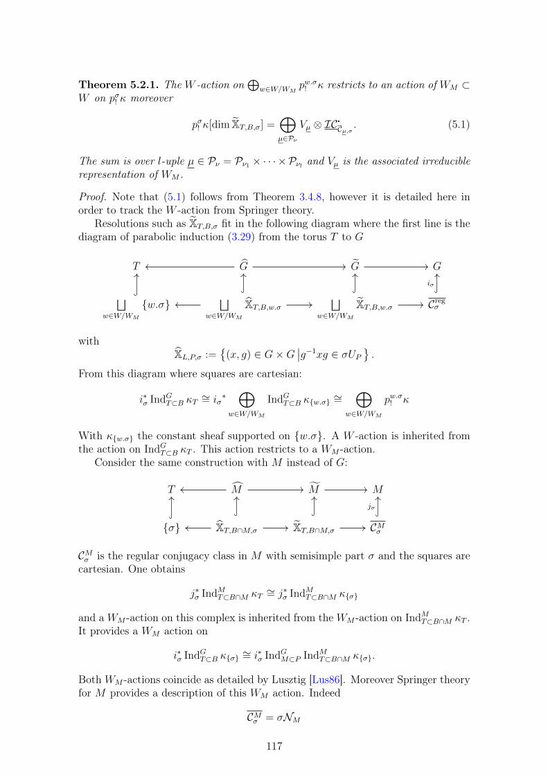
Theorem 5.2.1. The W -action on⊕

w∈W/WMpw.σ! κ restricts to an action of WM ⊂

W on pσ! κ moreover

pσ! κ[dim XT,B,σ] =⊕µ∈Pν

Vµ ⊗ IC •Cµ,σ . (5.1)

The sum is over l-uple µ ∈ Pν = Pν1 × · · · ×Pνl and Vµ is the associated irreduciblerepresentation of WM .

Proof. Note that (5.1) follows from Theorem 3.4.8, however it is detailed here inorder to track the W -action from Springer theory.

Resolutions such as XT,B,σ fit in the following diagram where the first line is thediagram of parabolic induction (3.29) from the torus T to G

T G G G

⊔w∈W/WM

w.σ⊔

w∈W/WM

XT,B,w.σ⊔

w∈W/WM

XT,B,w.σ Cregσ

iσ

withXL,P,σ :=

(x, g) ∈ G×G

∣∣g−1xg ∈ σUP.

From this diagram where squares are cartesian:

i∗σ IndGT⊂B κT∼= iσ

∗⊕

w∈W/WM

IndGT⊂B κw.σ∼=

⊕w∈W/WM

pw.σ! κ

With κw.σ the constant sheaf supported on w.σ. A W -action is inherited fromthe action on IndGT⊂B κT . This action restricts to a WM -action.

Consider the same construction with M instead of G:

T M M M

σ XT,B∩M,σ XT,B∩M,σ CMσ

jσ

CMσ is the regular conjugacy class in M with semisimple part σ and the squares arecartesian. One obtains

j∗σ IndMT⊂B∩M κT ∼= j∗σ IndMT⊂B∩M κσ

and a WM -action on this complex is inherited from the WM -action on IndMT⊂B∩M κT .It provides a WM action on

i∗σ IndGT⊂B κσ∼= i∗σ IndGM⊂P IndMT⊂B∩M κσ.

Both WM -actions coincide as detailed by Lusztig [Lus86]. Moreover Springer theoryfor M provides a description of this WM action. Indeed

CMσ = σNM

117

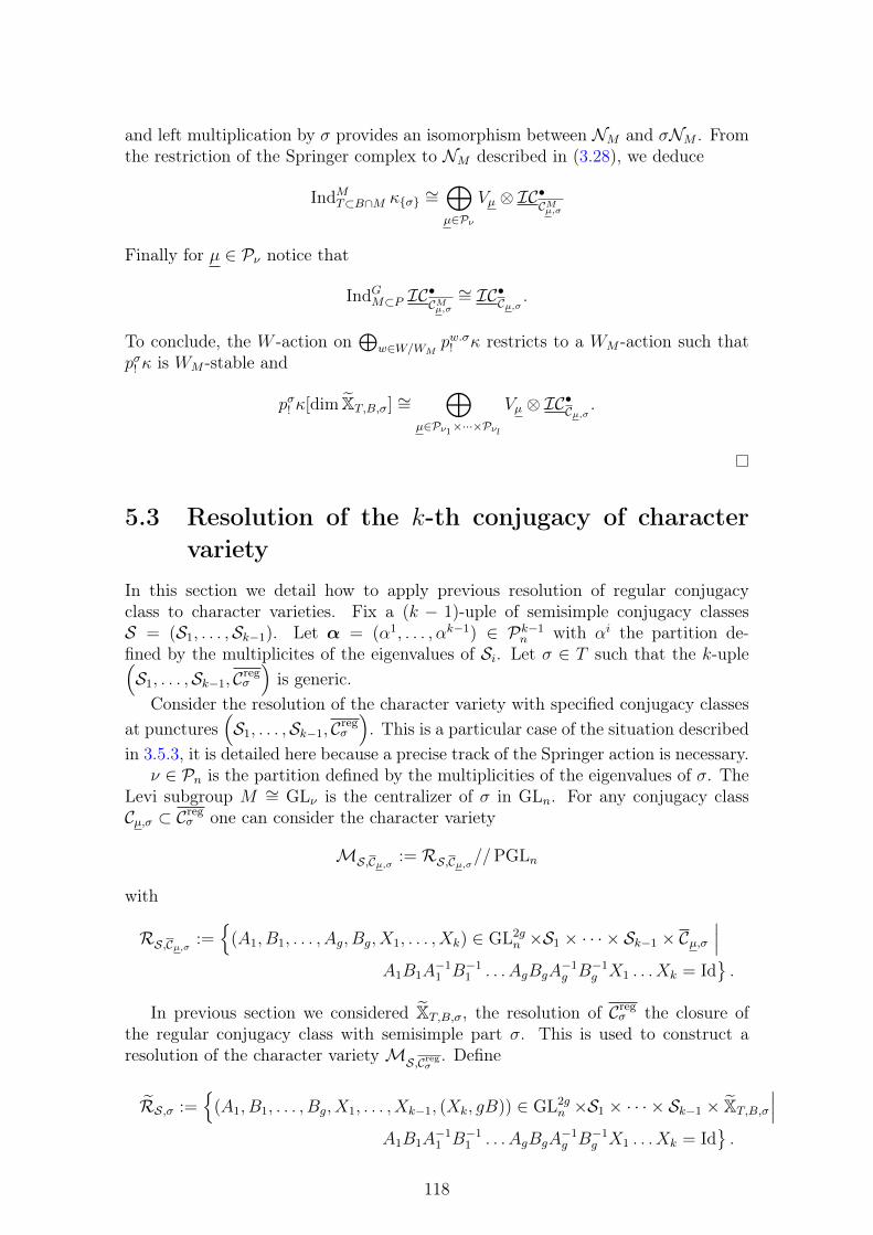
and left multiplication by σ provides an isomorphism between NM and σNM . Fromthe restriction of the Springer complex to NM described in (3.28), we deduce

IndMT⊂B∩M κσ ∼=⊕µ∈Pν

Vµ ⊗ IC•CMµ,σ

Finally for µ ∈ Pν notice that

IndGM⊂P IC•CMµ,σ∼= IC•Cµ,σ .

To conclude, the W -action on⊕

w∈W/WMpw.σ! κ restricts to a WM -action such that

pσ! κ is WM -stable and

pσ! κ[dim XT,B,σ] ∼=⊕

µ∈Pν1×···×Pνl

Vµ ⊗ IC•Cµ,σ .

5.3 Resolution of the k-th conjugacy of charactervariety

In this section we detail how to apply previous resolution of regular conjugacyclass to character varieties. Fix a (k − 1)-uple of semisimple conjugacy classesS = (S1, . . . ,Sk−1). Let α = (α1, . . . , αk−1) ∈ Pk−1

n with αi the partition de-fined by the multiplicites of the eigenvalues of Si. Let σ ∈ T such that the k-uple(S1, . . . ,Sk−1, Creg

σ

)is generic.

Consider the resolution of the character variety with specified conjugacy classesat punctures

(S1, . . . ,Sk−1, Creg

σ

). This is a particular case of the situation described

in 3.5.3, it is detailed here because a precise track of the Springer action is necessary.ν ∈ Pn is the partition defined by the multiplicities of the eigenvalues of σ. The

Levi subgroup M ∼= GLν is the centralizer of σ in GLn. For any conjugacy classCµ,σ ⊂ Creg

σ one can consider the character variety

MS,Cµ,σ := RS,Cµ,σ//PGLn

with

RS,Cµ,σ :=

(A1, B1, . . . , Ag, Bg, X1, . . . , Xk) ∈ GL2gn ×S1 × · · · × Sk−1 × Cµ,σ

∣∣∣A1B1A

−11 B−1

1 . . . AgBgA−1g B−1

g X1 . . . Xk = Id.

In previous section we considered XT,B,σ, the resolution of Cregσ the closure of

the regular conjugacy class with semisimple part σ. This is used to construct aresolution of the character varietyMS,Cregσ . Define

RS,σ :=

(A1, B1, . . . , Bg, X1, . . . , Xk−1, (Xk, gB)) ∈ GL2gn ×S1 × · · · × Sk−1 × XT,B,σ

∣∣∣A1B1A

−11 B−1

1 . . . AgBgA−1g B−1

g X1 . . . Xk = Id.

118

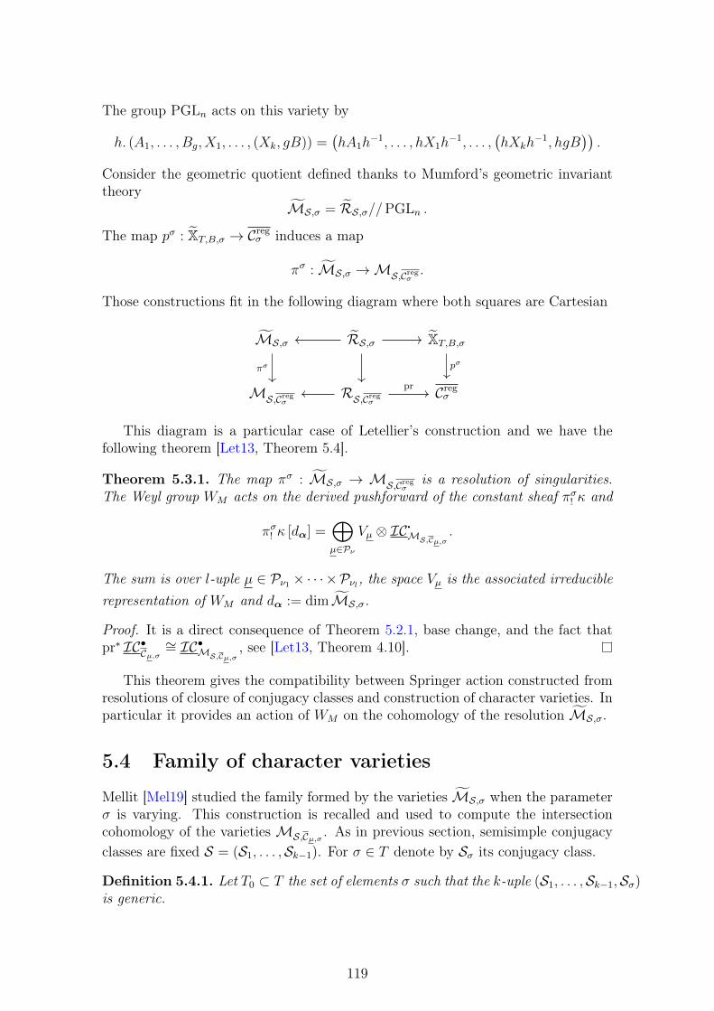
The group PGLn acts on this variety by

h. (A1, . . . , Bg, X1, . . . , (Xk, gB)) =(hA1h

−1, . . . , hX1h−1, . . . ,

(hXkh

−1, hgB)).

Consider the geometric quotient defined thanks to Mumford’s geometric invarianttheory

MS,σ = RS,σ//PGLn .

The map pσ : XT,B,σ → Cregσ induces a map

πσ : MS,σ →MS,Cregσ .

Those constructions fit in the following diagram where both squares are Cartesian

MS,σ RS,σ XT,B,σ

MS,Cregσ RS,Cregσ Cregσ

πσ pσ

pr

This diagram is a particular case of Letellier’s construction and we have thefollowing theorem [Let13, Theorem 5.4].

Theorem 5.3.1. The map πσ : MS,σ → MS,Cregσ is a resolution of singularities.The Weyl group WM acts on the derived pushforward of the constant sheaf πσ! κ and

πσ! κ [dα] =⊕µ∈Pν

Vµ ⊗ IC •MS,Cµ,σ .

The sum is over l-uple µ ∈ Pν1 × · · · ×Pνl, the space Vµ is the associated irreduciblerepresentation of WM and dα := dimMS,σ.

Proof. It is a direct consequence of Theorem 5.2.1, base change, and the fact thatpr∗ IC•Cµ,σ

∼= IC•MS,Cµ,σ , see [Let13, Theorem 4.10].

This theorem gives the compatibility between Springer action constructed fromresolutions of closure of conjugacy classes and construction of character varieties. Inparticular it provides an action of WM on the cohomology of the resolution MS,σ.

5.4 Family of character varieties

Mellit [Mel19] studied the family formed by the varieties MS,σ when the parameterσ is varying. This construction is recalled and used to compute the intersectioncohomology of the varietiesMS,Cµ,σ . As in previous section, semisimple conjugacyclasses are fixed S = (S1, . . . ,Sk−1). For σ ∈ T denote by Sσ its conjugacy class.

Definition 5.4.1. Let T0 ⊂ T the set of elements σ such that the k-uple (S1, . . . ,Sk−1,Sσ)is generic.

119

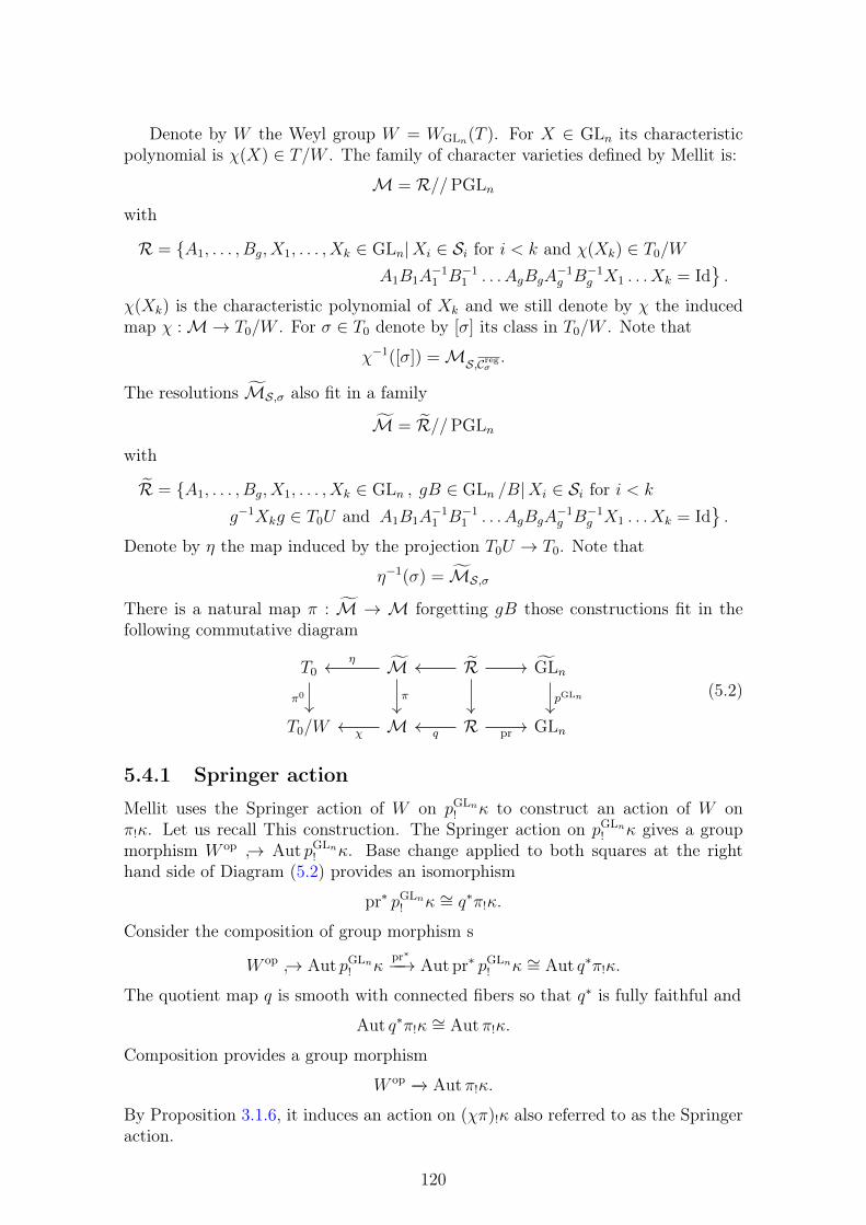
Denote by W the Weyl group W = WGLn(T ). For X ∈ GLn its characteristicpolynomial is χ(X) ∈ T/W . The family of character varieties defined by Mellit is:

M = R//PGLn

with

R = A1, . . . , Bg, X1, . . . , Xk ∈ GLn|Xi ∈ Si for i < k and χ(Xk) ∈ T0/W

A1B1A−11 B−1

1 . . . AgBgA−1g B−1

g X1 . . . Xk = Id.

χ(Xk) is the characteristic polynomial of Xk and we still denote by χ the inducedmap χ :M→ T0/W . For σ ∈ T0 denote by [σ] its class in T0/W . Note that

χ−1([σ]) =MS,Cregσ .

The resolutions MS,σ also fit in a family

M = R//PGLn

with

R = A1, . . . , Bg, X1, . . . , Xk ∈ GLn , gB ∈ GLn /B|Xi ∈ Si for i < k

g−1Xkg ∈ T0U and A1B1A−11 B−1

1 . . . AgBgA−1g B−1

g X1 . . . Xk = Id.

Denote by η the map induced by the projection T0U → T0. Note that

η−1(σ) = MS,σ

There is a natural map π : M → M forgetting gB those constructions fit in thefollowing commutative diagram

T0 M R GLn

T0/W M R GLn

π0

η

π pGLn

χ q pr

(5.2)

5.4.1 Springer action

Mellit uses the Springer action of W on pGLn! κ to construct an action of W on

π!κ. Let us recall This construction. The Springer action on pGLn! κ gives a group

morphism W op → Aut pGLn! κ. Base change applied to both squares at the right

hand side of Diagram (5.2) provides an isomorphism

pr∗ pGLn! κ ∼= q∗π!κ.

Consider the composition of group morphism s

W op → Aut pGLn! κ

pr∗−−→ Aut pr∗ pGLn! κ ∼= Aut q∗π!κ.

The quotient map q is smooth with connected fibers so that q∗ is fully faithful and

Aut q∗π!κ ∼= Autπ!κ.

Composition provides a group morphism

W op −→ Aut π!κ.

By Proposition 3.1.6, it induces an action on (χπ)!κ also referred to as the Springeraction.

120

5.4.2 Monodromic action

The Springer action on the complex pGLn! κ comes from aW -equivariant structure on

the constant sheaf over a regular locus GLreg

n . The same holds for π!κ. Let T reg0 ⊂ T0

the subset of regular elements. An element σ ∈ T0 is regular if its centralizer in GLnis ZGLn(σ) = T . Consider the pull back of Diagram (5.2) to the regular locus

T reg0 Mreg Rreg GL

reg

n

T reg0 /W Mreg Rreg GLreg

n

π0,reg

ηreg

χreg

. (5.3)

There is a W -action on Mreg induced by the maps gB 7→ gw−1B, for w ∈ W andw ∈ GLn a representative. κ ∈ Dbc

(Mreg

)is the constant sheaf concentrated in

degree 0. Define a W -action on κ, for w ∈ W let φw : w∗κ → κ be the morphismwhich is the identity on the stalks. Then by Proposition 3.1.6, W acts on ηreg

! κ. Letσ ∈ T reg

0 , for w ∈ W the action on Mreg induces an isomorphism

w : MS,σ → MS,w.σ.

Note that Hiση

reg! κ ∼= H i

c (MS,σ, κ). By Remark 3.1.3, on the stalks, the W -equivariant structure comes from the functoriality of the compactly supported co-homology

w∗ : H ic(MS,w.σ, κ)→ H i

c(MS,σ, κ).

Pushing forward to T reg0 /W provides a W -action on (π0,regηreg)!κ.

5.4.3 Comparison of monodromic action and Springer action

Mellit [Mel19] proved that the monodromic action and the Springer action coincideover the regular locus.

Theorem 5.4.2. The monodromic action on (π0,regηreg)!κ coincides with the Springeraction on (χregπ)!κ under the isomorphism

π0! η

reg! κ ∼= χreg

! π!κ.

Proof. Tracking the Springer action over the regular locus through Diagram (5.3),one sees that it comes from the W -equivariant structure of the constant sheaf overMreg, just like the monodromic action.

An important result is that the cohomology sheaves Hiη!κ are local systems overT0 [Mel19, Proposition 8.4.1]. This proposition together with Theorem 5.4.2 providethe following corollary

Corollary 5.4.3 (Corollary 8.4.3 [Mel19]). There exists a W -equivariant structureon the local systems Hiη!κ extending the W -equivariant structure on Hiηreg

! κ de-scribed in 5.4.2 and the pushforward of this W -equivariant structure on (π0η)!κ overT0/W coincide with the Springer action on (χπ)!κ.

121

Remark 5.4.4. This result could also be obtained like in the additive case: Theorem4.3.3. In the additive case, the cohomology sheaves Hiη!κ are constant thanks tothe quiver variety point of view. Here, in the multiplicative case, they are locallyconstant thanks to the cell decomposition from Mellit. In both case theW -equivariantstructure can be obtained either with [Mel19, Corollary 8.4.3] or with Theorem 4.3.3.This last theorem also works when K = Fq.

As in 5.3, let σ ∈ T0 and M the centraliser of σ in G. The following notationsare used

M ∼= GLν =∏i

GLνi

WM∼= Sν =

∏i

Sνi

Pν =∏i

Pνi .

Mellit suggested us to study restriction of the W action to the subgroup WM ⊂ W .

Theorem 5.4.5. WM acts on H ic

(MS,σ, κ

)and there is an isomorphism of WM -

representations:

H ic

(MS,σ, κ

)=⊕µ∈Pν

Vµ ⊗ IHi+dα,µ−dαc

(MS,Cµ,σ , κ

)with

dα,µ := dimMS,Cµ,σ and dα = dimMS,σ.

Proof. Consider the following pull back of Diagram (5.2):

W.σ⊔

w∈W/WM

MS,w.σ⊔

w∈W/WM

RS,w.σ⊔

w∈W/WM

XT,B,w.σ

[σ] MS,Cregσ RS,Cregσ Cregσ

⊔w∈W/WM

πw.σ

Previous corollary provides, for the stalk over [σ] ∈ T0/W , an isomorphism⊕w∈W/WM

H ic

(MS,w.σ, κ

)∼= Hi

[σ](π0η)!κ ∼= Hi[σ](χπ)!κ ∼=

⊕w∈W/WM

Hi[σ](χπ

w.σ)!κ.

This isomorphism is compatible with W -action and direct sum decomposition sothat

H ic

(MS,σ, κ

)∼= Hi

[σ](χπσ)!κ

after restriction of the W action to WM ⊂ W this isomorphism holds as a WM -representation isomorphism. A way to describe the action on the left hand side isthat H i

c

(MS,σ, κ

)is the stalk at σ of a W -equivariant local system, WM acts on

this stalk as it fixes σ. The theorem then follows from the description of (χπσ)!κfrom Theorem 5.3.1.

122

Let ζ a central element in GLn lying in T0.

Theorem 5.4.6. There is an isomorphism of WM representations⊕λ∈Pn

ResWWMVλ ⊗ IH

i+dα,λc

(MS,Cλ,ζ , κ

)∼=⊕µ∈Pν

Vµ ⊗ IHi+dα,µc

(MS,Cµ,σ , κ

).

with the notations from previous theorem and

dα,λ = dimMS,Cλ,ζ .

Proof. Previous theorem applied with the central element ζ instead of σ gives anisomorphism of W -representations

H ic

(MS,ζ , κ

)∼=⊕λ∈Pn

Vλ ⊗ IHi+dimMS,Cλ,ζ−dimMS,ζc

(MS,Cλ,ζ , κ

).

H ic (MS,ζ , κ) ∼= Hi

ζη!κ and H ic (MS,σ, κ) ∼= Hi

ση!κ are stalks of the same W -equivariant local system. Both σ and ζ are fixed by WM so that WM acts onthose stalks and the representations are isomorphic. The theorem then follows fromTheorem 5.4.5.

Corollary 5.4.7.⊕λ∈Pn

HomWM

(Vµ,ResWWM

Vλ

)⊗ IH i+dα,λ

c

(MS,Cλ,ζ , κ

)∼= IH

i+dα,µc

(MS,Cµ,σ , κ

)(5.4)

in particular⊕λ∈Pn

HomWM

(εν ,ResWWM

Vλ)⊗ IH i+dα,λ

c

(MS,Cλ,ζ , κ

)∼= H i+dα,ν

c (MS,Sσ , κ) (5.5)

with εν = εν1 ⊗ · · · ⊗ ενl and ενi the signature representation of Sνi.

5.5 Poincaré polynomial for intersection cohomol-ogy of character varieties with k− 1 semisimplemonodromies

Notations 5.5.1. As in previous section, (S1, . . . ,Sk−1) is a fixed (k − 1)-uple ofsemisimple conjugacy classes, their type is determined by α = (α1, . . . , αk−1) ∈Pk−1n . For f ∈ Sym[X] a symmetric function

hαf := hα1 [X1] . . . hαk−1 [Xk−1]f [Xk].

Let σ ∈ T0 with multiplicities of the eigenvalues given by a partition ν ∈ Pn.As in previous subsection Sσ is its conjugacy class in GLn. Before generalizing toany conjugacy class, let us recall Mellit’s result for semisimple monodromies at eachpunctures. From Equation (3.50) one obtains

Pc(MS,Sσ , v) = vdα,ν⟨hαhν ,HHLV

n (−1, v)⟩. (5.6)

with dα,ν = dimMS,Sσ .

123

Theorem 5.5.2. Let ζ ∈ T0 central in GLn and λ ∈ Pn a partition. The conjugacyclasse Cλ,ζ has semisimple part ζ and Jordan type λ. The Poincaré polynomial forintersection cohomology ofMS,Cλ,ζ is

Pc

(MS,Cλ,ζ , v

)= vdα,λ

⟨hαsλ′ ,HHLV

n (−1, v)⟩.

Proof. By adjunction

dim HomWM

(εν ,ResWWM

Vλ)

= dim HomW

(IndWWM

εν , Vλ).

Lemma 3.2.28 implies

dim HomW

(IndWWM

εν , Vλ)

= 〈hν , sλ′〉 .

Substituting (5.6) in (5.5) and taking the dimension∑λ∈Pn

〈hν , sλ′〉 t−dα,λPc(MS,Cλ,ζ , t

)=⟨hαhν ,HHLV

n (−1, t)⟩. (5.7)

For λ, ν ∈ Pn letMν,λ = 〈hν , sλ〉 .

Schur functions form an orthonormal basis of Sym[X] for the Hall pairing, thus

hν =∑λ

Mν,λsλ.

As (hν)ν∈Pn and (sλ)λ∈Pn are basis of Symn[X] the matrix (Mν,λ)ν,λ∈Pn is invertibleits inverse is denoted by (Nν,λ)ν,λ∈Pn . Such transition matrices are described byMacdonald [Mac15, I-6]. We conclude by multiplying (5.7) by Nη,ν and summingover ν.

For µ = (µ1, . . . , µl) ∈ Pν1 × · · · × Pνl we introduce the notation

sµ[X] := sµ1 [X] . . . sµl [X]

so thathαsµ = hα1 [X1] . . . hαk [Xk−1]sµ1 [Xk] . . . sµl [Xk].

Corollary 5.5.3. The Poincaré polynomial for intersection cohomology of the char-acter variety MS,Cµ,σ with k − 1 monodromies in the semisimple conjugacy classesS and one monodromy in Cµ,σ is

Pc

(MS,Cµ,σ , t

)= tdα,µ

⟨hαsµ′ ,HHLV

n (−1, t)⟩.

Proof. First note that after twisting both representations with the sign one has

dim HomWM

(Vµ,ResWWM

Vλ

)= dim HomWM

(Vµ′ ,ResWWM

Vλ′).

Then as IndWWMis left adjoint to ResWWM

dim HomWM

(Vµ′ ,ResWWM

Vλ′)

= dim HomWM

(IndWWM

Vµ′ , Vλ′)

=⟨sµ′ , sλ′

⟩.

124

Taking dimension in equation (5.4) and substituting result of previous theorem

t−dα,µPc

(MS,Cµ,σ , t

)=∑λ

⟨sµ′ , sλ′

⟩ ⟨hαsλ′ ,HHLV

n (−1, t)⟩.

As Schur functions form an orthonormal basis of Symn[X],

sµ′ =∑λ∈Pn

⟨sµ′ , sλ′

⟩sλ′

so that ∑λ∈Pn

⟨sµ′ , sλ′

⟩tdλ⟨hαsλ,HHLV

n (−1, t)⟩

=⟨hαsµ′ ,HHLV

n (−1, t)⟩

125

Chapter 6

Intersection cohomology of charactervarieties through non-Abelian Hodgetheory

6.1 IntroductionIn this chapter, the base field is C, we compute the Poincaré polynomial for inter-section cohomology of character varieties with the closure of conjugacy classes ofany type at each puncture. This proves the Poincaré polynomial specialization ofa conjecture from Letellier [Let13]. Mellit computed the Poincaré polynomial forcharacter varieties with semi-simple monodromies [Mel17a]. In previous chapter weassumed k − 1 among k monodromies are semisimple. This assumption is now re-laxed. As in previous chapter, the computation relies on the one hand on Mellit’sresult and on the other hand on resolutions of character varieties. Those construc-tions come with a combinatorial relation between the cohomology of the resolutionsand the intersection cohomology of character varieties. The main technical difficultyis to prove that the resolution is diffeomorphic to a character variety with semisimplemonodromies. Then the combinatorial relation can be inverted and gives a formulafor the intersection cohomology of character varieties. Contrarily to previous chap-ter where everything was algebraic, analytic methods such as non-Abelian Hodgetheory are now necessary to construct the diffeomorphism.

6.1.1 Intersection cohomology of character varieties andWeylgroup actions

Consider the resolution ML,P ,σ of a character varietyMCµ,σ as introduced in 3.5.3.Springer theory provides a combinatoric relation between the cohomology of ML,P ,σ

and intersection cohomology of character varietiesMCρ,σ :

H i+dµc

(ML,P ,σ, κ

)∼=

⊕ρ∈Pν1×···×Pνk

Aµ′,ρ ⊗ IH i+dρc

(MCσ,ρ , κ

). (6.1)

This relation is the main tool allowing to go from usual cohomology of smoothvarieties to intersection cohomology of singular varieties. We shall see that the

126

resolution ML,P ,σ is diffeomorphic to a character varietyMS with semisimple con-jugacy classes at punctures. With S = (S1, . . . ,Sk) and Sj is the class of an elementwith centralizer in GLn equal to Lj ∼= GLµj ′ .

Mellit [Mel17a] computed the Poincaré polynomial of those character varieties.The Poincaré polynomial is invariant under diffeomorphism so we deduce the Poincarépolynomial of the resolution. Then the combinatoric relation can be inverted usingtransition matrices between various basis of the space of symmetric funtions. Thisresults in the following theorem:

Theorem 6.1.1. For a generic k-uple of conjugacy classes Cµ,σ, the Poincaré poly-nomial for compactly supported intersection cohomology of the character varietyMCµ,σ is

Pc

(MCµ,σ , v

)= vdµ

⟨sµ′ ,HHLV

n (−1, v)⟩.

Moreover, as a by product of the diffeomorphism between resolution ML,P ,σ andMS , we obtain a Weyl group action on the cohomology ofMS from the Springeraction on the cohomology of ML,P ,σ. Similarly to the additive case, the twistedPoincaré polynomial is computed in 6.2.2

Theorem 6.1.2. WM (L) acts on the cohomology ofMS and the η-twisted Poincarépolynomial is

P ηc (MS , v) = (−1)r(η)vdimMS⟨hη,HHLV

n (−1, v)⟩.

The symmetric functions hη and r(η) are defined in 3.5.18.

6.1.2 Diffeomorphism between a resolution ML,P ,σ and a char-acter variety with semisimple monodromies MS

The technical part of the proof is to exhibit a diffeomorphism between the resolutionML,P ,σ andMS .

Theorem 6.1.3. Cµ,σ is a generic k-uple of conjugacy classes and ML,P ,σ is theresolution of MCµ,σ . Then ML,P ,σ is diffeomorphic to a character variety MS.With S = (S1, . . . ,Sk) and Sj is the class of an element with centralizer in GLnequal to Lj ∼= GLµj ′.

This theorem is proved in few steps in 6.6.1.The first step is the Riemann-Hilbert correspondence, it gives a diffeomorphism

between the resolutionMCµ,σ and a de Rham moduli space of parabolic connections.Riemann-Hilbert correspondence was developed by Deligne [Del70], and Simpsonfor the filtered case [Sim90]. Yamakawa proved that this correspondence induces acomplex analytic isomorphism between moduli spaces [Yam08].

The second step is the non-Abelian Hodge theory, a diffeomorphism betweende Rham moduli space and Dolbeault moduli space. It was established by Hitchin[Hit87] and Donaldson [Don87] for compact curves. Corlette [Cor88] and Simp-son [Sim88] generalized it for higher dimensions. The parabolic version over non-compact curves was proved by Simpson [Sim90]. This is the one needed here. It wasgeneralized for higher dimension by Biquard [Biq97]. The relevant moduli spaces to

127

obtain this correspondence as a diffeomorphism were introduced by Konno [Kon93]and Nakajima [Nak96]. Biquard-Boalch [BB04] generalized further to wild non-Abelian Hodge theory and constructed the associated hyperkähler moduli spaces.We use their construction of the moduli spaces. Biquard, García-Prada and Mundeti Riera [BGM15] established a parabolic non-Abelian Hodge correspondence for realgroups, generalizing Simpson construction for GLn.

After the diffeomorphism from non-Abelian Hodge theory we use the methodfrom Nakajima [Nak96] for GL2 and Biquard, García-Prada, Mundet i Riera [BGM15]for real groups. The weights defining the moduli space of parabolic Higgs bundlesare changed. This is done before going back to another de Rham moduli spacethanks to non-Abelian Hodge theory in the other direction. The change of stabilityon the Dolbeault side induces a change of eigenvalues of the residue on the de Rhamside.

Finally Riemann-Hilbert correspondence is applied in the other direction. Itgives a diffeomorphism to a character variety where the eigenvalues σ have beenperturbed, the monodromies are now semisimple.

In Section 6.2, we compute the Poincaré polynomial for intersection of charac-ter varieties, assuming the resolution is diffeomorphic to a character variety withsemisimple conjugacy classes at punctures.

In Section 6.3 the example of the sphere with four punctures and rank n = 2 isstudied. There, we can obtain the expected diffeomorphism using only tools fromalgebraic geometry. This example has been studied for a long time by Vogt [Vog89]and Fricke-Klein [FK97]. The character varieties are affine cubic surfaces satisfyingFricke-Klein relation. Cubic surfaces and line over them have been extensively stud-ied. They are classified for instance by Cayley [Cay69], see also Bruce-Wall [BW79],Manin [Man86] and Hunt [Hun96]. This rich theory proves that the minimal reso-lution is diffeomorphic to a character variety with semisimple monodromies. Bothappear to be diffeomorphic to the projective plane blown up in six points minusthree lines.

In Section 6.4 various filtered objects are introduced. First the filtered localsystem; the resolution ML,P ,σ appears to be the associated moduli space. Then theparabolic connections and finally the parabolic Higgs bundles.

In Sections 6.5 and 6.6 we recall Biquard-Boalch [BB04] analytic constructionsof Hyperkähler moduli space. This provides the non-Abelian Hodge theory as adiffeomorphism. Then the stability parameters are perturbed following ideas ofNakajima [Nak96] for GL2 and Biquard, García-Prada, Mundet i Riera [BGM15] fora larger family of groups. It finally provides the diffeomorphism between ML,P ,σ

andMS .

128

6.2 Poincaré polynomial and twisted Poincaré poly-nomial

6.2.1 Computation of the Poincaré polynomial

Consider a generic k-uple of conjugacy classes Cµ,σ =(Cµ1,σ1 , . . . , Cµk,σk

). As usual,

the class Cµj ,σj is characterized by its eigenvalues

σj1, . . . , σj1︸ ︷︷ ︸

νj1

, . . . , σjlj , . . . , σjlj︸ ︷︷ ︸

νjlj

and by µj,i ∈ Pνji the Jordan type of the eigenvalue σji . Denote by µj,i′ the transposedpartition. For each of this conjugacy classes consider the resolution of the closure(see 3.3.3)

XLj ,P j ,σj → Cµj ,σj .

The group Lj used to construct the resolution is

Lj ∼= GLµj,11

′ ×GLµj,12

′ × . . .︸ ︷︷ ︸⊂GL

νj1

× · · · ×GLµj,lj1

′ ×GLµj,lj2

′ × . . .︸ ︷︷ ︸⊂GL

νjlj

.

As detailed in 3.5.3, resolution of closure of conjugacy classes fit together in ML,P ,σ

a resolution of the character varietyMCµ,σ .

Definition 6.2.1 (Semisimple conjugacy classes of type µ′). Consider a k-upleof conjugacy classes S = (S1, . . . ,Sk). We say that S is of type µ′ if one of thefollowing equivalent condition is satisfied for all 1 ≤ j ≤ k

• The multiplicities of the eigenvalues of Sj are given by the partition⋃lji=1 µ

j,i′.

• The centralizer of an element in Sj is isomorphic to Lj ∼= GLµj ′.

The proof of next theorem is postponed to the remaining sections of this chapter.

Theorem 6.2.2. The resolution ML,P ,σ is diffeomorphic to a character varietyMS with S a generic k-uple of semisimple conjugacy classes of type µ′.

With this result we are ready to compute the Poincaré polynomial for intersectioncohomology of character varietiesMCµ,σ . As the Poincaré polynomial is a topologicalinvariant

Pc

(ML,P ,σ, t

)= Pc (MS , t) .

Let us translate (6.1) in terms of Poincaré polynomial.

t−dµPc (MS , t) =∑ρµ

(dimAµ′,ρ) t−dρPc

(MCρ,σ , t

). (6.2)

The idea is now to invert this relation. First we compute the dimension of themultiplicity spaces dimAµ′,ρ.

129

Lemma 6.2.3. The dimension of the multiplicity space is given by

dimAµ′,ρ =∏

1≤j≤k1≤i≤lj

⟨hµj,i′ , sρj,i′

⟩

Proof. By definition

Aµ′,ρ = HomWM

(IndWMWL εµ′ , Vρ

)=

⊗1≤j≤k

⊗1≤i≤lj

HomSνji

(εµj,i′ , Vρj,i

) .

We conclude with Lemma 3.2.28.

Theorem 6.2.4. For a generic k-uple of conjugacy classes Cµ,σ, the Poincaré poly-nomial for compactly supported intersection cohomology of the character varietyMCµ,σ is

Pc

(MCµ,σ , v

)= vdµ

⟨sµ′ ,HHLV

n (−1, v)⟩.

Proof. The complete symmetric functions (hµ)µ∈Pm and the Schur functions (sρ)ρ∈Pmare two basis of the space of degree m symmetric functions. Let (Mµ,ρ)µ,ρ∈Pm thetransition matrix between between those basis then

hµ =∑ρ∈Pm

Mµ,ρsρ.

As the Schur functions form an orthonormal basis, the transition matrix is givenexplicitly by

Mµ,ρ = 〈hµ, sρ〉 .

It is invertible and denote by (Nµ,ρ)µ,ρ∈Pm its inverse. Combining Equation (6.2),Lemma 6.2.3 and the formula for Poincaré polynomial of character varieties withsemisimple conjugacy classes:⟨

k∏j=1

lj∏i=1

hµj,i′ [Xj],HHLVn (−1, v)

⟩=∑ρµ

k∏j=1

lj∏i=1

⟨hµj,i′ , sρj,i′

⟩v−dρPc

(MCρ,σ , v

).

This relation can now be inverted. Fix λ ∈ Pν1 × · · · × Pνk . Multiply previousequation by Nλ1,1′,µ1,1′ and sum over µ1,1′ ∈ Pν11 . Repeating this process gives theexpected result: ⟨

sλ′ ,HHLVn (−1, v)

⟩= v−dλPc

(MCλ,σ , v

).

6.2.2 Weyl group action and twisted Poincaré polynomial

As in [Let13, Proposition 1.9], twisted Poincaré polynomial can be computed thanksto previous theorem. Using notations from 3.5.4 and Definition 3.6.6 for η-twistedPoincaré polynomial we have the following theorem

130

Theorem 6.2.5. Cµ,σ is a generic k-uple of conjugacy classes and ML,P ,σ is theresolution of MCµ,σ . For η indexing a conjugacy class in WM (L), the η-twistedmixed-Hodge polynomial of ML,P ,σ is

P ηc

(ML,P ,σ, v

)= (−1)r(η)vdµ

⟨hη,HHLV

n (−1, v)⟩

Proof. Theorem 3.5.20 and Proposition 3.5.19 give

v−dµP ηc

(ML,P ,σ, v

)=∑ρµ

k∏j=1

lj∏i=1

cρj,i

ηj,i

v−dρPc

(MCρ,σ , t

).

Apply Theorem 6.2.4:

v−dµP ηc

(ML,P ,σ, v

)=∑ρµ

k∏j=1

lj∏i=1

cρj,i

ηj,i

⟨sρ′ ,HHLVn (−1, v)

⟩.

Then using the relation cµω = (−1)r(ω)cµ′

ω′ (see Lemma 3.4.11) and Notations 3.5.18

v−dµP ηc

(ML,P ,σ, v

)= (−1)r(η)

⟨hη,HHLV

n (−1, v)⟩

Theorem 6.1.3 (which will be proved in Section 6.6) gives a diffeomorphismbetween ML,P ,σ and a character variety with semisimple monodromies MS . Thediffeomorphism transports the action on the cohomology of ML,P ,σ to an action onthe cohomology ofMS and we have the following corollary.

Corollary 6.2.6. WM (L) acts on the cohomology ofMS and the η-twisted Poincarépolynomial is

P ηc (MS , v) = (−1)r(η)vdµ⟨hη,HHLV

n (−1, v)⟩.

One can proceed as in the additive case (see 4.4.2) to give a cohomologicalinterpretation to another specialization of the coefficients cλµ,ν .

Theorem 6.2.7. For µ, ν in Pn, there exists a generic 4-uple of conjugacy classesof the following type:

• C1 has one eigenvalue with Jordan type µ′ ∈ Pn

• C2 has one eigenvalue with Jordan type ν ′ ∈ Pn.

• C3 is semisimple regular, it has n distinct eigenvalues

• C4 is semisimple with one eigenvalue of multiplicity n − 1 and the other ofmultiplicity 1

Then the Weyl group with respect to C3 is the symmetric group Sn and it acts onthe cohomology ofMC. Let w a n-cycle in this Weyl group then

c1n

µ,ν (1, t) = t−dC2

∑r

tr (w, IHrc (MC, κ)) t

r2 .

131

6.3 Example of the sphere with four punctures andrank 2

We study the particular case n = 2, k = 4. Then the character varieties are affinecubic surfaces. The defining equation was known by Vogt [Vog89] and Fricke-Klein[FK97]. The theory of cubic surfaces allows to obtain the expected diffeomorphism.Cubic surfaces and lines over them have been extensively studied. They are classi-fied for instance by Cayley [Cay69], see also Bruce-Wall [BW79], Manin [Man86] andHunt [Hun96]. This particular example of character varieties also appear in the the-ory of Painlevé VI differential equation. In this context resolution of cubic surfaceswere studied by Inaba-Iwasaki-Saito [IIS06a; IIS06b; IIS06c] with Riemann-Hilbertcorrespondence. It was also studied on the Dolbeault side by Hausel [Hau98].

6.3.1 Fricke relation

We consider representations of the fundamental group of the sphere with four punc-tures P1\p1, ..., p4. First we prescribe no particular condition on the monodromiesaround the puncture

R :=

(X1, . . . , X4) ∈ GL42 |X1 . . . X4 = Id

The group GL2 acts by conjugation on R, its center acts trivially, hence the actionfactors through an action of PGL2. Points of the following GIT quotient representclosed orbits for this action.

M := R//PGL2 := SpecC [R]PGL2

where C [R]PGL2 are the invariants under the GL2 action in the algebra of functionsof the affine variety R. There is an explicit description of this algebra. First notethat R ∼= GL3

2 as the fourth coordinate is determined by X4 = (X1X2X3)−1. Thealgebra of functions on a k-uple of matrices invariant under conjugation was studiedby Procesi.

Theorem 6.3.1 (Procesi [Pro76]). Let C[GLkn

]PGLn be the algebra of regular func-tion f : GLkn → C invariant under simultaneous conjugation

f(X1, ..., Xk) = f(gX1g−1, . . . , gXkg

−1).

This algebra is generated bytr(Xi1 . . . Xil) (6.3)

where 0 ≤ l ≤ k and i1, . . . , il ∈ 1, . . . , l not necessarily distinct. The relationsbetween those functions are spanned by∑

σ∈Sl

ε(σ) trσ(M1, . . . ,Ml) = 0 (6.4)

where Mi is any monomial in the coordinates (Xj)1≤j≤k and trσ is defined by

trσ(M1, . . . ,Ml) := tr(Ma1,1 . . .Ma1,l1) . . . tr(Mar,1 . . .Mar,lr

). (6.5)

for σ a product of r cycles with disjoint supports σ = (a1,1 . . . a1,l1) . . . (ar,1 . . . ar,lr).Moreover, to obtain a generating family we can restrict to function tr(Xi1 . . . Xil)

with l ≤ 2n − 1.

132

In particular C [R]PGL2 is generated by

tr(Xi), tr(XiXj), tr(XiXjXk) (6.6)

for i, j, k ∈ 1, 2, 3 not necessarily distincts. Our aim is to study character varietieswith prescribed closure of conjugacy classes at punctures, we can continue with theassumption:

Assumption 6.3.2. We assume that the (Xi)1≤i≤4 have determinant 1.

This assumption allows to get rid of some generators. Cayley-Hamilton theoremimplies

X2i − tr(Xi)Xi + Id = 0 (6.7)

so thattr(X2

i ) = tr(Xi)2 − 2. (6.8)

and multiplying (6.7) by Xj before taking trace

tr(X2iXj) = tr(Xi) tr(XiXj)− tr(Xj). (6.9)

Thus we can pick among (6.6) the following generators

a := tr(X1), b := tr(X2), c := tr(X3),x := tr(X2X3), y := tr(X1X3), z := tr(X1X2),d := tr(X1X2X3), d′ := tr(X1X3X2)

(6.10)

Moreover d′ can be expressed with the other generators using relation (6.4) withthe monomials Mi = Xi. The relations between those remaining generators are de-scribed in general by Procesi but it is convenient to obtain a finite description of therelations. Such a description was known by Vogt [Vog89] and Fricke-Klein [FK97],see also Goldman [Gol09] for a detailed discussion and Boalch-Paluba [BP16] forapplications to G2 character varieties. The relations boil down to a single equationknown as the Fricke relation

xyz + x2 + y2 + z2 + Ax+By + Cz +D = 0 (6.11)

with

A = −ad− bcB = −bd− acC = −cd− abD = abcd+ a2 + b2 + c2 + d2 − 4.

The character varieties we are interested in are obtained by specifying the Zariskiclosure of the conjugacy class of each Xi. First we assume that they are all semi-simple regular. For i = 1, . . . 4; Si is the conjugacy class of(

λi 00 λ−1

i

). (6.12)

S = (S1, . . . ,S4) is assumed to be generic. In terms of invariant functions, Xi ∈ Sifor all i, if and only if

tr(Xi) = λi + λ−1i for 1 ≤ i ≤ 3

tr(X1X2X3) = λ4 + λ−14 .

Then Fricke relation translates in next proproisition.

133

Proposition 6.3.3. The character variety MS is a smooth cubic surface in A3

given by Fricke relation (6.11) with coordinates x, y and z and constants A,B,Cand D.

Now consider non-semisimple conjugacy classes C = (C1, C2, C3, C4). With C1 theconjugacy class of (

−1 10 −1

)and C2 = C3 = C4 are the conjugacy classes of(

1 10 1

).

Note that this 4-uple of conjugacy classes is generic. The (Xi)1≤i≤4 are alreadyassumed to have determinant 1, then X1 belongs to the closure C1 if and only if

trX1 = −2.

Similarly the condition (X2, X3, X4) ∈ C2 × C3 × C4 is equivalent to

trX2 = trX3 = tr(X1X2X3) = 2.

Substituting this parameters in Fricke relation, the character variety is again a cubicsurface in A3 with equation:

xyz + x2 + y2 + z2 − 4 = 0. (6.13)

This cubic surface has exactly four singularities at (−2,−2,−2), (−2, 2, 2), (2,−2, 2)and (2, 2,−2). The classification of cubic surfaces (see for instance Bruce-Wall[BW79]) gives the following theorem:

Theorem 6.3.4. After compactification in P3, the character varietyMC is Cayley’snodal cubic, the only cubic surface with four singularities.

This particular character variety was studied by Cantat-Loray [CL09] in thecontext of Painlevé VI.

In this example, using only elementary algebraic geometry, we can prove that theminimal resolution ofMC is diffeomorphic to the character varieties with semisimplemonodromiesMS . We shall see that both varieties are obtained as the plane blown-up in six points minus three lines.

6.3.2 Projective cubic surfaces

Let us recall an important result in the classification of cubic surfaces. Smoothprojective cubic surfaces in P3 can be constructed by a blow-up of P2 in six points.

Let P = (P1, ..., P6) be six distinct points in the projective plane P2. The blow-upof P2 with respect to those six points is denoted YP → P2.

Definition 6.3.5 (Generic configuration for six points in P2). Such a configurationP of 6 points in P2 is called generic if no three of them lie on a line and no five ofthem lie on a conic.

134

The two following theorems are well-known results about cubic surfaces, see forinstance Manin [Man86] and Hunt [Hun96].

Theorem 6.3.6. Up to isomorphism, smooth projective cubic surfaces in P3 areobtained as P2 blown-up in six points in generic position.

Theorem 6.3.7. If the six points P = (P1, ..., P6) are the intersection of four lines(L1, ..., L4) in P2, then YP is isomorphic to a minimal resolution of singularities ofCayley’s nodal cubic.

The rest of this section is devoted to the proof of Theorem 6.3.7. Along the way,one direction of Theorem 6.3.6 is also proved: P2 blown-up in six points in genericposition is isomorphic to a smooth cubic surface in P3.

Those results rely on the theory of linear systems we briefly recall. A detailedpresentation can be found in Hartshorne [Har13, II-7].

Definition 6.3.8. A divisor D on a smooth variety Y is a formal sum D =∑

V nV Vover subvarieties of codimension one with nV ∈ Z and finitely many of them nonzero.D is effective if nV ≥ 0 for all V . A divisor D is principal if D = (f) for f a non-zero global section of the sheaf of rational functions. Two divisors D and D′ arelinearly equivalent if D −D′ is principal.

Definition 6.3.9. Let D be a divisor on a projective space Pn, the complete linearsystem denoted |D| is the set of effective divisors linearly equivalent to D.

Remark 6.3.10 (Hartshorne [Har13] II - 7.7, 7.8). The complete linear system |D|is identified with the projective space over the space of global sections of the invertiblesheaf L(D) associated with D. Indeed the zero set (s)0 of a section s is an effectivedivisor linearly equivalent to D

P(H0 (Y,L(D))) → |D|[s] 7→ (s)0

.

Moreover if L(D) is generated by its global section, it provides a morphism

ϕ : Y → P (H0 (Y,L(D))∗)x 7→ [ϕx]

(6.14)

Set theoretically, this morphism sends a point x ∈ Y to [ϕx] the line spanned by thelinear form

ϕx : H0 (Y,L(D)) → Cs 7→ s(x)

Let P = (P1, . . . , P6) be six points on P2, either in generic position or exactlythe intersection points of four lines. Linear systems allow to construct a morphismfrom YP to P3.

Definition 6.3.11. Let L a line in P2, the linear system |3L−P1 · · ·−P6| is a projec-tive subspace of |3L|. It is defined under the identification |3L| ∼= P (H0 (P2,L(3L)))by P(VP ) with

VP =s ∈ H0

(P2,L(3L)

)|s(Pi) = 0, for all 1 ≤ i ≤ 6

.

It is the set of cubic curves in P2 containing all the (Pi)1≤i≤6.

135

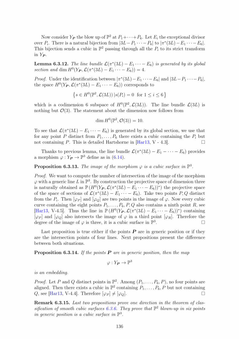
Now consider YP the blow up of P2 at P1+· · ·+P6. Let Ei the exceptional divisorover Pi. There is a natural bijection from |3L−P1 · · ·−P6| to |π∗(3L)−E1 · · ·−E6|.This bijection sends a cubic in P2 passing through all the Pi to its strict transformin YP .

Lemma 6.3.12. The line bundle L(π∗(3L)−E1 · · · −E6) is generated by its globalsection and dimH0(YP ,L(π∗(3L)− E1 · · · − E6)) = 4.

Proof. Under the identification between |π∗(3L)−E1 · · ·−E6| and |3L−P1 · · ·−P6|,the space H0(YP ,L(π∗(3L)− E1 · · · − E6)) corresponds to

s ∈ H0(P2,L(3L)) |s(Pi) = 0 for 1 ≤ i ≤ 6

which is a codimension 6 subspace of H0(P2,L(3L)). The line bundle L(3L) isnothing but O(3). The statement about the dimension now follows from

dimH0(P2,O(3)) = 10.

To see that L(π∗(3L)− E1 · · · − E6) is generated by its global section, we use thatfor any point P distinct from P1, . . . , P6 there exists a cubic containing the Pi butnot containing P . This is detailed Hartshorne in [Har13, V - 4.3].

Thanks to previous lemma, the line bundle L(π∗(3L)− E1 − · · · − E6) providesa morphism ϕ : YP → P3 define as in (6.14).

Proposition 6.3.13. The image of the morphism ϕ is a cubic surface in P3.

Proof. We want to compute the number of intersection of the image of the morphismϕ with a generic line L in P3. By construction the projective space of dimension threeis naturally obtained as P (H0(YP ,L(π∗(3L)− E1 · · · − E6))∗) the projective spaceof the space of sections of L(π∗(3L) − E1 · · · − E6). Take two points P,Q distinctfrom the Pi. Then [ϕP ] and [ϕQ] are two points in the image of ϕ. Now every cubiccurve containing the eight points P1, . . . , P6, P,Q also contains a ninth point R, see[Har13, V-4.5]. Thus the line in P (H0(YP ,L(π∗(3L)− E1 · · · − E6))∗) containing[ϕP ] and [ϕQ] also intersects the image of ϕ in a third point [ϕR]. Therefore thedegree of the image of ϕ is three, it is a cubic surface in P3.

Last proposition is true either if the points P are in generic position or if theyare the intersection points of four lines. Next propositions present the differencebetween both situations.

Proposition 6.3.14. If the points P are in generic position, then the map

ϕ : YP → P3

is an embedding.

Proof. Let P and Q distinct points in P2. Among (P1, . . . , P6, P ), no four points arealigned. Then there exists a cubic in P2 containing P1, . . . , P6, P but not containingQ, see [Har13, V-4.4]. Therefore [ϕP ] 6= [ϕQ].

Remark 6.3.15. Last two propositions prove one direction in the theorem of clas-sification of smooth cubic surfaces 6.3.6. They prove that P2 blown-up in six pointsin generic position is a cubic surface in P3.

136

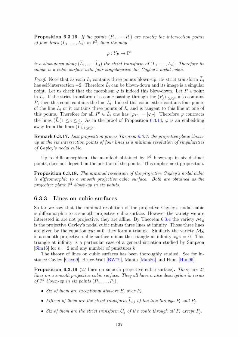
Proposition 6.3.16. If the points (P1, . . . , P6) are exactly the intersection pointsof four lines (L1, . . . , L4) in P2, then the map

ϕ : YP → P3

is a blow-down along (L1, . . . , L4) the strict transform of (L1, . . . , L4). Therefore itsimage is a cubic surface with four singularities: the Cayley’s nodal cubic.

Proof. Note that as each Li contains three points blown-up, its strict transform Lihas self-intersection −2. Therefore Li can be blown-down and its image is a singularpoint. Let us check that the morphism ϕ is indeed this blow-down. Let P a pointin Li. If the strict transform of a conic passing through the (Pj)1≤j≤6 also containsP , then this conic contains the line Li. Indeed this conic either contains four pointsof the line Li or it contains three points of Li and is tangent to this line at one ofthis points. Therefore for all P ′ ∈ Li one has [ϕP ′ ] = [ϕP ]. Therefore ϕ contractsthe lines (Li)1 ≤ i ≤ 4. As in the proof of Proposition 6.3.14, ϕ is an embeddingaway from the lines (Li)1≤i≤4.

Remark 6.3.17. Last proposition proves Theorem 6.3.7: the projective plane blown-up at the six intersection points of four lines is a minimal resolution of singularitiesof Cayley’s nodal cubic.

Up to diffeomorphism, the manifold obtained by P2 blown-up in six distinctpoints, does not depend on the position of the points. This implies next proposition.

Proposition 6.3.18. The minimal resolution of the projective Cayley’s nodal cubicis diffeomorphic to a smooth projective cubic surface. Both are obtained as theprojective plane P2 blown-up in six points.

6.3.3 Lines on cubic surfaces

So far we saw that the minimal resolution of the projective Cayley’s nodal cubicis diffeomorphic to a smooth projective cubic surface. However the variety we areinterested in are not projective, they are affine. By Theorem 6.3.4 the varietyMCis the projective Cayley’s nodal cubic minus three lines at infinity. Those three linesare given by the equation xyz = 0, they form a triangle. Similarly the varietyMSis a smooth projective cubic surface minus the triangle at infinity xyz = 0. Thistriangle at infinity is a particular case of a general situation studied by Simpson[Sim16] for n = 2 and any number of punctures k.

The theory of lines on cubic surfaces has been thoroughly studied. See for in-stance Cayley [Cay69], Bruce-Wall [BW79], Manin [Man86] and Hunt [Hun96].

Proposition 6.3.19 (27 lines on smooth projective cubic surface). There are 27lines on a smooth projective cubic surface. They all have a nice description in termsof P2 blown-up in six points (P1, . . . , P6).

• Six of them are exceptional divisors Ei over Pi.

• Fifteen of them are the strict transform Li,j of the line through Pi and Pj.

• Six of them are the strict transform Cj of the conic through all Pi except Pj.

137

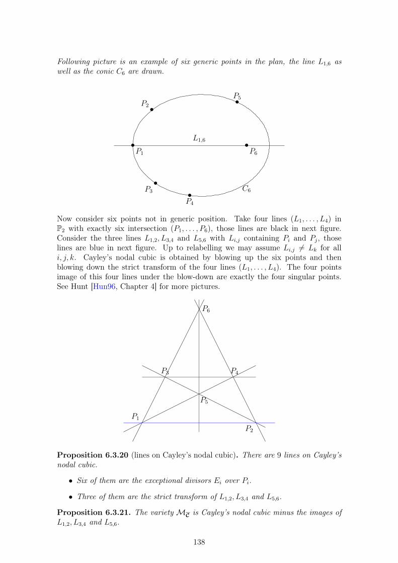
Following picture is an example of six generic points in the plan, the line L1,6 aswell as the conic C6 are drawn.

P1

•

P2•

P3

•

P4

•

P5•

P6

•L1,6

C6

Now consider six points not in generic position. Take four lines (L1, . . . , L4) inP2 with exactly six intersection (P1, . . . , P6), those lines are black in next figure.Consider the three lines L1,2, L3,4 and L5,6 with Li,j containing Pi and Pj, thoselines are blue in next figure. Up to relabelling we may assume Li,j 6= Lk for alli, j, k. Cayley’s nodal cubic is obtained by blowing up the six points and thenblowing down the strict transform of the four lines (L1, . . . , L4). The four pointsimage of this four lines under the blow-down are exactly the four singular points.See Hunt [Hun96, Chapter 4] for more pictures.

P1

P3 P4

P5

P6

P2

Proposition 6.3.20 (lines on Cayley’s nodal cubic). There are 9 lines on Cayley’snodal cubic.

• Six of them are the exceptional divisors Ei over Pi.

• Three of them are the strict transform of L1,2, L3,4 and L5,6.

Proposition 6.3.21. The varietyMC is Cayley’s nodal cubic minus the images ofL1,2, L3,4 and L5,6.

138

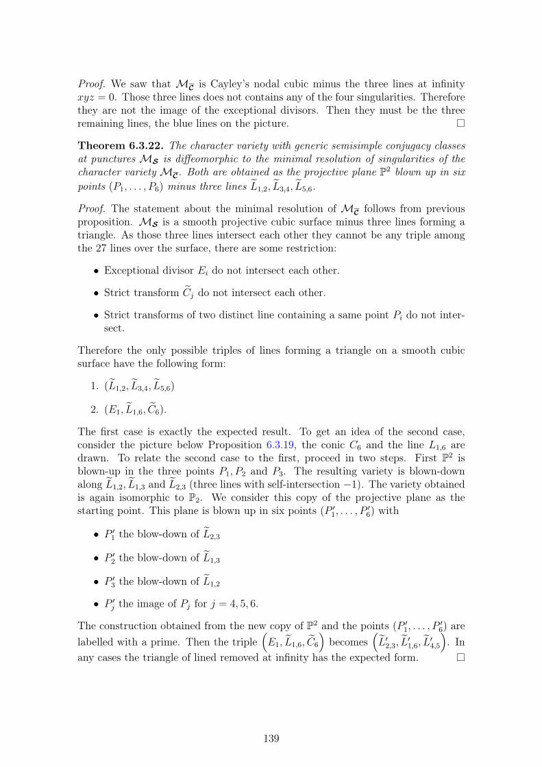
Proof. We saw that MC is Cayley’s nodal cubic minus the three lines at infinityxyz = 0. Those three lines does not contains any of the four singularities. Thereforethey are not the image of the exceptional divisors. Then they must be the threeremaining lines, the blue lines on the picture.

Theorem 6.3.22. The character variety with generic semisimple conjugacy classesat punctures MS is diffeomorphic to the minimal resolution of singularities of thecharacter varietyMC. Both are obtained as the projective plane P2 blown up in sixpoints (P1, . . . , P6) minus three lines L1,2, L3,4, L5,6.

Proof. The statement about the minimal resolution of MC follows from previousproposition. MS is a smooth projective cubic surface minus three lines forming atriangle. As those three lines intersect each other they cannot be any triple amongthe 27 lines over the surface, there are some restriction:

• Exceptional divisor Ei do not intersect each other.

• Strict transform Cj do not intersect each other.

• Strict transforms of two distinct line containing a same point Pi do not inter-sect.

Therefore the only possible triples of lines forming a triangle on a smooth cubicsurface have the following form:

1. (L1,2, L3,4, L5,6)

2. (E1, L1,6, C6).

The first case is exactly the expected result. To get an idea of the second case,consider the picture below Proposition 6.3.19, the conic C6 and the line L1,6 aredrawn. To relate the second case to the first, proceed in two steps. First P2 isblown-up in the three points P1, P2 and P3. The resulting variety is blown-downalong L1,2, L1,3 and L2,3 (three lines with self-intersection −1). The variety obtainedis again isomorphic to P2. We consider this copy of the projective plane as thestarting point. This plane is blown up in six points (P ′1, . . . , P

′6) with

• P ′1 the blow-down of L2,3

• P ′2 the blow-down of L1,3

• P ′3 the blow-down of L1,2

• P ′j the image of Pj for j = 4, 5, 6.

The construction obtained from the new copy of P2 and the points (P ′1, . . . , P′6) are

labelled with a prime. Then the triple(E1, L1,6, C6

)becomes

(L′2,3, L

′1,6, L

′4,5

). In

any cases the triangle of lined removed at infinity has the expected form.

139

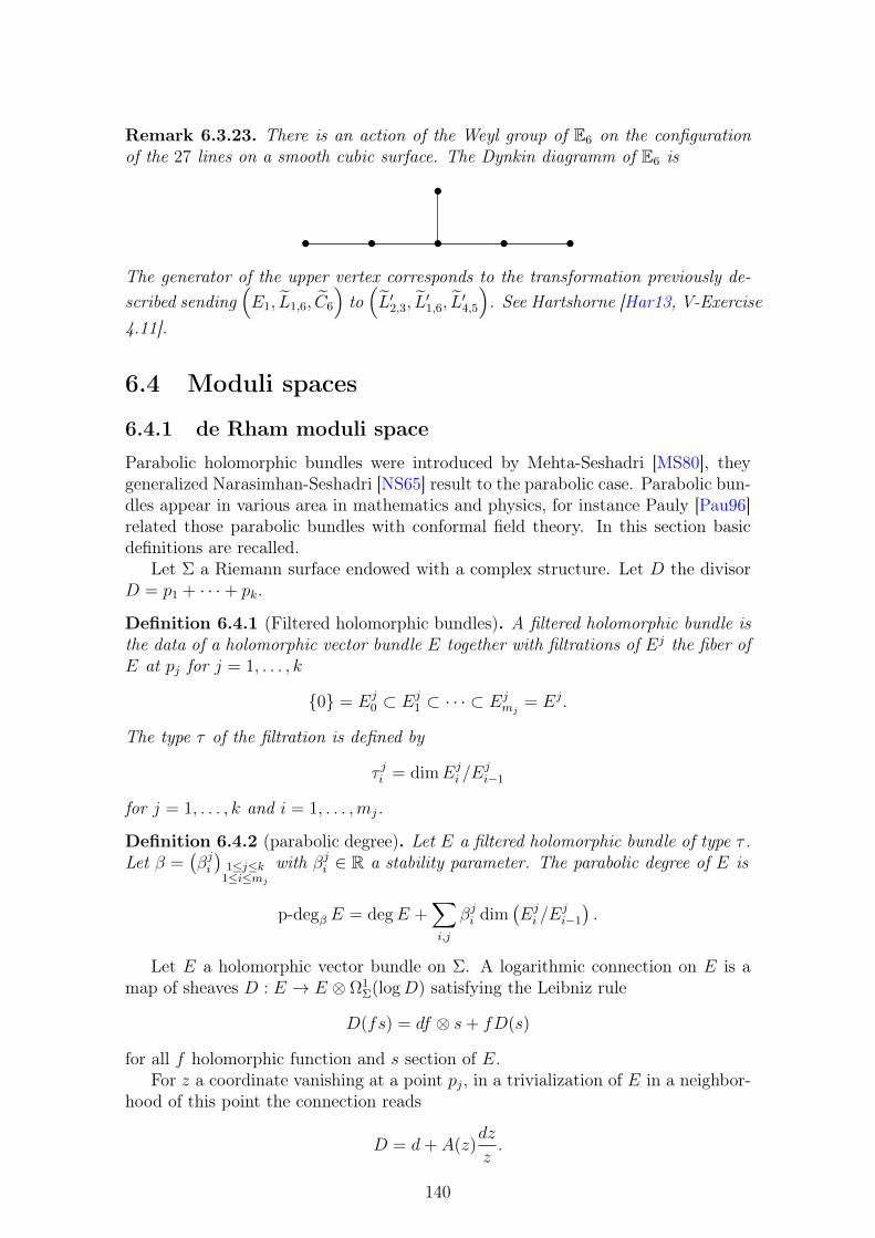
Remark 6.3.23. There is an action of the Weyl group of E6 on the configurationof the 27 lines on a smooth cubic surface. The Dynkin diagramm of E6 is

•

• • • • •

The generator of the upper vertex corresponds to the transformation previously de-scribed sending

(E1, L1,6, C6

)to(L′2,3, L

′1,6, L

′4,5

). See Hartshorne [Har13, V-Exercise

4.11].

6.4 Moduli spaces

6.4.1 de Rham moduli space

Parabolic holomorphic bundles were introduced by Mehta-Seshadri [MS80], theygeneralized Narasimhan-Seshadri [NS65] result to the parabolic case. Parabolic bun-dles appear in various area in mathematics and physics, for instance Pauly [Pau96]related those parabolic bundles with conformal field theory. In this section basicdefinitions are recalled.

Let Σ a Riemann surface endowed with a complex structure. Let D the divisorD = p1 + · · ·+ pk.

Definition 6.4.1 (Filtered holomorphic bundles). A filtered holomorphic bundle isthe data of a holomorphic vector bundle E together with filtrations of Ej the fiber ofE at pj for j = 1, . . . , k

0 = Ej0 ⊂ Ej

1 ⊂ · · · ⊂ Ejmj

= Ej.

The type τ of the filtration is defined by

τ ji = dimEji /E

ji−1

for j = 1, . . . , k and i = 1, . . . ,mj.

Definition 6.4.2 (parabolic degree). Let E a filtered holomorphic bundle of type τ .Let β =

(βji)

1≤j≤k1≤i≤mj

with βji ∈ R a stability parameter. The parabolic degree of E is

p-degβ E = degE +∑i,j

βji dim(Eji /E

ji−1

).

Let E a holomorphic vector bundle on Σ. A logarithmic connection on E is amap of sheaves D : E → E ⊗ Ω1

Σ(logD) satisfying the Leibniz rule

D(fs) = df ⊗ s+ fD(s)

for all f holomorphic function and s section of E.For z a coordinate vanishing at a point pj, in a trivialization of E in a neighbor-

hood of this point the connection reads

D = d+ A(z)dz

z.

140

A(0) is called the residue of D at pj and denoted by Respj D

Fix some parabolic weights βji ∈ [0, 1[ satisfying βji > βji−1. For j = 1, . . . , k andi = 2, . . . ,mj fix Aji ∈ C to specify a polar part. A logarithmic connection (E,D) iscompatible with the parabolic structure if the endomorphism

Respj D : Ej → Ej

satisfies(Respj D

)Eji ⊂ Ej

i . A logarithmic connection compatible with the parabolicstructure is called a parabolic connection.

It is compatible with the specified polar part if in addition the map induced byRespj D on the graded spaces Ej

i /Eji−1 is A

ji Id. A logarithmic connection compatible

with the parabolic structure is β-semistable if and only if, for sub bundle F ( Epreserved by D

p-degβ F

rankF≤

p-degβ E

rankE

it is stable if the inequality is strict unless F = 0. Two pairs of filtered holomorphicbundle and parabolic connections (E,D) and (E ′, D′) are isomorphic if there is anisomorphism of holomorphic bundle f : E → E ′ compatible with the filtrations andsuch that (f ⊗ Id) D = D′ f .

Notations 6.4.3 (de Rham moduli space). The de Rham moduli spaceMdRA,β classi-

fies isomorphism classes of β-stable parabolic connections with prescribed polar partA and parabolic degree 0.

6.4.2 Filtered local systems and resolutions of character va-rieties

Definition 6.4.4 (Filtered local system). A filtered local system is a local systemL over Σ \ p1, . . . , pk together with a filtration of the restrictions L|Uj to Uj somepunctured neighborhood of pj. Namely for all j = 1, . . . , k there are local systems Ljisuch at

0 = Lj0 ( Lj1 ( · · · ( Ljmj = L|Uj .

The type τ of the filtered local system is defined by

τ ji := rankLji/Lji−1.

Definition 6.4.5 (Parabolic degree of a filtered local system). Let γ =(γji)

1≤j≤k1≤i≤mj

a stability parameter. The parabolic degree of the filtered local system is defined by

p-degγ L =∑i,j

γji rankLji/Lji−1

A filtered local system L is γ-semistable if and only if for all sub local system0 ( L′ ( L

p-degγ L′

rankL′≤

p-degγ LrankL

it is γ-stable if the inequality is strict.Consider a character varietyMCµ,σ with a resolution of singularities ML,P ,σ. By

the usual equivalence of category between local systems and representations of the

141

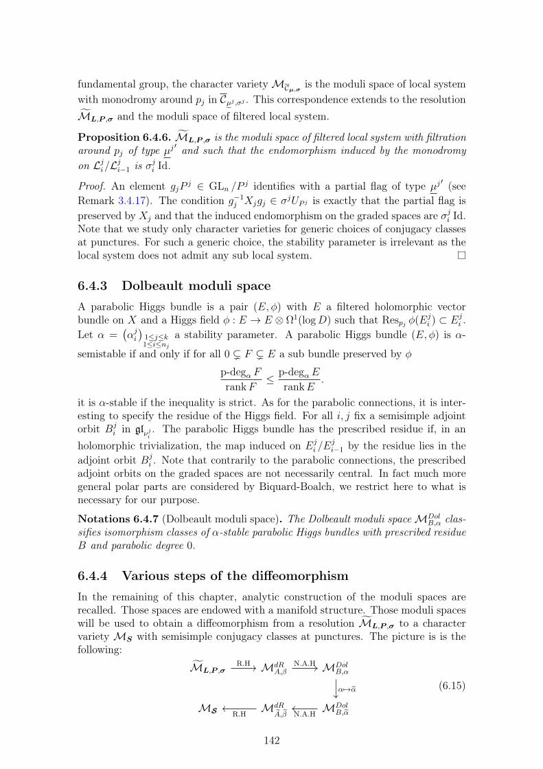
fundamental group, the character varietyMCµ,σ is the moduli space of local systemwith monodromy around pj in Cµj ,σj . This correspondence extends to the resolutionML,P ,σ and the moduli space of filtered local system.

Proposition 6.4.6. ML,P ,σ is the moduli space of filtered local system with filtrationaround pj of type µj ′ and such that the endomorphism induced by the monodromyon Lji/L

ji−1 is σji Id.

Proof. An element gjP j ∈ GLn /Pj identifies with a partial flag of type µj ′ (see

Remark 3.4.17). The condition g−1j Xjgj ∈ σjUP j is exactly that the partial flag is

preserved by Xj and that the induced endomorphism on the graded spaces are σji Id.Note that we study only character varieties for generic choices of conjugacy classesat punctures. For such a generic choice, the stability parameter is irrelevant as thelocal system does not admit any sub local system.

6.4.3 Dolbeault moduli space

A parabolic Higgs bundle is a pair (E, φ) with E a filtered holomorphic vectorbundle on X and a Higgs field φ : E → E ⊗ Ω1(logD) such that Respj φ(Ej

i ) ⊂ Eji .

Let α =(αji)

1≤j≤k1≤i≤nj

a stability parameter. A parabolic Higgs bundle (E, φ) is α-

semistable if and only if for all 0 ( F ( E a sub bundle preserved by φ

p-degα F

rankF≤ p-degαE

rankE.

it is α-stable if the inequality is strict. As for the parabolic connections, it is inter-esting to specify the residue of the Higgs field. For all i, j fix a semisimple adjointorbit Bj

i in glνji. The parabolic Higgs bundle has the prescribed residue if, in an

holomorphic trivialization, the map induced on Eji /E

ji−1 by the residue lies in the

adjoint orbit Bji . Note that contrarily to the parabolic connections, the prescribed

adjoint orbits on the graded spaces are not necessarily central. In fact much moregeneral polar parts are considered by Biquard-Boalch, we restrict here to what isnecessary for our purpose.

Notations 6.4.7 (Dolbeault moduli space). The Dolbeault moduli spaceMDolB,α clas-

sifies isomorphism classes of α-stable parabolic Higgs bundles with prescribed residueB and parabolic degree 0.

6.4.4 Various steps of the diffeomorphism

In the remaining of this chapter, analytic construction of the moduli spaces arerecalled. Those spaces are endowed with a manifold structure. Those moduli spaceswill be used to obtain a diffeomorphism from a resolution ML,P ,σ to a charactervariety MS with semisimple conjugacy classes at punctures. The picture is is thefollowing:

ML,P ,σ MdRA,β MDol

B,α

MS MdRA,β

MDolB,α

R.H N.A.H

α 7→α

R.H N.A.H

(6.15)

142

All the arrows are diffeomorphisms, R.H stands for Riemann-Hilbert correspondenceand N.A.H for non-Abelian Hodge theory. The vertical arrow accounts for a changeof stability parameter α → α. This is the same idea as Biquard, García-Pradaand Mundet i Riera [BGM15, Theorem 7.10]. It is detailed in the remaining of thechapter for this particular application.

6.5 Local modelIn this section the local model used by Biquard-Boalch [BB04] to construct modulispaces is recalled.

6.5.1 Local model for Riemann-Hilbert correspondence

Before constructing the moduli space, let us present what happens locally, near apuncture, and how the parameters of the moduli spaces are related. Consider La rank n filtered local system on a punctured disk D0 such that the monodromyinduces a central endomorphism on the graded spaces. The monodromy X haseigenvalues σi with multiplicity νi for 1 ≤ i ≤ l. We assume the filtration of thelocal system is finer than a filtration spanned by generalized eigenspaces ofM . Thenin a trivialization (lj)1≤j≤n compatible with the filtration, the monodromy reads

X =

Xσ1 ∗0 Xσ2 ∗... 0

. . .

with Xσi a block of size νi with further decomposition

Xσi =

σi Idµi1′ ∗0 σi Idµi2

′ ∗... 0

. . .

The type of the filtration is µ′ = (µ1

1′, µ1

2′, . . . , µ2

1′, µ2

2′, . . . ). Let Ai ∈ C such that

exp(−2iπAi) = σi

and 0 ≤ ReAi < 1. Then A is the diagonal matrix with diagonal coefficientsA1, . . . , A1︸ ︷︷ ︸ν1

, . . . , Al, . . . , Al︸ ︷︷ ︸νl

.

Let a a block strictly upper triangular matrix such that exp (−2iπ(A+ a)) = X.Define E a rank n holomorphic bundle on the disk D spanned by τj = e(A+a) log zljfor 1 ≤ j ≤ n. Let D the parabolic connection on E defined in the holomorphictrivialization (τj)1≤j≤n by

D = d+A+ a

zdz

= D0 +a

zdz

143

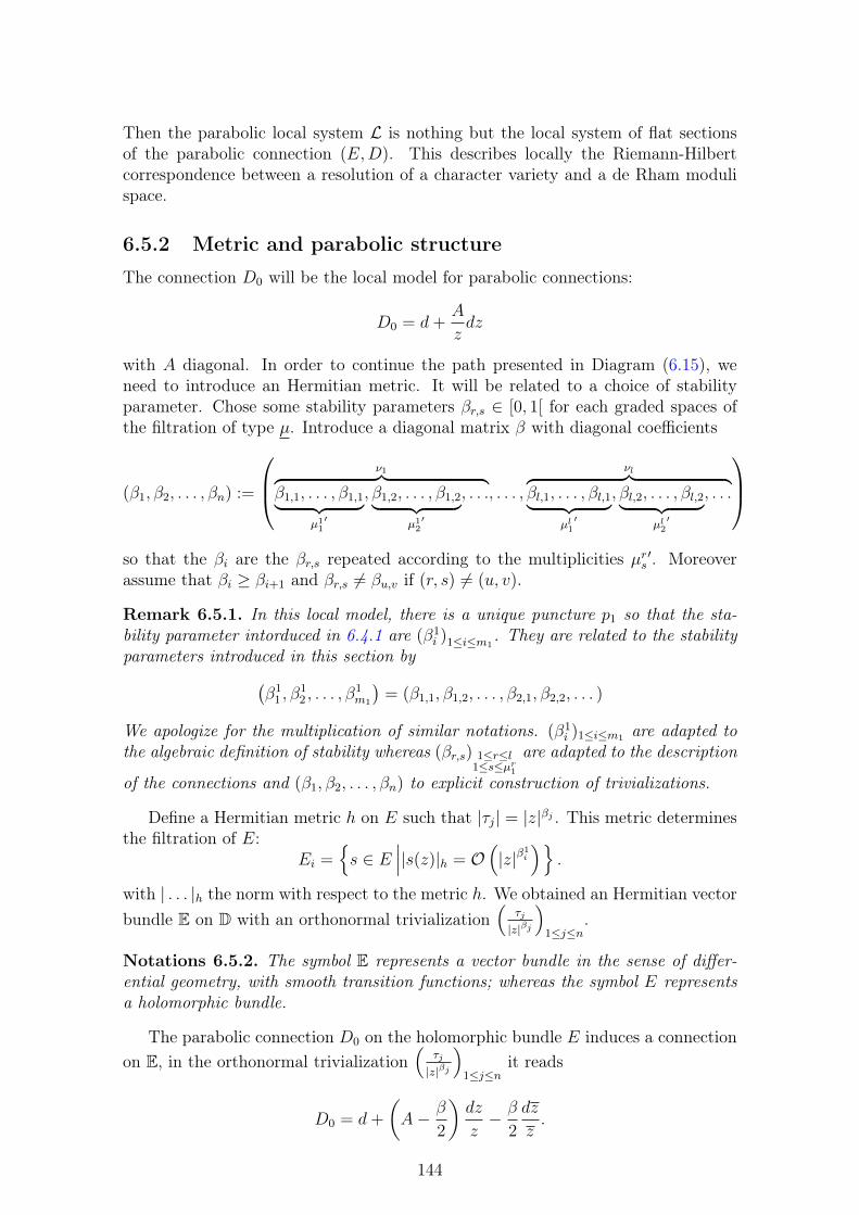
Then the parabolic local system L is nothing but the local system of flat sectionsof the parabolic connection (E,D). This describes locally the Riemann-Hilbertcorrespondence between a resolution of a character variety and a de Rham modulispace.

6.5.2 Metric and parabolic structure

The connection D0 will be the local model for parabolic connections:

D0 = d+A

zdz

with A diagonal. In order to continue the path presented in Diagram (6.15), weneed to introduce an Hermitian metric. It will be related to a choice of stabilityparameter. Chose some stability parameters βr,s ∈ [0, 1[ for each graded spaces ofthe filtration of type µ. Introduce a diagonal matrix β with diagonal coefficients

(β1, β2, . . . , βn) :=

ν1︷ ︸︸ ︷β1,1, . . . , β1,1︸ ︷︷ ︸

µ11′

, β1,2, . . . , β1,2︸ ︷︷ ︸µ12′

, . . ., . . . ,

νl︷ ︸︸ ︷βl,1, . . . , βl,1︸ ︷︷ ︸

µl1′

, βl,2, . . . , βl,2︸ ︷︷ ︸µl2′

, . . .

so that the βi are the βr,s repeated according to the multiplicities µrs

′. Moreoverassume that βi ≥ βi+1 and βr,s 6= βu,v if (r, s) 6= (u, v).

Remark 6.5.1. In this local model, there is a unique puncture p1 so that the sta-bility parameter intorduced in 6.4.1 are (β1

i )1≤i≤m1. They are related to the stability

parameters introduced in this section by(β1

1 , β12 , . . . , β

1m1

)= (β1,1, β1,2, . . . , β2,1, β2,2, . . . )

We apologize for the multiplication of similar notations. (β1i )1≤i≤m1 are adapted to

the algebraic definition of stability whereas (βr,s) 1≤r≤l1≤s≤µr1

are adapted to the description

of the connections and (β1, β2, . . . , βn) to explicit construction of trivializations.

Define a Hermitian metric h on E such that |τj| = |z|βj . This metric determinesthe filtration of E:

Ei =s ∈ E

∣∣∣|s(z)|h = O(|z|β

1i

).

with | . . . |h the norm with respect to the metric h. We obtained an Hermitian vectorbundle E on D with an orthonormal trivialization

(τj

|z|βj

)1≤j≤n

.

Notations 6.5.2. The symbol E represents a vector bundle in the sense of differ-ential geometry, with smooth transition functions; whereas the symbol E representsa holomorphic bundle.

The parabolic connection D0 on the holomorphic bundle E induces a connectionon E, in the orthonormal trivialization

(τj

|z|βj

)1≤j≤n

it reads

D0 = d+

(A− β

2

)dz

z− β

2

dz

z.

144

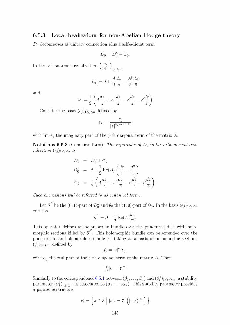
6.5.3 Local beahaviour for non-Abelian Hodge theory

D0 decomposes as unitary connection plus a self-adjoint term

D0 = Dh0 + Φ0.

In the orthonormal trivialization(

τj

|z|βj

)1≤j≤n

Dh0 = d+

A

2

dz

z− A†

2

dz

z

andΦ0 =

1

2

(Adz

z+ A†

dz

z− βdz

z− βdz

z

)Consider the basis (ej)1≤j≤n defined by

ej :=τj

|z|βj−i ImAj

with ImAj the imaginary part of the j-th diagonal term of the matrix A.

Notations 6.5.3 (Canonical form). The expression of D0 in the orthonormal triv-ialization (ej)1≤j≤n is

D0 = Dh0 + Φ0

Dh0 = d+

1

2Re(A)

(dz

z− dz

z

)Φ0 =

1

2

(Adz

z+ A†

dz

z− βdz

z− βdz

z

).

Such expressions will be referred to as canonical forms.

Let ∂F be the (0, 1)-part of Dh0 and θ0 the (1, 0)-part of Φ0. In the basis (ej)1≤j≤n

one has∂F

= ∂ − 1

2Re(A)

dz

z.

This operator defines an holomorphic bundle over the punctured disk with holo-morphic sections killed by ∂F . This holomorphic bundle can be extended over thepuncture to an holomorphic bundle F , taking as a basis of holomorphic sections(fj)1≤j≤n defined by

fj = |z|αjej.

with αj the real part of the j-th diagonal term of the matrix A. Then

|fj|h = |z|αj

Similarly to the correspondence 6.5.1 between (β1, . . . , βn) and (β1i )1≤i≤m1 , a stability

parameter (α1i )1≤i≤n1 is associated to (α1, . . . , αn). This stability parameter provides

a parabolic structure

Fi =s ∈ F

∣∣∣ |s|h = O(|s(z)|α

1i

)145

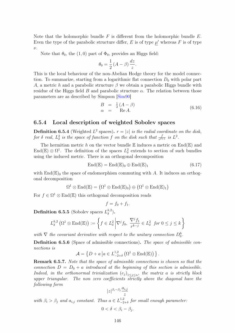
Note that the holomorphic bundle F is different from the holomorphic bundle E.Even the type of the parabolic structure differ, E is of type µ′ whereas F is of typeν.

Note that θ0, the (1, 0) part of Φ0, provides an Higgs field:

θ0 =1

2(A− β)

dz

z.

This is the local behaviour of the non-Abelian Hodge theory for the model connec-tion. To summarize, starting from a logarithmic flat connection D0 with polar partA, a metric h and a parabolic structure β we obtain a parabolic Higgs bundle withresidue of the Higgs field B and parabolic structure α. The relation between thoseparameters are as described by Simpson [Sim90]

B = 12

(A− β)α = ReA.

(6.16)

6.5.4 Local description of weighted Sobolev spaces

Definition 6.5.4 (Weighted L2 spaces). r = |z| is the radial coordinate on the disk,for δ real, L2

δ is the space of function f on the disk such that frδ+1 is L2.

The hermitian metric h on the vector bundle E induces a metric on End(E) andEnd(E) ⊗ Ω1. The definition of the spaces L2

δ extends to section of such bundlesusing the induced metric. There is an orthogonal decomposition

End(E) = End(E)0 ⊕ End(E)1 (6.17)

with End(E)0 the space of endomorphism commuting with A. It induces an orthog-onal decomposition

Ω1 ⊗ End(E) =(Ω1 ⊗ End(E)0

)⊕(Ω1 ⊗ End(E)1

)For f ∈ Ω1 ⊗ End(E) this orthogonal decomposition reads

f = f0 + f1.

Definition 6.5.5 (Sobolev spaces Lk,2δ ).

Lk,2δ(Ω1 ⊗ End(E)

):=

f ∈ L2

δ

∣∣∣∣∇jf0,∇jf1

rk−j∈ L2

δ for 0 ≤ j ≤ k

with ∇ the covariant derivative with respect to the unitary connection Dh

0 .

Definition 6.5.6 (Space of admissible connections). The space of admissible con-nections is

A =D + a

∣∣a ∈ L1,2−2+δ

(Ω1 ⊗ End(E)

).

Remark 6.5.7. Note that the space of admissible connections is chosen so that theconnection D = D0 + a introduced at the beginning of this section is admissible.Indeed, in the orthonormal trivialization (ej)1≤j≤n, the matrix a is strictly blockupper triangular. The non zero coefficients strictly above the diagonal have thefollowing form

|z|βi−βj ai,jz

with βi > βj and ai,j constant. Thus a ∈ L1,2−2+δ for small enough parameter:

0 < δ < βi − βj.

146

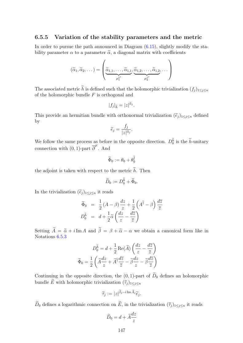
6.5.5 Variation of the stability parameters and the metric

In order to pursue the path announced in Diagram (6.15), slightly modify the sta-bility parameter α to a parameter α, a diagonal matrix with coefficients

(α1, α2, . . . ) =

α1,1, . . . , α1,1︸ ︷︷ ︸µ11′

, α1,2, . . . , α1,2︸ ︷︷ ︸µ12′

, . . .

The associated metric h is defined such that the holomorphic trivialization (fj)1≤j≤nof the holomorphic bundle F is orthogonal and

|fj|h = |z|αj .

This provide an hermitian bundle with orthonormal trivialization (ej)1≤j≤n definedby

ej =fj|z|αj

.

We follow the same process as before in the opposite direction. Dh0 is the h-unitary

connection with (0, 1)-part ∂F . And

Φ0 := θ0 + θ†0

the adjoint is taken with respect to the metric h. Then

D0 := Dh0 + Φ0.

In the trivialization (ej)1≤j≤n it reads

Φ0 =1

2(A− β)

dz

z+

1

2

(A† − β

) dzz

Dh0 = d+

1

2α

(dz

z− dz

z

)Setting A = α + i ImA and β = β + α − α we obtain a canonical form like inNotations 6.5.3

Dh0 = d+

1

2Re(A)

(dz

z− dz

z

)Φ0 =

1

2

(Adz

z+ A†

dz

z− β dz

z− β dz

z

)Continuing in the opposite direction, the (0, 1)-part of D0 defines an holomorphicbundle E with holomorphic trivialization (τj)1≤j≤n

τj := |z|βj−i Im Aj ej.

D0 defines a logarithmic connection on E, in the trivialization (τj)1≤j≤n it reads

D0 = d+ Adz

z

147

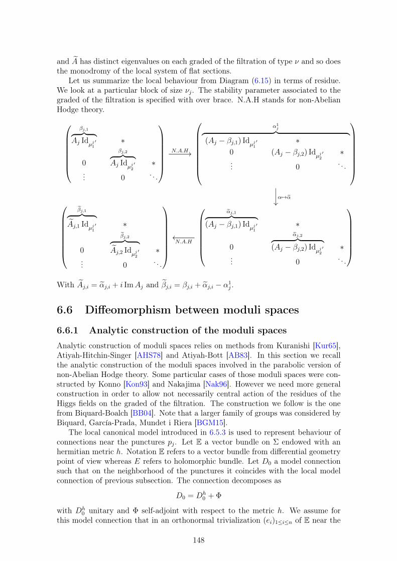
and A has distinct eigenvalues on each graded of the filtration of type ν and so doesthe monodromy of the local system of flat sections.

Let us summarize the local behaviour from Diagram (6.15) in terms of residue.We look at a particular block of size νj. The stability parameter associated to thegraded of the filtration is specified with over brace. N.A.H stands for non-AbelianHodge theory.

βj,1︷ ︸︸ ︷Aj Id

µj1′ ∗

0

βj,2︷ ︸︸ ︷Aj Id

µj2′ ∗

... 0. . .

α1j︷ ︸︸ ︷

(Aj − βj,1) Idµj1′ ∗

0 (Aj − βj,2) Idµj2′ ∗

... 0. . .

βj,1︷ ︸︸ ︷Aj,1 Id

µj1′ ∗

0

βj,2︷ ︸︸ ︷Aj,2 Id

µj2′ ∗

... 0. . .

αj,1︷ ︸︸ ︷(Aj − βj,1) Id

µj1′ ∗

0

αj,2︷ ︸︸ ︷(Aj − βj,2) Id

µj2′ ∗

... 0. . .

N.A.H

α7→α

N.A.H

With Aj,i = αj,i + i ImAj and βj,i = βj,i + αj,i − α1j .

6.6 Diffeomorphism between moduli spaces

6.6.1 Analytic construction of the moduli spaces

Analytic construction of moduli spaces relies on methods from Kuranishi [Kur65],Atiyah-Hitchin-Singer [AHS78] and Atiyah-Bott [AB83]. In this section we recallthe analytic construction of the moduli spaces involved in the parabolic version ofnon-Abelian Hodge theory. Some particular cases of those moduli spaces were con-structed by Konno [Kon93] and Nakajima [Nak96]. However we need more generalconstruction in order to allow not necessarily central action of the residues of theHiggs fields on the graded of the filtration. The construction we follow is the onefrom Biquard-Boalch [BB04]. Note that a larger family of groups was considered byBiquard, García-Prada, Mundet i Riera [BGM15].

The local canonical model introduced in 6.5.3 is used to represent behaviour ofconnections near the punctures pj. Let E a vector bundle on Σ endowed with anhermitian metric h. Notation E refers to a vector bundle from differential geometrypoint of view whereas E refers to holomorphic bundle. Let D0 a model connectionsuch that on the neighborhood of the punctures it coincides with the local modelconnection of previous subsection. The connection decomposes as

D0 = Dh0 + Φ

with Dh0 unitary and Φ self-adjoint with respect to the metric h. We assume for

this model connection that in an orthonormal trivialization (ei)1≤i≤n of E near the

148

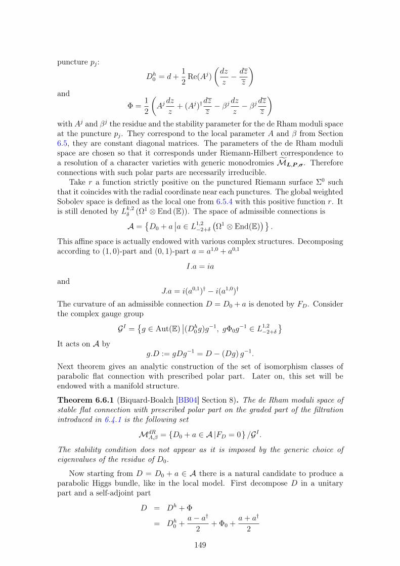
puncture pj:

Dh0 = d+

1

2Re(Aj)

(dz

z− dz

z

)and

Φ =1

2

(Ajdz

z+ (Aj)†

dz

z− βj dz

z− βj dz

z

)with Aj and βj the residue and the stability parameter for the de Rham moduli spaceat the puncture pj. They correspond to the local parameter A and β from Section6.5, they are constant diagonal matrices. The parameters of the de Rham modulispace are chosen so that it corresponds under Riemann-Hilbert correspondence toa resolution of a character varieties with generic monodromies ML,P ,σ. Thereforeconnections with such polar parts are necessarily irreducible.

Take r a function strictly positive on the punctured Riemann surface Σ0 suchthat it coincides with the radial coordinate near each punctures. The global weightedSobolev space is defined as the local one from 6.5.4 with this positive function r. Itis still denoted by Lk,2δ (Ω1 ⊗ End (E)). The space of admissible connections is

A =D0 + a

∣∣a ∈ L1,2−2+δ

(Ω1 ⊗ End(E)

).

This affine space is actually endowed with various complex structures. Decomposingaccording to (1, 0)-part and (0, 1)-part a = a1,0 + a0,1

I.a = ia

andJ.a = i(a0,1)† − i(a1,0)†

The curvature of an admissible connection D = D0 + a is denoted by FD. Considerthe complex gauge group

GI =g ∈ Aut(E)

∣∣(Dh0g)g−1, gΦ0g

−1 ∈ L1,2−2+δ

It acts on A by

g.D := gDg−1 = D − (Dg) g−1.

Next theorem gives an analytic construction of the set of isomorphism classes ofparabolic flat connection with prescribed polar part. Later on, this set will beendowed with a manifold structure.

Theorem 6.6.1 (Biquard-Boalch [BB04] Section 8). The de Rham moduli space ofstable flat connection with prescribed polar part on the graded part of the filtrationintroduced in 6.4.1 is the following set

MdRA,β = D0 + a ∈ A |FD = 0 /GI .

The stability condition does not appear as it is imposed by the generic choice ofeigenvalues of the residue of D0.

Now starting from D = D0 + a ∈ A there is a natural candidate to produce aparabolic Higgs bundle, like in the local model. First decompose D in a unitarypart and a self-adjoint part

D = Dh + Φ

= Dh0 +

a− a†

2+ Φ0 +

a+ a†

2

149

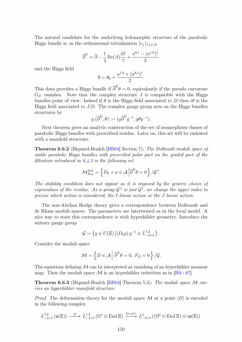
The natural candidate for the underlying holomorphic structure of the parabolicHiggs bundle is, in the orthonormal trivialization (ej)1≤j≤k

∂E

= ∂ − 1

2Re(A)

dz

z+a0,1 − (a1,0)†

2.

and the Higgs field

θ = θ0 +a1,0 + (a0,1)†

2.

This data provides a Higgs bundle if ∂Eθ = 0, equivalently if the pseudo curvatureGD vanishes. Note that the complex structure J is compatible with the Higgsbundles point of view. Indeed if θ is the Higgs field associated to D then iθ is theHiggs field associated to J.D. The complex gauge group acts on the Higgs bundlesstructures by

g.(∂E, θ) := (g∂

Eg−1, gθg−1).

Next theorem gives an analytic construction of the set of isomorphism classes ofparabolic Higgs bundles with prescribed residue. Later on, this set will be endowedwith a manifold structure.

Theorem 6.6.2 (Biquard-Boalch [BB04] Section 7). The Dolbeault moduli space ofstable parabolic Higgs bundles with prescribed polar part on the graded part of thefiltration introduced in 6.4.3 is the following set

MDolB,α =

D0 + a ∈ A

∣∣∣∂Eθ = 0/GJ .

The stability condition does not appear as it is imposed by the generic choice ofeigenvalues of the residue. As a group GJ is just GI , we change the upper index toprecise which action is considered, the I-linear action or the J-linear action.

The non-Abelian Hodge theory gives a correspondence between Dolbeault andde Rham moduli spaces. The parameters are intertwined as in the local model. Anice way to state this correspondence is with hyperkähler geometry. Introduce theunitary gauge group

G =g ∈ U(E)

∣∣(D0g) g−1 ∈ L1,2−2+δ

.

Consider the moduli space

M =D ∈ A

∣∣∣ ∂Eθ = 0, FD = 0/G.

The equations definingM can be interpreted as vanishing of an hyperkähler momentmap. Then the moduli spaceM is an hyperkähler reduction as in [Hit+87].

Theorem 6.6.3 (Biquard-Boalch [BB04] Theorem 5.4). The moduli spaceM car-ries an hyperkähler manifold structure.

Proof. The deformation theory for the moduli space M at a point [D] is encodedin the following complex

L2,2−2+δ (u(E)) L1,2

−2+δ (Ω1 ⊗ EndE) L2−2+δ ((Ω2 ⊗ EndE)⊕ iu(E))D D+D∗

.

150

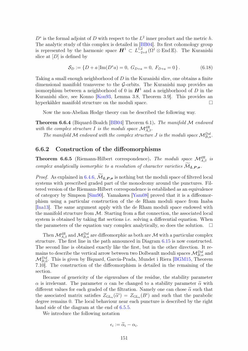
D∗ is the formal adjoint of D with respect to the L2 inner product and the metric h.The analytic study of this complex is detailed in [BB04]. Its first cohomology groupis represented by the harmonic space H1 ⊂ L1,2

−2+δ (Ω1 ⊗ EndE). The Kuranishislice at [D] is defined by

SD := D + a |Im(D∗a) = 0, GD+a = 0, FD+a = 0 . (6.18)

Taking a small enough neighborhood of D in the Kuranishi slice, one obtains a finitedimensional manifold transverse to the G-orbits. The Kuranishi map provides anisomorphism between a neighborhood of 0 in H1 and a neighborhood of D in theKuranishi slice, see Konno [Kon93, Lemma 3.8, Theorem 3.9]. This provides anhyperkähler manifold structure on the moduli space.

Now the non-Abelian Hodge theory can be described the following way.

Theorem 6.6.4 (Biquard-Boalch [BB04] Theorem 6.1). The manifoldM endowedwith the complex structure I is the moduli spaceMdR

A,β.The manifoldM endowed with the complex structure J is the moduli spaceMDol

B,α.

6.6.2 Construction of the diffeomorphisms

Theorem 6.6.5 (Riemann-Hilbert correspondence). The moduli space MdRA,β is

complex analytically isomorphic to a resolution of character varieties ML,P ,σ.

Proof. As explained in 6.4.6, ML,P ,σ is nothing but the moduli space of filtered localsystems with prescribed graded part of the monodromy around the punctures. Fil-tered version of the Riemann-Hilbert correspondence is established as an equivalenceof category by Simpson [Sim90]. Yamakawa [Yam08] proved that it is a diffeomor-phism using a particular construction of the de Rham moduli space from Inaba[Ina13]. The same argument apply with the de Rham moduli space endowed withthe manifold structure fromM. Starting from a flat connection, the associated localsystem is obtained by taking flat sections i.e. solving a differential equation. Whenthe parameters of the equation vary complex analytically, so does the solution.

ThenMdRA,β andMDol

B,α are diffeomorphic as both areM with a particular complexstructure. The first line in the path announced in Diagram 6.15 is now constructed.The second line is obtained exactly like the first, but in the other direction. It re-mains to describe the vertical arrow between two Dolbeault moduli spacesMDol

B,α andMDol

B,α. This is given by Biquard, García-Prada, Mundet i Riera [BGM15, Theorem7.10]. The construction of the diffeomorphism is detailed in the remaining of thesection.

Because of genericity of the eigenvalues of the residue, the stability parameterα is irrelevant. The parameter α can be changed to a stability parameter α withdifferent values for each graded of the filtration. Namely one can chose α such thatthe associated matrix satisfies ZGLn(αi) = ZGLn(Bi) and such that the parabolicdegree remains 0. The local behaviour near each puncture is described by the righthand side of the diagram at the end of 6.5.5.

We introduce the following notation

εi := αi − αi.

151

For the construction of the diffeomorphism in Theorem 6.6.7, it will be conveniantto assume

maxi,j|εi − εj| < δ

with δ the parameter appearing in the weighted Sobolev space L1,2−2+δ.

Proposition 6.6.6. For such choice of parameter there is a natural bijection betweenMDol

B,α andMDolB,α.

Proof. MDolB,α classifies isomorphism classes of parabolic Higgs bundles with parabolic

structure at pj0 = F j

0 ( F j1 ( · · · ( F j

nj= F j

and with the residue of the Higgs fields preserving this filtration and acting as asemisimple endomorphism Bj

i on the graded spaces

F ji /F

ji−1.

Such spaces decomposes as direct sum of eigenspaces for Bji . After ordering the

eigenvalues, we obtain a uniquely determined refinement of the initial parabolicstructure:

0 = F j0 ( F j

1 ( · · · ( F jmj

= F j.

Then the residue of the Higgs field acts as a central endomorphism on the gradedF ji /F

ji−1. This gives a map f :MDol

B,α →MDolB,α. Stability is not an issue as the polar

part of the residue is generic. The map forgetting part of the filtration is an inverseso that there is a natural bijection between both moduli spaces.

Before proving that this bijection is a diffeomorphism the manifold structure onMDol

B,α is detailed. It is constructed just likeMDolB,α but with different parameters.

Similarly to M, construct a moduli space Mh. Instead of the initial metric h,we use a metric h, similar to the local model from 6.5.5. Namely it is chosen so thatnear each puncture it admits as an orthonormal trivialization (ei)1≤i≤n with

ei = rεiei.

Where (ei)1≤i≤n is the orthnormal trivialization with respect to h near the punctureand εi = αi − αi.

First we construct D0, a starting point to construct an affine space of admissibleconnections. Recall that

D0 = Dh0 + Φ0

with Dh0 a h-unitary connection and Φ0 self-adjoint with respect to h. Take Dh

0′′ the

(0, 1)-component of Dh0 and Φ1,0

0 the (1, 0)-component of Φ0. There exists a unique

Dh0

′such that Dh

0

′+ Dh

0′′ is h-unitary. Let Φ1,0

0

†the adjoint of Φ1,0

0 with respect tothe metric h. Then D0 is defined by

D0 := Dh0

′+Dh

0

′′+ Φ1,0

0 + Φ1,00

†.

Near the puncture, in the trivialization (ei)1≤i≤n, the connection D0 behaves exactlylike the local model with the same name introduced in 6.5.5. Define the affine spaceof admissible connections with respect to D0 and the metric h.

Ah :=D0 + a | a ∈ L1,2

−2+δ

(Ω1 ⊗ End(E)

)152

The weighted Sobolev space L1,2

−2+δ(Ω1 ⊗ End(E)) is also defined using the metric

h. Moreover notice that we do not chose the same parameter δ for A and for Ah.It will be convenient to chose δ such that

0 < δ < δ −maxi,j|εi − εj|. (6.19)

With this set up, we are ready to prove that the bijection from previous propositionis a diffeomorphism.

Theorem 6.6.7. The natural bijection between MDolB,α and MDol

B,α is a diffeomor-phism.

Proof. MDolB,α is identified with the manifoldM with the complex structure J .

Take an element inMDolB,α identified with an element [D] ∈ M. [D] is the class

of D = D0 + a an admissible connection with vanishing curvature and pseudo-curvature. By construction of the manifold structure, a neighborhood of [D] inM is diffeomorphic with a neighborhood of D in the Kuranishi slice SD defined in(6.18). We shall prove that the bijection from Proposition 6.6.6 induces a smoothmap from a neighborhood of D in SD to Ah.

First we describe the image of the connection D, it is obtained exactly thesame way D0 is obtained from D0. It decomposes as a connection h-unitary plus ahermitian part

D = Dh0 +

a− a†

2+ Φ0 +

a+ a†

2.

It can be decomposed further in components of type (1, 0) and (0, 1). Then the(0, 1)-component of the h-unitary part is

∂F

= Dh0

′′+a0,1 − a1,0†

2

and the (1, 0)-component of the self-adjoint part is

θ = Φ1,0 +a1,0 + a0,1†

2.

The parabolic Higgs bundle associated to D is (∂F, θ). Now we switch to the metric

h. Near each puncture, in the h-orthonormal trivialization (ei)1≤i≤n

∂F

= Dh0

′′+

(α− α

2

)dz

z+ H

a0,1 − a1,0†

2H−1

and

θ = φ1,0 + Ha1,0 + a0,1†

2H−1.

with H a diagonal matrix with coefficients rεi . Using the metric h we construct D′h

such that D′h

+ ∂F is h-unitary. And θ† the adjoint of θ with respect to h. We want

to prove thatD′h

+ ∂F

+ θ + θ†

153

belongs to the space of admissible connections Ah. Let

a := D′h

+ ∂F

+ θ + θ† − D0.

Components of a are obtained from components of a by multiplication by rεi−εj .Thus for δ small enough (6.19), a belongs to L1,2

−2+δ. Therefore the bijection from

MDolB,α toMDol

B,α comes from a map

D0 + a ∈ A | FD0+a = GD0+a = 0 →D0 + a ∈ Ah

∣∣ GD0+a = 0

D0 + a 7→ D0 + a.

This restricts to a diffeomorphism from a neighborhood of D in the Kuranishi sliceSD to a manifold transverse to the GJ -orbits in a neighborhood of D. Therefore themapMDol

B,α →MDolB,α is a diffeomorphism.

To finish, let us detail the last step at the bottom left corner of Diagram (6.15).Applying successively non-Abelian Hodge theory and Riemann-Hilbert correspon-dence, the moduli space MDol

B,α is diffeomorphic to a moduli space of filtered localsystem ML,P ,σ. The parameters are such that ZGLn(σj) = Lj for 1 ≤ j ≤ k. Themap pσ : ML,P ,σ → MS from 3.5.11 is an isomorphism. MS is the charactervariety with monodromy at the puncture pj in Sj the conjugacy class of σj.

154

Bibliography

[AB83] M. F. Atiyah and R. Bott. “The Yang-Mills Equations over RiemannSurfaces”. In: Philosophical Transactions of the Royal Society of London.Series A, Mathematical and Physical Sciences 308.1505 (1983), pp. 523–615. issn: 00804614. url: http://www.jstor.org/stable/37156.

[AHS78] M. F. Atiyah, N. J. Hitchin, and I. M. Singer. “Self-Duality in Four-Dimensional Riemannian Geometry”. In: Proceedings of the Royal Soci-ety of London. Series A, Mathematical and Physical Sciences 362.1711(1978), pp. 425–461. issn: 00804630. url: http://www.jstor.org/stable/79638.

[Bei+18] A. A. Beilinson, J. Bernstein, P. Deligne, and O. Gabber. Faisceauxpervers. Vol. 100. Astérisque. Société mathématique de France, 2018.

[BG98] F. Bergeron and G. Garsia. “Science Fiction and Macdonald’s Polyno-mials”. In: CRM Proc. Lecture Notes 22 (Oct. 1998).

[Biq97] Olivier Biquard. “Fibrés de Higgs et connexions intégrables : le cas log-arithmique (diviseur lisse)”. fr. In: Annales scientifiques de l’École Nor-male Supérieure 4e série, 30.1 (1997), pp. 41–96. doi: 10.1016/s0012-9593(97)89915-6.

[BB04] Olivier Biquard and Philip Boalch. “Wild non-abelian Hodge theory oncurves”. In: Compositio Mathematica 140.1 (2004), pp. 179–204. doi:10.1112/S0010437X03000010.

[BGM15] Olivier Biquard, Oscar García-Prada, and Ignasi Mundet i Riera. “ParabolicHiggs bundles and representations of the fundamental group of a punc-tured surface into a real group”. In: Advances in Mathematics 372 (Oct.2015). doi: 10.1016/j.aim.2020.107305.

[BD12] Indranil Biswas and Arijit Dey. “SYZ duality for parabolic Higgs modulispaces”. In: Nucl. Phys. B 862 (2012), pp. 327–340. doi: 10.1016/j.nuclphysb.2012.04.020. arXiv: 1204.4740 [math.AG].

[BP16] Philip Boalch and Robert Paluba. “Symmetric cubic surfaces and G2

character varieties”. In: J. Algebraic Geom. 25 (2016).

[BY96] H. U. Boden and K. Yokogawa. “Moduli Spaces of Parabolic Higgs Bun-dles and Parabolic K(D) Pairs over Smooth Curves: I”. In: arXiv e-prints, alg-geom/9610014 (Oct. 1996), alg–geom/9610014. arXiv: alg-geom/9610014 [math.AG].

[BM83] W. Borho and R. MacPherson. Partial resolutions of nilpotent varieties,Analysis and topology on singular spaces, II, III. Vol. 101. Astérisque.Société mathématique de France, 1983.

155

[BW79] J. W. Bruce and C. T. C. Wall. “On the Classification of Cubic Surfaces”.In: Journal of the London Mathematical Society s2-19.2 (1979), pp. 245–256. doi: https://doi.org/10.1112/jlms/s2-19.2.245.

[CL09] Serge Cantat and Frank Loray. “Holomorphic dynamics, Painlevé VIequation and Character Varieties.” In: Annales de l’Institut Fourier 59.7(2009), pp. 2927–2978. url: https://hal.archives-ouvertes.fr/hal-00186558.

[CR18] Erik Carlsson and Fernando Rodriguez Villegas. “Vertex operators andcharacter varieties”. In: Advances in Mathematics 330 (2018), pp. 38–60.issn: 0001-8708. doi: https://doi.org/10.1016/j.aim.2017.12.024.

[CHM12] Mark Andrea A. de Cataldo, Tamás Hausel, and Luca Migliorini. “Topol-ogy of Hitchin systems and Hodge theory of character varieties: the caseA 1”. In: Annals of Mathematics 175.3 (2012), pp. 1329–1407. issn:0003486X. url: http://www.jstor.org/stable/23234639.

[CMS19] Mark Andrea A. de Cataldo, Davesh Maulik, and Junliang Shen. “Hitchinfibrations, abelian surfaces, and the P=W conjecture”. In: (2019). arXiv:1909.11885 [math.AG].

[Cay69] Arthur Cayley. “VII. A memoir on cubic surfaces”. In: PhilosophicalTransactions of the Royal Society of London 159 (1869), pp. 231–326.doi: 10.1098/rstl.1869.0010.

[CL16] Pierre-Henri Chaudouard and Gérard Laumon. “Sur le comptage desfibrés de hitchin nilpotents”. In: Journal of the Institute of Mathematicsof Jussieu 15.1 (2016), pp. 91–164. doi: 10.1017/S1474748014000292.

[CDP14] W. Y. Chuang, D. E. Diaconescu, and G. Pan. “BPS states and the P=Wconjecture”. In: Lond. Math. Soc. Lect. Note Ser. 411 (2014). Ed. byLeticia Brambila-Paz, Peter Newstead, Richard P. Thomas, and OscarGarcía-Prada, pp. 132–150. doi: 10.1017/CBO9781107279544.003.

[Chu+15] Wu-yen Chuang, Duiliu-Emanuel Diaconescu, Ron Donagi, and TonyPantev. “Parabolic refined invariants and Macdonald polynomials”. In:Commun. Math. Phys. 335.3 (2015), pp. 1323–1379. doi: 10.1007/s00220-014-2184-9.

[Cor88] Kevin Corlette. “Flat G-bundles with canonical metrics”. In: Journal ofDifferential Geometry 28.3 (1988), pp. 361–382. doi: 10.4310/jdg/1214442469.

[Cra01] William Crawley-Boevey. “Geometry of the Moment Map for Represen-tations of Quivers”. In: Compositio Mathematica 126.3 (2001), pp. 257–293. doi: 10.1023/A:1017558904030.

[Cra03a] William Crawley-Boevey. “Indecomposable parabolic bundles and theexistence of matrices in prescribed conjugacy class closures with productequal to the identity”. In: Publications mathématiques 100 (Aug. 2003).

[Cra03b] William Crawley-Boevey. “On matrices in prescribed conjugacy classeswith no common invariant subspace and sum zero”. In: Duke Math. J.118.2 (June 2003), pp. 339–352. doi: 10.1215/S0012-7094-03-11825-6.

156

[Cra06] William Crawley-Boevey. “Quiver algebras, weighted projective lines,and the Deligne-Simpson problem”. In: International Congress of Math-ematicians, ICM 2006 2 (May 2006).

[CV04] William Crawley-Boevey and Michel Van den Bergh. “Absolutely in-decomposable representations and Kac-Moody Lie algebras”. In: Inven-tiones mathematicae 155.3 (Mar. 2004), pp. 537–559. issn: 1432-1297.doi: 10.1007/s00222-003-0329-0.

[Del70] P. Deligne. Equations différentielles à points singuliers réguliers. LectureNotes in Mathematics. 1970.

[Del71] Pierre Deligne. “Théorie de Hodge : II”. fr. In: Publications Mathéma-tiques de l’IHÉS 40 (1971), pp. 5–57. url: http://www.numdam.org/item/PMIHES_1971__40__5_0/.

[Dia17] Duiliu-Emanuel Diaconescu. “Local curves, wild character varieties, anddegenerations”. In: Communications in Number Theory and Physics 12(May 2017). doi: 10.4310/CNTP.2018.v12.n3.a2.

[DDP18] Duiliu-Emanuel Diaconescu, Ron Donagi, and Tony Pantev. “BPS states,torus links and wild character varieties”. In: Commun. Math. Phys. 359.3(2018), pp. 1027–1078. doi: 10.1007/s00220- 018- 3097- 9. arXiv:1704.07412 [hep-th].

[Don87] S. K. Donaldson. “Twisted Harmonic Maps and the Self-Duality Equa-tions”. In: Proceedings of the London Mathematical Society s3-55.1 (1987),pp. 127–131. doi: https://doi.org/10.1112/plms/s3-55.1.127.

[EOR04] Pavel Etingof, Alexei Oblomkov, and Eric Rains. “Generalized doubleaffine Hecke algebras of rank 1 and quantized Del Pezzo surfaces”. In:Advances in Mathematics 212 (July 2004), pp. 749–796. doi: 10.1016/j.aim.2006.11.008.

[FSS20] Roman Fedorov, Alexander Soibelman, and Yan Soibelman. “MotivicDonaldson-Thomas Invariants of Parabolic Higgs Bundles and ParabolicConnections on a Curve”. In: Symmetry, Integrability and Geometry:Methods and Applications (July 2020). doi: 10.3842/SIGMA.2020.070.

[FSS17] Roman Fedorov, Yan Soibelman, and Alexander Soibelman. “Motivicclasses of moduli of Higgs bundles and moduli of bundles with connec-tions”. In: Communications in Number Theory and Physics 12 (May2017). doi: 10.4310/CNTP.2018.v12.n4.a3.

[FK97] Fricke and Klein. “Vorlesungen u ber die Theorie der automorphen Funk-tionen”. In: I, Druck und Verlag von B. G. Teubner, Leipzig (1897).

[GGM07] Oscar García-Prada, Peter Gothen, and Vicente Muñoz. “Betti numbersof the moduli space of rank 3 parabolic Higgs bundles.” In: Memoirsof the American Mathematical Society 187.879 (2007), pp. viii–80. issn:1947-6221. url: http://www.ams.org/bookstore-getitem/item=MEMO-187-879.

[GH13] Oscar García-Prada and Jochen Heinloth. “The y-genus of the modulispace of PGLn-Higgs bundles on a curve (for degree coprime to n)”.In: Duke Mathematical Journal 162.14 (2013), pp. 2731–2749. doi: 10.1215/00127094-2381369.

157

[GHS11] Oscar García-Prada, Jochen Heinloth, and Alexander Schmitt. “On themotives of moduli of chains and Higgs bundles”. In: Journal of the Eu-ropean Mathematical Society 16 (Apr. 2011). doi: 10.4171/JEMS/494.

[GH93] A. M. Garsia and M. Haiman. “A graded representation model for Mac-donald’s polynomials.” In: Proceedings of the National Academy of Sci-ences 90.8 (1993), pp. 3607–3610. issn: 0027-8424. doi: 10.1073/pnas.90.8.3607.

[GH96] A.M. Garsia and M. Haiman. “A Remarkable q,t-Catalan Sequence andq-Lagrange Inversion”. In: Journal of Algebraic Combinatorics 5 (1996),pp. 191–244.

[GRS13] Valentina Georgoulas, Joel Robbin, and Dietmar Salamon. The moment-weight inequality and the Hilbert-Mumford criterion. Nov. 2013.

[GK04] Victor Ginzburg and Dmitry Kaledin. “Poisson deformations of symplec-tic quotient singularities”. In: Advances in Mathematics 186.1 (2004),pp. 1–57. issn: 0001-8708. doi: https://doi.org/10.1016/j.aim.2003.07.006.

[Gol09] W. Goldman. “Trace Coordinates on Fricke spaces of some simple hy-perbolic surfaces”. In: arXiv: Geometric Topology (2009), pp. 611–684.

[Gon18] Ángel González-Prieto. “PhD Thesis: Topological Quantum Field The-ories for character varieties”. In: (Oct. 2018).

[GM83] Mark Goresky and Robert MacPherson. “Intersection Homology, II”. In:Inventiones Mathematicae 72 (Feb. 1983), pp. 77–129. doi: 10.1007/BF01389130.

[GO17] P. Gothen and A. Oliveira. “Topological Mirror Symmetry for ParabolicHiggs bundles”. In: Journal of Geometry and Physics 137 (2017), pp. 7–34.

[Got94] Peter Gothen. “The Betti Numbers of the Moduli Space of Rank 3 HiggsBundles on a Riemann Surface”. In: International Journal of Mathemat-ics 5 (Dec. 1994), pp. 861–875. doi: 10.1142/S0129167X94000449.

[Gre55] J. A. Green. “The Characters of the Finite General Linear Groups”.In: Transactions of the American Mathematical Society 80.2 (1955),pp. 402–447. issn: 00029947. url: http://www.jstor.org/stable/1992997.

[GWZ17] Michael Groechenig, Dimitri Wyss, and Paul Ziegler. “Mirror symmetryfor moduli spaces of Higgs bundles via p-adic integration”. In: Inven-tiones mathematicae 221 (2017), pp. 505–596.

[GS82] V. Guillemin and S. Sternberg. “Convexity Properties of the MomentMapping.” In: Inventiones mathematicae 67 (1982), pp. 491–514. url:http://eudml.org/doc/142923.

[Hai01] Mark Haiman. “Hilbert schemes, polygraphs and the Macdonald posi-tivity conjecture”. en. In: Journal of the American mathematical society14.4 (2001), pp. 941–1006.

158

[Hai02] Mark Haiman. “Combinatorics, symmetric functions, and Hilbert schemes”.In: Current Developments in Mathematics 2002 (2002), pp. 39–111. url:https://projecteuclid.org:443/euclid.cdm/1088530398.

[HW08] Megumi Harada and Graeme Wilkin. “Morse theory of the moment mapfor representations of quivers”. In: Geometriae Dedicata 150 (July 2008).doi: 10.1007/s10711-010-9508-5.

[Har13] R. Hartshorne. Algebraic Geometry. Graduate Texts in Mathematics.Springer New York, 2013. isbn: 9781475738490.

[Hau98] Tamás Hausel. “Compactification of moduli of Higgs bundles”. In: Jour-nal fur die Reine und Angewandte Mathematik 503 (May 1998). doi:10.1515/crll.1998.096.

[Hau04] Tamás Hausel. “Mirror symmetry and Langlands duality in the non-Abelian Hodge theory of a curve”. In: Geometric Methods in Algebraand Number Theory 235 (July 2004). doi: 10.1007/0-8176-4417-2_9.

[HT03a] Tamas Hausel and Michael Thaddeus. “Mirror symmetry, Langlands du-ality, and the Hitchin system”. In: Invent. Math. 153 (2003), p. 197. doi:10.1007/s00222-003-0286-7. arXiv: math/0205236.

[HLR11] Tamás Hausel, Emmanuel Letellier, and Fernando Rodriguez-Villegas.“Arithmetic harmonic analysis on character and quiver varieties”. In:Duke Math. J. 160.2 (Nov. 2011), pp. 323–400. doi: 10.1215/00127094-1444258. url: https://doi.org/10.1215/00127094-1444258.

[HLR13] Tamás Hausel, Emmanuel Letellier, and Fernando Rodriguez-Villegas.“Positivity for Kac polynomials and DT-invariants of quivers”. In: Ann.of Math. 177.3 (2013), pp. 1147–1168.

[HR08] Tamás Hausel and Fernando Rodriguez-Villegas. “Mixed Hodge polyno-mials of character varieties”. In: Inv. Math. 174.3 (2008), pp. 555–624.issn: arXiv:math.AG/0612668.

[HT01] Tamás Hausel and Michael Thaddeus. “Examples of mirror partners aris-ing from integrable systems”. In: Compt. Rend. Acad. Sci. Ser. I Math.333.4 (2001), pp. 313–318. doi: 10.1016/S0764-4442(01)02057-2.arXiv: math/0106140.

[HT03b] Tamás Hausel and Michael Thaddeus. “Relations in the CohomologyRing of the Moduli Space of Rank 2 Higgs Bundles”. In: Journal of theAmerican Mathematical Society 16.2 (2003), pp. 303–329.

[HT04] Tamás Hausel and Michael Thaddeus. “Generators for the cohomologyring of the moduli space of rank 2 Higgs bundles”. In: Proceedings of theLondon Mathematical Society 88.3 (2004), pp. 632–658. doi: 10.1112/S0024611503014618.

[Hit87] N. J. Hitchin. “The Self-Duality Equations on a Riemann Surface”. In:Proceedings of the London Mathematical Society s3-55.1 (1987), pp. 59–126. doi: https://doi.org/10.1112/plms/s3-55.1.59.

[Hit+87] N. J. Hitchin, A. Karlhede, U. Lindström, and M. Roček. “HyperKäh-ler Metrics and Supersymmetry”. In: Communications in MathematicalPhysics 108 (Nov. 1987), pp. 535–589. doi: 10.1007/BF01214418.

159

[Hit92] Nigel Hitchin. “Hyperkähler manifolds”. eng. In: Séminaire Bourbaki 34(1991-1992), pp. 137–166. url: http://eudml.org/doc/110151.

[Hos13] Victoria Hoskins. “Stratifications associated to reductive group actionson affine spaces”. In: The Quarterly Journal of Mathematics 65.3 (Oct.2013), pp. 1011–1047. issn: 0033-5606. doi: 10.1093/qmath/hat046.

[Hun96] B. Hunt. The Geometry of some special Arithmetic Quotients. LectureNotes in Mathematics. Springer Berlin Heidelberg, 1996.

[Ina13] Michi-aki Inaba. “Moduli of parabolic connections on curves and theRiemann-Hilbert correspondence”. In: Journal of Algebraic Geometry 22(July 2013). doi: 10.1090/S1056-3911-2013-00621-9.

[IIS06a] Michi-aki Inaba, Katsunori Iwasaki, and Masa-Hiko Saito. “Dynamics ofthe Sixth Painlevé Equation”. In: Séminaires et Congrès 14 (Feb. 2006),pp. 103–167.

[IIS06b] Michi-aki Inaba, Katsunori Iwasaki, and Masa-Hiko Saito. “Moduli ofStable Parabolic Connections, Riemann-Hilbert Correspondence and Ge-ometry of Painlevé Equation of Type VI, Part I”. In: Publications of theResearch Institute for Mathematical Sciences 42 (May 2006), pp. 987–.doi: 10.2977/prims/1166642194.

[IIS06c] Michi-aki Inaba, Katsunori Iwasaki, and Masa-Hiko Saito. “Moduli ofStable Parabolic Connections, Riemann-Hilbert Correspondence and Ge-ometry of Painlevé Equation of Type VI, Part II”. In: Advanced Studiesin Pure Mathematics 45 (2006), pp. 387–432. doi: 10.2969/aspm/04510387.

[KP84] V.G. Kac and D.H. Peterson. “Unitary structure in representations ofinfinite-dimensional groups and a convexity theorem.” In: Inventionesmathematicae 76 (1984), pp. 1–14. url: http://eudml.org/doc/143112.

[KN79] George Kempf and Linda Ness. “The length of vectors in representationspaces”. In: Algebraic Geometry. Ed. by Knud Lønsted. Berlin, Heidel-berg: Springer Berlin Heidelberg, 1979, pp. 233–243. isbn: 978-3-540-35049-1.

[KW01] Reinhardt Kiehl and Rainer Weissauer.Weil Conjectures, Perverse Sheavesand l’adic Fourier Transform. Jan. 2001. doi: 10.1007/978-3-662-04576-3.

[Kin94] A. D. King. “Moduli of representations of finite dimensional algebras”.In: The Quarterly Journal of Mathematics 45.4 (Dec. 1994), pp. 515–530. issn: 0033-5606. doi: 10.1093/qmath/45.4.515.

[Kir84] Frances Clare Kirwan. Cohomology of Quotients in Symplectic and Al-gebraic Geometry. (MN-31), Volume 31. Vol. 104. Princeton Univer-sity Press, 1984. isbn: 9780691083704. url: http://www.jstor.org/stable/j.ctv10vm2m8.

[Kon93] Hiroshi Konno. “Construction of the moduli space of stable parabolicHiggs bundles on a Riemann surface”. In: Journal of the Mathemati-cal Society of Japan 45.2 (1993), pp. 253–276. doi: 10.2969/jmsj/04520253. url: https://doi.org/10.2969/jmsj/04520253.

160

[Kos04] Vladimir Petrov Kostov. “The Deligne–Simpson problem—a survey”.In: Journal of Algebra 281.1 (2004), pp. 83–108. issn: 0021-8693. doi:https://doi.org/10.1016/j.jalgebra.2004.07.013.

[KP81] Hanspeter Kraft and Claudio Procesi. “Minimal Singularities in GLn.”In: Inventiones mathematicae 62 (1980/81), pp. 503–515. url: http://eudml.org/doc/142786.

[Kro89] P. B. Kronheimer. “The construction of ALE spaces as hyper-Kählerquotients”. In: J. Differential Geom. 29.3 (1989), pp. 665–683. doi: 10.4310/jdg/1214443066.

[Kur65] M. Kuranishi. “New Proof for the Existence of Locally Complete Fami-lies of Complex Structures”. In: Proceedings of the Conference on Com-plex Analysis. Ed. by Alfred Aeppli, Eugenio Calabi, and Helmut Röhrl.Berlin, Heidelberg: Springer Berlin Heidelberg, 1965, pp. 142–154. isbn:978-3-642-48016-4.

[LL19] Gérard Laumon and Emmanuel Letellier. “Notes on a conjecture ofBraverman-Kazhdan”. In: (2019). arXiv: 1906.07476 [math.RT].

[Let05] Emmanuel Letellier. Fourier Transforms of Invariant Functions on Fi-nite Reductive Lie Algebras. en. Ed. by Emmanuel Letellier. LectureNotes in Mathematics. Berlin, Heidelberg: Springer Berlin Heidelberg,2005. isbn: 978-3-540-31561-2. doi: 10.1007/978-3-540-31561-2_1.(Visited on 03/15/2019).

[Let11] Emmanuel Letellier. “Quiver varieties and the character ring of generallinear groups over finite fields”. en. In: arXiv:1103.2759 [math] (Mar.2011). arXiv: 1103.2759. url: http://arxiv.org/abs/1103.2759(visited on 02/21/2019).

[Let12] Emmanuel Letellier. “Tensor products of unipotent characters of generallinear groups over finite fields”. In: Transformation Groups 18 (Apr.2012). doi: 10.1007/s00031-013-9211-3.

[Let13] Emmanuel Letellier. “Character varieties with Zariski closures of GLnconjugacy classes at punctures”. In: Selecta Mathematica 21 (Sept. 2013).doi: 10.1007/s00029-014-0163-9.

[LW21] François Loeser and Dimitri Wyss. “Motivic integration on the Hitchinfibration”. In: Algebraic Geometry (Mar. 2021), pp. 196–230. doi: 10.14231/AG-2021-004.

[LM08] Marina Logares and Johan Martens. “Moduli of Parabolic Higgs Bun-dles and Atiyah Algebroids”. In: Journal fur die Reine und AngewandteMathematik 2010 (Nov. 2008). doi: 10.1515/CRELLE.2010.090.

[LM13] Marina Logares and Vicente Muñoz. “Hodge polynomials of the SL(2,C)-character variety of an elliptic curve with two marked points”. In: In-ternational Journal of Mathematics 25 (Nov. 2013). doi: 10 . 1142 /S0129167X14501250.

[LMN12] Marina Logares, Vicente Muñoz, and Peter E. Newstead. “Hodge-Delignepolynomials of SL(2,C)-character varieties for curves of small genus”. In:(2012). arXiv: 1106.6011 [math.AG].

161

[Lus81] G. Lusztig. “Green polynomials and singularities of unipotent classes”.In: Advances in Mathematics 42.2 (1981), pp. 169–178. issn: 0001-8708.doi: https://doi.org/10.1016/0001-8708(81)90038-4.

[Lus84] G. Lusztig. “Intersection cohomology complexes on a reductive group.”In: Inventiones mathematicae 75 (1984), pp. 205–272. url: http://eudml.org/doc/143096.

[Lus85] G. Lusztig. “Character sheaves I”. en. In: Advances in Mathematics56.3 (June 1985), pp. 193–237. issn: 00018708. doi: 10.1016/0001-8708(85)90034-9. url: https://linkinghub.elsevier.com/retrieve/pii/0001870885900349 (visited on 03/15/2019).

[Lus86] G. Lusztig. “On the Character Values of Finite Chevalley Groups atUnipotent Elements”. In: J. Algebra 104 (1986), pp. 146–194.

[Lus00] G. Lusztig. “Quiver varieties and Weyl group actions”. en. In: Annalesde l’Institut Fourier 50.2 (2000), pp. 461–489. doi: 10.5802/aif.1762.url: www.numdam.org/item/AIF_2000__50_2_461_0/.

[Mac15] I. G. Macdonald. Symmetric functions and Hall polynomials. Second.Oxford Classic Texts in the Physical Sciences. With contribution byA. V. Zelevinsky and a foreword by Richard Stanley, Reprint of the2008 paperback edition [ MR1354144]. The Clarendon Press, OxfordUniversity Press, New York, 2015, pp. xii+475. isbn: 978-0-19-873912-8.

[Maf02] Andrea Maffei. “A remark on quiver varieties and Weyl groups”. en. In:Annali della Scuola Normale Superiore di Pisa - Classe di Scienze Ser.5, 1.3 (2002), pp. 649–686. url: http://www.numdam.org/item/ASNSP_2002_5_1_3_649_0.

[Man86] Y.I. Manin. Cubic Forms: Algebra, Geometry, Arithmetic. ISSN. ElsevierScience, 1986. isbn: 9780080963167.

[MW74] Jerrold Marsden and Alan Weinstein. “Reduction of symplectic mani-folds with symmetry”. In: Reports on Mathematical Physics 5.1 (1974),pp. 121–130. issn: 0034-4877. doi: https://doi.org/10.1016/0034-4877(74)90021-4.

[Mar17] Javier Martínez. “E-polynomials of PGL(2,C)-character varieties of sur-face groups”. In: (2017). arXiv: 1705.04649 [math.AG].

[MM14a] Javier Martínez and Vicente Muñoz. “E-polynomial of SL(2,C)-charactervarieties of complex curves of genus 3”. In: 53 (May 2014).

[MM14b] Javier Martínez and Vicente Muñoz. “E-Polynomials of the SL(2, C)-Character Varieties of Surface Groups”. In: International MathematicsResearch Notices 2016 (July 2014). doi: 10.1093/imrn/rnv163.

[MS80] V. Mehta and C. Seshadri. “Moduli of vector bundles on curves withparabolic structures”. In:Mathematische Annalen 248 (Oct. 1980), pp. 205–239. doi: 10.1007/BF01420526.

[Mel17a] A. Mellit. “Poincaré polynomials of character varieties, Macdonald poly-nomials and affine Springer fibers”. In: Rep. Mathematical Phys. (2017).issn: arXiv:1710.04513.

162

[Mel17b] A. Mellit. “Poincaré polynomials of moduli spaces of Higgs bundles andcharacter varieties (no punctures)”. In: Inventiones mathematicae 221(2017), pp. 301–327.

[Mel18] Anton Mellit. “Integrality of Hausel–Letellier–Villegas kernels”. In: DukeMath. J. 167.17 (Nov. 2018), pp. 3171–3205. doi: 10.1215/00127094-2018-0030.

[Mel19] Anton Mellit. “Cell decompositions of character varieties”. In: (2019).arXiv: 1905.10685 [math.AG].

[Mer15] M. Mereb. “On the E-polynomials of a family of character varieties”. In:Mathematische Annalen 363 (2015), pp. 857–892.

[Mey73] K. R. Meyer. “Symmetries and integrals in mechanics”. In: Dynamicalsystems (M. Peixoto, ed.), Academic Press New York (1973), pp. 259–273.

[Mig96] L. Migliorini. “Stability of homogeneous vector bundles”. In: Boll. Un.Mat. Ital. 7-B (1996), pp. 963–990.

[Moz11] Sergey Mozgovoy. “Solutions of the Motivic ADHM Recursion Formula”.In: International Mathematics Research Notices 2012 (Apr. 2011). doi:10.1093/imrn/rnr187.

[MS14] Sergey Mozgovoy and Olivier Schiffmann. “Counting Higgs bundles”. In:arXiv e-prints, arXiv:1411.2101 (Nov. 2014).

[MS20] Sergey Mozgovoy and Olivier Schiffmann. “Counting Higgs bundles andtypeA quiver bundles”. In: Compositio Mathematica 156.4 (2020), pp. 744–769. doi: 10.1112/S0010437X20007010.

[MF82] D. Mumford and J. Fogarty. Geometric Invariant Theory. Ergebnisseder Mathematik und ihrer Grenzgebiete. Springer-Verlag, 1982. isbn:9780387032849. url: https://books.google.fr/books?id=IkUfAQAAIAAJ.

[Nak94] Hiraku Nakajima. “Instantons on ALE spaces, quiver varieties, and Kac-Moody algebras”. In: Duke Math. J. 76.2 (Nov. 1994), pp. 365–416. doi:10.1215/S0012-7094-94-07613-8.

[Nak96] Hiraku Nakajima. “Hyper-kähler structures on moduli spaces of parabolicHiggs bundles on Riemann surfaces”. In:Moduli of vector bundles (Sanda,1994; Kyoto 1994) (1996), pp. 199–208.

[Nak98] Hiraku Nakajima. “Quiver varieties and Kac-Moody algebras”. In: DukeMathematical Journal 91.3 (1998), pp. 515–560. doi: 10.1215/S0012-7094-98-09120-7.

[Nak00] Hiraku Nakajima. “Reflection Functors For Quiver Varieties And WeylGroup Actions”. In: Mathematische Annalen 327 (Aug. 2000). doi: 10.1007/s00208-003-0467-0.

[Nak01] Hiraku Nakajima. “Quiver Varieties and Finite Dimensional Representa-tions of Quantum Affine Algebras”. In: Journal of the American Math-ematical Society 14.1 (2001), pp. 145–238. issn: 08940347, 10886834.url: http://www.jstor.org/stable/2646205.

163

[NS65] M. S. Narasimhan and C. S. Seshadri. “Stable and Unitary Vector Bun-dles on a Compact Riemann Surface”. In: Annals of Mathematics 82.3(1965), pp. 540–567. issn: 0003486X. url: http://www.jstor.org/stable/1970710.

[NM84] Linda Ness and David Mumford. “A Stratification of the Null Cone Viathe Moment Map”. In: American Journal of Mathematics 106.6 (1984),pp. 1281–1329. issn: 00029327, 10806377.

[OVG94] A.L. Onishchik, E.B. Vinberg, and Vladimir Gorbatsevich. Lie groupsand Lie algebras III. Structure of Lie groups and Lie algebras. Transl.from the Russian by V. Minachin. Jan. 1994.

[Pau96] Christian Pauly. “Espaces de modules de fibrés paraboliques et blocsconformes”. In: Duke Mathematical Journal 84.1 (1996), pp. 217–235.doi: 10.1215/S0012-7094-96-08408-2.

[Pen76] R. Penrose. “Nonlinear Gravitons and Curved Twistor Theory”. In: Gen.Rel. Grav. 7 (1976), pp. 31–52. doi: 10.1007/BF00762011.

[Pro76] C. Procesi. “The invariant theory of n × n matrices”. In: Advances inMathematics 19.3 (1976), pp. 306–381. issn: 0001-8708. doi: https://doi.org/10.1016/0001-8708(76)90027-X.

[Sai86] Morihiko Saito. “Mixed Hodge modules”. In: Proc. Japan Acad. Ser. AMath. Sci. 62.9 (1986), pp. 360–363. doi: 10.3792/pjaa.62.360.

[Sal86] S. M. Salamon. “Differential geometry of quaternionic manifolds”. eng.In: Annales scientifiques de l’École Normale Supérieure 19.1 (1986),pp. 31–55. url: http://eudml.org/doc/82173.

[Sal82] Simon Salamon. “Quaternionic Kähler Manifolds.” In: Inventiones math-ematicae 67 (1982), pp. 143–172. url: http://eudml.org/doc/142905.

[ST19] Travis Schedler and Andrea Tirelli. “Symplectic resolutions for multi-plicative quiver varieties and character varieties for punctured surfaces”.In: (2019). arXiv: 1812.07687 [math.AG].

[Sch16] Olivier Schiffmann. “Indecomposable vector bundles and stable Higgsbundles over smooth projective curves”. In: Annals of Mathematics 183.1(2016), pp. 297–362. issn: 0003486X, 19398980. url: http://www.jstor.org/stable/24735171.

[Shm09] D. A. Shmelkin. “Some remarks on Nakajima’s quiver varieties of typeA”. In: (2009). arXiv: 0912.3130 [math.RT].

[Sho88] Toshiaki Shoji. “Geometry of orbits and Springer correspondence”. en.In: Orbites unipotentes et représentations - I. Groupes finis et Algèbresde Hecke. Astérisque 168. Société mathématique de France, 1988. url:http://www.numdam.org/item/AST_1988__168__61_0/.

[Sim88] Carlos Simpson. “Constructing Variations of Hodge Structure UsingYang-Mills Theory and Applications to Uniformization”. In: Journalof the American Mathematical Society 1.4 (1988), pp. 867–918. issn:08940347, 10886834. url: http://www.jstor.org/stable/1990994.

164

[Sim90] Carlos Simpson. “Harmonic Bundles on Noncompact Curves”. In: Jour-nal of the American Mathematical Society 3.3 (1990), pp. 713–770. issn:08940347, 10886834. url: http://www.jstor.org/stable/1990935.

[Sim92] Carlos Simpson. “Higgs bundles and local systems”. In: PublicationsMathématiques de l’Institut des Hautes Études Scientifiques 75 (1992),pp. 5–95.

[Sim94a] Carlos Simpson. “Moduli of representations of the fundamental groupof a smooth projective variety I”. en. In: Publications Mathématiques del’IHÉS 79 (1994), pp. 47–129. url: http://www.numdam.org/item/PMIHES_1994__79__47_0/.

[Sim94b] Carlos Simpson. “Moduli of representations of the fundamental groupof a smooth projective variety II”. en. In: Publications Mathématiquesde l’IHÉS 80 (1994), pp. 5–79. url: http://www.numdam.org/item/PMIHES_1994__80__5_0/.

[Sim16] Carlos Simpson. “The dual boundary complex of the SL_2 charactervariety of a punctured sphere”. en. In: Annales de la Faculté des sciencesde Toulouse Mathématiques Ser. 6, 25.2-3 (2016), pp. 317–361. doi:10.5802/afst.1496. url: https://afst.centre-mersenne.org/item/AFST_2016_6_25_2-3_317_0/.

[Sja98] Reyer Sjamaar. “Convexity Properties of the Moment Mapping Re-examined”. In: Advances in Mathematics 138.1 (1998), pp. 46–91. issn:0001-8708. doi: https://doi.org/10.1006/aima.1998.1739.

[Slo80] P. Slodowy. Four lectures on simple groups and singularities. 1980.

[Soi16] Alexander Soibelman. “Parabolic bundles over the projective line and theDeligne–Simpson problems”. In: The Quarterly Journal of Mathematics67.1 (Jan. 2016), pp. 75–108. issn: 0033-5606. doi: 10.1093/qmath/hav041.

[Spr76] T. Springer. “Trigonometric sums, green functions of finite groups andrepresentations of Weyl groups”. In: Inventiones Mathematicae 36 (1976),pp. 173–207.

[Vog89] H. Vogt. “Sur les invariants fondamentaux des équations différentielleslinéaires du second ordre”. fr. In: Annales scientifiques de l’École Nor-male Supérieure 3e série, 6 (1889), pp. 3–71. doi: 10.24033/asens.331.

[Yam08] Daisuke Yamakawa. “Geometry of Multiplicative Preprojective Algebra”.In: International Mathematics Research Papers (2008). doi: 10.1093/imrp/rpn008.

[Yok93] Kôji Yokogawa. “Compactification of moduli of parabolic sheaves andmoduli of parabolic Higgs sheaves”. In: Journal of Mathematics of KyotoUniversity 33.2 (1993), pp. 451–504. doi: 10.1215/kjm/1250519269.

165