Universal construction of feedback laws achieving ISS and integral-ISS disturbance attenuation

Systems & Control Letters 46 (2002) 111–127www.elsevier.com/locate/sysconle

Universal construction of feedback laws achieving ISS andintegral-ISS disturbance attenuation

Daniel Liberzona ; ∗; 1, Eduardo D. Sontagb; 2, Yuan Wangc; 3

aCoordinated Science Laboratory, University of Illinois at Urbana-Champaign, Urbana, IL 61801, USAbDepartment of Mathematics, Rutgers University, New Brunswick, NJ 08903, USA

cDepartment of Mathematics, Florida Atlantic University, Boca Raton, FL 33431, USA

Received 5 May 2001; received in revised form 1 February 2002

Abstract

We study nonlinear systems with both control and disturbance inputs. The main problem addressed in the paper isdesign of state feedback control laws that render the closed-loop system integral-input-to-state stable (iISS) with respectto the disturbances. We introduce an appropriate concept of control Lyapunov function (iISS-CLF), whose existence leadsto an explicit construction of such a control law. The same method applies to the problem of input-to-state stabilization.Converse results and techniques for generating iISS-CLFs are also discussed. c© 2002 Published by Elsevier Science B.V.

1. Introduction

Since the concept of input-to-state stability (ISS) was ;rst introduced in [21], there has been a greatdeal of research on the problem of designing input-to-state stabilizing control laws [7,13,12,25,30,31]. In itsusual setting, this problem consists in ;nding a state feedback control law that makes the closed-loop systeminput-to-state stable with respect to external disturbances. Most of this activity has centered around the conceptof ISS-control Lyapunov function (ISS-CLF). It has been shown that the knowledge of an ISS-CLF leads toexplicit formulas for input-to-state stabilizing control laws (see [7] and [25,31] for two di>erent constructions).For certain classes of systems, ISS-CLFs can be systematically generated via backstepping [13,12]. In addition,input-to-state stabilizing control laws possess desirable properties associated with inverse optimality [7,12].

In parallel with these developments, an integral variant of input-to-state stability (iISS) has been introducedand studied in [2,27]. Intuitively, while the state of an input-to-state stable system is small if inputs are small(a type of “L∞ to L∞ stability”), the state of an integral-input-to-state stable system is small if inputs have;nite energy as de;ned by an appropriate integral (analogous to “L2 to L∞ stability”). The concept of iISS isweaker than that of ISS, in the sense that every input-to-state stable system is necessarily integral-input-to-statestable, but the converse is not true. From the viewpoint of control design for systems with disturbances, this

∗ Corresponding author. Tel.: +217-244-6750; fax: +217-244-2352.E-mail addresses: [email protected] (D. Liberzon), [email protected] (E.D. Sontag), [email protected]

(Y. Wang).1 Supported by NSF Grant ECS-0114725.2 Supported by US Air Force Grants F49620-98-1-0242 and F49620-01-1-0063.3 Supported by NSF Grant DMS-9457826.

0167-6911/02/$ - see front matter c© 2002 Published by Elsevier Science B.V.PII: S 0167 -6911(02)00125 -1

112 D. Liberzon et al. / Systems & Control Letters 46 (2002) 111–127

leads to the existence of systems that are integral-input-to-state stabilizable but not input-to-state stabilizable(an example is given below). The notion of iISS has proved to be useful in a variety of nonlinear controlcontexts, including control of robotic manipulators [2] and switching control of uncertain systems [9]. (Onemay also introduce an ISS-like notion analogous to H∞, i.e., L2 to L2 stability. Interestingly, this turns outto be equivalent to plain ISS; see [27].)

This paper is concerned primarily with the problem of designing integral-input-to-state stabilizing con-trol laws. We introduce the concept of iISS-CLF, whose existence leads to an explicit construction ofan integral-input-to-state stabilizing state feedback control law. We present a uni;ed approach for bothinput-to-state and integral-input-to-state stabilization, which applies to nonlinear systems that are not aKne indisturbances. The developments reported here are based on characterizations of iISS obtained in [2] by DavidAngeli and two of the authors. The present paper is an updated version of our earlier conference paper [15],expanded and improved using ideas from the recent work of Teel and Praly [29].

In the next two sections we recall necessary de;nitions and review background results. In Section 4 wepresent explicit formulas for input-to-state and integral-input-to-state stabilizing control laws. In Section 5 wediscuss our ;ndings in the context of previous work. An illustrative example is given in Section 6. In Section7 we show how integral-input-to-state stabilizing control laws for certain cascade systems can be recursivelyconstructed via backstepping. Section 8 is devoted to converse results and the issue of regularity at the origin.Finally, Section 9 contains some remarks on other types of CLFs.

2. ISS and integral-ISS

A function � : [0;∞) → [0;∞) is said to be of class K if it is continuous, strictly increasing, and �(0)=0.If in addition � is unbounded, then it is said to be of class K∞. A function � : [0;∞)× [0;∞) → [0;∞) issaid to be of class KL if �(·; t) is of class K for each ;xed t¿ 0 and �(r; t) decreases to 0 as t → ∞for each ;xed r¿ 0.

Consider a general system of the form

x = f(x; d); (1)

where f is a locally Lipschitz function and d is a locally essentially bounded disturbance input. We recallfrom [21] that system (1) is called input-to-state stable (ISS) with respect to d if for some functions �∈K∞and �∈KL, for every initial state x(0), and every d the corresponding solution of (1) satis;es the followingestimate:

|x(t)|6 �(|x(0)|; t) + �(‖dt‖) ∀t¿ 0;

where ‖dt‖ := ess sup{|d(s)|: s∈ [0; t]}. As shown in [26], a necessary and suKcient condition for ISS is theexistence of an ISS-Lyapunov function, i.e., a positive de;nite radially unbounded smooth function V :Rn → Rsuch that for some class K∞ functions � and � we have

∇V (x)f(x; d)6− �(|x|) + �(|d|) ∀x; d: (2)

In this paper, we are particularly interested in the integral variant of the ISS property, introduced in [27]. Thesystem (1) is called integral-input-to-state stable (iISS) with respect to d if for some functions �0; �∈K∞and �∈KL, for every initial state x(0), and every d the corresponding solution of (1) satis;es the followingestimate:

�0(|x(t)|)6 �(|x(0)|; t) +∫ t

0�(|d(s)|) ds ∀t¿ 0: (3)

The result stated below summarizes equivalent characterizations of iISS obtained in [2,15].

D. Liberzon et al. / Systems & Control Letters 46 (2002) 111–127 113

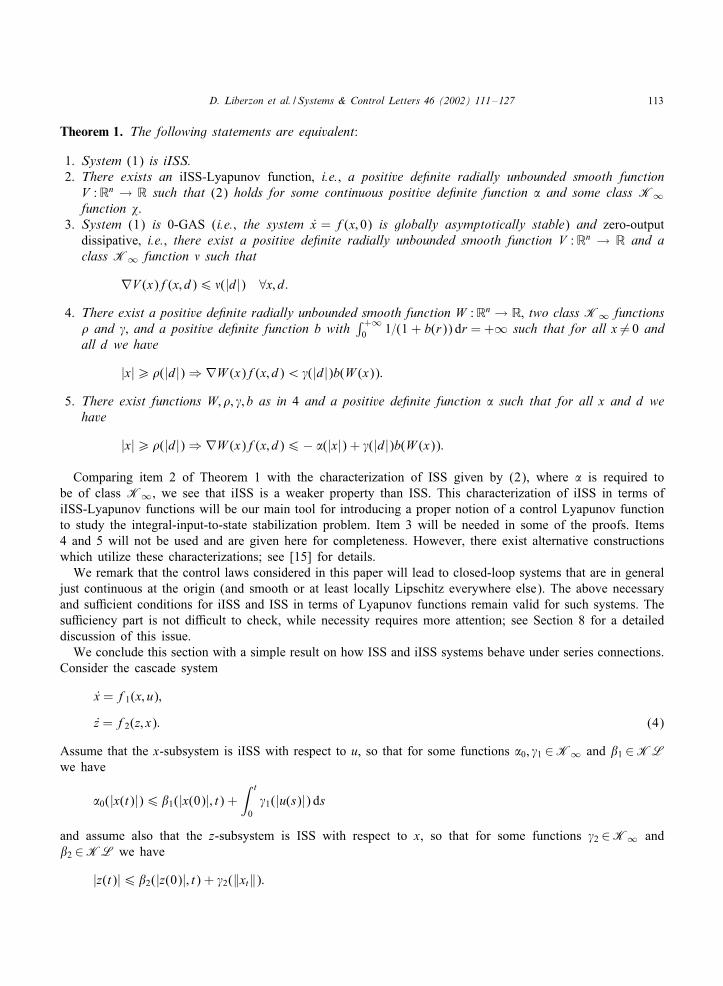
Theorem 1. The following statements are equivalent:

1. System (1) is iISS.2. There exists an iISS-Lyapunov function; i.e.; a positive de;nite radially unbounded smooth function

V :Rn → R such that (2) holds for some continuous positive de;nite function � and some class K∞function �.

3. System (1) is 0-GAS (i.e.; the system x = f(x; 0) is globally asymptotically stable) and zero-outputdissipative; i.e.; there exist a positive de;nite radially unbounded smooth function V :Rn → R and aclass K∞ function � such that

∇V (x)f(x; d)6 �(|d|) ∀x; d:4. There exist a positive de;nite radially unbounded smooth function W :Rn → R; two class K∞ functions

� and �; and a positive de;nite function b with∫ +∞

0 1=(1 + b(r)) dr = +∞ such that for all x = 0 andall d we have

|x|¿ �(|d|) ⇒ ∇W (x)f(x; d)¡�(|d|)b(W (x)):

5. There exist functions W; �; �; b as in 4 and a positive de;nite function � such that for all x and d wehave

|x|¿ �(|d|) ⇒ ∇W (x)f(x; d)6− �(|x|) + �(|d|)b(W (x)):

Comparing item 2 of Theorem 1 with the characterization of ISS given by (2), where � is required tobe of class K∞, we see that iISS is a weaker property than ISS. This characterization of iISS in terms ofiISS-Lyapunov functions will be our main tool for introducing a proper notion of a control Lyapunov functionto study the integral-input-to-state stabilization problem. Item 3 will be needed in some of the proofs. Items4 and 5 will not be used and are given here for completeness. However, there exist alternative constructionswhich utilize these characterizations; see [15] for details.

We remark that the control laws considered in this paper will lead to closed-loop systems that are in generaljust continuous at the origin (and smooth or at least locally Lipschitz everywhere else). The above necessaryand suKcient conditions for iISS and ISS in terms of Lyapunov functions remain valid for such systems. ThesuKciency part is not diKcult to check, while necessity requires more attention; see Section 8 for a detaileddiscussion of this issue.

We conclude this section with a simple result on how ISS and iISS systems behave under series connections.Consider the cascade system

x = f1(x; u);

z = f2(z; x): (4)

Assume that the x-subsystem is iISS with respect to u, so that for some functions �0; �1 ∈K∞ and �1 ∈KLwe have

�0(|x(t)|)6 �1(|x(0)|; t) +∫ t

0�1(|u(s)|) ds

and assume also that the z-subsystem is ISS with respect to x, so that for some functions �2 ∈K∞ and�2 ∈KL we have

|z(t)|6 �2(|z(0)|; t) + �2(‖xt‖):


Proposition 2. Under the above assumptions; the cascade system (4) is iISS with respect to the input u.

Proof (Sketch). We employ a standard argument used for analysis of cascade systems (cf. [21,23,9]). In viewof time-invariance, the ISS property of the z-subsystem can be written as

|z(t)|6 �2(|z(t=2); t=2) + �2(‖x‖[t=2; t]);

where ‖x‖[t=2; t] := ess sup{|x(s)|: s∈ [t=2; t]}. Using straightforward manipulations, we obtain

|z(t)|6 P�1(|x(0)|; t=2) + P�2(|z(0)|; t=2) + P�(∫ t

0�1(|u(s)|) ds

);

where

P�1(r; s) :=�2(3�2(2�−10 (2�1(r; 0))); s) + �2(2�−1

0 (2�1(r; s)));

P�2(r; s) :=�2(3�2(r; s); s); P�(r) :=�2(3�2(2�−10 (2r)); 0) + �2(2�−1

0 (2r)):

Applying P�−1 to both sides of the last inequality, we arrive at the desired result.

Proposition 2 can be added to the series of (well-known) results saying that a cascade of an ISS systemdriving another ISS system is ISS and a cascade of a GAS system driving an ISS system is GAS (see, e.g.,[23,24]). Cascades in which the driven system is iISS are studied in [3].

3. Control Lyapunov functions

A positive de;nite radially unbounded smooth function V :Rn → R is called a control Lyapunov function(CLF) for the system

x = f(x; u); x∈Rn; u∈U ⊂ Rm

if we have

infu∈U

{∇V (x)f(x; u)}¡ 0 ∀x = 0:

This notion goes back to Artstein [4] (see also [20] for parallel work which studied nonsmooth CLFs). If thesystem is aKne in controls, as given by x =f(x) +G(x)u, then the knowledge of a CLF V often leads to anexplicit formula for a state feedback control law that makes the closed-loop system globally asymptoticallystable (with Lyapunov function V ). For example, in the case when U =Rm, the “universal” formula derivedin [22] yields the stabilizing feedback law u=K(a(x); bT(x)), where a(x) :=∇V (x)f(x), b(x) :=∇V (x)G(x),and the function K :R× Rm → R is de;ned by the formula

K(a; b) :=

−a +√

a2 + |b|4|b|2 b; b = 0;

0; b = 0:

(5)

The above control law is smooth on Rn\{0} if the functions f and G are smooth. It is in addition continuous at0 if V satis;es the small control property: for each �¿ 0 there exists a �¿ 0 such that whenever 0¡ |x|¡�there exists some u with |u|¡� for which a(x) + b(x)u¡ 0. We will sometimes also say that the pair(a(x); b(x)) satis;es the small control property. Functions that are smooth away from the origin and continuousat the origin are in this context called almost smooth. Similar universal formulas have later been obtained forcontrols bounded in magnitude [16], positive controls [17], and controls restricted to Minkowski balls [18].


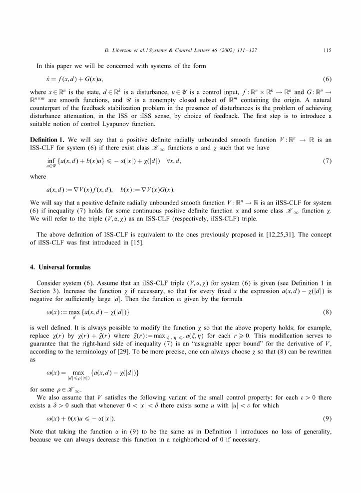
In this paper we will be concerned with systems of the form

x = f(x; d) + G(x)u; (6)

where x∈Rn is the state, d∈Rk is a disturbance, u∈U is a control input, f :Rn × Rk → Rn and G :Rn →Rn×m are smooth functions, and U is a nonempty closed subset of Rm containing the origin. A naturalcounterpart of the feedback stabilization problem in the presence of disturbances is the problem of achievingdisturbance attenuation, in the ISS or iISS sense, by choice of feedback. The ;rst step is to introduce asuitable notion of control Lyapunov function.

De"nition 1. We will say that a positive de;nite radially unbounded smooth function V :Rn → R is anISS-CLF for system (6) if there exist class K∞ functions � and � such that we have

infu∈U

{a(x; d) + b(x)u}6− �(|x|) + �(|d|) ∀x; d; (7)

where

a(x; d) :=∇V (x)f(x; d); b(x) :=∇V (x)G(x):

We will say that a positive de;nite radially unbounded smooth function V :Rn → R is an iISS-CLF for system(6) if inequality (7) holds for some continuous positive de;nite function � and some class K∞ function �.We will refer to the triple (V; �; �) as an ISS-CLF (respectively; iISS-CLF) triple.

The above de;nition of ISS-CLF is equivalent to the ones previously proposed in [12,25,31]. The conceptof iISS-CLF was ;rst introduced in [15].

4. Universal formulas

Consider system (6). Assume that an iISS-CLF triple (V; �; �) for system (6) is given (see De;nition 1 inSection 3). Increase the function � if necessary, so that for every ;xed x the expression a(x; d) − �(|d|) isnegative for suKciently large |d|. Then the function ! given by the formula

!(x) :=maxd

{a(x; d) − �(|d|)} (8)

is well de;ned. It is always possible to modify the function � so that the above property holds; for example,replace �(r) by �(r) + P�(r) where P�(r) :=max|"|; |#|6r a("; #) for each r¿ 0. This modi;cation serves toguarantee that the right-hand side of inequality (7) is an “assignable upper bound” for the derivative of V ,according to the terminology of [29]. To be more precise, one can always choose � so that (8) can be rewrittenas

!(x) = max|d|6�(|x|)

{a(x; d) − �(|d|)}

for some �∈K∞.We also assume that V satis;es the following variant of the small control property: for each �¿ 0 there

exists a �¿ 0 such that whenever 0¡ |x|¡� there exists some u with |u|¡� for which

!(x) + b(x)u6− �(|x|): (9)

Note that taking the function � in (9) to be the same as in De;nition 1 introduces no loss of generality,because we can always decrease this function in a neighborhood of 0 if necessary.


Let us take the disturbance-aKne system

x = f(x) + G(x)d + G(x)u (10)

as an example. Then a(x; d) = a(x) + b(x)d, where

a(x) :=∇V (x)f(x); b(x) :=∇V (x)G(x):

To ensure that ! is well de;ned, it is suKcient to demand that � grow faster than any linear function atin;nity, i.e., �(r)=r → ∞ as r → ∞. Increasing � if necessary so that it becomes greater than some linearfunction for all d, we see that (9) is equivalent to the condition a(x) + b(x)u6− �(|x|). This corresponds tothe standard small control property for the disturbance-free case.

The function ! de;ned by (8) is locally Lipschitz 4 but not necessarily smooth. Take another function, P!,which is smooth away from 0 and continuous at 0 (i.e., almost smooth) and satis;es

!(x) + �(|x|)=36 P!(x)6!(x) + 2�(|x|)=3 ∀x: (11)

Such a function can be constructed using standard smooth approximation techniques (cf. [6, Lemma 4.9]).From (7), (8) and (11) we have

infu∈U

{ P!(x) + b(x)u}6− �(|x|)=3: (12)

Moreover, using (11) and the small control property, we see that for each �¿ 0 there exists a �¿ 0 suchthat whenever 0¡ |x|¡� there exists some u with |u|¡� for which we have P!(x) + b(x)u6− �(|x|)=3.

In what follows, we take the control set U to be Rm and use the “universal” formula for asymptoticstabilization from [22]. As mentioned in Section 3, similar formulas are available for systems with controlstaking values in various restricted control spaces. The result given below can be carried over to these systemsby simply substituting an appropriate universal formula (cf. [14]).

Consider the feedback control law

k(x) :=K( P!(x); bT(x)); (13)

where the function K is de;ned by formula (5). In view of the above developments, it is now not diKcultto prove the following.

Theorem 3. Consider the system (6) with U=Rm. If V is an iISS-CLF satisfying the small control property(9); then the feedback law (13) is almost smooth and integral-input-to-state stabilizing. If V is an ISS-CLFsatisfying the small control property (9); then the feedback law (13) is almost smooth and input-to-statestabilizing.

Proof. It follows from the above analysis and from the results of [22] that the control law (13) is almostsmooth and that we have

P!(x) + b(x)k(x)¡ 0 ∀x = 0: (14)

The derivative of V along solutions of the closed-loop system

x = f(x; d) + G(x)k(x) (15)

satis;es

V = a(x; d) + b(x)k(x)6!(x) + b(x)k(x) + �(|d|);6 P!(x) − �(|x|)=3 + b(x)k(x) + �(|d|)6− �(|x|)=3 + �(|d|)

4 This is because on every compact subset of Rn it is obtained by taking the maximum of a parameterized family of smooth functionsof x, with the parameter d taking values in a compact set.


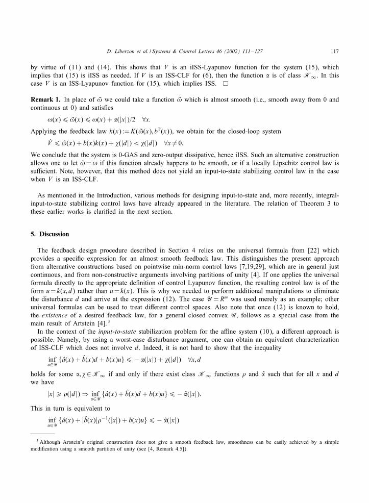
by virtue of (11) and (14). This shows that V is an iISS-Lyapunov function for the system (15); whichimplies that (15) is iISS as needed. If V is an ISS-CLF for (6); then the function � is of class K∞. In thiscase V is an ISS-Lyapunov function for (15); which implies ISS.

Remark 1. In place of P! we could take a function ! which is almost smooth (i.e.; smooth away from 0 andcontinuous at 0) and satis;es

!(x)6 !(x)6!(x) + �(|x|)=2 ∀x:Applying the feedback law k(x) :=K(!(x); bT(x)); we obtain for the closed-loop system

V 6 !(x) + b(x)k(x) + �(|d|)¡�(|d|) ∀x = 0:

We conclude that the system is 0-GAS and zero-output dissipative; hence iISS. Such an alternative constructionallows one to let !=! if this function already happens to be smooth; or if a locally Lipschitz control law issuKcient. Note; however; that this method does not yield an input-to-state stabilizing control law in the casewhen V is an ISS-CLF.

As mentioned in the Introduction, various methods for designing input-to-state and, more recently, integral-input-to-state stabilizing control laws have already appeared in the literature. The relation of Theorem 3 tothese earlier works is clari;ed in the next section.

5. Discussion

The feedback design procedure described in Section 4 relies on the universal formula from [22] whichprovides a speci;c expression for an almost smooth feedback law. This distinguishes the present approachfrom alternative constructions based on pointwise min-norm control laws [7,19,29], which are in general justcontinuous, and from non-constructive arguments involving partitions of unity [4]. If one applies the universalformula directly to the appropriate de;nition of control Lyapunov function, the resulting control law is of theform u= k(x; d) rather than u= k(x). This is why we needed to perform additional manipulations to eliminatethe disturbance d and arrive at the expression (12). The case U= Rm was used merely as an example; otheruniversal formulas can be used to treat di>erent control spaces. Also note that once (12) is known to hold,the existence of a desired feedback law, for a general closed convex U, follows as a special case from themain result of Artstein [4]. 5

In the context of the input-to-state stabilization problem for the aKne system (10), a di>erent approach ispossible. Namely, by using a worst-case disturbance argument, one can obtain an equivalent characterizationof ISS-CLF which does not involve d. Indeed, it is not hard to show that the inequality

infu∈U

{a(x) + b(x)d + b(x)u}6− �(|x|) + �(|d|) ∀x; dholds for some �; �∈K∞ if and only if there exist class K∞ functions � and � such that for all x and dwe have

|x|¿ �(|d|) ⇒ infu∈U

{a(x) + b(x)d + b(x)u}6− �(|x|):This in turn is equivalent to

infu∈U

{a(x) + |b(x)|�−1(|x|) + b(x)u}6− �(|x|)

5 Although Artstein’s original construction does not give a smooth feedback law, smoothness can be easily achieved by a simplemodi;cation using a smooth partition of unity (see [4, Remark 4.5]).


and now a universal formula can be invoked directly by virtue of the last inequality. This was the basicidea behind the constructions of input-to-state stabilizing controllers given in [12,25,31]. A small controlproperty must be imposed to guarantee continuity of the control law at the origin, so that one can applyto the closed-loop system the suKcient condition for ISS in terms of an ISS-Lyapunov function. Since thiscondition also requires that the system be smooth or at least locally Lipschitz away from the origin, one needsto replace the function a(x) + |b(x)|�−1(|x|) by a suitable smooth approximation.

If the function � is only positive de;nite and not of class K∞, the above equivalences break down. There-fore, the problem of integral-input-to-state stabilization requires a di>erent approach. The solution proposedin [15] for aKne systems of form (10) involves combining several control laws de;ned on appropriate re-gions of the state space. This can be done either by smooth “patching” or by hysteresis switching (the lattermethod is described in [14] for the case of bounded controls). The construction presented here is much morestraightforward, and can be used to solve both input-to-state and integral-input-to-state stabilization problems.It is based on de;ning the function ! as in (8), an idea that appears in the recent work of Teel and Praly[29] devoted to the general problem of assigning the derivative of a disturbance attenuation CLF. Within theframework of ISS and iISS disturbance attenuation, we described an explicit procedure for modifying the CLFtriple to ensure that the function ! is well de;ned (whereas in the more general setting of [29] this is notalways possible to achieve and needs to be assumed a priori). A similar function played a role in the earlierwork on robust stabilization reported in [17, Section 5].

Sometimes a control law of the form u=k(x; d) is acceptable, in other words, the disturbance can be directlymeasured and used in control design. This situation arises, for example, in supervisory control of uncertainnonlinear systems, where the disturbance corresponds to the output estimation error which is available forcontrol [8,9]. In such cases, the universal formula can be applied directly, starting from the de;nition of aCLF, to yield a control law u = k(x; d), as described in [14,15].

Finding an (integral-)input-to-state stabilizing control law u=k(x; d) can also be a ;rst step towards ;ndinga suitable feedback law u = k(x). Indeed, the closed-loop system

x = f(x; d) + G(x)k(x; d)

will then possess an (i)ISS-Lyapunov function, which is automatically an (i)ISS-CLF for the original system.The only condition that one needs to check before invoking Theorem 3 is the small control property. For exam-ple, given an aKne system of the form (10), one might ;rst want to look for a smooth 6 integral-input-to-statestabilizing control law u = k(x; d) satisfying k(0; 0) = 0. If such a control law exists, the closed-loop system

x = f(x) + G(x)d + G(x)k(x; d)

admits an iISS-Lyapunov function V , which is an iISS-CLF for the original system. This means that we have

a(x) + b(x)d + b(x)k(x; d)6− �(|x|) + �(|d|) ∀x; d; (16)

where � is continuous positive de;nite and �∈K∞. Moreover, letting d = 0 in (16), we obtain a(x) +b(x)k(x; 0)6 − �(|x|). Using the continuity of k at (0; 0) and the fact that k(0; 0) = 0, we conclude thatthe small control property is satis;ed. Now Theorem 3 can be applied to generate an integral-input-to-statestabilizing state feedback law u = k(x). A speci;c example along these lines is given in the next section.

Inequality (7) from De;nition 1 can be rewritten as

supd∈Rk

infu∈U

{a(x; d) + b(x)u− �(|d|)}6− �(|x|) ∀x: (17)

Since d and u on the left-hand side are decoupled, the sup and the inf commute and (17) is equivalent to

infu∈U

supd∈Rk

{a(x; d) + b(x)u− �(|d|)}6− �(|x|) ∀x: (18)

6 The smoothness requirement can be relaxed (see Section 8).


We used this fact implicitly in the control construction. For the more general system

x = f(x; d) + G(x; d)u (19)

the sup and the inf may not commute, and the above construction cannot be used. Indeed, an iISS-CLF forsystem (19) guarantees the existence of an integral-input-to-state stabilizing control law u = k(x; d) but doesnot guarantee the existence of a feedback law u=k(x) with the same property. In [7], this diKculty is avoidedby requiring a stronger condition of kind (18) in the de;nition of a CLF. See [5] for an interesting discussionof related issues in the context of robust stabilization.

6. Example

It is pointed out in [27] that the scalar system

x = −x + xd (20)

is iISS but not ISS. As an iISS-Lyapunov function one can take V (x) := log(1 + x2). Indeed, we have V =(−2x2 + 2x2d)=(1 + x2)6− 2x2=(1 + x2) + 2|d|. On the other hand, the bounded disturbance d ≡ 2 leads tounbounded trajectories, so the system is not ISS.

We will now use the above observation to construct an example of a system that is integral-input-to-statestabilizable but not input-to-state stabilizable 7 . Consider the system

x = −x + (x − x2)d + u;

y = −y + (y + x2)d− u (21)

No matter what control law u is applied, d ≡ 2 gives (d=dt)(x + y) = x + y. This means that the sys-tem (21) is not input-to-state stabilizable (and thus does not admit an ISS-CLF). On the other hand, it isintegral-input-to-state stabilizable: setting u = x2d, we obtain the system

x = −x + xd;

y = −y + yd

which is iISS in view of the above remarks. It is not at all clear how to integral-input-to-state stabilize system(21) without cancelling some of the terms that contain the disturbance, i.e., how to achieve iISS by applyinga state feedback law u = k(x). However, we can use the construction described in Section 4 to demonstratethat this is possible. Indeed, the function V (x; y) := log(1+ x2)+ log(1+y2) is an iISS-CLF for (21). In fact,all we need is the inequality

infu∈U

{a(x) + b(x)d + b(x)u}6− 2x2

1 + x2 − 2y2

1 + y2 + 4|d| ∀x; d:

Taking �(|d|) := 4|d| + |d|2, it is straightforward to check that function (8) is well de;ned and equals

!(x) =

− 2x2

1 + x2 − 2y2

1 + y2 ;∣∣∣∣x2 − x3

1 + x2 +y2 + x2y1 + y2

∣∣∣∣¡ 2;

− 2x2

1 + x2 − 2y2

1 + y2 +(x2 − x3

1 + x2 +y2 + x2y1 + y2 − 2

)2

;∣∣∣∣x2 − x3

1 + x2 +y2 + x2y1 + y2

∣∣∣∣¿ 2;

7 Incidentally, (20) already provides a trivial example of such a system; here we have G ≡ 0.


Since system (21) is aKne, and since � has a linear lower bound, it follows from the discussion given at thebeginning of Section 4 that the small control property for the pair (!(x); b(x)) holds if and only if it holdsfor the pair (a(x); b(x)). We have

(a(x); b(x)) =(− 2x2

1 + x2 − 2y2

1 + y2 ;2x

1 + x2 − 2y1 + y2

)

and the small control property is obviously satis;ed because a(x)¡ 0 for all (x; y) = (0; 0). Now an integral-input-to-state stabilizing feedback law, locally Lipschitz (actually, continuously di>erentiable) away from 0and continuous at 0, is given by the formula u = K(!(x); bT(x)). One could also take a function ! which isalmost smooth and satis;es

!(x)6 !(x)6!(x) +x2

1 + x2 +y2

1 + y2

and de;ne an almost smooth desired feedback law by u = K(!(x); bT(x)).

7. Backstepping

The following lemma shows that for certain classes of systems, aKne in both disturbance and controlinputs, integral-input-to-state stabilizing control laws can be systematically constructed by using backstepping.It exactly parallels the corresponding result for the ISS case [13,12].

Lemma 4. If a system of the form

x = f(x) + G(x)d + G(x)u; x∈Rn; d∈Rk ; u∈Rm (22)

is integral-input-to-state stabilizable with a smooth control law u=k(x) satisfying k(0)=0; then an augmentedsystem of the form

x = f(x) + G(x)d + G(x)";

" = u + F(x; ")d (23)

is integral-input-to-state stabilizable with a smooth control law u = k(x; ").

Proof. Since the system

x = f(x) + G(x)d + G(x)k(x)

is iISS; it admits a smooth iISS-Lyapunov function V so that we have

a(x) + b(x)d + b(x)k(x)6− �(|x|) + �(|d|) ∀x; d (24)

(in the notation of Section 4), where � is continuous positive de;nite and �∈K∞. Regarding (23); we claimthat an integral-input-to-state stabilizing feedback control law u = k(x; ") can be de;ned by

k(x; ") := − ("− k(x))(1 + |∇k(x)G(x)|2 + |F(x; ")|2

)− bT(x) + ∇k(x)f(x) + ∇k(x)G(x)": (25)

To verify this claim; de;ne the function

Va(x; ") :=V (x) + 12 |"− k(x)|2:


Calculating the derivative of Va along solutions of the closed-loop system

x = f(x) + G(x)d + G(x)";

" = k(x; ") + F(x; ")d (26)

with the help of (24); (25); and square completion; it is not hard to verify that

V a = a(x) + b(x)d + b(x)"

+("− k(x))T[k(x; ") + F(x; ")d−∇k(x)f(x) −∇k(x)G(x)d−∇k(x)G(x)"]

= a(x) + b(x)d + b(x)k(x)

+ ("− k(x))T[bT(x) + k(x; ") + F(x; ")d−∇k(x)f(x) −∇k(x)G(x)d−∇k(x)G(x)"]

= a(x) + b(x)d + b(x)k(x) − |"− k(x)|2 − |"− k(x)|2|∇k(x)G(x)|2

− ("− k(x))T∇k(x)G(x)d− |"− k(x)|2|F(x; ")|2 + ("− k(x))TF(x; ")d

6−�(|x|) + �(|d|) − |"− k(x)|2 + 12 |d|2 ¡�(|d|) + 1

2 |d|2

for all (x; ") = (0; 0) and all d. This implies that system (26) is 0-GAS and zero-output dissipative; henceiISS.

Remark 2. We can actually go further and show that Va is an iISS-Lyapunov function for the closed-loopsystem (26); and consequently an iISS-CLF for (23). Let �a be a continuous positive de;nite function suchthat for all r¿ 0; all x and " with |( x

")| = r; and all |d|6 r we have

�a(r)6− V a + �(|d|) + 12 |d|2:

Then for all x and d such that |( x")|¿ |d| we have

V a 6 −�a

(∣∣∣∣∣(

x

"

)∣∣∣∣∣)

+ �(|d|) +12|d|2: (27)

Next; let �a be a class K∞ function with the property that

�a(r)¿ V a + �a

(∣∣∣∣∣(

x

"

)∣∣∣∣∣)

− �(|d|) − 12|d|2

for all r¿ 0; all x and " with |( x")|6 r; and all |d| = r. Then for all x and d such that |( x

")|¡ |d| we have

V a6− �a

(∣∣∣∣∣(

x

"

)∣∣∣∣∣)

+ �(|d|) +12|d|2 + �a(|d|):

Together with (27) this implies that

V a6− �a

(∣∣∣∣∣(

x

"

)∣∣∣∣∣)

+ �a(|d|) ∀x; "; d

where �a(r) := �a(r) + �(r) + 12 |d|2. Thus Va is an iISS-Lyapunov function for (26); as claimed.


Suppose now that we start with a system of form (22) that satis;es the assumptions of Lemma 4. Repeatedapplication of this lemma leads to an explicit recursive procedure for designing integral-input-to-state stabilizingcontrol laws for cascade systems of the form

x = f(x) + G(x)d + G(x)"1;

"1 = "2 + F1(x; "1)d;...

"n−1 = "n + Fn−1(x; "1; : : : ; "n−1)d;

"n = u + Fn(x; "1; : : : ; "n)d:

As a byproduct, an iISS-CLF is also generated at each step (see Remark 2). We refer the reader to [29] fora more detailed analysis of these issues and for additional insights.

8. Regularity at the origin and converse results

We have shown that if system (6) admits an iISS-CLF, then there exists an almost smooth integral-input-to-state stabilizing feedback law u=k(x). To prove this result (Theorem 3), we exploited the fact that if a systemadmits an iISS-Lyapunov function, then it is iISS. This fact was established in [2] under the assumption thatthe system is locally Lipschitz. Since the control law that we used is not necessarily Lipschitz at the origin,the resulting closed-loop system may not satisfy this assumption. However, it is not diKcult to check that therelevant argument given in [2] is still valid if the system is merely continuous at the origin. The same remarkapplies to input-to-state stabilizing control laws.

We would like to show that the converse also holds, namely, that the existence of an almost smoothintegral-input-to-state stabilizing feedback law for system (6) implies the existence of an iISS-CLF. To thisend, take such a feedback law u = k(x). If it is smooth or at least locally Lipschitz at the origin, then theclosed-loop system (15) satis;es the assumptions of [2]. The converse part of the main theorem in that paperimplies that system (15) admits an iISS-Lyapunov function, which is automatically an iISS-CLF for system(6). However, if the feedback law does not have suKcient regularity at the origin, one cannot simply appealto the converse result of [2], and the above argument requires additional justi;cation.

A similar issue in fact arises in the context of ISS, and it has been frequently overlooked. One way to ;xthis problem in the case of an almost smooth input-to-state stabilizing feedback law is to consider a positivede;nite function ’ such that the right-hand side of the closed-loop system becomes smooth everywhere whenmultiplied by ’(x). More precisely, let u = k(x) be an almost smooth input-to-state stabilizing feedback lawfor system (6). Let ’ be a positive de;nite function such that the system

x = ’(x)[f(x; d) + G(x)k(x)] (28)

is smooth. The results of [26] allow one to show that the modi;ed system (28) is still ISS (see Lemmas2.12–2.14 in [26]). Therefore, a characterization of ISS proved in [26] guarantees the existence of a positivede;nite radially unbounded smooth function V :Rn → R whose derivative along solutions of (28) satis;es

|x|¿ �(|d|) ⇒ V 6− �(|x|);

where �∈K∞ and � is continuous positive de;nite. Since ’ is positive de;nite, the derivative of V alongsolutions of the original closed-loop system (15) also satis;es the same inequality for a di>erent �, hence Vis an ISS-CLF for the open-loop system (6). This “time reparameterization” trick was used in [4], althoughfor a di>erent purpose, namely, assuring continuity at the origin of a possibly discontinuous vector ;eld.


Alternatively, one can appeal to the work reported in [31], where a generalization of a converse Lyapunovtheorem was proved for systems that do not have regularity on the invariant sets. The desired conclusion alsofollows from the recent results of Teel and Praly [28].

To make this work self-contained, we now present a construction for the iISS case which is similar to theone described in the previous paragraph, although far less trivial to justify (because the results of [26] do notapply to iISS). Namely, we will prove that if an almost smooth feedback law u = k(x) integral-input-to-statestabilizes system (6) and if ’ is a suitably chosen positive de;nite function which makes the system (28)smooth, then (28) is iISS. We will then show how an iISS-Lyapunov function for the modi;ed closed-loopsystem (28) can be used to obtain an iISS-Lyapunov function for the original closed-loop system (15), whichautomatically yields an iISS-CLF for the open-loop system (6). This construction is based on the followingtwo results, which are of independent interest.

Lemma 5. Suppose that system (1) is iISS. Let ’ :Rn → R be a positive de;nite smooth function. Thenthe system

x = ’(x)f(x; d) (29)

is iISS.

Proof. Let �0; �∈K∞ and �∈KL be the functions appearing in the iISS estimate (3) for system (1). Pickan arbitrary initial state z0 = 0 and a disturbance d such that∫ ∞

0�(|d(s)|) ds6 b¡∞:

Denote by z(·) the corresponding solution of (29); de;ned on some maximal interval [0; T ). Let

)(t) :=∫ t

0’(z(s)) ds; t ∈ [0; T ):

Since ’(z(t))¿ 0 for all t ∈ [0; T ); the function )(·) is strictly increasing. Note that ) satis;es the followinginitial value problem:

)(t) = ’(z(t)); )(0) = 0:

Hence; by the uniqueness property of system (29); it holds that

z(t) = x()(t)) ∀t ∈ [0; T );

where x(·) is the solution of (1) with the initial state z0 and the disturbance function dx(t) :=d◦)−1(t) de;nedon [0; limt→T−)(t)). It then follows that for all t ∈ [0; T ) we have

�0(|z(t)|)6 �(|z0|; )(t)) +∫ )(t)

0�(|dx(s)|) ds

6 �(|z0|; )(t)) +∫ t

0�(|d(s)|) ds6 �(|z0|; )(t)) + b:

Hence; z(t) stays bounded on [0; T ); and consequently T = ∞. It is not hard to see now that system (29) is0-GAS and satis;es the so-called bounded energy frequently bounded state property (see [1]):∫ ∞

0�(|d(s)|) ds¡∞ ⇒ lim inf

t→∞ |z(t)|¡∞:

By Theorem 3 of [1]; the system (29) is iISS.


Lemma 6. Consider system (29); where ’ :Rn → R is a positive de;nite smooth function satisfying ’(x)6 1for all x and ’(x) = 1 for all |x|¿ 1 such that the right-hand side of (29) is smooth everywhere. If (29) isiISS; then system (1) admits an iISS-Lyapunov function.

Proof. System (29) is iISS and smooth; thus it admits an iISS-Lyapunov function V which satis;es

∇V (x)’(x)f(x; d)6− �(|x|) + �(|d|)for some continuous positive de;nite function � and some class K∞ function �. Let �0 be some smoothclass K function such that �0(V (x))6’(x) for all x; and de;ne

W (x) : =∫ V (x)

0�0(*) d*:

It then follows that W is positive de;nite; smooth; radially unbounded; and its derivative along solutions of(1) satis;es

∇W (x)f(x; d) = �0(V (x))∇V (x)f(x; d)6− �0(V (x))�(|x|) + �(|d|):Therefore; W is an iISS-Lyapunov function for system (1).

Choosing a function ’ satisfying the hypotheses of Lemma 6 and applying the two lemmas to the system(15), we immediately arrive at the following result.

Corollary 7. Consider system (15) with f;G smooth and k almost smooth. If this system is iISS; then itadmits an iISS-Lyapunov function.

We can now summarize our main ;ndings as follows.

Theorem 8. System (6) admits an iISS-CLF (respectively; an ISS-CLF) satisfying the small control prop-erty (9) if and only if there exists an almost smooth integral-input-to-state stabilizing (respectively; input-to-state stabilizing) feedback law u = k(x).

9. Remarks on other types of CLFs

The results discussed in Sections 3 and 4 can be generalized to deal with other types of control Lyapunovfunctions. Consider a system with output:

x = f(x; d) + G(x)u;y = h(x); (30)

where f and G are as before and the output map h :Rn → Rq is continuous. Suppose that for this systemthere exists a positive de;nite radially unbounded smooth function V :Rn → R such that

infu{∇V (x)f(x; d) + ∇V (x)G(x)u}6− �(|x|) + �(|d|) + �(|y|); (31)

where � is continuous positive de;nite and �; �∈K∞. Similarly to the discussion in Section 3, we let

a(x; d) :=∇V (x)f(x; d) − �(|h(x)|); b(x) :=∇V (x)G(x):


Then (31) becomes

infu{a(x; d) + b(x)u}6− �(|x|) + �(|d|) ∀x; d: (32)

As explained in Section 4, by modifying � if necessary, one may assume that the function ! given by

!(x) = supd{a(x; d) − �(|d|)}

is well de;ned and continuous. Let P!(·) be an almost smooth function as in (11). Then (32) together with(11) yield

infu{ P!(x) + b(x)u}6− �(|x|)=3: (33)

With the feedback control law

k(x) = K( P!(x); bT(x)) (34)

where K is de;ned by the universal formula (5), we obtain

∇V (x)f(x; d) + ∇V (x)G(x)k(x)6− �(|x|)=3 + �(|d|) + �(|y|):Hence, we arrive at the following generalization of Theorem 3.

Theorem 9. Suppose that system (30) admits a positive de;nite radially unbounded smooth function V thatsatis;es inequality (31) for some continuous positive function � and some class K∞ functions � and �.Assume that the small control property (9) holds for the pair (!(x); b(x)). Then; with the almost smoothfeedback law k(x) given by (34); we have the following:

1. The closed-loop system is integral-input integral-output to state stable; that is; there exist some �0; �1; �2 ∈K∞ and �∈KL such that for each trajectory x(·) with disturbance d we have

�0(|x(t)|)6 �(|x(0)|; t) +∫ t

0�1(|d(s)|) ds +

∫ t

0�2(|y(s)|) ds

for all t¿ 0 (see [10]).2. If �∈K∞; then the closed-loop system is input-output-to-state stable; that is; there exist some �∈KLand �1; �2 ∈K∞ such that for each trajectory x(·) with disturbance d we have

|x(t)|6 �(|x(0)|; t) + �1(‖d‖) + �2(‖yt‖)

for all t¿ 0 (see [11]).3. If �∈K∞ and � ≡ 0; then the closed-loop system is robustly output-to-state stable; that is; there existsome �∈KL and �∈K∞ such that

|x(t)|6 �(|x(0)|; t) + �(‖yt‖)

for all t¿ 0 and all d (see [11]).4. If � ≡ 0; then the closed-loop system is iISS.5. If � ≡ 0 and �∈K∞; then the closed-loop system is ISS.

Remark 3. By an argument similar to the one used in Section 8; one can show that the converse of statement2 in the above theorem about input-output-to-state stabilizability is also true. Namely; if there is an almostsmooth feedback u = k(x) under which the closed-loop system is input-output-to-state stable; then the system


admits a CLF V that satis;es inequality (31) and the small control property (9); with � of class K∞. Asfor statement 1; it is not clear to us at this stage if the converse statement is true (it was shown in [10] thatintegral-input integral-output to state stability implies the existence of a continuous V ). Regarding statement3; it was shown in [11] that robust output-to-state stability implies the existence of a smooth V when thedisturbance d takes values in a compact set; but this is in general not true for unbounded d.

Acknowledgements

We are grateful to Andy Teel for calling our attention to the paper [29] and for illuminating discussions.We also thank David Angeli and Murat Arcak for reading an earlier draft of this paper and providing helpfulcomments.

References

[1] D. Angeli, B. Ingalls, E.D. Sontag, Y. Wang, Asymptotic characterizations of IOSS, Proceedings of 40th IEEE Conference onDecision and Control, 2001, pp. 881–886.

[2] D. Angeli, E.D. Sontag, Y. Wang, A characterization of integral input to state stability, IEEE Trans. Automat. Control 45 (2000)1082–1097.

[3] M. Arcak, D. Angeli, E.D. Sontag, A unifying integral ISS framework for stability of nonlinear cascades, SIAM J. Control Optim.,40 (2002) 1888–1904.

[4] Z. Artstein, Stabilization with relaxed controls, Nonlinear Anal. 7 (1983) 1163–1173.[5] F. Blanchini, The gain scheduling and the robust state feedback stabilization problems, IEEE Trans. Automat. Control 45 (2000)

2061–2070.[6] W.M. Boothby, An Introduction to Di>erentiable Manifolds and Riemannian Geometry, Academic Press, Orlando, 1986.[7] R.A. Freeman, P.V. Kokotovic, Inverse optimality in robust stabilization, SIAM J. Control Optim. 34 (1996) 1365–1391.[8] J.P. Hespanha, A.S. Morse, Certainty equivalence implies detectability, Systems Control Lett. 36 (1999) 1–13.[9] J.P. Hespanha, D. Liberzon, A.S. Morse, Supervision of integral-input-to-state stabilizing controllers, Automatica, 2002, to appear.

[10] B. Ingalls, Comparisons of notions of stability for nonlinear control systems with outputs, Ph.D. Thesis, Department of Mathematics,Rutgers University, New Brunswick, NJ, 2001.

[11] M. Krichman, E.D. Sontag, Y. Wang, Input–output-to-state stability, SIAM J. Control Optim. 39 (2001) 1874–1928.[12] M. Krstic, Z.-H. Li, Inverse optimal design of input-to-state stabilizing nonlinear controllers, IEEE Trans. Automat. Control 43

(1998) 336–350.[13] M. Krstic, I. Kanellakopoulos, P.V. Kokotovic, Nonlinear and Adaptive Control Design, Wiley, New York, 1995.[14] D. Liberzon, ISS and integral-ISS disturbance attenuation with bounded controls, Proceedings of 38th IEEE Conference on Decision

and Control, 1999, pp. 2501–2506.[15] D. Liberzon, E.D. Sontag, Y. Wang, On integral-input-to-state stabilization, Proceedings of 1999 American Control Conference,

1999, pp. 1598–1602.[16] Y. Lin, E.D. Sontag, A universal formula for stabilization with bounded controls, Systems Control Lett. 16 (1991) 393–397.[17] Y. Lin, E.D. Sontag, Control-Lyapunov universal formulae for restricted inputs, Control Theory Adv. Technol. 10 (1995) 1981–2004.[18] M. Maliso>, E.D. Sontag, Universal formulas for CLF’s with respect to Minkowski balls, Proceedings of 1999 American Control

Conference, 1999, pp. 3033–3037.[19] I.R. Petersen, B.R. Barmish, Control e>ort considerations in the stabilization of uncertain dynamical systems, Systems Control Lett.

9 (1987) 417–422.[20] E.D. Sontag, A Lyapunov-like characterization of asymptotic controllability, SIAM J. Control Optim. 21 (1983) 462–471;

E.D. Sontag, A characterization of asymptotic controllability, in: A. Bednarek, L. Cesari (Eds.), Dynamical Systems II, AcademicPress, New York, 1982, pp. 645–648.

[21] E.D. Sontag, Smooth stabilization implies coprime factorization, IEEE Trans. Automat. Control 34 (1989) 435–443.[22] E.D. Sontag, A universal construction of Artstein’s theorem on nonlinear stabilization, Systems Control Lett. 13 (1989) 117–123.[23] E.D. Sontag, Further facts about input to state stabilization, IEEE Trans. Automat. Control 35 (1990) 473–476.[24] E.D. Sontag, A. Teel, Changing supply functions in input=state stable systems, IEEE Trans. Automat. Control 40 (1995) 1476–1478.[25] E.D. Sontag, Y. Wang, On characterizations of input-to-state stability with respect to compact sets, Proceedings of IFAC Non-Linear

Control Systems Design Symposium (NOLCOS ’95), Tahoe City, CA, June 1995, pp. 226–231.[26] E.D. Sontag, Y. Wang, On characterizations of the input-to-state stability property, Systems Control Lett. 24 (1995) 351–359.


[27] E.D. Sontag, Comments on integral variants of ISS, Systems Control Lett. 34 (1998) 93–100.[28] A.R. Teel, L. Praly, Results on converse Lyapunov functions from class-KL estimates, Proceedings of 38th IEEE Conference on

Decision and Control, 1999, pp. 2545–2550.[29] A.R. Teel, L. Praly, On assigning the derivative of a disturbance attenuation control Lyapunov function, Math. Control Signals

Systems 13 (2000) 95–124.[30] J. Tsinias, Control Lyapunov functions, input-to-state stability and applications to global feedback stabilization for composite systems,

J. Math. Systems Estimate Control 7 (1997) 1–31.[31] Y. Wang, A converse Lyapunov theorem with applications to ISS-disturbance attenuation, Proceedings of 13th IFAC World Congress,

Vol. E, 1996, pp. 79–84.

Universal construction of feedback laws achieving ISS and integral-ISS disturbance attenuation

Documents

Transcript of Universal construction of feedback laws achieving ISS and integral-ISS disturbance attenuation