Network Biology, 2015, Vol. 5, Iss. 1

Network Biology

Vol. 5, No. 1, 1 March 2015

International Academy of Ecology and Environmental Sciences

Network Biology ISSN 2220-8879 ∣ CODEN NBEICS Volume 5, Number 1, 1 March 2015 Editor-in-Chief WenJun Zhang Sun Yat-sen University, China International Academy of Ecology and Environmental Sciences, Hong Kong E-mail: [email protected], [email protected] Editorial Board Ronaldo Angelini (The Federal University of Rio Grande do Norte, Brazil) Sudin Bhattacharya (The Hamner Institutes for Health Sciences, USA) Andre Bianconi (Sao Paulo State University (Unesp), Brazil) Danail Bonchev (Virginia Commonwealth University, USA) Graeme Boswell (University of Glamorgan, UK) Jake Chen (Indiana University-Purdue University Indianapolis, USA) Ming Chen (Zhejiang University, China) Daniela Cianelli (University of Naples Parthenope, Italy) Kurt Fellenberg (Technische Universitaet Muenchen, Germany) Alessandro Ferrarini (University of Parma, Italy) Vadim Fraifeld (Ben-Gurion University of the Negev, Israel) Alberto de la Fuente (CRS4, Italy) Pietro Hiram Guzzi (University Magna Graecia of Catanzaro, Italy) Yongqun He (University of Michigan, USA) Shruti Jain (Jaypee University of Information Technology, India) Sarath Chandra Janga (University of Illinois at Urbana-Champaign, USA) Istvan Karsai (East Tennessee State University, USA) Caner Kazanci (University of Georgia, USA) Vladimir Krivtsov (Heriot-Watt University, UK) Miguel ángel Medina (Universidad de Málaga, Spain) Lev V. Nedorezov (Russian Academy of Sciences, Russia) Alexandre Ferreira Ramos (University of Sao Paulo, Brazil) Santanu Ray (Visva Bharati University, India) Dimitrios Roukos(Ioannina University School of Medicine, Greece) Ronald Taylor (Pacific Northwest National Laboratory,U.S. Dept of Energy, USA) Ezio Venturino (Universita’ di Torino, Italy) Jason Jianhua Xuan (Virginia Polytechnic Institute and State University, USA) Ming Zhan (National Institute on Aging, NIH, USA) TianShou Zhou (Sun Yat-Sen University, China) Editorial Office: [email protected]

Publisher: International Academy of Ecology and Environmental Sciences

Address: Unit 3, 6/F., Kam Hon Industrial Building, 8 Wang Kwun Road, Kowloon Bay, Hong Kong

Tel: 00852-2138 6086 Fax: 00852-3069 1955 Website: http://www.iaees.org/ E-mail: [email protected]

Network Biology, 2015, 5(1): 1-12

IAEES www.iaees.org

Article

A comparative analysis on computational methods for fitting an ERGM

to biological network data

Sudipta Saha1, Munni Begum2

1Dalla Lana School of Public Health, University of Toronto, Toronto, ONM5S 2J7, Canada 2Department of Mathematical Sciences, Ball State University, Muncie, IN47306, USA

E-mail: [email protected], [email protected]

Received 16 October 2014; Accepted 25 November 2014; Published online 1 March 2015

Abstract

Exponential random graph models (ERGM) based on graph theory are useful in studying global biological

network structure using its local properties. However, computational methods for fitting such models are

sensitive to the type, structure and the number of the local features of a network under study. In this paper, we

compared computational methods for fitting an ERGM with local features of different types and structures. Two

commonly used methods, such as the Markov Chain Monte Carlo Maximum Likelihood Estimation and the

Maximum Pseudo Likelihood Estimation are considered for estimating the coefficients of network attributes.

We compared the estimates of observed network to our random simulated network using both methods under

ERGM. The motivation was to ascertain the extent to which an observed network would deviate from a

randomly simulated network if the physical numbers of attributes were approximately same. Cut-off points of

some common attributes of interest for different order of nodes were determined through simulations. We

implemented our method to a known regulatory network database of Escherichia coli (E. coli).

Keywords biological networks; regulatory networks; exponential random graph models; Monte Carlo

maximum likelihood estimation; maximum pseudo likelihood estimation; E. coli.

1 Introduction

Over the last decade, there has been a growing interest in the study of biological interaction networks at the

macro and micro molecular levels (Zhang 2012). Identifying basic structural relationships among micro

components is the main goal in the field of systems biology (Li and Zhang, 2013). A formal basis for handling

such complex networks includes computational tools to support the modelling and simulation through methods

developed in mathematical biology and bioinformatics. Since 1960s, with some notable precursors in the

Network Biology ISSN 22208879 URL: http://www.iaees.org/publications/journals/nb/onlineversion.asp RSS: http://www.iaees.org/publications/journals/nb/rss.xml Email: [email protected] EditorinChief: WenJun Zhang Publisher: International Academy of Ecology and Environmental Sciences


IAEES www.iaees.org

preceding decades, a variety of mathematical formalisms have been proposed to describe this kind of complex

networking. During the last few years, modelling efforts targeted several distinct types of networks at the

molecular level, such as gene regulatory networks (Pavlopoulos et al., 2011; Mason and Verwoerd, 2007),

metabolic networks (Ideker et al., 2001), signal transduction networks (Stock, 1990) or protein-protein

interaction networks (Pavlopoulos et al., 2011), transcription regulatory networks (Begum et al., 2014).

Networks of interactions that are not restricted to a cell (intercellular communications) or take place at an

altogether different level of detail (immunological networks, ecological networks) are also of immense interest.

In this paper, we considered a transcription regulatory network for the model organism Escherichia coli

K-12 (E. coli) from RegulonDB (Salgado et al., 2006) version 7.4 (http://regulondb.ccg.unam.mx/). The

RegulonDB contains information on transcription initiation and the regulatory network of E. coli. Downloadable

experimental datasets are available on the regulatory network interactions RegulonDB. The transcription factor

(TF) - transcription factor (TF) interaction network data are considered in this work. A transcriptional unit is

defined as a set of one or more genes within an operon transcribed as a set through the utilization of a single

promoter. In the original dataset (represented as a table) of E.coli in the RegulonDB website, there are four

columns. The first column is the name of the Transcription Factor (TF), the second column is TF regulated by TF,

third column is Regulatory effect of the TF on the regulated gene (+ activator, - repressor, +- dual, ? unknown)

and the fourth column is the evidence of support of the existence of the regulatory interaction. The first two

columns are considered and it created the TF-TF interaction network. The observed TF-TF network, which is a

directed network with loops, is given in Fig. 1.

Fig. 1 Observed TF-TF network.

Each vertex is a TF and an edge between two TFs represents a regulation. An edge from a TF to another TF

represents that the first TF regulates the second. We explored this observed network and counted the number of

several network attributes i.e. edge, triangle and stars. In this observed network, there are 387 edges, 114

triangles, twenty 3-ostars, thirty-four 3-istars, ten 5-ostars, and nine 5-istars and the network has two big

clusters and several small clusters. The basic definitions of some network attributes are given below,

Edges or arcs: This term adds one network statistic that is equal to the number of edges in the network. For

undirected networks, an edge is same ask-star (1) [see below] whereas for directed networks, an edge represents

both ostar (1) and istar (1) (Morris et al., 2008).

Triangles: This term adds one statistic to the model that is equal to the number of triangles in the network. For an

undirected network, a triangle is defined to be any set , , , , , of three edges. For a directed network,

2


IAEES www.iaees.org

a triangle is defined as any set of three edges and either or (Morris et al.,

2008).

k-star: This term adds one statistic when there exists ties between one node and k number of other nodes. For a

directed network the star statistics are replaced by outgoing stars (k-ostar) and incoming stars (k-istar) (Morris et

al., 2008).

2 Exponential Random Graph Model (ERGM)

An Exponential Random Graph Model (ERGM) models the probability distribution (mass function / density

function) for a given class of graphs. Given an observed graph and a set of local features of that graph, the

probability distribution of the graph is estimated. The distribution provides a concise summary of the class of

graphs to which the observed graph belongs, i.e. the probability distribution can be used to calculate the

probability that any given graph is drawn from the same distribution as the observed graph (Fronczak, 2012;

Robins et al., 2007; Saul and Filkov, 2007; Wasserman and Pattison, 1996).

ERGMs represent the generative process of tie formation in networks with two basic types of processes

namely dyadic dependence and dyadic independence. A dyad refers to a pair of nodes and the relations between

them. Dyadic dependent processes are those in which the state of one dyad depends stochastically on the state of

other dyads. Dyadic independent processes exhibit no direct dependence among dyads. This distinction between

these two types of processes affects the specification, estimation, and behaviour of ERGMs. Models with only

dyadic independent terms have a likelihood function that simplifies to a form that can be maximized using

standard logistic regression models. In contrast, models for processes with dyadic dependence require

computationally intensive estimation and imply complex forms of feedback and global dependence that

confound both intuition and estimation (Handcock et al., 2003; Hunter and Handcock, 2006).

Although an ERGM presents a flexible means to model complex networks, the likelihood function for

parameter estimation involves a mathematically intractable normalizing constant. ERGMs generalize the

Markov random graph models (Frank and Strauss, 1986), and edge and dyadic independence models. Several

statistical computational methods had been proposed to address this difficulty in parameter estimation in an

ERGM. These are the Markov chain Monte Carlo maximum likelihood estimation (MCMCMLE) method and

the Maximum pseudo likelihood estimation (MPLE) method (Handcock et al., 2003; Robins et al., 2007;

Snijders, 2002). We briefly discuss the general ERGM, which is also known as model, to layout the

theoretical background of such models.

The general log-linear form of model is expressed as,

exp ′

1

here is a vector of model parameters, is a vector of network statistics, and . is a normalizing constant

which is hard to compute for large networks. In order to simplify the estimation process of the model parameters,

the log-linear model form of the model can be re-expressed as a logit model. In particular, as per

(Wasserman and Pattison, 1996), denotes an adjacency matrix where a tie from is forced to be present.

That is , 1 . denotes an adjacency matrix where a tie from is forced to be

absent. That is , 0 . Finally, denotes an adjacency matrix with complement relation

for the tie from . That is, , , . The model in Equation (1) can be turned to a

logistic regression model by considering a set of binary random variables , where 1 implying a tie

from as follows.

log1|X

0|X ′ 2

3


IAEES www.iaees.org

′ 3

Here is defined as vector of network statistic , is the vector of network statistic

and is the vector of difference statistics obtained from the network statistics . when the variable

changes from 1 to 0. The model in Equation (3) is referred to as the model for single binary relation.

One can work with either the log-linear form of model given in Equation (1) or the logit form given in

equation (3).

3 Computational Methods

There are two methods commonly used to estimate the maximum likelihood fit to exponential random graph

models. These are the maximum pseudo-likelihood estimation (MPLE) and the Markov chain Monte Carlo

maximum likelihood estimation (MCMCMLE) (Handcock et al., 2003; Robins et al., 2007; Snijders, 2002). The

pseudo likelihood function is simply the product of the probabilities of with each probability conditional on

the rest of the data. The method avoids the technical difficulty inherent in the maximum likelihood approach.

The maximum pseudo likelihood estimator (MPLE) for an ERGM, which maximize the pseudo likelihood, may

easily be found (at least in principle) by using logistic regression as a computational device. However, when the

ERGM in question is not a dyadic independence model, the statistical properties of pseudo likelihood estimators

for a network are not well understood (Hunter and Handcock, 2006).

Monte Carlo maximum likelihood estimation (MCMCMLE) is preferred for dyadic dependentp models.

The MCMCMLE of the parameter vector is obtained by maximizing the approximate likelihood. The

MCMCML estimation algorithm is implemented to the software package statnet (Handcock et al., 2003) under

the statistical computational environment R. We use these two packages statnet and ergm (Handcock et al., 2008)

to fit the exponential random model given in equation (1).

4 Simulation Study

We conduct a simulation study for generating random network under varying conditions. We choose conditions

by assigning different number of nodes and network statistics. The primary reason behind conducting the

simulation is to determine the cut-off points for different number of nodes for specific attributes and also to

compare our simulated models with an observed model. For the comparison part, we create two networks by

imposing the same number of network attributes to the models and then compare the results of estimates with the

TF-TF interaction network of E. coli by fitting ERGM.

We consider various network statistics such as arc, stars, and triangles. A k-star is defined where there exist

ties between one node and k number of other nodes. For a directed network the star statistics are replaced by

outgoing stars (k-ostar) and incoming stars (k-istar). In particular arc, 5-ostar, 5-istar, 6-ostar, 6-istar, and

triangles are considered as our network attributes. We physically impose these attributes into the simulated

network by keeping approximately the same number of attributes as the observed network. We also observe that

if we simulate triangles, ostars, istars, and arcs are automatically created. We randomly assign these attributes

to the simulated networks for different number of nodes (n=20, 50, 100) and determine the conditions for these

statistics to become insignificant. The cut-off points for single attributes and for a combination of attributes are

assessed. However, due to the convergence issues, we were unable to obtain the cut-off points for some cases. A

cut-off point is defined as the value where network attributes become significant to insignificant and vice versa.

The rationale is that if the biological network behaves almost the same as the random network, then if we have an

observed network with different number of nodes, we can determine up to which point (approximately) certain

statistics become insignificant.

4


IAEES www.iaees.org

We explore the TF-TF interaction network of E. coli from the RegulonDB database and found that there are

ten5-ostars, nine5-istars, ten6-ostars, eight6-istars and 114 triangles. The network contains 175 nodes with

density 0.012. Once we determine the number of attributes in the observed network, then we mimic this network

and randomly simulate two networks. Then we consider different combinations of attributes (ostars, istars and

triangles) and fit the models by ERGM. We fit the same models for the observed data by using ERGM and then

compare the estimates of ERGM for both MCMCMLE and MPLE method.

We begin with networks with small number of nodes and move toward networks with higher number of

nodes. With only 20 nodes, we consider reasonably smaller magnitude of network attributes such as arcs,

3-ostars, 3-istars and triangles as our attributes of interest and then fit the models with ERGM to get the

estimates and also to determine the cut-off points. We start with smaller number of attributes, two3-ostars, two

3-istars, and two triangles. We increment each attribute one at a time to determine the cut-off points. Simulated

network with 77 triangles, twelve3-istars and fourteen3-ostars is presented in Fig. 2.

Fig. 2 Simulated network for n=20.

Next we increased the number of nodes to 50 and 100. A summary of the simulated networks with nodes 20,

50, and 100including the cut-off points for each network statistics is presented in Table 1.

Table 1 Summary of simulation studies for different numbers of nodes.

a% of n (apps) means that the lower cut-offs are the percentage of n (i.e. node). For example, for n=20, lower cut-off of 3-Ostar is 7 which is 35% of n=20.

For n=20 For n=50 For n=100

Trian-

gles 3-Ostar 3-Istar

Trian-gl

es 3-Ostar 3-Istar

Trian-gle

s 3-Ostar 3-Istar

Lower cut-offs - 7 6 - - 3 - 4 5

% ofn (apps)a - 35% 30% - - 6% - 4% 5%

Higher cut-offs 76-80 17 17 - 35 - - 64 64

% ofn (apps) 390% 85% 85% - 70% - - 64% 64%

5


IAEES www.iaees.org

It is to be noted that the cut-off points for 3-ostar and 3-istar are quite similar, although we could not find

any conclusive answer when the number of nodes is 50. For 3-ostar and 3-istar, we can say that, the cut-off

points spread out with the increase in the number of nodes. That is if we move toward higher number of nodes,

the lower cut-off points become smaller and the higher cut-off points become smaller. For n=20, the total spread

of insignificant region is close to (85-35) = 50% and which is approximately 60% for n=100. For triangles,

cut-off points should be bigger than the number of nodes n. In summary, we can say that, for network data if we

increase the order of the nodes, the spread of the insignificant region gradually becomes larger for any specific

attributes. To determine the exact percentage of cut-off points, we have to do similar study for different other

nodes, and then we can generalize the idea.

4.1 Comparisons of results under simulation schemes

In our observed TF-TF model, we have 175 nodes, 114 triangles, ten 5-ostars, nine 5-istars, ten 6-ostars and

eight 5-istars. An R-script is written to count the number of attributes in the model. Then we randomly simulate

two different network models to compare the estimates of these network attributes with the observed network. In

both cases, we have very close estimates of network attributes from the simulated models compared to the actual

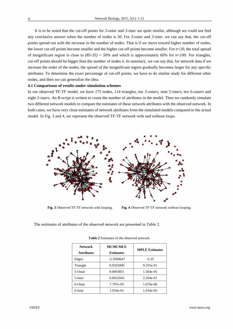
model. In Fig. 3 and 4, we represent the observed TF-TF network with and without loops.

Fig. 3 Observed TF-TF network with looping. Fig. 4 Observed TF-TF network without looping.

The estimates of attributes of the observed network are presented in Table 2.

Table 2 Estimates of the observed network.

Network

Attributes

MCMCMLE

Estimates MPLE Estimates

Edges -5.3500647 -5.35

Triangle 0.9355000 9.355e-01

5-Ostar 0.0003851 1.564e-05

5-Istar 0.0022043 2.204e-01

6-Ostar 7.797e-05 1.676e-06

6-Istar 1.034e-01 1.034e-03

6


IAEES www.iaees.org

To compare the estimates of network attributes between the observed and simulated network, we randomly

simulate two networks by imposing the same number of attributes as TF-TF, one with 5-ostars, 5-istars, and

triangles (network-1) and the other with same number of 6-ostars, 6-istars, and triangles (network-2). The

summary table of the number of network attributes is presented in Table 8.It is to be noted that we found very

similar estimates for the common network attributes edge and triangle from network-1 and network-2. In Tables

3 and 4, we presented the estimates of the observed and simulated networks for both MCMCMLE and MPLE

methods.

Table 3 Estimates from observed versus simulated networks with MCMC MLE.

Network

Attributes

Estimates from

observed networks

Estimates from

simulated networks

Edges -5.3500647 -5.73286

Triangle 0.9355000 2.90743

5-Ostar 0.0003851 -0.01720

5-Istar 0.0022043 -0.08434

6-Ostar 7.797e-05 -1.342e-01

6-Istar 1.034e-01 -8.702e-04

Table 4 Estimates from observed versus simulated networks with MPLE.

Network

Attributes

Estimates from

observed networks

Estimates from

simulated networks

Edges -5.35 -5.675632

Triangle 9.355e-01 2.905757

5-Ostar 1.564e-05 -0.016141

5-Istar 2.204e-01 -0.083797

6-Ostar 1.676e-06 -0.1343137

6-Istar 1.034e-03 -0.0006957

From Tables 3 and 4, we conclude that except triangles the rest of the estimates of network attributes are

very close for both MCMCMLE and MPLE method. Therefore, from the biological point of view, if the

observed network is available and the numbers of certain network attributes are known, then it behaves almost

same as the random model for most of the cases. However, to generalize the case we need more experiment and

more exploration among higher order of species. The simulated networks (1 & 2)are presented in Figs 5 and 6.

7


IAEES www.iaees.org

Fig. 5 Simulated network-1. Fig. 6 Simulated network-2.

From this experiment, we observe that if we want to simulate a biological data, then one way would be to

explore the observed data and count the number of statistics that we are interested and then physically impose the

number of statistic and then compare. There are several other ways to simulate network models using several

packages on R. The simplest one is to take the density of the observed model and simulate it using binomial

distribution. Also, once a model is fitted by using ERGM package, it can be simulated from the fitted model.

ERGM takes the estimates of the network attributes and simulates a similar type of model. However, in such a

case the physical number of attributes differs substantially. Again, we can also simulate networks by using

Erdos-Renyi model. The comparison of networks obtained using different simulation approaches is presented in

the following section.

4.2 Comparison over simulation methods

In this section, we simulate several networks by the existing simulation schemes. We simulated a network by

using Erdos-Renyi modelling scheme where we consider 175 nodes to create similarity with our observed

TF-TF network and then consider the density of the TF-TF model. The summary of the estimates that we obtain

under different approaches, are provided in Tables 5, 6, and 7 (for both MCMCMLE and MPLE).

Table 5 Estimates from Erdos-Renyi model

Network

Attributes

MCMCMLE

Estimates

MPLE

Estimates

Edges -4.438846 -4.42969

Triangle -0.058951 -0.06431

5-Ostar -0.007336 -0.00546

5-Istar -0.120974 -0.15166

6-Ostar -0.01302 -0.01366

6-Istar -0.75202 -0.84257

8


IAEES www.iaees.org

Table 6 Estimates from Binomial simulated model

Network

Attributes

MCMCMLE

Estimates

MPLE

Estimates

Edges -4.33561 -4.30465

Triangle -0.06395 -0.08794

5-Ostar -0.01032 -0.04404

5-Istar -0.07059 -0.07491

6-Ostar -0.10063 -0.25368

6-Istar -0.31184 -0.29370

Table 7 Estimates from fitted ERGM models

Network

Attributes

MCMCMLE

Estimates

MPLE

Estimates

Edges -5.3318479 -5.332e+00

Triangle 0.7194116 7.194e-01

5-Ostar 0.0001207 6.297e-06

5-Istar 0.0016440 1.644e-03

6-Ostar 1.484e-05 5.333e-07

6-Istar -5.887e-02 -5.887e-02

We notice that as long as we consider the same network, estimates of certain attributes are always similar.

Although some of the estimates we obtain in this simulation study are very close, the physical numbers of

statistics differ substantially. As the simulation scheme takes the fitted estimates into account, the physical

number of different attributes should be close to the observed model. It is important since the exact numbers of

network statistics might have a significant influence on the overall process. The simulated networks using

Erdos-Renyi modelling scheme, binomial density, and ergm package in R are presented in Figs 7, 8, and 9.

Fig. 7 Simulated from Erdos-Renyi model.

9


IAEES www.iaees.org

Fig. 8 Simulated network using binomial probability.

Fig. 9 Simulated network from fitted ERGM model.

The numbers of network attributes for different simulation models are presented in Table 8.

Table 8 Summary table of estimates observed versus simulated networks.

Network

Attributes

Observed

TF-TF

network

Our

Simulated

network

Simulation

using density

Erdos-Renyi

simulation

ERGM fitted

simulation

Edges 263 327 377 375 247

Triangle 114 115 12 9 82

5-Ostar 10 10 17 6 7

5-Istar 9 9 12 8 2

6-Ostar 10 10 6 2 1

6-Istar 8 8 3 1 3

10


IAEES www.iaees.org

From Table 8, we can see that the network attributes are different under all the simulation schemes. In our

process as we are physically imposing the attributes, it is very close to the observed model. The only difference

in the attributes is for the triangles which differ by just 1. From Table 8, we can say that, in terms of number, the

ERGM simulated network generates close result. However, the numbers of triangles substantially differ from the

original observed model. For the simple binomial simulation, the edges do not even come close and the other

attributes also significantly differ. We find similar characteristic for Erdos-Renyimodelling scheme. The reason

behind this could be that both the binomial and Erdos-Renyi consider the density only while simulation. Thus,

the number of attributes along with the edges is very close. However, other attributes such as the number of

5-istars or 5-ostars are not very close. In our random simulation, we emphasize on the number of attributes

because a biological process is a very complicated process. A single edge might have significant influence over

the entire process. Therefore, for biological simulation, we should always keep in mind the physical number of

attributes that we are interested in.

5 Conclusions

The number of commonly used network attributes such as k-istar, k-ostar and triangles in the TF-TF regulatory

network of E. coli is determined. These networks attributes statistically serve as the significant local structures

for the E. coli regulatory network. An observed regulatory network of the model organism E. coli was exploredin

terms of finding statisticallysignificant local structure in this study. Simulation of two network models,

network-1 and network-2, and comparison of the estimates of the observed and simulated models are presented.

In both cases, the estimates we obtain are very similar with the observed TF-TF network except for triangles.

Networks simulated using existing methods are compared in terms of these estimates as well. At the end, our

models provide close results and same number of network attributes, which is very important for biological

network data. Therefore, it can concluded that for theE. coil regulatory network, the network can be reproduced

by taking the counts for different attributes, and the simulated network will behave as the observed network.

Simulation of different networks with different number of nodes and network attributes were performed. The

cut-off points were determined for a number of attributes at which point specific attributes become significant to

insignificant, or vice versa. We observed that for smaller numbers of network attributes, the estimates usually

become significant. If the number of attributes increases in a given model, the attributes become insignificant.

We also observe that the models in ERGM do not always converge. Addressing the convergence issue would

be a desirable upgrade for the computational method. For the several models considered, convergence failure

occurred while estimating parameters for any of the methods. For example, for our observed network, the model

with edges, 4-istars, 4-ostars and triangles did not converge. Also, due to the convergence issue, cut-off points

could not be determined for several network attributes. In addition, computation for networks with self loops

demonstrates convergence problems. Therefore, while the ERGM provides flexible methodology, these issues

remain in need of further analysis.

References

Begum M, Bagga J, Blakey A, Saha S. 2014. Network motif identification and structure detection with graphical

models. Network Biology, 14(4): 155-169

Frank O, Strauss D. 1986. Markov graphs. Journal of the American Statistical Association, 81(395): 832-842

Fronczak A. 2012. Exponential Random Graph Models. ArXiv e-prints. Available at

http://arxiv.org/pdf/1210.7828.pdf

11


IAEES www.iaees.org

Handcock MS, Hunter DR, Butts CT, et al. 2003. Statnet: Software Tools for the Statistical Modeling of

Network data. Statnet Project. Available at http://statnetproject.org/

Handcock MS, Hunter DR, Butts CT, et al. 2008. ergm: A package to fit, simulate and diagnose

exponential-family models for networks. Journal of Statistical Software, 24. Available at

http://www.ncbi.nlm.nih.gov/pmc/articles/PMC2743438/

Hunter DR, Handcock MS. 2006. Inference in curved exponential family models for networks. Journal of

Computational and Graphical Statistics, 15(3): 565-583

Ideker T, Thorsson V, Ranish JA, et al. 2001. Integrated genomic and proteomic analysis of a systematically

perturbed metabolic network. Science, 292(5518): 929-934

Li JR, Zhang WJ. 2013. Identification of crucial metabolites/reactions in tumor signaling networks. Network

Biology, 3(4): 121-132

Mason O, Verwoerd M. 2007. Graph theory and networks in biology. IET Systems Biology, 1(2): 89-119

Morris M, Handcock MS, Hunter DR. 2008. Specification of exponential-family random graph models: Terms

and computational aspects. Journal of Statistical Software, 24(4): 1-24

Pavlopoulos GA, Secrier M, Moschopoulos CN, et al. 2011. Using graph theory to analyze biological networks.

BioData Mining, 4(10): 1-27

RobinsGL,Pattison PE,Kalish Y, LusherD. 2007. An introduction to exponential random graph (p*) models for

social networks. Social Networks, 29(2): 173-191

Salgado H, Gama-Castro S, Peralta-Gil M, et al. 2006. RegulonDB (version 5.0): Escherichia coli K-12

transcriptional regulatory network, operon organization, and growth conditions. Nucleic Acids Research,

34(1): 394-397

Saul ZM, Filkov V. 2007. Exploring biological network structure using exponential random graph models.

Bioinformatics, 23(19): 2604-2611

Snijders TAB. 2002. Markov Chain Monte Carlo Estimation of Exponential Random Graph Models.Journal of

Social Structure, 3: 1-40.

Stock JB, Stock AM, Mottonen JM. 1990. Signal Transduction in Bacteria. Europe PubMed Central, 344(6265):

395-400

Wasserman S, PattisonPE. 1996. Logit models and logistic regressions for social networks: I. An introduction to

Markov graphs and p*. Psychometrika, 61(3): 401-425

Zhang WJ. 2012. Computational Ecology: Graphs, Networks and Agent-based Modeling. World Scientific,

Singapore

12


IAEES www.iaees.org

Article

Determination of keystone species in CSM food web: A topological

analysis of network structure LiQin Jiang1, WenJun Zhang1,2 1School of Life Sciences, Sun Yat-sen University, Guangzhou 510275, China 2International Academy of Ecology and Environmental Sciences, Hong Kong


Received 20 August 2014; Accepted 28 September 2014; Published online 1 March 2015

Abstract

The importance of a species is correlated with its topological properties in a food web. Studies of keystone

species provide the valuable theory and evidence for conservation ecology, biodiversity, habitat management,

as well as the dynamics and stability of the ecosystem. Comparing with biological experiments, network

methods based on topological structure possess particular advantage in the identification of keystone species.

In present study, we quantified the relative importance of species in Carpinteria Salt Marsh food web by

analyzing five centrality indices. The results showed that there were large differences in rankings species in

terms of different centrality indices. Moreover, the correlation analysis of those centralities was studied in

order to enhance the identifying ability of keystone species. The results showed that the combination of degree

centrality and closeness centrality could better identify keystone species, and the keystone species in the CSM

food web were identified as, Stictodora hancocki, small cyathocotylid, Pygidiopsoides spindalis,

Phocitremoides ovale and Parorchis acanthus.

Key words keystone species; topological parameters; centrality indices; biological networks.

1 Introduction

Food webs are complex ecological networks describing trophic relationships between species in a certain area

(Pimm, 1982; Belgrano et al., 2005; Arii et al., 2007). If the entire food web is treated as a graph, the nodes in

the graph represent different species (individuals) in the ecosystem and the edges denote the interactions

between species (individuals). As a kind of network, food webs provide a new way to study communities

(Albert and Barabasi, 2002; Newman, 2003). To some extent, such a network is a formalized description for

complex relationships between species within the system.

The concept of keystone species originated from the thought that species diversity of an ecosystem was

controlled by the predators in the food chains, and they affected many other creatures in the ecosystem.



IAEES www.iaees.org

Keystone species refer to those that biomass is disproportionate with its impact on the environment, and the

extinction of keystone species may lead to the collapse of communities (Paine, 1969; Mills et al., 1993;

Springer et al., 2003). The concept of keystone species means that an ecological community is not just a

simple collection of species (Mouquet, 2013). As a result, the ecologically important species might not

necessarily be the rare species conservation biologists always believed (Simberloff, 1998), because rare

species are associated with the little biomass and abundance of species, and the importance of species is a kind

of functional properties of the network. Therefore, the traditional protection pattern for rare species should be

gradually transformed into the maintenance of keystone species (Wilson, 1987).

Keystone species strongly affect species richness and ecosystem dynamics (Piraino et al., 2002), so the

research of keystone species is an important area for predicting and maintaining the stability of ecosystem

(Naeem and Li, 1997; Tilman, 2000). Definition of keystone species emphasizes the functional advantages of

species in the ecosystem, and whether a species is a keystone species depends upon if it has a consistent effect

in ecological function (Power et al., 1996), namely its sensitivity to environmental changes, such as

competition, drought, floods and other ecological processes. In the past, researchers used many field

experimental methods to study keystone species, but they mainly focused on the impact of changes in the

abundance of a species on the other species (Paine, 1992; Wootton, 1994; Berlow, 1999). The main

identification methods include control simulation method (Paine, 1995; Bai, 2011), equivalent advantage

method (Khanina, 1998; Ji, 2002), competitive advantage method (Yeaton, 1988; Bond, 1989), the relative

importance of species interactions method (Tanner and Hughes, 1994), community importance index method

(Power et al., 1996), keystone index method (Jordán et al., 1999) and functional importance index method

(Hurlbert, 1997). However, these methods mainly concentrated on a few species. Thus researchers need to do

an assessment of the interactions between species in the community before the experiment, in order to

determine species not important or interesting. So these methods are obvious subjective and produce certain

mistake on identifying keystone species (Wootton 1994; Bustamante et al., 1995). Furthermore, monitoring

species reaction to changes in the external environment through the above experimental methods requires that

experimenters have a high professional quality. And because of the longer experimental time span, greater cost

(Ernest and Brown, 2001), as well as other factors during the experiment, they are only suitable for

semi-artificial or simple controllable ecosystems. It is more difficult to judge whether a species is a keystone

species based on certain characteristics of species (Menge et al., 1994). So far, we don’t have a perfect and

universally applicable method to identify keystone species.

Research of keystone species has evolved from the initial direct experimental methods to network/software

analysis. For example, Libralato et al. (2006) analyzed keystone indicators of functional groups of a species or

a group of species in food web model through the ecosystem modeling (the Ecopath with Ecosim, EwE), and

then ranked the level of the key indicators to obtain the keystone species. Jordán et al. (2008) pointed out that

there were at least two methods to quantitatively assess the importance of species in communities. One was the

structural importance of network analysis and another for the functional importance of network analysis. So

they calculated the structural importance and the functional importance of species in the food web in Prince

William Sound by CosBiLaB Graph software, and evaluated the advantages and disadvantages of the two

methods. They believed that the combination of these two methods in the future would be the most important

way to research dynamic mechanism. Kuang and Zhang (2011) analyzed the topological properties of the food

web in Carpinteria Salt Marsh and found that parasites played a very important role in the food web, and the

addition of parasites in the food web would change some properties and greatly increase the complexity of the

food web. Therefore, the relationship between keystone species and topological characteristics can provide an

effective method to understand and describe the topological structures, dynamic characteristics and the

14


IAEES www.iaees.org

complexity of functions between species within the food web. And it also can provide valuable theory and

evidence for conservation ecology, biodiversity, habitat management, as well as the dynamics and stability of

the ecosystem.

Nevertheless, so far we lack of effective methods to identify keystone species and quantify their relative

importance, so the quantitative assessment of species importance in the food web is becoming increasingly

important and urgent (Paine, 1966; Power et al, 1996; Jordán, 2008). In recent years, there have been some

major discoveries about the topological properties of complex systems (Strogatz, 2001; Albert and Barabási,

2002; Newman, 2003), and these also affect the definition and identification of keystone species. For example,

the highly connected species were found to have more important influence on sustainability of food webs

(Soulé and Simberloff, 1986), which promoted the generation of the concept of degree. Degree of nodes thus

become the most widely used topological parameter to measure the keystone species (Dunne et al., 2002a).

Degree refers to the direct impacts between species (Callaway et al., 2000; West, 2001; Zhang, 2011, 2012a,

2012b, 2012c, 2012d). However, indirect impacts between species are also important (Wooton, 1994; Huang,

et al., 2008). For example, Darwin (1859) described the influence of cats on the clovers. Although indirect

effects of chemical and behavioral studies may be difficult to quantify, some indirect impacts of network links

have been proposed (Ulanowicz and Puccia, 1990; Patten, 1991). Thus the concept of centrality is proposed to

address this problem. Centrality focuses on the indirect effects between species. The impacts of food webs are

generally spread through indirect ways, so it may require detailed research and quantitative description on the

effective range of indirect interactions from a specific point to the entire network (Jordán, 2001). In other

words, it is necessary to determine how relevant these species are in the food web (Yodzis, 2000; Williams et

al., 2002). The concept of centrality stemmed from the social network analysis (Wasserman and Faust, 1994),

namely the ability of a node communicates with other nodes or the intimacy of a node with the others (Go'mez

et al., 2003). These have resulted in a series of topological parameters relating to the relative importance of a

node, such as degree centrality, betweenness centrality, closeness centrality, clustering coefficient centrality,

eigenvector centrality and information centrality, etc. In present paper, we used various methods to detect and

quantify relative importance of species in a famous food web, CSM (Carpinteria Salt Marsh) food web,

reported by Lafferty et al. (2006a, 2006b, 2008), and further studied the correlation between topological

parameters of the food web, aiming to evaluate the effectiveness of various methods in quantifying relative

importance of species and detecting the keystone species in the food webs.

2 Materials and Methods

2.1 Data source

Data were collected from the food web, Carpinteria Salt Marsh, California, reported by Lafferty et al. (2006a,

2006b, 2008) (http: //www.nceas.ucsb.edu/interactionweb/html/carpinteria.html). CSM food web includes four

sub-webs, predator-prey sub-web, predator-parasite sub-web, parasite-host sub-web, and parasite-parasite

sub-web.

2.2 Methods

2.2.1 Pajek software

Pajek is a software platform for network analysis, which contains various methods/algorithms/models on

analysis of topological properties.

2.2.2 Centrality measures

Centrality indices are used to measure impact and importance of nodes in a network. The most commonly used

centrality indices are degree centrality, betweenness centrality, closeness centrality, clustering coefficient

15


IAEES www.iaees.org

centrality and eigenvector centrality (Navia et al., 2010; Zhang, 2012a, b).

(1) Degree centrality (DC)

DC is the simplest measure which considers the degree of a node (species) only. The degree of species i is:

Di=Din,i + Dout,i, where Din,i: number of prey species of species i, and Dout,i: number of predator species of

species i. The degree of species was calculated by Net/Partitions/DC/All in Pajek.

(2) Betweenness centrality (BC)

BC is calculated by the following formula

BCi =2∑j≤k gjk(i)/gjk /[(N-1)(N-2)]

where i≠j≠k, gjk: the shortest path between species j and k, gjk(i): number of the shortest paths containing

species i, N: total number of species in the food web. A greater BCi means that the effect of losing species i will

promptly disperse across the food web (Zhang, 2012a, b).

(3) Closeness centrality (CC)

CCi refers to the mean shortest path of species i

CCi=(N-1)/∑j=1N dij

where i≠j, dij is the length of the shortest path between species i and j. A greater CCi means a more importance

of species i.

In Pajek, we use Net/Vector/Centrality/Closeness/All and Net/Vector/Centrality/Betweenness to calculate

BC (Wasserman and Faust, 1994).

(4) Clustering coefficient centrality (CU)

Clustering coefficient centrality denotes the ratio of the actual edges Ei of node i connected with its neighbors

divided by the most possible edges Di(Di-1)/2 between them (Watts and Strogatz, 1998). In other words, it

refers to the ratio of the directly connected neighboring pairs divided by all the neighboring pairs in the

neighboring points of the node, that is

CUi=2Ei/ [Di(Di-1)]

It measures how close the current node is to its neighboring nodes. The averag clustering coefficient of all

nodes is the clustering coefficient of the entire network. Obviously, the clustering coefficient of a network is

weighted by the clustering coefficient of all nodes whose degree must be at least 2. 0≤CU≤1; if CU=0, all

nodes in the network are isolated, and if CU=1, the network is fully connected. Furthermore, studies have

shown that clustering coefficient is related to network modularity. Clustering coefficient of the entire network

reflects the overall trend of all the nodes gathering into a module (Eisenberg and Levanon, 2003; Ravasz et al,

2002).

(5) Eigenvector centrality (EC)

Eigenvector centrality is the dominant eigenvector of the adjacency matrix A of the network (Bonacich, 1987),

i.e., the extent of a node connected to the node with the highest eigenvector centrality. In the word of social

networks, a person tends to occupy the central place more likely if he (she) has contacted more people in the

center position. Eigenvector centrality reflects the prestige and status of nodes. This measure tries to find the

keystone node in the entire network rather than in the local structure. Here, eigenvector is e, and λe=Ae, where

A is the adjacency matrix of a food web. Therefore, the EC of node i is

ECi= e1 (i)

where e1 is the eigenvector corresponding to the maximum eigenvalue λ1. A greater value of ECi means a

greater number of the neighboring nodes connected with node i, and it indicates that the node is in the core

16


IAEES www.iaees.org

position.

3 Results

3.1 Degree centrality

As shown in Fig. 1, 2 and Table 1, the species with the greater DC values in the full CSM food web are largely

consistent with that in the predator-parasite sub-web, parasite-parasite sub-web and parasite-host sub-web. And

these species are substantially parasites. The species with the maximum DC value in the predator-prey

sub-web is Pachygrapsus crassipes, and the species with the forth DC value is Willet. Although DC values of

the two species are larger, they are slightly lower than nine parasite species, such as Mesostephanus

appendiculatoides, etc. In addition, the basal species, Marine detritus, is of greater importance also.

Fig. 1 Results of degree centrality for the four sub-webs of CSM food web (upper left: predator-prey sub-web; upper right:

predator-parasite sub-web; bottom right: parasite-parasite sub-web; bottom left: parasite-host sub-web). The numbers in

parentheses are total links (degree, or incoming degree + outgoing degree) and the numbers outside parentheses are species ID

codes. The ID codes of different sub-webs are different from the original species.

17


IAEES www.iaees.org

Fig. 2 Results of degree centrality for the full CSM food web. The numbers in parentheses are total links (degree, or incoming

degree + outgoing degree) and the numbers outside parentheses are species ID codes.

Table 1 Species with greater DC values in the full CSM food web and four sub-webs.

Predator-prey

sub-web

Predator-parasite

sub-web

Parasite-parasite

sub-web

Parasite-host sub-web Full CSM food web

ID Species ID Species ID Species ID Species ID Species

56 Pachygrapsus

crassipes

90 Culex

tarsalis

118 Mesostephanus

appendiculatoid

es

117 Stictodora

hancocki

118 Mesostephanus

appendiculatoid

es

46 Hemigrapsus

oregonensis

89 Aedes

taeniorhynchus

115 Renicola

cerithidicola

114 Phocitremoides

ovale

117 Stictodora

hancocki

47 Fundulus

parvipinnis

98 Plasmodium

107 Renicola

buchanani

119 Pygidiopsoides

spindalis

116 Small

cyathocotylid

57 Willet 117 Stictodora

hancocki

120 Microphallid 1

116 Small

cyathocotylid

119 Pygidiopsoides

spindalis

43 Cleavlandia

ios

119 Pygidiopsoides

spindalis

116 Small

cyathocotylid

118 Mesostephanus

appendiculatoid

es

114 Phocitremoides

ovale

73 Gillycthys

mirabilis

116 Small

cyathocotylid

110 Large

xiphideocercaria

111 Parorchis

acanthus

111 Parorchis

acanthus

33 Macoma

nasuta

114 Phocitremoides

ovale

109 Catatropis

johnstoni

113 Cloacitrema

michiganensis

113 Cloacitrema

michiganensis

18 Anisogammar 111 Parorchis 105 Probolocoryphe 104 Himasthla 105 Probolocoryphe

18


IAEES www.iaees.org

us

confervicolus

acanthus uca rhigedana uca

1 Marine

detritus

118 Mesostephanus

appendiculatoid

es

119 Pygidiopsoides

spindalis

105 Probolocoryphe

uca

108 Acanthoparyphi

um sp.

38 Geonemertes 113 Cloacitrema

michiganensis

117 Stictodora

hancocki

108 Acanthoparyphi

um sp.

56 Pachygrapsus

crassipes

31 Mosquito larva 57 Willet

3.2 Betweenness centrality

As illustrated in Fig. 3 and 4, the BC values of all nodes in the predator-parasite sub-web and parasite-host

sub-web are 0, because these species do not locate between other species in the network. But the radius of

Mesostephanus appendiculatoides in the parasite-parasite sub-web is very obvious, indicating that some

species in the parasite-parasite sub-web need to go through Mesostephanus appendiculatoides. Once this

species is removed, all the interaction chains will collapse and largely destruct the whole sub-web. From Table

2, the BC values of the top four species in the CSM food web are identical with that in the predator-prey

sub-web, while some parasites with larger DC values, such as Mesostephanus appendiculatoides, etc., whose

BC values are lower than that of some free-living species, such as Hemigrapsus oregonensis. It indicates that

the nutritional flow of free-living species in the food web has a greater effect than parasites.

Fig. 3 Results of betweenness centrality for the full CSM food web. The numbers in parentheses are betweenness centralities and

the numbers outside parentheses are species ID codes.

19


IAEES www.iaees.org

Fig. 4 Results of betweenness centrality for the four sub-webs of CSM food web (upper left: predator-prey sub-web; upper right:


parentheses are betweenness centralities and the numbers outside parentheses are species ID codes. The ID codes of different

sub-webs are different from the original species. The size of the node relates to the value of BC; the greater BC is, the bigger the

node radius is. The species ID codes of different sub-webs are different from the original species, and the magnification of each

figure is different.

20


IAEES www.iaees.org

Table 2 Species with greater BC values in the full CSM food web and four sub-webs.

Predator-prey

sub-web

Predator-parasit

e sub-web

Parasite-parasite sub-web Parasite-host

sub-web

Full CSM food web


46 Hemigrapsus

oregonensis

118 Mesostephanusap

pendiculatoides

46 Hemigrapsusore

gonensis

56 Pachygrapsus

crassipes

106 Himasthla species

B

56 Pachygrapsuscr

assipes

47 Fundulusparv

ipinnis

109 Catatropisjohnsto

ni

47 Fundulusparvipi

nnis

73 Gillycthys

mirabilis

111 Parorchis

acanthus

73 Gillycthys

mirabilis

72 Leptocottusar

matus

115 Renicola

cerithidicola

83 Triakis

semifasciata

38 Geonemertes 105 Probolocoryphe

uca

72 Leptocottus

armatus

43 Cleavlandiaio

s

110 Large

xiphideocercaria

57 Willet

48 Western

Sandpiper

116 Small

cyathocotylid

108 Acanthoparyphi

um sp.

50 Least

Sandpiper

120 Microphallid 1 52 Dowitcher

18 Anisogammar

usconfervicol

us

113 Cloacitrema

michiganensis

11 Phoronid

115 Renicola

cerithidicola

106 Himasthla

species B

118 Mesostephanus

appendiculatoid

es

116 Small

cyathocotylid

117 Stictodora

hancocki

111 Parorchis

acanthus

119 Pygidiopsoides

spindalis

120 Microphallid 1

3.3 Closeness centrality

CC values of species in food webs increases with the increase of species richness and completeness of food

web. Connection between species in the full CSM food web is closer than the other four sub-webs (Fig. 5 and

6, Table 3). Combined with Table 2, the species with the maximum CC value is Pachygrapsus crassipes

(species 56) in the full CSM food web, and it is also the greatest in the predator-prey sub-web, indicating it is

closer than other species in food web. The species with the tenth CC value is Fundulus parvipinnis (species 47)

21


IAEES www.iaees.org

in the full CSM food web, but it is the third in the predator-prey sub-web, just following behind Pachygrapsus

crassipes and Hemigrapsus oregonensis.

Fig. 5 Results of closeness centrality for the four sub-webs of CSM food web (upper left: predator-prey sub-web; upper right:


parentheses are closeness centralities and the numbers outside parentheses are species ID codes. Species ID codes of different

sub-webs are different from the original species.

22

IAEES

Fig. 6 Res

numbers o

Predator-p

sub-web

ID Sp

56 Pa

scr

46 He

ore

47 Fu

vip

73 Gi

mir

18 An

rus

olu

38 Ge

33 Ma

ta

72 Lep

rm

1 Ma

det

sults of closenes

outside parenthe

Tab

prey P

s

ecies ID

achygrapsu

rassipes

5

emigrapsus

egonensis

5

unduluspar

pinnis

5

llycthys

rabilis

5

nisogamma

sconfervic

us

6

eonemertes 1

acomanasu 6

ptocottusa

matus

6

arine

tritus

6

ss centrality for

eses are species

ble 3 Species w

Predator-parasit

ub-web

D Species

52 Dowitch

57 Willet

58 Black-b

d Plover

59 Californ

Gull

69 Clapper

117 Stictodo

hancock

62 Marbled

Godwit

63 Ring-bil

gull

64 Western

Gull

Network

r the full CSM f

s ID codes.

with greater CC

te Parasite

ID

her 116

107

ellie

r

109

nia 115

rail 120

ora

ki

105

d 118

lled 106

n 108

k Biology, 2015

food web. The n

values in the fu

e-parasite sub-w

Species

Small

cyathocotyli

Renicola

buchanani

Catatropis

johnstoni

Renicola

cerithidicola

Microphallid

Probolocory

uca

Mesostephan

appendicula

es

Himasthla

species B

Acanthopary

um sp.

5, 5(1): 13-33

numbers in pare

ull CSM food w

web Parasite

ID

id

119

116

114

a

117

d 1 118

yphe 111

nus

atoid

83

72

yphi 57

entheses are clo

web and four su

e-host sub-web

Species

Pygidiopsoides

spindalis

Small

cyathocotylid

Phocitremoide

ovale

Stictodora

hancocki

Mesostephanus

appendiculatoi

es

Parorchis

acanthus

Triakis

semifasciata

Leptocottus

armatus

Willet

w

oseness centrali

ub-webs.

Full CSM

ID Sp

s 56 Pa

cr

117 St

ha

es 116 Sm

cy

119 Py

sp

s

id

114 Ph

ov

111 Pa

ac

113 Cl

m

118 M

ap

es

108 Ac

um

www.iaees.org

ities and the

M food web

pecies

achygrapsus

rassipes

tictodora

ancocki

mall

yathocotylid

ygidiopsoides

pindalis

hocitremoides

vale

arorchis

canthus

loacitrema

ichiganensis

Mesostephanus

ppendiculatoid

s

canthoparyphi

m sp.

23


IAEES www.iaees.org

57 Willet 65 Bonaparte's

Gull

117 Stictodora

hancocki

113 Cloacitremamic

higanensis

47 Fundulus

parvipinnis

9 Oligochaete 111 Parorchis

acanthus

113 Cloacitrema

michiganensis

73 Gillycthys

mirabilis

11 Phoronid 114 Phocitremoi

des ovale

114 Phocitremoides

ovale

116 Small

cyathocotyli

d

119 Pygidiopsoides

spindalis

119 Pygidiopsoi

des

spindalis

111 Parorchis

acanthus

111 Parorchis

acanthus

3.4 Clustering coefficient centrality

CU values of predator-parasite sub-web and parasite-host sub-web appear in two patterns: one for the degree

values of some nodes are less than 2, and the CU values of these nodes are 999999998 in the Pajek; another for

the neighboring nodes of one node are less than 2, and the CU values of these nodes are 0. From Table 4, we

can find that the CU rankings of nodes in the full CSM food web and predator-prey sub-web are really

different.

Table 4 Species with greater CU values in the full CSM food web and four sub-webs.

Predator-prey

sub-web

Predator-parasite

sub-web

Parasite-parasite sub-web Parasite-host

sub-web

Full CSM food web


60 Whimbrel 104 Himasthla

rhigedana

25 Cerithidea

californica

81 Pied Billed

Grebe

106 Himasthla species

B

109 Catatropis

johnstoni

38 Geonemertes 108 Acanthoparyphium

sp.

70 Cooper's Hawk

78 Black-crown

ed Night

heron

111 Parorchis

acanthus

34 Protothaca

61 Mew Gull 113 Cloacitrema

michiganensis

110 Large

xiphideocercaria

63 Ring-billed

gull

103 Euhaplorchis

californiensis

35 Tagelus spp.

64 Western Gull 114 Phocitremoides

ovale

106 Himasthla

species B

65 Bonaparte's

Gull

117 Stictodora

hancocki

71 Northern Harrier

36 Cryptomya 119 Pygidiopsoides

spindalis

115 Renicola

cerithidicola

77 Snowy Egret 105 Probolocoryphe

uca

103 Euhaplorchis

californiensis

68 Bufflehead

107 Renicola

buchanani

107 Renicola

buchanani

24


IAEES www.iaees.org

3.5 Eigenvector centrality

Species with greater EC values in the full CSM food web are largely consistent with that in the predator-prey

sub-web (Table 5; Fig. 7, 8). Species with greater EC values in the full CSM food web and predator-prey

sub-web are free-living species, rather than parasites. Willet (species ID 57) has the largest EC value.

Otherwise, species with larger EC values in predator-parasite sub-web and parasite-parasite sub-web are

parasites.

Fig.7 Results of eigenvector centrality for the full CSM food web. The numbers in parentheses are eigenvector centralities and

the numbers outside parentheses are species ID codes.

25


IAEES www.iaees.org

Fig. 8 Results of eigenvector centrality for the four sub-webs of CSM food web (upper left: predator-prey sub-web; upper right:


parentheses are eigenvector centralities and the numbers outside parentheses are species ID codes. Species ID codes of different

sub-webs are different from the original species.

Table 5 Species with greater eigenvector values in the full CSM food web and four sub-webs.

Predator-prey

sub-web

Predator-parasite sub-web Parasite-parasite

sub-web

Parasite-host

sub-web

Full CSM food web


57 Willet 98 Plasmodium 111 Parorchis

acanthus

83 Triakis

semifasciata

57 Willet

58 Black-bellied

Plover

90 Culex tarsalis 106 Himasthla

species B

72 Leptocottus

armatus

52 Dowitcher

56 Pachygrapsu

s

crassipes

89 Aedestaeniorhync

hus

104 Himasthla

Rhigedana

73 Gillycthys

mirabilis

58 Black-bellied

Plover

52 Dowitcher 116 Small

cyathocotylid

113 Cloacitrema

michiganensis

57 Willet 72 Leptocottus

armatus

62 Marbled

Godwit

117 Stictodora

hancocki

108 Acanthoparyphi

um sp.

52 Dowitcher 73 Gillycthys

mirabilis

48 Western

Sandpiper

119 Pygidiopsoides

spindalis

119 Pygidiopsoides

Spindalis

58 Black-bellied

Plover

56 Pachygrapsus

crassipes

46 Hemigrapsus

oregonensis

114 Phocitremoides

ovale

117 Stictodora

Hancocki

77 Snowy Egret 83 Triakis

semifasciata

50 Least

Sandpiper

118 Mesostephanus

Appendiculatoides

114 Phocitremoides

Ovale

78 Black-crowne

d Night heron

67 Surf Scoter

59 California

Gull

111 Parorchis

acanthus

103 Euhaplorchis

californiensis

81 Pied Billed

Grebe

50 Least Sandpiper

47 Fundulus

parvipinnis

113 Cloacitrema

michiganensis

118 Mesostephanus

Appendiculatoid

es

69 Clapper rail 69 Clapper rail

26


IAEES www.iaees.org

3.6 Analysis of DC, BC, CC, CU and EC

According to Table 6, the change of species ranking with CU is larger: the top ten species are totally different

with species ranking by remaining four indices. The DC and CC analysis in the full CSM food web (species ID

No. 1 to No. 128) showed that the parasites are more important than free-living species, while reverse results

were obtained from BC and EC analysis. The more important parasites calculated from DC and CC analysis

are Stictodora hancocki, small cyathocotylid, Pygidiopsoides spindalis, Phocitremoides ovale and Parorchis

acanthus (species No. 117, 116, 119, 114, and 111, respectively). Species ranking by BC, DC and CC in the

full CSM food web (species ID No. 1 to No. 83) are basically consistent with the species in the predator-prey

sub-web, and the relative important species are Pachygrapsus crassipes, Hemigrapsus oregonensis and

Fundulus parvipinnis(species ID No.56, 46, and 47, respectively). These results show that parasites in the full

CSM food web do not change the relative importance of free-living species, but increase the DC value of

free-living species.

Table 6 The top ten species (ID codes) ranking by DC, BC, CC, CU and EC in the full CSM food web and predator-prey sub-web, respectively.

DC BC CC CU EC

Full CSM food

web (Species

ID No.1 to No.

128)

118 46 56 25 57

117 56 117 109 52

116 73 116 70 58

119 83 119 34 72

114 47 114 110 73

111 72 111 35 56

113 57 113 106 83

105 108 118 71 67

108 52 108 115 50

56 113 47 103 69

Full CSM food

web (Species

ID No.1 to No.

83)

56 46 56 25 57

57 56 47 70 52

52 73 46 34 58

47 83 57 35 72

73 47 73 71 73

58 72 72 43 56

68 57 52 19 83

50 52 58 16 67

72 75 43 12 50

46 74 83 23 69

Predator-prey

sub-web

(Species No.1

to No. 83)

56 56 56 60 57

46 46 46 81 58

47 47 47 38 56

43 73 73 78 52

57 72 18 61 62

73 38 38 63 48

33 43 33 64 46

18 48 72 65 50

1 50 1 36 59

38 18 57 77 47

27


IAEES www.iaees.org

3.7 Pearson correlation of five topological indices

As can seen from Table 7, the Pearson’s correlations of DC and CC are the largest in the full CSM food web

and predator-prey sub-web (0.917 and 0.877, respectively), so DC and CC are strong correlated. DC mainly

measures the importance of a node in the local scope, and thus denotes the self-correlation of the node. CC is a

measure of the ability of one node for controlling the other nodes, and denotes the centralization extent of a

node. Therefore, DC and CC analysis synthesizes the importance of a node locally and globally. Table 6

demonstrates that the keystone species in the CSM food web are Stictodora hancocki, small cyathocotylid,

Pygidiopsoides spindalis, Phocitremoides ovale and Parorchis acanthus (species ID No. 117, 116, 119, 114,

and 111, respectively).

Table 7 Pearson’s correlation coefficients of five topological indices.

Pearson’s correlation coefficient analysis DC BC CC CU EC

DC Full CSM food web 1.000 0.773 0.917 0.483 0.800

predator-prey sub-web 1.000 0.789 0.877 0.053 0.498

BC Full CSM food web 0.773 1.000 0.754 0.338 0.625

predator-prey sub-web 0.789 1.000 0.595 -0.032 0.402

CC Full CSM food web 0.917 0.754 1.000 0.525 0.695


CU Full CSM food web 0.483 0.338 0.525 1.000 0.307

predator-prey sub-web 0.053 -0.032 0.360 1.000 0.205

EC Full CSM food web 0.800 0.625 0.695 0.307 1.000


3.8 Efficiency analysis of the full CSM food web

Table 8 indicates the changes of topological properties after removing different keystone species from the full

CSM food web. The major topological changes before and after removing keystone species include

(1) Number of top species and basal species does not change. The top species are not necessarily the

keystone species of the food web.

(2) Number of links and cycles reduces significantly. It means that the keystone species play an

important role in the food web. There are less cycles between predators and preys due to the removal

of parasites.

(3) Number of total links and maximum links, and link density and connectance decreases respectively.

(4) The maximum chain length did not change significantly.

Compared with the results of removing important species, the changes of the full food web are not

significant in terms of all indices.

In conclusion, the topological structure of the full food web changed significantly after removing the

keystone species, which further validates the results achieved previously.

28


IAEES www.iaees.org

Table 8 Comparison of topological properties of the full CSM food web with removed different keystone species.

Removed

species

No.117

Removed

species

No.116

Removed

species

No.119

Removed

species

No.114

Removed

species

No.111

Removed

species

No.56

Full CSM

food web

Number of

species, S

127 127 127 127 127 127 128

Number of

links, L

2197 2197 2198 2199 2205 2212 2290

Number of

top species, T

3 3 3 3 3 3 3

Number of

intermediate

species, I

116 116 116 116 116 116 117

Number of

basal species,

B

8 8 8 8 8 8 8

Number of

Chain cycles

71142 70472 71111 71526 74331 80450 85214

Link density,

L/S

17.299 17.299 17.307 17.315 17.362 17.417 17.891

Connectance,

L/S2

0.13621 0.13621 0.13628 0.13634 0.13671 0.13714 0.13977

Mean

connectance,

D

34.598 34.598 34.614 34.630 34.724 34.835 35.781

Maximum

chain length

No.1-5: 3

No.6: 5

No.7-8: 4

No.1-5, 7:

3

No.6: 5

No.8: 4

No.1-5,

7: 3

No.6: 5

No.8: 4

No.1-5,

7: 3

No.6: 5

No.8: 4

No.1-5,

7: 3

No.6: 5

No.8: 4

No.1,3-5,7:

3

No.2,6,8: 4

No.1-5,7:

3

No.6: 5

No.8: 4

4 Discussion

Since the concept of keystone species was first proposed by Paine (1969), the importance of them for

conservation biology has been widely studied. However, due to the limitations of field experimental methods

and the temporal and spatial variation (Menge et al., 1994; Paine, 1995; Estes et al., 1998), more and more

researchers questioned the original concept of keystone species, and have developed various definitions of

keystone species (Mills et al., 1993; Bond, 2001; Davic, 2003). So far, quantitative methods to identify

keystone species remain to be little (Menge et al., 1994; Bond, 2001).

The traditional definitions of keystone species closely related to the richness and biomass of species,

however, the definitions can be considered by combining the topological importance (Jordán et al., 1999,

Jordán et al., 2003). Although the definitions of keystone species from network perspective and traditional

definition are not fully consistent, they provide a quantitative and complementary view for the importance of

species, and stress that the network theory and species conservation practices are highly correlated (Memmott,

1999; Dunne et al., 2002a). The identification of keystone species in food webs using network analysis

depends on the topological characteristics of the network. In present study, we calculated the five centrality

indices of nodes in the full CSM food web and its four sub-webs, and found that species rankings using

different centrality indices were different. Species importance ranking by the degree centrality and

betweenness centrality is based on their direct connection in the network. Degree considers the direct impact of

29


IAEES www.iaees.org

a species with its neighboring species directly connected. Betweenness centrality represents the influence of a

species in the "communication" process. On the other hand, closeness centrality, clustering coefficient

centrality and eigenvector centrality take the influence of a species in the global network into consideration

(Borgatti, 2005). In all of these indices, the importance of a species in the global or local network is equally

important, so the different rankings using different centrality indices should be taken as the comprehensive

measure of different topological properties, which are likely relevant to the direct target analysis of theoretical

ecology and conservation ecology (Estrada, 2007).

Studies have indicated that there is a significant correlation between different topological parameters of a

complex network (Wutchy and Stadler, 2003). Our results showed that DC and CC correlated significantly.

Thus the combined use of DC and CC can better reflect the importance ranking of species in the global and

local network.

Power et al. (1996) proposed that a quantitative and predictive generalization is a primary task for

identifying keystone species. Research on complex networks will give us new thoughts and methods to further

understand ecosystems (Abrams et al., 1996; Yodzis, 2001; Piraino et al., 2002). In this article, we identify

keystone species by only using Pajek software, so the analytical method may be more unitary and lack of

comparative study statistically. More methods, as Ecosim networks (Dunne et al., 2002b; Jordán et al., 2008),

CosBiLaB Graph software (Jordán et al., 2008), etc., are suggested using in the future. In addition, we have

used the conventional definition, i.e., taxonomical species, and simplify the life stages of species. In the further

studies, we may distinguish species in different life stages and then integrate their relationship.

Acknowledgment

We thank Mr. WenJin Chen for his pre-treatment on part data in this article.

References

Abrams PA, Menge BA, Mittelbach GG, et al. 1996. The Role of Indirect Effects in Food Webs. In: Integration

of Patterns and Dynamics. 371-395, Chapman and Hall, USA

Albert R, Barabási AL. 2002. Statistical mechanics of complex networks. Reviews of Modern Physics. 74:

47-97

Arii K, Derome R, Parrott L. 2007. Examining the potential effects of species aggregation on the network

structure of food webs. Bulletin of Mathematical Biology, 69: 119-133

Bai KS, Gao RH, et al. 2011. Study on relationship between the keystone species of Larixgmelinii forest and

rhododendron plant. Journal of Inner Mongolia Agricultural University, 32(2): 31-37

Beigrano A, Seharler UM, Dunne J, Ulanowicz RE. 2005. Aquatic Food Webs: An Ecosystem Approach.

Oxford University Press, New York, USA

Berlow EL. 1999. Strong effects of weak interactions in ecological communities. Nature, 398: 330-334

Bonaeich P. 1987. Power and centrality: a family of measures. American Journal of Sociology, 92: 1170-1182

Bond WJ. 1989. The tortoise and the hare: ecology of angiosperm dominance and gymnosperm persistence.

Biological Journal of the Linnean Society, 36(3): 227-249

Bond WJ. 2001. Keystone species - hunting the shark? Science, 292: 63-64

Borgatti SP. 2005. Centrality and network flow. Social Networks, 27: 55-71

Bustamante RH, Branch GM, Eekhout S. 1995. Maintenance of an exceptional intertidal grazer biomass in

South Africa-subsidy by subtidal kelps. Ecology, 76: 2314-2329

30


IAEES www.iaees.org

Callaway DS, Newman ME, et al. 2000. Network robustness and fragility: Percolation on random graphs.

Physical Review Letters, 85(25): 5468-5471

Davic RD. 2003.Linking keystone species and functional groups: a new operational definition of the keystone

species concept. Conservation Ecology, 7(1)

Dunne JA, Williams RJ, Martinez ND. 2002a. Network structure and biodiversity loss in food webs:

robustness increases with connectance. Ecology Letters, 5:558-567

Dunne JA, Williams RJ, Martinez ND, 2002b. Food-web structure and network theory: The role of

connectance and size. Proceeding of the National Academy of Sciences of the United States of America,

99: 12917-12922

Eisenberg E, Levanon EY. 2003. Preferential attachment in the Protein network evolution. Physical Review

Letters, 91: 1-4

Ernest SKM, Brown JH. 2001. Delayed compensation for missing keystone species by colonization. Science,

292: 101-104

Estes JA, Tinker MT, Williams TM, Doak DF. 1998. Killer whale predation on sea otters linking oceanic and

nearshore ecosystems. Science, 282: 473-476

Estrada E. 2007. Characterization of topological keystone species Local, global and ‘‘meso-scale’’ centralities

in food webs. Ecological Complexity, 4: 48-57

Go´mez D, González-Arangüena E, et al. 2003. Centrality and power in social networks: a game theoretic

approach. Mathematical Social Sciences, 46: 27-54

Huang HB, Yang LM, et al. 2008. Identification technique of essential nodes in protein networks based on

combined parameters. Acta Automatica Sinica, 34(11):1388-1395

Hurlbert SH. 1997. Functional importance vs keystoneness: reformulating some questions in theoretical

biocenology. Australian Journal of Ecology, 22(4): 369-382

Ji LZ, Liu ZG, et al. 2002. Effect on cones picking in broad-leaved pinuskoraiensis forest in Changbai

Mountain. Chinese Journal of Ecology, 21(3): 39-42

Jordán F. 2001. Trophic fields. Community Ecology, 2: 181-185

Jordán F, Liu WC, van Veen JF. 2003. Quantifying the importance of species and their interactions in a

host-parasitoid community. Community Ecology, 4: 79-88

Jordán F, Okey TA, Bauer B, Libralato S. 2008. Identifying important species: a comparison of structural and

functional indices. Ecological Modelling, 216: 75-80

Jordán F, Takács-Sánta A, Molnár I. 1999.A reliability for theoretical quest for keystones. Oikos, 86: 453-462

Khanina L. 1998. Determining keystone species. Conservation Ecology, 2(2): R2

Kuang WP, Zhang WJ. 2011. Some effects of parasitism on food web structure: a topological analysis.

Network Biology, 1(3-4): 171-185

Lafferty KD, Allesina S, Arim M, et al. 2008. Parasites in food webs: the ultimate missing links. Ecology

Letters, 11(6): 533-546

Lafferty KD, Dobson AP, Kuris AM. 2006a. Parasites dominate food web links. Proceedings of the National

Academy of Sciences of the United States of America, 103(30): 11211-11216

Lafferty KD, Hechinger RF, Shaw JC, et al. 2006b. Food webs and parasites in a salt marsh ecosystem. In:

Disease Ecology: Community Structure and Pathogen Dynamics (Collinge S, Ray C, eds). 119-134,

Oxford University Press, UK

Libralato S, Christensen V, Pauly D. 2006. A method for identifying keystone species in food web models.

Ecological Modelling, 1(195): 153-157

Memmott J. 1999. The structure of a plant-pollinator food web. Ecology Letters, 2: 276-280

31


IAEES www.iaees.org

Menge BA, Berlow EL, et al. 1994. The keystone species concept: variation in interaction strength in a rocky

intertidal habitat. Ecological Monographs, 64: 249-286

Mills LS, Soule ME, Doak DF. 1993. The keystone-species concept in ecology and conservation. Bioscience,

43: 219-224

Mouquet N, Gravel D, Massol F, Calcagno V. 2013. Extending the concept of keystone species to communities

and ecosystems. Ecology Letters, 16(1): 1-8

Naeem S, Li S. 1997. Biodiversity enhances ecosystem reliability. Nature, 390: 507-509

Navia AF, Cortes E, Mejia-Falla PA. 2010. Topological analysis of the ecological importance of elasmobranch

fishes: A food web study on the Gulf of Tortugas, Colombia. Ecological Modelling, 221(24): 2918-2926

Newman ME. 2003. The structure and function of complex networks. Siam Review, 45: 167-256

Paine RT. 1966. Food web complexity and species diversity. American Naturalist, 100: 65-75

Paine RT. 1969. A note on trophic complexity and community stability. American Naturalist, 103: 91-93

Paine RT. 1992. Food-web analysis through field measurement of per capita interaction strength. Nature, 355:

73-75

Paine RT. 1995. A conversation on refining the concept of keystone species. Conservation Biology, 9(4):

962-964

Patten BC. 1991. Network ecology: indirect determination of the life-environment relationship in ecosystems.

In: Theoretical Studies of Ecosystems: The Network Perspective. 288-351, Cambridge University, UK

Pimm SL. 1982. Food Webs. Chapman & Hall, London, UK

Piraino S, Fanelli G, Boero F. 2002. Variability of species’ roles in marine communities: change of paradigms

for conservation priorities. Marine Biology, 140: 1067-1074

Power ME, Tilman D, Estes JA, et al. 1996. Challenges in the quest for keystones. BioScience, 46: 609-620

Ravasz E, Somera AL, Mongru DA, et al. 2002. Hierarehieal organization of modularity in metabolic networks.

Science, 297: 1551-1555

Simberloff D. 1998. Flagships, umbrellas, and keystones: is single-species management passé in the landscape

area? Biological Conservation, 83: 247-257

Springer AM, Estes JA, van Vliet GB, et al. 2003. Sequential megafaunal collapse in the North Pacific Ocean:

an ongoing legacy of industrial whaling? Proceeding of the National Academy of Sciences of the United

States of America, 100: 12223–12228

Strogatz SH. 2001. Exploring complex networks. Nature, 410: 268-275

Soulé ME, Simberloff D. 1986. What do genetic sand ecology tell us about the design of nature reserve.

Biological Conservation, 35(1): 19-40

Tanner JE, Hughes TP. 1994. Species coexistence, key stone species, and succession: a sensitivity analysis.

Ecology, 75(8): 2204-2219

Tilman D. 2000.Causes, consequences and ethics of biodiversity. Nature, 405: 208-211

Ulanowicz RE, Puccia CJ. 1990. Mixed trophic impacts in ecosystems. Coenoses, 5: 7-16

Wassermann S, Faust K. 1994. Social Network Analysis. Cambridge University Press, USA

Watts D, Strogatz SH. 1998. Collective dynamics of “small-world” networks. Nature, 393: 440-442

West DB. 2001. Introduction to Graph Theory. Prentice Hall, USA

Williams RJ, Berlow EL, Dunne JA, et al. 2002. Two degrees of separation in complex food webs. Proceeding

of the National Academy of Sciences of the United States of America, 99: 12913-12916

Wilson EO. 1987. The little things that run the world. Conservation Biology, 1: 344-346

Wootton JT. 1994. Predicting direct and indirect effects: an integrated approach using experiments and path

analysis. Ecology, 75: 151-165

32


IAEES www.iaees.org

Wutchy S, Stadler PF. 2003. Centers of complex networks. Journal of Theoretical Biology, 223: 45-53

Yeaton RI. 1988. Porcupines, fires and the dynamics of the tree layer of the Burkeaafricana savanna. Journal of

Ecology. 76(4): 1017-1029

Yodzis P. 2000. Diffuse effects in food webs. Ecology, 81: 261-266

Yodzis P. 2001. Must top predators be culled for the sake of fisheries? Trends in Ecology Evolution, 16: 78-84

Zhang WJ. 2011. Constructing ecological interaction networks by correlation analysis: hints from community

sampling. Network Biology, 1(2): 81-98

Zhang WJ. 2012a. Computational Ecology: Graphs, Networks and Agent-based Modeling. World Scientific,

Singapore

Zhang WJ. 2012b. How to construct the statistic network? An association network of herbaceous plants

constructed from field sampling. Network Biology, 2(2): 57-68

Zhang WJ. 2012c. Modeling community succession and assembly: A novel method for network evolution.

Network Biology, 2(2): 69-78

Zhang WJ. 2012d. Several mathematical methods for identifying crucial nodes in networks. Network Biology,

2(4): 121-126

33


IAEES www.iaees.org

Article

Evolutionary Network Control also holds for nonlinear networks:

Ruling the Lotka-Volterra model Alessandro Ferrarini Department of Evolutionary and Functional Biology, University of Parma, Via G. Saragat 4, I-43100 Parma, Italy


Received 27 October 2014; Accepted 30 November 2014; Published 1 March 2015

Abstract

The proof of our understanding of ecological and biological systems is measured by our skill to rule them, i.e.

to channelize them towards a desired state. Control is a cardinal issue in most complex systems, but because a

general theory to apply it in a quantitative manner has been absent so far, little was known about how we can

rule weighted, directed networks that represent the most common configuration of real systems. To this

purpose, Evolutionary Network Control (ENC) has been developed as a theoretical and methodological

framework aimed to the control of ecological and biological networks by coupling network dynamics and

evolutionary modelling. ENC is a tools to address controllability for arbitrary network topologies and sizes.

ENC has proven to cover several topics of network control, e.g. a) the global control from inside and b) from

outside, c) the local (step-by-step) control, and the computation of: d) control success, e) feasibility, and f)

degree of uncertainty. Taken together, these results indicate that many aspects of controllability can be

explored exactly and analytically for arbitrary networks, opening new avenues to deepening our understanding

of complex systems. As yet, I have applied ENC only to linear ecological and biological networks. In this

work, I show that ENC also holds for any kind of nonlinear networks, and provide an applicative example

based on the nonlinear, widely-used, Lotka-Volterra model.

Keywords Evolutionary Network Control; genetic algorithms; global dynamics; nonlinear networks; predator-

prey model; sensitivity analysis; stochastic simulations.

1 Introduction

I have recently introduced a methodological framework, named Evolutionary Network Control (ENC;

Ferrarini, 2013a; Ferrarini, 2013b), so that ecological and biological networks can be controlled from the

outside (Ferrarini, 2013a) but also through the use of endogenous controllers (Ferrarini, 2013b), by coupling



IAEES www.iaees.org

network dynamics and evolutionary modelling (Holland, 1975; Goldberg, 1989). The endogenous control

requires that the network is optimized at the beginning of its dynamics, by acting upon nodes, edges or both, so

that it will inertially go to the desired state. On the contrary, the exogenous control requires that one or more

exogenous controllers act upon the network at each time step (Ferrarini, 2011a; Ferrarini, 2011b).

In another paper (Ferrarini, 2013c), I have examined a further issue: how reliable is the achieved solution?

This is an important question, because it’s not assured that while managing a network-like system we are able

to impose to nodes and edges exactly the optimized values we would need in order to achieve the desired

control. In order to face this topic, I have coined a 3-parts (network dynamics - genetic optimization -

stochastic simulations) solution.

I have further proposed a solution to the choice of the most feasible solution to network control by

introducing the concepts of control success and feasibility (Ferrarini, 2013d).

Later, I have faced another pivotal question, i.e. how to locally (step-by-step) drive ecological and biological

networks so that also intermediate steps (and not only the final state) are under our control (Ferrarini, 2014).

The ratio behind this question is that intermediate dynamics could potentially go below or above critical

ecological or biological thresholds, hence invalidating the final global control. To this purpose, I have

introduced a solution to the complete (local + global) control of ecological and biological networks by making

use of an intermediate control function.

As yet, I have applied ENC only to linear ecological and biological networks. While it is not goal of this

paper to discuss the implications of the ENC of ecological and biological networks, I show here that ENC also

holds for any kind of nonlinear networks, and provide an applicative example based on the nonlinear, widely-

used, Lotka-Volterra model (Lotka, 1925; Volterra, 1926).

2 Subduing the Lotka-Volterra Model via ENC: Mathematical Formulation

It’s given a generic ecological (or biological) dynamical system with n interacting actors

( , )dS

S tdt

(1)

where Si is the amount (e.g., number of individuals, total biomass, density, covered surface etc…) of the

generic i-th actor.

If we also consider inputs (e.g. species reintroductions) and outputs (e.g. hunting) from-to outside, we must

write

( , ) ( ) ( )dS

S t I t O tdt

(2)

with initial values

0 1 2 nS =<S (0), S (0)...S (0)>

(3)

and co-domain limits

1min 1 1max

nmin nmax

S ( ) S

...

S ( ) Sn

S t

t

S t

(4)

35


IAEES www.iaees.org

The Lotka-Volterra equations (Lotka, 1925; Volterra, 1926), otherwise known as the predator-prey

equations, are a combination of two first-order, non-linear, differential equations frequently used to describe

the dynamics of biological systems with two interacting species, one as a prey and the other as a predator.

The Lotka-Volterra model makes five assumptions about the environment and the dynamics of the two

interacting species: 1) the prey population finds food at any times; 2) the food supply for the predator depends

on the size of the prey population; 3) the rate of change of each population is proportional to its size; 4) while

interacting, the environment does not change; 5) predators have unbounded appetency. As differential

equations are used, the solution is deterministic and continuous so that the generations of both the predator and

prey persistently overlap.

The nonlinear Lotka-Volterra model with logistic grow of the prey S1 is a particular case of eq. (1) and it

reads as follows

1 11 1 2

21 2 2

(1 )dS S

S S SdtdS

S S Sdt

(5)

with initial values

0 1 2S =<S (0), S (0)>

(6)

and co-domain limits

1min 1 1max

2min 2 2max

S ( ) S

S ( ) S

S tt

S t

(7)

In order to get the global control of such model, ENC can act upon the previous Lotka-Volterra model as

follows

1 11 1 2

21 2 2

0 1 2

(1 )

S =<S (0), S (0)>

dS SS S S

dt

dSS S S

dt

(8)

with steady values at

1 2 0dS dS

dt dt (9)

where the tilde symbol means that the ENC is active over such actors by controlling equation parameters and

initial values.

The control equations in (8) are able to globally drive any ecological and biological network, and the

nonlinear Lotka-Volterra as a particular case, to the desired final state with an uncertainty degree that can be

calculated as proposed in Ferrarini (2013c).

36


IAEES www.iaees.org

1 11 1 2

21 2 2

0 1 2

(1 )

S =<S (0), S (0)>

dS SS S S

dt

dSS S S

dt

(10)

where the underscores represent 1%, 5% or 10% uncertainties about the optimized parameters. Thus for

example:

0.99* 1.01*

0.95* 1.05*

0.90* 1.10

*

or

or

(11)

If we stochastically vary n times (e.g. 10,000 times) the parameters that have been optimized via ENC, we can

compute how many times such uncertainty makes the optimization procedure useless. Hence, uncertainty

about network control can be computed as in Ferrarini (2013c)

% 100*k

Un

(12)

where k is the number of stochastic simulations acting upon the optimized parameters that make the

optimization procedure useless (i.e. the goal of the optimization procedure is not reached).

In order to apply the ENC framework, the software Control-Lab (Ferrarini, 2013e) has been developed using

Visual Basic (Balena, 2001; Pattinson, 1998).

3 An Applicative Example

Let’s consider the Lotka-Volterra system of eq. (5) with the following parameters and constants:

(13)

Fig. 1 shows its dynamical behaviour. Figure 2 depicts its phase plot.

37


IAEES www.iaees.org

Fig. 1 Time plot of the above-depicted nonlinear Lotka-Volterra dynamical system.

Fig. 2 Phase plot of the above-depicted nonlinear Lotka-Volterra dynamical system.

38


IAEES www.iaees.org

0

50

100

150

200

250

300

0 10 20 30

S1 S2S1(0) 100

S2(0) 10

a 4.451731398

b 0.035693864

k 500

c 1.005687682

d 3.570078492

The previous nonlinear system goes at the steady state with S1= 80.00 and S2= 67.20.

Let’s suppose we want that both the prey and the predator go to equilibrium with values close to 100. Fig. 3

shows the optimized solution (S1= 99.45 and S2= 99.91) detected via ENC by acting upon alpha, beta, gamma

and delta. The steady state happens at t= 42.15.

Fig. 3 The ruled Lotka-Volterra system with equilibrium values S1= 99.45 and S2= 99.91. The optimized parameters detected via Evolutionary Network Control are indicated above the two curves. The solution has been found through Control-Lab (Ferrarini, 2013e).

After 10,000 simulations (1% uncertainty) on the optimized parameters (alpha, beta, gamma and delta), we

achieve the results of Table 1. It is evident that the solution depicted in Fig. 3 is robust with regard to a 1%

sensitivity analysis, as mean and median values of the 10,000 simulations are very close to the desired solution

S1= S2= 100.

Table 1 Sensitivity analysis (1% uncertainty) on the optimized parameters of Fig. 3.

Statistics S1 S2

min 96.73 97.98

max 102.38 101.72

mean 99.52 99.92

median 99.57 99.92

std. dev. 1.02 0.74

39


IAEES www.iaees.org

0

50

100

150

200

250

300

0 10 20 30 40 50 60 70 80 90 100

S1 S2S1(0) 100

S2(0) 10

a 3.614049898

b 0.064913992

k 500

c 1.086066854

d 3.592714077

Now let’s suppose we want that both the prey and the predator go to equilibrium with values close to 50. Fig.

4 shows the optimized solution (S1= 50.96 and S2= 50.00) found via ENC by acting upon alpha, beta, gamma

and delta. The steady state happens at t= 74.48.

Fig. 4 Ruled Lotka-Volterra system with equilibrium values S1= 50.96 and S2= 50.00. The optimized parameters detected via Evolutionary Network Control are indicated above the two curves. The solution has been found through the software Control-Lab (Ferrarini, 2013e).


achieve the results of Table 2. It is clear that the solution depicted in Fig. 4 is robust with regard to a 5%

sensitivity analysis, as mean and median values of the 10,000 simulations are very close to the desired solution

S1= S2= 50.


Statistics S1 S2

min 44.55 45.50

max 58.45 55.12

mean 50.94 49.95

median 50.85 49.91

std. dev. 2.52 1.95

40


IAEES www.iaees.org

0

50

100

150

200

250

300

0 10 20 30 40 50 60 70 80 90 100

S1 S2S1(0) 100

S2(0) 10

a 3.69942185

b 0.093481399

k 500

c 0.551459224

d 2.830463157

Last, let’s suppose we require that the prey and the predator go to equilibrium with S1+S2= 90. Fig. 5 shows

the optimized solution (S1= 54.92 and S2= 35.23) detected via ENC by acting upon alpha, beta, gamma and

delta. The steady state happens at t= 95.00.

Fig. 5 Ruled Lotka-Volterra system with equilibrium values S1= 54.92 and S2= 35.23 and sum equal to 90.15. The optimized parameters detected via Evolutionary Network Control are indicated above the two curves. The solution has been found through the software Control-Lab (Ferrarini, 2013e).


achieve the results of Table 3. The solution depicted in Fig. 5 is robust with regard to a 10% sensitivity

analysis, as mean and median values of the 10,000 simulations are approximately equal to the desired solution

S1+S2= 90.


Statistics S1 S2

min 42.12 29.52

max 71.29 42.14

mean 55.22 35.27

median 54.91 35.13

std. dev. 5.66 2.65

Any other kind of network control is feasible using ENC, including the control of Lotka-Volterra models

with n>2 actors. ENC can also be employed to impose early (or late) stability to Lotka-Volterra models in

particular, but also to any arbitrary ecological and biological networks more in general (Ferrarini, 2015).

41


IAEES www.iaees.org

4 Conclusions

The control of ecological and biological networks has unlimited applications: a) neutralize damages to

ecological and biological networks, b) safeguard rare and endangered species, c) manage ecological systems at

the least possible cost, d) counteract the impacts of climate change.

While in previous papers I have showed how to globally and locally rule linear ecological and biological

networks, here I have showed that Evolutionary Network Control is on top of the control of nonlinear

networks as well.

References

Balena F. 2001. Programming Microsoft Visual Basic 6.0. Microsoft Press, Redmond, WA, USA

Ferrarini A. 2011a. Some thoughts on the controllability of network systems. Network Biology, 1 (3-4): 186-

188

Ferrarini A. 2011b. Some steps forward in semi-quantitative network modelling. Network Biology, 1(1): 72-78

Ferrarini A. 2013a. Exogenous control of biological and ecological systems through evolutionary modelling.

Proceedings of the International Academy of Ecology and Environmental Sciences, 3(3): 257-265

Ferrarini A. 2013b. Controlling ecological and biological networks via evolutionary modelling. Network

Biology, 3(3): 97-105

Ferrarini A. 2013c. Computing the uncertainty associated with the control of ecological and biological systems.

Computational Ecology and Software, 3(3): 74-80

Ferrarini A. 2013d. Networks control: introducing the degree of success and feasibility. Network Biology,

3(4): 115-120

Ferrarini A. 2013e. Control-Lab 5.0: a software for ruling Quantitative Ecological Networks using Ecological

Network Control Manual, 137 pages

Ferrarini A. 2014. Local and global control of ecological and biological networks. Network Biology, 4(1): 21-

30

Ferrarini A. 2015. Imposing early stability to ecological and biological networks through Evolutionary

Network Control. Proceedings of the International Academy of Ecology and Environmental Sciences, 5(1)

(in press)

Goldberg DE. 1989. Genetic Algorithms in Search Optimization and Machine Learning. Addison-Wesley,

Reading, USA

Holland JH. 1975. Adaptation in natural and artificial systems: an introductory analysis with applications to

biology, control and artificial intelligence. University of Michigan Press, Ann Arbor, USA

Lotka AJ. 1925. Elements of Physical Biology. Williams & Wilkins Co., Baltimore, USA

Pattison T. 1998. Programming Distributed Applications with COM and Microsoft Visual Basic 6.0.

Microsoft Press, Redmond, WA, USA

Volterra V. 1926. Variazioni e fluttuazioni del numero d'individui in specie animali conviventi. Memoriale

Accademia Nazionale dei Lincei di Roma, 2: 31-113

42

Network Biology

The Network Biology (ISSN 2220-8879; CODEN NBEICS) is an open access, peer/open reviewed online journal that considers scientific articles in all different areas of network biology. It is the transactions of the International Society of Network Biology.It dedicates to the latest advances in network biology. The goal of this journal is to keep a record of the state-of-the-art research and promote the research work in these fast moving areas. The topics to be covered by Network Biology include, but are not limited to:

Theories, algorithms and programs of network analysis Innovations and applications of biological networks Ecological networks, food webs and natural equilibrium Co-evolution, co-extinction, biodiversity conservation Metabolic networks, protein-protein interaction networks, biochemical reaction networks,

gene networks, transcriptional regulatory networks, cell cycle networks, phylogenetic networks, network motifs

Physiological networks Network regulation of metabolic processes, human diseases and ecological systems Social networks, epidemiological networks System complexity, self-organized systems, emergence of biological systems, agent-based

modeling, individual-based modeling, neural network modeling, and other network-based modeling, etc.

We are also interested in short communications that clearly address a specific issue or completely

present a new ecological network, food web, or metabolic or gene network, etc.

Authors can submit their works to the email box of this journal, [email protected] and(or)

[email protected]. All manuscripts submitted to Network Biology must be previously unpublished

and may not be considered for publication elsewhere at any time during review period of this journal.

In addition to free submissions from authors around the world, special issues are also accepted. The

organizer of a special issue can collect submissions (yielded from a research project, a research group,

etc.) on a specific topic, or submissions of a conference for publication of special issue.

Editorial Office: [email protected]

Publisher: International Academy of Ecology and Environmental Sciences

Address: Unit 3, 6/F., Kam Hon Industrial Building, 8 Wang Kwun Road, Kowloon Bay, Hong Kong

Tel: 00852-2138 6086

Fax: 00852-3069 1955

E-mail: [email protected]

Network Biology ISSN 2220-8879 ∣ CODEN NBEICS

Volume 5, Number 1, 1 March 2015

Articles

A comparative analysis on computational methods for fitting an ERGM

to biological network data

Sudipta Saha, Munni Begum 1-12

Determination of keystone species in CSM food web: A topological

analysis of network structure

LiQin Jiang, WenJun Zhang 13-33

Evolutionary Network Control also holds for nonlinear networks:

Ruling the Lotka-Volterra model

Alessandro Ferrarini 34-42

IAEES http://www.iaees.org/

Network Biology, 2015, Vol. 5, Iss. 1

Documents

Transcript of Network Biology, 2015, Vol. 5, Iss. 1