UNIT – I COMPUTER NETWORK – SECA1604
155
1 SCHOOL OF ELECTRICAL AND ELECTRONICS ENGINEERING DEPARTMENT OF ELECTRONICS AND COMMUNICATION ENGINEERING UNIT – I COMPUTER NETWORK – SECA1604
-
Upload
khangminh22 -
Category
Documents
-
view
3 -
download
0
Transcript of UNIT – I COMPUTER NETWORK – SECA1604
1
SCHOOL OF ELECTRICAL AND ELECTRONICS ENGINEERING DEPARTMENT
OF ELECTRONICS AND COMMUNICATION ENGINEERING
UNIT – I COMPUTER NETWORK – SECA1604
2
UNIT I DATA COMMUNICATION- BASICS
I. INTRODUCTION
Data communications refers to the transmission of this digital data between two or more
computers and a computer network or data network is a telecommunications network that allows
computers to exchange data. The physical connection between networked computing devices is
established using either cable media or wireless media.
Digital data is information stored on a computer system as a series of 0's and 1's in a binary
language. Information is stored on computer disks and drives as a magnetically charged switch which is
in either a 0 or 1 state.
A digital signal refers to an electrical signal that is converted into a pattern of bits. Unlike an
analog signal, which is a continuous signal that contains time-varying quantities, a digital signal has a
discrete value at each sampling point. The precision of the signal is determined by how many samples
are recorded per unit of time.
Bit rate describes the rate at which bits are transferred from one location to another. In other
words, it measures how much data is transmitted in a given amount of time. Bit rate is commonly
measured in bits per second (bps), kilobits per second (Kbps), or megabits per second (Mbps).
Bit length is the distance one bit occupies on the transmission medium
Bit Length=Propagation Speed x Bit Duration (1.1)
1.1 EFFECTIVENESS OF A DATA COMMUNICATIONS
The effectiveness of a data communications system depends on four fundamental
characteristics: delivery, accuracy, timeliness, and jitter.
Delivery: The system must deliver data to the correct destination. Data must be received by the
intended device or user and only by that device or user.
Accuracy: The system must deliver the data accurately. Data that have been altered in
transmission and left uncorrected are unusable.
3
Timeliness: The system must deliver data in a timely manner. Data delivered late are useless.
In the case of video and audio, timely delivery means delivering data as they are produced, in the same
order that they are produced, and without significant delay. This kind of delivery is called real-time
transmission.
Jitter: Jitter refers to the variation in the packet arrival time. It is the uneven delay in the
delivery of audio or video packets. For example, let us assume that video packets are sent every 3D ms. If
some of the packets arrive with 3D-ms delay and others with 4D-ms delay, an uneven quality in the video
is the result.
1.2 DATA REPRESENTATION
Information today comes in different forms such as text, numbers, images, audio, and video.
Text: In data communications, text is represented as a bit pattern, a sequence of bits (Os or Is).
Different sets of bit patterns have been designed to represent text symbols. Each set is called a code, and
the process of representing symbols is called coding. Today, the prevalent coding system is called
Unicode, which uses 32 bits to represent a symbol or character used in any language in the world. The
American Standard Code for Information Interchange (ASCII), developed some decades ago in the
United States, now constitutes the first 127 characters in Unicode and is also referred to as Basic Latin.
Appendix A includes part of the Unicode.
Numbers: Numbers are also represented by bit patterns. However, a code such as ASCII is not
used to represent numbers; the number is directly converted to a binary number to simplify
mathematical operations.
Images: Images are also represented by bit patterns. In its simplest form, an image is composed
of a matrix of pixels (picture elements), where each pixel is a small dot. The size of the pixel depends on
the resolution. For example, an image can be divided into 1000 pixels or 10,000 pixels. In the second
case, there is a better representation of the image (better resolution), but more memory is needed to store
the image. After an image is divided into pixels, each pixel is assigned a bit pattern. The size and the value
of the pattern depend on the image. For an image made of only blackand-white dots (e.g., a chessboard),
a I-bit pattern is enough to represent a pixel. If an image is not made of pure white and pure black pixels,
you can increase the size of the bit pattern to include gray scale. For example, to show four levels of
gray scale, you can use 2-bit patterns. A black pixel can be represented by 00, a dark gray pixel by 01, a
light gray pixel by 10, and a white pixel by 11. There are several methods to represent color images. One
method is called RGB, so called because each color is made of a combination of three primary colors:
red, green, and blue. The intensity of each color is measured, and a bit pattern is assigned to it. Another
method is called YCM, in which a color is made of a combination of three other primary colors: yellow,
cyan, and magenta.
Audio: Audio refers to the recording or broadcasting of sound or music. Audio is by nature
different from text, numbers, or images. It is continuous, not discrete.
4
Video: Video refers to the recording or broadcasting of a picture or movie. Video can either be
produced as a continuous entity (e.g., by a TV camera), or it can be a combination of images, each a
discrete entity, arranged to convey the idea of motion.
1.3 NETWORKS
A network is a set of devices (often referred to as nodes) connected by communication links. A
node can be a computer, printer, or any other device capable of sending and/or receiving data generated
by other nodes on the network.
1.3.1 Distributed Processing
Most networks use distributed processing, in which a task is divided among multiple computers.
Instead of one single large machine being responsible for all aspects of a process, separate computer
(usually a personal computer or workstation) handle a subset.
1.3.2 Network Criteria
A network must be able to meet a certain number of criteria. The most important of these are
performance, reliability, and security.
Performance: Performance can be measured in many ways, including transit time and response
time. Transit time is the amount of time required for a message to travel from one device to another.
Response time is the elapsed time between an inquiry and a response. The performance of a network
depends on a number of factors, including the number of users, the type of transmission medium, the
capabilities of the connected hardware, and the efficiency of the software.
Performance is often evaluated by two networking metrics: throughput and delay. We often
need more throughput and less delay. However, these two criteria are often contradictory. If we try to
send more data to the network, we may increase throughput but we increase the delay because of traffic
congestion in the network.
Reliability: In addition to accuracy of delivery, network reliability is measured by the
frequency of failure, the time it takes a link to recover from a failure, and the network's robustness in a
catastrophe.
Security: Network security issues include protecting data from unauthorized access, protecting
data from damage and development, and implementing policies and procedures for recovery from
breaches and data losses.
1.4 ANALOG AND DIGITAL
1.4.1 Analog and Digital Data
Both data and the signals that represent them can be either analog or digital in form. Analog
5
and Digital Data. Data can be analog or digital. The term analog data refers to information that is
continuous; digital data refers to information that has discrete states. For example, an analog clock that
has hour, minute, and second hands gives information in a continuous form; the movements of the hands
are continuous. On the other hand, a digital clock that reports the hours and the minutes will change
suddenly from 8:05 to 8:06. Analog data, such as the sounds made by a human voice, take on continuous
values. When someone speaks, an analog wave is created in the air. This can be captured by a
microphone and converted to an analog signal or sampled and converted to a digital signal. Digital data
take on discrete values. For example, data are stored in computer memory in the form of Os and 1s. They
can be converted to a digital signal or modulated into an analog signal for transmission across a medium.
1.4.2 Analog and Digital Signals
Like the data they represent, signals can be either analog or digital. An analog signal has infinitely
many levels of intensity over a period of time. As the wave moves from value A to value B, it passes
through and includes an infinite number of values along its path. A digital signal, on the other hand, can
have only a limited number of defined values. Although each value can be any number, it is often as
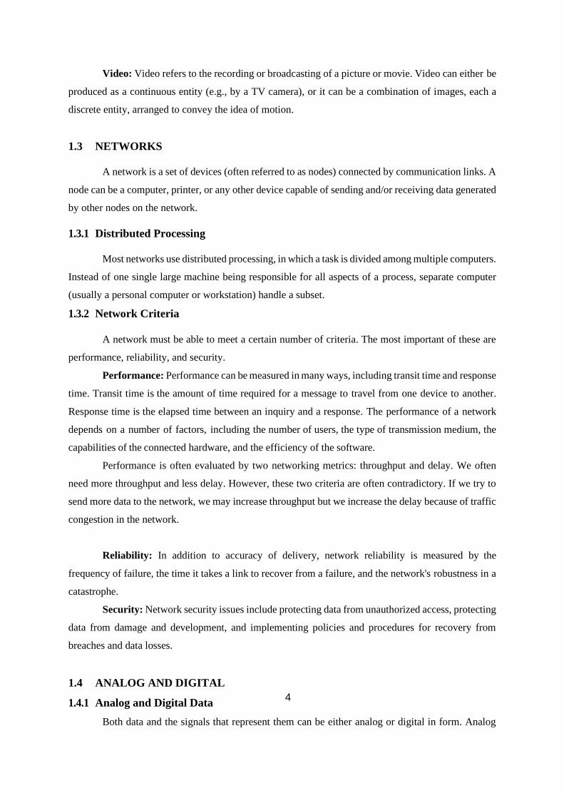
simple as 1 and O. The simplest way to show signals is by plotting them on a pair of perpendicular axes.
The vertical axis represents the value or strength of a signal. The horizontal axis represents time. Figure
1.1 illustrates an analog signal and a digital signal. The curve representing the analog signal passes
through an infinite number of points. The vertical lines of the digital signal, however, demonstrate the
sudden jump that the signal makes from value to value.
Fig. 1.1 Comparison of analog and digital signals
1.5 TIME DOMAIN CONCEPTS
Continuous signal - Infinite number of points at any given time
Discrete signal - Finite number of points at any given time; maintains a constant level then changes to
another constant level
6
7
Periodic signal - Pattern repeated over time
Aperiodic (non-periodic) signal - Pattern not repeated over time
✓ In data communications, we commonly use periodic analog signals andnonperiodic digital
signals.
✓ Periodic analog signals can be classified as simple or composite.
✓ A simple periodic analog signal, a sine wave, cannot be decomposed into simpler signals.
✓ A composite periodic analog signal is composed of multiple sine waves.
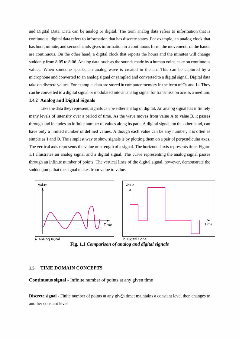
1.6 BANWIDTH
The bandwidth of a composite signal is the difference between the highest and the lowest
frequencies contained in that signal.
For example, a 1 can be encoded as a positive voltage and a 0 as zero voltage. A digital signal
can have more than two levels. In this case, we can send more than 1 bit for each level.
Fig. 1.2 The bandwidth of periodic and non-periodic composite signals
7
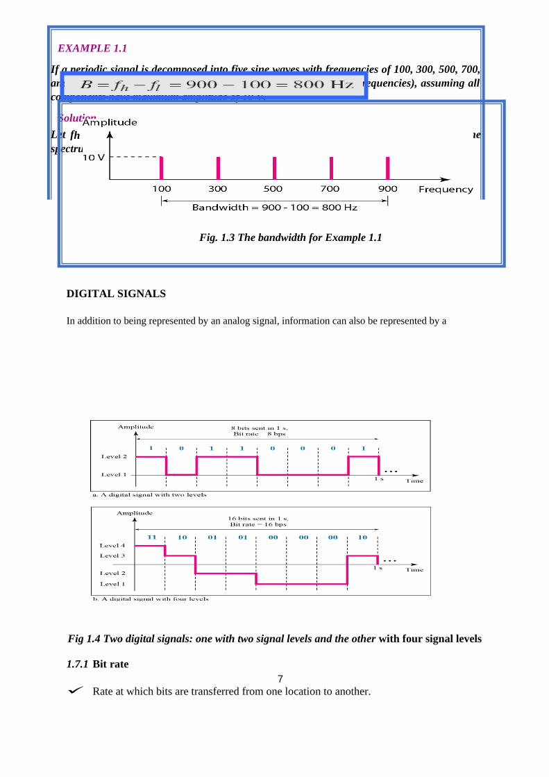
DIGITAL SIGNALS
In addition to being represented by an analog signal, information can also be represented by a
Fig 1.4 Two digital signals: one with two signal levels and the other with four signal levels
1.7.1 Bit rate
✓ Rate at which bits are transferred from one location to another.
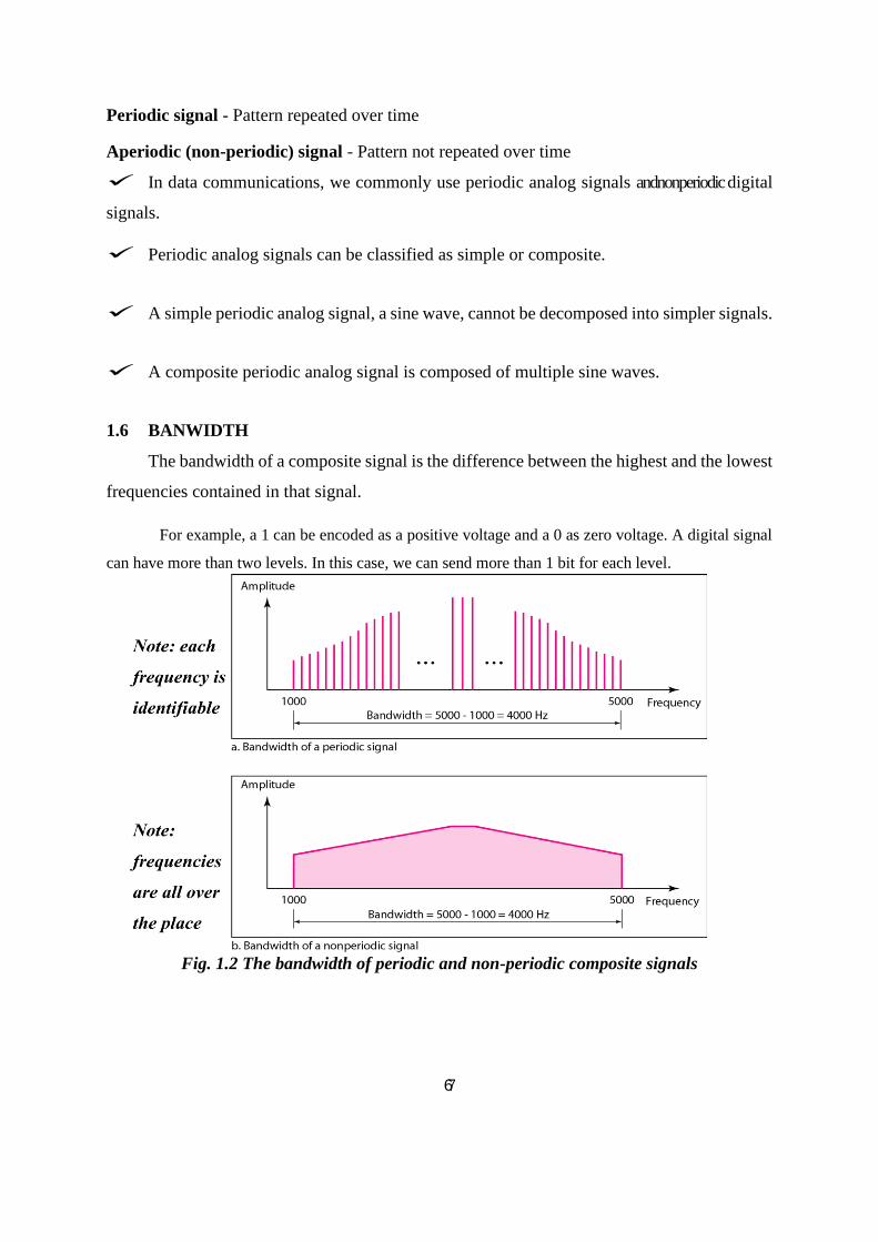
EXAMPLE 1.1
If a periodic signal is decomposed into five sine waves with frequencies of 100, 300, 500, 700,
and 900 Hz, what is its bandwidth? Draw the spectrum (range of frequencies), assuming all
components have maximum amplitude of 10 V.
Solution
Let fh be the highest frequency, fl the lowest frequency, and B the bandwidth. Then The
spectrum has only five spikes, at 100, 300, 500, 700, and 900 Hz
Fig. 1.3 The bandwidth for Example 1.1
8
✓ Measures how much data is transmitted in a given amount of time
✓ Measured in bits per second (bps), kilobits per second (Kbps), or megabits per second
(Mbps).
✓ A good rule of thumb is for the bitrate of your stream to use no more than 50% of your
available upload bandwidth capacity on a dedicate d line.
✓ For example, if the result you get from a speed test shows that you have 2Mbps of upload
speed available, your combined audio and video bit rate should not exceed 1Mbps.
1.7.2 Bit rate, Bit Length, Baud rate Estimation of Bit rate
Frequency × bit depth × channels = bit rate.
44,100 samples per second × 16 bits per sample × 2 channels = 1,411,200 bits per second (or
1,411.2 kbps)
Baud Rate: Baud Rate is the number of signal unit transmitted per second. Thus Baud Rate is always
less than or equal to bit rate.
Bit Length: The Bit Length is the distance of one Bit occupies on the transmission medium. Bit Length
= Propagation speed * Bit duration
42
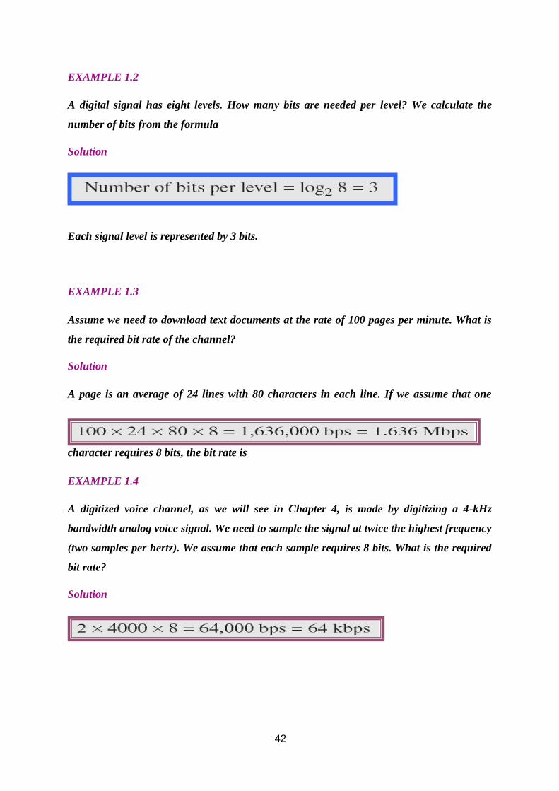
EXAMPLE 1.2
A digital signal has eight levels. How many bits are needed per level? We calculate the
number of bits from the formula
Solution
Each signal level is represented by 3 bits.
EXAMPLE 1.3
Assume we need to download text documents at the rate of 100 pages per minute. What is
the required bit rate of the channel?
Solution
A page is an average of 24 lines with 80 characters in each line. If we assume that one
character requires 8 bits, the bit rate is
EXAMPLE 1.4
A digitized voice channel, as we will see in Chapter 4, is made by digitizing a 4-kHz
bandwidth analog voice signal. We need to sample the signal at twice the highest frequency
(two samples per hertz). We assume that each sample requires 8 bits. What is the required
bit rate?
Solution
43
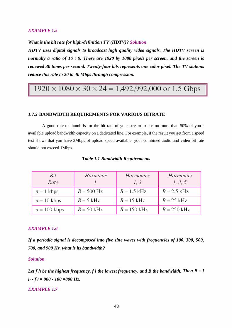
EXAMPLE 1.5
What is the bit rate for high-definition TV (HDTV)? Solution
HDTV uses digital signals to broadcast high quality video signals. The HDTV screen is
normally a ratio of 16 : 9. There are 1920 by 1080 pixels per screen, and the screen is
renewed 30 times per second. Twenty-four bits represents one color pixel. The TV stations
reduce this rate to 20 to 40 Mbps through compression.
1.7.3 BANDWIDTH REQUIREMENTS FOR VARIOUS BITRATE
A good rule of thumb is for the bit rate of your stream to use no more than 50% of you r
available upload bandwidth capacity on a dedicated line. For example, if the result you get from a speed
test shows that you have 2Mbps of upload speed available, your combined audio and video bit rate
should not exceed 1Mbps.
Table 1.1 Bandwidth Requirements
EXAMPLE 1.6
If a periodic signal is decomposed into five sine waves with frequencies of 100, 300, 500,
700, and 900 Hz, what is its bandwidth?
Solution
Let f h be the highest frequency, f l the lowest frequency, and B the bandwidth. Then B = f
h - f l = 900 - 100 =800 Hz.
EXAMPLE 1.7
44
A periodic signal has a bandwidth of 20 Hz. The highest frequency is 60 Hz. What is the
lowest frequency?
Solution
Let f h be the highest frequency, f l the lowest frequency, and B the bandwidth. Then B = f h
- f l = 20 ; 20 = 60 - f l; f l = 40 Hz.
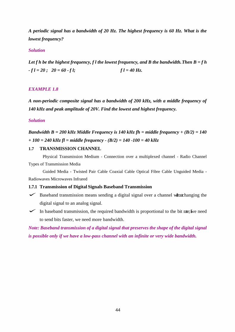
EXAMPLE 1.8
A non-periodic composite signal has a bandwidth of 200 kHz, with a middle frequency of
140 kHz and peak amplitude of 20V. Find the lowest and highest frequency.
Solution
Bandwidth B = 200 kHz Middle Frequency is 140 kHz fh = middle frequency + (B/2) = 140
+ 100 = 240 kHz fl = middle frequency - (B/2) = 140 -100 = 40 kHz
1.7 TRANSMISSION CHANNEL
Physical Transmission Medium - Connection over a multiplexed channel - Radio Channel
Types of Transmission Media
Guided Media - Twisted Pair Cable Coaxial Cable Optical Fibre Cable Unguided Media -
Radiowaves Microwaves Infrared
1.7.1 Transmission of Digital Signals Baseband Transmission
✓ Baseband transmission means sending a digital signal over a channel without changing the
digital signal to an analog signal.
✓ In baseband transmission, the required bandwidth is proportional to the bit rate; if we need
to send bits faster, we need more bandwidth.
Note: Baseband transmission of a digital signal that preserves the shape of the digital signal
is possible only if we have a low-pass channel with an infinite or very wide bandwidth.
45
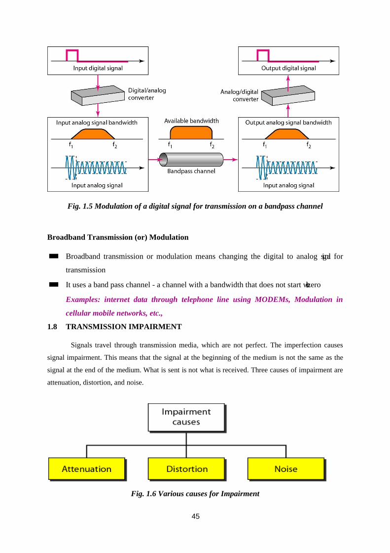
Fig. 1.5 Modulation of a digital signal for transmission on a bandpass channel
Broadband Transmission (or) Modulation
◼ Broadband transmission or modulation means changing the digital to analog signal for
transmission
◼ It uses a band pass channel - a channel with a bandwidth that does not start with zero
Examples: internet data through telephone line using MODEMs, Modulation in
cellular mobile networks, etc.,
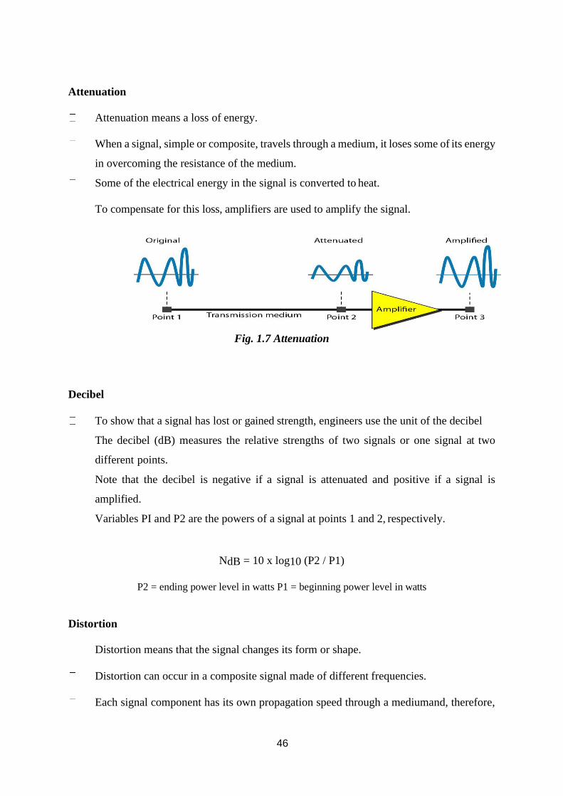
1.8 TRANSMISSION IMPAIRMENT
Signals travel through transmission media, which are not perfect. The imperfection causes
signal impairment. This means that the signal at the beginning of the medium is not the same as the
signal at the end of the medium. What is sent is not what is received. Three causes of impairment are
attenuation, distortion, and noise.
Fig. 1.6 Various causes for Impairment
46
Attenuation
Attenuation means a loss of energy.
When a signal, simple or composite, travels through a medium, it loses some of its energy
in overcoming the resistance of the medium.
Some of the electrical energy in the signal is converted to heat.
To compensate for this loss, amplifiers are used to amplify the signal.
Fig. 1.7 Attenuation
Decibel
To show that a signal has lost or gained strength, engineers use the unit of the decibel
The decibel (dB) measures the relative strengths of two signals or one signal at two
different points.
Note that the decibel is negative if a signal is attenuated and positive if a signal is
amplified.
Variables PI and P2 are the powers of a signal at points 1 and 2, respectively.
NdB = 10 x log10 (P2 / P1)
P2 = ending power level in watts P1 = beginning power level in watts
Distortion
Distortion means that the signal changes its form or shape.
Distortion can occur in a composite signal made of different frequencies.
Each signal component has its own propagation speed through a mediumand, therefore,
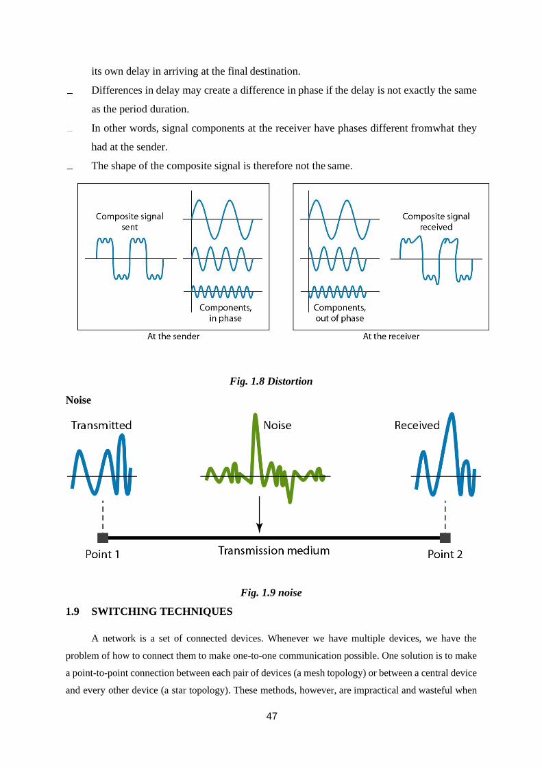
47
its own delay in arriving at the final destination.
Differences in delay may create a difference in phase if the delay is not exactly the same
as the period duration.
In other words, signal components at the receiver have phases different fromwhat they
had at the sender.
The shape of the composite signal is therefore not the same.
Fig. 1.8 Distortion
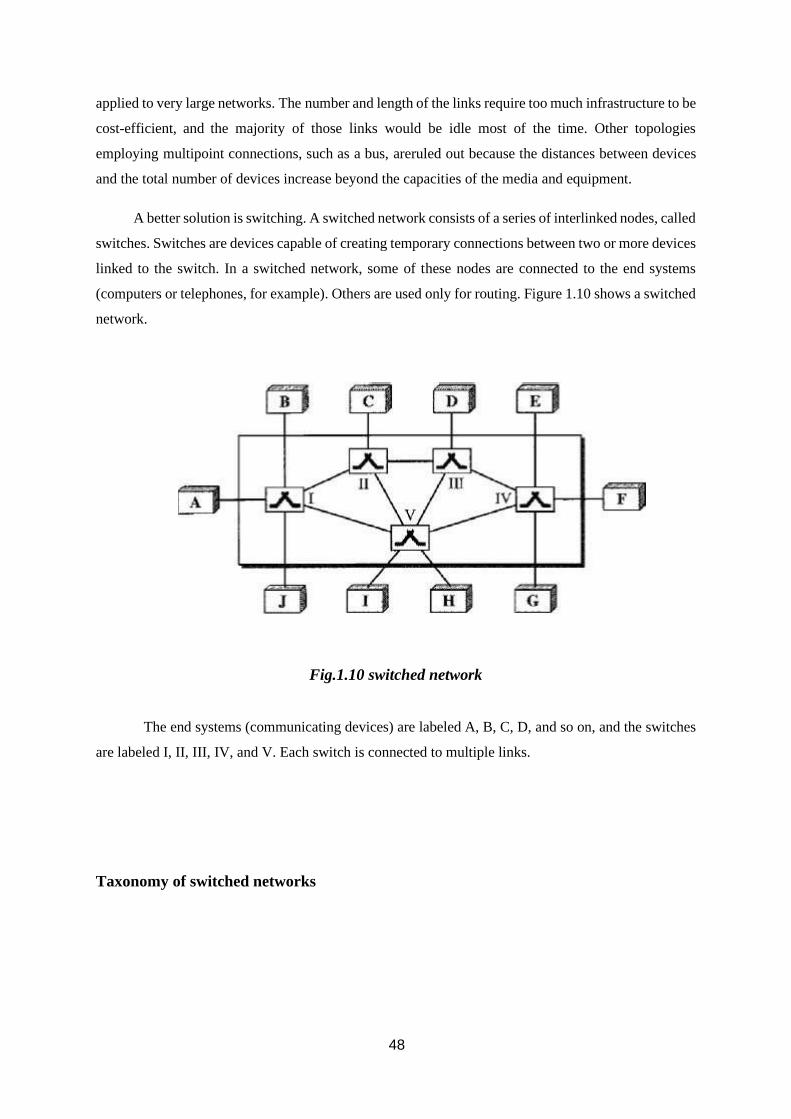
Noise
Fig. 1.9 noise
1.9 SWITCHING TECHNIQUES
A network is a set of connected devices. Whenever we have multiple devices, we have the
problem of how to connect them to make one-to-one communication possible. One solution is to make
a point-to-point connection between each pair of devices (a mesh topology) or between a central device
and every other device (a star topology). These methods, however, are impractical and wasteful when
48
applied to very large networks. The number and length of the links require too much infrastructure to be
cost-efficient, and the majority of those links would be idle most of the time. Other topologies
employing multipoint connections, such as a bus, areruled out because the distances between devices
and the total number of devices increase beyond the capacities of the media and equipment.
A better solution is switching. A switched network consists of a series of interlinked nodes, called
switches. Switches are devices capable of creating temporary connections between two or more devices
linked to the switch. In a switched network, some of these nodes are connected to the end systems
(computers or telephones, for example). Others are used only for routing. Figure 1.10 shows a switched
network.
Fig.1.10 switched network
The end systems (communicating devices) are labeled A, B, C, D, and so on, and the switches
are labeled I, II, III, IV, and V. Each switch is connected to multiple links.
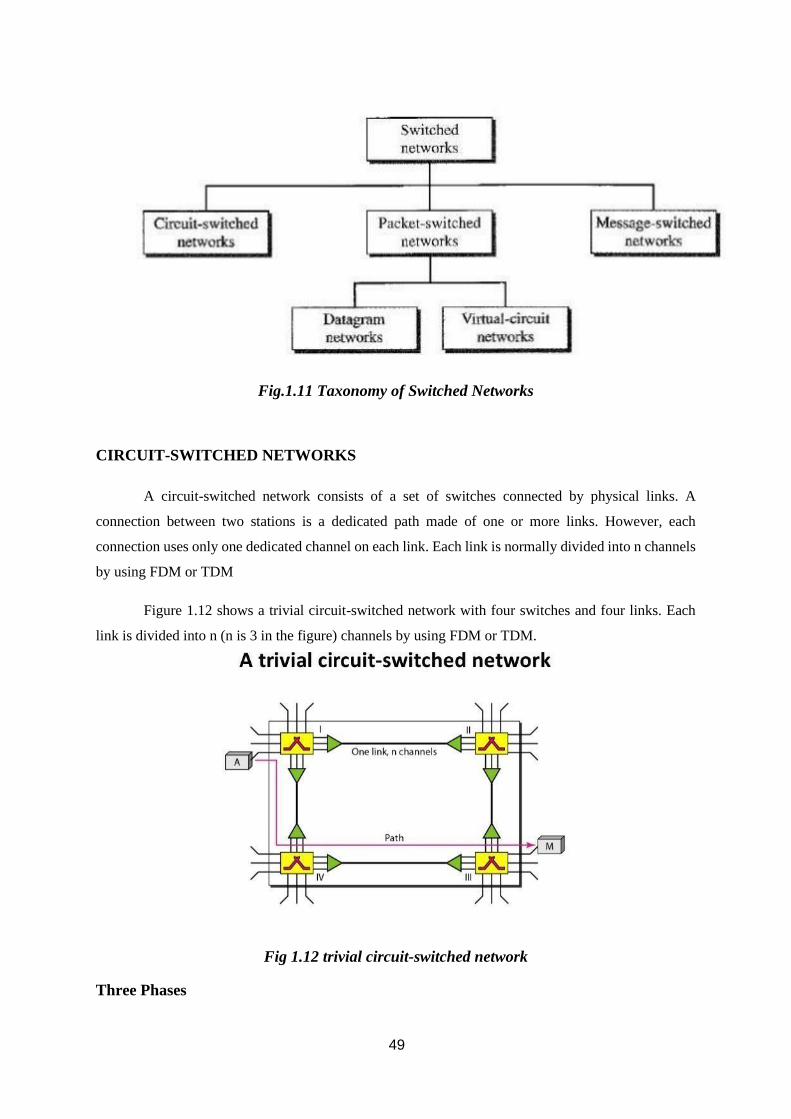
Taxonomy of switched networks
49
Fig.1.11 Taxonomy of Switched Networks
CIRCUIT-SWITCHED NETWORKS
A circuit-switched network consists of a set of switches connected by physical links. A
connection between two stations is a dedicated path made of one or more links. However, each
connection uses only one dedicated channel on each link. Each link is normally divided into n channels
by using FDM or TDM
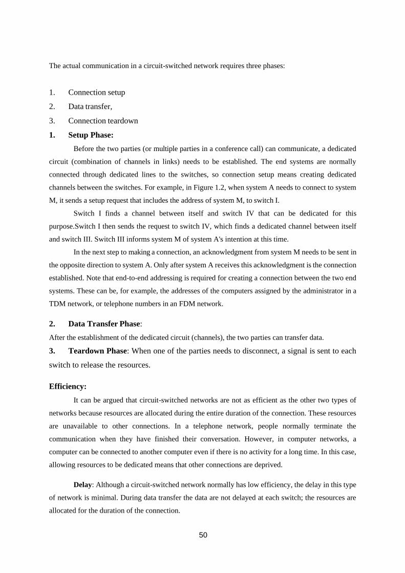
Figure 1.12 shows a trivial circuit-switched network with four switches and four links. Each
link is divided into n (n is 3 in the figure) channels by using FDM or TDM.
Fig 1.12 trivial circuit-switched network
Three Phases
50
The actual communication in a circuit-switched network requires three phases:
1. Connection setup
2. Data transfer,
3. Connection teardown
1. Setup Phase:
Before the two parties (or multiple parties in a conference call) can communicate, a dedicated
circuit (combination of channels in links) needs to be established. The end systems are normally
connected through dedicated lines to the switches, so connection setup means creating dedicated
channels between the switches. For example, in Figure 1.2, when system A needs to connect to system
M, it sends a setup request that includes the address of system M, to switch I.
Switch I finds a channel between itself and switch IV that can be dedicated for this
purpose.Switch I then sends the request to switch IV, which finds a dedicated channel between itself
and switch III. Switch III informs system M of system A's intention at this time.
In the next step to making a connection, an acknowledgment from system M needs to be sent in
the opposite direction to system A. Only after system A receives this acknowledgment is the connection
established. Note that end-to-end addressing is required for creating a connection between the two end
systems. These can be, for example, the addresses of the computers assigned by the administrator in a
TDM network, or telephone numbers in an FDM network.
2. Data Transfer Phase:
After the establishment of the dedicated circuit (channels), the two parties can transfer data.
3. Teardown Phase: When one of the parties needs to disconnect, a signal is sent to each
switch to release the resources.
Efficiency:
It can be argued that circuit-switched networks are not as efficient as the other two types of
networks because resources are allocated during the entire duration of the connection. These resources
are unavailable to other connections. In a telephone network, people normally terminate the
communication when they have finished their conversation. However, in computer networks, a
computer can be connected to another computer even if there is no activity for a long time. In this case,
allowing resources to be dedicated means that other connections are deprived.
Delay: Although a circuit-switched network normally has low efficiency, the delay in this type
of network is minimal. During data transfer the data are not delayed at each switch; the resources are
allocated for the duration of the connection.
51
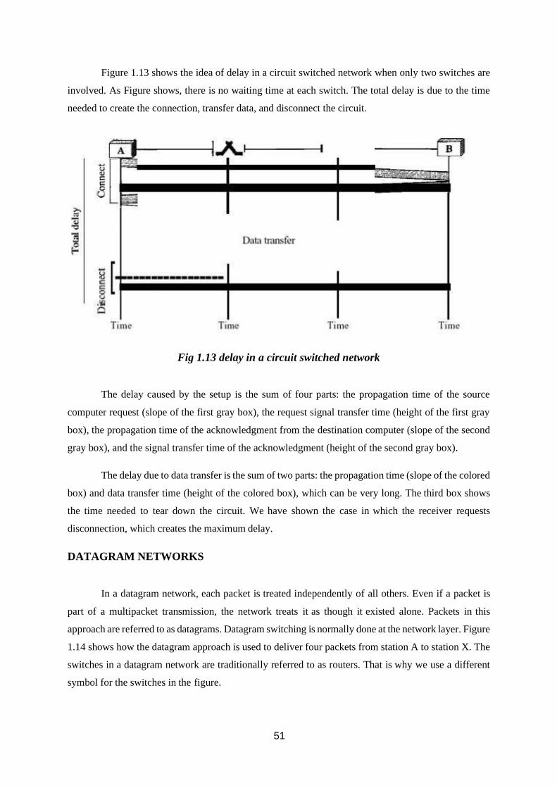
Figure 1.13 shows the idea of delay in a circuit switched network when only two switches are
involved. As Figure shows, there is no waiting time at each switch. The total delay is due to the time
needed to create the connection, transfer data, and disconnect the circuit.
Fig 1.13 delay in a circuit switched network
The delay caused by the setup is the sum of four parts: the propagation time of the source
computer request (slope of the first gray box), the request signal transfer time (height of the first gray
box), the propagation time of the acknowledgment from the destination computer (slope of the second
gray box), and the signal transfer time of the acknowledgment (height of the second gray box).
The delay due to data transfer is the sum of two parts: the propagation time (slope of the colored
box) and data transfer time (height of the colored box), which can be very long. The third box shows
the time needed to tear down the circuit. We have shown the case in which the receiver requests
disconnection, which creates the maximum delay.
DATAGRAM NETWORKS
In a datagram network, each packet is treated independently of all others. Even if a packet is
part of a multipacket transmission, the network treats it as though it existed alone. Packets in this
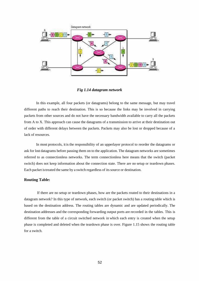
approach are referred to as datagrams. Datagram switching is normally done at the network layer. Figure
1.14 shows how the datagram approach is used to deliver four packets from station A to station X. The
switches in a datagram network are traditionally referred to as routers. That is why we use a different
symbol for the switches in the figure.
52
Fig 1.14 datagram network
In this example, all four packets (or datagrams) belong to the same message, but may travel
different paths to reach their destination. This is so because the links may be involved in carrying
packets from other sources and do not have the necessary bandwidth available to carry all the packets
from A to X. This approach can cause the datagrams of a transmission to arrive at their destination out
of order with different delays between the packets. Packets may also be lost or dropped because of a
lack of resources.
In most protocols, it is the responsibility of an upperlayer protocol to reorder the datagrams or
ask for lost datagrams before passing them on to the application. The datagram networks are sometimes
referred to as connectionless networks. The term connectionless here means that the switch (packet
switch) does not keep information about the connection state. There are no setup or teardown phases.
Each packet is treated the same by a switch regardless of its source or destination.
Routing Table:
If there are no setup or teardown phases, how are the packets routed to their destinations in a
datagram network? In this type of network, each switch (or packet switch) has a routing table which is
based on the destination address. The routing tables are dynamic and are updated periodically. The
destination addresses and the corresponding forwarding output ports are recorded in the tables. This is
different from the table of a circuit switched network in which each entry is created when the setup
phase is completed and deleted when the teardown phase is over. Figure 1.15 shows the routing table
for a switch.
53
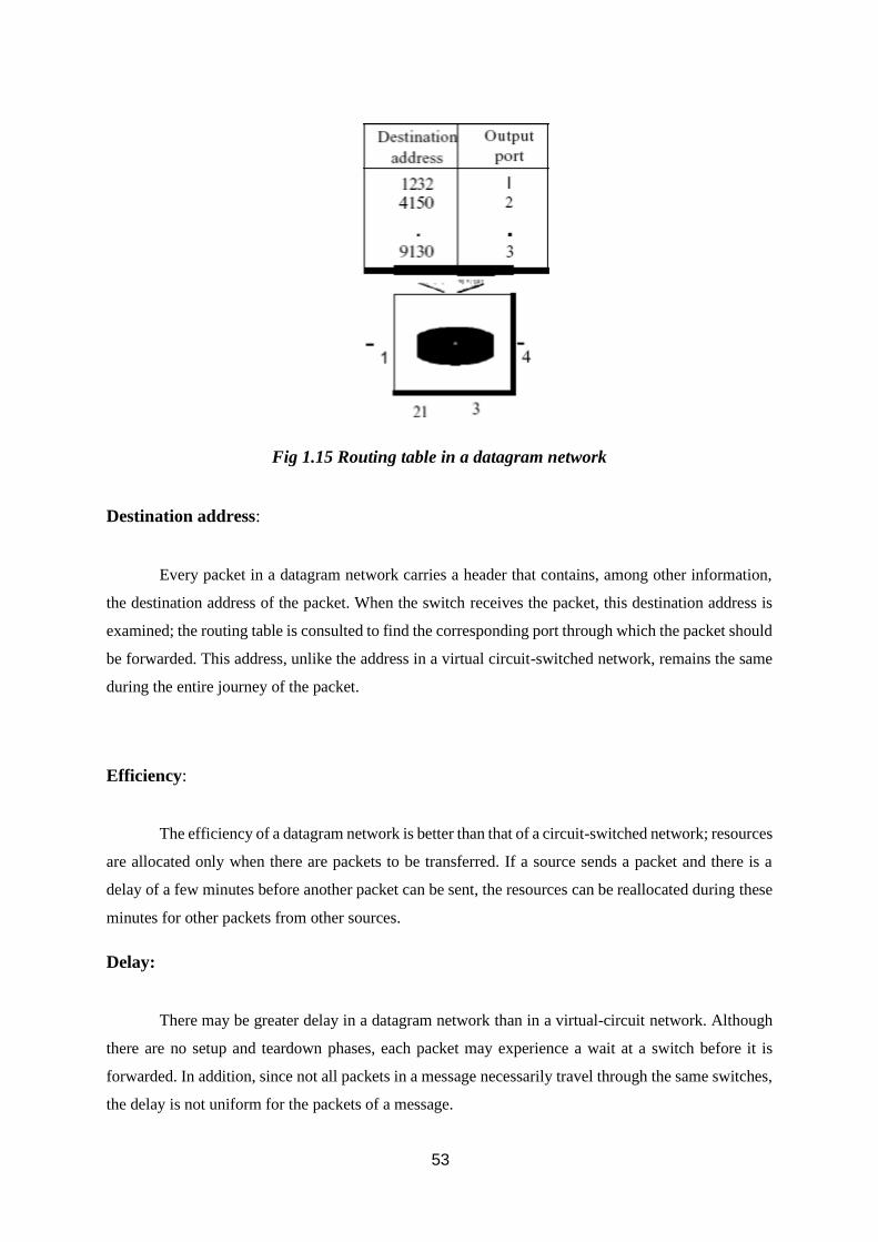
Fig 1.15 Routing table in a datagram network
Destination address:
Every packet in a datagram network carries a header that contains, among other information,
the destination address of the packet. When the switch receives the packet, this destination address is
examined; the routing table is consulted to find the corresponding port through which the packet should
be forwarded. This address, unlike the address in a virtual circuit-switched network, remains the same
during the entire journey of the packet.
Efficiency:
The efficiency of a datagram network is better than that of a circuit-switched network; resources
are allocated only when there are packets to be transferred. If a source sends a packet and there is a
delay of a few minutes before another packet can be sent, the resources can be reallocated during these
minutes for other packets from other sources.
Delay:
There may be greater delay in a datagram network than in a virtual-circuit network. Although
there are no setup and teardown phases, each packet may experience a wait at a switch before it is
forwarded. In addition, since not all packets in a message necessarily travel through the same switches,
the delay is not uniform for the packets of a message.
54
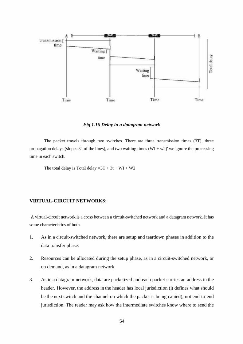
Fig 1.16 Delay in a datagram network
The packet travels through two switches. There are three transmission times (3T), three
propagation delays (slopes 3't of the lines), and two waiting times (WI + w2)' we ignore the processing
time in each switch.
The total delay is Total delay =3T + 3t + WI + W2
VIRTUAL-CIRCUIT NETWORKS:
A virtual-circuit network is a cross between a circuit-switched network and a datagram network. It has
some characteristics of both.
1. As in a circuit-switched network, there are setup and teardown phases in addition to the
data transfer phase.
2. Resources can be allocated during the setup phase, as in a circuit-switched network, or
on demand, as in a datagram network.
3. As in a datagram network, data are packetized and each packet carries an address in the
header. However, the address in the header has local jurisdiction (it defines what should
be the next switch and the channel on which the packet is being canied), not end-to-end
jurisdiction. The reader may ask how the intermediate switches know where to send the
55
packet if there is no final destination address carried by a packet. The answer will be clear when
we discuss virtual circuit identifiers in the next section.
4. As in a circuit-switched network, all packets follow the same path established duringthe
connection.
5. A virtual-circuit network is normally implemented in the data link layer, while a circuit
switched network is implemented in the physical layer and a datagram network in the
network layer. But this may change in the future. Figure 1.17 is an example of a virtual-
circuit network.
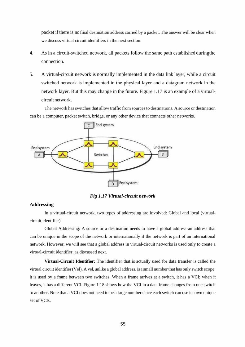
The network has switches that allow traffic from sources to destinations. A source or destination
can be a computer, packet switch, bridge, or any other device that connects other networks.
Fig 1.17 Virtual-circuit network
Addressing
In a virtual-circuit network, two types of addressing are involved: Global and local (virtual-
circuit identifier).
Global Addressing: A source or a destination needs to have a global address-an address that
can be unique in the scope of the network or internationally if the network is part of an international
network. However, we will see that a global address in virtual-circuit networks is used only to create a
virtual-circuit identifier, as discussed next.
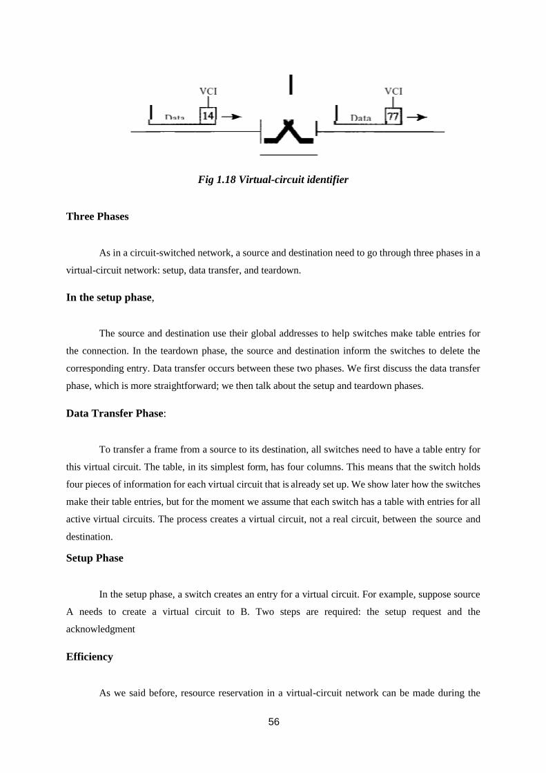
Virtual-Circuit Identifier: The identifier that is actually used for data transfer is called the
virtual circuit identifier (Vel). A vel, unlike a global address, is a small number that has only switch scope;
it is used by a frame between two switches. When a frame arrives at a switch, it has a VCI; when it
leaves, it has a different VCl. Figure 1.18 shows how the VCI in a data frame changes from one switch
to another. Note that a VCI does not need to be a large number since each switch can use its own unique
set of VCls.
56
Fig 1.18 Virtual-circuit identifier
Three Phases
As in a circuit-switched network, a source and destination need to go through three phases in a
virtual-circuit network: setup, data transfer, and teardown.
In the setup phase,
The source and destination use their global addresses to help switches make table entries for
the connection. In the teardown phase, the source and destination inform the switches to delete the
corresponding entry. Data transfer occurs between these two phases. We first discuss the data transfer
phase, which is more straightforward; we then talk about the setup and teardown phases.
Data Transfer Phase:
To transfer a frame from a source to its destination, all switches need to have a table entry for
this virtual circuit. The table, in its simplest form, has four columns. This means that the switch holds
four pieces of information for each virtual circuit that is already set up. We show later how the switches
make their table entries, but for the moment we assume that each switch has a table with entries for all
active virtual circuits. The process creates a virtual circuit, not a real circuit, between the source and
destination.
Setup Phase
In the setup phase, a switch creates an entry for a virtual circuit. For example, suppose source
A needs to create a virtual circuit to B. Two steps are required: the setup request and the
acknowledgment
Efficiency
As we said before, resource reservation in a virtual-circuit network can be made during the
57
setup or can be on demand during the data transfer phase. In the first case, the delay for each packet is
the same; in the second case, each packet may encounter different delays. There is one big advantage
in a virtual-circuit network even if resource allocation is on demand. The source can check the
availability of the resources, without actually reserving it. Consider a family that wants to dine at a
restaurant. Although the restaurant may not accept reservations (allocation of the tables is on demand),
the family can call and find out the waiting time. This can save the family time and effort.
Delay in Virtual-Circuit Networks
In a virtual-circuit network, there is a one-time delay for setup and a one-time delay for
teardown. If resources are allocated during the setup phase, there is no wait time for individual packets.
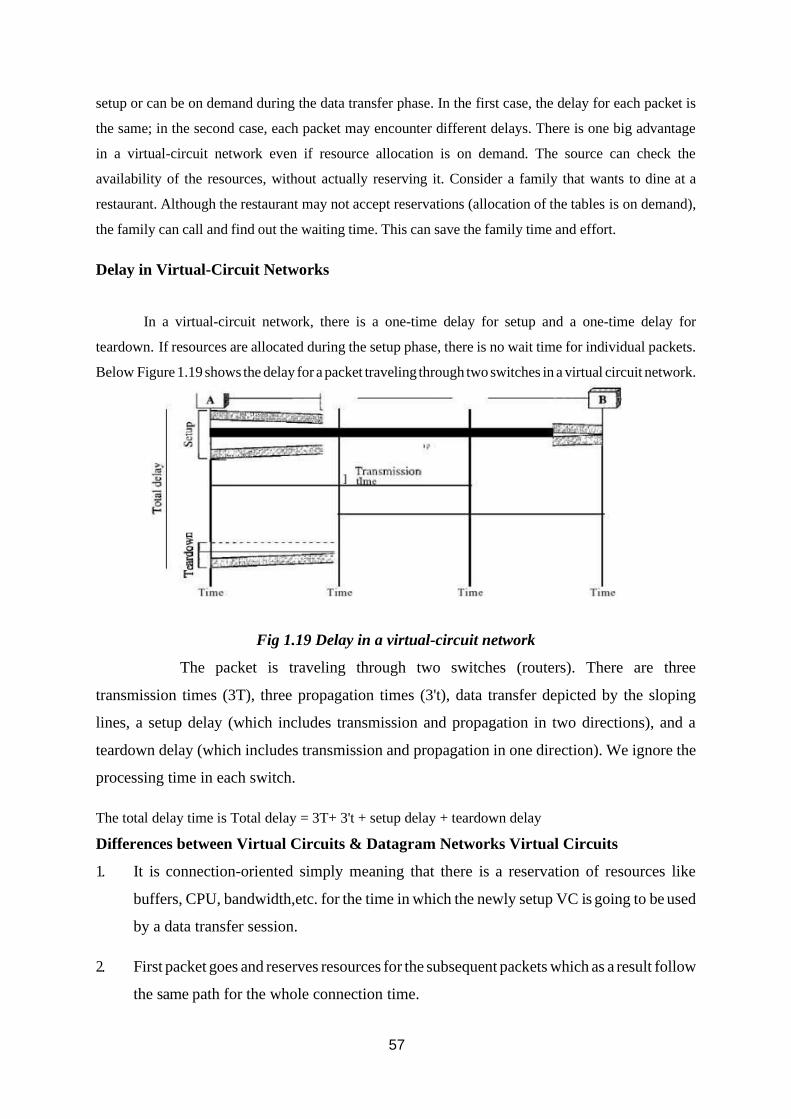
Below Figure 1.19 shows the delay for a packet traveling through two switches in a virtual circuit network.
Fig 1.19 Delay in a virtual-circuit network
The packet is traveling through two switches (routers). There are three
transmission times (3T), three propagation times (3't), data transfer depicted by the sloping
lines, a setup delay (which includes transmission and propagation in two directions), and a
teardown delay (which includes transmission and propagation in one direction). We ignore the
processing time in each switch.
The total delay time is Total delay = 3T+ 3't + setup delay + teardown delay
Differences between Virtual Circuits & Datagram Networks Virtual Circuits
1. It is connection-oriented simply meaning that there is a reservation of resources like
buffers, CPU, bandwidth,etc. for the time in which the newly setup VC is going to be used
by a data transfer session.
2. First packet goes and reserves resources for the subsequent packets which as a result follow
the same path for the whole connection time.
58
3. Since all the packets are going to follow the same path, a global header is required only
for the first packet of the connection and other packets generally don’t require global
headers.
4. Since data follows a particular dedicated path, packets reach inorder to the destination.
5. From above points, it can be concluded that Virtual Circuits are highly reliable means of
transfer.
6. Since each time a new connection has to be setup with reservation of resources and extra
information handling at routers, its simply costly to implement Virtual Circuits.
Datagram Networks:
1. It is connectionless service. There is no need of reservation of resources as there is no
dedicated path for a connection session.
2. All packets are free to go to any path on any intermediate router which is decided on the
go by dynamically changing routing tables on routers.
3. Since every packet is free to choose any path, all packets must be associated with a header
with proper information about source and the upper layer data.
4. The connectionless property makes data packets reach destination in any order, means
they need not reach in the order in which they were sent.
5. Datagram networks are not reliable as Virtual Circuits.
6. But it is always easy and cost efficient to implement datagram networks as there is no extra
headache of reserving resources and making a dedicated each time an application has to
communicate.
ISO / OSI MODEL:
ISO refers International Standards Organization was established in 1947, it is a multinational
body dedicated to worldwide agreement on international standards. OSI refers to Open System
Interconnection that covers all aspects of network communication. It is a standard of ISO. Here open
system is a model that allows any two different systems to communicate regardless of their underlying
59
architecture. Mainly, it is not a protocol it is just a model.
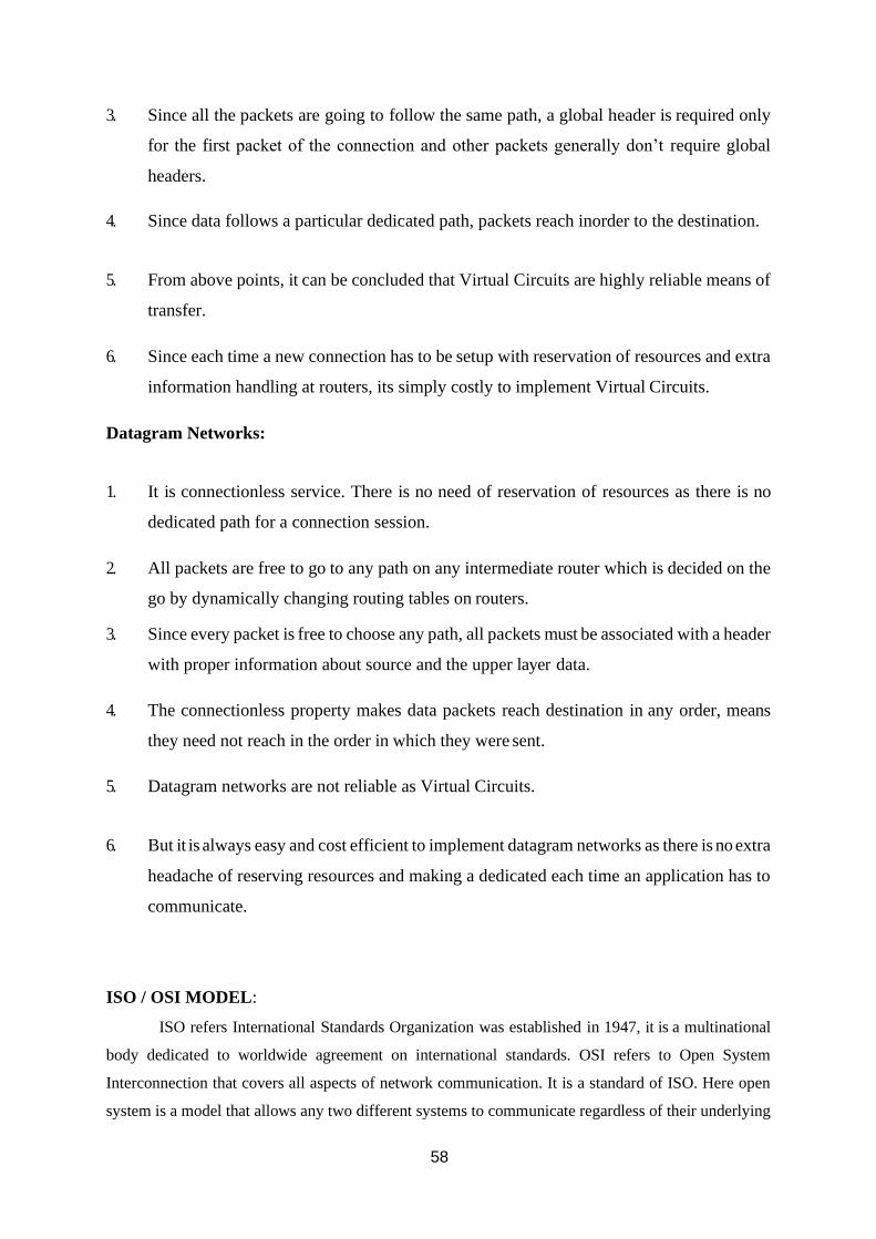
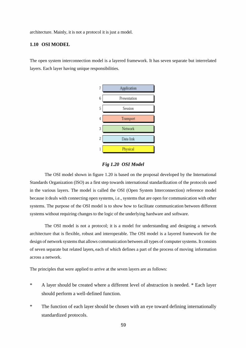
1.10 OSI MODEL
The open system interconnection model is a layered framework. It has seven separate but interrelated
layers. Each layer having unique responsibilities.
Fig 1.20 OSI Model
The OSI model shown in figure 1.20 is based on the proposal developed by the International
Standards Organization (ISO) as a first step towards international standardization of the protocols used
in the various layers. The model is called the OSI (Open System Interconnection) reference model
because it deals with connecting open systems, i.e., systems that are open for communication with other
systems. The purpose of the OSI model is to show how to facilitate communication between different
systems without requiring changes to the logic of the underlying hardware and software.
The OSI model is not a protocol; it is a model for understanding and designing a network
architecture that is flexible, robust and interoperable. The OSI model is a layered framework for the
design of network systems that allows communication between all types of computer systems. It consists
of seven separate but related layers, each of which defines a part of the process of moving information
across a network.
The principles that were applied to arrive at the seven layers are as follows:
* A layer should be created where a different level of abstraction is needed. * Each layer
should perform a well-defined function.
* The function of each layer should be chosen with an eye toward defining internationally
standardized protocols.
60
* The layer boundaries should be chosen to minimize the information flow across the
interfaces.
* The number of layers should be large enough that distinct functions need not be thrown
together in the same layer out of necessity and small enough that the architecture does not
become unwieldy.
Layered Architecture:
The OSI model is composed of seven layers: Physical, Data link, Network, Transport, Session,
Presentation, Application layers.
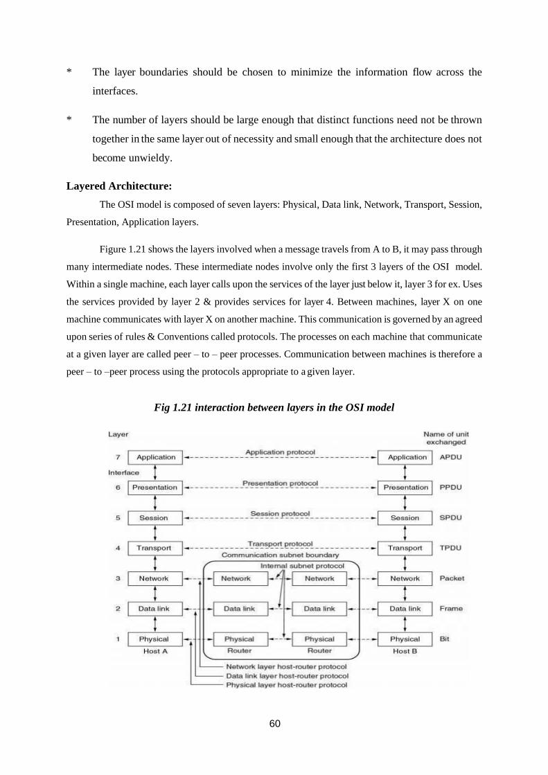
Figure 1.21 shows the layers involved when a message travels from A to B, it may pass through
many intermediate nodes. These intermediate nodes involve only the first 3 layers of the OSI model.
Within a single machine, each layer calls upon the services of the layer just below it, layer 3 for ex. Uses
the services provided by layer 2 & provides services for layer 4. Between machines, layer X on one
machine communicates with layer X on another machine. This communication is governed by an agreed
upon series of rules & Conventions called protocols. The processes on each machine that communicate
at a given layer are called peer – to – peer processes. Communication between machines is therefore a
peer – to –peer process using the protocols appropriate to a given layer.
Fig 1.21 interaction between layers in the OSI model
61
ORGANIZATION OF LAYERS
The seven layers are arranged by three sub groups.
1. Network Support Layers
2. User Support Layers
3. Intermediate Layer
Network Support Layers:
Physical, Datalink and Network layers come under the group. They deal with the physical
aspects of the data such as electrical specifications, physical connections, physical addressing, and
transport timing and reliability.
User Support Layers:
Session, Presentation and Application layers comes under the group. They deal with the
interoperability between the software systems.
Intermediate Layer:
The transport layer is the intermediate layer between the network support and the user support
layers.
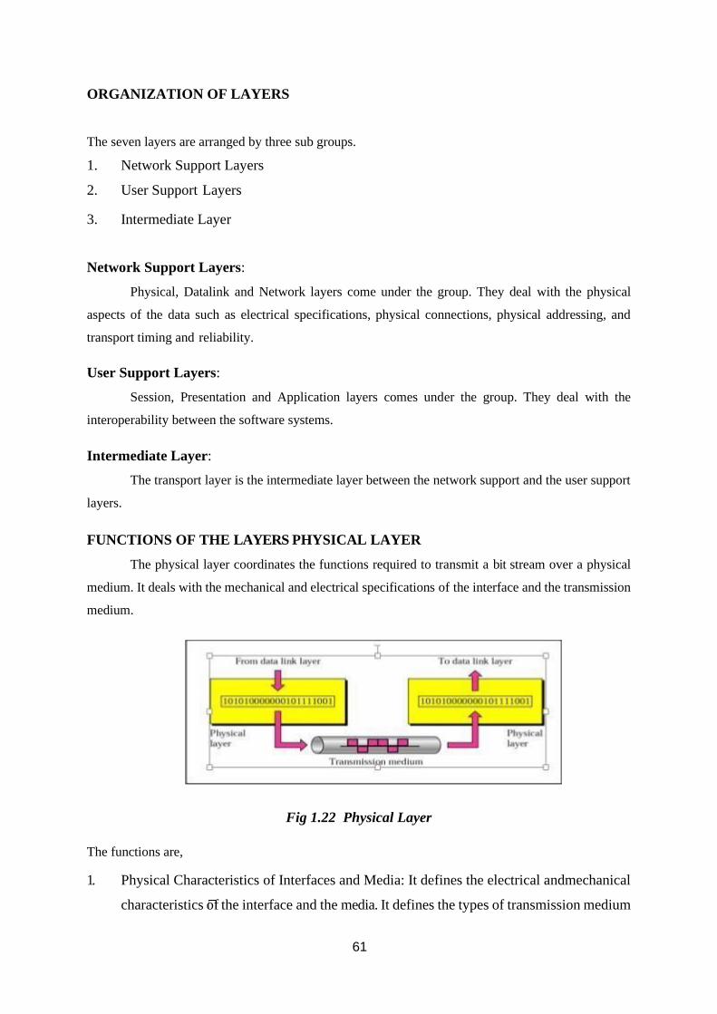
FUNCTIONS OF THE LAYERS PHYSICAL LAYER
The physical layer coordinates the functions required to transmit a bit stream over a physical
medium. It deals with the mechanical and electrical specifications of the interface and the transmission
medium.
Fig 1.22 Physical Layer
The functions are,
1. Physical Characteristics of Interfaces and Media: It defines the electrical andmechanical
characteristics of the interface and the media. It defines the types of transmission medium
62
2. Representation of Bits: To transmit the stream of bits they must be encoded into signal.
It defines the type of encoding weather electrical or optical.
3. Data Rate: It defines the transmission rate i.e. the number of bits sent per second.
4. Synchronization of Bits: The sender and receiver must be synchronized at bit level.
5. Line Configuration: It defines the type of connection between the devices.
Two types of connection are 1. Point to point 2. Multipoint
6. Physical Topology: It defines how devices are connected to make a network.
Five topologies are, 1. mesh 2. star 3. tree 4. bus 5. ring
7. Transmission Mode It defines the direction of transmission between devices.
Three types of transmission are, 1. simplex 2. half duplex3. full duplex
DATALINK LAYER
Datalink layer responsible for node-to-node delivery The responsibilities of Datalink layer are,
1. Framing: It divides the stream of bits received from network layer into manageable data
units called frames.
2. Physical Addressing: It adds a header that defines the physical address of the sender and
the receiver. If the sender and the receiver are in different networks, then the receiver
address is the address of the device which connects the two networks.
3. Flow Control: It imposes a flow control mechanism used to ensure the data rate at the
sender and the receiver should be same.
4. Error Control: To improve the reliability the Datalink layer adds a trailer which contains
the error control mechanism like CRC, Checksum etc
5. Access Control: When two or more devices connected at the same link, then the Datalink
layer used to determine which device has control over the link at any given time.
NETWORK LAYER
63
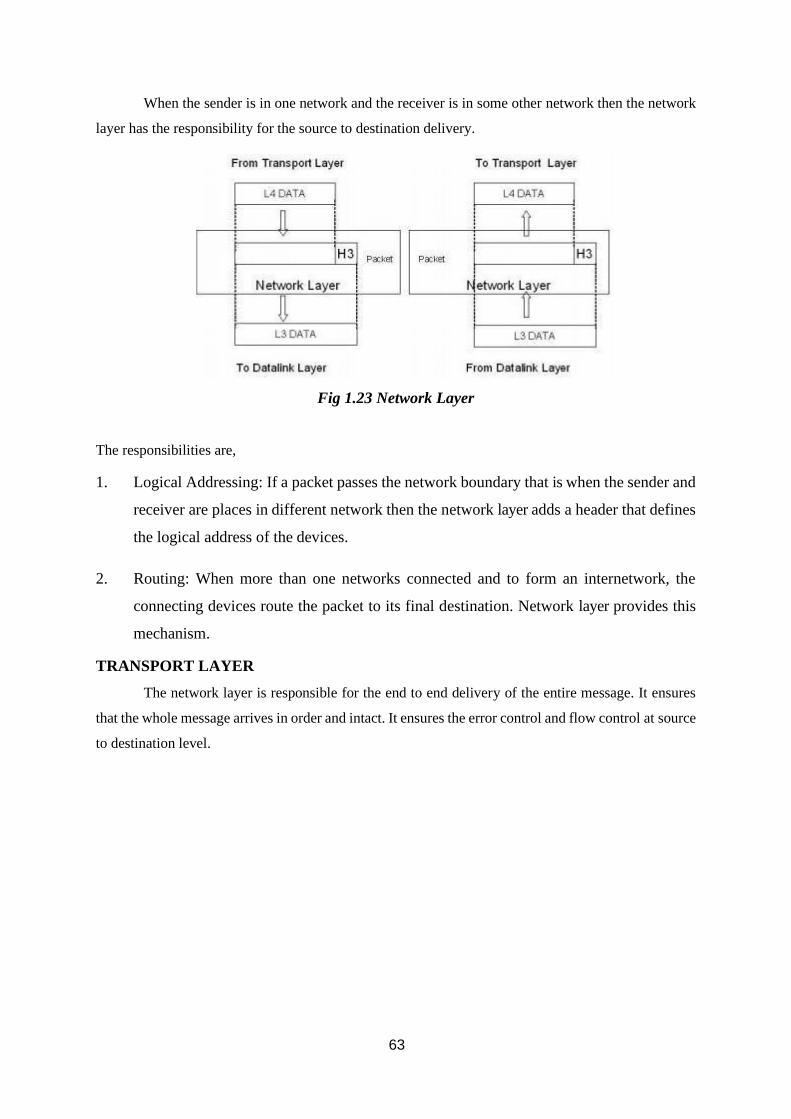
When the sender is in one network and the receiver is in some other network then the network
layer has the responsibility for the source to destination delivery.
Fig 1.23 Network Layer
The responsibilities are,
1. Logical Addressing: If a packet passes the network boundary that is when the sender and
receiver are places in different network then the network layer adds a header that defines
the logical address of the devices.
2. Routing: When more than one networks connected and to form an internetwork, the
connecting devices route the packet to its final destination. Network layer provides this
mechanism.
TRANSPORT LAYER
The network layer is responsible for the end to end delivery of the entire message. It ensures
that the whole message arrives in order and intact. It ensures the error control and flow control at source
to destination level.
64
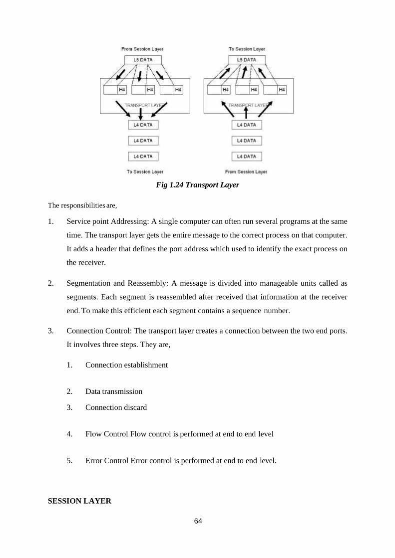
Fig 1.24 Transport Layer
The responsibilities are,
1. Service point Addressing: A single computer can often run several programs at the same
time. The transport layer gets the entire message to the correct process on that computer.
It adds a header that defines the port address which used to identify the exact process on
the receiver.
2. Segmentation and Reassembly: A message is divided into manageable units called as
segments. Each segment is reassembled after received that information at the receiver
end. To make this efficient each segment contains a sequence number.
3. Connection Control: The transport layer creates a connection between the two end ports.
It involves three steps. They are,
1. Connection establishment
2. Data transmission
3. Connection discard
4. Flow Control Flow control is performed at end to end level
5. Error Control Error control is performed at end to end level.
SESSION LAYER
65
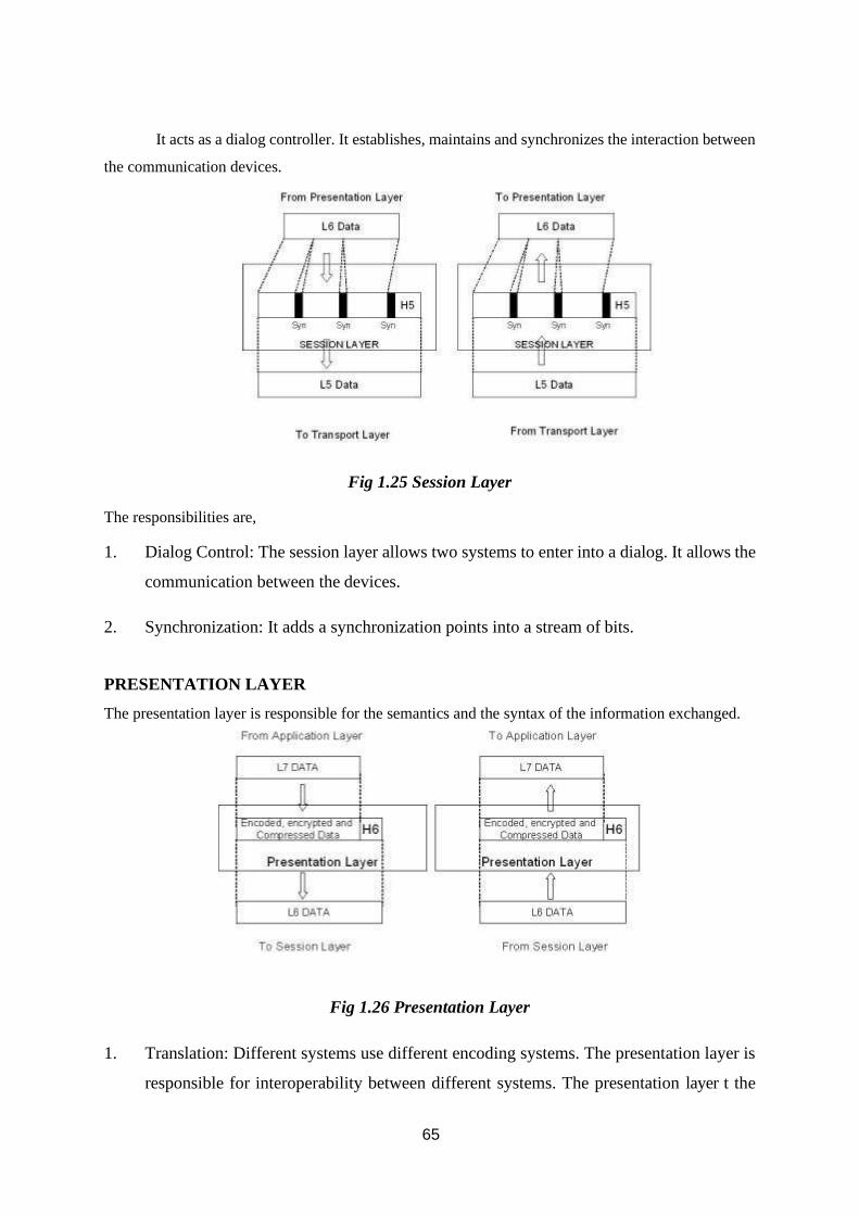
It acts as a dialog controller. It establishes, maintains and synchronizes the interaction between
the communication devices.
Fig 1.25 Session Layer
The responsibilities are,
1. Dialog Control: The session layer allows two systems to enter into a dialog. It allows the
communication between the devices.
2. Synchronization: It adds a synchronization points into a stream of bits.
PRESENTATION LAYER
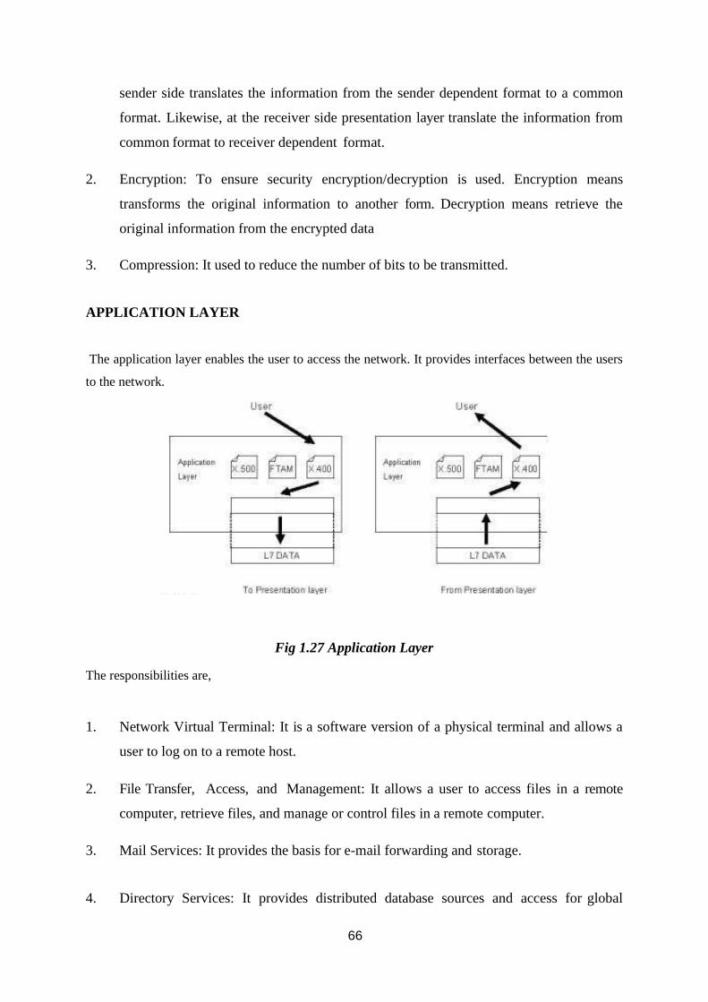
The presentation layer is responsible for the semantics and the syntax of the information exchanged.
Fig 1.26 Presentation Layer
1. Translation: Different systems use different encoding systems. The presentation layer is
responsible for interoperability between different systems. The presentation layer t the
66
sender side translates the information from the sender dependent format to a common
format. Likewise, at the receiver side presentation layer translate the information from
common format to receiver dependent format.
2. Encryption: To ensure security encryption/decryption is used. Encryption means
transforms the original information to another form. Decryption means retrieve the
original information from the encrypted data
3. Compression: It used to reduce the number of bits to be transmitted.
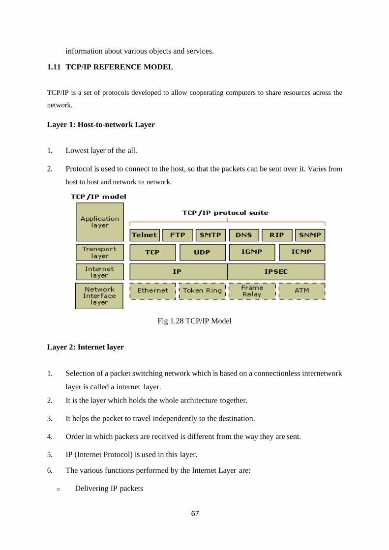
APPLICATION LAYER
The application layer enables the user to access the network. It provides interfaces between the users
to the network.
Fig 1.27 Application Layer
The responsibilities are,
1. Network Virtual Terminal: It is a software version of a physical terminal and allows a
user to log on to a remote host.
2. File Transfer, Access, and Management: It allows a user to access files in a remote
computer, retrieve files, and manage or control files in a remote computer.
3. Mail Services: It provides the basis for e-mail forwarding and storage.
4. Directory Services: It provides distributed database sources and access for global
67
information about various objects and services.
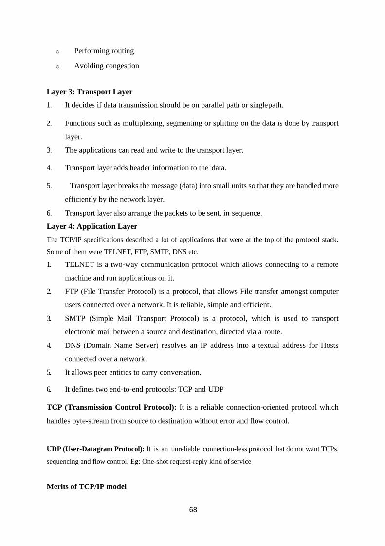
1.11 TCP/IP REFERENCE MODEL
TCP/IP is a set of protocols developed to allow cooperating computers to share resources across the
network.
Layer 1: Host-to-network Layer
1. Lowest layer of the all.
2. Protocol is used to connect to the host, so that the packets can be sent over it. Varies from
host to host and network to network.
Fig 1.28 TCP/IP Model
Layer 2: Internet layer
1. Selection of a packet switching network which is based on a connectionless internetwork
layer is called a internet layer.
2. It is the layer which holds the whole architecture together.
3. It helps the packet to travel independently to the destination.
4. Order in which packets are received is different from the way they are sent.
5. IP (Internet Protocol) is used in this layer.
6. The various functions performed by the Internet Layer are:
o Delivering IP packets
68
o Performing routing
o Avoiding congestion
Layer 3: Transport Layer
1. It decides if data transmission should be on parallel path or single path.
2. Functions such as multiplexing, segmenting or splitting on the data is done by transport
layer.
3. The applications can read and write to the transport layer.
4. Transport layer adds header information to the data.
5. Transport layer breaks the message (data) into small units so that they are handled more
efficiently by the network layer.
6. Transport layer also arrange the packets to be sent, in sequence.
Layer 4: Application Layer
The TCP/IP specifications described a lot of applications that were at the top of the protocol stack.
Some of them were TELNET, FTP, SMTP, DNS etc.
1. TELNET is a two-way communication protocol which allows connecting to a remote
machine and run applications on it.
2. FTP (File Transfer Protocol) is a protocol, that allows File transfer amongst computer
users connected over a network. It is reliable, simple and efficient.
3. SMTP (Simple Mail Transport Protocol) is a protocol, which is used to transport
electronic mail between a source and destination, directed via a route.
4. DNS (Domain Name Server) resolves an IP address into a textual address for Hosts
connected over a network.
5. It allows peer entities to carry conversation.
6. It defines two end-to-end protocols: TCP and UDP
TCP (Transmission Control Protocol): It is a reliable connection-oriented protocol which
handles byte-stream from source to destination without error and flow control.
UDP (User-Datagram Protocol): It is an unreliable connection-less protocol that do not want TCPs,
sequencing and flow control. Eg: One-shot request-reply kind of service
Merits of TCP/IP model
69
1. It operated independently.
2. It is scalable.
3. Client/server architecture.
4. Supports a number of routing protocols.
5. Can be used to establish a connection between two computers.
Demerits of TCP/IP
1. In this, the transport layer does not guarantee delivery of packets.
2. The model cannot be used in any other application.
3. Replacing protocol is not easy.
4. It has not clearly separated its services, interfaces and protocols.
TEXT / REFERENCE BOOKS
1. Andrew S Tanenbaum “Computer Networks” 5th Edition. Pearson Education/PH I/2011.
2. Behrouz A. Forouzan, “Data Communications and Networking” Fourth Edition, Mc
GrawHill HIGHER Education 2007.
3. Michael A.Gallo, William Hancock.M, Brooks/Cole Computer Communications and
Networking Technologies,2001
4. Richard Lai and Jirachief pattana, “Communication Protocol Specification and
Verification”, Kluwer Publishers, Boston, 1998.
5. Pallapa Venkataram and Sunilkumar S.Manvi, “Communication
protocol Engineering”, PHI Learning, 2008
1
SCHOOL OF ELECTRICAL AND ELECTRONICS ENGINEERING DEPARTMENT
OF ELECTRONICS AND COMMUNICATION ENGINEERING
UNIT – II COMPUTER NETWORKS – SECA1604
2
UNIT II NETWORKING
2.1 NETWORK TOPOLOGIES
The term topology refers to the way a network is laid out, either physically or logically.
Two or more devices connect to a link; two or more links form topology.
The topology of a network is the geometric representation of the relationship of all the links and linking
devices to each other.
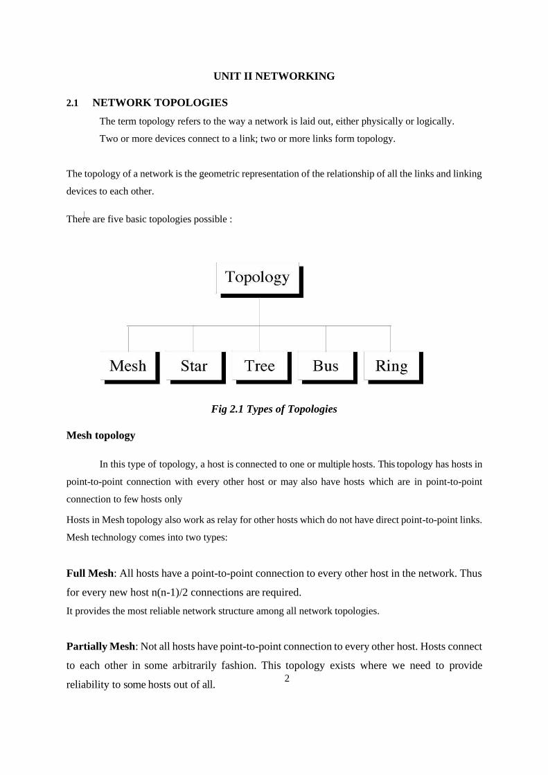
There are five basic topologies possible :
Fig 2.1 Types of Topologies
Mesh topology
In this type of topology, a host is connected to one or multiple hosts. This topology has hosts in
point-to-point connection with every other host or may also have hosts which are in point-to-point
connection to few hosts only
Hosts in Mesh topology also work as relay for other hosts which do not have direct point-to-point links.
Mesh technology comes into two types:
Full Mesh: All hosts have a point-to-point connection to every other host in the network. Thus
for every new host n(n-1)/2 connections are required.
It provides the most reliable network structure among all network topologies.
Partially Mesh: Not all hosts have point-to-point connection to every other host. Hosts connect
to each other in some arbitrarily fashion. This topology exists where we need to provide
reliability to some hosts out of all.
3
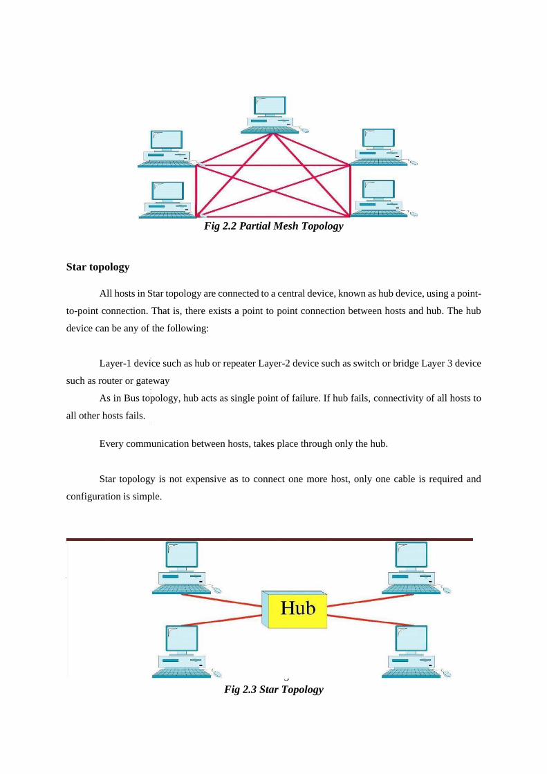
Fig 2.2 Partial Mesh Topology
Star topology
All hosts in Star topology are connected to a central device, known as hub device, using a point-
to-point connection. That is, there exists a point to point connection between hosts and hub. The hub
device can be any of the following:
Layer-1 device such as hub or repeater Layer-2 device such as switch or bridge Layer 3 device
such as router or gateway
As in Bus topology, hub acts as single point of failure. If hub fails, connectivity of all hosts to
all other hosts fails.
Every communication between hosts, takes place through only the hub.
Star topology is not expensive as to connect one more host, only one cable is required and
configuration is simple.
Fig 2.3 Star Topology
4
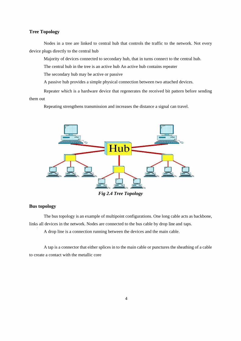
Tree Topology
Nodes in a tree are linked to central hub that controls the traffic to the network. Not every
device plugs directly to the central hub
Majority of devices connected to secondary hub, that in turns connect to the central hub.
The central hub in the tree is an active hub An active hub contains repeater
The secondary hub may be active or passive
A passive hub provides a simple physical connection between two attached devices.
Repeater which is a hardware device that regenerates the received bit pattern before sending
them out
Repeating strengthens transmission and increases the distance a signal can travel.
Fig 2.4 Tree Topology
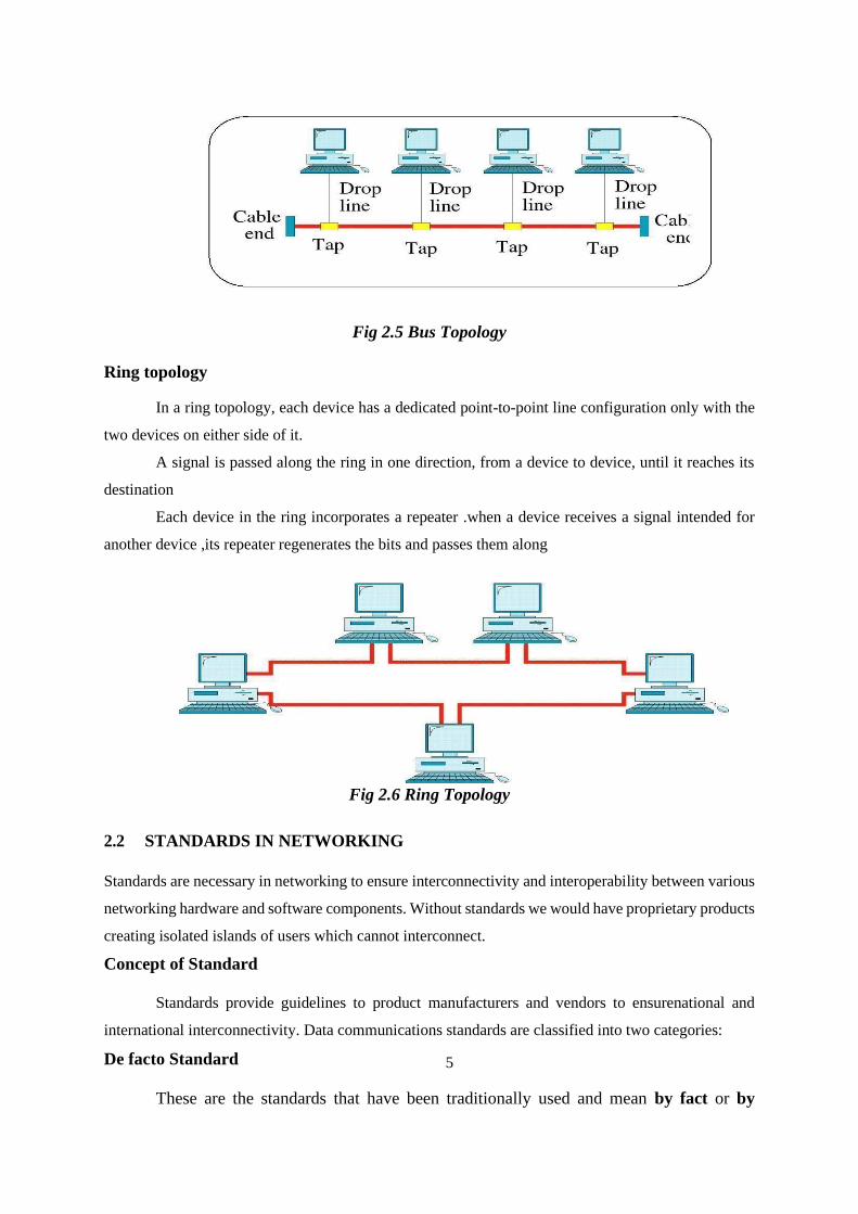
Bus topology
The bus topology is an example of multipoint configurations. One long cable acts as backbone,
links all devices in the network. Nodes are connected to the bus cable by drop line and taps.
A drop line is a connection running between the devices and the main cable.
A tap is a connector that either splices in to the main cable or punctures the sheathing of a cable
to create a contact with the metallic core
5
Fig 2.5 Bus Topology
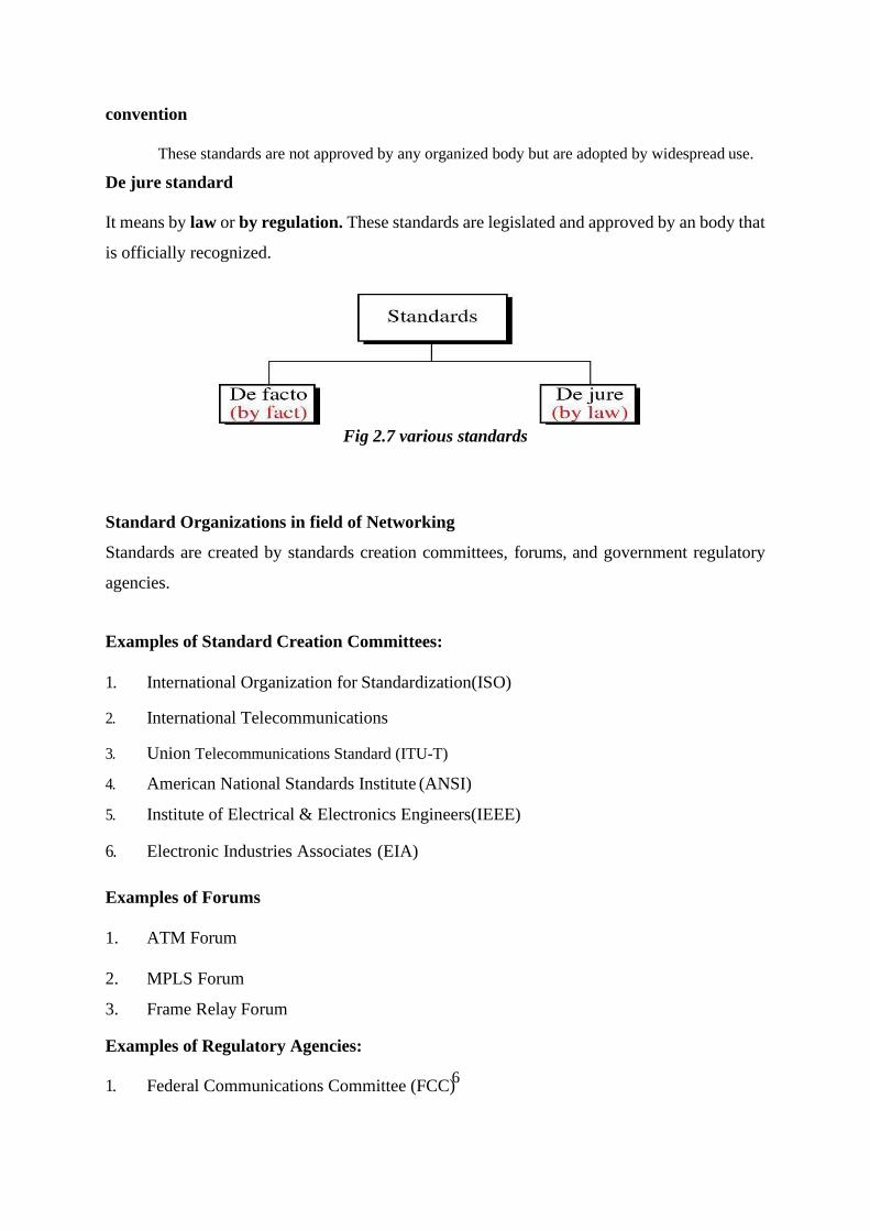
Ring topology
In a ring topology, each device has a dedicated point-to-point line configuration only with the
two devices on either side of it.
A signal is passed along the ring in one direction, from a device to device, until it reaches its
destination
Each device in the ring incorporates a repeater .when a device receives a signal intended for
another device ,its repeater regenerates the bits and passes them along
Fig 2.6 Ring Topology
2.2 STANDARDS IN NETWORKING
Standards are necessary in networking to ensure interconnectivity and interoperability between various
networking hardware and software components. Without standards we would have proprietary products
creating isolated islands of users which cannot interconnect.
Concept of Standard
Standards provide guidelines to product manufacturers and vendors to ensurenational and
international interconnectivity. Data communications standards are classified into two categories:
De facto Standard
These are the standards that have been traditionally used and mean by fact or by
5
6
convention
These standards are not approved by any organized body but are adopted by widespread use.
De jure standard
It means by law or by regulation. These standards are legislated and approved by an body that
is officially recognized.
Fig 2.7 various standards
Standard Organizations in field of Networking
Standards are created by standards creation committees, forums, and government regulatory
agencies.
Examples of Standard Creation Committees:
1. International Organization for Standardization(ISO)
2. International Telecommunications
3. Union Telecommunications Standard (ITU-T)
4. American National Standards Institute (ANSI)
5. Institute of Electrical & Electronics Engineers(IEEE)
6. Electronic Industries Associates (EIA)
Examples of Forums
1. ATM Forum
2. MPLS Forum
3. Frame Relay Forum
Examples of Regulatory Agencies:
1. Federal Communications Committee (FCC)
7
IEEE 802 is a family of IEEE standards dealing with local area networks and metropolitan area
networks. More specifically, the IEEE 802 standards are restricted to networks carrying variable- size
packets. By contrast, in cell relay networks data is transmitted in short, uniformly sized units called
cells. Isochronous networks, where data is transmitted as a steady stream of octets, or groups of octets, at
regular time intervals, are also out of the scope of this standard. The number 802 was simply the next
free number IEEE could assign, though ―802‖ is sometimes associated with the date the first meeting
was held February 1980. The services and protocols specified in IEEE 802 map to the lower two layers
(Data Link and Physical) of the seven-layer OSI networking reference model. In fact, IEEE 802 splits
the OSI Data Link Layer into two sub- layers named logical link control (LLC) and media access control
(MAC), so the layers can be listed like this:
• Data link layer
• LLC sublayer
• MAC sublayer
• Physical layer
The IEEE 802 family of standards is maintained by the IEEE 802 LAN/MAN Standards
Committee (LMSC). The most widely used standards are for the Ethernet family, Token Ring, RFID,
Bridging and Virtual Bridged LANs. An individual working group provides the focus for each area.
Wireless LAN and IEEE 802.11
A wireless LAN (WLAN or WiFi) is a data transmission system designed to provide location-
independent network access between computing devices by using radio waves rather than a cable
infrastructure In the corporate enterprise, wireless LANs are usually implemented as the final link
between the existing wired network and a group of client computers, giving these users wireless access
to the full resources and services of the corporate network across a building or campus setting. The
widespread acceptance of WLANs depends on industry standardization to ensure product compatibility
and reliability among the various manufacturers.
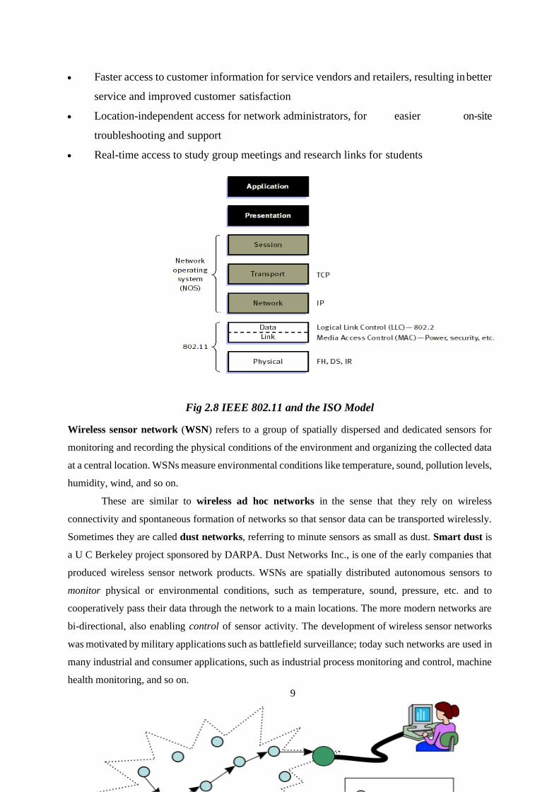
The 802.11 specification as a standard for wireless LANS was ratified by the Institute of
Electrical and Electronics Engineers (IEEE) in the year 1997. This version of 802.11 provides for 1
Mbps and 2 Mbps data rates and a set of fundamental signaling methods and other services. Like all
IEEE 802 standards, the 802.11 standards focus on the bottom two levels the ISO model, the physical
layer and link layer (see figure below). Any LAN application, network operating system, protocol,
including TCP/IP and Novell NetWare, will run on an 802.11-compliant WLAN as easily as they run
over Ethernet.
The major motivation and benefit from Wireless LANs is increased mobility. Untethered from
conventional network connections, network users can move about almost without restriction and access
8
LANs from nearly anywhere.The other advantages for WLAN include cost-effective network setup for
hard-to-wire locations such as older buildings and solid-wall structures and reduced cost of ownership-
particularly in dynamic environments requiring frequent modifications, thanks to minimal wiring and
installation costs per device and user. WLANs liberate users from dependence on hard-wired access to
the network backbone, giving them anytime, anywhere network access. This freedom to roam offers
numerous user benefits for a variety of work environments, such as:
• Immediate bedside access to patient information for doctors and hospital staff
• Easy, real-time network access for on-site consultants or auditors
• Improved database access for roving supervisors such as production line managers,
warehouse auditors, or construction engineers
• Simplified network configuration with minimal MIS involvement for temporarysetups
such as trade shows or conference rooms
9
• Faster access to customer information for service vendors and retailers, resulting in better
service and improved customer satisfaction
• Location-independent access for network administrators, for easier on-site
troubleshooting and support
• Real-time access to study group meetings and research links for students
Fig 2.8 IEEE 802.11 and the ISO Model
Wireless sensor network (WSN) refers to a group of spatially dispersed and dedicated sensors for
monitoring and recording the physical conditions of the environment and organizing the collected data
at a central location. WSNs measure environmental conditions like temperature, sound, pollution levels,
humidity, wind, and so on.
These are similar to wireless ad hoc networks in the sense that they rely on wireless
connectivity and spontaneous formation of networks so that sensor data can be transported wirelessly.
Sometimes they are called dust networks, referring to minute sensors as small as dust. Smart dust is
a U C Berkeley project sponsored by DARPA. Dust Networks Inc., is one of the early companies that
produced wireless sensor network products. WSNs are spatially distributed autonomous sensors to
monitor physical or environmental conditions, such as temperature, sound, pressure, etc. and to
cooperatively pass their data through the network to a main locations. The more modern networks are
bi-directional, also enabling control of sensor activity. The development of wireless sensor networks
was motivated by military applications such as battlefield surveillance; today such networks are used in
many industrial and consumer applications, such as industrial process monitoring and control, machine
health monitoring, and so on.
10
\
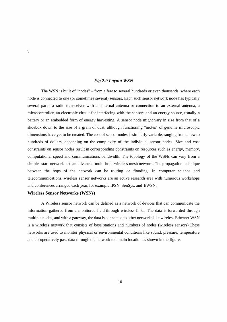
Fig 2.9 Layout WSN
The WSN is built of "nodes" – from a few to several hundreds or even thousands, where each
node is connected to one (or sometimes several) sensors. Each such sensor network node has typically
several parts: a radio transceiver with an internal antenna or connection to an external antenna, a
microcontroller, an electronic circuit for interfacing with the sensors and an energy source, usually a
battery or an embedded form of energy harvesting. A sensor node might vary in size from that of a
shoebox down to the size of a grain of dust, although functioning "motes" of genuine microscopic
dimensions have yet to be created. The cost of sensor nodes is similarly variable, ranging from a few to
hundreds of dollars, depending on the complexity of the individual sensor nodes. Size and cost
constraints on sensor nodes result in corresponding constraints on resources such as energy, memory,
computational speed and communications bandwidth. The topology of the WSNs can vary from a
simple star network to an advanced multi-hop wireless mesh network. The propagation technique
between the hops of the network can be routing or flooding. In computer science and
telecommunications, wireless sensor networks are an active research area with numerous workshops
and conferences arranged each year, for example IPSN, SenSys, and EWSN.
Wireless Sensor Networks (WSNs)
A Wireless sensor network can be defined as a network of devices that can communicate the
information gathered from a monitored field through wireless links. The data is forwarded through
multiple nodes, and with a gateway, the data is connected to other networks like wireless Ethernet.WSN
is a wireless network that consists of base stations and numbers of nodes (wireless sensors).These
networks are used to monitor physical or environmental conditions like sound, pressure, temperature
and co-operatively pass data through the network to a main location as shown in the figure.
11
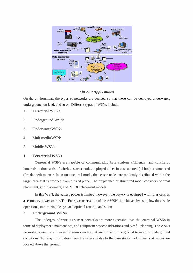
Fig 2.10 Applications
On the environment, the types of networks are decided so that those can be deployed underwater,
underground, on land, and so on. Different types of WSNs include:
1. Terrestrial WSNs
2. Underground WSNs
3. Underwater WSNs
4. Multimedia WSNs
5. Mobile WSNs
1. Terrestrial WSNs
Terrestrial WSNs are capable of communicating base stations efficiently, and consist of
hundreds to thousands of wireless sensor nodes deployed either in unstructured (ad hoc) or structured
(Preplanned) manner. In an unstructured mode, the sensor nodes are randomly distributed within the
target area that is dropped from a fixed plane. The preplanned or structured mode considers optimal
placement, grid placement, and 2D, 3D placement models.
In this WSN, the battery power is limited; however, the battery is equipped with solar cells as
a secondary power source. The Energy conservation of these WSNs is achieved by using low duty cycle
operations, minimizing delays, and optimal routing, and so on.
2. Underground WSNs
The underground wireless sensor networks are more expensive than the terrestrial WSNs in
terms of deployment, maintenance, and equipment cost considerations and careful planning. The WSNs
networks consist of a number of sensor nodes that are hidden in the ground to monitor underground
conditions. To relay information from the sensor nodes to the base station, additional sink nodes are
located above the ground.
Depending
12
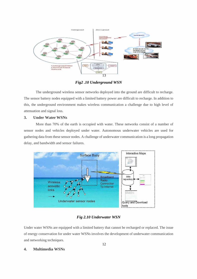
Fig2 .10 Underground WSN
The underground wireless sensor networks deployed into the ground are difficult to recharge.
The sensor battery nodes equipped with a limited battery power are difficult to recharge. In addition to
this, the underground environment makes wireless communication a challenge due to high level of
attenuation and signal loss.
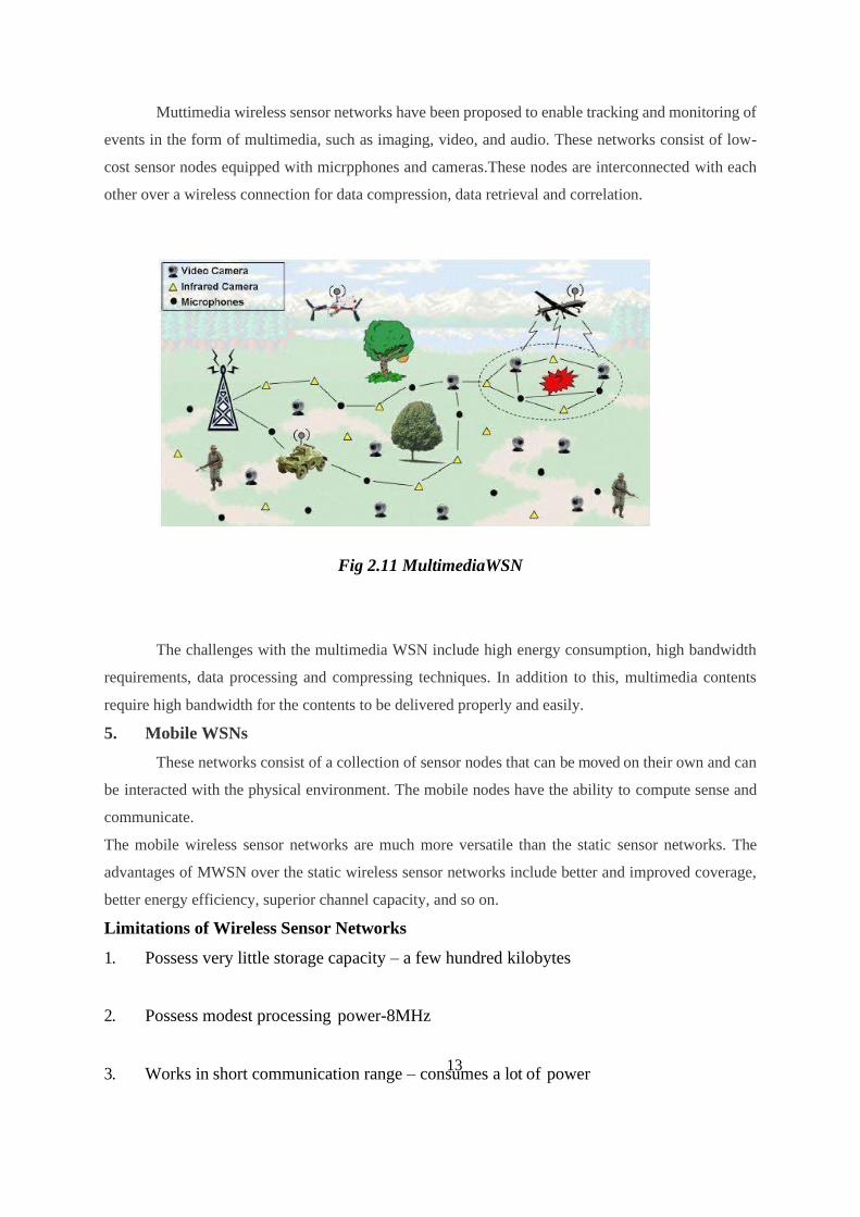
3. Under Water WSNs
More than 70% of the earth is occupied with water. These networks consist of a number of
sensor nodes and vehicles deployed under water. Autonomous underwater vehicles are used for
gathering data from these sensor nodes. A challenge of underwater communication is a long propagation
delay, and bandwidth and sensor failures.
Fig 2.10 Underwater WSN
Under water WSNs are equipped with a limited battery that cannot be recharged or replaced. The issue
of energy conservation for under water WSNs involves the development of underwater communication
and networking techniques.
4. Multimedia WSNs
13
13
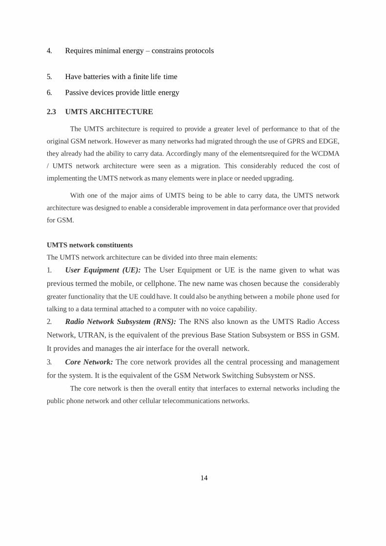
Muttimedia wireless sensor networks have been proposed to enable tracking and monitoring of
events in the form of multimedia, such as imaging, video, and audio. These networks consist of low-
cost sensor nodes equipped with micrpphones and cameras.These nodes are interconnected with each
other over a wireless connection for data compression, data retrieval and correlation.
Fig 2.11 MultimediaWSN
The challenges with the multimedia WSN include high energy consumption, high bandwidth
requirements, data processing and compressing techniques. In addition to this, multimedia contents
require high bandwidth for the contents to be delivered properly and easily.
5. Mobile WSNs
These networks consist of a collection of sensor nodes that can be moved on their own and can
be interacted with the physical environment. The mobile nodes have the ability to compute sense and
communicate.
The mobile wireless sensor networks are much more versatile than the static sensor networks. The
advantages of MWSN over the static wireless sensor networks include better and improved coverage,
better energy efficiency, superior channel capacity, and so on.
Limitations of Wireless Sensor Networks
1. Possess very little storage capacity – a few hundred kilobytes
2. Possess modest processing power-8MHz
3. Works in short communication range – consumes a lot of power
14
4. Requires minimal energy – constrains protocols
5. Have batteries with a finite life time
6. Passive devices provide little energy
2.3 UMTS ARCHITECTURE
The UMTS architecture is required to provide a greater level of performance to that of the
original GSM network. However as many networks had migrated through the use of GPRS and EDGE,
they already had the ability to carry data. Accordingly many of the elementsrequired for the WCDMA
/ UMTS network architecture were seen as a migration. This considerably reduced the cost of
implementing the UMTS network as many elements were in place or needed upgrading.
With one of the major aims of UMTS being to be able to carry data, the UMTS network
architecture was designed to enable a considerable improvement in data performance over that provided
for GSM.
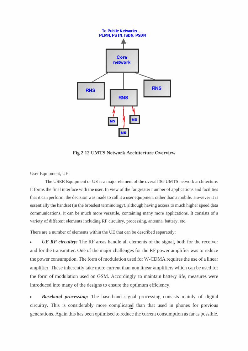
UMTS network constituents
The UMTS network architecture can be divided into three main elements:
1. User Equipment (UE): The User Equipment or UE is the name given to what was
previous termed the mobile, or cellphone. The new name was chosen because the considerably
greater functionality that the UE could have. It could also be anything between a mobile phone used for
talking to a data terminal attached to a computer with no voice capability.
2. Radio Network Subsystem (RNS): The RNS also known as the UMTS Radio Access
Network, UTRAN, is the equivalent of the previous Base Station Subsystem or BSS in GSM.
It provides and manages the air interface for the overall network.
3. Core Network: The core network provides all the central processing and management
for the system. It is the equivalent of the GSM Network Switching Subsystem or NSS.
The core network is then the overall entity that interfaces to external networks including the
public phone network and other cellular telecommunications networks.
15
Fig 2.12 UMTS Network Architecture Overview
User Equipment, UE
The USER Equipment or UE is a major element of the overall 3G UMTS network architecture.
It forms the final interface with the user. In view of the far greater number of applications and facilities
that it can perform, the decision was made to call it a user equipment rather than a mobile. However it is
essentially the handset (in the broadest terminology), although having access to much higher speed data
communications, it can be much more versatile, containing many more applications. It consists of a
variety of different elements including RF circuitry, processing, antenna, battery, etc.
There are a number of elements within the UE that can be described separately:
• UE RF circuitry: The RF areas handle all elements of the signal, both for the receiver
and for the transmitter. One of the major challenges for the RF power amplifier was to reduce
the power consumption. The form of modulation used for W-CDMA requires the use of a linear
amplifier. These inherently take more current than non linear amplifiers which can be used for
the form of modulation used on GSM. Accordingly to maintain battery life, measures were
introduced into many of the designs to ensure the optimum efficiency.
• Baseband processing: The base-band signal processing consists mainly of digital
circuitry. This is considerably more complicated than that used in phones for previous
generations. Again this has been optimised to reduce the current consumption as far as possible.
16
• Battery: While current consumption has been minimised as far as possible within the
circuitry of the phone, there has been an increase in current drain on the battery. With users
expecting the same lifetime between charging batteries as experienced on the previous
generation phones, this has necessitated the use of new and improved battery technology. Now
Lithium Ion (Li-ion) batteries are used. These phones to remain small and relatively light while
still retaining or even improving the overall life between charges.
• Universal Subscriber Identity Module, USIM: The UE also contains a SIM card,
although in the case of UMTS it is termed a USIM (Universal Subscriber Identity Module). This
is a more advanced version of the SIM card used in GSM and other systems, but embodies the
same types of information. It contains the International Mobile Subscriber Identity number
(IMSI) as well as the Mobile Station International ISDN Number (MSISDN). Other
information that the USIM holds includes the preferred language to enable the correct language
information to be displayed, especially when roaming, and a list of preferred and prohibited
Public Land Mobile Networks(PLMN).
The USIM also contains a short message storage area that allows messages to stay with the user
even when the phone is changed. Similarly "phone book" numbers and call information of the numbers
of incoming and outgoing calls are stored.
The UE can take a variety of forms, although the most common format is still a version of a
"mobile phone" although having many data capabilities. Other broadband dongles are also being widely
used.
UMTS Radio Network Subsystem
This is the section of the 3G UMTS / WCDMA network that interfaces to both the UE and the
core network. The overall radio access network, i.e. collectively all the Radio Network Subsystem is
known as the UTRAN UMTS Radio Access Network.
The radio network subsystem is also known as the UMTS Radio Access Network or UTRAN.
3G UMTS Core Network
The 3G UMTS core network architecture is a migration of that used for GSM with further
elements overlaid to enable the additional functionality demanded by UMTS.
In view of the different ways in which data may be carried, the UMTS core network may be
split into two different areas:
• Circuit switched elements: These elements are primarily based on the GSM network
entities and carry data in a circuit switched manner, i.e. a permanent channel for the duration
of the call.
17
• Packet switched elements: These network entities are designed to carry packet data. This
enables much higher network usage as the capacity can be shared and data is carried as packets
which are routed according to their destination.
Some network elements, particularly those that are associated with registration are sharedby
both domains and operate in the same way that they did with GSM.
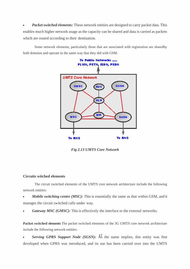
Fig 2.13 UMTS Core Network
Circuits witched elements
The circuit switched elements of the UMTS core network architecture include the following
network entities:
• Mobile switching centre (MSC): This is essentially the same as that within GSM, and it
manages the circuit switched calls under way.
• Gateway MSC (GMSC): This is effectively the interface to the external networks.
Packet switched elements The packet switched elements of the 3G UMTS core network architecture
include the following network entities:
• Serving GPRS Support Node (SGSN): As the name implies, this entity was first
developed when GPRS was introduced, and its use has been carried over into the UMTS
18
network architecture. The SGSN provides a number of functions within the UMTS network
architecture.
o Mobility management When a UE attaches to the Packet Switched domain of the UMTS
Core Network, the SGSN generates MM information based on the mobile's current location.
o Session management: The SGSN manages the data sessions providing the required
quality of service and also managing what are termed the PDP (Packet data Protocol) contexts,
i.e. the pipes over which the data is sent.
o Interaction with other areas of the network: The SGSN is able to manage its elements
within the network only by communicating with other areas of the network, e.g. MSC and other
circuit switched areas.
o Billing: The SGSN is also responsible billing. It achieves this by monitoring the flow of
user data across the GPRS network. CDRs (Call Detail Records) are generated by the SGSN
before being transferred to the charging entities (Charging Gateway Function, CGF).
• Gateway GPRS Support Node (GGSN): Like the SGSN, this entity was also first
introduced into the GPRS network. The Gateway GPRS Support Node (GGSN) is the central
element within the UMTS packet switched network. It handles inter-working between the
UMTS packet switched network and external packet switched networks, and can be considered
as a very sophisticated router. In operation, when the GGSN receives data addressed to a
specific user, it checks if the user is active and then forwards the data to the SGSN serving the
particular UE.
• Shared elements The shared elements of the UMTS core network architecture include
the following network entities:
• Home location register (HLR): This database contains all the administrative
information about each subscriber along with their last known location. In this way, the UMTS
network is able to route calls to the relevant RNC / Node B. When a user switches on their UE,
it registers with the network and from this it is possible to determine which Node B it
communicates with so that incoming calls can be routed appropriately. Even when the UE is
not active (but switched on) it re-registers periodically to ensure that the network (HLR) is
aware of its latest position with their current or last known location on the network.
• Equipment identity register (EIR): The EIR is the entity that decides whether a given
UE equipment may be allowed onto the network. Each UE equipment has a number known as
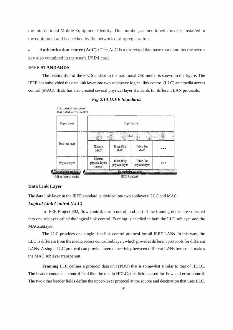
19
the International Mobile Equipment Identity. This number, as mentioned above, is installed in
the equipment and is checked by the network during registration.
• Authentication centre (AuC) : The AuC is a protected database that contains the secret
key also contained in the user's USIM card.
IEEE STANDARDS
The relationship of the 802 Standard to the traditional OSI model is shown in the figure. The
IEEE has subdivided the data link layer into two sublayers: logical link control (LLC) and media access
control (MAC). IEEE has also created several physical layer standards for different LAN protocols.
Fig 2.14 IEEE Standards
Data Link Layer
The data link layer in the IEEE standard is divided into two sublayers: LLC and MAC.
Logical Link Control (LLC)
In IEEE Project 802, flow control, error control, and part of the framing duties are collected
into one sublayer called the logical link control. Framing is handled in both the LLC sublayer and the
MACsublayer.
The LLC provides one single data link control protocol for all IEEE LANs. In this way, the
LLC is different from the media access control sublayer, which provides different protocols for different
LANs. A single LLC protocol can provide interconnectivity between different LANs because it makes
the MAC sublayer transparent.
Framing LLC defines a protocol data unit (PDU) that is somewhat similar to that of HDLC.
The header contains a control field like the one in HDLC; this field is used for flow and error control.
The two other header fields define the upper-layer protocol at the source and destination that uses LLC.
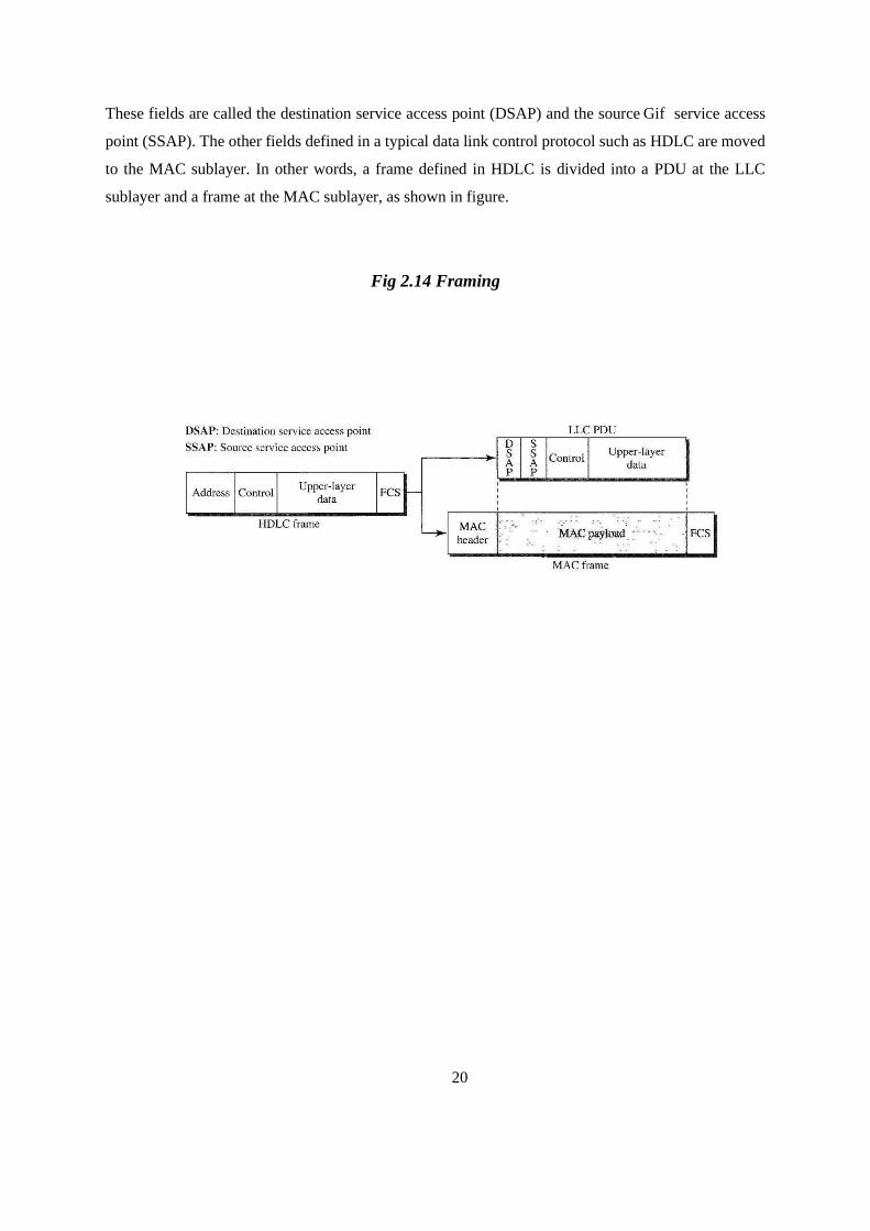
20
These fields are called the destination service access point (DSAP) and the source Gif service access
point (SSAP). The other fields defined in a typical data link control protocol such as HDLC are moved
to the MAC sublayer. In other words, a frame defined in HDLC is divided into a PDU at the LLC
sublayer and a frame at the MAC sublayer, as shown in figure.
Fig 2.14 Framing
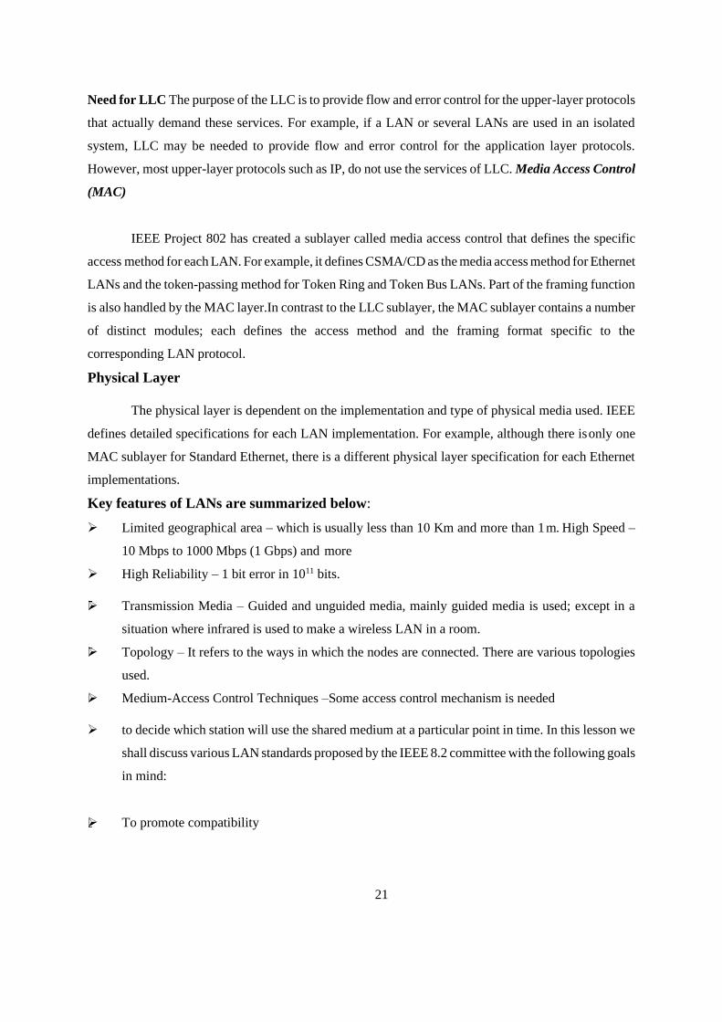
21
Need for LLC The purpose of the LLC is to provide flow and error control for the upper-layer protocols
that actually demand these services. For example, if a LAN or several LANs are used in an isolated
system, LLC may be needed to provide flow and error control for the application layer protocols.
However, most upper-layer protocols such as IP, do not use the services of LLC. Media Access Control
(MAC)
IEEE Project 802 has created a sublayer called media access control that defines the specific
access method for each LAN. For example, it defines CSMA/CD as the media access method for Ethernet
LANs and the token-passing method for Token Ring and Token Bus LANs. Part of the framing function
is also handled by the MAC layer.In contrast to the LLC sublayer, the MAC sublayer contains a number
of distinct modules; each defines the access method and the framing format specific to the
corresponding LAN protocol.
Physical Layer
The physical layer is dependent on the implementation and type of physical media used. IEEE
defines detailed specifications for each LAN implementation. For example, although there is only one
MAC sublayer for Standard Ethernet, there is a different physical layer specification for each Ethernet
implementations.
Key features of LANs are summarized below:
➢ Limited geographical area – which is usually less than 10 Km and more than 1 m. High Speed –
10 Mbps to 1000 Mbps (1 Gbps) and more
➢ High Reliability – 1 bit error in 1011 bits.
➢ Transmission Media – Guided and unguided media, mainly guided media is used; except in a
situation where infrared is used to make a wireless LAN in a room.
➢ Topology – It refers to the ways in which the nodes are connected. There are various topologies
used.
➢ Medium-Access Control Techniques –Some access control mechanism is needed
➢ to decide which station will use the shared medium at a particular point in time. In this lesson we
shall discuss various LAN standards proposed by the IEEE 8.2 committee with the following goals
in mind:
➢ To promote compatibility
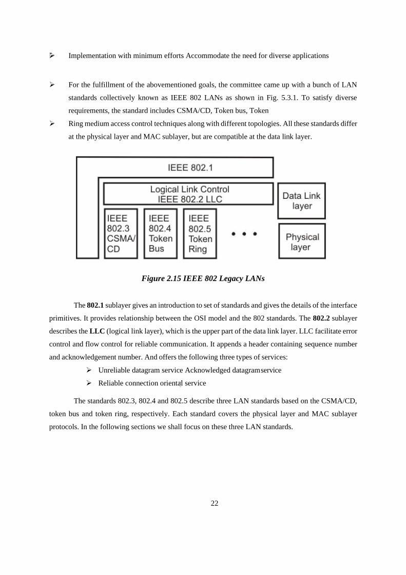
22
➢ Implementation with minimum efforts Accommodate the need for diverse applications
➢ For the fulfillment of the abovementioned goals, the committee came up with a bunch of LAN
standards collectively known as IEEE 802 LANs as shown in Fig. 5.3.1. To satisfy diverse
requirements, the standard includes CSMA/CD, Token bus, Token
➢ Ring medium access control techniques along with different topologies. All these standards differ
at the physical layer and MAC sublayer, but are compatible at the data link layer.
Figure 2.15 IEEE 802 Legacy LANs
The 802.1 sublayer gives an introduction to set of standards and gives the details of the interface
primitives. It provides relationship between the OSI model and the 802 standards. The 802.2 sublayer
describes the LLC (logical link layer), which is the upper part of the data link layer. LLC facilitate error
control and flow control for reliable communication. It appends a header containing sequence number
and acknowledgement number. And offers the following three types of services:
➢ Unreliable datagram service Acknowledged datagram service
➢ Reliable connection oriental service
The standards 802.3, 802.4 and 802.5 describe three LAN standards based on the CSMA/CD,
token bus and token ring, respectively. Each standard covers the physical layer and MAC sublayer
protocols. In the following sections we shall focus on these three LAN standards.
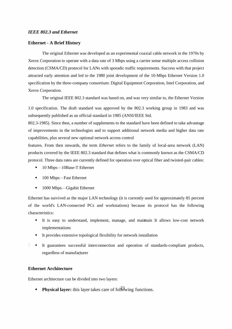
23
IEEE 802.3 and Ethernet
Ethernet - A Brief History
The original Ethernet was developed as an experimental coaxial cable network in the 1970s by
Xerox Corporation to operate with a data rate of 3 Mbps using a carrier sense multiple access collision
detection (CSMA/CD) protocol for LANs with sporadic traffic requirements. Success with that project
attracted early attention and led to the 1980 joint development of the 10-Mbps Ethernet Version 1.0
specification by the three-company consortium: Digital Equipment Corporation, Intel Corporation, and
Xerox Corporation.
The original IEEE 802.3 standard was based on, and was very similar to, the Ethernet Version
1.0 specification. The draft standard was approved by the 802.3 working group in 1983 and was
subsequently published as an official standard in 1985 (ANSI/IEEE Std.
802.3-1985). Since then, a number of supplements to the standard have been defined to take advantage
of improvements in the technologies and to support additional network media and higher data rate
capabilities, plus several new optional network access control
features. From then onwards, the term Ethernet refers to the family of local-area network (LAN)
products covered by the IEEE 802.3 standard that defines what is commonly known as the CSMA/CD
protocol. Three data rates are currently defined for operation over optical fiber and twisted-pair cables:
▪ 10 Mbps—10Base-T Ethernet
▪ 100 Mbps—Fast Ethernet
▪ 1000 Mbps—Gigabit Ethernet
Ethernet has survived as the major LAN technology (it is currently used for approximately 85 percent
of the world's LAN-connected PCs and workstations) because its protocol has the following
characteristics:
▪ It is easy to understand, implement, manage, and maintain It allows low-cost network
implementations
▪ It provides extensive topological flexibility for network installation
▪ It guarantees successful interconnection and operation of standards-compliant products,
regardless of manufacturer
Ethernet Architecture
Ethernet architecture can be divided into two layers:
▪ Physical layer: this layer takes care of following functions.
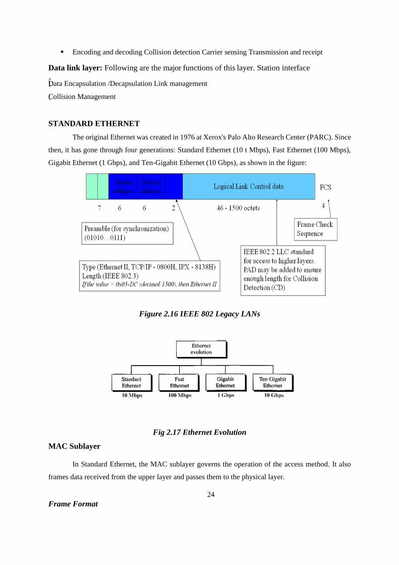
24
▪ Encoding and decoding Collision detection Carrier sensing Transmission and receipt
Data link layer: Following are the major functions of this layer. Station interface
Data Encapsulation /Decapsulation Link management
Collision Management
STANDARD ETHERNET
The original Ethernet was created in 1976 at Xerox's Palo Alto Research Center (PARC). Since
then, it has gone through four generations: Standard Ethernet (10 t Mbps), Fast Ethernet (100 Mbps),
Gigabit Ethernet (1 Gbps), and Ten-Gigabit Ethernet (10 Gbps), as shown in the figure:
Figure 2.16 IEEE 802 Legacy LANs
Fig 2.17 Ethernet Evolution
MAC Sublayer
In Standard Ethernet, the MAC sublayer governs the operation of the access method. It also
frames data received from the upper layer and passes them to the physical layer.
Frame Format
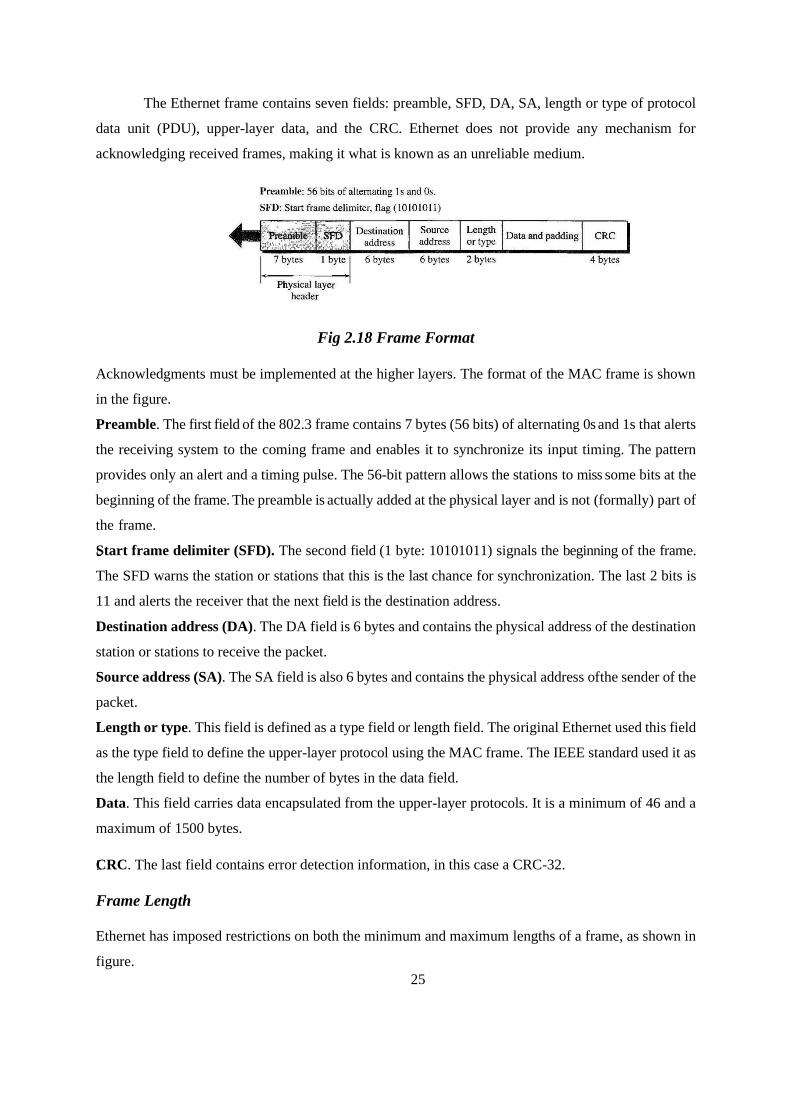
25
The Ethernet frame contains seven fields: preamble, SFD, DA, SA, length or type of protocol
data unit (PDU), upper-layer data, and the CRC. Ethernet does not provide any mechanism for
acknowledging received frames, making it what is known as an unreliable medium.
Fig 2.18 Frame Format
Acknowledgments must be implemented at the higher layers. The format of the MAC frame is shown
in the figure.
Preamble. The first field of the 802.3 frame contains 7 bytes (56 bits) of alternating 0s and 1s that alerts
the receiving system to the coming frame and enables it to synchronize its input timing. The pattern
provides only an alert and a timing pulse. The 56-bit pattern allows the stations to miss some bits at the
beginning of the frame. The preamble is actually added at the physical layer and is not (formally) part of
the frame.
Start frame delimiter (SFD). The second field (1 byte: 10101011) signals the beginning of the frame.
The SFD warns the station or stations that this is the last chance for synchronization. The last 2 bits is
11 and alerts the receiver that the next field is the destination address.
Destination address (DA). The DA field is 6 bytes and contains the physical address of the destination
station or stations to receive the packet.
Source address (SA). The SA field is also 6 bytes and contains the physical address of the sender of the
packet.
Length or type. This field is defined as a type field or length field. The original Ethernet used this field
as the type field to define the upper-layer protocol using the MAC frame. The IEEE standard used it as
the length field to define the number of bytes in the data field.
Data. This field carries data encapsulated from the upper-layer protocols. It is a minimum of 46 and a
maximum of 1500 bytes.
CRC. The last field contains error detection information, in this case a CRC-32.
Frame Length
Ethernet has imposed restrictions on both the minimum and maximum lengths of a frame, as shown in
figure.
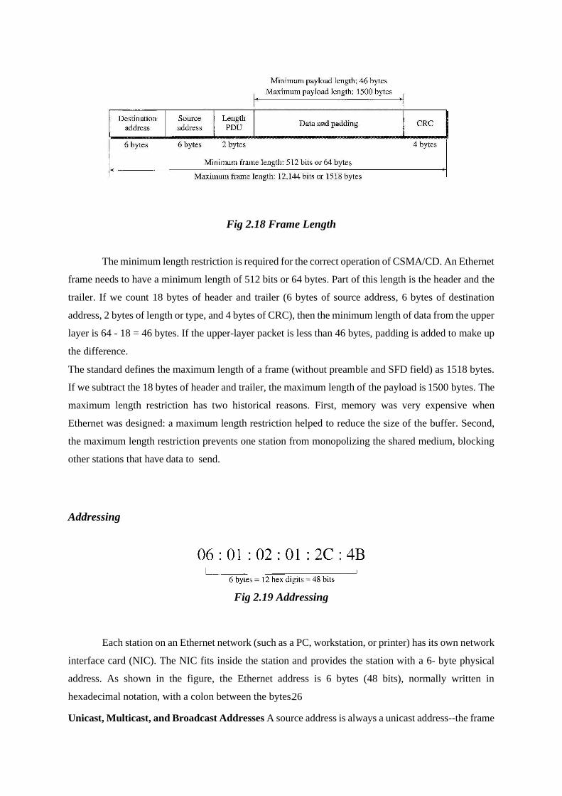
26
Fig 2.18 Frame Length
The minimum length restriction is required for the correct operation of CSMA/CD. An Ethernet
frame needs to have a minimum length of 512 bits or 64 bytes. Part of this length is the header and the
trailer. If we count 18 bytes of header and trailer (6 bytes of source address, 6 bytes of destination
address, 2 bytes of length or type, and 4 bytes of CRC), then the minimum length of data from the upper
layer is 64 - 18 = 46 bytes. If the upper-layer packet is less than 46 bytes, padding is added to make up
the difference.
The standard defines the maximum length of a frame (without preamble and SFD field) as 1518 bytes.
If we subtract the 18 bytes of header and trailer, the maximum length of the payload is 1500 bytes. The
maximum length restriction has two historical reasons. First, memory was very expensive when
Ethernet was designed: a maximum length restriction helped to reduce the size of the buffer. Second,
the maximum length restriction prevents one station from monopolizing the shared medium, blocking
other stations that have data to send.
Addressing
Fig 2.19 Addressing
Each station on an Ethernet network (such as a PC, workstation, or printer) has its own network
interface card (NIC). The NIC fits inside the station and provides the station with a 6- byte physical
address. As shown in the figure, the Ethernet address is 6 bytes (48 bits), normally written in
hexadecimal notation, with a colon between the bytes.
Unicast, Multicast, and Broadcast Addresses A source address is always a unicast address--the frame
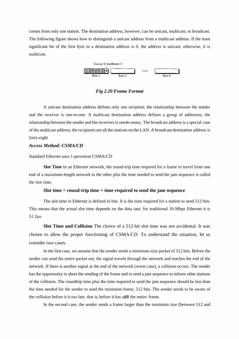
27
comes from only one station. The destination address, however, can be unicast, multicast, or broadcast.
The following figure shows how to distinguish a unicast address from a multicast address. If the least
significant bit of the first byte in a destination address is 0, the address is unicast; otherwise, it is
multicast.
Fig 2.20 Frame Format
A unicast destination address defines only one recipient; the relationship between the sender
and the receiver is one-to-one. A multicast destination address defines a group of addresses; the
relationship between the sender and the receivers is one4o-many. The broadcast address is a special case
of the multicast address; the recipients are all the stations on the LAN. A broadcast destination address is
forty-eight
Access Method: CSMA/CD
Standard Ethernet uses 1-persistent CSMA/CD
Slot Time In an Ethernet network, the round-trip time required for a frame to travel from one
end of a maximum-length network to the other plus the time needed to send the jam sequence is called
the slot time.
Slot time = round-trip time + time required to send the jam sequence
The slot time in Ethernet is defined in bits. It is the time required for a station to send 512 bits.
This means that the actual slot time depends on the data rate; for traditional 10-Mbps Ethernet it is
51.2µs.
Slot Time and Collision The choice of a 512-bit slot time was not accidental. It was
chosen to allow the proper functioning of CSMA/CD. To understand the situation, let us
consider two cases.
In the first case, we assume that the sender sends a minimum-size packet of 512 bits. Before the
sender can send the entire packet out, the signal travels through the network and reaches the end of the
network. If there is another signal at the end of the network (worst case), a collision occurs. The sender
has the opportunity to abort the sending of the frame and to send a jam sequence to inform other stations
of the collision. The roundtrip time plus the time required to send the jam sequence should be less than
the time needed for the sender to send the minimum frame, 512 bits. The sender needs to be aware of
the collision before it is too late, that is, before it has sent the entire frame.
In the second case, the sender sends a frame larger than the minimum size (between 512 and
28
1518 bits). In this case, if the station has sent out the first 512 bits and has not heard a collision, it is
guaranteed that collision will never occur during the transmission of this frame. The reason is that the
signal will reach the end of the network in less than one-half the slot time. If all stations follow the
CSMA/CD protocol, they have already sensed the existence of the signal (carrier) on the line and have
refrained from sending. If they sent a signal on the line before one- half of the slot time expired, a
collision has occurred and the sender has sensed the collision. In other words, collision can only occur
during the first half of the slot time, and if it does, it can be sensed by the sender during the slot time.
This means that after the sender sends the first 512 bits, it is guaranteed that collision will not occur
during the transmission of this frame. The medium belongs to the sender, and no other station will use
it. In other words, the sender needs to listen for a collision only during the time the first 512 bits are
sent.
Slot Time and Maximum Network Length There is a relationship between the slot time and the
maximum length of the network (collision domain). It is dependent on the propagation speed of the
signal in the particular medium. In most transmission media, the signal propagates at 2 x10⁸ m/s (two-
thirds of the rate for propagation in air). For traditional Ethernet, we calculate Of course, we need to
consider the delay times in repeaters and interfaces, and the time required to send the jam sequence.
These reduce the maximum-length of a traditional Ethernet network to 2500 m, just 48 percent of the
theoretical calculation.
MaxLength = 2500 m
Physical Layer
The Standard Ethernet defines several physical layer implementations; four of the most
common, are shown in figure.Because Ethernet devices implement only the bottom two layers of the
OSI protocol stack, they are typically implemented as network interface cards (NICs) that plug into the
host device's motherboard, or presently built-in in the motherboard. Various types cabling supported by
the standard are shown in Fig. 5.3.2. The naming convention is a concatenation of three terms indicating
the transmission rate, the transmission method, and the media type/signal encoding. Consider for
example, 10Base-T. where 10 implies transmission rate of 10 Mbps, Base represents that it uses
baseband signaling, and T refers to twisted-pair cables as transmission media. Various standards are
discussed below:
Encoding and Decoding
All standard implementations use digital signaling (baseband) at 10 Mbps. At the sender, data
are converted to a digital signal using the Manchester scheme; at the receiver, the received signal is
interpreted as Manchester and decoded into data. The figure shows the encoding scheme for Standard
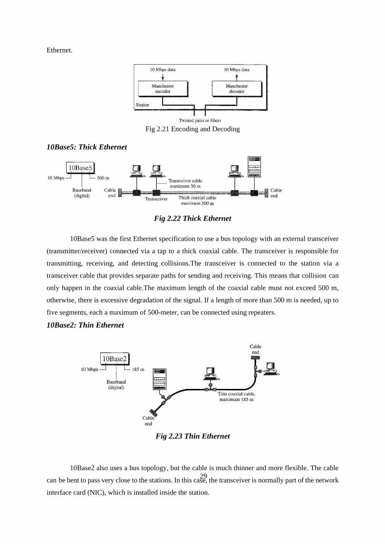
29
Ethernet.
Fig 2.21 Encoding and Decoding
10Base5: Thick Ethernet
Fig 2.22 Thick Ethernet
10Base5 was the first Ethernet specification to use a bus topology with an external transceiver
(transmitter/receiver) connected via a tap to a thick coaxial cable. The transceiver is responsible for
transmitting, receiving, and detecting collisions.The transceiver is connected to the station via a
transceiver cable that provides separate paths for sending and receiving. This means that collision can
only happen in the coaxial cable.The maximum length of the coaxial cable must not exceed 500 m,
otherwise, there is excessive degradation of the signal. If a length of more than 500 m is needed, up to
five segments, each a maximum of 500-meter, can be connected using repeaters.
10Base2: Thin Ethernet
Fig 2.23 Thin Ethernet
10Base2 also uses a bus topology, but the cable is much thinner and more flexible. The cable
can be bent to pass very close to the stations. In this case, the transceiver is normally part of the network
interface card (NIC), which is installed inside the station.
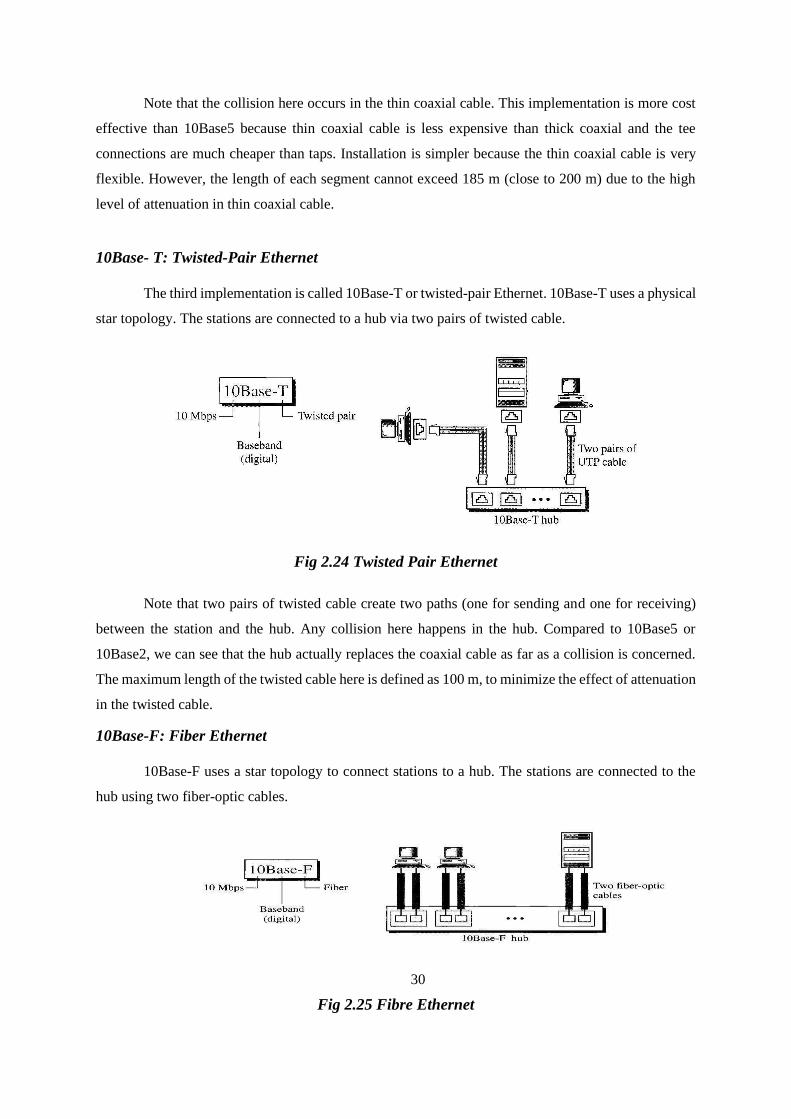
30
Note that the collision here occurs in the thin coaxial cable. This implementation is more cost
effective than 10Base5 because thin coaxial cable is less expensive than thick coaxial and the tee
connections are much cheaper than taps. Installation is simpler because the thin coaxial cable is very
flexible. However, the length of each segment cannot exceed 185 m (close to 200 m) due to the high
level of attenuation in thin coaxial cable.
10Base- T: Twisted-Pair Ethernet
The third implementation is called 10Base-T or twisted-pair Ethernet. 10Base-T uses a physical
star topology. The stations are connected to a hub via two pairs of twisted cable.
Fig 2.24 Twisted Pair Ethernet
Note that two pairs of twisted cable create two paths (one for sending and one for receiving)
between the station and the hub. Any collision here happens in the hub. Compared to 10Base5 or
10Base2, we can see that the hub actually replaces the coaxial cable as far as a collision is concerned.
The maximum length of the twisted cable here is defined as 100 m, to minimize the effect of attenuation
in the twisted cable.
10Base-F: Fiber Ethernet
10Base-F uses a star topology to connect stations to a hub. The stations are connected to the
hub using two fiber-optic cables.
Fig 2.25 Fibre Ethernet
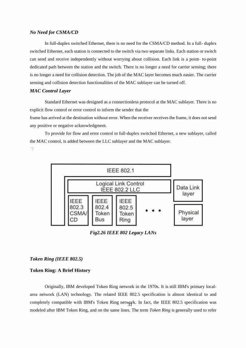
31
No Need for CSMA/CD
In full-duplex switched Ethernet, there is no need for the CSMA/CD method. In a full- duplex
switched Ethernet, each station is connected to the switch via two separate links. Each station or switch
can send and receive independently without worrying about collision. Each link is a point- to-point
dedicated path between the station and the switch. There is no longer a need for carrier sensing; there
is no longer a need for collision detection. The job of the MAC layer becomes much easier. The carrier
sensing and collision detection functionalities of the MAC sublayer can be turned off.
MAC Control Layer
Standard Ethernet was designed as a connectionless protocol at the MAC sublayer. There is no
explicit flow control or error control to inform the sender that the
frame has arrived at the destination without error. When the receiver receives the frame, it does not send
any positive or negative acknowledgment.
To provide for flow and error control in full-duplex switched Ethernet, a new sublayer, called
the MAC control, is added between the LLC sublayer and the MAC sublayer.
Fig2.26 IEEE 802 Legacy LANs
Token Ring (IEEE 802.5)
Token Ring: A Brief History
Originally, IBM developed Token Ring network in the 1970s. It is still IBM's primary local-
area network (LAN) technology. The related IEEE 802.5 specification is almost identical to and
completely compatible with IBM's Token Ring network. In fact, the IEEE 802.5 specification was
modeled after IBM Token Ring, and on the same lines. The term Token Ring is generally used to refer
32
to both IBM's Token Ring network and IEEE 802.5 networks.
Before going into the details of the Token Ring protocol, let’s first discuss the motivation
behind it. As already discussed, the medium access mechanism used by Ethernet (CSMA/CD) may
results in collision. Nodes attempt to a number of times before they can actually transmit, and even
when they start transmitting there are chances to encounter collisions and entire transmission need to
be repeated. And all this become worse one the traffic is heavy i.e. all nodes have some data to transmit.
Apart from this there is no way to predict either the occurrence of collision or delays produced by
multiple stations attempting to capture the link at the same time. So all these problems with the Ethernet
gives way to an alternate LAN technology, Token Ring. Token Ring and IEEE802.5 are based on token
passing MAC protocol with ring topology. They resolve the uncertainty by giving each station a turn
on by one. Each node takes turns sending the data; each station may transmit data during its turn. The
technique that coordinates this turn mechanism is called Token passing; as a Token is passed in the
network and the station that gets the token can only transmit. As one node transmits at a time, there is
no chance of collision. We shall discuss the detailed operation in next section.
Stations are connected by point-to-point links using repeaters. Mainly these links are of shielded
twisted-pair cables. The repeaters function in two basic modes: Listen mode, Transmit mode. A
disadvantage of this topology is that it is vulnerable to link or station failure. But a few measures can
be taken to take care of it.
TEXT / REFERENCE BOOKS
1. Andrew S Tanenbaum “Computer Networks” 5th Edition. Pearson Education/PH I/2011.
2. Behrouz A. Forouzan, “Data Communications and Networking” Fourth Edition, Mc
GrawHill HIGHER Education 2007.
3. Michael A.Gallo, William Hancock.M, Brooks/Cole Computer
Communications and Networking Technologies,2001
4. Richard Lai and Jirachief pattana, “Communication Protocol Specification and
Verification”, Kluwer Publishers, Boston, 1998.
5. Pallapa Venkataram and Sunilkumar S.Manvi, “Communication protocol Engineering”,
PHI Learning, 2008
1
SCHOOL OF ELECTRICAL AND ELECTRONICS ENGINEERING
DEPARTMENT OF ELECTRONICS AND COMMUNICATION ENGINEERING
UNIT – III COMPUTER NETWORKS-
SECA1604
2
UNIT III PHYSICAL LAYER AND DATALINK LAYER
Design Factors for Transmission Media
Bandwidth: All other factors remaining constant, the greater the band-width of a signal, the higher the
data rate that can be achieved.
Transmission impairments: Limit the distance a signal can travel.
Interference: Competing signals in overlapping frequency bands can distort or wipe out a signal.
Number of receivers: Each attachment introduces some attenuation and distortion, limiting distance
and/or data rate.
TYPES OF TRANSMISSION MEDIA
1. Conducted or Guided Media :
Use a conductor such as a wire or a fiber optic cable to move the signal from sender to receiver.
2. Wireless or Unguided Media:
Use radio waves of different frequencies and do not need a wire or cable conductor to transmit
signals.
Guided Transmission Media
Guided media includes everything that ‘guides’ the transmission. That usually takes the form
of some sort of a wire. Usually copper, but can also be an optical fiber.
Transmission capacity depends on the distance and on whether the medium is point-to-point or
multipoint. Ex: twisted pair wires, coaxial cables, optical fiber
Twisted Pair Wires
A transmission medium consisting of pairs of twisted copper wires arranged in a regular spiral
pattern to minimize the electromagnetic interference between adjacent pairs .Often used at customer
facilities and also over distances to carry voice as well as data communications .Low frequency
transmission medium.
We can transmit 1 Mbps over short distances (less than 100m). They are mainly used to transmit
analog signals, but they can be used for digital signals.
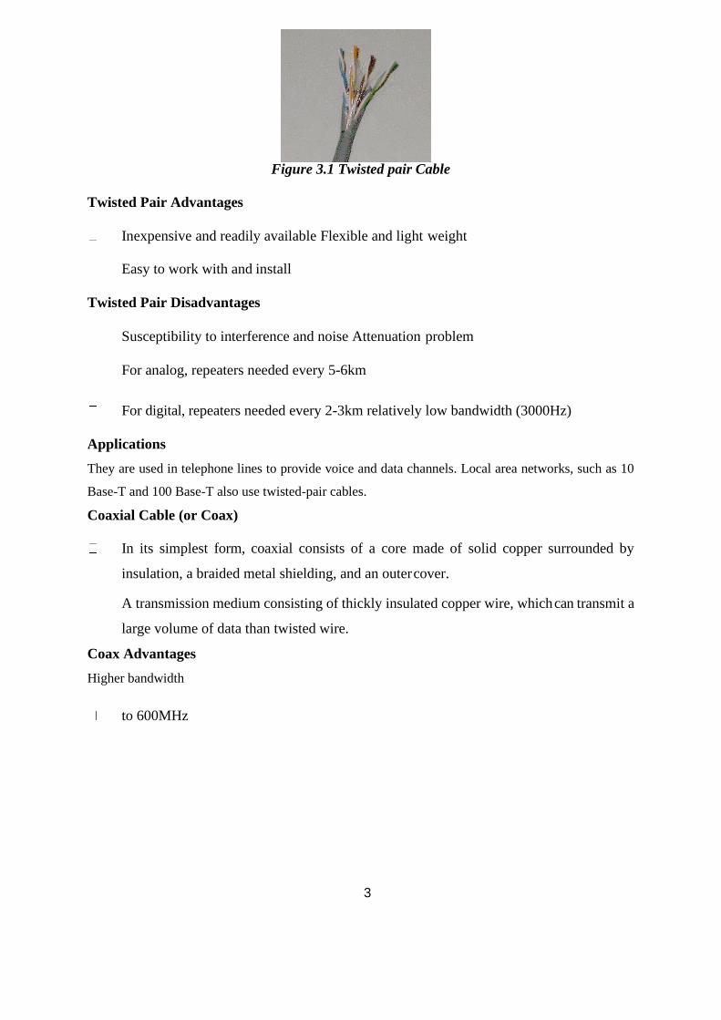
3
Figure 3.1 Twisted pair Cable
Twisted Pair Advantages
Inexpensive and readily available Flexible and light weight
Easy to work with and install
Twisted Pair Disadvantages
Susceptibility to interference and noise Attenuation problem
For analog, repeaters needed every 5-6km
For digital, repeaters needed every 2-3km relatively low bandwidth (3000Hz)
Applications
They are used in telephone lines to provide voice and data channels. Local area networks, such as 10
Base-T and 100 Base-T also use twisted-pair cables.
Coaxial Cable (or Coax)
In its simplest form, coaxial consists of a core made of solid copper surrounded by
insulation, a braided metal shielding, and an outer cover.
A transmission medium consisting of thickly insulated copper wire, which can transmit a
large volume of data than twisted wire.
Coax Advantages
Higher bandwidth
to 600MHz
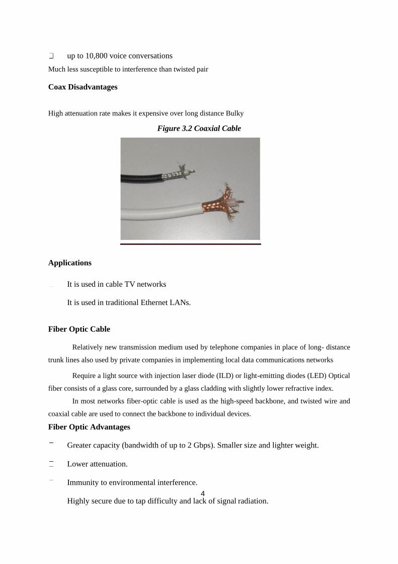
4
up to 10,800 voice conversations
Much less susceptible to interference than twisted pair
Coax Disadvantages
High attenuation rate makes it expensive over long distance Bulky
Figure 3.2 Coaxial Cable
Applications
It is used in cable TV networks
It is used in traditional Ethernet LANs.
Fiber Optic Cable
Relatively new transmission medium used by telephone companies in place of long- distance
trunk lines also used by private companies in implementing local data communications networks
Require a light source with injection laser diode (ILD) or light-emitting diodes (LED) Optical
fiber consists of a glass core, surrounded by a glass cladding with slightly lower refractive index.
In most networks fiber-optic cable is used as the high-speed backbone, and twisted wire and
coaxial cable are used to connect the backbone to individual devices.
Fiber Optic Advantages
Greater capacity (bandwidth of up to 2 Gbps). Smaller size and lighter weight.
Lower attenuation.
Immunity to environmental interference.
Highly secure due to tap difficulty and lack of signal radiation.
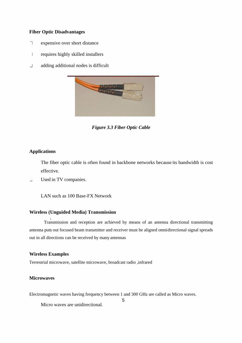
5
Fiber Optic Disadvantages
expensive over short distance
requires highly skilled installers
adding additional nodes is difficult
Figure 3.3 Fiber Optic Cable
Applications
The fiber optic cable is often found in backbone networks because its bandwidth is cost
effective.
Used in TV companies.
LAN such as 100 Base-FX Network
Wireless (Unguided Media) Transmission
Transmission and reception are achieved by means of an antenna directional transmitting
antenna puts out focused beam transmitter and receiver must be aligned omni directional signal spreads
out in all directions can be received by many antennas
Wireless Examples
Terrestrial microwave, satellite microwave, broadcast radio ,infrared
Microwaves
Electromagnetic waves having frequency between 1 and 300 GHz are called as Micro waves.
Micro waves are unidirectional.
6
Microwave propagation is line of sight.
Very high frequency Micro waves cannot penetrate walls.
The microwave band is relatively wide, almost 299 GHz
Terrestrial Microwave
Used for long-distance telephone service.
Uses radio frequency spectrum, from 2 to 40 Ghz.
Parabolic dish transmitter, mounted high.
Used by common carriers as well as private networks.
Requires unobstructed line of sight between source and receiver.
Curvature of the earth requires stations (repeaters) ~30 miles apart.
Satellite Microwave
A microwave relay station in space can relay signals over long distances geostationary
satellites
remain above the equator at a height of 22,300 miles (geosynchronous orbit)
travel around the earth in exactly the time the earth takes to rotate
Applications
• They are used in Cellular phones.
• They are used in satellite networks.
• They are used in wireless LANs.
7
Radio Waves Application
1. The omnidirectional characteristics of Radio waves make them useful for multicasting,
in which there is one sender but many receivers.
2. AM and FM Radio, television, maritime radio, cordless phone, and paging are examples
of multicasting.
PSTN
The public switched telephone network (PSTN) is the aggregate of the world's circuit- switched
telephone networks that are operated by national, regional, or local telephony operators, providing
infrastructure and services for public telecommunication. The PSTN consists of telephone lines, fiber
optic cables, microwave transmission links, cellular networks, communications satellites, and undersea
telephone cables, all interconnected by switching centers, thus allowing most telephones to communicate
with each other. Originally a network of fixed-line analog telephone systems, the PSTN is now almost
entirely digital in its core network and includes mobile and other networks, as well as fixed telephones.
The technical operation of the PSTN adheres to the standards created by the ITU-T. These standards
allow different networks in different countries to interconnect seamlessly. The E.163 and E.164
standards provide a single global address space for telephone numbers. The combination of the
interconnected networks and the single numbering plan allow telephones around the world to dial each
other.
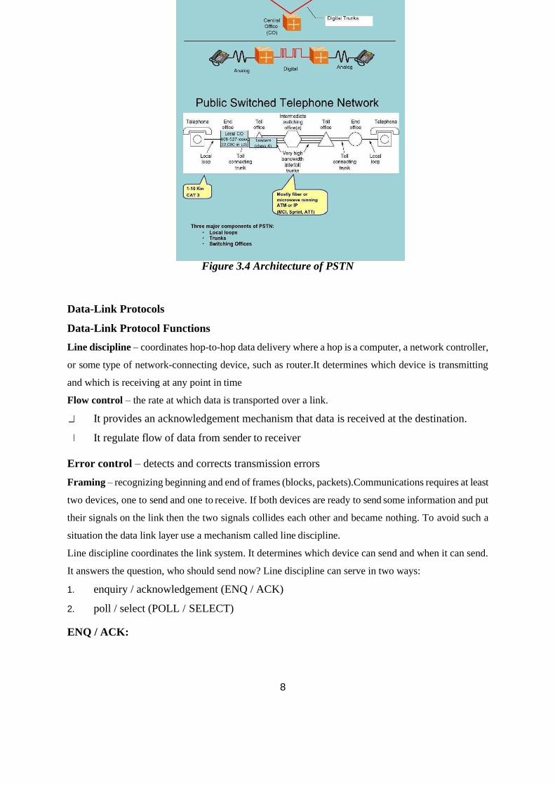
8
Figure 3.4 Architecture of PSTN
Data-Link Protocols
Data-Link Protocol Functions
Line discipline – coordinates hop-to-hop data delivery where a hop is a computer, a network controller,
or some type of network-connecting device, such as router.It determines which device is transmitting
and which is receiving at any point in time
Flow control – the rate at which data is transported over a link.
It provides an acknowledgement mechanism that data is received at the destination.
It regulate flow of data from sender to receiver
Error control – detects and corrects transmission errors
Framing – recognizing beginning and end of frames (blocks, packets).Communications requires at least
two devices, one to send and one to receive. If both devices are ready to send some information and put
their signals on the link then the two signals collides each other and became nothing. To avoid such a
situation the data link layer use a mechanism called line discipline.
Line discipline coordinates the link system. It determines which device can send and when it can send.
It answers the question, who should send now? Line discipline can serve in two ways:
1. enquiry / acknowledgement (ENQ / ACK)
2. poll / select (POLL / SELECT)
ENQ / ACK:
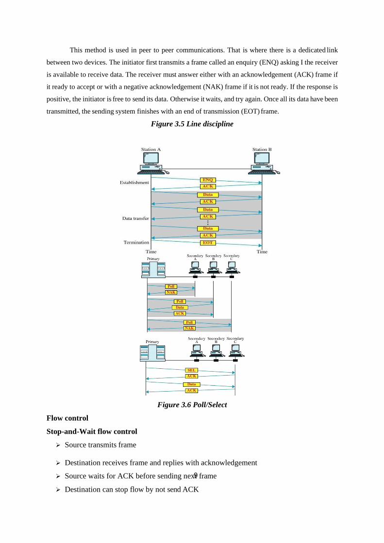
9
This method is used in peer to peer communications. That is where there is a dedicated link
between two devices. The initiator first transmits a frame called an enquiry (ENQ) asking I the receiver
is available to receive data. The receiver must answer either with an acknowledgement (ACK) frame if
it ready to accept or with a negative acknowledgement (NAK) frame if it is not ready. If the response is
positive, the initiator is free to send its data. Otherwise it waits, and try again. Once all its data have been
transmitted, the sending system finishes with an end of transmission (EOT) frame.
Figure 3.5 Line discipline
Figure 3.6 Poll/Select
Flow control
Stop-and-Wait flow control
➢ Source transmits frame
➢ Destination receives frame and replies with acknowledgement
➢ Source waits for ACK before sending next frame
➢ Destination can stop flow by not send ACK
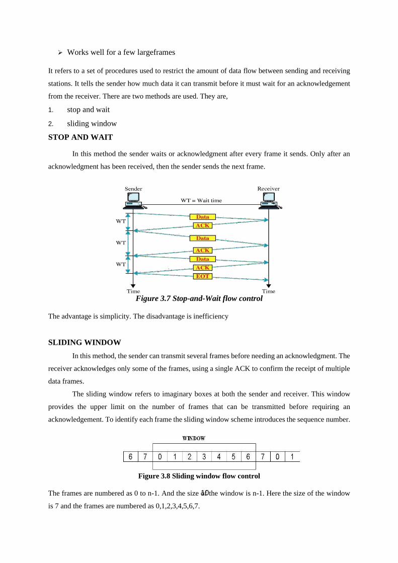
10
➢ Works well for a few largeframes
It refers to a set of procedures used to restrict the amount of data flow between sending and receiving
stations. It tells the sender how much data it can transmit before it must wait for an acknowledgement
from the receiver. There are two methods are used. They are,
1. stop and wait
2. sliding window
STOP AND WAIT
In this method the sender waits or acknowledgment after every frame it sends. Only after an
acknowledgment has been received, then the sender sends the next frame.
Figure 3.7 Stop-and-Wait flow control
The advantage is simplicity. The disadvantage is inefficiency
SLIDING WINDOW
In this method, the sender can transmit several frames before needing an acknowledgment. The
receiver acknowledges only some of the frames, using a single ACK to confirm the receipt of multiple
data frames.
The sliding window refers to imaginary boxes at both the sender and receiver. This window
provides the upper limit on the number of frames that can be transmitted before requiring an
acknowledgement. To identify each frame the sliding window scheme introduces the sequence number.
Figure 3.8 Sliding window flow control
The frames are numbered as 0 to n-1. And the size of the window is n-1. Here the size of the window
is 7 and the frames are numbered as 0,1,2,3,4,5,6,7.
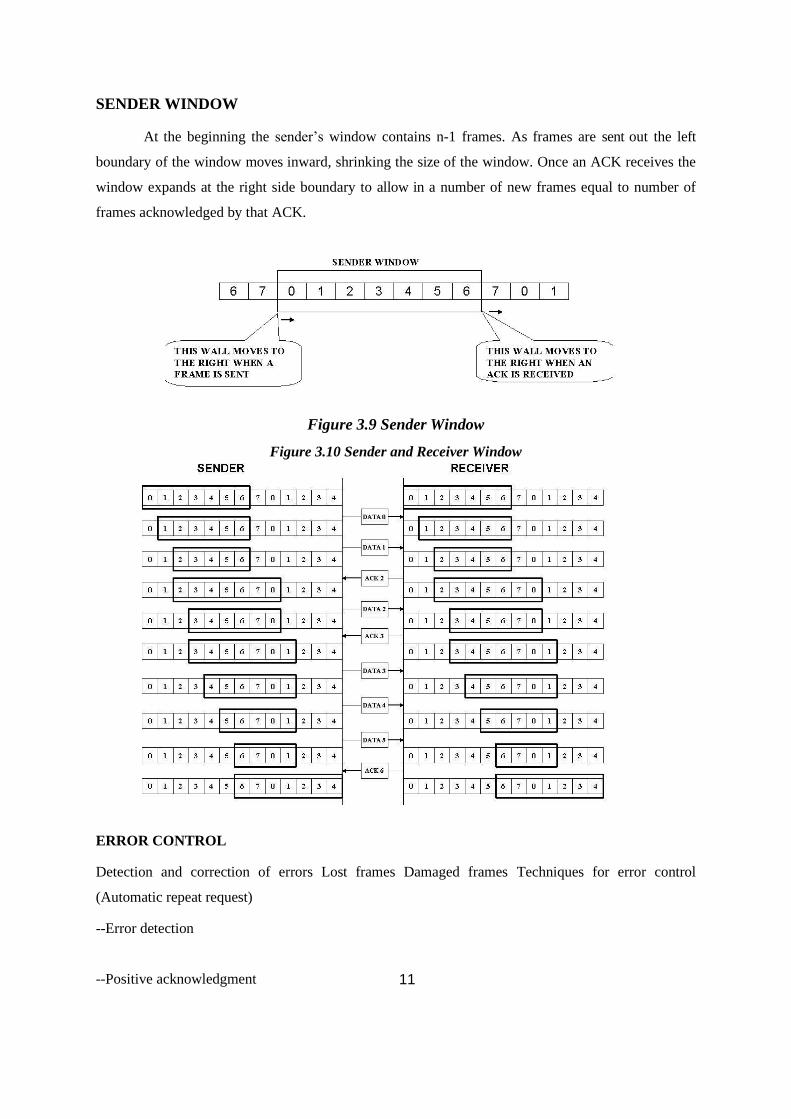
11
SENDER WINDOW
At the beginning the sender’s window contains n-1 frames. As frames are sent out the left
boundary of the window moves inward, shrinking the size of the window. Once an ACK receives the
window expands at the right side boundary to allow in a number of new frames equal to number of
frames acknowledged by that ACK.
Figure 3.9 Sender Window
Figure 3.10 Sender and Receiver Window
ERROR CONTROL
Detection and correction of errors Lost frames Damaged frames Techniques for error control
(Automatic repeat request)
--Error detection
--Positive acknowledgment
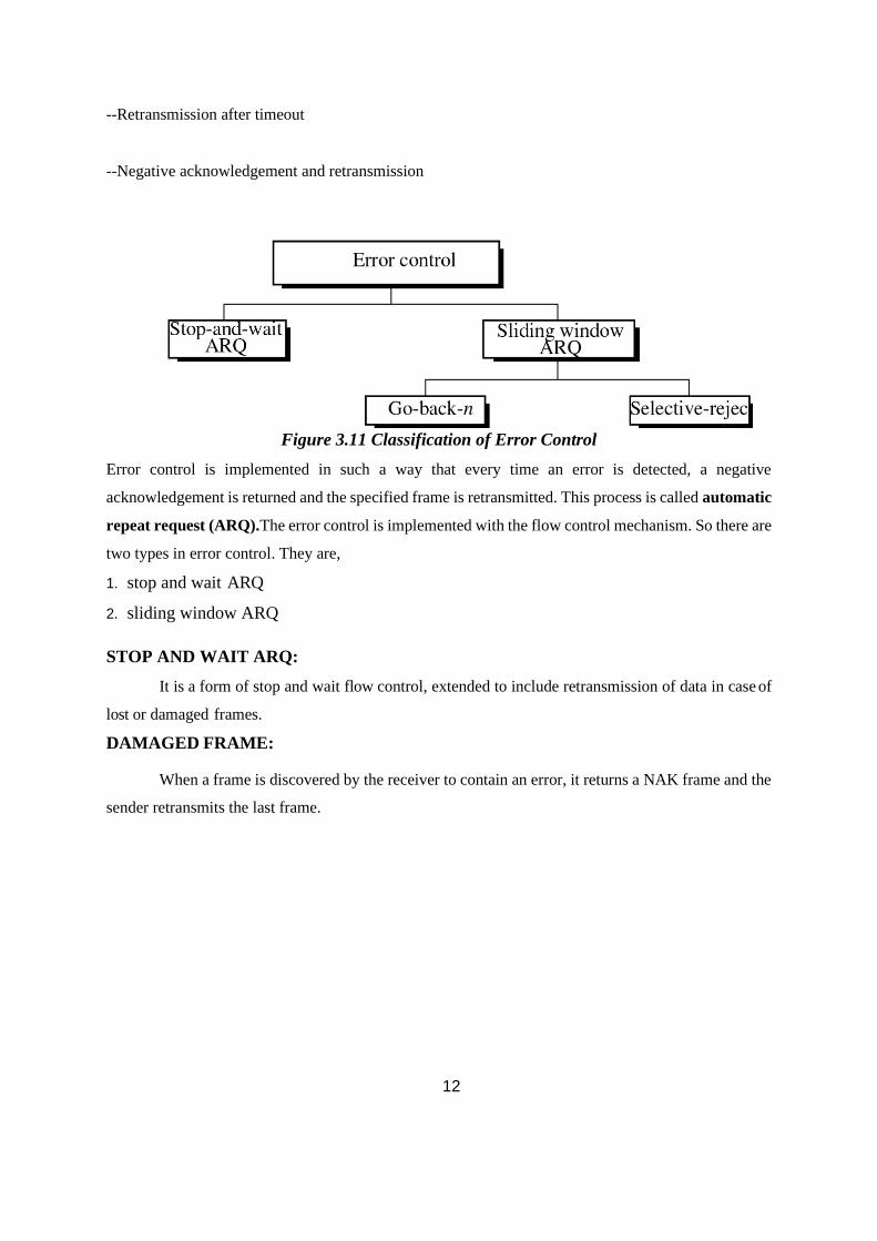
12
--Retransmission after timeout
--Negative acknowledgement and retransmission
Figure 3.11 Classification of Error Control
Error control is implemented in such a way that every time an error is detected, a negative
acknowledgement is returned and the specified frame is retransmitted. This process is called automatic
repeat request (ARQ).The error control is implemented with the flow control mechanism. So there are
two types in error control. They are,
1. stop and wait ARQ
2. sliding window ARQ
STOP AND WAIT ARQ:
It is a form of stop and wait flow control, extended to include retransmission of data in case of
lost or damaged frames.
DAMAGED FRAME:
When a frame is discovered by the receiver to contain an error, it returns a NAK frame and the
sender retransmits the last frame.
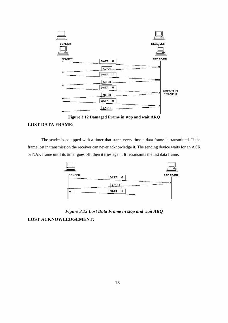
13
Figure 3.12 Damaged Frame in stop and wait ARQ
LOST DATA FRAME:
The sender is equipped with a timer that starts every time a data frame is transmitted. If the
frame lost in transmission the receiver can never acknowledge it. The sending device waits for an ACK
or NAK frame until its timer goes off, then it tries again. It retransmits the last data frame.
Figure 3.13 Lost Data Frame in stop and wait ARQ
LOST ACKNOWLEDGEMENT:
15
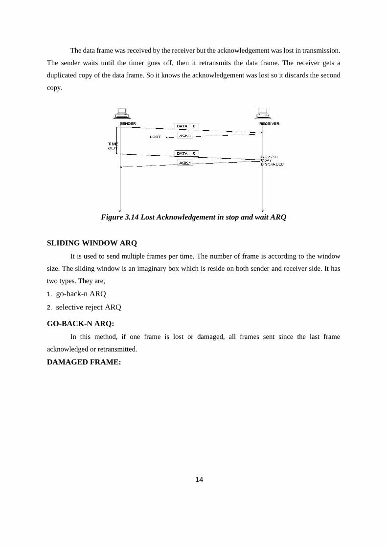
14
The data frame was received by the receiver but the acknowledgement was lost in transmission.
The sender waits until the timer goes off, then it retransmits the data frame. The receiver gets a
duplicated copy of the data frame. So it knows the acknowledgement was lost so it discards the second
copy.
Figure 3.14 Lost Acknowledgement in stop and wait ARQ
SLIDING WINDOW ARQ
It is used to send multiple frames per time. The number of frame is according to the window
size. The sliding window is an imaginary box which is reside on both sender and receiver side. It has
two types. They are,
1. go-back-n ARQ
2. selective reject ARQ
GO-BACK-N ARQ:
In this method, if one frame is lost or damaged, all frames sent since the last frame
acknowledged or retransmitted.
DAMAGED FRAME:
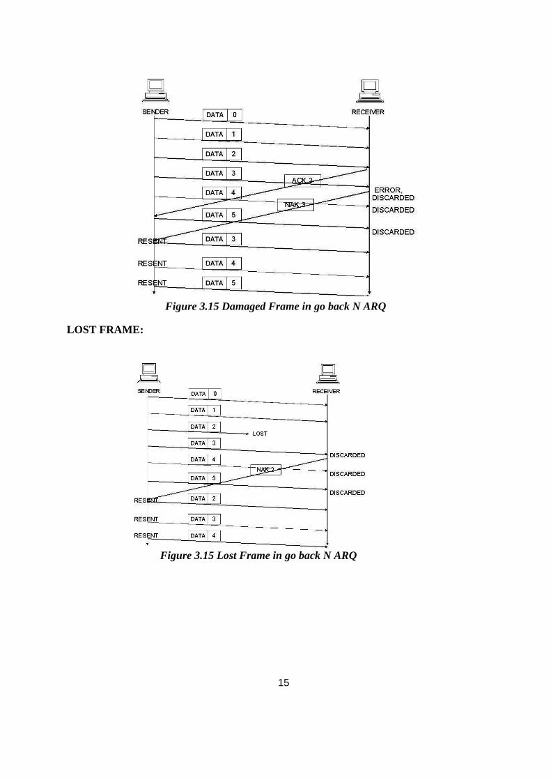
15
Figure 3.15 Damaged Frame in go back N ARQ
LOST FRAME:
Figure 3.15 Lost Frame in go back N ARQ
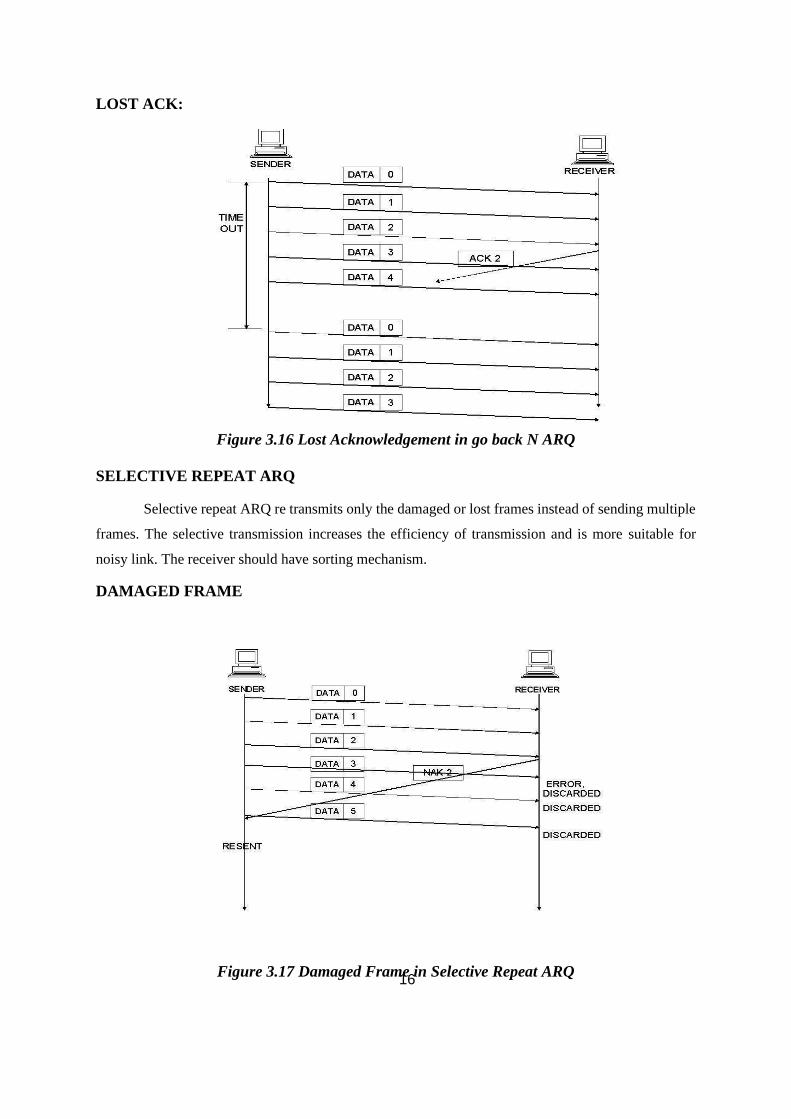
16
LOST ACK:
Figure 3.16 Lost Acknowledgement in go back N ARQ
SELECTIVE REPEAT ARQ
Selective repeat ARQ re transmits only the damaged or lost frames instead of sending multiple
frames. The selective transmission increases the efficiency of transmission and is more suitable for
noisy link. The receiver should have sorting mechanism.
DAMAGED FRAME
Figure 3.17 Damaged Frame in Selective Repeat ARQ
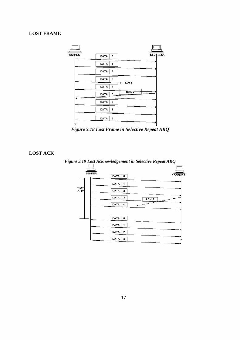
17
LOST FRAME
Figure 3.18 Lost Frame in Selective Repeat ARQ
LOST ACK
Figure 3.19 Lost Acknowledgement in Selective Repeat ARQ
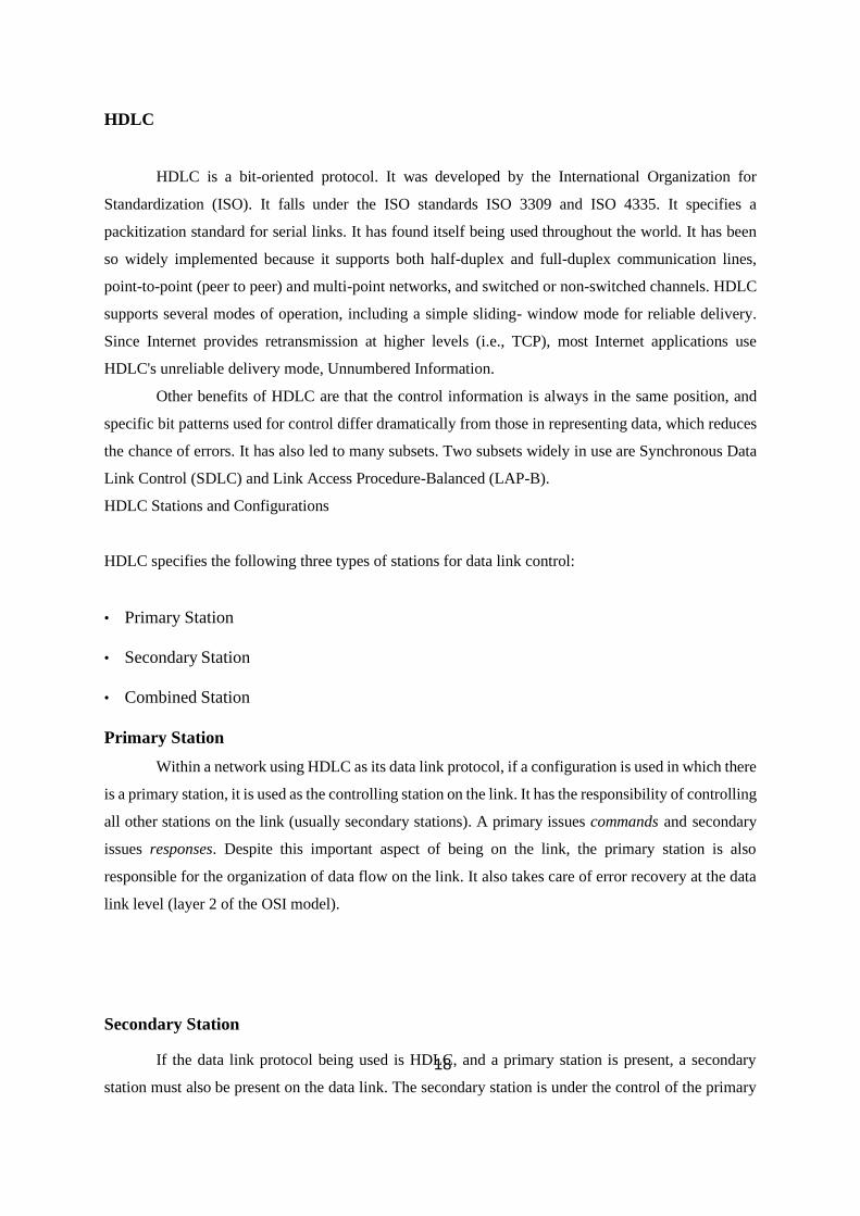
18
HDLC
HDLC is a bit-oriented protocol. It was developed by the International Organization for
Standardization (ISO). It falls under the ISO standards ISO 3309 and ISO 4335. It specifies a
packitization standard for serial links. It has found itself being used throughout the world. It has been
so widely implemented because it supports both half-duplex and full-duplex communication lines,
point-to-point (peer to peer) and multi-point networks, and switched or non-switched channels. HDLC
supports several modes of operation, including a simple sliding- window mode for reliable delivery.
Since Internet provides retransmission at higher levels (i.e., TCP), most Internet applications use
HDLC's unreliable delivery mode, Unnumbered Information.
Other benefits of HDLC are that the control information is always in the same position, and
specific bit patterns used for control differ dramatically from those in representing data, which reduces
the chance of errors. It has also led to many subsets. Two subsets widely in use are Synchronous Data
Link Control (SDLC) and Link Access Procedure-Balanced (LAP-B).
HDLC Stations and Configurations
HDLC specifies the following three types of stations for data link control:
• Primary Station
• Secondary Station
• Combined Station
Primary Station
Within a network using HDLC as its data link protocol, if a configuration is used in which there
is a primary station, it is used as the controlling station on the link. It has the responsibility of controlling
all other stations on the link (usually secondary stations). A primary issues commands and secondary
issues responses. Despite this important aspect of being on the link, the primary station is also
responsible for the organization of data flow on the link. It also takes care of error recovery at the data
link level (layer 2 of the OSI model).
Secondary Station
If the data link protocol being used is HDLC, and a primary station is present, a secondary
station must also be present on the data link. The secondary station is under the control of the primary
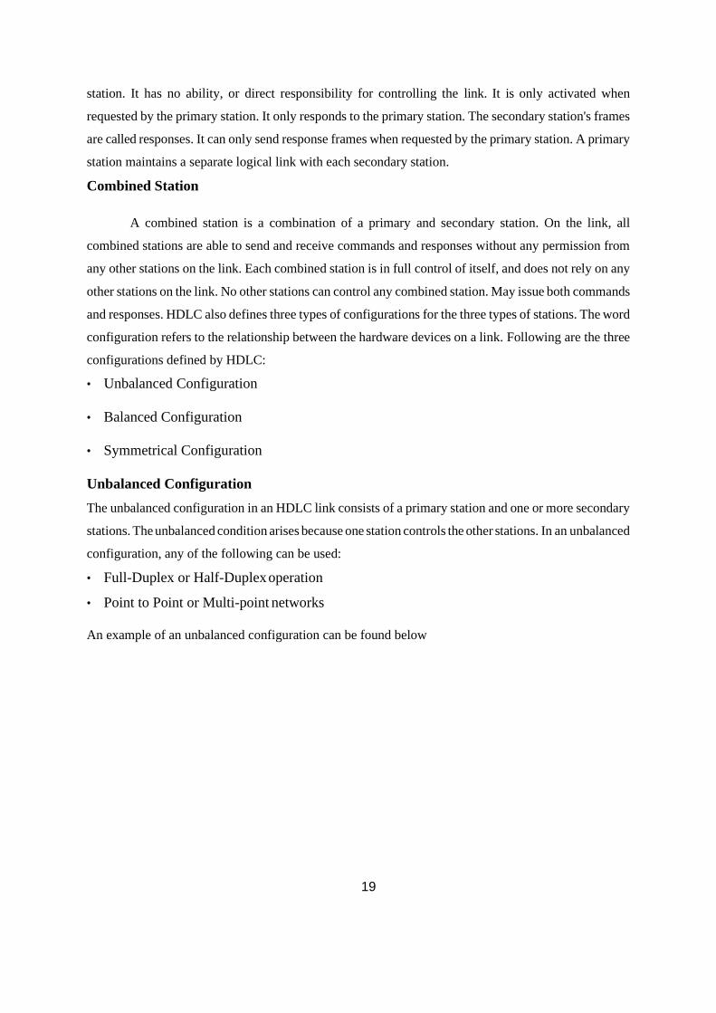
19
station. It has no ability, or direct responsibility for controlling the link. It is only activated when
requested by the primary station. It only responds to the primary station. The secondary station's frames
are called responses. It can only send response frames when requested by the primary station. A primary
station maintains a separate logical link with each secondary station.
Combined Station
A combined station is a combination of a primary and secondary station. On the link, all
combined stations are able to send and receive commands and responses without any permission from
any other stations on the link. Each combined station is in full control of itself, and does not rely on any
other stations on the link. No other stations can control any combined station. May issue both commands
and responses. HDLC also defines three types of configurations for the three types of stations. The word
configuration refers to the relationship between the hardware devices on a link. Following are the three
configurations defined by HDLC:
• Unbalanced Configuration
• Balanced Configuration
• Symmetrical Configuration
Unbalanced Configuration
The unbalanced configuration in an HDLC link consists of a primary station and one or more secondary
stations. The unbalanced condition arises because one station controls the other stations. In an unbalanced
configuration, any of the following can be used:
• Full-Duplex or Half-Duplex operation
• Point to Point or Multi-point networks
An example of an unbalanced configuration can be found below
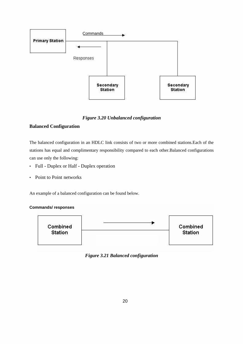
20
Figure 3.20 Unbalanced configuration
Balanced Configuration
The balanced configuration in an HDLC link consists of two or more combined stations.Each of the
stations has equal and complimentary responsibility compared to each other.Balanced configurations
can use only the following:
• Full - Duplex or Half - Duplex operation
• Point to Point networks
An example of a balanced configuration can be found below.
Figure 3.21 Balanced configuration
Commands
Commands/ responses
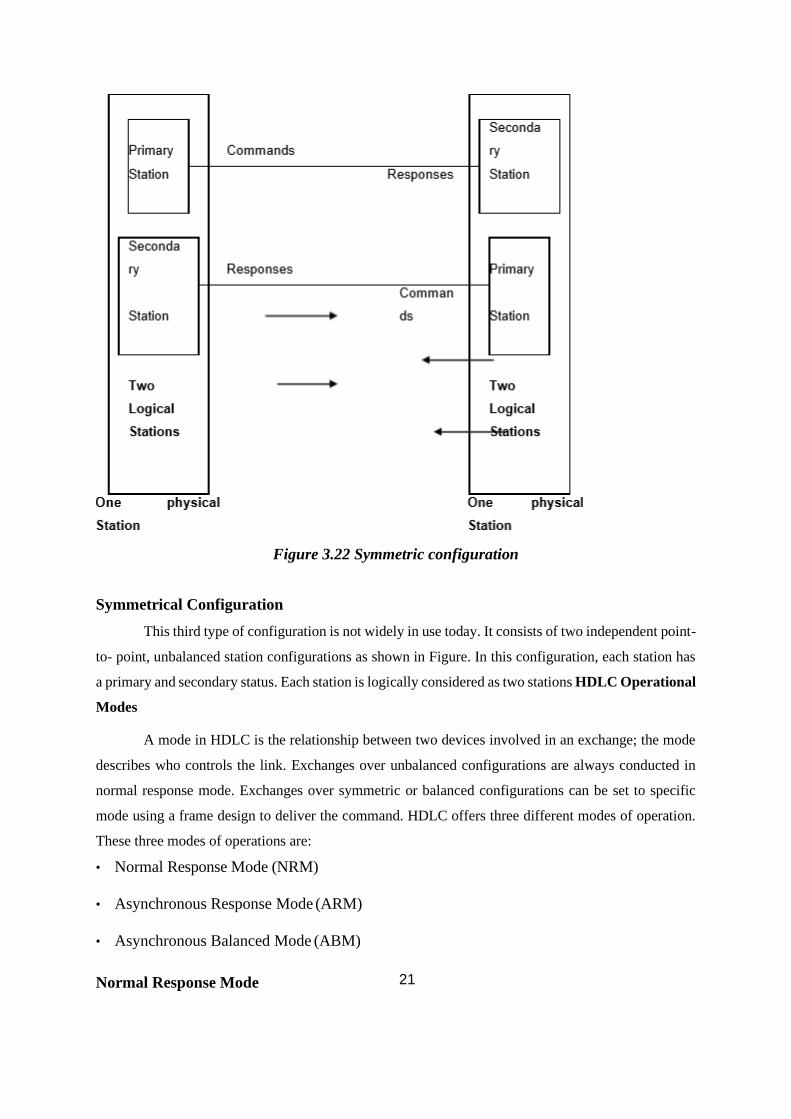
21
Figure 3.22 Symmetric configuration
Symmetrical Configuration
This third type of configuration is not widely in use today. It consists of two independent point-
to- point, unbalanced station configurations as shown in Figure. In this configuration, each station has
a primary and secondary status. Each station is logically considered as two stations HDLC Operational
Modes
A mode in HDLC is the relationship between two devices involved in an exchange; the mode
describes who controls the link. Exchanges over unbalanced configurations are always conducted in
normal response mode. Exchanges over symmetric or balanced configurations can be set to specific
mode using a frame design to deliver the command. HDLC offers three different modes of operation.
These three modes of operations are:
• Normal Response Mode (NRM)
• Asynchronous Response Mode (ARM)
• Asynchronous Balanced Mode (ABM)
Normal Response Mode
22
This is the mode in which the primary station initiates transfers to the secondary station. The
secondary station can only transmit a response when, and only when, it is instructed to do so by the
primary station. In other words, the secondary station must receive explicit permission from the primary
station to transfer a response. After receiving permission from the primary station, the secondary station
initiates its transmission. This transmission from the secondary station to the primary station may be
much more than just an acknowledgment of a frame. It may in fact be more than one information frame.
Once the last frame is transmitted by the secondary station, it must wait once again from explicit
permission to transfer anything, from the primary station. Normal Response Mode is only used within
an unbalanced configuration.
Asynchronous Response Mode
In this mode, the primary station doesn't initiate transfers to the secondary station. In fact, the
secondary station does not have to wait to receive explicit permission from the primary station to
transfer any frames. The frames may be more than just acknowledgment frames. They may contain
data, or control information regarding the status of the secondary station. This mode can reduce
overhead on the link, as no frames need to be transferred in order to give the secondary station
permission to initiate a transfer. However, some limitations do exist. Due to the fact that this mode is
asynchronous, the secondary station must wait until it detects and idle channel before it can transfer any
frames. This is when the ARM link is operating at half-duplex. If the ARM link is operating at full duplex,
the secondary station can transmit at any time. In this mode, the primary station still retains responsibility
for error recovery, link setup, and link disconnection.
Synchronous Balanced Mode
This mode is used in case of combined stations. There is no need for permission on the part of
any station in this mode. This is because combined stations do not require any sort of instructions to
perform any task on the link.Normal Response Mode is used most frequently in multi- point lines, where
the primary station controls the link. Asynchronous Response Mode is better for point-to- point links,
as it reduces overhead. Asynchronous Balanced Mode is not used widely today. The "asynchronous" in
both ARM and ABM does not refer to the format of the data on the link. It refers to the fact that any
given station can transfer frames without explicit permission or instruction from any other station.
HDLC Non-Operational Modes
HDLC also defines three non-operational modes. These three non-operational modes are:
• Normal Disconnected Mode (NDM)
• Asynchronous Disconnected Mode (ADM)
• Initialization Mode (IM)
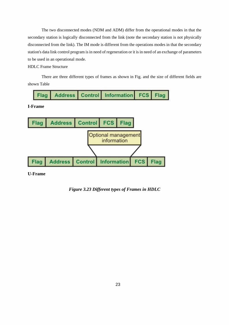
23
The two disconnected modes (NDM and ADM) differ from the operational modes in that the
secondary station is logically disconnected from the link (note the secondary station is not physically
disconnected from the link). The IM mode is different from the operations modes in that the secondary
station's data link control program is in need of regeneration or it is in need of an exchange of parameters
to be used in an operational mode.
HDLC Frame Structure
There are three different types of frames as shown in Fig. and the size of different fields are
shown Table
I-Frame
S-Frame
U-Frame
Figure 3.23 Different types of Frames in HDLC
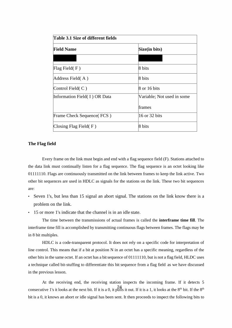
24
Table 3.1 Size of different fields
Field Name Size(in bits)
Flag Field( F ) 8 bits
Address Field( A ) 8 bits
Control Field( C ) 8 or 16 bits
Information Field( I ) OR Data Variable; Not used in some
frames
Frame Check Sequence( FCS ) 16 or 32 bits
Closing Flag Field( F ) 8 bits
The Flag field
Every frame on the link must begin and end with a flag sequence field (F). Stations attached to
the data link must continually listen for a flag sequence. The flag sequence is an octet looking like
01111110. Flags are continuously transmitted on the link between frames to keep the link active. Two
other bit sequences are used in HDLC as signals for the stations on the link. These two bit sequences
are:
• Seven 1's, but less than 15 signal an abort signal. The stations on the link know there is a
problem on the link.
• 15 or more 1's indicate that the channel is in an idle state.
The time between the transmissions of actual frames is called the interframe time fill. The
interframe time fill is accomplished by transmitting continuous flags between frames. The flags may be
in 8 bit multiples.
HDLC is a code-transparent protocol. It does not rely on a specific code for interpretation of
line control. This means that if a bit at position N in an octet has a specific meaning, regardless of the
other bits in the same octet. If an octet has a bit sequence of 01111110, but is not a flag field, HLDC uses
a technique called bit-stuffing to differentiate this bit sequence from a flag field as we have discussed
in the previous lesson.
At the receiving end, the receiving station inspects the incoming frame. If it detects 5
consecutive 1's it looks at the next bit. If it is a 0, it pulls it out. If it is a 1, it looks at the 8th bit. If the 8th
bit is a 0, it knows an abort or idle signal has been sent. It then proceeds to inspect the following bits to
25
determine appropriate action. This is the manner in which HDLC achieves code- transparency. HDLC
is not concerned with any specific bit code inside the data stream. It is only concerned with keeping
flags unique.
The Address field
The address field (A) identifies the primary or secondary stations involvement in the frame
transmission or reception. Each station on the link has a unique address. In an unbalanced configuration,
the A field in both commands and responses refer to the secondary station. In a balanced configuration,
the command frame contains the destination station address and the response frame has the sending
station's address.
The Control field
HDLC uses the control field (C) to determine how to control the communications process. This
field contains the commands, responses and sequences numbers used to maintain the data flow
accountability of the link, defines the functions of the frame and initiates the logic to control the
movement of traffic between sending and receiving stations. There three control field formats:
• Information Transfer Format: The frame is used to transmit end-user data between two
devices.
• Supervisory Format: The control field performs control functions such as acknowledgment
of frames, requests for re-transmission, and requests for temporary suspension of frames
being transmitted. Its use depends on the operational mode being used.
• Unnumbered Format: This control field format is also used for control purposes. It is used
to perform link initialization, link disconnection and other link control functions.
The Poll/Final Bit (P/F)
The 5th bit position in the control field is called the poll/final bit, or P/F bit. It can only be
recognized when it is set to 1. If it is set to 0, it is ignored. The poll/final bit is used to provide dialogue
between the primary station and secondary station. The primary station uses P=1 to acquire a status
response from the secondary station. The P bit signifies a poll. The secondary station responds to the P
bit by transmitting a data or status frame to the primary station with the P/F bit set to F=1. The F bit can
also be used to signal the end of a transmission from the secondary station under Normal Response Mode.
The Information field or Data field
This field is not always present in a HDLC frame. It is only present when the Information
Transfer Format is being used in the control field. The information field contains the actually data the
sender is transmitting to the receiver in an I-Frame and network management information in U- Frame.
The Frame check Sequence field
This field contains a 16-bit, or 32-bit cyclic redundancy check bits. It is used for error detection
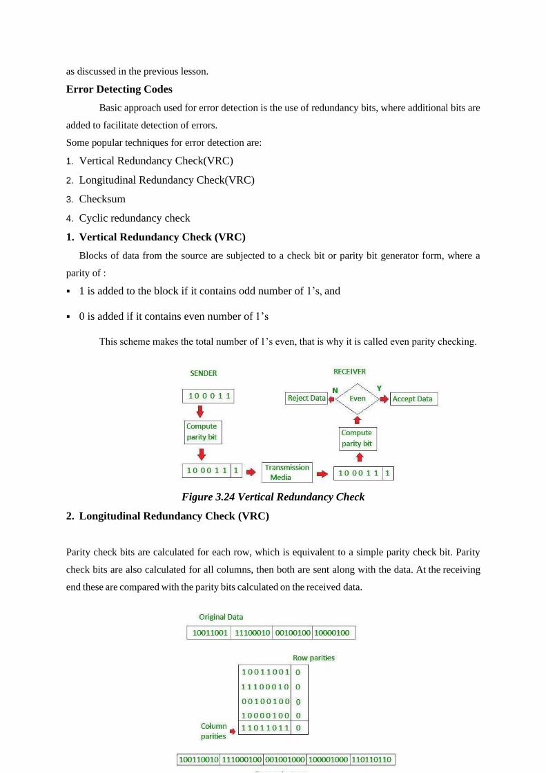
26
as discussed in the previous lesson.
Error Detecting Codes
Basic approach used for error detection is the use of redundancy bits, where additional bits are
added to facilitate detection of errors.
Some popular techniques for error detection are:
1. Vertical Redundancy Check(VRC)
2. Longitudinal Redundancy Check(VRC)
3. Checksum
4. Cyclic redundancy check
1. Vertical Redundancy Check (VRC)
Blocks of data from the source are subjected to a check bit or parity bit generator form, where a
parity of :
▪ 1 is added to the block if it contains odd number of 1’s, and
▪ 0 is added if it contains even number of 1’s
This scheme makes the total number of 1’s even, that is why it is called even parity checking.
Figure 3.24 Vertical Redundancy Check
2. Longitudinal Redundancy Check (VRC)
Parity check bits are calculated for each row, which is equivalent to a simple parity check bit. Parity
check bits are also calculated for all columns, then both are sent along with the data. At the receiving
end these are compared with the parity bits calculated on the received data.
27
Figure 3.25 Longitudinal Redundancy Check
3. Checksum
▪ In checksum error detection scheme, the data is divided into k segments each of m bits.
▪ In the sender’s end the segments are added using 1’s complement arithmetic to get the sum.
The sum is complemented to get the checksum.
▪ The checksum segment is sent along with the data segments.
▪ At the receiver’s end, all received segments are added using 1’s complement arithmetic to
get the sum. The sum is complemented.
▪ If the result is zero, the received data is accepted; otherwise discarded.
4. Cyclic redundancy check (CRC)
▪ Unlike checksum scheme, which is based on addition, CRC is based on binary division.
▪ In CRC, a sequence of redundant bits, called cyclic redundancy check bits, are appended to
the end of data unit so that the resulting data unit becomes exactly divisible by a second,
predetermined binary number.
▪ At the destination, the incoming data unit is divided by the same number. If at this step there
is no remainder, the data unit is assumed to be correct and is therefore accepted.
▪ A remainder indicates that the data unit has been damaged in transit and therefore must be
rejected.
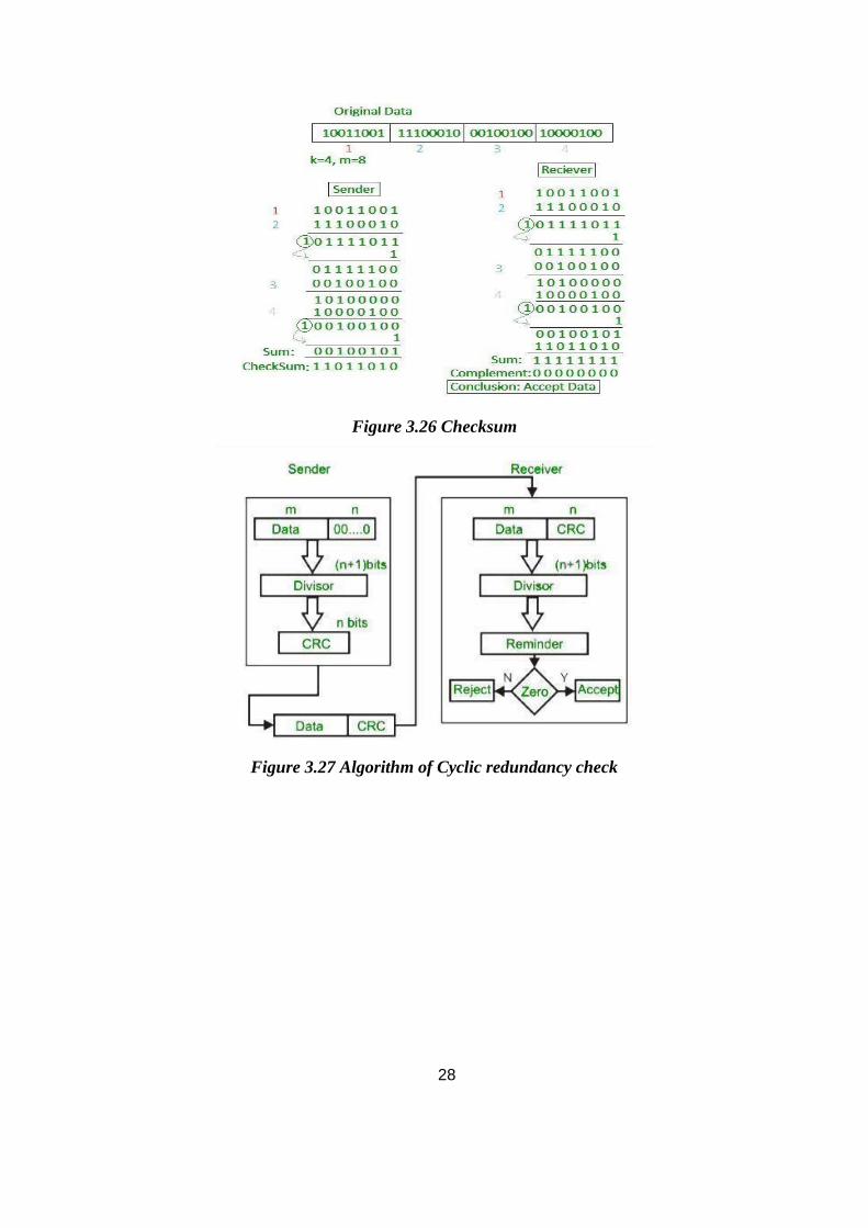
28
Figure 3.26 Checksum
Figure 3.27 Algorithm of Cyclic redundancy check
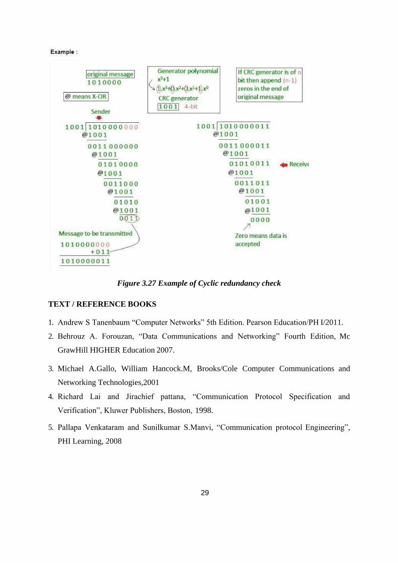
29
Figure 3.27 Example of Cyclic redundancy check
TEXT / REFERENCE BOOKS
1. Andrew S Tanenbaum “Computer Networks” 5th Edition. Pearson Education/PH I/2011.
2. Behrouz A. Forouzan, “Data Communications and Networking” Fourth Edition, Mc
GrawHill HIGHER Education 2007.
3. Michael A.Gallo, William Hancock.M, Brooks/Cole Computer Communications and
Networking Technologies,2001
4. Richard Lai and Jirachief pattana, “Communication Protocol Specification and
Verification”, Kluwer Publishers, Boston, 1998.
5. Pallapa Venkataram and Sunilkumar S.Manvi, “Communication protocol Engineering”,
PHI Learning, 2008
SCHOOL OF ELECTRICAL AND ELECTRONICS ENGINEERING
DEPARTMENT OF ELECTRONICS AND COMMUNICATON ENGINEERING
UNIT IV COMPUTER NETWORKS
SECA1604
UNIT 4 - MAC SUB LAYER AND NETWORK LAYER
MAC sub layer for Standard Ethernet, Fast Ethernet, Wireless LAN and broadband wireless.
Design issues of network layer - Routing algorithm - shortest path routing - Distance vector routing
- Broadcast routing –Inter domain routing, Congestion control algorithm - Congestion control in
virtual circuit and datagram switches - The network layer in the internet - The IP protocol-IP
Addresses - IPv6, ARP,DHCP,ICMP, Classless Addressing, Network Address Translation.
MAC sub layer for Standard
Ethernet operates in the data link layer and the physical layer. It is a family of networking
technologies that are defined in the IEEE 802.2 and 802.3 standards. Ethernet supports data
bandwidths of
10 Mb/s
100 Mb/s
1000 Mb/s (1 Gb/s)
10,000 Mb/s (10 Gb/s)
40,000 Mb/s (40 Gb/s)
100,000 Mb/s (100 Gb/s)
Ethernet standards define both the Layer 2 protocols and the Layer 1 technologies. For the Layer
2 protocols, as with all 802 IEEE standards, Ethernet relies on the two separate sublayers of the
data link layer to operate, the Logical Link Control (LLC) and the MAC sublayers.
LLC sublayer
The Ethernet LLC sublayer handles the communication between the upper layers and the lower
layers. This is typically between the networking software and the device hardware. The LLC
sublayer takes the network protocol data, which is typically an IPv4 packet, and adds control
information to help deliver the packet to the destination node. The LLC is used to communicate
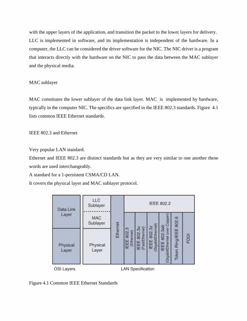
with the upper layers of the application, and transition the packet to the lower layers for delivery.
LLC is implemented in software, and its implementation is independent of the hardware. In a
computer, the LLC can be considered the driver software for the NIC. The NIC driver is a program
that interacts directly with the hardware on the NIC to pass the data between the MAC sublayer
and the physical media.
MAC sublayer
MAC constitutes the lower sublayer of the data link layer. MAC is implemented by hardware,
typically in the computer NIC. The specifics are specified in the IEEE 802.3 standards. Figure 4.1
lists common IEEE Ethernet standards.
IEEE 802.3 and Ethernet
Very popular LAN standard.
Ethernet and IEEE 802.3 are distinct standards but as they are very similar to one another these
words are used interchangeably.
A standard for a 1-persistent CSMA/CD LAN.
It covers the physical layer and MAC sublayer protocol.
Figure 4.1 Common IEEE Ethernet Standards
Fast Ethernet
Fast Ethernet is a collective term for a number of Ethernet standards that carry traffic at the
nominal rate of 100 Mbit/s (the earlier Ethernet speed was 10 Mbit/s). Of the Fast Ethernet
standards, 100BASE-TX is by far the most common.
Fast Ethernet was introduced in 1995 as the IEEE 802.3u standard and remained the fastest version
of Ethernet for three years before the introduction of Gigabit Ethernet.
wireless local area network (WLAN)
A wireless local area network (WLAN) is a wireless computer network that links two or more
devices using wireless communication within a limited area such as a home, school, computer
laboratory, or office building. This gives users the ability to move around within a local coverage
area and yet still be connected to the network. Through a gateway, a WLAN can also provide
a connection to the wider Internet.
Most modern WLANs are based on IEEE 802.11 standards and are marketed under the Wi-Fi
brand name.
4.3.1 Wireless broadband
It is technology that provides high-speed wireless Internet access or computer networking
access over a wide area. broadband means "having instantaneous bandwidths greater than
1 MHz and supporting data rates greater than about 1.5 Mbit/s.
The network layer design issues :
• Store and formed packet switching.
• Service provided to the transport layer.
• Implementation of connectionless service.
• Implementation of connection-oriented source.
• Comparison of virtual circuit and datagram submits.
• Store and formed packet switching :
• Store and forward operation : -
• Host transmits packet to router across LAN or oval point to point link.
• Packet is stored on router until fully arrived and processed.
• Packet is forward to next router.
• Service provide to transport layer
The network layer services have been designed with the goals : -
• The advice should independent of router telenet
• The transport layer should be shielded from the number type and topology of the router
present.
• The network addresses maid available to transport
Implementation of connectionless service :
Connectionless service is offered packets are injected into the subnet individually and routed
independently of each other. Each packet is transmitted independently.
Connectionless service used in network layer ID and transport layer.
Packet are frequently called datagram connectionless service is largely for data communication
the internet.
Implementation of connection-oriented service : -
Connection-oriented service is used a path from the source router to the destination router
must be established before any data packet can be sent.
Connection oriented service also called virtual circuit service. This service used network layer for
ATM. It also used in transport layer for TCP.
A connection must be established before any can be sent packets order preserved logical
connection is also established here.
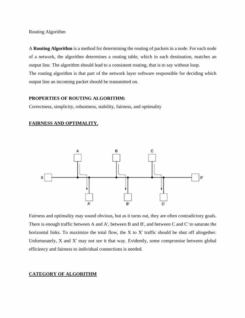
Routing Algorithm
A Routing Algorithm is a method for determining the routing of packets in a node. For each node
of a network, the algorithm determines a routing table, which in each destination, matches an
output line. The algorithm should lead to a consistent routing, that is to say without loop.
The routing algorithm is that part of the network layer software responsible for deciding which
output line an incoming packet should be transmitted on.
PROPERTIES OF ROUTING ALGORITHM:
Correctness, simplicity, robustness, stability, fairness, and optimality
FAIRNESS AND OPTIMALITY.
Fairness and optimality may sound obvious, but as it turns out, they are often contradictory goals.
There is enough traffic between A and A', between B and B', and between C and C' to saturate the
horizontal links. To maximize the total flow, the X to X' traffic should be shut off altogether.
Unfortunately, X and X' may not see it that way. Evidently, some compromise between global
efficiency and fairness to individual connections is needed.
CATEGORY OF ALGORITHM
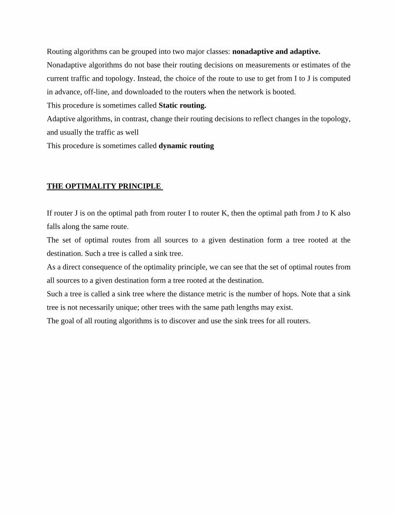
Routing algorithms can be grouped into two major classes: nonadaptive and adaptive.
Nonadaptive algorithms do not base their routing decisions on measurements or estimates of the
current traffic and topology. Instead, the choice of the route to use to get from I to J is computed
in advance, off-line, and downloaded to the routers when the network is booted.
This procedure is sometimes called Static routing.
Adaptive algorithms, in contrast, change their routing decisions to reflect changes in the topology,
and usually the traffic as well
This procedure is sometimes called dynamic routing
THE OPTIMALITY PRINCIPLE
If router J is on the optimal path from router I to router K, then the optimal path from J to K also
falls along the same route.
The set of optimal routes from all sources to a given destination form a tree rooted at the
destination. Such a tree is called a sink tree.
As a direct consequence of the optimality principle, we can see that the set of optimal routes from
all sources to a given destination form a tree rooted at the destination.
Such a tree is called a sink tree where the distance metric is the number of hops. Note that a sink
tree is not necessarily unique; other trees with the same path lengths may exist.
The goal of all routing algorithms is to discover and use the sink trees for all routers.
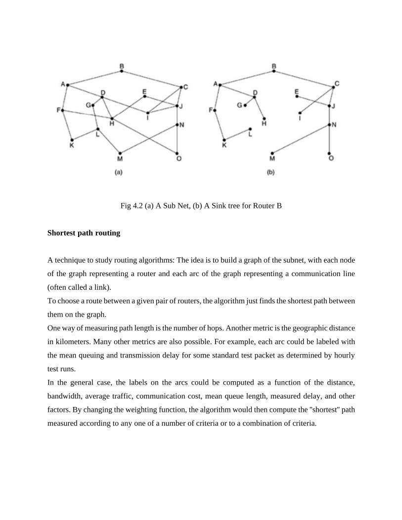
Fig 4.2 (a) A Sub Net, (b) A Sink tree for Router B
Shortest path routing
A technique to study routing algorithms: The idea is to build a graph of the subnet, with each node
of the graph representing a router and each arc of the graph representing a communication line
(often called a link).
To choose a route between a given pair of routers, the algorithm just finds the shortest path between
them on the graph.
One way of measuring path length is the number of hops. Another metric is the geographic distance
in kilometers. Many other metrics are also possible. For example, each arc could be labeled with
the mean queuing and transmission delay for some standard test packet as determined by hourly
test runs.
In the general case, the labels on the arcs could be computed as a function of the distance,
bandwidth, average traffic, communication cost, mean queue length, measured delay, and other
factors. By changing the weighting function, the algorithm would then compute the ''shortest'' path
measured according to any one of a number of criteria or to a combination of criteria.
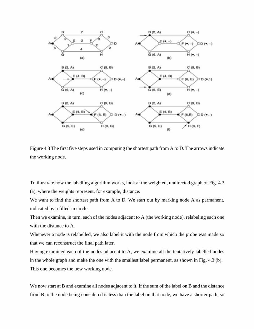
Figure 4.3 The first five steps used in computing the shortest path from A to D. The arrows indicate
the working node.
To illustrate how the labelling algorithm works, look at the weighted, undirected graph of Fig. 4.3
(a), where the weights represent, for example, distance.
We want to find the shortest path from A to D. We start out by marking node A as permanent,
indicated by a filled-in circle.
Then we examine, in turn, each of the nodes adjacent to A (the working node), relabeling each one
with the distance to A.
Whenever a node is relabelled, we also label it with the node from which the probe was made so
that we can reconstruct the final path later.
Having examined each of the nodes adjacent to A, we examine all the tentatively labelled nodes
in the whole graph and make the one with the smallest label permanent, as shown in Fig. 4.3 (b).
This one becomes the new working node.
We now start at B and examine all nodes adjacent to it. If the sum of the label on B and the distance
from B to the node being considered is less than the label on that node, we have a shorter path, so
the node is relabeled
After all the nodes adjacent to the working node have been inspected and the tentative labels
changed if possible, the entire graph is searched for the tentatively-labelled node with the smallest
value. This node is made permanent and becomes the working node for the next round. Figure 4.3
shows the first five steps of the algorithm.
Another example using Dijkstra's algorithm to compute the shortest paths from a given source
node to all other nodes in a network. Links are bi-directional, with the same distance in either
direction. Distance can be any measure of cost.
Example with 8 nodes and 11 links
nodeset = {'A', 'B', 'C', 'D', 'E', 'F', 'G', 'H'}
linklist = [('A', 'B', 2), ('B', 'C', 7), ('C', 'D', 3),
# (node,node,distance) ('B', 'E', 2), ('E', 'F', 2), ('F', 'C', 3), ('A', 'G', 6), ('G', 'E', 1), ('G', 'H', 4), ('F',
'H', 2), ('H', 'D', 2),
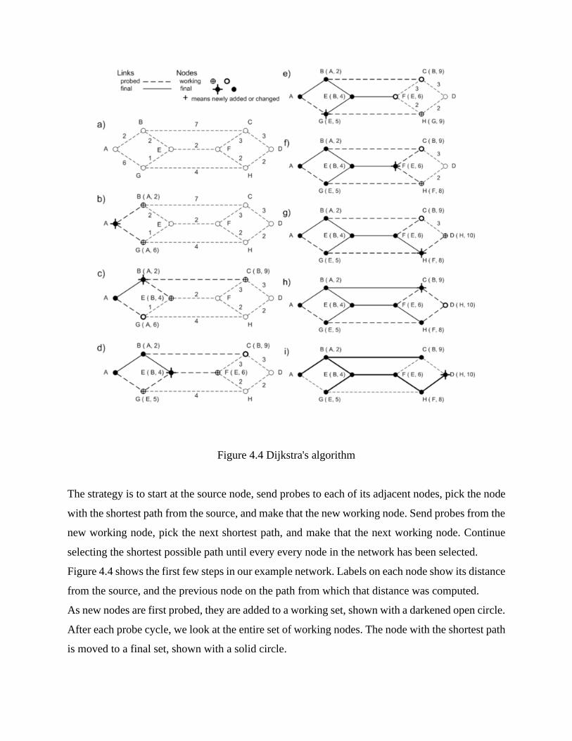
Figure 4.4 Dijkstra's algorithm
The strategy is to start at the source node, send probes to each of its adjacent nodes, pick the node
with the shortest path from the source, and make that the new working node. Send probes from the
new working node, pick the next shortest path, and make that the next working node. Continue
selecting the shortest possible path until every every node in the network has been selected.
Figure 4.4 shows the first few steps in our example network. Labels on each node show its distance
from the source, and the previous node on the path from which that distance was computed.
As new nodes are first probed, they are added to a working set, shown with a darkened open circle.
After each probe cycle, we look at the entire set of working nodes. The node with the shortest path
is moved to a final set, shown with a solid circle.
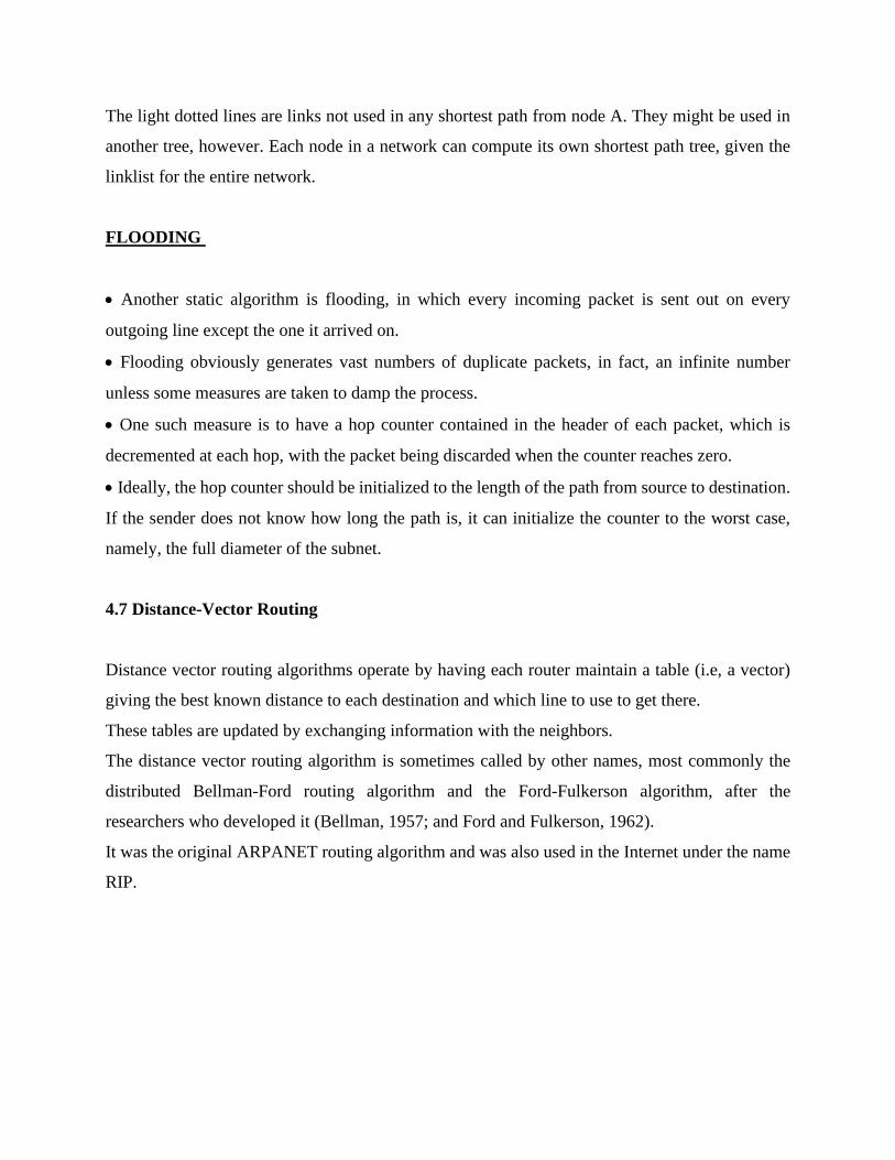
The light dotted lines are links not used in any shortest path from node A. They might be used in
another tree, however. Each node in a network can compute its own shortest path tree, given the
linklist for the entire network.
FLOODING
• Another static algorithm is flooding, in which every incoming packet is sent out on every
outgoing line except the one it arrived on.
• Flooding obviously generates vast numbers of duplicate packets, in fact, an infinite number
unless some measures are taken to damp the process.
• One such measure is to have a hop counter contained in the header of each packet, which is
decremented at each hop, with the packet being discarded when the counter reaches zero.
• Ideally, the hop counter should be initialized to the length of the path from source to destination.
If the sender does not know how long the path is, it can initialize the counter to the worst case,
namely, the full diameter of the subnet.
4.7 Distance-Vector Routing
Distance vector routing algorithms operate by having each router maintain a table (i.e, a vector)
giving the best known distance to each destination and which line to use to get there.
These tables are updated by exchanging information with the neighbors.
The distance vector routing algorithm is sometimes called by other names, most commonly the
distributed Bellman-Ford routing algorithm and the Ford-Fulkerson algorithm, after the
researchers who developed it (Bellman, 1957; and Ford and Fulkerson, 1962).
It was the original ARPANET routing algorithm and was also used in the Internet under the name
RIP.
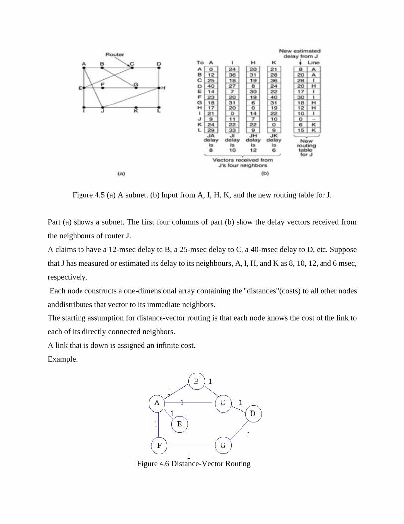
Figure 4.5 (a) A subnet. (b) Input from A, I, H, K, and the new routing table for J.
Part (a) shows a subnet. The first four columns of part (b) show the delay vectors received from
the neighbours of router J.
A claims to have a 12-msec delay to B, a 25-msec delay to C, a 40-msec delay to D, etc. Suppose
that J has measured or estimated its delay to its neighbours, A, I, H, and K as 8, 10, 12, and 6 msec,
respectively.
Each node constructs a one-dimensional array containing the "distances"(costs) to all other nodes
and distributes that vector to its immediate neighbors.
The starting assumption for distance-vector routing is that each node knows the cost of the link to
each of its directly connected neighbors.
A link that is down is assigned an infinite cost.
Example.
Figure 4.6 Distance-Vector Routing
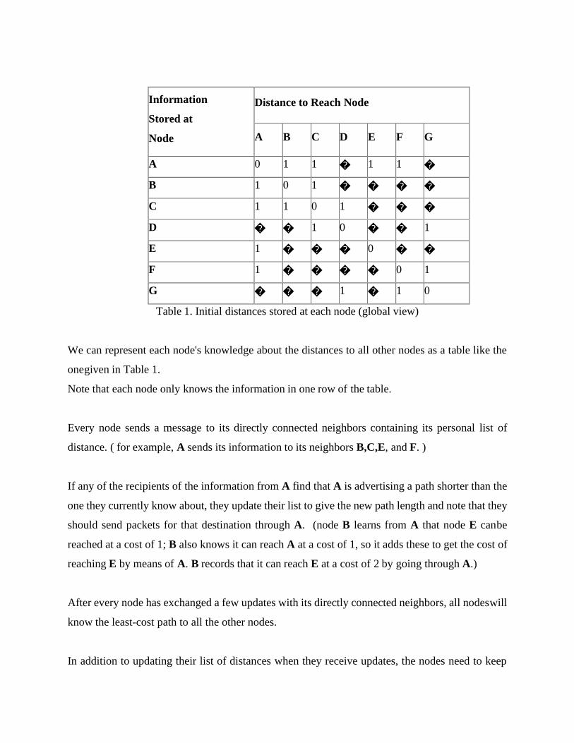
Information
Stored at
Node
Distance to Reach Node
A B C D E F G
A 0 1 1 � 1 1 �
B 1 0 1 � � � �
C 1 1 0 1 � � �
D � � 1 0 � � 1
E 1 � � � 0 � �
F 1 � � � � 0 1
G � � � 1 � 1 0
Table 1. Initial distances stored at each node (global view)
We can represent each node's knowledge about the distances to all other nodes as a table like the
one given in Table 1.
Note that each node only knows the information in one row of the table.
Every node sends a message to its directly connected neighbors containing its personal list of
distance. ( for example, A sends its information to its neighbors B,C,E, and F. )
If any of the recipients of the information from A find that A is advertising a path shorter than the
one they currently know about, they update their list to give the new path length and note that they
should send packets for that destination through A. (node B learns from A that node E can be
reached at a cost of 1; B also knows it can reach A at a cost of 1, so it adds these to get the cost of
reaching E by means of A. B records that it can reach E at a cost of 2 by going through A.)
After every node has exchanged a few updates with its directly connected neighbors, all nodes will
know the least-cost path to all the other nodes.
In addition to updating their list of distances when they receive updates, the nodes need to keep
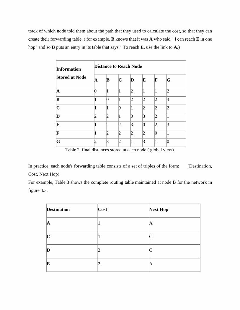
track of which node told them about the path that they used to calculate the cost, so that they can
create their forwarding table. ( for example, B knows that it was A who said " I can reach E in one
hop" and so B puts an entry in its table that says " To reach E, use the link to A.)
Information
Stored at Node
Distance to Reach Node
A B C D E F G
A 0 1 1 2 1 1 2
B 1 0 1 2 2 2 3
C 1 1 0 1 2 2 2
D 2 2 1 0 3 2 1
E 1 2 2 3 0 2 3
F 1 2 2 2 2 0 1
G 2 3 2 1 3 1 0
Table 2. final distances stored at each node ( global view).
In practice, each node's forwarding table consists of a set of triples of the form: (Destination,
Cost, Next Hop).
For example, Table 3 shows the complete routing table maintained at node B for the network in
figure 4.3.
Destination Cost Next Hop
A 1 A
C 1 C
D 2 C
E 2 A
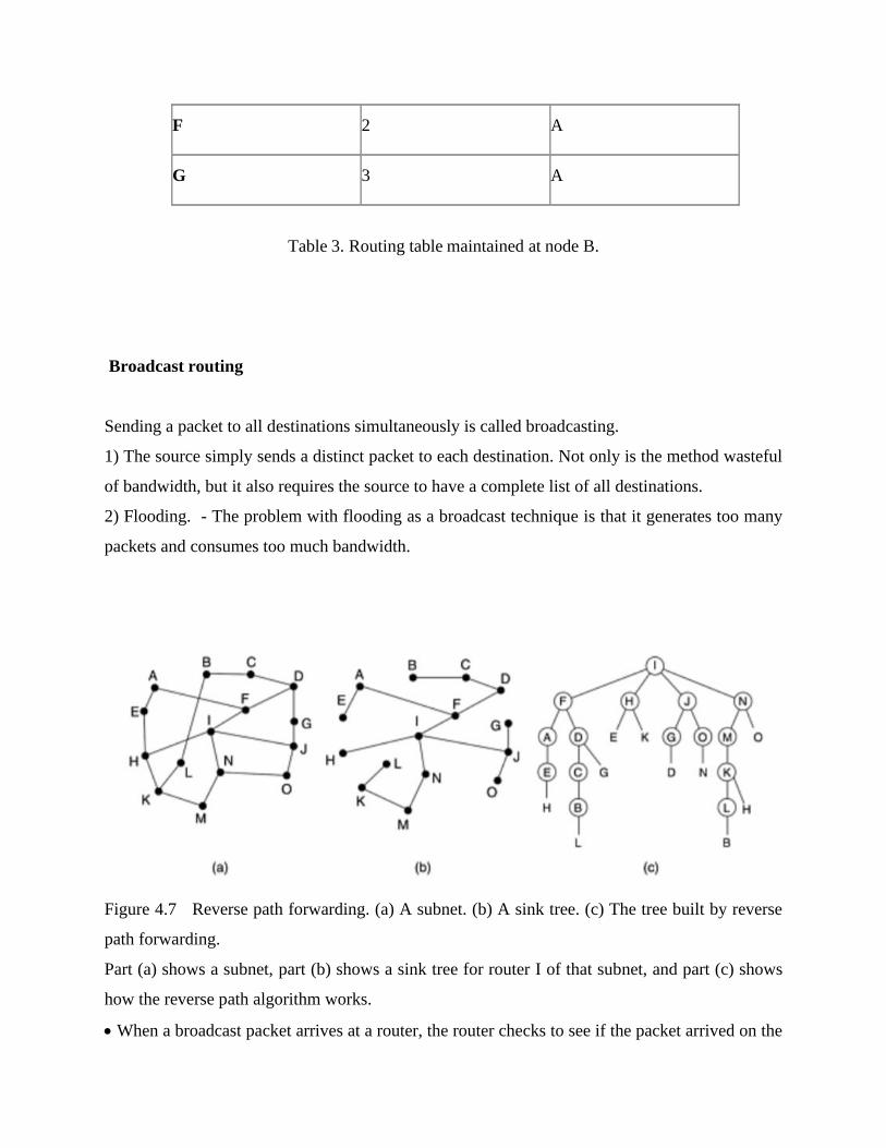
F 2 A
G 3 A
Table 3. Routing table maintained at node B.
Broadcast routing
Sending a packet to all destinations simultaneously is called broadcasting.
1) The source simply sends a distinct packet to each destination. Not only is the method wasteful
of bandwidth, but it also requires the source to have a complete list of all destinations.
2) Flooding. - The problem with flooding as a broadcast technique is that it generates too many
packets and consumes too much bandwidth.
Figure 4.7 Reverse path forwarding. (a) A subnet. (b) A sink tree. (c) The tree built by reverse
path forwarding.
Part (a) shows a subnet, part (b) shows a sink tree for router I of that subnet, and part (c) shows
how the reverse path algorithm works.
• When a broadcast packet arrives at a router, the router checks to see if the packet arrived on the
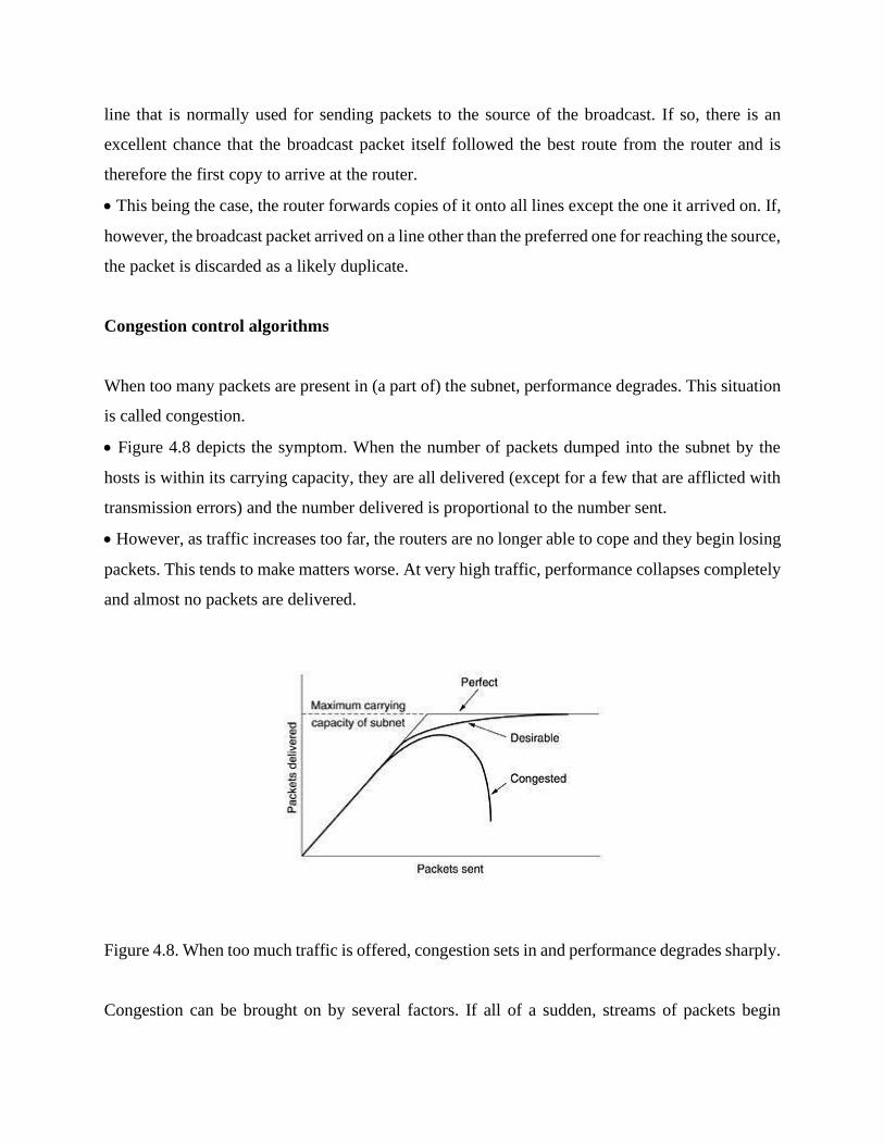
line that is normally used for sending packets to the source of the broadcast. If so, there is an
excellent chance that the broadcast packet itself followed the best route from the router and is
therefore the first copy to arrive at the router.
• This being the case, the router forwards copies of it onto all lines except the one it arrived on. If,
however, the broadcast packet arrived on a line other than the preferred one for reaching the source,
the packet is discarded as a likely duplicate.
Congestion control algorithms
When too many packets are present in (a part of) the subnet, performance degrades. This situation
is called congestion.
• Figure 4.8 depicts the symptom. When the number of packets dumped into the subnet by the
hosts is within its carrying capacity, they are all delivered (except for a few that are afflicted with
transmission errors) and the number delivered is proportional to the number sent.
• However, as traffic increases too far, the routers are no longer able to cope and they begin losing
packets. This tends to make matters worse. At very high traffic, performance collapses completely
and almost no packets are delivered.
Figure 4.8. When too much traffic is offered, congestion sets in and performance degrades sharply.
Congestion can be brought on by several factors. If all of a sudden, streams of packets begin
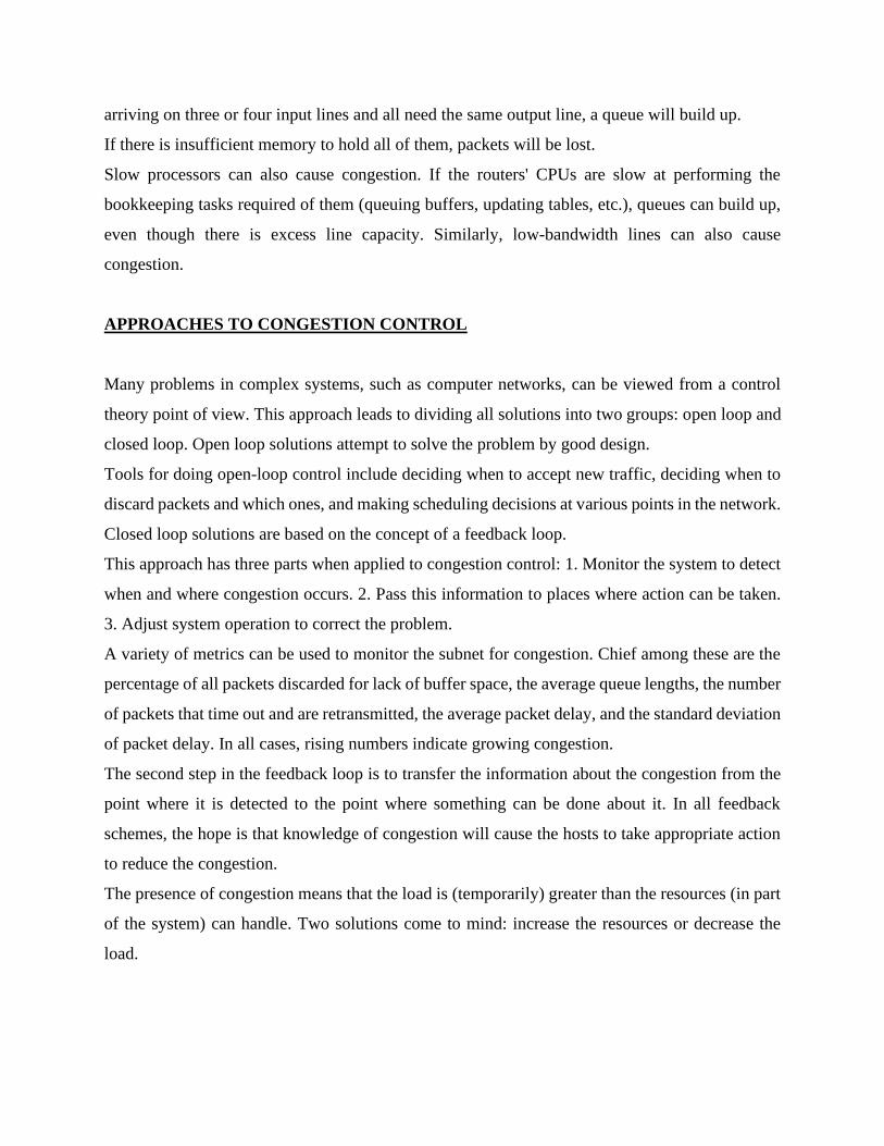
arriving on three or four input lines and all need the same output line, a queue will build up.
If there is insufficient memory to hold all of them, packets will be lost.
Slow processors can also cause congestion. If the routers' CPUs are slow at performing the
bookkeeping tasks required of them (queuing buffers, updating tables, etc.), queues can build up,
even though there is excess line capacity. Similarly, low-bandwidth lines can also cause
congestion.
APPROACHES TO CONGESTION CONTROL
Many problems in complex systems, such as computer networks, can be viewed from a control
theory point of view. This approach leads to dividing all solutions into two groups: open loop and
closed loop. Open loop solutions attempt to solve the problem by good design.
Tools for doing open-loop control include deciding when to accept new traffic, deciding when to
discard packets and which ones, and making scheduling decisions at various points in the network.
Closed loop solutions are based on the concept of a feedback loop.
This approach has three parts when applied to congestion control: 1. Monitor the system to detect
when and where congestion occurs. 2. Pass this information to places where action can be taken.
3. Adjust system operation to correct the problem.
A variety of metrics can be used to monitor the subnet for congestion. Chief among these are the
percentage of all packets discarded for lack of buffer space, the average queue lengths, the number
of packets that time out and are retransmitted, the average packet delay, and the standard deviation
of packet delay. In all cases, rising numbers indicate growing congestion.
The second step in the feedback loop is to transfer the information about the congestion from the
point where it is detected to the point where something can be done about it. In all feedback
schemes, the hope is that knowledge of congestion will cause the hosts to take appropriate action
to reduce the congestion.
The presence of congestion means that the load is (temporarily) greater than the resources (in part
of the system) can handle. Two solutions come to mind: increase the resources or decrease the
load.
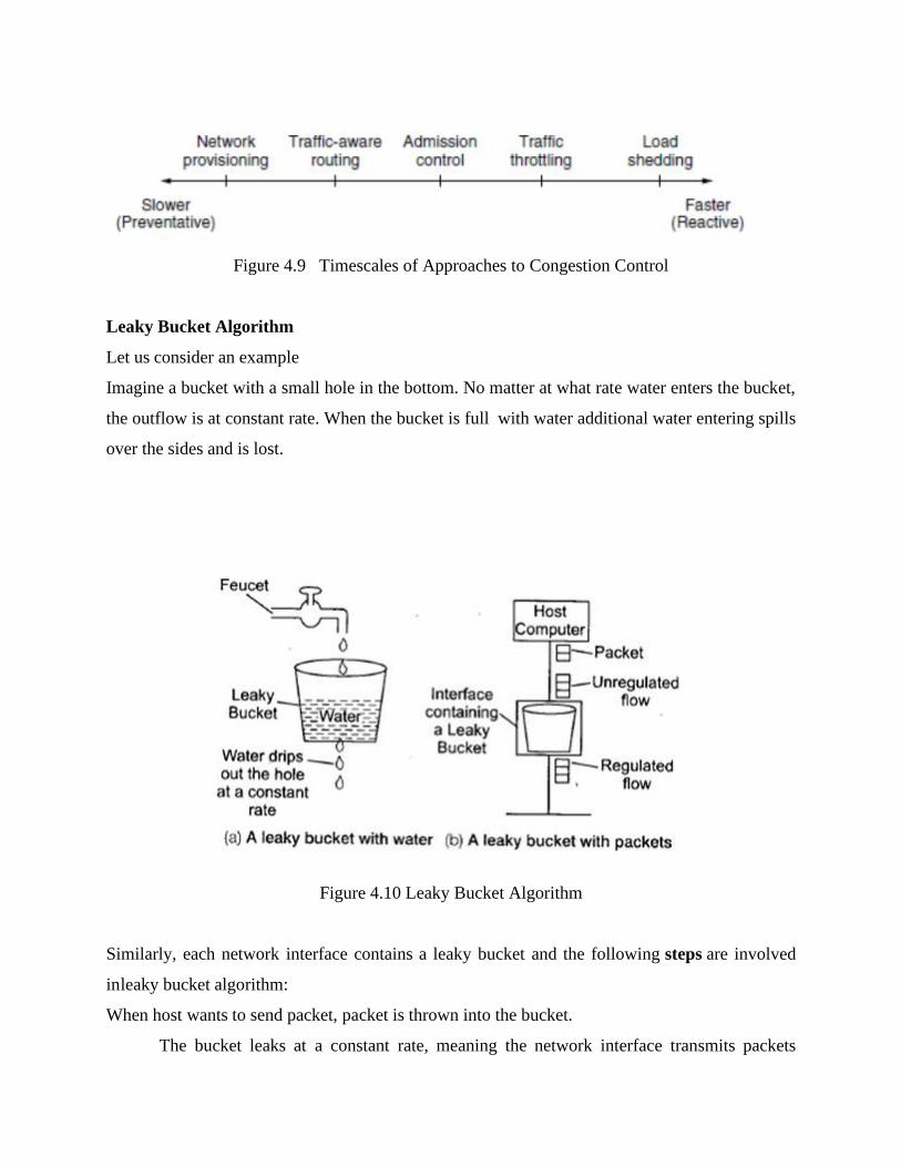
Figure 4.9 Timescales of Approaches to Congestion Control
Leaky Bucket Algorithm
Let us consider an example
Imagine a bucket with a small hole in the bottom. No matter at what rate water enters the bucket,
the outflow is at constant rate. When the bucket is full with water additional water entering spills
over the sides and is lost.
Figure 4.10 Leaky Bucket Algorithm
Similarly, each network interface contains a leaky bucket and the following steps are involved
in leaky bucket algorithm:
When host wants to send packet, packet is thrown into the bucket.
The bucket leaks at a constant rate, meaning the network interface transmits packets
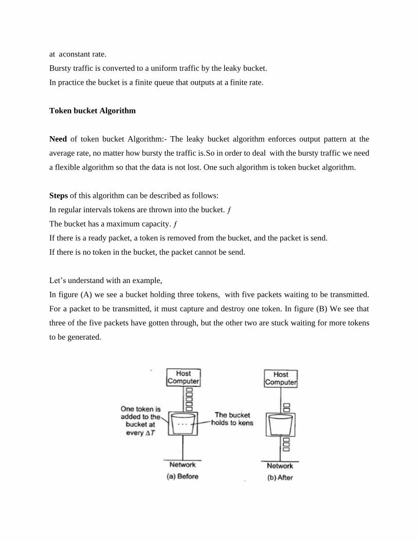
at a constant rate.
Bursty traffic is converted to a uniform traffic by the leaky bucket.
In practice the bucket is a finite queue that outputs at a finite rate.
Token bucket Algorithm
Need of token bucket Algorithm:- The leaky bucket algorithm enforces output pattern at the
average rate, no matter how bursty the traffic is. So in order to deal with the bursty traffic we need
a flexible algorithm so that the data is not lost. One such algorithm is token bucket algorithm.
Steps of this algorithm can be described as follows:
In regular intervals tokens are thrown into the bucket. ƒ
The bucket has a maximum capacity. ƒ
If there is a ready packet, a token is removed from the bucket, and the packet is send.
If there is no token in the bucket, the packet cannot be send.
Let’s understand with an example,
In figure (A) we see a bucket holding three tokens, with five packets waiting to be transmitted.
For a packet to be transmitted, it must capture and destroy one token. In figure (B) We see that
three of the five packets have gotten through, but the other two are stuck waiting for more tokens
to be generated.
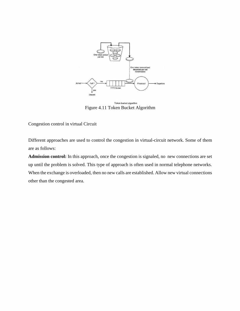
Figure 4.11 Token Bucket Algorithm
Congestion control in virtual Circuit
Different approaches are used to control the congestion in virtual-circuit network. Some of them
are as follows:
Admission control: In this approach, once the congestion is signaled, no new connections are set
up until the problem is solved. This type of approach is often used in normal telephone networks.
When the exchange is overloaded, then no new calls are established. Allow new virtual connections
other than the congested area.
51
Negotiate an agreement between the host and the network when the connection is setup. This
agreement specifies the volume and shape of traffic, quality of service, maximum delay and
other parameters. The network will reserve resources (Buffer space, Bandwidth and CPU
cycle) along the path when the connection is set up. Now congestion is unlikely to occur on
the new connections because all the necessary resources are guaranteed to be available. The
disadvantage of this approach is that it may leads to wasted bandwidth because of the some
idle connection.
Congestion control in Datagram Subnets
Congestion control in Datagram Subnets is achieved by sending warning to sender in advance.
Each router can easily monitor the utilization of its output lines. If utilization is greater than
threshold value then output line may be congested in future so mark it as warning state. Each
newly arriving packet is checked to see if its output line is in warning state. If it is, some action
is taken.
The actions are:
The warning bit
Choke packets
Hop-by-hop choke packet
The warning bit
When a new packet is to be transmitted on the output line marked as warning state, a special
bit is added in header to signal this state. At the destination, this information is sent back with
ACK to the sender so that it could cut the traffic. When warning bit is absent, sender increases
its transmitting rate.
Note: It uses a whole trip (source to destination to source) to tell the source to slow down
Choke Packet Technique
In this approach, the router sends a choke packet back to the source host. The original packet
is marked so that it would not generate any more choke packets further along the path and is
then forwarded in the usual way. When the source gets the choke packet, it is required to
reduce the traffic by X packets.
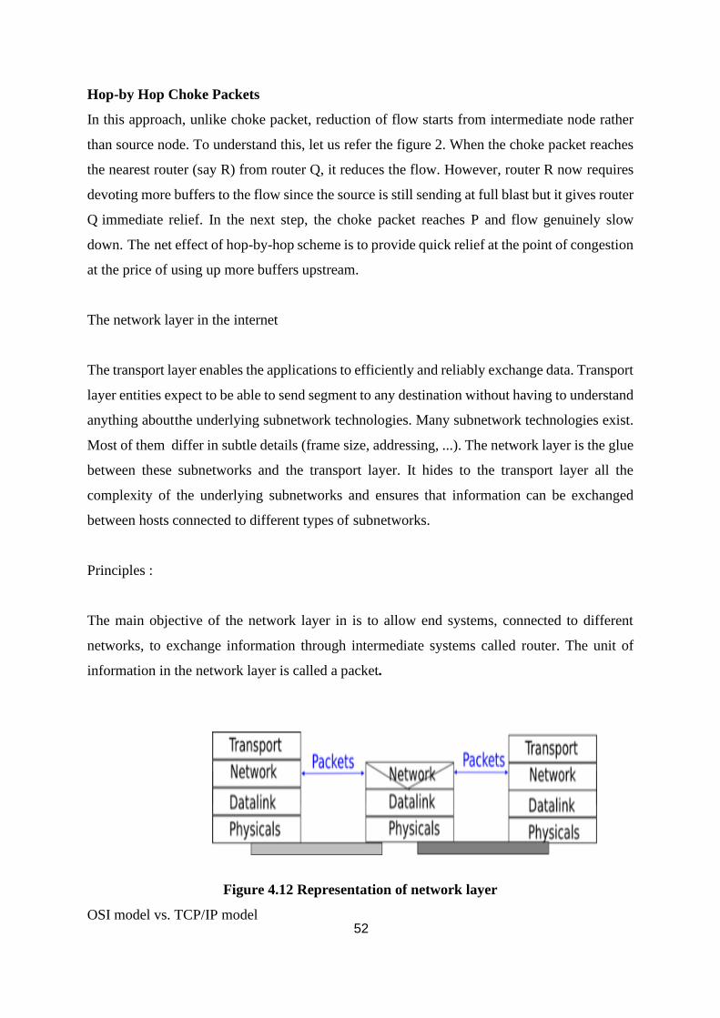
52
Hop-by Hop Choke Packets
In this approach, unlike choke packet, reduction of flow starts from intermediate node rather
than source node. To understand this, let us refer the figure 2. When the choke packet reaches
the nearest router (say R) from router Q, it reduces the flow. However, router R now requires
devoting more buffers to the flow since the source is still sending at full blast but it gives router
Q immediate relief. In the next step, the choke packet reaches P and flow genuinely slow
down. The net effect of hop-by-hop scheme is to provide quick relief at the point of congestion
at the price of using up more buffers upstream.
The network layer in the internet
The transport layer enables the applications to efficiently and reliably exchange data. Transport
layer entities expect to be able to send segment to any destination without having to understand
anything about the underlying subnetwork technologies. Many subnetwork technologies exist.
Most of them differ in subtle details (frame size, addressing, ...). The network layer is the glue
between these subnetworks and the transport layer. It hides to the transport layer all the
complexity of the underlying subnetworks and ensures that information can be exchanged
between hosts connected to different types of subnetworks.
Principles :
The main objective of the network layer in is to allow end systems, connected to different
networks, to exchange information through intermediate systems called router. The unit of
information in the network layer is called a packet.
Figure 4.12 Representation of network layer
OSI model vs. TCP/IP model
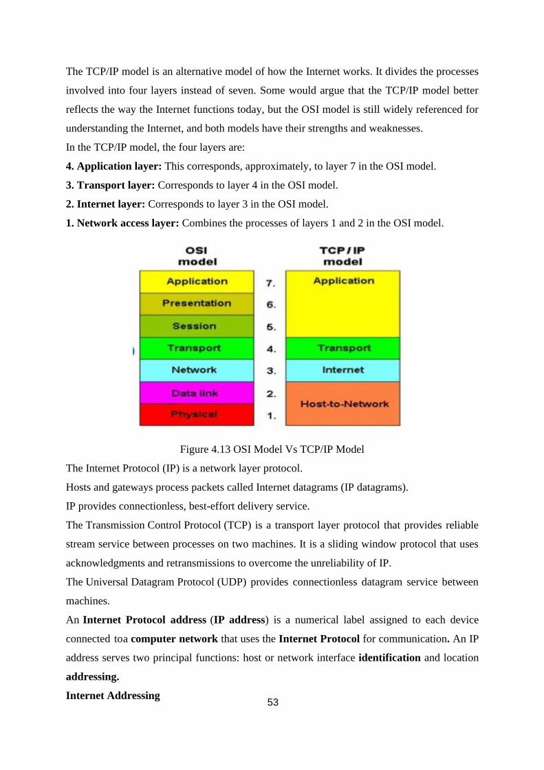
53
The TCP/IP model is an alternative model of how the Internet works. It divides the processes
involved into four layers instead of seven. Some would argue that the TCP/IP model better
reflects the way the Internet functions today, but the OSI model is still widely referenced for
understanding the Internet, and both models have their strengths and weaknesses.
In the TCP/IP model, the four layers are:
4. Application layer: This corresponds, approximately, to layer 7 in the OSI model.
3. Transport layer: Corresponds to layer 4 in the OSI model.
2. Internet layer: Corresponds to layer 3 in the OSI model.
1. Network access layer: Combines the processes of layers 1 and 2 in the OSI model.
Figure 4.13 OSI Model Vs TCP/IP Model
The Internet Protocol (IP) is a network layer protocol.
Hosts and gateways process packets called Internet datagrams (IP datagrams).
IP provides connectionless, best-effort delivery service.
The Transmission Control Protocol (TCP) is a transport layer protocol that provides reliable
stream service between processes on two machines. It is a sliding window protocol that uses
acknowledgments and retransmissions to overcome the unreliability of IP.
The Universal Datagram Protocol (UDP) provides connectionless datagram service between
machines.
An Internet Protocol address (IP address) is a numerical label assigned to each device
connected to a computer network that uses the Internet Protocol for communication. An IP
address serves two principal functions: host or network interface identification and location
addressing.
Internet Addressing
54
Host identifiers are classified as names, addresses, or routes, where:
A name suggests what object we want.
An address specifies where the object is.
A route tells us how to get to the object.
In the Internet, names consist of human-readable strings such as eve, percival,
or gwen.cs.purdue.edu.
Addresses consist of compact, 32-bit identifiers. Internet software translates names into
addresses; lower protocol layers always uses addresses rather than names.
Internet addresses are hierarchical, consisting of two parts:
Network:
The network part of an address identifies which network a host is on. Conceptually, each LAN
has its own unique IP network number.
Local:
The local part of an address identifies which host on that network.
Address Classes
The Internet designers were unsure whether the world would evolve into a few networks with
many hosts (e.g., large networks), or many networks each supporting only a few hosts (e.g.,
small networks). Thus, Internet addresses handle both large and small networks. Internet
address are four bytes in size, where:
Class A addresses start with a ``0'' in the most significant bit, followed by a 7-bit network
address and a 24-bit local part.
Class B addresses start with a ``10'' in the two most significant bits, followed by a 14-bit
network number and a 16-bit local part.
Class C addresses start with a ``110'' in the three most significant bits, followed by a 22-bit
network number and an 8-bit local part.
Class D addresses start with a ``1110'' in the four most significant bits, followed by a 28-bit
group number.
Note: The use of fixed-sized addresses makes the routing operation efficient. In the ISO world,
addresses are of varying format and length and just extracting the address from the packet may
not be straightforward.
Internet addresses can also refer to broadcast addresses. The all 1's address is used to mean
``broadcast on this network''. Of course, if the underlying network technology doesn't support
broadcasting, one can't broadcast Internet datagrams either.
Network addresses are written using dotted decimal notation. Each address consists of 4 bytes,
55
and each byte is written in decimal form. Sample addresses:
wpi.wpi.edu: 130.215.24.6 (class B)
owl.wpi.edu: 130.215.8.139 (class B)
wpi.edu: 130.215 (a network address)
rialto.mcs.vuw.ac.nz: 130.195.5.15 (class B)
gwen.cs.purdue.edu: 128.10.2.3 (class B)
c.nyser.net: 192.33.4.12 (Class C)
pescadero.stanford.edu: 36.8.0.8 (class A)
su-net-temp: 36 (network address)
Note: Internet addresses refer to network connections rather than hosts. Gateways, for instance,
have two or more network connections and each interface has its own IP address. Thus, there
is not a one-to-one mapping between host names and IP addresses.
4.11 IPv6
IPv6 is the replacement Internet protocol for IPv4. It corrects some of the deficiencies of IPv4
and simplifies the way that addresses are configured and how they are handled by Internet
hosts. IPv4 has proven to be robust, easily implemented, and interoperable, and has stood the
test of scaling an internetwork to a global utility the size of the Internet. However, the initial
design did not anticipate the following conditions:
• Recent exponential growth of the Internet and the impending exhaustion of the IPv4 address
space
• The ability of Internet backbone routers to maintain large routing tables
• Need for simpler auto configuration and renumbering
• Requirement for security at the IP level (IPSec)
• Need for better support for real-time delivery of data, known as quality of service (QoS)
Need for IPv6
With 32-bit address format, IPv4 can handle a maximum 4.3 billion unique IP addresses.
While this number may seem very large, it is not enough to sustain and scale the rapidly rising
growth of the Internet. Although improvements to IPv4, including the use of NAT, have
allowed the extended use of the protocol, address exhaustion is inevitable and could happen as
soon as 2012. With its 128-bit address format, IPv6 can support 3.4 x 1038 or 340, 282, 366,
920, 938,463,463,374,607,431,768,211,456 unique IP addresses.
This number of addresses is large enough to configure a unique address on every node in the
Internet and still have plenty of addresses left over. It is also large enough to eliminate the need
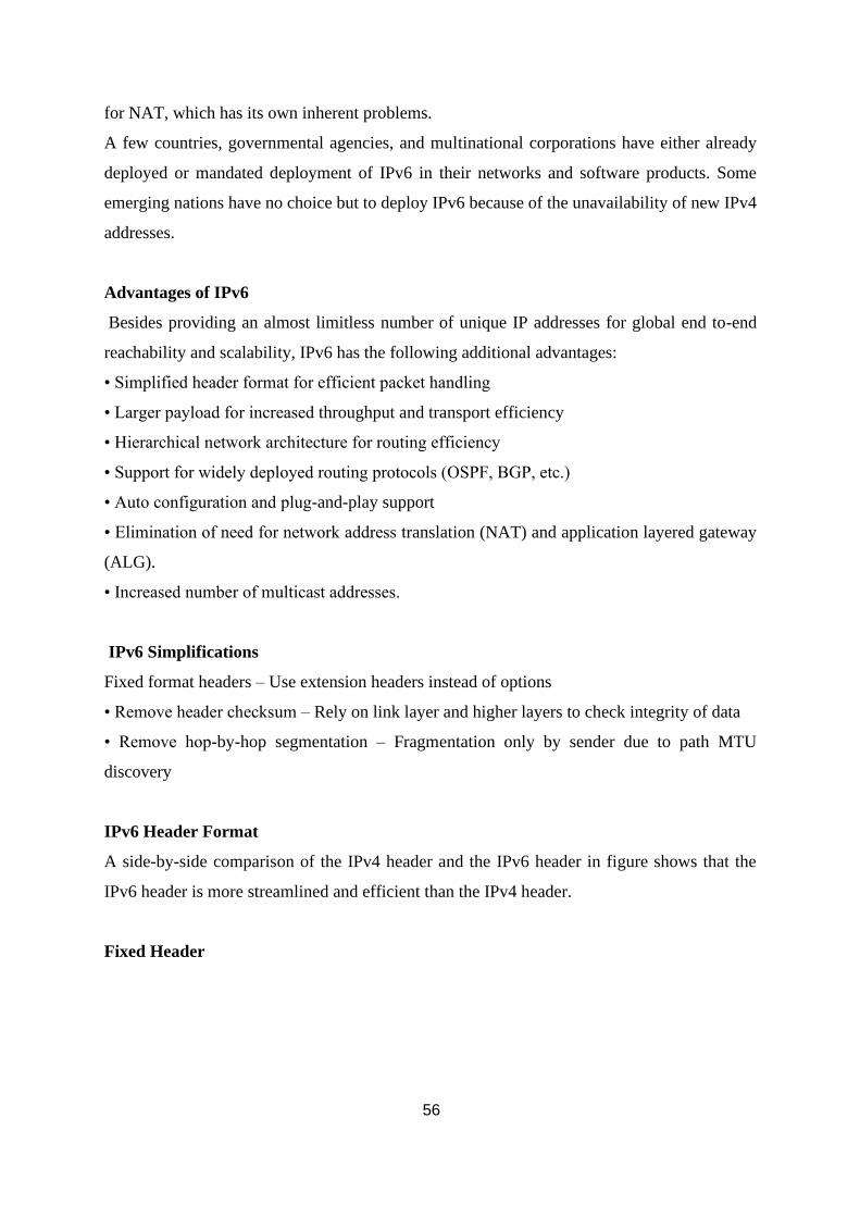
56
for NAT, which has its own inherent problems.
A few countries, governmental agencies, and multinational corporations have either already
deployed or mandated deployment of IPv6 in their networks and software products. Some
emerging nations have no choice but to deploy IPv6 because of the unavailability of new IPv4
addresses.
Advantages of IPv6
Besides providing an almost limitless number of unique IP addresses for global end to-end
reachability and scalability, IPv6 has the following additional advantages:
• Simplified header format for efficient packet handling
• Larger payload for increased throughput and transport efficiency
• Hierarchical network architecture for routing efficiency
• Support for widely deployed routing protocols (OSPF, BGP, etc.)
• Auto configuration and plug-and-play support
• Elimination of need for network address translation (NAT) and application layered gateway
(ALG).
• Increased number of multicast addresses.
IPv6 Simplifications
Fixed format headers – Use extension headers instead of options
• Remove header checksum – Rely on link layer and higher layers to check integrity of data
• Remove hop-by-hop segmentation – Fragmentation only by sender due to path MTU
discovery
IPv6 Header Format
A side-by-side comparison of the IPv4 header and the IPv6 header in figure shows that the
IPv6 header is more streamlined and efficient than the IPv4 header.
Fixed Header
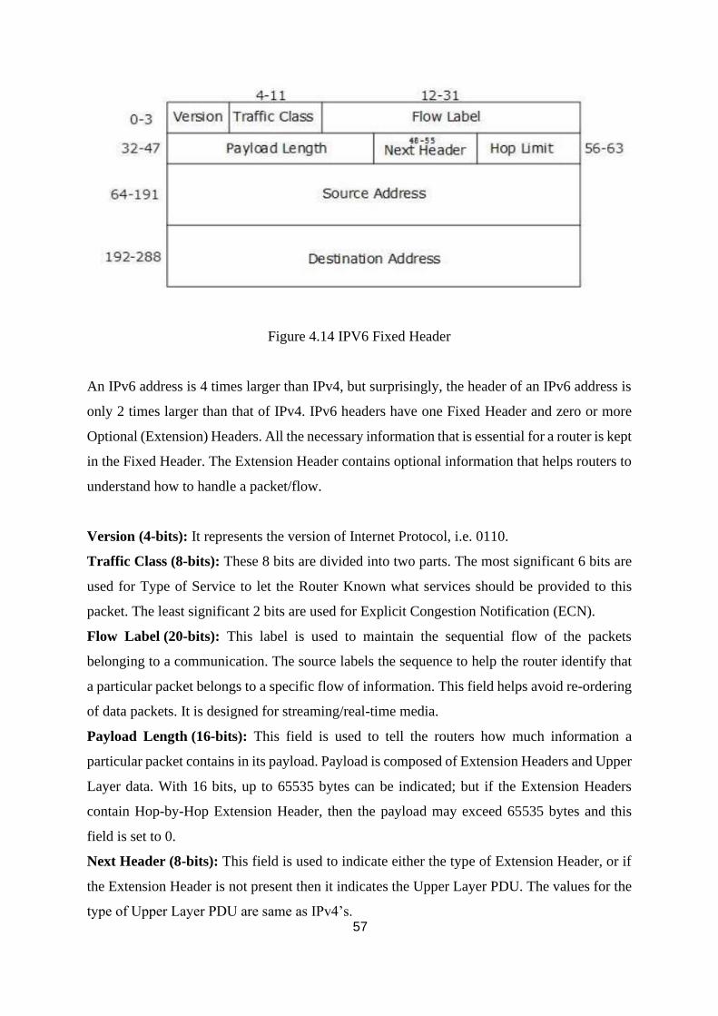
57
Figure 4.14 IPV6 Fixed Header
An IPv6 address is 4 times larger than IPv4, but surprisingly, the header of an IPv6 address is
only 2 times larger than that of IPv4. IPv6 headers have one Fixed Header and zero or more
Optional (Extension) Headers. All the necessary information that is essential for a router is kept
in the Fixed Header. The Extension Header contains optional information that helps routers to
understand how to handle a packet/flow.
Version (4-bits): It represents the version of Internet Protocol, i.e. 0110.
Traffic Class (8-bits): These 8 bits are divided into two parts. The most significant 6 bits are
used for Type of Service to let the Router Known what services should be provided to this
packet. The least significant 2 bits are used for Explicit Congestion Notification (ECN).
Flow Label (20-bits): This label is used to maintain the sequential flow of the packets
belonging to a communication. The source labels the sequence to help the router identify that
a particular packet belongs to a specific flow of information. This field helps avoid re-ordering
of data packets. It is designed for streaming/real-time media.
Payload Length (16-bits): This field is used to tell the routers how much information a
particular packet contains in its payload. Payload is composed of Extension Headers and Upper
Layer data. With 16 bits, up to 65535 bytes can be indicated; but if the Extension Headers
contain Hop-by-Hop Extension Header, then the payload may exceed 65535 bytes and this
field is set to 0.
Next Header (8-bits): This field is used to indicate either the type of Extension Header, or if
the Extension Header is not present then it indicates the Upper Layer PDU. The values for the
type of Upper Layer PDU are same as IPv4’s.
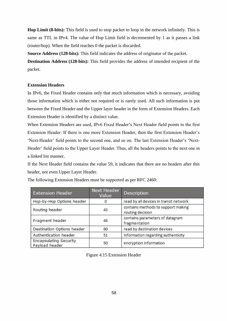
58
Hop Limit (8-bits): This field is used to stop packet to loop in the network infinitely. This is
same as TTL in IPv4. The value of Hop Limit field is decremented by 1 as it passes a link
(router/hop). When the field reaches 0 the packet is discarded.
Source Address (128-bits): This field indicates the address of originator of the packet.
Destination Address (128-bits): This field provides the address of intended recipient of the
packet.
Extension Headers
In IPv6, the Fixed Header contains only that much information which is necessary, avoiding
those information which is either not required or is rarely used. All such information is put
between the Fixed Header and the Upper layer header in the form of Extension Headers. Each
Extension Header is identified by a distinct value.
When Extension Headers are used, IPv6 Fixed Header’s Next Header field points to the first
Extension Header. If there is one more Extension Header, then the first Extension Header’s
‘Next-Header’ field points to the second one, and so on. The last Extension Header’s ‘Next-
Header’ field points to the Upper Layer Header. Thus, all the headers points to the next one in
a linked list manner.
If the Next Header field contains the value 59, it indicates that there are no headers after this
header, not even Upper Layer Header.
The following Extension Headers must be supported as per RFC 2460:
Figure 4.15 Extension Header
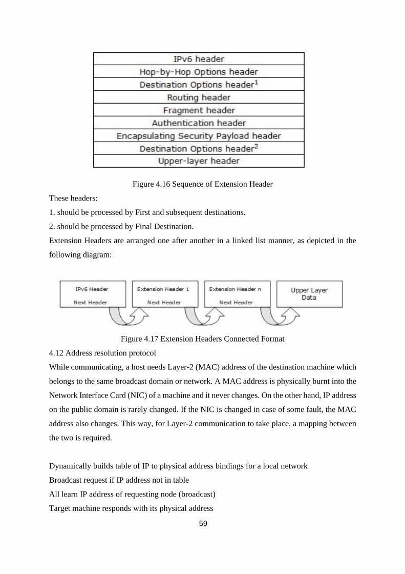
59
Figure 4.16 Sequence of Extension Header
These headers:
1. should be processed by First and subsequent destinations.
2. should be processed by Final Destination.
Extension Headers are arranged one after another in a linked list manner, as depicted in the
following diagram:
Figure 4.17 Extension Headers Connected Format
4.12 Address resolution protocol
While communicating, a host needs Layer-2 (MAC) address of the destination machine which
belongs to the same broadcast domain or network. A MAC address is physically burnt into the
Network Interface Card (NIC) of a machine and it never changes. On the other hand, IP address
on the public domain is rarely changed. If the NIC is changed in case of some fault, the MAC
address also changes. This way, for Layer-2 communication to take place, a mapping between
the two is required.
Dynamically builds table of IP to physical address bindings for a local network
Broadcast request if IP address not in table
All learn IP address of requesting node (broadcast)
Target machine responds with its physical address
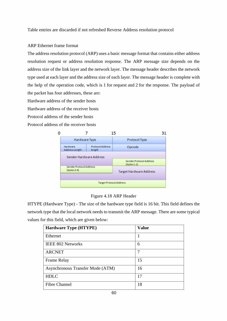
60
Table entries are discarded if not refreshed Reverse Address resolution protocol
ARP Ethernet frame format
The address resolution protocol (ARP) uses a basic message format that contains either address
resolution request or address resolution response. The ARP message size depends on the
address size of the link layer and the network layer. The message header describes the network
type used at each layer and the address size of each layer. The message header is complete with
the help of the operation code, which is 1 for request and 2 for the response. The payload of
the packet has four addresses, these are:
Hardware address of the sender hosts
Hardware address of the receiver hosts
Protocol address of the sender hosts
Protocol address of the receiver hosts
Figure 4.18 ARP Header
HTYPE (Hardware Type) - The size of the hardware type field is 16 bit. This field defines the
network type that the local network needs to transmit the ARP message. There are some typical
values for this field, which are given below:
Hardware Type (HTYPE) Value
Ethernet 1
IEEE 802 Networks 6
ARCNET 7
Frame Relay 15
Asynchronous Transfer Mode (ATM) 16
HDLC 17
Fibre Channel 18
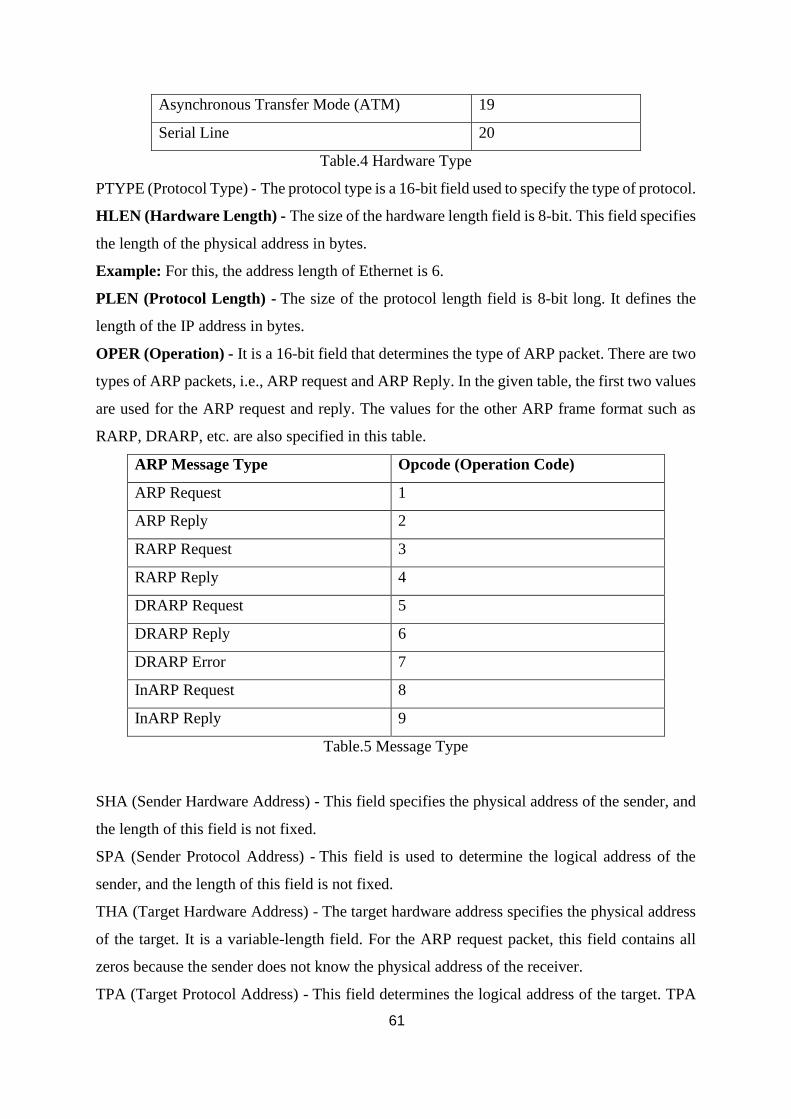
61
Asynchronous Transfer Mode (ATM) 19
Serial Line 20
Table.4 Hardware Type
PTYPE (Protocol Type) - The protocol type is a 16-bit field used to specify the type of protocol.
HLEN (Hardware Length) - The size of the hardware length field is 8-bit. This field specifies
the length of the physical address in bytes.
Example: For this, the address length of Ethernet is 6.
PLEN (Protocol Length) - The size of the protocol length field is 8-bit long. It defines the
length of the IP address in bytes.
OPER (Operation) - It is a 16-bit field that determines the type of ARP packet. There are two
types of ARP packets, i.e., ARP request and ARP Reply. In the given table, the first two values
are used for the ARP request and reply. The values for the other ARP frame format such as
RARP, DRARP, etc. are also specified in this table.
ARP Message Type Opcode (Operation Code)
ARP Request 1
ARP Reply 2
RARP Request 3
RARP Reply 4
DRARP Request 5
DRARP Reply 6
DRARP Error 7
InARP Request 8
InARP Reply 9
Table.5 Message Type
SHA (Sender Hardware Address) - This field specifies the physical address of the sender, and
the length of this field is not fixed.
SPA (Sender Protocol Address) - This field is used to determine the logical address of the
sender, and the length of this field is not fixed.
THA (Target Hardware Address) - The target hardware address specifies the physical address
of the target. It is a variable-length field. For the ARP request packet, this field contains all
zeros because the sender does not know the physical address of the receiver.
TPA (Target Protocol Address) - This field determines the logical address of the target. TPA
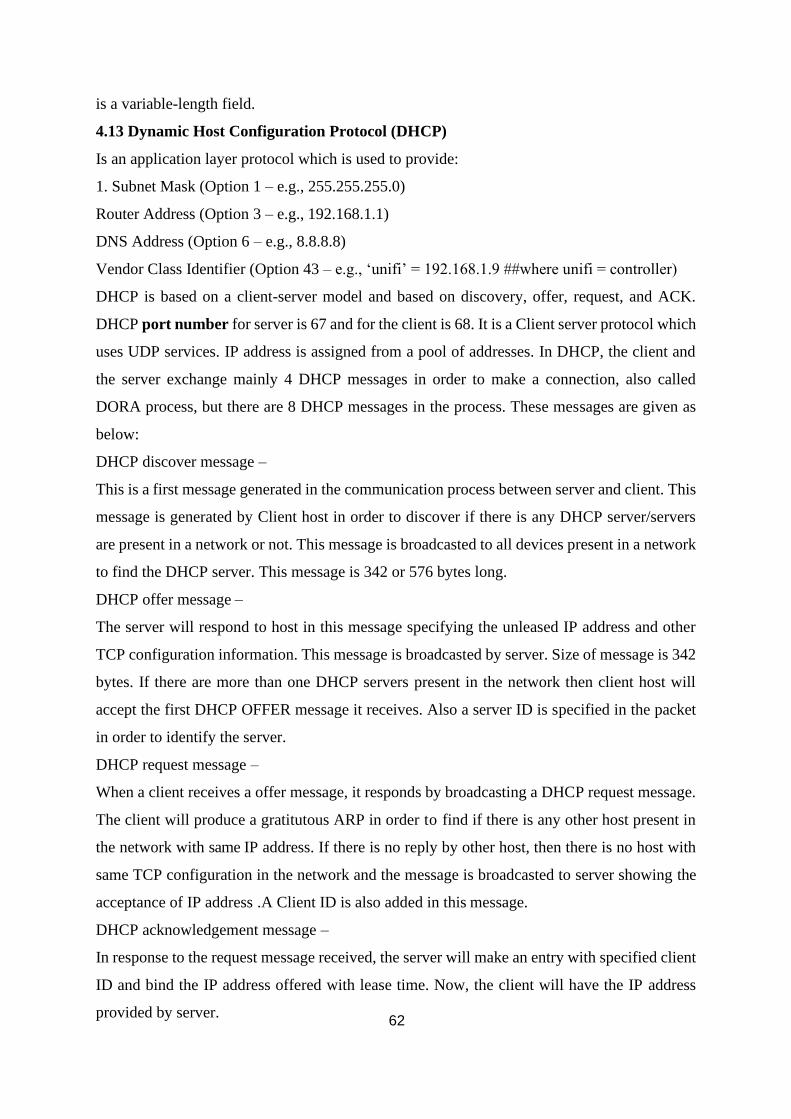
62
is a variable-length field.
4.13 Dynamic Host Configuration Protocol (DHCP)
Is an application layer protocol which is used to provide:
1. Subnet Mask (Option 1 – e.g., 255.255.255.0)
Router Address (Option 3 – e.g., 192.168.1.1)
DNS Address (Option 6 – e.g., 8.8.8.8)
Vendor Class Identifier (Option 43 – e.g., ‘unifi’ = 192.168.1.9 ##where unifi = controller)
DHCP is based on a client-server model and based on discovery, offer, request, and ACK.
DHCP port number for server is 67 and for the client is 68. It is a Client server protocol which
uses UDP services. IP address is assigned from a pool of addresses. In DHCP, the client and
the server exchange mainly 4 DHCP messages in order to make a connection, also called
DORA process, but there are 8 DHCP messages in the process. These messages are given as
below:
DHCP discover message –
This is a first message generated in the communication process between server and client. This
message is generated by Client host in order to discover if there is any DHCP server/servers
are present in a network or not. This message is broadcasted to all devices present in a network
to find the DHCP server. This message is 342 or 576 bytes long.
DHCP offer message –
The server will respond to host in this message specifying the unleased IP address and other
TCP configuration information. This message is broadcasted by server. Size of message is 342
bytes. If there are more than one DHCP servers present in the network then client host will
accept the first DHCP OFFER message it receives. Also a server ID is specified in the packet
in order to identify the server.
DHCP request message –
When a client receives a offer message, it responds by broadcasting a DHCP request message.
The client will produce a gratitutous ARP in order to find if there is any other host present in
the network with same IP address. If there is no reply by other host, then there is no host with
same TCP configuration in the network and the message is broadcasted to server showing the
acceptance of IP address .A Client ID is also added in this message.
DHCP acknowledgement message –
In response to the request message received, the server will make an entry with specified client
ID and bind the IP address offered with lease time. Now, the client will have the IP address
provided by server.
63
DHCP negative acknowledgement message –
Whenever a DHCP server receives a request for IP address that is invalid according to the
scopes that is configured with, it send DHCP Nak message to client. Eg-when the
server has no IP address unused or the pool is empty, then this message is sent by the server to
client.
DHCP decline –
If DHCP client determines the offered configuration parameters are different or invalid, it sends
DHCP decline message to the server .When there is a reply to the gratuitous ARP by any host
to the client, the client sends DHCP decline message to the server showing the offered IP
address is already in use.
DHCP release –
A DHCP client sends DHCP release packet to server to release IP address and cancel any
remaining lease time.
DHCP inform –
If a client address has obtained IP address manually then the client uses a DHCP inform to
obtain other local configuration parameters, such as domain name. In reply to the dhcp inform
message, DHCP server generates DHCP ack message with local configuration suitable for the
client without allocating a new IP address. This DHCP ack message is unicast to the client.
Note – All the messages can be unicast also by dhcp relay agent if the server is present in
different network.
Advantages – The advantages of using DHCP include:
centralized management of IP addresses
ease of adding new clients to a network
reuse of IP addresses reducing the total number of IP addresses that are required
simple reconfiguration of the IP address space on the DHCP server without needing to
reconfigure each client
The DHCP protocol gives the network administrator a method to configure the network from
a centralized area. With the help of DHCP, easy handling of new users and reuse of IP address
can be achieved.
Disadvantages – Disadvantage of using DHCP is: IP conflict can occur
4.13 INTERNET CONTROL MESSAGE PROTOCOL (ICMP)
IP provides unreliable connectionless datagram service, original aim being efficient use of
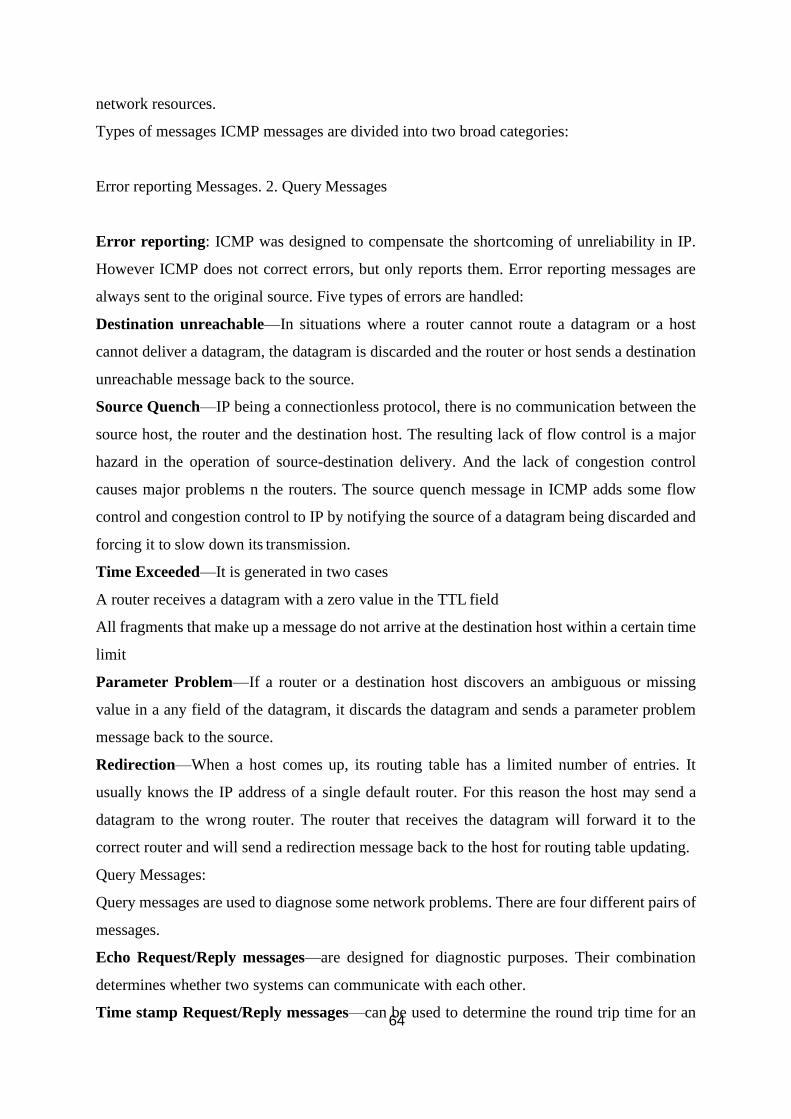
64
network resources.
Types of messages ICMP messages are divided into two broad categories:
Error reporting Messages. 2. Query Messages
Error reporting: ICMP was designed to compensate the shortcoming of unreliability in IP.
However ICMP does not correct errors, but only reports them. Error reporting messages are
always sent to the original source. Five types of errors are handled:
Destination unreachable—In situations where a router cannot route a datagram or a host
cannot deliver a datagram, the datagram is discarded and the router or host sends a destination
unreachable message back to the source.
Source Quench—IP being a connectionless protocol, there is no communication between the
source host, the router and the destination host. The resulting lack of flow control is a major
hazard in the operation of source-destination delivery. And the lack of congestion control
causes major problems n the routers. The source quench message in ICMP adds some flow
control and congestion control to IP by notifying the source of a datagram being discarded and
forcing it to slow down its transmission.
Time Exceeded—It is generated in two cases
A router receives a datagram with a zero value in the TTL field
All fragments that make up a message do not arrive at the destination host within a certain time
limit
Parameter Problem—If a router or a destination host discovers an ambiguous or missing
value in a any field of the datagram, it discards the datagram and sends a parameter problem
message back to the source.
Redirection—When a host comes up, its routing table has a limited number of entries. It
usually knows the IP address of a single default router. For this reason the host may send a
datagram to the wrong router. The router that receives the datagram will forward it to the
correct router and will send a redirection message back to the host for routing table updating.
Query Messages:
Query messages are used to diagnose some network problems. There are four different pairs of
messages.
Echo Request/Reply messages—are designed for diagnostic purposes. Their combination
determines whether two systems can communicate with each other.
Time stamp Request/Reply messages—can be used to determine the round trip time for an
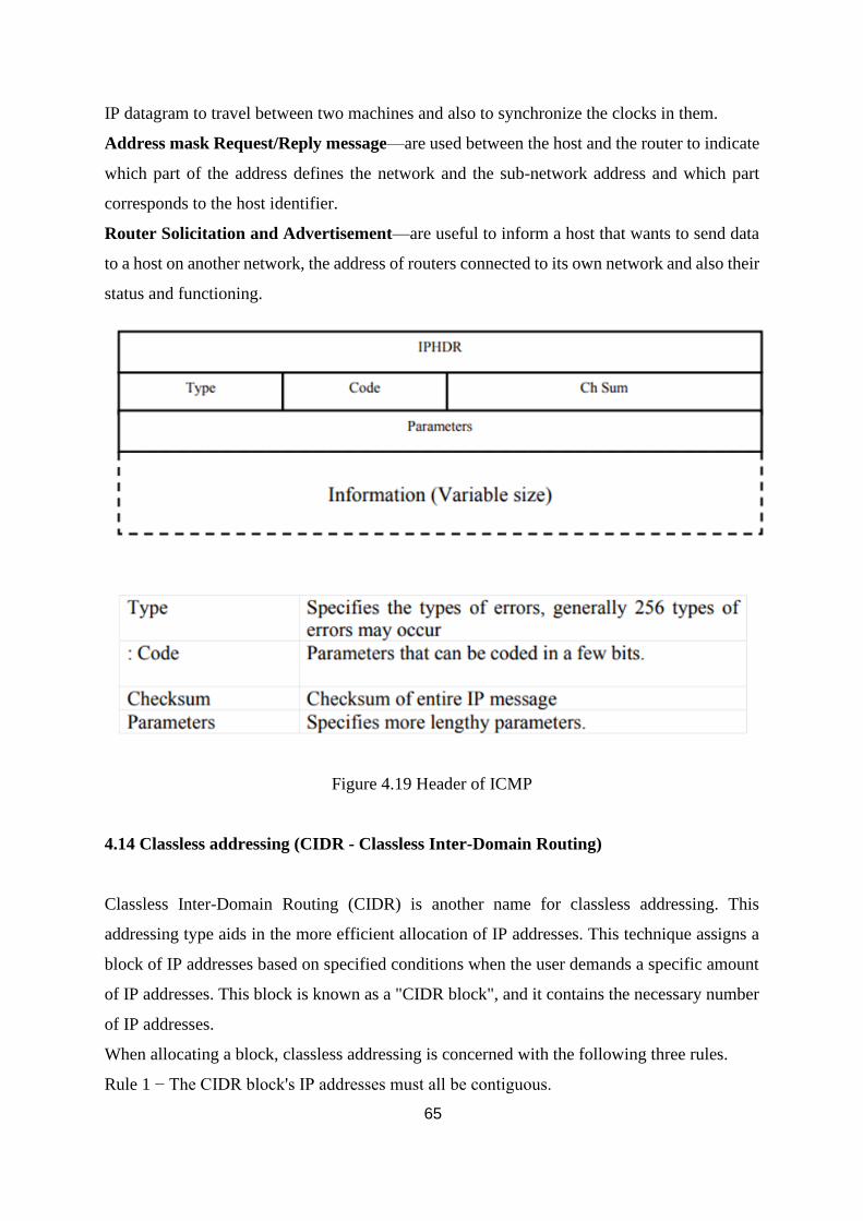
65
IP datagram to travel between two machines and also to synchronize the clocks in them.
Address mask Request/Reply message—are used between the host and the router to indicate
which part of the address defines the network and the sub-network address and which part
corresponds to the host identifier.
Router Solicitation and Advertisement—are useful to inform a host that wants to send data
to a host on another network, the address of routers connected to its own network and also their
status and functioning.
Figure 4.19 Header of ICMP
4.14 Classless addressing (CIDR - Classless Inter-Domain Routing)
Classless Inter-Domain Routing (CIDR) is another name for classless addressing. This
addressing type aids in the more efficient allocation of IP addresses. This technique assigns a
block of IP addresses based on specified conditions when the user demands a specific amount
of IP addresses. This block is known as a "CIDR block", and it contains the necessary number
of IP addresses.
When allocating a block, classless addressing is concerned with the following three rules.
Rule 1 − The CIDR block's IP addresses must all be contiguous.
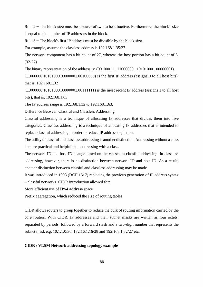
66
Rule 2 − The block size must be a power of two to be attractive. Furthermore, the block's size
is equal to the number of IP addresses in the block.
Rule 3 − The block's first IP address must be divisible by the block size.
For example, assume the classless address is 192.168.1.35/27.
The network component has a bit count of 27, whereas the host portion has a bit count of 5.
(32-27)
The binary representation of the address is: (00100011 . 11000000 . 10101000 . 00000001).
(11000000.10101000.00000001.00100000) is the first IP address (assigns 0 to all host bits),
that is, 192.168.1.32
(11000000.10101000.00000001.00111111) is the most recent IP address (assigns 1 to all host
bits), that is, 192.168.1.63
The IP address range is 192.168.1.32 to 192.168.1.63.
Difference Between Classful and Classless Addressing
Classful addressing is a technique of allocating IP addresses that divides them into five
categories. Classless addressing is a technique of allocating IP addresses that is intended to
replace classful addressing in order to reduce IP address depletion.
The utility of classful and classless addressing is another distinction. Addressing without a class
is more practical and helpful than addressing with a class.
The network ID and host ID change based on the classes in classful addressing. In classless
addressing, however, there is no distinction between network ID and host ID. As a result,
another distinction between classful and classless addressing may be made.
It was introduced in 1993 (RCF 1517) replacing the previous generation of IP address syntax
– classful networks. CIDR introduction allowed for:
More efficient use of IPv4 address space
Prefix aggregation, which reduced the size of routing tables
CIDR allows routers to group together to reduce the bulk of routing information carried by the
core routers. With CIDR, IP addresses and their subnet masks are written as four octets,
separated by periods, followed by a forward slash and a two-digit number that represents the
subnet mask e.g. 10.1.1.0/30, 172.16.1.16/28 and 192.168.1.32/27 etc.
CIDR / VLSM Network addressing topology example
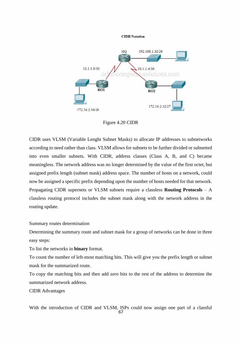
67
Figure 4.20 CIDR
CIDR uses VLSM (Variable Lenght Subnet Masks) to allocate IP addresses to subnetworks
according to need rather than class. VLSM allows for subnets to be further divided or subnetted
into even smaller subnets. With CIDR, address classes (Class A, B, and C) became
meaningless. The network address was no longer determined by the value of the first octet, but
assigned prefix length (subnet mask) address space. The number of hosts on a network, could
now be assigned a specific prefix depending upon the number of hosts needed for that network.
Propagating CIDR supernets or VLSM subnets require a classless Routing Protocols – A
classless routing protocol includes the subnet mask along with the network address in the
routing update.
Summary routes determination
Determining the summary route and subnet mask for a group of networks can be done in three
easy steps:
To list the networks in binary format.
To count the number of left-most matching bits. This will give you the prefix length or subnet
mask for the summarized route.
To copy the matching bits and then add zero bits to the rest of the address to determine the
summarized network address.
CIDR Advantages
With the introduction of CIDR and VLSM, ISPs could now assign one part of a classful
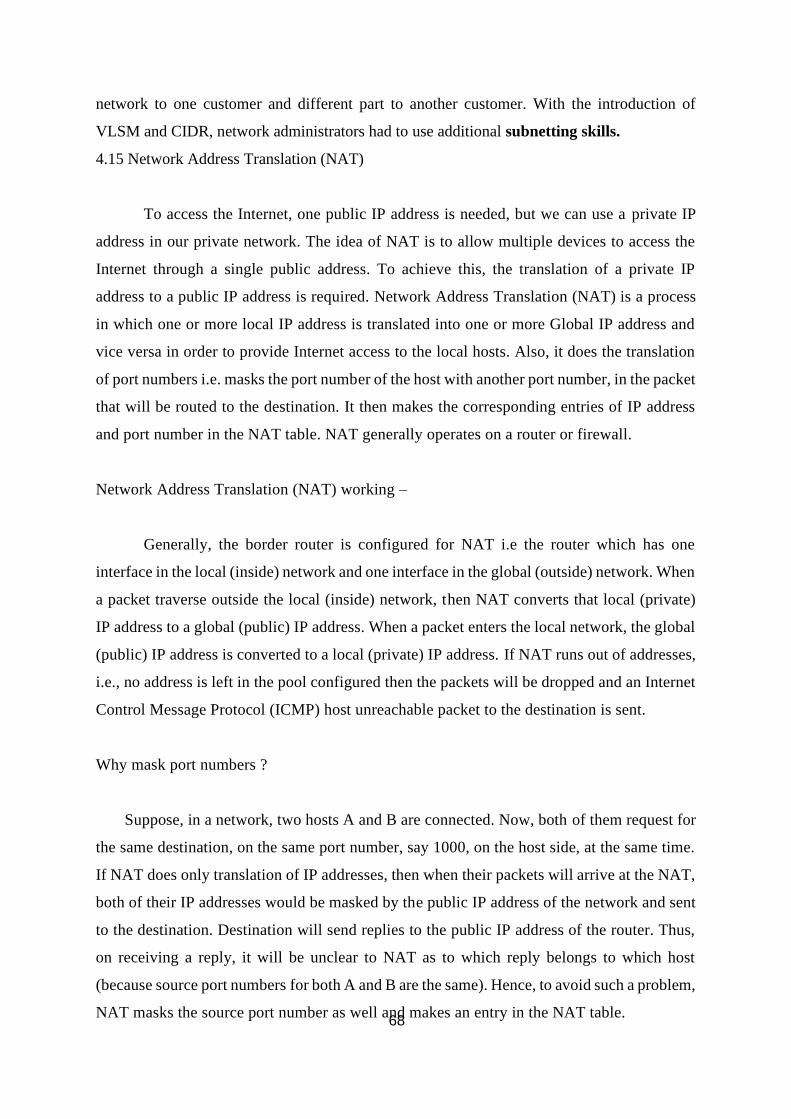
68
network to one customer and different part to another customer. With the introduction of
VLSM and CIDR, network administrators had to use additional subnetting skills.
4.15 Network Address Translation (NAT)
To access the Internet, one public IP address is needed, but we can use a private IP
address in our private network. The idea of NAT is to allow multiple devices to access the
Internet through a single public address. To achieve this, the translation of a private IP
address to a public IP address is required. Network Address Translation (NAT) is a process
in which one or more local IP address is translated into one or more Global IP address and
vice versa in order to provide Internet access to the local hosts. Also, it does the translation
of port numbers i.e. masks the port number of the host with another port number, in the packet
that will be routed to the destination. It then makes the corresponding entries of IP address
and port number in the NAT table. NAT generally operates on a router or firewall.
Network Address Translation (NAT) working –
Generally, the border router is configured for NAT i.e the router which has one
interface in the local (inside) network and one interface in the global (outside) network. When
a packet traverse outside the local (inside) network, then NAT converts that local (private)
IP address to a global (public) IP address. When a packet enters the local network, the global
(public) IP address is converted to a local (private) IP address. If NAT runs out of addresses,
i.e., no address is left in the pool configured then the packets will be dropped and an Internet
Control Message Protocol (ICMP) host unreachable packet to the destination is sent.
Why mask port numbers ?
Suppose, in a network, two hosts A and B are connected. Now, both of them request for
the same destination, on the same port number, say 1000, on the host side, at the same time.
If NAT does only translation of IP addresses, then when their packets will arrive at the NAT,
both of their IP addresses would be masked by the public IP address of the network and sent
to the destination. Destination will send replies to the public IP address of the router. Thus,
on receiving a reply, it will be unclear to NAT as to which reply belongs to which host
(because source port numbers for both A and B are the same). Hence, to avoid such a problem,
NAT masks the source port number as well and makes an entry in the NAT table.
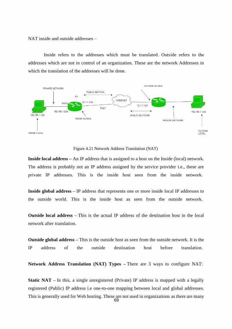
69
NAT inside and outside addresses –
Inside refers to the addresses which must be translated. Outside refers to the
addresses which are not in control of an organization. These are the network Addresses in
which the translation of the addresses will be done.
Figure 4.21 Network Address Translation (NAT)
Inside local address – An IP address that is assigned to a host on the Inside (local) network.
The address is probably not an IP address assigned by the service provider i.e., these are
private IP addresses. This is the inside host seen from the inside network.
Inside global address – IP address that represents one or more inside local IP addresses to
the outside world. This is the inside host as seen from the outside network.
Outside local address – This is the actual IP address of the destination host in the local
network after translation.
Outside global address – This is the outside host as seen from the outside network. It is the
IP address of the outside destination host before translation.
Network Address Translation (NAT) Types – There are 3 ways to configure NAT:
Static NAT – In this, a single unregistered (Private) IP address is mapped with a legally
registered (Public) IP address i.e one-to-one mapping between local and global addresses.
This is generally used for Web hosting. These are not used in organizations as there are many
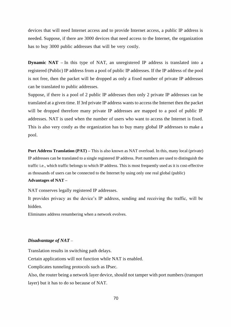
70
devices that will need Internet access and to provide Internet access, a public IP address is
needed. Suppose, if there are 3000 devices that need access to the Internet, the organization
has to buy 3000 public addresses that will be very costly.
Dynamic NAT – In this type of NAT, an unregistered IP address is translated into a
registered (Public) IP address from a pool of public IP addresses. If the IP address of the pool
is not free, then the packet will be dropped as only a fixed number of private IP addresses
can be translated to public addresses.
Suppose, if there is a pool of 2 public IP addresses then only 2 private IP addresses can be
translated at a given time. If 3rd private IP address wants to access the Internet then the packet
will be dropped therefore many private IP addresses are mapped to a pool of public IP
addresses. NAT is used when the number of users who want to access the Internet is fixed.
This is also very costly as the organization has to buy many global IP addresses to make a
pool.
Port Address Translation (PAT) – This is also known as NAT overload. In this, many local (private)
IP addresses can be translated to a single registered IP address. Port numbers are used to distinguish the
traffic i.e., which traffic belongs to which IP address. This is most frequently used as it is cost-effective
as thousands of users can be connected to the Internet by using only one real global (public)
Advantages of NAT –
NAT conserves legally registered IP addresses.
It provides privacy as the device’s IP address, sending and receiving the traffic, will be
hidden.
Eliminates address renumbering when a network evolves.
Disadvantage of NAT –
Translation results in switching path delays.
Certain applications will not function while NAT is enabled.
Complicates tunneling protocols such as IPsec.
Also, the router being a network layer device, should not tamper with port numbers (transport
layer) but it has to do so because of NAT.

1
SCHOOL OF ELECTRICAL AND ELECTRONICS ENGINEERING DEPARTMENT OF
ELECTRONICS AND COMMUNICATION ENGINEERING
UNIT –V COMPUTER NETWORKS – SECA1604
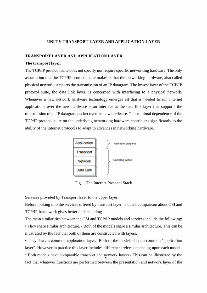
2
UNIT V TRANSPORT LAYER AND APPLICATION LAYER
TRANSPORT LAYER AND APPLICATION LAYER
The transport layer:
The TCP/IP protocol suite does not specify nor require specific networking hardware. The only
assumption that the TCP/IP protocol suite makes is that the networking hardware, also called
physical network, supports the transmission of an IP datagram. The lowest layer of the TCP/IP
protocol suite, the data link layer, is concerned with interfacing to a physical network.
Whenever a new network hardware technology emerges all that is needed to run Internet
applications over the new hardware is an interface at the data link layer that supports the
transmission of an IP datagram packet over the new hardware. This minimal dependence of the
TCP/IP protocol suite on the underlying networking hardware contributes significantly to the
ability of the Internet protocols to adapt to advances in networking hardware.
Fig.1. The Internet Protocol Stack
Services provided by Transport layer to the upper layer:
Before looking into the services offered by transport layer , a quick comparison about OSI and
TCP/IP framework gives better understanding.
The main similarities between the OSI and TCP/IP models and services include the following:
• They share similar architecture. - Both of the models share a similar architecture. This can be
illustrated by the fact that both of them are constructed with layers.
• They share a common application layer.- Both of the models share a common "application
layer". However in practice this layer includes different services depending upon each model.
• Both models have comparable transport and network layers.- This can be illustrated by the
fact that whatever functions are performed between the presentation and network layer of the
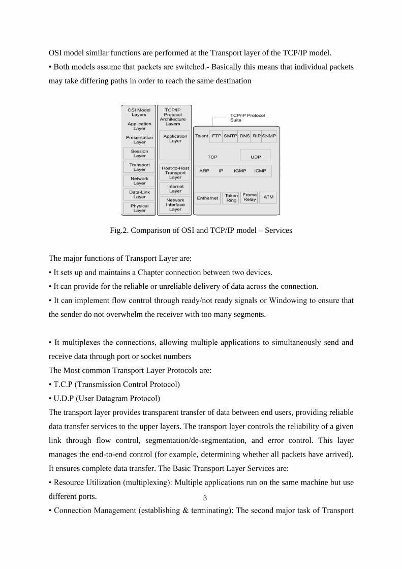
3
OSI model similar functions are performed at the Transport layer of the TCP/IP model.
• Both models assume that packets are switched.- Basically this means that individual packets
may take differing paths in order to reach the same destination
Fig.2. Comparison of OSI and TCP/IP model – Services
The major functions of Transport Layer are:
• It sets up and maintains a Chapter connection between two devices.
• It can provide for the reliable or unreliable delivery of data across the connection.
• It can implement flow control through ready/not ready signals or Windowing to ensure that
the sender do not overwhelm the receiver with too many segments.
• It multiplexes the connections, allowing multiple applications to simultaneously send and
receive data through port or socket numbers
The Most common Transport Layer Protocols are:
• T.C.P (Transmission Control Protocol)
• U.D.P (User Datagram Protocol)
The transport layer provides transparent transfer of data between end users, providing reliable
data transfer services to the upper layers. The transport layer controls the reliability of a given
link through flow control, segmentation/de-segmentation, and error control. This layer
manages the end-to-end control (for example, determining whether all packets have arrived).
It ensures complete data transfer. The Basic Transport Layer Services are:
• Resource Utilization (multiplexing): Multiple applications run on the same machine but use
different ports.
• Connection Management (establishing & terminating): The second major task of Transport
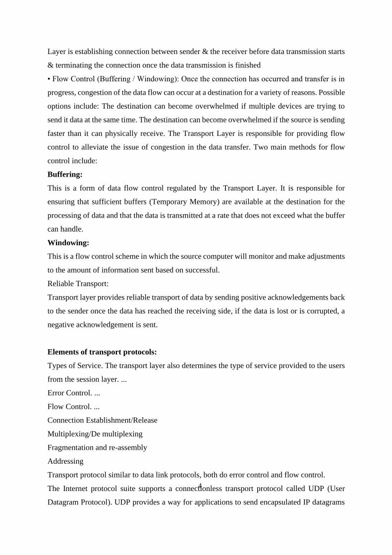
4
Layer is establishing connection between sender & the receiver before data transmission starts
& terminating the connection once the data transmission is finished
• Flow Control (Buffering / Windowing): Once the connection has occurred and transfer is in
progress, congestion of the data flow can occur at a destination for a variety of reasons. Possible
options include: The destination can become overwhelmed if multiple devices are trying to
send it data at the same time. The destination can become overwhelmed if the source is sending
faster than it can physically receive. The Transport Layer is responsible for providing flow
control to alleviate the issue of congestion in the data transfer. Two main methods for flow
control include:
Buffering:
This is a form of data flow control regulated by the Transport Layer. It is responsible for
ensuring that sufficient buffers (Temporary Memory) are available at the destination for the
processing of data and that the data is transmitted at a rate that does not exceed what the buffer
can handle.
Windowing:
This is a flow control scheme in which the source computer will monitor and make adjustments
to the amount of information sent based on successful.
Reliable Transport:
Transport layer provides reliable transport of data by sending positive acknowledgements back
to the sender once the data has reached the receiving side, if the data is lost or is corrupted, a
negative acknowledgement is sent.
Elements of transport protocols:
Types of Service. The transport layer also determines the type of service provided to the users
from the session layer. ...
Error Control. ...
Flow Control. ...
Connection Establishment/Release
Multiplexing/De multiplexing
Fragmentation and re-assembly
Addressing
Transport protocol similar to data link protocols, both do error control and flow control.
The Internet protocol suite supports a connectionless transport protocol called UDP (User
Datagram Protocol). UDP provides a way for applications to send encapsulated IP datagrams
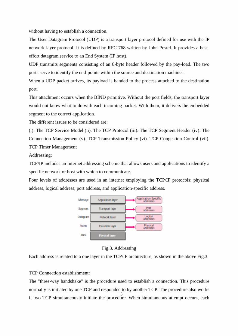
5
without having to establish a connection.
The User Datagram Protocol (UDP) is a transport layer protocol defined for use with the IP
network layer protocol. It is defined by RFC 768 written by John Postel. It provides a best-
effort datagram service to an End System (IP host).
UDP transmits segments consisting of an 8-byte header followed by the pay-load. The two
ports serve to identify the end-points within the source and destination machines.
When a UDP packet arrives, its payload is handed to the process attached to the destination
port.
This attachment occurs when the BIND primitive. Without the port fields, the transport layer
would not know what to do with each incoming packet. With them, it delivers the embedded
segment to the correct application.
The different issues to be considered are:
(i). The TCP Service Model (ii). The TCP Protocol (iii). The TCP Segment Header (iv). The
Connection Management (v). TCP Transmission Policy (vi). TCP Congestion Control (vii).
TCP Timer Management
Addressing:
TCP/IP includes an Internet addressing scheme that allows users and applications to identify a
specific network or host with which to communicate.
Four levels of addresses are used in an internet employing the TCP/IP protocols: physical
address, logical address, port address, and application-specific address.
Fig.3. Addressing
Each address is related to a one layer in the TCP/IP architecture, as shown in the above Fig.3.
TCP Connection establishment:
The "three-way handshake" is the procedure used to establish a connection. This procedure
normally is initiated by one TCP and responded to by another TCP. The procedure also works
if two TCP simultaneously initiate the procedure. When simultaneous attempt occurs, each
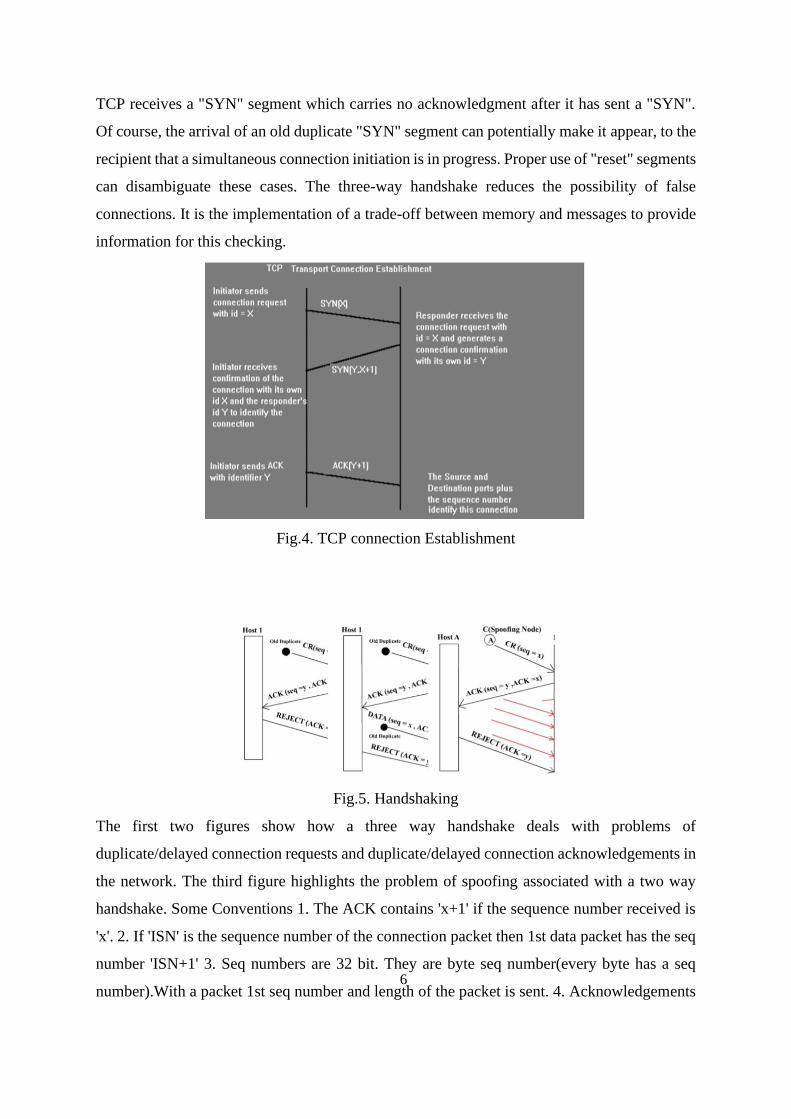
6
TCP receives a "SYN" segment which carries no acknowledgment after it has sent a "SYN".
Of course, the arrival of an old duplicate "SYN" segment can potentially make it appear, to the
recipient that a simultaneous connection initiation is in progress. Proper use of "reset" segments
can disambiguate these cases. The three-way handshake reduces the possibility of false
connections. It is the implementation of a trade-off between memory and messages to provide
information for this checking.
Fig.4. TCP connection Establishment
Fig.5. Handshaking
The first two figures show how a three way handshake deals with problems of
duplicate/delayed connection requests and duplicate/delayed connection acknowledgements in
the network. The third figure highlights the problem of spoofing associated with a two way
handshake. Some Conventions 1. The ACK contains 'x+1' if the sequence number received is
'x'. 2. If 'ISN' is the sequence number of the connection packet then 1st data packet has the seq
number 'ISN+1' 3. Seq numbers are 32 bit. They are byte seq number(every byte has a seq
number).With a packet 1st seq number and length of the packet is sent. 4. Acknowledgements
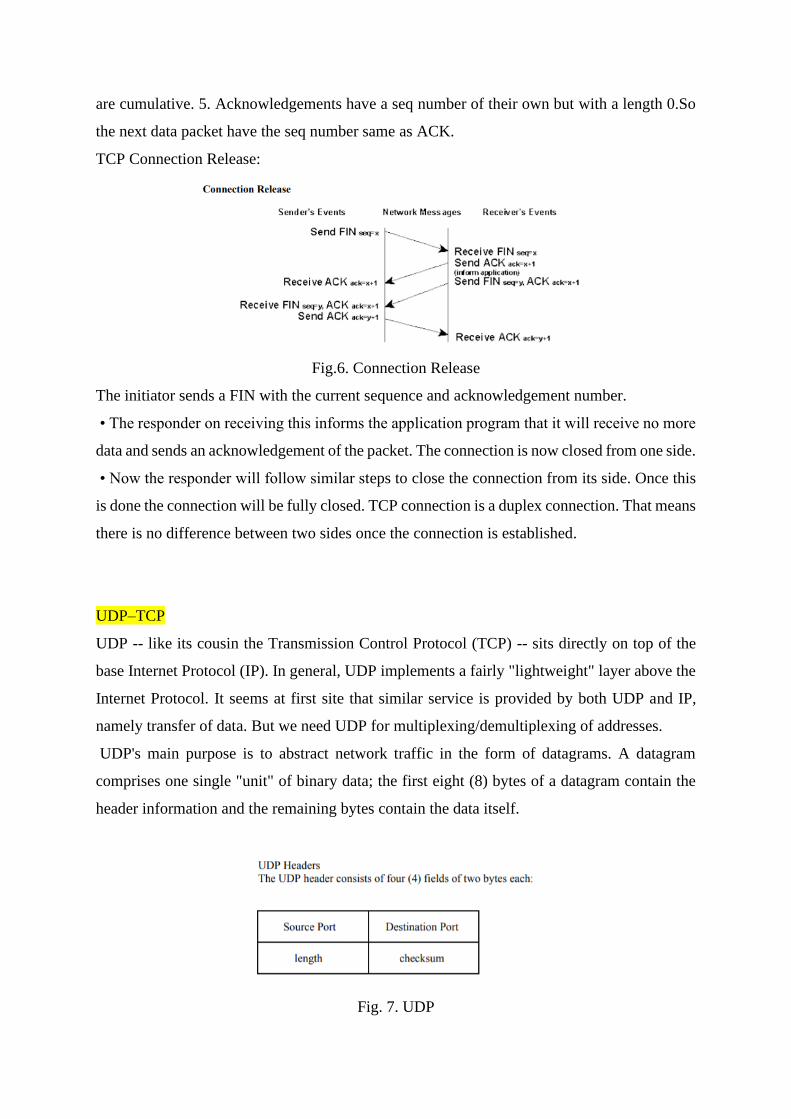
7
are cumulative. 5. Acknowledgements have a seq number of their own but with a length 0.So
the next data packet have the seq number same as ACK.
TCP Connection Release:
Fig.6. Connection Release
The initiator sends a FIN with the current sequence and acknowledgement number.
• The responder on receiving this informs the application program that it will receive no more
data and sends an acknowledgement of the packet. The connection is now closed from one side.
• Now the responder will follow similar steps to close the connection from its side. Once this
is done the connection will be fully closed. TCP connection is a duplex connection. That means
there is no difference between two sides once the connection is established.
UDP–TCP
UDP -- like its cousin the Transmission Control Protocol (TCP) -- sits directly on top of the
base Internet Protocol (IP). In general, UDP implements a fairly "lightweight" layer above the
Internet Protocol. It seems at first site that similar service is provided by both UDP and IP,
namely transfer of data. But we need UDP for multiplexing/demultiplexing of addresses.
UDP's main purpose is to abstract network traffic in the form of datagrams. A datagram
comprises one single "unit" of binary data; the first eight (8) bytes of a datagram contain the
header information and the remaining bytes contain the data itself.
Fig. 7. UDP
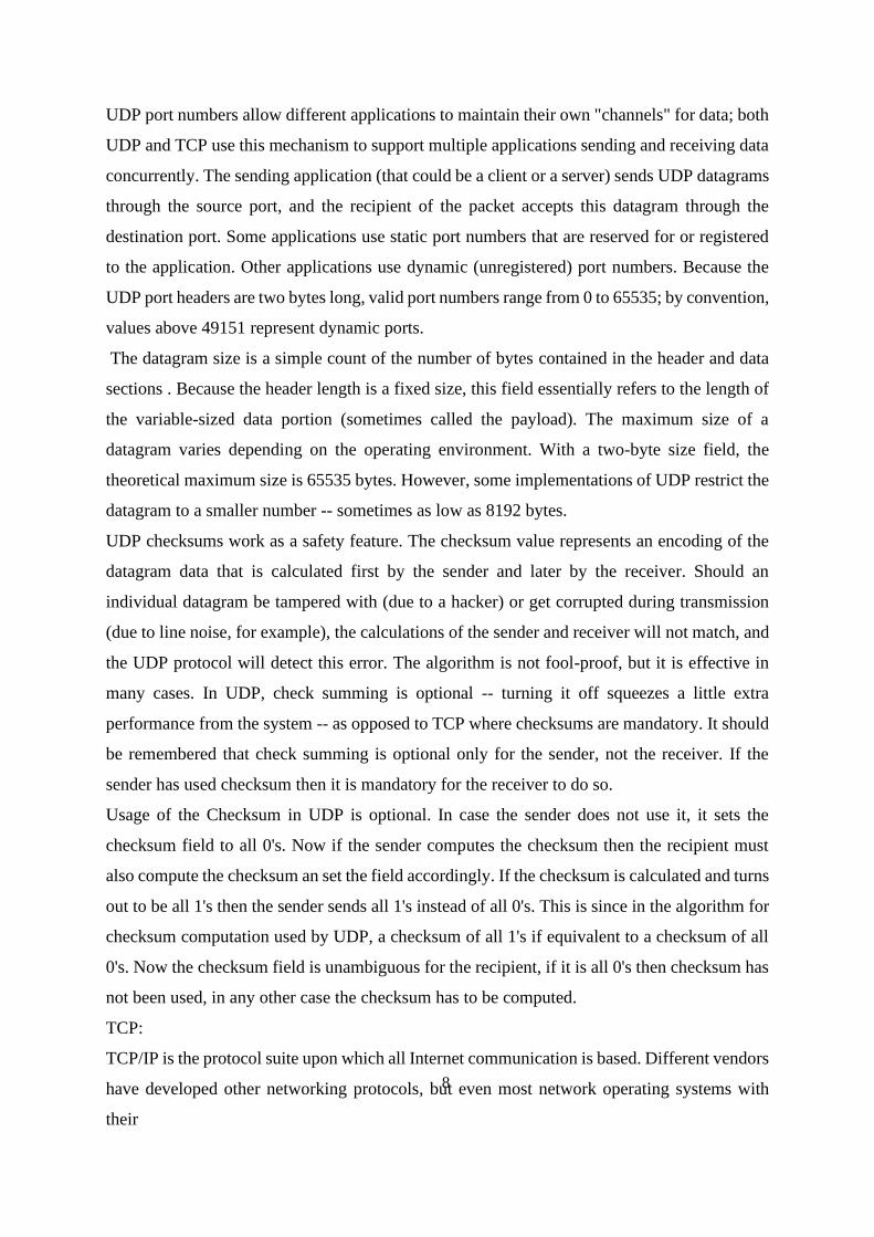
8
UDP port numbers allow different applications to maintain their own "channels" for data; both
UDP and TCP use this mechanism to support multiple applications sending and receiving data
concurrently. The sending application (that could be a client or a server) sends UDP datagrams
through the source port, and the recipient of the packet accepts this datagram through the
destination port. Some applications use static port numbers that are reserved for or registered
to the application. Other applications use dynamic (unregistered) port numbers. Because the
UDP port headers are two bytes long, valid port numbers range from 0 to 65535; by convention,
values above 49151 represent dynamic ports.
The datagram size is a simple count of the number of bytes contained in the header and data
sections . Because the header length is a fixed size, this field essentially refers to the length of
the variable-sized data portion (sometimes called the payload). The maximum size of a
datagram varies depending on the operating environment. With a two-byte size field, the
theoretical maximum size is 65535 bytes. However, some implementations of UDP restrict the
datagram to a smaller number -- sometimes as low as 8192 bytes.
UDP checksums work as a safety feature. The checksum value represents an encoding of the
datagram data that is calculated first by the sender and later by the receiver. Should an
individual datagram be tampered with (due to a hacker) or get corrupted during transmission
(due to line noise, for example), the calculations of the sender and receiver will not match, and
the UDP protocol will detect this error. The algorithm is not fool-proof, but it is effective in
many cases. In UDP, check summing is optional -- turning it off squeezes a little extra
performance from the system -- as opposed to TCP where checksums are mandatory. It should
be remembered that check summing is optional only for the sender, not the receiver. If the
sender has used checksum then it is mandatory for the receiver to do so.
Usage of the Checksum in UDP is optional. In case the sender does not use it, it sets the
checksum field to all 0's. Now if the sender computes the checksum then the recipient must
also compute the checksum an set the field accordingly. If the checksum is calculated and turns
out to be all 1's then the sender sends all 1's instead of all 0's. This is since in the algorithm for
checksum computation used by UDP, a checksum of all 1's if equivalent to a checksum of all
0's. Now the checksum field is unambiguous for the recipient, if it is all 0's then checksum has
not been used, in any other case the checksum has to be computed.
TCP:
TCP/IP is the protocol suite upon which all Internet communication is based. Different vendors
have developed other networking protocols, but even most network operating systems with
their
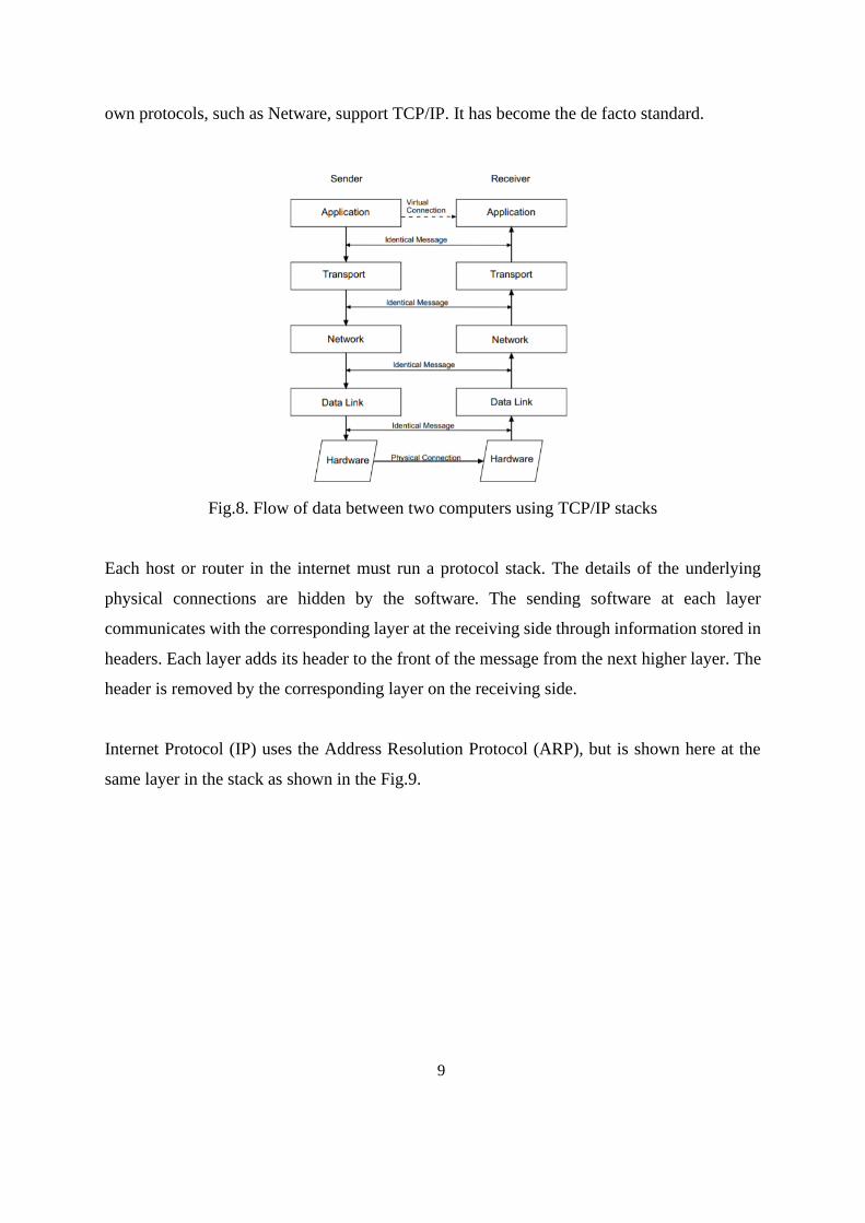
9
own protocols, such as Netware, support TCP/IP. It has become the de facto standard.
Fig.8. Flow of data between two computers using TCP/IP stacks
Each host or router in the internet must run a protocol stack. The details of the underlying
physical connections are hidden by the software. The sending software at each layer
communicates with the corresponding layer at the receiving side through information stored in
headers. Each layer adds its header to the front of the message from the next higher layer. The
header is removed by the corresponding layer on the receiving side.
Internet Protocol (IP) uses the Address Resolution Protocol (ARP), but is shown here at the
same layer in the stack as shown in the Fig.9.
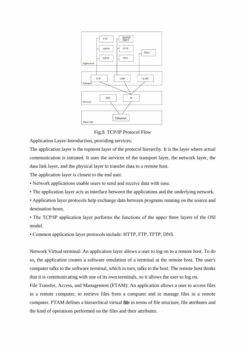
10
Fig.9. TCP/IP Protocol Flow
Application Layer-Introduction, providing services:
The application layer is the topmost layer of the protocol hierarchy. It is the layer where actual
communication is initiated. It uses the services of the transport layer, the network layer, the
data link layer, and the physical layer to transfer data to a remote host.
The application layer is closest to the end user.
• Network applications enable users to send and receive data with ease.
• The application layer acts as interface between the applications and the underlying network.
• Application layer protocols help exchange data between programs running on the source and
destination hosts.
• The TCP/IP application layer performs the functions of the upper three layers of the OSI
model.
• Common application layer protocols include: HTTP, FTP, TFTP, DNS.
Network Virtual terminal: An application layer allows a user to log on to a remote host. To do
so, the application creates a software emulation of a terminal at the remote host. The user's
computer talks to the software terminal, which in turn, talks to the host. The remote host thinks
that it is communicating with one of its own terminals, so it allows the user to log on.
File Transfer, Access, and Management (FTAM): An application allows a user to access files
in a remote computer, to retrieve files from a computer and to manage files in a remote
computer. FTAM defines a hierarchical virtual file in terms of file structure, file attributes and
the kind of operations performed on the files and their attributes.
11
Addressing: To obtain communication between client and server, there is a need for addressing.
When a client made a request to the server, the request contains the server address and its own
address. The server response to the client request, the request contains the destination address,
i.e., client address. To achieve this kind of addressing, DNS is used.
Mail Services: An application layer provides Email forwarding and storage.
Directory Services: An application contains a distributed database that provides access for
global information about various objects and services.
Authentication: It authenticates the sender or receiver's message or both.
Applications layer paradigms:
In this paradigm, communication at the application layer is between two running application
programs called processes: a client and a server. A client is a running program that initializes
the communication by sending a request; a server is another application program that waits for
a request from a client.
Client-Server Paradigm:
The service provider is an application program, called the server process;
• Server process runs continuously, waiting for another application program, called the client
process, to make a connection through the Internet and ask for service.
• The server process must be running all the time;
• The client process starts when the client needs to receive service.
• Several traditional services are still using this paradigm, e.g., WWW, HTTP, FTP, SSH, E-
mail, and so on. • Problems: – the server should be a powerful computer – there should be a
service provider willing to accept the cost and create a powerful server for a specific service.
Peer-to-Peer Paradigm:
There is no need for a server process to be running all the time and waiting for the client
processes to connect.
• The responsibility is shared between peers.
• E.g.: Internet telephony, Bit-Torrent, Skype, IPTV
• Advantages: – easily scalable and cost-effective in eliminating the need for expensive servers
to be running and maintained all the time
• Challenges: – more difficult to create secure communication between distributed services
• Few instant messaging application use both client-server and P2P
12
Client server model, Standard client-server application:
The client-server model, or client-server architecture, is a distributed application framework
dividing tasks between servers and clients, which either reside in the same system or
communicate through a computer network or the Internet.
Client-server model is a distributed application structure that partitions tasks or workloads
between the providers of a resource or service, called servers, and service requesters, called
clients. Often clients and servers communicate over a computer network on separate hardware,
but both client and server may reside in the same system. A server host runs one or more server
programs, which share their resources with clients. A client usually does not share any of its
resources, but it requests content or service from a server. Clients, therefore, initiate
communication sessions with servers, which await incoming requests. Examples of computer
applications that use the client-server model are email, network printing, and the
World Wide Web.
The "client-server" characteristic describes the relationship of cooperating programs in
an application. The server component provides a function or service to one or many clients,
which initiate requests for such services. Servers are classified by the services they provide.
For example, a web server serves web pages and a file server serves computer files. A shared
resource may be any of the server computer's software and electronic components, from
programs and data to processors and storage devices. The sharing of resources of a server
constitutes a service.
Clients and servers exchange messages in a request–response messaging pattern. The client
sends a request, and the server returns a response. This exchange of messages is an example of
inter-process communication. To communicate, the computers must have a common language,
and they must follow rules so that both the client and the server know what to expect. The
language and rules of communication are defined in a communications protocol. All protocols
operate in the application layer. The application layer protocol defines the basic patterns of the
dialogue. To formalize the data exchange even further, the server may implement an
application programming interface
When a bank customer accesses online banking services with a web browser (the client), the
client initiates a request to the bank's web server. The customer's login credentials may be
stored in a database, and the webserver accesses the database server as a client. An application
server interprets the returned data by applying the bank's business logic and provides the output
to the webserver. Finally, the webserver returns the result to the client web browser for display.
13
In each step of this sequence of client-server message exchanges, a computer processes a
request and returns data. This is the request-response messaging pattern. When all the requests
are met, the sequence is complete and the web browser presents the data to the customer. This
example illustrates a design pattern applicable to the client–server model
E mail - The user agent - Message transfer agent:
Electronic mail is a method of exchanging messages between people using electronic
devices. A message transfer agent (MTA) routes a mail message towards its final destination
by sending the message to another MTA. A user agent (UA) interacts with an end-user and
allows the user to send and receive mail messages. On the Internet, MTAs communicate with
each other using the Simple Mail Transfer Protocol (SMTP).
Messages exchanged across networks are passed between mail servers, including any attached
data files. These servers also often keep mailboxes for email. Access to this email by end users
is typically either via webmail or an email client.
A message transfer agent receives mail from either another MTA, a mail submission agent
(MSA), or a mail user agent (MUA). The transmission details are specified by the Simple Mail
Transfer Protocol (SMTP). When a recipient mailbox of a message is not hosted locally, the
message is relayed, that is, forwarded to another MTA. Every time an MTA receives an email
message, it adds a Received trace header field to the top of the header of the message, thereby
building a sequential record of MTAs handling the message. The process of choosing a target
MTA for the next hop is also described in SMTP, but can usually be overridden by configuring
the MTA software with specific routes.
A message transfer agent (MTA) is a software application used within an Internet message
handling system (MHS). It is responsible for transferring and routing an electronic mail
message from the sender’s computer to the recipient’s computer. The basic platform for an
MTA is an exchange system with client/server architecture.
SMTP:
SMTP stands for Simple Mail Transfer Protocol. SMTP is a set of communication
guidelines that allow software to transmit an electronic mail over the internet is called Simple
Mail Transfer Protocol. It is a program used for sending messages to other computer users
based on e-mail addresses.
SMTP or Simple Mail Transfer Protocol is an application that is used to send, receive,
and relay outgoing emails between senders and receivers. When an email is sent, it's transferred
over the internet from one server to another using SMTP. In simple terms, an SMTP email is
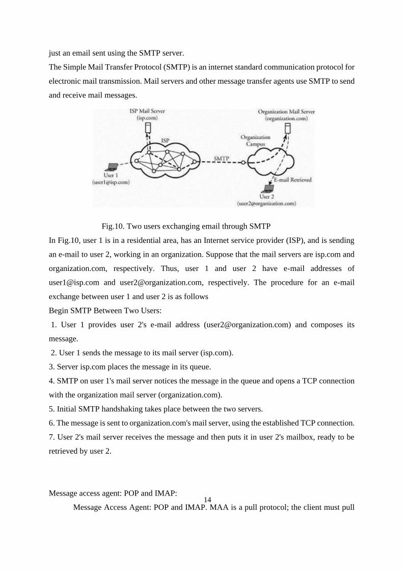
14
just an email sent using the SMTP server.
The Simple Mail Transfer Protocol (SMTP) is an internet standard communication protocol for
electronic mail transmission. Mail servers and other message transfer agents use SMTP to send
and receive mail messages.
Fig.10. Two users exchanging email through SMTP
In Fig.10, user 1 is in a residential area, has an Internet service provider (ISP), and is sending
an e-mail to user 2, working in an organization. Suppose that the mail servers are isp.com and
organization.com, respectively. Thus, user 1 and user 2 have e-mail addresses of
[email protected] and [email protected], respectively. The procedure for an e-mail
exchange between user 1 and user 2 is as follows
Begin SMTP Between Two Users:
1. User 1 provides user 2's e-mail address ([email protected]) and composes its
message.
2. User 1 sends the message to its mail server (isp.com).
3. Server isp.com places the message in its queue.
4. SMTP on user 1's mail server notices the message in the queue and opens a TCP connection
with the organization mail server (organization.com).
5. Initial SMTP handshaking takes place between the two servers.
6. The message is sent to organization.com's mail server, using the established TCP connection.
7. User 2's mail server receives the message and then puts it in user 2's mailbox, ready to be
retrieved by user 2.
Message access agent: POP and IMAP:
Message Access Agent: POP and IMAP. MAA is a pull protocol; the client must pull
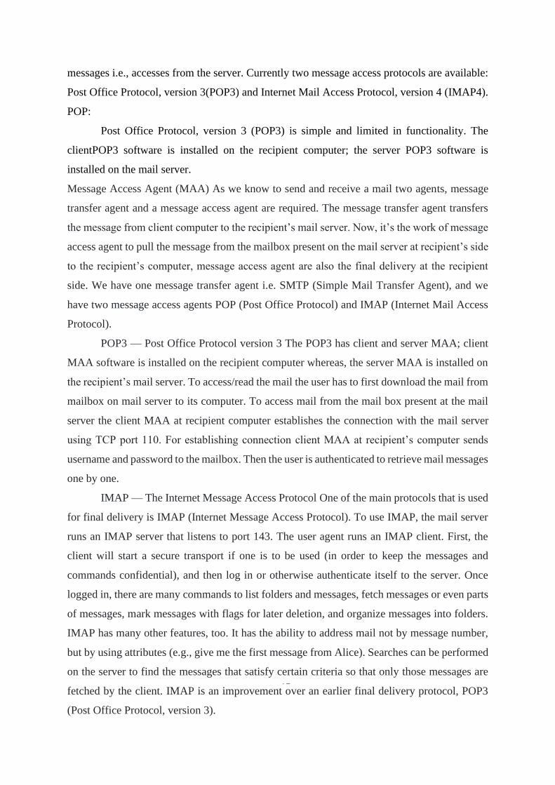
15
messages i.e., accesses from the server. Currently two message access protocols are available:
Post Office Protocol, version 3(POP3) and Internet Mail Access Protocol, version 4 (IMAP4).
POP:
Post Office Protocol, version 3 (POP3) is simple and limited in functionality. The
clientPOP3 software is installed on the recipient computer; the server POP3 software is
installed on the mail server.
Message Access Agent (MAA) As we know to send and receive a mail two agents, message
transfer agent and a message access agent are required. The message transfer agent transfers
the message from client computer to the recipient’s mail server. Now, it’s the work of message
access agent to pull the message from the mailbox present on the mail server at recipient’s side
to the recipient’s computer, message access agent are also the final delivery at the recipient
side. We have one message transfer agent i.e. SMTP (Simple Mail Transfer Agent), and we
have two message access agents POP (Post Office Protocol) and IMAP (Internet Mail Access
Protocol).
POP3 — Post Office Protocol version 3 The POP3 has client and server MAA; client
MAA software is installed on the recipient computer whereas, the server MAA is installed on
the recipient’s mail server. To access/read the mail the user has to first download the mail from
mailbox on mail server to its computer. To access mail from the mail box present at the mail
server the client MAA at recipient computer establishes the connection with the mail server
using TCP port 110. For establishing connection client MAA at recipient’s computer sends
username and password to the mailbox. Then the user is authenticated to retrieve mail messages
one by one.
IMAP — The Internet Message Access Protocol One of the main protocols that is used
for final delivery is IMAP (Internet Message Access Protocol). To use IMAP, the mail server
runs an IMAP server that listens to port 143. The user agent runs an IMAP client. First, the
client will start a secure transport if one is to be used (in order to keep the messages and
commands confidential), and then log in or otherwise authenticate itself to the server. Once
logged in, there are many commands to list folders and messages, fetch messages or even parts
of messages, mark messages with flags for later deletion, and organize messages into folders.
IMAP has many other features, too. It has the ability to address mail not by message number,
but by using attributes (e.g., give me the first message from Alice). Searches can be performed
on the server to find the messages that satisfy certain criteria so that only those messages are
fetched by the client. IMAP is an improvement over an earlier final delivery protocol, POP3
(Post Office Protocol, version 3).
16
POP3 is a simpler protocol but supports fewer features and is less secure in typical usage. It is
not easy to read mail on multiple computers, plus if the user agent computer breaks, all email
may be lost permanently. Nonetheless, POP3 is still in use.
File Transfer Protocol - HTTP - SNMP – VOIP:
File Transfer and FTP File transfer is another computer networking application. It is
always essential that files and information geographically distributed over different locations
be shared among the members of a working group. In a certain application, files are typically
saved in a server. A user then uses a file transfer protocol to access the server and transfer the
desired file. Two file transfer protocols are FTP and SCP
File Transfer Protocol (FTP) File Transfer Protocol (FTP) is part of the TCP/IP suite and is
very similar to TELNET. Both FTP and TELNET are built on the client/server paradigm, and
both allow a user to establish a remote connection. However, TELNET provides a broader
access to a user, whereas FTP allows access only to certain files. The essence of this protocol
is as follows. Begin File Transfer Protocol 1. A user requests a connection to a remote server.
2. The user waits for an acknowledgment. 3. Once connected, the user must enter a user ID,
followed by a password. 4. The connection is established over a TCP session. 5. The desired
file is transferred. 6. The user closes the FTP connection. FTP can also run through a Web
browser. Secure Copy Protocol (SCP) The Secure Copy Protocol (SCP) is similar to TELNET
but is secure. Incorporated in the SCP structure are a number of encryption and authentication
features that are similar to those in SSH. Also similar is the exchange of commands between
local and remote hosts. SCP commands automatically prompt the user for the password
information when it is time to access a remote machine. SCP cannot handle file transfer
between machines of significantly different architectures.
Network monitoring is an important tool for pro-active reaction on failures. When moving the
voice service to data networks, it is interesting to manage this service using existing tools for
data services. The Simple Network Management Protocol (SNMP) is the standard protocol for
monitoring TCP/IP networks. SNMP is not only used for network equipment management, but
it is also possible to use it to manage services such as hardware features, databases and many
others. As this protocol may be used for monitoring services, voice services might be monitored
using SNMP.
Voice over Internet Protocol (VoIP), also called IP telephony, is a method and group of
technologies for the delivery of voice communications and multimedia sessions over Internet
17
Protocol (IP) networks, such as the Internet. The terms Internet telephony, broadband
telephony, and broadband phone service specifically refer to the provisioning of
communications services (voice, fax, SMS, voice-messaging) over the Internet, rather than via
the public switched telephone network (PSTN), also known as plain old telephone
service (POTS).