National Library 1*1 ofCanada BibliothQue nationale du Canada

Acquisitions and Direction des acquisitions et Bibliographic Services Branch des services bibliographiques

395 Wel l i ton Street 395. rue Wellington Ottawa. Ontario Ottawa (Ontario) K I A ON4 K I A ON4

NOTICE AVIS

The quality of this microform is La qualite de cette microforme heavily dependent upon the depend grandernent de la qualite quality of the original thesis de la these soumise au submitted for microfilming. microfilmage. Nous avons tout Every effort has been made to fait pour assurer une qualite ensure the highest quality of superieure de reproduction. reproduction possible.

If pages are missing, contact the S'il manque des pages, veuillez university which granted the communiquer avec I'universite degree. qui a confer6 le grade.

Some pages may have indistinct La qualite d'impression de print especially if the original certaines pages p u t laisser a pages were typed with a poor dbsirer, surtout si les pages typewriter ribbon or if the originales ont ete university sent us an inferior dactylographibes a I'aide d'un photocopy. ruban use ou si I'universite nous

a fait parvenir une photocopie de qualit6 infbrieure.

Reproduction in full or in part of La reproduction, m6me partielle, this microform is governed by de cette microforme est soumise the Canadian Copyright Act, a la Loi canadienne sur le droit RSC. 1970, c. C-30, and d'auteur, SRC 1970, c. C-30, et subsequent amendments. ses amendements subs6quents.

Underwater Radio Remote Control and Telemetry

William Hue

B. A.Sc., Simon Frser University, 199 1

A THESIS SUBMITTED lN PARTIAL FULFILLMENT

OF THE REQUIREMENTS FOR THE DEGREE OF

MASTER OF APPLIED SCIENCE

in the School of Engineering Science

O Copyrisht 1994 William Hue

SIMON FRASER UNIVERSITY

July 1994

All rights reserved. This work may not be reproduced in whole or in part, by photocopy

or other means, without permission of the author.

Nationaltibfary 191 OfCanada BibIiiMque nationale du Canada

.. AcqutsRKxrsand Oirection des acquisitions et BiMiiraphic Sen/ices Branch des senrices biMiographiques 395 We#krglm Street 395. lue WeUington 0naWa.Onfario Ottawa (Ontario) KIA ON4 KlAON4

?"HI2 AUTHOR HAS GRANTED AN IRREVOCABLE NON-EXCLUSIVE LICENCE ALLOWING THE NATIONAL LIBRARY OF CANADA TO REPRODUCE, LOAN, DISTRIBUTE OR SELL COPIES OF HISJHER TMESIS BY ANY MEANS AND IN ANY FORM OR FORMAT, MAKING THIS THESIS AVAILABLE TO INTERESTED PERSONS.

L'AUTEUR A ACCORDE UNE LICENCE IRREVOCABLE ET NON EXCLUSNE PERMETTANT A LA BIBLIOTHEQUE NATIONALE DU CANADA DE REPRODUIRE, PRETER, DISTRIBUER OU VENDRE DES COPES DE SA THESE DE QUELQUE MAMERE ET SOUS QUELQUE FORME QUE CE SOIT POUR METTRE DES EXEMPLAIRES DE CETTE THESE A LA DISPOSITION DES PERSONNE INTEESSEES.

THE AUTHOR RETAINS OWNERSHIP L'AUTEUR CONSERVE LA PROPRIETE OF THE COPYRIGHT IN H I m R DU DROIT D'AUTEUR QUI PROTEGE THESIS. NEITHER THE THESIS NOR SA THESE. NI LA THESE NI DE•̃ SUBSTANTIAL EXTRACTS FROM IT EXTRAITS SUBSTANTIUS DE CELLE- MAY BE PRINTED OR OTHERWISE CI NE DOIVENT ETRE IMPRIMES OU REPRODUCED WITHOUT HISfHER AWRJ3ENT REPRODUlTS SANS SON PERMISSION. AUTORIS ATION.

ISBN 0-612-01008-2

Approval

Name: William Hue Degree: Master of Applied Science Title of Thesis: Underwater Radio Remote Control and Telemetry

Examining Committee:

Chair: Dr. John D. Jones Associate Professor School of Engineering Science

School of Engineering Science, SFU

Dr. Paul K, M. Ho Supervisor Associate Professor School of Engineering Science

Dr. R. H. S. (Steve) Hardy Examiner Professor School of Engineering Science

/ 4, 2s', m 4 - Date ~ ~ ~ r & e d

PARTIAL COPYRIGHT LICENSE

I hereby grant to Simon Fraser University the right to lend my thesis, project or extended essay

(the title of which is shown below) to users of the Simon Fraser University Library, anu to make

partial or single copies only for such users or in response to a request from the library of any

other university, or other educational institution, on its own behalf or for one of its users. I

further agree that permission for multiple copying of this work for scholarly purposes may be

granted by me or the Dean of Graduate Studies. It is understood that copying or publication of

this work for financial gain shall not be allowed without my written permission.

Title of Thesis/Project/Extended Essay

"Underwater Radio Remote Control and Telemetry"

Author:

Julv 18. 1994 (date)

Abstract An investigation into underwater radio remote control and telemetry is undertaken in this

thesis, with emphasis on fresh water applications involving small underwater vehicles. A

theoretical basis for electromagnetic propagation in water is presented with special attention to

conventional radio frequencies. Results of experimental verification of radio propagation

characteristics in several freshwater lakes in the Greater Vancouver Regional District are

presented. A prototype full-duplex radio modem is developed and evaluated in its application in

a small underwater vehicle developed at Simon Fraser University's Underwater Research Lab.

The possibility of transmitting higher-bandwidth information, especially video, using radio

signals from an underwater vehicle is considered. Concluding remarks call for continued

research and development, enhancements to be made to the radio modems, and development of

an underwater audiodvideo link.

Preface and Acknowledgements When I began working on my Master's degree in January of 199 1, I had already taken. as

an undergraduate, one of my four required graduatc courses. I had a different thesis topic, then;

it was to be "A 2 MHz Obstacle Avoidance Sonar". With only a few experinlents and the

write-up left to do, unforeseen circumstances arose in April of 1992 which forced me to tikc a

leave of absence until January of 1993. By then, I had moved out on my own, and had a

full-time job with the National Wireless Communications Research Foundation and Omncs

Engineering Ltd. The Underwater Research Lab (URL) had moved unto greater and hcttcr

things, so I started fresh with the thesis prvject which you are reading about. URL's plan was to

develop, as a 3-year project, a small, fully autonomous underwater vehicle, starting with a

radio-controlled unit which would provrde a development platform that is linked to the surf'acc

equipment but not bound by a physical tether. It appears now that we have, despite many

struggles with hardware and software bugs, come a good part of the way to fulfilling our goal.

Writing this thesis has been quite a challenge, as I had to balance it with a full-time job,

housekeeping, and feeding myself. In writing it, I attempted to make a break from t h ~

"traditional" very serious, very dry, and very abstract dissertation. Instcad, I havc wriltcn il as a

report, a manual, and a novel, in addition to being a thesis. 1 have uscd photographs liberally in

order to give a sense of realism and tangibility to my work, especially in thc description of

hardware and in giving accounts of experiments I did "in the field". I have tried to kccp lhc

writing interesting and entertaining while maintaining an academic and technical tonc. Whilc

some parts of the thesis may lean more to the academic side (for example, Chapter 2) or more to

the frivolous side (for example, section 3.1.2), I trust that the rcader will appreciate the ovcrall

balance I have tried to achieve.

During my tenure as a graduate student at SFU I have reccived much support and

inspiration from many people. I wish to thank illy supervisor, Dr. John Sterling Bird, for his

wisdom, supportiveness, and immense patience! Thanks to all the great peoplc at Nalional

Wireless, especially John J. Mele and J. Mark Fraser for their much appreciated assislance

during some difficult times in 1992, and for finding me a great employer. Thanks go to my

parents, for their love and support.

I want to also extend my thanks to h e Severinson and Leonard Dueckman of Omnex

Engineering Ltd., for their patience and support, especially the use of their facilities and

equipment and allowing me to stay late to work on my thesis! Thanks should also go to Strom

Christopher Beadle, for his assistance (providing moral support, playing packmule and gopher)

in the first experiment I did at Sasamat Lake, and whose spontaneous and offbeat sense of

humour combined with an always-smiling countenance managed to cheer me up even when I

thought I'd never finish my thesis.

I would also like to acknowledge the assistance of David Hobbs, Dr. Glenn Chapman,

Steven Kazemir, G. Au Yeung P.Eng., Sung Woo Park, Ian Radziejewski, Dr. J. S. Bird, , Neil

Fried, Xichi Zheng, Dr. James R. MacFarlane, Miron S. Cuperman, Dr. W. G. McMullan,

Patrick C. Leung, Ann Carlsen, T. Kin Leong, Graham McDermid, Tim Callings, Fred Heep,

Dr. M. (Ash) Parameswarm, Glen Springle, Kevin Kurtz (SMI), Dr. Lou Hafer, Charles Howes,

and Shane Simpson in 1992; Rick Novosel, GVRD Regional Park Assistance (Sasamat Lake);

Steve Bethel for pointing me to a reference I could not previously find; Harry Bohm and

Darrin Wolter lor their assistance during the first trip to Buntzen Lake; Denis Lizandier for his

assistance during the vehicle test trip to the SFU pool and to Loon Lake; Keith Burk (Maple

Ridgc Wilderness Programme) for his assistance at Loon Lake; Dr. William G. McMullan for

his hints and counsel in regard to some aspects of my thesis.

Last, but not least, I would like to extend my gratitude to Sharon V. Lindgren, for

without her dedication and graciousness this thesis may not have been possible.

William Hue

July 1994

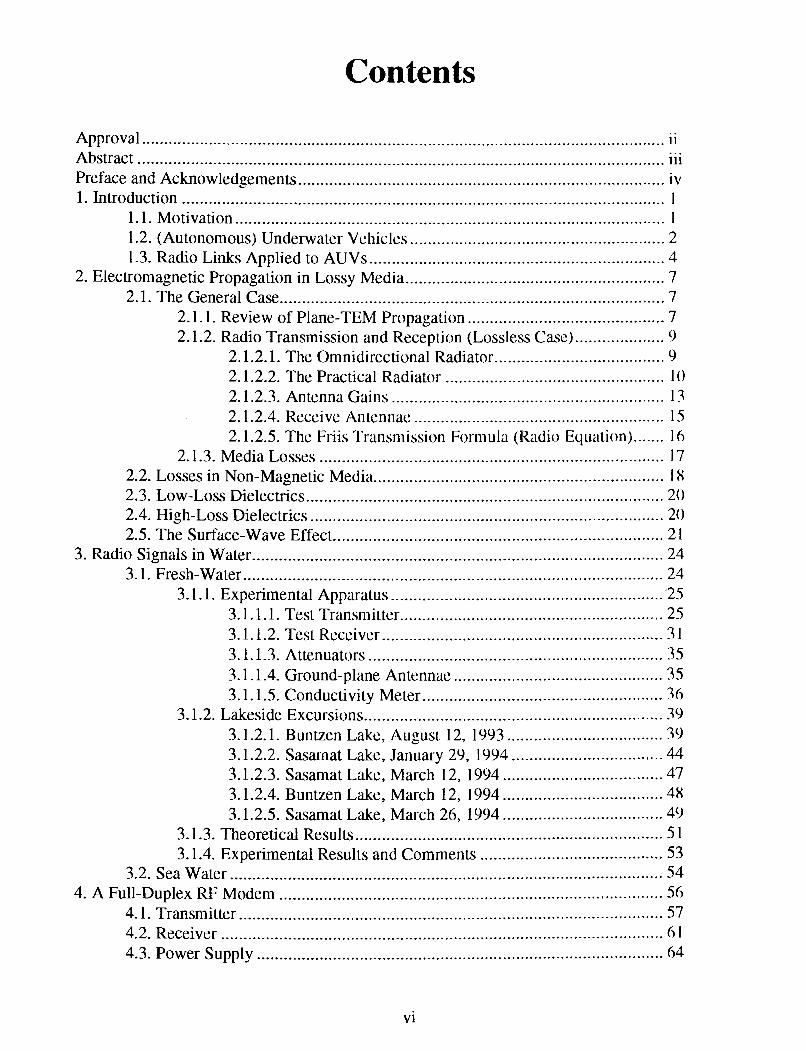
Contents

. . ..................................................................................................................... Approval I I

... Abstract ......................... .. ....................................................................................... 111

.................................................................................. Preface and Acknowledgements iv 1 . Introduction ................... ...... ............................................................................ 1

................................................................................................ 1.1. Motivation 1 1.2. (Autonomous) Underwater Vehicles ......................................................... 2 1.3. Radio Links Applied to AUVs .................................................................. 4

2 . Electromagnetic Propagation in Lossy Media .......................................................... 7 2.1. The General Case ...................................................................................... 7

2.1.1. Review of Plane-TEM Propagation ............................................ 7 2.1.2. Radio Transmission and Reception (Lossless Case) .................... 9

2.1.2.1. The Omnidirectional Radiator ...................................... 9 ................................................ 2.1.2.2. The Practical Radiator 10

2.1.2.3. Antenna Gains ............................................................. 13 .................. ............................ 2.1.2.4. Receive Anlennae .... 15

....... 2.1.2.5. The Friis Transmission Formula (Radio Equation) 16 2.1.3. Media Losses ............................................................................. 17

2.2. Losses in Non-Magnetic Media ............................................................... 18 2.3. Low-Loss Dielectrics ......... .. ................................................................. 20

............................................................................ 2.4. High-Loss Dielectrics 20 2.5. The Surface-Wave Effect .......................................................................... 21

3 . Radio Signals in Water ............................................................................................ 24 3.1. Fresh-Water .............................................................................................. 24

............................................................. 3.1.1. Experimental Apparatus '25 ........................................................... 3.1.1.1. Test Transmitter 25

3.1.1.2. Test Receiver ............................................................... 31 3.1.1.3. Attenuators .................................................................. 35 3.1.1.4. Ground-plane Antennae ............................................... 35

...................................................... 3.1.1.5. Conductivity Meter 36 3.1.2. Lakeside Excursions ............................................................... 39

................................... 3.1.2.1. Buntzen Lake, August 12, 1993 39 3.1.2.2. Sasarnat Lake, January 29, 1994 .................................. 44 3.1.2.3. Sasamat Lake, March 12, 1994 .................................... 47 3.1.2.4. Buntzen Lake, March 12, 1994 .................................... 48

.................................... 3.1.2.5. Sasarnat Lake, March 26, 1994 49 3.1.3. Theoretical Results ..................................................................... 51 3.1.4. Experimental Results and Comments ......................................... 53

3.2. Sea Water ................................................................................................. 54 4 . A Full-Duplex RF Modem ...................................................................................... 56

4.1. Transmitter ............................................................................................... 57 4.2. Receiver ................................ .. ............................................................... 61 4.3. Power Supply ........................................................................................... 64

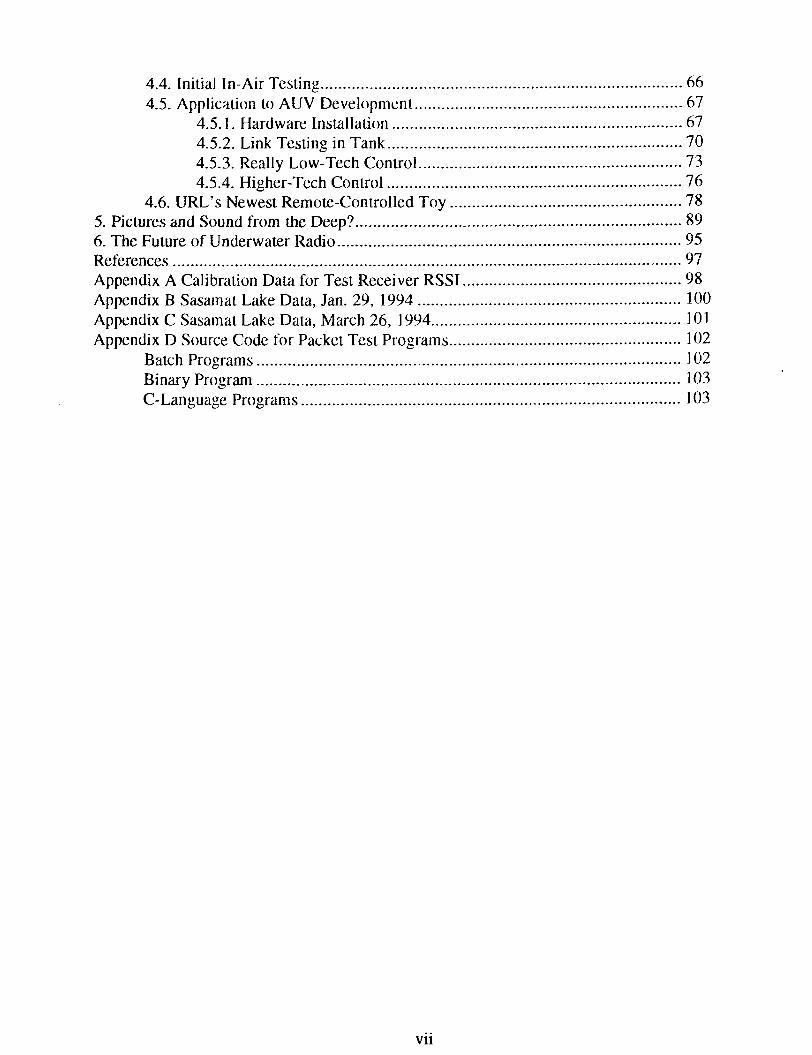
. . 4.4. Initla1 In-Air Testing ................................................................................. 66 4.5. Application to AUV Development ........................................................ 67

4.5.1. Hardware Installation ................................................................. 67 .................................................................. 4.5.2. Link Testing in Tank 70

4.5.3. Really Low-Tech Control ........................................................... 73 .................................................................. 4.5.4. Higher-Tech Control 76

4.6. URL's Newest Remote-Controlled Toy .................................................. 78 5 . Pictures and Sound from the Deep? ........................................................................ 89 6 . The Future of Underwater Radio ............................................................................. 95 References ............................................. ,. ................................................................. 97 Appendix A Calibration Data for Test Receiver RSSI ................... .. ........................ 98

........................................................... Appendix B Sasamat Lake Data, Jan . 29, 1994 100 ..................................................... Appendix C Sasalnat Lake Data, March 26, 1994 101

Appendix D Source Code for Packet Test Programs .................................................... 102 Batch Programs ................... ......,.. ........................................................... 102 Binary Program ............................................................................................ 103 C-Language Programs ..................................................................................... 103

vii

Figures

Figure 2-1 Transverse Electromagnetic Wave Propagating in +x Direction (from von HippA. 1954. page 27) .................................................................................................................... -8

Figure 2-2 Typical Far-Field Radiation Pattern of a Real Antenna (From Cheng. 19x9 . pagc 609) ................................................................................................................................. 1 1

Figure 2-3 Quarter-wave "Whip" Antenna (From Cheng, 1989. page 6 18) .............................. 13 Figure 2-4 Ground-Plane Antenna (From Army, 1953, pagc 1 32) ........................................... 14 Figure 2-5 a vs . o for various values of o ............................................................................... IC) Figure 2-6 Refraction from an Underwater Light Source (from Chcng, 1989. pages 409 and

73 410) ............................................................................................................................... Figure 3-1 Harry Bohm (left) with Dr . John Bird ......................... ,..... ........................... 2 6 Figure 3-2 Underwater Test Transmitter .................................................................................. 27 Figure 3-3 Test Transmitter Schematic .................................................................................... 29 Figure 3-4 Transmitter Harmonic Filter Response ................................................................... 30 Figure 3-5 Test Transmitter Output Spectrum ......................................................................... 31

......................................................................................................... Figure 3-6 Test Receiver 32 Figure 3-7 Test Receiver Schematic ........................................................................................ 33 Figure 3-8 Test Receiver RSSI Curve ...................................................................................... 34 Figure 3-9 Fixed 20 dB Attenuators ........................................................................................ 35 Figure 3-10 Underwater Ground-Plane Antenna ...................................................................... 36 Figure 3-1 1 Definition of Specific Conductivity ...................................................................... 37 Figure 3- 12 Home-Made Conductivity Meter .......................................................................... 38 Figure 3-13 AC Signal Generator for Conductivity Mcasurcmcnts .......................................... 3') Figure 3-14 Canoe Set-Up Used at Buntzcn Lake .................................................................... 41 Figure 3-15 Author With Test Transmitter and Test Receiver Antenna ................................... 42 Figure 3-16 Horizontal Range Test (Buntzen Lake) ................................................................. 412 Figure 3-17 The Author's Assistant on Sasamat Lake Trip ...................................................... 45 Figure 3-18 The Vehicle Used to Transport thn, Author and His Assistant ......................... ., .... 46 Figure 3-19 A Miserable Day at Sasarnat Lake ........................................................................ 48 Figure 3-20 Author's Friends at Buntzen Lake ........................................................................ 48 Figure 3-21 A Warm Sunny Afternoon at Sasarnat Lake ......................................................... 49 Figure 3-22 Water Collection Apparatus ................................................................................. 50 Figure 3-23 Received Power vs . Distance for various Conductivities (98 MHz, Fresh Walcr) . 52 Figure 3-24 Experimental Results: Received Power vs . Range ............................................... 53 Figure 4-1 Figure 4-2 Figure 4-3 Figure 4-4 Figure 4-5 Figure 4-6 Figure 4-7 Figure 4-8 Figure 4-9

.................................................................................. URL's Developmental AUV 56 Completed Radio Modem ...................................................................................... 57 Radio Modem Transmitter Schematic .................................................................... 59 Modem Transmitters' Output Spectra .................................................................... 60 Modem Transmitters' Phase Noise Plots ................................................................ 60 Radio Modem Receiver Schematic ......................................................................... 63

............................................................. Receiver Preselection Filter Characteristic 64 .................................................................................. Radio Modem Power Supply 65

......................................................................... Antennae Used For In-Air Testing 66

... V l l l

......................................................................................... Figure 4-10 Surface Radio Modem -68 Figure 4-1 1 Underwater Antennae in URL Tank ..................................................................... 68 Figure 4-1 2 Vehicle Main Electronics Tube ............................................................................ 69 Figure 4-13 Radio Modem Mounted Inside Vehicle .................... .. ....................................... 69 Figure 4-14 Close-up of Vehicle Antenna ....... .. ..................................................................... -70

. Figure 4-15 Typical Result Output From Receive Test Program ............................................. 72 Figure 4-16 Tank-Testing The Modem ................................... ..... ............................................ 73 Figure 4-17 Author of "Really Low Tech Control" Program (on right, with banana) ............... 75 Figure 4-18 Really Low-Tech Control Screen ......................................................................... 75 Figure 4-19 Denis, Harry and Paul Having Lunch at Loon Lake ............................................. 77 Figure 4-20 Denis' AUV Control Program .............................................................................. 77 Figure 4-21 Troubleshooting the Vehicle at the SFU Pool ....................................................... 78 Figure 4-22 Lowering the Vehicle Into the Pool ...................................................................... 79 Figure 4-23 Loon Lake Test Site ............................................................................................. 80 Figure 4-24 Truck Used to Transport Vehicle During Field Tests ............................................ 80 Figure 4-25 Surface Computer Set-up For Loon Lake Test ..................................................... 81 Figure 4-26 Harry and Paul Preparing For Dive at Loon Lake ................................................. 82 Figure 4-27 Vehicle Operating at Loon Lake ........................................................................... 83 Figure 4-28 Paul Having a Bad Day ........................................................................................ 84 Figure 4-29 Resetting Vehicle at Loon Lake ........................................................................ 85 Figure 4-30 Dr . Bird Watches as Harry Dives Into Loon Lake ................................................ 86 Figure 4-31 Test Set-up With Canoe on Loon Lake ................................................................ -87 Figure 5-1 TV Transmitter Schematic ..................................................................................... 91 Figure 5-2 Prototype TV Transmitter With Camera and Battery ........................................... 92 Figure 5-3 TV Transmitter Output Spectrum ........................................................................... 93 Figure 5-4 A Demonstration of The TV Transmitter ............................................................... 94

1. Introduction This thesis' primary objective is to investigate thc kasihility of using radio s igxh for

information exchange in an underwater setting. Special attention is given to exploring the

possibility of using existing radio technology to establish short-range (approximately ten to fifty

metres) telemetry and control links in fresh water between underwater vehicles and cquiplllcnt

located above the surface.

In the Introduction, I outline the reasons for wanting to use radio under water, describe

what underwater and especially autonomozrs underwater vehicles are, and cxplain how a radio

link between such vehicles and the surface can hcilitate research and devclopment. In the ncxl

chapter, I present a treatment of electromagnetic propagation in mediun~s h r which thc nlagnclic

field losses are near-zero but the electric field losses are significant. Such a theoretical

development applies, as we shall see, directly to the water medium. This thesis does not set out

to measure the physical electromagnetic properties of water, but does show that practical

observations of electromagnetic signals in water are consistent with theoretical predictions.

1.1. Motivation Ongoing research and development in untethered and autonomous undcrwatcr vehiclcs

has re-exposed a real need for a wireless, high-bandwidth, low-delay lclcmctry and conlrol link

between equipment above the water surface and equipment which is locatcd underwater only a

short distance (i.e. ten metres) away. In the context of underwater vehicles, sensor telcmclry is

data from positioning, distance-sensing, and imaging sonars; temperature, salinity, and pollution

metrology sensors; light and sound detectors; etc. Control data sent to underwater vehicles

would activate manoeuvring thrusters, dexterous manipulators, a s well as perform parametric

adjustment of vehicle sensors. These types of data, when used in a realtimc control scheme,

necessitate low propasation delay in the data channel, and can potentially require luge channcl

bandwidths to accommodate high data rates.

Underwater acoustics is currently the eslahlishment means for communicating

underwater. Sound propagation is well characteris& in the underwater environmenl and it quiu:

efficient in terms of transmit power requirement versus usable range of operation. However,

data links implemented with acoustics are limited in bandwidth due to the physical limitations of

currently-available transducers as well as the high noise power spectral density pre-existing in

the water column. Typically, less than five percent bandwidth (based on centre frequency) is

available [Burdic, 19841, which combined with the effects of multipath interference, restricts the

data rate to approximately 2400 bits per second. Additionally, the slow speed of acoustic

propagation (approximately 1500 m/s) can make it impossible to close a control loop based on a

sonar telemetry and control dafa link.

Electromagnetic propagation (i.e. radio) is the dominant communication medium for use

in atmosphere and free space. But its use for underwater communications has thus far been

limited to communications with military submarines in the oceans at extremely low frequencies

(ELF, 30 Hz to 3 kHz) and hence low data rates [Jones, 19851 due to the high attenuation

suffered by higher-frequency radio waves travelling through salt water. Radio frequencies

higher than ELF are attenuated so severely that a transmitted radio signal of a frequency capable

of carrying a reasonable data bandwidth, regardless of how strong (within practical limits), will

have a very short and finite r a s e (less than one metre in sea water) in which it is receivable and

usable. The advantages of radio over acoustics, however, make it ideal for the purposes of

kiemetry and control: High bandwidth, low noise spectral density, low propagation delay (and

hence minimal multipath interference) are just a few of these advantages.

Unlike salt water, fresh water does not present such a high attenuation to radio signals

that high-frequency radio is completely unusable. Since radio does work in fresh water for small

distances, it is a good candidate for providing a high-bandwidth, low-delay alternative to

acoustics at Ieast for the short ranges required in a research and development setting, in which

underwater vehicles are operated in fresh-water test tanks.

1.2. (Autonomous) Underwater Vehicles The term undenvater vehicles encompasses a wide range of ocean-going submersibles

ranging from huge manned submarines to tethered underwater cameras less than a metre in

length- The Underwater Research Lab (URL) at Simon Fraser's School of Engineering Science

is primarily concerned with unmanned submersible robots up to two metres in length, equipped

-with manoeuvring thrusters, environmental sensors, and perhaps manipulators/end-effectors

(robotic "arms") and cameras. These small underwater vchicles are usually tethered via an

umbilical cable to a ship or dock above the water surface, and are launched, retrieved, controlled

and draw power from the surface via the tether. These vehicles are u.sed for underwater

assembly work, retrieval of sunken objects, exploration and inspection of underwater structures,

et cetera down to more than 1000 metres beneath the ocean surface. Nunicrous companies in the

lower mainland (including International Submarine Engineering and CanDive) speciali~c(d) in

the development and manufacture of such underwater vehicles. Underwater vehicles have

become an industry-accepted "window" into workins underwater, especially in very deep or

dangerous waters where deep-sea diving would pose a high risk to human life.

In recent years, an increasing amount of attention has been paid to so-callcd autoncrnmus

underwater vehicles (AUVs). Unlike their standard counterparts, these AUVs do not rely on an

umbilical in order to operate. AUVs have the advantages of being able to go where an umbilical

would prohibit tethered vehicles, aid automatically' without necd for external guidance

fulfilling a predetermined mission, goal, or puipose. Lightweight AUVs could be carried, with a

minimum of supportive hardware, to the launch site and rcleased to serve their sole purpose h r

existing2, whatever that may be. By comparison, traditional underwater vehiclcs (usually)

require a ship, a launch van, an umbilical winch cage, a large crane to lift the cage, and an

operator.

AUV research is still in its infancy, and there is no standard for what attributes an AUV

should or should not have. To URL researchers, an AUV would, ideally, not rely on

above-surface facilities or information, once launched. In addition, a truly auzonomous AUV

would not be constrained to any range of manoeuvrability or distances fiom i b point of launch

by anything other than perhaps the design of its housing or on-board equipment.

The first requirement, that of self-reliance, means that all intclligcncc regarding mission,

god, manoeuvring and control must be self-contained. In other words, in order to fulfill ils

existential purpose, no information needs to be exchanged between an AUV and another sourcc

' The A W must be capable of (among other things) attitude control, obstacle avoidance and course plotting. WhiIe this description of an AUV reminds one poignmtly of a Cruisc Missile, i t is Ihc hope of this author that

AWs will be used for more peaceful, more constructive endeavours than that of the Cruise Missile.

of intelligence3 (say, the engineer who launched it). Note that this requirement does not restrict

the AUV from transmitting information, so long as doing so is not required for its functioning.

We will not even restrict an AUV from receiving information, so long as doing so is not

required for it to carry out its purpose. This means that an AUV can receive additional

(high-level) commands from the launcher, but that in the absence of such reception shall still

carry out its purpose. The first requirement precludes drawing power from external sources so

an AUV must possess its own power storage or generation systems.

The second requirement means that an AUV cannot have a tether, since anything other

than an infinitely long, mass-less and volume-less umbilical would restrict its range of

wandering from its launch point. Any communication an AUV might carry on with outside

sources of intelligence would entail the use of wireless media, and the absence thereof should

not affect its ability to carry out its purpose. An AUV, then, is an untethered, self-contained

underwater vehicle which, without the aid of external sources of intelligence, can fulfill its

purpose.

1.3. Radio Links Applied to AUVs At URL, we are interested in developing an AUV through a series of incremental

changes starting with a tethered underwater vehicle. The strategy is to first build an untethered

vehicle which is still controlled from the surface based on information from on-board vehicle

sensors. Through research and experiments with this untethered underwater vehicle (UUV), the

intelligence originally at the surface shall be systematically moved to the vehicle, turning the

UUV into an AUV a step at a time. This scheme was decided upon to avoid taking "too large a

jump", which might make research unmanageable because it would be impossible to separate the

large number of variables.

Having had experience with developing control algorithms and sensor maps [Wolter,

19931 and discriminators [Kooznetsoff, 19911 with tethered vehicles, URL researchers felt that

the first step towards an AUV is to remove the tether and determine the effects of a wireless link

on the control schen~es. The low-delay, high-bandwidth requirements of such a link preclude

'Ihe tern1 "source of intelligence" is used so as not to disallow gleaning of information from the AUV's environment.

the use of acoustics for reasons mentioned earlier. Successful integration of a wireless link

between vehicle and surface controllers would mean substantial savings in effort in developing

autonomous control intelligence, since there would be no need to disassemble and rcaswmbly

the vehicle each time a change was made to the control software. Control could run on a surface

computer with the control loop closed via a two-way radio link with the vehicle, or the control

program could be downloaded to the vehicle for on-board execution.

This thesis is concerned with high-frequency digital radios for the purposes of UUV and

AUV research, restricted to use with underwater vehicles in fresh water. Bcyond developmcnt

of AUVs, a viable short-range radio link in a fresh-water setting between a UUV and thc surl'ac~

can bring immediately realizable benefits to the subsea industry. The absence of an umbilical

makes deployment and manoeuvring of a UUV very easy. There are many freshwater

applications for underwater vehicles, such as underwater excavation (dead tree removal) in lakes

and reservoirs, water quality surveys (pollution source tracking) and exploration son^ imaging)

of lake bottoms. Vehicles operating under these conditions would no longer have their

versatility hindered by the need to drag a large cable. Radio telemetry can include high-quality

(and hence high bandwidth) video and audio information.

This thesis explores, with promising results, the possibility of using radio signalling in

the freshwater environment within its limited but usable range. The current requiremcnts of

URL researchers involved in untethered and autonomous underwater vehicle development fi t

nicely within the range limitations of underwater radio. It is my hope that my efforts will

contribute a means by which underwater researchers can free their vehicles from umbilicals so

that vehicle dynamics and autonomy can be fully studied and exploited.

My work consists of designing, constructing, and testing a full-duplex radio modem for

underwater operation. I chose to use the commercial FM broadcast band for my prototypes

mainly for expediency: receivers are readily available in the retail market. The 88 to 1 08 MHz

FM band is uncrowded, with many clear spots. Low-power transmissions (in unoccupied

frequencies) such as those from wireless microphones available at various electronics retailers,

are well tolerated by authorities. Accidental interference (e.g. from poorly-tuned prototypes)

with authorized band users are non-damaging as they would be in the emergency VHF bands.

The 100 MHz nominal centre frequency can potentially provide 10 MHz of bandwidth, and

since the intended use of the 88 to 108 MHz band provides for approximately 150 kHz

bandwidth occupancy, these frequencies were the most reasonable choices for transmitting data

at speeds approaching 120 kilobaud. This thesis concludes with a survey of current UUV- and

AUV- activities at URL, and with discourse on how radio fits into this research.

2. Electromagnetic Propagation in Lossy Media

In this chapter, I present a theoretical foundation for underwater communications using

radio. To this end, we will be focussing our attention primarily on plane

transversal-electromagnetic (TEM) propagation in non-ferromagnetic media with negligible

magnetic field loss (the permeability of the media is real and deviates negligibly tiom that of

free space). A brief review of general plane-TEM propagation and radio communication

precedes the development of the various cases which apply directly to the water medium. This

chapter closes with a brief introduction to the surface-wave effect associated with radio

transmissions from within a semi-conducting medium such as water.

2.1. The General Case We begin with a brief review of plane-TEM propagation, the mode in which radio

signals propagate. Then, we shall examine exactly how radio waves are transmitted and

received, and how media properties affect radio signals.

2.1.1. Review of Plane-TEM Propagation Plane waves have planar wavefronts that are perpendicular to ihe direction of

propagation; their equipotential surfaces are flat "walls". An electromagnetic wavc as seen from

a large distance away from a radiator closely approximates a plane wave since the curvalure of

the wavefronts approaches zero at large distances.

An electromagnetic wave is considered a trunsverae electromagnetic (TEM) wavc if the

electric field lines are oriented perpendicular to the direction of propagation (Figure 2- 1 ).

Elemental electric dipoles and practical radio antennae produce TEM waves.

Figure 2-1 Transverse Electromagnetic Wave Propagating in +x Direction (from von Hippel, 1954, page 27)

A TEM wave can be described by solving the differential Maxwell's equations for

source-free media (as applied to electromagnetic waves) to yield [von Hippel, 1954, Ch. 7;

Cheng, 1989, Ch. 7 & 81

for propagation in the positive x direction with a radian frequency o radians per second. The

quantity y is called the complexpropagation factor and has units of metres-'. It may be viewed

as Lhe (complex) spatial "frequency" with respect to X, as w is the (real) temporal frequency with

respect to t.

The solution to Maxwell's equations for time-varying harmonic fields yields y as:

y= a+ jS= jw,/e*p*, (2-2)

where * indicates complex conjugation and E and p are the complex electric permittivity and

magnetic permeability of the space around our source, respectively. Since y is complex, we can

expect an exponential envelope in addition to a sinusoidal variation with x. The non-negative

and real quantity a is called the attenuation factor and gives rise to an exponential decay in the

amplitude of the electric and magnetic fields of Eq. 2- 1.

spatid frequency, or propagation factor-. Rewriting E q .

The positive and real quantity P is the

2- 1 with a and we obtain

which describes a TEM wave with temporal frequency (I> radiandscond, a spatial frcqucncy -P radiandmetre, and which is decaying at a rate of a Neperdmetre4.

2.1.2. Radio Transmission and Reception (Lossless Case) We now turn our attention to how TEM waves are produced, and how real antennae and

media respond and interact with EM energy.

2.1.2.1. The Omnidirectional Radiator

EM radiation is produced whenever a changing electric or magnetic field is prcscnt. The

electric and magnetic fields of an EM wave are self-propagating--the presence of onc ncccssarily

gives rise to the other. Assume for the moment that we have an ideally omnidirectional,

point-source, EM radiator situated in a space-time observable to us. Suppose that it is emitting

EM energy of a time frequency 6.1 = 2@ radians per second. According to Maxwell's laws, wc

would observe the wavefronts propagating outwards from our EM source at a speed

Thus, time and space are related5 through c such that the spatial frequency is

(To see this, simply write Eq. 2-2 with , / E * ~ * expanded as its real part plus j times its

imaginary part, and then match real and imaginary terms on both sides of ths equation.) Thc

spatial frequency is the temporal frequency scaled by llc.

The wavefronts of the radiated EM energy would be spherical, and the radiation intensity

(the time-average radiated power per unit solid angle) would be uniform over all 4n: stcradians

around our omnidirectional source. If the total timc-average power being radiated by o u r source

The Neper is a dimensionless quantity used to describe the amount of exponential attenuation pcr unit of' some other quautity. To say that the attenuation is x Nepers per metre means that the original wave will have decayed to lle of its original strength after travelling l l x metres. After travelling d metres the wave will have decayed to liedr of its starting amplitude. In decibels, one Neper per metre is equivalent to 20log( l l e ) = 8.686 dB per metre.

The temporal frequency is always scaled by one over the propagation speed to obtain the spatial frqucncy fix C

any type of wave propagation, including sound. Recall that the wavelength A = - where c is the sped of f

propagation and f is the temporal frequency in cycles per second.

were P, (i.e. if our source were a 100%-efficient antenna and we were driving it with a power

P,), then our radiation intensity would be

P, u=- (Wlsr). 4z

To obtain the power density in watts per square metre at the wavefront, we note that at a distance

R from the source there are ~"cpare metres of area per steradian, and hence our power density

is simply

The power contained in each unit area of wavefront falls off with the square of the distance away

from the source. This power fall-off is called the spreading 1 0 ~ s . ~ We shall consider the effect

of spreading loss later when we calculate the power received by a receiving antenna given a

certain transmission power.

2.1.2.2. The Practical Radiator

Real EM radiators (antennae) are seldom omnidirectional. In fact, we would not want

antennae to be omnidirectional for real-life applications, for reasons we shall see shortly.

Practical antennae have non-uniform radiation patterns, with radiation intensities stronger in

some directions than others. This far-field (seen at distances for which = 27rR/h. >> 1 [Cheng,

1989, Ch. 1 I]) radiation pattern has nulls, main lobes, and side lobes (see Figure 2-2). The

radiation intensity is now a function of direction with respect to the source and is R' times the

magnitude of the time-average Poynting vector (in WIm2) for the direction of interest:

U ( R , = R ' ~ , ( R , 0, @) (Wlsr),

in polar coordinates.

Note that while the tenn "loss" implies that power is dissipated, the power is just being spread out over more ma and none of it is really "lost".

10

Figure 2-2 Typical Far-Field Radiation Pattern of a Real Antenna (From Cheng, 1989, page 609)

The radiation pattern shown in Figure 2-2 would be typical of a long, thin antenna lying

horizontally in the centre of the pattern and centre-driven (i.e. a dipole antenna). The plot is of

normalized radiation intensity vs. direction angle $. Note that the pattern is rotationally

symmetric about the axis of the antenna and the main beam looks somewhat like a torus in

three-dimensional space. Such radiation patterns have the advantage thal the energy can bc

directed in a specific direction, rather than being spread out in all directions with equal intensity.

More sophisticated antenna designs exhibit main beams which are narrower and evcn more

directed.

By concentrating most of the radiated power of an antenna in a specific direction, wc

obtain what is called directiviq gain. Whereas with an omnidirectional radiator thc powcr is

spread uniformly over 4x steradians, a (even modestly) directional antenna would produce a

higher radiation intensity in a specific direction with the same amount of drive power. The

amount of radiation intensity increase is usually given as a value normalized to the intensity

averaged over all directions (the omnidirectional or isotropic. case). Thc dircctivily gain is

defined as

C,<e,@ = U(@$J) - - U@,4)

e,/ (dimensionless). UO" / 4x

The directivity is the gain (over isotropic) in the direction of maximum radiation

intensity, and is given by

In the direction of maximum directivity gain, a directional antenna will appear to be driven with

D times more power than an isotropic antenna. Since directional antennae are usually aimed

such that the main beam is pointing in the desired direction of transmission, little power is

wasted (as compared to omnidirectional radiation) transmitting in directions where the radio

signal is not needed. Combining Eqs. 2-8 and 2-9 we obtain an expression for the magnitude of

the time-averaged Poynting vector in a given direction at a distance R from the radiator:

which, in the direction of maximum intensity (centre of main lobe) becomes

Practical antennae are not 100% efficient. For a real antenna, the total radiated power P,

is not equal to the electrical power with which it is being driven. The two main reasons for

less-than-perfect radiation of an antenna's input power are impedance-mismatch and resistive

losses. Since antennae are located at the terminating end of a transmission line leading from a

radio transmitter's output stage, the electrical impedance they present to the transmitter must

match the characteristic impedance of the transmission line, which in turn must match the output

impedance of the transmitter's power amplifier (PA). A mismatch would result in some part of

the power being reflected back from the antenna to the PA. The electrical impedance of a real

antenna, which depends on the antenna geometry, the intrinsic impedance of the medium around

it, and its resistive losses, can be made to match to the PA output impedance very closely, but

never perfectly. Resistive losses are always present in real antennae, and are usually kept to a

minimum, through the use of high-conductivity metals, to ensure maximum antenna efficiency.

2.1.2.3. Antenna Gains

The manufacturer of an antenna usually provides a figure called the overall "antenna

gain", G,, which takes into account the directivity as well a: the less-than- 100% efficiency of

the antenna. It is usually specified as decibels over isotropic (dBi) measured at the peak of the

main lobe of the radiation pattern, when driven by a source of a speciilc impedance. A common

antenna is the quarter-wave whip, which is one quarter of the wavelength of the frequency at

which it is used, in the medium in which i t is used. I t is ideally much thinner than it is long.

When mounted over a conducting ground plane, it behaves like the upper half of a half-wave

dipole due to the reflection in the ground plane, and has a main lobe which is as illustrated in

Figure 2-3.

(a) A vertical quarter-wave monopole over conducting ground.

(b) Equivalent half-wave dipole radiating into upper half-space.

Figure 2-3 Quarter-wave "Whip" Anlenna (From Cheng, 1989, page 6 18)

A quarter-wave whip with no resistive losses would exhibit an electrical impedance of

approximately 36.5 R (resistive) [Cheng, 1989, Ch. 111. Combined with some resistive los.ws,

real quarter-wave whips are typically specified to be driven with a 50 source impedance, and

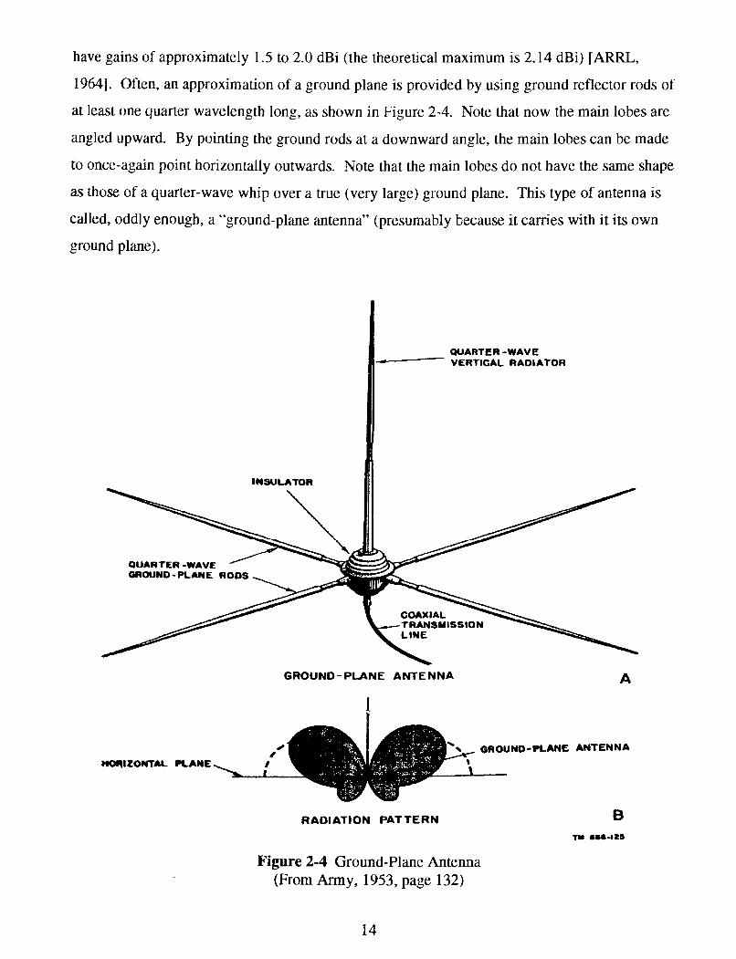
have gains of approximately 1.5 to 2.0 dBi (the theoretical maximum is 2.14 dBi) [ARRL,

19641. Often, an approximation of a ground plane is provided by using ground reflector rods of

at least one quarter wavelength long, as shown in Figure 2-4. Note that now the main lobes are

angled upward. By pointing the ground rods at a downward angle, the main lobes can be made

to once-again point horizontally outwards. Note that the main lobes do not have the same shape

as those of a quarter-wave whip over a true (very large) ground plane. This type of antenna is

called, oddly enough, a "ground-plane antenna" (presumably because it carries with it its own

ground plane).

TRANSMISSION

GROUND- PLANE ANTENNA A

OROUWD-PLANE ANTENNA

n01(lZO(CTM PLANE

RADIATiON PATTERN

Figure 2-4 Ground-Plane Antenna (From Army, 1953, page 132)

2.1.2.4. Receive Antennae

Throughout the preceding discussion we have assumed that the antenna is king uscd to

transmit a radio signal, given a driving source. In the case of radio reception, an EM wave

impinging on an antenna induces currents, which when multiplied by the electrical receive

impedance of the antenna, gives rise to an open-circuit voltage V,, at the antenna terminals (in

the case of a quarter-wave monopole, this voltage appears between the base of the antenna and

the ground plane). We are usually interested in the power delivered to a matched load by the

receive antenna, so we must obtain V,, as well as the receive impedance of the antenna.

Solving for these two quantities is not a simple task. Because the EM energy induccs

currents in the receive antenna, the receive antenna itself appears to be driven by a source (of

amplitude Vo,) and re-radiates energy. Similarly, the transmit antenna will receive the cnergy

re-radiated by the receive antenna and re-radiate it further. This re-radiation or scattering of EM

energy complicates the analysis by making the two antennae (transmit and receive) coupled. As

a matter of fact, there is no such thing as an antenna that only transmits or that only receives.

It can be shown [Cheng, 1989, Ch. 11; ARRL, 1964, Ch. 21 that, for a given antenna, the

following are independent of operating mode (transmit or receive): the electrical resistance R,

presented to a source/load, and the directional (radiation/sensitivity) pattcrn and directivity D.

For antennae which are located a large distance apart, the coupling effects are ncgligihle and wc

may use the values of R, and D computed for an antenna located in infinite free-space.

Furthermore, it can be shown that the maximum power PL transferred to a matched load (with

polarization properly oriented with respect to the incoming EM wave) by a receiving antenna is

related to the time-average power density 538, @) through a quantity calIed the eflective area:

for an EM wave coming from the 0,# direction.

The effective area is related [Cheng, 1989, Ch. 1 11 to the directivity gain G,,( 8, @) via

where h is the wavelength of the EM wave. Note that Eq. 2- 14 does not necessarily mean that

the effective area increases with the square of the wavelength, because directivity generally

decreases with longer wavelengths. When the main lobe of the receive antenna is pointed

directly into the incoming wavefronts, GD(8, t#) is replaced by its maximum value D:

2.1.2.5. The Friis Transmission Formula (Radio Euuationl

In a practical radio system where there exists a transmitter and a receiver located a

distance R apart, we are usually interested in the power P, which the receive antenna delivers to

a matched load in the radio receiver front-end ampliiier, given a certain power P, rxliated by the

transmit antenna. By combining Eqs. 2-1 1, 2-13, and 2-14 we obtain the Friis Transmission

Fonnuh,

when G,, is the directivity gain of the transmit antenna in the direction of the receiver, and GDR

is the directivity gain of the receive antenna in the direction of the transmitter. If we have

oriented the two antennae so that their main lobes align, then we have the best-case transmission

performance and the directivity gains would be replaced by the antenna directivities 4 and DR.

When dealing with practical radio systems it is customary to write Eq. 17 in terms of decibels:

Using the Friis Transmission Formula, we can easily calculate the range of a radio

system (given the source level, the antenna gains, as well as a minimum threshold elmin which

the mxiver requires to produce a usabIe output), at least in free space.7

For calmtations of range in Ihe Earth's atmosphere, for example, various correction factors need to be included to account for refiections from the ionosphere, the curvature of the Earth's surface, the bending of EM rays as they PS through h y m of air with varying densities and moisture content, etc.

2.1.3. Media Losses As we saw in Eq. 2-3, a factor e-" appears in the solutions for ,!? and A when an EM

wave suffers media losses of a Nplm. Since power is the cross product of and H (i.e. the

Poynting Vector), the Friis Transmission Formula can be modified to account for media losses

by including a factor e-2"R (note that the exponent has doubled to account for the cross product)

to yield

Provided we know a, we can solve (numerically, perhaps) these two equations l'or R and thus

predict the distance a radio system will work over.

Recall that from Eq. 2-2 we obtained an expression for P by matching the real and

imaginary components on both sides. The same procedure yields

indicating a complex duality between a and 0. Rather than trying to find the square root of a

complex number through complex geometrical arguments, I shall obtain a simply by syualing

both sides of Eq. 2-2 and equating real terms to real tcrms, and imaginary terms to imaginary

terms on either side:

Here, subscript r designates the real component of a quantity, and subscript i designaks the

imaginary component.

Solving this system of equations in a and p yields a quadratic in a':

Applying the quadratic formula to obtain a2, then taking the right sign and another square root

we obtain a general expression for a, given the frequency a, and the complex permittivity and

permeability of the medium:

Similarly, we find the spatial frequency P to be

2.2. Losses in Non-Magnetic Media Non-magnetic media are characterized by pr z p, and pi z 0; that is, having

approximately the permeability of free space and no magnetic losses. Substituting this into our

general expressions for a and P we obtain

The ratio ei/er is called the loss tangent because it is the tangent of the loss angle 4, tan 6, = S / E , , made between the vector E = E, + jq and the real axis in the complex plane.

Power engineers refer to 6, as the loss angle, and work with the power factor pf = cos6,. In

order to specify the loss tangent in terms of an empirically determinable constant, we define

[Cheng, 1988, Ch. 7) an equivalent conductivity 0 which represents all electric losses in the

medium:

We say that a medium is a good conductor (and hence exhibits high electric loss) if the

loss tangent e i / & , >> 1, or, from the definition of a, if a>> q. Conversely, should the loss

tangent be much less than 1, we say that the medium is a good insulator (and hence is a low-loss

dielectric). A note should be made here that the terms "high loss" and "low loss" are really

relative terms with respect to the frequency of interest. We shall see, later on, how a nlcdium

to this with a substantial electric attenuation can be considered a "low loss" dielectric accordin,

definition.

Figure 2-5 plots Eq. 2-26 for various values of a (with E, = c/o and e, = $ 0 ~ ~ which is

typical for water). Note that for E , / E , >> 1, the curves follow a 6 shape, and become

horizontal lines (constant attenuation) for e i / q << 1. We shall now examine these two cases in

detail, focussing only on non-magnetic media from hereon in.

Figure 2 5 a vs. o for various values of o

2.3. Low-Loss Dielectrics Media for which a<< w ~ , are commonly referred to as "low-loss" dielectrics and exhibit

attenuation losses which are nearly frequency-independent (the flat portions of the curves in

Figure 2-5. The term "low-loss" is a misnomer, however, since it is clear that any medium will

satisfy the criterion o<< wr if the frequency is high enough. Low-loss really refers to the size

of the loss tangent or loss angle, which is frequency dependent and diminishes with increasing

for any finite value of o. For the purposes of our discussion, then, we shall arbitrarily consider a

medium "low-loss" only if a 5 1 Np/m when o << w ~ , .

Since the loss tangent si/q << 1 we may approximate the inner square root in Eq. 2-26

with the first two terms in the general binomial expansion to obtain

which simplifies to

a frequency-independent attenuation. A similar procedure, applying the binomial expansion

twice, with the expression for p yields

which means that the speed of propagation, c, is slightly smaller in a medium with non-zero

conductivity than in a perfect insulator with the same E ~ .

2.4. High-Loss Dielectrics When E ~ / E , >> 1, the medium is commonly referred to as a "high-loss" dielectric. Again,

this is a misnomer since only the loss angle is large, yet for sufficiently low frequencies the

absolute attenuation a may be small. We may neglect the 1s under the square roots of Eqs. 2-26

and 2-27 to obtain

Eq. 2-32 indicates that in a good conductor, the speed of propagation (phase velocity)

is also proportional to the square root of the frequency. While this relationship may initially

appear to be erroneous in that it predicts a zero propagation speed at DC, it may be s e n that no

contradiction exists by realizing that a DC signal really does not "propagate", i.e. it does not

change phase.

2.5. The Surface-Wave Effect We are all familiar with SneN's h w of Repaction which, for light rays passing from one

medium into another of different density, states that the angle of the transmitted ray 8, with

respect to the normal to the interface and the angle of the incident ray ei are related by

sine, - c, - Pi - _ - _ - sin Oi ci p,

where c, is the speed of light in the medium into which the light ray passes, and L; is the spccd

of light in the medium whence the ray comes. (Takc carcful note of thc invcrsc relationship

between c and P .)

For light rays passing into a less-dense medium (such as from water into air), the speed

of light increases and the transmitted ray bends farther away from the normal (see Figure 2-6).

For large enough 8,, the incident ray will be totally reflected and there will be no transmitted

ray. The angle of incidence at which total internal reflection begins is called the critical angle,

and is obtained by setting 8, = 7r/2 in Snell's law:

Water Light Source

Reflected wave

Incident wave

Figure 2-6 Refraction from an Underwater Light Source (from Cheng, 1989, pages 409 and 410)

What happens to a light ray incident at the media interface at the criticai angle is

somewhat special. There is the reflected component which travels back into the first medium,

but the would-be "transmitted" ray does not exit into the second medium. Rather, it becomes a

sulfate wuve which is tightly coupled to the media interface. In fact, evanescent (surface) waves

are created even when 8, > 8, when part of the incident EM field becomes "entrapped" in the

interface between the two media [Cheng, 1989, Ch. 81. No surface wave is formed, however,

for 8, < 8,.

It can be shown [Bruxelle, 1993; Cheng, 1989, Ch. 81 that the surface wave propagates

unattenuated along the interface. The only attenuation suffered by the signal occurs when it is

travelling from the source to the interface where the surface wave forms. Note, however, that

for larger values of Oi , more of the incident energy will be reflected and less will become

evanescent waves. In addition, surface waves formed from incident rays with ei approaching

90 degrees will be weaker by virtue of the fact that the incident ray has travelled a larger

distance through the medium, undergoing spreading and medium losses. Thus, it should not be

expected that surface waves from a source embedded in a medium will be detectable at arbitrary

distances away.

Determining the proportion of the incident power which goes into the surface wave (the

rest goes into the reflected wave) involves knowing the exact polarization of the incident wave

with respect to the media interface. In addition, we must account for the interaction of the

continuum of surface waves created for all 8, 8,, and this is beyond the scope of this thesis.

However, enough power goes into the surface wave to make it easily detectable.

The laws governing light rays also applies to "rays" of radio energy, as light and radio

are both EM waves. If the underwater light source were replaced by a radiating antenna, there

would exist some portion of the TEM wavefront whose direction of propagation would he

incident with the water-air interface at the critical angle, giving rise to a surface EM wave. This

EM wave would, of course, no longer be a plane wave, but its wavefronts would be collapsed

into "lines" which propagate along the interface. In fact, the surface wave would manifest itsclf

as a wave-like disturbance in the potential at the surface of the water (i.e. it is a conducteil

wave).

Since the electric field has been collapsed into a very "thin" laycr, a standard antenna

cannot be used to detect a surface wave. Rather, a device which detects the varying voltagcs on

the surface of the water is needed. Such a device would likely consist of a small electrode in

contact with the surface of the water, and a second large (sheet-like) electrode suspended in the

air above the water so as to form a potential reference (i.e. a "ground"). Placing the ground

electrode in the water would not be effective since it would pick up the in-water (non-surface

wave) EM energy as well as disrupt the formation of the surface wave.

As a final comment on surface-wave behaviour, we must notc now that sincc the

wavefronts are lines rather than planes, the spreading losses are now proportional to just l/r, and

SO the -2Ologr term in the radio equation must be replaced by -1Ologr. Again, we should not

expect a surface wave to travel "forever".

3. Radio Signals in Water When I first started investigating the possibility of using radio ~ignals under water, I

thought to myself that someone else must have done it already. Indeed, various re~archers have

done work in this regime [Curran et al, 19928; Bruxelle, 99931, and the United States Navy

employs extremely low-frequency (ELF, 30 to 3000 Hz) electromagnetic signals to

communicate with their submarines [New Scientist, July 19851. Curran et a1 used an air-filled

underwater enclosure for the transmit electronics as well as the transmit antenna in their tests,

and the U.S. Navy has an antenna of 23 kilometres in length to communicate with submarines

which drag long underwater antennae behind them.

I realized that substantial increases in range could be realized by removing the air-water

interface, as the very different electric permittivities of air and water would result in much of the

EM energy being reflected by the water surface back into the air. I decided that it would be

worthwhile to build and evaluate a radio transmission-reception system which worked

completely in water, allowing one to treat water just as another electromagnetic medium with a

given permittivity and permeability, and no complex boundary conditions (as one had with the

air-water interface). Since fresh water, with its low conductivity, would present the lowest loss

to EM energy, and calm freshwater lakes are within easy access of SFU, I decided to concentrate

my efforts on freshwater radio research.

3.1. Fresh-Water To investigate the propagation characteristics of radio energy in fresh water, I decided to

experiment with a simple radio transmitter and receiver for the 88 to 108 MHz FM broadcast

band. I calculated the expected attenuation and operating range for various values of 0

representative of British Columbia rivers and lakes, and then built the transmitter, receiver and

antennae for measurements in local fresh-water lakes. I shall describe the experimental

It should be noted here that the curves given in Curran's paper for attenuation of RF signds in water vs. frequency appear to have the wrong shape, and do not match the formula used to plot Figure 2-5 or any other approximation for lossy media. Curran claims to have obtained his curves from formulas given in [ V O ~ Hippel, 19541; however, both [von Hippel, 19541 and [Cheng, 19891 give formulae which concur with my calculations to yield the graph in Figure 2-5.

apparatus first, followed by the trips to Buntzen and Sasamat lakes and the theoretical vs.

experimental results.

3.1.1. Experimental Apparatus To verify the theoretical predictions regarding operating range and EM attenuation in

water, I needed a submersible radio transmitter andlor receiver. I decided to design and build

the transmitter and house it in a water-tight canister for submersion into water. The receiver I

constructed by purchasing (for expediency) an inexpensive panasonicB AWFM headphone

radio from London DrugsTM and modifying it. The receiver would remain above the water

surface and be connected to an underwater antenna via a waterproof cable. The transmit and

receive antennae were identical ground-plane quarter-wave whips which I also made.

In addition to the radio equipment I also needed equipment which could measure the

conductivity of the water in which I was doing my experiments. The Underwater Research Lab

owns an Ocean SensorsTM CTD (conductivity, temperature, depth) profiler which I uscd during

my first "lake mission7'. Unfortunately, I discovered that its behaviour with respect to

conductivity readings was rather errant when the water had a conductivity below what it could

measure; instead of just producing less accurate readings or reading its minimum value, the CTD

profiler produced a maximum conductivity reading, which corresponded to twice the

conductivity of sea water! At the suggestion of URL's Dr. William McMullan, who also had

experience with the CTD profiler's rogue conductivity reading characteristic, I constructed a

simple device to measure the conductivity of water. I shall now describe, in detail, all of the

equipment I used.

3.1.1.1. Test Transmitter

Ever since the early 1980s, I have been experimenting with broadcast-band wirelcss

microphones. I never really liked the AM transmitters, partly because they involvcd loopstick

antennae but mainly because I could never get them to work very well ! By the timc I was ready

to begin work on my thesis, I had settled on FM band wireless microphones and had designed

and built a score of them. I decided, since I knew how to custom-build my own transmitter, and

that there were no commercially available FM wireless microphones with sufficiently high

power for underwater research, that I would design and construct my own.

Figure 3-1 Harry Bohm (left) with Dr. John Bird

I developed the transmitter in my workshop (a converted third bedroom in my rented

condominium) and used the equipment at a local radio-controls company, Omnex Engineering

Ltd., to tune and align it. URL's Harry Bohm (Figure 3-1) then designed and constructed an

underwater housing for the transmitter, battery, and antenna (the antennae are described later),

pictured in Figure 3-2. The housing is an old sonar housing salvaged from Simrad-Mesotech

Ltd., a local underwater sonar company; in fact, the bottom "cap" sitting to the right of tb.e

canister is actually the sonar transducer assembly!

Figure 3-2 Underwater Test Transmitter

The circuit schematic of the test transmitter is shown in Figure 3-3. All inductors arc

hand-wound air-core coils.9 Ql is a temperature-compensated L-C tuncd common-base

oscillator running from a regulated 5-volt supply. To improve stability, the plastic body of 01 is

wrapped in copper braid which is soldered to ground as a shield. To further improve stability

and to prevent the high-power output field from feeding back into the oscillator, the entire

oscillator section (Q1 and associated components) is surrounded on three sides with a grounded

The formula used to calculate the inductance values of air-core coils was obtained from another Engineering %ence student, Wing Yu, who had learned it through a course he took at BUT. This formula is:

r2n2 L =

22.91 + 25.4r where the inductance L is in pH, the radius rand length 1 of the coil are in centimetres, and n is the numtw of complete turns. I have found this formula to be agree well with values measured in-circuit.

tin "fence". The frequency is set by deforming L1 and then filling it with hot-melt glue; the

oscillator is then stable to within +8 kHz, sufficient for the wide-band nature of broadcast-band

FM. The oscillator output is fed to the base of Q2, whose base is also biased from the 5-volt

supply to prevent frequency-pulling due to fluctuations in the supply voltage.

Figure 3-3 Test Transmitter Schematic

The rest of the transmitter runs from an unregulated 12-volt (nominal) source. Q2 is a

tuned amplifier stage which provides over 20 dB of small-signal gain and feeds broadband

quasi-class-C driver Q3. Q4 operates as a class-C final power amplifier (FPA) with a double

L-section output-matching network and harmonic filter L7, C18, L8 and C17. The harmonic

filter was designed and simulated using software at Omnex, and has a theoretical response

shown in Figure 3-4; C17 and C18 are adjusted to tune the peak of the response to match the

fundamental frequency. The output power into 50 Q is just over half a watt, at +28 dBm. Take

note of the interstage matching networks; fixed components L2 and C11 form a moderately

broadband network while C14 and L4 form a higher-() match which must be tuned (via C14) for

optimum stability and efficiency. These matching networks were designed by using the

transistors' manufacturer-supplied data and working with Smith Charts.

k. -40.Q - -

1 % i T ' Y i ~ . 7 ' i i ; 2 ~ % . s Fw uency Cin WHal

e\aph-Jc S d e - 5, Fpgiqs- ! , B ~ ~ p h g - B, E P S P - E, bit- ~ p a m

Figure 3-4 Transmitter Harmonic Filter Response

Figure 3-5 shows the output spectrum of the test transmitter, as read with Omnex's

Avi i~ te~t R3361A spectrum analyser, a 10 dB attenuator and a coaxial cable with just over 1 dB

1- The first harmonic, which was near the upper edge of the police radio band and only 40 dB

down from the des-ired output, could be further reduced by adding another section to the FPA

output network, but was considered sufficiently suppressed for underwater work.

R E F 2 0 . 0 dBm A T T 30 d B A - w r i t e 0 - b l a n k i0dB/

91.7 MHz

RBW I MHz

V B W 1 MHz

SWP 50 m s

CENTER 288.1 MHz S P A N 5 0 0 M H z

Figure 3-5 Test Transmitter Output Spectrum

3.1.1.2. Test Receiver t

At the time I started working on my thesis, I was just learning to design and build radio

receivers. I decided, for expediency, to purchase a consumer-grade AWFM personal radio and

modify it, The Panasonic RF-423 headphone radio operates on two AAA batteries and cost

$29.991•‹ (PST and GST not included) at London Drugs. After taking it apart and probing and

analysing the circuitry, I determined that the FM receiver integrated circuit Panasonic used was

very similar to industry-standard monolithic FM IF strips like the Signetics NE615. This

consumer-grade IC, called an AN7025K, had a receive signal strength indicator (RSSI) output

and a demodulated baseband output (BB-OUT) which was then fed back into a slereo decodcr

section on the same IC. The undecoded BB-OUT signal contained the full bandwidth of FM

broadcast information, including L+R (left plus right channel), the 19 kHz stereo pilot tone, L-R,

and SCA (subcarrier audio) programmes--over 120 kHz of bandwidth! For the test receiver,

however, I was only interested in the RSSI output.

The first unit I purchased cost only $19.99, as it was on sale. The next three were their regular price.

To make the test receiver, I removed the RF-423's circuit board from the plastic

consumer package, added a regulator circuit so that I could power it from a 9 V battery, and

glued the assembly into an aluminum project box (Figure 3-6). I also disconnected the radio's

FM input pre-selection filter (a thick-film ceramic unit) from circuitry which allowed the

headphone cord to be used as the FM antenna and connected a length of RG-174lU coaxial cable

between the filter input and a BNC connector. (Earlier, I had determined that the pre-selection

filter's input impedance was compatible with a 50 l2 source impedance.) I changed the RSSI

output integration capacitor from the original 4.7 p F to a low-leakage polypropylene 0.1 p F

part to improve the linearity and response speed of the RSSI signal. The RSSI signal was wired

to an RCA jack and was intended to be read using a high-impedance DMM. The circuit

schematic of the test receiver is shown in Figure 3-7.

Figure 3-6 Test Receiver

-- - - - . - - . -. . - - . . - .

Figure 3-7 Test Receiver Schematic

Using a Fluke 6060A signal generator at Omnex to produce accurately calibrated power

levels of RF energy and a digital multimeter (DMM) to measure the RSSI output voltage, I

determined the RSSI-voltage versus RF-power input characteristic of the test receiver and

plotted it in Figure 3-8 (the raw data for this curve is in Appendix A). Note that inli like the

RSSI output of the NE615 which has a linear output over 90 dB of dynamic range) the

AN7025K's output saturates quickly with increasing input power and also has a verifiably

consistent "kink" (non-monotonicity) in its near-linear portion. However, by connecting fixed

attenuators between the antenna and the BNC input connector of the test receiver to keep the

RSSI output in its near-linear portion, this test receiver was adequate for my underwater range

tests.

UNDERWATER TEST RECEIVER Receive Signal Strength Indicator output voltage versus

receive input power

400 RSSI

300 (mv)

200

+---------+---- '--- t-------i---

-1 20 1 0

-1 00 -80 -60 -40 -20 0

Power In (dBmI50-ohms)

Figure 3-8 Test Receiver RSSI Curve

3.1.1.3. Attenuators

The restricted range of the test receiver's RSSI output required that I use tlxed

attenuators between the antenna and the receiver BNC antenna input connector for obtaining

input-power vs. distance data. Judging from the RSSI graph 1 dccidcd that I should use two

separate 20 dB attenuators, which could be stacked to provide 40 dB of attenuation. Since

high-quality, broadband attenuators from manufacturers such as Hewlett-Packard were quitc

expensiveH and I needed the attenuator to work only around 100 MHz, I constructed my own.

Shown in Figure 3-9 are two 50 CI resistive pads constructed from two BNC connectors, a brass

plate, and $-watt carbon resistors. Performing a frequency sweep on Omnex's Avantest

R3361A spectrum analyser with tracking signal generator, I found the attenuators to be good to

several hundred megahertz, both providing a constant 19.5 dB of attenuation with 50 SZ source

and load impedances. Tables for T-network attenuator resistor values can be found in [ARRL,

1989, Ch. 251.

2Oohms 29 ohms 2Oohms 2Oohms

I < 10 ohms

Figure 3-9 Fixed 20 dB Attcnuators

3.1.1.4. Ground- lane Antennae

The two ground-plane antennae used for the underwater rangc tcsts wcrc constructed

from commercially-available antenna parts, a piece of unetched fibreglass circuit board, and

some copper braid. As shown in Figure 3-10, an LMfCMB stud-mount, Q-CONE, and

Q-WHIP, all available from Canadian Larsen Electronics, Ltd. in Vancouver, are assembled

onto a ""ground plane" constructed by soldering segments of antenna rod to a 1.5" q u u e

l1 Omnex did not have any fixed 20 dB attenuators that I could borrow and thcy wcre scarce at Ihc linginccring Science microwave lab, too.

(approximate) piece of double-sided circuit board. Copper braid on the edges of the circuit board

connect the two sides of copper to form a high-conductivity anchor point for the four ground

rods (unfortunately, the antenna in the left and centre pictures, being used to operate URL's FM

radio, has lost one of its ground rods). The ground rods are made from cut pieces of Q-WHIP.

RG-58IU coaxial cable feeds the antenna, and the entire base of the antenna is potted in epoxy

resin to make it waterproof.

Figure 3-10 Underwater Ground-Plane Antenna

The theoretical length for a 114-wave antenna in fresh water at 100 MHz is 10 cm

27r (calculated from A = -). The whip lengths of the test antennae were tuned for a best-match to

B the transmitter frequency using a standing-wave ratio (SWR) meter (Radio Shack catalogue

#21-523) and were found to be close to 10 cm.

3.1.1.5. Conductivity Meter

Since the URL's CTD profiler could not measure conductivities as low as those found in

"fresh" water, I followed some advice from URL's Dr. William McMullan and constructed my

own instrument. The specific conductivity of a material is defined [Cheng, 1989, Ch. 51 as the

inverse of the resistance measured between two perfectly conductive plates affixed to a block of

the material having constant cross-sectional area along its length, times the plate separation

divided by the cross-sectional area of the block, taking the limit as the dimensions of the block

approach zero; see Figure 3-1 1. For a material with a unifoim conductivity throughout, the

block may be of any finite size.

specific - Amperes length X

conductivity - Volts area

Volts Amperes

Figure 3-11 Definition of Specific Conductivity

To obtain a "block" of water, I glued two single-sided copper circuit boards into the ends

of a plastic drawer taken from my workshop organizer (Figure 3- 12) with the copper facing into

the box. The copper surfaces were tinned with solder to minimize the effects of copper

oxidization on the measurements. The fibreglass dielectric of the circuit boards servcd to

prevent "back-side" conduction to water which may seep into the space between thc cndplatcs

and the ends of the drawer; all conduction through the water would occur directly off Lhc face of

the plates.

Figure 3-12 Home-Made Conductivity Meter

To measure the conductivity of water, the plates were first wiped clean, the box flushed

with plenty of clean water to remove any impurities, and then enough water was poured into the

box so that the surface of the water was just level with the top of the plates and the box. A

voltage was then applied between the two plates and the current through the water measured. It

was found that an alternating voltage should be used to prevent electrolysis of the ions in the

water (and hence produce erroneous current readings); the signal generator circuit in Figure 3- 13

produces a square wave of approximately 250 Hz and was used to provide the test voltage.

Several batteries of different voltages were used to power the signal generator circuit and the

resistance readings obtained with each voltage were averaged to obtain the final conductivity

figure. It has been found that the conductivity readings obtained with this home-made

instrument are precise to within lo%, depending on exactly how close the level of the water is to

being level with the top of the box. An RMS-reading digital multimeter was used to measure the

voltage and current.

Jumper for 250Hz A

M D

AC output. zero DC component

20 or 250Hz 2 x VIPD Vpp square wave.

Figure 3-13 AC Signal Generator for Conductivity Measurements

To verify that my conductivity apparatus worked, I measured first the conductivity of tap

water and then the conductivity of tap water in which a measured amount of salt was dissolved.

The tap water measured 10 pSIcm, which matched with the value of 1 o - ~ Slm that [Chcng,

1989, page 6751 gives for "fresh water". Using data from a table of specific conductivities of

aqueous solutions of sodium chloride for varying concentrations [CRC Prcss, 198 11, I prepared a

solution of 0.4% (by weight) NaCl using a crude (toy) balance and amounts of water (measured

using baker's liquid measuring spoons) for the counter-weight; theory predicted that the solution

should have a conductivity of 6.6 mS1cm. Taking the average of three readings, each tilkcn with

a different voltage, I obtained a value of 6.8 mS/cm. I was confident that my homc-madc

conductivity meter worked properly.

3,1.2. Lakeside Excursions Two near-by freshwater lakes were used to obtain experimental data on how far radio

signals travel in fresh water. In all, two trips were made to Buntzen Lake, and three trips were

made to Sasamat Lake. I will briefly give accounts of these five lake visits and then present

theoretical and experimental findings.

3.1.2.1. Buntzen Lake, August 12, 1993

The first "real-world" underwater radio propagation experiment was done in pristine

Buntzen Lake. This freshwater lake is level-controlled by BC Hydro and is and fed from

Coquitlam Lake. It provides drinking water for many parts of the Greater Vancouver Regional

District (GVRD) as well as excellent recreational facilities (picnic grounds, beaches, boat

launching).

Harry Bi3hm (URL) and Darrin Wolter (URL, M.A.Sc. 1993) assisted me on this trip,

which I can only describe, in hindsight, as a very preliminary experiment. The night before we

went to Buntzen Lake, I was in the URL trying to tune the lengths of the antennae. I asked

around tbe microwave lab to see if anyone had a standing wave ratio (SWR) meter or an

impedance bridge, but the only thing they had was a very large, very expensive, and very

overkill Hewlett Packard network analyser which didn't work below a few gigahertz! I

borrowed a spectrum analyser and a signal generator from the microwave lab and made an

impedance bridge out of several resistors and tried my best to tune the antennae given what I

had. (Incidentally, Omnex Engineering had an impedance bridge, but no large tank of water.)

When we arrived at the lake, we rented two 19-foot GrummannTM aluminum canoes

(very nice crafts, by the way) and lashed them together with two 2-by-4 inch studs and some

rope, leaving a water gap in between them. This gave us a very stable experiment platform from

which we could lower our apparatus into the water; see Figure 3-14. We rowed out to a central

location on the water and Harry used URL's CTD profiler to obtain a conductivity and

temperature profile of the water column. (At this time, I had not constructed my home-brew

conductivity meter.) The first profile didn't work, and Harry had to use the borrowed laptop

computer which we had with us to re-enter the profiler parameters for fresh water. We took

another profile. The conductivity data appeared peculiar at the time, and we discovered later

that the CTD profiler could not read conductivity below 0.5 mS/cm. (Buntzen Lake water, as I

found out later, has a conductivity of 10 pS/cm.)

Figure 3-14 Canoe Set-Up Used at Buntzen Lake

I then attempted to measure the drop-off in the received RF power at the test receiver. I

secured the receive antenna on the end of a PVC pipe to one of the 2-by-4s (see Figure 3- 15).

The antenna was pointing straight down with its ground plane rods 0.7 m below the water

surface. I then lowered the underwater test transmitter, attached to the end of a ropc, straight

down from a point one metre (horizontally) from the receive antenna. I took measurements of

the received signal strength every metre from 1 to 39 metres. What I found surprised me. Thc

signal did not fade out to any significant degree as I had anticipated (I was assuming, for thc

time being, that Buntzen Lake water was around 100 pS/cm as suggested in [Curran et al,

19921). In fact, for the first 20 metres, the receiver was saturated (on the top portion of its RSSl

curve). Beyond 20 metres, the signal dropped off, but I found that by tipping thc receivc

antenna I could bring the receiver back into saturation. This meant that the signal drop-off was

primarily due to increasing misalignment of the antennae main beams. We needed to do a

horizontal range test, during which the main lobes of the antennae could be kept better aligned.

Figure 3-15 Author With Test Transmitter and Test Receiver Antenna

I attached the receive antenna to the swim dock 0.7 m below the water surface. Harry

and Darrin then slowly rowed the canoes away from the dock with the transmitter suspended

10 m below the surface. A tape measure was stretched between my position on the dock and the

canoe the entire time; see Figure 3-16, When the canoe had reached the end of the tape measure

(60 m), the receiver RSSI was still in saturation. I changed the angle of the receive antenna and

noted a change in the receive signal strength, just to rule out the possibility that I was receiving

the surface wave (which I will discuss later). We disconnected the tape measure and I called out

to Harry to keep rowing away from me until I motioned him to stop. I stopped him when the

RSSl reached -93 dBm, when the test receiver begins to output some "static" noise. Darrin

called out to some divers on the shore and asked them how far they thought we were apart; from

their position, the divers could make a more accurate estimate than we could. "100 yards" was

the reply. To us, it looked like just over 100 metres.

Figure 3-16 Horizontal Range Test (Buntzen Lake)

The canoes still 100 metres from my position on the dock, I could see Harry and Darrin

discussing something and then handling the rope to the transmitter. The signal strength

increased slightly. They rowed back and Darrin explained that Hany knew of a very sharp

drop-off in the lake floor, and that they thought (correctly so, since the signal strength increased)

that by lifting the transmitter to 5 m depth, the signal would not be partially blocked by the

underwater escarpment. Thus, we determined that the -94 dBm range of the system in Buntzcn

Lake was in excess of 100 m. We separated the canoes and repeated the test between the canoes

in a deep part of the lake, and our best distance estimate confirmed our earlier dock-to-canoc

findings.

Finally, I performed a test to see how far the surface wave propagated. I lifted the

receive antenna up so that its ground rods were out of the water while the whip was still in the

water. This allowed me to detect the surface wave potential at the surface of the water, as the

ground rods were coupled to the potential of the air above the water surface (recall the

discussion at the end of Chapter 2 on the surface wave effect). Darrin held his canoe in position

with the transmitter 10 metres below the water surface. The test receiver was saturated Lo

approximately 400 m horizontal separation, when the RSSI output began to drop slightly (this

~ccurs at around -80 dBm), While a quantitative analysis of surface-wave propagation is beyond

the scope of this thesis, this experiment showed conclusively that significant advantages can he

realized by a radio receiver located at the water surface by detecting the surface wave rather than

the in-water signal.

After returning from this initial lake trip, I began analysing my fmdings, and became

somewhat puzzled. The conductivity readings all read 66 or 67 in the CTD profiler's output file,

and I just assumed at the time that they were in pSIcm. My initial calculations, however,

indicated that the 100 m operating range could not be achieved with such a conductivity. I

realized that the 100 m was still only an estimate, so I devised a procedure whereby I could use

fixed attenuators to keep the test receiver RSSI output in its usable (non-saturated) range and

thus obtain proper data.

3.1.2.2. Sasamat Lake. January 29, 1994

After many weeks of rethinking my experimental procedure, and then after many months

of waiting for the snow and rain to stop, I took the advice of my thesis supervisor, Dr. John Bird,

and went to Sasamat Lake where a floating walkway allowed me to perform horizontal range

tests without a boat. I managed to enlist the help of a friend, Strom Beadle (Figure 3-17), to act

as my assistant (i.e. he carried ail the heavy equipment for me!).

Figure 3-17 The Author's Assistant on Sasamat Lake Trip

Before going to the lake, I determined that I should make an effort in properly tuning the

test antennae. I purchased a ~icronta@' SWR meter from Radio shack' (catalogue number

21-52312) on sale for $19.95 and tuned the antennae whip lengths for less than 1.5: 1 VSWR in

the URL tank. The whip lengths were originally tuned too short with the makeshifl impedance

bridge used just before the trip to Buntzen Lake.

We drove in my boat (Figure 3-18) up to White Pine Beach at the north end of Sasamat

Lake and hiked ten minutes along the Sasamat Lake Trail to the floating walkway at the south

end. We had with us the underwater transmitter and receiver; we did not bring the CTD profiler

chxe to the short notice of good weather (the CTD profiler battery was not charged), though at the

time I still thought it worked in fresh water. I lowered the transmitter to a depth of I O m and

* While this unit is ody specified for operation up to 30 MHz, the author tested it with equipment at Omncx and fd that it gave proper readings to beyond 150 MHz.

walked along the walkway, dipping the receive antenna in the water to determine how far away

the signal would drop to -94 dBrn (300 mV of RSSI); it turned out to be at a slant range13 of

53 m. This number appeared more reasonable, and I spent the rest of the time there taking signal

strength vs. range measurements mainly for distances less than the -94 dBm range, though 1 did

take a few measurements beyond that along with some surface-wave readings. I proceeded by

dipping the receive antenna into the water at points located one to two meters apart along the

walkway and orienting it to maximize the signal strength. Strom then marked the signal strength

on a piece of tape which I affmed to the walkway fence at that location. After all the signal

strength readings were taken, Strom and I measured the horizontal distances from the transmitter

to the markers on the fence and recorded the results. In this way, I was able to obtain signal

strength versus distance measurements in just a couple of hours.

Mgwe 3-18 The Vehicle Used to Transport the Author and His Assistant

Using two fixed 19.5 dB (50 S Z ) attenuators, I was able to obtain good RSSI data from

just over 10 m slant range to almost 100 m. I found, by keeping the receive antenna in one place

relative to the transmitter and taking a reading with two, one, and zero attenuators, that (due to

" The slaat range is the true distance between the transmit and receive antennae, and is calculated as the square root of the sum of the vertical, horizontal, and lateral distances, each squared.

the exact matching between the antenna, the attenuators, and the receiver front-end) a single

attenuator actually provided 27 dB loss, and two attenuators together provided 5 1 dB. The data

in Appendix B is compensated for this fact. While no conductivity measurements were taken for

this trip, the data is plotted later in this chapter for comparison with theoretical predictions. The

surface wave in Sasamat Lake was found to propagate for over 110 m without the test receiver

RSSI coming out of saturation at around -80 dBm.

3.1.2.3. Sasamat Lake, March 12. 1994

After returning from Sasarnat Lake, I began some more detailed analysis of the CTD

profiler data obtained at Buntzen Lake. I had planned to take CTD profiles at Sasamal Lake h r

comparison, but in a conversation with Bill McMullan (URL) about the conductivity readings I

obtained at Buntzen Lake, I learned that the readings were erroneous. Bill had found that the

CTD profiler produces readings of 66 to 67 millisiemens per centimetre when the water

conductivity is below its minimum specification. Apparently, this behaviour was due to the fact

the CTD profiler's internal calculations (which were based on approximation curves) broke

down when the conductivity is below its lower limit. Bill suggested that I build my own

apparatus to measure water conductivity.

Again, I anxiously waited for another sunny day; none that were convenient came.

Armed with my home-made conductivity meter (described earlkr), I went up to Sasamal Lake

again--alone, this time. It was a wet and miserable day (Figure 3-19). The conductivity of the

surface water that day was 27 pS/cm. The thought occurred to me then that perhaps the

conductivity might vary with depth, from season to season, and with amount of rainfall. I

decided that I'd come back on a good day to repeat the RF propagation and conductivity

measurements with equipment for taking water samples from various depths.

Incidentally, I encountered the GVRD Regional Park Assistant for Sasamal Lakc again

that day (Strom and I had met him on the previous trip). I got his name this time, and Rick

Novosel told we that both Buntzen Lake and Sasarnat Lake were both natural lakes, originally

carved out by the same glacier that dug out Indian Arm. Both the lakes' levels have been raised

through the use of man-made dams.

Figure 3-19 A Miserable Day at Sasarnat Lake

3.1.2.4. Buntzen Lake, March 12. 1994

That same day, 1 went up to Buntzen Lake and took surface water samples and

conductivity readings there. Fortunately, I met several friends (Figure 3-20) there which

cheered me up in spite of the drizzly weather. The conductivity of Buntzen Lake surface water

that day was 10.6 pS1cm.

Figure 3-20 Author's Friends at Buntzen Lake

3.1.2.5. Sasarnat Lake, March 26, 1994

Two weekends after I collected conductivity data from Sasamat Lake and Buntm Lakc,

a sunny Saturday allowed me to perform a complete and proper radio propagation experiment.

This time, I had all the equipment with me to measure the water conductivity at various depths

as well as RF signal strength. I hiked 10 minutes from White Pine Beach to the floating

walkway; I had 50 or 60 pounds of gear in my backpack (including two 10-pound lead weights)

so it was a long 10 minutes. I arrived at the east end of the east swimdock at 14: 15. It was a

warm sunny afternoon (see Figure 3-21), at least 15•‹C; there were many people out fishing. At

14:26, one man caught a large fish but lost it as he was pulling it out of the water.

Figure 3-21 A Warm Sunny Afternoon at Sasarnat Lake

I took water conductivity measurements at the surface, 5 metres depth, and 10 metres

depth. To collect water at depths below the surface, I used, at the suggestion of Dr. Bird, a soda

bottle with weights and a stopper which could be pulled from a line at the surface (see Figure

3-22). After the stopper was pulled, the bottle would fill with water, and so long as one surfaccd

the bottle slowly there would be negligible changing of the water already in thc bottle. At (J and

5 metres, the conductivity was 26 pS/cm; at 10 metres I obtained 25 pS/cm. The variation in thc

readings were within the experimental error of my home-made conductivity apparatus (which 1

had found to be 10% of the reading), so I concluded that the conductivity was quite uniform

throughout the water column.

Figure 3-22 Water Collection Apparatus

1 performed the same signal strength versus distance experiment as Strom and I had done

on January 29, 1994. This time, I took great care in tuning the receiver to the transmitter's

frequency and orienting the receive antenna. This time the -94 dBm range was about 63 metres.

I have compensated the data in Appendix C for the seal attenuator losses and plotted the results

in the Experimental Results section of this chapter.

While I was measuring the distances (around 16:00), I had a tape measure stretched out

14 m along the walkway. A young couple came by and the man remarked, 'Gee, the fish must

be really big here to need a tape measure that long!" We got to talking, and it turns out that this

man, Steve Bethel, was an SFU Biology graduate. He was very knowledgeable in underwater

technology, and I asked him if he had ever seen a reference to underwater radio comnwnicaaion

involving military submarines. He said he had, and he pointed me to Science '84, Science '85 or

Discover magazines. When I finally removed my dark, wrap-around sun visor, the woman with

him recognized me--Brenda Alexander graduated, as did I, from Windermere Secondary School

in 1986! In all, we talked for about half an hour; it was a nice way to wind up the day. At 18:00

I finally finished my measurements and I packed up and left. The hike back to thc car was

exhausting, though--1 should have brought a lunch!

3.1.3. Theoretical Results According to Environment Canada's 1974 Water Quality Data report for British

Columbia [Environment Canada, 19741, "fresh" water lakes and rivers have conductivitics

ranging from about 10 to 500 pS1cm. Lakes which are used as sources of drinking water

typically have conductivities below 50 pSIcm while rivers which flow over mineral-rich lands

or which have industry along their banks will have conductivities above 400 pS1cm. The

majority of un-industrialized rivers contain enough naturally dissolved minerals and compounds

to have conductivities between 100 and 250 pSlcm.14 For the purposes of this thesis, I will

consider water "fresh" if its conductivity o 5 0.020 Slrn (200 p Slcm), noting that [Cheng, 1989,

page 6751 indicates that fresh water (i.e. tap water) is 0.001 Slm. For a = 0.020 Slrn the loss

tangent < 1 for frequencies f > 4.5 MHz in water, so at the nominal 100 MHz I was using

for my experiments I could definitely consider the water a "low-loss" medium. (At lower

conductivities, water can be considered "low-loss" starting at even lower frequencies.)

In order to evaluate the suitability of underwater radio for short-range control and

telemetry, we must determine how quickly a radio signal is attenuated in water. Knowing thc

attenuation constant cn and given the transmitted power <, antenna gains, and minimum

receiver operating threshold P , I . we can determine the distance over which the radio will work. rmn

For low-loss media, Eq. 2-30 applies for determining a and Eq. 2-3 1 applies for P . For fresh

water, I will assume a permittivity of E, = 76&,, half-way between that of distilled water

l4 For more information on water quality parameters, the reader is urged to consult "Watcr Quality Sourcehtmk, A Guide to Water Quality Parameters" Environment Ginada, 19791. While this guide does not specificidly di.wuss conductivity, it is extremely informative with regard to the various effects that dissolved minerals havc on humans and other animals.

(E, = 8 0 ~ ~ ~ ) and of seawater (E, = 72%) [Cheng, 1989, page 675].15 I will also assume the

receive and transmit antennae are identical ground-plane antennae and are of medium efficiency

with a conservative gain of 1 dBi (when the antennae's main lobes are aligned). Substituting Eq.

2-30 into Eq. 2-20, we obtain the Friis formula modified for low-loss media:

Given a transmitted power, antenna gains, wavelength, and conductivity, we can

calculate the received power at the receiver located a distance R from the transmitter. Figure

3-23 plots the received power P,,, as a function of the distance R for various values of a. The

transmitted power was assumed to be 0.0 dBm (dB with respect to 1 mW) and the wavelength

2 n was calculated from A = -- for a frequency of 98 MHz (at the centre of the FM broadcast band

P I used in my research).

Received Range (metres)

Figure 3-23 Received Power vs. Distance for various Conductivities (98 MHz, Fresh Water)

Is While the permittivity of water depends on its temperature, pressure, and concentration of dissolved con~pounds, the variation is small enough that using E, = 76e, as representative of fresh water yields good

results. It should be mentioned here, for completeness, that media permittivity in general is a function of frequency; at optical frequencies, water has only a permittivity of E , = L75&, . However, the permittivity of a

medium deviates negligibly ftom its static (DC) permittivity below 1012 Hz.

140

0.001 Slm 0.002 Slm 0.004 Slm

0.006 Slm

0.008 Slm

0.01 Slm

0.015 Slm

0.02 S/m

If the minimum receiver operating threshold is - 100 dBm, we can predict from the graph that a

transmission of 0.0 dBm will be received up to approximately 25 metres away for a conductivity

of 0.01 Slm.

3.1.4. Experimental Results and Comments Figure 3-24 plots the received signal strength versus slant range for data collected from

both Sasamat Lake experiments. Theoretical curves for 0.001,0.002 and 0.003 Slm (assuming a

transmit power of +28 dBm) are plotted for reference. While no conductivity data is available

for January 29, it is likely that the conductivity of Sasamat Lake was the same for both the

experiments since the overall slopes of the two data sets are the same. The January 29 data

points are consistently lower, and I believe that this is due to the fact that I did not carefully tune

the receiver during the first experiment; the receiver will show a lower signal strength than is

really being received if it is not tuned to centre on the received signal.

I I I - I - -- 1 - I I I Slant Range (metres)

Received , I I I I I I -1

I I 3 I L

Figure 3-24 Experimental Results: Received Power vs. Range

Particular attention should be paid to the March 26 data points. Note that the first 5 data

points concur very well with the theoretical predictions.16 All subsequent points, however, begin

to follow a much sharper slope downwards. This effect is due to the receive antenna moving out

of the main lobe of the underwater transmit antenna. During the experiment, I was able to angle

the receive antenna to optimize received signal strength; I was pointing the main lobe of the

receive antenna directly at the transmitter. However, there was no way I could align the transmit

antenna to point its main lobe at the receive antenna. The first 5 data points were all collected

with the receive antenna at approximately 45 degrees to the plane of the transmit antenna, near

the apex of the transmit antenna's main 10be.17 The rest of the points were taken at angles which

began to fall into the null under the main lobe of the transmit antenna's directivity pattern.

Considering the misalignment of the antennae, the experimental results of March 26

agree quite well with the theoretical predictions; the agreement is to within a factor of two even

with the deviations due to antenna misalignment. The data is representative of water with less

than 50 ~Slcrn conductivity, which is typical for glacier-carved freshwater lakes such as Sasamat

Lake.

3.2. Sea Water The data given in [Environment Canada, 19741 indicates that the Pacific Ocean has a

conductivity of between 3.2 and 4.6 Slm, while [Cheng, 19891 gives the conductivity of sea

water as 4 Slm. For 4 Slm, ei/er >> 1 and Eq. 2-32 yields an attenuation of 39 Nplm at

98 MHz; the media losses alone account for -340 dBIm! From Figure 2-5 we see that only at

extremely low frequencies would we obtain similar attenuation from sea water as we do from

fresh water at 98 MHz; in fact, we must use EM energy at frequencies less than 10 kHz to obtain

losses of several dBIm, as we do in fresh water. At such low frequencies, however, we would

not only require antennae of extremely large dimensions, but we would be restricted to data

l6 The conductivity of Sasamat Lake was 26 pS/cm, so the data should follow a curve between the 0.002 S/m and 0.003 S/m curves. We see here that the received power is slightly higher than expected; however, it is very likely that the antenna gains are actually slightly higher than the conservative estimates we assumed during the calculation of the theoretical curves. l7 A quarter-wave ground-plane antenna has its main lobes pointed upwards at approximately 45 degrees from the horizontal plane; see Figure 23.

bandwidths of less than 100 Hz which defeats the purpose of using radio as a higher-bandwidth

alternative to acoustics.

Theoretically, then, I expected that high-bandwidth radio communicaticm would be

unachievable in sea water. To verify this, I performed received-signal-strwth versus range

experiments in the S N pool. On April 14, 1994, Harry BOhm and I went to the SFU pool and

measured first the conductivity of the water and then the signal attenuation.

The pool water chemistry is regulated by a computerized electrolyte-balancing system

and had a conductivity of 0.10 Slm. We found that, with the test transmitter 2 m below the

water surface, the surface wave could be received at -81 dBm 19 m away. However, the

in-water signal was down to -70 dBm at only 3.2 m slant range, -83.5 dBm at 3.6 m, and

-98 dBm at 4.0 m. At the test frequency of 89 MHz, e , / ~ , = 0.27 E 1 and Eq. 2-26 yields

2.1 Nplrn, or -18.6 dB1m. The measured 18 dB difference in signal strength going from 3.2 n~ to

4.0 agrees well with the theory, and I concluded that there was no point in pursuing the usc of

radio frequency communication in sea water (or pool water, for that matter).

4. A Full-Duplex RF Modem In parallel with the work described in the previous chapter, I engineered a pair of

prototype full-duplex radio modem for communication between URL's developmental AUV

(Figure 4- 1) and the surface computer. This underwater vehicle was designed and constructed

by URL to be a platform for interactive research and development of autonomous vehicle

&nsors, actuators, and intelligence. The two-way radio link serves initially to facilitate

development of the intelligent control software on a surface computer; sensor information from

the vehicle would be transmitted up to the surface computer, computations would be made at the

surface, and actuator outputs would be transmitted back to the vehicle in a remote-control

fashion. As we incrementally move more of the intelligence to the vehicle's on-board computer,

the radio link allows us to monitor the operation of the on-board intelligence.

Figure 4-1 URL's Developmental AUV

The radio modem consists of a transmitter, a receiver, and a power supply, all housed in

a cast-aluminum project box donated by Omnex (Figure 4-2). The transmitter and receiver

operate on two different frequencies at opposite ends of the FM broadcast band, for maximum

rejection of the local transmitter in the receiver. The receiver in the surface modem is tuned to

the vehicle transmitter's frequency and the vehicle receiver is tuned to the surface modem's

transmitter. The transmitter is modulated directly from an RS-232 serial port's TxD output

signal, and the receiver directly drives the port's RxD input. There is no microprocessor in the

radio modem, and to the two computers linked together the modem looks like a hardwire with a

non-zero error ratio. This modem is intended to be used with error-detected, packetting protocol

software.

Figure 4-2 Completed Radio Modem

4.1. Transmitter The modem transmitter is virtually identical to the test transmitter described in the

previous chapter, with the exception that the oscillator transistor is modulated at the base by the

RS-232 signal. As shown in Figure 4-3, a digital signal which swings be tween + 12V and - 1 2V

is coupled into the base of oscillator Q1 via R 1, R2 and C 1. As Q 1's base bias changes, the

junction capacitances change and frequency modulation (FM) is produced as the resonant

frequency of collector tank L1 and C4 changes. Some minute amount of amplitude modulation

(AM) is also produced as Ql's gain changes with its base bias, but a limitting FM receiver will

not see the AM component.

The "1 15.2 kilobaud designation in the schematic title is the highest baud rate the

modem was tested at, and is also the maximum speed of the serial port on an DM@ compatible

computer; however, there is no fmed baud rate limitation in the transmitter. In fact, the

modulation time constant determined by C1 and the input impedance of Q1 allows proper FSK

signals to be generated from baud rates down to 1200 baud.

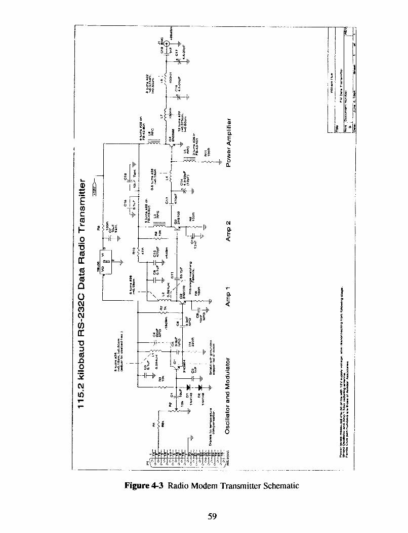
1 1

5.2

kilo

bau

d R

S-2

32

C D

ata

Rad

io T

ran

sm

itte

r

3s

Oscilla

tor

an

d M

od

ula

tor

Am

p 1

A

mp

2

Po

we

r A

mp

lifi

er

The fundamental and first two harmonic outputs of the two prototype transmitters is

plotted in Figure 4-4. Note that the first undesired harmonic is lower in the higher frequency

transmitter; the output harmonic filter is able to reduce the first harmonic level by 10 dB more

due to the larger separation between fundamental and harmonic outputs. The very small peaks

close to the fundamental are carriers and mixing products from FA4 radio stations being picked

up by the amplifier stages of the transmitter.

REF 21. I Odh/

R B I

$:L S I P

1 0 m n

: A i r 30 dB A-mrirc B-hlaat ......... .-- .. *. ... .- -. . . . . . . HKR i -

I I . . . . . . 6 9 . 6 MHz

" 5 5 "'rn 1 . . : . . . . ; ..:.....,.. : . ;

: . . . L . . . . . . . . . . . . . . . . . . . . . . . . . . .

. . . . . . . . . . . . . . . . . . .

, .. , - . . . . . . . ........ .; ; .;

I : ! . ! . . . . . . . --..... . . . . . . . . . . . . . . . ... - .:.

....

.... --____1

CENTER 177.6 Mfi+ SPAS 2 P B . @ MHZ

~ 1 1 3e d B L r r i t e B-blank

. . . . . . . . .

. . . . . .

. . . . . . . . . ; - ......-.... . < . . .

4 . . .

. . .

...... . . ...

. . .

CENTER 226.0 U k SPAS 2 5 0 . $ MHz

Figure 4-4 Modem Transmitters' Output Spectra

Close-in phase-noise plots of the transmitter outputs in Figure 4-5 indicate that, while the

L-C tuned oscillator is much noisier than a crystal-tuned design, overall phase noise is

respectable and more than adequate for a wide-band FM system.

38 dB 'vier 8-blank

. --... S P A K 2 0 . B t knz iENIEQ 1 t6.7757B MHz SWN 1 0 . 6 0 k H z

Figure 4-5 Modem Transmitters' Phase Noise Plots

4.2. Receiver The radio modem's receiver, like the test receiver, is based on a ~anasonic' RF-423

personal AM/FM stereo receiver; the schematic is shown in Figure 4-6. Due to the close

proximity of a strong RF signal (from the local transmitter), the receiver will become

desensitized to some degree.18 In order to reduce the amount of receiver desensitization, I

designed (using software at Omnex) a special preselector/amplifier to go between the receive

antenna and the RF input to the RF-423. The centre frequency of the preselection filter is

adjusted with adjustable coils Ll and L2 to match the receive frequency; a typical response is

shown in Figure 4-7. The frequency of the local transmitter, being 20 MHz away at the opposite

end of the band, is attenuated by more than 20 dB.

The receiver's sensitivity with the preselector is -104 dBm at 12 dB SINADI9 (signal to

noise and distortion, measured with a 1 kHz tone), as determined with equipment at Omnex.

This means that the SINAD ratio at the receiver output was 12 dB when the receiver was

presented with a carrier modulated with a 1 kHz tone at a signal level of - 104 dBm. The 12 dB

SINAD at 1 kHz specification is an old standard for measuring the sensitivity of voice radios.

For data radios, this benchmark provides a figure of merit, only. I estimate that good data could

be received with a level of - 100 dBm.

The sensitivity measurement was performed both with the transmitter operating and

switched off. No degradation in sensitivity was noticed when the receiver was being fed its

input signal via a coaxial cable to the signal generator. I expected, however, that some

desensitization would occur when the receiver was connected to an antenna close to the transmit

antenna, but did not have the equipment to measure the degree of receiver performance

degradation. I will further address this issue later in this chapter.

A special "data slicer'' is connected to the output of the FM demodulator. Operationd

amplifier U1 amplifies the receiver output to swing between +4SV and - 4 3 with the p r o p

- -

A receiver becomes desensirized because a strong transmitter signal, even if not on the receiver frequency, will nxhx the effective signal-*noise ratio which the discriminator "sees". This desensization effect is due to the tftermal ndsplnious output of the transmitter which does fall into the receiver bandwidth, the noise and -0as products generated within the receiver's own gain stages due to saturation, and induced RF interference in the discriminaurr itself (any nndesired signal can k considered noise). l9 Witbut the additional preselector/amplifiery the 12 dB SINAD sensitivity for the RF423 was -93 dBm.

modulation index setting at the transmitter. C12 in the gain-setting divider reduces the gain at

DC to unity to compensate for re.ceiver bias drift. C 13, D3, and D4 form a +4SV clamp circuit

which serves to centre the FSK waveform about ground using the start bit of each serial word.

A start bit is a positive excursion at the output of U1, and hence C13 will charge to a voltage

which will make the rest of the bits in the word centred about ground. Comparator U2 then

"slices" the signal about ground to produce a binary output to the RS-232 serial port. R6

(nominally 10 kR) serves to maintain the "idle" condition at the serial data output between

words where there are no transitions.

Note that the value of C13 must be small enough so that it will charge to the right value

in the duration of the start bit, but large enough so that it will not discharge in case all of the data

bits in the serial word are the same. For 38400 to 115200 baud operation, C13 must be 0.22 pF,

and for 2400 to 19200 baud C13 must be 10 pF. R6 is set to 10 kR for these values of C13, but

may be adjusted to allow the use of other capacitance values. By AC-coupling the transmitter

and receiver and using the start bit of every word to perform DC restoration, there is no need to

scramble the data to avoid long streams of similar bits, and the serial line may also remain idle

indefinitely without special handling to prevent the receiver's discriminator from sitting

bboff-frequency".

The RSSI output of the receiver is connected to a squelch circuit, which forces the serial

data output to an idle state if no received signal is detected. Doing so avoids slicing noise, which

generates a random data stream at the serial data output and creates extra overhead for the

receiving computer.

- - - - - - -- . .. .-

Figure 4-6 Radio Modem Receiver Schematic

Figure 4-7 Receiver Preselection Filter Characteristic

R E F 2 0 - 0 dBm A T T 30 dB rite B-b l a n k l 0 d B /

4.3. Power Supply

.

Figure 4-8 is the schematic for the power-supply section of the radio modem. A

low-dropout +12V regulator supplies power to the transmitter and the receiver supply regulators.

The receiver requires *8V, supplied by a +8V regulator and two ICL7660 voltage inverters

(ganged for increased current capacity).

............. f. . . . ................................... ! . . . - - : A MXR

2 0 . 0 MHz . '

.... :. ............... ...................................... -22.17 dB

. ...........;............;..........................~j....i.i............................... '.. ...........

.......................................~......-...~ ..

............. ; ............ ....... ............ ......... ......... ....I.--...... ..

............. ............. ........ ......... .......... ............. l.... RBW i MHz / XEm . 1 e k H z

SWP 58 m s

CENTER 1 8 0 . 0 MHz S P A N 1 @ 8 . 8 MHz

- -- - - - - -

Figare 4-8 Radio Modem Power Supply

4.4. Initial In-Air Testing Initial testing of the radio was done at the author's in-home office with in-air antennae.

These antennae, shown in Figure 4-9, are normal-mode helical "rubber duck" types purchased

from Larsen Electronics. There were two antennae for each modem--one for the transmitter and

one for the receiver; the antennae were custom-made at Larsen to operate at 88 MHz and

108 MHz.

Figure 4-9 Antennae Used For In-Air Testing

I connected the modems to my 486DX-43 and 386DX-34 computers and used

communications programs such as TeliXTM and Procomm PlusTM to d n d data back and forth via

the radio modem link. I found that the link was very good at speeds up to 1 15.2 kilobaud, the

maximum speed of the computers' serial ports. I transmitted a file which was over 950 kilobytes

in length, and only a single character was received incorrectly with one bit in error. Since the

asynchronous serial format required that 10 bits be transmitted for each byte, the test indicated a

bit error ratio (BER) of less than lo-'. The actual BER is likely much better, however, sincc I

ran the same test with a hardwired connection between the two computers and obtained similar

results (i.e. the BER bounding factor may be in the computers and not in the radio modem).

4.5. Application to AUV Development Having done enough tests in my apartment to show that the radio modems worked well

enough for a radio-control application, I made additional underwater antennae and coordinated

with Harry Bohm to have them fitted to URL's AUV development set-up.

4.5.1. Hardware Installation I equipped the surface radio modem with a DC power adapter20 and a DB-25 connector

to match the surface computer's serial port (Figure 4- 10). Shown in Figure 4- 1 1 are the surface

modem's underwater antennae pointing downward into the URL's test tank. The transmit

antenna is submerged at least a half metre below the water surface, and the receive antenna floats

on a piece of foam so that only its whip is submerged (for picking up the surface wave).

RG-58KJ coaxial cable run up from the antennae to the surface modem BNC connections.

20 The adapter shown contains a two-diode centre-tapped full-wave rectifier and works properly with the t~a~~mitter- I have found, with the modem transmitter as well as with a similar product at Omnex, that an adapkr with a fou~-diode full-wave rectifier will corrupt the transmitter's signal. The power radiated from the transmit mmna is picked up in the leads leading to the adapter, and the fourdiode full-wave rectifier acts as a double- tdawed mixer and generates a signal which is the transmitter's signal with 60 and 120 Hz sidebands added. This

signal appears to be coupled, common-mode, back to the transmitter's oscillator via the adapter leach and b%hmdulates the oscillator resulting in a corrupted signal. At Omnex, we found that the solution is to

keep the RF signal from getting into the rectifier diodes; a regulator with m i n i i lead length between it and the rediier would work, but a simpler (and preferred) solution is just to wind the adapter leads tbrougb a ferrite m e . A ferrite taroid such as Amidon Associates' FT-114-43 is inexpensive (about oae dollar) and is effective when the adapter ieads are wound throngh it abmt seven times right at the pint where the leads emerge from the adapter hoosin%-

Figure 4-10 Surface Radio Modem

Figure 4-11 Underwater Antennae in URL Tank

Hany mounted the radio modem for the vehicle into the main computer/electronics tube;

in Figure 4-12, it is the tube closest to the camera with two sets of cables protruding from the

endplate; note the ground-plane antennae mounted to the top of the vehicle. Figure 4- 13 is a

close-up view of the modem mounted in the vehicle electronics rack; one of the thruster control

subprocessors is visible to the right of the modem. A detailed view of one of the vehicle's

underwater antennae (in this case, the smaller-dimension, higher-frequency one) is in

Figure 4- 14.

Figure 4-12 Vehicle Main Electronics Tube

Figure 4-13 Radio Modem Mounted Inside Vehicle

69

Figure 4-14 Close-up of Vehicle Antenna

452 , Link Testing in Tank URL purchased a serial-port-based remote-control program called Carbon Copy Plus

(version 6.0) to operate the vehicle's computer from a surface computer. This software

essentially connected the surface computer's keyboard, monitor and mouse to those of the

vehicle's computer. By connecting a serial port of the vehicle's computer to a serial port of the

surface computer, either via a hardwire or my modems, we could work as though we had the

keyboard, monitor and mouse connected directly to the vehicle.

To obtain a quantitative measure of the link performance, I decided to measure the

packet error ratio (PER) rather than the usual bit error ratio (BER). The reason for this is

twofold: it is very difficult to detect bit errors in an asynchronous serial data stream, and in a

data radio it is the packet error ratio that really counts anyway since a packet is unusable

regardless of the exact number of (non-zero) bit errors in the packet. The PER gives a more

practically applicable indication of link performance than does the bit error ratio.

I decided to write very simple software which would perform PER measurement in only

one direction at a time. The transmitting computer would just transmit data packets at a

specified rate, and the receiving computer would have to perform the error detection and count

the bad packets as well as packets which it didn't even see the headers for because they were so

badly corrupted. In addition, since the modem and serial ports were used to gain control of the

vehicle's computer through Carbon Copy, my programs had to disable Carbon Copy, run their

course, and then restore the Carbon Copy Link.

The solution was to write a transmit program which would transmit packets for only a

certain amount of time, and then exit. The receive program would also exit after a certain

amount of time. Packets each had a serial number, and the receive program could detect packets

that were complete corrupted by noting good packets received with non-consecutive scrial

numbers. Packets with good headers but other bit errors would be detected by their bad 16-bit

CRCs. I also wrote a program which would, when invoked,'reboot the vehicle's computer.

To start a test I would, via Carbon Copy, manually edit the vehicle's AUTOEXEC.BAT

file to not load Carbon Copy but to run my own batch program. I would then reboot the vehicle

remotely. When the vehicle's computer reboots, my batch file would run either the transmit or

receive test program (depending on which direction of the link I was testing), which would exit

after a certain period of time. My batch program would then restore the original

AUTOEXEC.BAT and reboot the vehicle again to restore Carbon Copy. At the surface, I would

exit Carbon Copy after causing the first vehicle reboot and run the complementary test program. 0

The receive test program computes a PER along with other statistics and prints them out.

I redirect this output to a disk file when I run my tests so that I have an electronic record of the

result of each test. Figure 4-15 is a typical receive-test-program output. The first group of

statistics (overrun errors, frming errors, missed and lost characters, and incomplete packets) are

provided so that I can tell if the serial baud rate is faster than the computer can keep up with.

Overmn errors with a lot of incomplete packets indicates that the computer cannot process the

characters at the rate they are being received. The single framing error and the 325 lost

characters in this example are normal and are due to the fact that I started the receive lest

program after the transmit program was already running; the receive program sees the tail end of

a packet (likely p2cket #68) before recognizing the start of packet #69. The "real packet

ERROR ratio'' is computed by dividing the number of packets with CRC errors by the total

number of packers received (in this case, from #69 to #602) less the number of missed packets.

The program was written this way because I found that a baud rate which is too fast also caused

a lot of missed packets. However, in a real radio-!ink with a manageable baud rate, missed

packets are likely due to large signal fades and really should be counted--the "overall packet

error ratio" gives the correct statistic, then.

RX - Serial port packet test program ( C ) Copyright 1994 William Hue Portions ( C ) Copyright 1989 ENSC Student Enterprises, Inc .

Receiving for 60 seconds after receipt of first packet; press ESC to stop-,,

O overrun errors decected. 1 framing errors detected. 0 characters missed due to being too slow. 325 characters lost while waiting for start of packet, 0 incomplete packets.

Total of 534 packets received from #69 to #602; of those, O w e r e m i s s e d and 0 had CRC errors. The overall packet error ratio was 0.00000e+00- The missed packet ratio was 0.00000e+00. Using only the packets that were NOT missed, the real packet ERROR ratio was 0.00000e+00.

.-

Figure 4-15 Typical Result Output From Receive Test Program

To test the RF modem link integrity in the tank, I lowered the vehicle from a rope to the

bottom of the tank (see Figure 4-16). The underwater surface antennae were set up at the

opposite side of the tank so that there was approximately 3.5 metres of slant range between the

vehicle and surface antennae. I found that the maximum baud rate at which I could run the link

and still have the computers keep up was 57600 baud. The first test I ran was for 60 seconds,

fmmmitting data from the vehicle to the surface (this is the test shown in Figure 4-15); there

were no packet errors in 534 packets. The next test was with 577 packets transmitted from the

surface to the vehicle, also for 60 seconds and with no packet errors.

Figure 4-16 Tank-Testing The Modem

Since the URL tank test set-up is an idealized environment (no fading or interference,

short range for radio to work over), the error ratio should be so extremely low. To verify that

there was nothing else limitting the performance of the system, then, I decided to run the tests

for a more extended period of time. Sending from vehicle to surface for 900 seconds (1 5

RIinutes), 9186 packets were transferred without errors. In the reverse direction, 8805 packets

were transferred to the vehicle, and again no errors occurred.21 Since each packet is at least 522

bytes long (512 bytes of data plus start flag--2 bytes, serial number--4 bytes, CRC--2 bytes, and

stop flag--2 bytes) not counting DLE-stuffing of the data, and each character transferred

asynchronously involves 10 bits, 9000 error-free packets corresponds to at least 46980000 error-

free bits, or better than 2 x BER I was confident that the radio link system was working

properly, at least in this idealized setting.

4.5.3. Really Low-Tech Control Now that the URL vehicle had a radio link, the challenge was to actually control the

vehicle's thrusters via the link. The vehicle thrusters are driven by controller boards based on a

-- --

*' 'Ihe p C k t count is different in the two directions because of the diiferent or&r in which the Uansrnit and receive test programs are invoked Ifthe transmit test program is invoked first, fewer packets wilt be transferred becaosetfsetransmitprogramwillexitbef~thersceiveprogramtirmesout.

Motorola MC68HC05 microcontroller and a Hewlett-Packard HCTL1100 motor controller

integrated circuit. These controller boards were designed by Tim Collings (an Engineering

Science Laboratory Engineer) and are connected to the vehicle's main 486DLC computer via an

RS-232 serial l i k 2 * Paul Kraeutner (a Ph.D. student, Figure 4-17) wrote a program called

"Really Low Tech Control" which would allow a user to turn the vehicle thrusters on and off by

using the arrow keys on the vehicle computer keyboard. By running his program through

Carbon Copy from the surface computer, we had a simple but very effective means of driving

the vehicle around the tank. The "Really Low Tech Control" screen is shown in Figure 4- 18

with some of the thrusters activated.

l7.e serial link is currently impacketted awl thus prone to synchronization errors. The controller boards should be correded to mn an errorchecked and pckemd protocol to the main computer, and also time out and shut b w n the thrasters if the main computer malfunctiions. As with all industrial remote control systems, I suggest that a %itin contacts" also be iw;orporated into the vehicle so that the vehicle will shut down and suffke (or tum arrwmd and come back) if the radio link is lost

Figure 4-17 Author of "Really Low Tech Control" Program (on right, with banana)

Figure 4-18 Really Low-Tech Control Screen

75

4,5,4. Higher-Tech Control Paul's program was very functional and with it URL was able to debug the vehicle

hardware. The time came, however, for a more sophis~icated control program. I suggested that

Dr. Bird ask International Submarine Engineering Research Limited (ISER) for prmission to

use their in-house MS-DOS real-time scheduler .is the foundation for a proper control program;

during an industrial internship in the summer of 1987 I had worked on ISER's Turbo Scheduler

version 2.0 and found it to be a quality piece of software engineering. ISER gave URL

permission to use their scheduler, now called "Proteus".

A research scientist from France on sabbatical with URL named Denis Lizandier (far left

in Figure 4-19) used Proteus to write real-time control and telemetry software for the vehicle and

the surface computer. The program in the vehicle, called SUB, disables Carbon Copy and takes

over the radio link for communication with the program ROOMU in the surface computer.

Figure 4-20 shows the ROOM user interface. ROOM has many sophisticated features such as

watchdog timers and communication link monitors which allow the user to tell the status of the

various software tasks in the vehicle as well as the quality of the radio link A status display

window may be brought up by looking in the "System" menu.

" Oenis called the program ROOM= because it runs in the computer in the "room" at URL, as opposed to in tbe SUBmariae (vehicle),

Figure 4-19 Denis, Harry and Paul Having Lunch at Loon Lake

Figure 4-20 Denis' AUV Control Program

4.6. URL's Newest Remote-Controlled Toy L i e a child who has received a new toy, everyone at URL was anxious to try out the

vehicle's remote-control system. Initially, we drove the vehicle around in the URL test tank.

Some of the time, the system worked, but often we would experience extremely erratic data

communication using Carbon Copy and Denis' ROOM program. There were some minor

problems with the adjustment of the radio modems, incompatibility problems between Carbon

Copy and the Digital Research DOS used in the vehicle computer, power supply problems with

the surface modem, as well as bugs in the Proteus kernel. These problems have since been

resolved, but not without the knowledge gained through two field trips with the vehicle. URL

has taken the vehicle and its surface computer for tests in both the SFU pool as well as a local

fresh water lake.

Figure 4-21 Troubleshooting the Vehicle at the SFU Pool

The first 'field test" in the SFU pool was a disappointing but educational experience.

This test wits performed on April 13, 1994, one day before I determined that the pool water was

excessively conductive for radio communication with the frequencies we are using. Present was

Harry BGhm, Paul Kraeutner, Bill McMullan, Denis Lizandier and myself from UIQL;

Darrin Wolter, who graduated with a M.A.Sc. recently after completing his thesis at URL and

who now works at ISER, was also present for the vehicle's inaugural dip in non-URL tank

water. Doug Girling, an automation lab engineer from Engineering Science also came to

witness the event.

The entire time we were at the pool, we were plagued with signal drop-out as soon as thc

vehicle antennae became submerged, and Carbon Copy randomly rebooting the vehicle (Figure

4-21). From our efforts that day, we learned that Carbon Copy had to be configured a certain

way since it was really meant for telephone-line modems which do not receive random data

when no carrier is present. Our trouble with signal drop-out prompted Harry and I to perform

the conductivity and RF propagation tests the next day. We also learned that the best way for

two people to lower the vehicle into the water was to use two poles inserted into the frame of the

vehicle, as shown in Figure 4-22.

Figure 4-22 Lowering the Vehicle Into the Pool

The second venue for vehicle field testing was Maple Ridge's Loon Lake. This lake is

located in the heart of the UBC Research Forest, access to which is granted to researchers free of

charge. Harry brought a water sample back from Loon Lake on May 4, 1994 and I measured its

conductivity at 17 pS/cm. On May 12, 1994, everyone from URL met at the Loon Lake

campside dock Figure 4-23). Hany, Denis and I packed the vehicle and test gear into Harry's

pickup truck (Figure 4-24) and drove out to the lake where we met with Paul. Bill and Brad A.

Delanghe (a M.A.Sc. student with URL) joined us some time later, followed by Dr. Bird who

rode his bicycle to the dock from the Research Forest parking lot.

Figure 4-23 Loon Lake Test Site

Elgum 4-24 Truck Used to Transport Vehicle During Field Tests

We ran extension cords to the lakeside classroom and set up the surface computer on the

dock near the vehicle launch site as shown in Figure 4-25. I performed an on-site conductivity

test of the water, and obtained a value of 19 pS/cm. The slight increase in conductivity

concurred with the fact that the first water sample was collected during a period of heavy

rainfall, and the weather was dry and sunny on the day of the vehicle test.

Figwe 4-25 Surface Computer Set-up For Loon Lake Test

The first tests we performed involved driving the vehicle over the radio link using the

ROOM program. We wanted to see how well we could close the control loop between the

vehicle and a human operator; this information would give us an idea as to how well a computer

on the surface could control the vehicle, We launched the vehicle off the side of the walkway

leading to the dock, where the water was shallow (one person had to stand in the water to

accomplish this task). The underwater antennae for the surface modem were initially mountcd

on the inside comer of the dock where the floating walkway meets the widened platform at the

end (right hand inside comer in Figure 4-23), close to the computer. As we found out later, this

location did not give good communication to the vehicle, since it was being operated out in front

of the widened platform.

Figure 4-26 Harry and Paul Preparing For Dive at Loon Lake

Hany and Paul put on dry suits and diving gear so that they could follow the vehicle; the

pilot on the surface could not very well determine which way the vehicle was moving, even

though we had tied a float to the vehicle. Visible in Figure 4-26 are a pair of headphones and a

head-mounted sonar transducer worn by Harry (foreground); they are part of an underwater

intercom system called a "Scubaphone", which Harry owns. With the Scubaphone, we could

talk to Harry using the base unit (a battery-powered box with a weatherproof bullhorn speaker

and a push-to-talk microphone) so long 6s he had his head under water. The vehicle can be seen

at the lower left of the photograph, spouting water upward as it begins to dive. Figure 4-27 is

another view of the vehicle in action.

Figure 4-27 Vehicle Operating at Loon Lake

Denis drove the vehicle around at close range (15 m). The remote control worked well

except that the response latency was a bit high, making the vehicle response seem "sluggish".

This latency is due to the low packet update rate (approximately 10 packets per second) betwecn

the surface and vehicle computers, and can be reduced by increasing the packet rate. Harry

followed the vehicle around, talking to us over the Scubaphone, and often guiding the vehicle

back in the right direction when we could not tell which way it was headed. Unfortunately Paul

had to surface (Figure 4-28) after only a short while due to problems with his rented diving

equipment (and generally just having a bad day--Paul is an experienced diver). Keith Burk (left

in background, Figure 4-26) of the Maple Ridge Wilderness Programme helped Paul out of the

water and Harry recovered the flippers and weights that Paul had dropped.

Figure 4-28 Paul Having a Bad Day

Some longer-range tests indicated that the radio link worked only out to about 25 metres

slant range from the surface antennae, whereas theory would predict that at least 80 metres range

could be obtained if the receivers can provide reliable data reception down to -80 dBm received

power. Almost every time the vehicle went out of range, the software would not recover

properly once back in range, and we had to reset the vehicle many times (Figure 4-29).

Fortunately, Harry had installed a magnetic switch for this purpose which we could actuate with

a magnet through the aluminum endcap.

Figure 4-29 Resetting Vehicle at Loon Lake

We took a break for lunch, and then tried to determine the reasons for the poor range

perfom-mce. Harry put his diving suit back on and went back into the water; Figure 4-30 is

rather amusing, as it appears that Dr. Bird has just shoved Harry into the water and is saying,

"...and stay in there!" Denis' family is visible in the background of the photograph. We

confiied that the range was less than expected. Keith Burk informed us that the floating

platform contained a lot of metal, so we moved the su;face antennae around to the very front of

the dock, resulting in about 5 metres more range. We also found that the proximity of thc mctal

in the dock together with the angular location of the vehicle with respect to the surface rcceivc

antenna inhibited reception of the surface wave from the vehicle transmitter.

Figure 4-30 Dr. Bird Watches as Harry Dives Into Loon Lake

To further investigate the range problem, I performed a series of PER tests using the test

programs I had written. This time, Harry borrowed one of the camp's canoes and rowed out

from the dock with the vehicle dangling from a rope tied to the canoe. A rope marked off in

metres was stretched from the dock to the canoe to measure distance. Harry relaxed in the canoe

(Figure 4-31), and we talked (in loud voices) as we waited for the tests to complete; a UBC

silvaculture professor dropped by and we learned some things about forests, the oxygen-cycle

inefficiency of old-growth trees and natural bum cycles and deforestation.

An error-free link (base on one-minute tests) was available at a slant range of 26 metres.

At 30 metres, however, only 16% of the packets transmitted at the surface reached the vehicle

intact. The link from the vehicle to the surface was better, with 84% of the packets getting

through. The threshold from a good to a bad link was quite sharp, as is the case for all FM

systems. However, I needed to know the exact signal level at which the errors started occurring.

Figure 4-31 Test Set-up With Canoe on Loon Lake

I had Harry bring the vehicle back to the dock, and I had him row back out to the same

spot with the test transmitter on the end of the rope instead of the vehicle. Using the test

receiver at the same location as the vehicle surface antennae, I found the signal strength to be in

the saturation region of the RSSI curve; in fact, the signal strength was better than -70 dBm,

more than enough for an error-free link. Remembering that I still had not determined the degree

of receiver desensitization due to a local transmitter, I powered up the surface modem to

introduce a strong transmitted signal close to the test receiver's antenna. As I expected, the

RSSI signal dropped, indicating about -84 dBm of input signal; the close proximity of the

surface modem transmitter was mixing (in the receiver's input stage) some of the energy of the

desired receive signal (from the test transmitter) out of the receiver bandwidth.

In addition, the test receiver output became very noisy {I was listening to the test receiver

output with headphones). The test receiver, in the absence of an interfering signal, does not

exhibit audio output noise until the RF input signal drops to -92 dBm. The level of noise I heard

with -84 dBm indicated that much of the energy in the receiver bandwidth was no longer desired

signal, but out-of-band noise being mixed in by the local transmitter signal, in addition to some

of the local transmitter's broadband thermal noise. In essence, the strong signal from the

transmitter in close proximity to the test receiver was causing mixing in the receiver front-cnd so

as to replace some of the desired input signal with noise. The amount of noise I heard through

the headphones of the test receiver was enough to cause a data radio to become erratic. To

eliminate receiver desensitization, good filtering must be employed in the receiver to reject

undesired signals, and in the transmitter to reduce the output of broadband thermal noise. The

effects of receiver desensitization can be circumvented (without eliminating the desensitization

itself) by using a time-slotted half-duplex approach: Simply switch off the transmitter while

receiving, and don't try to receive while transmitting. Such a scheme would require that the two

communicating modems synchronize their "ping-pong" operations.

Ornnex Engineering is presently developing a two-way radio product which does just this

type of time-slotting to provide full-duplex communication without suffering from receiver

desensitization. It is, in fact, a frequency-hopped spread-spectrum radio operating in the 902-

928 MHz licensefree band. I would recommend that URL consider purchasing a pair of these

radios when they are in production. The higher operating frequency does not affect our

application since the water is fresh, and the attenuation for 900 MHz is virtually the same as it is

for 100 MHz The shorter wavelength will allow even smaller antennae to be used, which would

benefit the vehicle by making it more aesthetically pleasing as well as less prone to antenna

damage. The current antennae are quite large and have been bent a few times already.

5. Pictures and Sound from the Deep? An extension of high-bandwidth telemetry beyond computer data brings up the

possibility of sending live motion video to the surface from an underwater vehicle. Television

signals are broadcast at frequencies close to the nominal 100 MHz used my radio modems.

Television signals, however, occupy much more bandwidth (several megahertz as opposed to

several hundred kilohertz for broadcast-band FM), and are amplitude-modulated. This

difference means that the receiver will not be as sensitive or selective as that of an broadcast-

band FM radio. The theory for propagation and attenuation of radio signals in lossy media,

though, does not change.

Given that a underwater camera and TV transmitter could be fitted to an underwater

vehicle, I feel that satisfactory range could be obtained from an underwater RF video feed from

an ordinary consumer television receiver equipped with an underwater antenna; this range would

be less than what would be achieved with a good narrow-band FM voice or data radio, of course.

With the addition of a good preselection filter and amplifier to the front end of the television

receiver, and taking advantage of the surface-wave effect, longer range (100 metres or more)

video feeds in fresh water can be a reality.

On May 23,1989 I was at the Granville Book Company in Vancouver, where I

purchased an issue of Radio-Electronics magazine which contained plans for an amateur TV

transmitter [Graf and Sheets, 19891. I had, since then, been waiting for a good reason to build

the transmitter, and with a thesis involving radio telemetry together with being a Block Watch

Captain needing a wireless camera' for my underground parkade, I no longer had any excuses not

to. On January 30, 1993 I sketched out the first TV transmitter schematic, taking parts from the

magazine circuit and parts from the modem transmitter circuit.

The find circuit for my TV transmitter is in Figure 5- 1. It broadcasts on TV channel 5 at

76 MHz with a double-sideband suppressed-carrier (DSB-SC) amplitude-modulation for the

video and a 4.5 MHz monophonic audio subcarrier. Real TV signals are vestigial-sideband

amplitude-modulated [Lathi, 19891, but for an experimental transmitter I did not implement the

vestigial shaping filter; the TV receiver receives DSB-SC fine. It should be mentioned here that

TV channel 5 is used for cable television distribution only in Canada and in most parts of the

United States The frequencies from 72 to 77 MHz. are divided into various license-free bands

and low-power model-airplane radio control certificate bands. A TV signal near 75 MHz would

cover most of those frequencies so only channels 2 (near 58 MHz) and 6 (near 85 MHz) are used

for on-air TV broadcasting. With this in mind, I kept the output power of my TV transmitter to

the minimum required for broadcasting a signal from my underground parkade to my first-floor

suite.

Figure 5-1 TV Transmitter Schematic

9 1

Some special features to note about the T V transmitter circuit are the similarity of thc RF

section to that of the modem transmitter, and the audio and video modulation circuitry. The RF

section is identical to that of the modem transmitter except for some part value changes and the

addition of a frequency adjustment capacitor, C12. In the prototype TV transmitter, the shielded

portion of the RF circuitry was connected to the PA driver Q3 via a length of RG- 174/U coaxial

cable, but this amount of isolation may not be necessary. Note that the collector supply to the

PA, Q4, is amplitude modulated by Q7. Q8 acts as the video amplifier with active collector load

Q6. The 4.5 MHz FM subcarrier generated by VCO Q5 is injected into the video amplifier via

C30, R14 and R15. The frequency of the subcarrier is tuned via C27, which together with L9,

C24 and C26 form the resonant base tank for Q5; C25 serves only as a DC block. Line-level

(300 mVrms at 1 kQ) audio gives the right deviation for TV sound.

Figure 5-2 Prototype TV Transmitter With Camera and Battery

The author has tested and used the prototype transmitter with a colour video signal from

a VCR, and the broadcast quality is excellent, With a low-resolution black-and-white Radio

Shacke security camera (modified to include a microphone), the transmitter was used to monitor

the author's underground parkade; the system worked flawlessly. Figure 5-2 shows the video

camera with the transmitter taped on top; the gel battery in the background was used to power

the assembly. Note the dipole antenna emerging from the far side of the transmitter.

RB8 l e e I ~ H

VBV l e e kH

SWP 50 m s

CENTER 7 6 . 4 8 MHz SPAN 1 0 . 0 8 MHz

Figure 5-3 TV Transmitter Output Spectrum

Figure 5-3 is the output spectrum of the TV transmitter with a black-and-white video

signal, measured through a 10 dB attenuator with the spectrum analyser's maximum-hold

enabled; the output peak-envelope-power is just over 100 mW. Note the 4.5 MHz audio

subcarriers The carrier is not suppressed because there is a DC component in the video signal.

In Figure 5-4, the author's image (though somewhat washed-out) may be seen in the television

screen taking the picture of the camera (the 'Weird Al" record album is there only to draw

attention away from the author's cheap television set).

In Figure 5-4, the author's image (though somewhat washed-out) may be seen in the

television screen taking the picture of the camera (the "Weird Al" record album is there only to

draw attention away from the author's cheap television set).

Figure 5-4 A Demonstration of The TV Transmitter

I hope to incorporate a live video feed into the URL vehicle's regiment of sensors and

telemetry. The difficulty is obtaining an inexpensive, small, lightweight and low-power colour

video camera, preferably with audio pick-up. Once that is done, there is only the matter of

building a TV transmitter which can be inexpensively packaged in a watertight housing, but with

power and antenna connections as well as video and audio feeds from the camera if it is not in

the same housing. Mounting a compass in view of the camera will provide us with a way of

really piloting the vehicle from the surface. As it is now, there is no way we can tell which way

the vehicle is moving once it is underwater and out of sight; at Loon Lake, Harry had to dive and

follow the vehicle.

6. The Future of Underwater Radio Water, having negligible magnetic properties, and electric properties which can be

described in terms of its real electric permittivity E, and its specific conductivity 0, may be

treated simply as a lossy dielectric medium. For electromagnetic frequencies 6.1 such that

a> w,, the attenuation a in Nepers per metre is an increasing function of o. However, for

frequencies such that a< a,, the attenuation is nearly constant with respect to frequency.

Fresh water exhibits a constant attenuation of only a few dB/m for all frequencies above

lo6 Hz while sea water, having a nominal specific conductivity of 4 Slm, exhibits far greater

attenuation for frequencies above only 10 kHz, and the attenuation increases with frequency.

Radio-frequency communication in sea water is practically impossible. However, in freshwater

lakes and rivers, particularly those with conductivities of 40 pS1m or less, a sensitive receiver

combined with a +28 dBm (600 mW) transmitter can! provide high-bandwidth, radio-frequency

communication to 60 m or more. Longer-range telemetry (data transmission from underwater

equipment to the surface) can be obtained by taking advantage of the surface waves produced by

the underwater radio source, as RF energy no longer suffers media losses once it becomes a

surface wave.

In this thesis, I have demonstrated that existing radio technology can be successfully

applied to remote control and telemetry with underwater vehicles in the freshwater. Short-range

remote control, longer-range telemetry and video links (by virtue of surface wave reception) can

definitely be implemented using underwater radio technology. Underwater and AUV research,

as well as industrial applications such lake-bottom exploration and removal of underwater tree

stumps and debris can benefit from high-bandwidth radio links beyond what acoustic links can

provide.

I have constructed for the Underwater Research Lab at SFU pair of prototype full-duplex

radio modems, and they are being used for control of a small underwater vehicle in fresh water.

The modems function well except for being limited to less than full range due the desensitization

of the receivers by the local transmitters. A second-generation prototype should be developed

which eliminates the desensitization problem, either by use of duplexors or by switching to a

time-multiplexed half-duplex system in which the transmitter is not switched on while receiving.

A local radio remote control company, Omnex Engineerin3 Limited, is presently developing a

suitable duplex radio.

It is my hope and expectation that, a s a result of my work, full-range radio

remote-control and telemetry, including video, will be successfully incorporated into the URL

vehicle in the near future. Such a set-up would greatly enhance URL's research efforts in the

field of AUV development. Beyond URL, industrial application of radio systems to freshwater

vehicles and instrumentation may be realized in the not-so-distant future. I believe that the

underwater research community can extract many benefits (some yet to be discovered) through

the use of short-range radio in fresh water.

References Department of The Army, Antennas and Radio Propagation, TM 11-666, United States

Government Printing Office, Washington, 1953.

ARRL, The A. R.R.L. Antenna Book, Tenth Edition, The American Radio Relay League, Inc., Connecticut, 1964.

ARRL, The 1989 ARRL Handbook For The Radio Amateur, Sixty-Sixth Edition, The American Radio Relay League, Inc., Connecticut, 1988.

Bruxelle, Jean-Yves, "Electromagnetic field properties in sea water localization of a dipolar target,'' U.D.T. '93 Conference Proceedings, Cannes, France, 15-17 June 1993.

Burdic, William S., Underwater Acoustic System Analysis, Prentice-Hall, Englewood Cliffs, NJ, 1984.

Cheng, David K., Field and Wave Electromagnetics, Second Edition, Addison-Wesley Publishing Company, Inc., ISBN 0-20 1 - 128 19-5,1989-

Connor, Steve, "Vast submarine aerial planned for Scotland," New Scientist, ISBN 0262-4079, 14 March 1985.

Curran, Terry, ?.Eng. and Alan Thornson, "Electromagnetic Attenuation in Fresh Water, Results of Elk Lake Tests, 92 August 1 I," Institute of Ocean Sciences (Sidney, B.C.) internal report.

Environment Canada, Water Quality Data, British Columbia 1961 -71, Inland Waters Directorate, Water Quality Branch, Ottawa, 1974.

Environment Canada, Water Quality Sourcebook, A Guide to Water Quality Parameters, Inland Waters Directorate, Water Quality Branch, Ottawa, 1979.

Graf, Rudolf F. and William Sheets, "Amateur TV transmitter," Radio-Electronics, ISSN 0033- 7862,1989.

Jones, David Llanwyn, "Sending signals to submarines," New Scientist, ISBN 0262-4079,4 July 1985.

Koometsoff, Gary, Discriminators: A New Autonomous Underwater Vehicle Control Architecture (Preliminary Feasibility Smdy), B.A.Sc. Thesis, School of Engineering Science, Simon Eraser University, August 199 1.

Lathi, B. P., Modem ~ & i t a l and Analog Communication Systems, 2nd ed., H ~ l t , Rimhart and Winston, Philaoelphia, 1989.

von Hippel, Arthur Ri Dielectics and Waves, The M.I.T. Press, Massachusetts, 1954.

WoEter, Darrifl K., Autonomous Underwater Vehicle Control Xbrough Situation Identification, M.A.Sc. Thesis, School of Engineering Science, Simon Fraser University, November 10, 1993.

Appendix A Calibration Data for Test Receiver RSSI

Power In RSSI (dBrn/SO-ohms) (mV)

Appendix B Sasamat Lake Data, Jan. 29, 1994

Slant Range (metres) 10.4 11.5 13 15.1 17 19.1 21.3 24 25.9 27.8 29.4 31.4 33.2 35.4 37.2 39.2 4 1 43.4 46.3 48.6 50.8 53.2 96.1

Received Power (dBm) -38.5 -38.5 -38.5 -48.5 -50.5 -54.5 -52.5 -55 -57 -58 -59 -61 -69 -72 -73 -76 -81 -82 -85 -88 -90 -94 -108

Appendix C Sasamat ake Da

Slant h g e (metres) 10.9 11.8 14.2 17 2 1.4 25 28.8 34.1 37.4 42.7 46.8 51.7 56.6 64.3 66.2

Received Power (dBm) -23 -25 -29 -30 -36 -44.5 -48.5 -56 -63 -69.5 -70 -74 -86 -96 -97

Appendix D Source Code for Packet Test Programs

Batch Programs These batch programs are executed by placing their pathnames in the vehicle's

AUTOEXECBAT file, before the point where Carbon Copy is loaded. A copy of the original AUTOEXECBAT frle is in the directory \USERS\WILLIAM\TESTSW.

Listing of TX60.BAT - Transmits data for 60 seconds and then reboots vehicle. @echo off cd \users\william\testsw rem First order of business is to restore the AUTOEXEC.BAT: copy autoexec.bat \ tx /I /57

_rem Now, reboot :

Listing of TX930.BAT - Transmits data for 930 seconds and then reboots vehicle. -@echo off cd \users\william\testsw .ran First order of business is to restore the AUTOEXEC.BAT: copy autoexec.bgt j ~ t x 1% /57 930 :rem Raw, reboot : :$$boot

Listing of RX60.BAT - Receives data for 60 seconds and then reboots vehicle. @echo off cd \users\william\testsw rem First order of business is to restore the AUTOEXEC.BAT: copy autoexec-bat j rx /I /57 > m60,out rem Now, rebaot. : $$boot

Listing of RX900.BAT - Receives data for 900 seconds and then reboots vehicle. @echo off cd \users\william\testsw rem First order of business is to restore the AUTOEXEC.BAT: copy autoexec. bat \ rx /1 /57 900 > rx900.out rem Now, reboot : $$boot

Binary Program The program $$BOOT.COM used to reboot the computer is a binary program entered

and saved using the DOS program DEBUG.EXE.

Listing of $$BOOT.COM - Performs a warm reboot ofthe computer.

C-Language Programs There are two main programs, TX.C and RX.C, with several other C-language modules

linked with TX and RX to form the executables. These programs were compiled using Borland's Turbo C version 2.0.

Listing of TX.C - Transmits packetized data via serial port. / +

-------------*-----------------------------------------------------------------

TX.C - Transmits packets over serial port.

(Cl Copyright I994 by William Hue. All rights reserved-

This program packetizes and transmits 'random' data over a specified serial part. Each packet has a serial number which the receiver can check to determine if any consecutive packets are missing. The data begins with the

CFiC table (skipping the first 0x0000) and continues with the code of this program.

The serial port is configured for no parity, 8 data bits, 1 s tag b i t . loom3 is left between the end of a packet and the start of the next-

Run with the command 11~9:

ex [/I 1 /21 [/I9 1 /38 1 /57 1 /I151 [/Ppacketsize] [seconds]

*ere /1 and /2 allow you to select Corn or corn {default i s COM2), /19, /38, 157 and /I15 allw you to select 19200, 38400, 97600 ox 1152Q0 baud [default Is llEL?OO), Ijackerslze a l l m you to select the s jze in B y C W of. the data lexcludlg overhead, &fault is 512, max. i s 65535), and seconds allows you to specify how long the program should run (default is 60 seconds, max. is 65535).

I~odif ication history:

Descrlption ----------- --- ------- - Original program, polled serial port apexation (didn't work very well-- receiver kept missing characters) . Converted to int arrupt-driven operation. Noce: We are- aasumfag that the standard interrupt assignments are in place (COMI. gets IRQ4, CoM2 gets I R Q ~ ) . Changed to using DLE+STX/ETX & Stlifffllg. Added timeou t parameter arid changed packetsize parameter to a switch.

Listing of TX.C - continued.

#include <stdio-h> Mnclnde <dos. h> i #include <string-h> #include iconio . h> #include cstdiib-hz #include <time.hz

#include 'boolean.hg #include 'cmd1in.h' #include 8w~rdbyte.h* #include 'bitdefs.ha f include 'chars. h" #include *int8259.h-

I /* Local definitions: * /

#de fine TX-AVAIL BIT5 ilde f ine N-8-1 ( BIT0 Wefine BAUD-115200 1 #define BAUD-57600 2 #define E.ilUD-38400 3 #define BAUD-39200 6 #define DLAB &IT7 #define THRE-INT-EN BZTZ Pde flne OW2 BIT3

lCdef ine ID-BYTE; Ox50

f de f ine SN-LEN-BYTES 6

/ * Local macroes: */

/ * Transmitter holding register empty int. * /

I #define crc-ccitr (crc, byte) t ( (crc) i< 8) A crc-tabie[ ( (crc) s> 8 ) A (byte) 1 l

I I* CRC-CCITT Table: * /

const unsigned int crc_table/256] =

Listing of TX.C - continued. O X C B ~ D , OxDBSC, OxEB3F, O x F B l E , k 8 B F 9 , Ox9BD8, OxABBB, O X B B ~ A , O x 4 A 7 5 , O x 5 A 5 4 , O x 6 A 3 7 , O x 7 A 1 6 , OxOAF1, OxlADO, Ox2AB3, 0 x 3 ~ 9 2 , OxFD2E, OxEDOF, O X D D ~ C , OxCD4D, OxBDAA, OxADBB, Ox9DE8, O x e D C 9 , O x 7 C 2 6 , O x 6 C 0 7 , O x 5 C 6 4 , O x 4 C 4 5 , Ox3CA2, O x 2 C 8 3 , O x l C E O , OxOCCl , O x E F l F , O x F F 3 E , OxCFSD, OxDF7 C , O Y A F ~ B , OxBFBA, Ox8FD9, O x 9 f F 8 , O x 6 E 1 7 , O x 7 E 3 6 , O x 4 E 5 5 , O x 5 E 7 4 , O x 2 E 5 3 , 9 x j E 3 2 , 0 x 0 ~ ~ 1 , O x l ~ F o

1 ;

/* L O C ~ variables: */

I unoig4ed char baud = BAUD-115200; Ulbkgn6d int Comgort = COW2-BASE, packetsize = 512; Unsigned int comirq = COM2-TRQ, seconds = 6 0 ;

I void (Interrupt far * old-vector ( ; boolean masked; booleangarbage-collect--registered = FALSE;

/* Global variables needed for interrupt routine: * / enum { IDLE, TX-ID1, TX-ID2, TX-SN-LFZN, TX-DATA, TX-CRC2, TX-CRC~, TX-END 1

state = IDLE; const unsigned char * txaacket; unsigned int tx-length; unsigned char tx-sn-len[SN-LEN-BYTES];

I /* Local prototypes: */

boolean getsarams (int argc, char * argv [ I ) ; holeantransmit_paeket(const unsigned char * packet, unsigned int length,

unsigned long int serial-numl ; booleanwait-tx(uoid); void init-comport(void); void interrupt far transmit-irqivoid) ; void restore-all Ivoidl ;

/ * Functions? */

/*

get-raras - Gets command-line parameters-

El-itry: argc = mrnber of command-line argments in argv argv = command-line strings

I ~eturns: TRUE i f successful, FALSE otherwise.

I ?lean getgarams l inL argc, char * argv [ ] )

char * * token; int tokens; booleango~_packetsize = FALSE, got-seconds s FALSE; char switchar, dummy; unsigned long int s ;

token = parse-commanddline(argc-1, kargv f 13 , &tokens, &switcharT ;

while (tokens-- > 0 ) f

i f ((*token) [ O l == switchsr) {

t comport = COM1-BASE; comirq = COM1-IRQ;

i

I t

comport = COM2-BASE; comirq = COM2-TRQ;

1

Listing of TX.C - continued.

I else if istrcmp(*token, ' 1 9 ' ) == 0) I

baud = B4fJ3-19200; I alse if (strcmp(*token, ' 3 8 ' ) G Z 01 I

b u d = BAUD-38400;

alse if (sircmp(*token, '57') .- : 0) I

b u d = BAUD-57600; 1 else i f (strw(*token, *115*) == 0) C

baud = BAUD-115200; 1 else if ((*token) [ O ] == 'p' I t (+token) [Ol == 'P') f

if (gotqacketsize) I

return (FALSE) ;

1 packetsize = (unsigned 1nt)s; gotjacketsize = TRUE;

return (FALSE) ;

I Returns: nothing

~ * /

void init-comport(void) T

/ * Turn on DLAB bit Co write divisor: * / mtportb ~ c ~ ~ ~ + C O N T R O L - R E G , N-8-1 I DLAB ; outpoxtb (comport+DIVISOR-HIGH, 0 ; ou tpostb (ampart tDIVISORJOW, baud ) ; o u t p o r t b I c ~ r t C O ~ O L - R E G , N-8-1) ;

Listing of TX.C - continued, I'.iUIT / O W 2 line must be on for interrupts to work: * /

/+ Ensure loopback is off: * / outportb(comporttM0DEM-REG, O U T 2 ) ; r- / * Take over the appropriate interrupt: * / marked = takeover-intvect(cornirq, &old-vector, transmit-irq); if (!garbage-collection-registered) (

atexit[restore-all); garbage-collection-registered = TRUE;

1

I / * Reset state just in case . . . * / state = IDLE;

0 / * Leave interrupts disabled for now. * /

transmitqacket - Transmits a data packet with CRC. Entry: packet = the data to send

length = the length in bytes

I Returns : TRUE if successful, FALSE otherwise.

A packet consists of an identification header DLEtSTX, a serial number, the length, the data, a CCITT-16 CRC code which includes the serial number, length, and data, and a trailer DLE+ETX- Any DLE characters ZR the serial number, length, or data are doubled, but the CRC is computed for the data without DLE stuffing-

haoleantransmitqacl:et(const unsigned char * packet, unsigned int length, I I unsigned 1o11g int serial-nurn)

/ * Check parameters: * / if (packet == NULL && length ! = 0 ) I

I / * Store parameters for interrupt routine: * / txgaeket = packet;

/ * FQmat a string with serial number and length, MS bytes first: * / tx-sn,len[D] = hi((unsigned int) (serial-num >> 16) ) ; tx-sn-len[l] = lo((unsigned int) (serial-num >> 16)); tx_sn_len[2] = hi((unsigned int)serial-num); tx_sn_len[3] = lo((unsigned int)serial-num); tx-length = length; tx_sn_len[4] = hi(tx-length); tx-sn-len[5] = lo(tx-length);

/ * Change the state of our interrupt-driven state machine * / / * and switch on the UART interrupt to trigger the interrupt 'chain': * / state = TX-ID1; outgortb(comporttINT~ENA3LE-REG, THRE-INT-EN);

/ * Wait for the packet to finish transmitting: * / while (state ! = IDLE) I I

I / * Wait and do nothing for a while. * / / * If the user presses ESC, abort. * / i f (kbhit0 && getcho == Esc) I

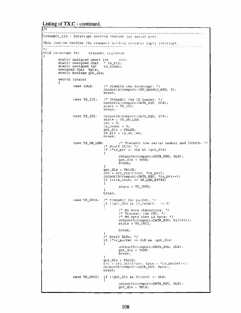
transmit-irq - Interrupt service routine tor serial port..

This routine handles the transmit holding r+ls t .e r en lp ty i n t e r r u p t . - - - - - - - - .

* / void interrupt far transmit-i rq (void)

static unsigned short int crc; static unsigned char * txstr; static unsigned int tx-count; unsigned char byte; static boolean got-dle;

switch (state) f

case IDLE: / * Disable the interrupt: + / outportb(comportt1NT-ENABLE-REG, 0 ) ; break;

case TX_IDl: / * Transmit the ID header: * / outportbIcomporttDATA-REG, DLE state = TX-ID2; break;

case TX-ID2: outportb(comport+DATA-REG, STX state = TX-SN-LEN; crc = 0; tx-count = 0; got-dle = FALSE; txqtr = tx-sn-len; break;

case TX-SN-LEN: / * Transmit the serial number and length: * / / * Stuff DLEs: * / if (*txqtr == DLE && Igot-dl@) I I

ou tpor t b ( compor t + DATA-REG , DLE ) ; got-dle = TRUE; break;

1 got-dle = FALSE; crc = crc-ccitK(crc, *txqtr); outportb[comport+DATAgEG, *tx_ptr++); if (++tx-count == SN-LEN-BYTES) I

state = TX-DATA;

break ;

case TX-DATA: / * Transmit t h e packet: + / if ( !got-dle 6 1 tx-length-- == 01 i l

/ * No more characters. * / / * Transmit the CRC, * / / * MS byte then LS byte: * / outportb(comport+DATA~REG, hi(crc) 1 ; state = TX-CRC2;

break; 1 / * Stuff DLEs: * / if ('txqacket == DtE && !got-dle) I 1

outportb( camport+DATA_REG, DLE) ; got-dle = TRUE; break;

1 got-dle = FALSE; crc = crc-ccitt(crc, byte = *tx_packettt); outportb(coeporrtDATA_REG, byte) ; break;

outportb(comport+DATA-REG, D L E ) ; got-dle = TRUE;

I break; I got-dle = FALSE; outportb(comporttDATA-REG, lo(crc) ) ;

state = TX-CRC3; break;

case TX-CRC3: if (!got-dle && lo(crc) == DLE) I

outportb ( comport +DATA-Rm, DLE) ; got-dle = TRUE; break;

I

/ * Output the final DLE/ETX: * / outportb(comport+DATA-REG, DLEl; state = TX-END; break;

case TX-EMD: outportblcomport+DATA-REG, ETX); / * No more characters, disable interrupt: * / outportb~comport+INT~ENABLLE~REG, 01; state = IDLE; break;

1

/ * Signal the interrupt controllers that we're done: * / end-of-hardware-interrupt(comirq);

I ------------*------------------------------------------------------------------

Wit- tx - Wait for the UNIT transmit buffer to be writable.

* / booleanwait-tx(void1 (

unsigned int timeout = 65535U;

while (timeout-- > 0 )

I / * Pause between characters, or the receiver * / / * will run out of time: * / timeout = 2000U/baud; while(timeout-- 0 ) C

/ * Wait. * / 3

Imain - The main program.

I~ntr~: command-line parameters as described at top of this file

unsignect l m g int serial-num; time-t start-time, current-time;

Listing of TX.C - continued. puts('TX - Serial port packet test program*); puts('fC) Copyright 1994 William Hue'); puts('Forcfons (C) Copyright 1989 ENSU Student Enterprises, Tnc.');

fputs('Usage:\n*, stderr); fputst'tx [/1 1 /2] [ / I 9 1 / 3 3 1 / 5 7 1 /I151 [packetsizej\n',

;tderr) ; fputs('wbere\n', stderr); fputs('/l and /2 allow you to select COMl or COM2 (default 1s

:QM2), \n*, stderr) ; fputs('/l9, / 3 8 , /57 and /I15 allow you to select 19200, 38400,

i7600 or\nS, stderr) ; fputs('115200 baud (default is 115200) , and\nS , stderr) ; Eputst*packetsize allows you to select the size in bytes of the

iataln', stderr) ; fputs('(exc1uding overhead, default is 512, max. 1s 6553S).\ne,

ini t-comgor t ( ) ;

printf(LTransmi!xing %u-byte (plus overhead) packets for %u smmds:' *\npress ESC to stop ... \n8, packetsize, seconds);

serlal-nm = 0;

t* Gat the current time: * / timc(&start,tirne);

while {(!&hit() I l getch0 ! = ESC) & & time(&current-time) - start-time c seconds)

f if (!transmitgacket( (unsigned char *)&crc-table[ll, packctslze,

serial-numtt) ) {

return(2) ; 1

/* Pause f ~ t 10 milliseconds: * / delay (101 ;

1

restore-all - Garbage collection routine.

his routine is registered via atexito.

h /

roid restore-all (void) r L

restore-intvecttcomirq, old-vector, masked); I

Listing of RX.C - Receives packetized data and calculates error statistics. C

R X - C - Receives packets over serial port. ((C) Copyright 1994 by William Hue. All rights reserved.

I Thiu program receives packets over the serial port and counts lost packets to Compute a packet error rate : P E R ) .

I The serial port is configured for no parity, 8 data bits, 1 stop bit

( ~ u n with the command line:

I r X E/1 1 / 2 ] 1/19 1 /38 1 /57 1 /I151 [seconds]

where /I and / 2 allow you to select COMl or COM2 (default is COM21, /19, / 3 8 , /57 and / I15 allow you to select 19200, 38400, 57600 or 115200 baud (default is 1152001, and seconds allows you to select how long the program will run for a f t e r receiving the first packet {default: is 60, pressing ESt will always end the program).

I~odification history:

Date By Whom Description ---.- ---- ------- - - - - - - - ----------- ----------- Mar. 20, 1994 William Hue Original program, polled serial port

operation {didn't work very well-- receiver kept missing characters).

Mar. 29, 1994 William Hue Converted to interrupt-driven operation. Apr. 01, 1994 William Hue Finally gat it working! Changed to

usirLg DLE+STX/E~X and stuffing.

#include kincluBe #include # inc lude tinclude $include

Cidclude Cinclude #include l include f include

I #include 'int8259.hs

I / * Local definitions: * /

#define COM1-BASE 0x3 f 8 ldefineCOM2-BASE Ox2f8 # d e f i n e COM1,IRQ 4 rde f ine coM2-1~Q 3

#Be fine DATA-REG 0 Cde fine INT-F51ABLE;REG 1 ikdef ine CONTROL-REG 3 #aef%w MODEM-REG 4 #define SPATUS-RJ~G 5 Xde f ine DIVISOR-LOW O l d e f i n e DIVISOR-HIGH 2

Cde f ine DATA-~XNY BIT0 tdef ine N-8-1 (BIT0 I BIT11 ltdefineBAUD-ll5200 1 #define BAUD-57600 2 Ildefine BAUD-38400 3 PdeEineBAUD-19200 6 #define DLAB BIT7

Listinp: of RX.C - continued. v

kdef i n e ID-BYTE Os5e

lde line D<IWT_WT BIT0 lde f ine OUT2 BIT3 kde f ine TSRE BIT6 ldefj rle OE BIT1 lde fine FE BIT3

'* Local macroes: * /

kdefine crc-ccittlcrc, byte) f ( fcscl i c 81 * crc-table[ [ (crc) >> 81 " (byte) 11

'* CRC-CcIm Tabie- */

:tatic const unsigned i n t crc-table [256 I =

0x2462, 0x3443, 0x0420, 0x1401, Ox64E6, Ox74C7, Ox44A4, 0x5465, OxASGA, OxB54B, 0x8528, 0x9509, OxESEE, OxFSCF, OxCSAC , OXDS~D, 0x3653, 0x2672, 0x1611, 0x0630, 0x76D7, Ox66F6, 0x5695, 0~46B4, OxB75B, -77A, 0x9719, 0x8738, OXF~DF, OXE~FE, OxD79~, O X C ~ B C , OxBBC4, OxSBES, 0x6886, 0x78A7, 0x0840, 0x1861, 0x2802, 0 ~ ~ 8 2 3 , OXC~CC, OXD~ED, OxE98E, OxF9RF. 0x8948, 0x9969, OxAgOA, O X m B , Ox5AP5, 0xaD4, OxTAB7, Ox6A96, OxlA71, OxOA50, Ox3A33, Ox2A12, OXDBPD, OxCBDC, OxEBBF, OxEBgE, 0x9879, 0x8358, OxBB3I3, OXAB~A, Ox6CA6, 0 x 7 ~ 8 7 , Ox4CE4, Ox5CC5, Ox2C22, 0 x 3 ~ 0 3 , OxOC60, OxlC41, OxEDAE, OxFD8F, OxCDEC, OxDDCD, OxAD2A, OxBDoB, 0 x 8 ~ 6 8 , 0~9D49, 0~7E97 , Ox6EB6, Ox5ED5, Ox4EF4, Ox3E13, Ox2E32, OxlE51, 0~0E70, OXFPgF, bEPBE, OXWD, OxCfFC, OxBPlB, OXAF~A, Ox9F59, 0 x 8 ~ 7 8 , 0x9188, 0x81A9, OxBlCA, OxAlEB, OxDlOC, OxC12D, OxF14E, O X E ~ ~ F , 0x1080, 0x00~1, Ox30C2, Ox20E3, 0x5004, 0x4025, 0x7046, 0x6067, Ox83B9, 0x9398, OxA3F3, OxB3DA, OxC33D, OxD31C, OxE37F, OxF35~, 0xO2B1, 0x1290, Ox22F3, Ox32D2, 0x4235, 0x5214, 0x6277, 0x7256, OxBSEA, OxA5C3, Ox95A8, 0x8589, OxF56E, OxE54F, OxD52~, OXC~OD, Ox34E2, Ox24C3, 0xl4A0, 0x0481, 0x7466, 0x6447, 0x5424, 0x4405, OxA7DB, OXB~FA, 0x8799. Ox57E8, OxE75F, 0xF77E, OxC71D, OXD~?C, Ox26D3, 0x36F2, 0x0691, Ox16BO. 0x6657, 0x7676, 0x4615, 0x5634, OxD94C, oxC96D, OxFgOE, OxE92F, Ox59C8, Ox89E9, OxB98~, OXA~AB, hr5844, 0x4865, 0x7806, 0x6827, Ox18C0, Ox08E1, 0x3682, 0 x 2 8 ~ 3 , OXCB7D, OxDBg, OxEB3F, OxPBlE, Ox8BF9, Ox9BD8, OxABBB, OxBB9A. Ox4A75, OxSA54, Ox6A37, Ox7A16, OxOAFl, Oxl~Do, 0 x 2 ~ ~ 3 , 0 x 3 ~ 9 2 , OXE'D~E, OxEDOF, OxDD6C, OxCD4D. OxBDAA, OxADSB, Ox9DE8, 0 x 8 ~ 9 , 0x7C26, Ox6C07, Ox5C64, Ox4C45, Ox3CA2, 0 ~ x 8 3 , 0 x 1 ~ ~ 0 , OXOCC~, OxEFlF, OxFF3E, OxCPSD, OxDF7C. OxAF9B. OxBFBA, OxaFD9, 0 ~ 9 F F 8 , 0x6E17, 0X7E36, 0x4E55, 0xSE74, Ox2E93, Ox3EB2, OXOED~, OxlEFO

I

'* W a l variables: */

&d i int-ermpL far * old-vector) t 1 ; ,aid t in tempt far * old-timer) ( l ; d e a n masked; looleangarbage-collection-registered = FALSE; tnsigned long in t w = O, f e = 0, crce = 0, ts = 0 , il = 0 , i p - 0;

* Global variables needed for i n t e r r u p t routlnr. * / tnum ( DISABLED, AWRITI~H~,-PACKET, RX-Z, RX SN-LEII, RX-DATA,

RX-EBD1, RX-END2, GOT-PACKET I s t a t e = DISABLED; asigned char rx_packet; nsigned int rx-length; s i g n e d long int rx_sn; mimed char rx_sn_fen [sN-LEi~-BYTES I ;

boolaangetgarams(fnt argc, char * argvljt; blemreceivegacket(~msigned char * packet, unsigned int * length,

ansigned long int * serial-num, time-t time-up]; booleanwaft-rxtvoid); void Snit-comport(void); void restore-allWoLd); void interrupt far receive-irq(voi d) ;

/* Functions: * /

/+

aetparams - Gecs command-fine parameters.

%try: argc = number of command-line arguments in asgv argv = command-line strings

ieturns : TRUE i f successful, FALSE otherwise.

Listing of RX.C - continued. /* m a 1 grototms: */

5

1

J

2

t i

L

-lean getqarams ( int argc , char * a r m [ )

char * * token; int tokens ; booleangot-seconds = FALSE; char s w i t c h a r , d u . ; unsigned isng int S ;

token = ~ 8 e - c ~ - l i n e (a~gc-1, &argv 11 3 , &t~keW, kstuftcm) ;

while (tokens-- > D) l

if ( (*token] [OJ == switchar) {

1 else i f (strcmptttoken, ' 2 . ) == 01 I 1

comport = COM2BASE; camirq = COM2-IRQ;

1 else i f tstrcmp(*token, '19') == 0) r L

baud = BAUD-19200; 1 else if (strcmp(*token, '38') == 0) I

baud = BAUD-38400; 1

baud = BAUD-57600; 1

baud = BAUD-115200; 1 else f

returnfPALSEl ; 3 token++ ; tokens--;

1 else f

i f ig&-seconds)

Listing of RX.C - continued. C

return ( F A L S E ) ; 3 Lf ~sscanE(*tokent+, * % l u % c n , hs, &dummy) ! = 1 1 1

s > 6 5 5 3 5 L ) f

seconds = (unsigned intis; got-seconds = TRUE;

1 1

returnlTRUE) ; ~ J

1 /'

init-comport - rnitalizes the serial port UART.

Returns: nothing

* /

void init-comport(void) t

/ * Turn on DLAB bit to write divisor: * / outportb~comport+CONTROL-REG, N-8-1 I DLAB) ; outportbt comport+DLVISOR-HIGH, 0 ) ; outportb(comport+DIVISOR~LOW, baud) ; outportbt comport+CONTROL-REG, N-8-1) ;

I /* Turn off interrupts: * / #utportb{co~ort+IWTWTENABLEEREG, 0 ) ;

I /* UART /OUT2 line must be on for interrupts to work: * / / * Ensure loopback is off: * / ~~~~~~~~~~~~~~~~~~~~~REG, OUT2);

/* Take over the appropriate interrupt: * / masked = takeover-intvect(comirq, &oldyector, receive-irq);

f f ( ! garbage-colletlon-registered) C

atex&ct~esEose-all) i garbge,ccllectlon,registered = TRUE;

3

/ f Rset 6t- te just in case. . . * / state = AWAITING_PACKm;

/ * Clear the status register: * / inportb(comport+STATUS-REG);

/ * Turn on the data ready interrupt: * / outportb ( comport + INT-ENABLE-RE , DR-IPJT-EN ) ;

I receiveqacket - Receives a data packet with CRC.

Entry: packet = &ere to put the received packet (NULL to not 6COre) length =where to put the packet length (NULL to not store) serial-num = where to put the serial number (NULL to not store) time-up = when to stop waiting for a packet, Ozforever

I~eturns : TRUE if successful, FALSE otherwise.

I This routine does a blocking wait to receive a packet. FALSE is returned i f the user presses ESC to abort.

I A packet consists of an identification header byte, a serial number,

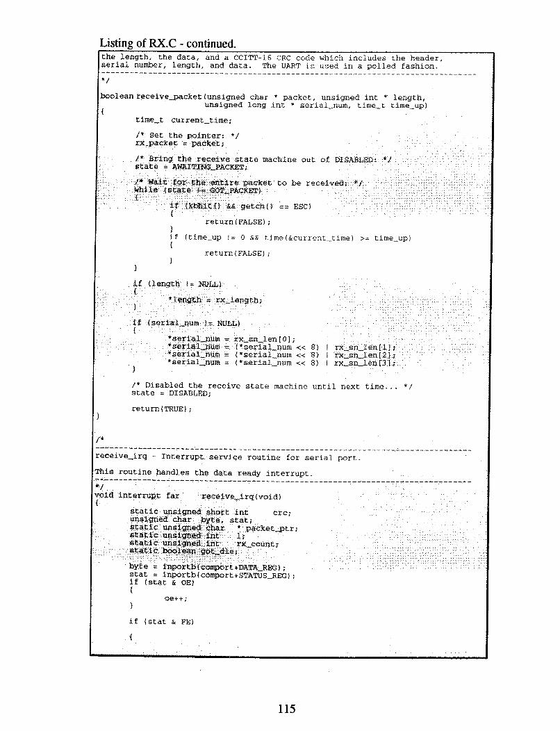
il++; break;

1 state = RX-2; break;

case RX-2: / * Looking for STX. + / /* We can only get Receive and Overrun ints. *I'

if (byte ! = S T X ) {

il++; if (byte ! = DLE) r

state = AWAITING-

E r = rx-sn-len; = RX-SN-LEN;

/ * Receive serial nqmber nstuf f DLEs: * /

PACKET;

and lengt

Listing of RX.C - continued.

ACKm: / * Looking for start of frame (DLE), * / i f (byte != DLEI

case =-DATA

if (byte == DLE && !got-dle) (

got-dle = TRUE; break;

1 if (got-dle & & byte ! = DLE) {

/ * DLE followed by non-DLE is not * / / * allowed in data. Incomplete * / / * packet! * / ip+ + ; / * Here, we could check whether the * / / * byte is a STX or an m, but we * / / * won't bother, for simplicity: * / state = AWAITING-PACKET; break;

1 got-dle = FALSE; crc = crc-ccitt(crc, *packetgtr++ = byte); if (++rx-count == SN-LENBYTES1 i

1 break

packetqtr = rxgacket; rx-length = rx_sn_len[4]; rx-length = (rx-length <4 8 ) 1

rx_sn_len[5]; /*Add 2 for CRC: * / 1 = rx-length t 2; state = RX-DATA;

/ * Unstuff DLEs: * / i f (byte == DLE && !got-dlel {

got-die = TRUE; break;

I if (got-dle && byte ! = DLE;

Listing of BX.C - continued.

Enterprises, Inc. ' 1

/I151 Isecondsl\nw,

fputsl'where\na, stderr); fputs{*/l and / 2 allow you to select COMl or COM2 (default is

:COM21,\na, stderrl; fpats(*/l9, / 3 8 , 157 and /I15 allow you to select 19200, 38400,

57600 ortn*, stderr) ; fputs('115200 baud (default is 1152001, andin*, stderr); fputsl'secands allows you to select how long the program will run

:forhe, stderr); fpwtsf'fdefault is 60, pressing ESC will always end the

program) - \n' , stderr 1 ;

%u seconds after receipt af first packet;\nB,

&f irst-serial-num, 0) )

st packet. * ) ;

/ * Get the current time: * / time(&start-time);

serial-num = prev-serial-num = first-serial-num; missed-packets = 0;

while {{!%hit0 I I getch0 ! = ESC) && time~current,time) - start-time 4 seconds)

i i f t lfecei~eqacket (NULL, NULL, &serial,num, start-t ime4

break; 1

rdssedaackets += serial-num - prev-serialjum - 1; pzev-serial_nurn = serial-num;

3

printf('\n%lu overrun errors detected.\n9, oe); printf{'%lu framing errors detected.\n9, fe); printf(.%lu characters missed due to being too slow.\n', ts); printf{'%lu characters lost while waiting for start of packet.\n', 11); printf('%lu incomplete packets.\n\nm, ip);

printf('Tata1 of %Lu packets received from #Blu to #%lU;\nw, prev-serial-num - first-serial-num + 1, first-serial-num, prev-serial-num) ;

printf(*of those, Blu were missed and Blu had CRC errors.\n', missedqackets - crce, crce);

prfntf('The Overall packet error ratio was %e.\n*, float) missed_gackets/ tprev,ser%al-num - first-serial-num t 1));

printf ('The awed packet ratio was 8e. \ne, f flQat) (missed_gackets - crce) / (prev-&rial-nurn - f lrst-serial-num + 1. ) ) ;

printf{Vsing ady the packets that were IWf mlssed,\n*

Listing of RX.C - continued. 'the real packet ERROR ratio was %e.\nn, (float)crce/ (prev-serial-num - first-serial-num + 1 - (missed-packets -

creel i I ;

returnt 0 ) ; 1

/ *

restore-all - Garbage collection routine.

This routine is registered via atexito.

* /

void restore-alltvoid) C

restore-intvect(comirq, old-vector, masked);

/ *

XNT8259.C - Hardware interrupt routines declared in INT8259-C. Copyright (C) 1989 ENSC Student Enterprises, Inc. By William Hue, February 02, 1989.

Routines are provided herein to take over and restore hardware interrupt vectors.

NOTE: The interrupt request lines on the IBM PC and compatible series computers are programmed to be EDGE-TRIGGERED. Make sure that your interrupt handler(s1 reset the interrupt source, or else the interrupt request line will remain in the active state, and never trigger another interrupt.

On AT-class machines, IRQ2 is actualiy I R Q 9 . If you encounter a problem taking over interrupt level 2 on an AT, try substituting ' 9 ' for the interrupt level.

Compilation: While debugging: tcc -c -1 -N -ml -a -w -C int8259.c After debugging: tcc -c -1 -N- -ml -a -w -C -2 -0 -G int8259.c

Modification history:

/+ For inp( ) and outp( k . * / /* For dos setvecto and * / / * - d ~ s ~ ~ e t ~ e c t ( ) . * /

Rinclude 'int8259.h- Alnclude *bitdefs.ha

/ * Function definitions: * /

/ * - - - - - - - - - - - - - - - - - - - - - - - - - - - - - - - - - - - - - - - - - - - - - - - - - - - - - - - - - - - - - - - - - - - - - - - - + - - - - -

takeoverJntvect0 - Takes over a given hardware interrupt level (0-15).

~ntry: int-level = hardware interrupt level [O-15) new-vect = new interrupt service routine

Returns : old-vect = pointer to old service routine function returns TRUE if interrupt level was masked off, FALSE if not.

The selected interrupt level is unmasked and the corresponding interrupt vector replaced with new-vect. No parameter checking is performed.

* /

bolean takeover-intvect(unsigned int int-level, void (interrupt far * * old-vect) 0 ,

void (interrupt far * new-vect) 0)

unsigned int intvect-number; unsigned char mask; booleanmasked;

/ * Get the vector number: * / intvect-number = int-level + ((int-level > 7 ) ? 0x68 : 0x08);

/ * Get the original vector: * / *old-vect = getvect(intvect-number);

/ * Set the new vector: * / setvect{intvect-number, new-vect);

/ * Get original mask and unmask: * /

If Ifnt-level <= 7) /+ Master controller? * / r

mask = (unsigned char)inportb(MASTER_B259J4ASK,REG); masked = (mask & (BITO r i int-level)) ? TRUE : FALSE;

/+ Unmask: + / if (masked) t

outportb(MASTER-E259-MASKKREG, mask & - ( B I T 0 << int-level));

1 1 else f

I

mask = (unsigned char)inportb(SLAVE-8259-MASK-REG): masked = (mask & (BITO << (int-level - 8))) ? TRUE : FALSE;

/* Unmask: * / if (masked) I

outportb(SLAVE-8259_MASK_REG, mask & -(BIT0 i< (int-level - 8 ) ) ) ;

1

---------------------------------------------------------------------------- cestore~intvect0 - restores a previously taken-over interrupt level.

%try: int-level = hardware interrupt level old-vect = the vector to be restored orig-masked = TRUE if lnt-level was originally masked off, FALSE if not

Listing of INT8259.C - continued. ,

1

1

C

old-vect is that set by takeover-intvect, and orig-mask is that returned by takeover-intvect .

Listing of INT8259.C - continued. Returns: Nothing

1

I

E t

E

E -

U

{

1

-

restore-intvect(unsigned int int-level, void [interrupt far * old-vectl [ I .

boolean orig-masked)

unsigned int intvect-number;

/ * Get the vecEor number: * / intvect-number = int-level + ((int-level > 7 ) ? 0x68 : 0x08);

/ * Restore the original mask: * / If (orig-masked) / * Otherwise leave unmasked- * / f

if (inL-level <= 7 ) / * Master controller? * / t

1 else I

outp~rtb(MASTER-8259_MASK_REG, inportb{MAsTER_8259-~~SK_REG) I

( BIT0 << int-level ) ;

setvect(intvect-number, old-vect);

knd-of_hardware,interrupt(l - sends general end-of-interrupt (EOI) commmds to .he 8259 interrupt controller(sl.

:ntry: int-level = the hardware interrupt level on which the interrupt i s finished

leturns : Nothing.

/

,old far end-o+-brdware-interrupt(unsigned int int-level)

/ * First tell the master 8259 interrupt controller:*/ O U ~ ~ O ~ ~ ~ ( M A S T E R - ~ ~ ~ ~ - C O M M A N D _ R E G , EOI-8259);

/ * Then, i f necessary, tell the slave: * / if (int-level > 7 ) (

outportb(SLAVE-8259_COMMAND_REG, EOI-8259) ; 1

-- --------------------------------------------------------------------------- INT8259.H - Declarations for hardware interrupt routines in INT6259.C. Copyright ( C ) 1989 ENSC Student Enterprises, Inc. By William Hue, February 02, 1989.

RoTltines are provided herein to take over and restore hardware interrupt vectors. The low-level constants defined for the 8259 interrupt controller are inzluded here for infcrrnation only, and application programs should never attempt to write directly to the 8259 interrupt controller registers.

WOTE: The interrupt ?quest lines on the IBM PC and compatible series computers are programmed to be EDGE-TRIGGERED. Make sure that your interrupt handler(s1 reset the interrupt source, or else the interrupt request line will remain in the active state, and never trigger another interrupt.

On AT-class machines, IRQ2 is actua problem taking ever interrupt level *9 ' for the interrupt level.

lly IRQ9. If you encounter a 2 on an AT,, try substituting

Modification history-

Wifndef HARDWARE-INT8259 / * Check that we haven't already #included. * /

/* Register locations for master 8259: * /

/ * Register locations for slave 8259: + /

Pdefine SLAVE-8259-COMMAND-REG OxOaO # ~ ~ • ’ ~ ~ ~ S L A V E - ~ ~ ~ ~ _ M A S K - R E G OxOal

/* Function prototypes: * /

/ * takeover-intvectc) - Takes over a given hardware interrupt level (0-151 * / /* and replaces the old-vect with the new-vect. The old vector 1s saved in * / /* *old-vect and the TRUE is returned if the interrupt level was masked o f f '/ /* and FALSE is returned if not. The returned parameters should be gassed * / /* to restore-intveatl to properly restore the original state Of the level. * /

boolean takeover-f ntvect (unsigned int int-level , void (Itnterrupt far * * old-vect) ( ) ,

void (interrupt far * new-vect) 0);

Listing of INT8259.H - Header file for exporting functions from INT8259.C. /*

I

1

1

-

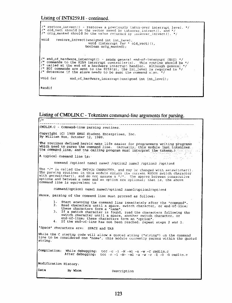
Listing of CMDL1N.C - continued.

I / * Local definitions: * /

%define SPACES SPACE, TAB

static cmst char spaces[] = { SPACES, ' \O ' };

' I * Local prototypes: */

static char * find-non-space(char *str);

static char * find-spacepr,switch(char *str, char switchar);

I /' Function definitions: * /

- ----------------------------------------------------------------------------- parse-command-line0 - Parses a command line and returns an array of string~. I / * Entry: argc = the number of elements in 'argv'

argv = an array of strings comprising the command line tokenc = where t~ put the size of the returned array switchar = where to put the switch character

Returns : An array of strings (array of character pointers), ordered as the names and options were found in 'argv'. Names are returned in the string exactly as they agpeared in che 'argvTV' array. Options are preceded by a painter to a single .Witch character (this pointer is equal to 'switchar'l. This array of character pointers may be passed to free0 when no longer needed.

I The first element is NULL and '*tokencm is set to 0 i f n0 arguments are found.

NULL is returned in case of memory allocation error or MULL pointers passed for *tokenc8 or 'switchar'.

l~xample: If the switch character were ' / ' and "argv" were

I this routine would return the following array: @name1 * Iswitchar) 'option1 ' *name2 I s w i t char) 'option2 '

Listing of Ch4DLIN.C - continued. (swftchar) 'option3 '

The argv array passed to main0 contains the pathname of the executable file in DOS 3.00 and higher. I r is up to the calling program to decide whether to Pass argvl01 to this routine, or &argv[ll to omit the pathname.

* * * NOTE: The original 'argv' array may be modified by this function. Specifically, any switch characters in 'argv' strings are replaced by NULL characters. In addition, some of the whitespace characters may also be replaced by NULL characters.

------------------------------------------------------------------------------ * /

char * * parse-command-linetint argc, char *argv[l, int *tokenc, char *switchar)

unsigned int arg-number; eha r **token9 = NULL, **temp-tokens = NULL; char * current-char; unsigned int current-size = 0;

i f rtokenc == NULL I I switchar == NULL) C

return (NULL> ; 3

/ * Get the switch character: * / *switchar = getswitcharo;

/ * In case no args are found, set up a dummy array: * / if ( (tokens : (char **)malloc(sizeof(char * ) ) ) == NULL) f

return (NULL) ; 1 tokensIO] = NULL;

for (arg-number = 0; arg-number < argc; arg-number++) I

/ * Start with the first character: * / current-char = argvfarg-number];

do {

I + If current character is a space, */ / * null it out to terminate token from * / / * previous iteration of loop: * / if (strchr(spaces, 'current-char) != NULL) (

/ * Skip past any leading spaces: * / if ( (current-char = find-non-space(current-char)) == NULL1 I

/ * Nothing but spaces. * / break; / * Go to next argv. * /

if (*current-char == *switchar) 1

/ * Expand the token array: * / current-size++; i f ( (temp-tokens = t char **I realloc t tokens,

urrent-size*sizeof(char ' 1 ) I == NULL] I

free(tokens) ; returntNULt) ;

1 tokens = temp-tokens;

/ * Signal switch: * / tokens[current-size-11 = switchar;

/ " In case the switch character ends a name, null

*zurrsnt-char++ = ' \ i l l ; 3

/ * Store the locatlon of chis t sken: *; /* Expand the token array: * / current-size++; if { (temp-tokens = Ichar **)reallocltokens,

:urrent-size*sizeof[char * ) ) 1 == NULL) f

freef tokens) ; r e t u r n (NULL) ;

1 tokens = temp-tokens;

tokenslcurrent-size-11 = current-char;

/ * Now skip to the next space or character and repeat: * /

1 while ( (current-char = finpspace-or-switch(current_char, switchar)) != NULL);

I

* find-non-space() - Returns point-er to first non-space character in 'str* * Returns NULL if non-space not found. * /

;Latic char * find-non-space(char *str)

if (str == NULL1 f

return f NULL) ; 1

if (*str == '\0')

return (NULL) ; 1 else f

return l str r 1

* find-space-ox-switch0 - Returns pointer to first space character or '/ '* switch character in str, or hVLL if none found. * /

:tatic char * find-space-or-switcb!ckar ' s c r , char switchar)

I char switch-spaces El = ( x ' , SPACES, ' \ @ ' 1 ;

lifndef CMDEM

Me f ine C m L I N

'* parse-comand-line[~ - Parses a c~mnand line and returns an array of * / '* ~Lrings. *argco should be the number of elements in 'argvB, 'argv' */ " should be an array of strings comprising the command line, 'tokenc' */ '* should point where to put the size of the returned array, and 'switchar' * / '* should point where to put the switch character. An array of strings * / " tarray of character pointers), ordered as che names and options were * / '* found in 'argvw, is returned. Names are returned in the string exactly 1 ~' as they appeared in r;he 'argvo array. Options are preceded by a pointer * / '+ to a single switch character (chis pointer is equal to 'switchar'). This * / " array of character pointers may be passed to free0 when no longer needed. * / '* NULL is returned in case of memory allocation error- * / '* *'* HOTE: The origtnal 'argv' array may be &tied by this function. * / ' t Specificdily, any switch characters in 'argv' strings are * /

replaced by EWLL characters- In addition, some of the * / 'L whitespace characters may also be replaced by NULL characters. * /

/ * ----------------+-------------------------------------------------------------

Cf4DLfN.H - Include file for command-line parsing routines.

Copyright IC ) 1984 ENSC Student Enterprises, Inc. By William Hue, October 13, 1983.

me rourfnes declared herein make life easier for programmers writing programs which need to parse the command line. (Actually, this module just tokenizes the command line, and the calling program must interpret the tokens-)

A typical command line is:

The '/' is called the SWITCH CHARACTER, and may be changed with setswitchar0. 'The parsing routines in this module cbrain the current M S W S switch character with getswitchar(1, and do not assume a * / ' . The spaces between consecutive optfons and between a name and an option are optional; that is, the above coaimand line is equivalent to

Hence, parsing of the command line musc proceed as follows:

1 Start scanning the command line immediately after the 'command'. 2. Read characters until a space, switch character, or end-of-line;

these characters form a 'name'. 3 . If a switch character is found, read the characters following the

switch character until a space, another switch character, or end-of-line; these characters form an 'option'.

4. If the end-of-lfne has not been reached, repeat steps 2 and 3.

'Space' characters are: SPACE and T?,B

bile the C startup code will allow a quoted string ('string*) on the command Line to be considered one 'name', this module currently parses within the quoted

Listing of CMDL1N.H - Exports functions from CMDLIN-C.

1

1

1

5

P

I

i

1

I

I, I

: I r( J 1 #

J , I

I

1 I I

L

Listinn of CMDLXN.H - continued. - t

Char * * parse-command-linetint argc, char *argvl l , int 'tokenc, char 'switchar);

fkendi f

Listing of B1TDEFS.H - Defrnes names for individual bits. / *

BITDEFS-H - Defines the bitmasks for a 16-bit word.

"ogyrighc tC1 1989 EWSC Student Enterprises, Inc. By William Hue, February 01, 1989.

Description ----------- -----------

l i fnde f BIT-DEFINITIONS * /

Udefine BITDEFINITIONS

/* LOW byte: * /

taef i ne BIT0 0x01 kdefineBIT1 0x02 Rdefine BIT2 0x04 %define BIT3 0x08 Bdefine BIT4 Oxlo ldefineBIT5 0x20 Udefine BIT6 0x40 tdefine BIT7 0x80

/* High byte; * /

tdef i ne BIT8 Cdefine BIT9 Udef ine BIT10 Cdef ine BIT11 [tdef ine BIT12 kdef ine BIT13 Cdefine BIT14 Bdef i n e BIT15

/ * Check t h a t w e haven ' t already #included.

Listing of CHARS.H - continued.

Listing of W0RDBYTE.H - Macroes to separate bytes from words. /*

WQRD$YTE;-H - Defines macros for extracting high and l a w bytes of 16-b i t words.

:Copmight (C) 1989 ENSC Student Enterprises, Inc . 1% WZlliam Hue, February 01, 1989.

Modlficatlon history :

~ a ~ e By Whom Description =P== - - - - - - - ----------- --...--------

I t: Ende f WORDBYTE-MACROS / * Check that we haven't already #included.

(Ide f ine WRDBYTEJULCROS

I,* Macro tor extracting low byte of a l h b i r word: * /

I ftde f ine lo (wo~d) (unsigned char) word

/* Macr~ for extracting high byte O E a 16-bit word: * /

#define h i (word) (unsigned char) (word >> 8 )