Predicting Aquaplaning Performance from Tyre Profile Images with Machine Learning
Upload
khangminh22Category
view
0download
0
HAL Id: tel-00126562https://tel.archives-ouvertes.fr/tel-00126562
Submitted on 25 Jan 2007
HAL is a multi-disciplinary open accessarchive for the deposit and dissemination of sci-entific research documents, whether they are pub-lished or not. The documents may come fromteaching and research institutions in France orabroad, or from public or private research centers.
L’archive ouverte pluridisciplinaire HAL, estdestinée au dépôt et à la diffusion de documentsscientifiques de niveau recherche, publiés ou non,émanant des établissements d’enseignement et derecherche français ou étrangers, des laboratoirespublics ou privés.
Tyre noise over impedance surfaces - Efficientapplication of the Equivalent Sources method
François-Xavier Bécot
To cite this version:François-Xavier Bécot. Tyre noise over impedance surfaces - Efficient application of the EquivalentSources method. Acoustics [physics.class-ph]. INSA de Lyon, 2003. English. �tel-00126562�

N° d’ordre 03ISALXXXX Year / Année 2003
PhD thesis / Thèse
Tyre noise over impedance surfaces – Efficient application of the Equivalent Sources method
Presented to / Présentée devant L’Institut National des Sciences Appliquées de Lyon, France
& Chalmers university of technology, Göteborg, Sweden
For / Pour obtenir
The grade of doctor of philosophy / le grade de docteur
Doctoral school / Ecole doctorale : M.E. G. A. (Mécanique, Energétique, Génie civil, Acoustique)
Spécialité : Acoustique
By / Par François-Xavier BÉCOT
Defended the 8th september 2003 in front of the examination committee
Soutenue le 8 septembre 2003 devant la Commission d’examen
Jury
KROPP Wolfgang Professor at Chalmers (Göteborg, Sweden), Directeur de thèse GUYADER Jean-Louis Professor at INSA (Lyon, France), Directeur de thèse DUHAMEL Denis Professor at ENPC (Paris, France), rapporteur OCHMANN Martin Professor at T.F. (Berlin, Germany), rapporteur KRISTIANSEN Ulf Professor at Norwegian Institute of Technology (Trondheim, Norway) HAMET Jean-François Research director at INRETS – LTE (Bron, France)
Research laboratories / Laboratoires de recherche :
Vibrations – Acoustics Laboratory (LVA), INSA of Lyon, France &
Department of Applied Acoustics, Chalmers university of technology, Göteborg, Sweden
Thesis for the degree of Doctor of Philosophy
Tyre noise over impedance surfaces
Efficient application of the Equivalent Sources method
Francois-Xavier Becot
Department of Applied Acoustics Vibrations - Acoustics Laboratory (LVA)Chalmers University of Technology & Insa – Scientific and Technical UniversityGoteborg, Sweden Lyon, France
May 2003Report F03-03
Tyre noise over impedance surfaces – Efficient application of
the Equivalent Sources method
Francois-Xavier Becot
ISBN 91-7291-313-4
c© Francois-Xavier Becot, 2003
Doktorsavhandlingar vid Chalmers tekniska hogskola
Ny serie Nr 1994
ISSN 0346-718X
Department of Applied Acoustics
Chalmers University of Technology
SE 412 96 Goteborg, Sweden
Telephone + 46 (0) 31-772 2200
Fax + 46 (0) 31-772 2212
Printed in Sweden by Chalmers Repro Service
Goteborg, Sweden

ii
Abstract
Tyre noise over impedance surfaces – Efficient application of the Equivalent Sources
method. Francois-Xavier Becot. Report F03-03 – ISBN 91-7291-313-4
Reduction of the transportation noise nuisance has become an important challenge in
today’s societies. As a consequence of engine noise reduction, tyre / road contact noise
is now the main source of traffic noise under normal driving conditions. In this respect,
the aim of the present work is to understand and to control the mechanisms of tyre
radiation by designing accurate tools to predict the tyre noise radiation over arbitrary
impedance surfaces.
Tyre radiation is modelled using the Equivalent Sources method. Besides low frequency
limitations because of two–dimensional simplifications, this model is proved to be an
accurate tool for predicting tyre noise over acoustically rigid surfaces. Ground effects
induced by absorbing surfaces are only approximated. Therefore, a model for the prop-
agation of sound due to an arbitrary order source over an arbitrary impedance plane is
developed. It is mainly an alternative to integral equation methods. In addition, the
exact solution to this problem is presented.
Based on the two previous models, an iterative model of the tyre radiation over arbi-
trary impedance surfaces is implemented. Comparison with horn effect sound amplifi-
cation indicate that this model is accurate for homogeneous as well as inhomogeneous
absorbing surfaces. Using this model, trends for the tyre radiation over absorbing
surfaces are discussed in a parametrical study.
The work presented in this thesis gives further insights into the mechanisms of tyre /
road noise radiation; furthermore, it allows to study the possibilities of reducing traffic
noise by the use of so–called “low–noise” road surfaces.
Keywords : tyre / road noise, tyre radiation, horn effect, equivalent
sources method, method of auxiliary sources (MAS), ground impedance,
cylindrical wave reflection coefficient, integral equations.

iv

Resume
Bruit de pneumatique au–dessus d’une surface d’impedance donnee – Application
efficiente de la methode des Sources Equivalentes. Francois-Xavier Becot.
Report F03-03 – ISBN 91-7291-313-4
La reduction du bruit des tansports est devenue un enjeu majeur dans nos societes.
En raison de la reduction du bruit de moteur, le bruit de contact pneumatique /
chaussee est aujourd’hui la principale source du bruit de trafic en conditions normales
de conduite. Dans ce contexte, le but du present travail est de comprendre et de
controler les mecanismes de rayonnement du pneumatique, ceci en concevant des outils
de prediction efficients pour la propagation du bruit pneumatique / chaussee au dessus
de surfaces d’impedances arbitraires.
Le rayonnement du pneumatique est modelise a l’aide de la methode des Sources Equi-
valentes. Malgre des limitations en basses frequences dues au caractere bi–dimensionel
du modele, calculs et mesures indiquent que cet outil convient bien au rayonnement au–
dessus de surface totalement reflechissantes. Les effets de sol induits par des surfaces
absorbantes n’est realisee que de maniere approchee. Un modele d’effets de sol dus a un
plan d’impedance donnee est donc develope pour des sources de directivite arbitraire.
Cette technique est essentiellement une alternative aux methodes dites des equations
integrales. Par ailleurs, la solution exacte du probleme est presentee.
Base sur les deux outils de prediction precedents, un modele iteratif est develope pour le
rayonnement d’un pneumatique au–dessus de surfaces dont l’impedance est arbitraire.
Des comparaisons avec des mesures d’amplification sonore due a l’effet diedre montrent
que ce modele est efficient pour des surfaces absorbantes homogenes et inhomogenes. A
l’aide de ce nouvel outil, une etude parametrique examine les tendances du rayonnement
du pneumatique au–dessus de chaussees absorbantes.
Le present travail apporte de nouveaux elements en matiere de rayonnement de
pneumatique / chaussee; il contribue en outre a l’etude des possibilites de reduction
du bruit de trafic, notamment en utilisant des chaussees dites “silencieuses”.
Mots cles : Bruit pneumatique / chaussee, rayonnement pneumatique,
effet diedre, methode des sources equivalentes, impedance de sol, co-
efficient de reflection pour ondes cylindriques, equations integrales.

vi

Acknowledgements
During my doctoral studies, I had the unvaluable chance to take the most of the super-
vision of Prof. Wolfgang Kropp and Dr. Jean-Francois Hamet. This work results from
the numerous fruitful and thorough discussions we have had. Therefore, I would like to
extend my warmest regards to them for their wise guidance and support along this time.
I am also very grateful to Prof. Tor Kihlman from the Chalmers University of Technol-
ogy and Prof. Jean-Louis Guyader from Insa of Lyon for giving me the opportunity to
do this work. I also would like to thank Jacques Beaumont for welcoming me at Inrets.
I would like to thank all the staff of the department of Applied Acoustics for the
studious and warm atmosphere they all contribute to. I especially thank Gunilla Skog
and Borje Wilk for their precious and friendly help with the administrative and the
computer things during this time.
Cordial thanks to the members of the tyre noise group and the members of the outdoor
sound propagation group for their skillful advice, comments and support.
I send my sincere regards to the members of the Transport and Environment Labora-
tory of Inrets, with a special mention to the members of the “Acoustique physique”
group. Thanks to all of you!
This work would not have been possible without the love and the patience of Sylvaine.
Sylvaine, this work is yours too.

viii
Context of the doctoral studies
The PhD work of Francois-Xavier Becot had the frame work of a collaboration between
Department of Applied Acoustics of Chalmers University of Technology
and
Vibrations – Acoustics Laboratory (LVA) of Insa of Lyon.
The research activities took place
in Sweden at the Department of Applied Acoustics of Chalmers University of Technology
and in France at the Transport and Environment Laboratory (LTE) of Inrets.
The work was also financially supported by Region Rhone-Alpes (France).

x

xi
Tableof Contents

xii TABLE
Introduction : Transportation Noise Nuisance 1
Chapter 1 Tyre / Road Contact Noise and Ground Effects 3
Section 1.1 . . . . . . . . . . . . . . . . . . . . . . . . . . . . . .Tyre road noise generation and radiation 4
Section 1.2 . . . . . . . . . . . . . . . . . . . . . . . . . . . . . . . . . . . . .Tyre road noise prediction models 8
Section 1.3 . . . . . . . . . . . . . . . . . . . . . . . . . . . Acoustical characterisation of road surfaces 11
Section 1.4 . . . . . . . . . . . . . . . . . . . . . . . . . . . . . . . . . . . . . . . . . . . . . . . . . . . . . . . . . . . . . Summary 15
Chapter 2 A Multipole Model of the Tyre Radiation 17
Section 2.1 . . . . . . . . . . . . . . . . . . . . . . . . . . The tyre as an acoustical source : definitions 18
Section 2.2 . . . . . . . . . . . . . . . . . . . . . . . . . . . . . . . . . . . . . . . . . . . . . . . . . .The multipole model 22
Section 2.3 . . . . . . . . . . . . . . . . . . . . . . . . . . . . . Implementation and amplification factors 27
Section 2.4 . . . . . . . . . . . . . . . . . . . . . . . . . . . . . . . . . . . . . . . . . . . . . . . . . . . . . .Model validation 33
Section 2.5 . . . . . . . . . . . . . . . . . . . . . . . . . . . . . . . . . . . . . . . . . . . . . . . . . . . . . . . . . . . . . Summary 44
Chapter 3 Ground Effects Modelling using the ES Method 47
Section 3.1 . . . . . . . . . . . . . . . . . . . . . . . . . . . . . . . . . . . . . . . . . . . . . .Principle and description 48
Section 3.2 . . . . . . . . . . . . . . . . . . . . . . . . . . . . . . . . . . . . . . . . . . . . . . . . . . . . . .Model validation 54
Section 3.3 . . . . . . . . . . . . . . . . . . . . . . . . . . . . . . . . . . . . . . . . . . . . . .Other directional sources 60
Section 3.4 . . . . . . . . . . . . . . . . . . . . . . . . . . . . . . . . . . . . . . . . . . . . . . . . . . . . . . . . . . . . . Summary 63
Chapter 4 Tyre / Road Noise Over Arbitrary Impedance Surfaces 65
Section 4.1 . . . . . . . . . . . . . . . . . . . . . . . . . . . . . . . . . . . . . . . . . . . . . . . . . . . . . . . . . . .Preliminary 66
Section 4.2 . . . . . . Iterative ES model of the tyre radiation over impedance surfaces 73
Section 4.3 . . . . . . . . . . . . . . . . . . . . . . . . . . . . . . . . . . . . . . . . . . . . . . . . . . . Model functionning 79
Section 4.4 . . . . . . . . . . . . . . . . . . . . . . . . . . . . . . . . . . . . . . . . . . . . . . . . Results and discussion 82
Section 4.5 . . . . . . . . . . . . . . . . . . . . . . . . . . . . . . . . . . . . . . . . . . . . . . . . . . . . . . . . . . . . . Summary 89
OF CONTENTS xiii
Chapter 5 Parameter Study of the Tyre / Road interface
Properties
91
Section 5.1 . . . . . . . . . . . . . . . . . . . . . . . . . . . . . . . . . . . . . . . . . . . . . . Geometry and notations 92
Section 5.2 . . . . . . . . . . . . . . . . . . . . . . . . . . . . . . . . . . . . . . . . . . . . . . .Geometrical parameters 93
Section 5.3 . . . . . . . . . . . . . . . . . . . . . . . . . . . . . . . . . . . . . . . . . . . . Ground surface impedance 97
Section 5.4 . . . . . . . . . . . . . . . . . . . . . . . . . . Geometrical and acoustical combined effects 104
Section 5.5 . . . . . . . . . . . . . . . . . . . . . . . . . . . . . . . . . . . . . . . . . . . . . . . . . . . . . . . . . . . . . Summary 105
Chapter 6 Conclusions 109
Chapter 7 Appendices 113
Appendix I . . . . . . . . . . . . . . . . . . . . . . . . . . . . . . . . .The Equivalent Sources (ES ) method 114
Appendix II . . . . . . . . . . . . . . . . . . . . . . . .Complements on the tyre boundary condition 120
Appendix III . . . . . . . . . . . . . . . . . . . Integration over the Green functions’ singularities 125
Appendix IV . . . . . . . . . . . . . . . . . . . Experimental determination of surface impedance 129
List of Figures 134
Bibliography 140
Appended Papers 153

xiv

Notations used in the text
The following text is organised in a number of
Chapter’s, numbered as 1, 2, . . . They are subdivided in a number of
Section’s, numbered as 1.1, 1.2, . . . , 2.1, 2.2, . . . , which themselves contain a series of
Paragraph’s, which are not numbered. All these are followed by
Appendix number I, II, . . .
Below, a number of abbreviations used in the following text are explained.
dB : decibels = 10 log10 | pressure(N.m−2) |2
2D : two-dimensional
3D : three-dimensional
FE : finite element (method)
BE : boundary element (method)
ES : equivalent sources method
SPL : sound pressure level, in decibels
SVD : singular value decomposition
resp. : respectively
Eq.3− 5 : Equation 5 in Chapter 3
Fig. 2-6 : Figure 6 in Chapter 2
Fig. III-1 : Figure 1 in Appendix III

xvi NOTATIONS
The following notations correspond to
j : imaginary number (=√−1),
i, j,m, n, . . . : integer indices.
A : matrix which contains the element denoted Am
H(2)m : Hankel functions, second kind, of order m
× : scalar product or matrix product,
· : vector product.
∇ : vector gradient (sometimes denoted grad in the literature).
~ur and ~uϕ : unit vectors in the radial and tangential direction,
u, v : (dummy) variable of integration.
Introduction :
Transportation Noise Nuisance
In the last century, car has turned from a “cult object” to the undesired host of our cities.
Today’s tendency in town planning is to make vehicles disappear from the city centres, this
by developing public transports, by encouraging individual but non–polluting transportation
means (bicycle, rollers, skate–board, trottinette, . . . ) or by encouraging alternate use (and
vision) of our vehicles (car–pooling, car–sharing, . . . ). The objective of these efforts is to
restore a more pleasant and, above all, a more healthy atmosphere in our towns.
The pollution, to which we are exposed, is composed of the atmospheric pollution and the
noise pollution. Whereas, the first one has engaged a large concern from politics, the effort for
fighting the second one has been quite moderate during the last thirty years. For instance in
France, almost 40 % of the population declare to be annoyed by noise, a large part of which
originates from the transportation network [Dufour 1990]. The study in [Stanners 1995] values
to 45 % the part of the population in Europe exposed to noise levels between 55 and 65 dB(A)
and to 20 % the population exposed to levels higher than 65 dB(A). To get the measure of
these values, a noise level of 60 dB is characterised as “annoying”; it corresponds for instance
to a conversation taking place in the listener’s room. In addition, dB(A) is an average value
over 24 hours, which means that measured noise levels may occasionally be higher, most likely,
during day hours.
Besides auditory effects such as hearing loss or communication disturbance, a noisy environ-
ment may also impact people’s physiology [Stansfeld 2002]. For the exposed population, noise
may be the cause of hypertension, cardio–vascular diseases or psychological disorder. Especially
among children, noise may be incriminated as altering the memory and the cognitive ability.

2 INTRODUCTION
Finally, noise is often involved in sleep disturbance for a large part of the exposed population.
The reduction of the noise nuisance is even more crucial as most of the effects mentioned above
are not reversible, which means that they cannot be repaired by stopping the noise disturbance
[Miedema 2001].
In Europe, to reduce this nuisance, the norms restricting the vehicle noise emission have
been constantly thightened during the last decades. However, the decrease of roadside noise
levels during this period has not been significant [Kragh 1991; Sandberg 1993]. In fact, the
reduction of engine noise has been partially masked by an increasing tyre noise. As a result,
tyre noise is dominant at driving speeds as low as 40 km/h for cars and 70 km/h for trucks
[Sandberg 2001]. Therefore, in reply to the work in [Sandberg 1982], one may argue that tyre
noise is very likely to become the limiting factor of vehicle noise reduction.
In this context, experts are needed to propose technical solutions to reduce traffic noise, and
in particular tyre noise. Several solutions are available, which migh be combined to offer the
optimal and most durable noise reduction [Watts 1999]. One drastic solution is to decrease the
traffic volume; this is however a fairly unrealistic solution, at least in a nearby future. Another
solution is to attenuate the propagation of vehicle noise, e.g. by placing noise barriers between
the source and the receiver. This alternative, which is the subject of a large research effort, has
been put in practice, for instance, on the borders of motorways. However, the noise reduction
offered by this type of solution might be very local and might also lead to a deterioration of the
visual environment. A last solution is to control the source itself, i.e. the interaction between
the tyre and the road, either by controlling the tyre parameters or by controlling the road
parameters [Ballie 2000; Ejsmont 1998].
As a part of a larger numerical tool for tyre noise prediction, the work presented in this
thesis participates to the effort of controlling the noise source. This tool is based on the study
in [Kropp 1992], and is under current development at the department of Applied Acoustics of
the Chalmers University of Technology. It chiefly comprises a model for the tyre dynamics, a
model for the contact between the tyre and the road, and a model for the tyre noise radiation.
In this respect, the present work aims at improving the radiation module by introducing the
influence of the acoustical properties of the road surface.
To achieve this goal, a number of techniques are available, the applications of which cover
the field of the noise radiation from vibrating structures to outdoor sound propagation; these
methods are reviewed in the next chapter.

Chapter 1
Tyre / Road Contact Noiseand Ground Effects
T raffic noise is a term, which may take on different meanings. It may stand for
a nuisance as explained in the previous introduction, and thus it may refer to the subjective
aspects of sound. In contrast, this chapter will look at tyre / road noise as regards to its
physical aspects. The objective is to define a strategy to design a model for the tyre radiation,
which could account for the ground effects due to the acoustical properties of the road.
First, the major characteristics of the involved sources of noise are presented. The modelling
effort is then reviewed concerning the tyre / road noise prediction. The possibilities of intro-
ducing the road absorption into a tyre radiation model are then discussed and the approach
adopted in this thesis is presented.
Section 1.1 . . . . . . . . . Tyre road noise generation and radiationGeneral description – Mechanical sources – Air-borne sound sources –Horn effect
Section 1.2 . . . . . . . . . . . . . . . . Tyre road noise prediction modelsStatistical models – Deterministic models : principle – Deterministicmodels : review – Hybrid models
Section 1.3 . . . . . . . Acoustical characterisation of road surfacesImpedance models – Modelling strategies for outdoor sound propagation
Section 1.4 . . . . . . . . . . . . . . . . . . . . . . . . . . . . . . . . . . . . . . . . .Summary
3

4 CHAPTER 1. TYRE ROAD CONTACT NOISE AND GROUND EFFECTS
1.1 Tyre road noise generation and radiation
General description
Traffic noise usually results from a few main contributions. According to [Sandberg 2002],
power train noise dominates at low driving speeds, namely up to around 40 to 50 km/h for
light vehicles and up to around 50 to 60 km/h for heavy vehicles. At higher driving speeds,
tyre / road contact noise dominates vehicle noise. At very high speeds (over 150 km/h), which
might be considered, as non usual driving conditions, the aerodynamic noise due to the air flow
around the vehicle body produces the major part of the total vehicle noise.
To appraise the tyre / road noise, a number of measurements techniques have been developed.
For instance, one can roll the tyre on a test–drum, as described in [Hayden 1971]. This equip-
ment can be used for measuring both the radiated noise and the tyre dynamics, as shown for
instance in [Hamet 1991; Perisse 2002]. However, real road surfaces cannot be laid on the
drum surface. Therefore, special trailers which avoid the contribution of power train noise,
have been designed to measure tyre noise in–situ [Ronneberger 1990]. With this equipment,
measurements can be performed using for instance the Near Acoustical Holography [Burroughs
2001], in order to identify the regions of high sound pressure levels. This technique consists in
placing the sensors on a plane in order to re-build the pressure field on a distant surface, which
(a) Tyre structure cross section
� � � � � � � �� � � � � � � �� � � � � � � �� � � � � � � �� � � � � � � �� � � � � � � �� � � � � � � �
� � � � � � � �� � � � � � � �� � � � � � � �� � � � � � � �� � � � � � � �� � � � � � � �� � � � � � � �
(b) Directions of motions
Circumferential
Tangential
Radial
Figure 1-1: Structure and geometry of the tyre.
1.1. TYRE ROAD NOISE GENERATION AND RADIATION 5
� � � � � � � � � �� � � � � � � � � �� � � � � � � � � �� � � � � � � � � �� � � � � � � � � �� � � � � � � � � �� � � � � � � � � �� � � � � � � � � �� � � � � � � � � �� � � � � � � � � �� � � � � � � � � �� � � � � � � � � �� � � � � � � � � �
� � � � � � � � � �� � � � � � � � � �� � � � � � � � � �� � � � � � � � � �� � � � � � � � � �� � � � � � � � � �� � � � � � � � � �� � � � � � � � � �� � � � � � � � � �� � � � � � � � � �� � � � � � � � � �� � � � � � � � � �� � � � � � � � � �
Stick-slip and stick-snap Tangential and radialtread block vibrations
Sidewall vibrations Tyre structure vibrations
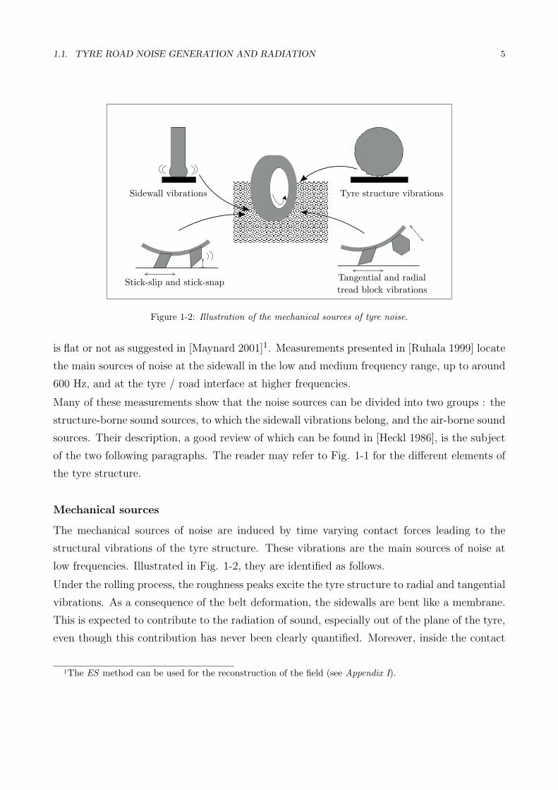
Figure 1-2: Illustration of the mechanical sources of tyre noise.
is flat or not as suggested in [Maynard 2001]1. Measurements presented in [Ruhala 1999] locate
the main sources of noise at the sidewall in the low and medium frequency range, up to around
600 Hz, and at the tyre / road interface at higher frequencies.
Many of these measurements show that the noise sources can be divided into two groups : the
structure-borne sound sources, to which the sidewall vibrations belong, and the air-borne sound
sources. Their description, a good review of which can be found in [Heckl 1986], is the subject
of the two following paragraphs. The reader may refer to Fig. 1-1 for the different elements of
the tyre structure.
Mechanical sources
The mechanical sources of noise are induced by time varying contact forces leading to the
structural vibrations of the tyre structure. These vibrations are the main sources of noise at
low frequencies. Illustrated in Fig. 1-2, they are identified as follows.
Under the rolling process, the roughness peaks excite the tyre structure to radial and tangential
vibrations. As a consequence of the belt deformation, the sidewalls are bent like a membrane.
This is expected to contribute to the radiation of sound, especially out of the plane of the tyre,
even though this contribution has never been clearly quantified. Moreover, inside the contact
1The ES method can be used for the reconstruction of the field (see Appendix I).

6 CHAPTER 1. TYRE ROAD CONTACT NOISE AND GROUND EFFECTS
� � � � � � � � � �� � � � � � � � � �� � � � � � � � � �� � � � � � � � � �� � � � � � � � � �� � � � � � � � � �� � � � � � � � � �� � � � � � � � � �� � � � � � � � � �� � � � � � � � � �� � � � � � � � � �� � � � � � � � � �� � � � � � � � � �
� � � � � � � � � �� � � � � � � � � �� � � � � � � � � �� � � � � � � � � �� � � � � � � � � �� � � � � � � � � �� � � � � � � � � �� � � � � � � � � �� � � � � � � � � �� � � � � � � � � �� � � � � � � � � �� � � � � � � � � �� � � � � � � � � �
� �� �� �� �
Air pumped out and sucked in Pipe resonances
Helmholtz resonatorsInternal resonances
Figure 1-3: Illustration of the air-borne sound sources of tyre noise.
patch, friction and adhesive forces, force the motion of the tread blocks in the tangential and in
the radial directions. The contribution of this phenomenon, usually referred to as stick-slip and
stick-snap motion, is significant for rather smooth road surfaces. Finally, for a patterned tyre,
the tread blocks hit the road surface in the leading edge and they are released when leaving
the contact patch at the trailing edge. The tread block motions contribute generally at higher
frequencies than the belt and the sidewall vibrations.
Air-borne sound sources
The air-borne sound sources include all displacements of air inside or near the tyre / road
interface, which are not induced by the tyre vibrations. The following mechanisms have been
identified (see Fig. 1-3). They are dominating the tyre / road noise in the high frequency
range, namely above 1000 Hz.
Resonances of the air cavity contained inside the tyre contribute to the radiation of sound in
narrow frequency bands, as suggested in [Nilsson 1979]. Therefore, their contribution may not
be visible in terms of radiated sound power. At the leading and the trailing edge, the air cavities
contained between the tread blocks and the outer road surface act as Helmholtz resonators.
Very similar to these sources, resonances inside the tyre grooves are known as pipe resonances.
Finally, air is pumped out or sucked in when the tread enters or leaves the contact area.

1.1. TYRE ROAD NOISE GENERATION AND RADIATION 7
Tyre radiating in the free-field Tyre radiating in the presence of the horns
Figure 1-4: Principle of the horn effect sound amplification
A last noise source, which cannot be classified in either of the two previous categories, is the
noise induced by the local deformation of the tyre. Sharp roughness peaks penetrate the tread
cap leading to the deformation of the rubber locally around the rouhgness peak. The resulting
displacement of air, which is often referred to as air–pumping, contributes mainly at high fre-
quencies.
Horn effect
In addition, the conditions of the tyre radiation modify significantly the aspect of the noise
generation. In the contact region, the tyre surface and the road form together a horn like
geometry (see Fig. 1-4). As a consequence, the radiation efficiency of the sound sources located
in this region is substantially enhanced compared to the case where the same sound sources
are radiating in the free-field [Kropp 1992, 2000b; Ronneberger 1989]. The corresponding
amplification coefficients are obtained by the ratio of the pressure radiated by the tyre in the
presence of the horn, relative to the pressure radiated by the same tyre in the free-field.
It has been shown by measurements, in [Ronneberger 1989; Schaaf 1982] among many others,
that the level and the frequency at which the maximum amplification occurs depend on the
geometry of the horn. In certain situations, the sound amplification could reach around 20
to 25 decibels in the middle frequency range around 1000 Hz. This means that the region of
maximum amplification corresponds to the frequencies having the dominant contribution in
A–weighted sound levels.
Another parameter which affects both the noise generation and the noise radiation, is the

8 CHAPTER 1. TYRE ROAD CONTACT NOISE AND GROUND EFFECTS
possible acoustical absorption due to the road surface. This effect is discussed more thorougly
in Section 1.3.
1.2 Tyre road noise prediction models
According to the previous section, many levels of modelling could be considered, which include
more or less noise generation mechanisms. A good review of the exisisting models for the pre-
diction of the tyre / road contact noise can be found in [Heckl 1979, 1986], and more recently
in [Kuijpers 2001] and [Hamet 2001b]. These are classified as statistical models, deterministic
models and hybrid models.
Statistical models
The principle of these models is to find the correlation between measured noise levels and few
parameters which are assumed to characterize the tyre / road interaction. These models are
mainly used to assess traffic noise.
In [Huschek 1996; Sandberg 1980], A–weighted noise levels are given as a function of selected
bands of the road texture spectrum. These models correlate the low frequency noise to the
macro–texture on one hand, and the high frequency noise to micro–texture of the road on
the other hand. This approach clearly follows the traditional classification of noise generation
mechanisms as presented above, i.e. vibrational sources and aero–dynamical sources. However,
in the case where the road texture is not the more relevant parameter of the tyre / road inter-
action, e.g. for porous road surfaces, these models fail to predict correct noise levels [Klein 2000].
Deterministic models : principle
In order to optimise the properties of the tyre road interface, deterministic models are needed.
These models embrace successive sub–models, which simulate the tyre dynamics, the contact
between the tyre and the road, and the tyre radiation.
The first sub–model predicts of the so-called Green functions of the tyre, that is, the response
of the tyre to an elementary excitation (an impulse force). It requires the knowledge of the
rubber mechanical properties, such as stiffness and Young’s modulus, and the tyre dimensions.
In a second model, the contact forces are computed. Since the contact between the tyre and
the road irregularities is non–linear, the calculation is performed in the time domain. As a

1.2. TYRE ROAD NOISE PREDICTION MODELS 9
result, the convolution between the tyre Green functions and the contact forces gives the time
history of the belt deformation as the tyre rolls.
Finally, the third sub–model comcerns the simulation of the radiated noise due to the previously
predicted tyre vibrations. The input is the belt deformation in the radial direction2, and the
output is the sound pressure field at a given receiving position of space, including the sound
amplification due to the horn effect.
The models which proceed in this way are reviewed in the next paragraph.
Deterministic models : review
Concerning the simulation of the tyre dynamics, one of the first attempt represents the tyre as a
ring under the tension caused by the inflating pressure [Bohm 1966]. This so–called ring model,
mainly valid at low frequencies, includes motion in the radial, tangential and circumferential
directions. An approach based on the same description of the tyre was also proposed in [Huang
1987, 1992]. In [Saigal 1986; Soedel 1975] the tyre is considered as a toroidal membrane. The
problem is then derived and solved according to a finite element scheme. This approach was
proved to give a good approximation of the free response of a tyre at low frequencies.
At frequencies above the ring frequency, namely above 300 Hz to 400 Hz, the wave propagation
is not influenced by the tyre curvature. Given this, works in [Kropp 1989, 1992] proposes to
represent the tyre as an orthotropic plate3, the vibrations of which can be described accurately
by the standard bending wave equation. In [Hamet 2001c], the Green functions of this model
are calculated analytically. This model has been extended to take the multi–layered structure
of the tyre [Larsson 2002a] and the tread blocks [Andersson 2002; Larsson 2002b] into account.
Studies in [Pinnington 2000, 2002] propose to model the tyre as a beam, along which impedances
are introduced to include the presence of the sidewalls.
As the computational power increases, a increasing number of tyre models are based on the finite
element method. For instance, work in [Richards 1991] describes the structural vibrations of the
tyre belt under the loading of the surrounding medium. The work in [Fadavi 2001, 2002] uses a
finite element method to predict the tyre dynamics with a view to the tyre radiation prediction.
The contact between the tyre and the road can be modelled by a Winkler bedding as suggested
2The motions in the two other directions are of less importance for the sound radiation.3An orthotropic plate has different bending stiffnesses in the circumferential and in the tangential direction.

10 CHAPTER 1. TYRE ROAD CONTACT NOISE AND GROUND EFFECTS
in [Johnson 1985]. This consists in considering a series of independent springs attached to the
tyre belt. This model has been adopted in [Kropp 1992] which solves the problem in the time
domain according to the scheme proposed in [Mc Intyre 1979] for musical instruments. It has
been extended to model a 3D contact in [Kropp 2001]. Hertz theory can also be applied to
contact the contact forces between the tyre and the road [Fujikawa 1999]. In [Clapp 1985], the
tyre tread is modelled as an elastic half space having the rubber stiffness.
One of the first modelling studies of the tyre radiation mechanisms was presented in [Ron-
neberger 1989]; this was however only dedicated to the simulation of the horn effect sound
amplification. Concerning the tyre radiation modelling, the study in [Kropp 1992] uses a multi-
pole expansion to reproduce the field radiated by the vibrating tyre. The horn effect is included
by introducing a mirror image source. This 2D model is proved in [Kropp 2000b] to be accurate
from around 600 Hz to higher frequencies for rigid surfaces. This approach has been adopted
in [Klein 1998], which further extends it to 3D geometries [Klein 1998] and includes the road
absorption [Klein 2002].
Radiation models are presented in [Kuo 2002], which make use of the expected behaviour of
the tyre at low and high frequencies. For the medium frequency range, a 3D model based on
the boundary element method is proposed [Graf 1999, 2002]. The boundary element method
is also used in [Anfosso 1996; Fadavi 2001, 2002] to reproduce the tyre radiation in 2D or 3D
geometries. So far, these models do not include the road absorption.
In conclusion, deterministic models for the tyre / road noise prediction can be built using the
aforementioned works. Works in [Kropp 1992] uses the orthotropic plate model for the tyre
dynamics, together with the Winkler bedding model for the contact and the multipole model for
the tyre radiation. In addition, this work includes a model based Hayden’s approach [Hayden
1971] for the air–pumping. Although the radiation model is limited at low frequencies due to
its 2D character, it is shown in [Wullens 2002] that it could be an efficient tool for studying
the possibilities of a reduction of tyre / road noise.
The TRIAS4 model [Gerretsen 1996; de Roo 2001] is developed on the basis of the orthotropic
plate model presented by Kropp. This model includes the noise contribution from the power–
4Tyre Road Interaction Acoustic Simulation

1.3. ACOUSTICAL CHARACTERISATION OF ROAD SURFACES 11
train, the tyre / road interaction and the so–called air–pumping. This model still needs to be
validated [Gerretsen 2001].
Hybrid models
As previously mentioned, statistical models do not account for the whole variety of tyre / road
combinations. Therefore, hybrid models have been developed that could give noise levels as a
function of a parameter which desribes better the tyre / road interaction than the road texture.
For instance in [Clapp 1985], it is proposed to relate contact forces to noise levels. For this,
the tyre deformation is estimated by modelling the penetration of the roughness peaks into an
elastic half space.
A similar approach is proposed in [Hamet 2001a; Klein 2000], which uses the othotropic plate
model and a dynamic contact model to predict the contact forces. The model proposed in
[Beckenbauer 2001] adopts the same approach and builds the statistical part of the model on
more than 800 tyre / road combinations. Finally, the hybrid model presented in [Fong 1998]
relates the sound intensity to contact pressure spectra.
1.3 Acoustical characterisation of road surfaces
Since the generation and the radiation of tyre road noise is strongly influenced by the acoustical
properties of the road surface, an accurate model for the tyre radiation must include these prop-
erties. Therefore, the next paragraph reviews the impedance models available from literature.
Then, the possible strategies for introducing the road absorption into a tyre model are discussed.
Impedance models
To model a possible sound absorption by the ground, the sound propagation must be described
within this medium. In acoustics, the propagation in a given medium is characterized by two
parameters [Zwikker 1949] : its propagation constant, which provides with the attenuation in-
formation, and the wave impedance, which relates the pressure and the velocity in this medium.
From these two values, the specific impedance of the material is determined at the interface
between the ground and the air above it. In this way, the sound propagation within the ground
is fully represented by a single variable defined at the interface, i.e. the acoustical impedance

12 CHAPTER 1. TYRE ROAD CONTACT NOISE AND GROUND EFFECTS
usually given in the normal direction to the surface.
A large number of impedance models can be found in the literature; a good review of the re-
search works can be found for instance in [Attenborough 2001]. These techniques are classified
in two major groups, depending on the scale of observation : the microstructural approach and
the phenomenological approach.
On one hand, the microstructural approach, as indicated by its name, investigates the sound
propagation within a pore of ground and extends this observation to a macroscopic scale. De-
pending on the number of parameters considered to describe the wave propagation, several
impedance models are then derived. A widely used model, presented in [Delany 1970], gives
the impedance as a function of the effective flow resistivity only. Many studies have proved that
this so–called one–parameter model, originally derived for fibrous materials, describe accurately
a large range of ground surfaces. More parameters such as the tortuosity, also called twistiness,
or the porosity of the ground can be included, which results in other impedance models [Atten-
borough 1985; Rasmussen 1981; Thomasson 1977]. Sophisticated impedance models have been
developed recently to include the effects of the surface roughness [Attenborough 2000].
On the other hand, in a phenomenological approach, the ground medium is considered as a dis-
sipative, compressible fluid. This thorough representation, proposed in [Hamet 1992], includes
effects of the viscosity and thermoconductivity. The resulting impedance model is a function
of the flow resistivity, the tortuosity and the porosity. This model was found to be particularly
suited to the determination of the acoustical properties of porous road surfaces [Berengier 1997].
Lastly, it should be mentioned that the application of these impedance models, as accurate
as they may be, is limited by the difficulty in measuring the parameters they depend on (the
flow resistivity, the tortuosity, etc.). Therefore, in parallel to the research efforts towards more
elaborated impedance models, a number of measurement techniques are being developed to
determine the acoustic absorption of road surfaces. A good summary of these techniques can
be found in [Berengier 2001]. These experimental methods are particularly interesting because
they allow access to the material data without directly measuring them. For instance, one can
match some measured absorption values with those obtained with a given impedance model.

1.3. ACOUSTICAL CHARACTERISATION OF ROAD SURFACES 13
In this way, the impedance model is optimised for this particular ground surface5.
Modelling strategies for outdoor sound propagation
Once the acoustical properties of the road are known, by measurements or by prediction, sound
propagation including the ground effects can be tackled. This problem is very complex, both
analytically and numerically, and is still the subject of numerous research works, as suggests
the discussion in [Kragh 2001]. Therefore, the purpose here is not to review this large research
effort. Instead, it aims at identifying general trends in the modelling in order to draw out the
possible strategies of introducing absorption into a tyre radiation model.
To deal with outdoor sound propagation, one can distinguish two main strategies. Firstly,
one chooses to proceed with the mathematical derivations, hoping that, besides the number of
approximations leading to obvious simplifications of the situation, one obtains an expression
that is better suited to a numerical evaluation. Or one treats the problem numerically straight
from the beginning; this results in a computationally heavy method. However, this method is
able to solve almost any kind of situations.
Belonging to the first group of methods, the following works must be mentioned. Considering
2D geometries, works in [Chandler-Wilde 1995] proposed to write the pressure field due to an
omnidirectional sound source above a homogeneous impedance plane as
ptotal = pdirect + pimage + pground
In this expression, pdirect and pimage fulfill together a rigid boundary condition on the ground.
Thus, pground compensates for the difference between an infinite impedance value and the actual
impedance value of the ground6. This last term was then evaluated using the steepest descent
method, which had as a consequence to limit the accuracy of the solution to the far field of
the source. Besides its limitations, this solution is widely used nowadays, especially in 2D BE
models, to include the effects of a homogeneous impedance plane without having to discretise
the ground surface. The study in [Mechel 2000] proposed to expand the well known reflection
5One of these methods, the level difference technique, is presented in Appendix IV.6A similar approach has been adopted in Chapter 3 and in Chapter 4 of the present thesis, where pground is
calculated using the ES method.
14 CHAPTER 1. TYRE ROAD CONTACT NOISE AND GROUND EFFECTS
factor for plane waves into cylindrical harmonics. The resulting solution, again restricted to
the far field of the source, is valid for 2D monopoles only.
To be complete, one should also mention that for 3D situations, a reflection factor for spherical
waves was first proposed in [Ingard 1951], and then corrected in [Thomasson 1976]. Finally,
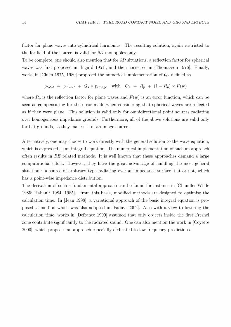
works in [Chien 1975, 1980] proposed the numerical implementation of Qs defined as
ptotal = pdirect + Qs × pimage with Qs = Rp + (1−Rp)× F (w)
where Rp is the reflection factor for plane waves and F (w) is an error function, which can be
seen as compensating for the error made when considering that spherical waves are reflected
as if they were plane. This solution is valid only for omnidirectional point sources radiating
over homogeneous impedance grounds. Furthermore, all of the above solutions are valid only
for flat grounds, as they make use of an image source.
Alternatively, one may choose to work directly with the general solution to the wave equation,
which is expressed as an integral equation. The numerical implementation of such an approach
often results in BE related methods. It is well known that these approaches demand a large
computational effort. However, they have the great advantage of handling the most general
situation : a source of arbitrary type radiating over an impedance surface, flat or not, which
has a point-wise impedance distribution.
The derivation of such a fundamental approach can be found for instance in [Chandler-Wilde
1985; Habault 1984, 1985]. From this basis, modified methods are designed to optimise the
calculation time. In [Jean 1998], a variational approach of the basic integral equation is pro-
posed, a method which was also adopted in [Fadavi 2002]. Also with a view to lowering the
calculation time, works in [Defrance 1999] assumed that only objects inside the first Fresnel
zone contribute significantly to the radiated sound. One can also mention the work in [Coyette
2000], which proposes an approach especially dedicated to low frequency predictions.
1.4. SUMMARY 15
1.4 Summary
In this chapter, the general characteristics of the tyre / road noise are presented. An important
fact is that tyre / road contact noise dominates the overall traffic noise at driving speeds as low
as around 50 to 60 km/h. At low frequencies, tyre noise is mainly due to the tyre vibrations,
whereas at higher frequencies, aero–dynamical sources contribute mostly to tyre noise. The
“cross–over” frequency depends on the tyre and the road properties, but it is generally situated
between 800 Hw to 1000 Hz.
The problem is further complicated by the radiation condition of the tyre. The horn formed
by the tyre and the road in the contact region enhances the radiation efficiency of the sources
located in this area. Another factor that influences not only the radiation but also the noise
generation is the acoustical absorption from the road surface.
From the modelling point of view, due to the large research effort during the last decades,
a number of tools are available for the prediction of tyre noise. They can be classified into
statistical models, deterministic models and hybrid models, which use approaches of the two
previous categories.
However, none of these models take the road absorption into account neither is adapted to
perform the necessary parametrical studies to optimise the tyre / road interface properties.
Therefore, a model for the tyre / road noise above arbitrary impedance planes, which is both
accurate and numerically efficient, may combine a simple model for the tyre radiation with an
integral equation based method to include the ground effects.
In this respect, works in the present thesis are organised as follows.
In Chapter 2, a multipole model for the tyre radiation, which is based on works presented in
[Kropp 1992], is presented. In Chapter 3, an ES based model for the ground effects is derived
as an alternative method to pure BE methods. Resulting from the combination of the two
previous models, a model for the tyre radiation over arbitrary impedance planes is derived in
Chapter 4. Finally, Chapter 5 presents a short parameter study where the general trends of the
tyre noise over impedance surfaces are discussed.

16 CHAPTER 1. TYRE ROAD CONTACT NOISE AND GROUND EFFECTS

Chapter 2
A Multipole Modelof the Tyre Radiation
As seen in the previous chapter, a crucial point of the noise radiation simulation is the
reproduction of the sound amplification known as the horn effect. This chapter presents a
model based on earlier studies that includes this effect. Special attention is addressed to the
understanding of the noise radiation and to the numerical efficiency of the resulting model.
In the first section, the sound amplification is characterized and explained. The multipole model
of the tyre radiation is then presented together with the theoretical basis of the approach. In
the third section, the model implementation is precised and a number of numerical examples as
well as comparisons to measurements are presented to appraise the robustness and the validity
of the present model.
Section 2.1 . . . . . The tyre as an acoustical source : definitionsExperimental results – Radiation efficiency of vibrating cylinders
Section 2.2 . . . . . . . . . . . . . . . . . . . . . . . . . . . . . The multipole modelThe Equivalent Sources method basis – Multipole velocity field – Calcu-lation of the modal amplitudes
Section 2.3 . . . . . . . . . Implementation and amplification factorsNumerical solution – Boundary condition – Horn effect amplificationfactors
Section 2.4 . . . . . . . . . . . . . . . . . . . . . . . . . . . . . . . . . Model validationBoundary condition prediction – Pressure field prediction – Comparisonto measurements
Section 2.5 . . . . . . . . . . . . . . . . . . . . . . . . . . . . . . . . . . . . . . . . .Summary
17
18 CHAPTER 2. A MULTIPOLE MODEL OF THE TYRE RADIATION
Measure with horn Measure without horn
Road
Tyre
Loudspeaker
Microphone
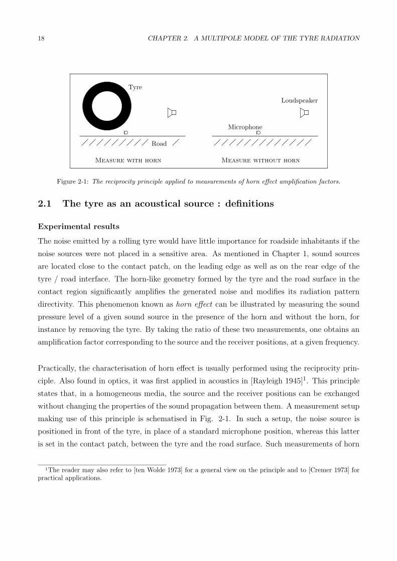
Figure 2-1: The reciprocity principle applied to measurements of horn effect amplification factors.
2.1 The tyre as an acoustical source : definitions
Experimental results
The noise emitted by a rolling tyre would have little importance for roadside inhabitants if the
noise sources were not placed in a sensitive area. As mentioned in Chapter 1, sound sources
are located close to the contact patch, on the leading edge as well as on the rear edge of the
tyre / road interface. The horn-like geometry formed by the tyre and the road surface in the
contact region significantly amplifies the generated noise and modifies its radiation pattern
directivity. This phenomenon known as horn effect can be illustrated by measuring the sound
pressure level of a given sound source in the presence of the horn and without the horn, for
instance by removing the tyre. By taking the ratio of these two measurements, one obtains an
amplification factor corresponding to the source and the receiver positions, at a given frequency.
Practically, the characterisation of horn effect is usually performed using the reciprocity prin-
ciple. Also found in optics, it was first applied in acoustics in [Rayleigh 1945]1. This principle
states that, in a homogeneous media, the source and the receiver positions can be exchanged
without changing the properties of the sound propagation between them. A measurement setup
making use of this principle is schematised in Fig. 2-1. In such a setup, the noise source is
positioned in front of the tyre, in place of a standard microphone position, whereas this latter
is set in the contact patch, between the tyre and the road surface. Such measurements of horn
1The reader may also refer to [ten Wolde 1973] for a general view on the principle and to [Cremer 1973] forpractical applications.

2.1. THE TYRE AS AN ACOUSTICAL SOURCE : DEFINITIONS 19
(a) Tyre alone (b) Tyre mounted on a vehicle
Figure 2-2: Amplification coefficient for different receiving angles directly over ground 7.5 m distance from thecentre of the contact (distance of the source d=10 mm). (Also in [Kropp 2000b])
effect amplification factors are shown in Fig. 2-2 (similar measurements can be found in earlier
studies, e.g. [Schaaf 1982]). Transfer functions are recorded for a series of source positions in
the horizontal plane around the tyre. The surface of the road, a rigid asphalt, is considered as
acoustically totally rigid.
First, in Fig. 2-2(a), the tyre is standing alone, that is without the influence of the car body.
For all incidences, the amplification increases with frequency. Below 400 Hz the amplification
is negligible, because the sound wavelength is not influenced by the presence of the tyre. At
these frequencies, the sound wavelength is at least about 5 times larger than the tyre width.
Around 1–2 kHz, the amplification reaches a maximum. For frequencies above this maximum,
the amplification varies because of interferences between different transmission paths. In this
frequency range, the amplification rarely exceeds 10 dB. Not surprinsigly, the overall maximum
value is found for measurements in the plane of the tyre, i.e. for 0◦ of incidence; it reaches
almost 20 dB at approximately 1.5 kHz. When moving out of the plane of the tyre, the maxi-
mum amplifications are lower and the frequencies at which they occur are shifted downwards.
However, for 90◦ of incidence, the amplification still reaches 10 dB, which is quite substantial.
For angles close to the perpendicular, the inference pattern is less significant. Amplification
factors vary within a few decibels around 10 dB in the measured frequency range.
Fig. 2-2(b) shows the influence of the car body on the horn effect. For this, transfer functions
are measured when the tyre is mounted on a light passenger vehicle. Maximum values of

20 CHAPTER 2. A MULTIPOLE MODEL OF THE TYRE RADIATION
(a) In the free-field (b) In presence of the road
Figure 2-3: Compared radiation efficiencies of cylinders. 20 first modes modes in circumferential direction (fromleft to right). The tyre radius is 0.3 m. (From [Kropp 2000b])
amplification are somewhat lower than if the tyre is standing alone. However, measured levels
in this case are less different for different angles compared to Fig. 2-2(a). This is due to
the fact that many more reflections contribute to the sound pressure level when the vehicle
body is present, which has the consequence of “equalising” the frequency spectra. The overall
maximum is still measured in the plane of the tyre and reaches here around 17 dB. From this set
of measured data, the contribution of the horn effect to pass-by noise levels can be estimated.
Calculations of Figure 13 and 14 in [Kropp 2000b] prove the horn effect to have a significant
influence on pass-by measurements.
Therefore, it seems crucial that an accurate tool for the tyre / road noise prediction includes
the correct estimation of the horn effect. Besides a clear simplification of the true geometry,
two-dimensional models could give deeper insights into the physics of the sound amplification,
as shown in the next paragraph.
Radiation efficiency of vibrating cylinders
In 2D models, the tyre is represented as an infinitely long cylinder. The radiation efficiency
of such a structure can easily be calculated as shown in [Cremer 1973]. The full details of the
calculation can also be found in [Kropp 1992]. The cylinder surface is assumed to vibrate with

2.1. THE TYRE AS AN ACOUSTICAL SOURCE : DEFINITIONS 21
a normal velocity given as
vn(ϕ) = An cos(nϕ + ϕ0)
where ϕ is the angular position of a point on the tyre surface and ϕ0 determines the orientation
of the mode with respect to the vertical direction. An is the amplitude of the n-th mode.
Fig. 2-3(a) shows the radiation efficiency of such a cylinder vibrating in a free-field for the
first 20 modes. All curves exhibit the same behaviour : the efficiency increases with frequency
up to a maximum when the wavelength on the cylinder corresponds to the wavelength in the
ambient medium. In the frequency range shown here, that is up to 5 kHz, the low order modes
seem responsible for most radiation of sound. This observation has to be related to the results
presented in [Kropp 1989] that prove the high order modes to be dominant for the determination
of the vibration pattern in the same frequency range. Furthermore, the efficiencies have fairly
low levels. All these observations would concur to conclude that the free-field tyre is a rather
ineffective radiator.
If the road surface is taken into account, the picture significantly changes. To correspond to a
“real” vibration pattern in presence of the road, the contact point always coincide with a node
in the vibrational mode. Radiation efficiencies obtained in this case are shown in Fig. 2-3(b).
They always have higher values than in the case of a free-field tyre, both below and beyond the
coincidence frequency. This result proves that the radiation efficiency is well enhanced by the
presence of the road surface. However, special care must be taken to calculate the pressure field
when the road is included. Due to the presence of the surface, the vibrational modes do not
constitute an orthogonal basis any longer. Therefore, one must include all possible interactions
between the modes to obtain the radiated field.
Furthemore, computations presented in [Kropp 1992] show that correct predictions are obtained
by including a low number of increasing modes. This confirms the fact that the low order modes
are responsible to a major extent for the sound radiated by the tyre whereas higher order modes
determine the vibration velocity. This result is of great interest on the numerical point of view
because it proves that 2D models are suited for the prediction of the sound radiation from
tyres.
In this respect, a two-dimensional multipole model based on the Equivalent Sources method is
presented in the next section.

22 CHAPTER 2. A MULTIPOLE MODEL OF THE TYRE RADIATION
2.2 The multipole model
The Equivalent Sources method basis
The ES method has been successfully applied to deal with the sound radiation from vibrating
structures as well as to model the scattering of sound by objects of arbitrary shapes. Appendix
I presents a thorough review of the method and its applications, in the field of acoustics and
electromagnetics. The basic idea of this approach is to reproduce the sound field scattered or
radiated by an object by a series of sources, i.e. equivalent sources, located inside the body
envelop. The unknown source amplitudes are determined so that a given boundary condition
on the object surface is best reproduced. Once this is done, the field from the equivalent sources
can be calculated at any point outside the body envelop. The accuracy of the prediction depends
on how well the boundary condition is fulfilled.
On this basis, a two-dimensional model for the radiation of sound by a tyre rolling on a road
surface could be designed [Kropp 1992]. The tyre is set to be an infinite cylinder, the points of
which vibrate in phase along its axis. Taking this geometry is an obvious shortcoming to the
real shape of a tyre. However, it has the major advantage to allow 2D cylindrical harmonics to
be used as equivalent sources. So that the resulting wave front matches the shape of the object
if such a multipole source is located at the tyre centre. This mutlipole is called the original
multipole because it is placed above the road surface. Its pressure field can be written as the
superposition each elementary harmonics of order m
p(r, ϕ, ω) =m=+∞∑m=−∞
AmH(2)m (kr)ejmϕ (2-1)
where k = ω/c is the wave number considered. H(2)m is the Hankel function, second kind of
order m. A time dependence in e+jωt is understood and will be omitted in the following. r and
ϕ are the distance and the angle from the multipole position to the observation point. Finally
Am is the amplitude of the m-th harmonic. It has the dimension of a pressure, that is a force
per unit are N ·m−2 or kg ·m−1 · s−2.
The influence of the road surface is accounted for using the image source technique. By placing
the mirror image of the multipole symmetrically aside the road surface, an impedance boundary
condition can be fulfilled on the infinite plane between them. The strength of the image
multipole is set equal to that of the original multipole so that zero normal velocity is achieved
on the road surface. The total pressure field at a point above the road surface and outside the

2.2. THE MULTIPOLE MODEL 23
ϕ1
ϕ2
ϕ2 − ϕ1
Multipole (x1)
Image multipole (x2)
bReceiver (xr)
~uϕ2
~ur1
~ur2~uϕ1
r1
r2
Figure 2-4: Radial and tangential directions of the contribution from the multipole source and its image.
tyre body is then expressed as
p(r, ϕ, ω) = p1(r1, ϕ1, ω) + p2(r2, ϕ2, ω)
p(r, ϕ, ω) =m=+∞∑m=−∞
Am
[H(2)
m (kr1)ejmϕ1 + H(2)
m (kr2)ejmϕ2
](2-2)
where the subscript 1, respectively (resp.) 2, relates to the co-ordinates of the original multipole,
resp. the image multipole. The conventions used for the model geometry are shown in Fig.
2-4.
Theoretically, any kind of velocity distribution can be reproduced by using an infinite number
of harmonics. However numerically, one can only include a limited number of these. Therefore,
the summation is truncated beyond the order Nmax which corresponds to the highest harmonic
to be included. The determination of Nmax is discussed in section 2.3.
From the value of Nmax strongly depends the ability of the resulting multipoles to reproduce
the given boundary condition. As far as the modelling is concerned, the sound radiation is
determined by the rate of change of the belt deformation, in other words, by the normal par-

24 CHAPTER 2. A MULTIPOLE MODEL OF THE TYRE RADIATION
ticle velocity of the belt points. This is the boundary condition of the present model. Thus
the velocity field due to the present sources is needed on the tyre surface in order to form the
boundary condition equation. The calculation of the multipole velocities on the tyre surface is
presented in the next paragraph.
Multipole velocity field
With the given time convention, the total velocity due to the original multipole at a point
xr(r, ϕ) in the direction ~n is written
vtotal,n(xr) = vn1(xr) + vn2(xr) = − 1
jωρ∇p1 · ~n − 1
jωρ∇p2 · ~n (2-3)
In cylindrical coordinates, the gradient is
∇pi =∂pi
∂ri· ~uri +
1
ri
∂pi
∂ϕi· ~uϕi (2-4)
where ~uri and ~uϕi are the unit vectors determining the direction of the field due to the multipole
i (i = 1, 2) at the observation point (see Fig. 2-4).
To simplify the calculations, at least for one multipole, the origin of the coordinate system is
set to coincide with the location of, for instance the original multipole. In this case, at any
point of the tyre surface, ~ur1 is parallel to ~n and ~uϕ1 is perpendicular to ~n. Thus at every point
xtyre of the tyre surface, ∇p1 is parallel to ~n and we obtain
vn1(xtyre) = − 1
jωρ
∂p1
∂r1= − 1
jωρ
m=+Nmax∑m=−Nmax
Am k H(2)′
m (kr1)ejmϕ1 (2-5)
The “ ’ ” symbol stands for the derivative of the Hankel function with respect to its argument,
here kr1, which can be written according to [Abramowitz 1972]
∀z 6= 0, H(2)′
m (z) = H(2)m−1(z) − m
zH(2)
m (z) (2-6)
Thus, at a given frequency, the velocity field due to the first multipole is constant over the tyre
surface; it does not depend on the angle of incidence. This property will be used in the next
paragraph for the determination of the unknown multipole amplitudes.
For the image multipole, the picture is a bit more complicated because the field has a component
in both the radial and the tangential directions. The velocity due to the image multipole,

2.2. THE MULTIPOLE MODEL 25
indicated by the subscript 2 can be expressed as
vn2(xtyre) = − 1
jωρ∇p2 · ~n = − 1
jωρ
[∂p2
∂r2~ur2 · ~n +
1
r2
∂p2
∂ϕ2~uϕ2 · ~n
]
Since ϕ1 also gives the direction of the normal to the tyre surface, one can write
vn2(xtyre) = − 1
jωρ
[∂p2
∂r2cos(ϕ2 − ϕ1) +
1
r2
∂p2
∂ϕ2sin(ϕ2 − ϕ1)
]
The cosine and the sine function can be expressed as depending only on ϕ1 by using the
following relationships :
r2 cos ϕ2 = r1 cos ϕ1 and r2 sin ϕ2 = r1 sin ϕ1 + b
where b is the distance between the two multipoles (see Fig. 2-4). One obtains then
cos(ϕ2 − ϕ1) =r1 + b sin ϕ1
r2and sin(ϕ2 − ϕ1) =
b cos ϕ1
r2
At this point one can show that these results are in concordance with those presented in [Klein
1998], who uses the angle with the vertical such that Φ1 = ϕ1 + π/2. With such a convention,
cos(ϕ2 − ϕ1) =r1 + b sin(Φ1 − π/2)
r2=
r1 − b cos Φ1
r2
sin(ϕ2 − ϕ1) =b cos(Φ1 − π/2)
r2=
b sin Φ1
r2
which are the expressions presented in [Klein 1998]. Finally the velocity on the tyre surface
due to the image multipole is written as
vn2(xtyre) = − 1
jωρ
m=+Nmax∑m=−Nmax
Am
[k
r1 + b sin ϕ1
r2H(2)′
m (kr2)
+ jmb cos ϕ1
r22
H(2)m (kr2)
]ejmϕ2 (2-7)
Thus, the total velocity at a point of the tyre surface is the superposition of the fields given by
Eq. 2-5 and Eq. 2-7. It has to fulfill the velocity boundary condition on the tyre surface (see
section 2.3).
Calculation of the modal amplitudes
The crucial step in the ES method is the calculation of the equivalent source strengths. The
present unknowns, the multipole amplitudes Am, are determined so that both multipoles fulfill

26 CHAPTER 2. A MULTIPOLE MODEL OF THE TYRE RADIATION
together the velocity boundary condition on the tyre surface, which is written vgiven2 . Given
the sources in presence, the condition that the tyre belt is acoustically rigid can be written as
vn1(xtyre) + vn2(xtyre) = vgiven(xtyre)
More explicitely the boundary equation writes
vgiven(xtyre) = − 1
jωρ
m=+Nmax∑m=−Nmax
Am
[k H(2)′
m (kr1)ejmϕ1
+ kr1 + b sin ϕ1
r2H(2)′
m (kr2) ejmϕ2
+ jmb cos ϕ1
r22
H(2)m (kr2) ejmϕ2
]
where (r1, ϕ1) and (r2, ϕ2) are defined on Fig. 2-4 for xtyre being the receiver. At this point,
one may notice that the problem may be ill–posed if xtyre happens to be also a point of the
road surface. This occurs if the boundary is directly in contact with the road. In this case, a
single point would be given two different velocity values : 0 due to the fact that the multipole
amplitudes are such that the road surface is rigid, and the value of the given velocity on the
tyre surface, which might be different from zero. The difficulty is removed by introducing a
small gap between the tyre and the road. A possible interpretation of the presence of such a
gap is discussed in section 2.4.
If one write the above equation for all points of the boundary, an equation system is formed.
The left hand side contains the velocity distribution on the tyre surface. The matrix on the
right hand side is composed of all the transfer functions from the original multipole and from
the image multipole to the boundary points. The vector of unknowns comprises the source
amplitudes Am and has (2Nmax + 1) elements.
Because of the large values of the Hankel function for large orders, the resulting equation
system may be badly scaled and approach a singular system. A simple solution to overcome
this consists of scaling the multipole amplitudes by the first constant term H(2)′
m (kr1) [Klein
1998]. The above equation is then solved for the new unknowns A∗m defined as
A∗m = Am H(2)′
m (kr1) (2-8)
2The consequences of the choice of vgiven are examined in section 2.3.
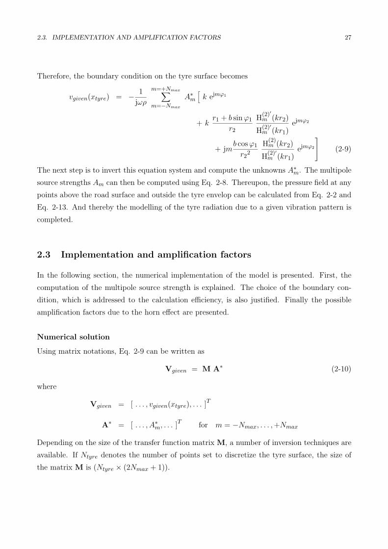
2.3. IMPLEMENTATION AND AMPLIFICATION FACTORS 27
Therefore, the boundary condition on the tyre surface becomes
vgiven(xtyre) = − 1
jωρ
m=+Nmax∑m=−Nmax
A∗m
[k ejmϕ1
+ kr1 + b sin ϕ1
r2
H(2)′
m (kr2)
H(2)′m (kr1)
ejmϕ2
+ jmb cos ϕ1
r22
H(2)m (kr2)
H(2)′m (kr1)
ejmϕ2
(2-9)
The next step is to invert this equation system and compute the unknowns A∗m. The multipole
source strengths Am can then be computed using Eq. 2-8. Thereupon, the pressure field at any
points above the road surface and outside the tyre envelop can be calculated from Eq. 2-2 and
Eq. 2-13. And thereby the modelling of the tyre radiation due to a given vibration pattern is
completed.
2.3 Implementation and amplification factors
In the following section, the numerical implementation of the model is presented. First, the
computation of the multipole source strength is explained. The choice of the boundary con-
dition, which is addressed to the calculation efficiency, is also justified. Finally the possible
amplification factors due to the horn effect are presented.
Numerical solution
Using matrix notations, Eq. 2-9 can be written as
Vgiven = M A∗ (2-10)
where
Vgiven = [ . . . , vgiven(xtyre), . . . ]T
A∗ = [ . . . , A∗m, . . . ]T for m = −Nmax, . . . , +Nmax
Depending on the size of the transfer function matrix M, a number of inversion techniques are
available. If Ntyre denotes the number of points set to discretize the tyre surface, the size of
the matrix M is (Ntyre × (2Nmax + 1)).
28 CHAPTER 2. A MULTIPOLE MODEL OF THE TYRE RADIATION
The simplest case, which also gives the most accurate solution, occurs if the matrix is square,
that is if Ntyre = (2Nmax + 1). It corresponds to taking as many equivalent sources as points
on the boundary. This yields a classical collocation technique, and the matrix inversion can be
performed using standard Gaussian elimination, also called method of pivots. In this case, the
system has a unique solution and the prediction error on the boundary is zero at each point.
The major drawback of this technique is that it becomes cumbersome when dealing with large
meshes because the size of the system increases with the square of the number of boundary
points. In the worst case, the ES becomes comparable to boundary integral equation based
methods, which also use collocated systems.
The most common case, but not the simplest one, is M being non-symmetric and having
dimensions such that Ntyre > (2Nmax + 1). This is encountered when the situation requires
a fine mesh while one wants to optimize the computational effort by keeping a reduced set of
sources. The resulting equation system is then over-determined and a minimisation technique
must be employed.
From a mathematical point of view, the inversion of a non-square matrix needs to be performed.
This can be done by using, for instance, the Singular Value Decomposition (SVD). The basic
idea of this technique is to isolate the eigen-values with the following scheme by introducing a
column orthogonal matrix V(Ntyre×(2Nmax+1)) and a square orthogonal matrix W((2Nmax+
1)× (2Nmax + 1)).
M = V
Ψ−Nmax
. . . 0
. . .. . . . . .
0 . . . Ψ+Nmax
WT
The determination of V and W can be found for instance in [Press et al. 1986]. The central
matrix, say L contains all the eigen values of M on the main diagonal.
The inverse of M is
M+ = W N+ VT
M+ and N+ are called pseudo-inverse because they are not square matrices.
The elements of N+ are the form 1/Ψi (i = −Nmax, . . . , +Nmax), all located on the main
diagonal. Clearly, if the matrix is nearly singular, few eigen-values are close to zero. To avoid
the obvious numerical problems in the computation of N+, 1/Ψi is replaced by 0 if Ψi is smaller
than the computer round-off error. Therefore M+ can be computed with good acuracy and the
optimisation process can be performed.

2.3. IMPLEMENTATION AND AMPLIFICATION FACTORS 29
It is important to note that, by using such a technique, the set of solutions
A∗ = M+ Vgiven do not satisfy Vgiven = M A∗
but provide the minimum mean square error ε defined as
ε =1√
Ntyre
| M A∗ − Vgiven |
The solutions A∗m of the equation system are said to be solutions in the least square sense.
The same procedure can be applied when Ntyre < (2Nmax + 1). This situation is however
not recommended because it corresponds to consider very few points on the boundary. This
would lead to a useful frequency range limited to low frequencies where the multipole model is
expected to be inaccurate due to its two-dimensional character.
The calculation of the multipole source strengths Am is then straightforward using Eq. 2-8.
Boundary condition
The values of the multipole amplitudes depends strongly on the prescribed velocity. Different
distributions yield undoubtedly to different amplifications. The amplification factors can be
defined in several ways depending on the type of boundary condition : either the tyre is
considered as a radiator or it is viewed as a scatterer. Actually, the scattering case can be also
seen as a radiation case where the multipole inside the tyre has to radiate in such a way that
a presecribed velocity on the tyre surface is fulfilled. Mathematically, the two approaches yield
different derivations, which are emphasised in the following.
On one hand, the tyre belt is assumed to be vibrating. This is referred to as the radiation
case because the tyre is effectively the noise source. The input to the model of the horn effect
prediction is the tyre belt velocity. As only radial motions of the tyre belt contribute to the
radiation of sound, the velocity is given only in the direction normal to the tyre surface. Ex-
amples of velocity distributions are shown in Fig. 2-5. In this figure, the broken line indicates
the position of the tyre belt at rest. The velocity pattern can take the form of a Hanning-like
distribution or a less smooth distribution such as a piston inserted in the tyre belt. More gen-
erally for the calculation of sound amplification, it can be the superposition of one single mode
or the superposition of an infinite number of modes. However, the Hanning-like distribution is
the more realistic pattern as it is most similar to the tyre belt deformations due to the contact
with the road. In this case, the prescribed velocity is directly given and the boundary condition

30 CHAPTER 2. A MULTIPOLE MODEL OF THE TYRE RADIATION
1
2
3
4
5
30
210
60
240
90
270
120
300
150
330
180 0
(a) Hanning-like
1
2
3
4
5
30
210
60
240
90
270
120
300
150
330
180 0
(b) Piston-like
1
2
3
4
5
30
210
60
240
90
270
120
300
150
330
180 0
(c) 10-th mode
Figure 2-5: Examples of velocity distributions in the “radiation” case.
writes
vgiven = vrad,n and vn1 + vn2 = vrad,n
On the other hand, the acoustical source responsible for the noise radiation can be considered
to be located somewhere inside the horn-like region. This assumption may be based on mea-
surements to localise the noise sources of a rolling tyre (see section 1.1 and for instance [Ruhala
1999]). In this case, the noise source is a simple source placed outside the tyre envelop and
the tyre belt is assumed to be rigid, i.e. it is not vibrating. This situation is referred to as
the scattering case because the tyre surface scatters the field produced by an external sound
source. The boundary condition in this case writes
vgiven = 0 and vn1 + vn2 + vscat,n = 0
Unlike the radiation case, the normal velocity distribution on the tyre belt must be deduced
from the field due to the source inside the horn. In most studies, this latter source is assumed
to be omnidirectional even though it can take any form from a dipole to more complicated
sound sources.
Between these two cases, the problem will be expressed as the scattering one throughout this
work. This choice is justified by the fact that most work found in litterature use this assumption
(see for instance [Graf 2002; Klein 1998]) and it may be useful to compare the results of these
studies with calculations from the present model. Moreover, this type of boundary condition
allows the use of the reciprocity principle, which presents several advantages. First, it permits

2.3. IMPLEMENTATION AND AMPLIFICATION FACTORS 31
one to best reproduce the experimental setup and thus to compare more closely measured
amplification factors with calculated ones. Secondly, it will be shown in the next section that it
is numerically of advantage in terms of accuracy and computational time to use the reciprocity
principle also for modelling.
For the sake of completeness however, horn effect predictions obtained considering a radiation
problem are shown in Appendix II.
Horn effect amplification factors
The above paragraph showed that in the scattering problem, an acoustical source exterior
to the tyre body is introduced. In this case, the pressure field from the source is given and
the resulting velocity field on the tyre surface must be deduced. This paragraph first derives
the corresponding field expressions. According to the expression of the pressure field, the
amplification factors due to the horn effect are presented.
In this study, a 2D monopole is chosen to represent the noise source. Its pressure field may be
written as
pscat(x0 | xr) = qscat ·G0(x0 | xr) with G0(x0 | xr) = − j
4H
(2)0 (k | xr − x0 |) (2-11)
G0(x0 | xr) is the free space Green function calculated at a point xr due to a source placed in
x0. qscat is the strength of such a source; it is homogeneous to a pressure.
The velocity on the tyre surface is derived from the previous equation. If ~n is the normal vector
at a point xtyre of the boundary, it writes
vscat,n(x0 | xtyre) = − 1
jωρ∇pscat · ~n
Because the Green function shows only a radial dependency, the resulting velocity is
vscat,n(x0 | xtyre) = − 1
4ρcqscat H
(2)1 (k | xtyre − x0 |) ~ur0 · ~n (2-12)
where ~ur0 is the unit vector that indicates the direction of the field due to the source located at
x0. Eq. 2-11, resp. Eq. 2-12, define the pressure field, resp. the velocity field, of this monopole
source placed in the free-field. In order to take into account the presence of the road surface,
a mirror image source is included. The total pressure is then
pscat(x0 | xr) + pscat(x0 | xr) = qscat ·[
G0(x0 | xr) + G0(x0 | xr)]
(2-13)
where x0 is the position of the monopole mirror source.
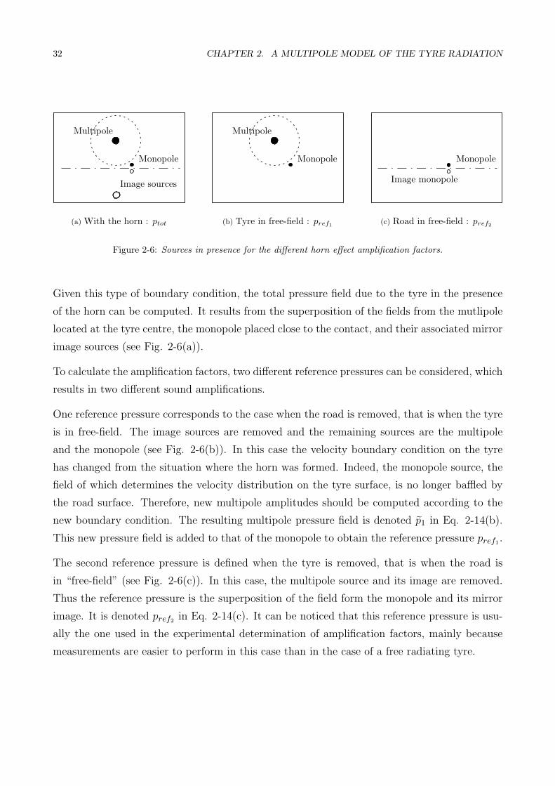
32 CHAPTER 2. A MULTIPOLE MODEL OF THE TYRE RADIATION
(a) With the horn : ptot
Multipole
Monopole
Image sources
(b) Tyre in free-field : pref1
Multipole
Monopole
(c) Road in free-field : pref2
Monopole
Image monopole
Figure 2-6: Sources in presence for the different horn effect amplification factors.
Given this type of boundary condition, the total pressure field due to the tyre in the presence
of the horn can be computed. It results from the superposition of the fields from the mutlipole
located at the tyre centre, the monopole placed close to the contact, and their associated mirror
image sources (see Fig. 2-6(a)).
To calculate the amplification factors, two different reference pressures can be considered, which
results in two different sound amplifications.
One reference pressure corresponds to the case when the road is removed, that is when the tyre
is in free-field. The image sources are removed and the remaining sources are the multipole
and the monopole (see Fig. 2-6(b)). In this case the velocity boundary condition on the tyre
has changed from the situation where the horn was formed. Indeed, the monopole source, the
field of which determines the velocity distribution on the tyre surface, is no longer baffled by
the road surface. Therefore, new multipole amplitudes should be computed according to the
new boundary condition. The resulting multipole pressure field is denoted p1 in Eq. 2-14(b).
This new pressure field is added to that of the monopole to obtain the reference pressure pref1.
The second reference pressure is defined when the tyre is removed, that is when the road is
in “free-field” (see Fig. 2-6(c)). In this case, the multipole source and its image are removed.
Thus the reference pressure is the superposition of the field form the monopole and its mirror
image. It is denoted pref2in Eq. 2-14(c). It can be noticed that this reference pressure is usu-
ally the one used in the experimental determination of amplification factors, mainly because
measurements are easier to perform in this case than in the case of a free radiating tyre.

2.4. MODEL VALIDATION 33
The expressions of the pressure field corresponding to the Fig. 2-6 are summarised below :
(a) ptot(xr) = p1(r1, ϕ1) + p2(r2, ϕ2) + pscat(x0 | xr) + pscat(x0 | xr)
(b) pref1(xr) = p1(r1, ϕ1) + pscat(x0 | xr)
(c) pref2(xr) = pscat(x0 | xr) + pscat(x0 | xr)
(2-14)
The amplification factors in decibels are then expressed as
AF 1 = 10 log
∣∣∣∣∣ ptot(xr)
pref1(xr)
∣∣∣∣∣2
AF 2 = 10 log
∣∣∣∣∣ ptot(xr)
pref2(xr)
∣∣∣∣∣2 (2-15)
2.4 Model validation
From the basis of the ES method [Machens 1999; Ochmann 1980, 1995], the correct prediction
of the boundary is necessary for the good functionning of the method (see also Appendix I).
However, this condition is not sufficient : a very good prediction of the boundary condition
may yield to poor field predictions. For instance, in the case of a vibrating tyre, the modes
which are important for the fulfillment of the boundary condition may not be those that are
relevant for the correct sound prediction.
In this regards, the fulfillment of the boundary condition is first examined. The computation
of the radiated field is then discussed focusing especially on the stability of the predictions.
Finally, horn effect amplification factors are compared to measurements to complete the model
validation.
Boundary condition prediction
As previously mentioned, the maximum order of the multipole determines to a large extent its
ability to reproduce the prescribed velocity on the tyre belt. In this paragraph, the achieved
boundary condition is examined as a function of both Nmax and the size of the equation system.
The geometry used in this study is shown in Fig. 2-7. A tyre of 0.3 m radius is placed at 1
mm above a rigid road surface and a monopolar line source is placed at a distance d of the
horn centre. The receiver is located on the same side of the tyre as the monopole, 1 m ahead
of the multipole, at the same height. Mirror image sources are placed symmetrically aside the
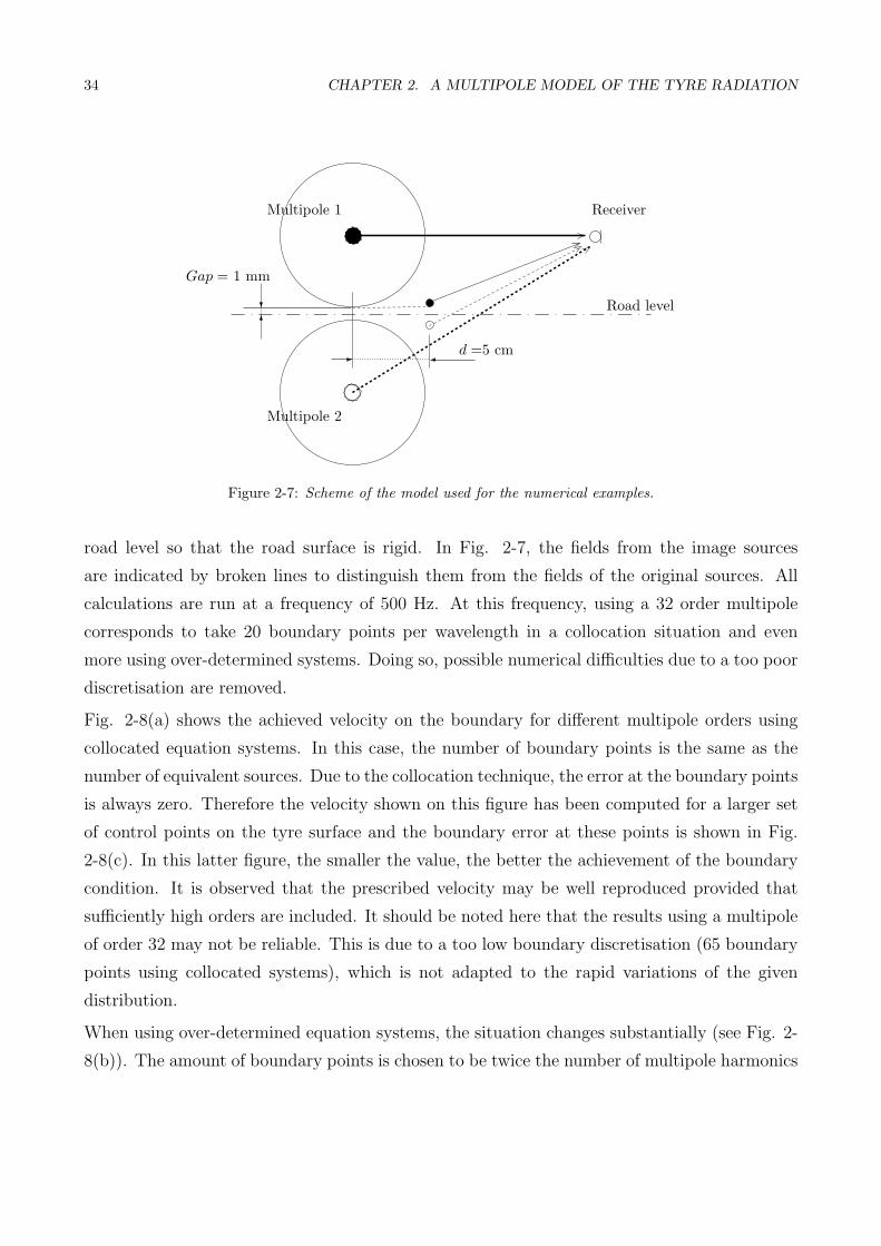
34 CHAPTER 2. A MULTIPOLE MODEL OF THE TYRE RADIATION
Multipole 1
Multipole 2
Gap = 1 mm
Receiver
Road level
d =5 cm
Figure 2-7: Scheme of the model used for the numerical examples.
road level so that the road surface is rigid. In Fig. 2-7, the fields from the image sources
are indicated by broken lines to distinguish them from the fields of the original sources. All
calculations are run at a frequency of 500 Hz. At this frequency, using a 32 order multipole
corresponds to take 20 boundary points per wavelength in a collocation situation and even
more using over-determined systems. Doing so, possible numerical difficulties due to a too poor
discretisation are removed.
Fig. 2-8(a) shows the achieved velocity on the boundary for different multipole orders using
collocated equation systems. In this case, the number of boundary points is the same as the
number of equivalent sources. Due to the collocation technique, the error at the boundary points
is always zero. Therefore the velocity shown on this figure has been computed for a larger set
of control points on the tyre surface and the boundary error at these points is shown in Fig.
2-8(c). In this latter figure, the smaller the value, the better the achievement of the boundary
condition. It is observed that the prescribed velocity may be well reproduced provided that
sufficiently high orders are included. It should be noted here that the results using a multipole
of order 32 may not be reliable. This is due to a too low boundary discretisation (65 boundary
points using collocated systems), which is not adapted to the rapid variations of the given
distribution.
When using over-determined equation systems, the situation changes substantially (see Fig. 2-
8(b)). The amount of boundary points is chosen to be twice the number of multipole harmonics

2.4. MODEL VALIDATION 35
(a) Collocated system (b) Over-determined system
(c) Collocated system (d) Over-determined system
Figure 2-8: Comparison of obtained boundary velocities for different sizes of the equation system using the“direct” geometry. The region of maximum velocity is focused on in the broken-line box.
(Ntyre = 2 × (2Nmax + 1)). Unlike the previous picture, Fig. 2-8(b), resp. Fig. 2-8(d), shows
the velocity, resp. the boundary error, computed at the boundary points directly. Because in
this case, the error made at these points is the least but not compulsorily zero; larger devia-
tions are expected at points between the boundary points. In fact, even a 128 order multipole
cannot provide a satisfactory correspondence with the boundary condition. Using higher order
sources would lead to numerical instabilities in the computation of the Hankel functions and

36 CHAPTER 2. A MULTIPOLE MODEL OF THE TYRE RADIATION
(a) Collocated system (b) Over-determined system
(c) Collocated system (d) Over-determined system
Figure 2-9: Same as Fig. 2-8 but using the “reciprocal” geometry.
the solution would not be accurate anymore. The failure of the SVD technique in this case
is due to the rapid changes in the velocity distribution, the pattern of which cannot be well
reproduced using least square methods. Increasing the number of boundary points reduces the
boundary error at the expense however of the computational time.
Thus, the collocation method seems more suitable to yield an accurate solution in the case of
a “direct” geometry. The direct term is employed here to distinguish with a geometry that

2.4. MODEL VALIDATION 37
applies the reciprocity principle. In such a “reciprocal” geometry, the positions of the noise
source and the receiver are exchanged. It is interesting to examine this situation as it best
approaches the configuration used to measure the horn effect amplification factors.
The model is run for the same parameters as in Fig. 2-8, but setting the monopole sound
source in place of the receiver, and the receiver in place of the monopole. As in the “direct”
configuration, a mirror image monopole is used to account for the presence of an infinite rigid
surface. As before, results are shown for both collocated equation systems in Fig. 2-9(a) and
(c), and over-determined equation systems in Fig. 2-9(b) and (d).
The main consequence of the new position of the monopole is that the prescribed boundary
velocity has a “smoother” pattern even though it presents a sharp and sizable minimum. With
this type of geometry, the predictions for both approaches are significantly better than using
the direct geometry. Achieved velocities using a 64 order multipole cannot be distinguished
from the given velocity distribution. Particularly, the SVD technique seems very accurate using
such a geometry as yet a 32 order multipole yields a good prediction of the boundary condition.
Therefore, the “reciprocal” geometry appears to be an interesting configuration to study the
horn effect from a modelling point of view too. With this type of geometry, both the colloca-
tion method and the least square technique show a true convergence towards the prescribed
distribution as the multipole order increases. Nevertheless, the use of collocated systems seems
preferable for it gives more stable solutions and higher calculation speeds.
If a very fine boundary discretisation is required, over-determined systems combined with a
reciprocal geometry could be thought of as an interesting alternative because it allows to use
an average number of sources together with a large set of boundary points. This property is
used for the comparison with measurements presented in the last paragraph of this section.
Pressure field prediction
After the boundary condition prediction is discussed, this paragraph examines the calculation
of the multipole amplitudes and the consequences on the calculation of the radiated field.
For the horn effect predictions, pressures corresponding to the tyre in free-field and in presence
of the road must be computed. An example of multipole amplitudes computed in these two
situations is shown in Fig. 2-10 for different frequencies. When the tyre is in free-field (Fig.

38 CHAPTER 2. A MULTIPOLE MODEL OF THE TYRE RADIATION
(a) Tyre free-field (b) Tyre with road
Figure 2-10: Set of multipole source strengths computed using collocated systems and a reciprocal geometry.Nmax = 128, only the 20 first positive and negative orders are shown.
2-10(a)), sources of equal order in absolute value have equal amplitudes, as expected. When the
road surface is included (Fig. 2-10(b)), the set of source strengths is clearly not symmetrical.
This means that all possible interactions between the modes should be accounted for in the
calculation of the radiated power. It is also observed that a larger number of modes contribute
significantly to the pressure field when the road surface is considered.
In the same figure, the amplitudes of a 64 order multipole obtained using an over-determined
equation system at 1500 Hz have been plotted (indicated by crosses). The number of boundary
points is set to be the same as for a 128 order multipole using a collocated system, that is
2Nmax + 1 = 257. Therefore, the boundary velocity “seen” by the multipoles is the same in
both cases. The two sets of amplitudes are almost identical3, which proves the reliability of the
least square minimisation proposed above. This two sets of sources would yield the same field
calculation, and thus the same horn effect prediction.
It is worth noting here that the solution using over-determined equation systems leads to higher
calculation times compared to the solution using collocated systems. Even though, in this ex-
ample, the number of elements of the matrix K to be inverted, is reduced when using the SVD
technique ((257× 129) elements) compared to when using the collocation method ((257× 257)
3Significant deviations are observed for higher orders, which can not be noted in the set of amplitudes shownin these figures.

2.4. MODEL VALIDATION 39
elements). Therefore, the difference in calculation times is only due to the type of resolution.
Negligible at low frequencies, it increases in the medium and high frequency range to reach
around 15 % increase at 5000 Hz, a value which becomes significant, e.g. when carrying pa-
rameter studies.
The question is still left open how the stability in the fulfillment of the boundary condition
relates to the computation of the amplification factors. For this, horn effect predictions are
computed for the geometries corresponding to Fig. 2-8 and Fig. 2-9. Results are shown in
Table 2-1 and Table 2-2. It can be observed that using the direct geometry yields more fluctu-
ating amplification factors than using the reciprocal geometry. This latter shows indeed a true
convergence of the results.
NmaxAF1 (in db) AF2 (in db)
Pivot technique SVD technique Pivot technique SVD technique
32 15.5340 18.6206 8.5590 15.9110
64 18.9572 18.5585 15.7395 14.4892
128 18.4799 18.5288 14.2167 14.5267
Table 2-1 : Compared horn effect predictions using a direct geometry (see Fig. 2-8).
NmaxAF1 (in db) AF2 (in db)
Pivot technique SVD technique Pivot technique SVD technique
32 18.5171 18.3602 14.5075 14.3506
64 18.5283 18.5264 14.5187 14.5167
128 18.5284 18.5284 14.5188 14.5188
Table 2-2 : Compared horn effect predictions using a reciprocal geometry (see Fig. 2-9).
Given these considerations, it seems reliable to use the present model to investigate some
properties of the horn effect, for instance, the re-direction of sound in space. For this, the ES
model has been run using a reciprocal geometry for several monopole positions in the space

40 CHAPTER 2. A MULTIPOLE MODEL OF THE TYRE RADIATION
0
5
10
15
20
25
−1 −0.5 0 0.5 1 1.5 20
0.2
0.4
0.6
0.8
1
Figure 2-11: Re-direction of sound due to the horn effect at 1.5 kHz. Reference pressure is pref1 in Eq. 2-14,distances are in meter. The right scale is in dB.
above the road and outside the tyre envelop. In a direct geometry, this corresponds to moving
the receiver while the monopole position is fixed. Again, the two possible reference pressures
as defined in Eq. 2-14 have been used to calculate the amplification factors. Results are shown
in Fig. 2-11 and Fig. 2-12 where the circular white part represents the tyre body.
Comparing these two figures clearly proves that the different reference pressures yield different
amplification factors, both in terms of the spatial distribution as well as the levels of ampli-
fication. In fact, taking the freely radiating tyre as reference pressure gives globally higher
amplification factors, as also shown in [Klein 1998]. As previously explained, the reason is
that the road plane has a stronger baffle effect than the cylinder. Moreover, in both cases, the
sound amplification is lessen on the rear side of the tyre compared to the front of the tyre,
as expected. Above the tyre, that is opposite to the monopole position, the sound is either
amplified or decreased depending on the chosen reference pressure. Interferences in this region
of space are important because they may be enhanced by the presence of the wheelhouse. Fi-
nally, the re-distribution of sound illustrated in these figures may substantiallly decrease the
efficiency of roadside noise protections such as noise barriers.
Comparison to measurements
In order to complete the validation of the multipole model, measurements of horn effect am-
plification factors are compared to calculations obtained using the present ES model and a BE
model, used as a reference approach.
Measurements have been carried out outdoors over a rigid asphalt, which was assumed to
be acoustically rigid. Surrounding objects were far enough so that possible reflections could

2.4. MODEL VALIDATION 41
0
5
10
15
20
25
−1 −0.5 0 0.5 1 1.5 20
0.2
0.4
0.6
0.8
1
Figure 2-12: Re-direction of sound due to the horn effect at 1.5 kHz. Reference pressure is pref2 in Eq. 2-14,distances are in meter. The right scale is in dB.
be removed by windowing the time signals. As already mentioned, the reciprocity principle
was used. This means that the noise source was placed in front of the tyre, 1 m ahead at the
ground level. The noise source was a loudspeaker driven with sequences of white noise organised
according to the MLS 4 procedure. Transfer functions were recorded by an electret microphone
mounted flush with the ground, in presence of the horn and without the horn by removing the
tyre. Measurements have been repeated for several values of the distance d from the contact
point to the microphone (see Fig. 2-1). The tyre, unloaded, was treadless; its diameter was 62
cm and its width 22 cm.
The multipole model is run using these parameters. Concerning the boundary discretisation, 6
points per wavelength are usually chosen to obtain a correct convergence. This means that a
set of 200 boundary points would have been enough up to a frequency of 6 kHz. However, in
order to insure a sufficient sensitivity of the model regarding the source displacements inside
the horn, the inter-nodal distance is set to be at least three times smaller than the smallest
source displacement. This gives a set of 700 boundary points. This implies the use of at least
a 350 order multipole in a collocated method, which would undoubtedly would give rise to
numerical difficulties. Therefore, it is decided to keep a 87 order multipole and to make use of
the least square minimisation presented in section 2.2 to determine the multipole amplitudes.
In parallel, calculations using the boundary element method are performed to remove experi-
mental uncertainties that could false the model validation, e.g. concerning the placement of the
noise source inside the horn, and the model limitations, namely it two-dimensional character.
Thus, a BE model is implemented using the Sysnoise c© software. Elements of type Line2
4Maximum Length Sequence (see for instance [Borish 1983; Schroeder 1979] for more details).

42 CHAPTER 2. A MULTIPOLE MODEL OF THE TYRE RADIATION
Figure 2-13: Measured horn effect amplification factors for several distances d (cf. Fig. 2-1). (Also in [Kropp2000b])
(a) ES model (b) BEM model
Figure 2-14: Predicted amplification factors related to measured values in Fig. 2-13. (Also in [Kropp 2000b])
are used to model an infinite rigid cylinder. The noise source is a cylindrical monopole of unit
source strength placed at the ground level. A space of 1 mm is set between the tyre and the
ground plane to remove possible singularities.
These two numerical models were run for each distance d. The reference pressure corresponding
to the ground in free-field is used for the calculation of the amplification factors (pref2in
Eq. 2-14). It is worth mentioning here that the required CPU time using the BE code is
approximately five times longer than using the multipole model. Both models were run on the
same computer for similar mesh size. Moreover, the ES model implemented in Matlab c© was
not compiled. Larger differences are therefore expected for a compiled version.
2.4. MODEL VALIDATION 43
Measured amplification factors are shown in Fig. 2-13. The amplification increases with fre-
quency up to a maximum which position depends on the distance d. As d decreases, that is,
as the noise source gets closer to the contact point, the maximum of amplification increases. It
reaches 22 dB at 2 kHz for a source 10 mm away from the centre of the horn.
The predictions are shown in Fig. 2-14(a) for the ES model and in Fig. 2-14(b) for the BE
model. Calculated amplification factors are clearly over estimated at low frequencies, due to
the two-dimensional character of the models. Besides this discrepancy, the maximum levels as
well as the frequencies at which they occur are correctly predicted. The interference pattern is
also well reproduced at high frequencies. The very good correspondence between the ES model
and the BE model validate the present approach5.
Besides the position of the source inside the horn, a key parameter for the horn effect is the
position of the reflecting plane. Indeed, lifting up the tyre over the road surface has the same
influence as moving the source out of the horn. For instance, the peaks of a very rough road
may induce a shift between the position of the outer road surface on which the tyre lays, and the
position of the acoustical reflecting plane. This parameter essentially determines the strength
of the amplification.
This effect is investigated experimentally by measuring amplification factors for different heights
of the tyre above the road. The tyre height is successively set to 0 mm (contact), 1.5 mm, 3 mm,
5.5 mm. The road surface is compact enough to liken the outer surface with its reflecting plane.
Measurements are shown in Fig. 2-15. A behaviour similar to that of Fig. 2-13 is observed.
Whereas the amplification is identical at low frequency, there exists a frequency, different for
each tyre height, from which the amplification is decreased in comparison to the case when the
tyre is in contact with the road. This frequency is lower for increasing heights. Calculations from
the ES model displayed on the same figure follow well this behaviour. These results may explain
the somewhat suprising observation that rolling on very rough roads leads to lower radiation
at high frequencies compared to rolling on roads having a smaller roughness amplitude. This
effect is also investigated numerically in Appendix II for the “radiation” problem.
5These results have been presented in [Kropp 2000b]

44 CHAPTER 2. A MULTIPOLE MODEL OF THE TYRE RADIATION
Figure 2-15: Measured horn effect amplification for different height of the tyre above the road. (Also in [Kropp2000b])
2.5 Summary
In this chapter, a mathematical model for the tyre noise radiation has been derived on the
basis of the ES method. This choice is addressed to the numerical efficiency of this technique
compared to other approaches such as BIE based methods.
The horn effect amplification factors calculated using the present model are in excellent corre-
spondence with those obtained using BE codes. Furthermore, comparisons with measurements
prove the ES model limitations to be only due to its two-dimensional character. Namely above
500 Hz, the ES model gives correct levels of amplification and reproduces well the interference
pattern due to the multiple reflections occuring inside the horn.
Because it is as accurate as to be sensitive to key parameters such as the source position
inside the horn or the position of the reflecting plane, the present model allows to give further
insights into the physics of the tyre / road noise emission. In particular, the vibrational modes
responsible for the noise emission were identified and distinguished from those determining the
vibrational velocity. Due to its numerical efficiency compared to BE codes, this model could
be used to perform the parametrical studies needed for the optimisation of the properties of
the tyre / road interface.
But some improvements are still needed. For instance, a 3D model would be required for the
correct prediction of tyre noise at low frequencies. This drawback is partially masked by the
use of Leq(A) levels to assess the roadside noise levels because this spectral filter reduces the
contribution of the low frequency components and strengthens the spectrum around 1 kHz,
frequencies at which the model is accurate.

2.5. SUMMARY 45
Another geometrical approximation concerns the shape of the tyre supposed to be perfectly
circular. In reality indeed, the tyre belt is deformed by the vehicle load (around 250 kg per
wheel for a light passenger car), which has for consequence to deform the tyre / road interface
and to modify substantially the horn effect amplification factors. However, it has been shown
recently in [Graf 2002] that the effect of the loading deformation could be reproduced to a large
extent by using an undeformed tyre while shifting the position of the noise source inside the
horn.
The last critical point of the model, which can be by no means compensated for, is the acoustical
property of the road surface. Due to the model design, the road is acoustically rigid and
an eventual absorption of sound by the road is not included in the present implementation.
Alternative methods, presented in Chapter 4, section 4.1, could be thought of but they result
in a very limited range of applications.
Instead the elected method should be numerically efficient and should still be able to account
for the elaborated acoustical properties of road surfaces. In this respect, an original model for
the sound propagation of arbitrary sound fields, which is based on the ES method, has been
designed and is presented in the next chapter.

46 CHAPTER 2. A MULTIPOLE MODEL OF THE TYRE RADIATION
Chapter 3
Ground Effects ModellingUsing the ES Method
A complete model for the tyre / road noise must include the acoustical properties of the
road surface. After having described the source field in the previous chapter, the modelling of
its propagation over arbitrary surfaces is proposed here.
In this respect, the present approach, which is based on the ES method, describes the radiation
of an arbitrary, 2D sound source over a piece-wise constant impedance ground. The aim is that
the resulting model for the ground effects could be coupled to the previous ES model for the
tyre radiation.
First, the technique is derived and its numerical implementation is presented. The resulting
model is then validated on the basis of comparisons with analytical solutions and measure-
ments. Finally, the features of the present approach are emphasised and addressed to the tyre
/ road noise modelling.
Section 3.1 . . . . . . . . . . . . . . . . . . . . . . . . . Principle and descriptionTheoretical basis – Green functions’ integration – Numerical implemen-tation
Section 3.2 . . . . . . . . . . . . . . . . . . . . . . . . . . . . . . . . . Model validationTrivial case : Dirichlet boundary condition – Robin boundary condition: Homogenoeous absorbing surfaces – Experimental validation
Section 3.3 . . . . . . . . . . . . . . . . . . . . . . . . . Other directional sourcesDipole source over impedance ground – High order source
Section 3.4 . . . . . . . . . . . . . . . . . . . . . . . . . . . . . . . . . . . . . . . . .Summary
47

48 CHAPTER 3. GROUND EFFECTS MODELLING USING THE ES METHOD
Arbitrary ordersource
Receiver (xr)
Zn(ξ)
Figure 3-1: Source radiating over a arbitrary impedance surface.
3.1 Principle and description
In this chapter, attention should be paid to the chosen time convention, even though, the
present derivation holds whatever the time dependence. In order to compare with analytical
solutions available from literature, a time dependence in e−jωt is assumed in this chapter. The
consequences of this choice compared to using e+jωt are mentioned in the text when appropriate.
Theoretical basis
The ES method has been suggested as an accurate technique to model the sound radiated
by vibrating structures. It was also proved to be an efficient tool to simulate the scattering
of sound by objects of arbitrary shape (see Appendix I). Normally sources are placed inside
the object body and the amplitudes of these sources are adjusted in such a way that a given
boundary condition on the object surface is fulfilled.
The basic idea of the technique proposed here is to replace the boundary by sources fulfilling
the prescribed condition even though these sources are located directly on the surface. This
approach, also used in [Kropp 1998], can be viewed as controlling the boundary impedance by
means of active sources at the points where the impedance value differs from that of the sur-
rounding medium. The use of physical sources clearly distinguishes this approach from integral
equation based approaches which use single or double layer potentials, although this difference
might be more academic.
The situation, two-dimensional, is that of an incident sound source radiating over a flat surface
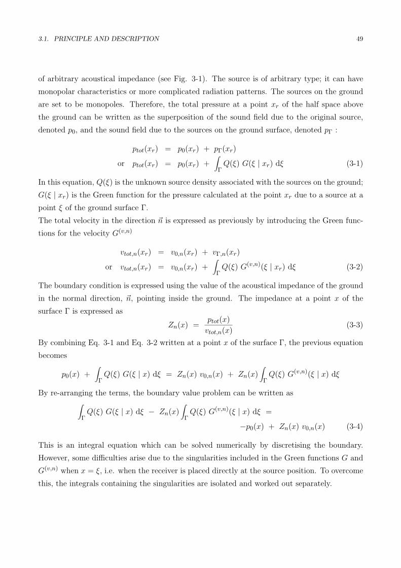
3.1. PRINCIPLE AND DESCRIPTION 49
of arbitrary acoustical impedance (see Fig. 3-1). The source is of arbitrary type; it can have
monopolar characteristics or more complicated radiation patterns. The sources on the ground
are set to be monopoles. Therefore, the total pressure at a point xr of the half space above
the ground can be written as the superposition of the sound field due to the original source,
denoted p0, and the sound field due to the sources on the ground surface, denoted pΓ :
ptot(xr) = p0(xr) + pΓ(xr)
or ptot(xr) = p0(xr) +∫Γ
Q(ξ) G(ξ | xr) dξ (3-1)
In this equation, Q(ξ) is the unknown source density associated with the sources on the ground;
G(ξ | xr) is the Green function for the pressure calculated at the point xr due to a source at a
point ξ of the ground surface Γ.
The total velocity in the direction ~n is expressed as previously by introducing the Green func-
tions for the velocity G(v,n)
vtot,n(xr) = v0,n(xr) + vΓ,n(xr)
or vtot,n(xr) = v0,n(xr) +∫Γ
Q(ξ) G(v,n)(ξ | xr) dξ (3-2)
The boundary condition is expressed using the value of the acoustical impedance of the ground
in the normal direction, ~n, pointing inside the ground. The impedance at a point x of the
surface Γ is expressed as
Zn(x) =ptot(x)
vtot,n(x)(3-3)
By combining Eq. 3-1 and Eq. 3-2 written at a point x of the surface Γ, the previous equation
becomes
p0(x) +∫Γ
Q(ξ) G(ξ | x) dξ = Zn(x) v0,n(x) + Zn(x)∫Γ
Q(ξ) G(v,n)(ξ | x) dξ
By re-arranging the terms, the boundary value problem can be written as∫Γ
Q(ξ) G(ξ | x) dξ − Zn(x)∫Γ
Q(ξ) G(v,n)(ξ | x) dξ =
−p0(x) + Zn(x) v0,n(x) (3-4)
This is an integral equation which can be solved numerically by discretising the boundary.
However, some difficulties arise due to the singularities included in the Green functions G and
G(v,n) when x = ξ, i.e. when the receiver is placed directly at the source position. To overcome
this, the integrals containing the singularities are isolated and worked out separately.

50 CHAPTER 3. GROUND EFFECTS MODELLING USING THE ES METHOD
The previous equation can be written as
Ip(x) − Zn(x) Iv(x) = −p0(x) + Zn(x) v0,n(x)
where Ip, resp. Iv, is an integral for the pressure, resp. for the velocity. Let us denote by Ej the
element of the ground surface on which the receiver x lies. Then Γ can be expressed as Γ′ ∪Ej
where Γ′ embraces the whole surface except the element Ej . Thus both Ip and Iv contains an
integral which is said to be regular over Γ′, and a singular integral over the element Ej :
Ip(x) =∫Γ′
Q(ξ′) G(ξ′ | x) dξ′ +∫Ej
Q(ξj) G(ξj | x) dξj
Iv(x) =∫Γ′
Q(ξ′) G(v,n)(ξ′ | x) dξ′︸ ︷︷ ︸regular integrals
+∫Ej
Q(ξj) G(v,n)(ξj | x) dξj︸ ︷︷ ︸singular integrals
The singularity is encountered when ξj “meets” x. Rigorously, the integrals should be evaluated
at all points of the element surface. Instead in this study, as usually done in standard numerical
integration schemes, the integral is evaluated only for values of x at the element’s mid point.
This is done while assuming that the source density function Q is slowly varying over the
element length. This assumption is valid only if the impedance is also slowly varying over the
element length, and the discretisation is fine enough.
Therefore, it is sufficient to compute the source density merely at the element mid point.
Furthermore Q can be taken out of the integrals in the previous equations and Eq. 3-4 becomes
Q(x)
[∫Γ′
G(ξ′ | x) dξ′ +∫Ej
G(ξj | x) dξj
− Zn(x)∫Γ′
G(v,n)(ξ′ | x) dξ′ +∫Ej
G(v,n)(ξj | x) dξj
]= −p0(x) + Zn(x) v0,n(x) (3-5)
This is a “simple” boundary equation from which the unknowns Q(x) can be determined using
for instance a standard Gaussian elimination. Once it is done, the pressure at any point of the
half space above the ground can be calculated using Eq. 3-1.

3.1. PRINCIPLE AND DESCRIPTION 51
Green functions’ integration
This paragraph presents the expression of the Green functions and the calculation of the inte-
grals contained in Eq. 3-5. In fact, this computation represents the main critical point of the
model.
The Green functions for a point source radiating over a flat, rigid or soft plane can easily be
found by introducing a mirror image source at xs. For the chosen time convention1, it is written
G(xs | xr) = − j
4
[H(1)
m (k | xr − xs |)ejmϕ ± H(1)m (k | xr − xs |)ejmϕ
](3-6)
where m is the order of the source and ϕ, resp. ϕ, is the angle with the horizontal direction
from the source, resp. from the image source, to the receiver. The plus sign corresponds to a
rigid ground whereas the minus sign corresponds to a perfectly soft ground.
Pressure and velocity Green functions are connected by2
G(v,n)(xs | xr) = +1
jωρ∇G(xs | xr) · ~n
In this study, the ground sources are set to be only monopoles embedded in a rigid baffle.
Hence, the Green functions for the ground sources can be written
G(xs | xr) = − j
2H
(1)0 (k | xr − xs |)
and G(v,n)(xs | xr) =1
2ρcH
(1)1 (k | xr − xs |) ~ur · ~n
where ~ur is the radial direction of the source contribution.
The integration of these expressions can be performed numerically with arbitrary accuracy on
the length Γ′ of ground. In particular, if the sources are on the ground, the integral for the
velocity vanishes : the vector ~ur is always perpendicular to the surface normal ~n, and their
product is indeed zero. Thus ∫Γ′
G(v,n)(ξ′ | x) dξ′ = 0 ∀x 6= ξ′
The computation of the singular part needs more attention. It has been shown in [Becot 2002]
that these integrals could be estimated by calculating the Cauchy principal value. It is also
proved in Appendix III that asymptotic expressions of the Hankel functions could be used to
1Hankel function of second kind are used for a time dependence as e+jωt.2A minus sign is required if one uses e+jωt.
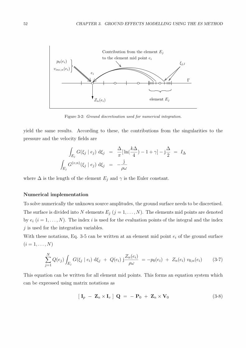
52 CHAPTER 3. GROUND EFFECTS MODELLING USING THE ES METHOD
element Ej
ξj,l
Γ
Zn(ei)
ei
p0(ei)
vinc,n(ei)
Contribution from the element Ej
to the element mid point ei
Figure 3-2: Ground discretisation used for numerical integration.
yield the same results. According to these, the contributions from the singularities to the
pressure and the velocity fields are∫Ej
G(ξj | ej) dξj =∆
π[ ln(
k∆
4)− 1 + γ]− j
∆
2= I∆∫
Ej
G(v,n)(ξj | ej) dξj = − j
ρω
where ∆ is the length of the element Ej and γ is the Euler constant.
Numerical implementation
To solve numerically the unknown source amplitudes, the ground surface needs to be discretised.
The surface is divided into N elements Ej (j = 1, . . . , N). The elements mid points are denoted
by ei (i = 1, . . . , N). The index i is used for the evaluation points of the integral and the index
j is used for the integration variables.
With these notations, Eq. 3-5 can be written at an element mid point ei of the ground surface
(i = 1, . . . , N)
N∑j=1
Q(ej)∫Ej
G(ξj | ei) dξj + Q(ei) jZn(ei)
ρω= −p0(ei) + Zn(ei) v0,n(ei) (3-7)
This equation can be written for all element mid points. This forms an equation system which
can be expressed using matrix notations as
[ Ip − Zn × Iv ] Q = − P0 + Zn ×V0 (3-8)

3.1. PRINCIPLE AND DESCRIPTION 53
where
Ip =
I∆∫E2
G(ξ2 | e1) dξ2 . . .∫EN
G(ξN | e1) dξN∫E1
G(ξ1 | e2) dξ1 I∆. . .
......
. . . I∆∫EN
G(ξN | eN−1) dξN∫E1
G(ξ1 | eN ) dξ1 . . .∫EN−1
G(ξN−1 | eN ) dξN−1 I∆
Iv =
−j/ρω 0 . . . 0
0 −j/ρω. . .
......
. . . −j/ρω 0
0 . . . 0 −j/ρω
Zn = [ Zn(e1), . . . , Zn(eN ) ]T
Q = [ Q(e1), . . . , Q(eN ) ]T
P0 = [ p0(e1), . . . , p0(eN ) ]T
V0 = [ v0,n(e1), . . . , v0,n(eN ) ]T
The largest part of the computational work is required for the computation of the integrals
contained in Ip. However, it only depends on the ground discretisation. Therefore, it is pos-
sible to reduce the computational effort for different impedance distributions on an invariant
geometry.
The numerical integration is also a critical part of the method also because it determines to
a large extent the accuracy of the results. In the present work, the numerical integration
is performed using a Gauss-Legendre quadrature. The principle of such a procedure is to
approximate an integral by a weighted summation. This summation consists of weighted values
of the integrand, calculated at different points of the interval of integration. According to this
technique [Abramowitz 1972], the integral of the above equation can be written, for i 6= j∫Ej
G(ξj | ei) dξj =∆
2
L∑l=1
wl G(ξj,l | ei) + RL where ξj,l = ej +∆
2xl
xl and wl are the abscissae and the weights of the quadrature of order L. RL is the remainder
of the quadrature, which is a measure of the error made using such a procedure. The resulting
ground discretisation used to perform the numerical integration is shown in Fig. 3-2.

54 CHAPTER 3. GROUND EFFECTS MODELLING USING THE ES METHOD
SourceReceivers
1.2 m
1.2 m
0
θ
x = +1.5 m x = −1.5 m
Figure 3-3: Geometry used for the numerical examples of this chapter.
Finally, Eq. 3-7 can be simplified by introducing the mirror image of the original source. If the
amplitudes of both sources are equal, then the total velocity due to these sources is zero and
the pressure is doubled on the ground. This corresponds to fulfill a rigid boundary condition,
which can be seen as a primary boundary impedance when Q is zero. In this case, the boundary
equation becomes
[ Ip − Zn × Iv ] Q = − 2×P0 (3-9)
On the contrary, if the amplitudes have opposite signs, the pressure on the ground vanishes
and the velocity is doubled. This corresponds to a totally soft boundary condition and Eq. 3-7
becomes
[ Ip − Zn × Iv ] Q = 2× Zn ×V0
As a consequence, in both cases, the layer of ground sources only compensate for the difference
between the desired boundary impedance and the impedance value achieved by the original
source and its mirror image.
3.2 Model validation
In order to demonstrate the accuracy of the proposed method, some examples are shown in
this section. For all the predictions shown below, the implemented Green function includes
an image source, which fulfills together with the original source a rigid primary boundary
condition on the ground surface (see Eq. 3-9). Details of the ground discretisation are given in
each paragraph.
The results are compared in terms of the relative sound pressure levels to remove the influence
of the source strength. For this, the pressure level of the source in the presence of the absorbing
3.2. MODEL VALIDATION 55
surface is normalised by the pressure level of the same source in the free field.
Numerical examples for homogeneous surfaces are presented in the first two paragraphs. The
last paragraph presents an experimental validation of the present ES model by comparisons to
measurements over surfaces having more complex impedance distributions3.
Trivial case : Dirichlet boundary condition
The geometry for the numerical examples in the first two paragraphs is shown in Fig. 3-3. The
geometry is chosen to cover a wide range of angles from grazing incidence to very steep. Two
values of the angle θ between the ground plane and the source, as seen from the origin, are
used in the examples: θ = 5◦ and θ = 45◦. These angles are chosen to represent a low source
and a high source respectively. The region on the ground where the surface is discretized is
between x = −1.5 m and x = +1.5 m, and a value of 10 elements per wavelength is used in
order to ensure good convergence. The results are compared in terms of the sound pressure
level relative to the free field. In all the following figures a receiving angle equal to 90◦ means
a receiving point on the ground.
The first comparison is made for the case of the so-called Dirichlet boundary condition. A 2D
monopole is radiating over a totally soft surface, which means that the impedance is zero on
the ground. In this case, the exact pressure field can be determined by introducing an image
source of opposite source strength as
pexact(xr) = Q0 G(xs | xr) − Q0 G(xs | xr)
or pexact(xr) = − j
4Q0
[H
(1)0 (k | xr − xs |) − H
(1)0 (k | xr − xs |)
]according to Eq. 3-6. As previsouly mentioned, the influence of Q0 is removed by comparing
relative pressure levels.
In the implementation of the present ES model, the primary impedance is infinite on the
ground; this corresponds to a totally rigid surface. Therefore, to achieve the desired impedance
value, that is Zn = 0, the ground sources are expected to contribute to their largest extent. As
seen in Fig. 3-4, the agreement is very good for both source positions. Calculations, which are
not shown here, at other frequencies and for other source and receiver positions demonstrate a
similarily high accuracy of the present method, at both low and high frequencies as well as for
3Some of these results can be found in [Becot 2002]

56 CHAPTER 3. GROUND EFFECTS MODELLING USING THE ES METHOD
(a) Low source position (θ = 5◦) (b) High source position (θ = 45◦)
Figure 3-4: Results for the Dirichlet boundary condition – Zn = 0, f = 1 kHz.
(a) Low source position (θ = 5◦) (b) High source position (θ = 45◦)
Figure 3-5: Results for Robin boundary conditions – β = 0.2, f = 4 kHz.
a large range of geometries.
Robin boundary condition : Homogeneous absorbing surfaces
This paragraph presents numerical examples of sound propagation over finite ground impedance.

3.2. MODEL VALIDATION 57
The ground absorption is considered in terms of dimensionless normalised admittances, i.e.
β = ρc/Zn. The geometry used here is the same as in the previous paragraph (see Fig. 3-3).
In this case, results are compared with results from the model presented in [Chandler-Wilde
1995]. In this latter approach, the total pressure above the ground is expressed as the superpo-
sition of the direct sound field and the field reflected at the ground surface. As in the present
ES model, the Green functions for the direct sound field include the field of an image source,
thus fulfilling a rigid boundary condition on the ground. The authors propose to evaluate
the reflected sound field by expanding it in plane waves. The resulting expession is however
not suitable for direct numerical evaluation. By means of the steepest descent method they
obtained an analytical approximation valid for grazing incidence and for limited values of the
ground impedance. This method is accurate for medium to low admittance values (β < 0.7)
and for admittance values close to one (|1− β| < 0.1).
Given these limitations, the case β = 0.2, which represents a rather rigid ground, is examined.
Results are presented in Fig. 3-5(a) for a low source position and in Fig. 3-5(b) for a high
source position. It is clear that the agreement between the models is good at grazing incidence,
a condition which is assumed in the analytical approximation. As expected for steeper angles of
incidence, the difference increases due to errors in the analytical approximation. Comparisons
for softer grounds impedances were also made, but the agreement was not satisfying because
of the limitations in the analytical approximation.
Experimental validation
To be able to compare measurements to model calculations, a 2D omnidirectional source would
be needed. Since such a source is difficult to realise, a 3D point source was used. This might
seem inappropriate for our purpose. However, it has been shown in [Duhamel 1996] that sound
pressure levels relative to the free field are equal for coherent line source and for a point source,
provided that the angle between the ground reflection path and the surface normal is rather
high. Therefore it is safe to compare measurements of attenuation for such a source with
predictions using the present model.
The source used for the measurements is an electrodynamic driver with a flexible hose attached.
The hose was made sufficiently long to be able to remove eventual reflections at the opening
inside the flexible tube by windowing the time signals. Considering its power output and its
directivity, the useful frequency range of this source lies between 200 Hz and 6 kHz. Measure-

58 CHAPTER 3. GROUND EFFECTS MODELLING USING THE ES METHOD
103
−15
−10
−5
0
5
10
15
Frequency (Hz)
Lp r
elat
ive
free
fiel
d (d
B)
CalculationsMeasurements
Figure 3-6: Measured and calculated relative pressure fields over a homogeneous absorbing surface – Sourceheight: 0.3 m, receiver height: 0.3 m, horizontal distance: 0.5 m.
ments were performed using the MLS 4 technique ensuring that the influence of the background
noise could be minimized. Note that some of the following results can be found in [Becot 2002].
For the impedance ground, panels of mineral wool employed for thermic insulation were used.
In all configurations, the flat panels of absorbing material were put directly on a rigid con-
crete floor. Thus, the material of interest is a hardbacked absorbing material. The acoustic
impedance was chosen to characterize the absorbing material. The impedance distribution
was determined experimentally using the Level Difference technique (see Appendix IV for the
details).
With the obtained data, three propagation situations were tested : propagation over an absorb-
ing plane, over a plane with an impedance step and over a strip of absorbing material in a rigid
baffle. Within the frequency range of interest, all geometrical configurations were assumed to
be two-dimensional. The propagation direction was always perpendicular across the impedance
discontinuities.
Results for the sound radiation over a homogeneous absorbing surface are shown in Fig. 3-6.
For all frequencies, the agreement between measurements and calculations is good. The largest
difference, about 3 dB, found around 500 Hz, might be due to the fact that the value of the
relative pressure field is very sensitive to errors in the area of the interference minimum. The
4Maximum Length Sequence

3.2. MODEL VALIDATION 59
103
−15
−10
−5
0
5
10
15
Frequency (Hz)
Lp r
elat
ive
free
fiel
d (d
B)
CalculationsMeasurements
(a) Receiver above discontinuity
absorber rigid
0.3
S R0.5
0.50.3
S R0.8
(b) Geometries
103
−15
−10
−5
0
5
10
15
Frequency (Hz)
Lp r
elat
ive
free
fiel
d (d
B)
CalculationsMeasurements
(c) Receiver away from discontinuity
Figure 3-7: Measured and calculated relative pressure fields over a step impedance surface.
errors can also be caused by the absorbent panels being to small. Besides this, predictions and
measurements are within about 1.5 dB. Moreover, the frequencies at which interference maxima
and minima occur are well predicted by the model. Measurements for other geometries (not
presented here) also showed good concordance with calculations. Results averaged over third
octave bands of frequencies presented in [Becot 2002] also showed very good concordance with
the measured values.
Measurements over a surface having one discontinuity of impedance were also performed. In
this configuration, a sheet of mineral wool is placed jointly to a large rigid plane. The source is
radiating above the rigid surface and the receiver is located above the absorber. This situation
is similar to typical traffic noise measurements, where the noise source radiates above a rigid
surface (the road surface) while the propagation occurs in most cases above softer grounds
like earth or grass lands. Fig. 3-7 shows the measured and predicted values for two different
geometries. The exact geometries are drawn in Fig. 3-7(b). In the ES model, the ground is
discretised from 1.5 m on the left of the source to the impedance step. Significant deviations
are observed between measurements and calculations below 1 kHz. However, values in third
octave band of frequencies shown in [Becot 2002] correspond well (less than 3 dB difference).
The deviations probably come from diffraction at the side edges of the rigid panel. Above this
frequency the predictions are good; the calculations follow the measurements well.
Finally, the sound radiation over a strip of absorbing material embedded in a rigid baffle is
investigated (see Fig. 3-8). The width of the strip is 0.43 m. The two geometries used in the

60 CHAPTER 3. GROUND EFFECTS MODELLING USING THE ES METHOD
103
−15
−10
−5
0
5
10
15
Frequency (Hz)
Lp r
elat
ive
free
fiel
d (d
B)
CalculationsMeasurements
(a) Source and receiver above the dis-continuities
absorberrigid rigid
0.3
S 0.43 R
0.2 0.20.3
S R0.83
(b) Geometries
103
−15
−10
−5
0
5
10
15
Frequency (Hz)
Lp r
elat
ive
free
fiel
d (d
B)
CalculationsMeasurements
(c) Source and receiver away from thediscontinuities
Figure 3-8: Measured and calculated relative pressure fields over a strip of absorbing material in a rigid baffle.
measurements are drawn in Fig. 3-8(b). For the ES model implementation, only the ground
length corresponding to the strip of absorbing material is discretised. Due to the Green func-
tions used for the incident sound field, the presence of the rigid baffle is automatically accounted
for. Large discrepencies are observed between 400 Hz and 600 Hz. It has been checked in [Becot
2002] that predicted and measured values in third octave band of frequencies correspond well
in this frequency range. The deviations are caused by the fact that the pressure levels are very
sensitive in this area of minimum interferences. Beyond this frequency range, predictions are
in good concordance with the measurements.
In conclusion, the numerical examples and the comparisons with measurements presented in
this section prove the method to be suitable for the sound radiation of an omnidirectional sound
source over an arbitrary impedance ground. The other features and limitations of the model
are examined in the next section.
3.3 Other directional sources
Dipole source over impedance ground
Omnidirectional sources, as examined in the previous section, may represent a heavy short-
coming in real traffic noise situations. As far as tyre noise is concerned, the characteristics
of the emitted sound field, which are strongly modified by the horn effect, are shown to be
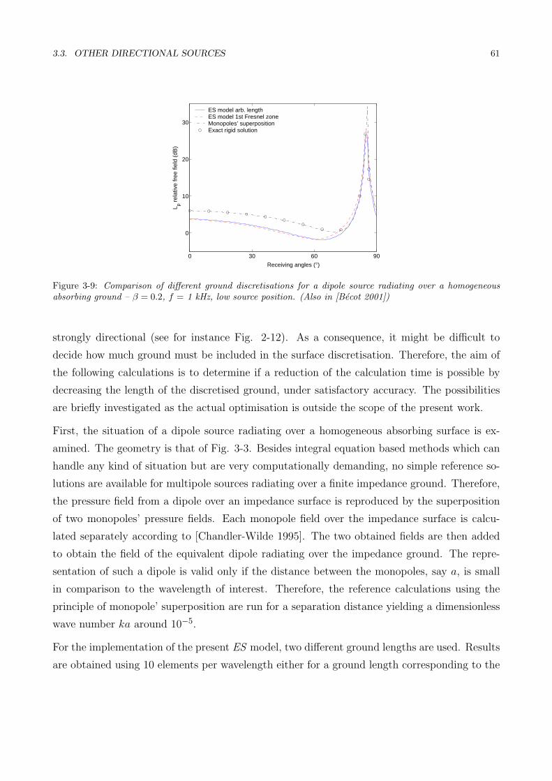
3.3. OTHER DIRECTIONAL SOURCES 61
0 30 60 90
0
10
20
30
Receiving angles (°)
L p rel
ativ
e fr
ee fi
eld
(dB
)
ES model arb. lengthES model 1st Fresnel zoneMonopoles’ superpositionExact rigid solution
Figure 3-9: Comparison of different ground discretisations for a dipole source radiating over a homogeneousabsorbing ground – β = 0.2, f = 1 kHz, low source position. (Also in [Becot 2001])
strongly directional (see for instance Fig. 2-12). As a consequence, it might be difficult to
decide how much ground must be included in the surface discretisation. Therefore, the aim of
the following calculations is to determine if a reduction of the calculation time is possible by
decreasing the length of the discretised ground, under satisfactory accuracy. The possibilities
are briefly investigated as the actual optimisation is outside the scope of the present work.
First, the situation of a dipole source radiating over a homogeneous absorbing surface is ex-
amined. The geometry is that of Fig. 3-3. Besides integral equation based methods which can
handle any kind of situation but are very computationally demanding, no simple reference so-
lutions are available for multipole sources radiating over a finite impedance ground. Therefore,
the pressure field from a dipole over an impedance surface is reproduced by the superposition
of two monopoles’ pressure fields. Each monopole field over the impedance surface is calcu-
lated separately according to [Chandler-Wilde 1995]. The two obtained fields are then added
to obtain the field of the equivalent dipole radiating over the impedance ground. The repre-
sentation of such a dipole is valid only if the distance between the monopoles, say a, is small
in comparison to the wavelength of interest. Therefore, the reference calculations using the
principle of monopole’ superposition are run for a separation distance yielding a dimensionless
wave number ka around 10−5.
For the implementation of the present ES model, two different ground lengths are used. Results
are obtained using 10 elements per wavelength either for a ground length corresponding to the

62 CHAPTER 3. GROUND EFFECTS MODELLING USING THE ES METHOD
first Fresnel zone5, or for an arbitrary ground length, namely from x = -1.5 m to x = +1.5 m.
Results for the two ground lengths are shown in Fig. 3-9 together with the reference calculations.
As in indication, the solution for a dipole radiating over a totally rigid surface is also shown.
Application of the Fresnel zone principle gives results which are in accordance with those
obtained using an arbitrary ground length. Note that the size of the Fresnel zones depends
on the source and the receiver position and on the frequency. In this case, the length of the
first Fresnel zone corresponds to at most 80 % of the arbitrary length. The correspondence
with the solution using the monopole superposition is good at and near the grazing incidence,
which is the condition assumed in the computation of the individual source fields. Therefore, an
optimisation of the computational time by considering a limited portion of discretised ground
seems to be possible in this case.
However, the solution using such a monopole superposition is limited to the case of low order
sources. At a given frequency, the simulation of a high order source implies the presence of
several monopoles in a small region of space, dominantly cancelling each others fields. As a
consequence, the reproduction of the interference pattern is not accurate numerically. Practi-
cally, it has been found that the simulation of such a multipole field is limited to around a 10-th
order source approximately. Also, the interaction between the fields due to the monopoles con-
stituting the dipole is not correctly predicted using such a superposition method. Discrepencies
due to this deficiency are expected to increase with the order of the source.
Therefore, in the following, the radiation of multipole sources is examined only over totally soft
surfaces because an exact solution is available in this case and is used as the reference.
High order source
To further examine if an optimisation of the discretised ground length is possible, the following
numerical examples deal with multipole sources radiating over totally soft surfaces. The ES
model has been run for different ground lengths obtained by introducing an increasing number
of Fresnel zones. For a 5-th order source (see Fig. 3-10(a)), including the first five Fresnel
zones gives predictions which correspond well with the exact solution. If one takes the five first
Fresnel zones, this corresponds to cover around 110 % of the horizontal distance between the
source and the receiver placed at 45◦ of incidence. If ones includes only the first Fresnel zone,
5Details on the Fresnel zone principle can be found in [Picaut 2000].

3.4. SUMMARY 63
0 30 60 90
−10
0
10
20
30
Receiving angles (°)
L p rel
ativ
e fr
ee fi
eld
(dB
)
Exact solution1st Fresnel zone5 first Fresnel zone
(a) 5-th order source – f = 1500 Hz, low position (b) 60-th order source – f = 5 kHz, high position
Figure 3-10: Comparison of different ground discretisations for multipole sources radiating over a totally softground Zn = 0.
then it corresponds to only half of the distance between the source and the receiver. For a
source of order 60 (see Fig. 3-10(b), also in [Becot 2002]), one must include at least the first
twenty Fresnel zones to obtain a good correspondence with the exact solution. In this case, for
the receiver placed at 45◦ of incidence, the size of the first Fresnel zone represents about 30 %
of the distance source to receiver projected on the ground, the 5-th Fresnel zone corresponds
to 70 % and the 20-th Fresnel zone to 140 %.
Therefore, these two examples prove that the present ES model is accurate in the case of high
order sources too, provided that the ground length included is large enough. An optimisation
of this length depending on the source order seems to be possible. However, the determination
of such an optimisation criteria is beyond the scope of this work.
3.4 Summary
To deal with the sound propagation over a flat, arbitrary impedance ground, an original method,
which is based on the ES method, has been developped and is presented in this chapter. This
method can handle arbitrary radiating sources, i.e. omnidirectional sources as well as strongly

64 CHAPTER 3. GROUND EFFECTS MODELLING USING THE ES METHOD
directional sources.
The basic idea is to place a layer of physical sources on the ground surface, which can be seen as
active sources controlling the ground impedance on a certain portion of the surface. Therefore,
it is assumed that the ground is locally reacting; any sound propagation inside the ground is
omitted. However, the impedance distribution is defined from point to point, allowing the study
of the effects of piece-wise constant impedance distributions and impedance discontinuities.
When determining the ground sources’ amplitudes, singularities are encountered due to the
fact that the sources are placed directly on the boundary. This problem is overcome here by
using the approximations of the Hankel functions for small argument, so that the contribution
from the singularity is calculated analytically6. Once this is done, the field can be estimated
at any point above the ground surface.
Results obtained with the present technique fit well with the exact solutions available for the
radiation over totally soft surfaces, and also in the case of a strongly directional incident field.
In the presence of impedance surfaces, the predictions from the present model correspond well
with the solutions given previously by other authors. Lastly, comparisons with measurements
proved the method to be accurate in the presence of impedance discontinuities also.
Due to its numerical efficiency, the present model is of interest for traffic noise purposes because
it allows one to include both the directivity of the sound source and the presence of surfaces
having different acoustical properties. More generally, this model could be used for the sound
propagation from complicated structures over inhomogeneous grounds.
In particular, the present model for the ground effects can be coupled to the model derived
in Chapter 2 for the prediction of tyre noise above impedance surfaces. Its implementation
is presented in the next chapter together with comparisons with measurements of horn effect
amplifications over arbitrary impedance surfaces.
6It has also been shown in [Becot 2002] that the Cauchy principal value could be used to estimate thesingularity contribution.

Chapter 4
Tyre / Road Noise OverArbitrary Impedance Surfaces
An efficient prediction of tyre / road noise requires an accurate modelling of the tyre
emission but also the introduction of the acoustical properties of the road surface. In this
respect, this chapter proposes different methods for introducing the presence of an arbitrary
impedance surface into the tyre noise model presented in Chapter 2. The surface is assumed
to be locally reacting.
In the first section, solutions using the image source technique and a reflection coefficient are
investigated. Besides that for plane waves, a reflection factor for cylindrical waves of arbitrary
order is derived. To model the tyre radiation over arbitrary impedance surfaces, an original
implementation based on the combination of the models presented in Chapter 2 and Chapter
3 is proposed. The functioning and the validity of the model is then discussed on the basis of
comparisons to measurements.
Section 4.1 . . . . . . . . . . . . . . . . . . . . . . . . . . . . . . . . . . . . . . PreliminaryOn the use of a reflection factor – Plane wave reflection coefficient –Cylindrical reflection coefficient
Section 4.2 . . . . . . . . . . Iterative ES model of the tyre radiationover impedance surfacesSolving principle – Mathematical derivation – Amplification factors –Numerical implementation
Section 4.3 . . . . . . . . . . . . . . . . . . . . . . . . . . . . . . .Model functionningThe iterative process – Sources’ amplitudes
Section 4.4 . . . . . . . . . . . . . . . . . . . . . . . . . . . .Results and discussionMeasurement and modelling procedure – Homogeneous surfaces – Inho-mogeneous surfaces – Discussion
Section 4.5 . . . . . . . . . . . . . . . . . . . . . . . . . . . . . . . . . . . . . . . . .Summary
65
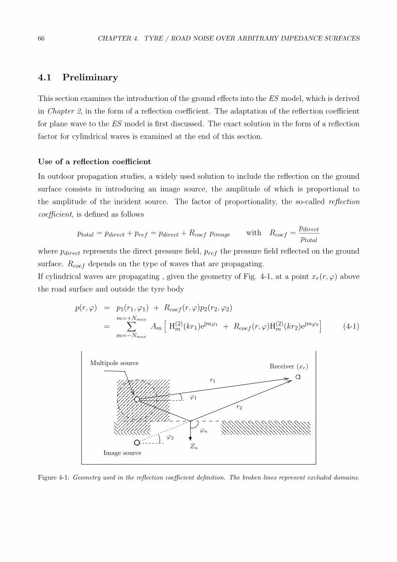
66 CHAPTER 4. TYRE / ROAD NOISE OVER ARBITRARY IMPEDANCE SURFACES
4.1 Preliminary
This section examines the introduction of the ground effects into the ES model, which is derived
in Chapter 2, in the form of a reflection coefficient. The adaptation of the reflection coefficient
for plane wave to the ES model is first discussed. The exact solution in the form of a reflection
factor for cylindrical waves is examined at the end of this section.
Use of a reflection coefficient
In outdoor propagation studies, a widely used solution to include the reflection on the ground
surface consists in introducing an image source, the amplitude of which is proportional to
the amplitude of the incident source. The factor of proportionality, the so-called reflection
coefficient, is defined as follows
ptotal = pdirect + pref = pdirect + Rcoef pimage with Rcoef =pdirect
ptotal
where pdirect represents the direct pressure field, pref the pressure field reflected on the ground
surface. Rcoef depends on the type of waves that are propagating.
If cylindrical waves are propagating , given the geometry of Fig. 4-1, at a point xr(r, ϕ) above
the road surface and outside the tyre body
p(r, ϕ) = p1(r1, ϕ1) + Rcoef (r, ϕ)p2(r2, ϕ2)
=m=+Nmax∑m=−Nmax
Am
[H(2)
m (kr1)ejmϕ1 + Rcoef (r, ϕ)H(2)
m (kr2)ejmϕ2
](4-1)
� � � � � � � � � � � � � � �� � � � � � � � � � � � � � �� � � �� � � �� � � �� � � �
� � � �� � � �� � � �� � � �
Receiver (xr)
Zn
ϕ1
Image source
ϕnϕ2
Multipole source
r1
r2
Figure 4-1: Geometry used in the reflection coefficient definition. The broken lines represent excluded domains.

4.1. PRELIMINARY 67
In this equation, the reflection coefficient depends a priori on the position of the receiver xr;
for the sake of brevity, it is denoted Rcoef in the following.
The velocity field in the direction ~n, deduced from the pressure field, is expressed as
vn(r, ϕ) = − 1
jωρ~∇p1 · ~n − 1
jωρ~∇(Rcoef p2) · ~n
According to the expression of the gradient in cylindrical coordinates (see Eq. 2-4), it can be
written
vn(r, ϕ) = − 1
jωρ
m=+Nmax∑m=−Nmax
Am
[kH(2)′
m (kr1) cos(ϕ1 − ϕn) +jm
r1H(2)
m (kr1) sin(ϕ1 − ϕn)]ejmϕ1
− 1
jωρ
m=+Nmax∑m=−Nmax
Rcoef Am
[kH(2)′
m (kr2) cos(ϕ2 − ϕn) +jm
r2H(2)
m (kr2) sin(ϕ2 − ϕn)]ejmϕ2
− 1
jωρ
m=+Nmax∑m=−Nmax
AmH(2)m (kr2)e
jmϕ2
[∂Rcoef
∂r2cos(ϕ2 − ϕn) +
1
r2
∂Rcoef
∂ϕ2sin(ϕ2 − ϕn)
](4-2)
This equation differs fondamentally from the expression for the velocity in the presence of a
rigid surface (see Eq. 2-5 and Eq. 2-7) : two additional terms are included, which contain the
partial derivatives of the reflection coefficient.
In the case where plane waves or spherical waves are propagating, expressions for the reflection
coefficient are available from the literature; they are fully used nowadays in outdoor propagation
studies (see Section 1.3 for references). By definition, these solutions are not suited for two-
dimensional geometries.
However, besides its obvious limitations, the reflection factor for plane waves is of interest for
our purpose because its implementation is effortless. The next paragraph examines the appli-
cation of this latter solution to the ES model for the tyre radiation. In the last paragraph
of this section, the derivation of the exact solution, i.e. in the form of a reflection factor for
cylindrical waves, is investigated.
Plane wave approximation
At an infinite distance from the source, the wave front of an omnidirectional cylindrical wave
becomes close to a plane. Therefore, the solution described in this paragraph can be seen as
an approximation of the true solution in the case where only omnidirectional cylindrical waves
are propagating and when the source is far from the ground surface.

68 CHAPTER 4. TYRE / ROAD NOISE OVER ARBITRARY IMPEDANCE SURFACES
According to [Morse 1968], the reflection coefficient for plane waves is defined as
Rp =sin ϕ− ρc/Zn
sin ϕ + ρc/Zn=
sin ϕ− β
sin ϕ + β(4-3)
where ϕ is defined in Fig. 4-1 and β = ρc/Zn, Zn is the normal acoustical impedance of the
road surface. This solution only holds for impedance surfaces, which are homogeneous.
Therefore, in the expression of the velocity field Eq. 4-2, one has
∂Rcoef
∂r2= 0 and
∂Rp
∂ϕ2=
2β cos ϕ2
(sin ϕ2 + β)2
By including this expression in Eq. 4-2 and after rearranging the terms, the total velocity at a
point xr(r, ϕ) above an homogeneous impedance plane can be expressed as1
vn(r, ϕ) = − 1
jωρ
m=+Nmax∑m=−Nmax
Am
[kH(2)′
m (kr1) cos(ϕ1 − ϕn) +jm
r1H(2)
m (kr1) sin(ϕ1 − ϕn)]ejmϕ1
− 1
jωρ
m=+Nmax∑m=−Nmax
Rp × Am kH(2)′
m (kr2)ejmϕ2 cos(ϕ2 − ϕn)
− 1
jωρ
m=+Nmax∑m=−Nmax
Am1
r2H(2)
m (kr2)ejmϕ2
[jm(sin2 ϕ2 − β2) + 2β cos ϕ2
(sin ϕ2 + β)2
]sin(ϕ2 − ϕn) (4-4)
Note that this equation also provides a measure of the error when using the reflection coefficient
in normal incidence. Though, this calculation is not examined further because of the more
important, inherent deficiencies of this approach.
To examine to what extent the solution using reflection factor for plane waves is reliable, horn
effect amplification factors are compared to measured ones over a rather soft surface.
The absorbing material used in the experiment is a panel of mineral rock wool, normally
employed for thermic insulation, layed on top of a concrete surface. The normal acoustical
impedance of the material was measured in a Kuntd’s tube (the measured impedance values are
shown in Appendix IV). Due to practical reasons, the domain of validity of the measurements
ranges from 200 Hz to 2 kHz. The measurement procedure is the same as for horn effect
measurements over rigid surfaces, i.e. the reciprocity principle is applied (see Fig. 2-1). Sound
pressure levels are first recorded in the presence of the tyre and the absorbing layer and in a
second stage, when the tyre is removed. The microphone is mounted flush with the absorbing
1This expression can be found in [Kropp 2000b]; besides the different angle dependency, mistakes have beencorrected in the present study regarding Eq. (10) of the mentioned work.

4.1. PRELIMINARY 69
Measured
Rp(ϕ2)
Rp(π/2)
•
◦
Figure 4-2: Measurements of amplification factors over an impedance surface compared to prediction from theES model using plane wave reflection coefficient.
panel at a distance d = 20 mm from the horn centre, and at the middle of the contact area
(see Fig. 2-7). The sound source, a standard loudspeaker positioned one meter ahead of
the microphone, is directed toward the microphone so that all sound reflections occur in the
geometrical plane which contains the tyre, the microphone and the loudspeaker.
Results from the ES model shown in Fig. 4-2 are denoted Rp(ϕ2). As expected, the amplifica-
tion factors obtained are overestimated at low frequencies due to the two-dimensional character
of the model. Above 500 Hz, the proposed solution corresponds fairly well with measurements.
The deviations between measurements and calculations increase again at frequencies above 1.5
kHz, probaby due to incertainties in the impedance measurements. In total, this yields a fre-
quency range of usability from 500 Hz to 1.5 kHz, which corresponds to the dominant frequency
range of the A-weighted noise levels used in pass-by measurements.
In the same figure, the solution using a reflection factor only for normal incidence has been
plotted; it is indicated as Rp(π/2). At very low frequencies, this solution gives results, which
are very similar to the solution including the angle dependence. However, as the frequency
increases, the solution deviates from the measurements due to an incorrect velocity field ex-
pressed on the tyre surface.
In conclusion, the solution using the plane wave reflection coefficient predicts amplification fac-
tors, which fit well with the measurements over an absorbing surface; a better correspondence
would certainly be achieved for harder surfaces. However, it is not mathematically correct to
use the plane wave reflection coefficient together with cylindrical harmonics. It does not include

70 CHAPTER 4. TYRE / ROAD NOISE OVER ARBITRARY IMPEDANCE SURFACES
the correct wave front and the “geometrical divergence” that occurs when cylindrical waves are
propagating. In fact, the impedance obtained when using the reflection coefficient for plane
waves is not the correct one, that is the one given as input to the model. This means that the
calculated sound field includes only partially the presence of the impedance plane. Therefore,
the next paragraph examines the expression and the application of a reflection coefficient for
cylindrical waves.
Cylindrical wave assumption
The idea of the following derivation is to design a reflection coefficient which gives the correct
impedance value given on the ground. The normal acoustical impedance at one point of the
surface is the ratio between the pressure and the normal velocity at this point. Therefore, let us
derive the expression of the pressure and velocity fields on the surface. Note that the following
derivation holds for any ground impedance but zero impedance. However, the solution in this
case is known : the reflection coefficient equals -1.
For all points of the ground surface, the symmetry of the construction imposes r1 = r2 and
ϕ1 = ϕ2. Let us denote r and ϕ the co-ordinates of one point of the ground surface. Therefore,
according to Eq. 4-1, the total pressure field impinging at one point (r, ϕ) of the surface is
p(r, ϕ) =m=+Nmax∑m=−Nmax
AmH(2)m (kr)ejmϕ (1 + Rm)
where Rm is the reflection factor for cylindrical waves. It depends a priori on the variable r
and ϕ, and on the order m of the source.
The total velocity field in the normal direction to the surface is obtained from Eq. 4-4 :
vn(r, ϕ) =
− 1
jωρ
m=+Nmax∑m=−Nmax
Am
[kH(2)′
m (kr) sin ϕ − jm
rH(2)
m (kr) cos ϕ]ejmϕ (1−Rm)
+1
jωρ
m=+Nmax∑m=−Nmax
AmH(2)m (kr)ejmϕ
[∂Rm
∂rsin ϕ− 1
r
∂Rm
∂ϕcos ϕ
]
One can thus express the impedance boundary condition as
p(r, ϕ) = Zn vn(r, ϕ)
using the two previous equations. The obtained equation must hold for each order m of the
Green function. Therefore, the summation can be removed. Moreover, because they appear on

4.1. PRELIMINARY 71
both sides of the equation, the modal amplitude Am and the exponential term can be removed
also. By doing so, one obtains, for each harmonic order m
H(2)m (kr) (1 + Rm) = − Zn
jωρ
[kH(2)′
m (kr) sin ϕ− jm
rH(2)
m (kr) cos ϕ]
(1−Rm)
+Zn
jωρH(2)
m (kr)
[∂Rm
∂rsin ϕ− 1
r
∂Rm
∂ϕcos ϕ
]
After rearranging the terms, one can write the differential equation which must be satisfied by
Rm at one point (r, ϕ) of the surface :[∂Rm
∂rsin ϕ− 1
r
∂Rm
∂ϕcos ϕ
]+[
am(r, ϕ)− jωρ
Zn
]×Rm =
[am(r, ϕ) +
jωρ
Zn
]where
am(r, ϕ) = kH
(2)′
m (kr)
H(2)m (kr)
sin ϕ− jm
rcos ϕ (4-5)
The differential equation above is always valid as the Hankel function never takes on zero values.
The derivation can therefore proceed.
For the points of the ground surface, the variables r and ϕ are connected through r sin ϕ = h,
where h is the height of the incident source (see Fig. 4-1). Hence, one has
∂Rm
∂ϕ= −−r2 cos ϕ
h
∂Rm
∂r
and
sin ϕ− cos ϕ
r(−−r2 cos ϕ
h) =
r
h(
h
rsin ϕ + cos2 ϕ)
=r
h(sin2 ϕ + cos2 ϕ) =
r
h=
1
sin ϕ
Thus, the previous partial differential equation, i.e. involving two independent variables, be-
comes an ordinary differential equation involving only the variable r
∂Rm
∂r+ fm(r)×Rm = gm(r) (4-6)
with fm(r) = [ am(r, ϕ) − jωρ/Zn ] h/r
gm(r) = [ am(r, ϕ) + jωρ/Zn ] h/r(4-7)
and am defined in Eq. 4-5.
In the above expressions, the dependency upon the angle of incidence ϕ is included implicitely
because the variables r and ϕ are not independent.

72 CHAPTER 4. TYRE / ROAD NOISE OVER ARBITRARY IMPEDANCE SURFACES
At this point, one can check the validity of the approach. As r tends to ∞, Eq. 4-6 can be
written∂Rm
∂r
∣∣∣∣∣∞
+ 0×Rm(∞) = 0 which gives∂Rm
∂r
∣∣∣∣∣∞
= 0
One then obtains
Rm(∞) =gm(∞)
fm(∞)=
−jk sin ϕ + jωρ/Zn
−jk sin ϕ − jωρ/Zn
which can also be written
Rm(∞) =sin ϕ − ρc/Zn
sin ϕ + ρc/Zn= Rp(∞) = −1
Therefore, as expected, the cylindrical wave reflection coefficient tends to the reflection coef-
ficient for plane waves at infinity. In addition, this value is found to be −1 at infinity, or at
grazing incidence, which is a known result from outdoor sound measurements2.
Eq. 4-6 is the differential equation that must satisfy, if it exists, the reflection coefficient for
cylindrical waves. This is a first order, linear differential equation of one variable, the solution
of which, according to [Ince 1956], is known. As the equation holds for any points of the ground
surface, it has the following general solution
Rm(r) = e−∫ r0
rfm(ν) dν
[ ∫ r0
rgm(ν)e
∫ r0ν
fm(µ) dµ dν + Rm(r0)]
(4-8)
where µ, ν are dummy integration variables, and r0 a bound fixed arbitrarily.
Clearly, the choice of r0 is crucial for the computation of the solution. As one knows the so-
lution at infinity, one may be willing to set r0 to infinity. However, the computation of the
integrals contained in the above equation are troublesome and has not solved yet. This will be
the subject of future works.
2Experimentally, the value of the reflection factor is always -1 at grazing incidence, and this, whatever theground impedance because the impedance, in reality, has always a finite value.

4.2. ITERATIVE ES MODEL OF THE TYRE RADIATION OVER IMPEDANCE SURFACES 73
4.2 Iterative ES modelof the tyre radiation over impedance surfaces
To overcome the lack of solution for a cylindrical reflection coefficient, this section presents
a solution, which is based on the combination of the models of Chapter 2 and Chapter 3.
However, contrary to the derivations of Chapter 3, a time dependence as e+jωt is assumed in
the following.
After the presentation of the general principle of the method, the implementation of the model
is explained in this section. The general functioning of the model and its validation are pre-
sented in Section 4.3.
Solving principle
The present model consists of two sub–models : one for the tyre radiation and one for the
ground effects. The unknowns of the problem are, on one hand, the amplitude of the multipole
source, which stands for the tyre radiation, and on the other hand, the amplitudes of the ground
sources, which control the value of the impedance on the ground surface. The sources included
in the complete model are illustrated in Fig. 4-3.
The key point of the model, and of the ES method in general, is that all sources have to fulfill
together the boundary conditions. There are two boundary conditions in our case : one on the
������������������������������������������������������������������������������������������������������������������������������������������������������������������������������������������������������������������������������������������������������������������������������������������������������������������������������������������������������������������������������������������������������������������������������������������
�������������������������������������������������������������������������������������������������������������������������������������������������������������������������������������������������������������������������������������������������������������������������������������������������������������������������������������������������������������������
Multipole
“Horn” monopole and its mirror image
Ground sources
Image multipole
Receiver
Figure 4-3: Illustration of the sources included in the iterative ES model.
74 CHAPTER 4. TYRE / ROAD NOISE OVER ARBITRARY IMPEDANCE SURFACES
tyre surface and one on the ground surface.
A straigthforward and somewhat rough method consists in putting up the entire equation sys-
tem and solving it for the different sources’ amplitudes. The system is then a concatenation of
the equations issued from the boundary condition on the tyre belt and of the equations resulting
from the impedance condition on the ground. However, such an equation system is found to be
ill–conditionned because of the too different order of magnitude of the two sub–systems. The
resulting set of amplitudes is not accurate enough to ensure a good reproduction of the sound
field.
Another approach consists in considering the multiple reflexions occuring inside the horn be-
tween the rigid tyre and the ground surface. In this approach, the amplitudes of the sources
are solved through an iterative process.
At the first stage, the amplitude of the multipole is tuned to fulfill the prescribed velocity on
the tyre surface. This results in a certain pressure field impinging on the road surface. Given
this incident pressure, the source strengths of the ground monopoles are tuned to reproduce the
prescribed impedance value on the ground. These monopoles produce a velocity distribution on
the tyre surface, in addition to the velocity originally prescribed as a tyre boundary condition.
Therefore, an additional multipole amplitude is computed to compensate for this unwanted
velocity. However, this new multipole amplitude creates an additional pressure field on the
ground. This perturbation is counteracted by computing new monople amplitudes, which
themselves create a new velocity field on the tyre surface. . .
The process stops when the achieved velocity on the tyre surface and the achieved impedance
value on the ground are lower than a given error value. At this point, an additional field from
one of the system of sources does not perturb the other system’s behaviour. Finally, the total
amplitudes of the multipole and of the ground monopoles, are the sum of all the amplitudes
computed during the iterative process.
Once the amplitudes of the sources are determined, the pressure or the velocity field can be
computed at any point above the ground surface and outside the tyre body. This field repre-
sents the field radiated by the vibrating tyre in the presence of an impedance plane.
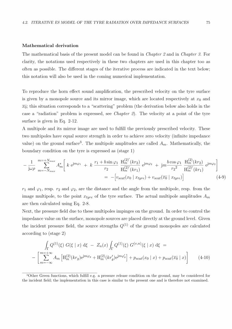
4.2. ITERATIVE ES MODEL OF THE TYRE RADIATION OVER IMPEDANCE SURFACES 75
Mathematical derivation
The mathematical basis of the present model can be found in Chapter 2 and in Chapter 3. For
clarity, the notations used respectively in these two chapters are used in this chapter too as
often as possible. The different stages of the iterative process are indicated in the text below;
this notation will also be used in the coming numerical implementation.
To reproduce the horn effect sound amplification, the prescribed velocity on the tyre surface
is given by a monopole source and its mirror image, which are located respectively at x0 and
x0; this situation corresponds to a “scattering” problem (the derivation below also holds in the
case a “radiation” problem is expressed, see Chapter 2). The velocity at a point of the tyre
surface is given in Eq. 2-12.
A multipole and its mirror image are used to fulfill the previously prescribed velocity. These
two multipoles have equal source strength in order to achieve zero velocity (infinite impedance
value) on the ground surface3. The multipole amplitudes are called Am. Mathematically, the
boundary condition on the tyre is expressed as (stage 1)
− 1
jωρ
m=+Nmax∑m=−Nmax
A∗m
[k ejmϕ1 + k
r1 + b sin ϕ1
r2
H(2)′
m (kr2)
H(2)′m (kr1)
ejmϕ2 + jmb cos ϕ1
r22
H(2)m (kr2)
H(2)′m (kr1)
ejmϕ2
]
= −[vscat(x0 | xtyre) + vscat(x0 | xtyre)
](4-9)
r1 and ϕ1, resp. r2 and ϕ2, are the distance and the angle from the multipole, resp. from the
image multipole, to the point xtyre of the tyre surface. The actual multipole amplitudes Am
are then calculated using Eq. 2-8.
Next, the pressure field due to these multipoles impinges on the ground. In order to control the
impedance value on the surface, monopole sources are placed directly at the ground level. Given
the incident pressure field, the source strengths Q(1) of the ground monopoles are calculated
according to (stage 2)∫Γ
Q(1)(ξ) G(ξ | x) dξ − Zn(x)∫Γ
Q(1)(ξ) G(v,n)(ξ | x) dξ =
−[
m=+∞∑m=−∞
Am
[H(2)
m (krg)ejmϕg + H(2)
m (kr′g)ejmϕ′
g
]+ pscat(x0 | x) + pscat(x0 | x)
](4-10)
3Other Green functions, which fulfill e.g. a pressure release condition on the ground, may be considered forthe incident field; the implementation in this case is similar to the present one and is therefore not examined.

76 CHAPTER 4. TYRE / ROAD NOISE OVER ARBITRARY IMPEDANCE SURFACES
where rg and ϕg, resp. r′g and ϕ′g, are the distance and the angle from the multipole source,
resp. from the multipole image, to a point x of the ground surface. Zn(x) is the value of the
prescribed impedance at the point x of the ground.
Note that, since multipole and image multipole of equal source strength are used, the inci-
dent field does not contribute to the velocity on the ground surface. Another consequence is
that the set of ground sources of amplitude Q(1), only compensate for the difference between
the impedance value fulfilled by the incident field, i.e. infinite impedance, and the prescribed
impedance distribution.
At this point, we have two sets of amplitudes, denoted Am for the multipole and Q(1) for the
ground sources, which are such that the two boundary conditions of the problem are fulfilled
separately. Therefore, one “just” has to counteract the perturbations due to one system of
sources with the other, to obtain the final solution to the problem.
The perturbations on the tyre surface are due to the field from the ground sources in the form
of an additional velocity. The new multipole amplitudes, denoted B(1)m , which counteract this
unwanted velocity, are determined according to (stage i)
− 1
jωρ
m=+Nmax∑m=−Nmax
B(1)∗m k ejmϕ1 = −
∫Γ
Q(1)(ξ) G(v,n)(ξ | xtyre) dξ (4-11)
As before, the actual multipole amplitudes B(1)m are then obtained using Eq. 2-8. In fact, the
field from the image multipole should not be included at this stage. If it was included, the
impedance value on the ground woud be re-set to infinity and this would annihilate the benefit
of the ground sources previously placed on the surface.
This new set of multipole amplitudes B(1)m create a new incident field on the ground surface so
that the impedance condition is not fulfilled any longer. Given the fact that the incident field
contributes now to both the pressure and the velocity, a new set of ground source amplitudes,
say Q(2), is computed according to (stage i + 1)
∫Γ
Q(2)(ξ) G(ξ | x) dξ − Zn(x)∫Γ
Q(2)(ξ) G(v,n)(ξ | x) dξ
= −m=+Nmax∑m=−Nmax
B(1)m H(2)
m (krg)

4.2. ITERATIVE ES MODEL OF THE TYRE RADIATION OVER IMPEDANCE SURFACES 77
+ Zn(x)m=+Nmax∑m=−Nmax
B(1)m
[kH(2)′
m (krg) sin ϕg −jm
rH(2)
m (krg) cos ϕg
]ejmϕg (4-12)
Next, additional source amplitudes for the multipole and for the ground sources are determined
using successively Eq. 4-11 and Eq. 4-12; in a general form, they are denoted B(i)m and Q(i) for
i = 1, . . . , iconv.
At the end of the iterative process, i.e. at i = iconv, the two boundary conditions are fulfilled
together by the two systems of sources, the mutlipole and the ground monopoles.
Amplification factors
Once the boundary conditions are fulfilled, the pressure field at any point above the road surface
and outside the tyre body can be determined. It is written, at a point xr
ptot(xr) =m=+∞∑m=−∞
Am
[H(2)
m (kr1)ejmϕ1 + H(2)
m (kr2)ejmϕ2
]+ pscat(x0 | xtyre) + pscat(x0 | xtyre)
+i=iconv∑
i=1
m=+∞∑m=−∞
B(i)m H(2)
m (kr1)ejmϕ1 +
∫Γ
Q(i) G(ξ | xr) dξ
For the calculation of the horn effect amplification factors, the reference pressures are
– when removing the road :
pref1(xr) =
m=+∞∑m=−∞
Am
[H(2)
m (kr1)ejmϕ1 + H(2)
m (kr2)ejmϕ2
]+ pscat(x0 | xtyre)
where Am is the multipole amplitude calculated for the prescribed velocity given by the original
monopole only (see Chapter 2);
– when removing the tyre :
pref2(xr) = pscat(x0 | xtyre) + pscat(x0 | xtyre) +
∫Γ
Q(ξ) G(ξ | xr) dξ
where Q is the amplitude of the ground source calculated for an incident field due to the “horn”
monopole and its image only.

78 CHAPTER 4. TYRE / ROAD NOISE OVER ARBITRARY IMPEDANCE SURFACES
Numerical implementation
The implementation of the iterative process is summarized in the following using matrix nota-
tions. The matrix elements can be identified easily from the equations above.
Stage 1
The prescribed tyre velocity, which is given by a monopole source placed inside the horn, is
fulfilled by the multipole and its image (see Eq. 4-9) :
A∗ = M−1 ×[−Vscat
]The set of multipole amplitudes A are then calculated according to Eq. 2-8.
Stage 2
Given the incident pressure field, the ground sources are “switched on” so that the prescribed
impedance value Zn is achieved on the ground surface (see Eq. 4-10) :
Q(1) = [ Ip − Zn × Iv ]−1 ×[− (P + Pscat)
]The matrix P contains the pressure contributions from the multipole and its image.
The iteration process starts here.
Stage i
Additional multipole amplitudes are computed to annihilate the undesired velocity on the tyre
due to the ground monopoles. For the iteration numbered i, this is expressed as (see Eq. 4-11)
B(i)∗ = M−11 ×
[−VΓ ×Q(i)
]On the contrary to the matrix M, the matrix M1 only includes the contribution from the
original multipole.
Stage i + 1
As the impedance condition might not be fulfilled any longer, additional ground source ampli-
tudes are calculated according to (see Eq. 4-12) :
Q(i+1) = [ Ip − Zn × Iv ]−1 ×[− P1 ×B(i)
]where P1, contrary to P in the previous equation, includes the pressure and the velocity field
due to the original multipole only. The iteration is stopped when the boundary conditions of
the tyre and on the ground are both satisfied.
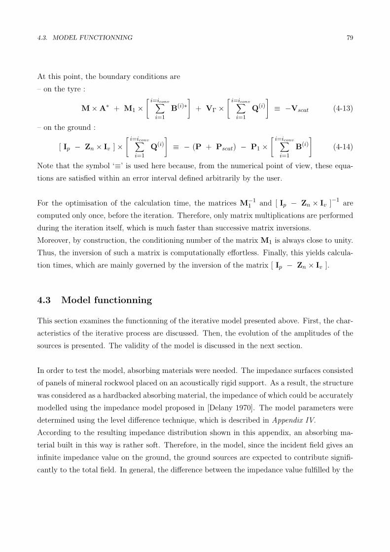
4.3. MODEL FUNCTIONNING 79
At this point, the boundary conditions are
– on the tyre :
M×A∗ + M1 ×[ i=iconv∑
i=1
B(i)∗]
+ VΓ ×[ i=iconv∑
i=1
Q(i)
]≡ −Vscat (4-13)
– on the ground :
[ Ip − Zn × Iv ]×[ i=iconv∑
i=1
Q(i)
]≡ − (P + Pscat) − P1 ×
[ i=iconv∑i=1
B(i)
](4-14)
Note that the symbol ‘≡’ is used here because, from the numerical point of view, these equa-
tions are satisfied within an error interval defined arbitrarily by the user.
For the optimisation of the calculation time, the matrices M−11 and [ Ip − Zn × Iv ]−1 are
computed only once, before the iteration. Therefore, only matrix multiplications are performed
during the iteration itself, which is much faster than successive matrix inversions.
Moreover, by construction, the conditioning number of the matrix M1 is always close to unity.
Thus, the inversion of such a matrix is computationally effortless. Finally, this yields calcula-
tion times, which are mainly governed by the inversion of the matrix [ Ip − Zn × Iv ].
4.3 Model functionning
This section examines the functionning of the iterative model presented above. First, the char-
acteristics of the iterative process are discussed. Then, the evolution of the amplitudes of the
sources is presented. The validity of the model is discussed in the next section.
In order to test the model, absorbing materials were needed. The impedance surfaces consisted
of panels of mineral rockwool placed on an acoustically rigid support. As a result, the structure
was considered as a hardbacked absorbing material, the impedance of which could be accurately
modelled using the impedance model proposed in [Delany 1970]. The model parameters were
determined using the level difference technique, which is described in Appendix IV.
According to the resulting impedance distribution shown in this appendix, an absorbing ma-
terial built in this way is rather soft. Therefore, in the model, since the incident field gives an
infinite impedance value on the ground, the ground sources are expected to contribute signifi-
cantly to the total field. In general, the difference between the impedance value fulfilled by the

80 CHAPTER 4. TYRE / ROAD NOISE OVER ARBITRARY IMPEDANCE SURFACES
10 20 30 40 50 6010
−4
10−2
100
102
104
Iteration number
Bou
ndar
y er
ror
(%)
Impedance error Tyre velocity error
(a) Boundary errors along the iterations. f =420 Hz, Zn = 625 − 3178j. Geometry of Fig.
4-7(b)
200 500 1000 1500 20000
20
40
60
Frequency (Hz)
Num
ber
max
of i
tera
tions
(b) Value of iconv as a function of the frequency.� : gap = 0.8 cm (see Fig. 4-7) – ◦ : gap = 1.85
cm (see Fig. 4-6)
Figure 4-4: Characteristics of the iterative process : boundary errors and value of iconv.
incident field and the prescribed impedance value, determines to a large extent the number of
iterations needed and the relative importance of the ground sources’ contribution.
The iterative process
The iterative process is stopped when the two boundary conditions of the problem are fulfilled
simultaneously. From a numerical point of view, this means that the error made is lower than
an arbitrary threshold value. In this work, it was set to 0.1 %. The error criteria used for this
is the relative surface velocity error proposed in [Schaaf 1982]; it is defined as
error =
∫S| valueprescribed − valueachieved |2∫
S| valueprescribed |2
Note that for the tyre surface boundary error, the prescribed value was set to be that given by
the monopole source located inside the horn.
One can observe that both boundary errors decrease almost constantly along the iterative
process. The impedance error shows some variations at the beginning of the iterative process
while the error on the tyre surface uniformly diminishes. The general behaviour depicted in
this figure also holds at other frequencies and for other system geometries, which are not shown

4.3. MODEL FUNCTIONNING 81
−10 −5 0 5 1010
−4
10−3
10−2
10−1
Order of the multipole
Mag
nitu
de v
alue
First amplitudeNext amplitudes
Increasing iteration number
(a) Multipole amplitudes
−0.5 0 0.5 1 1.5
10−2
10−1
100
101
Source position on the ground
Mag
nitu
de v
alue
First amplitudeNext amplitudes
Increasing iteration number
(b) Ground sources amplitudes. The arrow indi-cates the position of the “horn” monopole (the
reciprocity principle is used).
Figure 4-5: Successive amplitudes of the multipole and of the ground sources. f = 1595 Hz, Zn = 727 − 738j.Geometry corresponding to Fig. 4-7(b).
here. Therefore, it is clear that one can compute the source amplitudes with an arbitrary
accuracy.
It is also interesting to examine the evolution of the maximum number of iterations, denoted
iconv in Eq. 4-13 and Eq. 4-14, as a function of the frequency (see Fig. 4-4(b)). The boundary
errors are those defined above. The results, which are shown for two different gap values, are
very similar. This is due to the fact that the required number of iterations depends only on
the initial difference between the impedance value given the incident field and the prescribed
impedance value.
Concerning the general evolution of iconv, it appears that there exists a particular frequency,
i.e. impedance value, at which the interaction between the two systems is the largest. It is
situated here around 400 Hz; iconv is around 150. Above this frequency, the maximum number
of iterations decreases and reaches around 20 at 2000 Hz.
Sources’ amplitudes
An example of the successive amplitudes of the multipole and of the ground sources is shown
in Fig. 4-5. The results shown here are computed for a single frequency and the correspond-

82 CHAPTER 4. TYRE / ROAD NOISE OVER ARBITRARY IMPEDANCE SURFACES
ing impedance value of the absorbing material described above. In this case, a number of 20
iterations were needed to achieve the prescribed boundary values. It is observed for both the
multipole and for the ground sources, the successive sources’ amplitudes decrease along the
iteration process. This means that the correction is less and less important as new amplitudes
are calculated. Moreover, the first computed amplitude globally dominates the next ones. This
means that the initial system of sources is already quite reliable. After that, the successive
amplitudes “adjust” the field so that an energy balance is reached between the two systems of
sources.
4.4 Results and discussion
For the discussion of the model validity, horn effect amplification factors obtained with the
present model are compared to measured ones over absorbing surfaces. The measurement pro-
cedure and the model implementation is first presented. Then predicted and measured values
are compared in the case of homogeneous and inhomogeneous surfaces. The results are dis-
cussed in a last paragraph.
Measurement and modelling procedure
The absorbing material used is that described above. The measurements were performed by
making use of the reciprocity principle, as it was done for the measurements shown in Chapter
2. This means that the source was located in front of the tyre and that the receiver, a 1/4 inch
electret microphone, was placed inside the horn, close to the contact area. The source was the
same as the one used for the measurements shown in Chapter 3, i.e. an electrodynamic driver
with a flexible hose attached. This source was used for both the determination of the material
impedance and of the amplification factors. This source showed a good directivity diagram
between 200 Hz and 2000 Hz, thus restraining the measurements to this frequency range. The
tyre used was a non-commercial smooth tyre; its perimeter was 2 m (radius of 1/π) and its belt
width was 16 cm. The tyre was suspended over the absorbing surface, which might explain
some of the discprencies observed in the measurements. SPL were recorded when the tyre was
placed above the absorber and when removing the tyre, both using the MLS technique.
For the model implementation, the actual positions of the source and of the receiver are used.
This means that the receiver is located inside the horn region, whereas the monopole source,

4.4. RESULTS AND DISCUSSION 83
which provides the prescribed velocity on the tyre surface, is located ahead of the tyre outside
the horn. In fact, concerning the simulation of the tyre radiation, it was shown in Chapter 2
that such a configuration leads to a good stability in the field predictions. It also allows the
use of a lower order, multipole source for the simulation of the tyre radiation, which yields
lower calculation times. For the calculations shown below, numerical tests have shown that a
multipole of order Nmax = 64 yields stable field predictions. The tyre surface is discretised
into 2Nmax + 1 = 129 elements so that the collocation technique can be applied to solve the
resulting equation system.
Concerning the ground surface discretisation, a minimum of 10 elements per wavelength is as-
sured, with the constraint that the resulting element length should not be larger than the gap
between the tyre and the road. If this is the case, the element length is set to the gap value. It
should be underlined that if this additional criteria is not respected, the stability of the system
of sources is not ensured, i.e. the boundary error may not decrease along the iterative process.
This is due to the fact that if the discretisation is not fine enough, the assumption that the
source strength is a slowly varying function on the element is violated (see the derivation of Eq.
3-5), and the model is not accurate anymore. Finally, the numerical integration of the Green
functions is performed using a Gauss-Legendre quadrature of order 10.
Homogeneous surfaces
First, the tyre radiation over homogeneous impedance surfaces is examined. Results are shown
for two different gap values, and for two different positions of the receiver inside the horn. In the
ES model, preliminary numerical investigations proved that a ground discretisation spanning
from x = -0.5 m to x = +1.5 m yields stable field predictions for the geometry considered here.
For a gap of 1.85 cm (see Fig. 4-6), the correspondence between the measured values and the
predicted ones is globally statisfactory. The levels of amplifications are well estimated and the
frequency behaviour is also well reproduced. This holds for almost all the frequency range
available in the measurements, i.e. from 500 Hz to 2000 Hz.
For a smaller gap value (see Fig. 4-7), predictions fit well to the measured values as long as
the receiver is not too close to the horn centre. When the receiver is very close to the horn
centre, as in Fig. 4-7(a), the ES model predicts somewhat lower amplification factors than
those measured, in the frequency range between 500 Hz to 1200 Hz. The corrrespondence is
however still satisfactory since the error do not exceed 2 dB in this frequency range.

84 CHAPTER 4. TYRE / ROAD NOISE OVER ARBITRARY IMPEDANCE SURFACES
200 500 1000 1500 2000
−4
0
4
8
12
Frequency (Hz)
Am
plifi
catio
n fa
ctor
s (d
B)
MeasuredIterative ES model
(a) Distance horn centre/receiver = 4.2 cm
200 500 1000 1500 2000
−4
0
4
8
12
Frequency (Hz)
Am
plifi
catio
n fa
ctor
s (d
B)
MeasuredIterative ES model
(b) Distance horn centre/receiver = 18.2 cm
Figure 4-6: Horn effect amplification factors over homogeneous impedance surfaces. Gap = 1.85 cm – Sourceheight = 19.7 cm – Distance horn centre/source = 98 cm.
200 500 1000 1500 20000
4
8
12
Frequency (Hz)
Am
plifi
catio
n fa
ctor
s (d
B)
MeasuredIterative ES model
(a) Distance horn centre/receiver = 4.2 cm
200 500 1000 1500 20000
4
8
12
Frequency (Hz)
Am
plifi
catio
n fa
ctor
s (d
B)
MeasuredIterative ES model
(b) Distance horn centre/receiver = 12.2 cm
Figure 4-7: Horn effect amplification factors over homogeneous impedance surfaces. Gap = 0.8 cm – Sourceheight = 4.7 cm – Distance horn centre/source = 48 cm.
In total, the present model gives horn effect amplification factors which correspond within 2
dB to the measured values, and this from frequencies as low as 500 Hz to 2000 Hz, maximum
frequency available in the measurements. The model seems therefore accurate for the predic-
tion of the tyre radiation over homogeneous surfaces on the main frequency range of interest

4.4. RESULTS AND DISCUSSION 85
� � � � � � �� � � � � � �������������������������������������������������������������������������������������������������������������������������������������������������������������
Source
Impedance discontinuityReceiver
Gap
Distancehorn centre / receiver
58 cm 40 cm
Absorbing portion Rigid portion
Figure 4-8: Geometry of the measurement over inhomogeneous surfaces. Case where the tyre and the receiverare located above the absorbing portion and the source is placed over the rigid portion.
for tyre noise purposes.
Inhomogeneous surfaces
An interesting feature of the present ES model is that it handles possible impedance discon-
tinuities of the ground surface. Therefore, measurements of horn effect amplification factors
were performed over surfaces having one discontinuity of impedance. Two cases are examined.
First the receiver, which lies inside the horn, is placed over an absorbing surface and the source
is placed over a rigid plane. Secondly, the source radiates over the absorbing portion and the
receiver is located over a rigid plane.
From an experimental point of view, a panel of the absorbing material desribed previously was
placed jointly to an acoustically rigid panel. In both situations, the impedance discontinuity
was located at a 58 cm distance from the horn centre and at a 40 cm distance from the source
(see Fig. 4-8). The impedance discontinuity was always perpendicular to the propagation path
from the source to the receiver. In the ES model, monopole sources are placed at the ground
level, on the length of ground corresponding to the absorbing portion.
In the case the tyre is above the absorbing material, the ground surface is discretised from
behind the tyre (x = -0.5 m) up to the impedance discontinuity. Results are shown in Fig. 4-9

86 CHAPTER 4. TYRE / ROAD NOISE OVER ARBITRARY IMPEDANCE SURFACES
200 500 1000 1500 20000
4
8
12
Frequency (Hz)
Am
plifi
catio
n fa
ctor
s (d
B)
MeasuredIterative ES model
(a) Distance horn centre/receiver = 4.2 cm
200 500 1000 1500 20000
4
8
12
Frequency (Hz)
Am
plifi
catio
n fa
ctor
s (d
B)
MeasuredIterative ES model
(b) Distance horn centre/receiver = 12.2 cm
Figure 4-9: Horn effect amplification factors over inhomogeneous impedance surfaces. Tyre and receiver overabsorbing material and source over rigid surface. Gap = 0.8 cm – Source height = 19.7 cm – Distance horncentre/source = 98 cm.
for two different receiver positions inside the horn. It can be observed that the amplification
factors in this case are very similar to those obtained over a homogeneous surface (see Fig.
4-7). In the present situation too, a decent correspondence is observed as long as the receiver
is not too far inside the horn. If this is the case, predicted amplification factors are around 2
dB lower than the measured ones at frequencies between 500 Hz to around 1200 Hz.
The second case examined is when the tyre and the receiver are placed over the rigid portion of
ground and that the source is radiating over the absorbing portion of ground. In the ES model,
the ground surface is discretised from the impedance discontiniuty to a little farther from the
actual receiver position (x = +1.5 m). The geometry is reminded in Fig. 4-10(a). In this case,
Fig. 4-10(b) shows measured and predicted amplification factors with solid lines and broken
lines respectively. Results are shown in this figure for three different positions of the receiver
inside the horn.
The amplification factors shown here exhibit a pattern, which is very similar to those measured
over totally rigid surfaces (see for instance Fig. 2-15). Deviations at low frequencies are
undoubtedly ascribed in this case to the two–dimensional character of the ES model. At
frequencies above 800 Hz, the predictions fit well to the measured values. The levels and the
general pattern of the amplification factors are correctly reproduced.

4.4. RESULTS AND DISCUSSION 87
� � � � � � � � � �� � � � � � � � � � ��������������������������������������������������������������������������������������������
(a) Geometry of the experiment
Rigid portion Absorbing portion
SourceReceiver
“rec” 200 500 1000 1500 20000
4
8
12
16
20
Frequency (Hz)
Am
plifi
catio
n fa
ctor
s (d
B)
rec = 4.2 cmrec = 8.2 cmrec = 12.2 cm
(b) Measured (solid lines) and calculated (brokenlines) amplification factors
Figure 4-10: Horn effect amplification factors over inhomogeneous impedance surfaces. Tyre and receiver overrigid surface and source over absorbing material. Gap = 0.8 cm – Source height = 19.7 cm – Distance horncentre/source = 98 cm.
This proves the accuracy of the iterative ES model in the presence of inhomogeneous surfaces
too. In addition, the frequency range of validity of the model seems to depend on the impedance
distribution on the ground surface.
Discussion
The results shown above prove that the present ESmodel is reliable for the prediction of the tyre
radiation over homogeneous absobing surfaces from 500 Hz to the 2000 Hz. For inhomogeneous
surfaces, the lowest frequency from which the model is accurate appears to be different for
different impedance distribution. In particular, if the horn is located over an absorbing portion,
the frequency range of validity tends to that obtained in the case of homogeneous absorbing
surfaces. In contrast, if the horn is located over the rigid portion, the frequency range where
the model is valid is very similar to that obtained in the case the ground is totally rigid (see
Chapter 2).
These results support the fact that the part of the ground impedance laid in the contact region
is expected to determine to a large extent the effect of the horn. However, some of the results
may be discussed.

88 CHAPTER 4. TYRE / ROAD NOISE OVER ARBITRARY IMPEDANCE SURFACES
In particular, it is remarkable that in Fig. 4-6 and Fig. 4-7(b), calculated amplification factors
correspond well to the measured values, yet from frequencies as low as 500 Hz. This is contra-
dictory with the fact that the present model is two–dimensional, leading to an over–estimation
of the horn amplification at these frequencies. It might also be questionned why these results fit
well with the measurements if the receiver is not too far inside the horn, but do not correspond
to the same extent if the receiver is close to the horn centre ? Finally, where do these deviations
come from : experimental deficiencies or inaccuracy of the model ? The answer is probably a
combination of both but the following hypotheses may be thought of.
As a matter of fact, the largest deviations observed in Fig. 4-7(a) and Fig. 4-9(a) between
500 Hz and 1200 Hz occur when two conditions are gathered : the receiver is close to the horn
centre and the gap is very small. In this situation, the horn may be assumed to be totally closed
at its apex, and thus to have its maximum efficiency. Particularly, the horn may considered
as closed for the low frequencies, whereas the high frequencies may still “see” this small gap.
Moreover, the horn has its major effect on the path which lies in the plane of the tyre. Because
of the sound attenuation due to the absorbing material, the contribution from this path may
be masked by other contributions lying out of the plane of the tyre, which are not influenced in
the same manner by the presence of the horn. These contributions may increase significantly
the sound pressure levels measured in the plane of the tyre. This effect is clearly not included
in the present 2D model.
Over rigid surfaces, the 2D model over–estimates the amplification factors at low frequencies.
In the case the horn has substantial absorbing properties, the model may over–estimates the
attenuation, thus leading to amplification factors which are too low compared to the measured
values. This effect is expected to be very pronounced when the horn has its maximum efficiency,
i.e. when the receiver is close to the horn centre and the apex is almost closed.
A last hypothesis is that the model implementation considers that the ground surface is locally
reacting. This might be only partially true for the absorbing material used here at low frequen-
cies. If waves in the absorbing material were to be considered, it is likely that the horn effect
might enhance their contribution to the radiated field. The horn effect is increased if the apex
is closed and so would be the contribution from surface waves.

4.5. SUMMARY 89
4.5 Summary
The present chapter examines the problem of the tyre radiation over locally reacting, impedance
surfaces. Different solutions are proposed, which are adapted to the type of impedance distri-
bution of the ground surface.
In the case where the surface is homogeneous, that is where the impedance is constant along
the ground, simple solutions are presented. One of the solution is based on the well–known
reflection factor for plane waves. Due to its ease of implementation, it was shown that such a
solution, though not mathematically correct, could be a useful tool to predict general trends of
the tyre noise over impedance surfaces.
Moreover, an exact expression of a reflection coefficient for cylindrical waves of arbitrary order is
derived in this chapter. The principle consists in using a mirror image source, the amplitude of
which is multiplied by a reflection factor. The basic idea of the derivation is that the total field
above the ground must give the correct value of the acoustical impedance at any point of the
ground surface. Mathematically, this boundary condition takes the form of a linear differential
equation, the general solution of which is known from the literature. Finally, a solution for
such a reflection factor is expressed as a function of complex integrals and of the value of the
reflection factor for plane waves at infinity. The numerical implementation of such a reflection
factor is however difficult and will be the subject of future works.
A model for the tyre radiation over arbitrary impedance grounds is proposed. In particular,
this model can handle discontinuities of the impedance distribution on the ground. Based on
the ES method, it combines advantageously the numerical efficiency of a 2D model for the tyre
radiation and the large features of a BE alternate technique for the ground effects reproduction.
A multipole source is in charge of the simulation of the tyre radiation while monopole sources
are placed on the ground to control the impedance at the surface. This results in a large set of
amplitudes, which must be tuned in order to fulfill both the tyre boundary condition and the
impedance condition. Solving the whole set of amplitudes using a (large) matrix inversion is
not numerically accurate. Instead, the amplitude of the multipole and the amplitudes of the
ground sources are successively tuned to account for the multiple reflections occuring between
the tyre surface and the road. This is implemented in an iterative process, which is numerically
effortless. At the end of the iteration, the two boundary conditions are fulfilled simultaneously.
The model validity is tested by comparisons with measurements of the horn effect amplifica-
tion factors over homogeneous and inhomogeneous impedance surfaces. The model fails to

90 CHAPTER 4. TYRE / ROAD NOISE OVER ARBITRARY IMPEDANCE SURFACES
predict the correct amplification values due to its 2D character, particularly when the receiver
is very close to the horn centre. In fact in this case, propagation paths out of the plane of
the tyre, which are not considered in a 2D model, may contribute significantly to the sound
field. Besides these limitations, the predictions correspond well to the measured values over
homogeneous and inhomogeneous surfaces; the level of the amplification is correctly estimated
by the present model on a wide frequency range where the 2D simplification is valid.
In conclusion, this chapter presents a number of modelling tools to predict accurately the
radiation of the tyre in the presence of arbitrary impedance surfaces. Therefore, it seems
possible to examine the possibilities of a reduction of the tyre noise with such models. This is
the subject of the parametrical study proposed in the next chapter.

Chapter 5
Parameter Studyof the Tyre / Road Interface Properties
I n the previous chapter, a model for tyre radiation over arbitrary impedance surfaces
was derived. Furthermore, owing to its features, this model seems appropriate for studying
the possibilities of a reduction of tyre / road noise. Therefore, in this chapter, a number
of experiments, based on measurements or calculations, are presented, which investigate the
properties of tyre radiation over impedance surfaces.
The parameter study is organised as follows. First, the influence of the geometrical parameters
on tyre noise is examined. Next, the influence of the type of ground impedance is investigated.
Finally, the combined effects of geometrical and acoustical parameters on tyre radiation is dis-
cussed.
Section 5.1 . . . . . . . . . . . . . . . . . . . . . . . . . . Geometry and notations
Section 5.2 . . . . . . . . . . . . . . . . . . . . . . . . . . Geometrical parametersPosition of the source – Position of the reflecting plane – Tyre radius
Section 5.3 . . . . . . . . . . . . . . . . . . . . . . . Ground surface impedanceGround impedance in the horn region – Spatial redistribution of sound –Impedance optimisation
Section 5.4 . . . . . . Geometrical and acoustical combined effects
Section 5.5 . . . . . . . . . . . . . . . . . . . . . . . . . . . . . . . . . . . . . . . . .Summary
91
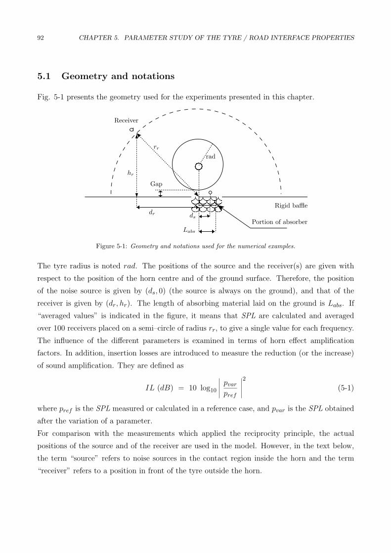
92 CHAPTER 5. PARAMETER STUDY OF THE TYRE / ROAD INTERFACE PROPERTIES
5.1 Geometry and notations
Fig. 5-1 presents the geometry used for the experiments presented in this chapter.
����������������������������
Receiver
rr
Gap
rad
ds
Labs
Rigid baffle
Portion of absorber
hr
dr
Figure 5-1: Geometry and notations used for the numerical examples.
The tyre radius is noted rad. The positions of the source and the receiver(s) are given with
respect to the position of the horn centre and of the ground surface. Therefore, the position
of the noise source is given by (ds, 0) (the source is always on the ground), and that of the
receiver is given by (dr, hr). The length of absorbing material laid on the ground is Labs. If
“averaged values” is indicated in the figure, it means that SPL are calculated and averaged
over 100 receivers placed on a semi–circle of radius rr, to give a single value for each frequency.
The influence of the different parameters is examined in terms of horn effect amplification
factors. In addition, insertion losses are introduced to measure the reduction (or the increase)
of sound amplification. They are defined as
IL (dB) = 10 log10
∣∣∣∣∣ pvar
pref
∣∣∣∣∣2
(5-1)
where pref is the SPL measured or calculated in a reference case, and pvar is the SPL obtained
after the variation of a parameter.
For comparison with the measurements which applied the reciprocity principle, the actual
positions of the source and of the receiver are used in the model. However, in the text below,
the term “source” refers to noise sources in the contact region inside the horn and the term
“receiver” refers to a position in front of the tyre outside the horn.

5.2. GEOMETRICAL PARAMETERS 93
5.2 Geometrical parameters
In this section, the influence of the following parameters is discussed : the position of the source
inside the horn, the position of the tyre height over the reflecting plane of the ground, and the
tyre radius.
Position of the source
First, the influence of the source position inside the horn is investigated. Fig. 5-2 shows horn
effect amplification factors as a function of the distance from the source to the horn centre.
Results are shown for different gap values. A gap value of 0 cm corresponds to the case when
the tyre and the road surface are in contact.
Globally, amplification factors here show the same behaviour as in the presence of rigid surfaces.
As the source moves out of the horn, the maximum amplification decreases and is shifted
towards the low frequencies. Amplification levels decrease with frequency as the absorption
500 1000 1500 20000
5
10
15Gap = 0 cm
500 1000 1500 2000−10
0
10
Frequency (Hz)
Am
plifi
catio
n fa
ctor
s (d
B)
500 1000 1500 20000
5
10
15Gap = 0.8 cm
500 1000 1500 2000−10
0
10
Frequency (Hz)
500 1000 1500 20000
5
10
15Gap = 1.85 cm
500 1000 1500 2000−10
0
10
Frequency (Hz)
Increasing ds
Increasing ds
Figure 5-2: Measured influence of the source position inside the horn for different tyre heights (gap). Top linefigures correspond to sources on the front side of the horn : ds = 4.2 cm, 8.2 cm, 18.2 cm – Bottom line figuresfor sources on the rear side of the horn : ds = -5.8 cm, -11.8 cm – dr = 0.48 m, hr = 0.20 m.

94 CHAPTER 5. PARAMETER STUDY OF THE TYRE / ROAD INTERFACE PROPERTIES
properties of the material increase. The maximum amplification is reached around 500 Hz and
lies around 12 dB, which is quite substantial. For a gap of almost 2 cm, the maximum still lies
around 7 dB for a source very close to the horn centre.
This figure also indicates that the noise sources located on the rear side of the tyre may con-
tribute significantly to the noise perceived in front of the tyre. For a 1.85 cm gap, the ampli-
fication reaches around 5 dB at 500 Hz, which is very close to the amplification value for the
sources located on the front side of the tyre with the same gap. When the sources moves out
of the horn (increasing ds), the amplification levels decrease, as was observed for the sources
placed on the same side of the horn as the receiver.
Position of the reflecting plane
The influence of the tyre height over the reflecting plane is interesting to examine because
rolling on very rough roads leads to lifting the tyre above the reflecting plane of the road.
The influence of this parameter may also be investigated from the measurements shown in
Fig. 5-2. For an increasing gap value between the tyre and the road, the amplification factors
appear to be more influenced when the source is close to the horn centre than when the source
is further out from the horn centre. In fact, for a source at a 18.2 cm distance from the horn
centre (lower amplification curves in the top line figures), the amplification factors are little
influenced by a change in the gap values. If the source is placed at 4.2 cm (larger amplification
curves in the top line figures), the maximum amplification drops from 13 dB when the tyre
and the ground are in contact, to 7 dB for a 1.85 cm gap. This may be explained by the fact
that the change in the horn geometry is more important for a source position close to the horn
centre than when the source is farther out of the horn. For sources on the rear side of the
horn, their contribution increase as the gap increase, especially at frequencies between 600 Hz
to 1200 Hz.
These tendencies are also found at other measurement positions. Results are more cleary shown
in Fig. 5-3(a) in terms of insertion loss. The reference case used here is the smallest gap value,
i.e. 0.8 cm. Thus, negative values correspond to lower SPL when the tyre is further up above
the ground than when the tyre is very close to it. Negative values are found on the whole
frequency range of the measurements for a gap change from 0.8 cm to 1.85 cm.
For a gap change from 0.8 cm to 10.45 cm, negative values are found only between 400 Hz to
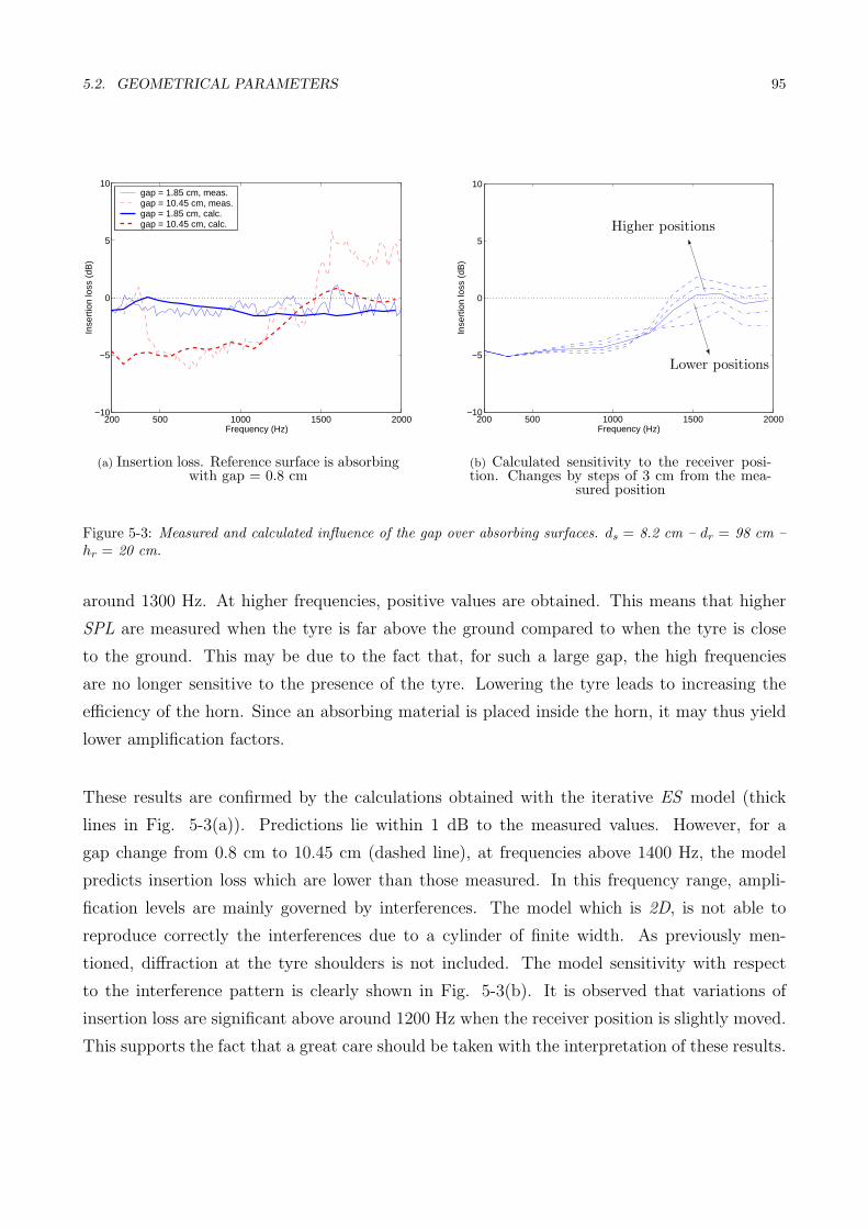
5.2. GEOMETRICAL PARAMETERS 95
200 500 1000 1500 2000−10
−5
0
5
10
Frequency (Hz)
Inse
rtio
n lo
ss (
dB)
gap = 1.85 cm, meas.gap = 10.45 cm, meas.gap = 1.85 cm, calc.gap = 10.45 cm, calc.
(a) Insertion loss. Reference surface is absorbingwith gap = 0.8 cm
200 500 1000 1500 2000−10
−5
0
5
10
Frequency (Hz)
Inse
rtio
n lo
ss (
dB)
(b) Calculated sensitivity to the receiver posi-tion. Changes by steps of 3 cm from the mea-
sured position
Higher positions
Lower positions
Figure 5-3: Measured and calculated influence of the gap over absorbing surfaces. ds = 8.2 cm – dr = 98 cm –hr = 20 cm.
around 1300 Hz. At higher frequencies, positive values are obtained. This means that higher
SPL are measured when the tyre is far above the ground compared to when the tyre is close
to the ground. This may be due to the fact that, for such a large gap, the high frequencies
are no longer sensitive to the presence of the tyre. Lowering the tyre leads to increasing the
efficiency of the horn. Since an absorbing material is placed inside the horn, it may thus yield
lower amplification factors.
These results are confirmed by the calculations obtained with the iterative ES model (thick
lines in Fig. 5-3(a)). Predictions lie within 1 dB to the measured values. However, for a
gap change from 0.8 cm to 10.45 cm (dashed line), at frequencies above 1400 Hz, the model
predicts insertion loss which are lower than those measured. In this frequency range, ampli-
fication levels are mainly governed by interferences. The model which is 2D, is not able to
reproduce correctly the interferences due to a cylinder of finite width. As previously men-
tioned, diffraction at the tyre shoulders is not included. The model sensitivity with respect
to the interference pattern is clearly shown in Fig. 5-3(b). It is observed that variations of
insertion loss are significant above around 1200 Hz when the receiver position is slightly moved.
This supports the fact that a great care should be taken with the interpretation of these results.

96 CHAPTER 5. PARAMETER STUDY OF THE TYRE / ROAD INTERFACE PROPERTIES
200 500 1000 1500 2000−5
0
5
10
15
20
Frequency (Hz)
Am
plifi
catio
n fa
ctor
s (d
B)
Radius = 30 cmRadius = 50 cmRadius = 70 cm
(a) Rigid surface
200 500 1000 1500 2000−5
0
5
10
15
20
Frequency (Hz)
Am
plifi
catio
n fa
ctor
s (d
B)
Radius = 30 cmRadius = 50 cmRadius = 70 cm
(b) Absorbing surface used in the previous mea-surements
Figure 5-4: Horn effect amplification factors for different tyre radii. Averaged values with rr = 3 × rad – Gap= 1 cm – ds = rad/2.
Tyre radius
Another parameter of interest is the influence of the tyre radius on the horn effect sound ampli-
fication. In the presence of an absorbing surface, the problem is to know if a given impedance
surface has the same effect with tyres having different radii.
First, Fig. 5-4(a) shows horn effect amplification factors calculated for different tyre radii
over a rigid surface. Amplification factors obtained over the absorbing surface used in the
previous experiments are shown in Fig. 5-4(b). Results are shown in averaged values obtained
as described in Section 5.1. The distance from the horn centre to the receivers is chosen to be
proportional to the tyre radius so that the distance between the receivers and the tyre surface
is constant. The gap between the tyre and the road is set to 1 cm to keep low calculation times
in the case the surface is absorbing (see the model implementation in Section 4.4).
For the radiation over rigid surfaces (Fig. 5-4(a)), amplification factors increase with increasing
frequency up to a maximum, the position of which depends on the tyre radius : the larger
the tyre radius, the lower the frequency of maximum. In addition, the level of maximum
amplification increase with increasing tyre radii. The maximum of amplification lies around
5.3. GROUND SURFACE IMPEDANCE 97
12 dB at 600 Hz for a 30 cm tyre radius; it exceeds 15 dB at 400 Hz for a 70 cm tyre radius.
At frequencies above this maximum, the amplification levels decrease and become similar for
different tyre radii.
For the tyre radiation over the absorbing surface (see Fig. 5-4(b)), there is no maximum of
amplification; levels decrease along the frequency range examined here. At frequencies below
500 Hz, amplification levels are higher with a larger tyre radius, as over rigid surfaces. This
is due to the fact that the impedance material has very low absorption properties at these
frequencies. Above 500 Hz, a different behaviour is observed. The amplification levels are
lower for larger tyre radii.
In conclusion, the effects of an absorbing plane on the tyre radiation appears to depend on the
tyre radius. At very low frequencies, below around 300 Hz, introducing an absorbing plane may
lead to higher SPL. At frequencies above around 500 Hz, the larger the tyre radius, the larger
the sound reduction.
5.3 Ground surface impedance
This section examines the effects of the presence of an absorbing surface on the tyre radia-
tion. First, the importance of the type of ground inside the horn is discussed. The spatial
re–distribution of sound due to the horn effect is then examined. Numerical examples for vari-
ous geometries are presented for the determination of the ground impedance value which give
the lowest sound amplification.
Ground impedance in the horn region
To be able to control the noise source, it is important to examine the importance of the type of
ground in its vincinity, namely inside the horn region. For this, measurements performed over
surfaces having a rigid and an absorbing portion are compared to measurements performed
over an entirely absorbing surface.
Results are compared in terms of insertion loss as calculated in Eq. 5-1, where the reference
surface is entirely absorbing. Insertion losses are displayed for several distances ds between the
horn centre to the source position. Results are shown in Fig. 5-5(a) for the case where the
tyre is radiating over the rigid ground and the receiver is placed over the absorbing portion.

98 CHAPTER 5. PARAMETER STUDY OF THE TYRE / ROAD INTERFACE PROPERTIES
200 500 1000 1500 2000−20
−10
0
10
20
Frequency (Hz)
Inse
rtio
n lo
ss (
dB)
ds = 4.17 cmds = 8.17 cmds = 12.17 cm
(a) Rigid portion inside the horn andreceiver above absorber
0.19
0.40.58
absorberrigid
0.19
0.40.58
absorber rigid
(b) Geometries
200 500 1000 1500 2000−20
−10
0
10
20
Frequency (Hz)
Inse
rtio
n lo
ss (
dB)
ds = 4.17 cmds = 8.17 cmds = 12.17 cm
(c) Absorber inside the horn and re-ceiver above rigid portion
Figure 5-5: Measured influence of the impedance of the ground inside the horn. Reference surface is entirelyabsorbing. Results for different source positions inside the horn – Gap = 0.8 cm.
In Fig. 5-5(c), the reverse situation is examined, that is when the tyre is over the absorbing
surface and the receiver is placed over the rigid portion. The exact corresponding geometries
are shown in Fig. 5-5(b). In both situations, the impedance surface lying inside the horn is
prolongated up to 60 % of the total distance from the horn centre to the receiver.
It is observed in these two figures that the insertion losses are almost always positive, which
means that an entirely absorbing surface yields lower amplification factors compared to when
the surface is only partially treated. However, this trend, clear in Fig. 5-5(a), is less pronounced
when the tyre is radiating directly over the absorbing portion. In this latter case, the situation
is worsened only by a few decibels compared to when the surface is entirely absorbing. This
means that the main part of the noise reduction is achieved by controlling the impedance in
the horn region as expected. This corresponds to controlling the radiation impedance of the
noise source inside the horn.
Moreover, positive values of insertion loss are found below around 600 Hz for the tyre radiating
over the rigid portion (see Fig. 5-5(a)). This is somehow surprising because it means that the
sound amplification when the ground surface inside the horn is rigid is lower than when it is
absorbing.
This tendancy is also displayed by the calculations obtained with the iterative ES model. Fig.
5-6 shows that the amplifications factors calculated over an entirely absorbing surface may
exceed those obtained over a rigid surface at low frequencies. However, the frequency, at which
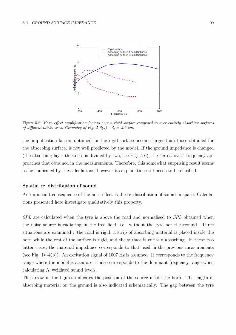
5.3. GROUND SURFACE IMPEDANCE 99
200 400 600 800 10000
5
10
15
20
Frequency (Hz)
Am
plifi
catio
n fa
ctor
s (d
B)
Rigid surface Absorbing surface 1.6cm thicknessAbsorbing surface 0.8cm thickness
Figure 5-6: Horn effect amplification factors over a rigid surface compared to over entirely absorbing surfacesof different thicknesses. Geometry of Fig. 5-5(a) – ds = 4.2 cm.
the amplification factors obtained for the rigid surface become larger than those obtained for
the absorbing surface, is not well predicted by the model. If the ground impedance is changed
(the absorbing layer thickness is divided by two, see Fig. 5-6), the “cross–over” frequency ap-
proaches that obtained in the measurements. Therefore, this somewhat surprising result seems
to be confirmed by the calculations; however its explanation still needs to be clarified.
Spatial re–distribution of sound
An important consequence of the horn effect is the re–distribution of sound in space. Calcula-
tions presented here investigate qualitatively this property.
SPL are calculated when the tyre is above the road and normalised to SPL obtained when
the noise source is radiating in the free–field, i.e. without the tyre nor the ground. Three
situations are examined : the road is rigid, a strip of absorbing material is placed inside the
horn while the rest of the surface is rigid, and the surface is entirely absorbing. In these two
latter cases, the material impedance corresponds to that used in the previous measurements
(see Fig. IV-4(b)). An excitation signal of 1007 Hz is assumed. It corresponds to the frequency
range where the model is accurate; it also corresponds to the dominant frequency range when
calculating A–weighted sound levels.
The arrow in the figures indicates the position of the source inside the horn. The length of
absorbing material on the ground is also indicated schematically. The gap between the tyre

100 CHAPTER 5. PARAMETER STUDY OF THE TYRE / ROAD INTERFACE PROPERTIES
and the ground is set to 1 cm to keep low calculation times.
Results are presented in decibels where white colors, resp. dark colors, indicate high amplifi-
cation levels, resp. low amplification levels.
Over a totally rigid surface (see Fig. 5-7), the sound is mainly directed in front and in the
rear side of the tyre. Due to the susbtantial gap value used here, sound levels are very similar
on both sides of the contact zone. High amplification levels are found, as expected, in the
horn and close to the ground. As the receiver height increases, the levels decrease. A shadow
zone appears clearly above the tyre. In this region, interferences appear, the pattern of which
depends on the frequency of the excitation signal. The lowest levels of amplification are found
in this region.
When a strip of absorbing material is introduced inside the horn, Fig. 5-8 shows amplification
levels which are globallly lower than for a rigid surface. The highest amplification levels are still
found in the horn region and close to the surface. In front of the tyre amplification levels are
only slightly lower than for a rigid surface. However, a significant decrease is observed on the
rear side of the tyre. Above the tyre, the interference pattern previously observed is modified.
First, it is “rotated” towards the rear side of the tyre. Secondly, in contrast to the rigid case,
the most contrasted interferences are not found opposite to the source position with respect to
the tyre; they are shifted towards the rear side of the tyre.
If the surface is now entirely absorbing (see Fig. 5-9), the directivity of the horn effect is
practically the same as for the rigid surface. However, the amplification levels are significantly
lower in the case the surface is absorbing. As previously, the maximum levels are found inside
the horn and close to the ground surface. In contrast to the two previous situations, amplifi-
cation levels decrease more rapidly as the receiver moves away from the horn, but still close
the ground. The interference pattern observed above the tyre seems to be inverted compared
to the rigid case : an increase is observed for the absorbing surface where there was a decrease
for the rigid surface, and vice versa. One should keep in mind that the distribution of sound
in this region is important because of the presence of the wheelhouse of the tyre.

5.3. GROUND SURFACE IMPEDANCE 101
Figure 5-7: Map of relative SPL over a rigid surface. f = 1007 Hz – gap = 1 cm – ds = 5 cm – The arrowindicates the position of the noise source – The scale is in dB.
� � �� � �� � �� � �
Figure 5-8: Map of relative SPL over a strip of absorbing material. Labs = 20 cm – Zn = 720 − 1226j – f =1007 Hz – gap = 1 cm – ds = 5 cm – The arrow indicates the position of the noise source – The scale is in dB.
� � � � � � � � � � � � � � � � � � � � � � � � � � �� � � � � � � � � � � � � � � � � � � � � � � � � � �� � � � � � � � � � � � � � � � � � � � � � � � � � �� � � � � � � � � � � � � � � � � � � � � � � � � � �
Figure 5-9: Map of relative SPL over an entirely absorbing surface. Zn = 720− 1226j – f = 1007 Hz – gap =1 cm – ds = 5 cm – The arrow indicates the position of the noise source – The scale is in dB.
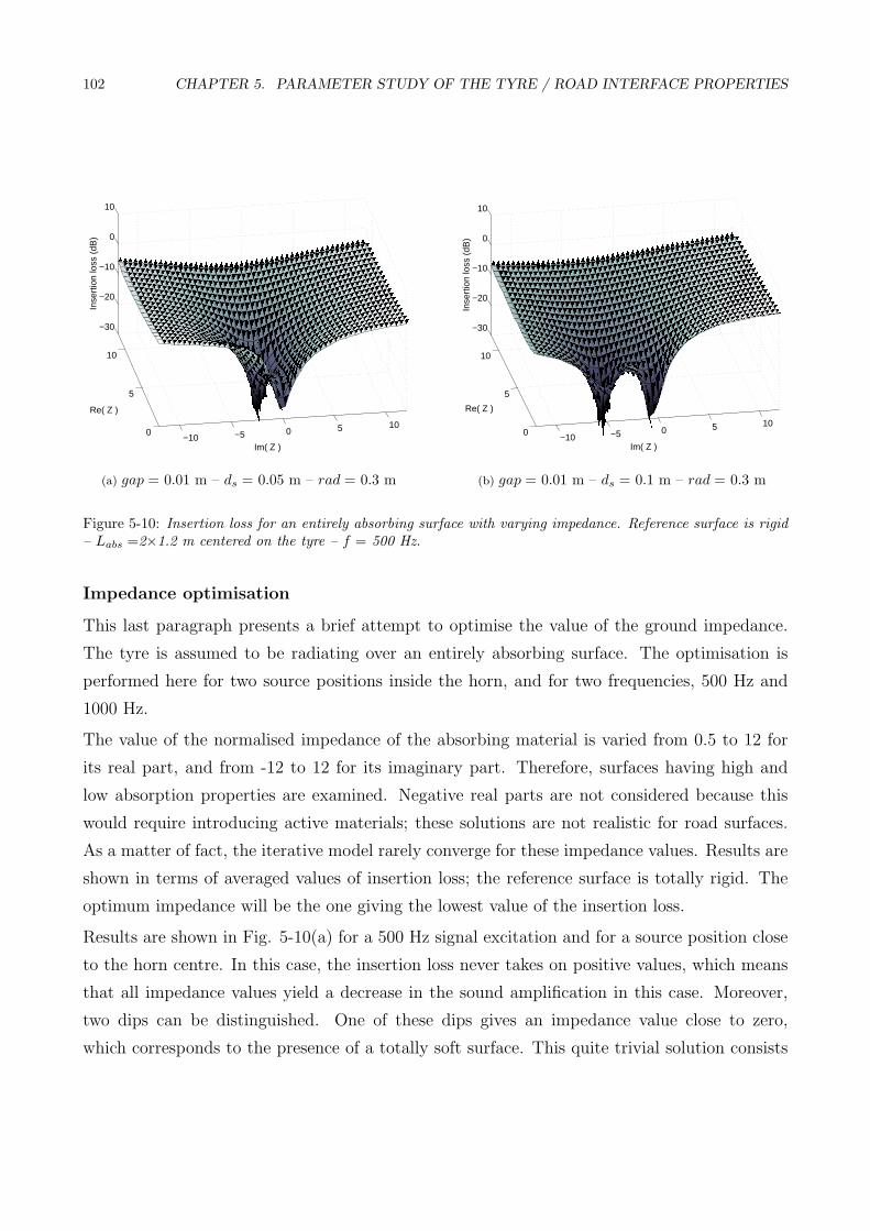
102 CHAPTER 5. PARAMETER STUDY OF THE TYRE / ROAD INTERFACE PROPERTIES
−10 −5 0 5 100
5
10
−30
−20
−10
0
10
Im( Z )
Re( Z )
Inse
rtio
n lo
ss (
dB)
(a) gap = 0.01 m – ds = 0.05 m – rad = 0.3 m
−10 −5 0 5 100
5
10
−30
−20
−10
0
10
Im( Z )
Re( Z )
Inse
rtio
n lo
ss (
dB)
(b) gap = 0.01 m – ds = 0.1 m – rad = 0.3 m
Figure 5-10: Insertion loss for an entirely absorbing surface with varying impedance. Reference surface is rigid– Labs =2×1.2 m centered on the tyre – f = 500 Hz.
Impedance optimisation
This last paragraph presents a brief attempt to optimise the value of the ground impedance.
The tyre is assumed to be radiating over an entirely absorbing surface. The optimisation is
performed here for two source positions inside the horn, and for two frequencies, 500 Hz and
1000 Hz.
The value of the normalised impedance of the absorbing material is varied from 0.5 to 12 for
its real part, and from -12 to 12 for its imaginary part. Therefore, surfaces having high and
low absorption properties are examined. Negative real parts are not considered because this
would require introducing active materials; these solutions are not realistic for road surfaces.
As a matter of fact, the iterative model rarely converge for these impedance values. Results are
shown in terms of averaged values of insertion loss; the reference surface is totally rigid. The
optimum impedance will be the one giving the lowest value of the insertion loss.
Results are shown in Fig. 5-10(a) for a 500 Hz signal excitation and for a source position close
to the horn centre. In this case, the insertion loss never takes on positive values, which means
that all impedance values yield a decrease in the sound amplification in this case. Moreover,
two dips can be distinguished. One of these dips gives an impedance value close to zero,
which corresponds to the presence of a totally soft surface. This quite trivial solution consists

5.3. GROUND SURFACE IMPEDANCE 103
−10 −5 0 5 100
5
10
−30
−20
−10
0
10
20
Im( Z )
Re( Z )
Inse
rtio
n lo
ss (
dB)
(a) gap = 0.01 m – ds = 0.05 m – rad = 0.3 m
−10 −5 0 5 100
5
10
−30
−20
−10
0
10
20
Im( Z )
Re( Z )
Inse
rtio
n lo
ss (
dB)
(b) gap = 0.01 m – ds = 0.1 m – rad = 0.3 m
Figure 5-11: Insertion loss for an entirely absorbing surface with varying impedance. Reference surface is rigid– Labs =2×1.2 m centered on the tyre – f = 1000 Hz.
in reducing the radiation impedance of the source inside the horn. The second dip gives an
impedance which has a negative imaginary part and a positive real part. Due to the time
dependence in the model as e+jωt, this is the impedance value of a low damped spring.
If the noise source is moved further out of the horn (see Fig. 5-10(b)), besides zero impedance,
an optimum impedance value is found, which has a lower real part and a higher negative imag-
inary part compared to the previous situation. In total, this impedance has a larger magnitude
than that found previously. The physical behaviour of such a surface would correspond to a
spring, which would be less damped and have a higher stiffness compared to that found for the
previous source position.
For a 1000 Hz excitation signal, the predicted insertion losses shown in Fig. 5-11(a) for a 1
cm gap present two minima, one of which corresponds to zero impedance. The other value of
the optimum impedance has a real part different from zero, though very small, and a negative
imaginary part. Again, this would physically imply the presence of springs with very little
damping on the surface.
If the source is moved further away from the horn centre (see Fig. 5-11(b)), the picture changes
considerably : insertion losses are now positive for most impedance values, except for a zero

104 CHAPTER 5. PARAMETER STUDY OF THE TYRE / ROAD INTERFACE PROPERTIES
impedance value. For most impedance values, the increase is about 10 dB, which is quite sub-
stantial. This means that for such a system geometry, the presence of an absorbing material
would lead to around a 10 dB amplification increase compared to the same system over rigid
surfaces, unless this material has zero impedance value. This example shows that the optimi-
sation of the acoustical properties of the ground surface is very sensitive to the exact geometry
of the tyre / road interface.
Therefore, for most of the geometries examined here, the model predicts two impedance values,
which give a substantial reduction of sound. One optimum impedance value corresponds to a
totally soft surface, and the second one corresponds to a material having the characteristics of
a low damped spring. These surfaces may be difficult to realise in practice because it is arduous
to control the impedance value of the surface on large portion of roads.
5.4 Geometrical and acoustical combined effects
It has been shown in the previous section that the only impedance optimisation could lead to
solutions, which may be difficult to realize and to maintain for real road surfaces. Therefore, it
is proposed in this section to examine the combined effects of the tyre height above the physical
reflecting plane and the presence of an absorbing material. This would correspond in reality to
very rough roads having substantial absorption properties, a solution which has already been
tested in reality.
Results are shown in Fig. 5-12 in terms of insertion loss with the reference surface as rigid
with a 5 mm gap. The impedance value of the absorbing material used here corresponds to
the material used in the previous experiments (see Fig. IV-4(b)). In addition, insertion losses
calculated over rigid surfaces by varying the gap only are shown in the same figure (thin lines),
to estimate the influence of the absorption. The same reference surface is used in this case.
At frequencies below around 400 Hz, positive value of the insertion loss are found, whereas
the gap increase over rigid surfaces lead to a decrease in the sound amplification. This result
coincides with the result observed in Fig. 5-5(a) which has not been clarified. Beyond this
frequency, the decrease in sound amplification is important. At 500 Hz for instance, the insertion
loss is around -2 dB for rigid surfaces. The additional effects of the ground impedance make

5.5. SUMMARY 105
200 500 1000 1500 2000−25
−20
−15
−10
−5
0
5
Frequency (Hz)
Inse
rtio
n lo
ss (
dB)
gap = 1 cmgap = 1.5 cmgap = 2 cm
Figure 5-12: Combined effects of the tyre height and surface impedance on tyre radiation. Averaged values ofinsertion loss. Reference surface is rigid with 5 mm gap – Solid lines : gap effect only – Thick lines : gap +impedance effect – ds = 0.05 m – rad = 0.3 m
this value drop to -6 dB. The decrease of the insertion loss along the frequency also correponds
to increasing absorption properties of the surface modelled here. Insertion losses for all gap
changes drop to -15 dB around 1000 Hz. Note that this reduction is achieved even with a 5
mm increase of the tyre height over the road reflecting plane. At 2000 Hz, the decrease lies
between -20 dB to -25 dB for 1 cm and 1.5 cm gap increases.
Although these examples do not consider the practical attainability, they show that a substan-
tial noise reduction may come from the combined effects of the acoustical and the geometrical
properties of the tyre road interface.
5.5 Summary
This chapter presents a brief parameter study of the tyre / road interface properties. The
discussion is based on measurements and on calculations obtained using the model presented
in Chapter 4. Due to its low computational demands, this model appears to be a convinient
tool for such parametrical studies.
The influence of the geometrical parameters on the tyre radiation is first discussed.
As for rigid surfaces, the position of the source inside the horn determines to a large extent
the level of sound amplification for absorbing surfaces. As the source moves out of the horn,
amplification levels decrease and the frequency of maximum amplification is shifted towards

106 CHAPTER 5. PARAMETER STUDY OF THE TYRE / ROAD INTERFACE PROPERTIES
low frequencies. This also holds for sources placed on the rear side of the horn.
As expected, the contribution from the sources on the rear side of the tyre increases with an
increasing gap. For sources on the front side of the tyre, increasing the tyre height leads to a
decrease in sound amplification on the whole frequency range. This tendency is well predicted
by the iterative ES model.
The influence of the tyre radius is also investigated using the model. For rigid surfaces, tyres
having larger radii give higher sound amplification at low frequencies. The frequency of max-
imum amplification is shifted towards lower frequencies as the tyre radius increases. Above
this frequency, i.e. around 600 Hz, amplification levels appear to be independent on the radius.
The picture is slightly different for the radiation over the absorbing surface. At low frequencies,
the same tendency as for rigid surfaces is observed due to the low absorption properties of the
impedance material. In the mid and high frequency range, the amplification levels are lower
for larger tyre radii.
The influence of the ground impedance on the radiation is also discussed from measurements
and from model calculations.
It is shown from the measurements that the sound attenuation due to the presence of an entirely
absorbing surface is mainly governed by the ground impedance which lies inside the horn. This
result could be expected as it consists in controlling the radiation impedance of the noise source.
Measurements also show that amplification levels at low frequencies could be higher over an
absorbing surface compared to a rigid surface. This result is confirmed by the calculations but
it has not been clarified.
The model allows one to investigate the re–direction of sound due to the horn effect. It is shown
that the horn effect over a homogeneous surface leads to a concentration of sound in front and
on the rear side of the tyre. However, the amplification levels are significantly lower in the
case the surface is absorbing than when the surface is rigid. In addition, amplification levels
decrease more rapidly as the receiver moves away from the horn over an absorbing surface than
over a rigid surface. Interferences occuring above the tyre, i.e. opposite to the contact zone,
are also substantially modified in the presence of an absorbing surface.
Some guidelines for the optimisation of the surface impedance are also given. By construction,
the ES model is independent of the type of ground impedance. Therefore, besides impedances
corresponding to active materials, any impedance value could be implemented in the model.

5.5. SUMMARY 107
The model predicts two impedance values which could give a substantial reduction of the sound
amplification. One of these is zero impedance, which corresponds to a totally soft surface. The
second value of impedance corresponds to a low damped spring. The calculations also prove
that the impedance value depends on the exact geometry of the tyre / road interface.
Finally, model calculations show that an efficient sound reduction is achieved by combining
the tyre height and the impedance of the road surface. This solution corresponds to surfaces
having a large roughness amplitude together with substantial absorption properties.

108 CHAPTER 5. PARAMETER STUDY OF THE TYRE / ROAD INTERFACE PROPERTIES
Chapter 6
Conclusions
Main results
The work presented in this thesis is motivated by the needs to understand and to control the
radiation mechanisms of tyre noise. The objective was to design a numerically efficient model
for the tyre radiation over impedance surfaces. The thesis describes the work in five chapters.
Chapter 1 presents the main sources of traffic noise. Under normal driving conditions, tyre /
road noise is predominant at driving speeds from 50 to 70 km/h for light vehicles or trucks.
The models for the prediction of tyre noise are reviewed and classified in three categories : the
statistical models, the hybrid models and the deterministic approaches. Whereas the models of
the two first groups are mainly addressed to the prediction of A–weighted noise levels, models
of the last group allows to optimise the properties of the tyre / road interface.
Deterministic approaches require the modelling of the tyre dynamics, the tyre / road contact
and the tyre radiation. In particular, 2D radiation models give lower computational times
compared to 3D models, but they give an overestimation of the horn effect sound amplification
at low frequencies. Hence, they are only accurate at frequencies above around 600 Hz.
Because the road absorption affects both the generation and the radiation of noise, it is im-
portant to take these effects into account. Therefore, Chapter 1 presents a review of the main
impedance models. The different techniques to include the ground effects into a model for
the tyre radiation are then discussed. Among these techniques, the integral equation–based
methods handle any arbitrary incident sound field, which is a prerequisite for handling the field
radiated by a vibrating tyre. In addition, these techniques can deal with homogeneous as well
as inhomogeneous grounds.
Therefore, to achieve the fixed objectives, the approach presented in this thesis chooses to com-
bine the numerical efficiency of a 2D radiation model to an integral equation–based method to
109

110 CHAPTER 6. CONCLUSIONS
include the ground effects.
In Chapter 2, a model for the tyre radiation, which has been derived in [Kropp 1992], is
implemented on the basis of the ES method. Using the basic properties of vibrating cylinders,
it is shown that low order modes are responsible for the major part of the radiated sound.
In fact, comparisons with a BE code prove that the deviations observed between the measure-
ments and the calculations at frequencies below 600 Hz, are due to the 2D simplifications of the
model. In the mid–frequency range and at higher frequencies, the levels and the interference
pattern of horn effect amplification factors are correctly predicted. Moreover, this multipole
model is shown to be numerically of advantage compared to BE methods. However, the ES
model does not include correctly the acoustical properties of the road surface.
To model the influence of the ground effects on the tyre sound field, a method which can handle
arbitrary sound sources is presented in Chapter 3. Based on the ES method, it is mainly an
alternative to standard integral equation methods. The technique proposed here consists in
placing physical sources directly at the ground to control the value of the acoustical impedance
at the surface. The main feature of this approach is that the impedance value is controlled
point–wise, which means that the model is able to handle any type of ground impedances.
Numerical examples prove this model to be accurate in the case of arbitrary order sources
radiating over a homogeneous impedance plane. In addition, comparisons with measurements
for homogeneous and inhomogeneous surfaces extend the validity of this approach to arbitrary
impedance distributions.
Subsequently, a model for the tyre radiation over impedance surfaces is developed in Chapter
4. As an introduction, the exact solution to the problem of an arbitrary order source radiating
over an impedance plane is derived. The computation of the solution is, however, subject to
numerical difficulties; it will be examined in future works. The model for the tyre radiation
over impedance surfaces is developed using the ES method, on the basis of the models derived
in the two previous chapters.
Therefore, the effects of impedance discontinuities are included in this model. The method is
also original in that the source strengths are determined through an iterative process, which is
computationally effortless.
111
This approach is validated by comparisons of horn effect amplification factors measured over
homogeneous and inhomogeneous surfaces. It is shown that this iterative ES model is accurate
at frequencies above around 600 Hz, which corresponds to the frequency range of validity of
the multipole model presented in Chapter 2.
Finally, Chapter 5 presents a parametrical study of the properties of the tyre / road interface.
This study is based on measurements and calculations using the previous iterative model. The
influence of geometrical parameters such as the source position inside the horn, the gap between
the tyre and the ground or the tyre radius, is examined and discussed. The influence of the
type of ground impedance on the sound amplification is also examined.
In particular, measurements and calculations show that at low frequencies, the sound ampli-
fication for absorbing surfaces may exceed that produced for rigid surfaces. This result has
not been clearly explained. It is also shown that combining both acoustical and geometrical
parameters of the road surface may substantially decrease the sound amplification compared
to the optimisation of one of these two parameters only.
Moreover, due to its low computational time, this model is proved to be adapted for the opti-
misation of the ground impedance. Calculations show however that the value of the impedance
which gives the lowest sound amplification is very sensitive to the exact geometry of the tyre /
road interface.
Perspectives and future work
The work presented in this thesis ends up with an efficient model for the tyre radiation over
arbitrary impedance surfaces. A brief parameter study is presented in Chapter 5. A more
thorough examination of the tyre radiation conditions is needed in order to fully understand
the mechanisms of noise emission.
This iterative ES model is aimed to be integrated to a complete model for prediction of tyre
/ road noise. The next step is thus to use real tyre data together with real road surface data,
to predict tyre / road noise over road surfaces having substantial absorption properties. As
proved in the last chapter of the thesis, this model can be used for the optimisation of the tyre
/ road interface properties. Constrains related to the tyre and the road construction could thus
be included to yield realistic solutions.
112 CHAPTER 6. CONCLUSIONS
The major drawback of tyre radiation model presented here is its 2D character. To predict
pass-by noise levels, a 3D model is required. It could be developed using the ES method after
numerical tests have been performed to optimise the system of sources placed inside the tyre
body.
The present ES model could also be coupled to other existing ES models to include the pres-
ence of elastic objects in the neighbourhood of the tyre, such as the wheelhouse. These objects
may modify significantly the field radiated by the tyre either by changing its directivity or by
contributing directly to the sound field. These effects could be modelled using the ES method
by placing sources inside the vibrating objects. This model could be implemented in a similar
way as the iterative ES model presented in this thesis.
Finally, the computation of the reflection coefficient for cylindrical waves presented in Chapter 4
will be further examined. The interesting feature of the proposed approach is that the solution
is expressed as a function of the order of the source, among other parameters. This solution is
particularly adapted to traffic noise prediction purposes, the models of which could thus include
the so far omitted, directivity of the noise source.
Chapter 7
Appendices
Appendix I . . . . . . . . . . . . The Equivalent Sources (ES) methodTheoretical basis – Numerical implementation – Applications
Appendix II . . . Complements on the tyre boundary conditionExpression of the radiation hypothesis – Boundary velocity in theradiation hypothesis – Comparisons of horn effect predictions
Appendix III . . . . . . . . . . . Integration over the Green functions’singularitiesValidity of the derivation – Pressure Green function – Velocity Greenfunction
Appendix IV . . . . . . . . . .Experimental determination of surfaceimpedanceKundt’s tube measurements – Level difference technique
113

114 CHAPTER 7. APPENDICES
Appendix I The Equivalent Sources (ES) method
The so–called equivalent sources (ES ) method is successfully applied to various situations in
this thesis. The present appendix aims at establishing a common framework for the functioning
and the field of application of this method. Found in the literature under various names, this
technique is an alternative to integral equations–based methods, for the radiation and the
scattering of sound from objects of arbitrary shape.
The theoretical basis of the method is first presented. Then, some critical considerations
concerning the numerical implementation of the method are drawn up based on the author’s
experience and on other works in other fields of application. A review of these latter works
completes this appendix.
Theoretical basis
The ES method has been developed independently by many researchers, which explains the
fact that several names are given to the same approach in the literature : the source simulation
technique, the auxiliary sources method, the substitute sources method, etc. This technique
is not restricted to the field of acoustics; for instance, the method is the subject of numerous
works in electromagnetics, a good review of which can be found in [Kaklamani 2002].
In the field of acoustics, the theoretical derivation of this technique as well as its physical inter-
pretation can be found in [Bobrovniskii 1980; Ochmann 1995, 2000; Song 1991], among many
others. As shown in [Koopmann 1989], the ES method is totally equivalent to standard BE
approaches. Therefore, the ES method should be mainly seen as a computationally efficient,
~n
Be
q
xr
∂B
Bi
Figure I-1: Typical geometry for an exterior radiation problem. The gray area represents the source distributioninside the vibating body.

APPENDIX I. THE EQUIVALENT SOURCES (ES) METHOD 115
alternative to BE techniques1.
The basic idea of this technique is that the radiation of sound due to an arbitrarily shaped
vibrating body can be reproduced by a set of acoustic sources placed inside its volume, provided
that these sources fulfil a prescribed boundary condition on the body surface.
Given a vibrating object of arbitrary shape, its interior volume is called Bi. The body surface
∂B represents the frontier with the exterior “free space” domain Be. The situation is depicted
in Fig. I-1. The time dependency of the pressure obeys e+jωt. Therefore at a given frequency
f , the pressure p at a receiving point xr of the free space due a volume source at ξ satisfies the
homogeneous Helmholtz equation
∆p(xr) + k2p(xr) = 0
where k = 2πf/c is the wave number and c is the speed of sound in Be. Only outoing waves are
of interest here, therefore the solutions of the equation above should also satisfy the Sommerfeld
radiation conditions, which express the quite natural concept that “the infinite is absorbent”.
This latter condition is expressed as
limr→∞
[√
r
(∂p(r)
∂r+ jkp(r)
)]= 0 with r =| xr − ξ |
In practical terms, this ensures that no other sources are present outside the volume Bi.
The solutions to the two above equations are solutions to the exterior radiation problem; they
can be written in the form of the Kirchoff-Helmholtz integral equations :
∮∂B
(p(η)
∂g(η | xr)
∂n− g(η | xr)
∂p(η)
∂n
)dη =
0 if xr ∈ Bi
pe(xr)/2 if xr ∈ ∂B
pe(xr) if xr ∈ Be
where η describes the surface ∂B and g(η | xr) denotes the free space Green function of the
problem. According to the above equation, the pressure pe at a point x of Be is the superposi-
tion of an infinite number of contributions due to a continuous layer of sources placed directly
on the border ∂B. Note at this point that a straightforward numerical implementation of the
above equation would yield the standard boundary element (BE ) method.
1The reader interested in an in–depth mathematical discussion of the method basis should refer to [Krutitskii2003].

116 CHAPTER 7. APPENDICES
Let us now examine the interior radiation problem. A distribution of sources q(xi) is located in
Bi, that is inside the vibrating body. The solution of the inhomogeneous Helmholtz equation
is now given as
−∫Bi
q(ξ)g(x|ξ) dξ−∮
∂B
(p(η)
∂g(η | xr)
∂n− g(η | xr)
∂p(η)
∂n
)dη =
pi(xr) if xr ∈ Bi
pi(xr)/2 if xr ∈ ∂B
0 if xr ∈ Be
Moreover, the surface integral for the interior radiation problem equals the surface integral for
the exterior radiation problem. By combining the two previous equations for a receiver xr in
Be, one obtains
pe(xr) = −∫Bi
q(ξ) g(ξ | xr) dξ
This equation shows that the pressure in the free space can be reproduced by a distribution
of volume sources inside the vibrating body. To be able to replicate the radiation pattern of
the object correctly, additional boundary conditions must be given. The boundary condition
can be of any type : Dirichlet, Neumann or Robin boundary condition. As a consequence, the
solution to this boundary value problem is unique. Furthermore, this solution is exact provided
that the boundary condition is exactly fulfilled.
From the numerical point of view, the boundary condition is always fulfilled within a confi-
dence interval, the choice of which might influence the accuracy of the prediction. Moreover,
the theoretical derivation presented above does not provide any information concerning the
placement of discrete sources inside the volume Bi. These open questions are discussed in the
next paragraph.
Numerical implementation
The great advantage of the ES method is that it can deal with vibrating objects of an arbitrary
shape, where standard BE codes become quite cumbersome [Ochmann 1980]. For instance,
works in [Miller 1991] showed that the ES method is always more efficient numerically than
BE methods. It should be underlined that these two approaches are equivalent, as shown in
[Koopmann 1989]. However, contrary to BE methods, it has no global criteria to ensure the
accuracy of the results. Hence only a few rules of thumb can be outlined.
The first step when implementing the method is to choose the geometry of the source system,
i.e. the shape of the so–called auxiliary surface and the type of sources. These two parameters

APPENDIX I. THE EQUIVALENT SOURCES (ES) METHOD 117
are strongly dependent on each other : the placement of a given source should account for its
radiation properties (importance of the near field, directivity, shape of the wave front, . . . ).
Often, the “trial and error” technique is the only way of assessing the source system and this
may become exhaustive for objects of large dimensions or very complex shape.
Discussions presented, for instance in [Machens 1999], try to draw out some global rules for
the functioning of the ES method. As a general trend, the use of high order sources is only
recommended when the object has a regular geometry. For instance, in the case of a radiating
tyre, which has an axis of symmetry around its center, the use of a high order multipole located
at its centre appears quite natural. For objects having a narrow geometry or sharp profile like
a thin noise barrier or a vibrating plate, the choice of low order sources seems better adapted.
Because high order sources have a strong near field, they should be placed at approximately
equal distances from all parts of the boundary. If this is not the case, the resulting equation
system becomes ill-conditioned and the solutions cease to be accurate.
In order to be complete, one should mention that the work presented in [Papakanellos 2001]
proposes to optimise the placement the auxiliary sources according to the complex image theory.
Developed for electromagnetic purposes, this theory, which could be extended to acoustics [Li
1996], states that the optimal position of the mirror image source is a function of the dissipation
at the surface [Weaver 1971]. However, this approach has not been investigated in the present
thesis because of the alternative approach presented in Chapter 3, which consists in placing the
auxiliary sources directly on the surface.
If the situation does not allow the fulfilment of these general requirements, the use of regular-
isation techniques such as those reviewed in [Nelson 1999] can stabilize the equation system.
Such techniques have mainly been developed for the purpose of pressure field reconstruction by
inverse methods, like the Singular Value Decomposition [Press et al. 1986] (see Chapter 2). For
the specific use of the ES method, the use of the Tikhonov’s technique was proposed in [Kress
1986]. Ochmann in [Ochmann 1999] further extends the use of weighting functions originally
proposed in [Cremer 1988], to handle non-full rank systems.
Once the source system is chosen and optimally placed, there is still no guarantee that the
prediction of the radiation will converge towards the true field. Although the convergence of
the method has been proven theoretically, it was shown in [Machens 1999] that the deviations
in the field predictions are not directly related to the error made on the boundary. In other
words, the boundary condition can be entirely fulfilled although this will not ensure that the

118 CHAPTER 7. APPENDICES
pressure field is correct. The validity of the modelisation should therefore be confirmed by
measurements or comparisons with finite element methods.
Applications
Given the above restrictions, the ES method can be applied to various situations. The review
below is not exhaustive; it tries to give the reader an overview of the different field of applications
of this technique.
In the field of traffic noise prediction, the following applications can be found in the literature.
For instance, works presented in [Ogren 2002] propose a model for the propagation of sound
from one street to another in a city environment. Due to its numerical efficiency, the ES method
can be applied to optimise the acoustical treatment of noise barriers, as shown in [Thorsson
2000]. The ES method has also been applied to outdoor propagation problems to include
the ground effects [Becot 2002] or the meteorological effects [Forssen 2000, 2002]. An original
application can be found in [Kropp 1998, 2000a] for the transmission of exterior sound across
balcony openings to the inside of apartments.
A large number of studies refer to the ES method to model the radiation sound from vibrating
structures. The accuracy of the method was proved in the case of a vibrating tyre [Klein 1998;
Kropp 2000b]. The method was also shown to be of advantage compared to pure BE models
to predict the radiation of vibrating objects having complex vibration patterns [Holste 1997;
Tomilina 1993; Too 2001] or for structures made of several parts [Bobrovniskii 1995]. It was also
proved that the method is efficient to model the scattering of sound in open spaces [Bouchet
2000] or in enclosures [Johnson 1998]. In particular, the ES method can accurately model the
scattering of sound from objects with sharp corners [Anastassiu 2002; Karamehmedovic 2001],
cases which are often difficult to solve with pure BE approaches. This latter study even showed
that losses at the object surface could be included in these cases using the ES method.
Another field of application concerns the reconstruction of acoustic pressure or velocity fields
on the surface of vibrating objects [Magalhaes 2001; Wang 1997]. Because of its flexibility con-
cerning the placement of the equivalent sources, the ES method seems particularly convinient
to be used together with the experimental technique of acoustical holography [Williams 2001].
Finally, the time domain formulation presented in [Kropp 1995] widens the already large field
of application of this approach.

APPENDIX I. THE EQUIVALENT SOURCES (ES) METHOD 119
In conclusion, the ES method appears to be an efficient alternative to pure BE codes in many
situations. With regards to the lack of rigorous criteria for the accuracy of the solution, this
may be overcome by the experience of the user or by the study of related works, e.g. in
electromagnetics.
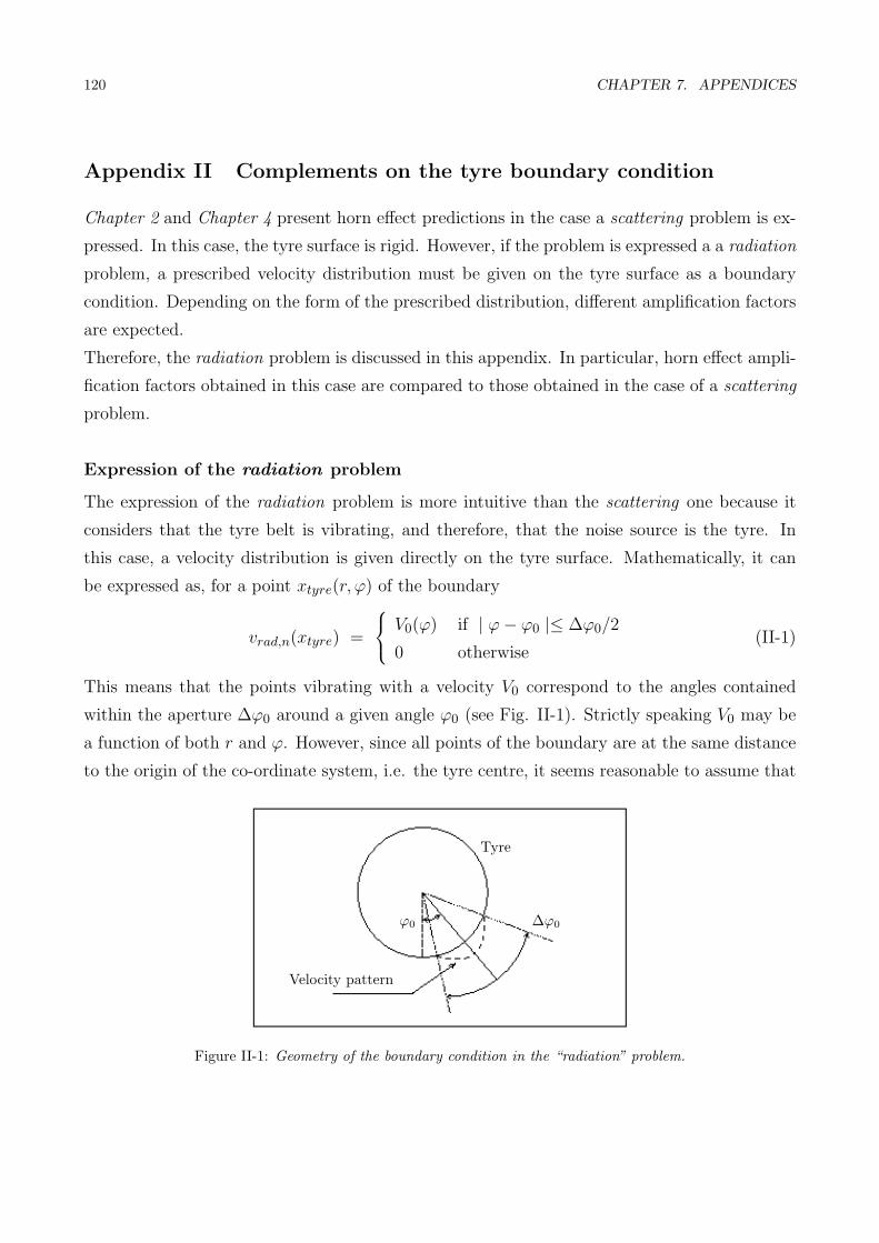
120 CHAPTER 7. APPENDICES
Appendix II Complements on the tyre boundary condition
Chapter 2 and Chapter 4 present horn effect predictions in the case a scattering problem is ex-
pressed. In this case, the tyre surface is rigid. However, if the problem is expressed a a radiation
problem, a prescribed velocity distribution must be given on the tyre surface as a boundary
condition. Depending on the form of the prescribed distribution, different amplification factors
are expected.
Therefore, the radiation problem is discussed in this appendix. In particular, horn effect ampli-
fication factors obtained in this case are compared to those obtained in the case of a scattering
problem.
Expression of the radiation problem
The expression of the radiation problem is more intuitive than the scattering one because it
considers that the tyre belt is vibrating, and therefore, that the noise source is the tyre. In
this case, a velocity distribution is given directly on the tyre surface. Mathematically, it can
be expressed as, for a point xtyre(r, ϕ) of the boundary
vrad,n(xtyre) =
V0(ϕ) if | ϕ− ϕ0 |≤ ∆ϕ0/2
0 otherwise(II-1)
This means that the points vibrating with a velocity V0 correspond to the angles contained
within the aperture ∆ϕ0 around a given angle ϕ0 (see Fig. II-1). Strictly speaking V0 may be
a function of both r and ϕ. However, since all points of the boundary are at the same distance
to the origin of the co-ordinate system, i.e. the tyre centre, it seems reasonable to assume that
Velocity pattern
Tyre
ϕ0 ∆ϕ0
Figure II-1: Geometry of the boundary condition in the “radiation” problem.
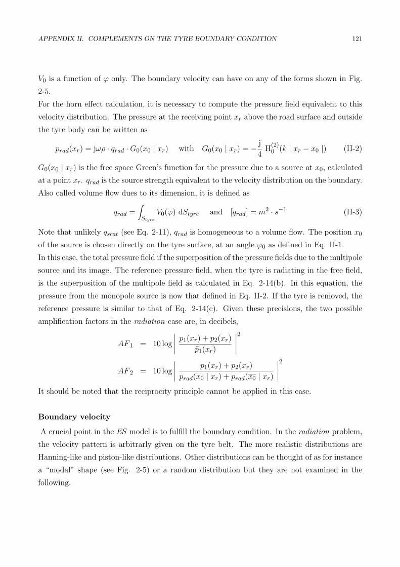
APPENDIX II. COMPLEMENTS ON THE TYRE BOUNDARY CONDITION 121
V0 is a function of ϕ only. The boundary velocity can have on any of the forms shown in Fig.
2-5.
For the horn effect calculation, it is necessary to compute the pressure field equivalent to this
velocity distribution. The pressure at the receiving point xr above the road surface and outside
the tyre body can be written as
prad(xr) = jωρ · qrad ·G0(x0 | xr) with G0(x0 | xr) = − j
4H
(2)0 (k | xr − x0 |) (II-2)
G0(x0 | xr) is the free space Green’s function for the pressure due to a source at x0, calculated
at a point xr. qrad is the source strength equivalent to the velocity distribution on the boundary.
Also called volume flow dues to its dimension, it is defined as
qrad =∫Styre
V0(ϕ) dStyre and [qrad] = m2 · s−1 (II-3)
Note that unlikely qscat (see Eq. 2-11), qrad is homogeneous to a volume flow. The position x0
of the source is chosen directly on the tyre surface, at an angle ϕ0 as defined in Eq. II-1.
In this case, the total pressure field if the superposition of the pressure fields due to the multipole
source and its image. The reference pressure field, when the tyre is radiating in the free field,
is the superposition of the multipole field as calculated in Eq. 2-14(b). In this equation, the
pressure from the monopole source is now that defined in Eq. II-2. If the tyre is removed, the
reference pressure is similar to that of Eq. 2-14(c). Given these precisions, the two possible
amplification factors in the radiation case are, in decibels,
AF 1 = 10 log
∣∣∣∣∣ p1(xr) + p2(xr)
p1(xr)
∣∣∣∣∣2
AF 2 = 10 log
∣∣∣∣∣ p1(xr) + p2(xr)
prad(x0 | xr) + prad(x0 | xr)
∣∣∣∣∣2
It should be noted that the reciprocity principle cannot be applied in this case.
Boundary velocity
A crucial point in the ES model is to fulfill the boundary condition. In the radiation problem,
the velocity pattern is arbitrarly given on the tyre belt. The more realistic distributions are
Hanning-like and piston-like distributions. Other distributions can be thought of as for instance
a “modal” shape (see Fig. 2-5) or a random distribution but they are not examined in the
following.

122 CHAPTER 7. APPENDICES
240 260 2800
0.5
1
1.5
2
Angular position on the boundary (zoom)
Vel
ocity
mag
nitu
de
PrescribedCollocatedOver determined
(a) Nmax = 64
240 260 2800
0.5
1
1.5
2
Angular position on the boundary (zoom)
Vel
ocity
mag
nitu
de
PrescribedCollocatedOver determined
(b) Nmax = 128
Figure II-2: Obtained and prescribed boundary velocities in the case of a Hanning-like boundary condition.
220 240 260 280 3000
0.5
1
1.5
2
Angular position on the boundary (zoom)
Vel
ocity
mag
nitu
de
PrescribedCollocatedOver determined
(a) Nmax = 64
210 220 230 240 250 260 270 280 290 300 3100
0.5
1
1.5
2
Angular position on the boundary (zoom)
Vel
ocity
mag
nitu
de
PrescribedCollocatedOver determined
(b) Nmax = 128
Figure II-3: Obtained and prescribed boundary velocities in the case of a piston-like boundary condition.
Examples of Hanning-like distribution and piston-like distribution are shown respectively in
Fig. II-2 and in Fig. II-3. Only the region of maximum velocity is shown in these figures.
Velocities achieved using a 64-th and a 128-th order multipole source are compared to the
prescribed velocity. Collocated and over-determined systems are used as in Chapter 2 to obtain
the best fulfillment. For both distributions, calculations are performed at a frequency of 800
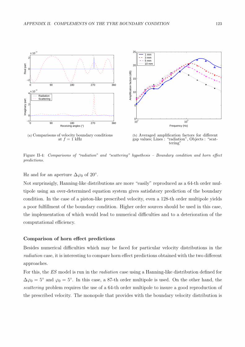
APPENDIX II. COMPLEMENTS ON THE TYRE BOUNDARY CONDITION 123
0 90 180 270 360
−2
0
2
x 10−4
Rea
l par
t
0 90 180 270 360−1
0
2
4x 10
−3
Receiving angles (°)
Imag
inar
y pa
rt
RadiationScattering
(a) Comparisons of velocity boundary conditionsat f = 1 kHz
102
103
0
5
10
15
20
25
Frequency (Hz)
Am
plifi
catio
n fa
ctor
s (d
B)
1 mm3 mm5 mm10 mm
(b) Averaged amplification factors for differentgap values; Lines : “radiation”, Objects : “scat-
tering”
Figure II-4: Comparisons of “radiation” and “scattering” hypothesis – Boundary condition and horn effectpredictions.
Hz and for an aperture ∆ϕ0 of 20◦.
Not surprinsigly, Hanning-like distributions are more “easily” reproduced as a 64-th order mul-
tipole using an over-determined equation system gives satisfatory prediction of the boundary
condition. In the case of a piston-like prescribed velocity, even a 128-th order multipole yields
a poor fulfillment of the boundary condition. Higher order sources should be used in this case,
the implementation of which would lead to numerical difficulties and to a deterioration of the
computational efficiency.
Comparison of horn effect predictions
Besides numerical difficulties which may be faced for particular velocity distributions in the
radiation case, it is interesting to compare horn effect predictions obtained with the two different
approaches.
For this, the ES model is run in the radiation case using a Hanning-like distribution defined for
∆ϕ0 = 5◦ and ϕ0 = 5◦. In this case, a 87-th order multipole is used. On the other hand, the
scattering problem requires the use of a 64-th order multipole to insure a good reproduction of
the prescribed velocity. The monopole that provides with the boundary velocity distribution is

124 CHAPTER 7. APPENDICES
located directly on the tyre belt at the same position as that of the equivalent monopole of the
radiation problem. In both cases, the boundary is discretised over 900 points. The prescribed
velocities of the two approaches are shown in Fig. II-4(a). Note that the real part of the
Hanning-like velocity has been scaled to fit the axis (this latter has a unit maximum value).
The pressure is calculated at 100 receiving positions on a 1 meter semi circle centered on the
“contact” point between the tyre and the road. The obtained values are then averaged to give
one single value of amplification at each frequency (see also Chapter 5). This procedure is
repeated for the following gap values : 1 mm, 3 mm, 5 mm, 10 mm. Results shown in Fig.
II-4(b) are indicated using lines in the radiation case and using objects in the scattering case.
In this latter case, amplification factors are plotted only at few frequencies for sake of clarity.
For all gap values, the two approaches give averaged amplification factors that are very similar
if not identical. The amplification increases up to frequency, the value of which depends on the
gap value. Beyond this frequency, the amplification decreases with a slope that is identical for
all gap values. As a general trend, amplification factors at low frequencies are slighlty larger
for larger gaps. Moreover, as expected, the closer the tyre is to the road surface, the stronger
the amplification. It reaches 24 dB for a 1 mm gap while it lies around 21 dB for a 3 mm gap;
it drops to 17 dB of maximum sound amplification for a 10 mm gap.
Finally, the main difference between the two configurations is the presence of higher modes in
the scattering case. The great similarity of the compared results further proves that low order
modes are responsible for the main part of the sound radiation from tyres.

APPENDIX III. INTEGRATION OVER THE GREEN FUNCTIONS’ SINGULARITIES 125
Appendix III Integration over the Green functions’ singularities
The present appendix proposes a calculation of the singular integrals in Eq. 3-5. The difficulty
is due to the fact that the Green functions, both for the pressure and for the velocity, are not
bounded when the integration variable meets the observation point. The numerical integration
of such integrals, using e.g. a Gauss-Legendre quadrature, drastically lacks accuracy.
Mathemetically, singular integrals can be evaluated by calculating the Cauchy principal value2.
Instead of using this method, the basic idea of the following derivation is to use the approx-
imations of the Hankel functions for very small arguments. The resulting integrals can be
performed analytically and evaluated numerically with good accuracy.
The validity of this assumption is briefly discussed in the first paragraph. Then, the integral
for the pressure Green function is examined and the integration of the velocity Green function
is finally treated.
The reader will note that, as in Chapter 3, a time dependence in e−jωt is assumed in the fol-
lowing. This choice implies the use of Hankel functions of first kind in the Green functions’
expressions. It is clear that an identical approach can be adopted when using a time depen-
dence as e+jωt and therefore, that one uses Hankel functions of second kind; in this case, only
the final results of the integration are indicated below.
Validity of the derivation
If all elements of the ground surface have the same length ∆, the maximum argument of the
Green functions is
| ei − ξj |max < ∆/2 or k | ei − ξj |max < k∆/2
If the ground discretization is such that Nel elements per wavelength are chosen, one has
Nel∆ ≡ λ =2π
kand hence k∆/2 ≡ π
Nel
For instance, if 10 elements per wavelength are chosen, the maximum value of the argument is
π/10 ≈ 0.31. The argument of the Hankel function being always smaller than that value, it is
thus safe to use the asymptotic expressions of the Hankel functions for argument values much
lower than 1.
2This procedure is applied for instance in [Becot 2002].
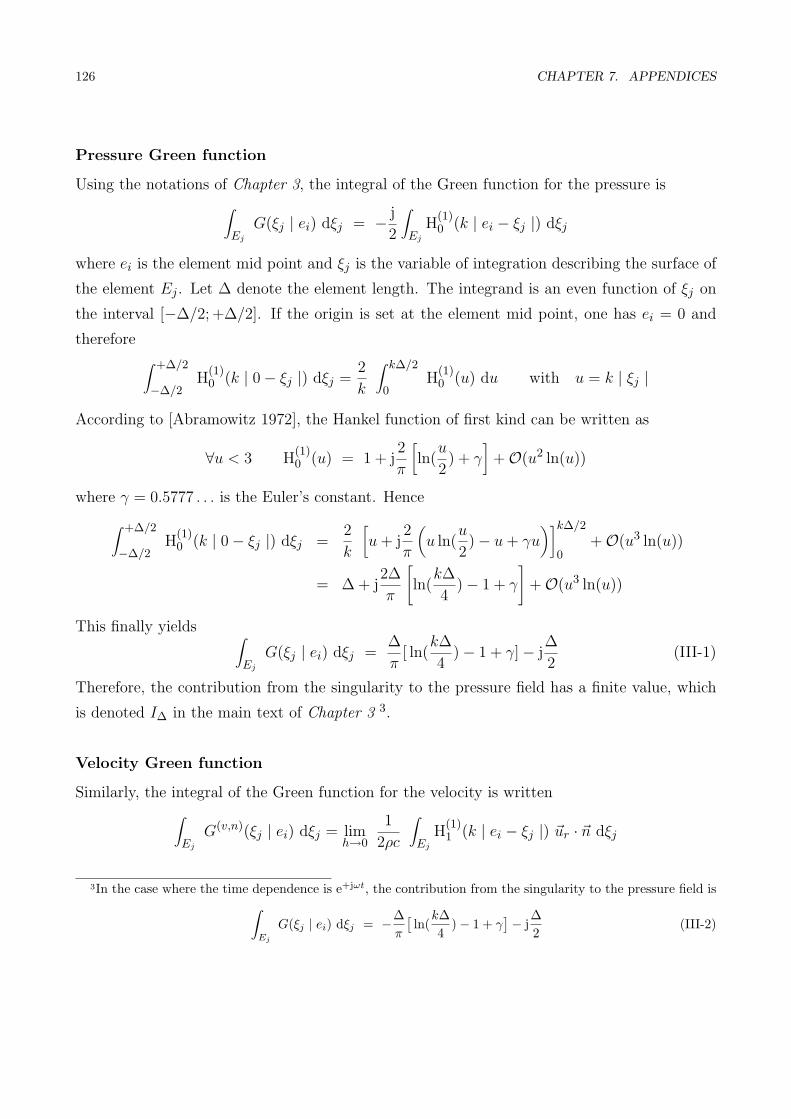
126 CHAPTER 7. APPENDICES
Pressure Green function
Using the notations of Chapter 3, the integral of the Green function for the pressure is∫Ej
G(ξj | ei) dξj = − j
2
∫Ej
H(1)0 (k | ei − ξj |) dξj
where ei is the element mid point and ξj is the variable of integration describing the surface of
the element Ej . Let ∆ denote the element length. The integrand is an even function of ξj on
the interval [−∆/2; +∆/2]. If the origin is set at the element mid point, one has ei = 0 and
therefore ∫ +∆/2
−∆/2H
(1)0 (k | 0− ξj |) dξj =
2
k
∫ k∆/2
0H
(1)0 (u) du with u = k | ξj |
According to [Abramowitz 1972], the Hankel function of first kind can be written as
∀u < 3 H(1)0 (u) = 1 + j
2
π
[ln(
u
2) + γ
]+O(u2 ln(u))
where γ = 0.5777 . . . is the Euler’s constant. Hence
∫ +∆/2
−∆/2H
(1)0 (k | 0− ξj |) dξj =
2
k
[u + j
2
π
(u ln(
u
2)− u + γu
)]k∆/2
0+O(u3 ln(u))
= ∆ + j2∆
π
[ln(
k∆
4)− 1 + γ
]+O(u3 ln(u))
This finally yields ∫Ej
G(ξj | ei) dξj =∆
π[ ln(
k∆
4)− 1 + γ]− j
∆
2(III-1)
Therefore, the contribution from the singularity to the pressure field has a finite value, which
is denoted I∆ in the main text of Chapter 3 3.
Velocity Green function
Similarly, the integral of the Green function for the velocity is written∫Ej
G(v,n)(ξj | ei) dξj = limh→0
1
2ρc
∫Ej
H(1)1 (k | ei − ξj |) ~ur · ~n dξj
3In the case where the time dependence is e+jωt, the contribution from the singularity to the pressure field is∫Ej
G(ξj | ei) dξj = −∆π
[ln(
k∆4
)− 1 + γ]− j
∆2
(III-2)

APPENDIX III. INTEGRATION OVER THE GREEN FUNCTIONS’ SINGULARITIES 127
~ur
~n
ξjθei
rh
Γ
+∆2
−∆2
Figure III-1: Geometry for the analytical calculation of the singular integral for the velocity.
Using the notations of Fig. III-1, one can write
limh→0
∫Ej
H(1)1 (k | ei − ξj |) ~ur · ~n dξj = lim
h→0
∫ +∆/2
−∆/2H
(1)1 (k | ei − ξj |)(− sin θ) dξj
= −2 limh→0
∫ +∆/2
0H
(1)1 (k | ei − ξj |) sin θ dξj
Again the origin is set at the position ei = 0. Let us introduce the variable r such that
r2 = ξj2 + h2. The above equation then becomes
limh→0
∫Ej
H(1)1 (k | ei − ξj |) ~ur · ~n dξj = −2 lim
h→0
∫ √∆2/4+h2
hH
(1)1 (kr)
h√r2 − h2
dr
One can make use here of the following asymptotic expression of the Hankel function
H(1)1 (kr) = −j
2
π
1
krfor kr � 1
One thus obtains
limh→0
∫Ej
H(1)1 (k | ei − ξj |) ~ur · ~n dξj = +j
4
kπlimh→0
∫ √∆2/4+h2
h
h
r√
r2 − h2dr
If v = r/h, this can be written
limh→0
∫Ej
H(1)1 (k | ei − ξj |) ~ur · ~n dξj = +j
4
kπlimh→0
∫ √1+∆2/4h2
1
1
v√
v2 − 1dv
= +j4
kπ
∫ +∞
1
1
v√
v2 − 1dv
The resulting integral is known and from [Abramowitz 1972] one obtains
limh→0
∫Ej
H(1)1 (k | ei − ξj |) ~ur · ~n dξj = +j
4
kπ
[arccos
1
v
]+∞1
= +j4
kπ[arccos 0− arccos 1]

128 CHAPTER 7. APPENDICES
This finally gives
limh→0
∫Ej
H(1)1 (k | ei − ξj |) ~ur · ~n dξj = +j
4
kπ
[π
2− 0
]= +j
2
k
Therefore, the integral of the Green function for the velocity is∫Ej
G(v,n)(ξj | ei) dξj = +j
ρω(III-3)
This results is in accordance with that presented in [Becot 2002], for which an error of sign has
been noticed 4.
Lastly, the use of such approximations for the Hankel functions also applies to the field calcu-
lations whenever the receiver is very close to some surface elements and that the computation
of the Green functions requires high accuracy. However, this aspect has not been further ex-
amined in this thesis because this situation has never been encountered.
4For a time dependence as e+jωt, one obtains the same value of the integral for the velocity. In this caseindeed, the opposite sign of imaginary part of the Hankel function approximation is compensated by the oppositesign of the pressure gradient.

APPENDIX IV. EXPERIMENTAL DETERMINATION OF SURFACE IMPEDANCE 129
Appendix IV Experimental determination of surface impedance
This appendix describes the experimental procedure as well as the impedance distributions of
the absorbing materials used in this thesis. Two techniques are reviewed : the Kundt’s tube
measurement and the level difference technique.
Kundt’s tube measurements
A Kundt’s tube, also called standing wave tube, can be used to measure the absorption prop-
erties of a given material. This type of measurement, widely used nowadays, is described in
the standard ISO/DIS 10354. The basic idea of the measurement is to exploit the properties
of a standing wave created in a tube, the extremity of which has certain absorbing properties
(see Fig. IV-1).
� �� �� �� �� �� �� �� �� �
� �� �� �� �� �� �� �� �� �
� �� �� �� �� �� �� �� �� �
� �� �� �� �� �� �� �� �� �
Tested material sampleMicrophone probe
Loudspeaker
Figure IV-1: Illustration of an absorption measurement using a standing wave tube.
A loudspeaker located at one end of the tube gives out a signal, which usually has a sinusoidal
form. A sample of the tested material is placed at the other end of the tube so that the incident
wave impinges perpendicularly to the sample surface. Thus, two waves co-exist inside the tube
: the incident wave, e.g. travelling from the right to the left in Fig. IV-1, and a reflected wave
travelling in the opposite direction. The superposition of these waves is a standing wave, which
presents a series of local minima and maxima. By measuring the ratio between the maxima
and the minima of sound pressure levels, one can determine the acoustical impedance of the
sample (see [Bruel 1967]).
The impedance of the material used for the measurements shown in Fig. 4-2 has been deter-
mined using this procedure. The impedance values are shown in Fig. IV-2.
It should be mentioned that as far as tyre / road noise is concerned, this method should be
considered with extreme care. The acoustical properties of a given road sample, which has been

130 CHAPTER 7. APPENDICES
200 500 1000 1500 2000−20
−15
−10
−5
0
Frequency (Hz)
Nor
mal
ised
impe
danc
e (Z
/ρc)
Real partImaginary part
(a) Real and imaginary part of the measuredimpedance.
200 500 1000 1500 20000
0.2
0.4
0.6
0.8
1
Frequency (Hz)
Abs
orpt
ion
(b) Corresponding absorption of the material(1− |R|2).
Figure IV-2: Impedance and absorption values of the material used for Fig. 4-2.
extracted from the road surface, may not reflect the acoustical behaviour of the all material
in-situ.
Level difference technique
As mentioned above, impedance measurements using a Kundt’s tube are not adapted to the
measurements of the acoustical properties of road surfaces. Therefore, a number of non–
destructive techniques have been developed, which may be applied to the determination of
road impedances. One of these methods is the level difference technique, which has been used
for some of the measurements presented in this thesis. The procedure and the impedance values
measured are presented in this paragraph.
General guidelines for the measurement can be found in [Ogren 1998]. The method consists in
finding the parameters of a given impedance model which give the best fit between the SPL
differences predicted in this way and the measured ones. Therefore, this method gives the values
of the parameters needed for the impedance model, without measuring them. In addition, the
chosen impedance model should be adapted to the type of surface considered.
In practical terms, sound pressure levels are measured at different receiver positions over the
studied surface (see Fig. IV-3). Thus, each measurement gives a set of parameter values, which
can then be averaged to obtain the final value. In particular, the obtained thickness of the

APPENDIX IV. EXPERIMENTAL DETERMINATION OF SURFACE IMPEDANCE 131
� � � � � � � � � � � �� � � � � � � � � � � �� � � � � � � � � � � �
� � � � � � � � � � � �� � � � � � � � � � � �� � � � � � � � � � � �
(a) The multiple height measurement.
Source Receiver 1
Receiver 2
Receiver 3
−10
0
10Receiver 1
−10
0
10Receiver 2
1000 2000 3000 4000 5000 6000−10
0
10
Frequency (Hz)
Leve
l diff
eren
ce (
dB)
Receiver 3
(b) Examples of curve–fitting the mea-sured level difference (solid lines) to pre-
dicted ones (broken lines).
Figure IV-3: Illustration of the principle of the level difference technique.
absorbing layer should correspond to the thickness measured in reality.
It should be mentioned that the parameter values are optimised for the frequency region where
the first minimum and first maximum of interference occur (maximum information on the
ground is supposed to be found in this region). However, this value is kept for the whole fre-
quency range of interest, thus assuming that the parameter values are frequency independent.
It is clear that this might be partly true for some of the parameters.
This technique has been applied to measure the impedance of the material used for the mea-
surements shown in Chapter 3 and in Section 4.2. For these two measurements, the absorbing
material was a panel of mineral rock wool laid on an acoustically rigid surface. Therefore, the
material was assumed to be of a hardbacked porous layer. It has been proved in [Attenborough
1985] that the impedance of such a material is accurately described by the model given in [De-
lany 1970]. This model gives the acoustical impedance in the normal direction to the surface
according to
ZL = Z∞ × j cot(Lk)
with k =2πf
c
[1 + 10.8 Fσ
-0.70 + j× 10.3 Fσ-0.59
],
where L is the thickness and σ the effective flow resistivity, in Ns/m4, of the material. Z∞ is

132 CHAPTER 7. APPENDICES
1000 2000 3000 4000 5000 60000
1
2
3
4
5
6
7
8
Frequency (Hz)
Nor
mal
ised
impe
danc
e (Z
/ρc)
Real part Imaginary part
(a) Impedance value for : σ = 22.4 kNs/m4 andL = 0.041 m.
1000 2000 3000 4000 5000 60000
1
2
3
4
5
6
7
8
Frequency (Hz)
Nor
mal
ised
impe
danc
e (Z
/ρc)
Real part Imaginary part
(b) Impedance value for : σ = 124 kNs/m4 andL = 0.016 m.
Figure IV-4: Impedance values obtained using the level difference technique.
the impedance of an infinitely thick layer of the same material. It is given as
Z∞ = 1 + 9.08 Fσ-0.75 + j× 11.9 Fσ
-0.73,
with Fσ = 1000f/σ.
The impedance values obtained with this procedure are shown in Fig. IV-4. Even though the
time dependence used in Chapter 3 and in Section 4.2 are not the same, impedance values are
shown here in the same assumption, namely e−jωt. The obtained values for the thickness of the
absorbing layers correspond well with those measured in reality. For the absorbing material
corresponding to Fig. IV-4(a), the obtained thickness is 4.1 cm (4 cm measured); for the
absorbing material corresponding to Fig. IV-4(b), the obtained thickness is 1.6 cm (1.5 cm
measured).
Finally, the absorption coefficient for the absorbing materials used in this thesis are shown in
Fig. IV-5.

APPENDIX IV. EXPERIMENTAL DETERMINATION OF SURFACE IMPEDANCE 133
200 500 1000 1500 20000
0.2
0.4
0.6
0.8
1
Frequency (Hz)
Abs
orpt
ion
coef
ficie
nt :
1−|R
|2
Fig. IV−2 Fig. IV−4(a)Fig. IV−4(b)
Figure IV-5: Absorption coefficient of the different impedance materials used in this thesis.

134
List of figures

List of figures
1-1 Structure and geometry of the tyre. . . . . . . . . . . . . . . . . . . . . . . . . . 4
1-2 Illustration of the mechanical sources of tyre noise. . . . . . . . . . . . . . . . . 5
1-3 Illustration of the air-borne sound sources of tyre noise. . . . . . . . . . . . . . . 6
1-4 Principle of the horn effect sound amplification . . . . . . . . . . . . . . . . . . 7
2-1 The reciprocity principle applied to measurements of horn effect amplification
factors. . . . . . . . . . . . . . . . . . . . . . . . . . . . . . . . . . . . . . . . . . 18
2-2 Amplification coefficient for different receiving angles directly over ground 7.5 m
distance from the centre of the contact (distance of the source d=10 mm). (Also
in [Kropp 2000b]) . . . . . . . . . . . . . . . . . . . . . . . . . . . . . . . . . . . 19
2-3 Compared radiation efficiencies of cylinders. 20 first modes modes in circum-
ferential direction (from left to right). The tyre radius is 0.3 m. (From [Kropp
2000b]) . . . . . . . . . . . . . . . . . . . . . . . . . . . . . . . . . . . . . . . . . 20
2-4 Radial and tangential directions of the contribution from the multipole source and
its image. . . . . . . . . . . . . . . . . . . . . . . . . . . . . . . . . . . . . . . . 23
2-5 Examples of velocity distributions in the “radiation” case. . . . . . . . . . . . . . 30
2-6 Sources in presence for the different horn effect amplification factors. . . . . . . 32
2-7 Scheme of the model used for the numerical examples. . . . . . . . . . . . . . . . 34
2-8 Comparison of obtained boundary velocities for different sizes of the equation
system using the “direct” geometry. The region of maximum velocity is focused
on in the broken-line box. . . . . . . . . . . . . . . . . . . . . . . . . . . . . . . . 35
2-9 Same as Fig. 2-8 but using the “reciprocal” geometry. . . . . . . . . . . . . . . . 36
135
136 LIST OF FIGURES
2-10 Set of multipole source strengths computed using collocated systems and a recip-
rocal geometry. Nmax = 128, only the 20 first positive and negative orders are
shown. . . . . . . . . . . . . . . . . . . . . . . . . . . . . . . . . . . . . . . . . . 38
2-11 Re-direction of sound due to the horn effect at 1.5 kHz. Reference pressure is
pref1in Eq. 2-14, distances are in meter. The right scale is in dB. . . . . . . . . 40
2-12 Re-direction of sound due to the horn effect at 1.5 kHz. Reference pressure is
pref2in Eq. 2-14, distances are in meter. The right scale is in dB. . . . . . . . . 41
2-13 Measured horn effect amplification factors for several distances d (cf. Fig. 2-1).
(Also in [Kropp 2000b]) . . . . . . . . . . . . . . . . . . . . . . . . . . . . . . . 42
2-14 Predicted amplification factors related to measured values in Fig. 2-13. (Also in
[Kropp 2000b]) . . . . . . . . . . . . . . . . . . . . . . . . . . . . . . . . . . . . 42
2-15 Measured horn effect amplification for different height of the tyre above the road.
(Also in [Kropp 2000b]) . . . . . . . . . . . . . . . . . . . . . . . . . . . . . . . 44
3-1 Source radiating over a arbitrary impedance surface. . . . . . . . . . . . . . . . . 48
3-2 Ground discretisation used for numerical integration. . . . . . . . . . . . . . . . 52
3-3 Geometry used for the numerical examples of this chapter. . . . . . . . . . . . . 54
3-4 Results for the Dirichlet boundary condition – Zn = 0, f = 1 kHz. . . . . . . . . 56
3-5 Results for Robin boundary conditions – β = 0.2, f = 4 kHz. . . . . . . . . . . . 56
3-6 Measured and calculated relative pressure fields over a homogeneous absorbing
surface – Source height: 0.3 m, receiver height: 0.3 m, horizontal distance: 0.5 m. 58
3-7 Measured and calculated relative pressure fields over a step impedance surface. . 59
3-8 Measured and calculated relative pressure fields over a strip of absorbing material
in a rigid baffle. . . . . . . . . . . . . . . . . . . . . . . . . . . . . . . . . . . . . 60
3-9 Comparison of different ground discretisations for a dipole source radiating over
a homogeneous absorbing ground – β = 0.2, f = 1 kHz, low source position.
(Also in [Becot 2001]) . . . . . . . . . . . . . . . . . . . . . . . . . . . . . . . . 61
3-10 Comparison of different ground discretisations for multipole sources radiating
over a totally soft ground Zn = 0. . . . . . . . . . . . . . . . . . . . . . . . . . . 63
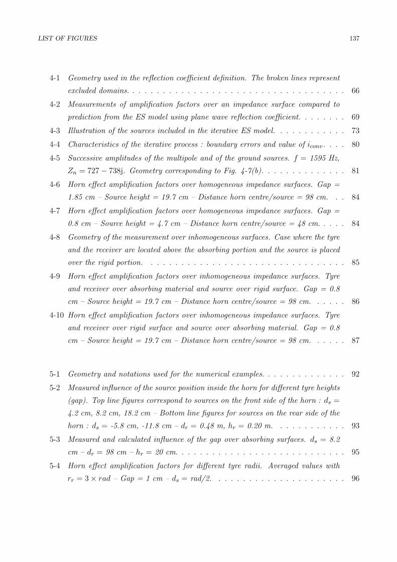
LIST OF FIGURES 137
4-1 Geometry used in the reflection coefficient definition. The broken lines represent
excluded domains. . . . . . . . . . . . . . . . . . . . . . . . . . . . . . . . . . . . 66
4-2 Measurements of amplification factors over an impedance surface compared to
prediction from the ES model using plane wave reflection coefficient. . . . . . . . 69
4-3 Illustration of the sources included in the iterative ES model. . . . . . . . . . . . 73
4-4 Characteristics of the iterative process : boundary errors and value of iconv. . . . 80
4-5 Successive amplitudes of the multipole and of the ground sources. f = 1595 Hz,
Zn = 727− 738j. Geometry corresponding to Fig. 4-7(b). . . . . . . . . . . . . . 81
4-6 Horn effect amplification factors over homogeneous impedance surfaces. Gap =
1.85 cm – Source height = 19.7 cm – Distance horn centre/source = 98 cm. . . 84
4-7 Horn effect amplification factors over homogeneous impedance surfaces. Gap =
0.8 cm – Source height = 4.7 cm – Distance horn centre/source = 48 cm. . . . . 84
4-8 Geometry of the measurement over inhomogeneous surfaces. Case where the tyre
and the receiver are located above the absorbing portion and the source is placed
over the rigid portion. . . . . . . . . . . . . . . . . . . . . . . . . . . . . . . . . 85
4-9 Horn effect amplification factors over inhomogeneous impedance surfaces. Tyre
and receiver over absorbing material and source over rigid surface. Gap = 0.8
cm – Source height = 19.7 cm – Distance horn centre/source = 98 cm. . . . . . 86
4-10 Horn effect amplification factors over inhomogeneous impedance surfaces. Tyre
and receiver over rigid surface and source over absorbing material. Gap = 0.8
cm – Source height = 19.7 cm – Distance horn centre/source = 98 cm. . . . . . 87
5-1 Geometry and notations used for the numerical examples. . . . . . . . . . . . . . 92
5-2 Measured influence of the source position inside the horn for different tyre heights
(gap). Top line figures correspond to sources on the front side of the horn : ds =
4.2 cm, 8.2 cm, 18.2 cm – Bottom line figures for sources on the rear side of the
horn : ds = -5.8 cm, -11.8 cm – dr = 0.48 m, hr = 0.20 m. . . . . . . . . . . . 93
5-3 Measured and calculated influence of the gap over absorbing surfaces. ds = 8.2
cm – dr = 98 cm – hr = 20 cm. . . . . . . . . . . . . . . . . . . . . . . . . . . . 95
5-4 Horn effect amplification factors for different tyre radii. Averaged values with
rr = 3× rad – Gap = 1 cm – ds = rad/2. . . . . . . . . . . . . . . . . . . . . . 96

138 LIST OF FIGURES
5-5 Measured influence of the impedance of the ground inside the horn. Reference
surface is entirely absorbing. Results for different source positions inside the
horn – Gap = 0.8 cm. . . . . . . . . . . . . . . . . . . . . . . . . . . . . . . . . 98
5-6 Horn effect amplification factors over a rigid surface compared to over entirely
absorbing surfaces of different thicknesses. Geometry of Fig. 5-5(a) – ds = 4.2
cm. . . . . . . . . . . . . . . . . . . . . . . . . . . . . . . . . . . . . . . . . . . . 99
5-7 Map of relative SPL over a rigid surface. f = 1007 Hz – gap = 1 cm – ds = 5
cm – The arrow indicates the position of the noise source – The scale is in dB. . 101
5-8 Map of relative SPL over a strip of absorbing material. Labs = 20 cm – Zn =
720 − 1226j – f = 1007 Hz – gap = 1 cm – ds = 5 cm – The arrow indicates
the position of the noise source – The scale is in dB. . . . . . . . . . . . . . . . 101
5-9 Map of relative SPL over an entirely absorbing surface. Zn = 720− 1226j – f =
1007 Hz – gap = 1 cm – ds = 5 cm – The arrow indicates the position of the
noise source – The scale is in dB. . . . . . . . . . . . . . . . . . . . . . . . . . . 101
5-10 Insertion loss for an entirely absorbing surface with varying impedance. Refer-
ence surface is rigid – Labs =2×1.2 m centered on the tyre – f = 500 Hz. . . . . 102
5-11 Insertion loss for an entirely absorbing surface with varying impedance. Refer-
ence surface is rigid – Labs =2×1.2 m centered on the tyre – f = 1000 Hz. . . . 103
5-12 Combined effects of the tyre height and surface impedance on tyre radiation.
Averaged values of insertion loss. Reference surface is rigid with 5 mm gap –
Solid lines : gap effect only – Thick lines : gap + impedance effect – ds = 0.05
m – rad = 0.3 m . . . . . . . . . . . . . . . . . . . . . . . . . . . . . . . . . . . 105
I-1 Typical geometry for an exterior radiation problem. The gray area represents the
source distribution inside the vibating body. . . . . . . . . . . . . . . . . . . . . . 114
II-1 Geometry of the boundary condition in the “radiation” problem. . . . . . . . . . 120
II-2 Obtained and prescribed boundary velocities in the case of a Hanning-like bound-
ary condition. . . . . . . . . . . . . . . . . . . . . . . . . . . . . . . . . . . . . . 122
II-3 Obtained and prescribed boundary velocities in the case of a piston-like boundary
condition. . . . . . . . . . . . . . . . . . . . . . . . . . . . . . . . . . . . . . . . 122

LIST OF FIGURES 139
II-4 Comparisons of “radiation” and “scattering” hypothesis – Boundary condition
and horn effect predictions. . . . . . . . . . . . . . . . . . . . . . . . . . . . . . . 123
III-1 Geometry for the analytical calculation of the singular integral for the velocity. . 127
IV-1 Illustration of an absorption measurement using a standing wave tube. . . . . . . 129
IV-2 Impedance and absorption values of the material used for Fig. 4-2. . . . . . . . . 130
IV-3 Illustration of the principle of the level difference technique. . . . . . . . . . . . . 131
IV-4 Impedance values obtained using the level difference technique. . . . . . . . . . . 132
IV-5 Absorption coefficient of the different impedance materials used in this thesis. . . 133

140
Bibliography

Bibliography
M. Abramowitz, I. A. Stegun: Handbook of mathematical functions. Dover Publications, New
York, 1972. 2.2, 13, 22, 23
H. T. Anastassiu, D. I. Kaklamani, D. P. Economou, O. Breinbjerg. Electromagnetic scattering
analysis of coated conductors with edges using the method of auxiliary sources (MAS) in
conjuction with the standard impedance boundary condition (SIBC). IEEE Transactions on
Antennas and Propagation, 50:59–66, 2002. 21
P. B. U. Andersson. High frequency tyre vibrations.. Technical report F 02-04, Department of
Applied Acoustics - Chalmers, 2002. 3
F. Anfosso-Ledee. Application de la methode des equations integrales a la modeisation du bruit
aux abords des routes - Interaction chaussee / ecran antibruit. PhD thesis, Ecole Nationale
des Ponts et Chaussees, Paris, France, 1996. 3
K. Attenborough. Acoustical impedance models for outdoor ground surfaces. Journal of Sound
and Vibration, 99(4):521–544, 1985. 1.3, Appendix IV
K. Attenborough T. Waters-Fuller. Effective impedance of rough porous ground surfaces. Journal
of the Acoustical Society of America, 108(3):949–956, 2000. 1.3
K. Attenborough Developments in modelling ground effects on outdoor sound. In Proceedings
of I.C.A. 2001, Rome, Italy, 2001. 1.3
M. Ballie J. Gal. Noise reduction induced by use of very thin wearing courses and crumb rubber
particles. In Proceedings of inter.noise 2000, Nice, France, 2000. (document)
T. Beckenbauer, A.Kuijpers. Prediction of pass-by levels depending on road surface parameters
141
142 BIBLIOGRAPHY
by means of a hybrid model. In Proceedings of inter.noise 2001, The Hague, The Netherlands,
2001. 4
F.-X. Becot, P.J. Thorsson, W. Kropp. Line source radiation over inhomogeneous ground using
an extended Rayleigh integral method.. In Proceedings of I.C.A. 2001, Rome, Italy, 2001. 3-9,
Appendix IV
F.-X. Becot, P.J. Thorsson, W. Kropp. An efficient application of equivalent sources to noise
propagation over inhomogeneous ground. Acustica - Acta Acustica, 88(6):853–860, 2002. 13,
3, 15, 15, 15, 15, 16, 6, 21, 2, 23
M. C. Berengier M. R. Stinson G. A. Daigle J. F. Hamet. Porous road pavements: Acoustical
characterization and propagation effects. Journal of the Acoustical Society of America, 101
(1):155–162, 1997. 1.3
M. Berengier and M. Garai. A state-of-the-art of in situ measurement of the sound absorption
coefficient of road pavements. In Proceedings of I.C.A. 2001, Rome, Italy, 2001. 1.3
Y. I. Bobrovniskii T. M. Tomilina. Calculation of radiation from finite elastic bodies by the
method of auxiliary sources. Sov. Phys. Acoust., 36(4), 1980. Appendix I
Y. I. Bobrovniskii T. M. Tomilina. General properties and fundamental errors of the method of
Equivalent Sources. Acoustical Physics, 41(5):649–660, 1995. 21
J. Borish, J. B. Angell. An efficient algorithm for measuring the impulse response using pseu-
dorandom noise. Journal of the Audio Engineering Society, 31:478–487, 1983. 4
L. Bouchet T. Loyau N. Hamzaoui C. Boisson. Calculation of acoustic radiation using
equivalent-sphere methods. Journal of the Acoustical Society of America, 107(5):2387–2397,
2000. 21
F. Bohm. Mechanik des Gurtelreifens. Ing.-Arch., 35:82–101, 1966. 2
Bruel & Kjær. Instructions and applications for standing wave apparatus Type 4002. Manual
Bruel & Kjær, 1967. Appendix IV
C. B. Burroughs Applications of nearfield acoustical holography in the research of mechanisms
of acoustic radiation. In Proceedings of inter.noise 2001, The Hague, The Netherlands, 2001.
1.1

BIBLIOGRAPHY 143
S. N. Chandler-Wilde D. C. Hothersall. Sound propagation above an inhomogeneous impedance
plane. Journal of Sound and Vibration, 98(4):475–491, 1985. 6
S. N. Chandler-Wilde D. C. Hothersall. Efficient calculation of the Green function for acoustic
propagation above a homogeneous impedance plane. Journal of Sound and Vibration, 180(5):
705–724, 1995. 5, 14, 3.3
C. F. Chien W. W. Soroka. Sound propagation along an impedance plane. Journal of Sound
and Vibration, 43:9–20, 1975. 6
C. F. Chien W. W. Soroka. A note on the calculation of sound propagation along an impedance
surface. Journal of the Acoustical Society of America, 69(2):340–343, 1980. 6
T. G. Clapp. Approximation and analysis of tire / pavement contact information resulting from
road surface roughness. PhD thesis, Rayleigh, USA, 1985. 3, 4
J. P. Coyette B. Van De Nieuwenhof. A conjugated infinite element method for half-space
acoustic problems. Journal of the Acoustical Society of America, 108(4):1464–1473, 2000. 6
L. Cremer, M. Heckl. Structure-borne sound – Structural vibrations and sound radiation at
audio frequencies. Springer-Verlag New-York, 528p, 1973. 1, 7
L. Cremer M. Wang. Die synthese eines von einem beliebigen korper in luft erzeugten feldes
aus kugelschallfeldern und deren realisierung in durchrechnung und experiment. Acustica, 65:
53–74, 1988. 21
J. Defrance Y. Gabillet. A new analytical method for the calculation of outdoor noise propaga-
tion. Applied Acoustics, 57:109–127, 1999. 6
E. Delany E. N. Bazley. Acoustical properties of fibrous absorbent materials. Journal of the
Acoustical Society of America, 3:105–116, 1970. 1.3, 4.3, Appendix IV
A. Dufour. Perception du cadre de vie et attitudes sur l’environnement. Rapport CREDOC 86,
1990. (document)
D. Duhamel. Efficient calculation of three-dimensional sound pressure field around a noise
barrier. Journal of the Acoustical Society of America, 197(5):547–571, 1996. 14

144 BIBLIOGRAPHY
J. A. Ejsmont U. Sandberg. Texturing of cement concrete pavements to reduce traffic noise.
Noise Control Engineering Journal, 46(6):231–243, 1998. (document)
A Fadavi, D Duhamel, H.P. Yin. Tyre road noise : finite element modelling. In Proceedings of
inter.noise 2001, The Hague, The Netherlands, 2001. 3
A Fadavi. Modelisation numerique des vibrations d’un pneumatique et de la propagation du
bruit de contact. PhD thesis, Ecole Nationale des Ponts et Chaussees, Paris, France, 2002.
3, 6
S. Fong. Tyre noise prediction from computed road surface texture induced contact pressure. In
Proceedings of inter.noise 98, Christchurch, New Zealand, 1998. 4
J. Forssen. Calculation of noise barrier performance in a turbulent atmosphere by using substi-
tute sources above the barrier. Acustica - Acta Acustica, 86:269-275, 2000. 21
J. Forssen. Calculation of noise barrier performance using the substitute-sources method for a
three-dimensional turbulent atmosphere. Acustica - Acta Acustica, 88:181-189, 2002. 21
T. Fujikawa H. Hoike Y. Oshino H. Tachibana. Generation mechanism of tire / road noise
- Part 1: Tire vibration caused by road roughness. In Proceedings of Internoise 1999, Fort
Lauderdale, Florida, USA, 1999. 3
E. Gerretsen F. de Roo F. van Gorkum. A prediction model for tyre-road noise emission.
In International Symposium on Pavement Surface Characteristics, Christchurch, Australia,
1996. 4
E. Gerretsen, E. H. Mulder. TRIAS : a comprehensive tyre-road noise model and its validation.
Technical Report, TNO report HAG-RPT-000121a, TNO Delft, The Netherlands, 2001. 4
R. A. G. Graf C. Y. Kuo A. P. Dowling W. R. Graham. Horn amplification at a tyre/road
interface – Part I: experiment and amplification. In Proceedings of Internoise 1999, Fort
Lauderdale, Florida, USA, 1999. 3

BIBLIOGRAPHY 145
R. A. Graf, C.-Y. Kuo, A. P. Dowling W. R. Graham On the horn effect of a tyre / road
interface, Part I : Experiment and computation. Journal of Sound and Vibration, 256(3):
417-431, 2002. 3, 2.3, 2.5
D. Habault. Etude de l’influence des sols sur la propagation sonore. PhD thesis, Universite de
Provence Aix–Marseille I, France, 1984. 6
D. Habault. Sound propagation above an inhomogeneous plane: boundary integral equation
methods. Journal of Sound and Vibration, 100(1):55–67, 1985. 6
J.-F. Hamet, J. M. Clairet, J. C. Bruyere. Bruit exterieur pneumatique / chaussee -
Amenagement et instrumentation du laboratoire de Grenoble. Rapport MMA 9103, INRETS,
1991. 1.1
J.-F. Hamet. Modelisation acoustique d’un enrobe drainant - Prise en compte des phenomenes
de thermoconductivite dans une nouvelle formulation phenomenologique. Rapport LTE 159,
INRETS, 1992. 1.3
J.-F. Hamet (a), P. Klein. Use of a rolling model for the study of the correlation between road
texture and tire noise. In Proceedings of inter.noise 2001, The Hague, The Netherlands, 2001.
4
J.-F. Hamet (b), P. Klein. Recherches physiques sur le bruit de roulement dans les projets
’Texture & Bruit’ et SI.R.U.US. In Proceedings of Journees d’etude Bruit du Trafic Routier,
Nantes, France, 2001. 1.2
J.-F. Hamet (c). Tire / road noise : Time domain Green’s function for the orthotropic plate
model. Acustica - Acta Acustica, 87(4):470–474, 2001. 3
R. E. Hayden. Road side noise from the interaction of a rolling tire with the road surface. In
81st meeting of the Acoust. Soc. of America, Washington, USA, 1971. 1.1, 3
M. Heckl. Tire noise generating mechanisms - State of the Art Report. In International Tire
Noise Conference, pages 41–55, Stockholm, Sweden, 1979. 1.2
M. Heckl. Tyre noise generation. In Seminar on Friction and Contact Noise, volume 113, pages
157–170, 1986. 1, 1.2

146 BIBLIOGRAPHY
F. Holste. An equivalent source method for calculation of the sound radiated from aircraft
engines. Journal of Sound and Vibration, 203(4):667–695, 1997. 21
S. C. Huang W. Soedel Response of rotating rings to harmonic and periodic loading and
comparison with the inverted problem. Journal of Sound and Vibration, 118(2):255–270,
1987. 2
S. C. Huang C. K. Su. In-plane dynamics of tires on the road based on an experimentally
verified ring model. Vehicle System Dynamic, 21:247–267, 1992. 2
S. Huschek. Characterization of pavement surface texture and its influence on tyre / road
noise. In 3rd International symposium on pavement surface characteristics, Christchurch,
New Zealand, 1996. 1.2
E. L. Ince. Ordinary differential equations. Dover Publications, New York, 1956. 19
U. Ingard. On the reflection of a spherical sound wave from an infinite plane. Journal of the
Acoustical Society of America, 23(3):329–335, 1951. 6
M. E. McIntyre, J. Woodhouse. On the fundamentals of bowed–string dynamics. Acustica, 43
(2):93–108, 1979. 3
P. Jean. A variational approach for the study of outdoor sound propagation and application to
railway noise. Journal of Sound and Vibration, 212(2):275–294, 1998. 6
K. L. Johnson. Contact mechanics. Cambridge University Press, Cambridge, 1985. 3
M. E. Johnson, S. J. Elliot, K-H. Baek, J. Garcia-Bonito. An equivalent source technique for
calculating the sound field inside an enclosure containing scattering objects. Journal of the
Acoustical Society of America, 104(3):1221–1231, 1998. 21
D. I. Kaklamani, H. T. Anastassiu. Aspects of the method of auxiliary sources (MAS) in
computational electromagnetics. IEEE Antenna’s and Propagation Magazine, 118(2):255–
270, 2002. Appendix I
BIBLIOGRAPHY 147
M. Karamehmedovic, O. Breinbjerg. A convergent method of auxiliary sources for two-
dimensional impedance scatterers with edges. In Conference on Applied Electromagnetic and
Communication, Croatia, 2001. 21
P. Klein. Effet diadre – Etude du modale de Kropp. Rapport MMA 9807, INRETS, 1998. 3,
2.2, 2.2, 8, 2.3, 9, 21
P. Klein. Projet PREDIT “Texture/ Bruit” – Etude de la relation bruit/texture sur la base de
mesures effectuees dans le cadre de la phase 1. Rapport LTE 2033, INRETS, 2000. 1.2, 4
P. Klein. Tyre noise horn effect on an absorbing surface - 2D analytical modelling using the
multipole synthesis. In Proceedings of Forum Acusticum 2002, Sevilla, Spain, 2002. 3
G. H. Koopmann L. Song J. B. Fahnline A method for computing acoustic fields based on
the principle of wave superposition. Journal of the Acoustical Society of America, 86(6):
2433–2438, 1989. Appendix I, 21
J. Kragh et al. Nordic prediction for road traffic noise. New basic input values due to the
tightening of vehicle noise limits?. Danish Acoustical Institute Report LI 971/91, Lyngby,
Danmark, 1991. (document)
J. Kragh. News and needs in outdoor noise prediction. In Proceedings of inter.noise 2001, The
Hague, The Netherlands, 2001. 5
R. Kress A. Mohsen. On the simulation Source Technique for exterior problems in acoustics.
Mathematical Methods in the Applied Science, 8:585–597, 1986. 21
W. Kropp. Structure-borne sound on a smooth tyre. Applied Acoustics, 26:181, 1989. 2, 7
W. Kropp. Ein Model zur Beschreibung des Rollgerausches eines unprofilierten Guertlreifens
auf rauher Strassenoberflache. PhD thesis, Institut fur Technische Akustik, Berlin, Germany,
1992. (document), 1, 2, 3, 1.4, 7, 2.2, 6
W. Kropp P. Svensson. Application of the time domain formulation of the method of Equivalent
Sources to radiation and scattering problems. Acustica, 81:528–543, 1995. 21
W. Kropp, J. Berillon. A theoretical model to investigate the acoustic performance of building
facades in the low and middle frequency range. Acustica - Acta Acustica, 84:681-688, 1998.
3.1, 21

148 BIBLIOGRAPHY
W. Kropp (a), J. Berillon. A theoretical model to consider the influence of absorbing surfaces
inside the cavity of balconies. Acustica - Acta Acustica, 86:485-494, 2000. 21
W. Kropp (b), F.-X. Becot, S. Barrelet. On the sound radiation from tyres. Acustica - Acta
Acustica, 86(5):769–779, 2000. 1, 3, 2-2, 2-3, 7, 2-13, 2-14, 5, 2-15, 1, 21, Appendix IV
W. Kropp, K. Larsson, F. Wullens, P. Andersson. F.-X. Becot, T. Beckenbauer. The modelling
of tyre / road noise – a quasi three-dimensional model. In Proceedings of inter.noise 2001,
The Hague, The Netherlands, 2001. 3
P. A. Krutitskii. Method of interior boundaries for the impedance problem in scattering theory.
Applied Mathematics and Computation, 135:147–160, 2003. 1
A.Kuijpers, G. J. van Bokland. Tyre / road noise models in the last two decades : a critical
evaluation. In Proceedings of inter.noise 2001, The Hague, The Netherlands, 2001. 1.2
C.-Y. Kuo, R. A. Graf, A. P. Dowling W. R. Graham. On the horn effect of a tyre / road
interface, Part II : Asymptotic theories. Journal of Sound and Vibration, 256(3):433-445,
2002. 3
K. Larsson (a). Modelling of dynamic contact – Exemplified on the tyre / road interaction. PhD
thesis, Department of Applied Acoustics, Gothenburg, Sweden, 2002. 3
K. Larsson (b), S. Barrelet, W. Kropp. The modelling of the dynamic behaviour of tyre tread
blocks. Applied Acoustics, 63(6):659–677, 2002. 3
Y. L. Li, M. J. White. Near–field computation for sound propagation above ground using complex
image theory. Journal of the Acoustical Society of America, 99(2):755–759, 1996. 21
K. U. Machens. Approximate solutions for acoustic radiation problems: a critical appraisal of
the method of comparative sources. Acustica - Acta Acustica, 85:764–779, 1999. 2.4, 21
M. B. S. Magalhaes, R. A. Tenenbaum, M. Zindeluk Application of equivalent sources methods
in acoustical holography. In Proceedings of inter.noise 2001, The Hague, The Netherlands,
2001. 21
BIBLIOGRAPHY 149
J. D. Maynard Near field acoustic holography : a review. In Proceedings of inter.noise 2001,
The Hague, The Netherlands, 2001. 1.1
F. P. Mechel. A line source above a plane absorber. Acustica - Acta Acustica, 86(2):203–215,
2000. 6
H. M. E. Miedema. Noise & health: how does noise affect us?. In Proceedings of inter.noise
2001, The Hague, The Netherlands, 2001. (document)
R. D. Miller, E. T. Moyer, H. Huang, H. Uberall. A comparison between the boundary element
method and the wave superposition approach for the analysis of the scattered fields from rigid
bodies and elastic shells. Journal of the Acoustical Society of America, 89(5):2185–2196, 1991.
21
P. M. Morse, K. U. Ingard Theoretical acoustics. Princeton University Press, 949p, 1968. 4.1
P. A. Nelson. Some inverse problems in acoustics. In Sixth International Congress on Sound
and Vibration, Copenhagen, Denmark, 1999. 21
N.-A. Nilsson. Air resonant and vibrational radiation – Possible mechanisms for noise from
cross-bar tires. In International Tire Noise Conference, pages 93–110, Stockholm, Sweden,
1979. 1
M. Ochmann. Calculation of sound radiation from complex machine structures using the mul-
tipole radiator synthesis and the boundary element multigrid method. Internal report, Tech-
nische Fashhochule, Berlin, Germany, 1980. 2.4, 21
M. Ochmann. The source simulation technique for acoustic radiation problems. Acustica, 81:
512–526, 1995. 2.4, Appendix I
M. Ochmann. The full-field equations for acoustic radiation and scattering. Journal of the
Acoustical Society of America, 105(5):2574–2584, 1999. 21
M. Ochmann. Source simulation techniques for the calculation of sound radiation and scat-
tering - An overview. In Sixth International Congress on Sound and Vibration, Garmisch-
Partenkirchen, Germany, 2000. Appendix I

150 BIBLIOGRAPHY
P. J. Papakanellos, D. I. Kaklamani, C. N. Capsalis. Analysis of an infinite current source
above a semi-infinite lossy ground using fictitious current auxiliary sources in conjuction with
complex image theory techniques. IEEE Transactions on Antennas and Propagation, 49(10):
491–1503, 2001. 21
J. Perisse. A study of radial vibrations of a rolling tyre for tyre-road noise characterisation .
Mechanical Systems and Signal Processing, 16(6):1043–1058, 2002. 1.1
J. Picaut. Contribution a l’etude de la reflexion du son par une facade. Partie I Bibliographies
et considerations qualitatives. Report JP-00-03, Laboratoire Central des Ponts et Chaussees,
Nantes, France, 2000. 5
R. J. Pinnington. A one dimensional wave model for an automotive tyre. In Proceedings of
inter.noise 2000, Nice, France, 2000. 3
R. J. Pinnington, A. R. Briscoe. A wave model for a pneumatic tyre. Journal of Sound and
Vibration, 253(5):941–959, 2002. 3
H. Press et al. Numerical recipies, the art of scientific computing. Cambridge University Press,
Cambridge, 994p, 1986. 2.3, 21
K. B. Rasmussen. Sound propagation over grass covered ground. Journal of Sound and Vibra-
tion, 78(2):247–255, 1981. 1.3
J. W. S. Rayleigh. The theory of sound. (two volumes), Dover Publication, New York, 1945.
2.1
T. L. Richards. Finite element analysis of structural-acoustical coupling in tyres. Journal of
Sound and Vibration, 149(2):235–243, 1991. 3
D. Ronneberger. Towards quantitative prediction of tire / road noise. In A workshop on rolling
noise generation, Newport Beach, USA, 1989. 1, 3
D. Ronneberger C. Preuss. Optimum positions of microphones in trailers. In International
tire/road noise conference INTROC 1990, Gothenburg, Sweden, 1990. 1.1
F. de Roo, E; Gerrestsen, E. H. Mulder. Predictive performance of the tyre-road noise model
TRIAS. In Proceedings of inter.noise 2001, The Hague, The Netherlands, 2001. 4

BIBLIOGRAPHY 151
R. J. Ruhala. A study of tire / pavement interaction noise using nearfield acoustical holography.
PhD thesis, Pennsylvania State University, USA, 1999. 1, 2.3
S. Saigal, T. Y. Yang. Free vibrations of a tire as a toroidal membrane. Journal of Sound and
Vibration, 107(1):71-82, 1986. 2
U. Sandberg G. Descornet. Road surface influence in tire/road noise. In Proceedings of in-
ter.noise 1980, Miami, Florida, 1980. 1.2
U. Sandberg. Will tire / road noise limit future vehicle noise reductions? In Proceedings of
inter.noise 1982, San Francisco, USA, 1982. (document)
U. Sandberg. Noise emission of road vehicles - effects of regulation. Status report of an I-INCE
party In Proceedings of inter.noise 93, Leuven, Belgium, 1993. (document)
U. Sandberg. Tyre / road noise – Myths and realities In Proceedings of Inter.Noise 2001, The
Hague, The Netherlands, 2001. (document)
U. Sandberg, J. A. Ejsmont. Tyre / road noise reference book Informex, Kisa, Sweden, 640p,
2002. 1.1
K. Schaaf D. Ronneberger. Noise radiation from rolling tires - Sound amplification by the ”horn
effect”. In Proceedings of inter.noise 1982, San Francisco, USA, 1982. 1, 7, 4.3
M. R. Schroeder. Integrated–impulse method measuring sound decay without using impulses.
Journal of the Acoustical Society of America, 66:497–500, 1979. 4
W. Soedel. On the dynamic response of rolling tires according to thin shell approximations.
Journal of Sound and Vibration, 41:(2): 233-246, 1975. 2
L. Song, G.H. Koopmann, J.B. Fahnline. A method for computing acoustic fields based on
the principle of wave superposition. Journal of the Acoustical Society of America, 89:(6):
2625–2633, 1991. Appendix I
S. A. Stansfeld. The non–auditory health effects of noise exposure. Acoustique et Techniques
28, CIDB publication, 2002. (document)
D. Stanners, P. Bourdeau. Europe’s environment. Technical report European Environment
Agency, 1995. (document)

152 BIBLIOGRAPHY
S.-I. Thomasson. Reflection from a point source by an impedance boundary. Journal of the
Acoustical Society of America, 146:: 303–322, 1976. 6
S.-I. Thomasson. Sound propagation above a layer with large refraction index. Journal of the
Acoustical Society of America, 61:659–674, 1977. 1.3
P. J. Thorsson Optimization of low-height noise barriers using the equivalent sources method.
Acustica - Acta Acustica, 86(5):811–821, 2000. 21
T.M. Tomilina. The equivalent sources approach to acoustical design of forced vibrating systems.
In Proceedings of inter.noise 1993, Moscow, Russia, 1993. 21
G.-P. J. Too S. M. wang. The application of Source Methods in estimation of an interior sound
field. Acustica - Acta Acustica, 63(3):295–310, 2001. 21
Z. Wang, S.F. Wu. Helmholtz equation-least-squares method for reconstructing the acoustic
pressure field. Journal of the Acoustical Society of America, 102(4):2020–2032, 1997. 21
G. R. Watts, S. N. Chandler-Wilde, P. A. Morgan. The combined effect of porous asphalt
surfacing and barriers on traffic noise. Applied Acoustics, 58:351–377, 1999. (document)
J. T. Weaver. Image theory for an arbitrary quasi–static field in the presence of a conducting
half space. Radio Science, 6(6):647–653, 1971. 21
E. G. Williams. Inverse Problems in Sound Radiation. In Proceedings of ICA 2001, Rome,
Italy, 2001. 21
T. ten Wolde. On the validity and application of reciprocity in acoustical mechano–acoustical
and other dynaminal systems. Acustica - Acta Acustica, 28:23–32, 1973. 1
F. Wullens. Towards an optimisation of tyre / road parameters for noise reduction. Technical
report F 02-01, Department of Applied Acoustics - Chalmers, 2002. 3
C. Zwikker, C. W. Kosten. Sound absorbing materials. Elsevier New-York, 175p, 1949. 1.3

BIBLIOGRAPHY 153
M. Ogren, H. Jonasson. Measurement of the acoustic impedance of the ground. SP Report
1998:28, Swedish National Testing and Research Institute, Boras, Sweden, 1998. Appendix
IV
M. Ogren, W. Kropp. The equivalent sources method applied to a 2D city canyon. In Proceedings
of Forum Acusticum 2002, Sevilla, Spain, 2002. 21

154 BIBLIOGRAPHY

Appended Papers
On the Sound Radiation from Tyres
W. Kropp, F.-X. Becot, S. Barrelet.
In Acustica - Acta Acustica, vol 86(5) : 769–779, 2000.
An Efficient Application of Equivalent Sources to Noise Propagation
Over Inhomogeneous Ground
F.-X. Becot, P. J. Thorsson, W. Kropp.
In Acustica - Acta Acustica, vol 88(6) : 853–860, 2002.
Line Source Radiation Over Inhomogeneous Ground Using an Ex-
tended Rayleigh Integral Method
F.-X. Becot, P. J. Thorsson, W. Kropp.
In Proceedings of I.C.A, Rome, Italy, 2001.
Modelisation du bruit de contact pneu / chaussee – Quels sont les
facteurs cles d’une reduction des nuisances sonores?
F.-X. Becot.
In 12emes Rencontres Regionales de la Recherche.
Copyright © 2022 FDOKUMEN