TURBULENT EXCHANGE ABOVE A PINE FOREST, I:

FLUXES AND GRADIENTS

ULF H6GSTR6M, HANS BERGSTRi)M, ANN-SOFI SMEDMAN Department of Meteorology, Box 516, S-751 20 Uppsala, Sweden

SVEN HALLDIN Section of Hydrology, V. Agaran 24, S-752 20 Uppsala, Sweden

and

ANDERS LINDROTH Department of Ecology and Environmental Research, Swedish University of Agricultural Sciences,

S- 750 07 Uppsala, Sweden

(Received in final form 24 May, 1989)

Abstract. Measurements of gradients of wind, temperature and humidity and of the corresponding turbulent fluxes have been carried out over a sparse pine forest at Jiidra&s in Sweden. In order to ascertain that correct gradient estimates were obtained, two independent measuring systems were employed: one system with sensors at 10 fixed levels on a 51 m tower and another with reversing sensors for temperature and humidity, covering the height interval 23 to 32 m. Turbulent fluxes were measured at three levels simultaneously. Data from three field campaigns: in June 1985, June 1987 and September 1987 have been analyzed. The momentum flux is found on the average to be virtually constant from tree top level, at 20 to 50 m. The average fluxes of sensible and latent heat are not so well behaved. The ratio of the non-dimensional gradients of wind and temperature to their cor- responding values under ‘ideal conditions’ (low vegetation) are both found to be small immediately above the canopy (about 0.3 for temperature and 0.4 for wind). With increasing height, the ratios increase, but the values vary substantially with wind direction. The ratios are not found to vary systematically with stability (unstable stratification only studied). The ratio of the non-dimensional humidity gradient to the corresponding nondimensional potential temperature gradient (equivalent to KH/KW) is found to be unity for (I - d)/L, less than about -0.1 and about 1.4 for near neutral stratification, but the scatter of the data is very large.

1. Introduction

The present paper is one in a series of reports from a field experiment at the Jadrais forest research site in Sweden, carried out as three field campaigns in 1985 and 1987. The origin of the experiment is the puzzling results concerning the evaporation obtained at the site in a previous study. As reported in Grip et al. (1979) and in Lindroth (1984), the energy balance/Bowen ratio method (EBBR- method) gave about twice as large seasonal evaporation as the water balance method.

In the 1985-l 987 experiment, it was decided to measure the turbulent fluxes of sensible heat and humidity directly, with the eddy correlation technique, and further, to employ two independent systems for estimating the very small gradients of potential temperature and humidity over the forest.

Boundary-Layer Meteorology 49: 197-217, 1989. @ 1989 Kluwer Academic Publishers. Printed in the Netherlands.

198 ULF H6GSTRdh.l ET AL.

The present paper concentrates on the relationships between the turbulent fluxes of momentum, sensible heat and humidity on the one hand and the corresponding gradients of wind, potential temperature and specific humidity on the other. In a companion paper: Bergstrom and Hogstrom (1989), the turbulent transport mechanism above the forest canopy is studied using a conditional sampling technique.

The relation between fluxes and gradients above a forest canopy has received great interest since the pioneering findings of Thorn et al. (1975) that universal flux-gradient relationships derived over low vegetation are invalid in a rather deep layer over a rough surface like a forest. Later studies (Garratt, 1980; and Denmead and Bradley, 1985) agree that the exchange of sensible heat is appreci- ably more effective over a forest than over low vegetation during otherwise identical conditions. This was also found in the careful wind tunnel study of Coppin et al. (1986). The corresponding result with respect to the exchange of momentum is more divided. The Thetford forest studies, reported by Thorn et al. (1975) and Raupach (1979), as well as the study of Denmead and Bradley (1985) indicate that the momentum flux-gradient relationship over the forest is identical to that over low vegetation, except possibly in a very shallow layer just above the crowns. Contrary to this, Garratt’s (1980) study over a Savannah as well as the wind tunnel study of Raupach et al. (1986) clearly indicate the momentum exchange process to be much more effective over a forest canopy than over low vegetation.

The situation concerning the water vapour -exchange is rather little studied, because of experimental difficulties. Denmead ad Bradley (1985), however, find that the ratio of the exchange coefficients for sensible heat, KH and for humidity, Kw is unity. Universally valid, this would be a very convenient situation for the application of the EBBR-method, which then only requires knowledge of net radiation, the rate of energy storage change below the reference level, and the ratio of vertical differences of potential temperature and of humidity. There is, however, the possibility that KH/Kw is not unity universally, and that this is the reason (or part of the reason) for the Jidrats evaporation discrepancy mentioned above. It is clearly indicated in the discrepancies found for momentum, briefly related above, that site-specific factors (related to forest architecture) are im- portant for the turbulent exchange process above a forest.

2. The Site

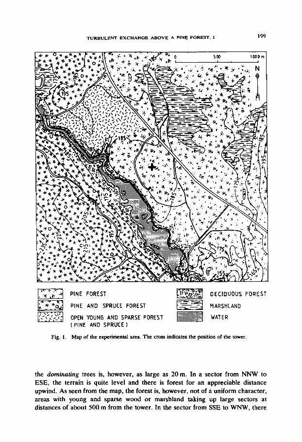
The JSidrals forest research site is situated in an extended wooded region in the eastern parts of central Sweden (60”49’N, 16”30’ E; altitude 185 m). Figure 1 is a map showing the site and its immediate surroundings. The rather flat area where the 51 m tower is situated (the cross in Figure 1) consists of glacifluvial deposits covered with a sparse Scats pine stand (Pinus siluestris L.), 135 years old in 1987. There are about 350 trees per hectare with a mean height of 16 m. The height of

TURBULENT EXCHANGE ABOVE A PINE FOREST, I

[FTj PINE FOREST m DECIDUOUS FOREST

LT$ PINE AND SPRUCE FOREST =q MARSHLAND

py,q OPEN YOUNG AND SPARSE FOREST pq WATER (PINE AND SPRUCE)

Fig. 1. Map of the experimental area. The cross indicates the position of the tower.

the dominating trees is, however, as large as 20m. In a sector from NNW to ESE, the terrain is quite level and there is forest for an appreciable distance upwind. As seen from the map, the forest is, however, not of a uniform character, areas with young and sparse wood or marshland taking up large sectors at distances of about 500 m from the tower. In the sector from SSE to WNW, there

200 ULF H&XTR&U ET AL.

is first a steep drop of 20 m at a distance of less than 500 m from the tower, then a river and then wooded land that rises ca. 60 m in one kilometer.

The ground vegetation at the site is of a lichen-dwarfshrub type with a field layer dominated by heather (Calluna uulgaris) and cowberry ( Vaccinium uitis- idea) and a bottom layer dominated by mosses (Pleurozium schreberi) and lichens (Cladonia rangifera and C. siluatica) (Persson, 1980). The total ground cover for the field layer is about 50%.

3. Instrumentation ad Measurement Accuracy

3.1. PROFILE INSTRUMENTATION

Two independent profile measuring systems were employed in the tower, one using sensors at fixed levels and one using movable sensors. The tower is triangular, with a side of 1 m. All instruments were mounted on booms ca. 3 m from the tower.

The system with sensors at fixed levels (‘the MIUU system’) consists of sensors for wind, temperature and humidity at ten levels, with the air intakes for the temperature and humidity sensors at: 2.5, 10.1, 18.5, 20.9, 23.4, 27.9, 32.4, 37.4, 42.0 and 48.7 m. Wind speed was measured 37 cm above these heights with modified Casella anemometers, that were calibrated individually in a wind tunnel prior to the experiment. The estimated overall accuracy is kO.05 m/s. Air temperature was measured with PtSOO-sensors in aspirated radiation shields as consecutive differences between the levels and with an additional sensor at the lowest level for ‘absolute temperature’. Humidity was measured with the psy- chometric method. Thus the difference between a dry and a wet sensor was recorded at each level. These sensors were placed after the sensors for air temperature in the ventilated shields, as described in detail in Lindroth ef al. (1989). The estimated accuracy in the temperature difference measurements is kO.02 “C and ztO.03 g/kg in the humidity differences.

The thermometer interchange system, TIS, is described in detail in Lindroth ef al. (1989). In short, it consists of two pairs of sensor units for temperature and humidity, where humidity is measured using the psychrometric method. The separation distance between the two sensors in each pair is 4.5 m. Reversing of sensors is made every five minutes, i.e., the sensor at the top level is moved to the middle level and vice versa for the sensor at the middle level. A corresponding reversal is made for the pairs at the middle and bottom levels, respectively. Thus, after one complete reversal cycle, i.e. a lo-min period, the temperature and humidity differences between levels can be estimated. The TIS system was used at the levels 23.4, 27.9 and 32.4 m.

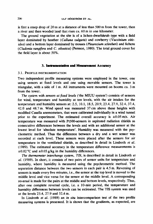
In Lindroth et al. (1989) an in situ intercomparison test of the two profile measuring systems is presented. It is shown that the gradients, as expected, are

Spec

ific

hum

idity

gr

adie

nt

-TIS

(.1

0-6m

-1)

” I

$2-

3 -. (I -. -2

A-

LP

2 CL

-.

dJ

u-l

u-l

ul u-l

73

Pote

ntia

l te

mpe

ratu

re

grad

ient

-T

IS

(K.1

0-*6

’) 0 4

.A

w

OI

0’

s z

2

202 ULF HCk3STRh.l ET AL,

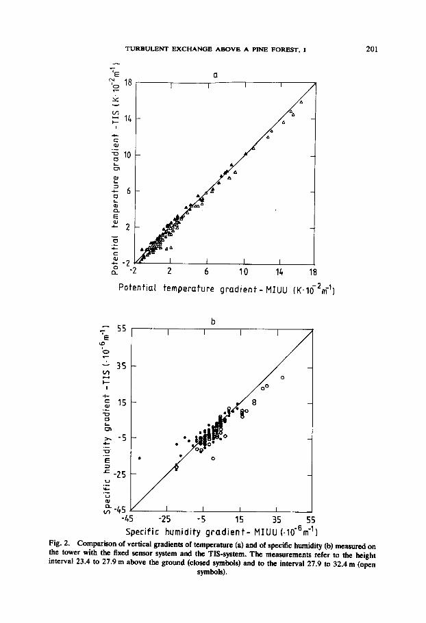
indeed small, the average summer daytime potential gradient being -0.0064 Km-’ and the corresponding humidity gradient -3.1 * lo-‘m-l. It is clear from the field test that the TIS system is capable of resolving these small gradients. In the comparison test, gradients from the fixed sensor system were obtained from smooth curves fitted to the data points. These were compared with the gradients measured at the same time with the TIS system; see Figure 2. The overall agreement between the two sets of measurements is quite good when the entire range of data is considered. During daytime, high flux conditions, the gradients are confined to a more restricted range of values. Then the relative scatter in the plots increases, and there is also a small systematic difference between the two data sets, at least for the upper difference measurement interval. This offset corresponds to slightly less than the estimated uncertainty mentioned above for the fixed sensor system.

In conclusion, the TIS system provides a highly accurate measuring system for the small gradients of temperature and humidity encountered over the JldraHs forest, but this system covers only a limited height range (23 to 32 m). As shown in Section 5, the accuracy of the fixed sensor system is, however, quite enough to resolve the features of relevance here, thus the flux - gradient analysis can be safely extended to encompass the entire range of measurements from the top of the trees at 20 m to the top of the tower, at 50 m.

Of the additional instrumentation at the field station, only data from the wind direction sensor, mounted at 51 m, was used in the present analysis.

3.2. TURBULENCEINSTRUMENTATION

The instrument employed is the MIUU turbulence instrument; see Hogstrom (1982) and Hogstrom (1988) for a detailed description. It is a wind vane based, three-axial hot film instrument with additional sensors for temperature and wet bulb temperature. The instrument has been carefully investigated for flow dis- tortion (see Hogstrom, 1982). The corrections employed as a result of this study are very simple and accurate as compared to corresponding corrections derived for sonic anemometers (see e.g., Zhang et al., 1986 or Baker, 1988). The directional characteristics of the particular hot film probes used have been investigated in a wind tunnel study (Bergstrom and Hogstrom, 1987). As demonstrated in Hogstrom (1988), the behaviour of the instrument in the field is very good, concerning both accuracy and long term stability, and there is a negligible systematic effect from sensor separation and other possible sources on the fluxes of momentum and sensible heat.

The ability of the instrument to record the humidity flux has not been demonstrated before. Previous experience with the psychrometric method in turbulence measurements has not been entirely successful. Thus Dyer et al. (1982) show a 40% loss in measurements of the covariance of the vertical velocity and the wet bulb temperature at heights of 2.8 and 4 m above the ground. This is due to the relatively long time constant of the wet bulb sensor.

TURBULENT EXCHANGE ABOVE A PINE FOREST. 1 203

But this error is a strong function of the dominating scale of the transport process, and as shown below, the scale of the humidity transport process is so large over a forest that the error becomes small at all heights above the canopy with the sensor used here. The sensor design is described in Smedman and Lundin (1987).

The humidity flux is proportional to the covariance between the vertical velocity w and the specific humidity q. Deviations in 4 can be expressed in terms of the corresponding deviations in temperature, T and in wet bulb temperature, T, with the aid of the psychrometric formula

q’ = aT;- /3T’, 0)

where primed values are deviations from mean values for the run, and a and p are constants during a particular run. Thus we get for the covariance between w’ and q’:

(2)

If we divide through with the temperature flux, we obtain

(3)

This equation is also valid for cospectral estimates, referring to a frequency interval dn, centered at the frequency n. Now, for frequencies that are small compared to the inverse of the time constant of the wet bulb, we expect this ratio to be recorded without loss, but for large enough frequencies, there will be a loss that increases in magnitude with frequency. As the constant p is positive, we expect the ratio even to become negative eventually.

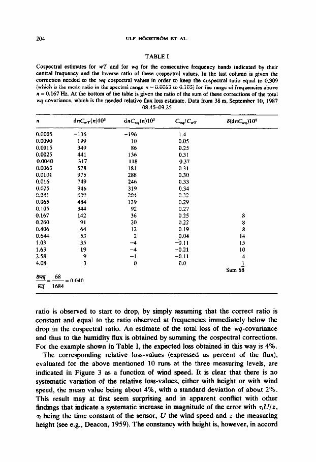
Table I displays a listing of the cospectral estimates for the temperature flux and for the humidity flux as well as the ratio of the two quantities for a typical run over the JidraHs forest. The ratio is seen to vary between frequencies in the low frequency range but then to stabilize at a constant value of about 0.3 1. At the frequency 0.167 Hz, it starts to drop in magnitude and becomes negative at frequencies above about 1 Hz.

The constancy of the cospectral ratio in a range of frequencies just before the drop caused by the slow response of the wet sensor observed in the example listed in Table I is worth noting. In all, 10 runs chosen at random in the data set from Jgldrals, containing altogether 30 measurements (measurements at three levels), have been evaluated in the manner illustrated in Table I. In every one of these 30 examples, such a range of constant spectral ratios is observed immediately before the drop occurs. Because of cospectral similarity at high enough frequencies (see Wyngaard and Cot&, 1972), we expect this constancy in reality to extend from the range of frequencies where it is observed in Table I up to frequencies where the cospectral levels are negligibly small. This result can be used to estimate the probable cospectral loss at all frequencies above the point where the cospectral

204 ULF HtbSTR6M ET AL.

TABLE I

Cospectral estimates for wT and for wq for the consecutive frequency bands indicated by their central frequency and the inverse ratio of these cospectral values. In the last column is given the correction needed to the wq cospectral values in order to keep the cospectral ratio equal to 0.309 (which is the mean ratio in the spectral range n = 0.0063 to 0.105) for the range of frequencies above n = 0.167 Hz. At the bottom of the table is given the ratio of the sum of these corrections of the total wq covariance, which is the needed relative flux loss estimate. Data from 38 m, September 10, 1987

08.45-09.25

n dnC,r(n)lOS

0.0005 -136 0.0090 199 0.0015 349 0.0025 441 0.0040 317 0.0063 578 0.0101 975 0.016 749 0.025 946 0.041 639 0.065 484 0.105 344 0.167 142 0.260 91 0.406 64 0.644 53 1.03 35 1.63 19 2.58 9 4.08 3

!%=68=0.040 w 1684

dnC,(n)lOs C,lG

-196 1.4 10 0.05 86 0.25

136 0.31 118 0.37 181 0.31 288 0.30 246 0.33 319 0.34 204 0.32 139 0.29 92 0.27 36 0.25 20 0.22 12 0.19 2 0.04

-4 -0.11 -4 -0.21 -1 -0.11

0 0.0

S(dnC,)lOs

8 8 8

14 15 10 4 1

Sum 68

ratio is observed to start to drop, by simply assuming that the correct ratio is constant and equal to the ratio observed at frequencies immediately below the drop in the cospectral ratio. An estimate of the total loss of the wq-covariance and thus to the humidity flux is obtained by summing the cospectral corrections. For the example shown in Table I, the expected loss obtained in this way is 4%.

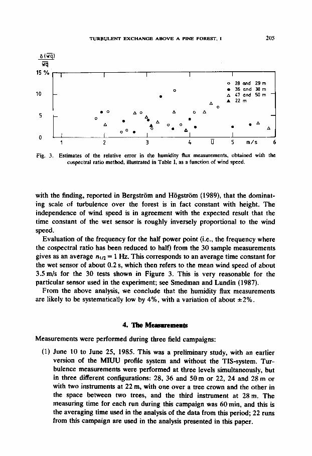
The corresponding relative loss-values (expressed as percent of the flux), evaluated for the above mentioned 10 runs at the three measuring levels, are indicated in Figure 3 as a function of wind speed. It is clear that there is no systematic variation of the relative loss-values, either with height or with wind speed, the mean value being about 4%, with a standard deviation of about 2%. This result may at first seem surprising and in apparent conflict with other findings that indicate a systematic increase in magnitude of the error with riU/Z, ri being the time constant of the sensor, U the wind speed and L the measuring height (see e.g., Deacon, 1959). The constancy with height is, however, in accord

TURBULENT EXCHANGE ABOVE A PINE FOREST, I 205

15%, , I I I I 1 I ̂

t 0 l 36 and 36 m

10 . A 47 and 50 m

A A 22m 0

5 DO A0 A o A -

0 0 4 A

b Ao 0.

' A' I

. . A A

0 I I 00.

1 2 3 4 u 5 m/s 6

Fig. 3. Estimates of the relative error in the humidity flux measurements, obtained with the cospectral ratio method, illustrated in Table I, as a function of wind speed.

with the finding, reported in Bergstrom and Hogstrom (1989), that the dominat- ing scale of turbulence over the forest is in fact constant with height. The independence of wind speed is in agreement with the expected result that the time constant of the wet sensor is roughly inversely proportional to the wind speed.

Evaluation of the frequency for the half power point (i.e., the frequency where the cospectral ratio has been reduced to half) from the 30 sample measurements gives as an average nl12 = 1 Hz. This corresponds to an average time constant for the wet sensor of about 0.2 s, which then refers to the mean wind speed of about 3.5 m/s for the 30 tests shown in Figure 3. This is very reasonable for the particular sensor used in the experiment; see Smedman and Lundin (1987).

From the above analysis, we conclude that the humidity flux measurements are likely to be systematically low by 4%, with a variation of about *2%.

4. The Measurements

Measurements were performed during three field campaigns:

(1) June 10 to June 25, 1985. This was a preliminary study, with an earlier version of the MIUU profile system and without the TIS-system. Tur- bulence measurements were performed at three levels simultaneously, but in three different configurations: 28, 36 and 50 m or 22, 24 and 28 m or with two instruments at 22 m, with one over a tree crown and the other in the space between two trees, and the third instrument at 28 m. The measuring time for each run during this campaign was 60min, and this is the averaging time used in the analysis of the data from this period; 22 runs from this campaign are used in the analysis presented in this paper.

206 ULF H6OSTRbM ET AL.

12.7 12.9 13.1 O("Cl

11

50

Ii,

40

30

20

10

0

I

I

i x

I --- -- x

I x

I x

'- -x' - -

f

0 12 3 U(mh.1

5.6 5.8 6.0

q (g/kg 1

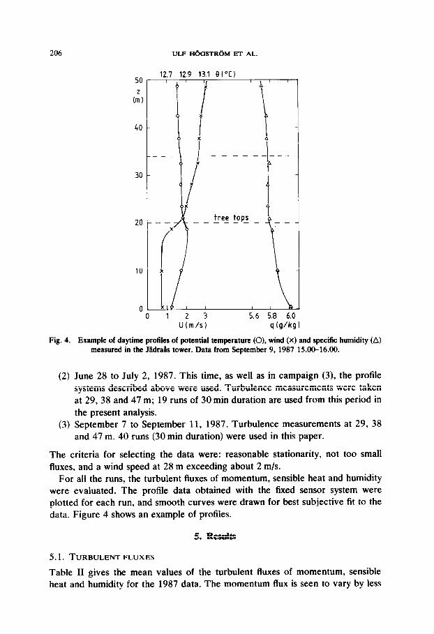
Fig. 4. Example of daytime profiles of potential temperature (O), wind (x) and specific humidity (A) measured in the JiidraHs tower. Data from September 9, 1987 15.00-16.00.

(2) June 28 to July 2, 1987. This time, as well as in campaign (3), the profile systems described above were used. Turbulence measurements were taken at 29, 38 and 47 m; 19 runs of 30 min duration are used from this period in the present analysis.

(3) September 7 to September 11, 1987. Turbulence measurements at 29, 38 and 47 m. 40 runs (30 min duration) were used in this paper.

The criteria for selecting the data were: reasonable stationarity, not too small fluxes, and a wind speed at 28 m exceeding about 2 m/s.

For all the runs, the turbulent fluxes of momentum, sensible heat and humidity were evaluated. The profile data obtained with the fixed sensor system were plotted for each run, and smooth curves were drawn for best subjective fit to the data. Figure 4 shows an example of profiles.

5. Resnlts

5.1. TURBULENTFLUXES

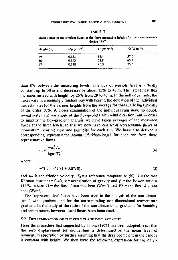
Table II gives the mean values of the turbulent fluxes of momentum, sensible heat and humidity for the 1987 data. The momentum flux is seen to vary by less

TURBULENT EXCHANGE ABOVE A PINE FOREST, I 207

TABLE II

Mean values of the trbulent fluxes at the three measuring heights for the measurements during 1987

Height (m) 7/p (mZ K2) H (W mS2) W(W rnm2)

29 0.183 53.4 57.0 38 0.193 52.8 65.7 47 0.178 45.3 75.5

than 8% between the measuring levels. The flux of sensible heat is virtually constant up to 38 m and decreases by about 15% to 47 m. The latent heat flux increases instead with height, by 26% from 29 to 47 m. In the individual runs, the fluxes vary in a seemingly random way with height, the deviation of the individual flux estimates for the various heights from the average for that run being typically of the order 10%. A closer examination of the individual runs may, no doubt, reveal systematic variations of the flux-profiles with wind direction, but in order to simplify the flux-gradient analysis, we have taken averages of the measured fluxes at the three levels, so that we now have one set of representative fluxes of momentum, sensible heat and humidity for each run. We have also derived a corresponding representative Monin-Obukhou-length for each run from these representative fluxes:

-&To L=-

kg=” ’ (4)

where -- w’T:= w’T’(l+O.O7//3), (5)

and u* is the friction velocity, To = a reference temperature (K), k = the von Karman constant = 0.40, g = acceleration of gravity and /3 = the Bowen ratio = H/EA, where H = the flux of sensible heat (W/m2) and EA = the flux of latent heat (W/m2).

The ‘representative’ fluxes have been used in the analysis of the non-dimen- sional wind gradient and for the corresponding non-dimensional temperature gradient. In the study of the ratio of the non-dimensional gradients for humidity and temperature, however, local fluxes have been used.

5.2. DETERMINATIONOFTHEZEROPLANEDISPLACEMENT

Here the procedure first suggested by Thorn (1971) has been adopted, viz., that the zero displacement for momentum is determined as the mean level of momentum absorption by further assuming that the drag coefficient in the canopy is constant with height. We then have the following expression for the deter-

208 ULF H&!iTR(IM ET AL.

mination of zero plane displacement d:

dJ” zW)*dz j,: U(z)* dz ’ (6)

where U(z) is the wind speed at height .z and the integration extends from the ground to the top of the canopy, at z = h.

Evaluating this expression with the aid of data from the 1985 campaign, when wind was measured at the following heights: 3.14, 7.57, 12.01, 17.30 and 20.32 m, gives the result

d = 15.2 f 0.8 m (standard deviation).

In this analysis 393 h of data were used. In keeping with Raupach (1979), we assume that this value is also relevant for

the temperature and the humidity profiles, bearing in mind that “. . . this pro- cedure does not imply equality of source-sink levels for momentum, heat and water vapour; rather, it is a parameterization of complex turbulent transfer processes governed by the turbulent properties of flow close to the very rough surface, and by the distributed nature of sources or sinks for momentum, heat and water vapour”.

The value 15 m for d corresponds to 0.95 of ‘the mean height of the trees’ (16 m) and to 0.75 of the height of the dominating trees. The sensitivity of the results to the choice of d is discussed in Section 5.4.

5.3. NON-DIMENSIONALPROFILES

In traditional surface-layer scaling, non-dimensional profiles of wind &, tem- perature +, and humidity 4, are defined as

dm = k(z - d) ali

-9 IA* az

(7)

4w= k(z - d) atj

q* g,

where T* = - w’T’/u*, q* = - w’q’/u*, aii/az is the wind gradient at height z, a#/laz the corresponding gradient of potential temperature and aq/az the gradient of specific humidity.

Gradients of wind, potential temperature and humidity have been evaluated for the turbulence measurement levels for each run from the best fit profile curves and inserted, together with the ‘representative turbulent fluxes’, into Equations (7), to give ‘measured non-dimensional gradients’. In addition, corresponding non-dimensional gradients have been derived from formulae representing ‘ideal

TURBULENT EXCHANOE ABOVE A PINE FOREST, I 209

conditions’, giving what we shall term bid and bid. We have used the expres- sions suggested by Hogstrom (1988) for unstable conditions:

q& = (1 - 19.35)~“4,

c#& = (1- 125)-l’“. 03)

Here 5 = (z - d)/l, where L, is the Monin-Obukhov length defined by Equation (4).

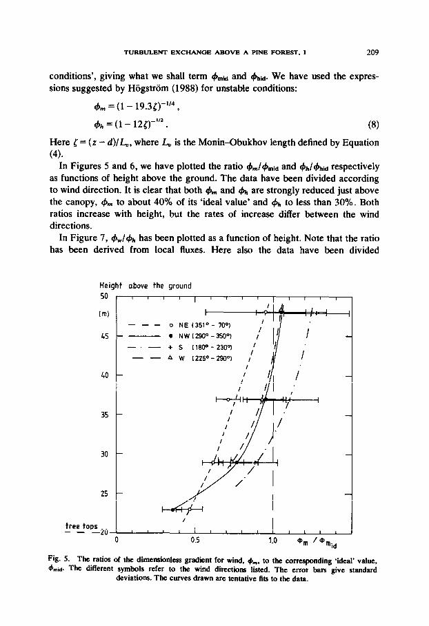
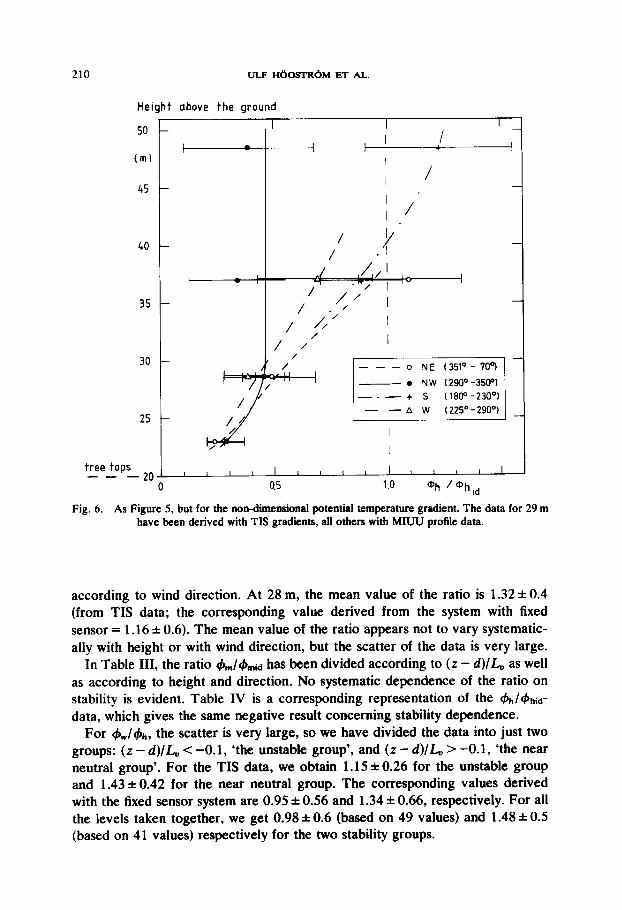
In Figures 5 and 6, we have plotted the ratio &/&id and 4,,/&,, respectively as functions of height above the ground. The data have been divided according to wind direction. It is clear that both &, and I#+, are strongly reduced just above the canopy, +,,, to about 40% of its ‘ideal value’ and c#+, to less than 30%. Both ratios increase with height, but the rates of increase differ between the wind directions.

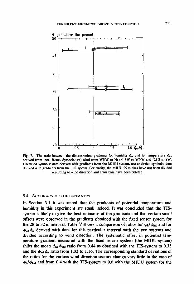
In Figure 7, &./& has been plotted as a function of height. Note that the ratio has been derived from local fluxes. Here also the data have been divided

Height above the ground

50

(ml

45

--- o NE f351° - W’)

- - 0 NW(290“-350“)

-. - + s (1800-2300) ---hw l225“-2909 ,'

LO

35

30

25

tree topiZO- -- ^ U 0.5 1.0

Fig. 5. The ratios of the dimensionless gradient for wind, 4”. to the corresponding ‘ideal’ value, Q,,,u. The different symbols refer to the wind directions listed. The error bars give standard

deviations. The curves drawn are tentative fits to the data.

210 ULF H6GSTRt)M ET AL.

Height above the ground

50

(ml

45

c I I ’ ,I

40

35

25

tree tops -- - 20 _ 0

I I

I I /

I /

o NE (351” - 709

. NW (290’-3509

0.5 1.0 @h ‘*h,,

Fig. 6. As Figure 5, but for the non-dimensional potential temperature gradient. The data for 29 m have been derived with TIS gradients, all others with MIUU profile data.

according to wind direction. At 28 m, the mean value of the ratio is 1.32 f 0.4 (from TIS data; the corresponding value derived from the system with fixed sensor = 1.16 f 0.6). The mean value of the ratio appears not to vary systematic- ally with height or with wind direction, but the scatter of the data is very large.

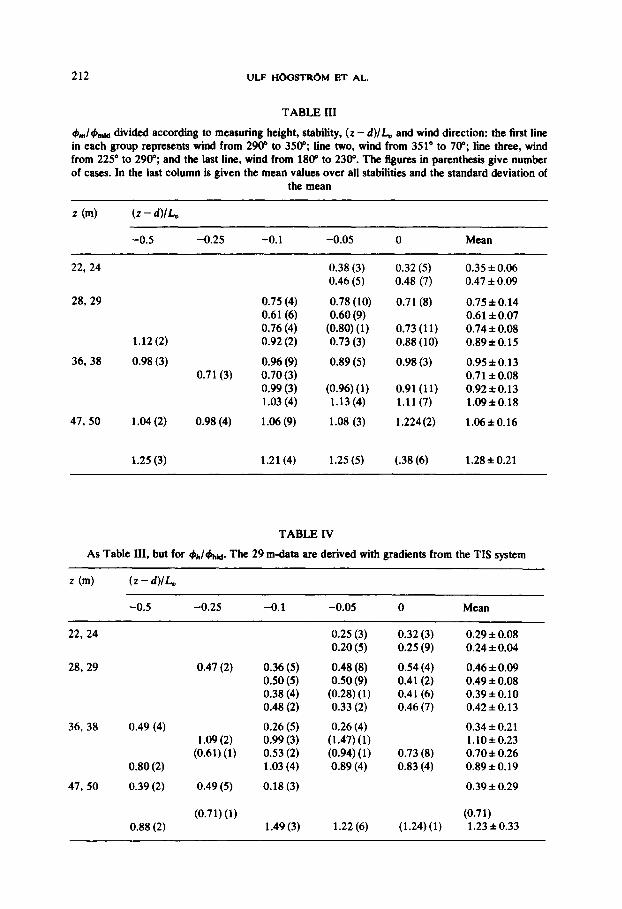
In Table III, the ratio &/c#+,,~ has been divided according to (z - d)/L, as well as according to height and direction. No systematic dependence of the ratio on stability is evident. Table IV is a corresponding representation of the 4,,h/&id- data, which gives the same negative result concerning stability dependence.

For &./& the scatter is very large, so we have divided the data into just two groups: (z - d)/L, < -0.1, ‘the unstable group’, and (z - d)/L, > -0.1, ‘the near neutral group’. For the TIS data, we obtain 1.15 f 0.26 for the unstable group and 1.43 f 0.42 for the near neutral group. The corresponding values derived with the fixed sensor system are 0.95 f 0.56 and 1.34 f 0.66, respectively. For all the levels taken together, we get 0.98 f 0.6 (based on 49 values) and 1.48 f 0.5 (based on 41 values) respectively for the two stability groups.

TURBULENT EXCHANGE ABOVE A PINE FOREST. I

Height above the ground

40

35

30

25

20

211

0 J I I I 11 11 11 1 ’ 11 1 ’ “1 1 ” 1

0.5 1 1.5 2.0 @,/I

Fig. 7. The ratio between the dimensionless gradients for humidity I$, and for temperature &,, derived from local fluxes. Symbols: (+) wind from WNW to N; (*) SW to WNW and (A) S to SW. Encircled symbols: data derived with gradients from the MIUU system, not encircled symbols: data derived with gradients from the TIS system. For clarity, the MIUU 29 m data have not been divided

according to wind direction and error bars have been deleted.

0 T-

5.4. ACCURACYOFTHEESTIMATES

In Section 3.1 it was stated that the gradients of potential temperature and humidity in this experiment are small indeed. It was concluded that the TIS- system is likely to give the best estimates of the gradients and that certain small offsets were observed in the gradients obtained with the fixed sensor system for the 28 to 32 m interval. Table V shows a comparison of ratios for c#+,/&,, and for c$,,,/& derived with data for this particular interval with the two systems and divided according to wind direction. The systematic offset in potential tem- perature gradient measured with the fixed sensor system (the MIUU-system) shifts the mean &/hid ratio from 0.44 as obtained with the TIS-system to 0.35 and the &,l& ratio from 1.32 to 1.16. The corresponding standard deviations of the ratios for the various wind direction sectors change very little in the case of &/& and from 0.4 with the TIS-system to 0.6 with the MIUU system for the

212 ULF Hth3TRbU ET AL.

TABLE III

&,,/s&~ divided according to measuring height, stability, (L - d)/L, and wind direction: the first line in each group represents wind from 2900 to 350”; line two, wind from 351” to 70“; line three, wind from 225” to 290”; and the last line, wind from 180’ to 230”. The figures in parenthesis give number of cases. In the last column is given the mean values over all stabilities and the standard deviation of

the mean

2 (4 (2 - 4lh

-0.5 -0.25 -0.1 -0.05 0 Mean

22, 24

28,29 0.75 (4) 0.61(6) 0.76 (4)

1.12 (2) 0.92 (2)

36,38 0.98 (3) 0.96 (9) 0.71(3) 0.70 (3)

0.99 (3) 1.03 (4)

47,50 1.04 (2) 0.98 (4) 1.06 (9)

1.25 (3) 1.21(4)

0.38 (3) 0.46 (5)

0.78 (10) 0.60 (9)

(0.80) (1) 0.73 (3)

0.89 (5)

(0.96) (1) 1.13 (4)

1.08 (3)

1.25 (5)

0.32 (5) 0.48 (7)

0.71 (8)

0.73 (11) 0.88 (10)

0.98 (3)

0.91 (11) l.ll(7)

1.224(2)

(38 (6)

0.35 f 0.06 0.47 f 0.09

0.75 f 0.14 0.61 f 0.07 0.74 f 0.08 0.89*0.15

0.95*0.13 0.7 1 f 0.08 0.92*0.13 1.09~0.18

1.06kO.16

1.28*0.21

TABLE IV

As Table III, but for &/hid. The 29 m-data are derived with gradients from the TIS system

2 (4 (2 - 4/h

-0.5 -0.25 -0.1 -0.05 0 Mean

22,24

28,29 0.47 (2)

36.38 0.49 (4) 1.09 (2)

(0.61) 0) 0.80 (2)

47,50 0.39 (2) 0.49 (5)

(0.71) (1) 0.88 (2)

0.36 (5) 0.48 (8) 0.50 (5) 0.50 (9) 0.38 (4) (0.28) (1) 0.48 (2) 0.33 (2)

0.26 (5) 0.99 (3) 0.53 (2) 1.03 (4)

0.26 (4) (1.47) (1) (0.94) (1) 0.89 (4)

0.18 (3)

1.49 (3)

0.25 (3) 0.20 (5)

1.22 (6)

0.32 (3) 0.25 (9)

0.54 (4) 0.41(2) 0.41 (6) 0.46 (7)

0.73 (8) 0.83 (4)

(1.24) (1)

0.29 f 0.08 0.24 f 0.04

0.46 f 0.09 0.49 f 0.08 0.39*0.10 0.42kO.13

0.34*0.21 l.lOhO.23 0.70 f 0.26 0.89 f 0.19

0.39 f 0.29

(0.71) 1.23 f 0.33

TURBULENT EXCHANGE ABOVE A PINE FOREST, I 213

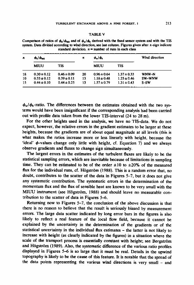
TABLE V

Comparison of ratios of I/J,,/& and of &/I),, derived with the fixed sensor system and with the TIS system. Data divided according to wind direction, see last column. Figures given after i-sign indicate

standard deviation. n = number of runs in each class

n 4hMhki n hJ#h Wind direction

MIUU TIS MIUU TIS

18 0.3OhO.12 0.46 f 0.09 20 0.96 f 0.64 1.37 f 0.33 WNW-N 10 0.33 f 0.12 0.39*0.11 13 1.18~0.48 1.25 f 0.46 SW-WNW 15 0.44*0.10 0.44 f 0.25 13 1.57 f 0.79 1.31*0.43 S-SW

#,/&,-ratio. The differences between the estimates obtained with the two sys- tems would have been insignificant if the corresponding analysis had been carried out with profile data taken from the lower TIS-interval (24 to 28 m).

For the other heights used in the analysis, we have no TIS-data. We do not expect, however, the relative errors in the gradient estimates to be larger at these heights, because the gradients are of about equal magnitude at all levels (this is what makes the ratios increase more or less linearly with height, because the ‘ideal’ #-values change only little with height, cf. Equation 7) and we always observe gradients and fluxes to change sign simultaneously.

The largest errors in the estimates of the turbulent fluxes are likely to be the statistical sampling errors, which are inevitable because of limitations in sampling time. They can be estimated to be of the order *lo to *20% of the measured flux for the individual runs, cf. Hogstrom (1988). This is a random error that, no doubt, contributes to the scatter of the data in Figures 5-7, but it does not give any systematic contribution. The systematic errors in the determination of the momentum flux and the flux of sensible heat are known to be very small with the MIUU instrument (see Hogstrom, 1988) and should leave no measurable con- tribution to the scatter of data in Figures 5-6.

Returning now to Figures 5-7, the conclusion of the above discussion is that there is no reason to believe that the result is seriously biased by measurement errors. The large data scatter indicated by long error bars in the figures is also likely to reflect a real feature of the local flow field, because it cannot be explained by the uncertainty in the determination of the gradients or of the statistical uncertainty in the individual flux estimates - the latter is not likely to increase with height (as clearly indicated by the figures) in a situation where the scale of the transport process is essentially constant with height; see Bergstrom and Hogstrom (1989). Also, the systematic difference of the various ratio profiles displayed in Figures 5-6 is so large that it must be real. Details in the upwind topography is likely to be the cause of this feature. It is notable that the spread of the data points representing the various wind directions is very small - and

214 ULF H6GSTR6M ET AL.

probably not significant - in the lowest point, which represents the rather homogeneous conditions immediately around the tower - cf. the map, Figure 1.

Finally, the sensitivity of the results to the determination of the zero plane displacement d will be discussed. To change the non-dimensional +-ratios from their values of 0.5 or 0.3, at 28 m (Figures 5 and 6) to unity, would require a negative d-value. Changing d from 15 to 10 m changes the corresponding +-ratio from 0.4 to 0.56. Thus, even if the method presented in Section 5.2 for the determination of d is crude, it is clear that the deviations of the &ratios from unity found cannot be explained on these grounds, as was also concluded by Raupach (1979).

6. Discussion and Conclusions

The results obtained in this study are in many ways confirmation of earlier findings reported in the literature. In particular, the strong reduction of the dimensionless gradient for temperature (Figure 6) seems to be a universal finding over forests. It has been reported from the Thetford forest (Thorn et al., 1975; and Raupach, 1979), by Garratt (1980) from a Savannah and by Denmead and Bradley (1985) from a forest in Australia “very similar to the Thetford forest”. It was also found by Coppin et al. (1986) in a wind tunnel study over an artificial, rough canopy.

The reduction of the dimensionless wind gradient (Figure 5) appears to be related in some way to the density of the canopy: it was found by Garratt (1980) over his sparse Savannah and in this study but not over the rather dense Thetford forest or over Denmead and Bradley’s (1985) forest. The effect is also clearly seen in the results of the wind tunnel study of Raupach er al. (1986). It was also observed in an earlier wind tunnel study by Raupach et al. (1980). In that paper, the authors made an attempt to express the depth of the layer in which the wind profile is being modified by the presence of the rough surface. They conclude that it is ‘the transverse element dimension’ that governs the depth of the modified layer. This can, however, hardly be applicable in the forest case: the width of the trees in the Jiidrais forest is not larger than the corresponding width of the trees in the Thetford forest (two of the authors, U. H. and A. S. can testify to this from having seen both sites). Raupach ef al. (1980) seem also to be aware that their model is very tentative.

The finding in this study that there is no variation with stability of the ratio between measured and ‘ideal’ values of the dimensionless gradients of wind and temperature is contrary to what Thorn et al. (1975) and Raupach (1979) report from the Thetford forest study and Denmead and Bradley (1985) from their site. It is, however, in qualitative agreement with the results of Garratt (1980), who found that during unstable conditions (the only conditions studied here), the ratio of observed non-dimensional gradients to their ‘ideal’ counterparts is only a function of height. Garratt also suggests an analytical expression:

TURBULENT EXCHANGE ABOVE A PINE FOREST. I 215

4O = 0.5~$(zlL.) exp(0.72/2*),

where z* is “equal to 36, S being the tree spacing”. With an average tree distance of 5 m, as obtained from the figure 350 trees/hectare quoted earlier, Garratt’s formula (with z in the equation exchanged for z - d) would make the gradient ratio larger than unity already from a height of about 30 m, which is not in accord with the data in Figures 5 and 6. If we interpret ‘tree spacing’ as “the spacing of the dominant trees” 6 is 6 or 7 m, which makes the gradient ratio equal to unity at about 35 m, in reasonable agreement with Figures 5 and 6.

This brings us to the fundamental question of the reason for the reported anomalies. Raupach (1987) and Coppin et al. (1986) identify two mechanisms that work against each other. The effect of ‘near field diffusion’ is to increase the magnitude of the nondimensional gradients. The factor that makes them decrease is rather loosely referred to as an increase in scale of the turbulent transport mechanism. This is similar to interpreting a relative reduction of the non- dimensional gradients (equivalent to a corresponding increase in the turbulent exchange coefficients) in terms of a corresponding increase in ‘mixing length’. This does not, however, lead to any deeper understanding of the actual transport mechanism. In Bergstrom and Hogstrom (1989), an attempt is made to study the transport process with the aid of a conditional sampling technique.

The result concerning the ratio &/+,, is not entirely conclusive because of the large data scatter. A formal significance test shows that the value obtained for the near neutral class, about 1.4, is significantly different from unity (p > 0.01). For the more unstable group, i.e., for (z - d)/L, < -0.1, the ratio is apparently close to unity. The large scatter found in the ratio can only partly be explained by measurement errors and must thus largely reflect the real situation at the site. A closer examination of the simultaneous cospectra for water vapor and tem- perature fluxes often reveals relatively large-amplitude irregularities in the low frequency region of the water vapour flux cospectra, absent in the temperature flux cospectra. These irregularities can usually be traced in the three measuring levels, although the amplitude of the irregularities may change with height. It is a reasonable interpretation that the heterogeneity of the surroundings has a stronger effect on the evaporation than on the sensible heat flux from the canopy in our case.

Acknowledgements

This paper is part of a cooperative effort focused on the evaporation problem at JPdrals, which was initiated by Sven Halldin. The TIS system was supplied by the Biogeophysics Group (here represented by S. H. and A. L.). The Dept. of Meteorology Group is responsible for the fixed profile measurements and the turbulence measurements. The authors would like to thank Mr Knut Lundin for his invaluable effort before and during the field campaigns to keep up the high

216 ULF HC)CiSTRC)M ET AL.

standard of performance of the Department of Meteorology equipment. The project was supported by a grant from the Swedish National Science Research Council (NFR Contract G-GU 1923-101).

Baker, B. C.: 1988, ‘Experimental Determination of Transducer Shadow Effect on a Sonic Ane- mometer’, in Proceedings from Eighth Symposium on Turbulence and Diffusion, April 25-29, 1988 in San Diego, CA, American Meteorological Society, pp. 104-107.

Bergstrom, H. and Hegstrom, U.: 1987, ‘Calibration of a Three Axial Fiber Film System for Meteorological Turbulence Measurements’, Dan&c Information 5, 16-20.

Bergstrom, H. and Hogstrom, U.: 1989, ‘Turbulent Exchange above a Pine Forest, II: Organized Structures’, Boundary-Layer Meteorol. (in press).

Coppin, P. A., Raupach, M. R. and Legg, B. J.: 1986, ‘Experiments on Scalar Dispersion within a Model Plant Canopy Part II: An Elevated Plane Source’, Boundary-Layer Meteorcl. 35, 167-191.

Deacon, E. L.: 1959, ‘The Measurement of Turbulent Transfer in the Lower Atmosphere’, in Proceedings of the Symposium on Atmospheric Di)@sion and Air Pollution 6 in Advances in Geophysics series, pp. 21 l-228.

Denmead, 0. T. and Bradley, E. F.: 1985, ‘Flux-gradient Relationships in a Forest Canopy’, in B. A. Hutchison and B. B. Hicks (eds.), The Forest-Atmosphere Interaction, pp. 4121-4142.

Dyer, A. J. and 20 co-authors: 1982, ‘An International Turbulence Comparison Experiment (ITCE 1976)‘, Boundary-Layer Meteo~~l. 24,181-209.

Garratt, J. R.: 1980, ‘Surface Influence upon Vertical Profiles in the Atmospheric Near-surface Layer’, Quart. .I. R. Meteorol. Sot. 106,803-819.

Grip, H., Halldin, S., Jansson, P.-E., Lindroth, A., Nor&n, B., and Perttu, K.: 1979, ‘Discrepancy between Energy Balance and Water Balance Estimates of Evapotranspiration’, in S. Halldin (ed.), Comparison of Forest Water and Energy Exchange Models, International Society for Ecological Modelling, Copenhagen, pp. 237-255.

Hogstrom, U.: 1982, ‘A Critical Evaluation of the Aerodynamical Error of a Turbulence Instrument’, J. Applied Mereorol. 21,1838-1844.

Hogstrom, U.: 1988, ‘Non-dimensional Wind and Temperature Profiles in the Atmospheric Surface Layer: A Reevaluation’, Boundary-Layer Meteorol. 42, 55-78.

Lindroth, A.: 1984, ‘Gradient Distributions and Flux Profile Relations above a Rough Forest’, Quarr. J. Roy. Meteorol. Sot. 110, 553-563.

Lindroth, A., Halldin, S., BergstrGm, H., Hogstriim, U., Lundin, K., and Smedman, A.: 1989, ‘Temperature and Humidity Gradient Measurements above a Forest Using Fixed and Reversing Sensor Systems’, subtnltted to Quart. J. Roy. Meteorol. Sot.

Persson, H.: 1980, ‘Structural Properties of the Field and Bottom Layers at Ivantjllrnsheden’, in T. Persson (ed.), Structure and Function of Northern Coniferous Forests - An Ecosystem Study. Ecol. Bull. 32, 153-163.

Raupach, hf. R.: 1979, ‘Anomalies in Flux-gradient Relationships over Forest’, Boundary-Layer Meteorol. 16,467-486.

Raupach. M. R.: 1987, ‘A Lagrangian Analysis of Scalar Transfer in Vegetation Canopies’, Quart. J. R. Meteorol. Sot. 113, 107-120.

Raupach, M. R., Thorn, A. S., and Edwards, I.: 1980, ‘A Wind-Tunnel Study of Turbulent Flow Close to Regularly Arrayed Rough Surfaces’, Boundary-Layer Meteorol. 18. 373-397.

Raupach, M. R., Coppin, P. A., and Legg, B. J.: 1986, ‘Experiments on Scalar Dispersion within a Model Plant Canopy Part I: The Turbulence Structure’, Boundary-Layer Meteorol. 35,21-52.

Smedman. A. and Lundin, K.: 1987, ‘Influence of Sensor Configuration on Measurements of Dry and Wet Bulb Temperature Fluctuations’. J. Atm. Ocean. Technol. 4.668-673.

Thorn, A. S.: 1971, ‘Momentum Absorption by Vegetation’, Quarr. J. Roy. Meteorol. Sot. W, 414-428.

Thorn, A. S., Stewart, J. B., Oliver, H. R., and Gash, J. H. C.: 1975, ‘Comparison of Aerodynamic

TURBULENT EXCHANGE ABOVE A PINJZ FOREST, I 217

and Energy Budget Estimates of Fluxes over a Pine Forest’, Quart. J. R. Meteorol. Sot. 101, 93-105.

Wyngaard, J. C. and Cot& 0. R.: 1972, ‘Cospectral Similarity in the Atmospheric Surface Layer’, Quart. J. R. Meteorol. Sot. 98.590-603.

Zhang, S. F., Wyngaard, J. C., Businger, J. A., and Oncley, S. P.: 1986, ‘Response Characteristics of the U.W. Sonic Anemometer’, J. Aims. Ocean. Technol. 2, 548-558.