Trenholm PhD Dissertation - SFU's Summit

Public Willingness to Pay for Improvements in

Ecosystem Services and Landowner Willingness to

Accept for Wetlands Conservation: An Assessment

of Benefit Transfer Validity and Reliability Using

Choice Experiments in Several Canadian Watersheds

by

Ryan Trenholm

M.Sc.F., University of New Brunswick, Fredericton, 2009

B.A. (Hons., Economics), University of New Brunswick, Fredericton, 2004

Thesis Submitted in Partial Fulfillment of the

Requirements for the Degree of

Doctor of Philosophy

in the

School of Resource and Environmental Management

Faculty of Environment

© Ryan Trenholm 2018

SIMON FRASER UNIVERSITY

Fall 2018

Copyright in this work rests with the author. Please ensure that any reproduction or re-use is done in accordance with the relevant national copyright legislation.

ii

Approval

Name: Ryan Trenholm

Degree: Doctor of Philosophy

Title: Public Willingness to Pay for Improvements in Ecosystem Services and Landowner Willingness to Accept for Wetlands Conservation: An Assessment of Benefit Transfer Validity and Reliability Using Choice Experiments in Several Canadian Watersheds

Examining Committee: Chair: Sean Markey Professor

Duncan Knowler Senior Supervisor Associate Professor

Van A Lantz Supervisor Professor and Dean Faculty of Forestry and Environmental Management University of New Brunswick

Pascal Haegeli Supervisor Assistant Professor

Murray Rutherford Internal Examiner Associate Professor

Wiktor (Vic) Adamowicz External Examiner Professor and Vice Dean Department of Resource Economics and Environmental Sociology University of Alberta

Date Defended/Approved: December 7, 2018

iii

Ethics Statement

iv

Abstract

Benefit-cost analyses are often used to evaluate the economic efficiency of proposed

policies or projects. Such analyses require analysts to estimate the benefits and costs in

monetary terms of any changes related to the policy being analyzed, including to the

environment (e.g., changes in water or air quality). However, estimating these monetary

values can be difficult since prices are often not available due to market failure. As such,

several non-market valuation techniques have been developed for use in assessing

these monetary values, including original research techniques, such as choice

experiments, and benefit transfer which applies existing non-market values estimated

using original research techniques to other contexts (e.g., locations). Several studies

have evaluated the validity and reliability of benefit transfer in a variety of contexts. In

this thesis, I contribute to this literature by assessing transfers in contexts not yet

evaluated. In doing so, I use choice experiments to investigate landowner preferences

for wetlands conservation in two Ontario watersheds and elicit the general public’s

willingness to pay values for changes in ecosystem services in four Canadian

watersheds. This research resulted in four papers. The first paper, motivated by the loss

of wetlands in Southern Ontario, involves assessing the preferences and willingness to

accept (WTA) of farm and non-farm landowners for enrolling their land in wetlands

conservation programs. Though preferences and values are heterogeneous, many

landowners are willing to enrol and at moderate cost. Using data from this paper, in the

second and third papers I evaluate the validity and reliability of transfers of WTA and

predicted program participation market shares, respectively. Results suggest that

transfers of WTA are similarly valid and reliable to transfers of willingness to pay, while

transfers of predicted participation market shares are considerably more valid and

reliable than a parallel assessment of transfers of WTA. Finally, using data from the

general public survey I evaluate alternatives for reconciling quantitative choice

experiment attributes with differing levels for benefit transfer. A key finding of this

research is that transfers rooted in “relative” preferences are more valid and reliable than

transfers rooted in “absolute” preferences.

Keywords: benefit transfer; choice experiment; willingness to pay; willingness to

accept; wetlands; convergent validity

v

Dedication

For family, friends, and colleagues — especially my two boys.

vi

Acknowledgements

My PhD has been an enjoyable, though non-linear, journey and I have many people to

thank. I began in early 2009 as a student in the Faculty of Forestry at the University of

British Columbia in Dr. Thomas Maness’s lab with the intention of working on forest

product supply chains and ecosystem services. However, Dr. Maness left for Oregon

State University within the year and I eventually moved to Simon Fraser University.

Sadly, Dr. Maness recently passed away. I benefited from my time at UBC through

research and coursework as well as the personal relationships with Dr. Maness and

members of his lab, in particular Francisco Vergara and his family. I transferred to the

School of Resource and Environmental Management (REM) at SFU in 2010 under the

supervision of Dr. Wolfgang Haider, a connection made possible by Dr. Van Lantz who

also joined my committee (Dr, Lantz supervised my master’s degree at the University of

New Brunswick). The committee was completed with the addition of Dr. Duncan

Knowler. At SFU I benefited from the coursework and relationships with faculty and

students alike. However, on August 17, 2015 I learned that Wolfgang had been in an

accident in Austria and he passed away on August 24th. This was devastating for his

family and friends, indeed everyone at REM myself included. In my experience, REM’s

response was thoughtful and they have accommodated the members of Wolfgang’s lab.

Dr. Duncan Knowler subsequently took over as senior supervisor and Dr. Pascal Haegeli

was added to my supervisory committee.

From my time at SFU I have many people to thank, including: 1) all members of my

supervisory committee; 2) the other students working on the same research project

(David Angus, Toni Anderson, and Monica McKendy); 3) the other students and

researchers at REM, including the too many to name members of Wolfgang’s lab (those

I worked most closely with include Ben Beardmore, Steve Conrad, Nina Mostegl, Amy

Suess (now Kitchen), Sergio Fernandez Lozada, Kornelia Dabrowska, and Rodrigo Solis

Sosa) as well as the many other students whose office space was in the Tourism Lab; 4)

the members of REM’s Water Research Group (Steve Conrad, Cedar Morten, Sarah

Breen, Lee Johnson, Dr. Murray Rutherford, and David Angus); and 5) last, but certainly

not least, the REM staff. Several others helped out during the research process and I’d

like to acknowledge the help of Tatiana Koveshnikova (Credit River Conservation

Authority), Jeff Brick (Upper Thames Conservation Authority), and Tracy Ryan (Grand

vii

River Conservation Authority). Financial support was provided by the Social Sciences

and Humanities Research Council as well as SFU. Furthermore, my research would not

have been possible without the participation of the survey respondents whom I hope I

did not annoy too much.

Existing and new relationships with people outside of the university bubble were also

important. Jess Metter and Steve Bornemann, the parents of a friend I met during my

master’s in New Brunswick, welcomed my wife and I when we moved to Vancouver and

even found our first apartment. Their son James Bornemann, though living in New

Brunswick, still keeps in regular contact despite the distance. I also thank other friends

made during my masters, Jeff Wilson and Wei-Yew Chang, now a post-doc at UBC, as

well as Wanggi Jaung a PhD from UBC who I got to know while a teaching assistant for

Wolfgang’s choice modeling course. I also had the opportunity to work casually for Jeff

Wilson at Green Analytics as well as for Amy and Patrick Kitchen at Yarrow Consulting

which helped me gain non-academic experience. Of course I thank my family, which has

expanded during my time as a PhD student. I got married in 2012 to Valerie LeBlanc and

this adventure would not have been possible without her invaluable support. We had a

child in late 2014 and another in 2018, which likely lengthened my studies, and they

continue to inspire. My parents, brother and sister, as well as in-laws have also been

very supportive. Finally, I’d like to acknowledge the local First Nations on whose land I

live and work as well as those at my research sites in New Brunswick, Southern Ontario,

and British Columbia

viii

Table of Contents

Approval .......................................................................................................................... ii

Ethics Statement ............................................................................................................ iii

Abstract .......................................................................................................................... iv

Dedication ....................................................................................................................... v

Acknowledgements ........................................................................................................ vi

Table of Contents .......................................................................................................... viii

List of Tables ................................................................................................................. xii

List of Figures............................................................................................................... xiv

Introduction .............................................................................................. 1 Chapter 1.

1.1. Theme 1: Private Landowner Preferences for Conservation Practices .................. 3

1.2. Theme 2: Benefits Transfer ................................................................................... 5

1.3. Brief Backgrounder on Non-Market Economic Valuation ....................................... 9

1.3.1. Economic Values ........................................................................................... 9

1.3.2. Basics of Measures of Economic Welfare .................................................... 10

1.3.3. Original Research Approaches to Non-Market Valuation ............................. 16

1.4. A Summary of the Dissertation ............................................................................ 17

1.5. Statement of Interdisciplinarity ............................................................................. 20

References .................................................................................................................... 21

Landowner Preferences for Wetlands Conservation Programs in Two Chapter 2.Southern Ontario Watersheds ............................................................... 26

Abstract ......................................................................................................................... 27

2.1. Introduction .......................................................................................................... 28

2.2. Study Sites .......................................................................................................... 31

2.3. Method ................................................................................................................ 33

2.3.1. The Choice Experiment ............................................................................... 33

2.3.2. Data Collection ............................................................................................ 36

2.3.3. Data Analysis............................................................................................... 37

2.4. Results ................................................................................................................ 40

2.4.1. Respondent Characteristics ......................................................................... 40

2.4.2. Choice Models ............................................................................................. 43

Farm Model ............................................................................................................ 43

Non-Farm Model .................................................................................................... 46

2.4.3. Applying Choice Model Results ................................................................... 48

Marginal Willingness to Accept............................................................................... 48

Compensating Surplus and Predicted Participation ................................................ 50

2.5. Discussion ........................................................................................................... 53

2.5.1. Policy Implications ....................................................................................... 55

2.6. Conclusion........................................................................................................... 58

2.7. Acknowledgements ............................................................................................. 60

ix

References .................................................................................................................... 61

Transfers of Landowner Willingness to Accept: A Convergent Validity Chapter 3.and Reliability Test Using Choice Experiments in Two Canadian Watersheds............................................................................................. 68

Abstract ......................................................................................................................... 69

3.1. Introduction .......................................................................................................... 70

3.2. Data and Methods ............................................................................................... 74

3.2.1. Data ............................................................................................................. 74

3.2.2. Econometric Model ...................................................................................... 78

3.2.3. Deriving WTA and CS from the Model in WTA Space .................................. 82

3.2.4. Transfer Reliability and Validity .................................................................... 83

Testing for Differences in Functions ....................................................................... 83

Testing for Differences in WTA or CS and Calculating Transfer Error .................... 84

3.3. Results ................................................................................................................ 87

3.3.1. Comparison of Respondent Characteristics ................................................. 87

3.3.2. Modelling Results ........................................................................................ 89

3.3.3. Willingness to Accept, Transfer Errors, and Testing .................................... 92

Marginal Willingness to Accept............................................................................... 92

Compensating Surplus ........................................................................................... 96

3.3.4. Sensitivity Analysis ...................................................................................... 98

3.4. Discussion and Conclusions .............................................................................. 100

3.5. Acknowledgements ........................................................................................... 103

References .................................................................................................................. 104

Assessing the Convergent Validity and Reliability of Transfers of Chapter 4.Market Shares Derived from Choice Experiments for Landowner Participation in Wetlands Conservation Programs ........................... 112

Abstract ....................................................................................................................... 113

4.1. Introduction ........................................................................................................ 114

4.2. Method .............................................................................................................. 118

4.2.1. Econometric Modeling ............................................................................... 118

4.2.2. Deriving market shares and compensating surplus .................................... 120

4.2.3. Assessing the Validity and Reliability of Transfers ..................................... 121

Testing the Similarity of Choice Models ................................................................ 121

Testing for Differences in MS or CS and Calculating Transfer Error ..................... 122

4.2.4. Comparing Sample Characteristics ............................................................ 125

4.3. Data................................................................................................................... 126

4.4. Results .............................................................................................................. 129

4.4.1. Respondent Characteristics ....................................................................... 129

4.4.2. Random Parameters Logit Models and Testing Model Similarity ............... 131

4.4.3. Market Share and Compensating Surplus Estimates ................................. 135

4.4.4. Transfer Validity and Reliability .................................................................. 136

4.5. Discussion and Conclusion ................................................................................ 140


x

References .................................................................................................................. 145

Reconciling Quantitative Attributes with Different Levels When Chapter 5.Transferring Willingness to Pay Elicited from Choice Experiments: Evidence from Benefit Transfers between Four Canadian Watersheds............................................................................................................... 151

Abstract ....................................................................................................................... 152

5.1. Introduction ........................................................................................................ 153

5.2. Data and Method ............................................................................................... 156

5.2.1. Study Sites ................................................................................................ 156

5.2.2. Data ........................................................................................................... 157

5.2.3. Data Collection .......................................................................................... 160

5.2.4. Comparing Respondent Characteristics..................................................... 161

5.2.5. Econometric Modeling and Derivation of Willingness to Pay ...................... 161

5.2.6. Benefit Transfer Assessment ..................................................................... 162

5.3. Results .............................................................................................................. 165

5.3.1. Respondent Characteristics ....................................................................... 165

5.3.2. Econometric Models .................................................................................. 168

Marginal WTP and CS Estimates ......................................................................... 174

5.3.3. Testing Transfer Validity and Reliability ..................................................... 176

Testing the Similarity of Models............................................................................ 176

The Validity and Reliability of Transfers of Wildlife Habitat and Producer Income Marginal WTP ...................................................................................................... 177

Examining Transfer Errors and Testing the Similarity of CS Estimates ................. 182

5.4. Discussion ......................................................................................................... 185

5.5. Conclusion......................................................................................................... 190


References .................................................................................................................. 192

Conclusion ........................................................................................... 196 Chapter 6.

6.1. Overview of Each Paper and Main Findings ...................................................... 197

6.2. Implications for Resource and Environmental Management or Policy ................ 199

6.3. Limitations and Extensions ................................................................................ 202

References .................................................................................................................. 208

Appendix A. Supplementary Material for Chapter 2 .......................................... 212

The Latent Class Model .............................................................................................. 213

References .................................................................................................................. 215

Appendix B. Supplementary Material for Chapter 3 .......................................... 216

B1. The Choice Experiment ......................................................................................... 217

B2. Estimated Variance-Covariance Matrix and Standard Deviation Parameters ........ 219

B3. Pooled Models for the Swait and Louviere Test .................................................... 220

B4. Explaining Extremely Large Non-Directional Errors ............................................... 222

B5. Sensitivity of our Results to Interactions with Demographic Characteristics .......... 224

B5.1 Respondent Characteristics ............................................................................. 226

xi

B5.2 Modelling Results ............................................................................................ 228

B5.3 Willingness to Accept, Transfer Errors, and Testing ........................................ 235

B5.3.1 Marginal Willingness to Accept ................................................................. 235

B5.3.2 Compensating Surplus .............................................................................. 243

B5.3.3 Effect of Dropping Insignificant Demographic Interactions ........................ 248

B5.4 Conclusion....................................................................................................... 248

References .................................................................................................................. 250

Appendix C. Supplementary Material for Chapter 4 .......................................... 251

C1. Potential Percentage Errors for Transfers of Predicted Participation Market Shares .................................................................................................................................... 252

C2. The Choice Experiment ........................................................................................ 253

C3. Variance-Covariance Matrix and Standard Deviation Parameters ......................... 255

C4. Results for Mean of Mean Derivation Approach .................................................... 257

C5. Selected Results for Other Models........................................................................ 262

C5.1 Output from the Model with Log-Normal Payment and No Calibration for Certainty .................................................................................................................. 267

C5.2 Output from the Model with Fixed Payment and Calibration for Certainty ........ 270

C5.3 Output from the Model with Fixed Payment and No Calibration for Certainty ... 273

References .................................................................................................................. 276

Appendix D. Supplementary Material for Chapter 5 .......................................... 277

D1. Demographic Characteristics of Each Watershed ................................................. 278

D2. The Choice Experiment Preamble and First Choice Set ....................................... 280

D3. The Random Parameters Logit Model .................................................................. 282

D4. Wildlife Habitat Level Comparisons for the ‘Relative’ and ‘Absolute’ Approaches . 284

D5. Response Rates ................................................................................................... 285

D6. Variance-Covariance and Standard Deviation Parameters Estimated from the Lower Triangular of the Cholesky-Matrix ................................................................................ 286

D7. Calculating Transfer Errors from the Quadratic Model .......................................... 291

D8. Direct Comparisons of Transfer Error or Tolerance Level by Approach for Each Compensating Surplus Estimate ................................................................................. 295

D9. Examining Transfer Errors and Testing the Similarity of Marginal Estimates for the ASC and Water Quality ............................................................................................... 297

References .................................................................................................................. 301

Appendix E. Landowner Choice Experiment Questionnaires .......................... 302

Farmer and Woodlot Owner Focussed Choice Experiment ......................................... 303

Non-Farm Rural Landowner Focussed Choice Experiment ......................................... 319

Appendix F. Public Benefits Choice Experiment Questionnaire ...................... 335

xii

List of Tables

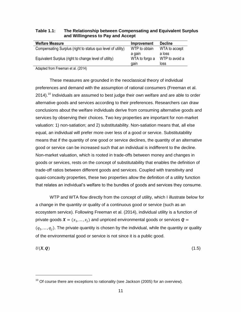
Table 1.1: The Relationship between Compensating and Equivalent Surplus and Willingness to Pay and Accept ............................................................... 11

Table 2.1: Attributes and levels for the farm and non-farm choice experiments....... 34

Table 2.2: Respondent socio-demographic characteristics (% unless otherwise indicated) ............................................................................................... 41

Table 2.3: Respondents’ land characteristics (% unless otherwise indicated) ......... 42

Table 2.4: Model for the farm survey ....................................................................... 45

Table 2.5: Model for the non-farm survey ................................................................ 47

Table 2.6: Mean marginal WTA per year (2013 $CAD) ........................................... 49

Table 2.7: Bounds on Participation (%) and Compensating Surplus (2013 $CAD) .. 51

Table 2.8: Summary of Class Characteristics and Keys to Increasing Participation 57

Table 3.1: Characteristics of Each Watershed ........................................................ 76

Table 3.2: Attributes and Levels used in the Choice Experiments in Both Watersheds ............................................................................................ 77

Table 3.3: Comparing Respondent Demographic Characteristics Across Watersheds ............................................................................................................... 88

Table 3.4: Comparing Respondent Land Characteristics Across Watersheds ......... 89

Table 3.5: Models in Willingness to Accept Space .................................................. 90

Table 3.6: Marginal WTA and Errors for Transfers Between Two Watersheds in Southern Ontario .................................................................................... 93

Table 3.7: Summary of Errors, Tolerance Levels, and Complete Combinatorial Tests for Transfers of Compensating Surplus Between Two Southern Ontario Watersheds ............................................................................................ 98

Table 4.1: Attributes and Levels ............................................................................ 127

Table 4.2: Respondent Characteristics and Features of their Land ....................... 130

Table 4.3: Random Parameter Models by Watershed ........................................... 132

Table 4.4: Summary of Reliability and Validity Tests ............................................. 136

Table 4.5: Regression of Errors and Tolerance Levels on Transfer Characteristics for Transfers Based on the “Mean of Median” Approacha ..................... 139

Table 5.1: Characteristics of the Little, Humber, Credit, and Salmon River Watersheds .......................................................................................... 157

Table 5.2: Attributes and levels ............................................................................. 159

Table 5.3: Respondent Characteristics ................................................................. 166

Table 5.4: Linear and Quadratic Specifications of the Choice Models by Watershed ............................................................................................................. 169

Table 5.5: Likelihood Ratio Test Results for Model Comparisons ......................... 177

Table 5.6: Errors, Tolerance Levels, and Complete Combinatorial p-values for Transfers of Wildlife Habitat Marginal WTPa ......................................... 178

xiii

Table 5.7: Errors, Tolerance Levels, and Complete Combinatorial p-values for Transfers of Marginal WTP for Changes in Producer Incomea ............. 182

Table 5.8: Mean of the Errors and Tolerance Levels, as well as Statistically Different Pairs for Transfers of CS Estimates by Model and Habitat Treatmenta . 184

Table 5.9: Average Percent Difference between the ‘Relative’ and ‘Absolute’ Reconciliation Approaches ................................................................... 187

xiv

List of Figures

Figure 1.1: Total Economic Value ............................................................................ 10

Figure 1.2: Welfare measures from indifference curves ........................................... 13

Figure 1.3: Prospect Theory Value Function ............................................................ 15

Figure 2.1: The Grand and Upper Thames Watersheds ........................................... 32

Figure 2.2: An example of a choice set from the farm version .................................. 35

Figure 2.3: The three stages of our data analysis ..................................................... 37

Figure 2.4: Participation Rates for all Possible Program Specifications by Latent Class ...................................................................................................... 52

Figure 2.5: Compensating Surplus for all Possible Program Specifications by Latent Class ...................................................................................................... 53

Figure 3.1: Location of the Grand and Upper Thames Watersheds .......................... 75

Figure 3.2: Compensating Surplus Estimates for All Possible Program Specifications by Watershed ......................................................................................... 97

Figure 3.3: Box Plots of Transfer Errors and Tolerance Levels ................................ 98

Figure 4.1: The Location of the Grand and Upper Thames Watersheds ................. 126

Figure 4.2: Market Share (a) and Compensating Surplus (b) Estimates ................. 135

Figure 4.3: Boxplots of Transfer Errors and Tolerance Levels ................................ 137

Figure 5.1: Study Sites ........................................................................................... 157

Figure 5.2: Marginal Willingness to Pay per Year Derived for the Four Watersheds (2011 CAD) .......................................................................................... 175

Figure 5.3: Compensating Surplus per Year Estimates (2011 CAD) ...................... 176

1

Chapter 1. Introduction

2

Natural capital provides many goods and services that benefit society, ranging

from forest and agricultural products to wildlife habitat, water purification, and carbon

sequestration (Costanza et al. 1997; Millennium Ecosystem Assessment 2005).

Ecosystem services are “the benefits that people obtain from ecosystems” (Vihervaara

et al. 2010) or, more specifically, “the aspects of ecosystems utilized (actively or

passively) to produce human well-being” (Fisher et al. 2008).1 Globally, environmental

degradation is a significant threat to the flow of many ecosystem services and therefore

the well-being of current and future generations (Millennium Ecosystem Assessment

2005; Liu et al. 2010; Vihervaara et al. 2010). This degradation stems at least in part

from market failures which occur when markets fail to incorporate all benefits provided

by or costs imposed on ecosystems (Brown et al. 2007; Bateman et al. 2011).2

Ultimately, market failures lead to environmental management practices that

undersupply ecosystem services (Fisher et al. 2008).

In response to this problem, governments around the world have used various

policy tools, such as prescriptive regulation or market-based instruments (Fisher et al.

2008; Kemkes et al. 2010). In Canada, governments have relied on command-and-

control regulation (e.g. minimum standards), research and infrastructure spending (e.g.

water treatment), as well as pressure from the general public and industry peers to solve

market failures (National Round Table on the Environment and the Economy 2002).

Canadian governments have also used programs incorporating economic incentives

(Kenny et al. 2011). A well-known example in Canada is the pricing of carbon emissions

via taxes or cap and trade systems. However, other programs may compensate

landowners in some form for altering their land management to improve the supply of

ecosystem services [so called payments for ecosystem services (PES) programs].

Among other criteria, it is important that such environmental policies, and their

implementation, account for the benefits received by, or costs imposed on, the relevant

1 The Millennium Ecosystem Assessment (2003) classifies ecosystem services into four groups:

1) supporting services that underpin all other ecosystem services (e.g., primary production or soil formation); 2) provisioning services, which are the products of ecosystems (e.g., food or fuelwood); 3) regulating services, which result from the regulation of ecosystem processes (e.g., climate regulation or water purification); and 4) cultural services, which are the nonmaterial benefits of ecosystems (e.g., aesthetics or recreation). 2 Market failures include: externalities, which occur when a third party agent is affected by the

economic transactions of other agents; and public goods, which are those goods that are non-excludable and non-rivalrous in consumption (Freeman et al. 2014).

3

stakeholders (e.g., the general public, who consume ecosystem services, and private

landowners, who supply the natural capital from which these services flow). Information

on these benefits and costs can be used in a benefit-cost analysis to evaluate the

economic efficiency of the alternative environmental policies being considered and to

better clarify trade-offs (Wainger and Mazzotta 2011). The results of this analysis can

then be used to inform government policy decisions (Freeman et al. 2014). Determining

monetary values for the appropriate benefits and costs is complicated since many

ecosystem services do not have market prices. As such economists have developed

various valuation techniques to elicit monetary values for non-market ecosystem

services in terms of willingness to pay (WTP) or willingness to accept (WTA) (Liu et al.

2010).

The papers forming my dissertation relate to non-market valuation techniques for

assessing the benefits and costs of policies aimed at conserving and protecting the

environment. These papers are divided into two main themes. The first theme relates to

informing the discussion surrounding the design of programs targeted at conserving or

restoring natural capital on private land. The second theme relates to assessing the

convergent validity of benefit transfer, which is a secondary non-market valuation

technique.3 The goal of this introductory chapter is threefold: 1) it serves as an

introduction to the topics covered in the subsequent chapters; 2) it provides the reader

with certain basic information related to these topics, though not necessarily included in

these chapters; and 3) it provides a summary of my dissertation’s findings.

1.1. Theme 1: Private Landowner Preferences for Conservation Practices

The supply of ecosystem services from natural capital situated on private land is

often threatened due to market failures (Jack et al. 2008). A common solution to this

problem is intervention by governments or non-governmental organizations. The primary

goal of these interventions is to modify the behaviour of stakeholders, such as farmers or

woodlot owners, leading them to adopt more environmentally benign practices.

Regulation is a common government intervention which requires stakeholders to comply

with legislated design or performance standards. While regulations can effectively

3 I refer to benefit transfer as a ‘secondary’ valuation technique since it relies on secondary data,

while I refer to valuation techniques using original research as ‘primary’ valuation techniques (e.g., stated or revealed preference techniques involve original research).

4

address many environmental problems, other instruments that harness economic

incentives are increasingly commonplace in conservation policy as they are often more

efficient (Fisher et al. 2008). Such economic instruments include payments to private

landowners for voluntarily protecting land or changing their management practices to

increase the supply of ecosystem services (Brown et al. 2007). In a sense these

payments modify a good or service’s price to reflect its true benefit or cost, thus acting

as an incentive for landowners to change their behaviour.

Examples of such programs include the Conservation Reserve Program in the

United States (United States Department of Agriculture 2017) and agri-environmental

measures that are part of the Common Agricultural Policy in Europe (European

Commission 2005). In Canada the Growing Forward 2 policy framework jointly

administered by the federal government and its provincial and territorial counterparts

includes a component that covers a portion of the costs of implementing certain

beneficial management practices (Agriculture and Agri-Food Canada and Ontario

Ministry of Agriculture, Food, and Rural Affairs 2016). Non-governmental organizations

also use financial instruments to achieve environmental goals. The Alternative Land Use

Services (ALUS) program, which pays farmers to restore ecosystems on their land to

provide ecosystem services, is also gaining momentum in Canada and is currently active

in regions of Alberta, Saskatchewan, Ontario, and all of Prince Edward Island (ALUS

Canada 2018). There are also local initiatives such as the Langley Ecological Services

Initiative pilot project in Metro Vancouver, British Columbia, a farmer-led program in the

early stages of development that is similar to ALUS (Langley Sustainable Agriculture

Foundation 2017). Another example is Ducks Unlimited Canada which purchases

conservation easements on ecologically significant land and even piloted an auction for

such purposes in 2002 (Brown et al. 2011).

From an economic perspective, the decision of a landowner to enrol some of

their land into a conservation program that provides an incentive payment depends on

how this change affects their utility (or well-being). When deciding whether to voluntarily

enrol some of their land in a payments-based conservation program, a landowner

compares the utility they may derive from participating in the program to the utility

obtained from not participating in the program. They will adopt more environmentally

beneficial land management practices as part of an incentive payment program if the

utility they expect to gain from doing so is at least as large as the utility they derive from

5

the status quo (Cooper and Keim 1996). In a sense if the incentive payment is larger

than the opportunity cost of implementing a conservation action then landowners will

enrol some of their land.

For policy-makers or managers, the problem is to determine how to design and

implement conservation programs to best encourage landowner participation at least

cost (Vercammen 2011). If such a program includes an incentive, then the appropriate

financial incentive to offer to landowners must be determined. The incentive should be

sufficiently large to induce landowners to participate and enrol enough of their land so as

to achieve the program’s environmental objectives. However, payments to landowners

and other program costs are constrained by budgets (Naidoo et al. 2006). While the

payment, which reflects landowner WTA, should be larger than the opportunity cost of

adopting the conservation action, this cost is only known by the targeted landowner

(Chen et al. 2010). Opportunity costs, and thus the payment required to induce

participation, also often vary across landowners reflecting heterogeneous preferences or

land characteristics (Fraser 2009). An additional problem is determining how

characteristics of the program other than the financial incentive may affect a landowner’s

WTA and decision to participate. As with opportunity costs, landowner preferences for

non-financial program characteristics may be heterogeneous (Broch and Vedel 2012).

Several studies assess these issues for landowners using a variety of techniques (e.g.,

Cooper and Keim 1996; Cortus et al. 2011; Franzén et al. 2016; Hansen et al. 2018).

However, the findings of such studies may not necessarily be applicable in all situations

necessitating further study in other contexts. As such, Chapter 2 reports on a case study

I conducted regarding landowner preferences for incentive-based conservation

programs in Southwestern Ontario. The results of this study are inputs into Chapters 3

and 4.

1.2. Theme 2: Benefits Transfer

It is common for governments to require a benefit-cost analysis of policies and

regulations (Treasury Board of Canada Secretariat 2007; United States Environmental

Protection Agency 2014). In fact, such economic analyses are required by law in the

United States for certain regulations (Newbold et al. 2018). These benefit-cost analyses

often require the valuation of non-market goods and services, especially in situations

where policies or regulations may have environmental impacts (e.g., affect ecosystem

6

services). While original research using revealed or stated preference techniques is

preferred, the resources required to undertake a proper valuation study, such as time,

money, or expertise, can be prohibitive (Brouwer 2000). In these cases analysts have a

few options. They may skip valuation altogether, essentially leaving the non-market good

or service out of the benefit-cost analysis, or use a secondary valuation technique known

as benefit transfer.

Benefit transfer involves assigning new economic values at the site or population

of interest, known as the policy site, using existing information that was collected for

other similar sites or populations, known as study sites, employing original valuation

exercises (Johnston et al. 2015). Two main approaches to benefit transfer have been

developed: 1) unit value transfer; and 2) function transfer. Unit value transfer involves

transferring estimates of willingness to pay (or accept) from the study site(s) to the policy

site. The transferred value may be a single estimate, a range of estimates, or the central

tendency of a set of estimates. These estimates can either be transferred directly, which

is known as simple unit transfer, or they can be adjusted for differing characteristics

according to expert opinion which is known as unit transfer with income (or other)

adjustments. Following Johnston et al. (2015), the existing marginal willingness to pay

(accept) value for study site 𝑗 and population 𝑠 reported in the primary valuation literature

can be denoted �̅�𝑗𝑠, while the value being estimated at policy site 𝑖 ≠ 𝑗 and population

𝑟 ≠ 𝑠 is denoted as �̂�𝑖𝑟𝐵𝑇. Simple unit value transfer for a change in a similar good or

service is thus represented as Equation 1.1 (note that the site and population need not

differ simultaneously).

�̂�𝑖𝑟𝐵𝑇 = �̅�𝑗𝑠 (1.1)

For adjusted value transfer Equation 1.1 is augmented by function 𝑓, which

adjusts the value from the study site for any site differences for transfer to the policy site

(Equation 1.2).

�̂�𝑖𝑟𝐵𝑇 = 𝑓(�̅�𝑗𝑠) (1.2)

Equations 1.1 and 1.2 can be modified to accommodate multiple primary

valuation estimates (see Johnston et al. 2015). In general, unit value transfers assume

that the marginal values of changes in the non-market goods or services at the study

7

and policy sites are the same or at least similar, as are the sites themselves. However,

marginal values often markedly differ and adjustments can only partially address these

differences. If this is the case then function transfer may be more appropriate, especially

when sites differ substantially (Johnston et al. 2015). This technique involves using more

information from the study site by transferring a model estimated at this site that relates

willingness to pay (or accept), �̂�𝑗𝑠, to its determinants such as study site characteristic

variables (𝒙𝑗𝑠) and corresponding parameters (�̂�𝑗𝑠) via a linear or non-linear function (𝑔)

(Equation 1.3).

�̂�𝑗𝑠 = 𝑔(𝒙𝑗𝑠, �̂�𝑗𝑠) (1.3)

The key requirements for function transfer are a model estimated from the study

site and data to populate this model’s variables from the policy site. In many cases data

for certain of the variables 𝒙𝑗𝑠 will not be available at the policy site and the set of

variables is therefore divided into those with (𝒙𝑖𝑟1 ) and without (𝒙𝑗𝑠

2 ) such data. Thus,

willingness to pay (or accept) at the policy site can be estimated according to Equation

1.4.

�̂�𝑖𝑟𝐵𝑇 = 𝑔([𝒙𝑖𝑟

1 , 𝒙𝑗𝑠2 ], �̂�𝑗𝑠) (1.4)

As illustrated above function transfer may involve transferring only a single

model. An alternative is to augment the single model with multiple benefit functions

resulting in a range of value estimates for use at the policy site. More advanced function

transfer approaches include meta-analysis and structural benefit transfers (see Johnston

et al. 2015). Briefly, the former involves using data from multiple primary valuation

studies to develop a meta regression model that relates willingness to pay (or accept) to

the characteristics of each study (e.g., valuation technique, year conducted, resource

attributes, etc.). The latter approach, although much more complicated and involved,

addresses certain limitations of the prior approaches by developing a theoretically

grounded utility function using data from multiple primary valuation studies.

Using benefit transfer for valuing the environment has been somewhat

controversial. Some of this controversy is rooted in general criticisms of non-market

valuation and benefit-cost analysis. However, problems with the accuracy of benefit

8

transfer have led researchers to express concerns about the technique. Three main

sources of error are thought to reduce the accuracy of benefit transfer (Rosenberger and

Stanley 2006): 1) measurement error; 2) publication selection bias; and 3) generalization

error. Measurement error arises when the studies that are the source of the transferred

values or functions contain either random errors or errors resulting from researcher

assumptions and judgements. Publication selection bias stems from the fact that most

original valuation research has been published for reasons other than to inform benefit

transfer and the criteria for its publication differ from the criteria useful for benefit

transfer. Generalization error results from the process of transferring value estimates

from study sites to policy sites with differing characteristics. If these errors are sufficiently

large they may affect policy or regulatory decisions informed by benefit transfer.

However, while these errors certainly complicate benefit transfer they do not preclude

the technique’s use — in fact the use of benefit transfer is common (Boyle et al. 2010).

Also commonplace are convergent validity studies that assess the validity and

reliability of the benefits transfer technique using percent errors and statistical

hypothesis tests (Kaul et al. 2013; Rosenberger 2015). These studies use data from

original research conducted at multiple case study sites in parallel to test the technique’s

validity and reliability by treating these sites as policy and study sites. Loomis (1992)

conducted the initial convergent validity assessment for transfers of recreational fishing

values between sites in Oregon and Washington as well as Idaho.4 Since then these

studies have become relatively common spanning several contexts with recently

published examples including: Hasan-Basri and Abd Karim's (2016) examination of

transfers of recreational values between two Malaysian parks; Interis and Petrolia's

(2016) evaluation of transfers of WTP across locations (Louisiana and Alabama) and

habitat types (oyster reefs, mangroves, and salt marshes); and Czajkowski et al.'s

(2017) assessment of different functional forms for transfers across nine European

countries.5 However, certain gaps in the benefit transfer convergent validity literature

remain and Chapters 3 through 5 of this dissertation report on three convergent validity

studies that aim to address some of them.

4 This paper is from a special issue of Water Resources Research examining the benefit transfer

technique (Brookshire and Neill 1992). Similar special issues have appeared in Ecological Economics (Wilson and Hoehn 2006) and recently in Environmental and Resource Economics (Smith 2018). 5 Kaul et al. (2013) and Rosenberger (2015) provide comprehensive lists of such convergent

validity studies.

9

1.3. Brief Backgrounder on Non-Market Economic Valuation

1.3.1. Economic Values

Economic valuation is anthropocentric and utilitarian in that it focusses on the

values of humans as defined by their preferences (National Research Council 2005).

Furthermore, the values assigned to environmental features are instrumental, rather

than intrinsic, meaning that economic values flow from the use of environmental goods

or services rather than them having value in and of themselves (regardless of use). In

sum, humans must benefit from something in order for it to have economic value.

However, within this perspective there is a wide spectrum of values and one of the main

frameworks is a hierarchy known as total economic value.6 The total economic value of

an environmental feature is composed of use and non-use values (Figure 1.1). Use

values result from current or future human interaction with the environment, while non-

use values arise from the existence of the resource without the prospect of such

interaction. Use values can be subdivided into direct use values, which arise from

consumptive and non-consumptive human interaction with environmental features, and

indirect use values, which do not result from such direct physical use.7 Direct use values

generally result from provisioning and cultural ecosystem services (Millennium

Ecosystem Assessment, 2003). Examples of these services that yield consumptive

direct use values include food or timber products, while those generating non-

consumptive direct use values include recreation and spiritual services. Indirect use

values generally result from supporting and regulating services, examples of which

include soil nutrients and pollination as well as water purification. Non-use values are

composed of existence values, which arise from the existence of the environmental

resource, and bequest values, which result from the environmental resource being left to

6 The typology presented here is not the only typology of value and is also not without criticism

(Admiraal et al. 2013). 7 Hanley and Barbier (2009) distinguish between direct and indirect environmental values in a

different sense. Direct values result from an environmental change that directly affects an individual’s well-being (e.g., swimmers benefit directly from an improvement in water quality). Indirect values result from a change in an ecosystem service that is an input into the production of a good or service that directly affects an individual’s well-being (e.g., improvements in water quality can also reduce the cost of producing a product such as beer, which results in price decreases that benefit consumers).

10

future generations (non-use values were introduced into the economics literature by

Krutilla (1967)).8

Figure 1.1: Total Economic Value Adapted from National Research Council (2005)

1.3.2. Basics of Measures of Economic Welfare

As alluded to above, changes in economic welfare are measured using the

concepts of WTP and WTA. For a change in environmental quantity or quality, WTP is

the maximum amount of money an individual would trade for a positive change or to

forgo a negative change, while WTA is the minimum amount of money they would

require to endure a negative change or to forgo a positive change (Freeman et al. 2014).

These measures of WTP and WTA are related to the more formal Hicksian terms of

compensating and equivalent surplus (Table 1.1).9

8 The Millennium Ecosystem Assessment (2003) notes that existence values in part reflect

intrinsic values to the extent that people believe that ecosystems have intrinsic value. 9 Similar measures for the welfare effects of changes in prices are known as compensating and

equivalent variation (Freeman et al. 2014).

11

Table 1.1: The Relationship between Compensating and Equivalent Surplus and Willingness to Pay and Accept

Welfare Measure Improvement Decline Compensating Surplus (right to status quo level of utility) WTP to obtain

a gain WTA to accept a loss

Equivalent Surplus (right to change level of utility) WTA to forgo a gain

WTP to avoid a loss

Adapted from Freeman et al. (2014)

These measures are grounded in the neoclassical theory of individual

preferences and demand with the assumption of rational consumers (Freeman et al.

2014).10 Individuals are assumed to best judge their own welfare and are able to order

alternative goods and services according to their preferences. Researchers can draw

conclusions about the welfare individuals derive from consuming alternative goods and

services by observing their choices. Two key properties are important for non-market

valuation: 1) non-satiation; and 2) substitutability. Non-satiation means that, all else

equal, an individual will prefer more over less of a good or service. Substitutability

means that if the quantity of one good or service declines, the quantity of an alternative

good or service can be increased such that an individual is indifferent to the decline.

Non-market valuation, which is rooted in trade-offs between money and changes in

goods or services, rests on the concept of substitutability that enables the definition of

trade-off ratios between different goods and services. Coupled with transitivity and

quasi-concavity properties, these two properties allow the definition of a utility function

that relates an individual’s welfare to the bundles of goods and services they consume.

WTP and WTA flow directly from the concept of utility, which I illustrate below for

a change in the quantity or quality of a continuous good or service (such as an

ecosystem service). Following Freeman et al. (2014), individual utility is a function of

private goods 𝑿 = (𝑥1, … , 𝑥𝑗) and unpriced environmental goods or services 𝑸 =

(𝑞1, … , 𝑞𝑗). The private quantity is chosen by the individual, while the quantity or quality

of the environmental good or service is not since it is a public good.

𝑈(𝑿, 𝑸) (1.5)

10

Of course there are exceptions to rationality (see Jackson (2005) for an overview).

12

For simplicity assume that all prices for elements of Q are zero. The prices of

each element of X are 𝑷 = 𝑝1, … , 𝑝𝑗 resulting in a budget constraint of 𝑷 ∙ 𝑿 = 𝑀, where

M represents monetary income. Given this, the individual seeks to maximize their utility

subject to the budget constraint which yields conditional demand functions for the set of

private goods (conditional on Q).

𝑥𝑗 = 𝑥𝑗(𝑷, 𝑀, 𝑸) (1.6)

Substituting the conditional demand function into the utility function yields the

conditional indirect utility function.

𝑉 = 𝑉(𝑷, 𝑀, 𝑸) (1.7)

For changes in the quantity or quality of a single environmental good or service

from q0 to q1, compensating and equivalent surplus are respectively represented by

Equations 1.8 and 1.9.11 Compensating surplus is the change in income that makes an

individual indifferent to a change in the quantity or quality of an environmental good or

service.12

𝑉(𝑷, 𝑀, 𝑞0) = 𝑉(𝑷, 𝑀 − 𝐶𝑆, 𝑞1) (1.8)

Similarly, equivalent surplus is the change in an individual’s income that yields

the same level of utility as a change in the quantity or quality of an environmental good

or service.

𝑉(𝑷, 𝑀 + 𝐸𝑆, 𝑞0) = 𝑉(𝑷, 𝑀, 𝑞1) (1.9)

The main difference between these two measures is the reference level of utility,

with compensating and equivalent measures assuming a right to the status quo and

change levels, respectively. This difference can be illustrated using indifference curves,

which represent levels of utility (Figure 1.2). Utility is constant along a given curve and

differs across curves, while different points along the curve represent alternative bundles

11

A key assumption for both CS and ES is that the individual’s utility is the same pre and post change. 12

An alternative illustration rests on the expenditure function. For brevity, I do not do not show this here and direct the interested reader to Freeman et al. (2014).

13

of goods or services. The slope of the indifference curve is the trade-off ratio, or

marginal rate of substitution. Given a composite private numeraire good (x) and an

environmental good or service (q), the compensating surplus for an increase from q0 to

q1 is the distance B to C (the amount of the numeraire good an individual is willing to pay

for the change in q).13 Holding q constant at its status quo, equivalent surplus is the

distance A to D (the amount of the numeraire good an individual is willing to accept to

forgo the change in q).

Figure 1.2: Welfare measures from indifference curves Adapted from National Research Council (2005) and Freeman et al. (2014)

Oftentimes the changes in a good or service are discrete rather than continuous.

In this case, assume that an individual selects a single good or service from 𝑗 = 1, … , 𝐽

alternatives, with each alternative associated with a vector of environmental quality Q

and each good j having price pj. Given this, the deterministic conditional indirect utility

function for a discrete change in the quantity or quality of an environmental good or

service is represented by Equation 1.10 (this function is conditional on 𝑸𝒋).

𝑉𝑗 = 𝑉𝑗(𝑀, 𝑝𝑗 , 𝑸𝒋), where 𝑗 = 1, ⋯ , 𝐽 (1.10)

13

A numeraire good or service is a one whose price is set to 1 so that the price of other goods or services is reflected in terms of the numeraire. A composite good or service is one that represents a basket of goods or services.

14

Given the choice of two alternative goods or services j and k, the individual

selects that which maximizes their utility. Compensating surplus is thus defined in

Equation 1.11 for a change in each alternative’s associated vector of environmental

quality characteristics.

Max𝑗 𝑉𝑗(𝑀, 𝑝𝑗 , 𝑄𝑗0) = Max𝑗 𝑉𝑗(𝑀 − 𝐶𝑆, 𝑝𝑗 , 𝑄𝑗

1) (1.11)

Equivalent surplus is defined as Equation 1.12.

Max𝑗 𝑉𝑗(𝑀 + 𝐸𝑆, 𝑝𝑗 , 𝑄𝑗0) = Max𝑗 𝑉𝑗(𝑀, 𝑝𝑗 , 𝑄𝑗

1) (1.12)

While neoclassical theory posits that the compensating and equivalent surplus

measures will approximate each other if the change being valued is small as are income

effects, empirical evidence suggests that this will not always be the case (Kim et al.

2015). Though neoclassical theory allows for smaller differences, researchers have

identified cases where the difference between the WTP and WTA measures is quite

large. There are several possible explanations or theories, some consistent with

neoclassical utility theory and others that are not (see Chapter 3 of this dissertation for a

brief overview or Kim et al. (2015) for more details). One of the more prevalent reasons

for the disparity in welfare measures, which is not consistent with neoclassical theory, is

the endowment effect (Thaler 1980; Knetsch 1989; Kahneman et al. 1990).14 In essence,

an individual’s status quo level of an environmental good or service, the initial

endowment, will influence how they value changes from this level. This effect is rooted in

the prospect theory concepts of loss aversion and reference dependence (Tversky and

Kahneman 1992). Essentially losses from a reference point are valued more than gains

from the same point. Following Freeman et al. (2014), Figure 1.3 illustrates the

endowment effect and the asymmetric value of gains and losses. The horizontal axis

represents the quality or quantity of the environmental good or service, while the vertical

axis represents the compensating surplus measure as either WTP or WTA. Two value

functions are plotted, w0 and w1, with each relating the payment or compensation

required to hold utility constant when the environmental good or service changes. These

functions are kinked at the reference points, where they intersect the horizontal axis,

14

One of the researchers examining this issue, near the outset and over the following decades, was Dr. Jack Knetsch, who was a professor here at Simon Fraser University’s School of Resource and Environmental Management and is currently Professor Emeritus.

15

with the marginal value of a gain less than the marginal value of a loss (it is easy to see

that WTP to go from q0 to q1 (a gain) is smaller than WTA to go from q1 to q0 (an

equivalent loss)).

Figure 1.3: Prospect Theory Value Function Adapted from Freeman et al. (2014)

However, there has been much debate about the endowment effect and several

other experimental studies highlight situations where no such effect is observed or

where the disparity is reduced (e.g., Plott and Zeiler (2007); Bateman et al. (2009); List

(2011)). Furthermore, there is empirical evidence for other explanations for the disparity

leading Kim et al. (2015) to summarize “…there are likely multiple factors at play in any

given empirical finding of a divergence”. Regardless of explanation, the disparity has

implications for applied valuation and related policy since certain situations are more

suited to WTA and others to WTP (as alluded to in Table 1.1).15 Often the decision about

which measure to use is related to property rights, with losses from a legally entitled

position measured via WTA and gains from this position measured using WTP.

15

Researchers have been reluctant to use WTA, even when it is the correct measure, opting instead to use WTP. Whittington et al. (2017) outlines four main reasons: 1) responses are perceived as unreliable as WTA may lack incentive compatibility in certain cases (e.g., open-ended question formats); 2) higher rate of responses deemed non-conforming (i.e., rejected scenarios, protest votes, or non-response); 3) confusion about the correct situations in which to apply WTA; and 4) political unpopularity as politicians won’t actually pay compensation (and may not even fund research that says they will). Arguably, the last point applies to WTP too if the payment vehicle is an increase in taxes. In addition, the influential National Oceanic and Atmospheric Administration commissioned report by Arrow et al. (1993) also recommended the use of WTP since it yields estimates that are more conservative.

16

However, Knetsch (2007) and Whittington et al. (2017) explain that legal entitlements will

not always determine the appropriate measure. Rather, the decision about whether to

apply WTP or WTA results from the interplay between the status quo situation an

individual is actually experiencing and their perceived reference condition, from which

they value a change in a good or service (see Whittington et al. (2017) for further

information on this and other issues related to applying WTA as part of stated

preferences valuation research).16

1.3.3. Original Research Approaches to Non-Market Valuation

Several alternative primary valuation techniques have been developed to

measure willingness to pay or accept (National Research Council 2005; Freeman et al.

2014). In general, these approaches can be divided into stated and revealed preference

techniques with each group containing a variety of alternative techniques. Stated

preference approaches involve using surveys to elicit WTP or WTA by observing an

individual’s choices in a hypothetical market. The main stated preference techniques are

the contingent valuation and choice experiment methods. Contingent valuation involves

asking survey respondents their WTP or WTA for a single change in an environmental

good or service. Choice experiments are similar, though elicit WTP or WTA by asking

respondents to choose among several alternative descriptions of the goods or services

from which economic values are inferred. Revealed preference techniques involve

eliciting WTP and WTA values from observations on an individual’s choices or behaviour

in actual markets. Multiple techniques fall into this group including a variety of household

production function models (e.g., travel cost/random utility models, hedonic pricing, and

averting behaviour) and production function models. Travel cost/random utility models

estimate WTP by calculating the cost of time and expense incurred for visiting a

recreational site (e.g., angling, hiking, swimming, etc.), while hedonic pricing models

infer WTP for an environmental resource by linking the price of a marketed good or

service, usually property, to its key characteristics at least one of which is the

environmental resource. Averting behaviour models, which are applied in the field of

health, evaluate WTP by assessing individual expenditures on improving health

outcomes or avoiding bad health outcomes. Production function models treat the

16

Whittington et al. (2017) notes that “…WTA is often the only relevant question” when using stated preferences to elicit values from landowners for modifying their land use to provide ecosystem services as part of PES schemes (which are similar to what my research investigates as part of Theme 1).

17

environmental resource as an input into the production of a marketed good or service.

The value of the environmental resource is estimated by assessing how changes in the

resource affect the production of the marketed good or service.

I chose to use choice experiments for my PhD research for several reasons.

First, this technique is able to elicit a wider range of economic values than revealed

preferences or models based on market prices alone (Flores 2003). Second, it enables

me to examine how program characteristics, other than the level of payment, affect

willingness to pay or accept (Matta et al. 2009). Finally, an additional output of choice

experiment models are market shares (Hensher et al. 2005). Market shares can be used

to represent the proportion of individuals or households who would select a certain

alternative good or service out of the set of alternatives and is useful for assessing

participation in conservation programs.

1.4. A Summary of the Dissertation

Four papers related to the aforementioned topics form the main part of this

dissertation, Chapters 2 through 5, and these are followed by a brief conclusion in

Chapter 6. In the paper presented in Chapter 2, titled Landowner Preferences for

Wetland Conservation in Two Southern Ontario Watersheds, I used choice experiments

to elicit the preferences of private landowners for wetlands conservation on their land in

the Grand and Upper Thames watersheds located in Southwestern Ontario. The

motivation for this study stems from an estimated decline of 70% in the extent of the

region’s wetlands since European colonization. Protecting or restoring wetlands will

improve the supply of ecosystem services in the area, notably moderating the impacts of

extreme weather and slowing nutrient runoff to Lake Erie. Since private landowners own

the majority of land in the two watersheds, they were surveyed to assess their

preferences for certain key attributes of voluntary incentive-based wetlands conservation

programs using a choice experiment. Two versions of the choice experiment were

developed, one tailored to agricultural and forest product producers and another to rural

private landowners more generally. Common attributes of the two versions included the

land area enrolled in the program, the conservation activity on that land (i.e., conversion

to wetland, trees, or meadow), public recognition of landowner conservation actions, and

financial compensation. Each version had an additional attribute, with the general

landowner version having an offer of technical help attribute and the producer focussed

18

version having a productivity of the enrolled land attribute. Data from the two watersheds

were pooled and the two versions were analysed independently using latent class

models, which group respondents with similar preferences together into subgroups, from

which WTA and participation rates were estimated. The analysis suggests that many

private landowners are willing to participate in wetlands conservation at reasonable cost,

particularly those who have past participation in incentive-based conservation programs.

In general, respondents favoured wetlands conservation programs that divert smaller

areas of land to wetlands conservation, target marginal agricultural land, use treed

buffers to protect wetlands, offer technical help, and pay financial incentives.

Landowners appear reluctant to receive public recognition for their wetland conservation

actions.

Chapters 3 through 5 include the papers assessing the validity and reliability of

benefit transfer. The paper that forms the third chapter, titled Transfers of Landowner

Willingness to Accept: A Convergent Validity and Reliability Test Using Choice

Experiments in Two Canadian Watersheds, involved testing the reliability and validity of

transferring estimates of WTA between the Grand and Upper Thames watersheds. This

study was motivated by the apparent lack of any published studies assessing the

convergent validity of transfers of WTA, though there are many such studies assessing

transfers of WTP. The data for this exercise was taken from the aforementioned choice

experiment version tailored to agricultural and forest product producers and was

modeled in WTA space using a generalized multinomial logit. The reliability of the

transfers were assessed by calculating percent transfer errors and validity was

examined by testing the similarity of utility functions and welfare estimates. The results

indicate that transfers of WTA are similarly valid and reliable to transfers of WTP already

assessed in the literature.

The paper included as Chapter 4, titled Assessing the Convergent Validity and

Reliability of Transfers of Market Shares Derived from Choice Experiments for

Landowner Participation in Wetlands Conservation Programs, involved assessing the

validity and reliability of transfers of market shares for landowner participation in the

aforementioned wetlands conservation programs (predicted participation in a wetlands

conservation program versus maintaining the status quo). Such market shares are

derived from choice experiments and are useful for informing policy, though can be

costly to obtain via original research which suggests a transfer approach. However, the

19

validity and reliability of transfers of such predicted participation market shares has not

been assessed using convergent validity techniques commonly used for benefit transfer

assessment, which motivated this paper. To provide context, the validity and reliability of

transfers of these market share estimates were compared with a parallel assessment of

the validity and reliability of transfers of WTA estimates. Both types of estimates were

generated from the general rural landowner choice experiment version discussed

previously. Validity and reliability were assessed using the same techniques employed

for the paper in Chapter 3. The results clearly show that transfers of predicted

participation market shares yield low transfer errors and tolerance levels, especially

relative to the parallel transfer of WTA, however whether this validity and reliability is

acceptable for policy analysis requires further research.

A paper titled Reconciling Quantitative Attributes with Different Levels When

Transferring Willingness to Pay Elicited from Choice Experiments: Evidence from Benefit

Transfers between Four Canadian Watersheds forms the fifth chapter. Since benefit

transfers involve taking value estimates for goods or services from certain sites and

transferring them to other sites they usually require the reconciliation of differing good or

service definitions. Multiple options for reconciling these differences are available for

transfers of values derived from choice experiments, though there is little research

examining which options lead to more valid and reliable transfers, providing the

motivation for this particular study. Three alternatives for reconciling quantitative choice

experiment attributes with levels that differ across sites were assessed, one based on a

linear model specification and two based on a quadratic specification. Reconciliation is

straightforward for linear relationships since values do not vary. However, reconciling

values derived from quadratic relationships is more complicated since values are not

constant enabling different reconciliation options. Two such options were assessed as

part of this paper including approaches rooted in: 1) ‘relative’ preferences that involve

matching levels according to their order in the set of levels; and 2) ‘absolute’ preferences

that involve matching levels according to their quantity. The data is from choice

experiments that sought the general public’s WTP for changes in four Canadian

watersheds (the Little River in New Brunswick; the Humber and Credit Rivers in Ontario;

and the Salmon River in British Columbia). Specifically, the choice experiments elicited

preferences for improvements in water quality and increases in the proportion of each

watershed as protected wildlife habitat, as well as associated declines in local farm and

20

forest product producer income (and an increase in taxes). The levels of the wildlife

habitat attribute differed across watersheds, while the levels used for the other attributes

were identical. I assessed the validity and reliability of each reconciliation approach

using the same techniques as those used in Chapters 3 and 4. Overall, the results

suggest that transfers based on the linear specification are more valid and reliable than

either quadratic approach for transfers of welfare estimates though not necessarily for

marginal estimates. Furthermore, transfers of marginal and welfare estimates based on

‘relative’ preferences are more valid and reliable than transfers based on ‘absolute’

preferences. Finally, if the attributes needing reconciliation have more similar levels, the

two approaches based on the quadratic specification yield more similar results though

only for transfers of welfare estimates.

1.5. Statement of Interdisciplinarity

I believe that the research reported in my dissertation achieves the School of

Resource and Environmental Management’s requirement of interdisciplinarity for the

PhD in Resource and Environmental Management. Two out of three of the School’s core

disciplines are represented: ecological economics and environmental policy.

Furthermore, the research includes elements of the following natural and social sciences

outlined in the PhD handbook: water management; conservation biology; and

conservation policy.

21

References

Arrow K, Solow R, Portney PR, et al (1993) Report of the NOAA Panel on Contingent Valuation. Fed Regist 58:4601–4614. doi: 10.1258/095646202760029804

Admiraal JF, Wossink A, de Groot WT, de Snoo GR (2013) More than total economic value: How to combine economic valuation of biodiversity with ecological resilience. Ecol Econ 89:115–122. doi: 10.1016/j.ecolecon.2013.02.009

Agriculture and Agri-Food Canada, Ontario Ministry of Agriculture, Food, and Rural Affairs (2016) Cost-share Funding Assistance Program Guide for Producers: 2017-2018 Program Year.

ALUS Canada (2018) What is ALUS? https://alus.ca/home/about-us/what-is-alus/. Accessed 2 Mar 2018

Bateman IJ, Day BH, Jones AP, Jude S (2009) Reducing gain-loss asymmetry: A virtual reality choice experiment valuing land use change. J Environ Econ Manage 58:106–118. doi: 10.1016/j.jeem.2008.05.003

Bateman IJ, Mace GM, Fezzi C, et al (2011) Economic analysis for ecosystem service assessments. Environ Resour Econ 48:177–218. doi: 10.1007/s10640-010-9418-x

Broch SW, Vedel SE (2012) Using Choice Experiments to Investigate the Policy Relevance of Heterogeneity in Farmer Agri-Environmental Contract Preferences. Environ Resour Econ 51:561–581. doi: 10.1007/s10640-011-9512-8

Brookshire DS, Neill H. (1992) Benefit Transfers: Conecptural and Empirical Issues. Water Resour Res 28:651–655.

Brouwer R (2000) Environmental value transfer: state of the art and future prospects. Ecol Econ 32:137–152. doi: 10.1016/S0921-8009(99)00070-1

Brown LK, Troutt E, Edwards C, et al (2011) A Uniform Price Auction for Conservation Easements in the Canadian Prairies. Environ Resour Econ 50:49–60. doi: 10.1007/s10640-011-9461-2

Brown TC, Bergstrom JC, Loomis JB (2007) Defining, valuing and providing ecosystem goods and services. Nat Resour J 47:329–376. doi: 10.1525/sp.2007.54.1.23.

Chen X, Lupi F, Viña A, et al (2010) Using cost-effective targeting to enhance the efficiency of conservation investments in payments for ecosystem services. Conserv Biol 24:1469–1478. doi: 10.1111/j.1523-1739.2010.01551.x

22

Cooper JC, Keim RW (1996) Incentive Payments to Encourage Farmer Adoption of Water Quality Protection Practices. Am J Agric Econ 78:54–64. doi: 10.2307/1243778

Cortus BG, Jeffrey SR, Unterschultz JR, Boxall PC (2011) The Economics of Wetland Drainage and Retention in Saskatchewan. Can J Agric Econ 59:109–126. doi: 10.1111/j.1744-7976.2010.01193.x

Costanza R, D’Arge R, de Groot R, et al (1997) The value of the world’s ecosystem services and natural capital. Nature 387:253–260. doi: 10.1038/387253a0

Czajkowski M, Ahtiainen H, Artell J, Meyerhoff J (2017) Choosing a Functional Form for an International Benefit Transfer: Evidence from a Nine-country Valuation Experiment. Ecol Econ 134:104–113. doi: 10.1016/j.ecolecon.2017.01.005

European Commission (2005) Agri-environment Measures: Overview on General Principles, Types of Measures, and Application.

Fisher B, Turner K, Zylstra M, et al (2008) Ecosystem Services and Economic Theory: Integration for Policy-Relevant Research. Ecol Appl 18:2050–2067. doi: 10.1890/07-1537.1

Flores NE (2003) Conceptual Framework for Nonmarket Valuation. In: Champ PA, Boyle KJ, Brown TC (eds) A Primer on Nonmarket Valuation. Kluwer Academic Publishers, Netherlands, pp 27–58

Franzén F, Dinnétz P, Hammer M (2016) Factors affecting farmers’ willingness to participate in eutrophication mitigation — A case study of preferences for wetland creation in Sweden. Ecol Econ 130:8–15. doi: 10.1016/j.ecolecon.2016.05.019

Fraser R (2009) Land heterogeneity, agricultural income forgone and environmental benefit: An assessment of incentive compatibility problems in environmental stewardship schemes. J Agric Econ 60:190–201. doi: 10.1111/j.1477-9552.2008.00183.x

Freeman MA, Herriges JA, Kling CL (2014) The Measurement of Environmental Resource Values: Theory and Methods, Third Edit. RFF Press, New York, NY

Hansen K, Duke E, Bond C, et al (2018) Rancher Preferences for a Payment for Ecosystem Services Program in Southwestern Wyoming. Ecol Econ 146:240–249. doi: 10.1016/j.ecolecon.2017.10.013

Hanley N, Barbier E (2009) Pricing Nature: Cost-benefit Analysis and Environmental Policy. Edward Elgar Publishing, Northampton, MA

Hasan-Basri B, Abd Karim MZ (2016) Can Benefits in Recreational Parks in Malaysia Be Transferred? A Choice Experiment (CE) Technique. Int J Tour Res 18:19–26. doi: 10.1002/jtr.2028

23

Hensher DA, Rose JM, Greene WH (2005) Applied Choice Analysis: A Primer. Cambridge University Press, New York, NY

Interis MG, Petrolia DR (2016) Location, Location, Habitat: How the Value of Ecosystem Services Varies across Location and by Habitat. Land Econ 92:292–307. doi: http://le.uwpress.org/content/by/year

Jack BK, Kousky C, Sims KRE (2008) Designing payments for ecosystem services: Lessons from previous experience with incentive-based mechanisms. Proc Natl Acad Sci 105:9465–9470. doi: 10.1073/pnas.0705503104

Jackson T (2005) Motivating Sustainable Consumption: A Review of Evidence on Consumer Behaviour and Behavioural Change. Guildford, UK

Johnston RJ, Rolfe J, Rosenberger RS, Brouwer R (2015) Introduction to Benefit Transfer Methods. In: Johnston RJ, Rosenberger RS, Rolfe J, Brouwer R (eds) The Economics of Non-Market Goods and Resources, Applications of Simulation Methods in Environmental and Resource Economics. Springer, New York, NY, pp 19–59

Kahneman D, Knetsch JL, Thaler RH (1990) Experimental Tests of the Endowment Effect and the Coase Theorem. J Polit Econ 98:1325–1348. doi: 10.1086/261737

Kaul S, Boyle KJ, Kuminoff N V, et al (2013) What can we learn from benefit transfer errors? Evidence from 20 years of research on convergent validity. J Environ Econ Manage 66:90–104. doi: 10.1016/j.jeem.2013.03.001

Kemkes RJ, Farley J, Koliba CJ (2010) Determining when payments are an effective policy approach to ecosystem service provision. Ecol Econ 69:2069–2074. doi: 10.1016/j.ecolecon.2009.11.032

Kenny A, Elgie S, Sawyer D, Wichtendahl CG (2011) Advancing the Economics of Ecosystems and Biodiversity in Canada: A Survey of Economic Instruments for the Conservation & Protection of Biodiversity. Sustainable Prosperity, Ottawa, Ontario

Kim Y, Kling CL, Zhao J (2015) Understanding Behavioral Explanations of the WTP-WTA Divergence Through a Neoclassical Lens: Implications for Environmental Policy. Annu Rev Resour Econ 7:169–187. doi: 10.1146/annurev-resource-100913-012501

Knetsch JL (1989) The endowment effect and evidence of nonreversible indifference curves. Am Econ Rev 79:1277–1284. doi: 10.2307/1831454

Knetsch JL (2007) Biased valuations, damage assessments, and policy choices: The choice of measure matters. Ecol Econ 63:684–689. doi: 10.1016/j.ecolecon.2007.02.012

24

Krutilla J V. (1967) Conservation reconsidered. Am Econ Rev 57:777–786.

Langley Sustainable Agriculture Foundation (2017) Langley Ecological Services Initiative.

List JA (2011) Does Market Experience Eliminate Market Anomalies? The Case of Exogenous Market Experience. Am Econ Rev 101:313–317. doi: 10.1257/aer.101.3.313

Liu S, Costanza R, Farber S, Troy A (2010) Valuing ecosystem services Theory, practice, and the need for a transdisciplinary synthesis, Annals of the New York Academy of Sciences Volume 1185, Issue 1. Ann N Y Acad Sci 1185:54–78.

Loomis JB (1992) The evolution of a more rigorous approach to benefit transfer: Benefit function transfer. Water Resour Res 28:701–705. doi: 10.1029/91WR02596

Matta JR, Alavalapati JRR, Mercer DE (2009) Incentives for Biodiversity Conservation Beyond the Best Management Practices: Are Forestland Owners Interested? Land Econ 85:132–143. doi: 10.3368/le.85.1.132

Millennium Ecosystem Assessment. (2003). Ecosystems and Human Well-being: A Framework for Assessment. Washington, D.C.: Island Press.

Millennium Ecosystem Assessment (2005) Ecosystems and Human Well-being: Synthesis. Island Press, Washington, D.C.

Naidoo R, Balmford A, Ferraro PJ, et al (2006) Integrating economic costs into conservation planning. Trends Ecol Evol 21:681–687. doi: 10.1016/j.tree.2006.10.003

National Research Council (2005) Valuing Ecosystem Services: Toward Better Environmental Decision-Making. National Academies Press, Washington, D.C.

National Round Table on the Environment and the Economy (2002) Toward a Canadian Agenda for Ecological Fiscal Reform: First Steps. Ottawa, Ontario

Newbold S, David Simpson R, Matthew Massey D, et al (2018) Benefit Transfer Challenges: Perspectives from U.S. Practitioners. Environ Resour Econ 69:467–481. doi: 10.1007/s10640-017-0207-7

Plott CR, Zeiler K (2007) Exchange Asymmetries Incorrectly Interpreted as Evidence of Endowment Effect Theory and Prospect Theory? Am Econ Rev 97:1449–1466. doi: 10.1257/aer.97.4.1449

Rosenberger RS (2015) Benefit Transfer Validity and Reliability. In: Johnston RJ, Rosenberger RS, Rolfe J, Brouwer R (eds) The Economics of Non-Market Goods and Resources, Benefit Transfer of Environmental and Resource Values: A Guide for Researchers and Practitioners. Springer, New York, NY, pp 307–326

25

Rosenberger RS, Stanley TD (2006) Measurement, generalization, and publication: Sources of error in benefit transfers and their management. Ecol Econ 60:372–378. doi: 10.1016/j.ecolecon.2006.03.018

Smith VK (2018) Benefits Transfer: Current Practice and Prospects. Environ Resour Econ 69:449–466. doi: 10.1007/s10640-017-0206-8

Thaler R (1980) Toward a positive theory of consumer choice. J Econ Behav Organ 1:39–60. doi: 10.1016/0167-2681(80)90051-7

Treasury Board of Canada Secretariat (2007) Canadian Cost-Benefit Analysis Guide: Regulatory Proposals. Ottawa, Ontario

Tversky A, Kahneman D (1992) Advances in Prospect-Theory - Cumulative Representation of Uncertainty. J Risk Uncertain 5:297–323. doi: Doi 10.1007/Bf00122574

United States Department of Agriculture (2017) Conservation Reserve Program. https://www.fsa.usda.gov/programs-and-services/conservation-programs/conservation-reserve-program/index. Accessed 19 Sep 2017

United States Environmental Protection Agency (2014) Guidelines for Preparing Economic Analyses. Washington, D.C.

Vercammen J (2011) Agri-Environmental Regulations, Policies, and Programs. Can J Agric Econ 59:1–18. doi: 10.1111/j.1744-7976.2010.01210.x

Vihervaara P, Rönkä M, Walls M (2010) Trends in ecosystem service research: Early steps and current drivers. Ambio 39:314–324. doi: 10.1007/s13280-010-0048-x

Wainger L, Mazzotta M (2011) Realizing the potential of ecosystem services: A framework for relating ecological changes to economic benefits. Environ Manage 48:710–733. doi: 10.1007/s00267-011-9726-0

Whittington D, Adamowicz W, Lloyd-Smith P (2017) Asking Willingness-to-Accept Questions in Stated Preference Surveys: A Review and Research Agenda. Annu Rev Resour Econ 9:317–336. doi: 10.1146/annurev-resource-121416-125602

Wilson MA, Hoehn JP (2006) Valuing environmental goods and services using benefit transfer : The state-of-the art and science. doi: 10.1016/j.ecolecon.2006.08.015

26

Chapter 2. Landowner Preferences for Wetlands Conservation Programs in Two Southern Ontario Watersheds

A version of this chapter has been published in the Journal of Environmental

Management as Trenholm, R., Haider, W., Lantz, V., Knowler, D., and Haegeli, P.

"Landowner Preferences for Wetlands Conservation Programs in Two Southern Ontario

Watersheds". I led the design of this research and was the lead on the fieldwork. I

authored nearly all of the text and conducted all of the data analyses.

27

Abstract

Wetlands in the region of Southern Ontario, Canada have declined substantially from

their historic area. Existing regulations and programs have not abated this decline.

However, reversing this trend by protecting or restoring wetlands will increase the supply

of important ecosystem services. In particular, these actions will contribute to moderating

the impacts of extreme weather predicted to result from climate change as well as

reducing phosphorous loads in Lake Erie and ensuing eutrophication. Since the majority

of land in the region is privately owned, landowners can play an important role. Thus, we

assessed landowner preferences for voluntary incentive-based wetlands conservation

programs using separate choice experiments mailed to farm and non-farm landowners in

the Grand River and Upper Thames River watersheds. Latent class models were

separately estimated for the two data sets. Marginal willingness to accept, compensating

surplus, and participation rates were estimated from the resulting models to gain insight

into the financial compensation required by landowners and their potential participation.

Many of the participating land owners appear willing to participate in wetlands

conservation at moderate cost, with more willing groups notably marked by past

participation in incentive-based conservation programs. They generally favour wetlands

conservation programs that divert smaller areas of land to wetlands conservation, target

marginal agricultural land, use treed buffers to protect wetlands, offer technical help, and

pay financial incentives. However, landowners appear reluctant to receive public

recognition of their wetland conservation actions. Our results are of interest to natural

resource managers designing or refining wetlands conservation programs.

Keywords: discrete choice experiment; latent class analysis; willingness to accept;

participation rate; agri-environmental programs; wetlands

28

2.1. Introduction

Wetlands are critically important ecosystems that produce ecosystem services

such as water purification and supply, flood control, recreational opportunities, and

carbon sequestration that have significant economic value (Zedler & Kercher, 2005;

Barbier, 2011; Brander, Brouwer, & Wagtendonk, 2013). Despite their value, the area of

wetlands has declined in many parts of the world, including Canada (Mitsch and

Hernandez, 2013). The area of wetlands in Southern Ontario, in particular, has

decreased significantly and continues to deteriorate. The extent of inland wetlands that

are 10 hectares or larger has declined 72% from over 2 million hectares to near 500,000

hectares since European settlement of the region, caused in part by land use change

associated with urbanization and agriculture (Ducks Unlimited Canada, 2010). Pressure

to convert wetlands is unlikely to abate since the population of Southern Ontario is

expected to grow 33% to 17 million by 2041 (Ontario Ministry of Finance, 2014).

Furthermore, the functions or distribution of existing wetlands may be altered by a

changing climate or invasive species (Mitsch and Hernandez, 2013; Zedler and Kercher,

2004). Though the area of wetlands, and consequently the ecosystem services supplied,

has decreased, there is local demand for their conservation (Lantz et al., 2013).

Wetland protection and restoration in Southern Ontario can play a significant role

in addressing the local hydrological impacts of climate change and eutrophication of the

Great Lakes, particularly Lake Erie. Climate change is expected to result in more intense

rainfalls, more frequent high and low streamflows, and increased damages from flooding

(Cheng et al., 2012). In certain cases wetlands can alleviate these impacts by storing

water, recharging groundwater, and moderating streamflows (Bullock and Acreman,

2003). Lake Erie’s eutrophication condition has recently worsened with harmful

cyanobacterial algae blooms and hypoxia in its western and central basins, respectively

(Joosse & Baker, 2011; Michalak et al., 2013; Scavia et al., 2014). Nuisance Cladophora

algae blooms regularly occur in the nearshore of the lake’s eastern basin (Depew,

Houben, Guildford, & Hecky, 2011). Consequently ecosystem health, recreation,

drinking water supplies, tourism, and property values have been negatively affected

(Joosse & Baker, 2011). Moreover, the harmful algae blooms pose a health risk

(Michalak et al., 2013). This eutrophication is thought to be driven mainly by soluble

reactive phosphorous loading from non-point sources much of which originates in

Southwestern Ontario (Joosse and Baker, 2011; Scavia et al., 2014). Wetland protection

29

and restoration can play a critical role in reducing such phosphorous loading since

wetlands are able to remove phosphorous from the water column and retain it or

transform it into biologically unavailable forms (Reddy, Kadlec, Flaig, & Gale, 1999;

Fisher & Acreman, 2004; Scavia et al., 2014).

As a party to the Ramsar Convention on Wetlands, the Canadian government

has an international obligation to conserve wetlands though it shares responsibility for

their management with provincial governments. Wetland conservation in the Province of

Ontario is embedded in legislation and policies governing land use (Ducks Unlimited

Canada, 2010; Rubec and Hanson, 2008). Tax incentive and grant programs are also

offered at the federal, provincial, and regional levels (Environment Canada, 2015; Clean

Water Program, 2013; Ontario Ministry of Natural Resources and Forestry, 2015a).

Other initiatives involve non-governmental organizations such as Ducks Unlimited

Canada. Despite these efforts, Southern Ontario’s wetland area continues to decline.

Reductions in wetland area can partly be attributed to market failure since few

wetland ecosystem services are traded in markets (Barbier, 2011). As such many

landowners have no incentive to maintain or restore wetlands and instead convert them

to produce marketable goods and services. In an agricultural context, draining wetlands

expands the area available for crops and increases the efficiency of field operations

(e.g., less turning of farm machinery) (Cortus et al., 2011). Compensating landowners to

protect or restore wetlands can provide an incentive to engage in conservation (Hansen

et al., 2015). In this case payments should be sufficiently large to induce enough

landowners to participate so as to achieve conservation objectives, though be within

budgetary constraints. To encourage participation, the incentive should at least cover the

opportunity costs of private landowners (Cortus et al., 2011).17 Several techniques have

been used to assess the opportunity cost of conserving wetlands or examine landowner

willingness to accept (WTA) for maintaining or restoring them, including hedonic

analysis, auctions, simulation, market prices, data from existing programs, and

contingent valuation (e.g., Brown et al., 2011; Cortus et al., 2011; Gelso et al., 2008;

Hansen et al., 2015; Lawley, 2014; van Vuuren and Roy, 1993; Yu and Belcher, 2011).

17

However, if landowners benefit from wetlands conservation then the required financial incentive may actually be less compensation than their opportunity cost.

30

An alternative technique is the choice experiment (CE). CEs are survey-based

techniques that are used to assess preferences for key attributes of a good or service

(e.g., conservation programs). If one of the attributes is financial then monetary values

can be estimated. CEs are able to incorporate a wider range of values than revealed

preference techniques, such as hedonic analysis, or other approaches relying on market

prices (Flores, 2003). Similarly, CEs can assess preferences for wetland conservation

programs that do not exist. Relative to contingent valuation, CEs are able to evaluate

how multiple program characteristics affect landowner support for wetlands protection

and restoration (Matta et al., 2009). CEs directed at assessing landowner WTA for

aspects of conservation programs or land management schemes are becoming common

and have been applied in a variety of contexts, including forest management and

conservation, biodiversity and endangered species conservation, agri-environmental

contracts, water quality protection, and carbon sequestration (e.g., Paulrud & Laitila,

2010; Sorice, Haider, Conner, & Ditton, 2011; Beharry-Borg, Smart, Termansen, &

Hubacek, 2013; Greiner, Bliemer, & Ballweg, 2014; Lienhoop & Brouwer, 2015;

Peterson, Smith, Leatherman, Hendricks, & Fox, 2015; Vedel, 2015; Villanueva, Gómez-

Limón, Arriaza, & Rodríguez-Entrena, 2015). Similarly, Lizin, Passel, & Schreurs, (2015)

used a CE to examine the cost of land use restrictions to farmers by assessing their

willingness to pay (WTP) for parcels with varying restrictions.

Our main objective is to examine the preferences of Southern Ontario

landowners for voluntary incentive-based wetland conservation programs. To do so we

use CEs to investigate landowner preferences for certain program characteristics from

which we predict WTA and participation rates for alternative program specifications.18

The remainder of this paper is structured as follows. The study sites are reviewed in

Section 2.2. Section 2.3 provides an overview of the method, with details on the choice

experiment, data collection, and data analysis. The results are presented in Section 2.4.

Finally, the results and policy implications are discussed in Section 2.5. The conclusion

follows in Section 2.6.

18

We could have used WTP, which is often lower than WTA thus yielding more conservative estimates of opportunity cost (Horowitz and McConnell, 2002). However, we chose to use WTA since landowners in Ontario hold the rights to their property and WTA better reflects incentive-based conservation programs. Furthermore, a WTP style question would have its own issues (e.g., landowner WTP to avoid having wetlands constructed on their land may not be realistic).

31

2.2. Study Sites

The study was conducted in the Grand River and Upper Thames River

watersheds (Figure 2.1). At 6,800 km2, the Grand River watershed is one of the largest

in Southern Ontario and the largest Canadian watershed that empties into Lake Erie.

The Upper Thames River watershed, also part of the Lake Erie basin, is 3,420 km2 and

drains into Lake St. Clair via the Lower Thames River. Agriculture occurs on 75% and

70% of the Upper Thames and Grand watersheds’ land area respectively (Upper

Thames River Conservation Authority, 2012; Grand River Conservation Authority, 2014).

There are over 6,000 farms in the Grand River watershed and more than 3,500 farms in

the Upper Thames River watershed (Grand River Conservation Authority, 2008; Upper

Thames River Conservation Authority, 2015). The Grand River watershed is home to

around one million residents concentrated in urban areas that cover 7% of its land area

and over 500,000 individuals reside in the Upper Thames River watershed with most

living in urban areas that cover 10% of its area. Forests, wetlands, and meadows

respectively cover 11.3%, 4.8%, and 2.6% of the Upper Thames River watershed.

Forests and wetlands cover 20% of the Grand River watershed (Grand River

Conservation Authority, 2014; Upper Thames River Conservation Authority, 2012). While

the Grand River watershed as a whole meets Environment Canada's (2013) minimum

thresholds for wetland area not all of its sub-basins do (Grand River Conservation

Authority, 2008) and the Upper Thames River watershed does not.

32

Figure 2.1: The Grand and Upper Thames Watersheds

Urban and agricultural land uses have lowered surface water quality in both watersheds,

notably via runoff of phosphorous, nitrogen, and sediment (Grand River Conservation

Authority, 2014; Nürnberg & Lazerte, 2015). Phosphorous concentrations exceed

provincial objectives (Ontario Ministry of Environment, 2013). The two watersheds are

also the main Ontarian contributors of phosphorous to Lake Erie (Lake Erie LaMP,

2011). Climate change is forecast to increase the frequency of extreme rainfall, and

consequent flooding, in the two watersheds. Higher flood damage costs are expected to

result, especially in larger cities such as London or Kitchener-Waterloo (Cheng et al.,

2012). Conservation authorities are actively working to address these issues and

recommended actions include wetland retention and restoration (Grand River

Conservation Authority, 2014; Nürnberg & Lazerte, 2015).

33

2.3. Method

2.3.1. The Choice Experiment

The choice experiment surveys used in this study were based on questionnaires

first implemented in the Credit River watershed, located immediately east of the Grand

River watershed, during spring 2012 (Trenholm et al., 2013). These original surveys,

targeted at agricultural landowners, were developed after a literature review coupled with

feedback from landowners (via several focus groups) and the local watershed

conservation authority. An important outcome from the focus groups was the necessity

to have separate, but similar, CEs for farm and rural non-farm landowners that differed in

a few attributes and levels (Table 2.1). Certain attributes targeted at farm landowners

were not sensible for those who do not farm their land or have smaller land holdings. In

addition non-farm landowners participating in the focus groups had lower expectations

for financial compensation. We created the non-farm CE by altering the original farm

version so that the attributes better correspond to the anticipated situations and

motivations of rural non-farm landowners: the ‘area converted’ levels were made

smaller; the ‘type of land converted’ attribute was dropped in favour of ‘technical

assistance’; and the ‘payment to landowner’ levels were lowered and were no longer per

acre. Non-CE questions were identical across the farm and non-farm versions. For the

present study, we used the same CEs, but the non-choice experiment questions were

slightly modified based on insight gained during their initial implementation and feedback

from the Grand River and Upper Thames River conservation authorities.

The rationale for each attribute follows. We included the ‘type of land to be

converted’ attribute to account for differences in the agricultural productivity of land

diverted to wetlands conservation. The ‘conversion activity’ attribute was included to

assess preferences for diverting land directly to wetland or to trees or meadow to help

retain nearby wetlands. The latter two levels act as critical function zones, adjacent

upland areas with biophysical functions and characteristics directly related to wetlands,

or protection zones which are upland areas of natural vegetation that protect wetland

ecosystem functions (Environment Canada, 2013). We included the ‘area converted’

attribute to examine preferences for the amount of land diverted to wetlands

conservation. The smaller acreages included were more palatable to focus group

participants and small-scale wetlands can produce many ecosystem services (Blackwell

34

and Pilgrim, 2011). We included ‘technical assistance’ and ‘public recognition’ attributes

in order to assess preferences for non-financial compensation and examine whether

their inclusion in an incentive-based wetlands conservation program could reduce the

required payment. ‘Technical assistance’, which is a feature of certain stewardship

programs in Ontario (Conservation Ontario, 2013), was only included in the non-farm CE

since non-farm focus group participants were more interested in this type of

compensation than farm participants. ‘Public recognition’ was of interest to the

conservation authority partner and was identified as important by some focus group

participants. Finally, the ‘payment to landowner’ attribute was included to assess

preferences for financial compensation and to allow estimation of WTA.

Table 2.1: Attributes and levels for the farm and non-farm choice experiments

Attribute Variable Name

Levels

Farm Non-Farm

Type of land to be converted Land can be productive or marginal (i.e., less fertile, sloping, etc.) farmland

Land Type Marginal Productive

N/A

Conversion activity Land can be converted to meadow or trees to help retain nearby wetlands, or directly into wetland

Meadow Trees Wetland

Meadows Trees Wetland


Area converted Area of land to be converted Acres

1.0 acre 3.0 acres 5.0 acres

0.5 acres 1.0 acre 1.5 acres

Technical assistance Technical advice from experts, the government or other groups involved

Technical N/A No Yes

Public recognition Signage on property, stewardship banquets, and awards are provided

Recognition No Yes

No Yes

Payment to landowner Annual payment to the landowner

Payment

$50 per acre $150 per acre $250 per acre $350 per acre $450 per acre $550 per acre

$0 $50 $100 $150 $200 $250

.

Macros in SAS 9.3 software were used to create a main effect fractional factorial

design with 72 alternatives grouped into 36 choice sets and allocated among 6 blocks

(Kuhfeld, 2010). The resulting design was used for both choice experiments, but

independently modified to address dominant alternatives yielding final farm and non-

farm designs with D-efficiencies of 92%, and 91 %, respectively.

35

The following preamble, describing the wetlands conservation program,

appeared at the beginning of the choice experiment (version administered in the Upper

Thames is the same):

Suppose that in an effort to enhance and restore wetlands within and adjacent to the Grand River watershed, the government offered a voluntary program that provided incentives (e.g., payments, public recognition) to landowners to set aside some of their lands. This land could be (i) converted to meadow or trees to help retain nearby wetlands; or (ii) converted directly into wetlands if appropriate.

This was immediately followed by program conditions, including: 1) a contract length of 5

years; 2) the possibility of renewing the contract after 5 years; 3) any land set aside is in

addition to existing commitments and legal requirements; and 4) that the government

covers any capital and material costs.19 Instructions on how to complete the choice task

were then provided along with information on each attribute. A cheap talk script aimed at

reducing hypothetical bias appeared next (Ladenburg & Olsen, 2014). It read “Please

consider the options carefully – as if you were entering into a real contract with the

government – since the program would have a limited budget and could only fund a

limited number of projects”. The 6 choice sets were then presented (Figure 2.2).

Figure 2.2: An example of a choice set from the farm version Note: the non-farm version appears similar

19

We initially used a contract length of 10 years but focus group participants felt that this was too long given their planning horizon. Five years, with the possibility to renew, was deemed more acceptable.

36

After each choice set, respondents were asked to indicate how certain they were

about their selection on a scale from 1 to 10. (Norwood, 2005; Brouwer, Dekker, Rolfe, &

Windle, 2010; Ready, Champ, & Lawton, 2010). Finally, respondents were asked the

primary reason for their choices at the end of the CE to allow screening for protests

(Meyerhoff et al., 2014).

2.3.2. Data Collection

The surveys were administered by mail using Canada Post’s Unaddressed

Admail™ (Canada Post, 2015). This service has been used in other studies to survey

Canadian farmers (e.g., Yu & Belcher, 2011; Anderson & McLachlan, 2012). Routes in

postal codes and forward sortation areas which were at least 70% within each

watershed’s boundaries were selected. All identified routes were surveyed except for the

non-farm survey in the Grand watershed where a random sample of identified routes

was surveyed. The farm version was sent to 8,004 farm households on 181 rural and

suburban routes while 10,086 houses on 77 rural routes were sent the non-farm version.

In partnership with the Grand River and Upper Thames River conservation authorities,

surveys were simultaneously administered to both watersheds during the months of April

and May 2013. Households were initially sent a survey package containing a cover

letter, a questionnaire, and a postage paid return envelope. One week later

reminder/thank you postcards were sent out and two weeks after that a second survey

package was mailed. Respondents were invited to complete a ballot to be entered into a

draw for a $100 Visa gift card (we maintained anonymity by separating ballots from

questionnaires when returned).

Surveys returned from non-targeted postal codes or forward sortation areas were

removed from further analysis. Respondents repeatedly selecting the same answer for

all Likert-style questions were deemed serial non-participants and removed. Similarly,

those choosing the same non-status quo option for all 6 choice sets were also removed

since it is unlikely that this response pattern reflects genuine preferences. Finally,

respondents selecting the status quo option for all 6 choice sets and whose answers to

37

the follow-up questions suggested they were protesting were also dropped (Meyerhoff et

al., 2014).20

2.3.3. Data Analysis

Our data analysis was divided into three stages (Figure 2.3). The first stage of

our analysis involved contrasting sociodemographic and land characteristics from both

surveys with each other and with farm operator and rural population data. Whether the

characteristics differed significantly across the two samples was assessed using

Pearson chi-squared tests for categorical data and t-tests for continuous data in SPSS

23 software. Whether the samples differed from the population was evaluated via

binomial tests for binomial data, Pearson chi-squared tests for categorical data, and t-

tests for continuous data. Since respondents were not asked directly to self-identify as

farmers or foresters we used farming and forestry related questions to create an

indicator of whether a respondent is engaged in agriculture or forest production on their

land. This was accomplished in SPSS 23 by first conducting a non-linear principal

components analysis (Linting and van der Kooij, 2012).21 The resulting components

were clustered via SPSS’s two-step clustering procedure yielding a binary variable.

Figure 2.3: The three stages of our data analysis

The second stage of our analysis involved modeling the CE data. We used latent

class analysis to model the utility functions for each choice experiment (the econometric

20

We identified protesting respondents as those selecting “I don’t trust the government” or providing an open-ended answer suggesting they did not state their true preferences. 21

The following variables were entered into the principal components analysis: ownership of at least 100 acres of land (dummy); primary land use is agriculture or forestry (dummy); generated income from their land in past 5 years via agriculture or forestry (dummy); land features agricultural land cover (dummy); percentage of income from on-farm sources (ordinal); and membership in a farming or woodlot organization (dummy).

38

model is reviewed in Appendix A). Latent class models group respondents with similar

preferences together to account for preference heterogeneity (preferences are

homogeneous within classes, but vary across classes). While other approaches account

for preference heterogeneity (e.g., random parameters logit), latent class models provide

better insight into how the wetland conservation program’s impacts are distributed since

it identifies distinct groups of respondents (Boxall and Adamowicz, 2002). To determine

the number of classes we initially estimated several models that differed according to the

number of classes and then selected the model yielding the lowest information criterion

(Louviere et al., 2000). Akaike’s (AIC) and Bayesian (BIC) information criteria are often

used (Akaike, 1974; Schwarz, 1978). We chose the BIC since it is better at determining

the number of classes (Nylund et al., 2007).

Following Johnston and Duke (2008), the utility functions were specified to

include interactions between the attributes that characterize the conserved land and the

acres attribute (Equations 2.1a and 2.1b for the farm and non-farm CEs, respectively).22

For the farm choice experiment, the acres attribute was interacted with the type of land

set aside and the conversion activity. Area converted was only interacted with the

conversion activity for the non-farm choice experiment. This allows the impacts of land

type or conversion activity on landowner utility to vary by the area conserved. These

interactions also ensure that land type and conversion activity do not impact utility when

no acres are conserved. Utility also varies by class s.

Vs =

αs(ASC) + β1s(Acres) + β2

s (Acres)(Land Type) + β3s (Acres)(Wetland) + β4

s (Acres)(Trees) +

β5s (Recognition) + β6

s (Payment per Acre)

(2.1a)

Vs = αs(ASC) + β1s(Acres) + β2

s (Acres)(Wetland) + β3s (Acres)(Trees) + β4

s (Technical) +

β5s (Recognition) + β6

s (Payment) (2.1b)

22

Though these interactions were not in the initial design, correlations and variance inflation factors indicate that collinearity is inconsequential.

39

The alternative specific constant (ASC) was set to one for ‘Program A’ or

‘Program B’ and zero for ‘No Program’. The numerical attributes ‘acres conserved’ and

‘payment attributes’ were coded according to their actual levels. The binary attributes

‘public recognition’ and ‘technical help’ were dummy coded with the parameter set to one

when present and zero when absent. The categorical attributes ‘land type’ and

‘conversion activity’ were effects coded. The functional form and coding scheme allow

the ASC parameter to represent utility when zero acres are conserved and no technical

help, public recognition, or payment are received.

The farm and non-farm CEs were analyzed independently in Latent Gold Choice

5.0 (Vermunt and Magidson, 2005). Following Beck, Rose, & Hensher (2013), each

choice was weighted by respondent certainty using Latent Gold’s replication weights.

Variables representing respondent characteristics, known as covariates, were included

to predict class membership.23 Certain respondents could not participate in some of the

alternatives since their owned land area is less than the acre attribute level (those

owning between 1 and 5 acres for the farm survey or 0.5 and 1.5 acres for the non-farm

survey). Rather than remove them from the sample, losing any insight into their

preferences, they were segmented into their own known class and a latent class

analysis performed on the remaining respondents. Models with 1 to 4 latent classes and

the full complement of covariates were estimated for both CEs (covariates significant at

10% were retained).

The third stage of our analysis involved applying the choice model. The resulting

model parameters were used to derive estimates of marginal WTA for changes in each

attribute, which involves taking the negative of a ratio of partial derivatives (Matta et al.,

2009). For example, the marginal WTA of class s for public recognition is calculated via

Equation 2.2.

WTAPublic recognitions = -

∂Vs ∂Recognition⁄

∂Vs ∂Payment⁄= -

β5s

β6s (2.2)

23

Variables representing personal characteristics (female, age in years, post-secondary education, employed, and midpoint of household income categories), land characteristics (forest cover, meadow cover, wetland cover, acres owned in watershed, succession plan, midpoint of years since land obtained), and other characteristics (Grand watershed, farm or forest producer, participated in an existing incentive-based conservation program, and distance of respondent’s postal code centroid from the nearest major city). All covariates are dummy variables unless otherwise indicated.

40

In addition, we examined the share of landowners predicted to participate in

different wetlands conservation program specifications versus the status quo using a

decision support tool (Hensher et al., 2005). The impact on landowner welfare was also

assessed via mean compensating surplus (CS). Following Hanemann (1984), CS for

changes from the baseline (V0s) to a given program (V1

s) can be estimated for class s

following Equation 2.3.

CSs = -(V0

s -V1s)

β6s (2.3)

2.4. Results

The rate of survey returns, including fully and partially completed questionnaires,

was 17.0% (1,713 surveys) for the non-farm survey and 19.2% (1,535 surveys) for the

farm survey. After accounting for missing data, returns from non-targeted postal codes,

serial non-participants, protest responses, and those owning less land than the lowest

acre attribute levels only 9.6% (n = 968) of the non-farm surveys and 10.7 % (n = 856) of

the farm surveys sent out were used.24

2.4.1. Respondent Characteristics

Aside from age, demographics differed significantly across the two versions with

farm respondents more likely to be male, employed, and have lower incomes compared

to non-farm respondents, though less likely to have a post-secondary degree (Table

2.2). Both the farm and non-farm samples were significantly more likely to be male and

older compared to the farm operator and rural populations, respectively. Additionally, the

farm sample was significantly more likely than the farm operator population to hold a

post-secondary degree, while the non-farm sample was significantly more likely to hold a

post-secondary degree than the farm operator and rural populations. The farm sample

was significantly more likely to be employed relative to the rural population. Income also

24

These rates are at the low end of those from similar CEs in Europe or North America which range from 10.5%, in the case of Rossi et al. (2011), to 87% for Sorice et al. (2011). However, they are within the range of 1.71% to 33% reported by surveys that have used Canada Post’s Admail service to contact farmers and other Canadian farmer surveys (e.g., Shaikh et al., 2007). Regardless, if non-respondent preferences are substantially different from respondent preferences then the low rate may result in non-response bias potentially making it difficult to extrapolate results to the wider population of landowners. One could conservatively assume that non-respondents are not willing to participate in the wetlands conservation programs.

41

differed significantly with farm and non-farm respondents on average reporting higher

incomes than the population of farm operators, but lower incomes than the rural

population.

Table 2.2: Respondent socio-demographic characteristics (% unless otherwise indicated)

Respondent Characteristics

Data Type

Survey Farm Operatorsa

Rural Populationb

Farm (1)

Non-Farm

(2)

Tests (3)

Estimate (4)

Tests (5)

Estimate (6)

Tests (7)

Gender

Male Binary 77.2 65.1 *** 70.8 ††† 50.4 ††† Female 22.8 34.9 29.2 49.6

Age (Adults) Under 35 Categorical 7.9 7.5 10.6 ††† 24.4 ††† 35 to 54 38.9 38.5 44.6 39.3 55 or older 53.2 53.9 44.8 36.3 Mean (years) Continuous 54.9 55.4 52.9 ††† 41.1 †††

Highest level of educationc

Not post-secondary Binary 47.5 34.5 *** 85.6 ††† 52.1 ‡‡‡ Post-secondary 52.5 65.5 14.4 47.9

Employment status Not in labour force Categorical 19.3 28.6 *** 29.0 §§§ Unemployed 1.1 1.4 2.1 Employed 79.7 69.9 68.9

Household Income Under $50,000 Categorical 22.9 19.9 ** 28.8 ††† 16.6 ††† $50,000 to $74,999 22.3 20.5 20.6 16.3 $75,000 to $99,999 23.6 21.4 16.9 24.5

$100,000 and over 31.2 38.2 33.7 42.7

*** and ** indicate farm (1) and non-farm (2) sample estimates differ at the 1% and 5% level of significance.

††† farm (1) and non-farm (2) sample estimates differ from the population estimate (4 or 6) at the 1% level of significance.

‡‡‡ non-farm sample estimate (2) only differs from the population estimate (6) at the 1% level of significance.

§§§ farm sample estimate (1) only differs from the population estimate (6) at the 1% level of significance

a Farm operator population data from the 2011 Census of Agriculture (Statistics Canada, 2012a) for census consolidated subdivisions intersecting with the two watersheds in the case of gender and age. Education and household income are at the provincial level.

b Rural population data from the 2011 Census of Population (Statistics Canada, 2012b) or the 2011 National Household Survey (Statistics Canada, 2013) for dissemination areas intersecting with the two watersheds.

c Data on farm operators represents those with and without a university degree, while survey data and rural population data represent those with or without a post-secondary degree or diploma.

42

Testing suggests that, other than having a succession plan, land characteristics

differed significantly across the two surveys (Table 2.3). Farm survey respondents were

more likely to have: each type of land cover; agriculture as a primary land use;

generated income from their land; earned higher portions of their income from farming;

larger land holdings; obtained land earlier; and participated in an incentive-based

conservation program.

Table 2.3: Respondents’ land characteristics (% unless otherwise indicated)

Characteristic Data Type Farm Non-Farm

Tests

Land Cover Has forests Binary 57.9 47.0 *** Has meadows Binary 22.5 19.2 * Has wetlands Binary 48.6 43.2 ** Has crop, pasture, or orchard (i.e., agricultural land cover) Binary 84.7 56.5 ***

Land Use Primary land use is agriculture Categorical 72.3 39.4 *** Primary land use is forestry 0.7 0.7 Primary land use is residential 25.4 57.3

Generated income from land in past 5 years Binary 79.0 47.8 *** Portion of household income from farming

0% Categorical 23.2 55.2 *** 1 % to 24 % 27.0 23.5 25 % to 49 % 13.9 5.6 50 % to 74 % 10.3 3.5 75 % to 99 % 13.6 5.0 100 % 12.0 7.3

Area of Land Holdings < 10 acres Categorical 15.7 45.4 *** 10 =< 70 acres 21.4 25.2 70 =< 130 acres 32.7 15.0 130 acres =< 30.3 14.5 Mean (acres) Continuous 136.7 68.0 ***

Year First Obtained Land in the Region Before 1970 Categorical 18.0 11.4 *** 1970 to 1980 16.0 12.9 1981 to 1990 22.1 19.6 1991 to 2000 19.5 21.2 2001 to 2006 12.6 15.9 2007 to 2013 11.3 18.8

Succession plan for land Binary 72.3 72.8 Participated in conservation program with incentive or cost-share payments

Binary 31.1 18.4 ***

***, **, and * indicate farm and non-farm sample estimates differ at the 1%, 5%, and 10% level of significance

43

Two groups of respondents resulted from the principal components analysis and

clustering of farm and forestry related questions — those more and less likely to be

agricultural or forest producers. The bulk of farm survey respondents were likely to be

engaged in agriculture or forestry (71.5 %), though a sizable minority of non-farm

respondents were similarly engaged (36.4 %).

2.4.2. Choice Models

The BIC indicates that the model with 3 latent classes and 1 known class

represents the data the best for both versions of the CE (Tables 2.4 and 2.5). In both

cases the means of the posterior class membership probabilities indicate decent

classifications (all 0.79 or larger).

Farm Model

The known class contains 98 respondents while the modal class sizes are 370,

222, and 166 for latent classes 2, 3, and 4, respectively. Members of the known class

favor converting fewer acres of their land to wetland conservation. They prefer if this

area is marginal rather than productive and is converted to trees relative to wetlands,

and wetlands over meadows. They favor larger amounts of compensation. The ASC and

public recognition parameters are insignificant. Respondents in this class are

significantly more likely to be post-secondary graduates and female relative to those in

latent class 4 (the base), though significantly less likely to have forests or wetlands on

their land and to be an agricultural or forest producer.

Class 2’s ASC parameter suggests that they strongly prefer participating in a

wetlands conservation program over maintaining their status quo all else equal. They

prefer if less of their land is set aside for conservation and would rather if this area is

marginally productive and converted to trees, followed by meadow, and wetland. They

favor larger incentive payments and dislike public recognition. Relative to those in class

4, respondents in class 2 are significantly more likely to be older, female, and hold a

post-secondary degree, though they are less likely to be farm or forest producers. While

their likelihood of having participated in an existing cost-share or incentive-based

conservation program is similar to class 3, they are significantly more likely to have done

so than class 4.

44

Class 3’s ASC parameter suggests that they prefer their status quo to

participating in a wetlands conservation program all else equal. They prefer converting

their land to trees, followed by meadow, and then wetland. They also favor larger

payments. Class 3’s acres, land type, and public recognition parameters are

insignificant. Members of class 3 are significantly more likely to be post-secondary

graduates and live further from large cities relative to class 4, but less likely to be farm or

forest producers. While their likelihood of participation in an existing cost-share or

incentive-based conservation program is similar to class 2, they are significantly more

likely than class 4 to have participated.

Class 4’s ASC parameter suggests that, all else equal, they strongly favour their

status quo situations over enrolling in a wetlands conservation program. They prefer to

divert smaller marginally productive areas of their land to conservation. Members of this

class prefer larger incentive payments and dislike public recognition. The conversion

activity parameters are all insignificant. Class 4 is the covariate reference group, though

relative to the two latent classes they are less likely to have a post-secondary degree

and to have participated in a cost-share or payments-based conservation program,

though more likely to be farm or forest producers.

45

Table 2.4: Model for the farm survey

Variable Known Class 1a Latent Classesa

Class 2 Class 3 Class 4

Attributes

ASC 0.2225 (0.2297)

1.4377*** (0.1954)

-0.8728*** (0.3291)

-3.3984*** (0.5148)

Acres -0.1039** (0.0491)

-0.0818** (0.0339)

0.0050 (0.0442)

-0.2018** (0.0992)

Acres*Land Type (Productive)

-0.1632*** (0.0258)

-0.2613*** (0.0236)

-0.0031 (0.0260)

-0.2807*** (0.0669)

Acres*Wetland -0.0246 (0.0316)

-0.0632*** (0.0217)

-0.1597*** (0.0267)

-0.0140 (0.0593)

Acres*Trees 0.0886*** (0.0315)

0.1170*** (0.0215)

0.0919*** (0.0255)

0.0635 (0.0564)

Acres*Meadow -0.0639** (0.0309)

-0.0538*** (0.0208)

0.0679** (0.0292)

-0.0495 (0.0532)

Recognition (Yes) -0.1508 (0.1543)

-0.1848* (0.1053)

0.0884 (0.1671)

-0.5908** (0.2694)

Annual payment per acre

0.0011** (0.0005)

0.0010*** (0.0004)

0.0069*** (0.0007)

0.0045*** (0.0009)

Covariates

Intercept 1.5387 (0.9560)

-0.8431 (0.6605)

0.2823 (0.7082)

Base

Age in years 0.0005 (0.0144)

0.0243*** (0.0087)

-0.0091 (0.0099)

Post-Secondary 1.1506*** (0.3765)

0.7611*** (0.2374)

1.4455*** (0.2841)

Gender (Female) 0.6943* (0.4173)

0.5585* (0.3052)

0.5150 (0.3489)

Forest cover -1.2656*** (0.4018)

0.1608 (0.2458)

-0.3010 (0.2881)

Wetland cover -1.9659*** (0.3982)

0.0277 (0.2356)

-0.1903 (0.2771)

Conservation Payment

0.7824 (0.5437)

0.7599*** (0.2546)

0.7930*** (0.2910)

Producer -8.5166*** (2.3989)

-0.6613** (0.3218)

-0.7020* (0.3669)

Distance from city (KM)

0.0299 (0.0205)

0.0035 (0.0130)

0.0254* (0.0147)

Modal class size 98 (11.4%) 370 (43.2%) 222 (25.9%) 166 (19.4%) Mean of posterior probabilities (S.D.)

1.00 (0.00)

0.84 (0.15)

0.80 (0.16)

0.92 (0.15)

Log-likelihood -3284.25

BIC (AIC) 6,939.87

(6,678.49)

ρ2 (overall) 0.3993 ***, **, and * indicate significance at the 1%, 5%, and 10% levels, respectively

a Standard errors appear in brackets below the corresponding coefficient

46

Non-Farm Model

The known class contains 215 respondents while the modal class sizes are 415

for latent class 2, 177 for latent class 3, and 161 for latent class 4. The known class

favors converting smaller areas of their land to trees relative to meadow and meadow

relative to wetland. They also prefer receiving technical help and larger payments. Their

ASC and public recognition parameters are insignificant. Members of this class are

significantly more likely to have a lower household income, be located in the Grand

watershed, and to live close to a large city relative to class 4, though they are

significantly less likely to have forest or wetlands on their land, be farm or forest

producers, and to have participated in an incentive-based conservation program.

Class 2’s ASC parameter suggests that, all else equal, they are inclined to

participate in a wetlands conservation program rather than maintain their status quo.

They prefer converting their land to trees, followed by wetland, and then meadow.

Technical help and larger incentive payments are favored by class 2, though they dislike

receiving public recognition for their conservation efforts. Class 2’s area parameter is

insignificant. Relative to class 4, class 2 is significantly more likely to have a lower

household income and to have wetland cover on their land.

Class 3’s ASC parameter indicates that they favour maintaining their status quo

situations over enrolling in a wetlands conservation program all else equal. They prefer

to convert smaller areas of their land and appear to favor wetland or tree cover over

meadow. Members of class 3 like receiving technical help. Their public recognition and

payment parameters are insignificant. In comparison to class 4, respondents in class 3

are significantly more likely to have a lower household income, owned their land for

longer, live closer to a large city, and have wetlands on their land, but are less likely to

have participated in an existing incentive-based conservation program.

Class 4’s ASC parameter suggests that, all else equal, they prefer participating in

a wetlands conservation program over maintaining their current situations. Members of

this class strongly favor converting fewer acres but prefer if this area is treed, followed

by meadow, and distantly wetland. They favour receiving technical help, dislike public

recognition, and prefer larger payments. Class 4 forms the covariate reference group,

though relative to the two latent classes this class is more likely to have higher

household incomes and less likely to have wetland cover on their land.

47

Table 2.5: Model for the non-farm survey

Variables Known Class 1a Latent Classesa

Class 2 Class 3 Class 4

Attributes

ASC -0.1061 (0.1684)

0.8918*** (0.1944)

-1.9572*** (0.4141)

0.5431** (0.272)

Acres -0.2970** (0.1297)

0.1054 (0.1025)

-1.4519*** (0.3543)

-1.6110*** (0.4735)

Acres*Wetland -0.2439*** (0.0683)

0.0723 (0.0772)

0.3337 (0.2151)

-2.6943*** (0.6027)

Acres*Trees 0.3822*** (0.0631)

0.3936*** (0.0606)

0.2615 (0.2092)

2.0638*** (0.3751)

Acres*Meadow -0.1383** (0.0669)

-0.4658*** (0.0628)

-0.5952** (0.2535)

0.6305** (0.3751)

Technical help (Yes) 0.2842*** (0.1073)

0.7844*** (0.0963)

0.6669*** (0.2647)

0.5787*** (0.1669)


-0.2034** (0.0821)

-0.3848 (0.2528)

-0.3404* (0.1788)

Annual payment 0.0014** (0.0006)

0.0073*** (0.0006)

0.0018 (0.0016)

0.0054*** (0.0011)

Covariates

Intercept 2.7209*** (0.7574)

1.7553** (0.697)

0.6440 (0.7371)

Base

Household income ($1,000s)

-0.0142** (0.0061)

-0.0106** (0.0054)

-0.0112** (0.0056)

Watershed (Grand) 0.5526* (0.3004)

-0.4022 (0.2966)

0.1635 (0.3003)

Land obtained -0.0117 (0.0111)

-0.0016 (0.0103)

0.0192* (0.0106)

Forest cover -1.5334*** (0.3495)

0.3597 (0.2885)

-0.0144 (0.2930)

Wetland cover -1.2943*** (0.3696)

1.0773*** (0.2861)

0.7333** (0.2997)

Conservation payment

-2.5432** (1.0494)

-0.0273 (0.3134)

-0.8594** (0.3649)

Producer -5.0562*** (0.9859)

-0.3896 (0.2819)

-0.3214 (0.2896)

Distance from city (KM)

-0.0511*** (0.0164)

0.0072 (0.0148)

-0.0380** (0.0171)

Modal class size 215 (22.2%) 415 (42.9%) 177 (18.3%) 161 (16.6%) Mean of posterior probabilities (S.D.)

1.00 (0.00)

0.91 (0.14)

0.94 (0.12)

0.79 (0.16)

Log-likelihood -3911.80

BIC (AIC) 8,201.74

(7,933.60)

ρ2 (overall) 0.3768 ***, **, and * indicate significance at the 1%, 5%, and 10% levels, respectively

a Standard errors appear in brackets below the corresponding coefficient

48

2.4.3. Applying Choice Model Results

Marginal Willingness to Accept

All statistically significant mean marginal WTA values appear sensible (Table

2.6). Positive and negative marginal estimates, respectively, increase and decrease the

total amount of compensation required by farm and non-farm respondents. This

compensation generally increases with the number of acres conserved, when this area

is productive or is converted to wetlands or meadows, and when public recognition is

provided. The required compensation generally decreases if the area conserved is

marginal or converted to trees and when technical help is provided. However, classes do

value attributes differently — for the same attribute some classes have a marginal WTA

that is not significantly different from $0, while other classes have significant marginal

WTA that is positive or negative. For example, in the case of the farm CE converting

land to meadows significantly increases the compensation required by class 2 though

decreases it for class 3 and such an action does not significantly impact the

compensation required by classes 1 or 4. In addition, the magnitudes of the marginal

estimates differ across classes. The values are generally larger for farm classes 1 and 2

as well as non-farm classes 3 and 4 (though class 3’s marginal values are all

insignificant). In sum this means that the compensation required by some classes is

larger than that required by other classes.

49

Table 2.6: Mean marginal WTA per year (2013 $CAD)

Attribute

Farma Non-Farma

Known Class 1

Latent Classes Known Class 1

Latent Classes

Class 2 Class 3 Class 4 Class 2 Class 3 Class 4

Acres (one acre) 98.37* [-16.31 to 213.05]

78.92* [-1.69 to 159.53]

-0.73 [-13.31 to

11.85]

45.26* [-6.37 to 96.89]

210.25* [-25.50 to 446.00]

-14.43 [-42.18 to

13.31]

785.53 [-587.42 to 2,158.48]

296.32*** [105.46 to

487.18] Acres*Land Type (Productive)

154.53** [26.79 to 282.27]

252.27*** [67.99 to 436.54]

0.45 [-6.97 to

7.88]

62.95*** [19.97 to 105.92]

Not applicable Acres*Land Type (Marginal)

-154.53** [-282.27 to

-26.79]

-252.27*** [-436.54 to

-67.99]

-0.45 [-7.88 to

6.97]

-62.95*** [-105.92 to

-19.97]

Acres*Wetland 23.31 [-39.00 to

85.62]

60.99** [6.64 to 115.33]

23.21*** [14.69 to

31.73]

3.15 [-22.60 to

28.89]

172.69* [-0.63 to 346.01]

-9.90 [-30.27 to

10.47]

-180.54 [-555.98 to

194.90]

495.57*** [228.28 to

762.85] Acres*Trees -83.83*

[-175.16 to 7.50]

-112.96** [-201.77 to

-24.16]

-13.35*** [-21.02 to -

5.68]

-14.24 [-37.51 to

9.04]

-270.60** [-520.00 to

-21.21]

-53.90*** [-72.8 to -34.99]

-141.48 [-486.52 to

203.56]

-379.59*** [-558.95 to

-200.24] Acres*Meadow 60.52

[-15.01 to 136.06]

51.97* [-5.68 to 109.63]

-9.86** [-18.28 to -

1.43]

11.09 [-12.36 to

34.54]

97.91 [-30.17 to 226.00]

63.80*** [46.35 to

81.24]

322.02 [-302.35 to

946.39]

-115.98** [-218.82 to

-13.13] Technical help (Yes)

Not applicable -201.22*

[-404.44 to 2.00]

-107.42*** [-132.85 to

-81.99]

-360.80 [-1,005.19 to

283.59]

-106.45*** [-178.08 to

-34.81] Recognition (Yes) 142.74

[-188.57 to 474.05]

178.42 [-85.11 to 441.95]

-12.84 [-59.63 to

33.95]

132.51* [-1.87 to 266.88]

109.85 [-62.83 to 282.53]

27.85** [4.94 to 50.76]

208.18 [-276.63 to

693.00]

62.61* [-4.25 to 129.47]

***, **, and * indicate significance at the 1%, 5%, and 10% levels, respectively. Significance assessed via Wald tests with standard errors estimated using the delta method.

a 95 % confidence intervals, estimated via the delta method, in square brackets.

50

Compensating Surplus and Predicted Participation

The lowest (L) and highest (H) predicted participation rates and the associated

program specifications appear in Table 2.7 alongside the corresponding CS estimates.

For the known classes the acres attributes were constrained to their lowest levels due to

the small area of respondent land holdings. The lowest (highest) predicted participation

rates correspond to the highest (lowest) CS estimates observed. Additionally, with the

exception of the acre attribute, the highest (lowest) participation rates occur when

attributes are set at their most (least) preferred levels.25

Direct comparisons across classes using upper and lower bounds are difficult

since the bounds often result from different program specifications. However, it is

evident that the two known classes are willing to participate and for reasonable

compensation despite their smaller land holdings. Indeed, for both known classes the

CS estimates corresponding to the program specifications yielding the highest

participation rates are negative. High participation rates can also be achieved for farm

latent classes 2 and 3 as well as for non-farm latent classes 2 and 4. The CS estimates

indicate that these groups require relatively low compensation compared to farm class 4

and non-farm class 2.

25

While counterintuitive, since diverting larger areas of land to conservation is disliked by most classes, the interaction of this attribute with the land type or conversion activity attributes leads to situations where the disutility associated with the higher acreage is offset by gains in utility from the land type or conversion activity attributes. The outcome depends on the relative size of the coefficients. When the land type or conversion activity coefficients are larger than the acres coefficient, such as when the attributes are at their preferred levels, classes will favour diverting more land rather than less (given the levels used in the CEs). Non-farm class 3 is the exception since their acres coefficient is larger in magnitude than their conversion activity coefficients.

51

Table 2.7: Bounds on Participation (%) and Compensating Surplus (2013 $CAD)

Farm Survey Acres Land Type Activity Recognition Payment Participation (%)a CS ($/acre/year)a

Known Class 1

L 1 Productive Meadow Yes $50 62 [53/71] 246 [-77/568] H 1 Marginal Trees No $550 84 [78/89] -351 [-973/272]

Class 2 L 5 Productive Wetland Yes $50 49 [38/61] 752 [193/1,310] H 5 Marginal Trees No $550 98 [98/99] -2,819 [-5,056/-583]

Class 3 L 5 Productive Wetland No $50 35 [20/50] 241 [162/321] H 5 Marginal Trees Yes $550 99 [98/99] 41 [-53/135]

Class 4 L 5 Productive Meadow Yes $50 0 [0/1] 1,491 [884/2,098] H 5 Marginal Trees No $550 61 [43/80] 603 [416/789]

Non-Farm Survey Acres Technical Help Activity Recognition Payment Participation (%) CS ($/year)

Known Class 1

L 0.5 No Wetland Yes $0 54 [47/61] 376 [108/645] H 0.5 Yes Trees No $250 78 [73/83] -156 [-434/121]

Class 2 L 1.5 No Meadow Yes $0 70 [61/79] -20 [-79/34] H 1.5 Yes Trees No $250 99 [99/100] -332 [-417/-251]

Class 3 L 1.5 No Meadow Yes $0 1 [0/2] 2,928 [-1,925/7,847] H 0.5 Yes Wetland No $250 33 [19/47] 1,001 [-527/2,550]

Class 4 L 1.5 No Wetland Yes $0 0 [-1/2] 1,151 [525/1,729] H 1.5 Yes Trees No $250 98 [97/99] -331 [-518/-141]

a 95 % confidence intervals, estimated via the delta method, in square brackets.

52

We separately plotted participation rates and CS against all possible program

specifications by class to better compare the latent classes. Participation rates vary

substantially and certain classes are more receptive to certain specifications (Figure

2.4). For the farm CE, classes 2 and 3 had higher rates than class 4 in all cases. Class

2’s participation rate was higher than class 3’s for more than half of the specifications —

generally when smaller areas are conserved, the land type is marginal, the conversion

activity is wetland or trees instead of meadow, and the payments lower. For the non-

farm CE, class 2 had the highest participation rate for all specifications. The majority of

class 4’s participation rates were higher than class 3’s, predominantly when smaller

areas are conserved and the conversion activity is meadow or trees (class 4’s predicted

participation plummets when the conversion activity switches from trees to wetland).

Figure 2.4: Participation Rates for all Possible Program Specifications by Latent Class

CS also varies substantially by program specification and certain classes require

less compensation than others (Figure 2.5).26 In terms of the farm CE, class 4 has the

highest CS for all specifications and most of class 3’s estimates are larger than class 2’s.

The signs on the estimates suggest that classes 3 and 4 require compensation for their

participation, and that class 2 often does not. For the non-farm CE, class 3 has the

highest CS for all specifications and class 4’s estimates are larger than class 2’s in all

but one case (though many of their estimates are similar). The signs on their estimates

suggest that class 2 may not require payment to participate in all specifications, while

26

We used Wald tests employing standard errors estimated via the delta method to assess significance. Most of the farm CS estimates are significant, as are those of non-farm classes 2 and 4. However, all of non-farm class 3’s estimates are insignificant.

53

class 3 requires compensation in all cases as does class 4 for the majority of

specifications.

Figure 2.5: Compensating Surplus for all Possible Program Specifications by Latent Class

Note: estimates differing significantly from $0 at 10% significance have solid markers while insignificant estimates have empty markers

2.5. Discussion

The results indicate that conservation programs similar to those examined may

help reverse the decline of southwestern Ontario’s wetlands since many farm and rural

non-farm landowners in the Grand and Upper Thames watersheds appear willing to

participate in such programs. However, the latent class analysis suggests that

landowner preferences for such schemes are heterogeneous, with certain groups more

willing to participate than others, a finding consistent with similar analyses (e.g., Sorice

et al., 2011; van Putten et al., 2011; Broch & Vedel, 2012; Beharry-Borg et al., 2013;

Villanueva et al., 2015).

Preferences for common attributes are consistent across both CEs. In all

significant cases both sets of respondents dislike converting larger areas of their land as

in Schulz et al. (2014), Lienhoop & Brouwer (2015), and Villanueva et al. (2015), which

is sensible since this constrains land use. Farm class 3 and non-farm class 2 were not

sensitive to the acres attribute, but these two groups did care about the cover to which

these acres were converted. Indeed, with the exception of farm class 4, respondents to

both CEs expressed significant preferences for at least one type of cover with trees

favored followed by meadow or wetlands depending on the CE and class. Thus creating

critical function or protection zones around existing wetlands appears more preferable

54

than restoring or creating new wetlands. The preference for trees may reflect their

relative amenity value or that their benefits have been emphasized through local

reforestation programs (Tracy Ryan, personal communication, November 19, 2014).

Wetlands in rural regions have also been found to be disamenities that negatively impact

property prices potentially because they harbour mosquitoes that are vectors for

diseases such as the West Nile Virus and limit land use (Bin and Polasky, 2005).

Meadows provide habitat for bobolinks and eastern meadowlarks whose presence limits

land use since their habitat is protected in Ontario (Ontario Ministry of Natural Resources

and Forestry, 2015b). Indeed, mosquitoes and limits to property development were

identified as drawbacks of wetlands during our focus groups as was the presence of

endangered species. Public recognition was largely disliked, though the negative

coefficients for both known classes and latent class 3s were insignificant. Landowners

may have concerns about privacy and worry that the public would be more likely to

access their land. All farm and non-farm classes prefer larger incentive payments.

However, non-farm class 3 does not appear concerned about financial compensation.

Farm survey respondents generally favor conserving marginal land instead of

productive land which is logical since by definition marginal land has less value than

productive land. However latent class 3 does not appear concerned about the difference

in land values. This class is less likely to contain forest or agricultural producers than the

reference class raising the prospect that the land type attribute did not apply to their

situations. All groups of non-farm respondents viewed technical help favourably,

reflecting the results of Espinosa-Goded et al. (2010), Sorice et al. (2011), and Lienhoop

& Brouwer (2015).

While many marginal WTA estimates are positive (e.g., acres), indicating that

respondents require compensation for the associated program characteristic, several are

negative (e.g., tree cover) implying that respondents would pay. In isolation, this can be

interpreted as not requiring compensation, however for the conservation program as a

whole it means that such characteristics reduce the size of the incentive-payment

required. Though our estimates of marginal WTA vary by attribute, class, and CE they

are comparable with those from similar landowner choice experiments (e.g., lump-sum

marginal WTA estimated by Broch & Vedel (2012) from their latent class model ranged

from -€1621 to €3644 per acre (-$2,749 to $6,180 in 2013 CAD)). Though the evaluated

wetlands programs, conservation practices, and valuation techniques are different, our

55

WTA estimates are also in the range of those resulting from studies evaluating WTA or

the costs to farmers of wetlands conservation (e.g., low of $1.72 per acre ($1.96 2013

CAD) in Gelso et al. (2008) to a high of $6116 per acre ($6170 2013 CAD) in Hansen et

al. (2015)).

2.5.1. Policy Implications

Whether to protect or restore wetlands in the Grand and Upper Thames

watersheds depends largely on resulting changes to ecosystem services. Not all

wetlands provide every ecosystem service (Zedler, 2003) and service provision may

vary temporally (Maltby and Acreman, 2011), while some services may never be

restored (Zedler and Kercher, 2005). However, there is evidence that wetlands created,

restored, or maintained as part of federal incentive programs in the Midwestern United

States have reduced nitrogen, phosphorous, and sediment runoff as well as increased

carbon sequestration (Fennessy & Craft, 2011; Marton, Fennessy, & Craft, 2014). It can

take a while to realize improvements, which conflicts with the 5 year horizon of our CE

(Zedler and Kercher, 2005). Although, our CE’s contract was renewable so longer term

participation is possible (Hansen et al. (2015) note the USDA’s Conservation Reserve

Program had a 50% renewal rate from 2009-2013 with non-renewing landowners not

necessarily draining restored wetlands).27

From an economic perspective, if the benefits of improvements in ecosystem

services outweigh the costs then it is worthwhile to proceed with wetlands protection and

restoration. Brander et al. (2013) found annual per acre mean values of wetlands in

agricultural landscapes of $2,803 for flood control, $1,372 for water supply, and $2,343

for nutrient cycling ($3,311, $1,621, and $2,769 in 2013 CAD). Furthermore, Lantz et al.

(2013) observed that households in and near the Credit River watershed, just east of the

Grand watershed, were willing to pay from $34.49 to $1,060.70 annually ($36.90 to

27

While the 5 year contract length makes it less likely that the benefits of wetland improvements are fully realized before the contract ends, longer contracts were rejected by landowners attending the focus groups. Furthermore, a follow-up question after the CE revealed that just over 50% of farm and non-farm respondents to this question prefer 5 year contract lengths and only 20% prefer 10 years. Such feedback suggests that a shorter contract length would lead to higher participation resulting in more wetlands being restored or protected for a shorter period, while a longer contract length would lead to lower participation resulting in fewer wetlands being restored or protected for a longer period. However, renewable contracts mean that wetlands conservation could be sustained for longer periods. How different contract lengths impact wetlands benefits over time requires more research.

56

$1,134.95 in 2013 CAD) to retain or restore wetlands. While a benefit-cost analysis is

beyond the scope of this research and our WTA estimates only account for landowner

opportunity cost, a basic comparison of our compensating surplus estimates with these

benefit estimates hints that protecting or restoring wetlands in our study region is

worthwhile.

To increase the likelihood that benefits outweigh costs, wetland conservation

programs can be designed to encourage landowner participation at least cost. Or results

suggest that landowner participation can be increased and the costs imposed on them

lessened if:

• smaller areas of land are diverted to conservation purposes, notably for less favoured land covers such as meadows or wetland;

• marginal rather than productive land is targeted for conservation;

• expert technical advice is provided; and

• wetlands are protected or enhanced with treed buffers instead of meadows or restored directly.

Certain conservation programs already incorporate these features (e.g., USDA’s

Wetland Reserve Easement). On the other hand, programs should not provide public

recognition as landowners appear reluctant to participate or even require higher

compensation if it is offered. Finally, while larger incentive payments can increase

participation, this is limited by budgetary constraints.

Similar to Sorice et al. (2011) and Broch & Vedel (2012), our results imply that

tailoring programs to subgroups of relatively willing landowners may reduce costs.

Assuming our samples are representative enough and depending on the program

specification, landowners sharing the characteristics of farm latent classes 2 or 3 should

be targeted, while for the non-farm group efficiencies can be achieved by targeting

landowners sharing the characteristics of latent class 2 and in certain cases latent class

4 (see Table 2.8 for a summary of each class). The two known classes, containing

respondents with small land holdings are also fairly willing to participate and for relatively

low cost. Our results also indicate that respondents in the farm known class and latent

class 2 as well as the non-farm known class and latent classes 2 and 4 would be willing

to pay to participate in many program specifications, which likely means that they would

do so for little or no compensation.

57

Table 2.8: Summary of Class Characteristics and Keys to Increasing Participation

Known Class 1 Class 2 Class 3 Class 4

Farm Survey

Member Characteristics (Relative to Class 4)

More likely… ▪ post-secondary degree Less likely… ▪ wetlands on land ▪ forest on land ▪ farm or forest producer

More likely… ▪ post-secondary degree ▪ older ▪ female ▪ participant in existing incentive-based program Less likely… ▪ farm or forest producer

More likely… ▪ post-secondary degree ▪ further from larger cities ▪ participant in existing incentive-based program Less likely… ▪ farm or forest producer

Reference group

Increasing Participation

▪ Smaller area ▪ Marginal land ▪ Trees>Wetland>Meadow ▪ Higher payment

▪ Smaller area ▪ Marginal land ▪ Trees>Meadow>Wetland ▪ No public recognition ▪ Higher payment

▪ Trees>Meadow>Wetland ▪ Higher payment

▪ Smaller area ▪ Marginal land ▪ No public recognition ▪ Higher payment

Non-Farm Survey

Member Characteristics (Relative to Class 4)

More likely… ▪ low household income ▪ in Grand watershed ▪ close to large cities Less likely… ▪ wetlands on land ▪ forest on land ▪ farm or forest producer ▪ participant in existing incentive-based program

More likely… ▪ low household income ▪ wetlands on land

More likely… ▪ low household income ▪ own land longer ▪ close to large cities ▪ wetlands on land Less likely… ▪ participant in existing incentive-based program

Reference group

Increasing Participation

▪ Smaller area ▪ Trees>Meadow>Wetland ▪ Technical help ▪ Higher payment

▪ Trees>Wetland>Meadow ▪ Technical help ▪ No public recognition ▪ Higher payment

▪ Smaller area ▪ Wetland>Trees>Meadow ▪ Technical help

▪ Smaller area ▪ Trees>Meadow>Wetland ▪ Technical help ▪ No public recognition ▪ Higher payment

58

For targeting to be feasible, the subgroups must be identifiable (Broch and Vedel,

2012). Perhaps the best and most convenient indicator of willingness to participate is

past involvement in an incentive-based conservation program, though not in the case of

the known classes. Targeted payments could also be controversial since participants

would be paid different amounts and in some cases nothing. Potentially less

controversial would be to target groups of landowners with education or outreach

activities. Even if targeting landowners is feasible the benefit of protecting or restoring

wetlands on their properties should be considered — if the least cost opportunities yield

relatively low societal benefit then targeting may not be worthwhile.

2.6. Conclusion

Despite certain limitations, such as the relatively low response rate and short

contract period used in the CEs, we believe that our research adds to the literature. We

build upon studies estimating the costs of wetlands conservation to private landowners

by using CEs to assess landowner preferences for wetland conservation programs from

which we estimate their WTA and predict their participation. A chief advantage of CEs is

that they allow an assessment of how landowners trade-off different aspects of wetlands

conservation programs yielding better insight into landowner preferences than methods

used in existing studies. For instance, most respondents favoured diverting land to trees,

followed by either meadow or wetlands suggesting that creating new or restoring former

wetlands is less appealing than protecting or enhancing existing wetlands. This research

also builds upon similar CEs in the literature, most notably by including public

recognition of conservation actions as an attribute. Respondents generally disliked such

recognition despite its use by conservation organizations (e.g., easement signage). We

also surveyed non-commodity producing rural landowners in addition to agriculture and

forest product producing landowners who are often engaged as part of similar CEs. Our

results indicate that wetlands conservation programs should not be limited to commodity

producers as many other landowners are willing to protect or restore wetlands.

Our results also confirm many findings from previous studies. The segmentation

resulting from the latent class model suggests that private landowners have

heterogeneous preferences for conservation schemes and that certain groups are more

receptive to participating than others. Consequently, tailoring programs to groups of

landowners who are more willing to participate and receptive to lower incentive

59

payments can lead to program efficiencies. Though preferences were heterogeneous,

we found that landowners generally dislike diverting larger areas of their land to

conservation purposes though favour receiving technical help and financial

compensation, similar to the results of existing research. Finally, the marginal WTA and

CS estimates derived from our model are in the range of those estimated as part of

previous landowner CEs and studies assessing the costs of wetland conservation to

private landowners.

In sum, given the attributes and levels used in the CEs, our results show that

many private landowners in Southern Ontario’s Grand and Upper Thames River

watersheds are willing to participate in wetlands conservation though participation

depends on the characteristics of the program. This is especially true for those who have

already participated in an incentive-based conservation scheme. We also provide

guidance to resource managers on how to design new wetlands conservation programs

or modify existing schemes to increase landowner participation and reduce costs

imposed on them (and thus compensation). Notably, wetlands conservation programs in

the region should allow diversion of smaller areas to conservation purposes, target

marginal agricultural land, protect existing wetlands with treed buffers, offer technical

help and not public recognition, and use financial incentives.

60

2.7. Acknowledgements

Funding for this research was provided by the Social Science and Humanities

Research Council of Canada through a Standard Research Grant (865-2008-0045) and

Doctoral Fellowship (752-2012-2435). The funding agency did not participate in the

conduct of the research or preparation of this article. We are thankful for the support and

assistance provided by the Upper Thames Conservation Authority, the Grand River

Conservation Authority, Jeff Brick, and Tracy Ryan. Finally, we are grateful to the

landowners who participated in all stages of this research.

61

References

Akaike, H., 1974. A new look at the statistical model identification. IEEE Trans. Automat. Contr. 19, 716–723. doi:10.1109/TAC.1974.1100705

Anderson, C.R., McLachlan, S.M., 2012. Exiting, enduring and innovating: Farm household adaptation to global zoonotic disease. Glob. Environ. Chang. 22, 82–93. doi:10.1016/j.gloenvcha.2011.11.008

Barbier, E., 2011. Wetlands as natural assets. Hydrol. Sci. J. 56, 1360–1373. doi:10.1080/02626667.2011.629787

Beck, M.J., Rose, J.M., Hensher, D.A., 2013. Consistently inconsistent: The role of certainty, acceptability and scale in choice. Transp. Res. Part E Logist. Transp. Rev. 56, 81–93. doi:10.1016/j.tre.2013.05.001

Beharry-Borg, N., Smart, J.C.R., Termansen, M., Hubacek, K., 2013. Evaluating farmers’ likely participation in a payment programme for water quality protection in the UK uplands. Reg. Environ. Chang. 13, 633–647. doi:10.1007/s10113-012-0282-9

Bin, O., Polasky, S., 2005. Evidence on the Amenity Value of Wetlands in a Rural Setting. J. Agric. Appl. Econ. 37, 589–602. doi:http://www.saea.org/jaae/jaae.htm

Blackwell, M.S. a., Pilgrim, E.S., 2011. Ecosystem services delivered by small-scale wetlands. Hydrol. Sci. J. 56, 1467–1484. doi:10.1080/02626667.2011.630317

Boxall, P.C., Adamowicz, W.L., 2002. Understanding heterogeneous preferences in random utility models: A latent class approach. Environ. Resour. Econ. 23, 421–446. doi:10.1023/A:1021351721619

Brander, L., Brouwer, R., Wagtendonk, A., 2013. Economic valuation of regulating services provided by wetlands in agricultural landscapes: A meta-analysis. Ecol. Eng. 56, 89–96. doi:10.1016/j.ecoleng.2012.12.104

Broch, S.W., Vedel, S.E., 2012. Using Choice Experiments to Investigate the Policy Relevance of Heterogeneity in Farmer Agri-Environmental Contract Preferences. Environ. Resour. Econ. 51, 561–581. doi:10.1007/s10640-011-9512-8

Brouwer, R., Dekker, T., Rolfe, J., Windle, J., 2010. Choice certainty and consistency in repeated choice experiments. Environ. Resour. Econ. 46, 93–109. doi:10.1007/s10640-009-9337-x

Brown, L.K., Troutt, E., Edwards, C., Gray, B., Hu, W., 2011. A Uniform Price Auction for Conservation Easements in the Canadian Prairies. Environ. Resour. Econ. 50, 49–60. doi:10.1007/s10640-011-9461-2

62

Bullock, A., Acreman, M., 2003. The role of wetlands in the hydrological cycle. Hydrol. Earth Syst. Sci. 7, 358–389. doi:10.5194/hess-7-358-2003

Canada Post, 2015. Canada Post Neighbourhood MailTM (Unaddressed AdmailTM). Toronto, Ontario.

Cheng, C.S., Auld, H., Li, Q., Li, G., 2012. Possible impacts of climate change on extreme weather events at local scale in south-central Canada. Clim. Change 112, 963–979. doi:10.1007/s10584-011-0252-0

Clean Water Program, 2013. Incentive Project Guidelines: Wetlands Conservation / Enhancement - Oxford County. Woodstock, ON.

Conservation Ontario, 2013. Watershed Stewardship Programs [WWW Document]. URL http://conservationontario.ca/what-we-do/watershed-stewardship/watershed-stewardship-programs (accessed 4.20.17).

Cortus, B.G., Jeffrey, S.R., Unterschultz, J.R., Boxall, P.C., 2011. The Economics of Wetland Drainage and Retention in Saskatchewan. Can. J. Agric. Econ. 59, 109–126. doi:10.1111/j.1744-7976.2010.01193.x

Depew, D.C., Houben, A.J., Guildford, S.J., Hecky, R.E., 2011. Distribution of nuisance Cladophora in the lower Great Lakes: Patterns with land use, near shore water quality and dreissenid abundance. J. Great Lakes Res. 37, 656–671. doi:10.1016/j.jglr.2011.08.011

Ducks Unlimited Canada, 2010. Southern Ontario wetland conversion analysis: Final report. Barrie, ON.

Environment Canada, 2015. National Wetland Conservation Fund: Application Guidelines 2015-2016. Ottawa, Ontario.

Environment Canada, 2013. How Much Habitat is Enough? Toronto, Ontario.

Espinosa-Goded, M., Barreiro-Hurlé, J., Ruto, E., 2010. What do farmers want from agri-environmental scheme design? A choice experiment approach. J. Agric. Econ. 61, 259–273. doi:10.1111/j.1477-9552.2010.00244.x

Fennessy, S., Craft, C., 2011. Agricultural conservation practices increase wetland ecosystem services in the Glaciated Interior Plains. Ecol. Appl. 21, 49–64. doi:10.1890/09-0269.1

Fisher, J., Acreman, M.C., 2004. Wetland nutrient removal: a review of the evidence. Hydrol. Earth Syst. Sci. 8, 673–685. doi:10.5194/hess-8-673-2004

Flores, N.E., 2003. Conceptual Framework for Nonmarket Valuation, in: Champ, P.A., Boyle, K.J., Brown, T.C. (Eds.), A Primer on Nonmarket Valuation. Kluwer Academic Publishers, Netherlands, pp. 27–58.

63

Gelso, B.R., Fox, J.A., Peterson, J.M., 2008. Farmers’ perceived costs of wetlands: Effects of wetland size, hydration, and dispersion. Am. J. Agric. Econ. 90, 172–185. doi:10.1111/j.1467-8276.2007.01056.x

Grand River Conservation Authority, 2014. Grand River Waterhed Management Plan. Cambridge, Ontario.

Grand River Conservation Authority, 2008. Grand River Watershed: Characterization Report Executive Summary. Cambridge, Ontario.

Greiner, R., Bliemer, M., Ballweg, J., 2014. Design considerations of a choice experiment to estimate likely participation by north Australian pastoralists in contractual biodiversity conservation. J. Choice Model. 10, 34–45. doi:10.1016/j.jocm.2014.01.002

Hanemann, W.M., 1984. Valuation Contingent Experiments in Responses. Am. J. Agric. Econ. 66, 332–341.

Hansen, L., Hellerstein, D., Ribaudo, M., Williamson, J., Nulph, D., Loesch, C., Crumpton, W., 2015. Targeting Investments To Cost Effectively Restore and Protect Wetland Ecosystems : Some Economic Insights. Washington, DC.

Hensher, D.A., Rose, J.M., Greene, W.H., 2005. Applied Choice Analysis: A Primer. Cambridge University Press, New York, NY.

Horowitz, J.K., McConnell, K.E., 2002. A Review of WTA/WTP Studies. J. Environ. Econ. Manage. 44, 426–447. doi:10.1006/jeem.2001.1215

Johnston, R.J., Duke, J.M., 2008. Benefit Transfer Equivalence Tests with Non-normal Distributions. Environ. Resour. Econ. 41, 1–23. doi:10.1007/s10640-007-9172-x

Joosse, P.J., Baker, D.B., 2011. Context for re-evaluating agricultural source phosphorus loadings to the Great Lakes. Can. J. Soil Sci. 91, 317–327. doi:10.4141/cjss10005

Kuhfeld, W., 2010. Marketing research methods in SAS: Experimental Design, Choice, Conjoint, and Graphical Techniques. SAS Institute Inc., Cary, NC.

Ladenburg, J., Olsen, S.B., 2014. Augmenting short Cheap Talk scripts with a repeated Opt-Out Reminder in Choice Experiment surveys. Resour. Energy Econ. 37, 39–63. doi:10.1016/j.reseneeco.2014.05.002

Lake Erie LaMP, 2011. Lake Erie Binational Nutrient Management Strategy: Protecting Lake Erie by Managing Phosphorous.

Lantz, V., Boxall, P.C., Kennedy, M., Wilson, J., 2013. The valuation of wetland conservation in an urban/peri urban watershed. Reg. Environ. Chang. 13, 939–953. doi:10.1007/s10113-012-0393-3

64

Lawley, C., 2014. Changes in Implicit Prices of Prairie Pothole Habitat. Can. J. Agric. Econ. Can. d’agroeconomie 62, 171–190. doi:10.1111/cjag.12022

Lienhoop, N., Brouwer, R., 2015. Agri-environmental policy valuation: Farmers’ contract design preferences for afforestation schemes. Land use policy 42, 568–577. doi:10.1016/j.landusepol.2014.09.017

Linting, M., van der Kooij, A., 2012. Nonlinear Principal Components Analysis With CATPCA: A Tutorial. J. Pers. Assess. 94, 12–25. doi:10.1080/00223891.2011.627965

Lizin, S., Van Passel, S., Schreurs, E., 2015. Farmers’ perceived cost of land use restrictions: A simulated purchasing decision using discrete choice experiments. Land use policy 46, 115–124. doi:10.1016/j.landusepol.2015.02.006

Louviere, J.J., Hensher, D.A., Swait, J.D., 2000. Stated Choice Methods: Analysis and Applications. Cambridge University Press, New York, NY.

Maltby, E., Acreman, M.C., 2011. Ecosystem services of wetlands: pathfinder for a new paradigm 37–41. doi:10.1080/02626667.2011.631014

Marton, J.M., Fennessy, M.S., Craft, C.B., 2014. USDA conservation practices increase carbon storage and water quality improvement functions: An example from Ohio. Restor. Ecol. 22, 117–124. doi:10.1111/rec.12033

Matta, J.R., Alavalapati, J.R.R., Mercer, D.E., 2009. Incentives for Biodiversity Conservation Beyond the Best Management Practices: Are Forestland Owners Interested? Land Econ. 85, 132–143. doi:10.3368/le.85.1.132

Meyerhoff, J., Mørkbak, M.R., Olsen, S.B., 2014. A Meta-study Investigating the Sources of Protest Behaviour in Stated Preference Surveys. Environ. Resour. Econ. 58, 35–57. doi:10.1007/s10640-013-9688-1

Michalak, A.M., Anderson, E.J., Beletsky, D., Boland, S., Bosch, N.S., Bridgeman, T.B., Chaffin, J.D., Cho, K., Confesor, R., Daloglu, I., Depinto, J. V, Evans, M.A., Fahnenstiel, G.L., He, L., Ho, J.C., Jenkins, L., Johengen, T.H., Kuo, K.C., Laporte, E., Liu, X., McWilliams, M.R., Moore, M.R., Posselt, D.J., Richards, R.P., Scavia, D., Steiner, A.L., Verhamme, E., Wright, D.M., Zagorski, M.A., 2013. Record-setting algal bloom in Lake Erie caused by agricultural and meteorological trends consistent with expected future conditions. Proc. Natl. Acad. Sci. U. S. A. 110, 6448–6452. doi:10.1073/pnas.1216006110

Mitsch, W.J., Hernandez, M.E., 2013. Landscape and climate change threats to wetlands of North and Central America. Aquat. Sci. 75, 133–149. doi:10.1007/s00027-012-0262-7

Norwood, F.B., 2005. Can Calibration Reconcile Stated and Observed Preferences? J. Agric. Appl. Econ. 37, 237–248.

65

Nürnberg, G., Lazerte, B., 2015. Water Quality Assessment in the Thames River Watershed - Nutrient and Sediment Sources. Baysville, ON.

Nylund, K., Asparouhov, T., Muthén, B.O., 2007. Deciding on the number of classes in Latent Class Analysis and Growth Mixture Modelling: A Monte Carlo Simulation Study. Struct. Equ. Model. 14, 535–569. doi:10.1080/10705510701575396

Ontario Ministry of Environment, 2013. Water Quality in Ontario: 2012 Report. Toronto, Ontario.

Ontario Ministry of Finance, 2014. Ontario Population Projections Fall 2014: Based on the 2011 Census. Toronto, Ontario. doi:10.1016/S0022-3913(12)00047-9

Ontario Ministry of Natural Resources and Forestry, 2015a. Wetland conservation [WWW Document]. URL http://www.ontario.ca/page/wetland-conservation (accessed 11.21.15).

Ontario Ministry of Natural Resources and Forestry, 2015b. Bobolink and Eastern Meadowlark habitats and land development: What you need to know if you want to develop land within the habitat of Bobolink or Eastern Meadowlark [WWW Document]. URL https://www.ontario.ca/page/bobolink-and-eastern-meadowlark-habitats-and-land-development (accessed 11.21.15).

Paulrud, S., Laitila, T., 2010. Farmers’ attitudes about growing energy crops: A choice experiment approach. Biomass and Bioenergy 34, 1770–1779. doi:10.1016/j.biombioe.2010.07.007

Peterson, J.M., Smith, C.M., Leatherman, J.C., Hendricks, N.P., Fox, J.A., 2015. Transaction Costs in Payment for Environmental Service Contracts. Am. J. Agric. Econ. 97, 219–238. doi:10.1093/ajae/aau071

Ready, R.C., Champ, P.A., Lawton, J.L., 2010. Using Respondent Uncertainty to Mitigate Hypothetical Bias in a Stated Choice Experiment. Land Econ. 86, 363–381. doi:10.1353/lde.2010.0036

Reddy, K.R., Kadlec, R.H., Flaig, E., Gale, P.M., 1999. Phosphorus Retention in Streams and Wetlands: A Review. Crit. Rev. Environ. Sci. Technol. 29, 83–146. doi:10.1080/10643389991259182

Rossi, F.J., Carter, D.R., Alavalapati, J.R.R., Nowak, J.T., 2011. Assessing landowner preferences for forest management practices to prevent the southern pine beetle: An attribute-based choice experiment approach. For. Policy Econ. 13, 234–241. doi:10.1016/j.forpol.2011.01.001

Rubec, C.D., Hanson, A.R., 2008. Wetland mitigation and compensation: Canadian experience. Wetl. Ecol. Manag. 17, 3–14. doi:10.1007/s11273-008-9078-6

66

Scavia, D., David Allan, J., Arend, K.K., Bartell, S., Beletsky, D., Bosch, N.S., Brandt, S.B., Briland, R.D., Daloǧlu, I., DePinto, J. V., Dolan, D.M., Evans, M.A., Farmer, T.M., Goto, D., Han, H., Höök, T.O., Knight, R., Ludsin, S. a., Mason, D., Michalak, A.M., Peter Richards, R., Roberts, J.J., Rucinski, D.K., Rutherford, E., Schwab, D.J., Sesterhenn, T.M., Zhang, H., Zhou, Y., 2014. Assessing and addressing the re-eutrophication of Lake Erie: Central basin hypoxia. J. Great Lakes Res. 40, 226–246. doi:10.1016/j.jglr.2014.02.004

Schulz, N., Breustedt, G., Latacz-Lohmann, U., 2014. Assessing Farmers’ Willingness to Accept “Greening”: Insights from a Discrete Choice Experiment in Germany. J. Agric. Econ. 65, 26–48. doi:10.1111/1477-9552.12044

Schwarz, G., 1978. Estimating the Dimension of a Model. Ann. Stat. 6, 461–464. doi:10.1214/aos/1176344136

Shaikh, S.L., Sun, L., van Kooten, G.C., 2007. Are Agricultural Values a Reliable Guide in Determining Landowners’ Decisions to Create Forest Carbon Sinks? Can. J. Agric. Econ. Can. d’agroeconomie 55, 97–114. doi:10.1111/j.1744-7976.2007.00082.x

Sorice, M.G., Haider, W., Conner, J.Ri., Ditton, R.B., 2011. Incentive Structure of and Private Landowner Participation in an Endangered Species Conservation Program. Conserv. Biol. 25, 587–596. doi:10.1111/j.1523-1739.2011.01673.x

Statistics Canada, 2013. National Household Survey Profile (99-004-X) [WWW Document]. URL http://www5.statcan.gc.ca/olc-cel/olc.action?ObjId=99-004-X&ObjType=2&lang=en&limit=0

Statistics Canada, 2012a. 2011 Farm and Farm Operator Data (95-640-X) [WWW Document]. URL http://www.statcan.gc.ca/pub/95-640-x/95-640-x2011001-eng.htm (accessed 11.21.15).

Statistics Canada, 2012b. Census: Age and Sex – Age (131) and Sex (3) for the Population of Canada, Provinces, Territories, Census Divisions, Census Subdivisions and Dissemination Areas (98-311-XCB2011018) [WWW Document]. URL http://www5.statcan.gc.ca/olc-cel/olc.action?objId=98-311-X2011018&objType=46&lang=en&limit=0 (accessed 11.21.15).

Trenholm, R., Anderson, T., Lantz, V., Haider, W., 2013. Landonwner Views on Wetland Enhancement and Restoration in and Adjacent to the Credit River Watershed. Mississauga, Ontario.

Upper Thames River Conservation Authority, 2015. Candidates Briefing Notes: Federal Election 2015. London, Ontario.

Upper Thames River Conservation Authority, 2012. Upper Thames River 2012 Watershed Report Card: Summary. London, Ontario.

67

van Putten, I.E., Jennings, S.M., Louviere, J.J., Burgess, L.B., 2011. Tasmanian landowner preferences for conservation incentive programs: A latent class approach. J. Environ. Manage. 92, 2647–2656. doi:10.1016/j.jenvman.2011.06.002

van Vuuren, W., Roy, P., 1993. Private and social returns from wetland preservation versus those from wetland conversion to agriculture. Ecol. Econ. 8, 289–305. doi:10.1016/0921-8009(93)90063-C

Vedel, S.E., 2015. Contracts for environmental goods and the role of monitoring for landowners’ willingness to accept. For. Policy Econ. 51, 1–23. doi:10.1016/j.forpol.2014.11.007

Vermunt, J.K., Magidson, J., 2005. Technical Guide for Latent GOLD Choice 4.0: Basic and Advanced. Belmont, Massachusetts.

Villanueva, A.J., Gómez-Limón, J.A., Arriaza, M., Rodríguez-Entrena, M., 2015. The design of agri-environmental schemes: Farmers’ preferences in southern Spain. Land use policy 46, 142–154. doi:10.1016/j.landusepol.2015.02.009

Yu, J., Belcher, K., 2011. An Economic Analysis of Landowners’ Willingness to Adopt Wetland and Riparian Conservation Management. Can. J. Agric. Econ. 59, 207–222. doi:10.1111/j.1744-7976.2011.01219.x

Zedler, J.B., 2003. Wetlands at your service: reducing impacts of agriculture at the watershed scale. Front. Ecol. Environ. 1, 65–72. doi:10.1890/1540-9295(2003)001[0065:WAYSRI]2.0.CO;2

Zedler, J.B., Kercher, S., 2005. Wetland Resources: Status, Trends, Ecosystem Services, and Restorability. Annu. Rev. Environ. Resour. 30, 39–74. doi:10.1146/annurev.energy.30.050504.144248

Zedler, J.B., Kercher, S., 2004. Causes and Consequences of Invasive Plants in Wetlands: Opportunities, Opportunists, and Outcomes. CRC. Crit. Rev. Plant Sci. 23, 431–452. doi:10.1080/07352680490514673

68

Chapter 3. Transfers of Landowner Willingness to Accept: A Convergent Validity and Reliability Test Using Choice Experiments in Two Canadian Watersheds

A version of this chapter has been published in the Canadian Journal of

Agricultural Economics as Trenholm, R., Lantz, V., Haider, W., and Knowler, D.

"Transfers of Landowner Willingness to Accept: A Convergent Validity and Reliability

Test Using Choice Experiments in Two Canadian Watersheds". I led the design of this

research and was the lead on the fieldwork. I authored nearly all of the text and

conducted all of the data analyses.

69

Abstract

We examined the reliability and validity of transferring estimates of marginal willingness

to accept and compensating surplus. In doing so we used data from two case studies

applying choice experiments to elicit landowner preferences for incentive-based wetland

conservation programs in two adjacent watersheds in Southern Ontario, Canada (Grand

and Upper Thames Rivers in parallel in 2013). The choice experiment data was modeled

in willingness to accept space using a generalized multinomial logit. Transfer reliability

was investigated by calculating transfer errors, while validity was investigated by testing

the equality of utility functions as well as by assessing the similarity in welfare estimates

using traditional hypothesis tests and equivalence tests. The main findings are that

transfers of willingness to accept are similar to existing transfers of willingness to pay in

terms of validity and reliability. Additionally, a sensitivity analysis finds that including

demographic variables in the choice model can lead to lower transfer validity though

does not substantially affect reliability. Though further research is required, our results

suggest that willingness to accept can be transferred as part of policy analyses.

Keywords: benefit transfer; convergent validity; transfer error; tolerance level;

willingness to accept; compensating surplus; choice experiment;

willingness to accept space; wetlands

70

3.1. Introduction

Benefit-cost and cost-effectiveness analyses often require values for non-market

goods and services that are obtained using stated or revealed preference methods.

However, these original research based techniques can be expensive and time

consuming (Brouwer, 2000). When funds and time are scarce it may be advantageous to

use benefit transfer to obtain non-market values. Benefit transfer involves transferring

existing values or functions from one or more sites, known as the study sites, to the

location of the current analysis, known as the policy site. Unit value and function

transfers are the two main approaches to benefit transfer (Boyle et al., 2010). Unit value

transfer involves transferring welfare estimates from the study site(s) to the policy site.

Benefit function transfer involves transferring models relating observable respondent or

site characteristics to welfare estimates. Meta-analysis is an additional technique, similar

to function transfer, which combines multiple studies into a single function.

Though benefit transfer is relatively inexpensive, there are concerns about its

accuracy, which is affected in part by generalization errors resulting from transfers

across space, time, or populations (Johnston and Rosenberger 2010). Rosenberger

(2015) summarizes transfer errors from 38 convergent validity studies published from

1992 to 2012 that assess transfers of willingness to pay (WTP). Errors range from 0% to

7496% for value transfer, with a mean and median of 140% and 45%, respectively.

Similarly, the range is 0% to 929% for function transfer with a mean of 65% and median

of 36%. Rosenberger (2015) also summarizes validity test results finding that 55% of

tests of model coefficients reject the null hypothesis of equal parameters, while 44% of

tests of WTP values reject the null hypothesis of equal estimates.

One of the main findings of the convergent validity literature is that generalization

error can be reduced by increasing the geographic similarity of study and policy sites.

For example, transfers conducted within subnational jurisdictions/regions or between like

countries are more accurate, as are those between communities sharing common

experiences/attitudes or with similar environmental characteristics (Loomis 1992;

Loomis et al. 1995; VandenBerg et al. 2001; Brouwer and Bateman 2005; Jiang et al.

2005; Johnston 2007; Johnston and Duke 2009; Czajkowski and Ščasný 2010; Bateman

et al. 2011). However, evidence from other studies such as Chattopadhyay (2003) and

Colombo & Hanley (2008) suggests that transfers between similar sites does not reduce

71

generalization error, while Johnston & Duke (2009) note that spatial proximity is not

sufficient for transfer validity. Finally, the results of Morrison & Bergland (2006) indicate

that transfers across different sites and populations are largely reliable and valid, but that

transfers across geographic scales are not. Choice model specification, for instance via

the inclusion of respondent characteristics, may also influence transfer validity and

reliability (Brouwer et al. 2015), though Ostberg et al. (2013) find similar transfer

performance for a specification with easily available respondent characteristic variables

and a statistically driven specification with more variables. Finally, Bateman et al. (2011)

note the effect of site similarity varies by transfer approach. When sites are similar, unit

value transfer results in less transfer error than function transfer and when sites are

dissimilar, function transfer performs better.28

To our knowledge, all of the published studies assessing reliability and validity of

benefit transfers across space, time, and populations have used estimates of WTP.29

Transfers may also be used to estimate willingness to accept (WTA) and source studies

for input into such transfers are increasingly available (e.g., Matta et al. 2009; Yu and

Belcher 2011; Broch and Vedel 2012; Lienhoop and Brouwer 2015; Hansen et al. 2018).

For certain policy analyses, WTA is theoretically more appropriate than WTP for

measuring a change in economic welfare (Knetsch 2007). The two measures differ in

their reference levels of utility (Freeman et al. 2014; Whittington et al. 2017). Using WTP

when WTA is the appropriate measure could result in incorrect policy decisions since the

measures will not necessarily be identical with WTA often exceeding WTP for the same

good, in many cases by a large margin (see Horowitz and McConnell (2002), Tunçel and

Hammitt (2014), or Kim et al. (2015) for overviews). As outlined by Kim et al. (2015),

there are several possible explanations for this disparity, including: substitution effects;

incentive compatibility; commitment cost; bounded rationality; value and institutional

learning; salience; as well as reference dependence and loss aversion (prospect theory).

28

The temporal reliability and validity of transfers have also been assessed by examining the stability of models or values over time (e.g., Brouwer and Logar 2014; Rigby et al. 2016; and Price et al. 2017). 29

Several stated preference valuation studies have elicited landowner WTA concurrently at multiple sites or regions, though none test transfers. Most have found evidence that WTA differs by region or soil zone (Gasson & Potter, 1988; Lohr & Park, 1995; Shaikh, Sun, & van Kooten, 2007; Paulrud & Laitila, 2010; Espinosa-Goded, Barreiro-Hurlé, & Ruto, 2010). However, Shaikh et al. (2007) and Yu & Belcher (2011) found that WTA does not differ by region or soil zone, respectively. Since these studies were not designed to test transfers they provide limited insight into the validity and reliability of transfers of WTA.

72

While it is well documented that WTA often exceeds WTP, the disparity between

the two measures does not guarantee disparate transfer validity or reliability. However, it

is conceivable that the cause of the disparity in the two measures differs by site so that

the validity and reliability of transfers of WTA or WTP differs. Consider reference

dependence and loss aversion, which Kim et al. (2015) note is the prevailing

explanation for the gap between the two measures. Their impact could differ across two

sites such that the difference in the marginal utilities of a gain between sites could be

less, or more, than the difference in the marginal utilities of a loss. There is evidence that

loss aversion differs by gender, education, and income (Booij and van de Kuilen 2009;

Booij et al. 2010). Similarly, Wang et al. (2017) find that loss aversion differs across

cultures, while Maddux et al. (2010) find that the gap between WTP and WTA varies

across cultures. Thus, if study and policy sites differ substantially — for instance in terms

of demographic or cultural makeup — then loss aversion or the endowment effect could

also differ resulting in the validity and reliability of WTA transfers diverging from that of

transfers of WTP. If sites are fairly similar then we would expect less disparity in the

validity and reliability of transfers of these two measures.

Not all research finds a significant disparity in the WTP and WTA measures and

the particulars of such findings could inform when transfers of the two measures have

more similar validity and reliability (if WTP≈WTA then transfers of these measures

should have the same validity and reliability). For instance, List (2003, 2004, 2011) has

shown in a series of experiments that there is no disparity between WTP and WTA for

individuals with market experience. Additionally, a recent meta-analysis by Tunçel and

Hammitt (2014) confirms that market experience reduces the disparity and also finds a

smaller disparity for ordinary private goods relative to non-market or public goods,

among other findings.30 Thus, we would expect the validity and reliability of transfers of

WTA to be more similar to that of transfers of WTP if the values being transferred are

elicited for goods more similar to ordinary market goods or from individuals with more

market experience.

Motivated by the lack of research into the validity and reliability of transfers of

WTA and the increasing availability of source studies for such transfers, our study’s main

objective is to investigate the reliability and validity of transferring marginal WTA and

30

Knetsch (2007) observes that the reduced disparity between WTP and WTA for those with market experience is expected, having been noted in Kahneman et al. (1990).

73

compensating surplus (CS) estimates. To do so, we relied on case studies in two

neighbouring watersheds in Southern Ontario, Canada that used choice experiment

surveys to elicit landowner WTA for enrolling their land in wetland conservation

programs (these case studies focussed on farm and forest product producers). Since the

two study sites are similar and adjacent we expect the disparity in WTP and WTA to be

constant across the two sites (i.e., no differences in loss aversion). Furthermore, as the

survey’s focus is on farm and forest product producers, a group with market experience,

we anticipate that WTA likely approaches WTP which narrows the disparity in the validity

and reliability of the two measures. Additionally, according to Whittington et al. (2017)

the good being valued is essentially a private good from the perspective of landowners,

which also works to narrow the gap between WTP and WTA. Given these points, we test

the hypothesis that transfers of WTA between the two sites are similarly valid and

reliable to transfers of WTP that have been assessed already in the convergent validity

literature. Our empirical assessment contributes to the literature in light of the recent

surge in primary valuation studies using WTA, especially those that elicit these values

from landowners, that increases the availability of source studies for benefit transfer. Left

unassessed, applied benefit transfer practitioners have little guidance about whether

transfers of WTA are desirable. In the remainder of this paper we review the data and

methods in Section 3.2, present the results in Section 3.3, and finish with a discussion

and conclusion in Section 3.4.

74

3.2. Data and Methods

Choice experiments are a survey-based stated preference technique used to

elicit an individual’s preferences for aspects of goods or services (Hoyos 2010). Goods

or services are described in terms of the levels taken by their key attributes and several

alternative profiles are generated. Respondents are asked to choose their favorite profile

from a set of alternative profiles, which forces them to trade-off the attributes of the good

or service, and this data is used to infer their preferences. The technique can be used for

non-market valuation if one of the attributes is monetary. In the following sections, we

describe the choice experiment data and the various analysis steps — analysis of choice

data, derivation of WTA and CS, and testing of transfer reliability and validity — in detail.

Choice experiments are common in benefit transfer testing, though Kaul et al. (2013)

find that they may result in larger transfer errors relative to other techniques.31 However,

this technique generates values for marginal changes, which makes it suitable for benefit

transfer (Morrison and Bergland 2006).

3.2.1. Data

We implemented the case study choice experiments in Southern Ontario’s Grand

River and Upper Thames River watersheds in 2013 (Figure 3.1). These watersheds are

part of the Great Lakes Basin with the Grand emptying into Lake Erie directly, and the

Upper Thames into Lake Erie via Lake St. Clair. The region is densely populated and

home to 11 million residents (Ontario Ministry of Finance, 2014). The area of wetlands in

the region has declined by around 72% since European colonization (Ducks Unlimited

Canada 2010).

31

Kaul et al. (2013) advise that this finding may only reflect the studies included in their meta-analysis and that it does not provide insight on each technique’s ability to predict actual values at the policy sites.

75

Figure 3.1: Location of the Grand and Upper Thames Watersheds

The Upper Thames watershed is about half the size of the Grand watershed

(Table 3.1). Though the Grand and Upper Thames watersheds are home to large

populations, agriculture is the dominant land use in both. The forest and wetland cover in

the Grand watershed is larger than in the Upper Thames watershed. However, the

Grand watershed has almost no meadow cover while the Upper Thames watershed has

3%. The average price of farmland in the Grand watershed is higher than in the Upper

Thames.

76

Table 3.1: Characteristics of Each Watershed

Characteristica Grand Upper Thames

Area (km2) 6800 3420 Population

Urban area (%) 6 10 Population 970,000 515,640 Population Density (#/km2)b 143 150

Agriculture Agriculture area (%) 70 75 Farm Count 6000 3500 Farm Density (#/km2)b 0.88 1.02 Average Farm size (ac)c 201 233 Farmland Price Per Acred $16,500 $11,000

Land Cover Forest area (%) 19 11 Wetlands area (%) 10 5 Meadow area (%) <1 3

a Unless otherwise indicated, information on the Grand is from Grand River Conservation Authority (2008, 2014, 2016), and on the Upper Thames from Upper Thames River Conservation Authority (2012, 2015).

b Population and farm densities were calculated by the authors.

c Average farm size estimated by authors using Statistics Canada data (Statistics Canada 2012).

d Average of prices per acre in nearest markets (RE/MAX 2013).

The choice experiment surveys sought to estimate the preferences of private

landowners — particularly farmers — located in and near the two watersheds for

restoring and protecting wetlands. They were part of a larger research program and

were initially used in the neighbouring Credit River watershed in 2012. We consulted the

literature and obtained feedback from landowners over several focus groups as well as

from members of the local conservation authority during the survey’s initial development.

After its initial implementation we made changes to the questionnaire guided by insight

gained from surveying Credit watershed landowners and from members of the Grand

and Upper Thames conservation authorities. The Grand and Upper Thames River

questionnaires were identical and the choice experiments were identical in content and

appearance (see Table 3.2 for an overview of the attributes and Appendix B1 for a copy

of the choice experiment up to the first choice set). Further details on each study are

available in Trenholm et al. (2017).The same main effects fractional factorial design was

used for both choice experiments. We used SAS 9.3 software to generate 72

alternatives, group them into 36 choice sets along with a status quo alternative, and

allocate these sets among 6 blocks (Kuhfeld 2010). We then made a few changes to

reduce dominance, resulting in a final D-efficiency of 92.4%.

77

Table 3.2: Attributes and Levels used in the Choice Experiments in Both Watersheds

Attribute Variable Name

Description Levels Coding

Area converted

Acres Area of land converted to wetlands conservation

1 acre 3 acres 5 acres

Numerically coded using actual values

Type of land to be converted

Land Type Land can be productive or marginal (i.e., less fertile, sloping, etc.)

Marginal Productive

Effects coded

Conversion activity


Land can be converted to meadow or trees to help retain nearby wetlands, or directly into wetland


Effects coded

Public recognition

Recognition Signage on property, stewardship banquets, and awards

No Yes

Dummy coded (No = 0; Yes = 1)

Payment to landowner

Payment Annual payment per acre $50 $150 $250 $350 $450 $550


We used a mixed coding scheme for the variables representing each attribute

(Table 3.2). Effects codes were used to ensure that the ‘type of land converted’ and

‘conversion activity’ attributes are not aliased with the alternative specific constant

(ASC). Thus, the ASC parameter represents landowner utility when no acres of their

land are converted to wetlands and no public recognition or payment is offered.32

We administered the questionnaires by mail to farm households using Canada

Post’s Unaddressed Admail service in conjunction with each watershed’s conservation

authority (Canada Post 2015). During the spring of 2013, we sent the choice experiment

to 4600 and 3404 farm households in the Grand River and Upper Thames watersheds,

respectively. There were 921 and 601 respondents to the Grand and Upper Thames

32

We investigated models with interactions between the area converted and land type attributes as well as area converted and conversion activity attributes and even conducted the convergent validity assessment using these models. However we do not report these results since the interactions are not built into the experimental design. Regardless, the results of the transfer assessments are fairly similar.

78

surveys, respectively. After data cleaning 531 observations remained in the Grand and

362 in the Upper Thames.33

3.2.2. Econometric Model

Following Glenk et al. (2015), who modeled their input into benefit transfer

assessment in WTP space, we model our data in WTA space. Compared to models in

preference space, those in WTA space generate more reasonable and efficient welfare

estimates with known distributional properties (Thiene and Scarpa 2009). To illustrate

the model in WTA space, it is useful to first review the random parameters logit (RPL)

model in preference space. Following Train (2009), the utility individual n gains from

consuming alternative j = 1, 2, 3,…, or J on choice occasion t can be represented as

Unjt. Utility is divisible into deterministic (Vnjt) and stochastic (εnjt) components, which

respectively account for observable (xnjt) and unobservable characteristics of the

alternative or individual that affect utility (Train, 2009). The two components typically

enter utility additively yielding Equation 3.1 (Hoyos 2010).

Unjt = Vnjt +εnjt

σ⁄ = βnxnjt +εnjt

σ⁄ (3.1)

βn is a vector of individual-specific preference parameters corresponding to the

attributes of the good or service (xnjt), while σ is a scale parameter that is inversely

related to the variance of εnjt (Louviere et al. 2000). Preference parameters may vary

across individuals and those that do are assumed to be randomly distributed in the

population with continuous density (Train, 2009). To estimate the population parameters

for the moments that describe the distribution, βn is split into components reflecting

mean population tastes (β) and individual-specific deviations from this mean (ηn) such

that βn = β + ηn (Revelt and Train 1998). The error term (εnjt) is assumed to be

independently and identically distributed (IID) following an extreme value distribution.

This conceptualization of utility conforms to the probabilistic model of choice

(Train, 2009). The unconditional probability is the integral of the product of standard

logits over each potential value of βn weighted by the density function f(βn|β, ηn).34

33

We removed observations due to missing choice experiment data, serial non-participation, protest responses, responses from non-targeted postal codes, and those owning less than 5 acres of land.

79

Prnjt = ∫e

σβn' xnjt

∑ eσβn

' xnjtj

f(βn|β, ηn) dβn (3.2)

Since this integral does not have a closed form, approximating the probability requires

maximum simulated likelihood estimation (Train, 2009).

A distribution must be assumed for the random parameters (Train, 2009). The

log-normal is often used when the preference parameter is expected to have the same

sign for all members of the population. Log-normal distributions are often assumed for

the payment parameter, though this can result in extremely large welfare estimates with

unknown distributional properties (Thiene and Scarpa 2009). A common solution leading

to more conservative estimates is to treat the payment parameter as non-random,

however this forces the sample to have homogeneous preferences for the payment

attribute.

An alternative is to specify models in WTA space (Train & Weeks, 2005; Scarpa,

Thiene, & Train, 2008). Such models yield marginal WTA estimates directly as

parameters, which circumvents unrealistically large welfare estimates with the added

benefits of efficiency and known distributional properties (Thiene and Scarpa 2009).

Following Train & Weeks (2005), we separate payment (p) from non-payment (x)

attributes to explain the model in WTA space. The scale parameter also varies randomly

over individuals.

Unjt = αnpnjt + βn' xnjt +

εnjtσn

⁄ (3.3)

As with βn, the payment preference parameter αn varies randomly across

individuals. The error term is still IID following an extreme value distribution but now has

variance (1 σn2⁄ )(π2 6⁄ ). Multiplying the utility function in Equation 3.3 by σn results in a

specification that is behaviourally unchanged and still in preference space (Train &

Weeks, 2005).

Unjt = λnpnjt + cn' xnjt + εnjt (3.4)

34

The scale parameter is confounded with the preference parameters. It cannot be estimated with a single dataset and is often assumed to equal one.

80

where λn = σnαn and cn' = σnβn

' , while εnjt is IID extreme value with an error variance of

π2 6⁄ . The WTA space model is derived by substituting ωn = cn λn⁄ = βn αn⁄ into the

utility function in Equation 3.4 and rearranging (Train & Weeks, 2005).

Unjt = λn(pnjt + ωn' xnjt) + εnjt = σnαn (pnjt +

βn

αnxnjt) + εnjt (3.5)

The resulting WTA space model is behaviourally equivalent to the scaled model in

preference space. As Equation 3.5 makes clear, the WTA parameters (ωn) are free of

the scale parameter though it is confounded with the payment parameter (λn).

It is convenient to use a generalized multinomial logit (GMNL) model to estimate

parameters in WTP or WTA space (Greene & Hensher, 2010). The GMNL model was

originally developed by Fiebig, Keane, Louviere, & Wasi (2010) to account for

heterogeneity in scale in addition to preferences. The GMNL model represents the

vector of attribute parameters for individual n (βn) as Equation 3.6.

βn = σnβ + [γ + σn(1-γ)]ηn (3.6)

where β, ηn, and σn are as previously defined, while γ is a parameter that controls

how ηn varies with scale. The individual specific scale parameter, σn, is assumed to be

distributed log-normally with mean σ̅ and standard deviation τ. In conjunction with

ε0~N(0,1), the standard deviation parameter (τ) captures unobserved scale

heterogeneity. Observed scale heterogeneity is captured by making σn a function of the

characteristics of individual n or choice occasion t (znt) with corresponding parameter θ.

σn = exp[σ̅ + θ'znt + τε0] (3.7)

Since β, σ̅, and τ cannot be separately identified the standard approach is to set

σ̅ = -τ2 2⁄ so that E[σn] = 1 and then estimate β and τ. As Greene & Hensher (2010)

illustrate, the WTA space model is obtained by setting γ to 0 and normalizing the price

parameter to 1.

βn = σnβ + σnηn = σn((α + β) + ηn) = σnα (1 + (1

α) (β + ηn)) = σnα (1 +

β+ηn

α) (3.8)

81

βn is incorporated into the logit formulation of the probabilistic model which is estimated

via maximum simulated likelihood.

We used Gu et al.'s (2013) ‘gmnl’ command in Stata 12.1 to model the data in

WTA space following Hole's (2011) instructions for implementing this model. We treated

all parameters as random with non-payment and payment parameters normally and log-

normally distributed, respectively. In addition, we estimated the models with a full set of

correlation coefficients for the random parameters so that the model accounts for taste

and scale parameter heterogeneity (Hess and Train 2017). We used 2000 draws for the

maximum simulated likelihood estimation. To incorporate respondent uncertainty, we

weighted the choices by respondent certainty on a 10 point scale (Beck et al. 2013).

Finally, we chose not to interact socio-economic variables with the attributes to simplify

modeling for our main analysis. Using this specification allowed us to explore for the

global log-likelihood maximum in a more reasonable amount of time. To do so, we

estimated each model ten times using different random starting values — those models

yielding the lowest log-likelihood were selected for use in the validity and reliability

assessment. Though interactions account for observed heterogeneity, for benefit

transfer they can be used to adjust for site differences. However, our samples share

reasonably similar characteristics and such adjustments can increase generalization

error in this situation (Johnston and Duke 2010).

Nonetheless, we did conduct a sensitivity analysis by modeling a specification

that includes demographic interactions with the ASC term (gender, age, education,

employment, and income). The goal of this analysis was to examine whether including

such interactions altered the validity and reliability of our transfers. Due to missing data

on the demographic variables we ran the models with no interactions again for the

sensitivity analysis so that identical data is used for the two specifications. We only ran

the models once using starting values for the non-interacted parameters from the

models estimated for the main analysis (starting values of 0 were used for the

parameters representing an interaction). As with the main analysis, we did not adjust the

WTA and CS values for site differences using these interactions and instead used the

mean values of each demographic variable.

82

3.2.3. Deriving WTA and CS from the Model in WTA Space

We used the procedures outlined by Czajkowski et al. (2015) and Hu, Veeman, &

Adamowicz (2005), originally developed for RPL models, to derive distributions of

marginal WTA and CS. The method involves two sequential rounds of simulation: 1) a

‘parameter simulation’ to account for the sampling distribution of the model parameters;

and 2) a ‘coefficient simulation’ for the random parameters to incorporate variation

introduced by heterogeneous preferences. For the parameter simulation, we took

R = 4000 draws from a multivariate normal distribution. The first and second moments of

this distribution, respectively, correspond to the model’s parameter vector and variance-

covariance matrix. Values of the mean parameters and elements of the lower-triangular

of the Cholesky matrix (L) are generated by each draw and over all R draws define the

asymptotically normal empirical density of each parameter. For each draw, we then used

the elements of L to generate a variance-covariance matrix (Σ) for the random

parameters (Σ = LL'). For the coefficient simulation, we took S = 4000 draws from a

normal distribution characterized by the mean parameter values and variance-

covariance matrix generated from each of the R draws (yielding R vectors of size S).

The elements of the resulting vectors are marginal WTA values and are an input

into calculating CS. We calculated CS for each of the r = 1, … ,4000 vectors using

Equation 3.9.35

CSs = -(βsxj0-βsxj

1) ∀ s = 1, … ,4000 (3.9)

βs represents the sth element of the parameter vector, while xj1 and xj

0 are attributes of

the alternative and baseline specifications, respectively.

We calculated point estimates over two stages via the ‘mean of mean’ approach

(Hu et al., 2005; Johnston & Duke, 2008). First we calculated the mean of the S marginal

WTA or CS estimates for each of the R draws (yielding one vector of size R). Then we

took the mean of the resulting R values, yielding the point estimate of marginal WTA or

CS. The vector of size R obtained after the first stage is an input into convergent validity

testing (Johnston and Duke 2008).

35

The payment parameter appearing in the denominator of Hanemann's (1984) equation for calculating CS is unnecessary since the WTA space model’s parameters are monetary values.

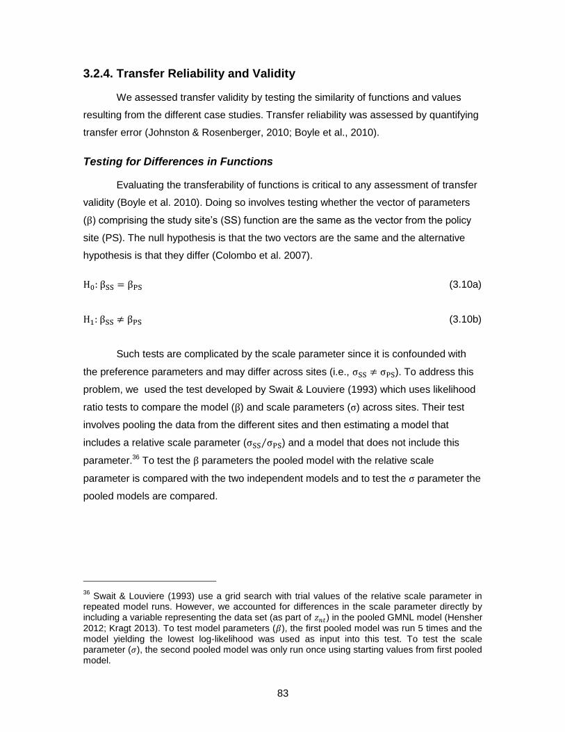
83

3.2.4. Transfer Reliability and Validity

We assessed transfer validity by testing the similarity of functions and values

resulting from the different case studies. Transfer reliability was assessed by quantifying

transfer error (Johnston & Rosenberger, 2010; Boyle et al., 2010).

Testing for Differences in Functions

Evaluating the transferability of functions is critical to any assessment of transfer

validity (Boyle et al. 2010). Doing so involves testing whether the vector of parameters

(β) comprising the study site’s (SS) function are the same as the vector from the policy

site (PS). The null hypothesis is that the two vectors are the same and the alternative

hypothesis is that they differ (Colombo et al. 2007).

H0: βSS = βPS (3.10a)

H1: βSS ≠ βPS (3.10b)

Such tests are complicated by the scale parameter since it is confounded with

the preference parameters and may differ across sites (i.e., σSS ≠ σPS). To address this

problem, we used the test developed by Swait & Louviere (1993) which uses likelihood

ratio tests to compare the model (β) and scale parameters (σ) across sites. Their test

involves pooling the data from the different sites and then estimating a model that

includes a relative scale parameter (σSS σPS⁄ ) and a model that does not include this

parameter.36 To test the β parameters the pooled model with the relative scale

parameter is compared with the two independent models and to test the σ parameter the

pooled models are compared.

36

Swait & Louviere (1993) use a grid search with trial values of the relative scale parameter in repeated model runs. However, we accounted for differences in the scale parameter directly by including a variable representing the data set (as part of 𝑧𝑛𝑡) in the pooled GMNL model (Hensher

2012; Kragt 2013). To test model parameters (𝛽), the first pooled model was run 5 times and the model yielding the lowest log-likelihood was used as input into this test. To test the scale parameter (𝜎), the second pooled model was only run once using starting values from first pooled model.

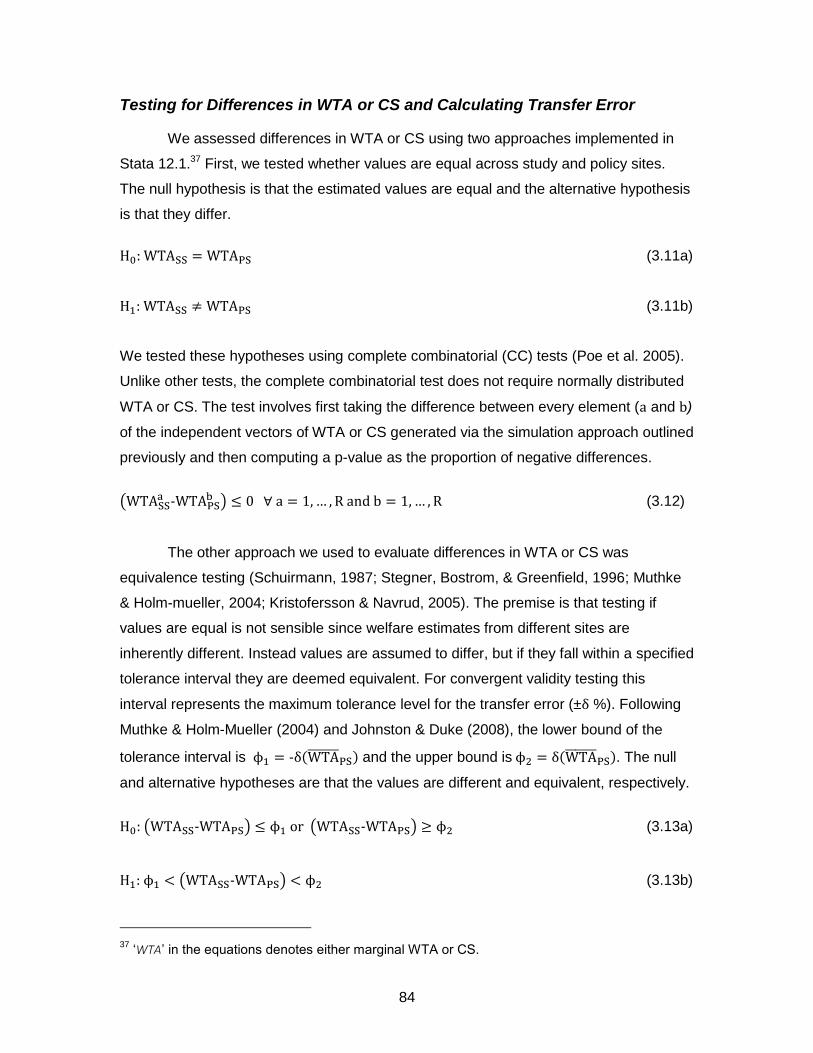
84

Testing for Differences in WTA or CS and Calculating Transfer Error

We assessed differences in WTA or CS using two approaches implemented in

Stata 12.1.37 First, we tested whether values are equal across study and policy sites.

The null hypothesis is that the estimated values are equal and the alternative hypothesis

is that they differ.

H0: WTASS = WTAPS (3.11a)

H1: WTASS ≠ WTAPS (3.11b)

We tested these hypotheses using complete combinatorial (CC) tests (Poe et al. 2005).

Unlike other tests, the complete combinatorial test does not require normally distributed

WTA or CS. The test involves first taking the difference between every element (a and b)

of the independent vectors of WTA or CS generated via the simulation approach outlined

previously and then computing a p-value as the proportion of negative differences.

(WTASSa -WTAPS

b ) ≤ 0 ∀ a = 1, … , R and b = 1, … , R (3.12)

The other approach we used to evaluate differences in WTA or CS was

equivalence testing (Schuirmann, 1987; Stegner, Bostrom, & Greenfield, 1996; Muthke

& Holm-mueller, 2004; Kristofersson & Navrud, 2005). The premise is that testing if

values are equal is not sensible since welfare estimates from different sites are

inherently different. Instead values are assumed to differ, but if they fall within a specified

tolerance interval they are deemed equivalent. For convergent validity testing this

interval represents the maximum tolerance level for the transfer error (±δ %). Following

Muthke & Holm-Mueller (2004) and Johnston & Duke (2008), the lower bound of the

tolerance interval is ϕ1 = -δ(WTA̅̅ ̅̅ ̅̅ ̅PS) and the upper bound is ϕ2 = δ(WTA̅̅ ̅̅ ̅̅ ̅

PS). The null

and alternative hypotheses are that the values are different and equivalent, respectively.

H0: (WTASS-WTAPS) ≤ ϕ1 or (WTASS-WTAPS) ≥ ϕ2 (3.13a)

H1: ϕ1 < (WTASS-WTAPS) < ϕ2 (3.13b)

37

‘WTA’ in the equations denotes either marginal WTA or CS.

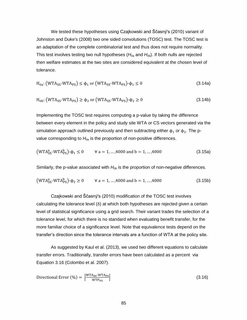
85

We tested these hypotheses using Czajkowski and Ščasný's (2010) variant of

Johnston and Duke's (2008) two one sided convolutions (TOSC) test. The TOSC test is

an adaptation of the complete combinatorial test and thus does not require normality.

This test involves testing two null hypotheses (H0a and H0b). If both nulls are rejected

then welfare estimates at the two sites are considered equivalent at the chosen level of

tolerance.

H0a: (WTASS-WTAPS) ≤ ϕ1 or (WTASS-WTAPS)-ϕ1 ≤ 0 (3.14a)

H0b: (WTASS-WTAPS) ≥ ϕ2 or (WTASS-WTAPS)-ϕ2 ≥ 0 (3.14b)

Implementing the TOSC test requires computing a p-value by taking the difference

between every element in the policy and study site WTA or CS vectors generated via the

simulation approach outlined previously and then subtracting either ϕ1 or ϕ2. The p-

value corresponding to H0a is the proportion of non-positive differences.

(WTASSa -WTAPS

b )-ϕ1 ≤ 0 ∀ a = 1, … ,4000 and b = 1, … ,4000 (3.15a)

Similarly, the p-value associated with H0b is the proportion of non-negative differences.

(WTASSa -WTAPS

b )-ϕ2 ≥ 0 ∀ a = 1, … ,4000 and b = 1, … ,4000 (3.15b)

Czajkowski and Ščasný's (2010) modification of the TOSC test involves

calculating the tolerance level (δ) at which both hypotheses are rejected given a certain

level of statistical significance using a grid search. Their variant trades the selection of a

tolerance level, for which there is no standard when evaluating benefit transfer, for the

more familiar choice of a significance level. Note that equivalence tests depend on the

transfer’s direction since the tolerance intervals are a function of WTA at the policy site.

As suggested by Kaul et al. (2013), we used two different equations to calculate

transfer errors. Traditionally, transfer errors have been calculated as a percent via

Equation 3.16 (Colombo et al. 2007).

Directional Error (%) = |WTASS-WTAPS

WTPPS| (3.16)

86

These errors are ‘directional’ since their magnitude depends on which site is treated as

the policy site as this changes the denominator. Chattopadhyay (2003) introduced ‘non-

directional’ errors that are made independent of the transfer’s direction by treating the

denominator as the average of the values from the two sites (Equation 3.17).

Chattopadhyay Error (%) = |WTASS-WTAPS

(WTASS+WTAPS) 2⁄| (3.17)

87

3.3. Results

3.3.1. Comparison of Respondent Characteristics

A key requirement for valid and reliable benefit transfer is the similarity of

populations at the study and policy sites (Johnston and Rosenberger 2010). To establish

the degree of similarity of our samples we compared them in terms of their demographic

characteristics and the features of the land they own. Our comparison of socio-

demographics among the two survey samples indicates significant differences in age

and education (Table 3.3). Respondents from the Upper Thames watershed are

generally older and more educated than respondents from the Grand watershed.

Similarly, there were few differences in land characteristics between the two watersheds

(Table 3.4). The Grand and Upper Thames samples only differ significantly in terms of

the proportion of respondents reporting meadows and wetlands on their land. A higher

proportion of respondents from the Grand watershed report having meadows and

wetlands than those from the Upper Thames watershed. Though certain characteristics

differ significantly across samples, they are still fairly similar, and the differences

observed are similar to those of previous benefit transfer assessments (e.g., Oh 2010;

Johnston and Duke 2010; Martin-Ortega et al. 2012; Brouwer et al. 2016). In addition,

our samples are reasonably similar to each watershed’s population of farm operators in

terms of gender, age, and income. However, a much higher proportion of each of our

samples holds a post-secondary education relative to the population of farm operators.

88

Table 3.3: Comparing Respondent Demographic Characteristics Across Watersheds

Respondent Characteristicsa

Data Typeb Watershed Test

Results

Farm Operatorsc

Grand U. Thames Grand U. Thames

Gender (%)

Male Binary 78.4 77.8 70.3 71.7 Female 21.6 22.2 29.7 28.3 n 529 360

Age (Adults) (%) Under 25 Ordinal 1.0 0.3 *** 25 to 44 26.0 14. 7 45 to 64 49.5 54.9 65 or older 23.5 30.1 Mean (years) Continuous 54.0 57.3 *** 52.5 52.2 n 519 355

Highest level of education (%)

Less than high school Ordinal 26.5 7.8 ***

High school 29. 0 31.9

Post-secondary 44.5 60.8 14.4 n 524 357

Employment status (%)

Not in labour force Categorical 20.9 18.2

Unemployed 1.3 0.3

Employed 77.8 81.5

n 522 357

Household Income (%)

Less than $10,000 Ordinal 1.4 0.3

$10,000 to $29,999 5.9 5.8

$30,000 to $49,999 17.7 15.8 28.8 $50,000 to $74,999 22.6 20.1 20.6 $75,000 to $99,999 21.2 26.1 16.9 $100,000 and more 31.2 31.9 33.7

n 491 329

*** indicates that the characteristic differs at the 99% level of significance

a Since we deleted missing values from this data the sample sizes do not always align with those from the choice model and are noted for each characteristic in the table.

b Testing was completed using Pearson’s chi-square tests for binary or categorical data (Fisher’s exact test was used if a cell count less than 5) and Wilcoxon / Mann-Whitney tests for ordinal and continuous data.

c Data on the gender and age of the population of farm operators is from the 2011 Census of Agriculture (Statistics Canada 2012) for census consolidated subdivisions intersecting with each watershed. Education and household income are at the provincial level. Education is only available as the proportion with a post-secondary education (or not) and income is only available for the following categories: Less than $50,000; $50,000 to $74,999; $75,000 to $99,999; $100,000 and more. Employment status is not available, though all farm operators are likely employed.

89

Table 3.4: Comparing Respondent Land Characteristics Across Watersheds

Land Characteristica Data Typeb Watershed Test Results Grand U. Thames

Land Cover (%)

Has forests Binary 63.3 63.3 Has meadows Binary 28.4 18.0 *** Has wetlands Binary 62.9 42.3 *** Has crop, pasture, or orchard (i.e., agricultural land cover)

Binary 91.9 93.6

Land Use (%) Primary land use is agriculture or forestry Categorical 81.1 85.8 Primary land use is residential 17.0 13.1 Primary land use is other 1.9 1.1

Generated income from land in past 5 years (%)

Binary 87.9 90.6

Area of Land Holdings

Mean (acres) Continuous 146.3 168.4

Farm or forest producerc (%) Binary 79.7 83.4

*** indicates that the characteristic differs at the 99% level of significance

a Sample sizes for each characteristic are generally 531 in the Grand and 362 in the Upper Thames. Exceptions include: ‘Has Wetlands’ is 528 in the Grand and 359 in the Upper Thames; ‘Land Use’ is 523 in the Grand and 360 in the Upper Thames; and ‘Farm or forest producer’ is 507 in the Grand and 344 in the Upper Thames.

b Testing was completed using Pearson’s chi-square tests for binary or categorical data (Fisher’s exact test was used if a cell count less than 5) and Wilcoxon / Mann-Whitney tests for continuous data.

3.3.2. Modelling Results

The pseudo-R2 measures indicate that the models estimated for the Grand and

Upper Thames watersheds fit the data well (Table 3.5). In terms of the mean

parameters, the ASC coefficients are positive and insignificant for both models. The

parameters estimated for the area conserved indicate that respondents in the Grand and

Upper Thames watersheds prefer to conserve smaller areas of their land. Respondents

in both watersheds prefer if the area conserved is marginal rather than productive and

they favour if this land is converted to trees, followed by meadow, and then wetlands.

The public recognition coefficients indicate that respondents in the Grand watershed

dislike receiving recognition for their conservation efforts, while the mean parameter

estimated for the Upper Thames is insignificant.

90

Table 3.5: Models in Willingness to Accept Space

Variables Grand Upper Thames

Meana

ASC 0.8732 (0.7511)

0.4840 (0.7609)

Acres -0.1863* (0.1040)

-0.3350*** (0.0993)

Land Type (productive) -2.4562*** (0.2655)

-2.0577*** (0.2225)

Activity: Wetland -1.0906*** (0.2631)

-1.1647*** (0.2391)

Activity: Trees 1.2675*** (0.2551)

1.1204*** (0.2060)

Recognition (yes) -0.9100*** (0.3212)

0.0584 (0.2672)

Elements of the Lower Triangular Cholesky Matrix ASC × ASC 9.9755***

(1.1793) 8.2197*** (0.9658)

Acres × ASC -0.0110 (0.1795)

-0.1386 (0.1532)

Land Type × ASC 0.3196 (0.3653)

0.0549 (0.3118)

Wetland × ASC 0.1815 (0.3829)

0.1457 (0.3584)

Trees × ASC -0.0781 (0.3809)

0.1342 (0.3296)

Recognition × ASC 0.6588 (0.4650)

-0.0185 (0.4198)

Acres × Acres -0.9235*** (0.1721)

-0.6647*** (0.1513)

Land Type × Acres -0.8498* (0.5065)

-0.1837 (0.3701)

Wetland × Acres -0.0308 (0.5201)

-0.8245* (0.4459)

Trees × Acres 0.2704 (0.4764)

0.5306 (0.3445)

Recognition × Acres 0.4236 (0.5610)

0.1868 (0.5240)

Land Type × Land Type -2.6687*** (0.3165)

1.7672*** (0.2495)

Wetland × Land Type 0.7983** (0.3485)

-0.4238 (0.3708)

Trees × Land Type -0.1004 (0.3528)

-0.1892 (0.3115)

Recognition × Land Type 0.6618 (0.4591)

-0.0292 (0.4127)

Wetland × Wetland -2.5907*** (0.3828)

1.7040*** (0.3249)

91

Variables Grand Upper Thames

Trees × Wetland 1.6115*** (0.3587)

-0.5810* (0.3374)

Recognition × Wetland 0.4688 (0.5234)

1.0332** (0.4168)

Trees × Trees 2.1302*** (0.2768)

1.1877*** (0.2384)

Recognition × Trees -0.2523 (0.4506)

-0.1550 (0.4865)

Recognition × Recognition

-2.4247*** (0.4383)

1.1270** (0.5714)

Scale

Constant (θ) -0.6327*** (0.1886)

-0.2085 (0.2576)

Tau (τ) 0.3833 (0.2567)

0.6463*** (0.2511)

Model Statistics

Observations 9492 6423 Log-likelihood -1760.97 -1154.23 Pseudo R2 0.29 0.31

a Coefficients represent the negative of WTA values scaled by 100 since the payment attribute was divided by 100 to aid model convergence. Standard errors appear in brackets below the corresponding coefficient.

*, **, and *** indicate that the parameter estimate differs from zero at the 90%, 95%, and 99% levels of significance, respectively

We used the elements of the lower triangular of the Cholesky matrix to estimate

each model’s variance-covariance matrix as well as the standard deviation parameters

via the Delta method (see Appendix B2). The standard deviation parameters estimated

from the models are all significant suggesting that preferences for each attribute are

heterogeneous in both watersheds. Further, certain off diagonal elements of the

variance-covariance matrix are significant, suggesting that preferences for these

attributes are related (the particular elements differ by watershed). For the Grand

watershed, preferences for land type are negatively related to the conversion activity

being wetland, while preferences for the conversion activity being wetland are negatively

related to the conversion activity being trees. For the Upper Thames, preferences for the

conversion activity being wetland are negatively related to this activity being trees.

Conversely, preferences for the conversion activity being wetland are positively related

to the number of acres conserved and public recognition. The constant for observed

scale heterogeneity, θ, is only significant in the case of the Grand watershed. The τ

parameter, which represents unobserved scale heterogeneity, is only significant for the

Upper Thames watershed model.

92

On the surface the models estimated for the Grand and Upper Thames are

similar and our Swait and Louviere (1993) likelihood ratio test bears this out (see

Appendix B3). The first pooled model yields a log-likelihood of -2929.00 and the

likelihood ratio test fails to reject the null hypothesis of equal model parameters (Χ(29)2 =

27.59 and p-value = 0.54). The pooled model for the second likelihood ratio test yields a

log-likelihood of -2929.16 and thus we also fail to reject the null hypothesis of equal

scale parameters (Χ(1)2 = 0.32 and p-value = 0.57) which aligns with the insignificance of

the parameter accounting for the differing scales in the first pooled model. Thus the two

models do not differ significantly from one another.

3.3.3. Willingness to Accept, Transfer Errors, and Testing

Marginal Willingness to Accept

Marginal WTA estimates reflect the model parameters since they were generated

from coefficients in WTA space. Note that for the land productivity and conversion

activity attributes we included estimates derived directly from the effects coded

coefficients as well as those representing a change.38 Annual per acre marginal WTA

point estimates for the Grand watershed range from -$239.27 for setting aside marginal

land (effects) to $478.53 for moving from marginal to productive land. Similarly, these

estimates for the Upper Thames watershed range from -$203.50 for setting aside

marginal land (effects) to $407.00 for changing from marginal to productive land (Table

3.6). In general, the marginal values estimated for the two watersheds are fairly similar

though notably different estimates were observed in the case of the area converted,

conversion activity being meadow, and receiving public recognition.

38

Note that the values estimated for the effects coded variables, as well as the ASC term, are not strictly marginal since they do not reflect a change in attribute levels. However, we have retained these values for the transfer validity and reliability assessment since they are used to calculate compensating surplus.

93

Table 3.6: Marginal WTA and Errors for Transfers Between Two Watersheds in Southern Ontario

Attribute

Marginal WTA (2013 CAD)a Errors (%) Testing

Grand Upper Thames

PS: Grand

PS: Thames

Mean Directional

Chatto- padhyay

CC

Tolerance Levels (%)b

Mean Tolerance

(%) PS:

Grand PS:

Thames

ASC -113.74 (-262.51 to 32.45)

-70.48 (-220.57 to 76.75)

38 61 50 47

0.34 194 312 253

Acres 14.30 (-5.86 to 34.28)

29.77 (10.62 to 48.58)

108 52 80 70

0.14 273 131 202

Land Type

Productive (effects)

239.27 (184.97 to

291.22)

203.50 (157.7 to 246.71)

15 18 16 16

0.15 39 46 43

Marginal (effects)

-239.27 (-291.22 to -

184.97)

-203.50 (-246.71 to -

157.70)

15 18 16 16

0.15 39 46 43

Marginal to productive

478.53 (369.93 to

582.44)

407.00 (315.39 to 493.41)

15 18 16 16

0.15 39 46 43

Activity

Wetland (effects)

111.53 (59.30 to 165.17)

120.65 (73.28 to 169.17)

8 8 8 8

0.40 62 58 60

Trees (effects)

-121.14 (-170.05 to -

70.26)

-109.67 (-149.64 to -

69.21)

9 10 10 10

0.36 55 60 58

Meadow (effects)

9.62 (-35.81 to 56.37)

-10.98 (-52.94 to 31.63)

214 188 201 3020

0.26 766 671 719

Meadow to trees

-130.76 (-211.21 to -

49.27)

-98.69 (-168.22 to -

31.28)

25 32 29 28

0.28 93 123 108

94

Attribute


Grand Upper Thames

PS: Grand

PS: Thames

Mean Directional

Chatto- padhyay

CC


Mean Tolerance

(%) PS:

Grand PS:

Thames

Meadow to wetland

101.91 (16.21 to 189.47)

131.64 (51.93 to 215.15)

29 23 26 25

0.31 127 98 113

Trees to wetland

232.67 (140.88 to

325.40)

230.33 (152.29 to 309.90)

1 1 1 1

0.49 45 46 46

Recognition (yes vs. no)

91.28 (28.47 to 155.20)

-6.52 (-58.68 to 46.46)

107 1500 804 231

0.01*** 183 2560 1372

Mean (Median) Error or Tolerance (%) Includes effects coded estimates 64

(27) 232 (35) 148 (28) 427 (32)

201 (123)

486 (96) 343 (97)

Includes change coded estimates 46 (29)

241 (32) 144 (31) 60 (28) 136

(127) 474 (123) 305 (125)

a 95% confidence intervals, estimated via the Krinsky-Robb method with 4000 draws, appear in brackets below each implicit price

b The tolerance levels represent the threshold at which the pairs of estimates are deemed equivalent at the 95% level of significance.

*** indicates that the CC test finds the pair of implicit prices to be different at the 99% level of significance

95

Depending on the site treatment and attribute, directional transfer errors range

from 8% to 1500%. In most cases, the directional transfer errors do not differ

substantially by treatment of the policy site. However, policy site treatment clearly

matters for transfers of marginal WTA for public recognition. For transfers of this value

from the Upper Thames to the Grand the directional error is 204%, while the reverse

direction yields an error of 1500%. While the magnitude of the errors sometimes

depends on the transfer's direction, the mean of the directional errors reveals that the

lowest errors are observed for changing the conversion activity from trees to wetland,

conversion activity being wetland (effects), followed by conversion activity being trees

(effects), land type (marginal/productive (effects) or change from marginal to productive),

changing the conversion activity from meadow to wetland, changing the conversion

activity from meadow to trees, ASC, area converted, conversion activity being meadow

(effects), and public recognition.

The non-directional errors generally confirm the results obtained for the

directional errors. However, the non-directional errors suggest that the conversion

activity being meadow yields the highest error rather than public recognition. In general,

the Chattopadhyay errors fall between the directional errors and are similar to the mean

of the directional errors. However, certain errors are much larger than their directional

counterparts and this occurs when the marginal values being compared are of similar

magnitude but opposing signs (e.g., conversion activity being meadow). These

conditions can lead to exploding non-directional errors (see Appendix B4). There is also

a disparity between the mean of the directional errors and the non-directional errors

when the values being compared have opposing signs, but are not of similar magnitude

(e.g., public recognition).

The complete combinatorial (CC) tests indicate that only the marginal WTA

estimates for public recognition significantly differ for transfers between the two

watersheds. All of the estimated tolerance levels are larger than the corresponding

transfer errors. As with the transfer errors they vary by the treatment of the policy site.

Depending on the site treatment and attribute, tolerance levels range from 39% to

2560% for transfers between the Grand and Upper Thames watersheds. The mean of

the tolerance levels across the two transfers reveals that the lowest and highest

tolerance levels are generally observed for the land type and public recognition

attributes, respectively. Note that transfers with the lowest (highest) errors do not

96

necessarily generate the lowest (highest) tolerance levels. In addition, even if the

complete combinatorial test deems a pair of estimates equal it does not guarantee that

the corresponding tolerance level will be lower than a pair deemed unequal by this test.

Contrasting the transfer assessment results for the effects coded estimates with

the associated change coded estimates reveals that the effects and change coded

estimates derived for the land type attribute yield identical errors, tolerance levels, and

CC p-values. This finding is not surprising since the land type attribute only has two

levels, ensuring that the two types of estimates are constant multiples of each other. For

the conversion activity attribute, the results are not identical across effects coded and

change coded estimates. On average, the effects coded estimates yield larger errors

and tolerance than their change coded counterparts (due to the larger errors and

tolerance levels observed for the meadow effects coded estimates). However, the

outcomes of the CC tests are the same.

Compensating Surplus

Plotting the compensating surplus point estimates for all 36 conservation

program specifications, with each specification representing a certain combination of the

non-payment attributes’ levels, reveals that mean compensating surplus estimates from

the two watersheds are clearly similar (Figure 3.2). Depending on the specification,

mean compensating surplus estimates range from -$459.85 to $399.82 for the Grand

River watershed and -$360.40 to $402.52 for the Upper Thames River watershed. The

CS estimates are always negative and positive when the land type being conserved is

marginal and productive, respectively.

97

Figure 3.2: Compensating Surplus Estimates for All Possible Program Specifications by Watershed

The observed errors and tolerance levels for transfers of CS vary by study or

policy site treatment and program specification (Table 3.7 and Figure 3.3). Directional

errors range from 1% to 3691%, non-directional errors from 1% to 190%, and tolerance

levels from 47% to 7914%. The average of the directional errors for transfers from the

Grand to the Upper Thames is larger than for transfers to the Upper Thames. A similar

finding is observed for the tolerance levels. In addition, the non-directional errors are

within the range of their directional counterparts. Furthermore, the complete

combinatorial tests indicate that only two pairs of CS estimates are significantly different

and only at the 10% significance level. Finally, box plots make apparent that the

distributions of compensating surplus transfer errors and tolerance levels are often right-

skewed (Figure 3.3). In addition, these plots indicate that the distribution of errors and

tolerance levels are more right-skewed for transfers to the Upper Thames than in the

other direction.

98

Table 3.7: Summary of Errors, Tolerance Levels, and Complete Combinatorial Tests for Transfers of Compensating Surplus Between Two Southern Ontario Watersheds

Transfer Transfer Errors (%) Tolerance Levels (%) CC (Different

Pairs) Mean Median Low High Mean Median Low High

Directional

Grand to U. Thames

157 29 1 3691 433 116 48 7914 N/A

U. Thames to Grand

38 23 1 184 161 102 47 1141

Non-Directional

Grand and U. Thames

41 26 1 190 N/A 2*, 0**, 0***

*, **, and *** indicate the number of pairs of compensating surplus estimates the CC test finds different at the 90%, 95%, and 99% levels of significance, respectively

Figure 3.3: Box Plots of Transfer Errors and Tolerance Levels Note: Outlier points are not plotted. Directional error boxes are dark grey, tolerance level boxes are light grey, and Chattopadhyay error boxes are white.

3.3.4. Sensitivity Analysis

The stages of our sensitivity analysis mirror those of the main analysis (see

Appendix B5). We first compared the sample characteristics and the two models without

interactions to establish the degree of similarity between the main and sensitivity

analyses. Our findings suggest that the samples used for the sensitivity and main

analyses share very similar respondent characteristics. Likewise, the two models without

0 100 200 300

Transfer Error or Tolerance Level (%)

Thames and Grand

Grand to Thames

Thames to Grand

Grand to Thames

Thames to Grand

99

demographic interactions are fairly similar as are the mean WTA and CS values derived

from these two specifications and the results of the validity and reliability assessments

for transfers of these values.

In terms of the model with demographic interactions, interactions with age are

significant in the case of the Upper Thames, while those with gender, age, and

education are significant for the Grand. These models fit the data better than the models

without interactions, though they are less parsimonious according to certain information

criteria. The interactions do not substantially change the reliability of our transfers. Aside

from a few outliers, the errors from the two model specifications were fairly similar

though the model with interactions did yield slightly higher errors overall. In terms of

validity, the outcomes of the Swait and Louviere (1993) likelihood ratio tests assessing

model similarity were identical as were the outcomes of the complete combinatorial tests

assessing the similarity of WTA or CS estimates. However, a marked difference in the

validity of transfers based on the two models emerges when looking at the estimated

tolerance levels. While these results are generally similar for most transfers of marginal

WTA, tolerance levels are notably higher for transfers of marginal WTA estimated for the

ASC term derived from the model with demographic interactions. Additionally, the

tolerance levels estimated for transfers of CS are much higher for transfers based on

this model relative to the model without interactions. This outcome reflects the higher

variation in WTA for the ASC term observed to result from the model with demographic

interactions. The highly variable marginal WTA for the ASC term also yields inefficient

CS estimates (standard deviations are much larger for CS values derived from the

model with interactions compared to the model without interactions). This finding persists

even after dropping insignificant interaction variables from the models.

100

3.4. Discussion and Conclusions

Overall, our results are similar to those found in the convergent validity literature

summarized by Rosenberger (2015) — given the evidence we reject the null hypothesis

that the validity and reliability of transfers of WTA differs from the validity and reliability of

transfers of WTP (the results of our sensitivity analysis do not change this conclusion).

For transfers of marginal WTA, our directional errors range from 8% to 1500% with a

mean of 148% and median of 28%, while directional errors for transfers of compensating

surplus range from 1% to 3691% with a mean of 97% and median of 25%. Non-

directional errors for transfers of marginal WTA range from 8% to 3020% with a mean of

427% and median of 32%. For transfers of compensating surplus these errors range

from 1% to 190% with a mean of 41% and median of 26%.

Our likelihood ratio test of model coefficients fails to reject the hypothesis of

parameter equality. In terms of values, 1 of 12 tests find marginal WTA estimates differ

and 2 of 36 tests find that CS estimates differ (significance level of at least 10%). The

tolerance levels estimated in our study for marginal WTA range from 39% to 2560% with

a mean of 343% and median of 97%, and range from 47% to 7914% with a mean of

297% and median of 111% for compensating surplus. Our mean tolerance level

estimates are generally higher than those in Czajkowski & Ščasný (2010). Additionally, if

a pair of estimates is deemed equal using the complete combinatorial test it does not

mean that the associated tolerance level will be lower than the level corresponding to a

pair deemed unequal by this test. This outcome may result if the estimates being tested

have a high variance (Kristofersson & Navrud, 2005; Johnston & Duke, 2008). In the

case of equivalence testing, if estimates are inefficient they are more likely to be deemed

unequal leading to higher tolerance levels. However, the complete combinatorial test

uses traditional hypotheses and is more likely to find such estimates equal.

The validity and reliability of our transfers of WTA may be similar to prior

transfers of WTP for a number of reasons. Importantly, the demographic and land

characteristics of our study sites are similar as are the characteristics of the two samples

drawn from these sites. As outlined in the introduction, such similarity is an important

consideration for benefit transfer. Our results for transfers of WTA may also be similar to

those observed for WTP if, as noted in the introduction, the disparity between the two

measures is relatively small or constant across our sites. This disparity is likely fairly

101

constant across sites since our case study sites share similar demographic

characteristics. Furthermore, the disparity in the measures is likely small for two

reasons. First, the vast majority of the respondents to our survey were agricultural or

forest product producers and they may not experience consequential loss aversion since

they are experienced economic actors. Second, WTP and WTA approximate one-

another when these values are elicited for ordinary private goods — the choice

experiment essentially asked respondents to lease portions of their land for wetlands

conservation, which is effectively a private good from the perspective of landowners.

Finally, Rosenberger (2015) notes that the higher directional errors observed in their

review could result from experimental studies comparing estimates that would rarely or

never be compared in policy analysis.

The findings of our sensitivity analysis reflect in part those of Ostberg et al.

(2013), that model specification does not substantially influence transfer performance.

Our assessment revealed that transfer reliability and certain aspects of validity are

largely the same for transfers based on models with and without demographic

interactions with the ASC term. However, tolerance levels estimated for transfers of

marginal WTA for the ASC term and CS based on the model with interactions were

notably larger than those based on the model without interactions suggesting that values

from the former model are less likely to be equivalent than those derived from the latter.

Basing the transfers on a model with significant interactions only did not address this

issue. This result is driven by variability in these WTA values introduced by the

interactions. As discussed earlier, equivalence testing penalizes transfers of inefficient

estimates yielding larger tolerance levels.

Our findings can also inform wetlands conservation policy in the Grand and

Upper Thames watersheds. On average, participation in wetlands conservation could be

increased if associated conservation programs: target smaller marginally productive

areas of land; buffer existing wetlands with trees or meadows rather than build new

wetlands; do not offer public recognition; and offer higher payments. However,

preferences for these attributes are heterogeneous and conservation groups should take

this into account when designing wetlands conservation programs in these watersheds.

Furthermore, given the results of our transfer assessment these relationships could be

used to aid wetlands conservation in other similar regions.

102

We believe that this research shows that the reliability and validity of transferring

WTA is similar to that found for transfers of WTP. Given the growing number of primary

valuation studies eliciting WTA, our findings suggest that these WTA values can be used

in benefit transfer as part of policy analysis (at least in the context examined in this

paper). Furthermore, our sensitivity analysis suggests that transfers of compensating

surplus based on choice models that include interactions of demographic characteristics

with the alternative specific constant can reduce validity relative to models without such

interactions. However, similar to transfers of WTP further research is required to better

understand other settings and conditions under which transfers of WTA are more likely

to be accurate. An extension of our research would be to implement parallel WTA and

WTP valuation case studies at the same sites (valuing the same goods). This would

allow an interesting twist on our research, which would be an assessment of the

implications of transferring a WTP measure estimated at a study site when the correct

measure for the change at the policy site is actually WTA (and vice versa). Benefit-cost

analyses often apply the WTP measure when WTA is more appropriate, even when

using original research, since WTP is seen by many as a more reasonable measure

(Hammitt 2015). Although theoretically inappropriate, as highlighted by Knetsch (2007),

and discouraged by the United States Office of Management and Budget (2003) such

transfers would be pragmatic and reflect policy analyses when existing values estimated

using the correct measure are unavailable for input into benefit transfer.

103


The Social Science and Humanities Research Council of Canada provided

funding for this research through a Standard Research Grant (865-2008-0045) and

Doctoral Fellowship (752-2012-2435). The funding agency did not participate in the

research process or the paper’s preparation. Support and assistance was provided by

the Upper Thames Conservation Authority and the Grand River Conservation Authority.

We thank the landowners who participated in this research. We are also thankful for

feedback on this manuscript provided by Dr. Pascal Haegeli. Dr.Wolfgang Haider, who

passed away on August 24, 2015, was a great supervisor, colleague, and friend.

104

References

Bateman IJ, Brouwer R, Ferrini S, et al (2011) Making Benefit Transfers Work: Deriving and Testing Principles for Value Transfers for Similar and Dissimilar Sites Using a Case Study of the Non-Market Benefits of Water Quality Improvements Across Europe. Environ Resour Econ 50:365–387. doi: 10.1007/s10640-011-9476-8

Beck MJ, Rose JM, Hensher DA (2013) Consistently inconsistent: The role of certainty, acceptability and scale in choice. Transp Res Part E Logist Transp Rev 56:81–93. doi: 10.1016/j.tre.2013.05.001

Booij AS, van de Kuilen G (2009) A parameter-free analysis of the utility of money for the general population under prospect theory. J Econ Psychol 30:651–666. doi: 10.1016/j.joep.2009.05.004

Booij AS, Van Praag BMS, Van De Kuilen G (2010) A parametric analysis of prospect theory’s functionals for the general population. Theory Decis 68:115–148. doi: 10.1007/s11238-009-9144-4

Boyle KJ, Kuminoff N V, Parmeter CF, Pope JC (2010) The Benefit-Transfer Challenges. Annu Rev Resour Econ 2:161–182. doi: 10.1146/annurev.resource.012809.103933

Broch SW, Vedel SE (2012) Using Choice Experiments to Investigate the Policy Relevance of Heterogeneity in Farmer Agri-Environmental Contract Preferences. Environ Resour Econ 51:561–581. doi: 10.1007/s10640-011-9512-8

Brouwer R (2000) Environmental value transfer: state of the art and future prospects. Ecol Econ 32:137–152. doi: 10.1016/S0921-8009(99)00070-1

Brouwer R, Bateman IJ (2005) Benefits transfer of willingness to pay estimates and functions for health-risk reductions : a cross-country study. 24:591–611. doi: 10.1016/j.jhealeco.2004.09.004

Brouwer R, Bliem M, Getzner M, et al (2016) Valuation and transferability of the non-market benefits of river restoration in the Danube river basin using a choice experiment. Ecol Eng 87:20–29. doi: 10.1016/j.ecoleng.2015.11.018

Brouwer R, Martin-Ortega J, Dekker T, et al (2015) Improving value transfer through socio-economic adjustments in a multicountry choice experiment of water conservation alternatives. Aust J Agric Resour Econ 59:458–478. doi: 10.1111/1467-8489.12099

Brouwer R, Logar I (2014) Do choice experiments produce more stable welfare measures than contingent valuation? A test-retest. Paper presented at the Fifth World Congress of Environmental and Resource Economists, 28 June–2 July 2014, Istanbul, Turkey, pp 1–42

105

Canada Post (2015) Canada Post Neighbourhood MailTM (Unaddressed AdmailTM). Toronto, Ontario: Canada Post.

Chattopadhyay S (2003) A Repeated Sampling Technique in Assessing the Validity of Bene t Transfer in Valuing Non-Market Goods. Land Econ 79:576–596.

Colombo S, Calatrava-Requena J, Hanley N (2007) Testing Choice Experiment for Benefit Transfer with Preference Heterogeneity. Am J Agric Econ 89:135–151. doi: 10.1111/j.1467-8276.2007.00968.x

Colombo S, Hanley N (2008) How Can We Reduce the Errors from Benefits Transfer ? An Investigation Using the Choice Experiment Method. Land Econ 84:128–147. doi: 10.3368/le.84.1.128

Czajkowski M, Hanley N, Lariviere J (2015) The effects of experience on preferences: Theory and empirics for environmental public goods. Am J Agric Econ 97:333–351. doi: 10.1093/ajae/aau087

Czajkowski M, Ščasný M (2010) Study on benefit transfer in an international setting. How to improve welfare estimates in the case of the countries’ income heterogeneity? Ecol Econ 69:2409–2416. doi: 10.1016/j.ecolecon.2010.07.008

Ducks Unlimited Canada (2010) Southern Ontario wetland conversion analysis: Final report. Barrie, ON: Ducks Unlimited Canada.

Espinosa-Goded M, Barreiro-Hurlé J, Ruto E (2010) What do farmers want from agri-environmental scheme design? A choice experiment approach. J Agric Econ 61:259–273. doi: 10.1111/j.1477-9552.2010.00244.x

Fiebig DG, Keane MP, Louviere J, Wasi N (2010) The Generalized Multinomial Logit Model: Accounting for Scale and Coefficient Heterogeneity. Mark Sci 29:393–421. doi: 10.1287/mksc.1090.0508

Freeman MA, Herriges JA, Kling CL (2014) The Measurement of Environmental Resource Values.

Gasson R, Potter C (1988) Conservation through land diversion: a survey of farmers’ attitudes. J Agric Econ 39:340–351. doi: 10.1111/j.1477-9552.1988.tb00593.x

Glenk K, Martin-Ortega J, Pulido-Velazquez M, Potts J (2015) Inferring Attribute Non-attendance from Discrete Choice Experiments: Implications for Benefit Transfer. Environ Resour Econ 60:497–520. doi: 10.1007/s10640-014-9777-9

Grand River Conservation Authority (2008) Grand River Watershed: Characterization Report Executive Summary. Cambridge, Ontario: Grand River Conservation Authority.

106

Grand River Conservation Authority (2014) Grand River Waterhed Management Plan. Cambridge, Ontario: Grand River Conservation Authority.

Grand River Conservation Authority (2016) Natural Heritage: Landscapes. Cambridge, ON: Grand River Conservation Authority. https://www.grandriver.ca/en/our-watershed/Landscapes.aspx. Accessed 11 Jul 2016

Greene WH, Hensher DA (2010) Does scale heterogeneity across individuals matter? An empirical assessment of alternative logit models. Transportation (Amst) 37:413–428. doi: 10.1007/s11116-010-9259-z

Gu Y, Hole AR, Knox S (2013) Fitting the generalized multinomial logit model in Stata. Stata J 13:382–397. doi: The Stata Journal

Hammitt JK (2015) Implications of the WTP–WTA Disparity for Benefit–Cost Analysis. J Benefit-Cost Anal 6:207–216. doi: 10.1017/bca.2015.1

Hanemann WM (1984) Valuation Contingent Experiments in Responses. Am J Agric Econ 66:332–341.

Hansen K, Duke E, Bond C, et al (2018) Rancher Preferences for a Payment for Ecosystem Services Program in Southwestern Wyoming. Ecol Econ 146:240–249. doi: 10.1016/j.ecolecon.2017.10.013

Hensher DA (2012) Accounting for scale heterogeneity within and between pooled data sources. Transp Res Part A Policy Pract 46:480–486. doi: 10.1016/j.tra.2011.11.007

Hess S, Train K (2017) Correlation and scale in mixed logit models. J Choice Model 23:1–8. doi: 10.1016/j.jocm.2017.03.001

Hole AR (2011) Estimation of willingness to pay in preference space vs . WTP space. Odense, Denmark.

Horowitz JK, McConnell KE (2002) A Review of WTA/WTP Studies. J Environ Econ Manage 44:426–447. doi: 10.1006/jeem.2001.1215

Hoyos D (2010) The state of the art of environmental valuation with discrete choice experiments. Ecol Econ 69:1595–1603. doi: 10.1016/j.ecolecon.2010.04.011

Hu W, Veeman MM, Adamowicz WL (2005) Labelling Genetically Modified Food: Heterogeneous Consumer Preferences and the Value of Information. Can J Agric Econ Can d’agroeconomie 53:83–102. doi: 10.1111/j.1744-7976.2005.04004.x

Jiang Y, Swallow SK, McGonagle MP (2005) Context-sensitive benefit transfer using stated choice models: Specification and convergent validity for policy analysis. Environ Resour Econ 31:477–499. doi: 10.1007/s10640-005-3366-x

107

Johnston RJ (2007) Choice experiments, site similarity and benefits transfer. Environ Resour Econ 38:331–351. doi: 10.1007/s10640-006-9073-4

Johnston RJ, Duke JM (2008) Benefit Transfer Equivalence Tests with Non-normal Distributions. Environ Resour Econ 41:1–23. doi: 10.1007/s10640-007-9172-x

Johnston RJ, Duke JM (2009) Willingness to Pay for Land Preservation across States and Jurisdictional Scale: Implications for Benefit Transfer. Land Econ 85:217–237. doi: 10.3368/le.85.2.217

Johnston RJ, Duke JM (2010) Socioeconomic adjustments and choice experiment benefit function transfer: Evaluating the common wisdom. Resour Energy Econ 32:421–438. doi: 10.1016/j.reseneeco.2009.11.003

Johnston RJ, Rosenberger RS (2010) Methods, Trends and Controversies in Contemporary Benefit Transfer. J Econ Surv 24:479–510. doi: 10.1111/j.1467-6419.2009.00592.x

Kaczan D, Swallow BM, Adamowicz WLV (2013) Designing payments for ecosystem services (PES) program to reduce deforestation in Tanzania: An assessment of payment approaches. Ecol Econ 95:20–30. doi: 10.1016/j.ecolecon.2013.07.011

Kahneman D, Knetsch JL, Thaler RH (1990) Experimental Tests of the Endowment Effect and the Coase Theorem. J Polit Econ 98:1325–1348. doi: 10.1086/261737


Kim Y, Kling CL, Zhao J (2015) Understanding Behavioral Explanations of the WTP-WTA Divergence Through a Neoclassical Lens: Implications for Environmental Policy. Annu Rev Resour Econ 7:169–187. doi: 10.1146/annurev-resource-100913-012501

Knetsch JL (2007) Biased valuations, damage assessments, and policy choices: The choice of measure matters. Ecol Econ 63:684–689. doi: 10.1016/j.ecolecon.2007.02.012

Kragt ME (2013) The Effects of Changing Cost Vectors on Choices and Scale Heterogeneity. Environ Resour Econ 54:201–221. doi: 10.1007/s10640-012-9587-x

Kristofersson D, Navrud S (2005) Validity tests of benefit transfer - Are we performing the wrong tests? Environ Resour Econ 30:279–286. doi: 10.1007/s10640-004-2303-8

Kuhfeld W (2010) Marketing research methods in SAS: Experimental Design, Choice, Conjoint, and Graphical Techniques. SAS Institute Inc., Cary, NC

108

Lienhoop N, Brouwer R (2015) Agri-environmental policy valuation: Farmers’ contract design preferences for afforestation schemes. Land use policy 42:568–577. doi: 10.1016/j.landusepol.2014.09.017

List JA (2003) Does Market Experience Eliminate Market Anomalies? Q J Econ 118:41–71. doi: 10.1162/00335530360535144

List JA (2004) Substitutability, experience, and the value disparity: Evidence from the marketplace. J Environ Econ Manage 47:486–509. doi: 10.1016/j.jeem.2003.05.001

List JA (2011) Does Market Experience Eliminate Market Anomalies? The Case of Exogenous Market Experience. Am Econ Rev 101:313–317. doi: 10.1257/aer.101.3.313

Lohr L, Park TA (1995) Utility-Consistent Discrete-Continuous Choices in Soil Conservation. Land Econ 71:474–490.

Loomis J, Roach B, Ward F, Ready R (1995) Testing Transferability of Recreation Demand Models Across Regions: A Study of Corps of Engineer Reservoirs. Water Resour Res 31:721–730. doi: 10.1029/94WR02895

Loomis JB (1992) The evolution of a more rigorous approach to benefit transfer: Benefit function transfer. Water Resour Res 28:701–705. doi: 10.1029/91WR02596

Louviere JJ, Hensher D a, Swait JD (2000) Stated Choice Methods: Analysis and Applications. Cambridge University Press, Port Melbourne, Australia

Maddux WW, Yang H, Falk C, et al (2010) For Whom Is Parting With Possessions More Painful? Psychol Sci 21:1910–1917. doi: 10.1177/0956797610388818

Martin-Ortega J, Brouwer R, Ojea E, Berbel J (2012) Benefit transfer and spatial heterogeneity of preferences for water quality improvements. J Environ Manage 106:22–29. doi: 10.1016/j.jenvman.2012.03.031

Matta JR, Alavalapati JRR, Mercer DE (2009) Incentives for Biodiversity Conservation Beyond the Best Management Practices: Are Forestland Owners Interested? Land Econ 85:132–143. doi: 10.3368/le.85.1.132

Morrison M, Bergland O (2006) Prospects for the use of choice modelling for benefit transfer. Ecol Econ 60:420–428. doi: 10.1016/j.ecolecon.2006.06.014

Muthke T, Holm-Mueller K (2004) National and international benefit transfer testing with a rigorous test procedure. Environ Resour Econ 29:323–336. doi: 10.1007/s10640-004-5268-8

Oh C (2010) Assessing Recreationists’ Economic Benefits and Their Transferability to Other Sites. Leis Sci 32:125–142. doi: 10.1080/01490400903547120

109

Ontario Ministry of Finance (2014) Ontario Population Projections Fall 2014: Based on the 2011 Census. Toronto, Ontario: Government of Ontario.

Östberg K, Håkansson C, Hasselström L, Bostedt G (2013) Benefit Transfer for Environmental Improvements in Coastal Areas: General versus Best-Fitting Models. Can J Agric Econ Can d’agroeconomie 61:239–258. doi: 10.1111/cjag.12010

Paulrud S, Laitila T (2010) Farmers’ attitudes about growing energy crops: A choice experiment approach. Biomass and Bioenergy 34:1770–1779. doi: 10.1016/j.biombioe.2010.07.007

Poe GL, Giraud KL, Loomis JB (2005) Computational Methods for Measuring the Difference of Empirical Distributions. Am J Agric Econ 87:353–365. doi: 10.1111/j.1467-8276.2005.00727.x

Price J, Dupont D, Adamowicz W (2017) As Time Goes By: Examination of Temporal Stability Across Stated Preference Question Formats. Environ Resour Econ 68:643–662. doi: 10.1007/s10640-016-0039-x

RE/MAX (2013) Market Trends, Farm Edition.

Revelt D, Train K (1998) Mixed Logit with Repeated Choices: Households’ Choices of Appliance Efficiency Level. Rev Econ Stat 80:647–657. doi: 10.1162/003465398557735

Rigby D, Burton M, Pluske J (2016) Preference Stability and Choice Consistency in Discrete Choice Experiments. Environ Resour Econ 65:441–461. doi: 10.1007/s10640-015-9913-1


Scarpa R, Thiene M, Train K (2008) Utility in Willingness to Pay Space: A Tool to Address Confounding Random Scale Effects in Destination Choice to the Alps. Am J Agric Econ 90:994–1010. doi: 10.1111/j.1467-8276.2008.01155.x

Schuirmann DJ (1987) A comparison of the Two One-Sided Tests Procedure and the Power Approach for assessing the equivalence of average bioavailability. J Pharmacokinet Biopharm 15:657–680. doi: 10.1007/BF01068419

Shaikh SL, Sun L, van Kooten GC (2007) Are Agricultural Values a Reliable Guide in Determining Landowners’ Decisions to Create Forest Carbon Sinks? Can J Agric Econ Can d’agroeconomie 55:97–114. doi: 10.1111/j.1744-7976.2007.00082.x

110

Statistics Canada (2012) 2011 Farm and Farm Operator Data (95-640-X). http://www.statcan.gc.ca/pub/95-640-x/95-640-x2011001-eng.htm. Accessed 21 Nov 2015

Stegner BL, Bostrom AG, Greenfield TK (1996) Equivalence testing for use in psychosocial and services research: An introduction with examples. Eval Program Plann 19:193–198. doi: 10.1016/0149-7189(96)00011-0

Swait J, Louviere J (1993) The Role of the Scale Parameter in the Estimation and Comparison of Multinomial Logit Models. J Mark Res 30:305–314.

Thiene M, Scarpa R (2009) Deriving and Testing Efficient Estimates of WTP Distributions in Destination Choice Models. Environ Resour Econ 44:379–395. doi: 10.1007/s10640-009-9291-7

Train K, Weeks M (2005) Discrete Choice Models in Preference Space and Willingness-to-Pay Space. In: Scarpa R, Alberini A (eds) The Economics of Non-Market Goods and Resources, Applications of Simulation Methods in Environmental and Resource Economics. Springer-Verlag, New York, NY, pp 1–16

Train KE (2009) Discrete Choice Methods With Simulation, Second Edi. Cambridge University Press, New York, NY

Trenholm R, Haider W, Lantz V, et al (2017) Landowner preferences for wetlands conservation programs in two Southern Ontario watersheds. J Environ Manage 200:6–21. doi: 10.1016/j.jenvman.2017.05.055

Tunçel T, Hammitt JK (2014) A new meta-analysis on the WTP/WTA disparity. J Environ Econ Manage 68:175–187. doi: 10.1016/j.jeem.2014.06.001

United States Office of Management and Budget (2003) Circular A-4: Regulatory Analysis. Washington, DC: Office of Management and Budget.

Upper Thames River Conservation Authority (2012) Upper Thames River 2012 Watershed Report Card: Summary. London, Ontario: Upper Thames River Conservation Authority.

Upper Thames River Conservation Authority (2015) Candidates Briefing Notes: Federal Election 2015. London, Ontario: Upper Thames River Conservation Authority.

VandenBerg T, Poe G, Powell J (2001) Accessing the accuracy of benefits transfer: evidence from a multi-state contingent valuation study of groundwater quality. In: Bergstrom JC, Boyle KJ, Poe GL (eds) The economic value of water quality. Edward Elgar Publishing, Northampton, MA, pp 100–120

Wang M, Rieger MO, Hens T (2017) The Impact of Culture on Loss Aversion. J Behav Decis Mak 30:270–281. doi: 10.1002/bdm.1941

111


Yu J, Belcher K (2011) An Economic Analysis of Landowners’ Willingness to Adopt Wetland and Riparian Conservation Management. Can J Agric Econ 59:207–222. doi: 10.1111/j.1744-7976.2011.01219.x

112

Chapter 4. Assessing the Convergent Validity and Reliability of Transfers of Market Shares Derived from Choice Experiments for Landowner Participation in Wetlands Conservation Programs

A version of this chapter is currently under peer review at Resource and Energy

Economics as Trenholm, R., Lantz, V., Knowler, D., and Haider, W. "Comparing the

Convergent Validity of Transfers of Choice Probability Market Shares and Welfare

Estimates". I led the design of this research and was the lead on the fieldwork. I

authored nearly all of the text and conducted all of the data analyses.

113

Abstract

Market shares derived from choice experiments can inform policy development in

several fields. For example, they can be used to predict the proportion of private

landowners who may participate in a given conservation program. Similar to non-market

values, these predicted participation market shares can be difficult to obtain using

original research, but transfers may be possible. However, such transfers have not been

assessed using convergent validity tests similar to those used to test benefit transfer.

We used standard techniques to assess the validity and reliability of transfers of these

market shares. To provide context we compared these results with a parallel

assessment of transfers of compensating surplus. Market share and compensating

surplus estimates were derived from choice experiments that elicited the preferences of

rural landowners in two Canadian watersheds for enrolling their land in wetlands

conservation programs. Validity was assessed by testing the similarity of models and

estimates, while reliability was assessed by calculating directional and non-directional

transfer errors. Structural differences dictate that transfers of market shares should be

more reliable and valid than transfers of compensating surplus estimated from the same

models and our results bear this out. Our findings hint that transfers of market shares

could be appealing for policy analysis when original research is not possible. However,

more research is required to determine the threshold levels of validity and reliability at

which such transfers are desirable.

Keywords: benefit transfer; convergent validity; willingness to accept; compensating

surplus; market share; choice experiment

114

4.1. Introduction

Benefit transfer is commonly applied in economic analyses such as benefit-cost

analysis when the resources required for estimating non-market values using original

research are limited. This technique involves transferring economic welfare estimates

across space, time, or populations from the location of the existing value, known as the

study site (SS), to the site of the current analysis, known as the policy site (PS) (Boyle,

Kuminoff, Parmeter, & Pope, 2010). Benefit transfers are subject to a range of errors,

notably generalization error which results from differences in study and policy sites

(Johnston & Rosenberger, 2010). As such, studies assessing the validity and reliability

of the technique have become commonplace (see Kaul, Boyle, Kuminoff, Parmeter, &

Pope (2013) or Rosenberger (2015) for a review).39 These convergent validity studies

have traditionally used estimates of willingness to pay (WTP), often estimated from

choice experiments, in their assessments (e.g., Brouwer et al., 2016; Colombo,

Calatrava-Requena, & Hanley, 2007). An additional output of choice experiments are

market or choice shares that indicate the proportion of respondents expected to select a

certain specification of a good or service out of a set of alternative specifications

(Hensher, Rose, & Greene, 2015). This output can be used in a decision support tool to

help predict the share of policy support received by any one of the possible scenarios or

states of the world that can be represented from a choice experiment’s attributes.

Choice experiments are widely applied worldwide and studies estimating market

shares span the literature, including fields such as recreation and tourism, farmer and

landowner decision making, transportation, food and beverage, as well as health and

medicine (e.g., Arellano et al., 2015; Koemle & Morawetz, 2016; U. Pröbstl-Haider et al.,

2016; Rose & Hensher, 2014; Wu et al., 2015). Few studies that have estimated market

shares implement similar choice experiments across space, time or populations and

those that do are not convergent validity analyses (e.g., Landauer, Pröbstl, & Haider,

2012). Obtaining market shares from original research can be expensive since it

involves the same amount of effort required to elicit welfare estimates. Therefore

39

Several factors influence the validity and reliability of benefit transfers (Kaul et al., 2013). For instance, transferring functions that relate economic values to observable site characteristics is more accurate than transferring adjusted or unadjusted unit values, particularly when sites are different, since functions can account for site characteristics. In addition, using values from multiple studies and geographically similar areas leads to more accurate benefit transfers (site similarity is a key condition for accurate transfers (Boyle et al., 2010)).

115

transferring market shares is desirable. However, to our knowledge the validity and

reliability these transfers has never been explicitly explored in the same sense as benefit

transfer.

Transfers of market shares could inform resource and environmental

management policy, such as the development or modification of voluntary conservation

or agri-environmental programs on private lands (a well-known example of such

schemes is the Conservation Reserve Program (United States Department of

Agriculture, 2017)). In these cases, transfers could be used to gauge the impact of key

program attributes on the proportion of landowners predicted to participate in

conservation programs. While informing the modification or development of these

programs through original research may be more desirable, we envision a few key

benefits of transferring predicted market shares. As previously mentioned, original

choice experiment research may not always be possible due to time or budget

limitations. However, even if possible such original research is still limited by available

resources, perhaps to a single choice experiment survey. In this case, transferring

market shares may enable policy makers to access a wider range of information than

might otherwise be available.

The validity and reliability of market share transfers should differ from that of

transfers of WTP or willingness to accept (WTA) due to differences in how the two types

of values are calculated (see Hensher, Rose, & Greene (2015) for an overview of how to

calculate these values). Market shares are bounded by 0 and 1, which limits the range of

possible transfer errors. For instance, assuming transfers of market shares that are non-

zero integers the range of possible percentage transfer errors is 0% to 9900% with mean

of 211% and median of 61% (errors are highest when the market shares are 0.01 and 1,

respectively, at the policy and study sites; see Appendix C1 for a visual representation of

the distribution of potential errors). Economic values such as WTP or WTA are not

similarly constrained, meaning that the range of possible transfer errors is larger.

Differences in the study and policy sites, such as the alternatives differing in

number or type, could pose a challenge for transfers of market shares not necessarily

faced by transfers of WTP or WTA. The policy and study sites may differ such that

different alternatives are required to properly represent the goods or services available

at each site (e.g., transfers of beach visitation between sites with a different number of

116

beaches or transfers of transportation mode choices between sites with different

transportation options). In this case market share transfer may be difficult, or even

impossible if there are substantial differences, since choices may be distributed over a

wider range of alternatives at one site relative to the other. Transfers would be especially

difficult if certain alternatives are not relevant at both sites. However, transfers between

substantially different policy and study sites, each with choice sets comprised of a very

different number or type of alternatives, is likely not desirable in the first place. Consider

that valid and reliable benefit transfers require similar site characteristics, including “the

availability of substitutes” (Boyle, Kuminoff, Parmeter, & Pope, 2010). This suggests that

choice sets at the study and policy sites should include the same, or at least a very

similar, number of alternatives since each alternative represents a substitute.

Furthermore, the set of alternatives from the study site should be relevant at the policy

site. Transfers of all types need to be carefully thought out and similar site or policy

characteristics are important — as with benefit transfer there will be cases where market

share transfer will and will not be feasible.

Our study contributes to the literature by reporting on research into the validity

and reliability of transfers of market shares derived from choice experiments using

convergent validity tests commonly used in benefit transfer validity and reliability testing.

To provide context, these results are contrasted with those from an assessment of the

validity and reliability of transfers of compensating surplus estimates derived from the

same models. Given that market shares are bounded by 0% and 100% by definition, and

compensating surplus estimates are unbound, transfers of market shares should be

more valid and reliable than transfers of compensating surplus. While such an 'apples to

oranges' comparison may seem uninformative given these structural differences, it

serves to benchmark the convergent validity of our market share transfers against that of

welfare estimates. Our analysis relied on data from case studies in two Canadian

watersheds that used choice experiments to elicit the preferences and willingness to

accept (WTA) of rural landowners for incentive-based wetlands conservation programs.

We focus on the decision of landowners to adopt a particular conservation program

relative to maintaining the status quo (i.e., the predicted share of landowners who would

enrol versus sticking with the status quo or the financial compensation required for them

117

to move to the conservation program from their status quo [hereafter "market share"]).40

We review our study’s method in the next section, followed by the data, the results, and

finally a discussion and conclusion.

40

The binary adoption decision is a subset of possible market shares (in the case of multiple alternatives versus the status quo, market shares could be calculated for each alternative and the status quo). However, the decision to adopt the conservation program or not does correspond with the change represented by compensating surplus values (which reflects the compensation required to adopt).

118

4.2. Method

4.2.1. Econometric Modeling

We analyzed our data using random parameter logit (RPL) models since they

improve the accuracy of benefit transfers relative to a conditional logit (Colombo et al.,

2007). The analysis is rooted in the random utility model (McFadden, 1974; Train, 2009).

The premise of this model is that individuals make choices among alternatives based on

relative utility (U). Given the set of alternative specifications of goods or services

j = 1, … , J a rational individual n will choose alternative i over all other alternatives j on

choice occasion t if Unit > Unjt ∀ i ≠ j all else equal. Utility (Unjt) is divisible into a

deterministic (Vnjt) component, which is a function of the alternative’s attributes (xnjt),

and a stochastic error term (εnjt).

The RPL explicitly incorporates heterogeneous tastes for the attributes by

allowing preference parameters (βn) to differ across individuals (known as random

parameters). Preferences are assumed to be randomly distributed in the population

according to a probability density function (Train, 2009). βn is segmented into a mean

component (β), which captures average sample preferences, and a standard deviation

component (ηn) that accounts for individual-specific deviations from the mean. Utility is

thus represented as Equation 4.1.

Unjt = Vnjt +εnjt

σ⁄ = αnjt + (β + ηn)xnjt +εnjt

σ⁄ (4.1)

where α is an alternative specific constant (ASC) term and σ is the scale parameter.41

Due to the error term, the RUM becomes the probability that individual n will choose

alternative i over all others j on occasion t such that Prnit(Vnit + εnit σ⁄ > Vnjt +

εnjt σ⁄ )∀ i ≠ j. This expression is reformulated using a logit formulation for the

unconditional probability that individual n will choose alternative i over all other

alternatives j (Equation 4.2).

41

The scale parameter is inversely related to the variance of the error term. Given a single dataset 𝜎 is typically assumed to equal 1, although it can differ over datasets (Swait & Louviere, 1993).

119

Prnit = ∫eσβnxnit

∑ eσβnxnjt

f(βn)d(βn) (4.2)

Since the integral is not of closed form, maximum simulated likelihood estimation

is required to generate the parameter estimates (Train, 2009). Our RPL models were

estimated in Stata 12.1 using the ‘mixlogit’ command with 2000 Halton draws (Hole,

2007). All parameters were treated as random to allow preference heterogeneity for all

choice experiment attributes with non-payment and payment parameters normally and

log-normally distributed, respectively. The log-normal payment forces a positive

parameter which conforms to theoretical expectations since larger payments should

increase landowner utility, though as discussed later this has implications for estimating

economic values. We ran models with and without correlated random coefficients and

used a likelihood ratio test to select the specification for our transfer assessment.42

Models with correlated random coefficients yield lower-triangular Cholesky matrix

coefficients in addition to mean parameters, while models with independent random

coefficients produce standard deviation coefficients. We did not interact any of the

choice experiment variables with socio-economic characteristics since the effect of such

interactions on transfer validity and reliability is unclear.43 To combat hypothetical bias

we calibrated our data for respondent certainty, a common approach in stated

preference research which has been used in previous choice experiment studies (Beck,

Rose, & Hensher, 2013; Ready, Champ, & Lawton, 2010). Following Beck, Rose, &

Hensher (2013), the choice data were calibrated for certainty by weighting the models

using responses to a numerical follow-up certainty question that appeared after each

choice set. We ran the independent models ten times using different random starting

values and chose those models yielding the lowest log-likelihood values for the transfer

validity and reliability assessment.44

42

Modeling correlations among random coefficients yields more accurate estimates of WTP or WTA (Hess & Train, 2017). 43

Such interactions can improve transfer accuracy (e.g., Brouwer et al., 2015). However, this does not hold in all cases (e.g., Ostberg, Cecilia, & Hasselstr, 2013) and can increase errors (e.g., Johnston & Duke, 2010). 44

We also ran models with data not calibrated for certainty and with a fixed payment parameter. For both weighted and unweighted data, likelihood ratio tests revealed that the models with log-normal payment were significantly different from, and thus preferred to, the models with fixed payment. While the specific results regarding transfer validity and reliability differed somewhat when using models not calibrated for certainty or with fixed payment, they were fairly similar and

120

4.2.2. Deriving market shares and compensating surplus

We derived market share and compensating surplus estimates from the RPL

models using the simulation approaches of Hu, Veeman, & Adamowicz (2005) and

Czajkowski, Hanley, & Lariviere (2015). Two sequential rounds of simulation were

conducted yielding vectors representing empirical densities for each attribute. An initial

‘parameter simulation’ accounts for the sampling distribution of all coefficients by taking

R draws from a multivariate normal distribution characterized by the RPL model’s mean

and standard deviation or lower-triangular Cholesky matrix coefficients as well as

variance-covariance matrix. For models with correlated random coefficients the

variance-covariance matrix, used in the next round of simulation, is generated from the

simulated lower-triangular Cholesky coefficients for each of the R draws. A subsequent

‘coefficient simulation’ incorporates the preference heterogeneity accounted for by the

random parameters. It is completed by taking S draws from a normal distribution defined

by the mean coefficients and standard deviation coefficients or variance-covariance

matrix generated from each of the R draws of the ‘coefficient simulation’. R vectors of

size S are generated for each random parameter. We used 2000 draws for each round of

simulation.

These vectors were used to predict participation in a particular wetlands

conservation program specification versus maintaining the status quo and then to

calculate the associated compensating surplus.45 For each of the R = 2000 vectors,

market shares (MS) were obtained by calculating the choice probabilities for each

alternative according to Equation 4.3 (Hudson et al., 2012; Hensher et al., 2015).

MSs =eVs

j

∑ eVsk ∀ S = 1, … ,2000 (4.3)

where Vsj represents the sth element of the indirect utility vector for a particular

alternative program specification and Vsk the sth element of the indirect utility vector of

the conclusions of this paper were unaffected (see Appendix C5 for results related to these models). 45

The exponent of log-normally distributed random parameters was taken after the coefficient simulation (Johnston & Duke, 2008).

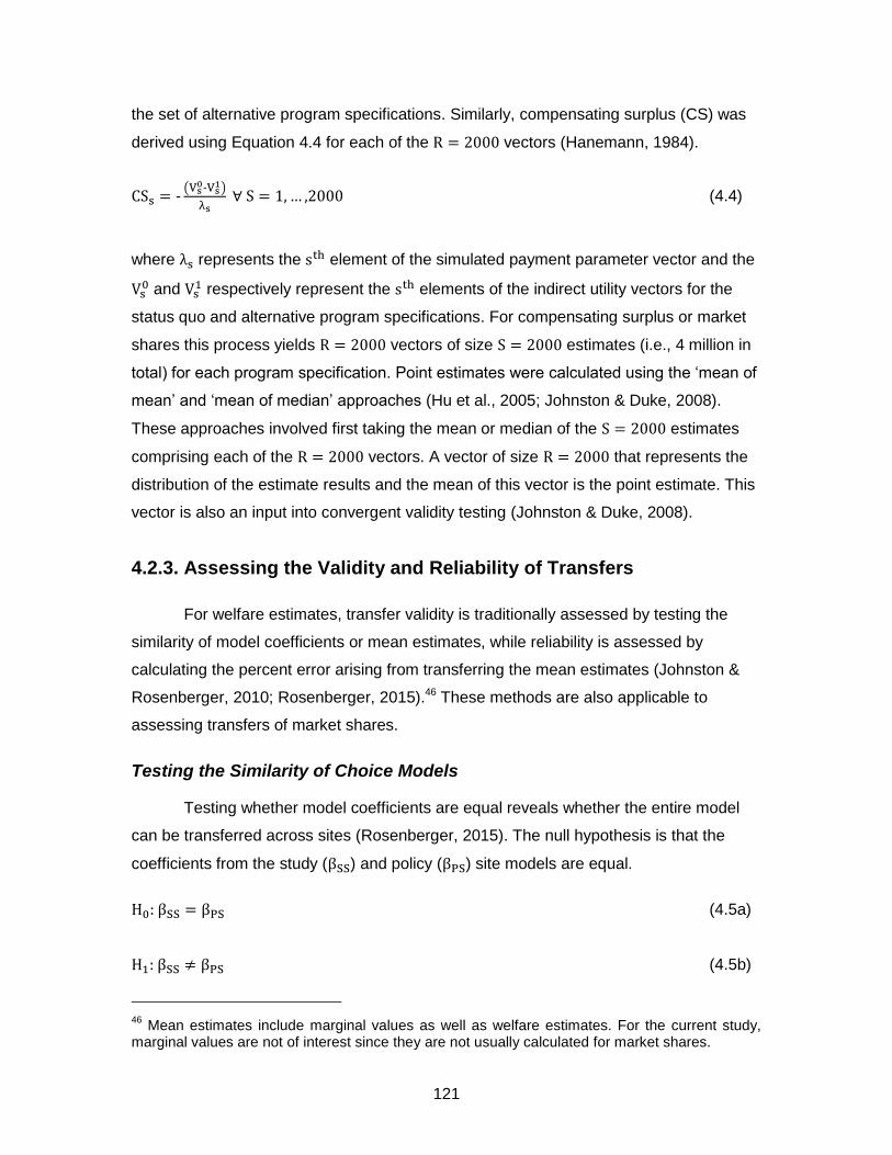
121

the set of alternative program specifications. Similarly, compensating surplus (CS) was

derived using Equation 4.4 for each of the R = 2000 vectors (Hanemann, 1984).

CSs = -(Vs

0-Vs1)

λs ∀ S = 1, … ,2000 (4.4)

where λs represents the sth element of the simulated payment parameter vector and the

Vs0 and Vs

1 respectively represent the sth elements of the indirect utility vectors for the

status quo and alternative program specifications. For compensating surplus or market

shares this process yields R = 2000 vectors of size S = 2000 estimates (i.e., 4 million in

total) for each program specification. Point estimates were calculated using the ‘mean of

mean’ and ‘mean of median’ approaches (Hu et al., 2005; Johnston & Duke, 2008).

These approaches involved first taking the mean or median of the S = 2000 estimates

comprising each of the R = 2000 vectors. A vector of size R = 2000 that represents the

distribution of the estimate results and the mean of this vector is the point estimate. This

vector is also an input into convergent validity testing (Johnston & Duke, 2008).

4.2.3. Assessing the Validity and Reliability of Transfers

For welfare estimates, transfer validity is traditionally assessed by testing the

similarity of model coefficients or mean estimates, while reliability is assessed by

calculating the percent error arising from transferring the mean estimates (Johnston &

Rosenberger, 2010; Rosenberger, 2015).46 These methods are also applicable to

assessing transfers of market shares.

Testing the Similarity of Choice Models

Testing whether model coefficients are equal reveals whether the entire model

can be transferred across sites (Rosenberger, 2015). The null hypothesis is that the

coefficients from the study (βSS) and policy (βPS) site models are equal.

H0: βSS = βPS (4.5a)

H1: βSS ≠ βPS (4.5b)

46

Mean estimates include marginal values as well as welfare estimates. For the current study, marginal values are not of interest since they are not usually calculated for market shares.

122

Such tests are not straightforward since model coefficients are confounded with

the scale parameter, which can differ across datasets (Louviere, Hensher, & Swait,

2000). Accounting for scale involves pooling the data from the sites being compared and

estimating a model with a relative scale parameter. For RPL models, this entails using

trial values of the relative scale parameter to search for the pooled model with the

largest log-likelihood. The results of this grid search are entered into a likelihood ratio

test along with results from the independent site specific models (Swait & Louviere,

1993).

LL Ratio Test: -2 (LLPooled-(LLSS + LLPS)) ~Χ2 with d. f. = K + 1 (4.6)

We conducted our grid search using trial values ranging from 0 to 2 at intervals of either

0.05 or 0.1.47 In contrast to the independent models run for each watershed, we only ran

the models using a single set of starting values to expedite the test.

Testing for Differences in MS or CS and Calculating Transfer Error

We used traditional hypothesis tests to assess whether mean estimates of

market shares or compensating surplus are equal across sites as well as equivalence

tests to assess whether the difference in mean estimates falls within a certain interval

(Johnston & Rosenberger, 2010). The traditional approach tests the null hypothesis that

the pair of estimates is equal.48

H0: ESS-EPS = 0 (4.7a)

H1: ESS-EPS ≠ 0 (4.7b)

The complete combinatorial method, which involves estimating the significance

of the difference in the pair of estimates, was used in testing this hypothesis since it

does not require normally distributed estimates (Poe, Giraud, & Loomis, 2005). This

method involves estimating a p-value by calculating the difference between every

element a and b of the vectors of estimates representing the empirical distribution of the

47

For trial values between 0 and 0.5, and greater than 1.5 but less than or equal to 2, intervals of 0.1 were used. We used intervals of 0.05 for trial values ranging from 0.5 to 1.5. 48

‘E’ represents either market share or compensating surplus estimates in hypotheses and equations.

123

estimates derived earlier (Equation 4.8). If the vectors are ordered such that the estimate

from the study site is larger than that from the policy site (ESS > EPS), the p-value is the

proportion of differences that are non-positive.

(ESSa -EPS

b ) ≤ 0 ∀ a = 1, … ,2000 and b = 1, … ,2000 (4.8)

Equivalence testing is potentially better suited to assessing the validity of

transfers. Since mean estimates result from different sites they are fundamentally

different and not necessarily identical. As such the traditional null hypothesis, testing

whether estimates are equal, is not appropriate. The basis of equivalence testing is that

the mean estimates from the sites are different unless testing reveals that the difference

in the estimates is within a pre-defined tolerance interval (Johnston & Rosenberger,

2010; Rosenberger, 2015). The bounds on this tolerance interval (θ1and θ2) are

calculated by multiplying the mean estimate from the policy site (E̅PS) by a chosen

tolerance level (±δ%), which represents the acceptable level of error in percent, yielding

θ1 = -δ(E̅PS) and θ2 = δ(E̅PS).

The equivalence test’s null hypothesis is whether the difference in mean

estimates from the policy and study sites is less (greater) than or equal to the lower

(upper) bound of the tolerance interval (i.e., the difference is not contained within the

tolerance interval).

H0: (ESS-EPS) ≤ θ1 or (ESS-EPS) ≥ θ2 (4.9a)

H1: θ1 < (ESS-EPS) < θ2 (4.9b)

In practice, the null is divided into two sub null hypotheses relating to the tolerance

interval’s lower or upper bounds.

H0a: (ESS-EPS) ≤ θ1 or (ESS-EPS)-θ1 ≤ 0 (4.10a)

H0b: (ESS-EPS) ≥ θ2 or (ESS-EPS)-θ2 ≥ 0 (4.10b)

We tested these hypotheses using a variant of the two one-sided combinatorial

(TOSC) test (Johnston & Duke, 2008). The TOSC test is an adaptation of the complete

124

combinatorial and thus does not require normally distributed estimates. It involves taking

the difference between all elements a and b that comprise the previously derived vectors

of mean estimates for the study and policy sites. The bounds on the tolerance interval

are then subtracted from this difference. The p-value corresponding to the first sub-

hypothesis is calculated as the proportion of differences that are less than or equal to

zero, while the p-value for the second sub-hypothesis is the proportion of differences

that are greater than or equal to 0.

(ESSa -EPS

b )-θ1 ≤ 0 ∀ a = 1, … ,2000 and b = 1, … ,2000 (4.11a)

(ESSa -EPS

b )-θ2 ≥ 0 ∀ a = 1, … ,2000 and b = 1, … ,2000 (4.11b)

Though 20% is the standard tolerance level in pharmaceutical research, such a

convention has not been established for benefit transfer (Johnston & Duke, 2008). As

such we instead used Czajkowski & Ščasný's (2010) variant of the TOSC test to

estimate the tolerance level at which mean estimates are considered equivalent given a

chosen level of statistical significance (95% for this study). The variant involves using a

grid search to determine the tolerance level at which both sub-hypotheses are rejected.

We calculated both directional and non-directional transfer errors (Kaul et al.,

2013). Typically errors are calculated using Equation 4.12, which produces directional

errors since the denominator depends on which watershed is assumed to be the policy

site.

Transfer Error (%) = 100 × |(E̅SS-E̅PS)

E̅PS| (4.12)

A non-directional alternative, introduced by Chattopadhyay (2003), is to treat the

denominator as the average of the values at the two sites (Equation 4.13).

Non-Directional Error (%) = 100 × |(E̅SS-E̅PS)

(E̅SS+E̅PS) 2⁄| (4.13)

Finally, we used ordinary least squares (OLS) regressions to help disentangle

the factors influencing transfer errors and tolerance levels for market shares as well as

compensating surplus (following Johnston & Duke, 2009). This analysis involved

125

separately pooling the transfer errors or tolerance levels and then regressing them on

variables representing the levels taken by attributes for each specification and the

transfer’s direction.

4.2.4. Comparing Sample Characteristics

The two samples were compared in terms of their socio-demographics and the

characteristics of the land owned by respondents. Testing was completed to compare

these characteristics across each watershed. We used chi2 or Fishers exact tests for

categorical and binary data, while we used Wilcoxon rank-sum tests for ordinal and

continuous data.

126

4.3. Data

The data for this study comes from two case studies eliciting preferences for

incentive-based wetlands restoration programs on private land conducted in 2013. We

conducted these studies in the Grand and Upper Thames watersheds, two neighbouring

river basins in Southern Ontario, Canada (Figure 4.1). The area of wetlands in this

region has declined by over 70% since European colonization due to growth in the

population and area devoted to agriculture (Ducks Unlimited Canada, 2010). Both

watersheds are part of the Lake Erie Basin, though the Upper Thames initially empties

into Lake St. Clair via the Lower Thames River. At 6800 square kilometers (km2), the

Grand River watershed is twice the size of the Upper Thames which is 3420 km2. The

watersheds are highly populated with the Upper Thames home to half a million residents

living in urban areas covering 10% of the watershed’s area and the Grand nearly 1

million residents living in urban areas covering 6% of the watershed (although the two

watersheds have similar population densities). Agriculture is the dominant land use in

both watersheds, respectively accounting for 70% and 75% of the area of the Grand and

Upper Thames watersheds. Forest cover is highest in the Grand (19% compared to 11%

in the Upper Thames), as is wetland cover (10% compared to 5% in the Upper Thames).

At 3%, meadow cover is highest in the Upper Thames compared to less than 1% in the

Grand (Grand River Conservation Authority, 2008, 2014, 2016; Upper Thames River

Conservation Authority, 2012, 2015).

Figure 4.1: The Location of the Grand and Upper Thames Watersheds

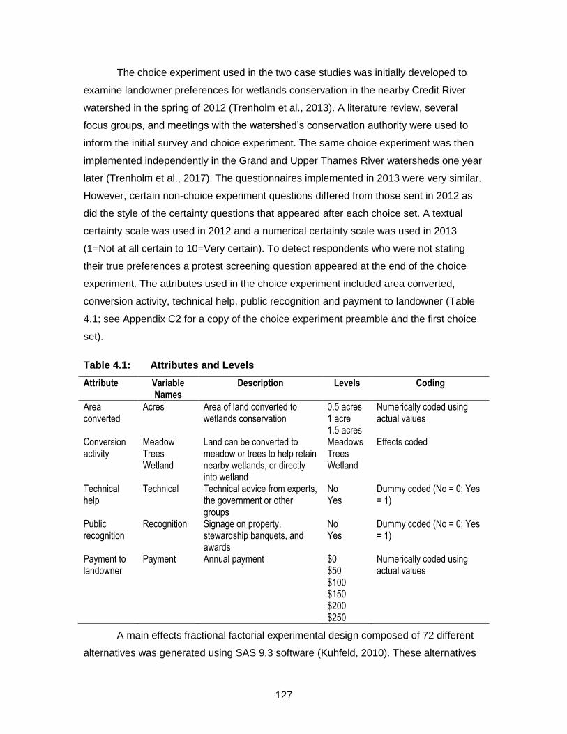
127

The choice experiment used in the two case studies was initially developed to

examine landowner preferences for wetlands conservation in the nearby Credit River

watershed in the spring of 2012 (Trenholm et al., 2013). A literature review, several

focus groups, and meetings with the watershed’s conservation authority were used to

inform the initial survey and choice experiment. The same choice experiment was then

implemented independently in the Grand and Upper Thames River watersheds one year

later (Trenholm et al., 2017). The questionnaires implemented in 2013 were very similar.

However, certain non-choice experiment questions differed from those sent in 2012 as

did the style of the certainty questions that appeared after each choice set. A textual

certainty scale was used in 2012 and a numerical certainty scale was used in 2013

(1=Not at all certain to 10=Very certain). To detect respondents who were not stating

their true preferences a protest screening question appeared at the end of the choice

experiment. The attributes used in the choice experiment included area converted,

conversion activity, technical help, public recognition and payment to landowner (Table

4.1; see Appendix C2 for a copy of the choice experiment preamble and the first choice

set).

Table 4.1: Attributes and Levels

Attribute Variable Names

Description Levels Coding

Area converted

Acres Area of land converted to wetlands conservation

0.5 acres 1 acre 1.5 acres


Conversion activity


Land can be converted to meadow or trees to help retain nearby wetlands, or directly into wetland


Effects coded

Technical help

Technical Technical advice from experts, the government or other groups

No Yes


Public recognition

Recognition Signage on property, stewardship banquets, and awards

No Yes


Payment to landowner

Payment Annual payment $0 $50 $100 $150 $200 $250


A main effects fractional factorial experimental design composed of 72 different

alternatives was generated using SAS 9.3 software (Kuhfeld, 2010). These alternatives

128

were allocated to 36 choice sets, with each set containing 2 alternatives and a status

quo option. A blocking variable was included in the design to allot the choice sets to 6

blocks. The resulting design was examined for dominance and a few changes made

yielding a final design with a D-efficiency of 90.8%.

We coded the variables following a mixed coding scheme (see final column of

Table 4.1). Using effects codes for the conversion activity variables ensures that they

are not aliased with the ASC. This coding scheme means that, similar to Kaczan,

Swallow, & Adamowicz (2013), the ASC term can be used to represent the utility

associated with the status quo (i.e., no area converted, conversion activity, technical

help, public recognition, or payment).

Private landowners located in and near the Grand and Upper Thames

watersheds were surveyed during the spring of 2013. Canada Post’s Admail (Canada

Post, 2015) service was used to send survey packages to 5,937 and 4,149 rural non-

farm households in the Grand and Upper Thames watersheds, respectively. These

households were located along rural routes in rural postal codes that intersected with

each watershed. Surveys were returned from 942 households in the Grand watershed

and 773 households in the Upper Thames watershed. This yielded response rates of

16% and 19%, respectively, in the Grand and Upper Thames watersheds. While these

rates are fairly low, they are within the range of those reported for similar choice

experiment studies and other Canadian landowner surveys (e.g., Rossi, Carter,

Alavalapati, & Nowak, 2011; Yu & Belcher, 2011). The data was cleaned to remove

observations from respondents who: were from non-targeted postal codes; did not

answer key questions; owned less than 1.5 acres of land; selected the same non-status

quo option in all choice sets (serial non-participation); or who selected the status quo

option in all sets and were identified as protesters (protest screening rules are similar to

Meyerhoff, Mørkbak, & Olsen, 2014). After cleaning, 405 returns from the Grand

watershed and 354 returns from the Upper Thames watershed were used in the

analysis.

129

4.4. Results


Tests reveal no statistically significant differences in socio-demographics

between the two watersheds (Table 4.2). Both samples had more male than female

respondents, the largest age group was 45 to 64 with a mean age in the mid-50’s, the

majority were employed full or part-time, most had a post-secondary degree, and the

majority made over $75,000 with the largest income group earning $100,000 or more.

130

Table 4.2: Respondent Characteristics and Features of their Land

Characteristic Data Type Grand (n = 405)

Upper Thames (n = 354)

Test Resultsa

Gender Male Binary 66% 71% Female 34% 29%

Age (Adults) Under 25 Ordinal 1% 1% 25 to 44 20% 18% 45 to 64 55% 53% 65 or older 24% 29% Mean (years) Continuous 55.2 56.4

Highest level of education Less than High School Ordinal 13% 5% High School 22% 30% Post-secondary 65% 64%

Employment status Employed Categorical 69% 72% Unemployed 1% 1% Not in labour force 30% 27%

Household Income Under $10,000 Ordinal 2% 0% $10,000 to $29,999 4% 5% $30,000 to $49,999 14% 16% $50,000 to $74,999 20% 21% $75,000 to $99,999 20% 22% $100,000 and over 40% 36%

Land Cover Has forests Binary 61% 55% ‡ Has meadows Binary 28% 16% ‡‡‡ Has wetlands Binary 63% 43% ‡‡‡ Has crop, pasture, or orchard (i.e., agricultural land cover)

Binary 66% 77%

‡‡‡

Land Use Primary land use is agriculture or forestry Categorical 45% 59% ‡‡‡ Primary land use is residential 52% 38% Primary land use is other 3% 3%

Generated income from land in past 5 years Binary 53% 70% ‡‡‡ Farm or forest producerb Binary 39% 56% ‡‡‡ Area of Land Holdings

5 acres or less Ordinal 27% 21% ‡‡‡ 5 to 30 acres 27% 15% 30< to 100 acres 31% 36% More than 100 acres 16% 29% Mean (acres) Continuous 66.2 111.9 ‡‡‡

a ‡ and ‡‡‡ indicate a difference across the Grand and Upper Thames watersheds at the 90% and 99% levels of significance

b This variable was generated from farm or forest related questions in SPSS 23 software using non-linear principal component analysis (Linting & van der Kooij, 2012) and two step cluster analysis.

131

Unlike socio-demographics, respondent land characteristics differed significantly

across the two watersheds (Table 4.2). In terms of land cover, the incidence of forest,

meadow, and wetland cover is highest in the Grand. Conversely, agriculture-related land

cover was more prevalent in the Upper Thames. Similarly, the primary land use was

almost evenly split between residential and agriculture/forestry in the Grand, and skewed

more towards agriculture/forestry in the Upper Thames. The majority of respondents in

both watersheds reported earning income from their land in the past 5 years, though

those in the Upper Thames were more likely to earn such income. Unsurprisingly, based

on farming and forestry related questions respondents were more likely to be clustered

into a farm or forest producer group in the Upper Thames. Finally, property sizes were

on average larger in the Upper Thames.

4.4.2. Random Parameters Logit Models and Testing Model Similarity

We initially assessed whether models with correlated and uncorrelated random

coefficients significantly differed. For both watersheds, likelihood ratio tests reject the

null hypothesis of uncorrelated random coefficients (Grand: Χ(21)2 = 78.85 with p < 0.01;

Upper Thames: Χ(21)2 = 47.15 with p < 0.01). Thus the models with correlated random

coefficients are preferred to those with independent random coefficients. The R2 values

suggest that the independent models are of decent fit according to criteria in Hensher,

Rose, & Greene (2015), with all mean and several lower-triangular Cholesky coefficients

significant (Table 4.3). Regarding the mean taste parameters, the ASC parameter

indicates that respondents in the Upper Thames watershed are willing to enroll all else

equal. Enrolling larger areas is disliked by respondents in both watersheds. In terms of

the conversion activity, respondents in the Grand and Upper Thames watersheds have a

preference for trees over wetland or meadow. Tastes for the other two activities differ by

watershed with those in the Upper Thames having a preference for wetland over

meadow and those in the Grand preferring meadow to wetland. Respondents in both

watersheds favour technical help and dislike public recognition. Transforming the log-

normal payment parameter reveals that respondents in both watersheds favour higher

amounts of compensation.

132

Table 4.3: Random Parameter Models by Watershed

Variablea Grand Upper Thames

Mean

ASC 1.0888* (0.5851)

1.2019** (0.5100)

Acres -0.7655*** (0.2561)

-0.7383*** (0.2591)

Conversion Activity: Wetland

-1.3125*** (0.2918)

-0.7964*** (0.2378)

Conversion Activity: Trees

1.6239*** (0.2461)

1.6996*** (0.2424)

Conversion Activity: Meadowb

-0.3115 (0.2027)

-0.9032*** (0.2156)


0.9252*** (0.2331)

Recognition (Yes) -0.5786*** (0.2138)

-0.6846*** (0.1951)

ln(Annual payment) -5.1530*** (0.2152)

-5.2494*** (0.2566)

Correlation (Lower-Triangular of the Cholesky Matrix) ASC × ASC 6.1532***

(0.9368) -5.5341*** (0.8283)

Acres × ASC 1.0301** (0.4175)

-0.5943 (0.3864)

Wetland × ASC 0.7533 (0.4724)

0.1104 (0.3672)

Trees × ASC -0.0765 (0.3628)

-0.6936* (0.3714)

Technical × ASC -0.1031 (0.3325)

0.0914 (0.3427)

Recognition × ASC -0.0008 (0.3520)

-0.1850 (0.2841)

Payment × ASC 0.0753 (0.1313)

-0.0086 (0.1419)

Acres × Acres 1.8544*** (0.4690)

1.7954*** (0.4395)

Wetland × Acres 0.3116 (0.5977)

0.4186 (0.4379)

Trees × Acres 0.0422 (0.4079)

-0.1288 (0.3926)

Technical × Acres 0.0369 (0.3901)

-0.7505* (0.3983)

Recognition × Acres -0.3120 (0.4422)

0.1948 (0.3285)

Payment × Acres 0.0970 (0.1346)

-0.3266** (0.1308)

Wetland × Wetland 2.9955*** (0.3964)

-2.3003*** (0.3338)

Trees × Wetland -1.8523*** (0.3068)

1.2049*** (0.2678)

133

Variablea Grand Upper Thames

Technical × Wetland 0.1832 (0.2723)

-0.4707* (0.2480)

Recognition × Wetland -0.2222 (0.2533)

-0.1737 (0.2181)

Payment × Wetland 0.1319 (0.1026)

-0.2070* (0.1183)

Trees × Trees 1.4925*** (0.2278)

-1.5489*** (0.2223)

Technical × Trees -0.6091** (0.2960)

0.3874 (0.2890)

Recognition × Trees -0.5236* (0.2977)

0.1535 (0.2378)

Payment × Trees -0.0394 (0.1080)

-0.4138*** (0.1283)

Technical × Technical -1.0209*** (0.3550)

0.9957** (0.4237)

Recognition × Technical 0.1298 (0.4228)

0.1460 (0.3798)

Payment × Technical 0.8827*** (0.1566)

-0.0807 (0.1235)


1.1546*** (0.3919)

-0.1779 (0.3333)

Payment × Recognition -0.9801*** (0.1452)

1.2445*** (0.1867)

Payment × Payment -0.0577 (0.1511)

-0.3365*** (0.1109)

Model Statistics Log-Likelihood -1248.34 -1113.83 Observations 7263 6363 Pseudo R2 0.36 0.35


a Standard errors appear in brackets below the corresponding parameter estimate.

b As activity variables are effects coded, meadow parameter derived as negative of other activity parameters. The corresponding standard errors were estimated via the Delta method.

The elements of the lower-triangular of the Cholesky matrix represent each

random parameter’s estimated contribution to the set of standard deviation parameters

(Hensher et al., 2015). The diagonal elements show a random parameter’s contribution

to its own standard deviation parameter net of the influence of other random parameters,

while the off-diagonal elements indicate contributions to standard deviation from

correlations with other random parameters. All diagonal elements are significant except

those for the public recognition and payment variables in the Upper Thames and Grand

models, respectively. The significant off-diagonal elements estimated for our models

indicate that preferences for certain random parameters are not independent.

134

Specifically, the Upper Thames model yields significant off-diagonal elements for:

conversion activity as trees and the ASC as well as conversion activity as wetlands;

technical help and acres as well as conversion activity as wetlands; and log-normal

payment and acres, conversion activity as wetlands, conversion activity as trees, as well

as recognition. For the Grand model the significant elements include: acres and the

ASC; conversion activity as trees and conversion activity as wetlands; technical help and

conversion activity as trees; recognition and conversion activity as trees; and log-normal

payment and technical help as well as recognition.

We also derived the variance-covariance matrix and standard deviation

parameters from the lower-triangular Cholesky matrix using the Delta method (see

Appendix C3). All of the estimated standard deviation parameters are significant for both

models indicating that preferences for each attribute are heterogeneous in both

watersheds. Significant positive covariances were observed between the ASC and

conversion activity as trees parameters for the Upper Thames model and the ASC and

acres parameters for the Grand model. We observed significant negative covariances

between the acres and log-normal payment parameters, conversion activity as trees and

conversion activity as wetland parameters, and technical help and conversion activity as

trees parameters for the Upper Thames model. For the Grand model, we observed

significant negative covariances between the conversion activity as trees and conversion

activity as wetland parameters, technical help and conversion activity as trees

parameters, log-normal payment and public recognition parameters, and log-normal and

technical help parameters.49

Pooling the data from the two watersheds and running the grid search revealed

that a trial value of the relative scale parameter of 1.2 (σGrand/σUpper Thames) results in

the largest log-likelihood (-2417.82). The likelihood ratio test using the log-likelihoods

from the independent and pooled models reveals that the Grand and Upper Thames

models are significantly different (Χ(36)2 = 111.31 with p < 0.01).

49

Positive (negative) covariances between two random parameter’s indicate that larger values along a random parameter’s distribution correspond with larger (smaller) values along the other random parameter’s distribution (Hensher, Rose, & Greene, 2015).

135

4.4.3. Market Share and Compensating Surplus Estimates

The ‘mean of mean’ approach resulted in exploding compensating surplus, which

is a common problem with estimates generated from models with log-normally

distributed payment parameters (Thiene & Scarpa, 2009). Thus, following Johnston &

Duke (2008) and Johnston, Schultz, Segerson, Besedin, & Ramachandran (2012) we

used estimates generated from the ‘mean of median’ approach since it resulted in more

sensible compensating surplus estimates (akin to those derived from a model with fixed

payment). Although we observed more reasonable compensating surplus estimates, the

market share estimates derived from the ‘mean of median’ approach were more variable

than their ’mean of mean’ counterparts (‘mean of mean’ output equivalent to Figures 4.1

and 4.2 as well as Tables 4.4 and 4.5 is provided in Appendix C4).

Market share estimates derived from the two models are closely aligned for all

possible program specifications as are the compensating surplus estimates (Figure 4.2).

Indeed the Pearson correlation coefficients are 0.92 for market shares and 0.96 for

compensating surplus. In general, the market share estimates suggest that many

respondents would participate. However, market shares are quite variable ranging from

just over 30% to near 100% depending on the program specification. Compensating

surplus is also variable, ranging from around -$400 per year/household to $130 per

year/household depending on the specification.

Figure 4.2: Market Share (a) and Compensating Surplus (b) Estimates Note: for both panels the x-axis represents all possible program specifications (e.g., for panel (a) a point on this axis represents a program with 0.5 acres converted to wetlands with no technical help or recognition and a payment of $50, etc., while the points on this axis in panel (b) are similar though do not include a payment component). The data were sorted in ascending order according to the MS or CS values estimated for the Upper Thames.

136

4.4.4. Transfer Validity and Reliability

The range in directional errors for transfers of market share estimates (MS) is

much narrower than the corresponding range in errors for transfers of compensating

surplus (CS) (Table 4.4). Similarly, the mean and median of the directional errors for

transfers of market shares are much lower than the related averages for transfers of

compensating surplus. The non-directional errors reflect these results. As with the

errors, the range in tolerance levels calculated for market shares is tighter and the

averages lower relative to those calculated for compensating surplus. Finally, the results

of the complete combinatorial tests are the same for transfers of market shares and

compensating surplus — none of the pairs of estimates differ at the 99%, 95%, or 90%

levels of significance.

Table 4.4: Summary of Reliability and Validity Tests

Transfer Transfer Errors (%) Tolerance Levels (%) Complete Combinatorial Mean Median Low High Mean Median Low High

Directional MS: Grand to Thames

5 3 0 36

24 15 1 133

N/A

MS: Thames to Grand

5 2 0 31

24 16 1 142

CS: Grand to Thames

141 52 1 879

591 266 79 3227

CS: Thames to Grand

124 56 1 1894

570 232 75 7977

Non-Directional MS: Grand and Thames

5 3 0 31

N/A 0*, 0**, 0***

CS: Grand and Thames

135 54 1 1120

0*, 0**, 0***

*, **, and *** indicate the number of pairs of estimates that are different at the 90%, 95%, and 99% levels of significance, respectively

Two sample Wilcoxon rank sum tests suggest that the distributions of directional

errors, non-directional errors, and tolerance levels differ significantly by type of transfer,

although the distributions do overlap somewhat (Figure 4.3).50 The boxplots show that

directional errors, non-directional errors, and tolerance levels calculated for market

shares are clearly smaller and less variable than those calculated for compensating

50

The p-values for these tests are <0.01 for directional errors regardless of direction, <0.01 for non-directional errors, and <0.01 for tolerance levels regardless of direction. The null hypothesis that the distributions are equal is rejected in all cases.

137

surplus. In addition, these plots appear to show that transfers of compensating surplus

and market share estimates are similarly affected by transfer direction since the

distributions of the directional errors and tolerance intervals for transfers to the Upper

Thames overlap with transfers to the Grand. Two sample Wilcoxon rank sum tests

confirm this finding for both types of transfer.51 However, for compensating surplus the

means of the errors and tolerance levels in Table 4.4 are slightly larger for transfers to

the Upper Thames than to the Grand (medians are not similarly impacted). For market

shares, the means and medians of the errors and tolerance levels are identical, or nearly

so, by transfer direction.

Figure 4.3: Boxplots of Transfer Errors and Tolerance Levels Note: outliers not plotted; non-directional errors are white and directional errors are differing shades of grey.

While these comparisons provide some insight into the impact of transfer

direction, they treat all errors and tolerance levels the same since they ignore the

particulars of the program specification being transferred. A simple one-to-one

comparison of the same specification by transfer direction reveals that transfers to the

Grand result in larger errors than transfers to the Thames in 56% of cases for market

shares and 44% of cases for compensating surplus (detailed output available from the

authors upon request). Tolerance levels for transfers to the Grand yield larger levels

than transfers to the Thames in 25% of cases for market shares and 44% of cases for

compensating surplus (transfers of market shares to the Grand and transfers to the

Thames result in identical tolerance levels in 52% of cases).

51

For transfers of compensating surplus the p-values are 0.76 for errors and 0.59 for tolerance levels, while they are 0.99 and 0.97 for transfers of market shares for errors and tolerance levels, respectively. The null hypothesis of distribution equality is not rejected in all cases.

138

The OLS regression does account for the program specification and site

treatment (Table 4.5).52 Errors and tolerance levels calculated for compensating surplus

are significantly larger for specifications involving conversion of land to wetlands or

meadow, and lower for specifications involving conversion to trees. In the case of market

shares, directional and non-directional errors are significantly lower for specifications

that involve smaller areas, converting land to trees, technical help, and higher payments.

These errors are significantly higher for specifications that involve larger areas,

converting land to wetland or meadow, smaller payments, and do not involve public

recognition. Market share tolerance levels are similarly affected. Transfer direction does

not significantly influence errors or tolerance levels (reflecting the similarities noted in

Table 4.4 and Figure 4.3). Our regression results suggest that compensating surplus

and market shares are differently affected by transfer characteristics.

52

Separate regressions were conducted for market shares and compensating surplus due to differing independent variables (i.e., payment). The dependent variables were transformed via natural log to better meet assumptions. The independent variables are all effects coded.

139

Table 4.5: Regression of Errors and Tolerance Levels on Transfer Characteristics for Transfers Based on the “Mean of Median” Approacha

Variable Directional Errors Tolerance Levels Non-Directional Errors

MS CS MS CS MS CS

Constant 0.3744*** (0.0347)

3.8456*** (0.1083)

2.5277*** (0.0076)

5.6791*** (0.0918)

0.3734*** (0.0496)

3.8801*** (0.1665)

Area: 0.5 ac

-0.2888*** (0.0490)

-0.0184 (0.1532)

-0.2620*** (0.0107)

-0.0726 (0.1298)

-0.2885*** (0.0701)

0.0213 (0.2355)

Area: 1 ac

-0.0142 (0.0490)

0.1862 (0.1532)

-0.0067 (0.0107)

0.1369 (0.1298)

-0.0142 (0.0701)

0.1489 (0.2355)

Area: 1.5 acb

0.3030*** (0.0490)

-0.1678 (0.1532)

0.2687*** (0.0107)

-0.0643 (0.1298)

0.3027*** (0.0701)

-0.1702 (0.2355)

Activity: Wetland

0.9291*** (0.0490)

0.5833*** (0.1532)

0.7937*** (0.0107)

0.4852*** (0.1298)

0.9288*** (0.0701)

0.7049*** (0.2355)

Activity: Trees

-2.3458*** (0.0490)

-1.6967*** (0.1532)

-1.4089*** (0.0107)

-1.0042*** (0.1298)

-2.3449*** (0.0701)

-1.7333*** (0.2355)

Activity: Meadowb

1.4167*** (0.0490)

1.1134*** (0.1532)

0.6152*** (0.0107)

0.5190*** (0.1298)

1.4160*** (0.0701)

1.0284*** (0.2355)

Technical help: Yes

-0.7188*** (0.0347)

-0.1604 (0.1083)

-0.3783*** (0.0076)

-0.0266 (0.0918)

-0.7184*** (0.0496)

-0.1113 (0.1665)

Technical help: Nob

0.7188*** (0.0347)

0.1604 (0.1083)

0.3783*** (0.0076)

0.0266 (0.0918)

0.7184*** (0.0496)

0.1113 (0.1665)

Recognition: Yes

0.1787*** (0.0347)

-0.0251 (0.1083)

0.1831*** (0.0076)

-0.0449 (0.0918)

0.1784*** (0.0496)

0.0365 (0.1665)

Recognition: Nob

-0.1787*** (0.0347)

0.0251 (0.1083)

-0.1831*** (0.0076)

0.0449 (0.0918)

-0.1784*** (0.0496)

-0.0365 (0.1665)

Payment: $0

1.1867*** (0.0775)

0.9913*** (0.0170)

1.1844*** (0.1109)

Payment: $50

0.7892*** (0.0775)

0.5550*** (0.0170)

0.7887*** (0.1109)

Payment: $100

0.2203*** (0.0775)

0.1256*** (0.0170)

0.2206** (0.1109)

Payment: $150

-0.2260*** (0.0775)

-0.2478*** (0.0170)

-0.2253** (0.1109)

Payment: $200

-0.7817*** (0.0775)

-0.5678*** (0.0170)

-0.7808*** (0.1109)

Payment: $250b

-1.1885*** (0.0775)

-0.8563*** (0.0170)

-1.1876*** (0.1109)

Grand to Thames

0.0022 (0.0347)

0.0681 (0.1083)

0.0015

(0.0076) 0.0682

(0.0918)

Thames to Grandb

-0.0022 (0.0347)

-0.0681 (0.1083)

-0.0015 (0.0076)

-0.0682 (0.0918)

n 432 72 432 72 216 36 R2 0.89 0.67 0.99 0.49 0.89 0.66 *, **, and *** indicate that the parameter estimate differs from zero at the 90%, 95%, and 99% levels of significance, respectively

a Standard errors appear in brackets below the associated parameter estimates.

b Parameter estimate calculated as the negative of the associated parameters. The corresponding standard error was estimated using the Delta method.

140

4.5. Discussion and Conclusion

The percent errors estimated for transfers of compensating surplus are in the

range of those reported in the literature while those resulting from transfers of market

shares are much smaller. In their comprehensive review of 38 convergent validity

studies that used WTP estimated from a variety of original research techniques,

Rosenberger (2015) finds that value transfer yields mean and median directional errors

of 140% and 45%, respectively, with a range of 0% to 7496%. Function transfer results

in even lower directional errors ranging from 0% to 929% with a mean of 65% and

median of 36%. The directional errors resulting from our transfers of compensating

surplus ranged from 1% to 1894%, while the errors resulting for our transfers of market

shares ranged from 0% to 36%. For compensating surplus, the mean of these transfer

errors is either 124% or 141% depending on transfer direction while the median is either

52% or 56%. In the case of market shares the averages are much lower with the mean

being 5% regardless of transfer direction, and median of 2% or 3% depending on the

transfer’s direction. Additionally, nearly half of the transfers reviewed by Rosenberger

(2015) fail the complete combinatorial test, while none of our transfers fail the same test

for compensating surplus or market shares. Finally, the likelihood ratio test revealed that

the RPL models on which the transfers are based are statistically different. We are not

surprised by this finding since the large number of parameters estimated for each model

makes it likely that some of them will differ significantly across models. Rosenberger

(2015) found 44% of such tests have rejected the null hypothesis of parameter or model

equality in past studies.

Our transfers may differ in reliability and validity from those reviewed by

Rosenberger (2015) for several reasons. First, the studies reviewed by Rosenberger

(2015) all involved transfers of WTP which may not yield the same results as transfers of

WTA, let alone market shares. Choice experiments have also been found to generate

larger errors than other original research techniques (Kaul et al., 2013). Other

methodological differences from the reviewed studies can affect convergent validity

testing too. For example, using compensating surplus and market share estimates

derived via the ‘mean of median’ approach yields somewhat different results than the

‘mean of mean’ approach although trends are similar (see Appendix C4). Furthermore,

as noted by Rosenberger (2015) studies of benefit transfer reliability and validity may be

141

more experimental than actual policy analysis since they may compare values that

would not be compared in practice. Finally, transfer accuracy depends on site

differences. The Grand and Upper Thames watersheds have similar geography and the

socio-demographic characteristics of the two samples were also very similar (although

respondent’s owned land characteristics differed significantly).

The results show that percent errors and tolerance levels for transfers of market

shares are much lower than those arising from transfers of compensating surplus. As

expected, transfers of market shares are more valid and reliable than transfers of

compensating surplus. Errors and tolerance levels generated from transfers of market

shares are also less variable. This is not unexpected given that market share estimates

are by definition bounded by 0% and 100% which limits the magnitude and variability of

errors and tolerance levels. Compensating surplus estimates are not similarly bounded

and therefore the associated errors and tolerance levels are larger in magnitude and

more variable. Interestingly, all pairs of estimates were deemed equal by the complete

combinatorial test for transfers of compensating surplus and market shares. On the

surface this result seems counter to the finding that transfers of compensating surplus

are less accurate — we might expect that a larger proportion of compensating surplus

estimates would differ statistically across sites. However, the complete combinatorial test

relies on a classical null hypothesis and the likelihood of rejecting the null of equal

estimates increases when variance is large or the difference in means small

(Kristofersson & Navrud, 2005; Johnston & Duke, 2008). Calculating the coefficient of

variation for each estimate reveals that compensating surplus is generally much more

variable than market shares. The high variance increases the likelihood that

compensating surplus estimates are found equal. Although conversely, transfer errors

reveal that the difference in market share estimates is smaller than the difference in

compensating surplus which increases the likelihood that market share estimates are

found equal.

The regression analysis provides some insight into situations where transfers are

more accurate. For example, in the case of market shares directional errors are lowest

for program specifications characterized by 0.5 acres, the conversion activity being

trees, technical help offered, no recognition offered, and payment of $250. In terms of

compensating surplus, fewer variables are significant which suggests that program

specifications do not affect errors or tolerance levels to the same extent. Thus, the

142

accuracy of transfers of market shares or compensating surplus are differently

influenced by program specification. However, the regression models did not include the

same variables and by extension the same number of observations. The direction of the

transfer was not significant in any regression.

While transfers of market shares appear more valid and reliable than transfers of

compensating surplus, whether the lower error is acceptable for policy analysis depends

on the project (Johnston & Duke, 2008). In general, analyses needing more accuracy

demand lower errors. However, given that market shares are less prone to high errors

by definition it is worth asking whether transfers of these estimates should meet a higher

threshold than transfers of welfare estimates in order to be considered accurate. This

means lower transfer errors and in the context of equivalence testing a lower tolerance

level. Nevertheless, the decision to use transfers in policy analysis rather than original

research depends on the opportunity cost involved in making a mistake (Allen & Loomis,

2008). This opportunity cost in turn depends in part on the likelihood of making the

wrong decision, which appears low for transfers of market shares.

This study contributes to the literature by examining the accuracy of transferring

predicted participation market shares derived from choice experiment data. To provide

context, these results are compared with the accuracy of transferring compensating

surplus generated from the same data. The main finding is that transfers of market

shares appear quite reliable and valid, especially when placed in the context of our

transfers of compensating surplus. However, given the difference in how each estimate

is calculated the threshold at which transfers of market shares could be considered valid

and reliable likely differs from that of welfare estimates. Investigating this threshold

should be the subject of additional inquiry. Additional avenues of research involve

investigating whether findings related to transfers of economic values also apply to

transfers of market shares. Further research specific to market shares would provide

more insight into when market share transfers are likely to be more or less accurate. For

instance, our work represents a best-case scenario, in that the same alternatives were

used at the study and policy sites and we only examined the adoption decision of

landowners which is a subset of possible market shares. Assessing market share

transfers between sites with different sets of alternatives, or transfers of the larger set of

market shares are other potential avenues of future research. Finally, a structural

approach to applied benefit transfer, which involves calibrating an indirect utility function

143

from available data and using it to predict estimates at the policy site, would be ideal for

transferring both market shares or economic values and deserves examination (Smith,

Houtven, & Pattanayak, 2002; Smith, Pattanayak, & Houtven, 2006). Regardless, our

examination of the issue suggests that transferring market shares has potential for use

in policy analysis.

144


Funding for this research was provided by the Social Science and Humanities

Research Council of Canada (SSHRC) through a Standard Research Grant (865-2008-

0045) and Doctoral Fellowship (752-2012-2435). SSHRC did not participate in the

research process or the preparation of this paper. The Upper Thames Conservation

Authority and Grand River Conservation Authority provided support and assistance

during the research process though did not participate in the preparation of this paper.

We thank the landowners who participated in this research. Dr. Pascal Haegeli provided

useful feedback during the preparation of this manuscript. All remaining errors are our

own. Dr.Wolfgang Haider passed away on August 24, 2015.

145

References

Allen, B. P., & Loomis, J. B. (2008). The Decision to Use Benefit Transfer or Conduct Origical Valuation Research for Benefit-Cost and Policy Analysis. Contemporary Economic Policy, 26(1), 1–12. http://doi.org/10.1111/j.1465-7287.2007.00066.x

Arellano, J., Hauber, A. B., Mohamed, A. F., Gonzalez, J. M., Collins, H., Hechmati, G., … Qian, Y. (2015). Physicians’ Preferences for Bone Metastases Drug Therapy in the United States. Value in Health, 18(1), 78–83. http://doi.org/10.1016/j.jval.2014.10.004

Beck, M. J., Rose, J. M., & Hensher, D. A. (2013). Consistently inconsistent: The role of certainty, acceptability and scale in choice. Transportation Research Part E: Logistics and Transportation Review, 56, 81–93. http://doi.org/10.1016/j.tre.2013.05.001

Boyle, K. J., Kuminoff, N. V, Parmeter, C. F., & Pope, J. C. (2010). The Benefit-Transfer Challenges. Annual Review of Resource Economics, 2(1), 161–182. http://doi.org/10.1146/annurev.resource.012809.103933

Brouwer, R., Bliem, M., Getzner, M., Kerekes, S., Milton, S., Palarie, T., … Wagtendonk, A. (2016). Valuation and transferability of the non-market benefits of river restoration in the Danube river basin using a choice experiment. Ecological Engineering, 87, 20–29. http://doi.org/10.1016/j.ecoleng.2015.11.018

Brouwer, R., Martin-Ortega, J., Dekker, T., Sardonini, L., Andreu, J., Kontogianni, A., … Windle, J. (2015). Improving value transfer through socio-economic adjustments in a multicountry choice experiment of water conservation alternatives. Australian Journal of Agricultural and Resource Economics, 59(3), 458–478. http://doi.org/10.1111/1467-8489.12099

Canada Post. (2015). Canada Post Neighbourhood MailTM (Unaddressed AdmailTM). Toronto, Ontario.

Chattopadhyay, S. (2003). A Repeated Sampling Technique in Assessing the Validity of Bene t Transfer in Valuing Non-Market Goods. Land Economics, 79(4), 576–596.

Colombo, S., Calatrava-Requena, J., & Hanley, N. (2007). Testing Choice Experiment for Benefit Transfer with Preference Heterogeneity. American Journal of Agricultural Economics, 89(1), 135–151. http://doi.org/10.1111/j.1467-8276.2007.00968.x

Czajkowski, M., Hanley, N., & Lariviere, J. (2015). The effects of experience on preferences: Theory and empirics for environmental public goods. American Journal of Agricultural Economics, 97(1), 333–351. http://doi.org/10.1093/ajae/aau087

146

Czajkowski, M., & Ščasný, M. (2010). Study on benefit transfer in an international setting. How to improve welfare estimates in the case of the countries’ income heterogeneity? Ecological Economics, 69(12), 2409–2416. http://doi.org/10.1016/j.ecolecon.2010.07.008

Ducks Unlimited Canada. (2010). Southern Ontario wetland conversion analysis: Final report. Barrie, ON. Retrieved from http://www.ducks.ca/assets/2010/10/duc_ontariowca_optimized.pdf

Grand River Conservation Authority. (2008). Grand River Watershed: Characterization Report Executive Summary. Cambridge, Ontario. Retrieved from http://www.sourcewater.ca/swp_watersheds_grand/Characterization_summary_Grand.pdf%5Cnhttp://scholar.google.com/scholar?hl=en&btnG=Search&q=intitle:No+Title#0

Grand River Conservation Authority. (2014). Grand River Waterhed Management Plan. Cambridge, Ontario.

Grand River Conservation Authority. (2016). Natural Heritage: Landscapes. Retrieved July 11, 2016, from https://www.grandriver.ca/en/our-watershed/Landscapes.aspx

Hanemann, W. M. (1984). Valuation Contingent Experiments in Responses. American Journal of Agricultural Economics, 66(3), 332–341.

Hensher, D. A., Rose, J. M., & Greene, W. H. (2015). Applied Choice Analysis (2nd Editio). Cambridge, UK: Cambridge University Press.

Hess, S., & Train, K. (2017). Correlation and scale in mixed logit models. Journal of Choice Modelling, 23(March), 1–8. http://doi.org/10.1016/j.jocm.2017.03.001

Hole, A. R. (2007). Fitting mixed logit models by using maximum simulated likelihood. The Stata Journal, 7(3), 388–401.

Hu, W., Veeman, M. M., & Adamowicz, W. L. (2005). Labelling Genetically Modified Food: Heterogeneous Consumer Preferences and the Value of Information. Canadian Journal of Agricultural Economics/Revue Canadienne d’agroeconomie, 53(1), 83–102. http://doi.org/10.1111/j.1744-7976.2005.04004.x

Hudson, D., Gallardo, R. K., & Hanson, T. R. (2012). A Comparison of Choice Experiments and Actual Grocery Store Behavior : An Empirical Application to Seafood Products. Journal of Agricultural and Applied Economics, 44(1), 49–62. http://doi.org/10.1017/S107407080000016X

Johnston, R. J., & Duke, J. M. (2008). Benefit Transfer Equivalence Tests with Non-normal Distributions. Environmental and Resource Economics, 41(1), 1–23. http://doi.org/10.1007/s10640-007-9172-x

147

Johnston, R. J., & Duke, J. M. (2009). Willingness to Pay for Land Preservation across States and Jurisdictional Scale: Implications for Benefit Transfer. Land Economics, 85(2), 217–237. http://doi.org/10.3368/le.85.2.217

Johnston, R. J., & Duke, J. M. (2010). Socioeconomic adjustments and choice experiment benefit function transfer: Evaluating the common wisdom. Resource and Energy Economics, 32(3), 421–438. http://doi.org/10.1016/j.reseneeco.2009.11.003

Johnston, R. J., & Rosenberger, R. S. (2010). Methods, Trends and Controversies in Contemporary Benefit Transfer. Journal of Economic Surveys, 24(3), 479–510. http://doi.org/10.1111/j.1467-6419.2009.00592.x

Johnston, R. J., Schultz, E. T., Segerson, K., Besedin, E. Y., & Ramachandran, M. (2012). Enhancing the content validity of stated preference valuation: The structure and function of ecological indicators. Land Economics, 88(1), 102–120. http://doi.org/10.1353/lde.2012.0000

Kaczan, D., Swallow, B. M., & Adamowicz, W. L. V. (2013). Designing payments for ecosystem services (PES) program to reduce deforestation in Tanzania: An assessment of payment approaches. Ecological Economics, 95, 20–30. http://doi.org/10.1016/j.ecolecon.2013.07.011

Kaul, S., Boyle, K. J., Kuminoff, N. V, Parmeter, C. F., & Pope, J. C. (2013). What can we learn from benefit transfer errors? Evidence from 20 years of research on convergent validity. Journal of Environmental Economics and Management, 66(1), 90–104. http://doi.org/10.1016/j.jeem.2013.03.001

Koemle, D. B. A., & Morawetz, U. B. (2016). Improving mountain bike trails in Austria: An assessment of trail preferences and benefits from trail features using choice experiments. Journal of Outdoor Recreation and Tourism, 1–11. http://doi.org/10.1016/j.jort.2016.04.003

Kristofersson, D., & Navrud, S. (2005). Validity tests of benefit transfer - Are we performing the wrong tests? Environmental and Resource Economics, 30(3), 279–286. http://doi.org/10.1007/s10640-004-2303-8

Kuhfeld, W. (2010). Marketing research methods in SAS: Experimental Design, Choice, Conjoint, and Graphical Techniques. Cary, NC: SAS Institute Inc. Retrieved from http://citeseerx.ist.psu.edu/viewdoc/download?doi=10.1.1.163.8176&rep=rep1&type=pdf

Landauer, M., Pröbstl, U., & Haider, W. (2012). Managing cross-country skiing destinations under the conditions of climate change – Scenarios for destinations in Austria and Finland. Tourism Management, 33(4), 741–751. http://doi.org/10.1016/j.tourman.2011.08.007

148

Linting, M., & van der Kooij, A. (2012). Nonlinear Principal Components Analysis With CATPCA: A Tutorial. Journal of Personality Assessment, 94(1), 12–25. http://doi.org/10.1080/00223891.2011.627965

Louviere, J. J., Hensher, D. a, & Swait, J. D. (2000). Stated Choice Methods: Analysis and Applications. Port Melbourne, Australia: Cambridge University Press. Retrieved from http://catdir.loc.gov/catdir/samples/cam031/00023024.pdf

McFadden, D. (1974). Conditional Logit Analysis of Qualitative Choice Behaviour. In P. Zarembka (Ed.), Frontiers in Econometrics (pp. 105–142). New York, NY: Academic Press.

Meyerhoff, J., Mørkbak, M. R., & Olsen, S. B. (2014). A Meta-study Investigating the Sources of Protest Behaviour in Stated Preference Surveys. Environmental and Resource Economics, 58(1), 35–57. http://doi.org/10.1007/s10640-013-9688-1

Östberg K, Håkansson C, Hasselström L, Bostedt G (2013) Benefit Transfer for Environmental Improvements in Coastal Areas: General versus Best-Fitting Models. Can J Agric Econ Can d’agroeconomie 61:239–258. doi: 10.1111/cjag.12010

Poe, G. L., Giraud, K. L., & Loomis, J. B. (2005). Computational Methods for Measuring the Difference of Empirical Distributions. American Journal of Agricultural Economics, 87(2), 353–365. http://doi.org/10.1111/j.1467-8276.2005.00727.x

Pröbstl-Haider, U., Mostegl, N. M., Kelemen-Finan, J., Haider, W., Formayer, H., Kantelhardt, J., … Trenholm, R. (2016). Farmers’ Preferences for Future Agricultural Land Use Under the Consideration of Climate Change. Environmental Management, 58(3). http://doi.org/10.1007/s00267-016-0720-4

Ready, R. C., Champ, P. A., & Lawton, J. L. (2010). Using Respondent Uncertainty to Mitigate Hypothetical Bias in a Stated Choice Experiment. Land Economics, 86(2), 363–381. http://doi.org/10.1353/lde.2010.0036

Rose, J. M., & Hensher, D. A. (2014). Demand for taxi services: new elasticity evidence. Transportation, 41(4), 717–743. http://doi.org/10.1007/s11116-013-9482-5

Rosenberger, R. S. (2015). Benefit Transfer Validity and Reliability. In R. J. Johnston, R. S. Rosenberger, J. Rolfe, & R. Brouwer (Eds.), The Economics of Non-Market Goods and Resources, Benefit Transfer of Environmental and Resource Values: A Guide for Researchers and Practitioners (pp. 307–326). New York, NY: Springer.

Rossi, F. J., Carter, D. R., Alavalapati, J. R. R., & Nowak, J. T. (2011). Assessing landowner preferences for forest management practices to prevent the southern pine beetle: An attribute-based choice experiment approach. Forest Policy and Economics, 13(4), 234–241. http://doi.org/10.1016/j.forpol.2011.01.001

149

Smith, V. K., Houtven, G. Van, & Pattanayak, S. K. (2002). Benefit Transfer via Preference Calibration: ‘“Prudential Algebra”’ for Policy. Land Economics, 78(1), 132–152. http://doi.org/10.3368/le.78.1.132

Smith, V. K., Pattanayak, S. K., & Houtven, G. L. Van. (2006). Structural benefit transfer : An example using VSL estimates, 0. http://doi.org/10.1016/j.ecolecon.2006.04.002

Swait, J., & Louviere, J. (1993). The Role of the Scale Parameter in the Estimation and Comparison of Multinomial Logit Models. Journal of Marketing Research, 30(3), 305–314.

Thiene, M., & Scarpa, R. (2009). Deriving and Testing Efficient Estimates of WTP Distributions in Destination Choice Models. Environmental and Resource Economics, 44(3), 379–395. http://doi.org/10.1007/s10640-009-9291-7

Train, K. E. (2009). Discrete Choice Methods With Simulation (Second Edi). New York, NY: Cambridge University Press. http://doi.org/978-0-521-74738-7

Trenholm, R., Anderson, T., Lantz, V., & Haider, W. (2013). Landonwner Views on Wetland Enhancement and Restoration in and Adjacent to the Credit River Watershed. Mississauga, Ontario. Retrieved from http://www.creditvalleyca.ca/wp-content/uploads/2013/03/CVC_LandownerWetlandSurvey_Finalreport_Feb1_2013.pdf

Trenholm, R., Haider, W., Lantz, V., Knowler, D., & Haegeli, P. (2017). Landowner preferences for wetlands conservation programs in two Southern Ontario watersheds. Journal of Environmental Management, 200, 6–21. http://doi.org/10.1016/j.jenvman.2017.05.055

United States Department of Agriculture. (2017). Conservation Reserve Program. Retrieved September 19, 2017, from https://www.fsa.usda.gov/programs-and-services/conservation-programs/conservation-reserve-program/index

Upper Thames River Conservation Authority. (2012). Upper Thames River 2012 Watershed Report Card: Summary. London, Ontario.

Upper Thames River Conservation Authority. (2015). Candidates Briefing Notes: Federal Election 2015. London, Ontario.

Wu, L., Liu, X., Zhu, D., Wang, H., Wang, S., & Xu, L. (2015). Simulation of Market Demand for Traceable Pork with Different Levels of Safety Information: A Case Study in Chinese Consumers. Canadian Journal of Agricultural Economics/Revue Canadienne d’agroeconomie, 63(4), 513–537. http://doi.org/10.1111/cjag.12083

150

Yu, J., & Belcher, K. (2011). An Economic Analysis of Landowners’ Willingness to Adopt Wetland and Riparian Conservation Management. Canadian Journal of Agricultural Economics, 59(2), 207–222. http://doi.org/10.1111/j.1744-7976.2011.01219.x

151

Chapter 5. Reconciling Quantitative Attributes with Different Levels When Transferring Willingness to Pay Elicited from Choice Experiments: Evidence from Benefit Transfers between Four Canadian Watersheds

A version of this chapter has been submitted for peer review to Environmental

and Resource Economics as Trenholm, R., Lantz, V., Knowler, D., and Haider, W.

"Reconciling Quantitative Attributes with Different Levels When Transferring Willingness

to Pay Elicited from Choice Experiments: Evidence from Benefit Transfers between Four

Canadian Watersheds". I co-led the design of this research, though led the transfer

portion, and was the co-lead on the fieldwork (with members of the supervisory

committee as well as three masters students: Toni Anderson; Monica McKendy; and

David Angus). I authored nearly all of the text and conducted all of the data analyses.

152

Abstract

Benefit transfers require the reconciliation of good or service definitions across policy

and study sites. In this study we assessed three alternatives, based on separate linear

and quadratic model specifications, for reconciling quantitative choice experiment

attributes with levels that differ across sites. Reconciliation of such differences is

straightforward for linear relationships since values are constant across levels. For

quadratic relationships there are multiple approaches to reconciliation since willingness

to pay (WTP) is not constant, including those rooted in ‘relative’ or ‘absolute’ preferences

that involve matching levels according to their order in the set of levels or their quantity,

respectively. Our data is from choice experiments eliciting WTP for changes in four

Canadian watersheds, with the levels of one of the attributes differing by site. We

assessed the validity and reliability of each reconciliation approach and used these

results to compare the performance of each approach. In general, the linear specification

yields more valid and reliable transfers than either quadratic approach for transfers of

compensating surplus though not necessarily for marginal WTP. Furthermore, transfers

of marginal WTP and compensating surplus based on ‘relative’ preferences are more

valid and reliable than those based on ‘absolute’ preferences. However, for welfare

estimates the quadratic approaches yield more similar results when the attributes

needing reconciliation have more similar levels.

Keywords: benefit transfer; attribute reconciliation; choice experiment; willingness to

pay; relative preferences; absolute preferences; convergent validity

153

5.1. Introduction

Benefit transfer is widely used to assign monetary values to changes in non-

market goods or services (Johnston and Rosenberger 2010). The technique involves

transferring monetary values across space, time, or populations from one or more study

sites (SS) to a policy site (PS). There are two main procedures: 1) unit value transfer

involves transferring mean or median economic values, either adjusted for differing site

characteristics, or not; and 2) benefit function transfer involves transferring functions that

relate site characteristics to the economic values. Both of these approaches are subject

to a range of errors, including generalization error that stems from transferring values

across dissimilar study and policy sites. Convergent validity studies have found percent

errors that range from 0% to over 7000% (Rosenberger 2015). These studies assess

benefit transfer by conducting the same original valuation research at different case

study sites and then assessing the validity and reliability of transfers by calculating

percent errors and testing the similarity of models or economic values. In general, a key

factor contributing to transfer accuracy is the similarity of study and policy sites

(Bateman et al. 2011; Kaul et al. 2013).

To maintain a direct comparison, convergent validity and reliability assessments

of benefit transfer usually value the same change at different case study sites (e.g., for

choice experiments, the use of the same attributes and levels). However, study sites are

inherently different which means that valuing somewhat different changes in the non-

market good or service, such as using different attributes or levels, better reflects applied

benefit transfer (Johnston and Duke 2010). There are two main implications of using

different non-market good or service changes for benefit transfer assessments. First,

such differences may result in larger generalization errors than would occur if changes

were identical across sites. Second, it means that the differences in the goods or

services need to be reconciled, which is also a key step in applied benefit transfer (Smith

and Pattanayak 2002; Smith et al. 2006; Van Houtven et al. 2007; Nelson and Kennedy

2009; Johnston and Rosenberger 2010). In their parallel choice experiments, Johnston

and Duke (2010) used qualitative attributes with differing numbers of levels or definitions

to better match conditions at each of their study sites. To reconcile these differences,

they matched approximately similar levels across sites and if no match was possible

then transfers were not completed. However, to our knowledge approaches to

154

reconciling quantitative choice experiment attributes with differing levels have not been

researched and our primary objective is to assess alternatives for doing so.

For choice experiments, reconciling quantitative attributes with different levels is

potentially more flexible as they may be modeled as discrete or continuous variables.

Modelling these attributes and levels as discrete variables requires the same approach

to reconciliation as qualitative attributes. When the attributes are modeled as continuous

variables the reconciliation approach depends on the variables’ functional form. If these

attributes are modeled linearly, which is the norm for benefit transfer (Johnston et al.

2015), then reconciliation is straightforward since marginal WTP is constant over all

levels. However, preferences may be non-linear due to diminishing marginal utility

meaning that marginal WTP varies by level. Thus using linear utility functions may

increase generalization errors, especially for transfers where the quantities differ across

sites. For transfers based on non-linear utility functions attribute reconciliation is not as

simple since WTP is not constant. In this case economic theory and empirical research

about respondent preferences point to a few approaches. Traditional economic theory

posits that individual preferences for a particular option are independent of the larger set

of options from which they can choose, which is the independence of irrelevant

alternatives axiom (Tversky and Simonson 1993). For choice experiments, this means

that choices are not influenced by the larger range of levels and that WTP values are

‘absolute’ (Luisetti et al. 2011). However, empirical studies provide contradicting

evidence (e.g., Ariely et al. 2003; Hensher 2004). Recent research using choice

experiments and split samples suggests that respondent preferences are ‘relative’ rather

than ‘absolute’ meaning that choices are influenced by the range of levels included in the

choice experiment, even for non-overlapping ranges (Luisetti et al. 2011; Kragt 2013).53

‘Relative’ and ‘absolute’ preferences suggest two alternative reconciliation

approaches for transferring non-linearly modeled quantitative attributes with different

levels. If preferences are ‘relative’, we would anticipate more valid and reliable transfers

if the levels of the quantitative attributes from the sites are matched according to their

53

The health risk literature on the sensitivity of willingness to pay (WTP) to the baseline characterization of the good or service is also informative. Gerking et al. (2017) summarize this literature, noting conflicting evidence that marginal WTP to reduce health risk is sensitive to baseline health risk (which would suggest that WTP is formed relative to the baseline). Certain studies find declining marginal WTP as baseline health risk rises and other studies find the opposite, while a few others find no sensitivity to the baseline. However, in their study Gerking et al. (2017) do find that such marginal WTP is sensitive to baseline health risk.

155

place in the range of levels and not their quantity (i.e., for an attribute with three levels

we would match the lowest levels, the middle levels, and the highest levels regardless of

their quantity). Alternatively, if preferences are ‘absolute’ transfer validity and reliability

may be increased if the levels are matched according to their quantities. This approach

suggests transferring the non-linear relationship relating WTP to the quantity of the

attribute from the study site to the policy site (i.e., populating the relationship estimated

from the study site with the levels from the policy site).These two approaches will yield

the same results if the levels are identical across study and policy sites.

We seek to test three hypotheses related to attribute reconciliation. First, since

Luisetti et al. (2011) and Kragt (2013) find that respondent preferences and values

elicited via choice experiments are ‘relative’ we test whether benefit transfers based on

matching levels according to their place in the range of levels (the ‘relative’ approach)

are more valid and reliable than transfers based on matching level quantities (the

‘absolute’ approach). Second, since both approaches yield the same results when levels

are identical we test whether the two approaches yield more similar results for transfers

between sites with more similar levels than between sites with more dissimilar levels.

Furthermore, we test a third hypothesis that transfers of WTP derived from non-linearly

modeled attributes are more valid and reliable than transfers of WTP derived from

linearly modeled attributes. To test these hypotheses we rely on choice experiments

implemented in four case study watersheds located in the Canadian provinces of New

Brunswick, Ontario, and British Columbia. These four case studies elicited WTP from

local residents for improvements in water quality, increases in the extent of wildlife

habitat, and changes in the income of local farm or forest producers.

156

5.2. Data and Method

Choice experiments are a stated preference technique that involves asking

survey respondents to choose among alternative descriptions of a good or service in a

hypothetical market (Hoyos 2010). The goods or services are characterized in terms of

their key attributes and associated levels (for valuation research one of these attributes

is monetary). Using a statistical design, multiple alternative descriptions are generated

from these attributes and levels which are divided into several choice sets. For each set,

respondents choose their favourite alternative and in doing so are forced to make trade-

offs among the attributes and levels. Marginal utilities of each attribute or level are

modeled from these choices, from which economic values are estimated.

5.2.1. Study Sites

We implemented our choice experiments in watersheds spanning Canada,

including the Little River in Northwestern New Brunswick, the Humber and Credit Rivers

in Southern Ontario, and the Salmon River in the Southern Interior of British Columbia

(Figure 5.1 and Table 5.1). In terms of area, the Little River watershed is the smallest,

while the Salmon River watershed is the largest (nearly 4 times larger than the Little).

The area of the two Ontario watersheds falls near the middle of this range. Given their

location in the Greater Toronto Area, the Humber and Credit watersheds have the

largest populations, while the other two watersheds are much less populated and largely

rural. In terms of land cover, the Little is majority forest or wetland, followed distantly by

cropland, then shrubland or grassland, with a very small urban cover. The two Ontario

watersheds have similar land cover, with cropland being the largest cover, followed by

forest or wetland, urban area, and then shrubland or grassland. The Salmon River is

majority forest or wetland, followed by shrubland or grassland, and cropland, with next to

no urban or built up area inside its boundary (although there is a small city near the

river’s mouth).54

54

Population data for each watershed is included in the supplementary material as Appendix D1.

157

Figure 5.1: Study Sites Clockwise: 1) Little River; 2) Humber River (east) and Credit River (west); and 3) Salmon River.

Table 5.1: Characteristics of the Little, Humber, Credit, and Salmon River Watersheds

Characteristic Little Humber Credit Salmon

Area (km2) 390 911 1000 1500 Populationa 6519 913,278 902,319 12,302 Land Coverb

Forest or Wetland 78.9% 29.5% 34.4% 58.9% Shrubland or Grassland 4.4% 1.2% 1.1% 37.7% Cropland 16.7% 48.2% 43.3% 2.8% Urban or Built-Up 0.1% 21.0% 20.6% 0%

a Population of the 2011 Census of Population dissemination areas intersecting with the watershed’s boundaries (Statistics Canada 2012)

b Land cover based on an analysis of spatial data from the 2010 Land Cover Database of North America (Natural Resources Canada et al. 2010)

5.2.2. Data

The questionnaires were developed over a one year period. Local experts from

the Eastern Canadian Soil and Water Conservation Centre (Little River), the Toronto and

158

Region Conservation Authority (Humber River), the Credit River Conservation Authority,

and the Salmon River Watershed Roundtable participated at various stages of survey

development. Initial survey drafts were written after consulting relevant literature and the

final iteration of these drafts were reviewed by students in a survey design class at

Simon Fraser University. Once suitable survey drafts were developed we held focus

groups with residents of each watershed to get feedback. This process resulted in four

nearly identical questionnaires that were divided into five sections with questions about:

1) respondents’ relationship with the watershed; 2) the use and management of land in

the watershed; 3) the current state, and concerns about the future state, of water quality,

wildlife habitat, and farm / woodlot owner income (the non-cost attributes); 4) the choice

experiment; and 5) socio-demographic characteristics.55

A concern when selecting the attributes for the choice experiment was that they

be applicable to each watershed to enable an assessment of benefit transfer. We initially

created a long list of potential environmental attributes and selected two indicators of

water quality and wildlife habitat since there are issues with declining water and wildlife

habitat quality in each watershed (McPhee et al. 1996; Kennedy and Wilson 2009; Chow

et al. 2010; Zhu et al. 2011; Toronto and Region Conservation Authority 2013). The

indicator used for our water quality attribute, the frequency of threats to water quality in

10 years, was based on part of the Canadian Council of Ministers of the Environment’s

Canadian Water Quality Guidelines for the Protection of Aquatic Life (Saffran et al.

2001). The same levels were used for each watershed (Table 5.2). The indicator used

for our wildlife habitat attribute was defined as the proportion of the watershed protected

as wildlife habitat in 10 years and the levels were tailored to each watershed. The status

quo levels in the Ontario watersheds were informed by the watershed conservation

authorities, while we approximated the proportion in the other watersheds using a

geographic information system. We added a third attribute, representing the change in

farm or woodlot owner income, since environmental stewardship programs required to

improve water quality or increase wildlife habitat may negatively impact farming or

forestry activities (e.g., taking land out of production). Finally, since our goal involves

55

The survey was developed in English, though was translated into French by a bilingual employee of the Eastern Canadian Soil and Water Conservation Centre for use in the Little River watershed. The translation was reviewed by several people with knowledge of both languages.

159

estimating WTP we added a payment attribute, defined as an increase in annual income

taxes over the next 10 years.56

Table 5.2: Attributes and levels

Attributes Levels

Coding Little Humber Credit Salmon

Water Quality Frequency of threats to water quality

Often Sometimes

Rarely

Often Sometimes

Rarely

Often Sometimes

Rarely

Often Sometimes

Rarely

Effects

Wildlife Habitat Percentage of private land in watershed that is protected for wildlife habitat

5% 15% 25%

30% 40% 50%

25% 35% 45%

10% 20% 30%

Mean centred and scaled

Farm/Woodlot Income Percentage change in farmer and woodlot owner income

0%, -10% -20%

0% -10% -20%

0% -10% -20%

0% -10% -20%

Mean centred and scaled

Additional Income Tax Increase in income tax paid each year

$25, $50, $75, $100, $150, $200

$25, $50, $75, $100, $150, $200

$25, $50, $75, $100, $150, $200

$25, $50, $75, $100, $150, $200

Numeric

Since a full factorial design would be too large we used an orthogonal fractional

factorial main effects design with 72 alternatives grouped into 36 choice sets (2

alternatives plus a status quo option per set).57 The choice sets were then divided into

six blocks so that respondents would only have to answer six choice sets (respondents

were randomly assigned to a survey block). We examined the design for dominant

alternatives and made slight modifications to reduce dominance with minimal

consequences for orthogonality.

The choice experiment began with a description of how government funded

programs can be used to maintain or improve environmental conditions in the watershed

followed by instructions on how to complete the choice experiment tasks (see Appendix

D2). A sample choice set was presented next, which provided respondents with

definitions of each attribute as well as an illustration of how to answer. A cheap talk

script, which may reduce hypothetical bias, was then presented to remind respondents

about their budget constraint (Ladenburg and Olsen 2014). The six choice sets

appeared next. Following each choice set, respondents were asked how certain they

56

See Angus (2012) or Anderson (2013) for further details on attribute and level selection as well as survey design. 57

Our design was developed by Dr. Don A. Anderson of StatDesign.

160

were about their answer using a textual scale with the following options: ‘very certain’;

‘certain’; and ‘uncertain’ (Lundhede et al. 2009). Finally, in an attempt to identify protest

and strategic responses respondents were asked to identify the most important reason

for their choices at the end of the choice experiment (Meyerhoff et al. 2014).

5.2.3. Data Collection

We mailed the questionnaires to a sample of households located in census

subdivisions (CSD) that intersected with each watershed’s boundaries. Households were

initially recruited by phone in June of 2011.58 A total of 2156 households were called in

the Little, 2334 in the Humber, 2201 in the Credit, and 2144 in the Salmon and around

800 households were recruited in each watershed (the household’s address was

obtained and, in the case of the Little River, their language preference).59 The surveys

were administered concurrently during July and August of 2011. Households were

initially sent a survey package containing a cover letter outlining the research and

providing instructions, the questionnaire, as well as a postage paid return envelope. One

week later a thank you/reminder post card was sent. A second survey package was sent

a few weeks later to households who had not yet responded. As an incentive,

respondents were entered into a draw for one of three $100 Visa Gift Cards (separate

draws were held for each watershed).

We cleaned the data to remove missing observations on variables used in the

modelling process. Furthermore, responses to each choice set deemed by the

respondent as ‘uncertain’ were also removed from the analysis as were those from

respondents who selected the status quo option for all choice sets and were also

identified as protest responses (i.e., the most important reason for their choices being

‘do not trust the government’ or an open-ended response suggesting that the respondent

did not state their actual preferences). Additional observations from those selecting the

same non-status quo option for all choice sets were also removed.

58

A tiny portion of the Credit watershed overlaps with the CSD of Toronto. Similarly, a small part of the Humber watershed overlaps with the CSD of Mississauga. However, households in the Toronto and Mississauga CSDs were not recruited for the Credit and Humber surveys, respectively. In addition, the number of households recruited for the Humber River survey from the CSD of Toronto was limited to no more than 50% of the total sample to ensure representation of the other regions of the watershed. 59

The number of surveys successfully delivered in each watershed was 779 in the Little, 783 in the Humber, 791 in the Credit, and 783 in the Salmon.

161

5.2.4. Comparing Respondent Characteristics

A key condition of transfer validity and reliability is the similarity of the sites. Thus

pairwise comparisons of demographic characteristics of respondents from each study

site were conducted to ascertain site similarity in terms of gender, age, education,

employment status, and income. We used Mann-Whitney tests for ordinal and

continuous data since this test does not require normally distributed data, while

Pearson’s Chi2 or Fisher’s exact tests were used for categorical and binary data. We

also compared sample characteristics to those of each watershed’s population using

binomial tests for binary data, Chi2 tests for ordinal or categorical data, and t-tests for

continuous data.

5.2.5. Econometric Modeling and Derivation of Willingness to Pay

We modeled our data using a random parameters logit (RPL) (see Appendix D3

for an overview). Among its advantages RPL models account for respondent

heterogeneity, which has been shown to reduce transfer errors (Colombo et al. 2007a).

We ran two types of models: 1) models with linear wildlife habitat and producer income;

and 2) models with quadratic wildlife habitat and producer income. For each type we

used Hole's (2007) ‘mixlogit’ command in Stata 12.1 to model our data using 2,000

Halton draws. All non-payment coefficients were treated as random and normally

distributed, while the payment parameter was left as fixed to avoid unreasonably large

WTP values. We specified the models so that all random parameters were correlated as

this accounts for all sources of correlation and yields the correct estimation of the

distribution of WTP (Hess and Train 2017). Thus our model output includes mean taste

parameters as well as the lower-triangular elements of the Cholesky matrix. Following

Johnston and Duke (2010), we also interacted select demographic variables with the

alternative specific constant (ASC) and the payment parameters to incorporate

observable respondent heterogeneity.60 In the final models we retained interactions that

were significant at the level of 10% for at least one watershed to ensure consistent

interactions across models used in the transfer assessment. These final specifications

60

The demographic variables interacted include: female; age in years; post-secondary education; employed full or part-time; and median household income or more. We initially ran these interactions for the quadratic specification only. The final specification for these interactions was then applied to the linear model specifications.

162

were then run for the linear and quadratic models five times each using different starting

values and we selected the models yielding the lowest log-likelihood value for the benefit

transfer assessment.

We derived marginal WTP and compensating surplus (CS) estimates following

the simulation procedures outlined by Hu et al. (2005) and Czajkowski et al. (2015). This

involved an initial round of ‘coefficient simulation’ to incorporate the uncertainty

introduced by the sampling process and a second round of ‘parameter simulation’ that

incorporates variation introduced by heterogeneous preferences. For the ‘coefficient

simulation’ we took R = 2000 draws from a multivariate normal distribution whose

moments were defined by each model’s mean and lower-triangular Cholesky matrix

parameters, and variance-covariance matrix. For each of these draws we generated a

variance-covariance matrix for use in the second round from the simulated elements of

the lower-triangular Cholesky matrix. For each of the R draws we conducted the

‘parameter simulation’ by taking S = 2000 draws from a normal distribution characterized

by the simulated random parameter and variance-covariance matrix. Marginal WTP and

CS estimates are calculated for each of these draws following Hanemann (1984).This

process yields R vectors of size S, or R × S estimates in total, representing the

distribution of marginal WTP or CS. To determine the point estimate we adopted

Johnston and Duke's (2008) mean of mean approach, which involves taking the mean of

each of the R vectors of size S yielding a single vector of size R of which we also take the

mean. The vectors of size R are also inputs into benefit transfer assessment.

5.2.6. Benefit Transfer Assessment

We examined transfer validity by testing the equality of models, using complete

combinatorial tests and equivalence testing. The model parameters from the policy and

study sites, βPS and βSS respectively, were compared using likelihood ratio tests that

accounted for the scale parameter using the grid search procedure (Swait and Louviere

1993). The null hypothesis is that the models being compared are the same.

H0: βSS = βPS (5.1a)

H1: βSS ≠ βPS (5.1b)

163

We examined the differences in WTP using two approaches. First we tested the

null hypothesis that the values from the sites were equal using the complete

combinatorial test (Poe et al. 2005). Unlike other tests, such as the t-test, these tests do

not require normally distributed WTP.

H0: WTPSS = WTPPS (5.2a)

H1: WTPSS ≠ WTPPS (5.2b)

However, testing whether values are equal may not make sense since the sites

from which they are derived are inherently different. Therefore, we also used

equivalence tests that do not assume that values are equal across different sites.

Instead, they test whether the difference in the values is within a set of bounds known as

the tolerance interval. The lower bound of the tolerance interval is ϕ1 = -δ(WTP̅̅ ̅̅ ̅̅PS) and

the upper bound is ϕ2 = δ(WTP̅̅ ̅̅ ̅̅PS), where δ is the tolerance level in percent which is

chosen by the researcher (Muthke and Holm-Mueller 2004; Johnston and Duke 2008).

Relative to the complete combinatorial test, the hypotheses are reversed such that the

null and alternative hypotheses are that the values are different and equivalent,

respectively.

H0: (WTPSS-WTPPS) ≤ ϕ1 or (WTPSS-WTPPS) ≥ ϕ2 (5.3a)

H1: ϕ1 < (WTPSS-WTPPS) < ϕ2 (5.3b)

In practice, this hypothesis is tested by assessing two sub hypotheses H0a and

H0b. If they are both rejected then the WTP from the two sites is considered equivalent

given the selected tolerance level.

H0a: (WTPSS-WTPPS) ≤ ϕ1 or (WTPSS-WTPPS)-ϕ1 ≤ 0 (5.4a)

H0b: (WTPSS-WTPPS) ≥ ϕ2 or (WTPSS-WTPPS)-ϕ2 ≥ 0 (5.4b)

We conducted this test using a variation of Johnston and Duke's (2008) two one-

sided convolutions test developed by Czajkowski and Ščasný (2010). This approach

trades the selection of a tolerance level for the selection of a significance level. We

164

estimated the tolerance level at which the estimates of WTP are equivalent at the 95%

level of significance.

Transfer reliability was tested via directional transfer errors calculated according

to Equation 5.5. Since the denominator is the WTP at the policy site the resulting error

will depend on the transfer’s direction.

Error (%) = |WTPPS-WTPSS

WTPPS| (5.5)

Note that the levels of the wildlife habitat attribute being compared for each

transfer depend on the approach used to reconcile the differences in this attribute (see

Table D2 in Appendix D4 for the level comparisons). In addition, the complete

combinatorial tests conducted for the approach based on absolute preferences are

directional since the quantities being compared for each test differ depending on which

watersheds are treated as the policy and study sites. The ‘relative’ approach is not

similarly affected.

165

5.3. Results

Depending on the watershed, survey response rates varied between 40% and

60%. After cleaning the data we only used between 30% and 45% of the surveys initially

delivered (see Table D3 in Appendix D5 for the rates for each watershed). The rates are

highest in the Salmon watershed, followed by the Little, Credit, and then Humber.


On the surface the demographic characteristics of our samples are similar to

those of the population in each watershed (Table 5.3). However, relative to their

respective populations our samples are generally significantly: more male (aside from

the Salmon sample); older; more educated; more employed (although the Salmon

watershed sample is less employed); and earning somewhat lower incomes (aside from

the Salmon sample). Tests reveal that gender differs significantly across the Little River

sample and the Humber and Salmon River samples which themselves differ

significantly. The mean age for the Salmon sample is significantly older than the mean

age observed for the other three watersheds, while the mean age of the Little sample is

significantly older than the mean age of the Credit sample. Education differs significantly

across all watersheds except the Little and Salmon. Employment differs significantly

across all watersheds except the Credit and Humber. Finally, income differs significantly

across all watersheds except the Credit and Humber. Overall, the Credit and Humber

samples share relatively similar demographic characteristics. The Little and Salmon

samples differ significantly from each other, and from the two Ontario samples, for most

characteristics.

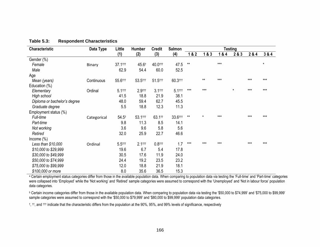
166

Table 5.3: Respondent Characteristics

Characteristic Data Type Little (1)

Humber (2)

Credit (3)

Salmon (4)

Testing

1 & 2 1 & 3 1 & 4 2 & 3 2 & 4 3 & 4

Gender (%) Female Binary 37.1††† 45.6† 40.0††† 47.5 ** *** *

Male 62.9 54.4 60.0 52.5

Age Mean (years) Continuous 55.6††† 53.5††† 51.5††† 60.3††† ** *** *** ***

Education (%) Elementary Ordinal 5.1††† 2.9††† 3.1††† 5.1††† *** *** * *** *** High school 41.5 18.8 21.9 38.1

Diploma or bachelor’s degree 48.0 59.4 62.7 45.5

Graduate degree 5.5 18.8 12.3 11.3

Employment status (%) Full-time Categorical 54.5† 53.1††† 63.1†† 33.6††† ** * *** *** ***

Part-time 9.8 11.3 8.5 14.1

Not working 3.6 9.6 5.8 5.6

Retired 32.0 25.9 22.7 46.6

Income (%) Less than $10,000 Ordinal 5.5††† 2.1††† 0.8††† 1.7 *** *** *** *** ***

$10,000 to $29,999 19.6 6.7 5.4 17.8

$30,000 to $49,999 30.5 17.6 11.9 24.0

$50,000 to $74,999 24.4 19.2 23.5 23.2

$75,000 to $99,999 12.0 18.8 21.9 18.1

$100,000 or more 8.0 35.6 36.5 15.3 a Certain employment status categories differ from those in the available population data. When comparing to population data via testing the ‘Full-time’ and ‘Part-time’ categories were collapsed into ‘Employed’ while the ‘Not working’ and ‘Retired’ sample categories were assumed to correspond with the ‘Unemployed’ and ‘Not in labour force’ population data categories.

b Certain income categories differ from those in the available population data. When comparing to population data via testing the ‘$50,000 to $74,999’ and ‘$75,000 to $99,999’ sample categories were assumed to correspond with the ‘$50,000 to $79,999’ and ‘$80,000 to $99,999’ population data categories.

†, ††, and ††† indicate that the characteristic differs from the population at the 90%, 95%, and 99% levels of significance, respectively

167

*, **, and *** indicate that the characteristic differs at the 90%, 95%, and 99% levels of significance, respectively

168

5.3.2. Econometric Models

We tested models with linear and quadratic specifications for the numerical

attributes (Table 5.4). With McFadden pseudo R2 values ranging from 0.27 to 0.36,

depending on watershed and modeling approach, the models are of decent fit (Hensher

et al. 2015). A likelihood ratio test reveals that the quadratic specification fits significantly

better than the linear specification for the Little and Salmon models, and barely so for the

Credit, while the specifications estimated for the Humber do not significantly differ

(Little: Χ(8)2 = 38.3 with p < 0.01; Humber: Χ(8)

2 = 2.5 with p = 0.96; Credit: Χ(8)2 =

13.5 with p = 0.10; and Salmon: Χ(8)2 = 37.7 with p < 0.01). Similarly, the AIC and BIC

suggest that the linear specification is more parsimonious for the Humber and Credit,

while the AIC indicates that the quadratic specification is best for the other two

watersheds though the BIC indicates otherwise.

169

Table 5.4: Linear and Quadratic Specifications of the Choice Models by Watershed

Variables Little Humber Credit Salmon

Linear Quadratic Linear Quadratic Linear Quadratic Linear Quadratic

Mean ASC 0.6996**

(0.3118) 0.7802** (0.3583)

1.7017*** (0.3513)

1.7883*** (0.3902)

2.0342*** (0.3312)

2.2994*** (0.3703)

1.5830*** (0.3042)

1.5667*** (0.3258)

Habitat -0.0036 (0.1230)

0.1269 (0.1524)

0.2965** (0.1327)

0.3495** (0.1527)

0.1680 (0.1238)

0.3596** (0.1540)

0.2599** (0.1194)

0.3240** (0.1293)

Habitat2

-0.6099*** (0.1643)

-0.1639 (0.1429)

-0.2280* (0.1380)

-0.6079*** (0.1140)

Water quality (WQ): sometimes

0.3521*** (0.1092)

0.4648*** (0.1295)

0.6705*** (0.1376)

0.6756*** (0.1460)

0.5229*** (0.1288)

0.6168*** (0.1520)

0.4442*** (0.0998)

0.5399*** (0.1057)

Water quality (WQ): rarely

0.7415*** (0.1566)

0.8454*** (0.1801)

1.9347*** (0.2121)

1.9669*** (0.2314)

1.6375*** (0.1814)

1.8328*** (0.2220)

1.6040*** (0.1629)

1.5956*** (0.1725)

Income -0.1671 (0.1025)

-0.2514** (0.1169)

-0.3383*** (0.1064)

-0.3790*** (0.1198)

-0.4160*** (0.1135)

-0.5330*** (0.1357)

-0.5753*** (0.0986)

-0.6225*** (0.0974)

Income2

-0.3108* (0.1621)

-0.5412*** (0.1610)

-0.5165*** (0.1556)

-0.3863*** (0.1238)

Tax -0.0053 (0.0063)

-0.0047 (0.0071)

-0.0368*** (0.0068)

-0.0389*** (0.0074)

-0.0171*** (0.0062)

-0.0212*** (0.0071)

-0.0088 (0.0057)

-0.0078 (0.0061)

ASC*Female 0.3404 (0.2771)

0.4238 (0.3119)

0.3266 (0.3820)

0.4065 (0.4191)

0.2426 (0.3206)

0.2639 (0.3375)

0.7559*** (0.2876)

0.8352*** (0.3059)

ASC*Household income

0.6543** (0.3134)

0.7268** (0.3489)

0.6431 (0.4162)

0.6104 (0.4848)

0.1080 (0.3194)

0.0754 (0.3336)

0.2367 (0.2951)

0.2205 (0.3112)

Tax*Age -0.0001 (0.0001)

-0.0001 (0.0001)

0.0003*** (0.0001)

0.0003*** (0.0001)

0.0001 (0.0001)

0.0001 (0.0001)

-0.0001 (0.0001)

-0.0001 (0.0001)

Tax*Female -0.0085*** (0.0029)

-0.0108*** (0.0035)

0.0057** (0.0028)

0.0054* (0.0029)

-0.0022 (0.0030)

-0.0017 (0.0034)

-0.0033 (0.0022)

-0.0041* (0.0024)

Tax*Household income

-0.0019 (0.0031)

-0.0030 (0.0036)

0.0099*** (0.0029)

0.0109*** (0.0031)

-0.0016 (0.0028)

-0.0028 (0.0033)

0.0041* (0.0023)

0.0043* (0.0025)

Elements of the Lower Triangular of the Cholesky Matrix

170



ASC & ASC 1.9705*** (0.1942)

2.1915*** (0.2354)

-2.1792*** (0.2602)

-2.3011*** (0.2865)

2.2585*** (0.2478)

2.4893*** (0.2949)

0 -2.4648*** (0.2363)

Habitat & ASC 0.7412*** (0.1931)

0.9597*** (0.2357)

-0.1709 (0.1935)

-0.1051 (0.2147)

0.5520*** (0.1902)

0.6864*** (0.2230)

0.7876*** (0.1687)

-0.8242*** (0.1817)

Habitat2 & ASC

-0.0757 (0.2456)

-0.0423 (0.2113)

-0.1515 (0.2222)

-0.0231 (0.1739)

WQ: Sometimes & ASC

1.1694*** (0.2401)

1.3630*** (0.2851)

-0.5773** (0.2676)

-0.6268** (0.3013)

1.1487*** (0.2315)

1.4032*** (0.2832)

0.8198*** (0.2054)

-0.8269*** (0.2106)

WQ: Rarely & ASC

0.1174 (0.1616)

0.1703 (0.1937)

0.0155 (0.1730)

-0.0377 (0.1928)

0.3240* (0.1842)

0.4709** (0.2155)

0.1910 (0.1365)

-0.2208 (0.1416)

Income & ASC -0.2079 (0.1638)

-0.3105* (0.1826)

0.0598 (0.1438)

0.1128 (0.1631)

-0.0383 (0.1793)

-0.1715 (0.2039)

0.1678 (0.1304)

-0.1703 (0.1307)

Income2 & ASC

-0.3057 (0.2391)

0.0247

(0.2519)

-0.3113 (0.2302)

0.0302

(0.1824) Habitat & Habitat

0.7039*** (0.1835)

-0.9045*** (0.2181)

0.9567*** (0.1827)

1.0436*** (0.1965)

0.6152*** (0.1858)

-0.8062*** (0.1926)

0.7646*** (0.1656)

0.8985*** (0.1790)

Habitat2 & Habitat

0.1080

(0.3687)

-0.1812 (0.2483)

0.2647

(0.2744)

-0.2780 (0.2222)

WQ: Sometimes & Habitat

-0.3037 (0.3251)

0.1326 (0.3372)

0.3866 (0.2715)

0.5390* (0.2769)

-0.1805 (0.2958)

0.0450 (0.2652)

-0.4150 (0.3000)

-0.3015 (0.2647)

WQ: Rarely & Habitat

-0.1982 (0.2354)

0.1992 (0.2741)

0.1607 (0.1749)

0.1906 (0.1782)

0.3726* (0.2201)

-0.2455 (0.2481)

-0.0930 (0.2028)

-0.0508 (0.1740)

Income & Habitat

-0.2698 (0.2280)

0.2168 (0.2493)

-0.0784 (0.1624)

-0.0251 (0.1687)

0.0470 (0.2425)

-0.2148 (0.2563)

-0.3004** (0.1451)

-0.1932 (0.1422)

Income2 & Habitat

-0.3682 (0.3065)

0.4246

(0.2760)

0.0868 (0.2872)

-0.1538 (0.2423)

Habitat2 & Habitat2

1.1201*** (0.2689)

0.4054

(0.3386)

-0.6122** (0.2681)

-0.2265 (0.2206)

WQ: Sometimes & Habitat2

0.2551

(0.3053)

-0.3220 (0.4306)

-0.3186 (0.2844)

-0.0765 (0.3484)

WQ: Rarely & Habitat2

0.1450

(0.2831)

0.1634 (0.2854)

0.0706

(0.3042)

-0.5740*** (0.1897)

171



Income & Habitat2

0.0800

(0.2564)

-0.1903 (0.2785)

0.5334* (0.2758)

0.0360

(0.1945) Income2 & Habitat2

-0.0824 (0.3503)

0.2335

(0.3685)

-0.1828 (0.2837)

0.2728

(0.2725) WQ: Sometimes & WQ: Sometimes

-1.1168*** (0.2203)

1.3475*** (0.2429)

-1.4020*** (0.2037)

-1.3837*** (0.2422)

0.9115*** (0.2088)

-0.9759*** (0.2016)

-1.3964*** (0.1955)

-1.4537*** (0.1880)

WQ: Rarely & WQ: Sometimes

-0.1208 (0.2071)

0.0469 (0.2189)

-0.5203*** (0.1792)

-0.5303** (0.2176)

0.6031** (0.2851)

-0.3745 (0.2597)

-0.2973* (0.1555)

-0.2423 (0.1873)

Income & WQ: Sometimes

0.1008 (0.1842)

-0.0129 (0.1931)

0.1386 (0.1398)

0.2026 (0.1673)

0.2176 (0.2020)

-0.5728** (0.2352)

0.2221* (0.1275)

0.1180 (0.1318)

Income2 & WQ: Sometimes

-0.1978 (0.2730)

0.3523

(0.2300)

0.4087* (0.2152)

0.2898

(0.1910) WQ: Rarely & WQ: Rarely

-0.6621*** (0.1926)

-0.7567*** (0.2753)

-0.2694 (0.3989)

-0.2890 (0.4471)

0.5211 (0.4404)

0.9403*** (0.2333)

0.6198*** (0.1592)

0.1505 (0.4300)

Income & WQ: Rarely

0.0384 (0.2224)

0.2119 (0.3157)

-0.0843 (0.3076)

-0.1135 (0.3742)

-0.4508 (0.5207)

-0.4121 (0.2999)

0.1672 (0.1534)

0.1544 (0.3001)

Income2 & WQ: Rarely

-0.3299 (0.3956)

0.1135

(0.5788)

0.0036 (0.2578)

-0.1136 (0.4828)

Income & Income

0.5662*** (0.1677)

0.5864*** (0.2148)

0.1434 (0.3586)

-0.1931 (0.3934)

-0.6231 (0.4494)

0.1879 (0.6809)

-0.0851 (0.3370)

-0.0964 (0.3749)

Income2 & Income

-0.3470 (0.3341)

0.1705

(0.5842)

-0.0684 (0.4256)

0.1764

(0.4962) Income2 & Income2

0.1093

(0.6167)

-0.0737 (0.6999)

0.0126

(0.3469)

0.0084 (0.5037)

Model Statistics Observations 4326 4011 4377 5898 Log-likelihood -1146.33 -1127.20 -895.33 -894.07 -1015.88 -1009.13 -1410.76 -1391.90 AIC (BIC) 2358.67

(2568.96) 2336.39

(2597.66) 1856.66

(2064.46) 1870.13

(2128.30) 2097.75

(2308.43) 2100.27

(2362.02) 2887.52

(3108.03) 2865.81

(3139.79) McFadden’s R2 0.27 0.29 0.36 0.36 0.33 0.34 0.32 0.33 a Standard errors appear in brackets below the corresponding coefficient.

172


173

For the linear specification, the mean habitat parameter is only significant for the

Humber and Salmon models and positive in both cases, suggesting that respondents in

these watersheds generally prefer higher levels of habitat. For the quadratic

specification, the linear and quadratic terms in all models are positive and negative,

respectively. However, the linear term is insignificant for the Little model as is the

Humber model’s quadratic term. These relationships suggest that respondents in the

Little and Salmon generally prefer the middle level of habitat, followed by the highest and

lowest levels, while those in the Ontario watersheds prefer the highest level, followed by

the middle and lowest levels. All quadratic relationships exhibit diminishing marginal

utility of habitat, though respondents in the Little and Salmon appear much more

sensitive to changes than those in the Ontario watersheds. The mean ASCs are positive

and significant for all models. Respondents in all watersheds held similar preferences for

changes in water quality regardless of model, with the most preferred level being ‘rarely

threatened’, followed by ‘sometimes threatened’, and then distantly ‘often threatened’.

Preferences for changes in producer income arising from the linear model indicate that

respondents generally dislike reductions in such income, though this relationship is

insignificant for the Little model. The relationships estimated as part of the quadratic

model reveal that respondents in the Little and Humber watersheds find modest losses

in producer income of 10% acceptable relative to no change though strongly dislike

larger 20% declines. Those in the Credit and Salmon watershed prefer no loss in

producer income, followed by a decline of 10%, and then a decline of 20%. The tax

parameters are generally negative, indicating that respondents dislike paying more,

though in the case of the Little and Salmon they are insignificant (likely due to the

interactions).

In terms of significant demographic interactions, findings are fairly consistent

across the linear and quadratic specifications. For the Little models, respondents with

higher incomes are more likely to choose a non-status quo option and female

respondents have a higher marginal utility of income. The marginal utility of income is

lower for wealthier, older, and female respondents for the Humber model, while all

interactions are insignificant for the Credit models. For the Salmon models, female

respondents are more likely to choose a non-status quo alternative and have a higher

marginal utility of income, the latter for the quadratic model only, while higher income

respondents have a lower marginal utility of income. The standard deviation parameters

174

calculated from the lower-triangular of the Cholesky matrix suggest that respondents in

the Little, Credit, and Salmon watersheds have heterogeneous preferences for all

attributes while those in the Humber hold such preferences for most attributes,

regardless of model (see Appendix D6).

Marginal WTP and CS Estimates

Marginal WTP estimated for changes in the ASC variable and water quality

attribute are fairly similar across model specifications, though the quadratic model yields

somewhat smaller estimates for all watersheds except the Humber (Figure 5.2). The

marginal values estimated for a change in the ASC variable are fairly similar for the

Humber, Credit, and Salmon watersheds, while the values elicited for the Little

watershed are much lower.61 For changes in water quality, respondents in the Humber

are willing to pay the most, followed by those in the Salmon or Credit, and more distantly

the Little. The marginal values estimated for the ASC and water quality are notably

larger than those estimated for the wildlife habitat and income attributes. The marginal

WTP for changes in wildlife habitat estimated from the linear model are all positive and

largest for the Humber or Salmon watersheds, followed by the Credit, and then the Little,

while the values estimated for changes in producer income are all negative with the

largest value observed for the Little, followed by the Humber, Credit, and then Salmon.

Diminishing marginal WTP is observed for changes in wildlife habitat and producer

income estimated from the quadratic model. Marginal WTP estimated for the Little and

Salmon watersheds is more sensitive to changes in wildlife habitat relative to the Ontario

watersheds, while marginal WTP estimated for the Little appears least sensitive to

declines in producer income, followed by the Salmon, Credit, and then Humber.

61

Though not an attribute, we include the ASC in our analysis of transfers of marginal WTP since it is a component of CS.

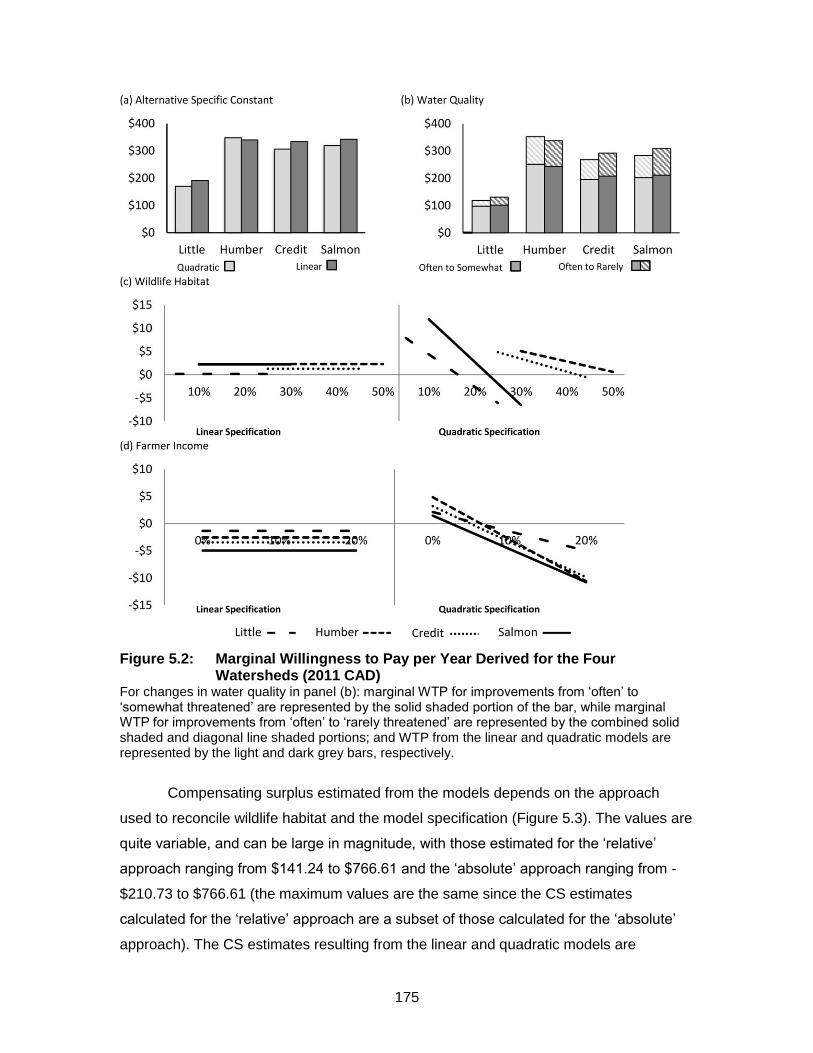
175

Figure 5.2: Marginal Willingness to Pay per Year Derived for the Four Watersheds (2011 CAD)

For changes in water quality in panel (b): marginal WTP for improvements from ‘often’ to ‘somewhat threatened’ are represented by the solid shaded portion of the bar, while marginal WTP for improvements from ‘often’ to ‘rarely threatened’ are represented by the combined solid shaded and diagonal line shaded portions; and WTP from the linear and quadratic models are represented by the light and dark grey bars, respectively.

Compensating surplus estimated from the models depends on the approach

used to reconcile wildlife habitat and the model specification (Figure 5.3). The values are

quite variable, and can be large in magnitude, with those estimated for the ‘relative’

approach ranging from $141.24 to $766.61 and the ‘absolute’ approach ranging from -

$210.73 to $766.61 (the maximum values are the same since the CS estimates

calculated for the ‘relative’ approach are a subset of those calculated for the ‘absolute’

approach). The CS estimates resulting from the linear and quadratic models are

176

somewhat similar though there are differences (e.g., for the ‘absolute’ approach the CS

values for each watershed diverge more for the quadratic models relative to the linear

model). The Little watershed is clearly an outlier as the CS estimates for this watershed

are much lower than those values estimated for the other watersheds. The Salmon and

Humber watersheds appear to have similar CS values, though they are more divergent

for the quadratic model when reconciled via the ‘absolute’ approach, and these

estimates are not terribly different from those estimated for the Credit.

Figure 5.3: Compensating Surplus per Year Estimates (2011 CAD)

5.3.3. Testing Transfer Validity and Reliability

Testing the Similarity of Models

For both the linear and quadratic specifications the likelihood ratio tests used to

compare the model parameters across watersheds reject the null hypothesis that the

models are equal at the 99% level of significance (Table 5.5). Thus, models differ by

watershed.

177

Table 5.5: Likelihood Ratio Test Results for Model Comparisons

Comparison Pooled Log Likelihood

Relative Scale Likelihood Ratio p-value

Linear Quadratic Linear Quadratic Linear Quadratic

Little & Humber -2108.88 -2092.87 0.60 0.60 <0.01*** <0.01*** Little & Credit -2212.56 -2196.30 0.65 0.65 <0.01*** <0.01*** Little & Salmon -2611.37 -2577.08 0.65 0.60 <0.01*** <0.01*** Humber & Credit -1960.61 -1939.79 0.95 0.90 <0.01*** <0.01*** Humber & Salmon -2377.03 -2357.26 1.25 1.20 <0.01*** <0.01*** Credit & Salmon -2501.84 -2477.99 1.15 1.05 <0.01*** <0.01*** *, **, and *** indicate that the models differ from each other at the 90%, 95%, and 99% levels of significance, respectively

The Validity and Reliability of Transfers of Wildlife Habitat and Producer Income Marginal WTP

For wildlife habitat the transfer yielding the lowest errors or tolerance levels

depends on transfer direction, model, level in the case of quadratic model, and

reconciliation approach (Table 5.6). For the linear model, transfers of marginal WTP for

changes in habitat involving the Little yield the highest errors and tolerance levels

especially when this site is the policy site, while those between the Humber and Salmon

result in the lowest errors and tolerance levels. For the quadratic model, averaging

across reconciliation approaches and transfer direction reveals that the errors are also

largest for transfers involving the Little, while the lowest errors are generally for transfers

between the Humber and Credit or Salmon depending on whether the average is the

mean or median. The order differs somewhat for tolerance levels. Average tolerance

levels are lowest for transfers between the Humber and Credit and highest for transfers

between the Little and Humber. The ‘relative’ approach results in the lowest errors and

tolerance levels overall, while the ‘absolute’ approach yields the largest errors overall

and using linear habitat results in the largest tolerance levels. However, the best

approach depends on the transfer. For instance, the linear approach yields the lowest

errors and tolerance levels for transfers between the Humber and Salmon, while the

‘relative’ approach yields lowest errors and tolerance levels for transfers between the

Little and Salmon.

178

Table 5.6: Errors, Tolerance Levels, and Complete Combinatorial p-values for Transfers of Wildlife Habitat Marginal WTPa

Transfer and Policy Site Linear Habitat

Quadratic Habitat

‘Relative’ ‘Absolute’

L1 L2 L3 L1 L2 L3

Little & Humber Little 1109 [2273] 36 [108] 211 [475] 110 [190] 35 [118] 822 [172] 202 [326] Humber 92 [188] 56 [168] 68 [153] 1098 [1893] 288 [416] 682 [969] 3967 [5874] CC p-value

0.06* 0.21 0.10* 0.01** 0.36

0.00*** 0.10*

0.00*** 0.00*** 0.00***

Little & Credit Little 576 [1684] 39 [104] 125 [364] 88 [163] 32 [314] 735 [184] 180 [158] Credit 85 [250] 63 [170] 56 [162] 731 [1354] 225 [149] 735 [199] 2644 [308] CC p-value

0.20 0.16 0.20 0.03** 0.34

<0.01*** 0.04**

<0.01*** <0.01*** <0.01***

Little & Salmon Little 1085 [2243] 51 [115] 198 [433] 7 [81] 109 [189] 700 [739] 69 [388] Salmon 92 [190] 34 [76] 66 [146] 6 [76] 63 [326] 195 [1053] 48 [4007] CC p-value

0.06* 0.10* 0.09* 0.44 0.01***

<0.01*** <0.01*** <0.01***

0.04** 0.18

Humber & Credit Humber 44 [145] 5 [115] 28 [115] 220 [976] 32 [221] 77 [167] 449 [152] Credit 79 [258] 5 [120] 38 [159] 183 [813] 28 [98] 93 [290] 336 [136] CC p-value

0.23 0.47 0.30 0.32 0.29 0.37

0.10* 0.17

0.21 0.14

Humber & Salmon Humber 2 [107] 135 [243] 4 [92] 1163 [1904] 227 [118] 651 [451] 4182 [259] Salmon 2 [109] 57 [104] 5 [96] 109 [180] 20 [88] 169 [125] 178 [429] CC p-value

0.49 0.02** 0.47 0.01*** <0.01***

0.37 <0.01***

0.16 <0.01*** <0.01***

Credit & Salmon Credit 75 [254] 146 [247] 32 [141] 786 [1360] 139 [759] 638 [181] 2672 [144] Salmon 43 [145] 59 [101] 24 [107] 89 [154] 24 [153] 129 [161] 153 [189]

179

Transfer and Policy Site Linear Habitat

Quadratic Habitat


L1 L2 L3 L1 L2 L3 CC p-value

0.24 0.01*** 0.31 0.01** <0.01***

0.29 <0.01***

0.13 <0.01*** <0.01***

Overall Errorb 274 (82) 170 (61) 609 (188) Toleranceb 654 (220) 368 (157) 556 (194) CC Different Pairsc 0% 33% 61%

a Errors [tolerance levels in square brackets]

b Mean (median in round brackets)

c Percentage of CC tests deeming a pair of estimates different at the 95% level of significance

*, **, and *** indicate that the values differ from each other at the 90%, 95%, and 99% levels of significance, respectively

180

In terms of the complete combinatorial test, the marginal WTP for changes in

habitat resulting from the linear model differ significantly for transfers between the Little

and the Humber or Salmon (Table 5.6). For quadratic habitat, results differ by

reconciliation approach and level. In terms of the ‘relative’ approach, we observed no

significant differences for transfers between the Humber and Credit watersheds, only a

single such difference for transfers between the Little and Credit, and two significant

differences for the remaining transfers. The complete combinatorial tests for the

‘absolute’ approach are directional, though the results are similar to the other

approaches in that the fewest statistically different pairs occur for transfers between the

Humber and Credit. Transfers between the Salmon and Humber or Credit yield the

second fewest number of significantly different pairs followed by transfers involving the

Little. Overall none of the pairs differ at the 95% level of significance for linear habitat,

while a third of the pairs differ at this significance level for the ‘relative’ approach, and

just over 60% for the ‘absolute’ approach.

Errors for transfers of wildlife habitat based on the quadratic model clearly

depend on the level and approach. For example, transfers between the Humber and

Salmon for level 2 of the ‘relative’ approach yield errors around 5% while transfers of the

other levels of habitat yield substantially higher errors. We observe similar variation for

transfers based on the ‘absolute’ approach. The large transfer errors may result from the

interplay between the equation used to calculate errors and the non-constant WTP

estimated for these attributes. The denominator of the transfer error equation varies by

wildlife habitat level and as the denominator approaches zero the errors increase rapidly

(as illustrated in Appendix D7, the point at which the denominator is zero is an

asymptote). When marginal WTP at the policy site is zero, the denominator is zero,

which occurs for wildlife habitat around 16% for the Little, 53% for the Humber, 42% for

the Credit, and 23% for the Salmon (e.g., when the Humber is the policy site and wildlife

habitat is at 50% the errors are 1000% and 4000% for the ‘relative’ and ‘absolute’

approaches, respectively). If the error equation’s numerator is small, which we observe

for transfers between the Humber and Credit, errors do not explode even when the

denominator is close to zero. Furthermore, we are more likely to observe extremely large

errors when the slope of the policy site’s marginal WTP function is flatter since the

denominator is near zero over a wider range of levels (e.g., Humber or Credit). We also

observed relatively large tolerance levels for the same transfers as the large errors and

181

similar reasoning applies. When marginal WTP values at the policy site approach zero

the tolerance levels must become large, increasing the size of the tolerance interval to

the point where the test deems a pair of estimates equivalent at the 95% level of

significance.

The validity and reliability of transfers of marginal WTP for changes in producer

income also vary by several factors (Table 5.7). For transfers based on the linear model,

the lowest errors result from transfers between the Credit and Humber or Salmon, while

the largest errors result from transfers between the Little and Humber. The

corresponding tolerance levels were lowest for transfers between the Credit and Salmon

and largest for transfers involving the Little. For quadratic producer income the results

differ by level. However, averaging across levels reveals that transfers between the

adjacent Humber and Credit yield the lowest errors overall and transfers between the

distant Little and Salmon result in the largest errors.62 On average, the corresponding

tolerance levels were lowest for transfers between the Credit and Humber or Salmon

and largest for transfers between the Little and Humber or Salmon. Results of the

complete combinatorial tests show that marginal WTP resulting from the linear model

specification differs significantly for transfers between the Little and Credit or Salmon as

well as between the Humber and Salmon. For the quadratic specification, no significant

differences were observed for transfers between the Credit and Humber or Salmon, a

single significant difference for transfers between the Humber and Little or Salmon, and

two such differences for the other transfers. Furthermore, we observe no significantly

different pairs of estimates at the status quo level and three for each of the other levels.

Overall, transfers of marginal WTP for changes in producer income based on the

quadratic specification yield lower average errors than transfers based on the linear

specification. However, the opposite holds for tolerance levels. In addition, the linear

model results in nearly twice the share of pairs that differ at the 95% level of significance

than the quadratic model.

62

Transfers of quadratic marginal WTP for changes in producer income are subject to the issue with very large errors and tolerance levels that we described earlier for wildlife habitat. For producer income, the asymptotes occur around the -6% level for the Little, -5% for the Humber, and -2% for both the Credit and Salmon.

182

Table 5.7: Errors, Tolerance Levels, and Complete Combinatorial p-values for Transfers of Marginal WTP for Changes in Producer Incomea

Transfer and Policy Site Linear Producer Income

Quadratic Producer Income

0% -10% -20%

Little & Humber Little 90 [221] 126 [384] 102 [239] 112 [223] Humber 48 [116] 56 [170] 50 [119] 53 [106] CC p-value 0.13 0.21 0.11 0.05**

Little & Credit Little 155 [295] 49 [277] 133 [260] 97 [191] Credit 61 [116] 33 [186] 57 [112] 49 [97] CC p-value 0.03** 0.36 0.04** 0.04**

Little & Salmon Little 267 [403] 32 [257] 225 [342] 115 [211] Salmon 73 [110] 47 [377] 69 [105] 54 [99] CC p-value <0.01*** 0.41 <0.01*** 0.02**

Humber & Credit Humber 34 [110] 34 [149] 15 [89] 7 [61] Credit 25 [82] 52 [226] 13 [77] 8 [66] CC p-value 0.23 0.31 0.36 0.41

Humber & Salmon Humber 93 [167] 70 [185] 61 [131] 2 [56] Salmon 48 [87] 232 [611] 38 [81] 1 [56] CC p-value 0.02** 0.16 0.07* 0.48

Credit & Salmon Credit 44 [103] 54 [208] 40 [96] 9 [60] Salmon 30 [72] 118 [454] 28 [69] 9 [55] CC p-value 0.11 0.28 0.12 0.38

Overall Errorb 81 (54) 63 (51) Toleranceb 157 (113) 180 (140) CC Different Pairsc 50% 28%

a Errors [tolerance levels in square brackets]




Examining Transfer Errors and Testing the Similarity of CS Estimates

Transfers of compensating surplus (CS) are also influenced by site treatment and

transfer direction, habitat reconciliation approach, as well as model specification (Table

5.8). Although the ‘relative’ and ‘absolute’ reconciliation approaches can be applied to

transfers of CS estimated from the linear model these approaches yield identical results

for this specification since the change in habitat is the same and marginal WTP does not

vary by habitat level. In addition, all approaches yield the same results when habitat is at

183

the status quo level since there is no change in habitat (though the other attributes do

change). For both the linear and quadratic specifications, and regardless of

reconciliation approach, transfer errors and tolerance levels are highest for transfers

involving the Little watershed. The lowest mean of the errors and tolerance levels are

observed for transfers between the Credit and Salmon. Transfers involving the Little

yield the largest share of pairs of estimates deemed different at the 95% level of

significance, while none of the pairs of estimates for transfers between the Humber and

Credit were deemed significantly different and only a small share for transfers between

the other watersheds (and only for the ‘absolute’ approach). The effect of transfer

direction is most pronounced for transfers involving the Little with those to this watershed

yielding much larger errors and tolerance levels on average than in the other direction.

However, errors and tolerance levels also clearly differ by direction for transfers between

the Salmon and Humber or Credit in the case of the ‘absolute’ reconciliation approach.

184

Table 5.8: Mean of the Errors and Tolerance Levels, as well as Statistically Different Pairs for Transfers of CS Estimates by Model and Habitat Treatmenta

Transfer and Policy Site Linear

Quadratic


Little & Humber Little 103 [159] 120 [179] 142 [219] Humber 51 [78] 54 [82] 87 [119] CC Different Pairsb 100% 100% 100%

Little & Credit Little 84 [139] 80 [135] 103 [167] Credit 45 [76] 44 [75] 76 [110] CC Different Pairsb 93% 93% 96%

Little & Salmon Little 87 [141] 89 [143] 108 [163] Salmon 46 [76] 47 [76] 54 [83] CC Different Pairsb 89% 89% 96%

Humber & Credit Humber 9 [39] 18 [47] 20 [50] Credit 11 [43] 22 [57] 24 [60] CC Different Pairsb 0% 0% 0%

Humber & Salmon Humber 8 [38] 14 [43] 48 [79] Salmon 9 [42] 16 [50] 26 [65] CC Different Pairsb 0% 0% 33%

Credit & Salmon Credit 3 [36] 6 [38] 27 [61] Salmon 3 [35] 5 [36] 6 [41] CC Different Pairsb 0% 0% 17%

Overall Errorsc 38 (25) 43 (30) 60 (50) Tolerancec 75 (69) 80 (70) 101 (81) CC Different Pairsb 47% 47% 57%

a Mean errors [mean tolerance levels in square brackets]

b Percentage of CC tests deeming a pair of estimates different at the 95% level of significance

c Mean (median in brackets)

In terms of the two reconciliation approaches based on the quadratic model, the

‘relative’ approach yields lower average errors and tolerance levels than the ‘absolute’

approach for all transfers. The ‘relative’ approach also yields an equal or lower share of

estimate pairs deemed different at the 95% level of significance for each transfer.

Furthermore, the mean of the errors and tolerance levels are appreciably higher for all

transfers based on the 'absolute' approach other than those between the Humber and

Credit and to a lesser extent the Little and Salmon (the two watershed pairs with the

most similar wildlife habitat levels). Comparing the same compensating surplus

185

specification reveals that the ‘relative’ approach yields the lowest errors and tolerance

levels in nearly all cases (see Appendix D8, Table D11).

Overall, transfers based on the linear model specification yield lower average

errors and tolerance levels than transfers based on the quadratic specification, although

the average errors and tolerance levels resulting from the ‘relative’ approach are close.

Similarly, the proportion of estimate pairs from the linear model deemed different at 95%

significance is equal to the share estimated for the ‘relative’ approach and lower than

that estimated for the ‘absolute’ approach. Comparing transfers for the same CS

estimate resulting from the linear and ’relative’ approaches reveals that the linear model

yields the lowest errors and tolerance levels in the vast majority of cases (see Appendix

D8, Table D12). When compared to the ‘absolute’ approach, transfers based on the

linear model yield the lowest errors and tolerance levels in nearly all cases.

5.4. Discussion

We evaluated the validity and reliability of transferring WTP for changes in

ecosystem services across four Canadian watershed case study sites using a

convergent validity approach. Our focus was to examine different approaches to

reconciling a quantitative attribute with levels that differ by case study site. Overall, the

directional transfer errors we observed for transfers of marginal WTP ranged from 1% to

4182% with a mean of 161% and median of 54%, while the corresponding tolerance

levels ranged from 30% to 5874% with a mean of 298% and median of 136%. For

compensating surplus, the directional transfer errors ranged from 0% to 191% with a

mean of 43% and median of 40%, while the associated tolerance levels ranged from

27% to 327% with a mean and median of 81% and 72%, respectively. Furthermore, the

null hypothesis of equal model parameters was rejected in all cases, which is not

surprising given that correlated random coefficients require a large number of model

parameters making it likely that there are differences (Colombo et al. 2007b). The null

hypothesis of equal values was rejected for marginal WTP 43% of the time and for

compensating surplus 49% of the time (at the 95% level of significance). The errors and

test results are comparable to those resulting from previous research outlined by Kaul et

al. (2013) and Rosenberger (2015) in their comprehensive reviews of the literature.

186

We now review the evidence pertaining to each of the hypotheses outlined in the

introduction. The first hypothesis we set out to assess was that transfers based on

relative preferences are more valid and reliable than transfers based on absolute

preferences, given that empirical research suggests that respondents to choice

experiments have relative preferences (e.g., Luisetti et al. (2011)). We rely on transfers

of wildlife habitat for this assessment as the levels of this attribute differed across the

case study sites. On average, the ‘relative’ approach yields the lowest transfer errors

and tolerance levels for transfers of marginal WTP and CS estimates. Furthermore,

when compared directly the ‘relative’ approach yielded lower errors and tolerance levels

than the ‘absolute’ approach for nearly every transfer. Similarly, the proportion of pairs of

marginal WTP or CS estimates deemed significantly different by the complete

combinatorial test is lowest for the ‘relative’ approach. In sum, evidence from our study

suggests that transfers based on ‘relative’ preferences are more valid and reliable than

those based on ‘absolute’ preferences.

The ‘absolute’ approach to reconciliation involves comparing certain values of

wildlife habitat outside of the range from which they were estimated, which may reduce

this approach’s validity and reliability. For instance, the relationship for wildlife habitat

estimated for the Humber, Credit, and Salmon are all used for values outside of the

range at which they were estimated when transferred to the Little. In some cases, such

as at the 5% level, this entails a loss from the status quo levels at these study sites

(10%, 25%, and 30%, respectively, in the Salmon, Credit, and Humber). Prospect theory

suggests that gains and losses are valued asymmetrically (Kahneman and Tversky

1979). Given this asymmetry, it is unlikely that the relationship estimated for a gain in

wildlife habitat could be extended to a situation that is actually a loss without increasing

generalization errors.

The second hypothesis we set out to examine was that the approach to

reconciling quantitative attributes with differing levels matters less when the levels are

closer together since the two approaches will provide identical results if the levels are

the same. The Credit and Humber as well as the Little and Salmon have similar levels

relative to the other case study site pairs. For these two pairs, the levels for the habitat

attribute differ by 5 percentage points, while the levels for the remaining pairs differ by at

least 15 points. Thus we expect less difference in errors and tolerance levels for

transfers between these watershed pairs relative to the other pairs. We do observe this

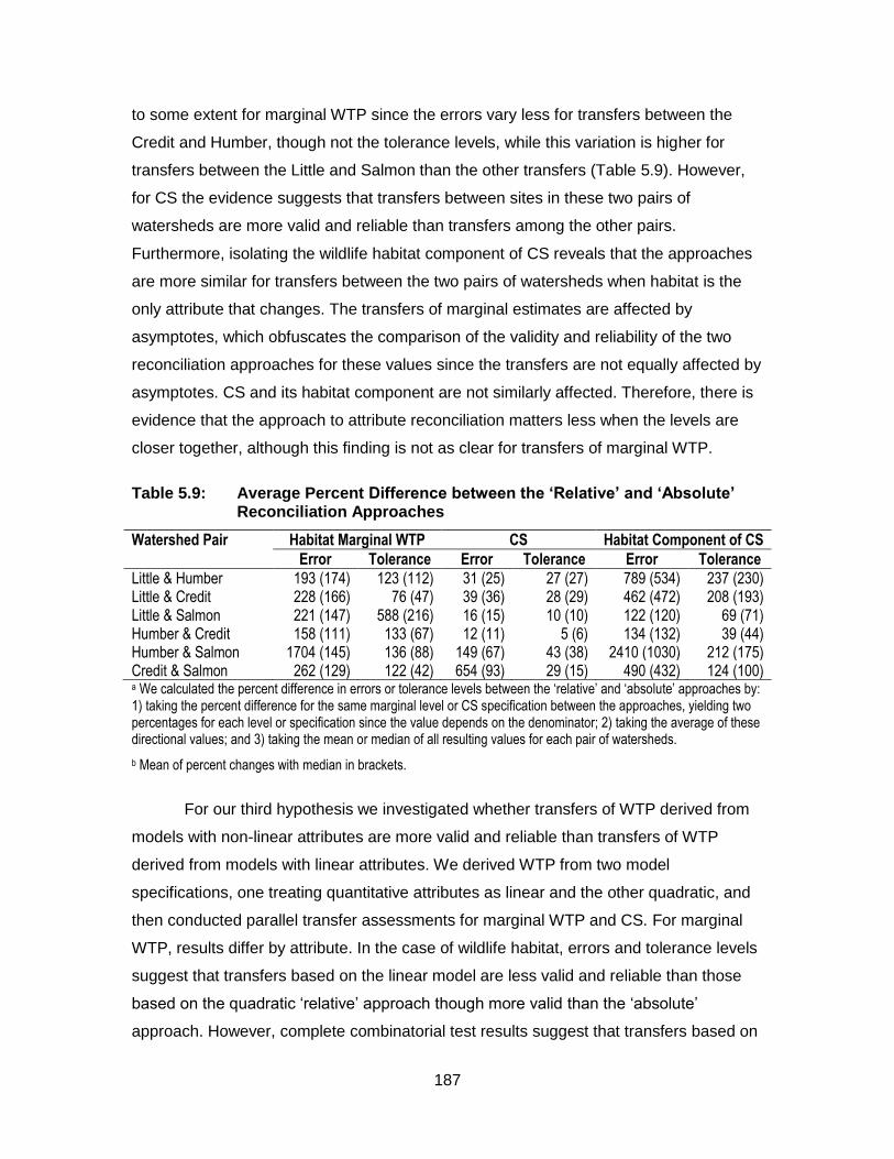
187

to some extent for marginal WTP since the errors vary less for transfers between the

Credit and Humber, though not the tolerance levels, while this variation is higher for

transfers between the Little and Salmon than the other transfers (Table 5.9). However,

for CS the evidence suggests that transfers between sites in these two pairs of

watersheds are more valid and reliable than transfers among the other pairs.

Furthermore, isolating the wildlife habitat component of CS reveals that the approaches

are more similar for transfers between the two pairs of watersheds when habitat is the

only attribute that changes. The transfers of marginal estimates are affected by

asymptotes, which obfuscates the comparison of the validity and reliability of the two

reconciliation approaches for these values since the transfers are not equally affected by

asymptotes. CS and its habitat component are not similarly affected. Therefore, there is

evidence that the approach to attribute reconciliation matters less when the levels are

closer together, although this finding is not as clear for transfers of marginal WTP.

Table 5.9: Average Percent Difference between the ‘Relative’ and ‘Absolute’ Reconciliation Approaches

Watershed Pair Habitat Marginal WTP CS Habitat Component of CS

Error Tolerance Error Tolerance Error Tolerance Little & Humber 193 (174) 123 (112) 31 (25) 27 (27) 789 (534) 237 (230) Little & Credit 228 (166) 76 (47) 39 (36) 28 (29) 462 (472) 208 (193) Little & Salmon 221 (147) 588 (216) 16 (15) 10 (10) 122 (120) 69 (71) Humber & Credit 158 (111) 133 (67) 12 (11) 5 (6) 134 (132) 39 (44) Humber & Salmon 1704 (145) 136 (88) 149 (67) 43 (38) 2410 (1030) 212 (175) Credit & Salmon 262 (129) 122 (42) 654 (93) 29 (15) 490 (432) 124 (100) a We calculated the percent difference in errors or tolerance levels between the ‘relative’ and ‘absolute’ approaches by: 1) taking the percent difference for the same marginal level or CS specification between the approaches, yielding two percentages for each level or specification since the value depends on the denominator; 2) taking the average of these directional values; and 3) taking the mean or median of all resulting values for each pair of watersheds.

b Mean of percent changes with median in brackets.

For our third hypothesis we investigated whether transfers of WTP derived from

models with non-linear attributes are more valid and reliable than transfers of WTP

derived from models with linear attributes. We derived WTP from two model

specifications, one treating quantitative attributes as linear and the other quadratic, and

then conducted parallel transfer assessments for marginal WTP and CS. For marginal

WTP, results differ by attribute. In the case of wildlife habitat, errors and tolerance levels

suggest that transfers based on the linear model are less valid and reliable than those

based on the quadratic ‘relative’ approach though more valid than the ‘absolute’

approach. However, complete combinatorial test results suggest that transfers based on

188

the linear model are more valid than either of those based on the quadratic model. The

divergent conclusion resulting from the complete combinatorial test may arise from its

use of a traditional hypothesis. In this case, more variable WTP estimates are more

likely to be deemed equal and thus transfers more valid, while the opposite is true for

equivalence tests (Kristofersson and Navrud 2005; Johnston and Duke 2008). Thus, our

results are sensible if estimates resulting from the linear model are less efficient than

those generated from the quadratic model for the ‘relative’ approach. For producer

income, errors and tolerance levels indicate that transfers based on the linear model are

less reliable though more valid than transfers based on the quadratic specification,

although the complete combinatorial tests suggest that transfers based on the linear

model are less valid. For CS, errors and tolerance levels suggest that transfers based on

the linear specification are more valid and reliable than those based on either of the

quadratic approaches. However, the complete combinatorial test results indicate that

transfers based on the linear model are similarly valid to those based on the quadratic

model’s ‘relative’ approach and more valid than transfers based on the ‘absolute’

approach.

One reason that transfers of CS based on the linear model are more valid and

reliable is that CS incorporates values of the ASC variable and water quality attribute. As

such, the validity and reliability of transfers of CS are not driven exclusively by wildlife

habitat or producer income. Since the ASC and water quality are valued at a much

higher magnitude than either wildlife habitat or producer income they have more

influence on the validity and reliability of CS transfers. Transfers of marginal WTP for the

ASC and water quality based on the linear model are generally more valid and reliable

than those based on the quadratic model, which may be driving the relatively better

validity and reliability of transfers of CS based on the linear model (see Appendix D9 in).

However, looking at changes in income in isolation from the other components of CS

reveals that the linear model yields lower errors and tolerance levels than the quadratic

model in 54% and 8% of cases, respectively. For isolated changes in wildlife habitat, the

linear model yields lower errors and tolerance levels than the ‘relative’ (’absolute’)

approach in 25% (79%) and 17% (75%) of cases, respectively. These results are similar

to those observed for transfers of marginal WTP. A related insight is that when

transferring CS values the functional relationship estimated for quantitative attributes

matters less if the marginal values of these attributes are small relative to the marginal

189

values of the other attributes. Another factor influencing the validity and reliability of the

linear and quadratic specifications is that extremely large errors or tolerance levels arise

for levels approaching asymptotes for transfers based on the quadratic model.

Asymptotes are not a factor for transfers based on the linear model.

Our results could differ if an alternative reconciliation approach was used. For

instance, though the wildlife habitat attribute levels change by 10 percentage points in

each watershed the difference relative to the baseline differs substantially across sites.

The changes are 3 or 5 times the baseline for the Little, 2 or 3 times for the Salmon, 1.4

or 1.8 times for the Credit, and 1.3 or 1.7 times for the Humber.63 An alternative

reconciliation approach, which falls outside the scope of this paper, involves comparing

WTP across sites at attribute levels calibrated to represent the same proportional

change from their respective status quos. For the current study, this could involve

evaluating transfer validity and reliability for reasonable proportional changes in wildlife

habitat (e.g., 10% or 20% increases in habitat at each site). Furthermore, we only

examined linear and quadratic specifications for the quantitative variables. Our results

could also differ if we assessed alternative specifications, such as the natural logarithm,

or changed the models in other ways.

63

The differences relative the baseline may explain why respondents in the Little and Salmon are more sensitive to changes in wildlife habitat relative to those from the two Ontario watersheds.

190

5.5. Conclusion

We sought to assess the validity and reliability of alternative approaches for

reconciling differently defined goods or services for purposes of applied benefit transfer.

We also examined how the validity and reliability of transfers varies with functional form

assumed for quantitative attributes (linear and quadratic). In doing so, we used nearly

identical choice experiments in four Canadian watersheds that sought to value changes

in wildlife habitat (whose levels differed by watershed), water quality, and farm and forest

producer income. Overall, the validity and reliability of our transfers are similar to the

validity and reliability of transfers studied in the convergent validity literature. For

transfers of quantitative attributes with different levels that have a quadratic functional

form, our results suggest that transfers rooted in ‘relative’ preferences outperform those

based on ‘absolute’ preferences. Furthermore, for these transfers the choice between

reconciliation approach matters less when the attributes needing reconciliation have

fairly similar levels, though only in the case of transfers of compensating surplus and

welfare for changes in the attribute levels relative the status quo. Finally, though

transfers based on the linear model specification result in more valid and reliable

transfers of compensating surplus than the quadratic model, the same is not necessarily

true for transfers of marginal WTP. We believe these results contribute to the literature

on best practices for applied benefit transfer and will be of interest to other researchers

and policy analysts.

191


The Social Science and Humanities Research Council of Canada (SSHRC)

provided funding for this research through a Standard Research Grant (865-2008-0045)

and Doctoral Fellowship (752-2012-2435). SSHRC did not participate in the research

process or the preparation of this paper. The Eastern Canadian Soil and Water

Conservation Centre, Toronto and Region Conservation Authority, Credit River

Conservation Authority, and Salmon River Watershed Roundtable provided support

during questionnaire development though did not help with analysis or the preparation of

this paper. Furthermore, David Angus, Toni Anderson, and Monica McKendy helped with

the survey process, including questionnaire development and implementation, though

did not participate in the analysis used in this paper nor the writing of this manuscript. Dr.

Pascal Haegeli provided feedback during the writing of this manuscript. We thank each

of the survey respondents who participated in this research. We are responsible for all

remaining errors. Sadly, Dr.Wolfgang Haider passed away on August 24, 2015 before

the manuscript was completed.

192

References

Anderson, T. (2013). Public preferences and values for ecological goods and services in the Little River watershed, Northern New Brunswick. University of New Brunswick.

Angus, D. (2012). Valuing Ecosystem Services in the Salmon River Watershed, British Columbia: A Choice Experiment Approach. Simon Fraser University. Retrieved from http://summit.sfu.ca/system/files/iritems1/12452/etd7426_DAngus.pdf

Ariely D, Loewenstein G, Prelec D (2003) “Coherent Arbitrariness”: Stable Demand Curves Without Stable Preferences. Q J Econ 118:73–106. doi: 10.1162/00335530360535153

Bateman IJ, Brouwer R, Ferrini S, et al (2011) Making Benefit Transfers Work: Deriving and Testing Principles for Value Transfers for Similar and Dissimilar Sites Using a Case Study of the Non-Market Benefits of Water Quality Improvements Across Europe. Environ Resour Econ 50:365–387. doi: 10.1007/s10640-011-9476-8

Chow L, Xing Z, Benoy G, et al (2010) Hydrology and water quality across gradients of agricultural intensity in the Little River watershed area, New Brunswick, Canada. J Soil Water Conserv 66:71–84. doi: 10.2489/jswc.66.1.71

Colombo S, Calatrava-Requena J, Hanley N (2007a) Testing Choice Experiment for Benefit Transfer with Preference Heterogeneity. Am J Agric Econ 89:135–151. doi: 10.1111/j.1467-8276.2007.00968.x

Colombo S, Calatrava-Requena J, Hanley N (2007b) Testing Choice Experiment for Benefit Transfer with Preference Heterogeneity. Am J Agric Econ 89:135–151. doi: 10.1111/j.1467-8276.2007.00968.x

Czajkowski M, Ahtiainen H, Artell J, Meyerhoff J (2017) Choosing a Functional Form for an International Benefit Transfer: Evidence from a Nine-country Valuation Experiment. Ecol Econ 134:104–113. doi: 10.1016/j.ecolecon.2017.01.005

Czajkowski M, Hanley N, Lariviere J (2015) The effects of experience on preferences: Theory and empirics for environmental public goods. Am J Agric Econ 97:333–351. doi: 10.1093/ajae/aau087

Czajkowski M, Ščasný M (2010) Study on benefit transfer in an international setting. How to improve welfare estimates in the case of the countries’ income heterogeneity? Ecol Econ 69:2409–2416. doi: 10.1016/j.ecolecon.2010.07.008

Gerking S, Adamowicz W, Dickie M, Veronesi M (2017) Baseline risk and marginal willingness to pay for health risk reduction. J Risk Uncertain 55:177–202. doi: 10.1007/s11166-017-9267-x

193

Hanemann WM (1984) Valuation Contingent Experiments in Responses. Am J Agric Econ 66:332–341.

Hensher DA (2004) Identifying the influence of stated choice design dimensionality on willingness to pay for travel time savings. 38:425–446.

Hensher DA, Rose JM, Greene WH (2015) Applied Choice Analysis, 2nd Editio. Cambridge University Press, Cambridge, UK

Hess S, Train K (2017) Correlation and scale in mixed logit models. J Choice Model 23:1–8. doi: 10.1016/j.jocm.2017.03.001

Hole AR (2007) Fitting mixed logit models by using maximum simulated likelihood. Stata J 7:388–401.

Hoyos D (2010) The state of the art of environmental valuation with discrete choice experiments. Ecol Econ 69:1595–1603. doi: 10.1016/j.ecolecon.2010.04.011

Hu W, Veeman MM, Adamowicz WL (2005) Labelling Genetically Modified Food: Heterogeneous Consumer Preferences and the Value of Information. Can J Agric Econ Can d’agroeconomie 53:83–102. doi: 10.1111/j.1744-7976.2005.04004.x

Johnston RJ, Duke JM (2008) Benefit Transfer Equivalence Tests with Non-normal Distributions. Environ Resour Econ 41:1–23. doi: 10.1007/s10640-007-9172-x

Johnston RJ, Duke JM (2010) Socioeconomic adjustments and choice experiment benefit function transfer: Evaluating the common wisdom. Resour Energy Econ 32:421–438. doi: 10.1016/j.reseneeco.2009.11.003

Johnston RJ, Rosenberger RS (2010) Methods, Trends and Controversies in Contemporary Benefit Transfer. J Econ Surv 24:479–510. doi: 10.1111/j.1467-6419.2009.00592.x

Johnston RJ, Rosenberger RS, Rolfe J, Brouwer R (2015) Benefit Transfer: The Present State and Future Prospects. In: Benefit Transfer of Environmental and Resource Values. pp 553–574

Kahneman D, Tversky A (1979) Prospect Theory: An Analysis of Decision under Risk. Econometrica 47:263. doi: 10.2307/1914185


Kennedy M, Wilson J (2009) Estimating the Value of Natural Capital in the Credit River Watershed.

194

Kragt ME (2013) The Effects of Changing Cost Vectors on Choices and Scale Heterogeneity. Environ Resour Econ 54:201–221. doi: 10.1007/s10640-012-9587-x

Kristofersson D, Navrud S (2005) Validity tests of benefit transfer - Are we performing the wrong tests? Environ Resour Econ 30:279–286. doi: 10.1007/s10640-004-2303-8

Ladenburg J, Olsen SB (2014) Augmenting short Cheap Talk scripts with a repeated Opt-Out Reminder in Choice Experiment surveys. Resour Energy Econ 37:39–63. doi: 10.1016/j.reseneeco.2014.05.002

Luisetti T, Bateman IJ, Turner RK (2011) Testing the Fundamental Assumption of Choice Experiments: Are Values Absolute or Relative? Land Econ 87:284–296. doi: 10.3368/le.87.2.284

Lundhede TH, Olsen SB, Jacobsen JB, Thorsen BJ (2009) Handling respondent uncertainty in Choice Experiments: Evaluating recoding approaches against explicit modelling of uncertainty. J Choice Model 2:118–147. doi: https://doi.org/10.1016/S1755-5345(13)70007-1

McPhee M, Gebauer M, Holman G, et al (1996) The Salmon River Watershed: An Overview of Conditions, Trends and Issues. Salmon Arm, B.C.

Meyerhoff J, Mørkbak MR, Olsen SB (2014) A Meta-study Investigating the Sources of Protest Behaviour in Stated Preference Surveys. Environ Resour Econ 58:35–57. doi: 10.1007/s10640-013-9688-1

Muthke T, Holm-Mueller K (2004) National and international benefit transfer testing with a rigorous test procedure. Environ Resour Econ 29:323–336. doi: 10.1007/s10640-004-5268-8

Natural Resources Canada, The Canada Centre for Mapping and Earth Observation, United States Geological Survey, et al (2010) 2010 North American Land Cover at 250 m spatial resolution.

Nelson JP, Kennedy PE (2009) The use (and abuse) of meta-analysis in environmental and natural resource economics: An assessment. Environ Resour Econ 42:345–377. doi: 10.1007/s10640-008-9253-5



195

Saffran K, Cash K, Hallard K (2001) CCME Water Quality Index 1.0 User’s Manual.

Smith VK, Pattanayak SK (2002) Is meta-analysis a Noah’s Ark for non-market valuation? Environ Resour Econ 22:271–296. doi: 10.1023/A:1015567316109

Smith VK, Pattanayak SK, Houtven GL Van (2006) Structural benefit transfer : An example using VSL estimates. doi: 10.1016/j.ecolecon.2006.04.002

Statistics Canada (2012) Census: Age and Sex – Age (131) and Sex (3) for the Population of Canada, Provinces, Territories, Census Divisions, Census Subdivisions and Dissemination Areas (98-311-XCB2011018). http://www5.statcan.gc.ca/olc-cel/olc.action?objId=98-311-X2011018&objType=46&lang=en&limit=0. Accessed 25 Jan 2018

Swait J, Louviere J (1993) The Role of the Scale Parameter in the Estimation and Comparison of Multinomial Logit Models. J Mark Res 30:305–314.

Toronto and Region Conservation Authority (2013) Humber River Watershed Report Card 2013. Toronto, Ontario

Tversky A, Simonson I (1993) Context- dependent Preferences. Manage Sci 39:1179–1189. doi: 10.1287/mnsc.39.10.1179

Van Houtven G, Powers J, Pattanayak SK (2007) Valuing water quality improvements in the United States using meta-analysis: Is the glass half-full or half-empty for national policy analysis? Resour Energy Econ 29:206–228. doi: 10.1016/j.reseneeco.2007.01.002

Zhu Z, Broersma K, Mazumder A (2011) Model assessment of cattle and climate impacts on stream fecal coliform pollution in the Salmon river watershed, British Columbia, Canada. Water Air Soil Pollut 215:155–176. doi: 10.1007/s11270-010-0467-0

196

Chapter 6. Conclusion

197

This dissertation makes several contributions to the literature and its findings

have applications to resource and environmental management and policy. I review the

main findings and provide examples of potential applications in this concluding chapter,

which is structured as follows. First, to refresh the reader’s memory I briefly review the

main takeaways from each of the four studies, and then discuss some implications for

management and policy. Finally, the dissertation closes with a general discussion of

certain limitations and potential areas of further research.

6.1. Overview of Each Paper and Main Findings

The papers forming my dissertation contribute to the literature in two main areas:

1) private landowner preferences for characteristics of conservation programs; and 2)

benefit transfer. Specifically, the paper presented in Chapter 2 sought to elicit private

landowner preferences for the attributes of a voluntary payments-based wetlands

conservation program using choice experiments in Southern Ontario’s Grand and Upper

Thames River watersheds. Two similar though distinct choice experiment versions were

administered separately to farm and non-farm landowners. The data from the two

versions were modeled independently using latent class models from which landowner

WTA and the proportion of respondents who would be willing to participate in certain

wetlands conservation programs were predicted. The results indicate that:

• Numerous landowners in the two watersheds are willing to conserve wetlands though their preferences for conservation program characteristics are heterogeneous and their participation or required financial compensation depends on the program’s attributes.

• In general, the favoured program characteristics included: diverting smaller areas of land to conservation; diverting marginal rather than productive land; converting land to trees, followed by either meadow or wetlands; technical help; no public recognition; and higher financial compensation.

• Many types of landowners are willing to protect or restore wetlands, including those who are commodity producers and those who are not.

• Marginal WTA and CS estimates are in the range of those from similar studies.

The paper forming Chapter 3 assessed the validity and reliability of transferring

landowner marginal WTA and CS values resulting from the producer-focused choice

experiments in Chapter 2. The data were modeled in WTA space and benefit transfers

were assessed by calculating directional and non-directional transfer errors as well as

198

conducting standard convergent validity hypothesis tests. The results from this study

indicate that:

• Overall, the reliability and validity of transfers of landowner WTA between the two sites is similar to the reliability and validity of transfers of WTP found in previous convergent validity studies.

• Including interactions of socio-demographic variables with the alternative specific constant does not substantially change transfer reliability and some aspects of validity. However, these interactions do inflate the tolerance levels estimated for transfers of the alternative specific constant and compensating surplus.

• Non-directional errors calculated according to the equation introduced in Chattopadhyay (2003) may be much larger than the corresponding directional errors and this occurs when the values being compared have similar magnitudes and opposing signs.

The paper presented in Chapter 4 assessed the validity and reliability of transfers

of predicted program participation market shares (the proportion of respondents

predicted to participate in a wetlands conservation program relative to maintaining the

status quo). To provide context, these results were contrasted with an assessment of the

validity and reliability of transfers of CS values derived from the same model. The data,

which were modeled using a random parameters logit model, were from the non-

producer choice experiments outlined in Chapter 2. Both transfers were assessed by

calculating transfer errors and using convergent validity hypothesis tests. The main

findings of this study are that:

• Transfers of predicted program participation market shares appear valid and reliable, especially relative to the validity and reliability of transfers of the CS values. However, given the differences in how the two measures are calculated further research is required to clarify if transfers of such market shares are reliable and valid enough for policy analysis.

• The validity and reliability of transfers of CS are similar to the validity and reliability reported for existing convergent validity studies using WTP values.

The fourth paper, included as Chapter 5, examined alternative approaches to

reconciling quantitative choice experiment attributes with levels that differ across sites

when conducting benefit transfer. Three alternative approaches for transferring such

quantitative variables were assessed, including one based on a linear model

specification and two approaches based on a quadratic specification (‘relative’ and

‘absolute’). The data are from choice experiments that elicited the preferences and

199

values of residents living in or near 4 Canadian watersheds for improving water quality

and the extent of protected wildlife habitat in each watershed (and associated declines in

farm and woodlot producer income as well as increases in the respondent’s taxes). The

data were modeled using a random parameters logit. The transfers were assessed by

calculating directional transfer errors and by conducting convergent validity hypothesis

tests. The performance of the alternative reconciliation approaches was compared

based on these measures. The results of this study indicate that:

• Although preferences are heterogeneous and differ across certain watersheds, respondents generally prefer improved water quality and to a certain extent larger areas of the watershed protected as wildlife habitat, while they generally dislike declines in producer income as well as higher tax payment levels.

• For all three reconciliation approaches, the transfers of marginal WTP and CS between the case study sites are of similar validity and reliability to previous convergent validity studies.

• Transfers based on the quadratic specification grounded in ‘relative’ preferences are more valid and reliable than transfers rooted in ‘absolute’ preferences.

• For transfers of non-marginal monetary values the choice between the ‘relative’ and ‘absolute’ reconciliation approaches matters less when the attributes needing to be reconciled have fairly similar levels.

• For CS, transfers based on the linear specification are more valid and reliable than both sets of transfers based on the quadratic model, although this does not necessarily hold for transfers of marginal WTP.

6.2. Implications for Resource and Environmental Management or Policy

The research that forms my dissertation can inform related policy development

and analysis as well as resource and environmental management. For example,

elements of each paper could inform the ongoing efforts to remedy environmental

problems related to the runoff of nutrients into Lake Erie. Recently, the Canadian and

Ontario governments released the Canada-Ontario Lake Erie Action Plan for reducing

phosphorus loadings to the lake (Environment and Climate Change Canada and Ontario

Ministry of the Environment and Climate Change 2018). The plan is an outcome of a

2016 binational agreement between Canada and the United States to reduce the

amount of phosphorous entering Lake Erie (Nutrients Annex Subcommittee Objectives

200

and Targets Task Team 2015). This agreement commits Canada and Ontario to

achieving a 40% reduction in total phosphorous entering the lake’s central and western

basins, as well as a 40% reduction in soluble phosphorous entering the lake via the

Thames and Leamington River watersheds (below 2008 levels by 2025). The plan takes

an adaptive management approach and involves an exhaustive list of actions and

research. The actions include conserving and restoring wetlands and involve a variety of

financial incentives for private landowners (e.g., existing cost-share programs and a new

$4.1 million commitment to financially support the implementation of best management

practices or other approaches to reduce phosphorous runoff). The planned research

includes examining the effectiveness of wetlands for reducing phosphorous runoff as

well as evaluating the feasibility of using economic incentives. Multiple stakeholders are

involved, including municipal, provincial, and federal governments, First Nations,

conservation authorities, non-governmental organizations, and the agricultural industry.

Indeed, certain stakeholders are already developing strategies for reducing phosphorous

runoff. For example, the Thames River Phosphorus Reduction Collaborative has been

working towards meeting the demands of the binational agreement since 2016 (Thames

River Phosphorus Reduction Collaborative 2018).

My research suggests a few lessons. The results of Chapter 2 regarding private

landowner preferences for protecting or restoring wetlands are directly applicable,

though wetlands would need to be properly situated to achieve reductions in

phosphorous runoff in order to maximize benefits.64 These results suggest that

landowners are more receptive to protecting existing wetlands rather than creating new

or restoring former wetlands. They also indicate that, since certain groups of landowners

are more receptive than others, conservation programs could be tailored to different

groups based on their willingness to participate (or in the context of financial incentives,

their willingness to accept compensation). While each group has certain distinct

64

There are potential challenges with preserving or restoring wetland habitat in Ontario. First, it can be challenging to identify areas for wetland restoration, such as areas where wetlands that have previously been drained, or creation since doing so requires detailed information on the land base as well as analysis (Uuemaa et al. 2018). Furthermore, creating wetlands in areas where they were not previously established may face higher engineering costs and the ecological benefits of such wetlands may not be substantial if they are not well enough connected to current or historical wetlands. An additional challenge relates to gaining approval for restoring or creating wetlands. For instance, the Ontario Lakes and Rivers Improvement Act “[r]equires approval for the construction, alteration and operation of water control structures, some of which may be used to restore or enhance wetland habitat” (Ontario Ministry of Natural Resources and Forestry 2017).

201

preferences, in general private landowner participation in wetlands conservation

programs could be increased if the program: allows them to divert smaller areas of land

to conservation purposes; targets marginal agricultural land; protects existing wetlands

with treed buffers; offers technical help and not public recognition; and uses financial

incentives (higher incentives will yield more participation). Finally, such programs should

not necessarily be limited to those with larger land holdings or commodity producers

since other types of private landowners are also willing to participate (though actions

need to be substantive enough to reduce phosphorous runoff).

The papers included in Chapters 3 through 5, which are those related to benefit

transfer, also have a few implications (as part of economic analyses of the action plan’s

components). The results of these studies suggest that policy analysts can use transfers

of landowner WTA in the same way they currently use transfers of WTP, for instance in

benefit-cost analysis, since they have similar validity and reliability. Furthermore, market

shares may also be transferred to inform the development or analysis of conservation

programs or actions since these transfers are more valid and reliable than transfers of

economic values. Finally, the results of Chapter 5 indicate that the economic benefits of

the actions, for instance regarding improvements in water quality, may be assessed by

transferring values from other regions of Ontario or even other Canadian provinces.

Since the Canada-Ontario Lake Erie Action Plan takes an adaptive management

framework it is worth noting that benefit transfer could play a role in this approach

(assuming a desired criteria includes measuring non-market benefits or costs). Adaptive

management is a decision-making approach for managing the environment and natural

resources in dynamic uncertain social-ecological systems (Gregory et al. 2006). The key

characteristic of this approach is that it allows managers to learn about the system

during the implementation of management actions by testing hypotheses. If certain

hypotheses relate to non-market economic values then benefit transfer is useful since it

may not be feasible to conduct primary research throughout the adaptive management

cycle, especially since the latter is an iterative process.

There are additional lessons for applied benefit transfer or future convergent

validity studies. For instance, future convergent validity studies should be cautious when

using non-directional errors based on Chattopadhyay's (2003) equation when values are

of similar magnitude with opposing signs as the errors may be unreasonably large (an

202

alternative would be to take the average of the directional errors). Furthermore, when

transferring values resulting from choice experiments the approach to reconciling

quantitative attributes with different levels matters. In general, analysts should use

approaches rooted in ‘relative’ preferences for transfers of values resulting from

quadratic variable specifications or use linear specifications.

6.3. Limitations and Extensions

Each of the studies contained in my dissertation has certain potential limitations,

many of which are noted in the previous chapters. Overall, while the research is nested

in resource and environmental management it takes an economic perspective,

specifically non-market valuation. As with any approach, this perspective is not immune

to criticism or limitations. For example, McCauley (2006) argues that nature should be

conserved because of its intrinsic value, rather than its instrumental value, and should

thus not be assigned monetary values. However, non-market valuation is not necessarily

less valid than other approaches to the same problem and provides additional

information to decision or policy makers (Freeman et al. 2014). Valuation is, however,

not necessarily desirable in all situations. For instance, the economic valuation

framework is only appropriate for marginal changes in ecosystem services (Fisher et al.,

2008). Two key implications for valuation, in the context of ecosystems, emerge from

marginality. First, the scale of the change needs to be meaningful. This involves

determining the appropriate scale for the unit change. Fisher et al. (2008) provide the

example that it is neither appropriate nor meaningful for this unit to be the world’s forests

and put forth the landscape scale as the largest possible scale (though note the need for

more research). Second, marginality assumes that the response of an ecosystem to

small changes in structure or function should not cause large step changes ecosystem

services. For example, valuation is not appropriate if the change results in an

environmental system flipping from one state to another (for example due to non-

linearties or threshold effects).65 This second implication also suggests that valuation is

only appropriate if the quantity of the ecosystem structure, from which the ecosystem

service being valued flows, is above the safe minimum standard (Fisher et al. 2008).

Finally, valuation is not the only applicable technique. The toolbox for informing problem

65

Certain studies do incorporate threshold effects into their valuations, such as Hein’s (2006) assessment of the net benefit of controlling eutrophication in a shallow lake.

203

solving in the environmental realm contains alternative techniques for evaluating policies

or decisions (e.g., multi-criteria analysis) — there is no perfect method for all situations.

Further limitations are related to using choice experiments as the primary

valuation technique. First, choice experiments assume that respondents make rational

decisions when completing the choice tasks, which may not be the case (Jackson 2005).

Similarly, the technique — and stated preferences generally — have received criticism

for being too hypothetical among other biases (see Hensher (2010) or Rakotonarivo et

al. (2016) for a review).66 The debate is rooted in whether respondents state their true

preferences in response to choice experiment questions — is the technique incentive

compatible?67,68 There is support for the choice experiment technique. For instance,

Lusk and Schroeder (2004) compared values derived for steak attributes from a

hypothetical choice experiment with those from a simulated market setting and found

similar marginal WTP values (although the probability of purchase was higher for choice

experiments as was total WTP). Furthermore, Hainmueller et al. (2015) found that

choice experiment results mirror actual choices for immigration policy preferences in

Switzerland (although this paper is not about valuation). However, Rakotonarivo et al.

(2016) systematically reviewed 107 environmental choice experiment studies published

66

The debate over the suitability of stated preferences reached its height after the contingent valuation method (CVM) was used to assess the non-use monetary damages of the Exxon Valdez oil spill off the coast of Alaska in 1989, which were used in court to set punitive damage costs. At the time the debate led to a National Oceanic and Atmospheric Administration blue ribbon panel on the CVM, from which a number of recommendations resulted on how to implement future CVM-based research (Arrow et al. 1993). For a review of the debate in the early 1990’s see Diamond and Hausman (1994), Hanemann (1994), and Portney (1994). The debate is ongoing (Carson 2012; Hausman 2012; Kling et al. 2012). 67

Respondents may not state their true preferences to influence the survey’s results (Whittington et al. 2017). Respondents to a stated preferences survey about payments to landowners for conservation actions may behave strategically to secure the program by stating a lower WTA if they are unsure if the program will be provided (e.g., if the program administrator is weighing costs) or a higher than minimum WTA if they feel that the program will be provided (to obtain a higher payment level). Similar rationale applies to WTP. In this case, respondents may state a higher WTP if they are unsure the program bringing about the environmental changes will be offered (and want the program) or a lower WTP if they think it will be provided (to reduce their eventual expenses). 68

As noted in Chapter 1, Whittington et al. (2017) highlights that the WTA measure may result in a higher rate of non-conforming responses (e.g., rejected scenarios, protest votes, and non-response) and list a few reasons, one of which is that payments may be viewed as unethical. Similarly, certain respondents to our landowner surveys were not willing to accept compensation from the government on religious grounds. Indeed, traditional Mennonite communities in the region surveyed have historically not accepted government assistance for conservation actions, instead bearing the costs themselves (Peters 2002). While they respect government, Mennonites do not want to be beholden to it — they believe in a clear separation of church and state.

204

between 2003 and 2016 to assess the validity and reliability of the technique. They

concluded that, while the technique is useful for non-market valuation, the resulting

values should be treated with some caution. As outlined by Whittington et al. (2017)

stated preference questions about public goods can be formatted such that they are

incentive compatible. However, doing so is more difficult when using WTA in a private

good setting, and as noted by Whittington et al. (2017), landowner conservation actions

are essentially private goods. Research is ongoing in this area, although I took certain

actions to address these issues, including using a “cheap talk script” and follow-up

questions, as noted earlier. In addition following best practices, such as those outlined

by Johnston et al. (2017), can improve the validity and reliability of non-market values

elicited via choice experiments (this paper was not available when I was designing the

choice experiment surveys, though I relied on other sources such as Louviere et al.

(2000), Holmes and Adamowicz (2003), and Hensher et al. (2005)). The choice

experiments used in my thesis were done over 5 years ago and the literature has

advanced quite a bit since their implementation. For instance, Vossler et al. (2012)

shows that choice sets with two alternatives are incentive compatible if they meet a

given set of conditions compared to choice sets with more alternatives (I used three

alternatives per choice set in all surveys). Furthermore, there is no perfect method for

valuation (e.g., certain other techniques are not capable of assessing the full spectrum of

values). Fully investigating this issue in the future could involve eliciting monetary values

and preferences using a variety of techniques and then triangulating the results.

An additional limitation of my research is the calibration of respondent certainty of

choice as an attempt to limit hypothetical bias. There are alternative techniques,

including the set of recalibration rules developed by Ready et al. (2010) that they found

to reduce this bias, as well as the approach I took which involved weighting the utility

function by certainty score as suggested by Hensher et al. (2012) and used in Beck et al.

(2013). However, recent stated preference guidance in Johnston et al. (2017) advises

caution when using such auxiliary questions for calibration since doing so lacks a basis

in theory and is not objective. Thus, perhaps not calibrating for certainty is the approach

I should have taken.69 Regardless, in the third paper (Chapter 4) I did assess transfers

69

Beck et al. (2016) compared multiple options for calibrating responses for certainty. One of their findings was that certainty weighting yields results similar to not calibrating for certainty in terms of addressing hypothetical bias. Furthermore, they found that recoding uncertain responses introduces more bias than doing nothing or weighting by certainty.

205

based on models that were calibrated for certainty using the Beck et al. (2013) approach

and were not calibrated and found both models yielded similarly valid and reliable

transfers.

An additional concern is that certain mean marginal willingness to accept or pay

values estimated resulting from my research were quite large (outside the range of the

bid values used). For instance, the mean marginal WTP for improvements in water

quality presented in Figure 5.2 are larger than the maximum bid value of $200 employed

in the choice experiment. This discrepancy suggests the presence of fat tailed

distributions and that the highest level of the payment attribute was set too low

(MacKerron et al. 2009; Brouwer et al. 2015). Approaches for addressing the issue of fat

tails have been developed, however, I completed the tests of transfer validity and

reliability using the unadjusted estimates similar to Brouwer et al. (2015). It is possible

that, if fat tails similarly affect estimates at all case study sites, the results of the transfer

assessments may be relatively unaffected by this measurement error.

Though including the acreage attribute in the landowner choice experiments

allowed me to directly elicit preferences for the area diverted to wetlands conservation

there are limitations to including this attribute. First, respondents who do not own enough

land to participate in any of the wetlands conservation alternatives are not able to

credibly answer and must be removed from the analysis (or may not respond initially).

Second, adding acreage as an attribute introduces possible issues with endogeneity as

the number of acres to be enrolled in a given conservation program is typically chosen

by the landowner (i.e., the area enrolled depends on the program’s other attributes and

levels). A more appropriate approach for including area in the choice model is to use a

discrete continuous approach (Greiner et al. 2014). In this case there is a discrete

component eliciting landowner preferences for the key conservation program

characteristics and a continuous component that follows which captures the decision

about the area to enroll in the preferred alternative. There are a few examples of discrete

continuous choice used in contingent valuation studies that elicit landowner WTA for

participation in agri-environmental programs (e.g., Lohr and Park 1995; Lynch et al.

2002). Greiner et al. (2014) appear to have used discrete continuous choice in a choice

experiment in an agri-environmental program context, but do not report on the results of

the continuous portion in this or subsequent publications (i.e., Greiner 2015; Greiner

2016).

206

There are additional concerns about the farm and woodlot owner income

attribute. This attribute was included to make the scenario more realistic and to elicit

preferences and willingness to pay for negative effects on these producers resulting from

actions taken to improve the other attributes (i.e., wildlife habitat and water quality). One

concern is that the farm and woodlot owner income attribute at least in part measures

willingness to pay for altruism, or concern for the well-being of others, which may have

implications for benefit-cost analyses (Johansson 1992; McConnell 1997). For instance

including these values could lead to double counting and a respondent’s motivation

dictate whether their altruistic value should be included in a benefit-cost analysis in the

first place (assessing such motivations in a survey is a difficult task). Another concern is

that this attribute is confounded with the others in that the wildlife habitat and water

quality attributes must change for farm or woodlot owner income to decline (i.e., this

attribute is not independent).

Another notable limitation was the low response rates, though as previously

noted they are in the range of other similar studies. However, the research may suffer

from non-response bias if the results do not reflect the preferences and values of those

who did not respond. From a practical perspective, I would advise caution with future

studies that choose to use Canada Post’s Admail service since some responses came

from non-targeted postal codes, while the occasional household received a follow-up

postcard or questionnaire but did not receive the initial questionnaire. However,

contacting farmers and other landowners using other means may not be feasible.

My research, especially the study assessing private landowner preferences for

wetlands conservation from Chapter 2, could be extended through integration with a

biophysical model of ecosystem services provided by wetlands. For example, the choice

model could be coupled with a hydrologic model such as that developed by Pattison-

Williams et al. (2017) to determine the impacts of varying conservation scenarios, that

could be constructed from the landowner choice experiment, on phosphorous exports.

The benefits of such actions, for instance in terms of water quality improvements, could

even be calculated via benefit transfer using values from Chapter 5. Furthermore, the

benefit transfer assessments only reflect the conditions at the sites included in my

studies and only for those periods of time considered. Transfers of WTA and market

shares should be assessed in other conditions (e.g., between sites that are more distant,

different types of respondents, etc.). For example, an additional analysis could include

207

comparing the validity and reliability of transfers between the same sites at different

periods of time. This would involve implementing the same choice experiment surveys in

the same watersheds at different points in time. Such an assessment would reflect the

actual conditions under which benefit transfer is used and enable researchers to

determine if geographic or temporal differences are the main drivers of generalization

error.

In addition, it would be interesting to investigate the relationship between the

economic estimates such as willingness to accept or compensating surplus and market

shares in the context of transfers since both types of estimates are derived from the

same model. Schlereth et al. (2012) note that willingness to pay “is the price at which a

consumer is indifferent between buying and not buying a product.” In other words, it is

the dollar value at which the predicted probability of selecting an alternative specification

is balanced with the probability of selecting the status quo (i.e., a share of 50%). Given

this, it could be informative to investigate the mapping of predicted participation market

share estimates onto corresponding compensating surplus values and assess how this

relates to the validity and reliability of transfers of each type of estimate. Among other

things, this research could potentially inform the threshold at which transfers of market

shares could be considered valid and reliable (in the same sense as economic values).

Finally, welfare estimates derived from choice experiments are random variables

since the parameters from which they are derived are random (Bockstael and Strand

1987). As such, the directional and non-directional errors calculated as part of

convergent validity analyses are also random since they are the product of random WTP

or WTA values. Thus, when comparing the performance of alternative approaches to

benefit transfer, as was done in Chapter 5 when reconciling attributes with different

levels, researchers could employ statistical tests rather than simply comparing the

magnitude of the errors. For instance, Poe et al.'s (2005) complete combinatorial test

could be modified to determine if the errors resulting from the alternative approaches are

statistically different. In future research, I intend to investigate this, and the other areas

inquiry identified above, to better understand the most robust way to estimate and

transfer non-market values for use in policy analysis.

208

References

Arrow K, Solow R, Portney PR, et al (1993) Report of the NOAA Panel on Contingent Valuation. Fed Regist 58:4601–4614. doi: 10.1258/095646202760029804

Beck MJ, Rose JM, Hensher DA (2013) Consistently inconsistent: The role of certainty, acceptability and scale in choice. Transp Res Part E Logist Transp Rev 56:81–93. doi: 10.1016/j.tre.2013.05.001

Beck MJ, Fifer S, Rose JM (2016) Can you ever be certain? Reducing hypothetical bias in stated choice experiments via respondent reported choice certainty. Transp Res Part B Methodol 89:149–167. doi: 10.1016/j.trb.2016.04.004

Bockstael NE, Strand IEJ (1987) The Effect of Common Sources of Regression Error on Benefit Estimates. Land Econ 63:11–20.

Brouwer R, Martin-Ortega J, Dekker T, et al (2015) Improving value transfer through socio-economic adjustments in a multicountry choice experiment of water conservation alternatives. Aust J Agric Resour Econ 59:458–478. doi: 10.1111/1467-8489.12099

Carson RT (2012) Contingent Valuation: A Practical Alternative when Prices Aren’t Available. J Econ Perspect 26:27–42. doi: 10.1257/jep.26.4.27

Chattopadhyay S (2003) A Repeated Sampling Technique in Assessing the Validity of Bene t Transfer in Valuing Non-Market Goods. Land Econ 79:576–596.

Diamond PA, Hausman JA (1994) Contingent Valuation: Is Some Number Better than No Number? J Econ Perspect 8:45–64. doi: 10.1257/jep.8.4.45

Environment and Climate Change Canada, Ontario Ministry of the Environment and Climate Change (2018) Canada-Ontario Lake Erie Action Plan: Partnering on Achieving Phosphorus Loading Reductions to Lake Erie from Canadian Sources. Queen’s Printer for Ontario, Toronto, Ontario

Fisher B, Turner K, Zylstra M, et al (2008) Ecosystem Services and Economic Theory: Integration for Policy-Relevant Research. Ecol Appl 18:2050–2067. doi: 10.1890/07-1537.1

Freeman MA, Herriges JA, Kling CL (2014) The Measurement of Environmental Resource Values: Theory and Methods, Third Edit. RFF Press, New York, NY

Gregory R, Ohlson D, Arvai J (2006) Deconsturcting adaptive management: criteria for applications to environmental management. Ecol Appl 16:2411–2425. doi: 10.1890/1051-0761(2006)016[2411:DAMCFA]2.0.CO;2

209

Greiner R (2015) Motivations and attitudes influence farmers’ willingness to participate in biodiversity conservation contracts. Agric Syst 137:154–165. doi: 10.1016/j.agsy.2015.04.005

Greiner R (2016) Factors influencing farmers’ participation in contractual biodiversity conservation: A choice experiment with northern Australian pastoralists. Aust J Agric Resour Econ 60:1–21. doi: 10.1111/1467-8489.12098

Greiner R, Bliemer M, Ballweg J (2014) Design considerations of a choice experiment to estimate likely participation by north Australian pastoralists in contractual biodiversity conservation. J Choice Model 10:34–45. doi: 10.1016/j.jocm.2014.01.002

Hainmueller J, Hangartner D, Yamamoto T (2015) Validating vignette and conjoint survey experiments against real-world behavior. Proc Natl Acad Sci 112:2395–2400. doi: 10.1073/pnas.1416587112

Hanemann M (1994) Valuing the Environment Through Contingent Valuation. J Econ Perspect 8:19–43. doi: 10.1257/jep.8.4.19

Hausman J (2012) Contingent Valuation: From Dubious to Hopeless. J Econ Perspect 26:43–56. doi: 10.1257/jep.26.4.43

Hein, L. (2006). Cost-efficient eutrophication control in a shallow lake ecosystem subject to two steady states. Ecological Economics, 59(4), 429–439. http://doi.org/10.1016/j.ecolecon.2005.10.021

Hensher DA (2010) Hypothetical bias, choice experiments and willingness to pay. Transp Res Part B Methodol 44:735–752. doi: 10.1016/j.trb.2009.12.012

Hensher DA, Rose JM, Beck MJ (2012) Are there specific design elements of choice experiments and types of people that influence choice response certainty? J Choice Model 5:77–97. doi: 10.1016/S1755-5345(13)70049-6

Hensher DA, Rose JM, Greene WH (2005) Applied Choice Analysis: A Primer. Cambridge University Press, New York, NY

Holmes TP, Adamowicz WL (2003) Attribute-Based Methods. In: Champ PA, Boyle KJ, Brown TC (eds) A Primer on Nonmarket Valuation. Kluwer Academic Publishers, Netherlands, pp 171–219

Jackson T (2005) Motivating Sustainable Consumption: A Review of Evidence on Consumer Behaviour and Behavioural Change. Guildford, UK

Johansson PO (1992) Altruism in cost-benefit analysis. Environ Resour Econ 2:605–613. doi: 10.1007/BF00330286

210

Johnston RJ, Boyle KJ, Adamowicz W (Vic), et al (2017) Contemporary Guidance for Stated Preference Studies. J Assoc Environ Resour Econ 4:319–405. doi: 10.1086/691697

Kling CL, Phaneuf DJ, Zhao J (2012) From Exxon to BP: Has Some Number Become Better than No Number? J Econ Perspect 26:3–26. doi: 10.1257/jep.26.4.3

Lohr L, Park TA (1995) Utility-Consistent Discrete-Continuous Choices in Soil Conservation. Land Econ 71:474–490.

Louviere JJ, Hensher D a, Swait JD (2000) Stated Choice Methods: Analysis and Applications. Cambridge University Press, Port Melbourne, Australia

Lusk JL, Schroeder TC (2004) Are Choice Experiments Incentive Compatible? A Test with Quality Differentiated Beef Steaks. Am J Agric Econ 86:467–482. doi: 10.1111/j.0092-5853.2004.00592.x

Lynch L, Hardie I, Parker D (2002) Analyzing Agricultural Landowners’ Willingness to Install Streamside Buffers. College Park, Maryland

MacKerron GJ, Egerton C, Gaskell C, et al (2009) Willingness to pay for carbon offset certification and co-benefits among (high-)flying young adults in the UK. Energy Policy 37:1372–1381. doi: 10.1016/j.enpol.2008.11.023

McCauley DJ (2006) Selling out on. Nature 443:27–28. doi: 10.1038/443027a

McConnell KE (1997) Does altruism undermine existence value? J Environ Econ Manage 32:22–37. doi: 10.1006/jeem.1996.0944

Nutrients Annex Subcommittee Objectives and Targets Task Team (2015) Recommended Phosphorus Loading Targets for Lake Erie: Annex 4 Objectives and Targets Task Team Final Report to the Nutrients Annex Subcommittee.

Ontario Ministry of Natural Resources and Forestry (2017) A Wetland Conservation Strategy for Ontario: 2017 - 2030. Queen’s Printer for Ontario, Toronto, Ontario

Peters JF (2002) The Ontario Old Order Mennonites as Canadian citizens. Ontario Mennon Hist 20:2–8.


Portney PR (1994) The Contingent Valuation Debate: Why Economists Should Care. J Econ Perspect 8:3–17. doi: 10.1257/jep.8.4.3

211

Rakotonarivo OS, Schaafsma M, Hockley N (2016) A systematic review of the reliability and validity of discrete choice experiments in valuing non-market environmental goods. J Environ Manage 183:98–109. doi: 10.1016/j.jenvman.2016.08.032

Ready RC, Champ PA, Lawton JL (2010) Using Respondent Uncertainty to Mitigate Hypothetical Bias in a Stated Choice Experiment. Land Econ 86:363–381. doi: 10.1353/lde.2010.0036

Schlereth C, Eckert C, Skiera B (2012) Using discrete choice experiments to estimate willingness-to-pay intervals. Mark Lett 23:761–776. doi: 10.1007/s11002-012-9177-2

Thames River Phosphorus Reduction Collaborative (2018) About Us - Thames River PRC. https://www.thamesriverprc.com/about-us. Accessed 12 Mar 2018

Uuemaa E, Hughes A, Tanner C (2018) Identifying Feasible Locations for Wetland Creation or Restoration in Catchments by Suitability Modelling Using Light Detection and Ranging (LiDAR) Digital Elevation Model (DEM). Water 10:464. doi: 10.3390/w10040464

Vossler C A, Doyon M, Rondeau D (2012) Truth in Consequentiality: Theory and Field Evidence on Discrete Choice Experiments. Am Econ J Microeconomics 4:145–171. doi: 10.1257/mic.4.4.145


212

Appendix A. Supplementary Material for Chapter 2

213

The Latent Class Model

The standard approach to analyzing choice experiment data is the random utility

model (RUM) which postulates that individuals choose among alternative goods or

services according to the utility they derive from them (McFadden, 1974). Following

Train (2009), the utility that individual n gains from alternative j = 1, 2, 3,…, J on choice

occasion t can be represented as Unjt. When faced with a choice among multiple

alternatives, an individual will select alternative j if the utility gained from it is larger than

the utility gained from the others (Unjt > Unit ∀ j ≠ i). While utility is not directly

observable, an individual’s choices among a set of alternatives are and can be used to

infer the utility derived from choosing a particular alternative (Hoyos, 2010). The random

utility model assumes that utility is divisible into deterministic and stochastic portions

(Train, 2009). The deterministic portion (Vnjt) accounts for the attributes of the good or

service (xnjt) as well as characteristics of participants (dn).

Vnjt = α + βxnjt + γdn (A1)

β and γ are vectors of coefficients corresponding to the attributes and characteristics and

α is a constant term. The random portion (εnjt) accounts for unobservable attributes and

characteristics that affect utility and is typically assumed to enter utility additively (Hoyos,

2010).

Unjt = Vnjt + εnjt (A2)

For estimation, the RUM is reformulated as a probabilistic model and a logit

distribution is assumed yielding the conditional logit model (McFadden, 1974; Train,

2009).

Prnjt =e

μβ′xnjt

∑ eμβ′xnjt

j

(A3)

214

β′ represents the part-worth utilities associated with the attributes and μ is the scale

parameter.70 A key assumption is that respondents have homogeneous preferences.

Latent class models relax this assumption by grouping respondents with similar

preferences together. Preferences are homogeneous within classes, but heterogeneous

across classes. The probability of individual n choosing alternative j on choice occasion t

is now conditional on their membership in class s (Boxall & Adamowicz, 2002; van

Putten et al., 2011). The probability that individual n is a member of class s is also a

logit. In this case σ is a scale factor (assumed to equal 1), λs is a vector of parameters

for class s, and Zn is a vector of characteristics, known in Latent Gold as ‘covariates’,

influencing the segmentation (latent attitudes and perceptions, and sociodemographic

characteristics).

Prnjt = ∑ [eσλsZn

∑ eσλsZnSs=1

] [e

μsβs′ xnjt

∑ eμsβs

′ xnjtj

]Ss=1 (A4)

Maximum likelihood estimation is used to estimate the latent class model.

70

For a single data set 𝜇 is assumed to equal 1. However, different data sets may have different scale parameters. We used the Swait & Louviere (1993) test to assess whether the data from the two watersheds can be combined for each version of the survey. Results of this test show that the data can be combined.

215

References

Boxall, P.C., Adamowicz, W.L., 2002. Understanding heterogeneous preferences in random utility models: A latent class approach. Environ. Resour. Econ. 23, 421–446. doi:10.1023/A:1021351721619

Hoyos, D., 2010. The state of the art of environmental valuation with discrete choice experiments. Ecol. Econ. 69, 1595–1603. doi:10.1016/j.ecolecon.2010.04.011

McFadden, D., 1974. Conditional Logit Analysis of Qualitative Choice Behaviour, in: Zarembka, P. (Ed.), Frontiers in Econometrics. Academic Press, New York, NY, pp. 105–142.

Swait, J., Louviere, J., 1993. The Role of the Scale Parameter in the Estimation and Comparison of Multinomial Logit Models. J. Mark. Res. 30, 305–314.

Train, K.E., 2009. Discrete Choice Methods With Simulation, Second Edi. ed. Cambridge University Press, New York, NY. doi:978-0-521-74738-7

van Putten, I.E., Jennings, S.M., Louviere, J.J., Burgess, L.B., 2011. Tasmanian landowner preferences for conservation incentive programs: A latent class approach. J. Environ. Manage. 92, 2647–2656. doi:10.1016/j.jenvman.2011.06.002

216

Appendix B. Supplementary Material for Chapter 3

217

B1. The Choice Experiment

The preamble, which sets up the choice experiment, and the first choice set are

provided below. The Grand and Upper Thames choice experiments are identical, with

the exception of the watershed names.

Section 4: Incentives for Enhancing & Restoring Wetlands

Suppose that in an effort to enhance and restore wetlands within and adjacent to the Grand River watershed, the government offered a voluntary program that provided incentives to landowners to set aside some of their lands. The incentives would include public recognition, technical assistance, and/or annual payments to acknowledge their provision of an environmental service to society. The land could be converted from manicured lawns, old fields, or other to: (i) meadow or trees to help retain nearby wetlands; or (ii) wetlands if appropriate.

PROGRAM CONDITIONS:

Participating landowners would:

Sign a 5-year contract to enroll some of their land and receive incentives (i.e., public recognition, technical assistance, and/or annual payments).

Have the opportunity to renew the contract, or transfer/terminate it if the land is sold.

Enroll land that is in addition to existing commitments under government or non-government programs and legal requirements.

Have a say in what type of land conversion activities are implemented (i.e. whether to convert land to meadow, trees, or wetlands). All planting/restoration costs would be paid for by the government (on top of any financial incentive to you).

We would now like to ask you to evaluate several program options.

On each of the next few pages, you’ll be presented with a set of 2 voluntary programs considered by the government. We ask you to choose between PROGRAM A, PROGRAM B, or NO PROGRAM.

PROGRAM CHARACTERISTICS:

Each program is described by the following range of PROGRAM CHARACTERISTICS:

Conversion activity land can be converted to Meadow, Trees, or Wetland

Number of acres area converted can be 0.5, 1, or 1.5 acres

Technical assistance can be Yes or No, depending on whether or not technical experts from the government or other groups are involved.

Public recognition can be Yes or No, depending on whether or not signage on property, stewardship banquets, & awards are provided.

Annual payments to you can be $0 to $250 per year (positive amounts acknowledge your provision of an environmental service to society).

Please consider the options carefully - as if you were entering into a real contract with the government - since the program would have a limited budget and could only fund a limited number of projects.

218

SET 1:

17a. If the following program options were the only ones available to you, which one would you choose?

Please check the box that corresponds with your answer.

PROGRAM A PROGRAM B NO PROGRAM

PROGRAM CHARACTERISTICS

Conversion activity Wetland Meadow ---

Number of acres 1.5 acres 1 acre ---

Technical assistance No No ---

Public recognition Yes No ---

Annual payments to you $200/year $200/year $0/year

Please choose only one

17b. On a scale 1 to 10, how certain are you about the program choice you made above?

Please circle the number that best represents your answer if 1 equals not at all certain and 10 equals very certain.

1 2 3 4 5 6 7 8 9 10

Not at all certain Somewhat certain Very certain

219

B2. Estimated Variance-Covariance Matrix and Standard Deviation Parameters

Table B1: Estimated Variance-Covariance Matrix and Standard Deviation Parameters

Variance Covariance Matrix Standard Deviation

ASC Acres Land Type (productive)

Activity: Wetland

Activity: Trees

Recognition (yes)

Grand River Watershed

ASC 99.5104*** (23.5285)

9.9755***

(1.1793)

Acres -0.1102 (1.7940)

0.8529*** (0.3188)

0.9235***

(0.1726) Land Type (productive)

3.1880 (3.7216)

0.7812 (0.4864)

7.9465*** (1.8046)

2.8190***

(0.3201) Activity: Wetland

1.8104 (3.8328)

0.0265 (0.4768)

-2.0463** (1.0183)

7.3829*** (2.0545)

2.7171***

(0.3781) Activity: Trees

-0.7794 (3.8037)

-0.2488 (0.4516)

0.0131 (0.9425)

-4.2776*** (1.3255)

7.2241*** (1.8603)

2.6878***

(0.3461) Recognition (yes)

6.5722 (4.7107)

-0.3985 (0.5223)

-1.9156 (1.3039)

-0.5798 (1.2723)

0.2148 (1.3523)

7.2139*** (2.1849)

2.6859*** (0.4067)

Upper Thames River Watershed

ASC 67.5628*** (15.8763)

8.2197***

(0.9658)

Acres -1.1393 (1.3135)

0.4610** (0.2119)

0.6790***

(0.1560) Land Type (productive)

0.4509 (2.5714)

0.1145 (0.2423)

3.1597*** (0.8687)

1.7776***

(0.2444) Activity: Wetland

1.1975 (2.9396)

0.5278* (0.3159)

-0.5894 (0.5747)

3.7843*** (1.1955)

1.9453***

(0.3073) Activity: Trees

1.1034 (2.7257)

-0.3713 (0.2614)

-0.4245 (0.5337)

-1.3278* (0.6939)

2.0837*** (0.7860)

1.4435***

(0.2723) Recognition (yes)

-0.1518 (3.4528)

-0.1216 (0.3665)

-0.0870 (0.7594)

1.6163** (0.8085)

-0.6822 (0.6920)

2.3977* (1.3231)

1.5485*** (0.4272)

220

B3. Pooled Models for the Swait and Louviere Test

Table B2: Pooled Models in Willingness to Accept Space Serving as Inputs into the Swait and Louviere Test

Variables Pooled 1 Pooled 2

Meana ASC 0.6116

(0.5272) 0.6084

(0.5251) Acres -0.2707***

(0.0699) -0.2691*** (0.0697)

Land Type (productive) -2.3224*** (0.1730)

-2.3241*** (0.1729)

Activity: Wetland -1.1136*** (0.1748)

-1.1128*** (0.1751)

Activity: Trees 1.1867*** (0.1657)

1.1871*** (0.1659)

Recognition (yes) -0.4009* (0.2095)

-0.4073* (0.2093)

Elements of the Lower Triangular Cholesky Matrix ASC × ASC 9.1330***

(0.7368) 9.1488*** (0.7379)

Acres × ASC -0.0421 (0.1114)

-0.0423 (0.1110)

Land Type × ASC 0.3247 (0.2179)

0.3226 (0.2167)

Wetland × ASC 0.1902 (0.2460)

0.1923 (0.2466)

Trees × ASC -0.0025 (0.2394)

-0.0019 (0.2393)


0.2690 (0.3036)

Acres × Acres -0.7509*** (0.1133)

-0.7509*** (0.1116)

Land Type × Acres -0.5110* (0.2860)

-0.5207* (0.2797)

Wetland × Acres -0.5049 (0.3270)

-0.4993 (0.3260)

Trees × Acres 0.5006 (0.3081)

0.5001 (0.3078)


0.3088 (0.3785)


-2.2111*** (0.1876)


0.5858** (0.2335)

Trees × Land Type 0.0357 (0.2254)

0.0330 (0.2248)


0.4306 (0.2891)

221

Variables Pooled 1 Pooled 2

Wetland × Wetland 2.1597*** (0.2420)

2.1727*** (0.2393)

Trees × Wetland -1.0739*** (0.2644)

-1.0854*** (0.2634)


0.2589 (0.3406)

Trees × Trees 1.7303*** (0.1903)

1.7349*** (0.1904)


-0.2108 (0.3298)


-2.0218*** (0.2706)

-2.0291*** (0.2690)

Scale Constant (𝜃) -0.3807*

(0.2055) -0.4201** (0.1920)

Grand dataset indicator -0.0705 (0.1241)

Tau (𝜏) -0.5253** (0.2114)

-0.5298** (0.2131)

Model Statistics Observations 15,915 Log-likelihood -2929.00 -2929.16



222

B4. Explaining Extremely Large Non-Directional Errors

To examine how errors estimated by the non-directional Chattopadhyay (2003)

equation are impacted when values being compared are of opposing signs assume two

hypothetical sites, Site A and Site B. The average WTA at Site A is negative, while the

average WTA at Site B is positive. To show the impact on errors when the magnitudes of

the values being compared approach one another, Site B’s WTA is set at a constant

$100 and WTA at Site A is allowed to vary. Thus the computation reduces to Equation

B.1.

𝐶ℎ𝑎𝑡𝑡𝑜𝑝𝑎𝑑ℎ𝑦𝑎𝑦 𝐸𝑟𝑟𝑜𝑟 (%) = |𝑊𝑇𝐴𝑆𝑖𝑡𝑒 𝐴−𝑊𝑇𝐴𝑆𝑖𝑡𝑒 𝐵

(𝑊𝑇𝐴𝑆𝑖𝑡𝑒 𝐴+𝑊𝑇𝐴𝑆𝑖𝑡𝑒 𝐵) 2⁄| = |

𝑊𝑇𝐴𝑆𝑖𝑡𝑒 𝐴−100

(𝑊𝑇𝐴𝑆𝑖𝑡𝑒 𝐴+100) 2⁄| (B.1)

Trial values of WTA at Site A are used to calculate directional and non-directional

Chattopadhyay errors (Table B3). The Chattopadhyay errors are also plotted against the

trail values at Site A (Figure B1).

Table B3: Non-Directional Transfer Errors

Values Transfer Errors (%): Sites A and B

Site A

Site B

Directional: Policy Site A

Directional: Policy Site B

Chatto- padhyay

-$25 $100 125 500 333 -$50 $100 150 300 600 -$75 $100 175 233 1400 -$85 $100 185 218 2467 -$95 $100 195 205 7800 -$96 $100 196 204 9800 -$97 $100 197 203 13,133 -$98 $100 198 202 19,800 -$99 $100 199 201 39,800

-$100 $100 200 200 Undefined -$101 $100 201 199 40,200 -$102 $100 202 198 20,200 -$103 $100 203 197 13,533 -$104 $100 204 196 10,200 -$105 $100 205 195 8200 -$115 $100 215 187 2867 -$125 $100 225 180 1800 -$150 $100 250 167 1000 -$175 $100 275 157 733

223

The results make clear: 1) that the Chattopadhyay error is undefined when the

magnitudes are equal but signs oppose; and 2) as the magnitudes of WTA from the two

sites approach one another the Chattopadhyay errors become extremely large. Indeed,

the value of Site A at which its magnitude is equal to Site B’s WTA is a vertical

asymptote — the errors will come close though never touch this line. Note that the

directional errors are around 200% at this point.

Figure B1: Chattopadhyay Errors for Transfers between Site A and Site B

Though Chattopadhyay’s approach to calculating non-directional errors was

recommended by Kaul, Boyle, Kuminoff, Parmeter, & Pope (2013), we suggest caution

for future convergent validity studies. We recommend that this approach only be used in

situations where the estimates being compared are of the same sign. While further study

is required, an alternative procedure for calculating non-directional errors could be as

simple as taking the average of the directional transfer errors. This simple approach

would work for tolerance levels too since they are also directional.

224

B5. Sensitivity of our Results to Interactions with Demographic Characteristics

We ran two additional model specifications as part of the sensitivity analysis and

conducted validity and reliability tests using willingness to accept and compensating

surplus estimates derived from these models. Our goal was to explore the impact of

interacting demographic characteristics with the alternative specific constant (ASC) term,

though we ran an additional specification without such interactions since the data used is

subset of that employed in the main text due to missing observations on each

demographic characteristic. We included five demographic characteristics: gender (is

female); age (age in years); education (holds a post-secondary education); employment

status (is employed full or part-time); and income (is a member of a household that at

least earns the sample’s median household income).

The models were largely run using the procedures outlined for those models

presented in the main text. However, given the time required to explore for local and

global maximums we only ran a single iteration for each model in this appendix. For all

models in Table A5 and the initial pooled models in Table A6 (“Pooled 1”) we used

starting values from the models presented in the main text for the non-interacted

parameters (the starting values for the parameters representing an interaction were each

set at 0). The second set of pooled models (“Pooled 2”) used starting values from the

initial pooled models (“Pooled 1”). The marginal willingness to accept (WTA) and

compensating surplus (CS) values derived from the model without demographic

interactions were estimated using a procedure identical to that used for the models in the

main text. For the model with demographic interactions, the main difference in the

procedure used to derive these estimates is that the variables representing the

interacted demographics were set at their mean values when predicting WTA and CS

(i.e., we did not use these interactions to adjust for differences in demographic

characteristics as our samples are reasonably similar). Finally, validity and reliability

were assessed using the techniques outlined in the main text.

Notably divergent results of our equivalence tests motivated us to model an

additional specification with significant demographic variables only. Our goal with this

specification was to assess whether dropping insignificant variables changed the results

related to the estimated tolerance levels. As such, we did not complete the Swait &

225

Louviere (1993) test to compare model parameters and we only provide limited

interpretation of the validity and reliability results flowing from this model since they are

very similar to those generated from the model with all demographic interactions. The

starting values used for this model were those from the model with all demographic

interactions.

226

B5.1 Respondent Characteristics

Since the data is a subset of that used in the main text we begin by examining

the demographic and owned land characteristics of our samples (Tables A3 and A4).

Our results are very similar to those of Tables 3 and 4 of the main text, though an

additional characteristic differs significantly across the Grand and Upper Thames

samples (the area of land holdings at the 10% level of significance). In the samples used

for the sensitivity analysis respondents from the Upper Thames watershed are still

generally older and more educated than respondents from the Grand watershed.

Table B4: Comparing Respondent Demographic Characteristics Across Watersheds

Respondent Characteristicsa

Data Typeb

Watershed Test Results Grand U. Thames

Gender (%) Male Binary 79.3 78.1 Female 20.8 21.9

Age (Adults) (%) Under 25 Ordinal 1.1 0.3 *** 25 to 44 26.0 15.7 45 to 64 49.5 54.6 65 or older 23.5 29.5 Mean (years) Continuous 53.9 57.1 ***

Highest level of education (%)

Less than high school Ordinal 25.6 7.8 *** High school 29.6 32.6 Post-secondary 44.9 59.6

Employment status (%) Not in labour force Categorical 20.3 17.6 Unemployed 1.5 0.3 Employed 78.2 82.1

Household Income (%) Less than $10,000 Ordinal 1.5 0.3 $10,000 to $29,999 5.9 5.6 $30,000 to $49,999 17.4 15.7 $50,000 to $74,999 22.6 20.1 $75,000 to $99,999 21.6 26.9 More than $100,000 32.0 31.0

*, **, and *** indicate that the characteristic differs at the 90%, 95%, and 99% levels of significance, respectively

a Sample sizes are 319 for the Upper Thames watershed and 477 for the Grand watershed.

b Testing was completed using Pearson’s chi-square tests for binary or categorical data (Fisher’s exact test was used if a cell count less than 5) and Wilcoxon / Mann-Whitney tests for ordinal and continuous data.

227

The Grand sample still generally has a larger proportion of respondents reporting

meadows and wetlands on their land than the Upper Thames sample, while the land

holdings are generally larger for the Upper Thames sample than the Grand sample

(reflecting the trend observed in the main text).

Table B5: Comparing Respondent Land Characteristics Across Watersheds

Land Characteristica Data Typeb

Watershed Test Results Grand U. Thames

Land Cover (%) Has forests Binary 62.7 63.9 Has meadows Binary 27.9 17.6 *** Has wetlands Binary 61.4 41.3 *** Has crop, pasture, or orchard (i.e., agricultural land cover)

Binary 91.6 93.4

Land Use (%) Primary land use is agriculture or forestry

Categorical 80.8 85.5

Primary land use is residential 17.3 13.3 Primary land use is other 1.9 1.3

Generated income from land in past 5 years (%)

Binary 87.4 90.3

Area of Land Holdings Mean (acres) Continuous 142.3 171.2 * Farm or forest producerc (%) Binary 79.1 83.4 *, **, and *** indicate that the characteristic differs at the 90%, 95%, and 99% levels of significance, respectively

a Sample sizes for each characteristic are generally 477 in the Grand and 319 in the Upper Thames. Exceptions include: ‘Has Wetlands’ is 474 in the Grand and 317 in the Upper Thames; ‘Land Use’ is 469 in the Grand and 317 in the Upper Thames; and ‘Farm or forest producer’ is 465 in the Grand and 314 in the Upper Thames.

b Testing was completed using Pearson’s chi-square tests for binary or categorical data (Fisher’s exact test was used if a cell count less than 5) and Wilcoxon / Mann-Whitney tests for continuous data.

228

B5.2 Modelling Results

The parameters estimated for the three additional specifications (Table B6) are

similar to those in of the main text (Table 3.5). The only notable difference is that the

‘Recognition × Wetland’ element of the lower triangular Cholesky matrix is insignificant

for the Upper Thames in the models presented in Table A5, while it is significant for the

corresponding model in the main text. The parameters for the models with all

demographic interactions are also very similar to those for the models with significant

demographic interactions. Since the parameters are largely the same we do not repeat

their interpretation here. In terms of interactions, only a single interaction with the ASC is

significant for the Upper Thames watershed (age). This suggests that older individuals

have a lower mean parameter for the ASC (essentially, older individuals are willing to

accept more for enrolling land in the program all else equal). Three such interactions are

significant for the Grand watershed (female gender, age, and having a post-secondary

education). These interactions indicate that older respondents, female respondents, and

those with a post-secondary education have a lower mean parameter for the ASC and

are willing to accept less compensation all else equal. Aside from the mean ASC

parameter and associated interactions the model parameters with and without

demographic interactions appear similar. For both watersheds, the McFadden’s pseudo

R2 suggests that the two models with demographic interactions appear to fit the data

similarly well and both slightly better than the model without interactions. Similarly, in the

case of the Grand watershed the AIC suggests that the model with all demographic

interactions is more parsimonious than the model without interactions. Although, the AIC

suggests the opposite for the Upper Thames watershed as does the more stringent BIC

for both watersheds. However, according to both information criteria the model with

significant interactions only is the most parsimonious in the case of the Grand, while the

AIC suggests that this model is the most parsimonious of the models estimated using

the Upper Thames data (though not the BIC).

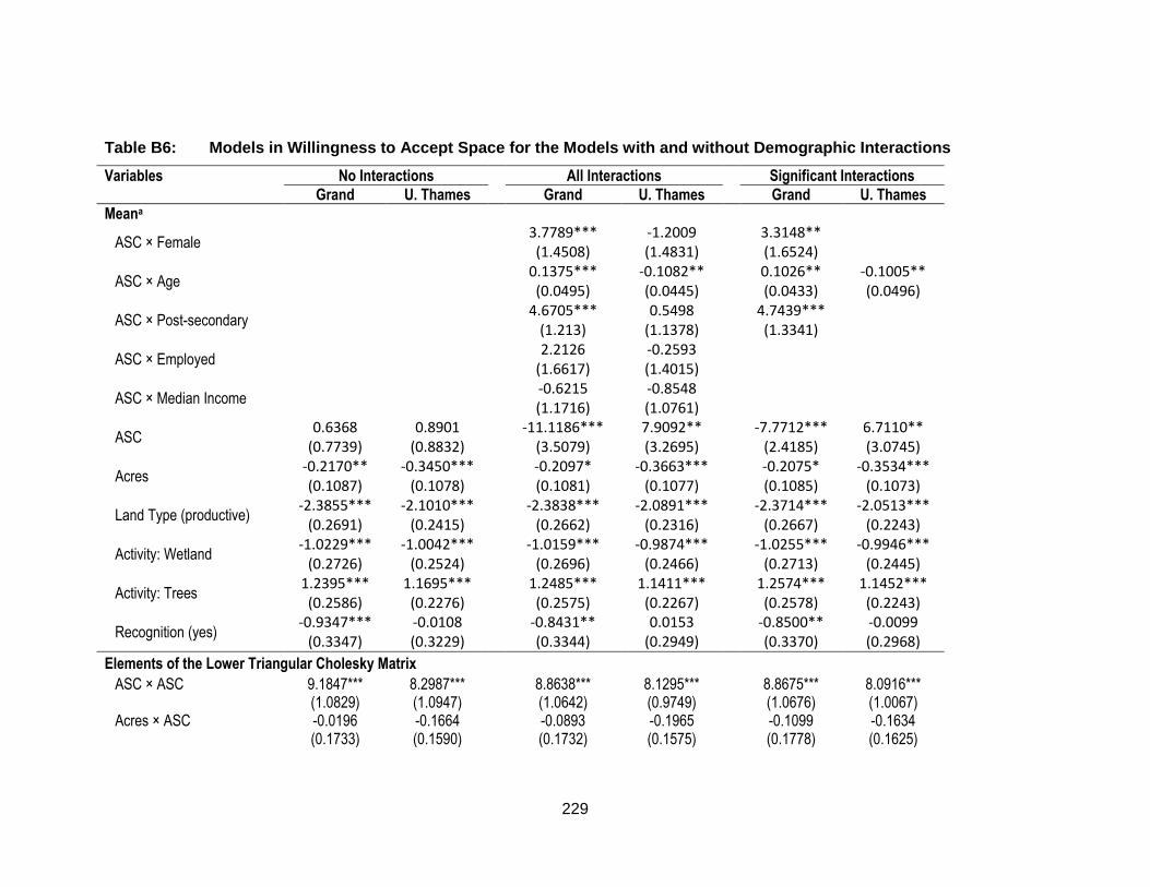
229

Table B6: Models in Willingness to Accept Space for the Models with and without Demographic Interactions

Variables No Interactions All Interactions Significant Interactions

Grand U. Thames Grand U. Thames Grand U. Thames

Meana

ASC × Female

3.7789*** (1.4508)

-1.2009 (1.4831)

3.3148** (1.6524)

ASC × Age

0.1375*** (0.0495)

-0.1082** (0.0445)

0.1026** (0.0433)

-0.1005** (0.0496)

ASC × Post-secondary

4.6705*** (1.213)

0.5498 (1.1378)

4.7439*** (1.3341)

ASC × Employed

2.2126 (1.6617)

-0.2593 (1.4015)

ASC × Median Income

-0.6215 (1.1716)

-0.8548 (1.0761)

ASC 0.6368

(0.7739) 0.8901

(0.8832) -11.1186***

(3.5079) 7.9092** (3.2695)

-7.7712*** (2.4185)

6.7110** (3.0745)

Acres -0.2170** (0.1087)

-0.3450*** (0.1078)

-0.2097* (0.1081)

-0.3663*** (0.1077)

-0.2075* (0.1085)

-0.3534*** (0.1073)

Land Type (productive) -2.3855***

(0.2691) -2.1010***

(0.2415) -2.3838***

(0.2662) -2.0891***

(0.2316) -2.3714***

(0.2667) -2.0513***

(0.2243)

Activity: Wetland -1.0229***

(0.2726) -1.0042***

(0.2524) -1.0159***

(0.2696) -0.9874***

(0.2466) -1.0255***

(0.2713) -0.9946***

(0.2445)

Activity: Trees 1.2395*** (0.2586)

1.1695*** (0.2276)

1.2485*** (0.2575)

1.1411*** (0.2267)

1.2574*** (0.2578)

1.1452*** (0.2243)

Recognition (yes) -0.9347***

(0.3347) -0.0108 (0.3229)

-0.8431** (0.3344)

0.0153 (0.2949)

-0.8500** (0.3370)

-0.0099 (0.2968)

Elements of the Lower Triangular Cholesky Matrix

ASC × ASC 9.1847*** (1.0829)

8.2987*** (1.0947)

8.8638*** (1.0642)

8.1295*** (0.9749)

8.8675*** (1.0676)

8.0916*** (1.0067)

Acres × ASC -0.0196 (0.1733)

-0.1664 (0.1590)

-0.0893 (0.1732)

-0.1965 (0.1575)

-0.1099 (0.1778)

-0.1634 (0.1625)

230



Land Type × ASC 0.2906 (0.3466)

0.1388 (0.2914)

0.2529 (0.3420)

-0.0197 (0.2843)

0.2031 (0.3477)

-0.0251 (0.3160)

Wetland × ASC 0.0928 (0.3890)

-0.0495 (0.3702)

0.0122 (0.3760)

-0.1321 (0.3275)

0.0568 (0.3802)

-0.0788 (0.3588)

Trees × ASC -0.1618 (0.3708)

0.1935 (0.3247)

-0.0896 (0.3640)

0.3069 (0.3075)

-0.1137 (0.3667)

0.2912 (0.3287)


0.0334 (0.4428)

0.2644 (0.4551)

0.0862 (0.4079)

0.2370 (0.4535)

0.0635 (0.4266)

Acres × Acres -0.9384*** (0.1639)

-0.6763*** (0.1300)

-0.8781*** (0.1698)

-0.7027*** (0.1160)

-0.8963*** (0.1745)

-0.7028*** (0.1272)

Land Type × Acres -0.8041* (0.4223)

-0.1149 (0.5588)

-0.8576* (0.5020)

-0.3539 (0.3380)

-0.8657* (0.5261)

-0.2190 (0.4600)

Wetland × Acres -0.0843 (0.4914)

-0.8512** (0.4282)

-0.0110 (0.5038)

-0.9865*** (0.3736)

0.0122 (0.5010)

-0.9501** (0.4048)

Trees × Acres 0.2016 (0.4441)

0.4627 (0.3934)

0.1971 (0.4560)

0.5192 (0.3865)

0.1857 (0.4574)

0.4985 (0.3581)


-0.0439 (0.5524)

0.4106 (0.6391)

-0.1489 (0.4431)

0.3831 (0.6398)

-0.1028 (0.5020)


1.8091*** (0.2765)

-2.5273*** (0.3225)

1.7328*** (0.2528)

-2.5125*** (0.3239)

1.7609*** (0.2528)


-0.4093 (0.3620)

0.9127** (0.3675)

-0.5123 (0.3582)

0.8969** (0.3674)

-0.4364 (0.3550)

Trees × Land Type -0.1564 (0.3436)

-0.1299 (0.3408)

-0.1458 (0.3485)

-0.0327 (0.3484)

-0.1348 (0.3533)

-0.0719 (0.3237)

Recognition × Land Type 0.8387* (0.4574)

0.2680 (0.5567)

0.7264 (0.4614)

0.1979 (0.4264)

0.7119 (0.4571)

0.2334 (0.4388)

Wetland × Wetland -2.6484*** (0.3651)

1.6876*** (0.3356)

-2.6057*** (0.357)

1.6425*** (0.3613)

-2.6154*** (0.3589)

1.6838*** (0.3287)

Trees × Wetland 1.4302*** (0.3674)

-0.4843 (0.4100)

1.4168*** (0.3773)

-0.3799 (0.5396)

1.4116*** (0.3800)

-0.4784 (0.4042)


0.8014 (0.5330)

0.3515 (0.4811)

0.7609 (0.5266)

0.3471 (0.4961)

0.8257 (0.5033)

231



Trees × Trees 2.0661*** (0.2994)

1.1069*** (0.3138)

2.0522*** (0.3008)

1.0568*** (0.3733)

2.0494*** (0.3010)

1.0710*** (0.3073)

Recognition × Trees 0.1441 (0.5155)

-0.1964 (0.5153)

0.0369 (0.4931)

-0.2543 (0.5347)

0.0186 (0.4864)

-0.1979 (0.5149)

Recognition × Recognition -2.2739*** (0.4584)

1.6800*** (0.4406)

-2.3070*** (0.4427)

1.7276*** (0.3626)

-2.3472*** (0.4365)

1.6900*** (0.3925)

Scale

Constant (𝜃) -0.7211*** (0.1658)

-0.3123 (0.3236)

-0.6833*** (0.183)

-0.1323 (0.4315)

-0.7091*** (0.1648)

-0.2267 (0.3805)

Tau (𝜏) 0.1999

(0.3735) 0.5825

(0.3690) 0.3157

(0.2985) 0.7574* (0.3918)

0.2537 (0.3095)

0.6593* (0.3758)

Model Statistics Observations 8550 5661 8550 5661 8550 5661 Log-likelihood -1607.67 -1028.95 -1590.64 -1026.11 -1591.48 -1027.04 Pseudo R2 0.28 0.29 0.29 0.30 0.29 0.30 AIC (BIC) 3273.35

(3477.90) 2115.89

(2308.49)

3249.28 (3489.11)

2120.23 (2346.04)

3246.96 (3472.68)

2114.09 (2313.33)



232

The outcome of the Swait & Louviere (1993) tests are the same for the models

with and without all demographic interactions (Table A7).71 In both cases the tests

indicate that models estimated for the Grand and Upper Thames watersheds do not

differ significantly. The first likelihood ratio tests fail to reject the null hypothesis of equal

model parameters for the model with all demographic interactions

(𝛸(34)2 = 40.90 and corresponding p − value = 0.19) and the model without demographic

interactions (𝛸(29)2 = 25.23 and corresponding p − value = 0.66). Furthermore, the

second likelihood ratio test also fails to reject the null hypothesis of equal scale

parameters for the model with all demographic interactions

(𝛸(1)2 = 0.10 and corresponding p − value = 0.75) and the model without demographic

interactions (𝛸(1)2 = 0.11 and corresponding p − value = 0.75) which corroborates the

insignificance of the parameters accounting for different scales in the initial pooled

models (“Pooled 1”). Though the specifics differ somewhat, the outcomes of these Swait

& Louviere (1993) tests are the same as those in the main text.

71

We do not compare the model with significant demographic interactions with any of the other models using this test.

233

Table B7: Pooled Models in Willingness to Accept Space Serving as Inputs into the Swait and Louviere Test

Variables No Interactions Demographic Interactions

Pooled 1 Pooled 2 Pooled 1 Pooled 2

Meana

ASC × Female

1.8656* (1.1035)

1.8674* (1.1076)

ASC × Age

0.0502 (0.0361)

0.0503 (0.0361)

ASC × Post-secondary

3.5402*** (0.8958)

3.5451*** (0.8960)

ASC × Employed

0.8304 (1.3410)

0.8419 (1.3417)

ASC × Median Income

-0.9195 (0.8562)

-0.9184 (0.8556)

ASC 0.6850

(0.5540) 0.6851

(0.5542) -4.4486

(2.8416) -4.4653 (2.8449)

Acres -0.2634***

(0.0763) -0.2628***

(0.0763) -0.2591***

(0.0770) -0.2584***

(0.0770)

Land Type (productive) -2.2291***

(0.1779) -2.2300***

(0.1780) -2.2256***

(0.1764) -2.2269***

(0.1765)

Activity: Wetland -1.0024***

(0.1848) -1.0023***

(0.1849) -0.9977***

(0.1849) -0.9976***

(0.1851)

Activity: Trees 1.1769*** (0.1741)

1.1769*** (0.1742)

1.1878*** (0.1752)

1.1887*** (0.1755)

Recognition (yes) -0.5269** (0.2233)

-0.5299** (0.2233)

-0.4901** (0.2215)

-0.4938** (0.2216)

Elements of the Lower Triangular Cholesky Matrix

ASC × ASC 8.6896*** (0.7485)

8.6916*** (0.7485)

8.5968*** (0.7489)

8.5986*** (0.7493)

Acres × ASC -0.0952 (0.1192)

-0.0961 (0.1189)

-0.1513 (0.1267)

-0.1517 (0.1265)

Land Type × ASC 0.2761 (0.2365)

0.2758 (0.2361)

0.2134 (0.2492)

0.2126 (0.2494)

Wetland × ASC -0.0423 (0.2666)

-0.0397 (0.2665)

-0.0843 (0.2729)

-0.0808 (0.2728)

Trees × ASC 0.0738 (0.2533)

0.0722 (0.2532)

0.0718 (0.2527)

0.0690 (0.2525)


0.3137 (0.3217)

0.1228 (0.3252)

0.1226 (0.3254)

Acres × Acres -0.8140*** (0.1111)

-0.8160*** (0.1108)

-0.8069*** (0.1153)

-0.8087*** (0.1157)

Land Type × Acres -0.3004 (0.3221)

-0.3083 (0.3222)

-0.3372 (0.3385)

-0.3427 (0.3387)

Wetland × Acres -0.5432 (0.3503)

-0.5397 (0.3511)

-0.5523 (0.3523)

-0.5493 (0.3521)

Trees × Acres 0.4253 (0.3422)

0.4263 (0.3422)

0.4048 (0.3376)

0.4047 (0.3370)

234

Variables No Interactions Demographic Interactions

Pooled 1 Pooled 2 Pooled 1 Pooled 2


0.1204 (0.4315)

0.0972 (0.4197)

0.0962 (0.4194)


-2.2201*** (0.2123)

-2.2240*** (0.2136)

-2.2268*** (0.2137)

Wetland × Land Type 0.6880*** (0.2613)

0.6866*** (0.2617)

0.6676** (0.2712)

0.6674** (0.2712)

Trees × Land Type 0.0259 (0.2476)

0.0244 (0.2478)

0.0378 (0.2533)

0.0374 (0.2534)


0.4150 (0.3431)

0.3615 (0.3416)

0.3669 (0.3413)

Wetland × Wetland 2.2274*** (0.2471)

2.2329*** (0.2461)

2.2410*** (0.2470)

2.2488*** (0.2453)

Trees × Wetland -1.0197*** (0.2723)

-1.0237*** (0.2707)

-1.0415*** (0.2677)

-1.0500*** (0.2653)


0.2937 (0.3523)

0.3024 (0.3551)

0.2970 (0.3534)

Trees × Trees 1.6983*** (0.1978)

1.7007*** (0.1971)

1.7192*** (0.1988)

1.7222*** (0.1983)


-0.0787 (0.3477)

-0.0636 (0.3434)

-0.0639 (0.3424)

Recognition × Recognition -2.0889*** (0.2966)

-2.0927*** (0.2959)

-2.1239*** (0.2936)

-2.1296*** (0.2928)

Scale

Constant (𝜃) -0.6025*** (0.1570)

-0.6217*** (0.1443)

-0.6070*** (0.1490)

-0.6292*** (0.1303)

Grand dataset indicator -0.0373 (0.1150)

-0.0370

(0.1145)

Tau (𝜏) 0.2490

(0.2769) 0.2564

(0.2696) 0.2316

(0.2575) 0.2317

(0.2559)

Model Statistics Observations 14,211 14,211

Log-likelihood -2649.24 -2649.29 -2637.20 -2637.25 a Coefficients represent the negative of WTA values scaled by 100 since the payment attribute was divided by 100 to aid model convergence. Standard errors appear in brackets below the corresponding coefficient.


235

B5.3 Willingness to Accept, Transfer Errors, and Testing

B5.3.1 Marginal Willingness to Accept

The marginal willingness to accept (WTA) estimates derived from the model

without demographic interactions in this appendix (Table B8) are not substantially

different from those estimated for the main text (Table 3.6). While the errors and

tolerance levels are broadly similar as well, these values are generally a lower for the

model without interactions in this appendix. However, there are exceptions – notably the

error and tolerance level values observed for public recognition derived from the model

without interactions in this appendix are much larger than the values in the main text.

Finally, the outcomes of the complete combinatorial tests are the same (at the 95% level

of significance).

Comparing the results for the models without and with demographic interactions

generates a narrative similar to that in the previous paragraph (Tables B8, B9, and B10).

Differences in marginal WTA are observed, though for the most part they are not

substantial. Similarly, transfer errors and tolerance levels resulting from the model

without demographic interaction are generally a little lower than those resulting from the

models with demographic interactions (as evidenced by the medians since the means

are influenced by certain very large errors or tolerance levels). Clear exceptions are

observed when transferring WTA estimates for public recognition to the Upper Thames

— substantially larger errors and tolerance levels result from the model without

interactions for public recognition relative to the model with all demographic interactions

(though not for the reduced specification with significant interactions only). Another

notable exception is observed for transfers of WTA values elicited for the ASC term.

Though the transfer errors observed for the models with demographic interactions are

somewhat larger than those observed for the model without interactions, the tolerance

levels calculated for transfers of WTA for the ASC term derived from the interacted

specifications are many times larger than those levels resulting from the non-interacted

specification. This outcome reflects the higher variation in WTA for the ASC term

observed to result from the model with demographic interactions. The difference in the

width of the confidence intervals between Table A7 and Tables A8 or A90 makes this

evident, and this reflects the difference in the standard deviations of these WTA

estimates (they jump from 88.64 to 328.30 for the Upper Thames and 77.50 to 348.59

236

for the Grand). Dropping insignificant interaction variables does not change this finding

substantially as the standard deviations are 304.94 for the Upper Thames and 240.47 for

the Grand. Lastly, the three model specifications yield the same outcomes for the

complete combinatorial test.

237

Table B8: Marginal WTA and Errors for Transfers Between Two Watersheds in Southern Ontario for the Model with No Demographic Interactions

Attribute


Grand Upper Thames

PS: Grand

PS: Thames

Mean Directional

Chatto- padhyay

CC


Mean Tolerance

(%) PS:

Grand PS:

Thames

ASC -88.21 (-240.64 to

61.63)

-111.59 (-286.1 to 59.51)

27 21 24 23

0.42 247 195 221

Acres 17.57 (-3.53 to 38.38)

30.59 (10.08 to 50.84)

74 43 58 54

0.20 216 124 170

Land Type


232.13 (177.13 to

283.96)

207.46 (156.81 to

255.08)

11 12 11 11

0.25 37 41 39

Marginal (effects)

-232.13 (-283.96 to -

177.13)

-207.46 (-255.08 to -

156.81)

11 12 11 11

0.25 37 41 39


464.27 (354.26 to

567.91)

414.92 (313.62 to

510.16)

11 12 11 11

0.25 37 41 39

Activity

Wetland (effects)

104.97 (50.94 to 160.16)

104.45 (54.72 to 155.56)

0 0 0 0

0.50 61 61 61

Trees (effects)

-118.47 (-168.19 to -

66.63)

-114.59 (-158.5 to -69)

3 3 3 3

0.46 52 54 53

Meadow (effects)

13.50 (-34.53 to 63.38)

10.14 (-34.37 to 56.50)

25 33 29 28

0.46 439 584 512

Meadow to trees

-135.65 (-222.62 to -

50.92)

-124.73 (-199.67 to -

51.30)

8 9 8 8

0.45 77 82 80

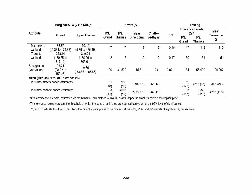
238

Attribute


Grand Upper Thames

PS:

Grand PS:

Thames Mean

Directional Chatto-

padhyay

CC


Mean Tolerance

(%) PS:

Grand PS:

Thames

Meadow to wetland

83.87 (-4.38 to 174.82)

90.12 (5.79 to 175.49)

7 7 7 7

0.48 117 113 115

Trees to wetland

223.44 (130.55 to

317.12)

219.03 (135.06 to

305.01)

2 2 2 2

0.47 50 51 51


92.74 (28.22 to 159.25)

-0.30 (-63.66 to 63.83)

100 31,522 15,811 201

0.02** 184 58,000 29,092


(18) 3956 (16)

1994 (16) 42 (17)

159

(123) 7388 (93) 3773 (93)


4516 (12)

2275 (11) 44 (11)

133 (117)

8372 (113)

4252 (115)



*, **, and *** indicate that the CC test finds the pair of implicit prices to be different at the 90%, 95%, and 99% levels of significance, respectively

239

Table B9: Marginal WTA and Errors for Transfers Between Two Watersheds in Southern Ontario for the Model with All Demographic Interactions

Attribute


Grand Upper Thames

PS: Grand

PS: Thames

Mean Directional

Chatto- padhyay

CC


Mean Tolerance

(%) PS:

Grand PS:

Thames

ASC -82.86 (-771.72 to

610.72)

-129.24 (-778.30 to

528.78)

56 36 46 44

0.46 1007 646 827

Acres 16.88 (-4.07 to 38.36)

32.68 (11.82 to 53.35)

94 48 71 64

0.15 242 125 184

Land Type


232.84 (179.32 to

282.49)

206.92 (160.91 to

252.06)

11 13 12 12

0.23 36 41 39

Marginal (effects)

-232.84 (-282.49 to -

179.32)

-206.92 (-252.06 to -

160.91)

11 13 12 12

0.23 36 41 39


465.69 (358.65 to

564.98)

413.83 (321.82 to

504.12)

11 13 12 12

0.23 36 41 39

Activity

Wetland (effects)

104.90 (51.22 to 158.44)

103.57 (53.28 to 152.64)

1 1 1 1

0.49 60 61 61

Trees (effects)

-119.85 (-170.38 to -

69.29)

-112.14 (-155.75 to -

67.64)

6 7 7 7

0.41 54 58 56

Meadow (effects)

14.95 (-33.07 to 63.21)

8.57 (-34.67 to 51.36)

43 74 58 54

0.42 408 711 560

Meadow to trees

-134.79 (-215.63 to -

50.72)

-120.71 (-191.91 to -

47.52)

10 12 11 11

0.40 80 89 85

240

Attribute


Grand Upper Thames

PS:

Grand PS:

Thames Mean

Directional Chatto-

padhyay

CC


Mean Tolerance

(%) PS:

Grand PS:

Thames

Meadow to wetland 89.95

(2.06 to 180.28)

95.00 (15.17 to 175.61)

6 5 5 5

0.47 118 111 115

Trees to wetland

224.74 (132.38 to

317.51)

215.71 (131.38 to

299.55)

4 4 4 4

0.44 51 53 52


84.38 (18.90 to 149.49)

-2.50 (-60.17 to 53.93)

103 3473 1788 212

0.03** 191 6412 3302


(27) 458 (24) 51 (28) 249 (24)

254 (126)

1012 (93) 633 (93)


513 (13) 50 (12) 277 (12)

246 (118)

1068 (111)

657 (115)




241

Table B10: Marginal WTA and Errors for Transfers Between Two Watersheds in Southern Ontario for the Model with Significant Demographic Interactions

Attribute


Grand Upper Thames

PS: Grand

PS: Thames

Mean Directional

Chatto- padhyay

CC


Mean Tolerance

(%) PS:

Grand PS:

Thames

ASC -80.81 (-551.52 to

391.05)

-118.45 (-714.49 to

487.84)

47 32 39 38

0.46 836 571 704

Acres 16.84 (-4.50 to 38.24)

31.38 (10.97 to 51.94)

86 46 66 60

0.17 235 126 181

Land Type


231.20 (179.19 to

283.75)

203.13 (159.33 to

247.38)

12 14 13 13

0.21 38 43 41

Marginal (effects)

-231.20 (-283.75 to -

179.19)

-203.13 (-247.38 to -

159.33)

12 14 13 13

0.21 38 43 41


462.40 (358.38 to

567.5)

406.25 (318.66 to

494.76)

12 14 13 13

0.21 38 43 41

Activity

Wetland (effects)

105.36 (50.40 to 159.56)

104.42 (55.38 to 153.79)

1 1 1 1

0.49 60 60 60

Trees (effects)

-120.63 (-171.12 to -

71.1)

-113.39 (-158.02 to -

68.18)

6 6 6 6

0.42 53 56 55

Meadow (effects)

15.26 (-33.60 to 63.31)

8.97 (-33.83 to 51.74)

41 70 56 52

0.43 400 680 540

Meadow to trees

-135.89 (-217.35 to -

55.63)

-121.50 (-194.23 to -

48.30)

11 12 11 11

0.41 78 87 83

242

Attribute


Grand Upper Thames

PS:

Grand PS:

Thames Mean

Directional Chatto-

padhyay

CC


Mean Tolerance

(%) PS:

Grand PS:

Thames

Meadow to wetland

82.42 (-8.80 to 173.15)

91.27 (9.62 to 172.09)

11 10 10 10

0.47 120 113 117

Trees to wetland

225.99 (134.20 to

319.94)

217.82 (134.39 to

301.83)

4 4 4 4

0.45 50 52 51


85.09 (19.97 to 150.55)

0.17 (-58.44 to 58.96)

100 48,742 24421 199

0.03** 188 91,000 45,594


(27) 6116 (23)

3077 (23) 48 (25)

231

(124) 11,572

(93) 5902 (93)


6980 (14)

3509 (13) 48 (13)

221 (120)

13,142 (113)

6681 (117)




243

B5.3.2 Compensating Surplus

The compensating surplus (CS) estimates derived from the model without

demographic interactions (Figure B2a) follow a trend similar to that of the CS estimates

presented in the main text (Figure 3.2). Additionally, the estimates derived from the

model without interactions appear quite similar to those estimated from the models with

demographic interactions (Figures B2b and B2c).

244

Figure B2: Compensating Surplus Estimates for All Possible Program Specifications by Watershed for the Models without Interactions (a), with all Demographic Interactions (b), and with Significant Demographic Interactions (c)

Comparing transfer results for the model without interactions in this appendix

(Table B11 and Figure B3) with those results for the model without interactions in the

main text (Table 3.7 and Figure 3.3) reveals that the latter yields modestly higher

transfer errors, in general, though the tolerance levels derived from this model are a little

lower according to the median values (the means indicate the opposite in terms of

245

tolerance levels). Transfers of values resulting from both of these models are generally

marginally larger when the Upper Thames is treated as the policy site relative to when

the policy site is the Grand. Additionally, the outcomes of the complete combinatorial

tests are nearly identical (though two pairs of estimates differ significantly at the 10%

level in the analysis completed as part of the main text compared to no significantly

different pairs in the assessment presented in this appendix). In sum, the validity and

reliability of transfers based on these two models are fairly similar.

Table B11: Summary of Errors, Tolerance Levels, and Complete Combinatorial Tests for Transfers of Compensating Surplus Between Two Southern Ontario Watersheds

Transfer Transfer Errors (%) Tolerance Levels (%) CC (Different

Pairs) Mean Median Low High Mean Median Low High

Model without Demographic Interactions

Directional Grand to U. Thames

67 25 3 1073 275 122 60 2839 N/A

U. Thames to Grand

30 23 3 91 158 106 59 688

Non-Directional Grand and U. Thames

34 23 3 169 N/A 0*, 0**, 0***

Model with All Demographic Interactions


197 27 0 3168 2395 416 191 47,000 N/A

U. Thames to Grand

32 25 0 104 506 367 190 1927


39 24 0 216 N/A 0*, 0**, 0***

Model with Significant Demographic Interactions


203 26 0 4542 1876 352 162 27,000

N/A U. Thames to Grand

30 22 0 98 426 303 157 1762


37 23 0 192 N/A 0*, 0**, 0***

*, **, and *** indicate the number of pairs of compensating surplus estimates the CC test finds different at the 90%, 95%, and 99% levels of significance, respectively

Given the similarity in CS estimates observed to result from the three model

specifications (Figure B2) it is not surprising that the transfer errors are fairly similar

246

overall as evidenced by the median values in Table B11 (certain large errors skew the

mean) and distributions illustrated in Figure B3. However, there is a notable difference in

tolerance levels across the models with and without interactions even when looking at

the median (which limits the influence of outliers). Tolerance levels are clearly larger for

transfers of CS estimates derived from the interacted specifications than transfers of

these estimates derived from the non-interacted specification. The divergent tolerance

levels likely result from the fact that WTA for the ASC term derived from the models with

demographic interactions is more variable than it is when estimated from the model

without such interactions (as observed in Tables B8 to B10). Indeed, the mean of the

standard deviation of the CS estimates is 323.40 for the Upper Thames and 351.26 for

the Grand for the model with interactions, while the standard deviations are 90.84 for the

Upper Thames and 83.44 for the Grand for the models without interactions. Dropping

insignificant interactions reduces the standard deviations somewhat to 301.73 and

243.88 for the Upper Thames and Grand, respectively. In all cases these standard

deviations are aligned with those of the marginal WTA for the ASC term. In addition, the

influence of transfer direction is the same for all specifications, as transfers to the Upper

Thames only result in slightly larger median errors and tolerance levels relative to

transfers in the other direction for the three models. Finally, in terms of the complete

combinatorial test, the three model specifications yield identical outcomes.

247

Figure A3: Box Plots of Transfer Errors and Tolerance Levels for the Model without Demographic Interactions (a), with All Demographic Interactions (b), and with Significant Demographic Interactions (c)a, b

Note: Outlier points are not plotted. Directional error boxes are dark grey, tolerance level boxes are light grey, and Chattopadhyay error boxes are white. In addition, the range of the x-axis for each panel differs from the range used for the boxplot in the main text, which has an upper limit of 300.

248

B5.3.3 Effect of Dropping Insignificant Demographic Interactions

Removing insignificant interaction variables has little effect on the parameters

common to the model with all interactions (although we did not formally test the similarity

of the two models). The marginal WTA and CS estimates are also similar across these

two specifications. Likewise, although we observed slight improvements in accuracy

there is little difference in the transfer errors resulting from this reduced model and the

model with all demographic interactions. In addition, the two models yield identical

outcomes for the complete combinatorial test. The issue motivating this extra model

specification, the large tolerance levels observed to result for transfers of WTA for the

ASC term and all the CS estimates, is still an issue for transfers based on the reduced

specification with significant interactions only. However, the tolerance levels are slightly

less as evidenced by Tables B10 and B11 as well as Figure B3.

B5.4 Conclusion

Overall, for the estimates derived from the model without interactions, the

directional errors for transfers of marginal WTA range from 0% to 31,522% with a mean

of 1331% and median of 11%, while these errors for transfers of CS range from 3% to

1073% with a mean of 48% and median of 24%. Non-directional Chattopadhyay errors

for transfers of marginal WTA from this model range from 0% to 201% with a mean of

30% and median of 11%. These errors range from 3% to 169% for transfers of

compensating surplus with a mean of 34% and median of 23%. For values elicited with

this model, tolerance levels estimated for marginal WTA range from 37% to 58,000%

with a mean of 2539% and median of 69%, while they range from 59% to 2839% for CS

with a mean of 216% and median of 117%.

In terms of the estimates derived from the model with all demographic

interactions, directional errors range from 1% to 3473% for transfers of marginal WTA

with a mean of 169% and median of 11%, while they range from 0% to 3168% for

transfers of CS with a mean of 115% and median of 26%. The corresponding non-

directional errors for transfers of marginal WTA range from 1% to 212% with a mean of

36% and median of 12%, while these errors range from 0% to 216% for transfers of CS

with a mean of 39% and median of 24%. The tolerance levels estimated from this model

for marginal WTA range from 36% to 6412% with a mean of 446% and median of 71%,

249

and range from 190% to 47,000% with a mean of 1451% and median of 391% for

compensating surplus.

For the model with significant demographic interactions only, directional errors

range from 1% to 48,742% for transfers of marginal WTA with a mean of 2054% and

median of 12%, while they range from 0% to 4542% for transfers of CS with a mean of

117% and median of 24%. The analogous non-directional errors range from 1% to 199%

with a mean of 35% and median of 13% for transfers of marginal WTA %, while these

errors range from 0% to 192% for transfers of CS with a mean of 37% and median of

23%. The related tolerance levels for marginal WTA range from 38% to 91,000% with a

mean of 3959% and median of 69%, and range from 157% to 47,000% with a mean of

1151% and median of 322% for compensating surplus.

Outliers aside, the errors from these two model specifications are fairly similar,

and not that different from those in the main text. Furthermore, most of the tolerance

levels for transfers of marginal WTA are similar for these specifications too. However,

the key difference between transfers based on the two model specifications is that the

tolerance levels are clearly higher for transfers of CS values derived from the model with

demographic interactions. These interactions clearly result in more inefficient CS

estimates via inflated variance of WTA for the ASC term. Basing our validity and

reliability assessment on a model with significant interactions only appears to reduce

tolerance levels, but only slightly — the issue still remains.

250

References

Chattopadhyay, S. (2003). A Repeated Sampling Technique in Assessing the Validity of Bene t Transfer in Valuing Non-Market Goods. Land Economics, 79(4), 576–596.

Kaul, S., Boyle, K. J., Kuminoff, N. V, Parmeter, C. F., & Pope, J. C. (2013). What can we learn from benefit transfer errors? Evidence from 20 years of research on convergent validity. Journal of Environmental Economics and Management, 66(1), 90–104. http://doi.org/10.1016/j.jeem.2013.03.001

Swait, J., & Louviere, J. (1993). The Role of the Scale Parameter in the Estimation and Comparison of Multinomial Logit Models. Journal of Marketing Research, 30(3), 305–314.

251

Appendix C. Supplementary Material for Chapter 4

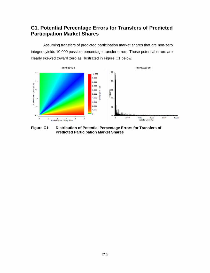
252

C1. Potential Percentage Errors for Transfers of Predicted Participation Market Shares

Assuming transfers of predicted participation market shares that are non-zero

integers yields 10,000 possible percentage transfer errors. These potential errors are

clearly skewed toward zero as illustrated in Figure C1 below.

Figure C1: Distribution of Potential Percentage Errors for Transfers of Predicted Participation Market Shares

253

C2. The Choice Experiment

We have included a copy of the choice experiment’s preamble and first choice

set for reference.



PROGRAM CONDITIONS:
















254

SET 1:













1 2 3 4 5 6 7 8 9 10


255

C3. Variance-Covariance Matrix and Standard Deviation Parameters

We generated each variance-covariance matrix (Σ) by multiplying the lower-triangular of the Cholesky matrix (𝐿) by its

transpose (Σ = 𝐿𝐿′) using the ‘mixlcov’ command in Stata 12.1 (Hole, 2007). To generate the standard deviation parameters we

squared each element of the lower-triangular of the Cholesky matrix, added the resulting values in each row, and then took the

square root if this sum.

Table C1: Variance-Covariance Matrix and Standard Deviation Parameters Estimated from the Lower-Triangular of the Cholesky Matrix

Variance-Covariance Matrix Standard Deviation ASC Acres Wetland Trees

Technical help (Yes)

Recognition (Yes)

ln(Annual payment)

Grand River Watershed

ASC 37.8621*** (11.5283)

6.1532*** (0.9368)

Acres 6.3383** (2.6185)

4.5000*** (1.6804)

2.1213*** (0.3961)

Wetland 4.6354 (3.1542)

1.3539 (1.0967)

9.6376*** (2.6312)

3.1045*** (0.4238)

Trees -0.4707 (2.2350)

-0.0005 (0.7607)

-5.5930*** (1.5825)

5.6662*** (1.5389)

2.3804*** (0.3232)


-0.6342 (2.0616)

-0.0377 (0.7039)

0.4826 (0.8356)

-1.2390* (0.7410)

1.4589* (0.7684)

1.2078*** (0.3181)


-0.5794 (0.7841)

-0.7634 (0.7941)

-0.3830 (0.6471)

0.1343 (0.4379)

1.7708* (0.9962)

1.3307*** (0.3743)

ln(Annual payment)

0.4636 (0.7987)

0.2574 (0.2746)

0.4821 (0.3500)

-0.3048 (0.2674)

-0.8571** (0.3785)

-1.0561* (0.5456)

1.7771*** (0.4168)

1.3331*** (0.1563)

Upper Thames River Watershed

ASC 30.6267*** (9.1682)

5.5341*** (0.8283)

256

Variance-Covariance Matrix Standard Deviation ASC Acres Wetland Trees


Recognition (Yes)

ln(Annual payment)

Acres 3.2891 (2.0972)

3.5766** (1.5207)

1.8912*** (0.4021)

Wetland -0.6112 (2.0331)

0.6860 (0.7994)

5.4788*** (1.4737)

2.3407*** (0.3148)

Trees 3.8384* (2.2375)

0.1810 (0.7249)

-2.9022*** (0.8845)

4.3486*** (1.2629)

2.0853*** (0.3028)


-0.5060 (1.9115)

-1.4019 (0.8558)

0.7786 (0.6888)

-1.1340* (0.6516)

1.9347** (0.9834)

1.3909*** (0.3535)

Recognition (Yes) 1.0239 (1.5615)

0.4597 (0.6008)

0.4607 (0.5063)

-0.3439 (0.4545)

0.1235 (0.3874)

0.1789 (0.2164)

0.4229* (0.2558)

ln(Annual payment)

0.0477 (0.7841)

-0.5813** (0.2778)

0.3385 (0.3420)

0.4396 (0.3131)

0.1011 (0.2429)

-0.3228 (0.4312)

1.9893*** (0.5340)

1.4104*** (0.1893)

*, **, and *** indicate that the estimate differs from zero at the 90%, 95%, and 99% levels of significance, respectively

257

C4. Results for Mean of Mean Derivation Approach

We did not include the predicted participation market share and compensating

surplus estimates generated via the ‘mean of mean’ approach and the ensuing transfer

assessment in the main text since in many cases this approach yields unreasonably

large CS estimates (see Figure C2 panel b). However, we did perform the transfer

validity and reliability assessment using these CS and MS estimates as input and we

have included these results as Appendix C4.

Figure C2: Market Share (a) and Compensating Surplus (b) Estimates Note: For both panels the x-axis represents all possible program specifications (e.g., for panel (a) a point on this axis represents a program with 0.5 acres converted to wetlands with no technical help or recognition and a payment of $50, etc. and the points on this axis in panel (b) are similar though do not include a payment component.

As can be seen in Table C2 and Figure C3, the results are similar to those

observed for the ‘mean of median’ derivation approach in that transfer errors and

tolerance levels are much lower for predicted participation market shares compared to

compensating surplus. However, transfers of estimates derived following the ‘mean of

mean’ approach often yield lower transfer errors and tolerance levels relative to those

resulting from the ‘mean of median’ approach. The results of the complete combinatorial

tests are similar for the two approaches, however 6 pairs of market share estimates

generated via the ‘mean of mean’ approach differ significantly at 10% while none of the

pairs generated via the ‘mean of median’ approach significantly differed.

258

Table C2: Summary of Reliability and Validity Tests


Directional

MS: Grand to Thames

4 3 0 9 15 15 7 25

N/A

MS: Thames to Grand

4 3 0 9 15 15 7 24

CS: Grand to Thames

74 34 0 346 372 253 133 1298

CS: Thames to Grand

144 36 0 1045 693 312 127 4173

Non-Directional

MS: Grand and Thames

4 3 0 9

N/A 6*, 0**, 0***


187 36 0 1612

0*, 0**, 0***

*, **, and *** indicate the number of pairs of estimates that are different at the 90%, 95%, and 99% levels of

significance, respectively

We can also see that transfer direction impacts transfers of the ‘mean of mean’

CS estimates with those to the Grand yielding a wider range of errors and tolerance

levels relative to transfers in the other direction (Figure C3). Such a finding is not evident

for the directional errors and tolerance levels calculated from the ‘mean of median’

estimates.

Figure C3: Boxplots of Transfer Errors and Tolerance Levels Note: outliers not plotted; non-directional errors are white and directional errors are differing shades of grey.

The directional and non-directional errors levels calculated for compensating

surplus derived via the ‘mean of mean’ approach are significantly larger for

259

specifications involving larger areas and conversion of land to wetlands, and lower for

specifications involving conversion to trees and technical help (Table C3). The

relationships observed for the compensating surplus tolerance levels are similar, though

the area conserved has no significant impact. For predicted participation market shares,

directional and non-directional errors are significantly lower for specifications that involve

converting land to trees, technical help, and higher payments. These errors are

significantly higher for specifications that involve converting land to wetland. Predicted

participation market share tolerance levels are lower for specifications that involve

smaller areas, converting land to trees, technical help, no public recognition, and higher

payments. Transfer direction only significantly impacts tolerance levels in the case of

compensating surplus tolerance levels. These results suggest that compensating surplus

and predicted participation market shares are differently impacted by transfer

characteristics. In many cases these relationships are similar to those observed for

transfers of the estimates derived via the ‘mean of median’ approach, with the notable

exception of the impact of the conversion activity attribute on errors and tolerance levels.

260

Table C3: Regression of Errors and Tolerance Levels on Transfer Characteristics for Transfers Based on the “Mean of Mean” Approacha

Variable Directional Errors Tolerance Levels Non-Directional Errors

MS CS MS CS MS CS

Constant 0.8946*** (0.0393)

3.5633*** (0.1544)

2.6781*** (0.0055)

5.8342*** (0.0622)

0.8943*** (0.0562)

3.7294*** (0.2252)

Area: 0.5 ac

-0.0248 (0.0555)

-0.5776*** (0.2184)

-0.0164** (0.0078)

-0.1238 (0.0879)

-0.0248 (0.0795)

-0.5708* (0.3185)

Area: 1 ac

-0.0021 (0.0555)

0.2024 (0.2184)

-0.0162** (0.0078)

-0.0192 (0.0879)

-0.0021 (0.0795)

0.2454 (0.3185)

Area: 1.5 acb

0.0269 (0.0555)

0.3752* (0.2184)

0.0327*** (0.0078)

0.1430 (0.0879)

0.0269

(0.0795) 0.3254

(0.3185)

Activity: Wetland

0.8333*** (0.0555)

0.9676*** (0.2184)

0.2438*** (0.0078)

0.5129*** (0.0879)

0.8330*** (0.0795)

1.3582*** (0.3185)

Activity: Trees

-0.7721*** (0.0555)

-0.8563*** (0.2184)

-0.2918***

(0.0078) -0.6118***

(0.0879)

-0.7720*** (0.0795)

-1.0351*** (0.3185)

Activity: Meadowb

-0.0611 (0.0555)

-0.1113 (0.2184)

0.0480*** (0.0078)

0.0989 (0.0879)

-0.0611 (0.0795)

-0.3231 (0.3185)

Technical help: Yes

-0.0661* (0.0393)

-0.8648*** (0.1544)

-0.0632***

(0.0055) -0.3930***

(0.0622)

-0.0660 (0.0562)

-1.0566*** (0.2252)

Technical help: Nob

0.0661* (0.0393)

0.8648*** (0.1544)

0.0632*** (0.0055)

0.3930*** (0.0622)

0.0660

(0.0562) 1.0566*** (0.2252)

Recognition: Yes

0.0194 (0.0393)

-0.2228 (0.1544)

0.0170*** (0.0055)

-0.0046 (0.0622)

0.0194

(0.0562) -0.2567 (0.2252)

Recognition: Nob

-0.0194 (0.0393)

0.2228 (0.1544)

-0.0170***

(0.0055) 0.0046

(0.0622)

-0.0194 (0.0562)

0.2567 (0.2252)

Payment: $0

0.2629*** (0.0878)

0.1862*** (0.0124)

0.2628** (0.1258)

Payment: $50

0.2210** (0.0878)

0.0945*** (0.0124)

0.2209* (0.1258)

Payment: $100

0.0908 (0.0878)

0.0075

(0.0124)

0.0908 (0.1258)

Payment: $150

-0.1285 (0.0878)

-0.0591***

(0.0124)

-0.1285 (0.1258)

Payment: $200

-0.1820** (0.0878)

-0.0964***

(0.0124)

-0.1820 (0.1258)

Payment: $250b

-0.2641*** (0.0878)

-0.1327***

(0.0124)

-0.2641** (0.1258)

Grand to Thames

-0.0061 (0.0393)

-0.1452 (0.1544)

-0.0047 (0.0055)

-0.1453** (0.0622)

Thames to Grandb

0.0061 (0.0393)

0.1452 (0.1544)

0.0047

(0.0055) 0.1453** (0.0622)

n 432 72 432 72 216 36 R2 0.43 0.50 0.84 0.62 0.43 0.62 *, **, and *** indicate that the parameter estimate differs from zero at the 90%, 95%, and 99% levels of significance, respectively

a Standard errors appear in brackets below the associated parameter estimates.

261

b Parameter estimate calculated as the negative of the associated parameters using the Delta method.

262

C5. Selected Results for Other Models

Certain results for the other models not presented in the main text are included in

Appendix C5: unweighted by certainty with ln(payment); weighted by certainty with fixed

payment; and unweighted by certainty with fixed payment. Each of these models was

run six times and the iteration yielding the lowest log-likelihood chosen as the final

model. We did not perform the Swait and Louviere test assessing the equality of model

parameters, nor did we perform regressions of errors or tolerance intervals on transfer

characteristics. Unlike Appendix C4, we do not include accompanying text.

263

Table C4: Random Parameter Models by Watershed

Variable Unweighted With ln(Payment) Weighted With Fixed Payment Unweighted With Fixed Payment

Grand Upper Thames Grand Upper Thames Grand Upper Thames

Mean

ASC 1.1561*** (0.4419)

0.9925** (0.4154)

0.9682** (0.4668)

1.4656*** (0.4718)

1.1013*** (0.3979)

1.3111*** (0.3782)

Acres -0.6759*** (0.2051)

-0.5543*** (0.2039)

-0.7072*** (0.2320)

-0.4534** (0.2095)

-0.6156*** (0.1788)

-0.3554** (0.1730)

Conversion Activity: Wetland -1.2139*** (0.2251)

-0.8556*** (0.1949)

-1.2181*** (0.2639)

-0.6805*** (0.1897)

-1.0172*** (0.1970)

-0.7098*** (0.1610)

Conversion Activity: Trees 1.5572*** (0.1930)

1.6761*** (0.1932)

1.4634*** (0.2161)

1.4327*** (0.1954)

1.2923*** (0.1627)

1.4134*** (0.1586)

Conversion Activity: Meadowa

-0.3433** (0.1614)

-0.8205*** (0.1675)

-0.2453 (0.1780)

-0.7521*** (0.1766)

-0.2751** (0.1382)

-0.7036*** (0.1455)


0.7516*** (0.1786)

1.1560*** (0.2154)

0.6722*** (0.1940)

0.9814*** (0.1643)

0.5924*** (0.1562)

Recognition (Yes) -0.6847*** (0.1790)

-0.6672*** (0.1609)

-0.4926*** (0.1896)

-0.5941*** (0.1553)

-0.5025*** (0.1465)

-0.5584*** (0.1289)

Annual payment -5.2185*** (0.1989)

-5.4795*** (0.2402)

0.0092*** (0.0012)

0.0075*** (0.0010)

0.0083*** (0.0009)

0.0070*** (0.0008)

Correlation (Lower-Triangular of the Cholesky Matrix) ASC × ASC 5.7724***

(0.7087) 5.4252*** (0.6496)

5.7609*** (0.7454)

4.7935*** (0.6277)

5.1523*** (0.5857)

-4.6578*** (0.4980)

Acres × ASC 0.7916** (0.3180)

0.2854 (0.3085)

1.0955*** (0.3583)

0.6591* (0.3378)

1.0566*** (0.2802)

-0.3663 (0.2840)

Wetland × ASC 0.6725** (0.3407)

-0.1317 (0.2866)

0.8052** (0.3749)

-0.1185 (0.3103)

0.6515** (0.2959)

0.1023 (0.2586)

Trees × ASC -0.1224 (0.2797)

0.5713** (0.2909)

-0.1804 (0.3071)

0.6227** (0.3133)

-0.2016 (0.2372)

-0.4711* (0.2532)

Technical × ASC -0.0984 (0.2622)

0.0124 (0.2648)

-0.3150 (0.3007)

-0.1668 (0.2845)

-0.3370 (0.2495)

0.0828 (0.2391)


0.2485 (0.2177)

-0.1172 (0.2846)

0.0572 (0.2410)

-0.0321 (0.2222)

-0.0462 (0.2032)

264



Payment × ASC -0.0520 (0.1137)

-0.3906*** (0.1033)

Acres × Acres 1.8686*** (0.3540)

1.6283*** (0.3060)

-1.6241*** (0.3949)

1.3325*** (0.4503)

1.1495*** (0.3786)

-1.4035*** (0.3595)

Wetland × Acres 0.1434 (0.3543)

0.4954 (0.3468)

-0.3218 (0.4475)

0.6432 (0.5650)

0.1828 (0.3994)

-0.5350 (0.3483)

Trees × Acres 0.0955 (0.2799)

-0.1000 (0.3040)

-0.0468 (0.3726)

-0.1014 (0.5005)

0.1877 (0.3721)

0.0491 (0.3052)

Technical × Acres -0.1568 (0.3237)

-0.6382** (0.3239)

0.1492 (0.4133)

-0.7813** (0.3972)

-0.1587 (0.4835)

0.7440** (0.3131)

Recognition × Acres -0.3206 (0.3399)

0.0297 (0.2466)

0.5076 (0.3524)

-0.0950 (0.3118)

-0.7275** (0.3674)

0.0122 (0.2397)

Payment × Acres 0.2454* (0.1299)

0.0136 (0.1310)

Wetland × Wetland 2.8884*** (0.3287)

2.2425*** (0.2670)

-2.6722*** (0.3230)

1.8978*** (0.3170)

-2.4080*** (0.2397)

1.9136*** (0.2212)

Trees × Wetland -1.7061*** (0.2575)

-1.2286*** (0.2231)

1.6531*** (0.2624)

-1.1290*** (0.2745)

1.4528*** (0.2068)

-1.1143*** (0.2004)

Technical × Wetland 0.1858 (0.2221)

0.4739** (0.1990)

-0.0695 (0.2323)

0.4687* (0.2557)

-0.1312 (0.1810)

0.4198** (0.1862)

Recognition × Wetland -0.2477 (0.2225)

0.2018 (0.1760)

0.1801 (0.2420)

0.2548 (0.2203)

0.1342 (0.2048)

0.1857 (0.1713)

Payment × Wetland 0.1224 (0.1476)

0.1472 (0.1313)

Trees × Trees -1.4339*** (0.1825)

-1.4194*** (0.1688)

-1.2943*** (0.1916)

-1.3485*** (0.1826)

1.1418*** (0.1622)

1.2680*** (0.1524)

Technical × Trees 0.7279*** (0.2430)

0.3678* (0.2104)

0.4246 (0.2755)

0.4292* (0.2585)

-0.4691* (0.2739)

-0.3452* (0.1958)

Recognition × Trees 0.3757 (0.2418)

0.2047 (0.1873)

0.4354 (0.2660)

0.2635 (0.2092)

-0.3515 (0.2677)

-0.1847 (0.1727)

Payment × Trees 0.1270 (0.1499)

-0.6169*** (0.1355)

265



Technical × Technical -1.0411*** (0.2732)

0.6689* (0.3422)

-1.2895*** (0.3347)

0.6673 (0.4115)

-1.0851*** (0.3093)

-0.5000 (0.3713)

Recognition × Technical 0.1417 (0.2986)

0.0292 (0.3172)

-0.1237 (0.3810)

0.0939 (0.4679)

-0.1227 (0.4127)

-0.5064* (0.3048)

Payment × Technical 0.8469*** (0.1582)

-0.1722 (0.1217)

Recognition × Recognition 1.2416*** (0.3095)

-0.1493 (0.2881)

1.1899*** (0.3331)

0.3517 (0.4760)

-0.8122** (0.3969)

0.1254 (0.4886)

Payment × Recognition -0.9667*** (0.1784)

1.4339*** (0.1662)

Payment × Payment 0.0934 (0.1362)

-0.0411 (0.2271)

Model Statistics Log-Likelihood -1755.78 -1548.62 -1265.89 -1131.23 -1780.84 -1573.11 Observations 7263 6363 7263 6363 7263 6363 Pseudo R2 0.34 0.33 0.35 0.34 0.33 0.32


a As activity variables are effects coded, meadow parameter derived as negative of other activity parameters via the Delta method

266

Table C5: Results of the Log-Likelihood Tests Comparing Models with Log-Normal and Fixed Payment

Watershed Certainty Calibration

Weighted Unweighted

Upper Thames 𝛸(7)2 = 34.79 with 𝑝 < 0.01 𝛸(7)

2 = 48.99 with 𝑝 < 0.01

Grand 𝛸(7)2 = 35.12 with 𝑝 < 0.01 𝛸(7)

2 = 50.12 with 𝑝 < 0.01

267

C5.1 Output from the Model with Log-Normal Payment and No Calibration for Certainty

Figure C4: Market Share (a, c) and Compensating Surplus (b, d) Estimates Note: for both panels the x-axis represents all possible program specifications (e.g., for panels (a) and (c) a point on this axis represents a program with 0.5 acres converted to wetlands with no technical help or recognition and a payment of $50, etc. and the points on this axis in panels (b) and (d) are similar though do not include a payment component.

268



Mean of Mean

Directional MS: Grand to Thames

3 2 0 9 12 12 5 22

N/A

MS: Thames to Grand

3 2 0 9 12 12 5 20

CS: Grand to Thames

75 69 44 135 223 209 175 336

CS: Thames to Grand

583 224 80 3856 1609 691 315 9811

Non-Directional MS: Grand and Thames

3 2 0 9

N/A 9*, 0**, 0***


132 106 57 416

17*, 7**, 1***

Mean of Median

Directional

MS: Grand to Thames

4 2 0 32 18 11 1 100

N/A

MS: Thames to Grand

4 2 0 24 18 11 1 100

CS: Grand to Thames

143 35 1 1394 537 244 69 3288

CS: Thames to Grand

65 30 1 310 313 184 68 1114

Non-Directional


4 2 0 28

N/A 4*, 0**, 0***


106 34 1 626

1*, 0**, 0***


269

Figure C5: Boxplots of Transfer Errors and Tolerance Levels Note: Outliers not plotted; non-directional errors are white and directional errors are differing shades of grey.

270

C5.2 Output from the Model with Fixed Payment and Calibration for Certainty


271



Mean of Mean

Directional

MS: Grand to Thames

5 4 0 14 16 15 8 26

N/A

MS: Thames to Grand

6 5 0 16 17 16 8 30

CS: Grand to Thames

199 45 1 4618 583 181 56 11,000

CS: Thames to Grand

168 61 1 1532 608 235 71 7665

Non-Directional


6 5 0 15

N/A 58*, 18**, 0***


465 47 1 12,779

7*, 0**, 0***

Mean of Median

Directional

MS: Grand to Thames

6 3 0 44 21 15 1 93

N/A

MS: Thames to Grand

7 3 0 79 24 15 1 166

CS: Grand to Thames

134 50 2 1153 465 225 56 3106

CS: Thames to Grand

144 68 1 964 509 221 71 3920

Non-Directional


6 3 0 57

N/A 12*, 0**, 0***


332 54 1 5744

6*, 0**, 0***


272


273

C5.3 Output from the Model with Fixed Payment and No Calibration for Certainty


274



Mean of Mean

Directional

MS: Grand to Thames

4 4 0 10 13 13 7 21

N/A

MS: Thames to Grand

4 4 0 11 14 13 7 24

CS: Grand to Thames

111 38 1 1111 413 150 48 3157

CS: Thames to Grand

159 46 1 2464 543 170 58 8094

Non-Directional


4 4 0 10

N/A 28*, 0**, 0***


108 47 1 945

7*, 0**, 0***

Mean of Median

Directional

MS: Grand to Thames

4 2 0 30 16 12 1 73

N/A

MS: Thames to Grand

4 2 0 42 17 12 1 104

CS: Grand to Thames

157 37 3 3012 559 199 49 9330

CS: Thames to Grand

447 54 3 12,904 1341 193 60 34,000

Non-Directional


4 2 0 35

N/A 6*, 0**, 0***


165 45 3 1376

4*, 0**, 0***


275


276

References


277

Appendix D. Supplementary Material for Chapter 5

278

D1. Demographic Characteristics of Each Watershed

There is a near even split of genders of the population in or near each

watershed, although the Ontario watersheds have slightly more females than males,

while the Salmon has slightly more males than females (Table D1). On average,

residents of the Humber are youngest, followed very closely by those in the Credit, and

then more distantly by residents of the Little and Salmon watersheds. Overall, residents

of the Humber appear most educated, followed by the Credit or Salmon, and then the

Little. However, those holding a post-secondary diploma or bachelor’s degree form the

largest group in each watershed. In all but the Little, the second largest group is those

with a high school diploma, followed by those with less than high school, and then those

with a graduate degree (in the Little the second and third largest groups switch places).

The proportion of those employed is similar across watersheds, though highest in the

Credit, followed by the Little, Humber, and then Salmon, while the proportion of those

not in the labour force forms the second largest group and is highest in the Salmon,

followed by the Humber, Little, and Credit. The unemployment rate is highest in the

Little, followed by the Humber, Credit, and then more distantly the Salmon. On average,

residents of the two Ontario watersheds have the highest income — with the income of

those in the Credit a little higher than the Humber — followed by the Salmon, and then

the Little.

279

Table D1: Key Demographic Characteristics for the Little, Humber, Credit, and Salmon River Watersheds

Watershed Characteristicsa Little Humber Credit Salmon

Gender (%) Female 50.0 51.4 51.0 49.6 Male 50.0 48.6 49.0 50.4

Age in years Weighted mean of dissemination area medians

44.2 38.3 38.5 49.3

Education (%) Less than high school 33.8 24.4 15.9 20.1 High school 29.7 27.9 26.6 32.3 Diploma or bachelor’s degree 34.7 40.1 47.1 43.5 Graduate degree 1.7 7.6 10.4 4.0

Employment status (%) Employed 59.2 59.1 64.0 57.5 Unemployed 6.8 5.4 5.3 4.0 Not in labour force 34.0 35.6 30.7 38.5

Income (%) Less than $10,000 0.0 2.2 1.7 0.8 $10,000 to $29,999 21.6 12.8 7.9 15.9 $30,000 to $49,999 27.9 17.9 12.0 24.2 $50,000 to $79,999 25.8 22.5 23.2 27.1 $80,000 to $99,999 7.0 11.7 13.8 16.4 $100,000 or more 17.8 32.9 41.3 15.6

a Data are for dissemination areas that intersect with each watershed’s boundaries. Gender and age data

are from the 2011 Census of Population, while education, employment status, and income data are from the

2011 National Household Survey (Statistics Canada 2012; Statistics Canada 2013).

280

D2. The Choice Experiment Preamble and First Choice Set

Section 4: Your Preferences for Environmental Stewardship

Programs in the Little River Watershed Environmental conditions in the watershed can be maintained and/or improved through various government-funded environmental stewardship programs. On the following pages, we will ask you to choose between different programs that would improve environmental conditions 10 years from now in the watershed. Each question will ask you to choose 1 of 3 environmental stewardship programs: A, B, or C.

Example:

Please assess each of the following 6 Choice Sets and choose your preferred option. Consider each set independently and imagine that you would have to actually dig into your household budget and pay the additional taxes.

281

CHOICE SET 1: 13. If Programs A, B, and C below were the only ones available in the watershed,

which one would you choose? Please check the box that corresponds with your answer.

Program A

(similar to today) Program B Program C

Wildlife Habitat

5% of land

protected

25% of land

protected

5% of land

protected

Water Quality

Quality often

threatened

Quality often

threatened

Quality rarely

threatened

Farm/Woodlot Income

0% decrease

in income

20% decrease

in income

20% decrease

in income

Additional Income Tax (for you for 10 years)

$0/yr $75/yr $25/yr

I WOULD CHOOSE (Please check only one) Program A

Program B Program C

15. How certain are you about the program choice you made above?

Certain Somewhat Certain Somewhat Uncertain Uncertain Don’t Know

282

D3. The Random Parameters Logit Model

Choice modelling is rooted in McFadden's (1974) random utility model. Given a

set of alternatives and assuming rational preferences, a respondent will select the

alternative that yields the largest utility (𝑈). Formally, individual n chooses alternative j

instead of alternative i if and only if 𝑈𝑛𝑗 > 𝑈𝑛𝑖 ∀ 𝑗 ≠ 𝑖. Utility is divisible into deterministic

(𝑉) and stochastic (𝜀) portions, which account for observable and unobservable

characteristics impacting utility, respectively (Train 2009). The most basic model, the

conditional logit, rests on a series of assumptions including homogenous preferences

(although heterogeneity may be introduced by interacting variables with observable

respondent characteristics). Random parameter logit (RPL) models relax these

assumptions and account for preference heterogeneity by allowing model parameters to

vary across individuals (Train 2009). Thus, the utility of consuming an alternative i varies

across individuals, as in Equation D1.

𝑈𝑛𝑖 = 𝑉𝑛𝑖 + 𝜀𝑛𝑖 = 𝛼𝑛 + 𝛽𝑛𝑥𝑛𝑖 + 𝜀𝑛𝑖 (D1)

Where 𝛼𝑛 is a constant term and 𝛽𝑛 is a parameter reflecting the marginal utility

of characteristics of the good or service 𝑥𝑛𝑖. Preference parameters are assumed to be

randomly distributed in the population with continuous density 𝑓(𝛽𝑛|𝜃). Using the RPL

model it is possible to estimate population parameters for the moments that describe

each preference parameter’s distribution (𝜃 = {𝑏, 𝜂𝑛}). Randomly distributed preference

parameters are split into mean tastes (𝑏) and individual-specific deviations from this

mean (𝜂𝑛) such that 𝛽𝑛 = 𝑏 + 𝜂𝑛 (Revelt and Train 1998). The model conforms to a

probabilistic model of choice since we can only observe 𝑥𝑛𝑖 and not 𝛽𝑛. The probability

of a sequence of choices is estimated as a weighted average of logits. In this case, the

unconditional probability is the integral of the product of standard logits over each

potential value of 𝛽𝑛 weighted by the density function 𝑓(𝛽𝑛|𝜃).

𝑃𝑟𝑛𝑖 = ∫𝑒𝜇𝛽𝑛

′ 𝑥𝑛𝑖

∑ 𝑒𝜇𝛽𝑛

′ 𝑥𝑛𝑗𝑗

𝑓(𝛽𝑛|𝜃) 𝑑𝛽𝑛 (D2)

This integral does not have a closed form, which requires the use of simulation to

approximate the probability and involves taking several Halton draws of the preference

283

parameters in a simulated maximum likelihood. In order to estimate the parameters

characterizing each random parameter’s distribution we must assume a distribution for

the random preference parameters (Train 2009).

284

D4. Wildlife Habitat Level Comparisons for the ‘Relative’ and ‘Absolute’ Approaches

The levels compared for each approach are listed in Table D2.

Table D2: Values of the Habitat Attribute Compared for Each Reconciliation Approach by Watershed Pair

Approach Little & Humber

Little & Credit

Little & Salmon

Humber & Credit

Humber & Salmon

Credit & Salmon

Relative 5 & 30, 15 & 40, 25 & 50

5 & 25, 15 & 35, 25 & 45

5 & 10, 15 & 20, 25 & 30

30 & 25, 40 & 35, 50 & 45

30 & 10, 40 & 20, 50 & 30

25 & 10, 35 & 20, 45 & 30

Absolute 5 & 5, 15 & 15, 25 & 25 30 & 30, 40 & 40, 50 & 50

5 & 5, 15 & 15, 25 & 25 25 & 25, 35 & 35, 45 & 45

5 & 5, 15 & 15, 25 & 25 10 & 10, 20 & 20, 30 & 30

30 & 30, 40 & 40, 50 & 50 25 & 25, 35 & 35, 45 & 45

30 & 30, 40 & 40, 50 & 50 10 & 10, 20 & 20, 30 & 30

25 & 25, 35 & 35, 45 & 45 10 & 10, 20 & 20, 30 & 30

285

D5. Response Rates

Response rates for each watershed are presented in Table A3.

Table D3: Response rates

Little Humber Credit Salmon

Returns (fully or partially completed) 386 318 345 460 Used in analysis 275 239 260 354

Returns/Delivered 50% 41% 44% 59% Used/Delivered 35% 31% 33% 45%

286

D6. Variance-Covariance and Standard Deviation Parameters Estimated from the Lower Triangular of the Cholesky-Matrix

The variance-covariance matrices (Σ) were generated by taking the product of

the lower-triangular of the Cholesky matrix (𝐿) and its transpose (Σ = 𝐿𝐿′). Standard

deviation parameters were derived by squaring each element of the lower-triangular of

the Cholesky matrix and then taking the square root of the of the sum of the resulting

values by row. We used Hole's (2007) Stata 12.1 ‘mixclov’ command for this task.

287

Table D4: Variance-Covariance and Standard Deviation Parameters for the Little Watershed Models

Little Variance-Covariance Matrix Standard Deviation

ASC Habitat Habitat2

WQ: sometimes

WQ: rarely

Income Income2

Linear Specification

ASC 3.8830*** (0.7655)

1.9705***

(0.1942) Habitat 1.4606***

(0.4488) 1.0449*** (0.3697)

1.0222***

(0.1809) WQ: sometimes

2.3044*** (0.5896)

0.6530* (0.3753)

2.7070*** (0.7416)

1.6453***

(0.2254) WQ: rarely 0.2314

(0.3197) -0.0525 (0.1795)

0.3324

(0.2658) 0.5060** (0.2337)

0.7113***

(0.1643) Income -0.4097

(0.3310) -0.3440 (0.2261)

-0.2738 (0.2874)

-0.0086 (0.1515)

0.4482* (0.2446)

0.6695*** (0.1827)

Quadratic Specification

ASC 4.8025*** (1.0318)

2.1915*** (0.2354)

Habitat 2.1031*** (0.6409)

1.7390*** (0.5961)

1.3187*** (0.2260)

Habitat2 -0.1659 (0.5375)

-0.1703 (0.3739)

1.2720** (0.6014)

1.1278*** (0.2666)

WQ: sometimes

2.9871*** (0.8151)

1.1881** (0.5782)

0.1969 (0.4264)

3.7562*** (1.1034)

1.9381*** (0.2847)

WQ: rarely 0.3733 (0.4269)

-0.0167 (0.2751)

0.1710 (0.3037)

0.3588 (0.3484)

0.6646* (0.3587)

0.8152*** (0.2200)

Income -0.6804 (0.4226)

-0.4941 (0.3215)

0.1365 (0.3165)

-0.3914 (0.4020)

-0.1591 (0.2292)

0.5388* (0.3164)

0.7340*** (0.2156)

Income2 -0.6699 (0.5327)

0.0397 (0.3506)

-0.1089 (0.3870)

-0.7531 (0.4855)

0.1030 (0.2609)

-0.2624 (0.2490)

0.5162 (0.4178)

0.7185** (0.2908)


288

Table D5: Variance-Covariance and Standard Deviation Parameters for the Humber Watershed Models

Humber Variance-Covariance Matrix Standard Deviation


WQ: sometimes

WQ: rarely

Income Income2


ASC 4.7490*** (1.1340)

2.1792***

(0.2602) Habitat 0.3725

(0.4274) 0.9445*** (0.3623)

0.9718***


1.2580** (0.5948)

0.4685 (0.3352)

2.4482*** (0.7306)

1.5647***

(0.2335) WQ: rarely -0.0337

(0.3775) 0.1511

(0.1721)

0.7826** (0.3132)

0.3693 (0.2418)

0.6077***

(0.1990) Income -0.1304

(0.3137) -0.0853 (0.1683)

-0.2592 (0.2660)

-0.0611 (0.1117)

0.0566 (0.1314)

0.2380 (0.2761)


ASC 5.2951*** (1.3183)

2.3011*** (0.2865)

Habitat 0.2419 (0.4964)

1.1002*** (0.4154)

1.0489*** (0.1980)

Habitat2 0.0975 (0.4877)

-0.1847 (0.2694)

0.1990 (0.2873)

0.4461


1.4424** (0.7174)

0.6284 (0.3858)

-0.2017 (0.2862)

2.7017*** (0.8598)

1.6437*** (0.2615)

WQ: rarely 0.0868 (0.4429)

0.2029 (0.1928)

0.0333 (0.1373)

0.8075** (0.3522)

0.4292 (0.2677)

0.6551*** (0.2043)

Income -0.2597 (0.3790)

-0.0381 (0.1841)

-0.0774 (0.1332)

-0.3033 (0.3119)

-0.1148 (0.1468)

0.1408 (0.1886)

0.3752

(0.2513) Income2 -0.0568

(0.5793) 0.4406

(0.2985) 0.0167

(0.1957) -0.3492 (0.3719)

-0.1014 (0.1850)

-0.0267 (0.1526)

0.4069 (0.3667)

0.6379** (0.2875)


289

Table D6: Variance-Covariance and Standard Deviation Parameters for the Credit Watershed Models

Credit Variance-Covariance Matrix Standard Deviation


WQ: sometimes

WQ: rarely

Income Income2


ASC 5.1007*** (1.1192)

2.2585***

(0.2478) Habitat 1.2467***

(0.4736) 0.6832** (0.2956)

0.8265***


2.5944*** (0.6549)

0.5231* (0.3038)

2.1830*** (0.6428)

1.4775***

(0.2175) WQ: rarely 0.7318*

(0.4308) 0.4081** (0.1862)

0.8547*** (0.3172)

0.8791*** (0.3292)

0.9376***

(0.1756) Income -0.0865

(0.4047) 0.0078

(0.1812)

0.1458 (0.2646)

-0.0986 (0.1779)

0.6425** (0.2683)

0.8015*** (0.1673)


ASC 6.1967*** (1.4683)

2.4893*** (0.2949)

Habitat 1.7088*** (0.6419)

1.1212** (0.4493)

1.0589*** (0.2122)

Habitat2 -0.3771 (0.5551)

-0.3174 (0.2716)

0.4678 (0.3302)

0.6839*** (0.2414)

WQ: sometimes

3.4930*** (0.9586)

0.9270** (0.4495)

-0.0056 (0.3468)

3.0249*** (0.9448)

1.7392*** (0.2716)

WQ: rarely 1.1723** (0.5821)

0.5212* (0.2772)

-0.1796 (0.2239)

0.9927** (0.4135)

1.3115*** (0.4827)

1.1452*** (0.2108)

Income -0.4269 (0.5123)

0.0555 (0.2476)

-0.3574* (0.2086)

0.1387 (0.3474)

-0.1634 (0.2462)

0.8932** (0.3708)

0.9451*** (0.1962)

Income2 -0.7749 (0.5907)

-0.2837 (0.3002)

0.1821 (0.1896)

-0.7735* (0.4292)

-0.3305 (0.2690)

-0.3112 (0.2328)

0.3098 (0.2321)

0.5566*** (0.2085)


290

Table D7: Variance-Covariance and Standard Deviation Parameters for the Salmon Watershed Models

Salmon Variance-Covariance Matrix Standard Deviation


WQ: sometimes

WQ: rarely

Income Income2


ASC 5.7388*** (1.0825)

2.3956*** (0.2259)

Habitat 1.8868*** (0.4890)

1.2049*** (0.3562)

1.0977*** (0.1623)

WQ: sometimes

1.9639*** (0.5630)

0.3283 (0.3184)

2.7944*** (0.6385)

1.6716*** (0.1910)

WQ: rarely 0.4576 (0.3326)

0.0794 (0.1658)

0.6104*** (0.2371)

0.5177** (0.2064)

0.7195*** (0.1434)

Income 0.4019 (0.3181)

-0.0975 (0.1607)

-0.0480 (0.2266)

0.0976 (0.1087)

0.2029 (0.1290)

0.4505*** (0.1432)


ASC 6.0755*** (1.1648)

2.4648*** (0.2363)

Habitat 2.0316*** (0.5377)

1.4867*** (0.4217)

1.2193*** (0.1729)

Habitat2 0.0569 (0.4288)

-0.2307 (0.2444)

0.1291 (0.1469)

0.3593* (0.2044)

WQ: sometimes

2.0381*** (0.5954)

0.4106 (0.3313)

0.1202 (0.1805)

2.8937*** (0.6837)

1.7011*** (0.2010)

WQ: rarely 0.5441 (0.3551)

0.1363 (0.1770)

0.1492 (0.1271)

0.5940** (0.2519)

0.4622** (0.2082)

0.6798*** (0.1531)

Income 0.4197 (0.3276)

-0.0332 (0.1649)

0.0495 (0.0811)

0.0248 (0.2244)

0.0214 (0.1027)

0.1146 (0.1337)

0.3386* (0.1974)

Income2 -0.0745 (0.4496)

-0.1630 (0.2610)

-0.0197 (0.0968)

-0.4208 (0.2871)

-0.2428 (0.1497)

0.0340 (0.1229)

0.2271 (0.2209)

0.4765** (0.2318)


291

D7. Calculating Transfer Errors from the Quadratic Model

Since the wildlife habitat and producer income attributes were modeled as

quadratic relationships the corresponding marginal WTP derived from these models is

not constant across levels. The equations relating marginal WTP to the levels of each

attribute are presented in Table D8 alongside the levels at which marginal WTP is zero

(the asymptote resulting for the transfer errors).

Table D8: Marginal WTP for Changes in Extent of Wildlife Habitat and Deceases in Producer Income Derived from the Quadratic Model

Watershed WTP Equation Level at which WTP is $0

Extent of Wildlife Habitat

Little −69.886(𝐻𝑎𝑏𝑖𝑡𝑎𝑡 𝐿𝑒𝑣𝑒𝑙) + 11.397 16.5%

Humber −22.353(𝐻𝑎𝑏𝑖𝑡𝑎𝑡 𝐿𝑒𝑣𝑒𝑙) + 11.785 52.7%

Credit −27.874(𝐻𝑎𝑏𝑖𝑡𝑎𝑡 𝐿𝑒𝑣𝑒𝑙) + 11.813 42.4%

Salmon −91.914(𝐻𝑎𝑏𝑖𝑡𝑎𝑡 𝐿𝑒𝑣𝑒𝑙) + 21.103 23.0%

Decline in Producer Income

Little −35.7(𝐼𝑛𝑐𝑜𝑚𝑒 𝐿𝑒𝑣𝑒𝑙) + 2.1381 6.0%

Humber −77.159(𝐼𝑛𝑐𝑜𝑚𝑒 𝐿𝑒𝑣𝑒𝑙) + 4.8285 6.3%

Credit −65.137(𝐼𝑛𝑐𝑜𝑚𝑒 𝐿𝑒𝑣𝑒𝑙) + 3.1815 4.9%

Salmon −61.1(𝐼𝑛𝑐𝑜𝑚𝑒 𝐿𝑒𝑣𝑒𝑙) + 1.4562 2.4%

Since marginal WTP for wildlife habitat and producer income varies by level, transfer

errors do as well. The equations for calculating directional errors are presented in Table

D9.

292

Table D9: Equations for Calculating Transfer Errors for the Quadratic Wildlife Habitat and Producer Income

Transfer and Policy Site

Habitat Error Income Error

Little & Humber

Little −69.886𝐻𝐿 + 22.353𝐻𝐻 − 0.388

−69.886𝐻𝐿 + 11.397

−35.7𝐼𝐿 + 77.159𝐼𝐻 − 2.6904

−35.7𝐼𝐿 + 2.1381

Humber −22.353𝐻𝐻 + 69.886𝐻𝐿 + 0.388

−22.353𝐻𝐻 + 11.785

−77.159𝐼𝐻 + 35.7𝐼𝐿 + 2.6904

−77.159𝐼𝐻 + 4.8285

Little & Credit

Little −69.886𝐻𝐿 + 27.874𝐻𝐶 − 0.416

−69.886𝐻𝐿 + 11.397

−35.7𝐼𝐿 + 65.137𝐼𝐶 − 1.0434

−35.7𝐼𝐿 + 2.1381

Credit −27.874𝐻𝐶 + 69.886𝐻𝐿 + 0.416

−27.874𝐻𝐶 + 11.813

−65.137𝐼𝐶 + 35.7𝐼𝐿 + 1.0434

−65.137𝐼𝐶 + 3.1815

Little & Salmon

Little −69.886𝐻𝐿 + 91.914𝐻𝑆 − 9.706

−69.886𝐻𝐿 + 11.397

−35.7𝐼𝐿 + 61.1𝐼𝑆 − 0.6819

−35.7𝐼𝐿 + 2.1381

Salmon −91.914𝐻𝑆 + 69.886𝐻𝐿 + 9.706

−91.914𝐻𝑆 + 21.103

−61.1𝐼𝑆 + 35.7𝐼𝐿 + 0.6819

−61.1𝐼𝑆 + 1.4562

Humber & Credit

Humber −22.353𝐻𝐻 + 27.874𝐻𝐶 − 0.028

−22.353𝐻𝐻 + 11.785

−77.159𝐼𝐻 + 65.137𝐼𝐶 + 1.647

−77.159𝐼𝐻 + 4.8285

Credit −27.874𝐻𝐶 + 22.353𝐻𝐻 + 0.028

−27.874𝐻𝐶 + 11.813

−65.137𝐼𝐶 + 77.159𝐼𝐻 − 1.647

−65.137𝐼𝐶 + 3.1815

Humber & Salmon

Humber −22.353𝐻𝐻 + 91.914𝐻𝑆 − 9.318

−22.353𝐻𝐻 + 11.785

−77.159𝐼𝐻 + 61.1𝐼𝑆 + 3.3723

−77.159𝐼𝐻 + 4.8285

Salmon −91.914𝐻𝑆 + 22.353𝐻𝐻 + 9.318

−91.914𝐻𝑆 + 21.103

−61.1𝐼𝑆 + 77.159𝐼𝐻 − 3.3723

−61.1𝐼𝑆 + 1.4562

Credit & Salmon

Credit −27.874𝐻𝐶 + 91.914𝐻𝑆 − 9.706

−27.874𝐻𝐶 + 11.813

−65.137𝐼𝐶 + 61.1𝐼𝑆 + 1.7253

−65.137𝐼𝐶 + 3.1815

Salmon −91.914𝐻𝑆 + 27.874𝐻𝐶 + 9.706

−91.914𝐻𝑆 + 21.103

−61.1𝐼𝑆 + 65.137𝐼𝐶 − 1.7253

−61.1𝐼𝑆 + 1.4562

Since WTP is not constant, there is an asymptote that occurs for errors when

WTP at the policy site is $0. We illustrate the effect of the asymptote on errors for

transfers of wildlife habitat marginal WTP between the Little and Humber watersheds

293

when the Little is treated as the policy site (Table D10 and Figure D1). For the sake of

illustration, we assume the same habitat level at each site (which mimics the ‘absolute’

transfer approach).

Table D10: Equations for Calculating Transfer Errors for the Quadratic Wildlife Habitat and Producer Income

Habitat Level

Marginal WTP Transfer Error Little Humber

5% $7.95 $10.67 34% 6% $7.26 $10.44 44% 7% $6.57 $10.22 55% 8% $5.89 $10.00 70% 9% $5.20 $9.77 88%

10% $4.51 $9.55 112% 11% $3.82 $9.33 144% 12% $3.13 $9.10 191% 13% $2.44 $8.88 264% 14% $1.75 $8.66 394% 15% $1.06 $8.43 692% 16% $0.38 $8.21 2088% 17% -$0.31 $7.98 2646% 18% -$1.00 $7.76 874% 19% -$1.69 $7.54 546% 20% -$2.38 $7.31 407% 21% -$3.07 $7.09 331% 22% -$3.76 $6.87 283% 23% -$4.45 $6.64 249% 24% -$5.14 $6.42 225% 25% -$5.82 $6.20 206%

As can be seen in Figure D1, the asymptote occurs when the extent of wildlife habitat is

around 16%. Errors near this level increase rapidly and are much higher than errors

further from this level.

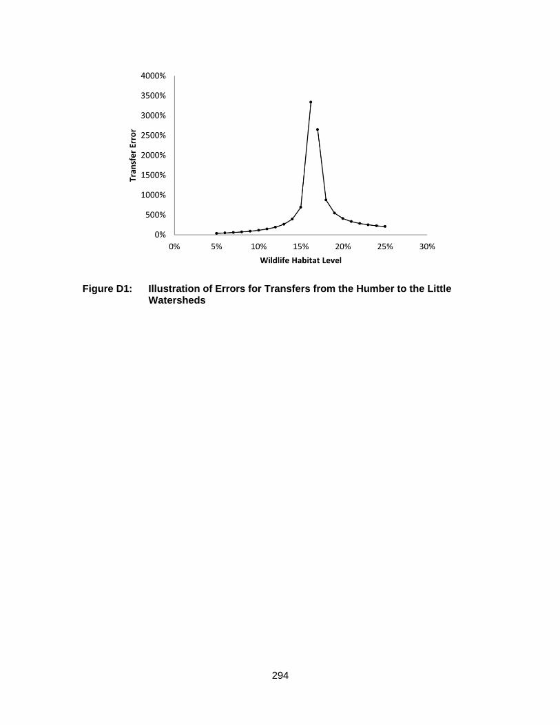
294

Figure D1: Illustration of Errors for Transfers from the Humber to the Little Watersheds

295

D8. Direct Comparisons of Transfer Error or Tolerance Level by Approach for Each Compensating Surplus Estimate

Table D11: Reconciliation Approach Generating the Lowest Errors or Tolerance Level for Transfers of Compensating Surplusa


Transfer Errors Tolerance Levels

‘Absolute’ ‘Relative’ Equalb ‘Absolute’ ‘Relative’ Equalb

Little & Humber Little 0 18 9 0 18 0 Humber 0 18 9 0 18 0

Little & Credit

Little 0 18 9 0 18 0 Credit 0 18 9 0 18 0

Little & Salmon

Little 0 18 9 0 18 0 Salmon 0 18 9 0 18 0

Humber & Credit

Humber 0 18 9 0 18 0 Credit 0 18 9 0 18 0

Humber & Salmon

Humber 0 18 9 0 18 0 Salmon 0 18 9 0 18 0

Credit & Salmon

Credit 8 10 9 8 10 0 Salmon 0 17 10 0 18 1

Total 8 207 109 8 208 1 a Each cell represents the number of times the approach yields the lowest transfer error or tolerance level

b When habitat is at the status quo level the approaches yield identical errors and tolerance levels by default (108 cases)

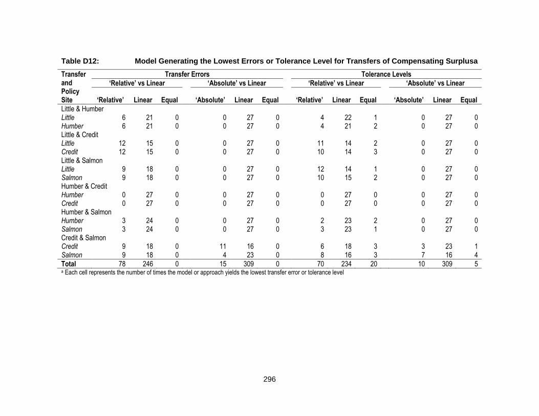
296

Table D12: Model Generating the Lowest Errors or Tolerance Level for Transfers of Compensating Surplusa


Transfer Errors Tolerance Levels

‘Relative’ vs Linear ‘Absolute’ vs Linear ‘Relative’ vs Linear ‘Absolute’ vs Linear

‘Relative’ Linear Equal

‘Absolute’ Linear Equal

‘Relative’ Linear Equal

‘Absolute’ Linear Equal

Little & Humber Little 6 21 0 0 27 0 4 22 1 0 27 0 Humber 6 21 0 0 27 0 4 21 2 0 27 0 Little & Credit Little 12 15 0 0 27 0 11 14 2 0 27 0 Credit 12 15 0 0 27 0 10 14 3 0 27 0 Little & Salmon

Little 9 18 0 0 27 0 12 14 1 0 27 0 Salmon 9 18 0 0 27 0 10 15 2 0 27 0 Humber & Credit Humber 0 27 0 0 27 0 0 27 0 0 27 0 Credit 0 27 0 0 27 0 0 27 0 0 27 0 Humber & Salmon

Humber 3 24 0 0 27 0 2 23 2 0 27 0 Salmon 3 24 0 0 27 0 3 23 1 0 27 0 Credit & Salmon

Credit 9 18 0 11 16 0 6 18 3 3 23 1 Salmon 9 18 0 4 23 0 8 16 3 7 16 4

Total 78 246 0 15 309 0 70 234 20 10 309 5 a Each cell represents the number of times the model or approach yields the lowest transfer error or tolerance level

297

D9. Examining Transfer Errors and Testing the Similarity of Marginal Estimates for the ASC and Water Quality

Overall, the ASC yields lower average errors and tolerance levels than the water

quality attribute for both model specifications (Table D13). The errors and tolerance

levels for changes in water quality from often to sometimes are larger than those for

changes from often to rarely for all transfers involving the Little. For the remaining

transfers the opposite holds for all tolerance levels and, in the case of the linear model,

for errors in the case of transfers from the Humber to the Credit or Salmon. For the

quadratic model, the errors are occasionally equal for the two changes in water quality

although errors for often to sometimes are smaller for transfers from the Salmon to the

Humber and errors for often to rarely are smaller for transfers from the Credit to the

Salmon. Errors and tolerance levels for the ASC and changes in water quality are

generally lower than the marginal values observed for the habitat and income attributes.

The linear and quadratic specification yield similar errors, though the errors and

tolerance levels are lower or equal for the linear model except for transfers of often to

sometimes between the Little and Credit as well as transfers of often to rarely to the

Salmon to the Credit. The tolerance levels are also smaller, except in the case of often

to sometimes for transfers from the Little to the Credit. The complete combinatorial tests

reveal that all of the pairs of estimates differ significantly at least at the 95% level of

significance for transfers involving the Little. A handful of other pairs of estimates

resulting from the quadratic specification differ significantly at the 90% level of

significance for transfers between the Humber and Credit (water quality both) and

Humber and Salmon (water quality often to rarely). Overall the share of estimate pairs

deemed significantly different at the 95% are the same across attributes/levels,

regardless of model specification.

298

Table D13: Errors, Tolerance Levels, and Complete Combinatorial p-values for Transfers of Non-Habitat Marginal WTP Estimates by Modela

Watersheds Linear Specification Quadratic Specification

ASC WQ: Often to Sometimes

WQ: Often to Rarely


WQ: Often to Rarely

Little & Humber Little 77 [136] 139 [198] 158 [214] 105 [173] 157 [222] 195 [260] Humber 44 [77] 58 [83] 61 [83] 51 [85] 61 [87] 66 [88] CC p-value 0.02** 0.00*** 0.00*** 0.01*** 0.00*** 0.00***

Little & Credit Little 74 [132] 103 [159] 123 [176] 80 [141] 96 [153] 125 [181] Credit 43 [76] 51 [78] 55 [79] 45 [78] 49 [79] 56 [81] CC p-value 0.01** 0.00*** 0.00*** 0.01** 0.00*** 0.00***

Little & Salmon Little 78 [136] 107 [158] 136 [185] 88 [150] 107 [159] 137 [189] Salmon 44 [77] 52 [76] 58 [79] 47 [80] 52 [77] 58 [80] CC p-value 0.01** 0.00*** 0.00*** 0.01*** 0.00*** 0.00***

Humber & Credit Humber 2 [37] 15 [44] 13 [38] 12 [46] 24 [53] 24 [49] Credit 2 [38] 18 [51] 16 [44] 13 [52] 31 [69] 31 [64] CC p-value 0.47 0.19 0.18 0.28 0.09* 0.05*

Humber & Salmon Humber 1 [37] 13 [40] 9 [33] 8 [44] 19 [47] 20 [44] Salmon 1 [36] 15 [46] 9 [36] 9 [48] 24 [58] 24 [54] CC p-value 0.49 0.20 0.28 0.35 0.12 0.08*

Credit & Salmon Credit 2 [38] 2 [32] 6 [31] 4 [40] 6 [38] 5 [33] Salmon 2 [37] 2 [31] 5 [30] 4 [38] 5 [36] 5 [32] CC p-value 0.45 0.45 0.35 0.42 0.39 0.37

Overall Errorb 31 (23) 48 (35) 54 (36) 39 (29) 53 (40) 62 (44) Toleranceb 71 (57) 83 (64) 86 (62) 81 (65) 90 (73) 96 (72)

299

Watersheds Linear Specification Quadratic Specification


WQ: Often to Rarely


WQ: Often to Rarely

CC Different Pairsc 50% 50% 50% 50% 50% 50% a Errors [tolerance levels in square brackets]




300

Transfer errors and tolerance levels are generally larger if a transfer involves the

Little watershed. For the ASC, errors are lowest for transfers between the Humber and

Salmon, followed by transfers between the Credit and Humber or Salmon, and the

transfers involving the Little. Tolerance levels for the ASC are similar for transfers among

the Humber, Credit, or Salmon and these levels are much smaller than those involving

the Little watershed. For the quadratic specification, the order differs somewhat with

transfers between the Credit and Salmon yielding the smallest errors, followed by

transfers between the Humber and Salmon, Humber and Credit, Little and Credit, Little

and Salmon, and Little and Humber. Tolerance levels for the quadratic ASC are lowest

for the transfers between the Credit and Salmon, followed by transfers between the

Humber and Credit or Salmon, and then Little and Credit, Little and Salmon, and Little

and Humber. For the water quality attributes, transfer errors are lowest for transfers

between the Credit and Salmon, followed by transfers between the Humber and Salmon

or Credit, and then transfers between the Little and Credit, Little and Salmon, and Little

and Humber (order same for linear and quadratic). Tolerance levels for the water quality

attribute are lowest for transfers between the Credit and Salmon, followed by transfers

between the Humber and Salmon, Humber and Credit, Little and Credit, Little and

Salmon, and then the Little and Humber. Transfer direction appears to be more of a

factor for transfers involving the Little watershed. Those transfers where the Little is the

policy site yield much larger errors and tolerance levels. Direction does not impact errors

and tolerance levels to the same extent for the other transfers, though transfers from the

Humber to the Credit or Salmon as well as the Salmon to Credit yield errors and

tolerance levels that are at least as large as in the other direction.

301

References


McFadden, D. (1974). Conditional Logit Analysis of Qualitative Choice Behaviour, in: Zarembka, P. (Ed.), Frontiers in Econometrics. Academic Press, New York, NY, pp. 105–142.

Statistics Canada (2012) Census: Age and Sex – Age (131) and Sex (3) for the Population of Canada, Provinces, Territories, Census Divisions, Census Subdivisions and Dissemination Areas (98-311-XCB2011018). http://www5.statcan.gc.ca/olc-cel/olc.action?objId=98-311-X2011018&objType=46&lang=en&limit=0. Accessed 25 Jan 2018

Statistics Canada (2013) National Household Survey (NHS) Profile, 2011. http://hdl.handle.net/11272/10060. Accessed 12 Sep 2013Train, K.E., 2009. Discrete Choice Methods With Simulation, Second Edi. ed. Cambridge University Press, New York, NY. doi:978-0-521-74738-7

Train KE (2009) Discrete Choice Methods With Simulation, Second Edi. Cambridge University Press, New York, NY

302

Appendix E. Landowner Choice Experiment Questionnaires

The questionnaires presented in this appendix are those used in the Grand River

watershed. Those questionnaires used in the Upper Thames River watershed are

identical in all respects except the map used on the cover page and the use of a different

watershed name.

303

Farmer and Woodlot Owner Focussed Choice Experiment

Survey of Farmer Views on Wetland Enhancement and Restoration in & near

the Grand River Watershed

When you have completed this survey, please place it in the postage-paid envelope provided in your survey package and drop it off in the mail. Thank you!

A watershed is an area of land that drains into

a common river system.

A wetland is an area of land that is saturated with water, either permanently or seasonally. It

includes marshes and swamps.

304

Section 1: Your Land

1. Which county or municipality do you live in? Please check one box only.

Dufferin County Regional Municipality of Waterloo Wellington County Oxford County Haldimand County Brant County

Perth County Other (Please specify): _____________________

2. What is the total area of land that you own inside and outside the Grand River watershed (if needed, consult the map on the back of the cover letter)? Please indicate the number of acres in the spaces provided.

Inside: ________ Acres

Outside: ________ Acres

3. When did you first obtain land in the region? Please check one box only.

Before 1970 1981-1990 2001-2006 Not Applicable

1970-1980 1991-2000 2007-2013

4. What is the primary use of the land you own? Please check one box only.

Agriculture Residence

Forestry Other: ________________________________

5. If you generated income from your land over the past 5 years, is it from any of the following? Please check all boxes that apply.

Farming Leasing land for recreation Not applicable

Forestry Leasing land for farming or forestry Other: ____________

Leasing land for hunting Development/sale of your land ____________

6. What will likely happen to your land after you retire? Please check one box only.

Sell Give to land trust Have not started planning for retirement

Give to family Don’t know Other: ____________________________

305

7. People own land for many different reasons. How important are each of the following reasons to you? For each reason, please check the box that corresponds with your answer.

Very

important

Important

Neither important or unimportant

Of little importance

Un- important

Don’t know

To make a living (farm, forest, or other income)

To complement my income

As an investment for future gain

As a location for my permanent residence

For recreation (hunting, fishing, walking, etc.)

To maintain a family legacy

For the sake of our future generations

To preserve ecosystems

8. Which of the following features do you have on your land?

Please check all boxes that apply.

Crop Pasture Meadows

Orchard Forests Other: _______________________

9a. Do you have wetlands on your land?

Yes If yes, please continue with question 9b No If no, please skip to question 10

9b. Did you create, or have you enhanced, any of these wetlands? Check all boxes that

apply.

Created them Enhanced them No

9c. If you created or enhanced any wetlands on your land, please explain what you did and

how it was funded. If you answered ‘No’ to question 9b please skip to question 10.

________________________________________________________________________

________________________________________________________________________

________________________________________________________________________

306

Section 2: Your Land Management

10. How many acres of your land are currently left untilled or dedicated to other land cover types, and how have these areas changed since 2006? Please indicate your answers using the spaces provided below. For any specific land cover type that does not apply to your situation, please leave the associated space blank.

Land cover type # of acres now

Change since 2006 Increase (acres)

Decrease (acres)

Land left untilled _______ _______ _______

Fence line _______ _______ _______

Wind break _______ _______ _______

Trees _______ _______ _______

Shrub land meadow _______ _______ _______

Ditch _______ _______ _______

Wet area / Wetland _______ _______ _______

Other conservation measure:

________________________

________________________

_______ _______ _______

11. Have you ever received financial incentives or cost-share payments from any of the

following programs for implementing conservation measures on your land? Please check all boxes that apply.

Stewardship Program offered by the local Conservation Authority

Ducks Unlimited Wetland Retention or Restoration Programs

Environmental Farm Plan Other: _________________________________

_________________________________ I have not received financial assistance from any program

307

12. To what extent do you agree or disagree with each of the following statements about your landowner rights? For each statement, please check the box that corresponds with your answer.

As a landowner, I have the right to…

Strongly agree

Agree Neither

agree nor disagree

Disagree Strongly disagree

Don’t know

…restrict others’ access to my land

…transfer ownership of my land to others without restriction

…do whatever I want with my land without regard for others

…do anything with my land as long as my actions do not infringe upon neighbours’ rights

…do anything with my land as long as my actions do not conflict with the interests and values of the local community

13. To what extent do you agree or disagree with each of the following statements about your

landowner responsibilities? For each statement, please check the box that corresponds with your answer.

As a landowner, I have the responsibility to…

Strongly agree

Agree Neither

agree nor disagree


Don’t know

… be a good steward of my land and to maintain it in a good condition for future generations

… leave the land in a better condition than when I acquired it

… take into account the values and interests of society at large when making decisions about my land

308

Section 3: Wetland Management

14. How important are the following wetland benefits in your area to you? Please check one box per item.

Very

important Somewhat important

Not important

No opinion

Water quality

Flood, drought, and erosion control

Wildlife habitat

Carbon storage

Recreation and education

15. How would you describe the current state of wetlands in your area?

Please check one box per item.

Excellent Good Fair Marginal Don’t know

Quantity (amount) of wetlands

Quality (health) of wetlands

Accessibility to view wetlands

Information: Wetland Benefits

Wetlands in your area provide a number of benefits to the community, including:

Water quality: Wetlands help purify water.

Flood, drought, and erosion control: Wetlands help control flooding and erosion, as

well as reduce the impacts of drought.

Wildlife habitat: Wetlands provide habitat for native and/or endangered plant and

wildlife species (both on land and in water).

Carbon storage: Wetlands store carbon helping to slow climate change.

Recreation and education: Wetlands provide recreational and educational

opportunities.

309

16. In your opinion, what would motivate landowners in your region to participate in wetland enhancement and restoration activities on their land? For each incentive, please check the box that corresponds with your answer.

Strongly

agree Agree Neutral Disagree

Strongly disagree

Don’t know

Public recognition (e.g., signage on property, stewardship banquets and awards, etc.)

Concern over loss of wetlands in this region

More information on how the decline in wetland area affects them personally

Access to technical assistance and information

If neighbours undertook this type of practice

A one-time payment to offset initial cost of enhancement or restoration

A small annual payment to acknowledge their environmental service provision to society and to help cover loss of revenue

Other (please specify): ___________________________________

Information: Decline in Wetland Area

The area of wetlands in and around the Grand River watershed has declined

significantly over the past century, largely due to human activities such as expansion

of urban areas, agriculture, and industrial developments.

While the rate of wetland loss has recently slowed, the area and/or quality of wetlands

in your region still declines each year, resulting in further loss of wetland benefits.

Landowners can help reverse the declining trend by enhancing existing wetlands and

restoring previously drained ones on the land they manage.

310


Suppose that in an effort to enhance and restore wetlands within and adjacent to the Grand River watershed, the government offered a voluntary program that provided incentives (e.g., payments, public recognition) to landowners to set aside some of their lands. This land could be (i) converted to meadow or trees to help retain nearby wetlands; or (ii) converted directly into wetlands if appropriate. PROGRAM CONDITIONS:


Sign a 5-year contract to enroll some of their land and receive annual payments (to help compensate for lost income & acknowledge provision of an environmental service to society).



Have a say in what type of land conversion activities are implemented (i.e. whether to convert land to meadow, trees, or wetlands). All capital/material costs would be paid for by the government (on top of any financial incentive to you).


On each of the next few pages, you’ll be presented with a set of 2 voluntary programs considered by the government. We ask you to choose between PROGRAM A, PROGRAM B, or NO PROGRAM. PROGRAM CHARACTERISTICS:


Type of land to be converted land can be Productive or Marginal (i.e., less fertile) farmland


Number of acres area converted can be 1, 3, or 5 acres


Annual payments to you can be $50 to $550 per acre per year (to help compensate you

for any lost income and to acknowledge your provision of an environmental service to society).


311

SET 1:





Type of land to be converted Marginal Marginal ---


Number of acres 5 acres 3 acres ---


Annual payments to you $450/acre $450/acre $0/acre




1 2 3 4 5 6 7 8 9 10


312

SET 2:





Type of land to be converted Productive Marginal ---

Conversion activity Trees Trees ---







1 2 3 4 5 6 7 8 9 10


313

SET 3:





Type of land to be converted Productive Marginal ---

Conversion activity Meadow Wetland ---

Number of acres 1 acre 1 acre ---




19b. On a scale 1 to 10, how certain are you about the program choice you made above? Please circle the number that best represents your answer if 1 equals not at all certain and 10 equals very certain.

1 2 3 4 5 6 7 8 9 10


314

SET 4:





Type of land to be converted Marginal Productive ---

Conversion activity Trees Meadow ---

Number of acres 1 acre 3 acres ---

Public recognition No Yes ---





1 2 3 4 5 6 7 8 9 10


315

SET 5:





Type of land to be converted Marginal Marginal ---

Conversion activity Meadow Trees ---







1 2 3 4 5 6 7 8 9 10


316

SET 6:





Type of land to be converted Productive Productive ---

Conversion activity Wetland Wetland ---

Number of acres 3 acres 1 acre ---






1 2 3 4 5 6 7 8 9 10


317

23. If you chose “NO PROGRAM” for any of the previous sets, please check the box that best explains why you chose this option. Please check one box only.

“The annual payments were too low”

“I believe these projects would lower my property value”

“The amount of land involved was too large”

“The amount of land involved was too small”

“I do not think retaining or restoring wetlands is an important issue”

“The 5-year contract length was too restrictive”

“I don’t trust the government”

Other: _____________________________________________

24. If you chose either “PROGRAM A” or “PROGRAM B” for any of the previous sets, please

check the box that best explains why you chose this option.

Please check one box only.

“The annual payments were the main reason for my choices”

“We should restore wetlands regardless of the payment levels”

“The public recognition of my conservation effort was the main reason for my choices”

“It’s equally important to provide payments and recognition to landowners who restore wetlands in my area”

Other: _____________________________________________


check the box that indicates your preferred renewable contract length. Please check one box only.

1 year 10 years 20 years 5 years 15 years More than 20 years

318

End of Survey. Thank You! Please place the completed survey in the postage-paid envelope and drop it off in the mail.

To be entered into the draw for one of three $100 Visa gift cards, please fill out the ballot at the bottom of the cover letter, detach, and return it with your completed survey.

Section 5: Your Personal Characteristics

26. What is your gender?

Female Male 27. In what year were you born? _________ 28. What is the highest level of education that you have completed?


Elementary school Post-secondary (diploma or bachelor’s degree)

High school Graduate or professional degree (e.g. law, MD, masters, or PhD) 29. Which of the following best describes your present employment status?


Working full time Retired Student Working part time Unemployed

30. Are you a member of any of the following types or organizations or associations?


Environmental/conservation Farmer

Hunting/fishing Woodlot

ATV/snowmobile Other: ___________________________ 31. What is your best estimate of your total household income (before taxes) over the past

12 months? Please check one box only.

Less than $10,000 $30,000 to $49,999 $75,000 to $99,999

$10,000 to $29,999 $50,000 to $74,999 More than $100,000 32. What percentage of your household income is from on-farm sources (i.e. crop /

livestock)?

0 % 1 to 24 % 25 to 49 % 50 to 74 % 75 to 99 % 100 % 33. What is your postal code and rural route number (example: RR 1)?

Postal Code: __________ Route Number: __________ 34. How would you describe your household’s debt load? Please check one box only.

Debt free Low Moderate High

319

Non-Farm Rural Landowner Focussed Choice Experiment

Survey of Landowner Views on Wetland Enhancement and Restoration in & near

the Grand River Watershed

When you have completed this survey, please place it in the postage-paid envelope provided in your survey package and drop it off in the mail. Thank you!

A watershed is an area of land that drains into

a common river system.

A wetland is an area of land that is saturated with water, either permanently or seasonally. It

includes marshes and swamps.

320

Section 1: Your Land

1. Which county or municipality do you live in? Please check one box only.

Dufferin County Regional Municipality of Waterloo Wellington County Oxford County Haldimand County Brant County

Perth County Other (Please specify): _____________________

2. What is the total area of land that you own inside and outside the Grand River watershed (if needed, consult the map on the back of the cover letter)? Please indicate the number of acres in the spaces provided.

Inside: ________ Acres

Outside: ________ Acres

3. When did you first obtain land in the region? Please check one box only.

Before 1970 1981-1990 2001-2006 Not Applicable

1970-1980 1991-2000 2007-2013

4. What is the primary use of the land you own? Please check one box only.

Agriculture Residence

Forestry Other: ________________________________

5. If you generated income from your land over the past 5 years, is it from any of the following? Please check all boxes that apply.

Farming Leasing land for recreation Not applicable

Forestry Leasing land for farming or forestry Other: ____________

Leasing land for hunting Development/sale of your land ____________

6. What will likely happen to your land after you retire? Please check one box only.

Sell Give to land trust Have not started planning for retirement

Give to family Don’t know Other: ____________________________

321

7. People own land for many different reasons. How important are each of the following reasons to you? For each reason, please check the box that corresponds with your answer.

Very

important

Important



Un- important

Don’t know

To make a living (farm, forest, or other income)

To complement my income

As an investment for future gain

As a location for my permanent residence

For recreation (hunting, fishing, walking, etc.)

To maintain a family legacy

For the sake of our future generations

To preserve ecosystems

8. Which of the following features do you have on your land?


Crop Pasture Meadows

Orchard Forests Other: _______________________

9a. Do you have wetlands on your land?

Yes If yes, please continue with question 9b No If no, please skip to question 10

9b. Did you create, or have you enhanced, any of these wetlands? Check all boxes that

apply.

Created them Enhanced them No

9c. If you created or enhanced any wetlands on your land, please explain what you did and

how it was funded. If you answered ‘No’ to question 9b please skip to question 10.

________________________________________________________________________

________________________________________________________________________

________________________________________________________________________

322

Section 2: Your Land Management

17. How many acres of your land are currently left untilled or dedicated to other land cover types, and how have these areas changed since 2006? Please indicate your answers using the spaces provided below. For any specific land cover type that does not apply to your situation, please leave the associated space blank.

Land cover type # of acres now

Change since 2006 Increase (acres)

Decrease (acres)

Land left untilled _______ _______ _______

Fence line _______ _______ _______

Wind break _______ _______ _______

Trees _______ _______ _______

Shrub land meadow _______ _______ _______

Ditch _______ _______ _______

Wet area / Wetland _______ _______ _______

Other conservation measure:

________________________

________________________

_______ _______ _______

18. Have you ever received financial incentives or cost-share payments from any of the

following programs for implementing conservation measures on your land? Please check all boxes that apply.

Stewardship Program offered by the local Conservation Authority

Ducks Unlimited Wetland Retention or Restoration Programs

Environmental Farm Plan Other: _________________________________

_________________________________ I have not received financial assistance from any program

323

19. To what extent do you agree or disagree with each of the following statements about your landowner rights? For each statement, please check the box that corresponds with your answer.

As a landowner, I have the right to…

Strongly agree

Agree Neither

agree nor disagree


Don’t know

…restrict others’ access to my land

…transfer ownership of my land to others without restriction

…do whatever I want with my land without regard for others

…do anything with my land as long as my actions do not infringe upon neighbours’ rights

…do anything with my land as long as my actions do not conflict with the interests and values of the local community

20. To what extent do you agree or disagree with each of the following statements about your

landowner responsibilities? For each statement, please check the box that corresponds with your answer.

As a landowner, I have the responsibility to…

Strongly agree

Agree Neither

agree nor disagree


Don’t know

… be a good steward of my land and to maintain it in a good condition for future generations

… leave the land in a better condition than when I acquired it

… take into account the values and interests of society at large when making decisions about my land

324

Section 3: Wetland Management

21. How important are the following wetland benefits in your area to you? Please check one box per item.

Very

important Somewhat important

Not important

No opinion

Water quality

Flood, drought, and erosion control

Wildlife habitat

Carbon storage

Recreation and education

22. How would you describe the current state of wetlands in your area?

Please check one box per item.

Excellent Good Fair Marginal Don’t know

Quantity (amount) of wetlands

Quality (health) of wetlands

Accessibility to view wetlands

Information: Wetland Benefits

Wetlands in your area provide a number of benefits to the community, including:

Water quality: Wetlands help purify water.

Flood, drought, and erosion control: Wetlands help control flooding and erosion, as

well as reduce the impacts of drought.

Wildlife habitat: Wetlands provide habitat for native and/or endangered plant and

wildlife species (both on land and in water).

Carbon storage: Wetlands store carbon helping to slow climate change.

Recreation and education: Wetlands provide recreational and educational

opportunities.

325

23. In your opinion, what would motivate landowners in your region to participate in wetland enhancement and restoration activities on their land? For each incentive, please check the box that corresponds with your answer.

Strongly

agree Agree Neutral Disagree

Strongly disagree

Don’t know

Public recognition (e.g., signage on property, stewardship banquets and awards, etc.)

Concern over loss of wetlands in this region

More information on how the decline in wetland area affects them personally

Access to technical assistance and information

If neighbours undertook this type of practice

A one-time payment to offset initial cost of enhancement or restoration

A small annual payment to acknowledge their environmental service provision to society

Other (please specify): ___________________________________

Information: Decline in Wetland Area

The area of wetlands in and around the Grand River watershed has declined

significantly over the past century, largely due to human activities such as expansion

of urban areas, agriculture, and industrial developments.

While the rate of wetland loss has recently slowed, the area and/or quality of wetlands

in your region still declines each year, resulting in further loss of wetland benefits.

Landowners can help reverse the declining trend by enhancing existing wetlands and

restoring previously drained ones on the land they manage.

326



PROGRAM CONDITIONS:
















327

SET 1:













1 2 3 4 5 6 7 8 9 10


328

SET 2:





Conversion activity Trees Trees ---

Number of acres 1 acre 1.5 acres ---

Technical assistance Yes Yes ---






1 2 3 4 5 6 7 8 9 10


329

SET 3:





Conversion activity Meadow Wetland ---

Number of acres 0.5 acres 0.5 acres ---

Technical assistance Yes No ---




19b. On a scale 1 to 10, how certain are you about the program choice you made above? Please circle the number that best represents your answer if 1 equals not at all certain and 10 equals very certain.

1 2 3 4 5 6 7 8 9 10


330

SET 4:





Conversion activity Trees Meadow ---


Technical assistance No Yes ---






1 2 3 4 5 6 7 8 9 10


331

SET 5:





Conversion activity Meadow Trees ---

Number of acres 1.5 acres 1.5 acres ---







1 2 3 4 5 6 7 8 9 10


332

SET 6:





Conversion activity Wetland Wetland ---

Number of acres 1 acre 0.5 acres ---

Technical assistance Yes Yes ---






1 2 3 4 5 6 7 8 9 10


333

23. If you chose “NO PROGRAM” for any of the previous sets, please check the box that best explains why you chose this option. Please check one box only.

“The annual payments were too low”

“I believe these projects would lower my property value”

“The amount of land involved was too large”

“The amount of land involved was too small”

“I do not think retaining or restoring wetlands is an important issue”

“The 5-year contract length was too restrictive”


Other: _____________________________________________


check the box that best explains why you chose this option.


“The annual payments were the main reason for my choices”

“We should restore wetlands regardless of the payment levels”

“The public recognition of my conservation effort was the main reason for my choices”

“It’s equally important to provide payments and recognition to landowners who restore wetlands in my area”

Other: _____________________________________________


check the box that indicates your preferred renewable contract length. Please check one box only.

1 year 10 years 20 years 5 years 15 years More than 20 years

334

End of Survey. Thank You! Please place the completed survey in the postage-paid envelope and drop it off in the mail.

To be entered into the draw for one of three $100 Visa gift cards, please fill out the ballot at the bottom of the cover letter, detach, and return it with your completed survey.


26. What is your gender?

Female Male 27. In what year were you born? _________ 28. What is the highest level of education that you have completed?


Elementary school Post-secondary (diploma or bachelor’s degree)

High school Graduate or professional degree (e.g. law, MD, masters, or PhD) 29. Which of the following best describes your present employment status?


Working full time Retired Student Working part time Unemployed

30. Are you a member of any of the following types or organizations or associations?


Environmental/conservation Farmer

Hunting/fishing Woodlot

ATV/snowmobile Other: ___________________________ 31. What is your best estimate of your total household income (before taxes) over the past

12 months? Please check one box only.

Less than $10,000 $30,000 to $49,999 $75,000 to $99,999

$10,000 to $29,999 $50,000 to $74,999 More than $100,000 32. What percentage of your household income is from on-farm sources (i.e. crop /

livestock)?

0 % 1 to 24 % 25 to 49 % 50 to 74 % 75 to 99 % 100 % 33. What is your postal code and rural route number (example: RR 1)?

Postal Code: __________ Route Number: __________ 34. How would you describe your household’s debt load? Please check one box only.

Debt free Low Moderate High

335

Appendix F. Public Benefits Choice Experiment Questionnaire

The questionnaire used in the Salmon River watershed is presented in this appendix.

The questionnaires used in the other three watersheds were similar, though differed in

terms of the map used on the cover page as well as the watershed names. Furthermore,

as outlined in Chapter 5 the levels used for the wildlife habitat attribute differed across

watersheds. The Salmon survey also included two extra questions about water use not

included in the other watershed questionnaires that were of interest to other researchers

in the Salmon watershed (questions 35 and 36).

336

Survey of Public Views on the Environment in the Salmon River Watershed, BC

When you have completed this survey, please place it in the postage-paid envelope provided in your package and drop-off in the mail. Thank you!

A watershed is a region that drains into a common body of water

The watershed boundary is represented by the thick grey line

337

Section 1: Your Watershed 1. Where do you live in relation to the Salmon River watershed?

Please refer to the map on the back of the letter to help you answer this question, and check one box only.

Within watershed Outside watershed I don’t know 2. Do you own a farm or a woodlot in the region?

Please check the box that corresponds with your answer. Farm Farm and Woodlot

Woodlot Neither 3. Are you a member of any of the following types of organizations or associations?

Please check all boxes that apply. Environmental/conservation ATV/snowmobile

Hunting/fishing Farm commodity producer Landowner Forestry producer

4. Over the past 12 months have you participated in any of the following outdoor

activities within the Salmon River Watershed? Please check all that apply.

Hunting Swimming Snowshoeing

Fishing Boating X-Country Skiing

Camping Berry/Mushroom picking Snowmobiling

Biking Bird watching Other Motor Sports

Running/Walking/Hiking Horseback riding Other 5. In your opinion, how important is it to have each of the following in your watershed

region? For each item, please check the box that corresponds with your answer.

Very

important Important



Unimportant Don’t know

Flood/Drought prevention

Soil erosion control

Carbon sequestration

Good water quality

Soil fertility for farming/forestry

Wildlife habitat

Visually pleasing landscapes

Large diversity of plants and animals

338

Section 2: Your Opinion on Land Management and Land Use Within the Salmon River Watershed

The following questions are about your opinion on landowners and their land use in the watershed. Landowners are people who own at least 10 acres of land and include farmers, woodlot owners, and people who own their land for other reasons.

6. To what extent do you agree or disagree with each of the following statements? For each statement, please check the box that corresponds with your answer.

Strongly Agree

Agree Neither

agree nor disagree

Disagree Strongly Disagree

Don’t know

Private land should provide for the needs of future plant and animal populations

What landowners do on their own land affects people aside from their family

What landowners do today on their land will matter in the long run

Landowners should work together if it means the land would be better off

There is too much government regulation of private land use

Individual properties are unimportant in the big picture of all the land in the region

Rare or endangered species should be protected on private land

Private land provides benefits to society

Sensitive areas on private land should be protected from being altered or damaged

I am aware of my rights with respect to my legal use of other people’s land

339

7. To what extent do you agree or disagree with each of the following statements? For each statement, please check the box that corresponds with your answer.

Landowners have a responsibility to…

Strongly Agree

Agree Neither

agree nor disagree


Don’t know

… be good stewards of their land and to maintain it in a good condition for future generations

… leave the land in a better condition than when they acquired it

… take into account the values and interests of society at large when making decisions about their land

8. To what extent do you agree or disagree with each of the following statements?

For each statement, please check the box that corresponds with your answer.

Landowners have the right to… Strongly Agree

Agree Neither

agree nor disagree


Don’t know

…restrict others access to their land

…transfer ownership of their land to others without restriction

…do whatever they want with their land without regard for others

…do anything with their land so long as their actions do not infringe upon neighbours’ rights

…do anything with their land so long as their actions do not conflict with the interests and values of the local community

340

9. Do you feel the public should be able to use private land for each of the following activities? Please check one box per item.

Yes, it is the public’s

right

Yes, but only with landowner

permission

No, this use should not be allowed

Walking

Hunting

Gathering berries, mushrooms, etc. for personal use

Gathering berries, mushrooms, etc. for commercial use

Operating recreational motorized vehicles

Accessing water for recreational purposes

Camping

10. To what extent do you agree or disagree with each of the following statements?


Landowners should be primarily responsible for… Strongly

Agree Agree

Neither agree nor disagree


Don’t know

Protecting wetlands from being altered or damaged

Providing wildlife habitat

Reducing the use of fertilizers Retaining trees in areas vulnerable to soil erosion

Protecting woodlots from being cleared

Reducing the use of pesticides Establishing watercourse buffers

Providing public access to land for recreation

11. Are there any activities or actions that you would like to be able to prevent

landowners in the watershed from doing on their own land? If so, please write them in the space provided below.

341

Section 3: Your Perspective on the State of the Salmon River Watershed

The Salmon River watershed provides many environmental, social, and economic services. These include fresh water, wildlife habitat, and farm/woodlot owner incomes among others. However, some citizens are concerned that recent trends in economic activity are threatening the watershed’s ability to supply these services. 12. In your opinion, how would you describe the current state of the watershed in terms

of each of the statements below? Please check one box per item. Excellent Good Fair Marginal Don’t know

Water quality is:

Wildlife habitat is:

Recreation opportunities are:

Farm/Woodlot owner incomes are:

14. How concerned are you about the future state of the watershed in terms of the

following aspects? Please check one box per item. I’m very

concerned I’m somewhat

concerned I’m not

concerned No opinion

Water quality:

Wildlife habitat:

Recreation opportunities:

Farm/Woodlot owner incomes:

342

Section 4: Your Preferences for Environmental Stewardship Programs in the Salmon River Watershed

Environmental conditions in the watershed can be maintained and/or improved through various government-funded environmental stewardship programs. On the following pages, we will ask you to choose between different programs that would improve environmental conditions 10 years from now in the watershed. Each question will ask you to choose 1 of 3 environmental stewardship programs: A, B, or C.

Example:

Please assess each of the following 6 Choice Sets and choose your preferred option. Consider each set independently and imagine that you would have to actually dig into your household budget and pay the additional taxes.

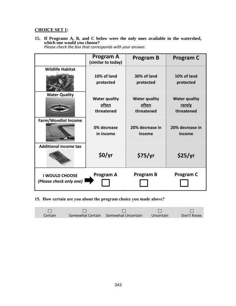
343



Program A


Wildlife Habitat

10% of land

protected

30% of land

protected

10% of land

protected

Water Quality

Water quality

often

threatened

Water quality

often

threatened

Water quality

rarely

threatened

Farm/Woodlot Income

0% decrease

in income

20% decrease in

income

20% decrease in

income

Additional income tax

$0/yr $75/yr $25/yr

I WOULD CHOOSE (Please check only one)

Program A

Program B Program C



344

CHOICE SET 2: 16. If Programs A, B, and C below were the only ones available in the watershed, which

one would you choose? Please check the box that corresponds with your answer.

Program A


Wildlife Habitat

10% of land

protected

20% of land

protected

10% of land

protected

Water Quality

Water quality

often

threatened

Water quality

rarely

threatened

Water quality

sometimes

threatened

Farm/Woodlot Income

0% decrease

in income

10% decrease in

income

0% decrease in

income


$0/yr $25/yr $50/yr


Program A

Program B Program C



345



Program A


Wildlife Habitat

10% of land

protected

20% of land

protected

30% of land

protected

Water Quality

Water quality

often

threatened

Water quality

sometimes

threatened

Water quality

rarely

threatened

Farm/Woodlot Income

0% decrease

in income

20% decrease in

income

0% decrease in

income


$0/yr $100/yr $200/yr


Program A

Program B Program C



346



Program A


Wildlife Habitat

10% of land

protected

20% of land

protected

20% of land

protected

Water Quality

Water quality

often

threatened

Water quality

often

threatened

Water quality

often

threatened

Farm/Woodlot Income

0% decrease

in income

0% decrease in

income

20% decrease in

income


$0/yr $50/yr $200/yr


Program A

Program B Program C



347



Program A


Wildlife Habitat

10% of land

protected

10% of land

protected

30% of land

protected

Water Quality

Water quality

often

threatened

Water quality

often

threatened

Water quality

sometimes

threatened

Farm/Woodlot Income

0% decrease

in income

20% decrease in

income

0% decrease in

income


$0/yr $25/yr $75/yr


Program A

Program B Program C



348



Program A


Wildlife Habitat

10% of land

protected

20% of land

protected

30% of land

protected

Water Quality

Water quality

often

threatened

Water quality

sometimes

threatened

Water quality

often

threatened

Farm/Woodlot Income

0% decrease

in income

10% decrease in

income

10% decrease in

income


$0/yr $75/yr $150/yr


Program A

Program B Program C



349

26. If you chose Program A (similar to today) as an answer for any of the Choice Sets 1 to 6 above, why did you choose so?

Please check the one explanation that most affected your choices above

“The increase in annual income taxes was too high”

“I think tax money could be better spent on other issues”

“I do not have enough information to make this decision”

“The proposed environmental changes were unrealistic”

“I do not think the environment is an important issue”


Other: _______________________________________________________

_______________________________________________________

27. If you chose either Program B or C as an answer for any of the Choice Sets 1 to 6

above, why did you do so? Please check the one explanation that most affected your choices above

“I think that this is a small price to pay for the environmental improvements”

“I think we should protect the environment regardless of the cost”

“It is important to invest in protecting the environment for future generations”

“I think our government does not do enough to protect our environment”

“I feel it is the ‘right thing’ to do”

Other: _______________________________________________________

_______________________________________________________

350


This section will assist us with our statistical analysis. Responses to these questions and all other questions will be treated anonymously. 28. What is your gender?

Female Male 29. In what year were you born? Please indicate the year in the space provided below.

______________ 30. What is the highest level of education that you have completed?

Please check one box. 31. Elementary school Post-secondary (diploma or bachelors degree)

High school Graduate university degree (Masters or PhD)

31. How would you best describe the place where you grew up and the place where you have lived most of your adult life?

Please check one box only for each item below.

Urban Suburban Rural Where I grew up:

Where I have lived most of my adult life:

32. Which of the following best describes your present employment status?


Working full time Not currently working Working part time Retired

33. What is your best estimate of your total household income over the past 12

months? Please check one box only.

Less than $10,000 $30,000 to $49,999 $75,000 to $99,999

$10,000 to $29,999 $50,000 to $74,999 More than $100,000

34. Where were you born? Please check one box only.

Born in Canada Not born in Canada

In what year did you arrive in Canada?

_____________

351

35. Do you use any of following water saving devices? Please check all that apply.

Low flow faucets Efficient sprinkler nozzles Low flow toilets Water meter

Other: _____________________________________ 36. To what extent do you agree or disagree with each of the following statements?


Landowners who irrigate their fields…

Strongly Agree

Agree Neither

agree nor disagree


Don’t know

…use water efficiently

…use water efficiently to improve stream and river flows

…use water efficiently to improve their own crops

Comments:

End of Survey, Thank You!!

Trenholm PhD Dissertation - SFU's Summit

Documents

Transcript of Trenholm PhD Dissertation - SFU's Summit