Transitive geostatistics to characterise spatial aggregations with diffuse limits: an application on...

Transitive geostatistics to characterise spatial aggregations withdiffuse limits: an application on mackerel ichtyoplankton

N. Bez*, J. RivoirardCentre de GeÂostatistique, 35 rue St HonoreÂ, F-77305 Fontainebleau, France

Abstract

In the context of the analysis of mackerel ichtyoplankton, and more generally of populations with diffuse limits (e.g. pelagic

®sh), we present a methodology that avoids the problem of the delineation of the area of presence. The principle, which leads

to the concept of Individual Based Statistics, is to give each sample a weight proportional to its density, i.e., proportional to the

number of individuals it represents. A level and an index of aggregation are proposed to characterise statistically population

with diffuse limits, while the inertia of locations and the transitive covariogram can be used as spatial characteristics. In

particular, a superposition of structural components with different scales can be described on the covariogram.

In the Northeast Atlantic, during the spawning seasons 1986, 1989, 1992 and 1995, the inertia of the population of stage I

mackerel eggs is remarkably stable despite inter- and intra-annual variations of the total abundance. The spatial structures, as

described by the covariograms, are made of two components: a small range component (nugget effect) and a long range

exponential component. The stability of the inertia is essentially due to the stability of the long range. On the other hand, the

observed variations of the index of aggregation are essentially due to the variations of the short range component. A

comparison between newly spawn eggs and stage V eggs (last stage before hatching) is also made and interpreted in terms of

diffusion and mortality rates. # 2001 Elsevier Science B.V. All rights reserved.

Keywords: Zero density values; Individual; Aggregation; Spatial structure; Covariogram

1. Introduction

Cooper et al. (1997) recently mentioned that there

has been little rigorous quanti®cation of terms like

`̀ patchiness'' or `̀ spatial heterogeneity'' in stream

ecology. This lack of de®nition can be extended to

®sh ecology as a whole. As a matter of fact, going

through the literature, we can ®nd various expressions

referring to the spatial organisation of ®sh such as

patch or patchiness, crowding, clumbing, clump, pat-

tern of variability, pattern intensity, spatial hetero-

geneity, spatial structure, contagious behaviour,

convergence, aggregation pattern and also merely,

aggregation like in the present paper or in Taylor

(1961). We might even ®nd references to patchiness

of micro aggregation (de Nie et al., 1980) which is a

combination of concepts. This rather long list is aimed

at underlining the numerous existing expressions

referring to the ®sh behaviours. The relevant scale,

if it exists, to which each of them is attached is not

clear.

From a statistical point of view, indications on the

distribution and the variability of a ®sh density are

commonly based on the variance s2, the standard

deviation s or the coef®cient of variation,

CV � s=m (where m is the mean density). Petitgas

(1994) and Myers and Cadigan (1995) use Gini's

Fisheries Research 50 (2001) 41±58

* Corresponding author.

E-mail address: [email protected] (N. Bez).

0165-7836/01/$ ± see front matter # 2001 Elsevier Science B.V. All rights reserved.

PII: S 0 1 6 5 - 7 8 3 6 ( 0 0 ) 0 0 2 4 1 - 1

index to quantify the skewness of data values. But

other statistical tools also exist. The ratio s2/m sug-

gested by Taylor's theory (1961) for counts of indi-

viduals, gives indications on over or under dispersion

compared to a Poisson distribution. Lloyd's index of

patchiness (1967), discussed further, is often used to

quantify the degree of patchiness of ichtyoplankton

distributions (Houde and Lovdal, 1985; Frank et al.,

1993; Matsuura and Hewitt, 1995; Stabeno et al.,

1996). All these statistics are based on the cumulative

distribution function of the sampled density. In parti-

cular, they are in¯uenced by the zero density samples

observed outside the area of presence of ®sh (Stabeno

et al., 1996; Cooper et al., 1997; Bez et al., 1996).

While extending sampling beyond the area of pre-

sence of ®sh can insure that the whole target popula-

tion has been sampled, the in¯uence of zero density

values is undesirable. Nevertheless, some authors

(Stabeno et al., 1996) suggest that the zeroes can

sometimes be legitimately considered as contributing

to the patchiness within a domain. This raises the

question of internal and external zeroes, illustrates

how dif®cult it may be to delineate a population ®eld,

and then indicates how carefully we should use sta-

tistics that are affected by zeroes and more generally

by low concentrations.

Interestingly, in the cited publication, Lloyd ®rst

de®ned the mean crowding m� as the mean number of

neighbours per individual in a given neighbourhood.

This makes use of averages over individuals rather

than averages over samples, and quoting Lloyd (1967,

p. 3): unlike m (the mean number of individuals), m� is

not affected by empty samples, which provide no

information about individuals. Unfortunately the

index of patchiness, P � 1� ��s2 ÿ m�=m2� which

has been retained from the same Lloyd's paper has

lost this desirable property. It may also be noted that m

and s2 used by Lloyd are the mean and variance of the

number of individuals in the neighbourhood chosen

for counting neighbours, not the mean and variance of

the density as currently taken.

In this article we present a methodology that avoids

the problem of the delineation of the ®eld and the

question of the treatment of the zero sample values.

This includes statistics (like a level of aggregation, an

index of aggregation, and an equivalent area or volume

for the population), and spatial statistics (the inertia of

locations and the geostatistical transitive covariogram,

which can be used to describe the spatial structure and

to de®ne the different scales involved in the aggrega-

tion). The methodology is presented in two steps: ®rst

very simplistic examples of statistics, then a formal

presentation of all tools. An illustration on European

mackerel (Scomber scombrus) eggs is then presented.

2. Simple illustrative examples

In these examples, we will suppose that sampling is

exhaustive: blocks are entirely ®shed with capturabil-

ity equal to 1. The area of a block is 10 area units.

Sample densities (catch/sample size) are noted

(Table 1).

Table 1

Simple examples: sensitivity to zero values

Notation/formula First survey Second survey

Number of samples N 2 3

Catches qi 80±20 80±20±0

Block size S 10 10

Densities zi � qi=S 8±2 8±2±0

Mean density

m �X

i

zi

!=N

5 3.33

Variance s2 �X

i

�zi ÿ m�2 !

=N 9 11.5

Abundance Q �X

i

Szi 100 100

Mean density per individual Lagg �X

i

z2i =X

i

zi 6.8 6.8

42 N. Bez, J. Rivoirard / Fisheries Research 50 (2001) 41±58

2.1. Mean fish density of samples or per individual?

Let us consider two surveys. In the ®rst one, two

blocks are sampled, with 8 and 2 individuals per

unit area in each block; in the second survey, a third

block is also sampled, where no ®sh is found

(Table 1).

The mean ®sh density of the population estimated

by the sample mean is smaller in the second case as it

includes the additional zero. The variance also varies.

On the other hand, the abundance, equal to 100, is

unchanged by additional zero values. So mean and

variance are sensitive to low density values (including

zero ones), usually very numerous, while the abun-

dance is mainly affected by large values.

Observations are made at a given scale, correspond-

ing to the size of the blocks over which distributions

are integrated. At this scale, the 80 individuals of the

®rst block have 79 neighbours and the 20 individuals

of the second block have 19 neighbours. So, for the

sampled population, the mean number of neighbours

in a block, i.e. the mean crowding (Lloyd, 1967), is

�80� 79� 20� 19�=�80� 20� � 67 for the two sur-

veys. In terms of density, 80 individuals stay in an area

where the ®sh density is 8 individuals/unit area, and 20

individuals are in an area where the ®sh density is

2 individuals/unit area. The mean block density

per individual is then �80� 8� 20� 2�=�80� 20�� 6:8. It corresponds to the mean of sample density

weighted by the number of individuals per sample,

that is, the density at which an individual is on

average. This will be called later the level of aggrega-

tion, and denoted as Lagg.

As each density value counts for the number of

individuals it represents, Lagg is not affected by zeroes

(and also poorly affected by the low densities).

2.2. Level and index of aggregation

Let us start with 100 individuals distributed as

indicated in Table 2, ®rst sampling period. Then ®sh

move as following: ®rst, 10 individuals out of the 20

located in the right block move step by step to the left

block in order to aggregate with the 80 ®sh present

there (Table 2, periods 2 and 3). Then the other 10 ®sh

move in the same way (Table 2, periods 4 and 5).

While the mean density and the abundance remain

constant, the mean density per individual can be used

to describe the level of aggregation from period 1 to 5:

slightly decreasing from 1 to 2, then increasing from 2

to 3, and from 4 to 5. This level does not change

through the spatial reorganisation from 3 to 4.

If all densities were multiplied by a factor of, say, 2,

the abundance and all the levels would also be multi-

plied by this factor. This is why the mean density per

individual is called a level of aggregation.

An index of aggregation (Iagg), independent of, or

relative to the total abundance, can be obtained by

Table 2

Simple examples: fluctuating levels of aggregation

Sampling

period

Sample density

values, zi

Mean fish

density, m

Abundance,

Q

Mean density per

individual, Lagg

1 8±0±2 3.33 100 6.8

2 8±1±1 3.33 100 6.6

3 9±0±1 3.33 100 8.2

4 9±1±0 3.33 100 8.2

5 10±0±0 3.33 100 10

Table 3

Simple examples: fluctuating levels of aggregation and fixed index of aggregation by increasing densities by a factor of 2

Densities,

zi

Abundance,

Q

Mean per individual �level of aggregation, Lagg

Mean per individual=abundance � index of aggregation,

Iagg � Lagg=Q �X

i

z2i =S�

Xi

zi�2

8±0±2 100 6.8 0.068

16±0±4 200 13.6 0.068

N. Bez, J. Rivoirard / Fisheries Research 50 (2001) 41±58 43

dividing the level of aggregation by the abundance:

Iagg � Lagg=Q. This is illustrated in Table 3.

2.3. Impact of the sample support

The sample support represents, in shape and mea-

sure, the area in 2D (for instance the trawling area) or

the volume in 3D (for instance the volume of water

®ltered) to which the catches are related. We have

supposed here that the blocks were exhaustively

sampled, that is, the sample support equals to block

size. An illustration of the support effect is given in

Table 4, the support being either a single block or a

double sized block. Unlike the usual mean and the

abundance, the level and the index of aggregation

depend on the sample support: the larger the support,

the lower the aggregation statistics.

3. Methods

In this section, the different tools and concepts are

formalised through four sections: de®nitions, support

effect, estimations and ®tting.

3.1. Definitions

3.1.1. Statistics

The density (of ®sh, larvae or eggs) taken as a

regionalised variable, positive or zero, will be denoted

by z(x). For instance x is a point in 2D. In the

applications the ®sh density is often measured on a

small sample support which can usually be considered

as a point compared to the whole ®eld. To avoid the

problems of zeroes or very low values, statistics are

built such as the weight of each location increases with

the density at this location. A basic example is the sum

of z(x) over space which gives the abundance:

Q �Z

z�x� dx

The square norm of z(x)

g0 �Z

z�x�2 dx

(with a notation which will be justified further) is a

statistical measure of the variability. However, in

practice, derived forms of it (see further) are more

convenient to handle.

Individuals (®sh, larvae or eggs) at a given location

are all the more numerous when the density at this

location is larger. So, if we consider an individual

I taken at random in the whole population, the prob-

ability density function (p.d.f.) of its location xI is the

relative density:

f �x� � z�x�Q

At the sample support scale, the density per individual

denoted z(xI) corresponds to the density at the location

of a random individual. It is a function of the random

location xI whose p.d.f. is known. So the expected

value of z(xI), the mean density per individual, also

called the level of aggregation, is

Lagg � E�z�xI�� Z

z�x� z�x�Q

dx �R

z�x�2 dx

Q� g0

Q

The index of aggregation Iagg is then obtained by

dividing the level of aggregation by the abundance:

Iagg �R

z�x�2 dx

Q2� g0

Q2

If all densities are multiplied by a constant, the index

of aggregation does not change, while the level of

aggregation is multiplied by the constant. While the

level of aggregation corresponds to the density at

which an individual is on average, the index has the

dimension of the inverse of an area in 2D (inverse

Table 4

Simple examples: support effect

Catches Sample

densities

Sample

support

Mean

density

Level of

aggregation

Index of

aggregation

90±10±0±0 9±1±0±0 10 2.5 8.2 0.082

100±0 5±0 20 2.5 5 0.05


square nautical miles, further in this paper), or of a

volume in 3D, and its meaning may be better under-

stood through its inverse. The inverse of the index of

aggregation gives, in 2D, an equivalent area (Se), or

volume in 3D, for the population, which is not based

upon a delineation of the population:

Se � 1

Iagg

Note the basic relationship: Q � Lagg � Se. In other

words, the equivalent area or volume equals the

measure of the space over which the population would

spread, if all individuals had the same density, equal to

Lagg. This relation can be used to study the spatial

strategy of populations, in the manner of Petitgas

(1994), but with tools that are independent of zero

densities and do not require the delineation of a

domain. If the equivalent area or volume (and so its

inverse, the aggregation index) remains practically

constant, variations of abundance are essentially

due to variations of the level of aggregation (e.g.

densities multiplied by a constant). On the other hand,

if the level of aggregation is constant, variations of

abundance come essentially from variations of the

equivalent area. Mixed situations can be thought of,

where variations of abundance go along with varia-

tions of the level of abundance and of the equivalent

area.

3.1.2. Spatial statistics

The previous statistics Ð and in particular the

equivalent area in 2D or volume in 3D whose name

could be equivocal Ð are independent on how the

values are spatially distributed (see Table 2, periods 3

and 4 for an illustration). They are not spatial statistics,

and would not change by inverting the values between

locations.

As z(x)/Q represents the p.d.f. of the location of a

random individual, the mean location of such an

individual, is also the centre of mass of the whole

population:

xI �R

xz�x� dxRz�x� dx

Then a simple way to measure the spatial variability of

a given distribution is through the variance of the

location of individuals, that is the square deviation

from its mean. This variance corresponds to the inertia

of the population (Bez et al., 1997):

Inertia �R �xÿ xI�2z�x� dxR

z�x� dx

Whatever the dimension of space, e.g. 2D or 3D, this is

expressed in square distance units, and so its square

root, the standard deviation of locations, is expressed

in distance units.

A step further in the description of the spatial

structure of the ®sh density z(x) is the transitive

covariogram (Matheron, 1971; Bez et al., 1997):

g�h� �Z

z�x�z�x� h� dx

which is a function of the vectorial distance h (in 2D,

the vectorial distance h can be defined by its two

components, or by its direction and its scalar distance).

So the covariogram is the sum of the product of

densities for all pairs of points separated by distance

h. Note that the contribution of zero densities to the

covariogram is zero (unlike the usual spatial cova-

riance or variogram, which necessitates the delinea-

tion of a domain).

The inertia is a summary of this covariogram, since

it can be written as

Inertia � 1

2

Rh2g�h� dh

Q2

The covariogram at distance zero equals the square

norm of z(x), hence its denotation g0 for g(0). The

behaviour of the covariogram at the origin (i.e. near

distance 0) characterises the more or less regularity of

the variable under study. In particular the drop (if any)

from the value at the origin, called the nugget effect,

corresponds to the discontinuous part of the structure

(it may be due either to microstructures, or to mea-

surement errors).

Usually the covariogram depends on the direction

of the distance h (existence of an anisotropy). In each

direction the covariogram is zero beyond a certain

distance called the range.

Matheron (1971) shows that the density of prob-

ability of the distance between two individuals,

taken at random and independently in the whole

population, is equal to the relative transitive covar-

iogram, g(h)/Q2 (p.d.f. of the difference between two


independent and identically distributed random vari-

ables xI ÿ xI0 ). The value at the origin g0/Q2 is then

the density of probability for two random ®sh to be

at the same location, that is, aggregated in the same

location. This ratio is nothing but the aggregation

index, con®rming this name in another manner. In

effect, the level and the index of aggregation are

clearly related to the covariogram at the origin g0

through

Lagg � g0

Q� Iagg � g0

Q2

Usually it is possible to distinguish different compo-

nents on the covariogram, whose amplitude sum to g0

(for instance, a nugget effect and a large scale struc-

ture, or a short structure and a large one). So, knowing

the covariogram g(h) makes it possible to split the

purely statistical quantities that are g0, Lagg or Iagg into

the different geographical scales involved.

3.2. Support effect

Compared to the survey domain, the support on

which density is measured at sample locations, is

generally small enough to be considered as a point.

But large tows, especially when compared to

small ones, may not be considered as punctual.

Let v be the support, v�x� this support when centred

at point x, and jvj the absolute size of the support.

The ®sh density on support v is the following moving

average:

zv�x� � 1

jvjZ

v�x�z�x� h� dh

It is a new regionalised variable. The abundance is

unchanged:R

z�x� dx � R zv�x� dx, but zv�x� is more

regular than z�x�, hence qualified as the variable

regularised over v (Matheron, 1971). The regularisa-

tion affects the covariogram. In particular, the value of

the covariogram at the origin, and so the level and

index of aggregation, decrease with regularisation:

gv�0� �Z

zv�x�2 dx � g�0� �Z

z�x�2 dx;

Lagg�zv� � Lagg�z�; Iagg�zv� � Iagg�z�This is why the same support should be used when

comparing the aggregation of two populations.

3.3. Estimations

3.3.1. Regular sampling patterns

Consider a regular sampling grid of origin x0 and

mesh size s. This 1D notation is used for simplicity. It

represents the usual notations (x0, y0) and (sx, sy) in 2D.

We have then the following estimates:

Q � sX

i

zi; Lagg � sP

iz2i

sP

izi

�P

iz2iP

izi

;

Iagg � sP

iz2i

sP

izi

ÿ �2�

Piz

2i

sP

izi

ÿ �2

where zi � z�xi� denotes the sample densities at grid

points xi. The zero values sampled (or assumed) on the

grid outside the area of presence of fish do not

contribute to these statistics.

The covariogram can be estimated along any direc-

tion regularly sampled by the grid (e.g. the principal

directions plus the diagonal ones) at the corresponding

distance lags:

g�h� � sX

i

z�xi�z�xi � h�

and in particular,

g�0� � sX

i

z2i

If the origin of the grid is randomly uniform, the

estimates of abundance and of covariogram are

unbiased, but not the ratios giving the estimates of

the level and index of aggregation.

3.3.2. Irregular sampling patterns

For irregular sampling designs, a weighting of

samples can be considered. For instance, using areas

of in¯uence, denoted si for sample i, we get the

following estimates:

Q �X

i

sizi; Lagg �P

isiz2iP

isizi

; Iagg �P

isiz2iP

isizi

ÿ �2

Estimating covariogram in such cases is more difficult

as it involves pairs of points. Possible estimates are

given in Bez et al. (1995).

3.4. Fitting

A model of covariogram can be ®tted to the experi-

mental covariogram computed from sample points.


This model will summarise the most important fea-

tures of the spatial structure and can be used, in certain

circumstances, to compute the estimation variance of

the abundance (Matheron, 1971), and to make kriging

maps (Bez et al., 1997). A model has to be a math-

ematically suited function (Matheron, 1971). An

example of model of covariogram is the sum of a

nugget component and of an exponential component:

C0 nugget�h� � C1 eÿjhj=a

where nugget(h) is the function equal to 1 for distance

h � 0, and to 0 otherwise. The nugget refers to the

discontinuous part of the spatial structure. The ampli-

tudes of the nugget effect and the exponential com-

ponents are respectively, C0 and C1. For the

exponential component, parameter a is called the

range. In the particular case of an exponential func-

tion, this means that this component of the spatial

structure vanishes for distances larger that the prac-

tical range equal to 3a. Linear transformation of

coordinates, transforming for instance an ellipse into

a circle, can be applied in order to include an aniso-

tropy.

The value of the covariogram at the origin g0 can

then be splitted into its C0 parameter for the discon-

tinuous part and C1 for the large structural component.

Similarly, the level of aggregation g0/Q, or the index of

aggregation g0/Q2, can be splitted into their C0 para-

meters for the discontinuous part and C1 for the large

structural component.

Note that structures at scale smaller than the sample

grid mesh cannot be distinguished on the experimental

covariogram. So the ®tted nugget effect may represent

in fact structures at any scale smaller than this mesh.

4. Application to early stages of mackerel

4.1. Material

Since 1977, international (triennal) eggs surveys,

coordinated by the International Council for the

Exploration of the Sea (ICES), have been carried

out to assess mackerel (S. scombrus) and horse mack-

erel (Trachurus trachurus) stock size (Lockwood et al.,

1981; Anon., 1987, 1990, 1993, 1996). The present

study deals with years 1986, 1989, 1992 and 1995.

The sampling tries to cover in space (Bay of Biscay,

Celtic Sea and West of Ireland) and time (March±July)

the whole spawning season. Depending on the year

(Table 5), 4 or 5 sampling periods are available (in

1989, the ®rst one is removed due to inconsistencies;

Anon., 1990). Each sampling period is referenced by

its mean cruise date (number of the days of the year)

Table 5

Description of the sampling periods. Country codes Ð 2: Scotland; 4: England; 5: Ireland; 6: France; 7: Netherlands; 8: Norway

Year Period Start

(day of the year)

End

(day of the year)

Mean

(day of the year)

Number of

samples

Latitude Country

1986 1 90 117 103 (13 April) 91 45.25±52.12 1

1986 2 131 155 146 (26 May) 421 43.75±59.75 4, 7, 5, 2

1986 3 165 182 172 (21 June) 273 43.42±58.72 2, 7

1986 4 189 198 192 (11 July) 51 45.25±52.25 7

1989 1 113 134 124 (4 May) 140 44.75±58.70 2

1989 2 141 157 151 (31 May) 329 44.73±59.75 4, 5, 6

1989 3 158 175 166 (15 June) 291 44.75±55.75 6, 7, 2

1989 4 185 200 191 (10 July) 88 45.25±52.75 7

1992 1 103 125 116 (26 April) 187 44.75±57.73 1, 2

1992 2 136 164 152 (1 June) 758 44.02±57.75 3, 4, 5, 6

1992 3 167 186 175 (24 June) 188 44.25±57.75 7, 2

1992 4 188 192 190 (9 July) 40 50.25±56.25 2

1995 1 85 104 96 (6 April) 129 44.25±51.75 3, 1

1995 2 112 137 125 (5 May) 189 45.25±57.75 4, 2

1995 3 137 159 151 (31 May) 232 44.12±56.20 4, 7, 5, 3

1995 4 158 183 169 (18 June) 370 44.12±57.77 5, 3, 5, 8, 2

1995 5 178 197 186 (5 July) 146 45.25±57.77 7, 8, 2


which amounts to consider that all the samples are

taken simultaneously.

The sampling is based on a regular grid of

0:5� longitude� 0:5� latitude. Nevertheless, some

additional samples are taken in the a priori rich areas

of egg productions, dif®culties at sea induce gaps,

irregularities in the ®nal sampling, and geographical

overlaps of two cruises taking place at different

moments in a given sampling period generates dupli-

cates in some of the sampling grid cells. So, for each

period, the sample values have been averaged over

0:5� longitude� 0:5� latitude rectangles centred on

each node of the intended regular sampling grid.

Samples correspond to oblique hauls at 5 knots

from the surface to a certain depth and then back to

the surface (Lockwood et al., 1981). Maximum sam-

pling depth is either the bottom, or 200 m depth, or

20 m below the thermocline when this exceeds 2.58Cper 10 m depth. Vertical hauls (CalVET net) have been

used by one country. The resulting density values are

thus derived from much smaller sample volumes and

so we are not included in the analysis.

Each sample is ®xed with a 4% solution of for-

maldehyde and analysed on shore. When possible (i.e.

for small quantities) all the eggs are identi®ed,

counted, and staged; otherwise sub-sampling is done.

Mackerel eggs are classi®ed into ®ve morphological

stages (Lockwood et al., 1981). We will only use the

stages I and V, respectively, noted E1 and E5 (Table 6).

Knowing the volume of water ®ltered, abundances

are ®rst turned into (3D) densities. Then knowing the

depth reached by the net, and assuming homogeneity

of distributions, abundances are cumulated along

depth and converted into (2D) densities expressed

in number of individuals per square meter (ind. mÿ2).

But densities are not directly comparable since an

individual has larger chances to be observed at a given

stage if the duration of this stage is larger (duration

depends on the stage and on the temperature). To make

comparisons possible, densities have been corrected to

represent daily productions expressed in number of

individuals per square meter and per day (ind. mÿ2 per

day). This correction has been performed according to

Lockwood et al. (1981), with sea surface temperature

measured at sample locations. As an example, Fig. 1

gives a proportional representation of the stage I egg

daily productions for 1989, period 3.

Global daily productions (expressed in ind. per day)

are estimated per sampling period by summing the

daily productions over the grid.

5. Results

5.1. Aggregation statistics of stages I and V eggs

To allow for intra- and inter-spawning season com-

parisons, results are represented by curves with the

day of the year on the x-axis and the value of a given

statistics on the y-axis. For the comparisons between

the stages I and V eggs, we are using the results of the

same sampling periods. This makes sense as the mean

age of a stage Vegg at 128C, is 6 days (Table 6), while

a sampling period is about 3 weeks long.

The curves giving daily egg productions versus date

are bell-shaped. The peak of egg production holds

around the end of May (day � 150), where the daily

production of eggs ranges, according to the year,

between 16� 1012 and 27� 1012 ind: per day for

the stage I eggs, and between 12� 1012 and

16� 1012 ind: per day for the stage V eggs (Fig. 2).

The production curves of stage Veggs are sharper and,

as expected, lower than the production curves of stage

I eggs.

Levels of aggregation of the eggs are bell-shaped,

with a ¯attened peak, at or before the production peak

(Fig. 3). For the stage I eggs the maximum level of

aggregation is about 250 ind. mÿ2 per day whatever

may be the year. Generally, the levels of aggregation

are lower for the stage V eggs, going along with lower

Table 6

Designation and duration of the stages of eggs (Lockwood et al., 1981)

Stage

of eggs

Code Designation Duration

at 128CTime from

fertilisation

I E1 From fertilisation to blastodisc as a `signet ring' 1 day� 20 h 44 h

V E5 Growth of the embryo until the tail is past the head 18 h 6 days


abundances due to high mortality during egg devel-

opment. However, in one occasion (1995, period 3;

Fig. 3) the stage V and I eggs have the same estimated

level of aggregation (256 ind. mÿ2 per day).

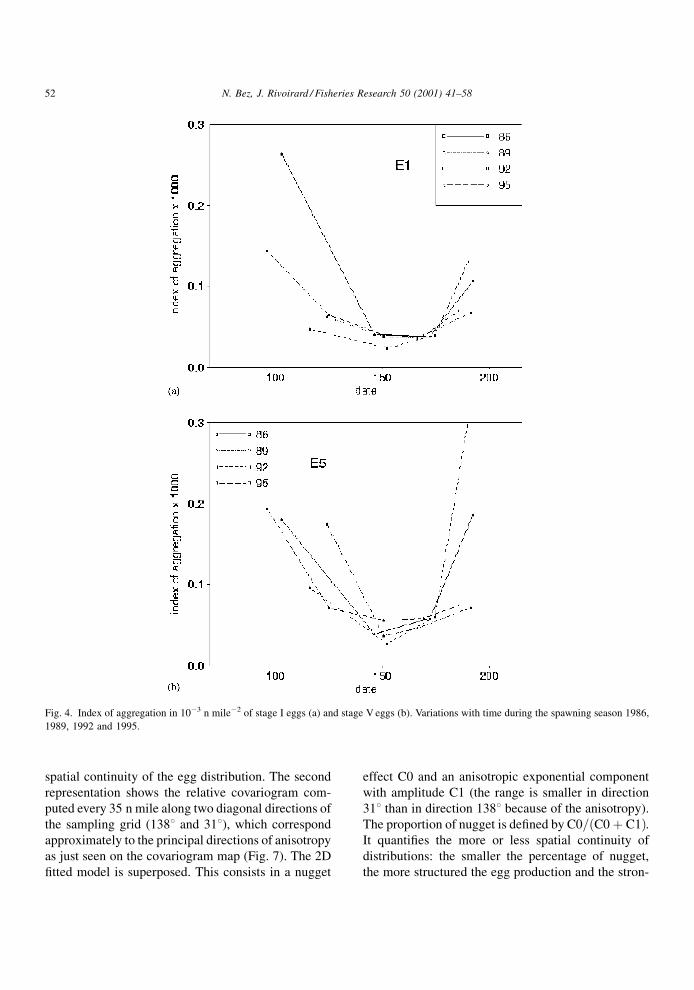
The indices of aggregation (Fig. 4) are U-shaped,

varying in a way opposite to the daily productions. For

a given year, the index of aggregation is then minimum

in the middle of the spawning season (the correspond-

ing equivalent area is 30 000 n mile2). At that time of

the year, the indices of aggregation for the stage I eggs

are the same in 1986, 1989 and 1995 despite large

differences in egg productions, and twice smaller in

1992. Indices of aggregation are most of the time

larger for stage V than for stage I eggs (Fig. 5) and the

more distant the date is from the peak date (size of

squares on Fig. 5) the larger are the differences

between the indices of the two stages.

The equivalent areas, inverse of the indices of

aggregation, are not represented here but bell-shaped

with a ¯attened peak, at or after the production peak,

and are larger for stage I than for stage V. As stated

before, the daily production is the product of the level

of aggregation and of the equivalent area. We can see

here that both the level of aggregation and the equiva-

lent area are directly responsible for the variations

observed on the daily production, either through time

for a given egg stage, or between stages within the

same sampling period.

5.2. Geostatistical aggregation of stages I and V eggs

Inertia are computed with the original longitude and

latitude converted in nautical miles by a simple cosine

transformation. No transformation of coordinates is

Fig. 1. Daily productions of stage I eggs, 1989, sampling period 2. Square areas are proportional to the data values. Zero data are represented

by a cross.


attempted to take into account the shape of the shelf

edge actually in¯uencing the egg distribution (Fig. 1).

For the stage I eggs, the (square root of the) inertia is

bell-shaped with a ¯attened peak and small differ-

ences between years are observed (Fig. 6a): from mid-

April to mid-June the inertia of the population of stage

I eggs is estimated around 30 000 n mile2 (square root

around 170 n mile). The same picture (shape and

magnitude of the curves) is observed for the stage

V eggs (Fig. 6b) and no clear tendency emerged while

comparing the inertia of both stages.

The relative covariograms of stages I and V eggs

have been computed for the different years and per-

iods. However, the poor number of samples in the

Fig. 2. Daily productions in 1012 ind. per day of stage I eggs (a) and stage V eggs (b). Variations with time during the spawning season 1986,

1989, 1992 and 1995.


starting and ending sampling periods of each year

(Table 5) leads to unexploitable covariograms. So

®nally, only middles of spawning seasons have been

considered. Spatial directions are given in degrees

clockwise from the north; for instance, 458 refers to

a southwest±northeast direction.

A typical example of relative covariogram, corre-

sponding to the stage I eggs of the second period of

1989 (post-plot on Fig. 1), is selected for illustration.

In Fig. 7, the covariogram is represented as a map,

function of the east±west and north±south components

of distance. This exhibits a narrow ellipse of high

values surrounded by low ones, the large and the small

axes of the ellipse being oriented along the directions

of, respectively, maximum (northwest±southeast,

1438) and minimum (southwest±northeast, 538)

Fig. 3. Level of aggregation in individuals per square meter per day of stage I eggs (a) and stage V eggs (b). Variations with time during the

spawning season 1986, 1989, 1992 and 1995.


spatial continuity of the egg distribution. The second

representation shows the relative covariogram com-

puted every 35 n mile along two diagonal directions of

the sampling grid (1388 and 318), which correspond

approximately to the principal directions of anisotropy

as just seen on the covariogram map (Fig. 7). The 2D

®tted model is superposed. This consists in a nugget

effect C0 and an anisotropic exponential component

with amplitude C1 (the range is smaller in direction

318 than in direction 1388 because of the anisotropy).

The proportion of nugget is de®ned by C0=�C0� C1�.It quanti®es the more or less spatial continuity of

distributions: the smaller the percentage of nugget,

the more structured the egg production and the stron-

Fig. 4. Index of aggregation in 10ÿ3 n mileÿ2 of stage I eggs (a) and stage V eggs (b). Variations with time during the spawning season 1986,

1989, 1992 and 1995.


ger the spatial continuity. Given the characteristics

of the sampling pattern of the egg surveys, this

corresponds to the importance of the structures taking

place at scale between 0 and 35 n mile relative to the

overall spatial structure of the eggs.

All covariograms have been ®tted by such a type of

model for comparison. The parameters are given in

Table 7 and the models are represented in Figs. 8 and

9. The percentage of nugget ranges between 9 and

83 with no tendency either within or between stages.

This percentage is particularly high for both egg

stages in 1995 (52 and 83%, respectively, for E1

and E5) indicating that more than half of their aggre-

gations come from spatial structures of scale between

0 and 35 n mile. Such proportions of nugget are due

to the fact that the 1995 total production of E1

and especially the one of E5 are made of very small

proportions of very high values spread over the spawn-

ing area.

The exponential component of the spatial structures

of E1 is stable over the 4 years: its amplitude varies

from 0:19� 10ÿ3 to 0:26� 10ÿ3 and its range in the

direction 318 varies between 52 and 57 n mile. The

particularly small index of aggregation estimated for

Fig. 5. Comparison of the index of aggregation (10ÿ3 n mileÿ2) of the stages I and V eggs estimated per sampling period. The bisector is

indicated by a line. Symbols have a size proportional to the number of days between the sampling period and the peak of spawning

(day � 150).

Table 7

Parameters of the relative covariogram models for stages I and V eggs. C0 is the value of the nugget component, C1 the sill of the exponential

component with parameter range R31 and R121 in the direction 318 and 1218, C0=�C0� C1� the proportion of nugget

Sampling period

1986-2 1989-2 1992-2 1995-3

Egg stage I Egg stage

V


V


V

Egg stage I Egg stage V

C0 (10ÿ3) 0.14 0.046 0.17 0.032 0.021 0.077 0.21 0.46

C0=�C0� C1� (%) 35 12 45 9 9 29 52 83

C1 (10ÿ3) 0.26 0.34 0.21 0.33 0.21 0.19 0.19 0.097

R31 (n mile) 52 41 52 43 57 80 55 130

R121 (n mile) 137 111 200 123 150 157 153 250


E1 in 1992 (value of g0/Q2 in Fig. 9) comes then

essentially from the exponential component.

Apart from the value and the direction of anisotropy

which are rather stable, no systematic results emerge

from the comparison of the spatial structures between

E1 and E5. In 1986 and 1989, it appears that the

stage V eggs have more regular spatial structure

than the stage I eggs: the value at the origin is roughly

the same for the two stages with a smaller nugget

effect in case of E5. In 1992, the nugget effect are

small, especially for E1. In 1995, both the index of

aggregation and the percentage of nugget are larger

for E5, indicating a destructuration during the egg

development.

Fig. 6. Square root of inertia in nautical miles of stage I eggs (a) and stage V eggs (b). Variations with time during the spawning season 1986,

1989, 1992 and 1995.


6. Discussion

It is worth reminding that the accuracy of the results

is directly linked to the accuracy of the estimations.

The data preparation, the data selection, and the

hypothesis required for the estimation have been

speci®ed. But no indication on the precision of the

estimations, for instance their variances, is proposed.

In addition to that, the representativity of the data

values (measurement errors) is not identi®ed.

The idea of giving each sample a weight propor-

tional to its density, has lead to the de®nition of

various Individual Based Statistics. Some of these

are strictly speaking statistical tools while the others

Fig. 7. Example of relative covariogram. Daily productions of stage I eggs, 1989, sampling period 2. Covariogram map: each point represents

the value of the relative covariogram for the corresponding vectorial distance. The axes represent the two components of the vectorial distance

expressed in nautical miles. Values are figured with a grey scale between 0.000025 n mileÿ2 (black) and 0 n mileÿ2 (white). Arrows indicate

the directions 1438 and 538 of the anisotropy.


are geostatistical tools. The application made on

mackerel egg distributions provides a good opportu-

nity to discuss the value and the relation between three

of them: the index of aggregation, the inertia and the

relative covariogram. The analysis exhibits that

despite differences in total productions of stage I eggs

between and within the spawning seasons 1986, 1989,

1992 and 1995, the inertia of the eggs populations is

remarkably stable. The inertia is, at ®rst sight, a

physical mass concept. It is also related to the covar-

iogram byR

h2g�h�=Q2 dh. This means that the inertia

is very poorly affected by the nugget effect and that it

summarises the structured part of spatial distributions.

In fact the exponential component of the spatial

structure of the stage I eggs is stable from year to year.

This explains why inertia are stable. This makes also

the variations of the index of aggregation essentially

related the ¯uctuations of the nugget effect. Nugget

happens to be more or less the same in 1986, 1989 and

1995 and very small in 1992, which explains why the

Fig. 8. Example of relative covariogram. Daily productions of stage I eggs, 1989, sampling period 2. Experimental and modelled relative

covariogram in 10ÿ3 n mileÿ2 represented in two particular directions (1388 and 318). These directions correspond to the diagonals available in

the sampling grid around the actual directions of anisotropy (see Fig. 7).


index of aggregation are equal in 1986, 1989 and 1995

and twice lower in 1992.

Even though this is a 4 years study only, this

suggests that, relatively to the abundance, constant

features exist in the spatial organisation of newly

spawn mackerel eggs, and thus in the mackerel spawn-

ing process. This intrinsic feature is the large scale

spatial structure, and the annual variability of the

aggregation pattern is essentially dependent on the

variability of the spatial structures between 0 and 35 n

mile, refer to as the short scale structures in this study

because of the inter sample distance.

Eggs can be transported (advection), can diffuse

and can die. A global advection of the egg population

will not change the index of aggregation, the inertia or

the relative covariogram, so as a constant or a density

independent mortality rate. Passive diffusion is sup-

posed to spread locally the eggs while they are devel-

oping. The index of aggregation and the percentage of

nugget are then expected to decrease while the large

scale structures are essentially maintained. Results are

sometimes consistent with what is intuitively expected

due to diffusion. The relative covariograms of E5

computed in 1986 and 1989 have a slightly smaller

Fig. 9. Relative covariograms for the four middle spawning season sampling periods for stage I eggs (continuous line) and stage V eggs

(dotted lines). Two directions (318 and 1388) are represented. The year and the mean date of the sampling periods are written on each figure.

Values at the origin, i.e. index of aggregation, are indexed by their names.


index of aggregation and a smaller nugget than the

observed structures of E1. However, in 1992 and

especially in 1995, the results go against what is

expected a priori. This could be explained by a

density-dependent mortality rate, as in such a case,

the contrast between data values is increased from E1

to E5. Of course it is not possible to eliminate the role

of local advection in the variation of aggregation.

7. Conclusions

The common problem encountered in ®sheries

related to the treatment of the zeroes and to the

delineation of the area of presence, becomes crucial

for populations with diffuse limits. Plankton and

pelagic ®sh provide good examples of such situations.

By giving each sample a weight proportional to its

density, Individual Based Statistics are not affected by

zeroes and more generally by low concentrations.

Index of aggregation or inertia are two examples of

such statistics and are recommended as basic statistics

in the aforementioned cases.

The index of aggregation is de®ned by the prob-

ability that two ®sh taken at random in the ®eld are in

the same sample. It measures the aggregation that

arise at the population level with no indication on how

the aggregation is generated spatially (short versus

large scale for instance). While a single scalar-like the

inertia is able to give information on the structured

part of spatial distributions, a more complete descrip-

tion of the spatial structure is accessible through the

transitive covariogram. Models of covariogram have

been used in the purpose of the comparison of various

situations, but it is recalled that more can be gained with

such models like the computation of a global estima-

tion variance or the computation of a kriging map.

Acknowledgements

This work has been done in the context of the EEC

project SEFOS (Shelf Edge Fisheries and Oceano-

graphic Study) that ended in December 1996. The

authors are grateful to all the participants of the project

and also to CEFAS Lowestoft (UK) for providing the

data used in this paper.

References

Anon., 1987. Report of the Mackerel Egg Production

Workshop. ICES CM 1987/H:2, 56 pp.

Anon., 1990. Report of the Mackerel/Horse Mackerel Egg

Production Workshop. ICES CM 1990/H:2, 89 pp.

Anon., 1993. Report of the Mackerel/Horse Mackerel Egg

Production Workshop. ICES CM 1993/H:4, 142 pp.

Anon., 1996. Report of the Working Group on Mackerel and Horse

Mackerel egg surveys. ICES CM 1996/H:2, 146 pp.

Bez, N., Rivoirard, J., Poulard, J.Ch., 1995. Approche transitive

et densiteÂs de poissons. Cahiers de GeÂostatistique 5, 161±

177.

Bez, N., Rivoirard, J., Walsh, M., 1996. Individual based statistics

for a spatially distributed population, with an application on

mackerel. ICES CM 1996/S:23, 8 pp.

Bez, N., Rivoirard, J., Guiblin, Ph., Walsh, M., 1997. Covariogram

and related tools for structural analysis of fish survey data. In:

Baafi, E.Y., Schofield, N.A. (Eds.), Geostatistics Wollon-

gong'96, Vol. 2, pp. 1316±1327.

Cooper, S.D., Barmuta, L., Sarnelle, O., Kratz, K., Diehl, S., 1997.

Quantifying spatial heterogeneity in streams. J. N. Am.

Benthol. Soc. 16 (1), 174±188.

Frank, K.J., Carscadden, J.E., Leggett, W.C., 1993. Causes of

spatio-temporal variation in the patchiness of larval fish

distribution: differential mortality or behavior. Fish. Oceanogr.

2 (3/4), 114±123.

Houde, E.D., Lovdal, J.D.A., 1985. Patterns of variability in

ichtyoplankton occurrence and abundance in Biscayne Bay.

Florida Est. Coast. Shelf Sci. 20, 79±103.

Lloyd, M., 1967. Mean crowding. J. Anim. Ecol. 36, 1±30.

Lockwood, S.J., Nichols, J.H., Dawson, W.A., 1981. The estima-

tion of a mackerel (Scomber scombrus L.) spawning stock size

by plancton survey. J. Plank. Res. 3 (2), 217±233.

Matheron, G., 1971. The theory of regionalized variables and its

applications. Les cahiers de Morphologie MatheÂmatique fasc 5,

212.

Matsuura, Y., Hewitt, R., 1995. Changes in the spatial patchiness of

Pacific mackerel, Scomber japonicus, larvae with increasing

age and size. Fish. Bull. 93, 172±178.

Myers, R.A., Cadigan, N.C., 1995. Was an increase in natural

mortality responsible for the collapse of northern cod? Can. J.

Fish. Aquat. Sci. 52, 1274±1285.

de Nie, H.W., Bromley, H.J., Vijverberg, J., 1980. Distribution

patterns of zooplankton in Tjeukemeer, the Netherlands. J.

Plank. Res. 2 (4), 317±334.

Petitgas, P., 1994. Spatial strategies of fish populations. ICES CM

1994/D:14, 7 pp.

Stabeno, P.J., Schumacher, J.D., Bailey, K.M., Brodeur, R.D.,

Cokelet, E.D., 1996. Observed patches of walleye pollock eggs

and larvae in Shelikof Strait, Alaska: their characteristics,

formation and persistence, formation and persistence. Fish.

Oceanogr. 5 (Suppl. 1), 81±91.

Taylor, L.R., 1961. Aggregation, variance and the mean. Nature

189, 732±735.


Transitive geostatistics to characterise spatial aggregations with diffuse limits: an application on...

Documents

Transcript of Transitive geostatistics to characterise spatial aggregations with diffuse limits: an application on...