Computationally efficient sup-t transitive

closure for sparse fuzzy binary relations ?

Manolis Wallace, Yannis Avrithis and Stefanos Kollias ??

School of Electrical and Computer Engineering,National Technical University of Athens, Greece

Abstract

The property of transitivity is one of the most important for fuzzy binary relations,especially in the cases when they are used for the representation of real life similarityor ordering information. As far as the algorithmic part of the actual calculation ofthe transitive closure of such relations is concerned, works in the literature mainlyfocus on crisp symmetric relations, paying little attention to the case of general fuzzybinary relations. Most works that deal with the algorithmic part of the transitiveclosure of fuzzy relations only focus on the case of max-min transitivity, disregardingother types of transitivity. In this paper, after formalizing the notion of sparsenessand providing a representation model for sparse relations that displays both compu-tational and storage merits, we propose an algorithm for the incremental update offuzzy sup-t transitive relations. The incremental transitive update (ITU) algorithmachieves the re-establishment of transitivity when an already transitive relation isonly locally disturbed. Based on this algorithm, we propose an extension to handlethe sup-t transitive closure of any fuzzy binary relation, through a novel incrementaltransitive closure (ITC) algorithm. The ITU and ITC algorithms can be applied onany fuzzy binary relation and t-norm; properties such as reflexivity, symmetricityand idempotency are not a requirement. Under the specified assumptions for theaverage sparse relation, both of the proposed algorithms have considerably smallercomputational complexity than the conventional approach; this is both establishedtheoretically and verified via appropriate computing experiments.

Key words: transitive closure, complexity, sparse matrix, fuzzy partial orderingrelations

? This work has been partially funded by the HERACLETUS project of the GreekMinistry of Education??Corresponding author: Manolis Wallace. 14 Aglavrou Str., Koukaki, Athens, 11741, Attica, GREECE. Email: wallace@image.ntua.gr. Tel.: +30 210 772 3039. Fax.:+30 210 772 2492.

Preprint submitted to Elsevier Science 6 March 2005

1 Introduction

Fuzzy binary relations and their properties have an important role in mod-elling of information in various scientific and applied fields. With descriptivepower ranging from the simple representation of information [47] to the rep-resentation of ontological [28] and multimedia structures [2][34], the fields ofapplication of fuzzy relations are countless. A field in which these relationshave a very special role is that of fuzzy information retrieval [10][12][39]. Inthat framework, fuzzy relational knowledge representation can contribute totasks such as query expansion [3], document analysis [4][40], multimedia anal-ysis [38], user profiling [41] and others.

In most cases, the fuzzy relation property that is most important for the repre-sentation of real life information is that of transitivity ; continuous Archimedeantransitivity is a property that describes the propagation of information in avery natural and intuitive way. Therefore, it is only natural that numerous ref-erences in the literature discuss the representation [23][26][31] and theoreticalproperties of transitive binary relations [11][13][15][16][17][18][24][35][45].

The transitive property of binary relations, due to its physical meaning, isclosely related to the study of graphs. In that framework, transitive closureof a relation is equivalent to the detection of the pairs of vertices that areeither directly connected or connected via some path. Thus, the majority ofexisting literature on transitive closure algorithms and has focused mainlyon the cases of undirected crisp graphs [33] and crisp graphs [9][32][36][43],most of which are based on the work of Warshall [44]. In [37], in addition tothe computational complexity of the process of the transitive closure, its I/Ocomplexity is examined as well; this study, similarly to the the ones mentionedabove, is also limited to the crisp case.

Transitive closure of general fuzzy binary relations has also been treated inthe literature. See, for example, [14][27][29]. In the latter two an impressivecomplexity of O(n2) is achieved; a result already accomplished in [19] witha different methodology. The application of all four reported algorithms islimited to similarity, i.e. symmetric and reflexive relations, and to the case ofmax-min transitivity, i.e. to a single non Archimedean case. Overall, not manyworks in the literature attempt to tackle the sup-t transitive closure of generalfuzzy binary relations; most of the attention is focused solely on the caseof max-min transitivity. (Exceptions to this can be found in [20][21].) Moreimportantly, there are no references in the literature specializing in the case ofsparse relations ; as the binary relations considered in the fields of ontologicalrepresentation and fuzzy information retrieval are both sparse and large, thehandling of sparse transitive relations is an issue with gaining importance.This is the topic of this paper.

2

Given the size of the considered binary relations, their representation is anequally important problem to that of their handling. Specifically, the memoryrequired for the storage of an n×n relation becomes prohibitive, as n surpassessome reasonably small threshold; we may overcome this problem with the uti-lization of a sparse representation format, since these relations are typicallyvery sparse; this of course adds an overhead to the time required to access aspecific element.In this paper we formalize the notion of sparseness and providea representation model for sparse relations that displays both computationaland storage merits. Based on this representation model, we develop an algo-rithm for the computationally efficient incremental update of fuzzy transitiverelations; the incremental transitive update (ITU) algorithm focuses on there-establishment of transitivity when an already transitive relation is only lo-cally disturbed, and is suitable for any type of sup-t transitivity and any typeof fuzzy relation. Based on this algorithm, we propose an extension to handlethe sup-t transitive closure of any fuzzy binary relation, through a novel incre-mental transitive closure (ITC) algorithm; this algorithm is computationallyefficient and has some unique properties. Under the specified assumptions forthe average sparse relation, both of the proposed algorithms have considerablysmaller computational complexity than the conventional approach; this is bothestablished theoretically and verified via appropriate computing experiments.

The structure of this paper is as follows: In section 2, after formally definingwhat “sparse relation” means in this work, we present the sparse represen-tation model we follow, as the properties of this data model directly affectthe properties of the algorithms to follow. Continuing, in section 3 we discussthe properties of the conventional transitive closure algorithm, when com-bined with the representation model presented in section 2. In sections 4 and5 we present the two algorithms that we propose. Specifically, in section 4 wepresent our approach for incremental update of a binary relation and discussits storage and computational merits and in section 5 we extend our discussionto explain how this can be utilized to handle the complete transitive closureof a relation as well. Section 6 lists some indicative experimental results thatsupport and validate our theory and section 7 lists our concluding remarks.

2 Representation of sparse relations

2.1 Assumptions on sparseness

Binary relations can be used to model numerous aspects of the real world.Depending on the case, the considered relations may display various formalmathematical properties, such as associativity, reflexivity, transitivity of oneform or another and so on. The specification of each one of these properties is

3

an objective task, which makes it feasible to discriminate between the differenttypes of relations and handle them in different ways.

On the other hand, some subjective properties are often important in reallife relations. The most important among them is sparseness; sparse relations,although having the same objective properties as their dense counterparts, are“best” handled using totally different approaches. By “best” we do not referto the validity of the methodologies applied, as their results are identical, butrather to their efficiency as far as storage and computational resources neededare concerned.

As sparse relations play an important role in various fields, specialized datamodels and corresponding algorithms have been developed just for them; oneof the most important problem with such data models and algorithms is theirevaluation. Traditionally, the efficiency of a data structure or algorithm ismeasured using its storage and computational complexity, which is closelyrelated to its operation in the worst possible case. This is of course inapplicablefor the case of models and algorithms that have been designed for the sparsecase, as, by definition, the notion of worst case is contradictory to that ofsparseness.

Thus, in order to make the evaluation possible, we typically refer to the per-formance in the average, rather than the worst case scenario. This, in turn,demands that we can formally define the statistical properties of the averagecase. In this work, driven by the statistical characteristics of sparse relationsappearing in the field of ontologies, we define the average case for sparse rela-tions as follows:

Let n = |S| be the cardinality of the universe of discourse. A small andconstant percentage pr of the rows and pc of the columns of an n × n typicalsparse relation may be non zero. Thus, we have O(n) non zero rows and O(n)non zero columns. Additionally, the count of non zero elements contained ina non zero row or column is proportional to the logarithm of the count of allthe elements in the relation. Thus we have O(log n) non zero elements in eachnon zero row and column. Overall, we have O(n log n) non zero elements inthe relation.

2.2 Proposed sparse representation

A fuzzy binary relation defined on a set S containing n distinct elements can berepresented using a square matrix of dimension n×n. The physical storage ofsuch an array requires the representation of n2 different decimal values, whichfor large numbers of n is prohibitive for a practical implementation. On theother hand, in such a representation access to a specific element of the array

4

has a computational complexity of O(1), as the position of the element in thearray directly specifies its position in storage as well, with the utilization of aformula of the form M = [(i−1) ·n+(j−1)] ·d+O where (i, j) is the positionof the element in the matrix, M is its actual position in storage, O is an offsetspecifying the position of the first element of the array in storage and d is thespace allocated for each element. As already explained, the utilization of sucha representation is not always possible. In cases where the relation is known tobe sparse, i.e. only a small subset of the elements of the corresponding arrayare non zero, then a sparse array implementation can be used to overcome thestorage problem.

Conventional sparse array implementations utilize linked lists to representelements, thus raising the computational complexity of accessing a specificelement from O(1) to O(n). In this case, although the storage requirements aremuch smaller, the representation model remains inapplicable for time criticalapplications, where complex operations utilizing a binary relation have to beperformed before the system response is determined, and number n is large.

The representation model proposed in order to overcome these limitations isas follows: a binary relation is represented using two AVL trees ; an AVL treeis a binary, balanced and ordered tree that allows for access, insertion anddeletion of a node in O(log m) time, where m is the count of nodes in the tree[1]. If n log n nodes exist in the tree, as will be the case for the typical sparserelation, then the access, insertion and deletion complexity is again O(log n)since n < n log n < n2 ⇒ O(log n) ≤ O(log(n log n)) ≤ O(log n2) = O(log n).

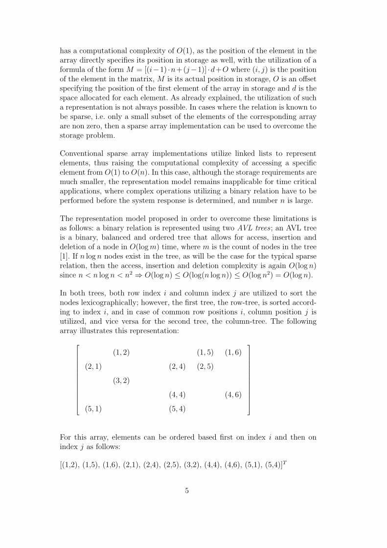
In both trees, both row index i and column index j are utilized to sort thenodes lexicographically; however, the first tree, the row-tree, is sorted accord-ing to index i, and in case of common row positions i, column position j isutilized, and vice versa for the second tree, the column-tree. The followingarray illustrates this representation:

(1, 2) (1, 5) (1, 6)

(2, 1) (2, 4) (2, 5)

(3, 2)

(4, 4) (4, 6)

(5, 1) (5, 4)

For this array, elements can be ordered based first on index i and then onindex j as follows:

[(1,2), (1,5), (1,6), (2,1), (2,4), (2,5), (3,2), (4,4), (4,6), (5,1), (5,4)]T

5

Fig. 1. Example of a row-tree, ordered by index i.

Fig. 2. Example of a column-tree, ordered by index j.

Similarly, elements can be ordered based first on index j and then on index ias follows:

[(2,1), (5,1), (1,2), (3,2), (2,4), (4,4), (5,4), (1,5), (2,5), (1,6), (4,6)]T

The vectors above can then be represented as AVL trees, as shown in figures1 and 2, depicting the corresponding row-tree and column-tree, respectively.Of course the trees are not unique, as more than one balanced binary treescan be created when the count of elements is not equal to (2k − 1) for somek ∈ N .

This representation model preserves the storage merits of the conventionalsparse matrix implementation using linked lists. Moreover, access time to aspecific element, row or column of the relation has a computational complexityof O(log n), which is considerably lower than the linear complexity of theconventional linked lists approach. Finally, the complexity of insertion anddeletion is also O(log n); note that both trees have to be kept up-to-date aftereach insert, delete or update operation.

6

3 Conventional sup− t transitive closure of fuzzy binary relations

3.1 Conventional algorithm using complete representation

A transitive closure of a fuzzy binary relation can be performed with a com-plexity of O(n4), where n = |S| is the dimension of the relation matrix, uti-lizing the methodology reported in [46], as described below.

In the general case, the transitive closure Trt(R) of relation R, given somet-norm, can be calculated as

Trt(R) =n−1⋃

f=1

Rf (1)

where Rf can be calculated recursively as

Rf = Rf−1 ◦t R (2)

R1 = R (3)

As a special case, when relation R is reflexive, it is proven that the transitiveclosure is given by equation

Trt(R) = Rn−1

thus making the calculation of the sup of equation 1 unnecessary [25].

The following lemma provides the basis for the calculation of the computa-tional complexities of relation operations using the complete representationmodel:

Lemma 1: When the complete representation model is utilized, the calcula-tion of the sup Rsup = sup(R1, R2) and composition Rcomp = R1 ◦t R2 of tworelations R1 and R2 of dimension n × n have computational complexities ofO(n2) and O(n3), respectively.

Proof: An element Rsup(i, j) of the sup is calculated as

Rsup(i, j) = sup(R1(i, j), R2(i, j))

7

An element Rcomp(i, j) of the sup-t composition is calculated as

Rcomp(i, j) =n⋃

c=1

R2(i, c) ∧t R1(c, j)

The former is an O(1) operation and the latter an O(n) operation. As theoutputs of the sup and composition have a dimension of n× n, n2 such oper-ations need to be performed, thus concluding in overall complexities of O(n2)and O(n3), respectively.

2

From this lemma, it is easy to conclude the following:

Lemma 2: In the case of complete representation, the calculation of the tran-sitive closure of two relations following the methodology of [46] as describedabove has a computational complexity of O(n4)

Proof: In the calculation of the transitive closure of a reflexive relation, Rn−1

needs to be calculated. Using the methodology described by equations 2 and3 this is performed in n− 1 compositions. The previous lemma provides thateach one of these compositions is performed with a computational complexityof O(n3), thus resulting in an overall complexity of O(n4) for the calculationof Rn−1, which is the transitive closure of relation R.

In the process of calculation of Rn−1, all Rf , f ∈ Nn−1 are calculated asbyproducts. Thus, for the calculation of the transitive closure in the general(not necessarily reflexive) case what is additionally needed is the calculationof the sup described by equation 1. According to the previous lemma, thesup of two relations is calculated in O(n2). In total, n − 2 such calculationsare required, resulting in a computational complexity of O(n3). Thus, theoverall computational complexity for transitive closure using this methodologyis O(n4) + O(n3) = O(n4).

2

Dunn has proposed a computationally enhanced algorithm to calculate thetransitive closure of a fuzzy binary relation, with a complexity of O(n3 log n)[20]. This algorithm relies on the recursive self composition of the relationmatrix until transitivity is achieved.

Specifically, the transitive closure of a relation R is given as:

Trt(R) =⋃

Rf∗ , f ∈ {1, 2, 4, 8, .., 2F}, F ≥ n− 1 (4)

8

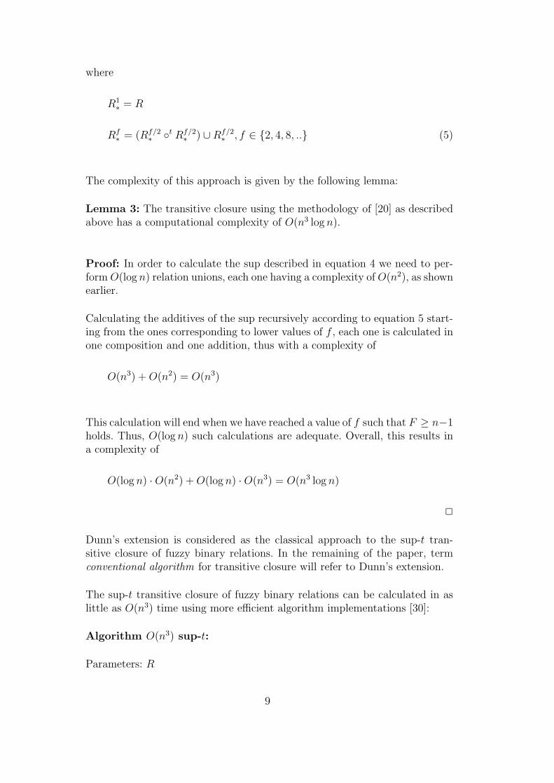
where

R1∗ = R

Rf∗ = (Rf/2

∗ ◦t Rf/2∗ ) ∪Rf/2

∗ , f ∈ {2, 4, 8, ..} (5)

The complexity of this approach is given by the following lemma:

Lemma 3: The transitive closure using the methodology of [20] as describedabove has a computational complexity of O(n3 log n).

Proof: In order to calculate the sup described in equation 4 we need to per-form O(log n) relation unions, each one having a complexity of O(n2), as shownearlier.

Calculating the additives of the sup recursively according to equation 5 start-ing from the ones corresponding to lower values of f , each one is calculated inone composition and one addition, thus with a complexity of

O(n3) + O(n2) = O(n3)

This calculation will end when we have reached a value of f such that F ≥ n−1holds. Thus, O(log n) such calculations are adequate. Overall, this results ina complexity of

O(log n) ·O(n2) + O(log n) ·O(n3) = O(n3 log n)

2

Dunn’s extension is considered as the classical approach to the sup-t tran-sitive closure of fuzzy binary relations. In the remaining of the paper, termconventional algorithm for transitive closure will refer to Dunn’s extension.

The sup-t transitive closure of fuzzy binary relations can be calculated in aslittle as O(n3) time using more efficient algorithm implementations [30]:

Algorithm O(n3) sup-t:

Parameters: R

9

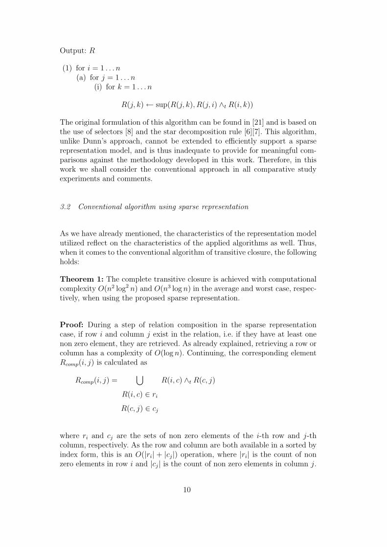
Output: R

(1) for i = 1 . . . n(a) for j = 1 . . . n

(i) for k = 1 . . . n

R(j, k) ← sup(R(j, k), R(j, i) ∧t R(i, k))

The original formulation of this algorithm can be found in [21] and is based onthe use of selectors [8] and the star decomposition rule [6][7]. This algorithm,unlike Dunn’s approach, cannot be extended to efficiently support a sparserepresentation model, and is thus inadequate to provide for meaningful com-parisons against the methodology developed in this work. Therefore, in thiswork we shall consider the conventional approach in all comparative studyexperiments and comments.

3.2 Conventional algorithm using sparse representation

As we have already mentioned, the characteristics of the representation modelutilized reflect on the characteristics of the applied algorithms as well. Thus,when it comes to the conventional algorithm of transitive closure, the followingholds:

Theorem 1: The complete transitive closure is achieved with computationalcomplexity O(n2 log2 n) and O(n3 log n) in the average and worst case, respec-tively, when using the proposed sparse representation.

Proof: During a step of relation composition in the sparse representationcase, if row i and column j exist in the relation, i.e. if they have at least onenon zero element, they are retrieved. As already explained, retrieving a row orcolumn has a complexity of O(log n). Continuing, the corresponding elementRcomp(i, j) is calculated as

Rcomp(i, j) =⋃

R(i, c) ∈ ri

R(c, j) ∈ cj

R(i, c) ∧t R(c, j)

where ri and cj are the sets of non zero elements of the i-th row and j-thcolumn, respectively. As the row and column are both available in a sorted byindex form, this is an O(|ri| + |cj|) operation, where |ri| is the count of nonzero elements in row i and |cj| is the count of non zero elements in column j.

10

For a single composition kr · kc such operations will be performed, where kr

is the count of non zero rows and kc is the count of non zero columns of therelation. Overall, the complexity for a single composition is

O(log n) + O(log n) + O(kr · kj) · [O(|ri|+ |cj|) + O(log n)]

where the last O(log n) factor corresponds to the complexity of the insertionof an element in the output relation.

In the average case for sparse relations, a small percentage of the rows andcolumns will be non zero. Of course, although this may affect the executiontime required, it does not alter the complexity, as

O(kr · kc) = O((pr · n) · (pc · n)) = (pr · pc) ·O(n2)) = O(n2)

where constants pr and pc is the percentage of non zero rows and columnsrespectively. As far as the count of elements contained in a non zero row orcolumn is concerned, as has already been mentioned in subsection 2.1, this isassumed to be proportional to the logarithm of the count of all elements inthe relation. Thus O(kr · kj) = O(log n). Overall, this leads to a complexity of

O(log n) + O(log n) + O(n2) · [O(log n) + O(log n)] = O(n2 log n)

for the composition.

In the worst case, all the elements of the relation exist. In that case, kr = kc =|ri| = |cj| = n, and thus the complexity of the composition becomes

O(log n) + O(log n) + O(n2) · [O(n) + O(log n)] = O(n3)

Considering the O(log n) compositions required by the conventional method-ology for the transitive closure, it is straightforward that in the average casethe complete transitive closure has a computational complexity of O(n2 log2 n)and in the worst case O(n3 log n).

2

3.3 Comparative study

As far as the computational complexity of the transitive closure algorithm isconcerned, it is O(n3 log n) for the complete representation and O(n2 log2 n)

11

Table 1Summary of computational complexities of conventional composition and transitiveclosure algorithms

Algorithm Data model Sparse relation Dense relation

Composition Complete n3 n3

Composition Sparse n2 log n n3

Transitive Closure Complete n3 log n n3 log n

Transitive Closure Sparse n2 log2 n n3 log n

and O(n3 log n) for the sparse representation, in the average and worst case, re-spectively. It is worth noting that the proposed sparse representation achievesenhanced computational complexity in the sparse case, without loosing in ef-ficiency in the dense case.

As far as storage requirements are concerned, using either of the two rep-resentation models, i.e. complete representation or the sparse representationproposed herein, the existence of two copies of the relation in memory duringthe execution of the transitive closure algorithm is required. The storage re-quirements of the two approaches, though, are fundamentally different in thecase of sparse relations:

(1) In the conventional approach n2 elements are represented for each copyof the relation, leading to the need for 2 · n2 distinct elements beingrepresented. This is an O(n2) space.

(2) In the proposed approach 2 trees are represented, each containing as manynodes as the relation at hand. In the average case of sparse relations thisresults in 2 · O(n log n) nodes, leading to an overall storage complexityof 4 · O(n log n) = O(n log n) for the two trees. In the worst case O(n2)storage space is required, as in the conventional approach.

Table 1 summarizes the above conclusions on computational complexity ofconventional composition and transitive closure algorithms, using completeand sparse representations. One can easily see that the proposed representa-tion model is ideal for the case of sparse relations, as they have been definedin section 2.1, as it can lead to enhanced computational and storage complex-ities, even when using algorithms that have not been designed especially forthe sparse case.

4 Incremental closure of fuzzy binary relations

A major disadvantage of the utilization of the conventional transitive closuremethodologies is that when for some reason an element of the relation is

12

Fig. 3. Graphical representation of the incremental update of the transitive relation.

updated, or when a new entity is inserted to the global set S and linked tosome existing entity, thus locally disturbing transitivity, a computationallydemanding operation needs to be performed again in order to re-establish thetransitivity property.

4.1 Conventional re-establishment of transitivity

Theorem 2: When a new element is inserted to the relation, or when anelement of the relation is updated, and assuming the conventional approachto transitive closure, an O(n2 log n) operation is adequate in order to assurethat the relation remains transitive in the average case. In the worst case thecomplexity is O(n3 log n).

Proof: Let R be a transitive relation. In Fig. 3 non zero elements of R arerepresented using continuous lines of type 0. Let as suppose that R(i, j) isinserted in the relation, or that its value is augmented. In Fig. 3 the update isrepresented using dash - dot lines of type 1. Then, we can no longer assumethat relation r is transitive.

After one self-composition, the ancestor a of i is linked to j and i is linked tothe descendant d of j. In Fig. 3 this is represented using dashed lines of type2. Finally, after one more self-composition, a is linked to b. In Fig. 3 this isrepresented using doted lines of type 3.

As R was initially assumed transitive, two compositions will always be enoughto assure transitivity. Thus, the complexity of the operation that re-establishestransitivity can be as low as that of the composition: O(n2 log n) in the averagecase and O(n3) in the worst case, as established in the theorem’s proof insection 3.

2

13

4.2 The incremental transitive update (ITU) algorithm

Having observed in Fig. 3 the way in which transitivity is achieved after asingle element has been altered, we can design an algorithm for incrementalupdate of transitive relations that has a considerably smaller computationalcomplexity. Specifically, the incremental transitive update (ITU) algorithmonly focuses on the changes that the self composition brings upon the relationafter the update of the single element.

For a given relation R, when the updated element is the one between entitiesi and j, this can be achieved with the following steps:

Algorithm ITU:

Parameters: R i j

Output: R

(1) Identify the fuzzy set A of ancestors of entity i in relation R. Degrees inA are determined as A(s) = R(s, j), s ∈ S.

(2) Identify the fuzzy set D of descendants of entity j in relation R. Degreesin D are determined as D(s) = R(i, s), s ∈ S.

(3) For each element s appearing in A assign

R(s, j) ← sup(R(s, j), A(s) ∧t R(i, j))

(4) For each element s appearing in D assign

R(i, s) ← sup(R(i, s), R(i, j) ∧t D(s))

(5) For each element s1 appearing in A and s2 appearing in D assign

R(s1, s2) ← sup(R(s1, s2), A(s1) ∧t R(i, j) ∧t D(s2))

When the algorithm terminates we have R = Trt(R).

If relation R is reflexive, then R(i, i) = 1 and R(j, j) = 1 and thus A(i) = 1and D(j) = 1. In this case, the above process can be simplified by omittingsteps (3) and (4), as they are included in step (5).

Theorem 3: The computational complexity of the incremental update al-gorithm is O(log3 n) in the average case and O(n2 log n) in the worst case,for both reflexive and non reflexive relations, assuming the proposed sparserepresentation model.

Proof: The complexity of steps (1) and (2) is O(log n), as computation of an

14

element’s ancestors or descendants requires access to a column or row of therelation, respectively. The complexity of steps (3) and (4) is O(|ri|) ·O(log n)and O(|cj|) · O(log n), respectively, and the complexity of step (5) is O(|ri| ·|cj|) ·O(log n).

In the average case |ri| = O(log n) and |cj| = O(log n), and thus the over-all complexity is 2 · O(log n) + 2 · O(log2 n) + O(log3 n) = O(log3 n). In theworst case |ri| = O(n) and |cj| = O(n), and thus the overall complexity is2 · O(log n) + 2 · O(n log n) + O(n2 log n) = O(n2 log n). Ignoring the influ-ence of steps (3) and (4) in the above calculations does not alter the overallcomplexity, as in all cases step (5) contributes more to it. Thus, the samecomplexity holds for the reflexive case as well.

2

Of course, it is easy to extend algorithm ITU in order to make it applicableto the case of complete representation as well:

Algorithm ITU for complete representation:

Parameters: R i j

Output: R

(1) For every element s1 in column i(a) For every element s2 in row j

Assign:

R(s1, s2) ← sup(R(s1, s2), R(s1), i ∧t R(i, j) ∧t R(j, s2)) (6)

Theorem 4: The computational complexity of the incremental update algo-rithm is O(n2), assuming a complete representation model.

Proof: When using the complete representation model, the relation is repre-sented as an n × n array. Thus, there are n elements in each row and eachcolumn. Since equation 6 describes simply two intersections, it is performedin O(1) time. Overall, we have a complexity of

O(n) ·O(n) ·O(1) = O(n2)

2

What remains to be established is that the output of the proposed ITU algo-rithms is indeed transitive. This proof is spit in two sections:

Lemma 4: If relation R is sup−t transitive on S, then it is also sup−t

15

transitive on S ′ ⊇ S.

Proof: A fuzzy relation R defined on S is called sup−t transitive if

R(x, z) ≥ supy∈S{t(R(x, y), R(y, z))}, ∀(x, z) ∈ S2

If x ∈ (S ′ − S), then R(x, z) = 0. In this case

supy∈S′

{t(R(x, y), R(y, z))} = supy∈S′

{0, R(y, z))} = 0

and thus transitivity on S ′ holds. Similarly if z ∈ (S ′ − S).

If (x, z) ∈ S2, then

supy∈S′

{t(R(x, y), R(y, z))} =

= sup(supy∈S{t(R(x, y), R(y, z))}, sup

y∈(S′−S){t(R(x, y), R(y, z))})

= sup(supy∈S{t(R(x, y), R(y, z))}, 0)

= supy∈S{t(R(x, y), R(y, z))}

Since R is transitive on S,

R(x, z) ≥ supy∈S{t(R(x, y), R(y, z))} = sup

y∈S′{t(R(x, y), R(y, z))}

and thus transitivity holds.

2

With this lemma we have established that extending the universe with theaddition of new elements, as the ITU does when needed, does not damage theproperty of transitivity for the already existing relations. We may now splitthe operation of ITU in two steps:

(1) insert new elements in the universe of discourse (if needed)(2) augment the value of a link between existing elements

According to lemma 4, only the second one of these steps affects transitivityand needs to be considered. Thus, we can limit our examination of the validity

16

of the ITU algorithm to the case where an existing link of the relation is aug-mented (the initial link can have any value in the [0 1] range). With the nextlemma we conclude the proof by establishing that ITU correctly re-establishestransitivity what an existing link in the input relation is augmented.

Lemma 5: Let R be a transitive relation on S. Let also i, j ∈ S. ∀q ∈ [01],relation R1 is defined as

R1(x, z) =

max(R(i, j), q), x=i and z=j;

R(x, z), otherwise.

Then relation R′, calculated as R′ = ITU(R1, i, j), is transitive.

Proof:

If R(i, j) ≥ q from construction R′ = R and thus transitivity holds. If R(i, j) <q ⇒ R′(i, j) > R(i, j). We then we need to prove that

R′(x, z) ≥ supy∈S

t(R′(x, y), R′(y, z)),∀(x, z) ∈ S2 (7)

For y such that R′(x, y) = R(x, y), easily

supy:R′(x,y)=R(x,y)

t(R′(x, y), R′(y, z)) =

= supy:R′(x,y)=R(x,y)

t(R(x, y), R(y, z))

≤ R(x, y)

≤ R′(x, y)

Focusing on the remaining cases of y such that R′(x, y) > R(x, y), the proof isbased on the observation that the ITU algorithm only affects specific elementsof the relation.

Let X = 0+A. This is the strong 0-cut of fuzzy set A of ancestors of i andcontains elements of S that participate in A to non zero degrees. Similarly, letZ = 0+D.

If x ∈ X ∪ {i} and z ∈ Z ∪ {j}, then eq. 7 holds by construction.

17

If x /∈ X and z /∈ Z, then by construction we have that R′(x, y) = R(x, y) andR′(y, z) = R(y, z). Thus

supy:R′(x,y)>R(x,y)

t(R′(x, y), R′(y, z)) =

= supy:R′(x,y)>R(x,y)

t(R(x, y), R(y, z))

≤ R(x, z)

= R′(x, z)

If x ∈ X ∪ {i} and z /∈ Z, then by construction we have that R′(y, z) =R(y, z) and that supy:R′(x,y)>R(x,y)t(R(j, y), R(y, z)) = 0. If R′(x, y) = R(x, y)eq. 7 obviously holds. If R′(x, y) > R(x, y), then from construction R′(x, y) =t(R(x, i), R1(i, j), R(j, y)). Then

supy:R′(x,y)>R(x,y)

t(R′(x, y), R′(y, z)) =

= supy:R′(x,y)>R(x,y)

t(R(x, i), R1(i, j), R(j, y), R(y, z))

≤ supy:R′(x,y)>R(x,y)

t(R(j, y), R(y, z))

= 0

because z /∈ Z. Thus eq. 7 holds. Similarly if x /∈ X and z ∈ Z. If x = iand z /∈ Z the proof follows closely the steps of the previous case. Similarly ifx /∈ X and z = j, which concludes all cases. Thus R′ is transitive.

2

4.3 Numerical example

In this subsection we provide a numerical example of the application of theITU algorithm, in order to best explain its operation. As input we assumethe transitive relation Rinput of table 2. The assumed t-norm for the sup−ttransitivity is the bounded difference. The element added to the relation is(#9,#6,0.95). In the following we explain the effect that each one of the stepsof algorithm ITU has on the initial relation Rinput so that relation Routput isacquired.

(1) Fuzzy set A is the #9 column.

18

Table 2Initial transitive relation Rinput

#1 #2 #3 #4 #7 #8 #9

#1 0.80 0.95 0.90 0.85 0.85 0.90 0.80

#2 0.85 0.80 0.95 0.90 0.90 0.95 0.85

#3 0.90 0.85 0.80 0.95 0.75 0.80 0.90

#4 0.95 0.90 0.85 0.80 0.80 0.85 0.95

#5 0.85 0.80 0.95 0.90 0.70 0.75 0.85

#6 0.95 0.90

#7 0.90 0.95

#8 0.95 0.90

Table 3Output relation Routput of ITU after the addition of element (#9,#6,0.95)

#1 #2 #3 #4 #6 #7 #8 #9

#1 0.80 0.95 0.90 0.85 0.75 0.85 0.90 0.80

#2 0.85 0.80 0.95 0.90 0.80 0.90 0.95 0.85

#3 0.90 0.85 0.80 0.95 0.85 0.80 0.80 0.90

#4 0.95 0.90 0.85 0.80 0.90 0.85 0.85 0.95

#5 0.85 0.80 0.95 0.90 0.80 0.75 0.75 0.85

#6 0.95 0.90

#7 0.90 0.95

#8 0.95 0.90

#9 0.95 0.90 0.80

(2) Fuzzy set D is the #6 row.(3) #6 column is created.(4) #9 row is created.(5) #3 → #7, #4 → #7 and #5 → #7 elements are updated.

4.4 Comparative study

In table 4 we present a summary of the computational complexities of thetransitive closure re-establishment approaches mentioned herein.

In the case of the average sparse relation, the proposed ITU algorithm out-performs the conventional one, for both representation models. It is worth

19

Table 4Summary of computational complexities of transitive closure re-establishment algo-rithms

Algorithm Data model Sparse relation Dense relation

Conventional Complete n3 n3

Conventional Sparse n2 log n n3

ITU Complete n2 n2

ITU Sparse log3 n n2 log n

mentioning, though, that only the combination of the proposed model andalgorithm reaches a sub-linear complexity, when the conventional approachcombined with a complete representation has a complexity of O(n3). In thecase of dense relations, the combination of the proposed model and ITU al-gorithm reaches a complexity of O(n2 log n), when the conventional approachcombined with a complete representation has a complexity of O(n3).

Even in the case that the complete representation model is followed, the ITUalgorithm outperforms the conventional one, having a complexity of O(n2),compared to a complexity of O(n3).

Finally, the proposed ITU algorithm is more efficient as far as the storagerequirements are concerned when compared to the conventional approach,when using either representation model, due to the fact that it does not requirethe storage of two copies of the relation.

5 Complete transitive closure of fuzzy binary relations

The ITU algorithm for incremental update of transitive fuzzy binary relationspresented in the previous section easily leads to the design of an algorithm fora complete transitive closure of a relation as well. The proposed incrementaltransitive closure (ITC) algorithm is described next, along with a theoreticalstudy on its computational complexity and comparison to the conventionalalgorithm.

5.1 The incremental transitive closure (ITC) algorithm

Algorithm ITC:

Parameters: R

20

Output: R′

(1) Create an empty binary relation R′.(2) For each non zero element R(i, j) in the initial relation R

(a) Assign

R′(i, j) ← sup(R′(i, j), R(i, j))

(b) Run the incremental update algorithm with parameters R′ i j:

R′ ← ITU(R′, i, j)

When the algorithm terminates we have R′ = Trt(R).

Theorem 5: The computational complexity of proposed ITC algorithm isO(n log4 n) in the average case and O(n4 log n) in the worst case, assumingthe proposed sparse representation model.

Proof: Step (1) is obviously completed in an O(1) operation. Step (2a) isexecuted in an O(log n) operation, while the complexity of step (2b) is asdescribed in the previous section. Step (2) is executed as many times, as isthe count of elements in relation r.

In the average case, there are O(n) rows in r, each one containing O(log n)elements, thus resulting in O(n log n) elements in r, and the complexity of step2b is O(log3 n). Thus, the overall complexity is

O(1) + O(n log n) · (O(log n) + O(log3 n)) = O(n log4 n)

In the worst case, the count of elements in r is n2, and step 2b has a complexityof O(n2 log n), thus resulting in

O(1) + O(n2) · (O(log n) + O(n2 log n)) = O(n4 log n)

2

5.2 Numerical example

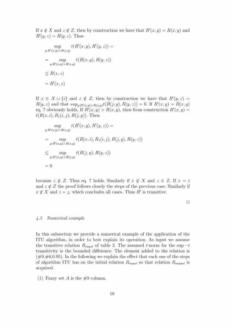
In this subsection we provide a step-by-step demonstration of the operationof the ITC algorithm. The relation upon which the algorithms is be applied ispresented in Fig. 4, where drawn links have a weight of 0.95, while all otherlinks have a weight of 0. It is worth noting that in the provided sample relationloops exist (see #1 → #2 → #3 → #4 → #1 as well as #7 → #8 → #1).

21

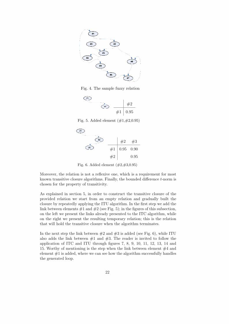
Fig. 4. The sample fuzzy relation

#2

#1 0.95

Fig. 5. Added element (#1,#2,0.95)

#2 #3

#1 0.95 0.90

#2 0.95

Fig. 6. Added element (#2,#3,0.95)

Moreover, the relation is not a reflexive one, which is a requirement for mostknown transitive closure algorithms. Finally, the bounded difference t-norm ischosen for the property of transitivity.

As explained in section 5, in order to construct the transitive closure of theprovided relation we start from an empty relation and gradually built theclosure by repeatedly applying the ITU algorithm. In the first step we add thelink between elements #1 and #2 (see Fig. 5); in the figures of this subsection,on the left we present the links already presented to the ITC algorithm, whileon the right we present the resulting temporary relation; this is the relationthat will hold the transitive closure when the algorithm terminates.

In the next step the link between #2 and #3 is added (see Fig. 6), while ITUalso adds the link between #1 and #3. The reader is invited to follow theapplication of ITC and ITU through figures 7, 8, 9, 10, 11, 12, 13, 14 and15. Worthy of mentioning is the step when the link between element #4 andelement #1 is added, where we can see how the algorithm successfully handlesthe generated loop.

22

#2 #3 #8

#1 0.95 0.90 0.90

#2 0.95 0.95

Fig. 7. Added element (#2,#8,0.95)

#2 #3 #4 #8

#1 0.95 0.90 0.85 0.90

#2 0.95 0.90 0.95

#3 0.90

Fig. 8. Added element (#3,#4,0.95)

#1 #2 #3 #4 #8

#1 0.80 0.95 0.90 0.85 0.90

#2 0.85 0.80 0.95 0.90 0.95

#3 0.90 0.85 0.80 0.95 0.80

#4 0.95 0.90 0.85 0.80 0.85

Fig. 9. Added element (#4,#1,0.95)

#1 #2 #3 #4 #8 #9

#1 0.80 0.95 0.90 0.85 0.90 0.80

#2 0.85 0.80 0.95 0.90 0.95 0.85

#3 0.90 0.85 0.80 0.95 0.80 0.90

#4 0.95 0.90 0.85 0.80 0.85 0.95

Fig. 10. Added element (#4,#9,0.95)

23

#1 #2 #3 #4 #8 #9

#1 0.80 0.95 0.90 0.85 0.90 0.80

#2 0.85 0.80 0.95 0.90 0.95 0.85

#3 0.90 0.85 0.80 0.95 0.80 0.90

#4 0.95 0.90 0.85 0.80 0.85 0.95

#5 0.85 0.80 0.95 0.90 0.75 0.85

Fig. 11. Added element (#5,#3,0.95)

#1 #2 #3 #4 #7 #8 #9

#1 0.80 0.95 0.90 0.85 0.90 0.80

#2 0.85 0.80 0.95 0.90 0.95 0.85

#3 0.90 0.85 0.80 0.95 0.80 0.90

#4 0.95 0.90 0.85 0.80 0.85 0.95

#5 0.85 0.80 0.95 0.90 0.75 0.85

#6 0.95

Fig. 12. Added element (#6,#7,0.95)

Table 5Summary of computational complexities of complete transitive closure algorithms

Algorithm Data model Sparse relation Dense relation

Conventional Complete n3 log n n3 log n

Conventional Sparse n2 log2 n n3 log n

ITC Complete - -

ITC Sparse n log4 n n4 log n

5.3 Comparative study

Table 5 summarizes the computational complexities of the conventional ap-proach to transitive closure and the proposed ITC algorithm. In the case where

24

#1 #2 #3 #4 #7 #8 #9

#1 0.80 0.95 0.90 0.85 0.90 0.80

#2 0.85 0.80 0.95 0.90 0.95 0.85

#3 0.90 0.85 0.80 0.95 0.80 0.90

#4 0.95 0.90 0.85 0.80 0.85 0.95

#5 0.85 0.80 0.95 0.90 0.75 0.85

#6 0.95 0.90

#7 0.95

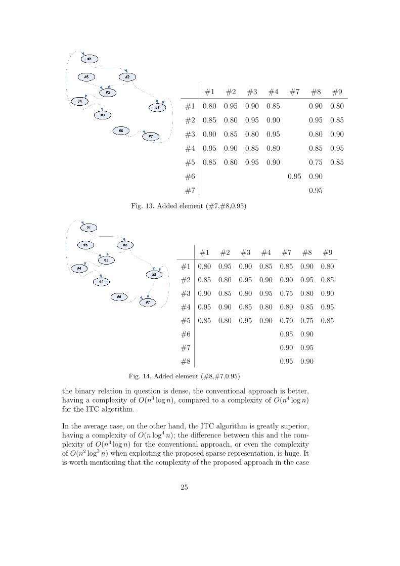
Fig. 13. Added element (#7,#8,0.95)

#1 #2 #3 #4 #7 #8 #9

#1 0.80 0.95 0.90 0.85 0.85 0.90 0.80

#2 0.85 0.80 0.95 0.90 0.90 0.95 0.85

#3 0.90 0.85 0.80 0.95 0.75 0.80 0.90

#4 0.95 0.90 0.85 0.80 0.80 0.85 0.95

#5 0.85 0.80 0.95 0.90 0.70 0.75 0.85

#6 0.95 0.90

#7 0.90 0.95

#8 0.95 0.90

Fig. 14. Added element (#8,#7,0.95)

the binary relation in question is dense, the conventional approach is better,having a complexity of O(n3 log n), compared to a complexity of O(n4 log n)for the ITC algorithm.

In the average case, on the other hand, the ITC algorithm is greatly superior,having a complexity of O(n log4 n); the difference between this and the com-plexity of O(n3 log n) for the conventional approach, or even the complexityof O(n2 log2 n) when exploiting the proposed sparse representation, is huge. Itis worth mentioning that the complexity of the proposed approach in the case

25

#1 #2 #3 #4 #6 #7 #8 #9

#1 0.80 0.95 0.90 0.85 0.75 0.85 0.90 0.80

#2 0.85 0.80 0.95 0.90 0.80 0.90 0.95 0.85

#3 0.90 0.85 0.80 0.95 0.85 0.80 0.80 0.90

#4 0.95 0.90 0.85 0.80 0.90 0.85 0.85 0.95

#5 0.85 0.80 0.95 0.90 0.80 0.75 0.75 0.85

#6 0.95 0.90

#7 0.90 0.95

#8 0.95 0.90

#9 0.95 0.90 0.80

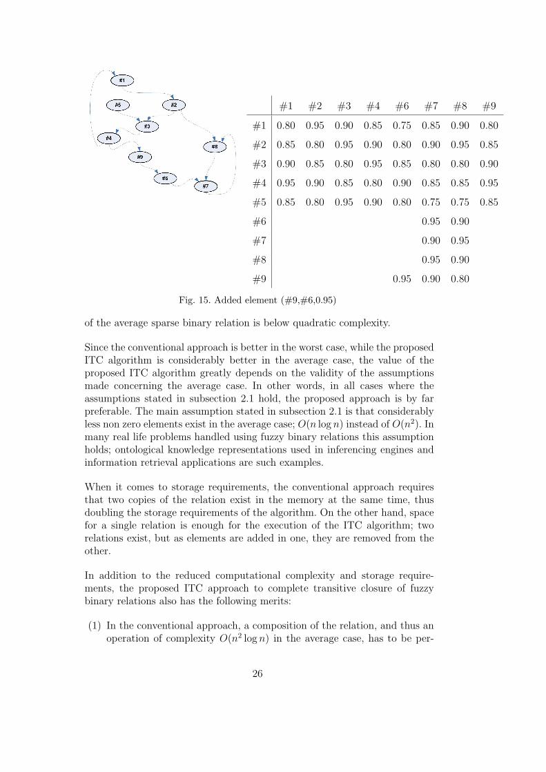
Fig. 15. Added element (#9,#6,0.95)

of the average sparse binary relation is below quadratic complexity.

Since the conventional approach is better in the worst case, while the proposedITC algorithm is considerably better in the average case, the value of theproposed ITC algorithm greatly depends on the validity of the assumptionsmade concerning the average case. In other words, in all cases where theassumptions stated in subsection 2.1 hold, the proposed approach is by farpreferable. The main assumption stated in subsection 2.1 is that considerablyless non zero elements exist in the average case; O(n log n) instead of O(n2). Inmany real life problems handled using fuzzy binary relations this assumptionholds; ontological knowledge representations used in inferencing engines andinformation retrieval applications are such examples.

When it comes to storage requirements, the conventional approach requiresthat two copies of the relation exist in the memory at the same time, thusdoubling the storage requirements of the algorithm. On the other hand, spacefor a single relation is enough for the execution of the ITC algorithm; tworelations exist, but as elements are added in one, they are removed from theother.

In addition to the reduced computational complexity and storage require-ments, the proposed ITC approach to complete transitive closure of fuzzybinary relations also has the following merits:

(1) In the conventional approach, a composition of the relation, and thus anoperation of complexity O(n2 log n) in the average case, has to be per-

26

formed before the decision to terminate the algorithm is taken. This istrue even when the relation is initially transitive, thus requiring no ad-justment. In the proposed approach, in the same situation the algorithmwould terminate in O(n log4 n) time.

(2) In the conventional approach, the relation is not transitive until the oper-ation terminates. Thus, in the case of a very large number n, a very longtime has to be spent before the relation becomes usable by algorithmsthat assume transitivity. On the contrary, relation R′ is transitive aftereach step when utilizing the ITC algorithm, and thus algorithms that as-sume it to be transitive can be applied to it before the closure operationis completed.

(3) The termination point of the conventional approach greatly depends onthe “depth” of the relation, i.e. on the count of vertices of the longestpath. Specifically, it may take the process anywhere between 1 and log niterations to terminate. On the contrary, the ITC algorithm assures tran-sitivity in one pass and thus the count of required steps is known be-forehand. Therefore, an indication of progress of the process is availableon-line, if we require it, in the form of percentage completed.

(4) The proposed approach is not affected by cycles in the relation, i.e. itdoes not require that the relation is ordering. This is is not a propertyshared by all specialized transitive closure algorithms [37].

(5) The computational complexity for the complete transitive closure in thesparse case is very close to the computational complexity of loading therelation from a storage location such as a hard disk; O(n log4 n) comparedto O(n log n). Consequently, we have the option to store the relation in anon transitive form, thus saving in disk space, and calculate the transitiveclosure at the time of loading using the ITC algorithm, only slightlyaffecting the overall complexity and execution time.

6 Experimental results

In this section we provide experimental results from the application of theconventional methodologies and ITU and ITC algorithms for transitivity re-establishment and complete transitive closure on a synthetic data set, as wellas on a real life data set from the field of knowledge based information retrieval[5][39]. Implementation of the proposed relation representation model, as wellas of the conventional and proposed algorithms, has been done using the Javaenvironment and execution has been performed on a PC (Centrino 1.6GHz,256MB RAM) with Windows XP operating system. The source code of theseexperiments, modified as to provide detailed step by step output, is freelyavailable at [48].

27

6.1 Data sets

In knowledge based information retrieval, the retrieval system needs to utilizeall or a part of the available knowledge when processing e.g. a user query,a user profile or a document, in order to provide a meaningful response. Incases where a fuzzy relational knowledge representation model is followed,having the fuzzy relations readily available in a closed transitive form typicallyalleviates the need for recursion in the processing algorithms, thus greatlyreducing computational complexity and processing time.

In this paper we utilize such a relation in order to experimentally validate ourtheory. Specifically, the universe of discourse S90,000 is the set of all conceptsdefined in WordNet for the English language verbs and nouns [22]; there isa 1-1 mapping between elements of this set and the verb and noun synsetsdefined in WordNet. The cardinality of this set is slightly over 90,000 elements.

A fuzzy binary relation on S90,000 is generated automatically, again usingWordNet as a source. Two of the lexical relations, hyponym and part meronym,are used to specify the pairs of connected elements in the relation. As theserelations are crisp in WordNet, degree 0.9 is assigned to all such pairs bydefault. Additionally, the relation is made reflexive. Overall, around 110,000pairs are connected to a degree 0.9 and 90,000 more elements to degree 1 dueto reflexivity. This forms fuzzy binary relation R90,000.

By randomly selecting elements from set S90,000 we form crisp set S50,000.This set contains 50,000 elements. Keeping only the rows and columns ofR90,000 that correspond to elements in S50,000 we construct relation R50,000.This is similar in structure and content with fuzzy binary relation R90,000,but smaller in size; the comparative study of algorithms’ performance on suchrelations provides for more intuitive evaluation of their complexities. Recur-sively, S20,000 is constructed from S50,000, S10,000 is constructed from S20,000 andso on, thus resulting in a wide range of corresponding binary relations: Rn,n ∈ {90000, 50000, 20000, 10000, 5000, 3000, 2000, 1000, 500}.

Fuzzy binary relation Rt90000, obtained using algorithm ITC, is the sup-t tran-

sitive closure of R90,000, where t is the bounded sum t-norm. Rt90000 contains

760,000 non zero elements; 90,000 elements having degree 1 due to reflexiv-ity, 110,000 elements with degree 0.9 also existing in the original R90,000 and560,000 elements with lesser degrees, produced during transitive closure. Sim-ilarly, we have constructed transitive relations Rt

n, all following the rule:

Rtn = Trt(Rn) (8)

The utilization of the complete representation model for R90,000 or other re-

28

A B

Fig. 16. Execution times for 2 compositions and for ITU on Rdn using complete

representation.

lations having a universe of discourse of considerable dimension is not practi-cally possible. For the case of R90,000, for example, the relation dimension of90, 000× 90, 000 requires the representation of approximately 8 billion doubleprecision numbers. With 8 bytes allocated for each such number, the requiredmemory space just for one copy of the relation is 65Gb of RAM. Thus, inall subsequent experiments only the proposed sparse representation model isconsidered for this series of data sets.

In order to experimentally verify the efficiency of the proposed methodologieswhen dealing with dense relations, or when combined with the complete rep-resentation model, we have synthetically constructed a suitable series of datasets. Specifically, we have generated n × n relations for various values of n,with random degrees of relation between any pair of elements, and performed atransitive closure operation on them. The sizes n of relations constructed aren ∈ {10, 20, 30, 40, 50, 60, 70, 80, 90, 100, 200, 300, 500, 1000, 2000}; the namesof the corresponding relations are Rd

n.

6.2 Re-establishment of transitivity using the complete representation model

As shown in section 4, ITU algorithm has a complexity of O(n2), compared toa complexity of O(n3) of the conventional approach, assuming the completerepresentation model. In order to experimentally verify this, we have appliedboth to the Rd

n data set. In the cases where size n was too small to lead to areliable measurement of time, the operations were executed 10, 100, 1,000 or1,000,000 times, and the total time was divided by the count of repetitions.Table 6 summarizes the experimental times.

It is easy to see that algorithm ITU requires considerably less time in orderto perform the same operation when compared to the conventional method-

29

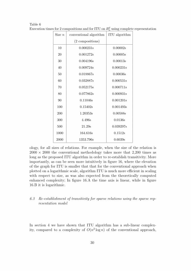
Table 6Execution times for 2 compositions and for ITU on Rd

n using complete representation

Size n conventional algorithm ITU algorithm

(2 compositions)

10 0.000231s 0.00002s

20 0.001272s 0.00005s

30 0.004196s 0.00013s

40 0.009724s 0.000231s

50 0.018867s 0.00036s

60 0.032887s 0.000531s

70 0.052175s 0.000711s

80 0.077862s 0.000931s

90 0.11046s 0.001201s

100 0.15402s 0.001493s

200 1.20353s 0.00588s

300 4.496s 0.0136s

500 21.29s 0.039297s

1000 164.616s 0.1512s

2000 1353.796s 0.6039s

ology, for all sizes of relations. For example, when the size of the relation is2000 × 2000 the conventional methodology takes more that 2,200 times aslong as the proposed ITU algorithm in order to re-establish transitivity. Moreimportantly, as can be seen more intuitively in figure 16, where the elevationof the graph for ITU is smaller that that for the conventional approach whenplotted on a logarithmic scale, algorithm ITU is much more efficient in scalingwith respect to size, as was also expected from the theoretically computedenhanced complexity; In figure 16.A the time axis is linear, while in figure16.B it is logarithmic.

6.3 Re-establishment of transitivity for sparse relations using the sparse rep-resentation model

In section 4 we have shown that ITU algorithm has a sub-linear complex-ity, compared to a complexity of O(n2 log n) of the conventional approach,

30

Table 7Execution times for 2 compositions and for ITU on Rn using sparse representation.

Size n conventional algorithm ITU algorithm

(2 compositions) (1,000,000 repetitions)

500 201.564s 7.64s

1000 1543.842s 8.95s

2000 13436s 9.74s

3000 10.29s

5000 10.45s

10000 10.95s

20000 12.40s

50000 13.53s

90000 17.80s

A B

C D

Fig. 17. Execution times for 2 compositions and for ITU on Rn using sparse repre-sentation.

assuming sparse relations and the proposed sparse representation model. Inorder to experimentally verify this, we have applied both to the Rn data set.Table 7 summarizes the results. In some cases execution time was too longand the experiment could not completed because of that. Therefore some val-ues are missing from the table. For a more intuitive presentation, the values

31

A B

Fig. 18. Execution times for 2 compositions and for ITU on Rdn using sparse repre-

sentation.

are graphed in figure 17. Note that both in the table and in the graphs, thetimes reported for algorithm ITU correspond to 1,000,000 repetitions, whilethe times reported for the conventional approach correspond to a single ap-plication.

In figure 17.A we can observe that the calculated complexity of O(n2 log n) isexperimentally verified. Similarly, figure 17.B verifies the sub-linear complexityfor algorithm ITU. Figures 17.C and 17.D contain measurements from bothexperiments to allow for a comparative study. We can easily see the superiorityof the algorithm ITU both in execution time and in scaling with respect tothe size of the relation.

6.4 Re-establishment of transitivity for dense relations using the sparse rep-resentation model

In section 4 we have shown that ITU algorithm has a complexity of n2 log n,compared to a complexity of O(n3) of the conventional approach, assumingdense relations and the proposed sparse representation model. In order toexperimentally verify this, we have applied both to the Rd

n data set, whichwas loaded on the AVL trees of the proposed sparse representation model.Table 8 summarizes the results, and figure 18 presents the data in a moreintuitive format. Note that both in the table and in the graphs, the timesreported for algorithm ITU correspond to 100 repetitions, while the timesreported for the conventional approach correspond to a single application.

Once more the superiority of the ITU algorithm in scaling that was proventheoretically is verified by the experimental results.

32

Table 8Execution times for 2 compositions and for ITU on Rd

n using sparse representation.

Size n conventional algorithm ITU algorithm

(2 compositions) (100 repetitions)

10 0.05s 0.07s

20 1.462s 0.211s

30 2.854s 0.481s

40 5.067s 0.911s

50 8.292s 1.522s

60 12.948s 2.283s

70 24.425s 3.205s

80 33.998s 4.286s

90 40.438s 5.618s

100 64.663s 7.181s

200 516.473s 55.83s

Fig. 19. Execution times for application of ITC on Rn and Rtn.

6.5 Complete transitive closure for sparse relations using the sparse repre-sentation model

In section 5 we have proven that algorithm ITC has a complexity of n log4 n,compared to a complexity of n2 log2 n of the conventional approach, whenconsidering sparse relations and the proposed sparse representation model. Inorder to verify the efficiency of algorithm ITC we have applied it to data setsRn and Rt

n. Results are presented in table 9 and summarized in figure 19.

We can see that the algorithm scales almost linearly for both data sets. More-over, the augmented density of the transitive relation has an effect on theoverall execution time. Still, as can be seen in the figure, this is an effect only

33

Table 9Execution times for application of ITC on Rn and Rt

n data sets.

size n Rn data set Rtn data set

500 0.03s 0.03s

1000 0.05s 0.04s

2000 0.07s 0.06s

3000 0.101s 0.1s

5000 0.17s 0.16s

10000 0.591s 0.761s

20000 5.518s 15.832s

50000 16.473s 52.745s

90000 32.106s 101.396s

on the elevation of the graph, not on its form; in other words, the complexityremains close to linear and certainly below the quadratic when dealing withsparse relations that are already transitive, and thus contain more non zeroelements.

Still, what is most important is to compare the efficiency of the ITC algo-rithm with that of the conventional transitive closure approach. As was madeobvious from the missing elements in table 7 and the form of figure 17, theexecution time even of a single composition is prohibitive for the applicationof the conventional approach on the Rn or Rt

n data sets. Therefore, we haveperformed estimations of the time it would take to apply the algorithm ondata set Rn, as follows:

We have edited the self-composition module, as to indicate the progress madeand the time elapsed after each row of the output relation has been computed.The output of the first steps of the execution of the self-composition algorithmon data set R90000 is reported in Table 10.

Figure 20.A graphically presents the computed times. There, we can see thatthe algorithm tends to slow down as the process progresses and the outputrelation is gradually augmented. Plotting the same points on a logarithmicscale, as in figure 20.B, we acquire much simpler curves, based on which wecan estimate probable execution times for 100% of the self-composition ina more intuitive manner. This way, we have produced the estimations thatare graphically presented in figure 20.C. In that figure, the first three pointsare the real measured execution times and the rest have been estimated; thefirst ones with a larger portion of the process already completed, and thus

34

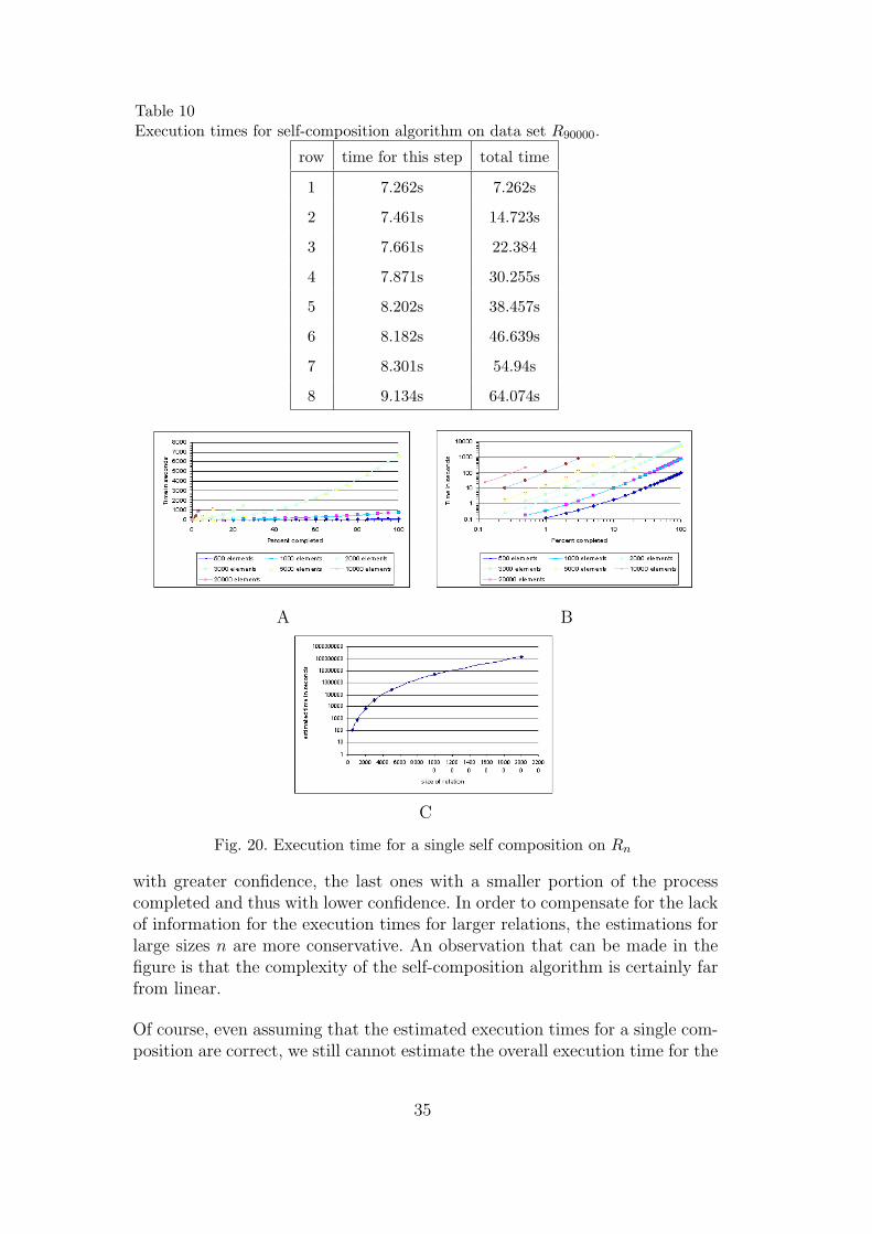
Table 10Execution times for self-composition algorithm on data set R90000.

row time for this step total time

1 7.262s 7.262s

2 7.461s 14.723s

3 7.661s 22.384

4 7.871s 30.255s

5 8.202s 38.457s

6 8.182s 46.639s

7 8.301s 54.94s

8 9.134s 64.074s

A B

C

Fig. 20. Execution time for a single self composition on Rn

with greater confidence, the last ones with a smaller portion of the processcompleted and thus with lower confidence. In order to compensate for the lackof information for the execution times for larger relations, the estimations forlarge sizes n are more conservative. An observation that can be made in thefigure is that the complexity of the self-composition algorithm is certainly farfrom linear.

Of course, even assuming that the estimated execution times for a single com-position are correct, we still cannot estimate the overall execution time for the

35

A B

Fig. 21. Execution times for application of ITC on Rn and Rtn.

transitive closure following the conventional approach, as it depends on the“depth” of the relations. For relation R90000, for example, in theory the conven-tional approach might require anywhere between 2 and 17 self-compositions.In order to be able to make some sort of comparison we follow the best case sce-nario for the conventional approach, thus assuming that 2 self-compositionsare adequate to guarantee transitivity. Comparative presentation of results,under these assumptions, are presented in figure 21. In the figure we can eas-ily see, as was expected, that there is a great difference between both theexecution time for the specific sizes and in the way that the algorithms scale,between the traditional approach and the proposed ITC algorithm.

7 Conclusions

In this paper we have dealt with the transitive closure of sparse fuzzy binaryrelations. We have started by formalizing the notion of sparseness and byproposing a compact representation model that allows for O(log n) access toa specific element, row or column in the relation, as well as O(log n) inser-tion time. Continuing, we have presented ITU, an algorithm for incrementalupdate of transitive binary relations. This algorithm has important practicalimplications in fields were transitive relations are constructed using a trialand error approach. Extending this, we have described ITC, an algorithmfor transitive closure of binary relations that relies on the above incrementalmethodology. The practical implications of this algorithm are found in fieldswere large and sparse transitive relational representations are meaningful. Asmost representative examples we can mention knowledge based systems, on-tological representations and intelligent information and multimedia retrieval.Other fields and applications that require the transitive closure of binary rela-tions, fuzzy or not, may benefit from the findings of this work, provided thatthe relations they need to handle are compliant with the given assumptions

36

on sparseness.

As further work, we have the intention to derive theoretical estimations of thecomputational complexities of algorithms ITU and ITC when assumptionson sparseness are variable, e.g. kr(n) non zero rows, kc(n) non zero columns,ri(n) non zero elements in row i, etc. Extending this work, we hope to reacha theoretical criterion determining which approach to complete transitive clo-sure, the conventional one or ITC, is best for a given relation, assuming thatsome statistical knowledge on the structure of the relation is available. Fi-nally, we intend to further investigate the practical implications of this workin diverse fields, such as the fields of context determination in ontologies, intel-ligent information retrieval, or even dynamic routing algorithms for computernetworks.

References

[1] Adelson-Velskii G.M., Landis E.M., “An algorithm for the organization ofinformation” Doklady Akademia Nauk SSSR, vol. 146, pp. 263-266, 1962;English translation in Soviet Math, vol. 3, pp. 1259-1263, 1962.

[2] Akrivas G. and Stamou G., “Fuzzy Semantic Association of AudiovisualDocument Descriptions”, International Workshop on Very Low Bitrate VideoCoding (VLBV), Athens, Greece, October 2001.

[3] Akrivas G., Wallace M., Andreou G., Stamou G. and Kollias S., “Context -Sensitive Semantic Query Expansion”, ICAIS, Divnomorskoe, Russia, 2002.

[4] Athanasiadis T., Avrithis Y., “Adding Semantics to Audiovisual Content: TheFAETHON Project” in Enser P.,, Kompatsiaris Y., OConnor N.E., et al. (Eds)Image and Video Retrieval, LNCS 3115, pp. 665-673, 2004.

[5] Avrithis Y., Stamou G., Wallace M., Marques F., Salembier P., Giro X., HaasW., Vallant H.,Zufferey M., “Unified Access to Heterogeneous AudiovisualArchives” .Journal of Universal Computer Science vol. 9 no. 6, pp. 510-519,2003

[6] Backhouse R.C.“Calculating the Floyd-Warshall path algorithm”, EindhovenUniversity of Technology, 1992.

[7] Backhouse R.C., van den Eijnde J.P.H.W., van Gasteren A.J.M., “Calculatingpath algorithms”, Sci. Comput. Programming vol. 22(3), pp. 3-19, 1994.

[8] Backhouse R.C., van Gasteren A.J.M., “Calculating a Path Algorithm”, SecondInternational Conference on Mathematics of Program Construction, 1992,Lecture Notes in Computer Science vol. 669, pp. 32-44, 1993.

[9] Baker J.J., “A note on multiplying Boolean matrices”, Comm. ACM vol. 5no. 2, pp. 102, 1962.

37

[10] Bedek J.C., Biswas G. and Huang L.Y., “Transitive closures of fuzzy thesauri forinformation retrieval systems”, International Journal of Man-Machine Studiesvol. 25, pp. 343-356, 1986.

[11] Boixader D., Jacas J. and Recasens J.,“Transitive closure and betweennessrelations”, Fuzzy Sets & Systems vol. 120, pp. 415-422, 2001.

[12] Chen S.-M., Horng Y.-J. and Lee C.-H.“Fuzzy information retrieval based onmulti-relationship fuzzy concept networks”, Fuzzy Sets & Systems vol. 140,pp. 183-205, 2003.

[13] Dasgupta M. and Deb R.,“Factoring fuzzy transitivity”, Fuzzy Sets & Systemsvol. 118, pp. 489-502, 2001.

[14] Dawyndt P., De Meyer H., De Baets B., “The complete linkage clusteringalgorithm revisited”, Soft Computing, in press.

[15] De Baets B., De Meyer H., “On the existence and construction of T-transitiveclosures”, Inform. Sc. vol. 152, pp. 167-179, 2003.

[16] De Baets B., De Meyer H., “Transitive approximation of fuzzy relations byalternating closures and openings”, Soft Computing, pp. 210-219, 2003.

[17] De Baets B., De Meyer H., Naessens H., “A top-down algorithm for generatingthe Hasse tree of a fuzzy preorder closure”, IEEE Trans. Fuzzy Systems, inpress.

[18] Duan J.-S., “The transitive closure, convergence of powers and adjoint ofgeneralized fuzzy matrices”, Fuzzy Sets & Systems vol. 145, pp. 301-311, 2004.

[19] Dunn J.C., “A graph-theoretical analysis of pattern classification via Tamura’sfuzzy relation”, IEEE Trans. SMC vol. 5, pp. 310-313, 1974.

[20] Dunn J.C., “Some recent investigations of a new fuzzy partitioning algorithmand its applications to pattern classification problems”, Journal of Cyberneticsvol. 4, pp. 1-15, 1974.

[21] Feijs L.M.G., van Ommering R.C., “Abstract derivation of transitive closurealgorithms”, Information Processing Letters vol. 63, pp. 159-164, 1997.

[22] Fellbaum C. (Ed), “WordNet: An Electronic Lexical Database”, MIT Press,1998.

[23] Fodor, J. and Roubens M., “Structure of transitive valued binary relations”,Mathematical Social Sciences vol. 30, pp. 71-94, 1995.

[24] Guu S.-M., Chen H.-H. and Pang C.-T., “Convergence of products of fuzzymatrices”, Fuzzy Sets & Systems vol. 121, pp. 203-207, 2001.

[25] Klir G., Yuan B., “Fuzzy Sets and Fuzzy Logic: Theory and Applications”,Prentice Hall, 1995.

[26] Kundu S.,“A representation theorem for min-transitive fuzzy relations”, FuzzySets & Systems vol. 109, pp. 453-457, 2000.

38

[27] Lee H.-S., “An optimal algorithm for computing the maxmin transitive closureof a fuzzy similarity matrix”, Fuzzy Sets & Systems vol. 123, pp. 129-136, 2001.

[28] Maedche A.,Motik B., Silva N., Volz R.,“ MAFRA - An Ontology MAppingFRAmework in the Context of the SemanticWeb”. Workshop on OntologyTransformation, ECAI, 2002.

[29] De Meyer H., Naessens H., De Baets B., “Algorithms for computing the min-transitive closure and associated partition tree of a symmetric fuzzy relation”,European J. Oper. Res. vol. 155, pp. 226-238, 2004.

[30] Naessens H., De Meyer H., De Baets B., “Algorithms for the computation ofT-transitive closures”, IEEE Trans. Fuzzy Systems vol. 10, pp. 541-551, 2002.

[31] Ovchinnikov S., “Numerical representation of transitive fuzzy relations”, FuzzySets & Systems vol. 126, pp. 225-232, 2002.

[32] Purdom P., “A transitive closure algorithm”, BIT vol. 10 pp. 76-94, 1970.

[33] Seidel R., “On the All-Pairs-Shortest-Path problem in unweighted undirectedgraphs”, J. Computer & System Sciences vol. 51, pp. 400-403, 1995.

[34] Stamou G., Avrithis Y., Kollias S., Marques F., Salembier P. “SemanticUnification of Heterogenous Multimedia Archives” Proc. of 4th EuropeanWorkshop on Image Analysis for Multimedia Interactive Services (WIAMIS),London, UK, April 9-11, 2003.

[35] Tan Y.-J., “On compositions of lattice matrices”, Fuzzy Sets & Systems vol. 129,pp. 19-28, 2002.

[36] Thorelli L.-E., “An algorithm for computing all paths in a graph”, BIT vol. 6pp. 347-349, 1966.

[37] Ullman, J.D., Yannakakis M., “The Input/Output Complexity of TransitiveClosure”, Annals of Mathematics and Artificial Intelligence, vol. pp. 331-360,1991.

[38] Wallace M., Akrivas G., Mylonas P., Avrithis Y., Kollias S. “Using contextand fuzzy relations to interpret multimedia content”, CBMI, IRISA, Rennes,France, 2003.

[39] Wallace M., Avrithis Y., Stamou G., Kollias S. “Knowledge-based MultimediaContent Indexing and Retrieval” Multimedia Content and Semantic Web:Methods, Standards and Tools, Stamou G., Kollias S. (Editors), Wiley, 2004.

[40] Wallace M., Akrivas G. and Stamou G., “Automatic Thematic Categorizationof Documents Using a Fuzzy Taxonomy and Fuzzy Hierarchical Clustering”,FUZZ-IEEE, St. Louis, MO, USA, 2003.

[41] Wallace M., Akrivas G., Stamou G. and Kollias S., “Representation of userpreferences and adaptation to context in multimedia content – based retrieval”,Workshop on Multimedia Semantics, SOFSEM, Milovy, Czech Republic, 2002.

39

[42] Wallace M., Kollias S., “Computationally efficient incremental transitive closureof sparse fuzzy binary relations”, FUZZ-IEEE, July 2004.

[43] Warren H.S., “A modification of Warshall’s algorithm for the transitive closureof binary relations”, Comm. ACM, vol. 18, no. 4, pp. 218-220, 1975.

[44] Warshall S., “A theorem on Boolean matrices”, J. ACM vol. 9 no. 1, pp. 11-12,1962.

[45] Yoshida Y.,“A limit theorem in dynamic fuzzy systems with transitive fuzzyrelations”, Fuzzy Sets & Systems, vol. 109, pp. 371-378, 2000.

[46] Zadeh L.A., “Fuzzy Sets”, Information and Control, vol. 3, pp. 338-353, 1965.

[47] Zadeh L.A., “Similarity relations and fuzzy orderings”, Information Sciences,vol. 3, pp. 177-200, 1971.

[48] http://image.ntua.gr/∼wallace/java/transitive

40