EVALUATION OF MANAGEMENT PROCEDURES:APPLICATION TO CHILEAN JACK MACKEREL FISHERY

V. Martinet∗, M. De Lara†, J. Pena‡ and H. Ramirez§

August 20, 2010

Abstract

This paper develops a theoretical framework to assess resourcesmanagement procedures from a sustainability perspective, when re-source dynamics is marked by uncertainty. Using stochastic viability,management procedures are ranked according to their probability toachieve economic and ecological constraints over time. This frame-work is applied to a fishery case-study, facing El Nino uncertainty.We study the viability of constant effort and constant quota strate-gies, when a minimal catch level and a minimal biomass are required.Conditions on the sustainability objectives are derived for the superi-ority of each of the two management methods.

Keywords: Sustainability, risk, fishery economics and management, vi-ability, stochastic.

∗Economie Publique, UMR INRA–AgroParisTech, 78850 Thiverval-Grignon, France.vincent.martinet@grignon.inra.fr†Universite Paris-Est, Cermics, 6-8 avenue Blaise Pascal, 77455 Marne la Vallee

Cedex 2, France. delara@cermics.enpc.fr‡Facultad de Economıa y Negocios/ILADES, Universidad Alberto Hurtado. Erasmo

Escala 1835, Santiago, Chile. jpena@uahurtado.cl§Departamento de Ingenierıa Matematica, Centro de Modelamiento Matematico(CNRS

UMI 2807), FCFM, Universidad de Chile, Avda. Blanco Encalada 2120, Santiago, Chile.hramirez@dim.uchile.cl

1

Contents

1 Introduction 3

2 Background and settings 5

3 A risk metrics for sustainability objectives 103.1 Management strategy assessment by stochastic viability . . . . 103.2 A “value function” for strategies and thresholds . . . . . . . . 143.3 Optimal management strategy . . . . . . . . . . . . . . . . . . 163.4 Sub-optimality of strategies for given sustainability objectives 17

4 Modeling the Chilean Jack-Mackerel fishery 184.1 A bioeconomic model for the Chilean Jack-Mackerel fishery . . 194.2 Management Strategy Evaluation of the Chilean Jack-Mackerel

fishery . . . . . . . . . . . . . . . . . . . . . . . . . . . . . . . 214.3 Viability assessment of constant quota and constant effort

management procedures for the Chilean Jack-Mackerel fish-ery . . . . . . . . . . . . . . . . . . . . . . . . . . . . . . . . . 24

5 Conclusions 28

2

1 Introduction

The model of this paper has its origin in some actual management practicesin Chilean fisheries. The Jack-Mackerel Chilean fishery faces El Nino uncer-tain cycles, which increase the uncertainty about this resource’s availability[3], and thus makes the sustainability assessments more difficult. In some ex-treme cases, recruitment uncertainty and applied management decisions haveled to the collapse of important pelagic stocks, as the Peruvian Anchovy in1972-1973. Since the late 1990s, the Chilean Jack-Mackerel fishery has beenmanaged under a yearly-defined Total Allowable Catches (TAC) regulation,complemented since year 2001 with the operation of an individual (companyallocated) quota scheme [26]. The TAC scheme has had a particular con-cern about the stability of quota levels over time. Additionally, since themid-2000s the Jack-Mackerel fishery has been one of the pioneering in Chileto include risk indicators in its management practice. Nevertheless, risk in-dicators are not yet implemented in a formally integrated decision-makingframework, but rather like an additional ad-hoc objective aiming at cappingbiological (collapse) risk [31].

We are here interested in the definition of a framework to address sustain-able resource management issues, accounting for both resource dynamics andrisk.1 Dynamic issues received a particular focus in the economic literature,especially in growth theory [33], providing the discounted utility criterion.The issue of decision under risk has also been widely addressed in the eco-nomic literature, back to the fundament of expected utility theory which hasbeen axiomatized by [47]. Given these important contributions on dynamicissues on the one hand, and risk on the other hand, one should be surprised tonotice that joint issues of risk and time have received less attention. Indeed,though discounted expected utility is the standard theoretical framework ineconomics, there seems to be few discussions on its axiomatic foundations.In his textbook, The Economics of Risk and Time [25], Gollier provides twoarguments to justify the use of discounted expected utility with exponentialdiscounting. First, it is time consistent, which is a good property. Second,it accounts for pure preference for the present (impatience) via discounting,which may have a sense in individual decision making but is criticized in the

1In the paper, we will use “risk” and “uncertainty” equivalently, with the underlyingeconomic meaning of risk, i.e., stochastic events with know probabilities. We do notaddress the economic uncertainty issue, i.e., unknown or uncomplete probabilities.

3

sustainability debate on long-run issues.2

Optimality in fishery economics has been usually defined as the maxi-mization of the total discounted revenue of the harvest, or its expected valueunder uncertainty [14, 38, 40]. This approach has the great advantage ofdefining optimal feedback decision rules, or making it possible to rank anyalternative management procedure, with respect to a unique criterion andthe associated value of discounted expected utility. However, from a sustain-ability point of view, discounted expected utility faces practical problems.First, there is controversy on the application of this framework for very longterm (intergenerational) environmental issues, as it heavily discounts futuregenerations utility [11]. Second, expected discounted utility is rarely used inthe real practice of environmental goods management, when environmentaland social issues have to be accounted for along with economic ones. In-deed, in practice, management strategies (often defined as simple “rule ofthumb”) are evaluated in so-called “multicriteria” frameworks with no clearaxiomatic foundations [21, 24, 32, 42]. In particular, such methods do not of-fer an explicit ranking of alternative management procedure, as they provideno common value for conflicting objectives and risk.

This paper tackles the challenge of providing a method to define optimalmanagement strategies or rank alternative management procedures, account-ing for risk and conflicting sustainability issues. We address this issue withthe so-called stochastic viability approach [18, 20]. Given a set of (multi-criteria) “outcome indicators” (for example, either referring to physical oreconomic variables) and its corresponding set of thresholds, the latter repre-senting sustainability objectives (e.g., minimal biomass, minimal catch level),we aim at evaluating management procedures by maximizing the probabil-ity of achieving these objectives jointly and for all periods. We offer anillustration of the implications of using this approach in the field of fisherymanagement under environmental uncertainty, using the case of the pelagicJack-Mackerel Chilean fishery facing El Nino uncertainty.

The contribution of the paper is to build a bridge between the economicliterature on optimal resource management under risk and the “practicaloriented” literature on sustainable fisheries management. By providing a“common value” to a practical multi-criteria approach, we obtain an op-

2Even if discounting implies a “dictatorship of the present,” in the book Sustainabil-ity: Dynamics and Uncertainty by [12], risk and dynamics are addressed mainly in thediscounted expected utility framework.

4

timality framework which allows us to rank alternative management pro-cedures according to their viability probability. Dealing with optimality,value, marginal analysis, and trade-offs, our approach appears to be closerto economics than the usual multicriteria Management Strategy Evaluationapproaches.

The paper is organized as follows. Section 2 presents the existing litera-ture in fisheries economics on the one hand, and fisheries management on theother hand, and motivates our approach. Section 3 presents our theoreticalframework to assess risk and sustainability, and to compare resources man-agement procedures when sustainability objectives are in conflict. We applythis framework to the Jack-Mackerel Chilean fishery case-study in section4, and illustrate our results comparing constant effort and quota strategies.We conclude with some remarks on the relevance of our results for practicalfisheries management in Section 5.

2 Background and settings

Optimality in fishery economics has been usually defined as the maximizationof the total discounted revenue of the harvest, or its expected value underrisk. In the deterministic case, constant harvest and escapement emerges asa possible stationary solution path [13]. However, ignoring uncertainties canlead to excessive harvest, and fishery collapse. In the stochastic case, theissue is no longer to define an optimal path but optimal strategies, that is,decision rules that depend on the state variables. When the resource stockis randomly fluctuating, the optimal harvest level corresponds to a constant-escapement policy when the stock is observed before decision-making [38],but implies much more complicated strategies when decision has to be madebefore knowing stock size [14], or in the presence of multiple uncertainties(e.g., when uncertainty on stock measurement and inaccurate implementa-tion of harvest quotas are added to stock growth uncertainty [40]).3 Theseresults have important policy implications, as an optimal feedback solution

3The solution may then be to adjust the quota level during the fishing season, whilethe information on the stock size is (costly) available [14], but it implies economic uncer-tainty for the fishing industry which is not well-accepted [10]. In the same way, reducinguncertainty by improving the forecast of uncertain events, such as El Nino, induces welfaregains [16].

5

may result in non constant harvest quotas responding to uncertain stockfluctuation, with strong variations of the Total Allowable Catches from yearto year and even fishery closure when the stock size is too low. Maximiz-ing the sum of expected discounted harvest levels [38, 14, 40] implies twoimportant underlying assumptions. First, it assumes that fishing industriesare risk-neutral. Second, it neglects the willingness to smooth revenue, andthus catches, over time. This could represent a serious limitation to theapplication of an optimal quota policy as, in practice, fishing industries fa-vor stability [10]. Moreover, when capital adjustment is costly, resource-rentmaximization results in an incentive to smooth the harvest over time, whichmay reduce average yield under stock growth uncertainty, inducing a trade-off between the stability of in-situ stock and the stability of harvest [41].Risk-aversion also implies a smoothing of the harvest over time [1].

Economic theory thus provides a description of optimal strategies thatcould be used to manage fisheries. However, in practice, fisheries are man-aged with much simpler tools. For example, [41] describes the Alaskan pacifichalibut stock as being managed by setting the yearly harvest as a fixed frac-tion of the exploitation biomass ; this constant harvest rate rule is shown tosmooth the catches over time more than the optimal policy would. Constanteffort and constant quotas are two other basic management strategies. Theformer approach, also known as fixed fishing mortality, is based on adviceby biologists and results in fluctuating harvest as the stock fluctuates. Froman economic point of view, it is linked to a constant use of the capital. Thelatter approach provides stabilized catch, which is a strategy gaining groundin the industry. The optimal strategy may be neither of these two [27], butthese rules of thumb are still discussed as potential management strategies insome fisheries.4 However, under usual economic conditions, constant fishingeffort dominates constant quotas, with respect to the discounted profit crite-rion [36]. Neither of these last two studies ([27, 36]) consider stock dynamics.When present catches affect future availability of the resource, constant effortstrategy reduces the risk of under-utilization and over-exploitation. Never-theless, when catches per unit of effort are also stochastic, this is not alwaystrue, and constant quota strategies may be superior [17]. The economicapproach generally focuses on an aggregated criterion (such as discounted

4De facto, Chilean fisheries were managed under a constant effort rule in the 80s and90s (with a frozen maximum effort which was reached). Since then, a quota system isused, with a posteriori small changes in the quota levels from year to year.

6

utility) to evaluate decision paths. This criterion may incorporate costs andbenefits, which measure conflicting issues in the same currency. Nevertheless,in all these economic studies, the unique criterion is the expected discountedprofit or harvest.

A key element of a sustainable fishery is the design of a managementframework best able to cope with uncertainty, being robust, adaptative andprecautionary [10]. Management decision must balance the risk of resourcecollapse due to excessive exploitation versus the risk of forgone economicbenefits if the harvests are lower than necessary. Fisheries in which manage-ment focuses on effort control perform better under uncertainty as such anapproach reduces uncertainty as effort is more easily observed than stock,and increases robustness since harvest will adapt naturally to the state ofthe resource [10].

Managing fisheries facing uncertainty in a sustainable way is a big prac-tical challenge. Sustainability objectives encompass economic profitability,ecological viability and overall stability of the bioeconomic system [15]. Whenone of the ecological, economic or social objective is not met, fisheries facea crisis/unsustainable situation. In particular, one of the reasons of man-agement failure in fisheries is the conflict between ecological constraints andsocial and economic priorities, the latter often having priority over resourceconservation [28]. In fact, management objectives are often different fromdiscounted expected profit. In particular, resource conservation may be anobjective in and of itself, along with obtaining long-term socio-economic ben-efits from fishing, in an Ecosystem-Based Fishery Management perspective[35]. Implementing sustainable fisheries management (or ecosystem-basedfisheries management) thus increases the number of objectives and stake-holders [23]. Without scientific support, “ad hoc” decision making processmay result in negotiations on simple management procedures, e.g., constantquotas or constant fishing effort. Scientific tools are required to supportmulti-criteria decision making, and evaluate proposed management proce-dures.

While the optimality approaches presented above are based on stochasticoptimization defining an optimal feedback management rule, the evaluationof management strategies is mainly done using simulation methods. Theselatter are used to compare, in stochastic dynamic models, harvesting or man-agement scenarios, and to evaluate (usually through Monte Carlo simulation)the mean performance and corresponding variability of the management pro-

7

cedure [10]. Simulation approaches are preferred to stochastic optimizationfor large models. Smith et al. [42] describe the various scientific tools whichhave been developed to support sustainable fisheries management, includ-ing Management Strategy Evaluation (MSE) and Ecological Risk Assessment(ERA). These frameworks have been developed to compare different fisheriesmanagement strategies with respect to conflicting issues, and taking into ac-count the time horizon and the uncertainties [24, 21]. In particular, Manage-ment Procedures robust to uncertainty should result in harvesting strategieswhich guaranty TACs that would provide acceptable socio-economic stabil-ity for industry while at the same time limiting biological risks [24]. SuchQuantitative Risk Assessment requires to define a list of issues, to evaluatepotential consequences of given strategies, and associated risk. In all theseapproaches, risk is defined as a probability to fall under a given threshold,which, employed in stock assessment analysis, defines the probability thatstock abundance will not meet some agreed level of performance. Whencomparing alternative Management Procedures, preference goes to smallerrisk to reduce abundance to a low level, lower variation in TAC over time,and higher average catches [21]. Naturally, these general objectives are inconflict, inducing necessary trade-offs. Trade-off curves between the risk toovershoot the biological constraint and mean catches [42], or between meanvalues of conflicting objectives [21] are produced. In particular, evaluatingthe constant fishing effort strategy used by the ICES for roundfish man-agement (Fpa), Kell et al. [32] emphasize the need to define managementstrategies based on the achievement of the objectives in the long-term. Theperformance of the various management procedures under consideration areoften represented in a map of “mean catch – risk to the resource,” whichleaves the decision-maker(s) with clearer perspectives but without tools torank MPs. The first objective is an aggregation of value over time and overuncertainty scenarios, while the second is a probability. There is no “commoncurrency” to aggregate these objectives, and thus to rank the various man-agement procedures.5 These approaches thus provide a clear description ofthe consequences of management procedures but with no common currencybetween the different objectives and risk to sum up the results and rank thealternative management procedures. In economic terms, we can say that

5Value and risk are then mixed in a way which is not usual in economics. The decision-maker should have preferences over a value and a risk, while the usual approach is todefine preferences on value and to aggregate risk by computing the expectation of value.

8

there is no value function, which does not make marginal analysis possible.Moreover, risk and value are intricate.

The present paper focuses on the assessment of resource management pro-cedures, and formally addresses the issue of sustainability under uncertainty,in a dynamic multicriteria framework, accounting for possibly conflicting ob-jectives such as ecological and economic for instance. Our objective is tocompute the likeliness of management strategies to avoid crises in the fish-ery. We make use of, and want to contribute to the recognition of stochasticviability in the definition of sustainability objectives. Viability has been ad-vocated to be a relevant framework to address sustainability issues underuncertainty [4]. We argue that the viability approach can be extended to-ward an optimality framework, making it closer to the economic approach,dealing with optimality, value, marginal analysis, and trade-offs.

The main ideas consist in the following conceptual and methodologicalpoints. Sustainability objectives are defined by constraints on indicatorswhich should be met at all times. In the absence of uncertainty (determin-istic case), problems of dynamic control under constraints refer to viability[2]. It has been applied for instance to models related to the sustainablemanagement of fisheries in [5, 6, 22, 19, 34]. Under uncertainty, stochasticviability aims at defining the probability to satisfy these constraints overtime. Management procedures (feedback decision rules) are evaluated withrespect to their probability of success in satisfying the constraints over time.

We offer a common currency to evaluate policies, developing a frameworkto treat our issue under the point of view of economist: production frontier,trade-offs, value function, smooth transition. In the discounted profit ap-proach, the common currency is the expected present value in US$. In ourapproach, the common currency is the probability to achieve all the objectivesover time. This framework allows us to describe trade-offs between objec-tives in a complementary way to the MSE approach. In particular, we clearlydescribe the interactions and necessary trade-offs between stock dynamics,sustainability objectives, and management controls, which is emphasized asimportant by [32]. Using the viability probability as a common currency,we exhibit the trade-offs between sustainability objectives, and risk. For thispurpose, we have extend the literature on stochastic viability by studying tworealistic management procedure while [20] only provided an optimal strategyfor a restrictive class of models. Altogether, our approach provides a basisfor dynamic decision-making under uncertainty.

9

In the fishery application of our general approach, we focus on two con-stant strategies: fixed quotas and fixed fishing effort. References [27] and [36]examine the dominance of either of these strategies with respect to expectedprofit, in a model based on the assumption that the resource stock is indepen-dently distributed over time. We compare these strategies in a model whichincludes uncertainty in the dynamics, and exhibit which strategy performsbetter with respect to the minimal catches upon time. Moreover, we alsoaccount for conservation issue and describe the conditions on the objectivesfor an instrument to dominate.

3 A risk metrics for sustainability objectives

In this section, we describe the theoretical framework which allows us toassess resource management procedures. We show how this framework canbe used to define an optimal viable management rule under uncertainty, butalso to compare the effectiveness of given (sub-optimal) management rules.We also present how our framework can be used to exhibit the necessarytrade-offs between sustainability objectives represented by constraints to besatisfied over time.

3.1 Management strategy assessment by stochastic vi-ability

Here, we formalize the optimization problem and describe the technical devel-opment. The general model and method below is appropriate for setting upand solving any stochastic viability analysis, with markovian uncertainties.

Dynamic system We start with a management resource mathematicalmodel, which accounts for the dynamics, the uncertainties and the possibleactions. For this, let us consider the following discrete-time control dynamicalsystem

x(t+ 1) = G(t, x(t), u(t), ω(t)

), t = t0, . . . , T − 1 , x(t0) = x0 , (1)

where

10

• the time index t is discrete, belonging to t0, . . . , T ⊂ N; in practice,the time period [t, t + 1[ may be a year or a month for instance; T isthe horizon, taken finite here;

• the state x(t) is a vector belonging to X := Rn; x(t) ∈ R may representthe biomass of a single species, while a predator-prey system may bedescribed by a couple x(t) ∈ R2 ; x(t) ∈ Rn may be a vector of abun-dances at ages for one or for several species, and it may also representabundances at different spatial patches; the state x(t) may also includecapital (boats or infrastructures) or labor force.

• the control u(t) ∈ U := Rp may represent catches or harvesting effort,or may be investment or consumption.

• ω(t) ∈ W := Rq denotes an uncertainty or disturbance which affectsthe dynamics at time t; this includes recruitment or mortality uncer-tainties in a population dynamic model, climate fluctuations or trends,unknown technical progress.

• G : N × X × U × W → X is the dynamics as, for instance, one ofthe numerous population dynamic models, such as logistic or age-classmodels; it may also include capital accumulation dynamics.

• x0 ∈ X is the initial state for the initial time t0.

Uncertainty and scenarios In what follows, the initial state x0 is sup-posed to be deterministic and known. For the time being, we make no as-sumptions that ω(t0), . . . , ω(T − 1) are random variables: they just form asequence of vectors. We define

Ω := WT−t0 (2)

as the set of scenarios, the notation6 for a scenario being

ω(·) :=(ω(t0), . . . , ω(T − 1)

). (3)

6In the sequel, the notation u(·) means a sequence(u(t0), . . . , u(T − 1)

), and x(·) =(

x(t0), . . . , x(T )). Indeed, by (1), there is a final state x(T ) produced by an ultimate

control u(T − 1).

11

Decision rules and management procedures In the deterministic case,where no uncertainties affect the dynamics, controlling a system can be madevia so-called open loop controls, namely by selecting a proper deterministicsequence of decisions u(·) =

(u(t0), . . . , u(T − 1)

). This latter induces a

single path of sequential states x(·) by the dynamics G. In the uncertaincase, where uncertainties affect the dynamics, open-loop controls dependingonly on time are no longer relevant as a sequence of decisions u(·) may resultin various paths of sequential states x(·), depending on the realisation ofuncertainty. In such a case, closed loop or feedback controls u

(t, x(t)

)display

more adaptive properties by taking the uncertain state evolution x(t) intoaccount.

To design controls, we shall focus on state feedback policies based on theobservation at time t of the state x(t). Let us define a (state) feedback asa mapping u : N × X → U. A feedback is a decision rule which assigns acontrol u(t) = u(t, x) ∈ U to any state x for any time t.7 From now on, weshall use equivalently the vocables state feedback, feedback or managementstrategy.

Sustainability objectives described with indicators and thresholds

Consider K real-valued functions8 Ik : N×X×U→ R, for k = 1, . . . , K, thatrepresent instantaneous indicators, having economic or biological meaning(spawning stock biomass, annual catches or profit, etc.). Attached to themare thresholds (reference points) ι1 ∈ R, . . . , ιK ∈ R, measured in the sameunit (tonnes, money, etc.).

Broadly speaking at this stage, we aim at finding paths along which theconstraints9 Ik

(t, x(t), u(t)

)≥ ιk, are satisfied for all times t = t0, . . . , T and

for all k = 1, . . . , K. This is the so-called viability approach.10 A trajectory

7With such a definition, we implicitly assume that the state is (at least partially)measured. As a consequence, we shall not consider the case where only a corruptedobservation of the state is available to the decision-maker (as it is the case in practicalsituations).

8In fact, at final time T , the indicator Ik(T, x, u) does not depend on u because, asnoticed in footnote 6, there is a final state x(T ) but the ultimate control is u(T − 1).

9The indicator Ik is above the threshold ιk. However, for an indicator – like CO2

concentration – to be below a threshold, we just change the sign.10The constraint functions formalism is quite general, as it can include absence of con-

straints (take Ik having constant value> ιk), or final target constraint (take Ik(t, x, u) > ιkfor all t = t0, . . . , T − 1 but not for Ik(T, x)).

12

that does not satisfy one (or more) of the constraints at some time is notviable, whatever is the level of violation of the constraints.

All the constraints must be satisfied at all times for sustainability. Withinthis “all or nothing” approach, there are trade-offs neither between time pe-riods (as would be the case with discounted utility) nor between indicators.In a sense, the absence of trade-offs between time periods is related to in-tergenerational equity issues: there is no compensation from one generationto another, at least for the indicators considered.11 In the same spirit, theabsence of trade-offs between instantaneous indicators has to do with strongsustainability, considering that objectives are not substitutable, i.e., a badrealisation of an objective cannot be compensated for by a high realisationof another one. For example, some stocks may be required to be maintained,in particular natural resources.

However, trade-offs cannot be escaped, due to limited resources, and weshall promptly “soften” this approach, first by accepting constraints viola-tions with low probability, second by treating the thresholds level as param-eters and providing a common value to evaluate trade-offs between theselevels.

Viability probability of a management strategy

In an uncertain framework, it is generally impossible that constraints aresatisfied for all scenarios. Following [18] and [20], we adapt the viabilityapproach to the stochastic case.

As said above, in contrast to the deterministic case, paths can no longerbe evaluated and compared, but decision rules can. For any managementstrategy u, initial state x0, and initial time t0, let us define the set of viablescenarios by:

Ωbu,t0,x0 :=

ω(·) ∈ Ω

∣∣∣∣∣∣∣∣∣∣∣∣

x(t0) = x0

x(t+ 1) = G(t, x(t), u(t), ω(t)

)u(t) = u

(t, x(t)

)Ik(t, x(t), u(t)

)≥ ιk

k = 1, . . . , Kt = t0, . . . , T

. (4)

11Note that from a general point of view, saying that time periods are treated separatelydoes not mean that they also are identically. Indicators may vary with time, and thresholdscould also vary from period to period.

13

Any viable scenario ω(·) in Ωbu,t0,x0 is such that the state and control trajec-tory driven by the feedback u satisfies the constraints.

In a sense, a management strategy u is better than another if the corre-sponding set of viable scenarios is “larger”. To give precise meaning to this,we shall from now on assume that the set Ω is equipped with a distributionprobability P.12 The notation ω(·) =

(ω(t0), . . . , ω(T )

)still denotes a generic

point in Ω; however, it may also be interpreted as a sequence of randomvariables when ω(·) is identified with the identity mapping from Ω to Ω. Inpractice, one assumes that the random variables

(ω(t0), . . . , ω(T − 1)

)are

independent and identically distributed, which defines the probability P, orthat they form a Markov chain.

We say that P [Ωbu,t0,x0 ] is the viability probability associated to the initialtime t0, the initial state x0 and the management strategy u.

Algorithmic considerations

From a practical point of view, such probability may be estimated by MonteCarlo simulations. A random generator is used to produce scenarios followingthe distribution P. For each scenario, we test for a given specific manage-ment procedure (either the optimal one or sub-optimal ones), whether ornot indicators are above threshold (constraints in (4)) on the whole planninghorizon. When this is true, we say that the management strategy is viablefor that scenario. The probability of viable scenario is then computed toassess the sustainability of the management procedure.

3.2 A “value function” for strategies and thresholds

In the stochastic viability framework described above, it is possible to rankmanagement procedures with respect to their viability probability, for anygiven set of sustainability objectives thresholds ι1, . . . , ιK .

12The set Ω, product of copies of R, is equipped with its Borel σ-field. The mappingsG, I1, . . . , IK , and all management strategies u are supposed to be measurable.

14

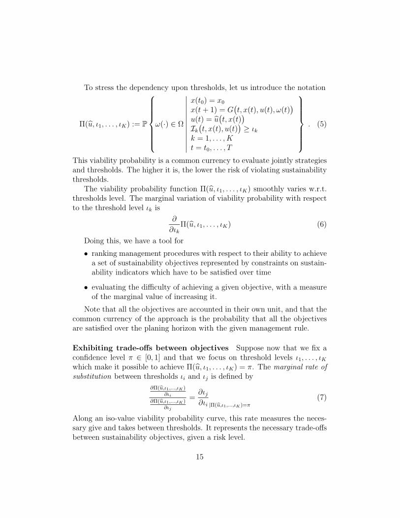
To stress the dependency upon thresholds, let us introduce the notation

Π(u, ι1, . . . , ιK) := P

ω(·) ∈ Ω

∣∣∣∣∣∣∣∣∣∣∣∣

x(t0) = x0

x(t+ 1) = G(t, x(t), u(t), ω(t)

)u(t) = u

(t, x(t)

)Ik(t, x(t), u(t)

)≥ ιk

k = 1, . . . , Kt = t0, . . . , T

. (5)

This viability probability is a common currency to evaluate jointly strategiesand thresholds. The higher it is, the lower the risk of violating sustainabilitythresholds.

The viability probability function Π(u, ι1, . . . , ιK) smoothly varies w.r.t.thresholds level. The marginal variation of viability probability with respectto the threshold level ιk is

∂

∂ιkΠ(u, ι1, . . . , ιK) (6)

Doing this, we have a tool for

• ranking management procedures with respect to their ability to achievea set of sustainability objectives represented by constraints on sustain-ability indicators which have to be satisfied over time

• evaluating the difficulty of achieving a given objective, with a measureof the marginal value of increasing it.

Note that all the objectives are accounted in their own unit, and that thecommon currency of the approach is the probability that all the objectivesare satisfied over the planing horizon with the given management rule.

Exhibiting trade-offs between objectives Suppose now that we fix aconfidence level π ∈ [0, 1] and that we focus on threshold levels ι1, . . . , ιKwhich make it possible to achieve Π(u, ι1, . . . , ιK) = π. The marginal rate ofsubstitution between thresholds ιi and ιj is defined by

∂Π(bu,ι1,...,ιK)∂ιi

∂Π(bu,ι1,...,ιK)∂ιj

=∂ιj∂ιi |Π(bu,ι1,...,ιK)=π

(7)

Along an iso-value viability probability curve, this rate measures the neces-sary give and takes between thresholds. It represents the necessary trade-offsbetween sustainability objectives, given a risk level.

15

3.3 Optimal management strategy

In our approach, a management rule is preferred if it results in a high via-bility probability. It is thus of interest to determine the optimal manage-ment rule, i.e., the management rule that maximizes the viability prob-ability. Given sustainability objectives ι1, . . . , ιK , an optimal strategy u?

is one which maximizes Π(u, ι1, . . . , ιK). The maximal viability probabilitymaxbu Π(u, ι1, . . . , ιK) is an upper bound for any strategy. Notice that opti-mal strategies depend on the objective levels.

From a general point of view, determining optimal feedback rules in dy-namic optimization problems under uncertainty is not easy, either for opti-mal control or stochastic viability problems. Such feedback rules will dependon the characteristics of dynamics of the system, and other assumptions orrestrictions to the model. We here characterize such a rule when the bioe-conomic system satisfies some restrictive, but sensible, conditions. For thispurpose, we use the mathematical result in [20]. We extend the interpre-tation of this result to the fisheries management issue. In particular, weinterpret the conditions in economic and ecological terms, and we provide aninterpretation of the optimal management rule.

Consider a fishery which dynamics G is increasing with the state x, anddecreasing with the control u, i.e., the larger the stock one year, the largerthe stock the following year, and the larger the effort one year, the lower thestock the following year. Consider also that the control u is scalar and belongsto a closed interval U := [u[, u]]. These assumptions make sense for singlespecies management (or for several species with economic interactions butno biological interactions), when the recruitment of next year only dependson the current Spawning Stock Biomass. They don’t hold for several specieswith biological interactions (such as prey-predator models), or for modelswith recruitment delays.

Consider that the sustainability objectives satisfy the following monotonyproperties:

• One of the indicator is increasing with the state x (i.e., the higherthe state, the higher the indicator) and continuous in the control u,and does not depend upon the uncertainty ω, namely I1(t, x, u, ω) =I1(t, x, u). This indicator can be considered as “economic.”

16

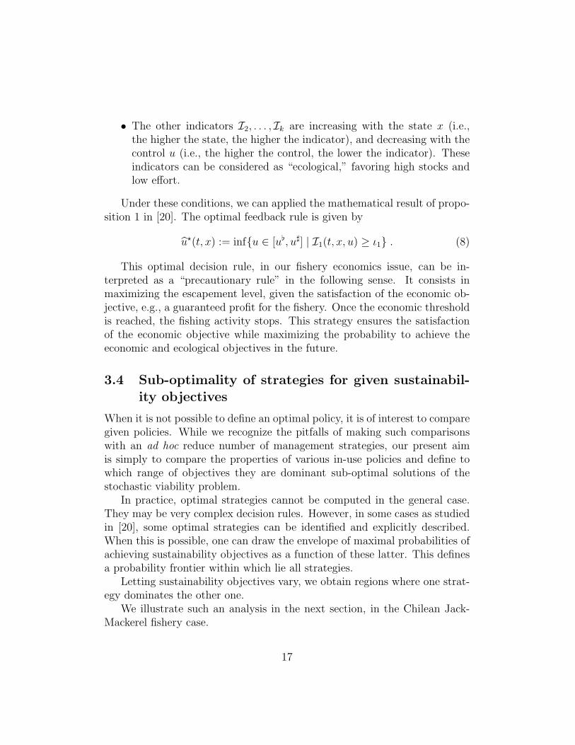
• The other indicators I2, . . . , Ik are increasing with the state x (i.e.,the higher the state, the higher the indicator), and decreasing with thecontrol u (i.e., the higher the control, the lower the indicator). Theseindicators can be considered as “ecological,” favoring high stocks andlow effort.

Under these conditions, we can applied the mathematical result of propo-sition 1 in [20]. The optimal feedback rule is given by

u?(t, x) := infu ∈ [u[, u]] | I1(t, x, u) ≥ ι1 . (8)

This optimal decision rule, in our fishery economics issue, can be in-terpreted as a “precautionary rule” in the following sense. It consists inmaximizing the escapement level, given the satisfaction of the economic ob-jective, e.g., a guaranteed profit for the fishery. Once the economic thresholdis reached, the fishing activity stops. This strategy ensures the satisfactionof the economic objective while maximizing the probability to achieve theeconomic and ecological objectives in the future.

3.4 Sub-optimality of strategies for given sustainabil-ity objectives

When it is not possible to define an optimal policy, it is of interest to comparegiven policies. While we recognize the pitfalls of making such comparisonswith an ad hoc reduce number of management strategies, our present aimis simply to compare the properties of various in-use policies and define towhich range of objectives they are dominant sub-optimal solutions of thestochastic viability problem.

In practice, optimal strategies cannot be computed in the general case.They may be very complex decision rules. However, in some cases as studiedin [20], some optimal strategies can be identified and explicitly described.When this is possible, one can draw the envelope of maximal probabilities ofachieving sustainability objectives as a function of these latter. This definesa probability frontier within which lie all strategies.

Letting sustainability objectives vary, we obtain regions where one strat-egy dominates the other one.

We illustrate such an analysis in the next section, in the Chilean Jack-Mackerel fishery case.

17

4 Modeling the Chilean Jack-Mackerel fish-

ery

The Jack-Mackerel fishery is currently the largest in Chile, both in termsof annual catch volume (about 1.5 million tons in 2008, while it peaked at4.5 million tons in 1995) and economic value generation (400-500 millionsUS$ of yearly sales in recent years). Like other small pelagic fisheries, italso faces the recurrent appearance of El Nino uncertain cycles. This fish-ery has been one of the pioneers in Chile in terms of including explicitlybiology-related risk indicators within its management procedures. However,this has been mostly done in a very ad-hoc way, using risk indicators as addi-tional information within the policy-decision process, but lacking a formallyintegrated framework to make choices between risk and economic return in-dicators. For instance, in [45, p.26-27], exogenously defined quota levels areassociated with the resulting probabilities of reducing the spawning stockbiomass (SSB) available at a future year (2013), relative to its present level(at year 2004). In [31, p.33-39], such calculations are extended to differenttime horizons. Nonetheless, none of these analyses incluye a formal frame-work for making choices about tradeoffs faced between risk indicators andmeasures of economic return.

In [48], the Chilean Jack-Mackerel fishery has been studied, using In-stituto de Fomento Pesquero (IFOP)’s official data [44, 30] and its age-structured model for this fishery, by adding to the model more structureinto the stock-recruitment function. Indeed, a Ricker recruitment function isestimated by using linear time-series analysis13. Additionally, a generating(sinusoidal) function for El Nino uncertain cycles is estimated by using anon-linear iterative technique [48, p. 64]. Then, and following the line of [8]and [9], [48] performs a Management Strategy Evaluation. The analysis atour paper will thus be based on the estimation results provided by [48].

13The Ricker model is normally used for species with highly fluctuating recruitment,involving high fecundity as well as high natural mortality rates. These two features areindeed present in the case of small pelagic species, such as jack mackerel. (Begon andMortimer 1986; Haddon 2001).

18

4.1 A bioeconomic model for the Chilean Jack-Mackerelfishery

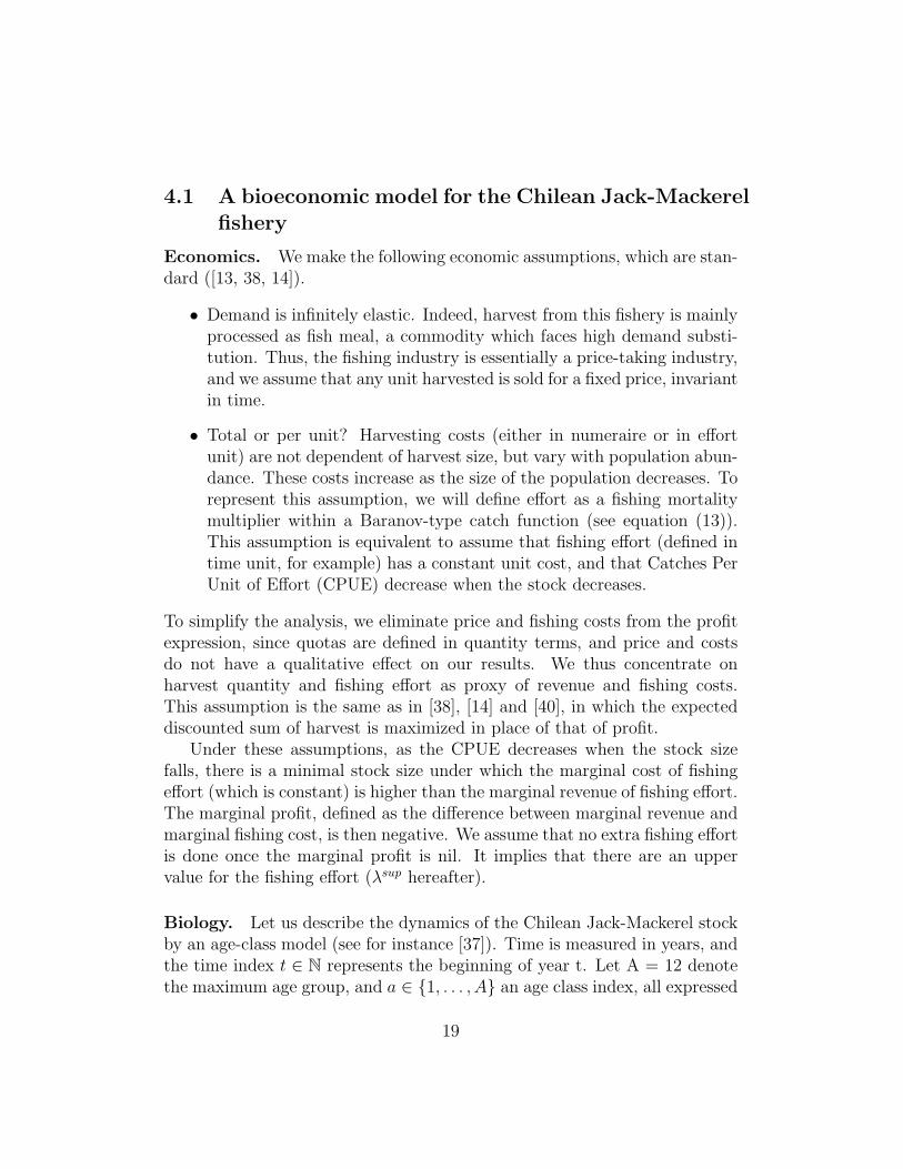
Economics. We make the following economic assumptions, which are stan-dard ([13, 38, 14]).

• Demand is infinitely elastic. Indeed, harvest from this fishery is mainlyprocessed as fish meal, a commodity which faces high demand substi-tution. Thus, the fishing industry is essentially a price-taking industry,and we assume that any unit harvested is sold for a fixed price, invariantin time.

• Total or per unit? Harvesting costs (either in numeraire or in effortunit) are not dependent of harvest size, but vary with population abun-dance. These costs increase as the size of the population decreases. Torepresent this assumption, we will define effort as a fishing mortalitymultiplier within a Baranov-type catch function (see equation (13)).This assumption is equivalent to assume that fishing effort (defined intime unit, for example) has a constant unit cost, and that Catches PerUnit of Effort (CPUE) decrease when the stock decreases.

To simplify the analysis, we eliminate price and fishing costs from the profitexpression, since quotas are defined in quantity terms, and price and costsdo not have a qualitative effect on our results. We thus concentrate onharvest quantity and fishing effort as proxy of revenue and fishing costs.This assumption is the same as in [38], [14] and [40], in which the expecteddiscounted sum of harvest is maximized in place of that of profit.

Under these assumptions, as the CPUE decreases when the stock sizefalls, there is a minimal stock size under which the marginal cost of fishingeffort (which is constant) is higher than the marginal revenue of fishing effort.The marginal profit, defined as the difference between marginal revenue andmarginal fishing cost, is then negative. We assume that no extra fishing effortis done once the marginal profit is nil. It implies that there are an uppervalue for the fishing effort (λsup hereafter).

Biology. Let us describe the dynamics of the Chilean Jack-Mackerel stockby an age-class model (see for instance [37]). Time is measured in years, andthe time index t ∈ N represents the beginning of year t. Let A = 12 denotethe maximum age group, and a ∈ 1, . . . , A an age class index, all expressed

19

in years. The vector N = (Na)a=1,...,A ∈ RA+ is made of abundances at age:

for a = 1, . . . , A− 1, Na(t) is the number of individuals of age between a− 1and a at the beginning of year t; NA(t) is the number of individuals of agegreater than A − 1. The fishing activity is represented by a fishing effortmultiplier λ(t), supposed to be applied in the middle of period t.

For all classes, except for the recruits, we have:

Na+1(t+ 1) = e−(Ma+λ(t)Fa)Na(t) , a = 2, . . . , A− 1 , (9)

where Ma is the natural mortality rate of individuals of age a, Fa is themortality rate of individuals of age a due to harvesting between t and t+ 1,supposed to remain constant during period t (the vector (Fa)a=1,...,A is termedthe exploitation pattern). The values for parameters Ma and Fa are takenfrom IFOP’s official model for this fishery, so that Ma is equal to 0.23 for alla and Fa will be equal to the vector of averages values of Fa during 2001-2002(cf. [46]).

For the recruits, we rely upon a statistical study in [48] which relatesthem to the spawning stock biomass

SSB(N) :=A∑a=1

γa$aNa , (10)

where (γa)a=1,...,A are the proportions of mature individuals (some may bezero) and ($a)a=1,...,A are the weights (all positive). The following two-yearsdelay dynamic relationship obtained is

N1(t+ 1) = αSSB(N(t− 1)

)exp

(βSSB

(N(t− 1)

)+ w(t)

), (11)

where parameters are set α = e2.39 and β = 2.2·10−7, and w(t) is a randomprocess reflecting the impact of climatic factors in the stock recruitmentrelationship. Notice that the recruitment relationship is given by a Rickertype function applied to the spawning stock biomass of two previous periods.

El Nino cycles model. The residual term w(t) in the estimated equation(11) has a periodic part and an error term and is supposed to capture theeffects of the El Nino phenomenon (a cycle with random shocks). Indeed,the statistical analysis at [48] implies the following structure for the residualw(t):

w(t) = −0.12× nino(t) + ε(t) , (12)

where

20

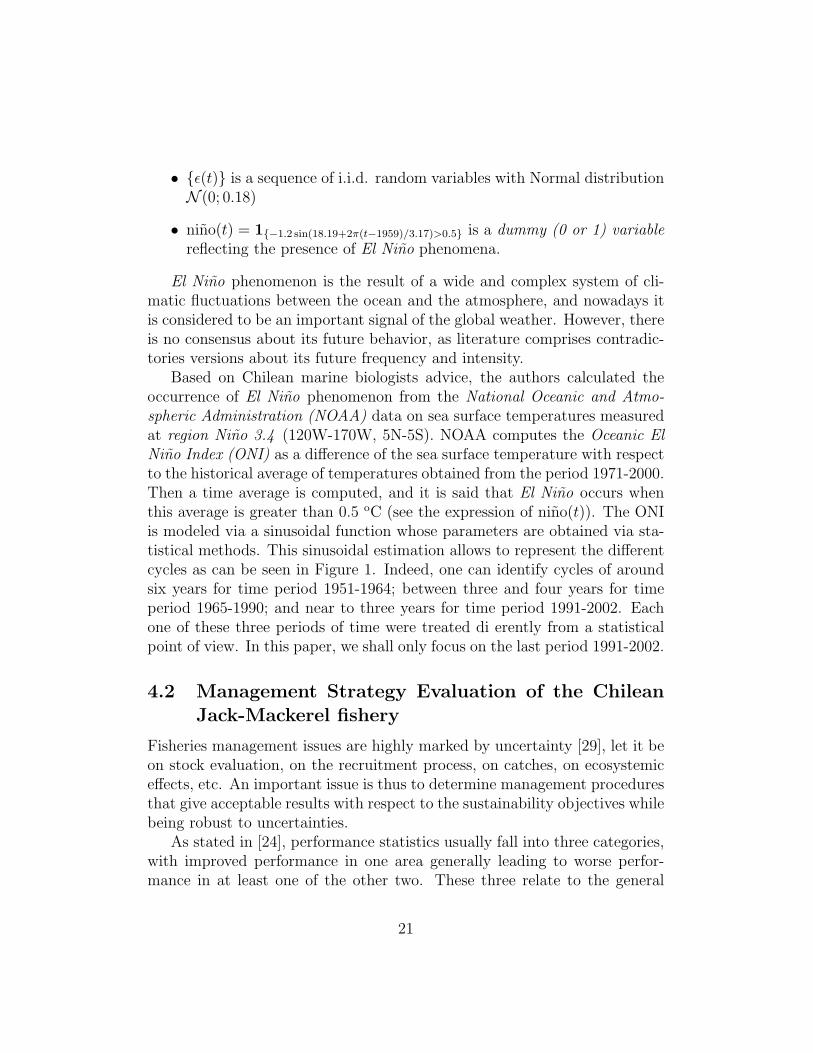
• ε(t) is a sequence of i.i.d. random variables with Normal distributionN (0; 0.18)

• nino(t) = 1−1.2 sin(18.19+2π(t−1959)/3.17)>0.5 is a dummy (0 or 1) variablereflecting the presence of El Nino phenomena.

El Nino phenomenon is the result of a wide and complex system of cli-matic fluctuations between the ocean and the atmosphere, and nowadays itis considered to be an important signal of the global weather. However, thereis no consensus about its future behavior, as literature comprises contradic-tories versions about its future frequency and intensity.

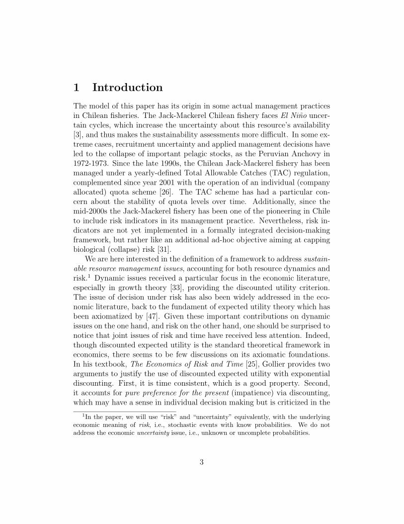
Based on Chilean marine biologists advice, the authors calculated theoccurrence of El Nino phenomenon from the National Oceanic and Atmo-spheric Administration (NOAA) data on sea surface temperatures measuredat region Nino 3.4 (120W-170W, 5N-5S). NOAA computes the Oceanic ElNino Index (ONI) as a difference of the sea surface temperature with respectto the historical average of temperatures obtained from the period 1971-2000.Then a time average is computed, and it is said that El Nino occurs whenthis average is greater than 0.5 oC (see the expression of nino(t)). The ONIis modeled via a sinusoidal function whose parameters are obtained via sta-tistical methods. This sinusoidal estimation allows to represent the differentcycles as can be seen in Figure 1. Indeed, one can identify cycles of aroundsix years for time period 1951-1964; between three and four years for timeperiod 1965-1990; and near to three years for time period 1991-2002. Eachone of these three periods of time were treated di erently from a statisticalpoint of view. In this paper, we shall only focus on the last period 1991-2002.

4.2 Management Strategy Evaluation of the ChileanJack-Mackerel fishery

Fisheries management issues are highly marked by uncertainty [29], let it beon stock evaluation, on the recruitment process, on catches, on ecosystemiceffects, etc. An important issue is thus to determine management proceduresthat give acceptable results with respect to the sustainability objectives whilebeing robust to uncertainties.

As stated in [24], performance statistics usually fall into three categories,with improved performance in one area generally leading to worse perfor-mance in at least one of the other two. These three relate to the general

21

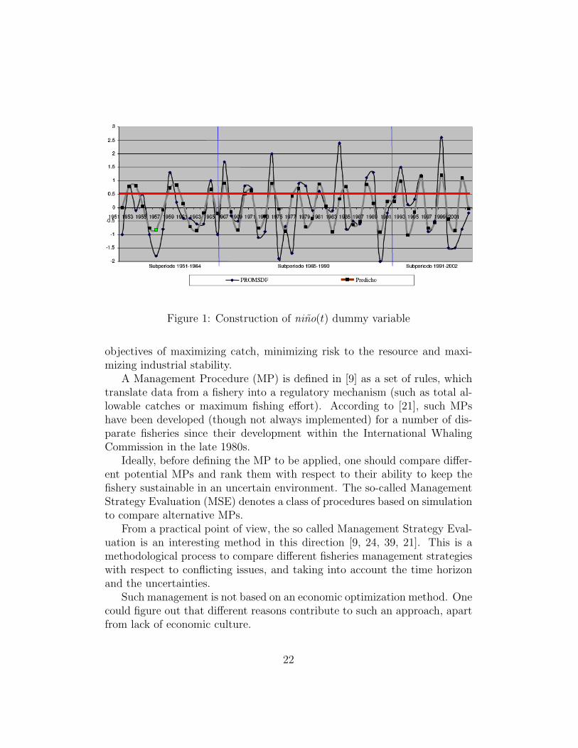
Figure 1: Construction of nino(t) dummy variable

objectives of maximizing catch, minimizing risk to the resource and maxi-mizing industrial stability.

A Management Procedure (MP) is defined in [9] as a set of rules, whichtranslate data from a fishery into a regulatory mechanism (such as total al-lowable catches or maximum fishing effort). According to [21], such MPshave been developed (though not always implemented) for a number of dis-parate fisheries since their development within the International WhalingCommission in the late 1980s.

Ideally, before defining the MP to be applied, one should compare differ-ent potential MPs and rank them with respect to their ability to keep thefishery sustainable in an uncertain environment. The so-called ManagementStrategy Evaluation (MSE) denotes a class of procedures based on simulationto compare alternative MPs.

From a practical point of view, the so called Management Strategy Eval-uation is an interesting method in this direction [9, 24, 39, 21]. This is amethodological process to compare different fisheries management strategieswith respect to conflicting issues, and taking into account the time horizonand the uncertainties.

Such management is not based on an economic optimization method. Onecould figure out that different reasons contribute to such an approach, apartfrom lack of economic culture.

22

• Stake-holders are multiple and are often arguing on thresholds.

• Long run issues and uncertainty may force to work on quantities, lessfragile than prices and costs [7, 43]

• Usually, a regulator has prices, but fishing costs are a private informa-tion, depending on the vessels. Profit functions cannot be estimatedwithout strong hypothesis on the fleet homogeneity. The usual ap-proach is to study catch levels.

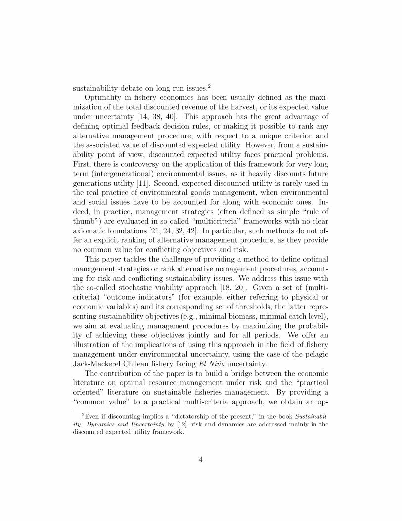
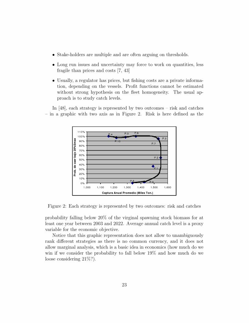
In [48], each strategy is represented by two outcomes – risk and catches– in a graphic with two axis as in Figure 2. Risk is here defined as the

Figure 2: Each strategy is represented by two outcomes: risk and catches

probability falling below 20% of the virginal spawning stock biomass for atleast one year between 2003 and 2022. Average annual catch level is a proxyvariable for the economic objective.

Notice that this graphic representation does not allow to unambiguouslyrank different strategies as there is no common currency, and it does notallow marginal analysis, which is a basic idea in economics (how much do wewin if we consider the probability to fall below 19% and how much do weloose considering 21%?).

23

4.3 Viability assessment of constant quota and con-stant effort management procedures for the ChileanJack-Mackerel fishery

In this section we used the stochastic viability approach to compare man-agement procedures for the Chilean Jack-Mackerel fishery. We focus on twodifferent types of MPs: constant constant quota and constant constant fish-ing effort, both stationary over a fixed period of time (T = 10 years). Forthese classes of MPs, we compute their viability probability associated to twoconstraints, biological and economical.

Economic and biological constraints We shall consider, on the onehand, the following economic constraint. Firstly, the total annual catch Y ,measured in biomass (millions of tons), is given by the Baranov catch equa-tion14 [37, p. 255-256]:

Y(N, λ

)=

A∑a=1

$aλFa

λFa +Ma

(1− e−(Ma+λFa)

)Na . (13)

With this definition, consider the economic constraint

Y (N(t), λ(t)) ≥ ymin , ∀t = t0, t0 + 1, ..., T , (14)

where the parameter ymin is the minimum level of landing (or annual totalcatches) that we expect to harvest each period of time. This parameter takesvalues from 1 to 1.5 millions of tons, which means that the yield should beabove landings of 1 to 1.5 millions of tons, respectively. Using the notationof Section 3.1, the constraint (14) corresponds to the following indicator andthreshold: I2(t, x(t), u(t)) := Y

(N(t), λ(t)

)and ι2 := ymin.

On the other hand, we consider the biological constraint

SSB(N(t)

)≥ pSSBvirg , ∀t = t0, t0 + 1, ..., T , (15)

14Y measures the aggregated catch in period t which adds up catches from the Chileanand foreign fleets. During the 2000s the chilean fleet’s annual catches have ranged between1.1-1.4 million tons (though at year 2009 this figure fell to 700 thousand tons), while foreignfleet’s annual catches have varied between 200-400 thousand tons.

24

where SSB is the spawning stock biomass defined in (10), SSBvirg = 6.44millions tons is the virginal spawning stock biomass of the fishery, and the pa-rameter p denotes the desired percentage of SSBvirg expected to be preservedalong the exploitation time. In all our computations, parameter p takes val-ues from 0 to 0.4, which means that SSB(N(t)) should be above the valuesof 0% to 40 % of the virginal spawning stock biomass, respectively. Usingthe notation of Section 3.1, the constraint (15) corresponds to the followingindicator and threshold: I1(t, x(t), u(t)) := SSB(N(t)) and ι1 := pSSBvirg .

Viability assessment of constant quota and constant effort strate-gies Considering the state vector (A+ 1-dimensional)

x(t) =(N1(t), . . . , NA(t), SSB

(N(t− 1)

)),

and a control variableu(t) = λ(t) .

From (9)–(10)–(11), we obtain a control dynamical system in state form:

x(t+ 1) = G(x(t), λ(t), w(t)

), t = t0, t0 + 1, . . . , T, x(t0) given.

In what follows, we shall take the initial year t0 = 2002. With this statemodel, we are in the framework of Section 3.1.

Definition of strategiesA constant effort strategy (CES) is a constant strategy defined by λ(t, N) =

λ, yielding the constant effort15 λ(t) = λ.

A constant quota strategy (CQS) is a strategy λ(t, N) = λ implicitly

defined by Y(N, λ

)= Y , when possible (else λ(t, N) = 0).

Viability assessment of one constant effort and of one constantquota strategies

Our first application consists in computing the viability probability oftwo specific management procedures: a CES λ = 0.2 and a CQS at levelY = 1.2 millions of tons, just about the current quota level in this fishery.

15In our model, fishing mortality is proportional to fishing effort when the fishing pat-tern, i.e. the technology, is constant. The constant effort strategy is thus identical to theconstant fishing mortality strategy depicted here.

25

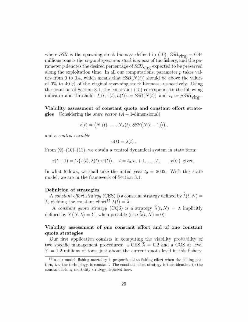
Following the framework of Sect. 3.1, these probabilities are computed foreach couple (p, ymin) ∈ [0, 0.4]× [1, 1.5] of biological and economic thresholds.We thus obtain 3D graphics in Figure 3 (left: CQS; right:CES).

Figure 3: Viability probabilities: left: CQS Y = 1.2 millions of tons; right:CES λ = 0.2

Let us illustrate how these graphics make different types of comparisonspossible. A preliminary visual comparison shows that, for moderate economicthresholds between 1.1 and 1.2 millions of tons and low biological thresholds,the CQS provides a higher viability probability than the CES.

Which constant quota and constant effort performs better withineach management strategy family?

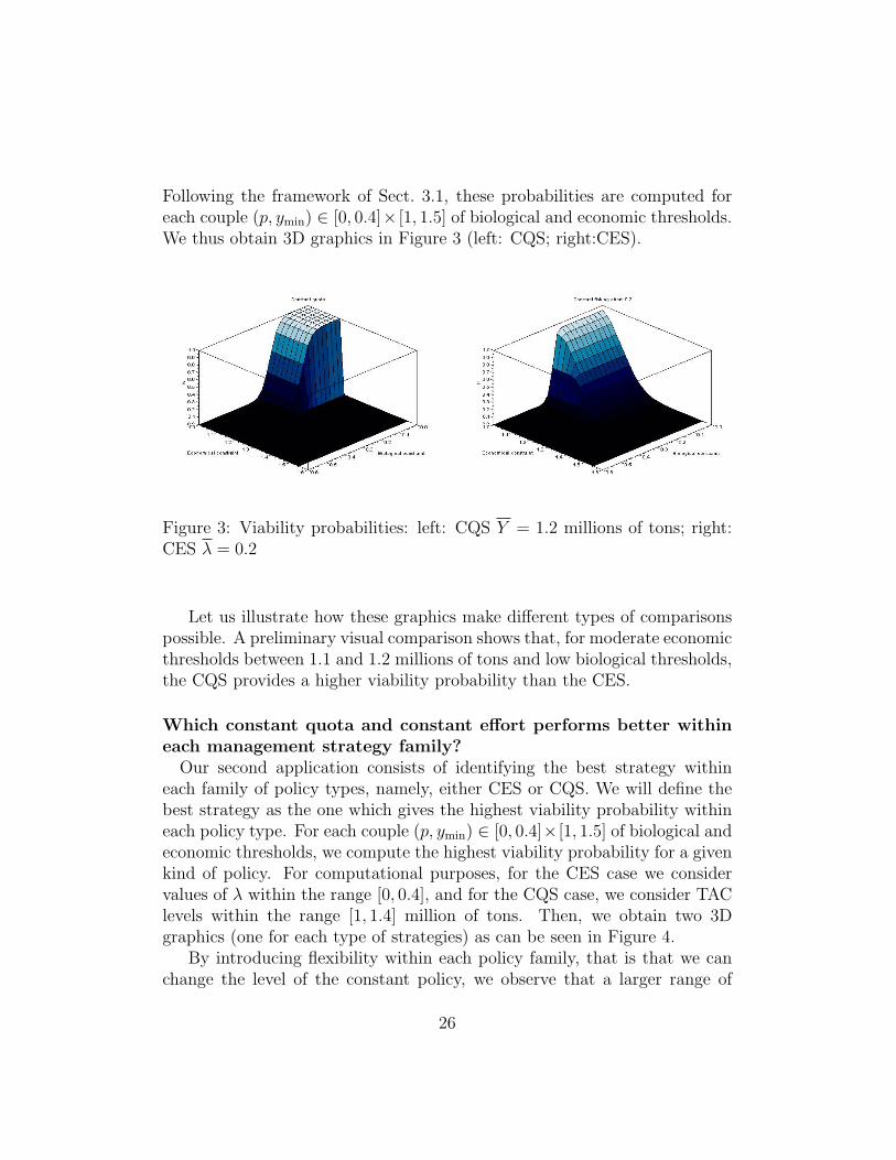
Our second application consists of identifying the best strategy withineach family of policy types, namely, either CES or CQS. We will define thebest strategy as the one which gives the highest viability probability withineach policy type. For each couple (p, ymin) ∈ [0, 0.4]× [1, 1.5] of biological andeconomic thresholds, we compute the highest viability probability for a givenkind of policy. For computational purposes, for the CES case we considervalues of λ within the range [0, 0.4], and for the CQS case, we consider TAClevels within the range [1, 1.4] million of tons. Then, we obtain two 3Dgraphics (one for each type of strategies) as can be seen in Figure 4.

By introducing flexibility within each policy family, that is that we canchange the level of the constant policy, we observe that a larger range of

26

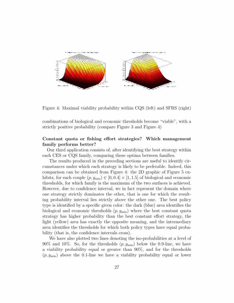
Figure 4: Maximal viability probability within CQS (left) and SFRS (right)

combinations of biological and economic thresholds become “viable”, with astrictly positive probability (compare Figure 3 and Figure 4)

Constant quota or fishing effort strategies? Which managementfamily performs better?

Our third application consists of, after identifying the best strategy withineach CES or CQS family, comparing these optima between families.

The results produced in the preceding sections are useful to identify cir-cumstances under which each strategy is likely to be preferable. Indeed, thiscomparison can be obtained from Figure 4: the 2D graphic of Figure 5 ex-hibits, for each couple (p, ymin) ∈ [0, 0.4]× [1, 1.5] of biological and economicthresholds, for which family is the maximum of the two surfaces is achieved.However, due to confidence interval, we in fact represent the domain whereone strategy strictly dominates the other, that is one for which the result-ing probability interval lies strictly above the other one. The best policytype is identified by a specific given color: the dark (blue) area identifies thebiological and economic thresholds (p, ymin) where the best constant quotastrategy has higher probability than the best constant effort strategy, thelight (yellow) area has exactly the opposite meaning, and the intermediaryarea identifies the thresholds for which both policy types have equal proba-bility (that is, the confidence intervals cross).

We have also plotted two lines denoting the iso-probabilities at a level of90% and 10%. So, for the thresholds (p, ymin) below the 0.9-line, we havea viability probability equal or greater than 90%, and for the thresholds(p, ymin) above the 0.1-line we have a viability probability equal or lower

27

than 10%.

Figure 5: Comparison of the CES and CQS policy families

From this output we can show that CQS seem to perform better thanCES for small values of biological threshold p. On the other hand, for largervalues of this parameter (p above 0.18), CES perform better than CQS.

5 Conclusions

Many natural resources management problems are marked by dynamics anduncertainty. This is for example the case of fishery management where con-flicting economic, ecological and social objectives require evaluation methodsto rank the potential management procedures, taking into account uncer-tainty. This is the purpose of the Management Strategy Evaluation approach,

28

which describes trade-offs in management objectives, and characterizes po-tential management procedures with a set of performance statistics. However,due to the absence of a “common currency” for conflicting performance mea-sures which should be approved by all parties, the decision-makers are leftwith clearer perspectives but without tools to rank the various managementprocedures.

To contribute to decision making in natural resource management prob-lems, we have developed a viability analysis based on the definition of a set ofconstraints that represents the various sustainability objectives. We proposeto rank management strategies by the probability that the resulting intertem-poral trajectory satisfies all of the objectives over the planning horizon. Anoptimal management rule is one that results in the highest viability proba-bility. The “common currency” to rank the various management decisions isthus the viability probability.

This stochastic viability framework allows us to exhibit the trade-offs be-tween sustainability objectives (thresholds) and viability probability. It alsodescribes the set of sustainability objectives that can be achieved given anassumed risk level, helping the decision maker in the definition of thresholds.

The results we present are based on a case-study, with estimated pa-rameters. While these results are derived using numerical techniques, theproposed stochastic viability methodology is general and can be applied toa wide range of problems.Our approach is a step toward defining consistentsustainable fishery management analysis, in a multicriteria framework. Weprovide a first application of stochastic viability to the assessment of re-sources management procedures. We examine the efficiency of two kind offishery management policies, namely constant quotas and fishing effort, toachieve sustainability objectives defined as intertemporal constraints on bi-ological and economic indicators. Monte Carlo simulations with markovianuncertainty are run to obtain viability probability of each policy, with respectto the objectives.

The method can thus be used to bridge the gap between optimality lit-erature and practical decision-making.

Acknowledgments. This paper was prepared within the MIFIMA (Math-ematics, Informatics and Fisheries Management) international research frame-work (cermics.enpc.fr/˜delara/MIFIMA 2006/MIFIMA web/) funded by CNRS,INRIA and the French Ministry of Foreign Affairs through the regional co-

29

operation program STIC–AmSud. We thank Claire Nicolas (ENSTA - Paris-Tech student), Pauline Dochez (Polytechnique - ParisTech student) and Pe-dro Gajardo (Universidad Federico Santa Maria - Valparaiso - Chile) forrelated works. The usual disclaimer applies.

References

[1] P. Andersen and J.G. Sutinen. Stochastic bioeconomics: A review ofbasic methods and results. Marine Resource Economics, 1(2):117–136,1984.

[2] J.-P. Aubin. Dynamic Economic Theory ; A Viability Approach.Springer ; Studies in Economic Theory, 1997.

[3] R.T. Barber and F.P. Chavez. Biological consequences of El Nino. Sci-ence, 222(4629):1203–1210, 1983.

[4] S. Baumgartner and M. Quaas. Ecological-economic viability as a cri-terion of strong sustainability under uncertainty. Ecological Economics,68:2008–2020, 2009.

[5] C. Bene and L. Doyen. Storage and viability of a fishery with re-source and market dephased seasonnalities. Environmental ResourceEconomics, 15:1–26, 2000.

[6] C. Bene, L. Doyen, and D. Gabay. A viability analysis for a bio-economicmodel. Ecological Economics, 36:385–396, 2001.

[7] M. Boiteux. A propos de la “critique de la theorie de l’actualisation tellequ’employee en France”. Revue d’Economie Politique, 5, 1976.

[8] D.S. Butterworth and M.O. Bergh. The development of a managementprocedure for the south african anchovy resource. In J.J. Hunt S.J. Smithand D. Rivard, editors, Risk Evaluation and Biological Reference Pointsfor Fisheries Management, pages 83–99. Canadian Special Publicationof Fisheries and Aquatic Science 120, National Research Council andDepartment of Fisheries and Oceans, Ottawa, 1997.

30

[9] D.S. Butterworth, K.L. Cochrane, and J.A.A. De Oliveira. Managementprocedures: a better way to manage fisheries? The South African expe-rience. In D. D. Huppert E. K. Pikitch and M. P. Sissenwine, editors,Global Trends: Fisheries Management, pages 83–90. American FisheriesSociety Symposium 20, 1997.

[10] A. Charles. Living with uncertainty in fisheries: analytical methods,management priorities and the canadian groundfishery experience. Fish-eries Research, 37:37–50, 1998.

[11] G. Chichilnisky. An axiomatic approach to sustainable development.Social Choice and Welfare, 13(2):219–248, 1996.

[12] G. Chichilnisky, G. Heal, and A. Beltratti. Sustainability: Dynamicsand Uncertainty. Kluwer Academic Publishers, Dordrecht, 1998.

[13] C. W. Clark. Mathematical Bioeconomics. Wiley, New York, secondedition, 1990.

[14] C.W. Clark and G.P. Kirkwood. On uncertainty renewable resourcestocks: Optimal harvest policy and the value of stock surveys. Journalof Environmental Economics and Management, 13:235–244, 1986.

[15] K. L. Cochrane. Reconciling sustainability, economic efficiency and eq-uity in fisheries: the one that got away? Fish and Fisheries, 1:3–21,2000.

[16] C.J. Costello, R.M. Adams, and S. Polasky. The value of el nino fore-casts in the management of salmon: A stochastic dynamic assessment.American Journal of Agricultural Economics, 80:765–777, 1998.

[17] A. Danielsson. Efficiency of catch and effort quotas in the presence ofrisk. Journal of Environmental Economics and Management, 43:20–33,2002.

[18] M. De Lara and L. Doyen. Sustainable Management of Natural Re-sources. Mathematical Models and Methods. Springer-Verlag, Berlin,2008.

[19] M. De Lara, L. Doyen, T. Guilbaud, and M.-J. Rochet. Is a managementframework based on spawning-stock biomass indicators sustainable? A

31

viability approach. ICES Journal of Marine Science, 64(4):761–767,2007.

[20] M. De Lara and V. Martinet. Multi-criteria dynamic decision under un-certainty: A stochastic viability analysis and an application to sustain-able fishery management. Mathematical Biosciences, 217(2):118–124,February 2009.

[21] J. A. A. De Oliveira and D. S. Butterworth. Developing and refining ajoint management proceduree for the multispecies South African pelagicfisheries. ICES Journal of Marine Science, 61:1432–1442, 2004.

[22] K. Eisenack, J. Sheffran, and J. Kropp. The viability analysis of manage-ment frameworks for fisheries. Environmental Modeling and Assessment,11(1):69–79, February 2006.

[23] W.J. Fletcher. The application of qualitative risk assessment method-ology to prioritize issues for fisheries management. ICES Journal ofMarine Science, 62:1576–1587, 2005.

[24] H. F. Geromont, J. A. A. De Oliveira, S. J. Johnston, and C. L. Cun-ningham. Development and application of management procedures forfisheries in Southern Africa. ICES Jounal of Marine Science, 56:952–966, 1999.

[25] C. Gollier. The Economics of Risk and Time. MIT Press, Cambridge,2001.

[26] A. Gomez-Lobo, J. Pe na Torres, and P. Barria. Itqs in chile: Mea-suring the economic benefits of reform. Working Papers Series I-179,Faculty of Economics & Business, Universidad Alberto Hurtado, March(http://economia.uahurtado.cl/pdf/publicaciones/inv179.pdf), 2007.

[27] R. Hannesson and S.I. Steinshamn. How to set catch quotas: Constanteffort or constant catch? Journal of Environmental Economics andManagement, 20:71–91, 1991.

[28] R. Hilborn. Defining success in fisheries and conflicts in objectives.Marine Policy, 31:153–158, 2007.

32

[29] R. Hilborn and C. F. Walters. Quantitative fisheries stock assessment.Choice, dynamics and uncertainty. Chapman and Hall, New York, Lon-don, 1992. 570 pp.

[30] IFOP. Informe complementario investigacion ctp jurel, 2003: Indi-cadores de reclutamiento. Technical report, Instituto de Fomento Pes-quero (IFOP), Valparaıso, 2003. Documento de trabajo.

[31] IFOP. Investigacion evaluacion de stock y ctp jurel 2006. Technicalreport, Intergovernmental Panel on Climate Change, Valparaiso, Chile,March 2006. Informe Final Proyecto BIP 30033881-0.

[32] L. T. Kell, G. M. Pilling, G. P. Kirkwood, M. Pastoors, B. Mesnil,K. Korsbrekke, P. Abaunza, R. Aps, A. Biseau, P. Kunzlik, C. Needle,B. A. Roel, and C. Ulrich-Rescan. An evaluation of the implicit man-agement procedure used for some ices roundfish stocks. ICES Journalof Marine Science, 62:750–759, 2005.

[33] T. C. Koopmans. On the concept of optimal economic growth. AcademiaScientiarium Scripta Varia, 28:225–300, 1965.

[34] V. Martinet, L. Doyen, and O. Thebaud. Defining viable recovery pathstoward sustainable fisheries. Ecological Economics, 64(2):411–422, 2007.

[35] E.K. Pikkitch, C. Santora, E.A. Babcock, A. Bakun, R. Bonfil, D.O.Conover, and et al P. Dayton. Ecosystem based fishery management.Science, 305:346–347, 2004.

[36] J. Quiggin. How to set catch quotas: A note on the superiority ofconstant effort rules. Journal of Environmental Economics and Man-agement, 22:199–203, 1992.

[37] T. J. Quinn and R. B. Deriso. Quantitative Fish Dynamics. BiologicalResource Management Series. Oxford University Press, New York, 1999.542 pp.

[38] W. Reed. Optimal escapement levels in stochastic and deterministic har-vesting models. Journal of Environmental Economics and Management,6:350–363, 1979.

33

[39] K. J. Sainsbury, A. E. Punt, and A. D. M. Smith. Design of operationalmanagement strategies for achieving fishery ecosystem objectives. ICESJournal of Marine Science, 57:731–741, 2000.

[40] G. Sethi, C. Costello, A. Fisher, M. Hanemann, and L. Karp. Fish-ery management under multiple uncertainty. Journal of EnvironmentalEconomics and Management, 50:300–318, 2005.

[41] R. Singh, Q. Weninger, and M. Doyle. Fisheries management with stockuncertainty and costly capital adjustment. Journal of EnvironmentalEconomics and Management, 52:582–599, 2006.

[42] A.D.M. Smith, E.J. Fulton, A.J. Hobday, D.C. Smith, and P. Shoulder.Scientific tools to support the practical implementation of ecosystem-based fisheries management. ICES Journal of Marine Science, 64:633–639, 2007.

[43] R. Solow. An almost pratical step toward sustainability. ResourcesPolicy, 19 (3):162–172, 1993.

[44] SUBPESCA. Cuota global de captura para la pesquerıa del recursojurel, ano 2001. Technical report, Subsecretaria de Pesca, SUBPESCA,Valparaıso, 2000. Documento de trabajo.

[45] SUBPESCA. Cuota global anual de captura de jurel, ano 2005. Tech-nical report, Subsecretaria de Pesca, SUBPESCA, Valparaıso, Octubre2004. Informe Tecnico (R. Pesq.) numero 79/2004.

[46] SUBPESCA. Pre informe final. investigacion evaluation y ctp jurel,2006. Technical report, Subsecretaria de Pesca, SUBPESCA, Valparaıso,Marzo 2006. BIP 30033881-0.

[47] J. von Neuman and O. Morgenstern. Theory of games and economicbehaviour. Princeton University Press, Princeton, 1947. 2nd edition.

[48] M. Yepes. Dinamica poblacional del jurel: Reclutamiento asociado afactores ambientales y sus efectos sobre la captura. Master’s thesis,Universidad Alberto Hurtado (Ilades-Georgetown Graduate Programs),Santiago, Chile, 2004. Master Thesis in Economics.

34