arX

iv:c

ond-

mat

/960

4163

v1 2

6 A

pr 1

996

Transition from localized to extended eigenstates in the ensemble

of power-law random banded matrices

Alexander D. Mirlin1†, Yan V. Fyodorov2†,

Frank-Michael Dittes3, Javier Quezada4 and Thomas H. Seligman5

1 Institut fur Theorie der Kondensierten Materie, Universitat Karlsruhe, 76128 Karlsruhe,

Germany

2 Fachbereich Physik, Universitat-GH Essen, 45117 Essen, Germany

3 Forschungszentrum Rossendorf, Institut fur Kern- und Hadronenphysik, 01314 Dresden,

Germany

4 Tecnologico de Monterey, Guadalajara Campus, Guadalajara, Mexico

5 IFUNAM Laboratorio de Cuernavaca, 62191 Cuernavaca, Morelos, Mexico

(February 1, 2008)

Abstract

We study statistical properties of the ensemble of large N × N random

matrices whose entries Hij decrease in a power-law fashion Hij ∼ |i − j|−α.

Mapping the problem onto a nonlinear σ−model with non-local interaction,

we find a transition from localized to extended states at α = 1. At this

critical value of α the system exhibits multifractality and spectral statistics

intermediate between the Wigner-Dyson and Poisson one. These features are

reminiscent of those typical for the mobility edge of disordered conductors. We

find a continuous set of critical theories at α = 1, parametrized by the value

of the coupling constant of the σ−model. At α > 1 all states are expected to

be localized with integrable power-law tails. At the same time, for 1 < α <

3/2 the wave packet spreading at short time scale is superdiffusive: 〈|r|〉 ∼t

1

2α−1 , which leads to a modification of the Altshuler-Shklovskii behavior of

the spectral correlation function. At 1/2 < α < 1 the statistical properties

of eigenstates are similar to those in a metallic sample in d = (α − 1/2)−1

dimensions. Finally, the region α < 1/2 is equivalent to the corresponding

Gaussian ensemble of random matrices (α = 0). The theoretical predictions

are compared with results of numerical simulations.

PACS numbers: 71.30.+h, 71.55.Jv, 05.45.+b, 72.15.Rn

Typeset using REVTEX

1

I. INTRODUCTION.

Recently, there has been a considerable interest in the properties of large N × N ran-dom banded matrices (RBM). The ensemble of RBM is defined as the set of matrices withelements

Hij = Gija(|i− j|) , (1)

where the matrix G runs over the Gaussian Orthogonal Ensemble (GOE), and a(r) is somefunction satisfying the condition limr→∞ a(r) = 0 and determining the shape of the band.In the most frequently considered case of RBM the function a(r) is considered to be fast (atleast, exponentially) decaying when r exceeds some typical value b called the bandwidth.Matrices of this sort were first introduced as an attempt to describe an intermediate levelstatistics for Hamiltonian systems in a transitional regime between complete integrabilityand fully developed chaos [1] and then appeared in various contexts ranging from atomicphysics (see [2] and references therein) to solid state physics [3] and especially in the courseof investigations of the quantum behavior of periodically driven Hamiltonian systems [4].The mostly studied system of the latter type is the so-called quantum kicked rotator (KR)[5] characterized by the Hamiltonian

H =l2

2I+ V (θ)

∞∑

m=−∞

δ(t−mT ) , (2)

where l = −ih ∂/∂θ is the angular momentum operator conjugated to the angle θ. Theconstants T and I are the period of kicks and the moment of inertia, correspondingly, andV (θ) is usually taken to be V (θ) = k cos θ. Classically, the KR exhibits an unbound diffusionin the angular momentum space when the strength of kicks k exceeds some critical value. Itwas observed, however, that in a quasi-classical regime quantum effects suppress the classicaldiffusion [5] in close analogy with the effect of Anderson localization of a quantum particleby a random potential [6].

It is natural to consider the evolution (Floquet) operator U that relates values of thewavefunction over one period of perturbation, ψ(θ, t+ T ) = Uψ(θ, t), in the “unperturbed”basis of eigenfunctions of the operator l: |l〉 = 1

(2π)1/2exp(inθ), n = ±0,±1, . . .. The matrix

elements 〈m|U |n〉 tend to zero when |m − n| → ∞. In the case V (θ) = k cos θ this decayis faster than exponential when |m − n| exceeds b ≈ k/h, whereas within the band of theeffective width b matrix elements prove to be pseudorandom [5]. All these observationsattracted much interest to the statistical properties of the ensemble of RBM in order to usethe extracted information for understanding the dynamical properties of the KR.

Let us note, however, that the fast decay of 〈m|U |n〉 in the above mentioned situationis due to the infinite differentiability of V (θ) = cos θ. If we took a function V (θ) having adiscontinuity in a derivative of some order the corresponding matrix elements of the evo-lution operator would decay in a power-law fashion when |n − m| → ∞1. In fact, there

1The authors are grateful to F. Izrailev for attracting their attention to this fact.

2

is an interesting example of a periodically driven system where the matrix elements of theevolution operator decay in a power-law way, namely the so-called Fermi accelerator [7].This system does not show the effect of dynamical localization in energy space typical forthe KR. One can hope to understand this difference in behavior studying properties of RBMwith power-law decay of the function a(r) at infinity.

One may also consider the random matrix (1) as the Hamiltonian of a one-dimensionaltight-binding model with long-ranged off-diagonal disorder (random hopping). A closelyrelated problem with non-random long-range hopping and diagonal disorder was studiednumerically in Ref. [8]. The qualitative effect of weak long-range hopping on the localizedstates in a 3D Anderson insulator was discussed by Levitov [9]. We will discuss the corre-spondence between our results and those of Ref. [9] later on. Let us note that similar modelswith a power-law hopping appear also in other physical contexts [10].

As it was shown in Ref. [11,3] the conventional RBM model can be mapped onto a 1Dsupermatrix non-linear σ−model, which allows for an exact analytical solution. The sameσ−model was derived initially for a particle moving in a quasi-1D system (a wire) and beingsubject to a random potential. All states are found to be asymptotically localized, with thelocalization length

ξ =B2(2B0 −E2)

8B20

∝ b2; Bk =∞∑

r=−∞

a2(r)rk . (3)

In the present paper we consider the case of a power-like shape of the band:

a(r) ∝ r−α for large r . (4)

Under these conditions, the derivation of the σ−model presented in [3,11] loses its validity.Reconsidering this derivation, we arrive at a more general 1D σ−model with long-range

interaction. Performing its perturbative and renormalization group analysis, we find thatthe model is much richer than the conventional short-range one. In particular, it exhibits anAnderson localization transition at α = 1. The main scope of the present work is to studythe statistical properties of the model in the whole range of the parameter α.

II. THE POWER-LAW RANDOM BANDED MATRIX ENSEMBLE AND THE

EFFECTIVE NON-LINEAR σ−MODEL

Let us consider the ensemble given by eq. (1) with the function a(r) having the form

a(r) =

{

1, r ≤ b(r/b)−α, r > b

. (5)

The parameter b will serve to label the critical models with α = 1. We will consider b tobe large: b ≫ 1, in order to justify formally the derivation of the σ−model. We will arguelater on that our conclusions are qualitatively valid for arbitrary b as well. We will call theensemble (1), (5) the power-law random banded matrix (PRBM) model.

In Ref. [11,3] it was shown that the RBM model (1) can be mapped, for arbitrarybandshape a(r), onto a field-theoretical model of interacting 8 × 8 supermatrices σi , (i =1, 2, ..., N) characterized by the action

3

S{σ} = Str

1

2

∑

i,j

Rijσiσj +∑

i

U(σi)

. (6)

Here Rij = (A−1)ij − 1Nδij∑

kl(A−1)kl; A is the matrix with elements Aij = a2(|i− j|),

U(σ) =1

2Str

ln (E − σ − iω

2Λ) +

1

N

∑

k,l

(A−1)klσ2

, (7)

ω is the frequency, and Λ = diag(I,−I) in the “advanced-retarded” representation. Thesupermatrix σi can be parametrized as σi = T−1

i PiTi, with Pi being block-diagonal in the“advanced-retarded” decomposition and Ti belonging to a certain graded coset space, seethe reviews [12,13]. For b ≫ 1 the integral over the matrices Pi can be evaluated by thesaddle-point method [11]. Then the action (6) is reduced to a σ−model on a lattice:

S{Q} = −1

4(πνA0)

2Str∑

ij

[

(A−1)ij − A−10 δij

]

QiQj −iπνω

4

∑

i

StrQiΛ . (8)

Here Qi = T−1i ΛTi satisfies the constraint Q2

i = 1, A0 is given by2 A0 =∑

lAkl ≈∑∞

r=−∞ a2(r), and ν is the density of states:

ν =1

2πA0

(

4A0 − E2)1/2

. (9)

The standard next step is to restrict oneself to the long wavelength fluctuations of theQ−field. For usual RBM characterized by a function a(r) decreasing faster than any powerof r as r → ∞, this is achieved by the momentum expansion of the first term in the action(8):

∑

ij

[

(A−1)ij − A−10 δij

]

QiQj ≡∑

q

[

A−1q − A−1

0

]

QqQ−q

≈ B2

2A0

∑

q

q2QqQ−q =B2

2A0

∫

dx (∂xQ)2 , (10)

where B2 =∑

l Akl(k − l)2, as defined in eq. (3). This immediately leads to the standardcontinuous version of the nonlinear σ−model:

S{Q} = −πν4

Str∫

dx[

1

2D0 (∂xQ)2 + iωQΛ

]

(11)

with the classical diffusion constant D0 = πνB2, which implies the exponential localizationof eigenstates with the localization length ξ = πνD0 ∝ b2.

2The expression for A0 is valid for α > 1/2 and in the limit N → ∞. When α < 1/2, A0 starts to

depend on N which can be removed by a proper rescaling of the matrix elements Hij in eq. (1).

Then, the properties of the model with α < 1/2 turn out to be equivalent to those of the GOE, so

we will not consider this case any longer.

4

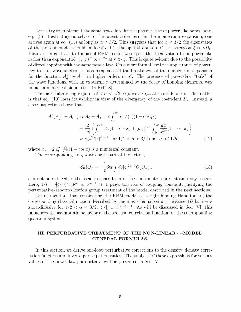
Let us try to implement the same procedure for the present case of power-like bandshape,eq. (5). Restricting ourselves to the lowest order term in the momentum expansion, onearrives again at eq. (11) as long as α ≥ 3/2. This suggests that for α ≥ 3/2 the eigenstatesof the present model should be localized in the spatial domain of the extension ξ ∝ νD0.However, in contrast to the usual RBM model we expect this localization to be power-likerather than exponential: |ψ(r)|2 ∝ r−2α at r ≫ ξ. This is quite evident due to the possibilityof direct hopping with the same power-law. On a more formal level the appearance of power-law tails of wavefunctions is a consequence of the breakdown of the momentum expansionfor the function A−1

q − A−10 in higher orders in q2. The presence of power-law “tails” of

the wave functions, with an exponent α determined by the decay of hopping elements, wasfound in numerical simulations in Ref. [8].

The most interesting region 1/2 < α < 3/2 requires a separate consideration. The matteris that eq. (10) loses its validity in view of the divergency of the coefficient B2. Instead, aclose inspection shows that

A20(A

−1q − A−1

0 ) ≈ A0 − Aq = 2∫ ∞

0dra2(r)(1 − cos qr)

=2

|q|

{

∫ b|q|

0dx(1 − cosx) + (b|q|)2α

∫ ∞

b|q|

dx

x2α(1 − cosx)

}

≈ cαb2α|q|2α−1 for 1/2 < α < 3/2 and |q| ≪ 1/b , (12)

where cα = 2∫∞0

dxx2α (1 − cos x) is a numerical constant.

The corresponding long wavelength part of the action,

S0{Q} = −1

tStr

∫

dq|q|2α−1QqQ−q , (13)

can not be reduced to the local-in-space form in the coordinate representation any longer.Here, 1/t = 1

4(πν)2cαb

2α ∝ b2α−1 ≫ 1 plays the role of coupling constant, justifying theperturbative/renormalization group treatment of the model described in the next sections.

Let us mention, that considering the RBM model as a tight-binding Hamiltonian, thecorresponding classical motion described by the master equation on the same 1D lattice issuperdiffusive for 1/2 < α < 3/2: 〈|r|〉 ∝ t1/(2α−1). As will be discussed in Sec. VI, thisinfluences the asymptotic behavior of the spectral correlation function for the correspondingquantum system.

III. PERTURBATIVE TREATMENT OF THE NON-LINEAR σ−MODEL:

GENERAL FORMULAS.

In this section, we derive one-loop perturbative corrections to the density–density corre-lation function and inverse participation ratios. The analysis of these expressions for variousvalues of the power-law parameter α will be presented in Sec. V.

5

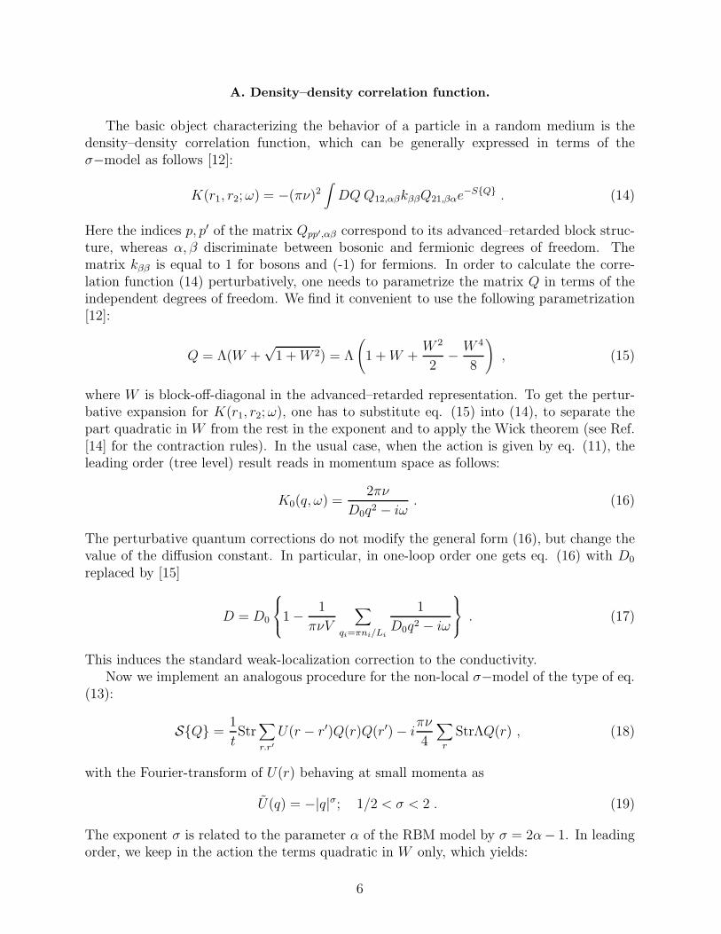
A. Density–density correlation function.

The basic object characterizing the behavior of a particle in a random medium is thedensity–density correlation function, which can be generally expressed in terms of theσ−model as follows [12]:

K(r1, r2;ω) = −(πν)2∫

DQQ12,αβkββQ21,βαe−S{Q} . (14)

Here the indices p, p′ of the matrix Qpp′,αβ correspond to its advanced–retarded block struc-ture, whereas α, β discriminate between bosonic and fermionic degrees of freedom. Thematrix kββ is equal to 1 for bosons and (-1) for fermions. In order to calculate the corre-lation function (14) perturbatively, one needs to parametrize the matrix Q in terms of theindependent degrees of freedom. We find it convenient to use the following parametrization[12]:

Q = Λ(W +√

1 +W 2) = Λ

(

1 +W +W 2

2− W 4

8

)

, (15)

where W is block-off-diagonal in the advanced–retarded representation. To get the pertur-bative expansion for K(r1, r2;ω), one has to substitute eq. (15) into (14), to separate thepart quadratic in W from the rest in the exponent and to apply the Wick theorem (see Ref.[14] for the contraction rules). In the usual case, when the action is given by eq. (11), theleading order (tree level) result reads in momentum space as follows:

K0(q, ω) =2πν

D0q2 − iω. (16)

The perturbative quantum corrections do not modify the general form (16), but change thevalue of the diffusion constant. In particular, in one-loop order one gets eq. (16) with D0

replaced by [15]

D = D0

1 − 1

πνV

∑

qi=πni/Li

1

D0q2 − iω

. (17)

This induces the standard weak-localization correction to the conductivity.Now we implement an analogous procedure for the non-local σ−model of the type of eq.

(13):

S{Q} =1

tStr

∑

r.r′U(r − r′)Q(r)Q(r′) − i

πν

4

∑

r

StrΛQ(r) , (18)

with the Fourier-transform of U(r) behaving at small momenta as

U(q) = −|q|σ; 1/2 < σ < 2 . (19)

The exponent σ is related to the parameter α of the RBM model by σ = 2α− 1. In leadingorder, we keep in the action the terms quadratic in W only, which yields:

6

K0(q, ω) =2πν

8(πνt)−1|q|σ − iω, (20)

corresponding to a superdiffusive behavior.To calculate the one-loop correction to K0(q) (we set ω = 0 for simplicity) we expand

the kinetic term in S{Q} up to fourth order in W :

∑

r,r′

StrU(r − r′)Q(r)Q(r′) |4th order=∑

r,r′

1

4StrW 2(r)W 2(r′) . (21)

The contraction rules are given by eqs. (8), (16) of Ref. [14], with the propagator Π(q)replaced by

Π(q) =t

8|q|σ . (22)

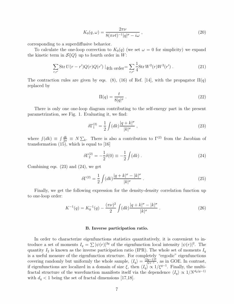
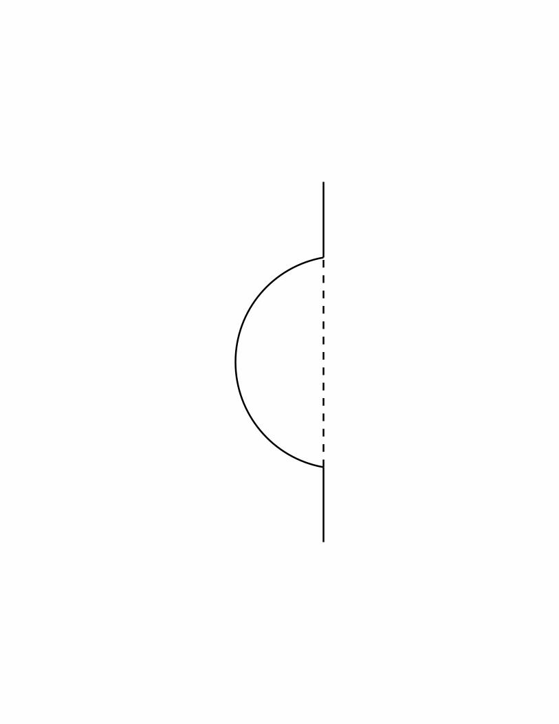
There is only one one-loop diagram contributing to the self-energy part in the presentparametrization, see Fig. 1. Evaluating it, we find:

δΓ(2)1 =

1

2

∫

(dk)|q + k|σ|k|σ , (23)

where∫

(dk) ≡ ∫ dk2π

≡ N∑

k. There is also a contribution to Γ(2) from the Jacobian oftransformation (15), which is equal to [16]

δΓ(2)2 = −1

2δ(0) ≡ −1

2

∫

(dk) . (24)

Combining eqs. (23) and (24), we get

δΓ(2) =1

2

∫

(dk)|q + k|σ − |k|σ

|k|σ . (25)

Finally, we get the following expression for the density-density correlation function upto one-loop order:

K−1(q) = K−10 (q) − (πν)2

2

∫

(dk)|q + k|σ − |k|σ

|k|σ . (26)

B. Inverse participation ratio.

In order to characterize eigenfunctions statistics quantitatively, it is convenient to in-troduce a set of moments Iq =

∑ |ψ(r)|2q of the eigenfunction local intensity |ψ(r)|2. Thequantity I2 is known as the inverse participation ratio (IPR). The whole set of moments Iqis a useful measure of the eigenfunction structure. For completely “ergodic” eigenfunctionscovering randomly but uniformly the whole sample, 〈Iq〉 = (2q−1)!!

Nq−1 , as in GOE. In contrast,if eigenfunctions are localized in a domain of size ξ, then 〈Iq〉 ∝ 1/ξq−1. Finally, the multi-fractal structure of the wavefunction manifests itself via the dependence 〈Iq〉 ∝ 1/Ndq(q−1)

with dq < 1 being the set of fractal dimensions [17,18].

7

The method allowing one to calculate perturbative corrections to the GOE-like results inthe weak localization regime was developed in [19,14]. It is straightforwardly applicable tothe present case of power-law RBM, provided the appropriate modification of the diffusionpropagator entering the contraction rules is made, see the text preceding eq. (22). One finds

〈Iq〉 =

{

1 +1

Nq(q − 1)

∑

r

Π(r, r)

}

(2q − 1)!!

N q−1, (27)

where Π(r, r′) = (1/N)∑

q Π(q) exp[iq(r − r′)] and Π(q) is given by eq. (22).

IV. RENORMALIZATION GROUP TREATMENT.

Our effective σ−model, eq. (18), is actually of one-dimensional nature. However, for thesake of generality, in the present section we find it convenient to consider it to be defined ind-dimensional space with arbitrary d. The form (20) of the generalized diffusion propagatorsuggests that d = σ should play the role of the logarithmic dimension for the problem. In thevicinity of this critical value it is natural to carry out a renormalization group (RG) treatmentof the model. We will follow the procedure developed for general non-linear σ−models in[16]. We start from expressing the action in terms of the renormalized coupling constantt = Z−1

1 tBµd−σ, where tB is the bare coupling constant and µ−1 is the length scale governing

the renormalization 3:

S =µd−σ

2tZ1

∑

rr′U(|r − r′|) Str

[

−W (r)W (r′) +√

1 +W 2(r)√

1 +W 2(r′)]

− iπνω

4

∑

r

Str√

1 +W 2(r) . (28)

Expanding the action in powers of W (r) and keeping terms up to 4-th order, we get

S = S0 + S1 +O(W 6) ,

S0 =µd−σ

4tZ1

∑

rr′U(|r − r′|) Str (W (r) −W (r′))2 − iπνω

8

∑

r

StrW 2(r) ,

S1 =µd−σ

8tZ1

∑

rr′U(|r − r′|)StrW 2(r)W 2(r′) +

iπνω

32

∑

r

StrW 4(r) . (29)

We have restricted ourselves to 4-th order terms, since they are sufficient for obtaining therenormalized quadratic part of the action in one-loop order. The calculation yields, afterthe cancellation of an

∫

(dk) ∝ δ(0) term with the contribution of the Jacobian:

Squad = S0 + 〈S1〉 =1

2

∑

q

StrWqW−q

−µd−σ

tZ1U(q) − 1

2

∫

(dk)U(k) − U(k + q)

−µd−σ

tZ1

U(k) − iπνω4

. (30)

3Note that the W -field renormalization is absent due to the supersymmetric character of the

problem, which is physically related to the particle number conservation [12].

8

According to the renormalization group idea, one has to chose the constant Z1(t) = 1+at+. . .so as to cancel the divergency in the coefficient in front of the leading |q|σ term. This willbe done in the next section.

V. ANALYSIS OF THE MODEL FOR DIFFERENT VALUES OF THE

EXPONENT σ = 2α − 1.

A. 1 < σ < 2 (1 < α < 3/2).

To evaluate the one-loop correction (26) to the diffusion propagator, we use the expansion

|q + k|σ|k|σ − 1 ≃

σqk

k2+σ

2

q2

k2+ σ

(

σ

2− 1

)

(

qk

k2

)2

+ . . . , q ≪ k

|q|σ|k|σ , q ≫ k

. (31)

Thus, the integral in eq. (26) can be estimated as

I ≡∫

(dk)

[

|q + k|σ|k|σ − 1

]

≈∫

k>q(dk)σ

(

1 +σ − 2

d

)

q2

2k2+∫

k<q(dk)

|q|σ|k|σ . (32)

For σ > d = 1 the integral diverges at low k, and the second term in eq. (32) dominates.This gives

I ∼ Lσ−1|q|σ , (33)

where L is the system size determining the infrared cut-off (in the original RBM formulationit is just the matrix size N). This leads to the following one-loop expression for the diffusioncorrelator

K(q) =(πν)2t

4|q|σ ; t−1 = t−1 − constLσ−1 . (34)

Now we turn to the renormalization group analysis, as described in Sec. IV. In one-loop order, the expression for the renormalization constant Z1 is determined essentially bythe same integral I, eq. (32), with the RG scale µ playing the role of the infrared cut-off(analogous to that of the system size L in eq. (34)). This yields (in the minimal subtractionscheme):

Z1(t) = 1 − 1

2π

t

σ − 1+O(t2) . (35)

It is easy to check that this results in a relation between the bare and the renormalizedcoupling constant analogous to eq. (34):

1

tµ1−σ ≡ Z1

tB=

1

tB− 1

2

1

σ − 1µ1−σ . (36)

9

From eq. (35), we get the expression for the β-function:

β(t) =∂t

∂ lnµ

∣

∣

∣

∣

∣

tB

=(1 − σ)t

1 + t∂t lnZ1(t)= −(σ − 1)t− t2

2π+O(t3) . (37)

Both eqs. (34) and (37) show that the coupling constant t increases with the system size L(resp. scale µ), which is analogous to the behavior found in the conventional scaling theoryof localization in d < 2 dimensions [20,21]. The RG flow reaches the strong coupling regime

t ∼ 1 at the scale µ ∼ t1/(σ−1)B . Remembering the relation of the bare coupling constant tB

and the index σ to the parameters of the original PRBM model: t−1B ∝ b2α−1; σ ∝ 2α − 1,

we conclude that the length scale

ξ ∼ t−1/(σ−1)B ∼ b

2α−1

2α−2 (38)

plays the role of the localization length for the PRBM model.This conclusion is also supported by an inspection of the expression for the IPR, eq.

(27). Evaluating the one-loop perturbative correction in eq. (27), one gets

〈Iq〉 =(2q − 1)!!

N q−1

{

1 + q(q − 1)t

8πσζ(σ)Nσ−1

}

, (39)

where ζ(σ) is Riemann’s zeta-function; ζ(σ) ≃ 1/(σ − 1) for σ close to unity. The cor-rection term becomes comparable to the leading (GOE) contribution for the system sizeN ∼ t1/(σ−1), parametrically coinciding with the localization length ξ. For larger N the per-turbative expression (39) loses its validity, and the IPR is expected to saturate at a constantvalue 〈Iq〉 ∼ ξ1−q for N ≫ ξ.

In conclusion of this subsection, let us stress once more that the localized eigenstates inthe present model are expected to have integrable power-law tails: |ψ2(r)| ∝ r−2α = r−σ−1

at r ≫ ξ.

B. 0 < σ < 1 (1/2 < α < 1)

We start again from considering the perturbative corrections to the diffusion propagator(26). The integral (32) is now dominated by the region k ∼ q, and is proportional to |q|.We get, therefore:

(πν)2K−1(q) =4|q|σt

− Cσ|q| (40)

with a numerical constant Cσ.We see that the correction term is of higher order in |q| as compared to the leading one.

Thus, it does not lead to a renormalization of the coupling constant t. This is readily seenalso in the framework of the RG scheme, where the one-loop integral in eq. (30) gives norise to terms of the form |q|σ. One can check that this feature is not specific to the one-loopRG calculation, but holds in higher orders as well. An analogous conclusion was reached forthe case of a vector model with long-ranged interaction by Brezin et al. [22].

10

In our case this implies that the renormalization constant Z1 is equal to unity and theβ−function is trivial:

β(t) = (1 − σ)t . (41)

This means that the model does not possess a critical point, and, for σ < 1, all statesare delocalized, for any value of the bare coupling constant t. This property should becontrasted with the behavior of a d−dimensional conductor described by the conventionallocal non-linear σ− model and undergoing an Anderson transition at some critical couplingt = tc [21].

Since all states of the model turn out to be delocalized, one might think that theirstatistical properties are the same as for GOE. This is, however, not quite true. In particular,calculating the variance of the inverse participation ratio I2 in the same way as it is done inRef. [14] we get:

δ(I) =〈I2

2 〉 − 〈I2〉2〈I2〉2

=8

N2

∑

rr′Π2(r, r′) =

8

N2

∑

q=πn/N ; n=1,2,..

Π2(q) . (42)

At σ > 1/2 the sum over q is convergent yielding

δ(I) =t2

8π2σ

ζ(2σ)

N2−2σ. (43)

Thus, in this regime the fluctuations of the IPR are much stronger than for the GOE whereδ(I) ∝ 1/N . Only for σ < 1/2 (α < 3/4) the IPR fluctuations acquire the GOE character.

Considering higher cumulants of the IPR, 〈〈In2 〉〉, one finds that the GOE behavior is

restored at σ < σ(n)c ≡ 1/n. In this sense, the model is analogous to a d-dimensional

conductor at d = 2/σ. Therefore, only when σ → 0 (correspondingly, α → 1/2 in theoriginal PRBM formulation) all statistical properties become equivalent to those typical forthe GOE.

C. Critical regime: σ = 1 (α = 1).

As we have seen, the case σ = 1 separates the regions of localized (σ > 1) and extended(σ < 1) states. It is then natural to expect some critical properties showing up just at σ = 1.Let us again start from considering the generalized diffusion propagator, eq. (26). At σ = 1the one-loop correction yields

1

(πν)2K−1(q) = 4|q|

[

t−1 − 1

2ln(|q|L)

]

. (44)

As it was natural to expect for the critical point, the correction to the coupling constantis of logarithmic nature. However, eq. (44) differs essentially from that typical for a 2Ddisordered conductor:

t−1 = t−1B − ln(L/l) , (45)

11

where the bare coupling constant tB corresponds to scale l. Comparing the two formulas, wesee that in eq. (44) the mean free path l is replaced by the inverse momentum q−1. Therefore,the correction to the bare coupling constant is small for low momenta q ∼ 1/L, and thecorrelator K(q) is not renormalized. This implies the absence of eigenstate localization,in contrast to the 2D diffusive conductor case, where eq. (45) results in an exponentiallylarge localization length ξ ∝ exp t−1

B . On a more formal level, the absence of essentialcorrections to the low-q behavior of K(q) is due to the fact that the region k > q doesnot give a logarithmic contribution. This is intimately connected with the absence of trenormalization at σ < 1.

To study in more details the structure of critical eigenfunctions, let us consider the setof IPR, Iq. The perturbative correction, eq. (27), is evaluated at σ = 1 as

〈Iq〉 ={

1 + q(q − 1)t

8πln (N/b)

}

(2q − 1)!!

N q−1, (46)

where the microscopic scale b, eq. (5), enters as the ultraviolet cut-off for the σ−model, therole usually played by the mean free path l. This formula is valid as long as the correction

is small: q ≪[

t8π

ln (N/b)]−1/2

. For larger q the perturbation theory breaks down, and one

has to use the renormalization group approach. This procedure, pioneered by Wegner [17]and developed by Altshuler, Kravtsov and Lerner [23] requires the introduction of highervertices of the type zq

∫

Strq(QkΛ)dr in the action of the non-linear σ−model, and theirsubsequent renormalization. This results in RG equations for the charges zq which in thepresent case, and in one-loop order, read:

dzq

d lnµ−1= q(q − 1)

t

8πzq , (47)

where µ−1 is the renormalization scale. Integrating eq. (47), we find:

〈Iq〉 =(2q − 1)!!

N q−1

(

N

b

)q(q−1) t8π

. (48)

Note, that this formula is reduced to the perturbative expression, eq. (46), in the regime

q ≪[

t8π

ln (N/b)]−1/2

.

The behavior described by eq. (48) is characteristic for a multifractal structure of wavefunctions, when

〈Iq〉 ∝ N−dq(q−1) (49)

with dq being the set of fractal dimensions. We find from eq. (48):

dq = 1 − qt

8π. (50)

This form of the fractal dimensions is similar to that found in two and 2 + ǫ dimensions forthe usual diffusive conductor [17,18,23]. The one-loop result (50) holds for q ≪ 8π/t.

The set of fractal dimensions dq (as well as spectral properties at σ = 1, see next section)is parametrized by the coupling constant t. Strictly speaking, our σ−model derivation is

12

justified for t ≪ 1 (i. e. b ≫ 1). However, the opposite limiting case can be also studied,following the ideas of Levitov [9]. This corresponds to a d−dimensional Anderson insulator,perturbed by a weak long-range hopping with an amplitude decreasing with distance asr−σ. The arguments of Levitov [9] suggest that the states delocalize at σ ≤ d, carryingsome fractal properties at σ = d. Our PRBM model in the limit b ≪ 1 is just the 1Dversion of this problem. This shows that the conclusion about localization (delocalization)of eigenstates for σ > 1 (resp. σ < 1), with σ = 1 being a critical point holds irrespective ofthe particular value of the parameter b. Alternatively, the regime of the Anderson insulatorwith weak power-law hopping can be described in the framework of the non-linear σ−model,eq. (18), by considering the limit t ≫ 1. Formally, the non-linear σ−model for arbitraryt can be derived from a microscopic tight-binding model by allowing n ≫ 1 “orbitals” persite [21].

At any rate, the PRBM model, eqs. (1), (5), with arbitrary 0 < b <∞, or the σ−model,eq. (18), with arbitrary coupling constant 0 < t <∞ display at σ = 1 a rich critical behaviorparametrized by the value of b (respectively, t).

VI. SPECTRAL PROPERTIES.

Let us consider now the issue of spectral statistics of the PRBM model. As is well known,a usual diffusive conductor exhibits the Wigner–Dyson (RMT) level statistics in the limit ofinfinite dimensionless conductance g = 2πνDLd−2. At finite g ≫ 1, there appear deviations[24,19,25]. In the present section we would like to address the analogous problem in the caseof the PRBM model.

The basic quantity characterizing the spectral properties is the two-level correlationfunction

R(s) =1

〈ν〉2 〈ν(E)ν(E + ω)〉 , (51)

where s = ω/∆, ∆ is the mean level spacing, ν(E) is the density of states at energy E, and〈. . .〉 denotes the ensemble averaging. Following [19], we find the leading correction to theWigner–Dyson form RWD(s) of the level correlation function, eq. (51), as

R(s) =

[

1 +1

2C d

2

ds2s2

]

RWD(s) , (52)

where

C =1

N2

∑

rr′Π2(r, r′) =

1

N2

∑

q=πn/N ; n=1,2,...

Π2(q) =

t2

64π2σN2σ−2 , σ > 1/2

constt2

64π2σb1−2σN−1 , σ < 1/2 .

(53)

At σ < 1/2 the sum divergent at high momenta is cut off at q ∼ π/b; the procedure leavingundetermined a constant of order of unity.

13

The correlation function R(s) is close to its RMT value if σ < 1 (the region of delocalizedstates), or else if σ > 1 and the system size N is much less than the localization length ξ,eq. (38). Under these conditions, eq. (52) holds as long as the correction term is smallcompared to the leading one. This requirement produces the following restriction on thefrequency s = ω/∆:

s < sc ∼{

t−1N1−σ , σ > 1/2

t−1b1

2−σN1/2 ∝ (Nb)1/2 , σ < 1/2

. (54)

At larger frequencies (s > sc), the form of the level correlation function changes from the1/s2 behavior typical for RMT to a completely different one [24]. Extending the calculationof Ref. [24] to the present case, we find

R(s) =∆2

π2Re

∑

n=0,1,...

1[

8πνt

(

πnN

)σ − iω]2

∝{

N1−1/σt1/σs1/σ−2 , σ > 1/2 (σ 6= 1)t2N−1b2σ−1 ∝ (Nb)−1 , σ < 1/2

. (55)

At last, let us consider the level statistics in the critical regime σ = 1. In this case thecoefficient of proportionality in the asymptotic expression (55) vanishes in view of analyticity:

R(s) ∼ ∆t

16π2

∫ ∞

−∞

dx

(x− iω)2= 0 . (56)

This is similar to what is known to happen in the case of a 2D diffusive conductor [26,27].A more accurate consideration requires taking into account the high-momentum cut-off atq ∼ b−1. In full analogy with the 2D situation mentioned [26,28,27], we find then a linearterm in the level number variance:

〈δN2(E)〉 ≃ κ〈N(E)〉κ =

∫

R(s)ds =t

8π. (57)

The presence of the linear term (57) (as well as the multifractality of eigenfunctions, Sec. V)makes the case σ = 1 similar to the situation on the mobility edge of a disordered conductorin d > 2 [28]. Let us finally mention that the value of κ, eq. (57), is in agreement with theformula κ = (d− d2)/2d, suggested recently by Kravtsov [29], where d2 is given by eq. (50)with q = 2, and d = 1 in the present case.

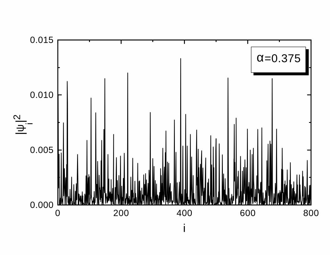
VII. NUMERICAL SIMULATIONS

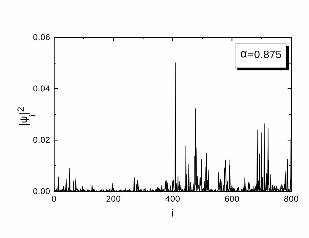
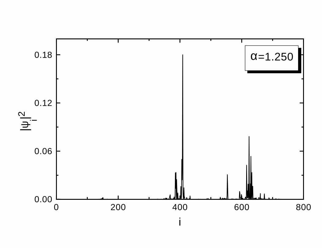
We have performed numerical simulations of the PRBM model for values of α ∈ [0, 2]and b = 1. In Fig. 2 we present typical eigenfunctions for four different regions of α. Inagreement with the theoretical picture presented above, the eigenstates corresponding toα = 0.375 and α = 0.875 are extended, whereas those corresponding to α = 1.25 andα = 1.625 are localized. At the same time, one can notice that the states with α = 0.875

14

and α = 1.25 exhibit a quite sparse structure, as opposed to the other two cases. We believethat this can be explained by the proximity of the former two values of α to the criticalvalue α = 1.0, where eigenstates should show the multifractal behavior, see Sec. V.

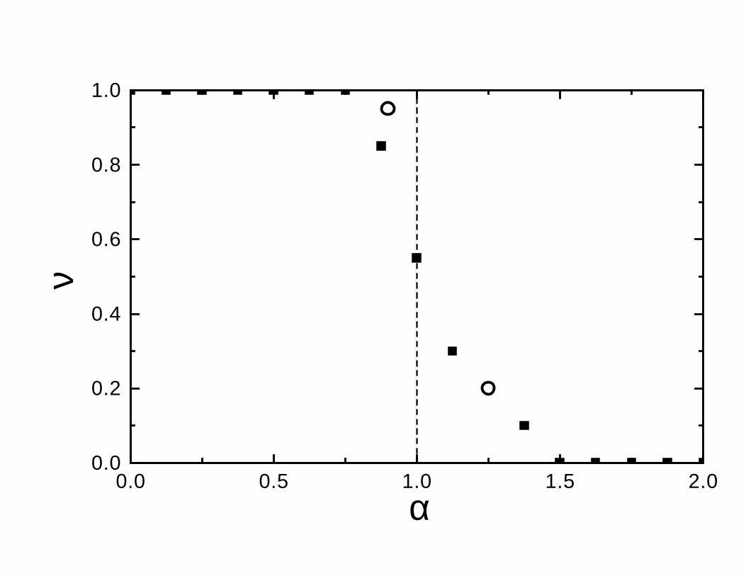
In order to get a more quantitative insight into the properties of the eigenstates, weconcentrated our attention on the behavior of the mean value of the IPR, 〈I2〉, and on therelative variance, δ = (〈I2

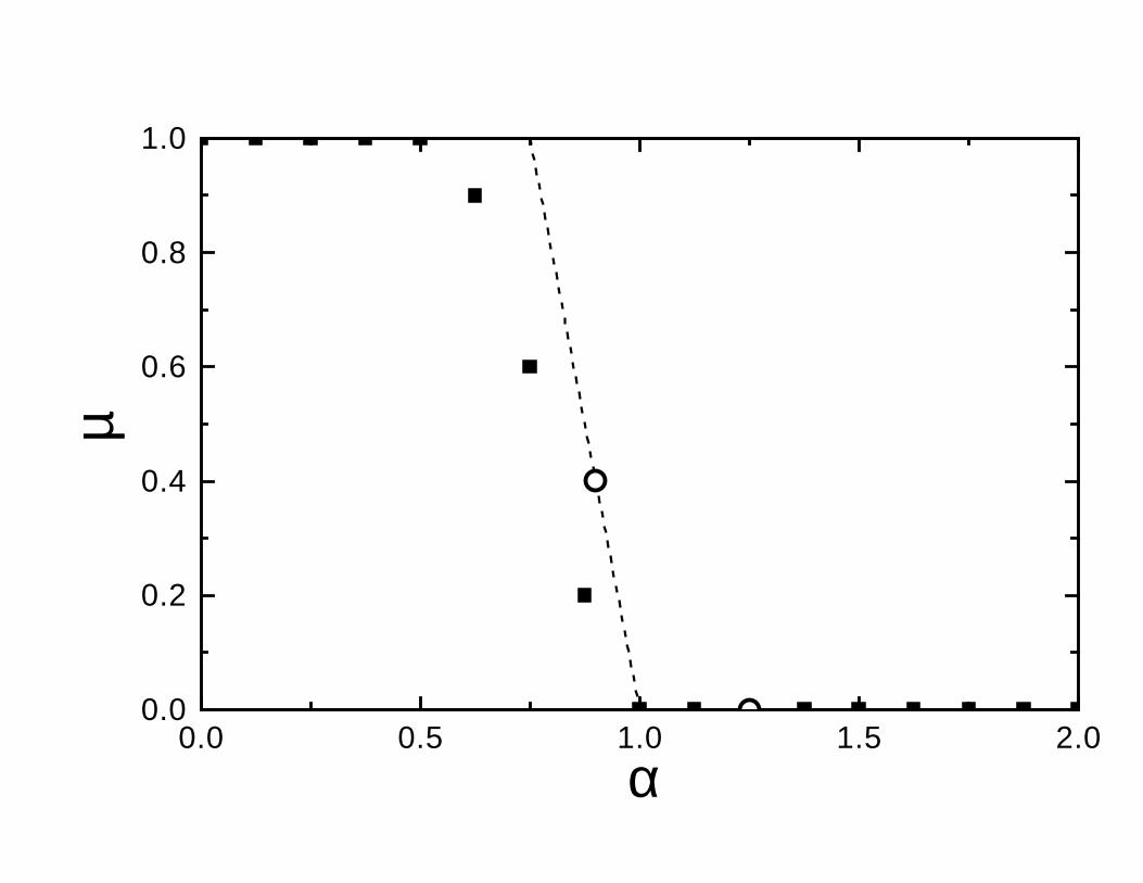
2 〉 − 〈I2〉2)/〈I2〉2. At any given α we studied the dependence ofthe quantities 〈I2〉 and δ on the matrix size N and approximated these dependencies bythe power-laws 〈I2〉 ∝ 1/Nν , δ ∝ 1/Nµ for N ranging from 100 to 2400. On Figs. 3 and4 we plotted the values of the exponents ν and µ obtained in this way, versus the PRBMparameter α. The expected theoretical curves following from the results of Sec. V arepresented as well. We see from Fig. 3 that the data show a crossover from the behaviortypical for extended states (ν = 1) to that typical for localized states (ν = 0), centeredapproximately at the critical point α = 1. We attribute the deviations from the sharp step-like theoretical curve ν(α) to the finite-size effects which are unusually pronounced in thePRBM model due to the long-range nature of the off-diagonal coupling. The data for theexponent µ (Fig. 4) also show a reasonable agreement with the expected linear crossover,µ = 4(1 − α) for 3/4 < α < 1, see eq. (43).

VIII. CONCLUSION.

In this paper, we have performed a detailed investigation of the RBM model with apower-law decay of the matrix elements, eq. (5). Physically, one can look at this modelas describing a particle in a 1D disordered system with a power-law hopping term. Asa theoretical tool, we have used a mapping of the problem onto a supermatrix non-linearσ−model, eqs. (18), (19). Depending on the value of the power-law exponent α in eq.(5) (or, equivalently, σ = 2α − 1 in eq. (19)), three different regimes are found: Forα > 1 (σ > 1) all eigenstates are localized with integrable power-law tails. For α < 1(σ < 1) the eigenstates are delocalized, for any value of the bandwidth b of the PRBMmodel, eq. (5) (resp. coupling constant t ∝ b1−2α of the σ−model, eq. (19)). These tworegimes are separated by the critical value α = 1 (σ = 1), where the structure of eigenstatesis multifractal, and energy levels show statistics intermediate between Wigner–Dyson andPoisson ones. These critical properties are similar to those found on the mobility edge of ad-dimensional disordered conductor. At σ = 1, we find a family of critical points labeled bythe value of the coupling constant t of the non-linear σ−model, so that the critical behavioris parametrized by the value of t. In particular, it determines the multifractal exponentsdq and the coefficient κ of the linear term in the level number variance, which are given att≪ 1 by eqs. (50) and (57), respectively.

Turning our attention to the regime of localized states, we find that it can be subdividedinto two domains. In the region α > 3/2 the properties of the model are rather close tothose of a conventional quasi-1D conductor [3]. On the other hand, for 1 < α < 3/2 thewave packet spreading on a short time scale is superdiffusive, 〈|r|〉 ∼ t1/(2α−1), which leadsto a modification of the Altshuler–Shklovskii “tail” of the spectral correlation function, eq.(55), and to an unusual scaling of the localization length ξ ∝ b2α−1. The regime of extendedstates, α < 1, can be also subdivided into two domains. For α < 1/2, all statisticalproperties are identical to those of the GOE (which corresponds to α = 0). On the other

15

hand, at 1/2 < α < 1 the model is quite similar to a diffusive conductor in d = (α− 1/2)−1

dimensions. This is reflected, in particular, in the fluctuations of the IPR (see eq. (43) andthe discussion following it), and in the large-frequency “tail” of the spectral correlator, eq.(55).

Our conclusion about the existence of a set of critical theories at α = 1, parametrized bythe coupling constant t, perfectly agrees with earlier results by Levitov [9]. He studied theeffect of a weak power-law hopping on an Anderson insulator, which corresponds to the limitt≫ 1 in the σ−model formulation, and arrived at the conclusion of criticality of the modelat α equal to the spatial dimension d. Let us also note that our results are in accordancewith the fact of absence of localization effects in the Quantum Fermi Accelerator model [7].As it was pointed out in [7], the evolution equation for this model takes the form of a finitedifference equation of the tight binding type with a long range hopping term decaying in apower-law fashion, eq. (5), with α = 1. Our results show that this case corresponds to thecritical point with extended eigenstates and intermediate level statistics, in agreement withthe behavior found in Ref. [7].

We have presented results of a direct numerical simulation of the PRBM model. Ourdata are in reasonable agreement with the above theoretical picture. However, a moredetailed numerical investigation of the structure of eigenstates and of spectral statistics iscertainly desirable. In particular, it would be very interesting to study the critical manifold,α = 1, where the multifractal properties of eigenstates and intermediate level statistics arepredicted by our theory.

IX. ACKNOWLEDGMENTS.

We are grateful to F. Izrailev and I. Guarneri for useful discussions on early stage ofthis work, and to V. E. Kravtsov, M. R. Zirnbauer, B. L. Altshuler, and A. M. Tsvelik fordiscussion of the results. A.D.M. and Y.V.F. acknowledge with thanks the warm hospitalityextended to them during the Program “Quantum Chaos in Mesoscopic Systems” in theInstitute for Theoretical Physics in Santa Barbara, where this research was completed. Thisresearch was supported in part by the National Science Foundation under Grant No. PHY94-07194 (A.D.M. and Y.V.F.), the Deutsche Forschungsgemeinschaft by SFB 195 (A.D.M.)and SFB 237 “Unordnung und Große Fluktuationen” (Y.V.F.), the Minerva Foundation(F.-M.D.), and the Minerva Center for Nonlinear Physics of Complex Systems (Y.V.F. andF.-M.D.).

16

REFERENCES

† On leave from Petersburg Nuclear Physics Institute, 188350 Gatchina, St.Petersburg,Russia.

[1] T. H. Seligman, J. J. M. Verbaarschot, and M. R. Zirnbauer, J. Phys. A: Math. Gen.

18, 2751 (1985).[2] V. V. Flambaum, A. A. Gribakina, G. F. Gribakin, and M. G. Kozlov, Phys. Rev. A

50, 267 (1994).[3] Y. V. Fyodorov, A. D. Mirlin, Int. J. Mod. Phys. B 8, 3795 (1994).[4] F. M. Izrailev, Chaos, Solitons, Fractals, 5, 1219 (1995); G. Casati, L. Molinari, and F.

M. Izrailev, Phys. Rev. Lett. 67, 2405 (1991).[5] F. M. Izrailev, Phys. Rep. 196, 299 (1990).[6] S. Fishman, D. R. Grempel, R. E. Prange, Phys. Rev. Lett. 49, 509 (1982).[7] J. V. Jose and R. Cordery, Phys. Rev. Lett. 56, 290 (1986).[8] G. Yeung and Y. Oono, Europhys. Lett. 4, 1061 (1987).[9] L. Levitov, Europhys. Lett. 9, 83 (1989); Phys. Rev. Lett. 64, 547 (1990).

[10] A. V. Balatsky and M. I. Salkola, Phys. Rev. Lett. 76, 2386 (1996); B. L. Altshuler andL. Levitov, private communication.

[11] Y. V. Fyodorov and A. D. Mirlin, Phys. Rev. Lett. 67, 2405 (1991); Phys. Rev. Lett.

69, 1093 (1992); Phys. Rev. Lett. 71, 412 (1993); A. D. Mirlin and Y. V. Fyodorov, J.

Phys. A: Math. Gen. 26, L551 (1993).[12] K. B. Efetov, Adv. Phys. 32, 53 (1983).[13] J. J. M. Verbaarschot, H. A. Weidenmuller, and M. R. Zirnbauer, Phys. Rep. 129, 367

(1985).[14] Y. V. Fyodorov and A. D. Mirlin, Phys. Rev. B 51, 13403 (1995).[15] L. P. Gor’kov, A. I. Larkin, and D. E. Khmelnitskii, JETP–Lett. 30, 228 (1979).[16] E. Brezin and J. Zinn-Justin, Phys. Rev. B 14, 3110 (1976); E. Brezin, J. Zinn-Justin,

and J. C. Le Guillou, Phys. Rev. D 14, 2615 (1976); E. Brezin, S. Hikami, and J.Zinn-Justin, Nucl. Phys. B 165, 528 (1980); J. Zinn-Justin, Quantum Field Theory and

Critical Phenomena, Clarendon Press, Oxford, 1989.[17] F. Wegner, Z. Phys. B 36, 209 (1980).[18] C. Castellani and L. Peliti, J. Phys. A: Math. Gen. 19, L429 (1986).[19] V. E. Kravtsov and A. D. Mirlin, Pis’ma Zh. Eksp. Theor. Fiz. 60, 645 (1994) [JETP

Lett. 60, 656 (1994)].[20] E. Abrahams, P. W. Anderson, D. C. Licciardello, and T. V. Ramakrishnan, Phys. Rev.

Lett. 42, 673 (1979).[21] F. Wegner, Phys. Rep. 67, 15 (1980).[22] E. Brezin, J. Zinn-Justin, and J. C. Le Guillou, J. Phys. A: Math. Gen. 9, L119 (1976).[23] B. L. Altshuler, V. E. Kravtsov, I. V. Lerner, in Mesoscopic Phenomena in Solids, ed.

by B. L. Altshuler et al. (North Holland, Amsterdam, 1991).[24] B. L. Altshuler and B. I. Shklovski, Zh. Eksp. Teor. Fiz. 91, 220 (1986) [Sov. Phys.

JETP 64, 127 (1986)].[25] A. V. Andreev and B. L. Altshuler, Phys. Rev. Lett. 75, 902 (1995).[26] A. Altland and Y. Gefen, Phys. Rev. Lett. 71, 3339 (1993); Phys. Rev. B 51, 10671

(1995).[27] V. E. Kravtsov and I. V. Lerner, Phys. Rev. Lett. 74, 2563 (1995).

17

[28] A. G. Aronov and A. D. Mirlin, Phys. Rev. B 51, 6131 (1995).[29] V. E. Kravtsov, unpublished.

18

Figure captions

Fig. 1

One-loop diagram contributing to the self-energy part of the density-density correlationfunction. The solid line denotes the Q-field propagator, whereas the dashed line representsthe interaction U(r − r′).

Fig. 2

Typical eigenfunctions for the matrix size N = 800 and four different values of α:a)α = 0.375; b)α = 0.875; c)α = 1.250; d)α = 1.625.

Fig. 3

Index ν characterizing the dependence of the inverse participation ratio 〈I2〉 on the matrixsize N via 〈I2〉 ∝ 1/Nν , as a function of α. Points refer to the best-fit values obtained frommatrix sizes between N = 100 and N = 1000 (squares) or N = 2400 (circles). The dashedline is the theoretical prediction for the transition from ν = 1, at small α, to ν = 0, at largeα.

Fig. 4

The same as Fig. 3, but for the index µ, derived from the N dependence of the variance δof the inverse participation ratio: δ ≡ (〈I2

2 〉 − 〈I2〉2)/〈I2〉2 ∝ 1/Nµ. The dashed line corre-sponds to the predicted linear crossover from µ = 1 at α < 3/4 to µ = 0 at α > 1.

19

0 200 400 600 8000.000

0.005

0.010

0.015

α=0.375

|ψi|2

i

0 200 400 600 8000.00

0.02

0.04

0.06

α=0.875

|ψi|2

i

0 200 400 600 8000.00

0.06

0.12

0.18 α=1.250

|ψi|2

i

0 200 400 600 8000.0

0.1

0.2

0.3

α=1.625

|ψi|2

i

0.0 0.5 1.0 1.5 2.00.0

0.2

0.4

0.6

0.8

1.0ν

α

0.0 0.5 1.0 1.5 2.00.0

0.2

0.4

0.6

0.8

1.0µ

α