Fergus, P, Selvaraj, M and Chalmers, C

Machine learning Ensemble Modelling to classify caesarean section and vaginal delivery types using cardiotocography traces

http://researchonline.ljmu.ac.uk/id/eprint/7696/

Article

LJMU has developed LJMU Research Online for users to access the research output of the University more effectively. Copyright © and Moral Rights for the papers on this site are retained by the individual authors and/or other copyright owners. Users may download and/or print one copy of any article(s) in LJMU Research Online to facilitate their private study or for non-commercial research.You may not engage in further distribution of the material or use it for any profit-making activities or any commercial gain.

The version presented here may differ from the published version or from the version of the record. Please see the repository URL above for details on accessing the published version and note that access may require a subscription.

For more information please contact researchonline@ljmu.ac.uk

http://researchonline.ljmu.ac.uk/

Citation (please note it is advisable to refer to the publisher’s version if you intend to cite from this work)

Fergus, P, Selvaraj, M and Chalmers, C (2017) Machine learning Ensemble Modelling to classify caesarean section and vaginal delivery types using cardiotocography traces. Computers in Biology and Medicine, 93 (1). pp. 7-16. ISSN 0010-4825

LJMU Research Online

1

Machine Learning Ensemble Modelling to Classify Caesarean

Section and Vaginal Delivery Types Using Cardiotocography

Traces

Paul Fergus, Selvaraj Malarvizhi, and Carl Chalmers

Liverpool John Moores University,

Faculty of Engineering and Technology,

Data Science Research Centre,

Department of Computer Science,

Byron Street,

Liverpool,

L3 3AF,

United Kingdom.

2

Machine Learning Ensemble Modelling to Classify Caesarean

Section and Vaginal Delivery Types Using Cardiotocography

Traces

ABSTRACT

Human visual inspection of Cardiotocography traces is used to monitor the foetus during

labour and avoid neonatal mortality and morbidity. The problem, however, is that visual

interpretation of Cardiotocography traces is subject to high inter and intra observer

variability. Incorrect decisions, caused by miss-interpretation, can lead to adverse perinatal

outcomes and in severe cases death. This study presents a review of human Cardiotocography

trace interpretation and argues that machine learning, used as a decision support system by

obstetricians and midwives, may provide an objective measure alongside normal practices.

This will help to increase predictive capacity and reduce negative outcomes. A robust

methodology is presented for feature set engineering using an open database comprising 552

intrapartum recordings. State-of-the-art in signal processing techniques is applied to raw

Cardiotocography foetal heart rate traces to extract 13 features. Those with low

discriminative capacity are removed using Recursive Feature Elimination. The dataset is

imbalanced with significant differences between the prior probabilities of both normal

deliveries and those delivered by caesarean section. This issue is addressed by oversampling

the training instances using a synthetic minority oversampling technique to provide a

balanced class distribution. Several simple, yet powerful, machine-learning algorithms are

trained, using the feature set, and their performance is evaluated with real test data. The

results are encouraging using an ensemble classifier comprising Fishers Linear Discriminant

Analysis, Random Forest and Support Vector Machine classifiers, with 87% (95%

Confidence Interval: 86%, 88%) for Sensitivity, 90% (95% CI: 89%, 91%) for Specificity,

and 96% (95% CI: 96%, 97%) for the Area Under the Curve, with a 9% (95% CI: 9%, 10%)

Mean Square Error.

Keywords: Perinatal Complications, Cardiotocography, Classification, Data Science,

Machine Learning, Ensemble Modelling

1. INTRODUCTION

UNICEF estimates that 130 million babies are born each year. One million of these will be

intrapartum stillbirths and more than three and a half million will die as a result of perinatal

complications [1]. The number of reported deliveries in the UK during 2012 was 671,255.

One in every 200 resulted in stillbirth and 300 died in the first four weeks of life [2]. Between

one and seven in every 1000 foetuses experienced hypoxia (impaired delivery of oxygen to

the brain and tissue) [3] that resulted in adverse perinatal outcomes and in severe cases death

[4]. During 2013, according to Tommy’s charity, the rate of stillbirths in the UK was 4.7 per

1000 births. In 2014, 1,300 babies were injured at birth due to mistakes made by maternity

staff, which cost the National Health Service (NHS) in the UK more than £1 billion in

compensation and more than £500 million in legal fees to resolve disputes.

3

Human visual pattern recognition in Cardiotocography (CTG) traces is used to monitor the

foetus during the early stages of delivery [5]. CTG devices, fitted to the abdomen, record the

foetal heartbeat and uterine contractions [6]. The foetal heart rate recordings represent the

modulation influence provided by the central nervous system. When the foetus is deprived of

oxygen, the cardiac function is impaired. Detecting its occurrence can be confirmed by cord

blood (umbilical artery) metabolic acidosis with a base deficit of more than 15mmol/L [7].

The etiology is not clear however, environmental factors, such as umbilical cord compression

and maternal smoking, are known risk factors [8].

Obstetricians and midwives use CTG traces to formulate clinical decisions. However, poor

human interpretation of traces and high inter and intra observer variability, [9]–[11] makes

the prediction of neonatal outcomes challenging. CTG was introduced into clinical practice

45 years ago. Since then there has been no significant evidence to suggest its use has

improved the rate of perinatal deaths. However, several studies do argue that 50% of birth-

related brain injuries could have been prevented if CTG was interpreted correctly [12].

Conversely, there is evidence to indicate that over-interpretation increases the number of

births delivered by caesarean section even when there are no known risk factors [13].

Computerised CTG has played a significant role in developing objective measures as a

function of CTG signals [14], particularly within the machine learning community [15]–[18],

[7],[12], [19]–[23]. According to a Cochrane report in 2015, computerised interpretation of

CTG traces significantly reduced perinatal mortality [24]. In this study, we build on previous

works and utilise an open dataset obtained from Physionet. The dataset contains CTG trace

recordings for normal vaginal births (506) and those that were delivered by caesarean section

(46). Several machine-learning algorithms are trained using features extracted from raw CTG

Foetal Heart Rate (FHR) traces contained in the dataset to distinguish between caesarean

section and vaginal delivery types. This would allow for the optimisation of decision making,

by obstetricians and midwives, in the presence of FHR traces, linked to caesarean section and

normal vaginal deliveries. The results demonstrate that an ensemble classifier produces better

results than several studies reported in the literature.

2. ANALYSIS

2.1 Cardiotocography Feature Extraction

Feature extraction techniques are used to gather specific parameters from a signal. These are

often more efficient to analyse than the raw signal samples themselves. Signal processing

does not increase the information content but rather incurs information loss caused by feature

extraction. However, this is preferable to raw data analysis, as it simplifies classification

tasks. The features extracted can be broadly divided into two groups, linear and nonlinear. In

both of these groups, all signal data points are transformed (using a linear or nonlinear

transformation) into a reduced dimensional space. Thus, the original data points are replaced

with a smaller set of discriminative variables. For a more detailed discussion on feature

extraction please refer to [25].

Linear features can be broadly defined as those features that are visible through human

inspection, for example accelerations and decelerations in the foetal heartbeat. While,

nonlinear features are much more difficult in interpret or even identify under normal visual

analysis. For example, formally quantifying the complexity of a signal and the differences

between two or more observations is practically impossible to achieve through visual

inspection alone.

4

The International Federation of Gynaecology and Obstetrics (FIGO) and the National

Institute for Health and Care Excellence (NICE) in the UK have developed guidelines used to

interpret CTG traces [26]. These are briefly described in Table 1.

Feature Baseline (bpm) Variability (bpm) Decelerations Accelerations

Reassuring 110-160 ≥5 None Present

Non-

Reassuring

100-109

161-180

<5 for 40-90 minutes Typical variable

decelerations with over

50% of contractions,

occurring for over 90

minutes. Single

prolonged deceleration

for up to 3 minutes

The absence of

accelerations with

otherwise normal trace

is of uncertain

significance

Abnormal <100

>180

Sinusoidal

pattern ≥ 10

minutes

<5 for 90 minutes Either typical variable

decelerations with over

50% of contractions or

late decelerations, both

for over 30 minutes.

Single prolonged

deceleration for more

than 3 minutes

Table 1 - Classification of FHR Trace Features (Baseline, Variability, Decelerations and

Accelerations)

The FIGO features include the real FHR baseline (RBL), Accelerations, Decelerations, Short-

Term variability (STV) and Long-Term variability (LTV). To understand how the RBL is

obtained (and used to derive all other features) consider Figure 1. The RBL is calculated as

the mean of the signal [27] with the peaks and troughs removed (signals that reside outside

the baseline min and max thresholds). Peaks and troughs are removed using a virtual baseline

(VBL) which is the mean of the complete signal (with peaks a troughs) and the removal of

signals that are ±10 bpm from the VBL.

Acceleration and Deceleration coefficients are obtained by counting the number of transient

increases and decreases from the RBL, that are ±10bpm and last for 10s or more [28].

Accelerations typically indicate adequate blood delivery and are reassuring for medical

practitioners. While decelerations result from physiological provocation (i.e. compromised

oxygenation resulting from uterine contractions). If Decelerations do not recover (the absence

of Accelerations), this can indicate the presence of umbilical cord compression, foetal

hypoxia or metabolic acidosis [29].

Meanwhile, STV is calculated as the average of 2.5-second blocks in the signal averaged over

the duration of the signal. LTV, on the other hand, describes the difference between the

minimum and maximum value in a 60-second block averaged over the duration of the signal.

The presence of both STV and LTV describe normal cardiac function [30]. If STV or LTV

decreases or is absent, this could indicate the onset of an adverse pathological outcome [31].

FIGO features represent the morphological structure of the FHR signal and are the visual

cues used by obstetricians and midwives to monitor the foetus. However, using these alone

has seen high inter and intra variability. This has led to studies designed to extract non-linear

features (not easily identifiable through human visual inspection) from the FHR signal to try

to improve and support outcome measures obtained by obstetricians and midwives [32].

5

Figure 1: Using the FHR signal (Beats per Minute) to calculate the Real Baseline

Root Mean Squares (RMS) and Sample Entropy (SampEn) are two signal processing

coefficients that are commonly used in antepartum and intrapartum studies to represent the

non-visual patterns contained in the FHR [33]–[36]. RMS measures the magnitude of the

varying quantity and is an effective signal strength indicator in heart rate variability studies.

Sample entropy on the other hand represents the non-linear dynamics and loss of complexity

in the FHR, and is a useful indicator for foetal hypoxia and metabolic-acidosis detection [37].

CTG signals are also translated into frequency representations, via Fast Fourier Transform

(FFT) [38] and Power Spectral Density (PSD) to minimise signal quality variations [39]. In

the context of FHR analysis, frequency features have been successfully used in [40] and more

recently in [41] and [42]. For example, Peak Frequency (FPeak) is derived from the PSD and

used in antepartum and intrapartum analysis to measure variability and normal sympathetic

and parasympathetic function [33], [34], [43].

Meanwhile, non-linear features [44], such as Poincare plots, have seen widespread use in

heart rate variability studies [45]. In this study, the difference between two beats (BB) is

calculated rather than the normal RR interval used in PQRST analysis. The two descriptors of

the plot are SD1 and SD2. These coefficients are associated with the standard deviation of

BB and the standard deviation of the successive difference of the BB interval. The ratio of

SD1/SD2 (SDRatio) describes the relation between short and long-term variations of BB.

The box-counting dimension (FD) enables the dynamics of the FHR to be estimated [46] and

is a direct measure of the morphological properties of a signal. The signal is covered with

6

optimally sized boxes where the number of boxes describes the box-counting dimension

coefficient. In previous studies, these features have proven to be an effective indicator for

foetal hypoxia and metabolic acidosis detection [47].

In the case of self-affinity measures in FHR signals, previous studies have demonstrated that

it is a beneficial coefficient in classification tasks [48]. Detrend Fluctuation Analysis (DFA)

produces an exponent value that indicates the presence or absence of self-similarity [49].

DFA examines the signal at different time scales and returns a fractal scaling exponent x. The

calculations are repeated for all considered window sizes defined as n. In this instance, the

focus is on the relation between F(n) and the size of the window n. In general, F(n) will

increase with the size of window n.

2.2 Automated Cardiotocography Classification

Computer algorithms are utilised extensively in biomedical research and are a fundamental

component within most clinical decision support systems. CTG is no different, where

machine learning algorithms have proven to be excellent decision makers in CTG analysis.

For example, Warrick et al. [15] developed a system to model FHR and Uterine Contraction

(UC) signal pairs to estimate their dynamic relation [50]. The authors conclude that it is

possible to detect approximately half of the pathological cases one hour and 40 minutes

before delivery with a 7.5% false positive rate. Kessler et al. [54] on the other hand applied

CTG and ST waveform analysis resulting in timely intervention for caesarean section and

vaginal deliveries [7].

In a similar study, Blinx et al. [51] compared a Decision Tree (DT), an Artificial Neural

Network (ANN), and Discriminant Analysis (DA). The ANN classifier obtain 97.78% overall

accuracy. The Sensitivity and Specificity values were not provided making accuracy alone an

insufficient performance measure. Ocak et al. [52] evaluated an SVM and Genetic Algorithm

(GA) classifier and reported 99.3% and 100% accuracies for normal and pathological

delivery outcomes. Similar results were reported in [53] and [54]. Again, Sensitivity and

Specificity values were not provided. Meanwhile Menai et al [55] classified foetal state using

a Naive Bayes (NB) classifier with four different feature selection (FS) techniques: Mutual

Information, Correlation-based, ReliefF, and Information Gain. The NB classifier in

conjunction with ReliefF features produced 93.97%, 91.58%, and 95.79% for Accuracy,

Sensitivity and Specificity, respectively.

While, Karabulut et al. [56] utilised an adaptive boosting (AdaBoost) classifier producing an

accuracy of 95.01% - again no Sensitivity or Specificity values were provided. While Spilka et

al., [13], used a Random Forest (RF) classifier and latent class analysis (LCA) [57] producing

Sensitivity and Specificity values of 72% and 78% respectively [5]. Generating slightly better

results in [45], Spilka et al. attempted to detect perinatal outcomes using a C4.5 decision tree,

Naive Bayes, and SVM. The SVM produced the best results using a 10-fold cross validation

method, which achieved 73.4% for Sensitivity and 76.3% of Specificity.

3. METHODOLOGY

In this study all experiments were run on a Dell XPS 13 Developer Edition laptop, with a 6th

Gen Intel Core processor and 16GB of memory on Ubuntu version 16.04 LTS. The software

developed uses R and RStudio. The data was obtained from Physionet using RDSamp.

Several packages from the CRAN repository are utilised in this study and include the Signal

package to filter the FHR signal and the following packages to support the feature extraction

process; fractaldim; fractal; pracma; psd; seewave and car. Finally, for the classification and

7

evaluation tasks the following packages were utilised; MASS, hmeasure, pROC, ROCR

randomForest, caret, e1071, and DMwR.

3.1 Dataset Description

Intrapartum recordings were collected between April 2010 and August 2012 from the

University Hospital in Brno in Czech Republic (UHB) with the support of the Czech

Technical University (CTU) in Prague [5]. The CTG-UHB database is publically available at

Physionet. The database contains 552 CTG recordings for singleton pregnancies with a

gestational age greater than 36 weeks. The STAN S21/S31 and Avalon FM 40/50 foetal

monitors were used to acquire the CTG records. The records do not contain prior known

development factors; the duration of stage two labour is less than or equal to 30 minutes;

foetal heart rate signal quality is greater than 50 percent in each 30 minute window; and the

pH umbilical arterial blood sample is available for each record. 46 records are for deliveries

by caesarean section due to pH ≤7.20 – acidosis, n=18; pH >7.20 and pH < 7.25 – foetal

deterioration, n=4; and n=24 due to clinical decision without evidence of pathological

outcomes) – the remaining 506 records are normal vaginal deliveries. Each record begins no

more than 90 minutes before delivery and contains FHR (measured in beats per minute) and

UC (measured in mmHg) time series signals – each sampled at 4Hz. The FHR was obtained

from an ultrasound transducer attached to the abdominal wall (cardio). The UC was obtained

from a pressure transducer also attached to the maternal abdomen (toco). The FHR signal is

only considered in this study as it provides direct information about the foetal state. Table 2

summarises the associated clinical data for all records contained in the CTG-UHB database.

For a full description of the dataset, please refer to [5].

Table 2: Clinical CTU-UHB Data Summary for Vaginal and Caesarean Section Delivery

Types

506 – Vaginal; 46 – Caesarean Section

Mean Min Max

Maternal Age (Years) 29.8 18 46

Parity 0.43 0 7

Gravidity 1.43 1 11

Gestational Age (Weeks) 40 37 43

pH 7.23 6.85 7.47

BE -6.36 -26.8 -0.2

BDecf (mmol/l) 4.60 -3.40 26.11

Apgar (1 Minute) 8.26 1 10

Apgar (5 Minute) 9.06 4 10

Length of Stage II. (min) 11.87 0 30

Neonate's Weight (grams) 3408 1970 4750

Neonate's Sex (Male/Female) 293 Male / 259 Female

8

Table 3 provides details of the outcome measures used in the CTU-UHB database. For the 46

caesarean section records, the ID is the file number in the CTU-UHB dataset; Age describes

the mothers age; pH describes the umbilical artery pH value for each case; BDef is base

deficit in extracellular fluid; pCO2 describes the partial pressure of carbon dioxide; BE is

base excess; and Apgar scores are a subjective evaluation of the delivery. For a more in-depth

discussion of the dataset and these parameters please refer to [5].

Table 3: Caesarean Section Outcome Measures for pH, BDecf, pCO2, BE, Apgar1 and

Apgar5

ID Age pH BDecf pCO2 BE Apgar1 Apgar5

2001 30 7.03 22.52 2.8 -23.7 10 10

2002 39 7.27 3.75 6.5 -4.5 7 4

2003 25 6.96 16.96 7.2 -19 6 8

2004 34 6.95 11.44 11.6 -15.3 6 8

2005 31 7.25 3.47 7 -5.5 10 10

2006 32 7.29 NaN NaN NaN 10 10

2007 27 7.04 20.42 3.8 -21.8 10 10

2008 26 6.98 13.43 9.3 -16.7 5 7

2009 21 6.96 20.34 5.4 -23 10 10

2010 19 7.3 -0.48 7.2 -1.5 10 10

2011 37 7.01 12.1 9.2 -14.8 3 7

2012 26 7.29 -0.44 7.4 -1.4 9 9

2013 27 6.85 22.63 6.4 -25.3 8 8

2014 34 7.32 2.28 6 -3.2 10 10

2015 29 7.33 4.15 5.3 -5.1 9 10

2016 38 7.27 1.88 7.1 -3.8 9 10

2017 34 7.32 -0.16 6.7 -2 10 10

2018 30 7.31 3.93 5.7 -5 10 10

2019 31 7.29 4.13 6 -5.6 9 9

2020 28 7.15 3.09 9.6 -5.8 4 7

2021 28 7.3 0.19 7 -2.2 9 10

2022 31 7.28 -0.38 7.6 -1.6 9 10

2023 28 6.98 14.49 8.7 -17.4 6 8

2024 39 7.01 7.14 12.1 -10.9 2 4

2025 29 6.99 12.61 9.5 -16 8 8

2026 32 7.23 -0.13 8.7 -2.1 10 10

2027 26 7.31 1.88 6.3 -3.2 9 10

2028 36 7.18 4.82 8.1 -7.2 8 9

2029 34 7.28 1.22 7.1 -3.4 10 10

2030 42 7.04 26.11 0.7 -26.8 10 10

2031 26 7.29 1.52 6.8 -2.9 9 9

2032 35 7.26 3.14 6.9 -4.7 9 10

2033 26 7.39 0.86 5.2 -1.5 9 9

2034 34 7.34 NaN NaN NaN 9 9

2035 27 7.26 2.23 7.2 -4.3 8 9

2036 34 7.29 2.5 6.5 -3.7 5 7

9

2037 29 7.25 1.09 7.8 -3 9 10

2038 27 7.36 3.5 5 -4 5 8

2039 29 7.32 -0.51 6.8 -0.5 9 10

2040 23 7.23 5.27 6.8 -7 2 6

2041 32 7.37 3.69 4.8 -3.1 9 9

2042 27 7.33 -0.5 6.6 -0.8 9 10

2043 26 7.08 10.92 7.9 -13.3 8 9

2044 27 7.02 9.13 10.6 -12.3 8 8

2045 32 7.03 8.91 10.4 -12.2 7 9

2046 19 7.01 NaN NaN NaN 5 7

3.2 Signal Pre-processing

The FHR signal contains noise and unwanted artefacts resulting from subjects themselves,

the equipment, and the environment [58]. Based on the findings in [59] and [12], the FHR

manifests itself predominantly in low frequencies. In [37], [60]–[62] several frequency bands

are defined: very low frequency (VLF) at 0-0.03Hz, low frequency (LF) at 0.03-0.15Hz,

movement frequency (MF) at 0.15-0.50Hz, and high frequency (HF) at 0.50-1Hz. LF is

mainly associated with the activity generated by the sympathetic system, HF with the

parasympathetic system, and the MF band with foetal movement and maternal breathing.

Both LF and HF frequencies are used in [63] with LF at 0.05-0.2Hz and HF at 0.2-1Hz.

However, according to Warrick et al. [59], FHR variability at frequencies greater than

0.03Hz are likely noise because there is no power in the FHR signal above this frequency.

In this paper, each of the 552 FHR signal recordings are filtered using a Finite Impulse

Response (FIR) 6th order high pass filter with a cut-off frequency of 0.03Hz in accordance

with [59]. This was achieved using the R Signal package in RStudio. Phase distortion,

introduced by a one-pass filter, is corrected using a two-pass filter. Cubic Hermite spline

interpolation is used to remove noise and low-quality artefacts.

3.3 Features Selection

The feature vectors in this study include RBL, Accelerations, Decelerations, STV, LTV,

SampEn, FD, DFA, FPeak, RMS, SD1, SD2 and SDRatio. There is general agreement among

experts that FIGO features, such as Accelerations and Decelerations, can effectively

discriminate between pathological and normal records [64]. However, Spilka et. al [45] argue

that non-linear features, such as FD and SampEn, have much better discriminative capacity

when classifying normal and pathological records, reporting 70% for Sensitivity, 78% for

Specificity and 75% for the Area Under the Curve (AUC) using an SVM classifier.

To verify these findings the discriminant capabilities for each feature is determined in this

study using a Recursive Feature Elimination algorithm (RFE) [65]. The complete feature set

is initially modelled using an RFE algorithm. RFE implements a backwards selection of

features based on feature importance ranking. The less important features are sequentially

eliminated prior to modelling. The goal is to find a subset of features that can be used to

produce an accurate model. Figure 2 highlights the accuracy (cross-validation results) using

different feature combinations.

10

Figure 2: Recursive Feature Elimination using an Accuracy (Cross-Validation) Measure of

Importance

The results indicate that it is possible to obtain high accuracies with good Kappa agreement

using just eight of the thirteen features as illustrated in Table 3.

Table 3: RFE Feature (Variables) Rankings Using Accuracy and Kappa Estimates

Variables Accuracy Kappa AccSD KapSD

1 0.8183 0.6384 0.0813 0.1628

2 0.8448 0.6890 0.0345 0.0693

3 0.8821 0.7630 0.0343 0.0685

4 0.8942 0.7861 0.0316 0.0640

5 0.8959 0.7891 0.0370 0.0752

6 0.9129 0.8237 0.0373 0.0755

7 0.9163 0.8305 0.0325 0.0662

8 0.9232 0.8444 0.0377 0.0766

9 0.9180 0.8336 0.0393 0.0798

10 0.9129 0.8231 0.0406 0.0825

11

11 0.9214 0.8402 0.0354 0.0721

The eight ranked features (Variables = eight in Table 3) are DFA, RMS, FD, SD1, SDRatio,

SD2, SampEn, and STV. Based on the CTU-UHB dataset, the results support the findings

made by Spilka et al. [45] that non-linear features, such as DFA, SD1, SD2, and SampEn,

have good discriminatory capabilities. Interestingly, the RFE did not rank any of the FIGO-

based features with the exception of STV.

3.4 Synthetic minority over-sampling

The CTU-UHB dataset is imbalanced in favour of normal vaginal deliveries (506 normal

delivery records and 46 caesarean section cases). Consequently, imbalanced datasets

introduce bias during the training phase [1]. Therefore, the probability of classifying a normal

vaginal delivery using a random sample will be 91.6% (506/552) compared with classifying a

caesarean section delivery, which will be 8.3% (46/552). Consequently, the cost of predicting

a term pregnancy that results in a serious pathological outcome is much higher than

predicting a caesarean section delivery to find there is no pathological evidence to support the

intervention. In this study, this problem is addressed by oversampling the minority class

using the Synthetic Minority Over-sampling Technique (SMOTE), which has been

successfully used in several biomedical studies [66]–[73]. Note, only the training set is

oversampling (the test set contains real data only).

3.5 Classification

Several simple, yet powerful, classifiers are considered in this study. First, Fishers Linear

Discriminant Analysis (FLDA) algorithm is utilised to determine the presence of linearity in

the CTU-UHB dataset. A linear combination of features is adopted to find the direction along

which the two classes are best separated. Data is projected onto a line in such a way that it

maximises the distance between the means of the two classes while minimizing the variance

within each class. Classification is performed in this one-dimensional space.

Ensemble classifiers have shown to have powerful classification and regression capabilities.

In this study, we consider the Random Forest (RF) classifier [23], [74]. This algorithm uses

an ensemble of many randomised decision-trees to vote on the classification outcome. Each

decision-tree is randomised using a bootstrap statistical resampling technique, with random

feature selection. The optimal split is calculated using different feature sets, which continues

until the tree is fully grown without pruning. This procedure is repeated for all trees in the

forest using different bootstrap samples of the data. Classifying new samples can then be

achieved using a majority vote.

Finally, a Support Vector Machine is considered, which has previously been used to solve

practical classification problems, particularly in biomedical domains [22], [75]–[77]. SVM

binary classifiers maximise the margins in a hyperplane in such a way that it increases the

distance between classes. In order to separate binary classes the SVM creates a linear

separating hyperplane. The SVM achieves this by maximizing the margin between

observations in this higher dimensional space.

3.6 Validation Methods

Holdout and k-Fold Cross-Validation are adopted as data splitting methods. In the Holdout

approach an 80/20 split is adopted (80% for training and 20% for testing). The training and

test sets contain randomly selected records from the CTG-UHB dataset. Since the exact

selection of instances is random, the learning and test stages are repeated (oversampling on

12

the training set occurs within this process). The performance metrics for each model is

averaged over 30 epochs. Under the k-fold method, five folds with one and 30 epoch

configurations are used. Both methods are compared to validate the suitability of an 80/20

split. Sensitivity and specificity measures are adopted to evaluate the performance of binary

classification tests. Sensitivities refer to the true positive rate for caesarean section deliveries,

while, specificities measure the true negative rate for normal vaginal deliveries.

The Area Under the Curve (AUC) is used to evaluate [78] model performance in binary

classification tasks [79]. While, Mean Squared Error (MSE) measures the differences

between actual and predicted values for all data points. A MSE value of zero indicates that

the model correctly classifies all instances. For miss-classifications, the MSE will be

progressively larger.

4. RESULTS

This section presents the results for classifying caesarean section and vaginal delivery types

using features extracted from the FHR signals contained in the CTG-UHB dataset. The

feature set is split using an 80% holdout technique and 5-fold cross-validation. The

performance metrics consist of Sensitivity, Specificity, AUC, and MSE values and are

substantiated using 95% confidence intervals (95% CI). The initial evaluation provides a

baseline for comparison with all subsequent evaluations considered in this study.

4.1 Using all Features from Original Data

In the first evaluation, all 13 FHR features extracted from the original data are utilised to train

the classifiers. The average performance of each classifier is evaluated using 30 simulations.

4.1.1 Classifier Performance

The results in Table 4 show that the Sensitivities (caesarean section deliveries) for all

classifiers are very low, while corresponding Specificities are high. This is expected, given

that the dataset is skewed in favour of vaginal delivery records. 95% CI adjusted for

Sensitivity, Specificity, AUC and MSE are determined using the FLDA, RF and SVM

classification models.

Table 4: Classification Performance Metrics Using all Features from Original Data

Classifier Sensitivity

(95% CI)

Specificity

(95% CI)

AUC

(95% CI)

MSE

(95% CI)

FLDA 0.02(0.01,0.03) 0.99(0.99,0.99) 0.68(0.65, 0.69) 0.08(0.07,0.08)

RF 0.02(0.00,0.04) 0.99(0.99,0.99) 0.71(0.68,0.73) 0.08(0.07, 0.08)

SVM 0.00(0.00,0.00) 0.99(0.99,0.99) 0.60(0.58,0.61) 0.08(0.07,0.08)

The AUC value for the SVM is relatively low, which equates to slightly better than chance,

while the FLDA produces a slightly higher value and the RF classifier slightly higher again

as shown in Table 4 and illustrated in Figure 3.

13

Figure 3: Sensitivity, Specificity and AUC Performance Measures for all Features and

Original Data Using the FLDA, RF and SVM Classifiers

Table 5 shows the error rates – see Figure 4 for visual comparison. The errors are more or

less consistent with the expected MSE base-rate of 8.3% (46 caesarean section deliveries/552

CTG FHR records). While 5-fold cross-validation does improve the error rates in the case of

the SVM, the results are not considered statistically significant.

Table 5: Cross-Validation Error Rates for Original Data Using the FLDA, RF and SVM

Classifiers

Classifier Cross-Val 5-Fold 1-Rep Cross-Val 5-Fold 30-Rep

Error Error

FLDA 0.09 0.09

RF 0.08 0.08

SVM 0.07 0.07

The primary reason Sensitivities are so low is that there are only 46 caesarean section records

to model the class verses 506 normal vaginal delivery records. Conversely, Specificities are

high because it is easier to classify normal vaginal deliveries due to better representation in

the classifier models. As such, caesarean section cases need to be oversampled to normally

distribute the data [80].

14

Figure 4: Cross-Validation Error Rates for all Features and Original Data Using the FLDA,

RF and SVM Classifiers

4.2 Using all Features from SMOTE Data

Using the holdout technique the 80% allocated for training is resampled using the SMOTE

algorithm (the remaining 20% is retained as real test data) by under sampling the majority by

100% and oversampling the minority by 600%. The classifiers are remodelled again using all

13 features and the average performance of each classifier is evaluated using 30 simulations.

4.2.1 Classifier Performance

The results, using the new SMOTEd training data (192 caesarean section records and 224

normal delivery records) and the real test data, can be found in Table 6 and illustrated in

Figure 5.

Table 6: Classification Performance Metrics Using all Features from SMOTE Data

Classifier Sensitivity

(95% CI)

Specificity

(95% CI)

AUC

(95% CI)

MSE

(95% CI)

FLDA 0.53(0.46,0.59) 0.70(0.68,0.72) 0.67(0.64,0.71) 0.08(0.07,0.08)

RF 0.59(0.54,0.65) 0.57(0.55,0.59) 0.62(0.60,0.64) 0.08(0.08,0.08)

SVM 0.66(0.58,0.74) 0.41(0.35,0.46) 0.55(0.52,0.57) 0.08(0.08,0.08)

These indicate that the Sensitivities, for all models have significantly improved. This is

however at the expense of lower Specificities. Interestingly, the AUC values for all classifiers

have decreased with the FLDA decreasing by one percent, the RF by nine percent and the

SVM by five percent. Given that the Sensitivity and Specificity values are now more evenly

distributed than the previous evaluation this is a much more accurate assessment of the AUC

values.

15

Figure 5: Sensitivity, Specificity and AUC Performance Measures for all Features and

SMOTEd Data Using the FLDA, RF and SVM Classifiers

Table 7 and Figure 6 show that the error rates are more or less consistent with the previous

set of results.

Table 7: Cross-Validation Error Rates for SMOTE Data Using the FLDA, RF and SVM

Classifiers

Classifier Cross-Val 5-Fold 1-Rep Cross-Val 5-Fold 30-Rep

Error Error

FLDA 0.09 0.09

RF 0.07 0.08

SVM 0.05 0.05

5-fold cross-validation does provide improvements over the holdout technique in some cases,

however these are not considered statistically significant with the exception of the SVM.

16

Figure 6: Cross-Validation Error Rates for all Features and SMOTEd Data Using the FLDA,

RF and SVM Classifiers

4.3 Using RFE Selected Features from SMOTE Data

The eight RFE ranked features (DFA, RMS, FD, SD1, SDRatio, SD2, SampEn and STV) are

used to remodel the classifiers and determine whether the previous results can be improved.

4.3.1 Classifier Performance

Looking at Table 8, there are some interesting results. The Sensitivity values remained

roughly the same with the exception of the SVM which improved by 26%. The Specificity

values have also improved slightly except the SVM. There were also notable improvements

in the AUC values.

Table 8: Classification Performance Metrics Using RFE Selected Features from SMOTE

Data

Classifier Sensitivity

(95% CI)

Specificity

(95% CI)

AUC

(95% CI)

MSE

(95% CI)

FLDA 0.59(0.53,0.63) 0.71(0.69,0.72) 0.68(0.66,0.71) 0.08(0.07,0.08)

RF 0.76(0.70,0.81) 0.56(0.54,0.58) 0.70(0.68,0.73) 0.08(0.07,0.08)

SVM 0.52(0.45,0.59) 0.67(0.65,0.69) 0.63(0.59,0.66) 0.08(0.08,0.08)

While the RF produced the best Sensitivity values, its Specificity value is much lower than in

the previous evaluation.

17

Figure 7: Sensitivity, Specificity and AUC Performance Measures for RFE Features from

SMOTEd Data Using the FLDA, RF and SVM Classifiers

The MSE values, in Table 9 and illustrated in Figure 8, remained more or less the same.

Table 9: Cross-Validation Error Rates for SMOTE Data Using the FLDA, RF and SVM

Classifiers

Classifier Cross-Val 5-Fold 1-Rep Cross-Val 5-Fold 30-Rep

Error Error

FLDA 0.09 0.09

RF 0.08 0.08

SVM 0.05 0.05

5-fold cross validation did not report any significant improvements on the MSE values

previously reported and did not outperform those produced using the holdout technique.

18

Figure 8: Cross-validation Error Rates for RFE Features and SMOTEd Data Using the

FLDA, RF and SVM Classifiers

4.4 Using RFE Selected Features from SMOTE Data and Ensemble Modelling

The previous results indicate slight improvements using oversampling. The best model fit is

achieved using the RF classifier with the RFE selected features from SMOTEd data, with

76% (95% CI: 70%,81%) for Sensitivity, 56% (95% CI: 54%,58%) for Specificity, 70% (95%

CI: 68%,73%) for the AUC, with a 8% (95% CI: 7%,8%) MSE. In an attempt to improve the

results, the next evaluation considers an ensemble model comprising FLDA, RF and SVM

combinations.

4.4.1 Model Correlation Analysis

Model correlation analysis is performed and models with correlations less than 0.75 between

predictions are retained and combined to form an ensemble classifier. Low correlation means

that the models have good predictive capabilities, but in different ways. Correlations that are

high, suggest that models are making the same or very similar predictions and this reduces

the benefits of combining predictions. Consequently, the goal is to create a new classifier that

utilises the strengths of each model to improve the overall metric values. Table 10 shows that

the three models used in this study are below the 0.75 correlation threshold and are thus

suitable candidates for ensemble modelling.

Table 10: Model Correlation Analysis for the FLDA, RF and SVM Classifiers

FLDA RF SVM

FLDA 1.0000 0.6781 0.3741

RF 0.6781 1.0000 0.4703

SVM 0.3741 0.4703 1.0000

19

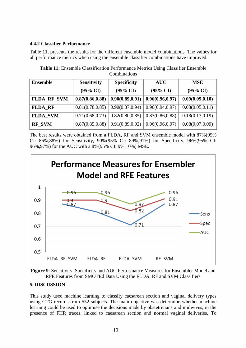
4.4.2 Classifier Performance

Table 11, presents the results for the different ensemble model combinations. The values for

all performance metrics when using the ensemble classifier combinations have improved.

Table 11: Ensemble Classification Performance Metrics Using Classifier Ensemble

Combinations

Ensemble Sensitivity

(95% CI)

Specificity

(95% CI)

AUC

(95% CI)

MSE

(95% CI)

FLDA_RF_SVM 0.87(0.86,0.88) 0.90(0.89,0.91) 0.96(0.96,0.97) 0.09(0.09,0.10)

FLDA_RF 0.81(0.78,0.85) 0.90(0.87,0.94) 0.96(0.94,0.97) 0.08(0.05,0.11)

FLDA_SVM 0.71(0.68,0.73) 0.82(0.80,0.85) 0.87(0.86,0.88) 0.18(0.17,0.19)

RF_SVM 0.87(0.85,0.88) 0.91(0.89,0.92) 0.96(0.96,0.97) 0.08(0.07,0.09)

The best results were obtained from a FLDA, RF and SVM ensemble model with 87%(95%

CI: 86%,88%) for Sensitivity, 90%(95% CI: 89%,91%) for Specificity, 96%(95% CI:

96%,97%) for the AUC with a 8%(95% CI: 9%,10%) MSE.

Figure 9: Sensitivity, Specificity and AUC Performance Measures for Ensembler Model and

RFE Features from SMOTEd Data Using the FLDA, RF and SVM Classifiers

5. DISCUSSION

This study used machine learning to classify caesarean section and vaginal delivery types

using CTG records from 552 subjects. The main objective was determine whether machine

learning could be used to optimise the decisions made by obstetricians and midwives, in the

presence of FHR traces, linked to caesarean section and normal vaginal deliveries. To

20

achieve this machine learning algorithms were modelled using the 552 records from the

CTU-UHB database. No pre-selection of perinatal complications was made. In the pre-

processing tasks, the FHR signal was filtered, and noise and low-quality artefacts were

removed based on findings in previous studies [38], [39], [81]–[83].

Several features were extracted from the raw FHR signal. The resulting feature set was used

to train FLDA, RF, and SVM classifiers. The initial classification results achieved high

Specificities (normal deliveries). However, this was at the cost of very low Sensitivities

(caesarean section deliveries) which in this study are considered more important. Cross-

validation was utilised to increase the Sensitivity values. However, the MSE improvements

were not statistically significant. This was attributed to the disproportionate number of

vaginal and caesarean section delivery records and a skewed distribution towards the majority

class. The minimum error rate displayed across all classifiers was approximately 8% using

the holdout technique. Low MSE error rates are subjected to classifiers minimizing the

probability of error when there is insufficient evidence to classify otherwise.

Using the SMOTE algorithm to oversample the training significantly improved the Sensitivity

for all classifiers but reduced all Specificities when 13 features were used. We argue that

while oversampling is not ideal, it is a recognised way to normally distribute datasets [66]–

[72]. The AUC values across all classifiers did not improve. The MSE values remained

broadly the same. The best results were achieved using the RF classifier with 59% (95% CI:

54%, 65%) for Sensitivity, 57% (95% CI: 55%, 59%) for Specificity, 62% (95% CI: 60%,

64%) for the AUC, with a 8% (95% CI: 8%, 8%) MSE. We considered the RF classifier to the

best as indicated by the approximate balanced between Sensitivity and Specificity values.

However, the results are not sufficient for use in a medical decision support system.

Using the RFE algorithm, five features were considered to have no or very low discriminative

capacity and were removed. This left eight features for further classifier modelling and

evaluation. The results showed improvements in all classifiers with the best results obtained

from the RF model with 76% (95% CI: 70%, 81%) for Sensitivity, 56% (95% CI: 54%, 58%)

for Specificity, 70% (95% CI: 68%, 73%) for the AUC, with a 8% (95% CI: 7%, 8%) MSE.

Combining the classifiers into ensemble models demonstrated a marked improvement in all

of the classifier models. The best results were obtained when the FLDA, RF and SVM

classifiers were combined with overall values of 87% (95% CI; 86%, 88%) for Sensitivity,

90% (95% CI: 89%, 91%) for Specificity, 96% (95% CI: 96%, 97%) for the AUC, with a 8%

(95% CI: 9%, 10%) MSE. Ensemble modelling is able to achieve this by running the

individual models and synthesising the results to improve the overall accuracy. In the case of

the SVM, it has good generalisation capabilities and in this study, the eight features were

used to maximise the margins in the hyperplane to increase the distance between classes to

provide better discrimination. In the case of the RF, each decision-tree is randomised using a

bootstrap statistical resampling technique, with random feature selection. Many randomised

decision-trees use the data points of a particular class to vote and classify new data points.

This is particularly useful for observations located close to the decision boundary, where

classifiers such as the SVM, based on isolated data points, find them difficult to classify. In

the context of linear discrimination, the results show that using the FLDA it is not possible to

maximise the between class variance sufficiently to remove class overlap. This shows that

classification errors are unavoidable around the decision boundary. In a similar way to the

SVM, the FLDA finds it easier to classify observations farthest away from the decision

boundary than those close to it or overlapping using the CTU-UHB dataset.

21

Consequently, it is clear to see that through ensemble modelling, the strengths of each model

can be utilised to distinguish between caesarean section and vaginal delivery types using the

FHR signal. In particular, the results demonstrate that the ensemble model, trained using the

DFA, RMS, FD, SD1, SDRatio, SD2, SampEn, and STV, features, provides significant

improvements, using a robust methodology, on many previously reported machine learning

studies in automated Cardiotocography trace interpretation [16], [45], [52], [53], [75], [84],

[85].

6. CONCLUSIONS AND FUTURE WORK

Complications during labour can result in adverse perinatal outcomes and in severe cases

death. Consequently, early detection and the prediction of pathological outcomes could help

to reduce foetal morbidity and mortality rates worldwide and indicate if surgical intervention,

such as caesarean section, is required. Human CTG analysis is used to monitor the foetus

during labour. However, poor human interpretation has led to high inter and intra observer

variability. A strong body of evidence has therefore suggested that automated computer

analysis of CTG signals might provide a viable way of diagnosing true perinatal

complications and predict the early onset of pathological outcomes with much less variability

and better accuracy.

The study presented in this paper explored this idea and utilised FHR signals from CTG

traces and supervised machine learning, to train and classify caesarean section and vaginal

deliveries. This was achieved using an ensemble classifier modelled using oversampled

training data consisting of eight RFE ranked features. The results demonstrate using an

ensemble model consisting of a FLDA, RF, and SVM model, it is possible to obtain 87%

(95% CI: 86%, 88%) for Sensitivity, 90% (95% CI: 89%, 91%) for Specificity, and 96% (95%

CI: 96%, 97%) for AUC, with a 9% (95% CI: 9%, 10%) MSE.

While, the results are encouraging, further more in-depth studies are required. For example,

mapping signals to pH values or a range of values for multivariate classification would be

interesting. This would provide a granular assessment of outcomes potentially more accurate

and inclusive than simply predicting whether a mother will have a caesarean section or

vaginal delivery. Future research will also explore opportunities to obtain a much larger

normally distribution dataset, removing the need for oversampling.

We only considered the FHR signal in this study, because it provides direct information about

the foetus’s state. However, it would be useful to create an extended dataset that encompasses

features extracted from the UC signal. Studying the effects UC has on the foetus during

pregnancy provides valuable information as can be seen in our previous work [83], and could

yield additional important information. Lastly, it would be interesting to remove the feature

engineering stage altogether in favour of deep learning and stacked autoencoders. This would

force models to learn meaning for information or structure in the data that could potentially

be more representative of the data than the features considered in this paper.

Overall, the study demonstrates that classification algorithms provide an interesting line of

enquiry worth exploring, when classifying caesarean section and vaginal delivery types.

REFERENCES

22

[1] J. B. Warren, W. E. Lambert, R. Fu, J. M. Anderson, and A. B. Edelman, “Global

neonatal and perinatal mortality: a review and case study for the Loreto Province of

Peru,” Res. Reports Neonatol., vol. 2, pp. 103–113, 2012.

[2] R. Brown, J. H. B. Wijekoon, A. Fernando, E. D. Johnstone, and A. E. P. Heazell,

“Continuous objective recording of fetal heart rate and fetal movements could reliably

identify fetal compromise, which could reduce stillbirth rates by facilitating timely

management,” Med. Hypotheses, vol. 83, no. 3, pp. 410–417, 2014.

[3] S. Rees and T. Inder, “Fetal and neonatal origins of altered brain development,” Early

Hum. Dev., vol. 81, no. 9, pp. 753–761, 2005.

[4] S. Rees, R. Harding, and D. Walker, “An adverse intrauterine environment:

implications for injury and altered development of the brain,” Int. J. Dev. Neurosci.,

vol. 26, no. 1, pp. 3–11, 2008.

[5] B. Chudacek, J. Spilka, M. Bursa, P. Janku, L. Hruban, M. Huptych, and L. Lhotska,

“Open access intrapartum CTG database,” BMC Pregnancy Childbirth, vol. 14, no. 16,

pp. 1–12, 2014.

[6] G. Bogdanovic, A. Babovic, M. Rizvanovic, D. Ljuca, G. Grgic, and J. Djuranovic-

Milicic, “Cardiotocography in the Prognosis of Perinatal Outcome,” Med. Arch., vol.

68, no. 2, pp. 102–105, 2014.

[7] J. Kessler, D. Moster, and S. Albrechfsen, “Delay in intervention increases neonatal

morbidity in births monitored with Cardiotocography and ST-waveform analysis,”

Acta Obs. Gynecol Scand, vol. 93, no. 2, pp. 175–81, 2014.

[8] J. Hasegawa, A. Sekizawa, T. Ikeda, M. Koresawa, S. Ishiwata, M. Kawabata, and K.

Kinoshita, “Clinical Risk Factors for Poor Neonatal Outcomes in Umbilical Cord

Prolapse,” J. Matern. Neonatal Med., vol. 29, no. 10, pp. 1652–1656, 2016.

[9] S. Kundu, E. Kuehnle, C. Shippert, J. von Ehr, P. Hillemanns, and I. Staboulidou,

“Estimation of neonatal outcome artery pH value according to CTG interpretation of

the last 60 min before delivery: a retrospective study. Can the outcome pH value be

predicted?,” Arch. Gynecol. Obstet., vol. 296, no. 5, pp. 897–905, 2017.

[10] C. Garabedian, L. Butruille, E. Drumez, E. S. Servan Schreiber, S. Bartolo, G. Bleu, V.

Mesdag, P. Deruelle, J. De Jonckheere, and V. Houfflin-Debarge, “Inter-observer

reliability of 4 fetal heart rate classifications,” J. Gynecol. Obstet. Hum. Reprod., vol.

46, no. 2, pp. 131–135, 2017.

[11] S. Kundu, E. Kuehnle, C. Schippert, J. von Ehr, P. Hillemanns, and I. Staboulidou,

“Estimation of neonatal outcome artery pH value according to CTG interpretation of

the last 60 min before delivery: a retrospective study. Can the outcome pH value be

predicted?,” Arch. Gynecol. Obstet., vol. 296, no. 5, pp. 897–905, 2017.

[12] P. A. Warrick, E. F. Hamilton, D. Precup, and R. E. Kearney, “Classification of

normal and hypoxic fetuses from systems modeling of intrapartum Cardiotocography,”

IEEE Trans. Biomed. Eng., vol. 57, no. 4, pp. 771–779, 2010.

23

[13] J. Spilka, G. Georgoulas, P. Karvelis, and V. Chudacek, “Discriminating Normal from

‘Abnormal’ Pregnancy Cases Using an Automated FHR Evaluation Method,” Artif.

Intell. Methods Appl., vol. 8445, pp. 521–531, 2014.

[14] M. Romano, P. Bifulco, M. Ruffo, G. Improta, F. Clemente, and M. Cesarelli,

“Software for computerised analysis of cardiotocographic traces,” Comput. Methods

Programs Biomed., vol. 124, pp. 121–137, 2016.

[15] A. Pinas and E. Chadraharan, “Continuous Cardiotocography During Labour:

Analysis, Classification and Management.,” Best Pract. Res. Clin. Obstet. Gynaecol.,

vol. 30, pp. 33–47, 2016.

[16] P. A. Warrick, E. F. Hamilton, D. Precup, and R. E. Kearney, “Classification of

Normal and Hypoxic Fetuses From Systems Modeling of Intrapartum

Cardiotocography,” IEEE Trans. Biomed. Eng., vol. 57, no. 4, pp. 771–779, 2010.

[17] H. Sahin and A. Subasi, “Classification of the cardiotocogram data for anticipation of

fetal risks using machine learning techniques,” Appl. Soft Comput., vol. 33, pp. 231–

238, 2015.

[18] H. Ocak and H. M. Ertunc, “Prediction of fetal state from the cardiotocogram

recordings using adaptive neuro-fuzzy inference systems,” Neural Comput.

Appliations, vol. 22, no. 6, pp. 1583–1589, 2013.

[19] C. Rotariu, A. Pasarica, G. Andruseac, H. Costin, and D. Nemescu, “Automatic

analysis of the fetal heart rate variability and uterine contractions,” in IEEE Electrical

and Power Engineering, 2014, pp. 553–556.

[20] C. Rotariu, A. Pasarica, H. Costin, and D. Nemescu, “Spectral analysis of fetal heart

rate variability associated with fetal acidosis and base deficit values,” in International

Conference on Development and Application Systems, 2014, pp. 210–213.

[21] K. Maeda, “Modalities of fetal evaluation to detect fetal compromise prior to the

development of significant neurological damage,” J. Obstet. adn Gynaecol. Res., vol.

40, no. 10, pp. 2089–2094, 2014.

[22] H. Ocak, “A Medical Decision Support System Based on Support Vector Machines

and the Genetic Algorithm for the Evaluation of Fetal Well-Being,” J. Med. Syst., vol.

37, no. 2, p. 9913, 2013.

[23] T. Peterek, P. Gajdos, P. Dohnalek, and J. Krohova, “Human Fetus Health

Classification on Cardiotocographic Data Using Random Forests,” in Intelligent Data

Analysis and its Applications, 2014, pp. 189–198.

[24] R. M. Grivell, Z. Alfirevic, G. M. L. Gyte, and D. Devane, “Cardiotocography (a form

of electronic fetal monitoring) for assessing a baby’s well-being in the womb during

pregnancy,” Syst. Rev., vol. 2015, no. 9, 2015.

[25] A. R. Webb and K. D. Copsey, Statistical Pattern Recognition. 2011, pp. 1–642.

[26] V. S. Talaulikar, V. Lowe, and S. Arulkumaran, “Intrapartum fetal surveillance.,”

Obstet. Gynaecol. Reprod. Med., vol. 24, no. 2, pp. 45–55, 2014.

24

[27] A. L. Goldberger, L. A. N. Amaral, L. Glass, J. M. Hausdorff, and E. Al.,

“PhysioBank, PhysioToolkit, and PhysioNet: Components of a new research resource

for complex physiologic signals.”

[28] R. Mantel, H. P. van Geijn, F. J. Caron, J. M. Swartjies, van W. E. E., and H. W.

Jongsma, “Computer analysis of antepartum fetal heart rate: 2. Detection of

accelerations and decelerations,” Int. J. Biomed Comput, vol. 25, no. 4, pp. 273–286,

1990.

[29] H. M. Franzcog, “Antenatal foetal heart monitoring,” Best Pract. Res. Clin. Obstet.

Gynaecol., vol. 38, pp. 2–11, 2017.

[30] J. Camm, “Heart rate variability: standards of measurement, physiological

interpretation and clinical use. Task Force of the European Society of Cardiology and

the North American Society of Pacing and Electrophysiology,” Circulation, vol. 93,

no. 5, pp. 1043–65, 1996.

[31] L. Stroux, C. W. Redman, A. Georgieva, S. J. Payne, and G. D. Clifford, “Doppler-

based fetal heart rate analysis markers for the detection of early intrauterine growth

restriction,” Acta Obstet. Gynecol. Scand., vol. 96, no. 11, pp. 1322–1329, 2017.

[32] M. Romano, L. Iuppariello, A. M. Ponsiglione, G. Improta, P. Bifulco, and M.

Cesarelli, “Frequency and Time Domain Analysis of Foetal Heart Rate Variability

with Traditional Indexes: A Critical Survey,” Comput. Math. Methods Med., vol. 2016,

no. 9585431, pp. 1–12, 2016.

[33] C. Buhimschi, M. B. Boyle, G. R. Saade, and R. E. Garfield, “Uterine activity during

pregnancy and labor assessed by simultaneous recordings from the myometrium and

abdominal surface in the rat.,” Am. J. Obstet. Gynecol., vol. 178, no. 4, pp. 811–22,

Apr. 1998.

[34] C. Buhimschi, M. B. Boyle, and R. E. Garfield, “Electrical activity of the human

uterus during pregnancy as recorded from the abdominal surface,” Obstet. Gynecol.,

vol. 90, no. 1, pp. 102–111, 1997.

[35] C. Buhimschi and R. E. Garfield, “Uterine contractility as assessed by abdominal

surface recording of electromyographic activity in rats during pregnancy.,” Am. J.

Obstet. Gynecol., vol. 174, no. 2, pp. 744–53, Feb. 1996.

[36] J. S. Richman and J. R. Moorman, “Physiological time-series analysis using

approximate entropy and sample entropy,” Am. J. Physiol. - Hear. Circ. Physiol., vol.

278: H2039, no. 6, 2000.

[37] M. G. Signorini, A. Fanelli, and G. Magenes, “Monitoring fetal heart rate during

pregnancy: contributions from advanced signal processing and wearable technology,”

Comput. Math. Methods Med., vol. 2014, no. 707581, pp. 1–10, 2014.

[38] M. Romano, M. Cesarelli, P. Bifulco, M. Ruffo, A. Frantini, and G. Pasquariello,

“Time-frequency analysis of CTG signals,” Curr. Dev. Theory Appl. Wavelets, vol. 3,

no. 2, pp. 169–192, 2009.

25

[39] M. J. Rooijakkers, S. Song, C. Rabotti, G. Oei, J. W. M. Bergmans, E. Cantatore, and

M. Mischi, “Influence of Electrode Placement on Signal Quality for Ambulatory

Pregnancy Monitoring,” Comput. Math. Methods Med., vol. 2014, no. 2014, pp. 1–12,

2014.

[40] M. G. Signorini, G. Magenes, S. Cerutti, and D. Arduini, “Linear and nonlinear

parameters for the analysis of fetal heart rate signal from cardiotocographic

recordings,” IEEE Trans. Biomed. Eng., vol. 50, no. 3, pp. 365–374, 2003.

[41] S. Siira, T. Ojala, E. Ekholm, T. Vahlberg, S. Blad, and K. G. Rosen, “Change in heart

rate variability in relation to a significant ST-event associates with newborn metabolic

acidosis,” BJOG An Int. J. Obstet. Gynaecol., vol. 114, no. 7, pp. 819–823, 2007.

[42] V. J. Laar, M. M. Porath, C. H. L. Peters, and S. G. Oei, “Spectral analysis of fetal

heart rate variability for fetal surveillance: review of the literature,” Acta Obs. Gynecol

Scand, vol. 87, no. 3, pp. 300–306, 2008.

[43] P. Melillo, R. Izzo, A. Orrico, P. Scala, M. Attanasio, M. Mirra, N. De Luca, and L.

Pecchia, “Automatic Prediction of Cardiovascular and Cerebrovascular Events Using

Heart Rate Variability Analysis,” PLoS One, vol. 10, no. 3, p. e0118504, 2015.

[44] H. Goncalves, D. Ayres-de-Campos, and J. Bernardes, “Linear and Nonlinear Analysis

of Fetal Heart Rate Variability. In Fetal Development,” in Fetal Development, 2016,

pp. 119–132.

[45] J. Spilka, V. Chudacek, M. Koucky, L. Lhotska, M. Huptych, P. Janku, G. Georgoulas,

and C. Stylios, “Using nonlinear features for fetal heart rate classification,” Biomed.

Signal Process. Control, vol. 7, no. 4, pp. 350–357, 2012.

[46] J. Spilka, V. Chudacek, M. Koucky, and L. Lhotska, “Assessment of non-linear

features for intrapartal fetal heart rate classification,” in The 9th International

Conference on Information Technology and Applications in Biomedicine, 2009, pp. 1–

4.

[47] P. Hopkins, N. Outram, N. Lofgren, E. C. Ifeachor, and K. G. Rosen, “A Comparative

Study of Fetal Heart Rate Variability Analysis Techniques,” in The 28th IEEE Annual

International Conference on Engineering in Medicine and Biology Society., 2006, pp.

1784–1787.

[48] P. Abry, S. G. Roux, V. Chudacek, P. Borgnat, P. Goncalves, and M. Doret, “Hurst

Exponent and IntraPartum Fetal Heart Rate: Impact of Decelerations,” in 26th IEEE

International Symposium on Computer-Based Medical Systems, 2013, pp. 131–136.

[49] M. Haritopoulos, A. Illanes, and A. K. Nandi, “Survey on Cardiotocography Feature

Extraction Algorithms for Foetal Welfare Assessment,” in Springer Mediterranean

Conference on Medical and Biological Engineering and Computing, 2016, pp. 1187–

1192.

[50] G. Koop, M. H. Pesaran, and S. M. Potter, “Impulse response analysis in nonlinear

multivariate models,” J. Econom., vol. 74, no. 1, pp. 119–147, 1996.

26

[51] E. Blinx, K. G. Brurberg, E. Reierth, L. M. Reinar, and P. Oian, “ST waveform

analysis versus Cardiotocography alone for intrapartum fetal monitoring: a systematic

review and meta-analysis of randomized trials,” Acta Obstet. Gynancelogica Scand.,

vol. 95, no. 1, pp. 16–27, 2016.

[52] H. Ocak, “A Medical Decision Support System Based on Support Vector Machines

and the Genetic Algorithm for the Evaluation of Fetal Well-Being,” Springer J. Med.

Syst., vol. 37, no. 9913, pp. 1–9, 2013.

[53] E. Yilmaz and C. Kilikcier, “Determination of Fetal State from Cardiotocogram Using

LS-SVM with Particle Swarm Optimization and Binary Decision Tree,” Comput.

Math. Methods Med., vol. 2013, no. 487179, pp. 1–8, 2013.

[54] H. Ocak and H. M. Ertunc, “Prediction of fetal state from the cardiotocogram

recordings using adaptive neuro-fuzzy inference systems,” Neural Comput. Appl., vol.

23, no. 6, pp. 1583–1589, 2013.

[55] M. E. Menai, F. J. Mohder, and F. Al-mutairi, “Influence of Feature Selection on

Naïve Bayes Classifier for Recognizing Patterns in Cardiotocograms,” J. Med.

Bioeng., vol. 2, no. 1, pp. 66–70, 2013.

[56] E. M. Karabulut and T. Ibrikci, “Analysis of Cardiotocogram Data for Fetal Distress

Determination by Decision Tree Based Adaptive Boosting Approach,” J. Comput.

Commun., vol. 2, no. 9, pp. 32–37, 2014.

[57] D. Rindskopf and W. Rindskopf, “The value of latent class analysis in medical

diagnosis,” Stat. Med., vol. 5, no. 1, pp. 21–27, 1986.

[58] M. Romano, G. Faiella, P. Bifulco, D. Addio, F. Clemente, and M. Cesarelli, “Outliers

Detection and Processing in CTG Monitoring,” in Mediterranean Conference on

Medical and Biological Engineering and Computing, 2013, pp. 651–654.

[59] P. A. Warrick, E. F. Hamilton, D. Precup, and R. E. Kearney, “Identification of the

dynamic relationship between intra-partum uterine pressure and fetal heart rate for

normal and hypoxic fetuses,” IEEE Trans. Biomed. Eng., vol. 56, no. 6, pp. 1587–

1597, 2009.

[60] H. Goncalves, A. Costa, D. Ayres-de-Campos, C. Costa-Santos, A. P. Rocha, and J.

Benardes, “Comparison of real beat-to-beat signals with commercially available 4 Hz

sampling on the evaluation of foetal heart rate variability,” Med. Biol. Eng. Comput.,

vol. 51, no. 6, 2013.

[61] P. A. Warrick and E. F. Hamilton, “Subspace detection of the impulse response

function from intrapartum uterine pressure and fetal heart rate variability,” in IEEE

Computing in Cardiology Conference, 2013, pp. 85–88.

[62] P. A. Warrick and E. F. Hamilton, “Discrimination of Normal and At-Risk Populations

from Fetal Heart Rate Variability,” Comput. Cardiol. (2010)., vol. 41, pp. 1001–1004,

2014.

27

[63] G. Improta, M. Romano, A. Ponsiglione, P. Bifulco, G. Faiella, and M. Cesarelli,

“Computerized Cardiotocography: A Software to Generate Synthetic Signals,” J Heal.

Med Informat, vol. 5, no. 4, pp. 1–6, 2014.

[64] I. Nunes and D. Ayres-de-Campos, “Computer Analysis of Foetal Monitoring

Systems,” Best Pract. Res. Clin. Obstet. Gynaecol., vol. 30, pp. 68–78, 2016.

[65] P. M. Granitto and A. B. Bohorquez, “Feature selection on wide multiclass problems

using OVA-RFE,” Intel. Artif., vol. 44, no. 2009, pp. 27–34, 2009.

[66] L. M. Taft, R. S. Evans, C. r. Shyu, M. J. Egger, N. Chawla, J. A. Mitchell, S. N.

Thornton, B. Bray, and M. Varner, “Countering imbalanced datasets to improve

adverse drug event predictive models in labor and delivery,” J. Biomed. Informatics2,

vol. 42, no. 2, pp. 356–364, 9AD.

[67] T. Sun, R. Zhang, J. Wang, X. Li, and X. Guo, “Computer-Aided Diagnosis for Early-

Stage Lung Cancer Based on Longitudinal and Balanced Data,” PLoS One, vol. 8, no.

5, p. e63559, 2013.

[68] W. Lin and J. J. Chen, “Class-imbalanced classifiers for high-dimensional data,” Brief.

Bioinform., vol. 14, no. 1, pp. 13–26, 2013.

[69] T. Sun, R. Zhang, J. Wang, X. Li, and X. Guo, “Computer-Aided Diagnosis for Early-

Stage Lung Cancer Based on Longitudal and Balanced Data,” PLoS One, vol. 8, no. 5,

p. e63559, 2013.

[70] J. Nahar, T. Imam, K. S. Tickle, A. B. M. Shawkat Ali, and Y. P. Chen,

“Computational Intelligence for Microarray Data and Biomedical Image Analysis for

the Early Diagnosis of Breast Cancer,” Expert Syst. Appl., vol. 39, no. 16, pp. 12371–

12377, 2012.

[71] R. Blagus and L. Lusa, “SMOTE for High-Dimensional Class-Imbalanced Data,”

BMC Bioinformatics, vol. 14, no. 106, 2013.

[72] Y. Wang, M. Simon, P. Bonde, B. U. Harris, J. J. Teuteberg, R. L. Kormos, and J. F.

Antaki, “Prognosis of Right Ventricular Failure in Patients with Left Ventricular Assist

Device Based on Decision Tree with SMOTE,” Trans. Inf. Technol. Biomed., vol. 16,

no. 3, 2012.

[73] N. V. Chawla, K. W. Bowyer, L. O. Hall, and W. P. Kegelmeyer, “SMOTE: Synthetic

Minority Over-Sampling Technique,” J. Artif. Intell. Res., vol. 16, no. 1, pp. 321–357,

2002.

[74] P. Tomas, J. Krohova, P. Dohnalek, and P. Gajdos, “Classification of

Cardiotocography records by random forest,” in 36th IEEE International Conference

on Telecommunications and Signal Processing, 2013, pp. 620–623.

[75] N. Krupa, M. A. Ma, E. Zahedi, S. Ahmed, and F. M. Hassan, “Antepartum fetal heart

rate feature extraction and classification using empirical mode decomposition and

support vector machine,” Biomed. Eng. Online, vol. 10, no. 6, pp. 1–15, 2011.

28

[76] G. Georgoulas, C. D. Stylios, and P. P. Groumpos, “Predicting the risk of metabolic

acidosis for newborns based on fetal heart rate signal classification using support

vector machines,” IEEE Trans Biomed Eng, vol. 53, no. 5, pp. 875–884, 2006.

[77] B. Moslem, M. Khalil, and M. Diab, “Combining multiple support vector machines for

boosting the classification accuracy of uterine EMG signals,” in 18th IEEE

International Conference on Electronics, Circuits and Systems, 2011, pp. 631–634.

[78] T. Fawcett, “An Introduction to ROC analysis,” Pattern Recognit. Lett., vol. 27, no. 8,

pp. 861–874, 2006.

[79] T. A. Lasko, J. G. Bhagwat, K. H. Zou, and L. Ohno-Machada, “The use of receiver

operating characteristic curves in biomedical informatics,” J. Biomed. Inform., vol. 38,

no. 5, pp. 404–15, 2005.

[80] L. Tong, Y. Change, and S. Lin, “Determining the optimal re-sampling strategy for a

classification model with imbalanced data using design of experiments and response

surface methodologies,” Expert Syst. Appl., vol. 38, no. 4, pp. 4222–4227, 2011.

[81] M. G. Signorini, G. Magenes, S. Cerutti, and D. Arduini, “Linear and nonlinear

parameters for the analysis of fetal heart rate signal from cardiotocographic

recordings,” IEEE Trans Biomed Eng, vol. 50, no. 3, pp. 365–74, 2003.

[82] G. Fele-Žorž, G. Kavsek, Z. Novak-Antolic, and F. Jager, “A comparison of various

linear and non-linear signal processing techniques to separate uterine EMG records of

term and pre-term delivery groups,” Med. Biol. Eng. Comput., vol. 46, no. 9, pp. 911–

22, 2008.

[83] P. Fergus, P. Cheung, P. Hussain, D. Al-Jumeily, C. Dobbins, and S. Iram, “Prediction

of Preterm Deliveries from EHG Signals Using Machine Learning,” PLoS One, vol. 8,

no. 10, p. e77154, 2013.

[84] R. Czabanski, J. Jezewski, A. Matonia, and M. Jezewski, “Computerized analysis of

fetal heart rate signals as the predictor of neonatal acidemia,” Expert Syst. Appl., vol.

39, no. 15, pp. 11846–11860, 2012.

[85] G. Georgoulas, C. Stylios, V. Chudecek, M. Macas, J. Bernardes, and L. Lhotska,

“Classification of fetal heart rate signals based on features selected using the binary

particle swarm algorithm,” in World Congress on Medical Physics and Biomedical

Engineering, 2006, pp. 1156–1159.