
G. Iaccarino - UQ & HPC: towards exascale ensemble ...
112
-
Upload
khangminh22 -
Category
Documents
-
view
0 -
download
0
Transcript of G. Iaccarino - UQ & HPC: towards exascale ensemble ...


Keynote Lecture - G. Iaccarino - UQ & HPC: towards exascale ensemblesimulations
Session Chair: M.V. SalvettiAuditorium

Workshop on Frontiers of Uncertainty Quantification in Fluid Dynamics
11–13 September 2019, Pisa, Italy
UQ & HPC: towards exascale ensemble simulations
Gianluca Iaccarino
ICME - Institute for Computational & Mathematical EngineeringMechanical Engineering Department
Stanford University - Stanford, CA USA – [email protected]
Key words: Uncertainty quantification, Multilevel Sampling, Exascale Computing, Multiphysics Simulations
In the framework of the Predictive Science Academic Alliance Program (PSAAP) the US Department of
Energy is funding a Multidisciplinary Simulation Center at Stanford University to explore exascale computing
strategies for multiphysics simulations. Stanford Center’s research portfolio blends efforts in computer science,
uncertainty quantification, and computational physics to tackle a challenging physical problem: the transfer of
radiative energy to a turbulent mixture of air and solid particles. The context is provided by a relatively untested
and poorly understood method of harvesting solar energy. The talk will describe the Center’s effort to develop
and validate a computational environment to simulate this challenging multi-physics problem emphasizing the
strategies employed to carry out high-fidelity simulations and how uncertainty quantification techniques can be
used to assess the overall performance of the system. A novel task-based programming system (Legion) is being
deployed to tackle heterogeneous compute systems and retain portability and performance on next-generation
computer architectures. Details of the implementation challenges and results obtained on various architectures
will be discussed. The integration of large scale simulations and multi-level sampling for uncertainty analysis
within the Legion framework will also be summarized.
[1] K. Duraisamy, G. Iaccarino, H. Xiao “Turbulence modeling in the age of data” Annual Review of Fluid Mechanics, Vol 51, pp.
357-377, 2019
[2] H. R Fairbanks, A. Doostan, C. Ketelsen, G. Iaccarino, “A low-rank control variate for multilevel Monte Carlo simulation of
high-dimensional uncertain systems”, J. of Computational Physics, Vol 341, pp 121-139, 2017
[3] L Jofre, G Geraci, HR Fairbanks, A Doostan, G Iaccarino “Multi-fidelity uncertainty quantification strategies for large-scale
multiphysics applications: PSAAP II particle-based solar energy receiver”, AIP Conference Proceedings 2018 (1), 140002

SW1 – Turbulence ISession Chair: G. Iaccarino
Auditorium

Workshop on Frontiers of Uncertainty Quantification in Fluid Dynamics
11–13 September 2019, Pisa, Italy
Bayesian field-inversion for turbulence anisotropy with informative priors
Arent van Korlaar1 and Richard P. Dwight1
1Aerodynamics Group, Faculty of Engineering, Delft University of Technology – [email protected]
Key words: Bayesian statistics, Reynolds-Averaged Navier-Stokes (RANS) equations, data-driven turbulencemodelling, machine-learning, continuous adjoint
Reynolds-Averaged Navier-Stokes (RANS) and its associated turbulence closure models will continue to
be necessary in order to perform computationally affordable flow simulations for the foreseeable future. The
errors inherent in the semi-empirical turbulence closures, means that significant uncertainty is associated with
the results [6, 2]. In this work we use data from expensive LES and DNS simulations to train new closure models
for RANS, similar to previous deterministic work [5]. Our procedure is a two-step process, following [3]:
(a) First we find a local turbulence anisotropy correction to the RANS model, which causes the model to
reproduce the given LES/DNS mean field.
(b) Secondly we regress the local correction discovered in part (a) as a function of the local mean-flow, using
machine-learning techniques.
Step (a) is a field-inversion problem with a large space of valid solutions. Rather than using Tikhonov regular-
ization, we introduce an informative prior on the correction derived using random matrix theory [7, 4]. This
prior guarantees the positive-definiteness of the Reynolds stress tensor, and encourages physically reasonable
corrections in the posterior. After doing this for several flows, in Step (b) we fit a stochastic regression model
to the resulting data set [1]. The posterior covariance, approximated using the Hessian of the simulation code,
is exploited to give the regression model realistic uncertainty. Unseen flows are then predicted with this model,
which include now informed estimates of model uncertainty.
The framework is trained on channel flows, backward-facing steps, and the converging diverging duct.
Predictions for the (unseen) periodic-hill are made (see Figure 1), demonstrating the ability of the framework
to generalize beyond the training set.
References
[1] J.H.S. de Baar, R.P. Dwight, and H. Bijl. “Improvements to Gradient-Enhanced Kriging using a Bayesian
Interpretation”. In: International Journal for Uncertainty Quantification 4.3 (2013), pp. 205–223.
[2] W.N. Edeling, P. Cinnella, and R.P. Dwight. “Predictive RANS simulations via Bayesian Model-Scenario
Averaging”. In: Journal of Computational Physics 275 (2015), pp. 65–91.
[3] Karthik Duraisamy Eric J. Parish. “A paradigm for data-driven predictive modeling using field inversion
and machine learning”. In: Journal of Computational Physics 305 (2016), pp. 758–774.
[4] Roger G. Ghanem Heng Xiao Jian-Xun Wang. “A Random Matrix Approach for Quantifying Model-Form
Uncertainties in Turbulence Modeling”. In: arXiv arXiv:1603.09656 [physics.flu-dyn] (2016).
[5] Mikael L. A. Kaandorp and Richard P. Dwight. Stochastic Random Forests with Invariance for RANS
Turbulence Modelling. 2018. eprint: arXiv:1810.08794.
[6] S.B. Pope. Turbulent flows. Cambridge Univ Pr, 2000.
[7] C. Soize. “Random matrix theory for modeling uncertainties in computational mechanics”. In: Computer
Methods in Applied Mechanics and Engineering 194.12 (2005), pp. 1333–1366. issn: 0045-7825.

(a) Horizontal velocity profiles.
(b) Skin-friction on lower wall.
Figure 1: Prediction of periodic-hill mean-flow using RANS with baseline k−ω, and two stochastic data-driven
closure models. Model βP learns a k-production correction; model βCαcalso learns an isotropy correction.

Workshop on Frontiers of Uncertainty Quantification in Fluid Dynamics
11–13 September 2019, Pisa, Italy
Using Machine learning to predict and understand turbulence modelling
uncertainties
Ashley Duncan Scillitoe1
1The Alan Turing Institute, London, UK – [email protected]
Key words: Epistemic uncertainty, Turbulence modelling, Sensitivity analysis, Machine learning.
Many industrial flows are turbulent in nature, and Reynolds-Averaged Navier-Stokes (RANS) based turbu-
lence models play an important role in the prediction of such flows. Many simplifying assumptions are made
in the development of a RANS model. These assumptions can lead to epistemic uncertainties which are still a
major obstacle for the predictive capability of RANS models. If experimental measurements or higher fidelity
simulation results are not available for comparison, it can be difficult to evaluate the accuracy of RANS predic-
tions. Recently, data-driven strategies have been proposed to either quantify model uncertainty [2], or improve
model accuracy [3]. Many of these strategies involve training supervised machine learning (ML) models on
high fidelity CFD data, such as that from large eddy simulations [1].
Ling and Templeton [4] proposed a technique whereby a machine learning classifier is trained to detect
whether a number of RANS modelling assumptions are broken. The classifier can then be used to predict re-
gions of high and low uncertainty in RANS simulations where corresponding high fidelity data is not available.
In the present work, the original technique is further refined, and applied to a number of flow configurations
such as a recent family of bumps dataset [5]. The non-dimensional “features" used by Ling and Templeton to
describe each flow to the ML model are revisited, with improvements made to ensure the ML classifier is more
generalisable to other flows. New error metrics are also proposed to allow for other areas of RANS modelling
uncertainty to be explored. Figure 1 shows a prediction made for one of the bump cases, with the region in red
being a region where the Boussinesq hypothesis used by many RANS models would be invalid due to the high
turbulent anisotropy.
Figure 1: Regions in the flow over a bump [5] where the Boussinesq hypothesis is predicted to be invalid due
to significant turbulent anisotropy, predicted by a random forest classifier.
Within the ML community there is an increasing interest in interpretability. Indeed, a common criticism of
ML augmented RANS models is that they are a “black box", with the machine able to make accurate predictions
but not explain why it has made them. The proposed RANS error classifier is examined using recently proposed
ML interpretation methods such as individual conditional expectation [6] and Shapley additive explanations
(SHAP) [7] plots. These novel techniques provide global and local explanations of model predictions. A SHAP
summary plot, which summarises the global effect of each flow feature (the model inputs) on the turbulent

anisotropy metric (a model output), is shown in Figure 2. More detailed SHAP plots are discussed, such as
SHAP dependence and local force plots. Now, the proposed classifier can not only be used to predict regions
of uncertainty, but also to explain what physical flow features have caused this uncertainty. This brings with it
the possibility of using the classifier to aid in the further understanding and development of turbulence models,
in addition to its use as a tool in predicting “trust" regions in RANS simulations.
Figure 2: A SHAP summary plot showing the impact of flow features on the turbulent anisotropy error metric
predicted in Figure 1.
[1] A. D. Scillitoe, P. G. Tucker and P. Adami, “Large eddy simulation of boundary layer transition mechanisms in a gas-turbine
compressor cascade" Journal of Turbomachinery 141, 6 (2019).
[2] W. Edeling, G. Iaccarino and P. Cinnella, “Data-Free and Data-Driven RANS Predictions with Quantified Uncertainty" Flow,
Turbulence and Combustion 100, 3 (2018).
[3] J. Wu, H. Xiao and E. Paterson, “Physics-informed machine learning approach for augmenting turbulence models: A comprehen-
sive framework" Physical Review Fluids 7, 3 (2018).
[4] J. Ling and J. Templeton, “Evaluation of machine learning algorithms for prediction of regions of high Reynolds averaged Navier
Stokes uncertainty" Physics of Fluids 27, 8 (2015).
[5] R. Matai and P. Durbin, “Large-eddy simulation of turbulent flow over a parametric set of bumps" Journal of Fluid Mechanics 866
(2019).
[6] A. Goldstein et al., “Peeking inside the black box: visualizing statistical learning with plots of individual conditional expectation"
Journal of computational and graphical statistics 24, 1 (2015).
[7] S. M. Lundberg and S. I. Lee, “A Unified approach to interpreting model predictions" Advances in neural information processing
systems 30 (2017).

Workshop on Frontiers of Uncertainty Quantification in Fluid Dynamics
11–13 September 2019, Pisa, Italy
State Estimation for wall-bounded turbulent flows using the Immersed Boundary
Method and Data Assimilation
Marcello Meldi1,2
1Institut Pprime, Department of Fluid Flow, Heat Transfer and Combustion CNRS - ENSMA - Université dePoitiers, UPR 3346, F86962 Futuroscope Chasseneuil Cedex, France
2Aix-Marseille Univ., CNRS, Centrale Marseille, M2P2 Marseille, France – [email protected]
Key words: Immersed Boundary Method, Data Assimilation, Kalman Filter
The accurate prediction of numerous bulk flow features of unstationary flows such as aerodynamic forces is
driven by the precise representation of localized near-wall dynamics, owing to the non-linear behavior of such
configurations. This aspect is particularly relevant for the flow prediction around complex geometries. In this
case classical body-fitted approaches may have to deal with high deformation of the mesh elements, usually
providing poor numerical prediction. Additionally, the simulation of moving bodies may require prohibitively
expensive mesh updates. In the last decades, the Immersed Boundary Method (IBM) [1, 2, 3, 4, 5] has emerged
as one of the most popular strategies to handle these two problematic aspects. The main difficulty with IBM is
the accurate representation of near wall flow features, which is a governing aspect in most engineering cases.
The wall resolution required increases with the Reynolds number as finer structures are observed due to multi-
scale interactions, leading to a faster rise of the resources demanded when compared with body-fitted methods.
The present work aims for the advancement of the IBM method recently developed by the Author via Data
Assimilation (DA). DA includes a wide spectrum of tools which derive an optimized state integrating a model
and available observation which are affected by uncertainties. Among these tools, the estimator recently pro-
posed by the Author [6] is one of the very first tools which successfully provided an augmented state estimation
integrating CFD and experimental data for the analysis of turbulent flows. Thus, the main objective is to im-
prove the accuracy of the IBM method (model) integrating high-fidelity data (observation) via DA.
The study is performed for the flow around a circular cylinder for ReD = 3900 [7, 8]. This flow configuration
has been identified because the flow exhibits turbulent features in the wake but the boundary layer is laminar.
This aspect allows to exclude the complex representation of wall turbulence effects in this initial analysis. In
addition, this configuration does not exhibit a boundary layer separation driven by the geometry, allowing to
perform a strong test of the capabilities of the IBM-DA approach to reconstruct essential physical features.
Table 1: Bulk flow quantities calculated with the numerical simulations of the database
Simulation CD C′L
S t Rec. length
DNS 0.977 0.118 0.209 1.53
LES 1.093 0.25 0.2 1.15
IBM 1.225 0.101 0.2 1.7
IBM-DA-W 1.109 0.107 0.206 1.62
IBM-DA-K 1.233 0.117 0.207 1.52
Three classical simulations have been initially performed namely a body-fitted direct numerical simulation
(DNS), a body-fitted large-eddy simulation (LES) and a classical, under-resolved IBM simulation (IBM). The
predicted bulk flow quantities reported in Table 1 indicate that the lack of near-wall resolution is responsible

for a significant error in the prediction of the CD when compared to the DNS. Thus, the IBM-DA strategy is
used to improve the performance of IBM integrating the high precision DNS data. Formally, this means that
the Kalman Filter strategy relies on:
• A continuous low-precision model, which is the IBM over the coarse mesh
• High confidence local observation, i.e. local, instantaneous velocity sampled from DNS data
The Kalman filter provides a precise state estimation which is used to calibrate the IBM volume forcing
term introduced in the discretized equations. The performance of this strategy is tested estimating its sensitivity
to the positions of the sensors. Two different distributions have been chosen for a cloud of 4000 sensors over
which DNS data have been sampled (see fig. 1).
(a) (b)
Figure 1: Positioning of the sensors for Data Assimilation
The performance of the IBM-DA simulations is assessed via observation of the computed bulk flow quan-
tities, which are reported in table 1. Results for the simulation IBM-DA-W (sensors in the wall region) are
remarkably good for all the physical quantities (≈ 50% improvement). On the other hand, the results for the
simulation IBM-DA-K (sensors in the wake) are less satisfying. An excellent agreement is obtained for C′L,
S t and the recirculation length, which are quantities associated with the behavior of the wake. However, the
drag coefficient CD is mostly unchanged when compared to the classical IBM simulation. This implies that the
accurate information obtained integrating the DNS data is not efficiently propagated upstream.
[1] C. S. Peskin, “Flow patterns around heart valves: A numerical method ,” Journal of Computational Physics, vol. 10, no. 2, pp. 252
– 271, 1972.
[2] R. Mittal and G. Iaccarino, “Immersed boundary methods,” Annual Review of Fluid Mechanics, vol. 37, pp. 239 – 261, 2005.
[3] M. Uhlmann, “An immersed boundary method with direct forcing for the simulation of particulate flows,” Journal of Computational
Physics, vol. 209, no. 2, pp. 448 – 476, 2005.
[4] A. Pinelli, I. Naqavi, U. Piomelli, and J. Favier, “Immersed-boundary methods for general finite-difference and finite-volume
Navier–Stokes solvers ,” Journal of Computational Physics, vol. 229, no. 24, pp. 9073 – 9091, 2010.
[5] H. Riahi, M. Meldi, J. Favier, E. Serre, and E. Goncalves, “A pressure-corrected immersed boundary method for the numerical
simulation of compressible flows,” Journal of Computational Physics, vol. 374, no. 1, pp. 361 – 383, 2018.
[6] M. Meldi and A. Poux, “A reduced order model based on Kalman Filtering for sequential Data Assimilation of turbulent flows,”
Journal of Computational Physics, vol. 347, pp. 207–234, 2017.
[7] M. Breuer, “Large eddy simulation of the subcritical flow past a circular cylinder: numerical and modeling aspects,” International
Journal for Numerical Methods in Fluids, vol. 28, pp. 1281–1302, 1998.
[8] P. Parnaudeau, J. Carlier, D. Heitz, and E. Lamballais, “Experimental and numerical studies of the flow over a circular cylinder at
Reynolds number 3900,” Physics of Fluids, vol. 20, no. 8, p. 085101, 2008.

SW2 – Turbulence IISession Chair: R. Dwight
Auditorium

Workshop on Frontiers of Uncertainty Quantification in Fluid Dynamics
11–13 September 2019, Pisa, Italy
Enhancing RANS with LES for Variable-Fidelity Optimization
Yu Zhang,1,2 Richard P. Dwight,2 and Javier F. Gómez2
1School of Aeronautics, Northwestern Polytechnical University, PRC – [email protected]
2Aerodynamics Group, Aerospace Engineering, TU Delft – [[email protected] | [email protected]]
Key words: Uncertainty quantification, Reynolds-Averaged Navier-Stokes equations, Turbulence modeling,variable-fidelity optimization, LES
Reynolds-Averaged Navier-Stokes (RANS) based aerodynamic optimization is widely used in aerospace engi-
neering due to its acceptable computational cost and turn-around time. However, in many important situations,
such as friction-drag reducing surfaces (e.g. dimples) and designs where separation is critical, the physics de-
mands scale-resolving simulations of turbulence such as large-eddy simulation (LES). LES is often useful for
a final analysis, but its high computation cost precludes its use within a design loop.
Variable-fidelity methods with high-fidelity (hi-fi) model from LES and low-fidelity (low-fi) model from
RANS are possible, but this class of methods rely for their efficiency on a high-correlation between the low-fi
and hi-fi models, and still require a large number of hi-fi evaluations – whereas our target is ∼ 3 LES sim-
ulations per optimization. Furthermore variable-fidelity methods typically use only the (scalar) cost-function
predictions, whereas LES contains a lot more information about the flow, potentially exploitable by RANS.
Therefore in this study, we propose an optimization procedure considering of two key steps:
1. Given ≃ 3 LES simulations in the parameter space, we train a customized and stochastic RANS model
which reproduces these LES mean-fields well, and provides estimates of remaining model error.
2. We use this enhanced RANS model to sample new locations in the parameter space, and build a variable-
fidelity surrogate using co-Kriging, and the enhanced RANS error estimates.
The optimization is then performed on the surrogate using an EGO-like sampling procedure [1] [2].
The enhanced RANS model is obtained by using stochastic machine-learning methodologies to provide
a prediction of the turbulence anisotropy tensor (bi j), and the turbulence kinetic-energy (k), in terms of the
mean-flow quantities resolved by RANS, in a manner analogous to algebraic Reynolds-stress models. We
investigate stochastic versions of several machine-learning methods, in particular the Tensor Basis Random
Forest (TBRF) [3], the Tensor Basis Neural Network (TBNN) [4], and a symbolic-regression method [5].
The variable-fidelity surrogate can not be a standard co-Kriging, as it must take into account the dependence
of the accuracy of the low-fi model (enhanced-RANS), on the hi-fi model samples (from LES). In particular,
the goal is that enhanced RANS is accurate on flows similar to the LES training cases; but errors increase far
from the LES samples. A statistical model representing the structure of the errors is devised.
The framework is tested on a periodic hill case with parameters controlling the hills’ shape [6]. All the
methods are trained for a specific periodic hill [7], and then used for predicting the flow fields of periodic hills
with different geometries to evaluate the statistic error. With the best-performed method, the variable-fidelity
optimization using LES as the hi-fi analysis and enhanced RANS as low-fi analysis is tested. Comparison
with single-fidelity optimization based on RANS and variable-fidelity optimization based on LES and standard
RANS will be given.
[1] D. R. Jones, M. Schonlau, and W. J. Welch, "Efficient global optimization of expensive black-box functions," Journal of Global
Optimization 13(4), 455-492 (1998).

[2] Y. Zhang, Z. H. Han, and K. S. Zhang, "Variable-fidelity expected improvement method for efficient global optimization of
expensive functions," Structural and Multidisciplinary Optimization 58(4), 1431-1451 (2018).
[3] M. Kaandorp, Machine learning for data-driven RANS turbulence modelling (Master thesis, Delft University of Technology,
2018).
[4] J. Ling, A. Kurzawski, and J. Templeton, "Reynolds averaged turbulence modelling using deep neural networks with embedded
invariance," Journal of Fluid Mechanics 807, 155-166 (2016).
[5] M. Schmelzer, R. Dwight, and P. Cinnella, "Data-Driven Deterministic Symbolic Regression of Nonlinear Stress-Strain Relation
for RANS Turbulence Modelling," In Fluid Dynamic Conference, 1-13 (AIAA, Atlanta, Georgia, 2018).
[6] J. F. Gómez, Multi-fidelity Co-kriging optimization using hybrid injected RANS and LES (Master thesis, Delft University of
Technology, 2018).
[7] M. Breuer, N. Peller, Ch. Rapp, and M. Manhart, "Flow over periodic hills - Numerical and experimental study in a wide range of
Reynolds numbers," Computers & Fluids 38, 433-457 (2009).

Workshop on Frontiers of Uncertainty Quantification in Fluid Dynamics
11–13 September 2019, Pisa, Italy
Stochastic analysis of the effect of modeling, numerical and geometrical
parameters in large-eddy simulations of the flow around a 5:1 rectangular
cylinder
Benedetto Rocchio,1 Alessandro Mariotti,1 and Maria Vittoria Salvetti,1
1DICI, University of Pisa, Italy – [email protected], [email protected],[email protected]
Key words: Rectangular 5:1 cylinder aerodynamics, upstream-corner rounding effect, polynomial chaos
The Benchmark on the Aerodynamics of a Rectangular Cylinder (BARC) having chord-to-depth ratio equal
to 5 collects a large number of flow realizations obtained both in wind tunnel tests and in numerical simulations,
part of them reviewed in [1]. This configuration (see Fig. 1a for a sketch) is often used in civil engineering, e.g.
tall buildings and bridges, for which the Reynolds number are usually high and the flow is turbulent. Moreover,
in spite of the simple geometry, the flow dynamics is complex, with flow separation at the upstream corners,
reattachment on the cylinder side and vortex shedding in the wake. A significant dispersion was observed
in numerical predictions, but also in experimental measurements, of the topology of the flow on the cylinder
and of some related quantities of practical interest, such as the distribution of mean and fluctuating pressure
on the cylinder sides. The wind tunnel tests in [2] indicated that the discrepancies observed between the
different experiments may be mainly explained by different levels of freestream turbulence. On the other hand,
the reasons of the discrepancies bewteen numerical predictions are not clear and different sensitivity studies
carried out by the contributors were not conclusive. For instance, Bruno et al. [3] indicated that increasing the
grid resolution in the spanwise direction in large-eddy simulations led to a significant reduction of the length of
the mean recirculation zone present on the cylinder sides. Unexpectedly, this also deteriorated the agreement
with the experiments. This gave the motivation to the stochastic analysis in [4], in which the sensitivity of LES
results to grid resolution in the spanwise direction and to the amount of subgrid-scale (SGS) dissipation was
investigated. We summarize herein the methodology and the main results; for more details we refer to [4].
The LES simulations are carried out for incompressible flow by using the open-source code Nek5000 that is
based on a spectral-element method. The basis functions inside each element consist of Legendre polynomials,
of the order N for velocity, and N−2 for pressure; N = 6 is adopted in the present study. The time discretization
is based on the high-order splitting method, in which a third-order backward differentiation scheme is used for
the time derivatives. The viscous terms are treated implicitly while an explicit scheme is considered for the non
linear convective terms, with a third order forward extrapolation in time. The time step is such that approxi-
mately 3000 time steps are present in each vortex-shedding cycle. The computational domain is sketched in
Fig. 1, in which its dimensions and the adopted boundary conditions are also reported. The spectral element
sizes in the xy−plane are ∆x = ∆y = 0.125D.
As previously said, the sensitivity to the following parameters is investigated: the spanwise grid size, ∆z
(motivated by the previously cited study in [3]) and the weight of a low-pass explicit filter in the modal space,
applied at the end of each step of the Navier-Stokes time integration, which can be considered as proportional
to the amount of introduced SGS dissipation (see [4]).
Due to the large costs of each LES simulation, a systematic deterministic sensitivity analysis would not
be affordable in practice. In order to obtain continuous response surfaces of the quantities of interest in the
parameter space starting from a limited number of LES, the so-called gPC approach is adopted herein in its
non-intrusive form. The input parameters are considered as random variables with a given PDF (assumed
uniform herein) and the output quantities are directly projected over the orthogonal basis spanning the random

(a) (b)
Figure 1: (a) Sketch of the computational domain and (a) mean pressure coefficient on the lateral sides of the
cylinder obtained with sharp edges (r/D = 0) and roundings r/D = 0.05. A comparison is provided with the
PDF of the stochastic analysis in [4] and with the ensemble statistics of the BARC experiments from [1]
space, without any modification of the deterministic solver. The polynomial expansion being truncated to
the third order in each of the input parameter, 16 simulations were needed to compute the coefficients of the
expansion. An example of the obtianed results is given in Figure 1b, in which the pdf of the mean pressure
coefficient distribution on the cylinder side is shown. It can be seen that most of the occurrences cluster around
a distribution which is significantly different from the experimental results (also reported in the figure). From
a more detailed analysis of the results (see [4]), it is found that, both for a fine discretization in the spanwise
direction or for a low SGS dissipation, numerical simulations tend to significantly under-predict the distance
from the upstream corners at which the mean flow reattachment occurs and, thus, to have a shorter mean
recirculation region aside the rectangular cylinder.
In principle, simulations with fine discretization and low SGS dissipation are expected to be the most reliable
ones, since they are able to accurately take into account smaller scales. Thus, the fact that they give the largest
disagreement with the experimental results is a sort of paradox. Since, this trend is consistent with that found
in [3] with a completely different numerical method and SGS model, we concluded that the disagreement
was most probably not due to the adopted numerics and modeling. A possible reason could be the presence
of perfectly sharp corners in numerical simulations, while in experiments a small uncontrolled roundness is
unavoidable. These perfectly sharp corners may generate some disturbances leading to a premature instability
of the shear layers and hence to a too short mean recirculation zone on the cylinder sides. This hypothesis has
been supported by the results of a LES simulations having a low subgrid-scale dissipation and highly refined
grid but with rounded upstream corners (r/D = 0.05, r being the radius of the corner rounding). The mean
pressure distribution obtained in this simulation is shown in Fig. 1b with a continuous line and can be compared
to the one with the same set-up and sharp edges indicated by a dotted line. It can be seen that the presence of
upstream corner roundings significantly improves the agreement with experimental results.
Therefore, we decided to carry out a stochastic sensitivity analysis to the rounding radius of the upstream
corners. Continuous response surfaces in the parameter space are again obtained from a small number of LES
simulations by using the generalized Polynomial Chaos (gPC) approach. The radius of the rounding is varied
in the range 0 ≤ r/D ≤ 0.058. The impact of the uncertainty in this parameter is evaluated on the quantities of
interest in the BARC benchmark, in particular on the distribution on the cylinder of the mean and of the standard
deviation of the pressure coefficient and the size of the main recirculation region on the cylinder lateral surface.
The results will be shown in the final presentation.
[1] L. Bruno, M. V. Salvetti, and F. Ricciardelli, “Benchmark on the aerodynamics of a rectangular 5:1 cylinder: and overview after
the first four years of activity," J. Wind Eng. Ind. Aerodyn. 126, 87-106 (2014).
[2] C. Mannini, A. M. Marra, L. Pigolotti, and G. Bartoli, “The effects of free-stream turbulence and angle of attack on the aerody-
namics of a cylinder with rectangular 5:1 cross section," J. Wind Eng. Ind. Aerodyn. 161, 42-58 (2017).
[3] L. Bruno, N. Coste, and D. Fransos, “Simulated flow around a rectangular 5:1 cylinder: spanwise discretisation effects and
emerging flow features," J. Wind Eng. Ind. Aerodyn. 104-106, 203-215 (2012).
[4] A. Mariotti, L. Siconolfi, and M. V. Salvetti, “Stochastic sensitivity analysis of large-eddy simulation predictions of the flow around
a 5:1 rectangular cylinder," Eur. J. Mech. B-Fluid 62, 149-165 (2017).
Workshop on Frontiers of Uncertainty Quantification in Fluid Dynamics
11–13 September 2019, Pisa, Italy
Numerical Uncertainties in Scale-Resolving Simulations of Wall Turbulence
Saleh Rezaeiravesh,1 Ricardo Vinuesa,1,2 and Philipp Schlatter,1,2
1Linné FLOW Centre, KTH Mechanics, Royal Institute of Technology, Sweden2Swedish e-Science Research Centre (SeRC), Sweden
[email protected], [email protected], [email protected]
Key words: Uncertainty quantification, Wall-bounded turbulent flows, Nek5000, OpenFOAM
High-fidelity scale-resolving numerical approaches such as direct numerical simulation (DNS) and large
eddy simulation (LES) are powerful tools to study the complex physics of wall-bounded turbulent flows. Two
main challenges are encountered when using these approaches: the high computational costs at high Reynolds
numbers (Re), and the accuracy of their predictions. The focus of the present study is on the latter. Using
uncertainty quantification (UQ) techniques, the aim is to investigate how the accuracy of the quantities of
interest (QoIs) of scale-resolving simulations is sensitive to various numerical parameters.
The numerical solutions of the Navier–Stokes equations for turbulent flows can be contaminated by some
level of uncertainties and errors originating from different sources. Assume ϕh(x, t) represents a discrete flow
quantity obtained by DNS/LES, where x is the position vector and t is time. The averaged value of this quan-
tity over statistically homogeneous directions and finite time T is considered to be a QoI and represented by
〈ϕh(x, t)〉T . Given reference true data, 〈ϕh(x, t)〉, we can write,
‖〈ϕh(x, t)〉T − 〈ϕh(x, t)〉‖ ≤ ‖〈ϕh(x, t)〉 − 〈ϕh(x, t)〉T ‖ + ‖〈ϕh(x, t)〉 − 〈ϕh(x, t)〉‖ .
On the right-hand side, the first and second terms represent the uncertainties due to finite time-averaging (sam-
pling error), ET , and the combination of all other numerical and modeling errors (excluding the projection
error), En, respectively. Due to the dominant non-linearity of the Navier–Stokes equations and the fact that
various numerical and modeling errors are intertwined, deriving accurate a-posteriori estimates for En in tur-
bulent flows is not feasible. Here, the strategy is to study the sensitivity and behavior of the En of different
QoIs with respect to several sources of uncertainty through systematic flow simulations. To this end, sufficient
instantaneous samples are considered to ensure ET ≪ En. Further, the error in the profiles of QoIs is measured
by ǫ∞[g] = ‖g − g‖∞/‖g‖∞, where g(y) = 〈ϕh(y, t)〉T and y denotes the wall-normal coordinate.
The wall-resolving simulations are performed using the open-source flow solvers Nek5000 and OpenFOAM,
which are respectively based on spectral-element and standard finite-volume methods. The focus is on canonical
wall-bounded turbulent flows such as channel flow. For Nek5000, the impact of filtering, the order of the
polynomial bases for velocity and pressure, the tolerance for iterative solutions for these quantities, and the
grid resolution in different directions are investigated. These sets of factors are more detailed than what has
been considered in previous studies, see e.g. Ref. [1]. For OpenFOAM, the study is focused on the effects of grid
resolution and the discretization scheme for the non-linear convective term in the momentum equation, see [2].
In line with the described strategy, a UQ forward problem is formulated, in which the numerical parameters,
such as grid resolution and filtering parameters, are considered to be uncertain. The associated uncertainties in
these parameters (hereafter shown by q) are propagated into the responses R. The latter are defined to be the
normalized deviation of the simulated flow QoIs from the reference DNS data. The parameters q are allowed
to vary over the presumed admissible space Q. Using polynomial chaos expansion (PCE) with stochastic collo-
cation samples [3] in a non-intrusive way, surrogates are constructed for R = f (q). Employing the surrogates,
the portraits of the errors in the QoIs are obtained over the whole space Q. Moreover, the Sobol indices provide
a quantitative basis to compare the global sensitivity of different errors with respect to variation of q.
510
20
30
40
50
60
70
80
90
100
110
120
130
∆x +
510
20
30
40
50
60
70∆z+
0.3
0.5
0.60.8
0.8
0.9
0.9 1.1 1.2
1.4 1.4
1.4
1.5 1.5
1.7
1.7
1.8
1.8
2.0
2.0
2.1
2.1
2.3
(a)
510
20
30
40
50
60
70
80
90
100
110
120
130
∆x +
510
20
30
40
50
60
70
∆z+
1.0
2.0
3.0 3.04.0 4.0
4.0
5.0 5.0
5.0 6.07.0
8.0
9.0
10.011.0
11.0
12.0
12.013.0
13.0
14.0 1
4.0
15.0
16.0
17.0
18.019.0
(b)
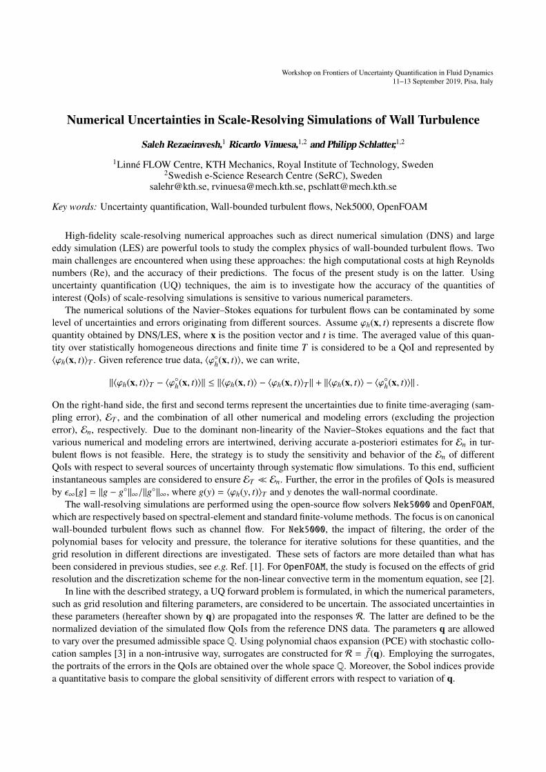
Figure 1: Isolines of (a) ǫ∞[〈u〉] % and (b) ǫ∞[K] % of turbulent channel flow in the admissible ∆x+-∆z+ space,
when using Nek5000. In all the simulations, Reτ = 300 and ∆y+w = 0.5.
ǫ[〈uτ〉] ǫ∞[〈u〉] ǫ∞[urms] ǫ∞[vrms] ǫ∞[wrms]ǫ∞[〈u′v′〉] ǫ∞[K]0.0
0.2
0.4
0.6
0.8
1.0
ST
∆x+ ∆z
+
(a)ǫ[〈uτ〉] ǫ∞[〈u〉] ǫ∞[urms] ǫ∞[vrms] ǫ∞[wrms]ǫ∞[〈u′v′〉] ǫ∞[K]
0.0
0.2
0.4
0.6
0.8
1.0
ST
∆x+ ∆z
+
(b)
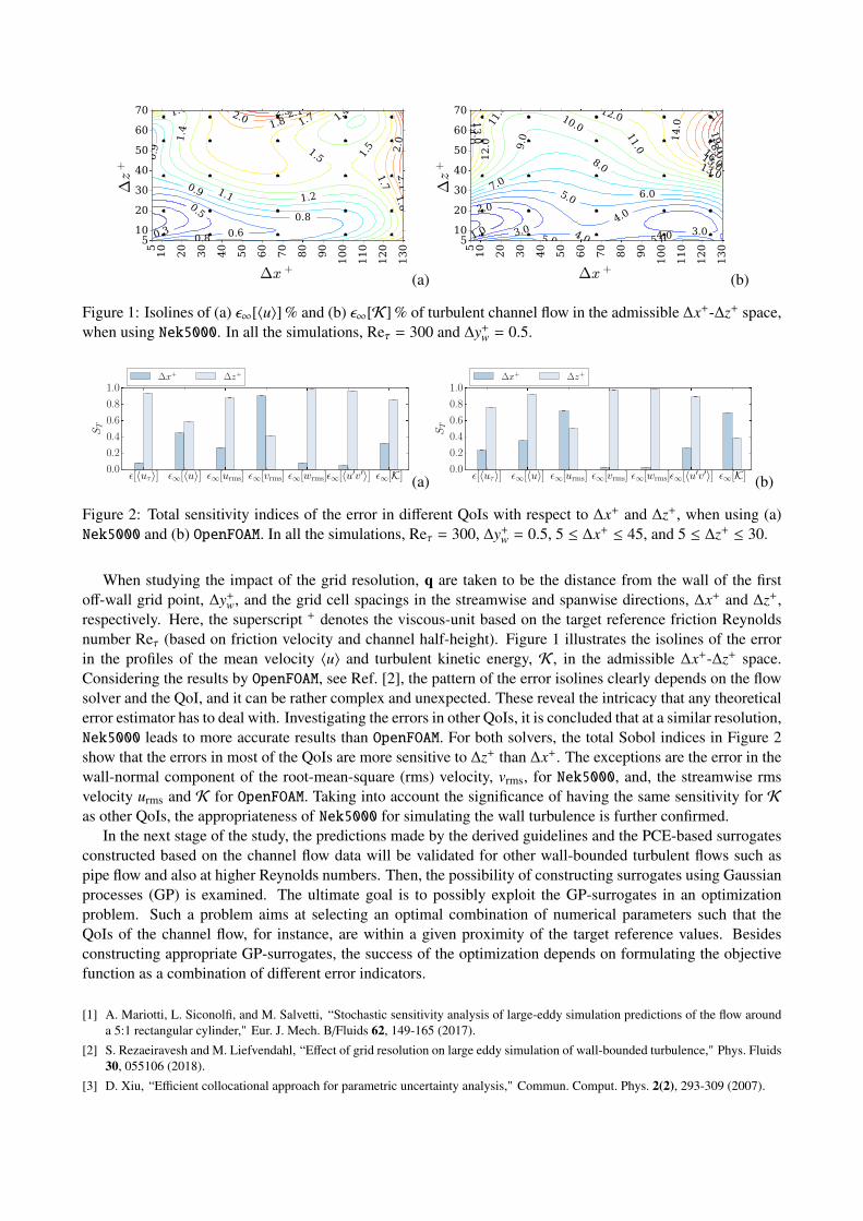
Figure 2: Total sensitivity indices of the error in different QoIs with respect to ∆x+ and ∆z+, when using (a)
Nek5000 and (b) OpenFOAM. In all the simulations, Reτ = 300, ∆y+w = 0.5, 5 ≤ ∆x+ ≤ 45, and 5 ≤ ∆z+ ≤ 30.
When studying the impact of the grid resolution, q are taken to be the distance from the wall of the first
off-wall grid point, ∆y+w, and the grid cell spacings in the streamwise and spanwise directions, ∆x+ and ∆z+,
respectively. Here, the superscript + denotes the viscous-unit based on the target reference friction Reynolds
number Reτ (based on friction velocity and channel half-height). Figure 1 illustrates the isolines of the error
in the profiles of the mean velocity 〈u〉 and turbulent kinetic energy, K , in the admissible ∆x+-∆z+ space.
Considering the results by OpenFOAM, see Ref. [2], the pattern of the error isolines clearly depends on the flow
solver and the QoI, and it can be rather complex and unexpected. These reveal the intricacy that any theoretical
error estimator has to deal with. Investigating the errors in other QoIs, it is concluded that at a similar resolution,
Nek5000 leads to more accurate results than OpenFOAM. For both solvers, the total Sobol indices in Figure 2
show that the errors in most of the QoIs are more sensitive to ∆z+ than ∆x+. The exceptions are the error in the
wall-normal component of the root-mean-square (rms) velocity, vrms, for Nek5000, and, the streamwise rms
velocity urms and K for OpenFOAM. Taking into account the significance of having the same sensitivity for K
as other QoIs, the appropriateness of Nek5000 for simulating the wall turbulence is further confirmed.
In the next stage of the study, the predictions made by the derived guidelines and the PCE-based surrogates
constructed based on the channel flow data will be validated for other wall-bounded turbulent flows such as
pipe flow and also at higher Reynolds numbers. Then, the possibility of constructing surrogates using Gaussian
processes (GP) is examined. The ultimate goal is to possibly exploit the GP-surrogates in an optimization
problem. Such a problem aims at selecting an optimal combination of numerical parameters such that the
QoIs of the channel flow, for instance, are within a given proximity of the target reference values. Besides
constructing appropriate GP-surrogates, the success of the optimization depends on formulating the objective
function as a combination of different error indicators.
[1] A. Mariotti, L. Siconolfi, and M. Salvetti, “Stochastic sensitivity analysis of large-eddy simulation predictions of the flow around
a 5:1 rectangular cylinder," Eur. J. Mech. B/Fluids 62, 149-165 (2017).
[2] S. Rezaeiravesh and M. Liefvendahl, “Effect of grid resolution on large eddy simulation of wall-bounded turbulence," Phys. Fluids
30, 055106 (2018).
[3] D. Xiu, “Efficient collocational approach for parametric uncertainty analysis," Commun. Comput. Phys. 2(2), 293-309 (2007).

Workshop on Frontiers of Uncertainty Quantification in Fluid Dynamics
11–13 September 2019, Pisa, Italy
Stochastic approach for the evaluation of aerodynamic flow over irregular rough
walls
Federico Bernardoni, 1 Umberto Ciri, 1 Maria Vittoria Salvetti2 and Stefano Leonardi,1∗
1 Department of Mechanical Engineering, University of Texas at Dallas, TX, USA2DICI, University of Pisa, Italy
Key words: Stochastic Analysis, Roughness
Despite increased attention over recent years, our knowledge of the flow over rough walls is far from com-
plete. For example, for an irregular rough wall we cannot predict with good accuracy what is the drag coeffi-
cient. Due to the large number of geometrical parameters affecting the flow it has been challenging to develop
parameterizations of rough walls. Given the high computational cost of performing deterministic numerical
simulations for each different surface, several models have been developed to describe the aerodynamic flow
field in terms of parameters such as the drag coefficient (Cd), the roughness length or the roughness function
(see for example [1], [2], [3]). However, they all work well in the limited application sector for which they have
been developed. The aim of the present study is to compute with a low computational cost the aerodynamic
parameters for an irregular roughness using a stochastic surrogate model which relies on high fidelity data ob-
tained from Direct Numerical Simulations (DNS). The streamwise and spanwise wavelengths of the roughness
are assumed as uncertain features able to describe the geometry of the rough surface and a response model is
then built in order to evaluate the drag coefficient, the roughness function and the velocity fluctuations by using
the Polynomial Chaos Expansion (PCE). Then, given any Probability Density Function (PDF) describing a gen-
eral rough surface, the aerodynamic properties of the overlying flow are evaluated using stochastic techniques
avoiding the need of carrying out computationally expensive numerical simulations.
The roughness is modeled as a sinusoidal wavy-wall within a channel with x, y and z as the coordinates in
the streamwise, vertical and spanwise directions, a as the amplitude of the roughness, λx and λz as respectively
the streamwise and spanwise wavelengths. The spanwise wavelength is allowed to vary between λz/2a = 10
and λz/2a = 100 while the streamwise wavelength between λx/2a = 1 and λx/2a = 20; the amplitude is kept
constant and equal to a = 0.1h, where h is the half height of the channel.
The response model able to efficiently evaluate each aerodynamic quantity of interest for each different
uniform roughness is obtained using a 5th order PCE for modelling of streamwise wavelength variability and
a 3th order polynomial for the spanwise wavelength. Gauss-Legendre polynomials were employed. Thus, in
order to compute the coefficients of the polynomials, a total of 24 DNSs of a channel flow were carried out
with regular roughness on the bottom wall, each of them characterized by different combinations of λz/2a
and λx/2a. All the simulations are performed at Reb = (Ubh)/ν = 2, 800, where Ub is the bulk velocity h
is the half height of the channel and ν is the kinematic viscosity. Periodic boundary conditions are applied
in both streamwise and spanwise directions; the walls are modeled with the immersed boundary technique
[4]. When an irregular rough surface is considered, the PDFs of the streamwise and spanwise wavelengths,
chosen as representative parameters, are extracted by treating the shape of the rough surface as a signal and
performing on it a time-frequency analysis using the Wavelet transform. Therefore, the ridges of the scalogram
that is obtained represent at each location in space what are the most probable wavelengths in the considered
roughness. Thus, the PDFs of both streamwise and spanwise wavelength across the entire domain are evaluated
and taken as input for the stochastic analysis.
Using the Latin Hypercube Sampling method (LHS), the irregular roughness is represented in the stochastic

0
0.05
0.1
0 5 10 15 20
PD
F
λx/2a
(a)
0
500
1000
1500
2000
2500
3000
3500
4000
0.0018 0.0021 0.0024 0.0027 0.003
PD
F
λ/2a (b)
Figure 1: (a) PDF of the streamwise wavelength of the validation rough surface; (b) comparison of the Cd
from the SA and from DNS: value of Cd from the DNS: Cd = 2.30 · 10−3; mean value from SA,
µ(Cd) = 2.29 · 10−3; mean value ± standard deviation of Cd from SA; PDF of Cd from SA.
approach (SA) as a set of samples; each of them corresponds to a roughness with uniform streamwise and
spanwise wavelength. The drag coefficient, the roughness function and the turbulence intensities are then
easily evaluated by means of the PCE response model. Finally, all the responses are statistically analyzed in
order to obtain the PDF and mean value of each aerodynamic quantity of interest over the considered irregular
rough wall.
So far the proposed approach has been validated considering only a random variability of the streamwise
wavelength of the roughness and keeping constant λz/2a = 100. Figure 1a) shows the PDF of the streamwise
wavelengths of the surface considered for the validation process. The drag coefficient, the roughness function
and the turbulence intensities over this irregular roughness have been evaluated with the proposed stochastic
approach and compared with those obtained in a DNS carried out on the same surface. Figure 1b) shows, as an
example, the PDF obtained from the SA of the drag coefficient. The comparison between the mean value (µ) of
Cd from SA (dashed line) and the mean Cd from the DNS over the entire rough surface (solid line) is reported
showing a good agreement. From the PDF it is also possible to obtain some information about the variability
of Cd on the surface. For instance, it appears that there are two values of Cd which are highly probable to occur
locally on different roughness elements: one is close to the mean value while the other one is significantly
higher. From the available response surface, the value of λx/2a leading to these high values of Cd and, thus
contributing to the total drag, could be identified.
Summarizing, a stochastic approach based on PCE has been presented, which allows the aerodynamic quan-
tities characterizing the flow over an irregular roughness distribution to be evaluated without the need of car-
rying out specific numerical simulations for each different roughness, largely reducing in this way the compu-
tational costs. Considering the variability of only the streamwise wavelength of the sinusoidal roughness, the
comparison with DNS data has shown a very good agreement in terms of mean values over the rough surface of
the quantities of interest. The validation of the proposed approach for irregular surface in both the streamwise
and spanwise directions is ongoing and the results will be presented in the final paper.
[1] Flack K. A., Schultz M. P. : Review of Hydraulic Roughness Scales in the Fully Rough Regime, J. Fluids Eng., 132, 041203
(2010).
[2] Macdonald R.W., Griffiths R.F., Hall D.J. : An improved method for the estimation of surface roughness of obstacle arrays, Atmos.
Environ., 32, 1857–1864 (1998).
[3] Zhu X., Iungo G. V., Leonardi S., Anderson W. : Parametric Study of Urban-Like Topographic Statistical Moments Relevant to a
Priori Modelling of Bulk Aerodynamic Parameters, Boundary-Layer Meteorol, 162, 231–253 (2017).
[4] Orlandi P., Leonardi S. : DNS of turbulent channel flows with two- and three-dimensional roughness, J. Turbul., 7, 1–22 (2006).

Keynote Lecture - S. Mishra - UQ for nonlinear hyperbolic PDEs with statisticalsolutions
Session Chair: L. TamelliniAuditorium

Workshop on Frontiers of Uncertainty Quantification in Fluid Dynamics
11–13 September 2019, Pisa, Italy
UQ for nonlinear hyperbolic PDEs with statistical solutions
Siddhartha Mishra
ETH Zürich, Switzerland – [email protected]
Key words: Uncertainty Quantification, Non Linear Hyperbolic PDEs
Hyperbolic systems of conservation laws arise in a wide variety of problems in physics and engineering.
Uncertainty quantification (UQ) is essential for these models on account of measurement errors for inputs and
possible chaotic dynamics of the system. However, efficient UQ is very challenging due to the low regularity
of underlying solutions, on account of shocks and turbulence as well as the need for possibly high dimensional
description of the probability space. We present the recently proposed concept of statistical solutions as a
suitable UQ framework for these PDEs. Statistical solutions are time-parameterized probability measures on
integrable functions and we present a convergent Monte Carlo algorithm for computing them. Moreover, we
will present several alternatives to accelerate the baseline Monte Carlo method. These include Multi-level
Monte Carlo (MLMC), Quasi-Monte Carlo (QMC) and machine learning algorithms and we evaluate their
applicability in this context.

SW3 – Methodology ISession Chair: L. Tamellini
Auditorium
Workshop on Frontiers of Uncertainty Quantification in Fluid Dynamics
11–13 September 2019, Pisa, Italy
Iterative construction of quadrature rules for Bayesian prediction
Laurent van den Bos1 and Benjamin Sanderse2
1 Centrum Wiskunde & Informatica, Amsterdam, The Netherlands – [email protected]
2 Centrum Wiskunde & Informatica, Amsterdam, The Netherlands – [email protected]
Key words: Numerical integration, Uncertainty Propagation, Bayesian prediction
A novel numerical integration framework for the purpose of uncertainty propagation in a Bayesian framework
is proposed (this is also known as Bayesian prediction). The framework is based on quadrature rules, i.e.
weighted averages of function evaluations, that are constructed as a subset of a large number of samples from the
distribution [1, 2]. The goal is to determine integrals of the following form:
E[u] =
∫Ω
u(x) q(x | z) dx.
Here, x is a vector with uncertain parameters defined in the space Ω ⊂ Rd (d = 1, 2, 3, . . .) with probability
distribution q(x | z). The function u describes a costly computational model and is typically the numerical
solution of a system of partial differential equations that model fluid flow for given parameters x.
The key challenge is that the distribution q(x | z) is a posterior. It follows from the statistical model that
describes the relation between the model and measurement data [4]. The posterior is not known explicitly and
depends directly on the computationally costly model u. The idea of the proposed approach is to iteratively
add nodes to a quadrature rule such that it converges to a quadrature rule that determines weighted integrals
−0.5 0 0.5 1 1.5−1
−0.5
0
0.5
1
x
y
−1 −0.5 0 0.5 1
Cp
(a) Mean
−0.5 0 0.5 1 1.5−1
−0.5
0
0.5
1
x
y
0 0.05 0.1 0.15 0.2 0.25
Cp
(b) Standard deviation
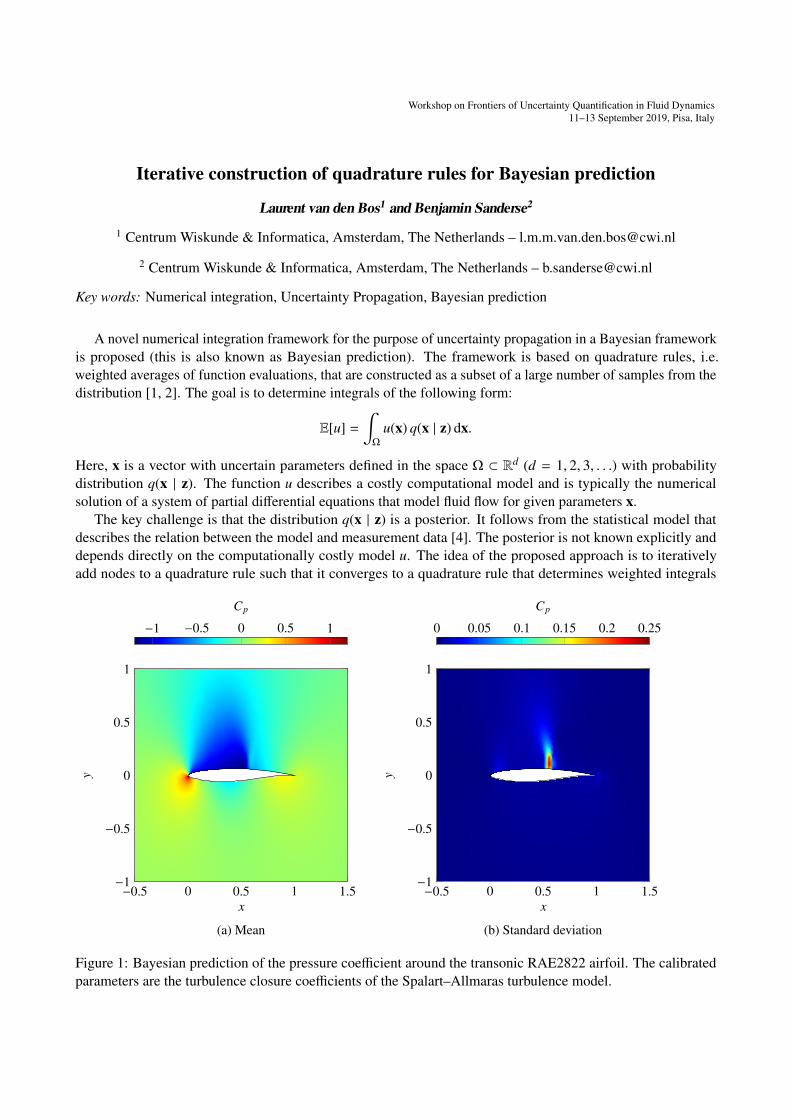
Figure 1: Bayesian prediction of the pressure coefficient around the transonic RAE2822 airfoil. The calibrated
parameters are the turbulence closure coefficients of the Spalart–Allmaras turbulence model.

with respect to the posterior. The nodes are nested, such that costly model evaluations are reused in subsequent
iterations. The rules are constructed such that they have positive weights, which ensures that the quadrature rule
estimations converge.
The efficiency and applicability of the integration framework is demonstrated by predicting the transonic
flow over the RAE2822 airfoil, where the turbulence closure coefficients of the Spalart-Allmaras turbulence
model are inferred from measurement data (see Figure 1). The results are comparable with existing literature on
this topic [3], demonstrating that the proposed approach is a promising alternative to existing approaches for
Bayesian model calibration and prediction.
[1] L. M. M. van den Bos, B. Koren, and R. P. Dwight. Non-intrusive uncertainty quantification using reduced cubature rules. Journal
of Computational Physics, 332:418–445, 2017. 10.1016/j.jcp.2016.12.011.
[2] L. M. M. van den Bos, B. Sanderse, W. A. A. M. Bierbooms, and G. J. W. van Bussel. Generating nested quadrature rules with
positive weights based on arbitrary sample sets. ArXiV 1809.09842, 2018.
[3] W. N. Edeling, P. Cinnella, R. P. Dwight, and H. Bijl. Bayesian estimates of parameter variability in the k − ǫ turbulence model.
Journal of Computational Physics, 258:73–94, 2014. 10.1016/j.jcp.2013.10.027.
[4] M. C. Kennedy and A. O’Hagan. Bayesian calibration of computer models. Journal of the Royal Statistical Society: Series B
(Statistical Methodology), 63(3):425–464, 2001. 10.1111/1467-9868.00294.

Workshop on Frontiers of Uncertainty Quantification in Fluid Dynamics
11–13 September 2019, Pisa, Italy
A stochastic Galerkin reduced basis method for parametrized
convection-diffusion-reaction equations based on adaptive snapshots
Christopher Müller,1 and Jens Lang,1
1Department of Mathematics , TU Darmstadt, [email protected]
Key words: Stochastic Galerkin, Finite elements, Model order reduction, Adaptive methods, Convection-diffusion-reaction equations
We consider convection-diffusion-reaction equations with parametrized random and deterministic inputs.
For a fixed value of the deterministic parameters, the problem reduces to a linear elliptic PDE with random
input data and statistical moments of its solution such as mean and variance can be approximated by a stochastic
Galerkin finite element (SGFE) method. There are scenarios, like robust optimization, where these statistical
information must be computed for numerous different values of the deterministic parameter. In these particular
cases, it can be computationally attractive to conduct a certain number of expensive preliminary computations
in order to set up a reduced order model. The reduction of the overall computational costs than results from
the fact that this reduced order model, here a so-called stochastic Galerkin reduced basis (SGRB) model [1], is
low dimensional and can thus be evaluated cheaply for each deterministic parameter value. We construct the
SGRB model using a proper orthogonal decomposition (POD) of SGFE snapshots. As a consequence, there is
no need for an additional sampling procedure in order to evaluate the statistics of the solution of the reduced
order model.
Computing the snapshots for the SGRB model means that several different SGFE problems have to be to
solved, each associated with a large block-structured system of equations. When the costs of solving these
systems are too high, adaptive methods can be applied to find favorable discrete spaces and lower the computa-
tional burden of the preliminary computations. Using an adaptive approach leads, however, to a setting where
the snapshots belong to different SGFE subspaces. This fact interferes the standard POD procedure which re-
lies on snapshots from the same static subspace. It is still possible to construct a reduced order model based
on adaptive snapshots [2] but there are different theoretical and numerical issues that emerge. We address the
issues that arise for the particular case of an SGRB model constructed with adaptively chosen SGFE snapshots
and illustrate our findings based on a convection-diffusion-reaction test case where the convective velocity is
the deterministic parameter and the parametrized reactivity field is the random input.
[1] S. Ullmann and J. Lang, “Stochastic Galerkin reduced basis methods for parametrized linear elliptic PDEs", arXiv: 1812.08519,
(2018).
[2] S. Ullmann, M. Rotkovic and J. Lang, “POD-Galerkin reduced-order modeling with adaptive finite element snapshots”, J. Comput.
Phys. 325, (2016).

Workshop on Frontiers of Uncertainty Quantification in Fluid Dynamics
11–13 September 2019, Pisa, Italy
Multiscale Uncertainty Quantification with Arbitrary Polynomial Chaos
Nick Pepper,1 Francesco Montomoli,1 and Sanjiv Sharma 2
1UQLab, Imperial College London, UK – [email protected]
2Airbus, UK
Key words: Uncertainty quantification; multiscale modelling; stochastic upscaling; polynomial chaos expan-sions; SAMBA; PDF matching
This work presents a methodology for upscaling uncertainty in multiscale models. The problem is rele-
vant to aerospace applications where it is necessary to estimate the reliability of a complete part such as an
aeroplane wing from scarce data of coupons. The upscaling equivalence is defined by a Probability Density
Function (PDF) matching approach. By representing the inputs of the coarse model with a Polynomial Chaos
Expansion (PCE) the stochastic upscaling problem can be recast as an optimisation problem. In order to define
a data driven framework able to deal with scarce data a Sparse Approximation for Moment Based Arbitrary
Polynomial Chaos is used. Sparsity allows the solution of this optimisation problem to be made less compu-
tationally intensive than upscaling methods relying on Monte Carlo sampling. Moreover this makes the PDF
matching method more viable for industrial applications where individual simulation runs may be computation-
ally expensive. Arbitrary Polynomial Chaos is used to allow the framework to use directly experimental data.
Finally, the difference between the distributions is quantified using the Kolmogorov-Smirnov (KS) distance and
the method of moments in the case of a multi-objective optimisation. It is shown that filtering of dynamical
information contained in the fine scale by the coarse model may be avoided through the construction of a low
fidelity, high order model.

SW4 – Methodology IISession Chair: S. Mishra
Auditorium

Workshop on Frontiers of Uncertainty Quantification in Fluid Dynamics
11–13 September 2019, Pisa, Italy
Intrusive Generalized Polynomial Chaos for the solution of the unsteady
Navier-Stokes Equations
C. F. Silva,1 P. Bonnaire1, S. Schuster1 and P. Pettersson,2
1 Technical University of Munich (TUM), Germany– [email protected]
2 Norwegian Research Center (NORCE), Norway
Key words: Uncertainty quantification, Computational Fluid Dynamics, generalized Polynomial Chaos.
Aiming at a robust design by means of Computational Fluid Dynamics (CFD) means not only aiming at
precisely quantifying CFD output variables, but also at quantifying the sensitivity of the CFD outputs to input
variations, and at evaluating probability density functions of the CFD outputs given input uncertainties. In other
words, robust design means introducing rigorous Uncertainty Quantification (UQ) in the CFD design chain.
The present work is devoted to the study of (intrusive) generalized Polynomial Chaos (gPC) [1, 2] on un-
steady CFD that exhibit limit cycles as solutions. Previous work on the long-time integration of oscillatory
problems include the adaptive multi-element generalized polynomial chaos expansion [3], and Haar wavelet
expansions [4]. Nevertheless, these approaches typically lead to very large number of basis functions. In the
context of non-intrusive polynomial chaos, a time warping method was proposed in [5] to counteract that lim-
itation. In this work we implement the asynchronous time integration proposed by [6], which is a method that
shares the same time-scaling philosophy of [5]. By doing so, UQ is performed by solving only two simulations:
one deterministic (reference) simulation and one computation on the set of extended equations that characterize
the system with uncertainties.
The incompressible and compressible set of Navier-Stokes equations are discretized by finite volumes and
finite differences, respectively. (i) The incompressible approach makes use of a Rhie-Chow interpolation. A
quasi-implicit scheme for time discretization is implemented, where the convective part is linearized by a
Crank-Nicolson approach. Additionally, the explicit Heun’s method can be chosen as time advancing scheme.
(ii) The compressible solver makes use of an adapted MacCormack method. This is an explicit finite difference
method that utilizes a predictor-corrector time stepping scheme. The deterministic version of both solvers
(incompressible and compressible) is validated against analytical flow solutions and experimental data. In
particular, we focus on flows characterized by the Karman-vortex street, which develops due to flow separation
around a bluff body.
A stochastic Galerkin projection is applied to both incompressible and compressible Navier-Stokes equa-
tions. Orthogonal polynomials are considered for the expansion and subsequent basis projection. Based on
the work of [6], we additionally scale time at each time step for each realization. The goal here is to mimic
an ‘in phase’ behaviour of the stochastic solutions. We study the Karman-Vortex street that is perturbed by an
uncertain inlet velocity and laminar viscosity of the flow. We show that by introducing a ‘local clock’ in the
stochastic domain it is possible to quantify the frequency of the limit cycles and the corresponding shift due
to the aforementioned uncertainties . Additionally, we avoid the well-known problem (blow-up) of gPC when
implemented in uncertain (long) time-dependent problems.

(a) Deterministic simulation (b) Expected value (igPC) (c) Standard deviation (igPC)
Figure 1: Deterministic and stochastic simulation for Re = 100 with uncertain inlet velocity of u1/u0 = 0.2.
Figure 1a shows one snapshot of the velocity field at time 3.87s, where no uncertainties are considered.
Figures 1b and 1c show the expected value and standard deviation of this flow at the same instant of time,
where uncertainty has been considered in the inlet velocity. By analyzing the field of standard deviation for
several instants of time, it is possible to assess regions where the input uncertainties do not strongly affect the
velocity field. This kind of study is of relevance since it suggests locations where measurements can be obtained
that are not strongly affected by the uncertainties present in the system.
[1] R. G. Ghanem and P. D. Spanos. Stochastic Finite Elements: A Spectral Approach. Courier Corporation, 1991.
[2] D. Xiu and G. E. Karniadakis. The Wiener–Askey polynomial chaos for stochastic differential equations. SIAM journal on scientific
computing, 24(2):619–644, 2002.
[3] X, Wan and G, E. Karniadakis. An adaptive multi-element generalized polynomial chaos method for stochastic differential equa-
tions. Journal of Computational Physics 209 (2):617-642, 2005
[4] O. P. Le Maıtre, O. M. Knio, H. N. Najm and R. G. Ghanem Uncertainty propagation using Wiener-Haar expansions Journal of
computational Physics 197 (1):28-57, 2004.
[5] C. V. Mai and B. Sudret. Surrogate models for oscillatory systems using sparse polynomial chaos expansions and stochastic time
warping SIAM/ASA Journal on Uncertainty Quantification 5 (1):540-571, 2017
[6] O. P. Le Maıtre, L. Mathelin, O. M. Knio and M. Y. Hussaini. Asynchronous time integration for polynomial chaos expansion of
uncertain periodic dynamics Discrete Contin. Dyn. Syst, (28):199–226, 2010.

Workshop on Frontiers of Uncertainty Quantification in Fluid Dynamics
11–13 September 2019, Pisa, Italy
RBF-FD Meshless Solver to Investigate the Propagation of Geometric
Uncertainty in Laminar Flows
Riccardo Zamolo1
and Lucia Parussini2
1DIA, University of Trieste, Italy – [email protected]
2DIA, University of Trieste, Italy – [email protected]
Key words: Polynomial Chaos, Meshless, RBF-FD, Spectral Element Method.
In this work we consider the uncertainty quantification in incompressible, laminar, 2D steady-state fluid dy-
namics problems where the domain geometries are described by stochastic variables. Such stochastic problems
arise in practical applications where geometric uncertainties are due to manufacturing tolerances which lead to
uncertainties in the performance of the product. The Non-Intrusive Polynomial Chaos method [1] is employed
to estimate statistical quantities regarding the flow fields, i.e., velocity, pressure and temperature. The advantage
of the non-intrusive formulation is that existing deterministic solvers can be employed as black boxes without
any modification since the random response is based on a set of deterministic response evaluations.
An isothermal flow over a backward-facing step is initially considered, where the geometric uncertainty is
given by the position of the step corner. The deterministic fluid-flow problems are solved by three different
approaches: a Fictitious Domain/Least Squares Spectral Element Method [2], a Finite Volume Method and a
Radial Basis Function-generated Finite Differences (RBF-FD) Meshless Method [3]. A comparison between
the methods is then carried out, showing a very good agreement in terms of estimated statistical quantities.
Due to its geometric flexibility and its ability to easily deal with complex-shaped domains, the RBF-FD
method is subsequently chosen and employed for the efficient prediction of geometric uncertainty effects in
different fluid dynamics test case problems. Furthermore, the order of accuracy of the RBF-FD method can be
easily increased by using larger stencils, i.e., more nodes in the local RBF expansion.
[1] S. Hosder, R. Walters and R. Perez, “A Non-Intrusive Polynomial Chaos Method for Uncertainty Propagation in CFD Simulations,"
In Proceedings of 44th AIAA aerospace sciences meeting and exhibit, 1-19 (AIAA, Reston, VA, 2006).
[2] L. Parussini, “Fictitious Domain Approach via Lagrange Multipliers with Least Squares Spectral Element Method," Journal of
Scientific Computing 37(3), 316-335 (2008).
[3] B. Fornberg and N. Flyer, “Solving PDEs with Radial Basis Functions" Acta Numerica 24, 215-258 (2015).

Workshop on Frontiers of Uncertainty Quantification in Fluid Dynamics11–13 September 2019, Pisa, Italy
Wavelet-Assisted Multi-Element Polynomial Collocation Method
Robert Sawko1, Małgorzata J. Zimoń1 and Alex Skillen2
1IBM Research, Daresbury Laboratory, UK – Corresponding author: [email protected] and Technology Facilities Council, Daresbury Laboratory, UK
Key words: polynomial chaos, polynomial annihilation, wavelet transform, surrogate modelling
Polynomial chaos (PC) is a widely used approach in uncertainty quantification (UQ) in compu-tational fluid dynamics (CFD) studies. It represents the simulator output as a series expansion inthe input parameters [5, 7] and has high rates of convergence for smooth quantities of interest. Inits non-intrusive form, it treats the model as a black box and uses the results to estimate expansioncoefficients either through regression or spectral projection.
Although very efficient for approximating low-order and smooth functions, the analysis becomesexpensive or even infeasible if the response of the system is irregular, contains sharp transitions, steepgradients, or discontinuities. Using global basis may never lead to accurate approximations. To tacklethis issue, a modification of PC for low-regular problems was proposed by Wan and Karniadakis [6].Its non-intrusive formulation was later introduced by Foo et al. [2] and referred to as multi-elementpolynomial collocation method (ME-PCM). In following years, variations of this approach have beenproposed, attempting to transform the problem into one that can be tackled with piecewise basisby first identifying the location of discontinuities (edge tracking) with the use of, e.g., polynomialannihilation [1, 3].
In this talk, we propose a two staged approach to tackle piecewise continuous or piecewise smoothfunctions. We first perform a random space decomposition coupled with local polynomial order esti-mation and then construct PC surrogates for each sub-domain. We use continuous wavelet transform(CWT) [4] to analyse local changes in power spectra and determine boundary separation by classifyingthe responses into related groups. The method is first demonstrated on model functions proposed inprevious work on discontinuities and highly varying regions [1]. Example of such study is shown inFig. 1. After dividing the parametric space, the points used for classification are re-used to generatelocal polynomial representation with determined number of terms.
−1.00 −0.75 −0.50 −0.25 0.00 0.25 0.50 0.75 1.00
Position
0
1
2
3
4
Freq
uenc
y
−35
−30
−25
−20
−15
−10
−5
0
5
100
101
Frequencies [Hz]
0.0
0.5
1.0
1.5
2.0
2.5
Am
plit
udes
Group 1Group 2
Figure 1: The scalogram (left) and classification (right) of functions based on an example in [1].
We then move to a quantity of interest from transient turbulent flow inside a U-bend pipe. A set of

Figure 2: Right: wall temperature is collected for several rings along the streamwise dimension of thepipe. Left: a visualisation of turbulent flow.
Reynolds-averaged Navier–Stokes equations (RANS) of hot shock waves is solved with the uncertaininput characterising the magnitude of the temperature jump. In the downstream of the pipe, theflow becomes unstably stratified leading to development of highly turbulent structures. We collectwall surface temperatures from rings as shown in Fig. 2. We then study the response temperature foreach point using the method proposed above. The response exhibits piecewise smoothness and thewavelet-assisted approach described above performs well in cross-validation tests and small samplesizes.
Two primary features of the proposed method are an automatic detection of piecewise continuousor smooth regions and estimation of a maximum order required for the subsequent PC expansion. De-tailed description of the adaptive method is presented. The results on model functions and simulateddata are compared with other edge-detection analyses in terms of computational efficiency and accu-racy of approximation for problems with low regularity. We show that application of wavelet-assistedapproach for transient heat transfer simulations can result in cost-effective and accurate surrogate. Atthe end of the talk, we draw conclusions and suggests further improvements.
[1] R. Archibald, A. Gelb, and J. Yoon, Polynomial fitting for edge detection in irregularly sampled signals andimages, SIAM Journal of Numerical Analaysis, 43 (2006), pp. 259–279.
[2] J. Foo, X. Wan, and G. E. Karniadakis, The multi-element probabilistic collocation method (ME-PCM): Erroranalysis and applications, Journal of Computational Physics, 227 (2008), pp. 9572–9595.
[3] J. D. Jakeman, R. Archibald, and D. Xiu, Characterization of discontinuities in high-dimensional stochasticproblems on adaptive sparse grids, Journal of Computational Physics, 230 (2011), pp. 3977–3997.
[4] S. Mallat, A wavelet tour of signal processing, Elsevier, 1999.[5] T. J. Sullivan, Introduction to Uncertainty Quantification, vol. 63, Springer, 2015.[6] X. Wan and G. E. Karniadakis, An adaptive multi-element generalized polynomial chaos method for stochastic
differential equations, Journal of Computational Physics, 209 (2005), pp. 617–642.[7] D. Xiu, Numerical Methods for Stochastic Computations: A Apectral Method Approach, Princeton University Press,
2010.

SW5 – Poster short presentationsSession Chair: M.V. Salvetti
Auditorium

Workshop on Frontiers of Uncertainty Quantification in Fluid Dynamics
11–13 September 2019, Pisa, Italy
Multi-continuum models for conjugate transport in random heterogeneous
media and application to molecular communication
Federico Municchi, John Couch, and Matteo Icardi
School of Mathematical Sciences, University of Nottingham, UK – [email protected]
Key words: heterogeneous media, dual porosity, multi-rate mass transfer, conjugate transfer, subsurface flows
In fluid dynamics, conjugate heat/mass transfer refers to the problem of coupling a "mobile" fluid domain,
where flow (Stokes or Navier-Stokes) and transport (advection-diffusion), with "immobile" inclusions, where
diffusion dominates. This is therefore relevant to a wide range of problems in subsurface flows, porous me-
dia, and heat transfer applications. Fully resolved simulations are often unfeasible due to their complexity in
capturing the possibly complicated, heterogeneous, and often uncertain micro-structures.
In this work, we derive a new upscaled (averaged) multi-continuum multi-rate transfer model [1] between
a mobile phase and an immobile phase that does not require to resolve the interfaces between the regions,
and implement it within the three-dimensional finite-volumes OpenFOAM(R) library. We show this is partic-
ularly suitable for Uncertainty Quantification studies where uncertainties in the material composition can be
represented by uncertain parameters (rather than geometry) and propagate through the model.
We then focus on a simplification, leading to the so-called dual-porosity model, solve it analytically in one-
dimension, and study the effects of uncertainties in the different parameters on specific quantities of interest for
molecular communication applications. Molecular communication is a recently developed and very active field
of research in communication theory, that deals with the design of low-energy communication strategies, based
on the transport of particles and molecules. To design optimal and robust communication, we define a family of
functionals of the fundamental solution of the PDE, representing communication-based optimality measures,
and study their robustness on the input uncertainty.
[1] F. Municchi and M. Icardi, “Generalised Multi-Rate Models for conjugate transfer in heterogeneous materials," arXiv:1906.01316
[physics.comp-ph]
[2] Y. Fang, W. Guo, M. Icardi, A. Noel, and N. Yang, “Molecular Information Delivery in Porous Media," arXiv:1903.03738 [cs.IT]

Workshop on Frontiers of Uncertainty Quantification in Fluid Dynamics
11–13 September 2019, Pisa, Italy
Enhancing the uncertainty quantification of pyroclastic density current dynamics
in the Campi Flegrei caldera.
Andrea Bevilacqua,1 Mattia de Michieli Vitturi,1 Tomaso Esposti Ongaro,1 and Augusto Neri,1
1INGV, Sezione di Pisa, Italy – [email protected]
Key words: Uncertainty quantification, Geophysical Flows, Volcanic Hazard Assessment
Figure 1: Temporal PDC invasion hazard map based on the box
model integral equations, the vent opening map and the areal size
distributions in [2], and the temporal estimates assuming that the
volcano entered a new eruptive epoch in A.D. 1538 (see [1]). Con-
tours and colors indicate the mean percentage probability of PDC
invasion in the next 10 years.
In this study we present a new ef-
fort to improve the uncertainty quantifi-
cation (UQ) of pyroclastic density cur-
rent dynamics in the Campi Flegrei cal-
dera, thanks to the implementation of a
new 2D depth-averaged granular flow mo-
del in the Monte Carlo simulation of key-
controlling variables.
Campi Flegrei caldera is an active and
densely populated volcanic area in the ur-
ban neighborhood of Napoli, characteri-
zed by the presence of many dispersed
cones and craters, and by a caldera wall
more than one hundred meters high, to-
wards East. Basic mapping of pyroclastic
density currents1 (PDC) hazard at Campi
Flegrei has been already reported in pre-
vious studies: some related to field recon-
struction and numerical modeling of spe-
cific past eruptions or individual scena-
rios, while others endeavored to produce
specific or integrated PDC hazard maps in
which the variability of important parame-
ters of the volcanic system was explicitly
accounted for. In particular, [4, 2] obtai-
ned quantitative estimates of probabilistic PDC hazard, based on the implementation of a simplified kinematic
invasion model able to represent main topographic effects. This model, called box model2, was extensively run
thousands of times in the Monte Carlo simulation varying vent location, eruptive scale, and time frequency of
the future activity (see Fig. 1).
In this study we build our effort upon the previous research started in [7, 5], and utilize the physical mo-
deling approach of [6], with the efficient numerical solution of depth-averaged equations for the flow mass and
momentum, considering the effects of basal and internal, velocity dependent, friction forces. The model des-
cribes the gas-particle mixture as a homogeneous flow, assuming a mechanism of particle deposition consistent
with that previously implemented in the box model.
UQ is performed by assuming three different components in the input space: (i) rheology parameters, (ii)
1laterally moving, buoyantly expanding mixtures of hot gas and fragmental particles.2a cylindrical box represents the current and changes in aspect ratio (i.e. stretches out) as the flow progresses.

volume scale, (iii) source location. Our statistical analysis focuses on the first two components, considering a
relatively small number of source locations or an uncertain source location inside a subregion of the caldera.
This is a first step before the exploration of the full spatial variability of the source location. The statistical
inversion of box model equations, varying the vent location (x, y) and the value of inundated area A, can provide
us with initial probability estimates for the volume scale of the PDC flow, either in terms of runout distance or
volume extent of the multiphase mixture (see Fig. 2). Our depth averaged model relies on these estimates for
setting up the volume scale of past flows. The calibration of rheology parameters is performed according to
that. Thus, the rheology and volume components of the input space are conjointly explored by means of Latin
Hypercube sampling, attempting a hierarchical conditioning on feasible inputs and plausible outputs [3].
Histograms of PDC runout
Runout w/out obstacles (km)
Pro
babili
ty
0 5 10 15 20
0.0
00.0
50.1
00.1
50.2
00.2
5
Log−Volume (log10 m3)
−
(a) (b)
(c) (d)
−
Histograms of Volume
84 6 10 12
0.0
0.1
0.2
0.3
0.4
0.5
0.6
Pro
babili
ty
Figure 2: Results of Monte Carlo simulation varying the vent opening location (x, y) and the value of inundated
area A, according to the probability models in [2]. Plot (a) shows the histograms of PDC runout obtained by
probabilistic inversion of the box model integral equations. Red colored bars assume a hypothetical kinetic
energy increase of three times in the flow front, due to the pressure rise before the obstacle [5]. Plot (b)
shows the histograms of PDC log-volume of the multiphase mixture of solid and gas obtained by probabilistic
inversion of the box model integral equations, with initial solid fraction of 1% volume. Different colors assume
different values of velocity of settling, 1.2 m/s and 0.05 m/s. These values correspond to particle diameters of
about 500µm and 25µm, and solid densities of 1000kg/m3 and 2000kg/m3 respectively.
[1] A. Bevilacqua, F. Flandoli, A. Neri, R. Isaia, S. Vitale, “Temporal models for the episodic volcanism of Campi Flegrei caldera
(Italy) with uncertainty quantification," Journal of Geophysical Research: Solid Earth 121, 11 (2016).
[2] A. Bevilacqua, A. Neri, M. Bisson, T. Esposti Ongaro, F. Flandoli, R. Isaia, M. Rosi, S. Vitale, “The effects of vent location, event
scale, and time forecasts on pyroclastic density current hazard maps at Campi Flegrei caldera (Italy)," Frontiers in Earth Science
5, 72 (2017).
[3] A. Bevilacqua, A.K. Patra, M.I. Bursik, E.B. Pitman, J.L. Macías, R. Saucedo, D. Hyman, “Probabilistic forecasting of plausible
debris flows from Nevado de Colima (Mexico) using data from the Atenquique debris flow, 1955," Natural Hazards Earth System
Science 19, 791-820 (2019).
[4] A. Neri, A. Bevilacqua, T. Esposti Ongaro, R. Isaia, W.P. Aspinall, M. Bisson, F. Flandoli et al., “Quantifying volcanic hazard at
Campi Flegrei caldera (Italy) with uncertainty assessment: 2. Pyroclastic density current invasion maps," Journal of Geophysical
Research: Solid Earth 120, 2330-2349 (2015).
[5] T. Esposti Ongaro, S. Orsucci and F. Cornolti, “A fast, calibrated model for pyroclastic density currents kinematics and hazard,"
Journal of Volcanology and Geothermal Research 327, 257 - 272 (2016).
[6] M. de’ Michieli Vitturi, T. Esposti Ongaro, G. Lari, and A. Aravena, “IMEXSfloW2D 1.0: a depth-averaged numerical flow model
for pyroclastic avalanches," Geoscientific Model Development, 12, 581-595 (2019).
[7] M. Todesco, A. Neri, T. Esposti Ongaro, P. Papale, and M. Rosi, “Pyroclastic flow dynamics and hazard in a caldera setting:
Application to Phlegrean Fields (Italy)," Geochemistry Geophysics Geosystems, 7, Q11003 (2006).

Workshop on Frontiers of Uncertainty Quantification in Fluid Dynamics
11–13 September 2019, Pisa, Italy
Intrusive Polynomial Chaos for CFD using OpenFOAM
Jigar Parekh∗, Roel Verstappen
Bernoulli Institute, University of Groningen, Netherlands
Key words: Intrusive Polynomial Chaos, OpenFOAM, Large Eddy Simulation
Computational Fluid Dynamics (CFD) involves simulating a physical system with a model. In such simu-
lations, uncertainties may arise from various sources, namely, initial and boundary conditions, material proper-
ties, model parameters etc. It is therefore important to compute the confidence intervals in the predictions made
using these CFD simulations. In order to reflect the uncertainty in the numerical solution, we need efficient
Uncertainty Quantification (UQ) methods.
Monte Carlo (MC) sampling is one of the simplest approach to carry out UQ analysis. However, due to its re-
quirement of large number of samples, MC method is computationally expensive for application in CFD. As an
alternative, we can use Polynomial Chaos (PC) representations to propagate and quantify uncertainty in CFD.
This approach is based on the spectral decomposition of the random variables in terms of basis polynomials con-
taining randomness and the unknown deterministic expansion coefficients, Y = f (x, q) =∑n
i=0 fi(x)φi(q). There
are two methods to determine these coefficients, namely, Intrusive Polynomial Chaos (IPC) and Non-intrusive
Polynomial Chaos (NIPC). In NIPC, these coefficients are approximated using quadrature for numerical evalu-
ation of the projection integrals, while in IPC, a reformulation of the original model is performed resulting in
governing equations for the PC mode strengths of the model output.
Figure 1: Probability distribution of the velocity in Poiseuille Flow with uncertain viscosity

Obviously, NIPC has an advantage that is uses the original model code without any modifications. However,
Xiu [1] asserts that the NIPC, in general, requires the solution of much larger set of equations as compared to
IPC, particularly for higher dimensional random space. Additionally, the aliasing error in NIPC can grow sig-
nificantly with the number of random dimensions. This suggests that the IPC approach delivers most accurate
solutions with least computational expense. Thus, in the present study, we focus on the IPC method for CFD –
fundamentals, implementation and applications.
As the model code, we use OpenFOAM [2,3], which is a C++ toolbox to develop numerical solvers, and
pre-/ post-processing utilities to solve continuum mechanics problems including CFD. OpenFOAM (a) is a
highly templated code, enabling the users to customize the default libraries as needed for their applications,
and, (b) gives access to most of the tensor operations (div, grad, laplaican etc.) directly at the top-level code.
This avails enough flexibility to implement the IPC frame-work for uncertainty quantification in CFD. To ob-
tain the inner products of polynomials, we use a python library called chaospy [4], as a pre-processing step to
the actual OpenFOAM simulation.
To this end, we have tested the IPC implementation in OpenFOAM for specific laminar and turbulent flow
problems in CFD. The results are in accordance with the analytical and MC approach. Currently, we are
working on the quantification of uncertainties in turbulent flows which are highly sensitive towards model pa-
rameters. As a future work, we look forward to make detailed comparisons with the non-intrusive counterpart.
[1] D. Xiu "Fast Numerical Methods for Stochastic Computations:A Review," Communications in Cmoputational Physics, 5 (2008).
[2] H. G. Weller, G. Tabor, H. Jasak, and C. Fureby, "A tensorial approach to computational continuum mechanics using object-
oriented techniques," Computers in Physics 12 (1998)
[3] ESI-OpenCFD, "OpenCFD Release OpenFOAMv1806," 2018
[4] J.Feinberg and H. P. Langtangenac, “Chaospy: An open source tool for designing methods of uncertainty quantification," The
Journal of Computational Science 11 (2015)

Workshop on Frontiers of Uncertainty Quantification in Fluid Dynamics
11–13 September 2019, Pisa, Italy
PolyChaos.jl – Toward an Open Source Julia Package
for Polynomial Chaos Expansion
Tillmann Mühlpfordt, Veit Hagenmeyer, Timm Faulwasser
Institute for Automation and Applied Informatics, Karlsruhe Institute of Technology, [email protected], [email protected], [email protected]
Key words: Uncertainty quantification, polynomial chaos, orthogonal polynomials, quadrature
The theoretical foundations of uncertainty quantification (UQ) constitute an amalgamation of several re-
search areas. Among those are statistics, applied mathematics, and numerical optimization. To apply UQ to
practical applications—such as fluid dynamics—means to have a deep understanding of the real problem at
hand, how it can be posed mathematically, and how it can be solved numerically. Nowadays, the approach to
solving UQ problems numerically involves to a large extent programming and making use of numerical soft-
ware tailored to UQ purposes. Hence, the successful application of UQ methods to real-world applications
hinges on fast, reliable, easy-to-use software. Furthermore, it is desirable to make this software accessible to
the public by publishing it as a transparent, open source software. Not only can potential errors be spotted and
corrected in open source software, but researchers across the globe are empowered to add features or contribute
otherwise, for instance by improving the documentation. Another advantage of open source UQ software is that
the very people who develop UQ methods can implement their methods. Arguably, the researchers who develop
UQ methods are the prime candidates to implement their UQ methods—a setting for which open source UQ
software provides an ideal setting. In light of this, our contribution to the UQ community is PolyChaos.jl, an
open source software package for polynomial chaos expansion written in the Julia programming language [1].
Polynomial chaos expansion (PCE) is a Hilbert space technique for random variables of finite variance. It is
widely applied in UQ with use cases ranging from fluid dynamics [2], geosciences [3], electrical engineering [4]
and power systems [5]. Polynomial chaos dates back to Norbert Wiener [6] and has had its renaissance around
the turn of the century [7, 8]. Mathematically, PCE is a spectral decomposition of random variables of finite
variance in terms of polynomials that are orthogonal relative to the probability density of the random variable.
Loosely speaking, PCE is to a random variable what a Fourier series is to a periodic signal, namely a represen-
tation of an infinite-dimensional mathematical object in terms of finitely many real-valued coefficients—which
also raises the question of truncation errors [9]. Polynomial chaos allows for efficient uncertainty propaga-
tion by employing intrusive or non-intrusive Galerkin projection for instance. Also, PCE provides stochastic
moments of random variables without having to sample, and PCE is by construction not restricted to a single
particular distribution such as Gaussian random variables.
As a numerical method PCE combines algorithms from orthogonal polynomials and Gauss quadrature.
There exist mature software tools that provide implementations of several orthogonal polynomials that can be
used in the context of PCE. For example, UQLab [10] offers a dedicated module for PCE in Matlab with a wide
range of functionalities: sparse and basis-adaptive PCE, least-angle regression, several truncation schemes
for orthogonal bases to name a few. While UQLab provides a rich suite of functionalities and an excellent
documentation it requires Matlab, which is in conflict with the idea of open source software. Another bundle
of software tools is the UQ Toolkit [11], which is written in C++, also offering a Python front end. The PCE
functionality in the UQ Toolkit comprises: construction of orthogonal bases, numerical quadrature, operations
for both intrusive and non-intrusive Galerkin projection. Unfortunately, UQ Toolkit is restricted to a pre-defined
set of orthogonal polynomials, not allowing for custom probability density functions. PolyChaos.jl now aims
to make a step toward an open source software package for polynomial chaos expansion that is applicable to

arbitrary probability densities, written in the Julia programming language.
Julia is a scientific programming language [12] that combines the readability of scripting languages such
as Matlab or Python with the computational speed of compiled languages such as C/C++. Doing so, it solves
the two-language problem where researchers rapid-prototype in one (usually scripting) language, and then
have to turn to a second (usually compiled) language to obtain fast code. To solve this problem Julia has an
intricate type inference system for variables, embedded in a just-in-time compilation. This allows researchers
for scripting-like development of code, at the same time they can enforce type stability, i.e. enforcing that an
integer variable has to remain an integer at run time. Finally, Julia is free to use and every software package is
publicly available.
Currently, the functionality of PolyChaos.jl includes: construction of orthogonal bases for standard pro-
bability densities by analytic formulae, construction of orthogonal bases arbitrary for probability density functi-
ons based on the Stieltjes or Lanczos procedure [13], Gauss-type quadrature rules by means of the Golub-
Welsch algorithm [13], multivariate basis construction by total-order truncation, computation of univariate
and/or multivariate scalar products of basis polynomials. Arguably, the functionality of PolyChaos.jl re-
presents just a small subset of established tools such as UQLab or UQ Toolkit, hence PolyChaos.jl should
currently be treated as a complement to existing packages. However, we believe that PolyChaos.jl in its
current state is nevertheless a useful contribution to the UQ community for several reasons: it provides the core
functionality for intrusive PCE; it helps publicize the capabilities of Julia for UQ; it strictly adheres to the open
source idea; its code architecture is simple, hence allowing for rapid addition of other PCE features such as
basis-adaptive PCE.
[1] T. Mühlpfordt, F. Zahn, F. Becker, T. Faulwasser, and V. Hagenmeyer. github.com/timueh/PolyChaos.jl: v0.1.2.
Mar. 2019.
[2] H. N. Najm. “Uncertainty Quantification and Polynomial Chaos Techniques in Computational Fluid Dynamics”.
In: Annual Review of Fluid Mechanics 41.1 (2009), pp. 35–52.
[3] S. Oladyshkin, H. Class, and W. Nowak. “Bayesian updating via bootstrap filtering combined with data-driven
polynomial chaos expansions: methodology and application to history matching for carbon dioxide storage in
geological formations”. In: Computational Geosciences 17.4 (2013), pp. 671–687.
[4] A. Monti, F. Ponci, and T. Lovett. “A polynomial chaos theory approach to the control design of a power converter”.
In: 2004 IEEE 35th Annual Power Electronics Specialists Conference (IEEE Cat. No.04CH37551). Vol. 6. 2004,
4809–4813 Vol.6.
[5] T. Mühlpfordt, T. Faulwasser, and V. Hagenmeyer. “Solving Stochastic AC Power Flow via Polynomial Chaos
Expansion”. In: IEEE International Conference on Control Applications. 2016, pp. 70–76.
[6] N. Wiener. “The homogeneous chaos”. In: American Journal of Mathematics (1938), pp. 897–936.
[7] R. G. Ghanem and P. D. Spanos. Stochastic Finite Elements: A Spectral Approach. Springer, 1991.
[8] D. Xiu and George E. M. Karniadakis. “The Wiener-Askey polynomial chaos for stochastic differential equations”.
In: SIAM Journal on Scientific Computing 24.2 (2002), pp. 619–644.
[9] T. Mühlpfordt, R. Findeisen, V. Hagenmeyer, and T. Faulwasser. “Comments on Truncation Errors for Polynomial
Chaos Expansions”. In: IEEE Control Systems Letters 2.1 (2018), pp. 169–174.
[10] S. Marelli and B. Sudret. “UQLab: A Framework for Uncertainty Quantification in Matlab”. In: Vulnerability,
Uncertainty, and Risk, pp. 2554–2563.
[11] B. Debusschere, K. Sargsyan, C. Safta, and K. Chowdhary. “Uncertainty Quantification Toolkit (UQTk)”. In:
Handbook of Uncertainty Quantification. Ed. by Roger, David Higdon, and Houman Owhadi. Cham: Springer
International Publishing, 2017, pp. 1807–1827.
[12] J. Bezanson, A. Edelman, S. Karpinski, and V. Shah. “Julia: A Fresh Approach to Numerical Computing”. In:
SIAM Review 59.1 (2017), pp. 65–98.
[13] W. Gautschi. Orthogonal Polynomials: Computation and Approximation. Oxford: Oxford University Press, 2004.

Workshop on Frontiers of Uncertainty Quantification in Fluid Dynamics
11–13 September 2019, Pisa, Italy
Stochastic fluid flow model to quantify the contribution of small-scale
inhomogeneity to large-scale flow structuration.
Pranav Chandramouli,1 and Etienne Memin,1
1INRIA Rennes Bretagne Atlantique, Rennes, France – [email protected]
Key words: Stochastic Large Eddy Simulation, Fluid Dynamics, Flow Structuration
A stochastic framework is developed for the simulation of fluid flows by decomposing the velocity (U) into
a large scale smooth component (u) and a small-scale fluctuating noise denoted by a brownian term (σBt) [4]:
U (Xt, t) = u (Xt, t) + σ (Xt, t) Bt (1)
This decomposition facilitates the rigorous development of the stochastic conservation equations from a
stochastic Reynolds Transport Theorem [4, 5]. The derived stochastic momentum conservation equation is
given as:
dtu +
((
( u −1
2∇ · a
︸ ︷︷ ︸
advection bias (u∗)
)dt + σdBt
)
· ∇
)
u −1
2∇ ·
(
(a∇)u)
dt︸ ︷︷ ︸
Dissipation
= −∇p + ν∆udt + ν∆σdBt (2)
The derivation intrinsically introduces terms denoting the contribution of the small-scales, i.e. the dissi-
pation and advection due to σdBt. Additionally we see two terms unique to this decomposition: an added
dissipation term similar to the “sub-grid scale dissipation” seen in the filtered Navier-Stokes equations and a
modification of the large-scale advection, both characterised by the inhomogeneity at the small noisy scales.
This inhomogeneity is represented by the tensor a = σσT which is henceforth referred to as the variance ten-
sor. The advection bias is similar to the “turbophoresis” phenomena that tends to drive fluid particles outside
regions of high fluctuation variance [1] (see also [2] for an analysis on a turbulent wake flow of this modified
advection)
Applying a change of variable from u to u∗ and rearranging, under a quasi-harmonic assumption on the ad-
vection modifier (( 12∇ · a), allows a direct parallel to be drawn between these stochastic conservation equations
and the Craik-Leibovich equations [3] for Langmuir turbulence. Within such a parallel, the advection modi-
fier plays the role of Stokes drift. This term quantifies the small-scale contribution to large-scale instabilities
and flow structuration by inducing a “vortex” force. Thus, a numerical simulation with this stochastic model
including the advection bias, defined by a well-characterised noise, should better structure the flow. This is
indeed observed in a stochastic simulation of flow through a channel at Reτ 590. As in Langmuir circulation
where wind driven surface waves lead to a Stokes drift induced vortex forces, the inhomogeneity at the scale of
the noise, characterised through the advection bias, in our stochastic LES induces vortex forces in a channel.
This vortex flows leads to flow structuration in the form of streaks, as is observed for Langmuir circulation.
Such numerically observed streaks with the stochastic LES framework for channel flow, both quantitatively
and qualitatively, match better with the reference data-set than a classical deterministic LES framework (see
Figure 1). The streak sizes observed with the stochastic model are of comparable size to the direct numerical
simulation data-set especially at larger distances from the wall. The classical LES, performed using the dy-
namic Smagorinsky model, is seen to mis-predict the size and energy of the streaks at all distances from the
wall.

Figure 1: 2D time-averaged streamwise velocity fluctuation (< u’u’ >) contours at three different heights from
wall (y+ = 50 (left), 100 (middle), and 200 (right)). From top to bottom, reference direct numerical simulation
data-set, stochastic simulation, and classical LES. Blue indicates low-speed streaks and red indicates high-speed
streaks.
[1] M. Caporaloni, F. Tampieri, F. Trombetti, and O. Vittori. Transfer of particles in non-isotropic air turbulence. J. Atmos. Sci. , 32,
565-568 (1975).
[2] P. Chandramouli, E. Memin, D. Heitz, S. Laizet. Coarse large-eddy simulations in a transitional wake flow with flow models under
location uncertainty. Comput. Fluids. 168, 170-189 (2018)
[3] A. D. D. Craik, S. Leibovich. A rational model for Langmuir circulations. J. Fluid Mech. 73, 401-426 (1976)
[4] E. Memin. Fluid flow dynamics under location uncertainty. Geophys. Astro. Fluid. 108, 119-146 (2014).
[5] V . Resseguier, E. Memin, B. Chapron. Geophysical flows under location uncertainty, Part I Random transport and general models.
Geophys. Astro. Fluid. 111, 149-176 (2017).

Workshop on Frontiers of Uncertainty Quantification in Fluid Dynamics
11–13 September 2019, Pisa, Italy
Embedded Ridge Approximation: Ideas and Algorithms in Vector-valued
Dimension Reduction
Chun Yui Wong,1 Pranay Seshadri,2 and Geoffrey Parks,3
1Department of Engineering, University of Cambridge – [email protected]
2Department of Engineering, University of Cambridge; The Alan Turing Institute, London –[email protected]
3Department of Engineering, University of Cambridge – [email protected]
Key words: Ridge Approximation, Dimension Reduction
Physical quantities of interest (qois) encountered in uncertainty quantification can often be expressed as a
function of primal quantities, such as the pressure field in a computational fluid dynamics solution. Usually,
a primal quantity at a certain point in the output domain will only be weakly affected by perturbations far
from it, which manifests as strongly anisotropic dependence on the input variables. By exploiting this fact, we
establish that these primal quantities often admit a stronger ridge structure than conventional qois, such as the
lift and drag coefficients of an airfoil, or the total deflection of an elastic structure. Thus, we can reduce the
quantity of simulation data required for the low-dimensional approximation of qois by considering them as a
function of primal quantities. We call this approach embedded ridge approximation. In this talk, we quantify
the improvement in accuracy that can be achieved via embedded ridge approximation compared to that of
conventional subspace-based dimension reduction.
Moreover, the dependence structure of primal quantities on the input variables is often smooth. That is,
neighbouring primal quantities often depend on a similar set of input variables. Motivated by this observation,
we propose sparse storage algorithms for PDE solution fields using a few ridge directions. Using an example
pertaining to the shape design of the NACA0012 airfoil, we demonstrate the efficacy of the ideas presented in
this talk. For example, in figure 1 we show the improvement in mean squared approximation error of the drag
coefficient of this airfoil by using embedded methods over direct methods given a limited amount of simulation
data.
Figure 1: Mean squared approximation error of embedded and direct dimension reduction methods for approx-
imating the drag coefficient of the NACA0012 airfoil (VP = Variable Projection, MAVE = Minimum Average
Variance Estimation).

Workshop on Frontiers of Uncertainty Quantification in Fluid Dynamics
11–13 September 2019, Pisa, Italy
Experimental investigation of the accuracy of the modelled frictional pressure
loss for annular pipe flow based on rheological characterization of a
non-Newtonian drilling fluid
Solveig Riisøen,1 and Fionn Iversen,2
1 NORCE - Norwegian Research Centre, Bergen – Solveig.Riisø[email protected] NORCE - Norwegian Research Centre, Bergen – [email protected]
Key words: Uncertainty Quantification, Fluid Dynamics, Experimental, Bayesian Regression, Drilling Fluid
During drilling operations, it is important to accurately model the pressure profile in the well in order to control
the drilling process and achieve a more efficient drilling program. The frictional pressure loss is the component
with the highest uncertainty compared to the hydrostatic component. It is therefore important to get a better
understanding of the uncertainties related to the modelling of this pressure loss. The pressure gradient is calcu-
lated amongst others with the fluid rheological properties as input.
This study compares the modelled frictional pressure loss using the rheological characterization of a drilling
fluid as measured with a high-precision rheometer with the actual pressure loss measured in a flow loop ex-
periment at the University of Stavanger (UoS). The rheometer measurement is carried out with shear rate as
control parameter, while in pipeline flow the readily available control parameter is the pressure gradient. An
important difference lies in uncertainties in the relation between shear rate and pressure gradient in pipelines.
The main contributors to the uncertainties are further investigated with focus on experimental errors and bias
with regards to the model used. The drilling fluid used in this study is the aqueous solution of Poly-Anionic
Cellulose (PAC) with viscoelastic shear thinning behaviour. The method of uncertainty quantification has been
performed in several steps:
1. First the uncertainty related to the experimental data were quantified. This uncertainty has been evaluated
by statistical methods based on a series of experiments.
2. Then the curve fitting of the experimental data and the propagation of the uncertainties of the estimated
regression parameters were handled. Bayesian regression and Monte Carlo simulations have been applied
for this purpose.
3. Finally, the propagation of uncertainty from the regression parameters to the frictional pressure loss of
fluid flow in pipe, based on functional relationship, is handled by the GUM theory (The Evaluation of
Measurement Data - Guide to the Expression of Uncertainty in Measurement).
Through finding a reliable method of identifying and quantifying the main sources of uncertainties for
pressure loss modelling, this work shall contribute to optimize the drilling process with respect to efficiency
and safety. The results are of importance also for other industries dealing with non-Newtonian fluid flow in
pipes.

Workshop on Frontiers of Uncertainty Quantification in Fluid Dynamics
11–13 September 2019, Pisa, Italy
Convective Heat Enhancement Uncertainties of Pressure and Temperature Data
Acquisition in Rectangular Channel
Aasa S.A.,1 Jen T.C.1 and Romeo Fono-Tamo,1
1University of Johannesburg, [email protected]
Key words: Uncertainty Analysis, Temperature, and pressure drop, heat Exchanger
Convective analysis in passive heat exchanger techniques is fast becoming a major solution to vast growing
modern technology that is saddled with high energy dispensing capacity. In this study, the uncertainty analysis
is carried out in a rectangular end-wall dimple channel for both the pressure and temperature of the end-wall.
This is based on the expected values and variances associated with deterministic errors of upper and lower
bias limits at 95 percent confidence level interval of the true measured data. These data are acquired using
the DAQTM instrument through pressure tube and T-type thermocouples attached to dimple end-wall. The
uncertainty details of the instrument the error in the data are analysis using Monte Carlo data procedures. The
data are repeated three consecutive times, for the first case (pressure drop); the velocity and the channel pressure
are kept constant and in the second case (Surface Temperature); Velocity and the temperature are kept constant.
The velocity of 10 ms-1 is used for each test time and this is equivalent to pressure variation of 12 to 34 Pa
and 28 to 63 degree Celsius respectively. The data were validated using the Kalma Nikuradse method for the
channel pressure drops. From the results the uncertainties of pressure drop were found to be in range of 2 -4.5
percent from the inlet to the exit of the test section and the uncertainties of the temperature were 1 – 2 percent
from the inlet to the exit of the test section.
[1] R. J. Moffat, “Using Uncertainty Analysis in the Planning of an Experiment," Journal of Fluids Engineeringl 107(2), 173 (1985).

Workshop on Frontiers of Uncertainty Quantification in Fluid Dynamics
11–13 September 2019, Pisa, Italy
Uncertainty Characteristic of Friction Factors and Nusselt Number in Heat
Enhancement Rectangular Channel
Jen T.C.,1 Aasa S.A.1 and Romeo Fono-Tamo,1
1University of Johannesburg, [email protected]
Key words: Uncertainty Analysis, Friction factor, Nusselt Number and pressure drop, Convective heat En-hancement
Burden of enormous energy dispenses heat exchanger, in a vastly growing modern technology, has turned
over affects on the design life span of the system. One way of improving this effect is through effective heat
enhancement, this is found in passive techniques, hence, the need for an accurate data acquisition system.
Uncertainty analysis is a major way to ensure accurate data acquisition, for this study, a rectangular dimple
end-wall channel uncertainty of friction factor and Nusselt number are analysed. This is based on the expected
values and variances associated with deterministic errors of upper and lower bias limits at 95 percent confidence
level interval of the true measured data. These data are acquired using the DAQTM instrument through pressure
tube and T-type thermocouples attached to dimple end-wall. The uncertainty details of the instrument errors in
the data are analysis using Monte Carlo procedures. The data are repeated three consecutive times, for the first
case (pressure drop); the velocity and the channel pressure are kept constant and in the second case (Surface
Temperature); velocity and the heat source are kept constant; constant velocity 7 ms-1 used for each test time.
The data were validated using the Kalma Nikuradse method for the channel pressure drops and Dittus Boetler
for Nusselt number. From the results the uncertainties of friction factors and Nusselt number were found to be
in range of 2 – 7 percent and 3 – 5.5 percent from the inlet to the exit of the test section.
[1] R. J. Moffat, “Using Uncertainty Analysis in the Planning of an Experiment," Journal of Fluids Engineeringl 107(2), 173 (1985).

Keynote Lecture - G. Karniadakis - Physics-informed neural networks (PINNs) withuncertainty quantification Session Chair: D. Lucor
Auditorium

Workshop on Frontiers of Uncertainty Quantification in Fluid Dynamics
11–13 September 2019, Pisa, Italy
Physics-Informed Neural Networks (PINNs) with Uncertainty Quantification
George Em Karniadakis
Brown University, United States – [email protected]
Key words: Physics-Informed Neural Networks, Uncertainty Quantification
We will present a new approach to develop a data-driven, learning-based framework for predicting outcomes
of physical and biological systems and for discovering hidden physics from noisy data. We will introduce a deep
learning approach based on neural networks (NNs) and generative adversarial networks (GANs). Unlike other
approaches that rely on big data, here we ’learn’ from small data by exploiting the information provided by the
physical conservation laws, which are used to obtain informative priors or regularize the neural networks. We
will also make connections between Gauss Process Regression and NNs and discuss the new powerful concept
of meta-learning. We will demonstrate the power of PINNs for several inverse problems in fluid mechanics,
solid mechanics and biomedicine including wake flows, shock tube problems, material characterization, brain
aneurysms, etc, where traditional methods fail due to lack of boundary and initial conditions or material prop-
erties. We will address the issue of total uncertainty quantification, namely the uncertainty associated with the
network separately from the uncertainty in the parameters, data and models. We will present different methods,
including dropout, Vadam, GANs and polynomial chaos variants for neural network implementations.

ST1 – Methodology IIISession Chair: G. Karniadakis
Auditorium
ST2 – Applications I Session Chair: A. Mariotti
Room B

Workshop on Frontiers of Uncertainty Quantification in Fluid Dynamics
11–13 September 2019, Pisa, Italy
Adaptive, Reinforcement Learning based, Model Management for Multifidelity
Monte-Carlo
Ludger Paehler,1 and Nikolaus A. Adams,2
1Institute of Aerodynamics and Fluid Mechanics, Technical University of Munich, Germany –[email protected]
2Institute of Aerodynamics and Fluid Mechanics, Technical University of Munich, Germany –[email protected]
Key words: Uncertainty quantification, Fluid Dynamics, Turbulent Flows, Reinforcement Learning
The quantification of uncertainties in turbulent flows poses a myriad of challenges for established ap-
proaches. While intrusive approaches are out of the question due to highly complex code libraries, traditional
non-intrusive, sampling-based approaches require too many samples to be feasible. As turbulent flows depend
on solving the finescale turbulent structures they must ideally be simulated in a direct approach, where the fine-
scale structures are resolved up to the Kolmogorov scale [2]. This poses a significant computational burden
with a single simulation costing≫100k CPU hours.
However, in most applications we have access to other models and surrogates, which encapsulate subaspects
of the process. Multifidelity Monte-Carlo allows us to relate lower-resolution models, different modelling ap-
proaches and surrogate models to the "true", high-fidelity model. This is done by linking the different fidelities
through correlation coefficients for the calculation of the Monte-Carlo estimator. Paramount to such an ap-
proach is an efficient model management strategy, which allows for the limitation of the computational cost to,
in this case, less than 30 high-fidelity models.
State-of-the-art model management techniques either rely on the calculation of error and cost rates [3] or
posing model management for Multifidelity Monte Carlo as optimization problems [4], where the right balance
between high-fidelity model evaluations and surrogate models has to be struck. But as the first approach requires
up front calculation of the model’s properties and the second approach scales poorly to larger model ensembles
both are ill-suited for the herein envisioned application to generic model ensembles with adaptive models.
Using Reinforcement learning [1] we propose a fully adaptive, intelligent model management routine which
has the ability to adapt to changes in arbitrarily large model ensemble or fidelity hierarchies. Moreover, it
also allows for the full incorporation of adaptive low-fidelity models. By applying a hierarchical approach the
algorithm is equipped with two overarching objectives; a variance threshold and unbiasedness. The "workers"
controlling the allocation to each sample then aim to satisfy the set objectives. In this task the workers are free
to decide on their respective actions, but are being evaluated and rewarded for meeting the assigned objectives.
The hierarchical construction of the proposed algorithm scales to arbitrarily many objectives and achieves close
to optimal computational ressource allocation for the computation of Monte-Carlo estimators with a specified
tolerance for variance.
[1] P. Dayan, and G. E. Hinton, “Feudal reinforcement learning," In Advances in Neural Information Processing System 6, pp. 271-278
(1993).
[2] F. Diegelmann, V. Tritschler, S. Hickel, and N. A. Adams, “On the pressure dependence of ignition and mixing in two-dimensional
reactive shock-bubble interaction," Combustion and Flame 163, (2016).
[3] M. B. Giles, “Multilevel monte carlo path simulation," Operations Research 56, 3 (2008).
[4] B. Peherstorfer, K. Willcox, and M. Gunzburger, “Optimal model management for multifidelity Monte Carlo estimation," SIAM
Journal on Scientific Computing 38, 5 (2016).

Workshop on Frontiers of Uncertainty Quantification in Fluid Dynamics
11–13 September 2019, Pisa, Italy
Interpretability Within a Level-Set Data Assimilation Framework
Hans Yu1, Matthew P. Juniper1, Luca Magri1,2
1Department of Engineering, University of Cambridge
2Institute for Advanced Study, Technical University of Munich
Key words: Uncertainty quantification, forward propagation, inverse problem, data assimilation, level-setmethod, reduced-order model, combustion
The advent of statistical learning in fluid mechanics is in various aspects reminiscent of the revolution
brought about by Computational Fluid Dynamics (CFD). One of these aspects pertains to the issue of trust:
While the rise of CFD happened in lockstep with the rapid developments in hardware and software at that time,
the a-priori fidelity of the results is best understood in terms of numerical analysis, i.e. the roles of numerical
dissipation and dispersion as well as the importance of numerical formulations that respect the conservative
nature of the governing equations. Statistical learning techniques such as deep learning have repeatedly proven
their worth in tasks previously considered inaccessible to machines [1, 2]. Nevertheless, their black-box nature
is the greatest obstacle to establishing the degree of trust necessary for wide-spread acceptance and application
to critical fluid mechanics problems [3].
This paper focuses on the issue of interpretability for data assimilation, a particular statistical learning tech-
nique, which is here applied to interface problems solved by so-called level-set methods [4]. Data assimilation
gives the statistically optimal estimate based on model predictions and experimental observations. On a spec-
trum of purely physics-driven methods (e.g. direct numerical simulations) on one end and purely data-driven
methods (e.g. deep neural networks) on the other end, data assimilation is a hybrid method. Level-set methods
are of interest to the fluid mechanics community because many physical phenomena are governed by interface
kinematics, e.g. shock waves, premixed flames and multi-phase flows. Despite the specific choice of statistical
learning technique and governing equations here, the considerations regarding interpretability are generic, and
thus relevant to statistical learning in fluid mechanics in general.
To verify the fidelity of a CFD code, one can use either a canonical testcase or the method of manufac-
tured solutions [5]. For statistical learning in fluid mechanics, there is no unified approach to interpretability
yet. In this paper, we highlight a number of interpretability features present in our level-set data assimilation
framework, which should be of general interest to statistical learning frameworks in fluid mechanics:
The role of representation. In deep learning, it has long been recognized that the performance of a neural
network heavily depends on the representation of the data [6]. Similarly, different formulations are
available for interface problems. We verify various formulations in one and two dimensions. Moreover,
we discuss how we combine data assimilation with an efficient level-set method in an encoder-decoder
type of architecture. Note how many of the so-called physics-informed machine learning frameworks
boil down to the question of representation, e.g. in turbulence closure models [7, 8, 9].
The role of information. It is notoriously impossible to gain insight into a neural network from only looking at
the nodes in each layer and their assigned weights. The situation is different for data assimilation, where
climatology in the form of covariance matrices gives us valuable insight into the interaction between
model and data. We look at both the limiting cases of sparse and complete data.
Uncertainty quantification. In our level-set data assimilation framework, we follow a Bayesian approach,
where the learning outcomes are probability distributions. The language of probability theory allows for
the precise statement of the inference performed, e.g. filtering, smoothing and prediction. We demon-

strate how careful manipulation of joint and marginal distributions yields conditional distributions suit-
able for visualization and parameter estimation.
−12
−6
0
6
12
Figure 1: Sensitivity of two-dimensional level sets (black dashed lines) to assimilation of individual data points
(black crosses).
This paper concludes with an example taken from combustion where our level-set data assimilation frame-
work is applied to the dynamics of a ducted premixed flame [10]. We demonstrate a Bayesian approach to
forward propagation, parameter estimation and uncertainty quantification.
[1] Alex Krizhevsky, Ilya Sutskever, and Geoffrey E. Hinton. ImageNet Classification with Deep Convolutional Neural Networks. In
Advances in Neural Information Processing Systems 25, pages 1097–1105. Curran Associates, Inc., 2012.
[2] David Silver, Aja Huang, Chris J. Maddison, Arthur Guez, Laurent Sifre, George van den Driessche, Julian Schrittwieser, Ioan-
nis Antonoglou, Veda Panneershelvam, Marc Lanctot, Sander Dieleman, Dominik Grewe, John Nham, Nal Kalchbrenner, Ilya
Sutskever, Timothy Lillicrap, Madeleine Leach, Koray Kavukcuoglu, Thore Graepel, and Demis Hassabis. Mastering the game
of Go with deep neural networks and tree search. Nature, 529(7587):484–489, January 2016.
[3] Been Kim, Rajiv Khanna, and Oluwasanmi O. Koyejo. Examples are not enough, learn to criticize! Criticism for Interpretability.
In Advances in Neural Information Processing Systems 29, pages 2280–2288. Curran Associates, Inc., 2016.
[4] Hans Yu, Matthew P. Juniper, and Luca Magri. Combined State and Parameter Estimation in Level-Set Methods.
arXiv:1903.00321 [physics], March 2019. arXiv: 1903.00321.
[5] Lee Shunn, Frank Ham, and Parviz Moin. Verification of variable-density flow solvers using manufactured solutions. Journal of
Computational Physics, 231(9):3801–3827, May 2012.
[6] Ian Goodfellow, Yoshua Bengio, and Aaron Courville. Deep learning. Adaptive computation and machine learning. The MIT
Press, Cambridge, Massachusetts, 2016.
[7] Eric J. Parish and Karthik Duraisamy. A paradigm for data-driven predictive modeling using field inversion and machine learning.
Journal of Computational Physics, 305:758–774, January 2016.
[8] Julia Ling, Andrew Kurzawski, and Jeremy Templeton. Reynolds averaged turbulence modelling using deep neural networks
with embedded invariance. Journal of Fluid Mechanics, 807:155–166, November 2016.
[9] Gianluca Iaccarino, Aashwin Ananda Mishra, and Saman Ghili. Eigenspace perturbations for uncertainty estimation of single-
point turbulence closures. Physical Review Fluids, 2(2), February 2017.
[10] Hans Yu, Thomas Jaravel, Jeffrey W. Labahn, Matthias Ihme, Matthew P. Juniper, and Luca Magri. Physics-informed data-driven
prediction of premixed flame dynamics with data assimilation. Technical report, Center for Turbulence Research, 2018.

Workshop on Frontiers of Uncertainty Quantification in Fluid Dynamics
11–13 September 2019, Pisa, Italy
Investigation of PDE-constrained deep neural networks
for efficient flow field assimilation
Atul Agrawal,1 Anne Sergent,1,2 Yann Fraigneau,1 and Didier Lucor1
1LIMSI, CNRS, Université Paris-Saclay, Campus universitaire bât 508 Rue John von Neumann, F - 91405Orsay cedex, France – [email protected]
2Sorbonne Université, UFR d’Ingénierie, F-75005, Paris, France – [email protected]
Key words: physics-informed machine learning, deep neural network, data assimilation.
The development of data-driven surrogate models for the prediction of complex fluid phenomena, in place
of more standard numerical simulations, is an ongoing challenge in various fields and may help when many-
query and/or real-time simulations (e.g. uncertainty quantification, data assimilation, control...) are required.
Here, we decide to investigate the potential of integrating deep neural networks (DNN), which are known to
be performant in capturing transient and intermittent phenomenon with the possibility of handling translations,
rotations and other invariances, in more classical numerical methods for computational fluid mechanics [1].
Inspired by recent works [2, 3], the strategy retained in this study is the one of training a DNN by leveraging
some underlying physical laws of the system. The idea is to incorporate prior scientific knowledge to be used as
a guideline for designing efficient deep learning models. In particular, a natural approach is to incorporate (some
of) the governing partial differential equations (PDEs) of the physical model (e.g. mass/momentum/energy
conservation) at the core of the DNN, i.e. in the loss/likelihood functions. We propose to investigate how
this additional information effectively regularizes the minimization procedure in the training of DNN for fluid
flows, and enables them to generalize well with fewer training samples. More specifically, we will report on
the influence of the choice and the dimensionality of the domain of interest for data acquisition as well as
subsequent training and predictions, in relation to the problem geometry, initial/boundary conditions and flow
regimes. Finally, we will report on the DNNs training attempt on large direct numerical simulations database
acquired for turbulent convective flow in rectangular cavity with buoyant effects.
Figs. (1-2) present some preliminary results for an incompressible, laminar, time-dependent 2D flow past
a stationary cylinder with an imposed fixed wall temperature (Reynolds and Peclet numbers: Re=100 and
Pec=71). Only the simulated temperature field within the domain depicted by the [2, 10] × [−3, 3] yellow
rectangle, cf. Fig. (1), is collected for several shedding cycles and used for the DNN training. In addition,
numerical constraints corresponding to the advection-diffusion temperature transport equation, conservation of
mass and momentum equations of the fluid are imposed to the DNN-predicted quantities during the training.
Results presented at a particular instant of the time-window, cf. Fig. (2), show that hidden quantities, here,
[u, v, p](t,x,y), are correctly learned and predicted through the implicit encoding of the underlying PDEs.
[1] J.N. Kutz. Deep learning in fluid dynamics. J Fluid Mech., 814:1-4, 2017.
[2] M. Raissi, P. Perdikaris, and G.E. Karniadakis. Physics-informed neural networks: A deep learning framework for solving forward
and inverse problems involving nonlinear partial differential equations. J. Comp. Phys., 378:686-707, 2019.
[3] Y. Zhu, N. Zabaras, P. Koutsourelakis, and P. Perdikaris. Physics-constrained deep learning for high-dimensional surrogate mod-
eling and uncertainty quantification without labeled data. arXiv:1901.06314, 2019.

Figure 1: System considered: DNS-simulated two-dimensional flow past a heated cylinder. The simulated
temperature field within the domain depicted by a [2, 10] × [−3, 3] yellow rectangle is collected for several
shedding cycles and used for the DNN training.
5 10x
−2.5
0.0
2.5
y
DNS T (t0, x, y)
0.2
0.4
5 10x
−2.5
0.0
2.5
y
DNN T (t0, x, y)
0.0
0.2
0.4
5 10x
−2.5
0.0
2.5
y% Error
1
2
3
5 10x
−2.5
0.0
2.5
y
DNS u(t0, x, y)
0
1
5 10x
−2.5
0.0
2.5
y
DNN u(t0, x, y)
0
1
5 10x
−2.5
0.0
2.5
y
% Error
1
2
5 10x
−2.5
0.0
2.5
y
DNS v(t0, x, y)
−0.5
0.0
0.5
5 10x
−2.5
0.0
2.5
y
DNN v(t0, x, y)
−0.5
0.0
0.5
5 10x
−2.5
0.0
2.5
y
% Error
2
4
5 10x
−2.5
0.0
2.5
y
DNS p(t0, x, y)
−0.2
0.0
0.2
5 10x
−2.5
0.0
2.5
y
DNN p(t0, x, y)
−0.2
0.0
0.2
5 10x
−2.5
0.0
2.5
y
% Error
2.5
5.0
7.5
Figure 2: System predicted: reference DNS-simulated (left column) and DNN-predicted (middle column)
snapshots of temperature (1st row), streamwise (2nd row) and crossflow (3rd row) velocities and pressure
(last row) fields at a particular time instant t0. The right column represents the relative error (in percentage)
normalized with the maximum value of the simulated field at that time. Only the simulated temperature field
data is used to train the DNN, which is capable of reconstructing the hidden fields with satisfactory accuracy.

Workshop on Frontiers of Uncertainty Quantification in Fluid Dynamics
11–13 September 2019, Pisa, Italy
Uncertainty Quantification of Time–Averaged Quantities and their Sensitivities
in Chaotic Systems
Kyriakos Dimitrios Kantarakias,1, Karim Shawki,1 and George Papadakis,1
1Imperial College London, Department of Aeronautics, United Kingdom – [email protected]
Key words: Uncertainty Quantification, Sensitivity Analysis, Least Squares Shooting Shadowing, PolynomialChaos Expansion
This paper focuses on quantifying the statistical behaviour of sensitivities of time-averaged quantities of
chaotic systems. Such systems, written in the general form
du
dt= f (u, s), (1)
where u are the field variables and s denotes the design parameters vector, have at least one positive Lyapunov
exponent. For many practical problems that involve turbulent flows, for example in aerodynamics, it is of
interest to compute cost functions that are time–averaged quantities of the flow field, i.e.
J∞ = limT→∞
1
T
∫ T
0
J(u, s)dt (2)
as well as their sensitivities dJ∞ds
, that can be used in gradient–based optimization. As shown in many publi-
cations in the literature ([5] is just one example), quantifying uncertainties in chaotic systems in the form of
equation (1) with the Polynomial Chaos Expansion (PCE) requires a large number of PCE coefficients in order
to compute accurately the statistical moments of an objective at a certain time instant, as the system evolves
further and further away from the initial condition. For large systems, this can make the computational demands
of the PCE prohibitive.
In this work, we focus on time-average objectives(
J∞)
, and their sensitivities
(
dJ∞ds
)
, for uniformly hyper-
bolic and ergodic systems. To that end, an approach for applying the PCE to chaotic dynamical systems is
discussed. Applications are made to the Lorenz attractor and the Kuramoto–Sivashinsky (KS) system, which
are ergodic and their time–averages vary smoothly with respect to s. It is shown that, at least for these systems
and the range of parameters examined, PCE can predict the statistical behavior of time-averaged objectives with
a low number of spectral PCE coefficients.
Results for the Lorenz system,
dx
dt= σ(y − x),
dy
dt= x(ρ − z) − y,
dz
dt= xy − βz (3)
with the the time–averaged objective function is
J =1
T
∫ T
0
z dt (4)
can be seen in table 1. Notice that results from non-intrusive PCE are in good agreement with the Monte–Carlo
simulations, ever for a low chaos order.
This approach is subsequently applied to the sensitivities with respect to some design parameters. It has
been shown by Ruelle [6] that such sensitivities exist and are smooth with respect to variations in the design

Stochastic
InputMoment PCE C = 1 PCE C = 2 PCE C = 3 Monte Carlo
ρ ∼ N(32, 1.5)
β ∼ U(2.4, 2.6)
µJ 27.816 27.809 27.822 27.821
σJ 1.533 1.523 1.553 1.549
ρ ∼ N(32, 1.5)
β ∼ U(2.0, 3.0)
µJ 27.786 27.774 27.788 27.779
σJ 1.593 1.593 1.593 1.595
ρ ∼ N(32, 0.5)
β ∼ U(2.0, 3.0)
µJ 27.809 27.779 27.785 27.780
σJ 0.713 0.720 0.723 0.721
Table 1: UQ of objective (4) in the Lorenz system for T = 1000 and m = 2 uncertain variables. Comparison
between PCE for 3 orders of chaos (C = 1, 2, 3) and the Monte Carlo for N = 5000 samples. The initial
conditions are random.
parameters for uniformly hyperbolic systems. However, conventional methods for computing the gradient of
time-average quantities, such as the adjoint method, fail when the system under investigation has at least one
positive Lyapunov exponent (refer to [3]).To address this challenge, Wang et al [1] successfully introduced the Least Squares Shadowing (LSS) al-
gorithm based on the shadowing lemma for uniformly hyperbolic and ergodic systems. We employ a modifi-cation of the LSS algorithm, the preconditioned version of the Multiple Shooting Shadowing(MSS) algorithm(proposed in [4]) to compute the sensitivities of time–averaged quantities that emerge from the Kuramoto–Sivashinsky (KS) system and the Lorenz attractor. The MSS method is coupled with non-intrusive PCE toquantify the effects of real–world uncertainties to the statistical moments of such sensitivities. It is shown thatthis coupling can lead to an accurate computation of the statistics of such sensitivities, again for a low chaosorder. Such sensitivities have been shown to be continuous and smooth, provided that the conditions for theshadowing lemma hold up. Some results can be seen for the sensitivity of objective 4 with respect to β, for theLorenz system. Notice that the results are in good agreement with the Monte–Carlo simulation.An efficient coupling approach is introduced, that takes advantage of the shadowing properties of such systems
Uncertain Input C = 1 C = 2 MC MSS MC FD
β ∼ N(0.5, 0.1)µdJβ −1.5834 −1.5793 −1.5796 −1.5801
σdJβ 0.0579 0.0573 0.0596 0.0601
Table 2: UQ of the sensitivity of the objective (4) with respect to β in the Lorenz system for T = 200s.
Uncertainty is introduced through β. Comparison between non-intrusive PCE for C = 1, C = 2, the Monte
Carlo for N = 5000 samples of the MSS solver and the Monte Carlo for N = 5000 with Finite Differences.
to reduce the computational cost of doing UQ with non-intrusive PCE in chaotic systems. This new method iscalled the shadowing PCE (sPCE).
[1] Qiqi Wang , Rui Hu and Patrick Blonigan, “Least Squares Shadowing sensitivity analysis of chaotic limit cycle oscillations,"
Journal of Computational Physics, (2014).
[2] Qiqi Wang and Patrick Blonigan, “Multiple shooting shadowing for sensitivity analysis of chaotic dynamical systems," Journal of
Computational Physics, (2018).
[3] G L Eyink, T W N Haine and D J Lea, “Ruelle’s linear response formula, ensemble adjoint schemes and Levy flights," Nonlinearity,
(2004).
[4] Karim Shawki, George Papadakis, “A Preconditioned Multiple Shooting Shadowing Algorithm for the Sensitivity Analysis of
Chaotic Systems" Journal of Computational Physics (under review, 2019, https://arxiv.org/abs/1810.12222).
[5] Michal Branicki and Andrew J. Majda, “Fundamental limitations of polynomial chaos for uncertainty quantification in systems
with intermittent instabilities," Communications in Mathematical Sciences, (2013).
[6] David Ruelle, “ A review of linear response theory for general differentiable dynamical systems," Nonlinearity, (2009).

Workshop on Frontiers of Uncertainty Quantification in Fluid Dynamics
11–13 September 2019, Pisa, Italy
Bayesian Network PDEs for Flow and Transport in Energy Materials
Eric Joseph Hall,1 Kimoon Um,2 Markos Katsoulakis,3 and Daniel Tartakovsky2
1Chair of Mathematics for Uncertainty Quantification, RWTH Aachen University, Germany –[email protected]
2Energy Resources Engineering, Stanford University, USA – [email protected],[email protected]
3Mathematics and Statistics, University of Massachusetts Amherst, USA – [email protected]
Key words: Bayesian networks, domain knowledge, multiscale modeling, energy storage, uncertainty quantifi-cation, global sensitivity analysis, mutual information
Microscopic (pore-scale) properties of porous media affect and often determine their macroscopic (Darcy-
or continuum-scale) counterparts. Understanding the relationship between processes on these two scales is es-
sential to both the derivation of macroscopic models of, e.g., transport phenomena in natural porous media, and
the design of novel materials, e.g., for energy storage. Most microscopic properties exhibit complex statistical
correlations and geometric constraints, which presents challenges for the estimation of macroscopic quantities
of interest (QoIs), e.g., in the context of global sensitivity analysis (GSA) of macroscopic QoIs with respect to
microscopic material properties. We present a systematic way of building correlations into stochastic multiscale
models through Bayesian networks. The proposed framework allows us to construct the joint probability den-
sity function (PDF) of model parameters through causal relationships that are informed by domain knowledge
and emulate engineering processes, e.g., the design of hierarchical nanoporous materials. These PDFs also
serve as input for the forward propagation of parametric uncertainty. To assess the impact of correlations and
causal relationships between microscopic parameters on macroscopic material properties, we use a moment-
independent GSA based on the differential mutual information that leverages the structure of the Bayesian
network and accounts for both correlated inputs and complex non-Gaussian QoIs. The global sensitivity in-
dices are used to rank the effect of uncertainty in microscopic parameters on macroscopic QoIs and to quantify
the impact of causality on the multiscale model’s predictions. Our findings from numerical experiments in
[1] indicate two practical outcomes. Firstly, that the inclusion of correlations through structured priors based
on causal relationships impacts predictions of QoIs which has important implications for decisions support,
engineering design, etc. Secondly, we observe the inclusion of structured priors with non-trivial correlations
yields different effect rankings than independent priors and moreover these rankings are more consistent with
the anticipated physics of a model problem.
[1] K. Um, E. J. Hall, M. A. Katsoulakis, and D. M. Tartakovsky, “Causality and Bayesian network PDEs for multiscale representations
of porous materials," arXiv: 1901.01604 (2018).

Workshop on Frontiers of Uncertainty Quantification in Fluid Dynamics
11–13 September 2019, Pisa, Italy
Uncertainty propagation through a simplified car Model
Fabien Taghon,1 Rémi Pradeau,2 and Antoine Dumas3
1Phimeca, France – [email protected]
2Phimeca, France – [email protected]
3Phimeca, France – [email protected]
Key words: Uncertainty propagation, DrivAer, OpenFOAM, openturns, natural wind, drag, lift
After the Volkswagen fraud scandal, the actual car fuel consumption began to raise more and more concerns.
This fuel consumption is directly driven by the aerodynamics performance of the car. In addition, the flow seen
by a car is defined by car speed and natural wind, the last one being usually less studied. Therefore, we aimed
at defining the role played by the natural wind in car fuel consumption. As wind is intrinsically a stochastic
process, we dealt with its influence in a probabilistic framework. To do this, we used openturns, an opensource
library dedicated to uncertainty engineering, and OpenFOAM to compute aerodynamics performance of the
three designs of the DrivAer simplified car model. Probability distributions have been chosen for natural wind
speed and direction and different designs of experiment have been tested, like quasi Monte-Carlo and Latin
Hypercube Sampling. As a result, it appeared that mean consumption over time was quite different than the
deterministic one, computed without natural wind. Moreover, it appeared that the variability of the lift applied
on the rear wheels was not the same for fastback, notchback and squareback designs.
(a) (b)
Figure 1: Q-criterion coloured with speed (a) and probability distribution of power consumption (b)
[1] R. Yazdani, Steady and Unsteady Numerical Analysis of the DrivAer Model (Department of Applied Mechanics, Chalmers
university of technology, Göteborg, 2015).
[2] G. Shinde, A. Joshi and K. Nikam, Numerical Investigations of the DrivAer Car Model using Opensource CFD Solver OpenFOAM,
In OSCIC 13, (Hamburg, 2013).

Workshop on Frontiers of Uncertainty Quantification in Fluid Dynamics
11–13 September 2019, Pisa, Italy
Multi-∆t approach for peak-locking error correction and uncertainty
quantification in PIV
Sagar Adatrao and Andrea Sciacchitano
Department of Aerospace Engineering, Delft University of Technology, Delft, The Netherlands[[email protected]; [email protected]]
Key words: particle image velocimetry, uncertainty quantification, peak locking, multi-∆t, linear regression
Peak-locking is a well-known error source in digital particle image velocimetry (PIV), which is mainly
ascribed to particle image diameters small with respect to the sensor’s pixel size [1], [2]. Such error source
is particularly relevant in high-speed PIV measurements with CMOS cameras, whose large pixel size (of the
order of 10 to 20 µm) yields particle image diameters often smaller than one pixel. Several approaches have
been proposed to quantify and reduce the peak-locking errors ( [3], [4] among others). Approaches based on
multi-∆t image acquisition have shown high potential and are considered in the present work. The recent work
of Legrand et al. [5] offers a 1-D analytical modelling of the peak-locking errors and allows for measurement
correction. However, the method is iterative and computationally expensive to estimate calibration coefficients
mentioned in the algorithm. Also, selection of two ∆t’s is not trivial in presence of turbulence in the flow and
∆t values should be adjusted for different levels of turbulence. In the present work, a simple approach based
on linear regression of the measured displacements from multiple ∆t acquisitions is proposed to correct the
peak-locking errors and quantify the uncertainty on the measured displacement.
The methodology considers a stationary process, where the local flow statistics are constant in time. Indi-
cating with utrue the local time-average true velocity, the true particle image displacement is proportional to the
time interval ∆t (provided that ∆t is sufficiently small, so that truncation errors can be neglected):
∆xtrue = utrue · ∆t (1)
In presence of peak locking, the measured particle image displacement is equal to the true displacement
(which increases linearly with ∆t) plus a measurement error, which is a non-linear function of the sub-pixel
particle image displacement. In the proposed approach, the image acquisition is conducted with multiple ∆t’s,
and for each ∆t the time-average particle image displacement ∆x(∆t) is evaluated. Then, a linear regression
is carried out among the measured time-average displacements at different ∆t’s, yielding a regression dis-
placement ∆xregr(∆t). When the ∆t’s are selected properly, the latter represents a correction to the measured
displacement where systematic errors due to peak locking are removed.
The uncertainty on the time-average particle image displacement at each ∆t can be expressed as:
U∆x
(∆t) =
√
U2p(∆t) + U2
regr (2)
where, Up and Uregr are the precision uncertainty from randomness in the measurements and regression uncer-
tainty, respectively [6]:
Up(∆t) =tC.I.,ν√
N
√
√
√
1
N − 1
N∑
i=1
[∆xi(∆t) − ∆x(∆t)]2 (3)
Uregr = tC.I.,ν
√
√
1
n − 2
n∑
i=1
[∆x(∆ti) − ∆xregr(∆ti)]2 (4)
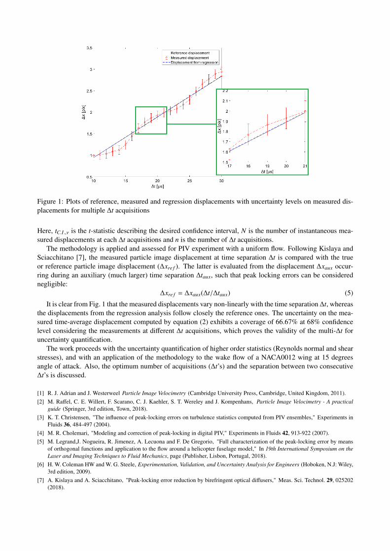
Figure 1: Plots of reference, measured and regression displacements with uncertainty levels on measured dis-
placements for multiple ∆t acquisitions
Here, tC.I.,ν is the t-statistic describing the desired confidence interval, N is the number of instantaneous mea-
sured displacements at each ∆t acquisitions and n is the number of ∆t acquisitions.
The methodology is applied and assessed for PIV experiment with a uniform flow. Following Kislaya and
Sciacchitano [7], the measured particle image displacement at time separation ∆t is compared with the true
or reference particle image displacement (∆xre f ). The latter is evaluated from the displacement ∆xaux occur-
ring during an auxiliary (much larger) time separation ∆taux, such that peak locking errors can be considered
negligible:
∆xre f = ∆xaux(∆t/∆taux) (5)
It is clear from Fig. 1 that the measured displacements vary non-linearly with the time separation ∆t, whereas
the displacements from the regression analysis follow closely the reference ones. The uncertainty on the mea-
sured time-average displacement computed by equation (2) exhibits a coverage of 66.67% at 68% confidence
level considering the measurements at different ∆t acquisitions, which proves the validity of the multi-∆t for
uncertainty quantification.
The work proceeds with the uncertainty quantification of higher order statistics (Reynolds normal and shear
stresses), and with an application of the methodology to the wake flow of a NACA0012 wing at 15 degrees
angle of attack. Also, the optimum number of acquisitions (∆t’s) and the separation between two consecutive
∆t’s is discussed.
[1] R. J. Adrian and J. Westerweel Particle Image Velocimetry (Cambridge University Press, Cambridge, United Kingdom, 2011).
[2] M. Raffel, C. E. Willert, F. Scarano, C. J. Kaehler, S. T. Wereley and J. Kompenhans, Particle Image Velocimetry - A practical
guide (Springer, 3rd edition, Town, 2018).
[3] K. T. Christensen, "The influence of peak-locking errors on turbulence statistics computed from PIV ensembles," Experiments in
Fluids 36, 484-497 (2004).
[4] M. R. Cholemari, "Modeling and correction of peak-locking in digital PIV," Experiments in Fluids 42, 913-922 (2007).
[5] M. Legrand,J. Nogueira, R. Jimenez, A. Lecuona and F. De Gregorio, "Full characterization of the peak-locking error by means
of orthogonal functions and application to the flow around a helicopter fuselage model," In 19th International Symposium on the
Laser and Imaging Techniques to Fluid Mechanics, page (Publisher, Lisbon, Portugal, 2018).
[6] H. W. Coleman HW and W. G. Steele, Experimentation, Validation, and Uncertainty Analysis for Engineers (Hoboken, N.J: Wiley,
3rd edition, 2009).
[7] A. Kislaya and A. Sciacchitano, "Peak-locking error reduction by birefringent optical diffusers," Meas. Sci. Technol. 29, 025202
(2018).

Workshop on Frontiers of Uncertainty Quantification in Fluid Dynamics
11–13 September 2019, Pisa, Italy
A Bayesian Approach for Predicting Thermoacoustic Oscillations in a Rijke Tube
Francesco Garita,1 Hans Yu1, and Matthew Juniper1
1Department of Engineering, University of Cambridge
Key words: Thermoacoustics, Data Assimilation, Ensemble Kalman Filter
Predicting and eliminating thermoacoustic oscillations is a significant challenge in gas turbine design. Here
we combine a thermoacoustic experiment with a thermoacoustic model and use data assimilation to infer the
parameters of the model, rendering it predictive. The experimental apparatus consists of a vertical Rijke tube
containing an electric heater (up to 300 Watts). The heater drives a base flow via natural convection, and ther-
moacoustic oscillations via velocity-driven heat release fluctuations. The growth/decay rates and frequencies
of these oscillations are measured every few seconds. There are two models: one for the base flow and one for
the acoustics. Both are unsteady. The parameters of the base flow model (Nusselt numbers and pressure loss
coefficient) are estimated from many thousand measurements using an ensemble Kalman filter that accounts
for both experimental and state and parameter errors. The parameters of the acoustic model are inferred by
regression. Figure 1 shows a comparison between experimental observations and model predictions of growth
rate and frequency of the thermoacoustic oscillations. As time progresses, the heater power is increased by 10
Watts, approximately every hour. In this case, no information is assimilated into the base flow model, and as
a result predictions are fairly poor. On the other hand, results significantly improve when data assimilation is
performed, as depicted in Figure 2. This study shows that, with thorough Bayesian inference, a simple model
with a few parameters can become a predictive model. The process reveals deficiencies in the model and, when
combined with physical insight, shows how to improve it. This work proves the concept for small systems and
prepares the ground for complex systems.
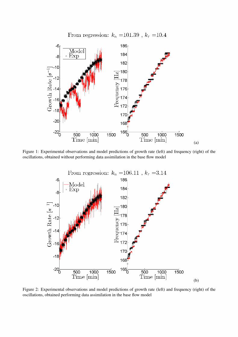
(a)
Figure 1: Experimental observations and model predictions of growth rate (left) and frequency (right) of the
oscillations, obtained without performing data assimilation in the base flow model
(b)
Figure 2: Experimental observations and model predictions of growth rate (left) and frequency (right) of the
oscillations, obtained performing data assimilation in the base flow model

ST3 – Applications IISession Chair: M. Diez
Auditorium
ST4 – Environmental I Session Chair: O. Knio
Room B

Workshop on Frontiers of Uncertainty Quantification in Fluid Dynamics
11–13 September 2019, Pisa, Italy
Stochastic calibration of cavitation model parameters for simulations of 3-phase
injector internal flows
Alessandro Anderlini,1 Maria Vittoria Salvetti,1 Antonio Agresta,2 and Luca Matteucci2
1DICI, University of Pisa, Italy – [email protected], [email protected] Automotive Italy S.p.A., Italy – [email protected],
Key words: Injector flow, hydraulic flip, cavitation, generalized Polynomial Chaos
This work focuses on numerical simulations of injector internal flows for automotive applications. It has
been widely demonstrated in the literature that the vehicle emission level is strictly related to the properties of
the spray exiting the injector which, in turn, is deeply influenced by the flow behavior inside the nozzle; the
study of this type of flow is thus of practical interest. The flow inside injectors is complex and characterized
by the interaction of turbulence and cavitation in channels of very small size and of very complicated geometry
(see Fig.1a containing a zoom of a realistic injector tip), and this makes simulations and experiments very
challenging. Moreover, in realistic applications, the fuel pumped inside the nozzle is injected in a domain
filled by a third gaseous phase (typically air). Depending on the injector geometry and the pressure difference
between inlet and outlet, indeed, the flow may go into the so-called "hydraulic flip" condition, i.e. a back flow
of air from outside the injector to the inlet corner, that replaces cavitation. The presence of hydraulic flip leads
to bad spray characteristics and, therefore, it must be avoided in practice.
From a numerical point of view, an accurate modeling of all the previously listed physical phenomena is
crucial for the reliability of the simulations. As for the multiphase model, we adopted an approach widely used
for this type of flow, i.e. a single set of equations for a fluid whose properties are weighted by the volume
fractions of the pure phases, using additional transport equations for the volume fractions of air and vapor, the
second of which has a source term containing the Scherr-Sauer cavitation model [2]. This model contains four
free-parameters that must be a-priori assigned, and it is reasonable to suppose that their uncertain values may
influence the simulation results. Regarding turbulence, we adopted an Unsteady Reynolds-Averaged-Navier-
Stokes (URANS) approach; this choice is motivated by the fact that, in an industrial context, the compromise
(a) (b)
Figure 1: Realistic multi-hole injector (a) and one-hole simplified (b) geometries

Figure 2: Instantaneous iso-surfaces of air and vapor fraction under unsteady hydraulic flip condition
between accuracy and computational cost can not be avoided, making the "cheap" URANS of practical interest.
In the present work, we want to quantify the impact of the cavitation model parameters on the numerical
predictions for a test-case geometry, i.e an axisymmetric real-size channel, for which experimental data are
available (see Fig.1b). In spite of the simplified geometry, this flow configuration is representative of a real
injectors and contains most of the aforementioned flow features. In a previous work [1], through stochastic
techniques such as generalized polynomial chaos and stochastic collocation, we showed that two parameters
among the four are the most important, so we decided to focus only on these two, namely the vaporization and
condensation factors.
Since a fully deterministic analysis would imply prohibitive computational costs also for this simplified
axisymmetric problem, we used a stochastic methodology, based on generalized polynomial chaos, in order
to obtain continuous response surfaces in the parameter space starting from a limited number of deterministic
simulations. The response surfaces has been thus used to carry out a parameter calibration against experimental
data. The quantities of interest taken into consideration are the critical cavitation point (CCP), i.e. the value of
the outlet pressure at which the flow inside the injector can be considered choked (for a fixed inlet pressure),
and the mass-flow-rate (MFR) at the CCP. In more details, we searched for the minimum percent difference
of MFR inside a parameter sub-domain in which the absolute difference of CCP was lower than 0.5 bar. An
’optimal’ set up of the cavitation model is thus found and is a-posteriori validated in the real 3D geometry
showing significant improvements respect to the default parameter set-up; then, we carry out a deeper analysis
in hydraulic flip conditions (see Fig.2) in order to give an accurate description of this phenomenon.
Moreover, this set-up has been applied to a complex one-hole injector geometry, as e.g. a sector of a real
geometry, containing all the difficulties encountered in real applications, and the results will be included in the
final presentation.
[1] A. Anderlini, M.V. Salvetti, A. Agresta and L. Matteucci, “Stochastic sensitivity analysis of numerical simulations of injector
internal flows to cavitation modeling parameters," Computers & Fluids 183, pages 130–147 (2019).
[2] J. Sauer and G.H. Schnerr, “Unsteady cavitating flow - a new cavitation model based on a modified front capturing method and
bubble dynamics," In Proceedings of the 2000 ASME Fluid Engineering Summer Conference, pages 1073–1079 (2000).

Workshop on Frontiers of Uncertainty Quantification in Fluid Dynamics
11–13 September 2019, Pisa, Italy
Comparison of uncertainty propagation methods applied to industrial
turbomachinery design with operational, geometrical and manufacturing
uncertainties
Dirk Wunsch,1, Charles Hirsch,1, Simon Abraham,2, Francesco Contino,2, Pieterjan Robbe,3, and StefanVandewalle,3
1Numeca International, Brussels, Belgium – [email protected]
2Vrije Universiteit Brussel (VUB), Brussels, Belgium
3KU Leuven, Department of Computer Science, Leuven, Belgium
Key words: Uncertainty Quantification, Probabilistic Collocation, Stepwise Regression, Multi-Level Monte-Carlo, Turbomachinery Design
Significant research and development effort has been dedicated over the past few years to the improvement
of uncertainty propagation techniques. A variety of uncertainty propagation methods spanning from advanced
sampling methods like Multi-Level Monte-Carlo, over various Stochastic Collocation and Polynomial Chaos
based methods to perturbation techniques were significantly advanced. They are now ready to address in the
order of ten uncertainties in industrial applications [3].
The current research work compares three of these methods. First, the Non-Intrusive Probabilistic Col-
location Method (NIPColM) [5], [7], which relies on Lagrange interpolating polynomials, second, a stepwise
regression method for sparse polynomial chaos expansions [1] and third, Multi-Level (MLMC) and Multi-Index
Monte-Carlo methods (MIMC) [2].
All three methods are benchmarked against the same industrial scale test case, which is the transonic NASA
rotor 37. This test case was defined in its original form with 5 simultaneous operational and geometrical un-
certainties [4] and all methods are run on this low dimensional configuration. In a second step, the number
of uncertainties is increased to demonstrate the potential of the respective methods. The stepwise regression
method is run in a configuration with 27 simultaneous operational and geometrical uncertainties, while 2007
uncertainties are accounted for the MLMC and Multi-Level Quasi Monte-Carlo (MLQMC). These 2007 uncer-
tainties replicate the manufacturing variability of the compressor blade surface.
In order to concentrate on the comparison of the uncertainty propagation methods applied to simultaneous
operational, geometrical and manufacturing uncertainties, the exact same simulation chain [6] from geome-
try modification, mesh generation and flow simulation is used for all three methods. This workflow is fully
automated.
The results include a comparison of the NIPColM with the stepwise regression method. This comparison
shows that the NIPColM is very efficient in estimating the mean value and standard deviation of various quan-
tities of interest, like the mass flow rate, isentropic efficiency, or total pressure ratio. Table 1 shows that for
5 simultaneous uncertainties the mean value is converged with 11 runs of CFD solver, while the stepwise re-
gression methods requires 20 CFD runs. Predicting higher moments, like skewness and kurtosis, the stepwise
regression method shows its potential as seen in table 1. For comparable values of these moments, the NIPColM
requires 71 and 341, while 30 and 50 CFD runs are sufficient for the stepwise regression method.
A second advantage of the stepwise regression method is that it does not rely on all samples run to be valid.
For example, a sample can be invalid if one of the points to evaluate lies in physically unfeasible regions. In
the medium dimensional case with 27 simultaneous uncertainties the NIPColM could predict values only for a

Figure 1: Predicted statistical moments for isentropic efficiency
Level 1, while the Level 2 that requires roughly 1000 CFD runs could not predict a result because of around ten
failed samples. The stepwise regression method simply omits potentially failed samples and is in this respect
more robust.
The MLMC, MLQMC and MIMC methods, which are used in this study, are not competitive in terms of
computational cost for low dimensional problems, but this was not expected. Its true potential lies in addressing
very high dimensional problems, which are unfeasible for both the NIPColM and stepwise regression method.
In addition to comparison with the other two methods, the speed-up resulting from these multi-level or multi-
index formulations is given with respect to standard Monte-Carlo methods. On the high dimensional case with
2007 uncertainties it reaches speed-up of a factor of 5 for MLMC and 15 for MLQMC, while significantly
larger speed-ups of up to 180 for MLQMC can be expected if the mesh strategy is tuned for the MLMC.
[1] Abraham, S., Raisee, M., Ghorbaniasl, G., Contino, F., and Lacor, C., “A robust and efficient stepwise regression method for
building sparse polynomial chaos expansions," J. Comput. Phys., Vol. 332, pp. 461-74 (2017).
[2] Blondeel P, Robbe P, Van hoorickx C, Lombaert C,Vandewalle S., “Multilevel Monte Carlo for uncertainty quantification in
structural engineering," arXiv:1808.10680v1 (2018).
[3] Hirsch C, Wunsch D, Szumbarski J, Laniewski-Wolk L, Pons-Prats J, Editors, Uncertainty Management for Robust Industrial
Design in Aeronautics, Notes on Numerical Fluid Mechanics and Multidisciplinary Design 140, Springer, 2019.
[4] Klostermann S, “UMRIDA test case database with prescribed uncertainties," Notes on Numerical Fluid Mechanics and Multidis-
ciplinary Design 140, pp. 15-32 (2019).
[5] Loeven GJA, Witteveen JAS, Bijl H, “Probabilistic collocation: an efficient non-intrusive approach for arbitrarily distributed
parametric uncertainties," Proc. of the 45th AIAA Aerospace Sciences Meeting and Exhibit, AIAA paper 2007-314 (2007).
[6] Numeca, “FINE/Design3D User manual version 13.2," (2019).
[7] Wunsch D, Nigro R, Coussement G, Hirsch C, “Quantification of combined operational and geometrical uncertainties in turbo-
machinery design," In Proceedings of the ASME TurboExpo GT2015, GT2015-43399, Montreal, (2015).

Workshop on Frontiers of Uncertainty Quantification in Fluid Dynamics
11–13 September 2019, Pisa, Italy
Sensitivity analysis on a CFD model for prediction of a gear pump leakages
Serena Morselli1, Cristian Ferrari1, Nicolò Beccati1, Pietro Marani1
1C.N.R. IMAMOTER
Keywords: CFD, gear pump, sensitivity analysis, dynamic mesh
In the field of modern fluid mechanical problems, the evolution of numerical simulation codes and the
availability of high-computational-power platforms allowed the spread of Computational Fluid Dynamics
(CFD) techniques with the aim of predicting complex fluid-flow phenomena. CFD is frequently used on
applications where the object needs a detailed analytic study in spite of the lack of parameters. A typical
example is represented by the clearances inside a volumetric pump during his functioning. This uncertainty
affects other potential sources of CFD errors like the numerical ones, caused by the discretization of the
equations, the modelling ones, due to the description of fluid phenomena and, at lower lever, the user or
software errors.
A complex model, that contains many important uncertainties, is presented in this work, which main
purpose is a sensitivity analysis on key operating parameters of a gear pump studied with both numerical and
experimental techniques. In particular, the study is focused on the calibration of the fixed displacement
machine clearances.
Gear pumps represent the majority of the fixed displacement machines used for flow generation in
fluid power systems. The internal conformation of this system contains many undetermined variables, due to
both the manufacturing techniques and the breaking-in pressure, that strongly affect the pump performance.
The 3D CFD model of this type of products is particularly difficult to develop [1], because of the deforming
volumes in-between the gears, the structural deformation of the case during the functioning and the moving
operating point. These transient modifications of the initial geometry of the pump highly influence the outer
mass flow and it must be estimated through mathematical methods.
A classical methodology was used for the purpose by starting from the 3D geometry of the pump.
Subsequently, the fluid domain was extracted, the mesh was created and the moving boundary conditions were
set. The deformation of the fluid domain was managed by the skewness level of the mesh and deformed with
a smoothing and remeshing approach by using a dynamic mesh. The model was solved with a commercial
code, and then post processed.
The comparison between experimental and numerical results, united with the widely investigated Richardson
Extrapolation (RE) method for the discretization error estimation [2], led to an accurate sensitivity analysis of
the clearances.
The future aim of this work is to obtain, thanks to the sensitivity analysis, the pump volumetric
efficiency as a function of the leakages between the machine gears and case, which highly affect the numerical
results. A future purpose is to provide the characteristic curves of the gear pump depending on the breaking-
in pressure.
The results obtained is a sensitivity analysis that is able to compare the gap between the gears, at different
mesh level of accuracy, with the experimental data in order to evaluate the influence of the analyzed parameters
on the numerical results.
[1] S. Mancò, N. Nervegna, “Simulation on an external gear pump and experimental verification” In Proceedings of the JHPS
International Symposium on Fluid Power, 139-152, (Tokio, Japan,1989).
[2] Celik, I. B., Ghia, U., Roache, P.J. Freitas, C. J., Coleman, Raad, P. E., “Procedure for Estimation and Reporting of Uncertainty
Due to Discretization in CFD Applications,” ASME J. Fluids Eng., 130(7), (2008).

Workshop on Frontiers of Uncertainty Quantification in Fluid Dynamics
11–13 September 2019, Pisa, Italy
Geometric Uncertainty Quantification of a Film Cooled Gas Turbine Blade
Andrea Gamannossi,1 and Alberto Amerini,2 and Lorenzo Mazzei,2 and Matteo Poggiali,2 and AntonioAndreini,2
1DIA, University of Parma, Italy – [email protected]
2DIEF, University of Florence, Italy – [email protected]
Key words: Uncertainty quantification, Computational Fluid Dynamics, Film Cooling, Gas Turbine, Blade
CFD is nowadays a must-have tool for the design phase of the gas turbine components. However, the results
are often presented in a deterministic way, with a “single-line” plot and a certain solution. Experimentalists are
required to insert a confidence interval with its relative error within the results, showing how the measurements
can be affected by all the source of errors arising from the experiment itself. Instead, most of numerical
studies do not include all the source of error arising from the simulation: starting from the boundary conditions,
passing by the numerical model and the discretization error. Uncertainty quantification is the field studying
these effects and how an input uncertain variable propagates through the simulations and affects the result.
This work presents an uncertainty quantification approach applied to CFD: an industrial prismatic gas turbine
blade with film cooling on the suction side only and standard shaped holes configuration. The blade is made
by additive manufacturing (AM) process and the hole are then manufactured by electric discharge machining
(EDM) process. Both manufacturing processes feature geometric uncertainty on the final shape: the AM is more
related to the shape itself while EDM is related to the difference between the nominal and the final geometry.
The blade was part of an initial experimental test campaign which revealed many output results in terms of
adiabatic effectiveness and heat transfer. CFD analyses are conducted on this profile; a bi-fluid approach to
measure the effectiveness is adopted: air for the main flow and CO2/SF6 for the coolant flow. Regarding
uncertainty quantification an analysis is carried out varying the hole dimension and position with respect to the
blade, including the fillet radius. Input variation are selected based on data available from an industrial partner.
Polynomial-chaos approach is used in conjunction with the probabilistic collocation method for both analyses.
With a 2nd order polynomial approximation the total number of simulation required is 8. This method is able
to reproduce what the normal Montecarlo analysis does (with more than a thousand of simulations) with an
optimum grade of accuracy. For the uncertainty quantification framework Dakota [1] is used. RANS approach
with k—w SST turbulence model is adopted for the simulations. Results show the confidence interval for
both analyses and prove how the position tolerance of the blade, as well as the hole dimension, is extremely
important for the effectiveness. In particular, when dealing with additive manufacturing and EDM processes.
[1] Adams, B.M., Bauman, L.E., Bohnhoff, W.J., Dalbey, K.R., Ebeida, M.S., Eddy, J.P., Eldred, M.S., Hough, P.D., Hu, K.T.,
Jakeman, J.D., Stephens, J.A., Swiler, L.P., Vigil, D.M., and Wildey, T.M., “Dakota, A Multilevel Parallel Object-Oriented
Framework for Design Optimization, Parameter Estimation, Uncertainty Quantification, and Sensitivity Analysis: Version 6.9
User’s Manual„" Sandia Technical Report SAND2014-4633, November 2018.

Workshop on Frontiers of Uncertainty Quantification in Fluid Dynamics
11–13 September 2019, Pisa, Italy
Towards a Consistent Stochastic Modeling of Oceanic Dynamics
L. Li,1,2 W. Bauer,2 and E. Mémin,2
1Université Rennes I France
2Fluminance Group Inria Rennes France
Key words: Stochastic Modeling, Oceanic Dynamics, Ensemble Forecasting, Uncertainty Quantification
For several years, there is a growing interest in geophysical sciences such as oceanography or meteorology
to incorporate random flows. These models aims at representing processes such as unknown physical forcing or
uncertainty coming either from a large–scale approximate description or from the nature of discrete numerical
schemes used. The modeling of these uncertainties along time is paramount in both uncertainty quantification
and ensemble forecasting.
In this work, we propose to follow a recent derivation [1, 2] that comes from a decomposition of the La-
grangian fluid particle displacement into a smooth component and a time–uncorrelated uncertainty
dXt = u(Xt)dt + σ(Xt)dBt. (1)
A random passive tracer transported along such a stochastic flow (1) is then found through a generalized Itô
formula,
Dtθ
= dtθ +(
(u −1
2∇·a)dt + σdBt
)
·∇θ −1
2∇·(a∇θ)dt = 0, (2)
in which a variance operator a of the random field σdBt is involved. The energy of such a random tracer is
shown to be well conserved along time for each realization, characterizing hence the essence of a transport.
Such stochastic transport operator can then be used as a fundamental tool to derive stochastic representation of
fluid flow dynamics [1, 2].
Such a stochastic principle, termed modeling under location uncertainty, has been tested for the numerical
simulation of the wind-driven circulation in a shallow ocean basin, which is widely used to characterize the
role of mesoscale eddies and their effect on mean circulation. This kind of model describes the incompressible
barotropic flows by assuming the hydrostatic balance, the beta–plane approximation, geostrophic balance and
horizontal eddy viscosity parametrization. The governing equations under our stochastic framework can be
written as
Dtq = S 1(∇u)dt + S 2(∇u)dBt + D + F, (3)
in which the potential vorticity (PV) q is driven by a symmetric double-gyre forcing F, a viscous dissipation
D and some source processes S 1, S 2 due to asymmetry of the stochastic advections in (2). In the absence of
dissipation and forcing, this random system (3) have a consistent set of energetics for each realization.
The numerical assement shows that the proposed random model (LU), compared to a classical large eddy
simulation (LES) approach, can capture better on a coarse mesh the correct four–gyre time–averaged circula-
tion structure, as predicted by a direct numerical simulation (DNS) at a much finer resolution (cf. figure 1).
Then the performance of our random model has been evaluated and analyzed in terms of uncertainty quan-
tification and ensemble forecasting. Some common criterions (e.g. Talagrand histogram) are used to quantify

the prediction accuracy, compared to observations provided by DNS (cf. figure 2). We will otherwise show that
the proposed random model, under both homogeneous and heterogeneous uncertainty, is more efficient than a
deterministic model with a pertubation of the initial condition. This ability is in particular essential for data
assimilation applications.
In this study we show also the influence of a structure-preserving numerical scheme on the performances of
both time–statistics and ensemble forecasting.
Figure 1: Illustration of time–averaged streamfunction contours : (a) DNS results at a fine resolution; (b)
LU results at a coarse resolution; (c) LES results at the same resolution as in LU, but by removing the time-
uncorrelated term in (2).
Figure 2: Illustration of a reliable ensemble forecasting prediction : (a) Ensemble of instantaneous PV field; (b)
Time history of locally averaged PV field (observed v.s. ensemble spread); (c) Rank histrogram of instantaneous
PV field.
[1] E. Mémin (2014), “Fluid flow dynamics under location uncertainty," Geophysical and Astrophysical Fluid Dynamics 108, 119-146.
[2] V. Resseguier, E. Mémin and B. Chapron (2017), “Geophysical flows under location uncertainty, Part I: random transport and
general models," Geophysical and Astrophysical Fluid Dynamics 111, 149-176.

Workshop on Frontiers of Uncertainty Quantification in Fluid Dynamics
11–13 September 2019, Pisa, Italy
Bayesian Inference and Markov Chain Monte Carlo Sampling for Lagrangian
Particle Tracking in the Ocean
Samah El Mohtar, Omar Knio, and Ibrahim Hoteit,
King Abdullah University of Science and Technology, Thuwal 23955, Saudi Arabia –[email protected], [email protected], [email protected]
Key words: Uncertainty quantification, Bayesian inference, MCMC, Lagrangian particle tracking
Estimation of Lagrangian particle tracking (LPT) model parameters is challenging due to the irreversible
nature of processes affecting the particles. In the ocean, several methods have been proposed to tackle this
problem, but each has its limitations. In this work, we present a generic method that employs Bayesian inference
and Markov chain Monte Carlo (MCMC) sampling to construct the probability distributions of parameters of
interest. The forward model used within the MCMC machinery enables the use of existing application-specific
modules built on top of LPT models. Furthermore, various types of observations can be considered depending
on available data. This framework allows the method to serve different applications of LPT in the ocean. The
method has been tested using a simple LPT advection-diffusion model in a double-gyre synthetic flow field.
Different data types were tested, ranging from the simple location of particles, to measurements of concentration
and contours of spills. Inference of the location of the source, time and duration of release is presented as a
probability distribution that quantifies uncertainties and correlations between parameters.

Workshop on Frontiers of Uncertainty Quantification in Fluid Dynamics
11–13 September 2019, Pisa, Italy
Forward and Backward Lagrangian Particle Tracking in Ensemble Flow Fields
Samah El Mohtar,1 Ibrahim Hoteit,1 Omar Knio,1 Leila Issa,2 and Issam Lakkis,3
1King Abdullah University of Science and Technology, Thuwal 23955, Saudi Arabia –[email protected], [email protected], [email protected]
2Department of Computer Science and Mathematics, Lebanese American University, Beirut, Lebanon –[email protected]
3Department of Mechanical Engineering, American University of Beirut, Beirut, Lebanon –[email protected]
Key words: Stochastic flow fields, Red sea, Lagrangian tracking
Ocean ensemble data assimilation systems generate ensembles of independent velocity field realizations af-
ter every assimilation cycle. Lagrangian tracking of passive tracers within such a framework is challenging due
to the exponential growth in the number of particles that arises from describing the behavior of velocity over
time as a set of possible combinations of the different realizations. This contribution addresses the problem
of efficiently advecting particles, forward and backward in time, in ensemble flow fields, whose statistics are
prescribed by an underlying assimilated ensemble. To this end, a parallel adaptive binning procedure that con-
serves the zeroth, first and second moments of probability is introduced to control the growth in the number of
particles. The adaptive binning process offers a tradeoff between speed and accuracy by limiting the number of
particles to a desired maximum. To validate the proposed method, we conducted various forward and backward
particles tracking experiments within a realistic high-resolution ensemble assimilation setting of the Red Sea,
focusing on the effect of the maximum number of particles, the time step, the variance of the ensemble, the
travel time, the source location, and history of transport. We also demonstrate the efficiency of the method for
possibly identifying (backward in time) a moving target from observed released materials.

Workshop on Frontiers of Uncertainty Quantification in Fluid Dynamics
11–13 September 2019, Pisa, Italy
Bayesian Convolutional Neural Networks as a Tool to Detect Discharges of
Pollutants to Marine Waters through Time Series Classification
Kristian Gundersen1, Guttorm Alendal2, Anna Oleynik3
1Department of Mathematics, University of Bergen, Norway – [email protected]
2University of Bergen, Norway – [email protected]
3University of Bergen, Norway – [email protected]
Key words: Deep Learning, Uncertainty quantification, Bayesian Convolutional Neural Network, Time SeriesClassification
The world’s oceans are already under tremendous stress from climate change, acidification and other hu-
man activities [1]. In fact, UN has declared 2021-2030 as the decade for marine science1. Monitoring the
marine environment is a part of ecosystem based Marine Spatial Planning [2] and Life under Water is one of
UN’s Sustainable Development Goals. Here we study the use of Bayesian Convolutional Neural Networks for
classification of time series from marine monitoring programs in order to detect discharges of pollutants in the
ocean. These discharges can in general be composed of a mixture of chemical, biological and radioactive mat-
ters, and a real challenge is to distinguish a signal of a discharge in noisy time series. The problem is even more
complicated if the pollutants are naturally present in the environment and if a large area has to be monitored.
Monitoring programs associated with offshore geological storage projects are in this category. Hence, there is
a need for data analysis methods that can detect a weak signal in noisy time series in a probabilistic manner, as
input to making decisions for mobilising more comprehensive and costly surveys.
The key concept of Bayesian Neural Network (BNN) is to introduce a prior distribution over the weights
of the neural network and, thus, add stochasticity in the framework. In the time-series classification settings,
the outcome of a traditional neural network is a probability (point-estimate) of the class that the time series
belongs to. The outcome of a BNN is a probability distribution that gives information not only about the
class, but also about the uncertainties in the predictive power of the model. Despite these uncertainties can be
expressed analytically [3], the practical use of the BNNs may fail due to large computational costs. Gal and
Ghahramani [4] have recently proposed an approach addressing this issue. The main idea is to use dropout
as a variational inference approximation; a method to estimate posteriori densities for Bayesian models. The
benefits of variational inference over more traditional methods, such as Markov Chain Monte Carlo (MCMC)
method, are better scalability to large datasets and an easier implementation [5]. Instead of using sampling, an
optimization problem can be formulated. It can be shown that the simple approach of using Bernoulli dropout
during both training and testing stages can be viewed as an approximative variational inference technique [4].
During prediction, we simply do n forward passes for each time series in the test data set to generate empirical
probability distributions of which class the time series belongs to.
Here we present a solution to a classification problem applied to the detection of CO2 seeps to the marine
environment from a subsurface reservoir at the Scottish Goldeneye area. We use Bayesian Convolutional Neural
Network (BCNN) [6] for time series classification, motivated by their ability to automatically generate features.
Some of the most promising advances in time series classification the last few year have been with different
1https://en.unesco.org/ocean-decade

variations of convolutional neural networks [7]. We use time series produced by a General Circulation Model
(GCM) with additional tracers for training, validating, and testing the network. All data is standardized and
labeled as "leak" or "no-leak".
We argue that the use of modeling data in this case is a necessity since the data corresponding to the leak
scenarios is difficult and, in some cases, impossible to obtain. Moreover, and this is our main argument, the
trained deep neural network can be used in a transfer learning setting [8]. That is, we can use a pre-trained
neural network on the model data, fix the parameter weights in the first few layers, and then train the network
with the limited real data as input. The conjecture is that the first few layers adequately represent the core
feature characteristics of the time series, and thus significantly reducing the need of in-situ data.
Figure 1: Left Panel: Plot of the predictive mean of the leak class for the Goldeneye area for a CO2 pollutant released at
the center with a flux of 300T per/day CO2. The red line enclosure indicates an area where the seepage is detected with
a predictive mean above 75 %. Middle Panel: KDE-estimate for the three different locations visualized on the predictive
mean plot. Right Panel: Shows the cumulative area vs the probability of detection.
We trained the network based on four 3D simulations, three leak and one no-leak scenario. Each of four
simulations contain 1736 × 23 time series of CO2 concentrations over approximately 100km × 100km area
with 23 vertical layers. In all leak scenarios the leakage was placed at the seafloor in the center of the two
dimensional domain. All the data, except the bottom layer, was used for training and validation, while the time
series at the bottom layer was used for testing. Figure 1(Left panel) shows the predictive mean of the ensemble
of the 1000 forward realizations for each of the 1736 time series at the bottom layer. The empirical standard
deviation is used as a measure of the uncertainty in the predictions, see Figure 1(Middle panel). Figure 1(Right
panel) shows trade - off between the footprint size and the confidence in the prediction. The uncertainty estimate
obtained from BCNN would allow for more informative decisions when designing monitoring program.
References
[1] Benjamin S Halpern, Catherine Longo, Darren Hardy, Karen L McLeod, Jameal F Samhouri, Steven K Katona, Kristin Kleisner, Sarah E Lester,
Jennifer O’Leary, Marla Ranelletti, Andrew A Rosenberg, Courtney Scarborough, Elizabeth R Selig, Benjamin D Best, Daniel R Brumbaugh,
F Stuart Chapin, Larry B Crowder, Kendra L Daly, Scott C Doney, Cristiane Elfes, Michael J Fogarty, Steven D Gaines, Kelsey I Jacobsen,
Leah Bunce Karrer, Heather M Leslie, Elizabeth Neeley, Daniel Pauly, Stephen Polasky, Bud Ris, Kevin St Martin, Gregory S Stone, U Rashid
Sumaila, and Dirk Zeller. An index to assess the health and benefits of the global ocean. Nature, 488(7413):615–620, August 2012.
[2] Elianny Domínguez-Tejo, Graciela Metternicht, Emma Johnston, and Luke Hedge. Marine Spatial Planning advancing the Ecosystem-Based
Approach to coastal zone management: A review. Marine Policy, 72:115–130, October 2016.
[3] David JC MacKay. A practical Bayesian framework for backpropagation networks. Neural computation, 4(3):448–472, 1992.
[4] Yarin Gal and Zoubin Ghahramani. Dropout as a Bayesian approximation: Representing model uncertainty in deep learning. In international
conference on machine learning, pages 1050–1059, 2016.
[5] David M Blei, Alp Kucukelbir, and Jon D McAuliffe. Variational inference: A review for statisticians. Journal of the American Statistical
Association, 112(518):859–877, 2017.
[6] Yarin Gal and Zoubin Ghahramani. Bayesian convolutional neural networks with Bernoulli approximate variational inference. arXiv preprint
arXiv:1506.02158, 2015.
[7] Hassan Ismail Fawaz, Germain Forestier, Jonathan Weber, Lhassane Idoumghar, and Pierre-Alain Muller. Deep learning for time series classifica-
tion: a review. Data Mining and Knowledge Discovery, pages 1–47, 2019.
[8] Sinno Jialin Pan and Qiang Yang. A survey on transfer learning. IEEE Transactions on knowledge and data engineering, 22(10):1345–1359, 2009.

Workshop on Frontiers of Uncertainty Quantification in Fluid Dynamics
11–13 September 2019, Pisa, Italy
Emulating environmental modeling systems in presence of uncertainties:
overview and challenges
Mélanie C. Rochoux1, Aurélien Costes1,2, Ronan Paugam1, Géraldine Rea1, Laëtitia Thouron1, AndreaTrucchia3, Cong Zhang4, Thomas Jaravel1, Christine Lac2, Valéry Masson2, Arnaud Trouvé4, Olivier
Vermorel5, Didier Lucor6
1CECI, Université de Toulouse, CNRS, CERFACS, Toulouse, France – [email protected],[email protected], [email protected], [email protected],
2CNRM, Université de Toulouse, CNRS, Météo-France, Toulouse, France – [email protected],[email protected], [email protected]
3BCAM, Basque Center for Applied Mathematics, Bilbao, Spain – [email protected]
4University of Maryland, Department of Fire Protection Engineering, Maryland, USA – [email protected],[email protected]
5CERFACS, Toulouse, France – [email protected]
6LIMSI, CNRS, Université Paris-Saclay, Orsay, France – [email protected]
Key words: Emulators, air quality, wildfire, front dynamics, plume dynamics, uncertainty quantification, sen-sitivity analysis, data assimilation
Accurately predicting the evolution of environmental systems remains a challenge for risk assessment.
Large eddy simulation has been identified as a promising tool to tackle this challenge. At the scale of micro-
meteorology, simulating the land surface processes and the flow dynamics is a multi-physics multi-scale prob-
lem due to the complex flow dynamics induced by land surface heterogeneity, time-transient meteorological
conditions and surface/atmosphere interactions. We thus need to analyze the impact of both modeling un-
certainties and aleatory uncertainties on the simulated quantities of interest due to modeling choices and the
internal variability of the target environmental systems. Since large eddy simulations are computationally ex-
pensive, we have access to a limited number of simulations. To overcome this issue, we investigate the use of
emulators to quantify model output uncertainties and analyze model output sensitivity with respect to inlet flow
conditions and physical model parameters. Fast emulators based on generalized polynomial chaos expansion
and gaussian process [1, 2] are trained to approximate probability distributions and corresponding statistical
moments as well as Sobol’ sensitivity indices. The use of sparse basis is investigated [3]. Specific measures
can be used to track flow structures in terms of shape and topology [2]. These emulators can be integrated
in ensemble-based data assimilation system to accelerate the inverse modeling procedure [4]. Our emulation
strategy will be illustrated for two environmental applications using field-scale experimental data sets: wildland
fire behavior modeling [5, 6] on the one hand, urban outdoor air quality modeling [7] on the other hand.
[1] P.T. Roy, N. El Moçayd, S. Ricci, J-C. Jouhaud, N. Goutal, M. De Lozzo and M.C. Rochoux: Comparison of polynomial chaos and
Gaussian process surrogates for uncertainty quantification and correlation estimation of spatially distributed open-channel steady
flows Stochastic Environmental Research and Risk Assessment 32, 1723-1741 (2018).
[2] M.C. Rochoux, A. Collin, C. Zhang, A. Trouvé, D. Lucor and P. Moireau: Front shape similarity measure for shape-oriented
sensitivity analysis and data assimilation for Eikonal equation, ESAIM Proceedings and Surveys 63, 215-236 (2018).

[3] A. Trucchia, V. Egorova, G. Pagnini and M.C. Rochoux: On the merits of sparse surrogates for global sensitivity analysis of
multi-scale nonlinear problems: Application to turbulence and fire-spotting model in wildland fire simulators Communications in
Nonlinear Science and Numerical Simulation 73, 120-145 (2019).
[4] M.C. Rochoux, S. Ricci, D. Lucor, B. Cuenot and A. Trouvé: Towards predictive data-driven simulations of wildfire spread - Part
I: Reduced-cost Ensemble Kalman Filter based on a Polynomial Chaos surrogate model for parameter estimation, Natural Hazards
and Earth System Science 14, 2951-2973 (2014).
[5] A. Costes, C. Lac, V. Masson and M.C. Rochoux: “Bi-directional fire-atmosphere coupling for on-demand simulations in case
of forest fires," In Proceedings of the VIII International Conference on Forest Fire Research, Advances in Forest Fire Research,
Imprensa da Universidade de Coimbra, Viegas, Domingo Xavier (ed.), Coimbra, Portugal (2018).
[6] R. Paugam, M.C. Rochoux, N. Cazard, C. Lapeyre, W. Mell and M. Wooster: “Computing high resolution fire behavior metrics
from prescribed burn using handheld airborne thermal camera observations," In Proceedings of the EGU General Assembly,
EGU2019-13804, Vienna, Austria (2019).
[7] G. Rea, M.C. Rochoux, L. Thouron, F. Auguste, T. Jaravel and O. Vermorel: Large eddy simulations of micro-scale meteorology
and pollutant dispersion: model intercomparison for the MUST experiment In preparation for submission to Atmospheric and
Environment.

Keynote Lecture - V. Heuveline - Uncertainty quantification with application tomedical engineering: towards a more reliable medicine?
Session Chair: O. ErnstAuditorium

Workshop on Frontiers of Uncertainty Quantification in Fluid Dynamics
11–13 September 2019, Pisa, Italy
Uncertainty quantification with application to medical engineering: towards a
more reliable medicine?
Vincent Heuveline
Universität Heidelberg, Germany – [email protected]
Key words: Uncertainty Quantification, Medical Engineering
In the last decades, the understanding of medical processes has been improved, which deals as a foundation
of applying mathematical modeling techniques in this application field. Numerical models provide the means
of predicting biomechanical behavior and processes, which is fundamental for improving current medical treat-
ment approaches. Medical applications benefit from numerical modeling including medical device design,
heart function simulation, disease diagnosis, tumor prediction, amongst others. However, many modeling ap-
proaches so far are deterministic. Especially in the life sciences, the occurring parameters can not always be
assumed to be known accurately due to complex geometry, unknown boundary conditions, measurement as well
as modeling errors. Taking such uncertainties into account by stochastic models results in a parametrization
by a set of independent random variables. This leads to a blown up system size requiring even more scalable
numerical schemes in order to take advantage of the capabilities of high performance computers (HPCs). As the
available compute power on HPCs is still increasing exponentially, the underlying biological mechanisms can
be simulated with increasing accuracy. This talk discusses the impact of emerging uncertainty quantification
(UQ) modeling for medical applications. The link between contemporary deterministic approaches and intru-
sive schemes based on stochastic Galerkin methods using Polynomial Chaos will be established. A simplified
performance model based on the computational intensity is presented and allows to evaluate the quality and
the efficiency of UQ approaches in the context of medicine. Numerical experiments assuming complex flow
problems arising in medical processes are presented.

ST5– Biological flowsSession Chair: V. Heuveline
Auditorium

Workshop on Frontiers of Uncertainty Quantification in Fluid Dynamics
11–13 September 2019, Pisa, Italy
Semi-intrusive uncertainty quantification analysis with a surrogate model for
in-stent restenosis 2D model
Dongwei Ye1, Anna Nikishova1, Lourens Veen2, Pavel Zun1,3 and Alfons G. Hoekstra1,3
1Computational Science Lab, Institute for Informatics, University of Amsterdam, The Netherlands– D.Ye, A.Nikishova, [email protected]
2Netherlands eScience Center, Amsterdam, The Netherlands – [email protected]
3ITMO University, Saint Petersburg, Russia – [email protected]
Key words: Uncertainty Quantification, Surrogate modelling, Gaussian process regression, Multiscale simula-tion, Semi-intrusive method
The two-dimensional in-stent restenosis model (ISR2D) is a multi-scale simulation of the post-stenting
healing response of a coronary artery [1, 2]. The model is composed of three submodels: a model to calculate
the initial geometry of vessel wall after stenting, an agent-based model to compute the proliferation of smooth
muscle cells and endothelium recovery, and a Lattice-Boltzmann model to simulate the blood flow through
the artery in changing geometries, reflecting the developing restenosis. An uncertainty quantification analysis
for the ISR2D model is performed based on the semi-intrusive multi-scale algorithm proposed by [3, 4]. The
algorithm allows the replacement of the most expensive part of the multiscale ISR2D simulation which is the
blood flow model, with a surrogate model. In this work, the surrogate model is based on a Gaussian process. The
vessel wall geometry features and blood flow velocity at the inlet are used as the input for the Gaussian process.
Results of uncertainty estimation of the neointimal area are well approximated compared to the estimation from
the quasi Monte-Carlo algorithm [5]. Result of sensitivity analysis shows that the overall variance and partial
variances are overestimated however the correct order of the partial variances is preserved. Additionally, both
accuracy and computational efficiency of the result outperformed previous results using nearest-neighborhood
interpolation [4]. The result shows that the semi-intrusive method with the surrogate is a valid method to
perform uncertainty quantification in an efficient way for the ISR2D model. The implication for the more
realistic 3D verison of the ISR model [6] will be discussed.
[1] H. Tahir, A. G. Hoekstra, E. Lorenz, P. V. Lawford, D. R. Hose, J. Gunn, D. J. W. Evans, “Multi-scale simulations of the dynamics
of in-stent resteno- sis: impact of stent deployment and design", Interface Focus 1 (3) (2011)
[2] H. Tahir, C. Bona-Casas, A. G. Hoekstra, “Modelling the effect of a functional endothelium on the development of in-stent
restenosis", PLoS One 8 (6) (2013)
[3] A. Nikishova, A. G. Hoekstra, “Semi-intrusive uncertainty quantification for multiscale models", arXiv:1806.09341
[4] A. Nikishova, L. Veen, P. Zun, A. G. Hoekstra, “Semi-intrusive multiscale metamodelling uncertainty quantification with applica-
tion to a model of in-stent restenosis", Phil. Trans R. Soc. A 377 (2142) (2019
[5] A. Nikishova, L. Veen, P. Zun, A. G. Hoekstra, “ Uncertainty quantification of a multiscale model for in-stent restenosis", Cardio-
vascular Engineering and Technology 9 (4) (2018)
[6] P. S. Zun, T. Anikina, A. Svitenkov, A. G. Hoekstra, “A Comparison of Fully-Coupled 3D In-Stent Restenosis Simulations to
In-vivo Data", Frontiers in Physiology 8 (2017) 284
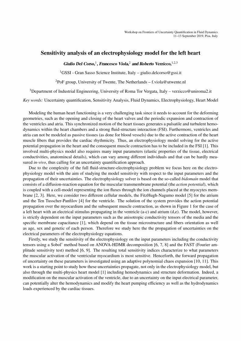
Workshop on Frontiers of Uncertainty Quantification in Fluid Dynamics
11–13 September 2019, Pisa, Italy
Sensitivity analysis of an electrophysiology model for the left heart
Giulio Del Corso,1, Francesco Viola,2 and Roberto Verzicco,1,2,3
1GSSI - Gran Sasso Science Institute, Italy – [email protected]
2PoF group, University of Twente, The Netherlands – [email protected]
3Department of Industrial Engineering, University of Roma Tor Vergata, Italy – [email protected]
Key words: Uncertainty quantification, Sensitivity Analysis, Fluid Dynamics, Electrophysiology, Heart Model
Modeling the human heart functioning is a very challenging task since it needs to account for the deforming
geometries, such as the opening and closing of the heart valves and the periodic expansion and contraction of
the ventricles and atria. This synchronized motion of the heart tissues generates a pulsatile and turbulent hemo-
dynamics within the heart chambers and a strong fluid-structure interaction (FSI). Furthermore, ventricles and
atria can not be modeled as passive tissues (as done for blood vessels) due to the active contraction of the heart
muscle fibers that provides the cardiac rhythmicity. Thus, an electrophysiology model solving for the active
potential propagation in the heart and the consequent muscle contraction has to be included in the FSI [1]. This
involved multi-physics model also requires many input parameters (elastic properties of the tissue, electrical
conductivities, anatomincal details), which can vary among different individuals and that can be hardly mea-
sured in-vivo, thus calling for an uncertainty quantification approach.
Due to the complexity of the full fluid-structure-electrophysiology problem we focus here on the electro-
physiology model with the aim of studying the model sensitivity with respect to the input parameters and the
propagation of their uncertainties. The electrophysiology solver is based on the so-called bidomain model that
consists of a diffusion-reaction equation for the muscular transmembrane potential (the action potential), which
is coupled with a cell-model representing the ion fluxes through the ion channels placed at the myocytes mem-
brane [2, 3]. Here, we consider two different cellular models, the FitzHugh-Nagumo model [5] for the atrium
and the Ten Tusscher-Panfilov [4] for the ventricle. The solution of the system provides the action potential
propagation over the myocardium and the subsequent muscle contraction, as shown in Figure 1 for the case of
a left heart with an electrical stimulus propagating in the ventricle (a-c) and atrium (d,e). The model, however,
is strictly dependent on the input parameters such as the anisotropic conductivity tensors of the media and the
specific membrane capacitance [1], which depend on the tissue microstructure and fibers orientation as well
as age, sex and genetic of each person. Therefore we study here the the propagation of uncertainties on the
electrical parameters of the electrophysiology equations.
Firstly, we study the sensitivity of the electrophysiology on the input parameters including the conductivity
tensors using a Sobol’ method based on ANOVA-HDMR decomposition [6, 7, 8] and the FAST (Fourier am-
plitude sensitivity test) method [6, 9]. The resulting total sensitivity indices characterize to what parameters
the muscular activation of the ventricular myocardium is most sensitive. Henceforth, the forward propagation
of uncertainty on these parameters is investigated using an adaptive polynomial chaos expansion [10, 11]. This
work is a starting point to study how these uncertainties propagate, not only in the electrophysiology model, but
also through the multi-physics heart model [1] including hemodynamics and structure deformation. Indeed, a
modification on the muscular activation of the ventricle, due to an uncertainty on the input electrical parameter,
can potentially alter the hemodynamics and modify the heart pumping efficiency as well as the hydrodynamics
loads experienced by the cardiac tissues.

Figure 1: Snapshots of the action potential for the left heart during a heart beat. The different cellular models
for atrium and ventricle are shown in the lateral insets.
[1] F. Viola, V. Meschini, R. Verzicco, "A multi-way coupled model for the left-heart: Fluid-Structure-Electrophysiology interaction
(FSEI), Under revision (2019).
[2] L. Tung, "A bi-domain model for describing ischemic myocardial dc potential", Ph.D. thesis, Massachusetts Institute of Technology
(1978)
[3] R. H. Clayton, A. V. Panfilov, "A guide to modelling cardiac electrical activity in anatomically detailed ventricles", Progress in
biophysics and molecular biology 96 (1) (2008) 19-43
[4] K. Ten Tusscher, A. Panfilov, "Cell model for efficient simulation of wave propagation in human ventricular tissue under normal
and pathological conditions", Physics in Medicine & Biology 51 (23) (2006)
[5] R. Fitzhugh, "Thresholds and plateaus in the Hodgkin-Huxley nerve equations", The Journal of general physiology 43 (5) (1960)
867-896
[6] K. Chanm S. Tarantola, A. Saltelli and I. Sobol’. "Variance-based methods". In: Sensitivity Analysis. Ed. by A. Saltelli, K. Chand
and E. M. Scott. Chinchester: John Wiley and Sons, Ltd., 2000.
[7] I. Sobol’. "Global sensitivity indices for nonlinear mathematical models and their Monte Carlo estimates". In: Mathematics and
Computers in Simulation 55.1-3 (Feb. 2001), pp. 271-280.
[8] I. Sobol’. "Sensitivity analysis for non linear mathematical models". In: Math. Model. Comput. Exp. 1 (1993) pp. 407-414.
[9] A. Saltelli, S. Tarantola, and K. P.-S- Chan, "A quantitative model independent method for global sensitivity analysys of model
output". In. Technometrics 41.1 (Feb. 1999), pp. 39-56.
[10] G. Blatman, B. Sudret. "Adaptive sparse polynomial chaos expansions based on least angle regression". Journal of Computational
Physics, (2011), pp. 2345-2367.
[11] B. Sudret. "Polynomial chaos expansions and stochastic finite element methods". In: Risk and Reliability in Geotechnical Engi-
neering (2014)

Workshop on Frontiers of Uncertainty Quantification in Fluid Dynamics
11–13 September 2019, Pisa, Italy
Stochastic analysis of the effect of inlet conditions in the hemodynamics
simulation of a thoracic aortic aneurysm
Alessandro Mariotti,1 Simona Celi,2 Katia Capellini,2,3 and Maria Vittoria Salvetti,1
1DICI, University of Pisa, Pisa, Italy – [email protected], [email protected] - Heart Hospital, Fondazione Toscana G. Monasterio, Massa, Italy – [email protected],
[email protected], University of Pisa, Pisa, Italy
Key words: Ascending thoracic aortic aneurysm, hemodynamics simulations, polynomial chaos
An Ascending Thoracic Aortic Aneurysm (ATAA) is a permanent dilatation occurring in the ascending
part of the thoracic aorta. This disease represents a clinical challenge due to the significant mortality risk
carried by both complications and surgical repair. Currently, decisions about clinical management are based
on the maximum aneurysm diameter: surgery is recommended whether the aneurysm diameter reaches 5.5cm.
However, ascending aortic dissections may occur also with smaller diameters. In the initiation and progression
of cardiovascular diseases, such as in case of ascending thoracic aortic aneurysm, an important role is played by
hemodynamic forces ([1]). Among the hemodynamic descriptors, the wall shear stresses can have an important
effect on vessel wall mechanical properties, and, therefore, on the aneurysm rupture risk.
In this context, Computational Fluid Dynamics (CFD) permits the investigation of pressure and flow field
at a temporal and spatial resolution unachievable by any clinical methodology. A variety of variables and
indicators difficult to be obtained from in-vivo measurements can be easily quantify through CFD and, even
better, the combination of medical imaging with CFD permits to investigate hemodynamics on a patient-specific
basis (see e.g. [4]). Nonetheless, the accuracy of CFD predictions strongly depends on modeling assumptions
and computational set-up. An important critical aspect is represented by boundary conditions, which must be
correctly prescribed to reproduce the effect of organs and vessels outside the portion of aorta that is actually
simulated. Both inflow and outflow boundary conditions should be patient specific and can only seldom be
obtained from in-vivo measurements (and, when available, experimental data are often characterized by a space
and time resolution not adequate for numerical simulation).
In an our previous work we investigated on the impact of outflow boundary conditions based on the three-
element Windkessel model, by performing a stochastic analysis of the effect of the uncertainties in the Wind-
kessel parameters ([2]). The results highlighted that a fine tuning of RCR parameters is not needed and that
the values of the RCR parameters can be set in order to obtain a desired physiological behavior of the pres-
sure profile in the simplified fully lumped model in which the contribution of the computational domain is
neglected. Moreover, we deterministic investigated on the effect of the wall compliance ([3]), observing some
discrepancies between numerical results, obtained with a homogeneous linear elastic model, and in-vivo data.
We focus herein on inlet boundary conditions. A common practice is the imposition of a flow rate waveform.
We consider a real aneurysm geometry acquired by Magnetic Resonance Imaging (MRI), shown in Figure
1a, and perform the simulations with the open-source software SimVascular. We carried out a systematic
sensitivity analysis to the shape of the inlet flow rate waveform, and, in particular, to the flow stroke volume
and to the period of the cardiac cycle. For this analysis we decide to consider plug flow (uniform spatial
distribution of the inlet velocity). Both rigid and deformable walls are considered. A deterministic analysis
of the influence of these parameters is difficult because of the significant cost of each simulation. An efficient
alternative is to use a stochastic approach, in which the selected parameters are considered as random variables
with a given probability distribution. The uncertainty can, thus, be propagated through the CFD model and a
continuous response surface of the output quantities of interest in the parameter space can be recovered through
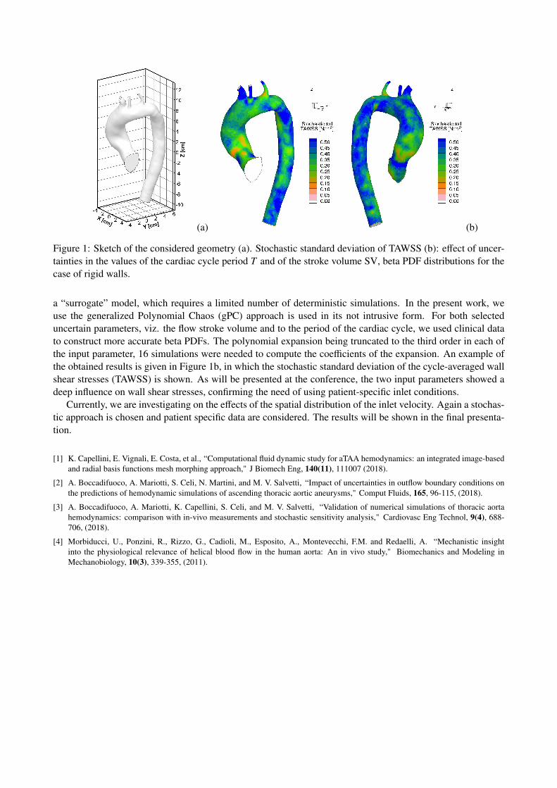
(a) (b)
Figure 1: Sketch of the considered geometry (a). Stochastic standard deviation of TAWSS (b): effect of uncer-
tainties in the values of the cardiac cycle period T and of the stroke volume SV, beta PDF distributions for the
case of rigid walls.
a “surrogate” model, which requires a limited number of deterministic simulations. In the present work, we
use the generalized Polynomial Chaos (gPC) approach is used in its not intrusive form. For both selected
uncertain parameters, viz. the flow stroke volume and to the period of the cardiac cycle, we used clinical data
to construct more accurate beta PDFs. The polynomial expansion being truncated to the third order in each of
the input parameter, 16 simulations were needed to compute the coefficients of the expansion. An example of
the obtained results is given in Figure 1b, in which the stochastic standard deviation of the cycle-averaged wall
shear stresses (TAWSS) is shown. As will be presented at the conference, the two input parameters showed a
deep influence on wall shear stresses, confirming the need of using patient-specific inlet conditions.
Currently, we are investigating on the effects of the spatial distribution of the inlet velocity. Again a stochas-
tic approach is chosen and patient specific data are considered. The results will be shown in the final presenta-
tion.
[1] K. Capellini, E. Vignali, E. Costa, et al., “Computational fluid dynamic study for aTAA hemodynamics: an integrated image-based
and radial basis functions mesh morphing approach," J Biomech Eng, 140(11), 111007 (2018).
[2] A. Boccadifuoco, A. Mariotti, S. Celi, N. Martini, and M. V. Salvetti, “Impact of uncertainties in outflow boundary conditions on
the predictions of hemodynamic simulations of ascending thoracic aortic aneurysms," Comput Fluids, 165, 96-115, (2018).
[3] A. Boccadifuoco, A. Mariotti, K. Capellini, S. Celi, and M. V. Salvetti, “Validation of numerical simulations of thoracic aorta
hemodynamics: comparison with in-vivo measurements and stochastic sensitivity analysis," Cardiovasc Eng Technol, 9(4), 688-
706, (2018).
[4] Morbiducci, U., Ponzini, R., Rizzo, G., Cadioli, M., Esposito, A., Montevecchi, F.M. and Redaelli, A. “Mechanistic insight
into the physiological relevance of helical blood flow in the human aorta: An in vivo study," Biomechanics and Modeling in
Mechanobiology, 10(3), 339-355, (2011).

Workshop on Frontiers of Uncertainty Quantification in Fluid Dynamics
11–13 September 2019, Pisa, Italy
An integrated approach of uncertainty quantification and 3D MRI techniques in
guiding CFD analysis for a non-invasive study of aortic coarctation
Maria Nicole Antonuccio1,2, Benigno Marco Fanni1,2, Katia Capellini1,2, Emilie Sauvage3,Alessandro Mariotti4, Claudio Capelli3 and Simona Celi,1
1BioCardioLab - Heart Hospital, Fondazione Toscana G. Monasterio, Massa, Italy – [email protected],[email protected], [email protected]
2DII, University of Pisa, Italy – [email protected], University of Pisa, Italy – [email protected], [email protected]
4DICI, University of Pisa, Italy – [email protected]
Key words: Uncertainty quantification, Computation Fluid Dynamics, Aortic coartation
Coarctation of aorta (CoA) is a congenital cardiovascular disease characterized by an abnormal narrowing
of the proximal descending aorta, leading to a pressure gradient (∆P) across the coarctation, increased afterload
and reduced peripheral perfusion pressures [1]. Currently, the correction of CoA is based on invasive treat-
ments and the main indication relies on the value of the maximal trans-coarctation pressure (∆P≥20 mmHg)
[2]. Investigations of the hemodynamics and biomechanical basis of morbidity in CoA plays a fundamental role
considering recent advancements in computational modeling. In this context, the computational fluid dynamics
(CFD) approach represents a powerful tool to investigate hemodynamic quantities in a non-invasive way.
In this work, a patient-specific CFD framework was developed for the non invasive assessment of the hemo-
dynamics of the CoA, starting from the patient-specific imaging to the related computational model and the
appropriate boundary conditions. In particular, the aim was to assess the capability of the presented framework
to capture the correct patient-specific ∆P across the CoA. In this context, the definition of the correct boundary
conditions within the computational models still represents a challenge since the overall patient-specific flow
dynamics strongly depends on the outflow conditions [3]. The work-flow of the process is reported in Figure
1. The 3D model was obtained from magnetic resonance imaging (MRI). The inflow boundary condition was
imposed at the valve level of the ascending aorta, considering patient-specific phase contrast MRI data.
Figure 1: Patient-specific CFD framework: MRI dataset segmentation (a); segmented model (b); 3D CFD mesh
with 0-D RCR coupling (c) and zoom on CoA (d).

The effects of the downstream organs and vessels were implemented with a three-element RCR Windkessel
model for each outlet, i.e. the three supra-aortic vessels and the descending aorta[4]. The initial RCR parameters
were firstly determined with a custom code based on the patient-specific flow, as retrieved from imaging, and in
vivo pressure measurements. After reconstructing the geometry and setting up the inlet and the outlet boundary
conditions, patient-specific CFD simulations were performed. The open-source software SimVascular was
used. The ∆P evaluated in silico at the coarctation level was compared against the invasive intravascular trans-
CoA pressure measurements. Hemodynamic quantities and indices of interest, including pressure loss, time-
averaged wall shear stress, and oscillatory shear index, were also quantified. A stochastic approach is still under
investigation for the assessment of the correct RCR parameters to be applied on each aortic branch in order to
obtain the best fit between in vivo and in silico data in terms of outflows and pressure drops. Figure 2 depicts,
as example, the results of a deterministic simulation.
Figure 2: Velocity field at systolic peak in a long axis plane (a); WSS at systolic peak (b) and zoom in CoA (c).
In particular, we are investigating how the uncertainties in the Windkessel model parameters may affect
the results of the numerical simulation. We are adopting a stochastic approach in which the parameters are
considered as random variables with a given probability distribution. We are analyzing different strategies to
obtain a continuous surface in the parameters space starting from a few deterministic numerical simulation.
The generalized polynomial chaos (gPC) seems to be the best choice in terms of feasibility and properties of
convergence. In particular, we are adopting the not intrusive form of the gPC with the big advantage that it is
possible to use deterministic finite element tools, such as the solver SimVascular, as a black box to sample the
model solutions.
[1] L.S. Teo, T. Cannel, A. Babu-Narayan, et al., "Prevalence of Associated Cardiovascular Abnormalities in 500 Patients with Aortic
Coarctation Referred for Cardiovascular Magnetic Resonance Imaging to a Tertiary Center," Pediatr Cardiol, 32(8), 1120-1127,
(2011)
[2] C. A. Warnes, R. Williams, et al., "ACC/AHA 2008 guidelines for the management of adults with congenital heart disease: a
report of the American College of Cardiology/American Heart Association Task Force on Practice Guidelines (writing committee
to develop guidelines on the management of adults with congenital heart disease)," Circulation 118(23), 714-833, (2008)
[3] A. Boccadifuoco, A. Mariotti, S. Celi, N. Martini, M.V. Salvetti, "Impact of uncertainties in outflow boundary conditions on the
predictions of hemodynamic simulations of ascending thoracic aortic aneurysms" Comput Fluids, 165, 96-115, (2018)
[4] I.E. Vignon-Clementel, C.A. Figueroa, K.E. Jansen, C.A. Taylor, "Outflow boundary conditions for three-dimensional finite
element modeling of blood flow and pressure in arteries" Comput. Methods Appl. Mech. Engrg., 195, 3776-3796, (2006)

ST6– Environmental IISession Chair: Gorodetsky A.A.
Auditorium

Workshop on Frontiers of Uncertainty Quantification in Fluid Dynamics
11–13 September 2019, Pisa, Italy
Refining the input space of plausible future debris flows using noisy data and
multiple models of the physics
Andrea Bevilacqua,1, Abani Patra,2 Marcus Bursik,3 E. Bruce Pitman,4
José Luis Macías,5 Ricardo Saucedo,6 David Hyman7
1INGV, Sezione di Pisa, Italy – [email protected]. of Mechanical and Aerospace Engineering, UB, NY, USA – [email protected]
3Dpt. of Earth Sciences, 4Dpt. of Material Design and Innovation, UB, NY, USA5Departamento de Vulcanología, Instituto de Geofísica, UNAM, Mexico City, DF, Mexico
6Instituto de Geología, Facultad de Ingeniería, UASLP, San Luis, SLP, Mexico7Cooperative Institute for Meteorological Satellite Studies, UW, Madison, WI, USA
Key words: Uncertainty quantification, Geophysical Flows, Inverse Problems, Model Inadequacy
Forecasts of future geophysical mass flows, fundamental in hazard assessment, usually rely on the recon-
struction of past flows that occurred in the region of interest using models of physics that have been successful
in hindcasting. The available pieces of data Di ∈ D, are commonly related to the properties of the deposit left
by the flows and to historical documentation. Nevertheless, this information can be fragmentary and affected by
relevant sources of uncertainty (e.g., erosion and remobilization, superposition of subsequent events, unknown
duration, and source). Moreover, different past flows may have had significantly different physical properties,
and even a single flow may change its physics with respect to time and location, making the application of a
single model inappropriate.
Figure 1: Diagram of input spaces, model functions, and output
space (blue), with feasible inputs domain (red), plausible output
codomain and specialized inputs (green), and observed data and
partial solutions subsets (orange). The question mark emphasizes
that the covering of other plausible outputs could be enabled by
adding more models if necessary.
In a probabilistic framework, for each
model M ∈ M we define (M, PM), where
PM is a probability measure over the pa-
rameter space of M. While the support
of PM can be restricted to a single value
by solving an inverse problem for the opti-
mal reconstruction of a particular flow, the
inverse problem is not always well posed.
That is, no input values are able to pro-
duce outputs consistent with all observed
information [5]. Choices based on limited
data using classical calibration techniques
(i.e. optimized data inversion) are often
misleading since they do not reflect all po-
tential event characteristics and can be er-
ror prone due to incorrectly limited event
space. Sometimes the strict replication of
a past flow may lead to overconstraining
the model, especially if we are interested
in the general predictive capabilities of a
model over a whole range of possible fu-
ture events.
In this study, we use a multi-model ensemble and a plausible region approach to provide a more prediction-
oriented probabilistic framework for input space characterization in hazard analysis. In other words, we gener-
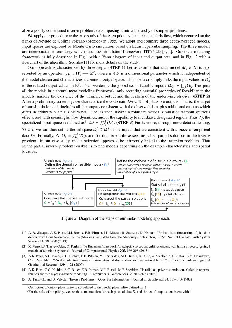
alize a poorly constrained inverse problem, decomposing it into a hierarchy of simpler problems.
We apply our procedure to the case study of the Atenquique volcaniclastic debris flow, which occurred on the
flanks of Nevado de Colima volcano (Mexico) in 1955. We adopt and compare three depth-averaged models.
Input spaces are explored by Monte Carlo simulation based on Latin hypercube sampling. The three models
are incorporated in our large-scale mass flow simulation framework TITAN2D [3, 4]. Our meta-modeling
framework is fully described in Fig.1 with a Venn diagram of input and output sets, and in Fig. 2 with a
flowchart of the algorithm. See also [1] for more details on the study.
Our approach is characterized by three steps: (STEP 1) Let us assume that each model M j ∈ M is rep-
resented by an operator: fM j: Ω
j
0−→ Rd
, where d ∈ N is a dimensional parameter which is independent of
the model chosen and characterizes a common output space. This operator simply links the input values in Ωj
0
to the related output values in Rd. Thus we define the global set of feasible inputs: ΩG :=⊔
jΩj
0. This puts
all the models in a natural meta-modeling framework, only requiring essential properties of feasibility in the
models, namely the existence of the numerical output and the realism of the underlying physics. (STEP 2)
After a preliminary screening, we characterize the codomain DG ⊂ Rd of plausible outputs: that is, the target
of our simulations – it includes all the outputs consistent with the observed data, plus additional outputs which
differ in arbitrary but plausible ways1. For instance, having a robust numerical simulation without spurious
effects, and with meaningful flow dynamics, and/or the capability to inundate a designated region. Thus ∀ j, the
specialized input space is defined as2: Ω j = f −1M j
(D) . (STEP 3) Furthermore, through more detailed testing,
∀i ∈ I, we can thus define the subspace Ωj
i⊆ Ω j of the inputs that are consistent with a piece of empirical
data Di. Formally, ∀i, Ωj
i= f −1
M j(Di), and for this reason those sets are called partial solutions to the inverse
problem. In our case study, model selection appears to be inherently linked to the inversion problem. That
is, the partial inverse problems enable us to find models depending on the example characteristics and spatial
location.
Construct the partial solutions
Ωij = fMj
-1[Di ∩ fMj(Ωj) ]
For each model Mj є For each piece of observed data Di є
For each model Mj є M
Statistical summary of:
fMj(Ωj) - plausible outputs
fMj(Ωij) - partial solutions
fMj(Ωi1j ∩... ∩ Ωik
j) intersection of partial solutions
Construct the specialized inputs
Ωj = fMj-1[DG ∩ fMj(Ω0
j) ]
For each model Mj є M
Define the codomain of plausible outputs - DG
- robust numerical simulation without spurious effects
- macroscopically meaningful flow dynamics
- inundation of a designated region
Define the domain of feasible inputs - Ω0j
- existence of the output
- realism in the physics
For each model Mj є M
Figure 2: Diagram of the steps of our meta-modeling approach.
[1] A. Bevilacqua, A.K. Patra, M.I. Bursik, E.B. Pitman, J.L. Macías, R. Saucedo, D. Hyman, “Probabilistic forecasting of plausible
debris flows from Nevado de Colima (Mexico) using data from the Atenquique debris flow, 1955”, Natural Hazards Earth System
Science 19, 791-820 (2019).
[2] K. Farrell, J. Tinsley Oden, D. Faghihi, “A Bayesian framework for adaptive selection, calibration, and validation of coarse-grained
models of atomistic systems”, Journal of Computational Physics 295, 189-208 (2015).
[3] A.K. Patra, A.C. Bauer, C.C. Nichita, E.B. Pitman, M.F. Sheridan, M.I. Bursik, B. Rupp, A. Webber, A.J. Stinton, L.M. Namikawa,
C.S. Renschler, “Parallel adaptive numerical simulation of dry avalanches over natural terrain”, Journal of Volcanology and
Geothermal Research 139, 1–21 (2005).
[4] A.K. Patra, C.C. Nichita, A.C. Bauer, E.B. Pitman, M.I. Bursik, M.F. Sheridan, “Parallel adaptive discontinuous Galerkin approx-
imation for thin layer avalanche modeling”, Computers & Geosciences 32, 912–926 (2006).
[5] A. Tarantola and B. Valette, “Inverse Problems = Quest for Information”, Journal of Geophysics 50, 159-170 (1982).
1Our notion of output plausibility is not related to the model plausibility defined in [2].2For the sake of simplicity, we use the same notation for each piece of data Di and the set of outputs consistent with it.
Workshop on Frontiers of Uncertainty Quantification in Fluid Dynamics
11–13 September 2019, Pisa, Italy
Surrogate-based parameter inference in a debris flow model
Maria Navarro,1 Olivier Le Maître,2 Ibrahim Hoteit3, David George,4 Kyle Mandli,5 and Omar M. Knio6
1King Abdullah University of Science and Technology, Saudi Arabia –[email protected]
2LIMSI-CNRS, France – [email protected]
3King Abdullah University of Science and Technology, Saudi Arabia – [email protected]
4U.S. Geological Survey, Vancouver, WA 98683 – [email protected]
5Columbia University, New York, NY 10027 – [email protected]
6King Abdullah University of Science and Technology, Saudi Arabia – [email protected]
Key words: Bayesian inference, Polynomial Chaos Expansion, Debris Flow, Uncertainty Quantification
This work tackles the problem of calibrating the unknown parameters of a debris flow model with the draw-
back that the information regarding the experimental data treatment and processing is not available. In particu-
lar, we focus on the the evolution over time of the flow thickness of the debris with dam-break initial conditions.
The proposed methodology consists of establishing an approximation of the numerical model using a polyno-
mial chaos expansion that is used in place of the original model, saving computational burden. The values of
the parameters are then inferred through a Bayesian approach with a particular focus on inference discrepan-
cies that some of the important features predicted by the model exhibit. We build the model approximation
using a preconditioned non-intrusive method and show that a suitable prior parameter distribution is critical to
the construction of an accurate surrogate model. The results of the Bayesian inference suggest that utilizing
directly the available experimental data could lead to incorrect conclusions, including the over-determination
of parameters. To avoid such drawbacks, we propose to base the inference on few significant features extracted
from the original data. Our experiments confirm the validity of this approach, and shown that it does not lead
to significant loss of information. It is further computationally more efficient than the direct approach, and can
avoid the construction of an elaborate error model.

Workshop on Frontiers of Uncertainty Quantification in Fluid Dynamics
11–13 September 2019, Pisa, Italy
Propagation of Uncertainties in Density-Driven Flow
Alexander Litvinenko1, Dmitry Logashenko2, Raul Tempone1,2, Gabriel Wittum2 and David Keyes2
1RWTH Aachen, Germany, – litvinenko, [email protected]
2KAUST, Thuwal, Saudi Arabia – dmitry.logashenko, raul.tempone, gabriel.wittum,[email protected]
Key words: Uncertainty quantification, density driven flow, subsurface flow, uncertain porosity
Accurate modeling of contamination in subsurface flow and water aquifers is crucial for agriculture and
environmental protection. Here, we demonstrate an efficient parallel algorithm to quantify the propagation of
the uncertainty in the dispersal of pollution in subsurface flow. Specifically, we consider the density-driven flow
and estimate how uncertainty from permeability and porosity propagates to the solution. We take an Elder-like
problem as a numerical benchmark and we use random fields to model the limited knowledge on the porosity
and permeability. We construct a low-cost generalized polynomial chaos expansion (gPCE) surrogate model,
where the gPCE coefficients are computed by projection on sparse and full tensor grids. We parallelize both
the numerical solver for the deterministic problem based on the multigrid method, and the quadrature over the
parametric space.
[1] A. Litvinenko, D. Logashenko, R. Tempone, G. Wittum, and D. Keyes “Propagation of Uncertainties in Density-Driven Flow”,
arXiv preprint, April 2019.
[2] S. Reiter, A. Vogel, I. Heppner, M. Rupp, and G. Wittum, “A massively parallel geometric multigrid solver on hierarchically
distributed grids”, Computing and visualization in science 16, 4 (2013), pp 151-164, DOI: 10.1007/s00791-014-0231-x
[3] A. Vogel, S. Reiter, M. Rupp, A.Nagel, and G. Wittum, “UG4 — a novel flexible software system for simulating PDE based models
on high performance computers”. Computing and visualization in science 16, 4 (2013), pp 165-179, DOI: 10.1007/s00791-014-
0232-9
[4] A. Schneider, H. Zhao, J. Wolf, D. Logashenko, S. Reiter, M. Howahr, M. Eley, M. Gelleszun, H. Wiederhold, “Modeling
saltwater intrusion scenarios for a coastal aquifer at the German North Sea”, E3S Web of Conferences 54, 00031 (2018),
DOI:10.1051/e3sconf/20185400031
[5] M. Espig, W. Hackbusch, A. Litvinenko, H.G. Matthies, E. Zander, “Efficient analysis of high dimensional data in tensor formats”,
Sparse Grids and Applications, LNCSE, volume 88, pp 31-56, 2012
[6] S. Dolgov, B.N. Khoromskij, A. Litvinenko, and H.G. Matthies, “Polynomial Chaos Expansion of Random Coefficients and the
Solution of Stochastic Partial Differential Equations in the Tensor Train Format”, IAM/ASA J. Uncertainty Quantification 3 (1),
pp 1109-1135, 2015
[7] A. Litvinenko, H.G. Matthies, T.A. El-Moselhy, “Sampling and low-rank tensor approximation of the response surface”, Monte
Carlo and Quasi-Monte Carlo Methods 2012, PROMS, volume 65, pp 535-551, 2013
[8] A. Litvinenko, H.G. Matthies, “Numerical Methods for Uncertainty Quantification and Bayesian Update in Aerodynamics”,
In: Eisfeld B., Barnewitz H., Fritz W., Thiele F. (eds) Management and Minimisation of Uncertainties and Errors in Numerical
Aerodynamics. Notes on Numerical Fluid Mechanics and Multidisciplinary Design, vol 122. Springer, Berlin, Heidelberg, 2013

Workshop on Frontiers of Uncertainty Quantification in Fluid Dynamics11–13 September 2019, Pisa, Italy
Uncertainty quantification in explosive volcanic eruptions: from volcanic column
generation to ash dispersion and deposition
Federica Pardini1, Mattia de’ Michieli Vitturi1, Samantha Louise Engwell2, Sara Barsotti3, and Augusto Neri1
1Istituto Nazionale di Geofisica e Vulcanologia, Sezione di Pisa, Pisa, Italy2British Geological Survey, Edinburgh, United Kingdom
3Vedurstofa Íslands, Icelandic Met Office, Reykjavík, Iceland
Key words: Uncertainty quantification, Eruptive column models, Ash dispersion, Volcanic hazard
Explosive volcanic eruptions produce hot plumes of gas and particles whose behaviour is complex anddependent on both eruptive source parameters (e.g. exit velocity, gas fraction, temperature and grain-size dis-tribution) and atmospheric environment. Assessing the way in which these elements influence plume height andsubsequent ash dispersal patterns (both in the atmosphere and on the ground) is of fundamental importance forvolcanic hazard mitigation. Here, we present the results of uncertainty quantification and sensitivity analysisperformed through latin hypercube sampling and polynomial chaos expansion, aimed at identifying and quanti-fying the source parameters exerting a major role on plume height and trajectory. The analysis is applied to theintegral column model PLUME-MoM 2.0. The model describes the rise of a pyroclastic mixture by solving theequations for the conservation of mass, momentum and energy for the gas-ash mixture, accounting for impor-tant processes such as particles settling, particle aggregation, phase changes of water and effects of moisture.The continuous polydispersity of pyroclastic particles is described using a quadrature-based moment method,an innovative approach in volcanology well-suited for the description of the multiphase nature of magmaticmixtures. The study is further extended beyond the dynamics of the rising plume to investigate the effects thatuncertain eruptive source parameters have on ash dispersion in the atmosphere and deposition on the ground.Indeed, the column model has been integrated with the dispersal model HYSPLIT, which simulates the trans-port and dispersion of particles into the atmosphere. Particles lost from the column enter into the atmosphericenvironment and are transported and dispersed until they deposit on the ground. The uncertainty quantificationanalysis allows us to construct statistical particle size distributions, both in the air and on the ground, at variousdistances from the volcanic vent. The cases study for the present analysis are two eruptive scenario, weak andstrong plume, at Mt.Etna, Italy.

x (km)
01
23
4
y (km)
0.00.5
1.01.5
2.02.5
3.03.5
z (km
)
4
5
6
7
(a) 13E 14E 15E 16E 17E
36N
37N
38N
39N
Total atmospheric loading
1.00 × 10 15
1.00 × 10 9
1.00 × 10 7
1.00 × 10 5
7.23 × 10 5
9.03 × 10 5
1.08 × 10 4
1.26 × 10 4Loading (kg/m^3)
(b)
Figure 1: Image of the volcanic column from PLUME-MoM 2.0 (a) and atmospheric ash loading as simulatedby HYSPLIT (b)
[1] M. de’ Michieli Vitturi, A. Neri, and S. Barsotti, “PLUME-MoM 1.0: A new integral model of volcanic plumes based on themethod of moments,” Geoscientific Model Development 8, 2447-2463 (2015).
[2] M. de’ Michieli Vitturi, S.L. Engwell, A. Neri, and S. Barsotti, “Uncertainty quantification and sensitivity analysis of volcaniccolumns models: Results from the integral model PLUME-MoM,” Journal of Volcanology and Geothermal Research 326, 77-91(2016).
[3] A.F. Stein, R.R. Draxler, G.D. Rolph, B.J.B. Stunder, M.D. Cohen, and F. Ngan, “NOAA’s HYSPLIT atmospheric transport anddispersion modeling system,” Bulletin of the American Meteorological Societyt 96, 2059-2077 (2015).

Keynote Lecture - E.F. Campana - Sailing in a storm: UQ for ship optimization in astochastic environment with operational uncertainty
Session Chair: P. CinnellaAuditorium

Workshop on Frontiers of Uncertainty Quantification in Fluid Dynamics
11–13 September 2019, Pisa, Italy
Sailing in a Storm: UQ for Ship Optimization in a Stochastic Environment with
Operational Uncertainty
Emilio F. Campana1 and Matteo Diez2
1CNR-DIITET, Italy – [email protected]
2CNR-INM, Italy – [email protected]
Key words: Ship Design, Uncertainty Quantification, Design Optimization, Stochastic Optimization
The ocean is an intrinsic stochastic environment and ships operations are permeated by uncertainty stem-
ming from environmental conditions (wave energy spectra, significant wave height, modal period, and direc-
tion, wind, etc.) and operational parameters (speed, heading, payload, etc.). Therefore, a robust and reliable
assessment of ship performance (resistance, seakeeping, maneuverability, stability and control) must consider
the uncertainty associated to all relevant input parameters and evaluate its propagation to the relevant outputs
through the analysis process. Furthermore, high-fidelity simulations (e.g., large-grid CFD and/or FEA com-
putations) are often required to ensure accuracy and reliability of the analysis outcomes and the subsequent
decision making. This is particularly true for stormy conditions, high sea states, high and steep waves, and
violent impacts, where low-fidelity tools usually fail to provide reliable predictions. It is worthwhile to recall
that international vessel registers expect, as an effect of climate changes, an increase in the near future of both
the average sea state in the oceans and the frequency of extreme wave events. Consequently, modern ship
design must incorporate uncertainty quantification (UQ) methods with high fidelity analyses. The affordability
of combining these tools with (global) optimization algorithms into a fully digital and automated design pro-
cesses depends on the availability of efficient methods for operational and design space exploration, i.e. UQ
and optimization.
The talk will focus on the integration of UQ methods into a simulation-based design global optimization
framework to increase ships operational efficiency and effectiveness in real ocean environments. The use of
collocation methods and adaptive metamodels with Monte Carlo simulation will be discussed as well as the
efficient application of design space dimensionality reduction techniques based on the Karhunen-Loève ex-
pansion of hull shape- and physics-related variables. Examples will be provided based on recent international
collaborative research within NATO Science and Technology Organization Applied Vehicle Technology task
group AVT-252 on ”Stochastic Design Optimization for Naval and Aero Military Vehicles,” where a naval-
destroyer hull form was optimized to increase its operational efficiency and effectiveness in realistic ocean
environment and operations.
[1] Serani, A., Diez, M., Wackers, J., Visonneau, M. and Stern, F., 2019. Stochastic Shape Optimization via Design-Space Augmented
Dimensionality Reduction and RANS Computations. In AIAA Scitech 2019 Forum (p. 2218).
[2] Diez, M., Campana, E.F. and Stern, F., 2018. Stochastic optimization methods for ship resistance and operational efficiency via
CFD. Structural and Multidisciplinary Optimization, 57(2), pp.735-758.
[3] Volpi, S., Diez, M., Gaul, N.J., Song, H., Iemma, U., Choi, K.K., Campana, E.F. and Stern, F., 2015. Development and validation
of a dynamic metamodel based on stochastic radial basis functions and uncertainty quantification. Structural and Multidisciplinary
Optimization, 51(2), pp.347-368.
[4] Diez, M., Campana, E.F. and Stern, F., 2015. Design-space dimensionality reduction in shape optimization by Karhunen-Loève
expansion. Computer Methods in Applied Mechanics and Engineering, 283, pp.1525-1544.

SF1 – Applications IIISession Chair: E.F. Campana
Auditorium

Workshop on Frontiers of Uncertainty Quantification in Fluid Dynamics
11–13 September 2019, Pisa, Italy
Uncertainty Quantification by Adaptive Multifidelity Surrogates
of Noisy CFD Data
Jeroen Wackers†, Michel Visonneau†, Andrea Serani∗, Riccardo Pellegrini∗, Riccardo Broglia,and Matteo Diez∗
† LHEEA Lab, Ecole Centrale de Nantes, CNRS-UMR 6598, Nantes, France– [email protected], [email protected]
∗ CNR-INM, National Research Council-Institute of Marine Engineering, Rome, Italy– [email protected], [email protected], [email protected], [email protected]
Key words: Uncertainty quantification, Multifidelity analysis, Surrogate models, Computational Fluid Dynam-ics, Adaptive grid refinement, Multi-grid method
Ship performance depends on design and operational/environmental parameters. The accurate prediction
of performance metrics (such as the hydrodynamic resistance) requires high-fidelity computational tools, es-
pecially for innovative configurations and extreme/off-design conditions. These tools are generally computa-
tionally expensive, making the design/operational-space exploration and associated uncertainty quantification
(UQ) a technological challenge.
To reduce the computational cost, supervised machine learning/surrogate (or metamodeling) methods are
applied. Dynamic/adaptive surrogates update dynamically their training sets, exploiting the information that
becomes available during the analysis process: training points are added where it is most useful, reducing the
number of function evaluations required to represent the desired function [1, 2]. Unfortunately, the adaptive
sampling process is affected by the computational-output noise. Adaptive sampling methods may react to noise
by adding many training points in noisy regions, rather than selecting new points in unseen regions. This
deteriorates the model quality/efficiency and has to be considered carefully [3].
In addition to dynamic/adaptive surrogates and with the aim of reducing further the computational cost,
multi-fidelity (MF) methods combine the accuracy of high-fidelity solvers with the computational cost of low-
fidelity solvers. MF metamodels use mainly low-fidelity simulations and only few high-fidelity simulations are
used to preserve the model accuracy. Several metamodels are used with MF data. An example of application
of radial basis functions (RBF) is shown in [1, 2]. In CFD-based UQ, different fidelity levels may be obtained
by varying the physical model, the grid size, and/or combining experimental data with simulations.
The objective of the present work is to present an adaptive RBF-based N-fidelity (NF) surrogate for UQ of
complex industrial problems, fully exploiting the potential of simulation methods that naturally produce results
spanning a range of fidelity levels: RANS (Reynolds-Averaged Navier-Stokes) simulations with adaptive grid
refinement [4], and/or multi-grid resolution [5]. The NF method is further advanced to reduce the effects of the
noise in the CFD outputs through regression and in-the-loop optimization of the model.
The NF method is developed based on authors’ previous work [1, 2, 6, 3, 7] and demonstrated for the UQ of
(i) a NACA hydrofoil and (ii) a roll-on/roll-off passengers (RoPax) ferry subject to uncertain shape/operating
parameters. CFD is based on two RANS solvers: (1) ISIS-CFD [4], developed at ECN/CNRS and integrated
in the FINE/Marine suite (NUMECA Int), and (2) Xnavis [5], developed at CNR-INM. In ISIS-CFD, different
fidelity levels are defined by the grid refinement ratio in adaptive grid refinement. In Xnavis, different fidelities
are obtained exploiting the multi-grid approach.
[1] S. Volpi, M. Diez, N. J. Gaul, H. Song, U. Iemma, K. K. Choi, E. F. Campana, and F. Stern, “Development and validation of a
dynamic metamodel based on stochastic radial basis functions and uncertainty quantification,” Structural and Multidisciplinary
Optimization, vol. 51, no. 2, pp. 347–368, 2015.

[2] R. Pellegrini, A. Serani, M. Diez, J. Wackers, P. Queutey, and M. Visonneau, “Adaptive sampling criteria for multi-fidelity meta-
models in CFD-based shape optimization,” in 7th European Conference on Computational Fluid Dynamics (ECFD 7), Glasgow,
UK, June, 2018.
[3] J. Wackers, A. Serani, R. Pellegrini, R. Broglia, M. Diez, and M. Visonneau, “Adaptive multifidelity shape optimization based on
noisy CFD data,” in International Conference on Adaptive Modeling and Simulation, ADMOS 2019, El Campello (Alicante), May,
2019.
[4] P. Queutey and M. Visonneau, “An interface capturing method for free-surface hydrodynamic flows,” Computers & fluids, vol. 36,
no. 9, pp. 1481–1510, 2007.
[5] R. Broglia and D. Durante, “Accurate prediction of complex free surface flow around a high speed craft using a single-phase level
set method,” Computational Mechanics, vol. 62, no. 3, pp. 421–437, 2018.
[6] A. Serani, R. Pellegrini, R. Broglia, J. Wackers, M. Visonneau, and M. Diez, “An adaptive n-fidelity metamodel for design and
operational-uncertainty space exploration of complex industrial problems,” in VIII International Conference on Computational
Methods in Marine Engineering, MARINE 2019, Gothenburg, Sweden, May, 2019.
[7] J. Wackers, M. Visonneau, A. Serani, R. Pellegrini, R. Broglia, and M. Diez, “Multi-fidelity machine learning from adaptive- and
multi-grid RANS simulations,” in submitted to 33rd Symposium on Naval Hydrodynamics, Osaka, Japan, May, 2020.

Workshop on Frontiers of Uncertainty Quantification in Fluid Dynamics
11–13 September 2019, Pisa, Italy
Gradient Based Empirical Cumulative Distribution Function Approximation for
Robust Aerodynamic Design
Andrea Bornaccioni,1 Elisa Morales Tirado,2 Domenico Quagliarella2 and Umberto Iemma1
1Roma Tre University, Italy – [email protected], [email protected]
2CIRA, Italy – [email protected], [email protected]
Key words: Robust Design, RANS Solver, Adjoint Solver, Uncertainty Quantification, Risk Functions, Empir-ical Cumulative Distribution Function
A robust optimization approach based on the use of risk functions, namely VaR and CVaR [1], is presented
together with an application to a robust aerodynamic design problem of the central airfoil of a tailless flying-
wing aircraft at transonic cruise conditions. The characteristic feature of this design exercise is that for such a
configuration the central section must provide not only a specified amount of lift but a definite nose-up pitching
moment too. Thus, an additional aerodynamic constraint is required. The robust approach to this optimization
problem helps to obtain solutions that do not deteriorate excessively in the presence of uncertainties on the
airfoil contour or the operating conditions. The uncertainties on the airfoil section are due, for example, to
machining tolerances, to deformations of the shape under load or the accumulation of debris on the wing
surface. Furthermore, the aircraft may operate in speed and load conditions quite different from the design ones,
and, hence they have to be considered as uncertain parameters too. Risk functions are here estimated using an
approach based on the empirical cumulative probability distribution (ECDF). The quantities of interest (QoI)
of the risk functions are the aerodynamic characteristics of the airfoil, namely lift, drag and pitching moment
coefficients, which are computed solving the compressible Reynolds-averaged Navier-Stokes equations with
the open source fluid-dynamic solver SU2 [3]. In the present work, we consider the effect of uncertainties
in the operational conditions, such as Mach number and angle of attack. Furthermore, we take into account
uncertainties on the pitching moment coefficient in order to account for changes in the aircraft center of gravity.
The use of a RANS solver makes VaR and CVaR calculation costly from the computational point of view,
and the characterizing aspect of the work is the use of techniques and methods for the reduction of the cost
mentioned above. In particular, the estimate of the empirical CDF is obtained by exploiting the QoI gradients
with respect to the uncertain variables computed through the discrete adjoint module of SU2 [4]. The ECDF
is thus approximated with a first-order series expansion using efficiently calculated gradients from SU2 which,
thanks to the adjoint method, are available at the computational cost of one CFD solution whatever the number
of uncertainties is. The robust approach based on risk functions is, without doubt, more powerful and flexible
than the deterministic multi-point methodology that is generally used in this type of problem, given that the high
number of uncertain operational parameters makes the definition of the multi-point design problem quite tricky
and cumbersome. On the other hand, however, the method of risk functions is computationally expensive due
to the relatively high number of samples required to define the ECDF estimation. The adjoint-based approach
presented here allows a substantial reduction of the computational cost needed to estimate the ECDF.
[1] D. Quagliarella, “Value-at-Risk and Conditional Value-at-Risk in Optimization Under Uncertainty," In Uncertainty Management
for Robust Industrial Design in Aeronautics, 541-565 (Springer, Cham, 2019).
[2] M. A. Sargeant, T. P. Hynes, W. R. Graham, J. I. Hileman and M. Drela, “Stability of hybrid-wing-body-type aircraft with
centerbody leading-edge carving. Journal of Aircraft," Journal of Aircraft 47, 3 (2010).
[3] T. D. Economon, F. Palacios, S. R. Copeland, T. W. Lukaczyk and J. J. Alonso, “SU2: An open-source suite for multiphysics
simulation and design," Aiaa Journal 54, 3 (2015).

[4] T. A. Albring, M. Sagebaum and N. R. Gauger, “Efficient aerodynamic design using the discrete adjoint method in SU2," In 17th
AIAA/ISSMO multidisciplinary analysis and optimization conference, 3518 (2016).

Workshop on Frontiers of Uncertainty Quantification in Fluid Dynamics11–13 September 2019, Pisa, Italy
Assessment of Gradient-Based Surrogate Models for Robust Optimization in
Computational Fluid Dynamics
Aldo Serafino,1,2 Benoit Obert,1 and Paola Cinnella,2
1 Enertime, Courbevoie, France – [email protected]
2 Lab. Dynfluid, École Nationale Supérieure d’Arts et Métiers, Paris, France – [email protected]
Key words: Robust optimization, CFD for industrial applications, continuous adjoint method, discrete adjoint,gradient enhanced Kriging
Robust Design (RD) represents an important tool for the design of industrial products under uncertainty [1].Because of the strong link between the concepts of design and optimization, RD is usually referred to as robustdesign optimization (RDO) or robust optimization (RO), as well. Several RO strategies are nowadays available:among them, some techniques can be considered rather prominent like Taguchi’s [2] or the Low-Quantile one[3] or the “Horsetail Matching” [4].
The RO approaches studied in the literature often combine evolutionary optimization algorithms, like geneticalgorithms (GA) and techniques for the quantification of the uncertainty (UQ). Unfortunately, the UQ forcomplex systems requiring to be simulated with Computational Fluid Dynamics (CFD) comes up against thehigh computational cost of CFD models for configurations of practical interest. As a consequence of this, thepropagation of the uncertainty is not feasible with methods like Montecarlo (MC), even with improved samplingtechniques (i.e., Latin Hypercube Sampling).
In the present work we investigate RDO techniques well-suited for industrial applications. The main require-ments are: 1) greatest possible parsimony in terms of costly CFD simulations (for a given accuracy level) and2) non intrusiveness (as in industry the use of black-box CFD codes can be usual). In this respect, a promisingnon-intrusive RDO technique has been introduced in [5], based on the coupling of two nested Kriging surro-gates: the first one is used to compute the required statistics of the objective functions in the uncertain parameterspace, while the second one is used to model the response of these statistics to the design variables. An ex-pected improvement criterion is used to update the second Kriging surrogate during convergence towards theoptimum. Such an approach has been successfully applied to the design of turbine blades for Organic RankineCycles [6] and to the RDO of the thermodynamic cycle [7]. The approach was shown to require O(10 × n × d)function evaluations (with n the number of uncertain parameters and d the number of design variables) at thefirst generation of the GA, in order to generate the Kriging surrogates, which can be efficiently parallelized on ahigh-performance computer, while additional O(10× n) evaluations are required for each update of the externalKriging surrogate. Typically, only a few updates during the GA iterations are sufficient to obtain an accurateapproximation of the Pareto front. Despite considerable efficiency gains with respect to other surrogate modelslike Polynomial Chaos Expansion (see for instance [8]) or Probabilistic Collocation Method [9], the nestedKriging approach remains too expensive for industrial problems, especially if a large number of uncertain pa-rameters has to be taken into account and if massively parallel computers are not available. Thus, RDO istypically limited to uncertain spaces of low to moderate dimensionality (up to about 8 uncertain parameters).
With the aim of enabling the application of RDO to higher dimensional parameter spaces and/or to morerealistic and complex fluid flow problems, a further reduction of the computational cost is mandatory. In orderto achieve this goal, in the present work we investigate a RDO methodology based on the coupling of a GradientEnhanced Kriging (GEK) [10] for the UQ step with a Kriging surrogate for the optimization step. The gradientsrequired for GEK are efficiently computed by means of the Continuous [11] or Discrete Adjoint method [12],allowing to strongly reduce the dependency of the computational cost of the UQ step on the number of uncertain

parameters. Specifically, the continous adjoint is suitable for a non-intrusive coupling with industrial CFDsolvers, although the discretization of the adjoint equations and the implementation of the boundary conditionsmay be a delicate task and introduce errors in the calculated gradients. The continuous-adjoint GEK RDOis assessed against the discrete-adjoint one and a GEK using finite-difference approximations of the functionderivatives in terms of accuracy and computational cost. For that purpose, we restrict our attention to aninexpensive test problem, namely, the supersonic flow in a quasi-1D nozzle, already studied in [13]. For thistoy problem, the solutions of the Gradient-Enhanced RDO strategies can be compared to a reference RDOusing Monte Carlo sampling for the UQ step and no surrogate modeling for the optimization step.
[1] H.G. Beyer and B. Sendhoff. “Robust optimization: A comprehensive survey." Computer Methods in Applied Mechanics andEngineering, 196(33), July 2007, pp. 3190-3218.
[2] G.Taguchi. System of experimental design: engineering methods to optimize quality and minimize costs. UNIPUB/Kraus Interna-tional Publications, 1987.
[3] M. Moustapha, B. Sudret, J.M. Bourinet and B. Guillaume. “Quantile-based optimization under uncertainties usingadaptive Krig-ing surrogate models." Struct Multidisc Optim (2016) 54:1403-1421.
[4] L.W. Cook and J.P. Jarrett. “Horsetail matching: a flexible approach to optimization under uncertainty." Engineering Optimiza-tion(2018), 50:4, 549-567.
[5] P. Cinnella and E. Bufi. “Robust Optimization Using Nested Kriging Surrogates: Application to Supersonic ORC Nozzle GuideVanes." ERCOFTAC Bulletin 110, mar 2017.
[6] E.A. Bufi and P. Cinnella. “Robust optimization of supersonic ORC nozzle guide vanes." J. Phys.(2017): Conf. Ser.821 012014.
[7] A. Serafino, B. Obert, H. Hagi and P. Cinnella. “Assessment of an Innovative Technique for the Robust Optimization of OrganicRankine Cycles." In ASME TurboExpo2019, 17-21 June 2019, Phoenix, AZ (USA).
[8] P. Cinnella and S.J. Hercus. “Robust Optimization of Dense Gas Flows Under Uncertain Operating Conditions." Computers Fluids,39(10):1893 - 1908, 2010.
[9] G.J.A. Loeven. Efficient Uncertainty Quantification in Computational Fluid Dynamics. PhD thesis, TU Delft, 2010.
[10] J.H.S. de Baar, R.P. Dwight, and H. Bijl. “Improvements to Gradient-Enhanced Kriging Using a Bayesian Interpretation." Inter-national Journal for Uncertainty Quantification, 4(3), 2014.
[11] A. Jameson, L. Martinelli and N.A. Pierce. “Optimum Aerodynamic Design Using the Navier-Stokes Equations." Theoret.Comput. Fluid Dynamics, 10(1):213-237, January 1998.
[12] M.B. Giles, M.C. Duta, J.D. Muller and N.A. Pierce. “Algorithm Developments for Discrete Adjoint Methods." AIAA Journal,41(2): 198-205, February 2003.
[13] P. Cinnella and M. Pini. “Hybrid Adjoint-based Robust Optimization Approach for Fluid-Dynamics Problems." In 54th
AIAA/ASME/ASCE/AHS/ASC Structures, Structural Dynamics, and Materials Conference.

Workshop on Frontiers of Uncertainty Quantification in Fluid Dynamics
11–13 September 2019, Pisa, Italy
Quantification of Parametric Uncertainty in Wind Farm Wake Modeling
Jincheng Zhang,1 and Xiaowei Zhao,1
1School of Engineering, The University of Warwick, Coventry, UK
Key words: Uncertainty Quantification, Wake Modeling, Bayesian Inference, Wind Farm Simulations
Accurate prediction of wind turbine wakes is essential for the optimal operation of wind farms. In order
to achieve this, the parametric uncertainty of analytical wake model is investigated for the first time in this
work. Specifically, Bayesian inference is employed for calibrating the wake model. A series of Large Eddy
Simulations (LES) of wind farms is carried out with different turbine settings and the generated high-fidelity
flow field data is used to infer the model parameters. After model calibration, the posterior model check
shows that the predicted mean velocity profile with the quantified uncertainty matches well with the high-
fidelity LES data. The prediction of other quantities, such as turbine power output, is also carried out. Further
analysis demonstrates that the data-driven wake model with the model parameters specified by their posterior
distributions can be seen as the stochastic extension of the original wake model. As most of the existing wake
models are static, the resulting stochastic model shows a great advantage over the original model, as it can give
not only the steady wind farm properties but also some estimations about the unsteadiness of the wind farm.
[1] P. Gebraad, F. Teeuwisse, J. Wingerden, P. A. Fleming, S. Ruben, J. Marden and L. Pao, “Wind plant power optimization through
yaw control using a parametric model for wake effects - a CFD simulation study," Wind Energy, 19, 95-114, 2016.
[2] P. A. Fleming, P. Gebraad, S. Lee, J. Wingerden, K. Johnson, M. Churchfield, J. Michalakes, P. Spalart and P. Moriarty, “Evaluating
techniques for redirecting turbine wakes using SOWFA," Renewable Energy, 70, 211-218, 2014.
[3] M.C. Kennedy and A. O’Hagan, “Bayesian calibration of computer models," Journal of the Royal Statistical Society: Series B
(Statistical Methodology), 63 (3): 425-464, 2001.
[4] S. H. Cheung, T. A. Oliver, E. E. Prudencio, S. Prudhomme and R. D. Moser, “Bayesian uncertainty analysis with applications to
turbulence modeling," Reliability Engineering & System Safety, 96(9), 1137-1149, 2011.
[5] J. Zhang and S. Fu, “An efficient Bayesian uncertainty quantification approach with application to k-ω-γ transition modeling,"
Computers & Fluids, 161: 211-224, 2018.
[6] J. Zhang and S. Fu, “An efficient approach for quantifying parameter uncertainty in the SST turbulence model," Computers &
Fluids, 181: 173-187, 2019.

SF2 – Methodology IVSession Chair: D. Lucor
Auditorium

Workshop on Frontiers of Uncertainty Quantification in Fluid Dynamics
11–13 September 2019, Pisa, Italy
Multifidelity Uncertainty Quantification for Fluid Dynamics applications
Alex A. Gorodetsky,1 Gianluca Geraci,2 Michael S. Eldred,2 and John D. Jakeman,2
1Aerospace Engineering, University of Michigan, MI, USA – [email protected]
2Optimization and Uncertainty Quantification, Sandia National Laboratories, NM, USA –ggeraci,mseldre,[email protected]
Key words: Uncertainty quantification, Multifidelity, Fluid Dynamics
Creating predictive numerical simulations requires characterizing and quantifying the impact of uncertainty.
In computational fluid dynamics (CFD) applications, computationally expensive models (Direct Numerical
Simulation, Large Eddy Simulation, etc.) are often required to resolve all the important spatial and temporal
scales of the solution. Moreover, practical engineering systems which involve fluid dynamics phenomena very
often also comprise additional physics (as for instance radiation transport [1], combustion [2], etc.) whose
accurate solution further increases the computational burden. In such situations the extreme computational cost
of the numerical simulation coupled with a very large number of uncertainty sources heavily limits our ability
to create large enough datasets for accurate Uncertainty Quantification (UQ).
Indeed, despite huge advances in UQ algorithms in the last two decades, UQ for realistic systems remains
prohibitive in these extreme computational regimes where even a few simulations can be prohibitively expen-
sive. To overcome this issue, the concept of multifidelity UQ has been introduced. This concept closely follows
ideas that matured in the field of optimization [3, 4]. Several flavors of multifidelity UQ have been introduced,
and they are all based on the aggregation of large numbers of lower accuracy realizations with a limited number
of high-fidelity data. Historically the most natural way of deriving lower accuracy models has been to directly
leverage coarsening along the spatial and temporal dimensions [9, 10, 11].
Recently, it has become increasingly important to also consider different modeling choices that share similar
physics during multifidelity analysis. In CFD applications for turbulence simulations one might rely on either
Large Eddy Simulations or Reynolds Averaged Navier-Stokes equations to produce very rough approximations
of some global trends in Direct Numerical Simulations. In these circumstances, existing algorithms must be
adapted to efficiently exploit relationship among models (see for instance [8, 7]).
In this work we consider algorithms for propagating uncertainty through computational simulation models
of varying fidelities. Our goal is to estimate, or predict, quantities of interest from a specified high-fidelity
model when only a limited number of these simulations is available. To aid in this task, lower fidelity models
can be used to reduce the uncertainty of the high-fidelity predictions. We discuss existing sampling-based and
surrogate-based algorithms from an information transfer perspective, and we first demonstrate the way in which
these algorithms leverage information (e.g., correlations and discrepancies) between models. We show that
algorithms based on recursion, e.g., multi-fidelity Monte Carlo [8] or recursive co-kriging [12], can inefficiently
make full use of available information. We then propose new approaches based on approximate control variates
(for sampling-based variance reduction) [6] and Bayesian networks (for surrogate-based approaches) [5] that
mitigate these problems and achieve significant, sometimes reaching an order of magnitude, gains in efficiency.
Numerical results for the proposed approach will be reported for several test cases and possibly for more
realistic applications.
[1] L. Jofre, G. Geraci, H. Fairbanks, A. Doostan and G. Iaccarino, “Multi-fidelity uncertainty quantification of irradiated particle-
laden turbulence,” arXiv preprint arXiv:1801.06062 (2018).

[2] X. Huan, C. Safta, K. Sargsyan, G. Geraci, M.S. Eldred, Z.P. Vane, G. Lacaze, J.C. Oefelein and H.N. Najm “Global Sensitivity
Analysis and Estimation of Model Error, Toward Uncertainty Quantification in Scramjet Computations,” AIAA Journal 56:3, pp.
1170–1184 (2018).
[3] M. Alexandrov, J. E. Dennis, Jr., R. M. Lewis, and V. Torczon “A trust-region framework for managing the use of approximation
models in optimization.” Structural Optimization, 15, pp. 16–23 (1998).
[4] M.S. Eldred and D.M. Dunlavy. “Formulations for surrogate-based optimization with data fit, multifidelity, and reduced-order mod-
els.” In AIAA/ISSMO Multidisciplinary Analysis and Optimization Conference. American Institute of Aeronautics and Astronautics
(AIAA), (AIAA 2006).
[5] A. Gorodetsky, G. Geraci, M.S. Eldred, J.D. Jakeman “Latent Variable Networks for Multifidelity Uncertainty Quantification and
Data Fusion.” In 7th European Conference on Computational Fluid Dynamics (ECFD 7), (International Center for Numerical
Methods in Engineering CIMNE, 2018).
[6] A. Gorodetsky, G. Geraci, M.S. Eldred, J.D. Jakeman “A Generalized Framework for Approximate Control Variates’.’ arXiv
preprint arXiv:1811.04988 (2018).
[7] G. Geraci, M.S. Eldred, G. Iaccarino. “A multifidelity multilevel Monte Carlo method for uncertainty propagation in aerospace
applications.” In 19th AIAA Non-Deterministic Approaches Conference (AIAA), (AIAA 2017).
[8] B. Peherstorfer, K. Willcox and M. Gunzburger “Optimal model management for multifidelity Monte Carlo estimation.” SIAM
Journal on Scientific Computing, 38:5, pp. A3163–A3194 (2016).
[9] M.B. Giles “Multilevel Monte Carlo path simulation.” Oper. Res., 56, pp. 607–617 (2008).
[10] M.B. Giles “Multilevel Monte Carlo methods.” Acta Numerica, 24, pp. 259–328 (2015).
[11] A. Haji-Ali, F. Nobile, R. Tempone “Multi-index Monte Carlo: when sparsity meets sampling” Numerische Mathematik, 132(4),
pp. 767-806 (2016)
[12] L. Le Gratiet, J. Garnier “Recursive co-kriging model for design of experiments with multiple levels of fidelity” International
Journal for Uncertainty Quantification, 4(5), pp. 365-386 (2014)

Workshop on Frontiers of Uncertainty Quantification in Fluid Dynamics11–13 September 2019, Pisa, Italy
Accurate statistical estimators by continuation mlmc for engineering design
problems
Fabio Nobile, Quentin Ayoul-Guilmard and Sundar Ganesh
CSQI, École Polytechnique Fédérale de Lausanne, Switzerlandfabio.nobile,quentin.ayoul-guilmard,[email protected]
Key words: uncertainty quantification; optimisation under uncertainty; multi-level Monte Carlo; parallel com-puting; fluid dynamics.
An important challenge in civil engineering is to study the effects of wind uncertainties on structural load-ing for use in risk-averse design. Optimising the design of a structure for safety without factoring in theseuncertainties can result in an unsafe or non-cost-optimal design. To control the effects of the uncertainties onstructural loading, one has to leverage a multitude of concurrent design parameters, one of which is the shapeof the structure. The optimal design problem can be written in abstract terms as
d∗ = argmin J(d) : d ∈ D (1)
with J(d) = E
(
φ(
Q(d, ·)))
+C(d − d0).
Here, C(d−d0) is a function that penalises the distance of a design d from a preferred design d0; D is the designspace; Q(d, ω) := Q(u(·, ω, d)) is the output quantity, whose statistics E(φ(Q)) we aim to optimise, and whichdepends on the solution u of a Partial Differential Equation (pde) with uncertain parameters ω that describes theunderlying physics:
Lu = 0 in Xd,
f (u) = 0 on Γd,
u = uω on Γω.
(2)
The domain boundary is partitioned as ∂Xd = Γd ∪ Γω where Γd is the shape-dependent part of the boundaryon which the boundary condition defined by f is prescribed and Γω is the portion on which the uncertain valueuω is applied (e.g. inflow wind condition). Through different choices of φ and C, the objective function beingminimised can depend on different types of statistics, ranging from the mean-variance risk measure to Condi-tional Value at Risk (cvar), as well as on design-dependent costs. The solution of the optimisation problem canbe solved in a number of ways, one of which is through gradient-based methods. These methods require thecomputation of the sensitivities ∇d J, which involve the solution of the adjoint problem corresponding to (2). Inorder to solve this optimisation problem, a number of challenges exist that we attempt to address in this work.
Of utmost importance is the accurate and efficient estimation of the target statistics and its sensitivity withrespect to design parameters to enable the use of gradient-based optimisation techniques. We propose novelMulti-Level Monte Carlo (mlmc) estimators for these statistics [2, 3], and present a systematic procedure toadaptively tune these estimations, based on error indicators [4]. We also discuss possible ways of estimatingthe sensitivities ∇d J by combining mlmc estimators with the adjoint equations corresponding to problem (2).
Mlmc algorithms are well-suited to parallelisation aimed towards high-performance exascale computing,for which we use the PyCOMPSs [5] and Hyperloom [1] schedulers; this implementation is a joint work withthe Centre Internacional de Mètodes Numèrics en Enginyeria, the Barcelona Supercomputing Centre and theTechnische Universität München.

We illustrate these accurate and cost-efficient statistical estimations on numerical examples of engineeringinterest inspired by civil engineering and aerodynamics applications, featuring fluid-flow problems in combi-nation with various uncertain inlet boundary conditions.
[1] Vojtech Cima, Stanislav Böhm, Jan Martinovic, Jirí Dvorsky, Katerina Janurová, Tom Vander Aa, Thomas J. Ashby, and VladimirChupakhin. Hyperloom: a platform for defining and executing scientific pipelines in distributed environments. In Proceedings of
the 9th Workshop and 7th Workshop on Parallel Programming and RunTime Management Techniques for Manycore Architectures
and Design Tools and Architectures for Multicore Embedded Computing Platforms, pages 1–6. ACM, 2018.
[2] Sebastian Krumscheid and Fabio Nobile. Multilevel Monte Carlo approximation of functions. SIAM/ASA Journal on Uncertainty
Quantification, 6(3):1256–1293, 2018.
[3] Michele Pisaroni, Sebastian Krumscheid, and Fabio Nobile. Quantifying uncertain system outputs via the multilevel Monte Carlomethod — Part I: central moment estimation. Technical Report 23.2017, MATHICSE, EPFL, 2017.
[4] Michele Pisaroni, Fabio Nobile, and Penelope Leyland. Continuation Multilevel Monte Carlo evolutionary algorithm for robustaerodynamic shape design. Journal of Aircraft, 56(2):771–786, 2019.
[5] Enric Tejedor, Yolanda Becerra, Guillem Alomar, Anna Queralt, Rosa M. Badia, Jordi Torres, Toni Cortes, and Jesús Labarta. Py-COMPSs: Parallel computational workflows in Python. The International Journal of High Performance Computing Applications,31(1):66–82, 2017.
This research is being carried out within the ExaQUte project, funded by the European Union’s Horizon2020 research and innovation program under grant agreement No. 800898.

Workshop on Frontiers of Uncertainty Quantification in Fluid Dynamics
11–13 September 2019, Pisa, Italy
Scalable distributed asynchronous Monte Carlo algorithms workflow design
Riccardo Tosi,1 Ramon Amela,2 Jordi Pons,3 Rosa M. Badia 4 and Riccardo Rossi 5
1CIMNE, Barcelona, Spain – [email protected]
2BSC, Barcelona, Spain – [email protected]
3CIMNE, Barcelona, Spain – [email protected]
4BSC, Barcelona, Spain – [email protected]
5CIMNE, UPC, Barcelona, Spain – [email protected]
Key words: Uncertainty quantification, HPC, Monte Carlo, Multi Level Monte Carlo, Fluid Dynamics
The aim of this work is to build a highly efficient framework in order to run Monte Carlo algorithms, such
as standard Monte Carlo (MC), Multi Level Monte Carlo (MLMC) or Continuation Multi Level Monte Carlo
(CMLMC) [3], in distributed environment. In the proposed models we work with adaptive mesh refinement,
and we propose two different approaches:
• mesh generation and simulation running one after the other for each simulation,
• storage of the mesh for each accuracy level.
The latter optimizes the execution times, but losing mesh accuracy.
1
6
start
234 5 9101112 13 17181920 21
7
8
25
26
27
1415
1628
29
30
2223
24
31
32
33
34
48
35
36
sync
37 38394041
45 50
sync
4243
44
46
47
49
ExecuteInstance
AddResults
UpdateLocalPowerSums
UpdateGlobalPowerSums
ComputeHStatistics
CheckConvergence
Figure 1: Graph connections of
asynchronous MC algorithm de-
pendencies.
The whole work is developed inside KratosMultiphysics [1] (Kratos)1,
"a framework for building parallel, multi-disciplinary simulation software".
The design is fully no file-based, meaning that the mesh has been read only
once, and then it has been retrieved through a serializer for all the indepen-
dent simulations, gaining remarkable computational time. The workflow is
integrated with PyCOMPSs [2]2, a library which eases the running of ap-
plications in distributed environments. The critical point is to set up the
optimal scheduling of the simulation onto the available hardware, due to
the presence of a lot of tasks with really different granularity. The aim is
to have a dynamic scheduling process, able to distribute the parallel Kratos
simulations.
A key element in distributed environments is to run asynchronous algo-
rithms. Currently, asynchronous MC and synchronous MLMC are currently
working, while asynchronous MLMC will be running soon. These algo-
rithms present the great advantage of avoiding synchronization points that
leave the machine empty when computing the statistics. Our idea is to run
many MC/MLMC batches and to synchronize only one batch per time, that
update the global statistics, while the others run and fill the machine. There-
fore, we have four levels of parallelism:
• between batches,
• between levels,
1https://github.com/KratosMultiphysics/Kratos2https://github.com/bsc-wdc/compss

Figure 2: Trace of asynchronous MC execution with 25 nodes, 11 convergence checks and 110000 samples.
• between samples on each level,
• on the simulation of each sample.
The computation of the local statistics of each batch is computed in mini-batches, improving the performance
of the algorithm.
The use of this framework is of interest for all complex engineering problems. In particular, our first appli-
cation was dedicated to the statistical analysis of a 2d airfoil with random angle of attack and Mach number.
This project has received funding from the European Union’s Horizon 2020 research and innovation pro-
gramme under grant agreement No 800898.
[1] Dadvand, Pooyan and Rossi, Riccardo and Oñate, Eugenio, “An object-oriented environment for developing finite element codes
for multi-disciplinary applications," Archives of computational methods in engineering 17, pp. 253-297 (2010).
[2] Amela, Ramon and Ramon-Cortes, Cristian and Ejarque, Jorge and Conejero, Javier and Badia, Rosa M “Executing linear algebra
kernels in heterogeneous distributed infrastructures with PyCOMPSs," Oil & Gas Science and Technology–Revue d’IFP Energies
nouvelles 73, 47 (2018).
[3] Pisaroni, Michele and Nobile, Fabio and Leyland, Pénélope “A continuation multi level Monte Carlo (C-MLMC) method for
uncertainty quantification in compressible aerodynamics," Computer Methods in Applied Mechanics and Engineering 326, pp.
20-50 (2017).

Workshop on Frontiers of Uncertainty Quantification in Fluid Dynamics
11–13 September 2019, Pisa, Italy
Towards risk averse structural design optimization with uncertain wind loading:
Two-dimensional benchmarks
B. Keith,1 A. Kodakkal,1 M. Nuñez,2 R. Rossi,2 R. Tosi,2 B. Wohlmuth,1 and R. Wüchner1
1Technische Universität München, Germany —
keith,[email protected], anoop.kodakkal,[email protected]
2CIMNE, Barcelona, Spain — rrossi,[email protected]
Key words: Wind loading, stochastic computational wind engineering, turbulent flow, shape optimization,risk-averse design
This talk will explore a longstanding question in civil engineering from a contemporary viewpoint: How
best to design a structure under uncertain environmental conditions? Modern buildings must satisfy a num-
ber of well-defined, but computationally challenging, serviceability and failure criteria. For instance, tall or
irregular structures are subjected to enormous stresses imparted by uncertain wind loading from turbulent at-
mospheric boundary layer flows and yet they must remain stable and reliable. Moreover, architects and other
planners generally have specific design objectives and fixed expenditures for the final project. Each of these
interests must be fully addressed long before construction begins. Informed by modern principles in risk-averse
engineering design [1, 2], we will balance both sets of criteria and objectives in order to arrive at a new class of
shape-optimization problems with uncertainty. We will then present and analyze a number of two-dimensional
benchmark problems in this class which pave the way to the full three-dimensional setting and an answer to the
question posed above.
This work was supported by ExaQUte, a European project funded by the European Unions Horizon 2020
research and innovation programme, that aims at constructing a framework to enable Uncertainty Quantification
(UQ) and Optimization Under Uncertainties (OUU) in complex engineering problems using computational
simulations on Exascale systems.
[1] R Tyrrell Rockafellar and Johannes O Royset, On buffered failure probability in design and optimization of structures, Reliability
Engineering & System Safety 95 (2010), no. 5, 499–510.
[2] R Tyrrell Rockafellar and Johannes O Royset, Engineering decisions under risk averseness, ASCE-ASME Journal of Risk and
Uncertainty in Engineering Systems, Part A: Civil Engineering 1 (2015), no. 2, 04015003.