
Transient phenomena during the emptying process of water in ...
200
UNIVERSITAT POLIT ` ECNICA DE VAL ` ENCIA HYDRAULIC AND ENVIRONMENTAL ENGINEERING DEPARTMENT DOCTORAL PROGRAM OF WATER AND ENVIRONMENTAL ENGINEERING Ph. D. THESIS TRANSIENT PHENOMENA DURING THE EMPTYING PROCESS OF WATER IN PRESSURIZED PIPELINES AUTHOR OSCAR ENRIQUE CORONADO HERN ´ ANDEZ THESIS DIRECTOR Ph. D. VICENTE SAMUEL FUERTES MIQUEL Valencia, Spain January, 2019
-
Upload
khangminh22 -
Category
Documents
-
view
2 -
download
0
Transcript of Transient phenomena during the emptying process of water in ...
UNIVERSITAT POLITECNICA DE VALENCIA
HYDRAULIC AND ENVIRONMENTAL ENGINEERING DEPARTMENT
DOCTORAL PROGRAM OF WATER AND ENVIRONMENTAL ENGINEERING
Ph. D. THESIS
TRANSIENT PHENOMENA DURING THE EMPTYING PROCESS OF WATER INPRESSURIZED PIPELINES
AUTHOR
OSCAR ENRIQUE CORONADO HERNANDEZ
THESIS DIRECTOR
Ph. D. VICENTE SAMUEL FUERTES MIQUEL
Valencia, SpainJanuary, 2019

This page is intentionally left blank.
——II

Esta tesis doctoral se ha desarrollado gracias al apoyo de la Fundacion Centro de EstudiosInterdisciplinarios Basicos y Aplicados (CEIBA) – Gobernacion de Bolıvar (Colombia).
III

This page is intentionally left blank.
——IV
Agradecimientos
Quiero agradecer al Dr. Vicente Samuel Fuertes-Miquel por haber sido mi director de tesisdoctoral, en donde sentı su apoyo desde que inicie estos estudios en la Universitat Politecnicade Valencia. Tambien deseo agradecer a la Prof. Helena M. Ramos por su ayuda durante laestancia de investigacion en la Universidad de Lisboa (Portugal).
Gracias al apoyo incondicional de mi amada esposa Claudia Milena, quien estuvo con-migo durante todo este proceso apoyandome constantemente y motivandome a finalizar misestudios de doctorado, y por supuesto a mi bebe Salomon por haberme cambiado la vida du-rante este proceso. De igual manera estoy muy agradecido por el amor de Mami Delcy, dehermani (Jairo Rafael) y de mi padre Jairo de Jesus (QEPD).
Gracias al Dios Triuno (Padre, Hijo y Espıritu) por haberme brindado la capacidad paraafrontar y terminar este reto.
Valencia (Espana), Enero de 2019
V

This page is intentionally left blank.
——VI
Abstract
The analysis of transient phenomena during water filling operations in pipelines of irregularprofiles has been studied much more compared to emptying maneuvers. In the literature,there is a lack of knowledge about mathematical models of emptying operations. This re-search starts with the analysis of a transient phenomenon during emptying maneuvers in sin-gle pipelines, which is a previous stage to understand the emptying operation in pipelines ofirregular profiles. Analysis are conducted under two typical situations: (i) one correspondingto either the situation where there are no air valves installed or when they have failed due tooperational and maintenance problems which represents the worse condition due to causingthe lowest troughs of subatmospheric pressure, and (ii) the other one corresponding to thesituation where air valves have been installed at the highest point of hydraulic installations togive reliability by admitting air into the pipelines for preventing troughs of subatmosphericpressure.
Particularly, this research developed a mathematical model to predict the behavior ofthe emptying operations. The mathematical model is proposed for the two aforementionedsituations. The liquid phase (water) is simulated using a rigid water column model (RWCM),which neglects the pipe and water elasticity given that the elasticity of the entrapped airpockets is much higher than the one from the pipe and the water. The air-water interface issimulated with a piston flow model assuming that the water column is perpendicular with themain direction of the flow. Gas phase is modeled using three formulations: (a) a polytropicmodel based on its energetic behavior, which considers an expansion of air pockets; (b) anair valve characterization to quantify the magnitude of admitted air flow; and (c) a continuityequation of the air. An ordinary differential equations system is solved using the Simulinktool of Matlab.
The proposed model has been validated using experimental facilities at the hydraulic labo-ratories of the Universitat Politecnica de Valencia, Valencia, Spain, and the Instituto SuperiorTecnico, University of Lisbon, Lisbon, Portugal. The results show how the mathematicalmodel adequately predicts the experimental data, including the pressure oscillation patterns,the water velocities, and the lengths of the water columns.
Finally, the mathematical model is applied to a case study to show a practical application,which can be used for engineers to study the phenomenon in real pipelines to make decisionsabout performing of the emptying operation.
VII

This page is intentionally left blank.
——VIII
Resumen
El analisis de los fenomenos transitorios durante las operaciones de llenado en conduccionesde agua ha sido estudiado de manera detallada comparado con las maniobras de vaciado. Eneste ultimo se encontro que no existen modelos matematicos capaces de predecir el fenomeno.Esta investigacion inicia estudiando el fenomeno transitorio generado durante el vaciado deagua en una tuberıa simple, como paso previo para entender el comportamiento de las prin-cipales variables hidraulicas y termodinamicas durante el vaciado de agua en conduccionespresurizadas de perfil irregular. Los analisis son realizados considerando dos situaciones: (i)la situacion No. 1 corresponde al caso donde no hay valvulas de aire instaladas o cuando estashan fallado por problemas operacionales o de mantenimiento, que representa la condicionmas desfavorable con respecto a la depresion maxima alcanzada; y (ii) la situacion No. 2corresponde al caso en donde se han instalado valvulas de aire en los puntos mas elevados dela conduccion para dar fiabilidad mediante el aire introducido al sistema previniendo de estamanera la depresion maxima.
En esta tesis doctoral se ha desarrollado un modelo matematico para predecir el compor-tamiento de las operaciones de vaciado. El modelo matematico es propuesto para las dossituaciones mencionadas anteriormente. La fase lıquida (agua) es simulada con un modelode columna rıgida, en el cual se desprecia la elasticidad del agua y de la tuberıa debido aque la elasticidad del aire es mucho mayor que estas; y la interfaz aire-agua es modelada conun modelo de flujo piston, el cual asume que la columna de agua es perpendicular a la di-reccion principal del flujo. La fase de aire es modelada usando tres ecuaciones: (a) un modelopolitropico basado en el comportamiento energetico, que considera la expansion de las bolsasde aire; (b) la formulacion de las valvulas de aire para cuantificar la magnitud del caudal deaire admitido; y (c) la ecuacion de continuidad de la bolsa de aire. Un sistema ordinario deecuaciones diferenciales es solucionado utilizando la herramienta de Simulink de Matlab.
El modelo matematico es validado empleando bancos experimentales localizados en loslaboratorios de hidraulica de la Universitat Politecnica de Valencia (Valencia, Espana) y enel Instituto Superior Tecnico de la Universidad de Lisboa (Lisboa, Portugal). Los resultadosmuestran que el modelo matematico predice adecuadamente los datos experimentales de laspresiones de las bolsas de aire, las velocidades del agua y las longitudes de las columnas deagua.
Finalmente, el modelo matematico es aplicado a un caso de estudio para mostrar su apli-
IX

cabilidad a situaciones practicas, con el fin de poder ser empleado por ingenieros para estudiarel fenomeno en conducciones reales y ası tomar decisiones acerca de la planificacion de estaoperacion.
——X
Resum
L’analisi dels fenomens transitoris durant les operacions d’ompliment en conduccions d’aiguaha sigut estudiat de manera detallada comparat amb les maniobres de buidatge. En este ultimes va trobar que no hi ha models matematics capaos de predir el fenomen. Esta investigacioinicia estudiant el fenomen transitori generat durant el buidatge en una canonada simple, coma pas previ per a entendre el comportament de les variables hidrauliques i termodinamiquesdurant el buidatge d’aigua en conduccions pressuritzades de perfil irregular. Les analisis sonrealitzats considerant dos situacions: (i) la situacio No. 1 correspon al cas on no hi ha valvulesd’aire instal·lades o quan estes han fallat per problemes operacionals o de manteniment, querepresenta la condicio mes desfavorable respecte a la depressio maxima aconseguida; i (ii)la situacio No. 2 correspon al cas on s’han instal·lat valvules d’aire en els punts mes elevatsde la conduccio per a donar fiabilitat per mitja de l’aire introdut al sistema prevenint d’estamanera la depressio maxima.
En esta tesi doctoral s’ha desenrotllat un model matematic per a predir el comportamentde les operacions de buidatge. El model matematic es proposat per a les dos situacionsmencionades anteriorment. La fase lıquida (aigua) es simulada amb un model de columnarıgida, en el qual es desprecia l’elasticitat de l’aigua i de la canonada pel fet que l’elasticitatde l’aire es molt major que estes; i la interfıcie aire-aigua es modelada amb un model deflux pisto, el qual assumix que la columna d’aigua s perpendicular a la direccio principaldel flux. La fase d’aire s modelada usant tres equacions: (a) un model politropic basat enel comportament energetic, que considera l’expansio de les bosses d’aire; (b) la formulaciode les valvules d’aire per a quantificar la magnitud del cabal d’aire admes; i (c) l’equaciode continutat de la bossa d’aire. Un sistema ordinari d’equacions diferencials es solucionatutilitzant la ferramenta de Simulink de Matlab.
El model matematic es validat emprant bancs experimentals localitzats en els laboratorisd’hidraulica de la Universitat Politecnica de Valencia (Valencia, Espanya) i en l’Institut Supe-rior Tecnic de la Universitat de Lisboa (Lisboa, Portugal). Els resultats mostren que el modelmatematic prediu adequadament les dades experimentals de les pressions de les bosses d’aire,les velocitats de l’aigua i les longituds de les columnes d’aigua.
Finalment, el model matematic es aplicat a un cas d’estudi per a mostrar la seua aplicabil-itat a situacions practiques, a fi de poder ser empleat per enginyers per a estudiar el fenomenen conduccions reals i aixı prendre decisions sobre la planificacio d’esta operacio.
XI

This page is intentionally left blank.
——XII
Contents
Agradecimientos . . . . . . . . . . . . . . . . . . . . . . . . . . . . . . . . . . . VAbstract . . . . . . . . . . . . . . . . . . . . . . . . . . . . . . . . . . . . . . . . VIIResumen . . . . . . . . . . . . . . . . . . . . . . . . . . . . . . . . . . . . . . . . IXResum . . . . . . . . . . . . . . . . . . . . . . . . . . . . . . . . . . . . . . . . . XIContents . . . . . . . . . . . . . . . . . . . . . . . . . . . . . . . . . . . . . . . . . . . . . . . . . . . . . . XIIIList of Figures . . . . . . . . . . . . . . . . . . . . . . . . . . . . . . . . . . . . . . . . . . . . . . . . . XVIIList of Tables . . . . . . . . . . . . . . . . . . . . . . . . . . . . . . . . . . . . . . . . . . . . . . . . . . XXI
1 Introduction 11.1 Background . . . . . . . . . . . . . . . . . . . . . . . . . . . . . . . . . . . 11.2 Motivation . . . . . . . . . . . . . . . . . . . . . . . . . . . . . . . . . . . . 21.3 Outline of this thesis . . . . . . . . . . . . . . . . . . . . . . . . . . . . . . 3
1.3.1 Objectives . . . . . . . . . . . . . . . . . . . . . . . . . . . . . . . . 31.3.2 Methodology . . . . . . . . . . . . . . . . . . . . . . . . . . . . . . 41.3.3 Thesis structure . . . . . . . . . . . . . . . . . . . . . . . . . . . . . 51.3.4 List of publications . . . . . . . . . . . . . . . . . . . . . . . . . . . 5
2 Hydraulic modeling during filling and emptying processes in pressurized pipelines:A literature review 92.1 Abstract . . . . . . . . . . . . . . . . . . . . . . . . . . . . . . . . . . . . . 92.2 Introduction . . . . . . . . . . . . . . . . . . . . . . . . . . . . . . . . . . . 102.3 Understanding of filling and emptying processes . . . . . . . . . . . . . . . . 112.4 Review of mathematical models . . . . . . . . . . . . . . . . . . . . . . . . 13
2.4.1 Water phase . . . . . . . . . . . . . . . . . . . . . . . . . . . . . . . 152.4.2 Air phase . . . . . . . . . . . . . . . . . . . . . . . . . . . . . . . . 182.4.3 Summary of mathematical models and methods of resolution . . . . . 21
2.5 Uncertainty of current models and prospects . . . . . . . . . . . . . . . . . . 232.5.1 Friction factor . . . . . . . . . . . . . . . . . . . . . . . . . . . . . . 242.5.2 Polytropic coefficient . . . . . . . . . . . . . . . . . . . . . . . . . . 252.5.3 Air pocket size . . . . . . . . . . . . . . . . . . . . . . . . . . . . . 262.5.4 Air valves behavior . . . . . . . . . . . . . . . . . . . . . . . . . . . 26
2.6 Practical considerations . . . . . . . . . . . . . . . . . . . . . . . . . . . . . 27
XIII
2.6.1 General practices . . . . . . . . . . . . . . . . . . . . . . . . . . . . 272.6.2 Air valves selection . . . . . . . . . . . . . . . . . . . . . . . . . . . 272.6.3 Typical pipe selection practices . . . . . . . . . . . . . . . . . . . . 27
2.7 Future research . . . . . . . . . . . . . . . . . . . . . . . . . . . . . . . . . 282.8 Conclusions . . . . . . . . . . . . . . . . . . . . . . . . . . . . . . . . . . . 29
3 Transient phenomena during the emptying process of a single pipe with water-air interaction 313.1 Abstract . . . . . . . . . . . . . . . . . . . . . . . . . . . . . . . . . . . . . 313.2 Introduction . . . . . . . . . . . . . . . . . . . . . . . . . . . . . . . . . . . 323.3 Mathematical model . . . . . . . . . . . . . . . . . . . . . . . . . . . . . . 33
3.3.1 Case No. 1: A simple pipe with the upstream end closed . . . . . . . 333.3.2 Case No. 2: A simple pipe with an air valve installed in the upstream
end . . . . . . . . . . . . . . . . . . . . . . . . . . . . . . . . . . . 363.4 Model verification . . . . . . . . . . . . . . . . . . . . . . . . . . . . . . . . 373.5 Case study and results . . . . . . . . . . . . . . . . . . . . . . . . . . . . . . 49
3.5.1 Case No. 1: A simple pipe with the upstream end closed . . . . . . . 493.5.2 Case No. 2: A simple pipe with an air valve installed in the upstream
end . . . . . . . . . . . . . . . . . . . . . . . . . . . . . . . . . . . 513.5.3 Sensitivity analysis . . . . . . . . . . . . . . . . . . . . . . . . . . . 53
3.6 Conclusions . . . . . . . . . . . . . . . . . . . . . . . . . . . . . . . . . . . 58
4 Subatmospheric pressure in a water draining pipeline with an air pocket 614.1 Abstract . . . . . . . . . . . . . . . . . . . . . . . . . . . . . . . . . . . . . 614.2 Introduction . . . . . . . . . . . . . . . . . . . . . . . . . . . . . . . . . . . 624.3 Mathematical model . . . . . . . . . . . . . . . . . . . . . . . . . . . . . . 62
4.3.1 Governing assumptions . . . . . . . . . . . . . . . . . . . . . . . . . 634.3.2 Equations . . . . . . . . . . . . . . . . . . . . . . . . . . . . . . . . 64
4.4 Model verification . . . . . . . . . . . . . . . . . . . . . . . . . . . . . . . . 654.4.1 Description of experimental facility . . . . . . . . . . . . . . . . . . 654.4.2 Conceptual description of the hydraulic event and limitations of the
mathematical model . . . . . . . . . . . . . . . . . . . . . . . . . . 664.4.3 Proposed model definition . . . . . . . . . . . . . . . . . . . . . . . 674.4.4 Results and discussion . . . . . . . . . . . . . . . . . . . . . . . . . 67
4.5 Case study and results . . . . . . . . . . . . . . . . . . . . . . . . . . . . . . 764.5.1 Description of case study . . . . . . . . . . . . . . . . . . . . . . . . 764.5.2 Proposed model definition . . . . . . . . . . . . . . . . . . . . . . . 764.5.3 Results . . . . . . . . . . . . . . . . . . . . . . . . . . . . . . . . . 78
4.6 Conclusions . . . . . . . . . . . . . . . . . . . . . . . . . . . . . . . . . . . 80
——XIV
Transient phenomena during the emptying process of water in pressurized pipelines
5 Experimental and numerical analysis of a water emptying pipeline using differ-ent air valves 835.1 Abstract . . . . . . . . . . . . . . . . . . . . . . . . . . . . . . . . . . . . . 835.2 Introduction . . . . . . . . . . . . . . . . . . . . . . . . . . . . . . . . . . . 845.3 Mathematical model . . . . . . . . . . . . . . . . . . . . . . . . . . . . . . 85
5.3.1 Equations for the water phase . . . . . . . . . . . . . . . . . . . . . 865.3.2 Equations for air pockets . . . . . . . . . . . . . . . . . . . . . . . . 865.3.3 Initial and boundary conditions . . . . . . . . . . . . . . . . . . . . 885.3.4 Gravity term . . . . . . . . . . . . . . . . . . . . . . . . . . . . . . 88
5.4 Model verification . . . . . . . . . . . . . . . . . . . . . . . . . . . . . . . . 885.4.1 Experimental model . . . . . . . . . . . . . . . . . . . . . . . . . . 885.4.2 Proposed model definition . . . . . . . . . . . . . . . . . . . . . . . 905.4.3 Experimental results . . . . . . . . . . . . . . . . . . . . . . . . . . 925.4.4 Sensitivity analysis . . . . . . . . . . . . . . . . . . . . . . . . . . . 98
5.5 Case study and results . . . . . . . . . . . . . . . . . . . . . . . . . . . . . . 985.5.1 Description of case study . . . . . . . . . . . . . . . . . . . . . . . . 985.5.2 Proposed model definition . . . . . . . . . . . . . . . . . . . . . . . 1015.5.3 Results . . . . . . . . . . . . . . . . . . . . . . . . . . . . . . . . . 104
5.6 Conclusions . . . . . . . . . . . . . . . . . . . . . . . . . . . . . . . . . . . 106
6 Rigid water column model for simulating the emptying process in a pipeline us-ing pressurized air 1096.1 Abstract . . . . . . . . . . . . . . . . . . . . . . . . . . . . . . . . . . . . . 1096.2 Introduction . . . . . . . . . . . . . . . . . . . . . . . . . . . . . . . . . . . 1106.3 Mathematical model . . . . . . . . . . . . . . . . . . . . . . . . . . . . . . 110
6.3.1 Equations . . . . . . . . . . . . . . . . . . . . . . . . . . . . . . . . 1116.3.2 Initial and boundary conditions . . . . . . . . . . . . . . . . . . . . 1126.3.3 Gravity term . . . . . . . . . . . . . . . . . . . . . . . . . . . . . . 1126.3.4 Pressure inside of pipeline . . . . . . . . . . . . . . . . . . . . . . . 112
6.4 Numerical model validation . . . . . . . . . . . . . . . . . . . . . . . . . . . 1136.4.1 Proposed model verification . . . . . . . . . . . . . . . . . . . . . . 1146.4.2 Influence of the length of the steel pipe . . . . . . . . . . . . . . . . 118
6.5 Conclusions . . . . . . . . . . . . . . . . . . . . . . . . . . . . . . . . . . . 119
7 Emptying operation of water supply networks 1217.1 Abstract . . . . . . . . . . . . . . . . . . . . . . . . . . . . . . . . . . . . . 1217.2 Introduction . . . . . . . . . . . . . . . . . . . . . . . . . . . . . . . . . . . 1227.3 Pipeline description . . . . . . . . . . . . . . . . . . . . . . . . . . . . . . . 1247.4 Application of the proposed model . . . . . . . . . . . . . . . . . . . . . . . 127
7.4.1 Equations . . . . . . . . . . . . . . . . . . . . . . . . . . . . . . . . 1287.4.2 Initial and boundary conditions . . . . . . . . . . . . . . . . . . . . 1297.4.3 Gravity term . . . . . . . . . . . . . . . . . . . . . . . . . . . . . . 129
7.5 Results and discussion . . . . . . . . . . . . . . . . . . . . . . . . . . . . . 130
——XV
7.5.1 Absolute pressure and density of the air pocket . . . . . . . . . . . . 1317.5.2 Length of the emptying columns . . . . . . . . . . . . . . . . . . . . 1317.5.3 Water and air flow of emptying columns . . . . . . . . . . . . . . . . 1327.5.4 Risk of pipeline collapse . . . . . . . . . . . . . . . . . . . . . . . . 134
7.6 Conclusions . . . . . . . . . . . . . . . . . . . . . . . . . . . . . . . . . . . 134
8 Discussion 1378.1 Context and identification of the research problem . . . . . . . . . . . . . . . 1398.2 Procedural stage . . . . . . . . . . . . . . . . . . . . . . . . . . . . . . . . . 140
8.2.1 Analytical stage . . . . . . . . . . . . . . . . . . . . . . . . . . . . . 1408.2.2 Experimental stage . . . . . . . . . . . . . . . . . . . . . . . . . . . 153
9 Conclusions and recommendations 1579.1 Main contributions . . . . . . . . . . . . . . . . . . . . . . . . . . . . . . . 1579.2 Conclusions . . . . . . . . . . . . . . . . . . . . . . . . . . . . . . . . . . . 1589.3 Future developments . . . . . . . . . . . . . . . . . . . . . . . . . . . . . . 161
Appendix
A CFD model for predicting emptying processes of water 163A.1 Implementation of a 2D CFD model . . . . . . . . . . . . . . . . . . . . . . 163A.2 Comparison of the proposed model and a 2D CFD model . . . . . . . . . . . 164
Bibliography . . . . . . . . . . . . . . . . . . . . . . . . . . . . . . . . . . . . . . . . . . . . . . . . . . 167
——XVI
List of Figures
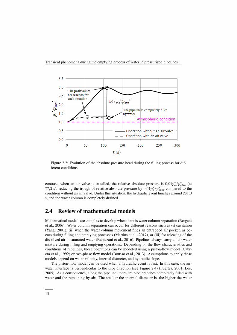
2.1 Basic hydraulic scheme . . . . . . . . . . . . . . . . . . . . . . . . . . . . . 122.2 Evolution of the absolute pressure head during the filling process for different
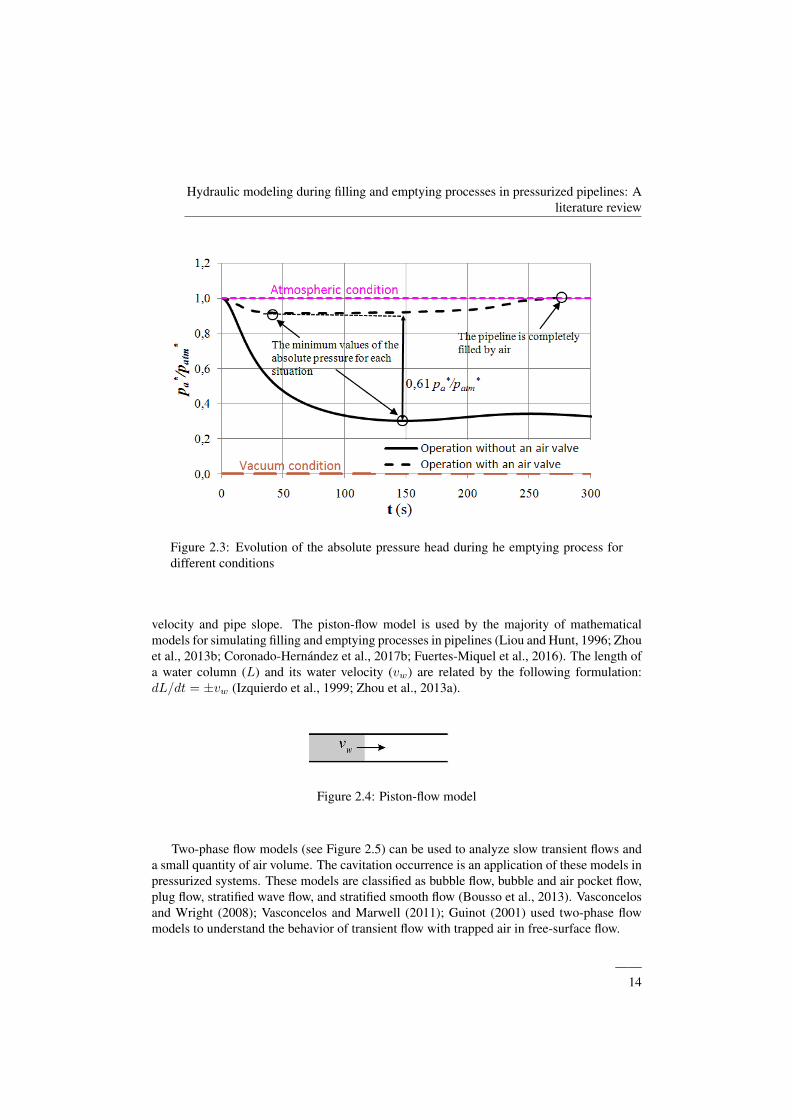
conditions . . . . . . . . . . . . . . . . . . . . . . . . . . . . . . . . . . . . 132.3 Evolution of the absolute pressure head during he emptying process for dif-
ferent conditions . . . . . . . . . . . . . . . . . . . . . . . . . . . . . . . . 142.4 Piston-flow model . . . . . . . . . . . . . . . . . . . . . . . . . . . . . . . . 142.5 Two-phases flow models . . . . . . . . . . . . . . . . . . . . . . . . . . . . 152.6 Diagram p∗a vs. Va . . . . . . . . . . . . . . . . . . . . . . . . . . . . . . . 182.7 Effects of air valves behavior during the filling and emptying processes . . . 202.8 Example of an air valve characterization . . . . . . . . . . . . . . . . . . . . 212.9 Comparison between a constant and unsteady friction factor (Fuertes, 2001) . 25
3.1 Schematic of an entrapped air pocket in a single pipe while water empties . . 343.2 Location of air valve . . . . . . . . . . . . . . . . . . . . . . . . . . . . . . 363.3 Schematic of experimental setup . . . . . . . . . . . . . . . . . . . . . . . . 383.4 Case No. 1 - Comparisons between calculated and measured absolute pres-
sure of the air pocket for tests 1 to 6 . . . . . . . . . . . . . . . . . . . . . . 413.5 Case No. 1 - Comparisons between calculated and measured absolute pres-
sure of the air pocket for tests 7 to 12 . . . . . . . . . . . . . . . . . . . . . . 423.6 Case No. 2 - Comparisons between calculated and measured absolute pres-
sure of the air pocket for tests 13 to 18 (Dav = 1,5 mm) . . . . . . . . . . . 433.7 Case No. 2 - Comparisons between calculated and measured absolute pres-
sure of the air pocket for tests 19 to 24 (Dav = 1,5 mm) . . . . . . . . . . . 443.8 Case No. 1 - Comparisons between calculated and measured absolute pres-
sure of the air pocket for tests 25 to 30 (Dav = 3,0 mm) . . . . . . . . . . . 453.9 Case No. 1 - Comparisons between calculated and measured absolute pres-
sure of the air pocket for tests 31 to 36 (Dav = 3,0 mm) . . . . . . . . . . . 463.10 Laboratory test results of air valves during air admission . . . . . . . . . . . 483.11 The comparison between computed and measured minimum pressures . . . . 493.12 Results of Case No. 1 - Full transient analysis of the system under consideration 503.13 Results of Case No. 2 - Full transient analysis of the system under consideration 52
XVII
3.14 Case No.1 - Influence of the opening times in the drain valve . . . . . . . . . 543.15 Case No.2 - Influence of the opening time in the valve . . . . . . . . . . . . . 553.16 Case No.2 - Influence of the air valve diameter . . . . . . . . . . . . . . . . 57
4.1 Scheme of entrapped air into a pipeline during the draining procedure . . . . 634.2 Experimental facility . . . . . . . . . . . . . . . . . . . . . . . . . . . . . . 664.3 Sequence of the hydraulic events . . . . . . . . . . . . . . . . . . . . . . . . 684.4 Comparison between computed and experiments of the absolute pressure pat-
tern for Type A . . . . . . . . . . . . . . . . . . . . . . . . . . . . . . . . . 704.5 Comparison between computed and experiments of the absolute pressure pat-
tern for Type B . . . . . . . . . . . . . . . . . . . . . . . . . . . . . . . . . 714.6 Comparison between computed and experiments of the water velocity for
Type B . . . . . . . . . . . . . . . . . . . . . . . . . . . . . . . . . . . . . . 734.7 Comparison between computed and experiments of the absolute pressure pat-
tern for Type C . . . . . . . . . . . . . . . . . . . . . . . . . . . . . . . . . 744.8 Comparison between computed and experiments of the water velocities for
Type C and run No. 5 . . . . . . . . . . . . . . . . . . . . . . . . . . . . . . 754.9 Comparison between computed and experiments of the length of water columns
for Type C (run No. 5) . . . . . . . . . . . . . . . . . . . . . . . . . . . . . 764.10 Pipeline of irregular profile without air valves . . . . . . . . . . . . . . . . . 774.11 Full transient analysis of the pipeline of irregular profile without air valves . . 79
5.1 Scheme of entrapped air pockets in a pipeline with irregular profile whilewater empties . . . . . . . . . . . . . . . . . . . . . . . . . . . . . . . . . . 85
5.2 Evolution of the gravity term of the emptying column j . . . . . . . . . . . . 895.3 The pipe system and its components . . . . . . . . . . . . . . . . . . . . . . 905.4 Two emptying columns in a pipeline . . . . . . . . . . . . . . . . . . . . . . 915.5 Comparison between computed and measured absolute pressure oscillation
pattern (air valve S050) . . . . . . . . . . . . . . . . . . . . . . . . . . . . . 945.6 Comparison between computed and measured absolute pressure oscillation
pattern (air valve D040) . . . . . . . . . . . . . . . . . . . . . . . . . . . . . 955.7 Comparison between computed and measured length of emptying column
(air valve S050) . . . . . . . . . . . . . . . . . . . . . . . . . . . . . . . . . 965.8 Comparison between computed and measured length of emptying column
(air valve D040) . . . . . . . . . . . . . . . . . . . . . . . . . . . . . . . . 975.9 Comparison of water velocity between computed and measured (air valve
S050) . . . . . . . . . . . . . . . . . . . . . . . . . . . . . . . . . . . . . . 995.10 Comparison of water velocity between computed and measured (air valve
D040) . . . . . . . . . . . . . . . . . . . . . . . . . . . . . . . . . . . . . . 1005.11 Effect of the air pocket sizes on the minimum pressure attained . . . . . . . . 1015.12 Comparison between computed and measured maximum water velocities . . 1025.13 Pipeline of irregular profile with air valves . . . . . . . . . . . . . . . . . . . 1035.14 Full transient analysis of the pipeline of irregular profile with air valves . . . 105
——XVIII
Transient phenomena during the emptying process of water in pressurized pipelines
6.1 Schematic of pressurized air in a water-emptying horizontal-vertical pipeline 1116.2 Schematic of the PVC-steel pipeline and instrumentation . . . . . . . . . . . 1136.3 Gauge pressure supplied by the air tank during the transient stage. Data are
based on experiments conducted by Laanearu et al. (2012). . . . . . . . . . . 1146.4 Comparisons between the calculated and measured water flow oscillation pat-
terns for runs 1, 4, 5 and 9 . . . . . . . . . . . . . . . . . . . . . . . . . . . 1156.5 Comparisons between the calculated and measured gauge pressure oscillation
patterns for run 4 . . . . . . . . . . . . . . . . . . . . . . . . . . . . . . . . 1176.6 Effects of the length of the vertical steel pipe . . . . . . . . . . . . . . . . . 118
7.1 Experimental facilities to validate the emptying process . . . . . . . . . . . . 1237.2 Location of the Ciudad del Bicentenario pipeline . . . . . . . . . . . . . . . 1257.3 Scheme of the Ciudad del Bicentenario pipeline . . . . . . . . . . . . . . . . 1267.4 Characteristics of the air valve - Type 9000 Pam manufacturer . . . . . . . . 1277.5 Evolution during the hydraulic event of the absolute pressure of the air pocket 1317.6 Evolution during the hydraulic event of the length of the emptying columns . 1327.7 Evolution of the water and air flow in the emptying column 1 . . . . . . . . . 1337.8 Evolution of the water and air flow in the emptying column 2 . . . . . . . . . 1337.9 Sensitivity analysis regarding to the failure of air valves . . . . . . . . . . . . 135
8.1 Flowchart showing research stages and proposed objectives. . . . . . . . . . 1388.2 Scheme of entrapped air pockets in a pipeline with irregular profile while
water empties . . . . . . . . . . . . . . . . . . . . . . . . . . . . . . . . . . 1418.3 Effects of air valves behavior during the emptying process . . . . . . . . . . 1438.4 Executed code in Simulink Library of Matlab . . . . . . . . . . . . . . . . . 1458.5 Comparison between proposed model and experiments of the absolute pres-
sure pattern in a single pipe . . . . . . . . . . . . . . . . . . . . . . . . . . . 1468.6 Comparison between proposed model and experiments of the absolute pres-
sure pattern in a pipeline of irregular profile . . . . . . . . . . . . . . . . . . 1488.7 Comparison between proposed model and CFD model of the absolute pres-
sure pattern for Test No.2 of the single pipeline (see Chapter 3) . . . . . . . . 1508.8 Comparison of the water flow oscillation pattern . . . . . . . . . . . . . . . . 1518.9 Comparison of the gauge pressures along the pipeline for run 4 . . . . . . . . 1528.10 Experimental facilies used to validate the mathematical model . . . . . . . . 154
A.1 The generated mesh in the pipe systems near drain valves . . . . . . . . . . . 165A.2 Comparison between the mathematical model and the 2D CFD model of air
pocket pressure for the single pipeline located at the Universitat Politecnicade Valencia (see Chapter 3) . . . . . . . . . . . . . . . . . . . . . . . . . . . 167
A.3 Comparison between the mathematical model and the 2D CFD model of airpocket pressure for the pipeline od irregular located at the University of Lis-bon (see Chapter 4) . . . . . . . . . . . . . . . . . . . . . . . . . . . . . . . 168
A.4 Backflow air development for Test No. 1 in the single pipeline . . . . . . . . 169
——XIX

This page is intentionally left blank.
——XX
List of Tables
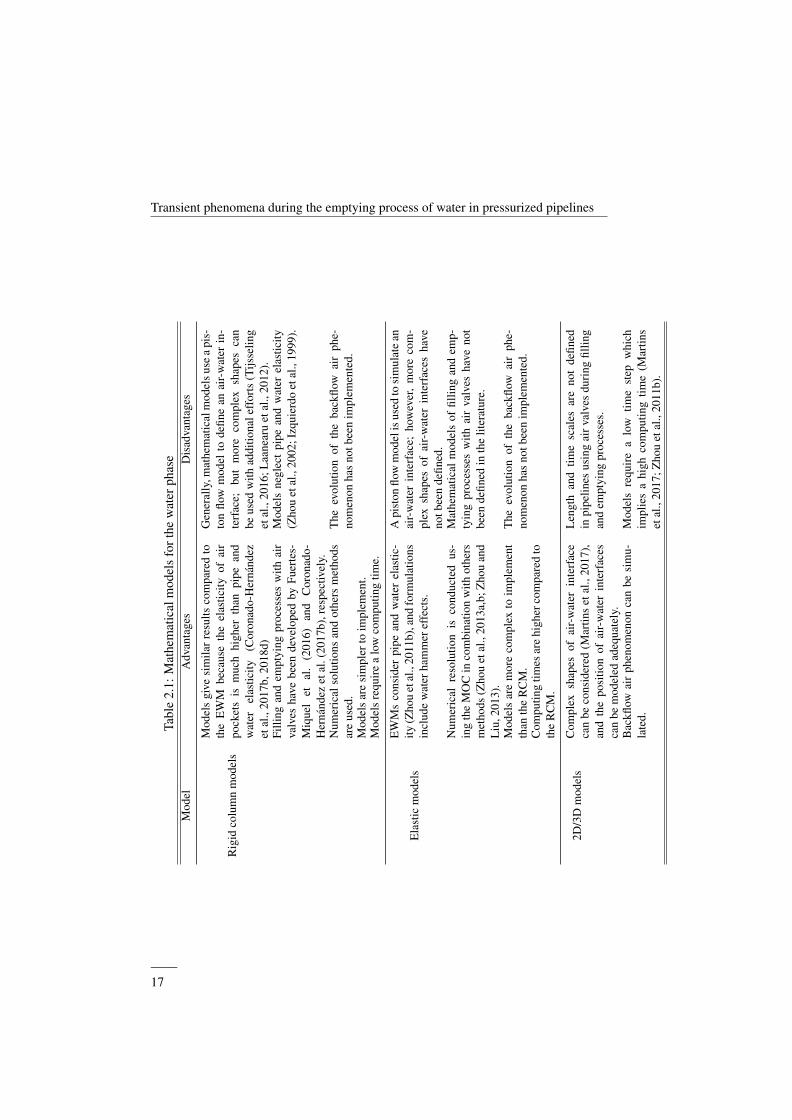
2.1 Mathematical models for the water phase . . . . . . . . . . . . . . . . . . . 172.2 Summary of mathematical models for water and air phase. . . . . . . . . . . 222.3 Summary of methods of resolution. . . . . . . . . . . . . . . . . . . . . . . . 24
3.1 Case No. 1 - Experimental setup - Characteristics of tests 1 to 12 . . . . . . . 393.2 Case No. 2 - Experimental setup - Characteristics of tests 13 to 36 . . . . . . 473.3 Case No.1 - Influence of air pocket sizes . . . . . . . . . . . . . . . . . . . . 533.4 Influence of polytropic coefficient (k) . . . . . . . . . . . . . . . . . . . . . 533.5 Characteristics of the air valves . . . . . . . . . . . . . . . . . . . . . . . . . 56
4.1 Types of behaviour . . . . . . . . . . . . . . . . . . . . . . . . . . . . . . . 69
5.1 Characteristics of tests . . . . . . . . . . . . . . . . . . . . . . . . . . . . . 92
6.1 Summary of the emptying process for the 9 runs . . . . . . . . . . . . . . . . 116
A.1 Mesh of pipeline installations . . . . . . . . . . . . . . . . . . . . . . . . . . 164
XXI

This page is intentionally left blank.
——XXII
Chapter 1
Introduction
1.1 Background
The analysis of transient phenomenon in water distribution systems is important due to theintricacy of computations and the particularities of the several configurations of each system.The phenomenon is complex to analyze even for a single-phase (water). When entrapped airpockets are present into installations, the analysis is much more complex because there aretwo fluids (water and air) in two different phases (liquid and gas) (Fuertes, 2001).
Filling and emptying processes may introduce entrapped air pockets to pipelines, wherethe implementation of hydraulic (water phase) and thermodynamic (air phase) equations isrequired since typical transient flow models (e.g Allievi, Hammer, among others) are not ca-pable of predicting a two-phase flow (water and air). These processes need to be implementedby the technical personnel working at water supply systems to protect hydraulic installations.
These operations are periodically performed in real hydraulic installations. The fillingoperation can generate dangerous pressure surges when air pockets are rapidly compressedand air valves are not expelling enough quantity of air (Izquierdo et al., 1999; Zhou et al.,2013a; Wang et al., 2017); while the emptying operation can produce subatmospheric pres-sure values due to the expansion of air pockets if air valves are not capable of admitting airflow with a similar ratio of the drained water (Coronado-Hernandez et al., 2017b). Extremevalues of the absolute pressure depend on the characteristics of installations (internal diame-ter, pipe roughness and pipe slope). Extreme pressures can affect not only pipelines but alsotheir devices (joints, pumps’ stations and valves).
Filling processes have been studied by several authors (Izquierdo et al., 1999; Zhou et al.,2013a; Zhou and Liu, 2013; Wang et al., 2017) based on the behavior of hydraulic and ther-modynamic variables. However, it has been detected, in the literature, a lack of knowledge re-garding the analysis of transient flow of a water emptying pipeline, where only semi-empiricalmodels have been developed in this field (Tijsseling et al., 2016; Laanearu et al., 2012); inthis sense, previous models cannot be extended for analyzing complex systems. A robust
1
Introduction
mathematical model based on physical equations is then required to compute the evolution ofthe main hydraulic and thermodynamic variables during emptying processes in pressurizedpipelines of irregular profiles. These variables are: air absolute pressure, air density, watervelocity, air flow, and length of a water column. At present, engineers follow some recom-mendations of the American Water Works Association (AWWA, 2001) and manufacturers toavoid lowest values of subatmospheric pressure, which can cause a pipeline collapse duringan emptying process. Air valves are installed along of piping systems to avoid both the riskof pipelines collapse and the cavitation occurrence by admitting air into installations untilatmospheric conditions are attained. Entrapped air can be entered in hydraulic installationsnot only by air valves but also through joints and water intakes, during pumps’ stoppages orfailure of the systems, by releasing of dissolved air, and by vortex formation at pump inlets.
1.2 MotivationSubatmospheric pressure patterns can be reached in water distribution systems with transientflow occurrence under two scenarios: (i) with a single phase (water), as occurs in pump’sstoppages, and by closing valves; and (ii) with a two-phase flow (air-water mixture) whichoccurs during an emptying process. At present, there is no mathematical model to simulate atransient flow during a water emptying process, which is crucial to ensure pipeline protection.In this sense, protection devices need to be sized not only in transient flow with a single phase(typical practice) but also during the emptying process (a missing practice). Hence, the mostcritical condition should be used to size a pipe stiffness class depending on the minimumvalue of a reached subatmospheric pressure during transient flows (both single and two-phaseflow) and characteristics of pipe installations (the type of soil in natural conditions, the typeof backfill and the cover depth).
Some situations are reported in the literature where an expansion of air pockets generateda systems collapse. Espert et al. (1991) reported an air vessel collapse with a volume of 56m3 located at Mediterranean coast, which was generated by a thermodynamic expansion ofan air pocket with a reached subatmospheric pressure value of 0,22 bar. De Paor et al. (2012)mentioned an example of pressure vessel collapse due to sheet blocking vent during a vacuumcondition. Tullis and Watkins (1991) studied the collapse of a large pipeline of a hydropower(with a diameter of 1,3 m and 4825 m long.) due to a pipe rupture which was generated bya low value of subatmospheric pressure, who mentioned that if an appropriate air valve hadbeen installed, then the pipe would not have collapsed. Cabrera et al. (2008) studied differentemergency scenarios related to transient flow of a 70-km-long pipeline with diameter of 1,6m, where a total pipe rupture was analyzed highlighting the importance to select adequatelyair valves to prevent pipe collapse during filling and emptying processes.
This research develops a mathematical model to predict emptying operations consider-ing different configurations of pipelines. A combination of hydraulic and thermodynamicequations is required for simulating the emptying operation. The mathematical model usesthe rigid water column model, the piston flow model (air-water interface perpendicular to thepipe direction), and the polytropic model of the entrapped air pocket. When air valves are
——2
Transient phenomena during the emptying process of water in pressurized pipelines
acting, then the continuity equation of the air pocket and the air valve characterization areincluded in the definition of the mathematical model. Two experimental facilities are used tovalidate the mathematical model.
1.3 Outline of this thesis
1.3.1 ObjectivesThe analysis of transient phenomena during the filling process of pipelines have been stud-ied by several authors; however, there is a lack of detailed studies related to the emptyingprocess of water pipelines, which is very important in order to avoid the systems collapse onthe trough of subatmospheric pressure reached by air pockets. The overall objective of thisresearch is:
To investigate as deeply as possible about the analysis of transient phenomenon of a wateremptying pipeline of irregular profile with several air pockets and various air valves
The overall objective was divided into several detailed objectives:
1. To perform a literature review regarding the analysis of transient phenomena withtrapped air in water distribution networks..
2. To develop a rigid water column model to simulate the emptying process of water insingle pipelines for two cases: (i) with an upstream end closed, and (ii) with admittedair located at upstream end.
3. To solve a differential-algebraic system to simulate the emptying process of water insingle pipelines using the Simulink Library in Matlab.
4. To prepare an experimental facility of a single pipe for simulating an emptying processfor the two aforementioned cases by measuring the air absolute pressure to validate themathematical model.
5. To develop a mathematical model for analyzing a water emptying pipeline of irregularprofile for two cases: (i) without the admitting air, and (ii) using air valves.
6. To solve a set of differential-algebraic equations of emptying processes consideringpipelines of irregular profiles using the Simulink Library of Matlab.
7. To validate the mathematical model of a water emptying pipeline of irregular profilethrough measurements of main hydraulic and thermodynamic variables (water velocity,air absolute pressure, and lengths of the water columns).
8. To perform a sensitivity analysis of the main hydraulic and thermodynamic parametersduring emptying processes.
——3
Introduction
9. To compare results of the mathematical model with previous models to simulate theemptying process of water pipelines.
10. To apply the mathematical model to simulate an emptying process under different sce-narios to check the risk of collapse of the pipeline network of the neighborhood Ciudaddel Bicentenario located in Cartagena de Indias, Colombia.
1.3.2 Methodology
This research is developed considering the following steps:
• A literature review: a complete literature review regarding the analysis of transientphenomena with trapped air was conducted considering these journals: Journal of Hy-draulic Research, Journal of Hydraulic Engineering, Journal of Water Resources Plan-ning and Managment, Water MDPI Journals, Urban Water Journal, Canadian Journalof Civil Engineering, among others. Also, conference contributions were investigated.
• Mathematical models: to simulate a transient flow with entrapped air pockets is nec-essary to understand the behavior of both water and air phase. In this sense, the waterphase was simulated considering a rigid water column model, which provides suffi-cient accuracy by taking a moving air-water interface. Moreover, the air phase wassimulated with a polytropic equation, the continuity equation of air pockets, and the airvalve characterization. Computational simulations were performed using the SimulinkLibrary of Matlab.
• Experimental facility and instrumentation: two experimental facilities were used tovalidate the mathematical model. A complete description of a single pipe is presentedin Chapter 3, and about a pipeline of irregular profile is shown in Chapters 4 and 5. Torecord the information of the main hydraulic variables, the following instrumentationwas used: (i) absolute pressure pattern was measured by using different transducerslocated at the high point of both installations; (ii) water velocity was measured us-ing an Ultrasonic Doppler Velocimetry (UDV) avoiding as much as possible the noise(electrical, hydraulic, vehicular, among others); (iii) and lengths of water columns wererecorded with a typical Camera.
• Verification of the mathematical model and limitations of proposed model: to val-idate the mathematical model was conducted a comparison between computed andmeasured of the main hydraulic variables (absolute pressure pattern, water velocities,and lengths of water columns). Also, the comparison showed the need to include somelimitations of the proposed model.
• Application to a case study: the mathematical model was applied to study the empty-ing process of water of a case study.
——4
Transient phenomena during the emptying process of water in pressurized pipelines
1.3.3 Thesis structureAn introduction is presented in this Chapter describing a background, the motivation, theproposed objectives, and the structure of this research. The remaining chapters are clearlyidentified as follows:
• Chapter 2 presents a literature review about transient flow with trapped air.
• Chapter 3 describes numerical and experimental analysis of a water emptying processperformed in a single pipe.
• Chapter 4 shows an experimental and numerical analysis of a water emptying pipelineof irregular profile with entrapped air.
• Chapter 5 is similar to Chapter 4, but the behavior of air valves have been included inthe proposed model.
• Chapter 6 contains additional experiments to validate the proposed model.
• Chapter 7 presents an application of the proposed model to a case study.
• Chapter 8 summarizes the discussion of this research, showing how each one of theobjectives was reached.
• Chapter 9 presents the main contributions, conclusions and future developments of thethesis.
At the end of the document is presented the references used in this research.
1.3.4 List of publicationsThis thesis is composed by collecting papers (Chapters 2 to 7) according to guidelines of theUniversitat Politecnica de Valencia, which are listed below:
1. Hydraulic modeling during filling and emptying processes in pressurized pipelines:A literature review
(a) Coauthors: Fuertes-Miquel, V. S; Coronado-Hernandez O. E; Mora-Melia, D;Iglesias-Rey P. L.
(b) Journal: Urban Water Journal ISSN 1573-062X.
(c) 2017 Impact Factor: 2.744. Position JCR 17/90 (Q1). Water Resources.
(d) State: Accepted with revisions. January 2019.
2. Transient phenomena during the emptying process of a single pipe with water-airinteraction
——5
Introduction
(a) Coauthors: Fuertes-Miquel, V. S; Coronado-Hernandez O. E; Iglesias-Rey P. L.;Mora-Melia, D.
(b) Journal: Journal of Hydraulic Research ISSN 0022-1686
(c) 2017 Impact Factor: 2.076. Position JCR 41/128 (Q2). Civil Engineering
(d) State: Published. Latest Articles. 2018; DOI: 10.1080/00221686.2018.1492465
3. Subatmospheric pressure in a water draining pipeline with an air pocket
(a) Coauthors: Coronado-Hernandez O. E; Fuertes-Miquel, V. S; Besharat, M.; andRamos, H. M.
(b) Journal: Urban Water Journal ISSN 1573-062X.
(c) 2017 Impact Factor: 2.744. Position JCR 17/90 (Q1). Water Resources.
(d) State: Published. 2018. Volume 15; Issue 4. DOI: 10.1080/1573062X.2018.1475578
4. Experimental and Numerical Analysis of a Water Emptying Pipeline Using DifferentAir Valves
(a) Coauthors: Coronado-Hernandez O. E; Fuertes-Miquel, V. S; Besharat, M.; andRamos, H. M.
(b) Journal: Water ISSN 2073-4441.
(c) 2017 Impact Factor: 2.069. Position JCR 34/90 (Q2). Water Resources.
(d) State: Published. 2017. Volume 9; Issue 2; 98. DOI: 10.3390/w9020098.
5. Rigid Water Column Model for Simulating the Emptying Process in a Pipeline UsingPressurized Air
(a) Coauthors: Coronado-Hernandez O. E; Fuertes-Miquel, V. S; Iglesias-Rey, P.L.;Martınez-Solano, F.J.
(b) Journal: Journal of Hydraulic Engineering ISSN 0733-9429.
(c) 2017 Impact Factor: 2.080. Position JCR 39/128 (Q2). Civil Engineering.
(d) State: Published. 2018. Volume 144; Issue 4. DOI: 10.1061/(ASCE)HY.1943-7900.0001446.
6. Emptying Operation of Water Supply Networks
(a) Coauthors: Coronado-Hernandez O. E; Fuertes-Miquel, V. S; Angulo-Hernandez,F. N.
(b) Journal: Water ISSN 2073-4441.
(c) 2017 Impact Factor: 2.069. Position JCR 34/90 (Q2). Water Resources.
(d) State: Published. 2018. Volume 10; Issue 1; 22. DOI: 10.3390/w10010022.
——6
Transient phenomena during the emptying process of water in pressurized pipelines
In addition, 6 conference presentations were conducted as presenting author:
1. The analysis of transient flow during the emptying process in a single pipeline
(a) Coauthors: Oscar E. Coronado-Hernandez, Vicente S. Fuertes-Miquel, Pedro L.Iglesias-Rey, and Daniel Mora-Melia.
(b) Event: XXVII Congreso Latinoamericano de Hidraulica, IAHR.
(c) Year: 2016.
(d) Place: Lima, Peru.
2. Sensitivity analysis of emptying processes in water supply networks
(a) Coauthors: Oscar E. Coronado-Hernandez, Vicente S. Fuertes-Miquel, Pedro L.Iglesias-Rey, and Daniel Mora-Melia.
(b) Event: V Jornadas de Ingenierıa del Agua.
(c) Year: 2017.
(d) Place: A Coruna, Spain.
3. Behavior of a water-draining pipeline of irregular profile with air valves
(a) Coauthors: Vicente S. Fuertes-Miquel, Oscar E. Coronado-Hernandez, Pedro L.Iglesias-Rey, and F. Javier Martınez-Solano.
(b) Event: XV Seminario Iberoamericano de Redes de Agua y Drenaje, SEREA2017.
(c) Year: 2017.
(d) Place: Bogota, Colombia.
4. Analysis of the draining operation in water supply networks. Application to a waterpipeline in Cartagena de Indias, Colombia
(a) Coauthors: Oscar E. Coronado-Hernandez, Vicente S. Fuertes-Miquel, and FredyN. Angulo.
(b) Event: XV Seminario Iberoamericano de Redes de Agua y Drenaje, SEREA2017.
(c) Year: 2017.
(d) Place: Bogota, Colombia.
5. Negative pressure occurrence during the draining operation of water pipelines withentrapped air
(a) Coauthors: Vicente S. Fuertes-Miquel, Oscar E. Coronado-Hernandez, DanielMora-Melia, and Pedro L. Iglesias-Rey.
(b) Event: XV Seminario Iberoamericano de Redes de Agua y Drenaje, SEREA2017.
——7

Introduction
(c) Year: 2017.
(d) Place: Bogota, Colombia.
6. A parametric sensitivity analysis of numerically modelled piston-type filling and emp-tying of an inclined pipeline with an air valve
(a) Coauthors: Oscar E. Coronado-Hernandez, Vicente S. Fuertes-Miquel, MohsenBesharat, and Helena M. Ramos.
(b) Event: 13th International Conference on Pressure Surges..
(c) Year: 2018.
(d) Place: Bordeaux, France.
——8
Chapter 2
Hydraulic modeling during fillingand emptying processes inpressurized pipelines: A literaturereview
This chapter is extracted from the paper:
Hydraulic modeling during filling and emptying processes in pressurized pipelines: A literaturereview
Coauthors: Fuertes-Miquel, V. S; Coronado-Hernandez O. E; Mora-Melia, D; Iglesias-Rey P. L.Journal: Urban Water Journal ISSN 1573-062X.
2017 Impact Factor: 2.744. Position JCR 17/90 (Q1). Water Resources.State: Accepted with revisions. January 2019.
2.1 AbstractFilling and emptying processes are common maneuvers while operating, controlling andmanaging water pipelines systems. Currently, these operations are executed following rec-ommendations from technical manuals and pipe manufacturers; however, these recommen-dations have a lack of understanding about the behavior of these processes. The applicationof mathematical models considering transient flows with entrapped air pockets is necessarybecause a rapid filling operation can cause pressure surges due to air pocket compressions,while an uncontrolled emptying operation can generate troughs of subatmospheric pressurecaused by air pocket expansion. Depending on pipe and installation conditions, either situ-ation can produce a rupture of pipe systems. Recently, reliable mathematical models have
9
Hydraulic modeling during filling and emptying processes in pressurized pipelines: Aliterature review
been developed by different researchers. This paper reviews and compares various mathe-matical models to simulate these processes. Water columns can be analyzed using a rigidwater column model, an elastic water model, or 2D/3D CFD models; air-water interfacesusing a piston flow model or more complex models; air pockets through a polytropic model;and air valves using an isentropic nozzle flow or similar approaches. This work can be usedas a starting point for planning filling and emptying operations in pressurized pipelines. Un-certainties of mathematical models of two-phases flow concerning to a non-variable frictionfactor, a polytropic coefficient, an air pocket sizes, and an air valve behavior are identified.
2.2 IntroductionThe analysis of transient phenomena of a single phase (only water) is complex considering theintricacy of calculations and configurations of water pipelines systems. Filling and emptyingprocesses are too complex to be captured by single-phase models because there are two fluids(water and air) in two phases (liquid and gas)(Fuertes, 2001). These operations must be per-formed periodically in pipelines for maintenance, cleaning or repairs by technical personnel(Fuertes-Miquel et al., 2018b). Planning water distribution systems requires considering theeffects of entrapped air pockets to guarantee successful maintenance and repair procedures.During filling processes, air pockets can be rapidly compressed, producing pressure surges;during emptying processes, air pockets expand, causing subatmospheric conditions. As aconsequence, the modeling of the air phase is crucial to determine extreme values of absolutepressure. The correct identification of a type of model (adiabatic, polytropic or isothermal)and an air valve characterization have to be considered.
The effects of trapped air in water pipelines are generated basically with regards to twofeatures: (i) air density is much lower than water density by a ratio approximately 1 : 800times considering atmospheric conditions and a temperature of 20◦C; and (ii) the elasticityof air is much higher than the elasticity of water. The elasticity depends on the type ofprocess (isothermal, polytropic or adiabatic) and the absolute pressure of the air pocket. Forinstance, the bulk modulus in an isothermal process, at atmospheric condition, presents aratio of 20000 times, and for an absolute pressure of 10 bar, the ratio is of 2000 times. Someof the problems cause by entrapped air pockets are: (i) additional head losses by increasingthe water velocity as a consequence of the reduction of the cross section (Stephenson, 1997),(ii) pressure surges for starting or stopping the system because of the compression of theair pocket, (iii) reduction of the efficiency of the pumps, (iv) vibrations in pipelines, whichgenerate rapid changes in the water velocity pattern, (iv) pipe corrosion owing to temperatureand absolute pressure changes, and (v) troughs of subatmospheric pressure by the expansionof the air pocket (Fuertes-Miquel et al., 2018b; Coronado-Hernandez et al., 2018a).
Entrapped air pockets are a problem for pipeline operations. It is important to perform afilling process correctly to eliminate air pockets from hydraulic systems. However, entrappedair could also enter through air valves, joints and valves, during the stopping and failure ofhydraulic systems, during the release of dissolved air, and by vortex generation at pump inlets.High points along pipelines are likely locations for the accumulation of air pockets (AWWA,
——10
Transient phenomena during the emptying process of water in pressurized pipelines
2001; Ramezani and Karney, 2017), which can experience pressure surges during a fillingprocess (Zhou et al., 2013b; Fontana et al., 2016; Martins et al., 2016; Covas et al., 2010) ordrops of subatmospheric pressure during an emptying process (Fuertes-Miquel et al., 2018b;Tijsseling et al., 2016; Coronado-Hernandez et al., 2018d). Air valves are used as protectivedevices to avoid these situations (AWWA, 2001).
Entrapped air can be expelled by permanent joints of hydraulic systems to the atmosphere(downstream conditions, fire hydrants, among others), but the most common method is viaair valves located along the system (Martino et al., 2001), such as high points or others whereentrapped air can accumulate.
The emptying and filling of a pipeline cannot be simulated with the commonly used 1Dtransient commercial packages like Bentley Hammer, H2O Surge, Allievi, among others;since they are not capable of predicting a two-phase flow (water and air).
This paper aims to accomplish the following: (1) review available knowledge regardingfilling and emptying processes in pressurized hydraulic systems, which is missing in thecurrent literature; (2) describe mathematical models for water and air phase; (3) describemethods of resolutions of transient flow during pipeline operations; (4) mention the sourcesof uncertainty in current models; and (5) comment regarding some considerations to protectpipelines during these operations.
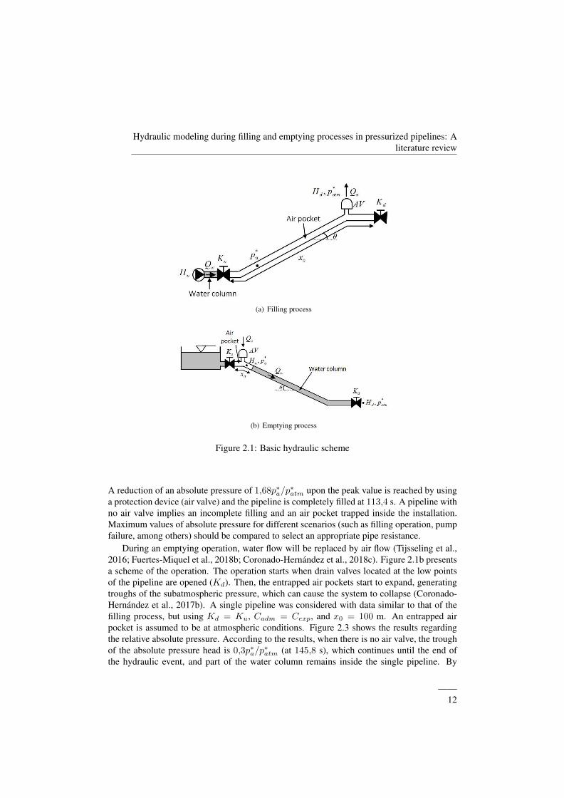
2.3 Understanding of filling and emptying processesA basic hydraulic scheme is presented to show the performance of filling and emptying pro-cesses (Figure 2.1).
The filling process begins when a discharge valve is opened (Ku). Consequently, thewater column driven by an energy source (tank or pump) starts to fill the hydraulic system(see Figure 2.1a) by compressing the entrapped air pocket (Zhou et al., 2013a; Martins et al.,2017; Malekpour et al., 2016) producing peaks of absolute pressure (pressure surges). ValveKd is closed to produce the rapid compression of an air pocket. The process is adequatelycompleted when the entrapped air is replaced by the water column (Apollonio et al., 2016;Balacco et al., 2015). Two situations can occur: (i) when the air valve (AV ) has been in-stalled, the process finishes successfully with a well-sized device; and (ii) when there is noair valve, it results in an unfinished process and the highest pressure surges.
To note the order of magnitude of a filling process, a numerical analysis has been con-ducted in a single pipeline where the authors used an own code in Matlab (Fuertes-Miquelet al., 2016, 2018b; Coronado-Hernandez et al., 2017b, 2018d). Figure 2.2 shows the peaksof the absolute pressure for the two aforementioned situations using the following data:Lt = 600 m, D = 0,3 m, f = 0,018, n = 1,2, Dav = 50 mm, Cexp = 0,6, ∆z = 12 m,x0 = 500 m, and Ku = 0,45 m/(m3s−1)2. A comparison is conducted with a relative valueof air pocket pressure (p∗a/p
∗atm) and the time. According to the results, when an air valve
has not been installed, the maximum peak of the absolute pressure head is rapidly reached at112,1 s with a value of 2,97 p∗a/p
∗atm. After that, oscillations of the absolute pressure con-
tinue. However, when an air valve is working, the maximum value is 1,29p∗a/p∗atm (at 53,4 s).
——11
Hydraulic modeling during filling and emptying processes in pressurized pipelines: Aliterature review
(a) Filling process
(b) Emptying process
Figure 2.1: Basic hydraulic scheme
A reduction of an absolute pressure of 1,68p∗a/p∗atm upon the peak value is reached by using
a protection device (air valve) and the pipeline is completely filled at 113,4 s. A pipeline withno air valve implies an incomplete filling and an air pocket trapped inside the installation.Maximum values of absolute pressure for different scenarios (such as filling operation, pumpfailure, among others) should be compared to select an appropriate pipe resistance.
During an emptying operation, water flow will be replaced by air flow (Tijsseling et al.,2016; Fuertes-Miquel et al., 2018b; Coronado-Hernandez et al., 2018c). Figure 2.1b presentsa scheme of the operation. The operation starts when drain valves located at the low pointsof the pipeline are opened (Kd). Then, the entrapped air pockets start to expand, generatingtroughs of the subatmospheric pressure, which can cause the system to collapse (Coronado-Hernandez et al., 2017b). A single pipeline was considered with data similar to that of thefilling process, but using Kd = Ku, Cadm = Cexp, and x0 = 100 m. An entrapped airpocket is assumed to be at atmospheric conditions. Figure 2.3 shows the results regardingthe relative absolute pressure. According to the results, when there is no air valve, the troughof the absolute pressure head is 0,3p∗a/p
∗atm (at 145,8 s), which continues until the end of
the hydraulic event, and part of the water column remains inside the single pipeline. By
——12
Transient phenomena during the emptying process of water in pressurized pipelines
Figure 2.2: Evolution of the absolute pressure head during the filling process for dif-ferent conditions
contrast, when an air valve is installed, the relative absolute pressure is 0,91p∗a/p∗atm (at
77,2 s), reducing the trough of relative absolute pressure by 0,61p∗a/p∗atm compared to the
condition without an air valve. Under this situation, the hydraulic event finishes around 281,0s, and the water column is completely drained.
2.4 Review of mathematical modelsMathematical models are complex to develop when there is water column separation (Bergantet al., 2006). Water column separation can occur for different reasons such as (i) cavitation(Yang, 2001), (ii) when the water column movement finds an entrapped air pocket, as oc-curs during filling and emptying processes (Martins et al., 2017), or (iii) for releasing of thedissolved air in saturated water (Ramezani et al., 2016). Pipelines always carry an air-watermixture during filling and emptying operations. Depending on the flow characteristics andconditions of pipelines, these operations can be modeled using a piston-flow model (Cabr-era et al., 1992) or two-phase flow model (Bousso et al., 2013). Assumptions to apply thesemodels depend on water velocity, internal diameter, and hydraulic slope.
The piston-flow model can be used when a hydraulic event is fast. In this case, the air-water interface is perpendicular to the pipe direction (see Figure 2.4) (Fuertes, 2001; Lee,2005). As a consequence, along the pipeline, there are pipe branches completely filled withwater and the remaining by air. The smaller the internal diameter is, the higher the water
——13
Hydraulic modeling during filling and emptying processes in pressurized pipelines: Aliterature review
Figure 2.3: Evolution of the absolute pressure head during he emptying process fordifferent conditions
velocity and pipe slope. The piston-flow model is used by the majority of mathematicalmodels for simulating filling and emptying processes in pipelines (Liou and Hunt, 1996; Zhouet al., 2013b; Coronado-Hernandez et al., 2017b; Fuertes-Miquel et al., 2016). The length ofa water column (L) and its water velocity (vw) are related by the following formulation:dL/dt = ±vw (Izquierdo et al., 1999; Zhou et al., 2013a).
Figure 2.4: Piston-flow model
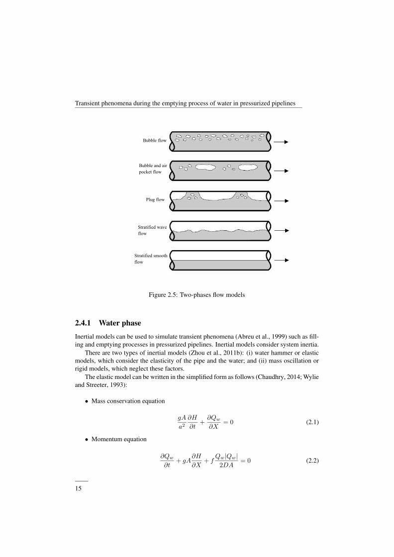
Two-phase flow models (see Figure 2.5) can be used to analyze slow transient flows anda small quantity of air volume. The cavitation occurrence is an application of these models inpressurized systems. These models are classified as bubble flow, bubble and air pocket flow,plug flow, stratified wave flow, and stratified smooth flow (Bousso et al., 2013). Vasconcelosand Wright (2008); Vasconcelos and Marwell (2011); Guinot (2001) used two-phase flowmodels to understand the behavior of transient flow with trapped air in free-surface flow.
——14
Transient phenomena during the emptying process of water in pressurized pipelines
Bubble flow
Bubble and air
pocket flow
Plug flow
Stratified wave
flow
Stratified smooth
flow
Figure 2.5: Two-phases flow models
2.4.1 Water phase
Inertial models can be used to simulate transient phenomena (Abreu et al., 1999) such as fill-ing and emptying processes in pressurized pipelines. Inertial models consider system inertia.
There are two types of inertial models (Zhou et al., 2011b): (i) water hammer or elasticmodels, which consider the elasticity of the pipe and the water; and (ii) mass oscillation orrigid models, which neglect these factors.
The elastic model can be written in the simplified form as follows (Chaudhry, 2014; Wylieand Streeter, 1993):
• Mass conservation equation
gA
a2
∂H
∂t+∂Qw
∂X= 0 (2.1)
• Momentum equation
∂Qw
∂t+ gA
∂H
∂X+ f
Qw|Qw|2DA
= 0 (2.2)
——15
Hydraulic modeling during filling and emptying processes in pressurized pipelines: Aliterature review
where g = gravity acceleration, A = the cross-sectional area of the pipe, t = time, a =wave speed, X = the distance along a pipe, H = the piezometric head, Qw = water discharge,f = the friction factor, and D = the internal diameter.
Elastic models have been used for analyzing the filling processes in water pipelines andanalyzing the influence of entrapped air pockets (Zhou et al., 2011a), the effects of two en-trapped air pockets (Zhou et al., 2013a), the phenomenon of white mist with entrapped airpockets (Zhou et al., 2013b), and the consequences of using a bypass (Wang et al., 2017).However, the elasticity of an entrapped air pocket into a pipeline is much higher than theelasticity of the water and pipe. As a consequence, a −→∝ or ∂H/∂t −→ 0, which impliesthat the water phase can be modeled by the rigid water model (RWM). The mass conservationequation reduces to:
∂Qw
∂X= 0 −→ Qw = Qw(t) (2.3)
Then, the momentum equation can be expressed as:
Hu = Hd +fL
2gDA2Qw|Qw|+RvQw|Qw|+
L
gA
dQw
dt(2.4)
where Hu = the upstream piezometric head, Hd = the downstream piezometric head, andRv = the resistance coefficient of the valve.
Several investigations have been conducted using rigid models for filling processes. Izquierdoet al. (1999) and Liou and Hunt (1996) applied the rigid model for analyzing a water pipelinewith different air pockets, Zhou et al. (2002) presented the analysis of the transient flow in arapidly filling horizontal pipe with an entrapped air pocket, and Hou et al. (2014) investigateda large-scale pipeline. Regarding the emptying process, Laanearu et al. (2012) experimentallyanalyzed this operation in a large-scale pipeline by pressurized air, Tijsseling et al. (2016)proposed a semiempirical model to predict the emptying process by pressurized air, Fuertes-Miquel et al. (2018b) proposed and validated a mathematical model of a single pipe, andCoronado-Hernandez et al. (2017b) studied emptying processes using various air valves in awater pipeline. CFD models have been established to simulate filling and emptying processes(Zhou et al., 2011b; Martins et al., 2017). Table 2.1 presents the main advantages and dis-advantages of various mathematical models for the water phase during filling and emptyingprocesses.
——16
Transient phenomena during the emptying process of water in pressurized pipelines
Tabl
e2.
1:M
athe
mat
ical
mod
els
fort
hew
ater
phas
eM
odel
Adv
anta
ges
Dis
adva
ntag
es
Rig
idco
lum
nm
odel
s
Mod
els
give
sim
ilar
resu
ltsco
mpa
red
toth
eE
WM
beca
use
the
elas
ticity
ofai
rpo
cket
sis
muc
hhi
gher
than
pipe
and
wat
erel
astic
ity(C
oron
ado-
Her
nand
ezet
al.,
2017
b,20
18d)
Gen
eral
ly,m
athe
mat
ical
mod
elsu
sea
pis-
ton
flow
mod
elto
defin
ean
air-
wat
erin
-te
rfac
e;bu
tm
ore
com
plex
shap
esca
nbe
used
with
addi
tiona
leff
orts
(Tijs
selin
get
al.,
2016
;Laa
near
uet
al.,
2012
).Fi
lling
and
empt
ying
proc
esse
sw
ithai
rva
lves
have
been
deve
lope
dby
Fuer
tes-
Miq
uel
etal
.(2
016)
and
Cor
onad
o-H
erna
ndez
etal
.(20
17b)
,res
pect
ivel
y.
Mod
els
negl
ect
pipe
and
wat
erel
astic
ity(Z
hou
etal
.,20
02;I
zqui
erdo
etal
.,19
99).
Num
eric
also
lutio
nsan
dot
hers
met
hods
are
used
.T
heev
olut
ion
ofth
eba
ckflo
wai
rph
e-no
men
onha
sno
tbee
nim
plem
ente
d.M
odel
sar
esi
mpl
erto
impl
emen
t.M
odel
sre
quir
ea
low
com
putin
gtim
e.
Ela
stic
mod
els
EW
Ms
cons
ider
pipe
and
wat
erel
astic
-ity
(Zho
uet
al.,
2011
b),a
ndfo
rmul
atio
nsin
clud
ew
ater
ham
mer
effe
cts.
Api
ston
flow
mod
elis
used
tosi
mul
ate
anai
r-w
ater
inte
rfac
e;ho
wev
er,
mor
eco
m-
plex
shap
esof
air-
wat
erin
terf
aces
have
notb
een
defin
ed.
Num
eric
alre
solu
tion
isco
nduc
ted
us-
ing
the
MO
Cin
com
bina
tion
with
othe
rsm
etho
ds(Z
hou
etal
.,20
13a,
b;Z
hou
and
Liu
,201
3).
Mat
hem
atic
alm
odel
sof
fillin
gan
dem
p-ty
ing
proc
esse
sw
ithai
rva
lves
have
not
been
defin
edin
the
liter
atur
e.
Mod
els
are
mor
eco
mpl
exto
impl
emen
tth
anth
eR
CM
.T
heev
olut
ion
ofth
eba
ckflo
wai
rph
e-no
men
onha
sno
tbee
nim
plem
ente
d.C
ompu
ting
times
are
high
erco
mpa
red
toth
eR
CM
.
2D/3
Dm
odel
sC
ompl
exsh
apes
ofai
r-w
ater
inte
rfac
eca
nbe
cons
ider
ed(M
artin
set
al.,
2017
),an
dth
epo
sitio
nof
air-
wat
erin
terf
aces
can
bem
odel
edad
equa
tely
.
Len
gth
and
time
scal
esar
eno
tde
fined
inpi
pelin
esus
ing
airv
alve
sdu
ring
fillin
gan
dem
ptyi
ngpr
oces
ses.
Bac
kflow
air
phen
omen
onca
nbe
sim
u-la
ted.
Mod
els
requ
ire
alo
wtim
est
epw
hich
impl
ies
ahi
ghco
mpu
ting
time
(Mar
tins
etal
.,20
17;Z
hou
etal
.,20
11b)
.
——17
Hydraulic modeling during filling and emptying processes in pressurized pipelines: Aliterature review
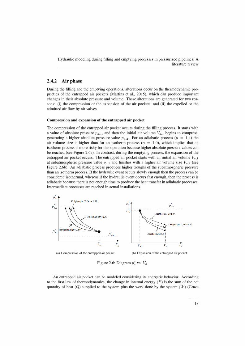
2.4.2 Air phaseDuring the filling and the emptying operations, alterations occur on the thermodynamic pro-prieties of the entrapped air pockets (Martins et al., 2015), which can produce importantchanges in their absolute pressure and volume. These alterations are generated for two rea-sons: (i) the compression or the expansion of the air pockets, and (ii) the expelled or theadmitted air flow by air valves.
Compression and expansion of the entrapped air pocket
The compression of the entrapped air pocket occurs during the filling process. It starts witha value of absolute pressure pa,1, and then the initial air volume Va,1 begins to compress,generating a higher absolute pressure value pa,2. For an adiabatic process (n = 1,4) theair volume size is higher than for an isotherm process (n = 1,0), which implies that anisotherm process is more risky for this operation because higher absolute pressure values canbe reached (see Figure 2.6a). In contrast, during the emptying process, the expansion of theentrapped air pocket occurs. The entrapped air pocket starts with an initial air volume Va,1at subatmospheric pressure value pa,1 and finishes with a higher air volume size Va,2 (seeFigure 2.6b). An adiabatic process produces higher troughs of the subatmospheric pressurethan an isotherm process. If the hydraulic event occurs slowly enough then the process can beconsidered isothermal, whereas if the hydraulic event occurs fast enough, then the process isadiabatic because there is not enough time to produce the heat transfer in adiabatic processes.Intermediate processes are reached in actual installations.
(a) Compression of the entrapped air pocket (b) Expansion of the entrapped air pocket
Figure 2.6: Diagram p∗a vs. Va
An entrapped air pocket can be modeled considering its energetic behavior. Accordingto the first law of thermodynamics, the change in internal energy (E) is the sum of the netquantity of heat (Q) supplied to the system plus the work done by the system (W ) (Graze
——18
Transient phenomena during the emptying process of water in pressurized pipelines
et al., 1996). A simplification of these relationships for an entrapped air pocket can be rep-resented by a polytropic model (Martin, 1976; Leon et al., 2010) where a constant polytropiccoefficient (n) considers the effects of the heat transfers in the variables p∗a and Va. As aconsequence, two formulations can be used for representing the behavior of an entrapped airpocket, which depends on whether the air mass is changing with time:
• If dma/dt 6= 0, then:
dp∗adt
= −np∗a
Va
dVadt
+p∗aVa
n
ρa
dma
dt(2.5)
• If dma/dt = 0, then:
p∗aVna = p∗a,0V
na,0 (2.6)
where ρa is the air density, ma is the air mass, and subscript 0 refers to initial conditionsof absolute pressure of air pocket and air volume.
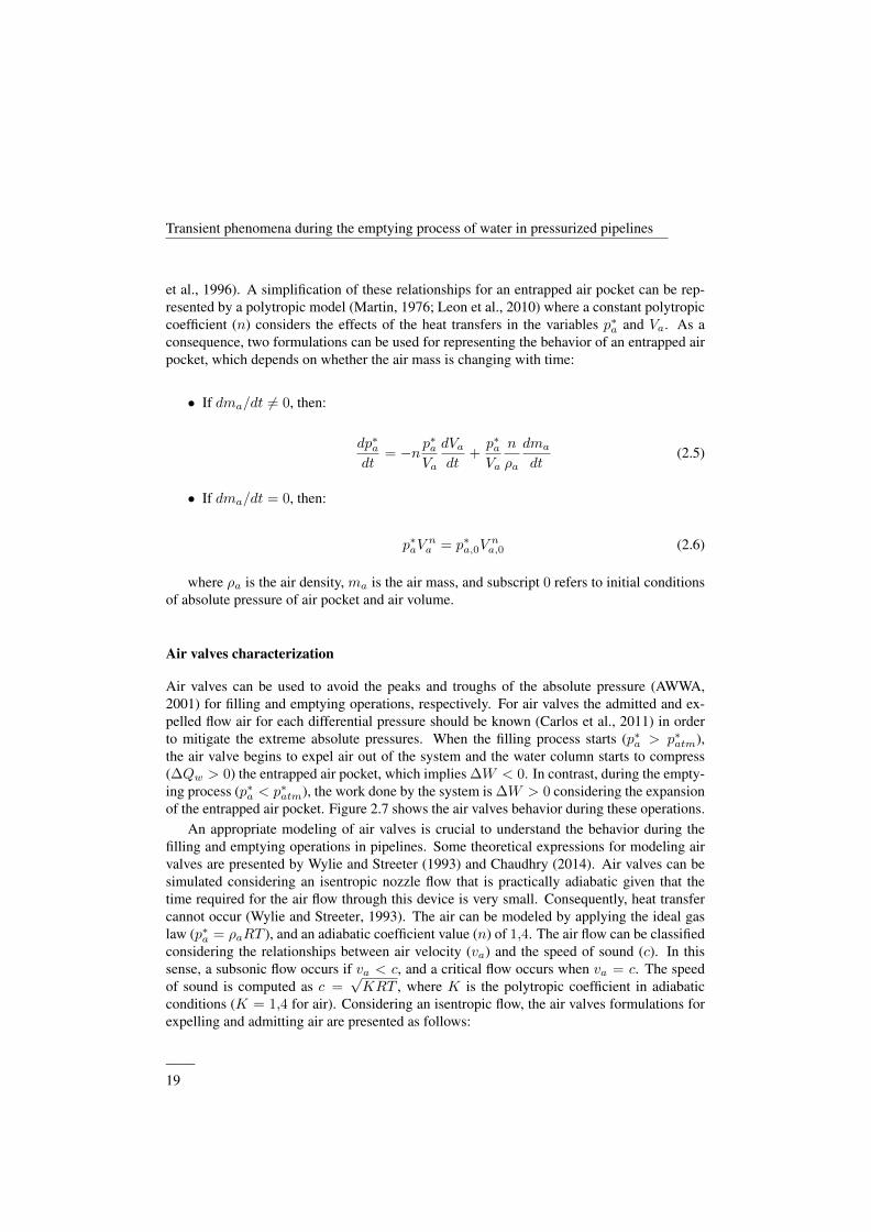
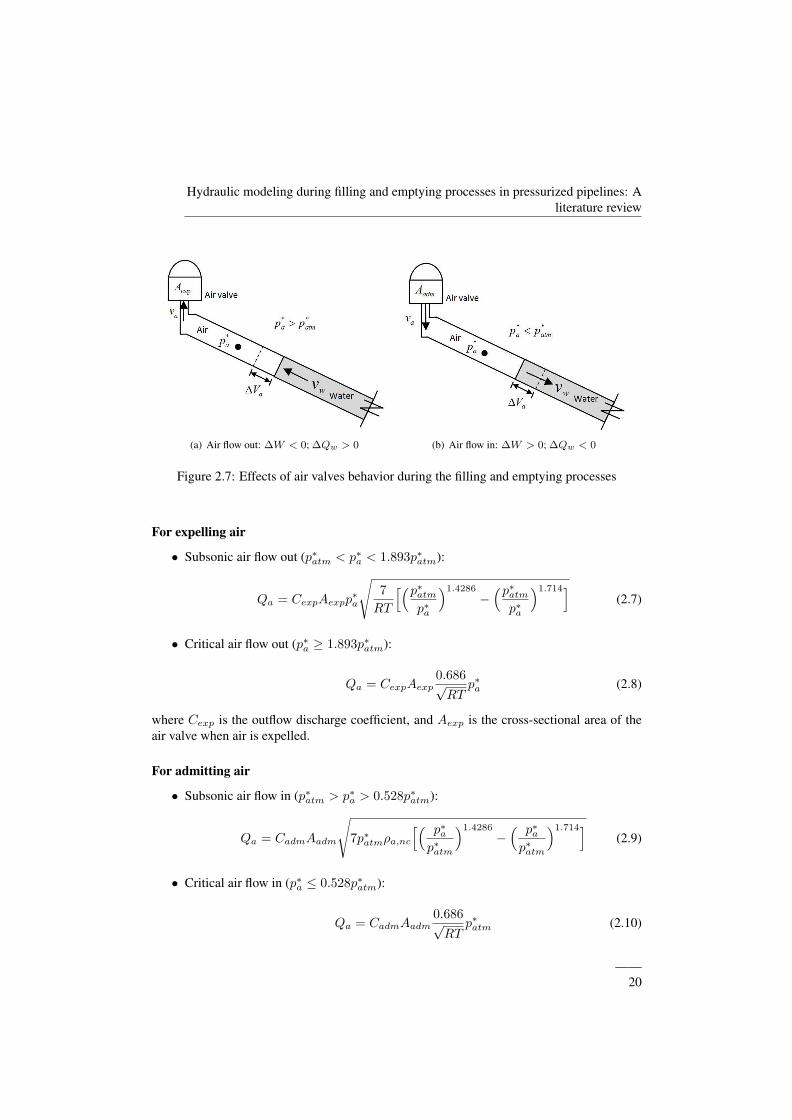
Air valves characterization
Air valves can be used to avoid the peaks and troughs of the absolute pressure (AWWA,2001) for filling and emptying operations, respectively. For air valves the admitted and ex-pelled flow air for each differential pressure should be known (Carlos et al., 2011) in orderto mitigate the extreme absolute pressures. When the filling process starts (p∗a > p∗atm),the air valve begins to expel air out of the system and the water column starts to compress(∆Qw > 0) the entrapped air pocket, which implies ∆W < 0. In contrast, during the empty-ing process (p∗a < p∗atm), the work done by the system is ∆W > 0 considering the expansionof the entrapped air pocket. Figure 2.7 shows the air valves behavior during these operations.
An appropriate modeling of air valves is crucial to understand the behavior during thefilling and emptying operations in pipelines. Some theoretical expressions for modeling airvalves are presented by Wylie and Streeter (1993) and Chaudhry (2014). Air valves can besimulated considering an isentropic nozzle flow that is practically adiabatic given that thetime required for the air flow through this device is very small. Consequently, heat transfercannot occur (Wylie and Streeter, 1993). The air can be modeled by applying the ideal gaslaw (p∗a = ρaRT ), and an adiabatic coefficient value (n) of 1,4. The air flow can be classifiedconsidering the relationships between air velocity (va) and the speed of sound (c). In thissense, a subsonic flow occurs if va < c, and a critical flow occurs when va = c. The speedof sound is computed as c =
√KRT , where K is the polytropic coefficient in adiabatic
conditions (K = 1,4 for air). Considering an isentropic flow, the air valves formulations forexpelling and admitting air are presented as follows:
——19
Hydraulic modeling during filling and emptying processes in pressurized pipelines: Aliterature review
(a) Air flow out: ∆W < 0; ∆Qw > 0 (b) Air flow in: ∆W > 0; ∆Qw < 0
Figure 2.7: Effects of air valves behavior during the filling and emptying processes
For expelling air
• Subsonic air flow out (p∗atm < p∗a < 1.893p∗atm):
Qa = CexpAexpp∗a
√7
RT
[(p∗atmp∗a
)1.4286
−(p∗atmp∗a
)1.714](2.7)
• Critical air flow out (p∗a ≥ 1.893p∗atm):
Qa = CexpAexp0.686√RT
p∗a (2.8)
where Cexp is the outflow discharge coefficient, and Aexp is the cross-sectional area of theair valve when air is expelled.
For admitting air
• Subsonic air flow in (p∗atm > p∗a > 0.528p∗atm):
Qa = CadmAadm
√7p∗atmρa,nc
[( p∗ap∗atm
)1.4286
−( p∗ap∗atm
)1.714](2.9)
• Critical air flow in (p∗a ≤ 0.528p∗atm):
Qa = CadmAadm0.686√RT
p∗atm (2.10)
——20
Transient phenomena during the emptying process of water in pressurized pipelines
where Aadm is the cross-sectional area of the air valve when air is admitted, and Cadm is theinflow discharge coefficient.
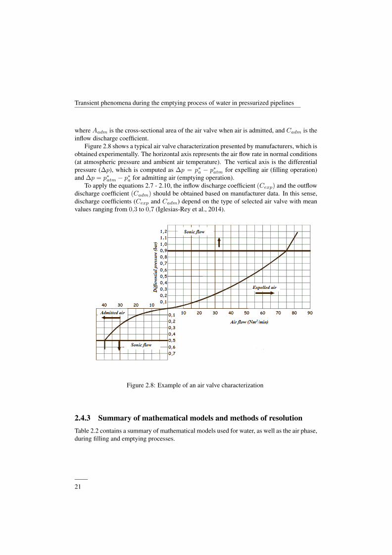
Figure 2.8 shows a typical air valve characterization presented by manufacturers, which isobtained experimentally. The horizontal axis represents the air flow rate in normal conditions(at atmospheric pressure and ambient air temperature). The vertical axis is the differentialpressure (∆p), which is computed as ∆p = p∗a − p∗atm for expelling air (filling operation)and ∆p = p∗atm − p∗a for admitting air (emptying operation).
To apply the equations 2.7 - 2.10, the inflow discharge coefficient (Cexp) and the outflowdischarge coefficient (Cadm) should be obtained based on manufacturer data. In this sense,discharge coefficients (Cexp and Cadm) depend on the type of selected air valve with meanvalues ranging from 0,3 to 0,7 (Iglesias-Rey et al., 2014).
Figure 2.8: Example of an air valve characterization
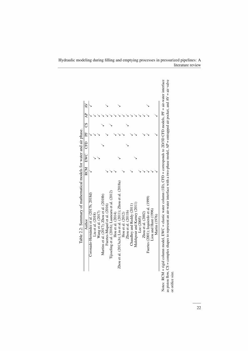
2.4.3 Summary of mathematical models and methods of resolutionTable 2.2 contains a summary of mathematical models used for water, as well as the air phase,during filling and emptying processes.
——21
Hydraulic modeling during filling and emptying processes in pressurized pipelines: Aliterature review
Tabl
e2.
2:Su
mm
ary
ofm
athe
mat
ical
mod
els
forw
ater
and
airp
hase
.A
utho
rR
CM
EW
CC
FDPF
CS
AP
AVC
oron
ado-
Her
nand
ezet
al.(
2017
b,20
18d)
XX
XX
Liu
etal
.(20
18)
XX
XW
ang
etal
.(20
17)
XX
XM
artin
set
al.(
2017
);Z
hou
etal
.(20
18b)
XX
XFu
erte
s-M
ique
leta
l.(2
016)
XX
XX
Tijs
selin
get
al.(
2016
);L
aane
aru
etal
.(20
12)
XX
XH
ouet
al.(
2014
)X
XX
Zho
uet
al.(
2013
a,b)
;Liu
etal
.(20
11);
Zho
uet
al.(
2018
a)X
XX
XH
ouet
al.(
2012
)X
XX
Zho
uet
al.(
2011
b)X
XX
Cha
udhr
yan
dR
eddy
(201
1)X
XX
Mal
ekpo
uran
dK
arne
y(2
011)
XX
XL
ee(2
005)
XX
Zho
uet
al.(
2002
)X
XX
Fuer
tes
(200
1);I
zqui
erdo
etal
.(19
99)
XX
XX
Lio
uan
dH
unt(
1996
)X
Mar
tin(1
976)
XX
X
Not
es:
RC
M=
rigi
dco
lum
nm
odel
,EW
C=
elas
ticw
ater
colu
mn
(1D
),C
FD=
corr
espo
nds
to2D
/3D
CFD
mod
els,
PF=
air-
wat
erin
terf
ace
aspi
ston
flow
,CS
=co
mpl
exsh
apes
tore
pres
enta
nai
r-w
ater
inte
rfac
ew
itha
two-
phas
em
odel
,AP
=en
trap
ped
airp
ocke
t,an
dAV
=ai
rval
veor
orifi
cesi
ze.
——22
Transient phenomena during the emptying process of water in pressurized pipelines
It is important to mention how is the resolution of mathematical models for these opera-tions. Currently, there is no single mathematical expression to directly solve the differential-algebraic equations (DAE) system for simulating the transient phenomena. Many techniqueshave been applied to solve a DAE system. Some of them are (i) the method of characteris-tics (Chaudhry, 2014; Wylie and Streeter, 1993), (ii) finite-difference methods (Cunge andWegner, 1964), (iii) finite-element methods (Watt, 1975; Baker, 1983), (iv) finite volumemethod (Guinot, 2003), (v) volume of fluids (Zhou et al., 2011b; Martins et al., 2017), and(vi) smoothed particle hydrodynamics (Hou et al., 2012).
Since the 60s, the method of characteristics was used to solve the characteristic equationsof a transient flow. At present, many researchers use it to model filling and emptying pro-cesses (Shimada et al., 2008; McInnis et al., 1997; Ghidaou and Karney, 1994; Wang et al.,2017; Zhou et al., 2013a) because of its computationally efficient and explicit resolutionscheme.
Finite-difference methods (explicit and implicit) (Chaudhry, 2014) are useful in combi-nation with the method of characteristics to solve complex situations in transient flow (Wanget al., 2017; Zhou and Liu, 2013). Zhou et al. (2013a,b) used this method to simulate anair-water interface and the method of characteristics to model the water phase.
Finite-element methods cannot efficiently solve problems related to the evolution of thehydraulic variables because temporal and spatial scaling are complex to model, resulting ininadequate wave propagation (Chaudhry, 2014).
Finite volume methods numerically solve the partial differential equations in the form ofalgebraic equations similar to finite-difference methods or finite-element methods. They areused to solve the conservation laws of hydraulic systems.
In this regard, Hou et al. (2012) presented a method based on Smoothed Particle Hydro-dynamics (SPH), Zhou et al. (2011b) solved the transient flow problem using a method ofVolume of Fluid (VOF), Coronado-Hernandez et al. (2017b) and Izquierdo et al. (1999) usednumerical solutions based on Runge-Kutta or Rosenbrock formula.
Air valves can be modeled using the method of characteristics (Ramezani et al., 2015;Zhou et al., 2013a,b) or numerical solutions of ordinary differential equations (Fuertes, 2001).
Table 2.3 presents a list of methods of resolution, where authors are mentioned. Allmethods of resolution are performed considering a constant friction factor, a non-variablepolytropic coefficient, considering a known air pocket size, and the characteristics of airvalves describe by manufacturers.
2.5 Uncertainty of current models and prospects
The sources of uncertainty that current models do not consider are the friction factor, thepolytropic coefficient, the air pocket size, and the air valve behavior. These parameters can af-fect the determination of extreme pressures (maximum and minimum) depending on pipelinecharacteristics
——23
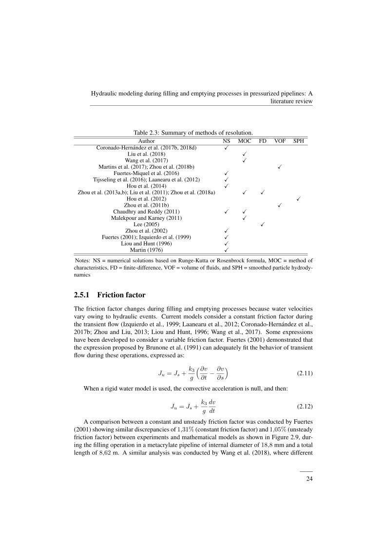
Hydraulic modeling during filling and emptying processes in pressurized pipelines: Aliterature review
Table 2.3: Summary of methods of resolution.Author NS MOC FD VOF SPH
Coronado-Hernandez et al. (2017b, 2018d) XLiu et al. (2018) X
Wang et al. (2017) XMartins et al. (2017); Zhou et al. (2018b) X
Fuertes-Miquel et al. (2016) XTijsseling et al. (2016); Laanearu et al. (2012) X
Hou et al. (2014) XZhou et al. (2013a,b); Liu et al. (2011); Zhou et al. (2018a) X X
Hou et al. (2012) XZhou et al. (2011b) X
Chaudhry and Reddy (2011) X XMalekpour and Karney (2011) X
Lee (2005) XZhou et al. (2002) X
Fuertes (2001); Izquierdo et al. (1999) XLiou and Hunt (1996) X
Martin (1976) X
Notes: NS = numerical solutions based on Runge-Kutta or Rosenbrock formula, MOC = method ofcharacteristics, FD = finite-difference, VOF = volume of fluids, and SPH = smoothed particle hydrody-namics
2.5.1 Friction factor
The friction factor changes during filling and emptying processes because water velocitiesvary owing to hydraulic events. Current models consider a constant friction factor duringthe transient flow (Izquierdo et al., 1999; Laanearu et al., 2012; Coronado-Hernandez et al.,2017b; Zhou and Liu, 2013; Liou and Hunt, 1996; Wang et al., 2017). Some expressionshave been developed to consider a variable friction factor. Fuertes (2001) demonstrated thatthe expression proposed by Brunone et al. (1991) can adequately fit the behavior of transientflow during these operations, expressed as:
Ju = Js +k3
g
(∂v∂t− ∂v
∂s
)(2.11)
When a rigid water model is used, the convective acceleration is null, and then:
Ju = Js +k3
g
dv
dt(2.12)
A comparison between a constant and unsteady friction factor was conducted by Fuertes(2001) showing similar discrepancies of 1,31% (constant friction factor) and 1,05% (unsteadyfriction factor) between experiments and mathematical models as shown in Figure 2.9, dur-ing the filling operation in a metacrylate pipeline of internal diameter of 18,8 mm and a totallength of 8,62 m. A similar analysis was conducted by Wang et al. (2018), where different
——24
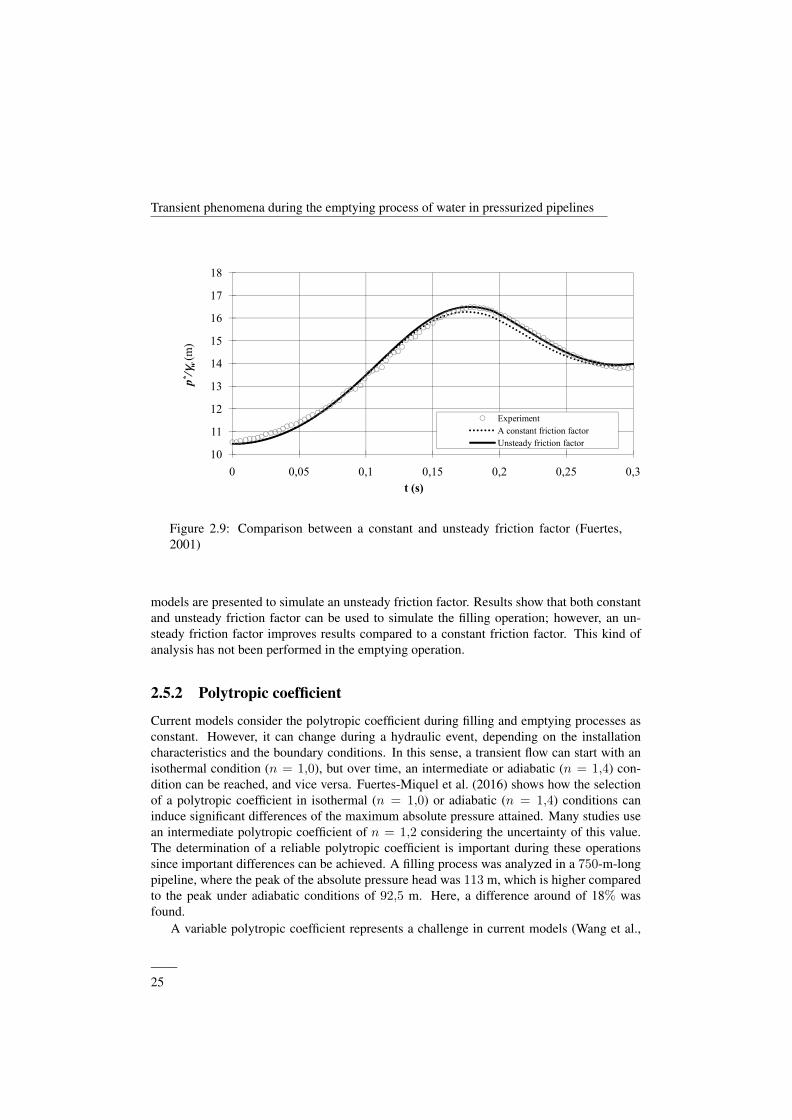
Transient phenomena during the emptying process of water in pressurized pipelines
12
13
14
15
16
17
18
p*/ γ
w (m
)
10
11
12
13
14
15
16
17
18
0 0,05 0,1 0,15 0,2 0,25 0,3
p*/ γ
w (m
)
t (s)
Experiment
A constant friction factor
Unsteady friction factor
Figure 2.9: Comparison between a constant and unsteady friction factor (Fuertes,2001)
models are presented to simulate an unsteady friction factor. Results show that both constantand unsteady friction factor can be used to simulate the filling operation; however, an un-steady friction factor improves results compared to a constant friction factor. This kind ofanalysis has not been performed in the emptying operation.
2.5.2 Polytropic coefficient
Current models consider the polytropic coefficient during filling and emptying processes asconstant. However, it can change during a hydraulic event, depending on the installationcharacteristics and the boundary conditions. In this sense, a transient flow can start with anisothermal condition (n = 1,0), but over time, an intermediate or adiabatic (n = 1,4) con-dition can be reached, and vice versa. Fuertes-Miquel et al. (2016) shows how the selectionof a polytropic coefficient in isothermal (n = 1,0) or adiabatic (n = 1,4) conditions caninduce significant differences of the maximum absolute pressure attained. Many studies usean intermediate polytropic coefficient of n = 1,2 considering the uncertainty of this value.The determination of a reliable polytropic coefficient is important during these operationssince important differences can be achieved. A filling process was analyzed in a 750-m-longpipeline, where the peak of the absolute pressure head was 113 m, which is higher comparedto the peak under adiabatic conditions of 92,5 m. Here, a difference around of 18% wasfound.
A variable polytropic coefficient represents a challenge in current models (Wang et al.,
——25
Hydraulic modeling during filling and emptying processes in pressurized pipelines: Aliterature review
2018; Izquierdo et al., 1999; Zhou et al., 2011b; Martins et al., 2015), which has been imple-mented for modeling air vessels (Akpan et al., 2014).
2.5.3 Air pocket size
Air pockets, which directly affect filling and emptying processes, can accumulate in severalparts in the system. In experimental facilities, different configurations regarding air pocketsizes have been conducted (Tijsseling et al., 2016; Coronado-Hernandez et al., 2017b; Zhouet al., 2013a,b). However, the air pocket size cannot be controlled in actual installations. It isvery important to note that small air pockets are more dangerous than large air pockets duringthese operations when air valves are not acting. Coronado-Hernandez et al. (2018b) analyzeda 1200-m-long pipeline for filling and emptying procedures finding that the air pocket size isnot sensitive over these events when air valves are acting. However, if there are no air valvesalong pipeline installations, the air pocket size can change remarkably the extreme values ofabsolute pressure. For instance, Izquierdo et al. (1999) shows a pipeline of a total length of2000 m where a filling operation is analyzed. Results confirm that an air pocket size of 79 mproduces a maximum absolute pressure head of 277 m, and considering an air pocket size of140 m, the absolute pressure head is 191 m, which implies a difference of 30%.
2.5.4 Air valves behavior
Two sources of uncertainties were detected in the characterization of air valves produced bya lack of experimental tests of some manufacturers: (i) the first one corresponds to the airand vacuum flow rate curves, and (ii) the second one corresponds to the dynamic closureof air valves with entrapped air. Iglesias-Rey et al. (2014) analyzed discrepancies betweenmanufacturer data and experimental tests considering different types of air valves.
On one hand, the development of experimental facilities to compute air and vacuumflow rate curves of air valves with large orifices is complex since an enough quantity ofexpelled/admitted air is required. Then, some manufacturers supply air and vacuum flowrate curves with discrepancies compared to experimental tests (Iglesias-Rey et al., 2014).An inappropriate characterization of air valves introduce an uncertainty in current modelsregarding inflow and outflow discharge coefficients.
On the other hand, the uncertainty associated to the dynamic closure with entrapped air inair valves is another deficiency of some manufacturers because they do not supply values ofdynamic closure occurrence. The phenomenon occurs when outlet air velocity in air valvesis too high (large volume of expelled air) producing a sustentation force on the float, whichcloses an air valve before the water arrives to this device and leaving a dangerous air pocketinside pipeline systems. The majority of air valves are prone to this phenomenon.
——26
Transient phenomena during the emptying process of water in pressurized pipelines
2.6 Practical considerations
2.6.1 General practicesIn water pipelines, pressure surges and troughs of subatmospheric pressure can occur duringfilling and emptying processes, respectively, which are generated by entrapped air pockets inhydraulic systems. Air/vacuum valves (AVVs) should be installed along pipelines to preventpressure surges, by exhausting air during filling processes and injecting a sufficient quantityof air during emptying processes, thus preventing subatmospheric conditions (AWWA, 2001;Ramezani et al., 2016). However, if AVVs are not correctly sized and well-maintained, prob-lems can continue in installations (Ramezani et al., 2015; Stephenson, 1997; Fuertes, 2001;Tran, 2016).
Filling processes should be executed carefully, through slow maneuvers in the operationof discharge valves to produce an adequate expelled airflow rate. A pressure differential of2 p.s.i (13,79 kPa) is recommended by the AWWA (2001) during this process. Water flowshould be similar to air flow (Qa) through AVVs with a water velocity of 0,3 m/s.
By contrast, a controlled emptying process should be performed replacing the water vol-ume by an admitted air volume with a similar ratio to avoid dangerous troughs of absolutepressure (Coronado-Hernandez et al., 2017b; Fuertes-Miquel et al., 2018b). (AWWA, 2001)recommends both water velocities from 0,3 to 0,6 m/s and a pressure differential of 5 p.s.i(34,5 kPa). If air valves are not installed or are undersized, then dangerous troughs of subat-mospheric pressure occur, and hydraulic systems cannot be drained.
2.6.2 Air valves selectionThe air valve selection during the air expulsion phase considers different aspects (Ramezaniet al., 2015; AWWA, 2001). If air valves have been undersized, then the quantity of expelledair is not enough and peaks of pressure surge can occur. In contrast, for the larger air valvesize, higher amounts of expelled air and water velocity are reached. If air valves have beenoversized, then greater values of absolute pressure are reached compared to the situationwithout these devices. When the water reaches the air valve position, the air valve closesrapidly, producing a water hammer in a single-phase (water). Another consideration is thedynamic closure of air valves, which is typically not provided by manufacturers. When anair valve closes without expelling the entrapped air pocket completely, the water columncompresses it, producing a dangerous pressure surge.
By contrast, during the emptying process, the air valve should be selected to protect thesystem from the troughs of subatmospheric pressure. In this sense, a larger air valve sizereduces the lowest values of subatmospheric pressure.
2.6.3 Typical pipe selection practicesThe pressure surges and troughs of subatmospheric pressure can be caused by a change inthe water velocity during the filling and the emptying process, respectively (Wang et al.,
——27
Hydraulic modeling during filling and emptying processes in pressurized pipelines: Aliterature review
2017; Coronado-Hernandez et al., 2017b). To select the pressure and the stiffness class inpipelines, the water hammer effects should be computed not only for these operations butalso for hydraulic events such as the stopping of pumps (power failure), the rapid opening orclosing of valves, and pipe failure, among others. Extreme values of absolute pressure shouldbe selected to design the pipe characteristics.
The highest peak of the pressure surge reached in the aforementioned hydraulic eventsshould be used to select the pressure class in pipelines. Pipe manufacturers usually specifythe pressure class of water distribution networks depending on pipe material with typicalvalues varying from 6 to 16 bar (Mays, 1999). In other installations pressure class can bedifferent.
The stiffness class is selected according to the following conditions: (i) burial conditionsgiven by native soil, type of backfill, and cover depth, and (ii) the troughs of subatmosphericpressure in the system. In this sense, designers can select the stiffness class based on manu-facturer data, for instance, SN2500, SN5000, or SN10000.
2.7 Future researchThis section provides future developments that should be considered to continue working inthis field, which are mentioned as follows:
1. Computational Fluid Dynamics (CFD) can be used to understand better the behavior ofair pockets considering, among other things, the following circumstances: (i) the en-trance of backflow air by drain valves during the emptying process, (ii) complex shapesof air-water interface, (iii) the variation of entrapped air pockets during these processes,(iv) the variation of thermodynamic proprieties of air inside air valves (Garcıa-Todolıet al., 2018), (v) the determination of absolute pressure caused by oversized air valves,and (vi) how an entrapped air causes a reduced cross section in pipelines.
2. The analysis of filling and emptying operations of water distribution networks has notbeen conducted neither numerically nor experimentally. The majority of experimentalfacilities correspond to single pipes or pipelines of undulating profiles. Also, the be-havior of air in pipelines bifurcations needs to be analyzed since there are no studiesrelated to the quantification of air volume fraction flowing to the downstream two pipebranches.
3. Current works consider the positing of air valves in high points of water pipelines;however, AWWA (2001) considers others locations of air valves which needs to bestudied in points such as horizontal pipe branches, at vertical pumps, long descents andascents, among others.
4. Many studies show that the determination of air and vacuum flow rate curves suppliedby some manufactures is inadequate, as well as they do not supply reference values ofdynamic closure occurrence. The correct air valves characterization is very importantto analyze filling and emptying processes.
——28
Transient phenomena during the emptying process of water in pressurized pipelines
5. Current models of filling and emptying operations consider that polytropic model canbe applied. However, there are some limitations of the polytropic model as reported byGraze et al. (1996).
2.8 Conclusions
This research presents current knowledge regarding the transient phenomena related to fillingand emptying processes in water pipelines. A literature review was conducted on variousmathematical models for the water phase, air-water interface, and air phase. Advantages anddisadvantages of water phase models were described, as well as an identification of actualresearchers. Air-water interface criteria are described, and the air phase and air valve charac-terization are explained. Four sources of uncertainty that need to be studied further, includingthe necessity to include a variable value for the polytropic coefficient and the friction fac-tor, as well as the air pockets sizes and air valves selection in the system, were identified incurrent models. Typical practices about the air valve selection and the pressure and stiffnessclass in pipelines are summarized showing how emptying and filling operations should beconsidered for selecting them in hydraulic systems. Finally, future research on filling andemptying processes in pressurized pipelines have also been presented in this work.
ddddddddddddddddddddd
——29
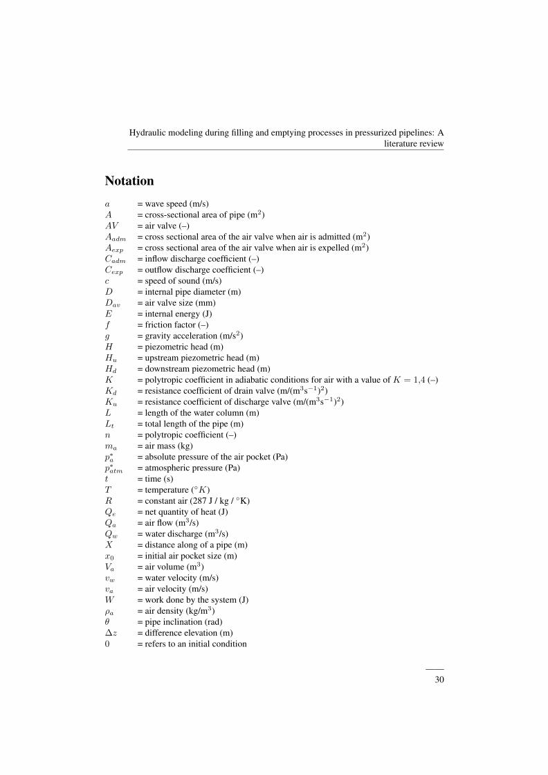
Hydraulic modeling during filling and emptying processes in pressurized pipelines: Aliterature review
Notation
a = wave speed (m/s)A = cross-sectional area of pipe (m2)AV = air valve (–)Aadm = cross sectional area of the air valve when air is admitted (m2)Aexp = cross sectional area of the air valve when air is expelled (m2)Cadm = inflow discharge coefficient (–)Cexp = outflow discharge coefficient (–)c = speed of sound (m/s)D = internal pipe diameter (m)Dav = air valve size (mm)E = internal energy (J)f = friction factor (–)g = gravity acceleration (m/s2)H = piezometric head (m)Hu = upstream piezometric head (m)Hd = downstream piezometric head (m)K = polytropic coefficient in adiabatic conditions for air with a value of K = 1,4 (–)Kd = resistance coefficient of drain valve (m/(m3s−1)2)Ku = resistance coefficient of discharge valve (m/(m3s−1)2)L = length of the water column (m)Lt = total length of the pipe (m)n = polytropic coefficient (–)ma = air mass (kg)p∗a = absolute pressure of the air pocket (Pa)p∗atm = atmospheric pressure (Pa)t = time (s)T = temperature (◦K)R = constant air (287 J / kg / ◦K)Qe = net quantity of heat (J)Qa = air flow (m3/s)Qw = water discharge (m3/s)X = distance along of a pipe (m)x0 = initial air pocket size (m)Va = air volume (m3)vw = water velocity (m/s)va = air velocity (m/s)W = work done by the system (J)ρa = air density (kg/m3)θ = pipe inclination (rad)∆z = difference elevation (m)0 = refers to an initial condition
——30
Chapter 3
Transient phenomena during theemptying process of a single pipewith water-air interaction
This chapter is extracted from the paper:
Transient phenomena during the emptying process of a single pipe with water-air interactionCoauthors: Fuertes-Miquel, V. S; Coronado-Hernandez O. E; Iglesias-Rey P. L.; Mora-Melia, D.
Journal: Journal of Hydraulic Research ISSN 0022-16862017 Impact Factor: 2.076. Position JCR 41/128 (Q2). Civil Engineering
State: Published. Latest Articles. 2018; DOI: 10.1080/00221686.2018.1492465.
3.1 Abstract
Emptying pipelines can be critical in many water distribution networks because subatmo-spheric pressure troughs could cause considerable damage to the system due to the expansionof entrapped air. Researchers have given relatively little attention to emptying processescompared to filling processes. The intricacy of computations of this phenomenon makes itdifficult to predict the behavior during emptying, and there are only a few reliable models inthe literature. In this work, a computational model for simulating the transient phenomenain single pipes is proposed, which was validated using experimental results. The proposedmodel is based on a rigid column to analyze water movement, the air-water interface, andair pocket equations. Two practical cases were used to validate the model: 1) a single pipewith the upstream end closed, and 2) a single pipe with an air valve installed on the upstreamend. The results show how the model accurately predicts the experimental data, including thepressure oscillation patterns and subatmospheric pressure troughs.
31
Transient phenomena during the emptying process of a single pipe with water-airinteraction
3.2 Introduction
Over recent decades, the analysis of transient phenomena for a single-phase liquid has beenstudied extensively by researchers and there are currently numerous models that representcorrectly the water behavior in any hydraulic system. However, transient flow with trappedair is much more complex to simulate because there are two fluids (water and air) in two dif-ferent phases (liquid and gas) (Fuertes, 2001), which implies a higher complexity to establishreliable mathematical models.
Filling and emptying maneuvers are common pipelines operations with trapped air. Theseoperations are repeated periodically and must be considered to avoid future problems associ-ated to extreme values of air pocket pressure. For this reason, many researchers have focusedtheir efforts on the development of different models for the analysis on entrapped air in wa-ter supply networks (Zhou et al., 2013a,b; Wang et al., 2016; Martins et al., 2015; Laanearuet al., 2012).
To date, researchers have mostly focused on filling processes, developing models thathave shown great accuracy in comparison to experimental data. In this sense, early studies onpipelines were conducted by Liou and Hunt (1996) and Izquierdo et al. (1999), and Zhou et al.(2013a,b) developed recently models to analyze the process of rapid filling. Additionally, afew pieces of research have been published analyzing the influence of different parametersthrough experimental investigations of the systems (Hou et al., 2014; Zhou and Liu, 2013).Fi-nally, others studies have focused on techniques and methods for solving the filling problem(Wang et al., 2016; Martins et al., 2015; Malekpour and Karney, 2014; Liu et al., 2011; Mar-tins et al., 2010b), analyzing the consequences of the formation of air pockets (Pozos et al.,2010), and the occurrence of cavitation in the propagation of transient phenomena (Wanget al., 2003; Guinot, 2001).
Emptying processes may also be critical, but they have received less attention from re-searchers. On this matter, Laanearu et al. (2012) developed a semi-empirical model for es-timating local energy losses and Tijsseling et al. (2016) presented a model for the emptyingprocess with pressurized air in a pipeline. Nevertheless, there is a lack of studies on the waterdraining maneuvers in engineering applications of real hydraulic systems.
Therefore, this paper presents a new mathematical model to be used for emptying pro-cesses. The proposed model simulates the liquid column with a rigid model using the massoscillation equation (Cabrera et al., 1992; Liou and Hunt, 1996; Izquierdo et al., 1999; Lee,2005), which provides sufficient accuracy by using a moving air-water interface (Izquierdoet al., 1999; Zhou et al., 2013a). Additionally, it is possible to consider thermodynamic be-haviors such as: (a) an isothermal process, where the temperature remains constant inside thehydraulic installation; (b) an adiabatic process, where the hydraulic installation exchangesno heat with its surroundings; and (c) an intermediate processes, which involves temperaturechange and heat transfer. In this sense, the relationship between the absolute pressure and to-tal volume of entrapped air characterizes the behavior of air, which is known as a polytropicprocess. If the transient process occurs slowly enough, it is considered isothermal, and thepolytrophic coefficient is 1,0. In contrast, if the transient process is fast enough, it is consid-
——32
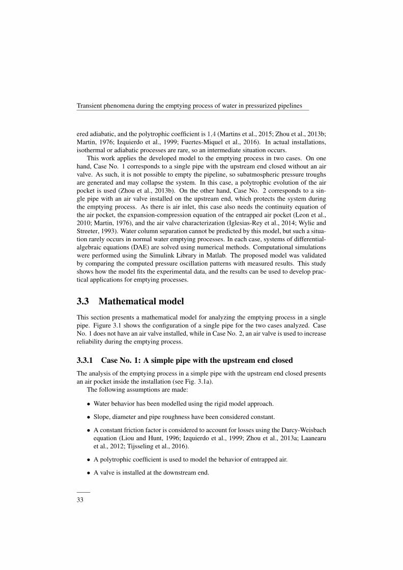
Transient phenomena during the emptying process of water in pressurized pipelines
ered adiabatic, and the polytrophic coefficient is 1,4 (Martins et al., 2015; Zhou et al., 2013b;Martin, 1976; Izquierdo et al., 1999; Fuertes-Miquel et al., 2016). In actual installations,isothermal or adiabatic processes are rare, so an intermediate situation occurs.
This work applies the developed model to the emptying process in two cases. On onehand, Case No. 1 corresponds to a single pipe with the upstream end closed without an airvalve. As such, it is not possible to empty the pipeline, so subatmospheric pressure troughsare generated and may collapse the system. In this case, a polytrophic evolution of the airpocket is used (Zhou et al., 2013b). On the other hand, Case No. 2 corresponds to a sin-gle pipe with an air valve installed on the upstream end, which protects the system duringthe emptying process. As there is air inlet, this case also needs the continuity equation ofthe air pocket, the expansion-compression equation of the entrapped air pocket (Leon et al.,2010; Martin, 1976), and the air valve characterization (Iglesias-Rey et al., 2014; Wylie andStreeter, 1993). Water column separation cannot be predicted by this model, but such a situa-tion rarely occurs in normal water emptying processes. In each case, systems of differential-algebraic equations (DAE) are solved using numerical methods. Computational simulationswere performed using the Simulink Library in Matlab. The proposed model was validatedby comparing the computed pressure oscillation patterns with measured results. This studyshows how the model fits the experimental data, and the results can be used to develop prac-tical applications for emptying processes.
3.3 Mathematical modelThis section presents a mathematical model for analyzing the emptying process in a singlepipe. Figure 3.1 shows the configuration of a single pipe for the two cases analyzed. CaseNo. 1 does not have an air valve installed, while in Case No. 2, an air valve is used to increasereliability during the emptying process.
3.3.1 Case No. 1: A simple pipe with the upstream end closedThe analysis of the emptying process in a simple pipe with the upstream end closed presentsan air pocket inside the installation (see Fig. 3.1a).
The following assumptions are made:
• Water behavior has been modelled using the rigid model approach.
• Slope, diameter and pipe roughness have been considered constant.
• A constant friction factor is considered to account for losses using the Darcy-Weisbachequation (Liou and Hunt, 1996; Izquierdo et al., 1999; Zhou et al., 2013a; Laanearuet al., 2012; Tijsseling et al., 2016).
• A polytrophic coefficient is used to model the behavior of entrapped air.
• A valve is installed at the downstream end.
——33
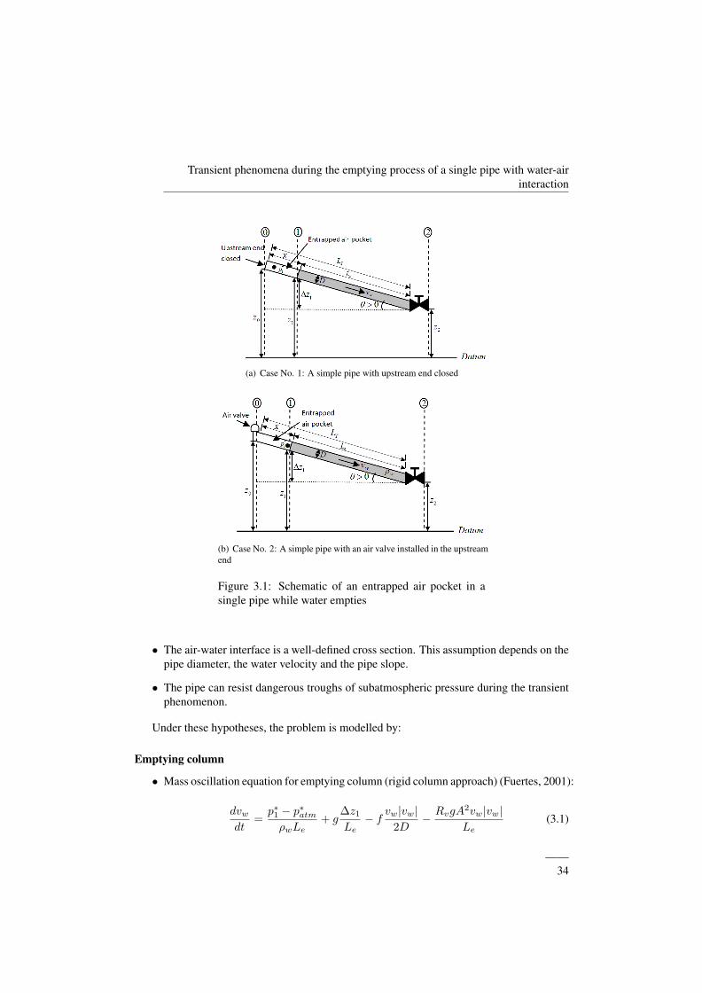
Transient phenomena during the emptying process of a single pipe with water-airinteraction
(a) Case No. 1: A simple pipe with upstream end closed
(b) Case No. 2: A simple pipe with an air valve installed in the upstreamend
Figure 3.1: Schematic of an entrapped air pocket in asingle pipe while water empties
• The air-water interface is a well-defined cross section. This assumption depends on thepipe diameter, the water velocity and the pipe slope.
• The pipe can resist dangerous troughs of subatmospheric pressure during the transientphenomenon.
Under these hypotheses, the problem is modelled by:
Emptying column
• Mass oscillation equation for emptying column (rigid column approach) (Fuertes, 2001):
dvwdt
=p∗1 − p∗atmρwLe
+ g∆z1
Le− f vw|vw|
2D− RvgA
2vw|vw|Le
(3.1)
——34
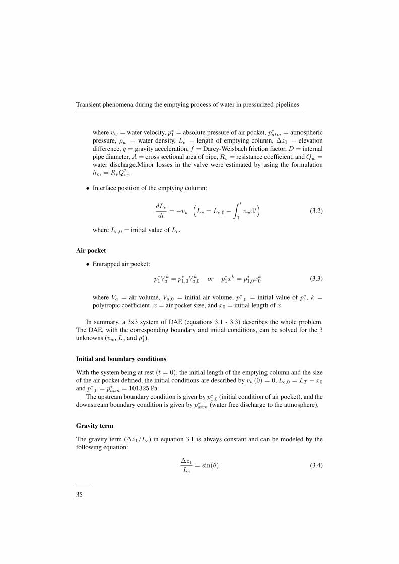
Transient phenomena during the emptying process of water in pressurized pipelines
where vw = water velocity, p∗1 = absolute pressure of air pocket, p∗atm = atmosphericpressure, ρw = water density, Le = length of emptying column, ∆z1 = elevationdifference, g = gravity acceleration, f = Darcy-Weisbach friction factor, D = internalpipe diameter,A = cross sectional area of pipe,Rv = resistance coefficient, andQw =water discharge.Minor losses in the valve were estimated by using the formulationhm = RvQ
2w.
• Interface position of the emptying column:
dLe
dt= −vw
(Le = Le,0 −
∫ t
0
vwdt)
(3.2)
where Le,0 = initial value of Le.
Air pocket
• Entrapped air pocket:
p∗1Vka = p∗1,0V
ka,0 or p∗1x
k = p∗1,0xk0 (3.3)
where Va = air volume, Va,0 = initial air volume, p∗1,0 = initial value of p∗1, k =polytropic coefficient, x = air pocket size, and x0 = initial length of x.
In summary, a 3x3 system of DAE (equations 3.1 - 3.3) describes the whole problem.The DAE, with the corresponding boundary and initial conditions, can be solved for the 3unknowns (vw, Le and p∗1).
Initial and boundary conditions
With the system being at rest (t = 0), the initial length of the emptying column and the sizeof the air pocket defined, the initial conditions are described by vw(0) = 0, Le,0 = LT − x0
and p∗1,0 = p∗atm = 101325 Pa.The upstream boundary condition is given by p∗1,0 (initial condition of air pocket), and the
downstream boundary condition is given by p∗atm (water free discharge to the atmosphere).
Gravity term
The gravity term (∆z1/Le) in equation 3.1 is always constant and can be modeled by thefollowing equation:
∆z1
Le= sin(θ) (3.4)
——35
Transient phenomena during the emptying process of a single pipe with water-airinteraction
3.3.2 Case No. 2: A simple pipe with an air valve installed in the up-stream end
The analyses of the emptying process in a simple pipe with an air valve installed at theupstream end is shown in Fig. 3.1b. The assumptions are the same as in Case No. 1. Conse-quently, equations 3.1 and 3.2 were used to represent the behavior of emptying the column.The air pocket was modelled using the following equations:
• Continuity equation: This equation was used, considering that the air density of airpocket (ρa) and the air density in air valve (ρa,nc) are different (see Fig. 3.2).
Figure 3.2: Location of air valve
Applying the continuity equation:
dma
dt= ρa,ncva,ncAadm (3.5)
and by deriving the expression:
dma
dt=d(ρaVa)
dt=dρadt
Va +dVadt
ρa (3.6)
where ma = air mass, va,nc = air velocity in normal conditions admitted by the airvalve, and Aadm = cross sectional area of the air valve.
If Va = xA = (LT − Le)A and dVa/dt = −(dLe/dt)A = vA, then:
dρadt
=ρa,ncva,ncAadm − vwAρa
A(LT − Le)(3.7)
• Expansion-compression equation (Leon et al., 2010; Martin, 1976; Lee, 2005):
dp∗1dt
= −k p∗1
Va
dVadt
+p∗1Va
k
ρa
dma
dt(3.8)
——36
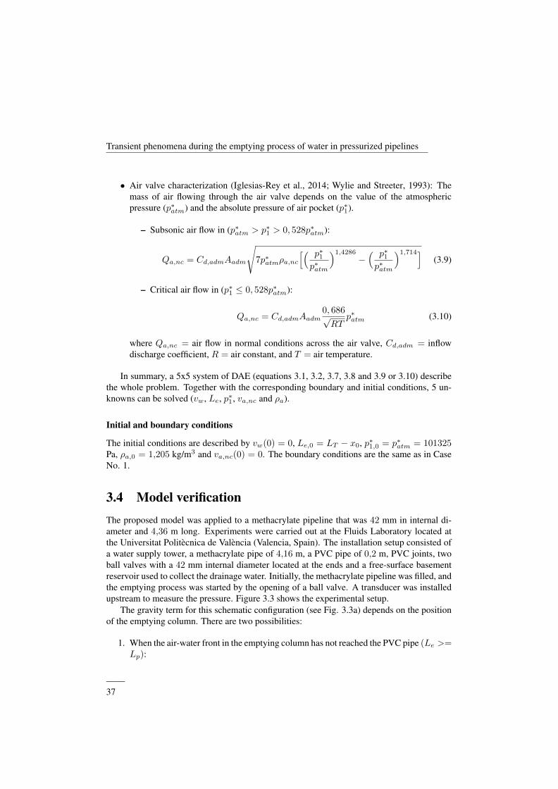
Transient phenomena during the emptying process of water in pressurized pipelines
• Air valve characterization (Iglesias-Rey et al., 2014; Wylie and Streeter, 1993): Themass of air flowing through the air valve depends on the value of the atmosphericpressure (p∗atm) and the absolute pressure of air pocket (p∗1).
– Subsonic air flow in (p∗atm > p∗1 > 0, 528p∗atm):
Qa,nc = Cd,admAadm
√7p∗atmρa,nc
[( p∗1p∗atm
)1,4286
−( p∗1p∗atm
)1,714](3.9)
– Critical air flow in (p∗1 ≤ 0, 528p∗atm):
Qa,nc = Cd,admAadm0, 686√RT
p∗atm (3.10)
where Qa,nc = air flow in normal conditions across the air valve, Cd,adm = inflowdischarge coefficient, R = air constant, and T = air temperature.
In summary, a 5x5 system of DAE (equations 3.1, 3.2, 3.7, 3.8 and 3.9 or 3.10) describethe whole problem. Together with the corresponding boundary and initial conditions, 5 un-knowns can be solved (vw, Le, p∗1, va,nc and ρa).
Initial and boundary conditions
The initial conditions are described by vw(0) = 0, Le,0 = LT − x0, p∗1,0 = p∗atm = 101325Pa, ρa,0 = 1,205 kg/m3 and va,nc(0) = 0. The boundary conditions are the same as in CaseNo. 1.
3.4 Model verificationThe proposed model was applied to a methacrylate pipeline that was 42 mm in internal di-ameter and 4,36 m long. Experiments were carried out at the Fluids Laboratory located atthe Universitat Politecnica de Valencia (Valencia, Spain). The installation setup consisted ofa water supply tower, a methacrylate pipe of 4,16 m, a PVC pipe of 0,2 m, PVC joints, twoball valves with a 42 mm internal diameter located at the ends and a free-surface basementreservoir used to collect the drainage water. Initially, the methacrylate pipeline was filled, andthe emptying process was started by the opening of a ball valve. A transducer was installedupstream to measure the pressure. Figure 3.3 shows the experimental setup.
The gravity term for this schematic configuration (see Fig. 3.3a) depends on the positionof the emptying column. There are two possibilities:
1. When the air-water front in the emptying column has not reached the PVC pipe (Le >=Lp):
——37
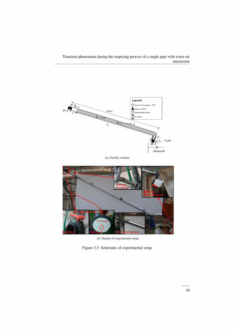
Transient phenomena during the emptying process of a single pipe with water-airinteraction
(a) Facility scheme
(b) Details of experimental setup
Figure 3.3: Schematic of experimental setup
——38
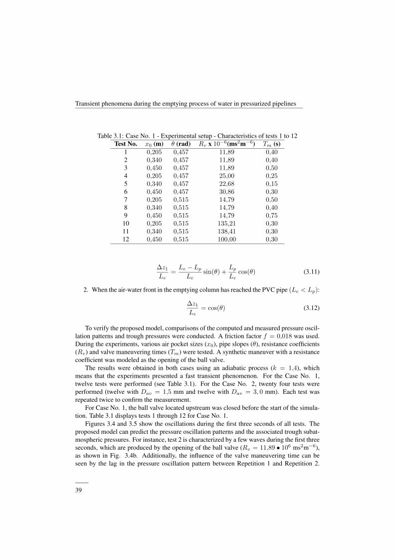
Transient phenomena during the emptying process of water in pressurized pipelines
Table 3.1: Case No. 1 - Experimental setup - Characteristics of tests 1 to 12Test No. x0 (m) θ (rad) Rv x 10−6(ms2m−6) Tm (s)
1 0,205 0,457 11,89 0,402 0,340 0,457 11,89 0,403 0,450 0,457 11,89 0,504 0,205 0,457 25,00 0,255 0,340 0,457 22,68 0,156 0,450 0,457 30,86 0,307 0,205 0,515 14,79 0,508 0,340 0,515 14,79 0,409 0,450 0,515 14,79 0,75
10 0,205 0,515 135,21 0,3011 0,340 0,515 138,41 0,3012 0,450 0,515 100,00 0,30
∆z1
Le=Le − Lp
Lesin(θ) +
Lp
Lecos(θ) (3.11)
2. When the air-water front in the emptying column has reached the PVC pipe (Le < Lp):
∆z1
Le= cos(θ) (3.12)
To verify the proposed model, comparisons of the computed and measured pressure oscil-lation patterns and trough pressures were conducted. A friction factor f = 0,018 was used.During the experiments, various air pocket sizes (x0), pipe slopes (θ), resistance coefficients(Rv) and valve maneuvering times (Tm) were tested. A synthetic maneuver with a resistancecoefficient was modeled as the opening of the ball valve.
The results were obtained in both cases using an adiabatic process (k = 1,4), whichmeans that the experiments presented a fast transient phenomenon. For the Case No. 1,twelve tests were performed (see Table 3.1). For the Case No. 2, twenty four tests wereperformed (twelve with Dav = 1,5 mm and twelve with Dav = 3, 0 mm). Each test wasrepeated twice to confirm the measurement.
For Case No. 1, the ball valve located upstream was closed before the start of the simula-tion. Table 3.1 displays tests 1 through 12 for Case No. 1.
Figures 3.4 and 3.5 show the oscillations during the first three seconds of all tests. Theproposed model can predict the pressure oscillation patterns and the associated trough subat-mospheric pressures. For instance, test 2 is characterized by a few waves during the first threeseconds, which are produced by the opening of the ball valve (Rv = 11,89 • 106 ms2m−6),as shown in Fig. 3.4b. Additionally, the influence of the valve maneuvering time can beseen by the lag in the pressure oscillation pattern between Repetition 1 and Repetition 2.
——39
Transient phenomena during the emptying process of a single pipe with water-airinteraction
The minimum subatmospheric pressure head of 8,23 m was reached. In contrast, test 10 haspractically no waves during the transient (see Fig. 3.4j) and a high flow resistance coefficientvalue (Rv = 135,21 • 106 ms2m−6) where the trough of the subatmospheric pressure headof 8,14 m was found.
In Case No. 2, an orifice was made upstream to represent the air valve (see Figures 3.6,3.7, 3.8 and 3.9). Two different orifice sizes were used to show the impact of the air inlet.The smallest orifice size corresponds to the lowest value of the inflow discharge coefficient.The inflow discharge coefficients for Dav = 1,5 mm and Dav = 3,0 mm are 0,55 and 0,65,respectively. These values have been calibrated. Figure 3.10 shows the experimental resultsand the characteristic curves for the two orifice sizes. The formulation presented by Wylieand Streeter (1993) predicts the experimental data. Table 3.2 shows the tests.
Figures 3.6 and 3.8 show a comparison between the computed and measured absolutepressure oscillation patterns for tests 13 to 36. Again, the proposed model shows a fairlygood overall agreement with the experiments. The subatmospheric pressure trough occursimmediately when the ball valve is opened. Then absolute pressure starts to increase slowlyuntil it reaches atmospheric conditions. For instance, the trough of the subatmospheric pres-sure head for test 14 (8,89 m) is lower than test 32 (9,51 m). Test 14 displays a transientlonger than test 32.
Finally, Fig. 3.12 shows a comparison between the calculated and measured subatmo-spheric pressure troughs for both cases. For all tests, the proposed model predicts the troughof the subatmospheric pressure, which is very important to ensure pipeline safety. The mainrisk is presented in Case No. 1 when there no air inlet. Case No. 2 shows that an orifice ofsize Dav = 1,5 mm reaches a greater subatmospheric pressure trough than an orifice of sizeDav = 3,0 mm.
dddddddddddddddddd
——40
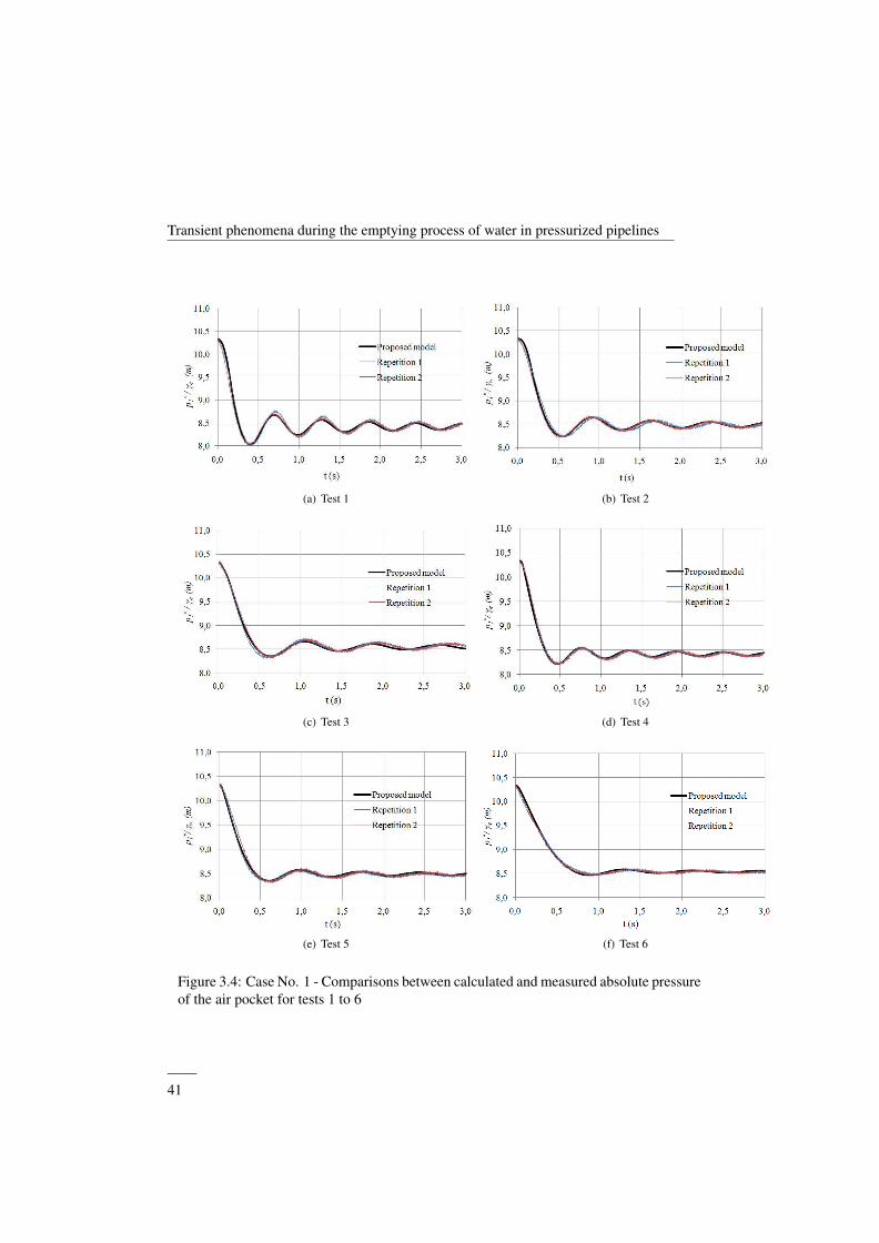
Transient phenomena during the emptying process of water in pressurized pipelines
(a) Test 1 (b) Test 2
(c) Test 3 (d) Test 4
(e) Test 5 (f) Test 6
Figure 3.4: Case No. 1 - Comparisons between calculated and measured absolute pressureof the air pocket for tests 1 to 6
——41
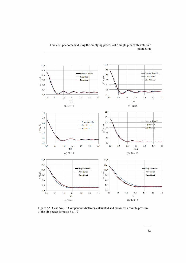
Transient phenomena during the emptying process of a single pipe with water-airinteraction
(a) Test 7 (b) Test 8
(c) Test 9 (d) Test 10
(e) Test 11 (f) Test 12
Figure 3.5: Case No. 1 - Comparisons between calculated and measured absolute pressureof the air pocket for tests 7 to 12
——42
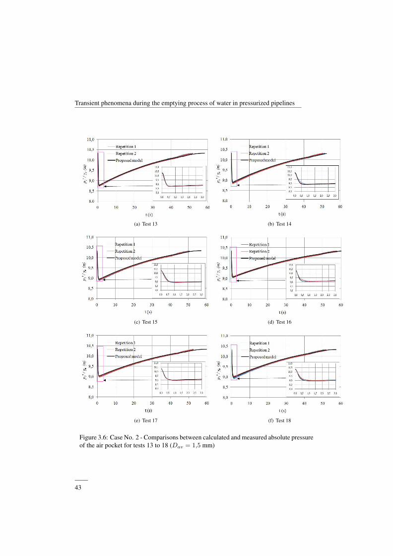
Transient phenomena during the emptying process of water in pressurized pipelines
(a) Test 13 (b) Test 14
(c) Test 15 (d) Test 16
(e) Test 17 (f) Test 18
Figure 3.6: Case No. 2 - Comparisons between calculated and measured absolute pressureof the air pocket for tests 13 to 18 (Dav = 1,5 mm)
——43
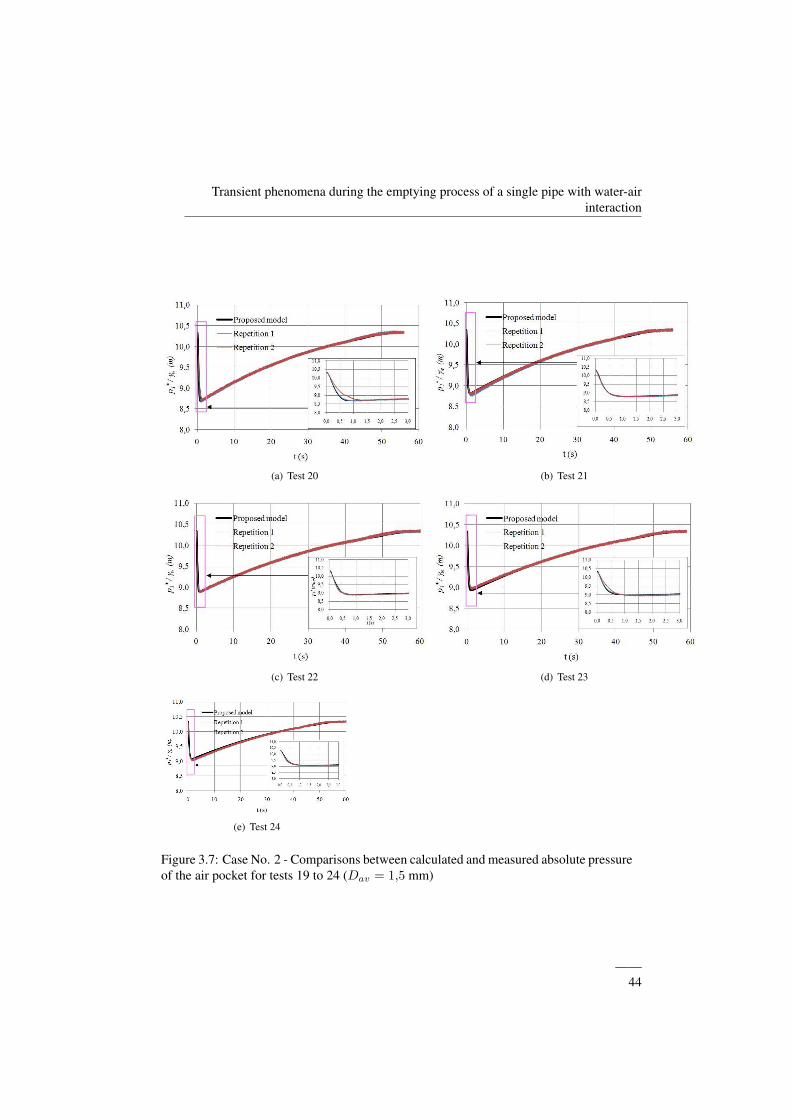
Transient phenomena during the emptying process of a single pipe with water-airinteraction
(a) Test 20 (b) Test 21
(c) Test 22 (d) Test 23
(e) Test 24
Figure 3.7: Case No. 2 - Comparisons between calculated and measured absolute pressureof the air pocket for tests 19 to 24 (Dav = 1,5 mm)
——44
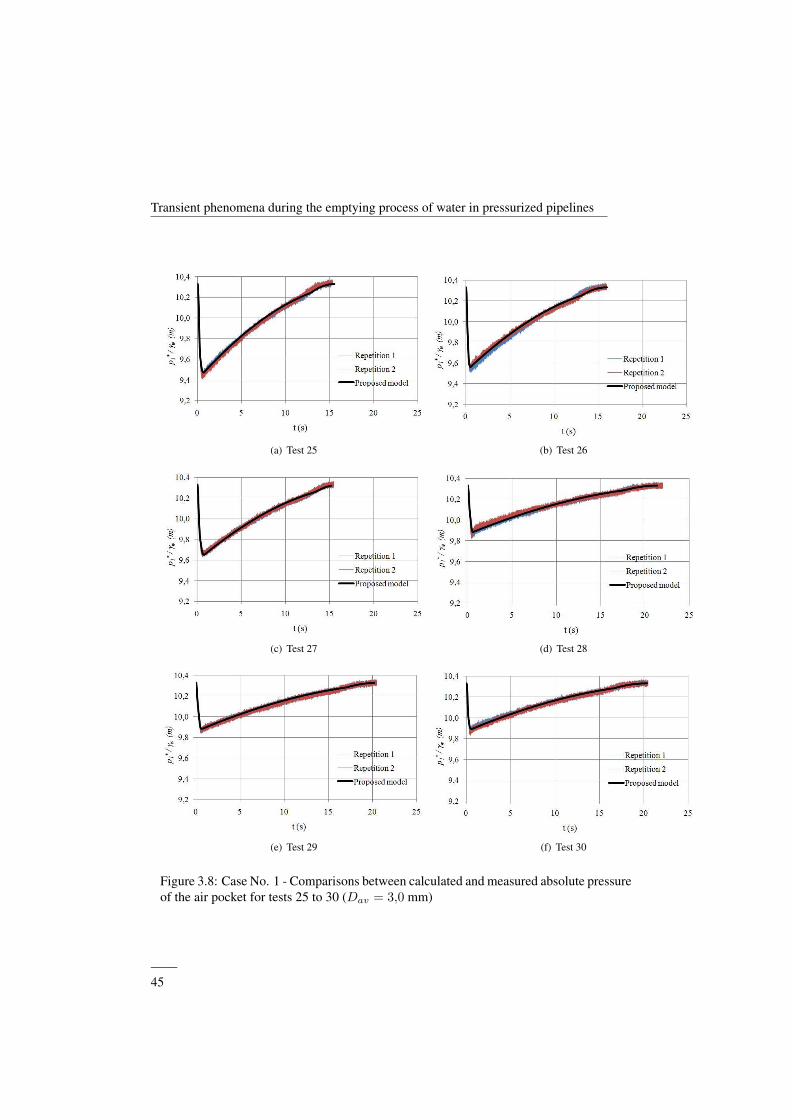
Transient phenomena during the emptying process of water in pressurized pipelines
(a) Test 25 (b) Test 26
(c) Test 27 (d) Test 28
(e) Test 29 (f) Test 30
Figure 3.8: Case No. 1 - Comparisons between calculated and measured absolute pressureof the air pocket for tests 25 to 30 (Dav = 3,0 mm)
——45
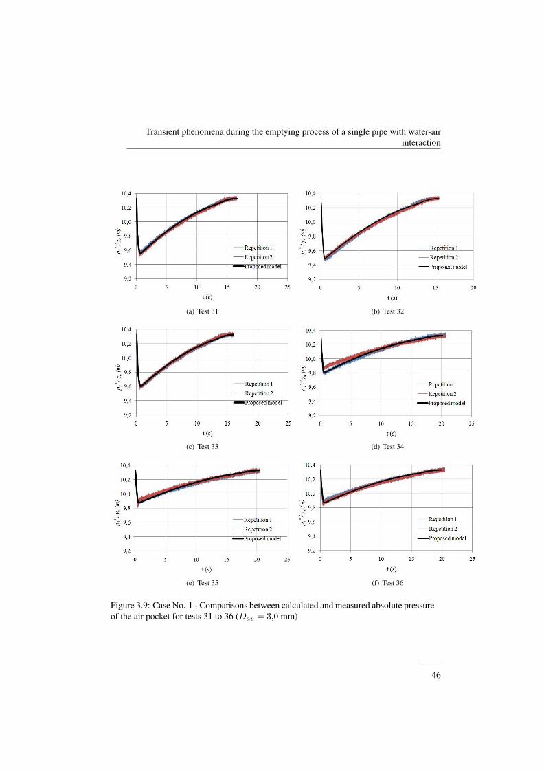
Transient phenomena during the emptying process of a single pipe with water-airinteraction
(a) Test 31 (b) Test 32
(c) Test 33 (d) Test 34
(e) Test 35 (f) Test 36
Figure 3.9: Case No. 1 - Comparisons between calculated and measured absolute pressureof the air pocket for tests 31 to 36 (Dav = 3,0 mm)
——46
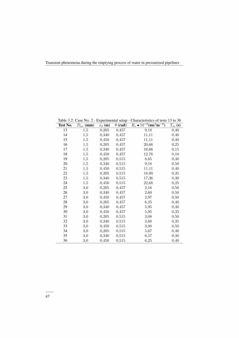
Transient phenomena during the emptying process of water in pressurized pipelines
Table 3.2: Case No. 2 - Experimental setup - Characteristics of tests 13 to 36Test No. Dav (mm) x0 (m) θ (rad) Rv • 10−6(ms2m−6) Tm (s)
13 1,5 0,205 0,457 9,18 0,4014 1,5 0,340 0,457 11,11 0,4015 1,5 0,450 0,457 11,11 0,4016 1,5 0,205 0,457 20,66 0,2517 1,5 0,340 0,457 16,66 0,1518 1,5 0,450 0,457 12,76 0,1019 1,5 0,205 0,515 8,65 0,4020 1,5 0,340 0,515 9,18 0,5021 1,5 0,450 0,515 11,11 0,4022 1,5 0,205 0,515 18,90 0,3523 1,5 0,340 0,515 17,36 0,3024 1,5 0,450 0,515 22,68 0,2525 3,0 0,205 0,457 2,16 0,5026 3,0 0,340 0,457 2,60 0,5027 3,0 0,450 0,457 2,97 0,5028 3,0 0,205 0,457 6,25 0,4029 3,0 0,340 0,457 5,95 0,4030 3,0 0,450 0,457 5,95 0,3531 3,0 0,205 0,515 3,08 0,5032 3,0 0,340 0,515 2,60 0,3533 3,0 0,450 0,515 3,08 0,5034 3,0 0,205 0,515 5,67 0,4035 3,0 0,340 0,515 6,57 0,4036 3,0 0,450 0,515 6,25 0,40
——47
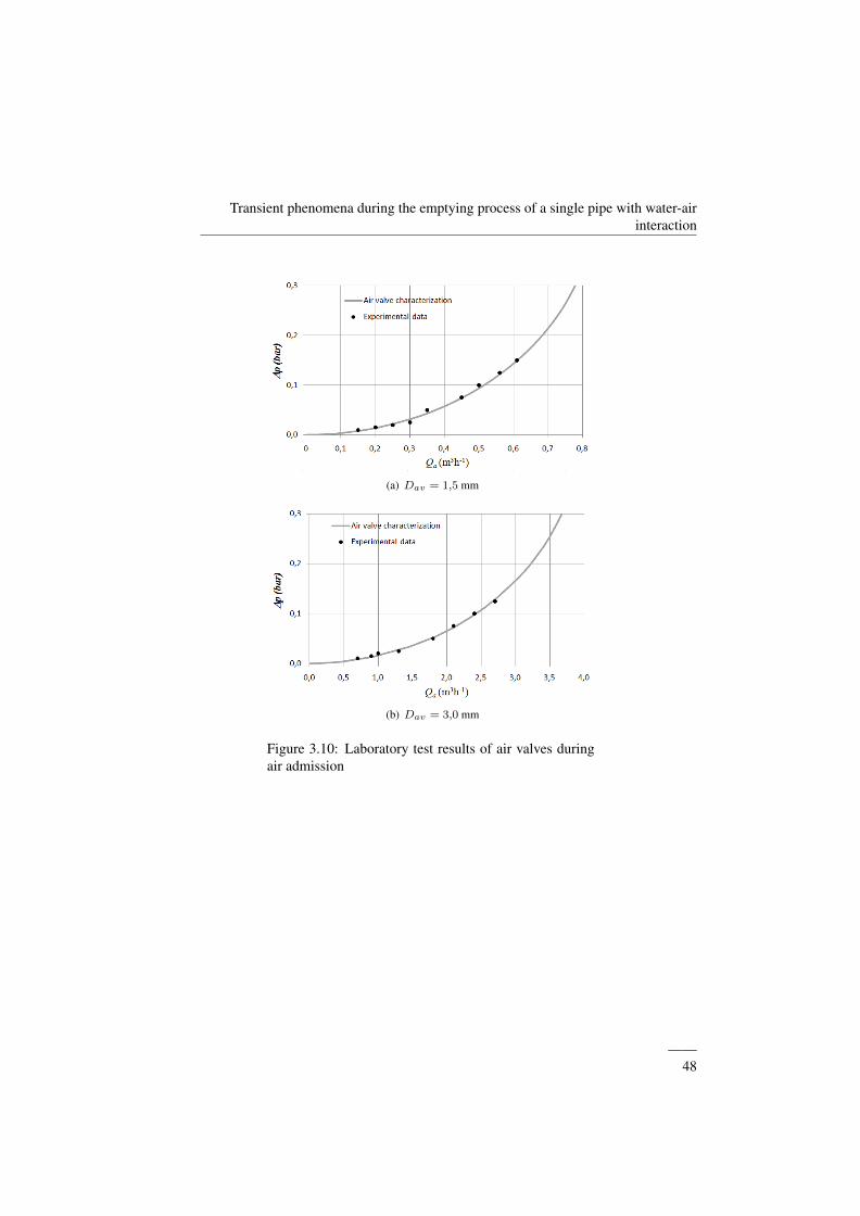
Transient phenomena during the emptying process of a single pipe with water-airinteraction
(a) Dav = 1,5 mm
(b) Dav = 3,0 mm
Figure 3.10: Laboratory test results of air valves duringair admission
ddddddddddd
——48

Transient phenomena during the emptying process of water in pressurized pipelines
Figure 3.11: The comparison between computed and measured minimum pressures
dd
3.5 Case study and results
To show what has been set forth, and to quantify the order of magnitude of some of theterms used, we present practical applications for the two cases mentioned. For both cases,a polytrophic coefficient k = 1,2 has been selected, which is a typical value in practicalapplications.
3.5.1 Case No. 1: A simple pipe with the upstream end closed
The system presented in Fig. 3.1a has been solved with the following data: LT = 600m,f = 0,018, D = 0,35 m; ∆z1 = 15 m, Rv = 0,06 ms2m−6, x0 = 200 m, k = 1,2, andp∗1,0 = 101325 Pa. The results obtained are shown in Fig. 3.12.
According to the results, the authors can deduce:
• Fig. 3.12a shows that the water flow increases rapidly until reaching a maximum valueof 0,26 m3s−1 at 23,5 s. Subsequently, the flow of water decreases until it reaches avalue of 0 m3s−1 at 123,6 s. Then it continues to decrease until −0,06 m3s−1 at 158,8s, indicating negative velocities occur. Hence, a setback occurs while emptying thecolumn. Finally, oscillations in the water flow are observed until it reaches a value of0 m3s−1, when draining is stopped, and part of the water remains in the installation.
——49
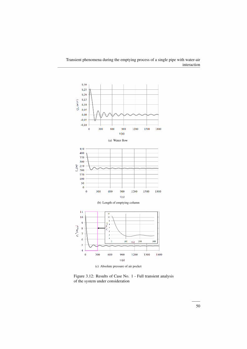
Transient phenomena during the emptying process of a single pipe with water-airinteraction
(a) Water flow
(b) Length of emptying column
(c) Absolute pressure of air pocket
Figure 3.12: Results of Case No. 1 - Full transient analysisof the system under consideration
——50
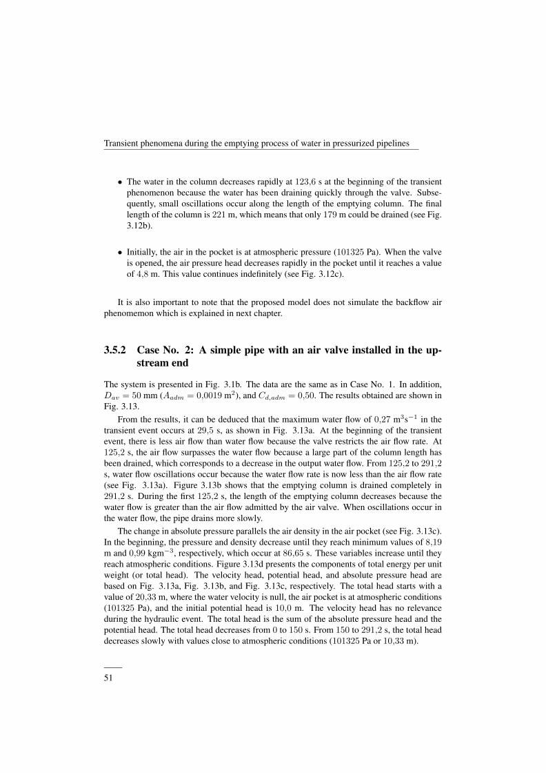
Transient phenomena during the emptying process of water in pressurized pipelines
• The water in the column decreases rapidly at 123,6 s at the beginning of the transientphenomenon because the water has been draining quickly through the valve. Subse-quently, small oscillations occur along the length of the emptying column. The finallength of the column is 221 m, which means that only 179 m could be drained (see Fig.3.12b).
• Initially, the air in the pocket is at atmospheric pressure (101325 Pa). When the valveis opened, the air pressure head decreases rapidly in the pocket until it reaches a valueof 4,8 m. This value continues indefinitely (see Fig. 3.12c).
It is also important to note that the proposed model does not simulate the backflow airphenomemon which is explained in next chapter.
3.5.2 Case No. 2: A simple pipe with an air valve installed in the up-stream end
The system is presented in Fig. 3.1b. The data are the same as in Case No. 1. In addition,Dav = 50 mm (Aadm = 0,0019 m2), and Cd,adm = 0,50. The results obtained are shown inFig. 3.13.
From the results, it can be deduced that the maximum water flow of 0,27 m3s−1 in thetransient event occurs at 29,5 s, as shown in Fig. 3.13a. At the beginning of the transientevent, there is less air flow than water flow because the valve restricts the air flow rate. At125,2 s, the air flow surpasses the water flow because a large part of the column length hasbeen drained, which corresponds to a decrease in the output water flow. From 125,2 to 291,2s, water flow oscillations occur because the water flow rate is now less than the air flow rate(see Fig. 3.13a). Figure 3.13b shows that the emptying column is drained completely in291,2 s. During the first 125,2 s, the length of the emptying column decreases because thewater flow is greater than the air flow admitted by the air valve. When oscillations occur inthe water flow, the pipe drains more slowly.
The change in absolute pressure parallels the air density in the air pocket (see Fig. 3.13c).In the beginning, the pressure and density decrease until they reach minimum values of 8,19m and 0,99 kgm−3, respectively, which occur at 86,65 s. These variables increase until theyreach atmospheric conditions. Figure 3.13d presents the components of total energy per unitweight (or total head). The velocity head, potential head, and absolute pressure head arebased on Fig. 3.13a, Fig. 3.13b, and Fig. 3.13c, respectively. The total head starts with avalue of 20,33 m, where the water velocity is null, the air pocket is at atmospheric conditions(101325 Pa), and the initial potential head is 10,0 m. The velocity head has no relevanceduring the hydraulic event. The total head is the sum of the absolute pressure head and thepotential head. The total head decreases from 0 to 150 s. From 150 to 291,2 s, the total headdecreases slowly with values close to atmospheric conditions (101325 Pa or 10,33 m).
——51
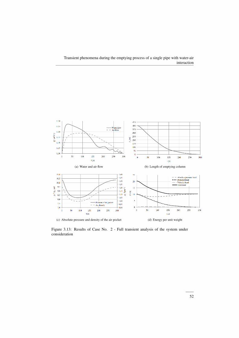
Transient phenomena during the emptying process of a single pipe with water-airinteraction
(a) Water and air flow (b) Length of emptying column
(c) Absolute pressure and density of the air pocket (d) Energy per unit weight
Figure 3.13: Results of Case No. 2 - Full transient analysis of the system underconsideration
——52
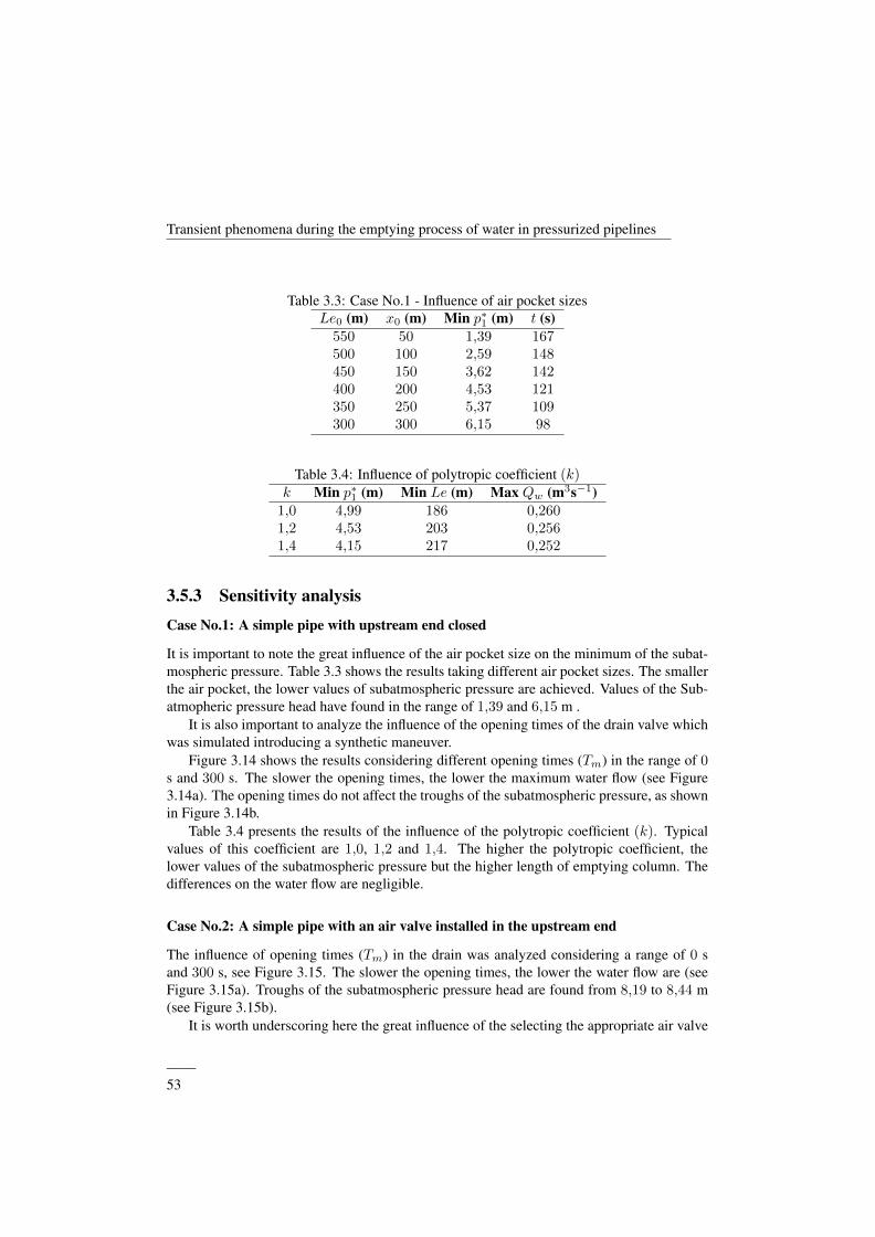
Transient phenomena during the emptying process of water in pressurized pipelines
Table 3.3: Case No.1 - Influence of air pocket sizesLe0 (m) x0 (m) Min p∗1 (m) t (s)
550 50 1,39 167500 100 2,59 148450 150 3,62 142400 200 4,53 121350 250 5,37 109300 300 6,15 98
Table 3.4: Influence of polytropic coefficient (k)k Min p∗1 (m) Min Le (m) Max Qw (m3s−1)
1,0 4,99 186 0,2601,2 4,53 203 0,2561,4 4,15 217 0,252
3.5.3 Sensitivity analysis
Case No.1: A simple pipe with upstream end closed
It is important to note the great influence of the air pocket size on the minimum of the subat-mospheric pressure. Table 3.3 shows the results taking different air pocket sizes. The smallerthe air pocket, the lower values of subatmospheric pressure are achieved. Values of the Sub-atmopheric pressure head have found in the range of 1,39 and 6,15 m .
It is also important to analyze the influence of the opening times of the drain valve whichwas simulated introducing a synthetic maneuver.
Figure 3.14 shows the results considering different opening times (Tm) in the range of 0s and 300 s. The slower the opening times, the lower the maximum water flow (see Figure3.14a). The opening times do not affect the troughs of the subatmospheric pressure, as shownin Figure 3.14b.
Table 3.4 presents the results of the influence of the polytropic coefficient (k). Typicalvalues of this coefficient are 1,0, 1,2 and 1,4. The higher the polytropic coefficient, thelower values of the subatmospheric pressure but the higher length of emptying column. Thedifferences on the water flow are negligible.
Case No.2: A simple pipe with an air valve installed in the upstream end
The influence of opening times (Tm) in the drain was analyzed considering a range of 0 sand 300 s, see Figure 3.15. The slower the opening times, the lower the water flow are (seeFigure 3.15a). Troughs of the subatmospheric pressure head are found from 8,19 to 8,44 m(see Figure 3.15b).
It is worth underscoring here the great influence of the selecting the appropriate air valve
——53
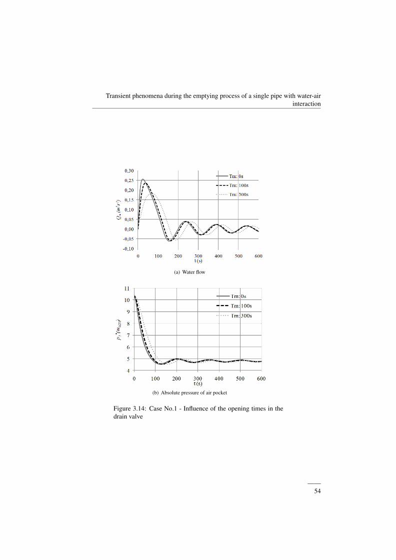
Transient phenomena during the emptying process of a single pipe with water-airinteraction
(a) Water flow
(b) Absolute pressure of air pocket
Figure 3.14: Case No.1 - Influence of the opening times in thedrain valve
——54

Transient phenomena during the emptying process of water in pressurized pipelines
(a) Water flow
(b) Absolute pressure of air pocket
Figure 3.15: Case No.2 - Influence of the opening time in thevalve
——55
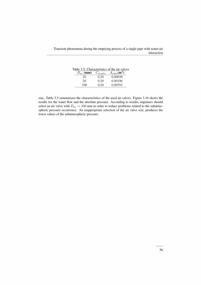
Transient phenomena during the emptying process of a single pipe with water-airinteraction
Table 3.5: Characteristics of the air valvesDav (mm) Cd,adm Aadm(m2)
25 0,50 0,0004950 0,50 0,00196100 0,50 0,00785
size. Table 3.5 summarizes the characteristics of the used air valves. Figure 3.16 shows theresults for the water flow and the absolute pressure. According to results, engineers shouldselect an air valve with Dav = 100 mm in order to reduce problems related to the subatmo-spheric pressure occurrence. An inappropriate selection of the air valve size, produces thelower values of the subatmospheric pressure.
dddddddddddddddddddddddddddddd
——56
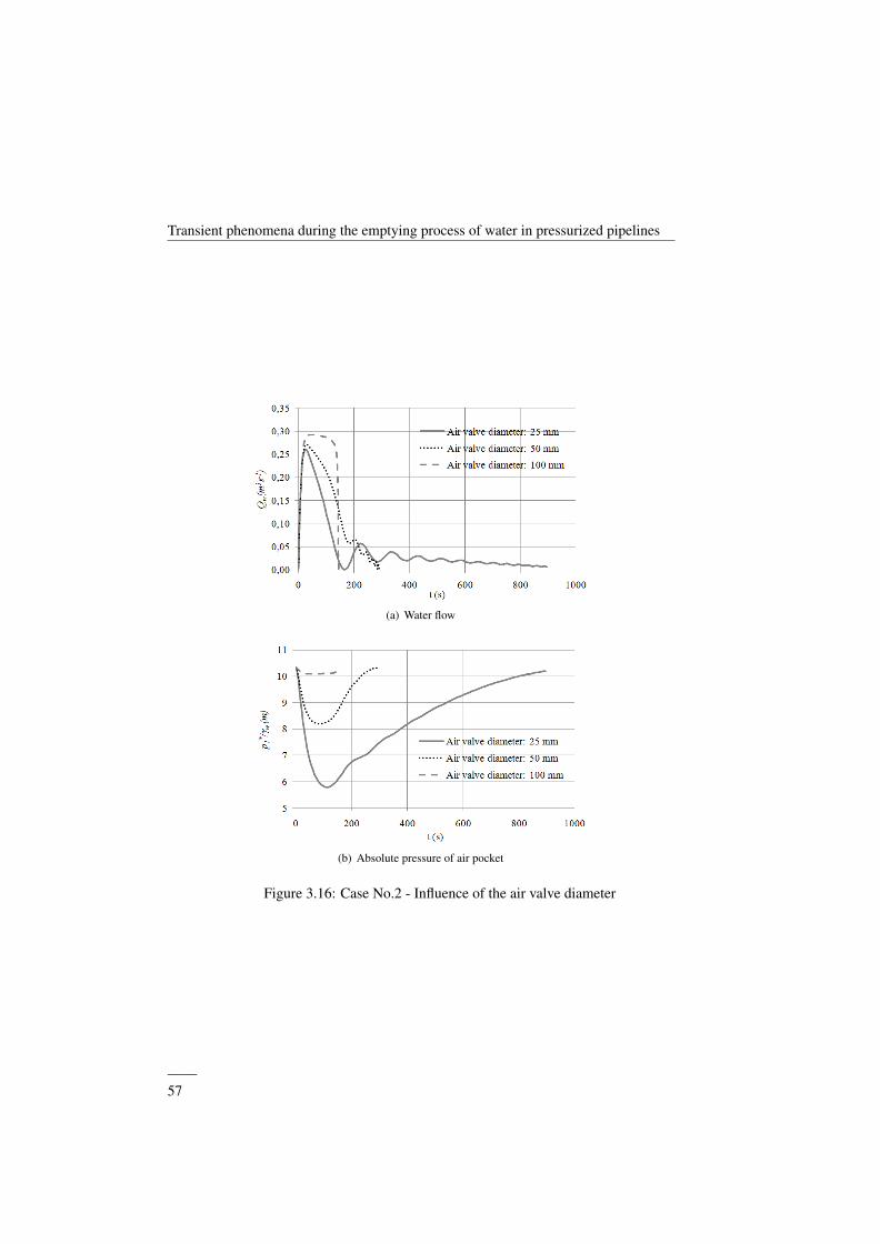
Transient phenomena during the emptying process of water in pressurized pipelines
(a) Water flow
(b) Absolute pressure of air pocket
Figure 3.16: Case No.2 - Influence of the air valve diameter
——57
Transient phenomena during the emptying process of a single pipe with water-airinteraction
3.6 ConclusionsTraditionally, emptying processes have received little attention from researchers. However,the development of models to simulate the transient behavior in these processes is consideredto be of great interest to the scientific community. In this chapter, a mathematical model foranalyzing the transient phenomenon during the emptying process of a single pipe is devel-oped.
First, the proposed model was validated using an experimental facility. A comparison be-tween computed and measured absolute pressure oscillation pattern shows that the proposedmodel accurately depicts this phenomenon. The proposed model can predict the subatmo-spheric pressure pattern, which is very important for pipe stiffness and air valve selection.
Finally, the proposed model was applied in a theoretical case to quantify the order ofmagnitude of the main hydraulic variables. Based on the analysis, the following conclusionscan be drawn: (i)during the emptying process of a single pipe without air valves (Case No. 1)troughs of subatmospheric pressure are generated that could cause the collapse of the system.Additionally, the total length of the emptying column will not completely drain. To avoidthese problems, air valves must be installed at the high points of the installation (Case No. 2).If the air valve size is suitable, i.e., it has been well designed, the pipe displays a small troughof subatmospheric pressure. However, if the air valve size is inappropriate, the amount ofair required does not enter into the system and important troughs of subatmospheric pressurecan be reached. As a consequence, the system could collapse; and (ii) it is recommended thatgreat care is taken during the emptying process, especially when an entrapped air pocket ispresent in the system. Slow maneuvers in ball valve are recommended as much as possibleto admit the air required into the system through an air valve.
ddddddddddddddd
——58
Transient phenomena during the emptying process of water in pressurized pipelines
NotationA = cross sectional area of pipe (m2)Aadm = cross sectional area of the air valve (m2)Cd,adm = inflow discharge coefficient (–)D = internal pipe diameter (m)Dav = air valve diameter or orifice size (mm)f = Darcy-Weisbach friction factor (–)g = gravity acceleration (ms−2)hm = minor losses (m)Le = length of emptying column (m)LT = pipe length (m)k = polytrophic coefficient (–)Rv = resistance coefficient (ms2m−6)m = mass (kg)p1 = pressure of air pocket (Pa)patm = atmospheric pressure (Pa)Q = discharge (m3s−1)R = air constant (287 Jkg−1◦K−1)t = time (s)T = air temperature (◦K)Tm = valve maneuvering time (s)v = velocity (ms−1)V = volume (m3)x = air pocket size (m)z = elevation of pipe (m)∆z1 = elevation difference (m)ρ = density (kgm−3)γ = unit weight (Nm−3)Superscripts∗ = absolute values (e.g., absolute pressure)Subscripts0 = initial condition (e.g., initial length of emptying column)a = refers to air (e.g., air density)w = refers to water (e.g., water density)nc = normal conditions
——59

Transient phenomena during the emptying process of a single pipe with water-airinteraction
This page is intentionally left blank.
——60
Chapter 4
Subatmospheric pressure in awater draining pipeline with an airpocket
This chapter is extracted from the paper:
Subatmospheric pressure in a water draining pipeline with an air pocketCoauthors: Coronado-Hernandez O. E; Fuertes-Miquel, V. S; Besharat, M.; and Ramos, H. M.
Journal: Urban Water Journal ISSN 1573-062X.2017 Impact Factor: 2.744. Position JCR 17/90 (Q1). Water Resources.
State: Published. 2018. Volume 15; Issue 4. DOI: 10.1080/1573062X.2018.1475578.
4.1 Abstract
the air pocket behavior inside of a pipeline during transient conditions is of great importancedue to its effect on the safety of the hydraulic systems and the complexity of modelling. In thisdomain, the emptying process from water pipelines needs more assessment because of gener-ating troughs of subatmospheric pressure which may lead to serious damages. This researchstudies the air pocket parameters during an emptying process from a water pipeline both ex-perimentally and numerically. A well-equipped experimental facility was used to measurethe pressure and the velocity change throughout the water emptying for different air pocketsizes and valve opening times. The phenomenon was simulated using a one-dimensional(1D) proposed model based on the rigid formulation. The mathematical model shows goodability in predicting the trough of subatmospheric pressure value as most important parameteraffecting the safety of the hydraulic systems.
61
Subatmospheric pressure in a water draining pipeline with an air pocket
4.2 IntroductionDrops of absolute pressure which can cause the collapse of the system depending on theconditions of the installation may occur during the draining water process in pipelines. Emp-tying process is a normal procedure that engineers have to face in order to plan the operation,control, and the management of the water supply networks.
The water drainage process has been studied by a few authors in the literature. Laanearuet al. (2012) studied the behavior of the draining process in a pipeline using pressurized airin an experimental facility. In chapter 3 is developed a mathematical model for simulatingthe draining process to compute the main hydraulic variables in a single pipe consideringtwo possible case: (i) corresponding to the case where an air valve has not been installedor when it has failed due to operational and maintenance problems (Ramezani et al., 2015)which represents the worse case due to causing the lowest troughs of subatmospheric pres-sure, and (ii) corresponding to the case where an air valve has been installed in the highestpoint to give reliability by admitting air into the pipe for preventing troughs of subatmo-spheric pressure. However, there is a lack of information regarding the behavior of a pipelinewith irregular profile and without air valves. To face this problem, it is important to con-sider that drain valves are located at low points along pipelines and when they are opened,then the atmospheric pressure is presented downstream them. Due to not admitting air intothe pipeline, the pipeline can not be completely emptied, and troughs of the subatmosphericpressure occurrence will affect not only the pipe but also some devices such as valves, joints,pumps, turbines, among others. The development of a reliability model for simulating thisevent, can be used for detecting problems related to subatmospheric pressure occurrence inreal pipelines. In chapter 5 will implement and validate the resolution of ii) aforementionedapplied to a pipeline of irregular profile with an air valve
This chapter presents a 1D mathematical model for simulating the draining process ina pipeline of irregular profile and without air valves. The mathematical model includesthe equation for the water phase describes by the rigid water column model (Coronado-Hernandez et al., 2017b; Fuertes-Miquel et al., 2016, 2018b; Izquierdo et al., 1999; Liou andHunt, 1996), the equation for the moving air-water interface (Zhou et al., 2013a,b; Izquierdoet al., 1999; Coronado-Hernandez et al., 2017b), and the equation for the air phase describedby the polytropic model (Zhou et al., 2013a; Zhou and Liu, 2013; Izquierdo et al., 1999; Mar-tins et al., 2015). The numerical resolution gives information about the air pocket pressure,the water velocity and the position of the water column. Finally, the mathematical model isvalidated in an experimental facility which consists of a pipeline with irregular profile of 7,3m long, with a nominal diameter of DN 63 mm, and without air valves.
4.3 Mathematical modelFigure 4.1 presents the emptying process in a pipeline where air valves have not been installedalong on it or where they are failed due to lack of maintenance and operational problems.This is the most critical situation in this procedure because it generates the lowest troughs of
——62
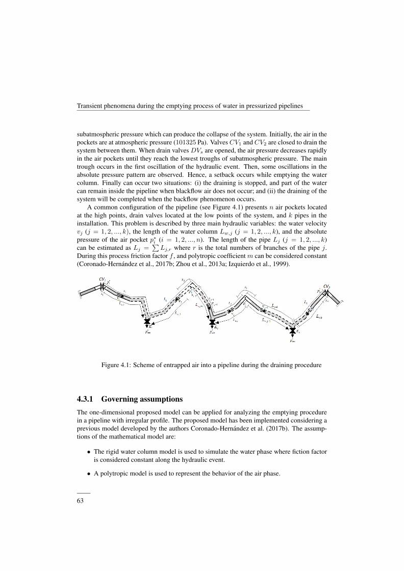
Transient phenomena during the emptying process of water in pressurized pipelines
subatmospheric pressure which can produce the collapse of the system. Initially, the air in thepockets are at atmospheric pressure (101325 Pa). Valves CV1 and CV2 are closed to drain thesystem between them. When drain valves DVs are opened, the air pressure decreases rapidlyin the air pockets until they reach the lowest troughs of subatmospheric pressure. The maintrough occurs in the first oscillation of the hydraulic event. Then, some oscillations in theabsolute pressure pattern are observed. Hence, a setback occurs while emptying the watercolumn. Finally can occur two situations: (i) the draining is stopped, and part of the watercan remain inside the pipeline when blackflow air does not occur; and (ii) the draining of thesystem will be completed when the backflow phenomenon occurs.
A common configuration of the pipeline (see Figure 4.1) presents n air pockets locatedat the high points, drain valves located at the low points of the system, and k pipes in theinstallation. This problem is described by three main hydraulic variables: the water velocityvj (j = 1, 2, ..., k), the length of the water column Lw,j (j = 1, 2, ..., k), and the absolutepressure of the air pocket p∗i (i = 1, 2, ..., n). The length of the pipe Lj (j = 1, 2, ..., k)can be estimated as Lj =
∑Lj,r where r is the total numbers of branches of the pipe j.
During this process friction factor f , and polytropic coefficient m can be considered constant(Coronado-Hernandez et al., 2017b; Zhou et al., 2013a; Izquierdo et al., 1999).
Figure 4.1: Scheme of entrapped air into a pipeline during the draining procedure
4.3.1 Governing assumptionsThe one-dimensional proposed model can be applied for analyzing the emptying procedurein a pipeline with irregular profile. The proposed model has been implemented considering aprevious model developed by the authors Coronado-Hernandez et al. (2017b). The assump-tions of the mathematical model are:
• The rigid water column model is used to simulate the water phase where fiction factoris considered constant along the hydraulic event.
• A polytropic model is used to represent the behavior of the air phase.
——63

Subatmospheric pressure in a water draining pipeline with an air pocket
• The moving air-water interface is considered perpendicular to the pipe direction.
• The backflow air phenomenon does not occur during the hydraulic event, which impliesthat there is not air admitted by the drain valves.
4.3.2 Equations
Considering the assumptions of the mathematical model, equations for the water phase, airphase, and for the moving air-water interface can be expressed as:
Water phase equation
The water phase can be modeled by using an inertial model. The water hammer (or elasticmodel) considers the elastic effects of the water and the pipe. However, the elasticity of theentrapped air pocket into the pipeline is much higher than the elasticity of the water whichmeans that the water phase can be modeled by the rigid water column model (Coronado-Hernandez et al., 2017b; Izquierdo et al., 1999; Laanearu et al., 2012). Then the momentumequation can be expressed as:
dvjdt
=p∗i − p∗atmρwLw,j
+ g∆zjLw,j
− fjvj |vj |2D
− gA2QT |QT |Lw,jK2
s
(4.1)
where p∗i = absolute pressure of the air pocket i, ρw = water density, p∗atm = atmosphericpressure (101325 Pa), ∆zj = elevation difference, A = cross-sectional area, QT = totaldischarge in the drain valve, and Ks = flow factor of the drain valve s.
Air phase equation
The compression and the expansion of the air pocket i obeys to the polytropic law, whichrelates the absolute pressure and the total volume of the air pocket:
p∗i Vma,i = p∗i,0V
ma,i,0 (4.2)
where Va,i = volume of the air pocket i, p∗i,0 = initial condition of the p∗i , and Va,i,0 =initial condition of the Va,i.
However, along of the pipeline the cross-sectional area (A) is constant, then:
p∗i xmi = p∗i,0x
mi,0 (4.3)
where xi = length of the air pocket i, and xi,0 = initial value of the xi.The air pocket size can be computed as xi = Lj − Lw,j + Lj+1 − Lw,j+1, thus:
p∗i (Lj − Lw,j + Lj+1 − Lw,j+1)m = p∗i,0(Lj − Lw,j,0 + Lj+1 − Lw,j+1,0)m (4.4)
——64
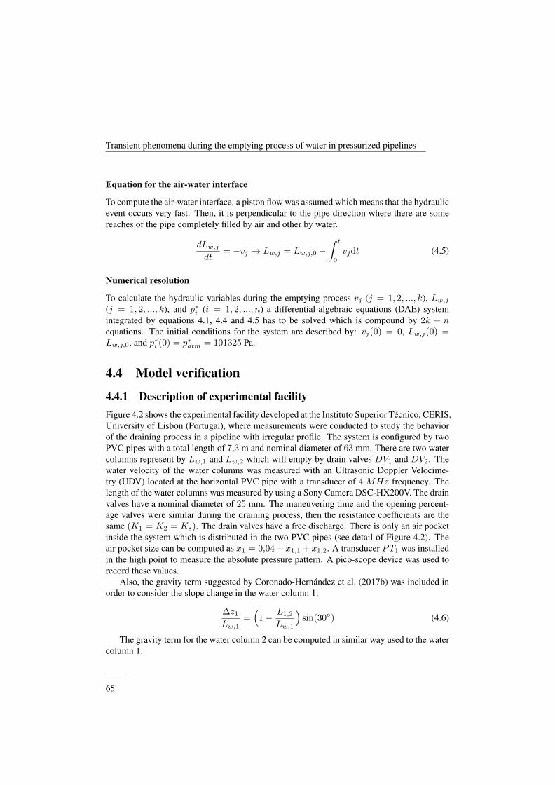
Transient phenomena during the emptying process of water in pressurized pipelines
Equation for the air-water interface
To compute the air-water interface, a piston flow was assumed which means that the hydraulicevent occurs very fast. Then, it is perpendicular to the pipe direction where there are somereaches of the pipe completely filled by air and other by water.
dLw,j
dt= −vj → Lw,j = Lw,j,0 −
∫ t
0
vjdt (4.5)
Numerical resolution
To calculate the hydraulic variables during the emptying process vj (j = 1, 2, ..., k), Lw,j
(j = 1, 2, ..., k), and p∗i (i = 1, 2, ..., n) a differential-algebraic equations (DAE) systemintegrated by equations 4.1, 4.4 and 4.5 has to be solved which is compound by 2k + nequations. The initial conditions for the system are described by: vj(0) = 0, Lw,j(0) =Lw,j,0, and p∗i (0) = p∗atm = 101325 Pa.
4.4 Model verification
4.4.1 Description of experimental facilityFigure 4.2 shows the experimental facility developed at the Instituto Superior Tecnico, CERIS,University of Lisbon (Portugal), where measurements were conducted to study the behaviorof the draining process in a pipeline with irregular profile. The system is configured by twoPVC pipes with a total length of 7,3 m and nominal diameter of 63 mm. There are two watercolumns represent by Lw,1 and Lw,2 which will empty by drain valves DV1 and DV2. Thewater velocity of the water columns was measured with an Ultrasonic Doppler Velocime-try (UDV) located at the horizontal PVC pipe with a transducer of 4 MHz frequency. Thelength of the water columns was measured by using a Sony Camera DSC-HX200V. The drainvalves have a nominal diameter of 25 mm. The maneuvering time and the opening percent-age valves were similar during the draining process, then the resistance coefficients are thesame (K1 = K2 = Ks). The drain valves have a free discharge. There is only an air pocketinside the system which is distributed in the two PVC pipes (see detail of Figure 4.2). Theair pocket size can be computed as x1 = 0,04 + x1,1 + x1,2. A transducer PT1 was installedin the high point to measure the absolute pressure pattern. A pico-scope device was used torecord these values.
Also, the gravity term suggested by Coronado-Hernandez et al. (2017b) was included inorder to consider the slope change in the water column 1:
∆z1
Lw,1=(
1− L1,2
Lw,1
)sin(30◦) (4.6)
The gravity term for the water column 2 can be computed in similar way used to the watercolumn 1.
——65
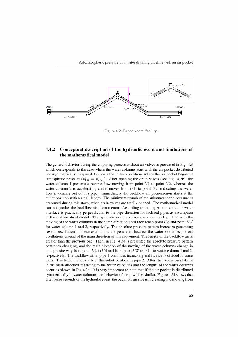
Subatmospheric pressure in a water draining pipeline with an air pocket
Figure 4.2: Experimental facility
4.4.2 Conceptual description of the hydraulic event and limitations ofthe mathematical model
The general behavior during the emptying process without air valves is presented in Fig. 4.3which corresponds to the case where the water columns start with the air pocket distributednon-symmetrically. Figure 4.3a shows the initial conditions where the air pocket begins atatmospheric pressure (p∗1,0 = p∗atm). After opening the drain valves (see Fig. 4.3b), thewater column 1 presents a reverse flow moving from point U1 to point U2, whereas thewater column 2 is accelerating and it moves from U1′ to point U2′ indicating the waterflow is coming out of this pipe. Immediately the backflow air phenomenon starts at theoutlet position with a small length. The minimum trough of the subatmospheric pressure ispresented during this stage, when drain valves are totally opened. The mathematical modelcan not predict the backflow air phenomenon. According to the experiments, the air-waterinterface is practically perpendicular to the pipe direction for inclined pipes as assumptionof the mathematical model. The hydraulic event continues as shown in Fig. 4.3c with themoving of the water columns in the same direction until they reach point U3 and point U3′
for water column 1 and 2, respectively. The absolute pressure pattern increases generatingseveral oscillations. These oscillations are generated because the water velocities presentoscillations around of the main direction of this movement. The length of the backflow air isgreater than the previous one. Then, in Fig. 4.3d is presented the absolute pressure patterncontinues changing, and the main direction of the moving of the water columns change inthe opposite way from point U3 to U4 and from point U3′ to U4′ for water column 1 and 2,respectively. The backflow air in pipe 1 continues increasing and its size is divided in someparts. The backflow air starts at the outlet position in pipe 2. After that, some oscillationsin the main direction regarding to the water velocities and the lengths of the water columnsoccur as shown in Fig 4.3e. It is very important to note that if the air pocket is distributedsymmetrically in water columns, the behavior of them will be similar. Figure 4.3f shows thatafter some seconds of the hydraulic event, the backflow air size is increasing and moving from
——66
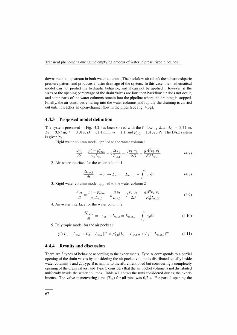
Transient phenomena during the emptying process of water in pressurized pipelines
downstream to upstream in both water columns. The backflow air reliefs the subatmoshpericpressure pattern and produces a faster drainage of the system. In this case, the mathematicalmodel can not predict the hydraulic behavior, and it can not be applied. However, if thesizes or the opening percentage of the drain valves are low, then backflow air does not occur,and some parts of the water columns remain into the pipeline where the draining is stopped.Finally, the air continues entering into the water columns and rapidly the draining is carriedout until it reaches an open-channel flow in the pipes (see Fig. 4.3g).
4.4.3 Proposed model definition
The system presented in Fig. 4.2 has been solved with the following data: L1 = 3,77 m,L2 = 3,57 m, f = 0,018, D = 51,4 mm, m = 1,1, and p∗1,0 = 101325 Pa. The DAE systemis given by:
1. Rigid water column model applied to the water column 1
dv1
dt=p∗1 − p∗atmρwLw,1
+ g∆z1
Lw,1− f v1|v1|
2D− gA2v1|v1|
K21Lw,1
(4.7)
2. Air-water interface for the water column 1
dLw,1
dt= −v1 → Lw,1 = Lw,1,0 −
∫ t
0
v1dt (4.8)
3. Rigid water column model applied to the water column 2
dv2
dt=p∗1 − p∗atmρwLw,2
+ g∆z2
Lw,2− f v2|v2|
2D− gA2v2|v2|
K22Lw,2
(4.9)
4. Air-water interface for the water column 2
dLw,2
dt= −v2 → Lw,2 = Lw,2,0 −
∫ t
0
v2dt (4.10)
5. Polytropic model for the air pocket 1
p∗1(L1 − Lw,1 + L2 − Lw,2)m = p∗1,0(L1 − Lw,1,0 + L2 − Lw,2,0)m (4.11)
4.4.4 Results and discussion
There are 3 types of behavior according to the experiments. Type A corresponds to a partialopening of the drain valves by considering the air pocket volume is distributed equally insidewater columns 1 and 2; Type B is similar to the aforementioned but considering a completelyopening of the drain valves; and Type C considers that the air pocket volume is not distributeduniformly inside the water columns. Table 4.1 shows the runs considered during the exper-iments. The valve maneuvering time (Tm) for all runs was 0,7 s. For partial opening the
——67
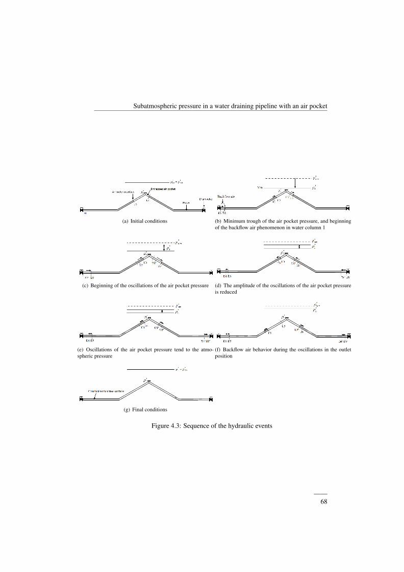
Subatmospheric pressure in a water draining pipeline with an air pocket
(a) Initial conditions (b) Minimum trough of the air pocket pressure, and beginningof the backflow air phenomenon in water column 1
(c) Beginning of the oscillations of the air pocket pressure (d) The amplitude of the oscillations of the air pocket pressureis reduced
(e) Oscillations of the air pocket pressure tend to the atmo-spheric pressure
(f) Backflow air behavior during the oscillations in the outletposition
(g) Final conditions
Figure 4.3: Sequence of the hydraulic events
——68
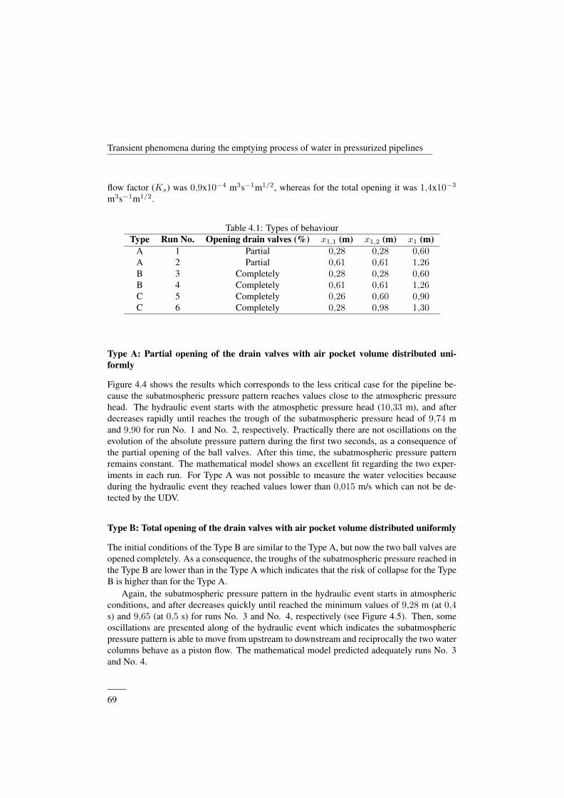
Transient phenomena during the emptying process of water in pressurized pipelines
flow factor (Ks) was 0,9x10⁻⁴ m3s−1m1/2, whereas for the total opening it was 1,4x10⁻³
m3s−1m1/2.
Table 4.1: Types of behaviourType Run No. Opening drain valves (%) x1,1 (m) x1,2 (m) x1 (m)
A 1 Partial 0,28 0,28 0,60A 2 Partial 0,61 0,61 1,26B 3 Completely 0,28 0,28 0,60B 4 Completely 0,61 0,61 1,26C 5 Completely 0,26 0,60 0,90C 6 Completely 0,28 0,98 1,30
Type A: Partial opening of the drain valves with air pocket volume distributed uni-formly
Figure 4.4 shows the results which corresponds to the less critical case for the pipeline be-cause the subatmospheric pressure pattern reaches values close to the atmospheric pressurehead. The hydraulic event starts with the atmosphetic pressure head (10,33 m), and afterdecreases rapidly until reaches the trough of the subatmospheric pressure head of 9,74 mand 9,90 for run No. 1 and No. 2, respectively. Practically there are not oscillations on theevolution of the absolute pressure pattern during the first two seconds, as a consequence ofthe partial opening of the ball valves. After this time, the subatmospheric pressure patternremains constant. The mathematical model shows an excellent fit regarding the two exper-iments in each run. For Type A was not possible to measure the water velocities becauseduring the hydraulic event they reached values lower than 0,015 m/s which can not be de-tected by the UDV.
Type B: Total opening of the drain valves with air pocket volume distributed uniformly
The initial conditions of the Type B are similar to the Type A, but now the two ball valves areopened completely. As a consequence, the troughs of the subatmospheric pressure reached inthe Type B are lower than in the Type A which indicates that the risk of collapse for the TypeB is higher than for the Type A.
Again, the subatmospheric pressure pattern in the hydraulic event starts in atmosphericconditions, and after decreases quickly until reached the minimum values of 9,28 m (at 0,4s) and 9,65 (at 0,5 s) for runs No. 3 and No. 4, respectively (see Figure 4.5). Then, someoscillations are presented along of the hydraulic event which indicates the subatmosphericpressure pattern is able to move from upstream to downstream and reciprocally the two watercolumns behave as a piston flow. The mathematical model predicted adequately runs No. 3and No. 4.
——69
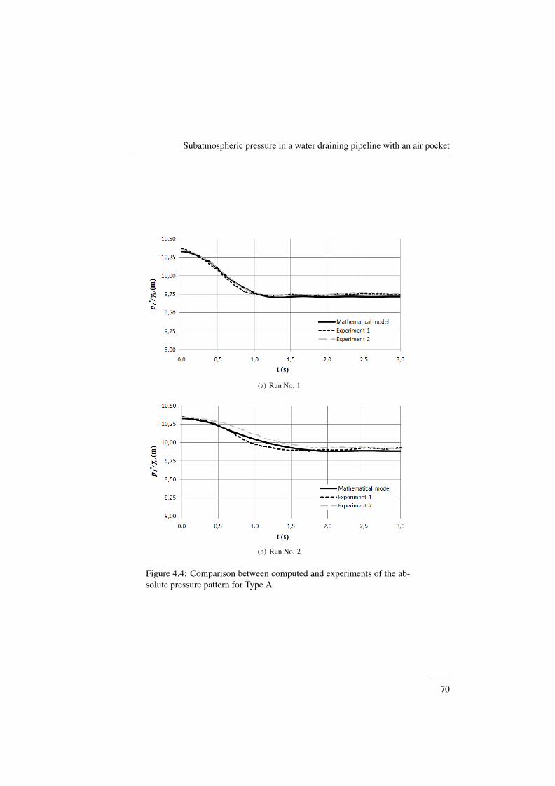
Subatmospheric pressure in a water draining pipeline with an air pocket
(a) Run No. 1
(b) Run No. 2
Figure 4.4: Comparison between computed and experiments of the ab-solute pressure pattern for Type A
——70
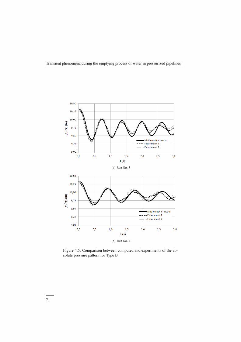
Transient phenomena during the emptying process of water in pressurized pipelines
(a) Run No. 3
(b) Run No. 4
Figure 4.5: Comparison between computed and experiments of the ab-solute pressure pattern for Type B
——71
Subatmospheric pressure in a water draining pipeline with an air pocket
Figure 4.6 shows the results concerning to the water velocities. For runs No. 3 and No. 4the values of the water velocities in the two water columns are similar due to the air pocketsize is distributed uniformly. For both runs, the water velocity increases rapidly until reachinga maximum value. Subsequently, the water velocity decreases until it reaches a value of 0 m/sat 0,4 s and 0,49 s for runs No. 3 and No. 4, respectively. Then it continues to decrease untilreaching a minimum value of the −0,11 m/s for run No. 3 and −0,125 m/s for run No. 4,indicating negative velocities occurrence. After some oscillations, with a similar amplitude,a setback of the water columns occur. The mathematical model can follow the behavior ofthe water velocity experiments.
Type C: Total opening of the drain valves with air pocket volume distributed non-uniformly
Type C is the most complex to be analyzed because the behavior of the two water columnsis so different. Figure 4.7a shows the results of the subatmospheric pressure pattern forrun No. 5 where according to the experiments the trough of the subatmospheric pressurepresented is 9,50 m at 0,4 s. The two water columns have different movements, then theamplitude of the oscillations of the air pocket along the transient is lower compared withthe Type B. The mathematical model predicts accurately the subatmospheric pressure patternalong of the hydraulic event. However, Figure 4.7b presents the results for run No. 6 wherethe mathematical model can predict only the first oscillation during the transient. This caseoccurs because the mathematical model considers an air-water interface perpendicular to pipewalls at downstream of the water columns, which does not really happen for an air pocketdistributed asymmetrically.
Figure 4.8 presents the results of the water velocities for two water columns for run No. 5which are different due to subatmospheric pressure pattern. Figure 4.8a shows the behavoiurof the water column 1 where velocity values always are positive generating that in this col-umn the emptying process occurs. According to the experiments, the maximum velocity ispresented at 1,05 s with a value of 0,175 m/s, which is very close to the value predicted by themathematical model (0,19 m/s). In contrast, Figure 4.8b presents the results for the water col-umn 2 where according to the experiments negative velocities occur. As a consequence, thewater column 2 moves from downstream to upstream during the hydraulic event. The math-ematical models predicts the tendency regarding water velocities for both water columns.
Type C represents the case where the evolution of the lengths of the water columns 1and 2 are different during the transient. Figure 4.9 shows that the water column 1 has at thebeginning of the transient an initial value of 3,5 m and at the end of the hydraulic event avalue of 3,2 m, indicating that 0,3 m could be drained during the process. In contrast, thewater column 2 starts with 3,0 m (at 0 s) and finishes with 3,2 m (at 3 s), indicating that theentire water column 2 was displaced 0,2 m from downstream to upstream and practically thiswater column could not be drained. The mathematical model predicts accurately the lengthof the water columns.
——72
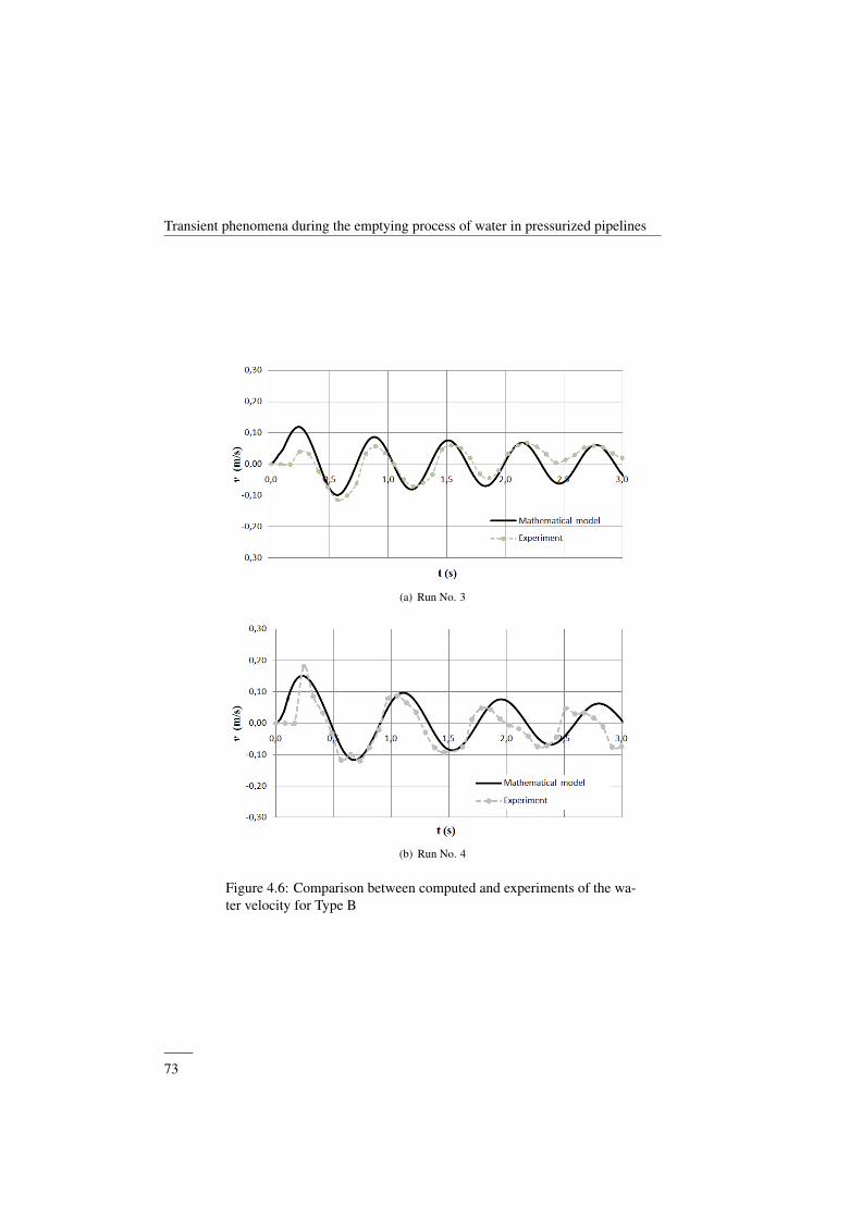
Transient phenomena during the emptying process of water in pressurized pipelines
(a) Run No. 3
(b) Run No. 4
Figure 4.6: Comparison between computed and experiments of the wa-ter velocity for Type B
——73
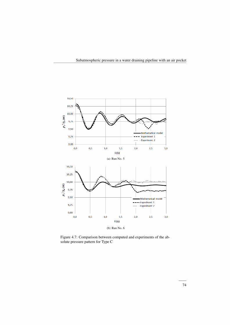
Subatmospheric pressure in a water draining pipeline with an air pocket
(a) Run No. 5
(b) Run No. 6
Figure 4.7: Comparison between computed and experiments of the ab-solute pressure pattern for Type C
——74

Transient phenomena during the emptying process of water in pressurized pipelines
(a) Water column 1
(b) Water column 2
Figure 4.8: Comparison between computed and experiments of the wa-ter velocities for Type C and run No. 5
——75
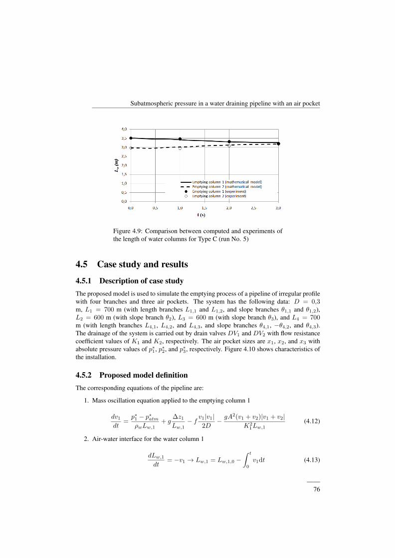
Subatmospheric pressure in a water draining pipeline with an air pocket
Figure 4.9: Comparison between computed and experiments ofthe length of water columns for Type C (run No. 5)
4.5 Case study and results
4.5.1 Description of case studyThe proposed model is used to simulate the emptying process of a pipeline of irregular profilewith four branches and three air pockets. The system has the following data: D = 0,3m, L1 = 700 m (with length branches L1,1 and L1,2, and slope branches θ1,1 and θ1,2),L2 = 600 m (with slope branch θ2), L3 = 600 m (with slope branch θ3), and L4 = 700m (with length branches L4,1, L4,2, and L4,3, and slope branches θ4,1, −θ4,2, and θ4,3).The drainage of the system is carried out by drain valves DV1 and DV2 with flow resistancecoefficient values of K1 and K2, respectively. The air pocket sizes are x1, x2, and x3 withabsolute pressure values of p∗1, p∗2, and p∗3, respectively. Figure 4.10 shows characteristics ofthe installation.
4.5.2 Proposed model definitionThe corresponding equations of the pipeline are:
1. Mass oscillation equation applied to the emptying column 1
dv1
dt=p∗1 − p∗atmρwLw,1
+ g∆z1
Lw,1− f v1|v1|
2D− gA2(v1 + v2)|v1 + v2|
K21Lw,1
(4.12)
2. Air-water interface for the water column 1
dLw,1
dt= −v1 → Lw,1 = Lw,1,0 −
∫ t
0
v1dt (4.13)
——76

Transient phenomena during the emptying process of water in pressurized pipelines
Figure 4.10: Pipeline of irregular profile without air valves
3. Mass oscillation equation applied to the emptying column 2
dv2
dt=p∗2 − p∗atmρwLw,2
+ g∆z2
Lw,2− f v2|v2|
2D− gA2(v1 + v2)|v1 + v2|
K21Lw,2
(4.14)
4. Air-water interface for the water column 2
dLw,2
dt= −v2 → Lw,2 = Lw,2,0 −
∫ t
0
v2dt (4.15)
5. Mass oscillation equation applied to the emptying column 3
dv3
dt=p∗3 − p∗atmρwLw,3
+ g∆z3
Lw,3− f v3|v3|
2D− gA2(v3 + v4)|v3 + v4|
K22Lw,3
(4.16)
6. Air-water interface for the water column 3
dLw,3
dt= −v3 → Lw,3 = Lw,3,0 −
∫ t
0
v3dt (4.17)
7. Mass oscillation equation applied to the emptying column 4
dv4
dt=p∗3 − p∗atmρwLw,4
+ g∆z4
Lw,4− f v4|v4|
2D− gA2(v3 + v4)|v3 + v4|
K22Lw,4
(4.18)
8. Air-water interface for the water column 4
——77
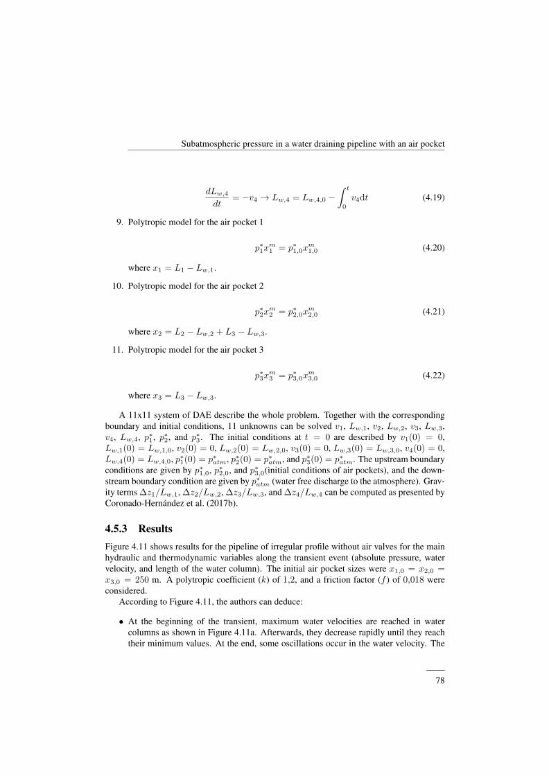
Subatmospheric pressure in a water draining pipeline with an air pocket
dLw,4
dt= −v4 → Lw,4 = Lw,4,0 −
∫ t
0
v4dt (4.19)
9. Polytropic model for the air pocket 1
p∗1xm1 = p∗1,0x
m1,0 (4.20)
where x1 = L1 − Lw,1.
10. Polytropic model for the air pocket 2
p∗2xm2 = p∗2,0x
m2,0 (4.21)
where x2 = L2 − Lw,2 + L3 − Lw,3.
11. Polytropic model for the air pocket 3
p∗3xm3 = p∗3,0x
m3,0 (4.22)
where x3 = L3 − Lw,3.
A 11x11 system of DAE describe the whole problem. Together with the correspondingboundary and initial conditions, 11 unknowns can be solved v1, Lw,1, v2, Lw,2, v3, Lw,3,v4, Lw,4, p∗1, p∗2, and p∗3. The initial conditions at t = 0 are described by v1(0) = 0,Lw,1(0) = Lw,1,0, v2(0) = 0, Lw,2(0) = Lw,2,0, v3(0) = 0, Lw,3(0) = Lw,3,0, v4(0) = 0,Lw,4(0) = Lw,4,0, p∗1(0) = p∗atm, p∗2(0) = p∗atm, and p∗3(0) = p∗atm. The upstream boundaryconditions are given by p∗1,0, p∗2,0, and p∗3,0(initial conditions of air pockets), and the down-stream boundary condition are given by p∗atm (water free discharge to the atmosphere). Grav-ity terms ∆z1/Lw,1, ∆z2/Lw,2, ∆z3/Lw,3, and ∆z4/Lw,4 can be computed as presented byCoronado-Hernandez et al. (2017b).
4.5.3 ResultsFigure 4.11 shows results for the pipeline of irregular profile without air valves for the mainhydraulic and thermodynamic variables along the transient event (absolute pressure, watervelocity, and length of the water column). The initial air pocket sizes were x1,0 = x2,0 =x3,0 = 250 m. A polytropic coefficient (k) of 1,2, and a friction factor (f ) of 0,018 wereconsidered.
According to Figure 4.11, the authors can deduce:
• At the beginning of the transient, maximum water velocities are reached in watercolumns as shown in Figure 4.11a. Afterwards, they decrease rapidly until they reachtheir minimum values. At the end, some oscillations occur in the water velocity. The
——78
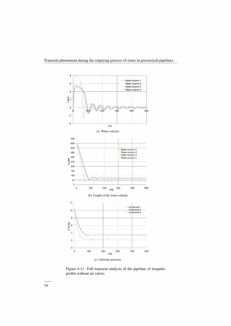
Transient phenomena during the emptying process of water in pressurized pipelines
(a) Water velocity
(b) Length of the water column
(c) Absolute pressure
Figure 4.11: Full transient analysis of the pipeline of irregularprofile without air valves
——79
Subatmospheric pressure in a water draining pipeline with an air pocket
maximum water velocity is reached in water column 1 when it abandons the branchL1,1 (300 m long.) and stars the branch L1,2 (400 m long.) at 16,63 m with a value of5,49 ms−1 (388,5 ls−1). For water columns 2, 3, and 4, the maximum water velocitiesare 7,86 ms−1, 5,39 ms−1, and 5,34 ms−1, respectively. The minimum water veloci-ties are: for water column 1, −1,47 ms−1; for water column 2, −2,63 ms−1; for watercolumn 3, −1,34 ms−1; and for water column 4, −1,47 ms−1.
• The lengths of the water columns start to be drained linearly until setback occurs whendraining is stopped, and part of the water columns remain in the pipeline (see Figure4.11b). If backflow phenomenon does not occur the pipeline cannot drain completely,and part of the water columns can remain in the installation with values of 70 m, 41 m,81 m, and 70 m for water columns 1, 2, 3, and 4, respectively.
• Initially, the air pockets are at atmospheric pressure (101325 Pa). The air pressureheads decrease rapidly in the pockets until reach the minimum values of 3,31 m, 2,18m, and 3,32 m, for the air pockets 1, 2, and 3, respectively, at 93 s (see Figure 4.11c).The backflow phenomenon does not affect the minimum values of the subatmosphericpressure.
4.6 Conclusions
The mathematical model developed by the authors predicts adequately the behavior of thedraining process for the first seconds of the transient. This is very important since the min-imum value of the subatmospheric pressure occurs in the first oscillation of the hydraulicevent. To validate the mathematical model, several experiments were carried out in an exper-imental facility where the comparison between the computed and the measured of the mainhydraulic variables (absolute pressure of the air pocket, water velocity and the length of thewater column) confirms the goodness of the mathematical model. Regarding the results, thefollowing conclusions can be drawn:
• Three types of behavior have been analyzed. They depend on the opening percentage ofthe drain valves, and the distribution of the air pocket volume inside the water columns.
• The backflow air phenomenon depends on the opening percentage of the drain valves:(i) for partial opening, it did not occur during the experiments (Type A), and (ii) fortotal opening, the air moved from downstream to upstream (Types B and C).
• The Type C is the most complex case to predict by the mathematical model. When theinitial difference elevation (∆zj) is very close for the water columns (run No. 5), thenthe mathematical model can predict the evolution of the hydraulic variables. However,when the difference elevation is high (run No. 6), then the mathematical model canonly predict the first oscillation during the hydraulic event.
——80
Transient phenomena during the emptying process of water in pressurized pipelines
The mathematical model cannot predict the backflow air phenomenon. However, it re-duces the risk of collapse the system by introducing air at atmospheric pressure into thepipeline. As a consequence, the backflow reliefs the troughs of the subatmospheric pressure,and rapidly the system can reach the atmospheric conditions.
NotationA = cross sectional area of pipe (m2)D = internal pipe diameter (m)f = Darcy-Weisbach friction factor (–)g = gravity acceleration (ms−2)Ks = flow factor of the drain valve s (m3s−1m1/2)Lw,j = length of the water column j (m)Lj = total length of the pipe j (m)m = polytrophic coefficient (–)pi = pressure of the air pocket i (Pa)patm = atmospheric pressure (Pa)QT = total discharge (m3s−1)t = time (s)Tm = valve maneuvering time (s)r = number of reaches of the pipe j (–)Va,i = volume of the air pocket i (m3)vj = water velocity of the water column j (ms−1)xi = length of the air pocket i (m)∆zj = elevation difference of the water column j (m)ρ = density (kgm−3)DVs = Drain valve sCVh = Used valves to establish the boundary conditions
Superscripts∗ = absolute values (e.g., absolute pressure)
Subscripts0 = initial condition (e.g., initial length of the water column)w = refers to water (e.g., water density)a = refers to air pocket (e.g., air pocket pressure)
——81

Subatmospheric pressure in a water draining pipeline with an air pocket
This page is intentionally left blank.
——82
Chapter 5
Experimental and numericalanalysis of a water emptyingpipeline using different air valves
This chapter is extracted from the paper:
Experimental and numerical analysis of a water emptying pipeline using different air valvesCoauthors: Coronado-Hernandez O. E; Fuertes-Miquel, V. S; Besharat, M.; and Ramos, H. M.
Journal: Water ISSN 2073-4441.2017 Impact Factor: 2.069. Position JCR 34/90 (Q2). Water Resources.
State: Published. 2017. Volume 9; Issue 2; 98. DOI: 10.3390/w9020098.
5.1 Abstract
the emptying procedure is a common operation that engineers have to face in pipelines. Thisgenerates subatmospheric pressure caused by the expansion of air pockets, which can pro-duce the collapse of the system depending on the conditions of the installation. To avoid thisproblem engineers have to install air valves in pipelines. However, if air valves are not ade-quately designed then the risk in pipelines continues. In this research a mathematical modelis developed to simulate an emptying process in pipelines, which can be used for planningthis type of operation. The one-dimensional proposed model analyzes the water phase prop-agation by a new rigid model and the air pockets effect using thermodynamic formulations.The proposed model is validated through measurements of the air pocket absolute pressure,the water velocity and the length of the emptying columns in an experimental facility. Resultsshow that the proposed model can accurately predict the hydraulic characteristic variables.
83
Experimental and numerical analysis of a water emptying pipeline using different airvalves
5.2 Introduction
The emptying procedure in a pipeline generates hydraulic events which can cause problemsif air valves are not well sized. In practical applications, engineers follow typical recom-mendations from the American Water Works Association (AWWA) (AWWA, 2001) or man-ufacturers about sizing and location of air valves along a pipeline in order to avoid subatmo-spheric pressure that can cause the collapse of the system. It is recommended in a pipelinethat the air volume admitted by air valves should be the same as the water volume drained(Ramezani et al., 2015), consequently air valves should work in subsonic flow condition.Air valves should be located at high points, in long horizontal pipe branches, long descents,long ascents, decrease in an up-slope and at increase in a down-slope of a pipeline, and onthe discharge side of deep well pumps and at vertical turbines/pumps (AWWA, 2001). Aninappropriate selection of the air valve size and location produces not only subatmosphericpressure but also a slow drainage of the system.
Presently there are only few studies related to the emptying process in the literature, butthey are not focused on practical applications because they do not consider a pipeline with anirregular profile and air valves (Tijsseling et al., 2016; Laanearu et al., 2012).
The analysis of an emptying process is not trivial because it requires the study of a twophase flow (Fuertes, 2001; Besharat et al., 2016; Apollonio et al., 2016; Balacco et al., 2015).This problem can be studied using one (1D) (Zhou et al., 2013a; Izquierdo et al., 1999),two (2D) (Zhou et al., 2011b) or three-dimensional (3D) (Martins et al., 2016) models. Thewater phase in 1D model can be analyzed considering two types of models (Abreu et al.,1999): (i) elastic models (Martins et al., 2010c,a), which consider the elasticity of the pipeand the water, or (ii) rigid models (Fuertes-Miquel et al., 2016), which ignore the elasticity ofthem. Normally, elastic models are solved by using the method of characteristics (Zhou andLiu, 2013; Covas et al., 2010), and rigid models by using the numerical solution of ordinarydifferential equations (Izquierdo et al., 1999; Fuertes-Miquel et al., 2016; Liou and Hunt,1996). In pressurized systems the air effect can be analyzed as a single-phase flow, where theabsolute pressure of the air pocket is computed between two water columns (Bousso et al.,2013; Zhou et al., 2013a; Izquierdo et al., 1999). Regarding the analysis of 2D and 3D CFDmodeling of air-water interface in closed pipes, they are still unyielding in the application ofpipeline draining because length and time scales are not appropriate.
This research develops a general 1D mathematical model that can be used for analyzingthe behavior of the main hydraulic variables during the emptying process in a pipeline withirregular profile and with several air valves installed along on it based on formulations ofprevious works (Izquierdo et al., 1999; Zhou et al., 2013a; Liou and Hunt, 1996; Leon et al.,2010; Wylie and Streeter, 1993; Fuertes-Miquel et al., 2016, 2018b). The proposed model cangive important information in real systems about: (i) the risk of collapse of pipeline installa-tions, by checking in a pipe manufacturer characteristics if the stiffness class is appropriateto support the subatmospheric pressure reached during the hydraulic event depending on thetype of soil in natural conditions, the type of backfill and the cover depth; (ii) the appropriateselection of the air valve during the emptying process; (iii) the size and the maneuver time of
——84
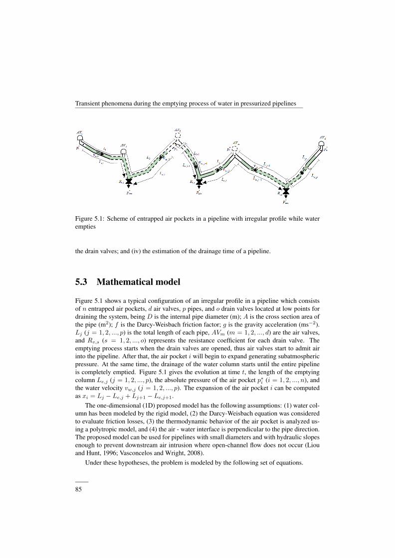
Transient phenomena during the emptying process of water in pressurized pipelines
Figure 5.1: Scheme of entrapped air pockets in a pipeline with irregular profile while waterempties
the drain valves; and (iv) the estimation of the drainage time of a pipeline.
5.3 Mathematical model
Figure 5.1 shows a typical configuration of an irregular profile in a pipeline which consistsof n entrapped air pockets, d air valves, p pipes, and o drain valves located at low points fordraining the system, being D is the internal pipe diameter (m); A is the cross section area ofthe pipe (m2); f is the Darcy-Weisbach friction factor; g is the gravity acceleration (ms−2).Lj (j = 1, 2, ..., p) is the total length of each pipe, AVm (m = 1, 2, ..., d) are the air valves,and Rv,s (s = 1, 2, ..., o) represents the resistance coefficient for each drain valve. Theemptying process starts when the drain valves are opened, thus air valves start to admit airinto the pipeline. After that, the air pocket i will begin to expand generating subatmosphericpressure. At the same time, the drainage of the water column starts until the entire pipelineis completely emptied. Figure 5.1 gives the evolution at time t, the length of the emptyingcolumn Le,j (j = 1, 2, ..., p), the absolute pressure of the air pocket p∗i (i = 1, 2, ..., n), andthe water velocity vw,j (j = 1, 2, ..., p). The expansion of the air pocket i can be computedas xi = Lj − Le,j + Lj+1 − Le,j+1.
The one-dimensional (1D) proposed model has the following assumptions: (1) water col-umn has been modeled by the rigid model, (2) the Darcy-Weisbach equation was consideredto evaluate friction losses, (3) the thermodynamic behavior of the air pocket is analyzed us-ing a polytropic model, and (4) the air - water interface is perpendicular to the pipe direction.The proposed model can be used for pipelines with small diameters and with hydraulic slopesenough to prevent downstream air intrusion where open-channel flow does not occur (Liouand Hunt, 1996; Vasconcelos and Wright, 2008).
Under these hypotheses, the problem is modeled by the following set of equations.
——85
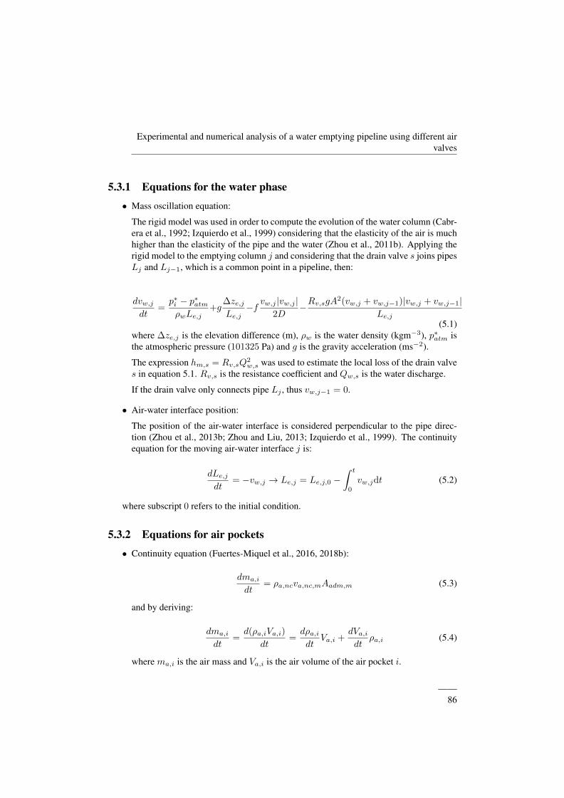
Experimental and numerical analysis of a water emptying pipeline using different airvalves
5.3.1 Equations for the water phase• Mass oscillation equation:
The rigid model was used in order to compute the evolution of the water column (Cabr-era et al., 1992; Izquierdo et al., 1999) considering that the elasticity of the air is muchhigher than the elasticity of the pipe and the water (Zhou et al., 2011b). Applying therigid model to the emptying column j and considering that the drain valve s joins pipesLj and Lj−1, which is a common point in a pipeline, then:
dvw,j
dt=p∗i − p∗atmρwLe,j
+g∆ze,jLe,j
−f vw,j |vw,j |2D
−Rv,sgA2(vw,j + vw,j−1)|vw,j + vw,j−1|
Le,j
(5.1)where ∆ze,j is the elevation difference (m), ρw is the water density (kgm−3), p∗atm isthe atmospheric pressure (101325 Pa) and g is the gravity acceleration (ms−2).
The expression hm,s = Rv,sQ2w,s was used to estimate the local loss of the drain valve
s in equation 5.1. Rv,s is the resistance coefficient and Qw,s is the water discharge.
If the drain valve only connects pipe Lj , thus vw,j−1 = 0.
• Air-water interface position:
The position of the air-water interface is considered perpendicular to the pipe direc-tion (Zhou et al., 2013b; Zhou and Liu, 2013; Izquierdo et al., 1999). The continuityequation for the moving air-water interface j is:
dLe,j
dt= −vw,j → Le,j = Le,j,0 −
∫ t
0
vw,jdt (5.2)
where subscript 0 refers to the initial condition.
5.3.2 Equations for air pockets• Continuity equation (Fuertes-Miquel et al., 2016, 2018b):
dma,i
dt= ρa,ncva,nc,mAadm,m (5.3)
and by deriving:
dma,i
dt=d(ρa,iVa,i)
dt=dρa,idt
Va,i +dVa,idt
ρa,i (5.4)
where ma,i is the air mass and Va,i is the air volume of the air pocket i.
——86
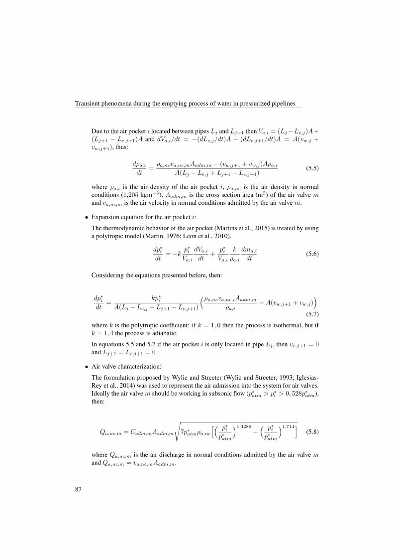
Transient phenomena during the emptying process of water in pressurized pipelines
Due to the air pocket i located between pipes Lj and Lj+1 then Va,i = (Lj−Le,j)A+(Lj+1 − Le,j+1)A and dVa,i/dt = −(dLe,j/dt)A − (dLe,j+1/dt)A = A(vw,j +vw,j+1), thus:
dρa,idt
=ρa,ncva,nc,mAadm,m − (vw,j+1 + vw,j)Aρa,i
A(Lj − Le,j + Lj+1 − Le,j+1)(5.5)
where ρa,i is the air density of the air pocket i, ρa,nc is the air density in normalconditions (1,205 kgm−3), Aadm,m is the cross section area (m2) of the air valve mand va,nc,m is the air velocity in normal conditions admitted by the air valve m.
• Expansion equation for the air pocket i:
The thermodynamic behavior of the air pocket (Martins et al., 2015) is treated by usinga polytropic model (Martin, 1976; Leon et al., 2010).
dp∗idt
= −k p∗iVa,i
dVa,idt
+p∗iVa,i
k
ρa,i
dma,i
dt(5.6)
Considering the equations presented before, then:
dp∗idt
=kp∗i
A(Lj − Le,j + Lj+1 − Le,j+1)
(ρa,ncva,nc,iAadm,m
ρa,i−A(vw,j+1 + vw,j)
)(5.7)
where k is the polytropic coefficient: if k = 1, 0 then the process is isothermal, but ifk = 1, 4 the process is adiabatic.
In equations 5.5 and 5.7 if the air pocket i is only located in pipe Lj , then ve,j+1 = 0and Lj+1 = Le,j+1 = 0 .
• Air valve characterization:
The formulation proposed by Wylie and Streeter (Wylie and Streeter, 1993; Iglesias-Rey et al., 2014) was used to represent the air admission into the system for air valves.Ideally the air valvem should be working in subsonic flow (p∗atm > p∗i > 0, 528p∗atm),then:
Qa,nc,m = Cadm,mAadm,m
√7p∗atmρa,nc
[( p∗ip∗atm
)1,4286
−( p∗ip∗atm
)1,714](5.8)
where Qa,nc,m is the air discharge in normal conditions admitted by the air valve mand Qa,nc,m = va,nc,mAadm,m.
——87
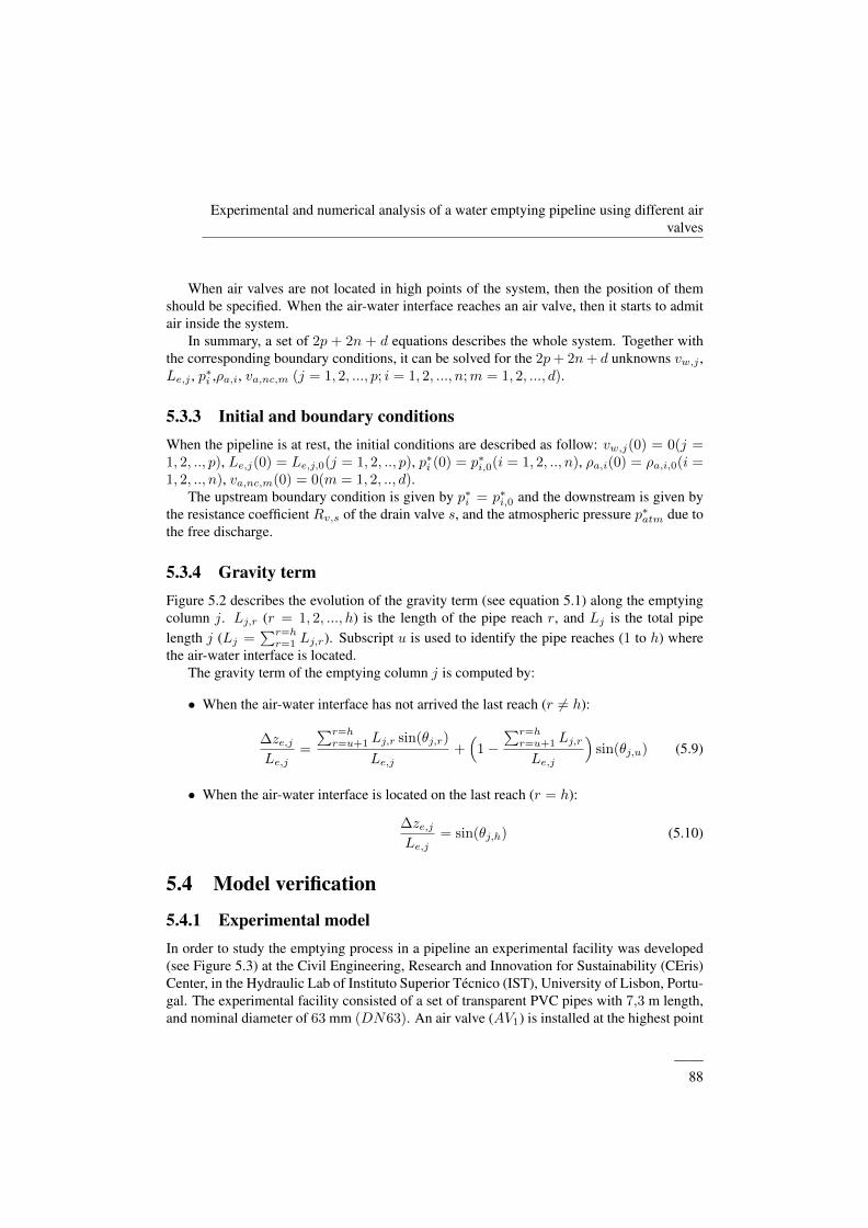
Experimental and numerical analysis of a water emptying pipeline using different airvalves
When air valves are not located in high points of the system, then the position of themshould be specified. When the air-water interface reaches an air valve, then it starts to admitair inside the system.
In summary, a set of 2p + 2n + d equations describes the whole system. Together withthe corresponding boundary conditions, it can be solved for the 2p+ 2n+ d unknowns vw,j ,Le,j , p∗i ,ρa,i, va,nc,m (j = 1, 2, ..., p; i = 1, 2, ..., n;m = 1, 2, ..., d).
5.3.3 Initial and boundary conditionsWhen the pipeline is at rest, the initial conditions are described as follow: vw,j(0) = 0(j =1, 2, .., p), Le,j(0) = Le,j,0(j = 1, 2, .., p), p∗i (0) = p∗i,0(i = 1, 2, .., n), ρa,i(0) = ρa,i,0(i =1, 2, .., n), va,nc,m(0) = 0(m = 1, 2, .., d).
The upstream boundary condition is given by p∗i = p∗i,0 and the downstream is given bythe resistance coefficient Rv,s of the drain valve s, and the atmospheric pressure p∗atm due tothe free discharge.
5.3.4 Gravity termFigure 5.2 describes the evolution of the gravity term (see equation 5.1) along the emptyingcolumn j. Lj,r (r = 1, 2, ..., h) is the length of the pipe reach r, and Lj is the total pipelength j (Lj =
∑r=hr=1 Lj,r). Subscript u is used to identify the pipe reaches (1 to h) where
the air-water interface is located.The gravity term of the emptying column j is computed by:
• When the air-water interface has not arrived the last reach (r 6= h):
∆ze,jLe,j
=
∑r=hr=u+1 Lj,r sin(θj,r)
Le,j+(
1−∑r=h
r=u+1 Lj,r
Le,j
)sin(θj,u) (5.9)
• When the air-water interface is located on the last reach (r = h):
∆ze,jLe,j
= sin(θj,h) (5.10)
5.4 Model verification
5.4.1 Experimental modelIn order to study the emptying process in a pipeline an experimental facility was developed(see Figure 5.3) at the Civil Engineering, Research and Innovation for Sustainability (CEris)Center, in the Hydraulic Lab of Instituto Superior Tecnico (IST), University of Lisbon, Portu-gal. The experimental facility consisted of a set of transparent PVC pipes with 7,3 m length,and nominal diameter of 63 mm (DN63). An air valve (AV1) is installed at the highest point
——88
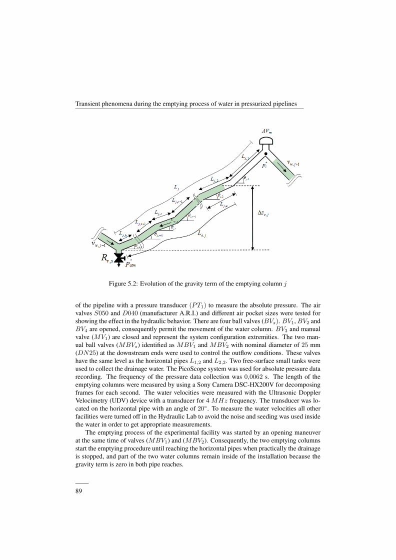
Transient phenomena during the emptying process of water in pressurized pipelines
Figure 5.2: Evolution of the gravity term of the emptying column j
of the pipeline with a pressure transducer (PT1) to measure the absolute pressure. The airvalves S050 and D040 (manufacturer A.R.I.) and different air pocket sizes were tested forshowing the effect in the hydraulic behavior. There are four ball valves (BVs). BV1,BV2 andBV4 are opened, consequently permit the movement of the water column. BV3 and manualvalve (MV1) are closed and represent the system configuration extremities. The two man-ual ball valves (MBVs) identified as MBV1 and MBV2 with nominal diameter of 25 mm(DN25) at the downstream ends were used to control the outflow conditions. These valveshave the same level as the horizontal pipes L1,2 and L2,2. Two free-surface small tanks wereused to collect the drainage water. The PicoScope system was used for absolute pressure datarecording. The frequency of the pressure data collection was 0,0062 s. The length of theemptying columns were measured by using a Sony Camera DSC-HX200V for decomposingframes for each second. The water velocities were measured with the Ultrasonic DopplerVelocimetry (UDV) device with a transducer for 4 MHz frequency. The transducer was lo-cated on the horizontal pipe with an angle of 20◦. To measure the water velocities all otherfacilities were turned off in the Hydraulic Lab to avoid the noise and seeding was used insidethe water in order to get appropriate measurements.
The emptying process of the experimental facility was started by an opening maneuverat the same time of valves (MBV1) and (MBV2). Consequently, the two emptying columnsstart the emptying procedure until reaching the horizontal pipes when practically the drainageis stopped, and part of the two water columns remain inside of the installation because thegravity term is zero in both pipe reaches.
——89

Experimental and numerical analysis of a water emptying pipeline using different airvalves
Figure 5.3: The pipe system and its components
Equations 5.13 to 5.19 were used to simulate the emptying process of this experimentalfacility. The gravity terms were computed for the two emptying columns. For the emptyingcolumn 1, it depends on:
• If the air-water interface is located on the sloped pipe reach θ = 30◦ (Le,1 ≤ L1,1 +L1,2 and Le,1 > L1,2) then:
∆ze,1Le,1
=(
1− L1,2
Le,1
)sin(θ1,1) (5.11)
• If the air-water interface is located on the horizontal pipe reach θ = 0◦(Le,1 > 0 andLe,1 ≤ L1,2) then:
∆ze,1Le,1
= 0 (5.12)
The gravity term for the emptying column 2 is similar in the emptying column 1.
5.4.2 Proposed model definitionIn Figure 5.4 is presented a case of two emptying columns. More complex systems can betreated in the same way based on the proposed model.
The corresponding equations of the pipeline are:1. Mass oscillation equation applied to the emptying column 1
dvw,1
dt=p∗1 − p∗atmρwLe,1
+ g∆ze,1Le,1
− f vw,1|vw,1|2D
− Rv,1gA21vw,1|vw,1|Le,1
(5.13)
2. Emptying column 1 position
dLe,1
dt= −vw,1 → Le,1 = Le,1,0 −
∫ t
0
vw,1dt (5.14)
3. Mass oscillation equation applied to the emptying column 2
——90
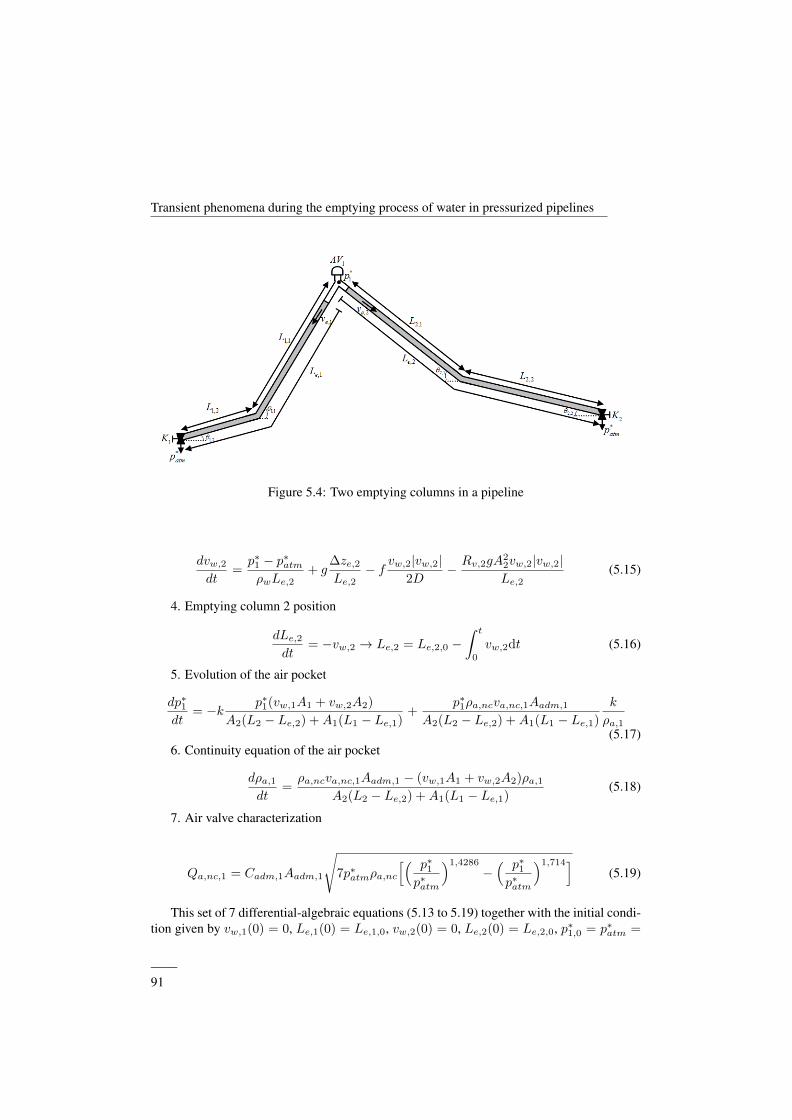
Transient phenomena during the emptying process of water in pressurized pipelines
Figure 5.4: Two emptying columns in a pipeline
dvw,2
dt=p∗1 − p∗atmρwLe,2
+ g∆ze,2Le,2
− f vw,2|vw,2|2D
− Rv,2gA22vw,2|vw,2|Le,2
(5.15)
4. Emptying column 2 position
dLe,2
dt= −vw,2 → Le,2 = Le,2,0 −
∫ t
0
vw,2dt (5.16)
5. Evolution of the air pocket
dp∗1dt
= −k p∗1(vw,1A1 + vw,2A2)
A2(L2 − Le,2) +A1(L1 − Le,1)+
p∗1ρa,ncva,nc,1Aadm,1
A2(L2 − Le,2) +A1(L1 − Le,1)
k
ρa,1(5.17)
6. Continuity equation of the air pocket
dρa,1dt
=ρa,ncva,nc,1Aadm,1 − (vw,1A1 + vw,2A2)ρa,1
A2(L2 − Le,2) +A1(L1 − Le,1)(5.18)
7. Air valve characterization
Qa,nc,1 = Cadm,1Aadm,1
√7p∗atmρa,nc
[( p∗1p∗atm
)1,4286
−( p∗1p∗atm
)1,714](5.19)
This set of 7 differential-algebraic equations (5.13 to 5.19) together with the initial condi-tion given by vw,1(0) = 0, Le,1(0) = Le,1,0, vw,2(0) = 0, Le,2(0) = Le,2,0, p∗1,0 = p∗atm =
——91
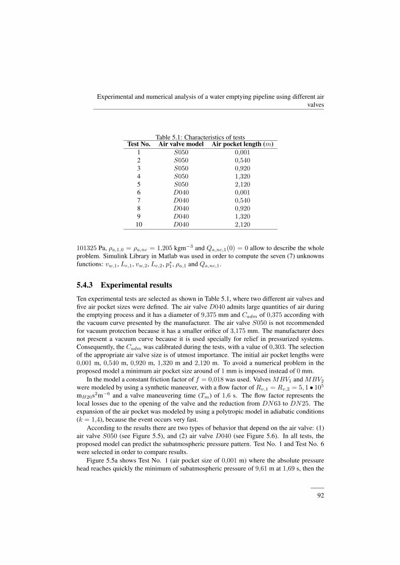
Experimental and numerical analysis of a water emptying pipeline using different airvalves
Table 5.1: Characteristics of testsTest No. Air valve model Air pocket length (m)
1 S050 0,0012 S050 0,5403 S050 0,9204 S050 1,3205 S050 2,1206 D040 0,0017 D040 0,5408 D040 0,9209 D040 1,320
10 D040 2,120
101325 Pa, ρa,1,0 = ρa,nc = 1,205 kgm−3 and Qa,nc,1(0) = 0 allow to describe the wholeproblem. Simulink Library in Matlab was used in order to compute the seven (7) unknownsfunctions: vw,1, Le,1, vw,2, Le,2, p∗1, ρa,1 and Qa,nc,1.
5.4.3 Experimental results
Ten experimental tests are selected as shown in Table 5.1, where two different air valves andfive air pocket sizes were defined. The air valve D040 admits large quantities of air duringthe emptying process and it has a diameter of 9,375 mm and Cadm of 0,375 according withthe vacuum curve presented by the manufacturer. The air valve S050 is not recommendedfor vacuum protection because it has a smaller orifice of 3,175 mm. The manufacturer doesnot present a vacuum curve because it is used specially for relief in pressurized systems.Consequently, the Cadm was calibrated during the tests, with a value of 0,303. The selectionof the appropriate air valve size is of utmost importance. The initial air pocket lengths were0,001 m, 0,540 m, 0,920 m, 1,320 m and 2,120 m. To avoid a numerical problem in theproposed model a minimum air pocket size around of 1 mm is imposed instead of 0 mm.
In the model a constant friction factor of f = 0,018 was used. Valves MBV1 and MBV2
were modeled by using a synthetic maneuver, with a flow factor of Rv,1 = Rv,2 = 5, 1 • 105
mH20s2m−6 and a valve maneuvering time (Tm) of 1,6 s. The flow factor represents thelocal losses due to the opening of the valve and the reduction from DN63 to DN25. Theexpansion of the air pocket was modeled by using a polytropic model in adiabatic conditions(k = 1,4), because the event occurs very fast.
According to the results there are two types of behavior that depend on the air valve: (1)air valve S050 (see Figure 5.5), and (2) air valve D040 (see Figure 5.6). In all tests, theproposed model can predict the subatmospheric pressure pattern. Test No. 1 and Test No. 6were selected in order to compare results.
Figure 5.5a shows Test No. 1 (air pocket size of 0,001 m) where the absolute pressurehead reaches quickly the minimum of subatmospheric pressure of 9,61 m at 1,69 s, then the
——92
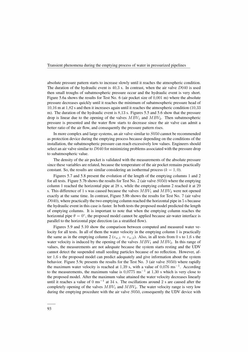
Transient phenomena during the emptying process of water in pressurized pipelines
absolute pressure pattern starts to increase slowly until it reaches the atmospheric condition.The duration of the hydraulic event is 40,3 s. In contrast, when the air valve D040 is usedthen small troughs of subatmospheric pressure occur and the hydraulic event is very short.Figure 5.6a shows the results for Test No. 6 (air pocket size of 0,001 m) where the absolutepressure decreases quickly until it reaches the minimum of subatmospheric pressure head of10,16 m at 1,82 s and then it increases again until it reaches the atmospheric condition (10,33m). The duration of the hydraulic event is 8,13 s. Figures 5.5 and 5.6 show that the pressuredrop is linear due to the opening of the valves MBV1 and MBV2. Then subatmosphericpressure is presented and the water flow starts to decrease since the air valve can admit abetter ratio of the air flow, and consequently the pressure pattern rises.
In more complex and large systems, an air valve similar to S050 cannot be recommendedas protection device during the emptying process because depending on the conditions of theinstallation, the subatmospheric pressure can reach excessively low values. Engineers shouldselect an air valve similar toD040 for minimizing problems associated with the pressure dropto subatmospheric value.
The density of the air pocket is validated with the measurements of the absolute pressuresince these variables are related, because the temperature of the air pocket remains practicallyconstant. So, the results are similar considering an isothermal process (k = 1, 0).
Figures 5.7 and 5.8 present the evolution of the length of the emptying columns 1 and 2for all tests. Figure 5.7b shows the results for Test No. 2 (air valve S050) where the emptyingcolumn 1 reached the horizontal pipe at 28 s, while the emptying column 2 reached it at 29s. This difference of 1 s was caused because the valves MBV1 and MBV2 were not openedexactly at the same time. In contrast, Figure 5.8b shows the results for Test No. 7 (air valveD040), where practically the two emptying column reached the horizontal pipe in 5 s becausethe hydraulic event in this case is faster. In both tests the proposed model predicted the lengthof emptying columns. It is important to note that when the emptying column reaches thehorizontal pipe θ = 0◦, the proposed model cannot be applied because air-water interface isparallel to the horizontal pipe direction (as a stratified flow).
Figures 5.9 and 5.10 show the comparison between computed and measured water ve-locity for all tests. In all of them the water velocity in the emptying column 1 is practicallythe same as in the emptying column 2 (vw,1 ≈ vw,2). Also, in all tests from 0 s to 1,6 s thewater velocity is induced by the opening of the valves MBV1 and MBV2. In this range ofvalues, the measurements are not adequate because the system starts resting and the UDVcannot detect the suspended small seeding particles because of no reflection. However, af-ter 1,6 s the proposed model can predict adequately and give information about the systembehavior. Figure 5.9c presents the results for the Test No. 3 (air valve S050) where rapidlythe maximum water velocity is reached at 1,39 s, with a value of 0,076 ms−1. Accordingto the measurements, the maximum value is 0,0775 ms−1 at 1,30 s which is very close tothe proposed model. After the maximum value attained the water velocity decreases linearlyuntil it reaches a value of 0 ms−1 at 34 s. The oscillations around 2 s are caused after thecompletely opening of the valves MBV1 and MBV2. The water velocity range is very lowduring the emptying procedure with the air valve S050, consequently the UDV device with
——93

Experimental and numerical analysis of a water emptying pipeline using different airvalves
(a) Test No. 1 (b) Test No. 2
(c) Test No. 3 (d) Test No. 4
(e) Test No. 5
Figure 5.5: Comparison between computed and measured absolute pressure oscillation pattern (airvalve S050)
——94
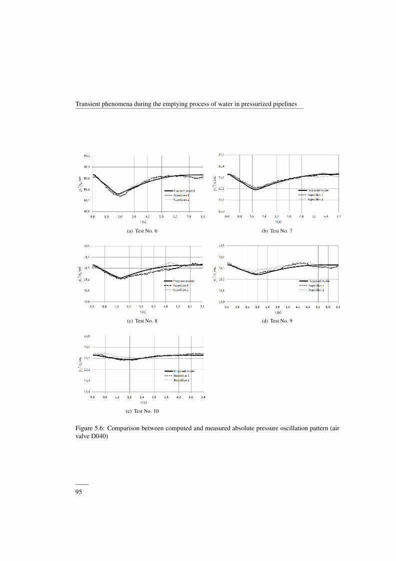
Transient phenomena during the emptying process of water in pressurized pipelines
(a) Test No. 6 (b) Test No. 7
(c) Test No. 8 (d) Test No. 9
(e) Test No. 10
Figure 5.6: Comparison between computed and measured absolute pressure oscillation pattern (airvalve D040)
——95
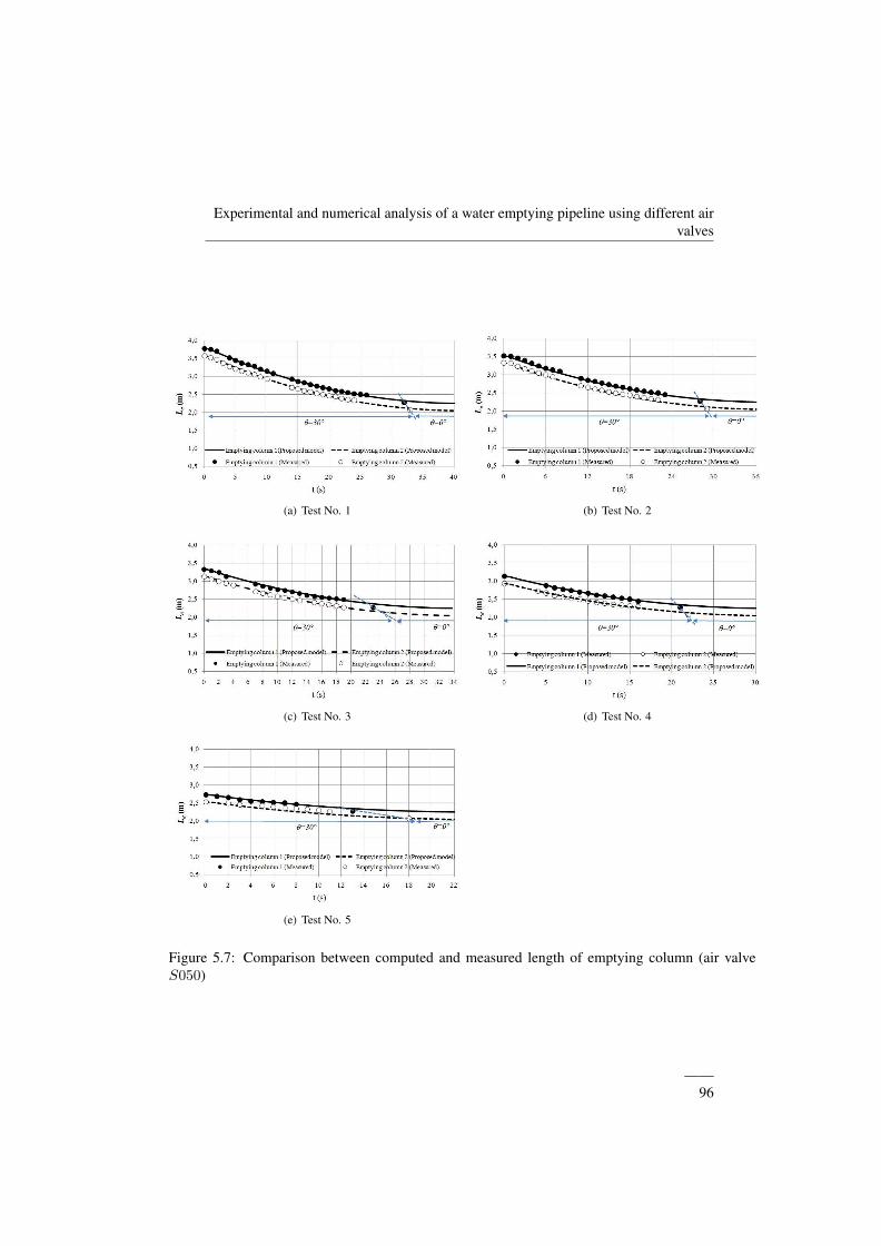
Experimental and numerical analysis of a water emptying pipeline using different airvalves
(a) Test No. 1 (b) Test No. 2
(c) Test No. 3 (d) Test No. 4
(e) Test No. 5
Figure 5.7: Comparison between computed and measured length of emptying column (air valveS050)
——96
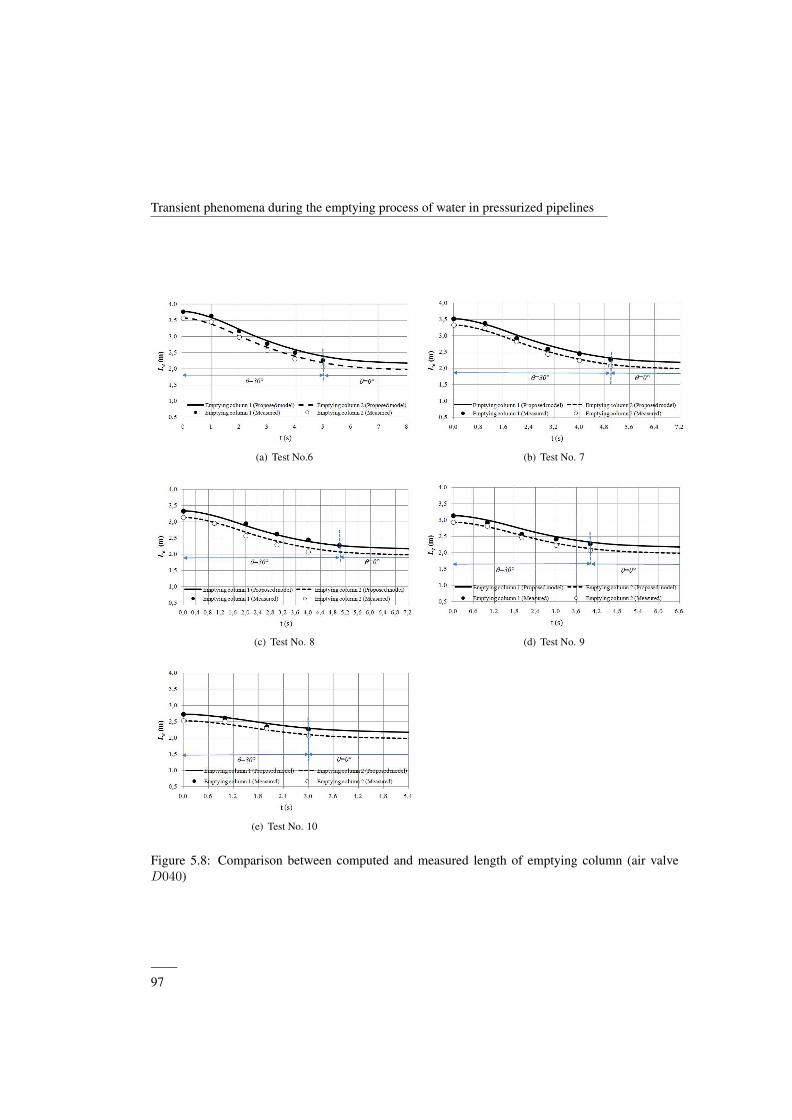
Transient phenomena during the emptying process of water in pressurized pipelines
(a) Test No.6 (b) Test No. 7
(c) Test No. 8 (d) Test No. 9
(e) Test No. 10
Figure 5.8: Comparison between computed and measured length of emptying column (air valveD040)
——97
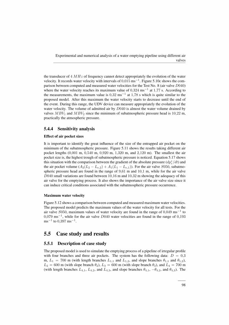
Experimental and numerical analysis of a water emptying pipeline using different airvalves
the transducer of 4 MHz of frequency cannot detect appropriately the evolution of the watervelocity. It records water velocity with intervals of 0,015 ms−1. Figure 5.10c shows the com-parison between computed and measured water velocities for the Test No. 8 (air valve D040)where the water velocity reaches its maximum value of 0,324 ms−1 at 1,77 s. According tothe measurements, the maximum value is 0,32 ms−1 at 1,78 s which is quite similar to theproposed model. After this maximum the water velocity starts to decrease until the end ofthe event. During this range, the UDV device can measure appropriately the evolution of thewater velocity. The volume of admitted air by D040 is almost the water volume drained byvalves MBV1 and MBV2 since the minimum of subatmospheric pressure head is 10,22 m,practically the atmospheric pressure.
5.4.4 Sensitivity analysisEffect of air pocket sizes
It is important to identify the great influence of the size of the entrapped air pocket on theminimum of the subatmospheric pressure. Figure 5.11 shows the results taking different airpocket lengths (0,001 m, 0,540 m, 0,920 m, 1,320 m, and 2,120 m). The smallest the airpocket size is, the highest trough of subatmospheric pressure is noticed. Equation 5.17 showsthis situation with the comparison between the gradient of the absolute pressure (dp∗i /dt) andthe air pocket volume (A2(L2 − Le,2) + A1(L1 − Le,1)). For the air valve S050, subatmo-spheric pressure head are found in the range of 9,61 m and 10,1 m, while for the air valveD040 small variations are found between 10,16 m and 10,32 m showing the adequacy of thisair valve for the emptying process. It also shows the importance of the air valve size since itcan induce critical conditions associated with the subatmospheric pressure occurrence.
Maximum water velocity
Figure 5.12 shows a comparison between computed and measured maximum water velocities.The proposed model predicts the maximum values of the water velocity for all tests. For theair valve S050, maximum values of water velocity are found in the range of 0,049 ms−1 to0,079 ms−1, while for the air valve D040 water velocities are found in the range of 0,193ms−1 to 0,397 ms−1.
5.5 Case study and results
5.5.1 Description of case studyThe proposed model is used to simulate the emptying process of a pipeline of irregular profilewith four branches and three air pockets. The system has the following data: D = 0,3m, L1 = 700 m (with length branches L1,1 and L1,2, and slope branches θ1,1 and θ1,2),L2 = 600 m (with slope branch θ2), L3 = 600 m (with slope branch θ3), and L4 = 700 m(with length branches L4,1, L4,2, and L4,3, and slope branches θ4,1, −θ4,2, and θ4,3). The
——98
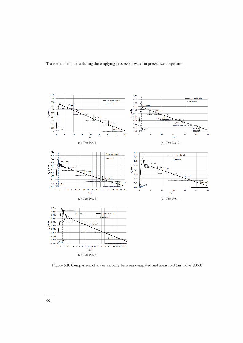
Transient phenomena during the emptying process of water in pressurized pipelines
(a) Test No. 1 (b) Test No. 2
(c) Test No. 3 (d) Test No. 4
(e) Test No. 5
Figure 5.9: Comparison of water velocity between computed and measured (air valve S050)
——99
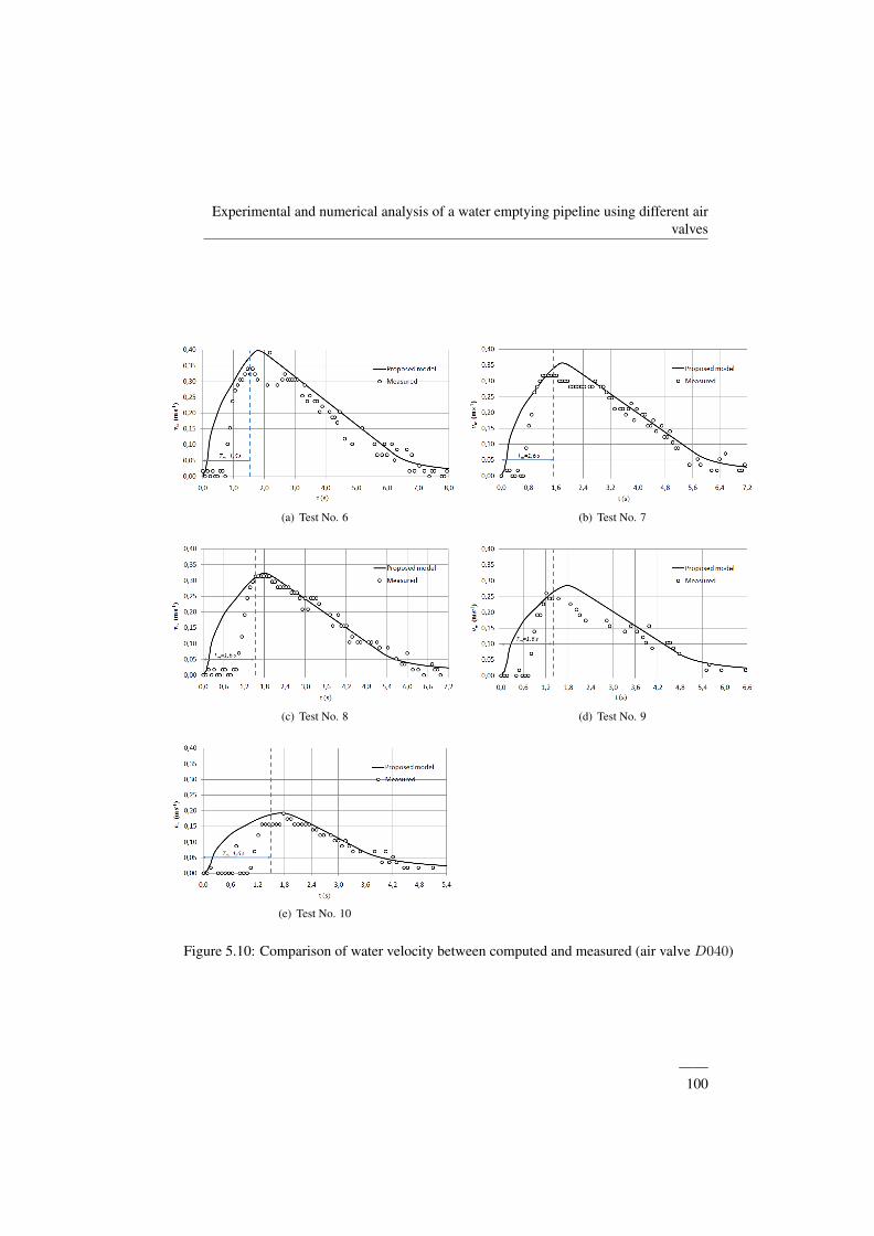
Experimental and numerical analysis of a water emptying pipeline using different airvalves
(a) Test No. 6 (b) Test No. 7
(c) Test No. 8 (d) Test No. 9
(e) Test No. 10
Figure 5.10: Comparison of water velocity between computed and measured (air valve D040)
——100
Transient phenomena during the emptying process of water in pressurized pipelines
Figure 5.11: Effect of the air pocket sizes on the minimum pressure attained
drainage of the system is carried out by drain valves DV1 and DV2 with a flow resistancecoefficient of K1 = K2 = 3,02 m3/s/m1/2. Air valves 1 and 3 have a nominal diameter of250 mm, and air valve 2 of 350 mm. All air valves have an inflow discharge coefficient of0,50. The air pocket sizes are x1, x2, and x3 with absolute pressure values of p∗1, p∗2, and p∗3,respectively. Figure 5.13 shows characteristics of the installation.
5.5.2 Proposed model definition
The corresponding equations of the pipeline are:
1. Mass oscillation equation applied to the emptying column 1
dv1
dt=p∗1 − p∗atmρwLw,1
+ g∆z1
Lw,1− f v1|v1|
2D− gA2(v1 + v2)|v1 + v2|
K21Lw,1
(5.20)
2. Air-water interface for the water column 1
dLw,1
dt= −v1 → Lw,1 = Lw,1,0 −
∫ t
0
v1dt (5.21)
3. Mass oscillation equation applied to the emptying column 2
dv2
dt=p∗2 − p∗atmρwLw,2
+ g∆z2
Lw,2− f v2|v2|
2D− gA2(v1 + v2)|v1 + v2|
K21Lw,2
(5.22)
4. Air-water interface for the water column 2
——101
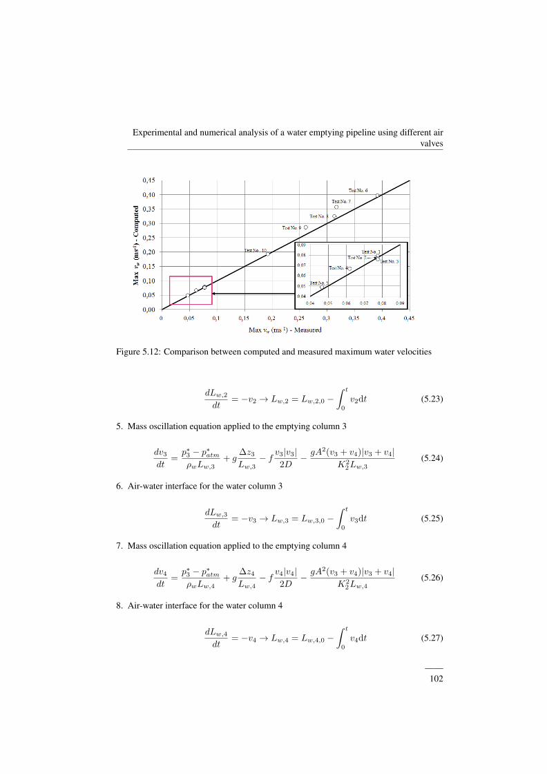
Experimental and numerical analysis of a water emptying pipeline using different airvalves
Figure 5.12: Comparison between computed and measured maximum water velocities
dLw,2
dt= −v2 → Lw,2 = Lw,2,0 −
∫ t
0
v2dt (5.23)
5. Mass oscillation equation applied to the emptying column 3
dv3
dt=p∗3 − p∗atmρwLw,3
+ g∆z3
Lw,3− f v3|v3|
2D− gA2(v3 + v4)|v3 + v4|
K22Lw,3
(5.24)
6. Air-water interface for the water column 3
dLw,3
dt= −v3 → Lw,3 = Lw,3,0 −
∫ t
0
v3dt (5.25)
7. Mass oscillation equation applied to the emptying column 4
dv4
dt=p∗3 − p∗atmρwLw,4
+ g∆z4
Lw,4− f v4|v4|
2D− gA2(v3 + v4)|v3 + v4|
K22Lw,4
(5.26)
8. Air-water interface for the water column 4
dLw,4
dt= −v4 → Lw,4 = Lw,4,0 −
∫ t
0
v4dt (5.27)
——102
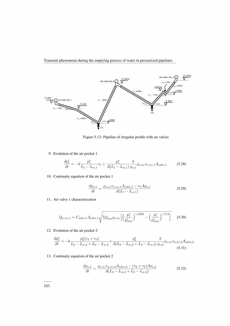
Transient phenomena during the emptying process of water in pressurized pipelines
Figure 5.13: Pipeline of irregular profile with air valves
9. Evolution of the air pocket 1
dp∗1dt
= −k p∗1L1 − Lw,1
v1 +p∗1
A(L1 − Lw,1)
k
ρa,1ρa,ncva,nc,1Aadm,1 (5.28)
10. Continuity equation of the air pocket 1
dρa,1dt
=ρa,ncva,nc,1Aadm,1 − v1Aρa,1
A(L1 − Lw,1)(5.29)
11. Air valve 1 characterization
Qa,nc,1 = Cadm,1Aadm,1
√7p∗atmρa,nc
[( p∗1p∗atm
)1,4286
−( p∗1p∗atm
)1,714](5.30)
12. Evolution of the air pocket 2
dp∗2dt
= −k p∗2(v2 + v3)
L2 − Lw,2 + L3 − Lw,3+
p∗2A(L2 − Lw,2 + L3 − Lw,3)
k
ρa,2ρa,ncva,nc,2Aadm,2
(5.31)
13. Continuity equation of the air pocket 2
dρa,2dt
=ρa,ncva,nc,2Aadm,2 − (v2 + v3)Aρa,2
A(L2 − Lw,2 + L3 − Lw,3)(5.32)
——103

Experimental and numerical analysis of a water emptying pipeline using different airvalves
14. Air valve 2 characterization
Qa,nc,2 = Cadm,2Aadm,2
√7p∗atmρa,nc
[( p∗2p∗atm
)1,4286
−( p∗2p∗atm
)1,714](5.33)
15. Evolution of the air pocket 3
dp∗3dt
= −k p∗3L4 − Lw,4
v4 +p∗3
A(L4 − Lw,4)
k
ρa,3ρa,ncva,nc,3Aadm,3 (5.34)
16. Continuity equation of the air pocket 3
dρa,3dt
=ρa,ncva,nc,3Aadm,3 − v4Aρa,3
A(L4 − Lw,4)(5.35)
17. Air valve 3 characterization
Qa,nc,3 = Cadm,3Aadm,3
√7p∗atmρa,nc
[( p∗3p∗atm
)1,4286
−( p∗3p∗atm
)1,714](5.36)
A 17x17 system of DAE describe the whole problem. Together with the correspondingboundary and initial conditions, 17 unknowns can be solved v1, Lw,1, v2, Lw,2, v3, Lw,3,v4, Lw,4, p∗1, p∗2, p∗3, ρa,1, ρa,2, ρa,3, va,cn,1, va,cn,2, va,cn,3. The initial conditions at t = 0are described by v1(0) = 0, Lw,1(0) = Lw,1,0, v2(0) = 0, Lw,2(0) = Lw,2,0, v3(0) = 0,Lw,3(0) = Lw,3,0, v4(0) = 0, Lw,4(0) = Lw,4,0, p∗1(0) = p∗atm, p∗2(0) = p∗atm, p∗3(0) =p∗atm, ρa,1,0 = 1,205 kg/m3, ρa,2,0 = 1,205 kg/m3, ρa,3,0 = 1,205 kg/m3, va,cn,1(0) = 0,va,cn,2(0) = 0, and va,cn,3(0) = 0. The upstream boundary conditions are given by p∗1,0,p∗2,0, and p∗3,0(initial conditions of air pockets), and the downstream boundary condition aregiven by p∗atm (water free discharge to the atmosphere). Gravity terms ∆z1/Lw,1, ∆z2/Lw,2,∆z3/Lw,3, and ∆z4/Lw,4 can be computed as presented by Coronado-Hernandez et al.(2017b).
5.5.3 ResultsFigure 5.14 shows results for the pipeline of irregular profile with air valves for the mainhydraulic and thermodynamic variables along the transient event (water flow, length of thewater column, absolute pressure, air density, and air flow). The initial air pocket sizes werex1,0 = x2,0 = x3,0 = 1 m, considering the most critical situation (Coronado-Hernandezet al., 2017b). A polytropic coefficient (k) of 1,2, and a friction factor (f ) of 0,018 wereconsidered.
——104

Transient phenomena during the emptying process of water in pressurized pipelines
(a) Water flow (b) Length of the water column
(c) Absolute pressure (d) Air density
(e) Air flow
Figure 5.14: Full transient analysis of the pipeline of irregular profile with airvalves
——105
Experimental and numerical analysis of a water emptying pipeline using different airvalves
According to Figure 5.14, the authors can deduce:
• In water column 1, the maximum water flow during the transient occurs at 70,2 s,with a value of 401,9 ls−1 (see Figure 5.14a). Two types of behavior are presentedbecause there are two branches. Water column 1 and 2 present a similar behavior withmaximum values of 565,3 ls−1 and 397,7 ls−1, respectively. Regarding to the watercolumn 4, the negative slope branch of −10% produces an effect of the water flowpattern as shown from 57,8 s to 67,5 s. The maximum value is reached at 16,6 s (406,5ls−1).
• Figure 5.14b shows that the water columns are drained completely indicating that airvalves are well sized. The water column behaviors are linear. The drainage times forwater column 1 trough 4 are in range from 79,5 s to 131,3 s.
• Air pockets are at atmospheric pressure (101325 Pa). Air pockets 1 and 3 present a sim-ilar behavior because they are admitting air for water columns 1 and 4. The minimumabsolute pressure head is 10,0 m. Air pocket 2 has the lowest values of subatmosphericpressure head with 8,9 m because air valve 2 has to admit simultaneously air into watercolumn 2 and 3, as shown in Figure 5.14c.
• The change in absolute pressure head parallels the air density in the air pockets (seeFigure 5.14d). The minimum values for air pockets 1, 2, and 3 are 1,17 kgm−3, 1,04kgm−3, and 1,17 kgm−3, respectively. Air pockets 1 and 3 present a similar behaviorbecause are located at the ends of the pipeline.
• Figure 5.14e presents the behavior of admitted air. Air valves 1 and 3 admit lower airvolume than air valve 2 because they are entering air into a one pipe. The maximum airflows are reached for air valve 1 at 77,1 s with a value of 389,2 ls−1; and for air valve 3at 17,5 s (393,5 ls−1). Air valve 2 has to admit air for two pipes. The maximum valueis 827,0 ls−1 (at 30,3 s).
5.6 ConclusionsSubatmospheric pressures occur during the emptying process in pipelines with undulatingprofile, which is a typical and common operation that engineers have to face. A rigid two-phases flow model was developed for analyzing it considering n possible air pockets, d airvalves, p pipes, and o drain valves. The proposed model is validated using an experimentalfacility of irregular profile of 7,3 m long and nominal diameter 63 mm (DN63) with an airvalve located at the high point and several drain valves along the pipeline. The main hydraulicvariables could be measured such as flow (both phases), pressure and air-water front position.Comparisons between computed and measured values of the absolute pressure, water velocityand the length of the emptying columns show that the proposed model can predict accuratelynot only the extreme values but also the patterns of them. According to the results, thefollowing conclusions can be drawn:
——106
Transient phenomena during the emptying process of water in pressurized pipelines
1. The proposed model can be used for planning the emptying operations in pipelineswith undulating profile considering its limitations.
2. The expansion of the air pocket produces minimum subatmospheric pressure. In orderto control these effects, air valves should be installed in pipelines.
3. It is very important to have a correct selection of air valves for vacuum protection foremptying pipelines. An inadequate selection produces both lower values of subatmo-spheric pressure and a slower drainage of the system. On the other hand, a larger airvalve orifice size reduces the lowest values of subatmospheric pressure.
4. Engineers should consider for the initial condition the pipeline is completely filled,which is the most critical condition, since the smallest air pocket sizes produce thelowest subatmospheric pressures.
In real hydraulic pressurized systems the proposed model can be used for: (i) checkingthe risk of a system collapse considering factors such as stiffness class, the soil in naturalconditions, the type of backfill and the cover depth, and (ii) selecting the air valve sizesdepending on the characteristics of each hydraulic system.
dddddddddddddddddddddddd
——107
Experimental and numerical analysis of a water emptying pipeline using different airvalves
d
NotationA Cross sectional area of the pipe (m2)Aadm,m Cross section area of the air valve m (m2)Cadm,m Inflow discharge coefficient of the air valve m (–)D Internal pipe diameter (m)f Darcy-Weisbach friction factor (–)g Gravity acceleration (m/s2)Le,j Length of the emptying column j (m)Lj Total length of the pipe j (m)k Polytropic coefficient (–)Ks Flow factor of the drain valve s (m3/s) with a pressure drop of 1 mH20
hm,s Local loss of the drain valve s (m)ma,i Air mass of the air pocket i (kg)p∗i Absolute pressure of the air pocket i (Pa)p∗atm Atmospheric pressure (Pa)t Time (s)Tm Valve maneuvering time (s)Qa,nc,m Air discharge in normal conditions admitted by the air valve m (m3/s)Qw,s Water discharge by the drain valve s (m3/s)Va,i Air volume of the air pocket i (m3)ve,j Water velocity of the emptying column j (m/s)va,nc,m Air velocity in normal conditions admitted by the air valve m (m/s)xi Length of the air pocket i (m)∆ze,j Elevation difference (m)ρa,i Air density of the air pocket i (kg/m3)ρa,nc Air density in normal conditions (kg/m3)ρa Water density (kg/m3)Superscripts∗ Absolute valuesSubscriptsa Refers to airi Refers to air pocketj Refers to pipem Refers to air valvenc Normal conditionsw Refers to water0 Initial condition
——108
Chapter 6
Rigid water column model forsimulating the emptying process ina pipeline using pressurized air
This chapter is extracted from the paper:
Rigid water column model for simulating the emptying process in a pipeline using pressurizedair
Coauthors: Coronado-Hernandez O. E; Fuertes-Miquel, V. S; Iglesias-Rey, P.L.; Martınez-Solano, F.J.Journal: Journal of Hydraulic Engineering ISSN 0733-9429.
2017 Impact Factor: 2.080. Position JCR 39/128 (Q2). Civil Engineering.State: Published. 2018. Volume 144; Issue 4. DOI: 10.1061/(ASCE)HY.1943-7900.0001446.
6.1 Abstract
This paper presents a mathematical model for analyzing the emptying process in a pipelineusing pressurized air. The rigid water column model (RWCM) is used to analyze the transientphenomena that occur during the emptying of the pipeline. The air-water interface is alsocomputed in the proposed model. The proposed model is applied along a 271, 6 m longPVC-steel pipeline with a 232 mm internal diameter. The boundary conditions are given by ahigh-pressure air tank at the upstream end and a manual butterfly valve at the downstream end.The solution was carried out using Simulink in Matlab. The results show that comparisonsbetween both the computed and measured water flow oscillations and gauge pressures arevery similar; hence, the model can effectively simulate the transient flow in this system. Inaddition, the results indicate that the proposed model can predict both the water flow andgauge pressure better than previous models.
109
Rigid water column model for simulating the emptying process in a pipeline usingpressurized air
6.2 IntroductionStudies related to the behavior of entrapped air during filling and emptying maneuvers inwater supply networks are very complex to analyze because there are two fluids (water andair) that exist in two different phases (liquid and gas) (Fuertes, 2001).
Filling and emptying processes can be analyzed using inertial models: the elastic watermodel (EWM) and the rigid water column model (RWCM). The EWM considers the elas-ticity of water and the pipe, while the RWCM ignores them. The solution is obtained usingnumerical methods (Zhou et al., 2011b).
Liou and Hunt (1996) developed an RWCM for analyzing the filling process that onlyconsiders the evolution of the water column. Izquierdo et al. (1999) developed an RWCMthat considers not only the evolution of the water column but also the air-water interfaceand the gravity term to represent the irregular profile in the pipeline. Zhou et al. (2013b)developed an EWM to analyze a rapidly filling process.
The emptying process is the reverse process of the filling process in pipelines; however,the emptying process in pipelines has not yet been studied as comprehensively. These studiesare very important because pipelines must be emptied periodically. Laanearu et al. (2012)carried out experiments on a PVC-steel pipeline with a 232 mm internal diameter and a 271, 6m length with the primary objective of providing data for future validation. This installationsetup consisted of a constant-head water supply tower, a high-pressure air tank, a 261 m longhorizontal PVC pipe, a 10,6 m long steel pipe (divided into a 6,1 m long horizontal pipe anda 4,5 m long vertical pipe), PVC and steel joints, steel inlet and outlet parts, various types ofvalves along the PVC-steel pipeline and a free-surface basement reservoir. Tijsseling et al.(2016) developed an RWCM for analyzing the emptying process using pressurized air. Thatmodel assumed that the velocity of the water column was not uniform because the movementof the front and tail ends were different.
In this paper, a mathematical model for the emptying process in a pipeline using pressur-ized air is developed based on two physical equations. The first equation is the mass oscil-lation equation, which provides sufficient accuracy for modeling this phenomenon (Cabreraet al., 1992; Liou and Hunt, 1996; Izquierdo et al., 1999). The second equation is the air-waterinterface equation (Zhou et al., 2013a,b). The gravity term is added in this model to repre-sent the irregular profile of the pipeline. For validation, the authors use the data providedby Laanearu et al. (2012). Comparisons between both the computed and measured waterflow oscillations and gauge pressures are conducted along the pipeline. In addition, compar-isons between the proposed model and previous models are conducted. Finally, a sensitivityanalysis of the height of the vertical pipe is performed.
6.3 Mathematical modelFig. 6.1 shows the scheme of the pipeline, which consists of a high-pressure air tank, a lengthof the emptying column, a regulating valve located at the downstream end, a horizontal pipeand a vertical pipe at the end.
——110
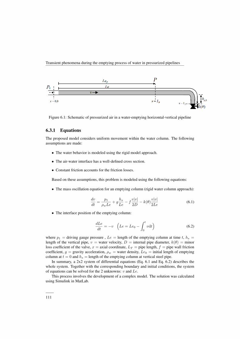
Transient phenomena during the emptying process of water in pressurized pipelines
Figure 6.1: Schematic of pressurized air in a water-emptying horizontal-vertical pipeline
6.3.1 Equations
The proposed model considers uniform movement within the water column. The followingassumptions are made:
• The water behavior is modeled using the rigid model approach.
• The air-water interface has a well-defined cross section.
• Constant friction accounts for the friction losses.
Based on these assumptions, this problem is modeled using the following equations:
• The mass oscillation equation for an emptying column (rigid water column approach):
dv
dt=
p1
ρwLe+ g
hsLe− f v|v|
2D− k(θ)
v|v|2Le
(6.1)
• The interface position of the emptying column:
dLe
dt= −v
(Le = Le0 −
∫ t
0
vdt)
(6.2)
where p1 = driving gauge pressure , Le = length of the emptying column at time t, hs =length of the vertical pipe, v = water velocity, D = internal pipe diameter, k(θ) = minorloss coefficient of the valve, x = axial coordinate, LT = pipe length, f = pipe wall frictioncoefficient, g = gravity acceleration, ρw = water density, Le0 = initial length of emptyingcolumn at t = 0 and hs = length of the emptying column at vertical steel pipe.
In summary, a 2x2 system of differential equations (Eq. 6.1 and Eq. 6.2) describes thewhole system. Together with the corresponding boundary and initial conditions, the systemof equations can be solved for the 2 unknowns: v and Le.
This process involves the development of a complex model. The solution was calculatedusing Simulink in MatLab.
——111

Rigid water column model for simulating the emptying process in a pipeline usingpressurized air
6.3.2 Initial and boundary conditions
The system is assumed to be initially static at t = 0. Therefore, the initial conditions aredescribed by v(0) = 0, Le(0) = Le0 and hs(0) = hs,0.
The boundary conditions are as follows:
a. The upstream boundary condition is the manometric pressure (p1) given by the air tank.
b. The downstream boundary condition is the valve loss described by k(θ). Water is freeto discharge to the atmosphere at patm = 0.
6.3.3 Gravity term
The gravity term (hs/Le) in Eq. 1 depends on the position of the emptying column. For thiscase, there are two possibilities:
a. When the air-water front of the emptying column has not reached the vertical pipe(Le >= hs,0):
hsLe
=hs,0Le
(6.3)
b. When the air-water front of the emptying column has reached the vertical pipe (Le <hs,0):
hsLe
= 1 (6.4)
If the configuration setup is different, then the gravity term will be different.
6.3.4 Pressure inside of pipeline
The manometric pressure along the pipeline (at point P ) can be computed as follows:
pP = p1 − ρwLeP( f
2Dv|v|+ dv
dt
)(6.5)
where LeP = length of the emptying column until point P at time t.To calculate LeP , the following expressions can be used:
LeP =
{LP − LT + Le, LT − Le < LeP
0, LT − Le ≥ LeP(6.6)
——112
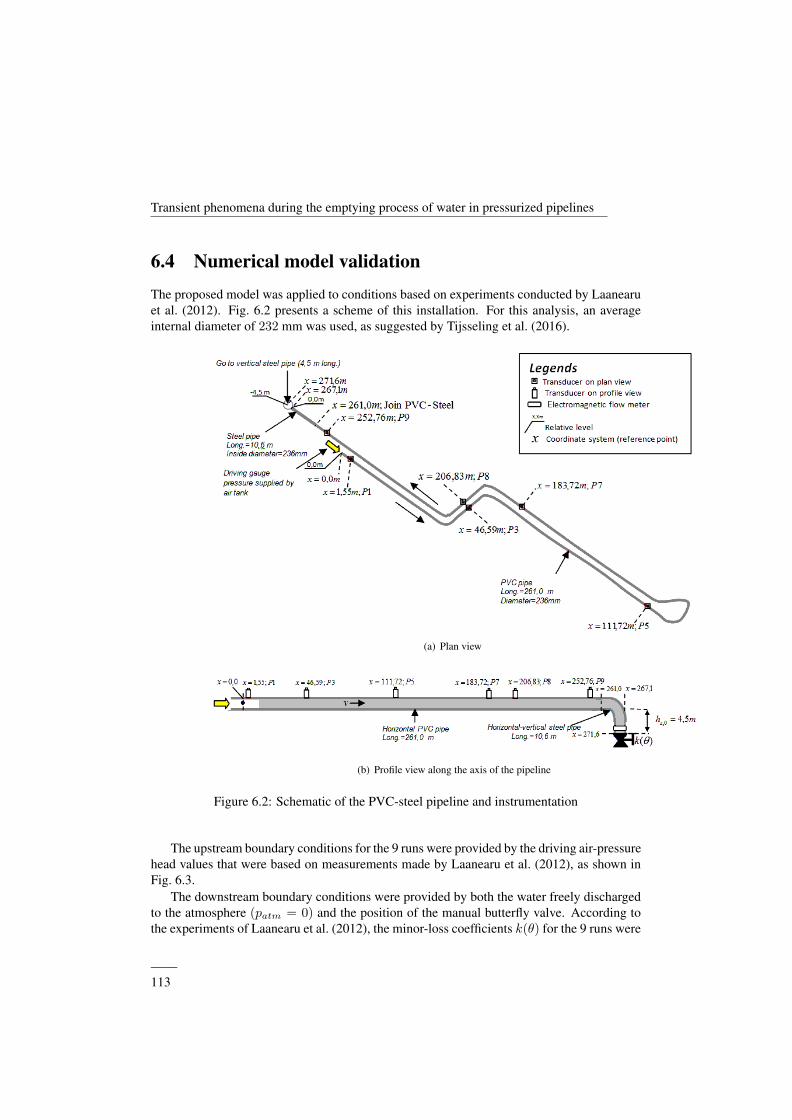
Transient phenomena during the emptying process of water in pressurized pipelines
6.4 Numerical model validation
The proposed model was applied to conditions based on experiments conducted by Laanearuet al. (2012). Fig. 6.2 presents a scheme of this installation. For this analysis, an averageinternal diameter of 232 mm was used, as suggested by Tijsseling et al. (2016).
(a) Plan view
(b) Profile view along the axis of the pipeline
Figure 6.2: Schematic of the PVC-steel pipeline and instrumentation
The upstream boundary conditions for the 9 runs were provided by the driving air-pressurehead values that were based on measurements made by Laanearu et al. (2012), as shown inFig. 6.3.
The downstream boundary conditions were provided by both the water freely dischargedto the atmosphere (patm = 0) and the position of the manual butterfly valve. According tothe experiments of Laanearu et al. (2012), the minor-loss coefficients k(θ) for the 9 runs were
——113
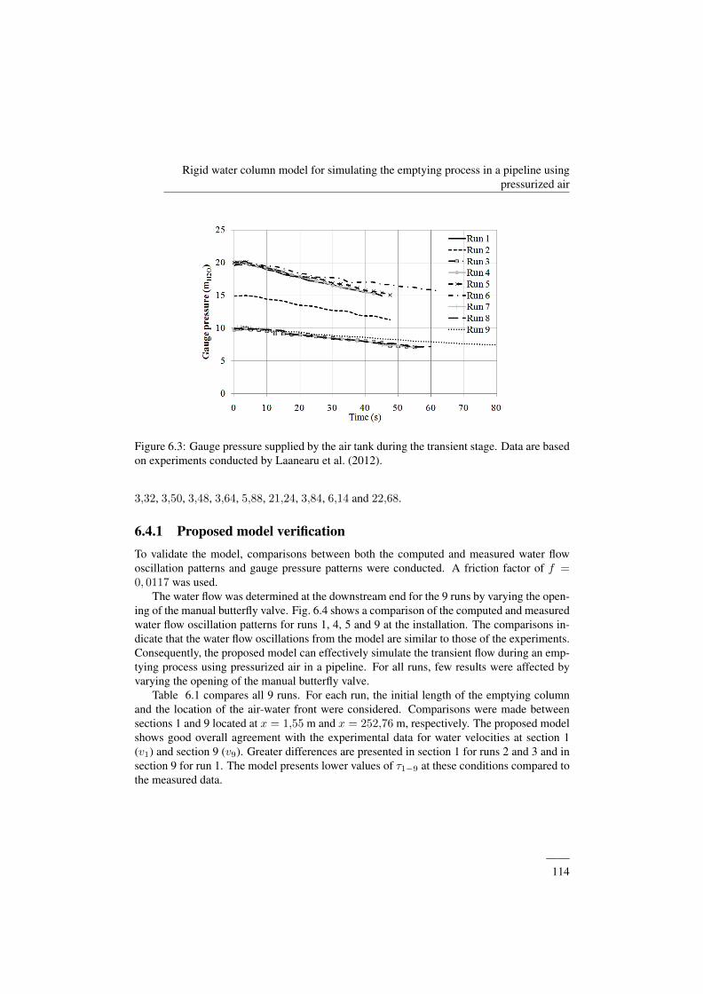
Rigid water column model for simulating the emptying process in a pipeline usingpressurized air
Figure 6.3: Gauge pressure supplied by the air tank during the transient stage. Data are basedon experiments conducted by Laanearu et al. (2012).
3,32, 3,50, 3,48, 3,64, 5,88, 21,24, 3,84, 6,14 and 22,68.
6.4.1 Proposed model verificationTo validate the model, comparisons between both the computed and measured water flowoscillation patterns and gauge pressure patterns were conducted. A friction factor of f =0, 0117 was used.
The water flow was determined at the downstream end for the 9 runs by varying the open-ing of the manual butterfly valve. Fig. 6.4 shows a comparison of the computed and measuredwater flow oscillation patterns for runs 1, 4, 5 and 9 at the installation. The comparisons in-dicate that the water flow oscillations from the model are similar to those of the experiments.Consequently, the proposed model can effectively simulate the transient flow during an emp-tying process using pressurized air in a pipeline. For all runs, few results were affected byvarying the opening of the manual butterfly valve.
Table 6.1 compares all 9 runs. For each run, the initial length of the emptying columnand the location of the air-water front were considered. Comparisons were made betweensections 1 and 9 located at x = 1,55 m and x = 252,76 m, respectively. The proposed modelshows good overall agreement with the experimental data for water velocities at section 1(v1) and section 9 (v9). Greater differences are presented in section 1 for runs 2 and 3 and insection 9 for run 1. The model presents lower values of τ1−9 at these conditions compared tothe measured data.
——114
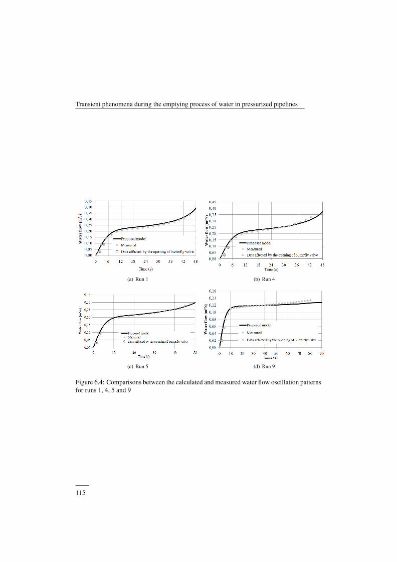
Transient phenomena during the emptying process of water in pressurized pipelines
(a) Run 1 (b) Run 4
(c) Run 5 (d) Run 9
Figure 6.4: Comparisons between the calculated and measured water flow oscillation patternsfor runs 1, 4, 5 and 9
——115
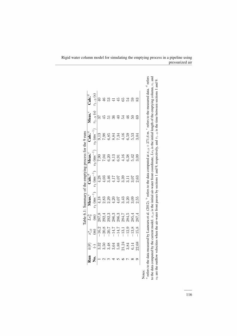
Rigid water column model for simulating the emptying process in a pipeline usingpressurized air
Tabl
e6.
1:Su
mm
ary
ofth
eem
ptyi
ngpr
oces
sfo
rthe
9ru
nsR
unk(θ
)x
a i,0
Leb 0
Mea
s.cC
alc.
dM
eas.c
Cal
c.d
Mea
s.cC
alc.
d
No.
(-)
(m)
(m)
v 1(m
s−1)
v 1(m
s−1)
v 9(m
s−1)
v 9(m
s−1)
τ 1−
9(s
)τ 1−
9(s
)1
3,32
−16,2
287,8
4,1
84,2
87,9
09,1
337
40
23,
50−
20,8
292,4
2,8
34,0
37,0
47,9
845
46
33,
48−
20,7
292,3
2,2
93,4
66,2
06,8
551
53
43,
64−
14,7
286,3
4,2
04,1
78,1
38,8
436
41
55,
88−
14,7
286,3
4,0
74,0
76,9
17,3
440
45
621,2
4−
13,1
284,7
3,4
33,3
94,1
64,1
654
65
73,
84−
12,9
284,5
3,2
03,1
16,3
86,5
946
54
86,
14−
13,8
285,4
3,0
93,0
75,4
25,5
350
59
922,6
8−
15,8
287,4
2,5
52,6
33,0
93,0
469
83
Not
es:
are
fers
toth
eda
tam
easu
red
byL
aane
aru
etal
.(20
12).
bre
fers
toth
eda
taco
mpu
ted
atxi,0+271,6
m.c
refe
rsto
the
mea
sure
dda
ta.d
refe
rsto
the
data
com
pute
dby
the
curr
entm
odel
.xi,0
isth
ein
itial
air-
wat
erfr
ontc
oord
inat
e,Le 0
isth
ein
itial
leng
thof
the
empt
ying
colu
mn,v 1
and
v 9ar
eth
eou
tflow
velo
citie
sw
hen
the
air-
wat
erfr
ontp
asse
sby
sect
ions
1an
d9,
resp
ectiv
ely,
andτ 1
−9
isth
etim
ebe
twee
nse
ctio
ns1
and
9.
——116
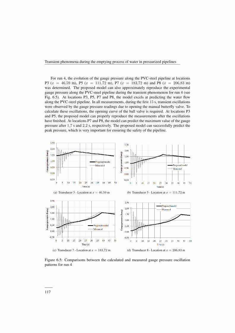
Transient phenomena during the emptying process of water in pressurized pipelines
For run 4, the evolution of the gauge pressure along the PVC-steel pipeline at locationsP3 (x = 46,59 m), P5 (x = 111,72 m), P7 (x = 183,72 m) and P8 (x = 206,83 m)was determined. The proposed model can also approximately reproduce the experimentalgauge pressure along the PVC-steel pipeline during the transient phenomenon for run 4 (seeFig. 6.5). At locations P3, P5, P7 and P8, the model excels at predicting the water flowalong the PVC-steel pipeline. In all measurements, during the first 15 s, transient oscillationswere observed by the gauge pressure readings due to opening the manual butterfly valve. Tocalculate these oscillations, the opening curve of the ball valve is required. At locations P3and P5, the proposed model can properly reproduce the measurements after the oscillationshave finished. At locations P7 and P8, the model can predict the maximum value of the gaugepressure after 1,7 s and 2,2 s, respectively. The proposed model can successfully predict thepeak pressure, which is very important for ensuring the safety of the pipeline.
(a) Transducer 3 - Location at x = 46,59 m (b) Transducer 5 - Location at x = 111,72 m
(c) Transducer 7 - Location at x = 183,72 m (d) Transducer 8 - Location at x = 206,83 m
Figure 6.5: Comparisons between the calculated and measured gauge pressure oscillationpatterns for run 4
——117
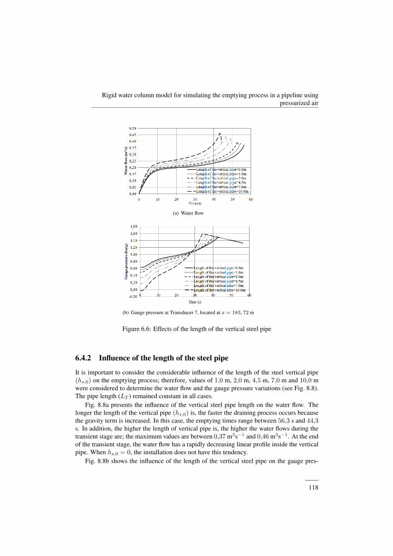
Rigid water column model for simulating the emptying process in a pipeline usingpressurized air
(a) Water flow
(b) Gauge pressure at Transducer 7, located at x = 183, 72 m
Figure 6.6: Effects of the length of the vertical steel pipe
6.4.2 Influence of the length of the steel pipe
It is important to consider the considerable influence of the length of the steel vertical pipe(hs,0) on the emptying process; therefore, values of 1,0 m, 2,0 m, 4,5 m, 7,0 m and 10,0 mwere considered to determine the water flow and the gauge pressure variations (see Fig. 8.8).The pipe length (LT ) remained constant in all cases.
Fig. 8.8a presents the influence of the vertical steel pipe length on the water flow. Thelonger the length of the vertical pipe (hs,0) is, the faster the draining process occurs becausethe gravity term is increased. In this case, the emptying times range between 56,3 s and 44,3s. In addition, the higher the length of vertical pipe is, the higher the water flows during thetransient stage are; the maximum values are between 0,37 m3s−1 and 0,46 m3s−1. At the endof the transient stage, the water flow has a rapidly decreasing linear profile inside the verticalpipe. When hs,0 = 0, the installation does not have this tendency.
Fig. 8.8b shows the influence of the length of the vertical steel pipe on the gauge pres-
——118
Transient phenomena during the emptying process of water in pressurized pipelines
sure at transducer P7. The maximum gauge pressures increase with increasing length of thevertical pipe steel along the pipeline, with gauge pressure values between 1,49 barg and 1,59barg. In addition, higher vertical steel pipe lengths cause higher minimum gauge pressuresalong the pipeline, which occur at the beginning of the transient stage. At transducer P7, thehighest minimum gauge pressure is −0,03 barg. The minimum gauge pressure occurs at theupstream end. The minimum and maximum gauge pressures occur simultaneously during thetransient stage. When the air-water front reaches a particular point during the transient stage,the gauge pressure is the driving gauge pressure.
6.5 Conclusions
A mathematical model for accurately determining the emptying process in a pipeline usingpressurized air was developed in this paper. It can be used for several pipeline configurationsby changing only the gravity term.
The proposed model was validated using data recorded by Laanearu et al. (2012) for aPVC-steel pipeline that was 271,6 m long with a 232 mm internal diameter. The modeleffectively simulated measurements of the transient water flow and gauge pressure along thepipeline for 9 runs.
The results indicate that the proposed model for analyzing the emptying process can betterpredict both the water flow and gauge pressure along a pipeline than previous models.
The length of the vertical pipe significantly influences the results. The time for drainagedecreases as the vertical steel pipe length increases, possibly because the water flow increases.However, it should be considered that the maximum and minimum gauge pressures will alsoincrease, putting the system at risk. Considering this, it is recommended to select a suitablelength for the vertical steel pipe to reduce the probability of system failure.
ddddddddddddddd
——119
Rigid water column model for simulating the emptying process in a pipeline usingpressurized air
NotationThe following symbols are used in this paper:
A = cross-sectional area of pipe (m2);D = internal pipe diameter (m);f = pipe wall friction coefficient (–);
k(θ) = minor-loss coefficient (–);g = gravity acceleration (m/s2);hs = length of the emptying column at the vertical pipe (m);hs,0 = height of the vertical pipe (m);Le = length of the emptying column (m);Le0 = initial length of the emptying column (m);LeP = length of the emptying column until point P (m);LT = pipe length (m);p1 = driving gauge pressure (Pa);
patm = atmospheric pressure (Pa);pP = gauge pressure at point P (Pa);Q = discharge (m3/s);t = time (s);v = water velocity (m/s);x = axial coordinate (m);
xi,0 = initial air-water front coordinate (m);ρw = water density (kg/m3);
——120
Chapter 7
Emptying operation of watersupply networks
This chapter is extracted from the paper:
Emptying operation of water supply networksCoauthors: Coronado-Hernandez O. E; Fuertes-Miquel, V. S; Angulo-Hernandez, F. N.
Journal: Water ISSN 2073-4441.
2017 Impact Factor: 2.069. Position JCR 34/90 (Q2). Water Resources.
State: Published. 2018. Volume 10; Issue 1; 22. DOI: 10.3390/w10010022.
7.1 Abstract
Recently emptying processes have been studied in experimental facilities in pipelines, butthere is lack regarding to applications in actual pipelines, which permits to establish the riskof collapse because of subatmospheric pressure occurrence. This research presents a mathe-matical model to simulate the emptying process of water supply networks, and the applicationto a water emptying pipeline with nominal diameter of 1000 mm and 578 m long which islocated on the southern of Cartagena, Bolıvar Deparment, Colombia. In the application wasconsidered both pipe and air valves data manufacturer. The behavior of all hydraulic andthermodynamic variables is considered. Results show that is crucial to know subatmosphericpressure values to prevent the collapse of the pipeline. The application of the mathematicalmodel confirms that the hydraulic system is well designed depending on air valve sizes andmaneuvering of drain valve.
121
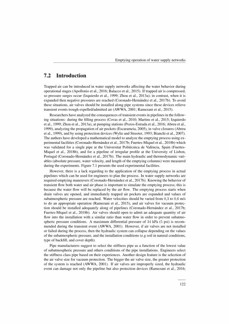
Emptying operation of water supply networks
7.2 Introduction
Trapped air can be introduced in water supply networks affecting the water behavior duringoperational stages (Apollonio et al., 2016; Balacco et al., 2015). If trapped air is compressed,so pressure surges occur (Izquierdo et al., 1999; Zhou et al., 2013a); in contrast, when it isexpanded then negative pressures are reached (Coronado-Hernandez et al., 2017b). To avoidthese situations, air valves should be installed along pipe systems since these devices relievetransient events trough expelled/admitted air (AWWA, 2001; Ramezani et al., 2015).
Researchers have analyzed the consequences of transient events in pipelines in the follow-ing situations: during the filling process (Covas et al., 2010; Martins et al., 2015; Izquierdoet al., 1999; Zhou et al., 2013a), at pumping stations (Pozos-Estrada et al., 2016; Abreu et al.,1999), analyzing the propagation of air pockets (Escarameia, 2005), in valve closures (Abreuet al., 1999), and by using protection devices (Wylie and Streeter, 1993; Bianchi et al., 2007).The authors have developed a mathematical model to analyze the emptying process using ex-perimental facilities (Coronado-Hernandez et al., 2017b; Fuertes-Miquel et al., 2018b) whichwas validated for a single pipe at the Universitat Politecnica de Valencia, Spain (Fuertes-Miquel et al., 2018b), and for a pipeline of irregular profile at the University of Lisbon,Portugal (Coronado-Hernandez et al., 2017b). The main hydraulic and thermodynamic vari-ables (absolute pressure, water velocity, and length of the emptying columns) were measuredduring the experiments. Figure 7.1 presents the used experimental facilities.
However, there is a lack regarding to the application of the emptying process in actualpipelines which can be used for engineers to plan the process. In water supply networks arerequired emptying maneuvers (Coronado-Hernandez et al., 2017b). Knowing the behavior oftransient flow both water and air phase is important to simulate the emptying process; this isbecause the water flow will be replaced by the air flow. The emptying process starts whendrain valves are opened, and immediately trapped air pockets are expanded and values ofsubatmospheric pressure are reached. Water velocities should be varied from 0,3 to 0,6 m/sto do an appropriate operation (Ramezani et al., 2015), and air valves for vacuum protec-tion should be installed adequately along of pipelines (Coronado-Hernandez et al., 2017b;Fuertes-Miquel et al., 2018b). Air valves should open to admit an adequate quantity of airflow into the installation with a similar ratio than water flow in order to prevent subatmo-spheric pressure conditions. A maximum differential pressure of 34 kPa (5 psi) is recom-mended during the transient event (AWWA, 2001). However, if air valves are not installedor failed during the process, then the hydraulic system can collapse depending on the valuesof the subatmospheric pressure, and the installation conditions (e.g soil in natural conditions,type of backfill, and cover depth).
Pipe manufacturers suggest to select the stiffness pipe as a function of the lowest valueof subatmospheric pressure and others conditions of the pipe installations. Engineers selectthe stiffness class pipe based on their experiences. Another design feature is the selection ofthe air valve size for vacuum protection. The bigger the air valve size, the greater protectionof the system is reached (AWWA, 2001). If air valves are improperly sized, the hydraulicevent can damage not only the pipeline but also protection devices (Ramezani et al., 2016;
——122
Transient phenomena during the emptying process of water in pressurized pipelines
(a) Single pipe (Universitat Politecnica de Valencia, Spain)
(b) Pipeline of irregular profile (University of Lisbon, Portugal)
Figure 7.1: Experimental facilities to validate the emptying pro-cess
——123
Emptying operation of water supply networks
Apollonio et al., 2016). Drain valves maneuvers should be considered during the emptyingprocess.
This Chapter presents the mathematical model developed by the authors (Coronado-Hernandez et al., 2017b; Fuertes-Miquel et al., 2018b) to analyze the emptying process,which was applied to the Ciudad del Bicentenario pipeline located in Cartagena, Bolıvar De-partment, Colombia, in order to show the behavior of hydraulic and thermodynamic variables.The mathematical model can be used for engineers to conduct a water emptying process inpipelines in the design and planning stages to avoid the collapse of pipe systems.
7.3 Pipeline descriptionThe Ciudad del Bicentenario pipeline is located on the southern of the city of Cartagena,Bolıvar Departament, Colombia (see Figure 7.2). The company Aguas de Cartagena (Carta-gena, Colombia) provided the entire information regarding to the pipeline (Aguas de Carta-gena, 2013).
Figure 7.3 shows the scheme of the analyzed pipeline which is located between chainagesfrom K2 + 360 m to K2 + 940 m. It is configured as a Glass-Reinforced Plastic (GRP)pipeline with nominal diameter of 1000 mm, 580 m long, pressure class of PN 10, andstiffness class of SN 5000 (Flowtite, 2008). Slope branches vary in a range from 0% to6,9%. The system presents the emptying column No. 1 (chainages from K2 + 360 m toK2 + 620 m), and the emptying column No. 2 (chainages from K2 + 940 m to K2 + 620m).
——124
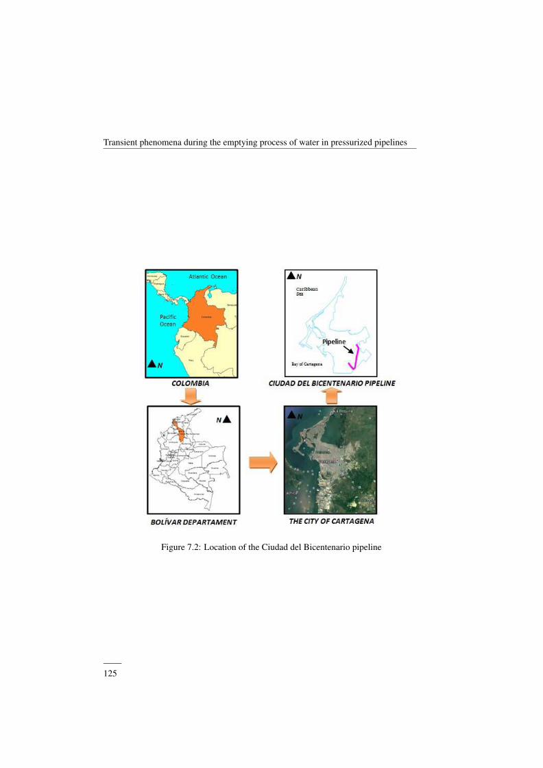
Transient phenomena during the emptying process of water in pressurized pipelines
Figure 7.2: Location of the Ciudad del Bicentenario pipeline
——125
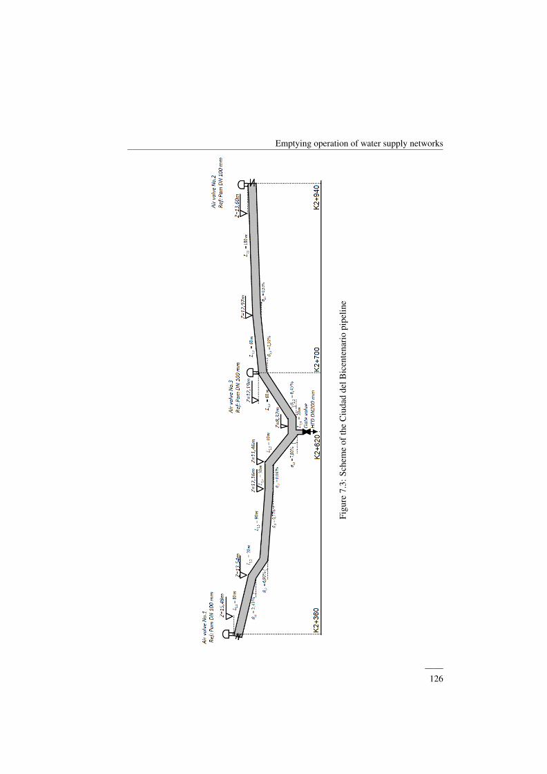
Emptying operation of water supply networks
Figu
re7.
3:Sc
hem
eof
the
Ciu
dad
delB
icen
tena
rio
pipe
line
——126
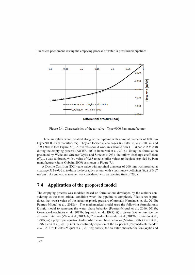
Transient phenomena during the emptying process of water in pressurized pipelines
Figure 7.4: Characteristics of the air valve - Type 9000 Pam manufacturer
Three air valves were installed along of the pipeline with nominal diameter of 100 mm(Type 9000 - Pam manufacurer). They are located at chainagesK2+360 m,K2+700 m, andK2+940 m (see Figure 7.3). Air valves should work in subsonic flow (−0,3 bar <∆P < 0)during the emptying process (AWWA, 2001; Ramezani et al., 2016). Using the formulationpresented by Wylie and Streeter Wylie and Streeter (1993), the inflow discharge coefficient(Cadm) was calibrated with a value of 0,68 to get similar values to the data provided by Pammanufacturer (Saint-Gobain, 2009) as shown in Figure 7.4.
A Ductile Cast Iron (DCI) gate valve with nominal diameter of 200 mm was installed atchainageK2+620 m to drain the hydraulic system, with a resistance coefficient (Rv) of 0,67ms2/m6. A synthetic maneuver was considered with an opening time of 200 s.
7.4 Application of the proposed modelThe emptying process was modeled based on formulations developed by the authors con-sidering as the most critical condition when the pipeline is completely filled since it pro-duces the lowest value of the subatmospheric pressure (Coronado-Hernandez et al., 2017b;Fuertes-Miquel et al., 2018b). The mathematical model uses the following formulations:i) rigid model to represent the water phase behavior (Fuertes-Miquel et al., 2016, 2018b;Coronado-Hernandez et al., 2017b; Izquierdo et al., 1999); ii) a piston flow to describe theair-water interface (Zhou et al., 2013a,b; Coronado-Hernandez et al., 2017b; Izquierdo et al.,1999); iii) a polytropic equation to describe the air phase behavior (Martin, 1976; Graze et al.,1996; Leon et al., 2010); (iv) the continuity equation of the air pocket (Coronado-Hernandezet al., 2017b; Fuertes-Miquel et al., 2018b); and (v) the air valve characterization (Wylie and
——127
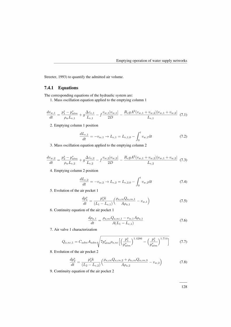
Emptying operation of water supply networks
Streeter, 1993) to quantify the admitted air volume.
7.4.1 EquationsThe corresponding equations of the hydraulic system are:
1. Mass oscillation equation applied to the emptying column 1
dvw,1
dt=p∗1 − p∗atmρwLe,1
+ g∆ze,1Le,1
− f vw,1|vw,1|2D
− RvgA2(vw,1 + vw,2)|vw,1 + vw,2|
Le,1(7.1)
2. Emptying column 1 position
dLe,1
dt= −vw,1 → Le,1 = Le,1,0 −
∫ t
0
vw,1dt (7.2)
3. Mass oscillation equation applied to the emptying column 2
dvw,2
dt=p∗2 − p∗atmρwLe,2
+ g∆ze,2Le,2
− f vw,2|vw,2|2D
− RvgA2(vw,1 + vw,2)|vw,1 + vw,2|
Le,2(7.3)
4. Emptying column 2 position
dLe,2
dt= −vw,2 → Le,2 = Le,2,0 −
∫ t
0
vw,2dt (7.4)
5. Evolution of the air pocket 1
dp∗1dt
=p∗1k
(L1 − Le,1)
(ρa,cnQa,cn,1
Aρa,1− vw,1
)(7.5)
6. Continuity equation of the air pocket 1
dρa,1dt
=ρa,ncQa,nc,1 − vw,1Aρa,1
A(L1 − Le,1)(7.6)
7. Air valve 1 characterization
Qa,nc,1 = CadmAadm
√7p∗atmρa,nc
[( p∗1p∗atm
)1.4286
−( p∗1p∗atm
)1.714](7.7)
8. Evolution of the air pocket 2
dp∗2dt
=p∗2k
(L2 − Le,2)
(ρa,cnQa,cn,2 + ρa,cnQa,cn,3
Aρa,2− vw,2
)(7.8)
9. Continuity equation of the air pocket 2
——128
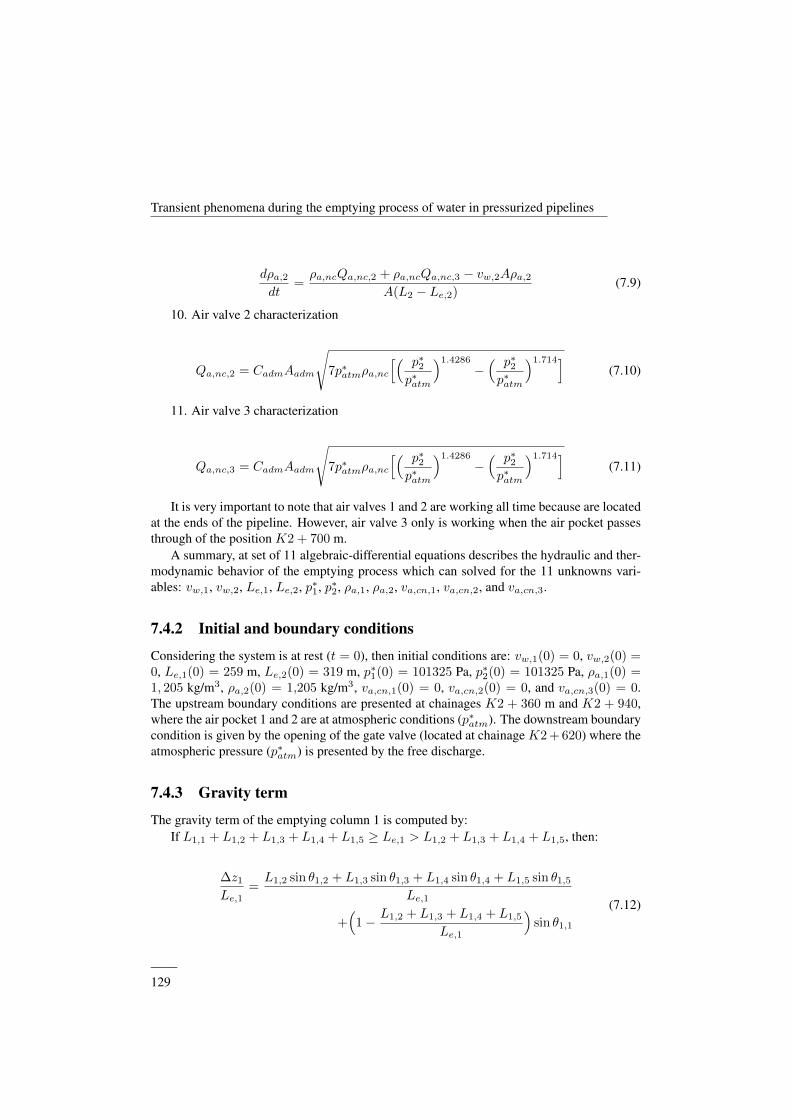
Transient phenomena during the emptying process of water in pressurized pipelines
dρa,2dt
=ρa,ncQa,nc,2 + ρa,ncQa,nc,3 − vw,2Aρa,2
A(L2 − Le,2)(7.9)
10. Air valve 2 characterization
Qa,nc,2 = CadmAadm
√7p∗atmρa,nc
[( p∗2p∗atm
)1.4286
−( p∗2p∗atm
)1.714](7.10)
11. Air valve 3 characterization
Qa,nc,3 = CadmAadm
√7p∗atmρa,nc
[( p∗2p∗atm
)1.4286
−( p∗2p∗atm
)1.714](7.11)
It is very important to note that air valves 1 and 2 are working all time because are locatedat the ends of the pipeline. However, air valve 3 only is working when the air pocket passesthrough of the position K2 + 700 m.
A summary, at set of 11 algebraic-differential equations describes the hydraulic and ther-modynamic behavior of the emptying process which can solved for the 11 unknowns vari-ables: vw,1, vw,2, Le,1, Le,2, p∗1, p∗2, ρa,1, ρa,2, va,cn,1, va,cn,2, and va,cn,3.
7.4.2 Initial and boundary conditions
Considering the system is at rest (t = 0), then initial conditions are: vw,1(0) = 0, vw,2(0) =0, Le,1(0) = 259 m, Le,2(0) = 319 m, p∗1(0) = 101325 Pa, p∗2(0) = 101325 Pa, ρa,1(0) =1, 205 kg/m3, ρa,2(0) = 1,205 kg/m3, va,cn,1(0) = 0, va,cn,2(0) = 0, and va,cn,3(0) = 0.The upstream boundary conditions are presented at chainages K2 + 360 m and K2 + 940,where the air pocket 1 and 2 are at atmospheric conditions (p∗atm). The downstream boundarycondition is given by the opening of the gate valve (located at chainage K2 + 620) where theatmospheric pressure (p∗atm) is presented by the free discharge.
7.4.3 Gravity term
The gravity term of the emptying column 1 is computed by:If L1,1 + L1,2 + L1,3 + L1,4 + L1,5 ≥ Le,1 > L1,2 + L1,3 + L1,4 + L1,5, then:
∆z1
Le,1=L1,2 sin θ1,2 + L1,3 sin θ1,3 + L1,4 sin θ1,4 + L1,5 sin θ1,5
Le,1
+(
1− L1,2 + L1,3 + L1,4 + L1,5
Le,1
)sin θ1,1
(7.12)
——129

Emptying operation of water supply networks
If L1,2 + L1,3 + L1,4 + L1,5 ≥ Le,1 > L1,3 + L1,4 + L1,5, then:
∆z1
Le,1=L1,3 sin θ1,3 + L1,4 sin θ1,4 + L1,5 sin θ1,5
Le,1+(
1− L1,3 + L1,4 + L1,5
Le,1
)sin θ1,2
(7.13)If L1,3 + L1,4 + L1,5 ≥ Le,1 > L1,4 + L1,5, then:
∆z1
Le,1=L1,4 sin θ1,4 + L1,5 sin θ1,5
Le,1+(
1− L1,4 + L1,5
Le,1
)sin θ1,3 (7.14)
If L1,4 + L1,5 ≥ Le,1 > L1,5, then:
∆z1
Le,1=L1,5 sin θ1,5
Le,1+(
1− L1,5
Le,1
)sin θ1,4 (7.15)
If L1,5 ≥ Le,1 > 0, then:
∆z1
Le,1= sin θ1,5 (7.16)
The gravity term of the emptying column 2 is computed by:If L2,1 + L2,2 + L2,3 + L2,4 ≥ Le,2 > L2,2 + L2,3 + L2,4, then:
∆z2
Le,2=L2,2 sin θ2,2 + L2,3 sin θ2,3
Le,2+(
1− L2,2 + L2,3 + L2,4
Le,2
)sin θ2,1 (7.17)
If L2,2 + L2,3 + L2,4 ≥ Le,2 > L2,3 + L2,4, then:
∆z2
Le,2=L2,3 sin θ2,3
Le,2+(
1− L2,3 + L2,4
Le,2
)sin θ2,2 (7.18)
If L2,3 + L2,4 ≥ Le,2 > L2,4, then:
∆z2
Le,2=(
1− L2,4
Le,2
)sin θ2,3 (7.19)
If L2,4 ≥ Le,2 > 0, then:
∆z2
Le,2= 0 (7.20)
7.5 Results and discussionThe resolution of these set of differential-algebraic equations (equations 7.1-7.11) was con-ducted using Matlab. In order to simulate the most critical situations, small air pocket sizes
——130
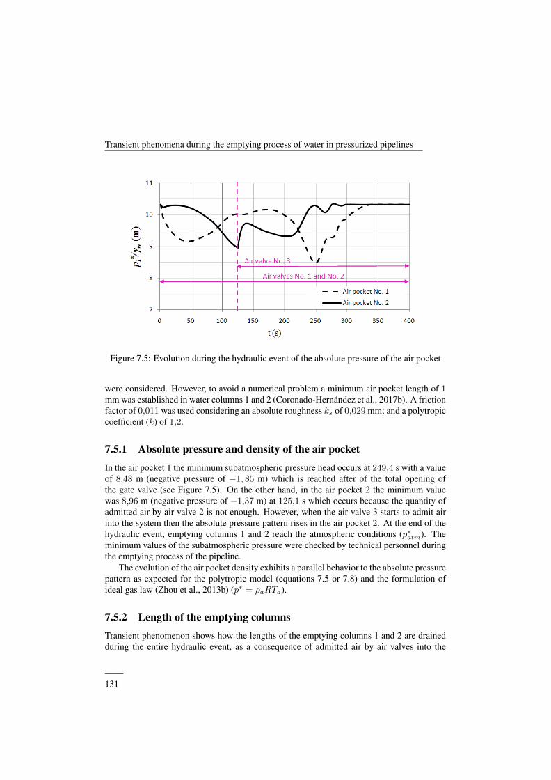
Transient phenomena during the emptying process of water in pressurized pipelines
Figure 7.5: Evolution during the hydraulic event of the absolute pressure of the air pocket
were considered. However, to avoid a numerical problem a minimum air pocket length of 1mm was established in water columns 1 and 2 (Coronado-Hernandez et al., 2017b). A frictionfactor of 0,011 was used considering an absolute roughness ks of 0,029 mm; and a polytropiccoefficient (k) of 1,2.
7.5.1 Absolute pressure and density of the air pocketIn the air pocket 1 the minimum subatmospheric pressure head occurs at 249,4 s with a valueof 8,48 m (negative pressure of −1, 85 m) which is reached after of the total opening ofthe gate valve (see Figure 7.5). On the other hand, in the air pocket 2 the minimum valuewas 8,96 m (negative pressure of −1,37 m) at 125,1 s which occurs because the quantity ofadmitted air by air valve 2 is not enough. However, when the air valve 3 starts to admit airinto the system then the absolute pressure pattern rises in the air pocket 2. At the end of thehydraulic event, emptying columns 1 and 2 reach the atmospheric conditions (p∗atm). Theminimum values of the subatmospheric pressure were checked by technical personnel duringthe emptying process of the pipeline.
The evolution of the air pocket density exhibits a parallel behavior to the absolute pressurepattern as expected for the polytropic model (equations 7.5 or 7.8) and the formulation ofideal gas law (Zhou et al., 2013b) (p∗ = ρaRTa).
7.5.2 Length of the emptying columnsTransient phenomenon shows how the lengths of the emptying columns 1 and 2 are drainedduring the entire hydraulic event, as a consequence of admitted air by air valves into the
——131
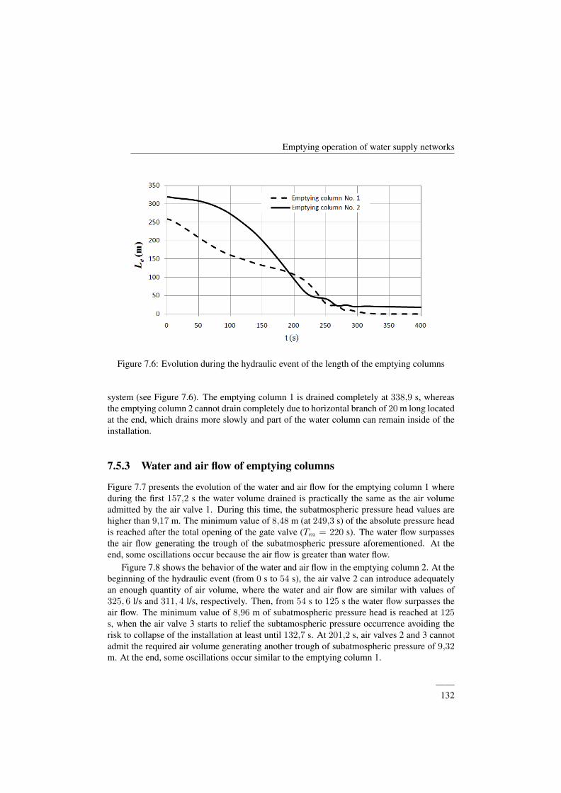
Emptying operation of water supply networks
Figure 7.6: Evolution during the hydraulic event of the length of the emptying columns
system (see Figure 7.6). The emptying column 1 is drained completely at 338,9 s, whereasthe emptying column 2 cannot drain completely due to horizontal branch of 20 m long locatedat the end, which drains more slowly and part of the water column can remain inside of theinstallation.
7.5.3 Water and air flow of emptying columns
Figure 7.7 presents the evolution of the water and air flow for the emptying column 1 whereduring the first 157,2 s the water volume drained is practically the same as the air volumeadmitted by the air valve 1. During this time, the subatmospheric pressure head values arehigher than 9,17 m. The minimum value of 8,48 m (at 249,3 s) of the absolute pressure headis reached after the total opening of the gate valve (Tm = 220 s). The water flow surpassesthe air flow generating the trough of the subatmospheric pressure aforementioned. At theend, some oscillations occur because the air flow is greater than water flow.
Figure 7.8 shows the behavior of the water and air flow in the emptying column 2. At thebeginning of the hydraulic event (from 0 s to 54 s), the air valve 2 can introduce adequatelyan enough quantity of air volume, where the water and air flow are similar with values of325, 6 l/s and 311, 4 l/s, respectively. Then, from 54 s to 125 s the water flow surpasses theair flow. The minimum value of 8,96 m of subatmospheric pressure head is reached at 125s, when the air valve 3 starts to relief the subtamospheric pressure occurrence avoiding therisk to collapse of the installation at least until 132,7 s. At 201,2 s, air valves 2 and 3 cannotadmit the required air volume generating another trough of subatmospheric pressure of 9,32m. At the end, some oscillations occur similar to the emptying column 1.
——132
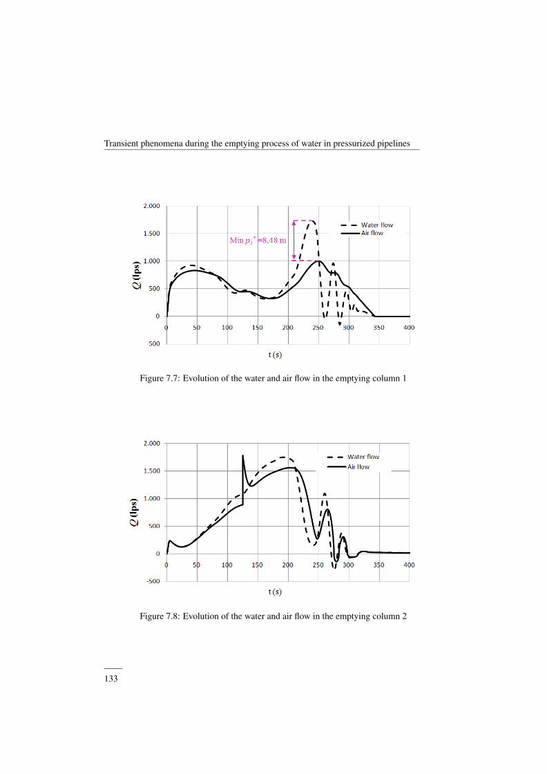
Transient phenomena during the emptying process of water in pressurized pipelines
Figure 7.7: Evolution of the water and air flow in the emptying column 1
Figure 7.8: Evolution of the water and air flow in the emptying column 2
——133
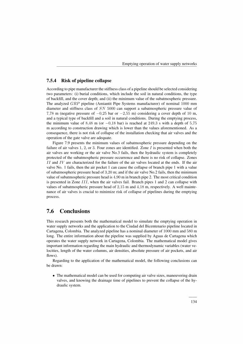
Emptying operation of water supply networks
7.5.4 Risk of pipeline collapse
According to pipe manufacturer the stiffness class of a pipeline should be selected consideringtwo parameters: (i) burial conditions, which include the soil in natural conditions, the typeof backfill, and the cover depth; and (ii) the minimum value of the subatmospheric pressure.The analyzed GRP pipeline (Amiantit Pipe Systems manufacturer) of nominal 1000 mmdiameter and stiffness class of SN 5000 can support a subatmospheric pressure value of7,78 m (negative pressure of −0,25 bar or −2,55 m) considering a cover depth of 10 m,and a typical type of backfill and a soil in natural conditions. During the emptying process,the minimum value of 8,48 m (or −0,18 bar) is reached at 249,3 s with a depth of 5,75m according to construction drawing which is lower than the values aforementioned. As aconsequence, there is not risk of collapse of the installation checking that air valves and theoperation of the gate valve are adequate.
Figure 7.9 presents the minimum values of subatmospheric pressure depending on thefailure of air valves 1, 2, or 3. Four zones are identified. Zone I is presented when both theair valves are working or the air valve No.3 fails, then the hydraulic system is completelyprotected of the subatmospheric pressure occurrence and there is no risk of collapse. ZonesII and IV are characterized for the failure of the air valves located at the ends. If the airvalve No. 1 fails, then the air pocket 1 can cause the collapse of branch pipe 1 with a valueof subatmospheric pressure head of 3,20 m; and if the air valve No.2 fails, then the minimumvalue of subatmospheric pressure head is 4,90 m in branch pipe 2. The most critical conditionis presented in Zone III , when the air valves fail. Branch pipes 1 and 2 can collapse withvalues of subatmospheric pressure head of 2,15 m and 4,18 m, respectively. A well mainte-nance of air valves is crucial to minimize risk of collapse of pipelines during the emptyingprocess.
7.6 Conclusions
This research presents both the mathematical model to simulate the emptying operation inwater supply networks and the application to the Ciudad del Bicentenario pipeline located inCartagena, Colombia. The analyzed pipeline has a nominal diameter of 1000 mm and 580 mlong. The entire information about the pipeline was supplied by Aguas de Cartagena whichoperates the water supply network in Cartagena, Colombia. The mathematical model givesimportant information regarding the main hydraulic and thermodynamic variables (water ve-locities, length of the water columns, air densities, absolute pressure of air pockets, and airflows).
Regarding to the application of the mathematical model, the following conclusions canbe drawn:
• The mathematical model can be used for computing air valve sizes, maneuvering drainvalves, and knowing the drainage time of pipelines to prevent the collapse of the hy-draulic system.
——134
Transient phenomena during the emptying process of water in pressurized pipelines
Figure 7.9: Sensitivity analysis regarding to the failure of air valves
• The minimum value of subatmospheric pressure is one of the most critical situationsduring the emptying process which is adequately predicted by the mathematical model.
• Air valves should be selected appropriately along of pipe systems admitting the re-quired air to avoid subatmospheric pressure conditions. If air valves have not beenwell sized, then extreme negative pressures are reached which can produce the col-lapse of pipe systems. The mathematical model can be used to check the air valvesbehavior during the emptying maneuvers in actual installations.
• The Ciudad del Bicentenario pipeline can resist the minimum value of subatmosphericpressure showing there is no risk of collapse since the total volume of admitted air issimilar to the volume of drained water. Both air valve sizes and the maneuver of thegate valve were adequately designed, so can be used to empty the pipeline without riskof collapse. Annual maintenance is required for the air valves located at the ends ofthe installation since a failure of these devices can produce the collapse of branch pipesaccording to the sensitivity analysis.
• Horizontal branches in pipelines are not recommended because part of the water col-umn can remain inside of the installation and free surface flow is presented, generatinga slow drainage of the system.
This research only analyzed the risk of pipeline collapse during the emptying process.However, others sources of subatmospheric pressure occurrence should be analyzed (e.gpumps’ stoppages).
——135
Emptying operation of water supply networks
NotationA cross-sectional area of pipe (m2);Aadm cross sectional area of the air valves (m2);Cadm inflow discharge coefficient of the air valves (–);D internal pipe diameter (m);f friction factor (–);g gravity acceleration (m/s2);Le,1 and Le,2 length of the emptying columns 1 and 2, respectively (m);L1 and L2 total length of the pipes 1 and 2, respectively (m);Li,j branch length i, j (m);k polytropic coefficient (–);p∗1 and p∗2 absolute pressure of the air pockets 1 and 2, respectively (Pa);p∗atm atmospheric pressure (Pa);R gas constant (J/kg/◦K);Rv resistance coefficient of the gate valve (s2/m5);t time (s);Ta absolute temperature of the air (◦K)Qa,nc,1, Qa,nc,2, and Qa,nc,3 admitted air flow by air valves 1, 2, and 3, respectively (m3/s);vw,1 and vw,2 water velocity of the emptying columns 1 and 2, respectively (m/s);ρa,1 and ρa,2 air density of the air pockets 1 and 2, respectively (kg/m3);ρa,nc air density in normal conditions (kg/m3);ρw water density (kg/m3);∆ze,1 and ∆ze,2 difference elevation of the water columns 1 and 2, respectively;θi,j branch slope i, j
——136
Chapter 8
Discussion
This chapter presents the doctoral thesis discussion. All the objectives established have beenaddressed to allow a better understanding of the transient phenomenon of a water emptyingpipeline by considering different situations (without and with air valves).
The mathematical model can give information of the emptying processes, specificallyabout: (i) the main hydraulic and thermodynamic variables such as water flow, length ofthe water column, air absolute pressure, air density, and air flow; (ii) the risk of pipelinescollapse, by checking if the stiffness class (supply by a pipe manufacturer) is appropriateto support the minimum value of subatmospheric pressure depending on the type of soil innatural conditions, the type of backfill, and the cover depth; (iii) the appropriate selectionof air valves; (iv) the planning size and maneuver of drain valves; and (v) the estimation ofdrainage time of a pipeline.
Figure 8.1 is a flowchart that compiles information about the research stages and theproposed objectives. It also shows the interrelation among the objectives and how they wereaddressed in each chapter. All chapters of this document are based on papers that were writtenand then published as a result of the progress of this research study.
137
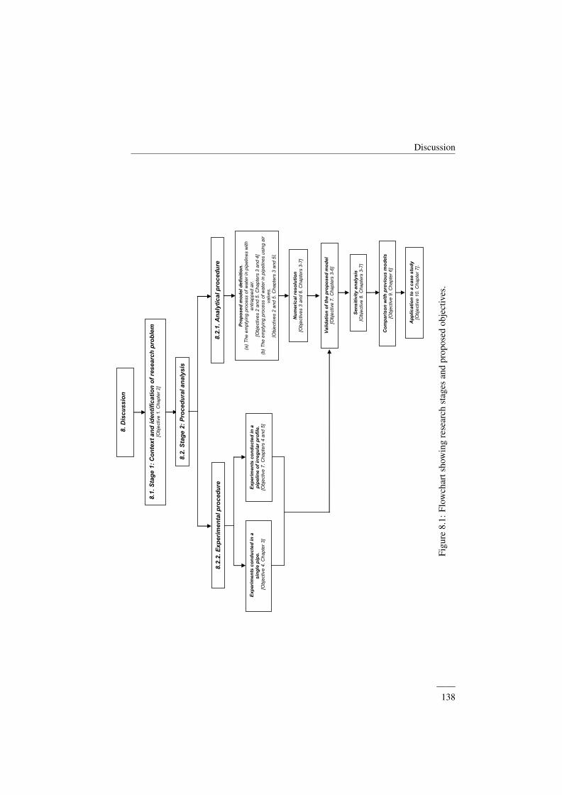
Discussion
8.
Dis
cu
ss
ion
8.1
.S
tag
e 1
: C
on
tex
t a
nd
id
en
tifi
ca
tio
n o
f re
se
arc
h p
rob
lem
[O
bje
ctive
1.
Cha
pte
r 2
]
8.2
. S
tag
e 2
: P
roc
ed
ura
l a
na
lys
is
8.2
.2.
Ex
pe
rim
en
tal p
roc
ed
ure
8.2
.1.
An
aly
tic
al p
roc
ed
ure
Exp
eri
me
nts
co
nd
ucte
d i
n a
sin
gle
pip
e.
[Obje
ctive 4
. C
hap
ter
3]
Exp
eri
men
ts c
on
du
cte
d in
ap
ipeli
ne
of
irre
gu
lar
pro
file
.[O
bje
ctive
7.
Cha
pte
rs 4
and
5]
Pro
po
se
dm
od
el
de
fin
itio
n.
(a)
The
em
pty
ing p
rocess o
f w
ate
r in
pip
elin
es
with
entr
ap
pe
d a
ir.
[Obje
ctive
s2
an
d 5
. C
hapte
rs 3
an
d 4
] (b
) T
he
em
pty
ing p
rocess o
f w
ate
r in
pip
elin
es
usin
g a
ir
valv
es.
[Obje
ctive
s 2
an
d5
. C
hapte
rs 3
an
d 5
].
Nu
meri
cal re
so
luti
on
[Obje
ctive
s3 a
nd 6
. C
hapte
rs 3
-7]
Valid
ati
on
of
the p
rop
ose
d m
od
el
[Obje
ctive
7.
Cha
pte
rs3-6
]
Sen
sit
ivit
y a
naly
sis
[Obje
ctive
8.
Cha
pte
rs 3
-7]
Ap
plic
ati
on
to
a c
as
e s
tud
y[O
bje
ctive
10
. C
hap
ter
7].
Co
mp
ari
so
n w
ith
pre
vio
us m
od
els
[Obje
ctive
9.
Cha
pte
r6]
Figu
re8.
1:Fl
owch
arts
how
ing
rese
arch
stag
esan
dpr
opos
edob
ject
ives
.
——138
Transient phenomena during the emptying process of water in pressurized pipelines
The flowchart presents two research stages: (i) the Stage 1 (8.1 Context and identificationof the research problem) contains a background of transient flow with trapped air in pressur-ized systems showing that there is a lack of knowledge related to transient phenomena duringa water emptying pipeline in practical applications; and (ii) the Stage 2 (8.2 Procedural anal-ysis) encompasses the development of a mathematical model to predict an emptying processin pressurized pipelines, which is divided in two parts (Point 8.2.1 Analytical procedure andPoint 8.2.2 Experimental procedure).
8.1 Context and identification of the research problemA literature review was conducted to detect a lack of knowledge regarding transient flow withtrapped air in water supply networks, as shown in Chapter 2 (Fuertes-Miquel et al., 2018a).In this sense, none mathematical model has been developed to predict the main hydraulic andthermodynamic variables during emptying operations in water pipelines. Commonly, theseoperations are performed based on experiences of technical personal, where slow maneuversare executed to avoid dangerous troughs of subatmospheric pressure. Air valves are installedalong of water pipelines to prevent subamospheric pressure occurrence following typical rec-ommendations suggested by AWWA (2001) or manufacturers. The lack of knowledge aboutemptying operations is identified in Chapter 2 and it is described on submitted paper:
Hydraulic modeling during filling and emptying processes in pressurized pipelines: Aliterature review
Coauthors: Fuertes-Miquel, V. S; Coronado-Hernandez O. E; Mora-Melia, D; Iglesias-ReyP. L..
Journal: Urban Water Journal ISSN 1573-062X.2017 Impact Factor: 2.744. Position JCR 17/90 (Q1). Water Resources.
State: Accepted with revisions. January 2019.
To develop a reliable mathematical model to simulate emptying operations in water pipelines,the literature review covered some topics:
1. Filling and emptying procedures: filling operations have been studied by several re-searchers (Cabrera et al., 1992; Zhou et al., 2011b; Izquierdo et al., 1999; Fuertes-Miquel et al., 2018b) knowing the behavior under different situations; however, beforethis research there were not mathematical models based on physical formulations topredict emptying operations in water pipelines.
2. Mathematical models: both hydraulic (water) and thermodynamic (air) formulationswere analyzed in transient flow with trapped air in order to get a robust model to predictemptying operations.
——139
Discussion
3. Methods of resolution: different methods were analyzed to solve transient flow withtrapped air in order to select an adequate technique to simulate a rigid water columnmodel to study the emptying process in pressurized pipelines.
4. Uncertainty of current models: many sources of uncertainties were identified. How-ever, a constant friction factor and polytropic coefficient were considered to analyzeemptying operations based on a literature review. On the other hand, air pocket sizeswere measured during experiments in transparent pipes.
5. Design considerations: air valves selection and stiffness class need to be designed ap-propriately in real pipelines to avoid a pipe collapse. During experiments these condi-tions were checked to prevent a collapse of the two experimental facilities.
8.2 Procedural stage
This stage was divided in two parts: (i) an analytical stage where the implementation ofthe mathematical model to simulate a water emptying pipeline was established; and (ii) anexperimental stage, which contains information about the two used experimental facilities tovalidate the proposed model.
8.2.1 Analytical stage
Proposed model definition
It is of great importance to explain each one of equations of the proposed model (Coronado-Hernandez et al., 2018b). The mathematical model is based on physical equations showing itsrobustness to predict an emptying process in real pipelines. The proposed model can be usedconsidering different conditions, such as: (i) situation No. 1 describes the condition when airvalves have been installed along of pipelines, which represents the more reliability situation toprotect hydraulic systems regarding to subatmospheric pressure occurrence (Fuertes-Miquelet al., 2017a); (ii) situation No. 2 describes a condition of not admitting air into pipelines,which can be produced when both air valves have failed due to maintenance problems orthey have not been installed (Fuertes-Miquel et al., 2017b); (iii) situation No. 3 correspondsto the scenario for a downstream total rupture, where the greatest trough of subatmosphericpressure is attained; and (iv) situation No. 4 corresponds to an operation and a condition ofdrain valves (types of maneuvers, a free surface discharge or a submerged discharge).
Initially, equations to predict an emptying procedure were established for a single pipeline,which is the simplest installation (Coronado-Hernandez et al., 2016). Two cases were ana-lyzed in Chapter 3: (i) a single pipe with the upstream end closed; and (ii) a single pipe withan air valve installed in the upstream end. After that, equations were expanded to a pipelineof irregular profile considering two cases: (i) a pipeline without air valves which representsthe worse case due to causing the lowest troughs of subatmospheric pressure (see Chapter 4),
——140
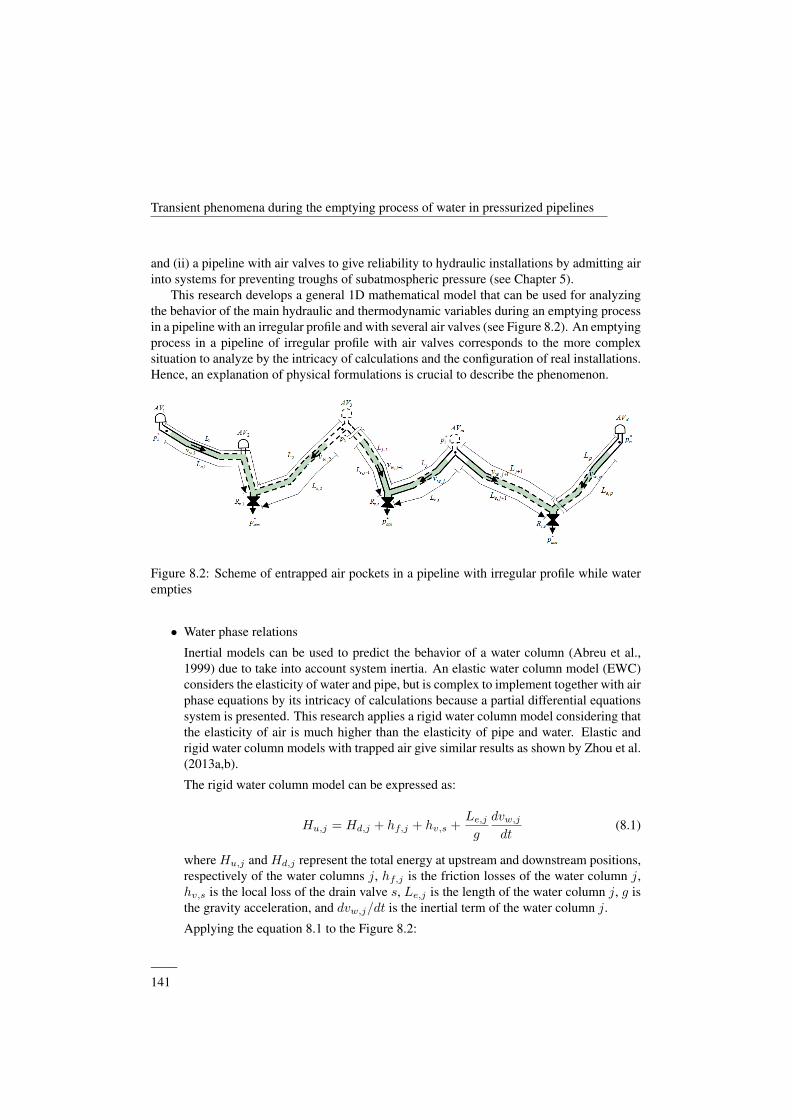
Transient phenomena during the emptying process of water in pressurized pipelines
and (ii) a pipeline with air valves to give reliability to hydraulic installations by admitting airinto systems for preventing troughs of subatmospheric pressure (see Chapter 5).
This research develops a general 1D mathematical model that can be used for analyzingthe behavior of the main hydraulic and thermodynamic variables during an emptying processin a pipeline with an irregular profile and with several air valves (see Figure 8.2). An emptyingprocess in a pipeline of irregular profile with air valves corresponds to the more complexsituation to analyze by the intricacy of calculations and the configuration of real installations.Hence, an explanation of physical formulations is crucial to describe the phenomenon.
Figure 8.2: Scheme of entrapped air pockets in a pipeline with irregular profile while waterempties
• Water phase relations
Inertial models can be used to predict the behavior of a water column (Abreu et al.,1999) due to take into account system inertia. An elastic water column model (EWC)considers the elasticity of water and pipe, but is complex to implement together with airphase equations by its intricacy of calculations because a partial differential equationssystem is presented. This research applies a rigid water column model considering thatthe elasticity of air is much higher than the elasticity of pipe and water. Elastic andrigid water column models with trapped air give similar results as shown by Zhou et al.(2013a,b).
The rigid water column model can be expressed as:
Hu,j = Hd,j + hf,j + hv,s +Le,j
g
dvw,j
dt(8.1)
where Hu,j and Hd,j represent the total energy at upstream and downstream positions,respectively of the water columns j, hf,j is the friction losses of the water column j,hv,s is the local loss of the drain valve s, Le,j is the length of the water column j, g isthe gravity acceleration, and dvw,j/dt is the inertial term of the water column j.
Applying the equation 8.1 to the Figure 8.2:
——141
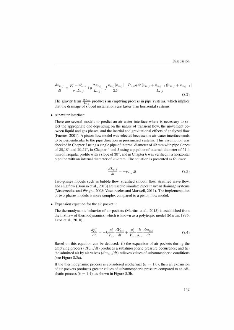
Discussion
dvw,j
dt=p∗i − p∗atmρwLe,j
+g∆ze,jLe,j
−f vw,j |vw,j |2D
−Rv,sgA2(vw,j + vw,j−1)|vw,j + vw,j−1|
Le,j
(8.2)
The gravity term ∆ze,jLe,j
produces an emptying process in pipe systems, which impliesthat the drainage of sloped installations are faster than horizontal systems.
• Air-water interface:
There are several models to predict an air-water interface where is necessary to se-lect the appropriate one depending on the nature of transient flow, the movement be-tween liquid and gas phases, and the inertial and gravitational effects of analyzed flow(Fuertes, 2001). A piston flow model was selected because the air-water interface tendsto be perpendicular to the pipe direction in pressurized systems. This assumption waschecked in Chapter 3 using a single pipe of internal diameter of 42 mm with pipe slopesof 26,18◦ and 29,51◦, in Chapter 4 and 5 using a pipeline of internal diameter of 51,4mm of irregular profile with a slope of 30◦, and in Chapter 6 was verified in a horizontalpipeline with an internal diameter of 232 mm. The equation is presented as follows:
dLe,j
dt= −vw,jdt (8.3)
Two-phases models such as bubble flow, stratified smooth flow, stratified wave flow,and slug flow (Bousso et al., 2013) are used to simulate pipes in urban drainage systems(Vasconcelos and Wright, 2008; Vasconcelos and Marwell, 2011). The implementationof two-phases models is more complex compared to a piston flow model.
• Expansion equation for the air pocket i:
The thermodynamic behavior of air pockets (Martins et al., 2015) is established fromthe first law of thermodynamics, which is known as a polytropic model (Martin, 1976;Leon et al., 2010).
dp∗idt
= −k p∗iVa,i
dVa,idt
+p∗iVa,i
k
ρa,i
dma,i
dt(8.4)
Based on this equation can be deduced: (i) the expansion of air pockets during theemptying process (dVa,i/dt) produces a subatmospheric pressure occurrence; and (ii)the admitted air by air valves (dma,i/dt) relieves values of subatmospheric conditions(see Figure 8.3a).
If the thermodynamic process is considered isothermal (k = 1,0), then an expansionof air pockets produces greater values of subatmospheric pressure compared to an adi-abatic process (k = 1,4), as shown in Figure 8.3b.
——142
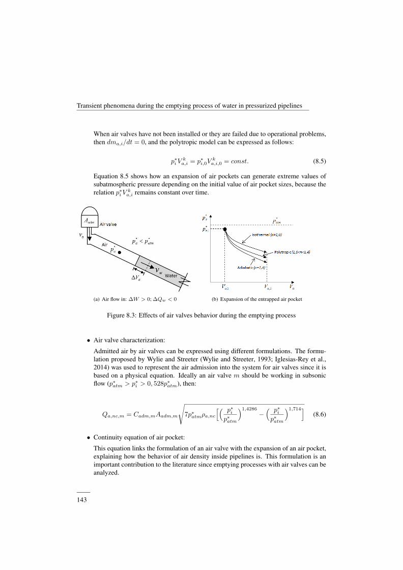
Transient phenomena during the emptying process of water in pressurized pipelines
When air valves have not been installed or they are failed due to operational problems,then dma,i/dt = 0, and the polytropic model can be expressed as follows:
p∗i Vka,i = p∗i,0V
ka,i,0 = const. (8.5)
Equation 8.5 shows how an expansion of air pockets can generate extreme values ofsubatmospheric pressure depending on the initial value of air pocket sizes, because therelation p∗i V
ka,i remains constant over time.
(a) Air flow in: ∆W > 0; ∆Qw < 0 (b) Expansion of the entrapped air pocket
Figure 8.3: Effects of air valves behavior during the emptying process
• Air valve characterization:
Admitted air by air valves can be expressed using different formulations. The formu-lation proposed by Wylie and Streeter (Wylie and Streeter, 1993; Iglesias-Rey et al.,2014) was used to represent the air admission into the system for air valves since it isbased on a physical equation. Ideally an air valve m should be working in subsonicflow (p∗atm > p∗i > 0, 528p∗atm), then:
Qa,nc,m = Cadm,mAadm,m
√7p∗atmρa,nc
[( p∗ip∗atm
)1,4286
−( p∗ip∗atm
)1,714](8.6)
• Continuity equation of air pocket:
This equation links the formulation of an air valve with the expansion of an air pocket,explaining how the behavior of air density inside pipelines is. This formulation is animportant contribution to the literature since emptying processes with air valves can beanalyzed.
——143
Discussion
This equation was developed from the continuity equation of an air pocket.
dρa,idt
=ρa,ncva,nc,mAadm,m − (vw,j+1 + vw,j)Aρa,i
A(Lj − Le,j + Lj+1 − Le,j+1)(8.7)
Numerical resolution
The resolution was conducted using the Simulink Library of Matlab. Simulations showed agreat fit compared to experimental data, which confirms the adequacy of the used solver inMatlab. The resolution was performed using the method ODE23s, which is supported on amodified Rosenbrock formula of order 2. The resolution method was used from Chapters 3to 7. Figure 8.4 shows the executed code to simulate an emptying process in pipe systemsconsidering the case of a single pipe with the upstream end closed (see Chapter 3). Formu-lations of the rigid water column model, the polytropic model and the the air-water interfaceequation are presented.
Validation of the proposed model
The validation of the proposed model was performed in two experimental facilities. Basedon the results, formulations to predict a water emptying pipeline were validated.
Initially, the validation was conducted in a single pipeline located at the hydraulic labo-ratory at the Universitat Politecnica de Valencia (Valencia, Spain). Figure 8.5 presents howthe proposed model predicts adequately the experimental data for two cases (see Chapter 3).Case No. 1 corresponds to a single pipe with the upstream end closed, where the followingformulations were tested: a rigid water column model (equation 8.2), a piston flow model torepresent an air-water interface (equation 8.3), and a polytropic model of an air pocket (equa-tion 8.5); and Case No. 2 represents a single pipe with an air valve installed on the upstreamend, where the air phase is described by the polytropic model with admitted air (equation8.4), the air valve characterization (equation 8.6), and the continuity equation of an air pocket(equation 8.7).
Results are described on published paper:
Transient phenomena during the emptying process of a single pipe with water-airinteraction
Coauthors: Fuertes-Miquel, V. S; Coronado-Hernandez O. E; Iglesias-Rey P. L.;Mora-Melia, D.
Journal: Journal of Hydraulic Research ISSN 0022-16862017 Impact Factor: 2.076. Position JCR 41/128 (Q2). Civil Engineering
State: Published. Latest Articles. 2018; DOI: 10.1080/00221686.2018.1492465
——144

Transient phenomena during the emptying process of water in pressurized pipelines
(a) Overview - Parameters, constants and initial conditions (b) Code of the rigid water column equation
(c) Code of the polytropic model (d) Code of the air-water interface equation
Figure 8.4: Executed code in Simulink Library of Matlab
——145
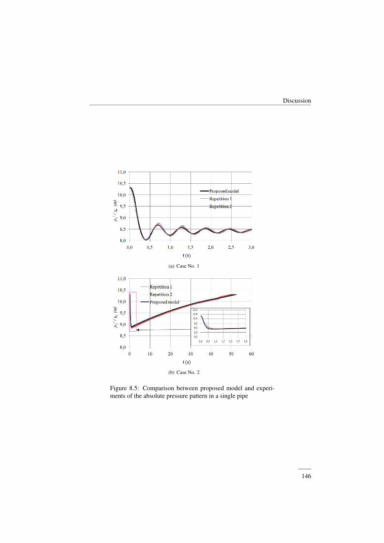
Discussion
(a) Case No. 1
(b) Case No. 2
Figure 8.5: Comparison between proposed model and experi-ments of the absolute pressure pattern in a single pipe
——146
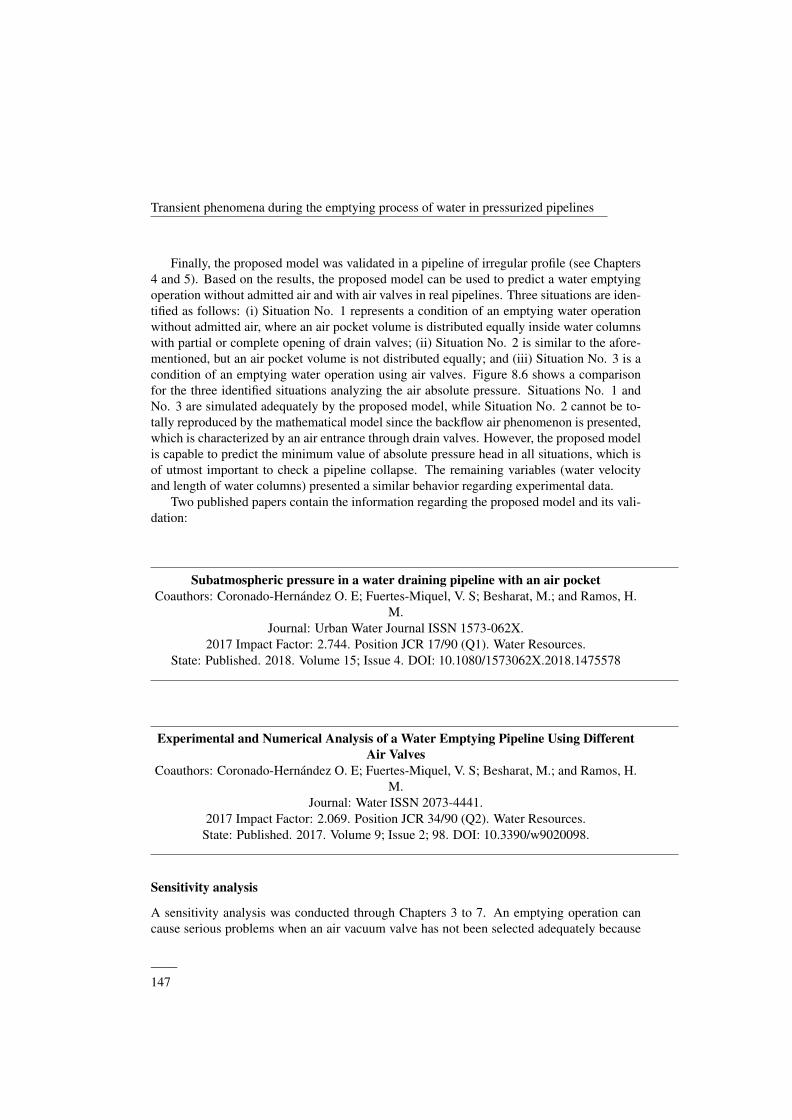
Transient phenomena during the emptying process of water in pressurized pipelines
Finally, the proposed model was validated in a pipeline of irregular profile (see Chapters4 and 5). Based on the results, the proposed model can be used to predict a water emptyingoperation without admitted air and with air valves in real pipelines. Three situations are iden-tified as follows: (i) Situation No. 1 represents a condition of an emptying water operationwithout admitted air, where an air pocket volume is distributed equally inside water columnswith partial or complete opening of drain valves; (ii) Situation No. 2 is similar to the afore-mentioned, but an air pocket volume is not distributed equally; and (iii) Situation No. 3 is acondition of an emptying water operation using air valves. Figure 8.6 shows a comparisonfor the three identified situations analyzing the air absolute pressure. Situations No. 1 andNo. 3 are simulated adequately by the proposed model, while Situation No. 2 cannot be to-tally reproduced by the mathematical model since the backflow air phenomenon is presented,which is characterized by an air entrance through drain valves. However, the proposed modelis capable to predict the minimum value of absolute pressure head in all situations, which isof utmost important to check a pipeline collapse. The remaining variables (water velocityand length of water columns) presented a similar behavior regarding experimental data.
Two published papers contain the information regarding the proposed model and its vali-dation:
Subatmospheric pressure in a water draining pipeline with an air pocketCoauthors: Coronado-Hernandez O. E; Fuertes-Miquel, V. S; Besharat, M.; and Ramos, H.
M.Journal: Urban Water Journal ISSN 1573-062X.
2017 Impact Factor: 2.744. Position JCR 17/90 (Q1). Water Resources.State: Published. 2018. Volume 15; Issue 4. DOI: 10.1080/1573062X.2018.1475578
Experimental and Numerical Analysis of a Water Emptying Pipeline Using DifferentAir Valves
Coauthors: Coronado-Hernandez O. E; Fuertes-Miquel, V. S; Besharat, M.; and Ramos, H.M.
Journal: Water ISSN 2073-4441.2017 Impact Factor: 2.069. Position JCR 34/90 (Q2). Water Resources.
State: Published. 2017. Volume 9; Issue 2; 98. DOI: 10.3390/w9020098.
Sensitivity analysis
A sensitivity analysis was conducted through Chapters 3 to 7. An emptying operation cancause serious problems when an air vacuum valve has not been selected adequately because
——147
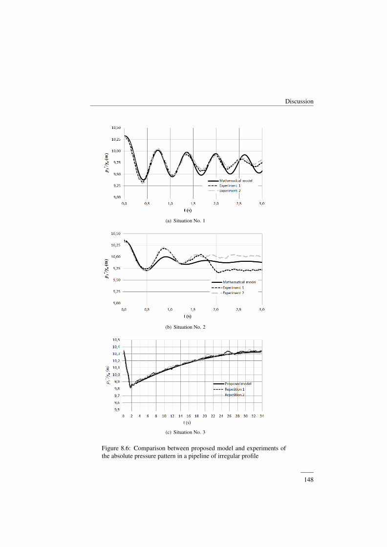
Discussion
(a) Situation No. 1
(b) Situation No. 2
(c) Situation No. 3
Figure 8.6: Comparison between proposed model and experiments ofthe absolute pressure pattern in a pipeline of irregular profile
——148
Transient phenomena during the emptying process of water in pressurized pipelines
troughs of subatmospheric pressure are reached. The most significant parameters during theoperation are air valve size, air pocket size, pipe slope, and internal pipe diameter. Frictionfactor and polytropic coefficient produce a despicable effect during the operation (Coronado-Hernandez et al., 2017c);. Each hydraulic system should be analyzed by engineers since anexpansion of air pockets can produce problems to the pipe system and its devices. Hence,the application of the mathematical model is crucial. It is recommended to perform emptyingoperations with slow maneuvers in valves in order to guarantee subsonic conditions in airvalves to prevent extreme values of the absolute pressure. Water velocity also should becontrolled according to technical manuals to avoid a system failure.
Comparison with previous models
This section presents a comparison between the proposed model and previous models. Twoprevious models were considered: a CFD 2D model, which is used in research to know thewater behavior in complex situation; and a semi-empirical model (Tijsseling et al., 2016),which was used as a first approximation to predict a water emptying operation.
Proposed model vs. CFD model
The proposed model is a physically based 1D model because it uses thermodynamicequations of air pockets and hydraulic formulations of water phase; while, a CFD modelsimulates the transient phenomenon using the law of mass conservation, Newton’s second lawand law of energy conservation. In this sense, both models represent adequately the behaviorof the emptying process in pressurized pipelines. To compare results the experimental facilityof a single pipeline (see Chapter 3) was used analyzing the scenario without admitted air.
The proposed model can simulate rapidly the emptying procedure compared to a CFDmodel. As a consequence, the proposed model is more appropriate to use in practical appli-cations. A CFD model permits to simulate the backflow air phenomenon, but this situationrarely occurs in real hydraulic systems. Figure 8.7 presents a comparison between the pro-posed model and a 2D CFD model in the two used experimental facilities, where initial andboundary conditions were identical. The comparison shows how both models are adequateto simulate an emptying procedure in pressurized pipelines. Appendix A shows all consider-ations using a 2D CFD model.
Proposed model vs. semi-empirical model
Tijsseling et al. (2016) developed a semi-empirical model to simulate an emptying pro-cess in a pipeline using pressurized air. Experiments were conducted by Laanearu et al.(2012). In this section, a comparison is presented between the proposed model and the Tijs-seling’s model. Chapter 6 presents details of this hydraulic installation. Figure 8.8 presents acomparison of the water flow oscillation for runs 2 and 6 (see Chapter 6) between the resultsobtained by the proposed model and Tijsseling’s model. In all cases, the proposed model canreproduce the water flow oscillations better than Tijsseling’s model. Figure 8.8b shows that
——149
Discussion
Figure 8.7: Comparison between proposed model and CFD model of the absolute pressurepattern for Test No.2 of the single pipeline (see Chapter 3)
the model developed by Tijsseling et al. (2016) cannot adequately reproduce run 6 becausethe water flow oscillation is too low. Figure 8.9 shows a comparison of the gauge pressurealong the pipeline for run 4 at locations P1 (x = 1,55 m) and P9 (x = 252,76 m). Again, theproposed model can better predict the gauge pressure oscillations than the model developedby Tijsseling et al. (2016).
Results are presented on published paper:
Rigid Water Column Model for Simulating the Emptying Process in a Pipeline UsingPressurized Air
Coauthors: Coronado-Hernandez O. E; Fuertes-Miquel, V. S; Iglesias-Rey, P.L.;Martınez-Solano, F.J.
Journal: Journal of Hydraulic Engineering ISSN 0733-9429.2017 Impact Factor: 2.080. Position JCR 39/128 (Q2). Civil Engineering.
State: State: Published. 2018. Volume 144; Issue 4. DOI:10.1061/(ASCE)HY.1943-7900.0001446.
Application to a case study
One of the most important contribution is to apply the proposed model to a case study. In thissense, the Ciudad del Bicentenario pipeline located in Cartagena de Indias, Colombia, was
——150

Transient phenomena during the emptying process of water in pressurized pipelines
(a) Run 2
(b) Run 6
Figure 8.8: Comparison of the water flow oscillation pattern
——151
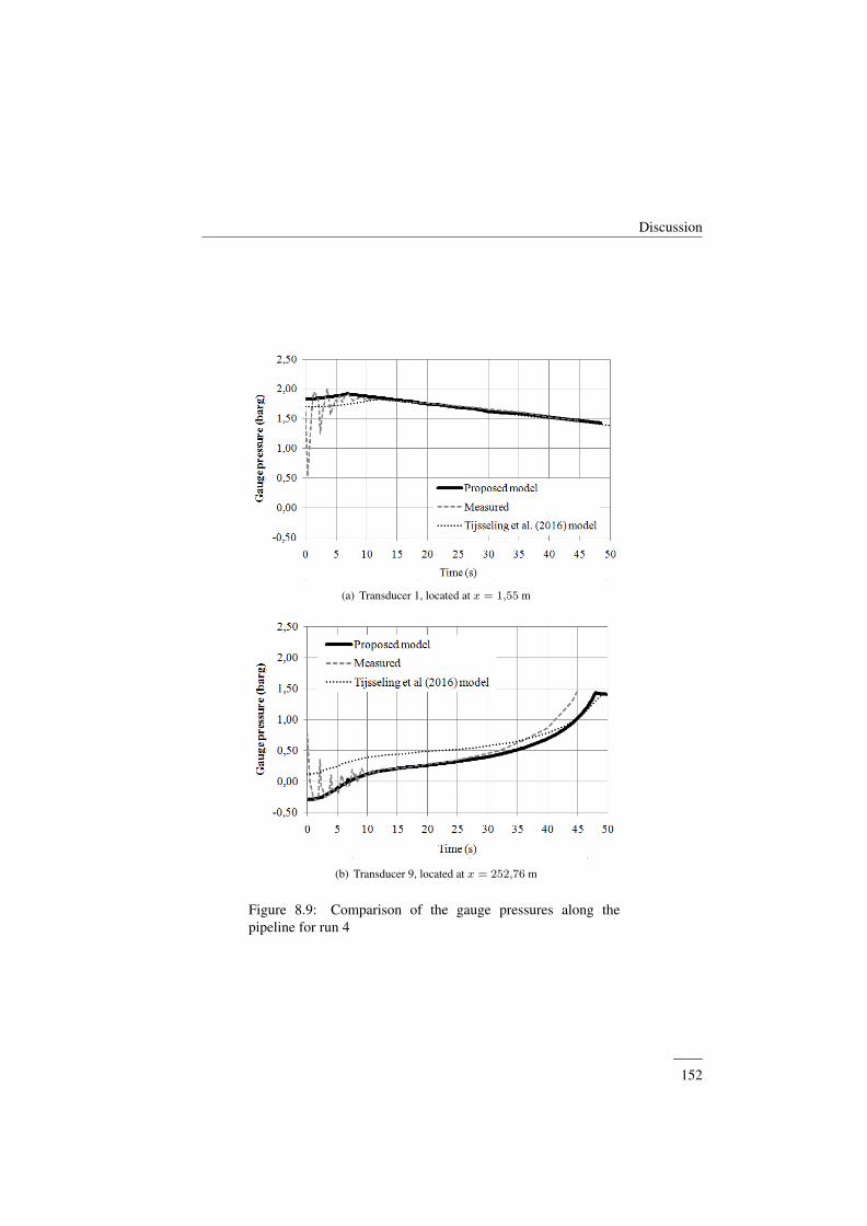
Discussion
(a) Transducer 1, located at x = 1,55 m
(b) Transducer 9, located at x = 252,76 m
Figure 8.9: Comparison of the gauge pressures along thepipeline for run 4
——152
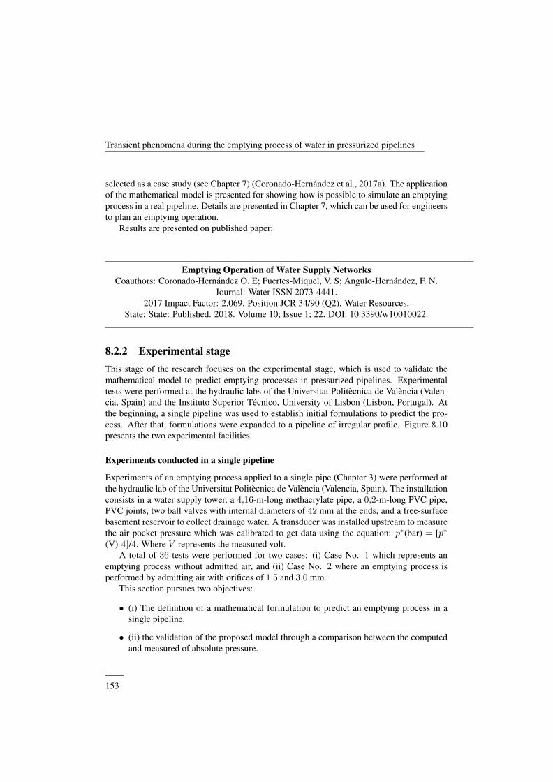
Transient phenomena during the emptying process of water in pressurized pipelines
selected as a case study (see Chapter 7) (Coronado-Hernandez et al., 2017a). The applicationof the mathematical model is presented for showing how is possible to simulate an emptyingprocess in a real pipeline. Details are presented in Chapter 7, which can be used for engineersto plan an emptying operation.
Results are presented on published paper:
Emptying Operation of Water Supply NetworksCoauthors: Coronado-Hernandez O. E; Fuertes-Miquel, V. S; Angulo-Hernandez, F. N.
Journal: Water ISSN 2073-4441.2017 Impact Factor: 2.069. Position JCR 34/90 (Q2). Water Resources.
State: State: Published. 2018. Volume 10; Issue 1; 22. DOI: 10.3390/w10010022.
8.2.2 Experimental stageThis stage of the research focuses on the experimental stage, which is used to validate themathematical model to predict emptying processes in pressurized pipelines. Experimentaltests were performed at the hydraulic labs of the Universitat Politecnica de Valencia (Valen-cia, Spain) and the Instituto Superior Tecnico, University of Lisbon (Lisbon, Portugal). Atthe beginning, a single pipeline was used to establish initial formulations to predict the pro-cess. After that, formulations were expanded to a pipeline of irregular profile. Figure 8.10presents the two experimental facilities.
Experiments conducted in a single pipeline
Experiments of an emptying process applied to a single pipe (Chapter 3) were performed atthe hydraulic lab of the Universitat Politecnica de Valencia (Valencia, Spain). The installationconsists in a water supply tower, a 4,16-m-long methacrylate pipe, a 0,2-m-long PVC pipe,PVC joints, two ball valves with internal diameters of 42 mm at the ends, and a free-surfacebasement reservoir to collect drainage water. A transducer was installed upstream to measurethe air pocket pressure which was calibrated to get data using the equation: p∗(bar) = [p∗
(V)-4]/4. Where V represents the measured volt.A total of 36 tests were performed for two cases: (i) Case No. 1 which represents an
emptying process without admitted air, and (ii) Case No. 2 where an emptying process isperformed by admitting air with orifices of 1,5 and 3,0 mm.
This section pursues two objectives:
• (i) The definition of a mathematical formulation to predict an emptying process in asingle pipeline.
• (ii) the validation of the proposed model through a comparison between the computedand measured of absolute pressure.
——153
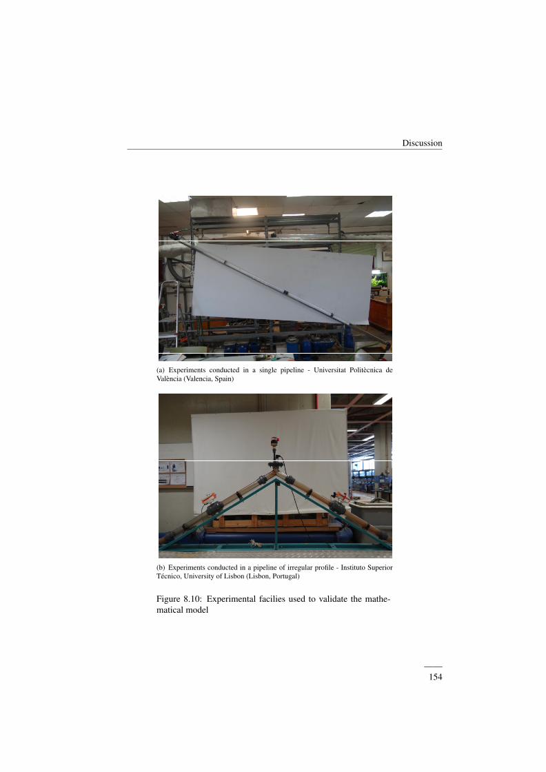
Discussion
(a) Experiments conducted in a single pipeline - Universitat Politecnica deValencia (Valencia, Spain)
(b) Experiments conducted in a pipeline of irregular profile - Instituto SuperiorTecnico, University of Lisbon (Lisbon, Portugal)
Figure 8.10: Experimental facilies used to validate the mathe-matical model
——154
Transient phenomena during the emptying process of water in pressurized pipelines
Experiments conducted in a pipeline of irregular profile
A second experimental facility was used to measure hydraulic and thermodynamic variablesconsidering the main objective of the research regarding to go deeply about transient flow ofan emptying process in a pipeline of irregular profile (Chapter 4 and 5). The used installationis located at the hydraulic lab at the Instituto Superior Tecnico, University of Lisbon (Lisbon,Portugal).
The used installation is composed by two PVC pipes with a total length of 7.3 m and anominal diameter of 63 mm. Two drain valves DV1 and DV2 are located at ends. Air valvesS050 and D040 of A.R.I. manufacturer were used to simulate the case No. 2 with admittedair.
The used instrumentation is described as follows: a WIKA transducer to measure the airpocket pressure located at the high point, an Ultrasonic Doppler Velocimetry (UDV) locatedat the horizontal PVC pipe with a transducer of 4 MHz frequency to measure the watervelocity, and a Sony Camera DSC-HX200V to measure the length of the water columns.
This section pursues three objectives:
• The complete definition of the proposed model using hydraulic and thermodynamicformulations.
• The analysis of more complex system which consists in a pipeline of irregular profilewith several pipe branches, various valves, and various air valves.
• Providing additional measurements not only air absolute pressure but also water veloc-ity and length of water column during an emptying process.
A total of 16 tests were performed for two cases: (i) Case No. 1 which corresponds to anemptying process in a water pipeline of irregular profile without admitted air, and (ii) CaseNo. 2 where an emptying pipeline process is performed by admitting air using air valvesS050 and D040 (A.R.I. manufacturer).
dddddddddddd
——155

Discussion
NotationA Cross sectional area of the pipe (m2)Aadm,m Cross section area of the air valve m (m2)Cadm,m Inflow discharge coefficient of the air valve m (–)D Internal pipe diameter (m)f Friction factor (–)g Gravity acceleration (m/s2)Hd,j Total energy at downstream of the water column j (m)Hu,j Total energy at upstream of the water column j (m)hf,j Friction loss of the water column j (m)hv,s Local loss of the drain valve s (m)k Polytropic coefficient (–)Le,j Length of the emptying column j (m)Lj Total length of the pipe j (m)ma,i Air mass of the air pocket i (kg)p∗i Absolute pressure of the air pocket i (Pa)p∗atm Atmospheric pressure (Pa)t Time (s)Qa,nc,m Air discharge in normal conditions admitted by the air valve m (m3/s)Rv,s Resistance coefficient of the drain valve s (s2/m5)Va,i Air volume of the air pocket i (m3)vw,j Water velocity of the emptying column j (m/s)∆ze,j Elevation difference (m)ρa,i Air density of the air pocket i (kg/m3)ρa,nc Air density in normal conditions (kg/m3)ρa Water density (kg/m3)Superscripts∗ Absolute valuesSubscriptsa Refers to airi Refers to air pocketj Refers to pipem Refers to air valvenc Normal conditionsw Refers to water0 Initial condition
——156
Chapter 9
Conclusions and recommendations
9.1 Main contributions
Entrapped air can be injected into water pipelines due to several situations, which can producemany problems because the elasticity of water and pipe is much lower than the elasticity ofthe air itself. This research focuses on the behavior of emptying maneuvers in water pipelineswhere air pockets are expanded during these operations producing values of subatmosphericpressure. Water pipelines should be emptied for maintenance, cleaning or repairs. Theseoperations are repeated periodically, and should be considered in the design stage to avoidfuture problems associated to pipeline collapse.
Commonly, water pipelines present an irregular profile (and elevations) depending on thetopography of the pipelines layout. Typically, air valves are chiefly located in high pointsand drain valves are usually located in low points. The emptying process starts when drainvalves are opened. This maneuver makes air valves start to admit air into pipelines, and thedrainage of water columns starts until pipes are completely emptied. However, if air valveshave not been installed or they have failed due to operational and maintenance problems, thenvalues of subatmospheric pressure can be reached. Air valves play a key role in making thepressure values not to drop drastically, which reduces the risk of having a pipeline collapse.Both situations (with and without air valves) have to be analyzed in order to optimize themaneuvers in pipelines during emptying operations. Understanding the transient flow in theemptying operation is crucial to evaluate subatmospheric pressure values, which, as previ-ously mentioned, can produce the collapse of hydraulic systems depending on installationconditions.
First of all, a literature review was conducted regarding the transient flow with trapped airto detect a lack of knowledge about transient phenomena in water supply networks.
Over recent decades, some of the topics involved in the transient phenomenon with twophases flow have been investigated. The cavitation phenomenon has been studied both know-ing the generation of vapor cavities into water (two phases flow) and how bubbles can change
157
Conclusions and recommendations
transient flow events. Also, the filling process in water supply networks has been analyzedby considering different scenarios and several devices. Despite these studies, there is a lackof detailed studies related to emptying processes in water pipelines. In this sense, this re-search investigates as deeply as possible about the analysis of transient phenomenon of awater emptying pipeline of irregular profile with several air pockets and various air valves.
The main contribution of this work is the development of a general one-dimensional (1D)mathematical model that can be used for analyzing the behavior of the main hydraulic andthermodynamic variables during emptying processes in pipelines of irregular profile. Further,the mathematical model can be used to both understand the performance of the process andcompute all variables involved . The mathematical model was validated in two experimentalfacilities: (i) using a single pipe at the Fluids Laboratory at the Universitat Politecnica deValencia (Valencia, Spain), and (ii) with a pipeline of irregular profile at the University ofLisbon (Lisbon, Portugal). Comparisons between computed and measured values of the mainvariables show that the mathematical model can predict accurately not only extreme values,but also their patterns. The mathematical model can be used by designers and engineers toanalyze emptying processes in real pipelines for different scenarios. Air absolute pressureis the main variable during emptying processes since the minimum value of subatmosphericpressure should be used to check the risk of pipelines collapse depending on the stiffnessclass recommended by manufacturer’s.
9.2 ConclusionsThe conclusions presented in this section are a compilation of the main conclusions presentedat the end of each of the chapter of this research.
Chapter 2: Hydraulic modeling during filling and emptying processes in pressurizedpipelines: A literature review
This chapter shows the main researches conducted about transient phenomena with en-trapped air pockets. The main conclusions are:
• Emptying processes in water pipelines have been studied by few authors. Probably dueto the intricacy of calculations and configurations of hydraulic systems, which allowsto make new contributions in this topic.
• The rigid water column model can be used adequately for simulating a transient phe-nomenon with entrapped air pockets considering that the elasticity of the air is muchhigher than the elasticity of both the water and the pipe. The greater the air pocketsize, the better results are obtained with the model. A piston flow model can be used tosimulate an air-water interface.
• Air pockets were modeled using thermodynamic formulations. In spite of its simplicity,the polytropic model represented adequately the behavior of entrapped air pockets. A
——158
Transient phenomena during the emptying process of water in pressurized pipelines
constant polytropic coefficient was used to simulate hydraulic events.
Chapter 3: Transient phenomena during the emptying process of a single pipe withwater-air interaction
This chapter presented the mathematical model to simulate the behavior of the emptyingprocess of a single pipe with an entrapped air pocket for two cases: (i) Case No.1 corre-sponded to the situation where there is no admitted air into the system; and (ii) Case No.2corresponded to the situation where an orifice size introduces air to relive drops of absolutepressure pattern. According to the results, the expansion of an entrapped air pocket producesvalues of subatmospheric pressure. The main conclusions are:
• The analysis of a transient flow during emptying processes of single pipelines can bemodeled using the proposed model. In Case No. 1 (a simple pipe with the upstream endclosed), the proposed model was reduced to a set of three equations, which provides theevolution of the three unknowns variables (vw, Le, and p∗1). In Case No. 2 (a simplepipe with an air valve installed in the upstream end), the mathematical model wasreduced to a set of five equations, which provides the evolution of the five unknownsvariables (vw, Le, p∗1, va,nc, and ρa).
• The mathematical model was validated in an experimental facility located at the Uni-versitat Politecnica de Valencia (Valencia, Spain). A comparison between computedand measured of absolute pressure was conducted showing how the proposed modelpredicted accurately the transient flow. The validation of transient flow equations topredict emptying processes in single pipelines is crucial to continue with the develop-ment of equations in water emptying pipelines of irregular profiles.
• Slow maneuvers in drain valves are recommended as much as possible so as to admitthe air required into the system.
Chapter 4: Subatmospheric pressure in a water draining pipeline with an air pocket
In this chapter a general 1D mathematical model was developed so that it can be used formodeling the emptying process of a pipeline of irregular profile without air valves. Measure-ments were conducted at the University of Lisbon (Lisbon, Portugal). A comparison betweenthe measurements and the mathematical model were made. The main conclusions are:
• The emptying process in water pipelines of irregular profile with k pipes and n air pock-ets without air admission generated a transient flow, which can be modeled through amathematical model with a set of 2k + n algebraic-differential equations. The resolu-tion of the system equations brings the evolution of the hydraulic and thermodynamicvariables such as absolute pressure, water velocity, and length of the water column.
• The mathematical model was validated in an experimental facility located at the Uni-versity of Lisbon (Lisbon, Portugal), where different situations were analyzed: (i) a
——159
Conclusions and recommendations
partial opening of drain valves with an air pocket volume distributed uniformly, (ii) atotal opening of the drain valves with an air pocket volume distributed uniformly, and(iii) a partial opening of the drain valves with an air pocket volume distributed non-uniform. The mathematical model predicted accurately the behavior both pattern andextreme values of air pocket pressure, water velocity, and length of the water columnfor the majority of the simulations.
• The backflow air phenomenon can occur during emptying processes without admittedair depending on an opening percentage of drain valves. The mathematical modelwas capable of predicting the lowest value of subatmospheric absolute pressure. Thephenomenon was able to minimize the subatmospheric pressure pattern by introducingair from down-stream to upstream.
• The mathematical model can be used to detect the risk of pipelines collapse in realpiping systems where air valves have not been installed or when they failed due tomaintenance and operational problems since the lowest value of the subatmosphericpressure was adequately represented.
Chapter 5: Experimental and numerical analysis of a water emptying pipeline usingdifferent air valves
The analysis of transient flow during emptying processes of pipelines of irregular profilewith n air pockets and d air valves was developed. The main conclusions are:
• The analysis of the transient flow of an irregular profile with n entrapped air pockets, ppipes, and d air valves can be simulated with the mathematical model which presents aset of 2p+2n+d algebraic-differential equations. The resolution gave information re-garding the main hydraulic variables (absolute pressure of air pocket, water velocities,air density of the air pockets, lengths o the emptying columns and air flow rates).
• The mathematical model with air valves was validated in an experimental facility lo-cated at the University of Lisbon (Lisbon, Portugal). A comparison between computedand measured of air pocket pressure, water velocity and length of water columns con-firmed that the mathematical model can be used to simulate the hydraulic event.
• Air valves are very important during emptying processes because they were able toreduce the values of subatmospheric pressure by introducing air into hydraulic instal-lations. The larger the orifice size of the air valve, the lowest values of subatmosphericpressures were obtained.
Chapter 6: Rigid water column model for simulating the emptying process in apipeline using pressurized air
This chapter was developed based on published experimental results obtained in a emp-tying process pipeline using pressurized air. The main conclusions are:
——160
Transient phenomena during the emptying process of water in pressurized pipelines
• The results obtained when comparing measured and computed values of water flowoscillations and gauge pressures confirmed that rigid water column model and pistonflow formulations can be used to simulate emptying operations.
• The mathematical model also represented adequately the behavior of the main hy-draulic variables considering different minor-loss coefficients.
• The mathematical model better predicted the behavior of emptying operations whencompared to semi-empirical models.
Chapter 7: Emptying operation of water supply networks
This chapter presented the application of the mathematical model to the case study oc-curred in the pipeline network of the neighborhood called Ciudad del Bicentenario located inCartagena de Indias (Colombia). All data was provided by Aguas de Cartagena (Acuacar).The main conclusions are:
• The mathematical model can be used to represent emptying processes in real pipelinesas presented in the referenced chapter.
• A pipeline collapse can be checked by comparing the minimum value of subatmo-spheric pressure with data supplied by any pipe manufacturer depending on installationconditions.
• Air valves behavior and drain valves maneuvers can be checked during emptying op-erations in full-scale pipeline networks.
9.3 Future developments
During the literature review process performed during this study, a lack of detailed studies onemptying processes in pipelines and engineering application was identified.
Future studies on emptying processes can address specific topics, such as:
• Improvements of the mathematical model: the behavior of a water column separationcannot be detected by the mathematical model, then some approximations can be con-ducted in this topic.
• Analysis of entrapped air pockets: according to the results obtained in this study, thepolytropic model reproduces adequately the behavior of entrapped air pockets intopipeline installations. This formulation is widely used considering its definition andsimplicity. In some situations the polytropic model cannot predict the behavior of anair pocket; therefore, a complex thermodynamic formulation can be applied.
——161
Conclusions and recommendations
• Evolution of the polytropic coefficient and the friction factor: the majority of the mod-els developed in this field considers both the polytropic coefficient and the frictionfactor a constant when analyzing hydraulic events. Unsteady coefficients can improvesimulations during emptying processes.
• Validity of a piston flow model: it considers an air-water interface perpendicular to thepipe direction, and its application depends mainly of the water velocity, the internalpipe diameter, and the pipe slope. Others two phases models can be used in morecomplex situations.
• Validity of a rigid water column model (RWCM): a RWCM could predict adequatelythe behavior of the water column during all experiments in this research. However, theapplication of an elastic water model (EWM) can be used to simulate emptying pro-cesses, which can give more information when using more complex hydraulic systems.
• Analysis in water distribution systems: this doctoral thesis focused on the analysis ofemptying processes of a single pipe and a pipeline of undulating profile. However,the analysis in water distribution systems was not studied. Then, researches can beconducted with new installations and layouts.
• The backflow air phenomenon cannot be simulated with the mathematical model sincethe admitted air, when draining the valves, needs to be addressed with additional for-mulations requiring new experiments. In this sense, a 2D CFD model could representmore accurately the backflow phenomenon, but it requires greater computing timescompared to the mathematical model.
It is also important to note that in pipelines operating in real conditions is practicallyimpossible to know the initial conditions of emptying processes with respect to air pocketsizes and their location. As a consequence, many engineers use recommendations of manualsand manufacturers to avoid the risk of pipelines collapse.
——162
Appendix A
CFD model for predictingemptying processes of water
This appendix focuses on a comparison between the mathematical model and a 2D CFDmodel showing results of air pocket pressure during emptying processes of water in the twoused experimental facilities (see Chapters 3 and 4). The improvement of computers andthe computational methods have urged researchers to use CFD models for their numericalcalculations to describe the beahvior of water column. Simulations using a 2D CFD wereperformed at the University of Lisbon by Besharat et al. (2018a,b).
A.1 Implementation of a 2D CFD model
Some considerations to implement a 2D CFD model were: (i) a 2D CFD simulation de-scribes adequately experimental results; (ii) an unstructured triangular mesh was considered;(iii) a sliding mesh zone was used to compute the movement of drain valves; (iv) the explicitvolume of fluid (VOF) multiphase model was considered using the enhanced wall treatment(EWT) feature for near-wall calculations; (v) the pressure implicit with the splitting of op-erators (PISO) method for coupling the pressure-velocity formulations was used; (vi) thespatial discretization was performed using a finite volume; (vii) the pressure staggering op-tion (PRESTO) discretization scheme is used for the pressure; (vii) drain valves actuationwas conducted using a user defined function (UDF) for the different opening percentages andvalve maneuvering times; and (vii) a time step of 0,001 s was used for all simulations. A com-plete description of the 2D CFD simulations is presented by Besharat et al. (2018a,b). Forboth pipe installations simulations were executed on a desktop computer: Intel(R) Core(TM)i7 − 4790K CPU @ 4.00 GHz, 4 Core(s), 8 Logical Processor(s) with an installed physicalmemory of 16 GB. The ANSYS Fluent R18.2 academic version was used to run simulations.
The two-equation k− ε was selected to perform simulations since it is capable to fix with
163
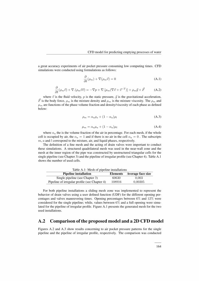
CFD model for predicting emptying processes of water
a great accuracy experiments of air pocket pressure consuming low computing times. CFDsimulations were conducted using formulations as follows:
∂
∂t(ρm) +∇(ρm~v) = 0 (A.1)
∂
∂t(ρm~v) +∇.(ρm~v~v) = −∇p+∇.[µm(∇~v + ~v−T )] + ρm~g + ~F (A.2)
where ~v is the fluid velocity, p is the static pressure, ~g is the gravitational acceleration,~F is the body force, ρm is the mixture density and µm is the mixture viscosity. The ρm andµm are functions of the phase volume fraction and density/viscosity of each phase as definedbelow:
ρm = αaρa + (1− αa)ρl (A.3)
µm = αaµa + (1− αa)µl (A.4)
where αa the is the volume fraction of the air in percentage. For each mesh, if the wholecell is occupied by air, the αa = 1 and if there is no air in the cell αa = 0 . The subscriptsm, a and l correspond to the mixture, air, and liquid phases, respectively.
The definition of a fine mesh and the acting of drain valves were important to conductthese simulations. A structured quadrilateral mesh was used in the near-wall zone and themesh at the inner region of the pipe was constructed by unstructured triangular cells for thesingle pipeline (see Chapter 3) and the pipeline of irregular profile (see Chapter 4). Table A.1shows the number of used cells.
Table A.1: Mesh of pipeline installationsPipeline installation Elements Average face size
Single pipeline (see Chapter 3) 60630 0,003Pipeline of irregular profile (see Chapter 4) 108916 0,00305
For both pipeline installations a sliding mesh zone was implemented to represent thebehavior of drain valves using a user defined function (UDF) for the different opening per-centages and valves maneuvering times. Opening percentages between 6% and 12% wereconsidered for the single pipeline; while, values between 6% and a full opening were simu-lated for the pipeline of irregular profile. Figure A.1 presents the generated mesh for the twoused installations.
A.2 Comparison of the proposed model and a 2D CFD modelFigures A.2 and A.3 show results concerning to air pocket pressure patterns for the singlepipeline and the pipeline of irregular profile, respectively. The comparison was conducted
——164

Transient phenomena during the emptying process of water in pressurized pipelines
(a) Single pipeline - Fully closeddrain valve
(b) Single pipeline - 10% opening
(c) Pipeline of irregular profile - 10% opening
(d) Pipeline of irregular profile - Fully closed drain valves
Figure A.1: The generated mesh in the pipe systems near drainvalves
——165
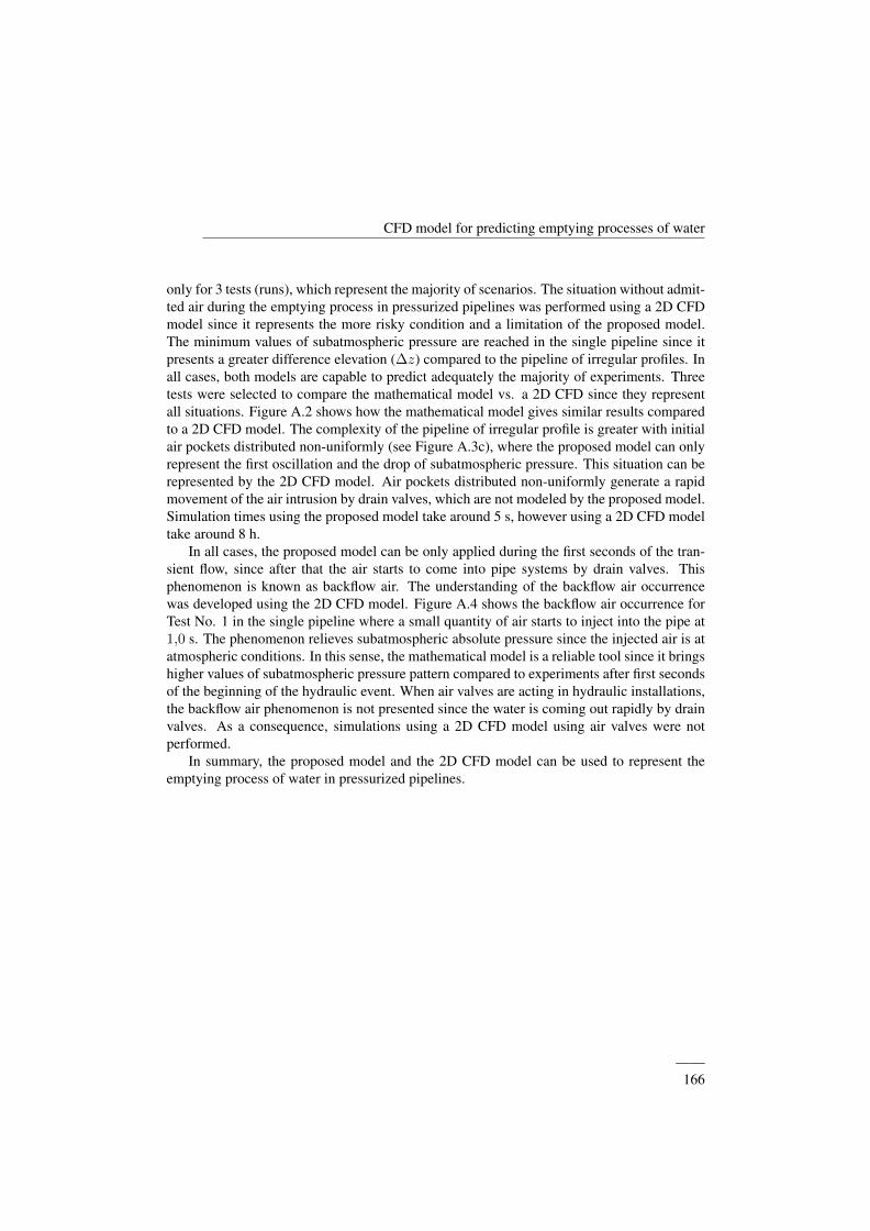
CFD model for predicting emptying processes of water
only for 3 tests (runs), which represent the majority of scenarios. The situation without admit-ted air during the emptying process in pressurized pipelines was performed using a 2D CFDmodel since it represents the more risky condition and a limitation of the proposed model.The minimum values of subatmospheric pressure are reached in the single pipeline since itpresents a greater difference elevation (∆z) compared to the pipeline of irregular profiles. Inall cases, both models are capable to predict adequately the majority of experiments. Threetests were selected to compare the mathematical model vs. a 2D CFD since they representall situations. Figure A.2 shows how the mathematical model gives similar results comparedto a 2D CFD model. The complexity of the pipeline of irregular profile is greater with initialair pockets distributed non-uniformly (see Figure A.3c), where the proposed model can onlyrepresent the first oscillation and the drop of subatmospheric pressure. This situation can berepresented by the 2D CFD model. Air pockets distributed non-uniformly generate a rapidmovement of the air intrusion by drain valves, which are not modeled by the proposed model.Simulation times using the proposed model take around 5 s, however using a 2D CFD modeltake around 8 h.
In all cases, the proposed model can be only applied during the first seconds of the tran-sient flow, since after that the air starts to come into pipe systems by drain valves. Thisphenomenon is known as backflow air. The understanding of the backflow air occurrencewas developed using the 2D CFD model. Figure A.4 shows the backflow air occurrence forTest No. 1 in the single pipeline where a small quantity of air starts to inject into the pipe at1,0 s. The phenomenon relieves subatmospheric absolute pressure since the injected air is atatmospheric conditions. In this sense, the mathematical model is a reliable tool since it bringshigher values of subatmospheric pressure pattern compared to experiments after first secondsof the beginning of the hydraulic event. When air valves are acting in hydraulic installations,the backflow air phenomenon is not presented since the water is coming out rapidly by drainvalves. As a consequence, simulations using a 2D CFD model using air valves were notperformed.
In summary, the proposed model and the 2D CFD model can be used to represent theemptying process of water in pressurized pipelines.
——166
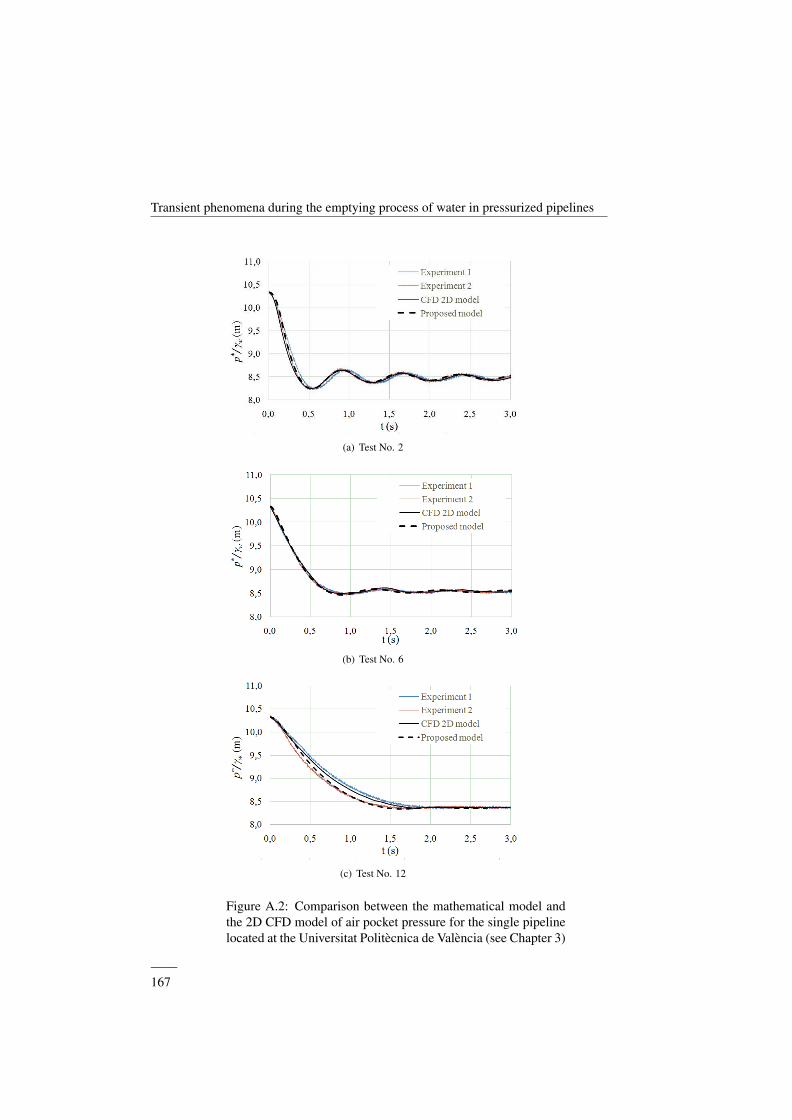
Transient phenomena during the emptying process of water in pressurized pipelines
(a) Test No. 2
(b) Test No. 6
(c) Test No. 12
Figure A.2: Comparison between the mathematical model andthe 2D CFD model of air pocket pressure for the single pipelinelocated at the Universitat Politecnica de Valencia (see Chapter 3)
——167
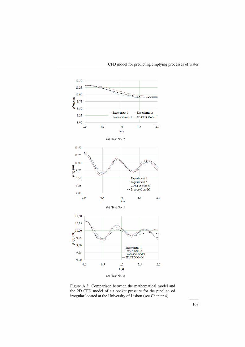
CFD model for predicting emptying processes of water
(a) Test No. 2
(b) Test No. 5
(c) Test No. 8
Figure A.3: Comparison between the mathematical model andthe 2D CFD model of air pocket pressure for the pipeline odirregular located at the University of Lisbon (see Chapter 4)
——168
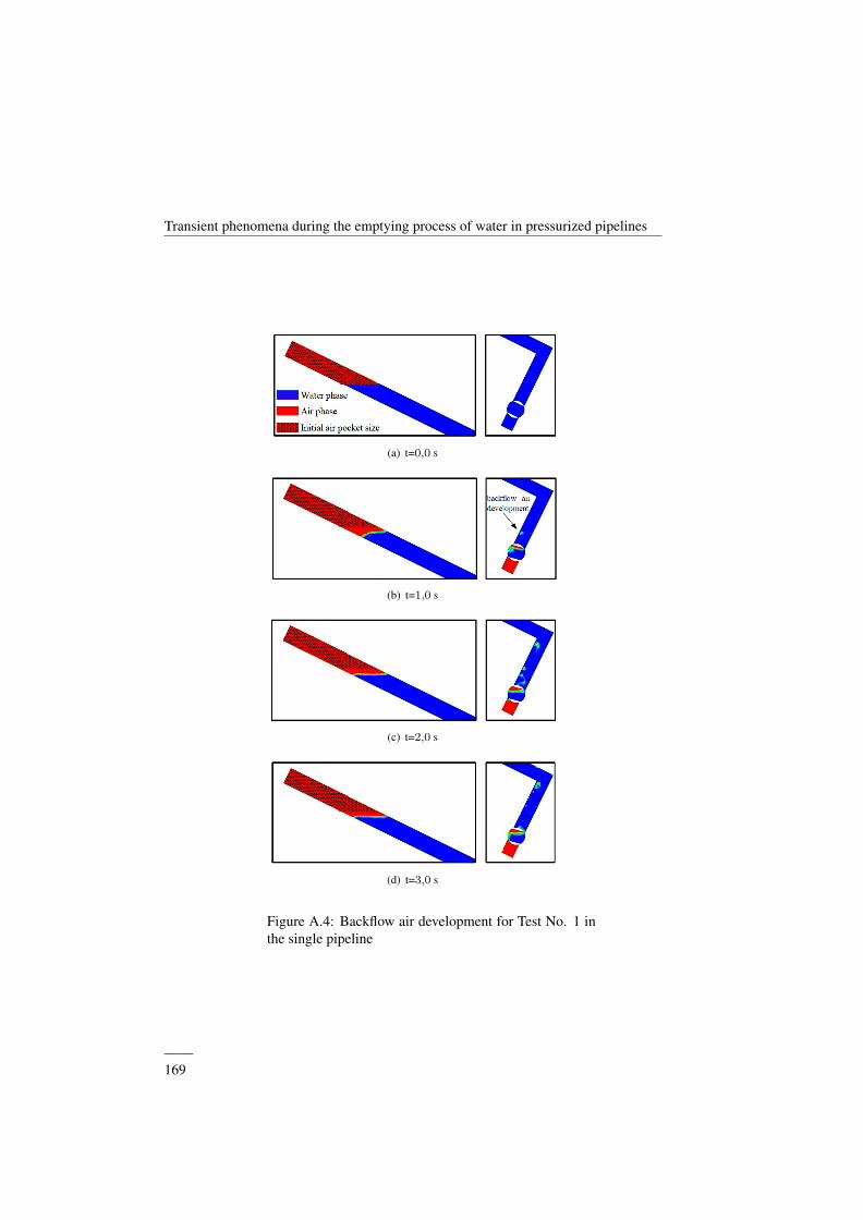
Transient phenomena during the emptying process of water in pressurized pipelines
(a) t=0,0 s
(b) t=1,0 s
(c) t=2,0 s
(d) t=3,0 s
Figure A.4: Backflow air development for Test No. 1 inthe single pipeline
——169

This page is intentionally left blank.
——170

Bibliography
Abreu, J., Cabrera, E., Izquierdo, J., and Garcıa-Serra, J. (1999). Flow modeling in pressur-ized systems revisited. Journal of Hydraulic Engineering, 125(11):1154–1169.
Aguas de Cartagena, G. T. (2013). Plano - conduccion agua potable ciudad del bicentenarioplanta-perfil k2+500.35 al k3+160.00.
Akpan, P. U., Yeung, H., Jones, S., Njoku, H., and Mgbemene, C. A. (2014). Mathematicalmodels of air vessels for pressure transient control in water pipelines - a review. Interna-tional Journal of Current Research, 6(2).
Apollonio, C., Balacco, G., Fontana, N., Giugni, M., Marini, G., and Piccinni, A. F. (2016).Hydraulic transients caused by air expulsion during rapid filling of undulating pipelines.Water, 8:1–12.
AWWA (2001). American Water Works Association (AWWA). Manual of water supply prac-ticesM51: Air-release, air-vacuum, and combination air valves. Denver, 1 st edition.
Baker, A. J. (1983). Finite Element Computational Fluid Mechanics. Ed. McGraw-Hill, NY,USA.
Balacco, G., Apollonio, C., and Piccinni, A. F. (2015). Experimental analysis of air valve be-haviour during hydraulic transients. Journal of Applied Water Engineering and Research,3(1):3–11.
Bergant, A., Simpson, A. R., and Tijsseling, A. S. (2006). Water hammer with columnseparation: A historical review. Journal of Fluids and Structures, 22:135–171.
Besharat, M., Coronado-Hernandez, O. E., Fuertes-Miquel, V. S., Viseu, M. T., and Ramos,H. M. (2018a). Backflow air and pressure analysis in emptying pipeline containing en-trapped air pocket. Urban Water Journal, 15(8).
Besharat, M., Coronado-Hernandez, O. E., Fuertes-Miquel, V. S., Viseu, M. T., and Ramos,H. M. (2018b). Computational fluid dynamics for sub-atmospheric pressure analysis inpipe drainage. Journal of Hydraulic Research, Submitted.
171
Besharat, M., Tarinejad, R., and Ramos, H. M. (2016). The effect of water hammer on a con-fined air pocket towards flow energy storage system. Journal of Water Supply: Researchand TechnologyAQUA, pages 116–126.
Bianchi, A., Mambretti, S., and Pianta, P. (2007). Practical formulas for the dimensioning ofair valves. Journal of Hydraulic Engineering, 133(10).
Bousso, S., Daynou, M., and Fuamba, M. (2013). Numerical modeling of mixed flows instorm water systems: Critical review of literature. Journal of Hydraulic Engineering,139(4):385–396.
Brunone, B., Golia, U. M., and Greco, M. (1991). Modeling of fast transients by numeri-cal methods. In Proc. of Hydrualic Transients with Water Column Separation, Valencia,IAHR,Spain.
Cabrera, E., Abreu, J., Perez, R., and Vela, A. (1992). Influence of liquid length variation inhydraulic transients. Journal of Hydraulic Research, 118(12):1639–1650.
Cabrera, E., Dolz, R., Izquierdo, J., Barbany, A., Onaindia, L., and Villaroel, J. (2008). Tran-sient analysis and waterhammer proteccion. a case study. Technical report, Eurostudios.Consulting Engineers., Madrid, Spain.
Carlos, M., Arregui, F. J., Cabrera, E., and Palau, C. V. (2011). Understanding air releasethrough air valves. Journal of Hydraulic Engineering, 137(4):461–469.
Chaudhry, M. H. (2014). Applied hydraulic transients. Springer, Columbia, SC, USA.
Chaudhry, M. H. and Reddy, H. P. (2011). Mathematical modeling of lake tap flows. Journalof Hydraulic Engineering, 137(5):611–614.
Coronado-Hernandez, O. E., Fuertes-Miquel, V. S., and Angulo-Hernandez, F. N. (2017a).Analysis of the draining operation in water supply networks. application to a water pipelinein cartagena de indias, colombia. In XV Seminario Iberoamericano de Redes de Agua yDrenaje, SEREA2017, Bogota, Colombia.
Coronado-Hernandez, O. E., Fuertes-Miquel, V. S., and Angulo-Hernandez, F. N. (2018a).Emptying operation of water supply networks. Water, 10(1)(22):1–11.
Coronado-Hernandez, O. E., Fuertes-Miquel, V. S., Besharat, M., and Ramos, H. M. (2017b).Experimental and numerical analysis of a water emptying pipeline using different airvalves. Water, 9(2)(98):1–15.
Coronado-Hernandez, O. E., Fuertes-Miquel, V. S., Besharat, M., and Ramos, H. M. (2018b).A parametric sensitivity analysis of numerically modelled piston-type filling and emptyingof an inclined pipeline with an air valve. In 13th International Conference on PressureSurges, pages 949–960.
——172
Transient phenomena during the emptying process of water in pressurized pipelines
Coronado-Hernandez, O. E., Fuertes-Miquel, V. S., Besharat, M., and Ramos, H. M. (2018c).Subatmospheric pressure in a water draining pipeline with an air pocket. Urban WaterJournal, 15(4):346–352.
Coronado-Hernandez, O. E., Fuertes-Miquel, V. S., Iglesias-Rey, P. L., and Martınez-Solano,F. J. (2018d). Rigid water column model for simulating the emptying process in a pipelineusing pressurized air. Journal of Hydraulic Engineering, 144(4).
Coronado-Hernandez, O. E., Fuertes-Miquel, V. S., Iglesias-Rey, P. L., and Mora-Melia, D.(2016). The analysis of transient flow during the emptying process in a single pipeline. InXXVII Congreso Latinoamericano de Hidraulica, IAHR, Lima, Peru, pages 1–8.
Coronado-Hernandez, O. E., Fuertes-Miquel, V. S., Iglesias-Rey, P. L., and Mora-Melia, D.(2017c). Sensitivity analysis of emptying processes in water supply networks. In V Jor-nadas de Ingenierıa del Agua, A Coruna, Spain.
Covas, D., Stoianov, I., Ramos, H. M., Graham, N., Maksimovic, C., and Butler, D. (2010).Water hammer in pressurized polyethylene pipes:conceptual model and experimental anal-ysis. Urban Water Journal, 1(2):177–197.
Cunge, J. A. and Wegner, M. (1964). Numerical integration of barre de saint-venants flowequations by means of implicit scheme of finite differences. Houille Blanche, 19(1):33–39.
De Paor, C., Kelliher, D., Cronin, K., Wright, W. M. D., and McSweeney, S. G. (2012).Prediction of vacuum-induced buckling pressures of thin-walled cylinders. Thin-WalledStructures, 55:1–10.
Escarameia, M. (2005). Air problems in pipelines: a design manual. HR Wallingford Ltd.
Espert, V., Cabrera, E., Martınez, F., Perez, R., and Vela, A. (1991). Air vessel collapse dueto a thermal change. a case study. In Hydraulic Transients with Water Column Separation- 9th and Last Round Table of the IARH Group, Valencia, Spain: IAHR.
Flowtite (2008). Product Guide - Amiantit Fiberglass Industries Limited (AFIL). Amiantit.
Fontana, N., Galdiero, E., and Giugni, M. (2016). Pressure surges caused by air release inwater pipelines. Journal of Hydraulic Research, 54(4).
Fuertes, V. S. (2001). Hydraulic transients with entrapped air pockets. PhD thesis, Depart-ment of Hydraulic Engineering, Polytechnic University of Valencia, Spain.
Fuertes-Miquel, V. S., Coronado-Hernandez, O. E., , Mora-Melia, D., and Iglesias-Rey,P. L. (2018a). Hydraulic modeling duirng filling and emptying processes in pressurizedpipelines: A literature review. Urban Water Journal, Submitted.
——173
Fuertes-Miquel, V. S., Coronado-Hernandez, O. E., Iglesias-Rey, P. L., and Martınez-Solano,F. J. (2017a). Behavior of a water-draining pipeline of irregular profile with air valves. InXV Seminario Iberoamericano de Redes de Agua y Drenaje, SEREA2017, Bogota, Colom-bia.
Fuertes-Miquel, V. S., Coronado-Hernandez, O. E., Iglesias-Rey, P. L., and Mora-Melia, D.(2018b). Transient phenomena during the emptying process of a single pipe with water-airinteraction. Journal of Hydraulic Research.
Fuertes-Miquel, V. S., Coronado-Hernandez, O. E., Mora-Melia, D., and Iglesias-Rey, P. L.(2017b). Negative pressure occurrence during the draining operation of water pipelineswith entrapped air. In XV Seminario Iberoamericano de Redes de Agua y Drenaje,SEREA2017, Bogota, Colombia.
Fuertes-Miquel, V. S., Lopez-Jimenez, P. A., Martınez-Solano, F. J., and Lopez-Patino, G.(2016). Numerical modelling of pipelines with air pockets and air valves. CanadianJournal of Civil Engineering, 43(12):1052–1061.
Garcıa-Todolı, S., Iglesias-Rey, P. L., Mora-Melia, D., Martınez-Solano, F. J., and Fuertes-Miquel, V. S. (2018). Computational determination of air valves capacity using cfd tech-niques. Water, 10(10).
Ghidaou, M. and Karney, B. W. (1994). Equivalent differential equations in fixed-grid char-acteristics method. Journal of Hydraulic Engineering, 120(10):1159–1175.
Graze, H. R., Megler, V., and Hartmann, S. (1996). Thermodynamic behaviour of entrappedair in an air chamber. In In A. P. Boldy (Ed.), Proceedings of the 7th International Con-ference on Pressure Surges and Fluid Transients in Pipelines and Open Channels, pages549–560.
Guinot, V. (2001). The discontinuous profile method for simulating two-phase flow in pipesusing the single component approximation. International Journal for Numerical Methodsin Fluids, 37(3):341–359.
Guinot, V. (2003). Godunov-type schemes: An introduction for engineers. Elsevier, Amster-dam, The Netherlands.
Hou, Q., Tijsseling, A., Laanearu, J., Annus, I., Koppel, T., Bergant, A., Vukovic, S., An-derson, A., and van t Westende, J. (2014). Experimental investigation on rapid filling of alarge-scale pipeline. Journal of Hydraulic Engineering, 140(11).
Hou, Q., Zhang, L., Tijsseling, A. S., and Kruisbrink, A. C. H. (2012). Rapid filling ofpipelines with the sph particle method. In Procedia Engineering, volume 31, pages 38–43.
Iglesias-Rey, P. L., Fuertes-Miquel, V. S., Garcıa-Mares, F. J., and Martınez-Solano, F. J.(2014). Comparative study of intake and exhaust air flows of different commercial air
——174
Transient phenomena during the emptying process of water in pressurized pipelines
valves. In 16th Conference on Water Distribution System Analysis, WDSA 2014, pages1412–1419.
Izquierdo, J., Fuertes, V. S., Cabrera, E., Iglesias, P., and Garcıa-Serra, J. (1999). Pipelinestart-up with entrapped air. Journal of Hydraulic Research, 37(5):579–590.
Laanearu, J., Annus, I., Koppel, T., Bergant, A., Vuckovic, S., Hou, Q., Tijsseling, A., An-derson, A., and Van’t Westende, J. (2012). Emptying of large-scale pipeline by pressurizedair. Journal of Hydraulic Engineering, 138(12):1090–1100.
Lee, N. H. (2005). Effect of pressurization and expulsion of entrapped air in pipelines. PhDthesis, School of Civil and Environmental Engineering, Georgia Institute of Technology,USA.
Leon, A., Ghidaoui, M., Schmidt, A., and Garcia, M. (2010). A robust two-equation modelfor transient-mixed flows. Journal of Hydraulic Research, 48(1):44–56.
Liou, C. and Hunt, W. A. (1996). Filling of pipelines with undulating elevation profiles.Journal of Hydraulic Engineering, 122(10):534–539.
Liu, D. Y., Zhou, L., Karney, B., Zhang, Q. F., and Ou, C. Q. (2011). Rigid-plug elastic watermodel for transient pipe flow with entrapped air pocket. Journal of Hydraulic Research,49(6):799–803.
Liu, J., Zhang, J., and Yu, X. (2018). Analytical and numerical investigation on the dynamiccharacteristics of entrapped air in a rapid filling pipe. Journal of Water Supply: Researchand Technology – AQUA, 67(2):137–146.
Malekpour, A. and Karney, B. (2014). Column separation and rejoinder during rapid pipelinefilling induced by a partial flow blockage. Journal of Hydraulic Research, 52(5):693–704.
Malekpour, A. and Karney, B. W. (2011). Rapid filling analysis of pipelines with undulatingprofiles by the method of characteristics. ISRN Applied Mathematics, 2011(Article ID930460):16.
Malekpour, A., Karney, B. W., and Nault, J. (2016). Physical understanding of sudden pres-surization of pipe systems with entrapped air: Energy auditing approach. Journal of Hy-draulic Engineering, 142(2).
Martin, C. S. (1976). Entrapped air in pipelines. In Proc. of the Second International Con-ference on Pressure Surges, London, England.
Martino, G., Fontana, N., and Giugni, M. (2001). Transient flow caused by air expulsionthrough an orifice. Journal of Hydraulic Engineering, 134(9):1395–1399.
Martins, N. M. C., Delgado, J. N., and Ramos, H. M. Covas, D. I. C. (2017). Maximum tran-sient pressures in a rapidly filling pipeline with entrapped air using a cfd model. Journalof Hydraulic Research, pages 1–14.
——175
Martins, N. M. C., Soares, A. K., Ramos, H. M., and Covas, D. I. C. (2016). Cfd modelingof transient flow in pressurized pipes. Computers & Fluids, 126:129–140.
Martins, S. C., Ramos, H. M., and Almeida, A. B. (2010a). Computational evaluation ofhydraulic system behaviour with entrapped air under rapid pressurization. In IntegratingWater Systems, pages 241–247.
Martins, S. C., Ramos, H. M., and Almeida, A. B. (2010b). Mathematical modeling of pres-surized system behaviour with entrapped air. In Environmental Hydraulics: Theoretical,Experimental and Computational Solutions, pages 61–64.
Martins, S. C., Ramos, H. M., and Almeida, A. B. (2010c). Mathematical modeling of pres-surized system behaviour with entrapped air. In Environmental Hydraulics: Theoretical,Experimental and Computational Solutions, pages 61–64.
Martins, S. C., Ramos, H. M., and Almeida, A. B. (2015). Conceptual analogy for modellingentrapped air action in hydraulic systems. Journal of Hydraulic Research, pages 678–686.
Mays, L. (1999). Hydraulic desing handbook. Ed. McGraw-Hill, New York, USA.
McInnis, D. A., Karney, B. W., and Axworthy, D. H. (1997). Efficient valve representationin fixed-grid characteristics method. Journal of Hydraulic Engineering, 123(8):709–718.
Pozos, O., Gonzalez, C., Giesecke, J., Marx, W., and Rodal, E. A. (2010). Air entrapped ingravity pipeline systems. Journal of Hydraulic Research, 48(3):338–347.
Pozos-Estrada, O., Sanchez-Huerta, A., Brena Naranjo, J., and Pedrozo-Acuna, A. (2016).Failure analysis of a water supply pumping pipeline system. Water, 8(9)(395).
Ramezani, L. and Karney, B. (2017). Water column separation and cavity collapse forpipelines protected with air vacuum valves: Understanding the essential wave process.Journal of Hydraulic Engineering, 143(12).
Ramezani, L., Karney, B., and Malekpour, A. (2015). The challenge of air valves: A selectivecritical literature review. Journal of Water Resources Planning and Management, 141(10).
Ramezani, L., Karney, B., and Malekpour, A. (2016). Encouraging effective air managementin water pipelines: A critical review. Journal of Water Resources Planning and Manage-ment, 142(12).
Saint-Gobain (2009). 612 Potable Water Double Orifice Air Valve. Pam.
Shimada, M., Brown, J. M. B., and Vardy, A. E. (2008). Interpolation errors in rectangularand diamond characteristic grids. Journal of Hydraulic Engineering, 134(10):1480–1490.
Stephenson, D. (1997). Effects of air valves and pipework on water hammer pressures. Jour-nal of Transportation Engineering, 123(2):101–106.
——176
Transient phenomena during the emptying process of water in pressurized pipelines
Tijsseling, A., Hou, Q., Bozkus, Z., and Laanearu, J. (2016). Improved one-dimensionalmodels for rapid emptying and filling of pipelines. Journal of Pressure Vessel Technology,138(3).
Tran, P. (2016). Pressure transients caused by air-valve closure while filling pipelines. Journalof Hydraulic Engineering, page Just Released.
Tullis, J. and Watkins, R. (1991). Pipe collapse caused by a pipe rupture - a case study. InHydraulic Transients with Water Column Separation - 9th and Last Round Table of theIARH Group, Valencia, Spain: IAHR.
Vasconcelos, J. G. and Marwell, D. T. (2011). Innovative simulation of unsteady low-pressureflows in water mains. Journal of Hydraulic Engineering, 137(11):1490–1499.
Vasconcelos, J. G. and Wright, S. J. (2008). Rapid flow startup in filled horizontal pipelines.Journal of Hydraulic Engineering, 134(7):984–992.
Wang, H., Zhou, L., Liu, D., Karney, B., Wang, P., Xia, L., Ma, J., , and Xu, C. (2016). Cfdapproach for column separation in water pipelines. Journal of Hydraulic Engineering, JustReleased.
Wang, K. H., Shen, Q., and Zhang, B. (2003). Modeling propagation of pressure surges withthe formation of an air pocket in pipelines. Computers & Fluids, 32(9):1179–1194.
Wang, L., Wang, F., Karney, B., and Malekpour, A. (2017). Numerical investigation of rapidfilling in bypass pipelines. Journal of Hydraulic Research, 0(0):1–10.
Wang, L., Wang, F., and Lei, X. (2018). Investigation on friction models for simulation ofpipeline filling transients. Journal of Hydraulic Research, (Article in Press).
Watt, C. S. (1975). Application of Finite Element Method to Unsteady Flow Problems. PhDthesis, Suntherland Polytechnic, England.
Wylie, E. and Streeter, V. (1993). Fluid transients in systems. Ed. Prentice Hall, EnglewoodCliffs, New Jersey, USA.
Yang, K. (2001). Practical method to prevent liquid-column separation. Journal of HydraulicEngineering, 127(7):620–623.
Zhou, F., Hicks, M., and Steffler, P. M. (2002). Transient flow in a rapidly filling horizontalpipe containing trapped air. Journal of Hydraulic Engineering, 128(6):625–634.
Zhou, L. and Liu, D. (2013). Experimental investigation of entrapped air pocket in a partiallyfull water pipe. Journal of Hydraulic Research, 51(4):469–474.
Zhou, L., Liu, D., and Karney, B. (2013a). Investigation of hydraulic transients of two en-trapped air pockets in a water pipeline. Journal of Hydraulic Engineering, 139(9):949–959.
——177
Zhou, L., Liu, D., and Karney, B. (2013b). Phenomenon of white mist in pipelinesrapidly filling with water with entrapped air pocket. Journal of Hydraulic Engineering,139(10):1041–1051.
Zhou, L., Liu, D., Karney, B., and Zhang, Q. (2011a). Influence of entrapped air pockets onhydraulic transients in water pipelines. Journal of Hydrualic Engineering, 137(12):1686–1692.
Zhou, L., Liu, D., and Ou, C. (2011b). Simulation of flow transients in a water filling pipecontaining entrapped air pocket with vof model. Engineering Applications of Computa-tional Fluid Mechanics, 5(1):127–140.
Zhou, L., Pan, T., Wang, H., Liu, D., and Wang, P. (2018a). Rapid air expulsion through anorifice in a vertical water pipe. Journal of Hydraulic Research, In Press.
Zhou, L., Wang, H., Karney, B., Liu, D., Wang, P., and Guo, S. (2018b). Dynamic behavior ofentrapped air pocket in a water filling pipeline. Journal of Hydraulic Engineering, 144(8).
——178