Transient Modeling of a Two Staged-Turbocharged

Medium-Speed Spark-Ignited Gas Engine

Anders Kanckos

Master’s thesis

Supervisor: Jesper Engström, Wärtsilä

Examinator: Prof. Margareta Björklund-Sänkiaho

Energy Technology, Vasa

Study programme in Chemical Engineering

Faculty of Science and Engineering

Åbo Akademi University

October 1, 2018

I

ABSTRAKT

Med den ökande mängden förnybara energikällor inom energiproduktion har det blivit

mera utmanande att bibehålla elnätets stabilitet. För att avlasta elnätet måste lasten

därför balanseras genom att kortsiktigt producera eller lagra energi. Jämfört med

traditionella dieseldrivna kraftverk är det bättre att använda flytande naturgas och

gaskraftverk för att lagra kemiskt bunden energi och producera el med mindre utsläpp.

För att naturgaskraftverk ska vara konkurrenskraftiga på en strikt reglerad marknad

måste de vara snabbstartade, reagera snabbt på variationer i effektbehovet samt vara

effektiva.

Syftet med det här arbetet var att utföra teoretiska beräkningar för styrningen av en

överstökiometrisk förbränning och effektuttaget för en gasmotor för att kunna simulera

motorns lastupptagningsförmåga då den körs vid ett konstant varvtal i olika

situationer. Huvudsyftet med dessa simuleringar var att producera realistiska data som

är jämförbara med en laborationsmotors prestanda samt att minska tiden det tar för

modellen att uppnå full lastkapacitet från basbelastning.

I denna avhandling har mjukvaran GT-SUITE använts för att bygga upp och simulera

motorn. Med mjukvaran har ett system byggts för att styra tändningen och

ventiltiderna baserat på flera kontrollparametrar. För att uppnå en realistisk prestanda

har Wiebe-funktioner använts för att justera förbränningen under

lastuppkörningsprocessen. För att sätta gränserna för motorns optimala

belastningshastighet har begränsande faktorer undersökts. Därtill har två funktioner

för att simulera motorknack applicerats i modellen. En annan begränsande faktor som

har simulerats i stor utsträckning är avgassystemets termiska kapacitet.

De simulerade resultaten visade sig vara jämförbara med laboratorietesterna, och den

optimerade belastningsrampen som producerades var över 60 % snabbare än den

referens som använts. Ytterligare försök gjordes för att öka förståelsen av hur effekten

vid olika gränsvillkor påverkar motorns prestanda. Framtida studier och förbättringar

kunde fokusera på att optimera motorknackmodellerna och förbränningsmodellen.

Nyckelord: överstökiometrisk förbränning, knack, förbränningsmodellering, Wiebe

II

ABSTRACT

Due to the increasing number of renewable energy sources available in energy

production, the power variability in the grid has increased as well, and to balance the

load, short-term power needs to either be produced or discharged for energy storages.

An efficient way to store chemical energy and produce power with less emission,

compared to traditional diesel power stations, is by using LNG and gas power plants.

For a natural gas power plant to be competitive in a strictly regulated market, it needs

to be fast-starting, responsive and efficient.

The objective of this work was to make a model of a lean-burn gas engine and to use

this model to simulate the engine in various ramp-type transient loading situations in

a constant speed operation. The main goal of these simulations was to produce realistic

loading performance and reduce the time it took for the engine to achieve full loading

capacity from a 10 % base load.

In this thesis GT-SUITE has been used to build and to simulate the engine. With the

software, a system has been built for controlling the ignition- and valve timing based

on several control parameters. For a realistic performance, Wiebe functions have been

used for adjusting the combustion during the loading process. To be able to find the

limitations of the optimum load rate the limiting factors of the engine have been

studied and two knock models using knock induction time integrals have been applied

to the model. Other limiting factors such as the thermal capacity of the exhaust system

have also been studied and simulated extensively.

The simulated results were comparable with laboratory tests and the optimized load

ramp produced was over 60 % faster than the reference ramp used. Additional

experiments were also performed to increase the understanding of how the effect of

boundary conditions affects the loading performance of the engine. Further work and

improvements of this study could focus on optimizing the knock models and the

combustion model.

Key words: lean-burn, knocking, combustion modeling, Wiebe

III

TABLE OF CONTENTS

ABSTRAKT ..................................................................................................................I

ABSTRACT ................................................................................................................ II

TABLE OF CONTENTS ........................................................................................... III

ACKNOWLEDGEMENTS ....................................................................................... VI

LIST OF SYMBOLS AND ABBREVIATIONS ..................................................... VII

1 INTODUCTION .................................................................................................. 1

1.1 Research Problem .......................................................................................... 2

1.2 Goal ................................................................................................................ 3

1.3 Scope and limitation ...................................................................................... 4

1.4 Methods ......................................................................................................... 5

2 THEORY .............................................................................................................. 6

2.1 About Wärtsilä ............................................................................................... 6

2.2 Wärtsilä 31 ..................................................................................................... 7

2.2.1 Emission Regulations ............................................................................. 9

2.3 Tools ............................................................................................................ 10

2.3.1 Gamma Technologies ........................................................................... 10

2.4 Combustion in Spark-Ignition Engines ....................................................... 12

2.5 Lean-Burn Combustion ............................................................................... 14

2.5.1 Miller Cycle .......................................................................................... 17

2.5.2 Ignition System and Spark Timing ....................................................... 20

2.5.3 Gas Admission and Pre-Chamber Combustion .................................... 21

2.6 Turbocharging .............................................................................................. 23

IV

2.6.1 Two-Stage Turbocharging .................................................................... 24

2.6.2 Control Strategy of Natural Gas Engines ............................................. 27

2.6.3 Thermal Load ....................................................................................... 29

2.7 Knocking Combustion ................................................................................. 30

2.7.1 Knock Definitions ................................................................................ 30

2.7.2 Conventional Knock ............................................................................. 32

2.7.3 Methods to Suppress Engine Knock .................................................... 33

2.7.4 Knock Detection Modeling .................................................................. 35

2.7.5 Knock Model for Lean-Burn Gas Engines ........................................... 37

2.7.6 Knock Modeling in GT-SUITE ............................................................ 38

2.8 Combustion Models ..................................................................................... 39

2.8.1 Three Pressure Analysis ....................................................................... 40

2.8.2 Spark-Ignition Wiebe Model ................................................................ 40

2.8.3 Multiple Wiebe Combustion Model ..................................................... 42

2.8.4 Spark-Ignited Turbulent Flame Combustion Model ............................ 42

3 MATERIAL AND METHODS ......................................................................... 44

3.1 Three Pressure Analysis Model ................................................................... 46

3.1 Steady-State Modeling ................................................................................. 48

3.2 Predictive Model .......................................................................................... 50

3.2.1 Measured and Predictive Combustion Analysis ................................... 51

3.2.2 Heat Release Based Calibration Model ................................................ 53

3.3 Semi-Predictive Models ............................................................................... 54

3.3.1 Wiebe Combustion Models .................................................................. 55

3.4 Engine Control and Automation .................................................................. 58

3.4.1 Test Automation ................................................................................... 60

V

3.4.2 Lookup Tables ...................................................................................... 63

3.5 Thermal Load Simulations .......................................................................... 65

3.6 Knock Models .............................................................................................. 68

3.6.1 Soylu and Van Grepen Knock Model .................................................. 68

3.6.2 Kinetics Fit Natural Gas Knock Model ................................................ 72

3.7 Transient Loading ........................................................................................ 75

3.7.1 Optimizing the Load Rate .................................................................... 75

3.7.2 Experiments with Boundary Conditions .............................................. 77

4 RESULTS ........................................................................................................... 80

4.1 The Final Transient Model .......................................................................... 81

4.2 Simulating the Burn Rate ............................................................................. 83

4.3 Knock Estimation ........................................................................................ 86

4.4 Sensitivity Analysis of the Thermal Capacity ............................................. 88

4.5 Optimized Load Rate ................................................................................... 90

4.6 Results from the Experiments ...................................................................... 92

4.7 New Automation Functionalities ................................................................. 97

5 DISCUSSION .................................................................................................... 99

6 CONCLUSIONS AND RECOMMENDATIONS ........................................... 103

SVENSK SAMMANFATTNING – SWEDISH SUMMARY ................................ 106

REFERENCES ......................................................................................................... 112

LIST OF APPENDICES .......................................................................................... 117

VI

ACKNOWLEDGEMENTS

This Master’s thesis was made in Vaasa for Wärtsilä Finland’s Product Performance

department from January to October 2018. I want to thank Wärtsilä for giving me the

opportunity of doing such an interesting and challenging thesis. I would also like to

thank Jesper Engström and Hannu Aatola and the rest of the Engine Performance

Expertise Team for all the help and support concerning engine performance and

modeling. The training I have received in GT-SUITE was of world class, and therefore

I would like to express my utmost gratitude to my supervisor Jesper Engström.

At Åbo Akademi University, I would also like to thank Professor Margareta

Björklund-Sänkiaho, head of the Energy Technology program in Vaasa, for the

valuable advice, comments and opinions along the way.

Furthermore, I would like to thank my family and friends for their support and patience

during my studies. Finally, I would like to thank my classmates and the other Master’s

thesis workers for keeping the spirit up.

Vaasa, October 1, 2018

Anders Kanckos

VII

LIST OF SYMBOLS AND ABBREVIATIONS

AA Anchor Angle

ABP Air Bypass

AFR Air-Fuel Ratio

AWG Air Wastegate

BD Burn Duration

BDC Bottom Dead Center

BMEP Break Mean Effective Pressure

CA° Crank Angle Degree

CAD Computer Aided Design

CAE Computer Aided Engineering

CFD Computational Fluid Dynamics

CO Carbon Monoxide

CO2 Carbon Dioxide

COV Coefficient of Variation

CR Compression Ratio

DOE Design of Experiments

ECU Engine Control Unit

EGR Exhaust Gas Recirculation

EPA Environmental Protection Agency

FEA Finite Element Analysis

GT Gamma Technologies

GUI Graphical User Interface

HFO Heavy Fuel Oil

HP High-Pressure

IMEP Indicated Mean Effective Pressure

IMO International Maritime Organization

ISE Integrated Simulation Environment

VIII

IVD Inlet Valve Dwell

KI Knock Index

LHV Lower Heating Value

LP Low-Pressure

M+P Measured and Predicted

MEPC Marine Environment Protection Committee

MN Methane Number

MON Motor Octane Number

MultiWiebe Multiple Wiebe Combustion Model

NG Natural Gas

NOx Nitrogen Oxide

PCC Pre-Combustion chamber

PID Proportional-Integral-Derivative

RLT Result

RMS Root-Mean-Square

RON Research Octane Number

SG Spark Gas

SI Spark-Ignition

SITurb Spark-Ignited Turbulent Flame Combustion Model

SOx Sulphur Oxide

ST Spark Timing

TA Luft Technische Anleitung zur Reinhaltung der Luft

TDC Top Dead Center

TPA Three Pressure Analysis

uHC Unburned Hydrocarbons

VVT Variable Valve Timing

1

1 INTODUCTION

As the population and industries continue growing in developing countries, the

demand for secure power increases as well. Renewables such as solar and wind cannot

solely be used due to the inconsistency in their power output and their demand on the

geographic settings. (Klimstra 2014) Four-stroke engines are an attractive solution for

balancing the power in the grid due to their fast response and the great power-density

of the four-stroke engine allowing them to be used both as power generation in cities

and in rural off-grid areas. Due to stricter engine emission regulations in many

countries, the more environmental-friendly natural gas (NG) engine has started to

replace traditional diesel engines. Lean-burn technology is an effective way to improve

fuel efficiency and reduce nitrogen oxide (NOx) emissions in NG engines. By running

a lean-burn engine on NG, carbon dioxide (CO2) emissions can be reduced by around

20 percent compared to running on heavy fuel oil (HFO), while the corresponding

reduction in NOx emissions is around 90 percent and sulphur oxide (SOx) emissions

and particulate emissions are almost eliminated. (MECA 2009)

Wärtsilä has developed a lean-burn NG engine of world class, the so-called Wärtsilä

31SG or W31SG. It is made for producing power with optimal efficiency while still

complying with the emission legislations. In this thesis, the transient loading capability

of W31SG will be studied, simulated and improved upon. From previous engine

development, a steady-state model has been made of this engine and has been used to

simulate the performance of the engine during constant loads. Simulating transient

loads is much more difficult, since the boundary conditions are ever-changing. This

was achieved by using a semi-predictive combustion model, which uses Wiebe

functions to describe the how the heat release changes with different air-fuel-ratio

(AFR). To be able to decrease the time for the engine to achieve full power output, the

limiting factors were studied and so-called knock-integrals were applied to predict

knocking combustion, which was the main limiting factor. The thermal load of the

exhaust system also needed to be modeled, since it was another factor limiting the

performance. This model was then validated against laboratory test data and was used

to perform different experiments, such as different load ramps and non-preheated

startups.

2

1.1 Research Problem

When an engine is run with constant speed and load within its optimum operation rage,

high thermal efficiency can be achieved. In case of transient loading it is hard to

produce power efficiently over the whole operation range, since the boundary

conditions keep on changing and components, such as turbochargers, need time to

spool up to get to its optimum operation range. In gas engines, the AFR needs to be

kept within a small range for the mixture to be able to ignite and burn fast enough to

produce an efficient combustion and yet uphold a very controlled manner to avoid

engine knocking or misfiring.

With the help of simulation software different loading strategies and functions can be

tested without the risk of damaging the real engine. Test engineers can then validate

the models to real engines, if they are showing good results. In this thesis different

load ramps will be tested, i.e. testing different ways of increasing the rate of output

power, so the maximum output can be reached fast without knocking or misfiring.

Figure 1 shows how a Wärtsilä power plant engine first gets up to speed from standstill

and thereafter how the output power starts to increase.

Figure 1: Load ramp from engine startup (Klimstra 2014)

0

20

40

60

80

100

NO

RM

ALI

ZED

RU

NN

ING

SP

EED

AN

D L

OA

D (

%)

TIME FROM START COMMAND (S)

Running speed Power output

ENGINE STARTUP

3

For a gas engine to be competitive and attractive for the market, there are certain grid

connection rules that the engine must meet and beat with marginal, to be better than

the competition. These grid connection rules or so-called grid codes, vary from

network to network and country to country, where ENTSO-E have drafted the rules

for Europe. Two of these categories that these simulations aim to improve upon are

the fast start loading rate and running loading rate. The fast start loading rate is defined

as the loading rate from hot standby conditions from no load to full load, i.e. the engine

is off, but all the fluids are preheated. The benchmark today is 5 minutes, but to be

able to compete with competitors the engine should be able to achieve full load even

faster. (ENTSO-E 2012)

The running loading rate is defined as the time it takes for the engine to go from

minimum load to full load when the engine has been operated for a predefined time.

To the current requirement according to ENTSO-E, the running loading rate should

achieve an increase in output of 10 % within 4 seconds, and this change of output

should be a sustained load ramp between minimum continuous load, in this case 10 %

load, to full output. Additionally, to this code the generating unit should also be able

to quickly and accurately react and adopt the output for frequency regulation.

(ENTSO-E 2012)

1.2 Goal

The goal of this research is to produce a model of a medium-speed gas engine for

simulations of transient loading, with the help of computer-aided simulation software.

The engine model should be able to produce realistic loading performance simulations,

where the data would be comparable to a real engine, during various ramp-type

transient loading situations in constant speed operation. The simulations should also

increase the understanding of how the effect of boundary conditions affects the loading

performance of the engine, such as different ambient conditions. Simulated load rates

should be validated against laboratory data and ultimately the model should be used to

find the optimum engine settings for the engine under different loading situations.

4

1.3 Scope and limitation

This is quite a big project for one thesis, therefore limitations have been made so that

the thesis can be done under a feasible time-schedule. For the engine model to react in

a similar manner to the real engine, the following things must be in the scope.

The combustion in the W31SG model should react to lambda, indicated mean effective

pressure (IMEP) and ignition timing, in the same way as the engine. Therefore, the

right combustion model must be chosen, so that test data from the real engine can be

used to simulate the combustion behavior of a spark-ignited gas engine with pre-

chamber. For the model to be able to estimate how fast the engine can be brought up

to full load, there must be some form of knock estimation. The knock estimation should

be able to tell when there is knock and preferable the scale of the oscillations. The

estimation could be done with a so-called knock integral or with compression and

temperature based sub-models. Thermal capacity also limits the engines loading

capacity, hence the thermal loading of the exhaust system must be realistically

modeled. The model also needs to be able to show the effects of different starting

temperatures. The final part of the project is to validate the simulations to certain real

loading situations and from there to recommend optimum engine settings and possibly

new automation functionalities.

The project is limited to one particular engine, the W10V31SG with its current

specifications. No new special measurements need to be done, e.g. thermal capacities

related to different engine parts and everything should be based on current test data.

The effect of different engine speed is also out of scope, and the same goes for step

loading, i.e. only transient load ramps with constant speed from 10-100 % load needs

to be validated, see figure 1. The model does not need to make emission estimations.

No new automation functionalities need to be modeled nor tested, they only need to

be recommended based on theory and the results from the simulations.

5

1.4 Methods

In this research, simulation software will be used to produce a model of a medium-

speed four-stroke two-stage turbocharged lean-burn gas engine. The model will be

built from a base model of the real gas engine used for steady-state performance

simulations, and will then converted to be able to perform transient load ramps under

different conditions. Heat release curves and performance maps for controlling the

engine will be made of real test data from the laboratory engine. Different combustion

models will be tested, both predictive and semi-predictive models, in order to find the

best one to simulate a gas engine with pre-chamber, in the case of transient loading.

Simulations will be performed on the model and parameters and multipliers will be

fitted until it behaves like the real engine when considering knocking combustion,

transient performance and thermal loading of the components.

Literature, internet and the in-house knowledge at Wärtsilä will be used for the theory

section and in order to choose the right combustion and knocking models. The theory

will mostly revolve around lean-burn gas engines, knocking and combustion

modeling. When the model is done it will be validated against real engine tests. New

test ramps will be tried out under different conditions, such as preheated and non-

preheated engine startup, and varying ambient conditions, such as cold outside

temperatures and high altitudes. The final part of the project will be to try to optimize

the models loading performance and suggest future improvement of the real engine.

6

2 THEORY

This part of the thesis contains the theory this master’s thesis is based on. First there

is an introduction to Wärtsilä and its new gas engine, the Wärtsilä 31SG, and then a

description of the modeling tools used for the simulation. The theory continues with

basic combustion engine knowledge and later discusses engine technology and finally

combustion phenomenons in detail.

2.1 About Wärtsilä

This master’s thesis is made for the Wärtsilä research and development department,

which is a part of the Wärtsilä concern. According to their homepage, Wärtsilä is a

global leader in smart technologies and complete lifecycle solutions for both marine

and energy markets. Wärtsilä maximizes the environmental and economic

performance of the vessels and power plants by emphasizing sustainable innovation,

total efficiency and data analytics. Wärtsilä’s net sales in 2017 were 4.9 billion euro

with approximately 18,000 employees and operations in over 200 locations in more

than 80 countries all around the world. The Wärtsilä concern is split in three major

divisions, Wärtsilä Marine Solutions, Wärtsilä Energy Solutions and Wärtsilä

Services. (Wärtsilä 2018)

Wärtsilä Marine Solutions is a leader both in the marine and the oil and gas industry,

providing customers with innovative products and integrated solutions. For all types

of vessels and offshore applications, Wärtsilä supplies engines and generating sets,

reduction gears, propulsion equipment, control systems, and sealing solutions. They

are also a leading supplier of power plants for the decentralized power generation

market. The power plants Wärtsilä offer, have a flexible design, high efficiency and

low emission levels, and are suitable for base load, peaking and industrial self-

generation operations for the oil and gas industry. (Wärtsilä 2018)

Wärtsilä Energy Solutions offer a broad range of environmentally sound solutions,

which includes ultra-flexible internal combustion engine based power plants, utility-

7

scale solar PV power plants, energy storage and integration solutions, as well as LNG

terminals and distribution systems. Wärtsilä had over 67 GW of installed power plant

capacity in 177 countries around the world at the end of 2017. (Wärtsilä 2018)

Wärtsilä Services provides high-quality services for its customers businesses,

throughout the lifecycle of their installations. Wärtsilä provides service, maintenance

and reconditioning solutions both for ship machinery and power plants. The solutions

range from spare parts and basic support for ensuring the maximized lifetime,

increased efficiency and guaranteed performance of the equipment. In parallel with its

main service operations Wärtsilä also has innovative new services that support its

customers’ business operations, such as service for multiple engine brands in key ports,

predictive and condition based maintenance and training. (Wärtsilä 2018)

2.2 Wärtsilä 31

One of Wärtsilä Marine Solutions many innovative products are the new Wärtsilä 31

engines. The Wärtsilä 31 engines are available in diesel, dual-fuel and pure gas models.

The laboratory engine, which was modeled in this thesis, was a W10V31SG genset,

which is a pure gas power generating engine. The letter and number combination in

the name comes from the manufacturer and engine specifications, where W stands for

Wärtsilä and 10V points out that it is a ten-cylinder engine in V-formation and SG

stands for the engines ignition method and fuel, which are spark-ignition and gas,

hence its name. The engine is also available from 8 to 20 cylinders configurations,

whose corresponding outputs range from 4.2 to 12 MW, at 720 and 750 rpm. They are

the first of a new generation of medium speed engines that are designed to set a new

benchmark in both efficiency and overall emissions performance. The most defining

feature of the Wärtsilä 31 engine, a feature that gained it a place in the Guinness World

Records, is its ability to reach efficiencies surpassing 50 percent, which made it the

world’s most efficient simple-cycle internal combustion engine. (Wärtsilä Engines

2017; Mäkinen & Jungner 2017)

8

The most critical advance in the new model, is the design of the engine structure, which

was made to accommodate two-stage turbocharging. The engine structure has a very

robust design that can hold the unparalleled break mean effective pressure (BMEP) of

almost 30 bar. While two-stage turbocharging have been on the market for quite some

time, there were no other existing engines designs that could take the advantage of its

full effect. No other engine could simply stand up to the loading and stress that results

from the step change in firing pressure.

Another major advantage of the Wärtsilä 31SG, is its flexibility. Which means in this

case, starting up quickly and maintaining high efficiency throughout the entire load

range. The W31SG can be continuously operated at 10 percent load and can reach full

capacity within two minutes from the start command. This is a crucial ability if you

want to stand out in today’s power generation landscape. The conventional power

generators’ role as base load is disappearing and the new role is to intermittently back

up the grid when the renewables output decreases. This is where the W31SG’s

flexibility dominates. The completely redesigned valve actuation method is a big

contributor to the engine’s increased flexibility. The new hydraulic valve system,

allows very smooth and precise control of valve timing, ensures that the AFR is

optimized at the all times. This gives the opportunity to take maximum advantage of

the boost provided by the two-stage turbocharging, specifically on partial loads.

Appendix 1 contains technical data about the engine geometry and performance.

(Mäkinen & Jungner 2017)

The advanced variable valve timing, injection system and second generation UNIC

control system, together with other optimized parameters, make the engine capable of

operating near its optimal running settings over the whole load spectrum. This vastly

improves the engines efficiency and lower emission levels under the IMO Tier III

regulations without additional installations. In 2.2.1 Emission Regulations, these terms

are explained further. (Mäkinen & Jungner 2017)

9

2.2.1 Emission Regulations

There are many regulations for emissions of stationary engines used in energy

production, both within countries, but also federal and regional regulations. The aim

of these regulations is to drive the emission levels incrementally lower while

increasing fuel efficiency in the future. Different laws and regulations controls the

emission levels of the lean-burn SI NG engine for operation both on land and on the

seas. At seas one of the most important regulations are maintained by the Marine

Environment Protection Committee (MEPC) of the International Maritime

Organization (IMO). The main purpose of the IMO is to ensure maritime safety and

promote control of the maritime pollution from ships inside the Emission Control

Areas (ECA). These IMO emission standards are often referred to as the MARPOL

Annex, which is also commonly called the Tier I, II and III standards. These Tier

standards are for monitoring the NOx emission levels at different engine speeds. The

Tier standards do not yet regulate any other emissions such as hydrocarbons and CO

to any big extent. Another important emission legislation is the Environmental

Protection Agency (EPA), which was founded and maintained by the US government.

(Duong et al. 2013)

The Wärtsilä 31 fulfills all current and anticipated IMO and EPA emission legislations

for marine applications. The engine also fulfills IMO Tier 3 and EPA Tier 3 without

any need for after-treatment in gas operation, supporting the clear trend towards the

increase of gas operated engines in the marine business on many segments. The

W31SG engine and other lean-burn NG engines are mostly used in power plant

applications. Technische Anleitung zur Reinhaltung der Luft, which translates into the

German TA Luft Air Pollution Regulation, limits the emissions of the lean-burn NG

engines. Unlike the IMO Tier standards, the TA Luft standard regulates other

emissions as well; in addition to the NOx emissions are also SOx, CO and hyrdocarbon

emissions regulated. Around the world, have the latest versions of the TA Luft

standard been applied to lean-burn NG power plants, and this is one of the strongest

driving forces for the development of future NG engines. In most of Europe the TA

Luft standard limit the NOx concentration in the NG engines emissions to 500 mg/Nm3.

(Åstrand et al, 2016; Duong et al. 2013)

10

2.3 Tools

In this thesis several tools have been used, both publicly accessible software programs

and in-house tools. The software programs used for doing the thesis project where:

Gamma Technologies GT-SUITE, ALV CONCERTO, Wärtsilä UNITool and

Microsoft Excel. Both CONCERTO and UNITool offer a variety of sophisticated

reporting and data acquisition functions. The spreadsheet calculation tool Excel was

used for a variety of things, such as post processing of the data from CONCERTO and

UNITool, and it was also used in some of the in-house programs.

The main tool used was the software bundle GT-SUITE, which was used for the model

building and for the engine simulations. The main functions and terms used in GT-

SUITE, or the former GT-Power which it is often still called even though it is actually

just the name of the component library, is presented in the following sub-chapters.

2.3.1 Gamma Technologies

Gamma Technologies develop and licenses GT-SUITE, which is an industry leading

computer-aided engineering (CAE) simulation software, and was the software of

choice when used to simulate a transient response of the W10V31SG engine in this

thesis. Gamma Technologies have three different package options of the software,

where GT-SUITE is the most comprehensive package. GT-SUITE can perform

advanced Navier-Stokes calculations, which simultaneously solves conservation of

mass, momentum, energy and species. With the additional applications, GT-SUITE

can perform full a 3D analysis, which includes computer aided design (CAD), finite

element analysis (FEA) and computational fluid dynamics (CFD). The package also

includes a tool-neutral platform for co-simulation with other widely used tools, such

as Simulink.

GT-SUITE features different applications, where the main graphical user interface

(GUI) for model building is GT-ISE. GT-ISE, where ISE stands for integrated

simulation environment, simplifies the task of creating models. By combining

different templates and user-defined objects with a drag-and-drop method and then

11

connecting them with links, accurate models of practically any system can be made,

for example gas-, diesel-, and turbine engines. The templates may represent pipes,

cylinders and valves etc., and contain many parameters and functions that can be

changed to fit real engine data. GT-SUITE also minimizes the amount of input data

needed, as only unique geometrical elements must be defined. (GT-Home 2018)

Some of the additional applications are simple and advanced optimizers. A simple

optimizer such as the DOE-optimizer, which was used most frequently in this thesis,

produces results by running the model with different input parameters. One or more

parameters can be chosen to be varied within a spectrum defined in a dialog by the

user, where all possible outcomes are saved. The advanced design optimizer works by

running the simulation and evaluating the responses, which the simple optimizer

cannot perform. The advanced design optimizer uses an algorithm to update the factor

value and then runs the simulation again. The process is repeated over multiple designs

until the optimal value is found under certain convergence criteria or until it reaches

the maximum number of designs specified by the user.

The simulations can be viewed in action with a simple dialog-window or with run-

time monitors and can later be viewed in GT-POST. GT-POST is a post-processing

platform for GT-SUITE, where the data from simulations can be viewed, compared

and processed. The data can be processed into graphs and tables, and then saved as

result files in the application or it can be saved into tool-neutral platform files, which

can be processed with common programs, such as Excel. (GT-Reference 2018)

GT-SUITE has comprehensive manuals for the modeling applications and the theory.

The manuals are split up in different categories and they explain, for example, engine

performance, optimization and thermal management. These manuals help to explain

the physics behind the functions on the platform and how to use them properly. GT-

SUITE also has step-by-step tutorials for model-building and example models of

different systems, such as SI engines and diesel engines. Most templates also have a

help button that explains how the template work and often refer to which theory to

read from the manual, which makes GT-SUITE a quite user-friendly program. (GT-

Reference 2018)

12

2.4 Combustion in Spark-Ignition Engines

As this thesis is about transient modeling of the W10V31SG engine, the theory will

revolve around said engine. The W31SG is a four-stroke spark-ignition (SI) engine

and works according to the Otto cycle. The four-stroke cycle consists of the following

four strokes: suction or intake stroke, compression stroke, expansion or power stroke,

and exhaust stroke. Each of the strokes consists of a 180-degree rotation of the

crankshaft and which means it takes 720 degrees of crank rotation to complete a four-

stroke cycle. This means there is just one power stroke in two cycles, while in a two-

stroke engine there would been two power strokes. (Heywood 1988)

Figure 2: Illustration of the Otto cycle (Knowledge base 2009)

In Otto engines, the fuel and combustion air are premixed together in the intake system.

The mixing can occur in the runner to the cylinder or in the cylinder via direct injection,

and for the W31SG the mixing happens in the runner. The air-fuel mixture then flows

through the intake valve into the cylinder, where it is often mixed with residual gas

from the previous combustion, and is then compressed. During normal operating

conditions in SI engines, the combustion is initiated by an electric discharge from a

spark plug, usually a couple of crank angle degrees (CA°), before top dead center,

(TDC), at the end of the compression stroke. A turbulent flame then develops and

propagates through the premixed fuel-, air- and burned gas-mixture, until the flame

reaches the walls of the combustion chamber and is extinguished. The exhaust valve

13

opens at bottom dead center (BDC), and piston pushes out the burned gas mixture. At

TDC the inlet valve opens and a new charge is loaded and completes the combustion

cycle. Scavenging is when both inlet and exhaust valves are kept open for a few CA°

and combustion air blows straight through the engine. This is used to cool the

combustion chamber and decreases the emissions, but should only be used in engines

where the fuel and combustion air can be controlled separately, to prevent gas slip,

which increases the unburned hydrocarbons (uHC) in the exhaust gas. (Heywood

1988)

The AFR needs to be kept in a certain range so that the fuel can ignite. Lambda denoted

by the Greek letter 𝜆, is the ratio between the actual AFR and the stoichiometric AFR

and is given by the following equation (1):

𝜆 = 𝐴𝐹𝑅

𝐴𝐹𝑅𝑠𝑡𝑜𝑖𝑐ℎ (1)

An Otto engine runs smoother and has a faster acceleration when it runs rich, λ<1, and

this is mainly a result from the higher combustion speed, but this also increases the

fuel consumption since not all fuel is properly burnt. The lower the lambda is, the

hotter the combustion will get, which gives higher emission levels and gives a higher

risk for engine knock. When an engine runs with high lambda, λ>1, it is called lean-

burn combustion. A higher lambda, increases the air excess and the combustion speed

decreases. This decreases the risk for engine knock and decreases NOx emissions, but

also increases the risk for misfire, which is the reason why the ignition timing needs

to be advanced during lean conditions. If the ignition timing is advanced too much, the

major part of the fuel will be burnt before TDC, and slows down the piston on its way

up. All of this increases the mechanical and thermodynamic losses, which also

decreases the BMEP of the engine. Too early ignition can also occur and is called pre-

ignition and can be caused by high cylinder wall temperatures, hot pistons or

overheated sparkplugs. Most of these topics will be described in detail in the following

chapters. (Alvarez 2006)

14

2.5 Lean-Burn Combustion

This chapter contains some repetition of engine performance theory, but goes more

into detail of the lean-burn mechanics. The natural gas engine is often compared to its

diesel counterpart, and to keep the output power and torque of NG engines comparable

to those, higher boost pressure and AFR should be used. The amount of fuel an engine

requires during stoichiometric conditions corresponds very well with the linear

Willans line, which describes the relation between output power and required fuel. It

would be easy to control the engine according to the Willians line, but since the

pressure in the receiver is nonlinear, NG engines must operate close to lean misfire

and knocking limits, in order to keep NOx emissions low and obtain the best fuel

economy. (Liljenfeldt 2016) Self-ignition of the end-gas ahead of the propagating

flame front is called knocking, and will be discussed thoroughly in chapter 2.7

Knocking Combustion. Knocking combustion results in lower engine efficiency, an

increase in emissions and even damages the engine under heavy knock operation.

Misfire is when the air-fuel mixture is too lean and the engine fails to ignite the

mixture, and this phenomenon will be processed later in this chapter. The following

picture shows how engine limiting factors changes with increased load and AFR.

Figure 3: Optimal operating window of a lean-burn gas engine (Gassner et al. 2016)

15

The major part of natural gas is methane and depending on the source, the methane

content usually varies between 60 to 98 %. The NG engine can work under the higher

load much thanks to the methane’s resistance of self-igniting under higher pressure

and temperature. High resistance of self-igniting at high pressure and temperature, or

so-called knock resistance, is a desired characteristic for fuel in a gas engine. The

research octane number (RON) and the motor octane number (MON) have been a way

to categorize the knock resistance in gasoline fuels since the 1920’s. Wärtsilä uses

methane number (MN) to define the knock resistance for gaseous hydrocarbon-based

fuels, for example NG and biogas. The MN can be approximately calculated from

MON with equation (2). (Cho & He 2006; Rahman 2016)

𝑀𝑁 = 1.624 ∗ 𝑀𝑂𝑁 – 119.1 (2)

The methane number also describes the fuels characteristic resistance of self-igniting

under high pressure and temperature. Pure methane has a good knock resistance and

therefore it has 100 in the MN scale. Hydrogen again is an easy-burning fuel and has

poor knock resistance properties, and hence has 0 in the MN scale. Therefore, a

gaseous hydrocarbon mixture that contains 80 % methane and 20 % hydrogen would

have 80 MN. Other hydrocarbons such as, ethane, propane and butane, have a

corresponding MN between 0-100, typically the longer and the more complex the

hydrocarbon-molecule is, the lower the MN. Also, other components in the fuel

mixtures such as nitrogen, carbon dioxide and hydrogen sulfide have a corresponding

MN, which decreases the total MN of the gas mix the more there are of them. (Gupta

et al. 2012; Wang et al. 2017)

When a lean NG engine is optimized for maximum efficiency, while being compliant

with local emission regulations, NOx emissions is a major limiting factor. See 2.2.1

Emission Regulations. When the mixture is leaned out to critical levels, in order to

suppress the NOx emissions, the burn rate in the lean conditions is reduced compared

to that under stoichiometric conditions. This leads to an increase in the overall

combustion time that in turn increases the heat transfer losses to the cylinder walls and

decreases the thermal efficiency. It is known the lean misfire limits increase with

temperature, and as the combustion temperature in the cylinder drops with too much

excess air. A too lean mixture will cause a far too slow flame propagation velocity and

flame initiation, which results in slow heat release and poor combustion quality, which

16

in turn will show in engine roughness, poor throttle response, higher CO and

hydrocarbon emissions, and an increase in cycle-to-cycle variations. Two important

measures of cyclic variations are the coefficient of variation (COV) in IMEP and peak

cylinder pressure. When searching for the optimum value of lambda to maximize the

trade-off between specific fuel consumption and specific NOx emissions, the type and

quality of ignition and combustion are big factors. (Cho & He 2006)

To successfully perform a lean-burn strategy for the NG engine, the NOx emission

levels can be adjusted in several ways, while still maintaining good efficiency, for

example with combustion phasing, stratified charge combustion and enhanced

turbulence. Combustion phasing is a delay of the combustion from TDC, which moves

the combustion to a point where cylinder volume is larger, and therefore decreases the

pressure and temperature rise during combustion process. However, this is a sacrifice

on the behalf of the optimal thermal efficiency, because for the best efficiency the

optimal combustion timing would be close to TDC. Nevertheless, at this point the

cylinder volume is very small and combustion results in a high pressure and

temperature rise, and a high amount of NOx. Thus, the modern lean NG engine needs

to have the combustion timing adjusted to get the best possible engine efficiency while

staying under the imposed NOx limits. (Wang et al. 2007; Heywood 1988)

Lean-burn NG engines can utilize either pre-mixed or stratified charge combustion

strategies to be able to ignite the leaner mixtures and avoid NOx emissions. To extend

the lean limit of NG engines, it is possible partially to stratify the air-fuel charge in the

cylinder. The total mixture in the cylinder is still very lean, but the mixture in the

region of the spark plug is richer than the surrounding homogeneous lean mixture, and

therefore easier to ignite. This can be done with a pre-chamber, see 2.5.3 Gas

Admission and Pre-Chamber Combustion. (Wang et al. 2017)

By controlling the fluid flow inside the combustion chamber, it is possible to achieve

combustion under lean operating conditions. Increasing the swirl and turbulence at the

end of the compression stroke enhances the lean-burn. The turbulence in the chamber

prior to ignition and during the combustion process has an important impact on the

burn rate of air-fuel mixture. High levels of charge turbulence in the combustion

chamber speeds up the combustion process in SI engines, reduces cyclic variability

and compensates for the decreased combustion quality under lean-burn conditions,

17

which can improve thermal efficiency. The turbulence intensity in the chamber is

greatly influenced by the valve lift but also the by the design of the combustion

chamber, intake ducts and valves. Even though turbulence overall improves the lean

combustion, very high turbulence levels may extinguish the flame kernel completely,

particularly with very lean or high exhaust gas recirculation (EGR) mixtures. By using

tumble or swirl enhancing piston crown geometry and optimizing the shape of the

intake duct and the combustion chamber, a stable lean combustion can be achieved.

(Wang et al. 2017; Cho & He 2006)

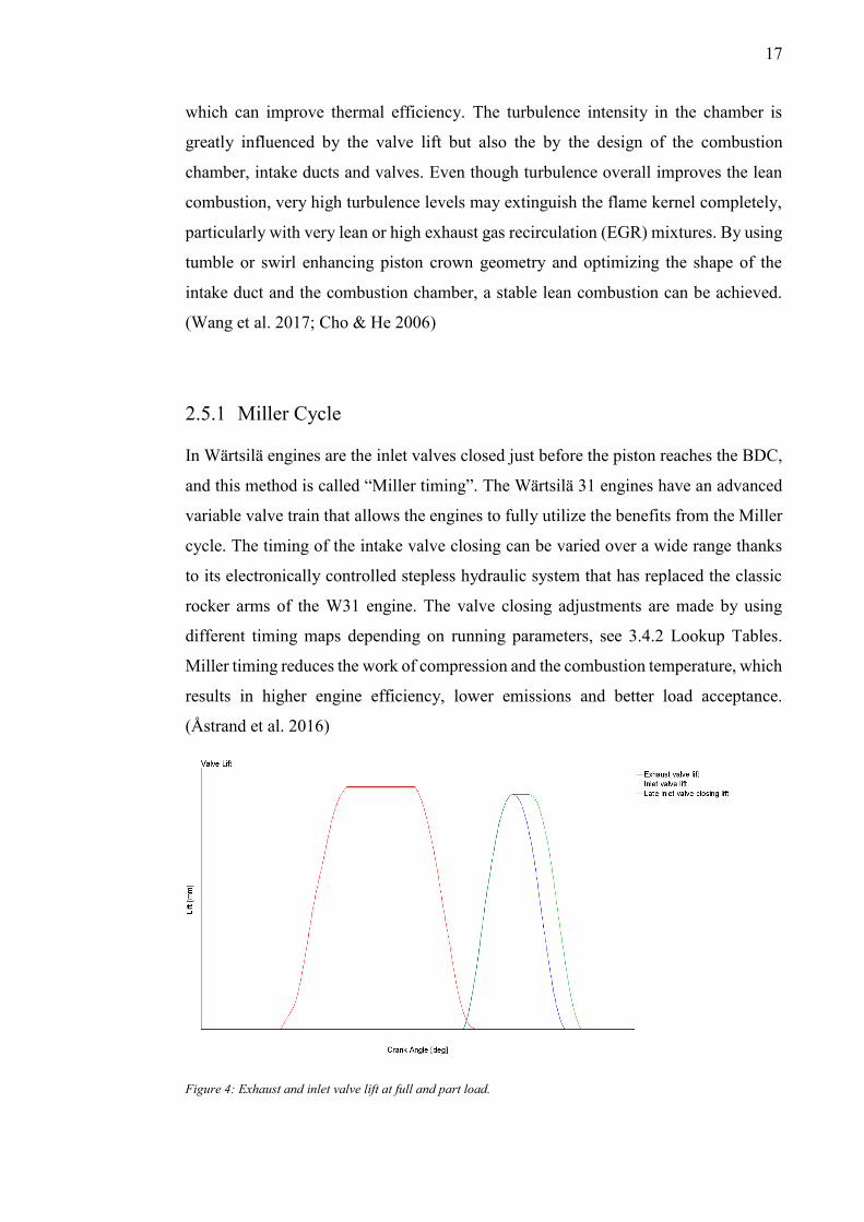
2.5.1 Miller Cycle

In Wärtsilä engines are the inlet valves closed just before the piston reaches the BDC,

and this method is called “Miller timing”. The Wärtsilä 31 engines have an advanced

variable valve train that allows the engines to fully utilize the benefits from the Miller

cycle. The timing of the intake valve closing can be varied over a wide range thanks

to its electronically controlled stepless hydraulic system that has replaced the classic

rocker arms of the W31 engine. The valve closing adjustments are made by using

different timing maps depending on running parameters, see 3.4.2 Lookup Tables.

Miller timing reduces the work of compression and the combustion temperature, which

results in higher engine efficiency, lower emissions and better load acceptance.

(Åstrand et al. 2016)

Figure 4: Exhaust and inlet valve lift at full and part load.

18

The W31SG uses the Miller cycle combined with two-stage turbocharging to achieve

its high BMEP and to keep the AFR lean also at part load. Figure 4 shows how the

miller timing affects valve lift for the engine model in GT-SUITE. The blue curve

shows the inlet valves lift on full load and the green curve shows the late inlet closing

lift at part load.

Modifying the working cycle of the internal combustion engine is nothing new. The

Miller cycle was introduced by Ralph Miller in 1947 and this cycle works almost in

the same way as the Atkinson cycle, which is an alternative engine working cycle that

James Atkinson came up with already in 1846. The so-called Atkinson cycle works by

shortening the intake and compression stroke, while keeping the expansion and

exhaust stroke length the same. This gives a higher expansion ratio than the

compression ratio, thus increasing the engine efficiency. The main difference between

the Miller cycle and the Atkinson cycle is that the Miller cycle has increased charge

air pressure, usually by turbocharging, so that the same amount of air is trapped in the

cylinder, as in the conventional Otto cycle when the inlet valve closes at BDC, and

this increases the efficiency while maintaining the cylinder output. See 2.6

Turbocharging. (Anderson 1998)

Figure 5: Otto working cycle to the left and the Miller cycle to the right (Wang 2007)

Figure 5 compares the standard Otto cycle to the Miller cycle with the help of two P-

V diagrams. The pressure in the cylinder at the starting point 0 is called P0, the volume

is called V0 and the swept volume of the cylinder for Otto Cycle is called Vc and for

P

V

2

3

1

4

0

V 0 V 0 + V c

P

V

2

3

1 a

4

0

V 0 V 0 + V c

4 a

1

V 0 + V’ c

P 0 P 0

19

the Miller cycle it is called V’c. The P-V diagram to the left shows the work process of

the Otto cycle, which is as followed: intake stroke is from 0-1, the compression stroke

is from 1-2, the combustion and the expansion stroke is from 2-3-4, and exhaust stroke

is from 4-1-0. The compression ratio is identical to the expansion ratio and the higher

expansion ratio causes a higher compression ratio, which can result in harmful engine

knocking. (Wang 2007)

The P-V diagram to the right shows the Miller cycle. The work process that starts with

the intake stroke is from 0-1a-1, that continues with a so-called ‘‘intake blow back’’

process from 1-1a, this process is the main difference between the Miller cycle and the

Otto cycle. Then comes the compression stroke from 1a-2 and the combustion from 2-

3 and the expansion stroke 4-4a, the exhaust stroke is from 4a-1-1a-0. The Miller cycle

from P-V diagram shows that a higher engine efficiency can be expected with the

increased expansion ratio, while engine knocking can be avoided by reducing the

effective compression ratio. (Wang 2007)

To further explain the how the Miller cycle works and how it increases the engine

efficiency, the thermodynamics behind needs to be understood. When the charge air is

trapped inside the cylinder while the piston is still moving down, the air expands,

which decreases its temperature. This means that the temperature of the charge air is

now lower at the beginning of compression than during the intake stroke. By

decreasing the temperature in the beginning of compression, the temperature at TDC

in the end of compression is also lower. The expansion and the compression back to

the volume at which the valve was closed is relatively cost free in terms of energy as

both processes are nearly isentropic at such low temperatures. In that way the Miller

cycle is able to reduce the compression pressure and temperature in the cylinder at the

end of compression stroke, while it also counter high combustion flame temperature

in the cylinder during the combustion process, which is the main cause of NOx

formation. (Anderson 1998; Wang 2007)

20

2.5.2 Ignition System and Spark Timing

Under the ideal conditions the common internal combustion engine burns the air-fuel

mixture in the cylinder in an orderly and controlled fashion. The combustion is started

by the spark plug somewhere between 10 to 40 CA° prior to TDC, depending on many

factors including engine speed and load. This ignition advance gives the time for the

peak pressure to develop during the combustion process at the ideal time for maximum

recovery of work from the expanding gases. (Wang et al. 2017)

There is a problem with the classic spark-ignited Otto cycle ignition system: it is not

limitlessly scalable. The spark plugs ignition energy and the durability become

insufficient as the engine grow in size. However, it is possible to overcome this

problem and widen the application range of spark plugs, using pre-chambers. See 2.5.3

Gas Admission and Pre-Chamber Combustion. The ignition timing or spark timing

(ST) is a critical and difficult parameter to control for lean combustion NG engines.

Operating under lean conditions the spark timing must be advanced compared to

stoichiometric operation, and this can effectively extend lean limits while keeping

thermal efficiency high. At extreme lean operating conditions, where the development

time and the burn periods of the flame kernels are long, cyclic variations inevitably

limit engine operation, and therefore more spark retardation and ignition energy are

required. This shows that the ignition energy and timing are closely related to optimum

AFR and an adaptive control system that simultaneously controls the AFR and the ST

is needed to control the lean combustion. (Codan et al. 2007; Cho & He 2006)

Retarding spark timing is the most effective method to simultaneously lower end-gas

temperature and pressure, which can reduce NOx. The problem with too late spark

timing in lean-burn engines is it usually leads to an un-optimized combustion phasing

with lower thermal efficiency. This is because overly retarded ignition timings in lean-

burn engines cause the mixture temperature in the end-zone to drop below the misfire

temperature, which is due to expansion of the air-fuel mixture and quenching of the

kernel. (Wang et al. 2017; Cho & He 2006)

21

2.5.3 Gas Admission and Pre-Chamber Combustion

Gas admission in large NG engines is usually done with timed dosing valves, with the

advantage of being able to control the gas exchange and output power in a similar way

to diesel engines. This means that NG engines with timed admission control in the

inlet port also can benefit from scavenging, which helps with the cooling of the

combustion chamber. As mentioned earlier does scavenging have a positive effect on

the thermal loading of components and the knock resistance of the engine. However,

it is important to pay attention to the valve overlap, since the optimal setting for the

scavenged gas quantity and increased gas exchange losses, shifts in proportion to the

charging pressure level and pressure differences over the cylinders. Engines that have

premixed gas with the combustion air should not use scavenging, since it leads to

increased emissions of uHC and lower engine efficiency. (Codan et al. 2007)

Figure 6: NG engine with pre-chamber (Wärtsilä 2011)

The rich burn engine has a balanced AFR, which usually results in a 0.5 % oxygen

content in the exhaust gases. This means there is very little play in the AFR, especially

during transient loading, before the mixture becomes too rich and uHC start to show

up in the exhaust or/and the engine start knocking. Due to the large combustion air

surplus in lean-burn gas engines, often twice the air needed for stoichiometric

combustion, the exhaust O2 content is typically above 8 %, which shows there is more

play in the AFR during lean combustion. But as stated earlier, the lean mixture is very

had to ignite, especially under high load and transient loading. (MECA 2015)

22

A modern lean-burn SI NG engine has two different combustion chambers with

separated fuel gas supplies, a pre-combustion chamber (PCC) and a main chamber.

The gas volume used for PCC is usually around 1-4 % of the compression volume of

the main chamber. The PCC can ignite the very lean NG mixture under different

conditions, using the stratified charge combustion strategy, described 2.5 Lean-Burn

Combustion. The PCC works by a spark igniting the stoichiometric air-fuel mixture

inside the PCC, the pressure inside rises fast and jet flames burst out of the nozzle

holes of the PCC. These flames ignite the lean mixture in the main chamber and

enables efficient combustion through the increased turbulence they cause. (Cho & He

2006)

Figure 7: Lambda in the in a cross section of the pre-chamber and main chamber (Prometheus 2016)

In other words, the main purpose of the PCC is to reduce the combustion instability,

but the quick flame propagation also leads to high burning rates and a short burn period

in the main chamber, which improves fuel economy and reduces NOx emissions.

Wärtsilä first introduced their first SI lean-burn four-stroke large bore engine in 1993

and the W31SG of today has one of the most advanced PCC systems in the world.

(Duong et al. 2013)

23

2.6 Turbocharging

To enhance the power density of the NG engines, turbocharging technology is used. It

is well known that the maximum engine power is limited by how much fuel can be

burned in a cylinder per power stroke. The amount of fuel that can be burned with

good efficiency is then limited by the amount of air that can be introduced to an engine.

Thus, when the density of the introduced air is increased with a compression device,

e.g. with a turbocharger an engine with a given displacement can produce more power.

The turbocharger is a device that consists of an exhaust gas driven turbine wheel and

a compressor wheel, which compresses the inlet air to a higher density, mounted on a

common shaft. (ABB 2012)

Figure 8: Cross-cut of an ABB turbocharger (Behr et al. 2013)

The turbocharger uses exhaust gas to drive a turbine, which does not draw any

mechanical power from the engine itself, unlike the parasitic supercharger that draws

mechanical power from the engine’s crankshaft. Approximately 35 % of the energy

content in the fuel is wasted to exhaust gases in naturally aspirated engines, however,

with a turbocharger the engine efficiency is increased since the exhaust gas is used to

charge more air into the engine. (Heywood 1988) The most important aspects of the

exhaust system when it comes to turbocharging are the manifolds between cylinders

and turbine. In order to increase the efficient use of exhaust gas energy, the gas first

needs to be transported with minimum energy losses from the cylinders to the turbine.

Then the exhaust gas energy is converted in the turbine into mechanical work, which

the compressor uses to build up the boost pressure in the receiver. There are several

24

benefits of using exhaust gas turbocharging: reduction in specific fuel consumption,

less emissions and power increase from an engine with same displacement. Additional

benefits are lower thermal and pumping losses. (Kesgin 2004)

Under transient engine operation i.e. under engine acceleration or retardation and load

pickup, the turbocharger plays a vital role in providing the necessary charge air

pressure for the engine to burn enough fuel and to meet the power demand. Relevant

turbocharger key parameters for transient engine performance are: compressor work

coefficient, specific volume flow, mass moment of inertia of the rotor and part-load

efficiency and effective turbine area. With improved part-load efficiency and turbine

effective flow area, the turbocharger provides better starting conditions. This is

because increased air pressure is already available at steady state conditions even

before the transient process is initiated. The higher AFR allows for a greater immediate

increase of fueling and results in torque increase. (Siebenfeiffer 2016)

2.6.1 Two-Stage Turbocharging

Nowadays turbocharging is used in all size classes of engines, e.g. in passenger cars,

trucks and ships. A turbocharged four-stroke engine in marine use can produce more

than three times as much power than a naturally aspirated engine of the same

dimensions and speed. The space for the engine installation is usually limited,

especially in vessels, so the importance of turbochargers cannot be stressed enough

when it comes to enabling high power densities in both modern four-stroke marine and

power plant engines. (ABB 2012)

Two-stage turbocharging is when two turbochargers are placed in a series, so that the

turbine on the high-pressure (HP) side is driven by the energy of the exhaust gases

leaving the turbine on the low-pressure (LP) side. A major advantage with two-stage

turbocharging, is the fact that two conventional turbochargers with normal pressure

ratio and efficiency can be used together, to create an overall high pressure and

expansion ratio. (Siebenfeiffer, 2016) The current limit in pressure ratios of modern

compressors in single-stage turbochargers is approximately 6.0. The industry standard

for the material used in the compressor wheels is aluminum, and if the pressure ratio

needs to be increased even further with a single-stage turbocharging system, additional

25

compressor cooling is required and/or the material must be changed to titanium. The

biggest challenge with a single-stage turbocharging system is maintaining a wide

compressor map in high-pressure ratios. With two-stage turbocharging a total

compressor pressure ratio of 12.0 can be achieved. This reduces the pressure ratio in a

single stage and does not need additional cooling or any material change from

aluminum. (Behr 2014)

The primary disadvantages with two-stage turbocharging are the increased cost of the

additional turbocharger, intercooler and manifolds, plus the total bulk of the system.

Intercooling between the turbochargers is an additional complication, but this also has

the additional advantage of reducing the in temperature at the inlet of the HP-

compressor, which also reduces the work of the HP-compressor for a given pressure

ratio, since this is a function of compressor inlet temperature. Another less obvious

disadvantage with two-stage systems is that performance is often poor at low load and

speed. With a two-stage system this causes the efficiency to drop with reduced load,

whereas the opposite would be true with a high-pressure ratio single-stage system.

(Behr 2014)

The Miller turbocharging system is one method of reducing this effect, which also

helps keeping the NOx emissions to a certain limit and to avoid engine knocking. The

efficient solution combines the lean-burn turbocharged combustion concept with the

Miller cycle. The effects of the miller cycle is reduced at lower loads, with the benefit

that the volumetric efficiency is improved, and hence more air is trapped in the

cylinders, see 2.5.1 Miller Cycle. (Behr et al. 2013)

The Wärtsilä 31 uses a two-stage system to achieve its high power-density and record-

breaking efficiency. The two-stage system archives a pressure ratio capability well

above 10 and the turbocharger efficiency is more than 75 %. A single-stage

turbocharger typically has an efficiency around 65-70 %. An issue with a two-stage

system is that it does not automatically provide any significant benefits, because the

engine needs to be specially designed for the system in order to fully utilize the

potential of high charge-air pressure and efficiency. This was a strong drive behind the

development of the W31-platform. The new two-stage turbocharging system gives

other advantages as well, other than increased pressure ratio. In diesel operation, it

enables improved use of earlier inlet valve closing resulting in lower combustion

26

temperatures and thus lower NOx. An advantage in gas operation is the increased

margin to knocking, but the main result with the two-stage turbocharging is higher

engine output and improved fuel efficiency with lower emissions. The two-stage

concept also offers benefits in terms of operational flexibility, by improving loading

performance and load acceptance from low loads. (Åstrand et al. 2016)

Figure 9: Engine pressure drop over pressure ratio (Behr et al. 2013)

Figure 9 is a generalized chart over the difference between turbine inlet pressure and

charge air pressure, which shows the importance of higher turbocharging efficiency

when aiming for higher pressure ratios. (Behr et al. 2013) Overall, a two-stage

turbocharging system offers higher efficiency, provides a boost pressure and greater

specific air consumption, and therefore also provides lower exhaust valve and turbine

inlet temperature. Since moderate pressure ratios can be used, both stages can operate

at a slower rotational speed, compared with the very high speed of a high-pressure

ratio single-stage unit. This entails several benefits for the components of the

turbocharger, e.g. it lowers impeller and turbine blade stresses, improves bearing life

and lessens the turbocharger noise level. (ABB 2012)

27

2.6.2 Control Strategy of Natural Gas Engines

The turbocharged diesel engine can be controlled over a wide operating range on the

basis of fuel injection quantity, since diesel can burn efficient under a wide AFR. Lean-

burn gas engines on the other hand must closely control of gas quantity and lambda,

i.e. the charging pressure must be controlled for the gas to burn efficiently and to

prevent knocking and misfiring. (Woodyard 2009) To be able to control the boost

pressure in the receiver and therefore the AFR, different types of valves and bypasses

are used to ensure the AFR is correct at all loads and independent of changing ambient

conditions, considering, for instance, temperature. There are several possible ways to

control the mass flow though the turbocharger and therefore the AFR in the

combustion. In the following paragraph, some of the control methods will be listed

and described how they are used on the W31 platform.

Exhaust wastegate valves, EWG, which are valves on turbine side, let the exhaust

gases bypass the turbine in the turbocharger. The W31SG uses an electrically

controlled EWG combined with the adjustable valve actuation, to ensure the optimal

performance on varying operating profiles and different conditions, see 2.5.1 Miller

Cycle. The electrical EWG has much less delay in responsiveness compared to the

typical pneumatic actuator normally used and the adjustable valve actuation further

improves the response time needed for transient operation. The EWG bypasses both

turbocharger-stages on the W31SG, but other engines can have other setups. (Åstrand

et al. 2016)

A wastegate for the charge-air is called AWG, and can be used when there is too much

boost pressure for the load. The W31 has an AWG between the two compressor stages.

Air bypass valves, ABP, which are valves on the compressor side, are used by the

W31SG for bypassing the cylinders, so that the compressor charge air is lead directly

to the HP-turbine. With both the ABP and AWG system the Wärtsilä 31 can fulfill

special costumer requirements, such as operating on a certain propeller curve with a

constant torque or being able to operate a vessel in arctic conditions where suction air

temperature down to -50°C, and both can be utilized without an impact on maximum

continuous rating. (Åstrand et al. 2016)

28

Most engines use throttle valves to change the AFR quickly and are generally required

for operation at low load. The Wärtsilä 31 does not need any throttle valves thanks to

the smart ECU and the stepless hydraulic valve train utilizing the Miller cycle.

Another reason not to use throttle valve control is because it makes it difficult to retain

enough margin against surge, since it would require very wide compressor maps and

limit achievable efficiency. (Codan et al. 2010) Figure 10 shows a simplified model of

the W10V31SG engine in GT-SUITE, where the control strategy of the engine can be

seen.

Figure 10: Simplified picture of the W31SG model in GT-SUITE

29

2.6.3 Thermal Load

Thermal load is quite an ambiguous concept that is linked with heat transfer and the

temperature. In internal combustion engines, the overall thermal load is usually

understood as a stream of heat in a specified place of the engine. Equation (3) shows

how the overall heat transfer can be calculated for an internal combustion engine,

where Q is the heat transfer, QHV heating value of the fuel, Bo is the mass of fuel under

a certain time unit and 𝜉 is the coefficient of heat utilization in combustion chamber.

(Sroka 2012)

𝑄 = 𝑄𝐻𝑉𝐵𝑜𝜉 (3)

The analysis of thermal loads in internal combustion engines as the whole object, as

well as in its separate components such as turbochargers and intercoolers, is based on

different kinds of heat exchange conditions such as conduction, convection, radiation

and diffusion. There are many complicated formulas to describe different components

heat transfer. In this thesis the Colburn analogy is used to calculate the heat transfer

coefficient of pipes in GT-SUITE’s engine simulation. The Colburn analogy can be

calculated with equation (4).

ℎ𝑔 = (1

2) 𝐶𝑓𝜌𝑈𝑒𝑓𝑓𝐶𝑝𝑃𝑟(−

2

3) (4)

Cf is the Fanning friction factor for a smooth pipe, ρ is the density, Ueff is the effective

velocity outside the boundary layer, Cp is the specific heat and Pr is the Prandtl

number. When operating an engine under boosted conditions it increases the thermal

load, primarily due to the increased charge mass flow rate through the engine. The

combustion of this increased charge mass directly transfers more heat to the engine

structure which must then be removed by the oil and cooling systems. The increased

back-pressure created by the turbine also increases the heat flux into the coolant and

the engine structure in general. Thermal loads and their effect on the mechanical

strength of the engines need to be taken into account when conducting full coupled

thermal and physical models of turbocharged engines. (GT-Flow 2018)

30

2.7 Knocking Combustion

Brake mean effective pressures of natural gas engines are limited by knocking and

thermal loading. This chapter goes into detail of the knocking phenomena. There are

many definitions that describe these different abnormal combustions. At Wärtsilä they

usually use the terms: light knock and heavy knock, to describe these different types

of knocking combustion of different severity. In literature and reports you can find

endless definitions that describe just a particular type of knock. In this thesis the terms

light knock and heavy knock, will be used to describe different types of knocking

combustion.

2.7.1 Knock Definitions

As mentioned earlier, abnormal combustion can occur in many ways. The two most

important phenomena of abnormal combustion are knock and surface ignition. The

reasons why these phenomena are to look out for and avoid if possible are that both

knock and surface ignition can cause major engine damage and even if not severe, they

are regarded as an objectionable source of noise. (Heywood 1988)

Knock has gotten its name from the noise that is transmitted through the structure of

the engine when there is autoignition of a portion of the air-fuel-mixture ahead of the

propagating flame. When this phenomenon takes place, it causes a very rapid release

of a big part of the chemical energy in the end-gas, which leads to extremely high local

pressures and propagating pressure waves with high amplitude across the combustion

chamber. (Wang et al. 2017)

Another type of autoignition is surface ignition. Surface ignition is as the name reveals,

the ignition of the fuel-air mixture by a hot spot on the combustion chamber walls i.e.

an ignition by other means than the normal spark discharge. Typical hot spots are:

exhaust valves, sparkplugs and glowing combustion chamber deposit. Surface ignition

that occurs before the spark discharge is often called pre-ignition and when it occurs

after the spark it is called post-ignition. (Heywood 1988)

31

Both knocking and surface ignition are dependent on the temperature and pressure of

the end-gas, which means various combinations of surface ignition and knock can

occur and can be hard to tell apart. If autoignition occurs repeatedly and often, under

otherwise normal combustion events, it is called spark-knock. Spark-knock can be

controlled by changing the ST, and if the timing is advanced it increases the knock

severity or intensity and retarding the ST decreases the knock. This is because surface

ignition usually causes a faster rise in the end-gas pressure and temperature, than with

normal spark-ignition. There are two major types of surface ignition, non-knocking

surface ignition and knocking surface ignition. The knocking surface ignition often

come from pre-ignition, which usually is caused by glowing combustion chamber

deposits and the knocks severity generally increase the earlier the pre-ignition happens.

Since the spark-ignited flame is not the cause of knock, knocking surface ignition

cannot normally be controlled by retarding the spark timing. Normally the non-

knocking surface ignition is associated with surface ignition that occurs late in the

operating cycle, and rarely causes any harm. (Heywood 1988)

There are also other abnormal combustion phenomena, wild ping for example is a

variation of knocking surface ignition that produces a sharp cracking sound in bursts.

Wild ping may be the cause of early ignition of the air-fuel-mixture in the combustion

chamber by loose glowing deposit particles. Another type of surface ignition is rumble,

which is a low frequency rumble type of noise that can be associated with surface

ignition caused by deposits in high compression engines. Rumble causes high pressure

shocks in the combustion chamber, and can occur together with knock. If the AFR

auto-ignites continuously after the ignition system has been switched off, it is called

run-on and this phenomenon also causes knock-like noises. Run-on seems to be the

result of compression ignition of the fuel-air mixture. (Heywood 1988)

The most destructive type of surface ignition is thought to be runaway surface ignition.

Runaway surface ignition causes the ignition to happen earlier and earlier in the cycle,

and happens because of overheated components. But then again, any process that

advances the start of combustion from the set ST and gives maximum torque will cause

higher heat rejection and in turn cause higher temperature of components, which can

advance the pre-ignition point even further until any critical components can fail.

(Heywood 1988)

32

2.7.2 Conventional Knock

Most types of surface knocking problems can be solved with proper attention to engine

design, and fuel and lubricant quality. In contrast, knock is an inherent constraint on

engine performance and efficiency since it limits the maximum compression ratio that

can be used with any given fuel. Knock primarily occurs under wide-open-throttle

operating conditions and the knock intensity tends to increase with a knock onset that

occurs near TDC. It is thus a direct constraint on engine performance. It also constrains

engine efficiency, since by effectively limiting the temperature and pressure of the

end-gas, as it limits the engines compression ratio. (Heywood 1988)

The occurrence and severity of knock depend on the knock resistance of the fuel and

on the antiknock characteristics of the engine. The ability of a fuel to resist knock is

measured with different systems. The classic way is with octane number, where higher

octane numbers indicate greater resistance to knock, see 2.5 Lean-Burn Combustion.

Thus, knock is a constraint that depends on both the quality of available fuels and on

the ability of the engine designer to achieve the desired normal combustion behavior

while holding the engine’s propensity to knock at a minimum. (Cho & He 2006)

Figure 11: Combustion parameters in a typical case of knocking combustion (Wang et al. 2017)

33

Figure 11 shows the pressure trace, pressure oscillation, heat release rate and unburned

gas temperature of the typical knocking case. Once knock occurs, the pressure

distribution across the combustion chamber will no longer be uniform and high-

frequency pressure fluctuations are observed whose amplitude decays with time. By

using knocking sensors located at different points in the combustion chamber, different

pressure levels can be recorded at any given time until the wave propagation

phenomena described above have been damped out. (Wang et al. 2017)

2.7.3 Methods to Suppress Engine Knock

As mentioned earlier engine knock is a race between the propagating flame and the

thermal autoignition of the unburned end gas in the engine. To be able to avoid engine

knock, the time of flame propagation to the end gas needs to be less than the time of

the end-gas autoignition. The most common strategies used to control pre-ignition and

knock is retarding ST, use of high octane fuel, cooled EGR, cooled intake air, and

enhancing turbulence in the combustion chamber. Possible ways to control and

suppress engine knock in SI engines are summarized in this chapter. (Soylu 2003)

Retarding ST is the most effective method to simultaneously reduce the end-gas

temperature and pressure. The lower end-gas temperature and pressure prolong the

ignition delay. However, late ST usually leads to an un-optimized combustion phase

with lower thermal efficiency. It also may deteriorate engine performance due to the

decrease in mean combustion chamber temperature and pressure. With cooled EGR,

the gas temperature can be lowered, which means more fuel can be consumed before

reaching the knock temperature limit and therefore can further widen the ignition

advance angle. Cooled EGR has the potential to decrease the knock tendency without

any loss of output power and can also improve engine efficiency through increased

compression ratio. (Cho & He 2006)

Lowering the effective compression ratio is another effective way to suppress heavy

knocking and VVT is a practical way to change effective compression ratio at

relatively low cost. Late intake valve closure is commonly used at high load to achieve

a lower effective compression ratio to avoid knock. The reduction in the amount of

intake also reduces pumping losses at part loads, due to the higher intake pressure

34

needed. Without modifying intake ducts, reducing the intake stroke also results in

lower swirl number and increased efficiency as well. Using a variable compression

ratio is a more ideal method, but the complex structure makes the cost increase

significant. See 2.5.1 Miller Cycle (Wang 2007)

With a great design and optimization of the engine, including the piston ring structure,

spray pattern, injection strategies, flow motion, sealing system, and cooling system,

both pre-ignition and heavy knock can be avoided. Optimized engine combustion

systems can for example reduce the end-of-compression temperature by scavenging of

hot residual gas. Scavenging is a practical method for cooling combustion chamber

walls. Scavenging by retarding the exhaust valve closing timing can suppress heavy

knocking, but also often increase fuel consumption and CO-emissions. (Cho & He

2006) The cooling of components is essential when avoiding knock, as mentioned

earlier there are many hotspots in a combustion chamber where autoignition can occur

such as pistons, cylinder walls and exhaust valves. Changing the coolant flow patterns

of the combustion chamber walls also improve the distribution of wall temperatures

and is an effective method to suppress knock. Cooling the intake charge is also useful,

because the initial condition of the end gas during a cycle is dependent on the intake

air temperature. In addition, cooling the exhaust manifold is also important. (Wang et

al. 2017)

Two of the origins of pre-ignition are oil droplets and deposit particles, which depend

on the properties of the lubricant oil and fuel, including their cleanliness, additives and

laminar flame thickness. Preventing oil from entering the combustion chamber can be

done by using a larger chamfer piston edge, an increased oil ring tension or an

optimized ring orientation. The use of a low volatility oil and improved oil ventilation

also help. Knock resistant oils should contain anti-wear additives such as ZnDTP and

MoDTC and very little calcium, sodium and sulphated ash. With the right fuel and

lubrication there will be less flammable particles floating in the combustion chamber,

including deposits, soot, and metal dusts Fe, Cu, etc. To prevent engine oil and fuel

mixing in a direct injection engine, several strategies can be employed, e.g. adjusting

the spray direction to reduce liner wall wetting, using a split injection strategy, or by

adopting high tumble to enhance air motion to reduce spray penetration. Even the

premixed charge used in gas engines is to some degree inhomogeneous in a

35

combustion chamber, and is likely to influence a developing detonation. Increasing

turbulence intensity usually helps to suppress this type of engine knock, because the

increased turbulence leads to faster combustion and decreases the tendency to knock

(Wang et al. 2017)

2.7.4 Knock Detection Modeling

There are many ways to detect knock and characterize it, see 2.7.1 Knocking

Definitions. The human ear is surprisingly good at detecting knock and was formerly

used in determining the octane requirement and the fuel quality the engine must have

to avoid knock. The modern engine management system uses different types of sensors

for detecting knock. A combustion pressure sensor can measure the pressure inside the

combustion chamber of a running engine. These types of sensors give the best signal

to analyze, but each cylinder needs its own sensor and they are rather costly. (Heywood

1988)

Another type of sensor is the mechanical vibration sensor. It is a piezoelectric vibration

probe that measures structure vibrations. The piezo-element generates a small voltage

that can be measured during knocking combustion. Other types of knock detecting

sensors are optical probes and ionization detectors. Spark plugs can serve as ionization

detectors when electrically charged ions and electrons are generated during the

combustion process. The ionization intensity depends on the flame temperature, the

air-fuel ratio and the fuel quality. High-speed optical diagnostics and advanced

numerical simulations have also been widely adopted to detect autoignition. (Kiencke

2005)

Computer models are valuable tools for analyzing and optimizing engine performance

and many models can predict engine performance parameters, i.e. knock indexes. Most

models use assumptions to simplify the flow and combustion process, while other

models use multi-dimensional reactive flow codes for detailed modeling of engine

flow and combustion processes. These types of models include knock sub-models to

predict the knock limited operating conditions. The knock models can be classified as:

empirical ignition delay correlations, detailed chemical models and reduced models.

(Soylu 2003)

36

The basic approach to predicting end-gas autoignition in SI engines is with the

empirical ignition delay correlation, also called the knock integral approach.

Liwengood and Wu developed the first published ignition delay correlation for SI

engines. By matching the Arrhenius equation to measured data for the induction period

over the relevant end-gas pressure and temperature ranges, an empirical correlation

can be derived. From equation (5) can it be derived that autoignition occurs when the

knock integral output is bigger or equal to 1.

∫𝑑𝑡

𝜏= 1

𝑡𝑖

𝑡=0 (5)

The term 𝜏 is the Arrhenius equations induction time at the instantaneous temperature

and pressure for the mixture, the term t is the elapsed time from the start of the end-

gas compression process, i.e. when t equals zero, and the term ti is the time of

autoignition. According to Heywood, this equation can be derived by assuming that

the overall rate of production of the critical species in the induction period chemistry,

for a given mixture, depends only on the gas state and that the concentration of the

critical species required to initiate autoignition is fixed. (Heywood 1988)

A method to determine the knock resistance of fuels based on the ignition delay

concept was proposed by Douad and Eyzat. The equation is based in the octane number

of the fuel and the end-gas from the measured pressure data. This can be calculated

with equation (6).

𝜏 = 𝐴 ∗ 𝑝−𝑛 exp (𝐵

𝑇) (6)

The parameters A, n, and B depend on the fuel. Douaud and Eyzat proposed using

following parameters, as seen in equation (7), which have been extensively tested:

𝜏 = 17.68 (𝑂𝑁

100)

3.402

𝑝−1.7 exp (3800

𝑇) (7)

The term 𝜏 is the induction time in milliseconds, p is absolute pressure in atmospheres,

T is the temperature in kelvin and ON is an appropriate octane number for the fuel.

(Heywood 1988; Melamies 2008)

37

2.7.5 Knock Model for Lean-Burn Gas Engines

Douaud and Eyzat knock integral equation is optimized for gasoline engines and

therefore Soylu and Van Grepen developed a knock model for NG engines, based on

the same knock integral technique. This is a fast-running and simple knock model that

does not require extensive computational power and its accuracy is comparable to

other knock models. This knock model also considers the variation of the natural gas

composition due to propane addition. It is assumed that autoignition occurs when the

output from the integral equals one, and looks as following:

∫𝑑𝜃

𝑋1∗𝑃(𝜃)−𝑋2 exp(𝑋3

𝑇𝑢(𝜃))

= 1𝜃=𝐾𝑂𝐶𝐴

𝜃=−180 (8)

The integral is reliant on the crank angle 𝜃, because the pressure P and the unburned

zone temperature Tu are not constant. KOCA stands for the knock occurrence crank

angle and X1 and X2 are experimental constants that are dependent on the fuel. The X3

parameter is a function of propane ratio PR and equivalence ratio ER. The propane

ratio is the amount of propane in the gas which can be calculated by dividing the mass

of the propane with the total weight natural gas, and the equivalence ratio is easily

calculated by dividing 1 with lambda. Even slight variations in X3 causes significant

variations of the KOCA because of the exponent term in the model. X3 can be

calculated with following formula:

𝑋3 = (−0.575 + (10.058 ∗ 𝑃𝑅 − 54.053 ∗ 𝑃𝑅2)) ∗ 𝐸𝑅 + (1.456 +

(−8.703 ∗ 𝑃𝑅 + 43.615 ∗ 𝑃𝑅2)) ∗ 7000 𝐾 (9)

In Soylu’s experiments, the natural gas was diluted with propane to study the effects

of lower MN gas qualities. The experiments proves that pure methane has a high knock

resistance, since high values of X3 and low values of X2 are needed for the equation

give a value higher than 1 and thus estimate knock. (Soylu 2003)

38

2.7.6 Knock Modeling in GT-SUITE

GT-SUITE has several knock models to choose from depending on what internal

combustion engine model and fuel you are using. Many of the models are based on the

same knock integral technique as mentioned in the two previous paragraphs. One of

these models is the Kinetics-Fit-Natural-Gas model. This model is based on detailed

kinetics simulations. As the name reveals, the fuel used for the kinetic reaction

mechanism is natural gas and therefore this model can only be used for natural gas

combustion. The induction time τ, for the Kinetics-Fit-Natural-Gas model can be

calculated with the following equation (10).

𝜏 = 𝑀1 ∗ 1.9858 ∗ 10−9 exp (18659

𝑀2∗𝑇) (

𝑀𝑁

100)

0.978

∗ 𝐹−0.578𝑂2−0.28𝐷0.03 (10)

In the equation M1 is a Knock Induction Time Multiplier, MN is the Fuel Methane

Number, M2 is the Activation Energy Multiplier. The parameters F, O2 and D are all

concentrations expressed in mol/m3, where F stands for fuel, O2 for oxygen and D for

diluent. The diluent parameter is the sum of the N2, CO2, and H2O concentrations. The

induction time can then be used with the Liwengood and Wu integral mentioned

earlier, in order to determine if there is autoignition. Gamma Technologies have also

developed a so-called knock index, which is a phenomenologically based parameter

and can be scaled to the loudness of knock as heard in the laboratory using the Knock

Index Multiplier. When knock occurs, the value of the knock index at the start of knock

is reported. The knock index is defined as a crank angle-dependent quantity and the

formula can be seen in the following equation (11).

𝐾𝐼 = 𝑀 ∗ 103 ∗ 𝑢(𝛼) ∗𝑉𝑇𝐷𝐶

𝑉(𝛼)exp (

−6000

𝑇(𝛼)) ∗ max (0,1 − (1 − 𝛷(𝛼))

2) ∗

𝐼𝑎𝑣𝑒(𝛼)

𝐼𝐾−𝑟𝑒𝑓∗𝐼𝐾−𝑐𝑜𝑟𝑟 (11)

KI stands for knock index, M is the knock index multiplier, u is the percentage of

unburned cylinder mass at a certain crank angle α, VTDC is the cylinder volume at top

dead center, V is the cylinder volume, T is the bulk unburned gas temperature in kelvin,

Φ is the equivalence ratio of the unburned zone, and Iave is the induction time integral

averaged over all end gas zones. IK-ref is the reference induction time integral and IK-

corr is the induction time integral correction factor, and both parameters are correlated

with the Douaud and Eyzat equation. (GT-Reference 2018)

39

2.8 Combustion Models

GT-SUITE’s one dimensional equations always assumes there is perfect mixing of all

fluids in a specific component, including the mixing of the final air-fuel mixture in the

cylinder, regardless of how the fluids would mix in reality. When the gas mixture is

ignited, a combustion occurs according to a heat release rate curve. The heat release

rate is calculated from a burn rate, which is the instantaneous rate of fuel consumption

within the cylinder combustion process. The input data for the burn rate may either be

imposed or predicted, depending on what combustion model is used. (GT-performance

2018; Mahmoundi et al. 2017)

A non-predictive combustion model imposes a burn rate as a function of crank angle,

the prescribed burn rate will then be followed regardless of the conditions in the

cylinder. An imposed combustion profile can be used with any type of fuel or injection,

and is particularly useful if the cylinder pressure from the engine has been measured

in the laboratory because the burn rate can be calculated from the cylinder pressure. In

a non-predictive combustion model, it is assumed that there is sufficient fuel available

in the cylinder to support the burn rate and therefore, the burn rate will not be affected

by factors such as residual fraction or injection timing. (GT-performance 2018)

A predictive model uses input data about cylinder geometry, spark timing, air flow,

and fuel properties, to predict a burn rate. In theory, predictive combustion models

should be an appropriate choice for all simulations, but much input data is needed and

even then, there is no guarantee that the predictive models correspond to a real

combustion process, since there is so many influencing factors. There are also semi-

predictive combustion models in GT-SUITE, which can be a good substitute for a

predictive model. (GT-performance 2018)

A semi-predictive combustion model is sensitive to the significant variables that effect

combustion rate, and responds appropriately to changes in those variables, but a semi-

predictive model does not use any physical models to predict that response. Instead

they utilize a non-predictive methodology, e.g. a Wiebe function, where the

combustion burn rate is imposed, with lookups or other methods to calculate the proper

Wiebe parameters based on the significant input variables. (Mahmoundi et al. 2017)

40

2.8.1 Three Pressure Analysis

In GT-SUITE calculating the burn rate from a measured cylinder pressure is

sometimes referred to as a “reverse run”. This is because the inputs and outputs are

reversed in the calculation from the typical combustion calculations in engine

simulation. In a typical “forward run” simulation, the burn rate is the input and the

cylinder pressure is the result, but in a reverse run, the cylinder pressure is the input

and the burn rate is the result. (GT-performance 2018)

There are two approaches available to calculate the burn rate from a measured cylinder

pressure trace within GT-SUITE, and in this thesis has the three pressure analysis been

used, abbreviated TPA. The TPA method requires three measured pressures: intake,

cylinder and exhaust, hence the acronym. For this analysis, no estimation of the

residual fraction and trapping ratio are needed as inputs. This approach requires an

engine model with geometric data for the engine cylinder, valves, ports and runners.

All pressure measurements must be crank angle resolved, as average quantities will

not be sufficient to impose at a location so close to the cylinder valves. In addition to

the measurements of the pressures the average temperatures are also required. Standard

engine dyno data are also useful for the model setup and correlation, i.e. volumetric

efficiency, fuel rates, etc. (GT-performance 2018)

2.8.2 Spark-Ignition Wiebe Model

When modelling the combustion in simple SI engine, is often a single Wiebe function

used, which approximates the typical shape of an SI burn rate. For more complicated

combustion processes such as diesel combustion and SI gas combustion with PCC,

double and multiple Wiebe functions is used to estimate the combustion process. In

these models, each of the Wiebe functions corresponds to a combustion phase. For

example, in an engine with PCC, the pilot ignition combustion phase is the first Wiebe

function and the second the main combustion phase. A third Wiebe function is added

if for example post knock occurs (GT-performance 2018)

To calculate the burn rate, several equations are needed. Equation (12) is the main

function to calculate the cumulative burn rate over range of CA degrees, where θ is

41

instantaneous crank angle and CE is the fractions of burned fuel or combustion

efficiency. WC is the Wiebe constant and SOC is the start of combustion, which is

typically between 20 and 10 CA° before TDC.

𝐶𝑜𝑚𝑏𝑢𝑠𝑡𝑖𝑜𝑛(𝜃) = (𝐶𝐸) [1 − 𝑒−(𝑊𝐶)(𝜃−𝑆𝑂𝐶)(𝐸+1)] (12)

𝑊𝐶 = [𝐵𝐷

𝐵𝐸𝐶1

𝐸+1−𝐵𝑆𝐶1

𝐸+1

]−(𝐸+1)

(13)

𝑆𝑂𝐶 = 𝐴𝐴 −(𝐵𝐷)(𝐵𝑀𝐶)1/(𝐸+1)

𝐵𝐸𝐶1/(𝐸+1)−𝐵𝑆𝐶1/(𝐸+1) (14)

Equation (13) and (14) show how the WC and SOC are calculated, where BD is the

burn duration, AA is the anchor angle and E is the Wiebe exponent. (Mahmoundi et

al. 2017) The AA, anchors the Wiebe curve to TDC, the specified angle is the number

of CA° between TDC and the 50 % combustion point of the Wiebe curve. The BD of

Wiebe combustion is usually set to exclude the first 10 % and last 10 % of the total

combustion duration. The Wiebe curve exponent determines the angle of the shape of

the curve and is usually set to 2. (GT-performance 2018)

𝐵𝐸𝐶 = − ln(1 − 𝐵𝐸) (15)

𝐵𝑆𝐶 = − ln(1 − 𝐵𝑆) (16)

𝐵𝑀𝐶 = − ln(1 − 𝐵𝑀) (17)

Three other equations are required to calculate the WC and SOC. Equation (15) derives

the burned end constant BEC, where BE is burned fuel percentage at duration end, and

is often set to 90 %. Equation (16) derives for the burned start constant BSC, where

BS is burned fuel percentage at duration start and is set to 10 % in most cases. Equation

(17) derives the burned midpoint constant BMC, where BM is burned fuel percentage

at anchor angle and is usually set to 50 %. (Yeliana et al. 2018; Mahmoundi et al.

2017)

42

2.8.3 Multiple Wiebe Combustion Model

The multiple Wiebe combustion model is a template in GT-SUITE. The so-called

MultiWiebe function is a simple yet powerful correlation model that is well suited for

zero- and one-dimensional engine cycle simulations. This template imposes the burn

rate of the combustion using multiple burn rate equations, see 2.8.2 Spark-Ignition

Wiebe Model. The combustion model adds Wiebe curves to each other to obtain the

burn rate, of an otherwise too complex shape for a single Wiebe function. (GT-

Reference 2018)

The main use of this template is to model fuel injection with multiple injection events,

such as pilot injection with a pre-chamber. The template can be used for any type of

injection, but it has its limitations. The combustion rate will be limited by the amount

of fuel available when using direct injection. The specified cumulative combustion

should not either exceed the specified injected fuel fraction, since the burn rate will

not then be properly reproduced. The fuel fractions per Wiebe curve do not necessarily

need to add up to 1 since the fractions will be normalized by the sum of the fractions.

Equation (18) finally derives the burn rate for the multiple Wiebe combustion model.

𝐶𝑜𝑚𝑏𝑢𝑠𝑡𝑖𝑜𝑛(𝜃) = (𝐶𝐸) ∑ (𝐹𝐹𝑖

∑ 𝐹𝐹𝑖𝑛1

𝑛1 ) 𝐶𝑜𝑚𝑏𝑢𝑠𝑡𝑖𝑜𝑛(𝜃)𝑖 (18)

Combustion(θ)i is the cumulative burn rate as a function of crank angle per each Wiebe

function, see equation (12), where θ is the crank angle and TDC has the reference of

zero degrees. FFi is the fraction of fuel per Wiebe curve, CE is the fraction of fuel

burned, and the “i” in the abbreviations is the column number index of each Wiebe

curve of the multi Wiebe functions. (Yeliana et al. 2008)

2.8.4 Spark-Ignited Turbulent Flame Combustion Model

The spark-ignited turbulent flame combustion template is the predictive combustion

model used to estimate the in-cylinder burn rate, emissions, and knocking occurrence

for SI engines. This model is called SITurb in GT-SUITE, and will also be referred to

in this thesis. This template takes into account the cylinder’s geometry, spark locations

and timing, air motion, and fuel properties, to make its predictions. Unless the head

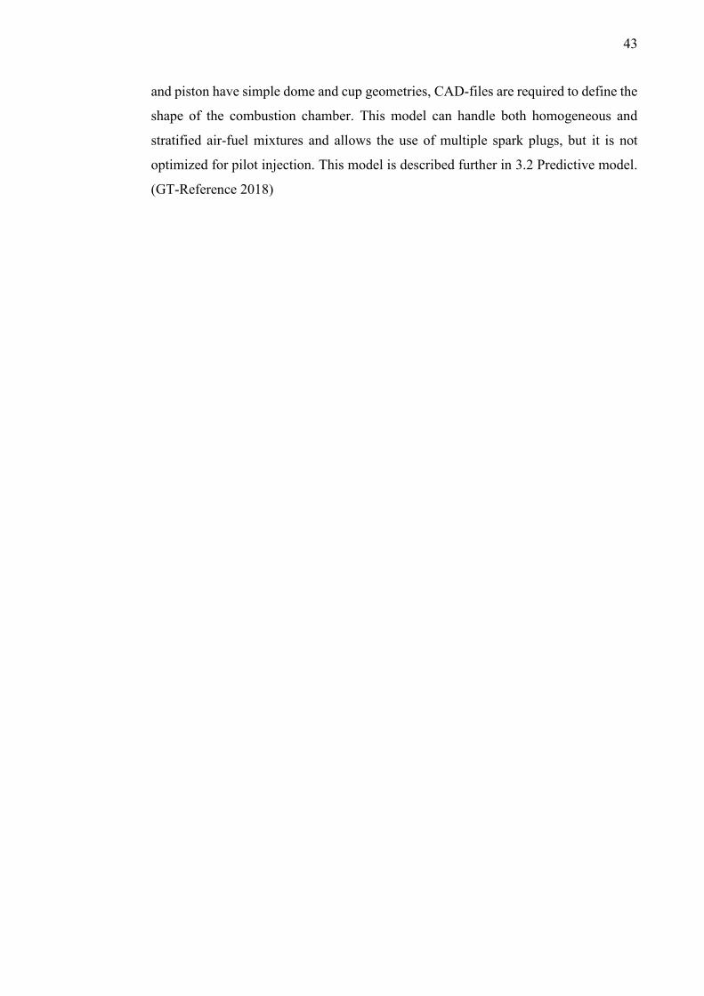
43

and piston have simple dome and cup geometries, CAD-files are required to define the

shape of the combustion chamber. This model can handle both homogeneous and

stratified air-fuel mixtures and allows the use of multiple spark plugs, but it is not

optimized for pilot injection. This model is described further in 3.2 Predictive model.

(GT-Reference 2018)

44

3 MATERIAL AND METHODS

The research started with learning how to use the tools needed to perform the project.

GT-SUITE was used at engine performance department of Wärtsilä and was therefore

also used to build the engine model. All tutorials that had to do with engine

performance in GT-SUITE were done and the corresponding chapters in the manuals

were carefully studied as well. The tutorials were easy to do, since everything was

well explained and the simple models could be built step-by-step.

Other important tools were AVL Concerto and UNITool, both used for data

acquisition, processing and viewing of the laboratory engine data. The data could be

processed within the tools, so that they could be used in GT-SUITE or exported to a

third-party program, such as Microsoft Excel to be further processed and interpreted.

In this thesis the latter mentioned method was chosen. Test data was first briefly

viewed in either Concerto or Unitool, and then processed in Excel. This was done

because the Excel spreadsheets allowed much data to be collected at one place and the

data could easily be processed further into graphs and useful tables for GT-SUITE.

See 2.3 Tools.

After the tutorials were completed and theory was read, some steady-state simulations

of the W31SG engine were done. There was a steady-state model of the engine from

previous engine development that used so-called user-imposed-combustion-profiles,

to impose the heat release from a combustion cycle. The model used these constant

heat release profiles to calculate the engines output power. This will be explained

further in following chapters. In transient models user-imposed-combustion-profiles

should not be used as input data, since the conditions are ever-changing. Therefore,

the old steady-state model was rebuilt with a control system that changes the ignition

timing and the valve timing depending on engine load and state and cylinder

conditions. For that an accurate combustion model needed to be found, one that could

calculate how the heat release changes depending on BMEP, receiver pressure and

lambda. For the heat release to be as accurate as possible, the shape of the heat release

curve should correspond to that of a spark-ignited gas engine with PCC.

45

The best way to replicate the combustion according to the performance theory in GT-

SUITE, was to build a predictive combustion model. A predictive combustion model

can estimate how the heat release rate will look like under different conditions, with

the help of engine geometry, fuel composition and in cylinder turbulence etc. There

were many advantages with a predictive combustion model, where the main advantage

was that realistic engine performance data can be produced without needing to have

input data for every load and condition. This has been tried out and documented in 3.2

Predictive model.

Another way to build a transient model were with the semi-predictive combustion

models, which proved to fit the W31SG engine better. The semi-predictive combustion

models could estimate how the heat releases changed with different load and

conditions, but demanded more work and were not as exact as a good calibrated

predictive model. Much steady state test engine data was also needed, since every load

and condition needed an accurate heat release curve, which a Wiebe function could be

fitted to. This will be further explained in 3.3 Semi-Predictive Models. To make the

heat releases change, the combustion model’s control system was integrated with the

system for controlling the ignition timing and valve timing. For that a rather complex

automation system was made with many engine performance maps, based on both real

and experimental data. This will be described in 3.4 Engine Control and Automation.

The thermal loading of the exhaust system of the W31SG engine was also studied and

simulated in GT-SUITE, since one of the goals of this thesis was to optimize the load

rate for the engine, therefore certain limitations had to be established. This will be

processed in 3.5 Thermal Load Simulations. The model was validated against real test

engine data, where cylinder pressures, temperatures and knocking were set as limits

for the optimal load rate. A lot of time went into studying different ways to estimate

when knocking combustion occurred. Two different knock models were made and

used in the transient model, one based on previous engine development and research

papers and the another one which was based on one of GT-SUITE’s templates, these

two knock models are presented in 3.6 Knock Models.

46

3.1 Three Pressure Analysis Model

The first thing that was done in GT-SUITE, after doing the tutorials, was to make user-

imposed-combustion-profiles, which impose a burn rate or the so-called cumulative

heat release. The burn rates were used to validate the main model in steady-state runs,

against laboratory tests, but was also used in the predictive and the semi-predictive

combustion model. The burn rates were made with the help of a TPA-model, which

have been described in 2.8.1 Three Pressure Analysis. TPA is a reverse run calculation,

as previously mentioned, where the amount of fuel that is transferred from the

unburned to the burned zone is iterated within each time step until the cylinder pressure

matches the measured cylinder pressure, which results in a profile that shows the

apparent burn rate for the current CA°. (GT-Perfromance 2018)

Among other interesting performance data, the cylinder pressure for the laboratory

engine can be found and viewed in Concerto. Since the pressure varied a little for

cylinder to cylinder, the input data required some processing first. The cylinder

pressure data from Concerto was first saved as text-file and then opened with Excel,

where the ten different cylinder pressures were merged and averaged to two columns,

one with the current CA° and the other with averaged cylinder pressure. Besides the

averaged cylinder pressure, also other input data was needed for the model, such as

intake and exhaust pressure, average temperatures, cylinder and valve geometry, and

ambient conditions. In the following picture, a simple one-cylinder TPA-model of the

engine is shown, which is based on an example model from the GT-SUITE’s model

library. (GT-Perfromance 2018)

Figure 12: Three pressure analysis model in GT-SUITE

47

With the TPA could simulated cylinder pressures and burn rates for the one cylinder

model be produced. The simulated cylinder pressures were based on the input data and

the calculated burn rates. In GT-POST were the simulated cylinder pressures compared

to real test cylinder pressures. When the simulated and measured cylinders pressures

matched each other over the whole cycle, the calculated apparent burn rates should be

close to real burn rates. Since the TPA was a steady-state simulation, it meant that the

burn rate was only valid for a certain engine load, and therefore many analyses had to

be done, to acquire burn rates for the whole operating range. To begin with, five cases

were made, based on laboratory tests with different loads, 100, 75, 50, 30 and 10 % of

the max load. With the changing load, the parameters in the case setup were changed,

since the valve and ignition timing changed with increasing load in the W31SG. A lot

of tests were also done on the same engine load but with a different performance

setting, so that look-up tables for the main model could be made, this is further

explained in 3.4.2 Lookup Tables.

It was often required to refine the burn rate curve afterwards and see if it had a

reasonable shape, because sometimes unrealistic abnormalities occurred before and

after the main combustion. The graph to the left in figure 13 shows the measured

cylinder pressure from the laboratory engine as a red curve and the blue curve is the

simulated cylinder pressure. The simulated cylinder pressure was calculated with the

estimated burn rate, shown in the graph to the right.

Figure 13: Average cylinder pressure and burn rate

48

3.1 Steady-State Modeling

There was a steady-state model of the W31 engine from previous research, from which

the new transient model was built. One of the first things that were done to the model

was to go through the old model and update outdated parts, e.g. the turbochargers had

been changed since the steady-state model was built. Then the estimated burn rate

curves from the TPA-model were imported to the main model. As mentioned in the

previous chapter, five main cases at different loads were made based on real test engine

data. These tests used user-imposed-combustion-profiles to simulate the combustion

process that in turn produced the cylinder pressures. These five cases were run and

their results where compared to the test data. Spreadsheets in Excel were made to store

and compare the data from the simulations.

Many parts of the steady-state model had to be changed to the current W31SG

specifications. As mentioned had the turbochargers been updated and hence many

simulations had to be run, in order to be able to validate the steady-state results to the

manufacturer’s specifications. The results where plotted in Excel over real

turbocharger charts, where the efficiency was shown, depending on compression ratio

and volume flow. The shape and scale of the efficiency curve were compared to the

measured values for both the HP- and LP-turbochargers, and the multipliers were

optimized so that the simulation would be as close as possible to the real data.

The valve timing was first set to the same as the laboratory engines, but slight changes

were made to the inlet valve dwell (IVD), which changes how long the inlet valve

should be kept open, in order to improve the results at low load for the steady-state

simulations. The exhaust temperatures were also a little too high in the simulations,

and therefore the exhaust valve timing was slightly advanced. This increased the

scavenging, by overlapping the inlet and exhaust valve opening, which in turn let more

air to be blown through the engine and hence cooling the exhaust gases, see 2.5.1

Miller Cycle.

The results from the simulations were overall better at higher load for the steady state

simulations. Most important parameters, such as receiver pressure and temperature,

exhaust temperature and pressure, before and after the turbochargers, were within 2 %

49

from the measured values. With lower engine loads, there was a bigger difference for

the test values, but they improved a lot with the updated turbocharger and valve

parameters.

A lot of time and research went into finding a way to convert the steady-state model

to a transient model. Several combustion models and automation systems were tried,

with varying success. The first transient model was a simple model, and its only

purpose was finding the parameters that needed to be changed to be able to convert the

steady-state model. That model used a single user-imposed-combustion-profile

template to produce the same burn rate for the entire loading process. In that

experiment was a burn rate used, which heat release was equivalent to a combustion

at full load. To the same experiment was also a simple load ramp made where the

engine would go from 10 to 100 % load with a constant load rate.

The experiment showed that this simple model already behaved quite like the real

engine. For example, an interesting phenomenon had occurred in the simulation, which

had also occurred in real test runs. At half load, there was an abnormality in the output

power curve, which was caused by a too slow reacting EWG, which had also been an

issue in real tests. Therefore, the PID-controller for the EWG was configured so it

would react faster. These settings were used throughout the project, except in the

simulations testing how the engine behaved to faster and slower PID settings.

A model using a constant burn rate would not have been a true transient model, since

the heat release from one combustion cycle would have been the same for at all loads.

This would have meant that the error in the heat release would have increased with

lower loads and other different operating conditions. Hence were quite a few other

combustion models tested. After studying the performance manual in GT-SUITE and

some previous research and further consulting with the supervisor, the predictive

“Spark-Ignited Turbulent Flame Combustion Model” was chosen.

50

3.2 Predictive Model

The first real attempt to make a transient model of the W31SG was with predictive

combustion model, see 2.9.4 Spark-Ignited Turbulent Flame Combustion Model. The

control system for SITurb combustion template could have been quite simple, since it

only needed inputs how the ST and valve timing changed with different load and

conditions, in order to change the burn rate. In figure 21, the engine’s control system

can be seen when using the SITurb combustion template. To use this combustion

model a calibration process must first be done. The goal of a predictive combustion

model calibration process was to find the single set of model constants that would

provide the best possible match to a wide variety of operating points. Therefore, no

user-imposed-combustion-profile would have been needed in the main model,

however many burn rate curves were needed to calibrate the model. (GT-Perfromance

2018)

The required measurement data needed for the calibration of the predictive combustion

model can be found in the GT performance manual. The calibration of the SITurb

model needed at least 25 operating points spread over the entire normal operating

range, which included speed, load, valve timing. Each data point also needed a burn

rate curve from TPA. In this research, were more than 50 operating points gathered,

since more points could be helpful, if points were rejected or extra points were needed

for a final calibration. Data about the dynamic cylinder, intake and exhaust pressures

were also needed. Other important input data was air flow and fuel flow and the ST,

and additional data about the timing and width of each fuel injection pulse were also

included. (GT-Perfromance 2018)

If the emission levels from the engine are to be simulated, engine out emissions such

as CO, NOx, uHC are required, but in this thesis, this was out of scope. This model

could also quite accurately have predicted knocking combustion, with the help of data

points where knock have occurred. This was not attempted, but two other ways to

detect knocking combustion where tried, see 3.6 Knock Models. (GT-Perfromance

2018)

51

The SITurb template required accurate data about the in-cylinder geometry and as the

W31 was a modern engine, was the geometry far too complex for a simple template

with just a few parameters to accurately describe it. Therefore cylinder head and piston

CAD-files in STL-format were needed. The flow through the cylinder and inlet

channels can be described just with coefficients in the SITurb template, but for more

accurate results, 3D CFD results were needed to describe the turbulence. There were

four parameters in the SITurb template that was used for the turbulence calibration and

these parameters played a major role for the shaping of burn rate curve, and should

therefore be optimized with the advanced design optimizer. (GT-Perfromance 2018)

In the SITurb template, there was a flame geometry option, where the spark location,

cylinder head and valve and piston geometry were to be defined, but there were no

option for pre-chambers. The solution to this was use several oversized sparks instead,

since it was impossible to ignite the lean mixture with just one spark plug with the

same settings as the one used in the pre-chamber. After setting up the SITurb

combustion template were two calibration methods the template tried, and these

methods are described in the two following chapters.

3.2.1 Measured and Predictive Combustion Analysis

To calibrate a SITurb combustion model a so-called measured and predictive

combustion analysis were required. In GT-SUITE this is in short called an M+P model.

This calibration process will run for two cycles, the first cycle will generate a predicted

cylinder pressure, and the second cycle will analyze the predicted cylinder pressure.

In the cylinder object, there were many templates with even more parameters to be

filled in, but to predict the burn rate profile, only the “combustion object”-folder was

of interest, since it contained all parameters that needed to be optimized. All other

settings could be left the same as in the main model, but getting those parameters right

were very difficult. The following parameters can be found in different folders of the

combustion object template and were optimized with the advanced design optimizer;

Laminar Flame Speed or Dilution Effect Multiplier, Turbulent Flame Speed

Multiplier, Taylor Length Scale Multiplier and Flame Kernel Growth Multiplier. The

following picture shows how the M+P model should be set up. (GT-Reference 2018)

52

Figure 14: Model for the measured and predictive calibration process

The goal of the calibration process was to find the constants that will provide the best

possible match to a wide variety of operating points, which seemed to be impossible

for the wide operation rage of the W31SG. No common parameters for the SITurb

template could be found, so it would produce an accurate burn rate curve for both high

and low loads. If the optimization parameters were chosen so the predictive

combustion model would give a suitable heat release for high loads, the model would

misfire or there would be no ignition at all. A similar problem occurred at low loads,

if the parameters were optimized for low loads, the heat release at higher loads were

too low. Another problem with the M+P calibration, was that there was no option for

a pre-chamber. This meant that the burn rate profile did not have the little peak

produced by the PCC before the main combustion, which could also have been the

reason for the misfire problem. (GT-Reference 2018)

Figure 15: Predictive cylinder pressures and burn rates

Figure 15 shows the results from a low load combustion with the predictive

combustion model when calibrated with the M+P method. The graph to the left shows

the cylinder pressures, where the red curve is the measured test engine pressure, the

blue curve is the simulated pressure from the TPA and the green curve is the predicted

cylinder pressure, which is calculated from the predicted burn rate.

53

3.2.2 Heat Release Based Calibration Model

The troubles with the M+P calibration, led to a new pressure analysis calibration

method was tried out. It was a full cycle heat release based calibration (HRBC) method

which provided an alternative method for calibration of predictive combustion models.

This was a new calibration method for the 2018 version of GT-SUITE, and was still a

beta-version. It was very similar the M+P, the main difference between the methods,

according to the help function in GT-SUITE, was that this mode did not perform a

detailed burn rate calculation, but rather a simpler calculation of apparent net heat

release rate. Hence a detailed burn rate analysis, such as the TPA, should be performed

before the HRBC, in order to validate the measurements. (GT-Support 2018)

Figure 16: Heat release based calibration method model for an engine with pre-chamber

The major advantage with the HRBC over the M+P calibration was that pre-chambers

could be simulated, as shown in figure 16. The reason for this was that the M+P

calibration was a closed volume analysis, which required careful an initialization

process, which was difficult to do when a pre-chamber was present. With the new

HRBC method, a model with gas exchange could to be calibrated, however the output

from HRBC model was now a heat release RMS error between measured and predicted

combustion rather than a burn rate error, as in the M+P analysis. The difference

between predicted cylinder pressure when it was calculated from burn rate and when

it is calculated from apparent net heat release rate was marginal, so for this thesis it

would not have mattered. (GT-Reference 2018) This method was sadly not any more

successful than the other predictive calibrations method, even though it could simulate

the PCC. Most of the heat release profiles were quite chaotic and did not have the same

shape as the burn rate from the TPA. The conclusion was that the HRBC method also

54

suffered from the same problem as the M+P calibration, which meant that no common

constants could be found for the SITurb template, to simulate how the combustion

changed over the whole W31SG’s operation range.

Figure 17: Predicted cylinder pressure from apparent net heat release rate with the HRBC method

The graph to the left in figure 17 shows a predicted cylinder pressure, calculated from

the apparent net heat release rate profile, shown in the graph to the right. As can be

seen in the graphs, the PCC heat release was far too aggressive and had too short burn

duration, which made the total heat release from the combustion too low, thus causing

a low cylinder pressure.

3.3 Semi-Predictive Models

Since the predictive combustion model with the SITurb template did not seem optimal

for modeling the transient combustion of the W31SG, yet another combustion model

was tried. The theory for the SI Wiebe combustion model was described in 2.8.2

Spark-ignition Wiebe Model, and as mentioned before, did the Wiebe model impose a

burn rate for SI engines using Wiebe functions, which approximates the typical profile

of an SI combustion. The goal with this model was to use the input parameters,

described in following paragraph, to make lookup tables. These lookup tables together

with function blocks could then be used to change the burn rate in a correct way under

transient loads.

55

There was a tool for Excel that Gamma Technologies supply with the GT-SUITE

bundle. This spreadsheet template has three folders for three different combustion

templates that can be used in GT-SUITE. The first folder contained the spreadsheet

for SI combustion, the second diesel combustion and third the MultiWiebe

combustion. The plan was to use the MultiWiebe template in the main model in GT-

SUITE, but as it is more complex, the SI Wiebe template was first tried out, since it

only has three main parameters to control. If the SI Wiebe combustion could be

controlled with a simple automation system, which will be described 3.4 Engine

Control and Automation, then the MultiWiebe combustion model can be applied with

a little more advanced automation system, but with the same operation principal.

Since over 50 TPA cases have been run from the predictive model attempt, a large

bank of burn rate-profiles had been created, which luckily came to good use here too.

To begin with only a few cases were used to create the look-up tables in GT-SUITE.

The Wiebe curves were also simplified; only the AA and the BD parameters, were

chosen to change with increasing load, receiver conditions, ignition timing and valve

timing. The rest of the parameters were assumed to be constant, which in most cases

they were. Together with real test engine performance maps, a simple automation

model was created and was used to prove that the Wiebe models could be used to

imitate the behavior of the combustion.

3.3.1 Wiebe Combustion Models

The SI Wiebe model proved that the combustion could be coarsely controlled with just

a few parameters, but they were still not accurate enough. The main advantage with

the Multiple Wiebe combustion model, was that the heat release from the PCC could

be modeled, and was therefore closer to the real combustion process. The main

challenge with this model was that more parameters needed to be controlled. The

MultiWiebe template in GT-SUITE could impose up to six Wiebe combustion

profiles, which were then merged together to one final combustion profile, similar to

the used-imposed-combustion-profile. To model the W31SG engine in this thesis, two

Wiebe curves were used, the first curve followed the form of the main combustion and

the second curve was used to model the PCC.

56

In the Excel file, which was mentioned in the previous chapter, there was a tab for a

MultiWiebe calculation spreadsheet. By choosing the right input parameters, the tool

used equation (18), described in 2.8.3 Multiple Wiebe Combustion Model, to produce

a MultiWiebe curve. This burn rate profile could then be matched over the measured

burn rate curve.

Figure 18: MultiWiebe modeling spreadsheet

Figure 18 shows the spreadsheet used to determine the inputs, in order to make the

normalized burn rate curve above the measured burn rate from the user-imposed-

combustion-profile created the TPA were needed. The burn rates acquired were first

copied from the user-imposed-combustion-profiles and then inserted in the calculation

spreadsheet. When the burn rate at a certain CA° data was inserted in the “Measured

Burn” column, a burn rate profile was plotted in the graph. In the “Inputs”-columns,

the inputs be inserted, which draws the simplified burn rate-profile. The main purpose

of this burn rate modeling tool was then to trace the experimental burn using the inputs.

The black profile in the graph in figure 18 shows the experimental burn rate and the

red the SI Wiebe burn rate.

The inputs in the modeling tool had the following impacts on the Wiebe curve. The

Anchor Angle locked the Wiebe curve to the TDC at a specified angle, as mentioned

57

earlier in the theory. This specified AA was the number of CA° between TDC and

typically the 50 % combustion point of the Wiebe curve. If that was not the case, the

attribute “Burned Fuel % at Anchor Angle” may optionally be used to change the burn

point in the Wiebe curve from 50 %. The AA moved the whole curve from left to right

with increased angle. (GT-Reference 2018)

The “Duration” attribute of Wiebe combustion curve specifies the BD. By default, the

first 10 % and last 10 % were excluded from the total combustion duration, but the

attribute “Burned Fuel % at Duration Start” may be used to set other burn points where

the duration was measured. The Duration parameter moved the peak up and down,

where less duration give a higher peak and the “Burned Fuel % at Duration Start”

moved the peak up and down, where less percentage also give a higher peak. The

“Burned Fuel % at Duration End”, caused the peak of the curve to rise with higher

percentage. The Wiebe exponent impacted the Wiebe curve, by tilting the curve from

left to right with increased exponent. The “Combustion efficiency” altered the size of

the whole curve, where less efficiency lead to a smaller curve. When Wiebe curves

were unused the “Fraction of Fuel per Wiebe Curve” parameters were set to zero,

which neglects their impact on the final burn rate curve. (GT-Reference 2018)

Figure 19 shows MultiWiebe template in GT-SUITE and where the input parameters

should be inserted. In the advanced setup tab in the MultiWiebe template, also the GT-

SUITE’s own knock modeling templates could be applied, which working principal

has been described in 2.7.6 Knock Modeling in GT-SUITE, and will also be further

described in 3.6.2 Kinetic Fit Natural Gas Knock Model.

Figure 19: MultiWiebe combustion model template

By matching the burn rate-curves the inputs could be stored in lookup-tables and be

used for controlling the main model in GT-SUITE, see 3.4.2 Lookup Tables. Some

58

simplifications were made, for instance, the “Fraction of Fuel per Wiebe Curve” and

the “Wiebe exponent” were set to be certain constants, since in most of the cases they

did not change, and if they did it was marginal. This left four parameters in the

MultiWiebe template to control, the AA and BD for the main combustion and the AA

and BD for the PCC. In figure 20 a measured burn rate profile can be seen from a SI

NG engine with PCC, modeled with a MultiWiebe calculation template.

Figure 20: Measured and simulated burn rate curves with the MultiWiebe template

3.4 Engine Control and Automation

The combustion in NG-engines is as mentioned highly sensitive to the AFR. The

system that mainly controlled the AFR in the model was the EWG, the secondary

control systems first got noticeable in the performance if the EWG was fully closed or

if the load rate changed fast. For example, the EWG did not necessary need to be closed

for the ignition retardation to kick in; if the load changed fast enough this will activate

the other systems even if the EWG was not fully closed. The system that controls the

EWG was already done in the steady-state model, which the transient model was built

from, thus was only minor modifications done to it. Originally there was three ways to

control the EWG, but the transient model was later set only to be controlled by the in-

receiver pressure lookup, since the same lookup was used for other functions in the

control system. The PID-regulator that adjusted the speed of the EWG, which the

59

parameters already had been experimented with in the early stages of the thesis, was

made a little faster, so it would behave more like the real EWG.

Figure 21: Simple control system for a one cylinder model.

The AFR was not only controlled with the EWG in W31SG engine, it was also

controlled by adjusting with the ignition timing and the valve timing. Therefore, was

a new control system needed that could control both the ignition and valve timing,

which outputs also could be used as inputs for the combustion template. Since

predictive model refused to work properly, the MultiWiebe combustion model was

chosen instead, but the first control system for the ignition and valve timing was

actually made for the predictive model. Figure 21 shows how the SITurb template

could be controlled, when the system was used to control one for GT-SUITE’s

example models, a one cylinder NG engine with PCC without turbochargers.

To prove that the Wiebe combustion models could be used, some simple control

functions were first tested in the previous mentioned control system. With some added

function blocks and the lookup tables, the effects of e.g. retarding ST and changing

IVD were examined on the burn rate profile. After concluding that the Wiebe

combustion model behaved in the right way with the changing conditions, a simple

fast running test control system was made, described in following chapter.

60

3.4.1 Test Automation

The first idea was make the whole control system in the main model right away, but

the simulation time was long and there were quite many varying factors that could lead

to deceptive results. Therefore, was first a simple fast-running automation model

created, where the automation functions could be tested, without having all of the

lookup tables done completely. The principal behind how the feedback loop control

system works was actually fairly simple and the layout of the system seen in figure 21

can be used as an example for this. The control objects were given orders by function

blocks, which in turn are controlled by two types of lookup tables, so-called target

maps and deviation maps.

The process started by comparing a reference value from the target map with a RLT,

which was what a result from an operation in GT-SUITE was called. This was done in

a function block, and the operation can for example be to compare the current receiver

pressure to the target receiver pressure for that specific engine load. The function

blocks output, then went to a deviation map and its output was then sent to a final

function block that calculates a control signal, either by subtracting or adding the

deviations output to the target output. Eventually all the functions and lookups got

linked to the final function blocks, from where control signals were sent to an operator,

e.g. the valve-train and the combustion template, which in turn affected the RLT that

was originally compared to the reference value in the target map. If steady state

occurred in the end, the RLT was the same as the target maps reference output, and

thus the loop was completed.

The control system for the fast-running SI Wiebe combustion model was made to

control adjust three parameters, the AA and the BD in the SI Wiebe combustion

template and the IVD for the inlet valves. The Final_AA, Final_BD and Final_IVD

were the math equations blocks that adjusted these parameters and can be seen in figure

22. The Final_ST block that controlled the ST for predictive models control system,

which can be seen in figure 21 and 22, was no longer used for starting the combustion,

but was used as a major input for determining the AA for the Wiebe models. The IVD

was still controlled by same lookup tables as in the predictive model, but the maps and

the math functions for controlling the IVD have been updated. With the help of the

61

fast-running automation model and some basic engine theory, the equations used in

the math function blocks were worked out to look as following:

𝐹𝑖𝑛𝑎𝑙_𝐴𝐴 = 𝑇𝑎𝑟𝑔𝑒𝑡_𝐴𝐴 + 𝐴𝐴_𝑙𝑎𝑚_𝑑𝑒𝑣 − 𝐴𝐴_𝐼𝑉𝐷_𝑑𝑒𝑣 (19)

𝐹𝑖𝑛𝑎𝑙_𝐵𝐷 = 𝑇𝑎𝑟𝑔𝑒𝑡_𝐵𝐷 + 𝐵𝐷_𝑙𝑎𝑚_𝑑𝑒𝑣 − 𝐵𝐷_𝐼𝑉𝐷_𝑑𝑒𝑣 − 𝐵𝐷_𝑆𝑇_𝑑𝑒𝑣 (20)

𝐹𝑖𝑛𝑎𝑙_𝐼𝑉𝐷 = 𝑇𝑎𝑟𝑔𝑒𝑡_𝐼𝑉𝐷 + 𝑎𝑏𝑠(𝐼𝑉𝐷_𝑑𝑒𝑣) (21)

When making the automation model, the real engine performance maps were

prioritized, and this led to the links between the function blocks and the maps not

always seeming the most logical, but the reasons the system and equations look the

way they do will become clearer in next chapter. Figure 22 shows how the blocks were

linked together in the SI Wiebe test automation.

Figure 22: Test automation for the SI Wiebe model

In the test automation model all base maps got their inputs from the load signal

generator block, which imposed a BMEP output signal according to a load ramp based

on time. The signal generator replaced the BMEP RLT that otherwise would have been

taken from the crank train to be used to simulate different load ramps. The receiver

pressure- and the in-cylinder lambda lookup, where just made up tables made to

replace real results. These two lookups were used to test the functions of the

automation. For example, the effects of changing lambda on the AA and BD were

tested. With the test automation, the function blocks could also be experimented with,

since it was not always clear how the math equations inside the blocks should affect

the AA and the BD. The results from these experiments could be seen in equations

(19), (20) and (21).

62

The automation system to control the MultiWiebe template had two more parameters

to control, since the Wiebe function for the pre-chamber burn rate profile needs to be

controlled. When the SI Wiebe automation model proved to affect the burn rate profile

and the IVD the right direction, the same model could be extended upon, since the

MultiWiebe combustion template could be controlled the same way, with some more

lookup tables and function blocks. Figure 23 shows the setup of the MultiWiebe

template and how the AA and BD were connected and how the template controlled

both the main and pre-chamber combustion. To simplify the model the amount of fuel

per Wiebe curve and the Wiebe exponents were set to be constant.

Figure 23: MultiWiebe combustion template

Updating the automation model for the MultiWiebe model was convenient, since the

math equations and the links between the blocks could be set up in almost the same

way. The main difficulty with controlling the template was that almost the double

amount of lookup tables were needed, which will be discussed in next chapter. Figure

24 shows the updated automation test system with new lookup tables for the PCC.

Figure 24: Test automation for MultiWiebe model

63

The lookup tables used here were still very crude, especially the ones for the pre-

chamber combustion, but no further testing to improve the maps could be done in this

fast-running model. Therefore, when this automation model made a decent burn rate

profile that behaved the right way to transient loading and changing conditions, it was

copied to the main model, with just some minor modifications. A lot of new maps had

to be made and they were usually made by combining test data from the laboratory

engine, data from simulation results and data from SI gas engine performance theory.

The data was then merged together to make the needed maps and were optimized for

the model either by trial and error or when possible with the design optimizer.

3.4.2 Lookup Tables

A big part of this thesis work went to making the lookup tables for the engine

automation. As stated earlier, two types of lookup tables were used to build the

automation model, the target maps and deviation maps. The target maps were set as

goals, where the optimal performance could be achieved and the deviation maps

described how the engine should behave to other conditions, such as low AFR and

retarded ST. Some of the lookups tables were as mentioned based on real engine maps,

these could be used as they were with little modification. Hence, these maps were also

prioritized when making the automation, which lead to the other maps, which there

were little to no data about, had been built around these maps. In the following

paragraphs will most of the lookup tables and function blocks be described.

The maps controlling the target ST, receiver pressure and IVD according to BMEP,

were all based on engine data. The lookup table that determined the target AA was

primarily controlled by the ST. The ST was adjusted from target spark timing table,

with the help of the deviation table for the ST. The target map for the AA was made

with the help of the MultiWiebe spreadsheet calculation tool, described in 3.3.1 Wiebe

Combustion Models. Burn rates from steady state tests were used, where the load had

been the same but ST had been different, and by combining and sorting these, a target

map for the AA could be made.

Since the AA was also affected by deviation caused by difference in IVD, another map

was needed. TPA tests were chosen where the load had been the same but the IVD

64

timing had been different, and by combining and sorting these outputs to increasing

IVD, a deviation map could be made. Later discoveries showed that this map had next

to no effect on the AA and could have been left out. The AA was also affected by the

AFR, therefore also needed a deviation map, which will be described further on in this

chapter.

The burn duration maps could be made using the same principals as when making the

AA maps, the difference was that the Final BD equation needed four inputs. This was

because the Target AA already took the deviation difference the ST causes into

consideration, which means one more deviation map was needed to calculate the final

BD. Hence a map that considers the BD deviation caused by the deflection from the

base spark timing map was made. The BD was logged from the spreadsheet tool, when

tests runs had been done on the same load but different ST.

Some of the harder maps to make were the lookups that determine the optimal lambda

according to BMEP and the ones that change the AA and BD according to divergence

from the target lambda map. There was no lambda map to directly use from the test

engine, so a new map was made. The limits of the lambda map were determined with

the help of the TA Luft standard, described in 2.2.1 Emission Regulations. According

to the TA Luft standard the NOx level should be kept at 500 mg/Nm3 and below for

lean-burn NG power plants. The lambda map could therefore be made with the steady-

state test runs of the W31SG, where the load was constant and the NOx levels have

been just under the limit. The test runs BMEP were then sorted from 10-100 % load

and were made into the target map. By doing this, the optimal lambda could be found

for every load, producing the maximal power within the NOx limits.

The lambda deviation maps that affects the AA and BD could be done in a similar

fashion as earlier, steady-state test runs were chosen where the load had been constant

but the NOx output and lambda had been different. TPA test were run for these tests

and burn rate profiles produced, then by using the MultiWiebe calculation tool, the

AA and BD could be determined. The AA, BD and the lambda were then compared to

a reference test were the NOx level had been 500 mg/Nm3 which was used to

normalized the deviation maps. The results from this were maps that give how the AA

or the BD should change depending how far the in-cylinder lambda is from the target

lambda.

65

As described in the preceding chapters, the fast running automation model was made

with the Wiebe combustion template to later upgrade to the MultiWiebe template,

which lead to more lookup tables to adjust the AA and BD for the pre-chamber had to

be made. Fortunately, the target and deviation maps for the pre-chamber burn rate

profiles could be made in the same way as the maps for the main combustion, i.e. by

using the MultiWiebe spreadsheet tool to sort the AA and BD inputs from PCC into

tables, according to load, ST and IVD.

3.5 Thermal Load Simulations

In this thesis one goal was to simulate the thermal loading of the exhaust system and

compare it to laboratory test runs. The steady-state model of the W31 engine that the

transient model was built from did not need that much modification when it came to

make the transient simulations of the thermal loading. During the steady-state

modeling, the laboratory tests had been compared to the model. In the high load tests,

the wall temperatures of the exhaust system were very accurate, the deviation from the

measured temperature in full load tests were less than 1 %, but in low load tests the

deviation could be over 5 %. To improve this, the thermal properties and materials

used in the exhaust system were investigated. This was important to get right because

the exhaust system and the turbochargers are two major components that limit the

maximum exhaust gas temperatures. Two points of the exhaust system were

particularly interesting, the junction before the HP-turbine and the junction before LP-

turbine, since temperature there affected the boost pressure, and hence the

performance.

In GT-SUITE the wall temperature can be solved with either a steady-state or transient

simulation. In a steady-state simulation the program tried to reach the final steady-state

wall temperatures as fast as possible so that a fully warmed system could be simulated

within a few cycles. When the warm up characteristics of the system are being studied,

the transient heat transfer option should be used instead, since this option included the

effects of the structural heat capacity. Figure 25 shows the thermal control folder in

66

the Run Setup, where the transient or the steady-state heat transfer solutions can be

chosen.

Figure 25: Thermal control in GT-SUITE

In the transient model, the Colburn analogy was used to calculate the heat transfer

coefficient, see equation (4). GT-SUITE used the heat transfer coefficient to calculate

the heat transfer from fluids inside of pipes, flow-splits and junctions to their wall. The

calculated wall temperatures of the exhaust system are then solved using the internal

heat transfer, the external heat transfer, the thermal capacitance of the walls, and the

initial wall temperatures. (GT-Flow 2018) The initialization state of the wall

temperatures in the simulations were set in two ways in this thesis. In the steady-state

simulations, the initial wall temperatures were taken from part attributes set in the case

setup, which used data from the laboratory the runs. The initialization state for

transient models was set with results from a pre-run of a steady state model. These

models were run at 10 %-load from a cold start for a set time and by changing the run-

time of these models, different start temperatures could be achieved. This method was

preferable during transient runs, since the model often behaved in an unrealistic and

restless way, when the initial part temperatures are set in the case setup.

The wall temperature solver mentioned earlier, used discretized energy conservations

derived from the finite volume method to produce its equations. The finite volume

method used control volumes for these energy equations, which were taken from the

wall layers for a pipe sub-volume. The external heat transfer from the outside of the

pipe walls to the environment, was calculated with the help of the data entered in the

WallThermalBoundary and WallThermalProperty reference objects, which describes

forced convection, free convection and radiation. The original steady state models

reference objects appeared to work at first, since the thermal load of the system had

67

worked well in steady state mode, but during the transient runs the temperatures rose

far too quickly. After updating the wall layer materials and correcting the properties

of the materials, by altering the conductivity, density and specific heat, the surface

emissivity, the wall layer thickness was optimized. Figure 26 shows the

WallThermalProperty-reference object with an example of how an exhaust pipe can

be set up together with a reference cross section of a pipe, where the different layers

can be seen. (GT-Flow 2018)

Figure 26: Wall layers and pipe sub-volumes in GT-SUITE

In the pipe-templates thermal folder there was also an option for thermocouples. The

drawings of the thermocouples used in the laboratory engine exhaust were found and

the templates parameters was filled in. The thermocouple still had to be optimized, so

yet another optimization had to be done, where the heat transfer area was changed until

the temperature curve looked the same as the ones for the test runs. In figure 27 the

thermocouple template can be seen, with the geometry setup folder open.

Figure 27: Thermocouple template in GT-SUITE

With the WallThermalProperty-references fixed in the pipes attributes and with the

help of the thermocouples and the initialization runs, the transient thermal loading of

the exhaust system could be compared to the test runs. There were quite a few issues

with the thermal modeling, and these will be discussed further in 5 DISCUSSION.

68

3.6 Knock Models

The theory has described the problems and consequences with engine knocking and

misfiring, therefore a system to avoid just that was needed. In GT-SUITE two

knocking detecting systems has been built and tested in this thesis, one built on

previous in-house research and the other model was the in-built system of GT-SUITE.

Both methods used the so-called a knock integral approach, where the system

measured certain parameters such as cylinder pressure and temperature, burned fuel

fraction and lambda, to estimate knock. This equation was then integrated, and the

output was the compared to a certain threshold knock level. For example, the output

from the integral can be set to correspond to light knock combustion when the output

is 1. The knock models only needed to simulate the knock from one cylinder, since all

cylinders in the model were set up the same and would therefore produce the same

results. The two following chapters will describe how these systems were set up and

how they work more thoroughly.

3.6.1 Soylu and Van Grepen Knock Model

Liwengood and Wu developed a basic approach to predict end-gas autoignition in SI

engines with the help of an integral, which is called the knock integral approach. The

equation used in the model was improved by Douad and Eyzat, which Soylu and Van

Grepen later modified in order to develop a knock integral model for the natural gas

engines, and this has been adapted in the transient model in GT-SUITE. See 2.7.5

Knock Model for Lean-Burn Gas Engines. This approach had been tried before for

another lean-burn gas engine at Wärtsilä, with some good results, and therefore this

model was also adapted for the main transient model. Since there was an in-house

model from before, it could be recycled and repurposed for the W31SG transient

model.

One of the challenges was that the model had to be modified in such a way it could be

used for transient loading. This was done by thoroughly reading through the research

papers behind the knock integral approach and by modifying the equations so that they

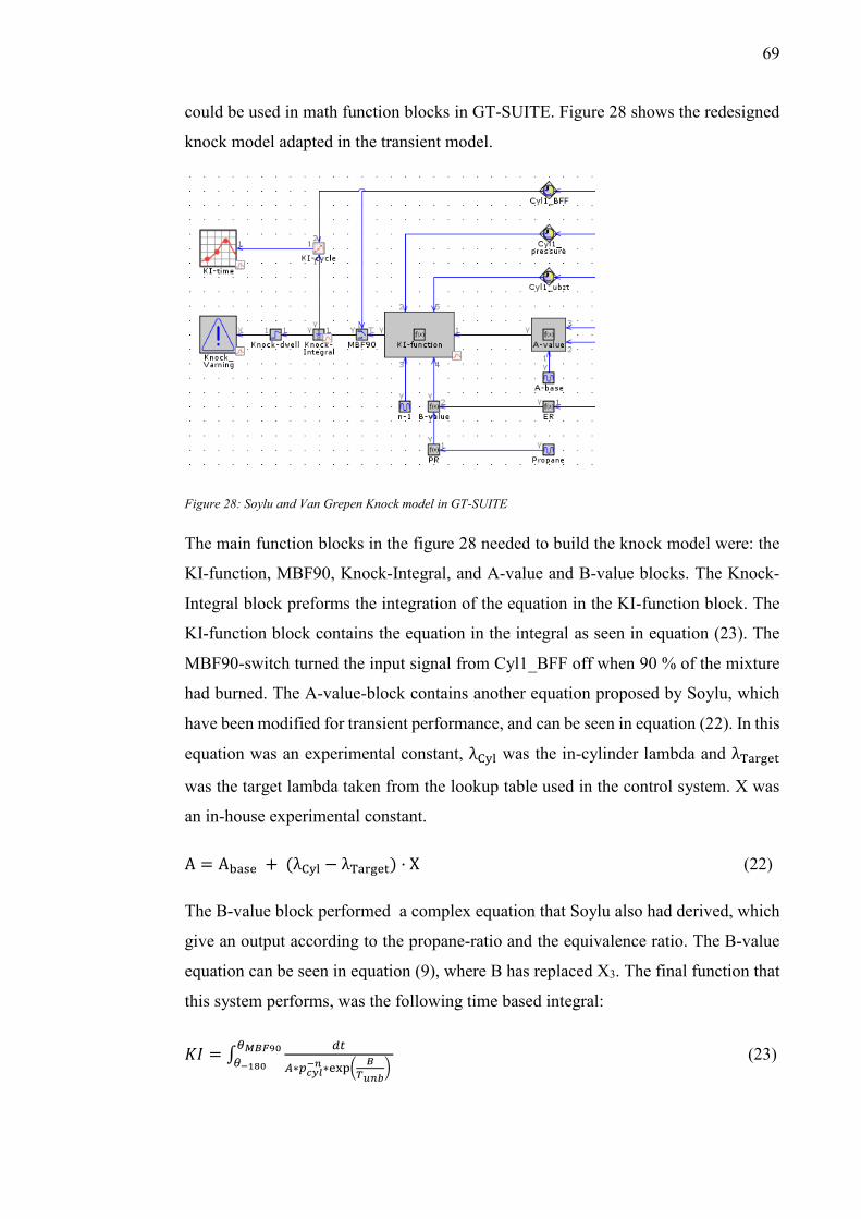
69

could be used in math function blocks in GT-SUITE. Figure 28 shows the redesigned

knock model adapted in the transient model.

Figure 28: Soylu and Van Grepen Knock model in GT-SUITE

The main function blocks in the figure 28 needed to build the knock model were: the

KI-function, MBF90, Knock-Integral, and A-value and B-value blocks. The Knock-

Integral block preforms the integration of the equation in the KI-function block. The

KI-function block contains the equation in the integral as seen in equation (23). The

MBF90-switch turned the input signal from Cyl1_BFF off when 90 % of the mixture

had burned. The A-value-block contains another equation proposed by Soylu, which

have been modified for transient performance, and can be seen in equation (22). In this

equation was an experimental constant, λCyl was the in-cylinder lambda and λTarget

was the target lambda taken from the lookup table used in the control system. X was

an in-house experimental constant.

A = Abase + (λCyl − λTarget) · X (22)

The B-value block performed a complex equation that Soylu also had derived, which

give an output according to the propane-ratio and the equivalence ratio. The B-value

equation can be seen in equation (9), where B has replaced X3. The final function that

this system performs, was the following time based integral:

𝐾𝐼 = ∫𝑑𝑡

𝐴∗𝑝𝑐𝑦𝑙−𝑛 ∗exp(

𝐵

𝑇𝑢𝑛𝑏)

𝜃𝑀𝐵𝐹90

𝜃−180 (23)

70

Where pcyl was the in-cylinder pressure in Pascal, Tund was the unburned zone

temperature in Kelvin and n was an experimental constant. The integrating limits are

set to be taken from BDC to the CA° when most of the fuel has burned, in this case

when 90 % of the fuel had burned. When the knock integrals output was one, it was

set to correspond to a light knocking. The model also had message-block that gave a

warning if the knock level went over the threshold level. The model had two run-time

monitors that showed the current knock level, one graph is CA° cycle based and the

other graph is time based. In figure 29 the two run-time monitors can be seen where a

load-ramp with constant load rate was tested. The graph to the right is time based and

the left one is CA° based and where the MBF curve shows when 90 % of fuel is burned.

Figure 29: Run-time knock monitors

This knock model could be adapted for certain cases and worked fine in the cases

where high MN had been used. The problem with this knock model was finding any

common Abase and n factors that could be used for all loads and conditions. The model

was validated against three laboratory tests with the same BMEP, where the engine

had operated near its knock limits but had different MN, ST and IVD. The output from

the knock model should therefore be close to 1 in all three tests, when modeled in GT-

SUITE. Steady-state tests were run off these experiments, hence the MultiWiebe

control system was disabled and a user-imposed-combustion-profile from the TPA

was used instead. The goal was then to find common parameters for the tests so the

output from the knock model would be close to one in all three tests, and therefore full

factorial discrete optimization simulations of the three cases were run, until they

reached steady-state, where the Abase and n parameters changed over a wide spectrum.

71

The results were plotted both in GT-POST and in Excel, so different types of graphs

could be made, and these graphs can be seen in appendix 2.

The results concluded that the n parameter had a too great of an impact on the knock

level, different Abase parameters can be used but the spectrum for n parameter was very

small, which meant no common n parameter could be found that worked for all loads

and gases. This model could still be used if the n parameter was calibrated before the

transient tests and if a high MN was used. Figure 30 shows an example how cases

with the same load ramp behaved to different MN. The calibrated and uncalibrated

values have their own y-axis. When the MN is lowered from 100 to 80 and the

parameters were kept the same, the knock level increases tremendously in the

uncalibrated case with MN 80. When the parameters were calibrated, the knock level

is quite similar to the case with a MN 100.

Figure 30: Knock integral calibration experiment

After comparing the simulations with the laboratory tests, it could also be concluded

that the model did not always knock at the same places as the real engine. Knocking

combustion usually occurs at high load as mentioned in the theory, which also was

true for the model, but the model rarely knocked at any other places.

72

3.6.2 Kinetics Fit Natural Gas Knock Model

The knock model described in the previous chapter did not produce the results that

were hoped for, hence the Kinetics Fit Natural Gas knock model was added to the

transient model in order to calculate the knock induction time integral and knock index

for predicting knock and pre-ignition. GT-SUITE uses two own knock equations for

calculating knock induction time integral and knock index, which were described in

2.7.6 Knock Modeling in GT-SUITE. These models were simple to add to the transient

model, since it was just a template added in the cylinder templates advanced tab. In

the knock template, the different knock models can be chosen, in this case the Kinetics

Fit Natural Gas knock model, and the template also contains two parameters and three

multipliers. In Figure 31 the content of the knock model can be seen.

Figure 31: Setup for the Kinetics Fit Natural Gas knock model

To keep the knock model simple the single-zone option was chosen, which calculated

the induction time integral using the bulk unburned gas temperature. The fuel methane

number was calculated with yet another in-house spreadsheet tool, where measured

data was used to calculate the exact MN for each test. There are three multipliers that

need optimization in this model, the Knock Induction Time Multiplier, Activation

Energy Multiplier and Knock Index. The first two mentioned of the multipliers are

used to calibrate the knock induction time integral and the last one is for calibrating

the knock index.

The knock integral and knock index of GT-SUITE were validated against the same

three tests as mentioned in the previous chapter, plus two newer tests. After a just a

few DOE-optimization runs it could be concluded that the knock index suffered from

73

similar problems as the Soylu and Van Grepen knock model. The Knock Index

Multiplier could not be optimized in a way that the knock index could predict knock

for the wide operating range and conditions of the W31SG. The GT-knock model again

showed more promising results and the time was focused to further investigate that

model. As cited in the theory, this method also uses the integral method, which

Liwengood and Wu developed, and the used formula also has some similarities to the

Soylu and Van Grepen knock equation, which gave opportunities for some interesting

comparisons.

When adding the GT-SUITE knock-template to the transient model, no added

function-blocks were actually needed, but in figure 32 can the structure used for

checking the knock level during the run-time simulation can be seen. This speeded up

the process of comparing this model to the Soylu and Van Grepen knock model in GT-

POST.

Figure 32: Simple knock model structure in GT-SUITE

The knock integral multipliers for the knock induction time and activation energy still

needed to be further optimized. The optimizer was used again when trying to find a

common knock induction time multiplier constant, which could be used with different

MN, ST and IVD. The simulations in the optimizer were run until they reached steady-

state and the results were sorted and stored in tables in Excel. After running wide cases

sweeps of the multiplier constant, and sorting and plotting the results in tables and

graphs in Excel, in order to see whether there were any trends that could be found, the

following conclusions were made:

74

The MN had a too large of an impact on the formula used in the knock model, which

can be seen in the equation (10) and which makes it impossible to have the same knock

induction time multiplier for all cases. Hence the multiplier should be calibrated, when

the MN is changed. The graph in figure 33 below uses the same load ramp as in figure

30, and is an example how the GT-knock model behaved to different MN and

multipliers. The shape of the curve remained the same with different MN, but with

lower MN the knock intensity increases, in particular if the multipliers were left the

same. In the figure 33 the green curve’s multipliers has been changed, so that the MN

100 and MN 80 were moved above each other as a test, to show that the MN has

minimal effect on the shape of the curve; it was just the scale that changed with

decreasing MN.

Figure 33: Calibration of the kinetics fit natural gas knock model

When the MN was the same as Soylu and Van Grepen knock model and the knock

induction time multiplier was calibrated to that particular MN-spectrum, the GT-knock

model produced more realistic results. During the transient runs the knock level at high

loads were close to the threshold and when the AFR became too lean, peaks also

occurred in the knock monitor. This knock model had it flaws and could still be further

improved, however it was a proof of concept and it was the best of the knock-models

that were tried out. Therefore, this knock integral model was used as a limit, together

with the limitations of the maximum cylinder pressure and previous modeled thermal

load of the exhaust system, in particular when it came to improving the transient

loading of the engine.

75

3.7 Transient Loading

As stated in 1.2. Goal, the main objective was to model the Wärtsilä 31SG engine in

various ramp-type transient loading situations in constant speed operation. This has

been done with the help of the new combustion model and the control system that went

with it, described in the previous chapters. The transient performance of the model

engine was compared to real laboratory tests, by using the same operating conditions

and using the same load rates. In the model the load rate was given with load ramps,

which were lookup tables for the gas admission. This was one of the main inputs for

the engine, since it was what the air mass-flow was regulated against. The gas

admission gave the right amount of gas according to BMEP and by making maps that

gave the desired BMEP according to time, and the load rate could be controlled. As

pointed out earlier the AFR was controlled in the model with the EWG and valve

timing, which are controlled by the system described in 3.4 Engine Control and

Automation.

Most laboratory test data used for the sensitivity analysis could be found in Unitool or

in Concerto. When validating the transient performance of the model Unitool was

mostly used, since its data could be easily copied into Excels spreadsheets. In these

spreadsheets data could be found, which could be used to calculate what the BMEP

had been at a particular time. This data was then used to make the lookup tables that

could mimic the performance of the laboratory test runs and thus validate the model.

In these spreadsheets could also other data needed for the sensitivity analyses of the

simulations be found, for example temperatures and pressures at different points of

inlet and exhaust system. This data was copied to GT-POST and made into plots for

the validation processes.

3.7.1 Optimizing the Load Rate

One of the goals of this thesis was to decrease the time it takes for the engine to reach

full load from ten percent of the maximal load. The load ramp tests were done under

the same ambient conditions as the laboratory engine and simulations were also done

with a preheated engine and with a gas of MN 77. The reason why MN was not chosen

76

to be 100, which had given the best knock resistance, was because the laboratory

engine was running on a gas with a MN 77 at that time when these simulations were

made. It was therefore interesting to use that particular MN, so that the optimized load

ramp could be validated, but due to delays in the schedule, the optimized load ramps

were never tested.

When optimizing the load rate for the model, a fast linear load rate from the laboratory

tests was chosen as reference load ramp. The MN and other conditions was known for

the reference test and only some light knock had occurred. Since the transient model

originally was made from a steady-state model were all the simulations first run at

constant load for a couple of seconds before the loading process started. This was done

so that the initialization process would not affect the loading process. The simulations

were also kept at full load for a couple of seconds, after the model had achieved full

load.

The limitations of the loading capacity were, as previously stated, set by the GT-knock

model, the thermal load of the exhaust system and the maximum cylinder pressure.

Three main limiting factors were chosen to stop the simulation, were the threshold

knock level from GT-knock model, the thermocouple temperature before the HP-

turbine and the maximal cylinder pressure in one cylinder. So-called Message- and

StopSimulation blocks were linked to these parameters in the transient model, which

gave a warning if the threshold level was near or stopped the simulation if threshold

level was exceeded. By doing this, unnecessary tests could be skipped and simulation

time could be saved.

Optimization runs were done where straight load ramps were run with increasing load

rate until a threshold limit was exceeded and the simulation was stopped. This gave an

optimal straight load ramp, but the transient loading could still be faster in certain

places, and therefore the load rate was increased where it could be faster until a new

threshold was reached. This was repeatedly done by trial and error until an optimal

load ramp was made. Figure 34 shows some tested load ramps. The load ramps were

as mentioned normalized to a reference ramp, where zero means the engine is

operating at 10 % of the maximal load and 100 means that the engine is running on

full capacity.

77

Figure 34: Optimized load ramps

By adjusting the load rate in different sections of the load ramp major improvements

could be done for the time for the transient loading. The results for the fastest load

rates are discussed and presented in 4.5 Optimized Load Rate and in appendix 6. The

loading performance depends as stated mainly on how the parameters are chosen for

the knock models and what the knock threshold level is set to. The validity and issues

of this will further be discussed in 5 DISCUSSION.

3.7.2 Experiments with Boundary Conditions

The previous chapter described the validation of the transient loading and how the

optimization of the load rate was done. This chapter will describe some of the

experiments done with the transient model. Not all simulations could be validated

against real tests, since no such test runs could be found with documented test data.

Most of the tests were simply done to confirm that the model behaved in the right way

to changing input parameters, since not all control maps were based on real engine

performance data.

0

10

20

30

40

50

60

70

80

90

100

0 1 0 2 0 3 0 4 0 5 0 6 0 7 0 8 0 9 0 1 0 0

NO

RM

ALI

ZED

LO

AD

(%

)

NORMALIZED TIME (%)

Reference Case 1 Case 2 Case 3 Case 4 Case 5

78

One of the goals of transient modeling of the W31SG engine was to see how the model

behaved with different engine starting temperatures. This was one of the few

experiments that could be validated, and which had already been used for the

sensitivity analysis of the thermal loading for the transient model, see 3.5 Thermal

Load Simulations. In these tests, the starting temperature was set by doing steady-state

pre-runs of the model with different initial temperatures. Three pre-runs were made,

starting with cold system and thereafter gradually increasing the temperature of the

exhaust systems. Then the same load rate was used in the three cases and the results

were compared in GT-POST, in order to see what effect the initial temperature had on

the model and the different parameters, such as the knock level. The results were

different from the initial engine temperature can be found in appendix 7.

Tests on how the MN affected the transient loading were also done, and same load

ramp was simulated with different MN. In the tests the multipliers that controlled the

knock model had been calibrated to a MN of 77, since the multipliers there had already

been validated in previous tests. Methane numbers from 100 down to 70 were tested

and the results can be found in the appendix 9.

As mentioned earlier, the settings for the EWG PID-controller have already been

improved in order to make the EWG react faster, decrease the pressure deviation from

the target pressure in the receiver and hence decrease the knock. In appendix 4 the

behavior of the simulated and measured throttle angle can be studied. In these

simulations the proportional and integral gain were also changed, in order to see what

the effects were on the knock level, and if the settings could be improved even further

for a faster transient loading. The results are discussed in 4.6 Results from the

Experiments. The graphs from this experiment can be found in appendix 11.

A test changing the compression ratio also needed to be done, since the laboratory

engines CR had been changed during the thesis project. Therefore it was interesting to

see how the thermal load of the engine changed with different CR. The lookup tables

for the engine control system were not changed since it would had taken too much

time. These results are presented in appendix 8.

Quite a few tests were done to see what the effects were on the engine performance

when adjusting the control maps. These tests where run with a much faster load rate,

79

because some of the effects only show when the EWG is fully closed. In one test, the

map that gives the target receiver pressure according to BMEP was shifted in a way

that the map either gave a 10 % higher or lower target receiver pressure. In another

tests the map, that gave the IVD-deviation according to BMEP and the pressure

deviation, was doubled and then halved. The same map was also set to do nothing in

order to see how the engine behaved. Experiments on the map changing ST according

to pressure deviation were also made. Here the outputs were also doubled, halved and

set to do nothing. These results can be found in appendix 12.

To simulate how the engine would perform with higher and lower boost pressure

another interesting experiment was done, where the HP-turbine area had been both

increased and decreased. These tests were just indicative, since some of the negative

effects of having a bigger or a smaller turbine wheel were not accounted for, such as

the change in inertia, which effected how fast the turbocharger got up its optimal

operational speed. The results for the boost pressure experiment can be found in

appendix 10.

A simple experiment was also done to simulate the effects of exchanging the current

HP-turbocharger with two smaller turbochargers while maintaining the same boost

pressure. This was simply done by lowering the inertia of the HP-turbocharger, since

two smaller turbines would have lower inertia than one big turbine that produces same

boost. This experiment did not consider the negative effects of having a more complex

exhaust and intake system that would be needed to add another turbocharger nor the

economic aspects. These results can be found in appendix 10.

The current laboratory engine was at sea level, so the ambient pressure was decreased

to simulate having a power plant at a higher altitude. The cases in the experiment went

from sea level up to 2000 meters above the sea, while the ambient temperature and

other initial conditions remained the same. An experiment with different ambient

temperatures was also done, both with higher and lower ambient temperatures with the

aim to see what effect it had on the transient loading capacity. The results from the

altitude and ambient temperature tests can be found in appendix 13.

80

4 RESULTS

In this chapter the most important results are presented and discussed. Further results

can be found in the appendices. Some of the results are confidential and are therefore

either normalized or left out. The credibility and the issues with results are presented

in 5 DISCUSSION. As mentioned in the introduction one of the goals was to make a

transient model of the Wärtsilä 31SG laboratory engine in GT-SUITE, with which

different load rates, performance maps and settings could be tested. Many technical

papers were studied to obtain a good understanding of how lean-burn gas engines work

and how different conditions affect them and how the parameters should be controlled

to optimize the performance of the engine. Therefore, a comprehensive theory part was

written, which also could be considered results for this thesis, considering that one of

the goals of this thesis was to do a literature survey on the combustion modeling for

the lean-burn gas engine. The method part of this thesis described the process behind

choosing the combustion model, how thermal loading was investigated and how the

automation and knock detecting system was built. This needed to be done, so that the

parameters that limit the performance of simulations could be established.

With this simulation model different tests can be done prior to real test runs and

perhaps give some insight in how the laboratory engine will behave, and hence save

some expensive engine running hours. The previous chapter described some of the

experiments that were performed with this model and could be used as examples for

what this model could be used for. If the model is calibrated right, the model can

predict knocking combustion with the help of two knock models and harmful

temperatures can be avoided with the thermal capacity modeling done to the model.

One of the major tests that could be done, thanks to the knock models and the thermal

load modeling, was presented in 3.7.1 Optimizing the Load Rate, where experiments

were done to find an optimal load ramp. Load ramps that were over 60 % faster than

the reference load ramp were produced. The finished transient model was still fully

modifiable and all settings and performance maps could still be changed if needed, for

example if any part of the laboratory engine is, tests can be done prior to that and give

a guideline to what the performance benefits would be. In the following chapters more

tangible results will be presented.

81

4.1 The Final Transient Model

This chapter contain general descriptions of the control system. Then follows a

sensitivity analysis, where measured data is compared to simulated results, and which

shows how the model reacted to different lambda and boundary conditions and how

the EWG, ST and IVD compensated for that. The most important results are shown in

the following figures while other graphs needed to elucidate the results are found in

the appendices.

In figure 35 the control system can be seen, which also could be seen in figure 10 in

2.6.2 Control Strategy of Natural Gas Engines, as sub-assemblies. The system for

controlling the combustion, described in 3.4.1 Test Automation, and the knock models

described in 3.6 Knock Models, were put into the main transient model together with

the rest of the systems that were used to find the limiting factors for the transient

performance. The system for controlling the parameters in the MultiWiebe template

shown in figure 24, was still very similar in the final model but the lookup tables have

been calibrated and the made-up signal generators and lookup tables, made for testing

the system, have been replaced by real feedback inputs from the system. Graphs for

how the MultiWiebe template change the burn rate, and therefore also the

performance, will be presented in the next chapter and the results from the knock

modeling will be presented in 4.3 Knock Estimation.

Figure 35: The final control system

82

Figure 36 shows a graph with load rates, where the red curve shows the desired load

rate, the blue curve shows the models output and the green curve is a reference load

rate from a similar laboratory test. All the load rates have been normalized, so that at

zero the engine is at 10 % load and at 100 the engine is at 100 % load. As can be seen

in the graph, the simulated load rate is almost the same as the desired load, it is only

in the beginning where the load rate lingers and the maximal load is achieved, when it

slightly overshoots. In appendix 4 the position of the EWG can be observed, including

how it closes with increasing load.

Figure 36: Validation of simulated load rate

Figure 37 is a contexture of how the deviation maps for ST and IVD together with the

EWG reacted to the changing lambda due to the increasing load. It was the same load

ramp as in the previous figure and here it was possible to see how the ST deviation

map retarded the ignition timing and how the inlet valve was closing was delayed

momentarily. All outputs in the graph were normalized, where 100 meant that the ST

deviation curve was at its most advanced option. The IVD deviation was normalized

to give 100 at the maximum IVD deviation and 0 when there was the least IVD

deviation. For the normalized EWG throttle angle curve 100 meant that the EWG was

at its most open position and at zero it was at the most closed. The lambda deviation

curve was placed on its own axis and shows the normalized difference between the in-

cylinder lambda and the target lambda. When the lambda deviation curve went below

zero could it be concluded there was a lack of combustion air.

83

Figure 37: Contexture of how the EWG, ST deviation and IVD deviation react to lambda deviation

It can also be seen in figure 37 that the EWG closed rapidly when the load started to

increase, but since it did not close fast enough, there was a sudden drop in the AFR,

and therefore the ST was retarded and the IVD extended for a moment, shown in the

pictures as valleys, in the otherwise straight lines of the deviation maps. This was the

function of the deviation lookup tables described in 3.4.1 Test Automation, but the

deviation functions did only activate when the EWG was insufficient to regulate the

AFR.

4.2 Simulating the Burn Rate

As pointed out many times before, different combustion models where used when

trying to simulate the combustion in the W31SG engine. In 3.2 Predictive Model, the

SITurb combustion template was tried out, but this model was abandoned since it could

not be calibrated well enough to give an accurate burn rate for the whole loading

spectrum. Hence the Wiebe combustion templates were used to simulate the NG SI

combustion, described in 3.3 Semi-Predictive Models. A challenge with the Wiebe

models was that the burn rate curves had to be adjusted manually. By adjusting

parameters in the MultiWiebe calculation tool the burn rate could be traced, and when

84

the curves of the Wiebe function followed the burn rates made in the TPA, the

parameters could be stored in tables and used as lookup tables in the combustion

control system. The so-called target maps are what mainly controlled the Wiebe

combustion and these maps gave the right parameters according to load and pressure

deviation from the target receiver pressure. Since the burn rate also changed with

different ST and IVD, so-called deviation maps had to be made. The burn rate was

very much affected by in-cylinder lambda, therefore, deviation maps were made for

that as well. In figure 38 the simulated burn rates produced by the MultiWiebe template

can be seen, which were normalized by the total fuel mass. It can be observed in the

figure how the burn rate profile changed with different load.

Figure 38: Normalized burn rates from different loads.

First a single Wiebe curve was controlled with a few lookup tables, in order to make

sure the equations made for function blocks affected the burn-rate the right way and to

prove such a control system could be used before the process of making all the lookup

tables were done. The concept was proved and the MultiWiebe combustion model was

incorporated, which meant the PCC could also be controlled. This had been a problem

with the other combustion models, but this also meant that the amount of lookup tables

in the control system had to be almost doubled. Not all parameters in the MultiWiebe

template had lookup tables, since it was concluded that they did not change the burn

rate enough, and therefore they were put to have a constant value. The final control

85

system for the MultiWiebe combustion template could be seen in figure 34 and the

way it works was described 3.4.1 Test Automation.

In figure 39 the same load ramp can be seen as earlier, together with the in-cylinder

lambda and the parameters that control the MultiWiebe template. The AA was

normalized against the target map and the green curve describes how the AA for the

main combustion increases with higher load and changing lambda. The AA for the

PCC is normalized against its own target map and the pink curve describes its reactions

to load and lambda. This means that the total Wiebe curve moves from the TDC with

higher load, and delays the combustion, which can also be seen figure 38.

Figure 39: The burn rates parameters reaction to changing lambda due to increasing load.

The BD for the main combustion is the turquoise curve in the graph and it was

normalized against its target map. The PCC BD was also normalized to its target map

and was constant for this type of transient load, however, with faster load rates the

PCC BD changes if the pressure deviation is too large in the receiver. The BD for the

main Wiebe curve decreased with higher load and lower lambda, which meant the

combustion occurred faster and the amplitude of the burn rate curve got higher. As can

be seen in the figure both the anchor angles were sensitive to lambda, while the BD

was not particularly affected. This was because the deviation map did not cover all

situations, which meant it extrapolated from the last values in the map, which created

quite a steep ramp that could give unrealistic values, see 5 DISCUSSION.

86

4.3 Knock Estimation

Two knock models have been studied and modeled in GT-SUITE and in figure 35 can

the layout for these models be seen. In the case-setup the parameters for the knock

models can be filled in, and these should be calibrated if another gas with a different

MN is used. Laboratory data should be used to calibrate the transient model. The data

used for the reference test should be at a constant load and light knock should occur,

so that the knock threshold can be set to a constant number, where in most cases 1 can

be used. The MN and weight percent of propane in the fuel gas needs to be documented

and the ambient conditions and the thermal load of the system should also be copied

to the simulation. The simulation should be set to run on the same constant load as the

reference run and an optimization run should be done for Abase and n factors in the

Soylu and Van Grepen knock model, and the knock induction time multiplier should

be optimized in the same way for the GT-knock model. The knock models can then be

used for determining the occurrence of knock in transient test runs.

Figure 40 shows the same load ramp with the lambda deviation curve as in the earlier

figures, but this time they were together with output from both of the knock models.

The blue threshold line was set to be one, and was set to correspond to light knock

level. According to the green knock curve from the Soylu and Van Grepen knock

model, no knock occurred at any point during the whole transient load. However, did

the GT-knock model claim there was some knocking combustion at the start of the

loading process. As mentioned earlier was the GT-knock model quite sensitive to

lambda, which can be seen here when the knock level went well above the threshold,

when the mixture temporarily got too rich. Half-way through the loading the shape of

both the knock curves were quite similar and no further knock occurs. In appendix 5 a

graph of knock index that Gamma technologies has developed can be seen. This knock

model predicted knock at the same point as when the lambda deviation was the largest.

The knock threshold for this knock model was set to 100, which the KI also was very

close to, but this model was only roughly calibrated, so the result was only indicative.

87

Figure 40: Transient loading and the knock levels

When looking at the cylinder pressures in Concerto it can be concluded that the

cylinder pressures had been quite restless when the loading process started, which can

indicate that some light knock had occurred, in approximately the same place as in the

GT-knock model. During the loading process, at full load, the cylinder pressures were

normal, but when looking on the heat release rate graph in Concerto, there were hints

that post knock occurred during loading. Remarkably, it seemed like the post knock

mostly occurred at the same place as were the sharp waves are in the Soylu and Van

Grepens knock model.

Considering that this was a fast load ramp, it was quite normal that some light knock

occurred, which made it hard to decide what level of knock should put as threshold.

The parameters for the knock models could also have been calibrated better, since the

real knock levels at full load would most likely have been just beneath the threshold.

In 5 DISCUSSION this issue will be further debated.

88

4.4 Sensitivity Analysis of the Thermal Capacity

The thermal load of the W31 engine has been investigated and many simulations have

been done in attempt to copy the thermal capacity in GT-SUITE. The structural heat

capacity was first studied in the steady state simulations and was concluded to by quite

accurate for most of the parts of the engine. To narrow down the workload for the

validation process for the thermal modeling, only one point of the exhaust system has

been used to create the results. This validation point was just before the HP-turbine in

the exhaust pipe and is where the temperature was measured with a thermocouple.

Modeling this part of the exhaust accurately is important, since it affects the boost

pressure and the overall performance of the engine. This was also the validation point

in the steady state simulations where the simulated temperate had deviated the most

from the measured laboratory tests.

Figure 41: Thermal loading of the exhaust system with preheated engine

Figure 41 shows a normalized temperature rise in the validation point in the exhaust,

when the engine has been preheated to operating temperature and the same fast load

rate has been used as in the previous tests in the result chapter. The result for this

particular setup was not credible, the simulated average inlet temperature rises way

too fast and the thermocouple temperature was also too fast in the beginning and did

not rise high enough. The exhaust systems structural heat capacity was probably the

89

reason for this, since it was not calibrated well enough and the exhaust system would

have needed more mass. A validation issue with this test was also that lower CR had

been used, which meant the final measured temperature will always be a little higher.

The thermocouple was not set up right for these operating conditions either, but in

figure 42 the results from another thermal loading test can be seen, and there with

much better results. This was non-preheated engine test with a slower load ramp. The

average inlet temperature still rose too fast, but the thermocouple was much better

calibrated for these operating conditions. The thermocouple curves were a little too

slow in the beginning to later overshoot the measured temperature.

Figure 42: Thermal loading of the exhaust system with cold engine

The same phenomenon also occurred in other validation points in the exhaust system,

for example when the temperature was measured in the just junction before the LP-

turbine. The simulations could also conclude that tests with slower load rates were

more accurate than the fast ones. The temperature rise seemed to be too fast in most

tests in the beginning, to later become closer to the measured temperature, where the

limiting temperature usually also is. Consequently, if the thermocouples were

calibrated correctly, the thermocouple can be used as a limiting factor for the

optimization of the load rates, as presented in the next chapter. In the next chapter can

also the effects of faster load rates be seen in the thermal loading and in 4.6 Results

from the Experiments, the effects of different starting temperatures will be presented.

90

4.5 Optimized Load Rate

In 3.7.1 Optimizing the Load Rate the process behind creating the best load ramp was

described and in figure 34 in that chapter, different tested load ramps can be seen that

got progressively better. In most cases it was the knock threshold that limited the

transient loading, but as the load rate went up, the HP-turbine temperatures also started

to limit the load rate. Some of these load ramps were a little older, so in cases 1 to 3

the HP-turbine temperature was measured without a thermocouple, which meant that

the temperature increased faster and which in turn limited the load rate. The lookup

table for the target lambda that the MultiWiebe control system uses had also been

updated, which together with the improved EWG control decreased the AFR deviation

at low loads, which also made it possible for the load rate become faster in the

beginning. The maximal cylinder pressure threshold only became a problem at the

maximal load, but could be overcome with a smoother transition to max load. With

these improvements, the load rate could made be faster in case 4 and 5.

The load ramp shown as curve case 4 in figure 34 was almost 59 % faster than the

reference load ramp, which was a considerable improvement, but the ramp was still

not yet fully optimized. Some of the last tests that was run during this project were

further optimization tests of the ramp, where all the limiting factors had been pushed

to its max limit, which produced a load ramp that was 62.5 % faster than the reference

ramp and can be seen in case 5. The validity if this experiment will be debated in the

5 DISCUSSION. When doing the experiment described 3.7.2 Experiments with

Boundary Conditions the load ramp from case 4 was used, since they were done before

load ramp in case 5 had been made.

In figure 43 illustrates the fastest load ramp plotted together with the limiting factors.

The temperatures and cylinder pressure are normalized so that 100 is the threshold

level where the laboratory engine would shut down and 0 corresponds to the output at

10 % load. The knock index goes between 1 and 0, where 1 is the threshold level at

which knock is predicted. The GT-knock model is as mentioned more sensitive to the

lambda deviation than the other knock model, which made it the most limiting factor

for this case of transient loading. The GT-knock level rose very fast when the load rate

started to increase and therefore the loading was also slower in the beginning to get

91

gradually faster. This was probably due to turbo lag, which meant that the

turbochargers did not get enough time to spool up and create significant boost pressure

in the receiver. The maximal cylinder pressure does not seem to be an issue until the

maximal load has been achieved. At the point where the load became constant and

where there was a little overshoot over the reference map, the pressure was almost at

its threshold level. The output from the Soylu and Van Grepen knock model can also

be seen in the graph, where the knock index mostly seems to rise with the load.

Figure 43: Optimized load rate and limiting factors

Another reason for using the load ramp from case 4 for the experiments was that the

average inlet temperature surpasses the threshold level briefly, but the thermocouple

temperature which has been put as limit does not, which made this load ramp validity

questionable. In appendix 6, figure III the HP-turbocharger’s average inlet temperature

is compared to the thermocouple temperature, which reinforces the previous statement.

In appendix 6, figure I a graph shows how the ST and IVD changes with lambda, and

which proves that the air-fuel mixture is too rich at start up.

92

4.6 Results from the Experiments

In chapter 3.7.2 Experiments with Boundary Conditions, some of the different

experiments were described that were done with the transient model. For these

experiments the second fastest load ramp was used, which is plotted in figure 34 as

case 4. In these tests the knock indexes were the most interesting parameters and were

therefore plotted in the appendices. In some of the experiments also other outputs were

plotted if they showed results that were interesting or otherwise unexpected, for

instance, if they affected the other limiting factors that were used to produce the

optimized load ramp.

For the experiment where a different initial operation temperature was tested, a couple

of different starting temperatures were tested and three of them were used to produce

the graphs in appendix 7. The results were as usual normalized, between the lowest

and the highest temperature documented in the test runs and shown as an output

between 0-100. The green curve corresponded to a cold start, the red curve for a warm

engine and the blue curve for a starting temperature in-between. For this test the

exhaust temperatures are plotted and both the average inlet gas temperature seen in

figure I and the thermocouple temperature measured in the junction before the HP-

turbine can be found in figure II in appendix 7. The same behavior of the thermal load

for the model can also be seen in this experiment as presented in 4.4 Sensitivity

Analysis of the Thermal Capacity, in which the temperature rise in the exhaust system

was much faster, when the starting temperature had been low.

As expected did the knocking combustion get worse with lower initial starting

temperature proved by the output of the GT-knock model, which can be seen in

appendix 7 figure IV. In figure V the knock levels can be seen for the Soylu and Van

Grepens knock model, where the results were not as unambiguous. The knock level

fluctuated a lot more in this model, where the low starting temperature gave the highest

knock index at low load to later give almost the same output as when the starting

temperature had been high. Interestingly the knock index is the highest for the blue

curve when the engine had achieved full load for the both knock models. The cylinder

pressures are plotted in figure III in same appendix, which seemed to be affected by

the initial starting temperature, since the final cylinder pressure was almost 20 percent

93

less when the engine had been cold. Surprisingly was the power output that only 1-2

% less during the transient run with a cold engine, compared a warm engines power

output.

Many experiments have been done running the model on different gases with high and

low methane numbers, where the most interesting aspect was the effect on the knock

indexes. Explained earlier in the sub-chapters of 3.6 Knock Models, the MN affects

the scale of the KI, but the shape of the knock curve is pretty much the same. In these

tests the parameters for the functions in the knock models have only been calibrated

for a MN 77, since it has been validated against measured data. The GT-knock model

reacts to the deviating MN in a more linear and realistic way than the Soylu and Van

Grepen knock model. In appendix 9, figure I the GT-SUITE knock models output and

how the KI decreases and how the curve seems to get a little smoother with higher MN

can be seen. In the Soylu and Van Grepen knock model the MN affects the KI

significantly more, which can be seen in appendix 9, figure II. Here the KI was also

lowered with higher MN, however when using a gas with a MN of 100 the KI became

unrealistically low and showed the importance of the calibration of this knock model.

Overall the MN seems to have very little effect other than limiting outputs for this

model, for example the exhaust temperature only becomes two percent higher when

switching from MN 77 to MN 100 and the difference in cylinder pressure is negligible,

which seems realistic since the MN generally does not influence the performance until

knock occurs.

An experiment was done to study the factor that had plagued the whole thesis work,

i.e. the parameters for the proportional and integral gain of the EWG PID controller.

Already in the early stages of the thesis project the PID had been made faster for better

transient performance. In this test the initial PID settings were compared to the new

settings used in the other experiments and two new settings, where one was set to react

faster and one slower, which can be seen in appendix 11, figure I. In the same appendix

the effects on the knock indexes can be studied in figures II and III. As expected, did a

faster EWG lowers the KI, since the AFR can be kept closer to its target ratio. The

difference in the knock level were more accurately seen in the GT-knock model, since

it reacted much more to deviation in AFR.

94

It can also be proven that performance of the PID could not be improved much after

the first time making it faster and in appendix 11, figure I the jagged behavior of the

fastest settings can be seen. From the same figure can it also be concluded that the new

fast setting was probably a little too fast, since its behavior for this load ramp is quite

restless. With the faster settings the exhaust temperature could also be kept a little

lower in the beginning of the transient loading to even level out at the higher loads.

The maximal cylinder pressure from this test did not change much either, and only

towards the end of the transient run was the cylinder pressure about five percent lower

for the fastest setting compared to the initial setting, and even to later also level out.

A simple yet interesting experiment had been done with the model where different

cylinder compression ratios had been tested. The CR had been increased and decreased

by three percent, without changing anything else. The results from the decreased CR

was particular interesting, since it raised the average exhaust gas temperature by about

seven percent, which can be seen in appendix 8, figure II. When the thermal capacity

had been validated, it became clear why that the final temperature in figure 41 had

been too low and the reason for that was blamed on the shimming of laboratory engine,

which resulted in a lower CR. This meant the simulated exhaust temperature shown in

figure 41 would come a lot closer to the measured temperature. The normalized

maximal cylinder pressure seems to move with same rate as the change in CR, where

a 3 % higher CR gave the equal increase in maximal cylinder pressure at full load and

vice versa. The plots for the knock models can be seen in appendix 8, figures III and

IV, where a higher CR increased the KI for both knock models with about 8 %.

The concept behind the experiments where the different changes in lookup tables have

been done was also explained in 3.7.2 Experiments with Boundary Conditions. In these

tests the focus was on the change in the GT-knock level, since the effect was best

shown there. In appendix 12, figure I was the map that gave the target receiver pressure

according to load changed, so that the output pressure would be either 10 % higher or

lower. With the higher receiver pressure the air-fuel mixture gets leaner and therefore

the KI is lowered, which can be seen especially well in the beginning of the process.

The opposite can be concluded when lowering the receiver pressure map, where a big

peak in the KI can be seen in the beginning.

95

In appendix 12, figure II the results of changing the ST deviation map can be seen. As

mentioned earlier this map shows how much the ignition timing should be retarded

depending on the pressure deviation in the receiver. In the experiment, the output from

the ST deviation map was changed in three different cases, the output was first

doubled, then halved and lastly set to be zero. The effects from these changes were

quite immense. When there was no ST retardation the knocking became much worse

and went over the threshold level, according to the GT-knock model. When doubling

the outputs from the deviation map the knocking was decreased significantly. As

expected did the knocking also become worse when the deviation lookup output was

halved. This meant the load rate could be faster in the late middle of the transient

loading if doubled outputs of the ST deviation map were used, but not as much as the

knock model suggested, since the normalized exhaust temperature also rises with

about two percent, which is already close to the threshold.

In appendix 12, figure III the result from modifying the IVD deviation map can be

seen. This plot was difficult to interpret, since in the case where there was no IVD,

was the KI got lower for most of the transient loading. Only at the very end, the KI got

over the initial settings and the threshold. When the IVD deviations output was halved

the same phenomenon occurred. However, when the output was doubled the KI got

worse for most of the transient run, until the very spot where the KI had been the worst

for the other modifications, the KI is decreased a bit from the initial setting. This meant

that a faster load ramp could be made without the IVD deviation function, if the load

rate was faster until the last point where the threshold was breached, but the exhaust

temperature would then again limit the performance. The IVD deviation functions did

not seem to have much effect on the maximal cylinder pressure but without the IVD

deviation function the exhaust temperature was increased as much as 15 % in the end

of the loading process, which made it go well over the threshold. This was because

one of the main functions with IVD was to keep the exhaust temperature down and

thus avoid to high NOx emissions. The load rate could be faster with a little less IVD

in the beginning, but overall was the deviation map is well configured and should not

be altered.

As mentioned in the 3.10 Simulations Experiments two experiments were done

concerning the HP-turbocharger and the boost pressure. In the first test the HP-turbine

96

area was increased and decreased by five percent too simulate the behavior of an up

and down boosted engine. In the case where turbine area had been decreased, the KI

had been lowered significantly in the later part of the loading process and when the

boost pressure had been lowered the KI was increased during most of the simulation.

The exhaust temperature was just merely effected and neither was the maximal

cylinder pressure. This means that the engine would perform better with higher boost

pressure, especially on higher loads if the other negative effects were neglected, see 5

Discussion. The result from this experiment can be found in appendix 10, figure III

and IV, where the knock indexes are plotted.

In the other test modifying the turbocharger parameters, the HP-turbocharger shaft

inertia was decreased to a half and then to the quarter of the initial inertia. This

experiment was done in order to see if it would be beneficial to exchange the current

HP-turbocharger for two smaller turbochargers. In appendix 10, figure I is the GT-

knock models output plotted. The benefits of having two HP-turbochargers can only

be seen in the beginning of the loading process where the KI was lowered quite a bit,

but in the other part of transient loading did the knock curve look the same for the

other cases. This was also expected and with this result it can also be concluded that

the KI would be higher with more inertia, and thus the total KI would not be lowered

as much as predicted in the previous test, where the boost pressure was increased. In

this experiment as well, did the exhaust temperature and cylinder pressure remain the

same.

Two experiments were also done concerning the outside boundary conditions, i.e. how

ambient temperature and pressure would affect the performance of the simulated

engine. In the appendix 13, figures II and III the plots show how the knock levels differ

with changed ambient temperature. The red curve represented the normal temperature

the laboratory engine was tested in, the blue curve corresponded to 40°C and the green

curve is corresponded to 5°C outside temperature. As can be seen in the plots, the

knock levels are neither much worsened nor improved with different ambient

temperatures, and the highest peaks are just moved around a little. However, this

influenced the exhaust temperatures. When the ambient temperatures were as hot as

40°C, the normalized exhaust temperature almost overshoot the threshold, while with

the colder ambient conditions the threshold marginal got larger.

97

The other experiment dependent on the geography was an altitude test. The test engine

was at sea level and thus in this test ambient pressure was changed to that of 1000 and

2000 meters above sea level, in order to see the effects on the knocking. In appendix

13, figure V and VI the knock indexes are plotted. The knock levels got a little higher

at higher the altitudes at full load, which was expected since the air get thinner which

leads to a richer AFR. In this test the exhaust temperature was significantly affected at

high loads, which can be seen in appendix 13, figure IV. The normalized exhaust

temperature was almost 20 % higher than the test at sea level, which meant this ramp

could not be used at such high altitudes.

4.7 New Automation Functionalities

For the scope of the thesis was it decided that new automation functionalities and

optimum engine settings based on the results of the simulations would be

recommended in the thesis. The MultiWiebe combustion model got one control signal

from a so-called lambda lookup table, and a similar map could be used to control the

ST, IVD and other control means. Direct lambda control of the engine would probably

be more accurate than controlling the AFR according to the receiver pressure, which

the current engine did. The burn duration has also been controlled in this model, in

which a similar system could be built in to the UNIC ECU and could be measured with

the current fast cylinder pressure sensors. This system could control and limit the

combustion, so that the BD would not get too long and give an ineffective combustion,

nor too short, which would create too high peak cylinder pressures, which in turn could

be harmful to the engine.

The knock integrals could also be built into the UNIC control system, in order to

predict knock and change the load rate accordingly. The system would work in that

way, so that it slowed down the load rate just before the calculated KI would reach the

threshold KI. The system would probably work the other way around as well, so that

it would increase the speed of the transient loading until the threshold was reached.

98

In the 4.6 Results from the Experiments it was concluded that the engine would

perform better with higher boost pressure. The experiments showed that there was an

air deficit during the time the turbochargers spooled up, and compressed air could be

used as an upboost function for this. Compressed air could either be injected straight

into the receiver or it could be used to get the turbocharger turbine up to speed during

the aggressive loading period part. The compressed air could either be created

externally by a separate compressor when the electricity was cheap, or perhaps with

the engine itself. The compressed air could be created as a byproduct when slowing

down or stopping the engine, and the pumping of the pistons could compress air into

separate tanks and be stored for later usage.

99

5 DISCUSSION

In the introduction the goals and the scope were specified and thus the thesis contains

theory about the lean-burn gas engine, combustion modeling and knocking, all of

which cover the subjects which were in scope. The lean-burn chapters contain the most

vital parts that needed to be understood to be able to model the Wärtsilä 31SG. During

the project the focus had shifted a little more to the knock modeling of the engine than

originally intended and therefore a comprehensive theory part about engine knock and

knock modeling was included. The combustion modeling part of the theory became

quite extensive as well, especially the part about the Wiebe models, since their

functions were crucial to understand when making the control system.

One of the goals was to produce a model that could produce realistic data of the loading

performance of the lab engine. The main purpose of the model was to increase the

understanding of how the effect of boundary conditions, such as ambient conditions,

turbocharger specifications and inertia affected the loading performance of the engine.

When knowing how the engine model reacted to these specifics, optimum engine

settings for different loading situations could be made and studied. Thereafter the

model of the Wärtsilä 31SG laboratory engine could be made in GT-SUITE, from an

older model meant for steady-state experiments. A simplified picture of the model can

be seen in figure 10. The structure of the model still looked quite the same on the

outside, since the model was still new, but many templates have been updated or

changed. The biggest changes made to the model that can be seen on the outside of the

model were the control system and the two knock models. All of these changes can be

put in so-called sub-models in the future if the layout of the model needed to stay

unchanged. Important changes to the templates inside the model were, for example,

the MultiWiebe combustion template for the cylinders, wall layer properties of the

exhaust system together with the added thermocouple sensors and an updated HP-

turbine map. As stated many times earlier, the most time-consuming thing to do in this

thesis was to make the lookup tables for the combustion model.

Many of the lookup tables were, as mentioned, based on real performance maps, such

as the target and deviation maps controlling the ST and IVD. All the maps controlling

the parameters in the combustion template have been made with data from laboratory

100

test runs. The procedure for making these maps were explained in 3.3 Semi-Predictive

Models and this method left a lot of room for human interpretation, since there might

be multiple acceptable solutions. The laboratory test runs also varied a lot in age, with

some of the tests being quite old which could affect the outcome since the boundary

conditions might have been different. It was also hard to do any type of sensitivity

analysis for these parameters since little to no data could be found for the validation

process. Therefore, for most of the test the most important thing was to make the burn

rate change in the right direction within a moderate scale. Another issue with the

lookup tables was that data in them did not cover all situations, thus when input went

out of the lookup tables spectrum, the output was extrapolated which could result in

big errors. This has been restricted with the help of limiter-blocks for the maps that

had the tendency to give to extreme outputs.

Some simplifications to the control system had to be made in order to be able to finish

the thesis in a reasonable time spectrum, and has the combustion has only been

controlled by changing the ST, IVD and boost pressure with the EWG. The W31SG

has as mentioned a stepless inlet valve and variable exhaust valve, but in these

simulations only the effects of changing IVD have been investigated. The PID-

regulator for the EWG has also been speeded up for better performance in most of the

experiments and has been validated for a couple of tests, including a normalized

sensitivity analysis, which can be found in appendix 4.

Overall a considerable amount of time has been put on trying to make the predictive

model work, however the predictive model would have been convenient to use, since

the system for controlling the combustion could have been much simpler. If the SITurb

template would have been set up right, the burn rate could have been predicted for all

loads and conditions, without the system for changing the AA and BD parameters in

the combustion template. The ST and the IVD could then have been controlled with a

much simpler system, as the one seen in figure 21. The main problem with using the

predictive model was that there was no template for the calibration process that suited

a lean combustion gas engine with pre-chamber well enough, and which in turn made

transient modeling impossible, since no common parameters could be found that

would work for both high and low loads. Instead the rather complex control system

101

had to be built, including a lot of lookup tables, in order to produce the burn rate that

the predictive SITurb template would have produced automatically.

As mentioned in 3.5 Thermal Load Simulations, the heat transfer of the exhaust system

has been studied and validated against laboratory tests, and the parameters for the

thermocouples had to be adjusted according to that. This turned out to be complicated,

because when the parameters for the thermocouples were adjusted so that the

temperature-curve would be comparable to the test data, it would not suit the other

tests where the heat transfer had been faster or much slower. For example, if the

thermocouple parameters were set up for a non-preheated simulation the temperature

rise would have been too fast for a test with preheated engine. The thermal loading

could still be validated for laboratory tests when “WallThermalProperty”-references

was adjusted for the pipes attributes and with the help of the thermocouples and the

initialization runs. Another problem thermal validation was that the laboratory engines

CR had been lowered for low MN testing, and therefore the measured exhaust

temperature was higher than in the simulations. Also, in older transient tests, different

parts had been used and this led to there being quite few tests to validate the model

against. The CR and the parts of the model could have been adjusted, but then all the

lookup-tables for the control system should as well have needed to be updated.

A lot of the time went to fitting the parameters for the knock model. In appendix 2

three charts can be found that show how the knock index changes with high, medium

and low MN and with the different parameters in the Soylu and Van Grepen knock

model. The reason for making these charts was to find the common Abase and n factors

that could be used for all cases. This could not be done, because of the sensitivity of

the n factor, which was due to it being an exponent in the knock formula, seen in

equation (23). If the knock threshold level was to be 1, the output from the knock

model should be in the near spectrum of threshold. The charts illustrate this problem,

with there being a very small spectrum of n factors that works for a particular MN to

get a reasonable knock level. A probable cause for this problem could be that the

original knock model that Soylu made did not operate this leanly, but this could

perhaps be fixed if the constants in the equations that Soylu defined were configured

better for this engine.

102

There are a lot of uncertainties that can affect how fast a load ramp can be, and most

of them have already been described in 3.7.1 Optimizing the Load Rate. After many

tests it could be concluded that the biggest uncertainties that affected the load rate for

this model were the parameters in the knock model, the way the limiting temperatures

were measured and the lookup tables. As stated the GT-knock model has been the main

limiting factor for the transient performance in this thesis, and thus the calibration

process that determines the sensitivity of the knock model had to be done carefully. A

recurring question that often came to mind when calibrating the knock model was how

much knock was acceptable? The threshold level was set to 1 and was to correspond

to light knocking, but when studying the cylinder pressures and the heat release curves

in Concerto it was hard to determine when the light knocking started and when it was

normal fluctuations. It might have been better to establish that one corresponds to

knocking or heavy knocking, which was easier to determine in Concerto since those

peaks in the cylinder pressure really stood out.

The optimized load rate was never tested, but it would have been interesting to see

how the real engine would have performed, since the load ramps of laboratory engine

have been quite different. The load rate of the laboratory engine has been faster in the

beginning than the simulated one, to later get slower with increasing load, whereas the

simulated load rate mostly got faster and faster. If the simulated load ramp would work,

significant improvements could be archived in the time it takes to get the engine up to

full load and hence the engine would get even more attractive for maintaining grid

stability.

103

6 CONCLUSIONS AND RECOMMENDATIONS

The subject for this thesis project has been quite broad and several different

experiments have been done on different combustion, thermal load and knock models.

With the final transient model even further testing has been done, including both

validation tests and experiments with different boundary conditions. In the methods

and results part of the thesis these experiments have been explained and the most

important results have been featured. This chapter contains more general conclusions

and future recommendations.

Almost a quarter of the time spent on this thesis was spent on studying the predictive

combustion model and trying to make it work, and thus the question remains: should

it be further investigated? Perhaps not at the moment, but it may well be a future project

since the HRBC-method, described in 3.2.2 Heat Release Based Calibration Model,

was only a beta-version in GT-SUITE 2018 and there was no proper manual for it.

With appropriate CAD-files that describe the combustion chamber geometry and with

CFD-data about the turbulence changes in the cylinder during different loads, the

common parameters needed could possibly be found for the predictive combustion

template.

The semi-predictive MultiWiebe combustion model that was used worked to predict

the behavior of the combustion process for the whole transient loading, but it could

still be much improved. New laboratory tests should be done, with the specific goal to

find all the parameters needed in order to fill both the target and deviation maps for all

loads and conditions. In particular, low load tests should be done, since the data from

those tests were quite scarce. As mentioned, some factors were also set to be constant

and lookup tables for these could be made in the future and could be controlled in a

similar fashion as the AA and BD parameters. The variable exhaust valve closing

system was as mentioned left out, but the system for controlling it could also be added

in the same way as the IVD was controlled.

In the previous chapter, most of the issues with the thermal modeling and the knock

models were already discussed. Both of these subjects were very hard to model, since

there were so many factors that affected the outcome. The thermal loading of the

104

exhaust system was fairly accurate when the thermocouples were calibrated, but the

structural heat capacity was still far from perfect. To solve these issues should the

materials used in the exhaust system and effect the rising temperature has on the

structural heat capacity be further studied. A good thermal model of the exhaust system

could be a good separate thesis.

The GT-knock model proved to be the best for these simulations, since it reacted more

like that of the real engine when the AFR got too rich, but the behavior of the knock

model at low loads could still be much improved. The calibration and the threshold

levels of the knock model would be a good subject to study in the future. The model

could still be used as indication if the knocking got worse or better with different load

ramps and boundary conditions.

Since both the knock and the thermal load modeling was used as limits for the load

rate, and their outputs were quite questionable, the optimized load rate should perhaps

also be taken with a pinch of salt. Such an improvement as an over 60% faster load

rate to the constant reference load rate with no knocking, may seem too good to be

true. Even if this load ramp was too fast, it could possibly be scaled in such a way that

the total loading time got longer but the shape of the load rate curve remained the same,

i.e. starting with a little slower load rate to progressively become faster until the very

end when it slowed down again.

In 3.7.2 Experiments with Boundary Conditions, it could be concluded in the test

where different boost pressures were examined that up-boosting greatly increased the

loading performance. With the higher boost-pressure a smaller HP-turbine would

bring, the knock levels would decrease and the exhaust temperature and maximal

cylinder pressure would decrease as well. This would decrease the stress on the engine

and lower the NOx emissions and it would allow using an even faster load rate. The

negative effect of altering the turbocharger would be the added inertia, which would

increase the time to spool up the turbocharger and would make it less responsive. In

the simple experiment where the inertia-multiplier was changed, to simulate how the

engine would behave with two smaller turbochargers instead of one equally powerful

HP-turbocharger, could it be concluded that the engine would draw a minimal benefit

from having a little less inertia. A qualified guess based on these observations, would

be that the added complexity that another turbocharger would add to this system would

105

not be worth the lowered knock levels. In appendix 10 some of these results can be

seen.

The performance of the EWG is crucial, since it plays a major roll controlling the AFR,

and should close as soon as possible during at fast load rates. In some simulations was

the performance worse with a slower ramp than a fast one. This was because the slower

ramp rates might not trigger the loading offsets functions that the deviation maps

perform and cause knock or high exhaust gas temperature. Therefore, should the PID-

controller be optimized and be tested at several ramp rates and engine temperatures.

The control system could also be made to react proactively by activating the functions

before lambda gets to low or high.

In the experiment where the ST map was changed, the increase in the KI showed the

importance of retarding the ignition timing. When approaching higher load and the

EWG was closed the benefits could be seen in the lower KI, but it had the negative

effect of making the exhaust temperature a little bit higher. Increased IVD offset did

not decrease the knocking in any favorable way and might even have worsened the

performance, but it did decrease the exhaust temperature, which showed the reason

why these functions should be used together for optimal performance and low

emissions. The deviation maps for these functions should be further investigated and

optimized.

Overall has this been an interesting and challenging thesis, and it has been great fun to

participate in the laboratory tests. This thesis has been written in such a comprehensive

way that the person who continues with this project knows what has been done and

what theory it is based on. Hopefully the transient model that was built can be of help

in future development of the W31SG.

106

SVENSK SAMMANFATTNING – SWEDISH SUMMARY

Modellering av lastupptagningsförmågan för en medelvarvig

gnisttänd gasmotor med tvåstegs turboladdning

I och med att andelen förnybara energikällor ökar stiger även obalansen i elnätet. Sol-

och vindkraftens effekt ändras kontinuerligt och är årstidsberoende, vilket gör att

elproduktionen blir svårare att förutsäga än tidigare. För att upprätthålla balansen i

elnätet måste el produceras kortsiktigt eller laddas ur till någon typ av energireserv.

Energi kan lagras på många sätt, t.ex. i form av mekanisk energi i pumpkraftverk, men

tillgången på sådana kraftverk är geografiskt begränsad. Att lagra kemiskt bunden

energi i form av flytande naturgas och producera el med gasmotorer är ett fördelaktigt

sätt att omvandla energi, eftersom de yttre omständigheterna inte är lika begränsande.

Moderna gasmotorer är även ett miljövänligare alternativ än många kraftverkstyper,

t.ex. de traditionella dieselkraftverken. Jämfört med utsläppen från förbränningen av

tung dieselolja kan man genom att använda gasmotorer minska koldioxidutsläppen

med ca 20 % och kväveoxidutsläppen med upp till 90 % och svavelutsläppen kan till

och med nästan elimineras.

För att naturgaskraftverk ska vara konkurrenskraftiga i en strikt reglerad marknad

måste de vara effektiva, snabbstartade och reagera snabbt på variationer i

effektbehovet. Det finns även särskilda nätverksregler enligt vilka man kan

kategorisera och belöna kraftverken bl.a. beroende på deras lastupptagningsförmåga.

Detta sker för att göra det lönsamt att ha en motor som kan t.ex. snabbt startas upp vid

plötsliga kraftverksbortfall eller användas för att bibehålla balansen i elnätet.

Med hjälp av mjukvaror kan man idag skapa allt mer krävande beräkningsmodeller

med vilka man kan simulera och lösa komplexa problem, vilket kan minska på antalet

dyra körtimmar med laboratorieutrustning. Wärtsilä har utvecklat en effektiv motor

som kallas W31SG och som är en tvåstegs turboladdad gnisttänd medelvarvig

gasmotor. Syftet med den här avhandlingen var att göra en modell av Wärtsiläs

gasmotor och därefter simulera, studera och optimera dess lastupptagningsförmåga.

Modellen och simulationerna av gasmotorn gjordes med hjälp av mjukvaran GT-

SUITE, som är det mest använda dataassisterade ingenjörsverktyget för avancerade

107

motorsimulationer. I simulationerna har modellen körts från 10 % last till fullast vid

konstant varvtal i olika lastupptagningssituationer.

Huvudsyftet med modellen var att den kunde producera realistiska data som är

jämförbara med de från laborationsmotorns tester. Kontrollparametrar från

simulationerna jämfördes med gamla laborationstest då motorn har körts upp i last och

därmed kunde man validera modellens noggrannhet. Därefter skulle modellens

lastupptagningsförmåga optimeras genom att justera belastningsgraden och därmed

minska uppkörningstiden. Med modellen gjordes även experiment med syftet att öka

kunskapen om hur olika gränsvillkor påverkar motorns prestanda, t.ex. genom

experiment med olika turboladdtryck och hur omgivande förhållanden påverkar

lastupptagningsförmågan. Med hjälp av de simulerade resultaten gavs sedan

rekommendationer för hur man kan förbättra lastupptagningsförmågan.

För det här diplomarbetet har teori studerats som berör överstökiometrisk förbränning

i gasmotorer, knackning och förbränningsmodellering. Teoriöversikten innehåller

även en kort beskrivning av gasmotorn som modellerats. Här beskrivs även de verktyg

som används för att utföra arbetet, varav GT-SUITE beskrivs lite närmare, eftersom

det var programmet som främst använts för att bygga upp och simulera

motormodellen.

I teoridelen repeteras grunderna i Otto-cykeln och skillnaden mellan stökiometrisk och

överstökiometrisk förbränning. Vid en överstökiometrisk, eller en så kallad mager

förbränning, förbränns luft-bränsleblandningen med luftöverskott. Wärtsilä 31SG

använder sig av Miller-arbetscykeln, som är en version av Otto-cykeln, i vilken

insugsventilerna hålls öppna längre och tillåter att luft-bränsleblandningen blir

magrare. Detta medför att förbränningen blir effektivare, eftersom det garanterar att

det finns tillräckligt med syre för att förbränna all gas. Detta sänker dessutom

förbränningstemperaturen, vilket i sin tur minskar uppkomsten av kväveoxider i

avgaserna.

För att W31SG ska uppnå en riktigt effektiv överstökiometrisk förbränning krävs det

att man använder sig av tvåstegs turboladdning och ett intelligent styrsystem för att

justera tändningen och ventilerna. Eftersom motorn har ett avancerat tvåstegs

turboladdningssystem innehåller teoridelen både grundläggande information om

108

turboladdning och specifik teori om tvåstegs turboladdning samt hur laddtrycket

justeras med olika styrdon i W31SG. Teorin berör även termisk modellering av

avgassystemet, eftersom det var en begränsade faktor för lastupptagningsförmågan i

simulationerna.

Motorknack är en av de främsta faktorerna som begränsar lastupptagningsförmågan

hos gasmotorer, vilket inträffar då en okontrollerad förbränning sker innan

gnistbildningen. Därför innehåller diplomarbetet en genomgående beskrivning av

olika typer av motorknack och hur det detekteras, eftersom det krävdes för att bygga

modellerna som används för att förutspå motorknack i simulationerna.

I det här projektet har ett flertal förbränningsmodeller studerats och prövats, med

varierande framgång. Huvudsakligen har två typer av förbränningsmodeller använts,

en fullt prediktiv och en semiprediktiv förbränningsmodell. Den fullt prediktiva

modellen använder data från mjukvarans mallar som man använder för att definiera

motorns specifikationer och flöden, t.ex. data om cylinderns, topplockets och kolvens

geometri samt ventiltiderna och bränsletillförseln.

För att kalibrera den prediktiva förbränningsmodellen användes så kallade

tretrycksanalyser, som använder en encylindrig modell av motorn för att simulera

värmefrisättningen från en förbränningscykel. Över 50 sådana analyser gjordes för att

kunna jämföra förbränningen under alla skeden av lastupptagningen. Med ett inbyggt

optimeringstillägg i GT-SUITE blev parametrarna i den prediktiva

förbränningsmodellen optimerande, men på grund av att den prediktiva

förbränningsmodellen inte var helt ämnad för motorer med förbränningsförkammare,

kunde modellen varken optimeras eller tillämpas. Orsaken till detta var att samma

parametrar inte kunde användas för att simulera förbränningen under alla laster. Detta

ledde till att en ny kalibreringsmetod prövades för den prediktiva modellen, som tillät

den encylindriga modellen att ha en förbränningsförkammare, men tyvärr blev inte

värmeavgivningshastigheten från förbränningsprocessen bättre. Kalibreringsmetoden

var även enbart en betaversion år 2018, vilket gjorde att det fanns väldigt lite

dokumentation att tillgå för hur kalibreringsmetoden ska justeras.

På grund av att den fullt prediktiva modellen inte klarade av att skapa tillräckligt

noggranna värmeavgivningshastighetskurvor, användes semiprediktiva modeller för

109

att simulera förbränningen under lastupptagningen. De semiprediktiva modellerna

använder Wiebe-funktioner för att beskriva värmeavgivningshastigheten. Ett

beräkningsverktyg användes för att få ut viktiga kontrollparametrar för

förbränningsmodellen. Med verktyget kunde man kontrollera Wiebe-funktionerna och

efterlikna formen av värmeavgivningshastigheten från tretrycksanalyserna genom att

ändra kontrollparametrarnas värden. Dessa kontrollparameterar dokumenterades och

användes sedan för att bygga upp kartor som kunde användas i GT-SUITE för att

beskriva hur förbränningen ändrar vid olika laster och inställningar.

För att justera den semiprediktiva förbränningsmodellen och för att styra tändningen

och ventiltiderna byggdes ett komplext styrsystem upp. Styrsystemet använder sig av

två typer av kartor. De så kallade målkartorna ger det optimala körförhållandet och

avvikelsekartorna ger anvisningar hur förbränningsmodellen, tändningen och

ventiltiderna ska justerats då deras uteffekt skiljer sig från målkartorna. En stor del av

projekttiden gick till att ta fram dessa kartor och testa dem.

För att begränsa modellens lastupptagningsförmåga måste motorknack kunna

estimeras. För diplomarbetet har två motorknackmodeller använts och i båda

modellerna tillämpades så kallade knackintegraler. Modellernas utslag för gnisttända

motorer bygger på en korrelation mellan antändningsfördröjning och avgasens

temperatur och tryck. I dessa modeller har man antagit att motorknack uppstår då

knackintegralen ger ett värde större än 1. För att ytterligare kunna begränsa motorns

lastupptagningsförmåga krävdes att den termiska belastningen av motorns

avgassystem, med tvåstegs turboladdningspaket, modellerades och validerades mot

gamla laborationstester. För att uppnå en verklig temperaturstegring vid

lastupptagningen kalibrerades termoelement i de mätpunkter som validerades. Det

maximala cylindertrycket användes även för att begränsa för modellens prestanda.

Med modellen testades sedan olika lastupptagningsramper. Syftet var att uppnå en så

snabb lastupptagning som möjligt utan att överskrida någon av de begränsande

faktorerna. Testerna visade att knackmodellen som GT-SUITE framtagit och

högtrycksturbinens temperatur var de faktorer som begränsade

lastupptagningsförmågan mest, och genom att hålla sig under deras tröskelvärden

kunde en optimal lastupptagningsramp framställas. Med motormodellen gjordes

ytterligare flera experiment för att öka förståelsen av hur olika gränsvillkor påverkar

110

motorns prestanda, t.ex. hur laddtrycket, de omgivande förhållandena och gasens

metannummer påverkar lastupptagningsförmågan.

Under projektarbetets gång har många simulationer gjorts för att anpassa

förbränningsmodellen och motorstyrningen så att de slutliga resultaten skulle bli

jämförbara med laboratorietesten. Värmeavgivningshastigheten från

förbränningsmodellen var väldigt lik laborationsmotorns. Vid låg last då luft-

bränsleblandningen var mer överstökiometrisk blev värmeavgivningshastigheten

långsammare och vid hög belastning blev värmeavgivningshastigheten kraftigare,

snabbare och senarelagd. Förbränningsmodellen kunde ännu förbättras, eftersom

utsignalen från kartorna vid hårt lastpådrag måste extrapoleras, vilket kan ge extrema

och overkliga värden. Därför borde skilda laborationstest göras för att erhålla mera

data för att fullborda styrkartorna.

Av de två knackmodeller som användes visade sig programvarans egen knackmodell

vara mer lämplig för simulationerna. Den modellen var mycket känsligare då det

gällde att hålla rätt luft-bränsleblandning jämfört med den andra modellen som endast

förutspådde motorknack vid hög belastning. Den termiska modelleringen av

avgassystemet som användes för att begränsa lastupptagningsförmågan fungerade

bättre i test då motorn inte varit förvärmd. En orsak till detta var att

kompressionsförhållandet hade varit lägre i de laborationstest som använts för

valideringen, vilket medför att den slutliga temperaturen blir högre då man uppnått full

belastning. I framtida simulationer borde därför kompressionsförhållandet sänkas och

styrkartorna justeras.

Den optimerade belastningsrampen som tagits fram var över 60 % snabbare än

referensrampen som använts och hade annorlunda form än de i laborationstesten. Detta

berodde på att GT-SUITE-motorknacksmodell var överkänslig för avvikelser i

målkartans rekommenderade luft-bränsleförhållande. Detta medförde att den effekt av

laddtrycksbristen som uppstod innan turboladdarna hunnit komma upp i rätt varvtal

hade för stor inverkan på knackmodellen. Framtida studier kunde därför vara att

optimera knackmodellens parametrar.

I experimenten där effekten av olika gränsvillkor studerats kom det fram att motorns

prestanda skulle förbättras med högre laddtryck i början av lastupptagningen.

111

Simulationerna visade också att en PID-regulator för avgassystemets övertrycksventil

som reagerar snabbare också skulle vara fördelaktig. Experimenten med olika

metannummer visade att naturgaser som innehåller mer metan förbättrade motorns

knackmotstånd, vilket var förväntat. Modellen tycks däremot ha en större tendens att

knacka på låg last och under lastupptagningen då motormodellen inte varit förvärmd,

vilket inte var lika förväntat. Modellen betedde sig överlag som laborationsmotorn och

den framtagna lastupptagningsmodellen kommer att vidareutvecklas och användas för

framtida studier av gränsvillkor under lastupptagningen.

112

REFERENCES

ABB Turbo Systems. (2012). ABB Turbocharging, We multiply power. 20 p. Baden:

ABB Turbo Systems LTD. [pdf-document]. Available at:

https://library.e.abb.com/public/3a8a405f56da7489c1257b360029260b/ABBTC_BR

O1000_WEMULTIPLYPOWER.pdf.

Alvarez H. (2006). Energiteknik, del 1. 674 p. Lund: Studentlitteratur. [103-114, 481-

514]

Alvarez H. (2006). Energiteknik, del 2. 652 p. Lund: Studentlitteratur. [997-1136]

Anderson MK, Assanis DN & Filipi ZS. (1998). First and Second Analyses of a

Naturally-Aspirated, Miller Cycle, SI Engine with Late Intake Valve Closure. 20 p.

SAE Technical Paper 980889. SAE International.

Åstrand U, Aatola H & Myllykoski J. (2016). Wärtsilä 31-Worlds most efficient four

stroke engine. 8 p. CIMAC PAPER NO.: 225. Helsinki: CIMAC.

Behr T. (2014). Power2 leading the way in two-stage turbocharging. AAB charge!

1/14, pp 4-7. ABB Turbo Systems LTD. [pdf-document]. Available at:

https://library.e.abb.com/public/497e1317b4ec7add48257d8d00507f5e/ABB_Power

2_2-stage_turbocharger.pdf.

Behr T, Kahi M, Reichl A & Hubacher M. (2013). Second generation of two-stage

turbocharging Power2 systems for medium speed gas and diesel engines. 12 p.

CIMAC PAPER NO.:134. Shanghai: CIMAC. [pdf-document]. Available at:

https://library.e.abb.com/public/6f1f0d5be25cddaa85257c35005b7939/Full_Paper_N

o_134.pdf.

Blizard N & Keck J. (1974). Experimental and Theoretical Investigation of Turbulent

Burning Model for Internal Combustion Engines. 19 p. SAE Technical Paper 740191.

SAE International.

Cho HM & He B. (2006). Spark ignition natural gas engines-A review. pp 608-618.

Energy Conversion and Management. Vol. 48. Elsevier.

113

Codan E, Mathey C & Rettig A. (2010). 2-Stage Turbocharging – Flexibility for

Engine Optimization. 16 p. CIMAC PAPER NO.: 293. Bergen: CIMAC. [pdf-

document]. Available at: https://library.e.abb.com/public/

1b04b0465568a75b852578110051ffc0/2-Stage%20Turbocharging.pdf.

Codan E, Vögelih S & Mathey C. (2007). High Pressure Turbocharging on Gas

Engines. Baden: ABB Turbo Systems LTD. 20 p. [pdf-document]. Available at:

https://library.e.abb.com/public/d065c27161fad510852576d9007305ed/High%20Pre

ssure%20Turbocharging.pdf.

Duong J, Wellander R, Hyvönen J, Andersson Ö & Richer M. (2013). Visualization of

the combustion in Wärtsilä 34SG pre-chamber ignited lean burn gas engine. 12 p.

CIMAC PAPER NO.:414. Shanghai: CIMAC.

ENTSO-E. (2012). ENTSO-E Network Code for Requirements for Grid Connection

Applicable to all Generators. 85 p. Brussels: ENTSO-E. [pdf-document]. Available

at:https://www.entsoe.eu/fileadmin/user_upload/_library/resources/RfG/130308_Fin

al_Version_NC_RfG.pdf.

Gassner G, Cenini P & Ulstein KO. (2016). World's first ethane-powered marine

vessels. [www]. Available at: https://www.wartsila.com/twentyfour7/in-detail/worlds-

first-ethane-powered-marine-vessels. 10.9.2018

GT-Flow. (2018). GT-SUITE Flow Theory Manual. Gamma Technologies.

GT-Home. (2018). Gamma Technologies - The Leading CAE Platform for Multi-

Physics System Simulations. [www]. Available at: https://www.gtisoft.com/. 10-9-

2018

GT-Performance. (2018). GT-SUITE Engine Performance Application Manual.

Gamma Technologies.

GT-Reference. (2018). GT-SUITE Help Manual. Gamma Technologies.

GT-Support. (2018). Personal communication. 5.3.2018.

Gupta SB, Biruduganti M, Bihari B & Sekar R (2012). Natural Gas Fired

Reciprocating Engines for Power Generation: Concerns and Recent Advances. pp

114

211-234. InTech. [pdf-document]. Available at: www.ourenergypolicy.org/wp-

content/uploads/2012/11/InTech-Natural_gas_fired_reciprocating_engines_for_

power_generation_concerns_ and_recent_advances.pdf.

Heywood JB. (1988). Internal Combustion Engine Fundamentals. 930 p. New York:

McGraw-Hill. [9-41, 205-234, 248-255, 371-477, 673-676, 784-788, 816-818, 886-

896]

Hires S, Tabaczynski R & Novak J. (1978). The Prediction of Ignition Delay and

Combustion Intervals for a Homogeneous Charge, Spark Ignition Engine. 15 p. SAE

Technical Paper 780232. SAE International.

Kesgin U. (2004). Efficiency improvement and NOx emission reduction potentials of

two-stage turbocharged Miller cycle for stationary natural gas engines. pp 189-216.

International journal of energy research. Elsevier.

Kiencke U & Nielsen L. (2005). Automotive Control Systems, For Engine, Driveline,

and Vehicle. 512 p. Berlin: Springer-Verlag. [99-146]

Klimstra J. (2014). Power Supply Challenges. 182 p. Vaasa: Wärtsilä Finland Oy. [13-

76, 99-120, 165-171]

Knowledge base. (2009). Otto Cycle. [www]. Retrieved from:

http://yanswerz.blogspot.com/2009/12/four-stroke-engine-spark-ignition.html. 10-9-

2018.

Liljenfeldt N. (2016). Active cylinder technology in Wärtsilä engines. 9 p. CIMAC

PAPER NO.: 134. Helsinki: CIMAC.

Mahmoundi AR, Khazaee I & Ghazikhani M. (2017). Simulating the effects of

turbocharging on the emission levels of a gasoline engine. pp 737-748. Alexandria

Engineering Journal. Vol 56. Elsevier.

Mäkinen J & Jungner E (2017). Wärtsilä 31SG, the world's most efficient 4-stroke

engine. [www]. Retrieved from: https://www.wartsila.com/twentyfour7/in-

detail/wartsila-31sg-the-worlds-most-efficient-4-stroke-engine. 10-9-2018

115

MECA. (2015). Emission Control Technology for Stationary Internal Combustion

Engines. 15 p. Arlington: Manufacturers of Emission Control Association.

Melamies A. (2008). Turboexpansion and Divided Exhaust Period Applied on a Lean

Burn Gas Engine. 174 p. Oulu: University of Oulu. [65-77]

Morel T, Rackmil C, Keribar R & Jennings M. (1988). Model for Heat Transfer and

Combustion in Spark Ignited Engines and its Comparison with Experiments. 19 p.

SAE Technical Paper 880198. SAE International.

Prometheus. (2016). Lean Burn PCC: The Prometheus Differentiator. [www].

Available at: http://prometheus-at.com/precombustion-chambers/. 10-9-2018

Rahman M. (2016). Methane Number: Basic Understanding. [www]. Available at:

https://www.linkedin.com/pulse/methane-number-basic-understanding-atm-

mustafizur-rahman-peng. 10-9-2018

Siebenfeiffer W. (2017). Heavy-Duty-, On- und Off-Highway Motoren. 313 p.

Stuttgart: Springer-Verlag. [37-57]

Soylu S. (2003). Prediction of knock limited operating conditions of a natural gas

engine. pp 121-138. Energy Conversion and Management. Vol 46. Elsevier.

Sroka ZJ. (2012). Some aspects of thermal load and operating indexes after

downsizing for internal combustion engine. [pdf-document]. pp 51-58. Journal of

Thermal Analysis and Calorimetry. Vol 110. Springer. Available at:

https://link.springer.com/content/pdf/10.1007%2Fs10973-011-2064-x.pdf.

Wang Y, Lin L, Roskilly AR Zeng S, Huang J, He Y, Huang X, Huang H, Wei H, Li

S & Yange J. (2007). An analytic study of applying Miller cycle to reduce NOx

emission from petrol engine. pp 1779-1789. Applied Thermal Engineering. Vol 27.

Elsevier.

Wang Z, Hui L & Reitz RD. (2017). Knocking combustion in spark-ignition engines.

pp 78-122. Progress in Energy and Combustion Science. Vol 61. Elsevier.

Wärtsilä. (2011). Lean Burn Process. [www]. Retrieved from:

https://www.youtube.com/watch?v=KnNX6gtDyhg. 10-9-2018

116

Wärtsilä. (2018). This is Wärtsilä. [www]. Retrieved from:

https://www.wartsila.com/about. 10-9-2018

Wärtsilä Engines. (2017). Wärtsilä 31. [www]. Available at:

https://cdn.wartsila.com/docs/default-source/product-files/engines/ms-

engine/brochure-o-e-w31.pdf?sfvrsn=22f3f345_13. 10-9-2018

Woodyard D. (2009). Pounder's Marine Diesel Engines and Gas Turbines. 928 p.

Burlington: Elsevier. [664-714]

Yeliana C, Cooney J, Worm D, Mishalek J & Naber J. (2008). Wiebe function

parameter determination for mass fraction burn calculation in an ethanol-gasoline

fueled SI Engine. pp 567-574. Michigan: Michigan Technological University.

117

LIST OF APPENDICES

Appendix 1. Wärtsilä 31 Specifications. 1 page.

Appendix 2. Soylu and Van Grepen Knock Integral Parameters. 2 pages.

Appendix 3. Calibrating the Thermocouple. 1 page.

Appendix 4. Calibrating the Exhaust Wastegate. 1 page.

Appendix 5. Gamma Technologies Knock Index. 1 page.

Appendix 6. Optimized Load Ramp Experiment. 2 pages.

Appendix 7. Starting Temperature Experiment. 3 pages.

Appendix 8. Cylinder Compression Ratio Experiment. 2 pages.

Appendix 9. Methane Number Experiment. 1 page.

Appendix 10. Turbocharger Experiments. 2 pages.

Appendix 11. Exhaust Wastegate Controller Experiment. 2 pages.

Appendix 12. Control System Experiments. 2 pages.

Appendix 13. Ambient Conditions Experiments. 3 pages.

118

Appendix 1.

Wärtsilä 31 Specifications

Engine platform A* A B C F Weight (tons)

Wärtsilä 10V31 6820 6225 3205 3100 1500 62

Engine parameters

Cylinder bore 310 mm

Piston stroke 430 mm

Engine speed 750 RPM

Cylinder output 600 kW/cyl

Number of cylinders 10

Cylinder volume 32.5 l

Mean effective pressure 29.6 bar

Piston Speed 10.75 m/s

Figure I: Engine specifications for the Wärtsilä 31 platform. (Wärtsilä Engines 2017)

119

Appendix 2

Soylu and Van Grepen Knock Integral Parameters

Figure I: Low MN parameters

Figure II: Intermediate MN parameters

120

Figure III: High MN parameters

121

Appendix 3

Calibrating the Thermocouple

Figure I: Calibrating the thermocouple using input parameters from the simple DOE-optimizer.

122

Appendix 4

Calibrating the Exhaust Wastegate

Figure I: Calibrating the PID parameters for the EWG controller

123

Appendix 5

Gamma Technologies Knock Index

Figure I: With a calibrated knock index multiplier, the knock index at 100 means there is audible knocking

according to Gamma Technologies knock index.

124

Appendix 6

Optimized Load Ramp Experiment

Figure I: Control system parameters

Figure II: Burn rate parameters

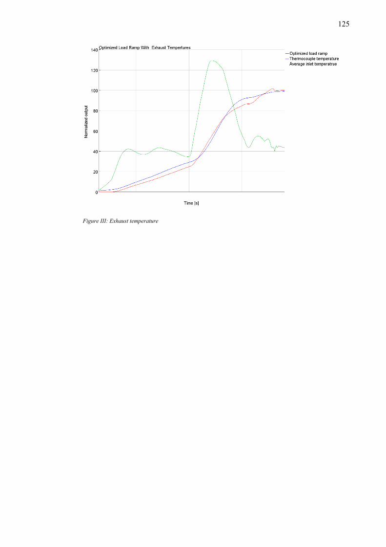
125

Figure III: Exhaust temperature

126

Appendix 7

Starting Temperature Experiment

Figure I: Different starting temperature, exhaust temperature measured without thermocouple

Figure II: Different starting temperature, exhaust temperature measured with thermocouple

127

Figure III: Cylinder pressures with different starting temperature

Figure IV: Knock levels at different starting temperature with the GT-knock model

128

Figure V: Knock levels at different starting temperature with the Soylu and Van Grepen knock model

129

Appendix 8

Cylinder Compression Ratio Experiment

Figure I: Cylinder Pressures with different CR

Figure II: Exhaust temperatures at different CR measured with thermocouples

130

Figure III: Knock levels with different CR, estimated with the GT-knock model

Figure IV: Knock levels with different CR, estimated with the Soylu and Van Grepen knock model

131

Appendix 9

Methane Number Experiment

Figure I: Knock levels with different MN, estimated with the GT-knock model

Figure II: Knock levels with different MN, estimated with the Soylu and Van Grepen knock model

132

Appendix 10

Turbocharger Experiments

Figure I: Knock levels with different HP-turbocharger inertia estimated, with the GT-knock model

Figure II: Knock levels with different HP-turbocharger inertia estimated, with the Soylu and Van Grepen knock

model

133

Figure III: Knock levels with different boost pressure, estimated with the GT-knock model

Figure IV: Knock levels with different boost pressure, estimated with the Soylu and Van Grepen knock model

134

Appendix 11

Exhaust Wastegate Controller Experiment

Figure I: EWG throttle opening with different PID parameters

Figure II: Knock levels with different EWG PID-controller settings, estimated with the GT-knock model

135

Figure III: Knock levels with different EWG PID-controller settings, estimated with the Soylu and Van Grepen

knock model

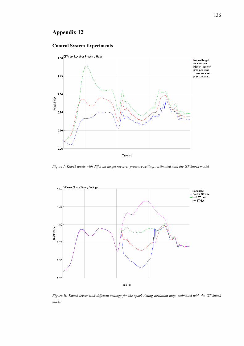
136

Appendix 12

Control System Experiments

Figure I: Knock levels with different target receiver pressure settings, estimated with the GT-knock model

Figure II: Knock levels with different settings for the spark timing deviation map, estimated with the GT-knock

model

137

Figure III: Knock levels with different settings for the inlet valve dwell deviation map, estimated with the GT-knock

model

138

Appendix 13

Ambient Conditions Experiments

Figure I: Thermocouple Exhaust temperatures with different ambient temperature.

Figure II: Knock levels at different ambient temperatures, estimated with the GT-knock model

139

Figure III: Knock levels at different ambient temperatures, estimated with the Soylu and Van Grepen knock model

Figure IV: Thermocouple Exhaust temperatures at different altitudes.

140

Figure V: Knock levels at different altitudes, estimated with the GT-knock model

Figure VI: Knock levels at different altitudes, estimated with the Soylu and Van Grepen knock model.