1

MODELLING OF TURBOCHARGED DIESEL ENGINES IN TRANSIENT OPERATION. PART 1: INSIGHT INTO THE RELEVANT PHYSICAL PHENOMENA

Benajes, J.; Luján, J.M.; Bermúdez, V.; Serrano, J.R.

Universidad Politécnica de Valencia. CMT-Motores Térmicos.

Camino de Vera, s/n. 46022. Valencia, SPAIN.

Contact: @ mail: jbenajes@mot.upv.es phone: + 34 96 387 76 55 fax: + 34 96 387 76 59

ABSTRACT

A new calculation model, able to predict the engine performance during an engine transient, has been

developed, based on an existing wave action code. Previously to the model development, the turbocharged

diesel engines transient phenomena (turbocharger lag, thermal transient and energy transport delay) have

been deeply analysed based on experimental information.

The study has been focused on the load transient, i.e. torque increase from idle, at constant engine speed of

a high-speed direct injection (HSDI) turbocharged engine. Experimental load transient tests have been

performed, with the aim of obtaining a combustion database during engine transient operation, to input a

combustion simulation sub-model. The applied methodology allows to characterise the transient combustion

process in any DI turbocharged engine.

KEYWORDS

Turbocharger lag. Transient. Direct injection Diesel engines. Thermal transient. Combustion characterisation.

1. INTRODUCTION

Oncoming anti-pollution directives and the extremely competitive market have forced engine manufacturers

to contemplate innovative techniques and complex systems to improve the behaviour and performance of

their products. Multi-valve cylinder heads with variable valve timing, high-pressure injection systems with

electronic control, variable geometry turbines in turbochargers and exhaust after-treatment strategies such

as cooled exhaust gas re-circulation (EGR) combined with particulate traps or catalytic converters are some

2

of the strategies, considered unconventional in the past, but being seriously thought about nowadays

[1][2][3].

Aside from this upsurge in elaborated systems, more and more severe exhaust emissions directives (Euro

IV, Euro V in Europe) [4] have forced engine manufactures to drawn the attention to the operation of

automotive engines in transient conditions.

Several of these systems and the elements that compose them are difficult to design and even to test on real

operating conditions. Additionally, complex devices are often introduced, whose configuration is variable with

the engine operation conditions.

This changing scenario is demanding a great effort from researchers to cope with the exigencies, and in

general more involved research tools are being put to work. Among these research tools, a technique that is

producing indisputable success is the combination of experimental tests with calculation models. Calculation

models are not only able to guide the expensive experimental studies on engines towards the optimal

solutions, but also to generate much more information than experiments can reasonably yield on the physical

phenomena taking place in the engine.

A very important part of transient modelling is the correct prediction of engine combustion behaviour along

the transient process [5][6][7][8]. This is necessary for the correct calculation of the indicated mean effective

pressure (imep), but even also for the accurate evaluation of pressure and temperature values at exhaust

valve opening (EVO), that strongly influence exhaust gasses energy [9] and consequently turbocharger

response. To overcome the intricate task of combustion modelling, a common procedure is the simulation of

the rate of heat release (RoHR), by means of a heat release law (HRL) based on the combination of several

Wiebe laws [10]. The actual values of the parameters for the corresponding equations should be dependent

on the engine operating conditions, such as rotating speed, induced air flow rate and injected fuel mass.

Since these operating conditions change in every cycle during the transient, it is convenient to count on a

database containing the right values, as it is described in Figure 1 for a certain engine speed.

Moreover, the in-cylinder conditions during the transient are quite different from the corresponding steady

state conditions. As a consequence, the RoHR of the transient evolution is quite different from the steady

combustion ones [5][6] and its reproduction requires specific transient tests that will provide experimental

information to allow transient combustion characterisation. A suitable procedure for calculating the

3

combustion process along the transient process is based on determining the RoHR for every transient cycle

via a combustion diagnostic code, which is fed mainly with the records of instantaneous in-cylinder pressure

[11][12]. The use of this code has been widely validated for engine steady state operation [13][14][15][16].

The main difficulty in using this combustion diagnostic model during a transient process is feeding the code

with accurate input data, which must be also precisely synchronised with the crank angle position. As the

transient process of the engine generally takes very few seconds, especially if they are high-speed engines,

high precision transducers and a very high frequency data acquisition system are required.

Among the different transient conditions automotive vehicles can be run in, the load transient (engine torque

rising at constant engine speed) has been considered the most representative of the engine response. This

fact is corroborated in the European load response (ELR) test cycle for heavy-duty (HD) engines, where the

engine operation conditions impose constant engine speed and changing load. Even in the European

transient cycle (ETC), a great part of the test conditions consist in a rapid load increase from 40 to 60% of

the rated value, while engine speed is kept unchanged [1]. Therefore, although the procedures and targets

discussed in this work may be easily extended to other transient evolutions of the engine, the load transient

will be the main concern of this study.

2. RELEVANT PHENOMENA IN ENGINE TRANSIENT

The causes of the time delay in the transient operation of a turbocharged engine can be classified in three

groups: mechanical, thermal and fluid-dynamic phenomena. Included in the first group are mechanical

friction and inertia of the turbocharger and other rotating elements of the engine. Relevant thermo- and fluid-

dynamic causes are the mass and energy transfer processes from the exhaust valve up to the turbine and

from the compressor outlet to the cylinder. Among these processes, pressure pulses, gas friction, flow inertia

and heat transfer must be highlighted.

As additional causes of this time delay, some authors have pointed to the malfunctioning or the mismatching

of the injection system during the transient [17][18][5]. Interestingly, one of the claimed causes is the over-

penetration of the fuel jet in the combustion chamber, since the injection pressure was suspected to rise

faster than the boost pressure, and consequently faster than the in-cylinder air density. Although these

problems were observed in old injection systems with mechanical control, they could appear in the presently

4

employed systems too, even though their flexibility allows, during the engine transient, to adapt the injection

parameters to the actual in-cylinder conditions, provided that they are known.

It makes sense to discuss the delay related to the turbocharger operation first, due to its major relevance. In

this phenomenon, it is pertinent to analyse the transfer of energy, from the instant when the injected fuel

mass raises, until the point when the maximum energy at the turbine inlet and the maximum torque at the

crankshaft are attained. This includes also the transient phenomena coupled with the heat transfer between

the gas and the engine walls, both in the cylinder and along the exhaust ducts.

2.1 Turbocharger transient The transient response of the turbocharger is the critical phenomenon in the delay in the increase of speed

or load in a turbocharged engine [19][20]. This condition is due to the specific characteristics of the energy

transfer between the cylinder and the turbocharger.

It is well understood that during the transient operation, the energy transported by the exhaust gases arrives

very quickly to the turbine [19]. Nevertheless, only a fraction of this energy is converted into mechanical work

and transferred to the compressor, since the largest part of the thermal energy is employed in the

acceleration of the turbocharger rotor. One efficient way of improving this situation is increasing further the

supply of energy to the exhaust gases by injecting more fuel in the combustion chamber. However, this

measure will produce as a direct effect the rise in the fuel-air ratio, and, probably, the increase in the soot

emissions. This action cannot be fully exploited, since during the transient operation, the fuel-air ratio values

that produce excessive soot emission are much lower than those yielding the maximum engine torque.

Hence, the fuel delivery needs to be restrained during the transient by the smoke corrector system, which

controls (Figure 1) the increase in injected fuel mass according to the pressure build-up in the intake or the

air mass flow rate.

As it will be commented later, the actuation strategy of the smoke corrector is a key factor in the transient

response of the turbocharged engine. The actuation of this device can be described in the plot of fuel mass

versus air mass of Figure 2, for a full-load transient test, where straight lines represent the points of constant

fuel-air ratio.

The engine idle corresponds in the graph to point A. At the start of the transient process, the accelerator is

pushed virtually instantaneously to its full load position. At this moment, the pressure in the intake manifold

5

or the air mass flow rate, which usually are the input signals for the smoke corrector device, has not changed

from its value at idle condition, due to the turbocharger lag. Consequently, the smoke corrector allows only a

small increase in the injected fuel mass, while the intake air mass flow rate remains unchanged. This

condition is represented by point B, in the case of a particular fuel delivery strategy. This is one of the points

where usually, the maximum F/A ratio is attained.

During a short time, when the engine is running with the increased injected fuel mass, the induced air flow is

increasing slowly, due to the higher energy in the exhaust, and consequently higher boost pressure. The

result is the reduction in F/A ratio until point C. Point C is determined by the value of the boost pressure from

where the smoke corrector starts to increase the injected fuel mass. From this point on, the injected fuel

mass is increased according to the rise in the boost pressure, reaching point D, which represents the

maximum fuel delivery. The shape of the line C-D, is the result of the actuation of the particular smoke

corrector system. In the case of Figure 2 a strategy of constant fuel-air ratio has been represented, which is

usual for engines without EGR. In the case of very steep C-D lines, the point D will correspond to the

maximum F/A ratio of the evolution. Of course, the steeper this line C-D, the faster the engine transient, but

also the larger the soot emissions.

At point D the turbocharger system has still not reached the steady operation condition, and hence the boost

pressure and the intake air mass increase further up to point E, where all the involved systems have attained

their steady state. The value of the operation variables at point E should be similar to the values observed in

the engine steady operation conditions, being eventual differences due to the longer time required for the

thermal stabilisation of the engine, which will be commented later.

2.2 The energy transfer delay The first feature of importance in this phenomenon is the quantity of air trapped when the inlet valve closes,

which limits the quantity of fuel that can be burned. In the case of mechanical pumps, the fuel pump rack is

moving even after the inlet valve closure, and the fuel mass to be injected has not been determined yet. In

the case of modern common-rail or injector-pump systems, the time response of the air mass flow meter and

the injection system will influence this delay. Combustion starts after the ignition delay, before or around top

dead centre (TDC), but does not produce a useful power output until after TDC. Winterbone [17] states that

the kinematics of the slider-crank mechanism further delays the maximum torque to about 90 crank angle

6

degrees after TDC. Hence, there is a delay of about 120 crank angle degrees angle between the start of fuel

injection and the maximum effect on the crankshaft.

The effect of combustion on the energy reaching the turbocharger turbine is delayed too, since it can not

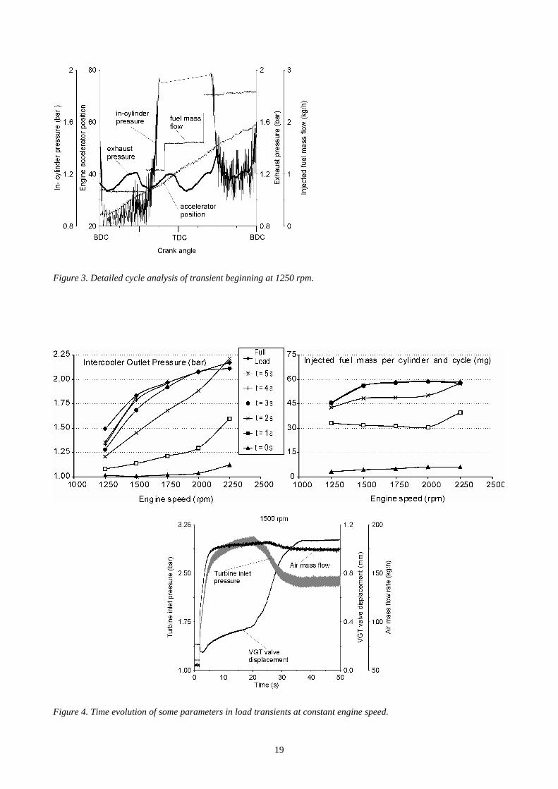
affect the turbine before EVO. This delay can be observed in Figure 3, which depicts the transient process in

a 2.2 litres HSDI turbocharged diesel engine (details are given in Table 1) around combustion TDC of the

first cycle in a load transient test. The plots correspond to the injected fuel mass and the pressure evolution

in the cylinder and at the turbine inlet.

From Figure 3 it can be calculated that the existing delay between the increment of injected fuel signal,

obtained from the engine control unit (ECU) and the first increase in pressure at turbine inlet is about 270

crank angle degrees. This means 150 crank angle degrees more than stated in the literature for the

maximum effect of fuel injection on the crankshaft [17]. During these 150 degrees the maximum energy is

transported down the exhaust pipe and arrives to the turbine. Included in this angular period are: the time

until EVO and the energy and mass transfer delay.

In Figure 3, it can be also observed that this energy transport delay is completely unimportant in small HSDI

engines, compared with the time to EVO, due to the quick increase in exhaust pressure after EVO. Similar

results for more than one cycle of a transient evolution with the same engine can be observed in Figure 9.

2.3 The thermal transient During the transient operation of the engine, the thermal phenomena relevant for the process are not

exclusive to turbocharged engines, since the cylinder walls of any engine will absorb, during their heating,

part of the energy to be transferred to the crankshaft.

Additionally, in turbocharged engines the walls of the exhaust pipes will be colder than the gas, and thus

they will absorb some energy during a transient operation, thus reducing the energy transfer to the turbine.

The extent of this accumulation of energy depends on the heat diffusivity of the walls in contact with the

gases, aside from their geometry and dimensions.

The thermal transient is always longer than the turbocharger acceleration transient. This is logical, since the

rise in the temperature of the walls will end only after the attainment of the steady conditions in the

turbocharger. In the case of the piston temperature transient, some authors have reported duration of

7

several minutes [21][22]. The outcome of this is that at the end of the turbocharger transient, the brake mean

effective pressure (bmep) could be lower than in steady operation, after the thermal transient is finished.

Woschni [23] described this phenomenon for heavy-duty engines, and explained it mainly by the heat loss in

the exhaust manifold and turbine case. Measurements performed in transient conditions by Winterbone and

Backhouse [24] yielded a similar result, and these authors found out that the thermal inertia of the engine

walls was a component of the global delay.

This circumstance, which means that the actual transient condition of the engine can be much longer than

the acceleration time of the turbocharger or than the achievement of the apparent steady torque value

shortly afterwards, can be observed in Figure 4.

Figure 4 shows the evolution of some variables in the HSDI engine described in Table 1 during full load

transient evolutions at constant engine speed. In the top part of the figure it can be observed how the boost

pressure and the injected fuel mass arrive to their full-load steady values after a few seconds (between 3

and 5 seconds). However, in the bottom part of Figure 4 it is showed how in the case of a low engine speed

of 1500 rpm, pressure at turbine inlet, the position of the variable-geometry turbine (VGT) and the air mass

flow rate are not yet stable, even after about 40 seconds.

The reason for this behaviour can be found in the control strategy of the VGT and in the engine thermal

transient. Concerning the former, the VGT is closed-loop controlled by a proportional-integral regulator that

modifies the stator effective area, with the aim of keeping a desired boost pressure level.

As a result of its control strategy, the VGT stator is closed at the outset of the transient process, and it starts

to open after the first seconds (bottom-centre of Figure 4) in order to maintain a constant value in the boost

pressure (top-left of Figure 4). The question may arise as why the VGT is not opened earlier, when the

injected fuel mass and the boost pressure have reached their steady values (top of Figure 4).

The answer lies in the thermal transient. Due to the progressive heating of the exhaust line, the heat

transferred from the gas to the walls decreases, and more energy is delivered to the turbine. This means that

the targeted boost pressure level can be achieved with larger stator areas in the VGT, and the proportional-

integral control reacts in this sense. As a consequence of the area increase, the turbine inlet pressure (i.e.

the engine back-pressure) declines, causing a reduction in the pumping losses, while injected fuel mass

remains constant. This altogether means an increase in bmep and a reduction in specific fuel consumption.

8

Another interesting feature is the reduction in air mass flow that can be observed in the bottom-centre of

Figure 4 about 25 seconds after the transient start off. A plausible cause for this behaviour is the reduction in

volumetric efficiency due to the progressive heating of cylinder walls (liner, piston and cylinder head).

These facts underline the relevance of the heat transfer between gas and walls along the exhaust system, at

least up to the turbine inlet. Consequently, the modelling of this transient phenomenon requires some

specific attention.

3. EXPERIMENTAL CHARACTERISATION OF THE TRANSIENT COMBUSTION

One of the objectives of the experimental work exposed here is to characterise the transient engine

operation by means of measuring the variables that can shed light on the relevant phenomena taking place.

A second important aim is to establish some model which should be able to depict and even to predict the

combustion process, this being one of the most important processes affecting the transient response. This is

to be accomplished by post-processing the obtained information, and finding out some plausible calculation

model.

The method of work has been to reproduce the transient evolution previously illustrated in the scheme of

Figure 2, but with real engine conditions, what is called load transient evolution. In order to sweep a wide

range of the fuel-air ratio this test must be reproduced for different engine speeds and for different limitation

laws of the fuel delivery.

An example of this idea is shown in Figure 5 for 1250 rpm, with some of the tests that have been performed

on a HSDI turbocharged engine. In the plots it can be observed how there are several fuel limited evolutions:

the minimum F/A ratio values are those at steady partial load and the maximum ones are limited by the

stoichiometric F/A ratio.

The main objective of these tests is to obtain information for the modelling of combustion. The procedure has

been to record actual values of in cylinder pressure, air mass and its corresponding value of injected fuel, for

every engine cycle along the transient, and for every fuel delivery limitation law. These variables will be the

main input data to a combustion diagnostic code, which will be used to study the cycles of the load transient.

9

3.1. Description of a load transient The transient tests have been performed starting with the engine idling at a given speed, and suddenly

pushing the accelerator to its top end. The dynamometer in the test bed modifies the braking torque, so as to

maintain the engine speed constant, while the injected fuel mass rises from idle to full load conditions,

controlled by the smoke corrector system. This evolution is depicted in the plots of Figure 6 for two different

strategies of the smoke corrector, which produce two limitation laws in the fuel delivery. In left part of Figure

6 there is a 3-D scheme of two compared evolutions that illustrates the load transient description and in the

right part can be observed real measured variables during a load transient test.

This engine transient operation clearly shows the turbocharger lag effect, with the corresponding increment

in smoke opacity during the first instants of the transient. The measured results in Figure 6 show how the

higher the F/A ratio during the transient evolution, the higher is the peak in the smoke opacity evolution.

3.2. Experimental set-up and methodology The engine object of this study has been a HSDI turbocharged diesel engine with cooled air charge, whose

main characteristics are shown in Table 1. The engine is installed on a test bench in the test cell, with the

required equipment and instrumentation to control the engine operation and to measure the desired

variables.

The dynamometer is an AC motor, operating at variable frequency, with the ability of controlling braking

torque with a very rapid response. Maximum power is 200 kW, either absorbed when braking, or generated

when driving the engine. Specific software for the control of the dynamometer allows performing load

transients and simulating road-load, road gradient, engine to wheel chain of forces, vehicle mass and system

inertia.

The time-dependent variables were recorded by means of a high frequency data acquisition system (16 bit)

capable of simultaneously acquiring 8 channels at 100 KHz with 0.5 Mb of memory per channel. During the

transient operation of the engine it is of utmost importance to record simultaneously the instantaneous value

of those variables that will be used later in the description of the process. Among these variables, the most

relevant are: in-cylinder pressure, boost pressure, exhaust pressure, air and fuel mass flow rate and

accelerator position.

10

These rapidly changing variables were synchronously recorded during the full load transient tests with an

acquisition frequency equivalent at 0.5 crank angle degrees, that allows to record 1440 data every transient

cycle. Since tests were conducted at engine speed values of 1250, 1750 and 2250 rpm, the sampling

frequency ranged from 15 KHz to 27 KHz. Additionally, last generation test room control devices and data

acquisition system employed in the tests were: the VS-100 software and a PC-ECU interface (INCA) which

also translate ECU signals from digital to analogic format, what able to synchronize ECU variables

(introducing them in the high frequency data acquisition system) with the rest of measured ones.

In order to precisely synchronise the acquired data of instantaneous variables with the actual crankshaft

position, the output of an optical angle encoder with 0.1 crank angle resolution was used as sampling signal.

Pressure variation in the intake and exhaust flows was measured using suitable water-cooled piezoresistive

transducers.

In-cylinder pressure was measured by means of a non-cooled piezoelectric transducer. The reference level

for the pressure is fixed by assuming that the pressure at BDC after the intake stroke is equal to the mean

intake pressure. In the case of the transient evolution, the in-cylinder pressure trace is separated in complete

cycles, and the same procedure is applied to every cycle, now unconnected.

The sensor type was selected with the aim of avoiding the signal fluctuation of some pressure transducers

when exposed to fast temperature changes. This condition would make impossible to record an accurate

pressure signal during a whole load transient, due to the important changes in the in-cylinder gas

temperature along this process. The pressure trace shown in Figure 7 is the raw pressure signal along 87

engine cycles, with no correction at all, and without referencing with the intake pressure. The thermal drift of

the piezoelectric sensor is evident in the decreasing trend of the minima in the pressure pulses. This figure

shows that this drift is of about 5 bar in 87 cycles. This justifies that in one single cycle, the drift can be

neglected for the purpose of heat release analysis.

The fuel flow was measured by means of two independent procedures. On one hand, a gravimetric balance

that provides mass flow values at a frequency of 10 Hz was installed in the fuel line feeding the injection

pump. On the other hand, the information delivered by the own engine control unit (ECU) was recorded

through the VS-100 software. The ECU provides a value of volumetric fuel flow at a frequency of 200 Hz. In

11

order to obtain an accurate measurement of the instantaneous fuel mass flow delivered to the engine, the

combination of the two signals was required. An example of the obtained measurement is shown in Figure 8.

The digital information obtained, through the VS-100 software, from the ECU is synchronized with the rest of

analogic measurements via the INCA system, which translates the ECU signal into analogic format and

introduces them to the high frequency analogic data acquisition system. In addition, all the measured

variables are synchronised with the engine crankshaft angular position by the output of the optical encoder.

The intake air mass flow was evaluated by a non-intrusive flow meter, based on a hot-wire sensor. This

device yields directly values of mass flow rate, and is able to follow time variations of the flow, with a time

response, which is fast enough for the requirements of the tests.

EGR rate is calculated from intake air mass, pressure and temperature measurements and assuming

constant volumetric efficiency during the first instants of the transient. The mass of residual gas is calculated

taking into account short-circuit and backflows, by using a specific emptying-and-filling model in the cylinder

[25].

Pollutant emissions during the transient were evaluated by using state of the art exhaust gas analysers,

while a continuous smoke measurement device (Hartridge opacimeter) measured the soot emission.

3.3. Calculation of cycle-averaged information As it is required for the RoHR calculation model, cycle-averaged values of the different variables were

calculated by averaging the 1440 data recorded each cycle during the transient. These values could be

employed for characterising the transient evolution, or as input values for a diagnostic model to achieve the

objective, previously referred, of combustion process characterisation.

To illustrate this technique, Figure 9 shows an example of instantaneous values recorded during the first

cycles of a load transient test at 1250 rpm. It can be observed how the initial rise in injected fuel is firstly and

trustworthily detected by the sudden change in the amplitude of the exhaust pressure peaks. It is worth

mentioning how the instant when fuel delivery increases, is also detected in the signals of injected fuel,

accelerator position, air mass flow and in-cylinder pressure.

An example is also shown in Figure 3 where between the variables plotted there are very small delays as

described in section 2.2. It is interesting to signal that in Figure 3 and in Figure 9 the recorded in-cylinder

12

pressure does not correspond to the first cylinder in which fuel injected is increased, but to the next firing

one.

These preliminary results validate both the data acquisition frequency and the calculation procedure for

obtaining cycle-averaged values, which should be used to feed the diagnostic combustion model. This latter

is an essential subject, since the possibility if obtaining relevant information from the different cycles along a

single transient run, makes the experimental procedure time-effective, as described in section 3.2.

Otherwise, the combustion characterisation of different engines would be an excessive time consuming task.

The fuel injected at every transient cycle has been divided by the number of cylinders to obtain the fuel

injected in each cylinder and the air mass trapped in each cylinder has been calculated taking into account

the number of cylinders, air mass flow, EGR flow, and short circuit flow or back flows.

Table 2 contains the cycle-averaged values of the most relevant variables calculated from beginning of a

load transient appear. Each row corresponds to one engine cycle during the transient. Cycles labelled as -1

and 0 are cycles before the increase in load, that is, when the engine is still in a steady state at idle, as it can

be corroborated by the coincidence of the tabulated values

The transient process actually starts in cycle 1, when the fuel delivery starts to increase, although the rest of

variables show only slight changes, if any. Cycles 2 to 8 are the seven first cycles after the transient start,

when all the parameters start to change noticeably, growing practically monotonically. The clear exception to

this behaviour is the EGR valve, which is already fully closed four cycles after the start off, and consequently

the EGR mass flow rate is cut off, so that the transient is not further delayed. The transient will continue

during many more cycles, about 30 at this particular engine speed.

A more subtle departure from the monotonic behaviour is the small decrease in the intake air mass flow rate

appearing in cycle 2. In fact, it is interesting to note how engine torque is increased and how the EGR valve

closing delay affects to intake air mass flow.

The EGR effect is evident in cycle number 2, which is the first cycle after the transient start, when the air

mass flow is reduced in spite of the increasing in boost pressure. The cause for this effect is the increase in

EGR flow during the first cycles, which is a consequence of the retard in the closing of the EGR valve. This

condition is responsible for a large difference in mean pressure values between exhaust and intake. This

interesting outcome, usual in turbocharged engines with EGR at the beginning of the transient, can be also

13

observed in the recorded data of air mass flow that have been plotted in Figure 9. As it can be guessed, this

phenomenon will negatively influence the engine dynamic performance during the first instants of any load

transient evolution.

3.4. ROHR calculated from transient cycles and analysis of the results The main target of this preliminary experimental work is the calculation of the RoHR of each transient cycle

to generate a database that characterise transient combustion of a certain HSDI engine. The methodology

exposed in section 3 allows achieving this objective, which is basic to model the turbocharged HSDI engines

transient behaviour and to study the transient phenomena of these engines.

The RoHR here considered is the “gross” one. In order to get this, the heat transfer is calculated during the

cycle by means of a Woschni-type equation [26], as explained in references [11][12][13]. The particular

values for the coefficients in the Woschni equation are adjusted for the particular engine in a preliminary

engine test. In this test, external motor drives the engine with no fuel injection, and the RoHR is calculated,

adjusting the coefficients so that the heat released is equal to zero. The cylinder walls temperatures during

the transient are estimated by using a heat transfer model [7], and the obtained values are introduced in the

thermodynamic model as boundary conditions in a kind of rough iterative process.

Two engine speeds have been studied: 1250 rpm and 2250 rpm. Load transients have been performed at

these engine speeds and the combustion process has been analysed cycle by cycle during the first 80

cycles. The reason for choosing these engine speeds is that low engine speed torque is normally a limitation

in turbocharged HSDI engines and it is in this zone where transient problems are more significant. The

obtained curves of RoHR are shown in left part of Figure 10. The data appear as 3D surfaces where the

RoHR is plotted versus crank angle for each engine cycle. Through the calculation of the combustion

efficiency, typical values were obtained in the range between 95 and 100 %.

The studied HSDI engine works with pilot injection strategy, whose effects can be observed in the evolution

showed in the left part of Figure 10 for these engine speeds. In right part of Figure 10 is shown a more

detailed analysis of some transient cycles. It can be observed how the first cycles feature a significant

premixed combustion, which can not been completely eliminated even with pilot injection. The reason could

be the cold engine temperatures that increase ignition delay and allow a relatively large amount of fuel to mix

14

with air before combustion starts. The bottom right plots of Figure 10 show how the premixed fraction

progressively disappears as the combustion delay is reduced when the transient process evolves.

Comparing with results obtained in similar studies by other authors [6], where only a main injection was

produced, it can be concluded that the pilot injection strategy is responsible for a sharp reduction in the

premixed combustion at intermediate cycles during the transient.

4. SUMMARY AND CONCLUSIONS

The main physical processes that take place in the transient operation of turbocharged diesel engines have

been analysed using experimentally obtained information like the thermal transient phenomena affecting

important variables for transient performance as turbine work and volumetric efficiency. From this study it

has been ascertained that the turbocharger lag and the thermal transient are quite relevant in engine

transient performance and emissions, nevertheless, the energy transport delay has been concluded not to

have any significant effect, especially in HSDI turbocharged engines.

The combustion characterisation is going to be provided through a database formed by the RoHR of every

transient cycle, obtained via a combustion diagnostic thermodynamic code, which analyses the in-cylinder

pressure recorded along specific load transient tests. The load transient tests have been described and it is

important to highlight the difficulty to measure in transient evolutions engine relevant variables.

An experimentally based procedure has been developed to obtain the heat release laws along the changing

conditions of the transient. This process is based on specific load transient tests, which have been also

described, needed to obtain a wide enough database that allow reproducing the entire possible engine

transient situations. The experimental set up needed to perform the test have been detailed. The

instantaneous measured variables have been described together with the problems associated to their

acquisition and post-processing. The RoHR of every cycle during a load transient have been obtained. With

this last step a process to characterise diesel engine transient combustion has been finished and therefore a

protocol has been defined to reproduce combustion characterisation. The use of mean variables makes the

exposed combustion characterization process a task functioning enough to generate databases necessary

for feeding modelling processes. In addition, it makes it a feasible task to characterise the combustion

process, for different HSDI engines, in operative periods of time.

15

Form the analysis of the calculated RoHR has been concluded that along the transient process, combustion

delay is progressively reduced, especially due to engine temperatures increasing and therefore the effect of

pilot injection is becoming more efficient.

5. REFERENCES

1 Zelenka, P., Aufinger, H., Walter, R. and Wolfgang, C. Cooled EGR - a key technology for future efficient H: D:

diesels. SAE paper 980190. 1998.

2 Dekker, H.J. and Sturm, W.L. Simulation and control of a H. D. diesel engine equipped with a new EGR technology.

SAE paper 960871. 1996.

3 Lüders, H. and Stommel, P. Diesel exhaust treatment-new approaches to ultra low emission diesel vehicles. SAE

paper 1999-01-0108. 1999.

4 Walsh, M.P. Global trends in diesel emissions control – A 1999 update. SAE paper 1999-01-0107. 1999.

5 Winterbone, D.E. and Tennant, D.W.H. The variation of friction and combustion rates during diesel engine

transients”. SAE paper 810339. 1981.

6 Assanis, D., Filipi, Z., Fiveland, S. and Syrimis, M. A Methodology for cycle-by-cycle transient heat release analysis

in turbocharged direct injection diesel engine. SAE paper 2000-01-1185. 2000.

7 Serrano, J.R. Analysis and modelling of the load transient in turbocharged diesel engines. (Text in Spanish) Doctoral

Thesis. Univ. Politécnica de Valencia, Spain. 1999.

8 Rodriguez, A. Comparative analysis and synthesis of the turbocharged direct injection diesel engines transient

response. (Text in Spanish) Doctoral Thesis. Univ. Politécnica de Valencia, Spain. 2001.

9 Santos, R. A study on the available energy in the exhaust gases of diesel engines. (Text in Spanish) Doctoral

Thesis. Univ. Politécnica de Valencia, Spain. 1999.

10 Wiebe, I. Halbempirische formel fur die verbrennungs-geschwindigkeit, Verlag der akademie der Wissenschaften

der Vd SSR (Academia de las ciencias de la URSS), Moscow, 1956.

11 Armas, O. Experimental diagnosis of the combustion process in direct injection diesel engines. (Text in Spanish)

Doctoral Thesis. Univ. Politécnica de Valencia, Spain. 1998.

12 Payri, F., Armas, O., Desantes, R. and Leiva, A. Thermodynamic model for the experimental diagnosis of the

combustion process in D.I. diesel engines. (Text in Spanish). Proc III Congreso Iberoamericano de Ingeniería

Mecánica. La Habana. Cuba. 1997.

13 Lapuerta, M., Armas, O. and Hernández, J.J. Diagnostic of DI Diesel combustion from in-cylinder pressure signal by

estimation of mean thermodynamic properties of the gas. Vol 19. pp: 513-529. Applied Thermal Engineering. Oxford,

UK. 1999.

16

14 Lapuerta, M., Armas, O. and Hernández, J.J. Effect to the Injection Parameters of a Common Rail Injection System

on Diesel Combustion through Thermodynamic Diagnosis. SAE paper 1999-01-0194. 1999.

15 Lapuerta, M., Armas, O. and Bermúdez, V. Sensitivity of Diesel engine thermodynamic cycle calculation to

measurement errors and estimated parameters. Vol: 20. pp: 843-861. Applied Thermal Engineering. Oxford, UK.

2000.

16 Desantes, J.M., Arregle J. and Pastor, JV. Influence of the fuel characteristics on the injection process in a D.I.

Diesel engines. SAE paper 980802. 1998.

17 Horlock, J.H. and Winterbone, D.E. The thermodynamics and gas dynamics of internal combustion engines. Volume

II. CLARENDON PRESS. ISBN 0198562128. Oxford 1986.

18 Murayama, T., Miyamoto, N., Tsuda, T., Suzuki, H. and Hasegawa, S. Combustion behaviours under accelerating

operation of an IDI diesel engine. SAE paper 800966. 1980.

19 Watson, N. and Janota, S. Turbocharging the internal combustion engine MACMILLAN PUBLISHERS LTD. ISBN

0333242904. London 1982.

20 Watson, N. Transient performance simulation and analysis of turbocharged diesel engines. SAE paper 810338,

1981.

21 Assanis, D., Baker, D.M. and Bohac, V. A global model for steady-state and transient SI engine heat transfer

studies. SAE paper 960073. 1996.

22 Miyamoto, N., Enomoto, Y., Kitamura, T., et al. Time-resolved nature of exhaust gas emissions and piston wall

temperature under transient operation in a small diesel engine. SAE paper 960031. 1996.

23 Woschni, G., Doll, M. and Spindler, W. Simulation des stationären und instationären Verhaltens von aufgeladenen

Pkw-Dieselmotoren. MTZ Motortechnische Zeitschrift 52 (1991) 9, pp 468-477. 1991.

24 Winterbone, D.E., Backhouse, R. Dynamic behaviour of a turbocharged diesel engine. SAE paper 860453. 1986.

25 Benajes, J., Reyes, E. and Lujan, J.M. Modelling study of the scavenging process in a turbocharged Diesel engine

with modified valve operation. Proceedings of the IMechE. Part C: Journal of Mechanical engineering Science. Vol

210, 1996.

26 Woschni, G.A. Universally applicable equation for instantaneous heat transfer coefficient in the internal combustion

engine. SAE paper 670931, 1967.

17

TABLES CAPTIONS

Table 1: Engine basic characteristics.

Table 2. Cycle-averaged variables during the first cycles of a load transient. 1750 rpm.

FIGURES CAPTIONS

Figure 1. Control program for the load transient model

Figure 2. Scheme of a transient evolution in the plane fuel mass vs. air mass.

Figure 3. Detailed cycle analysis of transient beginning at 1250 rpm.

Figure 4. Time evolution of some parameters in load transients at constant engine speed.

Figure 5. Full load transient tests with changed fuel limitation maps. 1250 rpm

Figure 6. Load transient scheme and experimental results with two different fuel limitation strategies. 2250 rpm

Figure 7. In-cylinder pressure (piezoelectric transducer signal) 1250 rpm.

Figure 8. Transient fuel mass flow measurements comparison.

Figure 9. First cycles of a HSDI engine load transient at 1250 rpm.

Figure 10. Plot of RoHR versus cycle and crank angle along a 1250 and 2250 rpm load transient test and detailed analysis of some transient cycles.

TABLES

Type of engine HSDI Turbocharged Diesel Engine

Number of cylinders 4 in line

Bore 85 mm

Stroke 96 mm

Compression ratio 18:1

Maximum engine speed 4500 rpm

Number of valves 4 per cylinder

Injection System Common-rail

Turbocharger VGT

Charge cooling Air-air

Table 1: Engine basic characteristics.

18

Cycle

# Torque

(Nm)

Boost press

(bar)

Exh. Press

(bar)

Air flow

(g/s)

Fuel flow

(g/s)

EGR valve displacement

(mm)

EGR flow

(g/s)

-1 0.7 1.045 1.181 13.25 0.36 5.32 14.79

0 0.7 1.046 1.183 12.97 0.36 5.32 15.09

1 5.1 1.046 1.182 12.96 0.45 5.32 17.03

2 40.5 1.049 1.271 11.80 0.89 4.35 18.79

3 61.7 1.025 1.482 18.04 0.93 1.00 11.73

4 61.5 1.026 1.658 31.11 0.99 0.3 0.00

5 73.1 1.041 1.768 34.43 1.24 0.3 0.00

6 80.7 1.060 1.882 36.09 1.44 0.3 0.00

7 110.1 1.081 1.965 38.83 1.59 0.3 0.00

8 133.2 1.109 1.982 40.54 1.74 0.3 0.00

Table 2. Cycle-averaged variables during the first cycles of a load transient. 1750 rpm.

FIGURES

Figure 1. Control program for the load transient model.

Figure 2. Scheme of a transient evolution in the plane fuel mass vs. air mass.

19

Figure 3. Detailed cycle analysis of transient beginning at 1250 rpm.

Figure 4. Time evolution of some parameters in load transients at constant engine speed.

20

Figure 5. Full load transient tests with changed fuel limitation maps. 1250 rpm.

Figure 6. Load transient scheme and experimental results with two different fuel limitation strategies. 2250 rpm.

21

Figure 7. In-cylinder pressure (piezoelectric transducer signal) 1250 rpm.

Figure 8. Transient fuel mass flow measurements comparison.

22

Figure 9. First cycles of a HSDI engine load transient at 1250 rpm.

23

1250 rpm

2250 rpm

Figure 10. Plot of RoHR versus cycle and crank angle along a 1250 and 2250 rpm load transient test and detailed analysis of some transient cycles.