Transient boiling of water under exponentiallyescalating heat inputs. Part I: Pool boiling

The MIT Faculty has made this article openly available. Please share how this access benefits you. Your story matters.

Citation Su, Guan-Yu et al. “Transient Boiling of Water Under ExponentiallyEscalating Heat Inputs. Part I: Pool Boiling.” International Journal ofHeat and Mass Transfer 96 (May 2016): 667–684 © 2016 Elsevier Ltd

As Published http://dx.doi.org/10.1016/j.ijheatmasstransfer.2016.01.032

Publisher Elsevier

Version Author's final manuscript

Citable link http://hdl.handle.net/1721.1/115210

Terms of Use Creative Commons Attribution-NonCommercial-NoDerivs License

Detailed Terms http://creativecommons.org/licenses/by-nc-nd/4.0/

prepared for submission to the

International Journal of Heat and Mass Transfer

Transient boiling of water under exponentially escalating heat inputs 1

Part I: Pool boiling 2

Guan-Yu Sua, Matteo Buccia, b,, Thomas Mckrella, Jacopo Buongiornoa,+ 3

a Department of Nuclear Science and Engineering, Massachusetts Institute of Technology, Cambridge MA 02138, USA 4 b CEA Saclay, DEN/DANS/DM2S/STMF/LATF, 91191 Gif-sur-Yvette Cedex, France 5 6

ABSTRACT 7

This paper presents an investigation of transient pool boiling heat transfer phenomena in water at atmospheric pressure under 8

exponentially escalating heat fluxes on plate-type heaters. Exponential power escalations with periods ranging from 5 to 100 9

milliseconds, and subcooling of 0, 25 and 75 K were explored. What makes this study unique is the use of synchronized state-of-10

the-art diagnostics such as InfraRed (IR) thermometry and High-Speed Video HSV, which enabled accurate measurements and 11

provided new and unique insight into the transient boiling heat transfer phenomena. The onset of nucleate boiling (ONB) 12

conditions were identified. The experimental data suggest that ONB temperature and heat flux increase monotonically with 13

decreasing period and increasing subcooling, in accordance with the predictions of a model based on transient conduction and the 14

nucleation site activation criterion. Various boiling regimes were observed during the transition from ONB to fully developed 15

nucleate boiling (FDNB). Onset of the boiling driven (OBD) heat transfer regime and overshoot (OV) conditions were identified, 16

depending on the period of the power escalation and the subcooling. Forced convection effects have also been investigated and 17

are discussed in the companion paper (Part II). 18

Keywords 19

Exponential power escalation 20

Heat transfer mechanisms 21

Infrared thermometry 22

High speed video 23

Transient Pool boiling 24

1. Introduction 25

Transient boiling heat transfer is important to the safety of nuclear reactors. Step inputs of reactivity in a nuclear reactor might 26

result in a power excursion in which the heat generation in the nuclear fuel rises exponentially with time q′′′(t) ∝ et τ⁄ . The 27

period of the exponential power excursion τ depends upon the size of the reactivity step. Large steps yield to periods that can be 28

as short as a few milliseconds. The heat generated within the fuel is transferred to the water coolant which then starts to boil. 29

The reactivity feedbacks caused by the heating (Doppler in the fuel and void in the coolant) represent an important mitigation 30

mechanism for such accidents. Depending on the magnitude and the delay of these feedbacks, a safe conclusion to the accident 31

is rapidly achieved or, in extreme cases, the fuel can melt, the molten material can be expulsed, fragmented and possibly lead to 32

———

Corresponding author. Tel.: +33.(0)1.69.08.84.24; fax: +33.(0)1.69.08.82.29; e-mail: matteo.bucci@cea.fr

+ Corresponding author. Tel.: +1-617-253-7316; fax: +1-617-258-8863; e-mail: jacopo@mit.edu

steam explosion. The time delay between heat generation within the fuel and its transfer to the coolant is key to determining the 33

outcome of the accident, in particular for experimental reactors using highly enriched fissile fuel with a very low Doppler effect. 34

This time delay depends on conduction heat transfer within the fuel, single-phase convective heat transfer and eventually 35

transient boiling heat transfer in the coolant. 36

Transient boiling of water under exponentially escalating heat fluxes has been studied since the 1950s. Most of these 37

investigations were carried out in pool boiling conditions, using ribbon [1, 2] and wire [3, 4, 5, 6, 7] heaters. Some forced 38

convection studies also exist for ribbon [8] and wire [9] heaters. Table 1 summarizes the experimental conditions and diagnostics 39

of these earlier investigations. 40

All these studies used the same technique to determine the instantaneous heater average temperature and net heat flux to water. 41

The average heater temperature was determined through measurement of the heater resistance, generally made of Platinum, 42

Aluminum or Deltamax®, whose resistivity changes with temperature. The instantaneous net heat flux to water was determined 43

as the difference between the power released by Joule heating V(t) ∙ I(t) and the rate of change of the energy stored within the 44

heater itself Ch ∙ dTh(t) dt⁄ . For thin heaters with a negligible thermal resistance [1, 2, 8], the average temperature on the boiling 45

surface could be assumed equal to the average heater temperature. For relatively thick heaters [3, 4, 5, 6, 7, 9], the temperature 46

on the boiling surface could be determined by solving the unsteady thermal conduction equation in the heater, having the time 47

dependent generation rate (Joule heating) as source term and the net heat flux to water as boundary condition at the boiling 48

surface. 49

High speed video (HSV) was used to identify ONB and visualize the boiling process [1, 5, 6, 8]. Piezoelectric hydrophones were 50

used to detect ONB in subcooled conditions [3]. X-ray absorption was used to measure void fractions in transient flow boiling 51

experiments [8]. 52

Table 1. Experimental conditions and diagnostics used in studies of transient boiling heat transfer with exponentially escalating heat inputs.

Authors Year Boiling conditions Heater Subcooling Periods Pressures HSV ONB detection

Rosenthal [1] 1957 Pool Pt and Al ribbon

0.025 mm thick

2.5 mm wide

0 to 68 K 5 to 75 ms Ambient 6000 fps Temperature overshoot and HSV

Hall and Harrison [2] 1967 Pool Pt ribbon

0.025 mm thick

2.5 mm wide

0 to 80 K 0.7 to 5 ms Ambient Temperature overshoot

Johnson [8] 1971 Stagnant and forced flow Deltamax® ribbon

0.10/0.36 mm thick

3.2 mm wide

5 to 62 K 5 to 50 ms Ambient to 13.8 MPa Yes HSV

Sakurai and Shiotsu [3] 1977 Pool Pt wire

diameter 1.2 mm

25 to 75 K 5 ms to 10 s Ambient Acoustic detection by piezoelectric hydrophone

Sakurai and Shiotsu [4] 1977 Pool Pt wire

diameter 1.2 mm

0 K 5 ms to 10 s Ambient to 2.1 MPa No ONB detection

Kataoka et al. [9] 1983 Forced flow Pt wire

diameter 0.8/1.2/1.5 mm

10 to 70 K 5 ms to 10 s 0.143 to 1.503 MPa No ONB detection

Sakurai et al. [5, 6] 2000 Pool Pt wire

diameter 1.2 mm

0 K 2 ms to 20 s Ambient to 2.063 MPa 200 fps HSV

Park et al. [7] 2010 Pool Pt wire

diameter 1.0 mm

0 to 160 K 5 ms to 50 s Ambient to 1.572 MPa Not discussed

This study 2015 Pool / Flow ITO/sapphire heater 0 to 75K 5 ms to 500 s Ambient 5000 fps HSV and IR thermometry

In a transient pool boiling test it is typical to identify several characteristic features, i.e. the single-phase heat transfer regime, the 1

onset of nucleate boiling (or boiling inception), the fully developed nucleate boiling regime and ultimately the boiling crisis. A 2

brief summary of the previous work on and current understanding of each of these features is presented next. 3

1.1. Single-phase heat transfer 4

Transient non-boiling heat transfer is a well understood phenomenon. For short periods, typically smaller than 100 ms, the 5

temperature rise on the heater surface is too fast for natural convection to develop and contribute to heat transfer [1, 2, 3, 10]. 6

Conduction is the leading heat transfer mechanism. Thus, transient conduction equations can be solved to determine the 7

temperature on the heater surface and the temperature distribution in water. For longer periods, the temperature rise on the heater 8

surface is slow. Buoyancy forces set the fluid in motion and natural convection supersedes pure conduction [3]. 9

1.2. Onset of nucleate boiling 10

There is general agreement that the transient ONB superheat decreases with decreasing subcooling and increasing pressure, as 11

implied by the steady boiling inception criteria, i.e. the Hsu’s model [11]. Transient effects are also qualitatively clear. ONB 12

superheat and heat flux decrease as the exponential period is increased. However ONB data reported in the literature are often 13

very scattered and are not free from discrepancies, as explained next. 14

Rosenthal [1] was the first to identify the ONB conditions using a high-speed camera synchronized with measurements of 15

voltage and current through a ribbon heater. Accordingly, the ONB detected through HSV coincides with a maximum of the 16

heater temperature, which was called overshoot (OV). Rosenthal observed a significant rise in the boiling inception temperature 17

with respect to the steady heat transfer tests, however, for saturation condition, no major differences were observed with respect 18

to steady boiling and surprisingly the superheat was found to be negligible small for periods larger than 70 ms. 19

Later, Hall and Harrison [2] investigated boiling inception conditions for very short periods (<5 ms). Based on the observation of 20

Rosenthal, they assumed that boiling inception coincides with the overshoot. To predict the ONB superheat, they tried to apply 21

the model proposed by Hsu [11] combined with the transient conduction temperature profile. However, the measured incipient 22

boiling superheats were much higher (~30 K) than the predicted values. 23

The first to point out the difference between boiling inception and overshoot was likely Johnson [8], who used HSV to image the 24

boiling surface and X-ray absorption to measure the void fraction. According to Johnson, boiling inception occurs at the 25

intersection between the transient non-boiling heat transfer curve and the steady-state fully developed nucleate boiling curve. 26

In 1977, Sakurai and Shiotsu [3] identified boiling inception conditions at ambient pressure and various subcoolings (25 to 75 K) 27

through a piezoelectric hydrophone synchronized with the measurement of the heater temperature (through the heater resistance). 28

They showed that ONB temperatures are significantly lower than overshoot temperatures, and can be predicted with models 29

developed from the formulations of Hsu [11] and Rohsenow [12]. Tuning of the largest unflooded cavity size was however 30

required to fit the experimental data for each subcooling explored. 31

In 2000, Sakurai et al. [5, 6] measured the boiling inception superheat for saturation conditions at ambient pressure using HSV 32

(200 fps). In doing so, they discussed the difference between highly wetting fluids and water, both pre-pressurized to flood the 33

cavities, and non-pre-pressurized. In particular, they argued that even for non-pre-pressurized water, for very short period, 34

boiling inception could be triggered by heterogeneous spontaneous nucleation instead of nucleation in active unflooded cavities. 35

Contrary to Rosenthal, they showed that the onset of nucleate boiling temperature can be significantly higher than in steady 36

boiling also for saturation conditions and relatively long periods. Surprisingly, the ONB superheats for saturation conditions 37

reported in this work are higher than superheats previously measured by the same author for subcooled conditions [3]. 38

1.3. From ONB to critical heat flux 39

Rosenthal [1] reported that after ONB the number of bubbles on the surface grows rapidly. These bubbles re-condense and the 40

inrush of cold liquid cools down the surface and hinders further nucleation, until boiling restarts in a fashion similar to steady 41

boiling. For relatively long period (larger than 15 ms), the behavior of the system was not appreciably different than steady 42

boiling and thus critical heat flux conditions were not influenced by the power excursion period. 43

A similar description of the transition between non-boiling regime and boiling crisis was reported by Johnson [8]. No major 44

differences with respect to steady boiling were observed for the fully developed nucleate boiling regime for periods of 5 ms or 45

longer. However, measured transient critical heat fluxes were higher than the steady-state values. 46

Based on the observation of temperature fluctuations after ONB, Hall and Harrison [2] speculated that even at very short periods 47

(< 5 ms) the transition from single–phase heat transfer to the boiling crisis was not instantaneous but was preceded by nucleation 48

of individual bubbles. During this phase the heat flux could exceed the critical heat flux for steady conditions by an order of 49

magnitude. A similar behavior was also observed through HSV by Tachibana et al. [13] for linear power excursions. 50

Sakurai and Shiotsu [3, 4] confirmed the presence of a large temperature overshoot after boiling inception and postulated the 51

existence of two different boiling processes. The overshoot was explained as the result of the time leg of activation of small 52

cavities and initially flooded cavities for the increasing rate of heat flux [4]. In the quasi-static boiling process (i.e. for relatively 53

long periods), fully developed nucleate boiling is attained shortly after the temperature overshoot. In the rapid boiling process, 54

when the power excursion period is very short, the critical heat flux condition is instead reached before potential active cavities 55

are fully activated. Contrary to Rosenthal, CHF was observed to vary as a function of power excursion period and pressure. 56

Sakurai found that, for subcooled conditions, CHF increases as the pressure increases and the period decreases, also for relatively 57

long periods (> 5ms) [6]. For saturation conditions the trend is more complicated. Depending on the pressure, the critical heat 58

flux could increase, then decrease and finally increase again as the power excursion period decreases [5, 6]. In particular, at short 59

power excursion periods, when boiling is triggered by heterogeneous spontaneous nucleation (HSN), the transition from ONB to 60

CHF is rapid even for non-pre-pressurized water. Similar trends were observed by Kataoka et al. [9] in transient tests with forced 61

convection and by Park et al. [7]. 62

Although the previous experimental databases form a highly valuable source of information, it must be remarked that sometimes 63

the conclusions of the different authors are quantitatively and qualitatively in disagreement with each other. This is likely due to 64

differences in experimental setups and also limitations in the accuracy of diagnostics available in those experiments. In order to 65

clarify these discrepancies and shed light on the mechanisms of transient boiling heat transfer, this paper and its companion paper 66

[14] present the results of a new experimental program devoted to the study of exponential power excursion in both pool boiling 67

and flow boiling conditions, respectively. In this paper, periods in the range from 5 ms to 100 ms and bulk temperatures from 68

saturation to 75 K of subcooling have been explored at ambient pressure in pool boiling conditions. What makes this study 69

unique is the use of synchronized state-of-the-art diagnostics such as IR thermometry and HSV which can improve the accuracy 70

of measured quantities and provide new and unique insight into the transient boiling heat transfer phenomena. 71

2. Description of pool boiling facility and diagnostics 72

The custom designed and built experimental setup used in this study is sketched in Figure 1. It consists of a stainless steel boiling 73

cell surrounded by an isothermal bath, a heater with its cartridge installed at the bottom of the boiling cell, a sampling line to 74

measure dissolved oxygen concentration and a volume compensation system. A high-level 5V signal is used to trigger two 75

function generators (FG1 and FG2) and the high-speed data acquisition system (HDAS). FG1 is used to drive HSV and IR 76

cameras. FG2 is used to drive the high-speed direct current power supply (DCPS, sketched as a battery in Figure 1) in order to 77

output the desired exponential power excursion. The HDAS acquires trigger signal, camera input signal (output of FG1), as well 78

as voltage and current through the heater. 79

80

Figure 1. Schematic diagram of experimental setup and diagnostics for pool boiling tests. 81

2.1. Boiling cell 82

The pool boiling cell features a concentric-double-cylinder structure made of 316L stainless steel. Boiling of DI water takes place 83

in the inner cell, while the outer enclosure functions as an isothermal bath. The whole facility is surrounded by thermal insulating 84

foam. The temperature (and thus the degree of subcooling) of the water in the inner cell is regulated by circulating a temperature-85

controlled fluid through the isothermal bath with an accuracy of ±1°C. The heater cartridge sits at the bottom of the cell and 86

accommodates heater samples. There are four glass windows spaced equally at 90° around the outer surface of the boiling cell 87

which are used by the HSV camera for imaging the boiling phenomena on the heater surface. 88

2.2. Heater 89

Boiling was induced by a specially-designed heater (see Figure 2) installed in the boiling cell by means of a graphite-macor 90

cartridge. The heater and cartridge were designed to prevent the occurrence of corrosion, which could influence the results. The 91

heater consists of: (i) a 1 mm thick, IR quasi-transparent sapphire substrate, (ii) a 0.7 μm thick, electrically conductive, IR 92

opaque, indium tin oxide (ITO) wrapped-around coating, and (iii) 0.7 μm thick wrapped-around gold pads. The ITO film (boiling 93

surface) has a constant resistivity of approximately 2.5 Ohms/square in the temperature range of interest [15]. It is typically 94

nano-smooth (see Figure 3) and hydrophilic (the contact angle is approximately 85°). However, scanning electron microscope 95

(SEM) investigations revealed the presence of randomly distributed imperfections with typical equivalent diameter in the order 96

of a few microns. The desired power excursion was generated by applying a transient voltage to the ITO coating through the gold 97

pads, using the DCPS. The heat thus generated within the ITO film (active area: 1cm × 1cm) is partially transferred to water and 98

partially to the sapphire substrate (see Section 2.5). 99

100

Figure 2. Heater schematic drawing (left, not to scale), and picture (right) 101

102

Figure 3. SEM image of the ITO surface 103

2.3. High-speed direct current power supply (DCPS) 104

A Chroma 62050P-100-100 DCPS generated the desired exponential power escalation. The maximum output power of the DCPS 105

is 5kW, with maximum current and voltage of 100A and 100V respectively. The nominal maximum voltage slew rate is 10V/ms, 106

while the current slew rate follows the voltage variation with respect to the electrical resistance. These high power and high slew 107

rate features enabled exponential heat flux excursions with periods as small as 5ms, with a precision of ± 0.1 ms. 108

2.4. High-speed data acquisition system (HDAS) 109

An Agilent U2542A USB modular high speed data acquisition system (HDAS) was adopted to acquire trigger signal, camera 110

input signal (output of FG1), as well as signals of current and voltage through the heater. Current was measured through a shunt, 111

which converts the actual heater current to a voltage signal (50mV/30A) with a manufacturer-specified accuracy of 0.25%. A 112

voltage divider was applied to reduce the actual voltage through the heater (up to 100V) to a range acceptable to the HDAS (0-113

10V input). In the present study, a sampling rate of 50 kHz (50 samples/ms) for each channel was used. The measuring accuracy 114

for the heater voltage and current were 0.15 mV and 11.4 mA, respectively. The thermal power released by Joule heating per unit 115

area of the ITO was calculated as 116

qtot′′ (t) =

V(t) ∙ I(t)

Ah (1)

where Ah is the active area of the ITO film. The size of active area (approximately 1 cm2) was measured by means of the scanning 117

electron microscope. Using this technique, we could safely assume that the uncertainty on the size of the actual active area was smaller 118

than ±1%. 119

2.5. Infrared (IR) camera and IR thermometry 120

An IRC-800 high-speed infrared camera was used to record the temperature distribution on the heater surface, equipped with a 121

100mm germanium lens (f/2.3) and a 1/2” extension ring. The achieved spatial resolution was 115 microns at a frame rate of 122

2500 fps. An integration time of 200 μs was used. The sensor of the IR camera captures Mid-IR radiation (in the 3-5μm 123

wavelength range) from the ITO heater surface, which was reflected through a gold coated mirror (see Figure 1). The mirror 124

reflectivity is more than 0.99, which ensures the purity of the IR signal after reflection. The camera sensor detects the IR 125

radiation intensity and outputs the signal as counts. Radiation counts depend on the temperature of the boiling surface (ITO film). 126

However, due to the slightly emitting nature of the sapphire substrate between 4.0 and 5.0 microns, the signal emitted by the ITO 127

is partially “contaminated” by the emission of the substrate. Therefore, to achieve an accurate estimate of wall temperature and 128

heat flux in transient conditions, the solution of a coupled 3D conduction/radiation inverse problem was required. A description 129

of this technique is reported in Appendix A. More details can be found in Ref. [16]. The temperature distribution Ts (x, y, zs, t) in 130

the sapphire substrate (see Figure 4) and the local heat flux from the ITO heater to sapphire qs′′(x, y, t) are known through the 131

solution of this coupled radiation-conduction inverse problem. Then, since the ITO film has negligible thermal resistance and 132

thermal capacity, the local heat flux to water was calculated as 133

qw′′ (x, y, t) = qtot

′′ (t) − qs′′(x, y, t) =

V(t) ∙ I(t)

Ah − qs

′′(x, y, t) (2)

It must be emphasized that accurate synchronization of the camera input, voltage and current signals was essential to estimate 134

with precision the heat flux to water by Eq. (2). 135

136

137

Figure 4. Distribution of heat fluxes at the sapphire-ITO-water interface. 138

2.6. High speed Video (HSV) 139

A Phantom 12.1 high speed video camera (Vision Research) was used for imaging the boiling process. An AF Micro-Nikkor 140

200mm f/4D lens (Nikon) was mounted on the camera for “close-up” imaging of the boiling area with a spatial resolution of 25 141

μm. In the present study, a sampling rate of 5,000 fps was applied with exposure time of 90 μs. Such high spatial and temporal 142

resolutions allowed for precise identification of the ONB moment. Combining HSV and IR images, the ONB moment could be 143

identified within an interval of 100 μs. 144

2.7. Dissolved oxygen (DO) control and measurement 145

To quantify the presence of non-condensable gases and minimize their effect on the onset of nucleate boiling, a system to sample 146

water and measure the dissolved oxygen (DO) concentration was installed on the lid of the boiling cell (see Figure 1). A volume 147

compensation system was also deployed to eliminate the contact between water in the boiling cell and air from the environment, 148

and adjust volume changes maintaining the ambient pressure in the boiling cell. To reduce the concentration of non-condensable 149

gas, the deionized water used in these experiments was vigorously boiled for 1h. Steady boiling on the test surface was also 150

carried out to eliminate non-condensable gases trapped inside surface cavities (20 mins). The DO concentration of the water 151

sample was monitored with an Extech 407510 DO meter before and after each series of experiments. The DO concentration 152

measured at the operating temperatures was always steady (typically between 2.1 and 2.5 ppm) and much lower than the 153

saturation value (typically around 8.6 ppm at ambient conditions). Combining Young-Laplace equation and Henry’s law, we 154

estimated that, for a DO concentration of 2.5 ppm and cavity diameter of 5 microns, the temperature decrease at ONB would be 155

approximately 0.35°C with respect to fully degased water, with a sensitivity of 0.13 °C/ppm. 156

3. Analysis of experimental results 157

Transient pool boiling tests were conducted at atmospheric pressure. Six periods were tested: 5, 10, 20, 50, 70 and 100 ms. The 158

effect of subcooling was also investigated by running tests at saturation condition (0 K), low subcooling (25 K) and very high 159

subcooling (75 K). Each test condition was run several times (three to five times) to check the repeatability of the measurements. 160

All these tests were run with the same heater in order to eliminate the uncertainty associated with the distribution and the size of 161

cavities available on the boiling surface. 162

3.1. Single phase transient heat transfer 163

substrate water ITO

Ts(x, y, z, t) V(t) ∙ I(t)

Ah

Lh → 0 qs′′(x, y, t)

qw′′ (x, y, t)

radiation/conduction

z y

x ∙

164

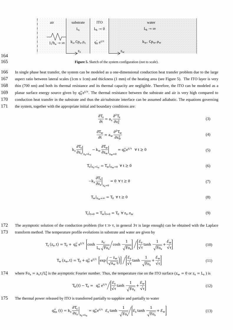
Figure 5. Sketch of the system configuration (not to scale). 165

In single phase heat transfer, the system can be modeled as a one-dimensional conduction heat transfer problem due to the large 166

aspect ratio between lateral scales (1cm x 1cm) and thickness (1 mm) of the heating area (see Figure 5). The ITO layer is very 167

thin (700 nm) and both its thermal resistance and its thermal capacity are negligible. Therefore, the ITO can be modeled as a 168

planar surface energy source given by q0′′et/τ. The thermal resistance between the substrate and air is very high compared to 169

conduction heat transfer in the substrate and thus the air/substrate interface can be assumed adiabatic. The equations governing 170

the system, together with the appropriate initial and boundary conditions are: 171

∂Ts∂t= as

∂2Ts∂zs2

(3)

∂Tw∂t

= aw∂2Tw∂zw2

(4)

ks∂Ts∂zs|zs=Ls

− kw∂Tw∂zw

|zw=0

= q0′′et/τ ∀ t ≥ 0 (5)

Ts|zs=Ls = Tw|zw=0 ∀ t ≥ 0 (6)

−ks∂Ts∂zs|zs=0

= 0 ∀ t ≥ 0 (7)

Tw|zw=∞ = T0 ∀ t ≥ 0 (8)

Ts|t=0 = Tw|t=0 = T0 ∀ zs, zw (9)

The asymptotic solution of the conduction problem (for t ≫ τ, in general 3τ is large enough) can be obtained with the Laplace 172

transform method. The temperature profile evolutions in substrate and water are given by 173

Ts (zs, t) = T0 + q0′′ et/τ [cosh

zs

Ls √Foscosh

1

√Fos⁄ ] [

ℰs

√τtanh

1

√Fos+ℰw

√τ]⁄ (10)

Tw (zw, t) = T0 + q0′′ et/τ [exp (

− zw

√aw τ)] [

ℰs

√τtanh

1

√Fos+ℰw

√τ]⁄ (11)

where Fos = asτ/Ls2 is the asymptotic Fourier number. Thus, the temperature rise on the ITO surface (zw = 0 or zs = Ls ) is 174

Th(t) − T0 = q0′′ et/τ [

ℰs

√τtanh

1

√Fos+ℰw

√τ]⁄ (12)

The thermal power released by ITO is transferred partially to sapphire and partially to water 175

qhs′′ (t) = ks

∂Ts ∂zs|zs=Ls

= q0′′et/τ ℰs tanh

1

√Fos[ℰs tanh

1

√Fos+ ℰw]⁄ (13)

air substrate water ITO

Ls Lh → 0 Lh → ∞

1/ha → ∞

zs zw

ks, Cps, ρs kw, Cpw, ρw q0" et/τ

qhw′′ (t) = −kw

∂Tw ∂ zw

|xw=0

= q0′′et/τ ℰw [ℰs tanh

1

√Fos+ ℰw]⁄ (14)

and the ratio of thermal power transferred to water is 176

Rhw = qhw′′ (t) q0

′′et/τ⁄ = ℰw [ℰs tanh 1

√Fos+ ℰw]⁄ (15)

This term does not depend on time, but only on physical properties and power excursion period. The temperature dependence of 177

the term is shown in Figure 6 for periods from 5 to 100 ms. It can be seen that due to the high thermal diffusivity of sapphire, 178

only a small fraction of the heat released by the ITO coating is transferred to water. The term Rhw depends very slightly on 179

temperature (less than 1% of change from room to saturation temperature). It increases as the power excursion period increase. 180

However, when the diffusion length scale √asτ is small compared to the substrate thickness Ls (and so Fos is very small), e.g. 181

for cases at 5 and 10 ms, the substrate acts like an infinite heat sink and the period has little or no effect on Rhw, which then 182

approaches ℰw (ℰw + ℰs)⁄ . 183

184

Figure 6. Temperature dependence of 𝐑𝐡𝐰. 185

Asymptotic conduction heat transfer coefficients to water and sapphire are given by 186

hw,c =qhw′′ (t)

Th(t) − T0=ℰw

√τ (16)

hs,c =qhs′′ (t)

Th(t) − T0=ℰs

√τtanh

1

√Fos (17)

A comparison between measured and analytic temperature rise for highly subcooled tests is shown in Figure 7 as a function of 187

time normalized by the power excursion period (note that experimental data shown in Figure 7 are limited to the single phase 188

heat transfer regime). The theoretical temperature rise curves (labelled “cond”) are obtained from Eq. (12), substituting the 189

theoretical surface power source q0′′et/τ with the actual one V(t) ∙ I(t) Ah ⁄ : 190

Th(t) − T0 = V(t) ∙ I(t)

Ah [ℰs

√τtanh

1

√Fos+ℰw

√τ]⁄ (18)

191

Figure 7. Measured and calculated temperature rise vs. period in tests at 75 K of subcooling (single-phase regime only). 192

Figure 8 shows a comparison between measured and calculated heat transfer coefficients (note that the error bars are covered by 193

dots). The physical properties for the calculation of the theoretical trends are taken at saturation temperature. The near-perfect 194

agreement between data and theoretical trends confirms the quality of experimental data and the validity of the analytic solution. 195

196

Figure 8. Measured and calculated heat transfer coefficient vs. period in the non-boiling regime (all test conditions). 197

3.2. Onset of nucleate boiling 198

The ONB conditions are identified by synchronized IR and HSV images. For each test, an ONB time range can be determined 199

depending on when the first bubble appears on HSV and IR recordings. The time in the middle of the range is taken as the 200

nominal ONB time which gives the nominal ONB temperature. The temporal uncertainty (ete) is calculated by half the difference 201

between the upper limit and lower limit temperature of the ONB time range (100 µs in the worst case). In addition to temporal 202

uncertainty, there is an uncertainty related to the test repeatability. The standard deviation of ONB temperatures from repeated 203

runs is used to represent such uncertainty (ere). Compared to the temporal and repeatability uncertainties, the nominal instrument 204

uncertainties are much smaller, and therefore can be safely neglected in the present analysis. Since the temporal uncertainty and 205

the repeatability uncertainty are independent and assumed to be Gaussian, the total uncertainty is calculated as below: 206

etot = √ere2 + ete

2 (19)

Usually, at short periods the total uncertainty is dominated by temporal uncertainty while at long periods by repeatability 207

uncertainty. The ONB heat flux and corresponding uncertainty are calculated using the same procedure as the ONB temperature. 208

In Figure 9 (left), ONB heat fluxes as functions of the period are shown for tests with 0 K, 25 K and 75 K of subcooling (error 209

bars shown in this figure and in the following figures correspond to ± etot). We observe that for the same period the higher is the 210

subcooling, the higher is the heat flux required to start boiling. In Figure 9 (right), ONB wall superheats show qualitatively the 211

same dependency as ONB heat fluxes. 212

213

Figure 9. Heat flux (left) and wall superheat (right) vs. period at the onset of nucleate boiling (all test conditions). 214

Error bars are present but very small. 215

216

A mechanistic ONB model was derived from the combination of Hsu’s criterion [11] and the analytical transient conduction 217

solution. Hsu’s criterion is based on a developing thermal boundary layer model. It states that the bubble can grow out of the 218

nucleation site if the saturation temperature corresponding to the local internal pressure of the vapor embryo is reached or 219

exceeded all over its surface. Since our surface is hydrophilic (i.e. contact angle < 90°), the internal pressure at the tip of the 220

vapor embryo can be expressed by 221

pv − pl =2σ

rc (20)

where we neglected the effect of non-condensable gases and rc is the radius of the cavity. By combining Eq. 20 with the transient 222

conduction analytic solution (Eq. 11), the mechanistic ONB model is given by: 223

qw,onb′′ =

εw

√τ[Tsat(patm + 2σ/rc) − Tbulk] exp (

rc

√awτ) (21)

ΔTsat, onb = [Tsat(patm + 2σ/rc) − Tsat(patm)] exp (rc

√awτ) + ΔTsub [exp (

rc

√awτ) − 1] (22)

Moreover, since the term rc √awτ⁄ is close to zero in all our test conditions, Eq. 22 can be conveniently simplified as 224

qw,onb′′ =

εw

√τ[Tsat(patm + 2σ/rc) − Tbulk] = hw,c [Tsat(patm + 2σ/rc) − Tbulk] (23)

where emerges that the ONB heat flux is proportional to the transient conduction heat transfer coefficient, which in turn is 225

proportional to 1/√𝜏, as shown by Eq. (16). 226

In our case, the application of the ONB model requires knowledge of the radius (or the distribution of radii) of the micro-cavities 227

(nucleation sites) on the heating surface. Thus, the coordinates of the ONB nucleation site were first identified from the IR 228

image. Then, the heater was examined with the SEM, making it possible to identify the cavity that served as nucleation site at 229

ONB. The size of the imperfection is approximately 5 microns (see Figure 10) which corresponds to rc ≅ 2.5 µm. Using this 230

value, the ONB heat flux, Eq. (21), and wall superheat, Eq. (22), could be predicted and plotted in Figure 9 (solid colored lines). 231

The ONB model captures the trend of the experimental results quite well, and thus is recommended for prediction of ONB in 232

transient pool boiling. 233

234

Figure 10. SEM image of the probable nucleation site 235

3.3. Mechanisms of heat transfer from ONB to FDNB 236

Several boiling heat transfer mechanisms have been identified during the transition from ONB to fully developed nucleate 237

boiling (FDNB). These mechanisms depend on the conditions under which boiling commences, which in turn are determined by 238

the subcooling and power escalation period. To better understand these mechanisms, it is helpful to characterize the conditions of 239

the boiling surface at the ONB moment. It is noteworthy that the growth rate of the heat flux to water and the rate of temperature 240

rise at the measured ONB moment (estimated by differentiating Eq. (14) and Eq. (12) at t = tonb) depend on the subcooling and 241

the period of the exponential power input, as shown in Figure 11. High subcooling and short periods result in a rapid escalation 242

of heat flux and temperature on the boiling surface. Thus, we can expect that, for high subcooling and short period the activation 243

of new nucleation sites on the boiling surface is much faster than for long periods and low subcooling. 244

245

Figure 11. Calculated rate of rise of the heat flux to water (left) and ITO temperature (right) at the ONB moment 246

An estimate of the bubble radius at the end of the inertia-controlled phase can be made with the model proposed by Mikic et al. 247

[17] for a uniformly superheated medium. The duration of the inertia-controlled phase (t+ = 1) is given by 248

tic =B2

A2 (24)

and the corresponding bubble radius is 249

Ric = A tic (25)

where 250

A = √π

7

ΔTsat hlv ρvTsat ρl

(26)

B = √12

πJa2al (27)

The bubble radii at the end of the inertia-controlled phase estimated from Eq. (24) are plotted in Figure 12 as a function of period 251

and subcooling (colored dots, labeled BR). An estimate of the superheated layer thickness at ONB is also shown (colored lines, 252

labeled SHL), calculated from Eq. (11) as the thickness for which Tw > 100.1 °C when t = tonb + tic. 253

254

Figure 12. Comparison between the bubble radii at the end of the inertia-controlled phase and the superheated layer thickness at ONB. 255

In saturation condition, once a bubble grows out of the cavity, it can successfully grow through the inertia-controlled phase and 256

keep growing by evaporation of the thermal boundary layer surrounding the bubble (thermally-controlled growth) [18]. For long 257

periods, e.g. 100 ms (see video 0K_100ms), a few nucleation sites are activated and generate bubbles of large size, comparable to 258

the length scale of the heating surface (1cm). Bubbles keep growing until they reach the departure diameter. Then, after the 259

detachment, the heating surface is rewetted by water. In this situation, the increase of the heater power is slow compared to the 260

time scale of bubble growth and detachment (see Figure 11). Thus, the heat transfer associated with the nucleation of a few big 261

bubbles vastly exceeds transient conduction and the rise of the boiling surface temperature is abruptly halted. This condition, 262

which we called OBD (Onset of Boiling Driven heat transfer), is reflected by a sharp inflection of the heat transfer curve from 263

the non-boiling transient conduction asymptote (see Sections 3.4 and 3.5). During the boiling process, the evaporation of the 264

liquid microlayer consumes the energy locally released by the heater and also the sensible energy stored in the substrate (see 265

circles with negative heat flux to sapphire, from 0.3876s in video 0K_100ms). As boiling proceeds after OBD, at saturation, this 266

phenomenon can lead to a decrease of the average boiling surface temperature (see Sections 3.4 and 3.5), which is known as 267

overshoot (OV). At short periods, e.g. 5 ms, since the rates of heat generation and temperature rise at ONB are higher than at 100 268

ms (see Figure 11), more nucleation sites are activated within a short time (see video 0K_5ms). Several big bubbles crowd the 269

heating surface and tend to merge with each other before they can reach the departure diameter, creating a large vapor cushion 270

above the heater. As a result, the rewetting of the surface is inhibited and the surface temperature increases rapidly due to the 271

formation of big dry spots below each bubble (0.0328s in video 0K_5ms). Under these circumstances, boiling proceeds from 272

ONB almost instantaneously to CHF. 273

At subcooled conditions, except for 25 K subcooling and 100 ms, the estimated bubble radii are larger than the superheated layer 274

thickness (see Figure 12). In particular, in highly subcooled conditions, e.g. 75 K, the thickness of the superheated layer at ONB 275

is very small compared to the size of the bubbles at the end of the inertia-controlled phase. Thus, after the inertia-controlled 276

phase, bubbles contract rapidly due to the condensation of the vapor in contact with subcooled liquid (see video 75K_5ms and 277

video 75K_100ms). The rates of heat generation and temperature rise at ONB are much higher than in saturation conditions (see 278

Figure 11) and thus a huge number of cavities is rapidly activated. Therefore, shortly after ONB, the boiling surface is 279

completely covered by tiny bubbles that undergo continuous cycles of growth and contraction with frequency comparable to the 280

HSV frame rate, i.e. 5000 Hz. This boiling mechanism is very effective. In fact, in tests with 75 K subcooling and 5 ms of period, 281

heat fluxes as large as 10 MW/m2 were reached without undergoing any boiling crisis. It is also noteworthy that, contrary to 282

saturation condition where the thermal behavior is determined by the nucleation and the growth of a few individual bubbles of 283

large size, under highly subcooled conditions, OBD and OV are due to the explosive activation of new nucleation sites on the 284

boiling surface. 285

At low subcooled conditions, e.g. 25 K, except for 100 ms case, the thickness of the superheated layer at ONB is still smaller 286

than the size of the bubbles at the end of the inertia-controlled phase (see Figure 12). In addition, the rates of heat generation and 287

temperature rise at ONB are still much higher than the ones at saturation condition, although smaller than those at 75 K of 288

subcooling (see Figure 11). At these conditions, bubbles still experience the phases of inertia-controlled growth, condensation 289

and cycles of oscillation as bubbles at 75 K of subcooling (see video 25K_5ms and video 25K_100ms). However, due to the 290

smaller subcooling and thicker superheated layer at ONB, the size of bubbles is larger than the ones at 75 K subcooling and a 291

small number of cavities is activated. As a result, the boiling mechanism is less effective than at 75 K subcooling, although still 292

more effective than saturation condition. 293

3.4. Transient boiling processes 294

In transient boiling tests there are generally two types of boiling curves: with temperature overshoot and without temperature 295

overshoot. Several transient boiling steps are identified depending on the type of boiling curves. 296

297

Figure 13. Typical boiling curves with temperature overshoot for the a test at 5 ms and 75K subcooling (left) and without temperature 298

overshoot at 5 ms and 25K subcooling 299

Figure 13 (left) shows a typical boiling curve with temperature overshoot, where the subcooling is 75 K and the period is 5 ms. 300

Five features are identified with dots of varying color. 301

Before ONB the boiling curve closely follows single-phase transient conduction. While heat flux to water and wall superheat 302

keep increasing (and so does the superheated layer (SHL) thickness in water), at a certain moment ONB occurs (green dot). 303

Several small standalone bubbles can be seen on the HSV image, but it barely shows any change in the IR image since boiling is 304

still highly localized (0.0376 s in video 75K_5ms and Figure 14[there is no 0.0376s pic in figure 14]). 305

Shortly after ONB, the boiling curve starts to deviate from the transient conduction asymptote. When more bubbles are 306

generated, the associated heat transfer mechanism supersedes transient conduction. The heat flux increases, whereas the wall 307

superheat does not show a significant increase. The combination of heat flux to water and wall superheat results in an inflection 308

of the boiling curve. Such inflection denotes the occurrence of the onset of boiling driven heat transfer regime OBD (blue dot). 309

We can clearly see many bubbles and their temperature footprints on the HSV and IR images (0.0380 s in video 75K_5ms and 310

Figure 14). It is emphasized that at saturation conditions the OBD is achieved by bubble departure and surface rewetting (around 311

0.4004 s in video 0K_100ms and Figure 15), while at subcooled condition OBD depends on the rapid activation of nucleation 312

sites. 313

After OBD, boiling becomes more and more vigorous. The heat flux to water increases sharply while the heat flux to substrate 314

decreases significantly. Such conjugate heat transfer among water, substrate and power input causes the wall temperature to drop; 315

this is the overshoot (OV) point (magenta dot in Figure 13, 0.0384 s in video 75K_5ms and Figure 14). 316

After the OV, the wall superheat keeps decreasing due to the cooling effect of vigorous boiling. However, heat flux to water still 317

increases sharply. This rapid process reaches an end when the SHL is fully depleted (cyan dot in Figure 13). After that, boiling is 318

suppressed. The HSV image shows that bubbles condense and become smaller, while the IR image reveals a lower surface 319

temperature (0.0388 s in video 75K_5ms and Figure 14). 320

Finally, when the exponential increase of power input catches up with the energy consumption of the system, heat flux to water 321

and to substrate reach a new balance. The boiling curve progresses towards FDNB (red dot in Figure 13, 0.0392 s in video 322

75K_5ms and Figure 14) which is predicted reasonably well by the Rohsenow correlation [19] with Csf =0.0135. 323

324

325

Figure 14. HSV, ITO temperature and heat flux from OBD to FDNB for the test at 5 ms and 75K subcooling 326

Figure 13 (right) shows a typical boiling curve without temperature overshoot, where the subcooling is 25 K and the period is 5 327

ms. This type of boiling curve usually exists at low period and low subcooling. In such conditions the boiling process presents 328

three steps. Before OBD, the heat transfer regimes are basically the same as for the case with overshoot. However, the boiling 329

process differs after OBD. Instead of progressing through OV and SHL depletion, there is no visible temperature overshoot. Wall 330

superheat increases monotonically at these conditions, which means the power input is always sufficiently high and the SHL is 331

thick enough to support boiling. Eventually, the boiling curve can progress toward FDNB at subcooled condition (0.0356 s in 332

video 25K_5ms and Figure 15) or transfer toward CHF without returning to FDNB at saturation condition (0.0328 s in video 333

0K_5ms and Figure 16). 334

335

336

Figure 15. HSV, ITO temperature and heat flux to water during the FDNB regime for the test at 5 ms and 25K subcooling. 337

0.0380 s 0.0384 s 0.0388 s 0.0392 s

TEM

PER

ATU

RE

[°C

] H

EAT

FLU

X T

O W

ATE

R

[MW

/m2]

338

Figure 16. HSV, ITO temperature and heat flux to water during the fully nucleate boiling regime for the test at 5 ms and 0K subcooling. 339

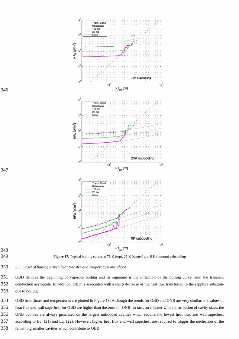
The typical boiling curves for three different subcoolings are plotted in Figure 17. For each subcooling, the boiling curve is 340

plotted for three periods i.e. 5ms, 20ms and 100ms, along with the corresponding analytic transient conduction curve (grey lines). 341

The corresponding values predicted by Rohsenow correlation are also plotted (black dashed line). It is clearly shown that, for the 342

same subcooling, the boiling curve is shifted towards higher heat fluxes and higher wall superheats as the period becomes 343

smaller. For the same period, the boiling curve is shifted towards higher heat fluxes and higher wall superheats with increasing 344

subcooling. 345

346

347

348

Figure 17. Typical boiling curves at 75 K (top), 25 K (center) and 0 K (bottom) subcooling 349

3.5. Onset of boiling driven heat transfer and temperature overshoot 350

OBD denotes the beginning of vigorous boiling and its signature is the inflection of the boiling curve from the transient 351

conduction asymptote. In addition, OBD is associated with a sharp decrease of the heat flux transferred to the sapphire substrate 352

due to boiling. 353

OBD heat fluxes and temperatures are plotted in Figure 18. Although the trends for OBD and ONB are very similar, the values of 354

heat flux and wall superheat for OBD are higher than the ones for ONB. In fact, on a heater with a distribution of cavity sizes, the 355

ONB bubbles are always generated on the largest unflooded cavities which require the lowest heat flux and wall superheat 356

according to Eq. (21) and Eq. (22). However, higher heat flux and wall superheat are required to trigger the nucleation of the 357

remaining smaller cavities which contribute to OBD. 358

359

Figure 18. OBD heat flux (left) and wall superheat (right) versus power excursion periods at different subcoolings 360

OV wall superheats (if OV is present) are obtained by searching for the first temperature peak on the boiling curve between OBD 361

and the SHL depletion point. The results are plotted in Figure 19. As shown, there is usually no temperature overshoot at short 362

periods and small subcoolings due to rapid increase of heat generation and insufficient enhancement of the boiling heat transfer 363

coefficient. The trend for the OV wall superheat is also similar to the ONB wall superheat. For a given subcooling, the OV wall 364

superheat increases with decreasing power excursion periods. For a given power excursion period, the OV wall superheat 365

increases with increasing subcooling. It is also noteworthy that the OV values at subcooled conditions, i.e. 25 K and 75 K, are 366

close to each other while distant from the ones at saturation conditions. This is likely caused by the different boiling mechanisms 367

at subcooled and saturation conditions, as discussed in Section 3.3. 368

369

Figure 19. OV wall superheat versus power excursion periods at different subcoolings 370

4. Conclusions 371

Transient heat transfer phenomena occurring during exponential power escalations were investigated on a plate-type, IR-372

transparent heater. Exponential periods in the range from 5 ms to 100 ms and bulk temperatures from saturation to 75 K of 373

subcooling have been explored at ambient pressure in pool boiling conditions. Synchronized state-of-the-art diagnostics such as 374

IR thermometry and HSV were used to provide new and unique insight into the transient boiling heat transfer phenomena and to 375

improve the accuracy and the reliability of measured quantities compared to existing studies. Various boiling regimes were 376

observed during the transition from ONB to fully developed nucleate boiling. ONB, OBD and OV conditions were identified, 377

depending on the period of the power escalation and the subcooling. 378

The main findings are as follows: 379

The measured single phase heat transfer coefficient, before boiling inception, is inversely proportional to the square root 380

of the period. Moreover, the heat flux to water, the wall temperature rise and the heat transfer coefficient can be 381

predicted by analytic expressions developed from the solution of the 1D transient conduction problem. 382

The measured ONB heat flux and superheat increase as the period decreases, and can be predicted by a combination of 383

the analytic transient conduction temperature profile in water and the Hsu’s nucleation criterion. Accordingly, ONB was 384

observed on the largest unflooded active cavity available on the heater surface. 385

The photographic study of the boiling process from ONB to FDNB reveals two different boiling mechanisms. At 386

saturation condition where the thickness of the superheated layer is large, the boiling process depends on the growth and 387

departure of a few individual bubbles with large size. At subcooled conditions where the superheated layer is very thin, 388

the boiling process is promoted effectively by the rapid activation of a large number of nucleation sites. Here the 389

inability of a bubble to grow beyond the thin superheated layer leads to highly localized cooling. In particular, a heat 390

flux as high as 10 MW/m2 was reached without undergoing the boiling crisis at 75 K subcooling and 5 ms condition. 391

The measured OBD heat flux and superheat follow the same trend as ONB; they increase as the period decreases and 392

the subcooling increases. This is to be expected as ONB and OBD are governed by the same physical phenomena. OBD 393

occurs when several nucleation sites are activated, which requires higher superheat and heat flux compared to ONB. We 394

may expect that OBD changes according to the size and the distribution of nucleation sites present on the boiling 395

surface. 396

Measured OV wall superheat also follows the same trend as ONB superheat; superheat increases as the period decreases 397

and the subcooling increases. However, there is usually no temperature overshoot at short periods and small subcoolings 398

due to a rapid increase of heat generation and insufficient enhancement of the heat transfer coefficient. The measured 399

OV wall superheats are consistent with the observation of different boiling mechanisms at saturation and subcooled 400

conditions. 401

FDNB conditions are achieved if the rate of heat transfer enhancement is faster than the rate of heat generation, 402

typically at long period, or under subcooled conditions (whether long or short periods are explored). Otherwise, close to 403

saturation conditions, CHF could be reached directly from ONB at short periods. 404

Follow-up investigations including the study of forced convection effects under the same exponential power escalation scenarios 405

are presented in the companion paper [14]. 406

Acknowledgments 407

Ms. Carolyn P. Coyle and Dr. Reza Azizian are warmly acknowledged for their support in using the focused ions beam and the 408

scan electron microscope. This research project was sponsored by CEA through contract 021439-001. 409

410

411

Appendix A. Coupled radiation-conduction model 412

To achieve an accurate estimation of the temperature and heat flux distributions on the boiling surface is necessary to solve a 413

coupled conduction/radiation inverse problem. The problem is inverse because the boundary condition for the conduction 414

problem (the boiling surface temperature) is not known, but is part of the solution. What is known is the radiation measured by 415

the IR camera, which combines the radiation emitted by the boiling surface (ITO in our case), the radiation emitted by the 416

sapphire substrate and also reflection of the background radiation (at ambient temperature), as sketched in Figure 20. With this 417

technique we can estimate the time-dependent 3D temperature distribution in the heater, as well as local temperature and local 418

heat flux distributions on the boiling surface, starting from the time-dependent 2D radiation measured by the IR camera. A brief 419

description of this technique is given below. Further details can be found in Ref. [16]. 420

421

Figure 20. Sketch of the optical setup. 422

A.1. Conduction model 423

The transient heat transfer equation in the substrate physical domain is discretized with an implicit 3D finite volume scheme. The 424

boundary corresponding to the active ITO coating serves as temperature boundary condition. Its local temperature Tito(x, y) is 425

determined according to the radiation recorded by the infrared camera, as described later. All other boundaries are modelled as 426

diabatic surfaces: appropriate heat transfer coefficient h and sink temperature 𝑇∞ have to be assigned for each surface. 427

Once a converged solution is achieved for a prescribed ITO temperature, the heat flux to sapphire at the ITO-sapphire interface 428

can be simply calculated by the discretized Fourier’s conduction law 429

qs′′(t) = ks(Tito)

Tito(x, y, t) − Ts(x, y, zc, t)

zc (28)

ITO SAPPHIRE BACKGROUND

ITO

SAPPHIRE

MIRROR

IR CAMERA HEATER RADIATION

WATER

Ts(x, y, z, t)

Tito(x, y, t)

where zc is the distance between the ITO boundary and the center of the adjacent cell, and ks(Tito) is the sapphire thermal 430

conductivity at the ITO temperature. An estimate of the local instantaneous heat flux to water qw′′ can thus be obtained 431

subtracting the total power qtot′′ generated by Joule heating in the ITO and the heat flux transferred to sapphire 432

qw′′ (x, y, t) = qtot

′′ (t) − qs′′(x, y, t) =

V(t) ∙ I(t)

Ah − ks(Tito)

Tito(x, y, t) − Ts(x, y, zc, t)

zc (29)

433

A.2. Radiation model 434

The radiation measured by the IR camera includes the radiation emitted by the ITO coating, the radiation emitted by the sapphire 435

substrate and the reflection of the background radiation, as sketched in Figure 20. 436

The radiation model is inspired by the radiation model proposed in the work of Kim et al. [20] . However, the present model is 437

not based on average energy radiance, but spectral photon radiation. This is necessary because sapphire has a highly variable 438

spectral absorption coefficient in the range of wavelengths between 4 and 5 µm. Photons are emitted by the ITO and by the 439

substrate. Water emissions are completely shielded by the ITO layer, which is opaque in the range 3 to 5 µm used in our 440

investigations. We have assumed that the light source is planar, that is, light is only emitted in the direction normal to the boiling 441

surface (2D radiation normal to the x-y plane). 442

Emissions from the ITO 443

The spectral photon flux per wavelength emitted by a black body surface is 444

Npλ = Npλ(T, λ) = Epλ(T, λ)

eλ =

2 π c

λ4 (eC2λT − 1)

(30)

Since ITO is thick enough to be opaque and thin enough to neglect temperature gradient across its thickness, the spectral photon 445

flux emitted at the ITO/substrate interface is 446

Npλ,Tito . (1 − ρλ,hs) (31)

where ρλ,hs is the spectral reflection coefficient at the interface between ITO and sapphire. To obtain the effective photon flux 447

emitted by the ITO, one must take into account multiple reflections at the ITO/substrate and substrate/air interfaces and 448

absorption within the substrate, as sketched in Figure 21. Summing all the contributions we get 449

Npλito = Npλ,Tito(1 − ρλ,hs) τλ,s(1 − ρλ,sa)∑(ρλ,hs ρλ,sa τλ,s

2 )n

∞

n=0

= Npλ,Tito(1 − ρλ,hs) τλ,s(1 − ρλ,sa)

1 − ρλ,hs ρλ,sa τλ,s2

= Npλ,Titoτλ,app

(32)

450

451

WATER ITO SAPPHIRE AIR

Npλ,Tito →

→ Npλ,Tito . (1 − ρλ,hs)

Npλ,Tito . (1 − ρλ,hs). τλ,s →

→ Npλ,Tito . (1 − ρλ,hs). τλ,s. (1 − ρλ,sa)

Npλ,Tito . (1 − ρλ,hs). τλ,s. ρλ,sa ←

← Npλ,Tito . (1 − ρλ,hs). τλ,s2 . ρλ,sa

→ Npλ,Tito . (1 − ρλ,hs). τλ,s2 . ρλ,sa. ρλ,hs

Npλ,Tito . (1 − ρλ,hs). τλ,s3 . ρλ,sa. ρλ,hs →

→ Npλ,Tito . (1 − ρλ,hs). τλ,s3 . ρλ,sa. ρλ,hs. (1 − ρλ,sa)

Npλ,Tito . (1 − ρλ,hs). τλ,s3 . ρλ,sa

2 . ρλ,hs ←

← Npλ,Tito . (1 − ρλ,hs). τλ,s4 . ρλ,sa

2 . ρλ,hs

→ Npλ,Tito . (1 − ρλ,hs). τλ,s4 . ρλ,sa

2 . ρλ,hs2

Npλ,Tito . (1 − ρλ,hs). τλ,s5 . ρλ,sa

2 . ρλ,hs2 →

. → Npλ,Tito . (1 − ρλ,hs). τλ,s5 . ρλ,sa

2 . ρλ,hs2 . (1 − ρλ,sa)

. .

. .

Figure 21. Multiple reflections and absorptions determining the apparent transmissivity 𝛕𝛌,𝐚𝐩𝐩 of sapphire 452

Emissions from the sapphire substrate 453

A substrate layer of thickness dz emits a photon flux equal to αλNpλ,T(z)dz in two directions. Half of the flux is emitted forward, 454

towards the camera, half is emitted backward, towards the ITO heater. In the first case, the spectral photon flux reaching the 455

substrate/air interface is 456

Npλs,+ =

1

2∫αλ Npλ,T(z) exp(−αλ(L − z)) dz

L

0

(33)

In the second case, the photon flux reaching the ITO/substrate interface is given by 457

Npλs,− =

1

2∫αλ Npλ,T(z) exp(−αλz) dz

L

0

(34)

Part of this flux is reflected back at the substrate/ITO interface and crosses the substrate to reach the substrate/air interface. At the 458

substrate/air interface, the two light beams can be transmitted or reflected. Once multiple reflections and absorptions are 459

accounted for (see Figure 22 and Figure 23), the effective spectral photon flux crossing the substrate/air interface is 460

Npλs =

Npλs,− ρλ,hs τλ,s (1 − ρλ,sa) + Npλ

s,+ (1 − ρλ,sa)

1 − ρλ,hs ρλ,sa τλ,s2 = Npλ

s,−ϵλ,app− + Npλ

s,+ϵλ,app+ (35)

461

462

463

WATER ITO SAPPHIRE AIR

← Npλs,−

→ Npλs,−. ρλ,hs

Npλs,−. ρλ,hs. τλ,s →

→ Npλs,−. ρλ,hs. τλ,s. (1 − ρλ,sa)

Npλs,−. ρλ,hs. τλ,s. ρλ,sa ←

← Npλs,−. ρλ,hs. τλ,s

2 . ρλ,sa

→ Npλs,−. ρλ,hs

2 . τλ,s2 . ρλ,sa

Npλs,−. ρλ,hs

2 . τλ,s3 . ρλ,sa →

→ Npλs,−. ρλ,hs

2 . τλ,s3 . ρλ,sa. (1 − ρλ,sa)

Npλs,−. ρλ,hs

2 . τλ,s3 . ρλ,sa

2 ←

← Npλs,−. ρλ,hs

2 . τλ,s4 . ρλ,sa

2

→ Npλs,−. ρλ,hs

3 . τλ,s4 . ρλ,sa

2

Npλs,−. ρλ,hs

3 . τλ,s5 . ρλ,sa

2 →

. → Npλs,−. ρλ,hs

3 . τλ,s5 . ρλ,sa

2 . (1 − ρλ,sa)

. .

. .

Figure 22. Multiple absorption and reflections determining the apparent backward emissivity 𝛜𝛌,𝐚𝐩𝐩− of sapphire 464

465

WATER ITO SAPPHIRE AIR

Npλs,+ →

→ Npλs,+. (1 − ρλ,sa)

Npλs,+. ρλ,sa ←

← Npλs,+. ρλ,sa. τλ,s

→ Npλs,+. ρλ,sa. τλ,s. ρλ,hs

Npλs,+. ρλ,sa. τλ,s

2 . ρλ,hs →

→ Npλs,+. ρλ,sa. τλ,s

2 . ρλ,hs. (1 − ρλ,sa)

Npλs,+. ρλ,sa

2 . τλ,s2 . ρλ,hs ←

← Npλs,+. ρλ,sa

2 . τλ,s3 . ρλ,hs

→ Npλs,+. ρλ,sa

2 . τλ,s3 . ρλ,hs

2

Npλs,+. ρλ,sa

2 . τλ,s4 . ρλ,hs

2 →

. → Npλs,+. ρλ,sa

2 . τλ,s4 . ρλ,hs

2 . (1 − ρλ,sa)

. .

. .

Figure 23. Multiple absorption and reflections determining the forward apparent emissivity 𝛜𝛌,𝐚𝐩𝐩+ of sapphire 466

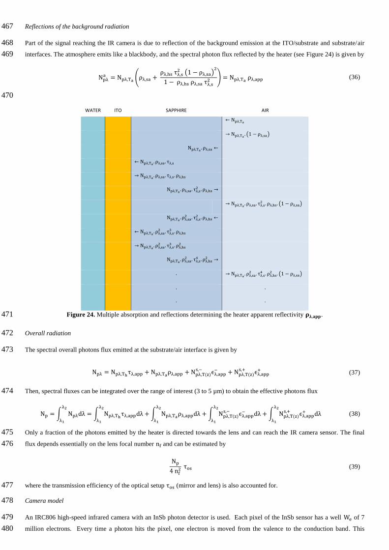
Reflections of the background radiation 467

Part of the signal reaching the IR camera is due to reflection of the background emission at the ITO/substrate and substrate/air 468

interfaces. The atmosphere emits like a blackbody, and the spectral photon flux reflected by the heater (see Figure 24) is given by 469

Npλa = Npλ,Ta (ρλ,sa +

ρλ,hs τλ,s2 (1 − ρλ,sa)

2

1 − ρλ,hs ρλ,sa τλ,s2 ) = Npλ,Ta ρλ,app (36)

470

WATER ITO SAPPHIRE AIR

← Npλ,Ta

→ Npλ,Ta . (1 − ρλ,sa)

Npλ,Ta . ρλ,sa ←

← Npλ,Ta . ρλ,sa. τλ,s

→ Npλ,Ta . ρλ,sa. τλ,s. ρλ,hs

Npλ,Ta . ρλ,sa. τλ,s2 . ρλ,hs →

→ Npλ,Ta . ρλ,sa. τλ,s2 . ρλ,hs. (1 − ρλ,sa)

Npλ,Ta . ρλ,sa2 . τλ,s

2 . ρλ,hs ←

← Npλ,Ta . ρλ,sa2 . τλ,s

3 . ρλ,hs

→ Npλ,Ta . ρλ,sa2 . τλ,s

3 . ρλ,hs2

Npλ,Ta . ρλ,sa2 . τλ,s

4 . ρλ,hs2 →

. → Npλ,Ta . ρλ,sa2 . τλ,s

4 . ρλ,hs2 . (1 − ρλ,sa)

. .

. .

Figure 24. Multiple absorption and reflections determining the heater apparent reflectivity 𝛒𝛌,𝐚𝐩𝐩. 471

Overall radiation 472

The spectral overall photons flux emitted at the substrate/air interface is given by 473

Npλ = Npλ,Thτλ,app + Npλ,Taρλ,app + Npλ,T(z)s,− ϵλ,app

− + Npλ,T(z)s,+ ϵλ,app

+ (37)

Then, spectral fluxes can be integrated over the range of interest (3 to 5 µm) to obtain the effective photons flux 474

Np = ∫ Npλdλ = ∫ Npλ,Thτλ,appdλλ2

λ1

+∫ Npλ,Taρλ,appdλλ2

λ1

+∫ Npλ,T(z)s,− ϵλ,app

− dλλ2

λ1

+∫ Npλ,T(z)s,+ ϵλ,app

+ dλλ2

λ1

λ2

λ1

(38)

Only a fraction of the photons emitted by the heater is directed towards the lens and can reach the IR camera sensor. The final 475

flux depends essentially on the lens focal number nf and can be estimated by 476

Np

4 nf2 τos (39)

where the transmission efficiency of the optical setup τos (mirror and lens) is also accounted for. 477

Camera model 478

An IRC806 high-speed infrared camera with an InSb photon detector is used. Each pixel of the InSb sensor has a well We of 7 479

million electrons. Every time a photon hits the pixel, one electron is moved from the valence to the conduction band. This 480

phenomenon creates a voltage difference proportional to the photon flux, which is the signal measured as photon counts, R. The 481

quantum efficiency of the sensor, QE, which is determined by the photon/electron conversion efficiency (internal quantum 482

efficiency), as well as reflection on the surface of the sensor (external quantum efficiency), must be also taken into account. 483

To convert camera counts to photons, the contribution of the noise must be cancelled. This is given by empty well counts ncew 484

when the integration time dtint is zero (approximately 420 counts, to be measured before each experimental campaign) and the 485

dark current (ncdc = 9570 counts/second as per manufacturer specifications), whose noise is proportional to the integration time 486

dtint (200 µs). The effective photons flux measured by the camera is thus given by 487

NpIRC =

R − (ncew + ncdc ∙ dtint)

dtint∙

We(ncfw − ncew)

∙1

QE ∙ Apixel (40)

where ncfw is the full well counts when the signal is saturated (approximately 16000 counts, to be measured before each 488

experimental campaign) and Apixel is the area of the sensor pixel (20 µm × 20 µm). 489

A.3. Coupled conduction/radiation model 490

The flow chart of the coupled conduction/radiation model is shown in Figure 25. At a given time step, the local distribution of 491

photon counts R from the IR camera is obtained. Then a guess of the local heater temperature Tito∗ is made based on the photon 492

counts R. The temperature distribution through the substrate T∗ is calculated by the heat conduction code as detailed in Sec. 2. 493

Then, the overall emission of the heater Np is calculated as detailed above and converted to photon counts as follows 494

R∗ = Np dtint QE Apixel(ncfw − ncew)

We+ (ncew + ncdc ∙ dtint) (41)

If the difference of photon counts |R∗ − R | is less than a prescribed tolerable error, as explained below, the guessed temperature 495

of ITO heater is accepted and the algorithm is moved to the next time step, otherwise, the code keeps iterating with an adjusted 496

guess of the ITO temperature as boundary condition. 497

498

Figure 25. Flow chart of the coupled conduction-radiation model. 499

It should be noted that verification of the conduction/radiation coupling is required before every experimental campaign (every 500

heater and optical setup). Fine tuning of the product τos QE is also necessary to reduce the error on the measured photons flux. 501

BC for 3D conduction

NO YES

Initial condition

for step t+1

R(x, y, t)

3D Conduction

in the substrate

T∗(x, y, z, t)

Counts

R∗(x, y, t)

|R∗ − R | < 𝜀 ?

adjust

Tito∗ (x, y, t)

T(x, y, z, t)

guess

Tito∗ (x, y, t)

This is normally achieved by in-situ steady-state calibration (with uniform temperature within the heater), to be run before every 502

experimental campaign (see Figure 26). Optimal values of the τos QE product are usually between 0.7 and 0.9, where we assume 503

that the quantum efficiency does not depend on the wavelength. It is emphasized that this is the only empiricism required in the 504

whole model. 505

506

Figure 26. Comparison between measured and calculated radiation in steady-state conditions (uniform temperature). 507

The radiation model curve in Figure 26 can be approximated with a polynomial Pcal(T) that can be used as “steady-state” 508

calibration curve. Even though this polynomial is not appropriate for accurate time-dependent local temperature measurements, it 509

provides meaningful information on how the radiation changes as a function of temperature. We use this information to adjust 510

the iterative ITO temperature in the conduction/radiation loop (see Figure 25). The iterative temperature distribution at the 511

iteration n+1 is calculated as 512

Tito∗,n+1(x, y, t) = Tito

∗,n(x, y, t) −R∗(x, y) − R(x, y)

dPcaldT

|Tito∗,n(x,y,t)

(42)

We consider that the model has converged in a time step when the maximum local temperature adjustment is smaller than 10−4 513

°C. 514

max

(

|R∗(x, y) − R(x, y)|

dPcaldT

|Tito∗,n(x,y,t) )

< 10−5 (43)

Using this method, the convergence of the conduction/radiation model is normally achieved in less than 5 internal iterations. 515

A.4. Optical properties 516

Fundamental and apparent optical properties required for the implementation of the radiation model were measured as detailed in 517

Ref. [16] by means of a FTIR Bruker spectrometer. Fundamental optical properties are shown in Figure 27. Apparent optical 518

properties are shown in Figure 28. 519

520

Figure 27. Fundamental optical properties of the ITO-sapphire heater. 521

522

523

Figure 28. Apparent optical properties of the ITO-sapphire heater. 524

525

References 526 527

[1] M. W. Rosenthal, "An experimental study of transient boiling," Nuclear Science and Engineering, vol. 2, pp. 640-656,

1957.

[2] W. B. Hall and W. C. Harrison, "Transient boiling of water under atmospheric pressure," in Proceedings of the International

Heat Transfer Conference, Chicago, IL, 1966.

[3] A. Sakurai and M. Shiotsu, "Transient pool boiling heat trasnsfer. Part 1: Incipient boiling superheat," Journal of Heat

Transfer, vol. 99, pp. 547-553, 1977.

[4] A. Sakurai and M. Shiotsu, "Transient pool boiling heat trasnsfer. Part 2: Boiling heat transfer and burnout," Journal of Heat

Transfer, vol. 99, pp. 554-560, 1977.

[5] A. Sakurai, M. Shiotsu, K. Hata and K. Fukuda, "Photographic study of transition from non-boiling and nucleate boiling

regime to film boiling due to increasing heat inputs in liquid nitrogen and water," Nuclear Engineering and Design, vol.

200, pp. 39-54, 2000.

[6] A. Sakurai, "Mechanism of transition to film boiling at CHF in subcooled and pressurized liquids due to steady and

increasing heat inputs," Nuclear Engineering and Design, vol. 197, pp. 301-356, 2000.

[7] J. Park, K. Fukuda and Q. Liu, "Transient CHF phenomena due to exponentially increasing heat inputs," Nuclear

Engineering and Technology, vol. 41, no. 9, pp. 1205-1214, 2009.

[8] H. A. Johnson, "Transient boiling heat transfer to water," International Journal of Heat and Mass transfer, vol. 14, pp. 67-

82, 1971.

[9] I. Kataoka, A. Serizawa and A. Sakurai, "Transient boiling heat transfer under forced convection," International Journal of

Heat and Mass Transfer, vol. 26, pp. 583-595, 1983.

[10] L. Sargentini, M. Bucci, G.-Y. Su, J. Buongiorno and T. Mckrell, "Experimental and analytical study of exponential power

excursion in plate-type fuel," in Proceeding of the 2014 International Topical Meeting on Advances in Thermal-Hydraulics

(ATH'14), Reno, NV, 2014.

[11] Y. Y. Hsu, "On the size range of active nucleation cavities on a heating surface," Journal of Heat Transfer, vol. 14, pp. 67-

82, 1971.

[12] W. M. Rohsenow, "Nucleation in boiling heat transfer," in ASME symposium, Detroit, MI, 1970.

[13] F. Tachibana, M. Akiyama and H. Kawamura, "Heat transfer and critical heat flux in transient boiling," Journal of Nuclear

Science and Technology, vol. 5, pp. 117-126, 1968.

[14] G.-Y. Su, M. Bucci, T. Mckrell and J. Buongiorno, "Transient boiling heat transfer of water under exponential heat inputs.

Part II: Flow boiling," International Journal of Heat and Mass Transfer, 2015.

[15] C. Gerardi, "Investigation of the pool boiling heat transfer enhancement of nano-engineered fluids by means of high-speed

infrared thermography," PhD Thesis, Massachusetts Institute of Technology, Cambridge, MA, 2009.

[16] M. Bucci, G.-Y. Su, A. Richenderfer, T. Mckrell and J. Buongiorno, "A mechnaistic IR calibration technique for boiling

heat transfer investigations," Submitted to Experimental Thermal and Fluid Science, 2015.

[17] B. B. Mikic, W. M. Rohsenow and P. Griffith, "On the bubble growth rates," International Journal of heat and Mass

Transfer, vol. 13, pp. 657-666, 1970.

[18] V. P. Carey, Liquid-vapor phase change phenomena, Taylor and Francis, 2008, pp. 226-232.

[19] W. M. Rohsenow, "A method for correlating heat tranfer data for surface boiling of liquids," Transaction of ASME, vol. 74,

pp. 969-975, 1952.

[20] T. H. Kim, S. Dessiatoun and J. Kim, "Measurement of two-phase flow and heat transfer parameters using infrared

thermometry," International Journal of Multiphase Flow, vol. 40, pp. 56-67, 2012.

528 529

Nomenclature 530

Latin letters Greek letters

a Thermal diffusivity [m2 s]⁄ α Absorption coefficient (appendix) [1 m⁄ ]

A Area [m2] ℰ Thermal effusivity [W√s m2K]⁄

C Heat capacity [J K]⁄ ϵ Apparent emissivity [−]

c Speed of light (appendix) [m s]⁄ λ Wavelength [m]

C2 =1.439x10-2 (appendix) [mK] ρ Density [kg m3]⁄

Cp Specific heat [J kgK]⁄ ρ Reflectivity (appendix) [−]

e Uncertainty [K or W m2⁄ ] τ Exponential period [s]

dt Time step (appendix) [s] τ Transmissivity (appendix) [−]

ΔT Temperature difference [K]

Fo Fourier number (= aτ/L2) [−]

h Heat transfer coefficient [W m2K]⁄

I Current [A] Subscripts

Ja Jacob number (= ρlCplΔTsat/hlvρv) [−] 0 Initial

k Thermal conductivity [W mK]⁄ atm Atmosphere

L Thickness [m] bulk Bulk

Np Photons flux (appendix) [phot m2s m]⁄ c Cavity or conduction

nc Noise counts (appendix) [counts] dc Dark current (appendix)

ncounts IR camera counts (appendix) [counts] ew Empty well (appendix)

nf Focal number (appendix) [−] fw Full well (appendix)

p Pressure [Pa] h Heater (ITO)

q′′ Heat flux [W m2]⁄ ic Inertia-controlled

q′′′ Energy source [W m3]⁄ int Integration time (appendix)

QE Quantum efficiency (appendix) [−] l Liquid

R Fraction of heat flux to water [−] onb Onset of nucleate boiling

r Radius [m] pixel Pixel (appendix)

t Time [s] re Repeatability

T Temperature [K] s Substrate

V Voltage [V] sat Superheat

x Spatial coordinate [m] sub Subcooling

y Spatial coordinate [m] tot Total

z Spatial coordinate [m] te Temporal

v Vapor

Acronyms

CHF Critical Heat Flux

FDNB Fully Developed Nucleate Boiling

FTIR Fourier Transform Infrared Spectrometry

IR Infrared

IRC IR Camera

ITO Indium-Tin oxide

HDAS High-Speed Data Acquisition System

DCPS High-Speed Direct-Current Power Supply

HSN Heterogeneous Spontaneous Nucleation

HSV High-Speed Video

OBD Onset of Boiling Driven regime

ONB Onset of Nucleate Boiling

OV Overshoot

531