micromachines

Article

Transfer Function of Macro-Micro Manipulation ona PDMS Microfluidic Chip

Koji Mizoue, Kaoru Teramura, Chia-Hung Dylan Tsai * and Makoto Kaneko

Department of Mechanical Engineering, Osaka University, Suita 565-0871, Japan;mizoue@hh.mech.eng.osaka-u.ac.jp (K.M.); teramura@hh.mech.eng.osaka-u.ac.jp (K.T.);mk@mech.eng.osaka-u.ac.jp (M.K.)* Correspondence: tsai@hh.mech.eng.osaka-u.ac.jp; Tel.: +81-6-6879-7333

Academic Editor: Kwang W. OhReceived: 19 January 2017; Accepted: 1 March 2017; Published: 4 March 2017

Abstract: To achieve fast and accurate cell manipulation in a microfluidic channel, it is essentialto know the true nature of its input-output relationship. This paper aims to reveal the transferfunction of such a micro manipulation controlled by a macro actuator. Both a theoretical modeland experimental results for the manipulation are presented. A second-order transfer function isderived based on the proposed model, where the polydimethylsiloxane (PDMS) deformation playsan important role in the manipulation. Experiments are conducted with input frequencies up to300 Hz. An interesting observation from the experimental results is that the frequency responsesof the transfer function behave just like a first-order integration operator in the system. The role ofPDMS deformation for the transfer function is discussed based on the experimentally-determinedparameters and the proposed model.

Keywords: cell manipulation; transfer function; microfluidic channel; macro actuator

1. Introduction

There are various situations where cell manipulation is required in microfluidic applications [1].The manipulation speed and resolution have been previously achieved up to 130 Hz and 240 nm asmoving a micro object in a simple harmonic motion (SHM) on a microfluidic chip [2]. In order tofurther improve the manipulation speed and accuracy, as well as for a better understanding of thesystem, it is important to know the transfer function of the system. With such a transfer function,a controller can be customized and optimized based on the system characteristics.

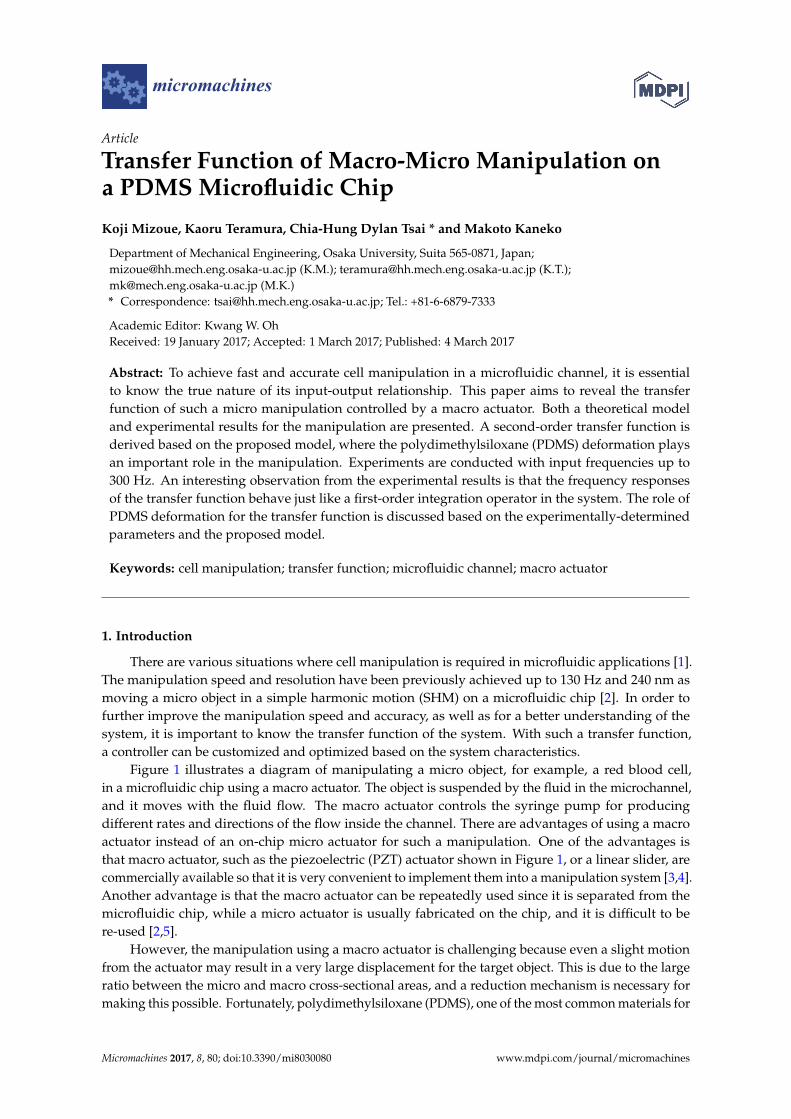
Figure 1 illustrates a diagram of manipulating a micro object, for example, a red blood cell,in a microfluidic chip using a macro actuator. The object is suspended by the fluid in the microchannel,and it moves with the fluid flow. The macro actuator controls the syringe pump for producingdifferent rates and directions of the flow inside the channel. There are advantages of using a macroactuator instead of an on-chip micro actuator for such a manipulation. One of the advantages isthat macro actuator, such as the piezoelectric (PZT) actuator shown in Figure 1, or a linear slider, arecommercially available so that it is very convenient to implement them into a manipulation system [3,4].Another advantage is that the macro actuator can be repeatedly used since it is separated from themicrofluidic chip, while a micro actuator is usually fabricated on the chip, and it is difficult to bere-used [2,5].

However, the manipulation using a macro actuator is challenging because even a slight motionfrom the actuator may result in a very large displacement for the target object. This is due to the largeratio between the micro and macro cross-sectional areas, and a reduction mechanism is necessary formaking this possible. Fortunately, polydimethylsiloxane (PDMS), one of the most common materials for

Micromachines 2017, 8, 80; doi:10.3390/mi8030080 www.mdpi.com/journal/micromachines

Micromachines 2017, 8, 80 2 of 12

making a microfluidic system, is embedded with a natural reduction mechanism from its deformablecharacteristic [6].

Micromachines 2017, 8, 80 2 of 12

for making a microfluidic system, is embedded with a natural reduction mechanism from its deformable characteristic [6].

Figure 1. An illustrative diagram demonstrates how cell manipulation is controlled by a macro actuator outside the microfluidic chip.

The transfer function and its frequency responses are experimentally investigated in this work. An open-loop control system is employed for determining the transfer function of the system. Different frequencies of sinusoidal inputs are applied to the PZT actuator as the inputs of the transfer function, while the motions of micro-objects are tracked as the outputs. The maximum frequency of the input signal is up to 300 Hz SHM, which is more than double that of previous works [2,7]. The gains and phase at different frequencies are determined using a fast Fourier transform (FFT). It is found that the system response is very similar to an integration operator that the gain is linearly decreased in Bode plots while the phase is constantly around −90°. The experimental results are applied back to the derived model and a very well fit is obtained. Finally, the system parameters are identified and discussed.

In summary, we focus on directly identifying the transfer function from the experimental inputs and outputs. A mechanical model of the system is proposed, and the experimental results are discussed with the model. The rest of this paper is organized as follows. After briefly reviewing the related works in Section 2, a mechanical model for the macro-micro manipulation system is proposed in Section 3. The experimental method and results are presented in Sections 4 and 5. The results are discussed in Section 6. Finally, concluding remarks are summarized in Section 7.

2. Related Works

Various approaches have been developed for cell manipulation, for example, using flow control in a microfluidic channel [2,6,8,9], optical tweezers [10,11], micro grippers [12–15], electrical or magnetic force [16], and acoustic trapping [17–19]. The combination of a high-speed pump and a high-speed vision is often used together for high-speed manipulation in a microfluidic channel. For example, Chen et al. performed high-speed cell sorting of single bacterial cells by a PZT pumping [20]. The manipulation is especially important for active cell assessments. For example, Monzawa et al. introduced an actuation transmitter for cell manipulation and evaluation [2]. Sakuma et al. applied a fatigue test to human red blood cells by imparting periodical mechanical stress [8]. Murakami et al. investigated the shape recovery of a cell by controlling different loading time in a constriction [21]. The throughput and stability of such active assessments directly depend on the manipulation speed and resolution. While the frequency characteristics under such closed-loop manipulation systems were previously discussed [2,6], the open-loop transfer function is important to know for designing a faster and more accurate cell manipulation system. To the best of our knowledge, there have been no works discussing the transfer function of the open-loop PDMS microfluidic channel, and this is the first work that exploits the true nature of the macro-micro manipulation on a PDMS chip.

3. Modeling of Transfer Function with a PDMS Microfluidic Channel

Figure 2 shows the model of the cell manipulation system where 𝑥𝑥1 and 𝑥𝑥2 are the input, the PZT actuator motion, and the output, the micro object motion of the system. 𝑀𝑀, 𝑘𝑘, c,𝐴𝐴𝑐𝑐, and 𝑥𝑥𝑐𝑐 are the equivalent mass, stiffness, damping, cross-sectional area, and displacement of a virtual element

Figure 1. An illustrative diagram demonstrates how cell manipulation is controlled by a macro actuatoroutside the microfluidic chip.

The transfer function and its frequency responses are experimentally investigated in this work.An open-loop control system is employed for determining the transfer function of the system.Different frequencies of sinusoidal inputs are applied to the PZT actuator as the inputs of the transferfunction, while the motions of micro-objects are tracked as the outputs. The maximum frequency of theinput signal is up to 300 Hz SHM, which is more than double that of previous works [2,7]. The gainsand phase at different frequencies are determined using a fast Fourier transform (FFT). It is found thatthe system response is very similar to an integration operator that the gain is linearly decreased in Bodeplots while the phase is constantly around−90◦. The experimental results are applied back to the derivedmodel and a very well fit is obtained. Finally, the system parameters are identified and discussed.

In summary, we focus on directly identifying the transfer function from the experimental inputsand outputs. A mechanical model of the system is proposed, and the experimental results are discussedwith the model. The rest of this paper is organized as follows. After briefly reviewing the related worksin Section 2, a mechanical model for the macro-micro manipulation system is proposed in Section 3.The experimental method and results are presented in Sections 4 and 5. The results are discussed inSection 6. Finally, concluding remarks are summarized in Section 7.

2. Related Works

Various approaches have been developed for cell manipulation, for example, using flow control ina microfluidic channel [2,6,8,9], optical tweezers [10,11], micro grippers [12–15], electrical or magneticforce [16], and acoustic trapping [17–19]. The combination of a high-speed pump and a high-speedvision is often used together for high-speed manipulation in a microfluidic channel. For example,Chen et al. performed high-speed cell sorting of single bacterial cells by a PZT pumping [20].The manipulation is especially important for active cell assessments. For example, Monzawa et al.introduced an actuation transmitter for cell manipulation and evaluation [2]. Sakuma et al. applieda fatigue test to human red blood cells by imparting periodical mechanical stress [8]. Murakami et al.investigated the shape recovery of a cell by controlling different loading time in a constriction [21].The throughput and stability of such active assessments directly depend on the manipulation speedand resolution. While the frequency characteristics under such closed-loop manipulation systems werepreviously discussed [2,6], the open-loop transfer function is important to know for designing a fasterand more accurate cell manipulation system. To the best of our knowledge, there have been no worksdiscussing the transfer function of the open-loop PDMS microfluidic channel, and this is the first workthat exploits the true nature of the macro-micro manipulation on a PDMS chip.

3. Modeling of Transfer Function with a PDMS Microfluidic Channel

Figure 2 shows the model of the cell manipulation system where x1 and x2 are the input, the PZTactuator motion, and the output, the micro object motion of the system. M, k, c, Ac, and xc are the

Micromachines 2017, 8, 80 3 of 12

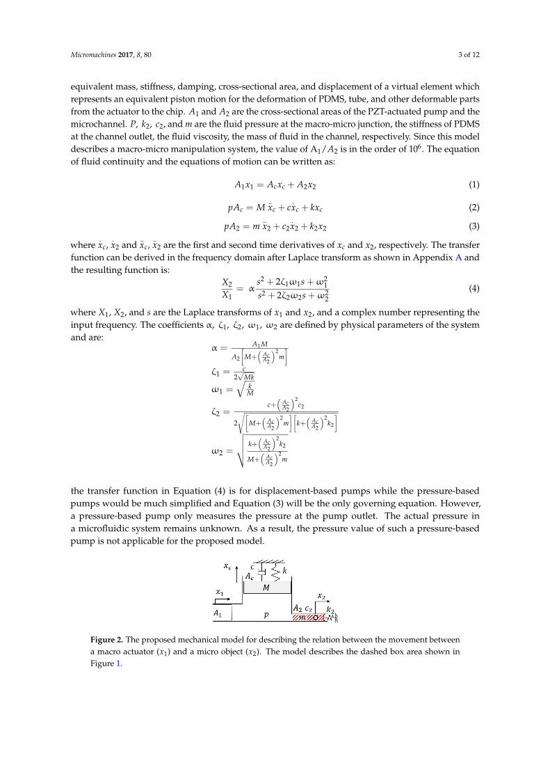
equivalent mass, stiffness, damping, cross-sectional area, and displacement of a virtual element whichrepresents an equivalent piston motion for the deformation of PDMS, tube, and other deformable partsfrom the actuator to the chip. A1 and A2 are the cross-sectional areas of the PZT-actuated pump and themicrochannel. P, k2, c2, and m are the fluid pressure at the macro-micro junction, the stiffness of PDMSat the channel outlet, the fluid viscosity, the mass of fluid in the channel, respectively. Since this modeldescribes a macro-micro manipulation system, the value of A1/A2 is in the order of 106. The equationof fluid continuity and the equations of motion can be written as:

A1x1 = Acxc + A2x2 (1)

pAc = M..xc + c

.xc + kxc (2)

pA2 = m..x2 + c2

.x2 + k2x2 (3)

where.xc,

.x2 and

..xc,

..x2 are the first and second time derivatives of xc and x2, respectively. The transfer

function can be derived in the frequency domain after Laplace transform as shown in Appendix A andthe resulting function is:

X2

X1= α

s2 + 2ζ1ω1s +ω21

s2 + 2ζ2ω2s +ω22

(4)

where X1, X2, and s are the Laplace transforms of x1 and x2, and a complex number representing theinput frequency. The coefficients α, ζ1, ζ2, ω1, ω2 are defined by physical parameters of the systemand are:

α = A1 M

A2

[M+

(AcA2

)2m]

ζ1 = c2√

Mk

ω1 =√

kM

ζ2 =c+(

AcA2

)2c2

2

√[M+

(AcA2

)2m][

k+(

AcA2

)2k2

]

ω2 =

√√√√ k+(

AcA2

)2k2

M+(

AcA2

)2m

the transfer function in Equation (4) is for displacement-based pumps while the pressure-basedpumps would be much simplified and Equation (3) will be the only governing equation. However,a pressure-based pump only measures the pressure at the pump outlet. The actual pressure ina microfluidic system remains unknown. As a result, the pressure value of such a pressure-basedpump is not applicable for the proposed model.

Micromachines 2017, 8, 80 3 of 12

which represents an equivalent piston motion for the deformation of PDMS, tube, and other deformable parts from the actuator to the chip. 𝐴𝐴1 and 𝐴𝐴2 are the cross-sectional areas of the PZT-actuated pump and the microchannel. 𝑃𝑃, 𝑘𝑘2, 𝑐𝑐2, and 𝑚𝑚 are the fluid pressure at the macro-micro junction, the stiffness of PDMS at the channel outlet, the fluid viscosity, the mass of fluid in the channel, respectively. Since this model describes a macro-micro manipulation system, the value of A1/𝐴𝐴2 is in the order of 106. The equation of fluid continuity and the equations of motion can be written as:

𝐴𝐴1𝑥𝑥1 = 𝐴𝐴𝑐𝑐𝑥𝑥𝑐𝑐 + 𝐴𝐴2𝑥𝑥2 (1)

𝑝𝑝𝐴𝐴𝑐𝑐 = 𝑀𝑀 �̈�𝑥𝑐𝑐 + 𝑐𝑐�̇�𝑥𝑐𝑐 + 𝑘𝑘𝑥𝑥𝑐𝑐 (2)

𝑝𝑝𝐴𝐴2 = 𝑚𝑚 �̈�𝑥2 + 𝑐𝑐2�̇�𝑥2 + 𝑘𝑘2𝑥𝑥2 (3)

where �̇�𝑥𝑐𝑐, �̇�𝑥2 and �̈�𝑥𝑐𝑐, �̈�𝑥2 are the first and second time derivatives of 𝑥𝑥𝑐𝑐 and 𝑥𝑥2, respectively. The transfer function can be derived in the frequency domain after Laplace transform as shown in Appendix A and the resulting function is:

𝑋𝑋2𝑋𝑋1

= α𝑠𝑠2 + 2ζ1ω1𝑠𝑠 + ω1

2

𝑠𝑠2 + 2ζ2ω2𝑠𝑠 + ω22 (4)

where 𝑋𝑋1, 𝑋𝑋2, and 𝑠𝑠 are the Laplace transforms of 𝑥𝑥1 and 𝑥𝑥2, and a complex number representing the input frequency. The coefficients α, ζ1, ζ2,ω1,ω2 are defined by physical parameters of the system and are:

α =𝐴𝐴1𝑀𝑀

𝐴𝐴2 �𝑀𝑀 + �𝐴𝐴𝑐𝑐𝐴𝐴2�2𝑚𝑚�

ζ1 =𝑐𝑐

2√𝑀𝑀𝑘𝑘

ω1 = �𝑘𝑘𝑀𝑀

ζ2 =𝑐𝑐 + �𝐴𝐴𝑐𝑐𝐴𝐴2

�2𝑐𝑐2

2��𝑀𝑀 + �𝐴𝐴𝑐𝑐𝐴𝐴2�2𝑚𝑚� �𝑘𝑘 + �𝐴𝐴𝑐𝑐𝐴𝐴2

�2𝑘𝑘2�

ω2 = �𝑘𝑘 + �𝐴𝐴𝑐𝑐𝐴𝐴2

�2𝑘𝑘2

𝑀𝑀 + �𝐴𝐴𝑐𝑐𝐴𝐴2�2𝑚𝑚

the transfer function in Equation (4) is for displacement-based pumps while the pressure-based pumps would be much simplified and Equation (3) will be the only governing equation. However, a pressure-based pump only measures the pressure at the pump outlet. The actual pressure in a microfluidic system remains unknown. As a result, the pressure value of such a pressure-based pump is not applicable for the proposed model.

Figure 2. The proposed mechanical model for describing the relation between the movement between a macro actuator (𝑥𝑥1) and a micro object (𝑥𝑥2). The model describes the dashed box area shown in Figure 1. Figure 2. The proposed mechanical model for describing the relation between the movement betweena macro actuator (x1) and a micro object (x2). The model describes the dashed box area shown inFigure 1.

Micromachines 2017, 8, 80 4 of 12

4. Experiments

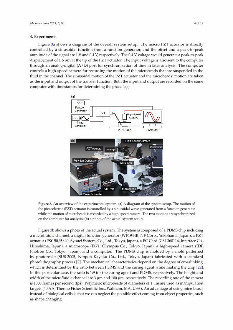
Figure 3a shows a diagram of the overall system setup. The macro PZT actuator is directlycontrolled by a sinusoidal function from a function generator, and the offset and a peak-to-peakamplitude of the signal are 1 V and 0.4 V, respectively. The 0.4 V voltage would generate a peak-to-peakdisplacement of 1.6 µm at the tip of the PZT actuator. The input voltage is also sent to the computerthrough an analog-digital (A/D) port for synchronization of time in later analysis. The computercontrols a high-speed camera for recording the motion of the microbeads that are suspended in thefluid in the channel. The sinusoidal motion of the PZT actuator and the microbeads’ motion are takenas the input and output of the transfer function. Both the input and output are recorded on the samecomputer with timestamps for determining the phase lag.

Micromachines 2017, 8, 80 4 of 12

4. Experiments

Figure 3a shows a diagram of the overall system setup. The macro PZT actuator is directly controlled by a sinusoidal function from a function generator, and the offset and a peak-to-peak amplitude of the signal are 1 V and 0.4 V, respectively. The 0.4 V voltage would generate a peak-to-peak displacement of 1.6 µm at the tip of the PZT actuator. The input voltage is also sent to the computer through an analog-digital (A/D) port for synchronization of time in later analysis. The computer controls a high-speed camera for recording the motion of the microbeads that are suspended in the fluid in the channel. The sinusoidal motion of the PZT actuator and the microbeads’ motion are taken as the input and output of the transfer function. Both the input and output are recorded on the same computer with timestamps for determining the phase lag.

Figure 3. An overview of the experimental system. (a) A diagram of the system setup. The motion of the piezoelectric (PZT) actuator is controlled by a sinusoidal wave generated from a function generator while the motion of microbeads is recorded by a high-speed camera. The two motions are synchronized on the computer for analysis; (b) a photo of the actual system setup.

Figure 3b shows a photo of the actual system. The system is composed of a PDMS chip including a microfluidic channel, a digital function generator (WF1944B, NF Corp., Yokohama, Japan), a PZT actuator (PSt150/5/40, Syouei System, Co., Ltd., Tokyo, Japan), a PC Card (CSI-360116, Interface Co., Hiroshima, Japan), a microscope (IX71, Olympus Co., Tokyo, Japan), a high-speed camera (IDP, Photron Co., Tokyo, Japan), and a computer. The PDMS chip is molded by a mold patterned by photoresist (SU8-3005, Nippon Kayaku Co., Ltd., Tokyo, Japan) fabricated with a standard photolithography process [2]. The mechanical characteristics depend on the degree of crosslinking, which is determined by the ratio between PDMS and the curing agent while making the chip [22]. In this particular case, the ratio is 1:9 for the curing agent and PDMS, respectively. The height and width of the microfluidic channel are 3 µm and 100 µm, respectively. The recording rate of the camera is 1000 frames per second (fps). Polymeric microbeads of diameters of 1 µm are used as manipulation targets (4009A, Thermo Fisher Scientific Inc., Waltham, MA, USA). An advantage of using microbeads instead of biological cells is that we can neglect the possible effect coming from object properties, such as shape changing.

Figure 3. An overview of the experimental system. (a) A diagram of the system setup. The motion ofthe piezoelectric (PZT) actuator is controlled by a sinusoidal wave generated from a function generatorwhile the motion of microbeads is recorded by a high-speed camera. The two motions are synchronizedon the computer for analysis; (b) a photo of the actual system setup.

Figure 3b shows a photo of the actual system. The system is composed of a PDMS chip includinga microfluidic channel, a digital function generator (WF1944B, NF Corp., Yokohama, Japan), a PZTactuator (PSt150/5/40, Syouei System, Co., Ltd., Tokyo, Japan), a PC Card (CSI-360116, Interface Co.,Hiroshima, Japan), a microscope (IX71, Olympus Co., Tokyo, Japan), a high-speed camera (IDP,Photron Co., Tokyo, Japan), and a computer. The PDMS chip is molded by a mold patternedby photoresist (SU8-3005, Nippon Kayaku Co., Ltd., Tokyo, Japan) fabricated with a standardphotolithography process [2]. The mechanical characteristics depend on the degree of crosslinking,which is determined by the ratio between PDMS and the curing agent while making the chip [22].In this particular case, the ratio is 1:9 for the curing agent and PDMS, respectively. The height andwidth of the microfluidic channel are 3 µm and 100 µm, respectively. The recording rate of the camerais 1000 frames per second (fps). Polymeric microbeads of diameters of 1 µm are used as manipulationtargets (4009A, Thermo Fisher Scientific Inc., Waltham, MA, USA). An advantage of using microbeadsinstead of biological cells is that we can neglect the possible effect coming from object properties, suchas shape changing.

Micromachines 2017, 8, 80 5 of 12

5. Results

5.1. Input-Output Relation

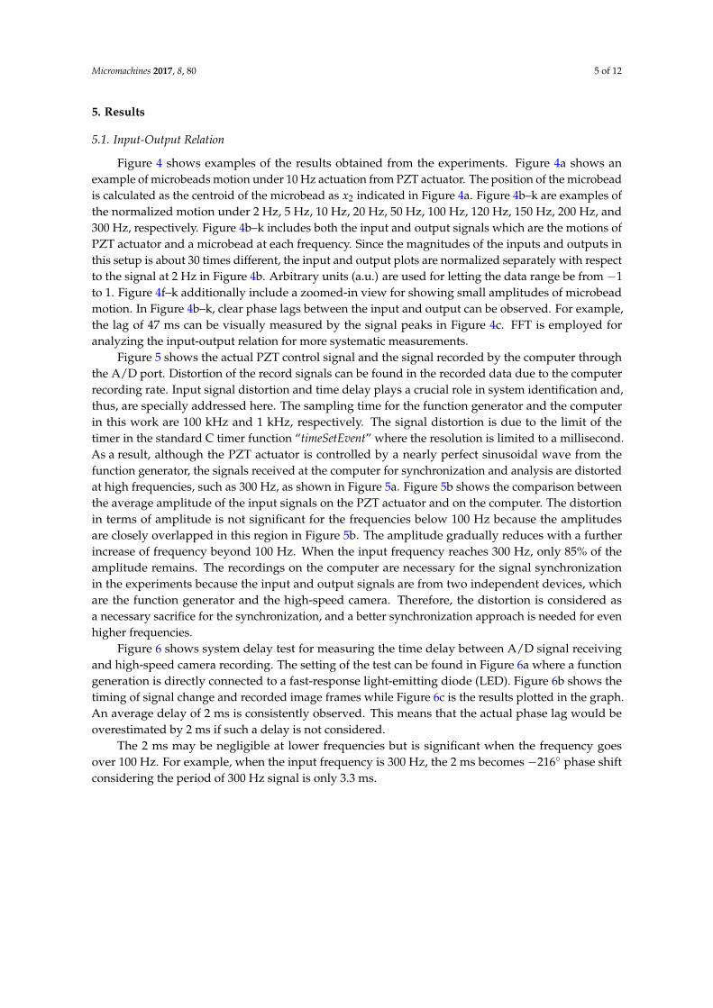
Figure 4 shows examples of the results obtained from the experiments. Figure 4a shows anexample of microbeads motion under 10 Hz actuation from PZT actuator. The position of the microbeadis calculated as the centroid of the microbead as x2 indicated in Figure 4a. Figure 4b–k are examples ofthe normalized motion under 2 Hz, 5 Hz, 10 Hz, 20 Hz, 50 Hz, 100 Hz, 120 Hz, 150 Hz, 200 Hz, and300 Hz, respectively. Figure 4b–k includes both the input and output signals which are the motions ofPZT actuator and a microbead at each frequency. Since the magnitudes of the inputs and outputs inthis setup is about 30 times different, the input and output plots are normalized separately with respectto the signal at 2 Hz in Figure 4b. Arbitrary units (a.u.) are used for letting the data range be from −1to 1. Figure 4f–k additionally include a zoomed-in view for showing small amplitudes of microbeadmotion. In Figure 4b–k, clear phase lags between the input and output can be observed. For example,the lag of 47 ms can be visually measured by the signal peaks in Figure 4c. FFT is employed foranalyzing the input-output relation for more systematic measurements.

Figure 5 shows the actual PZT control signal and the signal recorded by the computer throughthe A/D port. Distortion of the record signals can be found in the recorded data due to the computerrecording rate. Input signal distortion and time delay plays a crucial role in system identification and,thus, are specially addressed here. The sampling time for the function generator and the computerin this work are 100 kHz and 1 kHz, respectively. The signal distortion is due to the limit of thetimer in the standard C timer function “timeSetEvent” where the resolution is limited to a millisecond.As a result, although the PZT actuator is controlled by a nearly perfect sinusoidal wave from thefunction generator, the signals received at the computer for synchronization and analysis are distortedat high frequencies, such as 300 Hz, as shown in Figure 5a. Figure 5b shows the comparison betweenthe average amplitude of the input signals on the PZT actuator and on the computer. The distortionin terms of amplitude is not significant for the frequencies below 100 Hz because the amplitudesare closely overlapped in this region in Figure 5b. The amplitude gradually reduces with a furtherincrease of frequency beyond 100 Hz. When the input frequency reaches 300 Hz, only 85% of theamplitude remains. The recordings on the computer are necessary for the signal synchronizationin the experiments because the input and output signals are from two independent devices, whichare the function generator and the high-speed camera. Therefore, the distortion is considered asa necessary sacrifice for the synchronization, and a better synchronization approach is needed for evenhigher frequencies.

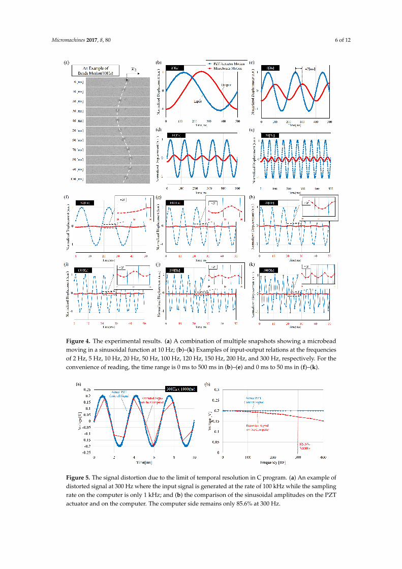
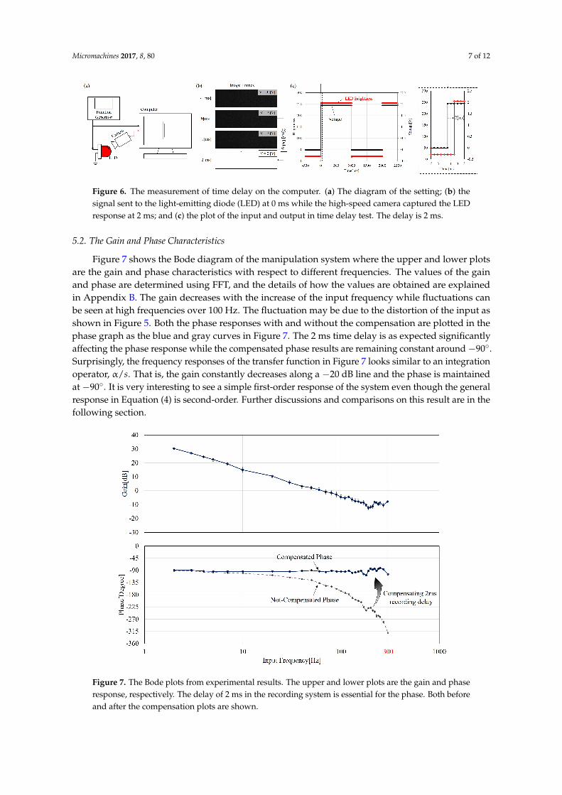
Figure 6 shows system delay test for measuring the time delay between A/D signal receivingand high-speed camera recording. The setting of the test can be found in Figure 6a where a functiongeneration is directly connected to a fast-response light-emitting diode (LED). Figure 6b shows thetiming of signal change and recorded image frames while Figure 6c is the results plotted in the graph.An average delay of 2 ms is consistently observed. This means that the actual phase lag would beoverestimated by 2 ms if such a delay is not considered.

The 2 ms may be negligible at lower frequencies but is significant when the frequency goesover 100 Hz. For example, when the input frequency is 300 Hz, the 2 ms becomes −216◦ phase shiftconsidering the period of 300 Hz signal is only 3.3 ms.

Micromachines 2017, 8, 80 6 of 12Micromachines 2017, 8, 80 6 of 12

Figure 4. The experimental results. (a) A combination of multiple snapshots showing a microbead moving in a sinusoidal function at 10 Hz; (b)–(k) Examples of input-output relations at the frequencies of 2 Hz, 5 Hz, 10 Hz, 20 Hz, 50 Hz, 100 Hz, 120 Hz, 150 Hz, 200 Hz, and 300 Hz, respectively. For the convenience of reading, the time range is 0 ms to 500 ms in (b)–(e) and 0 ms to 50 ms in (f)–(k).

Figure 5. The signal distortion due to the limit of temporal resolution in C program. (a) An example of distorted signal at 300 Hz where the input signal is generated at the rate of 100 kHz while the sampling rate on the computer is only 1 kHz; and (b) the comparison of the sinusoidal amplitudes on the PZT actuator and on the computer. The computer side remains only 85.6% at 300 Hz.

Figure 4. The experimental results. (a) A combination of multiple snapshots showing a microbeadmoving in a sinusoidal function at 10 Hz; (b)–(k) Examples of input-output relations at the frequenciesof 2 Hz, 5 Hz, 10 Hz, 20 Hz, 50 Hz, 100 Hz, 120 Hz, 150 Hz, 200 Hz, and 300 Hz, respectively. For theconvenience of reading, the time range is 0 ms to 500 ms in (b)–(e) and 0 ms to 50 ms in (f)–(k).

Micromachines 2017, 8, 80 6 of 12

Figure 4. The experimental results. (a) A combination of multiple snapshots showing a microbead moving in a sinusoidal function at 10 Hz; (b)–(k) Examples of input-output relations at the frequencies of 2 Hz, 5 Hz, 10 Hz, 20 Hz, 50 Hz, 100 Hz, 120 Hz, 150 Hz, 200 Hz, and 300 Hz, respectively. For the convenience of reading, the time range is 0 ms to 500 ms in (b)–(e) and 0 ms to 50 ms in (f)–(k).

Figure 5. The signal distortion due to the limit of temporal resolution in C program. (a) An example of distorted signal at 300 Hz where the input signal is generated at the rate of 100 kHz while the sampling rate on the computer is only 1 kHz; and (b) the comparison of the sinusoidal amplitudes on the PZT actuator and on the computer. The computer side remains only 85.6% at 300 Hz.

Figure 5. The signal distortion due to the limit of temporal resolution in C program. (a) An example ofdistorted signal at 300 Hz where the input signal is generated at the rate of 100 kHz while the samplingrate on the computer is only 1 kHz; and (b) the comparison of the sinusoidal amplitudes on the PZTactuator and on the computer. The computer side remains only 85.6% at 300 Hz.

Micromachines 2017, 8, 80 7 of 12Micromachines 2017, 8, 80 7 of 12

Figure 6. The measurement of time delay on the computer. (a) The diagram of the setting; (b) the signal sent to the light-emitting diode (LED) at 0 ms while the high-speed camera captured the LED response at 2 ms; and (c) the plot of the input and output in time delay test. The delay is 2 ms.

5.2. The Gain and Phase Characteristics

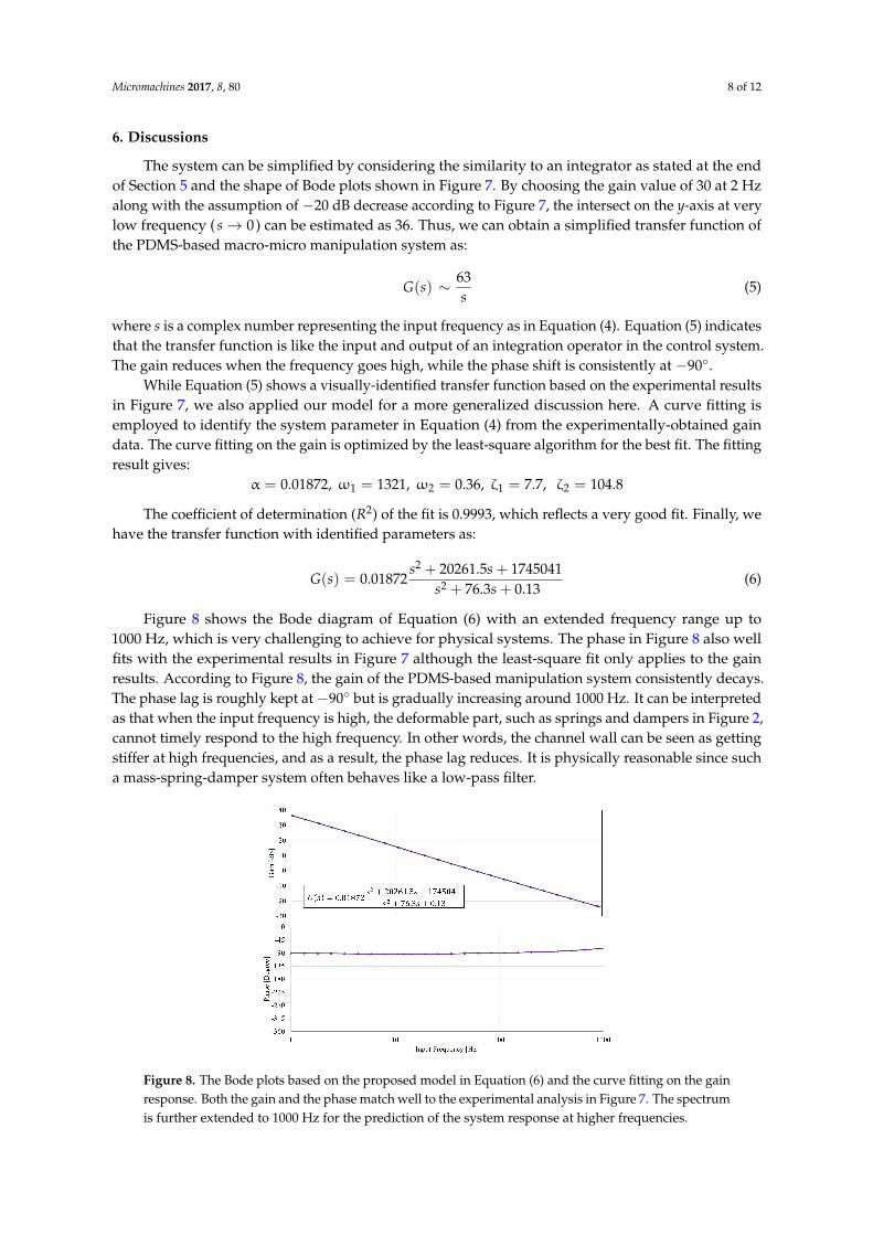
Figure 7 shows the Bode diagram of the manipulation system where the upper and lower plots are the gain and phase characteristics with respect to different frequencies. The values of the gain and phase are determined using FFT, and the details of how the values are obtained are explained in Appendix B. The gain decreases with the increase of the input frequency while fluctuations can be seen at high frequencies over 100 Hz. The fluctuation may be due to the distortion of the input as shown in Figure 5. Both the phase responses with and without the compensation are plotted in the phase graph as the blue and gray curves in Figure 7. The 2 ms time delay is as expected significantly affecting the phase response while the compensated phase results are remaining constant around −90°. Surprisingly, the frequency responses of the transfer function in Figure 7 looks similar to an integration operator, α/𝑠𝑠. That is, the gain constantly decreases along a −20 dB line and the phase is maintained at −90°. It is very interesting to see a simple first-order response of the system even though the general response in Equation (4) is second-order. Further discussions and comparisons on this result are in the following section.

Figure 7. The Bode plots from experimental results. The upper and lower plots are the gain and phase response, respectively. The delay of 2 ms in the recording system is essential for the phase. Both before and after the compensation plots are shown.

Figure 6. The measurement of time delay on the computer. (a) The diagram of the setting; (b) thesignal sent to the light-emitting diode (LED) at 0 ms while the high-speed camera captured the LEDresponse at 2 ms; and (c) the plot of the input and output in time delay test. The delay is 2 ms.

5.2. The Gain and Phase Characteristics

Figure 7 shows the Bode diagram of the manipulation system where the upper and lower plotsare the gain and phase characteristics with respect to different frequencies. The values of the gainand phase are determined using FFT, and the details of how the values are obtained are explainedin Appendix B. The gain decreases with the increase of the input frequency while fluctuations canbe seen at high frequencies over 100 Hz. The fluctuation may be due to the distortion of the input asshown in Figure 5. Both the phase responses with and without the compensation are plotted in thephase graph as the blue and gray curves in Figure 7. The 2 ms time delay is as expected significantlyaffecting the phase response while the compensated phase results are remaining constant around −90◦.Surprisingly, the frequency responses of the transfer function in Figure 7 looks similar to an integrationoperator, α/s. That is, the gain constantly decreases along a −20 dB line and the phase is maintainedat −90◦. It is very interesting to see a simple first-order response of the system even though the generalresponse in Equation (4) is second-order. Further discussions and comparisons on this result are in thefollowing section.

Micromachines 2017, 8, 80 7 of 12

Figure 6. The measurement of time delay on the computer. (a) The diagram of the setting; (b) the signal sent to the light-emitting diode (LED) at 0 ms while the high-speed camera captured the LED response at 2 ms; and (c) the plot of the input and output in time delay test. The delay is 2 ms.

5.2. The Gain and Phase Characteristics

Figure 7 shows the Bode diagram of the manipulation system where the upper and lower plots are the gain and phase characteristics with respect to different frequencies. The values of the gain and phase are determined using FFT, and the details of how the values are obtained are explained in Appendix B. The gain decreases with the increase of the input frequency while fluctuations can be seen at high frequencies over 100 Hz. The fluctuation may be due to the distortion of the input as shown in Figure 5. Both the phase responses with and without the compensation are plotted in the phase graph as the blue and gray curves in Figure 7. The 2 ms time delay is as expected significantly affecting the phase response while the compensated phase results are remaining constant around −90°. Surprisingly, the frequency responses of the transfer function in Figure 7 looks similar to an integration operator, α/𝑠𝑠. That is, the gain constantly decreases along a −20 dB line and the phase is maintained at −90°. It is very interesting to see a simple first-order response of the system even though the general response in Equation (4) is second-order. Further discussions and comparisons on this result are in the following section.

Figure 7. The Bode plots from experimental results. The upper and lower plots are the gain and phase response, respectively. The delay of 2 ms in the recording system is essential for the phase. Both before and after the compensation plots are shown.

Figure 7. The Bode plots from experimental results. The upper and lower plots are the gain and phaseresponse, respectively. The delay of 2 ms in the recording system is essential for the phase. Both beforeand after the compensation plots are shown.

Micromachines 2017, 8, 80 8 of 12

6. Discussions

The system can be simplified by considering the similarity to an integrator as stated at the endof Section 5 and the shape of Bode plots shown in Figure 7. By choosing the gain value of 30 at 2 Hzalong with the assumption of −20 dB decrease according to Figure 7, the intersect on the y-axis at verylow frequency ( s→ 0) can be estimated as 36. Thus, we can obtain a simplified transfer function ofthe PDMS-based macro-micro manipulation system as:

G(s) ∼ 63s

(5)

where s is a complex number representing the input frequency as in Equation (4). Equation (5) indicatesthat the transfer function is like the input and output of an integration operator in the control system.The gain reduces when the frequency goes high, while the phase shift is consistently at −90◦.

While Equation (5) shows a visually-identified transfer function based on the experimental resultsin Figure 7, we also applied our model for a more generalized discussion here. A curve fitting isemployed to identify the system parameter in Equation (4) from the experimentally-obtained gaindata. The curve fitting on the gain is optimized by the least-square algorithm for the best fit. The fittingresult gives:

α = 0.01872, ω1 = 1321, ω2 = 0.36, ζ1 = 7.7, ζ2 = 104.8

The coefficient of determination (R2) of the fit is 0.9993, which reflects a very good fit. Finally, wehave the transfer function with identified parameters as:

G(s) = 0.01872s2 + 20261.5s + 1745041

s2 + 76.3s + 0.13(6)

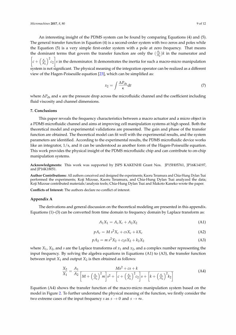
Figure 8 shows the Bode diagram of Equation (6) with an extended frequency range up to1000 Hz, which is very challenging to achieve for physical systems. The phase in Figure 8 also wellfits with the experimental results in Figure 7 although the least-square fit only applies to the gainresults. According to Figure 8, the gain of the PDMS-based manipulation system consistently decays.The phase lag is roughly kept at −90◦ but is gradually increasing around 1000 Hz. It can be interpretedas that when the input frequency is high, the deformable part, such as springs and dampers in Figure 2,cannot timely respond to the high frequency. In other words, the channel wall can be seen as gettingstiffer at high frequencies, and as a result, the phase lag reduces. It is physically reasonable since sucha mass-spring-damper system often behaves like a low-pass filter.

Micromachines 2017, 8, 80 8 of 12

6. Discussions

The system can be simplified by considering the similarity to an integrator as stated at the end of Section 5 and the shape of Bode plots shown in Figure 7. By choosing the gain value of 30 at 2 Hz along with the assumption of −20 dB decrease according to Figure 7, the intersect on the y-axis at very low frequency (𝑠𝑠 → 0) can be estimated as 36. Thus, we can obtain a simplified transfer function of the PDMS-based macro-micro manipulation system as:

𝐺𝐺(𝑠𝑠)~63𝑠𝑠

(5)

where 𝑠𝑠 is a complex number representing the input frequency as in Equation (4). Equation (5) indicates that the transfer function is like the input and output of an integration operator in the control system. The gain reduces when the frequency goes high, while the phase shift is consistently at −90°.

While Equation (5) shows a visually-identified transfer function based on the experimental results in Figure 7, we also applied our model for a more generalized discussion here. A curve fitting is employed to identify the system parameter in Equation (4) from the experimentally-obtained gain data. The curve fitting on the gain is optimized by the least-square algorithm for the best fit. The fitting result gives:

α = 0.01872,ω1 = 1321,ω2 = 0.36, ζ1 = 7.7, ζ2 = 104.8

The coefficient of determination (𝑅𝑅2) of the fit is 0.9993, which reflects a very good fit. Finally, we have the transfer function with identified parameters as:

𝐺𝐺(𝑠𝑠) = 0.01872𝑠𝑠2 + 20261.5𝑠𝑠 + 1745041

𝑠𝑠2 + 76.3𝑠𝑠 + 0.13 (6)

Figure 8 shows the Bode diagram of Equation (6) with an extended frequency range up to 1000 Hz, which is very challenging to achieve for physical systems. The phase in Figure 8 also well fits with the experimental results in Figure 7 although the least-square fit only applies to the gain results. According to Figure 8, the gain of the PDMS-based manipulation system consistently decays. The phase lag is roughly kept at −90° but is gradually increasing around 1000 Hz. It can be interpreted as that when the input frequency is high, the deformable part, such as springs and dampers in Figure 2, cannot timely respond to the high frequency. In other words, the channel wall can be seen as getting stiffer at high frequencies, and as a result, the phase lag reduces. It is physically reasonable since such a mass-spring-damper system often behaves like a low-pass filter.

Figure 8. The Bode plots based on the proposed model in Equation (6) and the curve fitting on the gain response. Both the gain and the phase match well to the experimental analysis in Figure 7. The spectrum is further extended to 1000 Hz for the prediction of the system response at higher frequencies.

Figure 8. The Bode plots based on the proposed model in Equation (6) and the curve fitting on the gainresponse. Both the gain and the phase match well to the experimental analysis in Figure 7. The spectrumis further extended to 1000 Hz for the prediction of the system response at higher frequencies.

Micromachines 2017, 8, 80 9 of 12

An interesting insight of the PDMS system can be found by comparing Equations (4) and (5).The general transfer function in Equation (4) is a second-order system with two zeros and poles whilethe Equation (5) is a very simple first-order system with a pole at zero frequency. That meansthe dominant terms that govern the transfer function are only the ( A1

A2)k in the numerator and[

c +(

AcA2

)2c2

]s in the denominator. It demonstrates the inertia for such a macro-micro manipulation

system is not significant. The physical meaning of the integration operator can be realized as a differentview of the Hagen-Poiseuille equation [23], which can be simplified as:

x2 =∫ ∆Pch

κdt (7)

where ∆Pch and κ are the pressure drop across the microfluidic channel and the coefficient includingfluid viscosity and channel dimensions.

7. Conclusions

This paper reveals the frequency characteristics between a macro actuator and a micro object ina PDMS microfluidic channel and aims at improving cell manipulation systems at high speed. Both thetheoretical model and experimental validations are presented. The gain and phase of the transferfunction are obtained. The theoretical model can fit well with the experimental results, and the systemparameters are identified. According to the experimental results, the PDMS microfluidic device workslike an integrator, 1/s, and it can be understood as another form of the Hagen-Poiseuille equation.This work provides the physical insight of the PDMS microfluidic chip and can contribute to on-chipmanipulation systems.

Acknowledgments: This work was supported by JSPS KAKENHI Grant Nos. JP15H05761, JP16K14197,and JP16K18051.

Author Contributions: All authors conceived and designed the experiments; Kaoru Teramura and Chia-Hung Dylan Tsaiperformed the experiments; Koji Mizoue, Kaoru Teramura, and Chia-Hung Dylan Tsai analyzed the data;Koji Mizoue contributed materials/analysis tools; Chia-Hung Dylan Tsai and Makoto Kaneko wrote the paper.

Conflicts of Interest: The authors declare no conflict of interest.

Appendix A

The derivations and general discussion on the theoretical modeling are presented in this appendix.Equations (1)–(3) can be converted from time domain to frequency domain by Laplace transform as:

A1X1 = AcXc + A2X2 (A1)

pAc = M s2Xc + csXc + kXc (A2)

pA2 = m s2X2 + c2sX2 + k2X2 (A3)

where X1, X2, and s are the Laplace transforms of x1 and x2, and a complex number representing theinput frequency. By solving the algebra equations in Equations (A1) to (A3), the transfer functionbetween input X1 and output X2 is then obtained as follows:

X2

X1=

A1

A2

Ms2 + cs + k[M +

(AcA2

)2m]

s2 +

[c +

(AcA2

)2c2

]s +

[k +

(AcA2

)2k2

] (A4)

Equation (A4) shows the transfer function of the macro-micro manipulation system based on themodel in Figure 2. To further understand the physical meaning of the function, we firstly consider thetwo extreme cases of the input frequency s as s→ 0 and s→ ∞ .

Micromachines 2017, 8, 80 10 of 12

When s→ 0 , Equation (A4) becomes:

X2

X1=

A1

A2

k[k +

(AcA2

)2k2

] (A5)

If we assume the outlet of the channel is opened to the atmosphere, which gives k2 = 0, thetransfer function becomes X2/X1 = A1/A2. It means the gain of the function only depends on thespatial ratio between the cross-sectional areas. It is physically reasonable, because the gain at thefrequency approaching to zero has nothing to do with temporal elements, such as the dampers inFigure 2, and the pushed in fluid would fully transform to the movement of the object. On the otherhand, if we assume the spring on the outlet k2 → ∞ , it means that the outlet is rigid and no fluid canbe pushed into the channel. As a result, the gain of the manipulation becomes X2/X1 = 0. That means,all the movement of the macro actuator would only result in the motion of PDMS chip deformation, xc.

When the input frequency is infinity s→ ∞ , the response becomes:

X2

X1=

A1

A2

M[M +

(AcA2

)2m] (A6)

In typical microfluidic modeling, the inertia of the fluid in the microchannel is neglected asm = 0 and, thus, the response also only depends on the ratio between the cross-sectional areas asx2/x1 = A1/A2. This result can be understood as that the PDMS walls as low-pass filters, and behavelike rigid walls when the frequency is very high. For a more general solution without assuming m = 0,a greater inertia m of the fluid in the channel would lead to a smaller gain.

Based on Equation (4), the zeros and poles of the transfer function are defined as:

Zeros:ω1(−ζ1 ±√ζ2

1 − 1) (A7)

Poles:ω2(−ζ2 ±√ζ2

2 − 1) (A8)

When the manipulation frequency hits the zeros, no motion of the micro object will be detectedsince the gain is zero as the numerator in Equation (4) equals zero. On the other hand, the gainwill be out of control if the manipulation frequency hits the poles, which makes the denominator ofEquation (4) zero. Equation (4) will later be used to perform the numerical fitting for determining theparameters from experimental results.

The response of a sinusoidal input can be calculated by letting s = jω, which gives:

G(jω) = α

(ω2

1 −ω2)+ j(2ζ1ω1ω)(ω2

2 −ω2)+ j(2ζ2ω2ω)

(A9)

The gain can then be derived as:

|G(jw)| = |α|∣∣(ω2

1 −ω2)+ j(2ζ1ω1ω)∣∣∣∣(ω2

2 −ω2)+ j(2ζ2ω2ω)

∣∣ = α

√ω4 + ((2ζ2

1ω1)2 − 2ω2

1)ω2 +ω4

1√ω4 + ((2ζ2

2ω2)2 − 2ω2

2)ω2 +ω4

2

(A10)

Appendix B

In order to obtain the frequency responses of the system, such as phase and gain, the experimentalresults, as the input and output signals are plugged into FFT for performing spectrum analysis. A seriesof complex values with respect to frequencies can be obtained after FFT. The gain and phase of themcan be calculated as their distance and angle from the origin on a complex coordinate. This appendix

Micromachines 2017, 8, 80 11 of 12

explains the step-by-step procedure of how the gain and phase is determined using an example of theresults at 10 Hz.

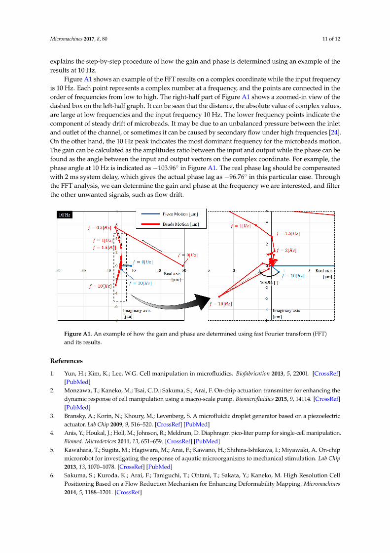
Figure A1 shows an example of the FFT results on a complex coordinate while the input frequencyis 10 Hz. Each point represents a complex number at a frequency, and the points are connected in theorder of frequencies from low to high. The right-half part of Figure A1 shows a zoomed-in view of thedashed box on the left-half graph. It can be seen that the distance, the absolute value of complex values,are large at low frequencies and the input frequency 10 Hz. The lower frequency points indicate thecomponent of steady drift of microbeads. It may be due to an unbalanced pressure between the inletand outlet of the channel, or sometimes it can be caused by secondary flow under high frequencies [24].On the other hand, the 10 Hz peak indicates the most dominant frequency for the microbeads motion.The gain can be calculated as the amplitudes ratio between the input and output while the phase can befound as the angle between the input and output vectors on the complex coordinate. For example, thephase angle at 10 Hz is indicated as −103.96◦ in Figure A1. The real phase lag should be compensatedwith 2 ms system delay, which gives the actual phase lag as −96.76◦ in this particular case. Throughthe FFT analysis, we can determine the gain and phase at the frequency we are interested, and filterthe other unwanted signals, such as flow drift.

Micromachines 2017, 8, 80 11 of 12

secondary flow under high frequencies [24]. On the other hand, the 10 Hz peak indicates the most dominant frequency for the microbeads motion. The gain can be calculated as the amplitudes ratio between the input and output while the phase can be found as the angle between the input and output vectors on the complex coordinate. For example, the phase angle at 10 Hz is indicated as −103.96° in Figure A1. The real phase lag should be compensated with 2 ms system delay, which gives the actual phase lag as −96.76° in this particular case. Through the FFT analysis, we can determine the gain and phase at the frequency we are interested, and filter the other unwanted signals, such as flow drift.

Figure A1. An example of how the gain and phase are determined using fast Fourier transform (FFT) and its results.

References

1. Yun, H.; Kim, K.; Lee, W.G. Cell manipulation in microfluidics. Biofabrication 2013, 5, 22001. 2. Monzawa, T.; Kaneko, M.; Tsai, C.D.; Sakuma, S.; Arai, F. On-chip actuation transmitter for enhancing the

dynamic response of cell manipulation using a macro-scale pump. Biomicrofluidics 2015, 9, 14114. 3. Bransky, A.; Korin, N.; Khoury, M.; Levenberg, S. A microfluidic droplet generator based on a piezoelectric

actuator. Lab Chip 2009, 9, 516–520. 4. Anis, Y.; Houkal, J.; Holl, M.; Johnson, R.; Meldrum, D. Diaphragm pico-liter pump for single-cell

manipulation. Biomed. Microdevices 2011, 13, 651–659. 5. Kawahara, T.; Sugita, M.; Hagiwara, M.; Arai, F.; Kawano, H.; Shihira-Ishikawa, I.; Miyawaki, A. On-chip

microrobot for investigating the response of aquatic microorganisms to mechanical stimulation. Lab Chip 2013, 13, 1070–1078.

6. Sakuma, S.; Kuroda, K.; Arai, F.; Taniguchi, T.; Ohtani, T.; Sakata, Y.; Kaneko, M. High Resolution Cell Positioning Based on a Flow Reduction Mechanism for Enhancing Deformability Mapping. Micromachines 2014, 5, 1188–1201.

7. Sakuma, S.; Kuroda, K. Realization of 240 nanometer resolution of cell positioning by a virtual flow reduction mechanism. In Proceedings of the 2014 IEEE 27th International Conference on Micro Electro Mechanical Systems (MEMS), San Francisco, CA, USA, 26–30 January 2014; pp. 1031–1034.

8. Sakuma, S.; Kuroda, K.; Tsai, C.D.; Fukui, W.; Arai, F.; Kaneko, M. Red blood cell fatigue evaluation based on the close-encountering point between extensibility and recoverability. Lab Chip 2014, 14, 1135–1141.

9. Mizoue, K.; Phan, M.; Tsai, C.-H.; Kaneko, M.; Kang, J.; Chung, W. Gravity-based precise cell manipulation system enhanced by in-phase mechanism. Micromachines 2016, 7, 116.

10. Ashkin, A.; Dziedzic, J.; Yamane, T. Optical trapping and manipulation of single cells using infrared laser beams. Nature 1987, 330, 769–771.

11. Hellmich, W.; Pelargus, C.; Leffhalm, K.; Ros, A.; Anselmetti, D. Single cell manipulation, analytics, and label-free protein detection in microfluidic devices for systems nanobiology. Electrophoresis 2005, 26, 3689–3696.

12. Chronis, N.; Lee, L.P. Electrothermally activated SU-8 microgripper for single cell manipulation in solution. J. Microelectromechanical Syst. 2005, 14, 857–863.

Figure A1. An example of how the gain and phase are determined using fast Fourier transform (FFT)and its results.

References

1. Yun, H.; Kim, K.; Lee, W.G. Cell manipulation in microfluidics. Biofabrication 2013, 5, 22001. [CrossRef][PubMed]

2. Monzawa, T.; Kaneko, M.; Tsai, C.D.; Sakuma, S.; Arai, F. On-chip actuation transmitter for enhancing thedynamic response of cell manipulation using a macro-scale pump. Biomicrofluidics 2015, 9, 14114. [CrossRef][PubMed]

3. Bransky, A.; Korin, N.; Khoury, M.; Levenberg, S. A microfluidic droplet generator based on a piezoelectricactuator. Lab Chip 2009, 9, 516–520. [CrossRef] [PubMed]

4. Anis, Y.; Houkal, J.; Holl, M.; Johnson, R.; Meldrum, D. Diaphragm pico-liter pump for single-cell manipulation.Biomed. Microdevices 2011, 13, 651–659. [CrossRef] [PubMed]

5. Kawahara, T.; Sugita, M.; Hagiwara, M.; Arai, F.; Kawano, H.; Shihira-Ishikawa, I.; Miyawaki, A. On-chipmicrorobot for investigating the response of aquatic microorganisms to mechanical stimulation. Lab Chip2013, 13, 1070–1078. [CrossRef] [PubMed]

6. Sakuma, S.; Kuroda, K.; Arai, F.; Taniguchi, T.; Ohtani, T.; Sakata, Y.; Kaneko, M. High Resolution CellPositioning Based on a Flow Reduction Mechanism for Enhancing Deformability Mapping. Micromachines2014, 5, 1188–1201. [CrossRef]

Micromachines 2017, 8, 80 12 of 12

7. Sakuma, S.; Kuroda, K. Realization of 240 nanometer resolution of cell positioning by a virtual flow reductionmechanism. In Proceedings of the 2014 IEEE 27th International Conference on Micro Electro MechanicalSystems (MEMS), San Francisco, CA, USA, 26–30 January 2014; pp. 1031–1034.

8. Sakuma, S.; Kuroda, K.; Tsai, C.D.; Fukui, W.; Arai, F.; Kaneko, M. Red blood cell fatigue evaluation basedon the close-encountering point between extensibility and recoverability. Lab Chip 2014, 14, 1135–1141.[CrossRef] [PubMed]

9. Mizoue, K.; Phan, M.; Tsai, C.-H.; Kaneko, M.; Kang, J.; Chung, W. Gravity-based precise cell manipulationsystem enhanced by in-phase mechanism. Micromachines 2016, 7, 116. [CrossRef]

10. Ashkin, A.; Dziedzic, J.; Yamane, T. Optical trapping and manipulation of single cells using infraredlaser beams. Nature 1987, 330, 769–771. [CrossRef] [PubMed]

11. Hellmich, W.; Pelargus, C.; Leffhalm, K.; Ros, A.; Anselmetti, D. Single cell manipulation, analytics,and label-free protein detection in microfluidic devices for systems nanobiology. Electrophoresis 2005, 26,3689–3696. [CrossRef] [PubMed]

12. Chronis, N.; Lee, L.P. Electrothermally activated SU-8 microgripper for single cell manipulation in solution.J. Microelectromechanical Syst. 2005, 14, 857–863. [CrossRef]

13. Avci, E.; Ohara, K.; Nguyen, C.N.; Theeravithayangkura, C.; Kojima, M.; Tanikawa, T.; Mae, Y.; Arai, T.High-speed automated manipulation of microobjects using a two-fingered microhand. IEEE Trans.Ind. Electron. 2015, 62, 1070–1079. [CrossRef]

14. Hagiwara, M.; Kawahara, T. High-speed magnetic microrobot actuation in a microfluidic chip by a fineV-groove surface. IEEE Trans. Robot. 2013, 29, 363–372. [CrossRef]

15. McDaid, A.J.; Aw, K.C.; Haemmerle, E.; Shahinpoor, M.; Xie, S.Q. Adaptive tuning of a 2DOF controller forrobust cell manipulation using IPMC actuators. J. Micromech. Microeng. 2011, 21, 125004. [CrossRef]

16. Voldman, J. Electrical Forces for Microscale Cell Manipulation. Annu. Rev. Biomed. Eng. 2006, 8, 425–454.[CrossRef] [PubMed]

17. Gedge, M.; Hill, M. Acoustofluidics 17: Theory and applications of surface acoustic wave devices for particlemanipulation. Lab Chip 2012, 12, 2998. [CrossRef] [PubMed]

18. Wood, C.D.; Evans, S.D.; Cunningham, J.E.; O’Rorke, R.; Wälti, C.; Davies, A.G. Alignment of particles inmicrofluidic systems using standing surface acoustic waves. Appl. Phys. Lett. 2008, 92, 10–13. [CrossRef]

19. Bruus, H. Acoustofluidics 02: Perturbation theory and ultrasound resonance modes. Lab Chip 2012, 12, 20–28.[CrossRef] [PubMed]

20. Chen, C.H.; Chou, S.H.; Chiang, H.; Tsai, F.; Zhang, K.; Lo, Y. Specific sorting of single bacterial cells withmicrofabricated. Anal. Chem. 2011, 83, 7269–7275.

21. Murakami, R.; Tsai, C.D.; Ito, H.; Tanaka, M.; Sakuma, S.; Arai, F.; Kaneko, M. Catch, Load and Launchtoward On-Chip Active Cell Evaluation. In Proceedings of the 2016 IEEE International Conference onRobotics and Automation (ICRA), Stockholm, Sweden, 16–21 May 2016; pp. 1713–1718.

22. Armani, D.; Liu, C.; Aluru, N. Re-configurable fluid circuits by PDMS elastomer micromachining.In Proceedings of the 1999 IEEE 12th International Conference on Micro Electro Mechanical Systems (MEMS),Orlando, FL, USA, 17–21 January 1999; pp. 222–227.

23. Schlichting, H. Boundary-Layer Theory; McGraw-Hill: New York, NY, USA, 2014.24. Ahn, Y.-C.; Jung, W.; Chen, Z. Optical sectioning for microfluidics: Secondary flow and mixing in

a meandering microchannel. Lab Chip 2008, 8, 125–133. [CrossRef] [PubMed]

© 2017 by the authors. Licensee MDPI, Basel, Switzerland. This article is an open accessarticle distributed under the terms and conditions of the Creative Commons Attribution(CC BY) license (http://creativecommons.org/licenses/by/4.0/).