Transcriptome network component analysis with limited microarray data

1

Transcriptome Network Component Analysis with Limited Microarray Data

Simon J Galbraith†1,2, Linh M Tran†2 and James C Liao*2

1Department of Computer Science, and 2Department of Chemical Engineering,

University of California, Los Angeles, USA † These authors contributed equally to this publication

* Corresponding author

[email protected]

[email protected]

[email protected]

© The Author (2006). Published by Oxford University Press. All rights reserved. For Permissions, please email: [email protected]

Associate Editor: Golan Yona

Bioinformatics Advance Access published June 9, 2006 by guest on D

ecember 11, 2013

http://bioinformatics.oxfordjournals.org/

Dow

nloaded from



2

Abstract Network component analysis (NCA) is a method to deduce transcription factor

(TF) activities and TF-gene regulation control strengths from gene expression data and a TF-gene binding connectivity network. Previously, this method could analyze a maximum number of regulators equal to the total sample size because of the identifiability limit in data decomposition. As such, the total number of source signal components was limited to the total number of experiments rather than the total number of biological regulators. However, networks that have less transcriptome data points than the number of regulators are of interest. Thus it is imperative to develop a theoretical basis that allows realistic source signal extraction based on relatively few data points. On the other hand, such methods would inherently increase numerical challenges leading to multiple solutions. Therefore, solutions to both problems are needed. Results We have improved NCA for transcription factor activity (TFA) estimation, based the observation that most genes are regulated by only a few TFs. This observation leads to the derivation of a new identifiability criterion which is tested during numerical iteration that allows us to decompose data when the number of TFs is greater than the number of experiments.

To show that our method works with real microarray data and has biological utility, we analyze Saccharomyces cerevisiae cell cycle microarray data (73 experiments) using a TF-gene connectivity network (96 TFs) derived from ChIP-chip binding data. We compare the results of NCA analysis to results obtained from ChIP-chip regression methods, and we show that NCA and regression produce TFAs that are qualitatively similar, but the NCA TFAs outperform regression in statistical tests. We also show that NCA can extract subtle TFA signals that correlate with known cell cycle TF function and cell cycle phase. Overall we determined that 31 TFs have statistically periodic TFAs in one or more experiments, 75% of which are known cell cycle regulators. In addition we find that the 12 TFAs that are periodic in two or more experiments correspond to well known cell cycle regulators. We also investigated TFA sensitivity to the choice of connectivity network we constructed two networks using different ChIP-chip p-value cut-offs.

Availability The NCA Toolbox for MATLAB is available at http://www.seas.ucla.edu/~liaoj/download.htm

by guest on Decem

ber 11, 2013http://bioinform

atics.oxfordjournals.org/D

ownloaded from



3

1. Introduction

1.1 Background Transcription factors (TFs) act alone or in combination on target promoters to

control gene expression. TF regulatory activity is controlled by higher-level cellular functions such as signaling pathways to reflect cellular physiology and environment, typically through post-transcriptional regulation, such as phosphorylation, oligomerization, ligand binding, or subcellular translocation. Activated TFs control transcriptional initiation through interaction with DNA or RNA polymerase. Thus TFAs in principle can be inferred from the transcript levels of the genes they control. In the simplest case, where one TF controls one gene, the activity of this TF is directly proportional to the gene it controls. In reality, however, TF-promoter connectivity is more complicated requiring non-trivial mathematics for deconvolution.

Network Component Analysis (NCA) (Liao, et al., 2003; Tran, et al., 2005) is a model-based decomposition method to deduce such information, namely transcription factor activity (TFA) and regulation control strength (CS), from transcriptome data and transcription factor (TF)-promoter connectivity network. Connectivity networks are constructed by preprocessing ChIP-chip data, DamID methylation profiling, or extensive literature search (Lee, et al., 2002; van Steensel and Henikoff, 2000). To allow unique mathematical decomposition, three identifiability criteria need to be satisfied (Liao, et al., 2003; Tran, et al., 2005), which govern the applicability of this method. In particular, one of the criteria requires that the number of data points be greater than the number of TFs. In this work, we relaxed this theoretical limitation to allow analysis based on limited data points.

Other approaches to deduce TFA include the REDUCE (and equivalently MATRIX REDUCE) methods that fit a linear model of gene regulation to mRNA expression data by regression (Bussemaker, et al., 2001; Gao, et al., 2004). These methods are �cluster free� and only require as input promoter sequence (or ChIP-chip binding data) and mRNA expression data. From this set REDUCE evaluates all possible candidate motifs, where each motif corresponds to a known or unknown (but shared sequence) regulatory factor. The motifs are fit individually across genes and the authors select a final set of regulatory motifs as those that have the largest reduction of variance of the corresponding gene expressions. Here normalized motif binding copy number is taken as the regulation strength of the TF for that gene, and TFA profiles are obtained from gene expression data by linear regression. The advantage of REDUCE is that it is not limited by the identifiability criteria governing NCA, since its CS is fixed. However, because the method uses the copy number of binding sites as a surrogate for regulatory strength, it does not distinguish between positive and negative regulation of the same TF on different genes and may compromise the accuracy of TFA estimates.

Other methods to deduce underlying regulatory signals (not TFA per se) include Principal Components Analysis (PCA) and Independent Components Analysis (ICA). These methods explain the collection of gene expression profiles by the set of underlying basis profiles (vectors) termed eigengenes or expression modes (Alter, et al., 2000). In PCA the eigengenes are orthonormal. In ICA the expression modes are statistically independent and non-Gaussian (Lee and Batzoglou, 2003; Liebermeister, 2002). In this case independence is a stronger assumption than uncorrelatedness. The top k significant

by guest on Decem



ownloaded from



4

basis vectors describe the majority of the observed gene expression variance, and have been shown to correspond to major biological phenomena in the cell cycle (Alter, et al., 2000).

However, both ICA and PCA approaches fail to incorporate the biological structure of the network, and accordingly the description is based on statistical properties. To provide biological insight, one may integrate these basis vectors with expression profiles by robust regression (Yeung, et al., 2002) or with binding site data (ChIP-chip) by pseudo-inverse projection (Alter and Golub, 2004). The latter provides a dynamic temporal view of TF-gene binding activity in select cell-cycle and replication initiation factors.

That PCA and ICA methods prove useful for mapping highly coordinated transcriptional responses such as the cell cycle, is encouraging because it suggests that data decompositions can find independent features of related biological processes. However, orthogonal (or independent) basis vectors do not necessarily have to correspond to underlying biological features and in fact may depend on rotation. We argue that it is the topology (or structure) of the network that is important for determining TFA because TFs may work together to regulate gene expression. This insight, is the motivation for NCA, a method that takes network topology into account in order to compute the component TFAs and control strengths from a dynamic non-linear model (Liao, et al., 2003; Tran, et al., 2005).

1.2 Network Component Analysis

For transcriptional regulatory networks, NCA formulates gene expression as the product of the contribution of each regulating TFA using a combinatorial power-law model, which can be viewed as a log-linear approximation of any non-linear kinetic system in multiple dimensions (Almeida and Voit, 2003; Savageau, 1976; Torres and Voit, 2002; Voit and Almeida, 2004). It captures some nonlinear synergistic effects and yet still remains mathematically tractable and generally applicable to most genes.

The model used in NCA includes the synthesis and degradation of mRNA, which are assumed to be in a quasi-steady state:

deg

1

[ ]

[ ]ij

isynthesis radataion

L

p j d ij

d mRNA V Vdt

k TFA k mRNAα

=

= −

= −∏ (1)

Note that the quasi-steady state of mRNA does not imply that mRNA levels are constant. It only means that the rate of mRNA change is much smaller then its synthesis rate or degradation rate. At the quasi-steady state, the synthesis rate is about the same as the degradation rate.

TFA itself is driven by interactions between proteins (P), metabolites (M), and other internal and external parameters Θ ). The change in activity per time can be represented mathematically as a non-linear function:

by guest on Decem



ownloaded from



5

( ( ), ( ), )jj

dTFAF P t M t

dt= Θ (2)

These functions are unknown and are not explicitly considered in the model. However, we assume that the time scale of TFA change is longer than that of the mRNA. Therefore, mRNAs can reach a quasi-steady state (within 10 min) while TFAs are �drifting� in a time scale of hours (cell division time).

Since DNA microarray is commonly expressed in log-ratio with respect to a reference state, we derive the following log-linearized form of equation 1 at steady-state:

[ ]1

log ( ) logL

i i j jj

mRNA t TFAα=

∑= (3)

This system can be expressed in canonical matrix form as: E = AP + Γ (4)

The log ratios of gene expression are expressed as a linear combination of the log

ratios of TFAs weighted by their control strengths (equation 4). NCA is a decomposition of the data matrix E (containing the log expression ratios) into two matrices A (containing the control strengths) and P (containing the log TFA ratios) via equation (3), where Γ is the residual to be minimized.

NCA differs from PCA and ICA in that it constrains solutions by the known missing connectivity between the TF and promoters (i.e. the A matrix) and the known zero TFAs (i.e. the P matrix) from mixed wild-type and knockout data sets. The connectivity constraints are derived from genome-wide DNA binding assays or extensive literature search. The presence of potential TF-promoter interaction indicates non-zero control strength to be estimated as an element in A. Otherwise, the corresponding elements in A are constrained to zero.

Note that A and P are both unknown which makes the objective of NCA decomposition similar to PCA and ICA. However, the results of PCA and ICA yield full connectivity between TF and genes. The orthogonal or independent assumption and the resulting full connectivity are not always satisfied by biological networks. Yet without additional constraints (orthogonal or independence), the solution to the matrix decomposition problem is not unique.

The data matrix E can be a composite of parallel experiments from different strains, different conditions, in addition to time series, the corresponding columns of P represents the TFA ratio under that condition or in that strain. Thus, if the TFA ratio is known to be unchanged between the experimental condition and the reference (e.g. TF knockouts), the log TFA ratio in the corresponding P elements can also be constrained to zero. If the zero patterns of A and P satisfy a set of mathematical criteria, then the decomposition of E to A and P, is unique (Liao, et al., 2003; Tran, et al., 2005).

2. Results 2.1 The revised third criterion for NCA

by guest on Decem



ownloaded from



6

To ensure unique solutions to the matrix decomposition problem, NCA requires that three criteria be satisfied (Liao et al. 2003, Tran et al. 2005). In particular, one criterion requires that the P matrix must have full row rank. This implies that the number of TFA analyzed must be smaller or equal to the number of data points. This criterion significantly limits the number of TFAs that can be derived to microarray data. To alleviate this problem, we noted that most genes are only regulated by a much smaller number of TFs than the total TFs of interest. On the basis of this observation, the third criterion is revised as follows (see proof in section 5). Given a data matrix E, the decomposition E AP= + Γ ,A PA Z P Z∈ ∈ is unique to scaling factors (or essentially unique) for a given residual Γ if each reduced matrix

( )1,...,ri i N=P has full row rank, and ∈ PP Z . The other two criteria remain the same (see section 5). Here E is an NxM matrix of gene expression data with N genes and M conditions, A is defined by a suitable zero pattern ZA and is NxL, where L is the number of TFAs (N<L) and P is LxM , also defined by a zero pattern ZP (Tran et al. 2005). Pri is defined as a matrix composed of rows of P corresponding to the nonzero elements in row i of A. This new criterion is checked during iteration gene by gene. The revised criterion implies that the number of data points for each gene must be greater than or equal to the number of TFs regulating that gene. This improves the applicability of NCA, because it is likely that for most organisms, the maximal number of TFs regulating a gene is less than 5 or 6. For example, at least in S. cerevisiae genes regulated by a high number of TFs likely occupy a small portion of the whole genome (Lee, et al., 2002). According to the revised third criterion, the TFs regulating each gene must be linearly independent in the available experiments. This mathematical condition cannot be satisfied a priori, but can be tested during the numerical procedure. In general, analyzing multiple dissimilar experimental conditions is likely to generate linearly independent TFAs. In practice, the condition number is checked instead of the rank of the matrix, as noisy data may have full row rank but a condition number that is high. Therefore, the condition number of each Pri must be lower than a set threshold. This condition number must be checked during numerical iteration, which minimizes the Frobenius norm of Γ, ||Γ||F, subject to the specific zero constraints in A and P: ( ) ( ), arg min

F= − ⋅A P E A P st. ,Z Z∈ ∈A PA P (5)

Many minimization techniques can be used, but we used the bi-linear QR factorization (Tran, et al., 2005) to successively iterate A and P from a set of initial guesses until convergence. 2.2 Probabilistic Aspects of Identification Since A and P are unknown we seek essentially unique decompositions of E which are related by an invertible scaling matrix X that preserves the zero pattern of A and P. Thus, A = AX and -1P = X P represent all equivalent solutions. If X is diagonal, it represents legitimate scaling factors. If X is not diagonal then any non-diagonal elements in X will recombine contributions between different TFs and degenerate the results. If NCA criteria are violated, then it is possible to have a non-diagonal X such that

by guest on Decem



ownloaded from



7

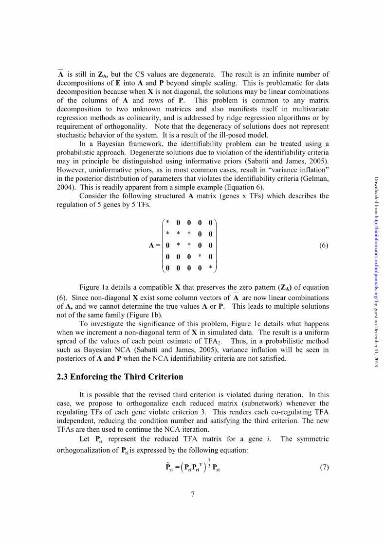
A is still in ZA, but the CS values are degenerate. The result is an infinite number of decompositions of E into A and P beyond simple scaling. This is problematic for data decomposition because when X is not diagonal, the solutions may be linear combinations of the columns of A and rows of P. This problem is common to any matrix decomposition to two unknown matrices and also manifests itself in multivariate regression methods as colinearity, and is addressed by ridge regression algorithms or by requirement of orthogonality. Note that the degeneracy of solutions does not represent stochastic behavior of the system. It is a result of the ill-posed model. In a Bayesian framework, the identifiability problem can be treated using a probabilistic approach. Degenerate solutions due to violation of the identifiability criteria may in principle be distinguished using informative priors (Sabatti and James, 2005). However, uninformative priors, as in most common cases, result in �variance inflation� in the posterior distribution of parameters that violates the identifiability criteria (Gelman, 2004). This is readily apparent from a simple example (Equation 6). Consider the following structured A matrix (genes x TFs) which describes the regulation of 5 genes by 5 TFs.

** * *

* **

*

0 0 0 00 0

A = 0 0 00 0 0 00 0 0 0

(6)

Figure 1a details a compatible X that preserves the zero pattern (ZA) of equation (6). Since non-diagonal X exist some column vectors of A are now linear combinations of A, and we cannot determine the true values A or P. This leads to multiple solutions not of the same family (Figure 1b). To investigate the significance of this problem, Figure 1c details what happens when we increment a non-diagonal term of X in simulated data. The result is a uniform spread of the values of each point estimate of TFA2. Thus, in a probabilistic method such as Bayesian NCA (Sabatti and James, 2005), variance inflation will be seen in posteriors of A and P when the NCA identifiability criteria are not satisfied. 2.3 Enforcing the Third Criterion It is possible that the revised third criterion is violated during iteration. In this case, we propose to orthogonalize each reduced matrix (subnetwork) whenever the regulating TFs of each gene violate criterion 3. This renders each co-regulating TFA independent, reducing the condition number and satisfying the third criterion. The new TFAs are then used to continue the NCA iteration. Let riP represent the reduced TFA matrix for a gene i. The symmetric orthogonalization of riP is expressed by the following equation:

( )�1-T 2

ri ri ri riP = P P P (7)

by guest on Decem



ownloaded from



8

Here the inverse square root of ( )1-T 2

ri riP P is found by eigenvalue decomposition

of Tri riP P by taking the inverse square root of each component eigenvalue. In this form,

one can see that no vector in riP is favored over another. For speed and numerical stability, the algorithm can be expressed without matrix inversion as:

[ ]

[ ]

Tri ri ri ri ri

ri ri ri

3 1P = P - P P P2 2

P = P / P (8)

The norm in equation (2) is any suitable norm except the Frobenius norm, and [=] indicates assignment. The above equation is iterated until convergence. The convergence property and the mathematical proof is detailed in (Hyvarinen, 1999; Hyvarinen and Oja, 2000). For clarity, what is proved is that after a suitable number of iterations, the matrix T

ri riP P converges to the identify matrix. We then return to recalculate matrix A until the bilinear optimization convergences. Note that the TFAs not included in riP are not affected here. Symmetric orthogonalization (SO) methods are fundamental mathematical developments in matrix theory that have been extensively used in ICA decompositions (Hyvarinen and Oja, 2000). 2.4 Whitening Transformation Computation time is a significant factor for algorithms that analyze large regulatory networks. For NCA faster convergence may be obtained by preprocessing the microarray data by a whitening procedure. This method, common in neural network and data preprocessing applications, has the principal feature of flattening noise and amplifying the signal. Optimization can be performed in this transformed feature space, and the solution in the original space can be obtained by the inverse procedure as with ICA methods (Hyvarinen and Oja, 2000). A zero-mean random vector x is white if its elements are uncorrelated and unit variance. Any input data matrix can be made white by a linear transformation that decorrelates the experimental input vectors and scales them to unit variance (Hyvarinen and Oja, 2000). For microarray data, the whitening transformation can be computed from eigenvalue decomposition of the variance-covariance matrix of E. Let

( ) TM M× ≡EΣ E E represent the variance-covariance matrix of the microarray data E. Since EΣ is positive definite and symmetric, it can always be represented as

TEΣ = UDU where U is an orthogonal matrix having 1, , ne e… eigenvectors of EΣ , and the

diagonal eigenvalues of EΣ . Then one possible whitening transformation for E is:

T

T

⋅

⋅

-1/2W = D U

E = E W (9)

The whitening matrix ( )M M×W is positive symmetric and nonsingular, and E is the whitened microarray data. NCA decomposition is then performed on the new whitened matrix ⋅E = A P , with A constrained by the same zero pattern as A. De-whitening of

by guest on Decem



ownloaded from



9

matrix P (or transformation back to the original feature space) is easily accomplished by -TP = PW . After de-whitening P we then calculate the matrix A from the original microarray data matrix E by NCA decomposition. For this reason, the NCA identifiability criteria are preserved when A is calculated. 3. Application and Results

3.1 Network Component Analysis of the S. cerevisiae Cell Cycle To test the biological applicability of our new algorithm, we analyzed S. cerevisiae cell-cycle data (Spellman, et al., 1998). We restricted the analysis to α-factor, cdc15, elutriation, and cdc28 experiments (73 data points). We generate the connectivity network from ChIP-chip binding data by selecting TF-gene interactions those genes whose ChIP-chip binding p-value < 0.001 (Lee, et al., 2002). A TF-gene pair is connected if the binding p-value < 0.001 and disconnected (set to zero in the A matrix otherwise). Note that the presence of a connection does not indicate its final value. An edge may go to ~0 after decomposition, or to some regulation strength value. The initial values of the non-zero connections in A may be set randomly. This procedure results in a connectivity network (N1) that covers 96 TFs over ~2200 genes. The remaining 17 TFs were excluded due to NCA condition 2 violations. Note that this network is data limited and not identifiable (more TFs > experiments) if we were to use the previous NCA criteria (Liao, et al., 2003; Tran, et al., 2005). However, most genes are regulated by < 7 TFs so we can apply our new criterion and numerical procedure. We ran NCA using whitening and the SO procedure (as described above) starting with a random initial guess for the non-zero CS values in the connectivity network.

3.2 Comparison of Methods that Compute TFA: NCA and REDUCE

To compare these results with REDUCE (e.g. MATRIX REDUCE) we obtained the TFAs reported by (Bussemaker, et al., 2001; Gao, et al., 2004). These data consist of 37 TFAs reported from the analysis of 113 TFs covering ~6000 genes over ~750 experimental data points. The authors determined that only 37 transcription factor ChIP-chip binding patterns out of 113 were significant predictors of gene expression in one or more experiments. As REDUCE analyzes each microarray experiment individually, we can extract cell cycle TFA data points without effecting the results. The common experiments include alpha factor arrest, cdc15, elutriation experiments (Spellman, et al., 1998). In addition Gao et al. analyzed additional cell cycle data from (Zhu, et al., 2000) that includes fkh1/fkh2 double knockout in α-factor treatment, as well as fkh1/fkh2 double knockout cell cycle experiments. The cdc15 data includes a replicate at time t=160, so we averaged these two data points for further analysis.

The S. cerevisiae cell cycle is periodic with cell divisions approximately every 60 mins. An interesting question to ask is which TFs have periodic TFAs as these may indicate regulated/coordinated transcriptional responses and possibly provide additional evidence that a TF is in fact a cell cycle regulator. We tested the TFAs for periodicity in each individual cell cycle experiment using a robust estimator (Ahdesmaki, et al., 2005) with the standard false discovery rate (FDR) adjusted p-value < 0.05. We did not detect

by guest on Decem



ownloaded from



10

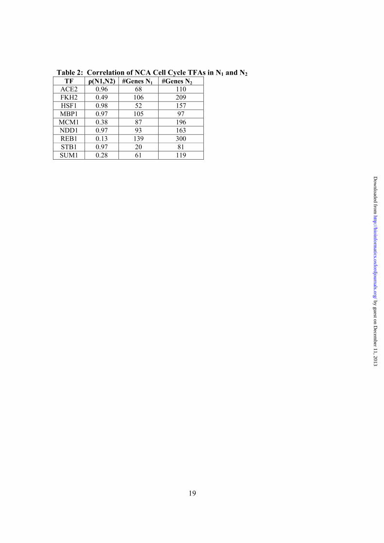
periodicity in any of the exclusive experiments (cdc28, fkh1/fkh2 knockouts), however, in the common experiments we did detect periodic TFAs for both REDUCE and NCA (Table 1). In the case of NCA some TFAs were periodic in two or more experiments. In REDUCE most TFAs were statistically periodic in one cell cycle experiment only. For the cdc15 data we adopted an additional Bonferrori p-value correction (0.05/23) because the data might be noisy due to periodic stress responses induced by heat-shock arrest method (Zhang, 1999). Figure 2 shows plots of NCA and REDUCE computed TFAs for a few common cell cycle TFs. Overall the results suggest that the REDUCE TFAs (Figure 2 a-f dotted lines) are in noisier than NCA TFAs (Figure 2 a-f solid lines), but qualitatively are in agree with each other. For example, Figure 2a shows that the result of NCA and REDUCE are similar for the well known cell cycle regulator ACE2. Both methods predict periodic phases that peak near cell division and this peak is characteristic of ACE2 regulation of early G1 specific gene transcription (Spellman, et., al 1998). Figure 2b shows that the TFAs of SWI4 exhibits two major peaks within a cell cycle that both correspond to late G1 transcriptional activity (Spellman, et., al 1998). Thus unlike the original periodicity measure by (Spellman, et al., 1998) we are able to extract and detect multiple periodic peaks that correlate with the cell cycle. The remaining REDUCE TFAs (Figures 1d 1e, 1f) are not statistically periodic when the corresponding NCA TFAs are. The most likely reason for this is that the REDUCE introduce numerical error due to fitting a fixed CS value. Of interest is the TFA of DIG1. Figure 1c shows the NCA TFA which peaks in approximately one cell cycle. This peak correlates with the current known function of DIG1; a TF that mediates cell cycle arrest in response to mating factor (α-factor) at Start (Mendenhall and Hodge, 1998). 3.3 What is the Effect of False Connectivity? False connectivity includes incorrect edges (false positives) and the non-detection of true edges (false negatives) by binding site analysis or experimental methods. The sensitivity of TFAs to false connectivity in the S. cerevisiae cell cycle was investigated previously (Yang, et al., 2005). The authors altered up to 10% of the connectivity for each network by randomly deleting and inserting connections between TFs and genes. They found that most TFAs, especially the cell cycle regulators, are robust and not affected by perturbation. In this work, we assessed TFA variability by using two connectivity networks constructed from ChIP-chip data using different p-value cut-offs. Here network N1 is selected from ChIP-chip data with a binding p-value < 0.001 (as described previously), and network N2 is selected analogously with ChIP-chip binding p-values < 0.01. We eliminate any genes and TFs that do not satisfy NCA condition 2. In N1 we found 31 periodic TFAs out of 96 total (FDR p-value < 0.05), 23 are known cell-cycle regulators (Table 1). In N2 we found 29 periodic TFAs out of 112 (FDR p-value < 0.05), 14 are known cell-cycle regulators. Between these two networks, we identified 9 well known cell cycle regulators and computed their correlation coefficients between the two networks N1 and N2 (Table 2). These results are consistent with previous results obtained with NCA by subnetwork decomposition on similar cell cycle data (Yang, et al., 2005),

by guest on Decem



ownloaded from



11

and with the results of other statistical methods to identify cell cycle regulated TFs computed by a nonparametric test of differential expression between sets of genes bound or not bound by a ChIP-chip TF (Tsai, et al., 2005). Thus TFA computations are robust to connectivity network selection provide the NCA criteria are satisfied. 3.4 Statistical Significance of TFA The researcher may be interested in identifying experiments where one or more TFAs are significantly perturbed with respect to the reference. To determine the statistical significance we construct a null hypothesis distribution for each experimental data point using the network connectivity pattern and shuffling (scrambling) the genes. The distribution is built by multiple iterations of permutation testing (~100). From this distribution we compute the z-score of the original TFA for each experimental data point. The result is a p-value at each data point that determines if the computed TFA is different then the null hypothesis.

4. Discussion NCA is a method to deduce TFAs and CS from gene expression data and a

connectivity network. However, previous mathematical requirements limit the total number of TFAs inferred in any single analysis to the experiment sample size. In this work, we developed a new identifiability criterion that relaxes this requirement such that the number of data points only has to exceed the maximal number of TFs regulating any single gene. Since most genes are regulated by less than 5 TFs, one needs only 5 transcriptome data points for NCA, but can analyze far more TFs than the number of data points. NCA compared to Linear Methods for computing TFAs. Another method similar to NCA is REDUCE which computes TFAs from gene expression data and a connectivity network. Similar to REDUCE, NCA uses the connectivity network as a model of the global regulatory network. The significant difference between these methods is that NCA models CS as a function of gene expression data whereas REDUCE fixes CS to binding affinity (as determined by ChIP-chip assay or from promoter binding site analysis). Thus unlike NCA, REDUCE does not distinguish between positive and negative regulation of the same TF on different genes and this may affect the accuracy of TFA estimates. It is well established that binding strength does not correlate with regulation activity. Thus, using binding data as the fixed CS may compromise TFA estimates. On the other hand, NCA is also similar to PCA or ICA methods in that it specifies constraints that guarantee a unique bi-linear data decomposition. These constraints are derived from the connectivity network. From a bipartite network point of view, PCA and ICA, assume full connectivity of TFs and genes. In addition, PCA and ICA requires that each basis vector is decorrelated or independent from the others. Thus these decompositions represent a statistical interpretation of gene regulation. We argue that integrating the connectivity network directly rather then by projection methods or regression methods provides a more detailed description of biological phenomena at the TF level and thus more accurate quantification of TFAs and CS.

by guest on Decem



ownloaded from



12

The Importance of Identifiability NCA identifiability violations result in infinite solutions that represent linear combinations of TFAs. Therefore, these degenerative results are not interpretable from a biological standpoint. One possible way to circumvent this problem is to use a Bayesian approach that uses different prior probabilities for different solutions (Sabatti and James, 2005). In this framework, the equivalent solutions due to non-identifiability are distinguished based on given prior probability distributions. This approach may work well if informative prior distributions are available. However, without such information, violation of the identifiability criteria leads to variance inflation, and the ability to distinguish among equivalent solutions is degenerated. This situation is particularly severe if a large fraction of the network violates the identifiability criteria. Therefore, it is important to detect whether the problem is well-posed before analysis. In conclusion, we note that it is important to determine the identifiability of bi-linear data decomposition such as NCA. In this regard, this article provides a new criterion that allows realistic TFAs to be determined from less data in both deterministic and probabilistic approaches.

5. Proof of Criterion 3 for Network Component Analysis Definition 1: All N L× matrices (defined as A) in which a given set of positions are zero are said to have the same zero pattern. Such matrices belong to the set ZA, which is defined as

( ){ }0 for a given set of ,N LijZ A i j×≡ ∈ =A A ! (10)

The elements not specified by the zero pattern can take positive, negative, or zero values. Similarly, the zero pattern for P (LxM) is defined as

( ){ }0 for a given set of ,L MklZ P k l×≡ ∈ =P !P (11)

Definition 2:

To define the reduced matrices Grj (j = 1,�,L), which is used in criterion 2 below, we will first build the combination matrices ( ) ( )( )1j N ML L+ × +G from A (NxL) and P (LxM). jG is mathematically describes as:

( )1 ,

cj

Tc

j Tcj

TcL

Q

=

A

PG

P

P

A

" (12)

by guest on Decem



ownloaded from



13

where cjM stands for the column vector j of matrix any M, (which could be either A or

PT) and ( )Q v stands for the block diagonal matrix with each block being vector v. For example, consider a matrix P,

2 0 10 5 4

=

P (13)

the matrix T1cQ P is:

( )T1

2 00 01 00 20 00 1

cQ

=

P (14)

The reduced matrix Grj is now defined as matrix Gj without rows corresponding to nonzero elements in the left most column. Theorem: Given a matrix E N M , if the following conditions are satisfied, then the decomposition of = +E AP Γ , where ( )A N L ZA× ∈ , ( ) PP L M Z× ∈ is unique up to a

scaling nonsingular diagonal matrix ( )L L×X . In other words, for the same allowable Γ ,

any alternative decompositions of = +E AP Γ where ( )N L Z× ∈ AA , and

( )L M Z× ∈ PP are different only by a diagonal matrix ( )L L×X , i.e.

1A AX−= (15) P XP= (16) Criterion 1. A has full column rank. Criterion 2. Each reduced matrix Grj (j = 1,�,L), defined in Tran et al. 2005 and in Definition 2, has a rank of L − 1. Criterion 3. Each row of E is regulated by rows of P that are linearly independent. Conditions 1 and 2 are the same as those proven previously in Tran et al. 2005, and the Condition 3 will be proved in the following section. Proof of the third criterion:

by guest on Decem



ownloaded from



14

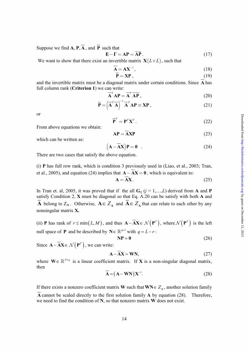
Suppose we find A, P, A , and P such that − = =E Γ AP AP . (17) We want to show that there exist an invertible matrix ( )L L×X , such that

1−=A AX , (18) =P XP , (19) and the invertible matrix must be a diagonal matrix under certain conditions. Since A has full column rank (Criterion 1) we can write:

T TA AP A AP= , (20)

( )1T T−

= ≡P A A A AP XP , (21)

or

T T TP P X= . (22) From above equations we obtain: AP AXP= (23) which can be written as: ( )A AX P 0− = . (24)

There are two cases that satisfy the above equation. (i) P has full row rank, which is condition 3 previously used in (Liao, et al., 2003; Tran, et al., 2005), and equation (24) implies that A AX 0− = , which is equivalent to: =A AX . (25) In Tran et. al, 2005, it was proved that if the all Grj (j = 1,�,L) derived from A and P satisfy Condition 2, X must be diagonal so that Eq. A.20 can be satisfy with both A and A belong to ZA . Otherwise, Z∈ AA and Z∈ AA that can relate to each other by any nonsingular matrix X. (ii) P has rank of ( )min ,r L M≤ , and thus ( )T− ∈A AX PN , where ( )TPN is the left

null space of P and be described by q L×∈N ! with q L r= − : =NP 0 (26) Since ( )T− ∈A AX PN , we can write:

,− =A AX WN (27) where N q×∈W ! is a linear coefficient matrix. If X is a non-singular diagonal matrix, then ( ) 1.−= −A A WN X (28) If there exists a nonzero coefficient matrix W such that Z∈ AWN , another solution family A cannot be scaled directly to the first solution family A by equation (28). Therefore, we need to find the condition of N, so that nonzero matrix W does not exist.

by guest on Decem



ownloaded from



15

If there exist a nontrivial W, such that Z∈ AWN , then for each row (gene) vector i of ZA, ( )1i L×A , can be written as the product of row vector i of W, ( )1i q×W , and

matrix ( )q L×N : i i=A W N (29) Since we only know the zero elements j�s in row vector Ai, Eq. A.24 is reduced to: i ri=0 W N (30) Where reduced matrix ( )ri q z×N consists only columns j that correspond to z zero elements in Ai. However, iff matrix Nri has rank q, the row vector Wi must be zero. Therefore, the necessary condition is z q≥ . If ( )min ,r M L M= = , then z L M≥ − , and hence the number of nonzero element in Ai (i.e. the number of transcription factors regulating gene i), l L z= − , must be less than M (i.e. the number of experiments). Note that the left null matrix q L×∈N ! having rank q represents q sets of linear constraints on the dependent rows of P, and each column j of N defines linear coefficient of row j with other rows in P. That means if row j of P is linearly independent to all other rows, the column j of N will be zero. For example, if row 1 and 2 of P ( )5 4× are linearly dependent, the left null matrix N is: [ ]1 2 0 0 0n n=N (31)

where ni represent the linear coefficient of row 1 and 2 of P such that:

1 1 2 2 0 1, ,k kn P n P for k M+ = = … (32)

Because the reduced matrix Nri is full row rank (= q), then the nonzero members in each rows of N (corresponding to dependent rows of P) cannot be eliminated all together, which means the dependent rows of P will not combine together in regulating row i of E (Criterion 3). For the above example, Nri is rank deficiency when both the first and second columns are eliminated. That means the corresponding row Ai has nonzero elements in both the first and second columns. Therefore, each row i of E must be regulated by rows of P that are linearly independent. Acknowledgements This work was supported by NSF grant CCF-0326605 and the UCLA-DOE Genomics and Proteomics Institute. Galbraith, S.J. was partially supported by a UCLA-IGERT bioinformatics traineeship (NSF-IGERT 9987641). Tran, L.M. was supported by a UCLA-IGERT bioinformatics traineeship (NSF-IGERT 9987641).

by guest on Decem



ownloaded from



16

References

• Ahdesmaki, M., Lahdesmaki, H., Pearson, R., Huttunen, H. and Yli-Harja, O. (2005) Robust detection of periodic time series measured from biological systems, BMC Bioinformatics, 6, 117.

• Almeida, J.S. and Voit, E.O. (2003) Neural-Network-Based Parameter Estimation in S-System Models of Biological Networks, Genome Informatics, 14, 114-123.

• Alter, O., Brown, P.O. and Botstein, D. (2000) Singular value decomposition for genome-wide expression data processing and modeling, PNAS, 97, 10101-10106.

• Alter, O. and Golub, G.H. (2004) Integrative analysis of genome-scale data by using pseudoinverse projection predicts novel correlation between DNA replication and RNA transcription, Proc Natl Acad Sci U S A, 101, 16577-16582.

• Bussemaker, H.J., Li, H. and Siggia, E.D. (2001) Regulatory element detection using correlation with expression, Nat Genet, 27, 167-171.

• Gao, F., Foat, B.C. and Bussemaker, H.J. (2004) Defining transcriptional networks through integrative modeling of mRNA expression and transcription factor binding data, BMC Bioinformatics, 5, 31.

• Gelman, A. (2004) Bayesian data analysis. Chapman & Hall/CRC, Boca Raton, Fla.

• Hyvarinen, A. (1999) Fast and robust fixed-point algorithms for independent component analysis, Neural Networks, IEEE Transactions on, 10, 626-634.

• Hyvarinen, A. and Oja, E. (2000) Independent component analysis: algorithms and applications, Neural Netw, 13, 411-430.

• Lee, S.I. and Batzoglou, S. (2003) Application of independent component analysis to microarrays, Genome Biology, 4, R76.

• Lee, T., Rinaldi, N., Robert, F., Odom, D., Bar-Joseph, Z., Gerber, G., Hannett, N., Harbison, C., Thompson, C., Simon, I., Zeitlinger, J., Jennings, E., Murray, H., Gordon, D., Ren, B., Wyrick, J., Tagne, J., Volkert, T., Fraenkel, E., Gifford, D. and Young, R. (2002) Transcriptional regulatory networks in Saccharomyces cerevisiae, Science, 298, 799 - 804.

• Liao, J., Boscolo, R., Yang, Y., Tran, L., Sabatti, C. and Roychowdhury, V. (2003) Network component analysis: reconstruction of regulatory signals in biological systems, Proc Natl Acad Sci U S A, 100, 15522 - 15527.

• Liebermeister, W. (2002) Linear modes of gene expression determined by independent component analysis, Bioinformatics, 18, 51-60.

• Mendenhall, M.D. and Hodge, A.E. (1998) Regulation of Cdc28 cyclin-dependent protein kinase activity during the cell cycle of the yeast Saccharomyces cerevisiae, Microbiol Mol Biol Rev, 62, 1191-1243.

• Sabatti, C. and James, G.M. (2005) Bayesian sparse hidden components analysis for transcription regulation networks, Bioinformatics.

• Savageau, M.A. (1976) Biochemical systems analysis: A study of function and design in molecular biology. Addison-Wesley, Reading, Massachusetts.

by guest on Decem



ownloaded from



17

• Spellman, P.T., Sherlock, G., Zhang, M.Q., Iyer, V.R., Anders, K., Eisen, M.B., Brown, P.O., Botstein, D. and Futcher, B. (1998) Comprehensive identification of cell cycle-regulated genes of the yeast Saccharomyces cerevisiae by microarray hybridization, Mol Biol Cell, 9, 3273-3297.

• Torres, N.V. and Voit, E.O. (2002) Pathway analysis and optimization in metabolic engineering. Cambridge University Press, New York.

• Tran, L., Brynildsen, M., Kao, K., Suen, J. and Liao, J. (2005) gNCA: a framework for determining transcription factor activity based on transcriptome: identifiability and numerical implementation, Metab Eng, 7, 128 - 141.

• Tsai, H.K., Lu, H.H. and Li, W.H. (2005) Statistical methods for identifying yeast cell cycle transcription factors, Proc Natl Acad Sci U S A, 102, 13532-13537.

• van Steensel, B. and Henikoff, S. (2000) Identification of in vivo DNA targets of chromatin proteins using tethered dam methyltransferase, Nat Biotechnol, 18, 424-428.

• Voit, E.O. and Almeida, J. (2004) Decoupling dynamical systems for pathway identification from metabolic profiles, Bioinformatics, 20, 1970-1681.

• Yang, Y.L., Suen, J., Brynildsen, M.P., Galbraith, S.J. and Liao, J.C. (2005) Inferring yeast cell cycle regulators and interactions using transcription factor activities, BMC Genomics, 6, 90.

• Yeung, M.K.S., Tegner, J. and Collins, J.J. (2002) Reverse engineering gene networks using singular value decomposition and robust regression, PNAS, 99, 6163-6168.

• Zhang, M.Q. (1999) Large-Scale Gene Expression Data Analysis: A New Challenge to Computational Biologists , Genome Res., 9, 681-688.

• Zhu, G., Spellman, P.T., Volpe, T., Brown, P.O., Botstein, D., Davis, T.N. and Futcher, B. (2000) Two yeast forkhead genes regulate the cell cycle and pseudohyphal growth, Nature, 406, 90-94.

by guest on Decem



ownloaded from



18

Table 1: Periodic TFAs deduced in the Cell Cycle NCA REDUCE

ACE2 CIN5 ACE2 ADR1** CRZ1 ABF1 DIG1** FZF1 ZAP1 FKH1** GCN4 FKH2 FKH2** HSF1 GAT3 MBP1** NDD1 MBP1 MCM1** PHO4 MCM1 MSS11** REB1 NDD1 RME1** RFX1 NRG1 STB1** RME1 SOK2 SUM1** SMP1 SWI4 SWI4** STB1 YAP1** STE12 BAS1 SWI5 CAD1 SWI6 ** (double asterix) indicates periodicity detected in two or more experiments. Bold highlights known cell-cycle regulators in the literature. REDUCE data is reported from (Gao et al, 2004).

by guest on Decem



ownloaded from



19

Table 2: Correlation of NCA Cell Cycle TFAs in N1 and N2 TF ρ(N1,N2) #Genes N1 #Genes N2

ACE2 0.96 68 110 FKH2 0.49 106 209 HSF1 0.98 52 157 MBP1 0.97 105 97 MCM1 0.38 87 196 NDD1 0.97 93 163 REB1 0.13 139 300 STB1 0.97 20 81 SUM1 0.28 61 119

by guest on Decem



ownloaded from



20

Figure Legend Figure 1: (a) The effect of non-diagonal X that preserve Za on TFAs (b). Density of each point

estimate for TFA2 when the off-diagonal term of X (asterix) is incremented uniformly.

Figure 2: Analysis of selected NCA and REDUCE determined TFAs in the S. cerevisiae cell cycle data. α-factor arrest time course for (a) ACE2, (b) SWI4 and (c) DIG1; Cdc15 arrest time course for (d) SWI4, (e) DIG1, and (f) STB1. All data is scaled to unit norm. Black arrows indicated cell divisions as reported by Spellman et al (1998). Alpha factor consists of 2 divisions at 66 +- 11min (alpha factor); cdc15 consists of 3 cycles at 60-90min, 120-150min, and 270min.

by guest on Decem



ownloaded from



21

Figure 1

by guest on Decem



ownloaded from



22

Figure 2

by guest on D

ecember 11, 2013


Dow

nloaded from



Transcriptome network component analysis with limited microarray data

Documents

Transcript of Transcriptome network component analysis with limited microarray data