Trade Liberalization and the Efficiency of Firms inIndian Manufacturing

Nigel L. Driffield and Uma S. Kambhampati*

AbstractHas the efficiency of firms in India improved since its liberalization in 1991? The authors attempt to answerthis question by analyzing the determinants of firm-level efficiency in six manufacturing sectors in Indiawhile focusing on the effects of liberalization and domestic competition.They find that there was an increasein overall efficiency in the post-reform period in India in five out of the six sectors. While imports do notseem to improve efficiency, liberalization did increase efficiency in four of the sectors.

1. Introduction

The 1991 liberalization in India sought to deregulate industries and expose firms tointernational competition. It represented both a challenge, and an opportunity, to thehitherto protected manufacturing sector in India. The effect of trade liberalization onfirms has been a matter for considerable debate. On the one hand, the traditional infantindustry argument maintains that the removal of protection should result in largenumbers of firms becoming bankrupt. On the other hand, proponents of liberalizationmaintain that the effect should be marginal, as only the very inefficient firms will exit,the other firms being forced by competition to improve their performance. In thispaper, we consider whether the latter is true. Has the productivity/efficiency of firmsin India improved since liberalization?

In order to answer this question, we estimate frontier production functions for agroup of manufacturing industries in India. Unlike earlier studies on India, we do notestimate average productivity functions. Instead, we estimate the best-practice pro-duction function for each sector and consider how far short of this individual firms fall.In very efficient economies, we might expect most firms to be on or close to the fron-tier. In such economies, firms falling short of this frontier would be forced out of themarket. In developing economies, especially those like India, which have been regu-lated and protected for a long period, the dispersion below the frontier could be verylarge.This is because both the entry and exit of firms in these economies is highly regu-lated. Firms are not allowed to exit unless they obtain government permission to doso. They continue to operate even though they are inefficient because the governmentsupports them.1 In these economies, the dispersion of firms below the frontier isexpected to decrease after liberalization.2 In this paper, we analyze the determinants

Review of Development Economics, 7(3), 419–430, 2003

*Driffield: Birmingham Business School, University of Birmingham, Edgbaston, Birmingham B15 2TT, UK.Tel: 0121-414-3555; Fax: 0121-414-6707; E-mail: N.L.Driffield@bham.ac.uk. Kambhampati: Department ofEconomics, University of Reading, Whiteknights, Reading RG6 2AA, UK. Tel: 0118-9875123; Fax: 0118-9750236; E-mail: Les98usk@rdg.ac.uk. We would like to thank the Reserve Bank of India (particularly MrD. V. Sastry and Mrs Rama Ananthakrishnan) for making the data freely available to us. Dr Kambhampatiis also grateful to the Asia Centre, LSE, where she was an academic visitor when this work was begun.Thanks are also due to two anonymous referees for some particularly useful comments on a previous versionof the paper.

© Blackwell Publishing Ltd 2003, 9600 Garsington Road, Oxford OX4 2DQ, UK and 350 Main Street, Malden, MA 02148, USA

of firm-level efficiency in India while focusing on the effects of liberalization anddomestic competition.

2. Liberalization in India: Instruments of Reform

In 1991, the Indian government’s structural adjustment program encompassed the firstsustained attempts to increase the autonomy of the private sector (Ahluwalia, 1999).The program attempted to deregulate foreign trade and the labor market. As part ofthis program, the government abolished or eased licensing requirements in a largenumber of industries, removed most licensing and other nontariff barriers on importsof capital and intermediate goods, relaxed antitrust rules, and devalued the rupee3 (seeAhluwalia et al., 1996). Though exit continues to be difficult,4 the government hasbegun to decrease its support of inefficient firms.

3. Trade Reforms and Productivity: the Literature

The literature concerning the impact of trade reforms on microeconomic performanceshows little consistency regarding the effects of such reforms (Rodrik, 1992; Harrison,1994). Ignoring for a moment the possibility of perfect competition or Bertrand oligopoly in the home market, liberalization will increase competition and reduceprice, assuming that foreign competitors exist. Liberalization is generally expected toincrease overall welfare by increasing imports into sectors where the domestic price is higher than the world price; by increasing output in sectors with excess profits; byallowing firms in sectors with unexploited scale economies to increase output; and byincreasing technical efficiency (Rodrik, 1992).

The extent to which, this in turn, will improve production efficiency in domestic firmsindividually will then depend on the degree to which such firms are able to becomemore efficient as price is reduced. To begin with, by increasing competition anddecreasing market power, liberalization will increase the elasticity of demand facingdomestic firms, as well as shifting their demand curve to the left. However, if theincreased demand elasticity offsets this shift—which is plausible, following Rodrik(1992)—then domestic firms may actually increase, rather than decrease, output aftera liberalization. In the context of unexploited scale economies, this would lead todecreases in costs. Srivastava (1996) also claims that the increased potential marketsize enables firms to utilize excess capacity (an especially significant issue in India) andwill therefore lead to decreased costs.

Secondly, the domestic sector will become more efficient as individual firms exit theindustry in the face of increased competition.5 These firms may experience a furtherincrease in technical efficiency because liberalization is expected to increase competi-tion, forcing managers to become more competitive and dynamic if they are to surviveand succeed.

As can be seen from the above, the outcome of liberalization depends upon the con-ditions within the industry and firms, to begin with. Thus, whether the industry/firm isimport competing, experiences economies of scale, has excess capacity, is competitiveor monopolistic, are all likely to affect the outcome. It is therefore not surprising thatthe results have differed from study to study and across industries within the samestudy (Harrison, 1994; Tybout, 1998).

Empirical studies of productivity take two forms. The first set of studies—and moststudies of the Indian economy fall into this category—estimate average productivityfunctions and measure total factor productivity growth in the traditional manner

420 Nigel Driffield and Uma Kambhampati

© Blackwell Publishing Ltd 2003

(Krishna and Mitra, 1998; Bhalotra, 1998; Chand and Sen, 2002). The second type ofstudies estimate a frontier production function and measure the distance between thefrontier and the individual firms as a direct measure of efficiency; for a short survey ofthese studies, see Tybout (1998).

Srivastava (1996), in a detailed study analyzing the effect of the limited reform ofthe Indian economy in the mid-1980s, finds that the average total factor productivitygrowth (TFPG) was higher in the post-reform period. However, his firm-level estimatesare considerably higher than his growth accounting estimates of -2.27% to -2.37% forthe post-1985 period (Srivastava, 1996, p. 89). Krishna and Mitra (1998) study the effectof the more comprehensive 1991 reforms on a number of manufacturing sectors inIndia. Relying on firm-level production functions, they find that competition increasedafter 1991 and so did productivity.

As already indicated, there are few studies that have estimated efficiency for Indianfirms using frontier functions. Table 1 summarizes the results of some of these studies(Tybout, 1998). We can see that average efficiency levels are generally lower when adeterministic frontier is estimated, rather than a stochastic one. This is because, as wewill see in the next section, the stochastic frontier method further decomposes the errorterm into an inefficiency component and a random component. This enables a moreprecise estimation of efficiency. Ramaswamy (1994), for instance, found that averageefficiency in the machine tools industry estimating deterministic frontiers was 0.432,while it was 0.727 when estimating stochastic frontiers. The difference for plastic prod-ucts was 0.608 and 0.82, while for motor vehicles it was 0.638 and 0.846.

The purpose of this paper is to analyze the impact of the reforms of the Indianeconomy in 1991 on the efficiency of Indian firms. We begin by estimating efficiencyusing stochastic frontiers and analyze its determinants, particularly the effect of domes-tic market competition and liberalization. We use panel data to estimate our modelsand are therefore able to obtain better estimates of efficiency (see below).

TRADE LIBERALIZATION AND EFFICIENCY 421

© Blackwell Publishing Ltd 2003

Table 1. Results of Frontier Estimation Studies for Indian Studies

Study Methodology Average efficiency levels

Little et al. (1987) Translog, linear programming Shoes: 0.424Page (1984) Deterministic frontiers Printing: 0.645

Soap: 0.579Machine tools: 0.688

Ramaswamy (1994) Cobb–Douglas, linear programming Machine tools: 0.432Deterministic frontiers Agricultural machinery: 0.349

Plastic products: 0.608Motor vehicles: 0.638

Stochastic frontiers Machine tools: 0.727Plastic products: 0.82Motor vehicles: 0.846

Bhavani (1991) Stochastic frontiers (small firms Structural metal products: 0.719only) Agricultural hand tools: 0.704

Source: Extracted from Tybout (1998).

4. Estimation Methodology

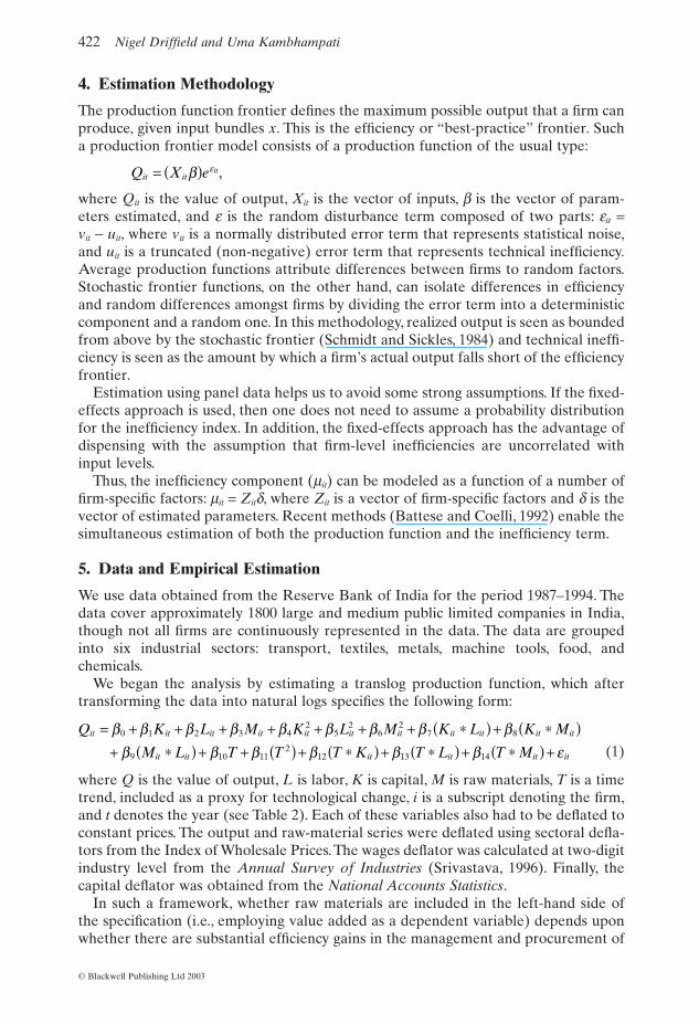
The production function frontier defines the maximum possible output that a firm canproduce, given input bundles x. This is the efficiency or “best-practice” frontier. Sucha production frontier model consists of a production function of the usual type:

where Qit is the value of output, Xit is the vector of inputs, b is the vector of param-eters estimated, and e is the random disturbance term composed of two parts: eit =vit - uit, where vit is a normally distributed error term that represents statistical noise,and uit is a truncated (non-negative) error term that represents technical inefficiency.Average production functions attribute differences between firms to random factors.Stochastic frontier functions, on the other hand, can isolate differences in efficiencyand random differences amongst firms by dividing the error term into a deterministiccomponent and a random one. In this methodology, realized output is seen as boundedfrom above by the stochastic frontier (Schmidt and Sickles, 1984) and technical ineffi-ciency is seen as the amount by which a firm’s actual output falls short of the efficiencyfrontier.

Estimation using panel data helps us to avoid some strong assumptions. If the fixed-effects approach is used, then one does not need to assume a probability distributionfor the inefficiency index. In addition, the fixed-effects approach has the advantage ofdispensing with the assumption that firm-level inefficiencies are uncorrelated withinput levels.

Thus, the inefficiency component (mit) can be modeled as a function of a number offirm-specific factors: mit = Zitd, where Zit is a vector of firm-specific factors and d is thevector of estimated parameters. Recent methods (Battese and Coelli, 1992) enable thesimultaneous estimation of both the production function and the inefficiency term.

5. Data and Empirical Estimation

We use data obtained from the Reserve Bank of India for the period 1987–1994. Thedata cover approximately 1800 large and medium public limited companies in India,though not all firms are continuously represented in the data. The data are groupedinto six industrial sectors: transport, textiles, metals, machine tools, food, and chemicals.

We began the analysis by estimating a translog production function, which aftertransforming the data into natural logs specifies the following form:

(1)

where Q is the value of output, L is labor, K is capital, M is raw materials, T is a timetrend, included as a proxy for technological change, i is a subscript denoting the firm,and t denotes the year (see Table 2). Each of these variables also had to be deflated toconstant prices. The output and raw-material series were deflated using sectoral defla-tors from the Index of Wholesale Prices. The wages deflator was calculated at two-digitindustry level from the Annual Survey of Industries (Srivastava, 1996). Finally, thecapital deflator was obtained from the National Accounts Statistics.

In such a framework, whether raw materials are included in the left-hand side of the specification (i.e., employing value added as a dependent variable) depends uponwhether there are substantial efficiency gains in the management and procurement of

Q K L M K L M K L K M

M L T T T K T L T Mit it it it it it it it it it it

it it it it it it

= + + + + + + + *( ) + *( )+ *( ) + + ( ) + *( ) + *( ) + *( ) +b b b b b b b b b

b b b b b b e0 1 2 3 4

25

26

27 8

9 10 112

12 13 14

Q X eit itit= ( )b e ,

422 Nigel Driffield and Uma Kambhampati

© Blackwell Publishing Ltd 2003

raw materials to firms (Patibandla, 1998), and is essentially an empirical question.Clearly, this requires that the production function be re-specified as

(2)

which effectively imposes a coefficient of unity on b3. As illustrated in Table 3 below,this constraint is strongly rejected by our data. Similarly, the inclusion of T in the pro-duction function is an empirical issue. A variable deletion test was done in this case(an LR-test) and the hypothesis that T could be excluded was rejected. The statisticsare presented in Table 3.

To be certain that our methodology was appropriate, we conducted three sets oftests. First, we tested our six sectors for poolability using likelihood ratio tests (Greene,1993). We found that pooling into the sectors was acceptable but no further mergingof the groups was possible. Equally, the tests were also carried out to validate therestriction of imposing a uniform production function for each sector over time andagain failed to reject such a restriction. We therefore present the results for thesegroups as they stand. Secondly, we tested our final model for the skewness of the errorterms (i.e., with skewness varying directly with l. We found that theskewness permits estimation of a stochastic frontier6 in all six sectors. Finally, thetranslog specification was tested against the restriction to Cobb–Douglas specification.In four sectors the Cobb–Douglas specification could not be rejected, while thetranslog was most appropriate in two sectors. We therefore present these results inTable 3.

The inefficiency component is then modeled as follows:

(3)

m d d d d dd d d d d

it it t t

it it t it

R D Market share HHI Age

Libdum Trend K L M X

= + + + ++ + + + +

- -

-

0 1 2 1 3 1 4

5 6 7 8 1 9

&

.

1

l s s s= +( ))u u v2 2 2

Q M K L K L K L

T T T K T Lit it it it it it it it

it it

- = + + + + + *( )+ + ( ) + *( ) + *( )b b b b b b

b b b b0 1 2 4

25

27

10 112

12 13 ,

TRADE LIBERALIZATION AND EFFICIENCY 423

© Blackwell Publishing Ltd 2003

Table 2. Description and Sources of Variables

Variable Description

Q Value of salesL Wage billK Gross fixed capitalM Materials and fuelR&D Research and developmentMS Market share; calculated in Kambhampati and Kattuman (1999)HHI Market concentration measure (Herfindahl indices) from Kambhampati and

Kattuman (1999)Age1 Age from year of incorporation > 75 yearsAge2 50 years < age from year of incorporation < 75 yearsAge3 25 years < age from year of incorporation < 50 yearsAge4 Age from year of incorporation < 25 years (reference category)Libdum 1, if year > 1990; else = 0T Time trend (1986 = 1 . . . 1994 = 9)KL Capital–labor ratioX Export earnings/QM Import expenditure/Q

424N

igel Driffield and U

ma K

ambham

pati

© B

lackwell P

ublishing Ltd 2003 Table 3. Summary Statistics for Data Used

MachineTransport Textiles Metals tools Food Chemicals

Q 4.162 0.737 4.082 0.536 3.887 0.642 3.954 0.680 4.067 0.624 4.127 0.706K 3.563 0.743 3.552 0.593 3.341 0.677 3.267 0.717 3.319 0.698 3.457 0.825L 5.859 0.698 6.034 0.572 5.658 0.611 5.732 0.658 5.915 0.688 5.740 0.708M 3.922 0.802 3.803 0.566 3.709 0.676 3.686 0.749 3.843 0.749 3.790 0.733T 4.913 2.559 4.767 2.535 4.854 2.516 4.821 2.553 4.774 2.534 4.967 2.571R&D 0.003 0.008 0.000 0.002 0.001 0.004 0.002 0.007 0.001 0.005 0.013 0.543M 0.070 0.119 0.034 0.078 0.097 0.273 0.115 0.230 0.012 0.045 0.094 0.194X 0.008 0.012 0.004 0.017 0.006 0.033 0.023 0.367 0.002 0.007 0.016 0.414MS 0.052 0.132 0.040 0.093 0.041 0.113 0.025 0.068 0.053 0.107 0.034 0.088HHI 0.134 0.126 0.109 0.127 0.123 0.164 0.078 0.104 0.122 0.108 0.114 0.123Age1 (0.000) (0.000) 0.057 0.233 0.009 0.093 0.014 0.117 0.037 0.189 0.007 0.083Age4 0.289 0.454 0.218 0.413 0.362 0.481 0.283 0.451 0.246 0.431 0.264 0.441Libdum 0.416 0.493 0.385 0.487 0.398 0.490 0.394 0.489 0.386 0.487 0.424 0.494K/L 0.007 0.008 0.005 0.008 0.008 0.017 0.008 0.049 0.006 0.020 0.012 0.017

In general, we might expect firms that spend more on R&D to increase efficiency. Ahigher capital–labor ratio is seen to increase efficiency because capital is less variablethan labor, creates fewer management problems, and produces a more standardizedproduct.Very old firms (Age1 > 75 years) might be expected to be less efficient becausethey are operating with relatively old technology. In addition, of course, old firms maylose their dynamism and become less flexible. On the other hand, such old firms mayalso gather considerable experience along the way and therefore improve efficiency(both productive and managerial). We also include Age4 (age less than 25 years). It isexpected that with more up-to-date capital, these firms would be more efficient thanthe older firms though they may also be less experienced.

Many studies have hypothesized that large firms are able to operate, not only at alower point on their cost functions than small firms, but also on lower cost functions(Clarke et al., 1984). It is well known that there is likely to be a two-way relationshipbetween market share and efficiency, a simultaneity that has been commented on inmany studies. To take this into account, we lag the market share (MS) variable by oneyear. This would imply that a large market share in the previous period could increaseefficiency in the current period. According to traditional analysis, highly concentratedindustries (HHI) are likely to have high barriers to entry and low levels of competi-tion, allowing considerable inefficiency to persist.7 On the other hand, these may alsobe industries where rivalry amongst the large firms increases rather than decreases effi-ciency. Again, the effect (as in the case of market shares) is likely to be lagged and wetherefore include HHIt-1 in our specification.

Finally, we include three variables that are expected to capture the effect of the 1991reforms in India. We include import intensity (M), which is expected to influence effi-ciency because firms are now able to import capital goods and the latest technology.Highexport intensity (X) is expected to increase efficiency because exporting firms have tocompete against very efficient and competitive firms in world markets and thereforemight be expected to decrease X-inefficiency. Finally, we include a liberalization dummy(Libdum) to capture the effect of reforms not captured by X and M,especially the effectsof deregulation of entry, expansion, and exit. We expect efficiency to increase as, in thenew open and deregulated environment, inefficiencies are less likely to be tolerated.These three variables, together with the impact of liberalization on export and importintensities, will determine the effect of liberalization on efficiency more generally.

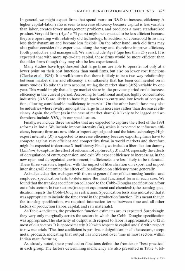
As indicated earlier,we began with the most general form of the translog function andemployed specification tests to determine the final functional form in each case. Wefound that the translog specification collapsed to the Cobb–Douglas specification in fourout of six sectors. In two sectors (transport equipment and chemicals), the translog spec-ification rejects the Cobb–Douglas restrictions. Specification tests also indicated that itwas appropriate to include the time trend in the production function.This meant that, inthe translog specification, we required interaction terms between time and all otherfactors of production (labor, capital, and raw materials).

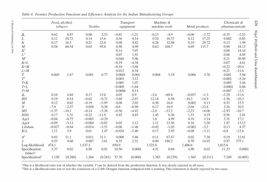
As Table 4 indicates, the production function estimates are as expected. Surprisingly,they vary only marginally across the sectors in which the Cobb–Douglas specificationwas appropriate. The elasticity of output with respect to labor is approximately 0.12 inmost of our sectors. It is approximately 0.20 with respect to capital and 0.6 with respectto raw materials.8 The time coefficient is positive and significant in all the sectors, exceptmetal products, indicating that output has increased over time in most sectors withinIndian manufacturing.

As already noted, these production functions define the frontier or “best practice”in each group. The factors determining inefficiency are also presented in Table 4, fol-

TRADE LIBERALIZATION AND EFFICIENCY 425

© Blackwell Publishing Ltd 2003

426N

igel Driffield and U

ma K

ambham

pati

© B

lackwell P

ublishing Ltd 2003

Table 4. Frontier Production Functions and Efficiency Analysis for Six Indian Manufacturing Groups

Food, alcohol, Transport Machine & Chemicals &tobacco Textiles equipment machine tools Metal products pharmaceuticals

b0 0.62 8.87 0.08 2.33 -0.41 -1.21 -0.13 -4.9 -0.08 -2.72 -0.35 -2.52L 0.11 10.72 0.14 15.6 0.56 4.14 0.10 16.57 0.12 17.25 0.002 0.05K 0.17 16.5 0.21 23.8 0.09 4.42 0.26 32.88 0.19 29.72 0.15 1.99M 0.58 60.34 0.63 95.6 0.58 4.99 0.63 104.7 0.69 115.7 0.98 18.13K2 0.14 7.07 0.08 14.16L2 0.07 1.91 0.06 4.85M2 0.044 5.96 0.21 20.89K*L -0.19 -4.34 0.07 4.61K*M -0.10 -3.68 -0.22 -20.4L*M 0.012 0.34 -0.21 -11.6T 0.005 1.67 0.001 0.77 0.0001 0.001 0.004 3.19 0.006 3.76 0.041 3.94T2 0.003 3.12 -0.002 -5.24T*K 0.005 1.07 0.005 2.44T*L -0.009 -1.64 0.0001 0.04T*M 0.0006 0.13 -0.007 -2.5d0 0.16 4.69 0.17 15.6 0.05 0.9 -2.6 -69.4 -0.057 -1.3 -2.29 -11.6RD 0.19 0.14 -0.62 -0.71 -3.69 -2.67 12.14 6.58 -10.3 -14.9 -1.58 -10.3M 0.12 0.62 -0.19 -5.95 0.08 2.03 0.36 16.6 0.002 0.13 0.52 12.5X -7.9 -2.37 0.058 0.38 -0.8 -0.99 0.17 18.9 -2.04 -12.8 2.26 10.5MS -1.37 -10.1 -0.14 -5.36 -0.56 -4.45 -2.0 -12.2 -2.23 -6.06 -2.93 -10.7HHI 0.17 1.51 -0.22 -11.0 0.45 4.83 1.45 6.36 1.53 4.19 0.56 2.81Age1 -0.04 -0.75 -0.003 -0.29 1.6 4.99 0.10 2.14 2.31 17.2Age4 -0.09 -3.13 -0.004 -0.82 0.05 2.12 1.11 12.56 0.10 2.20 1.87 13.12Libdum -0.027 -0.84 -0.014 -3.51 -0.06 -1.46 -0.02 -1.03 -0.062 -3.2 0.13 4.57K/L 1.11 3.9 0.61 1.47 -0.024 -2.40 0.17 2.92 -0.08 -3.11 -0.8 -12.6

s 2 0.03 11.1 0.011 31.1 0.008 5.86 0.11 67.67 0.02 7.38 0.19 12.81g 0.55 9.68 0.007 3.61 0.35 2.31 0.89 180.2 0.70 14.93 0.97 375.1Log-likelihood 474.1 1,537.3 650.9 1,525.8 1,406.6 1,815.6Specification 5.37 0.02 6.90 0.01 10.56 0.0001 4.31 0.04 4.98 0.03 11.23 0.0001

(time)a

Specificationb 1.130 (0.288) 1.264 (0.261) 37.70 (0.000) 1.383 (0.239) 1.565 (0.211) 7.189 (0.005)

a This is a likelihood-ratio test of whether the variable T can be deleted from the production function. It was clearly rejected in all cases.b This is a likelihood-ratio test to test the restriction of a Cobb–Douglas function compared with a translog. This restriction is clearly rejected in two cases.

lowing directly on from the production function estimates. Since the variables aredeterminants of inefficiency, a positive coefficient increases inefficiency (or decreasesefficiency) and vice versa. In what follows, we will discuss the results in terms of thedeterminants of efficiency, as this is more straightforward and intuitive. Before we dothis, let us consider the average levels of efficiency in each sector before and after the1991 reforms.

Table 5 indicates that if we take averages across the whole period, efficiency levelswere between 0.87 and 0.96. Dividing the period into the pre- and post-91 years, wefind that the food sector is the least efficient in both subperiods. The machine toolssector is the most efficient in both subperiods, followed closely by the transport equip-ment sector. In all sectors, except machine tools, average efficiency levels increased inthe post-91 period. The figures for coefficient of variation indicate that the dispersionof efficiency levels decreased in four sectors (and increased very marginally in the foodsector) between the two periods. Thus, liberalization does seem to have pushed sur-viving firms towards the frontier, decreasing the dispersion below it. In the next sectionwe consider the factors that determine these efficiency levels in more detail.

6. Analysis of Efficiency

In all sectors (except metal products), productivity has been increasing over time. Thecoefficient of time (t) is positive in all cases and is negative and significant only in metalproducts. More specifically we find that in textiles, transport equipment, and metalproducts, efficiency further increased after the 1991 reforms. We will discuss this result,together with those relating to openness and competitive conditions, in the next sub-section. Before we do this, let us summarize the other results.

We find that age decreases efficiency in transport, machine tools, metal products, andchemicals. In these sectors, firms over 75 years of age are significantly less efficient thanother firms. However, we found that very young firms (age less than 25 years) are alsonot very efficient. In fact, in machine tools, metals, and chemicals, such young firms are also less efficient than others. Thus, our results seem to indicate that it is the middle-aged firms (between 25 and 75 years of age) that are most efficient. This is notsurprising as these firms have passed the early learning phase and may now be con-solidating their knowledge and technology. They are also not so old that their tech-nology and methods are obsolete. Only in the food products industry are young firms(less than 25 years) more efficient.

TRADE LIBERALIZATION AND EFFICIENCY 427

© Blackwell Publishing Ltd 2003

Table 5. Average Efficiency for Six Manufacturing Groups in India

IndustryMean efficiency Coefficient of variation

Sector classification All years t < 1990 t > 1991 All years t < 1990 t > 1991

Chemicals 461–470 0.9303 0.9221 0.9405 0.0642 0.0671 0.0510Food 310–342, 370 0.8730 0.8676 0.8794 0.0729 0.0720 0.0723Metals 410–430, 452–457 0.9392 0.9371 0.9477 0.0370 0.0351 0.0316Textiles 351–360 0.9299 0.9232 0.9385 0.0347 0.0323 0.0367Transport 441–444 0.9538 0.9540 0.9.55 0.0218 0.0252 0.0194Machine tools 445–451 0.9616 0.9624 0.9614 0.0190 0.0223 0.0158

Notes: Inefficiency is measured as the distance from the “best practice” frontier. Three-digit RBI industriesthat have been grouped together to form our manufacturing groups.

R&D is seen to increase efficiency in three sectors (transport equipment, metal prod-ucts, and chemicals). In two sectors (food and textiles) it is insignificant, while inmachine tools, R&D seems to reduce efficiency. In the latter case it might be relatedto the way in which Indian firms report R&D expenditure. In some cases, expenditureon executive travel or entertainment expenditure is reported as R&D expenditure andis therefore unsurprisingly not significantly related to efficiency.9

The Effect of Domestic Competition

In all six sectors, lagged market share (MS) is significant and has a positive effect onefficiency. This is a very consistent effect and indicates that firms with larger marketshares are able to increase efficiency to higher levels than are smaller firms. This seemsto confirm the “new learning” argument that large market shares enable firms to func-tion at the minimum point of existing cost curves, and more significantly enable themto operate on lower cost curves through learning-by-doing.10

Market concentration (HHI) decreases efficiency in four sectors—machine tools,chemicals, transport equipment, and metal products—where high concentration levelsseem to imply collusion and the tolerance of inefficiency within the industry. However,in the textiles sector, high levels of concentration seem to create sufficient rivalrybetween firms to force them to operate at minimum costs. Thus, the fear that high con-centration levels would result not only in high profit margins but also inefficient firmsis confirmed in most of our sample of industries, except textiles.

Liberalization and the Impact of “Openness”

We have included three variables—import intensity (M), export intensity (X), and aliberalization dummy (Libdum)—that may be expected to capture the effect ofincreased openness and of deregulation. In addition to these variables, the impact ofliberalization on export and import intensities themselves would also determine theeffect of liberalization on efficiency.Ahluwalia (1999) shows that export growth pickedup after 1991 and reached a peak of 20% in 1993/94. Imports, too, grew after 1991reaching a peak in 1995/96. However, the trends varied across industries. Thus, resultsobtained elsewhere (Kambhampati and Parikh, 2000), using a similar dataset, indicatethat exports decreased in 25/66 industries after 1991 but they also show an increasingtrend in 26/66 industries since 1991.

The ability to import new and up-to-date technology and capital is often seen as oneof the major benefits of trade liberalization (Tybout, 1998; Chand and Sen, 2002).Whilethis seems to be true in certain sectors like textiles, where imports significantlyincreased efficiency (Howell and Kambhampati, 1998), it does not in general seem tobe true. Thus, in the transport, machine tools, metal products, and chemicals sectors,import intensity decreased, rather than increased efficiency. These results seem toconfirm Patibandla’s results (1998) that large firms (which are likely to be particularlycommon in industries like transport equipment, machine tools, and chemicals) do notfeel the need to “undertake systematic reorganizational efforts in adapting importedtechnologies to local conditions most efficiently” (p. 421).The results relating to exportintensity (X) are similarly mixed. Contrary to expectations, in sectors like machinetools and chemicals, export intensity seems to decrease efficiency. Earlier studies of theimpact of reforms in India, however, seem to confirm these findings. Aksoy (1992)found that, while the reforms significantly enhanced the profitability of exports in thetextiles and auto components sectors, they did not work so well in the two capital-

428 Nigel Driffield and Uma Kambhampati

© Blackwell Publishing Ltd 2003

intensive sectors studied—chemicals and machinery. These are two of the sectorswhere we, too, found that export intensity decreases rather than increases efficiency.

In addition to X and M, we also include Libdum, a variable which it is hoped willcapture the effect of all the other changes that occurred in 1991 (including other tradereforms and any deregulation of product and labor markets that did take place). Thisvariable is a dummy which takes the value 1 for all years from 1991 and is zero beforethat. We find that in the textiles, transport (marginal), metal products, and chemicalssectors, liberalization did increase efficiency as expected. It seemed to decrease effi-ciency only in the chemicals sector.

7. Conclusion

This study finds that there was an increase in overall efficiency in the post-reformperiod in India in five out of the six sectors. Analyzing the determinants of efficiencyin greater detail, we found that middle-aged firms with higher market shares werelikely to be more efficient than others. R&D significantly increases efficiency in threesectors, while high levels of industry concentration are associated with lower efficiencylevels. While imports do not seem to improve efficiency, possibly because firms do notmake systematic efforts to adapt them to domestic conditions, we find that liberaliza-tion did increase efficiency in four sectors.

References

Ahluwalia, Isher J., Rakesh Mohan, and Omkar Goswami, Policy Reform in India, New Delhi:Oxford and IBH Publishing (1996).

Ahluwalia, Montek S., “India’s Economic Reforms: an Appraisal,” in Jeffrey D. Sachs, AshutoshVarshney, and Nirupam Bajpai (eds.), India in the Era of Economic Reforms, Delhi: OxfordUniversity Press (1999).

Aksoy, M. Ataman, “The Indian Trade Regime,” World Bank working paper 989 (1992).Battese, George E. and Tim J. Coelli, “Frontier Production Functions, Technical Efficiency and

Panel Data: With Application to Paddy Farmers in India,” Journal of Productivity Analysis 3(1992):153–69.

Bhalotra, Sonia R., “Changes in Utilization and Productivity in a Deregulating Economy,”Journal of Development Economics 57 (1998):391–420.

Bhavani, T. A., “Technical Efficiency in Indian Modern Small Scale Sector: an Application ofFrontier Production Function,” Indian Economic Review 31 (1991):149–66.

Central Statistical Organisation Annual Survey of Industries (various issues), Government ofIndia: Department of Statistics, Ministry of Planning.

Central Statistical Organisation, National Accounts Statistics, Government of India: Departmentof Statistics, Ministry of Planning.

Chand, Satish and Kunal Sen, “Trade Liberalization and Productivity Growth: Evidence fromIndian Manufacturing,” Review of Development Economics 6 (2002):120–32.

Clarke, Roger, Stephen W. Davies, and Michael Waterson, “The Profitability–ConcentrationRelation: Market Power or Efficiency?” Journal of Industrial Economics 32 (1984):435–50.

Goswami, Omkar, “Legal and Institutional Impediments to Corporate Growth,” in Isher J.Ahluwalia, Rakesh Mohan, and Omkar Goswami (eds.), Policy Reform in India, New Delhi:Oxford and IBH Publishing (1996).

Greene, William. H., Econometrics Analysis, New York: Macmillan (1993).Harrison, Anne E., “Productivity, Imperfect Competition and Trade Reform: Theory and

Evidence,” Journal of International Economics 36 (1994):53–73.Howell, J. and Kambhampati, U. S., “Liberalisation and Labour: The Effect on Formal Section

Worker,” Journal of Intinational Development, Vol. 10, No. 4, pp. 439–52 (1998).Joshi, V. and Little, I. M. D., India’s Economic Reforms: 1991–2001, Delhi: Oxford University

Press (1996).

TRADE LIBERALIZATION AND EFFICIENCY 429

© Blackwell Publishing Ltd 2003

Kambhampati, Uma S. and Paul Kattuman, “Industrial Concentration: Are Large Firms DrivingMarket Structure Changes in India?” paper presented at the Indian Economists Forum con-ference, December (1999).

Kambhampati, Uma. S. and Ashok Parikh, “Disciplining Firms?: the Impact of Trade Reformson Profit Margins in Indian Industry,” Applied Economics 35 (2003):461–70.

Krishna, Pravin and Devashish Mitra, “Trade Liberalisation, Market Discipline and Productiv-ity Growth: New Evidence from India,” Journal of Development Economics 56 (1998):447–62.

Little, Ian M. D., Dipak Mazumdar, and John M. Page, Small Manufacturing Enterprises: a Com-parative Analysis of India and Other Economies, New York: Oxford University Press (1987).

Page, John M., “Firm Size and Technical Efficiency: Applications of Production Frontiers toIndian Survey Data,” Journal of Development Economics 16 (1984):129–52.

Patibandla, Murali, “Structure, Organizational Behaviour, and Technical Efficiency: the Case ofan Indian Industry,” Journal of Economic Behaviour and Organization 34 (1998):419–34.

Ramaswamy, K.V.,“Technical Efficiency in Modern Small-Scale Firms in Indian Industry:Appli-cations of Stochastic Production Frontiers,” Journal of Quantitative Economics 10(1994):309–24.

Reserve Bank of India, data provided on tape for 1700 firms (1986–94).Rodrik, Dani, “The Limits of Trade Policy Reform in Developing Countries,” Journal of Eco-

nomic Perspectives 6 (1992):87–105.Sachs, Jeffrey, Ashutosh Varshney, and Nirupam Bajpai, (eds.), India in the Era of Economic

Reforms, Delhi: Oxford University Press (1999).Schmidt, Peter and Robin Sickles, “Production Frontiers and Panel Data,” Journal of Business

Economics and Statistics 2 (1984):367–74.Srivastava, Vijay, Liberalisation, Productivity and Competition, Delhi: Oxford University Press

(1996).Tybout, James, “Manufacturing Firms in Developing Countries: How Well Do They Do, and

Why?” working papers in economics, Georgetown University (1998).

Notes

1. There is a growing literature cataloguing the problems faced by firms wishing to exit in India(Sachs et al., 1999, p. 6; Goswami, 1996; Joshi and Little, 1996).2. Kambhampati and Parikh (2003) consider the effect that liberalization has on profit margins.They find that liberalization affects profit margins mainly through its effect on firm behavioralvariables like market shares, R&D, advertising, export and import intensities.3. The government devalued the rupee in July 1991 by 24% in two phases. In March 1993, itmoved to a unified floating exchange rate which settled at Rs31 = $1.4. A firm that wishes to exit has to be “declared” bankrupt by the Board for Industrial andFinancial Restructuring. The process can take up to 2–3 years and sometimes as long as 10 years(Goswami, 1996).5. With price at marginal cost, removing trade barriers will not improve production efficiency,although under standard Hecksher–Ohlin assumptions it may cause a reallocation of resourceswithin the economy based on comparative advantage.6. If = 0, then l = 0 and the stochastic frontier is irrelevant because there is no inefficiency.The “average” production function would then be a good description of the data.7. There has been considerable disagreement regarding whether high concentration leads toincreased profit margins because it increases the market power of firms within the industry orbecause it increases efficiency. This debate has not been resolved.8. As mentioned earlier, since the latter (raw material coefficient is significantly different from1), a three- rather than two-input production function was seen as more appropriate.9. We are grateful to one of the referees of this paper for this interpretation of our result.10. Note that according to this view, learning-by-doing is influenced not simply by age but alsoby size because a larger output provides greater opportunities for learning and therefore moreexperience.

su2

430 Nigel Driffield and Uma Kambhampati

© Blackwell Publishing Ltd 2003