“Bankruptcy risk and productive efficiency in manufacturing firms”

LEONARDO BECCHETTI, JAIME SIERRA

CEIS Tor Vergata - Research Paper Series, Vol. 2003, No. 30, August 2003

This paper can be downloaded without charge from the Social Science Research Network Electronic Paper Collection:

http://ssrn.com/abstract=428545

CEIS Tor Vergata

RESEARCH PAPER SERIES

Working Paper No. 30 August 2003

1

Bankruptcy risk and productive efficiency in manufacturing firms1

Leonardo Becchetti Università di Roma “Tor Vergata”, Rome, Italy E-mail: Becchetti@economia.uniroma2.it Jaime Sierra Università di Roma “Tor Vergata”, Rome, Italy e-mail: jaime@seneca.uniroma2.it

Abstract

The paper investigates the determinants of bankruptcy in three representative unbalanced samples of Italian firms for the periods 1989-1991, 1992-94 and 1995-97. Two important results are that: i) the degree of relative firm inefficiency measured as the distance from the efficient frontier has significant explanatory power in predicting bankruptcy ii) qualitative regressors such as customers' concentration and strength and proximity of competitors have significant predictive power and suggest that banks should not restrict their monitoring activity to balance sheet variables. These findings remain significant after controlling for balance sheet liquidity and profitability variables usually considered in these estimates.

Keywords: bankruptcy prediction, stochastic frontiers, qualitative indicators JEL codes: G21, D21

1 The paper is part of a CNR research project on "Measures and techniques for controlling financial risk: from market to credit risk" and was presented at the IX Tor Vergata Financial Conference. MURST 40% and CNR grants are acknowledged. A special thank goes to G. Scanagatta and all other members of the "Osservatorio sulle piccole e medie imprese" of Mediocredito Centrale for their suggestions and their support on the database. We also thank S. Caiazza, R. Castellano, I. Hazan, G. Piga, L. Wall, two anonymous referees and all other participants to the Conference for useful comments and suggestions. The usual disclaimer applies.

2

1. Introduction

The empirical literature of bankruptcy prediction has recently gained further momentum and

attention from financial institutions.2 Academicians and pratictioners have realised that the problem

of asymmetric information between banks and firms lies at the heart of an important market failure

such as credit rationing and that the improvement in monitoring technologies represents a valuable

alternative to any incomplete contractual arrangement aimed at reducing borrowers' moral hazard

(Stiglitz-Weiss, 1981, 1986 and 1992; De Meza-Webb, 1987; Milde-Riley, 1989, Xu, 2000).

Among the three existing approaches to the problem (accounting analytical approach, option

theoretical approach and statistical approach),3 the statistical approach tries to assess corporate

failure risk through four widely known methods that make use of balance-sheet ratios: linear or

quadratic discriminant analysis, logistic regression analysis, probit regression analysis and neural

network analysis.

Many empirical studies adopt the statistical approach. They aim to classify correctly a

sample of firms into one of two pre-established categories (sound or unsound firms) on the basis of

selected balance sheet variables in levels or trends. After the pioneering research of Beaver (1966)

and Altman (1968), relevant results in this field have been obtained by Zmijewsky (1984),

Frydman, Altman and Kao (1985) and Gentry, Newbold and Whitford (1987). Examples of

empirical analyses on Italian data are given by Appetiti (1984), Barontini (1992), Altman et al.

(1994), Laviola and Trapanese (1997) and Foglia et al. (1998).

2 An example is the more risk sensitive framework for bank capital adequacy set by the New Basel Capital Accord promoted by the Basel Committee on Banking Supervision. According to the Committee “ The new framework intends to provide approaches which are both more comprehensive and more sensitive to risks than the 1988 Accord, while maintaining the overall level of regulatory capital. Safety and soundness in today’s dynamic and complex financial system can be attained only by the combination of effective bank-level management, market discipline, and supervision” (BIS, 2001). The New Basel Capital Accord (see first and second pillar) requires banks to have sound internal processes in place to assess the adequacy of its capital based on a thorough evaluation of its risks. This creates a great incentive for banks to implement their own risk management skills. 3 The accounting analytical approach is largely followed by rating agencies. For recent applications of the structural or reduced form option approach see Duffie and Lando (1998) and Nickell, Perraudin and Varotto (2000).

3

The contribution of our paper to this literature goes in two directions: i) a broader test on the

significance of non balance sheet data (such as market share, customers' concentration, strength of

local competitors and others); 4 ii) a test on whether remoteness from the “best practice” (distance

from the efficient productive frontier) has some predictive power on the probability of failure.

The paper is divided into five sections including introduction and conclusions. In the second

section we describe our database and outline the methodology adopted to classify sound and

unsound firms. In the third we outline the stochastic frontier approach and comment the results

obtained with this method. In the fourth section we present logit estimates of the determinants of

bankruptcy and test the explanatory power of the distance from the efficiency frontier and of non

balance sheet indicators recorded by the Survey and included in the estimates.

2.1 Sample features and the definition of variables

The database used in our empirical analysis is extracted from three different Mediocredito Centrale

Surveys covering respectively the 1989-91, the 1992-94 and the 1995-1997 periods.5 The sample is

stratified by industry activity, geographical area and size6 for firms from 10 to 500 employees,

4 As to this point Zavgren (1985) affirms that "any econometric model containing only financial statement information will not predict accurately the failure or non failure of a firm", while Keasey and Watson (1987) conclude that their results "indicate that marginally better predictions, concerning small company failure may be obtained from non-financial data as compared to those which can be achieved from using traditional financial ratios". On the same point see Ohlson (1980). Among the few authors using qualitative variables, Fisher (1981) identifies permanent and temporary information on sample firms from qualitative and socio-political data, while Keasey and Watson (1987) evaluate the impact of qualified audit on the probability of failure. 5 Significant attrition among the three different sample periods of the Survey prevented the creation of a large panel. While each three-year sample includes about 4,500 firms, only 800 firms participated in both of the last two Surveys and only 300 firms in all of them. This number drops considerably when we rule out observations with missing values. We therefore analyse the three periods as separate samples and consider even firms participating in only one Survey. In this way we have more than 4,000 firms for each sample period as indicated in Table 1. 6 Size and composition of each stratum have been defined according to the Neyman’s (1934) formula in order to minimise sample variance.

4

while it includes all firms above 500 employees. Collected data are of two types: quantitative

(balance-sheet data) and qualitative (questionnaire). 7

Sample firms are classified into three mutually exclusive categories: “Failed”,“Active” and

“Stressed”. Failed enterprises8 are those that ceased existing, while Stressed firms are those placed

under different kinds of intervention procedures (procedure concorsuali)9 as envisaged by the

Italian law. These include composition with creditors, receivership, extraordinary administration,

voluntary liquidation, forced liquidation, and winding-up. Firms which continue to operate without

problems are classified as Active. 10 The relative share of these three groups on total sample is

presented in Table 1.

7 All balance sheet data contained in the Mediocredito database are accurately checked. Balance sheet data come from CERVED which obtains the official information from the Italian Chambers of Commerce and is currently the most authoritative and reliable source of information on Italian companies. Qualitative data from questionnaire are based on answers from a representative appointed by the firm collecting information from the relevant firm division. The questionnaire has a system of controls based on “long inconsistencies”, namely inconsistencies between answers to questions placed at a certain distance in the questionnaire. As an example answers on the use of government subsidies (export subsidies) are matched with answers on the exact composition of the flow of funds available for investment - internal finance, debt finance, grants, soft loans. – (on the share of exported net sales). In case of inconsistent information the firm is subject to a second phone interview. Firms which do not provide reliable information after being recontacted are excluded from the sample. A supplementary list of 8000 firms is built for each of the three year surveys in order to avoid that exclusions, generated by missing answers or inaccuracies in the questionnaire may alter the sample design. Substitutions follow the criteria of consistency between the sample size and the population of the Universe. 8 The “Failed” status is defined on the basis of the information provided by CERVED. Data available on firm failure may be underestimated since not all such cases are dutifully reported to the competent authority to avoid paying the fines established by Italian laws. The problem of misreporting is common to almost all countries. Gilson and Vetsuypens (1993) find that in the US “many corporate filings are missing for bankrupt firms.” To evaluate effects on the sampling methodology, see Zmijewsky (1984) and Zagrev (1985). This literature shows that random sampling tends to overstate the probability of financial distress, while “complete data” studies such as ours tend to understate this probability since distressed firms are less likely to have complete data before failure. Zmijewsky (1984) finds, however, that these two biases are likely to affect (rather unsubstantially) classification and prediction rates but do not affect statistical inferences on the impact of independent variables. 9 The present and past legal status of any natural and legal body in Italy is reported to the Federation of Chambers of Commerce by means of a special document known as modello AN/6 (modello CF and S3 currently). The range of intervention procedures for firms failing to meet their debt payments includes: bankruptcy (fallimento), winding-up (liquidazione), compulsory administrative liquidation (liquidazione coatta amministrativa), winding-up subject to supervision of the Court (liquidazione giudiziaria), voluntary winding-up (liquidazione volontaria), dissolution (scioglimento), dissolution with liquidation (scioglimento e liquidazione), dissolution without going into liquidation (scioglimento senza messa in liquidazione), early dissolution without going into liquidation (scioglimento anticipato senza messa in liquidazione), dissolution by the Court (scioglimento per atto dell'Autorità ), fraudulent bankruptcy (bancarotta fraudolenta), bankruptcy (bancarotta semplice), adjustment of creditors’ claims (concordato fallimentare), composition with creditors (concordato preventivo), receivership (amministrazione giudiziaria), temporary receivership (amministrazione controllata), extraordinary administration (amministrazione straordinaria), judicial attachment (sequestro giudiziario), writ of attachment of company shares (sequestro conservativo di quote). 10 All procedures considered for the definition of stressed firms imply the impossibility to meet obligations with banks. Our definition of stressed firms therefore coincides with the definitions produced in the most relevant Italian studies

5

[Table 1 here]

Each three-year sample is numerically unbalanced in favour of active firms,11 but it has the

advantage of being generated randomly and not for the specific purpose of the credit risk analysis.

This is a relevant difference as compared to many previous studies, e.g., Beaver (1966), Altman

(1968) and Barontini (1992), who adopt a balanced-sampling approach and select a given number

of sound and unsound firms to generate two rather reduced, homogeneous (same firm size and

industry) and equally-sized groups (50% sound, 50% unsound firms).

On the basis of the financial ratios successfully identified by past studies, 20 balance-sheet indices12

have been considered as potential bankruptcy determinants (Table 2).13 These indices reflect six

different aspects of firm structure and performance: liquidity, turnover, leverage, operating structure

and efficiency, size and capitalisation, and, finally, profitability.14 The indices have been calculated

as three-year, two-year and one-year averages.15

[Table 2 here]

Other indices (totally or partially based on non balance-sheet data) have been calculated to control

additional firm characteristics such as: market share (firm sales / industry sales), strength and

proximity of competitors,16 export status, subcontracting status, group membership, size, location in

(Appetiti, 1984; Laviola and Trapanese, 1997) and it is not more restrictive than those usually found in the international literature (Beaver, 1966; Gilson, 1988 and 1989; Everett and Watson, 1998). 11 For previous empirical papers on bankruptcy using unbalanced samples see Ohlson (1980) and Zmijewsky (1984). A problem with unbalanced sampling is that the intercept (but not the regressors' coefficients) needs to be decreased by (log p1-log p2) where p1 and p2 are respectively the proportion of unsound and sound firms (Maddala, 1992). 12 By analysing the existing empirical literature it is clear that there is not a definite index group presenting a high discriminant ability and forecasting power common to all previous studies. For this reason we agree with Edmister’s (1972) assertion that “…Although some ratios were found to be good predictors in more than one study, no one group of ratios is common to the [four] studies. This implies that the discriminant functions can be applied reliably only to situations very similar to those from which the function was generated.” 13 In most of the empirical literature the selection criteria for regressors are based upon the choices of previous empirical studies (Zavgren, 1984; Skogsvik, 1988) or on a combination of these choices with theoretical a priori (Edmister, 1972; Lo, 1986; Keasey and Watson, 1987; Keasey and Mc Guiness, 1990). 14 These index categories are taken from Appetiti (1984) and are close to those of Keasey and Watson (1987) and Laviola and Trapanese (1997). 15 A three-year time interval is not too long or uncommon in the literature. Skogsvik (1988) and Gilson-Vetsuypens (1993) start analysing the behaviour of firms in their sample six years before, Keasey and McGuiness (1988) and Laviola and Trapanese (1997) five years before, while Edmister (1972), Appetiti (1984) and Lo (1986) three years before default. 16 This qualitative information was collected from managers' answers to the Mediocredito questionnaire.

6

a macro area (South and Isles, Centre, North-West, North-East) and share of sales to the first three

customers (only for the 1995-1997 database).

As an alternative to static ratios, a three-year trend has been calculated for each of the selected

indicators following the Edmister's methodology17. We define a trend as “three consecutive years

during which the ratio moves along the same direction” and we generate up-trend (down-trend)

dummy variables with a value of 1 if the trend is positive (negative) and 0 otherwise. The up-trend

and down-trend dummy variables are used alternatively to static indices as regressors in a dynamic

specification of the logit estimation (Table 2).18

2.2 Descriptive features of sound and unsound firms

We provide descriptive statistics for stressed and failed firms (as defined in Section 2) jointly as

well as separately. Average values for static (ratios) and dynamic (trends) indices are presented in

an Appendix available from the authors upon request.

Our findings show that: i) liquidity ratios are generally higher for active than for failed firms when

we consider stressed and failed firms together; ii) the pattern of liquidity variation is alternatively

favourable to active (second period) and failed companies (first and third period); iii) turnover

indices (and, specifically, sales to assets ratios) are higher for active firms. Assets to net worth

ratios are higher for failed firms presumably because of their reduced capital resources (as will be

confirmed by other ratios in which the same item is implied), but variations of this index are

generally more positive for active companies; iv) the leverage indices, in turn, display greater

solvency for active firms, even though debts are slightly higher for active firms, presumably

17Appetiti (1984) instead, runs a regression on the indices’ values for the three periods prior to the crisis and uses the coefficients (Betas) in order to substitute for the static ratios in the discriminant function. 18 Estimates presented in the paper include outliers. Estimates with 95% cut-off for regressors have been alternatively generated without showing results that are significantly different from those shown in the paper. These latter are available from the authors upon request.

7

reflecting higher creditworthiness, over the three-year periods examined; v) the operating structure

ratios indicate that active companies have lower interest charges to sales and lower interest charges

to value added ratios, and higher depreciation charges over gross fixed assets than failed companies.

The analysis of trend indicators generally confirms the following findings: i) both size and

capitalization indices and their three-year trends clearly reflect the superior growth of active versus

failed firms; ii) the various profitability indices and trends emphasise the overall higher profitability

of active enterprises and, finally, iii) additional indices such as market share, competitors' location,

share of sales to three largest customers, return and operating risk significantly discriminate sound

companies from stressed and failed ones, the latter having higher operating risk, higher customers'

concentration and higher local competitive pressure.

3. 1 The stochastic frontier approach and the probability of bankruptcy: the specification of

the model

The adoption of a stochastic frontier approach19 to predict bankruptcy risk is, to our knowledge, an

original attempt in this literature.20 We here test the hypothesis that financial unsoundness, in

19 The literature frequently adopts the Total Factor Productivity indicator for productivity comparisons. TFP is an accounting method which measures growth in output not explained by growth in inputs. It is purely descriptive even though it leaves the possibility to check, in a second stage, whether subgroups of firms classified according to a chosen variable have different TFPs (Maximovic-Phillips, 1998). The Stochastic Frontier Analysis presents at least two relative advantages with respect to TFP. First, the SFA - in the Battese and Coelli (1995) approach – simultaneously evaluates the degree of firm inefficiency and the relationship between inefficiency and various potential determinants. This approach has been widely recognised to be superior to the two-stage estimation which inconsistently assumes the independence of the inefficiency effects in the two estimation stages. The two-stage estimation procedure is unlikely to provide estimates which are as efficient as those that could be obtained using a single-stage estimation procedure (Battese and Coelli, 1995). Second, in the SFA, we separate an inefficiency component which is random and not affected by any variable and a component which is affected by several factors. The distinction between firm specific inefficiency and random shocks or statistical noise is a relevant advantage of the stochastic frontier approach as compared to any deterministic approach (Kaparakis, Miller and Noulas, 1994). 20 The SFA has two main applications in finance: i) to evaluate the efficiency of industries in the financial sector: (Aly, Grabowsky, Pasurka and Rangan, 1990, Kaparakis, Miller and Noulas, 1994; Allen and Rai, 1996; Berger and Mester, 1997); ii) as an original approach to generate inefficiency measures which are relevant in typical finance issues (Hunt, Coh and Francis, 1996). We apply it to test whether productive efficiency may predict the incidence of bankruptcy in an unbalanced panel, in addition to typical balance sheet variables. Maximovic and Phillips (1998) focus on the same issue using total factor productivity instead of the stochastic frontier approach for a panel of large US firms.

8

general, and the failure condition, in our particular case, are directly related to productive

efficiency. 21 At least three definitions of efficiency may be recalled when referring to the analysis

of productivity of single firms or industries: i) technical efficiency which implies maximizing

output from a given combination of factors; ii) allocative efficiency which refers to minimizing

costs of the input mix, at given relative prices, for any output level (that is equivalent to equating

the marginal product of every variable input to its corresponding opportunity cost or maximizing

the profit); iii) revenue efficiency which is related to the maximization of value added, gross

earnings or any other financial parameters.22

We focus on technical efficiency using a parametric approach. According to Battese and Coelli

(1995) approach, we define the following generic production function:

[1] ,,...,1,,...,1)( TtNiUVXY itititit ==−+= β

where Yit is the production of the i-th firm; Xit is a k*1 vector of input quantities of the i-th firm; β

is a vector of unknown parameters; the Vit are random variables which are assumed to be iid. N(0,

σV2), and independent of the Uit which are non-negative random variables that account for technical

inefficiency in production and are assumed to be independently distributed as truncations at zero of

the N(mit, σU2) distribution.23 mit =zitδ, zit is a p*1 vector of variables that may influence the

efficiency of a firm, and δ is a 1*p vector of parameters to be estimated.

As for the parameters σV2 and σU

2 they are replaced with σ2=σV 2+σU2 and γ=σU

2/(σV 2+σU2).

The measure of technical efficiency is defined as:

21 An illustrative explanation on the origin and operative variations of the concept of efficiency applied to economic analysis is provided by Scazzieri (1981). 22 The last type of efficiency depends on the first two classes and, as noted by Fanti (1997), if output, labor, and capital are empirically proxied in the production function by value added, cost of labor, and capital stock respectively, the resulting readout measuring "revenue inefficiency" caused by technical and allocative inefficiency does not tell one from the other. 23 It has been shown that these strong distributional assumptions have limited effects for the purpose of our analysis (Aigner et al., 1977; Cowing, Reifshneider and Stevenson, 1983; Greene, 1990). In particular, even though the absolute level of inefficiency differs over different distributional assumptions on the one-sided error term, the ranking of firms seems unaffected (Greene, 1990).

9

[2] ),,0|(/),|( **iiiiiii XUYEXUYEEFF ==

where Yi* is the production of the i-th firm, which is equal to Yi if the dependent variable is in

original units, and is equal to exp(Yi) if the dependent variable is in logs. EFFi takes up a value

between zero and one. The efficiency measures relative to the production function may be defined

as exp(-Ui) if the dependent variable is lagged, or as (Xiβ-Ui)/(Xiβ) if it is not. These

expressions for EFFi rely upon the value of the unobservable Ui being predicted.

Within this general framework, we choose a Cobb-Douglas production function specified as

follows:

[3] ∑−

=−+++=

1

110 )(*)/ln()/ln()/ln(

m

jititjitjitit UVIndustryLKLKLY λββ

in which real output is proxied by the log of real sales value per worker of the ith firm at time t

(I=1,…,N; t=1,…,T), production inputs are represented by the log of the capital stock per worker,

the latter being evaluated at the replacement cost of capital. The prices of both inputs and output

have been deflated using the industry inflation indexes computed by ISTAT.

The Cobb-Douglas production function includes output and capital stock per worker. The input

variables have been multiplied by the corresponding industry dummies24 in order to account for

industry specificities which may influence the intercept and the slope of the production function. In

fact, each industry is expected to have a different production function. This implies the existence of

variations in the output-per-worker/capital-per-worker elasticities across industries.

The non-zero mean residual of the production function is regressed on the following variables that

are assumed to affect efficiency:

24 Nineteen industries have been defined according to the four-digit ISTAT classification: 1 Food, beverages, and tobacco; 2 Textile and clothing; 3 Leather and shoes; 4 Wood, wood products, and furniture; 5 Paper, paper products, printing, and publishing; 6 Chemicals; 7 Rubber and plastic products; 8 Glass and ceramic products; 9 Building industry; 10 Metal extraction; 11 Metal products; 12 Mechanical materials; 13 Mechanical equipment; 14 Electronic equipment; 15 Electric equipment; 16 Precision instrument and apparels; 17 Transport vehicles; 18 Transport - Other; 19 Energy production.

10

[4]

∑ ∑ ∑−

=

−

=

−

=+++++=

1

1

1

1

1

1210

m

i

p

j

q

kkkjjiiit SubsidieseMarketsharSizeAreaIndustryU δδθηαδ

itwFdummyAAgeExportInnovation +++++ /6543 δδδδ

while, for the 1995-1997 model, three additional regressors (available only for this data set) are

included:

...CaputäCompetareaäLargestclä... ++++ 987

The variables affecting efficiency are: number of employees (size), market share (Market share),

sales to the three biggest customers (Largestcl), capacity utilisation rate (Caput), age and a series of

dummy variables: Area (geographic location in the North-East, North-West, Centre, South and

isles), sector of economic activity (Industry), export status (Export), access to state subsidies

(Subsidies), process and/or product innovating status (Innovation), Active/Failed status (A/F

dummy) and presence of direct competitors in the same geographic area (Competarea).

The model is estimated for each of the three samples as a cross-section in which all the quantitative

variables are expressed as three-year averages.

3.2 The stochastic frontier approach and the probability of bankruptcy: econometric results

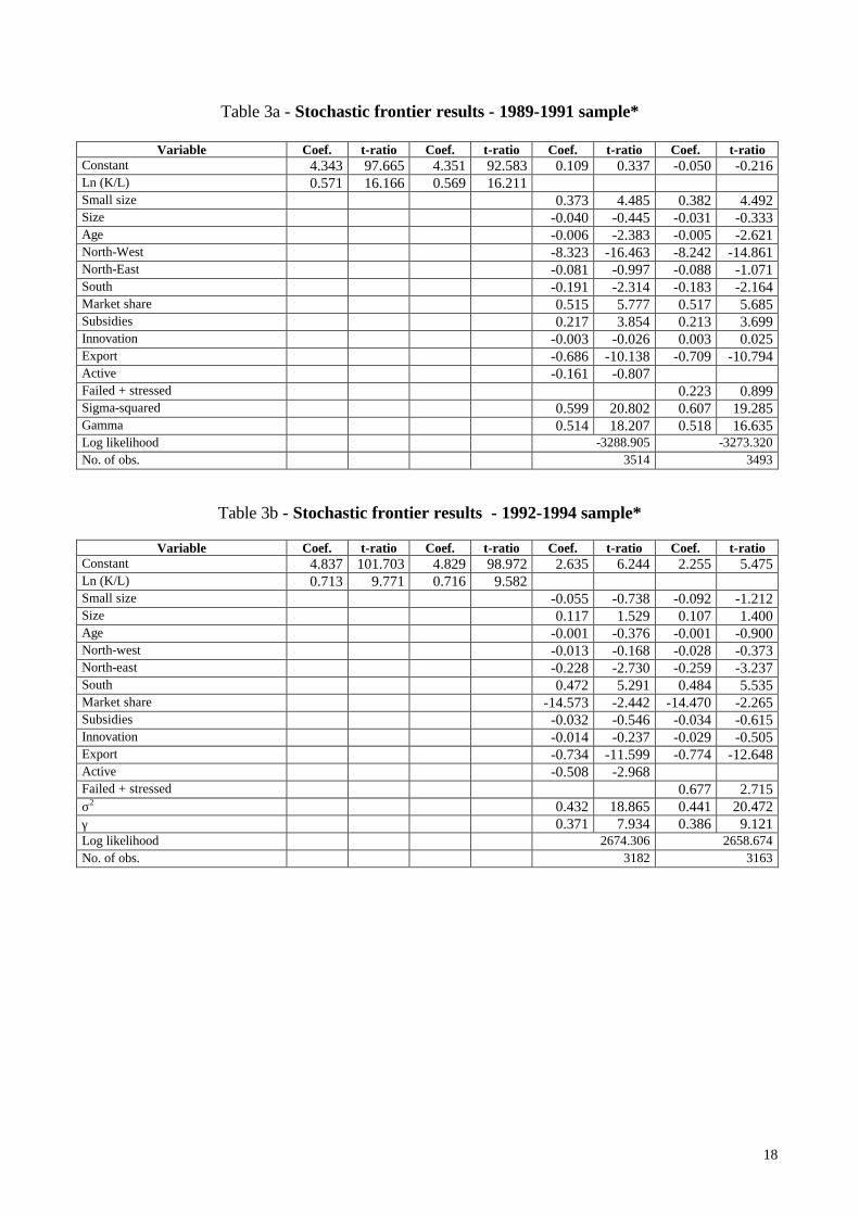
A positive and statistically significant gamma coefficient indicates that the variance of the nonzero

mean residual explains a significant part of the overall variability (Tables 3a to 3c). The model

specified therefore fits well the data and supports the presence of relevant technical inefficiencies.

[Tables 3a-3c here]

11

As expected, the signs and coefficients reported show that firms which we know are going to fail in

the near future are significantly more distant from the "best practice" in two of the three periods,

while the coefficient has the expected sign but is not significant in the first period.25

Among other factors affecting the distance from the efficiency frontier, we find that firms located in

the South are significantly less efficient.26 Another result, which is not sample specific, and holds

for all of the three considered periods is the relatively higher efficiency of exporting firms vis-à-vis

those which sell only in the domestic market. This result is consistent with most of the empirical

literature (Aw and Hwang, 1995; Clerides, Lach and Tybout, 1998, Becchetti and Santoro, 2001)

and is generally explained by two non mutually excluding rationales: i) export is a learning process

that improves firm productivity; ii) export markets select the most efficient firms (Delgado and

Farinas, 1999).

The impact of size and age on productive efficiency seems less robust and more sample specific.

This means that it is probably affected by changes in fiscal, monetary and exchange rate policies

which crucially altered the economic framework in the three sample periods.27

4. The distance from the efficiency frontier and the logit model

The finding that ex post failed firms are ex ante significantly more distant from the efficiency

frontier confirms the link between productive efficiency and the probability of bankruptcy. It does

not imply however that remoteness from the best practice has a significant marginal impact on the

25 This result is consistent with the hypothesis of the strong relevance of financial factors on bankruptcy for firms surveyed in the first period in which they are presumably affected by a shift in monetary policy and by the consequent increase in real interest rates. Since the distance from the frontier mainly measures firm inefficiency on the real side (and not financial difficulties), its significance in the second and third sample period parallels the higher relevance of nonfinancial efficiency in the logit estimate for the same two periods (see in this section below). 26 To interpret this finding we may consider the influence of productive efficiency of factors such as weakness in the infrastructure, a stronger criminal control and lower social capital (Putnam, 1993).

12

probability of failure, net of the effect of other qualitative and quantitative factors. In other terms,

the above mentioned result does not tell whether the stochastic frontier approach adds valuable

information to banks which already possess financial information and the relevant qualitative

information considered in this paper.

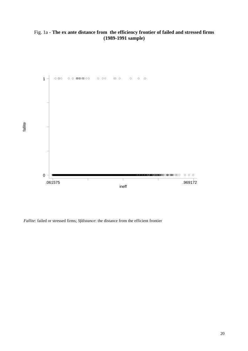
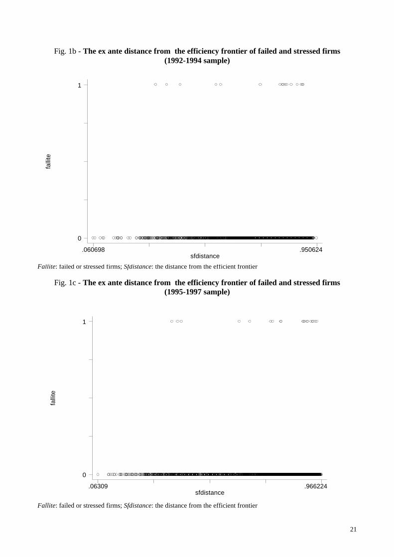
At a first glance, descriptive evidence on the relationship between firm soundness and the distance

from the frontier seems to support our hypothesis for the last two sample periods (Figures 1a-1c).

Our results are strikingly similar for both the second and third sample as (ex post) failed and

stressed firms are gathered in the right end of the distance from the efficiency frontier axis.28

[Figures 1a-1c here]

To verify whether descriptive evidence is econometrically robust we test whether the distance from

the efficiency frontier has additional predictive power in traditional logit estimates measuring the

effects of potential determinants of bankruptcy. In these estimates the dependent dichotomic

variable stands for the probability of "firm failure", delimited by the [0,1] interval, and is

represented by the dual "active/failed" enterprise state, according to the definitions explained in

section 2.29 We present here only one estimate for each sample period (Table 4) and we provide a

synthetic description of a sensitivity analysis carried on by considering one, two three year averages

or three year trends for the regressors. (Table 5).30

[Table 4 here]

27 Expansionary fiscal policy and fixed exchange rates with real exchange rate appreciation in 1989-91. Public debt and currency crisis with devaluation and shift to flexible exchange rates and restrictive fiscal and monetary policies after 1992. Fixed exchange rates again in the last sample period. 28 The result obviously does not hold in the first period consistently with what found in the stochastic frontier estimate where ex post failed firms are ex ante not significantly more distant from the efficiency frontier. 29 The model takes on the usual specification:

[5] ))exp(1/()exp()|( 1 ZZXgP −+−= ))exp(1/(1)|( 2 ZXgP −+=

where P(gi|X) - i=1, 2, …, n - is the probability of belonging to group i given a set of observed variables X, and Z is a linear combination of the set of X-variables:

[6] ....22110 nn XXXZ ββββ ++++= The set of X -variables consists of 24 financial indices adopted to

evaluate the strength of the firms' structure and performance (see Table 2). 30 Detailed results of these estimates are available from the authors upon request.

13

[Table 5 here]

Econometric findings support the hypothesis of a marginal significant effect of the distance-from-

frontier factor net of balance sheet and qualitative regressors included in the estimates in the last

two periods (Table 4). The significance is between 5 and 10 percent and in one case (1995-97

sample) we also find evidence of nonlinearity as the interaction term of the continuous variable with

a dummy for the highest distance quartile is positive and strongly significant.31

A first comparison of the other regressors that are statistically significant in different

specifications (Table 5) shows that only four ratios (earnings before taxes to total debt, net working

capital to medium and long term debt, total debts to total assets, and operating profits to total assets)

are significant in the expected direction in at least two periods in the case of the three-year model.

This suggests that indices of liquidity, leverage, and profitability have a predominant role in the

assessment of the probability of failure in our samples. Five more indices of leverage (current

liabilities to net worth), operating structure (interest charges to value added), size and capitalization

(reserve to total assets) and profitability (current profit/loss to net worth, current profit/loss to sales)

are significant in only one period and their signs fit the expectations. This is consistent with the

heterogeneity of results across studies conducted in different periods and in different countries, as

already noted by Edmister (1972) Begley et al. (1996)32 and Barontini (1992),33 among others.

By comparing the effects of regressors across different periods we find no common factors

affecting the dependent variable in the two-year model, and only one common factor (interest

31 The distance from the efficiency frontier has low correlation coefficients with other regressors confirming its significant marginal contribution in predicting bankruptcy. The average correlation coefficient is around 0.05 in absolute value and the strongest correlation concerns the export status (-0.45 in the 1992-94 sample and –0.19 in the 1995-97 sample). The higher negative correlation in the 1992-94 sample should reflect the impact of the exchange rate devaluation in 1992 which increased by far the share of exporting firms in Italy. 32 In this paper the performance of Altman (1968) and Ohlson (1980) models is tested and found less satisfactory in periods different from those originally considered by the authors, with Ohlson (1980) yielding a better performance than Altman (1968). A nice result is that the reduced model performance in different sample periods is found consistent with authors’ predictions on the effects on borrowers’ of changes in bankruptcy laws and increased use of debt in the 80es. 33 Barontini (1992) tests on a balanced sample of 70 manufacturing firms the classification efficiency of more than 10 models, their transferability across time, and their sensitivity to changes in the cut-off point. He concludes that the performance of the models does not guarantee transferability given the high percentage of cut-off sensitive type I and type II errors.

14

charges/value added) in the one-year model.34 Several indices, however, have common effects with

the expected sign in at least two periods.35

Results from the trend specification confirm that many of the variables affecting the probability of

bankruptcy are sample specific. Table 5 shows no common factors across the three sample periods,

though the interest charges/sales and the sales/gross fixed assets ratios have common expected

effects in two out of the three samples. Once again, group membership is inversely related with the

probability of failure. Results from balance sheet factors are broadly consistent with findings from

previous empirical literature. Evidence on the significance of the sales/total assets ratio is

widespread (Bilderbeek, 1977; Altman, Baidya and Riberio-Dias, 1979; Altman and Lavallee,

1981; Altman, 1984). The total debt/total asset indicator significant in two out of three periods in

the three-year-model is also a crucial determinant of bankruptcy in many empirical papers (Altman

and Lavallee, 1981; Zavgren, 1984; Keasey-Watson, 1987).

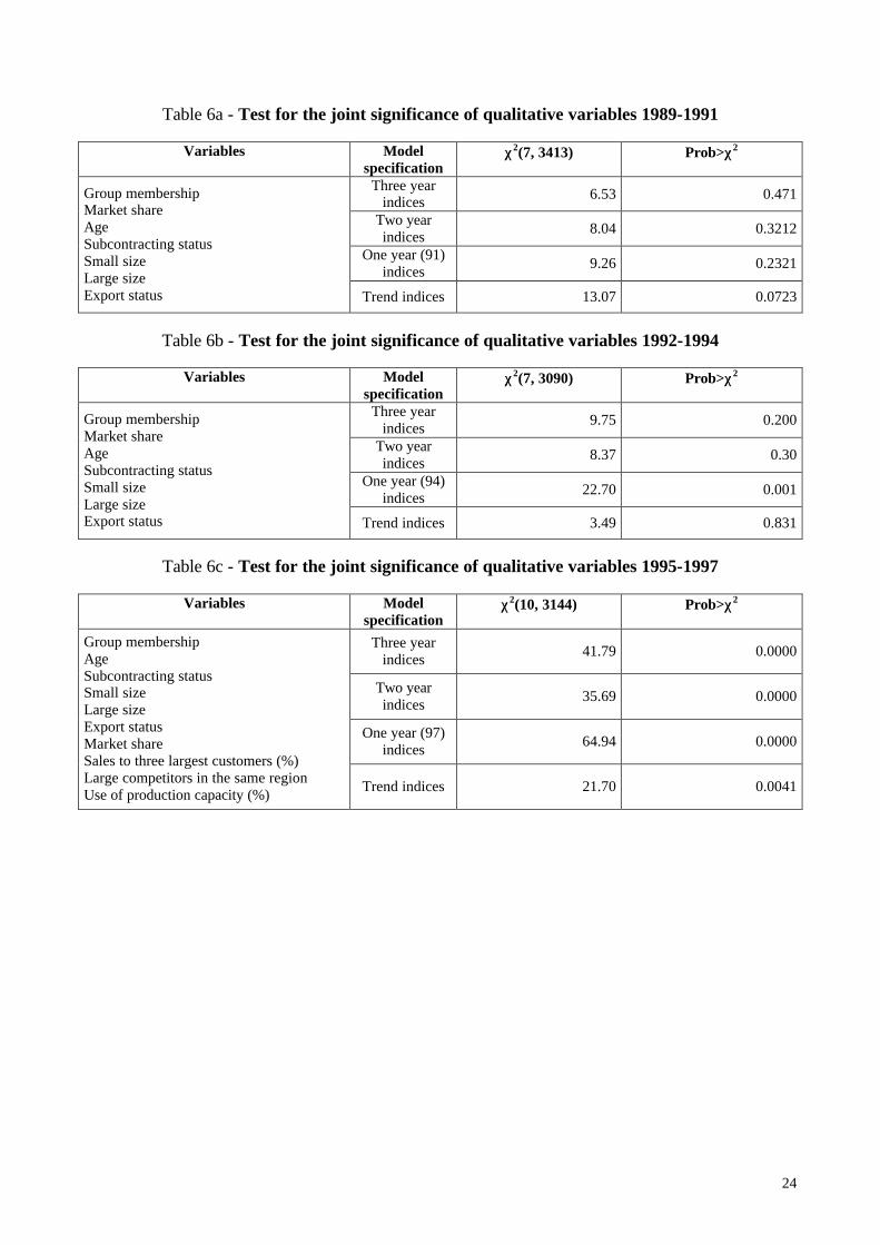
Finally, Tables 6a-5c show that qualitative variables (Group membership, strength of local

competitors, customers’ concentration) become jointly significant in the logit estimate as long as

their information gets richer and new variables are added (second and third sample periods).

[Table 6a to 6c here]

5. Conclusions

34 If we consider differences in macroeconomic scenarios across the three sample periods and evaluate them in the light of theory and empirical findings of the credit view (Gertler et al., 1990; Kashyap et al., 1993), we may consider part of sample specificity as depending on changes in the monetary policy stance. In fact, the public debt and currency crisis occurred in Italy in 1992 generated a shift toward restrictive fiscal and monetary policies which may have significantly increased the relative relevance of financial over real bankruptcy risk factors. This would be consistent with the significance, only in the first sample period, of liquidity and leverage indicators which include firm debt. This evidence parallels the large relevance of leverage indicators in Lo (1986) who examines a sample of US firms until 1982 during the shift toward a severe antinflationary monetary policy which generated a significant rise in real interest rates. 35 A result which needs to be interpreted is the positive and significant sign of the net working capital/medium and long term debt ratio, which might reasonably mean that inventories build up more rapidly than usual -i.e., for diving sales- in unsound firms during the considered period(s).

15

A problem of the empirical literature on bankruptcy risk consists in the fact that results cannot

be easily generalised since the significance of the relevant variables tends to be sample specific. In

addition, limits to the information available and the traditional approach adopted by banks generally

lead researchers to restrict the scope of the analysis to balance sheet variables. Furthermore, the

potentially unlimited number of firms that can be included in the control sample leads them to build

ad hoc balanced samples with the obvious limits arising when the dependent variable is observed

before sampling.

We think that our paper provides insights to solve some of the above mentioned problems in at least

four respects.

First, results from this paper suggest that only one of the indicators traditionally considered in the

empirical analysis – interest charges over value added - is not sample specific being significant in

each of the three considered sample periods.

Second, our results show that non-balance sheet items (such as customers' concentration,

subcontracting status, export status, presence of large competitors in the same region) significantly

improve the explanatory power of models predicting bankruptcy.

Third, our findings indicate that a firm’s productive inefficiency (measured as the distance from the

“best practice” with the stochastic frontier approach) is a significant ex ante indicator of business

failure.

Fourth, our results show that, in the second and third sample periods, a firm’s productive efficiency

adds additional explanatory power to models that include balance sheet and qualitative variables to

predict business failure.

16

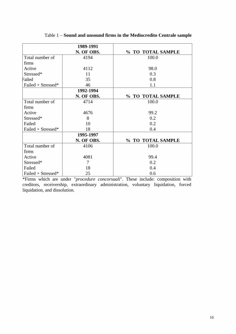
Table 1 – Sound and unsound firms in the Mediocredito Centrale sample

1989-1991 N. OF OBS. % TO TOTAL SAMPLE

Total number of firms

4194 100.0

Active 4112 98.0 Stressed* 11 0.3

ffffff Failed 35 0.8 Failed + Stressed* 46 1.1 1992-1994 N. OF OBS. % TO TOTAL SAMPLE Total number of firms

4714 100.0

Active 4676 99.2 Stressed* 8 0.2 Failed 10 0.2 Failed + Stressed* 18 0.4

1995-1997 N. OF OBS. % TO TOTAL SAMPLE

Total number of firms

4106 100.0

Active 4081 99.4 Stressed* 7 0.2 Failed 18 0.4 Failed + Stressed* 25 0.6

*Firms which are under "procedure concorsuali". These include: composition with creditors, receivership, extraordinary administration, voluntary liquidation, forced liquidation, and dissolution.

17

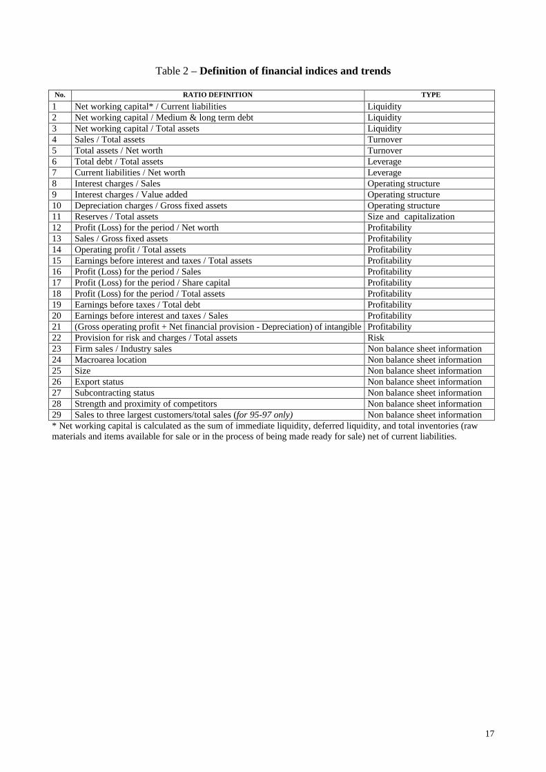
Table 2 – Definition of financial indices and trends

No. RATIO DEFINITION TYPE

1 Net working capital* / Current liabilities Liquidity 2 Net working capital / Medium & long term debt Liquidity 3 Net working capital / Total assets Liquidity 4 Sales / Total assets Turnover 5 Total assets / Net worth Turnover 6 Total debt / Total assets Leverage 7 Current liabilities / Net worth Leverage 8 Interest charges / Sales Operating structure 9 Interest charges / Value added Operating structure 10 Depreciation charges / Gross fixed assets Operating structure 11 Reserves / Total assets Size and capitalization 12 Profit (Loss) for the period / Net worth Profitability 13 Sales / Gross fixed assets Profitability 14 Operating profit / Total assets Profitability 15 Earnings before interest and taxes / Total assets Profitability 16 Profit (Loss) for the period / Sales Profitability 17 Profit (Loss) for the period / Share capital Profitability 18 Profit (Loss) for the period / Total assets Profitability 19 Earnings before taxes / Total debt Profitability 20 Earnings before interest and taxes / Sales Profitability 21 (Gross operating profit + Net financial provision - Depreciation) of intangible Profitability 22 Provision for risk and charges / Total assets Risk 23 Firm sales / Industry sales Non balance sheet information 24 Macroarea location Non balance sheet information 25 Size Non balance sheet information 26 Export status Non balance sheet information 27 Subcontracting status Non balance sheet information 28 Strength and proximity of competitors Non balance sheet information 29 Sales to three largest customers/total sales (for 95-97 only) Non balance sheet information * Net working capital is calculated as the sum of immediate liquidity, deferred liquidity, and total inventories (raw materials and items available for sale or in the process of being made ready for sale) net of current liabilities.

18

Table 3a - Stochastic frontier results - 1989-1991 sample*

Variable Coef. t-ratio Coef. t-ratio Coef. t-ratio Coef. t-ratio Constant 4.343 97.665 4.351 92.583 0.109 0.337 -0.050 -0.216 Ln (K/L) 0.571 16.166 0.569 16.211 Small size 0.373 4.485 0.382 4.492 Size -0.040 -0.445 -0.031 -0.333 Age -0.006 -2.383 -0.005 -2.621 North-West -8.323 -16.463 -8.242 -14.861 North-East -0.081 -0.997 -0.088 -1.071 South -0.191 -2.314 -0.183 -2.164 Market share 0.515 5.777 0.517 5.685 Subsidies 0.217 3.854 0.213 3.699 Innovation -0.003 -0.026 0.003 0.025 Export -0.686 -10.138 -0.709 -10.794 Active -0.161 -0.807 Failed + stressed 0.223 0.899 Sigma-squared 0.599 20.802 0.607 19.285 Gamma 0.514 18.207 0.518 16.635 Log likelihood -3288.905 -3273.320 No. of obs. 3514 3493

Table 3b - Stochastic frontier results - 1992-1994 sample*

Variable Coef. t-ratio Coef. t-ratio Coef. t-ratio Coef. t-ratio Constant 4.837 101.703 4.829 98.972 2.635 6.244 2.255 5.475 Ln (K/L) 0.713 9.771 0.716 9.582 Small size -0.055 -0.738 -0.092 -1.212 Size 0.117 1.529 0.107 1.400 Age -0.001 -0.376 -0.001 -0.900 North-west -0.013 -0.168 -0.028 -0.373 North-east -0.228 -2.730 -0.259 -3.237 South 0.472 5.291 0.484 5.535 Market share -14.573 -2.442 -14.470 -2.265 Subsidies -0.032 -0.546 -0.034 -0.615 Innovation -0.014 -0.237 -0.029 -0.505 Export -0.734 -11.599 -0.774 -12.648 Active -0.508 -2.968 Failed + stressed 0.677 2.715 σ2 0.432 18.865 0.441 20.472 γ 0.371 7.934 0.386 9.121 Log likelihood 2674.306 2658.674 No. of obs. 3182 3163

19

Table 3c - Stochastic frontier results - 1995-1997 sample* Variable Coef. t-ratio Coef. t-ratio Coef. t-ratio Coef. t-ratio

Constant 5.217 105.816 5.265 113.467 3.111 8.526 2.214 7.067 Ln (K/L) 0.563 9.334 0.516 8.675 Small size -0.359 -9.120 -0.346 -8.842 Size -0.013 -0.236 0.045 0.752 Age 0.002 1.769 0.002 2.065 North-west 0.098 1.881 0.081 1.490 North-east 0.078 1.370 0.061 1.028 South 0.504 8.358 0.468 7.627 Market share -20.256 -4.926 -36.293 -10.586 Subsidies -0.007 -0.202 0.003 0.076 Innovation -0.038 -0.999 -0.028 -0.709 Export -0.338 -8.273 -0.331 -8.023 Sales to the three largest customers 0.004 5.621 0.003 4.668 Competitors in same area 0.054 1.630 0.048 1.471 Capacity utilization -0.009 -7.099 -0.008 -6.079 Active -0.644 -4.008 Failed + stressed 0.670 3.644 σ2 0.338 27.795 0.343 29.159 γ 0.235 6.220 0.264 7.469 Log likelihood 2546.678 2541.386 No. of obs. 3195 3195 *Coefficents and t-stats for the following 19 industry dummy variables are omitted for reasons of space and are available upon request:

1 Food, beverages, and tobacco; 2 Textile and clothing; 3 Leather and shoes; 4 Wood, wood products, and furniture; 5 Paper, paper products, printing, and publishing; 6 Chemicals; 7 Rubber and plastic products; 8 Glass and ceramic products; 9 Construction industry; 10 Metal extraction; 11 Metal products; 12 Mechanical materials; 13 Mechanical equipment; 14 Electronic equipment; 15 Electric equipment; 16 Precision instrument and apparels; 17 Transport vehicles; 18 Transport - Other; 19 Energy production.

20

Fig. 1a - The ex ante distance from the efficiency frontier of failed and stressed firms (1989-1991 sample)

Fallite: failed or stressed firms; Sfdistance: the distance from the efficient frontier

falli

te

ineff.061575 .969172

0

1

21

Fig. 1b - The ex ante distance from the efficiency frontier of failed and stressed firms (1992-1994 sample)

Fallite: failed or stressed firms; Sfdistance: the distance from the efficient frontier

Fig. 1c - The ex ante distance from the efficiency frontier of failed and stressed firms (1995-1997 sample)

Fallite: failed or stressed firms; Sfdistance: the distance from the efficient frontier

falli

te

sfdistance.06309 .966224

0

1

falli

te

sfdistance.060698 .950624

0

1

22

Table 4 – Distance from efficiency frontier and the logit model 1989-91 sample 1992-94 sample 1995-97 sample Odds

Ratio z-value Odds

Ratio z-value Odds

Ratio z-value

Net working capital / Current liabilities 0.998 -0.39 -1.733 -2.12 0.028 1.66 Net working capital / Medium & long term debt 1.060 3.29 -0.015 -0.55 0.108 3.19 Net working capital / Total assets 0.254 -0.84 7.327 2.25 -4.415 -1.78 Sales / Total assets 0.859 -0.23 -0.493 -0.65 0.770 1.69 Total debt / Total assets 58.005 2.77 5.278 2.21 1.139 0.98 Current liabilities / Net worth 1.004 1.85 0.017 1.99 0.003 0.56 Interest charges / Value added 3.205 2.98 0.012 0.1 0.179 1.54 Depreciation charges / Gross fixed assets 0.001 -1.46 -19.273 -2.11 -1.561 -0.33 Reserves / Total assets 0.002 -2 -3.160 -1.2 -1.424 -0.54 Profit (Loss) for the period / Net worth 0.944 -1.63 0.077 1.2 -0.052 -2.92 Sales / Gross fixed assets 1.000 -0.25 -0.180 -0.83 -0.080 -1.23 Operating profit / Total assets 3.653 0.38 -8.413 -3.84 -11.185 -2.88 Profit (Loss) for the period / Sales 1.308 1.16 -1.112 -2.93 0.092 0.08 Earnings before taxes / Total debt 9.707 2.2 -0.566 -1.07 -0.334 -3.54 Group membership 0.885 -0.3 -1.456 -1.72 -1.554 -1.67 Age 1.002 0.65 -0.016 -1.14 -0.019 -1.02 Subcontracting status 1.616 1.24 -0.427 -0.61 -0.121 -0.19 Small size 0.888 -0.21 0.618 0.69 -1.297 -1.73 Large size 1.902 1.07 0.571 0.72 -1.544 -0.63 Export status 1.199 0.41 0.729 0.84 -0.211 -0.36 Operating risk 2.03 1.87 -15.670 -0.87 6.066 1.12 Inefficiency 26.620 0.84 6.369 1.84 8.089 1.83 Inter25 0.089 -0.54 0.056 0.01 23.819 2.7 Inter75 0.154 -0.93 -2.761 -1.02 -5.056 -1.22 Market share 0.03 -1.39 42.423 2.11 Sales to the three largest customers (%) 0.023 1.66 Competitors in the same area 1.802 2.79 Capacity utilisation 0.03587 1.14 Number of Observations 2911 3147 Wald test χ2(35,

3405) 147.78 χ2(30,

2911) 240.77 χ2(33,

3147) 406.66

Log likelihood -168.307 64.3948 69.37983 Pseudo R2 0.193 0.3148 0.402 Inefficiency: Distance from the efficiency frontier; Inter25: Inefficiency*D25 where D25 is a dummy taking up the value of one for the quartile of firms with the highest distance from the efficiency frontier; Inter75: Inefficiency*D75 where D75 is a dummy taking up the value of one for the quartile of firms with the lowest distance from the efficiency frontier

23

Table 5 – Variables significantly affecting the probability of bankruptcy in the logit analysis Model 1989 - 1991 1992 - 1994 1995 - 1997

Three-year

Indices

Net working capital / Medium & long term debt (+) Total debt / Total assets (+) Current liabilities / Net worth (+) (+) Interest charges / Value added (+)Reserves / Total assets (-) Earnings before taxes / Total debt (+)

Total debt / Total assets (+)Operating profit / Total assets (-) group members. (-) Current Profit (Losses) / Sales (-) market share (+) Earnings before taxes / Total debt (-)

Net working capital / Medium & long term debt (+) Current Profits (Losses) / Net worth (-) Operating profit / Total assets (-) Earnings before taxes / Total debt (-) Customers' concentration (+) Strength of local competitors (+)

Two-year

Indices

Net working capital / Medium & long term debt (+) Total debt / Total assets (+) Interest charges / Value added (+) Reserves / Total assets (-)

Reserves / Total assets (-) Operating profit / Total assets (-) group members. (-) market share (+)

Net working capital / Medium & long term debt (+) Interest charges / Value added (+) Earnings before taxes / Total debt (-) Group members. (-) small size (-) Strength of local competitors (+)

One-year

Indices

Current liabilities / Net worth (+) Total debt / Total assets (+) Industry 8 (+) Interest charges / Value added (+) Reserves / Total assets (-)

Interest charges / Value added (+) Operating profit / Total assets (-) market share (+) Reserves / Total assets (-)

Net working capital / Current liabilities (+) group members. (-) Interest charges / Value added (+) Current Profits (Losses) / Net worth (-) customers' concentration (+)

Three-year

Trends*

Interest charges / Sales (Up) (+) Net working capital / Total assets (Down) (-) Industry 11 (+) Total assets / Net worth (Down )(+) Depreciation charges / Gross fixed assets (Down )(-) Reserves / Total assets (Down )(+)

Interest charges / Sales (Up) (+) Sales / Gross fixed assets (Up) (-)Group members. (-)

Interest charges / Value added (Up) (+) Group members. (-) Sales / Gross fixed assets (Up) (+) Size (+) Sales / Gross fixed assets (Down) (+) Operating profit / Total assets (Down )(-) Current profits (Losses) / Total assets (Down) (-)

The dependent dichotomic variable stands for the probability of "firm failure", delimited by the [0,1] interval, and is represented by the dual "active/failed" enterprise state, according to the definitions explained in section 2. Three year model means three year averages of data (from year –3 to year –1) plus the year of the distress (year 0). Two year model means two year averages of data (from year –2 to year –1) plus the year of the distress (year 0).

(+): the variable has positive and significant effect on the dependent variable at 95 percent significance level

(-): the variable has negative and significant effect on the dependent variable at 95 percent significance level

*A trend is represented by a three-year period in which the indicator moves in the same direction.

(Up) (Down). For increasing (decreasing) trends the dummy variable is called up (down) and it is given the value of 1 or zero otherwise.

24

Table 6a - Test for the joint significance of qualitative variables 1989-1991

Variables Model specification

χχ2(7, 3413) Prob>χχ2

Three year indices 6.53 0.471

Two year indices

8.04 0.3212

One year (91) indices

9.26 0.2321

Group membership Market share Age Subcontracting status Small size Large size Export status Trend indices 13.07 0.0723

Table 6b - Test for the joint significance of qualitative variables 1992-1994

Variables Model

specification χχ2(7, 3090) Prob>χχ2

Three year indices

9.75 0.200

Two year indices

8.37 0.30

One year (94) indices

22.70 0.001

Group membership Market share Age Subcontracting status Small size Large size Export status Trend indices 3.49 0.831

Table 6c - Test for the joint significance of qualitative variables 1995-1997

Variables Model

specification χχ2(10, 3144) Prob>χχ2

Three year indices

41.79 0.0000

Two year indices

35.69 0.0000

One year (97) indices

64.94 0.0000

Group membership Age Subcontracting status Small size Large size Export status Market share Sales to three largest customers (%) Large competitors in the same region Use of production capacity (%)

Trend indices 21.70 0.0041

25

REFERENCES

Aigner D., Knox Lovell, C.A., Schmidt, P., 1977, Formulation and estimation of stochastic frontier production function models, Journal of Econometrics, 6, 21-37.

Allen, L. Rai A., 1996, Operational efficiency in banking: an international comparison, Journal of Banking and Finance, 20 655-672

Altman, E., 1968, Financial ratios, discriminant analysis and prediction of corporate bankrupcty, Journal of Finance, 22, 589-610.

Altman, E., 1984, A Further Empirical Investigation of the Bankruptcy Cost Question, in Journal of Finance, September, v. 39, iss. 4, pp. 1067-89

Altman, E., Baidya, T. K. N., Ribeiro Dias, L. M., 1979, Assessing Potential Financial Problems for Firms in Brazil, in Journal of International Business Studies, Fall, v. 10, iss. 2, pp. 9-24

Altman, E., and Lavallee, M., 1981, Business failure classification, in Canada in Journal of Business Administration, summer

Altman, E., Marco, G., and Varetto, F., 1994. Corporate distress diagnosis: Comparisons using linear discriminant analysis and neural networks (the Italian experience). Journal of Banking and Finance, (18), 505-529.

Aly H.Y., Grabowsky R., Pasurka, C., Rangan N., 1990, Technical scale and allocative efficiencies in US banking: an empirical investigation, Review of Economics and Statistics, 72, 211-18.

Appetiti, S., 1984. Identifying unsound firms in Italy. An attempt to use trend variables. Journal of Banking an Finance, (8), 269-279.

Aw, B.Y., A.Hwang, 1995, Productivity and export marker: a firm level analysis, Journal of Development Economics, 47, 209-231.

Bank for International Settlements, 2001, The New Basel Capital Accord: an explanatory note, January, Barontini, R., 1992. L'efficacia dei modelli di previsione delle insolvenze: Risultati di una verifica

empirica. Finanza, Imprese e Mercati, (1), 141-185.

Battese, G. E., and Coelli, T.J., 1995. A model for technical inefficiency effects in a stochastic frontier production function for panel data. Empirical economics, (20), 325-332.

Beaver, W., 1966. Financial ratios as predictors of failure. Empirical Research in Accounting: Selected Studies, supplement to Journal of Accounting Research, (4), 71-127.

Becchetti, L. Santoro, M., 2001, The determinants of small-medium firm internationalisation and its effects on productive efficiency, Weltwirtschaftliche Archiv, 2, (forth.)

Begley, J., Ming, J. and Watts, S., 1996, Bankruptcy Classification Errors in the 1980's: An Empirical Analysis of Altman's and Ohlson's Models, Review of accounting studies, Berger, A. N. and L. J. Mester (1997), "Inside the Black Box: What Explains Differences in the

Efficiencies of Financial Institutions?" Journal of Banking and Finance 21:7 (July), 895-947. Bilderbeek, J., 1977, Financiële ratio analyse (Stenfert-Kroese, Leiden). Clerides, S.K., Lach, S. and Tybout, 1998, Is learning-by-exporting important? Micro-dynamic

evidence from Colombia, Mexico and Morocco, Quarterly Journal of Economics, vol CXIII, August, 903-947

Cowing T.G., Reifschneider D., R.E. Stevenson, 1983, A comparison of alternative frontier cost function specifications, In Developments in Econometric Analyses of productivity, A. Dogramaci (ed.), Kluwer, Nijhoff.

Hunt Mc Cool, J.; Koh, S. C.; Francis, B. B., 1996, Testing for Deliberate Underpricing in the IPO Premarket: A Stochastic Frontier Approach, Review of Financial Studies; 9(4), pp. 1251-69.

26

Kashyap A.K., Lamont O. A.,Stein J. C., (1993), “Credit conditions and the cyclical behaviour of inventories”, Federal Reserve Bank of Chicago, Working Paper n. 7.

Delgado, M.A., Farinas, J.C., 1999, Firm's productivity and export markets: a nonparametric approach, mimeo.

De Meza D., Webb D.C., (1987), “Too Much Investment : A Problem of Asymmetric Information”, Quarterly Journal of Economics, 101, pp. 282-292.

Duffie D. and Lando D. (1998). “Term Structure of Credit Spreads with Incomplete Accounting Information”, Stanford University Working Paper.

Edmister, R., 1972. An empirical test of financial ratio analysis for small business failure prediction. Journal of Financial and Quantitative Analysis. 7 (2), 1477-1493.

Everett, J., and Watson, J., 1998. Small business failure and external risk factors. Small Business Economics, (11), 371-390.

Fanti, L., 1997. Inefficienza tecnica e di scala: un'applicazione all'industria italiana di una frontiera flessibile di produzione. L'Industria, a. XVIII (2), 271-282.

Foglia, A., Laviola, S., and Marullo-Reedtz, P., 1998. Multiple banking relationships and the fragility of corporate borrowers. Journal of Banking and Finance, (22), 1441-1456.

Frydman, H.; Altman, E. I.; Kao, D. L., 1985, Introducing Recursive Partitioning for Financial Classification: The Case of Financial Distress, Journal of Finance; 40(1), 269-91.

Gentry, J.A., Newbold, P., and Whitford, D.T., 1987, Flow of funds components, financial ratios and bankruptcy, Journal of Business Finance & Accounting, 14(4), 595-606.

Gertler, M.; Hubbard, R. G.; Kashyap, A. K., 1990, Interest Rate Spreads, Credit Constraints, and Investment Fluctuations: An Empirical Investigation, Board of Governors of the Federal Reserve System Finance and Economics Discussion Series: 137, October 1990, pages 42.

Gilson S.C., 1988, Transaction costs and capital structure choice: evidence from financially distressed firms, Journal of Finance, 52(1), 160-196.

Gilson, A.C. 1989, Management turnover and financial distress, Journal of Financial Economics, 25 241-262. Gilson S.C., Vetsuypens, 1993, M.R., CEO compensation in financially distressed firms: an

empirical analysis, Journal of Finance, 48(2), 425-458. Greene, W., 1990, A gamma distributed stochastic frontier model, Journal of Econometrics, 46,

141-63. Kaparakis, E. I.; Miller, S. M.; Noulas, A.G., 1994, Short-Run Cost Inefficiency of Commercial

Banks: A Flexible Stochastic Frontier Approach, Journal of Money Credit and Banking; 26(4), 875-93.

Keasey, K., and Watson, R., 1987. Non-financial symptoms and the prediciton of small company failure: a test or Argenti's hypotheses. Journal of Business Finance and Accounting. 14 (3), 335-354.

Keasey, K., and Mc Guinnes, P., 1990, The failure of UK industrial firms for the period 1976-1984, logistic analysis and entropy measures, Journal of Business Finance & Accounting, 17(1), pp. 119-135.

Laviola, S., and Trapanese, M., 1997. Previsione delle insolvenze delle imprese e qualità del credito bancario: Un’analisi statistica. Temi di discussione del Servizio Studi, Banca D’Italia, (318).

Lo, A. W., 1986. Logit versus discriminant analysis. A specification test and application to corporate bankruptcies. Journal of Econometrics. 31, 151-178.

Maddala G.S., Introduction to econometrics 2nd edition, MacMillan Publishing Company 1992

Maksimovic, V., Phillips, G., 1998, Asset efficiency and reallocation decisions of bankrupt firms, Journal of Finance, 53(5), 1495-1532.

27

Milde, H. and Riley, J.G., 1988, Signalling in Credit Markets, Quarterly Journal of Economics, 103, 101-29.

Ministero dell’Industria and MedioCredito Centrale, 1999. Indagine sulle imprese manifatturiere. Settimo rapporto sull’industria italiana e sulla politica industriale. MCC. Roma.

Neyman, J. (1934). On two different aspects of the representative method: the method of stratified sampling and the method of purposive selection, Journal of the Royal Statistical Society, 97: 558-625. Nickell, P.; Perraudin, W.; Varotto, S., 2000, Stability of Rating Transitions, Journal of Banking

and Finance; 24(1-2), pp. 203-27. Nickell, S.J., 1996. Competition and corporate performance. Journal of Political Economy. 104 (4),

724-746.

Ohlson, J.A., 1980, Financial rations and the probabilistic prediction of bankruptcy, Journal of Accounting Research, 18 (1), 109-131.

Putnam, R., (with Robert Leonardi and Raffaella Y.Nanetti) Making Democracy Work (Princeton NJ, Princeton University Press, 1993)

Scazzieri, R., 1981. Efficienza produttiva e livelli di attività. Un contributo di teoria economica. Il Mulino, Bologna.

Skogsvik, K., 1990. Current cost accounting ratios as predictors of business failure: the Swedish case. Journal of Business Finance & Accounting, 17 (1), 137-160.

Stiglitz, J. and A.Weiss, 1981, Credit Rationing in Markets with Imperfect Information, American Economic Review 71, 912-927.

Stiglitz J., Weiss A., (1986), “Credit rationing: reply”, American Economic Review, 77, 228-31. Stiglitz, J., Weiss, A. (1992), “Asymmetric Information in credit markets and its implications for

macroeconomics”, Oxford Economic Papers, 44, pp. 694-724. Xu, B, ,2000, The Welfare Implications of Costly Monitoring in the Credit Market: a Note Economic JournalVol. 110, Issue 463, p576. Zavgren, C. V., 1985. Assessing the vulnerability to failure of American industrial firms: a logistic

analysis. Journal of Business Finance & Accounting, 12 (1), 19-45.

Zmijewsky, M.E., 1984, Methodological issues related to the estimation of financial distress prediction models, Journal of Accounting Research, Vol. 22, 59-82.

28

Appendix (not to be published)

Table A1.a – Comparison of index mean values 1989-1991 (broad failure definition) RATIO LEVEL RATIO VARIATION INDICES

ACTIVE FAILED ACTIVE FAILED No. Variable Mean Mean Mean Mean 1 Cc_pscme 1.585 0.197 0.297 3.946 2 Cc_dmlme 1.299 0.661 0.217 17.510 3 Cc_atme 0.126 0.020 0.146 2.905 4 Fat_atme 0.993 0.926 0.195 0.050 5 At_patme 8.667 22.957 0.083 0.013 6 Db_attme 0.576 0.692 -0.0003 0.011 7 Ps_patme 4.603 17.643 0.144 0.065 8 Of_fatme 0.055 0.080 0.626 0.193 9 Of_vame 0.137 0.290 0.374 0.110 10 Am_iflme 0.089 0.074 0.176 0.246 11 Ri_attme 0.101 0.046 0.585 -2.114 12 Pr_patme 0.058 -0.112 -10.07 -13.75 13 Fa_iflme 5.934 5.782 0.122 0.099 14 Mon_atme* 0.066 0.051 -0.199 -0.744 15 Pr_fatme 0.013 -0.028 -1.940 -4.184 16 Pr_csme 1.716 -11.796 -0.600 1.103 17 Pr_atme 0.018 0.00003 -1.847 -6.843 18 Ui_dtme 0.084 0.045 -0.700 -1.642 19 Mon_fame 0.071 0.031 -0.299 -1.007 20 Returnme 0.030 -0.023 -0.798 -1.826 21 Opriskme 0.006 0.008 0.568 0.840 22 Market share 0.002 0.001 0.602 0.209

Table A.1b – Comparison of index mean values 1989-1991 (conservative failure definition) RATIO LEVEL RATIO VARIATION INDICES

ACTIVE STRESSED FAILED ACTIVE STRESSED FAILED No. Variable Mean Mean Mean Mean Mean Mean 1 Cc_pscme 1.585 0.257 0.007 0.297 5.347 -0.259 2 Cc_dmlme 1.299 0.670 0.634 0.217 23.378 -0.092 3 Cc_atme 0.126 0.025 0.004 0.146 3.949 -0.228 4 Fat_atme 0.993 0.859 1.139 0.195 0.055 0.034 5 At_patme 8.667 7.912 70.827 0.083 -0.039 0.169 6 Db_attme 0.576 0.673 0.752 -0.0004 0.012 0.007 7 Ps_patme 4.603 4.432 59.676 0.144 0.021 0.198 8 Of_fatme 0.055 0.082 0.071 0.626 0.202 0.169 9 Of_vame 0.137 0.299 0.260 0.374 0.089 0.172 10 Am_iflme 0.089 0.071 0.085 0.176 0.208 0.361 11 Ri_attme 0.101 0.052 0.027 0.585 -3.389 2.190 12 Pr_patme 0.058 -0.104 -0.137 -10.069 -18.282 -0.169 13 Fa_iflme 5.934 3.184 14.049 0.122 0.055 0.231 14 Mon_atme* 0.066 0.052 0.045 -0.199 -0.923 -0.204 15 Pr_fatme 0.013 -0.034 -0.007 -1.940 -5.499 -0.240 16 Pr_csme 1.716 -15.458 -0.147 -0.600 1.522 -0.153 17 Pr_atme 0.018 0.002 -0.008 -1.847 -9.016 -0.324 18 Ui_dtme 0.084 0.062 -0.011 -0.700 -2.113 -0.231 19 Mon_fame 0.071 0.030 0.033 -0.299 -1.278 -0.193 20 Returnme 0.030 -0.030 -0.002 -0.798 -2.370 -0.195 21 Opriskme 0.006 0.006 0.014 0.568 0.978 0.358 22 Market share 0.002 0.001 0.001 0.602 0.148 0.393 *Operating profit not available from 1989 balance-sheet data. EBIT has been used to calculate the index. Ratio ut_atme is then equivalent to mon_atme.

29

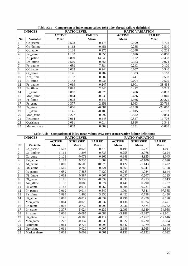
Table A2.a – Comparison of index mean values 1992-1994 (broad failure definition)

RATIO LEVEL RATIO VARIATION INDICES ACTIVE FAILED ACTIVE FAILED

No. Variable Mean Mean Mean Mean 1 Cc_pscme 0.503 0.178 -0.199 -3.702 2 Cc_dmlme 1.112 -0.451 0.255 -2.510 3 Cc_atme 0.128 0.175 -0.348 -3.201 4 Fat_atme 1.182 0.855 0.076 -0.068 5 At_patme 6.869 14.048 0.122 -0.458 6 Db_attme 0.560 0.758 0.363 0.071 7 Ps_patme 4.659 7.684 0.243 0.109 8 Of_fatme 0.062 0.244 0.057 0.340 9 Of_vame 0.176 0.282 0.333 0.163 10 Am_iflme 0.137 0.082 0.441 0.508 11 Ri_attme 0.142 0.035 -0.004 -0.505 12 Pr_patme 0.019 -0.247 -1.901 -38.468 13 Fa_iflme 7.895 2.340 0.422 0.243 14 Ut_atme 0.067 -0.025 0.496 -0.802 15 Mon_atme 0.064 -0.030 0.436 -1.040 16 Pr_fatme -0.002 -0.449 -2.936 -20.275 17 Pr_csme 0.377 -2.853 -2.093 -20.739 18 Pr_atme 0.006 -0.087 -3.188 -24.050 19 Ui_dtme 0.145 -0.108 -0.015 -9.102 20 Mon_fame 0.227 -0.092 0.522 -0.884 21 Returnme 0.014 -0.445 -0.547 -11.726 22 Opriskme 0.011 0.014 2.888 2.341 23 Market share 0.002 0.002 0.131 -0.088

Table A.2b – Comparison of index mean values 1992-1994 (conservative failure definition)

RATIO LEVEL RATIO VARIATION INDICES ACTIVE STRESSED FAILED ACTIVE STRESSED FAILED

No. Variable Mean Mean Mean Mean Mean Mean 1 Cc_pscme 0.503 0.025 0.370 -0.199 -5.771 -1.041 2 Cc_dmlme 1.112 -1.398 0.733 0.255 -3.978 -0.624 3 Cc_atme 0.128 -0.079 0.166 -0.348 -4.925 -1.045 4 Fat_atme 1.182 0.735 1.004 0.076 -0.106 -0.020 5 At_patme 6.869 16.506 10.975 0.122 -1.143 0.422 6 Db_attme 0.560 0.788 0.721 0.363 0.041 0.108 7 Ps_patme 4.659 7.888 7.429 0.243 -1.084 1.644 8 Of_fatme 0.062 0.387 0.067 0.057 0.507 0.125 9 Of_vame 0.176 0.539 -0.039 0.333 0.253 0.013 10 Am_iflme 0.137 0.089 0.074 0.441 0.290 0.787 11 Ri_attme 0.142 0.014 0.062 -0.004 -0.721 -0.228 12 Pr_patme 0.019 0.014 -0.540 -1.901 7.341 -97.365 13 Fa_iflme 7.895 1.460 3.330 0.422 0.758 0.458 14 Ut_atme 0.067 -0.017 -0.034 0.496 0.278 -2.190 15 Mon_atme 0.064 -0.025 -0.037 0.436 0.074 -2.471 16 Pr_fatme -0.002 -0.730 -0.098 -2.936 -7.474 -36.732 17 Pr_csme 0.377 -5.024 -0.139 -2.093 -9.680 -34.958 18 Pr_atme 0.006 -0.085 -0.088 -3.188 -9.387 -42.901 19 Ui_dtme 0.145 -0.103 -0.114 -0.015 -2.457 -17.646 20 Mon_fame 0.227 -0.137 -0.035 0.522 0.220 -2.304 21 Returnme 0.014 -0.727 -0.093 -0.547 -1.979 -24.259 22 Opriskme 0.011 0.020 0.007 2.888 2.565 1.894 23 Market share 0.002 0.002 0.001 0.131 -0.132 -0.022

30

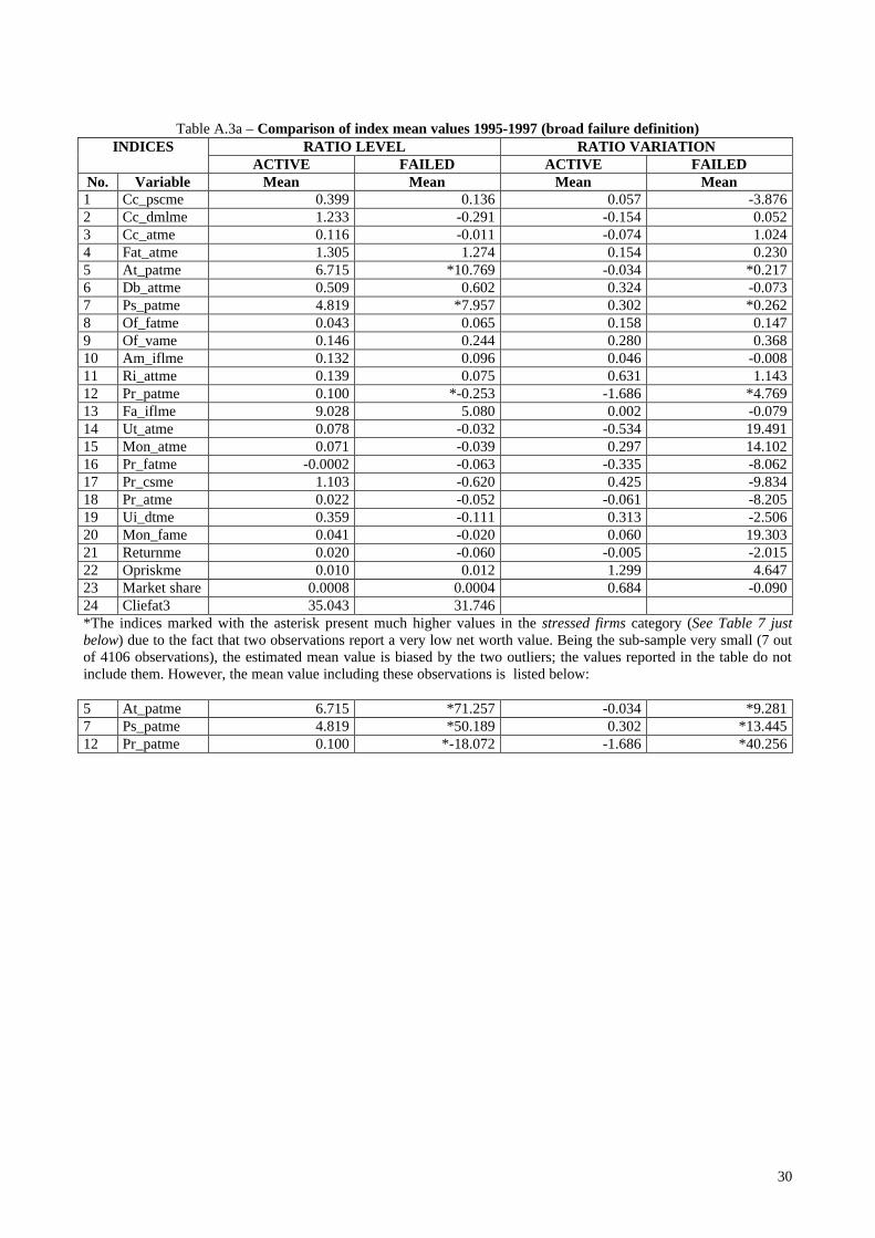
Table A.3a – Comparison of index mean values 1995-1997 (broad failure definition)

RATIO LEVEL RATIO VARIATION INDICES ACTIVE FAILED ACTIVE FAILED

No. Variable Mean Mean Mean Mean 1 Cc_pscme 0.399 0.136 0.057 -3.876 2 Cc_dmlme 1.233 -0.291 -0.154 0.052 3 Cc_atme 0.116 -0.011 -0.074 1.024 4 Fat_atme 1.305 1.274 0.154 0.230 5 At_patme 6.715 *10.769 -0.034 *0.217 6 Db_attme 0.509 0.602 0.324 -0.073 7 Ps_patme 4.819 *7.957 0.302 *0.262 8 Of_fatme 0.043 0.065 0.158 0.147 9 Of_vame 0.146 0.244 0.280 0.368 10 Am_iflme 0.132 0.096 0.046 -0.008 11 Ri_attme 0.139 0.075 0.631 1.143 12 Pr_patme 0.100 *-0.253 -1.686 *4.769 13 Fa_iflme 9.028 5.080 0.002 -0.079 14 Ut_atme 0.078 -0.032 -0.534 19.491 15 Mon_atme 0.071 -0.039 0.297 14.102 16 Pr_fatme -0.0002 -0.063 -0.335 -8.062 17 Pr_csme 1.103 -0.620 0.425 -9.834 18 Pr_atme 0.022 -0.052 -0.061 -8.205 19 Ui_dtme 0.359 -0.111 0.313 -2.506 20 Mon_fame 0.041 -0.020 0.060 19.303 21 Returnme 0.020 -0.060 -0.005 -2.015 22 Opriskme 0.010 0.012 1.299 4.647 23 Market share 0.0008 0.0004 0.684 -0.090 24 Cliefat3 35.043 31.746 *The indices marked with the asterisk present much higher values in the stressed firms category (See Table 7 just below) due to the fact that two observations report a very low net worth value. Being the sub-sample very small (7 out of 4106 observations), the estimated mean value is biased by the two outliers; the values reported in the table do not include them. However, the mean value including these observations is listed below:

5 At_patme 6.715 *71.257 -0.034 *9.281 7 Ps_patme 4.819 *50.189 0.302 *13.445 12 Pr_patme 0.100 *-18.072 -1.686 *40.256

31

Table A.3b – Comparison of index mean values 1995-1997 (conservative failure definition)

RATIO LEVEL RATIO VARIATION INDICES ACTIVE STRESSED FAILED ACTIVE STRESSED FAILED

No. Variable Mean Mean Mean Mean Mean Mean 1 Cc_pscme 0.399 0.219 -0.774 0.057 -4.342 -2.478 2 Cc_dmlme 1.233 0.024 -1.101 -0.154 0.748 -2.034 3 Cc_atme 0.116 0.016 -0.080 -0.074 2.202 -2.510 4 Fat_atme 1.305 1.398 0.955 0.154 0.321 -0.042 5 At_patme 6.715 *8.557 15.509 -0.034 *0.329 -0.064 6 Db_attme 0.509 0.604 0.595 0.324 -0.049 -0.144 7 Ps_patme 4.819 *6.124 11.885 0.302 *0.346 0.053 8 Of_fatme 0.043 0.063 0.069 0.158 0.119 0.231 9 Of_vame 0.146 0.264 0.193 0.280 0.523 -0.047 10 Am_iflme 0.132 0.100 0.086 0.046 0.00001 -0.029 11 Ri_attme 0.139 0.096 0.022 0.631 0.594 3.120 12 Pr_patme 0.100 *-0.331 -0.075 -1.686 *-0.973 20.081 13 Fa_iflme 9.028 4.453 6.693 0.002 -0.085 -0.062 14 Ut_atme 0.078 -0.044 0.00004 -0.534 26.741 -2.259 15 Mon_atme 0.071 -0.052 -0.005 0.297 19.583 -2.341 16 Pr_fatme -0.0002 -0.067 -0.053 -0.335 -0.979 -29.311 17 Pr_csme 1.103 -0.001 -2.211 0.425 -0.990 -36.367 18 Pr_atme 0.022 -0.054 -0.047 -0.061 -0.492 -31.344 19 Ui_dtme 0.359 -0.068 -0.221 0.313 0.973 -12.945 20 Mon_fame 0.041 -0.026 -0.002 0.060 26.486 -2.245 21 Returnme 0.020 -0.063 -0.052 -0.005 0.310 -8.989 22 Opriskme 0.010 0.005 0.030 1.299 1.734 12.415 23 Market share 0.0008 0.0005 0.0003 0.684 -0.096 -0.077 24 Cliefat3 35.043 41.824 69.333 *The indices marked with the asterisk present much higher values in the stressed firms category due to the fact that two observations report a very low net worth value. Being the sub-sample very small (7 out of 4106 observations), the estimated mean value is biased by the two outliers; the values reported in the table do not include them. However, the mean value including these observations is listed below: 5 At_patme 6.715 *92.938 15.509 -0.034 *12.397 -0.064 7 Ps_patme 4.819 *65.085 11.885 0.302 *17.909 0.053 12 Re_patme 0.100 *-25.070 -0.075 -1.686 *46.981 20.081