ICT Investments and Technical Efficiency in Italian Manufacturing Firms:

The Productivity Paradox Revisited

Concetta Castiglione

TEP Working Paper No. 0408

October 2008

Trinity Economics Papers Department of Economics Trinity College Dublin

1

ICT Investments and Technical Efficiency in Italian Manufacturing

Firms: The Productivity Paradox Revisited

Concetta Castiglione1

Department of Economics

Trinity College Dublin

castiglc@tcd.ie

Abstract: From the Seventies the importance of information and communication technologies (ICTs) has

been a much debated question. A lot of studies are made in order to understand if the ICTs are able to

increase economic growth, firm productivity and firm efficiency. In this study both the translog and the

Cobb-Douglas production function are used in order to estimate the impact of information and

communication technology on technical efficiency (TE) in the Italian manufacturing firms over the period

1995-2003. Results show that ICT investments positively and significantly affect firm technical

efficiency. Moreover, group, size and geographical position are able to influence positively TE. Finally,

results show that older firms are in average more efficient than younger ones.

Keywords: ICT investment, Productivity Paradox, Stochastic Frontier, Italian manufacturing firms

Jel: D21, L63, O33

Introduction

The impact of information and communication technology (ICT) is a topic that has

received increased attention from economist during the past two decades. In fact, for the

past twenty years, the impact of ICTs on economic growth has been the subject of

numerous studies at aggregate and firm level.

During the 1980s and early 1990s many researchers asserted that the ICT

contribution to productivity and economic growth was either very small or non-existent.

These findings are often associated with Solow's paradox, which states that: “You can

see the computer age everywhere but in the productivity statistics”. Nevertheless, the

latest studies increasingly assert the importance of new technologies.

The empirical literature studies, overall, the relationship between ICT investments

and labour productivity or ICT investments and multifactor productivity (MFP). Some

attempt is done to study the relationship between ICT investments and technical

efficiency at firm level.

This work starts from previous literature and moves in two directions. Firstly, two

different production functions, Cobb-Douglas and Translog, are used to explore

investments and the distance from the ‘‘best practice’’ by using a stochastic frontier

approach. Both production functions are used since the Cobb-Douglas requires the

elasticity of substitution between factors to be unity and, on the other side, the translog

production function is a generalization of the Cobb-Douglas which relaxes this

1 This study was financially supported by a Scholarship provided by “Regione Calabria”. The author

wishes to thank Prof. Davide Infante and Dr. Carol Newman for valuable comments and suggestions on

an earlier draft.

2

restriction. Secondly, ICT technologies are considered as a factor able to influence the

technical efficiency.

In this work the impact of ICT technologies on technical efficiency is analysed under

the hypothesis that a greater use of ICT at firm and economy level may help the firms to

increase their production process efficiency. The purpose of this work it is investigate

whether ICT investments significantly affect firm distance from optimal production

frontier. In order to test this hypothesis the stochastic frontier production function is

adopted, utilising an unbalanced panel data of Italian manufacturing firms constructed

from the VII, VIII and IX survey provided by Mediocredito Centrale-Capitalia (MCC).

Other works use the same survey (VII or VIII) to study the relationship between ICT

investments and productivity growth and multifactor productivity growth or technical

efficiency.

Results show that ICT investments have a positive effect on technical efficiency of

Italian manufacturing firms when ICT is considered as a firm specific factor.

The remainder of the work is structured as follows: the first section focuses on the

productivity paradox in an historical perspective. The second section presents the

economic literature on ICT investments at firm level. The third section analyses the

methodology, which encompasses the economic model and the empirical approach to

evaluate the relationship between ICT and the distance from “efficient frontier” and

description of the data used. Finally results and comments are presented.

1. Information Technology: Paradox Lost?

Robert Solow's (1987) assertion that “You can see the computer age everywhere but in

the productivity statistics” is still object of investigation, although the latest studies

increasingly assert the importance of new technologies. In fact, the recent productivity

and GDP growth has been related mainly to the impact of information and

communication technology investments.

A lot of economists described this debated controversy as “the productivity

paradox”. The paradox was raised in the late 1980s and questioned if ICT fails to

deliver its promised returns in increasing productivity. However, the productivity

paradox seemed to disappear after Brynjolfsson and Hitt (1996) presented their

significant firm-level empirical evidence to claim that the paradox was solved by the

beginning of 1990s.

Today, the importance of new technologies can be observed in many studies, both in

theoretical and applied economics. In fact, for the past twenty years the impact of ICTs

on economic growth has been the subject of numerous studies at different levels: i.e.

firms, industries and countries (Oliner and Sichel, 2000; Jorgenson, 2001).

Gordon (2000, 2002) which expressed different conclusions in the past, now affirm

that ICT investments contribute, more than other technologies, to economic growth.

Moreover, more than ten years after the statement of the paradox, Solow himself

admitted that the statistics are beginning to measure the computer age, even if modestly

at the moment2. There is now persuasive evidence that the information and

communication technology investments boom of the 1990s has led to significant

changes in the absolute and relative productivity performance of firms, sectors and

countries. For example, at microeconomic level, Brynjolfsson and Hitt (2000) and

2 Solow is quoted as such in Gordon (2002)

3

Gilchrist et al. (2001) show that those payoffs to ICT investments occur not just in

labour productivity but also in multifactor productivity.

Empirical analysis of economic growth and productivity typically distinguishes three

effects of ICT (Kenneth et al., 1994; Pilat, 2004). The first one is the “production

effect”: the firms where these technologies are produced can help economic growth at

an aggregate level, either through a rapid increase in demand for these products,

compared to other sectors, or through a higher productivity in the same sector. The

second one is the “using effect”: the firms belonging to traditional sectors increase the

capital stock per worker (capital deepening) in order to gain new technologies, this

implies an increase in products per worker. Moreover, a greater use of ICT throughout

the economy may help firms to increase their overall efficiency. Furthermore, greater

use of ICT may contribute to network effects, such as lower transaction costs and more

rapid innovation, which should also improve MFP. In fact, the third one is “total factor

productivity” effect: the new technology adoption improves the performance of all the

used factors. Consequently, the output increases without further input of investments.

An increase in total factor productivity means that, at a given input level and a fixed

quality, an economy always obtains higher output levels (Castiglione, 2008).

2. Stochastic Frontier Approach

In this work, to verify the contribution of ICT investment on firm productivity, a

stochastic production frontier approach is adopted. The production frontier, which

characterizes the relationship between inputs and output, specifies the maximum output

achievable by employing a combination of inputs. The distance between the production

frontier and the actual output is regarded as its technical inefficiency. Thus, a firm either

operates below the frontier when it is technically inefficient or it operates on the

production frontier when it is technically efficient.

Technical efficiency is concerned with the maximization of output for a given set of

inputs and indicates how far the firm can increase its output without absorbing further

resources. A technically inefficient firm could produce the same output with less or at

least one input or could use the same inputs to produce more of at least one output.

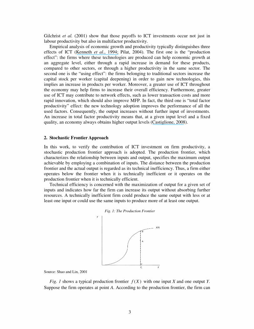
Fig. 1: The Production Frontier

Source: Shao and Lin, 2001

Fig. 1 shows a typical production frontier )(Xf with one input X and one output Y.

Suppose the firm operates at point A. According to the production frontier, the firm can

4

increase its output level to the point B using the same amount of input 1X and, hence,

the distance AB can be regarded as technical inefficiency for the firm under

consideration. “However a better definition is to use the ratio AB/BC to represent

technical inefficiency and AC/BC (=1-AB/BC) to represent the TE. One advantage of

these ratio measures for technical efficiency is that they are unit invariant; i.e. changing

the units of measurements does not change the scores of efficiency measurement. This

ratio of technical efficiency will take on a value between zero and one, with a higher

score implying higher technical efficiency” (Shao and Lin, 2001: 448).

The concept of TE was elaborated by Farrell (1957). Farrell stated that the efficiency

of a firm consists of two components: technical efficiency and allocative efficiency. TE

is concerned with the maximization of output for a given set of resource inputs and

indicates the ability of a firm to obtain maximal output from a given set of inputs. The

allocative efficiency reflects the ability of a firm to use the inputs in optimal

proportions, given their respective price and the production technology.

Together the technical and the allocative efficiency provide a measure of a total

economic efficiency.

The measurement of technical efficiency has widely been associated with the use of

production frontier functions. Several techniques to determine these frontier functions

have been used: parametric and non-parametric. The choice of the estimation method

has been an issue of debate (Seiford, 1996) since every method has its advantages and

disadvantages.

The principal advantage of the estimation of a non-parametric production frontier,

using for example the data envelopment analysis (DEA) technique, is that it does not

require any assumptions on the functional form. “The data points in the data set are

compared with one another for efficiency. The most efficient observations are utilized

to construct the piece-wise linear convex nonparametric frontier” (Shao and Lin, 2002:

393). Neither does DEA require an explicit assumption about the inefficiency term.

However, “because DEA is deterministic and attributes all the deviations from the

frontier to inefficiencies, a frontier estimated by DEA is likely to be sensitive to

measurement errors or other noise in the data” (Odeck, 2007: 2618). In other words,

using this kind of technique, it is not possible to distinguish if the lack of efficiency is

due to technical inefficiency or to statistical noise effects.

The parametric approach requires the assumption of a specific functional form (e.g.

Cobb-Douglas, translog, constant elasticity of substitution - CES) for the technology

(constant or variable returns to scale) and an explicit distributional assumption for the

inefficiency term. It uses the statistical technique to estimate the coefficients of the

production function as well as the technical efficiency.

The main strengths are that the parametric approach deals with stochastic noise and

also allows statistical tests of hypotheses concerning production structure and degree of

inefficiency. Then, the first step in parametric stochastic frontier estimation is to select

an appropriate functional form for the production function.

The Cobb-Douglas functional form is easy to estimate, since a logarithmic

transformation provides a model that is linear. However, this simplicity is associated

with a number of restrictive properties. It assumes constant input elasticities and

constant returns to scale for all firms in the sample. Further, the elasticities of

substitution for the Cobb-Douglas function are equal to one.

The alternative functional forms used in the stochastic frontier literature are:

translog, CES and Zellner-Revankar generalized production function. The latter avoids

5

the returns to scale restriction while the former imposes no restrictions upon returns to

scale or substitution possibilities.

A number of studies (Carroll et al., 2007, Shao and Lin, 2001 and Gholami et al.,

2004) have estimated both the Cobb-Douglas and the translog functional form and some

of them (Carroll et al., 2007) have tested the null hypothesis that the Cobb-Douglas

form is an adequate representation of the data, given the specifications of the translog

model.

2.1 Cobb-Douglas and Translog Production Frontier

The Cobb-Douglas production frontier has been one of the most frequently used

functional specification in the research on production economics. It satisfies the basic

requirements for production frontiers, such as quasi-concavity and monotonicity. It

imposes properties upon the production structure such as a fixed return to scale value

and an elasticity of substitution equal to the unity.

The Cobb-Douglas stochastic production frontier with two inputs, capital (K) and

labour (L), and one output (Y) can be specified as: iiLk uv

iii eLKY−= ββα

where i is the index that considers the number of firms. After taking natural logarithm

the production function can be rewritten in the following way:

iiiLiKi uvLKY −+++= lnln)ln( ββα

The random error iv is assumed to be independent and identically distributed (i.i.d.)

with zero mean and constant variance ),0( 2

vN σ .

On the other hand, the residual component iu of technical inefficiency represents the

effects of events incurred by the firm. “These technical inefficiency are assumed to be

non-negative random variable of independently (but not identically distributed)

truncated normal distributions. The underlying normal distribution is assumed to be

),( 2

µσµiN . The truncated normal distribution of iu stipulates technical inefficiency be

non-negative only and dependent on some firm-specific characteristics” (Shao and Lin,

2001: 449).

TE is predicted using the conditional expectations of )exp( iU− , given the composed

error term of the stochastic frontier. Thus, given the above model specification, the

technical efficiency of a firm can be defined as:

)exp( iUTE −= .

Technical efficiency equals to one only if a firm has an inefficiency effect equal to

zero; otherwise it is less than one. If iU is equal to zero, this means that there is no

inefficiency in production, the firm is technically efficient and produces its maximum

potential output. Conversely, when iU takes values less than zero this implies that there

is inefficiency in the firm’s production and it produces less than its maximum possible

output given the technology. The magnitude of iU specifies the “efficiency gap”, that is

how far a given firm’s output is from its potential output. In order to compute TE it is,

therefore, necessary to estimate the potential output, which can be done by the

econometric estimation of the stochastic frontier production function.

6

A number of alternative functional forms have also been used in the production

frontier literature. The most popular is the translog function.

The two input translog stochastic production frontier can be specified in the

following way:

[ ] iiiiKLiLLiKKiLiKi uvLKLKLKY −++++++= lnln)(ln)(ln2

1lnln)ln( 22 βββββα

The assumptions on the random error iv and the technical efficiency

iu remain the

same as in the Cobb-Douglas stochastic production frontier.

The translog function does not impose the same restriction upon the production

structure such as the Cobb-Douglas production function does, but it can suffer from

degrees of freedom and multicollinearity problems. However, the Cobb-Douglas

stochastic production frontier is a special case of the translog stochastic production

frontier under the following restrictions:

0=β=β=β KLLLKK

The translog function is non-homogeneous and belongs to the class of flexible

functional form, which provides a second-order local approximation to any functional

form (Coelli et al., 1998).

2.2 Stochastic Frontier for Panel Data Panel data models have some advantages over cross-sectional data in the estimation of

stochastic frontier models. Schmidt and Sickles (1984) assert that the first advantage is

that while cross-section models assume that the inefficiency term and the input levels

are independent, for panel data estimation this hypothesis is not needed. This is useful

in order to introduce time-invariant regressors in the specification of the model.

Moreover, by adding temporal observations in the same unit, panel data stochastic

frontier models yield consistent estimates of the inefficiency term. Furthermore, by

exploiting the link between the “one-sided inefficiency term” and the “firm effect”

concepts, Schmidt and Sickles (1984) observed that, when panel data are available,

there is no need for any distribution assumption for the inefficiency effect and all the

relevant parameters of the frontier technology can be obtained by simply using the traditional estimation procedures for panel data; i.e. fixed-effects model and random-

effects model approaches. Finally, panel data permit the simultaneous investigation of

both technical change and technical efficiency change over time.

The panel data stochastic frontier models can be written in the following way:

TtNiuvXYN

n

ititnitnit ,...,2,1 ;,...,2,1 ,1

0 ==−++= ∑=

ββ

where itY denotes the output for the thi firm at the th

t time period, itX denotes a (1xk)

vector of inputs associated with the suitable functional form, β is a (kx1) vector of

unknown scalar parameters to be estimated, itu are the inefficiency effects in the model

and itv are random errors, assumed to be i.i.d. and have )σN( v

20, distribution,

independent of the itu .

Sometimes it is assumed that technical inefficiency effects are time invariant:

TtNiuu iit ,...,2,1 ;,...,2,1 === .

“The assumption that technical inefficiency effects are time-invariant is more

difficult to justify as T becomes larger. One would expect that managers learn from

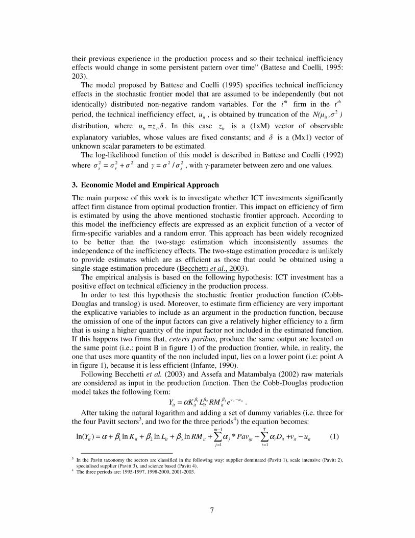
7

their previous experience in the production process and so their technical inefficiency

effects would change in some persistent pattern over time” (Battese and Coelli, 1995:

203).

The model proposed by Battese and Coelli (1995) specifies technical inefficiency

effects in the stochastic frontier model that are assumed to be independently (but not

identically) distributed non-negative random variables. For the thi firm in the th

t

period, the technical inefficiency effect, itu , is obtained by truncation of the )σ,N(µit

2

distribution, where δ=zu itit . In this case itz is a (1xM) vector of observable

explanatory variables, whose values are fixed constants; and δ is a (Mx1) vector of

unknown scalar parameters to be estimated.

The log-likelihood function of this model is described in Battese and Coelli (1992)

where 222 σ+σ=σ vs and 22 / sσσ=γ , with γ-parameter between zero and one values.

3. Economic Model and Empirical Approach

The main purpose of this work is to investigate whether ICT investments significantly

affect firm distance from optimal production frontier. This impact on efficiency of firm

is estimated by using the above mentioned stochastic frontier approach. According to

this model the inefficiency effects are expressed as an explicit function of a vector of

firm-specific variables and a random error. This approach has been widely recognized

to be better than the two-stage estimation which inconsistently assumes the

independence of the inefficiency effects. The two-stage estimation procedure is unlikely

to provide estimates which are as efficient as those that could be obtained using a

single-stage estimation procedure (Becchetti et al., 2003).

The empirical analysis is based on the following hypothesis: ICT investment has a

positive effect on technical efficiency in the production process.

In order to test this hypothesis the stochastic frontier production function (Cobb-

Douglas and translog) is used. Moreover, to estimate firm efficiency are very important

the explicative variables to include as an argument in the production function, because

the omission of one of the input factors can give a relatively higher efficiency to a firm

that is using a higher quantity of the input factor not included in the estimated function.

If this happens two firms that, ceteris paribus, produce the same output are located on

the same point (i.e.: point B in figure 1) of the production frontier, while, in reality, the

one that uses more quantity of the non included input, lies on a lower point (i.e: point A

in figure 1), because it is less efficient (Infante, 1990).

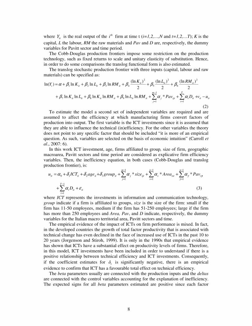
Following Becchetti et al. (2003) and Assefa and Matambalya (2002) raw materials

are considered as input in the production function. Then the Cobb-Douglas production

model takes the following form: itit uv

itititit eRMLKY−= 321 βββα .

After taking the natural logarithm and adding a set of dummy variables (i.e. three for

the four Pavitt sectors3, and two for the three periods

4) the equation becomes:

(1) *lnlnln)ln(1

1 1

321 itit

m

j

T

t

itiijtjitititit uvDPavRMLKY −++++++= ∑ ∑−

= =

ααβββα

3 In the Pavitt taxonomy the sectors are classified in the following way: supplier dominated (Pavitt 1), scale intensive (Pavitt 2),

specialised supplier (Pavitt 3), and science based (Pavitt 4). 4 The three periods are: 1995-1997, 1998-2000, 2001-2003.

8

where itY is the real output of the thi firm at time t (i=1,2,…,N and t=1,2,…T); K is the

capital, L the labour, RM the raw materials and Pav and D are, respectively, the dummy

variables for Pavitt sector and time period.

The Cobb-Douglas production frontiers impose some restriction on the production

technology, such as fixed returns to scale and unitary elasticity of substitution. Hence,

in order to do some comparisons the translog functional form is also estimated.

The translog stochastic production frontier with three inputs (capital, labour and raw

materials) can be specified as:

*lnlnlnlnlnln

2

)(ln

2

)(ln

2

)(lnlnlnln)ln(

1

1 1

987

2

6

2

5

2

4321

itit

m

j

T

t

ittijtjitititititit

ititititititi

uvDPavRMLRMKLK

RMLKRMLKY

−++++++

++++++=

∑ ∑−

= =

ααβββ

ββββββα

(2)

To estimate the model a second set of independent variables are required and are

assumed to affect the efficiency at which manufacturing firms convert factors of

production into output. The first variable is the ICT investments since it is assumed that

they are able to influence the technical (in)efficiency. For the other variables the theory

does not point to any specific factor that should be included “it is more of an empirical

question. As such, variables are selected on the basis of economic intuition” (Carroll et

al., 2007: 6).

In this work ICT investment, age, firms affiliated to group, size of firm, geographic

macroarea, Pavitt sectors and time period are considered as explicative firm efficiency

variables. Then, the inefficiency equation, in both cases (Cobb-Douglas and translog

production frontier), is:

(3)

***

1

1

1

1

1

1

1

1

3210

it

T

t

itt

n

ti

n

s

ists

m

j

ijtjitititit

D

PavAreasizegroupageICTu

εα

αααδδδαγ

γγ

++

++++++=

∑

∑∑∑

−

=

−

=

−

=

−

=

where ICT represents the investments in information and communication technology,

group indicate if a firm is affiliated to groups, size is the size of the firm: small if the

firm has 11-50 employees, medium if the firm has 51-250 employees; large if the firm

has more than 250 employees and Area, Pav, and D indicate, respectively, the dummy

variables for the Italian macro territorial area, Pavitt sectors and time.

The empirical evidence of the impact of ICTs on firm performance is mixed. In fact,

in the developed countries the growth of total factor productivity that is associated with

technical change has even declined in the face of increased use of ICTs in the past 10 to

20 years (Jorgenson and Stiroh, 1999). It is only in the 1990s that empirical evidence

has shown that ICTs have a substantial effect on productivity levels of firms. Therefore,

in this model, ICT investments have been included in order to understand if there is a

positive relationship between technical efficiency and ICT investments. Consequently,

if the coefficient estimates for 1δ is significantly negative, there is an empirical

evidence to confirm that ICT has a favourable total effect on technical efficiency.

The beta parameters usually are connected with the production inputs and the deltas

are connected with the control variables accounting for the explanation of inefficiency.

The expected signs for all beta parameters estimated are positive since each factor

9

contributes in a positive way to production. For delta parameters the economic literature

is taken into account.

A positive relationship between age and technical efficiency can be expected due to

learning by doing which occurs through production experience. Over time firms become

more efficient as a result of growing stock of experience in the production process.

However, other economists argue that when an innovation is introduced, younger firms

generally easily adopt it, while older firms may have to delay their adoption as it may

become too expensive and costly to substitute the old products, thus implying that

efficiency may decrease with age. Empirical studies also report mixed results on the

relationship between a firm’s age and technical efficiency. “Some studies have found a

positive relationship between firm age and efficiency (see for instance, Cheng and

Tang, 1987; Haddad, 1993; Biggs, Shah and Srivastava, 1996; Mengiste, 1996). But

other studies have reported a negative relationship between firm efficiency and age (see

for instance, Pitt and Lee, 1981; Little, Mazumdar and Page, 1987; Hill and Kalirajan,

1993). Some other studies have indicated that the effect of age could be neutral (Cheng

and Tang, 1987)” (Assefa and Matambalya, 2002: 20).

The relationship between firms affiliated to groups and TE should be positive in

accord with the literature that affirms that there exists a relatively higher productivity

and superior competitiveness performance of groups with respect to individual firms

(Becchetti, 2003) (i.e. the expected sign is negative).

The effect of firm size on efficiency is ambiguous since empirical evidence does not

suggest a strong link between efficiency and firm size in either direction. “While a

positive effect may be expected on the grounds of scale of economies, firm size may be

negatively linked to efficiency if large firms experience management and supervision

problems” (Assefa and Matambalya, 2002: 20).

Finally, dummy variables for the Italian macro territorial area are also included to

control for regional differences; Pavitt dummy are included because any industrial

sector may have in principle a different production function; and temporal dummies are

included to take into account technological progress. The expected sign for firms

located in the centre or in the north Italy is negative since those firms should be more

efficient than firms located in the south. For the time dummy the expected sign for the

parameter is negative because if technological progress increases then inefficiency can

decrease.

4. Variables and Descriptive Statistics

For this analysis, the VII (1995-1997), VIII (1998-2000) and IX (2001-2003) surveys of

manufacturing firms by MCC were used. The database is published every three years

since 1968.

The survey offers a large amount of observations on the production and financial

indicators of Italian manufacturing firms. In the last survey the database considers a

stratified sample of 3,452 Italian manufacturing firms. The sample is stratified

according to industry, geographical and dimensional distribution for firms from 11 to

500 employees. It is by census for firms with more than 500 employees.

The database contains questionnaire information on the individual firms’ structure

and behaviour and three years of balance sheets data, additional data on employees,

employees’ education, age of the firm, turnover, etc. Information relating to the ICT

expenditure is present only from 1995 and is displayed at a three-year level (1995-1997,

1998-2000 and 2001-2003) and the total annual investment is provided. However, data

10

on the stock of ICT capital are not provided. Also the variable for the employees’

education is displayed as one value in three years.

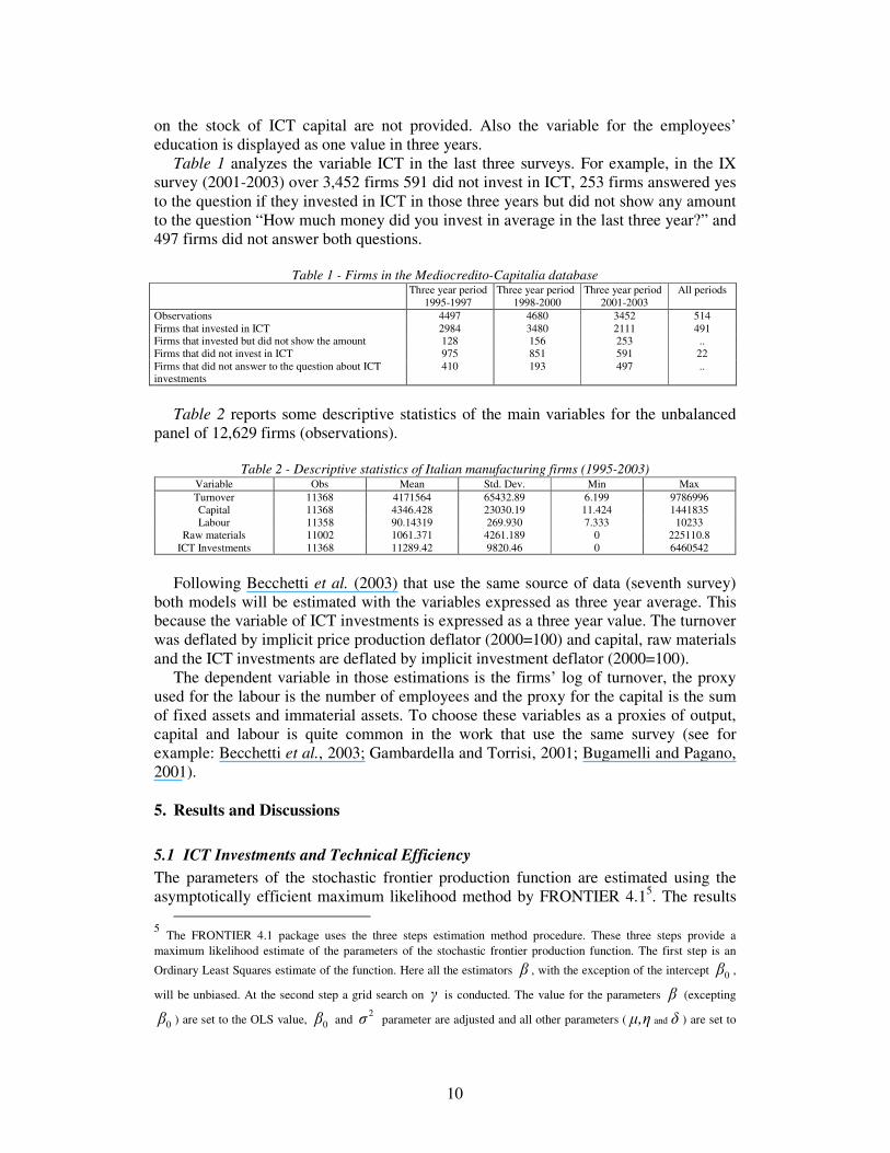
Table 1 analyzes the variable ICT in the last three surveys. For example, in the IX

survey (2001-2003) over 3,452 firms 591 did not invest in ICT, 253 firms answered yes

to the question if they invested in ICT in those three years but did not show any amount

to the question “How much money did you invest in average in the last three year?” and

497 firms did not answer both questions.

Table 1 - Firms in the Mediocredito-Capitalia database

Three year period

1995-1997

Three year period

1998-2000

Three year period

2001-2003

All periods

Observations 4497 4680 3452 514

Firms that invested in ICT 2984 3480 2111 491 Firms that invested but did not show the amount 128 156 253 ..

Firms that did not invest in ICT 975 851 591 22

Firms that did not answer to the question about ICT investments

410 193 497 ..

Table 2 reports some descriptive statistics of the main variables for the unbalanced

panel of 12,629 firms (observations).

Table 2 - Descriptive statistics of Italian manufacturing firms (1995-2003)

Variable Obs Mean Std. Dev. Min Max

Turnover 11368 4171564 65432.89 6.199 9786996

Capital 11368 4346.428 23030.19 11.424 1441835

Labour 11358 90.14319 269.930 7.333 10233

Raw materials 11002 1061.371 4261.189 0 225110.8

ICT Investments 11368 11289.42 9820.46 0 6460542

Following Becchetti et al. (2003) that use the same source of data (seventh survey)

both models will be estimated with the variables expressed as three year average. This

because the variable of ICT investments is expressed as a three year value. The turnover

was deflated by implicit price production deflator (2000=100) and capital, raw materials

and the ICT investments are deflated by implicit investment deflator (2000=100).

The dependent variable in those estimations is the firms’ log of turnover, the proxy

used for the labour is the number of employees and the proxy for the capital is the sum

of fixed assets and immaterial assets. To choose these variables as a proxies of output,

capital and labour is quite common in the work that use the same survey (see for

example: Becchetti et al., 2003; Gambardella and Torrisi, 2001; Bugamelli and Pagano,

2001).

5. Results and Discussions

5.1 ICT Investments and Technical Efficiency

The parameters of the stochastic frontier production function are estimated using the

asymptotically efficient maximum likelihood method by FRONTIER 4.15. The results

5 The FRONTIER 4.1 package uses the three steps estimation method procedure. These three steps provide a

maximum likelihood estimate of the parameters of the stochastic frontier production function. The first step is an

Ordinary Least Squares estimate of the function. Here all the estimators β , with the exception of the intercept 0β ,

will be unbiased. At the second step a grid search on γ is conducted. The value for the parameters β (excepting

0β ) are set to the OLS value, 0β and 2σ parameter are adjusted and all other parameters ( δηµ, and ) are set to

11

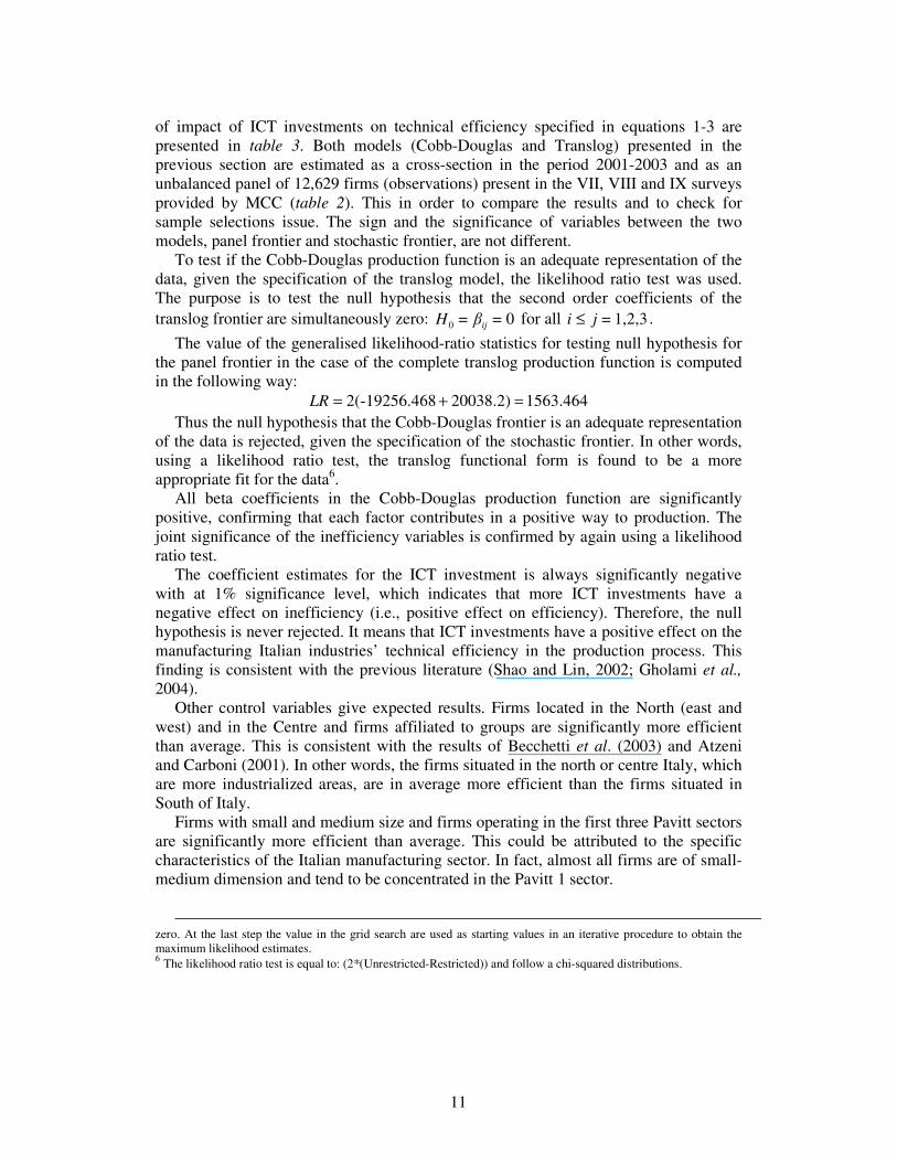
of impact of ICT investments on technical efficiency specified in equations 1-3 are

presented in table 3. Both models (Cobb-Douglas and Translog) presented in the

previous section are estimated as a cross-section in the period 2001-2003 and as an

unbalanced panel of 12,629 firms (observations) present in the VII, VIII and IX surveys

provided by MCC (table 2). This in order to compare the results and to check for

sample selections issue. The sign and the significance of variables between the two

models, panel frontier and stochastic frontier, are not different.

To test if the Cobb-Douglas production function is an adequate representation of the

data, given the specification of the translog model, the likelihood ratio test was used.

The purpose is to test the null hypothesis that the second order coefficients of the

translog frontier are simultaneously zero: 00 =β=H ij for all 1,2,3=ji ≤ .

The value of the generalised likelihood-ratio statistics for testing null hypothesis for

the panel frontier in the case of the complete translog production function is computed

in the following way:

.464156320038.2)-19256.468(2 =+=LR

Thus the null hypothesis that the Cobb-Douglas frontier is an adequate representation

of the data is rejected, given the specification of the stochastic frontier. In other words,

using a likelihood ratio test, the translog functional form is found to be a more

appropriate fit for the data6.

All beta coefficients in the Cobb-Douglas production function are significantly

positive, confirming that each factor contributes in a positive way to production. The

joint significance of the inefficiency variables is confirmed by again using a likelihood

ratio test.

The coefficient estimates for the ICT investment is always significantly negative

with at 1% significance level, which indicates that more ICT investments have a

negative effect on inefficiency (i.e., positive effect on efficiency). Therefore, the null

hypothesis is never rejected. It means that ICT investments have a positive effect on the

manufacturing Italian industries’ technical efficiency in the production process. This

finding is consistent with the previous literature (Shao and Lin, 2002; Gholami et al.,

2004).

Other control variables give expected results. Firms located in the North (east and

west) and in the Centre and firms affiliated to groups are significantly more efficient

than average. This is consistent with the results of Becchetti et al. (2003) and Atzeni

and Carboni (2001). In other words, the firms situated in the north or centre Italy, which

are more industrialized areas, are in average more efficient than the firms situated in

South of Italy.

Firms with small and medium size and firms operating in the first three Pavitt sectors

are significantly more efficient than average. This could be attributed to the specific

characteristics of the Italian manufacturing sector. In fact, almost all firms are of small-

medium dimension and tend to be concentrated in the Pavitt 1 sector.

zero. At the last step the value in the grid search are used as starting values in an iterative procedure to obtain the

maximum likelihood estimates. 6 The likelihood ratio test is equal to: (2*(Unrestricted-Restricted)) and follow a chi-squared distributions.

12

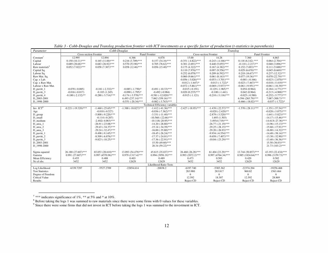
Table 3 - Cobb-Douglas and Translog production frontier with ICT investments as a specific factor of production (t-statistics in parenthesis)

Parameter Cobb-Douglas Translog

Cross-section Frontier Panel Frontier Cross-section Frontier Panel Frontier

Constant7 12.995 12.894 6.366 6.078 15.00 14.28 7.360 6.863

Capital 0.150 (10.11)*** 0.165 (11.00)*** 0.216 (3.709)*** 0.157 (34.16)*** -0.351 (-4.822)*** -0.243 (-4.166)*** 0.118 (6.142) *** 0.064 (2.704)***

Labour 0.689 (28.68)*** 0.683 (26.92)*** 0.570 (53.90)*** 0.705 (78.62)*** 0.301 (2.691)*** 0.440 (5.055)*** -0.110 (-2.217)** 0.048 (3.896)***

Raw materials8 0.052 (7.022)*** 0.058 (7.307)*** 0.058 (12.46)*** 0.056 (15.40)*** 0.175 (4.322)*** 0.167 (4.382)*** 0.152 (7.693)*** 0.111 (5.688)***

Capital Sq. 0.110 (7.976)*** 0.097 (9.556)*** 0.029 (6.670)*** 0.045 (8.669)***

Labour Sq. 0.252 (6.078)*** 0.209 (6.592)*** 0.218 (16.67)*** 0.237 (12.32)***

Raw Mat. Sq. 0.060 (9.661)*** 0.061 (8.163)*** 0.077 (19.36)*** 0.078 (22.79)***

Cap. x Lab. -0.056 (-3.026)*** -0.053 (-3.701)*** -0.001 (-0.166) -0.023 (-2.870)***

Cap. x Raw Mat. -0.012 (-1.647)* -0.013 (-1.722)* -0.023 (-7.467)*** -0.018 (-5.419)***

Labour x Raw Mat. -0.072 (-5.861)*** -0.069 (-5.937)*** -0.061 (-9.951)*** -0.061 (-10.39)***

D_pavitt_1 -0.070 (-0.085) -0.181 (-2.332)** -0.085 (-1.750)* -0.491 (-10.33)*** -0.015 (-0.191) -0.129 (-1.965)** 0.054 (0.964) -0.184 (-4.771)***

D_pavitt_3 -0.016 (-0.017) -0.103 (1.245) -0.090 (-1.795)* -0.492 (-0.984) 0.020 (0.235)*** -0.100 (-1.441) 0.042 (0.964) -0.213 (-4.900)***

D_pavitt_4 -0.180 (-2.132)** -0.288 (-3.714)*** -0.174 (-3.578)*** -0.581 (-12.020)*** -0.915 (-1.121) -0.210 (-3.116)*** -0.025 (-0.580) -0.252 (-5.777)***

D_2003-2001 6.493 (237.14)*** 7.062 (359.16)*** 6.594 (265.79)*** 7.087 (300.7)***

D_1998-2000 -0.551 (-20.34)*** -0.082 (-3.743)*** -0.466 (-18.02)*** -0.037 (-1.722)*

Technical Efficiency variables

Inv. ICT9 -0.221 (-19.320)*** -1.460 (-25.65)*** -1.388 (-18.827)*** -1.412 (-41.36)*** -2.427 (-18.95)*** -1.439 (-22.57)*** -1.570 (-28.11)*** -1.351 (-57.54)***

Age -0.010 (-0.527) -0.036 (-7.362)*** -0.020 (-2.420)** -0.028 (-3.875)***

D_group -5.800 (-9.220)*** -3.331 (-11.40)*** -2.879 (-3.520)*** -1.641 (-5.823)***

D_small -0.114 (-0.207) -10.568 (-22.66)*** 1.693 (1.503) -14.17 (-15.46)***

D_medium -2.402(-4.083)*** -10.118(-20.95)*** 3.493(4.719)*** -14.613(-27.36)***

D_area_1 -26.91 (-23.08)*** -14.20 (-28.80)*** -26.77 (-21.19)*** -14.96 (-15.13)***

D_area_2 -29.43 (-34.37)*** -15.14 (-34.39)*** -29.25 (-28.15)*** -15.68 (-17.91)***

D_area_3 -29.24 (-32.47)*** -16.00 (-35.80)*** -29.20 (-26.93)*** -16.80 (-14.32)***

D_pavitt_1 -9.498 (-9.145)*** -18.45 (-26.24)*** -9.934 (-6.554)*** -14.48 (-38.14)***

D_pavitt_2 -8.509 (-6.876)*** -17.37 (-24.01)*** -9.658 (-7.407)*** -13.38 (-32.90)***

D_pavitt_3 -9.823 (-10.25)*** -17.36 (-22.91)*** -10.04 (-23.29)*** -13.40 (-36.36)***

D_2003-2001 15.50 (49.60)*** 15.50 (36.03)***

D_1998-2000 20.34 (59.22)*** 21.73 (103.2)***

Sigma-squared 26.188 (27.607)*** 65.053 (28.610)*** 13.093 (54.479)*** 45.615 (35.037)*** 26.468 (26.28)*** 61.404 (23.29)*** 13.744 (50.857)*** 43.193 (22.434)***

Gamma 0.991 (27.607)*** 0.997 (4570.96)*** 0.979 (1317.4)*** 0.994 (3958.19)*** 0.993 (2072.2)*** 0.997 (4764.34)*** 0.985 (1824.64)*** 0.996 (3159.73)***

Mean Efficiency 0.455 0.488 0.403 0.489 0.473 0.503 0.420 0.502

Nr of obs 3452 3452 12629 12629 3452 3452 12629 12629

Likelihood Ratio Tests

Log Likelihood -6339.7297 -5527.2709 -22854.614 -20038.2 -6197.740 -5385.362 -22374.204 -19256.468

Test Statistics 283.980 283.817 960.82 1563.464

Degree of Freedom 6 6 6 6

Critical Value 12.592 18.307 12.592 28.869

Results Reject CD Reject CD Reject CD Reject CD

7 *** indicates significance of 1%, ** at 5% and * at 10%. 8 Before taking the logs 1 was summed to raw materials since there were some firms with 0 values for these variables. 9 Since there were some firms that did not invest in ICT before taking the logs 1 was summed to the investment in ICT.

13

Results show, moreover, that older firms are significantly more efficient than

average. This agrees with the theory that over time firms become more efficient as a

result of growing stock of experience in the production process (see Pitt and Lee 1981;

Page 1984; Little, Mazumdar and Page 1987; Haddad and Harrison 1993; Mengiste

1996; Brada, King and Ying Ma 1997).

Mean efficiency is 0.49 which implies that output could theoretically be increased.

This could be ascribed to the fact that ICT investments are still a little portion of total

investments (22%). This partially confirms David’s hypothesis (1990), which states that

new technologies have to reach a spread rate of 50% to show their better effects.

The individual coefficients for the Cobb-Douglas model are elasticities and thus

could be directly interpreted. In the case of the translog model, the elasticities at the

mean levels of output are functions of the parameters and the level of the explanatory

variables, and thus the individual coefficients cannot be directly interpreted as

elasticities. Henceforth, we have calculated the translog elasticities in the following

way, respectively, for capital, labour and raw materials:

1,2,3 t11553,....2,1 3827141

1

==+++= ixxxdx

dYititit

it

ββββ

1,2,3 t;11553,....2,1 3917252

2

==+++= ixxxdx

dYititit

it

ββββ

1,2,3 t11553,....2,1 2918363

3

==+++= ixxxdx

dYititit

it

ββββ

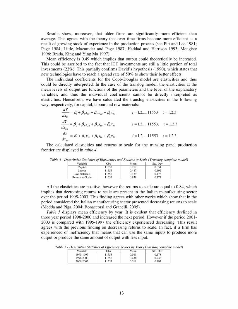
The calculated elasticities and returns to scale for the translog panel production

frontier are displayed in table 4.

Table 4 - Descriptive Statistics of Elasticities and Returns to Scale (Translog complete model)

Variable Obs Mean Std. Dev.

Capital 11553 0.212 0.054

Labour 11553 0.487 0.192

Raw materials 11553 0.139 0.176

Returns to Scale 11553 0.838 0.171

All the elasticities are positive, however the returns to scale are equal to 0.84, which

implies that decreasing returns to scale are present in the Italian manufacturing sector

over the period 1995-2003. This finding agrees with other works which show that in the

period considered the Italian manufacturing sector presented decreasing returns to scale

(Medda and Piga, 2004; Bonaccorsi and Granelli, 2005).

Table 5 displays mean efficiency by year. It is evident that efficiency declined in

three year period 1998-2000 and increased the next period. However if the period 2001-

2003 is compared with 1995-1997 the efficiency experienced decreasing. This result

agrees with the previous finding on decreasing returns to scale. In fact, if a firm has

experienced of inefficiency that means that can use the same inputs to produce more

output or produce the same amount of output with less input.

Table 5 - Descriptive Statistics of Efficiency Scores by Year (Translog complete model)

Variable Obs Mean Std. Dev.

1995-1997 11553 0.561 0.178

1998-2000 11553 0.438 0.235

2001-2003 11553 0.511 0.197

14

5.1.1 Unbalanced Panel and Attrition

With a balanced panel the same units appear in each time period. Conversely, with an

unbalanced panel some units do not appear in each time period. If the reason a firm

leaves the sample (attrition) is correlated with the idiosyncratic error, then the resulting

sample section problem can cause biased estimators (Wooldridge, 2002).

In other words, unbalanced panel data can arise for several reasons (i.e. rotating

panel, incidental truncation). A “problem arises when attrition from a panel is due to

units electing to drop out. If this decision is based on factors that are systematically

related to the response variable, even after we condition on explanatory variables, a

sample selection problem can result” (Wooldridge, 2002: 578).

In order to check if selection is an issue in this paper the balanced panel data is

estimated and a selection indicator is added in the unbalanced panel data.

The results for the balanced panel data estimations are presented in table 6.

Table 6 - Cobb-Douglas and translog production frontier with ICT investments as a specific factor of

production (t-statistics in parenthesis)

Parameter Balanced Panel Frontier

Cobb-Douglas Panel Frontier Translog Panel Frontier

Constant9 6.027 5.579 7.588 7.360

Capital 0.169 (10.03)*** 0.132 (8.75)*** 0.021 (3.248)*** -0.344 (5.303)***

Labour 0.656 (23.07)*** 0.736 (28.91)*** 0.021 (1.603) 0.047 (3.492)*** Raw materials10 0.058 (5.45)*** 0.059 (6.12)*** -0.007 (1.115) 0.039 (6.674)***

Capital Sq. 0.031 (1.96)** 0.040 (2.456)***

Labour Sq. 0.100 (3.39)*** 0.147 (3.609)*** Raw Mat. Sq. 0.058 (6.10)*** 0.060 (6.512)***

Cap. x Lab. 0.006 (3.135)*** -0.001 (-0.920)

Cap. x Raw Mat. -0.016 (-1.588)*** -0.013 (-1.400) Lab. X Raw

Mat.

-0.008 (-4.321)*** -0.026 (-1.350)

D_pavitt_1 -0.107 (-0.629) -0.233 (-1.76)* 0.133 (0.964) -0.131 (-1.080)

D_pavitt_3 -0.088 (-0.508) -0.053 (-0.383) 0.136 (0.996) -0.054 (-4.254)***

D_pavitt_4 -0.170 (-1.003) -0.236 (-1.723)* 0.097 (0.715) -0.102 (-0.805)

D_2003-2001 6.557 (114.60)*** 7.072 (137.98)*** 6.581 (125.81)*** 6.955 (141.7)***

D_1998-2000 -0.239 (-9.36)*** -0.022 (-3.743)*** -0.226 (-4.218)*** -0.011 (-2.211)**

Technical Efficiency variables

Inv. ICT11 -1.139 (-9.358)*** -1.019 (-13.99) *** -1.321 (-10.06)*** -0.671 (-10.61)***

Age -0.065 (-7.507)*** -0.068 (-10.063)***

D_group 0.862 (0.138) -1.350 (-2.498)**

D_small -1.292 (-2.00)** -6.136 (-7.139)***

D_medium -2.215(-3.51)*** -10.784(-11.727)*** D_area_1 -4.53 (-6.07)*** -7.013 (-10.217)***

D_area_2 -8.47 (-10.22)*** -12.381 (-14.40)***

D_area_3 -9.98 (-14.02)*** -13.99 (-14.42)*** D_pavitt_1 -8.24 (-5.93)*** -12.41 (-9.18)***

D_pavitt_2 -1.198 (0.92) -5.00 (-3.290)***

D_pavitt_3 -7.21 (-5.26)*** -10.03 (-6.153)*** D_2003-2001 16.26 (28.97)*** -7.79 (-12.46)***

D_1998-2000 9.28 (-10.77)*** 9.28 (-10.77)***

Sigma-squared 8.289 (16.597) *** 25.943 (11.379)*** 8.547 (16.855)*** 26.330 (22.434)***

Gamma 0.973 (367.2) *** 0.992 (1099.90)*** 0.978 (446.69)*** 0.994 (1580.65)***

Mean Efficiency 0.485 0.574 0.503 0.580

Nr of obs 1542 1542 1542 1542

Likelihood Ratio Tests

Log Likelihood -22854.614 -20038.2 -2341.86 -1939.39

Test Statistics 57.33 107.78

Degree of Freed. 6 6

Critical Value 12.592 28.869

Results Reject CD Reject CD 9*** indicates significance of 1%, ** at 5% and * at 10%. 10 Before taking the logs 1 was summed to raw materials since there were some firms with 0 values for these variables. 11 Since there were some firms that did not invest in ICT before taking the logs 1 was summed to the investment in ICT.

15

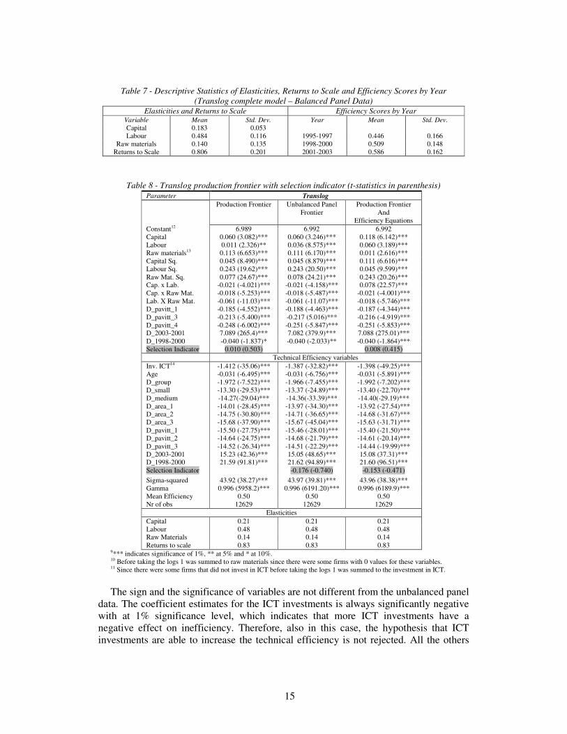
Table 7 - Descriptive Statistics of Elasticities, Returns to Scale and Efficiency Scores by Year

(Translog complete model – Balanced Panel Data)

Elasticities and Returns to Scale Efficiency Scores by Year Variable Mean Std. Dev. Year Mean Std. Dev.

Capital 0.183 0.053

Labour 0.484 0.116 1995-1997 0.446 0.166

Raw materials 0.140 0.135 1998-2000 0.509 0.148

Returns to Scale 0.806 0.201 2001-2003 0.586 0.162

Table 8 - Translog production frontier with selection indicator (t-statistics in parenthesis)

Parameter Translog

Production Frontier Unbalanced Panel

Frontier

Production Frontier

And

Efficiency Equations

Constant12 6.989 6.992 6.992

Capital 0.060 (3.082)*** 0.060 (3.246)*** 0.118 (6.142)***

Labour 0.011 (2.326)** 0.036 (8.575)*** 0.060 (3.189)***

Raw materials13 0.113 (6.653)*** 0.111 (6.170)*** 0.011 (2.616)***

Capital Sq. 0.045 (8.490)*** 0.045 (8.879)*** 0.111 (6.616)***

Labour Sq. 0.243 (19.62)*** 0.243 (20.50)*** 0.045 (9.599)***

Raw Mat. Sq. 0.077 (24.67)*** 0.078 (24.21)*** 0.243 (20.26)*** Cap. x Lab. -0.021 (-4.021)*** -0.021 (-4.158)*** 0.078 (22.57)***

Cap. x Raw Mat. -0.018 (-5.253)*** -0.018 (-5.487)*** -0.021 (-4.001)***

Lab. X Raw Mat. -0.061 (-11.03)*** -0.061 (-11.07)*** -0.018 (-5.746)*** D_pavitt_1 -0.185 (-4.552)*** -0.188 (-4.463)*** -0.187 (-4.344)***

D_pavitt_3 -0.213 (-5.400)*** -0.217 (5.016)*** -0.216 (-4.919)***

D_pavitt_4 -0.248 (-6.002)*** -0.251 (-5.847)*** -0.251 (-5.853)*** D_2003-2001 7.089 (265.4)*** 7.082 (379.9)*** 7.088 (275.01)***

D_1998-2000 -0.040 (-1.837)* -0.040 (-2.033)** -0.040 (-1.864)***

Selection Indicator 0.010 (0.503) 0.008 (0.415)

Technical Efficiency variables

Inv. ICT14 -1.412 (-35.06)*** -1.387 (-32.82)*** -1.398 (-49.25)***

Age -0.031 (-6.495)*** -0.031 (-6.756)*** -0.031 (-5.891)***

D_group -1.972 (-7.522)*** -1.966 (-7.455)*** -1.992 (-7.202)***

D_small -13.30 (-29.53)*** -13.37 (-24.89)*** -13.40 (-22.70)***

D_medium -14.27(-29.04)*** -14.36(-33.39)*** -14.40(-29.19)***

D_area_1 -14.01 (-28.45)*** -13.97 (-34.30)*** -13.92 (-27.54)*** D_area_2 -14.75 (-30.80)*** -14.71 (-36.65)*** -14.68 (-31.67)***

D_area_3 -15.68 (-37.90)*** -15.67 (-45.04)*** -15.63 (-31.71)***

D_pavitt_1 -15.50 (-27.75)*** -15.46 (-28.01)*** -15.40 (-21.50)*** D_pavitt_2 -14.64 (-24.75)*** -14.68 (-21.79)*** -14.61 (-20.14)***

D_pavitt_3 -14.52 (-26.34)*** -14.51 (-22.29)*** -14.44 (-19.99)***

D_2003-2001 15.23 (42.36)*** 15.05 (48.65)*** 15.08 (37.31)*** D_1998-2000 21.59 (91.81)*** 21.62 (94.89)*** 21.60 (96.51)***

Selection Indicator -0.176 (-0.740) -0.153 (-0.471)

Sigma-squared 43.92 (38.27)*** 43.97 (39.81)*** 43.96 (38.38)***

Gamma 0.996 (5958.2)*** 0.996 (6191.20)*** 0.996 (6189.9)***

Mean Efficiency 0.50 0.50 0.50

Nr of obs 12629 12629 12629

Elasticities

Capital 0.21 0.21 0.21

Labour 0.48 0.48 0.48 Raw Materials 0.14 0.14 0.14

Returns to scale 0.83 0.83 0.83 9*** indicates significance of 1%, ** at 5% and * at 10%. 10 Before taking the logs 1 was summed to raw materials since there were some firms with 0 values for these variables. 11 Since there were some firms that did not invest in ICT before taking the logs 1 was summed to the investment in ICT.

The sign and the significance of variables are not different from the unbalanced panel

data. The coefficient estimates for the ICT investments is always significantly negative

with at 1% significance level, which indicates that more ICT investments have a

negative effect on inefficiency. Therefore, also in this case, the hypothesis that ICT

investments are able to increase the technical efficiency is not rejected. All the others

16

variables are of the expected sign and the interpretation can be the same as before. The

Cobb-Douglas panel frontier is rejected in favour of the translog panel frontier.

Table 7 presents the results for elasticities, returns to scale and efficiency by year for

the translog complete model.

The results for the calculated elasticities and the returns to scale are similar to the

previous point. In fact, the elasticities are all positive and the returns to scale are equal

to 0.81, which confirms the previous finding that decreasing returns to scale are present

in the Italian manufacturing sector over the period 1995-2003.

The only difference with the unbalanced panel is that in this case the efficiency

scores by year is also increasing from 1995-1997 to 1998-2000. However, also in this

case mean efficiency is 0.51 which implies that output could theoretically be increased.

The second step of the attrition analysis is to construct the selection indicator. The

selection indicator assumes a value of 0 for the firms that are always present in the

panel and for attriters the selection indicator is equal to 1 in the period just before

attrition (Wooldridge, 2002).

The selection indicator is included in the production function and in the efficiency

equation (and separately, to make sure identification is not an issue). The results are

displayed in Table 8. In this case the null hypothesis is: itu is uncorrelated with its for

all periods, where its represents the selection indicators. In all cases the null hypothesis

cannot be rejected, then it is possible conclude that selection is not a problem in this

sample.

Conclusions

The impact of ICT investments on firms’ performances was a much debated topic since

the Solow’s assertion that “You can see the computer age everywhere but in the

productivity statistics”. A lot of economists referred to this assertion as “the

productivity paradox”.

However, the productivity paradox seemed solved after Brynjolfsson and Hitt (1996)

presented their significant firm-level empirical evidence. In fact, recent studies have

been able to show the positive relation between ICT investments and productivity, and

consequently, aim the controversy over the ICT productivity paradox.

In this work the impact of ICT technologies on technical efficiency is analysed using

an unbalanced panel data (1995-2003) of Italian manufacturing firms. The data utilized

were the VII, VIII and IX surveys of MCC.

Compared to the existing empirical literature on the role of ICT investments at firm

level, this work provides two novelties. The first deals with the functional form to be

used in modelling the impact of ICT on technical efficiency, the second is that this work

focus on a longer period of time (1995-2003) to estimate the impact of ICT on technical

efficiency in the Italian manufacturing firms. Not many studies have considered

economic performance measures like technical efficiency of the production process in

the area of the ICT. However, this methodology could be interpreted as another way to

explain the productivity paradox since the close relationship between productivity and

technical efficiency.

As far as functional form is concerned both the Cobb-Douglas and the translog

production function frontier were used, because the translog is more flexible than the

Cobb-Douglas. The results support this choice, since the assumption inherent the

technology of a Cobb Douglas was rejected in all models. Moreover, the literature to

17

which this work refers on ICT investments generally omits the testing of the suitability

of the Cobb-Douglas specification.

Our results indicate that information and communication technology investments

have a positive and significant effect on technical efficiency in the production process

of the Italian manufacturing firms. In fact, the coefficient on ICT investments is

significantly negative, which indicates that if ICT investments increase the Italian

manufacturing firms tend to have smaller value of the inefficiency effects (i.e. bigger

value of efficiency).

Other control variables used in the inefficiency equation give the expected results.

Firm located in the North and in the Centre and firm affiliated to groups are

significantly more efficient than average. This is consistent with the results of Becchetti

et al. (2003) and Atzeni and Carboni (2001).

Moreover older firms are significantly more efficient than average. This agrees with

the theory that over time firms become more efficient as a result of growing stock of

experience in the production process (Assefa and Matambalya, 2002).

Mean efficiency is 0.49 which implies that output could theoretically be increased.

This could be ascribed to the fact that ICT investments are still a little portion of total

investments (22%). This partially confirms David’s hypothesis (1990), which states that

new technologies have to reach a spread rate of 50% to show their better effects.

Finally, in order to check if selection is an issue in this sample the balanced panel

data is estimated and a selection indicator is added in the unbalanced panel data. The

results for the balanced panel data are really closed to the unbalanced ones and in the

test done on the selection indicator we can never reject the null hypothesis. Then it is

possible conclude that selection is not a problem in this sample.

However, it should be noted that the investments in technological capital are not the

only way to achieve a higher growth; other factors, can be positive externalities due to

the ICT investment growth in some sectors, human capital and structural change of

different sectors.

References Arvanitis, S. (2004), “Information Technology, Workplace Organisation, Human

Capital and Firm Productivity: Evidence for the Swiss Economy”, in OECD (2004),

The Economic Impact of ICT – Measurement, Evidence and Implications, Paris

Assefa, A. and Matambalya, F.A.S.T. (2002), “Technical Efficiency of Small and

Medium-Scale Enterprises”, EASSRR, vol. XVIII, 2

Atzeni, G. and Carboni, O.A. (2001), “The Economic Effects of Information

Technology: Firm Level Evidence from the Italian Case”, presented at the

Conference organised by Centro Ricerche Economiche Nord-Sud (CRENoS),

University of Cagliari, Italy

Battese, G.E. and Coelli, T.J. (1995), “A model for technical efficiency effect in a

stochastic frontier production functions for panel data”; Empirical Economics, 20,

325-332

Becchetti, L., Londono Bedoya, D.A. and Paganetto, L. (2003), “ICT Investment,

Productivity and Efficiency: Evidence at Firm Level Using a Stochastic Frontier

Approach”, Journal of Productivity Analysis, 20, 143-167

Bonaccorsi, A. and Granelli, A. (2005), L'intelligenza s'industria. Creatività e

innovazione per un nuovo modello di sviluppo, Il Mulino, Bologna

18

Brynjolfsson, E. and Hitt, L. (1996), “Paradox lost? Firm-level evidence on the returns

to information systems spending”, Management Science, 42, 541-558

Brynjolfsson, E. and Hitt, L. (2000), “Beyond computation: Information Technology,

Organization Transformation and Business Performance”, Journal of Economic

Perspectives, 14, 4, 23-48

Bugamelli, M. and Pagano, P. (2001), “Barriers to Investment in ICT”, Banca di Italia,

Temi di discussione, n. 420

Carroll, J., Newman, C. and Thorne, F. (2007), “Understanding the Factors that

Influence Dairy Farm Efficiency in the Republic of Ireland”, RERC Working Paper

Series 07-WP-RE-06

Castiglione, C. (2008), “The impact of Information and Communication Technology on

Italian manufacturing firms”, Journal of Postgraduate Research, Trinity College

Dublin, vol. 7, 136-152

Coelli, T., Rao, D.S.P. and Battese, G.E. (1998), An Introduction to Efficiency and

Productivity Analysis,. Norwell, MA: Kluwer Academic Publishers

Farrell, M.J. (1957), “The measurement of productive efficiency”, Journal of the Royal

Statistical Society, 120, 253-281

Gambardella, A. and Torrisi, S. (2001), “Nuova industria o nuova economia? L’impatto

dell’informatica sulla produttività dei settori manifatturieri in Italia”, Moneta e

Credito, 39-76

Gholami, R., Moshiri, S. and Lee, S.Y.T. (2004), “ICT and Productivity of the

Manufacturing Industries in Iran”, Electronic Journal on Information System in

Developing Countries, 19, 4, 1-19

Gilchrist, S., Gurbaxani, V. and Town, R. (2001), “Productivity and the PC

Revolution”, CRITO

Gordon, R.J. (2000), “Does the New Economy Measure Up to the Great Inventions of

the Past?”, Journal of Economic Perspective, 14, 4, 49-74

Gordon, R.J. (2002), “Technology and Economic Performance in the American

Economy”, NBER working paper no. 8771

Infante, D. (1990), “Produzione, fattori e progresso tecnico nell'industria manifatturiera

italiana (1973-1984)”, L'Industria, n.s., XI, 1, 49-78

Jorgenson, D.W. (2001), “Information technology and the U.S. economy”, American

Economic Review, 91, 1, 1-32

Jorgenson, D.W. and Stiroh, K.J. (2000), “U.S. Economic Growth at the Industry

Level”, American Economic Review, American Economic Association, 90, 2, 161-

167

Kenneth, L.K. and Dedrick, J. (1994), “Payoffs from Investment in Information

Technology: Lessons from the Asia-Pacific Region”, World Development, 22, 12,

1991-1931

Medda, G. and Piga, C. (2004), “R&S e Spillover industriali: un’analisi sulle imprese

italiane”, CRENOS

Odeck, J. (2007), “Measuring technical efficiency and productivity growth: a

comparison of SFA and DEA on Norwegian grain production data” Applied

Economics, 39, 2617-2630

Oliner, S.D. and Sichel, D.E. (2000), “The Resurgence of Growth in the Late 1990s: Is

Information Technology the Story?”, Journal of Economic Perspectives, 14, 4, 3-22

O'Mahony, N. and Ark, V.B. (2003), CD-ROM: http://www.ggdc.net/dseries/60-

industry.shtml

19

Pilat, D. (2004), “The ICT Productivity Paradox: Insights from Micro Data”, OECD

Economic Studies, 2004/1, 37-65, OECD, Paris

Schmidt, P. and Sickles, R.C. (1984), “Production Frontiers and Panel Data”, Journal of

Business and Economic Statistics, 2, 299-326

Seiford, L.M. (1996), “Data envelopment analysis: the evolution of the state of the art

(1978-1995)”, Journal of Productivity Analysis, 7, 99-137

Shao, B.B.M. and Lin, W.T. (2001), “Measuring the value of information technology in

technical efficiency with stochastic production frontiers”, Information and Software

Technology, 43, 447-456

Shao, B.B.M. and Lin, W.T. (2002), “Technical efficiency analysis of information

technology investments: a two-stage empirical investigation”, Information and

Management, 39, 391-401

Solow, R.M. (1987), “We’d better watch out”, New York Review of Books, July 12, 36

Wooldridge, J.M. (2002), Econometric analysis of cross section and panel data, MIT,

Cambridge.