Toward Autonomous Scientific Exploration of Ice-covered Lakes—FieldExperiments with the ENDURANCE AUV in an Antarctic Dry Valley

Shilpa Gulati1, 2, *, Kristof Richmond1, Christopher Flesher1, Bartholomew P. Hogan1,Aniket Murarka2, Gregory Kuhlmann2, Mohan Sridharan3, William C. Stone1, and Peter T. Doran4

1Stone Aerospace, Del Valle, TX, USA2The University of Texas at Austin, Austin, TX, USA

3Texas Tech University, Lubbock, TX, USA4University of Illinois at Chicago, Chicago, IL, USA

Abstract— Chemical properties of lake water can providevaluable insight into its ecology. Lakes that are permanentlyfrozen over with ice are generally inaccessible to comprehensiveexploration by humans. This paper describes the integrationof several novel and existing technologies into an autonomousunderwater robot, ENDURANCE, that was successfully usedfor gathering scientific data in West Lake Bonney in TaylorValley, Antarctica, in December 2008.

This paper focuses on three novel technological and algo-rithmic solutions. First, a robust position estimation systemthat uses an acoustic beacon to complement traditional dead-reckoning is described. Second, a novel vision-based dockingalgorithm for locating and ascending a vertical shaft by trackinga blinking light source is presented. Third, a novel profilingsystem for measuring water properties while causing minimalwater disturbance is described. Finally, experimental resultsfrom the scientific missions in 2008 in West Lake Bonney arepresented.

I. INTRODUCTION

ENDURANCE (Environmentally Non-Disturbing Under-ice Robotic Antarctic Explorer) is a hovering autonomousunderwater vehicle. It was developed to perform scientificexploration of ice-covered lakes that are otherwise inacces-sible to extensive exploration by humans. ENDURANCEsuccessfully performed a four-week long scientific missionin the west lobe of Lake Bonney in Taylor Valley, one of theMcMurdo Dry Valleys in December 2008 [1].

The McMurdo Dry Valleys are the largest ice-free regionin Antarctica with a total area of about 4800 km2. Thesedry valleys are a polar desert environment with mean annualtemperatures of the valley floor between −30◦C to −14.8◦Cand precipitation of less than 10 cm per year [2]. There areabout 20 lakes in the McMurdo Dry Valleys almost all ofwhich maintain a perennial ice-cover (2.8-6.0 m) over liquidwater. These lakes are remnants of glacial lakes believed tobe as old as 4.6 million years [3].

Lake Bonney consists of two lobes - the west lobe and theeast lobe, connected by a channel (Fig. 1(a)). The dimensionsof the west lobe are approximately 3 km × 1.5 km, with amaximum depth of about 40 m. Under the ice cover liesa freshwater lens which extends down to a sharp halocline

∗Corresponding author (gulati@mail.utexas.edu).

(a) (b)

Fig. 1. (a) Aerial view of Lake Bonney. ENDURANCE performed scientificexploration of the west in 2008. (b) ENDURANCE being deployed throughthe melt hole from the mission-control center. The melt hole diameter isonly slightly larger than the vehicle diameter leaving a clearance of ≈ 30cm on each side when the vehicle is centered in the hole.

(a sharp salinity gradient) at a depth of about 12 m [4].Below the halocline is a salty body of water which reachesa salinity of about four times seawater at its greatest depths.Taylor Glacier, an outlet glacier of the east Antarctic icesheet, flows into the west end of the west lobe [5].

Scientific exploration of West Lake Bonney withENDURANCE had three primary objectives. First, the chem-ical properties such as pH, density, electrical conductivity,bioluminescence, etc. had to be measured for the entire westlobe. These properties form a useful basis for understandingthe unique ecology and geochemistry of lakes in the DryValleys [4], [6]. Second, a high resolution bathymetric mapof the underwater part of Taylor glacier face had to beconstructed. In addition, visual imaging of the groundingline (the line where glacier meets water) was desired. Third,bathymetric mapping of the lake bottom was required toestablish the physical geometry hidden by the ice cover.

In this paper, we describe some of the unique challengesfaced in accomplishing the scientific missions and discussnovel technological and algorithmic solutions that were de-veloped to meet these challenges. The solutions presentedare applicable to AUV navigation in other ice-covered orotherwise poorly accessible underwater environments.

II. BACKGROUND AND CONTRIBUTIONS

Lake Bonney presents a unique and challenging environ-ment for autonomous exploration by a robotic vehicle. Theice-cover on Lake Bonney means that the vehicle must be

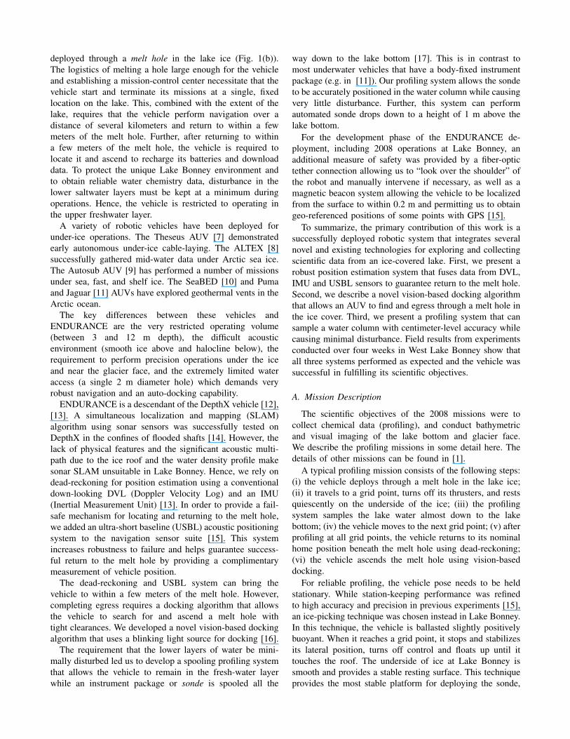
deployed through a melt hole in the lake ice (Fig. 1(b)).The logistics of melting a hole large enough for the vehicleand establishing a mission-control center necessitate that thevehicle start and terminate its missions at a single, fixedlocation on the lake. This, combined with the extent of thelake, requires that the vehicle perform navigation over adistance of several kilometers and return to within a fewmeters of the melt hole. Further, after returning to withina few meters of the melt hole, the vehicle is required tolocate it and ascend to recharge its batteries and downloaddata. To protect the unique Lake Bonney environment andto obtain reliable water chemistry data, disturbance in thelower saltwater layers must be kept at a minimum duringoperations. Hence, the vehicle is restricted to operating inthe upper freshwater layer.

A variety of robotic vehicles have been deployed forunder-ice operations. The Theseus AUV [7] demonstratedearly autonomous under-ice cable-laying. The ALTEX [8]successfully gathered mid-water data under Arctic sea ice.The Autosub AUV [9] has performed a number of missionsunder sea, fast, and shelf ice. The SeaBED [10] and Pumaand Jaguar [11] AUVs have explored geothermal vents in theArctic ocean.

The key differences between these vehicles andENDURANCE are the very restricted operating volume(between 3 and 12 m depth), the difficult acousticenvironment (smooth ice above and halocline below), therequirement to perform precision operations under the iceand near the glacier face, and the extremely limited wateraccess (a single 2 m diameter hole) which demands veryrobust navigation and an auto-docking capability.

ENDURANCE is a descendant of the DepthX vehicle [12],[13]. A simultaneous localization and mapping (SLAM)algorithm using sonar sensors was successfully tested onDepthX in the confines of flooded shafts [14]. However, thelack of physical features and the significant acoustic multi-path due to the ice roof and the water density profile makesonar SLAM unsuitable in Lake Bonney. Hence, we rely ondead-reckoning for position estimation using a conventionaldown-looking DVL (Doppler Velocity Log) and an IMU(Inertial Measurement Unit) [13]. In order to provide a fail-safe mechanism for locating and returning to the melt hole,we added an ultra-short baseline (USBL) acoustic positioningsystem to the navigation sensor suite [15]. This systemincreases robustness to failure and helps guarantee success-ful return to the melt hole by providing a complimentarymeasurement of vehicle position.

The dead-reckoning and USBL system can bring thevehicle to within a few meters of the melt hole. However,completing egress requires a docking algorithm that allowsthe vehicle to search for and ascend a melt hole withtight clearances. We developed a novel vision-based dockingalgorithm that uses a blinking light source for docking [16].

The requirement that the lower layers of water be mini-mally disturbed led us to develop a spooling profiling systemthat allows the vehicle to remain in the fresh-water layerwhile an instrument package or sonde is spooled all the

way down to the lake bottom [17]. This is in contrast tomost underwater vehicles that have a body-fixed instrumentpackage (e.g. in [11]). Our profiling system allows the sondeto be accurately positioned in the water column while causingvery little disturbance. Further, this system can performautomated sonde drops down to a height of 1 m above thelake bottom.

For the development phase of the ENDURANCE de-ployment, including 2008 operations at Lake Bonney, anadditional measure of safety was provided by a fiber-optictether connection allowing us to “look over the shoulder” ofthe robot and manually intervene if necessary, as well as amagnetic beacon system allowing the vehicle to be localizedfrom the surface to within 0.2 m and permitting us to obtaingeo-referenced positions of some points with GPS [15].

To summarize, the primary contribution of this work is asuccessfully deployed robotic system that integrates severalnovel and existing technologies for exploring and collectingscientific data from an ice-covered lake. First, we present arobust position estimation system that fuses data from DVL,IMU and USBL sensors to guarantee return to the melt hole.Second, we describe a novel vision-based docking algorithmthat allows an AUV to find and egress through a melt hole inthe ice cover. Third, we present a profiling system that cansample a water column with centimeter-level accuracy whilecausing minimal disturbance. Field results from experimentsconducted over four weeks in West Lake Bonney show thatall three systems performed as expected and the vehicle wassuccessful in fulfilling its scientific objectives.

A. Mission Description

The scientific objectives of the 2008 missions were tocollect chemical data (profiling), and conduct bathymetricand visual imaging of the lake bottom and glacier face.We describe the profiling missions in some detail here. Thedetails of other missions can be found in [1].

A typical profiling mission consists of the following steps:(i) the vehicle deploys through a melt hole in the lake ice;(ii) it travels to a grid point, turns off its thrusters, and restsquiescently on the underside of the ice; (iii) the profilingsystem samples the lake water almost down to the lakebottom; (iv) the vehicle moves to the next grid point; (v) afterprofiling at all grid points, the vehicle returns to its nominalhome position beneath the melt hole using dead-reckoning;(vi) the vehicle ascends the melt hole using vision-baseddocking.

For reliable profiling, the vehicle pose needs to be heldstationary. While station-keeping performance was refinedto high accuracy and precision in previous experiments [15],an ice-picking technique was chosen instead in Lake Bonney.In this technique, the vehicle is ballasted slightly positivelybuoyant. When it reaches a grid point, it stops and stabilizesits lateral position, turns off control and floats up until ittouches the roof. The underside of ice at Lake Bonney issmooth and provides a stable resting surface. This techniqueprovides the most stable platform for deploying the sonde,

and has the additional advantages of reducing energy usageand increasing the vertical extent of water column sampling.

III. POSITION ESTIMATION

The position estimation system inherited from DepthXconsists of an Inertial Measurement Unit (IMU), a DopplerVelocity Log (DVL) and depth sensors which together pro-vide data for estimating the 6-DOF pose and velocity of thevehicle. The orientation and acceleration measurements fromthe IMU are fused with bottom-relative velocities from theDVL. The bottom-relative DVL velocity is rotated into worldcoordinates using the IMU orientation measurements andcombined with IMU accelerations in a linear Kalman filter.This has the advantage of allowing the vehicle to operatefor several seconds without DVL lock, relying solely on ac-celerometer readings. The fused, world-frame velocity is thenintegrated to arrive at the horizontal components of vehicleposition. The vertical component is taken from measurementsby two 6 mm resolution pressure-depth sensors. The detailsof dead-reckoning pose-estimation can be found in [18].

This dead-reckoning system is able to provide accuraciesof less than 0.2% of distance traveled. However, it facedseveral challenges in Lake Bonney in guaranteeing safereturn of the vehicle to the melt hole. First, an inherentlimitation of dead-reckoning is that error in estimated stateaccumulates as the vehicle moves. For the longest missions(up to 2.5 km), this has the potential to make reachingthe melt hole difficult on return, particularly because verylittle battery energy would be left to execute an exten-sive search (see Section IV). Second, DVL performancein the acoustically challenging environment was unknown.Position accuracy could be severely affected by degradedDVL measurements or drop-outs due to the difficult acousticenvironment or minimum range violations when operating inclosed confines.

To make the navigation robust for return to the melt hole,we added an inverted Ultra-Short Baseline (USBL) system tothe sensor suite. The USBL is an acoustic positioning systemconsisting of a transceiver on the AUV which periodicallypings a stationary transponder. The transponder immediatelyresponds with its own ping, and based on the measuredbearing angle and time-of-flight at the transceiver, the systemreturns the position of the transponder relative to the vehicle.The USBL operates at a relatively low update rate (every 2-5 s). USBL positioning error is proportional to distance tothe transponder (Fig. 2(b)). It provides an absolute referenceto the melt hole location, improving as the vehicle nears thetransponder location, ensuring safe and swift recovery.

USBL transponder position measurements are first con-verted to give the vehicle position in world coordinates.These measurements are then filtered for outliers based on athreshold distance from the current best estimate of vehicleposition, given the expected range-proportional measurementerror. The remaining measurements are then fused with dead-reckoned position in a linear Kalman filter taking into ac-count the accumulated drift error and the USBL measurementerror.

A. Results from Field Experiments

Due to a number of logistical delays, USBL positionestimates were not fully integrated into the ENDURANCEcontrol system in time for the 2008 Lake Bonney missions.The USBL was used primarily as a backup position sensorin case of failure of other systems. However, USBL datawas recorded throughout the missions and an analysis ofUSBL performance in the Lake Bonney environment wascompleted.

DVL dead-reckoning was able to provide sufficient accu-racy for most missions. However, dead-reckoning failuresoccurred during Mission 2 (due to bubble formation onthe DVL transducers), Mission 15 (due to DVL minimumrange violations), and Mission 16 (due to a software failure).When failures did occur, extensive manual intervention wasrequired to safely recover the vehicle, proving the needfor the fail-safe security provided by the USBL for fullyautonomous operations.

The USBL horizontal position measurement was generallyreliable even at the greatest distances from the melt hole(≈650 m). USBL performance degraded in shallow water atthe lake edges and near the glacier face and accompanyingsubmerged moraine. In these areas, significant offsets wereobserved, depending on vehicle orientation (Fig. 2(a)), mostlikely due to multipath effects from the nearby surfaces.By comparing USBL position measurements to the GPS-corrected dead-reckoning pose measurements, the error dis-tribution in the USBL data can be studied. During operationsin Lake Bonney, the USBL achieved a horizontal error distri-bution, 50% circular error probable (CEP), of approximately2.5% of range (Fig. 2(b)).

Vertical errors in the USBL position measurements wereof much greater magnitude (Fig. 2(c)), displaying a cone-like distribution over several hundred meters as a result ofreflections from the overhead ice at 3 m depth and theunderlying strong halocline at about 12 m depth (theseboundaries essentially act as an acoustic waveguide). As thiscomponent of USBL position is ignored, these errors do notaffect navigation on ENDURANCE.

Based on the data gathered at Lake Bonney, the perfor-mance of the USBL-aided position estimation was evaluatedin a post-processing simulation (Fig. 2(d)). For missions per-formed away from the glacier face, and where USBL positionfixes were available during the return, positioning accuracyat the melt hole was improved and was not a function ofdistance traveled. However, for missions near the glacierface, where operations did not ensure USBL fixes duringthe return run, accuracy was often degraded, indicating aneed for more intelligent filtering of USBL measurements.With full integration into the on-board navigation system,including system calibration and operational modifications,it is anticipated that USBL-aided navigation will improvebeyond the results demonstrated in post-processing.

IV. VISION-BASED DOCKING

Once the vehicle has reached its nominal home positionusing the positioning system described in the previous sec-

(a) (b)

(c) (d)

Fig. 2. USBL position estimation performance at Lake Bonney. (a) USBL position measurements plotted along with the IMU + DVL dead-reckoning data.USBL position measurements at the lake margins often displayed large errors as these represent extreme acoustic environments (ice-to-bottom separationof less than 7 m, close proximity to glacier ice face and moraines). (b) USBL horizontal error as a function of range (excluding outliers). The empirical1-σ error is 0.9 m + 0.019 × range. (c) Vertical component of USBL position measurement as a function of range. The USBL transponder was deployedat a depth of 8 m, and the vehicle with the transceiver operated between 3.5 m and 8 m. The significantly greater vertical distribution of USBL positionmeasurements is due to the horizontal reflecting layers in Lake Bonney. (d) Comparison of the return-to-hole accuracy of pure dead-reckoning and USBL-aided position, from post-processed data. During early missions (1-14), the vehicle stayed far from the lake margins and the USBL transceiver was pointedtoward the transponder during the return. These missions show overall improvement in the position accuracy. During later missions (15-19), the vehicleoperated near the glacier face and the transceiver was pointed away from the transponder during the return. These missions show a degradation due toincorporation of systematically erroneous position fixes. Dead-reckoning failed during Missions 2, 15, and 16. Missions 1, 3, 4, and 11 did not record dataor were aborted for other reasons.

tion, it ascends the melt hole using vision-based docking. Forthis, a downward-facing blinking light is suspended roughlycentered above the melt hole. A light detection algorithmtracks the light in the images captured by an upward-facingcamera mounted on top of the vehicle.

Vision-based docking begins when the vehicle reaches itsnominal home position. First, a search behavior is initiatedwhere the vehicle moves in a spiral pattern to look for

2/38

θy

Light

Source

Center

θx

Fig. 3. Coordinates of the light sourcecenter are expressed as angles in theimage from the upward-facing camera.The light source is not necessarily cen-tered in the image.

the light. Next, when thelight is detected, an as-cent behavior is initiated.Here the vehicle ascendsup the melt hole whilekeeping the light centeredin the upward camera im-ages. The coordinates ofthe light source centerare expressed as angles(θtx, θty) in the imageframe (Fig. 3). The ve-hicle’s control enables itto move independently inthe lateral (x, y) plane and

the vertical direction (z).

• Spiraling Behavior: Using dead-reckoned position, thevehicle follows a spiral r = b

2π θ to search for a lightsource. The parameter b is the distance between the arms

of the spiral and is determined from the depth at whichthe spiral search is performed and the field of view of thecamera – b is chosen to ensure that the under-surface ofthe ice is completely and efficiently scanned by the camerafor the light source. The parameter θ is varied from zero toθmax such that a maximum radius of rmax is reached. Thesearch radius itself is calculated from the lateral distancetraveled by the vehicle and its dead-reckoning accuracy.

• Ascent/Descent Behavior: The ascent controller uses aPD control law for lateral velocity control and a PIDcontrol law for vertical velocity control. For lateral control(θtx, θ

ty) (Fig. 3) is used as the error signal. The control

law tries to center the light source in the image therebycentering the robot on the light source. For vertical control,a non-zero z-velocity is commanded only when the light isapproximately centered in the image. The ascent controllerstops when the vehicle reaches the water surface. Fordescent, the vehicle uses the same controller as for ascentexcept that control in the z-direction is disabled. A descentweight is placed on top of the vehicle so that it sinksdown the melt hole while being controlled in the x and ydirections. When the transit depth is reached, the weightis manually retrieved.

A. Light Detection Algorithm

The controllers described in the previous section requireaccurate detection and tracking of the target light sourcein the camera image. At the camera frame rate of around

��������

���������� ����������� ����������� ����������� �

��� ��

px(x, y)

���

(x, y)

(x, y)

px

px

I������ ����� ���

������ �������� �������� �������� ��

��� �� ���

(x, y)

(x, y)

(x, y)

px

px

px

(x, y) px

��� ���

���

Fig. 4. The set of tracked light sources L is updated when a set of candidatelight sources C are identified in a newly captured image frame. This is doneby establishing correspondence between tracked light sources and the newlyidentified candidates. (a) Three light sources are currently being tracked. (b)Four candidates have been identified in the most recent image frame. (c)The process of establishing correspondence begins by constructing a graphthat connects each element of L to each element of C where edge weightis the distance between the corresponding tracked and candidate light.

6 Hz, frames are captured and then processed by our low-level vision routines (built on the OpenCV image processinglibrary [19]) to identify high-contrast contours as candidatesfor the target light. These contours are then filtered based ontheir roundness and size to eliminate obvious false positives.For each candidate contour that passes the filters, we pass thecenter and radius of the bounding circle to the light trackingalgorithm.

The light detection algorithm must perform robustly in thepresence of ambient light sources, such as direct light fromthe sun and indirect reflections from the ice. To distinguishthe target light source from these persistent sources, we trackthe target’s unique blinking signature. Our novel solutiondoes not require synchronization between the camera andlight, and only makes the straightforward assumption thatthe vehicle does not move too quickly from frame to frame.

Our tracking algorithm extends the point-correspondencemethod of Salari and Sethi [20] to track blinking lights inaddition to persistent lights in the presence of occlusion. Thealgorithm maintains a set, L, which contains the current lightsources being tracked, including their bounding circles andhistories. A history is a list that contains whether or not thelight source was seen or unseen for each frame going backto some upper bound on the history length (24 frames in ourexperiments). The algorithm updates this data structure byincorporating C, the set of candidate light sources seen inthe current frame (Fig. 4). The tracker must identify whichcandidates correspond to light sources that have already beenseen and which candidates are new. We take a greedy edge-elimination approach as illustrated in Fig. 5.

The algorithm begins by computing a matrix containingthe distances between all currently tracked light sources andthe candidates in the frame (Fig. 5(a)). The first round ofelimination removes all edges with distance greater than a

3/38

(a) (b) (c)

LLLL CCCC LLLL CCCC LLLL CCCC

Fig. 5. (a) To process new candidate light sources, the light-detectionalgorithm begins with a complete bipartite graph between the set ofcandidates (C) and the set of currently tracked light sources (L). (b) Next,edges are removed if the distance between the sources is too large or if thedisparity in their sizes is too high. (c) Finally, edges are removed in orderfrom greatest distance to smallest, while not removing edges (l ∈ L, c ∈ C)if doing so would orphan both l and c at the same time.

threshold of 10◦ in the camera’s field of view. This thresholdwas determined experimentally, and depends on the vehicle’sspeed and expected minimum distance to the target. Weset this threshold large enough to allow the robot to movesome significant amount between frames, but small enoughto avoid clumping all light sources together. At the sametime, we eliminate edges if they connect light sources withdrastically different sizes. The primary motivation for thisfilter is to prevent specular glare on the light source glassfrom being recognized as the light when it is off, a problemwe encountered during early experimentation.

After the first culling, the edges that remain appear asdepicted in Fig. 5(b). Notice that some nodes still havemore than one edge, which means that there are multiplepotential matches to be made. The next round of eliminationdetermines which of those potential matches is best. Thealgorithm sorts the remaining edges by decreasing distanceand then eliminates them one-by-one. An edge will not beeliminated if it is the only edge remaining for the nodes itconnects, because that edge is treated as a correct match.

Finally, the graph that results from the greedy cullingalgorithm is shown in Fig. 5(c). No node has more thanone edge. The edges that remain connect the candidatesin the current frame with their corresponding light sourcehistories. Orphaned nodes in L (one in the figure) aretracked light sources that were not seen in the current frame.Their histories are updated to reflect that they were unseen.Orphaned nodes in C (two in the figure) are newly-observedcandidates, which are added to the list of tracked lightsources with a fresh history.

With L updated, we compute a score for each trackedlight source. After some experimentation with alternatives,the score that worked best was the number of transitions.Every time the light switches from seen to unseen or unseento seen in its bounded history, that light source receives apoint. The highest possible score, then, is half the historylength. In practice, however, a true positive tends to score inthe 3–7 range. Through informal experimentation, we arrivedat a value of 4 for the minimum threshold value on the score.Thus, the light source with the highest score above thresholdis returned as the target. If no light sources score above thethreshold, then the algorithm returns a null value.

(a) ascent-10 (b) ascent-9Fig. 6. Plots showing the vehicle’s path for two ascents once the visualhoming algorithm starts. (a) The robot searches spirally for the light source;once it locks onto the light source, the robot begins to rise while stayingcentered on the light. (b) The robot fails to find the light the first time itspirals. It then drifts for a short distance before the visual homing algorithmis restarted, the robot finds the light source, and rises.

(a) (b)

Fig. 7. Sequence of images taken by the upward-facing camera duringMission 3 showing various stages of the visual homing behavior. (a) Duringsearch, the light-detection module identifies a candidate light source (redcircle). Note that the light source is not centered in the image. (b) Afterobserving the light source blink a few times, the source is confirmed as thedesired target (blue circle). The robot also starts centering the light sourcein the image.

B. Results from Field Experiments

Visual homing was used for 10 missions in West LakeBonney with the ascent behavior being used all 10 timesand descent used 8 times. Spiraling behavior was executedin 5 ascents. Twice the vehicle was farther from the melt holethan could be reached with a single spiral search. Here, spiralsearch was executed multiple times by manually issuing acommand through the user-interface. The transit depth ofthe vehicle was 5 m and hence most ascents were initiatedat a depth of 5 m.

For all the 18 instances, visual homing was successfulin guiding the vehicle up or down the melt hole withoutcollisions with the walls. Fig. 6 shows the path of the vehiclefor two ascents. Fig. 7 shows some images taken by theupward-facing camera during an ascent. The spiral searchproved to be a simple yet effective way to search for thelight source.

1) Ascent/Descent Controller Precision: We analyze theprecision of the ascent controller by measuring the overallstandard deviation in the vehicle’s x and y coordinates afterit has approximately centered itself with respect to the lightsource and starts rising. We analyze data for 7 missions forwhich both image and pose data is available.

To compute the overall standard deviation we first nor-malize all x and y values for each mission by their means.If x is the mean x coordinate for an ascent/mission, thenthe normalized value x̂ for a particular x coordinate is givenby x̂ = x − x. The normalized values are combined into a

single vector and the overall precision is then given by thevector’s standard deviation. The overall precision for the ycoordinates is similarly computed.

The overall value for the standard deviation is 5.70 cmin the x direction and 4.60 cm in the y direction. Thevehicle has a clearance of 10 cm on all sides when it isin the melt hole implying that for about 92% of the time,the vehicle was fairly well centered in the melt hole andnot touching any walls. Qualitatively, the vehicle came upthe melt hole successfully every time without suffering anydamage, suggesting that at worst the vehicle only lightlygrazed the melt hole walls. Thus, the controller and the lightdetection algorithm were able to successfully surface therobot. The precision for the descents is numerically similarto that for the ascents.

2) Light Detection Accuracy: To evaluate algorithm per-formance, we are primarily interested in four criteria. First,the algorithm should acquire and detect the blinking lightquickly. Second, it should not lose track of the light once ithas been acquired, producing false negatives. Third, it shouldnot produce false positives by misclassifying non-target lightsources. And fourth, it should maintain an accurate estimateof the target center.

For seven separate ascents of the vehicle, we evaluatedthe light tracking algorithm against these criteria. Our per-formance metrics require a comparison with the true locationof the target light source. Without access to ground truth,we approximated the location of the target light source byhand-labeling the images in our data set. For each frame inwhich the true target light source was present, we manuallyrecorded the pixel location that appeared to be closest to thecenter of the target. We then ran the same images throughthe light-detection algorithm and computed the error in thisestimate along with several other statistics. The completeresults are shown in Table I.

The first statistic, “Total frames”, is the number of framesstored by the camera from the time the first candidatelight source is identified until the vehicle completes ascent.Although the camera operated at 30 Hz, images were storedat about 6 Hz, recording roughly every fifth frame. Thus, forexample, for an ascent that lasts around 30 s, roughly 180frames would be recorded.

The next metric, “Acquisition time”, is the number offrames between the first candidate light and the first identifiedblinking target. If the target is lost after initial acquisition,then we consider that a “Drop”. We record the number ofdrop occurrences and the total duration (in frames) over theoccurrences. We do the same for “Misclassifications”, whichare instances when the algorithm locks on to the incorrectlight source. Finally, we measure the Euclidean distance (inpixels) between the true target position and the algorithmoutput. Because misclassifications have a large impact onthis metric, we record two versions of this statistic: one withmisclassified instances included, and one without.

From Table I it is clear that the algorithm performed wellduring the Lake Bonney deployment. In only one of theseven ascents did the algorithm ever encounter any drops

Ascent No. 3 5 8 9 10 12 13Total frames 190 278 243 150 193 179 153

Acquisition time (frames) 21 12 162 101 123 95 8Number of Drops 1 0 0 0 0 0 0

Total drop time (frames) 11 0 0 0 0 0 0Number of Misclassifications 1 0 0 0 0 0 0

Misclassification time (frames) 15 0 0 0 0 0 0Average distance (pixels) 11.2 1.91 3.63 4.44 2.24 3.02 3.38

Avg. dist. w/o misclassified (pixels) 2.83 1.91 3.63 4.44 2.24 3.02 3.38

TABLE ISTATISTICS EVALUATING BLINKING LIGHT TRACKER ALGORITHM ACROSS SEVEN SEPARATE ASCENTS AT LAKE BONNEY.

or misclassifications. Also, the low-level contour algorithmappears to have done a good job of finding the centers of thelight sources, as is evidenced by the average distance values.

V. PROFILING SYSTEM

Once the vehicle reaches a grid point, water propertiesare sampled with a profiling system. The profiling systemconsists of three main components—the spooler, the sondeand the electronic-control housing (Fig. 8). The spooler isa servo-driven winch. We designed the servo controllers toachieve precise control over payload position and speed.The sonde has nine instruments which measure conductiv-ity, temperature, pressure, pH, oxidation-reduction potential(ORP), chlorophyll, turbidity, chromatic dissolved organicmatter (CDOM), and ambient light. In addition, the sonde hasa high-definition camera, a high power LED light, a bottomranging altimeter, and an on-board lithium battery. A electro-mechanical Kevlar reinforced cable connects the sonde to theelectronics-control housing. The electronics-control housingcontains communications, power, servo-control and logiccomponents.

Automated profiling begins when the vehicle ice-picks ata grid point. Once the vehicle’s position has stabilized, apre-programmed sequence is initiated where the sonde issmoothly spooled down to a height of 1 m above the lakebottom. Altimeter readings are used for position estimationin this process. The LED lights are switched on and the high-definition camera takes a sequence of pictures (see Fig. 9)of the lake bottom while the sonde is slowly moved up 1 m.The sonde is then smoothly spooled back up and stowed inthe vehicle.

A. Results from Field Experiments

The profiling system was tested in various facilities, in-cluding the Neutral Buoyancy Lab (NBL) at Johnson Spacecenter. One of the issues faced at NBL was that the altimeteron the sonde gave erroneous readings while close to thepool surface. Once a few meters down, the readings wereaccurate and enabled automated sonde drops down to aheight of 1 m above the pool floor. However, in Lake Bonney,because of soft lake floor and multipath due to haloclineand ice roof, we encountered altimeter dropouts of variableduration during sonde drops. This precluded us from usingthe profiler in the automated mode. Instead, we relied onspooling down the sonde by manually issuing commands tothe servos. In the future, we plan to fix this problem by

Fig. 8. The profiling system hardware. The sonde consists of variousinstruments that measure water properties. A high-definition camera is alsopart of the sonde. The sonde is smoothly lowered or raised with a winch-based spooler.

integrating information from multiple sensors such as thedown looking DVL, the servo encoders, and the altimeterfor robust position estimation.

ENDURANCE performed profiling at 108 points in WestLake Bonney during 2008 missions. The data from eachsonde drop included chemical property data (Fig. 10(a))sampled at a resolution of 0.1 m in depth, and lake-bottomimages (Fig. 10(b)).

VI. CONCLUSIONS

ENDURANCE was the first entity (human or robot) toextensively explore the sub-ice world of West Lake Bonneyand gather a large amount of scientific data. A total of19 sub-ice missions were performed by ENDURANCE in2008, including 8 profiling missions with 108 sonde drops(Fig. 11) and 5 glacier mapping missions. At Lake Bonney,the dead-reckoning system with IMU and downward-facingDVL demonstrated a 50% CEP drift error of about 0.1%of distance traveled. USBL positioning demonstrated 50%CEP errors of 2.5% of range, and demonstrated the abilityto improve position accuracy and serve as a fail-safe systemto improve system autonomy. The vision-based dockingalgorithm was successfully used a total of 18 times for ascentand descent. Quantitative and qualitative results show thatthe light-detection is robust and the ascent/descent controlleris sufficiently precise to keep the vehicle centered morethan 90% of the time. The profiler performed smoothly withno serious issues in the harsh environment. ENDURANCEreturned to West Lake Bonney in the austral summer of 2009to continue its scientific missions.

VII. ACKNOWLEDGMENTS

ENDURANCE was a NASA sponsored research activity,funded through the ASTEP program office, NASA Science

(a) (b)

Fig. 9. A profiling operation, captured by under-water cameras at theNeutral Buoyancy Lab (NBL) at Johnson Space Center. Initially, the sondeis stowed in the vehicle. (a) During profiling, the sonde is smoothly spooleddown. (b) When the sonde reaches a height of 1 m above the floor, a cameratakes images of the floor.

(a) (b)

Fig. 10. Examples of data collected during the profiling missions. (a) Plotof conductivity data measured by the sonde. Plot thanks to the ElectronicVisualization Lab at the University of Illinois at Chicago [21]. (b) Microbialmats are visible in an image taken by the sonde camera. Such mats wereusually seen on the lake bottom in shallow coastal regions.

Fig. 11. Summary of profiling missions. Green circles mark the locationsof successful sonde drops during the 2008 season. Different colored linesshow different missions. The longest mission length was ≈1800 m.

Directorate under grant NNX07AM88G. Peter Doran at theUniversity of Illinois at Chicago is the principal investigator.The authors would like to thank John Priscu at MontanaState University; Andrew Johnson, Maciej Obryk, ShriramIyer, and Alessandro Febretti at the University of Illinois atChicago.

Logistical support in Antarctica was provided by theNational Science Foundation through the U.S. AntarcticProgram. The authors would also like to thank the Center forLimnology at the University of Wisconsin at Madison, theHyde Park Baptist Church at The Quarries in Austin, Texas,and the Sonny Carter Training Facility Neutral BuoyancyLab at NASA Johnson Space Center, for their enthusiasticsupport of the ENDURANCE test program.

REFERENCES

[1] W. C. Stone, B. Hogan, C. Flesher, S. Gulati, K. Richmond, A. Mu-rarka, G. Kuhlman, M. Sridharan, V. Siegel, R. M. Price, P. Doran, andJ. Priscu, “Sub-ice exploration of West Lake Bonney: ENDURANCE2008 mission,” in International Symposium on Unmanned UntetheredSubmersible Technology (UUST), 2009.

[2] P. T. Doran, C. P. McKay, G. D. Clow, G. L. Dana, A. G. Fountain,T. Nylen, and W. B. Lyons, “Valley floor climate observations from theMcMurdo dry valleys, Antarctica,” Journal of Geophysical Research,vol. 107, 2002.

[3] P. T. Doran, R. A. W. J. 1, and W. B. Lyons, “Paleolimnology ofthe McMurdo Dry Valleys, Antarctica,” Journal of Paleolimnology,vol. 10, pp. 85–114, 1994.

[4] J. C. Priscu, “The biogeochemistry of nitrous oxide in permanentlyice-covered lakes of the McMurdo Dry Valleys, Antarctica,” GlobalChange Biology, vol. 3, pp. 301–315, 1997.

[5] A. G. Fountain, W. B. Lyons, M. B. Burkins, G. L. Dana, P. T. Doran,K. J. Lewis, D. M. McKnight, D. L. Moorhead, A. N. Parsons, J. C.Priscu, D. H. Wall, R. A. W. Jr., , and R. A. Virginia, “Physical controlson the Taylor Valley Ecosystem, Antarctica,” BioScience, vol. 49,no. 12, pp. 961–971, 1999.

[6] W. B. Lyons and S. K. F. K. A.Welch, “History of McMurdo DryValley lakes, Antarctica, from stable chlorine isotope data,” Geology,vol. 27, no. 6, pp. 527–530, 1999.

[7] J. M. Thorleifson, L. T. C. Davies, M. R. Black, D. A. Hopkin, andR. I. Verrall, “The Theseus autonomous underwater vehicle: A Cana-dian success story,” in Proceedings of the OCEANS 97 Conference,vol. 2. Halifax, Nova Scotia: MTS/IEEE, Oct. 6–9 1997, pp. 1001–1006.

[8] R. McEwen, H. Thomas, D. Weber, and F. Psota, “Performance ofan AUV navigation system at arctic latitudes,” in Proceedings of theOCEANS 2003 Conference. San Diego, CA: MTS/IEEE, Sept. 22–272003.

[9] S. McPhail, “Autosub operations in the Arctic and Antarctic,” inProceedings of the Masterclass in AUV Technology for Polar Science,G. Griffiths and K. Collins, Eds., National Oceanography Centre,Southampton, UK. Society for Underwater Technology, Mar. 28–30 2006, pp. 27–38.

[10] M. V. Jakuba, C. N. Roman, H. Singh, C. Murphy, C. Kunz, C. Willis,T. Sato, and R. A. Sohn, “Long-baseline acoustic navigation forunder-ice autonomous underwater vehicle operations,” Journal of FieldRobotics, no. 25, pp. 861–879, 2008.

[11] C. Kunz, C. Murphy, H. Singh, C. Pontbriand, R. A. Sohn, S. Singh,T. Sato, C. Roman, K. Nakamura, M. Jakuba, R. Eustice, R. Camilli,and J. Bailey, “Toward extraplanetary under-ice exploration: Steps inthe Arctic,” Journal of Field Robotics, vol. 26, no. 4, pp. 411–429,Apr. 2009.

[12] N. Fairfield, D. Jonak, G. A. Kantor, and D. Wettergreen, “Field resultsof the control, navigation and mapping system of a hovering AUV,”in International Symposium on Unmanned Untethered SubmersibleTechnology (UUST), 2007.

[13] N. Fairfield, G. Kantor, D. Jonak, and D. Wettergreen, “DEPTHXautonomy software: Design and field results,” Carnegie Mellon Uni-versity, Tech. Rep. CMU-RI-TR-08-09, 2008.

[14] N. Fairfield, G. A. Kantor, and D. Wettergreen, “Real-time SLAM withoctree evidence grids for exploration in underwater tunnels,” Journalof Field Robotics, vol. 24, pp. 3–21, 2007.

[15] K. Richmond, S. Gulati, C. Flesher, B. P. Hogan, and W. C. Stone,“Navigation, control, and recovery of the ENDURANCE under-icehovering AUV,” in International Symposium on Unmanned UntetheredSubmersible Technology (UUST), 2009.

[16] A. Murarka, G. Kuhlmann, S. Gulati, M. Sridharan, C. Flesher,and W. C. Stone, “Vision-based frozen surface egress: A dockingalgorithm for the ENDURANCE AUV,” in International Symposiumon Unmanned Untethered Submersible Technology (UUST), 2009.

[17] B. P. Hogan, C. Flesher, and W. C. Stone, “Development of asub-ice automated profiling system for Antarctic lake deployment,”in International Symposium on Unmanned Untethered SubmersibleTechnology (UUST), 2009.

[18] G. A. Kantor, N. Fairfield, D. Jonak, and D. Wettergreen, “Experimentsin navigation and mapping with a hovering AUV,” in InternationalConference on Field and Service Robotics, 2007.

[19] “OpenCV,” http://opencv.willowgarage.com/.[20] V. Salari and I. K. Sethi, “Feature point correspondence in the presence

of occlusion,” IEEE Transactions on Pattern Analysis and MachineLearning, vol. 12, no. 1, pp. 87–91, 1990.

[21] A. Johnson, “Homepage of Andrew Johnson at University of Illionoisat Chicago,” http://www.evl.uic.edu/aej, 2009.