1

Tokamak elongation – how much is too much? I Theory

J. P. Freidberg1, A. Cerfon2, J. P. Lee1,2

Abstract

In this and the accompanying paper the problem of the maximally achievable elongation κ in a tokamak is investigated. The work represents an extension of many earlier studies, which were often focused on determining κ limits due to (1) natural elongation in a simple applied pure vertical field or (2) axisymmetric stability in the presence of a perfectly conducting wall. The extension investigated here includes the effect of the vertical stability feedback system which actually sets the maximum practical elongation limit in a real experiment. A basic resistive wall stability parameter

γτw is introduced

to model the feedback system which although simple in appearance actually captures the essence of the feedback system. Elongation limits in the presence of feedback are then determined by calculating the maximum κ against 0n = resistive wall modes for fixed

γτw. The results are obtained by means of a general formulation culminating in a

variational principle which is particularly amenable to numerical analysis. The principle is valid for arbitrary profiles but simplifies significantly for the Solov'ev profiles, effectively reducing the 2-D stability problem into a 1-D problem. The accompanying paper provides the numerical results and leads to a sharp answer of “how much elongation is too much”? 1. Plasma Science and Fusion Center, MIT, Cambridge MA 2. Courant Institute of Mathematical Sciences, NYU, New York City NY

2

1. Introduction It has been known for many years that tokamak performance, as measured by

pressure and energy confinement time, improves substantially as the plasma cross section becomes more elongated. There are, however, also well known limits on the maximum achievable elongation, which arise from the excitation of 0n = vertical instabilities. When designing next generation reactor scale tokamak experiments [Aymar et al. 2002; Najmabadi et al. 1997; Najmabadi et al. 2006; Sorbom et al. 2015], where high performance is critical, it is thus important to be able to accurately predict the maximum achievable elongation κ as a function of inverse aspect ratio

ε = a /R0,

where a is the minor radius of the device, and R0

is the major radius.

The inverse aspect ratio is a particularly important parameter since different reactor designs have substantially different values for this quantity. Specifically, standard and high field tokamak reactor designs have 1/ ε ∼ 3− 4.5 [Aymar et al. 2002; Najmabadi et al. 1997; Najmabadi et al. 2006; Sorbom et al. 2015; Schissel et al. 1991; Hutchinson et al. 1994], while spherical tokamaks have smaller 1/ ε ∼ 1.5 [Sabbagh et al. 2001; Sykes et al. 2001]. Since optimized plasma performance and corresponding minimized cost depend strongly on κ it is important to have an accurate determination of κ = κ(ε) and this is the goal of the present and accompanying paper.

The problem of determining κ = κ(ε) has received considerable attention in past studies but, as discussed below, there is still an important gap in our knowledge. To put the problem in perspective we note that earlier studies generally fall into one of three main categories, each one providing valuable information, but not the whole story. These are summarized as follows.

The first class of studies involves the concept of “natural elongation”. Here, the tokamak is immersed in a deliberately simple external poloidal magnetic field, usually a pure vertical field. The plasma is expected to be stable against 0n = vertical instabilities since one vertical position is the same as any other. In these studies [Peng and Strickler 1986; Roberto and Galvão 1992] the free boundary equilibrium surface is calculated (i.e. the elongation κ and the triangularity δ are determined) for a range of ε from which it is straightforward to extract the desired κ = κ(ε) . Excellent physical insight is provided by these calculations. Even so, the maximum predicted natural elongations are substantially smaller than those achieved in experiments. The reason is that experiments have feedback systems that can stabilize 0n = vertical instabilities, thereby allowing larger κ ’s than those predicted by marginally stable naturally elongated configurations.

The second class of studies involves the calculation of the critical normalized wall radius /b a for an ideal perfectly conducting conformal wall required to stabilize a desired elongation; that is the analysis basically determines b /a = f (ε,κ). Here too, the studies [Wesson 1978] (and references therein) provide valuable insight. Specifically, the

3

studies determine the maximum /b a that might potentially be able to be stabilized by feedback. However, the analysis does not actually predict whether or not a practical feedback system can be constructed to provide stability. Equally important, from a practical point of view the actual value of /b a does not vary much from experiment to experiment.

The third class of studies consists of detailed, engineering level designs that predict the maximum elongation and which include many effects such as plasma profiles, real geometry, safety margins, and most importantly, engineering properties of the feedback system. Such studies [Kessel et al. 2006] are very realistic and are exactly what is required to design an actual experiment. Nevertheless, these are point designs whose main goals are focused on a specific machine rather than providing scaling insight in the form of κ = κ(ε) .

The present analysis attempts to fill an important gap in our knowledge, namely determining the maximum elongation as a function of inverse aspect ratio including the constraints arising from the feedback system. The calculation is largely analytic combined with some straightforward numerics. In our model the plasma is assumed to be up-down symmetric and is characterized by the following parameters: inverse aspect ratio

ε = a /R0, elongation κ , triangularity δ , poloidal beta

β

p , normalized wall radius

/b a , and an appropriately defined parameter representing the capabilities of the feedback system. Defining this feedback parameter and including it in the analysis is the main new contribution of the research.

A simple but reliable definition of the feedback parameter is based on the following two observations. First, practical feedback is feasible when the growth rate γ of the

0n = vertical instability is small. Since the plasma is surrounded by a finite conductivity wall the instability of interest is actually a resistive wall mode. The second observation is that if the feedback coils are located outside the resistive wall, as they usually are, then an effective feedback system must have a rapid field diffusion time

τw.

This is important because once an unstable plasma motion is detected the feedback response fields must quickly diffuse through the wall in order to reach the plasma. In other words

τw should be short.

In principle it is possible to trade off growth rate in favor of response time or vice-versa. However, the overall effectiveness of the feedback system is dependent upon the combined smallness of γ and

τw. The conclusion is that a simple parameter that takes

into account the feedback system is the product of these two quantities:

γτw = feedback capability parameter (1)

A good way to think about this parameter is as follows. In designing a new

experiment the properties of the feedback system depend mainly on the geometry of the

4

vacuum chamber, the availability of fast-response power supplies, the maximum feedback power available, the number of feedback coils, and the sensitivity of the detectors. These represent a combination of engineering and economic constraints that should not vary much as ε changes. Consequently, the engineering value of

γτw is a

good measure of the feedback capability. It represents the maximum value of the resistive wall growth rate that can be feedback stabilized.

Now, consider the design of a new experiment with ε as a parameter over which optimization is to be performed. For a fixed ε the plasma elongation should be increased until the growth rate of the 0n = resistive wall mode is equal to the value of the feedback capability parameter given in Eq. (1). In this process, the triangularity δ may also be adjusted to find the maximum allowable κ . This resulting κ is the elongation that maximizes performance for the given ε . By repeating the procedure for different ε it is then possible to determine the optimum aspect ratio, including the effects of transport, heating, magnetic design, etc., that results in the peak value of maximum performance and corresponding minimizes cost. In our analysis practical engineering values of

γτw are chosen by examining the data from existing experiments

as well as ITER [Aymar et al. 2002]. Based on this discussion we can state that the goals of the analysis are to determine

the maximum allowable elongation κ and corresponding triangularity δ as a function of inverse aspect ratio ε subject to the constraints of fixed poloidal beta

β

p , normalized

wall radius /b a , and feedback parameter γτw

; that is we want to determine

κ = κ(ε;βp,b /a,γτ

w)

δ = δ(ε;βp,b /a,γτ

w)

(2)

This paper presents the analytic theory necessary to determine these quantities. The

analysis is valid for arbitrary plasma profiles. An additional useful result presented as the derivation progresses is an explicit relationship between vertical stability and neighboring equilibria of the Grad-Shafranov equation, a relationship long believed to be true but to the authors’ knowledge, never explicitly appearing in the literature.

The second paper in the two part series presents the numerical results. For numerical simplicity the results are obtained for the Solov'ev profiles [Solov’ev 1968] although with some additional equilibrium numerical work it is possible to include arbitrary profiles. One may expect Solov’ev profiles to provide reliable physical insight since axisymmetric MHD modes are thought to not depend too sensitively on the details of the current profile [Bernard et al. 1978]. The overall conclusions are that the maximum elongation (1) decreases substantially as ε becomes smaller and (2) is substantially higher than that predicted by natural elongation calculations, much closer to what is observed experimentally. The maximum elongation is weakly dependent on

5

β

p and also does not vary much with b /a primarily because this quantity itself has

only limited variation in practical designs. There is, however, a substantial increase in maximum elongation as

γτw increases. As expected, feedback is very effective in

increasing elongation and overall plasma performance. A slightly more subtle effect is the value of the optimum triangularity corresponding to maximum elongation, which is noticeably smaller than that observed experimentally in high performance plasma discharges. The reason is presumably associated with the fact that maximum overall performance depends on turbulent energy transport as well as MHD stability. Although turbulent transport is known to be reduced with increasing triangularity, which helps explain the data, it is unfortunate that the current empirical scaling laws do not explicitly include this effect.

The analysis is now ready to proceed.

2. Equilibrium

The equilibrium of an axisymmetric tokamak is described by the well-known Grad-Shafranov equation [Grad and Rubin 1958; Shafranov 1958]

Δ*Ψ =−µ

0R2 dp

dΨ−

12

dF 2

dΨ (3)

Here, Ψ(R,Z) = poloidal flux/2π and p(Ψ), F(Ψ) are two free functions. The Δ

*

operator, plus the magnetic field B = B

p+ B

φeφ and current density

J = J

p+J

φeφ are

given by

Δ*Ψ ≡ R∂∂R

1R∂Ψ∂R

⎛

⎝⎜⎜⎜⎜

⎞

⎠⎟⎟⎟⎟

+∂2Ψ∂Z 2

B =1R∇Ψ×e

φ+

FR

eφ

µ0J =

dFdΨ

Bp−

1RΔ*Ψ e

φ

(4)

For the study of 0n = resistive wall modes the essential physics is captured by

considering up-down symmetric equilibria and this is the strategy adopted here. Also, great analytic simplicity follows by choosing the free functions to correspond to the Solov'ev profiles [Solov’ev 1968] for which

F′F (Ψ) =C

1 and

′p (Ψ) =C

2, with prime

denoting d /dΨ . Only two constants, C1

and C2

, are needed to specify an equilibrium.

6

The Grad-Shafranov equation can now be conveniently normalized in terms of two equivalent constants,

Ψ0 and A , one of which (

Ψ0) scales out entirely from the final

formulation. The full set of normalizations is given by

R = R0X

Z = R0Y

Ψ = Ψ0Ψ

µ0

dpdΨ

=−Ψ

0(1−A)

R04

FdFdΨ

=−Ψ

0A

R02

(5)

Note that the normalized flux has an upper case italic font. In terms of these normalizations the Grad-Shafranov equation plus the critical field quantities needed for the analysis reduce to

ΨXX−

1XΨ

X+ Ψ

YY= A + (1−A)X 2

(R02 /Ψ

0)B

p=

1X−Ψ

Ye

R+ Ψ

Xe

Z( )

(R03 /Ψ

0)µ

0Jφ

=−1X

A + (1−A)X 2⎡⎣⎢

⎤⎦⎥

(6)

The boundary conditions require regularity in the plasma and

Ψ(SP) = 0 with

SP the

plasma boundary. This implies that Ψ(X,Y ) < 0 in the plasma volume. Typical values of the free constant A in decreasing order are as follows

A = 1 p(Ψ) = 0 (force free)

A = 0 F(Ψ) = R0B

0 (vacuum toroidal field)

A =−(1− ε)2

1−(1− ε)2Jφ(1− ε,0) = 0 (inner edge current reversal)

(7)

The task now is to find a solution for Ψ(X,Y ) . Exact solutions to the Grad-

Shafranov equation for Solov'ev profiles have been derived by a number of authors [Zheng et al. 1996; Weening 2000; Shi 2005]. Here, we follow the formulation of

7

reference [Cerfon and Freidberg 2010; Freidberg 2014]. Specifically, an exact solution to Eq. (6) can be written as

Ψ X,Y( ) =X 4

8+ A

12

X 2 lnX −X 4

8

⎛

⎝⎜⎜⎜⎜

⎞

⎠⎟⎟⎟⎟⎟

+c1Ψ

1+c

2Ψ

2+cΨ

3+c

4Ψ

4+c

5Ψ

5+c

6Ψ

6+c

7Ψ

7

Ψ1

= 1

Ψ2

= X 2

Ψ3

=Y 2−X 2 lnX

Ψ4

= X 4 − 4X 2Y 2

Ψ5

= 2Y 4 −9X 2Y 2 + 3X 4 lnX −12X 2Y 2 lnX

Ψ6

= X 6 −12X 4Y 2 + 8X 2Y 4

Ψ7

= 8Y 6 −140X 2Y 4 + 75X 4Y 2−15X 6 lnX +180X 4Y 2 lnX −120X 2Y 4 lnX

(8)

The free constants

c

j are chosen to match as closely as possible the well-known analytic

model for a smooth, elongated, “D” shaped boundary cross section PS given

parametrically in terms of τ by [Miller et al. 1998]

X = 1+ εcos(τ + δ0sin τ)

Y = εκ sin τ (9)

Here,

ε = a /R0 is the inverse aspect ratio, κ is the elongation, and δ = sin δ

0 is the

triangularity. The geometry is illustrated in Fig. 1. In practice the jc are determined by requiring that the exact plasma surface Ψ = 0 ,

plus its slope and curvature match the model surface at three points: (1) the outer equatorial point, (2) the inner equatorial point, and (3) the high point maximum. Taking into account the up-down symmetry we see that the requirements translate to

8

Ψ(1+ ε,0) = 0 outer equatorial point

Ψ(1− ε,0) = 0 inner equatorial point

Ψ(1− δε,κε) = 0 high point

ΨX(1− δε,κε) = 0 high point maximum

ΨYY

(1+ ε,0) =−N1Ψ

X(1+ ε,0) outer equatorial point curvature

ΨYY

(1− ε,0) =−N2Ψ

X(1− ε,0) inner equatorial point curvature

ΨXX

(1− δε,κε) =−N3Ψ

Y(1− δε,κε) high point curvature

(10)

where for the given model surface,

N1

=d 2XdY 2

⎡

⎣⎢⎢⎢

⎤

⎦⎥⎥⎥τ=0

=−1+ δ

0( )2

εκ2

N2

=d 2XdY 2

⎡

⎣⎢⎢⎢

⎤

⎦⎥⎥⎥τ=π

=1− δ

0( )2

εκ2

N3

=d 2YdX 2

⎡

⎣⎢⎢⎢

⎤

⎦⎥⎥⎥τ=π/2

=−κ

εcos2 δ0

(11)

The determination of the jc has been reduced to finding the solution to a set of seven

linear, inhomogeneous algebraic equations, a very simple numerical problem. Hereafter, we assume that the jc have been determined, thereby completely defining the

equilibrium solution. A typical set of flux surfaces corresponding to the high β , tight aspect ratio NSTX spherical tokamak is illustrated in Fig. 2, where A has been chosen so that

Jφ(1− ε,0) = 0 . The surfaces look quite reasonable and as expected, exhibit a

large shift of the magnetic axis. The one final piece of information required for the resistive wall stability analysis is

the value of poloidal beta β

p . In general β

p and the toroidal current I can be

expressed in terms of the free constants A, Ψ

0. The advantage of the normalizations

introduced by Eq. (5) is that β

p is only a function of A but not Ψ0

. This can be seen

by noting that the average pressure and toroidal current can be written as,

• Average pressure:

9

p ≡pdr∫dr∫

=−2πΨ

02(1−A)

µ0R

0V

ΨX dX dY∫

V = dr =∫ 2πR03 X dX dY∫

(12)

• Toroidal current:

µ

0I = B

pdl

Ψ=0!∫ = µ

0Jφ

Ψ≤0∫ dS =−

Ψ0

R0

1X

A + (1−A)X 2⎡⎣⎢

⎤⎦⎥

Ψ≤0∫ dXdY (13)

where

B

p is the magnitude of the poloidal magnetic field. We now define

β

p as

βp≡

2µ0p

Bp2

Bp

=

Bpdl

Ψ=0!∫

dlΨ=0!∫

=µ

0I

LP

LP

= dlΨ=0!∫

(14)

Substituting for p and I yields

βp

=−4πR

0L

P2

V

(1−A) ΨX dX dYΨ≤0∫

1X

A + (1−A)X 2⎡⎣⎢

⎤⎦⎥dX dY

Ψ≤0∫⎧⎨⎪⎪⎪

⎩⎪⎪⎪

⎫⎬⎪⎪⎪

⎭⎪⎪⎪

2 (15)

Since Ψ is a function of A but not

Ψ0 it follows that as stated

β

p= β

p(A,ε,κ,δ) . Note

also that the volume V and poloidal plasma circumference PL are purely geometric

factors that can be calculated from the solution given by Eq. (8) once the jc have been

determined. Furthermore, with our normalizations the ratio R0

LP2 /V is independent of

0R and Ψ0

; that is R0

LP2 /V = f (A,ε,κ,δ) . This completes the discussion of the

equilibrium.

10

3. Resistive wall stability formulation

In this section we derive a variational principle describing the stability of 0n = resistive wall modes in a tokamak. The analysis starts from the ideal MHD normal mode equation for plasma stability. To obtain the variational principle we will need to decompose the volume surrounding the plasma into three regions: an interior vacuum region, a thin wall, and an exterior vacuum region [Haney and Freidberg 1989]. The final variational principle is expressed in terms of three perturbed flux functions for the (1) plasma, (2) interior vacuum region and (3) exterior vacuum region. To obtain this variational principle use is made of two natural boundary conditions.

The final step in the formulation is to derive relationships between the two perturbed vacuum fluxes and the perturbed plasma flux, a task accomplished by the application of Green’s theorem. The analysis is somewhat simplified by focusing on up-down symmetric equilibria and considering only vertical-type displacements which are the most dangerous experimentally. The final form of the variational principle is straightforward to evaluate numerically and most importantly directly takes into account the feedback constraint γτw

= constant as described in the Introduction.

The variational formulation, when implemented numerically, allows us to determine the maximum elongation and corresponding triangularity as a function of aspect ratio.

• The basic ideal MHD stability equations

The starting point for the analysis is the ideal MHD linear stability equations for the plasma given by

ω2ρξ+ F(ξ) = 0

F(ξ) = J1×B + J×B

1−∇p

1

B1

=∇×(ξ⊥×B)

µ0J

1=∇×∇×(ξ

⊥×B)

p1

=−ξ⊥⋅∇p− γp∇⋅ξ

(16)

where ξ is the plasma displacement vector and quantities with a 1 subscript represent first order perturbations [Freidberg 2014]. For resistive wall modes the inertial effects can be neglected because the corresponding growth rates are very slow compared to the characteristic MHD time / Tia V where

TiV is the ion thermal speed. Thus, the plasma

behavior is described by

F(ξ) = 0 (17)

11

In other words, referring to the general ideal MHD formulation of the energy principle [Freidberg 2014], only δW(ξ,ξ) is needed to describe the plasma behavior, and ω

2K(ξ,ξ) can be ignored.

Next, form the total energy integral δW for 0n = modes in the usual way:

δW =−

12ξ ⋅F(ξ)dr∫ = 0 (18)

Using standard analysis [21] we can rewrite Eq. (18) as follows

δW(ξ,ξ) = δWF(ξ,ξ)+ BT = 0

δWF(ξ,ξ) =

12µ

0

[(Q)2∫ + γµ0p(∇⋅ξ)2−µ

0ξ⊥⋅ J×Q + µ

0(ξ⊥⋅∇p)(∇⋅ξ

⊥)]dr

BT =1

2µ0

(n ⋅ξ⊥)[B ⋅Q− γµ

0p∇⋅ξ−µ

0ξ⊥⋅∇p]dS

PSP

∫

(19)

where

Q =∇×(ξ⊥×B) , n is the outward unit surface normal vector, and the surface

integral in BT is evaluated on the plasma surface PS given by Ψ = 0 . This form is

general, and in particular is valid for 0n = modes in a tokamak with arbitrary profiles. Many researchers have long believed that 0n = stability is closely related to the

problem of neighboring equilibria of the Grad-Shafranov equation. This is indeed a correct belief although to the authors’ knowledge a derivation of this connection has not appeared in the literature. We have derived a relationship which explicitly shows this connection. The analysis is somewhat lengthy and is given in Appendix A. The final result is a simplified form of

δWF valid for up-down symmetric tokamaks undergoing

vertical-like displacements; that is, displacements for which ξZ(R,Z) = ξ

Z(R,−Z) and

ξR(R,Z) =−ξR(R,−Z) , (e.g.

ξZ = ξ0

= constant, ξR

= 0 ). Because of up-down symmetry

these displacements exactly decouple from the horizontal-like displacements for which

ξZ(R,Z) =−ξZ(R,Z), ξ

R(R,Z) = ξ

R(R,−Z) . In addition, it is shown in Appendix A that

the most unstable displacements are incompressible: ∇⋅ξ = 0 . The simplified form of

δWF is conveniently expressed in terms of the perturbed

plasma flux ψ which is related to the displacement vector by ψ =−ξ

⊥⋅∇Ψ (20)

12

The resulting form of δWF

, valid for arbitrary equilibrium profiles, is given by

δW

F=

12µ

0

(∇ψ)2

R2− µ

0′′p +

12R2

F 2′′⎛

⎝⎜⎜⎜⎜

⎞

⎠⎟⎟⎟⎟ψ2

⎡

⎣⎢⎢⎢

⎤

⎦⎥⎥⎥

∫ dr +12

µ0Jφ

R2Bp

ψ2⎛

⎝

⎜⎜⎜⎜⎜

⎞

⎠

⎟⎟⎟⎟⎟⎟SP

∫ dSP (21)

Where, as before, a prime denotes a derivative with respect to the poloidal flux function, i.e. d /dΨ . Note that

δWF is already written in self adjoint form.

The connection to Grad-Shafranov neighboring equilibria is now apparent. The differential equation in ψ obtained by setting the variation in

δWF to zero is identical

to the neighboring equilibrium equation obtained by letting Ψ → Ψ+ ψ in the Grad-Shafranov equation and setting the first order contribution to zero.

Observe that there is a boundary term arising from several integrations by parts in the derivation. This term is often zero since

Jφ(S) = 0 on the plasma surface for many

realistic profiles. However, it is not zero for the Solov'ev profiles since the edge current density is finite and is, in fact, is the main drive for vertical instabilities. To

compensate this difficulty note that ′′p = F 2′′ = 0 for the Solov'ev profiles implying that the volume contribution to

δWF reduces to that of a vacuum field. In other words, the

perturbed toroidal current density in the plasma is zero for the Solov'ev profiles. This simplification greatly outweighs the difficulty of maintaining the surface contribution. Specifically, it will ultimately allow us to make use of an analytic form of the Green’s function for the plasma region when evaluating

FWd , a mathematical advantage that

does not apply to general profiles. The task now is to evaluate and simplify the boundary term BT , recasting it in a

form that is automatically self-adjoint. • The inner vacuum region

The first step in the simplification of BT in Eq. (19) focuses on the inner vacuum

region between the plasma and the resistive wall. By making use of incompressibility and rewriting Eq. (20) as

n ⋅ξ

⊥= ψ /RB

p where n is the unit normal vector to the

plasma surface, we see that the boundary term reduces to

BT =−

12µ

0

ψRB

p

(B ⋅Q−µ0ξ⊥⋅∇p)dS

P∫ (22)

Next, assume that the perturbed magnetic field in the inner vacuum region is also

written in terms of a flux function ψ̂i

. This is convenient because the previous analysis

13

for the plasma region in terms of ψ is directly applicable to the inner vacuum region by simply setting the equilibrium J = p = 0 in the vacuum region.

Now, the jump conditions across PS require that (for incompressible displacements

and no surface currents) [21]

ψ̂i SP

= ψSP

B̂ ⋅ B̂i SP

= (B ⋅Q−µ0ξ⊥⋅∇p)

SP

(23)

with ̂B the equilibrium vacuum field in the inner vacuum region. At this point the first natural boundary condition is introduced into the formulation by substituting Eq. (23) into Eq. (22)

BT =−

12µ

0

ψ̂i

RBp

(B̂ ⋅ B̂i)dS

SP

∫ (24)

Continuing, in the inner vacuum region the total (i.e. equilibrium plus perturbation) magnetic field can be written as

B̂

Tot=

1R∇(Ψ̂+ ψ̂

i)×e

φ+

F̂(Ψ̂+ ψ̂i)

Reφ (25)

Since

F̂(Ψ̂+ ψ̂i) = R

0B

0= constant in a vacuum region it follows that the perturbation

F̂i= (∂F̂ /∂Ψ̂)ψ̂

i= 0 . Thus the perturbed magnetic field in the inner vacuum region for

an 0n = perturbation is given by

B̂

i=

1R∇ψ̂

i×e

φ (26)

from which it follows that

B̂ ⋅ B̂

i SP

=1R2

(∇Ψ ⋅∇ψ̂i)

SP

=B

p

R(n ⋅∇ψ̂

i)

SP

(27)

14

Here we have used the equilibrium continuity relation B̂(SP) = B(S

P) which is valid

when no surface currents are present. The boundary term can thus be written as

BT =−

12µ

0

1R2ψ̂

i(n ⋅∇ψ̂

i)dS

PSP

∫ (28)

The last part of this first step is to recognize that the magnetic energy in the inner

vacuum region (with subscript i) can be written as

δW

VI=

12µ

0

(B̂i∫ )2dr =

12µ

0

(∇ψ̂i)2

R2∫ dr (29)

with

ψ̂i satisfying

Δ*ψ̂

i= 0 (30)

Using Eq. (30) we can easily convert Eq. (29) into two surface integrals, one on the plasma surface

PS and the other on the inner wall surface WS ,

δW

VI=

12µ

0

(∇ψ̂i)2

R2∫ dr =12

1R2ψ̂

i(n ⋅∇ψ̂

i)dS

WSW

∫ −12

1R2ψ̂

i(n ⋅∇ψ̂

i)dS

PSP

∫ (31)

Here and below n always refers to an outward pointing normal. This relation allows us to write Eq. (28) as

BT = δW

VI−

12

1R2ψ̂

i(n ⋅∇ψ̂

i)dS

WSW

∫ (32)

• The outer vacuum region

The boundary term can be further simplified by introducing the magnetic energy in the outer vacuum region. In analogy with Eqs. (29) - (31) we can write the outer vacuum energy (with subscript o) as

15

δWV

O

=1

2µ0

(B̂o∫ )2

dr =1

2µ0

(∇ψ̂o)2

R2∫ dr

=1

2µ0

1R

2ψ̂

o(n ⋅∇ψ̂

o)dS

∞S∞

∫ −1

2µ0

1R

2ψ̂

o(n ⋅∇ψ̂

o)dS

W

SW

∫ (33)

The contribution at the surface at infinity,

S∞, vanishes because of the regularity

boundary condition far from the plasma. Thus, Eq. (33) reduces to

δW

VO

+1

2µ0

1R

2ψ̂

o(n ⋅∇ψ̂

o)dS

W

SW

∫ = 0 (34)

This expression is now added to Eq. (32) leading to

BT = δW

VI

+ δWV

O

+1

2µ0

1R

2[ψ̂

o(n ⋅∇ψ̂

o)− ψ̂

i(n ⋅∇ψ̂

i)]dS

W

SW

∫ (35)

In Eq. (35) it is understood that the

ψ̂i terms are evaluated on the inner surface of the

wall while the ψ̂o terms are evaluated on the outer surface.

Equation (35) is in a convenient form since in the limit of a thin wall the surface terms are ultimately transformed into a simple set of jump conditions arising from the solution for the fields within the resistive wall. • The fields within the resistive wall

The perturbed fields within the resistive wall are determined as follows. We write

Bw

=∇×Aw

Ew

=−γAw−∇V

w=−γA

w

Jw

= σEw

(36)

Here, σ is the wall conductivity, the scalar electric potential

wV has been set to zero as

the gauge condition, and all quantities are assume to vary as Q(r,t) =Q(r)exp(γt) . Ampere’s Law then can be written as

∇×∇×A

w=−µ

0σγA

w (37)

16

Now, form the dot product of Eq. (37) with

eφ/R and define

A

w⋅ eφ

= ψw

/R . A short

calculation for 0n = symmetry yields

∇2ψ

w−

2R∇ψ

w⋅∇R = µ

0σγψ

w (38)

It is at this point that the thin wall approximation is introduced in order to obtain

an analytic solution for ψw

. Assume that the wall thickness is denoted by d while the

minor radius of the wall at 0Z = is denoted by b ∼ L

W/ 2π where

WL is the wall

circumference. The thin wall approximation assumes that d /b≪ 1 . The thin wall ordering is then given by

µ0γσbd ∼ γτ

w∼ 1

n ⋅∇∼ 1d

t ⋅∇∼ 1b

(39)

The physical interpretation is as follows. The growth time

γ−1 ∼ µ

0σbd ∼ τ

w is the

characteristic diffusion time of magnetic flux through a wall of thickness d and conductivity σ into a vacuum region of thickness b . The unit vector n is the outward normal to the wall and the ordering n ⋅∇∼ 1/d implies rapid variation across the wall. Similarly the unit vector t is tangential to the wall in the poloidal direction. The ordering t ⋅∇∼ 1/b implies that tangential variation is slower (on the scale of the device size) than normal variation.

The analytic solution to Eq. (38) can now be obtained using the resistive wall analog of the “constant ψ ” approximation that arises in tearing mode theory [Furth et al. 1963]. We define a tangential poloidal arc length l and a normal distance s measured with respect to the inner surface of the resistive wall such that 0 s d< < . This implies that

n ⋅∇=∂∂s

t ⋅∇=∂∂l

(40)

17

The thin wall expansion for ψw

is then written as

ψw(s,l) = ψ(l)+ !ψ(s,l)+… (41)

where

!ψ /ψ ∼ d /b . After some analysis we find that the first non-vanishing contribution to Eq. (38) is given by

∂2 !ψ∂s2

= µ0σγψ (42)

This equation can be easily integrated leading to the following analytic solution for ψw

ψ

w(s,l) = 1+ µ

0σγ

s2

2+c

1+c

2

sd

⎛

⎝⎜⎜⎜⎜

⎞

⎠⎟⎟⎟⎟⎟ψ (43)

where

1 2( ), ( )c l c l are two free, order /d b integration constants arising from the solution

to Eq. (42). The critical information to extract from these solutions is the change in

ψw and its

normal derivative across the resistive wall. These values are given by

ψw(d,l)−ψ

w(0,l) = ψ

αd2

+c2

⎛

⎝⎜⎜⎜⎜

⎞

⎠⎟⎟⎟⎟∼

dbψ ≈ 0

n ⋅∇ψw(d,l)−n ⋅∇ψ

w(0,l) =

∂ψw(d,l)∂s

−∂ψ

w(0,l)∂s

= αψ

(44)

Here,

α = γµ0σd ∼ 1/b is related to the resistive wall growth time. Observe that there

is a small, negligible jump in the flux across the wall. There is, however, a finite jump in the normal derivative, representing the current flowing in the wall.

The information in Eq. (44) is related to the inner and outer vacuum solutions by recognizing that even though the wall is thin, it still has a small finite thickness. The implication of finite thickness is that there are no ideal infinitesimally thin surface currents on either face of the wall. Therefore, across each face of the wall the flux and its normal derivative must be continuous with the adjacent vacuum fields. Specifically, coupling from the wall to the vacuum regions requires that

18

Inner Surface Outer surface

ψ̂i(s,l)−ψ

w(s,l)⎡

⎣⎢⎤⎦⎥s=0

= 0 ψ̂o(s,l)−ψ

w(s,l)⎡

⎣⎢⎤⎦⎥s=d

= 0

n ⋅∇ψ̂i(s,l)−n ⋅∇ψ

w(s,l)⎡

⎣⎢⎤⎦⎥s=0

= 0 n ⋅∇ψ̂o(s,l)−n ⋅∇ψ

w(s,l)⎡

⎣⎢⎤⎦⎥s=d

= 0

(45)

By combining Eqs. (44) and (45) we obtain a set of jump conditions on the vacuum magnetic fields that takes into account the effects of the resistive wall. Simple substitution yields

ψ̂o(d,l)− ψ̂

i(0,l) = 0

n ⋅∇ψ̂o(d,l)−n ⋅∇ψ̂

i(0,l) = αψ̂

i(0,l)

(46)

This is the information required to complete the variational principle. • The final variational principle

Return now to the expression for the boundary term given by Eq. (35). By substituting the top relation in Eq. (46) we obtain an expression for the boundary term in the thin wall limit that can be written as

BT = δW

VI

+ δWV

O

+1

2µ0

ψ̂i

R2[(n ⋅∇ψ̂

o)−(n ⋅∇ψ̂

i)]dS

W

SW

∫ (47)

The second natural boundary condition is introduced into Eq. (47) by substituting

the bottom relation from Eq. (46),

BT = δWV

I

+ δWV

O

+α

2µ0

ψ̂i

2

R2dS

W

SW

∫ (48)

Observe that the last term is now in a self-adjoint form.

By combining Eq. (48) with Eq. (19) we finally obtain the desired variational principle

19

δW = δWF

+ δWV

I

+ δWV0

+αWD

= 0

δWF

=1

2µ0

(∇ψ)2

R2− µ

0′′p +

12R2

F2′′

⎛

⎝⎜⎜⎜⎜

⎞

⎠⎟⎟⎟⎟ψ2

⎡

⎣⎢⎢⎢

⎤

⎦⎥⎥⎥V

P

∫ dr +1

2µ0

µ0Jφ

R2B

p

ψ2⎛

⎝

⎜⎜⎜⎜⎜

⎞

⎠

⎟⎟⎟⎟⎟⎟S

P

∫ dSP

δWV

I

=1

2µ0

(∇ψ̂i)2

R2

VI

∫ dr

δWV

O

=1

2µ0

(∇ψ̂o)2

R2

VO

∫ dr

WD

=1

2µ0

ψ̂i

2

R2dS

W

SW

∫

(49)

The variational principle is very similar in form to ideal MHD. When substituting trial functions all that is necessary is to insure that the perturbed fluxes are continuous across the plasma-vacuum interface and across the resistive wall. The normal derivative requirements are automatically accounted for by means of the natural boundary conditions. 4. Summary

We have presented a general formulation of the 0n = resistive wall stability

problem. The end result is a variational principle which, as shown in the accompanying paper, is quite amenable to numerical analysis. The key new feature introduced in the analysis is the presence of a feedback system. A simple but reliable measure of the effect of feedback is determined by calculating the maximum stable k and corresponding d for fixed

γτw∝ αb 1. Numerical results obtained with this formalism and

implications for reactor designs are given in the accompanying paper.

Acknowledgments

The authors would like to thank Prof. Dennis Whyte (MIT) for providing the motivation for this work and for many insightful conversations. J.P. Lee and A.J. Cerfon were supported by the U.S. Department of Energy, Office of Science, Fusion Energy Sciences under Award Numbers. DE-FG02-86ER53223 and DE-SC0012398. J.

1 The precise definition of the wall diffusion time,

τw= µ

0σdL

W/ 2π with

WL the wall

circumference, will appear naturally during the discussion of the numerical analysis.

20

P. Freidberg was partially supported by the U.S. Department of Energy, Office of Science, Fusion Energy Sciences under Award Number DE-FG02-91ER54109.

21

Appendix A

Relation between MHD stability and neighboring equilibria

1. Introduction We present a derivation of the fluid contribution (

δWF) to the total potential energy

( δW ) describing the 0n = stability of a tokamak. The derivation is presented for arbitrary profiles and then simplified at the end for the Solov’ev profiles. The derivation requires a substantial amount of analysis. However, the final result is quite simple and is shown to be directly related to neighboring equilibria of the Grad-Shafranov equation. 2. The starting point

The starting point for the analysis is the expression for the total MHD potential

energy δW written in the “standard” form (see Eq. 19) [21]

δW(ξ,ξ) = δWF(ξ,ξ)+ BT

δWF(ξ,ξ) =

12

[(Q)2∫ + γp(∇⋅ξ)2−ξ⊥⋅ J×Q + (ξ

⊥⋅∇p)(∇⋅ξ

⊥)]dr

BT =12

(n ⋅ξ⊥)[B ⋅Q− γp∇⋅ξ−ξ

⊥⋅∇p]dS

PSP

∫

(A.1)

Here

Q =∇×(ξ⊥×B) and for convenience

µ0 has been set to unity. It can be re-

inserted at the end of the calculation. The quantity δWF

is the fluid contribution while

BT is the boundary term that will ultimately be related to the vacuum energy and the resistive dissipated wall power. Note also that for the 0n = mode in an up-down symmetric tokamak we can assume that ξ is purely real.

The present analysis is focused solely on obtaining a simple form for δWF

. Observe

that even though our goal is to calculate the eigenvalue ω for resistive wall modes, we can neglect the ω

2 contribution due to the plasma inertia. The reason is that resistive wall growth rates are much slower than ideal MHD growth rates, thus justifying the neglect of MHD inertial effects. This is the explanation of why only δW(ξ,ξ) and not

ω2K(ξ,ξ) is needed to describe the plasma behavior. The eigenvalue ω will appear in

the evaluation of BT . 3. Incompressibility

22

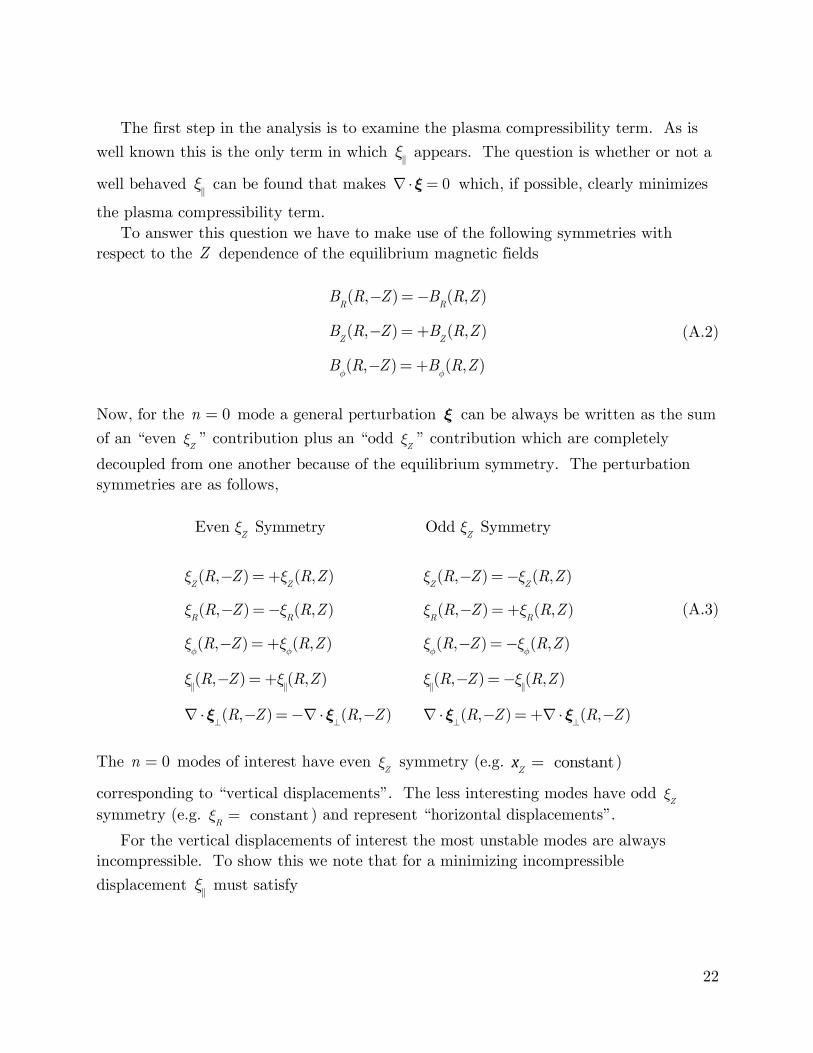
The first step in the analysis is to examine the plasma compressibility term. As is

well known this is the only term in which ξ! appears. The question is whether or not a

well behaved ξ! can be found that makes ∇⋅ξ = 0 which, if possible, clearly minimizes

the plasma compressibility term. To answer this question we have to make use of the following symmetries with

respect to the Z dependence of the equilibrium magnetic fields

BR(R,−Z) =−B

R(R,Z)

BZ(R,−Z) = +B

Z(R,Z)

Bφ(R,−Z) = +B

φ(R,Z)

(A.2)

Now, for the 0n = mode a general perturbation ξ can be always be written as the sum of an “even

ξZ ” contribution plus an “odd ξZ ” contribution which are completely

decoupled from one another because of the equilibrium symmetry. The perturbation symmetries are as follows,

Even ξZ Symmetry Odd ξ

Z Symmetry

ξZ(R,−Z) = +ξ

Z(R,Z) ξ

Z(R,−Z) =−ξ

Z(R,Z)

ξR(R,−Z) =−ξ

R(R,Z) ξ

R(R,−Z) = +ξ

R(R,Z)

ξφ(R,−Z) = +ξ

φ(R,Z) ξ

φ(R,−Z) =−ξ

φ(R,Z)

ξ!(R,−Z) = +ξ

!(R,Z) ξ

!(R,−Z) =−ξ

!(R,Z)

∇⋅ξ⊥(R,−Z) =−∇⋅ξ

⊥(R,−Z) ∇⋅ξ

⊥(R,−Z) = +∇⋅ξ

⊥(R,−Z)

(A.3)

The 0n = modes of interest have even

ξZ symmetry (e.g. constantZx = )

corresponding to “vertical displacements”. The less interesting modes have odd ξZ

symmetry (e.g. ξR = constant ) and represent “horizontal displacements”.

For the vertical displacements of interest the most unstable modes are always incompressible. To show this we note that for a minimizing incompressible displacement

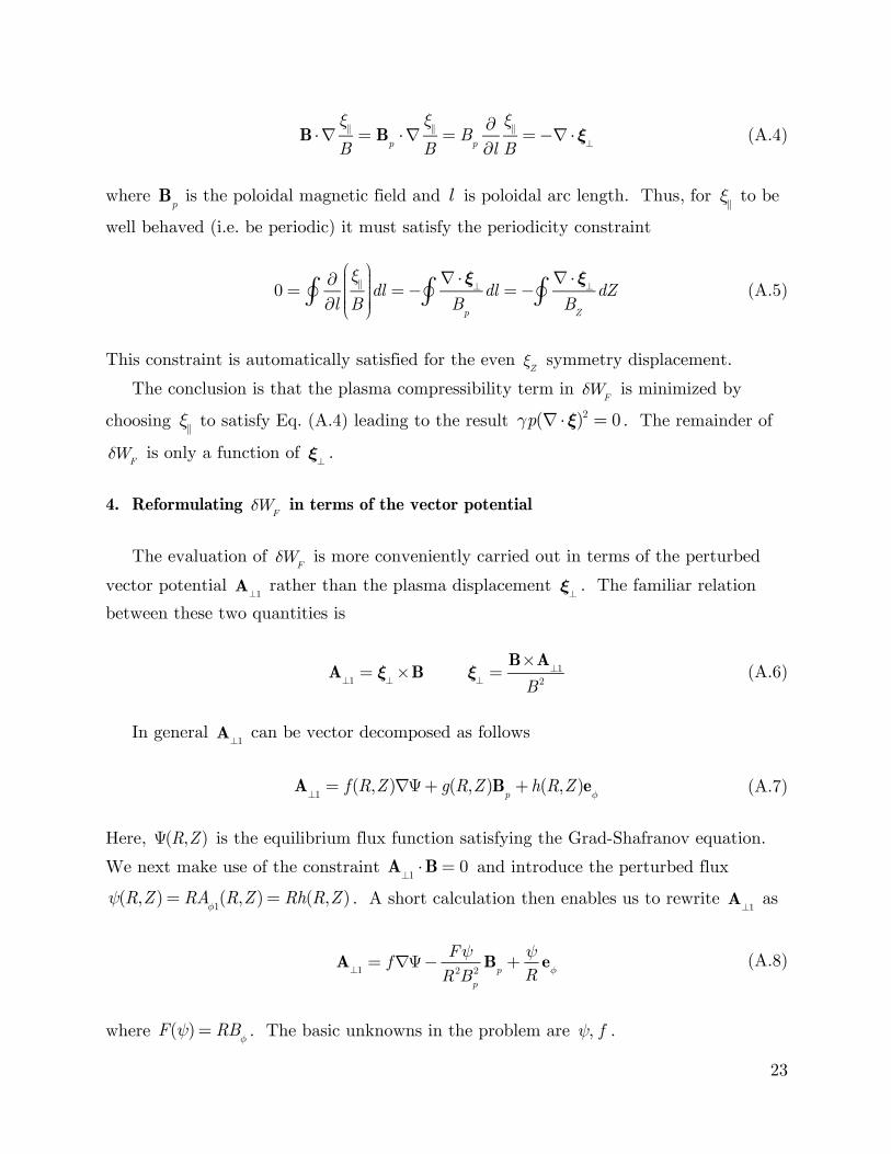
ξ! must satisfy

23

B ⋅∇

ξ!

B= B

p⋅∇ξ!

B= B

p

∂∂l

ξ!

B=−∇⋅ξ

⊥ (A.4)

where

pB is the poloidal magnetic field and l is poloidal arc length. Thus, for

ξ! to be

well behaved (i.e. be periodic) it must satisfy the periodicity constraint

0 =∂∂l

ξ!

B

⎛

⎝

⎜⎜⎜⎜⎜

⎞

⎠

⎟⎟⎟⎟⎟⎟"∫ dl =−∇⋅ξ

⊥

Bp

"∫ dl =−∇⋅ξ

⊥

BZ

"∫ dZ (A.5)

This constraint is automatically satisfied for the even

ξZ symmetry displacement.

The conclusion is that the plasma compressibility term in δWF

is minimized by

choosing ξ! to satisfy Eq. (A.4) leading to the result γp(∇⋅ξ)

2 = 0 . The remainder of

δWF is only a function of

ξ⊥ .

4. Reformulating

δWF in terms of the vector potential

The evaluation of

δWF is more conveniently carried out in terms of the perturbed

vector potential A⊥1

rather than the plasma displacement ξ⊥ . The familiar relation

between these two quantities is

A⊥1

= ξ⊥×B ξ

⊥=

B×A⊥1

B2 (A.6)

In general

A⊥1 can be vector decomposed as follows

A⊥1

= f (R,Z)∇Ψ+ g(R,Z)Bp

+h(R,Z)eφ (A.7)

Here, Ψ(R,Z) is the equilibrium flux function satisfying the Grad-Shafranov equation.

We next make use of the constraint A⊥1⋅B = 0 and introduce the perturbed flux

ψ(R,Z) = RA

φ1(R,Z) = Rh(R,Z) . A short calculation then enables us to rewrite

A⊥1 as

A⊥1

= f∇Ψ−Fψ

R2Bp2B

p+ψR

eφ (A.8)

where

F(ψ) = RB

φ . The basic unknowns in the problem are ψ, f .

24

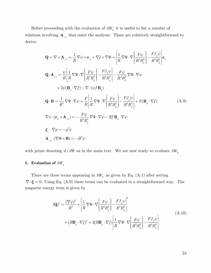
Before proceeding with the evaluation of δWF

it is useful to list a number of

relations involving A⊥1

that enter the analysis. These are relatively straightforward to

derive.

Q =∇×A⊥1

=1R∇ψ×e

φ+∇f ×∇Ψ+

1R∇Ψ ⋅∇

FψR2B

p2

⎛

⎝

⎜⎜⎜⎜⎜

⎞

⎠

⎟⎟⎟⎟⎟⎟−

FJφψ

R2Bp2

⎡

⎣

⎢⎢⎢

⎤

⎦

⎥⎥⎥eφ

Q ⋅A⊥1

=ψR

1R∇Ψ ⋅∇

FψR2B

p2

⎛

⎝

⎜⎜⎜⎜⎜

⎞

⎠

⎟⎟⎟⎟⎟⎟−

FJφψ

R2Bp2

⎡

⎣

⎢⎢⎢

⎤

⎦

⎥⎥⎥−

FψR4B

p2∇Ψ ⋅∇ψ

+ 2ψ(Bp⋅∇f )−∇⋅(ψf B

p)

Q ⋅B =1R2∇Ψ ⋅∇ψ+

FR

1R∇Ψ ⋅∇

FψR2B

p2

⎛

⎝

⎜⎜⎜⎜⎜

⎞

⎠

⎟⎟⎟⎟⎟⎟−

FJφψ

R2Bp2

⎡

⎣

⎢⎢⎢

⎤

⎦

⎥⎥⎥+ F(B

p⋅∇f )

∇ψ ⋅(eφ×A

⊥1) =−

FψR3B

p2∇Ψ ⋅∇ψ−Rf B

p⋅∇ψ

ξ⊥⋅∇p =− ′p ψ

A⊥1⋅(∇Ψ×B) =−B2ψ

(A.9)

with prime denoting d /dΨ as in the main text. We are now ready to evaluate

δWF

5. Evaluation of

δWF

There are three terms appearing in

δWF as given by Eq. (A.1) after setting

∇⋅ξ = 0. Using Eq. (A.9) these terms can be evaluated in a straightforward way. The magnetic energy term is given by

(Q)2 =(∇ψ)2

R2+

1R∇Ψ ⋅∇

FψR2B

p2

⎛

⎝

⎜⎜⎜⎜⎜

⎞

⎠

⎟⎟⎟⎟⎟⎟−

FJφψ

R2Bp2

⎡

⎣

⎢⎢⎢

⎤

⎦

⎥⎥⎥

2

+ (RBp⋅∇f )2 + 2(RB

p⋅∇f )

1R∇Ψ ⋅∇

FψR2B

p2

⎛

⎝

⎜⎜⎜⎜⎜

⎞

⎠

⎟⎟⎟⎟⎟⎟−

FJφψ

R2Bp2

⎡

⎣

⎢⎢⎢

⎤

⎦

⎥⎥⎥

(A.10)

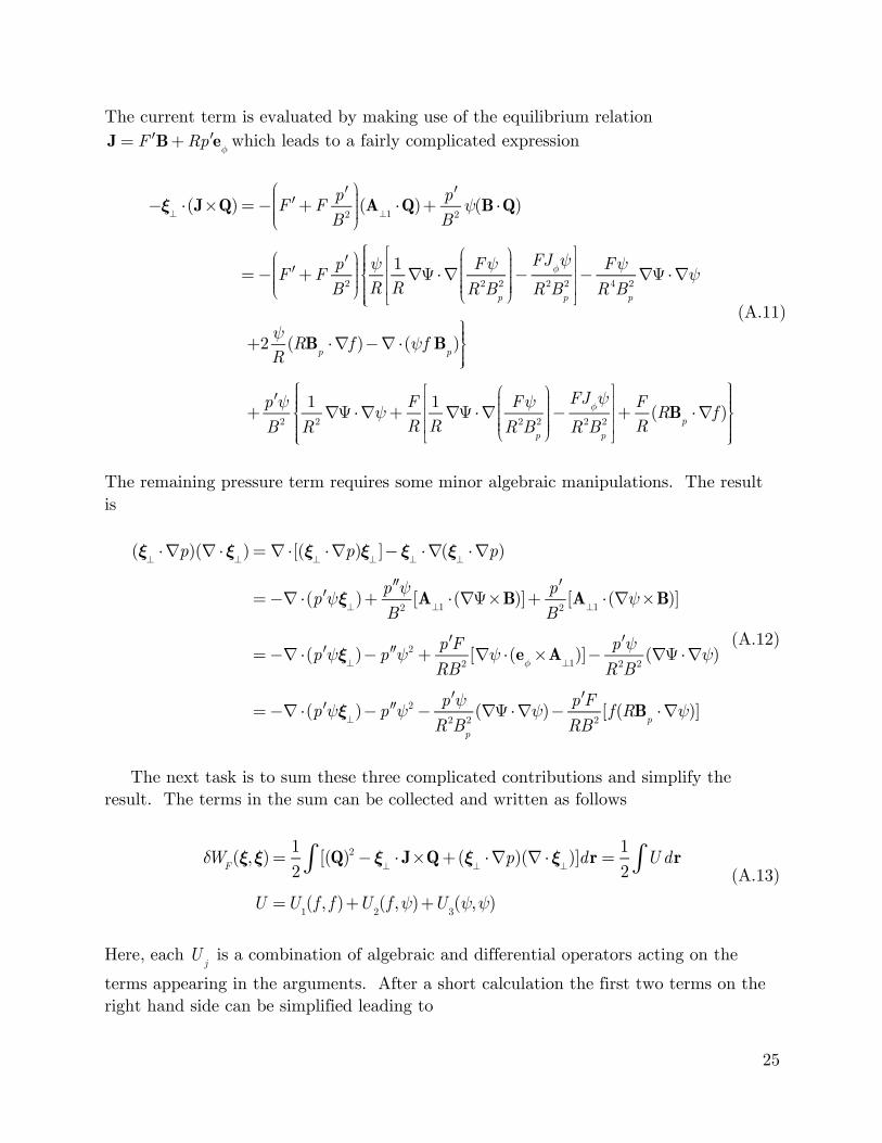
25

The current term is evaluated by making use of the equilibrium relation

J = ′F B + R ′p e

φwhich leads to a fairly complicated expression

−ξ⊥⋅(J×Q) =− ′F + F

′pB2

⎛

⎝⎜⎜⎜⎜

⎞

⎠⎟⎟⎟⎟(A⊥1⋅Q)+

′pB2ψ(B ⋅Q)

=− ′F + F′p

B2

⎛

⎝⎜⎜⎜⎜

⎞

⎠⎟⎟⎟⎟ψR

1R∇Ψ ⋅∇

FψR2B

p2

⎛

⎝

⎜⎜⎜⎜⎜

⎞

⎠

⎟⎟⎟⎟⎟⎟−

FJφψ

R2Bp2

⎡

⎣

⎢⎢⎢

⎤

⎦

⎥⎥⎥−

FψR4B

p2∇Ψ ⋅∇ψ

⎧⎨⎪⎪⎪

⎩⎪⎪⎪

+2ψR

(RBp⋅∇f )−∇⋅(ψf B

p)⎫⎬⎪⎪

⎭⎪⎪

+′p ψ

B2

1R2∇Ψ ⋅∇ψ+

FR

1R∇Ψ ⋅∇

FψR2B

p2

⎛

⎝

⎜⎜⎜⎜⎜

⎞

⎠

⎟⎟⎟⎟⎟⎟−

FJφψ

R2Bp2

⎡

⎣

⎢⎢⎢

⎤

⎦

⎥⎥⎥+

FR

(RBp⋅∇f )

⎧⎨⎪⎪⎪

⎩⎪⎪⎪

⎫⎬⎪⎪⎪

⎭⎪⎪⎪

(A.11)

The remaining pressure term requires some minor algebraic manipulations. The result is

(ξ⊥⋅∇p)(∇⋅ξ

⊥) =∇⋅[(ξ

⊥⋅∇p)ξ

⊥]−ξ

⊥⋅∇(ξ

⊥⋅∇p)

=−∇⋅( ′p ψξ⊥)+

′′p ψB2

[A⊥1⋅(∇Ψ×B)]+

′pB2

[A⊥1⋅(∇ψ×B)]

=−∇⋅( ′p ψξ⊥)− ′′p ψ2 +

′p FRB2

[∇ψ ⋅(eφ×A

⊥1)]−

′p ψR2B2

(∇Ψ ⋅∇ψ)

=−∇⋅( ′p ψξ⊥)− ′′p ψ2−

′p ψR2B

p2(∇Ψ ⋅∇ψ)−

′p FRB2

[f (RBp⋅∇ψ)]

(A.12)

The next task is to sum these three complicated contributions and simplify the

result. The terms in the sum can be collected and written as follows

δWF(ξ,ξ) =

12

[(Q)2∫ −ξ⊥⋅ J×Q + (ξ

⊥⋅∇p)(∇⋅ξ

⊥)]dr =

12

U dr∫U =U

1(f , f )+U

2(f ,ψ)+U

3(ψ,ψ)

(A.13)

Here, each

jU is a combination of algebraic and differential operators acting on the

terms appearing in the arguments. After a short calculation the first two terms on the right hand side can be simplified leading to

26

U1(f , f )+U

2(f ,ψ) = (RB

p⋅∇f )2 +∇⋅( ′F fψB

p)

+2(RBp⋅∇f )

1R∇Ψ ⋅∇

FψR2B

p2

⎛

⎝

⎜⎜⎜⎜⎜

⎞

⎠

⎟⎟⎟⎟⎟⎟−

FJφψ

R2Bp2−′F ψR

⎡

⎣

⎢⎢⎢

⎤

⎦

⎥⎥⎥

(A.14)

The divergence term integrates to zero over the plasma surface. The f dependence of

the remaining terms involves only (RB

p⋅∇f ) . These terms are simplified by completing

the square on (RB

p⋅∇f ) . The fluid energy

δWF is then minimized by choosing

(RB

p⋅∇f ) =−

1R∇Ψ ⋅∇

FψR2B

p2

⎛

⎝

⎜⎜⎜⎜⎜

⎞

⎠

⎟⎟⎟⎟⎟⎟+

FJφψ

R2Bp2

+′F ψR

(A.15)

Note that as for the incompressibility analysis, the periodicity constraint on

(RB

p⋅∇f )

is automatically satisfied for the perturbation with even ξZ symmetry. The end result is

that

U1(f , f )+U

2(f ,ψ) =−

1R∇Ψ ⋅∇

FψR2B

p2

⎛

⎝

⎜⎜⎜⎜⎜

⎞

⎠

⎟⎟⎟⎟⎟⎟−

FJφψ

R2Bp2−′F ψR

⎡

⎣

⎢⎢⎢

⎤

⎦

⎥⎥⎥

2

(A.16)

which is only a function of ψ .

The complete integrand U is now evaluated by adding Eq. (A.16) to U3(ψ,ψ). After

another tedious calculation we obtain

U =(∇ψ)2

R2− ′′p +

′F 2

R2+

F ′F Jφ

R3Bp2

⎛

⎝

⎜⎜⎜⎜⎜

⎞

⎠

⎟⎟⎟⎟⎟⎟ψ2−∇⋅( ′p ψξ

⊥)

+′F ψ

R2∇Ψ ⋅∇

FψR2B

p2

⎛

⎝

⎜⎜⎜⎜⎜

⎞

⎠

⎟⎟⎟⎟⎟⎟+

FR2B

p2(∇Ψ ⋅∇ψ)

⎡

⎣

⎢⎢⎢

⎤

⎦

⎥⎥⎥

(A.17)

After some further manipulations that make use of the equilibrium Grad-Shafranov equation we find that the term on the second line of Eq. (A.17) can be rewritten as

′F ψR2∇Ψ ⋅∇

FψR2B

p2

⎛

⎝

⎜⎜⎜⎜⎜

⎞

⎠

⎟⎟⎟⎟⎟⎟+

FR2B

p2(∇Ψ ⋅∇ψ)

⎡

⎣

⎢⎢⎢

⎤

⎦

⎥⎥⎥=∇⋅

F ′F ψ2

R4Bp2∇Ψ

⎛

⎝

⎜⎜⎜⎜⎜

⎞

⎠

⎟⎟⎟⎟⎟⎟−

F ′′FR2−

F ′F Jφ

R3Bp2

⎛

⎝

⎜⎜⎜⎜⎜

⎞

⎠

⎟⎟⎟⎟⎟⎟ψ2 (A.18)

27

Equation (A.18) is substituted into Eq. (A.17). The divergence terms are converted into surface integrals and then simplified using the equilibrium Grad-Shafranov equation. This leads to the final desired form of

δWF

δW

F=

12

(∇ψ)2

R2− ′′p +

12R2

F 2′′⎛

⎝⎜⎜⎜⎜

⎞

⎠⎟⎟⎟⎟ψ2

⎡

⎣⎢⎢⎢

⎤

⎦⎥⎥⎥

∫ dr +12

Jφ

R2Bp

ψ2⎛

⎝

⎜⎜⎜⎜⎜

⎞

⎠

⎟⎟⎟⎟⎟⎟SP

∫ dS (A.19)

There are three points worth noting. First, a simple variational analysis shows that

the function ψ that minimizes the volume contribution satisfies

Δ*ψ =− R2 ′′p +

12F 2′′

⎛

⎝⎜⎜⎜⎜

⎞

⎠⎟⎟⎟⎟ψ (A.20)

This equation is identical to the perturbed Grad-Shafranov equation corresponding to neighboring equilibria. Second, the surface contribution is nonzero only if there is a jump in the edge current density. For many profiles

Jφ is zero at the plasma edge but

it is finite for the Solov’ev profiles. Third, there is a great simplification in the volume

contribution for the Solov’ev model in that ′′p = F 2′′ = 0 . Thus the fluid energy for the Solov’ev model reduces to

δW

F=

12

(∇ψ)2

R2

⎡

⎣⎢⎢⎢

⎤

⎦⎥⎥⎥

∫ dr +12

Jφ

R2Bp

ψ2⎛

⎝

⎜⎜⎜⎜⎜

⎞

⎠

⎟⎟⎟⎟⎟⎟SP

∫ dS (A.21)

with ψ satisfying

Δ*ψ = 0 (A.22)

Assuming a solution to this equation can be found then the volume contribution can be converted into a surface integral. The fluid energy can then be written solely in terms of a surface integral

δW

F=

12

1R2ψn ⋅∇ψ+

Jφ

R2Bp

ψ2⎛

⎝

⎜⎜⎜⎜⎜

⎞

⎠

⎟⎟⎟⎟⎟⎟SP

∫ dS (A.23)

28

This form is actually valid for any equilibrium profile. The beauty of the Solov’ev profiles is that n ⋅∇ψ on the plasma surface can be conveniently evaluated in terms of

ψ on the surface using Green’s theorem since we know the analytic form of the Green’s function corresponding to Eq. (A.22). For general profiles this procedure is not as convenient since we do not know the Green’s function in a simple analytic form.

29

References – Paper 1

Aymar, R., Barabaschi, P. and Shimomura Y., The ITER design, Plasma Physics and Controlled Fusion 44, 519 (2002) Bernard, L. C., Berger, D., Gruber, R. and Troyon, F., Axisymmetric MHD stability of elongated tokamaks, Nuclear Fusion 18, 1331 (1978) Cerfon, A. J. and Freidberg, J. P., “One size fits all” analytic solutions to the Grad--Shafranov equation, Physics of Plasmas 17, 032502 (2010) Freidberg, J. P., Ideal MHD, Cambridge University Press (2014) Furth, H. P., Killeen, J. and Rosenbluth, M. N., Finite-Resistivity Instabilities of a Sheet Pinch, Physics of Fluids 6, 459 (1963) Grad, H. and Rubin, H., Hydromagnetic equilibria and force-free fields, Proceedings of the Second United Nations Conference on the Peaceful Uses of Atomic Energy 31, 190 (1958) Haney, S. W. and Freidberg, J. P., Variational methods for studying tokamak stability in the presence of a thin resistive wall, Physics of Fluids B 1, 1637 (1989) Hutchinson, I. H., Boivin, R., Bombarda, F., Bonoli, P., Fairfax, S., Fiore, C., Goetz, J., Golovato, S., Granetz, R., Greenwald, M., Horne, S., Hubbard, A., Irby, J., LaBombard, B., Lipschultz, B., Marmar, E., McCracken, G., Porkolab, M., Rice, J., Snipes, J., Takase, Y., Terry, Y., Wolfe, S., Christensen, C., Garnier, D., Graf, M., Hsu, T., Luke, T., May, M., Niemczewski, A., Tinios, G., Schachter, J. and Urbahn, J., First results from Alcator-C-MOD, Physics of Plasmas 1, 1511 (1994) Kessel, C. E., Mau, T. K., Jardin, S. C. and Najmabadi, F., Plasma profile and shape optimization for the advanced tokamak power plant, ARIES-AT , Fusion Engineering and Design 80, 63 (2006) Miller, R. L., Chu, M. S., Greene, J. M., Lin-Liu, Y. R. and Waltz, R. E., Noncircular, finite aspect ratio, local equilibrium model , Physics of Plasmas 5, 973 (1998) Najmabadi, F., The Aries Team: Bathke, C.G., Billone, M.C., Blanchard, J.P., Bromberg, L. Chin, E., Cole, F.R. , Crowell, J.A., Ehst, D.A., El-Guebaly, L.A., Herring, J.S., Hua, T.Q., Jardin, S.C., Kessel, C.E., Khater, H., Lee, V.D., Malang, S., Mau, T-K., Miller, R.L., Mogahed, E.A., Petrie, T.W., Reis, E.E., Schultz, J., Sidorov,

30

M., Steiner, D., Sviatoslavsky, I.N., Sze, D-K., Thayer, R., Tillack, M.S., Titus, P., Wagner, L.M., Wang, X., Wong, C.P.C., Overview of the ARIES-RS reversed-shear tokamak power plant study, Fusion Engineering and Design 38, 3 (1997) Najmabadi, F., The ARIES Team: Abdou, A., Bromberg, L., Brown, T., Chan, V.C., Chu, M.C., Dahlgren, F., El-Guebaly, L., Heitzenroeder, P., Henderson, D., St. John, H.E., Kessel, C.E., Lao, L.L., Longhurst, G.R., Malang, S., Mau, T.K., Merrill, B.J., Miller, R.L., Mogahed, E., Moore, R.L., Petrie, T., Petti, D.A., Politzer, P., Raffray, A.R., Steiner, D., Sviatoslavsky, I., Synder, P., Syaebler, G.M., Turnbull, A.D., Tillack, M.S., Wagner, L.M., Wang, X., West, P., Wilson, P., The ARIES-AT advanced tokamak, Advanced technology fusion power plant, Fusion Engineering and Design 80, 3 (2006) Peng, Y-K. M. and Strickler, D. J., Features of spherical torus plasmas, Nuclear Fusion 26, 769 (1986) Roberto, M. and Galvão, R. M. O., “Natural elongation” of spherical tokamaks, Nuclear Fusion 32, 1666 (1992) Sabbagh, S. A., Kaye, S. M., Menard, J., Paoletti, F., Bell, M., Bell, R. E., Bialek, J. M., Bitter, M., Fredrickson, E. D., Gates, D. A., Glasser, A. H., Kugel, H., Lao, L. L., LeBlanc, B. P., Maingi, R., Maqueda, R. J., Mazzucato, E., Wurden, G. A., Zhu, W. and NSTX Research Team, Equilibrium properties of spherical torus plasmas in NSTX, Nuclear Fusion 41, 1601 (2001) Schissel, D. P., DeBoo, J. C., Burrell, K. H., Ferron, J. R., Groebner, R. J., St. John, H., Stambaugh, R. D., Tubbing, B. J. D., Thomsen, K., Cordey, J. G., Keilhacker, M., Stork, D., Stott, P.E., Tanga, A. and JET Team, H-mode energy confinement scaling from the DIII-D and JET tokamaks, Nuclear Fusion 31, 73 (1991) Shafranov, V. D., On magnetohydrodynamical equilibrium configurations, Sov. Phys. JETP 6, 545 (1958) Shi, B., Analytic description of high poloidal beta equilibrium with a natural inboard poloidal field null, Physics of Plasmas 12, 122504 (2005) Sorbom, B. N., Ball, J., Palmer, T. R., Mangiarotti, F. J., Sierchio, J. M., Bonoli, P., Kasten, C. K., Sutherland, D. A., Barnard, H. S., Haakonsen, C. B., Goh, J., Sung, C. and Whyte, D. G., ARC: A compact, high-field, fusion nuclear science facility and demonstration power plant with demountable magnets, Fusion Engineering and Design, in press.

31

Solov'ev, L. S., The theory of hydromagnetic stability of toroidal plasma configurations, Sov. Phys.- JETP 26, 400 (1968) Sykes, A., Ahn, J.-W., Akers, R., Arends, E., Carolan, P. G., Counsell, G. F., Fielding, S. J., Gryaznevich, M., Martin, R., Price, M., Roach, C., Shevchenko, V., Tournianski, M., Valovic, M., Walsh, M. J., Wilson, H. R., and MAST Team, First physics results from the MAST Mega-Amp Spherical Tokamak, Physics of Plasmas 8, 2101 (2001) Weening, R. H., Analytic spherical torus plasma equilibrium model, Physics of Plasmas 7, 3654 (2000)

Wesson, J. A., Hydromagnetic stability of tokamaks, Nuclear Fusion 18, 87 (1978) Zheng, S. B., Wootton, A. J. and Solano, E. R., Analytical tokamak equilibrium for shaped plasmas, Physics of Plasmas 3, 1176 (1996)

32

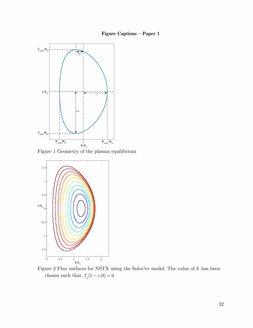
Figure Captions – Paper 1

Figure 1 Geometry of the plasma equilibrium

Figure 2 Flux surfaces for NSTX using the Solov'ev model. The value of A has been

chosen such that Jφ(1− ε,0) = 0

R/R01

Z/R0

Zmin/R0

Zmax/R0

Rmin/R0 Rmax/R0

δϵ

ϵ

κϵ

R/R00 0.5 1 1.5 2

Z/R0

-1.5

-1

-0.5

0

0.5

1

1.5