NBER WORKING PAPER SERIES

ADJUSTMENT IS MUCH SLOWER THAN YOU THINK

Ricardo J. CaballeroEduardo Engel

Working Paper 9898http://www.nber.org/papers/w9898

NATIONAL BUREAU OF ECONOMIC RESEARCH1050 Massachusetts Avenue

Cambridge, MA 02138August 2003

We are grateful to William Brainard, Pablo García, Harald Uhlig and seminar participants at HumboldtUniversität, Universidad de Chile (CEA) and University of Pennsylvania for their comments. Financialsupport from NSF is gratefully acknowledged. The views expressed herein are those of the authors andnot necessarily those of the National Bureau of Economic Research.

©2003 by Ricardo J. Caballero and Eduardo Engel. All rights reserved. Short sections of text, not toexceed two paragraphs, may be quoted without explicit permission provided that full credit, including ©notice, is given to the source.

Adjustment is Much Slower than You ThinkRicardo J. Caballero and Eduardo EngelNBER Working Paper No. 9898August 2003JEL No. C22, C43, D2, E2, E5

ABSTRACT

In most instances, the dynamic response of monetary and other policies to shocks is

infrequent and lumpy. The same holds for the microeconomic response of some of the most

important economic variables, such as investment, labor demand, and prices. We show that the

standard practice of estimating the speed of adjustment of such variables with partial-adjustment

ARMA procedures substantially overestimates this speed. For example, for the target federal funds

rate, we find that the actual response to shocks is less than half as fast as the estimated response. For

investment, labor demand and prices, the speed of adjustment inferred from aggregates of a small

number of agents is likely to be close to instantaneous. While aggregating across microeconomic

units reduces the bias (the limit of which is illustrated by Rotemberg’s widely used linear aggregate

characterization of Calvo’s model of sticky prices), in some instances convergence is extremely

slow. For example, even after aggregating investment across all establishments in U.S.

manufacturing, the estimate of its speed of adjustment to shocks is biased upward by more than 80

percent. While the bias is not as extreme for labor demand and prices, it still remains significant at

high levels of aggregation. Because the bias rises with disaggregation, findings of microeconomic

adjustment that is substantially faster than aggregate adjustment are generally suspect.

Ricardo Caballero Eduardo M. EngelDepartment of Economics Department of EconomicsMIT, 50 Memorial Drive P.O. Box 208268E52-252 New Haven, CT 06520Cambridge, MA 02142 and NBERand NBER eduardo.engel@yale.educaball@mit.edu

1 Introduction

The measurement of the dynamic response of economic and policy variables to shocks is of central impor-

tance in macroeconomics. Usually, this response is estimated by recovering the speed at which the variable

of interest adjusts from a linear time-series model. In this paper we argue that, in many instances, this

procedure significantly underestimates the sluggishness of actual adjustment.

The severity of this bias depends on how infrequent and lumpy the adjustment of the underlying vari-

able is. In the case of single policy variables, such as the federal funds rate, or individual microeconomic

variables, such as firm level investment, this bias can be extreme. If no source of persistence other than

the discrete adjustment exists, we show that regardless of how sluggish adjustment may be, the econometri-

cian estimating linear autoregressive processes (partial adjustment models) will erroneously conclude that

adjustment is instantaneous.

Aggregation across establishments reduces the bias, so we have the somewhat unusual situation where

estimates of a microeconomic parameter using aggregate data are less biased than those based upon microe-

conomic data. Lumpiness combined with linear estimation procedures is likely to give the false impression

that microeconomic adjustments is significantly faster than aggregate adjustment.

We also show that, when aggregating across units, convergence to the correct estimate of the speed of ad-

justment is extremely slow. For example, for U.S. manufacturing investment, even after aggregating across

all the continuous establishments in the LRD (approximately 10,000 establishments), estimates of speed of

adjustment are 80 percent higher than actual speed — at the two-digit level the bias easily can exceed 400

percent. Similarly, estimating a Calvo (1983) model using standard partial-adjustment techniques is likely

to underestimate the sluggishness of price adjustments severely. This is consistent with the recent findings

of Bils and Klenow (2002), who report much slower speeds of adjustment when looking at individual price

adjustment frequencies than when estimating the speed of adjustment with linear time-series models. We

also show that estimates of employment adjustment speed experience similar biases.

The basic intuition underlying our main results is the following: In linear models, the estimated speed of

adjustment is inversely related to the degree of persistence in the data. That is, a larger first order correlation

is associated with lower adjustment speed. Yet this correlation is always zero for an individual series that is

adjusted discretely (and has i.i.d. shocks), so that the researcher will conclude, incorrectly, that adjustment

is infinitely fast. To see that this crucial correlation is zero, first note that the product of current and lagged

changes in the variable of concern is zero when there is no adjustment in either the current or the preceding

period. This means that any non-zero serial correlation must come from realizations in which the unit

adjusts in two consecutive periods. But when the unit adjusts in two consecutive periods, and whenever it

acts it catches up with all accumulated shocks since it last adjusted, it must be that the later adjustment only

involves the latest shock, which is independent from the shocks included in the previous adjustment.

The bias falls as aggregation rises because the correlations at leads and lags of the adjustments across

individual units are non-zero. That is, the common components in the adjustments of different agents at

different points in time provides the correlation that allows us to recover the microeconomic speed of ad-

1

justment. The larger this common component is —as measured, for example, by the variance of aggregate

shocks relative to the variance of idiosyncratic shocks— the faster the estimate converges to its true value as

the number of agents grows. In practice, the variance of aggregate shocks is significantly smaller than that

of idiosyncratic shocks, and convergence takes place at a very slow pace.

In Section 2 we study the bias for microeconomic and single-policy variables, and illustrate its im-

portance when estimating the speed of adjustment of monetary policy. Section 3 presents our aggregation

results and highlights slow convergence. We show the relevance of this phenomenon for parameters consis-

tent with those of investment, labor, and price adjustments in the U.S. Section 4 discusses partial solutions

and extensions. It first extends our results to dynamic equations with contemporaneous regressors, such as

those used in price-wage equations, or output-gap inflation models. It then illustrates an ARMA method to

reduce the extent of the bias. Section 5 concludes and is followed by an appendix with technical details.

2 Microeconomic and Single-Policy Series

When the task of a researcher is to estimate the speed of adjustment of a state variable —or the implicit

adjustment costs in a quadratic adjustment cost model (see e.g., Sargent 1978, Rotemberg 1987)— the

standard procedure reduces to estimating variations of the celebratedpartial adjustment model(PAM):

∆yt = λ(y∗t −yt−1), (1)

wherey and y∗ represent the actual and optimal levels of the variable under consideration (e.g., prices,

employment, or capital), andλ is a parameter that captures the extent to which imbalances are remedied in

each period. Taking first differences and rearranging terms leads to the best known form of PAM:

∆yt = (1−λ)∆yt−1 +vt , (2)

with vt ≡ λ∆y∗t .

In this model,λ is thought of as the speed of adjustment, while the expected time until adjustment

(defined formally in Section 2) is(1−λ)/λ. Thus, asλ converges to one, adjustment occurs instantaneously,

while asλ decreases, adjustment slows down.

Most people understand that this model is only meant to capture the first-order dynamics of more real-

istic but complicated adjustment models. Perhaps most prominent among the latter, many microeconomic

variables exhibit only infrequent adjustment to their optimal level (possibly due to the presence of fixed

costs of adjustments). And the same is true of policy variables, such as the federal funds rate set by the

monetary authority in response to changes in aggregate conditions. In what follows, we inquire how good

the estimates of the speed of adjustment from the standard partial adjustment approximation (2) are, when

actual adjustment is discrete.

2

2.1 A Simple Lumpy Adjustment Model

Let yt denote the variable of concern at timet —e.g., the federal funds rate, a price, employment, or capital—

andy∗t be its optimal counterpart. We can characterize the behavior of an individual agent in terms of the

equation:

∆yt = ξt(y∗t −yt−1), (3)

whereξt satisfies:Pr{ξt = 1} = λ,

Pr{ξt = 0} = 1−λ.(4)

From a modelling perspective, discrete adjustment entails two basic features: (i) periods of inaction fol-

lowed by abrupt adjustments to accumulated imbalances, and (ii) increased likelihood of an adjustment with

the size of the imbalance (state dependence). While the second feature is central for the macroeconomic im-

plications of state-dependent models, it is not needed for the point we wish to raise in this paper. Therefore,

we suppress it.1

It follows from (4) that theexpectedvalue ofξt is λ. Whenξt is zero, the agent experiences inaction;

when its value is one, the unit adjusts so as to eliminate the accumulated imbalance. We assume thatξt is

independent of(y∗t − yt−1) (this is the simplification that Calvo (1983) makes vis-a-vis more realistic state

dependent models) and therefore have:

E[∆yt | y∗t , yt−1] = λ(y∗t −yt−1), (5)

which is the analog of (1). Henceλ represents theadjustment speedparameter to be recovered.

2.2 The Main Result: (Biased) Instantaneous Adjustment

The question now arises as to whether, by analogy to the derivation from (1) to (2), the standard procedure

of estimating

∆yt = (1−λ)∆yt−1 + εt , (6)

recovers theaverageadjustment speed,λ, when adjustment is lumpy. The next proposition states that the

answer to this question is clearly no.

Proposition 1 (Instantaneous Estimate)

Let λ denote the OLS estimator ofλ in equation (6). Let the∆y∗t ’s be i.i.d. with mean0 and varianceσ2,

1The special model we consider —i.e., without feature (ii)— is due to Calvo (1983) and was extended by Rotemberg (1987)to show that, with a continuum of agents,aggregatedynamics are indistinguishable from those of a representative agent facingquadratic adjustment costs. One of our contributions is to go over the aggregation steps in more detail, and show the problems thatarise before convergence is achieved.

3

and letT denote the time series length. Then, regardless of the value ofλ:

plimT→∞λ = 1. (7)

Proof See Appendix B.1.

While the formal proof can be found in the appendix, it is instructive to develop its intuition in the main

text. If adjustment were smooth instead of lumpy, we would have the classical partial adjustment model, so

that the first order autocorrelation of observed adjustments is1−λ, thereby revealing the speed with which

units adjust. But when adjustment is lumpy, the correlation between this period’s and the previous period’s

adjustment necessarily is zero, so that the implied speed of adjustment is one, independent of the true value

of λ. To see why this is so, consider the covariance of∆yt and∆yt−1, noting that, because adjustment is

complete whenever it occurs, we may re-write (3) as:

∆yt = ξt

lt−1

∑k=0

∆y∗t−k =

∑lt−1k=0 ∆y∗t−k if ξt = 1,

0 otherwise,

(8)

wherelt denotes the number of periods since the last adjustment took place, (as of periodt).2

Table 1:CONSTRUCTING THEMAIN COVARIANCE

Adjust in t−1 Adjust in t ∆yt−1 ∆yt Contribution toCov(∆yt ,∆yt−1)No No 0 0 ∆yt∆yt−1 = 0No Yes 0 ∆y∗t ∆yt∆yt−1 = 0Yes No ∑lt−1

k=0 ∆y∗t−1−k 0 ∆yt∆yt−1 = 0Yes Yes ∑lt−1

k=0 ∆y∗t−1−k ∆y∗t Cov(∆yt−1,∆yt) = 0

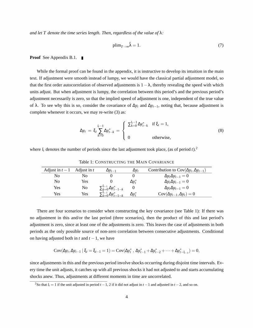
There are four scenarios to consider when constructing the key covariance (see Table 1): If there was

no adjustment in this and/or the last period (three scenarios), then the product of this and last period’s

adjustment is zero, since at least one of the adjustments is zero. This leaves the case of adjustments in both

periods as the only possible source of non-zero correlation between consecutive adjustments. Conditional

on having adjusted both int andt−1, we have

Cov(∆yt ,∆yt−1 | ξt = ξt−1 = 1) = Cov(∆y∗t , ∆y∗t−1 +∆y∗t−2 + · · ·+∆y∗t−lt−1) = 0,

since adjustments in this and the previous period involve shocks occurring during disjoint time intervals. Ev-

ery time the unit adjusts, it catches up with all previous shocks it had not adjusted to and starts accumulating

shocks anew. Thus, adjustments at different moments in time are uncorrelated.

2So thatlt = 1 if the unit adjusted in periodt−1, 2 if it did not adjust int−1 and adjusted int−2, and so on.

4

2.3 Robust Bias: Infrequent and Gradual Adjustment

Suppose now that in addition to the infrequent adjustment pattern described above, once adjustment takes

place, it is only gradual. Such behavior is observed, for example, when there is a time-to-build feature in

investment (e.g., Majd and Pindyck (1987)) or when policy is designed to exhibit inertia (e.g., Goodfriend

(1987), Sack (1998), or Woodford (1999)). Our main result here is that the econometrician estimating a

linear ARMA process —a Calvo model with additional serial correlation— will only be able to extract the

gradual adjustment component but not the source of sluggishness from the infrequent adjustment compo-

nent. That is, again, the estimated speed of adjustment will be too fast, for exactly the same reason as in the

simpler model.

Let us modify our basic model so that equation (3) now applies for a new variableyt in place ofyt ,

with ∆yt representing thedesiredadjustment of the variable that concerns us,∆yt . This adjustment takes

place only gradually, for example, because of a time-to-build component. We capture this pattern with the

process:

∆yt =K

∑k=1

φk∆yt−k +(1−K

∑k=1

φk)∆yt . (9)

Now there are two sources of sluggishness in the transmission of shocks,∆y∗t , to the observed variable,∆yt .

First, the agent only acts intermittently, accumulating shocks in periods with no adjustment. Second, when

he adjusts, he does so only gradually.

By analogy with the simpler model, suppose the econometrician approximates the lumpy component of

the more general model by:

∆yt = (1−λ)∆yt−1 +vt . (10)

Replacing (10) into (9), yields the following linear equation in terms of the observable,∆yt :

∆yt =K+1

∑k=1

ak∆yt−k + εt , (11)

witha1 = φ1 +1−λ,

ak = φk− (1−λ)φk−1, k = 2, ...,K,

aK+1 = −(1−λ)φK ,

(12)

andεt ≡ λ(1−∑Kk=1 φk)∆y∗t .

By analogy to the simpler model, we now show that the econometrician will miss the source of persis-

tence stemming fromλ.

Proposition 2 (Omitted Source of Sluggishness)

Let all the assumptions in Proposition 1 hold, withy in the role ofy. Also assume that (9) applies,

with all roots of the polynomial1−∑Kk=1 φkzk outside the unit disk. Letak,k = 1, ...,K +1 denote the OLS

estimates of equation (11).

5

Then:plimT→∞ak = φk, k = 1, ...,K,

plimT→∞aK+1 = 0.(13)

Proof See Appendix B.1.

Comparing (12) and (13) we see that the proposition simply reflects the fact that the (implicit) estimate

of λ is one.

The mapping from the biased estimates of theak’s to the speed of adjustment is slightly more cumber-

some, but the conclusion is similar. To see this, let us define the following index ofexpected response time

to capture the overall sluggishness in the response of∆y to ∆y∗:

τ≡ ∑k≥0

kEt

[∂∆yt+k

∂∆y∗t

], (14)

whereEt[ · ] denotes expectations conditional on information (that is, values of∆y and∆y∗) known at time

t. This index is a weighted sum of the components of the impulse response function, with weights equal to

the number of periods that elapse until the corresponding response is observed.3 For example, an impulse

response with the bulk of its mass at low lags has a small value ofτ, since∆y responds relatively fast to

shocks.

It is easy to show (see Propositions A1 and A2 in the Appendix) that both for the standard Partial

Adjustment Model (1) and for the simple lumpy adjustment model (3) we have

τ =1−λ

λ.

More generally, for the model with both gradual and lumpy adjustment described in (9), the expected

response to∆y satisfies:

τlin = ∑Kk=1kφk

1−∑Kk=1 φk

,

while the expected response to shocks∆y∗ is equal to:4

τ =1−λ

λ+ ∑K

k=1kφk

1−∑Kk=1 φk

. (15)

3Note that, for the models at hand, the impulse response is always non-negative and adds up to one. When the impulse responsedoes not add up to one, the definition above needs to be modified to:

τ≡∑k≥0kEt

[∂∆yt+k∂∆y∗t

]

∑k≥0E[

∂∆yt+k∂∆y∗t

] .

4For the derivation of both expressions forτ see Propositions A1 and A3 in the Appendix.

6

Let us label:

τlum ≡ 1−λλ

.

It follows that that the expected response when both sources of sluggishness are present is the sum of the

responses to each one taken separately.

We can now state the implication of Proposition 2 for the estimated expected time of adjustment,τ.

Corollary 1 (Fast Adjustment) Let the assumptions of Proposition 2 hold and letτ denote the (classical)

method of moments estimator forτ obtained from OLS estimators of:

∆yt =K+1

∑k=1

ak∆yt−k +et .

Then:

plimT→∞τ = τlin ≤ τ = τlin + τlum, (16)

with a strict inequality forλ < 1.

Proof See Appendix B.1.

To summarize, the linear approximation for∆y (wrongly) suggests no sluggishness whatsoever, so that

when this approximation is plugged into the (correct) linear relation between∆y and ∆y, one source of

sluggishness is lost. This leads to an expected response time that completely ignores the sluggishness

caused by the lumpy component of adjustments.

2.4 An Application: Monetary Policy

Figure 1 depicts the monthly evolution of the intended federal funds rate during the Greenspan era.5 The

infrequent nature of adjustment of this policy variable is evident in the figure. It is also well known that

monetary policy interventions often come in gradual steps (see, e.g., Sack (1998) and Woodford (1999)),

fitting the description of the model we just characterized.

Our goal is to estimate both components ofτ, τlin and τlum. Regarding the former, we estimate AR

processes for∆ywith an increasing number of lags, until finding no significant improvement in the goodness-

of-fit. This procedure is warranted since∆y, the omitted regressor, is orthogonal to the lagged∆y’s. We

obtained an AR(3) process, withτlin estimated as 2.35 months.

If the lumpy component is relevant, the (absolute) magnitude of adjustments of∆y should increase with

the number of periods since the last adjustment. The longer the inaction period, the larger the number of

shocks in∆y∗ to which y has not adjusted, and hence the larger the variance of observed adjustments.

To test this implication of lumpy adjustment, we identified periods with adjustment iny as those where

the residual from the linear model takes (absolute) values above a certain threshold,M. Next we partitioned

5The findings reported in this section remain valid if we use different sample periods.

7

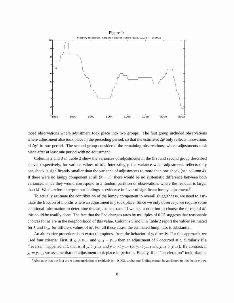
Figure 1:

1988 1990 1992 1994 1996 1998 2000 20021

2

3

4

5

6

7

8

9

10Monthly Intended (Target) Federal Funds Rate. 9/1987 − 3/2002

those observations where adjustment took place into two groups. The first group included observations

where adjustment also took place in the preceding period, so that the estimated∆y only reflects innovations

of ∆y∗ in one period. The second group considered the remaining observations, where adjustments took

place after at least one period with no adjustment.

Columns 2 and 3 in Table 2 show the variances of adjustments in the first and second group described

above, respectively, for various values ofM. Interestingly, the variance when adjustments reflects only

one shock is significantly smaller than the variance of adjustments to more than one shock (see column 4).

If there were no lumpy component at all (λ = 1), there would be no systematic difference between both

variances, since they would correspond to a random partition of observations where the residual is larger

thanM. We therefore interpret our findings as evidence in favor of significant lumpy adjustment.6

To actually estimate the contribution of the lumpy component to overall sluggishness, we need to esti-

mate the fraction of months where an adjustment iny took place. Since we only observey, we require some

additional information to determine this adjustment rate. If we had a criterion to choose the thresholdM,

this could be readily done. The fact that the Fed changes rates by multiples of 0.25 suggests that reasonable

choices forM are in the neighborhood of this value. Columns 5 and 6 in Table 2 report the values estimated

for λ andτlum for different values ofM. For all these cases, the estimated lumpiness is substantial.

An alternative procedure is to extract lumpiness from the behavior ofyt directly. For this approach, we

used four criteria: First, ifyt 6= yt−1 andyt−1 = yt−2 then an adjustment ofy occurred att. Similarly if a

“reversal” happened att, that is, ifyt > yt−1 andyt−1 < yt−2 (or yt < yt−1 andyt−1 > yt−2). By contrast, if

yt = yt−1, we assume that no adjustment took place in periodt. Finally, if an “acceleration” took place at

6Also note that the first order autocorrelation of residuals is−0.002, so that our finding cannot be attributed to this factor either.

8

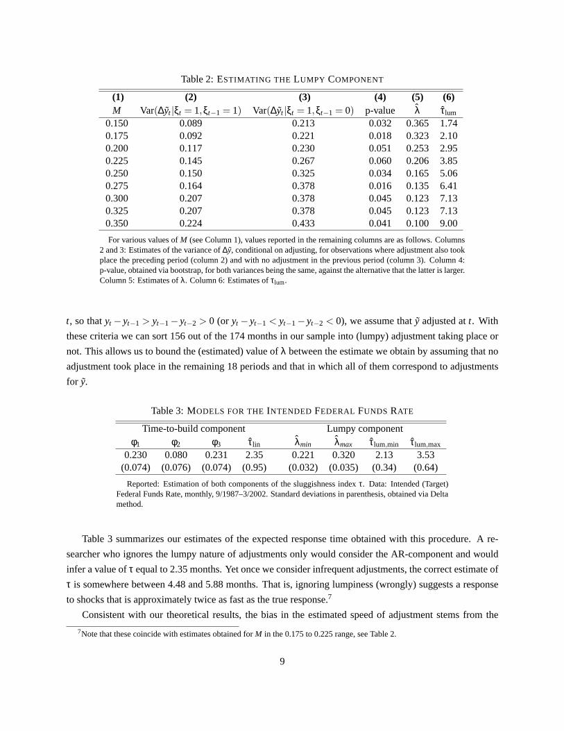
Table 2:ESTIMATING THE LUMPY COMPONENT

(1) (2) (3) (4) (5) (6)M Var(∆yt |ξt = 1,ξt−1 = 1) Var(∆yt |ξt = 1,ξt−1 = 0) p-value λ τlum

0.150 0.089 0.213 0.032 0.365 1.740.175 0.092 0.221 0.018 0.323 2.100.200 0.117 0.230 0.051 0.253 2.950.225 0.145 0.267 0.060 0.206 3.850.250 0.150 0.325 0.034 0.165 5.060.275 0.164 0.378 0.016 0.135 6.410.300 0.207 0.378 0.045 0.123 7.130.325 0.207 0.378 0.045 0.123 7.130.350 0.224 0.433 0.041 0.100 9.00

For various values ofM (see Column 1), values reported in the remaining columns are as follows. Columns2 and 3: Estimates of the variance of∆y, conditional on adjusting, for observations where adjustment also tookplace the preceding period (column 2) and with no adjustment in the previous period (column 3). Column 4:p-value, obtained via bootstrap, for both variances being the same, against the alternative that the latter is larger.Column 5: Estimates ofλ. Column 6: Estimates ofτlum.

t, so thatyt −yt−1 > yt−1−yt−2 > 0 (or yt −yt−1 < yt−1−yt−2 < 0), we assume thaty adjusted att. With

these criteria we can sort 156 out of the 174 months in our sample into (lumpy) adjustment taking place or

not. This allows us to bound the (estimated) value ofλ between the estimate we obtain by assuming that no

adjustment took place in the remaining 18 periods and that in which all of them correspond to adjustments

for y.

Table 3:MODELS FOR THEINTENDED FEDERAL FUNDS RATE

Time-to-build component Lumpy componentφ1 φ2 φ3 τlin λmin λmax τlum,min τlum,max

0.230 0.080 0.231 2.35 0.221 0.320 2.13 3.53(0.074) (0.076) (0.074) (0.95) (0.032) (0.035) (0.34) (0.64)

Reported: Estimation of both components of the sluggishness indexτ. Data: Intended (Target)Federal Funds Rate, monthly, 9/1987–3/2002. Standard deviations in parenthesis, obtained via Deltamethod.

Table 3 summarizes our estimates of the expected response time obtained with this procedure. A re-

searcher who ignores the lumpy nature of adjustments only would consider the AR-component and would

infer a value ofτ equal to 2.35 months. Yet once we consider infrequent adjustments, the correct estimate of

τ is somewhere between 4.48 and 5.88 months. That is, ignoring lumpiness (wrongly) suggests a response

to shocks that is approximately twice as fast as the true response.7

Consistent with our theoretical results, the bias in the estimated speed of adjustment stems from the

7Note that these coincide with estimates obtained forM in the 0.175 to 0.225 range, see Table 2.

9

infrequent adjustment of monetary policy to news. As shown above, this bias is important, since infrequent

adjustment accounts for at least half of the sluggishness in modern U.S. monetary policy.

3 Slow Aggregate Convergence

Could aggregation solve the problem for those variables where lumpiness occurs at the microeconomic

level? In the limit, yes. Rotemberg (1987) showed that the aggregate equation resulting from individual

actions driven by the Calvo-model indeed converges to the partial-adjustment model. That is, as the number

of microeconomic units goes to infinity, estimation of equation (6) for the aggregate does yield the correct

estimate ofλ, and thereforeτ. (Henceforth we return to the simple model without time-to-build).

But not all is good news. In this section, we show that when the speed of adjustment is already slow, the

bias vanishes very slowly as the number of units in the aggregate increases. In fact, in the case of investment

even aggregating across all U.S. manufacturing establishments is not sufficient to eliminate the bias.

3.1 The Result

Let us define the N-aggregate change at timet, ∆yNt , as:

∆yNt ≡

1N

N

∑i=1

∆yi,t ,

where∆yi,t denotes the change in the variable of interest by uniti in periodt.

Technical Assumptions (Shocks)

Let ∆y∗i,t ≡ vAt + vI

i,t , where the absence of a subindexi denotes an element common to alli (i.e, that

remains after averaging across alli’s). We assume:

1. thevAt ’s are i.i.d. with meanµA and varianceσ2

A > 0,

2. thevIi,t ’s are independent (across units, over time, and with respect to thevA’s), identically distributed

with zero mean and varianceσ2I > 0, and

3. theξi,t ’s are independent (across units, over time, and with respect to thevA’s andvI ’s), identically

distributed Bernoulli random variables with probability of successλ ∈ (0,1].

As in the single unit case, we now ask whether estimating

∆yNt = (1−λ)∆yN

t−1 + εt , (17)

yields a consistent (asT goes to infinity) estimate ofλ, when the true microeconomic model is (8). The

following proposition answers this question by providing an explicit expression for the bias as a function of

10

the parameters characterizing adjustment probabilities and shocks (λ, µA, σA andσI ) and, most importantly,

N.

Proposition 3 (Aggregate Bias)

Let λN denote the OLS estimator ofλ in equation (17). LetT denote the time series length. Then, under

the Technical Assumptions,

plimT→∞λN = λ +1−λ1+K

, (18)

with

K ≡λ

2−λ(N−1)σ2A−µ2

A

σ2A +σ2

I + 2−λλ µ2

A

. (19)

It follows that:

limN→∞

plimT−>∞λN = λ. (20)

Proof See Theorem B1 in the Appendix.

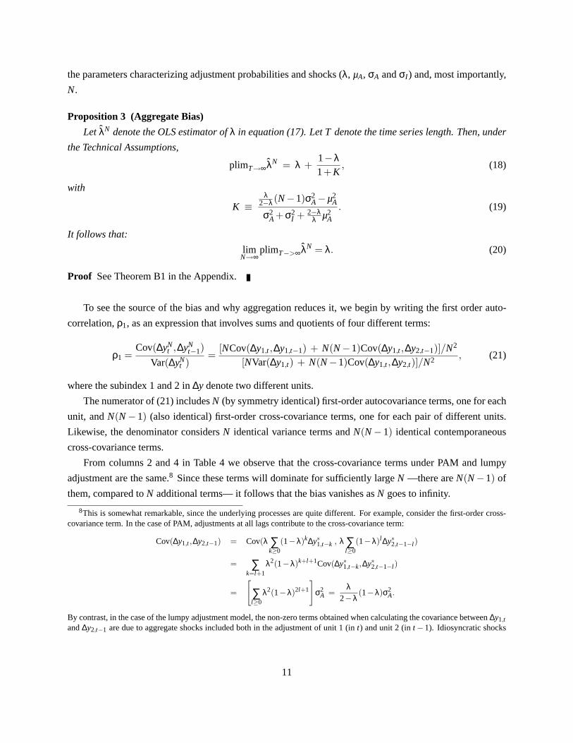
To see the source of the bias and why aggregation reduces it, we begin by writing the first order auto-

correlation,ρ1, as an expression that involves sums and quotients of four different terms:

ρ1 =Cov(∆yN

t ,∆yNt−1)

Var(∆yNt )

=[NCov(∆y1,t ,∆y1,t−1) + N(N−1)Cov(∆y1,t ,∆y2,t−1)]/N2

[NVar(∆y1,t) + N(N−1)Cov(∆y1,t ,∆y2,t)]/N2 , (21)

where the subindex 1 and 2 in∆y denote two different units.

The numerator of (21) includesN (by symmetry identical) first-order autocovariance terms, one for each

unit, andN(N−1) (also identical) first-order cross-covariance terms, one for each pair of different units.

Likewise, the denominator considersN identical variance terms andN(N−1) identical contemporaneous

cross-covariance terms.

From columns 2 and 4 in Table 4 we observe that the cross-covariance terms under PAM and lumpy

adjustment are the same.8 Since these terms will dominate for sufficiently largeN —there areN(N−1) of

them, compared toN additional terms— it follows that the bias vanishes asN goes to infinity.

8This is somewhat remarkable, since the underlying processes are quite different. For example, consider the first-order cross-covariance term. In the case of PAM, adjustments at all lags contribute to the cross-covariance term:

Cov(∆y1,t ,∆y2,t−1) = Cov(λ ∑k≥0

(1−λ)k∆y∗1,t−k , λ ∑l≥0

(1−λ)l ∆y∗2,t−1−l )

= ∑k=l+1

λ2(1−λ)k+l+1Cov(∆y∗1,t−k,∆y∗2,t−1−l )

=

[∑l≥0

λ2(1−λ)2l+1

]σ2

A =λ

2−λ(1−λ)σ2

A.

By contrast, in the case of the lumpy adjustment model, the non-zero terms obtained when calculating the covariance between∆y1,tand∆y2,t−1 are due to aggregate shocks included both in the adjustment of unit 1 (int) and unit 2 (int−1). Idiosyncratic shocks

11

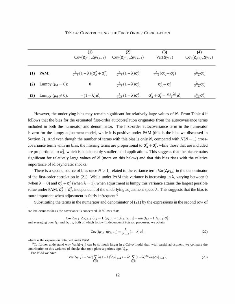
Table 4:CONSTRUCTING THEFIRST ORDER CORRELATION

(1) (2) (3) (4)Cov(∆y1,t ,∆y1,t−1) Cov(∆y1,t ,∆y2,t−1) Var(∆y1,t) Cov(∆y1,t ,∆y2,t)

(1) PAM: λ2−λ(1−λ)(σ2

A +σ2I )

λ2−λ(1−λ)σ2

Aλ

2−λ(σ2A +σ2

I )λ

2−λ σ2A

(2) Lumpy (µA = 0): 0 λ2−λ(1−λ)σ2

A σ2A +σ2

Iλ

2−λ σ2A

(3) Lumpy (µA 6= 0): −(1−λ)µ2A

λ2−λ(1−λ)σ2

A σ2A +σ2

I + 2(1−λ)λ µ2

Aλ

2−λ σ2A

However, the underlying bias may remain significant for relatively large values ofN. From Table 4 it

follows that the bias for the estimated first-order autocorrelation originates from the autocovariance terms

included in both the numerator and denominator. The first-order autocovariance term in the numerator

is zero for the lumpy adjustment model, while it is positive under PAM (this is the bias we discussed in

Section 2). And even though the number of terms with this bias is onlyN, compared withN(N−1) cross-

covariance terms with no bias, the missing terms are proportional toσ2A +σ2

I , while those that are included

are proportional toσ2A, which is considerably smaller in all applications. This suggests that the bias remains

significant for relatively large values ofN (more on this below) and that this bias rises with the relative

importance of idiosyncratic shocks.

There is a second source of bias onceN > 1, related to the variance termVar(∆y1,t) in the denominator

of the first-order correlation in (21). While under PAM this variance is increasing inλ, varying between 0

(whenλ = 0) andσ2A+σ2

I (whenλ = 1), when adjustment is lumpy this variance attains the largest possible

value under PAM,σ2A+σ2

I , independent of the underlying adjustment speedλ. This suggests that the bias is

more important when adjustment is fairly infrequent.9

Substituting the terms in the numerator and denominator of (21) by the expressions in the second row of

are irrelevant as far as the covariance is concerned. It follows that:

Cov[∆y1,t , ∆y2,t−1|ξ1,t = 1,ξ2,t−1 = 1, l1,t , l2,t−1] = min(l1,t −1, l2,t−1)σ2A,

and averaging overl1,t andl2,t−1, both of which follow (independent) Poisson processes, we obtain:

Cov(∆y1,t ,∆y2,t−1) =λ

2−λ(1−λ)σ2

A, (22)

which is the expression obtained under PAM.9To further understand whyVar(∆y1,t) can be so much larger in a Calvo model than with partial adjustment, we compare the

contribution to this variance of shocks that took placek periods ago,Vk,t .For PAM we have

Var(∆y1,t) = Var(∑k≥0

λ(1−λ)k∆y∗1,t−k) = λ2 ∑k≥0

(1−λ)2kVar(∆y∗1,t−k), (23)

12

Table 4, and dividing numerator and denominator byN(N−1)λ/(2−λ) leads to:

ρ1 =1−λ

1+ 2−λλ(N−1)

(1+ σ2

Iσ2

A

) . (24)

This expression confirms our discussion. It illustrates clearly that the bias is increasing inσI/σA and de-

creasing inλ andN.

Finally, we note that a value ofµA 6= 0 biases the estimates of the speed of adjustment even further.

The reason for this is that it introduces a sort of “spurious” negative correlation in the time series of∆y1,t .

Whenever the unit does not adjust, its change is, in absolute value, below the mean change. When adjustment

finally takes place, pent-up adjustments are undone and the absolute change, on average, exceeds|µA|. The

product of these two terms is clearly negative, inducing negative serial correlation.10

Summing up, the bias obtained when estimatingλ with standard partial adjustment regressions can be

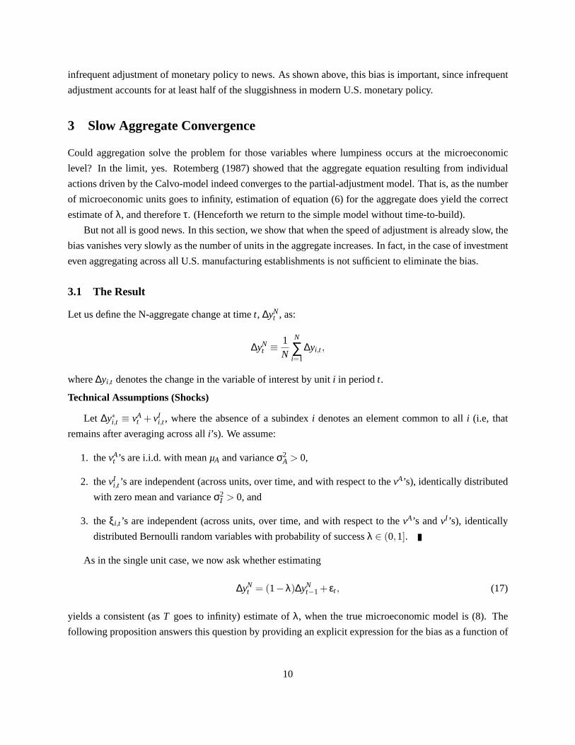
expected to be significant when eitherσA/σI , N or λ is small, or|µA| is large. Figure 2 illustrates howλN

converges toλ. The baseline parameters (solid line) areµA = 0, λ = 0.20, σA = 0.03 andσI = 0.24. The

solid line depicts the percentage bias asN grows. ForN = 1,000, the bias is above 100%; by the time

N = 10,000, it is slightly above 20%. The dash-dot line increasesσA to 0.04, speeding up convergence.

By contrast, the dash-dot line considersµA = 0.10, which slows down convergence. Finally, the dotted line

shows the case whereλ doubles to0.40, which also speeds up convergence.

Corollary 2 (Slow Convergence)

The bias in the estimator of the adjustment speed is increasing inσI and|µA| and decreasing inσA,N and

λ. Furthermore, the four parameters mentioned above determine the bias of the estimator via a decreasing

expression ofK.11

Proof Trivial.

so thatVPAM

k,t = λ2(1−λ)2k(σ2A +σ2

I ).

By contrast, in the case of lumpy adjustment we have:

V lumpyk = Pr{l1,t = k}Var(∆y1,t |l1,t = k)

= Pr{l1,t = k}[λVar(∆y1,t |l1,t = 1,ξ1,t = 1)+(1−λ)Var(∆y1,t |l1,t = 0,ξt = 0)]

= λ(1−λ)k−1[λk(σ2A +σ2

I )].

Vk,t is much larger under the lumpy adjustment model than under PAM. With infrequent adjustment the relevant conditional distri-bution is a mixture of a mass at zero (corresponding to no adjustment at all) and a normal distribution with a variance that growslinearly withk (corresponding to adjustment int). Under PAM, by contrast,Vk,t is generated from a a normal distribution with zeromean and variance that decreases withk.

10We also have thatµA 6= 0 further increases the bias due to the variance term, see entry (3,3) in Table 4.11The results forσI andλ may not hold if|µA| is large. For the results to hold we needN > 1+(2−λ)µ2

A/λσ2A. WhenµA = 0

this is equivalent toN≥ 1 and therefore is not binding.

13

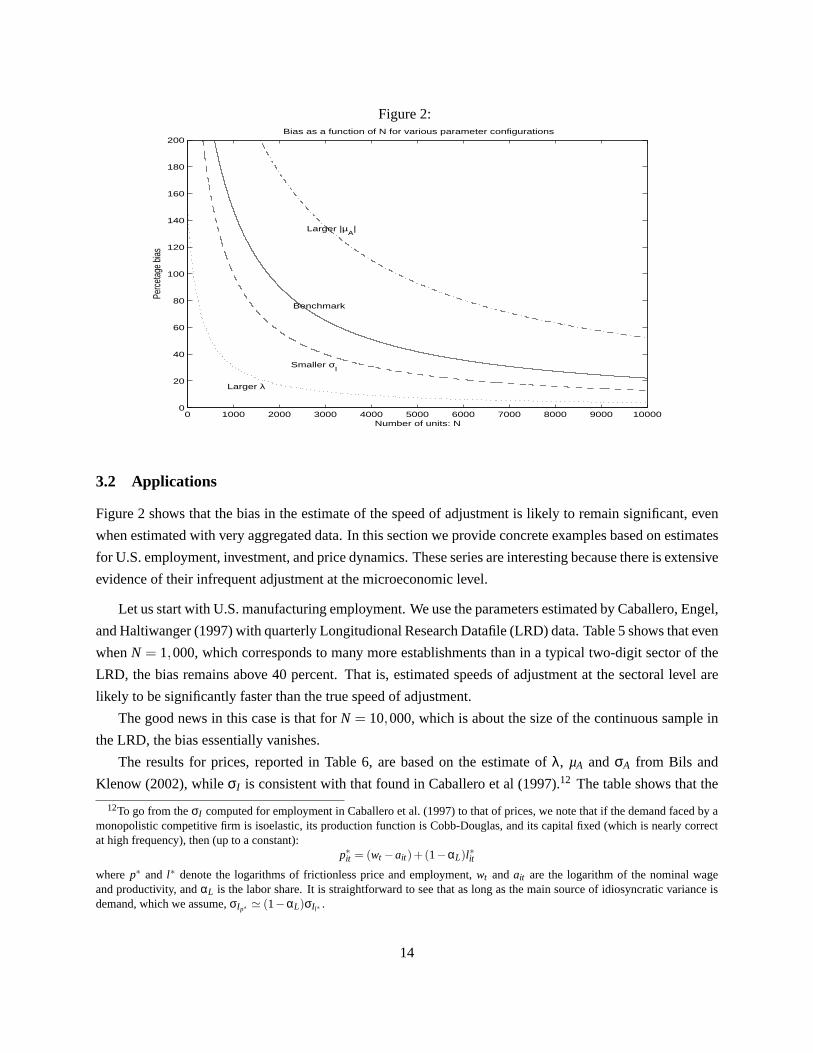
Figure 2:

0 1000 2000 3000 4000 5000 6000 7000 8000 9000 100000

20

40

60

80

100

120

140

160

180

200Bias as a function of N for various parameter configurations

Number of units: N

Perc

etag

e bia

s

Benchmark

Larger |µA|

Smaller σI

Larger λ

3.2 Applications

Figure 2 shows that the bias in the estimate of the speed of adjustment is likely to remain significant, even

when estimated with very aggregated data. In this section we provide concrete examples based on estimates

for U.S. employment, investment, and price dynamics. These series are interesting because there is extensive

evidence of their infrequent adjustment at the microeconomic level.

Let us start with U.S. manufacturing employment. We use the parameters estimated by Caballero, Engel,

and Haltiwanger (1997) with quarterly Longitudional Research Datafile (LRD) data. Table 5 shows that even

whenN = 1,000, which corresponds to many more establishments than in a typical two-digit sector of the

LRD, the bias remains above 40 percent. That is, estimated speeds of adjustment at the sectoral level are

likely to be significantly faster than the true speed of adjustment.

The good news in this case is that forN = 10,000, which is about the size of the continuous sample in

the LRD, the bias essentially vanishes.

The results for prices, reported in Table 6, are based on the estimate ofλ, µA andσA from Bils and

Klenow (2002), whileσI is consistent with that found in Caballero et al (1997).12 The table shows that the

12To go from theσI computed for employment in Caballero et al. (1997) to that of prices, we note that if the demand faced by amonopolistic competitive firm is isoelastic, its production function is Cobb-Douglas, and its capital fixed (which is nearly correctat high frequency), then (up to a constant):

p∗it = (wt −ait )+(1−αL)l∗itwherep∗ and l∗ denote the logarithms of frictionless price and employment,wt andait are the logarithm of the nominal wageand productivity, andαL is the labor share. It is straightforward to see that as long as the main source of idiosyncratic variance isdemand, which we assume,σIp∗ ' (1−αL)σIl∗ .

14

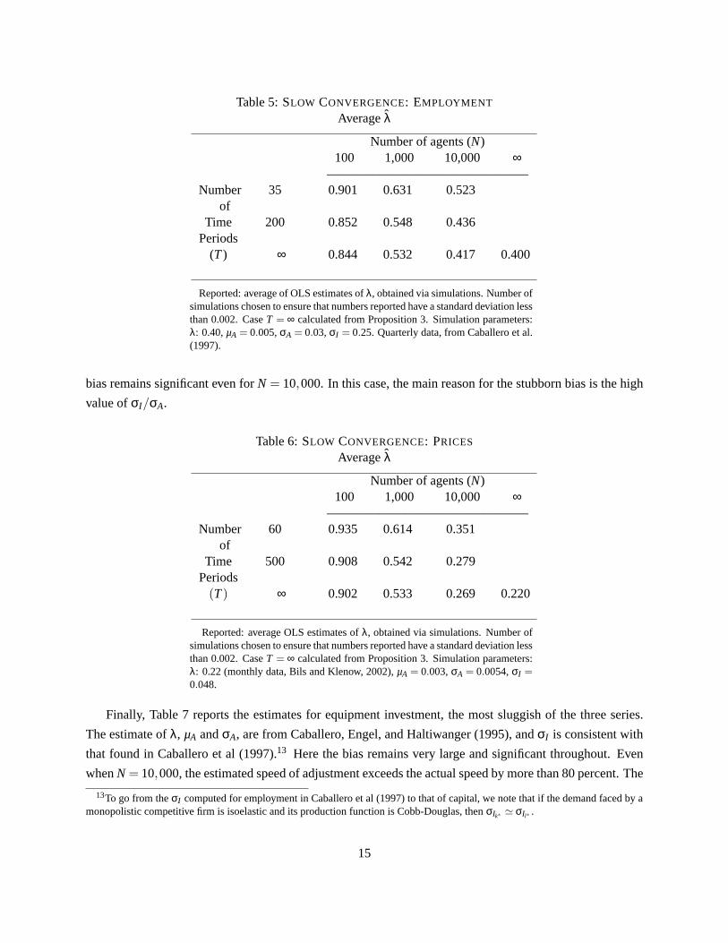
Table 5:SLOW CONVERGENCE: EMPLOYMENT

Averageλ

Number of agents (N)100 1,000 10,000 ∞

———————————————–Number 35 0.901 0.631 0.523

ofTime 200 0.852 0.548 0.436

Periods(T) ∞ 0.844 0.532 0.417 0.400

Reported: average of OLS estimates ofλ, obtained via simulations. Number ofsimulations chosen to ensure that numbers reported have a standard deviation lessthan 0.002. CaseT = ∞ calculated from Proposition 3. Simulation parameters:λ: 0.40,µA = 0.005, σA = 0.03, σI = 0.25. Quarterly data, from Caballero et al.(1997).

bias remains significant even forN = 10,000. In this case, the main reason for the stubborn bias is the high

value ofσI/σA.

Table 6:SLOW CONVERGENCE: PRICES

Averageλ

Number of agents (N)100 1,000 10,000 ∞

———————————————–Number 60 0.935 0.614 0.351

ofTime 500 0.908 0.542 0.279

Periods(T) ∞ 0.902 0.533 0.269 0.220

Reported: average OLS estimates ofλ, obtained via simulations. Number ofsimulations chosen to ensure that numbers reported have a standard deviation lessthan 0.002. CaseT = ∞ calculated from Proposition 3. Simulation parameters:λ: 0.22 (monthly data, Bils and Klenow, 2002),µA = 0.003, σA = 0.0054, σI =0.048.

Finally, Table 7 reports the estimates for equipment investment, the most sluggish of the three series.

The estimate ofλ, µA andσA, are from Caballero, Engel, and Haltiwanger (1995), andσI is consistent with

that found in Caballero et al (1997).13 Here the bias remains very large and significant throughout. Even

whenN = 10,000, the estimated speed of adjustment exceeds the actual speed by more than 80 percent. The

13To go from theσI computed for employment in Caballero et al (1997) to that of capital, we note that if the demand faced by amonopolistic competitive firm is isoelastic and its production function is Cobb-Douglas, thenσIk∗ ' σIl∗ .

15

reasons for this is the combination of a lowλ, a highµA (mostly due to depreciation), and a largeσI (relative

to σA).

Table 7:SLOW CONVERGENCE: INVESTMENT

Averageλ

Number of agents (N)100 1,000 10,000 ∞

———————————————–15 1.060 0.950 0.665

Numberof 50 1.004 0.790 0.400Time

Periods 200 0.985 0.723 0.305(T)

∞ 0.979 0.696 0.274 0.150

Reported: average of OLS estimates ofλ, obtained via simulations. Numberof simulations chosen to ensure that numbers reported have a standard deviationless than 0.002. Simulation parameters:λ: 0.15 (annual data, from Caballero etal, 1995),µA = 0.12, σA = 0.056, σI = 0.50.

We have assumed throughout that∆y∗ is i.i.d. Aside from making the results cleaner, it should be

apparent from the time-to-build extension in Section 2 that adding further serial correlation does not change

the essence of our results. In such a case, the cross correlations between contiguous adjustments are no

longer zero, but the bias we have described remains. In any event, for each of the applications in this

subsection, there is evidence that the i.i.d. assumption is not farfetched (see, e.g., Caballero et al [1995,

1997], Bils and Klenow [2002]).

4 Fragile Solutions: Biased Regressions and ARMA Correction

Can we fix the problem while remaining within the class of linear time-series models? In this section, we

show that in principle this is possible, but in practice it is unlikely (especially for smallN).

4.1 Biased Regressions

So far we have assumed that the speed of adjustment is estimated using only information on the economic

series of interest,y. Yet often the econometrician can resort to a proxy for the targety∗. Instead of (2), the

estimating equation is:

∆yt = (1−λ)∆yt−1 +λ∆y∗t +et , (25)

with some proxy available for the regressor∆y∗.

16

Equation (25) hints at a procedure for solving the problem. Since the regressors are orthogonal,λin principle can be estimated directly from the parameter estimate associated with∆y∗t , while dropping

the constraint that the sum of the coefficients on the right hand side add up to one. Of course, if the

econometrician does impose the latter constraint, then the estimate ofλ will be some weighted average of

an unbiased and a biased coefficient, and hence will be biased as well. We summarize these results in the

following proposition.

Proposition 4 (Bias with Regressors)

With the same notation and assumptions as in Proposition 3, consider the following equation:

∆yNt = b0∆yN

t−1 +b1∆y∗t +et , (26)

where∆y∗t denotes the average shock in periodt, ∑∆y∗i,t/N. Then, if (26) is estimated via OLS, andK

defined in (19),

(i) without any restrictions onb0 andb1:

plimT→∞b0 =K

1+K(1−λ), (27)

plimT→∞b1 = λ, (28)

(ii) imposingb0 = 1−b1:14

plimT→∞b1 = λ +λ(1−λ)2(K +λ)

.

In particular, for N = 1 andµA = 0:

plimT→∞b1 = λ+1−λ

2.

Proof See Corollary B1 in the Appendix.

Of course, in practice the “solution” above is not very useful. First, the econometrician seldom observes

∆y∗ exactly, and (at least) the scaling parameters need to be estimated. In this situation, the coefficient es-

timate on the contemporaneous proxy for∆y∗ is no longer useful for estimatingλ, and the latter must be

estimated from the serial correlation of the regression, bringing back the bias. Second, when the econometri-

cian does observe∆y∗, the adding up constraint typically is linked to homogeneity and long-run conditions

14The expression that follows is a weighted average of the unbiased estimatorλ and the biased estimator in the regression without∆y∗ as a regressor (Proposition 3). The weight on the biased estimator isλK/2(K + λ), which corresponds to the harmonic meanof λ andK.

17

that a researcher often will be reluctant to drop (see below).

Fast Micro – Slow Macro?: A Price-Wage Equation Application

In an intriguing article, Blanchard (1987) reached the conclusion that the speed of adjustment of prices

to cost changes is much faster at the disaggregate than the aggregate level. More specifically, he found that

prices adjust faster to wages (and input prices) at the two-digit level than at the aggregate level. His study

considered seven manufacturing sectors and estimated equations analogous to (26), with sectoral prices in

the role ofy, and both sector-specific wages and input prices as regressors (they∗). The classic homogeneity

condition in this case, which was imposed in Blanchard’s study, is equivalent in our setting tob0 +b1 = 1.

Blanchard’s preferred explanation for his finding was based on the slow transmission of price changes

through the input-output chain. This is an appealing interpretation and likely to explain some of the dif-

ference in speed of adjustment at different levels of aggregation. However, one wonders how much of the

finding can be explained by biases like those described in this paper. We do not attempt a formal decompo-

sition but simply highlight the potential size of the bias in price-wage equations for realistic parameters.

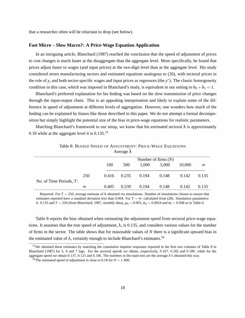
Matching Blanchard’s framework to our setup, we know that his estimated sectoralλ is approximately

0.18 while at the aggregate level it is 0.135.15

Table 8:BIASED SPEED OFADJUSTMENT: PRICE-WAGE EQUATIONS

Averageλ

Number of firms (N)100 500 1,000 5,000 10,000 ∞——————————————————————–

250 0.416 0.235 0.194 0.148 0.142 0.135No. of Time Periods,T:

∞ 0.405 0.239 0.194 0.148 0.142 0.135

Reported: ForT = 250, average estimate ofλ obtained via simulations. Number of simulations chosen to ensure thatestimates reported have a standard deviation less than 0.004. ForT = ∞: calculated from (28). Simulation parameters:λ: 0.135 andT = 250(from Blanchard, 1987, monthly data),µA = 0.003, σA = 0.0054andσI = 0.048as in Table 6.

Table 8 reports the bias obtained when estimating the adjustment speed from sectoral price-wage equa-

tions. It assumes that the true speed of adjustment,λ, is 0.135, and considers various values for the number

of firms in the sector. The table shows that for reasonable values ofN there is a significant upward bias in

the estimated value ofλ, certainly enough to include Blanchard’s estimates.16

15We obtained these estimates by matching the cumulative impulse responses reported in the first two columns of Table 8 inBlanchard (1987) for 5, 6 and 7 lags. For the sectoral speeds we obtain, respectively,0.167, 0.182 and 0.189, while for theaggregate speed we obtain0.137, 0.121and0.146. The numbers in the main text are the averageλ’s obtained this way.

16The estimated speed of adjustment is close to 0.18 forN = 1,000.

18

4.2 ARMA Corrections

Let us go back to the case of unobserved∆y∗. Can we fix the bias while remaining within the class of linear

ARMA models? In the first part of this subsection, we show that this is indeed possible. Essentially, the

correction amounts to adding a nuisance MA term that “absorbs” the bias.

However, the second part of this subsection warns that this nuisance parameter needs to be ignored when

estimating the speed of adjustment. This is not encouraging, because in practice the researcher is unlikely

to know when he should or should not drop some of the MA terms before simulating (or drawing inferences

from) the estimated dynamic model.

On the constructive side, nonetheless, we show that whenN is sufficiently large, even if we do not ignore

the nuisance MA parameter, we obtain better —although still biased— estimates of the speed of adjustment

than with the simple partial adjustment model.

4.2.1 Nuisance Parameters and Bias Correction

Let us start with the positive result.

Proposition 5 (Bias Correction) Let the Technical Assumptions (see page 10) hold.17 Then∆yNt follows

an ARMA(1,1) process with autoregressive parameter equal to1−λ. Thus, adding an MA(1) term to the

standard partial adjustment equation (2):

∆yNt = (1−λ)∆yN

t−1 +vt −θvt−1, (29)

and denoting byλN any consistent estimator of one minus the AR-coefficient in the equation above, we have

that:

plimT→∞λN = λ.

The moving average coefficient,θ, is a ”nuisance” parameter that depends onN (it converges to zero asN

tends to infinity),µA, σA andσI . We have that:

θ =12(L−

√L2−4) > 0,

with

L≡ 2+λ(2−λ)(K−1)1−λ

,

andK defined in (19).

Proof See Theorem B1 in the Appendix.

17Strictly speaking, to avoid the case where the AR and MA coefficients coincide, we need to rule out the knife-edge caseN−1 = (2−λ)µ2

A/λσ2A. In particular, whenµA = 0 this amounts to assumingN > 1.

19

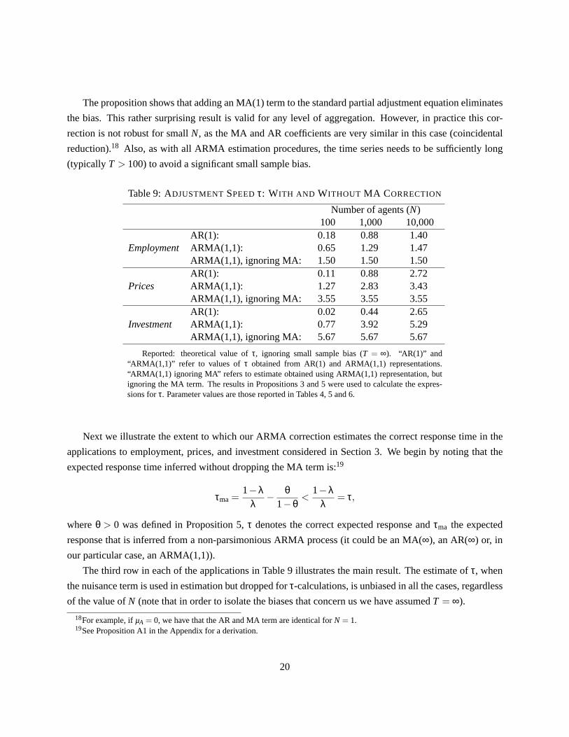
The proposition shows that adding an MA(1) term to the standard partial adjustment equation eliminates

the bias. This rather surprising result is valid for any level of aggregation. However, in practice this cor-

rection is not robust for smallN, as the MA and AR coefficients are very similar in this case (coincidental

reduction).18 Also, as with all ARMA estimation procedures, the time series needs to be sufficiently long

(typically T > 100) to avoid a significant small sample bias.

Table 9:ADJUSTMENTSPEEDτ: WITH AND WITHOUT MA CORRECTION

Number of agents (N)100 1,000 10,000

AR(1): 0.18 0.88 1.40Employment ARMA(1,1): 0.65 1.29 1.47

ARMA(1,1), ignoring MA: 1.50 1.50 1.50AR(1): 0.11 0.88 2.72

Prices ARMA(1,1): 1.27 2.83 3.43ARMA(1,1), ignoring MA: 3.55 3.55 3.55AR(1): 0.02 0.44 2.65

Investment ARMA(1,1): 0.77 3.92 5.29ARMA(1,1), ignoring MA: 5.67 5.67 5.67

Reported: theoretical value ofτ, ignoring small sample bias (T = ∞). “AR(1)” and“ARMA(1,1)” refer to values ofτ obtained from AR(1) and ARMA(1,1) representations.“ARMA(1,1) ignoring MA” refers to estimate obtained using ARMA(1,1) representation, butignoring the MA term. The results in Propositions 3 and 5 were used to calculate the expres-sions forτ. Parameter values are those reported in Tables 4, 5 and 6.

Next we illustrate the extent to which our ARMA correction estimates the correct response time in the

applications to employment, prices, and investment considered in Section 3. We begin by noting that the

expected response time inferred without dropping the MA term is:19

τma =1−λ

λ− θ

1−θ<

1−λλ

= τ,

whereθ > 0 was defined in Proposition 5,τ denotes the correct expected response andτma the expected

response that is inferred from a non-parsimonious ARMA process (it could be an MA(∞), an AR(∞) or, in

our particular case, an ARMA(1,1)).

The third row in each of the applications in Table 9 illustrates the main result. The estimate ofτ, when

the nuisance term is used in estimation but dropped forτ-calculations, is unbiased in all the cases, regardless

of the value ofN (note that in order to isolate the biases that concern us we have assumedT = ∞).

18For example, ifµA = 0, we have that the AR and MA term are identical forN = 1.19See Proposition A1 in the Appendix for a derivation.

20

The first and second rows (in each application) show the biased estimates. The former repeats our basic

result while the latter illustrates the problems generated by not dropping the nuisance MA term (τma). The

bias from not dropping the MA term is smaller than that from inferringτ from the first order autocorrela-

tion,20 yet it remains significant even at fairly high levels of aggregation (e.g.,N = 1,000).

5 Conclusion

The practice of approximating dynamic models with linear ones is widespread and useful. However, it can

lead to significant overestimates of the speed of adjustment of sluggish variables. The problem is most severe

when dealing with data at low levels of aggregation or single-policy variables. For once, macroeconomic

data seem to be better than microeconomic data.

Yet this paper also shows that the disappearance of the bias with aggregation can be extremely slow.

For example, in the case of investment, the bias remains above 80 percent even after aggregating across all

continuous establishments in the LRD (N = 10,000).

While the researcher may think that at the aggregate level it does not matter much which microeconomic

adjustment-cost model generates the data, it does matter greatly for (linear) estimation of the speed of

adjustment.

What happened to Wold’s representation, according to which any stationary, purely non-deterministic,

process admits an (eventually infinite) MA representation? Why, as illustrated by the analysis at the end

of Section 4, do we obtain an upward biased speed of adjustment when using this representation for the

stochastic process at hand? The problem is that Wold’s representation expresses the variable of interest as

a distributed lag (and therefore linear function) of innovations that are the one-step-aheadlinear forecast

errors. When the relation between the macroeconomic variable of interest and shocks is non-linear, as is the

case when adjustment is lumpy, Wold’s representation misidentifies the underlying shock, leading to biased

estimates of the speed of adjustment.

Put somewhat differently, when adjustment is lumpy, Wold’s representation identifies the correct ex-

pected response time to the wrong shock. Also, and for the same reason, the impulse response more gener-

ally will be biased. So will many of the dynamic systems estimated in VAR style models, and the structural

tests that derive from such systems. We are currently working on these issues.

20This can be proved formally based on the expressions derived in Theorem B1 and Proposition A1 in the appendix.

21

References

[1] Bils, Mark and Peter J. Klenow, “Some Evidence on the Importance of Sticky Prices,” NBER WP #

9069, July 2002.

[2] Blanchard, Olivier J., “Aggregate and Individual Price Adjustment,”Brookings Papers on Economic

Activity 1,1987, 57–122.

[3] Box, George E.P., and Gwilym M. Jenkins,Time Series Analysis: Forecasting and Control, San Fran-

cisco: Holden Day, 1976.

[4] Caballero, Ricardo J., Eduardo M.R.A. Engel, and John C. Haltiwanger, “Plant-Level Adjustment and

Aggregate Investment Dynamics”,Brookings Papers on Economic Activity, 1995 (2), 1–39.

[5] Caballero, Ricardo J., Eduardo M.R.A. Engel, and John C. Haltiwanger, “Aggregate Employment

Dynamics: Building from Microeconomic Evidence”,American Economic Review, 87 (1), March

1997, 115–137.

[6] Calvo, Guillermo, “Staggered Prices in a Utility-Maximizing Framework,”Journal of Monetary Eco-

nomics, 12, 1983, 383–398.

[7] Engel, Eduardo M.R.A., “A Unified Approach to the Study of Sums, Products, Time-Aggregation and

other Functions of ARMA Processes”,Journal Time Series Analysis, 5, 1984, 159–171.

[8] Goodfriend, Marvin, “Interest-rate Smoothing and Price Level Trend Stationarity,”Journal of Mone-

tary Economics, 19, 19987, pp. 335-348.

[9] Majd, Saman and Robert S. Pindyck, “Time to Build, Option Value, and Investment Decisions,”Jour-

nal of Financial Economics, 18, March 1987, 7–27. (1987).

[10] Rotemberg, Julio J., “The New Keynesian Microfoundations,” in O. Blanchard and S. Fischer (eds),

NBER Macroeconomics Annual, 1987, 69–104.

[11] Sack, Brian, “Uncertainty, Learning, and Gradual Monetary Policy,” Federal Reserve Board Finance

and Economics Discussion Series Paper 34, August 1998.

[12] Sargent, Thomas J., “Estimation of Dynamic Labor Demand Schedules under Rational Expectations,”

Journal of Political Economy, 86, 1978, 1009–1044.

[13] Woodford, Michael, “Optimal Monetary Policy Inertia,” NBER WP # 7261, July 1999.

22

APPENDIX

A The Expected Response Time Index:τ

Lemma A1 (τ for an Infinite MA) Consider a second order stationary stochastic process

∆yt = ∑k≥0

ψkεt−k,

with ψ0 = 1, ∑k≥0 ψ2k < ∞, the εt ’s uncorrelated, andεt uncorrelated with∆yt−1,∆yt−2, ... Assume that

Ψ(z)≡ ∑k≥0 ψkzk has all its roots outside the unit disk.Define:

Ik ≡ Et

[∂∆yt+k

∂εt

]and τ ≡ ∑k≥0kIk

∑k≥0 Ik. (30)

Then:

Ik = ψk and τ =Ψ′(1)Ψ(1)

=∑k≥1kψk

∑k≥0 ψk.

Proof That Ik = ψk is trivial. The expressions forτ then follow from differentiatingΨ(z) and evaluating atz= 1.

Proposition A1 (τ for an ARMA Process) Assume∆yt follows an ARMA(p,q):

∆yt −p

∑k=1

φk∆yt−k = εt −q

∑k=1

θkεt−k,

whereΦ(z)≡ 1−∑pk=1 φkzk andΘ(z)≡ 1−∑q

k=1 θkzk have all their roots outside the unit disk. The assump-tions regarding theεt ’s are the same as in Lemma A1.

Defineτ as in (30). Then:

τ =∑p

k=1kφk

1−∑pk=1 φk

− ∑qk=1kθk

1−∑qk=1 θk

.

Proof Given the assumptions we have made about the roots ofΦ(z) andΘ(z), we may write:

∆yt =Θ(L)Φ(L)

εt ,

whereL denotes the lag operator. Applying Lemma A1 withΘ(z)/Φ(z) in the role ofΨ(z) we then have:

τ =Θ′(1)Θ(1)

− Φ′(1)Φ(1)

=∑p

k=1kφk

1−∑pk=1 φk

− ∑qk=1kθq

1−∑qk=1 θk

.

Proposition A2 (τ for a Lumpy Adjustment Process) Consider∆yt in the simple lumpy adjustment model (8)andτ defined in (14). Thenτ = (1−λ)/λ.21

21More generally, if the number of periods between consecutive adjustments are i.i.d. with meanm, thenτ = m−1. What followsis the particular case where interarrival times follow a Geometric distribution.

23

Proof ∂∆yt+k/∂∆y∗t is equal to one when the unit adjusts at timet +k, not having adjusted between timestandt +k−1, and is equal to zero otherwise. Thus:

Ik ≡ Et

[∂∆yt+k

∂∆y∗t

]= Pr{ξt+k = 1 , ξt+k−1 = ξt+k−2 = ... = ξt = 0}= λ(1−λ)k. (31)

The expression forτ now follows easily.

Proposition A3 (τ for a Process With Time-to-build and Lumpy Adjustments) Consider the process∆yt

with both gradual and lumpy adjustments:

∆yt =K

∑k=1

φk∆yt−k +(1−K

∑k=1

φk)∆yt , (32)

with

∆yt = ξt

lt−1

∑k=0

∆y∗t−k, (33)

where∆y∗ is i.i.d. with zero mean and varianceσ2.Defineτ by:

τ ≡∑k≥0kEt

[∂∆yt+k∂∆y∗t

]

∑k≥0E[

∂∆yt+k∂∆y∗t

] .

Then:

τ = ∑Kk=1kφk

1−∑Kk=1 φk

+1−λ

λ.

Proof Note that:

Ik ≡ Et

[∂∆yt+k

∂∆y∗t

]=

k

∑j=0

Et

[∂∆yt+k

∂∆yt+ j

∂∆yt+ j

∂∆y∗t

]=

k

∑j=0

Et

[Gk− j

∆yt+ j

∆y∗t

]=

k

∑j=0

Gk− jH j , (34)

where, from Proposition A1 and (31) we have that theGk are such thatG(z) ≡ ∑k≥0Gkzk = 1/Φ(z), andHk = λ(1− λ)k. DefineH(z) ≡ ∑k≥0Hkzk and I(z) = G(z)H(z). Noting that the coefficient ofzk in theinfinite seriesI(z) is equal toIk in (34), we have:

τ =I ′(1)I(1)

=G′(1)G(1)

+H ′(1)H(1)

= ∑Kk=1kφk

1−∑Kk=1 φk

+1−λ

λ.

24

B Bias Results

B.1 Results in Section 2

In this subsection we prove Proposition 2 and Corollary 1. Proposition 1 is a particular case of Proposition 3,which is proved in Section B.2. The notation and assumptions are the same as in Proposition A3.

Proof of Proposition 2 and Corollary 1 The equation we estimate is:

∆yt =K+1

∑k=1

ak∆yt−k +vt , (35)

while the true relation is that described in (32) and (33).An argument analogous to that given in Section 2.2 shows that the second term on the right hand side

of (32), denoted bywt in what follows, is uncorrelated with∆yt−k, k≥ 1. It follows that estimating (35) isequivalent to estimating (32) with error term

wt = = (1−K

∑k=1

φk)ξt

lt−1

∑k=0

∆y∗t−k,

and therefore:

plimT→∞ak =

φk if k = 1,2, ...,K,

0 if k = K +1.

The expression for plimT→∞τ now follows from Proposition A3.

B.2 Results in Sections 3 and 4

In this section we prove Propositions 3, 4, and 5. The notation and assumptions are those in Proposition 3.The proof proceeds via a series of lemmas. Propositions 3 and 5 are proved in Theorem B1, while Proposi-tion 4 is proved in Corollary B1.

Lemma B1 AssumeX1 andX2 are i.i.d. geometric random variables with parameterλ, so thatPr{X = k}=λ(1−λ)k−1,k = 1,2,3, . . . Then:

E[Xi ] =1λ,

Var[Xi ] =1−λ

λ2 .

In particular, thel i,t ’s (defined in the main text) are all geometric random variables with parameterλ.Furthermore,l i,t andl j,s are independent ifi 6= j .

Next define, for any integers larger or equal than zero:

Ms ={

0 if X1 ≤ s,min(X1−s,X2) if X1 > s.

25

Then

E[Ms] =(1−λ)s

λ(2−λ).

Proof The expressions forE[Xi ] andVar[Xi ] are well known. The properties of thel i,t ’s are also trivial.To derive the expression forE[Ms], denote byF(k) and f (k) the cumulative distribution and probabilityfunctions common toX1 andX2. Then:

Pr{Ms = k} = Pr{X1−s= k,X2 ≥ k+1}+Pr{X2 = k,X1−s≥ k+1}+Pr{X1−s= k,X2 = k}= f (s+k)[1−F(k)]+ f (k)[1−F(k+s)]+ f (k) f (k+s),

and, since1−F(k) = (1−λ)k, with some algebra we obtain:

Pr{Ms = k}= λ(2−λ)(1−λ)s+2k−2.

Using this expression to calculateE[Ms] via ∑k≥1kPr{Ms = k} completes the proof.

Lemma B2 For any strictly positive integers,

Cov(∆yi,t ,∆yi,t+s) =−(1−λ)sµ2A.

Proof We have:

Cov(∆yt+s,∆yt) = E[∆yt+s∆yt ] − µ2A

=∞

∑k=1

s

∑q=1

E[∆yt+s∆yt |lt+s = q, lt = k,ξt+s = 1,ξt = 1]Pr{lt+s = q, lt = k,ξt+s = 1,ξt = 1} − µ2A

= µ2A

∞

∑k=1

s

∑q=1

qkPr{lt+s = q, lt = k,ξt+s = 1,ξt = 1} − µ2A,

where in the second (and only non-trivial) step we add up over a partition of the set of outcomes where∆yt+s∆yt 6= 0.

The expression above, combined with:

Pr{lt+s = q, lt = k,ξt+s = 1,ξt = 1} =

λ4(1−λ)k+q−2, if q = 1, ...,s−1,

λ3(1−λ)k+q−2, if q = s,

and some patient algebra completes the proof.

Lemma B3 For q 6= r and any integers larger or equal than zero we have:

Cov(∆yq,t+s,∆yr,t) =λ

2−λ(1−λ)sσ2

A.

Proof Denotevi,t ≡ ∆y∗i,t = vAt +vI

i,t . Then:

E[∆yq,t+s∆yr,t |lq,t+s, lr,t ] = E[ξq,t+s(lq,t+s−1

∑j=0

vq,t+s− j)ξr,t(lr,t−1

∑k=0

vr,t−k)|lq,t+s, lr,t ]

26

= λ2lq,t+s−1

∑j=0

lr,t−1

∑k=0

E[vAt+s− jv

At−k]

= λ2lq,t+slr,tµ2A + λ2Ms(lq,t+s, lr,t)σ2

A.

Where the first identity follows from the definition of the∆yi,t ’s, the second from conditioning on the fourpossible combinations of values ofξq,t+s andξr,t , andMs(lq,t+s, lr,t) denotes the random variable analogousto Ms in Lemma B1, based on the i.i.d. geometric random variableslq,t+s andlr,t . The remainder of the proofis based on the expressions in Lemma B1 and straightforward algebra.

Lemma B4 We have:

Var(∆yi,t) =2(1−λ)

λµ2

A +σ2A +σ2

I .

Proof The proof is based on calculating both terms on the right hand side of the well known identity:

Var(∆yi,t) = Varl i,t (E[∆yi,t |l i,t ])+El i,t (Var(∆yi,t |l i,t)). (36)

Since[∆yi,t |l i,t ] has meanl i,tµA and variancel i,tσ2A, we have:

E[∆y2i,t |l i,t ] = E[ξ2

i,t(l i,t−1

∑j=0

vi,t− j)2] = λ(l i,t(σ2A +σ2

I )+ l i,tµ2A.

A similar calculation shows that:E[∆yi,t |l i,t ] = λl i,tµA.

Hence:Var(∆yi,t |l i,t) = λl i,t(σ2

A +σ2I )+λ(1−λ)l2

i,tµ2A

and taking expectation with respect tol i,t (and using the expressions in Lemma B1) leads to:

El i,t Var(∆yi,t |l i,t) = σ2A +σ2

I +(1−λ)(2−λ)

λµ2

A. (37)

An analogous (and considerably simpler) calculation shows that:

Varl i,t (E[∆yi,t |l i,t ]) = (1−λ)µ2A. (38)

The proof concludes by substituting (37) and (38) in (36).

Lemma B5 For N≥ 1:

Var(∆yNt ) =

1N

{[1+

λ2−λ

(N−1)]σ2A +σ2

I +2(1−λ)

λµ2

A

}.

Proof The caseN = 1 corresponds to Lemma B4. ForN≥ 2 we have:

Var(∆yNt ) =

1N2

N

∑i=1

N

∑j=1

Cov(∆yi,t ,∆y j,t)

27

=1

N2 {NVar(∆y1,t)+N(N−1)Cov(∆y1,t ,∆y2,t)} .

The first identity follows from the bilinearity of the covariance operator, the second from the fact thatVar(∆yi,t) does not depend oni andCov(∆yi,t ,∆y j,t), i 6= j, does not depend oni or j.

The remainder of the proof follows from using the expressions derived in Lemmas B3 and B4.

Lemma B6 Recall that in the main text we defined∆y∗t ≡ ∑Ni=1 ∆y∗i,t/N. We then have:

Var(∆y∗t ) = σ2A +

σ2I

N,

Cov(∆yNt , ∆y∗t ) = λ[σ2

A +σ2

I

N].

Proof The proof of the first identity is trivial. To derive the second expression we first note that:

Cov(∆yi,t ,∆y∗j,t) = E[ξt(l i,t−1

∑k=0

∆y∗i,t−k)∆y∗j,t ] − µ2A

= ∑k≥1

E[ξt(l i,t−1

∑k=0

∆y∗i,t−k)∆y∗j,t | l i,t = k,ξi,t = 1]λ2(1−λ)k−1 − µ2A

= λ2 ∑k≥1

[(σ2A +δi, jσ2

I +µ2A)+(k−1)µ2

A](1−λ)k−1 − µ2A

= λ(σ2A +δi, jσ2

I ),

with δi, j = 1 if i = j and zero otherwise. The expression forCov(∆yNt , ∆y∗t ) now follows easily.

Theorem B1 ∆yNt follows an ARMA(1,1) process:22

∆yt −φ∆yt−1 = εt −θεt−1,

whereεt denotes the innovation process and

φ = 1−λ,

θ =12(L−

√L2−4).

with

L≡ 2+λ(2−λ)(K−1)1−λ

.

Also, asN tends to infinityθ converges to zero, so that the process for∆yNt approaches an AR(1) (and we

recover Rotemberg’s (1987) result).We also have:

σNs =

1N

{λ

2−λ(N−1)σ2

A−µ2A

}(1−λ)s, s= 1,2, ...

22We have thatφ = θ, so that the process reduces to white noise, if and only ifN = 1+ 2−λλ

µ2A

σ2A.

28

ρNs =

K1+K

(1−λ)s; s= 1,2,3, . . .

whereσNs and ρN

s denote thes-th order autocovariance and autocorrelation coefficients of∆yNt , respec-

tively.23

Proof We have:

Cov(∆yt+s,∆yt) =N

∑i=1

N

∑j=1

Cov(∆yi,t+s,∆y j,t)

= NVar(∆y1,t)+N(N−1)Cov(∆y1,t+s,∆y2,t).

Where the justification for both identities is the same as in the proof of Lemma B5. The expression forσN

s now follows from Lemmas B3 and B4. The expression for the autocorrelations follow trivially usingLemma B5 and the formula for the autocovariances.

The expressions we derived for the autocovariance function of∆yt and Theorem 1 in Engel (1984) implythat ∆yt follows an ARMA(1,1) process, with autoregressive coefficient equal to1− λ. The expressionfor θ follows from standard method of moments calculations (see, for example, equation (3.4.8) in Boxand Jenkins (1976)) and some patient algebra.24 Finally, some straightforward calculations prove thatθconverges to zero asn tends to infinity.

Corollary B1 Proposition 4 is a direct consequence of the preceding theorem.

Proof Part (i) follows trivially from Proposition 3 and the fact that both regressors are uncorrelated. Toprove (ii) we first note that:

b1 =Cov(∆yN

t −∆yNt−1 , ∆y∗t −∆yN

t−1)Var(∆y∗t −∆yN

t−1).

From Lemma B6 and the fact that∆y∗t and∆yt−1 are uncorrelated it follows that:

Cov(∆yNt −∆yN

t−1 , ∆y∗t −∆yNt−1) = λ

(σ2

A +σ2

I

N

)+(1−ρN

1 )Var(∆yNt ),

Var(∆y∗t −∆yNt−1) = σ2

A +σ2

I

N+Var(∆yN

t ).

The expressions derived earlier in this appendix and some patient algebra complete the proof.

23The expressions for plimT→∞λN in Proposition 3 follow from noting thatλN = 1−ρN1 .

24A straightforward calculation shows thatL > 2, so that we do have|θ|< 1.

29