How Much Does Violence Tax Trade
43
HOW MUCH DOES VIOLENCE TAX TRADE? S. BROCK BLOMBERG GREGORY D. HESS CESIFO WORKING PAPER NO. 1222 CATEGORY 7: TRADE POLICY JUNE 2004 An electronic version of the paper may be downloaded • from the SSRN website: www.SSRN.com • from the CESifo website: www.CESifo.de
Transcript of How Much Does Violence Tax Trade
HOW MUCH DOES VIOLENCE TAX TRADE?
S. BROCK BLOMBERG GREGORY D. HESS
CESIFO WORKING PAPER NO. 1222 CATEGORY 7: TRADE POLICY
JUNE 2004
An electronic version of the paper may be downloaded • from the SSRN website: www.SSRN.com • from the CESifo website: www.CESifo.de
CESifo Working Paper No. 1222
How Much Does Violence Tax Trade?
Abstract We investigate the empirical impact of violence as compared to other trade impediments on trade flows. Our analysis is based on a panel data set with annual observations on 177 countries from 1968 to 1999, which brings together information from the Rose [2004] dataset, the ITERATE dataset for terrorist events, and datasets of external and internal conflict. We explore these data with traditional and theoretical gravity models. We calculate that, for a given country year, the presence of terrorism, as well as internal and external conflict is equivalent to as much as a 30 percent tariff on trade. This is larger than estimated tariff-equivalent costs of border and language barriers and tariff-equivalent reduction through GSPs and WTO participation.
JEL Classification: E6, H1, H5, D74, O11.
Keywords: trade, conflict, terrosism.
S. Brock Blomberg Department of Economics
Claremont McKenna College 500 E. 9th Street – Bauer Center
Claremont, CA 91711 USA
Gregory D. Hess Department of Economics
Claremont McKenna College 500 E. 9th Street – Bauer Center
Claremont, CA 91711 USA
1 Introduction
What are the major impediments to trade and what can be done to remove them? In a recent
and controversial paper, Andrew Rose (2004) asserts that “while theory, casual empiricism, and
strong statements abound, there is, to my knowledge, no compelling empirical evidence showing
that the GATT/WTO has actually encouraged trade.” Several researchers have re-examined this
finding, but the general thrust of Rose’s view is well taken – what are the trade creating and trade
destroying factors that affect world trade?1
This question is our paper’s focal point but with a twist. The purpose of our paper is
to calculate the economic cost of violence on trade and compare it to the economic cost of other
trade barriers to see which is larger in magnitude. We assert that world peace is an important
consideration to trade and one that may actually provide a larger impact than even bilateral trade
pacts. Using data from 177 countries over more than 30 years, we find that peace has a strong
statistical and economic impact on trade. We estimate the impact of peace to be greater than the
impact from either multilateral or bilateral trade agreements emanating from WTO membership
or from generalized set of preferences (GSPs). Moreover, the negative impact of conflict is greater
than language and border effects. These results are robust across regions, time and country income
groups.
Estimating the trade costs of conflict has received less attention in the economic literature
relative to the vast literature on the economic benefits to tariff reduction and non-tariff barrier
reduction.2 There is, however, a growing body of literature which explores how conflict impacts
economies through two channels– a domestic channel and a globalization (i.e. trade) channel.1For example, Subramanian and Wei (2004) have shown that the death of WTO as a trade promotion device may
be overstated, as they demonstrate that the WTO can improve trade strongly but unevenly.2For examples of the benefits to lowering trade barriers see among others, Anderson (1979) who championed use
of the gravity equation from different structural models, including Ricardian models, Heckscher-Ohlin (H-O) models,and increasing returns to scale (IRS) models. See also Eaton and Kortum (2002).
1

While the purpose of this paper is to concentrate on analyzing the globalization channel,
it is first instructive to consider the domestic channel.3 The domestic channel is a basic story of
economic allocation. That is if the government spends more on the military to quell or to create
conflict, consumption and/or investment may in turn be crowded out. One consequence of the
decrease in investment would be a decline in future economic growth.4
Recently, Blomberg, Hess and Orphanides (2004), investigate the impact of various forms of
conflict such as terrorism, internal wars and external wars on a country’s economic growth. They
find that, on average, the incidence of terrorism may have an economically significant negative
effect on growth, albeit one that is considerably smaller and less persistent than that associated
with either external wars or internal conflict. Terrorism is associated with a redirection of economic
activity away from investment spending and towards government spending. They also find that
the impacts are largest in Africa and amongst non-democratic states.
A second channel by which economic prosperity is affected by conflict is the globalization
channel. The traditional view of the globalization channel is that violence harms the real economy
in the same manner as any trade cost. In this case, external conflict, internal conflict, or an
international terrorist attack leads to a fall in trade thereby leading to a decline in aggregate
activity and a fall in output. Put differently, an increase in terrorism in country A increases the
cost to doing business with country A so that country B will either purchase goods or services
domestically or from another more peaceful country. Thus, violence acts as a distorting tax or
tariff that limits the attainment of the benefits from free trade.
Anderson and Marcouiller (2002) have pursued this angle employing corruption and imper-3There is also the issue of how economic activity affects a nation’s proclivity towards violence – see Hess and
Orphanides (1995, 2001a,b) and Blomberg Hess and Thacker (2004).4Of course, other factors could reduce growth. The rise in uncertainty from a conflict could make households and
firms reduce spending, the nations’s productive capacity could be directly affected – e.g. see Blomberg (1996).
2
fect contract enforcement as impediments to international trade. They find that omitting indexes
of institutional quality obscures the negative relationship between per capita income and the share
of total expenditure devoted to traded goods. Their paper, however, does not consider direct mea-
sures of conflict.5 In a complementary study to ours, Glick and Taylor (2004) do consider the direct
effect of very large external wars on trade from a broader historical perspective. However, they
do not consider the effect of terrorism and internal wars on international trade., and the cost to
their analysis of a longer time period is that it reduces the number of countries for which there is
available data.
Our paper investigates the globalization channel by directly analyzing the impact of all types
of conflict on trade. We employ the workhorse trade model – the gravity model – to determine
the economic benefit of peace. We estimate both a traditional and a theoretical gravity model
to determine the cost of conflict. We divide conflict into several sub-categories to isolate the
individual impacts from terrorism (T), external war (E), revolutions (R) and inter-ethnic fighting
(IF) on trade. Furthermore, we also analyze the aggregate effect of conflict on trade by using
factor analysis to create a synthetic measure of violence (TERIF). In summary, we find that, in
total, violent conflict is a larger impediment to trade than traditional tariff barriers. This result
should refocus policymakers attention to encourage peace as a trade-promoting device to improve
economic welfare.
2 The Data and Basic Empirical Regularities
We combine data from five different sources for our project. First, the trade data is obtained from
Rose (2004). This is a bilateral data set on trade flows from 1948 to 1999 that has approximately
two hundred thousand dyadic observations.5Nitsch and Schumacher (2004) also analyze some aspects of conflict’s impact on trade but over a significantly
shorter time horizon.
3
The data we use for organized violence comes from three different individual sources and
is given in country year form which we then convert to dyadic form.6 There are four main sources
of organized violence that we consider: The first is Terrorism (T), which is adopted from the
ITERATE data set – see Mickolus (1993). In order to be considered an international/transnational
terrorist event, the definition in ITERATE is as follows:
“the use, or threat of use, of anxiety-inducing, extra-normal violence for political pur-poses by any individual or group, whether acting for or in opposition to establishedgovernmental authority, when such action is intended to influence the attitudes andbehavior of a target group wider than the immediate victims and when, through thenationality or foreign ties of its perpetrators, its location, the nature of its institutionalor human victims, or the mechanics of its resolution, its ramifications transcend nationalboundaries. ” (page 2)
The ITERATE project began as an attempt to quantify characteristics, activities and im-
pacts of transnational terrorist groups. The data set is grouped into four categories. First, there are
incident characteristics which code the timing of each event. Second, the terrorist characteristics
yield information about the number, makeup and groups involved in the incidents. Third, victim
characteristics describe analogous information on the victims involved in the attacks. Finally, life
and property losses attempt to quantify the damage of the attack. Following Blomberg, Hess and
Orphanides (2004), since we cannot control for the significance of individual events, we define a
dummy variable T which takes the value 1 if a terrorist event is recorded for either country in a
given dyad country year pair. This measure also has the advantage of defining the incidence of
terrorism in a manner comparable to the incidence of other forms of conflict in the data set.7
The second type of conflict we consider is External conflict (E), which is the initiation or
escalation of a foreign policy crisis that results in violence. A foreign policy crisis is defined by6See the Data Appendix for more details.7In Blomberg, Hess and Orphanides (2004) we demonstrate that the effects of terrorism on growth are similar if
we use the number of incidents-per-capita in a given year as a measure of the incidence of terrorism.
4

Brecher, Wilkenfeld and Moser (1988) as:
“a specific act, event or situational change which leads decision-makers to perceive athreat to basic values, time pressure for response and heightened probability of in-volvement in military hostilities. A trigger may be initiated by: an adversary state; anon-state actor; or a group of states (military alliance). It may be an environmentalchange; or it may be internally generated.” (page 3)
Based on these criteria, we code E to equal one if an external conflict is recorded for either country
involved in the same dispute in a given dyad country year pair. Such a definition is also used in
Hess and Orphanides (1995,2001a,b), Blomberg, Hess and Weerapana (2004), and Blomberg, Hess
and Orphanides (2004).
Data for Revolutions (R) and Interethnic Fighting (IF) are obtained from Gurr et al (2003).
Revolutionary conflict (R) is defined as conflict between the government and politically organized
groups seeking to overthrow those in power. Groups include political parties, labor organizations,
or parts of the regime itself. Note that for these internal conflicts to be considered, more than
1,000 individuals had to be mobilized and 100 fatalities must have occurred. An example of such
a conflict would be the Chinese Tiananmen Square massacre of 1989. Again, R takes the value 1
if a revolution event is recorded for either county in a given dyad country year pair.
Inter-ethnic Fighting and Genocide, denoted (IF), is defined to include the execution,
and/or consent of sustained policies by governing elites or their agents that result in the deaths of
a substantial portion of a communal group (genocide) or a politicized non-communal group (politi-
cide). The victims counted are non-combatants and the percentage of those killed in each group
is given more weight than the number of dead. IF takes the value 1 if an inter-ethnic fighting or
genocide event is recorded for either county in a given dyad country year pair.
Finally, in an attempt to capture the broad features of all the types of conflict in our data,
5

we construct a synthetic measure of violence from the principle components of the underlying
factors of violence. Such a method has been used in other contexts in cross-country analysis such
as Kaufman et al (2000). Specifically, we create a measure of TERIF that is obtained from the
largest principal component from a principal components model that is a linear combination of T,
E, R and IF. In short, the first principal component explains the largest fraction of the variation
in the underlying data and hence we focus on that as our synthetic measure of the dyad’s overall
measure of latent conflict. Formally, let TERIFijt represent dyad ij’s unobserved level of terror
from j factors T, E, R, and IF, so that:
TERIFijt = α1 · Tijt + α2 · Eijt + α3 · Rijt + α4 · IFijt + εijt (1)
Therefore, using this principle components model, we estimate TERIF by employing in-
formation from our four different measures of conflict T, E, R and IF. The model optimally selects
one factor with the relevant output given below. From this analysis, the factor TERIF is given as
TERIFijt = .41873 ∗N(Tijt) + .04526 ∗N(Eijt) + .58256 ∗N(Rijt) + .50414 ∗N(IFijt) (2)
where N(.) standardizes the variable T,E,R,IF to be standard normal. Given the relative
frequencies of each underlying factor, it is not surprising that there is more weight associated with
T, R, IF versus E.
In summary, we have constructed various measures of violence to include terrorism (T), ex-
ternal conflict (E), revolutions (R), inter-ethnic fighting (IF) and an amalgam measure (TERIF).
The basic cross-national and time properties of conflict have been well documented in Blomberg,
Hess and Orphanides (2004) but are given in the appendix in Tables A1-A4. There are four main
facts shown in the violence data. First, terrorism occurs more frequently than other forms of vio-
lence, with the greatest incidence occurring in the Americas and Europe.8 But before concluding8This is partly due to the fact that terrorism is measured rather crudely in ITERATE and partly due to the fact
6
that there is a causal relationship between rich democracies and terrorism, it is worth noting that
two of the highest incidence countries, France and Germany, are located geographically, politically
and economically close to Nordic countries such as Sweden, Norway and Finland with virtually no
terrorism. Hence, the relationship is not straightforward.
Second, other forms of internal conflict (R and IF) have been most persistent in non-
democratic regimes and in low-income countries. A possible suggested interpretation is that many
non-democratic and/or low-income countries are inundated with internal strife and that conflict
may explain, in large part, why certain countries fail to advance.
Third, external wars are a much less frequent event largely due to the high cost of waging a
war with border state. This is possibly why others such as Blomberg, Hess and Orphanides (2004)
find it has the largest negative impact on growth. Ceteris paribus, a shock from external war is less
frequent but extremely harmful to an economy.9
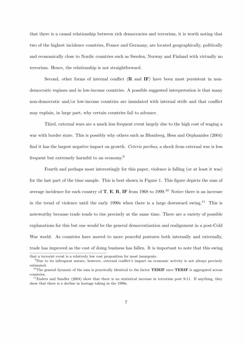
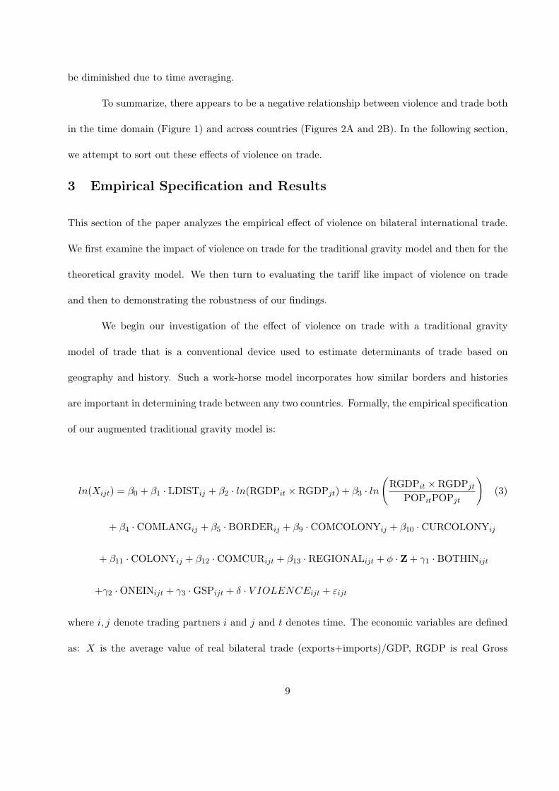
Fourth and perhaps most interestingly for this paper, violence is falling (or at least it was)
for the last part of the time sample. This is best shown in Figure 1. This figure depicts the sum of
average incidence for each country of T, E, R, IF from 1968 to 1999.10 Notice there is an increase
in the trend of violence until the early 1990s when there is a large downward swing.11 This is
noteworthy because trade tends to rise precisely at the same time. There are a variety of possible
explanations for this but one would be the general democratization and realignment in a post-Cold
War world. As countries have moved to more peaceful postures both internally and externally,
trade has improved as the cost of doing business has fallen. It is important to note that this swing
that a terrorist event is a relatively low cost proposition for most insurgents.9Due to its infrequent nature, however, external conflict’s impact on economic activity is not always precisely
estimated.10The general dynamic of the sum is practically identical to the factor TERIF once TERIF is aggregated across
countries.11Enders and Sandler (2004) show that there is no statistical increase in terrorism post 9-11. If anything, they
show that there is a decline in hostage taking in the 1990s.
7

Figure 1: Time Series Averages of Terror and Trade over 177 countries
9.2
9.4
9.6
9.8
10
10.2
10.4
10.6
10.8
11
1968 1973 1978 1983 1988 1993 1998
Log
of T
otal
Tra
de
0.45
0.55
0.65
0.75
0.85
0.95
1.05
1.15
1.25
Terr
or In
dex:
Sum
of P
erce
nt o
f Cou
ntry
Yea
r Pai
rs w
ith a
Con
flict
ltradeT+E+R+IFF
has occurred at a distinct point and time whereas other international movements to encourage
trade such as WTO ascension etc. have been more gradual in nature. Hence, this suggests that
peace, rather than statutory promotion, appears to play an important role in encouraging trade.
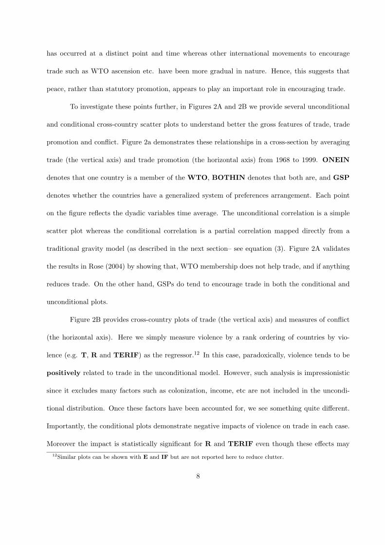
To investigate these points further, in Figures 2A and 2B we provide several unconditional
and conditional cross-country scatter plots to understand better the gross features of trade, trade
promotion and conflict. Figure 2a demonstrates these relationships in a cross-section by averaging
trade (the vertical axis) and trade promotion (the horizontal axis) from 1968 to 1999. ONEIN
denotes that one country is a member of the WTO, BOTHIN denotes that both are, and GSP
denotes whether the countries have a generalized system of preferences arrangement. Each point
on the figure reflects the dyadic variables time average. The unconditional correlation is a simple
scatter plot whereas the conditional correlation is a partial correlation mapped directly from a
traditional gravity model (as described in the next section– see equation (3). Figure 2A validates
the results in Rose (2004) by showing that, WTO membership does not help trade, and if anything
reduces trade. On the other hand, GSPs do tend to encourage trade in both the conditional and
unconditional plots.
Figure 2B provides cross-country plots of trade (the vertical axis) and measures of conflict
(the horizontal axis). Here we simply measure violence by a rank ordering of countries by vio-
lence (e.g. T, R and TERIF) as the regressor.12 In this case, paradoxically, violence tends to be
positively related to trade in the unconditional model. However, such analysis is impressionistic
since it excludes many factors such as colonization, income, etc are not included in the uncondi-
tional distribution. Once these factors have been accounted for, we see something quite different.
Importantly, the conditional plots demonstrate negative impacts of violence on trade in each case.
Moreover the impact is statistically significant for R and TERIF even though these effects may12Similar plots can be shown with E and IF but are not reported here to reduce clutter.
8
Figure 2a: The Impact of Trade Promotion on Trade
Figure 2b: The Impact of Violence on Trade
be diminished due to time averaging.
To summarize, there appears to be a negative relationship between violence and trade both
in the time domain (Figure 1) and across countries (Figures 2A and 2B). In the following section,
we attempt to sort out these effects of violence on trade.
3 Empirical Specification and Results
This section of the paper analyzes the empirical effect of violence on bilateral international trade.
We first examine the impact of violence on trade for the traditional gravity model and then for the
theoretical gravity model. We then turn to evaluating the tariff like impact of violence on trade
and then to demonstrating the robustness of our findings.
We begin our investigation of the effect of violence on trade with a traditional gravity
model of trade that is a conventional device used to estimate determinants of trade based on
geography and history. Such a work-horse model incorporates how similar borders and histories
are important in determining trade between any two countries. Formally, the empirical specification
of our augmented traditional gravity model is:
ln(Xijt) = β0 + β1 · LDISTij + β2 · ln(RGDPit × RGDPjt) + β3 · ln(
RGDPit × RGDPjt
POPitPOPjt
)(3)
+ β4 · COMLANGij + β5 · BORDERij + β9 · COMCOLONYij + β10 · CURCOLONYij
+ β11 · COLONYij + β12 · COMCURijt + β13 · REGIONALijt + φ · Z + γ1 · BOTHINijt
+γ2 ·ONEINijt + γ3 ·GSPijt + δ · V IOLENCEijt + εijt
where i, j denote trading partners i and j and t denotes time. The economic variables are defined
as: X is the average value of real bilateral trade (exports+imports)/GDP, RGDP is real Gross
9

Domestic Product, POP is population, and LDIST is the natural log of distance between two
countries13. The descriptive and geographic variables are defined as: COMLANG is a dummy
variable which is 1 if countries have a common language and 0 otherwise, COLONY is a dummy
variable which is 1 if countries were ever colonies before 1945, CURCOLONY a dummy variable
which is 1 if countries were colonized by the given year, COMCUR is a dummy variable which is 1
if both countries use the same currency, BORDER is a dummy variable for whether the countries
share a border, REGIONAL is a dummy variable which is 1 if both countries belong to the same
regional trade agreement, and Z is a vector of a comprehensive set of time and dyad fixed effects
14. The trade variables are defines as: BOTHIN is a dummy variable which is 1 if both countries
are members of WTO, ONEIN is a dummy variable which is 1 if one country is a member of WTO,
and GSP is a dummy variable which is 1 if both countries are a part of a GSP. VIOLENCE is a
measure of organized violence that can include Terrorism (T), External War (E), Revolution and
Coups (R), Inter-ethnic Conflict and Genocide (IF), while TERIF is the principle component
from the Factor model described above.15
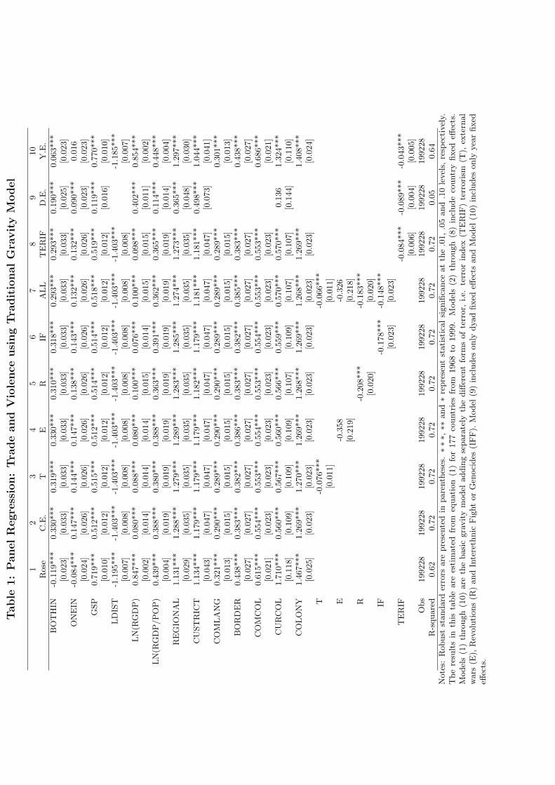
Table 1 presents a comprehensive set of regression results for the traditional gravity model.
The results in the first column generally replicate those in Rose (2004). There are four noteworthy
elements of this baseline specification. First, is that all the standard control variables for common
language, common currency, colonial status, distance, etc ... are of the expected sign and are statis-
tically significant. Second, the income terms are also of the expected sign (positive) and statistically
significant. Third, that the presence of a regional trade agreement and a generalized system of trade
preferences (GSP) raises bilateral trade and does so in an economically and statistically significant13As in Rose (2004), this is measured as the average value of bilateral trade from country i to j from FOB exports
and CIF imports deflated by the United States’ CPI.14Of course, when these dyad fixed effects are included, other variables such as BORDER and others cannot
separately be estimated.15These variables are coded such that the dummy variables are equal to one if either country has experienced an
episode of violence of a certain type. This issue is examined further in Table 4 below.
10
Table
1:
PanelR
egre
ssio
n:
Tra
de
and
Vio
lence
usi
ng
Tra
ditio
nalG
ravity
Model
12
34
56
78
910
Rose
C.E
.T
ER
IFA
LL
TE
RIF
D.E
.Y
.E.
BO
TH
IN-0
.119***
0.3
30***
0.3
19***
0.3
30***
0.3
10***
0.3
18***
0.2
93***
0.2
93***
0.1
90***
0.0
63***
[0.0
23]
[0.0
33]
[0.0
33]
[0.0
33]
[0.0
33]
[0.0
33]
[0.0
33]
[0.0
33]
[0.0
25]
[0.0
23]
ON
EIN
-0.0
84***
0.1
47***
0.1
44***
0.1
47***
0.1
38***
0.1
43***
0.1
32***
0.1
32***
0.0
90***
0.0
16
[0.0
24]
[0.0
26]
[0.0
26]
[0.0
26]
[0.0
26]
[0.0
26]
[0.0
26]
[0.0
26]
[0.0
23]
[0.0
23]
GSP
0.7
19***
0.5
12***
0.5
15***
0.5
12***
0.5
14***
0.5
14***
0.5
18***
0.5
19***
0.1
19***
0.7
70***
[0.0
10]
[0.0
12]
[0.0
12]
[0.0
12]
[0.0
12]
[0.0
12]
[0.0
12]
[0.0
12]
[0.0
16]
[0.0
10]
LD
IST
-1.1
95***
-1.4
03***
-1.4
03***
-1.4
03***
-1.4
03***
-1.4
03***
-1.4
03***
-1.4
03***
-1.1
85***
[0.0
07]
[0.0
08]
[0.0
08]
[0.0
08]
[0.0
08]
[0.0
08]
[0.0
08]
[0.0
08]
[0.0
07]
LN
(RG
DP
)0.8
47***
0.0
80***
0.0
88***
0.0
80***
0.1
00***
0.0
76***
0.1
00***
0.0
98***
0.4
02***
0.8
54***
[0.0
02]
[0.0
14]
[0.0
14]
[0.0
14]
[0.0
15]
[0.0
14]
[0.0
15]
[0.0
15]
[0.0
11]
[0.0
02]
LN
(RG
DP
/P
OP
)0.4
39***
0.3
88***
0.3
80***
0.3
88***
0.3
63***
0.3
91***
0.3
62***
0.3
65***
0.1
14***
0.4
48***
[0.0
04]
[0.0
19]
[0.0
19]
[0.0
19]
[0.0
19]
[0.0
19]
[0.0
19]
[0.0
19]
[0.0
14]
[0.0
04]
RE
GIO
NA
L1.1
31***
1.2
88***
1.2
79***
1.2
89***
1.2
83***
1.2
85***
1.2
74***
1.2
73***
0.3
65***
1.2
97***
[0.0
29]
[0.0
35]
[0.0
35]
[0.0
35]
[0.0
35]
[0.0
35]
[0.0
35]
[0.0
35]
[0.0
48]
[0.0
30]
CU
ST
RIC
T1.1
34***
1.1
79***
1.1
79***
1.1
79***
1.1
82***
1.1
79***
1.1
81***
1.1
81***
0.4
98***
1.0
44***
[0.0
43]
[0.0
47]
[0.0
47]
[0.0
47]
[0.0
47]
[0.0
47]
[0.0
47]
[0.0
47]
[0.0
73]
[0.0
41]
CO
MLA
NG
0.3
21***
0.2
90***
0.2
89***
0.2
90***
0.2
90***
0.2
89***
0.2
89***
0.2
89***
0.3
01***
[0.0
13]
[0.0
15]
[0.0
15]
[0.0
15]
[0.0
15]
[0.0
15]
[0.0
15]
[0.0
15]
[0.0
13]
BO
RD
ER
0.4
38***
0.3
83***
0.3
82***
0.3
86***
0.3
83***
0.3
82***
0.3
85***
0.3
83***
0.4
38***
[0.0
27]
[0.0
27]
[0.0
27]
[0.0
27]
[0.0
27]
[0.0
27]
[0.0
27]
[0.0
27]
[0.0
27]
CO
MC
OL
0.6
15***
0.5
54***
0.5
53***
0.5
54***
0.5
53***
0.5
54***
0.5
53***
0.5
53***
0.6
86***
[0.0
21]
[0.0
23]
[0.0
23]
[0.0
23]
[0.0
23]
[0.0
23]
[0.0
23]
[0.0
23]
[0.0
21]
CU
RC
OL
1.7
10***
0.5
60***
0.5
67***
0.5
60***
0.5
66***
0.5
59***
0.5
70***
0.5
70***
0.1
36
1.3
24***
[0.1
18]
[0.1
09]
[0.1
09]
[0.1
09]
[0.1
07]
[0.1
09]
[0.1
07]
[0.1
07]
[0.1
44]
[0.1
10]
CO
LO
NY
1.4
67***
1.2
69***
1.2
70***
1.2
69***
1.2
68***
1.2
69***
1.2
68***
1.2
69***
1.4
08***
[0.0
25]
[0.0
23]
[0.0
23]
[0.0
23]
[0.0
23]
[0.0
23]
[0.0
23]
[0.0
23]
[0.0
24]
T-0
.076***
-0.0
66***
[0.0
11]
[0.0
11]
E-0
.358
-0.3
26
[0.2
19]
[0.2
18]
R-0
.208***
-0.1
83***
[0.0
20]
[0.0
20]
IF-0
.178***
-0.1
48***
[0.0
23]
[0.0
23]
TE
RIF
-0.0
84***
-0.0
89***
-0.0
43***
[0.0
06]
[0.0
04]
[0.0
05]
Obs
199228
199228
199228
199228
199228
199228
199228
199228
199228
199228
R-s
quare
d0.6
20.7
20.7
20.7
20.7
20.7
20.7
20.7
20.0
50.6
4N
ote
s:R
obust
standard
erro
rsare
pre
sente
din
pare
nth
eses
.∗∗
∗,∗∗
and∗
repre
sent
stati
stic
alsi
gnifi
cance
at
the
.01,.0
5and
.10
level
s,re
spec
tivel
y.T
he
resu
lts
inth
ista
ble
are
esti
mate
dfr
om
equati
on
(1)
for
177
countr
ies
from
1968
to1999.
Model
s(2
)th
rough
(8)
incl
ude
countr
yfixed
effec
ts.
Model
s(1
)th
rough
(10)
are
the
basi
cgra
vity
model
addin
gse
para
tely
the
diff
eren
tfo
rms
of
terr
or,
i.e.
terr
or
index
(TE
RIF
)te
rrori
sm(T
),ex
tern
al
wars
(E),
Rev
olu
tions
(R)
and
Inte
reth
nic
Fig
ht
or
Gen
oci
des
(IFF).
Model
(9)
incl
udes
only
dyad
fixed
effec
tsand
Model
(10)
incl
udes
only
yea
rfixed
effec
ts.

way. However, as emphasized by Rose (2004), membership in the WTO is statistically significant
but with the incorrect sign: namely, membership by one country or both countries in the WTO
lowers trade. As noted by Subramanian and Wei (2004), however, the results in column 2 of Table
1 demonstrate that when one includes country fixed effects, the sign of the coefficient on BOTHIN
and ONEIN become positive rather than negative, and are statistically significant.
Beginning with column 3 of Table 1, we explore the direct effect of violence on bilateral trade.
Columns 3 through 6 sequentially include our measures of terrorism, external conflict, revolutions
and inter-ethnic fighting into the empirical specification and all four measures of conflict are included
in the results in column 7. The results in these five columns, which include country fixed effects,
demonstrate three key findings that will be shown to be robust throughout the remainder of our
paper. First, conflict has a statistically significant and robust negative impact on bilateral trade
flows. Second, different types of conflict have different negative impacts on trade. For example, a
country that has a terrorist incident is associated with a 7.6 percentage point decline in bilateral
trade. While this is an important effect, it is less than half as large as the negative impact on
trade from external conflict and inter-ethnic conflict, which are associated with declines of −20.8
and −17.8 percentage points, respectively. Third, while external conflict is associated with a
tremendous decline in trade, the estimate is not statistically significant. As noted in Blomberg,
Hess and Orphanides (2004), the difficulty in estimating the impact of external conflict on economic
activity is that external wars are infrequent, that many countries that have faced the greatest
costs of external conflict (e.g. Afghanistan, Iraq, etc...) simply do not have reliable data, and
that countries that get into external conflict with one another usually do not trade much with
each other. The results in column 7, where all measures of violence are included, demonstrates
remarkably similar findings to when each measure is included separately.
11

The results in columns 8 through 10 of Table 1 demonstrates the robustness of these findings
on violence when we use our summary measure of violence from factor analysis, TERIF. The results
in column 8 suggest that a one standard deviation shock to the TERIF indicator is associated
with a −8.4 percentage point decline in bilateral trade. The results in column 9 demonstrate
that this finding is robust to the inclusion of dyadic fixed effects.16 Finally, the inclusion of time
effects in column 10 weakens the finding on TERIF, though the estimate remains statistically and
economically significant.
As an alternative to estimating the effects of violence on trade in a traditional gravity
equation, one can estimate the theoretical counterpart of the above gravity equation, namely:
ln(Xijt/(RGDPit × RGDPjt)) = β0 + β1 · LDISTij + β4 · COMLANGij (4)
+ β5 · BORDERij + β9 · COMCOLONYij + β10 · CURCOLONYij + β11 · COLONYij
+ β12 · COMCURijt + β13 · REGIONALijt + φ · Z + γ1 · BOTHINijt + γ2 ·ONEINijt
+γ3 ·GSPijt + δ · V IOLENCEijt + εijt
and include country dummies to control for multilateral resistance terms (see Fenstra (2002)).
Notice that the restrictions on the traditional gravity equation (3) that produce the theoretical
gravity equation are that β2 = 1 and β3 = 0.
Table 2 provides the estimation results for the impact of violence in a theoretical gravity
model. The results in this table differ somewhat from those for the traditional gravity specification
in Table 1. For instance, in all specifications, the measures of WTO participation, BOTHIN
and ONEIN, both imply significantly lower bilateral trade. This is in keeping with Rose’s (2004)
findings, and it is clearly robust across all modifications to the specification in Table 2. Second,16The dyadic fixed effects are not included in the calculation of the R-squared.
12
Table
2:
PanelR
egre
ssio
n:
Tra
de
and
Vio
lence
Theore
tica
lM
odel
12
34
56
78
910
Ros
eC
.E.
TE
RIF
ALL
TE
RIF
D.E
.Y
.E.
BO
TH
IN-0
.215
***
-0.7
67**
*-0
.774
***
-0.7
67**
*-0
.771
***
-0.7
75**
*-0
.781
***
-0.7
95**
*-0
.586
***
-0.0
75**
*[0
.024
][0
.030
][0
.030
][0
.030
][0
.030
][0
.030
][0
.030
][0
.030
][0
.024
][0
.023
]O
NE
IN-0
.120
***
-0.4
00**
*-0
.400
***
-0.4
00**
*-0
.401
***
-0.4
04**
*-0
.403
***
-0.4
09**
*-0
.292
***
-0.0
44*
[0.0
24]
[0.0
25]
[0.0
25]
[0.0
25]
[0.0
25]
[0.0
25]
[0.0
25]
[0.0
25]
[0.0
22]
[0.0
24]
GSP
1.00
8***
0.26
9***
0.27
5***
0.26
9***
0.27
7***
0.26
9***
0.28
2***
0.28
0***
-0.2
46**
*1.
049*
**[0
.010
][0
.012
][0
.012
][0
.012
][0
.012
][0
.012
][0
.012
][0
.012
][0
.016
][0
.010
]LD
IST
-1.2
39**
*-1
.416
***
-1.4
16**
*-1
.416
***
-1.4
15**
*-1
.416
***
-1.4
16**
*-1
.416
***
0-1
.211
***
[0.0
07]
[0.0
08]
[0.0
08]
[0.0
08]
[0.0
08]
[0.0
08]
[0.0
08]
[0.0
08]
[0.0
00]
[0.0
07]
RE
GIO
NA
L1.
781*
**1.
131*
**1.
117*
**1.
132*
**1.
125*
**1.
130*
**1.
113*
**1.
113*
**-0
.039
1.95
2***
[0.0
29]
[0.0
37]
[0.0
37]
[0.0
37]
[0.0
37]
[0.0
37]
[0.0
37]
[0.0
37]
[0.0
49]
[0.0
29]
CU
STR
ICT
0.85
5***
1.29
6***
1.29
5***
1.29
6***
1.29
8***
1.29
6***
1.29
7***
1.29
7***
0.67
8***
0.71
2***
[0.0
45]
[0.0
48]
[0.0
48]
[0.0
48]
[0.0
48]
[0.0
48]
[0.0
48]
[0.0
48]
[0.0
75]
[0.0
43]
CO
MLA
NG
0.44
4***
0.29
7***
0.29
6***
0.29
7***
0.29
6***
0.29
7***
0.29
5***
0.29
5***
00.
417*
**[0
.013
][0
.015
][0
.015
][0
.015
][0
.015
][0
.015
][0
.015
][0
.015
][0
.000
][0
.013
]B
OR
DE
R-0
.018
0.37
0***
0.36
9***
0.37
3***
0.37
0***
0.37
0***
0.37
1***
0.37
0***
00.
034
[0.0
27]
[0.0
28]
[0.0
28]
[0.0
28]
[0.0
28]
[0.0
28]
[0.0
28]
[0.0
28]
[0.0
00]
[0.0
27]
CO
MC
OL
0.69
4***
0.55
9***
0.55
8***
0.55
9***
0.55
8***
0.55
9***
0.55
7***
0.55
8***
00.
687*
**[0
.021
][0
.024
][0
.024
][0
.024
][0
.024
][0
.024
][0
.024
][0
.024
][0
.000
][0
.021
]C
UR
CO
L2.
285*
**1.
016*
**1.
023*
**1.
016*
**1.
016*
**1.
016*
**1.
023*
**1.
023*
**0.
569*
**1.
888*
**[0
.119
][0
.122
][0
.121
][0
.122
][0
.119
][0
.121
][0
.119
][0
.119
][0
.147
][0
.112
]C
OLO
NY
1.36
9***
1.27
7***
1.27
7***
1.27
6***
1.27
5***
1.27
7***
1.27
6***
1.27
6***
01.
347*
**[0
.027
][0
.024
][0
.025
][0
.024
][0
.024
][0
.024
][0
.025
][0
.025
][0
.000
][0
.026
]T
-0.1
24**
*-0
.108
***
[0.0
11]
[0.0
11]
E-0
.319
-0.2
8[0
.226
][0
.226
]R
-0.3
25**
*-0
.304
***
[0.0
20]
[0.0
20]
IF-0
.090
***
-0.0
41*
[0.0
23]
[0.0
24]
TE
RIF
-0.1
06**
*-0
.099
***
-0.1
99**
*[0
.006
][0
.004
][0
.005
]O
bs19
9228
1992
2819
9228
1992
2819
9228
1992
2819
9228
1992
2819
9228
1992
28R
-squ
ared
0.25
0.45
0.45
0.45
0.45
0.45
0.45
0.45
0.01
0.29
Not
es:
Rob
ust
stan
dard
erro
rsar
epr
esen
ted
inpa
rent
hese
s.∗∗
∗,∗∗
and∗
repr
esen
tst
atis
tica
lsi
gnifi
canc
eat
the
.01,
.05
and
.10
leve
ls,r
espe
ctiv
ely.
The
resu
lts
inth
ista
ble
are
esti
mat
edfr
omeq
uati
on(2
)fo
r17
7co
untr
ies
from
1968
to19
99.
Col
umn
(1)
isth
eba
sic
theo
reti
calg
ravi
tym
odel
.C
olum
n(2
)is
the
basi
cth
eore
tica
lgra
vity
mod
el,i
nclu
ding
coun
try
fixed
effec
ts.
Col
umns
(3)
-(7
)ar
eth
eth
eore
tica
lgr
avity
mod
elin
clud
ing
coun
try
fixed
effec
ts.
Col
umns
(8)
-(1
0)in
clud
eth
efa
ctor
TE
RIF
Ffir
stw
ith
coun
try
fixed
effec
ts,th
enw
ith
dyad
fixed
effec
tsal
one
and
final
lyw
ith
year
fixed
effec
tsal
one.
the remainder of the estimated coefficients, excluding for the moment those for the measures of
violence, are largely unaffected by adopting the theoretical specification over the traditional spec-
ification. Finally, and most importantly, the impact of violence as measured by terrorism and
revolutions become much larger (and negative), while that for inter-ethnic fighting actually be-
comes smaller. Overall, however, the measures of violence significantly reduce international trade,
with the continuing exception of external conflict.
While it is important to understand the negative trade consequences of conflict, it is also
important to place some perspective on how this impediment to trade compares to other impedi-
ments to trade. In other words, if we were to consider violence to be a tariff (i.e. a tax) on trade,
how big of a tariff would it be?17 Fortunately, there is a methodology to help us study this specific
question. Following earlier studies, Feenstra (2002) demonstrates that exp {τij} = exp{β̂/(1− σ)
}
where σ is the elasticity of substitution between domestic and foreign goods and β̂ is the estimated
value of the impact of a particular variable on international trade. Maximizing a C.E.S. utility
function subject to resource constraints yields the following estimating relationship between trade
and tariff costs τ :
ln(Xijt
rgdpijt
) = β0 + ρ(1− σ)ldistij + (1− σ)lnτijt + (1− σ)lnpi + (1− σ)lnpj + (1− σ)εijt (5)
where σ denotes the C.E.S. parameter and ρ denotes the impact of distance on transportation cost
and p are prices. This specification has the added benefit of allowing us to calculate the tariff cost
associated with T, E, R, IF versus other widely accepted costs such as border effects, language
and colony effects.
Unfortunately, tariff costs are unobservable. Instead we observe multilateral resistance17This tax measures the pure distortion and does not incorporate the further unfortunate consequence that it would
be a tax that generated zero direct revenue.
13

terms such as borders, conflicts, etc... that are given as a vector of dummy variables, Dij =
comlangij ,borderij , comcolij , curcolij , colonyij , custrictij , regionalij ,bothinij , oneinij , gspij , so that
our empirical representation is actually
ln(Xijt
rgdpijt
) = β1ldistij + βDijt + εijt (6)
with country dummies and intercepts suppressed in the exposition (but included in the regression)
to control for price terms. Combining these two expressions we get βD = (1 − σ)lnτ , so that for
any given resistance term, we can calculate the tariff equivalent by substituting elasticities values,
i.e. τ = eβ
1−σ .
Unfortunately, in order to implement this calculation, the elasticity of substitution, σ, must
be separately provided. It is straightforward to see that σ scales up and down the estimated effects
such that an increase in σ lowers the estimated trade effect from any impediment to trade. Based
on empirical research, however, such as in Anderson and Van Wincoop (2003), it is typical for
researchers to calculate these tariff equivalent factors using values of σ equal to 5 and 10.
In Table 3 we provide these estimated effects on trade from the usual suspects and our
measures of violence. The first five columns report the estimates with the lower bound of CES
elasticity of 5 and the last five columns report the estimates with the higher bound of CES elasticity
of 10.
We begin by analyzing the impacts of the usual suspects and trade. Table 3 reports that
regional trade agreements and currency unions have the most positive impacts on trade at about 12
to 28 percent each, depending on the elasticity. These effects are similar to what has been found in
Rose and Van Wincoop (2001) and have the largest magnitude from the standard tariff equivalent
trade cost literature. Common language tariff equivalent trade costs have a magnitude of about
4 to 9 percent, which is a few percent below what was found in the literature (see Eaton and
14

Table
3:
Tari
ffEquiv
ale
nt
Tra
de
Cost
sof:
σ=
5σ
=10
BO
TH
IN-2
1.35
-21.
14-2
1.26
-21.
38-2
1.56
-8.9
8-8
.90
-8.9
4-8
.99
-9.0
7O
NE
IN-1
0.52
-10.
52-1
0.54
-10.
63-1
0.60
-4.5
4-4
.54
-4.5
6-4
.59
-4.5
8G
SP6.
646.
506.
696.
506.
813.
012.
943.
032.
943.
08R
EG
ION
AL
24.3
624
.65
24.5
224
.61
24.2
911
.67
11.8
211
.75
11.8
011
.63
CU
STR
ICT
27.6
627
.67
27.7
127
.67
27.6
913
.40
13.4
113
.43
13.4
113
.42
CO
MLA
NG
7.13
7.16
7.13
7.16
7.11
3.24
3.25
3.24
3.25
3.22
BO
RD
ER
8.81
8.90
8.84
8.84
8.86
4.02
4.06
4.03
4.03
4.04
CO
MC
OL
13.0
213
.04
13.0
213
.04
13.0
06.
016.
026.
016.
026.
00C
UR
CO
L22
.57
22.4
322
.43
22.4
322
.57
10.7
410
.68
10.6
810
.68
10.7
4C
OLO
NY
27.3
327
.31
27.2
927
.33
27.3
113
.23
13.2
213
.21
13.2
313
.22
T-3
.15
-2.7
4-1
.39
-1.2
1E
-8.3
0-7
.25
-3.6
1-3
.16
R-8
.46
-7.9
0-3
.68
-3.4
4IF
-2.2
8-1
.03
-1.0
1-0
.46
VIO
LE
NC
E-3
.15
-8.3
0-8
.46
-2.2
8-1
8.91
-1.3
9-3
.61
-3.6
8-1
.01
-8.2
6N
otes
:Se
eTab
le2.
The
resu
lts
inth
ista
ble
are
esti
mat
edfr
omeq
uati
on(2
)fo
r17
7co
untr
ies
from
1968
to19
99.
The
first
five
colu
mns
are
the
basi
cth
eore
tica
lgra
vity
mod
elim
pact
sby
indi
vidu
ally
and
then
join
tly
incl
udin
gm
easu
res
ofco
nflic
tas
sum
ing
aC
ES
elas
tici
tyof
5.T
hefin
alfiv
eco
lum
nsar
eth
eba
sic
theo
reti
cal
grav
ity
mod
elim
pact
sby
indi
vidu
ally
and
then
join
tly
incl
udin
gm
easu
res
ofco
nflic
tas
sum
ing
aC
ES
elas
tici
tyof
10.
VIO
LE
NC
Eca
lcul
ates
the
sum
ofth
eim
pact
sof
T,E
,R,a
ndIF
.E
ach
num
ber
repr
esen
tsa
tari
ffeq
uiva
lent
perc
enta
ge.
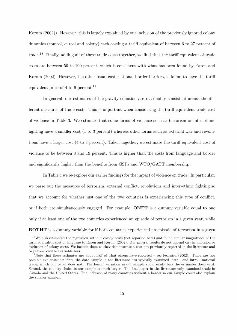
Korum (2002)). However, this is largely explained by our inclusion of the previously ignored colony
dummies (comcol, curcol and colony) each costing a tariff equivalent of between 6 to 27 percent of
trade.18 Finally, adding all of these trade costs together, we find that the tariff equivalent of trade
costs are between 50 to 100 percent, which is consistent with what has been found by Eaton and
Korum (2002). However, the other usual cost, national border barriers, is found to have the tariff
equivalent price of 4 to 9 percent.19
In general, our estimates of the gravity equation are reasonably consistent across the dif-
ferent measures of trade costs. This is important when considering the tariff equivalent trade cost
of violence in Table 3. We estimate that some forms of violence such as terrorism or inter-ethnic
fighting have a smaller cost (1 to 3 percent) whereas other forms such as external war and revolu-
tions have a larger cost (4 to 8 percent). Taken together, we estimate the tariff equivalent cost of
violence to be between 8 and 19 percent. This is higher than the costs from language and border
and significantly higher than the benefits from GSPs and WTO/GATT membership.
In Table 4 we re-explore our earlier findings for the impact of violence on trade. In particular,
we parse out the measures of terrorism, external conflict, revolutions and inter-ethnic fighting so
that we account for whether just one of the two countries is experiencing this type of conflict,
or if both are simultaneously engaged. For example, ONET is a dummy variable equal to one
only if at least one of the two countries experienced an episode of terrorism in a given year, while
BOTHT is a dummy variable for if both countries experienced an episode of terrorism in a given18We also estimated the regression without colony costs (not reported here) and found similar magnitudes of the
tariff equivalent cost of language to Eaton and Korum (2002). Our general results do not depend on the inclusion orexclusion of colony costs. We include them as they demonstrate a cost not previously reported in the literature andto prevent omitted variable bias.
19Note that these estimates are about half of what others have reported – see Feenstra (2002). There are twopossible explanations: first, the data sample in the literature has typically examined inter - and intra - nationaltrade, which our paper does not. The loss in variation in our sample could easily bias the estimates downward.Second, the country choice in our sample is much larger. The first paper in the literature only examined trade inCanada and the United States. The inclusion of many countries without a border in our sample could also explainthe smaller number.
15
Table
4:
Tra
de
and
Vio
lence
:Tre
ati
ng
Vio
lence
Diff
ere
ntly
Tra
diti
onal
Gra
vity
Mod
elT
heor
etic
alG
ravi
tyM
odel
12
34
56
78
910
TE
RIF
ALL
TE
RIF
ALL
ON
ET
-0.0
74**
*-0
.069
***
-0.1
18**
*-0
.108
***
[0.0
11]
[0.0
11]
[0.0
11]
[0.0
11]
BO
TH
T-0
.095
***
-0.0
82**
*-0
.190
***
-0.1
68**
*[0
.015
][0
.015
][0
.015
][0
.015
]O
NE
E-0
.083
***
-0.0
73**
*-0
.103
***
-0.0
90**
*[0
.014
][0
.014
][0
.014
][0
.014
]B
OT
HE
-0.2
99-0
.291
-0.2
46-0
.234
[0.2
19]
[0.2
18]
[0.2
26]
[0.2
25]
ON
ER
-0.1
78**
*-0
.151
***
-0.2
65**
*-0
.243
***
[0.0
20]
[0.0
21]
[0.0
20]
[0.0
21]
BO
TH
R-0
.485
***
-0.4
40**
*-0
.644
***
-0.6
12**
*[0
.114
][0
.114
][0
.115
][0
.116
]O
NE
IF-0
.146
***
-0.1
11**
*-0
.036
0.01
5[0
.025
][0
.026
][0
.026
][0
.026
]B
OT
HIF
-0.1
13-0
.059
0.12
30.
196
[0.1
38]
[0.1
38]
[0.1
42]
[0.1
41]
Tot
alIm
pact
-7.8
6-8
.95
-24.
322.
12-3
2.97
σ=
5
Obs
1992
2819
9228
1992
2819
9228
1992
2819
9228
1992
2819
9228
1992
2819
9228
R-s
quar
ed0.
720.
720.
720.
720.
720.
450.
450.
450.
450.
45N
otes
:R
obus
tst
anda
rder
rors
are
pres
ente
din
pare
nthe
ses.∗∗
∗,∗∗
and∗
repr
esen
tst
atis
tica
lsi
gnifi
canc
eat
the
.01,
.05
and
.10
leve
ls,
resp
ecti
vely
.T
here
sult
sin
this
tabl
ear
ees
tim
ated
from
eith
ereq
uati
on(1
)or
(2)
for
177
coun
trie
sfr
om19
68to
1999
.C
olum
ns(1
)-
(5)
are
the
basi
cgr
avity
mod
el.
Col
umns
(6)
-(1
0)ar
eth
eth
eore
tica
lgr
avity
mod
elin
clud
ing
coun
try
fixed
effec
ts.
The
coeffi
cien
tas
soci
ated
wit
hO
NE
Xm
easu
res
the
impa
ctif
one
ofth
edy
adpa
irha
sco
nflic
tty
peX
.T
heco
effici
ent
asso
ciat
edw
ith
Bot
hXm
easu
res
the
impa
ctif
both
ofth
edy
adpa
irha
sco
nflic
tty
peX
.N
one
ofth
eco
ntro
lva
riab
les
are
repo
rted
.Tot
alIm
pact
mea
sure
sth
ees
tim
ated
impa
cton
trad
efr
omal
lte
rror
vari
able
sw
ith
σ=
5.
year. Similarly, ONEE, BOTHE, ONER, BOTHR, ONEIF and BOTHIF are defined for
external conflict, revolutions and inter-ethnic fighting, respectively. In each of the first five columns
of Table 4 we report regression results using the traditional gravity equation in expression (3) while
columns six through ten report the results when the theoretical gravity equation in expression (4)
is estimated.
Column one presents the estimation results for terrorism’s impact on trade. Terrorism,
whether felt by one country or both countries, appears to lower international trade by approximately
the same amount, −8 percentage points. Second, if just one country is engaged in an external war,
this appears to lower bilateral trade by a similar amount. The result, however, for if both countries
are in an external conflict is not statistically different from zero, for likely the same reasons for
why external conflict was not significant in Tables 1 or 2 – namely, this occurs very infrequently.20
Thirdly, revolutions limit trade but especially so if both countries face revolutions, as it is associated
with an almost 50 percentage point reduction. Finally, if one country is engaged in inter-ethnic
fighting this is associated with a −14 percentage point decline in trade, though the effect on trade
if both face such a type of conflict is not statistically significant, likely due to the reason that such
a scenario is very rare.
The results from the theoretical gravity specification in columns 6 through 10 of Table 4
are very similar to those in the first five columns with the exception that the effect of the impact
of violence on trade is larger. For example, in column six, where we estimate the theoretical
gravity specification, the impact of terrorism is larger, and significantly larger still if both countries
face terrorism. Indeed, on average the impact is approximately 20 percent larger. One exception,
however, is that the effect of inter-ethnic fighting on trade is no longer statistically significant.
Of course, the additional bonus to estimating the theoretical gravity specification is that one can20ONEE occurs in approximately 1.5 percent of the observations whereas BOTHE occurs at a 0.04 percent rate.
16
interpret the tariff equivalent effect of violence on trade. As demonstrated in column ten, conflict
is equivalent to an approximate 32 percent tariff, which for a value of σ = 5 is larger than the effect
presented in Table 2 which was 19 percent. In sum, the results in Tables 1, 2 and 3 would therefore
appear to be a lower bound estimate of the effect of conflict on trade.
As the results in Table 4 demonstrate, our baseline estimates of the traditional gravity
specification in (3) reported Table 1 are robust across modifications considered in Tables 2 and
4. In Table 5, however, we examine further the robustness of our result of the impact of conflict
on trade across different regions and time periods. Columns 1 through 7 of Table 5 report the
results from a traditional gravity specification where we include the factor index TERIF in each
specification.21 As can be seen from the appropriate rows of the table, the estimate is statistically
significant at below the .01 level in all cases, and the coefficient estimates vary between −.035 in
high income countries to −.125 in South East Asia. Finally, columns 8 and 9 explore the impact of
violence on trade when we split the sample in 1983. Interestingly, the estimated impact of violence
is much lower, though still statistically significant at the 10 percent level, for the 1968-1983 sub-
sample. The coefficient is 4 times larger for the second half of the sample.
As a final step, we consider the issue of endogeneity. If peace can improve trade, then it
is possible that trade can cause peace. Indeed, some of the political science literature discusses
the issue of whether trade and substantively important benefit to reducing interstate violence –
among other papers in this vast literature, see Mansfield (1994) and Oneal and Russett (1999).
To consider this possibility, we estimate the traditional gravity equation and use instruments for
violence through the strategic components of trade. In this case, we instrument for conflict using
UN voting records as in Bennett and Stamm (1999), and dummy variables for for international21The regions we consider are, respectively, South East Asia, East Asia, the Middle East and North Africa, Latin
America and the Caribbean, and High and Low Income countries. The latter classification is from Rose (2004) andis obtained from the World Bank Development Indicators.
17

Table
5:
Sensi
tivity
Analy
sis:
Tra
de
and
Vio
lence
by
Regio
n&
Tim
e
12
34
56
78
9SA
SIA
EA
SIA
SSA
FR
MID
EA
FLA
TC
AH
IGH
INLO
WIN
1968
-83
1984
-99
BO
TH
IN0.
829*
**0.
295*
**-0
.072
-0.0
130.
213*
**0.
254*
**0.
121*
*-0
.344
***
0.27
1***
[0.2
23]
[0.0
72]
[0.0
72]
[0.0
64]
[0.0
53]
[0.0
52]
[0.0
62]
[0.0
71]
[0.0
58]
ON
EIN
0.45
3**
0.17
9***
-0.2
48**
*-0
.022
0.06
20.
216*
**-0
.063
-0.1
59**
*0.
118*
*[0
.208
][0
.057
][0
.055
][0
.045
][0
.043
][0
.048
][0
.044
][0
.042
][0
.047
]G
SP0.
031
0.25
3***
0.45
7***
0.50
0***
0.22
2***
0.35
8***
0.43
1***
0.40
0***
0.60
7***
[0.0
73]
[0.0
45]
[0.0
26]
[0.0
40]
[0.0
30]
[0.0
14]
[0.0
24]
[0.0
16]
[0.0
20]
LD
IST
-1.1
70**
*-1
.418
***
-1.6
68**
*-1
.663
***
-1.6
77**
*-1
.376
***
-1.4
13**
*-1
.281
***
-1.4
93**
*[0
.136
][0
.052
][0
.027
][0
.033
][0
.026
][0
.011
][0
.019
][0
.011
][0
.011
]LN
(RG
DP
)0.
568*
**0.
745*
**-0
.153
***
0.14
3***
0.18
0***
0.02
7-0
.037
*0.
399*
**1.
063*
**[0
.038
][0
.045
][0
.022
][0
.026
][0
.032
][0
.020
][0
.020
][0
.044
][0
.044
]LN
(RG
DP
/PO
P)
-0.3
90**
*-0
.203
***
0.44
7***
0.39
6***
0.34
8***
0.61
6***
0.33
7***
0.36
6***
-0.9
74**
*[0
.050
][0
.061
][0
.031
][0
.038
][0
.043
][0
.027
][0
.027
][0
.065
][0
.046
]R
EG
ION
AL
1.42
4***
1.85
7***
0.39
4***
1.66
3***
1.68
6***
1.10
0***
[0.0
93]
[0.0
60]
[0.0
39]
[0.0
96]
[0.0
61]
[0.0
44]
CU
STR
ICT
1.10
9***
1.42
0***
1.47
2***
-0.6
45-0
.147
*0.
829*
**1.
574*
**1.
121*
**1.
120*
**[0
.388
][0
.173
][0
.064
][0
.736
][0
.081
][0
.085
][0
.063
][0
.061
][0
.068
]C
OM
LA
NG
0.11
1*0.
038
0.29
7***
0.10
4**
0.60
0***
0.32
7***
0.11
1***
0.21
4***
0.35
1***
[0.0
59]
[0.0
48]
[0.0
30]
[0.0
44]
[0.0
29]
[0.0
17]
[0.0
27]
[0.0
20]
[0.0
21]
BO
RD
ER
-0.7
17**
*-0
.609
***
1.13
5***
0.05
2-0
.179
***
-0.4
46**
*0.
872*
**0.
264*
**0.
509*
**[0
.155
][0
.129
][0
.053
][0
.066
][0
.049
][0
.038
][0
.048
][0
.038
][0
.037
]C
OM
CO
L0.
332*
**0.
480*
**0.
466*
**0.
826*
**0.
380*
**0.
029
0.55
1***
0.45
3***
0.61
1***
[0.0
81]
[0.0
63]
[0.0
38]
[0.0
57]
[0.0
64]
[0.0
36]
[0.0
34]
[0.0
32]
[0.0
32]
CU
RC
OL
1.63
6***
-0.4
86*
0.89
9***
1.30
9***
0.65
7***
-0.1
930.
831*
**-0
.338
*[0
.202
][0
.272
][0
.166
][0
.102
][0
.116
][0
.388
][0
.126
][0
.194
]C
OLO
NY
0.22
1**
1.10
3***
1.69
3***
0.59
7***
0.84
1***
1.30
1***
1.46
2***
1.37
2***
1.18
9***
[0.0
99]
[0.0
69]
[0.0
40]
[0.0
56]
[0.0
45]
[0.0
24]
[0.0
40]
[0.0
32]
[0.0
32]
TE
RIF
-0.0
75**
*-0
.125
***
-0.0
63**
*-0
.076
***
-0.0
97**
*-0
.035
***
-0.0
78**
*-0
.017
*-0
.068
***
[0.0
17]
[0.0
13]
[0.0
10]
[0.0
13]
[0.0
10]
[0.0
07]
[0.0
09]
[0.0
09]
[0.0
10]
Obs
1645
032
021
7544
533
704
6183
810
6991
9232
286
861
1123
67R
-squ
ared
0.75
0.72
0.59
0.68
0.69
0.82
0.62
0.72
0.73
Not
es:
Rob
ust
stan
dard
erro
rsar
epr
esen
ted
inpa
rent
hese
s.∗∗
∗,∗∗
and∗
repr
esen
tst
atis
tica
lsi
gnifi
canc
eat
the
.01,
.05
and
.10
leve
ls,
resp
ecti
vely
.T
here
sult
sin
this
tabl
ear
ees
tim
ated
from
equa
tion
(1)
for
177
coun
trie
sfr
om19
68to
1999
.E
ach
colu
mn
isth
eba
sic
grav
ity
mod
elin
clud
ing
tim
ean
dco
untr
yfix
edeff
ects
.E
ach
colu
mn
repr
esen
tsa
diffe
rent
regi
onor
tim
epe
riod
.SA
SIA
repr
esen
tsSo
uth
Asi
a,E
ASI
Ais
Eas
tA
sia,
MID
EA
Fis
Mid
dle
Eas
tan
dN
orth
Afr
ica,
LA
TC
Ais
Lat
inA
mer
ica
and
Car
ibbe
an,
HIG
HIN
ishi
ghin
com
ean
dLO
WIN
islo
win
com
eco
untr
y.
peace treaties. Table 6 reports the results from this estimation. In this case, we again find a strong
negative impact of violence on trade. Note that the magnitudes of the coefficients are somewhat
larger, although there is no evidence of mis-specification as the over-identifying restrictions are not
rejected in each of the specifications. Hence, our earlier results of the tariff cost withstand the
scrutiny of exogeneity.
4 Conclusions
Our work follows from Rose (2004) who shows that many of the usual suspects in determining
the magnitude of trade flows, e.g. WTO/GATT, are not as important as the adoption of the
Generalized System of Preferences [GSPs]. From the analysis presented in this paper, it appears
that the impact of conflict on trade is quite strong – even larger than GSPs.
What are the policy implications of our paper? While pursuing trade promotion through
bilateral vehicles like GSPs have important effects on trade, another avenue is likely to have a
larger impact on trade – peace. We find peace has a large and positive impact on trade. This
is obviously a lower bound on the welfare gain to peace, though it is an important component to
raising economic welfare.
Along the same line, Hess (2003) analyzes the consumption welfare loss from internal and
external conflict in order to answer “How much would individual be willing to pay to avoid just the
economic costs of conflict?” Remarkably, his estimates suggest that these pure economic welfare
losses from conflict are quite large: namely, on average, individuals who live in a country that
have experienced some conflict since 1960 would permanently give up to approximately 8 percent
of their current level of consumption to live in a purely peaceful world. Taken together, the
large potential welfare gains to consumption identified in Hess (2003), in addition to those from
bilateral trade identified in this paper, suggests that economists and policy-makers should continue
18

Table 6: IV Panel Regression: Trade and Violence
1 2 3 4 5TERIF T E R IF
ONEIN -0.097** -0.006 0.1 -0.085** -0.146***[0.041] [0.066] [0.141] [0.039] [0.050]
GSP 0.562*** 0.611*** 0.565*** 0.556*** 0.552***[0.024] [0.072] [0.122] [0.024] [0.025]
BOTHIN -0.271*** -0.183 0.063 -0.186*** -0.396***[0.083] [0.196] [0.227] [0.068] [0.106]
LN(RGDP) 0.106** 0.745 -0.164* 0.236*** -0.248***[0.051] [0.471] [0.095] [0.064] [0.021]
LN(RGDP/POP) 0.702*** 0.225 0.916*** 0.539*** 1.030***[0.060] [0.411] [0.170] [0.077] [0.030]
REGIONAL 1.021*** 0.55 2.238*** 1.088*** 1.104***[0.062] [0.343] [0.860] [0.060] [0.061]
CUSTRICT 1.252*** 1.232*** 1.480*** 1.286*** 1.221***[0.058] [0.089] [0.354] [0.062] [0.062]
LDIST -1.437*** -1.450*** -1.694*** -1.428*** -1.439***[0.010] [0.018] [0.216] [0.011] [0.011]
COMLANG 0.292*** 0.267*** 0.424*** 0.291*** 0.300***[0.018] [0.035] [0.127] [0.019] [0.019]
BORDER 0.373*** 0.284*** 4.011 0.374*** 0.358***[0.035] [0.065] [2.941] [0.037] [0.037]
COMCOL 0.529*** 0.467*** 0.736*** 0.531*** 0.546***[0.025] [0.050] [0.203] [0.026] [0.027]
CURCOL 3.082 4.551 3.169 2.81 2.835[2.030] [3.260] [10.071] [2.136] [2.175]
COLONY 1.226*** 1.303*** 0.481 1.209*** 1.226***[0.044] [0.076] [0.645] [0.047] [0.047]
TERIF -1.108***[0.175]
T -6.542**[3.243]
E -453.555[364.793]
R -4.822***[0.688]
IF -5.365***[0.888]
Chi-Sq(1) 1.302 1.702 1.640 1.522 1.054P-Value [0.254] [0.192] [0.200] [0.217] [0.305]
Observations 149862 149862 149862 149862 149862Notes: robust standard errors are presented in parentheses. ∗ ∗ ∗, ∗∗ and ∗ representstatistical significance at the .01, .05 and .10 levels, respectively. Each column is the basicgravity model including country fixed effects. Instruments include factors based on annualUN voting records. Test of over-identifying restrictions are reported as Chi-Sq(1) with theassociated P-Values.

to investigate and advocate for domestic and international institutions that promote peace in order
to realize such gains.
19
References
[1] Anderson, J. (1979) “A Theoretical Foundation for the Gravity Equation,” American EconomicReview, 69(1): 106-116.
[2] Anderson, J. and Marcouiller, D. (2002) “ Insecurity and the Pattern of Trade: An EmpiricalInvestigaton,” Review of Economics and Statistics.
[3] Anderson, J. and Van Wincoop, E. (2003) “Gravity with Gravitas: A Solution to the BorderPuzzle,” American Economic Review, May 2003.
[4] Bennett, Scott and Alan Stam (1999), EUGENE: Expected Utility Generation and Data Man-agement Program.
[5] Brecher, Michael, Wilkenfeld, Jonathan, and Moser, Sheila. “Crises in the Twentieth Century,”In Handbook of International Crises, Volume I, Oxford, UK: Pergamon Books, 1988.
[6] Blomberg, S. Brock, 1996 “Growth, Political Instability and the Defence Burden,” Economica.
[7] Blomberg, S. Brock, Gregory D. Hess, and Athansios Orphanides, 2004 “The MacroeconomicConsequences of Terrorism,” Journal of Monetary Economics, forthcoming.
[8] Blomberg, S. Brock, Gregory D. Hess, and Akila Weerapana, 2004 “Economic Conditions andTerrorism,” European Journal of Political Economy , forthcoming.
[9] Blomberg, S. Brock, and Gregory D. Hess, 2002 “The Temporal Links Between Conflict andEconomic Activity,” Journal of Conflict Resolution, 46(1), 74-90.
[10] Blomberg, S. Brock, Hess, Gregory D., and Siddharth Thacker, 2004. “Is There a Conflict-Poverty Trap?,” mimeo.
[11] Eaton, J., and S. Kortum (2002), “Technology, Geography and Trade”, Econometrica Septem-ber 2002, 1741-1779.
[12] Enders, Walter and Todd Sandler, (2004). “9-11, Is it all different now?,” mimeo.
[13] Feenstra, Robert, 2002. Advanced International Trade: Theory and Evidence , Princeton Uni-versity Press.
[14] Glick, Reuven and Alan Taylor, 2004. “Collateral Damage: The Economic Impact of War,”mimeo.
[15] Gurr, T.R., K. Jaggers, and W. Moore, 2003. Polity Handbook IV, 2003, University of ColoradoPress, Boulder.
[16] Hess, Gregory D., 2003. “The Economic Welfare Cost of Conflict: An Empirical Assessment,”CESifo Working Paper, # 852.
[17] Hess, Gregory D. and Athanasios Orphanides, 1995. “War Politics: An Economic, Rational-Voter Framework,” American Economic Review, 85(4), 828-846.
20

[18] Hess, Gregory D. and Athanasios Orphanides, 2001a. “Economic Conditions, Elections, andthe Magnitude of Foreign Conflicts,” Journal of Public Economics, 80(1), 121-140.
[19] Hess, Gregory D. and Athanasios Orphanides, 2001b. “War and Democracy,” The Journal ofPolitical Economy, 109(4), 776-810.
[20] Kaufmann, D., Kraay, A., Zoido-Lobatn, P., (2000). “Governance matters: From Measurementto Action”, Finance and Development June 2000.
[21] Mansfield, Edward 1994 Poverty, Trade and War, Princeton University Press.
[22] Mickolus, Edward, Sandler, Todd, Murdock, Jean and Peter Flemming, 1993. “InternationalTerrorism: Attributes of Terrorist Events (ITERATE),” Dunn Loring: VA, Vinyard Software.
[23] Nitsch, Volber and Dieter Schumacher 2004. “Terrorism and interational trade: an empricalinvestigation,” European Journal of Political Economy, forthcoming.
[24] Oneal, John, and Bruce Russett 1999 “The Kantian Peace: The Pacific Benefits of Democracy,Interdependence, and International Organizations, 1885-1992”World Politics, 52(1): 1-37.
[25] Rose, Andrew 2004. “Do we really know that the WTO increases trade,” American EconomicReview, forthcoming.
[26] Rose, Andrew and Eric Van Wincoop, 2001. “National Money as a Barrier to Trade: the RealCase for Currency Union,” American Economic Review Paper and Preceedings, 386-390.
[27] Subramanian, Arvind and Shang-Jin Wei 2004. “The WTO Promotes Trade Strongly butUnevenly,” mimeo.
21
Key Non-Conflict Variables of Interest
BORDER is a dummy variable which is 1 if both countries share a border.
BOTHIN is a dummy variable which is 1 if both countries are members of WTO.
COLONY is a dummy variable which is 1 if countries were ever colonies before 1945.
COMCOL is a dummy variable which is 1 if both countries have common colonizer.
COMLANG is a dummy variable which is 1 if countries have a common language and 0 otherwise.
CURCOL is a dummy variable which is 1 if countries were colonized by the given year.
CUSTRICT is a dummy variable which is 1 if both countries use the same currency.
GSP is a dummy variable which is 1 if both countries are a part of a GSP.
LDIST is natural log of the distance between countries as measured in Rose (2004).
ONEIN is a dummy variable which is 1 if one country is a member of WTO.
POP is population.
REGIONAL is a dummy variable which is 1 if both countries belong to the same regional tradeagreement.
RGDP is real Gross Domestic Product.
X denotes the average value of real bilateral trade as calculated in Rose (2004).
Z is a vector of a comprehensive set of time and dyad fixed effects.
22
Supplemental Appendix
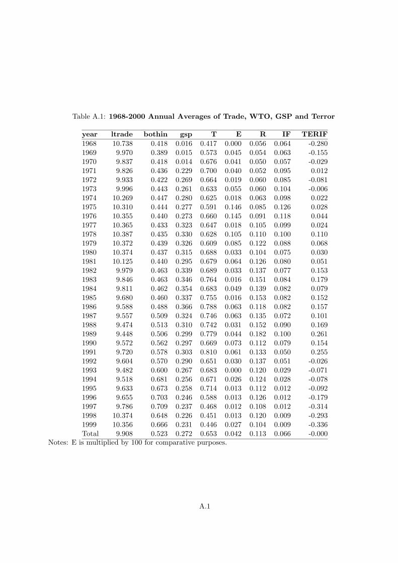
Table A.1: 1968-2000 Annual Averages of Trade, WTO, GSP and Terror
year ltrade bothin gsp T E R IF TERIF1968 10.738 0.418 0.016 0.417 0.000 0.056 0.064 -0.2801969 9.970 0.389 0.015 0.573 0.045 0.054 0.063 -0.1551970 9.837 0.418 0.014 0.676 0.041 0.050 0.057 -0.0291971 9.826 0.436 0.229 0.700 0.040 0.052 0.095 0.0121972 9.933 0.422 0.269 0.664 0.019 0.060 0.085 -0.0811973 9.996 0.443 0.261 0.633 0.055 0.060 0.104 -0.0061974 10.269 0.447 0.280 0.625 0.018 0.063 0.098 0.0221975 10.310 0.444 0.277 0.591 0.146 0.085 0.126 0.0281976 10.355 0.440 0.273 0.660 0.145 0.091 0.118 0.0441977 10.365 0.433 0.323 0.647 0.018 0.105 0.099 0.0241978 10.387 0.435 0.330 0.628 0.105 0.110 0.100 0.1101979 10.372 0.439 0.326 0.609 0.085 0.122 0.088 0.0681980 10.374 0.437 0.315 0.688 0.033 0.104 0.075 0.0301981 10.125 0.440 0.295 0.679 0.064 0.126 0.080 0.0511982 9.979 0.463 0.339 0.689 0.033 0.137 0.077 0.1531983 9.846 0.463 0.346 0.764 0.016 0.151 0.084 0.1791984 9.811 0.462 0.354 0.683 0.049 0.139 0.082 0.0791985 9.680 0.460 0.337 0.755 0.016 0.153 0.082 0.1521986 9.588 0.488 0.366 0.788 0.063 0.118 0.082 0.1571987 9.557 0.509 0.324 0.746 0.063 0.135 0.072 0.1011988 9.474 0.513 0.310 0.742 0.031 0.152 0.090 0.1691989 9.448 0.506 0.299 0.779 0.044 0.182 0.100 0.2611990 9.572 0.562 0.297 0.669 0.073 0.112 0.079 0.1541991 9.720 0.578 0.303 0.810 0.061 0.133 0.050 0.2551992 9.604 0.570 0.290 0.651 0.030 0.137 0.051 -0.0261993 9.482 0.600 0.267 0.683 0.000 0.120 0.029 -0.0711994 9.518 0.681 0.256 0.671 0.026 0.124 0.028 -0.0781995 9.633 0.673 0.258 0.714 0.013 0.112 0.012 -0.0921996 9.655 0.703 0.246 0.588 0.013 0.126 0.012 -0.1791997 9.786 0.709 0.237 0.468 0.012 0.108 0.012 -0.3141998 10.374 0.648 0.226 0.451 0.013 0.120 0.009 -0.2931999 10.356 0.666 0.231 0.446 0.027 0.104 0.009 -0.336Total 9.908 0.523 0.272 0.653 0.042 0.113 0.066 -0.000
Notes: E is multiplied by 100 for comparative purposes.
A.1
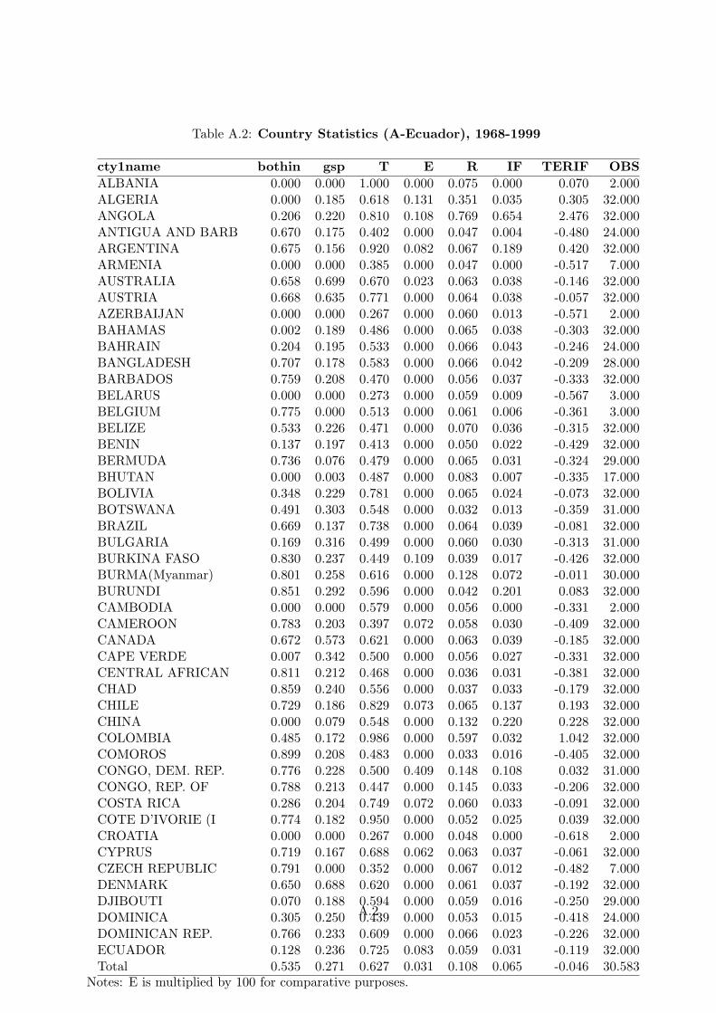
Table A.2: Country Statistics (A-Ecuador), 1968-1999
cty1name bothin gsp T E R IF TERIF OBSALBANIA 0.000 0.000 1.000 0.000 0.075 0.000 0.070 2.000ALGERIA 0.000 0.185 0.618 0.131 0.351 0.035 0.305 32.000ANGOLA 0.206 0.220 0.810 0.108 0.769 0.654 2.476 32.000ANTIGUA AND BARB 0.670 0.175 0.402 0.000 0.047 0.004 -0.480 24.000ARGENTINA 0.675 0.156 0.920 0.082 0.067 0.189 0.420 32.000ARMENIA 0.000 0.000 0.385 0.000 0.047 0.000 -0.517 7.000AUSTRALIA 0.658 0.699 0.670 0.023 0.063 0.038 -0.146 32.000AUSTRIA 0.668 0.635 0.771 0.000 0.064 0.038 -0.057 32.000AZERBAIJAN 0.000 0.000 0.267 0.000 0.060 0.013 -0.571 2.000BAHAMAS 0.002 0.189 0.486 0.000 0.065 0.038 -0.303 32.000BAHRAIN 0.204 0.195 0.533 0.000 0.066 0.043 -0.246 24.000BANGLADESH 0.707 0.178 0.583 0.000 0.066 0.042 -0.209 28.000BARBADOS 0.759 0.208 0.470 0.000 0.056 0.037 -0.333 32.000BELARUS 0.000 0.000 0.273 0.000 0.059 0.009 -0.567 3.000BELGIUM 0.775 0.000 0.513 0.000 0.061 0.006 -0.361 3.000BELIZE 0.533 0.226 0.471 0.000 0.070 0.036 -0.315 32.000BENIN 0.137 0.197 0.413 0.000 0.050 0.022 -0.429 32.000BERMUDA 0.736 0.076 0.479 0.000 0.065 0.031 -0.324 29.000BHUTAN 0.000 0.003 0.487 0.000 0.083 0.007 -0.335 17.000BOLIVIA 0.348 0.229 0.781 0.000 0.065 0.024 -0.073 32.000BOTSWANA 0.491 0.303 0.548 0.000 0.032 0.013 -0.359 31.000BRAZIL 0.669 0.137 0.738 0.000 0.064 0.039 -0.081 32.000BULGARIA 0.169 0.316 0.499 0.000 0.060 0.030 -0.313 31.000BURKINA FASO 0.830 0.237 0.449 0.109 0.039 0.017 -0.426 32.000BURMA(Myanmar) 0.801 0.258 0.616 0.000 0.128 0.072 -0.011 30.000BURUNDI 0.851 0.292 0.596 0.000 0.042 0.201 0.083 32.000CAMBODIA 0.000 0.000 0.579 0.000 0.056 0.000 -0.331 2.000CAMEROON 0.783 0.203 0.397 0.072 0.058 0.030 -0.409 32.000CANADA 0.672 0.573 0.621 0.000 0.063 0.039 -0.185 32.000CAPE VERDE 0.007 0.342 0.500 0.000 0.056 0.027 -0.331 32.000CENTRAL AFRICAN 0.811 0.212 0.468 0.000 0.036 0.031 -0.381 32.000CHAD 0.859 0.240 0.556 0.000 0.037 0.033 -0.179 32.000CHILE 0.729 0.186 0.829 0.073 0.065 0.137 0.193 32.000CHINA 0.000 0.079 0.548 0.000 0.132 0.220 0.228 32.000COLOMBIA 0.485 0.172 0.986 0.000 0.597 0.032 1.042 32.000COMOROS 0.899 0.208 0.483 0.000 0.033 0.016 -0.405 32.000CONGO, DEM. REP. 0.776 0.228 0.500 0.409 0.148 0.108 0.032 31.000CONGO, REP. OF 0.788 0.213 0.447 0.000 0.145 0.033 -0.206 32.000COSTA RICA 0.286 0.204 0.749 0.072 0.060 0.033 -0.091 32.000COTE D’IVORIE (I 0.774 0.182 0.950 0.000 0.052 0.025 0.039 32.000CROATIA 0.000 0.000 0.267 0.000 0.048 0.000 -0.618 2.000CYPRUS 0.719 0.167 0.688 0.062 0.063 0.037 -0.061 32.000CZECH REPUBLIC 0.791 0.000 0.352 0.000 0.067 0.012 -0.482 7.000DENMARK 0.650 0.688 0.620 0.000 0.061 0.037 -0.192 32.000DJIBOUTI 0.070 0.188 0.594 0.000 0.059 0.016 -0.250 29.000DOMINICA 0.305 0.250 0.439 0.000 0.053 0.015 -0.418 24.000DOMINICAN REP. 0.766 0.233 0.609 0.000 0.066 0.023 -0.226 32.000ECUADOR 0.128 0.236 0.725 0.083 0.059 0.031 -0.119 32.000Total 0.535 0.271 0.627 0.031 0.108 0.065 -0.046 30.583
Notes: E is multiplied by 100 for comparative purposes.
A.2
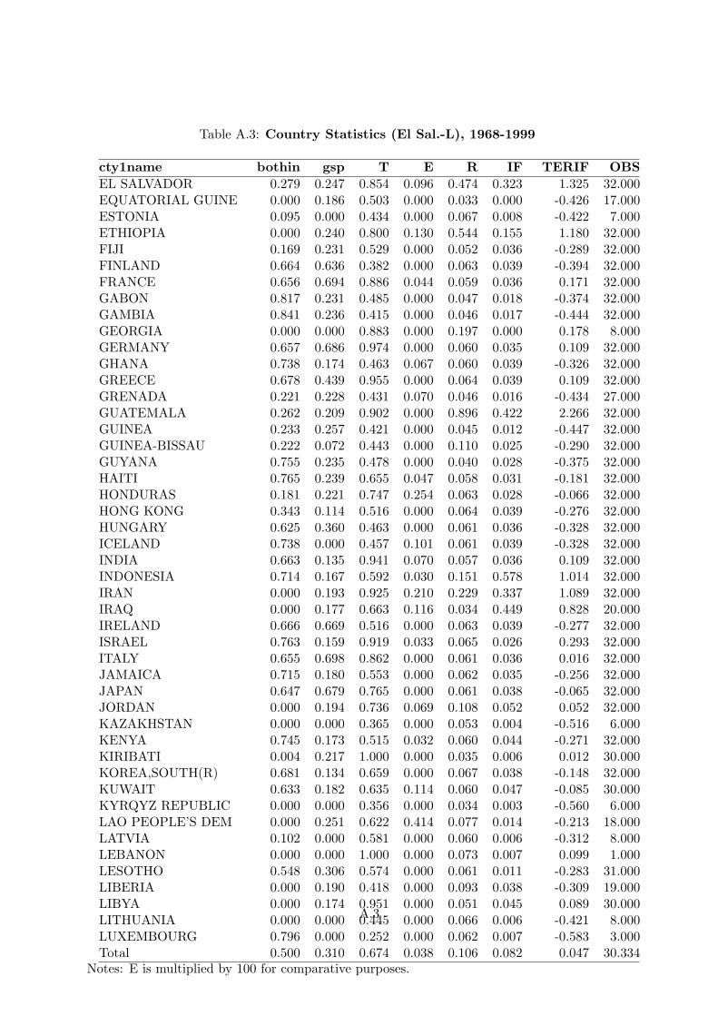
Table A.3: Country Statistics (El Sal.-L), 1968-1999
cty1name bothin gsp T E R IF TERIF OBSEL SALVADOR 0.279 0.247 0.854 0.096 0.474 0.323 1.325 32.000EQUATORIAL GUINE 0.000 0.186 0.503 0.000 0.033 0.000 -0.426 17.000ESTONIA 0.095 0.000 0.434 0.000 0.067 0.008 -0.422 7.000ETHIOPIA 0.000 0.240 0.800 0.130 0.544 0.155 1.180 32.000FIJI 0.169 0.231 0.529 0.000 0.052 0.036 -0.289 32.000FINLAND 0.664 0.636 0.382 0.000 0.063 0.039 -0.394 32.000FRANCE 0.656 0.694 0.886 0.044 0.059 0.036 0.171 32.000GABON 0.817 0.231 0.485 0.000 0.047 0.018 -0.374 32.000GAMBIA 0.841 0.236 0.415 0.000 0.046 0.017 -0.444 32.000GEORGIA 0.000 0.000 0.883 0.000 0.197 0.000 0.178 8.000GERMANY 0.657 0.686 0.974 0.000 0.060 0.035 0.109 32.000GHANA 0.738 0.174 0.463 0.067 0.060 0.039 -0.326 32.000GREECE 0.678 0.439 0.955 0.000 0.064 0.039 0.109 32.000GRENADA 0.221 0.228 0.431 0.070 0.046 0.016 -0.434 27.000GUATEMALA 0.262 0.209 0.902 0.000 0.896 0.422 2.266 32.000GUINEA 0.233 0.257 0.421 0.000 0.045 0.012 -0.447 32.000GUINEA-BISSAU 0.222 0.072 0.443 0.000 0.110 0.025 -0.290 32.000GUYANA 0.755 0.235 0.478 0.000 0.040 0.028 -0.375 32.000HAITI 0.765 0.239 0.655 0.047 0.058 0.031 -0.181 32.000HONDURAS 0.181 0.221 0.747 0.254 0.063 0.028 -0.066 32.000HONG KONG 0.343 0.114 0.516 0.000 0.064 0.039 -0.276 32.000HUNGARY 0.625 0.360 0.463 0.000 0.061 0.036 -0.328 32.000ICELAND 0.738 0.000 0.457 0.101 0.061 0.039 -0.328 32.000INDIA 0.663 0.135 0.941 0.070 0.057 0.036 0.109 32.000INDONESIA 0.714 0.167 0.592 0.030 0.151 0.578 1.014 32.000IRAN 0.000 0.193 0.925 0.210 0.229 0.337 1.089 32.000IRAQ 0.000 0.177 0.663 0.116 0.034 0.449 0.828 20.000IRELAND 0.666 0.669 0.516 0.000 0.063 0.039 -0.277 32.000ISRAEL 0.763 0.159 0.919 0.033 0.065 0.026 0.293 32.000ITALY 0.655 0.698 0.862 0.000 0.061 0.036 0.016 32.000JAMAICA 0.715 0.180 0.553 0.000 0.062 0.035 -0.256 32.000JAPAN 0.647 0.679 0.765 0.000 0.061 0.038 -0.065 32.000JORDAN 0.000 0.194 0.736 0.069 0.108 0.052 0.052 32.000KAZAKHSTAN 0.000 0.000 0.365 0.000 0.053 0.004 -0.516 6.000KENYA 0.745 0.173 0.515 0.032 0.060 0.044 -0.271 32.000KIRIBATI 0.004 0.217 1.000 0.000 0.035 0.006 0.012 30.000KOREA,SOUTH(R) 0.681 0.134 0.659 0.000 0.067 0.038 -0.148 32.000KUWAIT 0.633 0.182 0.635 0.114 0.060 0.047 -0.085 30.000KYRQYZ REPUBLIC 0.000 0.000 0.356 0.000 0.034 0.003 -0.560 6.000LAO PEOPLE’S DEM 0.000 0.251 0.622 0.414 0.077 0.014 -0.213 18.000LATVIA 0.102 0.000 0.581 0.000 0.060 0.006 -0.312 8.000LEBANON 0.000 0.000 1.000 0.000 0.073 0.007 0.099 1.000LESOTHO 0.548 0.306 0.574 0.000 0.061 0.011 -0.283 31.000LIBERIA 0.000 0.190 0.418 0.000 0.093 0.038 -0.309 19.000LIBYA 0.000 0.174 0.951 0.000 0.051 0.045 0.089 30.000LITHUANIA 0.000 0.000 0.445 0.000 0.066 0.006 -0.421 8.000LUXEMBOURG 0.796 0.000 0.252 0.000 0.062 0.007 -0.583 3.000Total 0.500 0.310 0.674 0.038 0.106 0.082 0.047 30.334
Notes: E is multiplied by 100 for comparative purposes.
A.3

Table A.4: Country Statistics (M-Som.), 1968-1999
cty1name bothin gsp T E R IF TERIF OBSMACEDONIA 0.000 0.000 0.610 0.000 0.045 0.000 -0.322 2.000MADAGASCAR 0.772 0.214 0.404 0.000 0.051 0.024 -0.429 32.000MALAWI 0.826 0.230 0.421 0.000 0.055 0.033 -0.383 32.000MALAYSIA 0.677 0.142 0.591 0.000 0.062 0.036 -0.220 32.000MALDIVES 0.863 0.005 1.000 0.000 0.044 0.018 0.052 14.000MALI 0.225 0.224 0.435 0.105 0.039 0.027 -0.415 32.000MALTA 0.710 0.161 0.554 0.000 0.065 0.039 -0.238 31.000MAURITANIA 0.808 0.237 0.419 0.438 0.038 0.021 -0.443 32.000MAURITIUS 0.748 0.203 0.410 0.000 0.049 0.034 -0.403 32.000MEXICO 0.369 0.175 0.786 0.000 0.066 0.032 -0.049 32.000MOLDVA 0.000 0.000 1.000 0.000 0.054 0.003 0.038 5.000MONGOLIA 0.176 0.056 0.508 0.000 0.041 0.000 -0.400 19.000MOROCCO 0.326 0.155 0.593 0.243 0.057 0.037 -0.220 32.000MOZAMBIQUE 0.235 0.202 0.710 0.000 0.515 0.037 0.670 32.000NAMIBIA 0.482 0.000 0.450 0.000 0.026 0.004 -0.471 30.000NEPAL 0.000 0.336 0.541 0.000 0.233 0.008 -0.019 32.000NETHERLANDS 0.655 0.699 0.640 0.000 0.061 0.036 -0.176 32.000NEW ZEALAND 0.668 0.620 0.486 0.000 0.062 0.038 -0.308 32.000NICARAGUA 0.778 0.261 0.733 0.298 0.343 0.032 0.462 32.000NIGER 0.824 0.253 0.433 0.000 0.029 0.021 -0.445 32.000NIGERIA 0.753 0.173 0.539 0.063 0.231 0.036 0.029 32.000NORWAY 0.660 0.648 0.546 0.000 0.061 0.038 -0.254 32.000OMAN 0.000 0.190 0.498 0.000 0.215 0.043 -0.021 30.000PAKISTAN 0.672 0.142 0.906 0.074 0.055 0.202 0.409 32.000PANAMA 0.089 0.202 0.744 0.076 0.067 0.027 -0.097 32.000PAPUA N.GUINEA 0.157 0.253 1.000 0.000 0.051 0.034 0.100 32.000PARAGUAY 0.199 0.233 0.605 0.000 0.064 0.028 -0.221 32.000PERU 0.727 0.192 0.887 0.067 0.582 0.035 0.936 32.000PHILIPPINES 0.514 0.158 0.957 0.000 0.820 0.157 1.654 32.000POLAND 0.706 0.379 0.540 0.000 0.060 0.036 -0.267 30.000PORTUGAL 0.680 0.058 0.656 0.000 0.064 0.040 -0.150 32.000QATAR 0.126 0.216 0.482 0.000 0.054 0.050 -0.286 30.000REUNION 0.816 0.000 0.463 0.000 0.047 0.023 -0.386 22.000ROMANIA 0.658 0.124 0.497 0.000 0.092 0.041 -0.238 32.000RUSSIA 0.000 0.000 1.000 0.000 0.065 0.008 0.077 2.000RWANDA 0.838 0.280 0.535 0.301 0.046 0.069 -0.223 32.000SAMOA 0.000 0.322 1.000 0.000 0.047 0.011 0.043 22.000SAO TOME & PRINC 0.000 0.000 1.000 0.000 0.026 0.000 -0.015 15.000SAUDI ARABIA 0.000 0.131 0.639 0.051 0.064 0.043 -0.077 32.000SENEGAL 0.746 0.180 0.441 0.095 0.060 0.033 -0.362 32.000SEYCHELLES 0.005 0.270 0.488 0.000 0.047 0.022 -0.365 31.000SIERRA LEONE 0.827 0.261 0.552 0.000 0.306 0.027 0.150 32.000SINGAPORE 0.602 0.161 0.488 0.000 0.062 0.039 -0.301 32.000SLOVAK REPUBLIC 0.783 0.000 0.337 0.000 0.062 0.010 -0.509 7.000SLOVENIA 0.675 0.000 0.334 0.000 0.063 0.010 -0.509 7.000SOLOMON ISLANDS 0.255 0.245 1.000 0.000 0.045 0.005 0.027 31.000SOMALIA 0.000 0.204 0.569 0.209 0.130 0.141 0.202 22.000Total 0.531 0.240 0.607 0.045 0.129 0.045 -0.063 30.595
Notes: E is multiplied by 100 for comparative purposes.
A.4
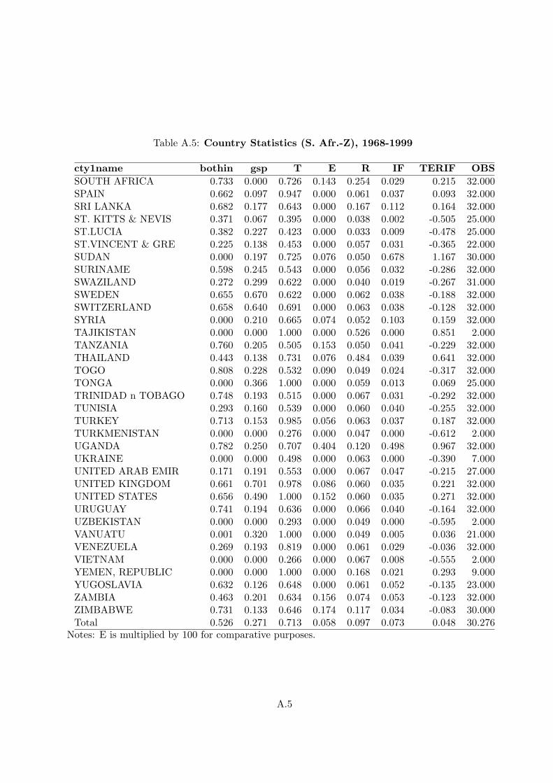
Table A.5: Country Statistics (S. Afr.-Z), 1968-1999
cty1name bothin gsp T E R IF TERIF OBSSOUTH AFRICA 0.733 0.000 0.726 0.143 0.254 0.029 0.215 32.000SPAIN 0.662 0.097 0.947 0.000 0.061 0.037 0.093 32.000SRI LANKA 0.682 0.177 0.643 0.000 0.167 0.112 0.164 32.000ST. KITTS & NEVIS 0.371 0.067 0.395 0.000 0.038 0.002 -0.505 25.000ST.LUCIA 0.382 0.227 0.423 0.000 0.033 0.009 -0.478 25.000ST.VINCENT & GRE 0.225 0.138 0.453 0.000 0.057 0.031 -0.365 22.000SUDAN 0.000 0.197 0.725 0.076 0.050 0.678 1.167 30.000SURINAME 0.598 0.245 0.543 0.000 0.056 0.032 -0.286 32.000SWAZILAND 0.272 0.299 0.622 0.000 0.040 0.019 -0.267 31.000SWEDEN 0.655 0.670 0.622 0.000 0.062 0.038 -0.188 32.000SWITZERLAND 0.658 0.640 0.691 0.000 0.063 0.038 -0.128 32.000SYRIA 0.000 0.210 0.665 0.074 0.052 0.103 0.159 32.000TAJIKISTAN 0.000 0.000 1.000 0.000 0.526 0.000 0.851 2.000TANZANIA 0.760 0.205 0.505 0.153 0.050 0.041 -0.229 32.000THAILAND 0.443 0.138 0.731 0.076 0.484 0.039 0.641 32.000TOGO 0.808 0.228 0.532 0.090 0.049 0.024 -0.317 32.000TONGA 0.000 0.366 1.000 0.000 0.059 0.013 0.069 25.000TRINIDAD n TOBAGO 0.748 0.193 0.515 0.000 0.067 0.031 -0.292 32.000TUNISIA 0.293 0.160 0.539 0.000 0.060 0.040 -0.255 32.000TURKEY 0.713 0.153 0.985 0.056 0.063 0.037 0.187 32.000TURKMENISTAN 0.000 0.000 0.276 0.000 0.047 0.000 -0.612 2.000UGANDA 0.782 0.250 0.707 0.404 0.120 0.498 0.967 32.000UKRAINE 0.000 0.000 0.498 0.000 0.063 0.000 -0.390 7.000UNITED ARAB EMIR 0.171 0.191 0.553 0.000 0.067 0.047 -0.215 27.000UNITED KINGDOM 0.661 0.701 0.978 0.086 0.060 0.035 0.221 32.000UNITED STATES 0.656 0.490 1.000 0.152 0.060 0.035 0.271 32.000URUGUAY 0.741 0.194 0.636 0.000 0.066 0.040 -0.164 32.000UZBEKISTAN 0.000 0.000 0.293 0.000 0.049 0.000 -0.595 2.000VANUATU 0.001 0.320 1.000 0.000 0.049 0.005 0.036 21.000VENEZUELA 0.269 0.193 0.819 0.000 0.061 0.029 -0.036 32.000VIETNAM 0.000 0.000 0.266 0.000 0.067 0.008 -0.555 2.000YEMEN, REPUBLIC 0.000 0.000 1.000 0.000 0.168 0.021 0.293 9.000YUGOSLAVIA 0.632 0.126 0.648 0.000 0.061 0.052 -0.135 23.000ZAMBIA 0.463 0.201 0.634 0.156 0.074 0.053 -0.123 32.000ZIMBABWE 0.731 0.133 0.646 0.174 0.117 0.034 -0.083 30.000Total 0.526 0.271 0.713 0.058 0.097 0.073 0.048 30.276
Notes: E is multiplied by 100 for comparative purposes.
A.5
CESifo Working Paper Series (for full list see www.cesifo.de)
________________________________________________________________________ 1160 Romain Ranciere, Aaron Tornell, and Frank Westermann, Crises and Growth: A Re-
Evaluation, March 2004 1161 Assaf Razin and Efraim Sadka, Transparency, Specialization and FDI, March 2004 1162 Ludger Woessmann, How Equal Are Educational Opportunities? Family Background
and Student Achievement in Europe and the United States, March 2004 1163 B.M.S. van Praag and Barbara E. Baarsma, Using Happiness Surveys to Value
Intangibles: The Case of Airport Noise, March 2004 1164 Aaron Tornell, Frank Westermann, and Lorenza Martínez, The Positive Link Between
Financial Liberalization, Growth, and Crises, March 2004 1165 Helge Berger and Carsten Hefeker, One Country, One Vote? Labor Market Structure
and Voting Rights in the ECB, March 2004 1166 Clemens Fuest and Martin Kolmar, A Theory of User-Fee Competition, March 2004 1167 Friedrich Schneider and Robert Klinglmair, Shadow Economies around the World:
What Do We Know?, April 2004 1168 Horst Raff and Nicolas Schmitt, Exclusive Dealing and Common Agency in
International Markets, April 2004 1169 M. Hashem Pesaran and Allan Timmermann, Real Time Econometrics, April 2004 1170 Sean D. Barrett, Privatisation in Ireland, April 2004 1171 V. Anton Muscatelli, Patrizio Tirelli and Carmine Trecroci, Can Fiscal Policy Help
Macroeconomic Stabilisation? Evidence from a New Keynesian Model with Liquidity Constraints, April 2004
1172 Bernd Huber and Marco Runkel, Tax Competition, Excludable Public Goods and User
Charges, April 2004 1173 John McMillan and Pablo Zoido, How to Subvert Democracy: Montesinos in Peru,
April 2004 1174 Theo Eicher and Jong Woo Kang, Trade, Foreign Direct Investment or Acquisition:
Optimal Entry Modes for Multinationals, April 2004 1175 Chang Woon Nam and Doina Maria Radulescu, Types of Tax Concessions for
Attracting Foreign Direct Investment in Free Economic Zones, April 2004
1176 M. Hashem Pesaran and Andreas Pick, Econometric Issues in the Analysis of
Contagion, April 2004 1177 Steinar Holden and Fredrik Wulfsberg, Downward Nominal Wage Rigidity in Europe,
April 2004 1178 Stefan Lachenmaier and Ludger Woessmann, Does Innovation Cause Exports?
Evidence from Exogenous Innovation Impulses and Obstacles, April 2004 1179 Thiess Buettner and Johannes Rincke, Labor Market Effects of Economic Integration –
The Impact of Re-Unification in German Border Regions, April 2004 1180 Marko Koethenbuerger, Leviathans, Federal Transfers, and the Cartelization
Hypothesis, April 2004 1181 Michael Hoel, Tor Iversen, Tore Nilssen, and Jon Vislie, Genetic Testing and Repulsion
from Chance, April 2004 1182 Paul De Grauwe and Gunther Schnabl, Exchange Rate Regimes and Macroeconomic
Stability in Central and Eastern Europe, April 2004 1183 Arjan M. Lejour and Ruud A. de Mooij, Turkish Delight – Does Turkey’s accession to
the EU bring economic benefits?, May 2004 1184 Anzelika Zaiceva, Implications of EU Accession for International Migration: An
Assessment of Potential Migration Pressure, May 2004 1185 Udo Kreickemeier, Fair Wages and Human Capital Accumulation in a Global
Economy, May 2004 1186 Jean-Pierre Ponssard, Rent Dissipation in Repeated Entry Games: Some New Results,
May 2004 1187 Pablo Arocena, Privatisation Policy in Spain: Stuck Between Liberalisation and the
Protection of Nationals’ Interests, May 2004 1188 Günter Knieps, Privatisation of Network Industries in Germany: A Disaggregated
Approach, May 2004 1189 Robert J. Gary-Bobo and Alain Trannoy, Efficient Tuition Fees, Examinations, and
Subsidies, May 2004 1190 Saku Aura and Gregory D. Hess, What’s in a Name?, May 2004 1191 Sjur Didrik Flåm and Yuri Ermoliev, Investment Uncertainty, and Production Games,
May 2004 1192 Yin-Wong Cheung and Jude Yuen, The Suitability of a Greater China Currency Union,
May 2004
1193 Inés Macho-Stadler and David Pérez-Castrillo, Optimal Enforcement Policy and Firms’ Emissions and Compliance with Environmental Taxes, May 2004
1194 Paul De Grauwe and Marianna Grimaldi, Bubbles and Crashes in a Behavioural Finance
Model, May 2004 1195 Michel Berne and Gérard Pogorel, Privatization Experiences in France, May 2004 1196 Andrea Galeotti and José Luis Moraga-González, A Model of Strategic Targeted
Advertising, May 2004 1197 Hans Gersbach and Hans Haller, When Inefficiency Begets Efficiency, May 2004 1198 Saku Aura, Estate and Capital Gains Taxation: Efficiency and Political Economy
Consideration, May 2004 1199 Sandra Waller and Jakob de Haan, Credibility and Transparency of Central Banks: New
Results Based on Ifo’s World Economicy Survey, May 2004 1200 Henk C. Kranendonk, Jan Bonenkamp, and Johan P. Verbruggen, A Leading Indicator
for the Dutch Economy – Methodological and Empirical Revision of the CPB System, May 2004
1201 Michael Ehrmann, Firm Size and Monetary Policy Transmission – Evidence from
German Business Survey Data, May 2004 1202 Thomas A. Knetsch, Evaluating the German Inventory Cycle – Using Data from the Ifo
Business Survey, May 2004 1203 Stefan Mittnik and Peter Zadrozny, Forecasting Quarterly German GDP at Monthly
Intervals Using Monthly IFO Business Conditions Data, May 2004 1204 Elmer Sterken, The Role of the IFO Business Climate Indicator and Asset Prices in
German Monetary Policy, May 2004 1205 Jan Jacobs and Jan-Egbert Sturm, Do Ifo Indicators Help Explain Revisions in German
Industrial Production?, May 2004 1206 Ulrich Woitek, Real Wages and Business Cycle Asymmetries, May 2004 1207 Burkhard Heer and Alfred Maußner, Computation of Business Cycle Models: A
Comparison of Numerical Methods, June 2004 1208 Costas Hadjiyiannis, Panos Hatzipanayotou, and Michael S. Michael, Pollution and
Capital Tax Competition within a Regional Block, June 2004 1209 Stephan Klasen and Thorsten Nestmann, Population, Population Density, and
Technological Change, June 2004 1210 Wolfgang Ochel, Welfare Time Limits in the United States – Experiences with a New
Welfare-to-Work Approach, June 2004

1211 Luis H. R. Alvarez and Erkki Koskela, Taxation and Rotation Age under Stochastic
Forest Stand Value, June 2004 1212 Bernard M. S. van Praag, The Connexion Between Old and New Approaches to
Financial Satisfaction, June 2004 1213 Hendrik Hakenes and Martin Peitz, Selling Reputation When Going out of Business,
June 2004 1214 Heikki Oksanen, Public Pensions in the National Accounts and Public Finance Targets,
June 2004 1215 Ernst Fehr, Alexander Klein, and Klaus M. Schmidt, Contracts, Fairness, and
Incentives, June 2004 1216 Amihai Glazer, Vesa Kanniainen, and Panu Poutvaara, Initial Luck, Status-Seeking and
Snowballs Lead to Corporate Success and Failure, June 2004 1217 Bum J. Kim and Harris Schlesinger, Adverse Selection in an Insurance Market with
Government-Guaranteed Subsistence Levels, June 2004 1218 Armin Falk, Charitable Giving as a Gift Exchange – Evidence from a Field Experiment,
June 2004 1219 Rainer Niemann, Asymmetric Taxation and Cross-Border Investment Decisions, June
2004 1220 Christian Holzner, Volker Meier, and Martin Werding, Time Limits on Welfare Use
under Involuntary Unemployment, June 2004 1221 Michiel Evers, Ruud A. de Mooij, and Herman R. J. Vollebergh, Tax Competition
under Minimum Rates: The Case of European Diesel Excises, June 2004 1222 S. Brock Blomberg and Gregory D. Hess, How Much Does Violence Tax Trade?, June
2004