i

Status of Thesis

Title of thesis

I, RAWIA ABD ELGADIR ELTAHIR ELTILIB

hereby allow my thesis to be placed at the Information Resource Center (IRC) of

Universiti Teknologi PETRONAS (UTP) with the following conditions:

1. The thesis becomes the property of UTP.

2. The IRC of UTP may make copies of the thesis for academic purposes only.

3. This thesis is classified as

Confidential

Non-confidential

If this thesis is confidential, please state the reason:

_____________________________________________________________________

_____________________________________________________________________

The contents of the thesis will remain confidential for ___________ years.

Remarks on disclosure:

_____________________________________________________________________

_____________________________________________________________________

_____________________________________________________________________

Endorsed by

________________ ____________________

Signature of Author Signature of Supervisor

Permanent: Omdurman Name of Supervisor

Address Khartoum, Sudan Ap. Dr. Hussain Al Kayiem

Date: _____________________ Date: __________________

√

INVESTIGATION ON THE CUTTING PARTICLES

TRANSPORT IN HORIZONTAL WELL DRILLING

ii

UNIVERSITI TEKNOLOGI PETRONAS

INVESTIGATION ON THE CUTTING PARTICLES TRANSPORT IN

HORIZONTAL WELL DRILLING

Approval Page

By

RAWIA ABD ELGADIR ELTAHIR ELTILIB

The undersigned certify that they have read, and recommend to the Postgraduate

Studies Programme for acceptance this thesis for the fulfillment of the requirements

for the degree stated.

Signature: ____________________________

Main Supervisor: Assoc. Prof. Dr. Hussain H. Al Kayiem

Signature: ___________________________

Head of Department: Dr. Ahmad Majdi Bin Abdul Rani

Date: ___________________________

iii

INVESTIGATION ON THE CUTTING PARTICLES TRANSPORT IN

HORIZONTAL WELL DRILLING

By

Title Page

RAWIA ABD ELGADIR ELTAHIR ELTILIB

A Thesis

Submitted to the Postgraduate Studies Programme

as a Requirement for the Degree of

MASTERS OF SCIENCE

MECHANICAL ENGINEERING DEPARTMENT

UNIVERSITI TEKNOLOGI PETRONAS

BANDAR SRI ISKANDAR

PERAK

JULY 2010

iv

Declaration of Thesis

Title of thesis

I RAWIA ABD ELGADIR ELTAHIR ELTILIB, hereby declare that the thesis is

based on my original work except for quotations and citations which have been duly

acknowledged. I also declare that it has not been previously or concurrently submitted

for any other degree at UTP or other institutions.

Witnessed by

________________________ ______________________

Signature of Author Signature of supervisor

Permanent: Omdurman Name of Supervisor

Address Khartoum, Sudan Ap. Dr. Hussain Al Kayiem

Date: _____________________ Date: __________________

INVESTIGATION ON THE CUTTING PARTICLES

TRANSPORT IN HORIZONTAL WELL DRILLING

v

Acknowledgements

I thank ALLAH for the strength that keeps me standing and for the hope that

keeps me believing that this affiliation would be possible and more interesting.

I also wanted to thank my family who inspired, encouraged and fully supported

me for every trial that come to my way, In giving me not just financial, but morally

and spiritually.

I would like to express my most sincere gratitude to my supervisor, Dr. Hussain al

Kayiem for his guidance and supervision of this research work.

Many thanks to my brother Dr/ Abd Alwahab for his helpful advices regarding the

MATLAB coding. Thanks to my kind sister Samira and many thanks to my friend

Eng. Mr/ Omer Eisa, Eng. Mr/ Antena and my brother Eng. Mohd Shommo for their

appreciated help in the arrangement of my thesis.

Finally, a very special tribute to Universiti Teknologi PETRONAS for providing

me this opportunity of study, wishing for UTP all the progress and development.

Special thanks for Mechanical Department.

All other colleagues are very well thanked for providing an inspiring and relaxed

working atmosphere.

vi

Dedication

To my family

To my friends

To my colleagues

To special persons in my life

vii

Abstract

Arguably the most important prerequisite function to permit further progress in well

drilling operations up to reach production is a complete removal of drilled cuttings

from the well bore. This target becomes more challenging in highly-deviated to

horizontal wells, where the cuttings particles have more tendency to accumulate in the

lower side of the well bore and form a bed of standstill cuttings. In this study, a

mathematical model based on the mechanistic theory and the three-layer approach

was developed to simulate the cutting particles transport in annular flow during the

horizontal drilling process. Two mathematical models were developed to investigate

the cuttings transportation performance in horizontal wells. Due to high non- linearity,

both were solved numerically after conversion to computer algorithms using

MATLAB. The master model examined the performance of irregular shaped cuttings

transported in concentric annulus by non-Newtonian fluids. The model predicted the

velocities of the layers, the layer’s concentration, the dispersive shear stress, and the

pressure drop. The transport performance was adequately simulated under various

operational and design conditions, namely the effect of the cuttings size, cuttings

shape, annular size, rate of penetration and the mud rheology in term of fluid

viscosity. The second model represented a modified model which used to test the

sensitivity of the frictional forces calculations, where empirical correlations were

employed to replace Szilas formula to calculate the layers and wall friction stresses.

The cuttings size, mud viscosity and annular size demonstrated significant effect on

transport process. While the operational rate of penetration performed the lowest

effect between the entire parameters of the cuttings transport. The results compared

favorably with those obtained by previous investigators. Accordingly, the simulations

demonstrated that the basic model could be used to analyze the cuttings transport.

Thereby, it could potentially be used as design and/or analysis tools for the follow-up

of transport processes in horizontal wells.

viii

Abstrak

Lazimnya, kepentingan fungsi prasyarat adalah untuk menyingkirkan keseluruhan

serpihan-serpihan gerudi dari lubang telaga bagi menperolehi pencapaian yang bagus

dalam operasi penggerudian telaga hingga ke peringkat pengeluaran. Target ini

menjadi lebih mencabar bagi telaga yang sangat berarah dan telaga mendatar, di mana

zarah-zarah serpihan gerudi mempunyai kecenderungan untuk berkumpul di bahagian

dasar lubang telaga dan membentuk satu mendakan serpihan-serpihan yang tidak

bergerak. Dalam kajian ini, model matematik berdasarkan teori mekanistik dan

pendekatan tiga lapis telah dikembangkan untuk mensimulasikan pengangkutan

zarah-zarah serpihan dalam aliran annular semasa proses penggerudian mendatar. Dua

model matematik telah dihasilkan untuk menyiasat prestasi pengangkutan serpihan-

serpihan. Oleh sebab kualiti bukan linear yang tinggi, kedua-duanya dipecahkan

secara berangka selepas penukaran ke komputer algoritma menggunakan MATLAB.

Model master menyemak prestasi serpihan-serpihan yang berbentuk tidak teratur

diangkut dalam annulus konsentrik oleh bendalir bukan Newtonian. Model telah

meramalkan kelajuan lapisan, kepekatan lapisan, tegangan geseran dispersif, dan

penurunan tekanan. Prestasi pengangkutan telah disimulasikan dengan pelbagai

keadaan operasi dan rekabentuk, iaitu kesan saiz serpihan, bentuk serpihan, saiz

annular, kadar penetrasi, dan rheologi lumpur. Model kedua merupakan model yang

telah diubahsuai untuk digunakan dalam menguji sensitiviti pengiraan daya geseran,

di mana, korelasi empirik telah digunakan untuk menggantikan Szilas formula bagi

mengira lapisan dan ketegangan geseran dinding. Saiz serpihan, rheologi lumpur dan

saiz annular menunjukkan pengaruh yang besar kepada proses

pengangkutan. Sedangkan kadar penetrasi adalah parameter yang lebih rendah

kesannya dalam pengangkutan serpihan-serpihan gerudi. Hasil daripada kajian ini

telah dibandingkan dengan hasil kajian yang diperolehi oleh penyelidik-penyelidik

sebelum ini. Simulasi telah menunjukkan bahawa kedua-dua model boleh digunakan

ix

untuk menganalisis pengangkutan serpihan-serpihan gerudi. Dengan demikian, ia

berpotensi untuk digunakan sebagai rekabentuk dan/atau alat analisis untuk tindakan

lanjut proses pengangkutan di telaga mendatar.

x

In compliance with the terms of the Copyright Act 1987 and the IP Policy of the

university, the copyright of this thesis has been reassigned by the author to the legal

entity of the university,

Institute of Technology PETRONAS Sdn Bhd.

Due acknowledgement shall always be made of the use of any material contained

in, or derived from, this thesis.

© Rawia Eltilib, 2010

xi

Table of Contents

STATUS OF THESIS................................................................................................. I

APPROVAL PAGE ................................................................................................... II

TITLE PAGE .......................................................................................................... III

DECLARATION OF THESIS ................................................................................. IV

ACKNOWLEDGEMENTS ............................................................................................... V

DEDICATION.............................................................................................................. VI

ABSTRACT ............................................................................................................... VII

ABSTRAK ................................................................................................................ VIII

TABLE OF CONTENTS ................................................................................................. XI

LIST OF FIGURES .................................................................................................... XVII

LIST OF TABLES ....................................................................................................... XXI

NOMENCLATURE ................................................................................................... XXIII

GREEK SYMBOLS ..................................................................................................XXVII

CHAPTER 1.............................................................................................................. 1

INTRODUCTION ........................................................................................................... 1

xii

1.1 BACKGROUND ....................................................................................................... 1

1.2 PROBLEM STATEMENT ........................................................................................... 2

1.2.1 THE TWO-PHASE FLOW PROBLEM ....................................................................... 3

1.2.2 NON-VERTICAL DRILLING ORIENTATION PROBLEM ............................................. 3

1.2.3 NON-NEWTONIAN FLUIDS PROBLEM ................................................................... 3

1.3 OBJECTIVE OF THE STUDY ..................................................................................... 4

1.4 SCOPE OF THE STUDY ............................................................................................ 5

1.5 SUMMARY AND LAYOUT OF THE THESIS ................................................................. 6

CHAPTER 2 .............................................................................................................. 8

LITERATURE REVIEW .................................................................................................. 8

2.1 INTRODUCTION ...................................................................................................... 8

2.2 EXPERIMENTAL WORK ........................................................................................ 11

2.3 MATHEMATICAL MODELING ................................................................................ 17

2.3.1 MECHANISTIC MODELING ................................................................................. 18

2.3.2 LAYERS MODELING .......................................................................................... 24

2.4 COMPUTATIONAL FLUID DYNAMICS CFD ............................................................ 33

2.5 SUMMARY OF PREVIOUS WORK ........................................................................... 35

CHAPTER 3 ............................................................................................................ 38

RESEARCH METHODOLOGY ....................................................................................... 38

xiii

3.1 INTRODUCTION ................................................................................................... 38

3.2 MODEL HYPOTHESES .......................................................................................... 39

3.3 THE MATHEMATICAL MODEL FORMULATION....................................................... 40

3.3.1 MASS BALANCE ............................................................................................... 40

3.3.2 MOMENTUM BALANCE ..................................................................................... 42

3.3.2.1 Momentum for the Heterogeneous Suspended-layer ---------------------------- 42

3.3.2.2 Momentum for the Moving-bed Layer -------------------------------------------- 45

3.3.2.3 Momentum for the Stationary-bed Layer ----------------------------------------- 48

3.3.3 ANALYSIS OF THE MOVING-BED LAYER ........................................................... 49

3.3.4 MEAN VELOCITY OF THE MOVING-BED LAYER ................................................. 50

3.3.5 AVERAGE CONCENTRATION OF THE MOVING-BED LAYER.................................. 51

3.3.6 CONVECTION-DIFFUSION EQUATION ................................................................ 52

3.3.7 CUTTINGS SETTLING VELOCITY........................................................................ 53

3.3.8 THE HINDERED SETTLING VELOCITY ................................................................ 55

3.4 MODELS SOLUTION PROCEDURES ........................................................................ 59

3.4.1 THE OPERATIONAL AND DESIGN PARAMETERS .................................................. 60

3.4.2 CALCULATION OF THE WELL GEOMETRY .......................................................... 62

3.4.3 ALGORITHM DEVELOPMENT ............................................................................. 64

3.4.3.1 Assumptions -------------------------------------------------------------------------- 65

3.4.3.2 Iteration procedure ------------------------------------------------------------------- 66

xiv

3.4.3.3 Constrains ---------------------------------------------------------------------------- 66

3.5 SEQUENCE OF MODEL SOLUTION ......................................................................... 69

3.6 SUMMARY ........................................................................................................... 71

CHAPTER 4 ............................................................................................................ 73

RESULTS AND DISCUSSION ........................................................................................ 73

4.1 INTRODUCTION .................................................................................................... 73

4.2 PARTICLE SETTLING BEHAVIOUR ......................................................................... 73

4.2.1 RESULTS AND DISCUSSION OF THE SETTLING BEHAVIOUR ................................. 74

4.2.1.1 Effect of Particle Density on Particle Settling ------------------------------------ 74

4.2.1.2 Effect of Particle Size on Particle Settling ---------------------------------------- 75

4.2.1.3 Effect of Fluid Density on Particle Settling --------------------------------------- 77

4.2.1.4 Effect of Fluid Viscosity on Particle Settling ------------------------------------- 78

4.3 HINDERED SETTLING BEHAVIOUR ........................................................................ 79

4.3.1 RESULTS AND DISCUSSIONS OF THE HINDERED SETTLING BEHAVIOUR ............... 79

4.4 SIMULATION RESULTS ......................................................................................... 84

4.4.1 BASIC MODEL SIMULATION RESULTS AND DISCUSSION ..................................... 85

4.4.1.1 Effect of Annular Velocity on Cuttings Transport ------------------------------- 85

4.4.1.2 Effect of Cuttings Size on Cuttings Transport ------------------------------------ 86

4.4.1.3 Effect of Particle Sphericity on Cuttings Transport ------------------------------ 93

xv

4.4.1.4 Effect of Fluid Viscosity on Cuttings Transport---------------------------------- 95

4.4.1.5 Effect of Rate of Penetration ROP on Cuttings Transport ---------------------- 99

4.4.1.6 Effect of Annular Size on Cuttings Transport ---------------------------------- 102

4.4.2 THE MODIFIED MODEL SIMULATION RESULTS AND DISCUSSION ..................... 107

4.4.2.1 Effect of Annular Velocity on Cuttings Transport ----------------------------- 107

4.4.2.2 Effect of Friction Factor on Cuttings Transport -------------------------------- 109

4.5 MODELS CONTRASTING AND VALIDATION ......................................................... 110

4.6 SUMMARY OF THE MODELLING RESULTS ........................................................... 114

CHAPTER 5.......................................................................................................... 116

CONCLUSION AND RECOMMENDATION .................................................................... 116

5.1 CONCLUSION .................................................................................................... 116

5.2 RECOMMENDATIONS ......................................................................................... 118

REFERENCES .......................................................................................................... 120

APPENDIX A ........................................................................................................... 131

GEOMETRY ENGINE ................................................................................................ 131

APPENDIX B ........................................................................................................... 137

RESULTS OF THE BASIC SIMULATION ...................................................................... 137

APPENDIX C ........................................................................................................... 148

CORRELATION OF MOVING-BED BUILT UP UNDER DIFFERENT DRILLING PARAMETERS

.............................................................................................................................. 148

xvi

APPENDIX D ........................................................................................................... 150

DIMENSIONLESS ANALYSIS ..................................................................................... 150

xvii

List of Figures

Figure 1-1: Process of well drilling and hole cleaning ............................................... 1

Figure 1-2: Vertical and directional wells drilling ..................................................... 2

Figure 2-1: Acting forces during vertical annular transport ...................................... 19

Figure 2-2: Layers and acting forces during deviated annular transport .................... 20

Figure 2-3: Layers and acting forces during horizontal annular transport ................. 20

Figure 2-4: The three-layer approach in the annular section ..................................... 25

Figure 2-5: Irregular particles shape ........................................................................ 30

Figure 3-1: Dimensions of the annular section ......................................................... 41

Figure 3-2: The exerted shears in the annular suspended-layer ................................. 43

Figure 3-3: The exerted shears in the annular moving-bed layer. .............................. 46

Figure 3-4: The angular bed layers thicknesses ........................................................ 48

Figure 3-5: The exerted shears in the annular stationary-bed layer ........................... 49

Figure 3-6: The approximated concentration profile for the three-layer by Ramadan et

al. [3] ....................................................................................................................... 51

Figure 3-8: The Three layers angular thicknesses, highest and witted perimeters ..... 63

Figure 3-9: Different cases for the formed bed heights ............................................. 64

xviii

Figure 3-10: Hierarchy Chart to solve and hinder the particle settling ....................... 67

Figure 3-11: Hierarchy Chart to solve the developed models. ................................... 68

Figure 4-1: Particle settling in vertical, inclined and horizontal flow ........................ 74

Figure 4-2: Effect of particle density on settling velocity of (a) large particle sizes, (b)

small particle size ..................................................................................................... 75

Figure 4-3: Effect of particle size on settling at (a) low fluid density, (b) high fluid

density. .................................................................................................................... 76

Figure 4-4: Effect of particle density on settling at (a) low fluid density, and (b) high

fluid density ............................................................................................................. 77

Figure 4-5: Effect of the fluid viscosity on settling behavior of (a) small particle size,

and (b) large sized particle........................................................................................ 78

Figure 4-6: Case A, particles hindered settling velocity at (1) ROP/Ua=0.0069, (2)

ROP/Ua=0.0028, (3) ROP/Ua=0.0021, (4) ROP/Ua=0.0008. ................................... 80

Figure 4-7: Case B, particles hindered settling velocity at (1) ROP/Ua=0.0069, (2)

ROP/Ua=0.0028, ROP/Ua=0.0021 (3), (4) ROP/Ua=0.0008. ................................... 81

Figure 4-8: Case C, particles hindered settling velocity at (1) ROP/Ua=0.0069, (2)

ROP/Ua=0.0028, ROP/Ua=0.0021 (3), (4) ROP/Ua=0.0008. ................................... 82

Figure 4-9: Case D, particles hindered settling velocity at (1) ROP/Ua=0.0069, (2)

ROP/Ua=0.0028, ROP/Ua=0.0021 (3), (4) ROP/Ua=0.0008. ................................... 83

Figure 4-10: Effet of annular velocity on suspended layers concentration at different

particle sizes ............................................................................................................ 88

Figure 4-11: Eddy Diffusivity of the different particle size ....................................... 88

Figure 4-12: Ratio of the bed layers shear stress for the different cuttings size .......... 89

xix

Figure 4-13: The pressure drop predicted at the different particle sizes .................... 90

Figure 4-14: Final suspension layer of the three cuttings sizes at maximum cleaning 90

Figure 4-15: Moving-bed layer growth under increasing annular velocity ................ 91

Figure 4-16: Percentages of moving-bed thickness before and after cleaning for the

different particle sizes .............................................................................................. 92

Figure 4-17: Slip lines on particle of regular and irregular shape .............................. 93

Figure 4-18: Effect of sphericity on the suspension concentration during cuttings

transport .................................................................................................................. 94

Figure 4-19: Suspension thickness at the bed termination condition for different

cuttings sphericity .................................................................................................... 95

Figure 4-20: Suspension concentration under different mud viscosity ...................... 96

Figure 4-21: Pressure gradient at different power law viscosities ............................. 97

Figure 4-22: Effect of the fluid viscosity on the exerted shear stress ........................ 97

Figure 4-23: The Maximum suspension thickness reached with different mud

viscosities ................................................................................................................ 98

Figure 4-24: Maximum suspension thickness under different ROP ........................ 101

Figure 4-25: Effect of the operational ROP on the total cuttings concentration exerted

in the annulus ........................................................................................................ 102

Figure 4-26: Effect of the different annular size on the suspension concentration ... 103

Figure 4-27: Effect of the different annular sizes on the pressure drop ................... 104

Figure 4-28: Effect of the different annular sizes on the ratio of shear stress. ......... 104

xx

Figure 4-29: Comparison of final cleaning performance for the different annular sizes

.............................................................................................................................. 105

Figure 4-30: Change of total annular cuttings concentration at the different annular

size ........................................................................................................................ 106

Figure 4-31: Moving-bed behavior-modified model ............................................... 108

Figure 4-32: Basic and modified simulation tracks ................................................. 109

Figure 4-33: The contrasted transport track on pipe flow ........................................ 110

Figure 4-34: The contrasted transport track on eccentric annulus flow .................... 111

Figure 4-35: Moving bed behavior (Current model) ............................................... 113

Figure 4-36: Moving-bed behavior (Cho’s Model ) ................................................ 113

xxi

List of Tables

Table 2-1: Targets and outcome of some Mechanistic models studies ...................... 23

Table 2-2: The two layers models. ........................................................................... 32

Table 2-3: The three layers models. ......................................................................... 33

Table 3-1: The adopted viscosities of the drill-mud .................................................. 60

Table 3-2: Density of drill mud ................................................................................ 60

Table 3-3: The provided cuttings mean diameters (cuttings size) ............................. 61

Table 3-4: The tested particle densities .................................................................... 61

Table 3-5: The annular sizes studied in the simulation ............................................. 62

Table 3-6: The selected value of operational ROP.................................................... 62

Table 4-1: prepared conditions to examine the particle hinder behavior case A ........ 80

Table 4-2: Prepared conditions to examine the particle hinder behavior case B ........ 81

Table 4-3: Prepared conditions to examine the particle hinder behavior case C ........ 82

Table 4-4: Prepared conditions to examine the particle hinder behavior case D ........ 83

Table 4-5: Differences between the current model and previous models................... 85

Table 4-6: The considerable velocity of the moving-bed layer and bed termination for

the different particle sizes ........................................................................................ 87

xxii

Table 4-7: Dimension of the different annular Sizes ............................................... 102

Table 4-8: Increasing of the suspension thickness under the different annular sizes 106

Table 4-9: Simulation results of the modified model .............................................. 108

Table 4-10: The moving-bed thickness under the concentric and eccentric annulus 112

xxiii

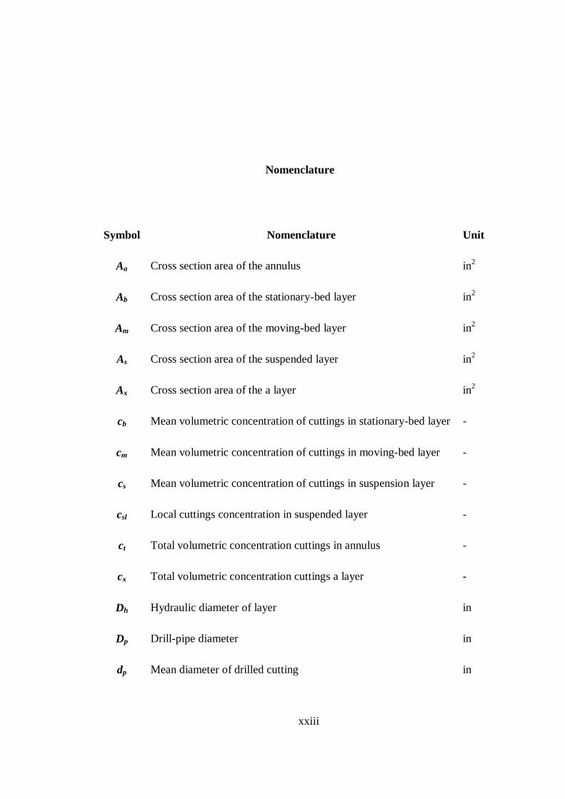
Nomenclature

Symbol Nomenclature Unit

Aa Cross section area of the annulus in2

Ab Cross section area of the stationary-bed layer in2

Am Cross section area of the moving-bed layer in2

As Cross section area of the suspended layer in2

Ax Cross section area of the a layer in2

cb Mean volumetric concentration of cuttings in stationary-bed layer -

cm Mean volumetric concentration of cuttings in moving-bed layer -

cs Mean volumetric concentration of cuttings in suspension layer -

csl Local cuttings concentration in suspended layer -

ct Total volumetric concentration cuttings in annulus -

cx Total volumetric concentration cuttings a layer -

Dh Hydraulic diameter of layer in

Dp Drill-pipe diameter in

dp Mean diameter of drilled cutting in

xxiv

dp/dz Pressure drop Psi/ft

Dw Well diameter in

dz Well length ft

fb Friction factor between the channel and bed layer -

FB Buoyancy force lbf

Fb Force between stationary-bed layer and walls lbf

Fd Dry force at well boundary and moving-bed layer lbf

FD Drag force lbf

Fg Gravity force lbf

FL Lift force lbf

Fm Force between moving-bed layer and walls lbf

fm Friction factor between the channel and moving-bed layer -

Fmb Friction force between moving-bed and stationary-bed layers lbf

fmb Interfacial friction factor between the moving and stationary bed

layer

-

Fn Normal force lbf

fp Friction factor between the channel and drill-pipe -

Fs Force between suspension and walls lbf

fs Friction factor between the channel and suspension layer -

xxv

Fsm Friction force between suspension and moving-bed layers lbf

fsm Interfacial friction factor between the suspended and moving bed

layer

-

FΔP Pressure force lbf

g Gravity ft/s2

hb Thickness of the stationary-bed layer in

hs Thickness of the suspension in

K Fluid consistency lbf.sn/ft

2

k Von Karman constant = 0.4 -

Ks Consistency index of fluid in suspension lbf.sn/ft

2

n Fluid flow behavior index -

Regen Generalized Reynolds number -

Rem Reynolds number of moving-bed -

Rep Cutting particle Reynolds number -

Res Reynolds number of suspension -

Sb Perimeter of stationary-bed contact with the well in

Sm Perimeter of moving-bed contact with the well in

Smb Perimeter surface between the moving-bed and stationary-bed

layer

in

Sp Perimeter of the drill-pipe in

xxvi

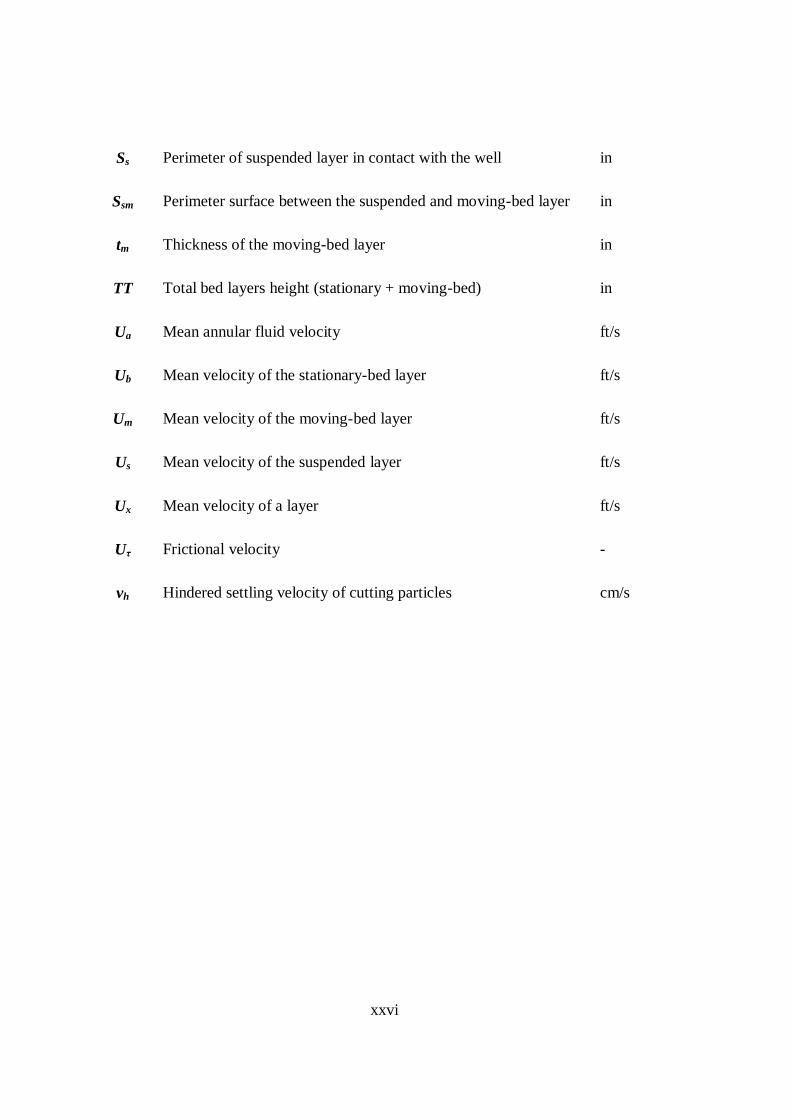
Ss Perimeter of suspended layer in contact with the well in

Ssm Perimeter surface between the suspended and moving-bed layer in

tm Thickness of the moving-bed layer in

TT Total bed layers height (stationary + moving-bed) in

Ua Mean annular fluid velocity ft/s

Ub Mean velocity of the stationary-bed layer ft/s

Um Mean velocity of the moving-bed layer ft/s

Us Mean velocity of the suspended layer ft/s

Ux Mean velocity of a layer ft/s

Uτ Frictional velocity -

vh Hindered settling velocity of cutting particles cm/s

xxvii

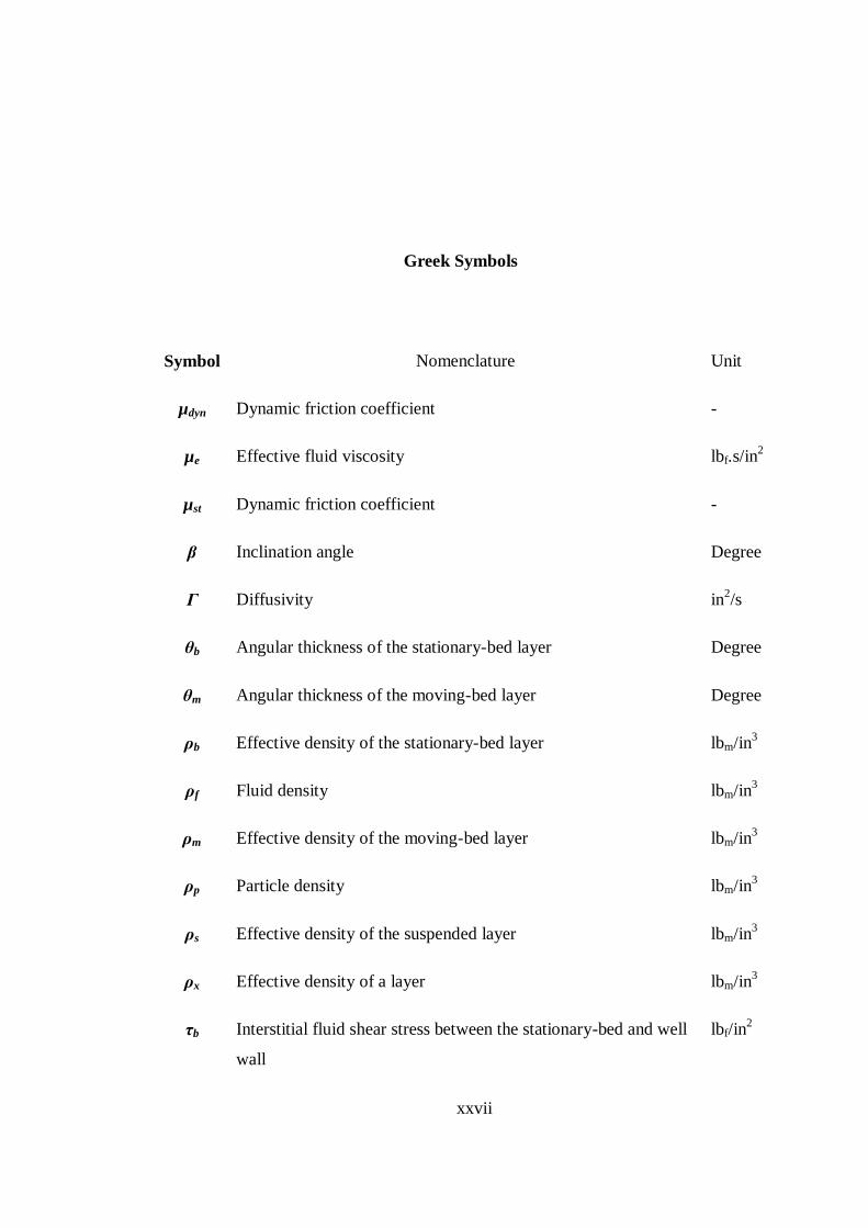
Greek Symbols

Symbol Nomenclature Unit

µdyn Dynamic friction coefficient -

µe Effective fluid viscosity lbf.s/in2

µst Dynamic friction coefficient -

β Inclination angle Degree

Γ Diffusivity in2/s

θb Angular thickness of the stationary-bed layer Degree

θm Angular thickness of the moving-bed layer Degree

ρb Effective density of the stationary-bed layer lbm/in3

ρf Fluid density lbm/in3

ρm Effective density of the moving-bed layer lbm/in3

ρp Particle density lbm/in3

ρs Effective density of the suspended layer lbm/in3

ρx Effective density of a layer lbm/in3

τb Interstitial fluid shear stress between the stationary-bed and well

wall

lbf/in2

xxviii

τdis Equivalent dispersive shear stress between the stationary and

moving-bed layers

lbf/in2

τm Fluid shear stress between the well wall and suspended layer lbf/in2

τmb Fluid shear stress between the stationary and moving bed layer lbf/in2

τs Interstitial shear stress between the annular and suspended layer lbf/in2

τsm Interfacial shear stress between the suspended and moving-bed

layer

lbf/in2

φ Particle sphericity -

φD The equivalent dynamic friction angle = 0.75 -

1

Chapter 1

Introduction

1.1 Background

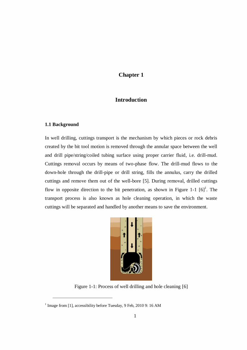
In well drilling, cuttings transport is the mechanism by which pieces or rock debris

created by the bit tool motion is removed through the annular space between the well

and drill pipe/string/coiled tubing surface using proper carrier fluid, i.e. drill-mud.

Cuttings removal occurs by means of two-phase flow. The drill-mud flows to the

down-hole through the drill-pipe or drill string, fills the annulus, carry the drilled

cuttings and remove them out of the well-bore [5]. During removal, drilled cuttings

flow in opposite direction to the bit penetration, as shown in Figure 1-1 [6]1. The

transport process is also known as hole cleaning operation, in which the waste

cuttings will be separated and handled by another means to save the environment.

Figure 1-1: Process of well drilling and hole cleaning [6]

1 Image from [1], accessibility before Tuesday, 9 Feb, 2010 9: 16 AM

2

Since the first oil well was drilled in Titusville 1859 [7], up to present times,

several problems have emerged and maintained a special prominence in the field of

well drilling. Simultaneously, several benefits were gained from wells and needs are

hugely increased as well. In order to cope with these needs of globalization, oil and

gas fields are developing more sophisticated drilling methods, production schemes

and technology. The Trajectories of wells are now extended to be established in

inclined and horizontal drilling as shown in Figure 1-2, with high extended reach,

multi-branches and ultra deep offshore wells.

Figure 1-2: Vertical and directional wells drilling [1]

1.2 Problem Statement

Currently, there is no general method of drilling operation application that can assure

the operator of optimal drilling performance, independent of conditions, equipment

and objectives. Thus, intention of the drilling technology is to enhance an effective

drilling technique, in order to reduce both cost and time of the operation and improve

recovery from reservoirs.

Even with such knowledge of cuttings behavior, there are some limitations

concerning control of the annular environment [8]. The problem for this present

research can be explicitly placed within three major aspects as following:

3

1.2.1 The Two-phase Flow Problem

The transport of cuttings occurred during the drilling operation is an engineering

application which involves solid-liquid two-phase flow. The liquid-phase is mostly a

non-Newtonian fluid known as drill-mud which formulated as either water or oil

based system [9].

1.2.2 Non-vertical Drilling Orientation Problem

By non-vertical or directional borehole practices, drilling operation can be performed

in various kinds of reservoirs by implementing inclined and horizontal drilling

orientations and this is more advanced and complicated than the traditional vertical

wells. Recently, horizontal well applications have been practiced in many plants

around the world. The major purpose of horizontal drilling is to enhance reservoir

contact over vertical drilling, and thereby enhance the productivity of the well.

Besides, the main objective of the horizontal drilling is to intersect multiple zones.

[10].

1.2.3 Non-Newtonian Fluids Problem

Non-Newtonian fluids are kind of fluids those perform a complicated behavior during

their flow. However, for necessity drill-muds are optimized to possess behavior of the

non-Newtonian fluids to accomplish their functions [9].

Due to lack of recommendation in the field, a series of problems were recognized

in wells drilling, i.e. (losing of a 3000 ft, 60ο inclined well in Texas Gulf Coast) [11].

These problems increased the disaster expectations in the field of the wells drilling.

Malfunction of drilling tools, drilling preparation and re-drilling incurs costs of

millions of dollars. Several costs start with exploration, development of the oil field,

rig, drilling tools and equipment up to the final production steps. Hence, the drilling

operation cost has significant importance in the total cost. However, compared to the

4

tragic consequences of losing the well itself those are very low costs. Therefore, such

an annoying problem should be handled with more consciousness, wisdom and

knowledge, in order to develop an efficient drilling and transport technology that

preserves the well intact. Hence, maintaining of a successful drilling operation is a

great challenge which basically depends upon the removal of all drilled cuttings out of

the wellbore.

It can be concluded that the combination of the three major sources of

complications represent a serious challenge to modeling and analyzing the process of

cutting transport in inclined and horizontal oriented wells.

In the directional cuttings transport, aggregation of settled particles due to the low

cutting fluidity and high static fraction returned high stationary bed or slow motion

[12]. Cutting particles tends to settle downward responding to the gravity force while

contrasted forces acting on the cuttings struggling to overcome settling. As result,

further accumulation of particles in the conduit would reduce the flow area. In the oil

well drilling application, this will generate many problems, such as low ROP ,over

load on mud pumps, excessive drill pipe and tools wear, loose of circulation due to

transient hole blockage, extra mud additive costs, problems in cementing and

difficulties in running casing operations, waste of the limited energy available to the

drill bit and hole packing off [9][4].Those problems could finally lead to terminate of

the drilling operation and loose the well itself.

1.3 Objective of the Study

In view of the problem statement, the most critical and interesting problem in drilling

operation has been the efficient removal of the cuttings. Therefore, the main purpose

of this study is to develop a three-layer, mathematical model in order to simulate the

drilled cuttings transportation, to estimate the performance of the horizontal wells

cleaning, with more focus on the effect of the cutting particles and other drilling

parameters.

5

In general, this study aimed to:

To investigate settling and hindered behaviors of particles and to determine the

two-phase annular flow of cuttings-mud during the cleaning process of horizontal

well drilling.

To estimate the transport performance under different operating (annular velocity

and arte of penetration)

To estimate the transport performance under various design conditions (annular

size and mud viscosity).

1.4 Scope of the Study

The solution of the three inter-related problems of solid-liquid and non-Newtonian

fluid flow and flow through horizontal annulus presented a formidable challenge.

Because of the competitive advantages of modeling over experiments such as

availability, flexibility in addition to the time and cost factors, this research initiative

was intended to undertake a mathematical modeling technique specifically adopting

the three-layer approach based on a mechanistic model to perform a study of cuttings

transport through the horizontal annulus.

The study covered a variety of operational cases in which the effect of mud

discharge was examined over the turbulent annular flow. Moreover, operational and

design parameters were also involved in this study, through investigation of the

operational Rate of Penetrations or, (ROP) and the annular size.

In this context, the effect of the rheological property in term of mud viscosity was

investigated by changing of the power law viscosity (n and K).

The cutting particles specifications were accounted for, by adopting various types

of particle sphericities and sizes.

6

The scope of the study involved:

A. Obtain the requirements of the drilled cutting particles movement in the

cleaning operation.

B. Model the two-phase annular flow of cuttings-mud during the transport in

horizontal wells drilling.

C. Implement a new method of layers model for annular flow and transport of

non-sphere particles derived from the bases of non-Newtonian channel flow

and sphere particles transport.

D. Code the two-phase model into a computer program using MATLAB soft

ware to simulate the horizontal transport of drilled cuttings.

E. Conduct a parametric study for some factors affecting on the transport and

examine the model performance by compare with previous studies.

1.5 Summary and Layout of the Thesis

This dissertation is subdivided into seven separate chapters. The introduction chapter

presents introductory remarks about the drill cuttings transport process and its

cohesive importance in the well drilling operations. Then, in the statement of problem

section, problems associated with the cuttings transport and the procedures to solve

this problem and provide further understanding in the topic of drilling operation is

given. Furthermore, the objectives of the work, the scope of the study and the main

features of the methodology have also been provided in the introductory chapter.

Presentation, critical evaluation and discussion of other related research on

cuttings transport are reported in the second chapter (the literature review). Special

consideration is directed to the modelling techniques used, and to the three-layer

approach studies. Comments and some conclusion were provided at the end of the

second chapter.

7

Likewise, the third chapter generalizes the overall strategy and methodology of

the research. This chapter demonstrates the details of the two mathematical models

which were built to simulate the horizontal cuttings transport. Models hypotheses and

importance of some essential equations was highlighted in chapter four. Furthermore

this chapter underlines the solution procedures that followed to code and solve the

mathematical model using MATLAB.

Chapter four documents preliminary results which displays the behaviours of

particles settling and hindered settling. Moreover the chapter presents the obtained

simulation results for the different parameters studied. Additional results are also

presented in this chapter to provide a comprehensive comparison for the basic model

results trend and to validate the usability of the model. A concise outcome was arrived

at after rigorous analyses which facilitated evaluation of the developed model

performance.

The last chapter provides a conclusion for the preceding chapters. Major outcomes

from the work is summarised in this chapter. For further improving on the cuttings

transport simulation, valuable recommendations are highlighted on the basis of the

generated model results and subsequent conclusions pointed out.

A list of figures, tables and acronyms used in the model formulations are provided

at the beginning of the thesis. A list of all references used to develop this research and

necessary appendices are also attached at the end of this dissertation

8

Chapter 2

Literature Review

2.1 Introduction

Transportation of cutting particles is known as a mechanism by which vital factors of

drilling should effectively be employed [7]. In the solid-liquid two-phase flow during

the transport process the drill-mud is utilized as a carrier for the solid-phase of rocks

that are drilled by the tool-bit.

A substance is termed non-Newtonian when its flow curve is nonlinear.

Alternatively, its flow curve may be linear, but it does not pass through the origin.

This happens when its viscosity is not constant at a given temperature and pressure

and it exhibits non-equal normal stress in a simple shearing flow. The value of the

viscosity depends upon the flow conditions, such as flow geometry, shear rate or

stress developed within the fluid, time of shearing, kinematic history of the sample.

Under appropriate conditions, some materials can exhibit a blend of solid and fluid-

like responses. Though somewhat arbitrarily, it is customary to classify the non-

Newtonian fluid behavior into three general categories [13] as follows:

1. Purely viscous, time-independent, or GNF (Generalized Newtonian Fluids),

where the applied rate of shear is dependent only on the current value of the

shear stress or vice versa.

9

2. Time-dependent systems in which the relation between the shear stress and the

shear rate depend upon the duration of shearing with respect to the previous

kinematic history.

3. Visco-elastic fluids. Those exhibiting combined characteristics of both an

elastic solid and a viscous fluid, and showing partial elastic and recoil

recovery after deformation.

Drilling mud is non-Newtonian fluid that exhibits Thixotropy behavior, in which

it displays a decrease in viscosity over time at a constant shear rate [14]. Most of the

drilling fluids are non Newtonian fluids, with viscosity decreasing as shear rate

increases [15]. This is similar behavior to the Pseudoplastic or shear thinning fluids.

At both adiabatic and non-adiabatic conditions, a two-phase flow system can be a

very complex physical process. This is because such systems combine the

characteristics of deformable interface, conduit geometry, flow direction, and, in some

cases, the compressibility of one of the phases. In addition to inertia, viscous and

pressure forces, the two-phase flow systems are also affected by the interfacial tension

forces, as well as the characteristics of the phases, the exchange of mass, momentum,

and energy between the phases [16]. The ability of drill-fluids to suspend and

transport the drilled solids out of the wellbore is the critical target to gain a successful

well drilling operation. For further expansion to the production and refinery stages,

proper transport and thereby successful drilling demand an adequate drilling plan. The

problem of well-bores cleaning has been recognized as a serious problem in drilling

fields as long as wells have been drilled. Therefore it is necessary to identify where

the critical spots are with regard to the wellbore cleaning.

Many parameters are found to affect hole cleaning operation. These may generally

be categorized into major three groups as follows:

The first group: parameters which are related to the carrier fluid, such as

fluid density, fluid viscosity and fluid flow rate.

10

The second group: solid cutting parameters include cuttings density,

cutting shape and size and cutting concentration.

The third group: operational parameters which may be related to geometric

features or other effects. This group contains inclination, pipe rotation and

pipe positioning in the hole (concentric / eccentric).

Over the previous three decades, many researchers have attempted to clarify some

of ambiguities related to the matter of transport. Various studies were conducted to

investigate and hopefully improve the mechanism of drilled cuttings transport. Much

difficult and painstaking work was directed at trying to obtain a realistic

understanding of the phenomena. It was noticed that most of the previous studies were

focused upon only a few parameters while neglecting various others. This approach is

a common strategy, frequently used to reduce the level of complexity of the problem.

Notice that, simplifying of such problem should be done via rational assumptions to

avoid distortion. An extensive survey was carried out on the available sources, such as

research centers, universities, journals and conference proceedings, in addition to

some private communications. Research efforts can be classified into three categories:

(a) experimental investigation, (b) mathematical modeling, and (c) computational

fluid dynamics or, (CFD) simulations.

Researchers working within the previously- mentioned three groups of parameters

to investigate their influence and their interaction through diverse conditions of

drilling practices. These efforts facilitate drilling operations and help overcome

barriers involved in the directional drilling. Nearly all Former studies were

excessively focused upon the transport problems in vertical wellbores. Unfortunately,

there still is an absence of some the basic data required to fully evaluate the present

field practices in the directional drilling operation.

The collected reviews were subdivided into three subsections. The first part

reviews the experimental works. The second part reviews the mathematical and

mechanistic modeling, and the third part reviewed the studies on CFD simulation. At

11

the end of the chapter, the private communications, conclusions and comments are

presented.

2.2 Experimental Work

Obviously, experiments were the first method of choice to investigate the transport

phenomena. Normally, experimental loops oblige researchers to follow the actual

field conditions in order to attain useful and reliable results. However, short

laboratory loops for experiments may not yield confident and reliable results; this is

because of lack of the relatively short well lengths to give the necessary settling time

[17]. Different outcomes can be achieved from experimental findings, such as

correlations and ―rules of thumb‖. Those, to somehow help to simplify the complex

parameters involved in the cuttings transport process. In addition, data collected from

one site location is impractical to analyze the different applications of cutting

transport [18].

For instance, earlier experimental studies were focused on the transport in the pipe

flow and vertical well drilling. Besides, the continuous rise in the global demand for

energy has lead to a continuing search for more sources of energy. These

requirements of this search, together with other technical reasons, have imposed the

need to introduce and implement the directional or non-vertical drilling systems.

Because of this, ongoing research has become essential to enhance the knowledge

needed to meet the requirement of the new methods, and also to handle any new

obstacles that emerge, such as particles settling, bed formation and bed sliding.

Tomren et al. [19] performed a comprehensive experimental study in inclined

wells at steady state cuttings transport. They used a 40 ft long test section with pipe

rotation and eccentricity. Dividing the test into three inclination parts, they

investigated numerous parameters. Their results showed that the bed thickness

increases as fluid flow rate decreases, and that the fluid flow velocity plays a major

role in cuttings transport. High viscous mud provided better transport than low mud

12

viscosity. These same authors confirmed that use of the transport ratio (average

particle velocity to annular velocity) to evaluate the performance of the inclined

transport was misleading. Hence, use of this ratio should be restricted on the vertical

transport due to the existence of solids segregation. They also visually identified the

occurrence of sliding beds in some critical angles. These findings support the

hypothesis of layers occurrence during the annular directional transport.

Okranjni and Azar [20], experimentally studied the effects of mud rheology on

cuttings transport in directional wells. They studied some of mud properties, such as

apparent viscosity, plastic viscosity, yield value and gel strength. They identified three

zones of inclination, and suggested that laminar flow dominated transport at the lower

range zone (0-45ο). At high angle zones (55-90

ο), turbulent flow was required to

achieve cuttings removal. However, at the intermediate inclination (45-55ο), both

laminar and turbulent, flow demonstrated the same effect. Since different mud could

have the same rheological properties, they found that higher Yield Point or (YP) -

where the permanent deformation of a stressed specimen begins to take place- and

ratio of yield point to the Plastic Viscosity or (PV) -which is the slope of the shear

stress/shear rate line above the yield point- provides good transport, and that these

parameters have more significance at the lower flow velocities. In the turbulent flow,

mud rheology does not affect the transport. The researchers suggested that cuttings

volumetric concentration is a very important parameter. Thus, the worst cutting

transport was pronounced at high concentration, which takes place at inclination

combined with relatively low flow rates. They also claimed that the flow rate of mud

is a dominant parameter in hole cleaning.

A complementary experimental and theoretical study was carried out by Brown et

al. [21]. Their investigations focused on deviated holes cleaning. A 50 ft long loop

was designed to simulate the field conditions under various modes with an eccentric

rotated drill-pipe. The complimented mathematical model was programmed. The

results showed that water in a turbulent flow was most efficient in transport. At low

annular velocities, viscous fluids were inevitably used to transport cuttings for low

holes deviations.

13

After series of problems, and due to the loss of a 3000 ft, 60ο inclined well in

Texas Gulf Coast, Seeberger et al. [11] carried out an emergent experimental study in

order to solve cuttings removal problems in highly deviated wells. Informed by a

detailed review of the lost well’s problem, researchers set up their flow loop to study

large diameter deviated wells using field oil/water-based mud. They found that oil-

based mud has a lower efficiency than water-based mud for cuttings removing, and

oil-based mud needs additives in order to meet the qualifications for cuttings removal.

They also reported that oil-base mud and water-based polymer fluids could be equally

efficient for the transport of cuttings once they possessed the similar rheological

properties.

Ford et al. [22]investigated drilled cuttings transport in inclined boreholes

experimentally. Their study aimed to determine the effect of the drilling parameters

on the needed circulation rate in order to ensure efficient transport. Using 21 ft allow

(0-90ο) angles of inclination with rotating tubes; they identified two transport

mechanisms to clean the holes. The first mechanism was the rolling/sliding motion,

and the second was suspension by the circulating fluid. In addition seven flow

patterns were observed. Accordingly, they defined the Minimum Transport Velocity

or, (MTV) as the point at which cuttings are being visually transported up the annulus.

Therefore, MTV can be used to measure the drilling fluid carrying capacity. They

concluded that the fluid annular velocity is sensitive to the degree of deviation angle,

and the required annular velocity for transportation is a function of the cuttings size.

With Newtonian fluids (water), rotation was found to have a minor effect on the

transport of cuttings. Cutting transport depends not only upon the rheology of fluids,

but also depends upon whether the flow is laminar or turbulent. Furthermore, they

also recorded that the MTV required for transport by each of the two mechanisms

increases with the particle size, and vice versa.

Sifferman and Becker [23] presented several multifactor experiments which

covered a wide range of variables affecting cuttings particle accumulation and bed

formation. The ten parameters involved in this study have distributed and emerged

into three phases in order to achieve the interrelation between the variables, and to

14

adjust of the controllable factors. A 60 ft long 3 x 4.5 inch annular section that

provided various hole deviation angles (45-90ο) was used in this study. The results of

statistical analysis showed that the most influential variables in the bed were the

annular velocity, the mud density, the inclination angle and the drill pipe rotation.

Also, they reported that the cleaning efficiency partially depends upon the particle

size.

Martins et al. [24] determined the interfacial friction factor which occurred due to

cuttings bed existence during the horizontal transport. Several parameters were tested

through this work by varying the fluid, the geometry and the particle factors. Using a

12 m long loop, solids were injected into two typical annular geometries to assure the

bed buildup. The flow rates of the fluid were increased in order to enable bed eroding,

and measurements were made to record the pressure drop and the bed heights.

Theoretical correlations and formulation of momentum equations for two-layer were

presented. An accurate interfacial friction factor correlation for cuttings transport was

derived through this work. The presented friction factor satisfies the condition of no

drill pipes rotation.

Li and Walker [25] tested the sensitivity of directional holes with respect to

several parameters affecting the drilling transport. Through mathematical modeling,

they analyzed the cuttings bed height. Based on this study, predictions were made for

hole-cleaning time with circulation mode, and wiper-trip speed that followed by

developing of computer program. Results of their work specified that the volume

fraction has a great impact on underbalanced drilling. When the liquid/volume

fraction was less than 50%, the cuttings transport was significantly reduced. The most

influential variable on cuttings transport in this study was the minimum fluid in-situ

velocity. The time required for hole cleaning by the circulation mode showed a non-

linear decrease as the fluid flow rate increased. The above-mentioned team extended

their work in a subsequent study published in 2000 [26], concentrating upon the

evaluation of the influenced cuttings transport parameters, such as cutting particles

size, fluid rheology and pipe eccentricity. The effect of the rheology was studied

according to the transport flow direction. Analysis of their experimental work

15

indicated that fluid rheology plays a significant role in the hole cleaning. The authors

also reported the best way to pickup cuttings is via the low fluid viscosity and

turbulent flow. They also recommended that, in order to obtain maximum fluid

carrying capacity, a gel or multi-phase system should be used. The position of inner

tube was affecting the cutting transport. Better hole cleaning requires more circulation

periods, which was found to be critical in order to have a better cost effectiveness.

On 2001 Li and Walker [27] continued their analysis by studying the directional

holes cleaning. A computer program was developed in order to predict the cuttings

bed height at different angles of inclination. The achieved results strongly supported

their previous findings. They suggested that importance of the in situ-velocity

emphasizes the need for multi-phase flow correlations that came from empirical data

in the issuance of cuttings beds.

Masuda et al. [28]conducted both an experimental investigation and a numerical

simulation to determine the critical cutting transport velocity in inclined annuli of

arbitrary eccentricity. With specified assumptions, their numerical modeling reflected

the interaction between the cuttings and the fluid, which was achieved through use of

the two-layer model. Experiments were carried out with water and three different

muds in 9 meter long, 5 x 2.063 , and 5 x 2.875 m sections. The behavior of the

drilled cuttings at both steady and unsteady states was recorded by video camera in

order to capture images to obtain the velocity profile, as well as the cross-sectional

distribution and average velocity of cuttings in the annulus. Results from the

experimental investigation were contrasted with the numerical model results. Their

formulation allowed the fluid and the solid components in the suspension layer to

have different velocities, rather than assuming a single velocity for the whole

suspension. The results indicated that the match between experimentation and

simulation was extremely poor at low cuttings injection rates. Moreover, they

concluded that the two-layer model failed to describe the interfacial phenomena

involved in the bed dynamics at thin cuttings bed.

16

Duan et al. [29]carried out an experimental investigation of cuttings transport

focusing on the small cuttings sizes (1.3-7.0 mm). Constructing a 100 ft long flow

loop with a section of 8 x 4.5 inches diameter. Transport behavior of the smaller

cuttings sizes was recognized with both water and polymeric fluids. In addition,

correlations were developed to predict the small cuttings concentration and the

dimensional bed height. It was observed that smaller cuttings were difficult to

transport in water compared to the larger-sized cuttings, while use of Polyacrylic Co-

Polymer or, (PAC) solutions facilitated their transport. Furthermore, pipe rotation

combined with fluid rheological factors was one of the important parameters in the

matter of smaller cutting sizes transport. Further still, it was observed that as flow

rate increased the cutting concentration decreased. It was also shown that the hole

inclination has only a minor influence on small cuttings transport.

Normally, in each unique case, the application will be different and the procedures

which could lead to a successful outcome for one application may lead to the opposite

results in another case. Traditionally, the use of correlations and ―rule of thumb‖ are

probably not capable of handling the wide range and variety of mud, cuttings,

directions and other parameters related to drilling operation and hole cleaning. In

addition to the two-phase flow matter, flow through annular geometry and the use of

rheological non-Newtonian liquids add more complexity to the problem. This is

because of the complicated behavior of these fluids.

By means of experimental investigations, and/or mathematical modeling and

computational simulations, researchers have conducted a significant number of

studies. Most of the experimental observations have been found to be restricted to a

limited range of variables and could not be applied on the wide range of variations.

Besides, most of the reported recommendations are related to vertical drilling, which

are not valid for directional drilling. Even today, researchers have not arrived at a

standard method to practice the different types of non-vertical drilling safely.

Repetition of experimental work for the purpose to plan and design the actual fields

requires a considerable modification in the flow testing loops, which is not practical.

17

From an economic point of view, come up with a dependable standard method by

issuance and modifications of the experiment loops is mostly unbeneficial.

2.3 Mathematical Modeling

In contrast, using mathematical modeling would be more practical in terms of time

savings and cost reduction. In this respect, one simple mathematical model cannot be

applied from vertical to horizontal orientation. The first challenge of the two-phase

system is to define a mathematical model that could adequately integrate the physics

involved in this complicated system, noting that solutions of the two–phase flow

equations present special challenges beyond those of the single–phase flow. However,

by writing of spirit set of complete governing equations which can be solve for each

phase, this target may adequately be achieved. Therefore, it is necessary to establish

operational procedures by building a precise mathematical model that represents the

physics of cuttings transport operation and a procedure generally applicable with the

diversity of the available variables and conditions involved. Hence, the proper

mathematical system is that one which would go beyond the challenges of describing

the core of the phenomena, and should be flexible enough to cover a wide range of

variables affecting the phenomena and various interferences between these

parameters. Proficient understanding and accurate selection of the correct

mathematical approach to formulate the system efficiently are the focal points which

may enable the mathematical techniques to simulate the actual phenomena.

Definitely, complicated mathematical systems are very difficult to solve directly.

Moreover, numerical methods and procedures are notoriously difficult to implement

without the assistance of sufficiently useful software [26].

Mathematical modeling based upon an accurate understanding of the physics of

the phenomena can be effectively utilized to produce general controllable forms,

which can then be applied at the various system conditions. In addition, most of the

drilling models are complicated and require numerical methods to be solved.

18

Therefore, both computer programs and iterative methods are necessary to arrive at

accurate solutions in a time effective manner.

In terms of modeling concepts, two distinct categories may be defined. The first

category is the mechanistic and empirical engagement modeling. The second category

is the layered-modeling approach where special consideration would be given to this

section.

2.3.1 Mechanistic Modeling

Generally, the mechanistic model is known as a structure that explicitly represents an

understanding of physical, chemical, and/or biological processes. Mechanistic models

are used to quantitatively describe the relationship between some phenomenon and its

underlying first principles or causes. Hence, at least in theory, such models are quite

useful for inferring solutions outside of the domain where the initial data was

collected, and used to parameterize the mechanisms [30]. Mechanistic modeling is the

superior technique for conducting a precise investigation and helpful to deal with/and

control this phenomena.

In case of the vertical flow, cuttings fall in the opposite direction of the force of

gravity. The contrast between the flow and saltation directions resulted in no bed

formation. Thus, all cuttings were supposed to be in suspension and displaying the

same behavior. Accordingly, the annular flow in the vertical orientation can be

represented as one mixed layer of mud with suspended cuttings. Figure 2.1 shows the

mechanism of the single layer in the vertical transport.

19

Figure 2-1: Acting forces during vertical annular transport

Observed facts confirm that increase in the wellbore inclination leads to faster

accumulation of cuttings, which in turn increases the time required to clean the

borehole [31].

In the inclined orientation, the direction of cutting settling is still vertical but the

fluid annular velocity reduced its vertical component according to the deviation angle

[20]. The common layers of cuttings found in the inclined transport were two distinct

layers.

The upper layer consisted of suspended cuttings. This layer has similar behavior

as the single layer in the vertical orientation. The lower layer can either be moving-

bed or stationary-bed layer. The upper suspension layer was always found to have a

very small portion of cuttings concentration compared to the lower layer. Figure 2-2

shows the mechanism on the two inclined layers of transport.

20

Figure 2-2: Layers and acting forces during deviated annular transport

At high deviated angles up to a horizontal orientation, in addition to the two

common layers, a third layer was also observed. Therefore, three distinct behaviors

would be observed in the horizontal transport. In this orientation, each particle has a

greater tendency to settle down. Clusters of accumulated particles aggregate to form a

bed of stationary particles, i.e. dead motion. In addition, acting forces vary between

the different layers. An additional force was identified only in the stationary-bed

layer of the horizontal orientation. This force is called plastic force which results due

to the yield stress of the mud [32]. The mechanism of particles in the three layers is

displayed in Figure 2-3.

Figure 2-3: Layers and acting forces during horizontal annular transport

21

When horizontal wellbores become longer and deeper or are used for extended

reach, wellbore cleaning becomes increasingly difficult and poses different challenges

than are encounter with vertical wells. Moreover, in horizontal wells, the cuttings bed

is deeper at high rate of penetration than for low rate of penetration at the same flow

rate [27].

Utilize the mechanistic approach some researchers are heavily focused upon the

mechanism of force analysis to explain the cuttings particles movement within the

carrier fluid during the transport. Clark et al. [32] presented a mechanistic model for

inclined cuttings transport. Their model related the mechanism of particle transport in

three ranges of angles to three modes of transport. The first one was in the

vertical/near to vertical transport, where the settling velocity determined the transport

of particles. The second was in the intermediate angles, where the transport of moving

bed cuttings can be formed via a lifting mechanism. In the third range of high

inclination angles, the transport depended upon the rolling mechanism.

Campos [33] developed two mechanistic models to predict cuttings transport in

the highly inclined wells. The first model was classified as two-phase one-

dimensional model, while the second one was two-phase, two-dimensional model,

which could only be used in the case of cuttings bed absence. Each of the models

assumed the same hypothesis of steady states and incompressible flow for the two-

phase. However, both of the models can be used to generate some useful information.

Zou et al. [34] attempted to develop a computer package to simulate the cuttings

transport in inclined and horizontal wells. They used a mathematical technique

following the mechanistic modeling concept. The Bingham-Plastic rheological model

was used to signify the fluid phase. The model in this study passed through a

comprehensive review of the three-layer model. Eccentricity and rotation were

involved to describe the drill pipe condition. The determination of the particles’

settling velocity and drag covered a wide range of the particles Reynolds numbers.

The calculation of the cutting concentration was carried on the vertical and near to

vertical section, while for the inclined section calculations were divided into three

22

parts. Precise software was constructed which operated in Windows environment

using Visual Basic. The organized package allows the user to simulate the effect of

the operating parameters. It was also able to predict whether the bed was formed or

not, and evaluated the hole cleaning process.

Ramadan et al. [35] presented a mechanistic model in order to determine

requirements of cuttings flow velocity to achieve successful transport. They analyzed

the forces acting upon a bed of spherical particles in an inclined channel. They

determined the critical flow rate through equilibrium of the forces. Experimental

procedures were conducted in a 4 meter long and 70 mm2 channel section to validate

their modeling results. They have accepted most of the results obtained from this

model, except those for vertical or close to the vertical orientation. In contrast to the

previous studies, the model results were satisfactory. They also found that the critical

velocity was influenced by the angle of inclination, as well as by the size of particle in

relation to the viscous layer thicknesses and angles.

Duan et al. [36] developed a mechanistic model for sand-sized solids to predict

the Critical Re-suspension Velocity or, (CRV), as well as the Critical Deposition

Velocity or, (CDV). They investigated the forces acting upon the particles in

horizontal and high-angles wells of eccentric annulus. Model predictions were

examined with experiments. To somehow the model prediction for CRV and CDV

involved some errors. Generally the model they developed was in good agreement

with their experimental results. They found that, for smaller particles, the inter-

particle force dominated with forces that resist particles movement. They also

remarked that water, as drill fluid, was effective in particles bed erosion, whereas the

polymer solution was more helpful than water to prevent the bed formation.

Zhou [37] attempted to improve the model previously created by Zhou et al. [38],

in which they generated a mathematical model to validate their experimental work for

aerated mud transport. However, the modified mechanistic model was developed by

means of the two-phase hydraulic equations, the boundary layer theory and the

transport mechanism. The new model was capable of predicting bed thickness and

23

minimum transport velocity in inclined and horizontal holes of Under Balanced

Drilling or, (UBD) wells. Several transport parameters were studied. The most

noteworthy results reported were that large cuttings were harder to clean, and that an

increase in fluid density has a positive effect on transport.

The most impressive studies that used the mechanistic modeling approach are

summarized in Table 2-1 as follows:

Table 2-1: Targets and outcome of some Mechanistic models studies

Researchers Target Outcome

Clark et al,1994 [32]

To Investigate the

transport mechanism in the three orientations.

In vertical wells, mechanism of settling

manages the transport. At intermediate orientation transport depends on the

lifting mechanism, where the rolling was

the mechanism governs the transport at

high inclined angles.

Campos, 1995 [33]

To investigate transport

of cuttings in directional

wells.

The two models feed information but the

second one is restricted only in case of

no bed.

Zou et al, 2000 [34]

To predict formation of cuttings bed and bed

height.

Developed computer package to simulate transport.

Ramadan et al, 2003

[35]

To Determine the required flow velocity.

Influence by angle, size in relation with viscous layer thickness.

Duan et al, 2009

[36]

To Determine the required flow velocity

for sand-sized cuttings.

Water is better in bed erosion, while polymers help to avoid bed formation.

Zhou, 2008 [37]

To Improve the previous mathematical model of

aerated mud transport.

The modified model succeeded in predicting hole cleaning in inclined and

horizontal wellbore of UBD.

24

2.3.2 Layers Modeling

On the basis of the mechanistic modeling concept, the integrated layers modeling

approach was launched in the area of transport. As cited by Kamp and Rivero [39],

primary layers modeling was practiced to investigate transport in the pipe flow

slurries. Meanwhile, the layers concept was introduced to study the annular flow

applications. Previously, transport with only two layers had been modeled and was

widely used in the field. Tomren et al. [19] observed existence of a third layer during

their experiments on the directional cuttings transport. As a result of this observation,

the layers concept was extended to address the advanced drilling and transport

research. Since cuttings layers concepts were introduced to the directional wells

drilling, the layers approach has acquired a very important position in the studies of

the particles transport process. There have been a number of research projects that

have investigated and modeled the transport operation in directional wells using the

layers approach.

As an advanced extension of mechanistic modeling, the layers modeling approach

utilized the general strategy for forces acting on each coat of similar cuttings behavior

inside the annulus. Solving of multiphase continuity equations and momentum

conservations equations for each layer allowed for a closer prediction for the annular

flow rates required to remove the drilled cutting particles out of the wellbores.

The three-layer approach is an extension of the layered concept, which has

basically been developed on the basis of realistic observation of two-layer during

transport. The progress of the layered approach has passed through different stages,

up to the recent important observation of the existence of a third layer during

directional transport. Thus, the third layer was confirmed and found to behave

differently from the other two known layers. In drilling transport studies, researchers

and other interested parties have generally claimed that Tomren et al. 1986 [19] was

the first researcher who identified the action of three mixed layers during mud annular

flow during directional transport.

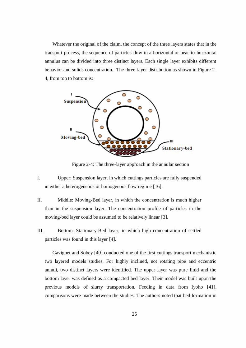
25

Whatever the original of the claim, the concept of the three layers states that in the

transport process, the sequence of particles flow in a horizontal or near-to-horizontal

annulus can be divided into three distinct layers. Each single layer exhibits different

behavior and solids concentration. The three-layer distribution as shown in Figure 2-

4, from top to bottom is:

Figure 2-4: The three-layer approach in the annular section

I. Upper: Suspension layer, in which cuttings particles are fully suspended

in either a heterogeneous or homogenous flow regime [16].

II. Middle: Moving-Bed layer, in which the concentration is much higher

than in the suspension layer. The concentration profile of particles in the

moving-bed layer could be assumed to be relatively linear [3].

III. Bottom: Stationary-Bed layer, in which high concentration of settled

particles was found in this layer [4].

Gavignet and Sobey [40] conducted one of the first cuttings transport mechanistic

two layered models studies. For highly inclined, not rotating pipe and eccentric

annuli, two distinct layers were identified. The upper layer was pure fluid and the

bottom layer was defined as a compacted bed layer. Their model was built upon the

previous models of slurry transportation. Feeding in data from Iyoho [41],

comparisons were made between the studies. The authors noted that bed formation in

26

inclined wells must not be predicted on the saltation mechanism, and should instead

be determined according to the momentum exchange between the two phases. They

also suggested that friction coefficient between cuttings and wall would strongly

influence the bed formation. The model results indicated that pipe and particles sizes

as well as eccentricity were the most influential variables rather the rate of penetration

and rheology. They also recommended the use of large drill-pipe size to prevent bed

formation problems.

Martins and Santana [42] published a two-layer mechanistic model for horizontal

and near horizontal eccentric annuli. The top layer consisted of homogeneous mixture

of mud and cuttings while the bottom layer consisted of compacted cuttings. The

model represented a new formulation that draw upon the work of Doron et al, 1987 on

sand-water flow in a horizontal pipe. In addition, they also used a dimensionless

approach based upon the use of Lokhart-Martinelli parameters. Conservation laws of

mass and linear momentum, and constitutive relations describing the interactions

between the two phases and between phases and walls were solved simultaneously.

Numerical values for unknowns, such as the bed heights, average solids concentration

and frictional loss, were calculated based on the flow pattern presented by Iyoho

1980. The results showed that increasing the drill-pipe diameter, the fluid density and

the fluid flow rate could effectively contribute in solving of cuttings transport

problems.

Walton [17] presented a one dimensional, mechanistic two-layer model. A

suspension layer and bed layer with coiled tubing in deviated drilling orientation were

studied. He assumed that settling and diffusivity of particles were independent of the

concentration. Settling of the particles in this study was formulated in an identical

way as used by Doron et al. 1987. A computer code was incorporated to form

graphical map to show the flow regime and the minimum suspension flow rate. The

simulated model yielded acceptable results compared to the experimental results of

Tomren et al. [19]. Based upon the results, the author suggested that moderate-

viscosity fluids were more efficient than low and high-viscosity fluids to transport the

27

drilled cuttings. The author also reported that it is more complicated to clean

horizontal and deviated wells than vertical ones.

Nguyen and Rahaman [43, 44] carried out series of studies to set a layers

hydraulic program for cuttings transport and hole cleaning in an eccentric annulus of

highly deviated and horizontal wells. They presented a mathematical model and a

geometrical calculator to obtain the required annular section configurations. Their

program algorithms fed in results for a range of velocities and various input

parameters. The effect of the fluid rheology, the mud weight, the solid density and

concentration, the friction coefficients, the pipe eccentricity and inclination were

studied in order to inter-relate the effect of these parameters on the cleaning operation.

Generally, the simulated results demonstrated the suitability of the layered modeling

approach to achieve an effective design of the horizontal and high inclined wells.

Kamp and Rivero [39] utilized the layer approach, and established a preliminary

unique two-layer model. In addition to the steady state, they assumed eccentricity and

no pipe rotation. They also assumed there is no significant slip velocity difference

between the particles and the mud. The upper layer was a heterogynous layer of

cuttings and mud, while the bottom layer was the bed of drilled particles. Three mass

conservation equations were constructed: one for the cuttings, one for the fluid in

heterogeneous layer, and one for the mixture in bed layer. Two momentum equations

were built for each separated layer. To solve the system numerically, the boundary

conditions were used to define dimensionless quantities those put in matrix forms.

Average flux of cuttings and turbulent diffusivity were used to calculate the

concentration. Regarding the particle settling, the researchers excluded the influence

of the particle hinder behavior, and referred that to the requirement of the diffusion

solution. Their results found that an increase in the interfacial shear would lead to the

re-suspension and bed velocity. They observed that the dimensionless bed height (as a

function of mud flow rate, rate of penetration, mud viscosity, particle diameter, and

pipe eccentricity) increased with the particle size, and as a result, they confirmed that

transport of small cuttings was considerably easier. Kamp and Rivero also reported

that the transport of larger particles was more efficient. In addition, they also reported

28

that increasing the eccentricity increased the bed height. However, their model over

predicts the transportation at a given mud flow rate than was actually observed.

Therefore the researchers anticipate the possibility of further improvement of their

model.

The layered model conducted by Kamp and Rivero [39] to study the transport

phenomena in the wellbores excluded the influence of hinder behavior on the particles

settling, referring that to the solution requirement of diffusion. However, at a given

mud flow rate, their model over predicted the particles transportation.

Feng et al. [45] mentioned that with any type of particulate flow, collision

between particles is unavoidable, and this issue should be considered especially when

the flow is dense and the particles moves at high a Reynolds number. Accordingly, it

could be expected that errors of the two-layer model of Kamp and Rivero 1999 may

particularly be caused by neglecting the hinder behavior effect on the particles settling

velocity which occurs during the transport.

Santana et al. [46] created a two-layer model for high angles and horizontal wells.

The well-known conservation equations of mass, written for solid and liquid phase,

were solved together with the momentum equations written for suspension and bed

layer. In this study, the accuracy of the assumption of no solid-liquid slip, which was

proposed by Martins and Santana [42], was also examined. The pressure gradient was

obtained by Darcy’s equation for a porous media. The computational implementation

of their two layer model indicated that the difference of the obtained results refer to

their choices of the rheological model. Accordingly, both models were sensible for

rheology parameters. They also verified their use of the interfacial friction factor

correlation and reported its impact on the cleaning prediction. Generally, their results

proved the reasonability of the no-slip assumption between solid and liquid phase.

As part of the previously mentioned research by Masuda et al. [28] in addition to

the experimental study they have studied the transport of the drilled cuttings by

simulation procedures. The simulation was performed using the two-layer modeling

29

approach as suspended and moving-bed layers. The mass balance and the momentum

conservation have been set based on two-layer regions. Region one was the moving-

bed. Region two was the suspension. By solving six equations, the velocities of each

layer and mud annular velocity, the bed height, the suspension concentration and the

pressure were obtained. They performed comparisons between simulation and

experiments, and the results showed that majority of the studied cases were found to

match successfully. However, for the calculated velocities, relatively poor results

were obtained. This demonstrates the limitation of two-layer approach models to

predict the transport process.

Cho [4] divided the directional orientation of drilling into three sections and

introduced the discipline of the three segments hydraulic model. The three segments

were built on the basis of the inclination angles range (0-90ο). They developed a

three-layer model of cuttings transport which combined with their new derived

concept of segments. An eccentric annular section with coiled tubing drilling was

detailed in this study. An analysis of the forces acting upon cuttings layers was carried

out, based on the continuity and Navier Stokes equations, in addition to broad analysis

of the annular velocity, pressure gradient and fluid rheology. Six equations of six

unknowns were solved numerically, and a computer program was built in order to be

utilized in the planning steps of drilling. They reported effects of the annular velocity,

the fluid rheology, and the angle of inclination on the cuttings transport. The results

showed good agreement with experimental data which had been obtained by others.

Ramadan et al. [3] applied a three-layer model on horizontal and inclined

channels. Transport of spherical-shaped particles through 70 mm pipe diameter was

determined in the context of certain assumptions. The study utilized the

pseudohydrostatic pressure concept in a wide range of the analysis. The concept was

repeatedly utilized in several parts of their model. It was used to approximate the dry

frictional force, to estimate the normal force between the wall and the bed layer, as

well as to model the moving bed thickness. For the inclined pipe flow, numerical

producers were issued to solve a set of eleven equations, hoping to obtain estimated

values for eleven unknowns. The equations were solved simultaneously, and the

30

results reflected the reasonability of the layers-model approach. Very thin moving-bed

layer became thicker with increasing flow rate. This study encountered various

criticisms from Stevenson [47], who commented that authors a parented had

overlooked an earlier study by Doron and Bernea on 1997. Stevenson claimed the

model described by Ramadan et al was identical to the model by Doron and Bernea

1997. However, the authors responded to Stevenson’s comments and strongly

defended the unique features of their model. Frankly, Ramadan et al. [48], have

illustrated the confusions involved in the study and replied to the criticisms to justify

their model findings. However their three-layer application was impressive despite of

that investigation was not on drilling transport mainly since they haven’t considered

the drilled cuttings size, cuttings shape as shown in Figure 2-5 or either annular space.

Figure 2-5: Irregular particles shape [2]

Various empirical factors were employed in order to describe the shape of man-

made particles. Those efforts provided some empirical description by identifying the

parameters of the particle’s characterization, such as volume, surface area, projected

area and projected perimeter. Selection of the shape factors should be handled with

further awareness to their relevance. Wadell 1933 [49] suggested the important

concept of spheristy to describe the irregular shaped particles. However Sphericity of

crushed sandstone varies between 0.8-0.9 [50], and drilled cuttings sphericity ranges

between 0.75-0.85 [4].

31

Doan et al. [51] described a simulation of cuttings transport for eccentric annuli in

Under Balanced Drilling Or, (UBD). It was arbitrarily assumed to have either vertical

or horizontal orientation rather than any specific inclination. The model was examined

under different conditions, including an unsteady state. Compared to the experiments

conducted, the calculated cuttings velocity was in reasonable agreement with what

was measured. However, there was a poor match between the measured and the

predicted results of dilute cuttings injection rates. Even so, this strongly reflects the

weakness of the two layers model approach in the issue of describing the interfacial

phenomena.

Naganawa [52] described a modified two-layer model of cuttings transport that

enabled more practical use of their simulator. Modification was carried out in order to

enable the model simulation to cover more particles on the directional wells

trajectories. The extended model was capable of describing the behavior of the

relatively low inclination wells. In order to evaluate the model, post analysis of hole

cleaning for actual Extended Reach Well or, (ERW) in Japan was handled by the new

simulator. Output of the simulations for the modified two-layer model produced

successful results for the transition behavior of cuttings over the hole trajectory.

Costa et al. [53] used a two-layered model to simulate the transit cuttings transport

and Equivalent Circulation Density or, (ECD), in the wells drilling. Their model

assumed a steady states flow, pipe eccentricity and sphericity of particles. The two-

layers represented an upper suspension layer and a bottom bed layer with 52% solids

concentration in the bed. Power low fluid was employed to simulate properties of the

liquid phase. Mass conservation of the separated phases, momentum conservation for

the separated layers, and other equations for shear stress and friction factor

correlations for both laminar and turbulent flow were stated. Using Carten’s 1969

relation the mass diffusivity was determined. The established numerical

computational system was solved using the finite element method, where Newton-

Raphson techniques of equation’s linearization were also utilized. The results

demonstrated the capability of their technique to estimate the bed height, the cuttings

concentration, as well as the pressure and the ECD observed variations. They reported

32

the influence of the ROP on the bed formation and pressure distribution in the well.

The influence of the cuttings concentration on EDC profile was also reported. Despite

the need for further development, their two-layer model was computationally

effective.

The various studies which used the two- and three-layer models are summarized

in Table 2-2 and 2-3 respectively.

Table 2-2: The two layers models.

Researcher Layers

Gravignet and Sobey, 1986 [40] Mud-bed

Martins and Santana, 1992 [42] Homogenous mixture-bed

Walton, 1995 [17] Suspension- bed layer

Kamp and Rivero, 1999 [39] Heterogynous-bed

Santana et al, 1998 [46] Suspension-bed layer

Masuda et al, 2000 [28] Suspension- moving-bed layer

Doan et al, 2003 [51] Suspension-bed layer

Costa et al, 2008 [53] Suspension-bed layer

As an extension of the segments concept created by Cho [4], Cheng and Wang

[54] presented a three-segment hydraulic multi phase model. Foam was employed as

the main drill fluid while gas was used as a third phase in horizontal drilling. Based

on two critical inclination angles, Cheng and Wang used the power law rheological

model to represent the fluid viscosity. They considered the two phase (fluid and solid

phase) only in the built-up of continuity. In addition, the one dimensional diffusion

equation was used in order to solve the concentration question. To somehow their

simulation output compared to the drilling practices was exhibited incorrect behavior.

Thus, the results showed an over estimation compared to the experimental results of

Capo [55].

33

The following table summarizes the highlighted studies of cuttings transport

which were conducted in the light of the three layer approach:

Table 2-3: The three layers models.

Researcher Orientation Conduit features

Nguyen and Rahaman,

1996-98 [43, 44]

highly deviated and horizontal Eccentric annulus

Cho [4] Horizontal and Deviated Eccentric annulus

Ramadan et al. 2005 [3] Highly Inclined & horizontal Channel/pipe flow

Cheng and Wang, 2008 [54] Horizontal and inclined drilling Multi phase in eccentric annulus

2.4 Computational Fluid Dynamics CFD

The Computational Fluid Dynamics or, (CFD) methods involve revaluation

techniques in the area of simulations. Through the use of these methods, highly

sophisticated and detailed analyses of many engineering problems became possible.

The use of CFD in different areas as a simulation tool demonstrated its capability as

an exclusive measurement for examining a field’s process and providing bundles of

valuable information. Since predicting of the processes applicability is necessary to

judge weather is it difficult or impossible to achieve the targets, CFD can be

employed as a forecasting tool without expensive hardware [56]. Recently, CFD

simulation techniques have been introduced into the field of solids transport studies.

CFD software became necessary for the concerned parties in order to ensure process

improvement in the plant applications, such as pneumatic transport lines, risers,

fluidized bed reactors, hoppers [57].

Ali [18] was the first researcher who studied and analyzed the cutting transport

parameters using CFD. He have applied hole cleaning simulation using the Discrete

34

Phase Modeling (DPM) in FLUENT and conducted the analysis for horizontal and

vertical wells. He judged the qualities of the hole cleaning through the transport

efficiency. The effect of the mud flow rate, mud weight, mud viscosity, drilling rate,

cutting size and cutting density were analyzed. Relative deviation between the model

prediction and the experimental data was observed at high velocities, and this was

related to difference of the cuttings sizes tested in each case. Ali’s results indicated

the importance of the annular velocity in cuttings removal. He also reported that

horizontal well cleaning was better than for vertical wells.

It was eventually noticed that some of the researchers’ findings obtained through

CFD did not closely correspond to observable reality since those results do not match

either physical facts or valid results which obtained from both experimental work and

numerical procedures e.g. [17, 27, 35].

Another CFD technique used to investigate steady state cuttings transport in

horizontal and deviated wells was employed by Mishra [56]. Instead of DPM,

Eulerian Mixture Modeling capabilities in FLUENT software were used in the study.

The parameters this study was concerned with the fluid flow rate, ROP, angle of

inclination, drill-pipe rotation and cutting size. The results indicated that fluid flow

rate, angle of inclination, and ROP have a major impact on the cutting concentration.

Furthermore, they recorded that larger particles were more efficiently cleaned, and

pipe rotation would greatly enhance the hole cleaning, especially for the smaller sizes.

Once again, the CFD results were noted to be in conflict with the experimental

and analytical works, where it has been repeatedly demonstrated that smaller particles

are indeed easier to clean, as noted in [26, 39, 58]. This is especially in the cases

where pipe rotation is involved. Even so, we can compare Mishra’s results to the

claims of Wilson and Judge on 1978, who have also claimed that smaller particles are

harder to clean than larger one. The particle sizes used in the study by Mishra were

within the given range of the easiest removable sizes cited in [26].

35

The nature of the available commercial software in its simplest practice is still

inconvenient since it lacks to capture some facts. This may refer to incapability of this

soft ware to own some features involve in the transport phenomena such as the layers.

However, both CFD simulations were unique to studies of the cuttings transport

phenomena

2.5 Summary of Previous Work

In essence, direct information and sufficient recommendations were utilized to satisfy

the requirements of cuttings transport in vertical drilling. In contrast, directional

drilling practices still facing problems and conflicting opinions about some of

important variables, such as effect of the particle size. Therefore, further consideration

should be given to this type of directional transport. Bed tumbling and sliding in

inclined drilling transport and high bed formation in horizontal transport are critical

problems. Moreover, additional attention must be devoted to the long-horizontal wells

in which deeper beds may form and serious transport problems might be encountered

[17].

Due to the static force resulting from the absence of the essential force that

overcomes the gravity during the horizontal transport, the buildup of cuttings bed is

strongly enforced. As a result, the complex turbulent flow becomes necessary to

create the turbulent eddies required to achieve the transport, which causes additional

difficulty for horizontal drilling.

The use of experimental observation only does not permit assessment of wide

variation among the variables that affect the cuttings transport. With the respect to the

outcome of empirical models, experimental results from specific field inputs data and

conditions will no longer be useful for the high diversity of cases that are

encountered. This issue may restrict the outcome in a narrow range, and limit the

outcome into the typical or closer sets of conditions. Seeking an accurate

understanding of a different field data or wider range of cases requires continuous

36

experiments, more duplication and many loop modifications in order to satisfy the

requirement of new set of conditions with which the researchers are confronted.

Since such efforts and very time consuming and expensive, the means experimental

work has some limitations.

Nevertheless, investigation of the transport problem with mathematical models

has been anticipated to able to handle a broad range of variations. Modeling

techniques facilitate the simplification of the complex interactions that exist between

variables that need to be studied under many different conditions. The opportunity of

model development and modification gives this technique a greater possibility for

application. In addition, the relative ease and flexibility of applying models upon a

very diverse range of cases and materials also ranks such modeling techniques as

being superior to actual experimentation. These models could be precisely and cost-

effectively applied to different angles, fluids, cuttings and other variables.

In addition, several modifications were constructed for the two-layer model after

observations of its deficiency in order to match with the mechanism of cuttings

transport [28]. This led to a more adequate modeling approach, which was then able

to distinguish between three different mixer behaviors during the transport, i.e. the

three-layer approach. Even so, at least some of the phenomena formulation may need

some empirical facilities to be adopted and embedded in the models.

Therefore, from the literature survey, it can conclude that:

Still there is some ambiguity in the area of directional wells that requires more

investigation to increase the efficiency of this style of drilling.

Problems of transport as tool blockages and cutting’s bed formation are

associated with horizontal drilling orientations. Significant reduction of the

transport capacity is more expected in the horizontal wells.

Mathematical techniques were more capable to produce general applicable

concepts and principles. They are flexible methods which facilitates extraction

37

of the facts for the various cases and scenarios encountered in the field with

time and cost effectiveness

In many instances, the two-layer approach has failed to describe the

directional transport phenomena [19, 28, 53]. In contrast, the three-layer

approach has become a more widely accepted means of modeling what occurs

during the transportation of drilled cutting particles, particularly during

directional and horizontal cleaning.

Many of the previous research efforts did not involve the sphericity effects.

Using the three-layer, studies [4, 43, 44, 54] have followed similar

considerations for the eccentric of annulus in spite of the disadvantages of this

condition.

With CFD, it has been observed that using of the simplest conditions in the

commercial software (FLUENT) was impractical. Thus, the commercially-

available software still requires a considerable amount of modification and

improvement, even beyond its accessibility by the User Define Function tool

or, (UDF), in order to perform a better analysis of the drill cuttings transport

process.

38

Chapter 3

Research Methodology

3.1 Introduction

Since the first introduction of the layers-model approach, which was based on

mechanistic theorem to describe the process of annular cuttings transport, significant

progress has occurred the field of the analytical modeling. These advances have led to

a deeper understanding of how drilled cuttings move within the drill mud flow, as

solid-in-liquid two-phase flow.

As cited by Cho [4], Doron et al. argued that two-layer models are not capable of

describing the mechanism of cuttings transport. This is because such models lack the

ability to predict the existence of the stationary-bed. Furthermore, as pointed out by

Kamp and Rivero [39], the two layer model has proven itself to be unable to represent

the cuttings transport process in both horizontal and near to horizontal wells.

Similarly, this fact has also been confirmed by the study carried out by Masuda et al.

[28] and partially through the by Duan et al. [36].

In this section, the proposed mathematical model applied by Ramadan et al. [3]

for a channel flow was extended to the horizontal annular flow of drilled cutting

particles. In fact, their work was not directly related to the cutting transport in drilling

operation. Hence, in this study, the three-layer model would specifically be used to

investigate the cuttings transport performance in the annular geometry of well, with

much consideration to several vital factors that affect the cuttings transport process.

These factors would include the particles shape, the particle size, the fluid viscosity,

39

the annular size and the rate of penetration in concentric drilling. Besides, the

frictional factors effect would also be inspected.

3.2 Model Hypotheses

Informed by an awareness of conservation laws of mass and momentum principals, a

three layer model was developed for horizontal cuttings transport in annular flow. The

model was mainly targeted to predict cutting bed heights, pressure drop, and transport

velocities. The following hypotheses were used in the current model:

Flow states

Steady state ( 0/ t ).

Incompressible ( f = constant).

Turbulent flow ( 2400Re f ).

Drilled cutting particles

Cuttings size was represented by mean particle diameter, and cuttings

shape was represented by sphericity.

Particle distribution in the suspension layer is approximately uniform,

linear in the moving-bed layer and uniform with constant value in the

stationary-bed layer.

Volumetric concentration in each layer is uniform along the well length.

Rolling effect is negligible.

Carrier/drilling fluid

40

Drilling mud is a non-Newtonian fluid and will be modeled as power- law

fluid.

Rheological properties and density of fluid are constants.

Drill-pipe conditions

Concentric.

No rotation.

Other hypotheses

Two-phase solid-in-liquid flow.

The process is adiabatic.

No slip condition. According to [42]Martins and Santana and [48].

3.3 The Mathematical Model formulation

Transport of heterogeneous mixer of non-Newtonian fluid and drilled cuttings in

annulus is based on the fact that mud flow with cutting particles in horizontal

transport results in three layers, where each layer displaying different behavior.

Hence, the transport phenomena, under the previous mentioned can be illustrated

mathematically through set of equations as follows:

3.3.1 Mass Balance

The mass transport equation for a one-dimensional, two-phase, horizontal flow in an

annular element of length z, under steady states can be written in general terms for the

unit length dz as follows:

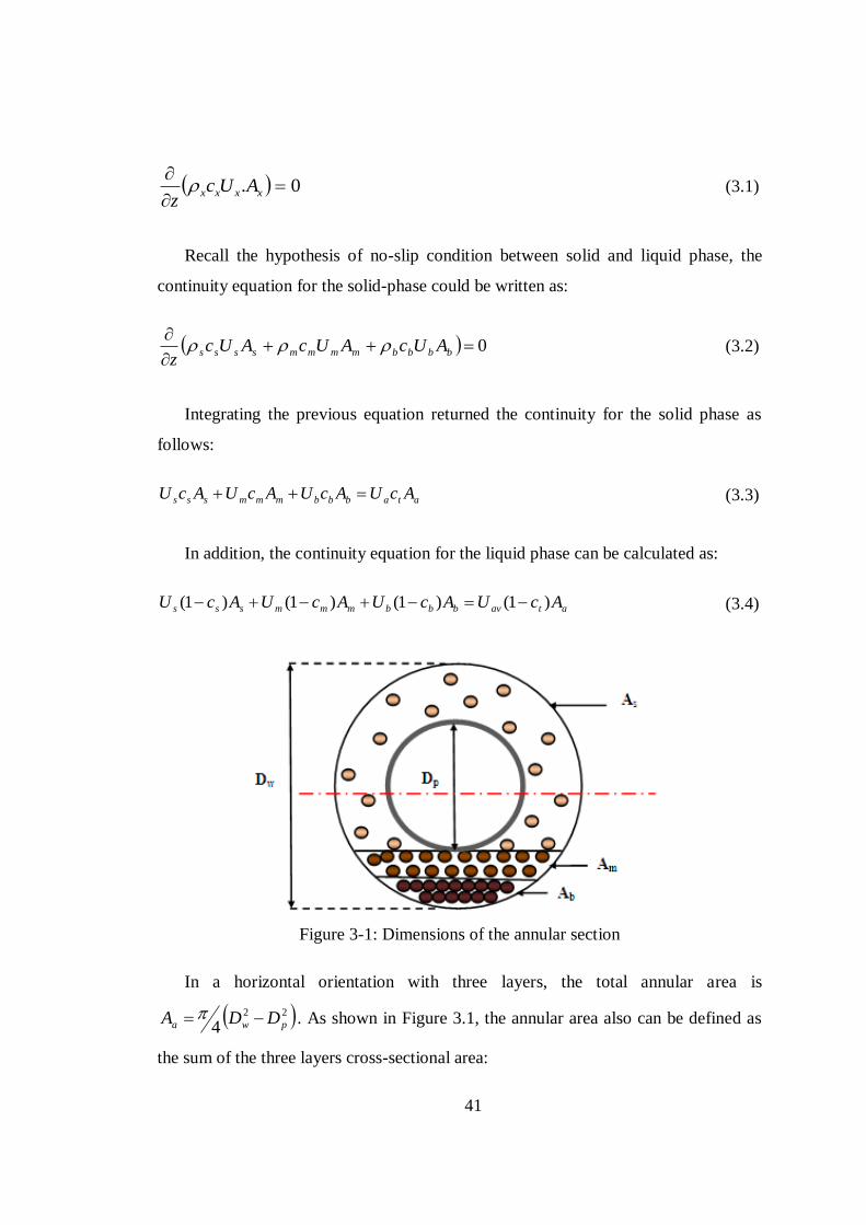
41

0.

xxxx AUc

z (3.1)

Recall the hypothesis of no-slip condition between solid and liquid phase, the

continuity equation for the solid-phase could be written as:

0

bbbbmmmmssss AUcAUcAUc

z (3.2)

Integrating the previous equation returned the continuity for the solid phase as

follows:

atabbbmmmsss AcUAcUAcUAcU (3.3)

In addition, the continuity equation for the liquid phase can be calculated as:

)1()1()1()1( atavbbbmmmsss AcUAcUAcUAcU (3.4)

Figure 3-1: Dimensions of the annular section

In a horizontal orientation with three layers, the total annular area is

22

4 pwa DDA . As shown in Figure 3.1, the annular area also can be defined as

the sum of the three layers cross-sectional area:

42

abms AAAA (3.5)

The total cuttings volumetric concentration can be specified as a function of the

average rate of penetration or, (ROP). Under steady state conditions, the total

concentration created by the drill-bit is given by the equation [43]:

1

2

hole

pipe

a

t

D

dU

ROPc

(3.6)

3.3.2 Momentum Balance

The momentum analysis was written according to the diverse layers. Accordingly,

three momentum equations are involved to describe the suspension layer, the moving

bed layer and the stationary bed layer.

3.3.2.1 Momentum for the Heterogeneous Suspended-layer

The upper layer is relatively pure fluid or heterogeneous mixer of non-Newtonian

fluid and drilled solids. It is important here to mention that all forces in the

momentum balance are based on a unit length dz =1.

The forces applied to the fluid in this layer were: (a) the pressure, (b) the shear

forces at its wall, and (c) the shear at the tangency with moving-bed layer.

Considering a steady state condition, the force acting upon the horizontal flow per

unit length, shown in Figure 3-2, could be specified by:

0 smsmsss SSdz

dpA (3.7)

Which is corresponding to the form (Pressure forces=∑shear forces).

43

The shear stress between the upper layer and the wall surface resulted from the

contact between the well walls and the pipe wall. This shear is defined by [59]:

8/2

ssss Uf (3.8)

At the interface between the upper suspension layer and the moving bed layer

below it, the shear stress is given by [3]:

)(8

1 2

mssmssm UUf (3.9)

Figure 3-2: The exerted shears in the annular suspended-layer

Since the flow in the suspension layer is heterogeneous, the effective layer density

is calculated from [4]:

)1( fspss cc (3.10)

Turbulent flow is still complex even for Newtonian fluids flows in quite simple

geometry. Moreover, accumulation of particles in this type of flow will result in

complex, unsteady motion and distribution of particles [16]. Therefore, the calculation

of a Reynolds number in turbulent, non-Newtonian liquid, attached with particles in

annular flow, will became more complicated.

Calculation of a Reynolds number is a preliminary and essential step to

classifying the flow type, and consequently necessary to calculate the friction factor.

44

Here, a generalized Reynolds number for the suspension layer under the power low

model can be written as:

268

Re

)2( n

s

n

h

n

ss

gsn

n

K

DU

(3.11)

Where n is the flow index behavior and Ks is the adoption of the fluid consistency

index K and the concentration cs. Considering the concept provided by Einstein

1906for solid volume fraction cs < 0.01 [60], the suspension layer viscosity will be

calculated according to:

)5.21( ss cKK (3.12)

Many correlations were suggested to derive the friction factor in the turbulent

two-phase flow. Some of the available correlations used in studies of cuttings

transport included the features of non-Newtonian power low fluid to evaluate the

friction factor. It can be observed that most of studies used Televantos correlation2

because of its simplicity, such as in [42, 51, 53, 54]. It has been claimed by Martins

et al. [24] that this correlation does not provide specific accuracy for the annular

geometry and the non-Newtonian fluids behavior effect simultaneously. Reference [3]

used another correlation, which was proposed by Szilas et al.3. This correlation

matches the finding of the friction factor in both smooth and rough walls, two-phase

flow and the explicit power low behavior:

71.3Re

10log2

1

22

2/

h

p

nn

sgssD

d

ff

(3.13)

While the constant depends upon the index behavior and is related as

following:

2 Citied in [42], [51], [53] & [54] 3 Cited in [3]

45

057.1015.4

12.2707.0

151.1

1

nnn (3.14)

As cited in [3], Doron and Barnea suggested that the interfacial friction factor

between the two layers will be accounted as twice the wall friction factor:

2 ssm ff (3.15)

As stated in the literature, the friction factor for the turbulent flow could be

predicted by other correlations. In parallel, Cho [4] and Cheng and Wang [54] have

constructed their mathematical models using a three-layer approach and agreed with

the use of the empirical relations shown below to calculate the friction factors in the

boundary of the upper layer. (a) Correlation by Doron and Barnea 1993 for

suspension:

Re645.000454.0 7.0 ssf (3.16)

(b) The correlation by Martin et al 1996 [24] for the interface between suspension

and moving bed layers:

Re966368.0

34439.2

360211.207116.1

hs

p

ssmD

dnf (3.17)

These methods to predict the friction factor in the layers have been implemented

in two different simulation models of cuttings transport in order to highlight the

difference between them.

3.3.2.2 Momentum for the Moving-bed Layer

Referring to Figure 3-3, the sum of the forces per unit length on the moving-bed layer

is given by the following momentum equation:

46

0 mbmbmbdmmsmsmm FSFSSdz

dpA (3.18)

The shear stress between the moving-bed layer and the well boundary is:

8/2

mmmm Uf (3.19)

The interface shear between the moving-bed layer and the stationary-bed layer is:

)(8

1 2

bmmbmmb UUf (3.20)

Figure 3-3: The exerted shears in the annular moving-bed layer.

Equation (3-13) will be used to calculate the friction factor in the middle moving-

bed layer. In case of laminar flow other correlations sould be use. Televantos et al.

1979 recommended that the dispersive force will take care of the dispersive shear

stress between the moving-bed and the stationary-bed layers. Therefore, to account

for the friction factor between the moving-bed and the stationary-bed layer, the same

value of the friction factor between the moving-bed layer and the walls will be

considered, [3]. Hence:

mbm ff (3.21)

Furthermore, the following empirical equation by Dorn et al 1993 for moving-

layer and for the interface with a stationary bed will be examined:

47

Re046.0 02.0 mmbf (3.22)

The effective density for the moving-bed will be:

)1( fmpmm cc (3.23)

The dispersive shear stress between the moving-bed and the stationary-bed layer

has important implications for the present model. Thus, the previously mentioned

shear would give an impressive indicator about the formation of the third moving-bed

layer in the middle. The dispersive shear can be represented by the following relation:

mb

mb

disS

F (3.24)

Indeed, the concept of pseudo-phenomena is a common application in many of the

engineering mathematical applications, as employed in [61].

Ramadan et al. [3] used the pseudohydrostatic pressure distribution to

approximate an equation for the dry friction force between the moving bed and the

wall boundary. Considering Figure 3-4, their estimated dry friction force formula for

the horizontal orientation was as indicated below:

2

cos

mb

mmmfpdd tScgF

(3.25)

48

Figure 3-4: The angular bed layers thicknesses

A study by Nguyen and Rahaman [44] approximated the dynamic friction

coefficient to be half of the static coefficient relating their value to each other.

Therefore, a similar manner and value will be imposed in the current model, as

following:

2.02

sd

(3.26)

This value of the friction coefficient seems high, but should bear in mind that this

is for solid-in-liquid two-phase flow.

3.3.2.3 Momentum for the Stationary-bed Layer

The forces in Figure 3-5 represent the momentum equation for the bottom stationary-

bed layer given by:

0 bbbmbmbmbb FSFSdz

dpA (3.27)

Where:

49

8/2

bbbb Uf (3.28)

The effective stationary bed-layer density is given by:

)1( fmpbb cc (3.29)

Figure 3-5: The exerted shears in the annular stationary-bed layer

3.3.3 Analysis of the Moving-Bed Layer

Inclusion of an additional formula to calculate the moving-bed thickness is necessary

in the model set-up. The importance of the layer thickness calculation goes beyond

the purpose of checking the existence of the third layer during the horizontal cuttings

transport. This formula also helps to determine whether the observed middle layer

will either increase or decrease during the transport. Furthermore, this formula

validates the approach of the three layers. The formula used by Ramadan et al. was

[3]:

tan)( Dfpb

dis

mgc

t

(3.30)

Where, dynamic friction factor tanØD, of the equivalent dynamic friction angle ØD

was estimated experimentally by Bagnold 1954 to have a value of approximately 0.75

[62].

50

3.3.4 Mean Velocity of the Moving-Bed Layer

Fredoe and Deigaard [63] defined the velocity profile for the moving-bed layer

relative to the bed as follows:

2

2)(,

m

rdt

y

k

UyU (3.31)

While the definition of the friction velocity U is given by:

s

smU

(3.32)

Averaging the moving-bed velocity profile over the layer thickness is returned the

following mean moving-bed layer velocity:

3

24b

p

sm

m Uk

U

(3.33)

Substituting the shear sm as given in equation (3-9) and re-arranging the equation

(3-33) according to Doron and Barnea concept returns the mean moving-bed velocity

as a function of the suspension and bed layer velocities, as the following:

3

221

3

22

p

ss

p

sssb

mf

k

f

kUU

U

(3.34)

51

3.3.5 Average Concentration of the Moving-bed layer

To predict cuttings concentration on the moving bed-layer, Fredsoe and Deigaard [63]

suggested the assumption of linear variation for the dispersed layer. By adopting the

pseudohydrostatic gradient, the average concentration of the moving-bed layer can be

approximated as follows:

2

bsm

ccc

(3.35)

Figure 3-6: The approximated concentration profile for the three-layer by Ramadan et

al. [3]

As shown in Figure 3-6, the concentration in the suspended layer is very low in

contrast to the moving and stationary bed layer, where the particle aggregation is

high. By both experimental and statistical methods, the bed concentration is found to

have the range value (0.48-0.52) [4]. Hence, in this study, the solid bed concentration

was taken as cb≈0.5.

52

3.3.6 Convection-Diffusion Equation

The convection-diffusion equation describes a physical phenomenon of particles or

energy transfers in a certain system due to two different processes, the convection and

the diffusion. One-dimensional, time dependent convection-diffusion equation is

normally written as:

sls

slsl cvy

c

yt

c (3.36)

The first term in the brackets represents the diffusion, while the second term

represents the convection.

To acquire the local concentration of the suspension layer, the convection-

diffusion equation is implemented to fulfill the steady state condition. As a result, the

equation became:

0

sls

sl cvy

c

y (3.37)

The above expression specifies that either the first term or the second term is

equal zero. Yielding the first term returned the equation:

scvy

csls

sl

(3.38)

According to the convection-diffusion hypotheses, this equation could not be

applied to the moving-bed layer. This is because of the settling effect due to collision.

Hence, in the present case, the equation was applied to the suspended layer.

Consequently, the distance y represents the elevation above the interface between

moving-bed and suspension layers.

53

Assuming a constant diffusion coefficient and settling velocity, the average

concentration of the suspension layer was approximately estimated in [3] as the

following:

1.)(

h

hsv

s

ms

v

e

h

cc

h

(3.39)

Where the turbulent diffusivity coefficient of particles in the suspension will be

calculated by the below formula:

1 yh

ykU

s

(3-40)

To avoid zero diffusivity, the distance y is recommended to be taken in a very

short range. Ramdan et al. [3] estimated the distance y as a function of the thin middle

layer thickness (y=tm/100). In this study, it was decided to consider this value as

recommended by Fredsze and Deigaard [63] to have twice the value of the particle

mean diameter (y=2dp) which makes more sense to the presence of physical

geometry. Accordingly, the final expression of the turbulent diffusivity became:

2

15.0)( p

s

p

smms dh

dfUUk

(3-41)

3.3.7 Cuttings Settling Velocity

The characteristic size, shape and density of a solid particle greatly influence its

dynamic behavior in the flowing media. Some of the previous studies assumed a

uniform sphere shape when studying the solids transport phenomena [3]. Apparently

almost all man-made and natural solid particles have a non-spherical shape. In

addition, it is well known that the drilled cutting particles created by drill-bit tools

54

will never have regular shape. Therefore, this assumption might distort the obtained

results and limits their usefulness and will never allow predicting the phenomena

accurately.

Various empirical factors were employed in order to describe the shape of man-

made particles. Selection of the shape factors should be handled with further

awareness to their relevance. Thus, Wadell 1933 [49] shape factor that described the

degree of particle sphericity φ, as deviation of the irregular particle shape from the

true sphere. Wadell did this through the following ratio:

particle of area surface

particle as volumeequivalent of shpere a of area surface (3-42)

This relation emphasizes that the factor of the regular sphere has a maximum

value of 1, while for non-regular shaped particles the sphericity value will be less than

this value. The drag coefficient of a spherical solid particle moving in a fluid is less

than that for an irregularly shaped particle. This implies that settling behavior would

occur faster for the spheres rather than for irregularly shaped particles. Hence, usage

of the sphericity concept increases the reliability in the modeling of drilled cuttings

transport.

Therefore, the proper selection of the most suitable formulas in the mathematical

modeling will enhance prediction of the critical factors effects. Between the several

empirical relations describing a single particle settling velocity, the equation proposed

by Chien [50] is a unique relation to predict particle settling velocity. This formula

involves the particle shape to fit the concept of sphericity. Based on the French units

system, Chien’s model for irregular particle settling was given as:

0103.5exp449.1903.5exp458.42

f

p

ps

fp

es dv

dv

(3-43)

In addition to the shape factor effect, this equation able to handle different

rheological models, and could be applied for wide range of particle Reynolds number

55

(0.001-10,000). Moreover, this equation matches different properties of the fluids,

according to their rheological characteristics, which clearly appear in the term of the

effective viscosity. Therefore, the effective viscosity term can be selected according

to the operated fluid properties.

Among the four familiar rheological models, the Bingham plastic, Herschel-

Bulkley, Power-law and Casson, the most suitable rheological model to characterizes

the drilling-mud behavior is the power-law model, at which it has (n<1). The use of

Bingham Plastic and Casson models has proven their inability to model the behavior

of drill-mud [46]. Therefore, the effective viscosity of the drill-mud will be

represented by the formula:

1

n

p

se

d

vK (3-44)

Particles drag coefficient and particle Reynolds number were extremely important

when dealing with saltaion behavior. Since the viscous and inertia forces were the

most effective forces during the settling, results of particle settling in this

investigation were analyzed on the light of Rep, which, Rep in non-Newtonian fluid is

defined as following [4]:

K

dvn

n

p

n

s

p 1

2

36

1617.0Re

(3-45)

3.3.8 The Hindered Settling Velocity

There is no doubt that poor solid proceeding plant performance and erosion caused by

the particle impacts could add a high cost to the execution of engineering applications.

In addition, the economics of well drilling is greatly related to the cleaning process,

which is also crucial to the industry. Hence, for the sake of precision, attention must

be directed to the impact of particles once multi-phase flow is involved.

56

Interference between particles greatly affected their movement behavior.

Therefore, clustering of cutting particles must consciously be accounted once deal

with solid particle transport process. The particle hindered behavior defined as

function of suspension concentration [4] which uses to interpret the influence of

particle collision.

To simulate the transport of the solids, it is extremely important to take into

account the existence of interference between the particles cluster during the settling.

Richardson and Zaki 1954 [13], Thomas 1963 [4], and Ham and Homsy 1988 [64]

studied the collision behavior of solid particles. By use of correlation factors, they

have related the settling of solids cluster to a single particle settling velocity.

Accordingly, a multiplication factor to account for the cuttings collision was involved

in the present model.

The most two familiar correlation used in the field of the cuttings transport studies

to used to evaluate the hindered settling were, Thomas, and Ham and Homsy. The

former developed hindered settling velocity correlation as stoke’s law correction

using a multiplying factor, and attained to the expression shown in equation (3-46).

The later emphasized that, the hydrodynamic dispersion of the suspended particles

was an outcome of the viscous forces between the particles, and they presented their

hindering velocity relation as given in equation (3-47). This correlation was valid for

solids volume fractions cs in the range 2.5–10%.

Repeatable use of the correlation provided by Thomas was observed in some of

the previous particles transport studies, such as in [3, 65], which is given by:

9.5 sc

sh evv

(3-46)

In the current model formulation it’s meant to avoid this repetition where a more

recent factor at [64] was used to hinder the drilled cuttings settling velocity, as given

by the following:

57

841 2

sssh ccvv (3-47)

Together, the above set of equations represent our proposed numerical model for a

concentric, horizontal, annular and two-phase flow of power-law non-spherical

cuttings, used to study transport during the wells cleaning process. Highlighting that

the main seven equations in the system are (3-4), (3-7), (3-18), (3-30), (3-34), (3-35)

and (3-39) targets to find seven unknowns. These seven unknowns are:

1. The velocity of the suspension layer Us.

2. The velocity of the moving-bed layer Um.

3. The cuttings concentration in the suspension layer cs.

4. The cuttings concentration in the moving-bed layer cm.

5. The thickness of the moving-bed layer tm.

6. The dispersive shear stress between the moving-bed and stationary-bed

layers τmb.

7. The annulus pressure drop dp/dz.

Notice that the work is going to flow as per Figure 3-7

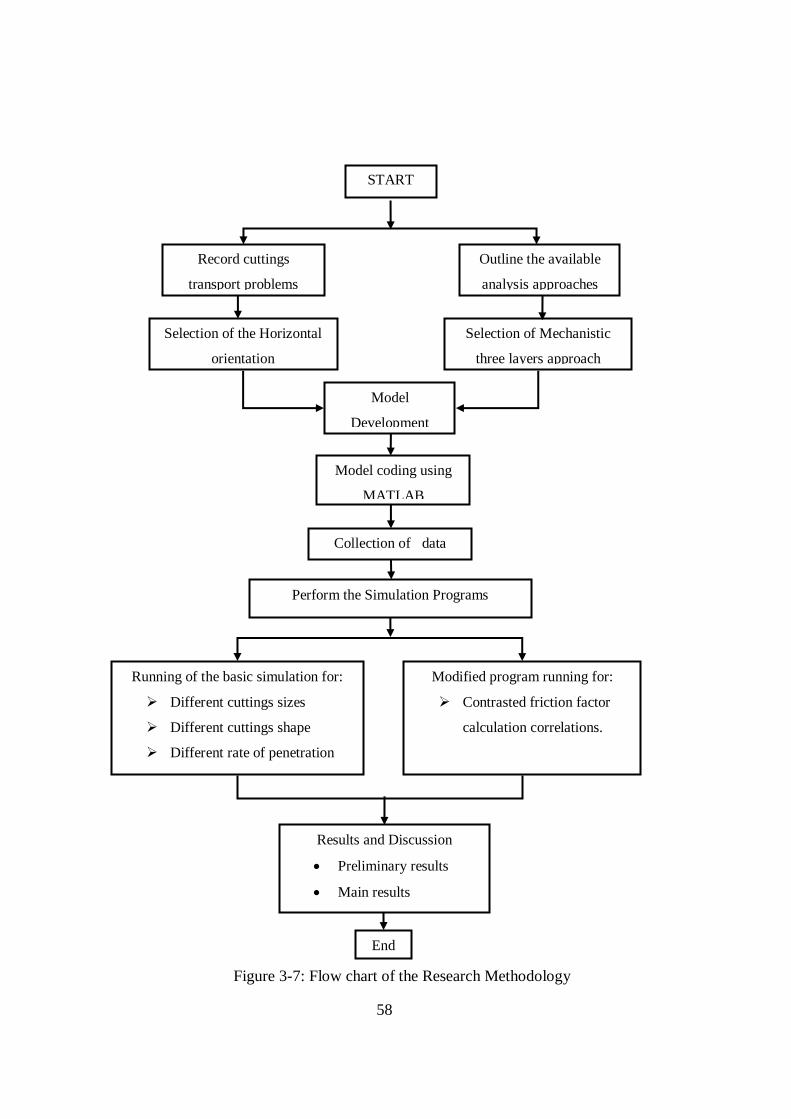
58

START

Collection of data

Outline the available

analysis approaches

Record cuttings

transport problems

Selection of Mechanistic

three layers approach

Model

Development

Selection of the Horizontal

orientation

Running of the basic simulation for:

Different cuttings sizes

Different cuttings shape

Different rate of penetration

Different fluid viscosities

Results and Discussion

Preliminary results

Main results

End

Model coding using

MATLAB

Modified program running for:

Contrasted friction factor

calculation correlations.

Perform the Simulation Programs

Figure 3-7: Flow chart of the Research Methodology

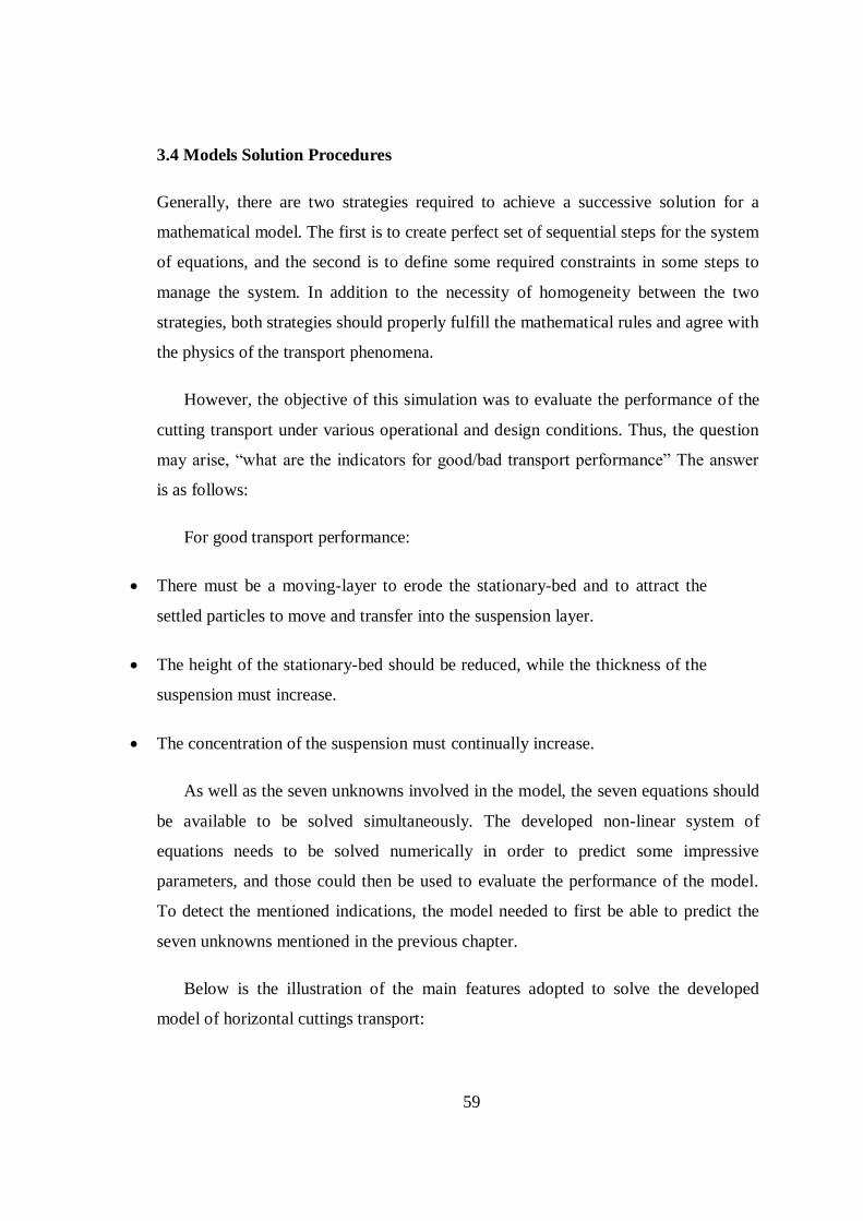
59

3.4 Models Solution Procedures

Generally, there are two strategies required to achieve a successive solution for a

mathematical model. The first is to create perfect set of sequential steps for the system

of equations, and the second is to define some required constraints in some steps to

manage the system. In addition to the necessity of homogeneity between the two

strategies, both strategies should properly fulfill the mathematical rules and agree with

the physics of the transport phenomena.

However, the objective of this simulation was to evaluate the performance of the

cutting transport under various operational and design conditions. Thus, the question

may arise, ―what are the indicators for good/bad transport performance‖ The answer

is as follows:

For good transport performance:

There must be a moving-layer to erode the stationary-bed and to attract the

settled particles to move and transfer into the suspension layer.

The height of the stationary-bed should be reduced, while the thickness of the

suspension must increase.

The concentration of the suspension must continually increase.

As well as the seven unknowns involved in the model, the seven equations should

be available to be solved simultaneously. The developed non-linear system of

equations needs to be solved numerically in order to predict some impressive

parameters, and those could then be used to evaluate the performance of the model.

To detect the mentioned indications, the model needed to first be able to predict the

seven unknowns mentioned in the previous chapter.

Below is the illustration of the main features adopted to solve the developed

model of horizontal cuttings transport:

60

3.4.1 The Operational and Design parameters

The research was carried out under various operational parameters and design

parameters, as shown by the following:

a. The rheological characteristic as viscosity of the drill-mud have impeded in

this work, as formulated in the power law of non-Newtonian fluid, which is

specified by the value of index behavior n and consistency index K given in

Table 3-1.

Table 3-1: The adopted viscosities of the drill-mud

Source

Class of Power-Law

Viscosity

Fluid Viscosity / power-law

K lbf.sn/ft

2 n

[4] Low viscosity 0.00600 0.68

[19]

Low viscosity 0.00084 0.68

Intermediate viscosity 0.00436 0.61

High viscosity 0.00930 0.61

b. The fluid density given in French units to investigate the particles behavior

given in Table 3-2

Table 3-2: Density of drill mud

Source Fluid Density g/cm3

[18]

0.9982

1.1983

1.4379

[4] 1.1024

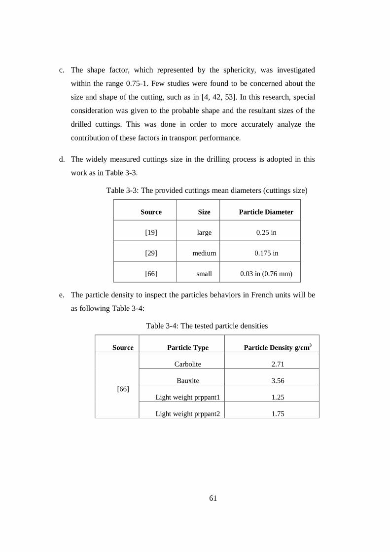
61

c. The shape factor, which represented by the sphericity, was investigated

within the range 0.75-1. Few studies were found to be concerned about the

size and shape of the cutting, such as in [4, 42, 53]. In this research, special

consideration was given to the probable shape and the resultant sizes of the

drilled cuttings. This was done in order to more accurately analyze the

contribution of these factors in transport performance.

d. The widely measured cuttings size in the drilling process is adopted in this

work as in Table 3-3.

Table 3-3: The provided cuttings mean diameters (cuttings size)

Source Size Particle Diameter

[19] large 0.25 in

[29] medium 0.175 in

[66] small 0.03 in (0.76 mm)

e. The particle density to inspect the particles behaviors in French units will be

as following Table 3-4:

Table 3-4: The tested particle densities

Source Particle Type Particle Density g/cm3

[66]

Carbolite 2.71

Bauxite 3.56

Light weight prppant1 1.25

Light weight prppant2 1.75

62

f. The annular size as per common practices of wells drilling is given below in

Table 3-5.

Table 3-5: The annular sizes studied in the simulation

Source Dw (in) Dp (in)

[39] 8.75 4.50

[29] 8.00 4.50

[4] 5.00 1.90

- 5.00 2.375

g. The Rate of Penetration or, (ROP) values were selected as in Table 3-6.

Table 3-6: The selected value of operational ROP

Source ROP (ft/hr)

[4] 50

[23] 60

[29] 30

[42] 15

Highlighting that in the basic and modified models the particle and the fluid

density are fixed at 163.60 lbm/ft3 or (2.62 g/cm

3), and 68.82 lbm/ft

3 or (9.2 lb/gal)

respectively. Drilled-cuttings removal occurs at high annular velocity rather than low

velocity. Incremental annular velocity might be applied to achieve wellbore cleaning.

3.4.2 Calculation of the Well Geometry

As a result of the gradual increase in the mud annular velocity, the layers heights and

other dependant geometrical quantities will automatically change. At the same time, a

cross section of the annular geometry combined with existence of three diverse layers

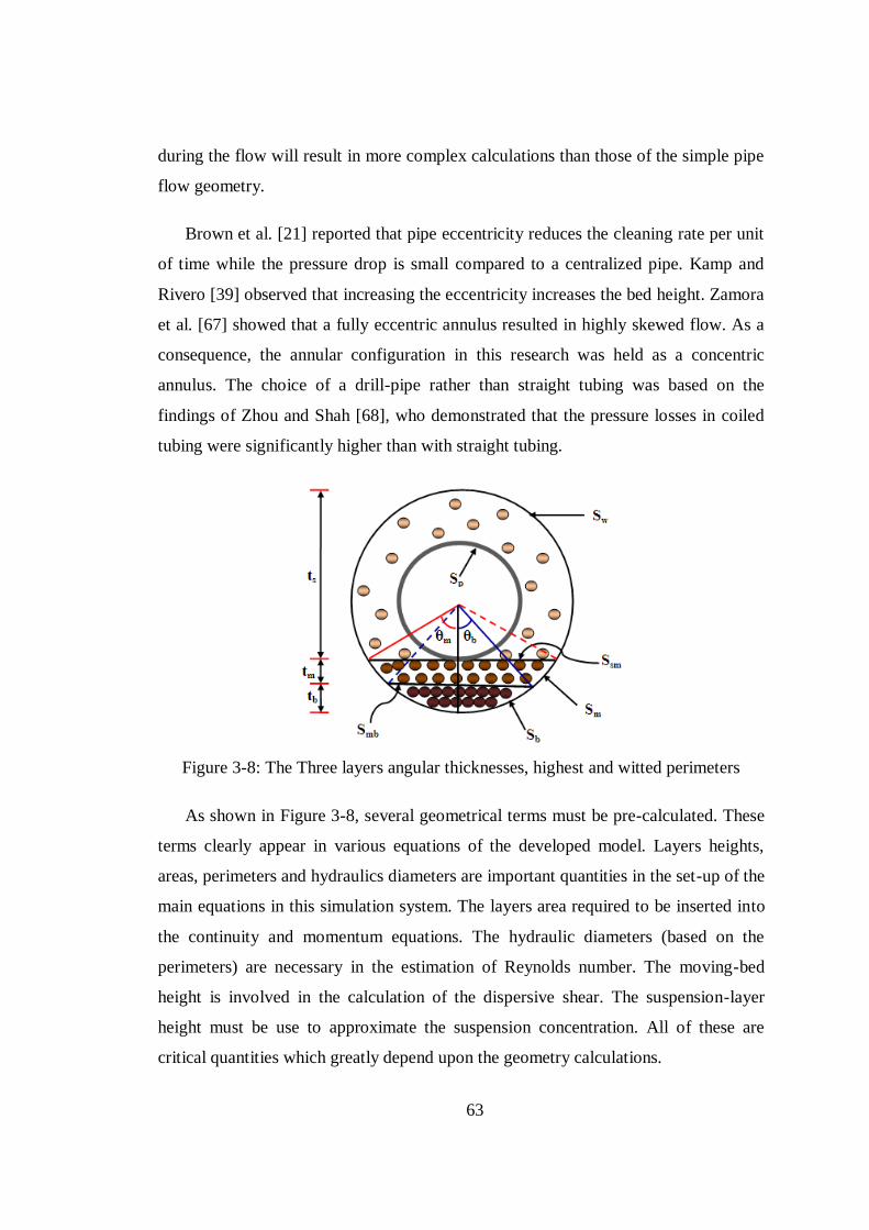
63

during the flow will result in more complex calculations than those of the simple pipe

flow geometry.

Brown et al. [21] reported that pipe eccentricity reduces the cleaning rate per unit

of time while the pressure drop is small compared to a centralized pipe. Kamp and

Rivero [39] observed that increasing the eccentricity increases the bed height. Zamora

et al. [67] showed that a fully eccentric annulus resulted in highly skewed flow. As a

consequence, the annular configuration in this research was held as a concentric

annulus. The choice of a drill-pipe rather than straight tubing was based on the

findings of Zhou and Shah [68], who demonstrated that the pressure losses in coiled

tubing were significantly higher than with straight tubing.

Figure 3-8: The Three layers angular thicknesses, highest and witted perimeters

As shown in Figure 3-8, several geometrical terms must be pre-calculated. These

terms clearly appear in various equations of the developed model. Layers heights,

areas, perimeters and hydraulics diameters are important quantities in the set-up of the

main equations in this simulation system. The layers area required to be inserted into

the continuity and momentum equations. The hydraulic diameters (based on the

perimeters) are necessary in the estimation of Reynolds number. The moving-bed

height is involved in the calculation of the dispersive shear. The suspension-layer

height must be use to approximate the suspension concentration. All of these are

critical quantities which greatly depend upon the geometry calculations.

64

Therefore, the well known trigonometric functions and areas of the plane shapes

were engaged to create a geometrical calculator. This is according to the possible

cases showed in Figure 3-9. The special program was written to generate the required

calculations, and attached to the main program as sub-routine. The derived

geometrical formulas are called the geometry engine (Appendix A)

Figure 3-9: Different cases for the formed bed heights

3.4.3 Algorithm Development

An algorithm is a description of how a sequence of the established instructions will be

executed to achieve the simulation tasks. The MATLAB R2008a software was used in

this research to write the sequence of tasks which represented the simulation code.

The development algorithm is crucial to the understanding of the vital parameters,

the equations, and the physics of the annular transport phenomena. The main

challenge in this research was assessing a possible perfect solution matching with the

logical mathematics and physics of the phenomena for the complicated non-linear

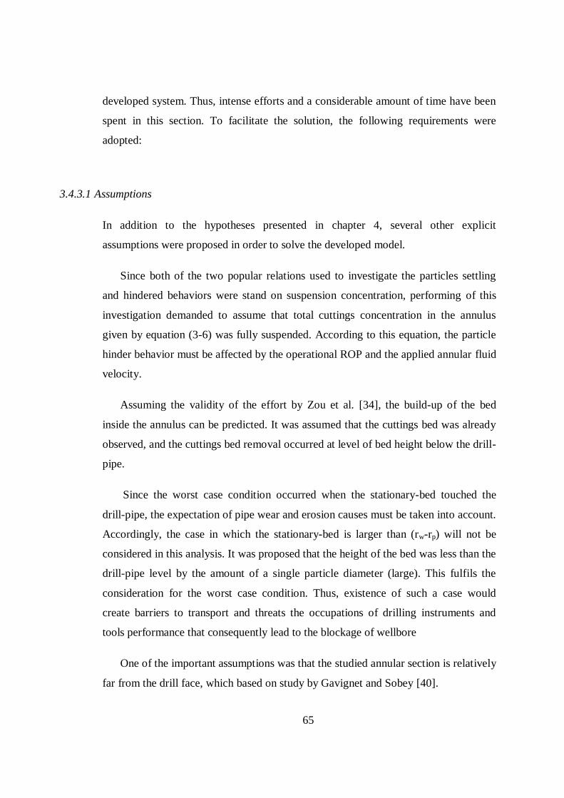
65

developed system. Thus, intense efforts and a considerable amount of time have been

spent in this section. To facilitate the solution, the following requirements were

adopted:

3.4.3.1 Assumptions

In addition to the hypotheses presented in chapter 4, several other explicit

assumptions were proposed in order to solve the developed model.

Since both of the two popular relations used to investigate the particles settling

and hindered behaviors were stand on suspension concentration, performing of this

investigation demanded to assume that total cuttings concentration in the annulus

given by equation (3-6) was fully suspended. According to this equation, the particle

hinder behavior must be affected by the operational ROP and the applied annular fluid

velocity.

Assuming the validity of the effort by Zou et al. [34], the build-up of the bed

inside the annulus can be predicted. It was assumed that the cuttings bed was already

observed, and the cuttings bed removal occurred at level of bed height below the drill-

pipe.

Since the worst case condition occurred when the stationary-bed touched the

drill-pipe, the expectation of pipe wear and erosion causes must be taken into account.

Accordingly, the case in which the stationary-bed is larger than (rw-rp) will not be

considered in this analysis. It was proposed that the height of the bed was less than the

drill-pipe level by the amount of a single particle diameter (large). This fulfils the

consideration for the worst case condition. Thus, existence of such a case would

create barriers to transport and threats the occupations of drilling instruments and

tools performance that consequently lead to the blockage of wellbore

One of the important assumptions was that the studied annular section is relatively

far from the drill face, which based on study by Gavignet and Sobey [40].

66

Another assumption made was to suppose that the bottom bed layer was

completely stilled, this building a dead-layer. Hence, the velocity of the stationary-bed

layer was approximated to be zero (Ub =0) [42]. Note that, behavior of the flow near

to the bed may tend to be slower, that could return alternatively laminar flow patterns.

3.4.3.2 Iteration procedure

As clearly visible, the model is a complex non-linear system, which required a huge

application of iterative procedures at many parts of the system to achieve solution for

the seven previously mentioned unknowns. Newton’s methods for non-linear

equations were employed in wide range to obtain solutions for some of the involved

variables. In order to solve Chien’s equation (3-43) for cutting settling velocity, the

well known Newton-Raphson method has been used. The solution algorithm to solve

and hinder the particle settling velocity is shown in Figure 3-10.

The Bisection method was used to solve the non-linear Szilas equation (3-13), in

order to achieve an effective solution for the friction factors in the guess ranges

between (0-1).

Particular iterative procedures to calculate Us, cs, Um, and tm based upon deep

understanding of the physics of the phenomena and the equations were applied in

order to obtain a satisfactory solution for the complicated horizontal cuttings transport

model.

3.4.3.3 Constrains

Because of the broad applicable values for the annular velocity and different

parameters during the iteration, the manual follow-up of the solution is not a practical

issue. Therefore, some constraints must be invoked in order to binding the limits of

the solutions. Nevertheless, the program run-stop criterion must also be constructed to

terminate the running of the program and enable results printing.

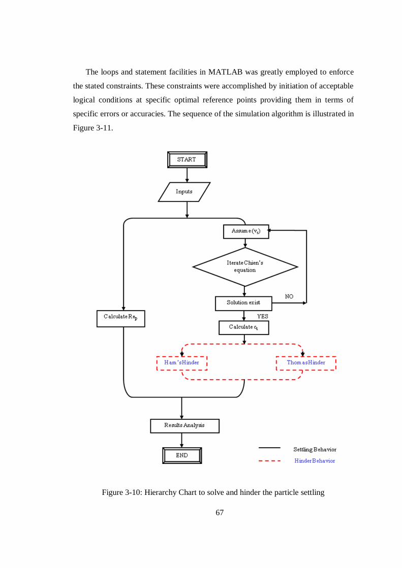
67

The loops and statement facilities in MATLAB was greatly employed to enforce

the stated constraints. These constraints were accomplished by initiation of acceptable

logical conditions at specific optimal reference points providing them in terms of

specific errors or accuracies. The sequence of the simulation algorithm is illustrated in

Figure 3-11.

Figure 3-10: Hierarchy Chart to solve and hinder the particle settling

68

Figure 3-11: Hierarchy Chart to solve the developed models.

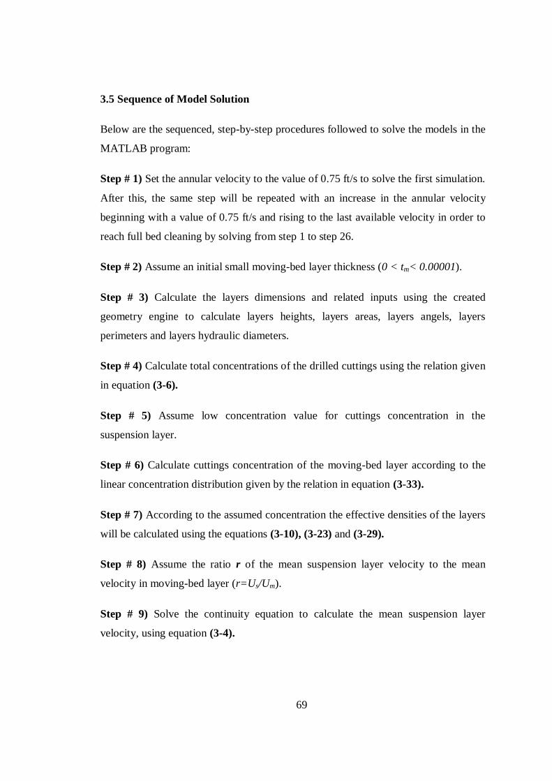
69

3.5 Sequence of Model Solution

Below are the sequenced, step-by-step procedures followed to solve the models in the

MATLAB program:

Step # 1) Set the annular velocity to the value of 0.75 ft/s to solve the first simulation.

After this, the same step will be repeated with an increase in the annular velocity

beginning with a value of 0.75 ft/s and rising to the last available velocity in order to

reach full bed cleaning by solving from step 1 to step 26.

Step # 2) Assume an initial small moving-bed layer thickness (0 < tm< 0.00001).

Step # 3) Calculate the layers dimensions and related inputs using the created

geometry engine to calculate layers heights, layers areas, layers angels, layers

perimeters and layers hydraulic diameters.

Step # 4) Calculate total concentrations of the drilled cuttings using the relation given

in equation (3-6).

Step # 5) Assume low concentration value for cuttings concentration in the

suspension layer.

Step # 6) Calculate cuttings concentration of the moving-bed layer according to the

linear concentration distribution given by the relation in equation (3-33).

Step # 7) According to the assumed concentration the effective densities of the layers

will be calculated using the equations (3-10), (3-23) and (3-29).

Step # 8) Assume the ratio r of the mean suspension layer velocity to the mean

velocity in moving-bed layer (r=Us/Um).

Step # 9) Solve the continuity equation to calculate the mean suspension layer

velocity, using equation (3-4).

70

Step # 10) Calculate the generalized Reynolds number. of suspension (3-11) based

upon the suspended layer mean velocity and effective density.

Step # 11) Import the hydraulic diameter of the suspension from the Geometry engine

and iterate Szilas equation (3-13) to calculate the friction factor between the upper

suspension layer and walls of the well, and pipe up to accuracy ׀ƒ-ƒ’0.00001>׀.

Step # 12) Calculate the interfacial friction factor between suspension and moving

bed layers according to (3-15).

Step # 13) Calculate the mean velocity of the Moving-bed layer using equation (3-34)

Step # 14) Calculate the new ratio r’ between the obtained suspension and moving

bed mean velocities to check the error of the assumption in Step # 8 up to accuracy of

.0.00001>׀’r-r ׀

Step # 15) Using the mean layers velocities and interfacial friction factor, calculate

the cutting particles diffusivity coefficient equation (3-41).

Step # 16) Iterate Chein’s settling velocity equation (3-43) to obtain the particle

settling velocity.

Step # 17) Hinder the particle settling velocity using the suspension concentration by

Hams and Homey’s correlation (3-47).

Step # 18) Calculate the suspension layer concentration using the convection-

diffusion equation. Check the error of suspension concentration assumption in Step #

5 up to accuracy of ׀cs-cs’0.00001>׀, and thereby the following calculations would be

amended.

Step # 19) Calculate generalized Re no. in the moving bed layer using the layer

effective density and mean velocity.

Step # 20) Iterate Szilas’s equation to calculate the friction factor between the moving

bed layer and the well wall.

71

Step # 21) Obtain the interfacial friction between the moving and stationary-bed using

the concept at (3-21).

Step # 22) Calculate all exerted shear stresses according to the layers movement using

the set of equations (3-8), (3-9), (3-19), and (3-20).

Step # 23) Calculate the pressure drop using the upper layer momentum equation

(4.9).

Step # 24) Utilize the relation between equation (3-25) and (3-30) in (3-18) to

calculate the dispersive shear stress.

Step # 25) Calculate the moving-bed thickness from its relation with the dispersive

shear stress given by equation (3-30). Check the moving bed thickness assumption in

Step # 2 up to accuracy of ׀tm-tm’0.00001>׀

Step # 26) Print the results of the seven unknowns, the important parameters, and then

end the program.

Note that, the above 26 steps were followed to obtain the values of the seven

required unknowns at bed height and each given annular velocity.

Without further alter on the previous theoretical steps, an additional solution

beyond the first set was obtained by making changes to some of the model equations.

Mainly, Szilas’ correlation in (3-13) was replaced by the other frictional factor

empirical relations, which is given by (3-16) and (3-17), that enabled opportunity of

diverse model simulation.

3.6 Summary

In this current chapter, all aspects of the equations required to initiate simulation of

the cutting particles transport in horizontal annular conduit have been specified. The

chapter reviewed the main features of the developed three layered model. The

72

importance of some equations needed for the installation of the model, such as

convection-diffusion, settling velocity and hinder settling velocity factor were

highlighted.

Moreover, extra equations beyond the model requirement were added to this

section for the purpose of generating an alternative method to calculate the friction

factors and to examine its effect. Thus, preparation of modified model will permit a

contrasted program to be run, and thereby comprehensive comparisons could be

conducted.

The chapter denotes the referenced input data, and presented the details of the

developed system solution procedures. Beside justifications of selection of the fluid

and particle features, several essential assumptions were justified. In addition, some of

the constraints necessary to proceed with the simulation and to activate the model

were presented. The scenario of the model solution in a step-by-step manner was also

specified.

With incremental increase in the annular velocity, identical steps were similarly

followed to simulate the process of cleaning for the modified model, except that in the

modified case there was no need to apply the Bisection method.

73

Chapter 4

Results and Discussion

4.1 Introduction

This chapter presenting analysis of the results obtained from the developed

models. As well known, particle settling behavior plays a major role in the formation

of cuttings bed layer. Accordingly this chapter document two important phenomena,

first, is the settling behavior of single non spherical particle falls in non Newtonian

fluid, and second is the hinder behavior cased by collision of solid particles. Besides,

the influence of the sphericity factor φ in the behaviors was involved. In advance the

chapter also presented the results obtained from the developed model where the

cuttings transportation process was investigated into two different evaluation

procedures for the frictional shear forces. Hence, the models results are presented into

two subsections. The first subsection present and discuss performance of the cuttings

transport by evaluating the frictional shear stresses according to Szilas hypothesis,

which consequently will be called the basic model results. The second subsection

present and discuss performance of the cuttings transportation using other empirical

correlations captured from the literature to evaluate the frictional shear stresses, and

this will be called the modified model results.

4.2 Particle Settling Behaviour

The behavior of particles settling is very important in various multi phase flow

applications. In petroleum applications, slurry flow of drill-mud with the drilled

74

cuttings in transport process is an important application. As shown in Figure 4-1,

transport of single cutting particle strongly influenced by the flow direction. Hence,

the settling behavior represents important tangible phenomena especially in the

directional drilling. Indeed that deeper understanding of this phenomenon is crucial to

model and analyze the targeted performance in drilling process. The required

minimum velocity to transport solids depends upon the amount and behavior of

settled particles.

Figure 4-1: Particle settling in vertical, inclined and horizontal flow

4.2.1 Results and Discussion of the Settling Behaviour

Investigation of the settling behaviour was carried through different particles

characteristics and different fluid properties and the results showed the following:

4.2.1.1 Effect of Particle Density on Particle Settling

To vary the particle density, an intermediate fluid viscosity properties of K = 0.2088

Pa.sn, n = 0.61 was engaged. Settling behavior for the different particle densities was

examined using large and small particle sizes. Results of large particle size dp=0.7 cm

were shown in Figure 4-2 (a). Study of four level of particle density reflected that

large particle density merged with large cuttings size fall at high velocities. In

addition, the shape factor effect was clearly appeared at the highest particles density.

Where at low particle density 1.25 g/cm3, the contribution of the shape factor on

75

settling velocity was small. Thus, settling velocity of low particle density 1.25 g/cm3

of shape factor range 0.75-0.9 was changed in a range of 2.22 and 2.34 cm/s. The

settling velocity of the high particle density for the same sphericity range is observed

to range between 30.82-42.95 cm/s.

0 100 200 300 400 500 6000

5

10

15

20

25

30

35

40

45

Particle Reynolds Number (Rep)

Sett

ling V

elo

city (

vs)c

m/s

-0.05 0 0.05 0.1 0.15 0.2 0.25 0.3 0.35 0.4 0.45

0

0.1

0.2

0.3

0.4

0.5

0.6

0.7

0.8

Particle Reynolds Number (Rep)

Sett

ling V

elo

city (

vs)c

m/s

Figure 4-2: Effect of particle density on settling velocity of (a) large particle sizes, (b)

small particle size

As shown in Figure 4-2 (b), flow of small particle size of 0.08 cm diameter with

different particle density was lower. Highest particle density of 3.56 g/cm3 was settled

down at 0.7 m/s velocity, meaning that lower particle density would exert much lower

settling velocity. In general, particle settling velocity increases as long as particle

density increase and this was also found to be crucial to the particle shape and size.

Ozbayoglu et al. [69], agreed that due to the gravitational effect greater particle

density is harder to be lift.

4.2.1.2 Effect of Particle Size on Particle Settling

To examine the particle size effect, the settling behavior was encountered at

intermediate fluid viscosity K=0.2088 Pa.sn, n=0.61. Figure 4-3 (a) shows the settling

results for different four particle sizes which flow at low fluid density 0.9982 g/cm3. It

(

a)

(

b)

ρp=3.56

ρp=2.71

ρp=1.25

ρp=1.75

ρp=3.56

ρp=2.71

ρp=1.25

ρp=1.75

76

can be observed that, high particle size having more regular shape was behaved high

settling. At high fluid density of 1.4379 g/cm3, result of the all size were in low

settling behavior compared to their behavior at lower fluid density of 0.9982 g/cm3, as

shown in Figure 4-3 (b). Thus, such increase on the fluid density from 0.9982 to

1.4379 g/cm3 was capable to suspend larger cutting and reduces the settling behavior.

The settling velocity of high size particle 0.70 cm and 0.9 shape factor was reduced

from 17.98 to 6.44 cm/s.

Moreover, flow of small size particle of 0.08 cm at low fluid density was low.

Small size has lower settling velocity even at high sphericity factor 0.9 compared to

the large sized particles which has a significant settling velocity of 17.98 cm/s.

0 20 40 60 80 100 120 1400

2

4

6

8

10

12

14

16

18

Particle Reynolds Number (Rep)

Sett

ling V

elo

city (

vs)c

m/s

-10 0 10 20 30 40 500

1

2

3

4

5

6

7

Particle Reynolds Number (Rep)

Sett

ling V

elo

city (

vs)c

m/s

Figure 4-3: Effect of particle size on settling at (a) low fluid density, (b) high fluid

density.

Large sized cuttings found to behave more settling, Zhou [37], observed that

larger cuttings cleaning are the most difficult. On the other hand Ozbayoglu et al. [69]

, announced that contribution of the cutting size effect depend on the direction of the

fluid flow. As fluid flow vertically prevention of small size settling was the easy.

(

a)

(

b)

dp=0.70

dp=0.64

dp=0.44

dp=0.08

dp=0.70

dp=0.64

dp=0.44

dp=0.08

77

4.2.1.3 Effect of Fluid Density on Particle Settling

To inspect the effect of fluid density, medium particle size of 0.44 cm mean diameter

and relatively medium particle density 1.75g/cm3 were used. Maintaining the power

law fluid viscosity at K = 0.0402 Pa.sn, n = 0.68, Figure 4-4 (a) demonstrated that, the

particle settling velocities were high at low fluid density. The lowest settling velocity

was encountered at higher fluid density of 1.4379 g/cm3, where 0.75 particle

sphericity was found to settle at 6.84 cm/s. While at low fluid density of 0.9982

g/cm3, similar particle exerted 14.18 cm/s settling velocity.

In Figure 4-4 (b) the fluid viscosity was upgraded to have K = 0.4453Pa.sn, n =

0.61. It can be realized that, regardless of the particle shape all fluid densities were

resulted in less settling velocities. Thus, at low fluid densities increasing of the

viscosity would help to reduce the high settling behaviors and vice versa.

100 150 200 250 300 350 4006

8

10

12

14

16

18

20

Particle Reynolds Number (Rep)

Sett

ling V

elo

city (

vs)c

m/s

0.5 1 1.5 2 2.5 3 3.5 4 4.5

0.5

1

1.5

2

2.5

3

3.5

Particle Reynolds Number (Rep)

Sett

ling V

elo

city (

vs)c

m/s

Figure 4-4: Effect of particle density on settling at (a) low fluid density, and (b) high

fluid density

This agrees with Zhou [37], where increasing of the fluid density resulted in better

hole cleaning, that indicate high fluid density able to prevent high settling behavior. In

addition Ozbayoglu et al. [69] reported that increase of the fluid density allows

improving the bouncy effect as low force would be required to perform on the settled

cuttings.

(

a)

(

b)

ρf=0.9982

ρf=1.1024

ρf=1.1983

ρf=1.4379

ρf=0.9982

ρf=1.1024

ρf=1.1983

ρf=1.4379

78

4.2.1.4 Effect of Fluid Viscosity on Particle Settling

Figure 4-5 (a) shows the effect of the viscosity on the settling. Settling of a small

particle at different levels of fluid viscosity was low. Generally the settling behavior

increased with decreasing of the fluid viscosity.

Larger regular particles of 0.70 cm fall faster in the lower fluid viscosity

K=0.0402 Pa.sn, n=0.68, as shown in Figure 4-5 (b). In instance, for large particle

with sphericity 0.75, the minimum observed settling velocity was 5.22 cm/s which

occurred at the lowest fluid viscosity. For large particle, the minimum velocity at

sphericity of 0.75, was 14.85 cm/s, and the maximum velocity was 20.97 cm/s for

particle of 0.9 sphericity. The results shown that, the shape factor was a significant

parameter in the settling. As the particle shape approaches spherical shape, the setting

rapidly increased. This referred to the reduction of the drag force acting opposite to

the settling direction.

0 0.2 0.4 0.6 0.8 1 1.2 1.4 1.6 1.80

0.1

0.2

0.3

0.4

0.5

0.6

0.7

0.8

Particle Reynolds Number (Rep)

Sett

ling V

elo

city (

vs)c

m/s

0 100 200 300 400 500 600 700

4

6

8

10

12

14

16

18

20

22

Particle Reynolds Number (Rep)

Sett

ling V

elo

city (

vs)c

m/s

Figure 4-5: Effect of the fluid viscosity on settling behavior of (a) small particle size,

and (b) large sized particle.

Increase in K value from 0.2088 to 0.4453 Pa.sn reduces the settling velocity for

large particle 0.70 cm diameter at maximum sphericity 0.9 from 12.65 cm/s to 5.65

cm/s. Such increasing on K from 0.0402 to 0.2873 Pa.sn improved the viscosity and

served to avoid settling of particle from 20.97 cm/s to 7.96 cm/s and also reduced Rep.

(

a)

(

b)

K=0.0402, n=0.68

K=0.2088, n=0.61

K=0.2873, n=0.68

K=0.4453, n=0.61

K=0.0402, n=0.68

K=0.2088, n=0.61

K=0.2873, n=0.68

K=0.4453, n=0.61

79

Thus, particle exerts high Rep at maximum settling velocity. Generally, slight

increasing of the fluid viscosity helped to suspend the particle.

Ozbayoglu [69] denoted that increase on the fluid viscosity improves the fluid

carrying capacity. Also they reported that reducing of the index behavior n increase

the flow velocity and thereby decrease cutting bed’s height i.e. resists settling

behavior. Besides, Adari et al [31], stated that removal of settled cuttings on bed

enhance as n/K ratio increases notice that their mentioned recommendation was made

to meet highly inclined to horizontal flow direction.

4.3 Hindered Settling Behaviour

As much as particle settling velocity became higher, it will have more influence on

the transport process. The previous investigation on the particle settling behavior

indicated that, the high settling velocities occur at:

Low fluid viscosities

Low fluid densities

High particle size

High particle density

Therefore, the four condition were adopted in order to inspect the hinder behavior

on the cuttings settling velocity using the two correlations in (3-46) and (3-47).

4.3.1 Results and Discussions of the Hindered Settling Behaviour

According to adoption of the four situations, different cases of settling velocities were

stated to encounter the hinder behavior through them. To generalize the outcome of

the results, this inspection was made at high and low ROP 50 and 15 ft/hr, and

performed for two annular velocities 2 ft/s as low velocity, and high velocity of 5 ft/s.

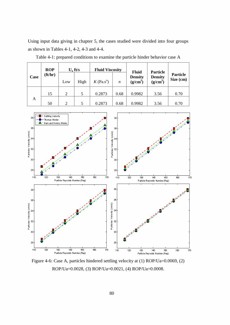
80

Using input data giving in chapter 5, the cases studied were divided into four groups

as shown in Tables 4-1, 4-2, 4-3 and 4-4.

Table 4-1: prepared conditions to examine the particle hinder behavior case A

Case

ROP

(ft/hr)

Ua ft/s Fluid Viscosity Fluid

Density

(g/cm3)

Particle

Density

(g/cm3)

Particle

Size (cm) Low High K (Pa.s

n) n

A 15 2 5 0.2873 0.68 0.9982 3.56 0.70

50 2 5 0.2873 0.68 0.9982 3.56 0.70

Figure 4-6: Case A, particles hindered settling velocity at (1) ROP/Ua=0.0069, (2)

ROP/Ua=0.0028, (3) ROP/Ua=0.0021, (4) ROP/Ua=0.0008.

(

1)

(

2)

(

3)

(

4)

(

1)

(

2)

(

3)

(

4)

81

Table 4-2: Prepared conditions to examine the particle hinder behavior case B

Case

ROP

(ft/hr)

Ua ft/s Fluid Viscosity Fluid

Density

(g/cm3)

Particle

Density

(g/cm3)

Particle

Size (cm) Low High K (Pa.s

n) n

B

15 2 5 0.0402 0.68 1.1024 2.71 0.64

50 2 5 0.0402 0.68 1.1024 2.71 0.64

Figure 4-7: Case B, particles hindered settling velocity at (1) ROP/Ua=0.0069, (2)

ROP/Ua=0.0028, ROP/Ua=0.0021 (3), (4) ROP/Ua=0.0008.

(

1)

(

2)

(

3)

(

4)

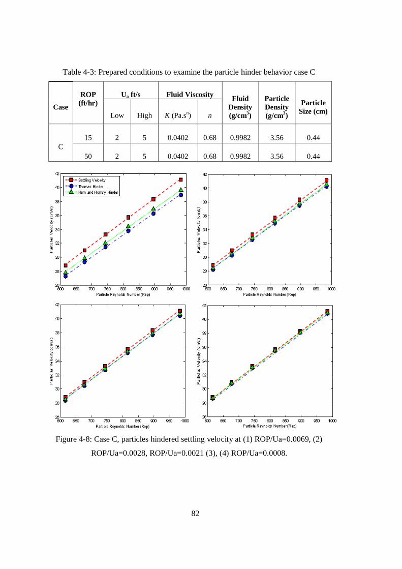
82

Table 4-3: Prepared conditions to examine the particle hinder behavior case C

Case

ROP

(ft/hr)

Ua ft/s Fluid Viscosity Fluid

Density

(g/cm3)

Particle

Density

(g/cm3)

Particle

Size (cm) Low High K (Pa.s

n) n

C

15 2 5 0.0402 0.68 0.9982 3.56 0.44

50 2 5 0.0402 0.68 0.9982 3.56 0.44

Figure 4-8: Case C, particles hindered settling velocity at (1) ROP/Ua=0.0069, (2)

ROP/Ua=0.0028, ROP/Ua=0.0021 (3), (4) ROP/Ua=0.0008.

(

1)

(

2)

(

3)

(

4)

83

Table 4-4: Prepared conditions to examine the particle hinder behavior case D

Case

ROP

(ft/hr)

Ua ft/s Fluid Viscosity Fluid

Density

(g/cm3)

Particle

Density

(g/cm3)

Particle

Size (cm) Low High K (Pa.s

n) n

D

15 2 5 0.2873 0.68 1.1024 2.71 0.64

50 2 5 0.2873 0.68 1.1024 2.71 0.64

Figure 4-9: Case D, particles hindered settling velocity at (1) ROP/Ua=0.0069, (2)

ROP/Ua=0.0028, ROP/Ua=0.0021 (3), (4) ROP/Ua=0.0008.

(

1)

(

2)

(

3)

(

4)

84

According to the schematic results shown in Figure 4-6, 4-7, 4-8 and 4-9, with

increasing the sphericity by portion of 0.03 from 0.75 up to 0.90, it was recognized

that always Thomas correlation gives relatively less hinder velocity values than those

by Ham and Homsy’s equation.

At the same annular size, the higher difference between settling velocities and

hinder settling velocity was greatly encountered at the highest ratio of the ROP to the

annular velocity ROP/Ua=0.0069. That indicates the significant role of cuttings

concentration in the hindered behavior. Thus, under similar conditions and at low

cuttings concentration the effect of the hinder behavior seems negligible, which is

more significant at the lowest ratio ROP/Ua=0.0008.

According to the upper four cases, ignore of the hinder behavior of cluster of

particles generated 5.60-0.70% error measured on Ham and Homsy’s correlation.

While returned 3.80-0.45% error based on Thomas correlation. Whereas, such errors

as primary calculations able to disturb reliability of dependable calculations that may

use as basis in design and/or operational tasks.

Cluster of cuttings found to behave lower settling compared to a single particle

settling velocity, particle collision should carefully be considered especially at high

cuttings concentrations and high sphericity. Since horizontal transport demonstrates

higher cuttings concentration, it was recommended that hinder velocity correlations

should be used to avoid errors regardless of settling velocity values or concentration.

4.4 Simulation Results

Ramadan et al. [3], presented a mathematical model on the particle flow in highly

deviated pipe flow. Stevenson [47] commented on Ramadan et al.’s paper mentioning

that, their model is extremely identical to the model of pipe flow by Doron et al. 1997.

However, in spite of that criticism, work by Ramadan et al. was used as base back

ground for the presented model. In this research multiple changes were carried out on

85

Ramadan et al.’s model. Therefore, what is developed in the current research is

entirely differ as shown in Table 4-5.

Table 4-5: Differences between the current model and previous models.

Feature Previous Models Current Model

Section Pipe/Eccentric Concentric Annulus

Total concentration assumed input Calculated, Ct=f(ROP, Dp, Dw, Ua)

[43]

Particle shape Sphere Irregular shapes (sphericity)

Diffusivity distance hm/100 2dp, FredsZe & Deigaard (1992) [3]

Fluid Bentonite & PAC

solution Various Non-Newtonian muds

Settling velocity Dedegil (1987) Chien (1994) model [50]

4.4.1 Basic Model Simulation Results and Discussion

Simulation results of the basic model are presented in (Appendix B) and analyzed in

term of the examined parameters, which were, the annular mud velocity, the drilled

cuttings size, the drilled cuttings shape, the fluid viscosity, the ROP and the annular

geometry size, as shown in the following analysis:

4.4.1.1 Effect of Annular Velocity on Cuttings Transport

Regardless of all factors affecting on the process of the cuttings removal, simulation

of horizontal transport indicated the great importance of the annular fluid velocity on

the transport. This is clearly understood from the extracted correlations shown in

(Appendix C). Li and Walker [25], recorded that, at all drilling modes the most

important variable affecting the cuttings transport was the in-situ liquid velocity. The

transport performance was parallel increase as annular flow velocity increases. For

86

the range of the input data, where cuttings transport inspected in range of 0.75-6.3 ft/s

annular velocity, the better hole cleaning was repeatedly recorded at higher annular

mud velocities which reported to be occurred between 4.5-6.3 ft/s.

However, increasing the annular velocity returned thicker suspension layers at all

cases, meaning that higher annular velocities guarantees considerable reduction on the

cuttings bed layer. Increasing of the annular mud velocity enhanced removal of the

stationary particles to travel to the upper moving-bed layer delivering thicker moving-

bed layer as noticed in the moving-bed built up (Appendix C). This was also

supported by Okrajni and Azar [20] , where they have reported that higher annular

velocity intended to limit cuttings bed formation in the directional transport. As well,

the results agrees with [27] and assured that high flow rate is quietly demanded in

order to generate high shear force to erode cuttings beds.

4.4.1.2 Effect of Cuttings Size on Cuttings Transport

Through testing of three different particle sizes (large medium and small cuttings)

increasing of the annular fluid velocity was also essentially to accomplish vanish of

the stationary-bed layer. Highlighting that, existence of the moving-bed layer at a

certain mud velocity did not mean vanishing of the bed layer corresponding to this

velocity. Supposing that the moving-bed layer is considerable once tm became higher

than/or equal to dp, existence of true moving-bed layer at the different cutting sizes

was considered as in Table 4-6.

As noticed in Table 4-6, higher annular fluid velocity is extremely required to

terminate the bed layer. In case of large size of 0.25 in, moving-bed layer appears at

relatively higher annular velocity compared to the case of smaller sized particles. The

reason behind the difference in the bed termination velocity is related to the different

requirements of the erosion at the upper surface of the bed-layer for the different

cuttings sizes. Naturally high drags are demanded to overcome the opposite hindered

forces of large sizes. For the smaller particles lower drag force are needed to erode

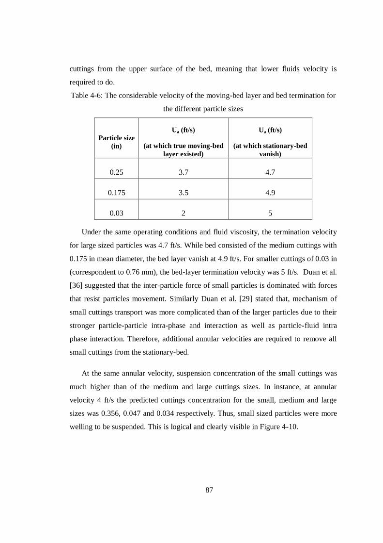
87

cuttings from the upper surface of the bed, meaning that lower fluids velocity is

required to do.

Table 4-6: The considerable velocity of the moving-bed layer and bed termination for

the different particle sizes

Particle size

(in)

Ua (ft/s)

(at which true moving-bed

layer existed)

Ua (ft/s)

(at which stationary-bed

vanish)

0.25 3.7 4.7

0.175 3.5 4.9

0.03 2 5

Under the same operating conditions and fluid viscosity, the termination velocity

for large sized particles was 4.7 ft/s. While bed consisted of the medium cuttings with

0.175 in mean diameter, the bed layer vanish at 4.9 ft/s. For smaller cuttings of 0.03 in

(correspondent to 0.76 mm), the bed-layer termination velocity was 5 ft/s. Duan et al.

[36] suggested that the inter-particle force of small particles is dominated with forces

that resist particles movement. Similarly Duan et al. [29] stated that, mechanism of

small cuttings transport was more complicated than of the larger particles due to their

stronger particle-particle intra-phase and interaction as well as particle-fluid intra

phase interaction. Therefore, additional annular velocities are required to remove all

small cuttings from the stationary-bed.

At the same annular velocity, suspension concentration of the small cuttings was

much higher than of the medium and large cuttings sizes. In instance, at annular

velocity 4 ft/s the predicted cuttings concentration for the small, medium and large

sizes was 0.356, 0.047 and 0.034 respectively. Thus, small sized particles were more

welling to be suspended. This is logical and clearly visible in Figure 4-10.

88

0.5 1 1.5 2 2.5 3 3.5 4 4.5 50

0.05

0.1

0.15

0.2

0.25

0.3

0.35

0.4

Annular Velocity (ft/s)

Suspensio

n C

oncentr

ation (

fraction)

Large cuttings

Medium cuttings

Small cuttings

Figure 4-10: Effet of annular velocity on suspended layers concentration at different

particle sizes

0 1 2 3 4 5 6 7

x 104

0

0.2

0.4

0.6

0.8

1

1.2

1.4

1.6

1.8

Reynolds Number

Eddy D

iffu

siv

ity (

in2/s

)

Large cuttings

Medium cuttings

Small cuttings

Figure 4-11: Eddy Diffusivity of the different particle size

The evaluated eddy diffusivity as function of particle size showed in Figure 4-11.

This figure specifies that higher eddy diffusivity was needed by the large sized

particles.

89

Altunbas et al. [70], concluded that eddy diffusivity of particles in horizontal flow

increase as their sedimentation velocity increases, where it is confirmed that larger

cuttings exerting high settling velocities. Therefore large particles demanded to

generate higher eddy diffusivity than of small ones. Accordingly, diffusivity of

cutting particles enlarges with their size. This truth is also visible through formula of

the eddy diffusivity at [17] where the eddy diffusivity coefficient of cutting is

enlarges with their size.

As shown in Figure 4-12, at equivalent annular velocity, transport of large and

medium cuttings size exerted less shear stress ratio at the bed surface compared to the

small size which is agrees with the trend observed by Ramadan et al.

0.5 1 1.5 2 2.5 3 3.5 4 4.5 50

2

4

6

8

10

12

14

16

18

20

Annular Velocity (ft/s)Ratio o

f D

ispers

ive s

hear

to M

ovin

g-b

ed-S

tationary

-bed S

hear

str

ess

Large cuttings

Medium cuttings

Small cuttings

Figure 4-12: Ratio of the bed layers shear stress for the different cuttings size

Figure 4-13 shows the predicted pressure drop along the annulus at various

annular velocities. Large sized particles needs to apply more pressure force to be

transported.

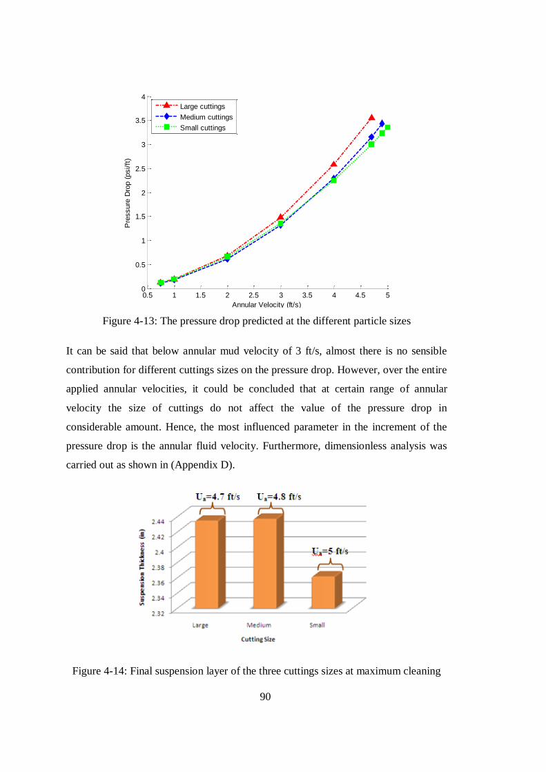
90

0.5 1 1.5 2 2.5 3 3.5 4 4.5 50

0.5

1

1.5

2

2.5

3

3.5

4

Annular Velocity (ft/s)

Pre

ssure

Dro

p (

psi/ft

)

Large cuttings

Medium cuttings

Small cuttings

Figure 4-13: The pressure drop predicted at the different particle sizes

It can be said that below annular mud velocity of 3 ft/s, almost there is no sensible

contribution for different cuttings sizes on the pressure drop. However, over the entire

applied annular velocities, it could be concluded that at certain range of annular

velocity the size of cuttings do not affect the value of the pressure drop in

considerable amount. Hence, the most influenced parameter in the increment of the

pressure drop is the annular fluid velocity. Furthermore, dimensionless analysis was

carried out as shown in (Appendix D).

Figure 4-14: Final suspension layer of the three cuttings sizes at maximum cleaning

91

Figure 4-14 presented a zoom in view on the thickness of the suspended layer

under different particles sizes. The figure confirmed that, height of the suspension of

the small sized cuttings is lower than in case of large and medium sized particles.

Built up of the moving-bed layer is an indication for the particles transfer from the

stationary-bed as shown in Figure 4-15. Due to the velocity flow, eddies will be

generated at the bed surface consequently the shear force enhance transport of the

cuttings particles to the upper layers. Here also annular velocity of the carrier fluid

plays the significant role to move the stationary cuttings.

0.5 1 1.5 2 2.5 3 3.5 4 4.5 50

0.1

0.2

0.3

0.4

0.5

0.6

0.7

0.8

Annular Velocity (ft/s)

Movin

g-b

ed B

uild

-up (

in)

Large cuttings

Medium cuttings

Small cuttings

Figure 4-15: Moving-bed layer growth under increasing annular velocity

Once stationary-bed vanishes, two layers remains as suspension and moving-bed

layer. At this point the transport performance of each layer is shown in Figure 4-16,

for the large, medium and small particles as percentage of initial and resulted layers.

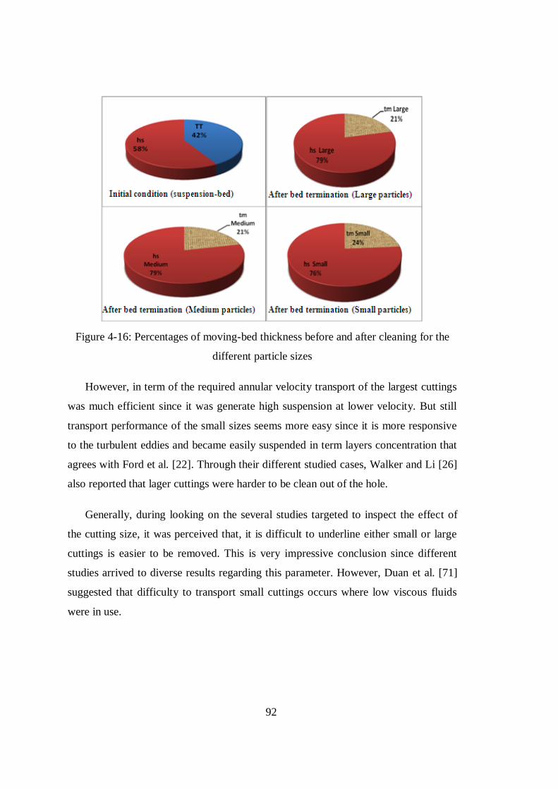
92

Figure 4-16: Percentages of moving-bed thickness before and after cleaning for the

different particle sizes

However, in term of the required annular velocity transport of the largest cuttings

was much efficient since it was generate high suspension at lower velocity. But still

transport performance of the small sizes seems more easy since it is more responsive

to the turbulent eddies and became easily suspended in term layers concentration that

agrees with Ford et al. [22]. Through their different studied cases, Walker and Li [26]

also reported that lager cuttings were harder to be clean out of the hole.

Generally, during looking on the several studies targeted to inspect the effect of

the cutting size, it was perceived that, it is difficult to underline either small or large

cuttings is easier to be removed. This is very impressive conclusion since different

studies arrived to diverse results regarding this parameter. However, Duan et al. [71]

suggested that difficulty to transport small cuttings occurs where low viscous fluids

were in use.

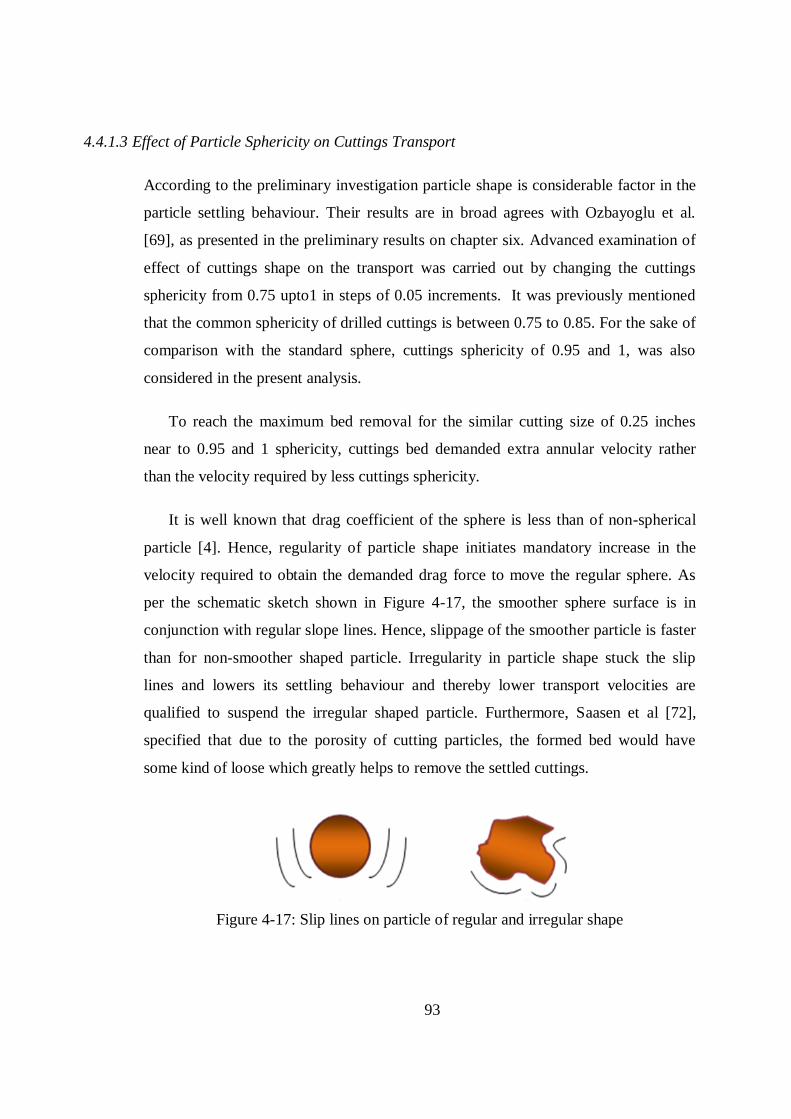
93

4.4.1.3 Effect of Particle Sphericity on Cuttings Transport

According to the preliminary investigation particle shape is considerable factor in the

particle settling behaviour. Their results are in broad agrees with Ozbayoglu et al.

[69], as presented in the preliminary results on chapter six. Advanced examination of

effect of cuttings shape on the transport was carried out by changing the cuttings

sphericity from 0.75 upto1 in steps of 0.05 increments. It was previously mentioned

that the common sphericity of drilled cuttings is between 0.75 to 0.85. For the sake of

comparison with the standard sphere, cuttings sphericity of 0.95 and 1, was also

considered in the present analysis.

To reach the maximum bed removal for the similar cutting size of 0.25 inches

near to 0.95 and 1 sphericity, cuttings bed demanded extra annular velocity rather

than the velocity required by less cuttings sphericity.

It is well known that drag coefficient of the sphere is less than of non-spherical

particle [4]. Hence, regularity of particle shape initiates mandatory increase in the

velocity required to obtain the demanded drag force to move the regular sphere. As

per the schematic sketch shown in Figure 4-17, the smoother sphere surface is in

conjunction with regular slope lines. Hence, slippage of the smoother particle is faster

than for non-smoother shaped particle. Irregularity in particle shape stuck the slip

lines and lowers its settling behaviour and thereby lower transport velocities are

qualified to suspend the irregular shaped particle. Furthermore, Saasen et al [72],

specified that due to the porosity of cutting particles, the formed bed would have

some kind of loose which greatly helps to remove the settled cuttings.

Figure 4-17: Slip lines on particle of regular and irregular shape

94

As shown in Figure 4-18, as cuttings shape became irregular, suspending of the

cuttings is easier. With high sphericity, cuttings exerted lower suspension

concentration. In instance, difference of 0.2 in, on the particle sphericity resulted in

0.0133 difference in suspension concentration at the same annular velocity 4.7 ft/s.

Thus, assuming regular shape for cutting particles returned around 27-23% error in

suspension concentration based on 0.8 sphericity factor.

0.5 1 1.5 2 2.5 3 3.5 4 4.5 50

0.005

0.01

0.015

0.02

0.025

0.03

0.035

0.04

0.045

0.05

Annular Velocity (ft/s)

Suspensio

n C

oncentr

ation (

fraction)

Sphericity@0.75

Sphericity@0.8

Sphericity@0.85

Sphericity@0.9

Sphericity@0.95

Sphericity@1

Figure 4-18: Effect of sphericity on the suspension concentration during cuttings

transport

Precise result of the suspension thickness presented in Figure 4-19, showed that

increase of the particle sphericity from 0.75 to 0.9, caused slight increase on the

thickness of the suspension layer. For the cuttings sphericity range 0.75- 0.9, the

maximum velocity required to transfer all cuttings from the stationary-bed to the

upper layers was 4.7 ft/s. Whereas reversed behaviour was recognized at sphericity

0.95 and 1, which exerted much lower suspension thickness at same higher velocity of

4.8 ft/s, that followed by increase in the moving bed thickness. Perhaps this was also

happened due to the slippage at high sphericity. That is very interesting and enhances

importance of further investigation on the sphericity effect.

95

Figure 4-19: Suspension thickness at the bed termination condition for different

cuttings sphericity

However, among the tested shape factors, cuttings with 0.95 sphericity was the

unlikely shaped particle compared to the sphere since it altered the lowest suspension

layer as shown in Figure 4-19.

4.4.1.4 Effect of Fluid Viscosity on Cuttings Transport

The described four types of mud demonstrated that performance of the cuttings

transport increases with the annular fluid velocity and fluid viscosity. The

experimental results obtained in [22] stated that increasing of the viscosity assisting

the hole cleaning.

Figure 4-20 showed that lower mud’s viscosity were more able to catch the same

cuttings to the upper suspension layer.

96

0.5 1 1.5 2 2.5 3 3.5 4 4.5 50.005

0.01

0.015

0.02

0.025

0.03

0.035

0.04

0.045

Annular Velocity (ft/s)

Suspensio

n C

oncentr

ation (

fraction)

Low viscous.1

Low viscous.2

Intermid. viscous.

High viscous.

Figure 4-20: Suspension concentration under different mud viscosity

Higher viscous fluid resulted in higher pressure drop relatively. Increase of the

viscosity of the fluid returned higher frictions as shown in (Appendix D). Low viscous

fluids exerted higher shear stress ratio at the bed surface compared to the intermediate

and low fluid viscosities. As shown in Figure 4-21 and 4-22 respectively.

97

0.5 1 1.5 2 2.5 3 3.5 4 4.5 50

0.5

1

1.5

2

2.5

3

3.5

4

Annular Velocity (ft/s)

Pre

ssure

Dro

p (

psi/ft

)

Low viscous.1

Low viscous.2

Intermid. viscous.

High viscous.

Figure 4-21: Pressure gradient at different power law viscosities

0.5 1 1.5 2 2.5 3 3.5 4 4.5 50

2

4

6

8

10

12

14

Annular Velocity (ft/s)Ratio o

f D

ispers

ive s

hear

to M

ovin

g-b

ed-S

tationary

-bed S

hear

str

ess

Low viscous.1

Low viscous.2

Intermid. viscous.

High viscous.

Figure 4-22: Effect of the fluid viscosity on the exerted shear stress

98

Previously Nguyen and Rahaman [43], suggested that contribution of rheology

comparing to other parameters may have lower effect, but this do not erases the

noticeable effect of rheology in the transport. Recently, case studies and analysis of

75 wells done by Shahbazi et al. [73], proved that rheology and other properties of

drill-mud are closely related to the stuck pipe problem. Using try and error, the mud

properties and mud equipments employed to arrive at a reducing stuck index, or, RSI,

which is recommended to be in focus in order to mange this problem.

From Figure 4-23, once cuttings of the stationary bed layer transferred to the

upper layers by means of high viscous mud of K=0.00084 lbf.sn/ft

2; n=0.68, thicker

suspension of 2.454 in, which became slightly thinner as viscosity reduced to

K=0.00084 lbf.sn/ft

2 and n= 0.68.

Figure 4-23: The Maximum suspension thickness reached with different mud

viscosities

From one side view, high viscous non-Newtonian mud was the best media to

transport horizontally since it enables cuttings removal from the bottom bed layer to

the upper moving bed and to the suspension layers better than low fluid viscosities.

Thereby, high mud viscosity provided thicker suspension at lower annular velocities

4.6 ft/s as shown in Figure 4-23.

99

On the other hand, important observation on the Reynolds number was realized in

the tests of the fluid viscosity, where high viscous fluids exerted less Reynolds

numbers. This agreed with observation by Cho [4], where he noticed that viscous

fluids are qualified to suspend transported cuttings longer. But, functionality of the

horizontal transport efficiency is built on both time and turbulence in parallel. Balance

between fluid properties and velocity must handle with more attention at horizontal

orientation. Increase of the fluid viscosity causes reductions on the Reynolds number.

Therefore it will be harder to obtain the required turbulent conditions. Accordingly in

case of highly inclined to horizontal transport relatively low viscous fluid is

recommended to achieve the required flow rates as advised by Ozbayoglu et al. [69].

Walker and Li [26], concluded that fluid rheology plays an important role in the

transport, and agreed that low viscous fluid with turbulent flow was the best way to

pick up cuttings.

Furthermore, Saasen et al. [72], suggested that drilling fluids should be optimize

in their design to minimize the gel formation on the bed as much as to ensure

sufficient shear stress on cuttings to be removed. As viscosity and gel strength of mud

decrease, formations of the gel on the cuttings bed will be decrease. As consequent

this lead to improve the hole’s cleaning. Adari et al. [31], mentioned that for a given

drilling fluid flow rate, lower cuttings bed height is achieved as the n/K ratio

increases. This means that cuttings removal is enhanced by reducing the viscosity of

the fluid. It was also observed that increase of the fluid flow/annular velocity has a

noticeable impact on transport, since it caused faster bed erosion.

4.4.1.5 Effect of Rate of Penetration ROP on Cuttings Transport

Supported by results of the layered model by Gavignet and Sobey [40], lower effect

was accounted for the applied ROP. Meaning that varying of the operational ROP has

no observable influence on the performance of cuttings transport.

100

Within the tested range of rate ROP (60, 50, 30 and 15 ft/hr), very small

difference was observed in the suspension concentration. At the same annular

velocity, the lowest ROP 15 ft/hr, demonstrated suspension concentration of 0.0420,

while the highest ROP 60 ft/hr, a 0.0418 suspension concentration was recorded.

However, increasing of the annular velocity, increase the suspension

concentration with reduction of the ROP. In spite of the small difference registered on

the suspension concentration under different ROP, the obtained results are satisfied

with the results achieved at [56] it was observed that concentration of the cuttings in

the annulus dropped with decreasing of the ROP.

Moreover, increasing of the ROP from15 ft/hr up to 60 ft/hr has intangible impact

on the maximum annular velocity to achieve complete bed erosion, since all applied

ROP demanded the same termination velocity of 4.7 ft/s. Hence, the predicted results

through this model indicated that cuttings transport was not much sensible to the ROP

as compared to other affected parameters.

Despite of the weak effect of ROP in cuttings removal, zooming into suspended

layers reflected little difference of suspension thickness. Results shown in Figure 4-

24, captured a thicker suspension layer at the higher ROP 60 ft/hr, while lowest ROP

15 ft/hr, had the thinner suspended layer. Ozbayoglu et al. [69] supporting that the

operated ROP has a slight effect on the bed thickness. Furthermore, he suggested that

contribution of the ROP is related to the issue of time rather than in cuttings removal.

101

Figure 4-24: Maximum suspension thickness under different ROP

The prediction of the total cuttings concentration ct in the annulus at different

ROP is shown in Figure 4-25. Total concentartion created by the drill-bit increase as

ROP increases. It was also relized that, as much as pumping flow velocity increases

high reduction in the total concentration is occurred, mainly after annular velocity 2

ft/s. Meaning that to control high concentartion in annulus high annular velocity will

be required.

While high ROP is preferable to be adopted in the drillings fields for the sake of

time, high ROP increase the cuttings concentration in the annulus. If the limits of this

increase compensate the sequential problems of the cuttings accumulation, Azar and

Sanchez [74] claimed that the only one alternative is to reduce the ROP.

102

0.5 1 1.5 2 2.5 3 3.5 4 4.5 50

0.5

1

1.5

2

2.5

3

Annular Velocity (ft/s)

Tota

l C

utt

ings C

oncentr

ation (

%)

ct ROP @ 60 ft/hr

ct ROP @ 50 ft/hr

ct ROP @ 30 ft/hr

ct ROP @ 15 ft/hr

Figure 4-25: Effect of the operational ROP on the total cuttings concentration exerted

in the annulus

4.4.1.6 Effect of Annular Size on Cuttings Transport

The obtained results for the four different annular sizes involved in the recent

analysis are in close agreement with recent results from [40, 42] and [75].

Table 4-7: Dimension of the different annular Sizes

Dp (in) Dw

(in)

0.5(Dw-Dp)

(in)

Area

(in2)

Bed Termination Velocity Ua (ft/s)

2.375 5 1.3125 15.2064 4.5

1.9 5 1.5500 16.8048 4.9

4.5 8 1.7500 34.3728 5.8

4.5 8.75 2.1250 44.2368 6.3

For the entire targeted unknowns in the presented model, change in the annular

size was a considerable parameter since its altered countable differences in the

103

required annular velocity, suspension concentration, pressure drop as well as the

dispersive shear stress.

Considering Table 4-7, lower annulus area or smallest annular gap reflected

higher suspension concentration, pressure drop and dispersive shear stress, as per

Figures 4-26, 4-27, and 4-28, respectively.

0 1 2 3 4 5 6 70

0.005

0.01

0.015

0.02

0.025

0.03

0.035

0.04

0.045

Annular Velocity (ft/s)

Suspensio

n C

oncentr

ation (

fraction)

Aa @ 15.21 in2

Aa @ 16.81 in2

Aa @ 34.37 in2

Aa @ 44.24 in2

Figure 4-26: Effect of the different annular size on the suspension concentration

Figure 4-27, shows a broad reduction on the pressure drop as annular area

increased. Annular velocity required to transport all cuttings from lower bed layer to

the upper moved layers increase as annular area increase. The required annular

velocity to completely remove the cuttings bed was higher for the large annular area

which reached 6.3 ft/s. Such velocity seems to be very high that wellbore erosion may

occur.

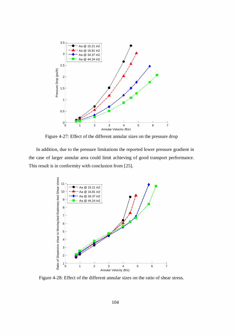
104

0 1 2 3 4 5 6 70

0.5

1

1.5

2

2.5

3

3.5

Annular Velocity (ft/s)

Pre

ssure

Dro

p (

psi/ft

)

Aa @ 15.21 in2

Aa @ 16.81 in2

Aa @ 34.37 in2

Aa @ 44.24 in2

Figure 4-27: Effect of the different annular sizes on the pressure drop

In addition, due to the pressure limitations the reported lower pressure gradient in

the case of larger annular area could limit achieving of good transport performance.

This result is in conformity with conclusion from [25].

0 1 2 3 4 5 6 71

2

3

4

5

6

7

8

9

10

11

Annular Velocity (ft/s) Ratio o

f D

ispers

ive s

hear

to M

ovin

g-b

ed-S

tationary

-bed S

hear

str

ess

Aa @ 15.21 in2

Aa @ 16.81 in2

Aa @ 34.37 in2

Aa @ 44.24 in2

Figure 4-28: Effect of the different annular sizes on the ratio of shear stress.

105

In term of transport performance showed in Figure 4-29, to obtain the optimal

cleaning the required annular velocity increases as annular area (gap) increased.

Figure 4-29: Comparison of final cleaning performance for the different annular sizes

For the same pipe size according to the ratio of the well annular (Dp/Dw), given in

Table 4-8, the lowest ratio demonstrates lowest total cuttings concentration and vice

virca, as shown in Figure 4-30. Obviously, it was remarked that the additional

increasing on the suspemsion layer Δhs was also related to this ratio, where the largest

additonal suspension thickness Δhs is occured at the smallest ratio and vice versa as

106

shown in Table 4-8. For the same bed height 1.0632 in, growth of suspension layer

was faster at low annulus sizes.

Table 4-8: Increasing of the suspension thickness under the different annular sizes

Annular

Ratio

Dp/Dw

Bed Termination

Velocity

Ua (ft/s)

ct

Increase in

suspension

Δhs (in)

tm (in)

0.48 4.5 0.0040 0.487 0.576

0.38 4.9 0.0033 0.504 0.560

0.56 5.8 0.0035 0.412 0.652

0.51 6.3 0.0030 0.456 0.607

0 1 2 3 4 5 6 70

0.5

1

1.5

2

2.5

3

Annular Velocity (ft/s)

Tota

l C

utt

ings C

oncentr

ation (

%)

Aa @ 15.21 in2

Aa @ 16.81 in2

Aa @ 34.37 in2

Aa @ 44.24 in2

Figure 4-30: Change of total annular cuttings concentration at the different annular

size

According to the observation on the annular gap and annular ratio, the lowest

annular size (2.75x5 in), is most efficient size among the tested sizes since it is

demonstrates higher suspension at lower annular velocity combined with higher

suspension concentration. Accordingly it can be recognized that lower annular size is

the better. Typically, findings from [42], agreed that increase of the drill pipe diameter

107

would effectively solve the drilling problems, and that classifying the annular size as

one of the controllable factors to gain smooth transport of cuttings.

Recall Figure 4-25, sensitivity of the total exertied cuttings by the bit to the

annular size Figure 4-30 is lower compared to its sensitvity to the different ROP.

4.4.2 The Modified Model Simulation Results and Discussion

Proper selection for the inputs data is a key variable to achieve sufficient accuracy on

the output results of the modelled phenomena. As well, technical selection of the

mathematical calculation media represents a vital factor to attain rational outcomes

which could be confidently valid in purpose of prediction.

As extra test for the developed model, the additional simulation aims to examine

the influence of alternative equations available in the literature of the three layers

models of cuttings transport. Contrasted equations by Doron et al. 1993 and Martin et

al. 1996 are used in order to calculate the friction factors in the layers boundaries. In

order to conduct direct comparison, same inputs data used by Cho [4] was adopted to

perform this simulation.

4.4.2.1 Effect of Annular Velocity on Cuttings Transport

Through the modified model interesting observation were noticed in the behaviour of

the moving-bed layer with an incremental annular velocity. As recorded in Table 4-9,

and shown in Figure 4-31, very thin moving-bed layer appeared at very low annular

velocity. The Moving-bed layer is dramatically increased with increment annular

velocity up to have a considerable thickness at annular velocity 1 ft/s. The layer

continues enlarge and reach its maximum thickness at annular velocity 1.9 ft/s. Then

the observed moving-bed is gradually diminished and entirely disappeared at annular

velocity around, 3.5 ft/s.

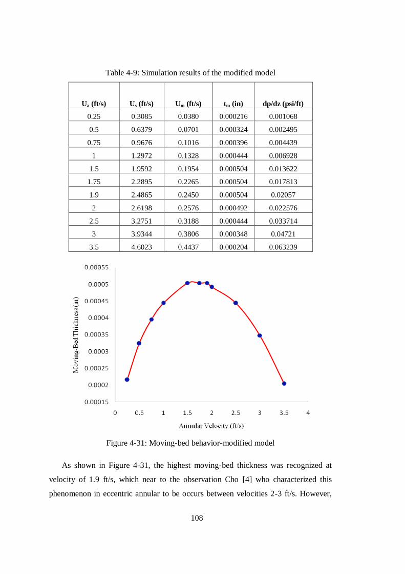
108

Table 4-9: Simulation results of the modified model

Ua (ft/s)

Us (ft/s)

Um (ft/s)

tm (in)

dp/dz (psi/ft)

0.25 0.3085 0.0380 0.000216 0.001068

0.5 0.6379 0.0701 0.000324 0.002495

0.75 0.9676 0.1016 0.000396 0.004439

1 1.2972 0.1328 0.000444 0.006928

1.5 1.9592 0.1954 0.000504 0.013622

1.75 2.2895 0.2265 0.000504 0.017813

1.9 2.4865 0.2450 0.000504 0.02057

2 2.6198 0.2576 0.000492 0.022576

2.5 3.2751 0.3188 0.000444 0.033714

3 3.9344 0.3806 0.000348 0.04721

3.5 4.6023 0.4437 0.000204 0.063239

Figure 4-31: Moving-bed behavior-modified model

As shown in Figure 4-31, the highest moving-bed thickness was recognized at

velocity of 1.9 ft/s, which near to the observation Cho [4] who characterized this

phenomenon in eccentric annular to be occurs between velocities 2-3 ft/s. However,

109

the obtained values for moving-bed thickness in his case were much larger than the

values obtained in this study.

4.4.2.2 Effect of Friction Factor on Cuttings Transport

Changing of the friction factor evaluation altered considerable change on the moving-

bed behaviour and thereby the combinations of the transport layers. Change of the

friction factor formula influence on the transport performance and accordingly two

different tracks achieved as shown in Figure 4-32.

Figure 4-32: Basic and modified simulation tracks

To reach the desirable cleaning removals through single suspension layer, each of

the two models used different combination of two layers. Thus, mass transfer through

the basic model vanish the bottom stationary bed layer by exerting suspension and

moving-bed layers. While the modified model attempt to reach the suspension layer

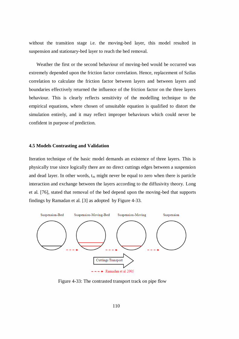
110

without the transition stage i.e. the moving-bed layer, this model resulted in

suspension and stationary-bed layer to reach the bed removal.

Weather the first or the second behaviour of moving-bed would be occurred was

extremely depended upon the friction factor correlation. Hence, replacement of Szilas

correlation to calculate the friction factor between layers and between layers and

boundaries effectively returned the influence of the friction factor on the three layers

behaviour. This is clearly reflects sensitivity of the modelling technique to the

empirical equations, where chosen of unsuitable equation is qualified to distort the

simulation entirely, and it may reflect improper behaviours which could never be

confident in purpose of prediction.

4.5 Models Contrasting and Validation

Iteration technique of the basic model demands an existence of three layers. This is

physically true since logically there are no direct cuttings edges between a suspension

and dead layer. In other words, tm might never be equal to zero when there is particle

interaction and exchange between the layers according to the diffusivity theory. Long

et al. [76], stated that removal of the bed depend upon the moving-bed that supports

findings by Ramadan et al. [3] as adopted by Figure 4-33.

Figure 4-33: The contrasted transport track on pipe flow

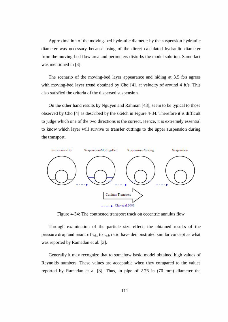
111

Approximation of the moving-bed hydraulic diameter by the suspension hydraulic

diameter was necessary because using of the direct calculated hydraulic diameter

from the moving-bed flow area and perimeters disturbs the model solution. Same fact

was mentioned in [3].

The scenario of the moving-bed layer appearance and hiding at 3.5 ft/s agrees

with moving-bed layer trend obtained by Cho [4], at velocity of around 4 ft/s. This

also satisfied the criteria of the dispersed suspension.

On the other hand results by Nguyen and Rahman [43], seem to be typical to those

observed by Cho [4] as described by the sketch in Figure 4-34. Therefore it is difficult

to judge which one of the two directions is the correct. Hence, it is extremely essential

to know which layer will survive to transfer cuttings to the upper suspension during

the transport.

Figure 4-34: The contrasted transport track on eccentric annulus flow

Through examination of the particle size effect, the obtained results of the

pressure drop and result of τdis to τmb ratio have demonstrated similar concept as what

was reported by Ramadan et al. [3].

Generally it may recognize that to somehow basic model obtained high values of

Reynolds numbers. These values are acceptable when they compared to the values

reported by Ramadan et al [3]. Thus, in pipe of 2.76 in (70 mm) diameter the

112

maximum flow velocity values was less than 3.9 ft/s (0.6 m/s), which is relatively low

compared to the maximum values required in the annulus.

Performance of the modified model to simulate the cuttings transport is still weak.

Installation of the modified model was held through the model at [3]. The frictional

equations implemented in the modified model are same to previous model Cho [4],

where estimation of the wall shear and interfacial shear equations in these models (3-

8), (3-9), (3-19) and (3-20) is lower than previous studies. Therefore, it might be

inconsistent to examine the moving-bed behaviour observed at [4] on the

approximated bases. However, the modified model succeeds to capture the trend of

the moving-bed layer as well as Cho model.

Table 4-10: The moving-bed thickness under the concentric and eccentric annulus

Current Model Cho et al 2001

Ua (ft/s)

tm (in)

Ua (ft/s)

ym (in)

0.25 0.000216 0.75 0

1 0.000444 1 0.01

1.9 0.000504 2 0.32

2.5 0.000444 3 0.2

3.5 0.000204 4 0

Table 4-10, compares the results obtained through the current model and Cho[4].

As shown in Figure 4-35 and 4-36, low thickness for moving-bed layer was predicted

in the concentric annulus compared to the eccentric. Low thickness for moving-bed

can be explained through the area distribution at the different locations of the drill-

pipe. Where concentric annulus had the similar dimensions along the well, the

eccentric annular had less area below the drill pipe surface. Hence, for the same well

and drill pipe, moving-bed layer having a wider area should exert less height.

However, Kamp and Reviro [39], mentioned that eccentric position of annulus would

increase the bed height.

113

Figure 4-35: Moving bed behavior (Current model)

Figure 4-36: Moving-bed behavior (Cho’s Model [4])

However, lower than 3 ft/s performance of the annular mud velocity exerts less

pressure drop and less portion of the stationary cuttings are willing to transfer to the

upper layers compared to the annular velocity higher than 3 ft/hrs. Therefore agreeing

with [4], annular velocity range between 3-4 ft/s is preferable to enhance bed

movement at quite suitable pressure drop and save the borehole and tools from wear

114

and erosion effects. Generally, the obtained results demonstrate suitability of the

model for the effective design.

4.6 Summary of the Modelling Results

This chapter present and discuss the obtained results. Using Chien’s settling velocity

equation to investigate the particle settling behavior under different particles

sphericities the results demonstrated that large sizes and high density of drilled

cuttings companied with regularity of shape motivate faster settling. In term of the

fluid properties low fluid viscosity and density compensated the settling behavior.

Furthermore results of the particles hindered behavior investigation was much

pronounced at high suspension concentration. Such analysis could be helpful in the

field of cuttings transport specially in drilling application simulations. The analysis

was tangent the valuable positions of the settling velocity and assessed prediction tool

to judge where hinder settling effect should be taken with sufficient consideration in

the transport modeling.

The results of the different casts of models equations presented and discussed

separately. Cuttings transport simulation results for the seven targeted unknowns were

predicted under the basic model. The parametric results captured the effect of cuttings

size and shape, annular size, ROP, and fluid viscosity in the horizontal transport and

compared to others findings. The ROP ranked lowest effect whiles cuttings size,

annular size, and rheological viscosity of the drill mud returned considerable effects

on the horizontal transport. Besides, the modified simulation under contrasted

empirical frictional factor correlations resulted in different behaviour for the middle

moving-bed layer. To achieve the horizontal cuttings transport, the annular mud

velocity was the most effective factor on the transport performance.

However the two models were informative. The simulations results proved the

capability of the basic model to estimate the influence of the drilling parameters on

the transport performance and satisfied the dispersed suspension criteria. The

115

modified model successfully captured distinct behaviour of the moving-bed layer.

Dominant results with previous models results by Ramadan et al. [3] and Cho [4]

were achieved.

116

Chapter 5

Conclusion and Recommendation

5.1 Conclusion

Based on this work the following can be concluded from the investigation:

1. Preliminary results of the investigation of the particle settling behaviour

assured settling behavior increase with increase of the particle size and density

combined with regular particle shape, while decrease with increase of fluid

density and viscosity.

2. Particle hindered behaviour is as important consideration as dealing with

cluster of particles. For the range of the input data, excluding of the cuttings

hindered behaviour returned maximum error of 5.6% based on Ham’s and

hosmy correlation and 3.8% based on Thomas correlation.

3. The mathematically-formulated three-layer model is capable of simulating the

behaviour of the horizontal cuttings transport and interpreting the impact of

the drilling parameters in an acceptable manner and is in good agreement with

what was published in previous works.

4. The two models based on different frictional factors calculations, both

captured a thin moving-bed layer at low mud velocities and returned the

following two behaviours:

117

First: By using the Szilas equation, the transport exhibits a similar trend to

that observed by Ramadan et al. [3], with continuous growth of the middle

moving bed layer in response to increasing annular fluid velocity.

Second: By using other empirical correlations in place of the Szilas et al.

equation, the observed moving-bed layer increases with the annular

velocity up to a velocity of approximately 1..9 ft/s. It started to diminish

with increasing annular velocity and disappeared at annular mud velocity

of 3.5 ft/s. This behaviour trend agrees with the findings of Cho [4].

The observed moving-bed behaviours reflected the sensitivity of the mathematical

modelling to predict the friction resistance to the flow of the two phases. The second

model produced insufficient cuttings transport.

5. Between all examined parameters, the annular mud velocity was the most

important variable. Increasing the annular velocity guarantees a better

wellbore cleaning and enhances the shear between layers and bed erosion. In

general, mud velocity, within range of 3-4 ft/s, is recommended.

6. The cuttings size, fluid viscosity and annular size have a significant impact on

the horizontal cuttings transport. Small cuttings size was most easily removed.

A bed that consisted of larger sized particles demanded less annular velocity in

order to be cleaned.

7. The impact of the cuttings sphericity was realized during analysis of layers

concentration. Near to true sphere low concentration was observed in the

suspension layer. In spite of the lower influence of the cuttings sphericity on

the transport compared to the other tested parameters, approximation of

spherical shape for the drilled cuttings returned considerable error in the

suspension concentration that reached 27% measured on sphericity of 0.8.

8. The higher the viscosity of the fluid, the more efficient the transport of

cuttings would be. This was because it reached the highest suspension

thickness at the lower annular velocity.

118

9. The influence of the operational ROP was lower compared to the whole set of

tested parameters. ROP exerted a considerable impact on the total cuttings

concentration, whereas high ROP demonstrated higher total concentration.

10. As controllable factor, lower annular size and large drill pipes were the

optimal conditions to enhance cuttings removal. Large annulus sizes required

application of high annular velocity to achieve cleaning.

5.2 Recommendations

On account of the above conclusions, it appears that the study performed requires

further improvement. Accordingly, the following recommendations are suggested to

achieve a better understanding and analysis of the transportation phenomena:

1. Experimental work is strongly demanded in order to observe the actual

behaviour of the moving-bed layer in the annuli. This facilitates the ability to

judge whether the behavioural analysis made by Cho [4], and Nugeyn and

Rahaman [43], or that reported by Ramadan et al. [3] and Long et al [76], are

the most probable.

2. Some modification is essential to compensate lack of the model’s to predict

the cuttings transfer between two layers which enables detailed follow-up of

the layer thicknesses during transport.

3. Involve more length for the well and observe the mud carrying capacity and

concentration on the layers.

4. Extend the model to handle more drilling parameters, such as eccentricity,

inclination in addition to the influence of the drill-pipe rotation, which

immensely affects settling velocity.

5. Modify the solution algorithm to predict the stationary-bed velocity Ub and

observe the pressure drop behaviour.

6. Estimate the influence of the down hole pressure and temperature, which

affect the fluid density and the properties of mud.

119

7. Trace the unsteady states situation through the model and inspect the effect of

time to present more adequate data about the impact of the ROP on the

transport.

Experimental work to observe the cuttings settling and hindered behaviors in non-

Newtonian fluids under different particles sphericity

120

References

[1] Horizontal drilling - directional oil - gas well - drilling engineering tools

Retrieved 6/24/2010, 2010, available: http://www.horizontaldrilling.org/

[2] Cuttings analysis - PanTerra recruitment Retrieved 6/24/2010, 2010, available:

http://www.panterra.nl/index.php/cms_categorie/15183/content/categorie/id/1

5183/CurrentLanguage/.

[3] A. Ramadan, P. Skalle and A. Saasen, "Application of a three-layer modeling

approach for solids transport in horizontal and inclined channels," Chemical

Engineering Science, vol. 60, pp. 2557-2570, 5, 2005.

[4] H. Cho, "Development of a three-segment hydraulic model for cuttings

transport in horizontal and deviated wells," Ph.D. dissertation, Graduate

Faculty, Univ. of Oklahoma, Norman-Oklahoma pp. 259, 2001.

[5] Welldrilling.pdf (application/pdf object) Retrieved 6/24/2010, 2010,

Available: http://www.agwt.org/info/pdfs/welldrilling.pdf.

[6] Drilling and cuttings transport. Retrieved 2/9/2010, 2010, available:

www.oilandgas.org.uk/issues/drillcuttings/faq.cfm.

[7] M. N. Belavadi and G. A. Chukwu, "Experimental Study of the Parameters

Affecting Cutting Transportation in A vertical Wellbore Annulus," SPE

Paper 27880, presented SPE Western Regional Meeting, 23-25 March 1994,

Long Beach, California, 1994.

121

[8] T. E. Becker and J. J. Azar, "Mud-Weight and Hole-Geometry Effects on

Cuttings Transport While Drilling Directionally," SPE Paper 14711-MS,

1985.

[9] H. C. H. Darley and G. R. Gray, "Composition and properties of drilling and

completion fluids," in , fifth edition ed.Anonymous USA: Gulf Professional

Publishing, 1988, pp. 2-401-466.

[10] S. Joshi, "Horizontal well technology," at Tulsa,Oklahoma-USA: Pennwell

Corp, 1991, pp. 1-5.

[11] M. H. Seeberger, R. W. Matlock and P. M. Hanson, "Oil Muds in Large-

Diameter, Highly Deviated Wells: Solving the Cuttings Removal Problem,"

SPE Paper 18635-MS, presented at SPE/IADC Drilling Conference, 28

February-3 March 1989, New Orleans, Louisiana, 1989.

[12] A. Ramadan, P. Skalle, S. T. Johansen, J. Svein and A. Saasen, "Mechanistic

model for cuttings removal from solid bed in inclined channels," Journal of

Petroleum Science and Engineering, vol. 30, pp. 129-141, 9, 2001.

[13] R. Chhabra and J. F. Richardson, "Non-newtonian flow in the process

industries: Fundamentals and engineering applications," , first edition ed.,

Great Britain: Butterworth-Heinemann, 1999, pp. 5-7,222.

[14] Oilfield glossary: Term 'thixotropy' Retrieved 6/24/2010, 2010, available:

http://www.glossary.oilfield.slb.com/Display.cfm?Term=thixotropy

[15] M. Viloria Ochoa, "Analysis of drilling fluid rheology and tool joint effect to

reduce errors in hydraulics calculations," Ph.D. dissertation, Petroleum Eng,

Texas A&M University, Texas pp. 191, 2006.

[16] C. E. Brennen, "Fundamentals of multiphase flow," in , first edition ed. NY-

USA: Cambridge Univ Pr, 2005, pp. 21-53,134.

122

[17] I. C. Walton, "Computer Simulator of Coiled Tubing Wellbore Cleanouts in

Deviated Wells Recommends Optimum Pump Rate and Fluid Viscosity," SPE

Paper 29491-MS, presented at SPE Production Operations Symposium, 2-4

April 1995, Oklahoma City, Oklahoma, 1995.

[18] M. W. Ali, "A parametric study of cutting transport in vertical and horizontal

well using computational fluid dynamics (CFD)," M.S. thesis, Dept. of

Petroleum and Natural Gas Eng., WVU, Morgantown, West Virginia, pp.

108, 2002.

[19] P. H. Tomren, A. W. Iyoho and J. J. Azar, "Experimental Study of Cuttings

Transport in Directional Wells," SPE Drilling Engineering Paper 12123-PA,

vol. 1, pp. 43-56; 43, 1986.

[20] [20] S. Okrajni and J. J. Azar, "The Effects of Mud Rheology on Annular Hole

Cleaning in Directional Wells," SPE Paper 14178-PA vol. 1, pp. 297-308,

1986.

[21] N. P. Brown, P. A. Bern and A. Weaver, "Cleaning Deviated Holes: New

Experimental and Theoretical Studies," SPE Paper 18636-MS, presented at

SPE/IADC Drilling Conference, 28 February-3 March 1989, New Orleans,

Louisiana, 1989.

[22] J. T. Ford, J. M. Peden, M. B. Oyeneyin, E. Gao and R. Zarrough,

"Experimental investigation of drilled cuttings transport in inclined

boreholes," SPE Paper 20421-MS Presented at SPE Annual Technical

Conference and Exhibition, New Orleans, Louisiana, 1990, .

[23] T. R. Sifferman and T. E. Becker, "Hole Cleaning in Full-Scale Inclined

Wellbores," SPE Paper 20422-PA vol. 7, pp. 115-120, 1992.

123

[24] A. L. Martins, C. H. M. Sa, A. M. F. Lourenco, L. G. M. Freire and W.

Campos, "Experimental Determination of Interfacial Friction Factor in

Horizontal Drilling With a Bed of Cuttings," SPE Paper 36075-MS, presented

at SPE Latin America/Caribbean Petroleum Engineering Conference, 23-26

April 1996, Port-of-Spain, Trinidad, 1996.

[25] J. Li and S. Walker, "Sensitivity Analysis of Hole Cleaning Parameters in

Directional Wells," SPE Paper 54498-MS, presented at SPE/ICoTA Coiled

Tubing Roundtable, 25-26 May 1999, Houston, Texas, 1999.

[26] S. Walker and J. Li, "The Effects of Particle Size, Fluid Rheology, and Pipe

Eccentricity on Cuttings Transport," SPE Paper 60755-MS, presented at

SPE/ICoTA Coiled Tubing Roundtable, 5-6 April 2000, Houston, Texas, 2000.

[27] J. Li and S. Walker, "Sensitivity Analysis of Hole Cleaning Parameters in

Directional Wells," SPE Journa Paper 74710-PA , vol. 6, pp. 356-363; 356,

2001.

[28] Y. Masuda, Q. Doan, M. Oguztoreli, S. Naganawa, T. Yonezawa, A. Kbayashi

and A. Kamp, "Critical Cuttings Transport Velocity in Inclined Annulus:

Experimental Studies and Numerical Simulation," SPE Paper 65502-MS,

presented at SPE/CIM International Conference on Horizontal Well

Technology, 6-8 November 2000, Calgary, Alberta, Canada, 2000.

[29] M. Duan, S. Z. Miska, M. Yu, N. E. Takach, R. M. Ahmed and C. M. Zettner,

"Transport of Small Cuttings in Extended Reach Drilling," SPE Paper

104192-MS, presented at International Oil & Gas Conference and Exhibition

in China, 5-7 December 2006, Beijing, China, 2006.

[30] Forest stand neighbourhood dynamics research and modelling Retrieved

6/24/2010, 2010, available: http://www.bvcentre.ca/sortie-nd/glossary .

124

[31] R. B. Adari, S. Miska, E. Kuru, P. Bern and A. Saasen, "Selecting Drilling

Fluid Properties and Flow Rates For Effective Hole Cleaning in High-Angle

and Horizontal Wells," Paper SPE 63050-MS, presented at SPE Annual

Technical Conference and Exhibition, 1-4 October 2000, Dallas, Texas, 2000 .

[32] R. K. Clark and K. L. Bickham, "A mechanistic model for cuttings transport,"

SPE Paper 28306-MS, presented at SPE Annual Technical Conference and

Exhibition, New Orleans, Louisiana, 1994.

[33] W. Campos, "Mechanistic modeling of cuttings transport in directional wells,"

Ph.D. dissertation, Petroleum Eng., The University of Tulsa, Tulsa, pp. 75,

1995.

[34] L. ZOU, M. H. PATEL and G. HAN, "A new computer package for

simulating cuttings transport and predicting hole cleaning in deviated and

horizontal wells," SPE Paper 64646-MS, presented at International Oil and

Gas Conference and Exhibition in China, Beijing, China, 2000, .

[35] A. Ramadan, P. Skalle and S. T. Johansen, "A mechanistic model to determine

the critical flow velocity required to initiate the movement of spherical bed

particles in inclined channels," Chemical Engineering Science, vol. 58, pp.

2153-2163, 5, 2003.

[36] M. Duan, S. Z. Miska, M. Yu, N. E. Takach, R. M. Ahmed and C. M. Zettner,

"Critical Conditions for Effective Sand-Sized Solids Transport in Horizontal

and High-Angle Wells," SPE Drilling & Completion paper 106707-PA, vol.

24, pp. pp. 229-238; pp. 229, 2009.

[37] L. Zhou, "Hole Cleaning During Underbalanced Drilling in Horizontal and

Inclined Wellbore," SPE Drilling & Completion Paper SPE-98926-PA, vol.

23, pp. pp. 267-273; pp. 267, 2008.

125

[38] L. Zhou, R. M. Ahmed, S. Z. Miska, N. E. Takach, M. Yu and M. B. Pickell,

"Experimental Study and Modeling of Cuttings Transport with Aerated Mud

in Horizontal Wellbore at Simulated Downhole Conditions," SPE Paper

90038-MS, presented at SPE Annual Technical Conference and Exhibition,

26-29 September 2004, Houston, Texas, 2004.

[39] A. M. Kamp and M. Rivero, "Layer modeling for cuttings transport in highly

inclined wellbores," SPE Paper 53942-MS, presented at Latin American and

Caribbean Petroleum Engineering Conference, Caracas, Venezuela, 1999, .

[40] A. A. Gavignet and I. J. Sobey, "Model Aids Cuttings Transport Prediction,"

SPE Journal of Petroleum Technology Paper 15417-PA, vol. 41, pp. 916-921;

916, 1989.

[41] A. W. Iyoho, "Drilled-Cuttings Transport by Non-Newtonian Drilling Fluids

through Inclined, Eccentric Annuli," Ph.D. dissertation, U of Tulsa, Tulsa, pp.

282, 1980.

[42] A. L. Martins and C. C. Santana, "Evaluation of Cuttings Transport in

Horizontal and Near Horizontal Wells -A Dimensionless Approach," SPE

Paper 23643-MS, presented at SPE Latin America Petroleum Engineering

Conference, 8-11 March 1992, Caracas, Venezuela, 1992.

[43] [43] D. Nguyen and S. S. Rahman, "A three-layer hydraulic program for

effective cuttings transport and hole cleaning in highly deviated and horizontal

wells," SPE Paper 36383-MS presented at SPE/IADC Asia Pacific Drilling

Technology, Kuala Lumpur, Malaysia, 1996, .

[44] D. Nguyen and S. S. Rahman, "A Three-Layer Hydraulic Program for

Effective Cuttings Transport and Hole Cleaning in Highly Deviated and

Horizontal Wells," SPE Drilling & Completion SPE Paper 51186-PA, vol. 13,

pp. 182-189; 182, 1998.

126

[45] Z. G. Feng and E. Michaelides, "Proteus—A new computational scheme for

deformable particles and particle interaction problems," presented at IUTAM

Symposium on Computational Approaches to Multiphase Flow, 2006, pp. 153-

161.

[46] M. Santana, A. L. Martins and A. Sales Jr, "Advances in the modeling of the

stratified flow of drilled cuttings in high horizontal wells," in SPE Paper

39890-MS Presented at International Petroleum Conference and Exhibition of

Mexico, Villahermosa, Mexico, 1998, .

[47] P. Stevenson, "Comments on ―Application of a three-layer modelling

approach for solids transport in horizontal and inclined channels‖: A.

Ramadan, P. Skalle, A. Saasen [Chemical Engineering Science 2005, 60,

2557–2570]," Chemical Engineering Science, vol. 61, pp. 3791-3791, 6,

2006.

[48] A. Ramadan, "Response to comments on: ―Application of a three-layer

modeling approach for solids transportation in horizontal and inclined

channels‖ by A. Ramadan, P. Skalle, and A. Saasen," Chemical Engineering

Science, vol. 61, pp. 3792-3793, 6, 2006.

[49] W. C. Yang, "Particle Characterization and Dynamics," Handbook of

Fluidization and Fluid-Particle Systems, pp. 1, 2003.

[50] [50] S. Chien, "Settling Velocity of Irregularly Shaped Particles," SPE Paper

26121-PA, vol. 9, pp. 281-289, 1994.

[51] Q. T. Doan, M. Oguztoreli, Y. Masuda, T. Yonezawa, A. Kobayashi, S.

Naganawa and A. Kamp, "Modeling of Transient Cuttings Transport in

Underbalanced Drilling (UBD)," SPE Journa Paper 85061-PA,l, vol. 8, pp.

160-170; 160, 2003.

127

[52] S. Naganawa and T. Nomura, "Simulating Transient Behavior of Cuttings

Transport over Whole Trajectory of Extended Reach Well," SPE Paper

103923-MS, presented at IADC/SPE Asia Pacific Drilling Technology

Conference and Exhibition, 13-15 November 2006, Bangkok, Thailand, 2006.

[53] S. S. Costa, S. Stuckenbruck, S. A. B. Fontoura and A. L. Martins,

"Simulation of transient cuttings transportation and ECD in wellbore drilling,"

SPE 113893-MS, presented at Europec/EAGE Conference and Exhibition,

Rome, Italy, 2008, .

[54] R. CHENG and R. WANG, "A Three-Segment Hydraulic Model for Annular

Cuttings Transport With Foam in Horizontal Drilling," Journal of

Hydrodynamics, Ser.B, vol. 20, pp. 67-73, 2, 2008.

[55] J. Capo, M. Yu, S. Z. Miska, N. Takach and R. Ahmed, "Cuttings Transport

with Aqueous Foam at Intermediate Inclined Wells," SPE Paper 89534-MS,

presented at SPE/ICoTA Coiled Tubing Conference and Exhibition, 23-24

March 2004, Houston, Texas, 2004.

[56] N. Mishra, "Investigation of hole cleaning parameters using computational

fluid dynamics in horizontal and deviated wells," M.S. thesis, Dept. of

Petroleum and Natural Gas Eng., WVU, Morgantown, West Virginia, pp. 75,

2007.

[57] H. Massah, L. Oshinowo, F. Incorporated and N. H. Lebanon, "Advanced

Gas-Solid Multiphase Flow Models Offer Significant Process Improvements,"

Journal Articles by Fluent Software Users, pp. 1–6, 2000.

[58] A. L. Martins, C. H. M. Sa, A. M. F. Lourenco and W. Campos, "Optimizing

Cuttings Circulation In Horizontal Well Drilling," SPE Paper 35341-MS,

presented at International Petroleum Conference and Exhibition of Mexico, 5-

7 March 1996, Villahermosa, Mexico, 1996.

128

[59] J. Brill and H. Mukherjee, "Multiphase flow in wells," in , first edition ed.,

SPE, Texas: Richardson, 1999, pp. 5-6.

[60] CHEE2940 lecture 8 - multiple particle settling Retrieved 6/24/2010, 2010,

available: http://www.scribd.com/doc/7213729/CHEE2940-Lecture-8-

Multiple-Particle-Settling .

[61] G. Haagh and V. D. Vosse, "Simulation of three-dimensional polymer mould

filling processes using a pseudo-concentration method," International

Journals for Numrical Methods in Fluids, vol. 28, pp. 1355-1369, 1998.

[62] R. Bagnold, "Experiments on a gravity-free dispersion of large solid spheres in

a Newtonian fluid under shear," Proceedings of the Royal Society of

London.Series A, Mathematical and Physical Sciences, vol. 225, pp. 49-63,

1954.

[63] J. Freds√∏e and R. Deigaard, "Mechanics of coastal sediment transport," in ,

firist edition ed., London, Singapore: World Scientific Pub Co Inc, 1992, pp.

219-220,222.

[64] J. Ham and G. Homsy, "Hindered settling and hydrodynamic dispersion in

quiescent sedimenting suspensions," International Journal of Multiphase

Flow, vol. 14, pp. 533-546, 1988.

[65] H. Cho, S. N. Shah and S. O. Osisanya, "A three-layer modeling for cuttings

transport with coiled tubing horizontal drilling," SPE Paper 63269-MS,

presented at SPE Annual Technical Conference and Exhibition, Dallas, Texas,

2000, .

[66] J. Li and G. Wilde, "Effect of Particle Density and Size on Solids Transport

and Hole Cleaning With Coiled Tubing," SPE Paper 94187-MS, presented at

SPE/ICoTA Coiled Tubing Conference and Exhibition, 12-13 April 2005, The

Woodlands, Texas, 2005.

129

[67] M. Zamora, D. T. Jefferson and J. W. Powell, "Hole-Cleaning Study of

Polymer-Based Drilling Fluids," SPE Paper 26329-MS, presented at SPE

Annual Technical Conference and Exhibition, 3-6 October 1993, Houston,

Texas, 1993.

[68] Y. Zhou and S. N. Shah, "Rheological Properties and Frictional Pressure Loss

of Drilling, Completion, and Stimulation Fluids in Coiled Tubing " Journal of

Fluids Engineering, vol. 126, pp. 153, 2004.

[69] M. E. Ozbayoglu, S. Z. Miska, T. Reed and N. Takach, "Analysis of the

Effects of Major Drilling Parameters on Cuttings Transport Efficiency for

High-Angle Wells in Coiled Tubing Drilling Operations," SPE Paper 89334-

MS, presented at SPE/ICoTA Coiled Tubing Conference and Exhibition, 23-24

March 2004, Houston, Texas, 2004.

[70] A. Altunbas, G. Kelbaliyev and K. Ceylan, "Eddy diffusivity of particles in

turbulent flow in rough channels," J. Aerosol Sci., vol. 33, pp. 1075-1086, 7,

2002.

[71] M. Duan, S. Z. Miska, M. Yu, N. E. Takach, R. M. Ahmed and J. H. Hallman,

"Experimental Study and Modeling of Cuttings Transport Using Foam With

Drillpipe Rotation," SPE Paper 116300-MS, presented at SPE Annual

Technical Conference and Exhibition, 21-24 September 2008, Denver,

Colorado, USA, 2008.

[72] A. Saasen and G. L√∏klingholm, "The Effect of Drilling Fluid Rheological

Properties on Hole Cleaning," SPE Paper 74558-MS, presented at IADC/SPE

Drilling Conference, 26-28 February 2002, Dallas, Texas, 2002.

[73] K. Shahbazi, M. R. Meschi and M. P. Shahri, "A New Criteria to Predict Stuck

Pipe Occurrence," SPE Paper 128376-MS, presented at North Africa

Technical Conference and Exhibition, 14-17 February 2010, Cairo, Egypt,

2010.

130

[74] J. J. Azar and R. A. Sanchez, "Important Issues in Cuttings Transport for

Drilling Directional Wells," SPE Paper 39020-MS, Latin American and

Caribbean Petroleum Engineering Conference, 30 August-3 September 1997,

Rio de Janeiro, Brazil, 1997.

[75] P. S. Vinod and L. V. McIntire, "Rheology Effects on Laminar and Turbulent

Flow of Model Drilling Fluids Through Deviated Wells," , SPE Paper 28287-

MS, 1994. ―Unsolicited‖

[76] Z. Long, Z. Wang and X. Guo, "Transport mechanism of cuttings in annulus

during deviated and horizontal drilling," Journals of University of Petroulim,

Chaina, vol. 29, pp. 42-45, 2005.

131

Appendix A

Geometry Engine

(1) If TT=(rw-rp) or <(rw-rp) (rw=Dw/2 , rp=Dp/2)

Figure A-1: The Bed Layers below the Drill-Pipe

Angles

w

bw

br

hr1cos

w

w

mr

TTr1cos

Areas

bbbwb rA )(cossin2

bbbmmmwm rA cossincossin2

bmas AAAA

132

Perimeters

bwbwbw DrS 2

bwmb rS sin2

mwsm rS sin2

bmwmw rS 2

pipebwmwwellsw SSSSS

pipebSwbmwwsw SrrrS 222

pmwsw rrS 22

Hydraulic diameter

smswp

shs

SSS

AD

4

(2) If TT>(rw-rb)

Figure A-2: The Bed Layers reach the Drill-Pipe

133

Areas

bbbwb rA cossin2

mwpmw

p

mw

p

bmwwbmwmbw

bmwmbmmwm

rrrr

rr

rtrrr

rrA

22212

2222222

22

cos.coscos

cos

sinsin4

1.sinsincoscos

coscossinsin

mbas AAAA

Perimeters

bwbw rS 2

bwmb rS sin2

p

mw

pbmwmwr

rrrS

coscos22 1

p

mw

pmwsmr

rrrS

coscossinsin2 1

p

mw

pmwswr

rrrS

coscos22 1

134

Figure A-3: The Bed Layers touch the Drill-Pipe

Areas

))(cos(sin2

bbbwb rA

.coscoscos

cos

sinsin4

1.sinsincoscos

coscossinsin

22212

2222222

22

mwpmw

p

mw

p

bmwwbmwmbw

bmwmbmmwm

rrrr

rr

rtrrr

rrA

mbas AAAA

Perimeters

bwbw rS 2

bwmb rS sin2

p

mw

pbmwmwr

rrrS

coscos22 1

135

p

mw

pmwsmr

rrrS

coscossinsin2 1

p

mw

pmwswr

rrrS

coscos22 1

Figure A-4: The Bed Layers over the Drill-Pipe

Areas

bwpbw

p

bw

pbbwbwb rrrr

rrrrA

2221222 coscos

coscossincos

bwpbw

p

bwpmwpmwm

p

wp

mmwmwmbbmwm

rrr

r

rrrrr

r

rr

rrrA

222

122212

222

coscos

coscoscoscoscoscos

cossin)cos)(cossin(sin

mbas AAAA

136

Perimeters

p

mw

pmwswr

rrrS

coscos22 1

p

bw

p

mw

pbmwmwr

r

r

rrrS

coscos

coscos22 11

p

bw

pbwbwr

rrrS

coscos22 1

p

mw

pmwsmr

rrrS

coscossinsin2 1

p

bw

pbwmbr

rrrS

coscossinsin2 1

137

Appendix B

Results of the Basic Simulation

Results of the cuttings sizes:

Table B-1: Large size of 0.25 in

Large Cuttings Size dp = 0.25 in

Ua

(ft/s)

Res Us

(ft/s)

Um

(ft/s)

cs cm tm (in) τdis

(lb/ft2)

dpz /dz

(psi/ft)

0.75 5806 0.9676 0.3686 0.006 0.253 0.0072 0.6709 0.118059

1 8427 1.2973 0.4795 0.008 0.254 0.0132 1.2185 0.194837

2 20809 2.6161 0.9145 0.0158 0.2579 0.0552 5.2793 0.683883

3 35407 3.9348 1.3459 0.0245 0.2623 0.1428 13.6283 1.47371

4 51666 5.2535 1.7768 0.0343 0.2671 0.3252 31.0298 2.579816

4.7 63870 6.1766 2.0785 0.0418 0.2709 0.666 63.4897 3.552158

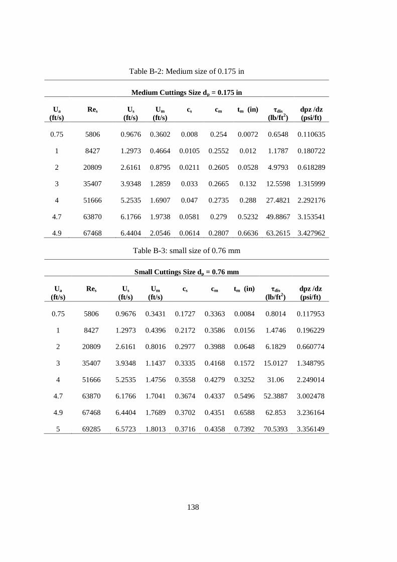
138

Table B-2: Medium size of 0.175 in

Medium Cuttings Size dp = 0.175 in

Ua

(ft/s)

Res Us

(ft/s)

Um

(ft/s)

cs cm tm (in) τdis

(lb/ft2)

dpz /dz

(psi/ft)

0.75 5806 0.9676 0.3602 0.008 0.254 0.0072 0.6548 0.110635

1 8427 1.2973 0.4664 0.0105 0.2552 0.012 1.1787 0.180722

2 20809 2.6161 0.8795 0.0211 0.2605 0.0528 4.9793 0.618289

3 35407 3.9348 1.2859 0.033 0.2665 0.132 12.5598 1.315999

4 51666 5.2535 1.6907 0.047 0.2735 0.288 27.4821 2.292176

4.7 63870 6.1766 1.9738 0.0581 0.279 0.5232 49.8867 3.153541

4.9 67468 6.4404 2.0546 0.0614 0.2807 0.6636 63.2615 3.427962

Table B-3: small size of 0.76 mm

Small Cuttings Size dp = 0.76 mm

Ua

(ft/s)

Res Us

(ft/s)

Um

(ft/s)

cs cm tm (in) τdis

(lb/ft2)

dpz /dz

(psi/ft)

0.75 5806 0.9676 0.3431 0.1727 0.3363 0.0084 0.8014 0.117953

1 8427 1.2973 0.4396 0.2172 0.3586 0.0156 1.4746 0.196229

2 20809 2.6161 0.8016 0.2977 0.3988 0.0648 6.1829 0.660774

3 35407 3.9348 1.1437 0.3335 0.4168 0.1572 15.0127 1.348795

4 51666 5.2535 1.4756 0.3558 0.4279 0.3252 31.06 2.249014

4.7 63870 6.1766 1.7041 0.3674 0.4337 0.5496 52.3887 3.002478

4.9 67468 6.4404 1.7689 0.3702 0.4351 0.6588 62.853 3.236164

5 69285 6.5723 1.8013 0.3716 0.4358 0.7392 70.5393 3.356149

139

Results of the cuttings sphericity:

Table B-4: Cuttings sphericity of 0.75

φ= 0.75

Ua

(ft/s)

Re Us

(ft/s)

Um

(ft/s)

cs cm tm (in) τdis

(lb/ft2)

dpz /dz

(psi/ft)

0.75 5806 0.9676 0.3686 0.0065 0.2533 0.0072 0.6715 0.118139

1 8427 1.2973 0.4795 0.0086 0.2543 0.0132 1.2199 0.195014

2 20809 2.6161 0.9145 0.0172 0.2586 0.0552 5.2922 0.685181

3 35407 3.9348 1.3459 0.0269 0.2634 0.144 13.6879 1.478269

4 51666 5.2535 1.7768 0.0378 0.2689 0.3276 31.2884 2.591944

4.7 63870 6.1766 2.0785 0.0464 0.2732 0.6816 65.0048 3.573254

Table B-5: Cuttings sphericity of 0.8

φ= 0.8

Ua

(ft/s)

Re Us (ft/s) Um (ft/s) cs cm tm (in) τdis (lb/ft2) dpz /dz

(psi/ft)

0.75 5806 0.9676 0.3686 0.006 0.253 0.0072 0.6709 0.118059

1 8427 1.2973 0.4795 0.008 0.254 0.0132 1.2185 0.194837

2 20809 2.6161 0.9145 0.0158 0.2579 0.0552 5.2793 0.683883

3 35407 3.9348 1.3459 0.0245 0.2623 0.1428 13.6283 1.47371

4 51666 5.2535 1.7768 0.0343 0.2671 0.3252 31.0298 2.579816

4.7 63870 6.1766 2.0785 0.0418 0.2709 0.666 63.4897 3.552158

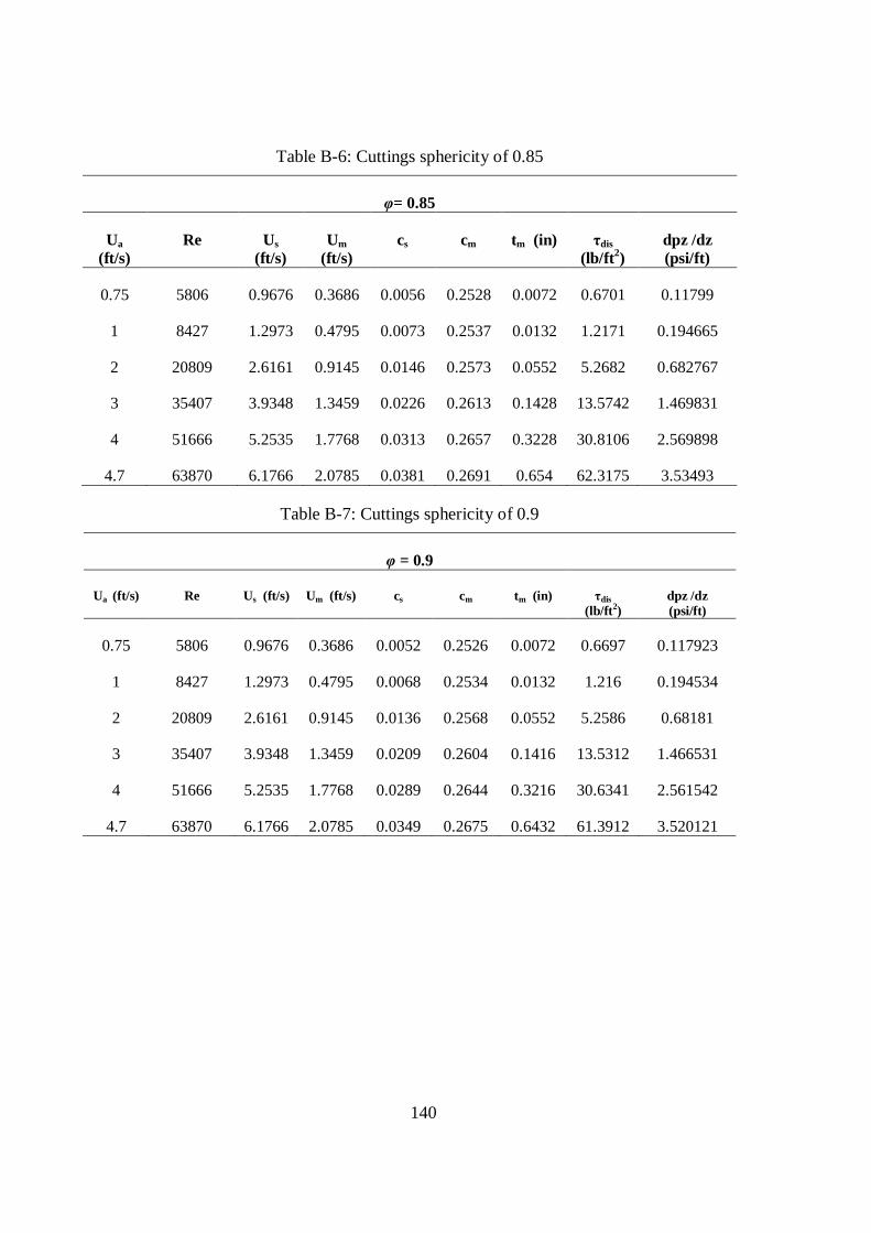
140

Table B-6: Cuttings sphericity of 0.85

φ= 0.85

Ua

(ft/s)

Re Us

(ft/s)

Um

(ft/s)

cs cm tm (in) τdis

(lb/ft2)

dpz /dz

(psi/ft)

0.75 5806 0.9676 0.3686 0.0056 0.2528 0.0072 0.6701 0.11799

1 8427 1.2973 0.4795 0.0073 0.2537 0.0132 1.2171 0.194665

2 20809 2.6161 0.9145 0.0146 0.2573 0.0552 5.2682 0.682767

3 35407 3.9348 1.3459 0.0226 0.2613 0.1428 13.5742 1.469831

4 51666 5.2535 1.7768 0.0313 0.2657 0.3228 30.8106 2.569898

4.7 63870 6.1766 2.0785 0.0381 0.2691 0.654 62.3175 3.53493

Table B-7: Cuttings sphericity of 0.9

φ = 0.9

Ua (ft/s) Re Us (ft/s) Um (ft/s) cs cm tm (in) τdis

(lb/ft2)

dpz /dz

(psi/ft)

0.75 5806 0.9676 0.3686 0.0052 0.2526 0.0072 0.6697 0.117923

1 8427 1.2973 0.4795 0.0068 0.2534 0.0132 1.216 0.194534

2 20809 2.6161 0.9145 0.0136 0.2568 0.0552 5.2586 0.68181

3 35407 3.9348 1.3459 0.0209 0.2604 0.1416 13.5312 1.466531

4 51666 5.2535 1.7768 0.0289 0.2644 0.3216 30.6341 2.561542

4.7 63870 6.1766 2.0785 0.0349 0.2675 0.6432 61.3912 3.520121

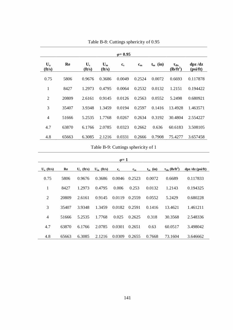
141

Table B-8: Cuttings sphericity of 0.95

φ= 0.95

Ua

(ft/s)

Re Us

(ft/s)

Um

(ft/s)

cs cm tm (in) τdis

(lb/ft2)

dpz /dz

(psi/ft)

0.75 5806 0.9676 0.3686 0.0049 0.2524 0.0072 0.6693 0.117878

1 8427 1.2973 0.4795 0.0064 0.2532 0.0132 1.2151 0.194422

2 20809 2.6161 0.9145 0.0126 0.2563 0.0552 5.2498 0.680921

3 35407 3.9348 1.3459 0.0194 0.2597 0.1416 13.4928 1.463571

4 51666 5.2535 1.7768 0.0267 0.2634 0.3192 30.4804 2.554227

4.7 63870 6.1766 2.0785 0.0323 0.2662 0.636 60.6183 3.508105

4.8 65663 6.3085 2.1216 0.0331 0.2666 0.7908 75.4277 3.657458

Table B-9: Cuttings sphericity of 1

φ= 1

Ua (ft/s) Re Us (ft/s) Um (ft/s) cs cm tm (in) τdis (lb/ft2) dpz /dz (psi/ft)

0.75 5806 0.9676 0.3686 0.0046 0.2523 0.0072 0.6689 0.117833

1 8427 1.2973 0.4795 0.006 0.253 0.0132 1.2143 0.194325

2 20809 2.6161 0.9145 0.0119 0.2559 0.0552 5.2429 0.680228

3 35407 3.9348 1.3459 0.0182 0.2591 0.1416 13.4621 1.461211

4 51666 5.2535 1.7768 0.025 0.2625 0.318 30.3568 2.548336

4.7 63870 6.1766 2.0785 0.0301 0.2651 0.63 60.0517 3.498042

4.8 65663 6.3085 2.1216 0.0309 0.2655 0.7668 73.1604 3.646662

142

Results of the fluid Viscosity:

Table B-10: power law viscosity at K=0.00084 lbf.sn/ft2; n=0.68

K=0.00084 lbf.sn/ft

2; n=0.68

Ua

(ft/s)

Re Us

(ft/s)

Um

(ft/s)

cs cm tm (in) τdis

(lb/ft2)

dpz /dz

(psi/ft)

0.75 41474 0.9676 0.3298 0.0054 0.2527 0.0072 0.6452 0.085967

1 60192 1.2973 0.4375 0.0072 0.2536 0.012 1.1673 0.150498

2 148640 2.6161 0.8689 0.015 0.2575 0.0528 5.091 0.593387

3 252910 3.9348 1.301 0.0236 0.2618 0.138 13.1498 1.341215

4 369040 5.2535 1.7334 0.0332 0.2666 0.3108 29.6483 2.407873

4.6 443490 6.0447 1.9929 0.0397 0.2698 0.5364 51.1194 3.207971

4.7 456210 6.1766 2.0361 0.0408 0.2604 0.6036 57.5205 3.353336

4.8 469020 6.3085 2.0794 0.0419 0.2709 0.7032 67.0779 3.502144

Table B-11: power law viscosity at K=0.006 lbf.sn/ft2; n=0.68

K=0.006 lbf.sn/ft

2; n=0.68

Ua

(ft/s)

Re Us

(ft/s)

Um

(ft/s)

cs cm tm (in) τdis

(lb/ft2)

dpz /dz

(psi/ft)

0.75 5806 0.9676 0.3686 0.006 0.253 0.0072 0.6709 0.118059

1 8427 1.2973 0.4795 0.008 0.254 0.0132 1.2185 0.194837

2 20809 2.6161 0.9145 0.0158 0.2579 0.0552 5.2793 0.683883

3 35407 3.9348 1.3459 0.0245 0.2623 0.1428 13.6283 1.47371

4 51666 5.2535 1.7768 0.0343 0.2671 0.3252 31.0298 2.579816

4.6 62088 6.0447 2.0354 0.0407 0.2704 0.5784 55.1324 3.403004

4.7 63870 6.1766 2.0785 0.0418 0.2709 0.666 63.4897 3.552158

143

Table B-12: power law viscosity at K=0.00436 lbf.sn/ft2; n=0.61

K=0.00436 lbf.sn/ft

2; n=0.61

Ua

(ft/s)

Re Us

(ft/s)

Um

(ft/s)

cs cm tm (in) τdis

(lb/ft2)

dpz /dz

(psi/ft)

0.75 9811 0.9676 0.3763 0.0054 0.2527 0.0072 0.6669 0.125305

1 14530 1.2973 0.4881 0.007 0.2535 0.0132 1.2175 0.204933

2 37662 2.6161 0.9246 0.014 0.257 0.0552 5.2869 0.703474

3 65928 3.9348 1.3558 0.0214 0.2607 0.1428 13.6172 1.49768

4 98160 5.2535 1.7861 0.0296 0.2648 0.324 30.9066 2.601093

4.6 119120 6.0447 2.0443 0.0349 0.2674 0.5736 54.6635 3.417617

4.7 122720 6.1766 2.0873 0.0358 0.2679 0.6576 62.708 3.565325

Table B-13: power law viscosity at K=0.0093 lbf.sn/ft2; n=0.61

K=0.0093 lbf.sn/ft

2; n=0.61

Ua

(ft/s)

Re Us

(ft/s)

Um

(ft/s)

cs cm tm (in) τdis

(lb/ft2)

dpz /dz

(psi/ft)

0.75 4600 0.9676 0.4035 0.0058 0.2529 0.0072 0.6378 0.155058

1 6812 1.2973 0.5204 0.0075 0.2538 0.0132 1.2072 0.24791

2 17657 2.616 0.9687 0.0147 0.2574 0.0552 5.4453 0.803913

3 30908 3.9348 1.4051 0.0223 0.2612 0.1428 14.2144 1.656788

4 46019 5.2535 1.8375 0.0306 0.2653 0.324 32.8565 2.817549

4.6 55846 6.0447 2.0962 0.036 0.268 0.5736 61.6358 3.667771

144

Results of the Rate of penetration:

Table B-14: ROP at 60 ft/r

60 ft/r

Ua

(ft/s)

Re Us

(ft/s)

Um

(ft/s)

cs cm tm (in) τdis

(lb/ft2)

dpz /dz

(psi/ft)

0.75 5840 0.9634 0.3672 0.006 0.253 0.0072 0.6647 0.117181

1 8464 1.293 0.478 0.0078 0.2539 0.0132 1.2102 0.193703

2 20855 2.6118 0.9131 0.0158 0.2579 0.0552 5.2613 0.681822

3 35459 3.9305 1.3445 0.0245 0.2623 0.1428 13.5887 1.470645

4 51723 5.2492 1.7754 0.0342 0.2671 0.324 30.9474 2.575701

4.7 63930 6.1723 2.0771 0.0418 0.2609 0.6624 63.1676 3.547292

Table B-15: ROP at 50 ft/r

50 ft/r

Ua

(ft/s)

Re Us

(ft/s)

Um

(ft/s)

cs cm tm (in) τdis

(lb/ft2)

dpz /dz

(psi/ft)

0.75 5806 0.9676 0.3686 0.006 0.253 0.0072 0.6709 0.118059

1 8427 1.2973 0.4795 0.008 0.254 0.0132 1.2185 0.194837

2 20809 2.6161 0.9145 0.0158 0.2579 0.0552 5.2793 0.683883

3 35407 3.9348 1.3459 0.0245 0.2623 0.1428 13.6283 1.47371

4 51666 5.2535 1.7768 0.0343 0.2671 0.3252 31.0298 2.579816

4.7 63870 6.1766 2.0785 0.0418 0.2709 0.666 63.4897 3.552158

145

Table B-16: ROP at 30 ft/r

30 ft/r

Ua

(ft/s)

Re Us

(ft/s)

Um

(ft/s)

cs cm tm (in) τdis

(lb/ft2)

dpz /dz

(psi/ft)

0.75 5739 0.9762 0.3715 0.0061 0.253 0.0072 0.6829 0.119826

1 8353 1.3059 0.4823 0.008 0.254 0.0132 1.2348 0.19707

2 20717 2.6246 0.9173 0.0159 0.2579 0.0552 5.3181 0.68803

3 35302 3.9433 1.3487 0.0246 0.2623 0.144 13.7007 1.479847

4 51551 5.2621 1.7796 0.0343 0.2672 0.3276 31.1955 2.588057

4.7 63749 6.1852 2.0813 0.0419 0.271 0.6732 64.1546 3.561957

Table B-17: ROP at 15 ft/r

15 ft/r

Ua

(ft/s)

Re Us

(ft/s)

Um

(ft/s)

cs cm tm (in) τdis

(lb/ft2)

dpz /dz

(psi/ft)

0.75 5689 0.9826 0.3737 0.0061 0.253 0.0072 0.6921 0.121157

1 8298 1.3123 0.4845 0.008 0.254 0.0132 1.2472 0.198753

2 20648 2.631 0.9194 0.0159 0.258 0.0564 5.3453 0.691147

3 35224 3.9498 1.3508 0.0246 0.2623 0.144 13.7589 1.484469

4 51465 5.2685 1.7817 0.0344 0.2672 0.3288 31.3208 2.594266

4.7 63658 6.1916 2.0834 0.042 0.271 0.678 64.6705 3.569329

146

Results of the Annular Size:

Table B-18: Annular Size of 5x2.75 in

Annular size 5x2.75 in

Ua

(ft/s)

Re Us

(ft/s)

Um

(ft/s)

cs cm tm (in) τdis

(lb/ft2)

dpz /dz

(psi/ft)

0.75 5201 0.9159 0.3572 0.0063 0.2532 0.006 0.6068 0.121797

1 7543 1.2287 0.4648 0.0084 0.2542 0.012 1.1123 0.200862

2 18605 2.4798 0.8875 0.0168 0.2584 0.0516 4.9068 0.704659

3 31644 3.7309 1.3068 0.0261 0.263 0.1356 12.9035 1.519337

4 46167 4.982 1.7257 0.0366 0.2683 0.3204 30.6067 2.66251

4.5 53896 5.6076 1.9351 0.0424 0.2712 0.576 54.9139 3.363273

Table B-19: Annular Size of 5x1.9 in

Annular size 5x1.9 in

Ua

(ft/s)

Re Us

(ft/s)

Um

(ft/s)

cs cm tm (in) τdis

(lb/ft2)

dpz /dz

(psi/ft)

0.75 5806 0.8967 0.3417 0.0051 0.2526 0.006 0.5708 0.096172

1 8427 1.2022 0.4438 0.0067 0.2533 0.0108 1.034 0.157857

2 20809 2.4242 0.8433 0.0133 0.2567 0.04608 4.4044 0.546827

3 35407 3.6462 1.2388 0.0204 0.2602 0.11592 11.0581 1.169028

4 51666 4.8681 1.6335 0.0281 0.264 0.24972 23.8208 2.034187

4.5 60319 5.4791 1.8308 0.0322 0.2661 0.3708 35.3667 2.561147

4.9 67468 5.9679 1.9887 0.0357 0.2678 0.55956 53.3725 3.029405

147

Table B-20: Annular Size of 8x4.5 in

Annular size 8x4.5 in

Ua

(ft/s)

Re Us

(ft/s)

Um

(ft/s)

cs cm tm (in) τdis

(lb/ft2)

dpz /dz

(psi/ft)

0.75 6351 0.8249 0.3103 0.004 0.252 0.0048 0.4737 0.058724

1 9201 1.1076 0.4027 0.0053 0.2527 0.0084 0.8537 0.095908

2 22660 2.2381 0.7626 0.0104 0.2552 0.0372 3.5294 0.327081

3 38521 3.3687 1.1175 0.0157 0.2579 0.0888 8.4471 0.692165

4 56183 4.4992 1.4712 0.0214 0.2607 0.1752 16.7413 1.195274

4.5 65583 5.0645 1.6479 0.0244 0.2622 0.24 22.8782 1.499932

4.9 73349 5.5167 1.7892 0.0268 0.2634 0.3084 29.4046 1.76969

5.8 91554 6.5342 2.1073 0.0327 0.2664 0.6516 62.188 2.463557

Table B-21: Annular Size of 8.75x4.5 in

Annular size 8.75x4.5 in

Ua

(ft/s)

Re Us

(ft/s)

Um

(ft/s)

cs cm tm (in) τdis

(lb/ft2)

dpz /dz

(psi/ft)

0.75 7229 0.8071 0.2966 0.0031 0.2516 0.0048 0.4441 0.04368

1 10480 1.0831 0.3843 0.004 0.252 0.0084 0.7924 0.071047

2 25832 2.1871 0.7245 0.0078 0.2539 0.0336 3.1919 0.239485

3 43928 3.2911 1.0589 0.0118 0.2559 0.078 7.4547 0.502787

4 64081 4.3951 1.3918 0.0159 0.2579 0.15 14.2506 0.863008

4.5 74809 4.9471 1.558 0.018 0.259 0.1992 19.0066 1.080107

4.9 83667 5.3887 1.6909 0.0197 0.2599 0.2484 23.7181 1.271852

5.8 104440 6.3823 1.99 0.0238 0.2619 0.4152 39.6271 1.76306

6.3 116440 6.9343 2.1561 0.0261 0.2631 0.6072 57.9539 2.072017

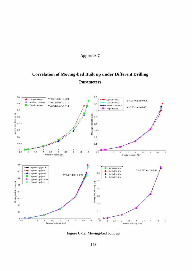
148

Appendix C

Correlation of Moving-bed Built up under Different Drilling

Parameters

0.5 1 1.5 2 2.5 3 3.5 4 4.5 50

0.1

0.2

0.3

0.4

0.5

0.6

0.7

0.8

Annular Velocity (ft/s)

Movin

g-b

ed B

uild

-up (

in)

Large cuttings

Medium cuttings

Small cuttings

0.5 1 1.5 2 2.5 3 3.5 4 4.5 50

0.1

0.2

0.3

0.4

0.5

0.6

0.7

0.8

Annular Velocity (ft/s)

Movin

g-b

ed B

uild

-up (

in)

Low viscous.1

Low viscous.2

Intermid. viscous.

High viscous.

0.5 1 1.5 2 2.5 3 3.5 4 4.5 50

0.1

0.2

0.3

0.4

0.5

0.6

0.7

0.8

Annular Velocity (ft/s)

Movin

g-b

ed B

uild

-up (

in)

Sphericity@0.75

Sphericity@0.8

Sphericity@0.85

Sphericity@0.9

Sphericity@=0.95

Sphericity@=1

0.5 1 1.5 2 2.5 3 3.5 4 4.5 50

0.1

0.2

0.3

0.4

0.5

0.6

0.7

Annular Velocity (ft/s)

Movin

g-b

ed B

uild-u

p (

in)

ROP@60 ft/hr

ROP@50 ft/hr

ROP@30 ft/hr

ROP@15 ft/hr

Figure C-1a: Moving-bed built up

Y=0.339ln(x)-0.015

Y=0.274ln(x)-0.003

Y=0.282ln(x)-0.004

Y=0.329ln(x)-0.014 Y=0.310ln(x)-0.008

Y=0.278ln(x)-0.003

Y=0.251ln(x)-0.001 Y=0.307ln(x)-0.008

Y=0.291ln(x)-0.011

Y=0.344ln(x)-0.014

149

0 1 2 3 4 5 6 70

0.1

0.2

0.3

0.4

0.5

0.6

0.7

Annular Velocity (ft/s)

Movin

g-b

ed B

uild

-up (

in)

Aa @ 15.21 in2

Aa @ 16.81 in2

Aa @ 34.37 in2

Aa @ 44.24 in2

Figure C-1b: Moving-bed built up

Y=0.251ln(x)-0.000

Y=0.234ln(x)-0.006

Y=0.219ln(x)-0.023

Y=0.210ln(x)-0.029

150

Appendix D

Dimensionless Analysis

0 1 2 3 4 5 6 7

x 104

0.06

0.08

0.1

0.12

0.14

0.16

0.18

Reynolds Number

Suspensio

n F

riction

Large cuttings

Medium cuttings

Small cuttings

103

104

105

10-2

10-1

100

Reynolds Number

Suspensio

n F

riction

0 1 2 3 4 5 6 7

x 104

0.1

0.15

0.2

0.25

0.3

0.35

Reynolds Number

Friction (

Suspensio

n-M

ovin

g-b

ed)

Large cuttings

Medium cuttings

Small cuttings

103

104

105

10-0.9

10-0.8

10-0.7

10-0.6

10-0.5

Reynolds Number

Friction (

Suspensio

n-M

ovin

g-b

ed)

Figure D-1a: Frictions at different cuttings sizes

151

0 1 2 3 4 5 6 7

x 104

0.08

0.1

0.12

0.14

0.16

0.18

0.2

0.22

0.24

Reynolds Number

Friction (

Movin

g-B

ed)

Large cuttings

Medium cuttings

Small cuttings

103

104

105

10-2

10-1

100

Reynolds Number

Friction (

Movin

g-B

ed)

Figure D-1b: Frictions at different cuttings sizes

152

0 0.5 1 1.5 2 2.5 3 3.5 4 4.5 5

x 105

0.1

0.12

0.14

0.16

0.18

0.2

0.22

Reynolds Number

Suspensio

n F

riction

Low viscous.1

Low viscous.2

Intermid. viscous.

High viscous.

103

104

105

106

10-0.9

10-0.8

10-0.7

Reynolds Number

Suspensio

n F

riction

0 0.5 1 1.5 2 2.5 3 3.5 4 4.5 5

x 105

0.2

0.25

0.3

0.35

0.4

0.45

Reynolds Number

Friction (

Suspensio

n-M

ovin

g-b

ed)

Low viscous.1

Low viscous.2

Intermid. viscous.

High viscous.

103

104

105

106

10-0.6

10-0.5

10-0.4

Reynolds Number

Friction (

Suspensio

n-M

ovin

g-b

ed)

0 0.5 1 1.5 2 2.5 3 3.5 4 4.5 5

x 105

0.1

0.15

0.2

0.25

0.3

0.35

Reynolds Number

Friction (

Movin

g-B

ed)

Low viscous.1

Low viscous.2

Intermid. viscous.

High viscous.

103

104

105

106

10-0.9

10-0.8

10-0.7

10-0.6

Reynolds Number

Friction (

Movin

g-B

ed)

Figure D-2: Frictions at different mud viscosity

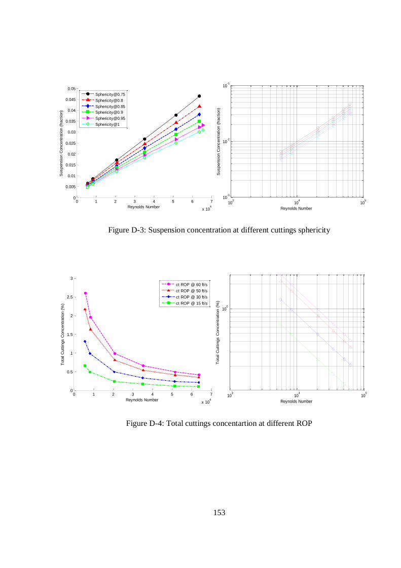
153

0 1 2 3 4 5 6 7

x 104

0

0.005

0.01

0.015

0.02

0.025

0.03

0.035

0.04

0.045

0.05

Reynolds Number

Suspensio

n C

oncentr

ation (

fraction)

Sphericity@0.75

Sphericity@0.8

Sphericity@0.85

Sphericity@0.9

Sphericity@0.95

Sphericity@1

103

104

105

10-3

10-2

10-1

Reynolds Number

Suspensio

n C

oncentr

ation (

fraction)

Figure D-3: Suspension concentration at different cuttings sphericity

0 1 2 3 4 5 6 7

x 104

0

0.5

1

1.5

2

2.5

3

Reynolds Number

Tota

l C

utt

ings C

oncentr

ation (

%)

ct ROP @ 60 ft/s

ct ROP @ 50 ft/s

ct ROP @ 30 ft/s

ct ROP @ 15 ft/s

103

104

105

100

Reynolds Number

Tota

l C

utt

ings C

oncentr

ation (

%)

Figure D-4: Total cuttings concentartion at different ROP

154

0 2 4 6 8 10 12

x 104

0.08

0.09

0.1

0.11

0.12

0.13

0.14

0.15

0.16

0.17

0.18

Reynolds Number

Suspensio

n F

riction

Aa @ 15.21 in2

Aa @ 16.81 in2

Aa @ 34.37 in2

Aa @ 44.24 in2

103

104

105

106

10-2

10-1

100

Reynolds Number

Suspensio

n F

riction

0 2 4 6 8 10 12

x 104

0.16

0.18

0.2

0.22

0.24

0.26

0.28

0.3

0.32

0.34

0.36

Reynolds Number

Friction (

Suspensio

n-M

ovin

g-b

ed)

Aa @ 15.21 in2

Aa @ 16.81 in2

Aa @ 34.37 in2

Aa @ 44.24 in2

103

104

105

106

10-0.7

10-0.6

10-0.5

Reynolds Number

Friction (

Suspensio

n-M

ovin

g-b

ed)

0 2 4 6 8 10 12

x 104

0.08

0.1

0.12

0.14

0.16

0.18

0.2

0.22

0.24

Reynolds Number

Friction (

Movin

g-B

ed)

Aa @ 15.21 in2

Aa @ 16.81 in2

Aa @ 34.37 in2

Aa @ 44.24 in2

103

104

105

106

10-1

100

Reynolds Number

Friction (

Movin

g-B

ed)

Figure D-5: Frictions with different annular sizes.