1

CHAPTER 1

INTRODUCTION

1.1 Background

Thermal Energy Storage (TES) tank is normally used to enhance utilization of thermal

energy to meet the fluctuating demand in the supply of chilled water for air-

conditioning systems. The advantage of TES tank is that it enables shifting of energy

usage from off-peak demand to on-peak demand requirement. This is achieved by

charging the tank during off-peak periods and discharging it during on-peak periods.

The capability of increasing the thermal energy utilization has led TES tank to be

incorporated to cogeneration plants, such as district cooling or heating, and some

other plants that are involved in energy utilization.

In district cooling plant where electricity and cooling capacity are generated, TES

tank could function in supporting chillers to meet cooling demand. The benefits of

using TES tank incorporated to district cooling are [1]:

i. Reduces equipment size,

ii. Capital cost saving,

iii. Energy cost saving,

iv. Energy saving,

v. Improves chillers operation.

District cooling plant normally utilizes two types of chillers namely absorption

and electric chillers. Absorption chillers are operated inexpensively by recovering

waste heat from the gas turbines. Even though low in cost operation, absorption

chillers are not utilized for charging of TES tank [2]. On the other hand, electric

chillers are costly to operate, since they consume electricity. Thus, the current

practises of charging TES tank using electric chillers could lead to cost reduction if

absorption chillers are also used to charge the TES tank. Among the reason absorption

2

chillers not being utilized for charging the TES tank is due to temperature limitation

in the absorption chillers. The restriction is that the outlet charging temperatures

during charging have to be maintained above the operation temperature limit of

absorption chillers [3]. If the limitation can be solved, absorption chillers can be

effectively used for charging the TES tank by utilizing waste heat from gas turbines.

Thus, it would increase energy utilization of district cooling plant.

Important considerations to overcome temperature limitation in the charging of

TES tank using absorption chillers involve two aspects namely identification of

temperature distribution characteristics and determination of charging parameters.

The first aspect is related to water temperature distribution in a stratified TES tank

incorporated to cogeneration plant. Stratified TES tank has naturally separation

mechanism in which water temperature forms a stratified formation. The water

temperature distribution characteristic holds important role for evaluating charging

performance. Besides reflecting cumulative cooling capacity, temperature distribution

is also used to measure the important TES tank parameters such as mixing factor and

separation performance [4].

The other aspect is determination of charging parameter of stratified TES tank.

The charging parameter is required for enabling determination of charging duration as

well as cumulative cooling capacity. Among the charging parameters, limit capacity

is an important basis for determination of initial and final states charging stratified

TES tank. Initial state of the charging has to be set properly to ensure supply cooling

demand with proper temperature. Final state of the charging needs to be served

effectively in achieving full capacity in the charging stratified TES tank.

Determination of final state charging is also essential to avoid excessive partial load

charging from the chillers [5].

This research focuses on the study of temperature distribution of charging

stratified TES tank. The results of temperature distribution analysis are subjected to

overcome temperature limitation of absorption chillers to complement electric chillers

to charge stratified TES tank. In the purpose of identification and validation, historical

data of operating TES tank were acquired in this study.

3

1.2 Problem Statement

The main consideration on the charging of stratified TES tank involving absorption

chillers is solution of temperature limitation problem. Related to this consideration,

two issues that were required to be resolved are as follows:

i. Temperature distribution has important role in the charging stratified TES tank

characteristics. Intensive analysis of temperature distribution is required to

determine charging parameters as well as identification of temperature distribution

characteristic in the charging of stratified TES tank.

ii. Charging characteristic is significantly influenced by the working parameters of

TES tank and chillers. Simulation model which covers TES tank and chillers

parameters could assist in identification of charging characteristic under various

temperature limitations in the charging stratified TES tank.

1.3 Objective of Study

The main objective of this study is to develop simulation models which incorporate

absorption chillers in combination with electric chillers to charge stratified TES tank.

This is to be achieved by developing single and two-stage charging models as

follows:

i. Development of single and two-stage charging models in an open charging

system that is capable of synthesizing temperature distribution characteristics

and determining charging parameters using the stratified TES tank.

ii. Development of single and two-stage charging models using a close system

that enable integrating of TES tank and chillers parameters.

1.4 Scope of Study

The scope of the study covers the following:

4

i. The TES used in this study is stratified cylindrical tank for storing of chilled

water.

ii. The simulation charging models that were developed based on open charging

system used temperature distribution analysis of stratified TES tank.

iii. The simulation charging models in close system were established on one

dimensional conduction-convection equation based. Assumption of the model was

due to conduction between cool-warm water and mixing effect factors. The

conduction through the wall and heat loss to surrounding is assumed negligible.

1.5 Organization of Thesis

The organization of the thesis is as follows:

Chapter 1 contains a review of the research background, the problem statement,

the dissertation objectives, the scope of study and the organization of thesis.

Chapter 2 reviews literatures related to the stratified TES tank. It contains

introduction to TES system in cogeneration plant, water temperature distribution,

charging cycle in stratified TES tank, simulation model of TES tank and its solution,

chiller models and non linear regression fitting.

Chapter 3 explains the methodology used in developing single and two-stage

charging models in open and close system. The models of the open charging system

are developed based on temperature distribution analysis. In the water temperature

distribution analysis, it involves defining parameters of temperature distribution

profile and selecting the function with non linear regression fitting. Formulation of

charging parameters of the models based on temperature distribution function. In the

close charging system, the models are developed by integrating TES tank and chillers.

For both open and close charging system, the models are developed for single stage

and enhanced for two-stage charging model. The verification and validation is

performed at the single stage charging model using historical data of operating TES

system. Finally, comparison of the two models in open and close charging system is

5

carried out through several simulation cases in single and two-stage charging

stratified TES tank.

Chapter 4 contains the results and discussion of the work accomplished. The

results is divided into three main parts : development of the single and two-stage

charging models in open system, development of single and two-stage charging

models in close charging system and comparison analysis of the models. It continues

for its verification and validation using historical data of operating TES. The

simulation of the single and two-stage of charging and comparison analysis of these

two models are carried out. Summary is presented in the final section of Chapter 4.

Chapter 5 draws the overall conclusions and recommendations for future works,

based on the findings of this research. These conclusions, contributions and

recommendations address the objectives stated in the Section 1.3.

6

CHAPTER 2

LITERATURE REVIEW

This chapter reviews relevant literatures on stratified thermal energy storage (TES)

tank incorporated to district cooling plant. The review covers TES tank in

cogeneration plant, details of stratified TES tank, temperature distribution in the

stratified TES tank, factors degrading stratification of temperature distribution,

charging of stratified TES tank, models of stratified TES tank, chiller models and non

linear regression fitting.

2.1 Thermal Energy Storage Systems in Cogeneration Plant

Cogeneration work as combined heat and power (CHP) plant which generate

electricity and heat simultaneously [6]. The electricity is generated from mechanical

works from turbine, while the heat is produced by utilizing waste heat of the turbine.

The main advantage of cogeneration is that less consumed energy to generate heat for

demand requirements. Utilizing cogeneration, it has benefit in reducing more than

35% electricity cost as well as plenty of free cooling and or heating [7]. An additional

benefit of cogeneration is reducing of environment emissions and more economic

operation.

The cogeneration is constructed as district heating or district cooling. For

supplying heating demand, cogenerations are constructed as district heating. District

cooling, on the other hand, is more suitable for tropical countries where substantial

cooling is required. In the district cooling, absorption chiller is incorporated to the

cogeneration plants. The absorption chiller generates cooling capacity that is obtained

by utilizing waste heat from the turbine [8]. It offers benefit to supply the space

cooling requirement of building in the residential, commercial and institutional

sectors in tropical countries [9, 10].

7

In a district cooling system, chilled water is supplied from the chillers plant and

transported to meet cooling demand. Several chillers can be used, including

electrically driven vapor compression chillers and absorption chillers. Absorption

chillers can operate on steam utilized from waste heat of gas turbine [11-14], hence

increase the thermal efficiency of cogeneration plant [15, 16].

Beside implementing absorption chiller for utilizing waste heat, district cooling

store excess thermal energy as chilled water in TES tank [17]. Having capability to

store chilled water, the TES tank is efficient for shifting energy utilization from on-

peak to off-peak demand periods. It is realized that if chilled water could be generated

and stored during off-peak demand, more cooling capacity would be utilized later for

on-peak demand [18]. Beside avoiding mismatch between cooling supply and

demand, the TES tank also has advantages in meeting society’s preference for more

efficient and economic operation [19]. The TES tank can be implemented into two

types of storage namely latent or sensible. In the latent storage, the tank use ice cool

storage whereas in sensible storage uses chilled water [20]. The chilled water

temperature in the sensible storage form stratified, therefore it is well known as

stratified TES tank.

2.2 Stratified Thermal Energy Storage Tank

TES tank application was introduced in 1980’s and become popular and widespread

currently in response to the efforts of increasing of energy utilization [21]. TES tank

has also been utilized for many years incorporated to district cooling plant as a load

shifting cooling demand technology. This takes advantage from its capability to store

cooling capacity during off-peak and supply it within on-peak demand periods,

allowing it to make more effective utilization of meeting cooling requirement.

Several technologies for TES tank have been implemented to enhance its

applications. The important factor of the TES tank is separation mechanism between

cool and warm water [22]. This is obtained either by providing physical barrier inside

tanks or using natural stratification. Physical barrier separation have been

implemented with labyrinth, baffle and membrane, whereas natural is achieved in

8

thermally stratified systems [22]. In the first case, separation is obtained with a maze

mechanism, whereas in latter case separation is made by natural process of

stratification that permit the warm water to float on the top of cool water [23].

Compared to the first case, naturally stratified tanks are simple, low cost, and equal or

superior in thermal performance [24], therefore they have become a choice for many

TES design.

Most stratified chilled-water storage tanks are cylindrical vessels provided with

two nozzles installed at lower and upper parts of the tank [25]. Diffusers are provided

at the end connection of the nozzles to preserve stratification by minimizing the

disturbance caused by inlet and outlet water flows in the tank [26]. This configuration

allows the TES tank to be operated either by charging or discharging. Charging is

conducted during off-peak cooling demand while discharging during the on-peak

cooling demand [27]. Charging is performed by introducing cool water into the lower

nozzle while warm water is withdrawn from the upper nozzle of TES tank [28].

Reversely, discharging is carried out by withdrawing the cool water from the lower

nozzle while warm water is introduced from the upper nozzle. Schematic flow

diagram of charging and discharging stratified TES tank is presented in Figure 2.1.

(a) Charging (b) Discharging

Figure 2.1 Schematic flow diagram of charging and discharging stratified TES

9

2.3 Water Temperature Distribution in the Stratified TES Tank

In a stratified TES tank, warm water resides above cool water without an intervening

physical barrier. Separation is maintained by the natural density difference between

the warm and cool water. The warm and cool layers are separated by a thin transition

region namely thermocline. Temperature distribution form stratified layers similar to

S-curve in which cool water settled in the lower part and warm water in the upper

part, whereas thermocline settled in middle region [29]. This typical stratification

temperature distribution were confirmed by some fundamental literatures [22, 30] and

[28, 29, 31]. A typical temperature profile in a stratified TES tank is presented in

Figure 2.2.

Figure 2.2 A typical temperature profile in stratified TES tank [29]

From Figure 2.2, it is inferred that cool water volume exists in the lower part of

the TES tank, whereas warm water exists in the upper part. The boundary limit

between cool and warm water volume is located at midpoint of thermocline thickness.

10

The cool water temperature has small difference and often has accounted exist at its

average temperature, this also occurs at warm water temperature [32]. The inclined

line of cool and warm water is assumed to be straight line which indicates the average

temperature of that two water volume in the stratified TES tank.

2.3.1 Researches in Temperature Distribution of Stratified TES Tank

Temperature distributions have been a subject of number of researches, both for full

scale and experimental measurements. This is important to identify not only

cumulative cooling capacity but also its performance [33]. Temperature distribution

was used to observe stratified TES tank in several purposes such as performance

evaluations, parametric studies, characterization as well as determination of mixing

effects. Observations were carried out using both field measurement and experimental

approaches.

Musser and Bahnfleth [34] used temperature profile of a full scale stratified

chilled water TES tank for determining thermocline thickness at various charging and

discharging flow rate. The temperature was also carried out to evaluate the

performance in term of half-cycle figure of merit. Half-cycle figure of merit is

defined as a metric performance which measure lost capacity due to mixing and

conduction between the cool and warm water volume in the stratified TES tank [35].

Bahnfleth, et al. [36] used temperature distribution to evaluate thermocline thickness

on a full scale stratified TES tank with slotted pipe diffuser.

Temperature distribution was also used to conduct parametric study on special

diffuser configuration of stratified TES tank. Musser and Bahnfleth [37, 38] utilized

temperature distribution for radial diffuser configuration. In this work, temperature

distribution was used for validation of a computational fluid dynamics (CFD) model

of stratified TES tank. Parametric study was also performed by Jing Song and

Bahnfleth [39] which utilized temperature distribution for single pipe diffuser in

stratified chilled water storage tank.

Bahnfleth and Jing Song [40] conducted charging characterization of chilled water

storage tank with double ring octagonal slotted pipe diffusers. This research was

11

conducted in constant flow rate. Initial temperature distribution was at a relatively

uniform temperature after being fully discharged. In this research, the performance

was quantified using thermocline thickness and half-cycle figure of merit. Caldwell

and Bahnfleth [41] used the temperature distribution data to validate one-dimensional

model of TES tank that used to identify mixing effect in stratified chilled water

storage tank.

The researches have also been conducted through experimental study related to

temperature distribution in stratified TES tank. Nelson, et al. [42] conducted

experimental studies on thermal stratification in chilled water storage system. The

experimental were conducted in static and dynamic modes operation with variation of

parameters aspect ratio (height over diameter of the tank), flow rates, initial

temperature difference and thickness of insulations. The static mode was performed

on a certain portion of cool and warm volume occupying the tank. On the dynamic

mode, experiment was performed through charging and discharging cycles. In this

research, temperature distributions were used to evaluate percentage of recoverable

cooling capacity and mixing effect.

Karim [43] investigated performance evaluation of a stratified chilled water tank

using experimental study. The experiments were conducted on the charging of

stratified TES tank. In this study, water temperature distribution was used to evaluate

the performance of stratified TES tank with respect to various inlet diffuser

configurations and charging flow rates.

Walmsley et al. [44] used siphoning method to manage thermocline thickness in

experimental stratified TES tank. Water temperature distribution was used to evaluate

the effect of re-established method on stratified TES tank operations.

2.3.2 Parameters Derived from Temperature Distribution

Temperature distribution are utilized to determine parameters in stratified TES tank

such as thermocline thickness and half-cycle figure of merit [35]. Thermocline

thickness is often used to measure the separation performance of the TES tank with

different inlet diffuser configurations of stratified TES tank. Thinner thermocline is

12

desired, since it expresses a small portion of mixing in tank [27]. The other

performance parameter in stratified TES tank, half-cycle figure of merit was

determined based on lost capacity due to mixing and conduction in the stratified TES

tank. Conceptually, half-cycle figure of merit reflects the ratio of useful capacity over

theoretical capacity within charging or discharging cycles.

Determination of performance parameters was based on the thickness of

thermocline profile in the temperature distribution. The thickness of thermocline is

defined as a region limited by upper and bottom limit points in the temperature

distribution. Arbitrary values in determination of the edges of thermocline thickness

has been defined based on different approaches [45].

Yoo, et al. [45] estimated thermocline thickness by extrapolating the thermocline

edges from mid point of thermocline. Using interpolation, thermocline edges is

determined as region fringed to linear gradient of thermocline profile. This approach

has drawback in determination of thermocline edges not at the real upper and lower

limit of thermocline profile.

Homan, et al. [46] implemented the lower edge of the thermocline at the point

where temperature located at the highest usable temperature for the application. The

upper edge is assumed to be located at the linear region from midpoint of thermocline

thickness. The shortcoming of this approach is that temperature profile would have

two different values of thermocline thickness.

Musser and Bahnfleth [47] used a flexible and more reliable method. A

dimensionless cut-off temperature on each edge of the profile was chosen to bind the

region in which most of the overall temperature change occurs. It was suggested that

the amount of the temperature profile to discard should be large enough to eliminate

the effects of small temperature fluctuation at the extremities of the thermocline, but

small enough to capture most of temperature change. The dimensionless cut-off

temperature (Θ) take forms as the following.

Θ = (T-Tc)/(Th-Tc) (2.1)

13

With T is a determined water temperature, Tc and Th are average cool and water

warm water temperature, respectively.

Comparing the approaches that have been reviewed, dimensionless cut-off ratio

temperature by Musser and Bahnfleth [47] offers advantage as it could cover wider

implementation for determining thermocline thickness in stratified TES tank.

Method for determination of the thermocline thickness was carried out by

estimation from continuous temperature distribution profile. In order to have accurate

solution, continues profile was obtained using temperature distribution recorded in

short time interval such as minute [34]. As it was determined based on estimation, the

method has drawback from its accuracy. Another difficulty in determination of

thermocline thickness arose if the temperature distribution are available as discrete

data, such as hourly interval time, due to ambiguity in determining the thermocline

edges [48].

Several literatures reported the current efforts for improving the method for

determination parameters using temperature distribution function [48-50]. It has been

initiated by formulating thermocline thickness based on functional relationship of

temperature distribution. The improved approach offers beneficial in determination

parameters exactly from formulation.

2.3.3 Degradation of Stratification Temperature Distribution

Identification of temperature distribution characteristics requires consideration of

several factors affecting degradation of temperature stratification. There are four

factors that mainly affect degradation of stratifications namely conduction across the

thermocline, mixing during the initial stages of charging and discharging, heat loss to

the surroundings and conduction through the walls [23]. Degradation of the

stratification identifies changing in shape of the typical temperature distribution

expressing as broadening of thermocline thickness and changing the inclination cool

and warm water temperature.

14

i. Conduction across the thermocline

Conduction across the thermocline was found to be a minor factor in degradation of

stratification. This is due to low thermal conductivity of water inside stratified TES

tank. This factor is commonly available in the form of conductivity parameter in one-

dimensional model [51]. Since the stratified TES tank store both cool and warm

water, therefore this factor can not be avoided.

ii. Mixing effect on stratified TES tank

Mixing introduced by the inflow in the TES tank operations as a major contributor to

the degradation of the stored energy [52]. The mixing affects the degradation of

temperature distribution as well as cumulative cooling capacity in the stratified TES

tank. This leads to turbulent flows that enhance mixing and broaden the thermocline.

The mixing near the inlet nozzles has more significant effect on the temperature

distribution in the tank and mainly affected by diffuser characteristics [26]. Hence, In

the operation of stratified TES tank, it is recommended to install appropriate diffuser

at nozzle connections [30].

Mixing can also affect water temperature difference between supplied and existing

water in the stratified TES tank. In the case of charging cycle where cooler water is

introduced into the cool water volume settled in the lower part of the tank, mixing

effect has small influence in degrading of temperature distribution. On the other hand,

at condition of initial discharging where warm water enters the cool water in the

upper part of the tank, mixing has highest influence to the temperature water

distribution degradation [45]. This is due to infringement of warm water into cool

water volume that enhances mixing in the stratified TES tank.

iii. Conduction through the wall

The conduction along the wall affects cooling the warm water region close to the wall

and heating the cool water region. This leads to buoyancy induced convective currents

that broaden the thermocline. The conducting wall factor exist in the static condition

in the tank as reported in the experimental researches by [53, 54].

15

However, in some dynamic cases such as in the charging mode, the heat conduction

through the wall was found to have a negligible effect on stratification [55]. Small

effect of conduction through the wall has also been shown on analytical studies of

stratified TES tank [46]. In the temperature distribution analysis, the conduction

through the wall was eliminated [34].

In the construction of stratified TES tank, there are some suggestions to reduce the

conducting wall factors. The recommendation is that an insulation layer should be

applied at the interior surface of the tank and the tank wall must be made of a material

with has smaller conductivity [27] .

iv. Heat loss to surrounding

Together with other factors, heat loss to surrounding influence degradation of

temperature distribution in enhancing the mixing and broadening thermocline.

Experimental study shows that heat loss surrounding affecting stratification of water

temperature distribution [42]. The occurrence of heat loss to surrounding can be

reduced by installing sufficient external insulation of the tank [23].

2.4 Charging Cycle in Stratified TES Tank

The stratified TES tank is operated either at charging or discharging mode. The

charging mode is performed when no cooling demand has to be served whereas

discharging mode is performed for meeting cooling demand. Both modes are

performed while the TES tank remains full of water. In the charging cool water is

introduced from the lower nozzle while the warm water is withdrawn from the upper

nozzle. Due to changing of cool-warm during the cycle, water temperature

distribution in the TES tank change with respect to time [42]. During charging the

temperature profile move upward to the upper tank [30, 47].

Temperature distribution profile in the charging cycle is mainly affected by the

preceding discharging. The highest degradation temperature profile occurred at initial

discharging. As temperature profile move away from the nozzle, mixing effect

decrease and conduction across thermocline increases with respect to time [34].

16

The former temperature profile is brought over as the discharging progressing and the

final state of discharging cycles will be initial state of charging. In the charging

cycles, mixing effect has no significant influence to the degradation of temperature

distribution. This is due to commencing of cool water into cool water region in the

lower part of the TES tank. For this condition, some researches use a constant

assumption of thermocline thickness during charging periods [56, 57].

2.4.1 Empty and Full Capacities

Monitoring of empty and full capacity of charging stratified TES tank is required on

the TES tank system incorporated to the utility plant. For the case of stratified TES

tank incorporated to district cooling plant, the cut-off water temperature has important

role in determination limit capacity in the charging mode [29]. Empty capacity

reflects the lowest capacity of the TES tank to serve cooling demand is identified at

lower nozzle elevation has cut-off water temperature. Exceeding this temperature

causes supplying higher temperature to meet cooling demand. Full capacity of

stratified TES tank, on the other hand, is reached when upper nozzle elevation

temperature equals to cut-off water temperature. If the charging is continued, the

chillers operate in part load condition which indicates less additional cumulative

cooling capacity on the charging. Limit capacity is defined as capacity difference

between full and empty capacity in the charging. Temperature distributions at empty

and full capacity of charging stratified TES tank are illustrated at the beginning and

the end of charging in Figure 2.1.

At empty capacity condition, cool water depth is located above lower nozzle

elevation. This condition is identified when the cumulative cooling capacity of TES

tank has been discharged [58]. The full capacity of the stratified is determined at full

charged condition. It is identified when outlet charging temperature equal to

secondary limit temperature, that is normally determined approximately to cool water

temperature [22].

For the purpose of measuring the performance of stratified TES tank,

determination of empty and full test capacity is referred to charging temperature. For

17

measuring half-cycle figure of merit [35], the empty capacity has uniform temperature

at average warm temperature. Whereas full test capacity is determined at the outlet

temperature is equal to the inlet temperature.

2.4.2 Inlet and Outlet Charging Temperature

Charging cycle is considered as a close charging system between TES tank and

chillers equipment [22]. The charging inlet temperature is the water temperature

entering the TES tank through lower nozzle after being cooled by the chillers. The

outlet charging temperature is exit water temperature from the tank through upper

nozzle. Figure 2.3 illustrates the inlet and outlet temperature during charging cycles.

Initially, the inlet temperature stays fairly constant and slightly decreases later as

charging progress. Similarly, this trend occurs in charging outlet temperature, with

steeper decrease. The outlet and inlet water temperature characteristic is influenced by

temperature distribution in the stratified TES tank. The decreased temperature

emerges after upper limit point of thermocline profile commencing the upper nozzle

[30]. Decreasing trends of outlet temperature is also used as an indication of the

occurrence of partial load in the chillers during charging [29].

Figure 2.3 Inlet and outlet stratified TES tank temperature during charging [22]

18

The relationship between outlet and charging temperature depend on working

cooling capacity of the chillers. The chillers parameters such as working evaporator

temperature and flow rate affect the values of the inlet water in the charging of

stratified TES tank [22].

2.4.3 Stratified TES Tank Operation

In the operation of stratified TES tank, the important parameter to be monitored is

cumulative cooling capacity stored in the tank. The cumulative cooling capacity is

determined by multiplication of water mass, specific heat and temperature difference

in the storage to reference temperature [25]. This is calculated based on reference

temperature criterion reflecting initial warm water temperature. The other parameter

that has to be identified in the operation of stratified TES tank is the charging

duration. This is conducted to estimate sufficient charging duration during off-peak

demands [44].

2.5 Model of Stratified TES Tank

A number of studies of stratified TES tanks were conducted based on heat transfer

aspect utilizing one-, two- and three- dimensional models [59]. Selection of the model

depends upon the dimensional flow in the study. One-dimensional flow model is

suitable for study in one flow direction; otherwise two- or three-dimensional models

can be utilized. Comparing between the models, two- and three-dimensional model

have specific requirement, which make them suitable for accounting hydrodynamic,

thermal and geometric conditions only for specific configuration of stratified TES

tank [23]. Because of specific requirements two- and three-dimensional models are

generally avoided despite their potential for assessing stratified TES tank design

concepts.

One dimensional that is highlighted here has an advantage that could be

performed as general simulation model. It does not require detailed heat transfer

aspect that makes it only suitable for specific configuration of stratified TES tank. The

other consideration is that one-dimensional flow models lies in the fact that they are

19

computationally more efficient than two- or three-dimensional models, which make

them ideal to be utilized for simulation of charging model. Even though it is simple,

more accurate result can be achieved [23].

2.5.1 One-Dimensional Model

One-dimensional model covers general heat transfer aspect in the storage tank.

Conceptually, the one-dimensional model is established based on uniform temperature

at horizontal layers with one-dimensional flow direction. The one-dimensional nature

of the temperature distribution of a stratified TES tank was recognized from early

experimental studies [54] and [60]. Jaluria and Gupta [54] investigated thermal decay

of an initially stratified fluid in two insulated rectangular tanks. After initially

stratified temperature distributions were established and the thermal decay was

monitored in term of temperature distribution with respect to time. The measured

temperature distribution in static tests exist uniform at horizontal direction. The

experimental studies using cylindrical tank was carried out by Gross [60]. The result

showed that the radial measurement of temperature distribution in the stratified tank

also has horizontal uniformity temperature.

The one-dimensional model of stratified TES tank may be classified into two

categories depending on inlet temperature conditions. The classification of the models

is suitable for varied inlet temperature and relatively constant inlet temperature. In the

case of varied inlet temperature, the model has two types namely fully mixed and non

mixed TES tank [61]. These models characterize temperature distribution of the TES

tank in term of mass flow rate, temperature difference and overall heat transfer

coefficient. A number of literatures reported the usage of the model, however, most

application are used for hot water storage tank and solar energy [62]. This is related to

its capability of covering variation of inlet temperatures.

For the case of relatively constant inlet temperature as chilled water stratified TES

tank, one accurate model has been developed based on one-dimensional conduction

and convection equation [63]. The equation can be derived using an energy balance

on the control volume of stratified TES tank. The control volume represents a fluid

20

region of uniform temperature on horizontal direction. It is assumed that the flow is

one-dimensional subject to convection occurrence of the charging flow rate and

conduction between cool and warm water inside the tank.

The thermo-physical properties of the fluid are assumed at the constant average of

cool and warm water temperature. Conduction from the wall is assumed to be

negligible. Justification for the assumptions has been demonstrated by Gretarsson et

al. [63], resulting in energy equation of laminar flow as shown in Equation 2.2.

)(..

.2

2

TTCA

UP

x

T

x

Tv

t

Ta

p

−+∂∂

=∂∂

+∂∂

ρα (2.2)

With A is the cross-sectional area of the tank, v is the vertical velocity in the tank, U

is the overall heat transfer coefficient, P is the tank perimeter, α is thermal

diffusivity, Ta ambient temperature and x is tank elevation.

The conduction and convection equation is capable of covering the factor

degradation of temperature distribution. The conduction across the thermocline

exhibit as thermal diffusivity (α) and heat loss to surrounding is expressed in the last

right term of Equation 2.2. The conducting wall factor is not explicitly derived in the

parameter, however can be accommodated through initial temperature condition.

Factor of the mixing effects which cause turbulent flow is accounted for by

introducing effective diffusivity factor [64] as defined as Equation 2.3.

εeff = (α + εH)/α (2.3)

Hence, the Equation 2.4 can be described as a parabolic equation as follows.

)(..

.2

2

TTCA

UP

x

T

x

Tv

t

Ta

p

eff −+∂∂

=∂∂

+∂∂

ρεα (2.4)

Solution of the conduction and convection model can be carried out based on 2

methods namely analytical and numerical solution. Homan [65] used analytical

solution on the conduction and convection equation model based on Laplace

transform. The solution reveals characterization of temperature distribution and

thermocline thickness as a function of Peclet and Froude number.

21

Jaluria [66] performed analytical solution with assumption of steady state in

stratified TES tank. Using this solution, temperature distribution was obtained as a

function of TES dimension and time. However, analytical solution is suitable for a

few idealized circumstances. Numerical solutions are required for most realistic and

practical conditions [67].

Numerical solution can be carried out to solve conduction and convection

equation model either using finite element or finite difference. Finite element solution

was conducted by Al Najem et al. [68] adopting Chapeau-Galarkin method to

correlate mixing factor to Reynolds and Richardson numbers. However, the utilization

of finite element was not expanded in the stratified TES tank application. This is due

to difficulties in specifying related parameter of mixing in the stratified TES tank. On

the other hand, finite difference was often used by many researchers. The advantage

of finite difference are ready to be extended to solve various dimensional model [69]

and capable of solving partial differential equations such as elliptic, hyperbolic and

parabolic [70]. Extensive of finite difference literatures exist on the fluid dynamic and

heat transfer aspects [67, 71, 72].

2.5.2 Finite Difference Solution

One scheme for solving all kinds of partial-differential equations is to replace

derivatives by difference quotients and converting to difference equation. Solving

these equations simultaneously give values for the function to approximate the true

values [73]. The difference equations can be written corresponding to each point of

grid that subdivides the region with unknown functions.

Using finite difference, the partial difference equation is discretized so that the

values of the unknown variable are considered only a finite number of nodal points

instead of continuous region. Hence, finite difference method used small segmental

element of the tank (∆x) and is observed within time interval (∆t). The basic

approaches of discretization is based on Taylor series expansion with backward,

central or upward methods [74].

22

The finite difference solution is subjected to the appropriate initial and boundary

conditions. Using ordinary solution, however, the equation generates numerical

conduction as a pseudo mixing in the result [75]. Special procedure to eliminate the

numerical conduction is by splitting the equation into two cases namely conduction

and convection cases [76].

The conduction case is presented as Equation 2.5.

)(..

.2

2

TTCA

UP

x

T

t

Ta

p

eff −+∂∂

=∂∂

ρεα (2.5)

And the convection case is expressed as Equation 2.6.

0=∂∂

+∂∂

x

Tv

t

T (2.6)

The splitted equation of conduction-convection is performed using buffer-tank

concept [76]. Conceptually, the buffer concept tank regulates combination of

conduction-convection equations. Conduction is implemented continuously in the

calculation, whereas convection is periodically applied at regular time. The buffer

tank is used to solve pseudo-mixing in the numerical solution covering variation of

flow rate, therefore it has been used for finite difference solution in stratified thermal

energy storage cases [77].

The finite different solution can be chosen either implicit or explicit method [74].

The finite difference is unconditionally stable in implicit solution, whereas in explicit

solution requires some conditions for stability requirement. The difference between

the two solutions is that implicit need iterative method to solve simultaneous

calculation, whereas an explicit method is solved using sequential calculation [67].

The accuracy of results between implicit and explicit methods are approximately

similar [78].

A number of researches were conducted using finite different to solve one-

dimensional flow conduction and convection equation model for various purposes

[57], [24], [79] and [80].

23

Zurigat, et al. [57] utilized the one-dimensional conduction and convection model

to compare parameters in six models based on varied inlet temperature models of

stratified TES tank. The comparison was conducted using experimental data of TES

tank model with insulated externally. The comparison showed that conduction and

convection model is capable of quantifying the parameters on varied inlet temperature

models.

Nelson et al. [24] utilized non-dimensional equation to perform parametric study

on thermally stratified chilled water storage in charging, discharging and static mode.

The solution used finite difference with crank nicholson implicit method.

Models of Wildin and Truman [79] used finite difference to solve one-

dimensional model to evaluate mixing at the inlet region, thermal capacitance of the

tank wall and heat exchange with the surroundings. Mixing in the inlet is quantified

by averaging the temperatures of a specified number of liquid elements, NM, near

inlet nozzle. Results show that the model capable to quantify the thermocline and

mixing temperature at several of NM parameters.

Zurigat, et al. [80] used one-dimensional flow to predict thermocline development

in stratified TES tank. A practical measure of quantifying the mixing was obtained by

introducing effective diffusivity factor in one-dimensional model. The solution used

finite difference method based on implicit method.

These literatures showed evidence that conduction and convection model are

capable in expressing TES tank characteristic. In performing conduction and

convective model, mixing effect factor requires to be specified by selecting effective

diffusivity (εeff). The value of effective diffusivity depends on different inlets nozzle

conditions and inflow mixing conditions [80]. In the charging of stratified TES tank,

however, the effective diffusivity is assumed constant. Among the reason due to

charging is conducted when cool water depth located above inlet nozzle elevation.

Hence, the mixing does not have significant effect to the degradation of temperature

distribution. With regard to this phenomenon, the selection of effective diffusivity

parameter in conduction and convection model is performed by referring to initial

condition in the charging of stratified TES tank [81, 82].

24

Votsis, et al. [81] also assumed a constant effective diffusivity factor in their study

which involve an insulated tank. Truman and Wildin [82] used conduction and

convection model to characterize inlet mixing factor using specified number of

segments adjacent to the inlet flows. This model was validated with experimental

measurements and reveals that constant effective diffusivity is suitable for charging

mode in the TES tank.

2.6 Chillers

The literature reviews are related to vapor compression and absorption chillers.

Models of the chiller are also reviewed both for compression and absorption chillers.

2.6.1 Vapor Compression Chillers

The vapor compression cycle is often used for air conditioning and refrigeration

applications [83]. There are four main equipments in the vapor compression chillers

namely evaporator, compressor, condenser and expansion valve [84]. In the four

equipments, refrigerant is circulated as a close charging system. Condenser works at

high pressure is used to condense the refrigerant vapor, whereas evaporator is used to

vaporize the refrigerant in the low pressure stage. Compression and expansion of the

refrigerant are carried out by compressor and expansion valve, respectively. In the

condenser, the refrigerant vapor is condensed by rejecting the condenser heat

(Qcond). Vaporization of the refrigerant in the evaporator is obtained from the load

(Qev). In district cooling plant, the evaporator heat is used to generate cool chilled

water. Schematic cycle of vapor compression chiller is presented in Figure 2.4.

The vapor compression chillers require electrical power to operate the compressor

and circulate the refrigerant. The vapor compression chillers are categorized based on

the type of compressor being used such as reciprocating, centrifugal and screw

compressor [85].

25

Expansion

ValveCompressor

Condenser

Evaporator

Qcond

Qev

Figure 2.4 Schematic cycle of vapor compression chiller [84]

2.6.2 Absorption Chillers

Absorption chillers were also widely used in cooling and refrigerating purposes. The

different working process of the absorption chiller compare to vapor compression

chiller is that it replaces the electric driven compressor with a combination of

generator-absorber equipments [29]. Absorption chillers require much less electricity

than vapor compression chillers. Although electricity is required to drive the

circulation pumps in the absorption chillers, the amount of electricity is very small

compared to vapor compression chillers [86].

Absorption chillers are often incorporated to cogeneration plant. This take

advantage from its capability working at low temperature operation served by waste

heat from the turbines of cogeneration plant [87]. Utilization of waste heat by

absorption chiller increase heat recovery of the cogeneration plant thereby increases

the thermal efficiency of cogeneration plant.

The main equipments of absorption chiller are absorber, generator, condenser,

evaporator and expansion valve [88, 89]. Absorption chillers use a liquid solution

which is made of mixed adsorbent and refrigerant. Evaporator and absorber works at

low pressure whereas condenser and generator at high pressure stage. Refrigerant

26

from the evaporator enter the absorber at low pressure stage. Utilizing external

cooling in the absorber (Qabs), the refrigerant is absorbed by adsorbent. Since the

solution has much more refrigerant, it becomes a weak solution. The weak solution is

pumped to the generator which has external supplied heat (Qgen). Having heated in

the generator, the refrigerant is released from the solution that makes it as strong

solution. The strong solution which has higher concentration of adsorbent is re-

circulated into the absorber, whereas the refrigerant is circulated to condenser. After

being cooled by the condenser heat (Qcond), the refrigerant condenses at high

pressure. The condensed refrigerant pressure is reduced in expansion valve and

circulated to the evaporator. Evaporator heat (Qev) for vaporizing the refrigerant is

obtained from heat load. In district cooling plant, the evaporator is used to generate

cool chilled water. The main heat to operate the absorption chiller is obtained utilizing

waste heat to the generator. Schematic cycle of absorption chiller is presented in

Figure 2.5.

Figure 2.5 Schematic cycle of absorption chiller [90]

27

Absorption chillers are classified according to the type of heat used as the input,

whether it has a single, two are more stages generator [89]. Chillers having one

generator are called single-stage absorption chillers, and those with two generators are

called two-stage absorption chillers. Absorption chillers operate using steam, hot

water or hot gas as externally heat energy source for indirect fires chillers. While

those which has its own flame source are categorized as direct-fired absorption

chillers.

Several liquid solutions are commonly used in absorption chillers, such as water-

lithium bromide, water-ammonia and water-ammonia-hydrogen. Among the most

common absorbent-refrigerant is lithium bromide and water [90]. The advantage of

using liquid of water-lithium bromide is trouble free and easy to operate. However,

careful attention should be noted regarding to its operational limitation. The

operational limitation are freezing refrigerant and crystallization [89].

i. Freezing refrigerant

The freezing refrigerant limitation in the absorption chiller is due to water work as

refrigerant. Related to this limitation, leaving chilled water temperature in the

evaporator has to be kept not too close to freezing temperature of 0oC at atmospheric

pressure. As a precaution to this limitation, the supply chilled water temperature and

flow rate into the evaporator should be maintained within a limited range. At constant

flow rate of absorption chillers, the supply chilled water entering the evaporator has to

be maintained above limit temperature.

ii. Crystallization

The basic mechanism of crystallization is that lithium bromide solution becomes so

concentrated that crystals of the lithium bromide are formed and plug the equipment

connection. The location where crystallization most likely to occur is when the strong

solution entering the absorber, that is the concentrated solution at the lowest

temperature [91]. Several factors which causes crystallization of the absorption

chillers are air leakage, excessive condenser cooling, excessive heat input to generator

and electric power failures [92, 93]. The value of temperature limit of absorption

28

chillers depends on the working pressure, temperature and concentration of the

solution in each component.

2.6.3 Model of Chillers

The requirement for predicting chiller performance characteristic has led to the

development of different simulation technique [94]. In a simple chillers, the simple

model seems to be satisfactory solution to predict energy performance of the chillers,

however, in a complex chillers system, the calculation are lengthy by utilizing

complicated model. The main consideration for selecting the parameter in the

simulation is strongly depending upon the intended purposes of the simulation. The

other consideration is the relationship between the parameters used in the simulation

[95].

According to the literatures of the chillers, two types of model can be

implemented namely first principle and correlation-based models [96]. First principle

model are based on thermodynamics equations related to chillers component, used

solely or coupled integrally in the chillers. The usage of thermodynamic equation at

the chillers component encourages development of general model. The second type,

correlation based models relate the energy performance of the chillers to different

operating parameters using regression analysis of the measured data.

In the vapor compression chillers, numerous models were developed both for first

principle and correlation-based. First principle models are used for several purposes.

Cecchini and Marshal [97] developed first principle model for simulating refrigerating

and air conditioning. The models used assumption of steady state operation, pressure

drop neglected, constant sub cooling at the condenser outlet and constant superheating

at the evaporator outlet. Gordon and Ng [98] developed model to relate coefficient of

performance and cooling energy of the chillers model using a simple thermodynamic

model. The model was developed to relate condenser and evaporator internal losses,

the chilled water leaving temperature and condenser water entering temperature.

The correlation based model for vapor compression chillers have been used for

several purposes. Strand et al. [99] developed models for direct and indirect ice-

29

storage simulation. The evaporator, compressor and condenser were linked into a

simulation program. Figuera et al. [100] developed model for water-cooled centrifugal

chillers by correlating data of condenser supply temperature in water cooled chillers.

Jahing et al. [101] presented a semi-empirical method for representing domestic

refrigerator/freezer compressor. McIntosh et al. [102] developed two models for vapor

compression chillers using a simple refrigeration cycle as the framework for

compressor and heat exchangers. The model was developed in the simulation for fault

detection and diagnosis of vapor compression chillers.

Models of absorption chillers have also been developed for simulation in

predicting the performance [103-108]. In the first principle model, the simulations

model used mass balances and energy balances related to operation condition of

pressure, temperature and concentration of solution at each component [109, 110].

This involved parameters of chilled water, cooling water, heat input and cooling

capacity. With these parameters, a simulation is used to calculate the required heat

supply temperature, cooling water flow rate, temperature, pressure and concentration

at all state points [90].

First principle model was used for simulation as a whole or specified component

of absorption chillers. For the whole absorption chiller, first principle model was

developed to simulate various configurations with different working fluids Grossman

et al. [103, 104]. Later this model was enhanced for predicting performance of single

and double stages absorption chillers Gommed and Grossman [105], and three stages

of absorption chillers, Grossman et al. [106]. For the case of specified component, the

first principle model was developed for simulation in absorber, Seewald and Perz-

Blanco [107]. The model was developed as a simple approach covers the effect of

various parameters on the performance in the absorber.

Hellmann and Zieger [108] introduced a simple model for absorption chillers and

heat pumps. The model simplified the complexity of thermodynamic equations to

only two algebraic equations, one for coefficient of performance and the other for

cooling capacity.

30

Determination of outlet temperature as a function of inlet temperature was

performed based on two equations of energy balance in the evaporator component of

the chillers [111]. The model can be used as general model both vapor compression

and absorption chillers.

The energy balance in the chilled water side is obtained from the evaporator.

Hence chillers cooling capacity (QC) is equal to evaporator heat (Qev), take form as

Equation 2.7.

).(.CoutinCpCC TTCmQ −= & (2.7)

Energy balance from both chilled water and refrigerant sides in the evaporator

part of the chillers is formed as Equation 2.8.

[ ])/()(ln

)()(

evoutCevinC

evoutCevinCC

TTTT

TTTTUAQ

−−−−−

= (2.8)

With Cm& is mass flow rate, Cp is specific heat, UA is overall heat transfer coefficient

times area, TinC and ToutC are inlet and outlet chilled water temperatures, whereas Tev

is evaporator temperature.

Evaporator part of the chillers is assumed working at constant evaporator

temperature [67, 111]. Determination of outlet chilled water temperature as a function

of inlet chilled water temperature was obtained by equalizing both Equations 2.6 and

2.7. Using the model, cooling capacity can also be determined based on the size of the

chillers involving of flow rate, inlet and outlet chilled water temperature and UA

parameters.

Partial working load can be calculated as the actual capacity over design cooling

capacity the chillers (QC,des), that is expressed as Equation 2.9.

desC

CoutinCpC

Q

TTCmPL

,

).(. −=

& (2.9)

31

2.7 Non Linear Regression Fitting

A method to represent a series of data into a mathematical model is curve fitting. The

advantage of using curve fitting is it enables visualization of data characteristics, to

obtain important parameters and to summarize the relationships among variables

[112]. Conceptually, fitting a mathematical model on data set is to establish equation

that defines the dependent variable as a function of an independent variable with one

or more parameters.

2.7.1 Non Linear Regression Fitting Steps

The important steps in data fitting analysis are determination of the model, selection

of fitting equations suitable to the model and interpreting the best fitting analysis

[113].

i. Selection of the model

Models are categorized into two parts depend on how it was described namely

empirically and mechanistically [114]. Empirical model simply describe the general

shape of the data set. In contrast, mechanistic model are specifically formulated to

provide insight into physical process that is thought to govern the phenomenon under

study. Parameters derived from mechanistic models are in quantitative estimated of

real system properties. In general, the mechanistic model is more useful in the

implementation, because they represent quantitative formulation in the process.

ii. Selection of fitting equations

Fitting equations suitable to the model can be selected based on linear or non linear

equations. Several fitting equations that could be categorized as non linear regression

equations are polynomial, peak, hyperbola, logarithm, exponential decay, exponential

rise, exponential growth, power, sigmoidal, rational, ligand binding and wave form

[20], [115]. Fitting to the equations are performed by using non linear regression

fitting that requires iterative method [116]. In the iterative method, fitting was

performed by minimizing deviation between the observed and predicted values by

32

successive small variations and reevaluation until a minimum deviation is reached.

Non linear fitting always starts with an initial guess of parameter values [117].

iii. Interpreting the best-fitting parameters

Several evaluations have to be considered in ensuring the accuracy of fitting analysis

result, such as close requirement to the data, suitability and precision the best fit

parameter values [118]. For this purpose, interpreting the best fit parameter of non

linear regression fitting utilizes some statistical approach for evaluating the goodness

of fitting and important intervals [64].

In assessing modeling results, the important evaluation is whether the iteration

converged to a set of values for the parameters. The possible error caused by choosing

initial values or iterative procedure that could not find a minimum deviation [117].

There is a quantitative value that describes how well the model fits the data. An even

better quantitative value is coefficient of determination, R2. It is computed as the

fraction of the total variation of the y values of data points that is attributable to the

assumed model curve, and its values typically range from 0 to 1. Values close to 1

indicate a reliable best fitting [118].

2.7.2 Curve Fitting Software Package

Even though solution of non linear regression fitting has been established, the key

factor in having satisfactorily results for the fitting is in selecting the mathematical

function. The mathematical function are determined contain the related parameter

suitable to data characteristics. The parameter values must also be evaluated to make

sense from standpoint of the model. The solution of non linear regression in the fitting

can be solved utilizing some commercial software. Many commercial software

programs perform linear and nonlinear regression analysis and curve fitting, among

them is SIGMAPLOT [119]. Selection of the appropriate fitting software considers its

capability in conducting non linear regression fitting and performing best fitting of the

data.

33

2.8 Summary of the Literature Reviews

Chapter two has presented a general review of the stratified TES tank. The reviews

discussed previous works of the TES tank, the requirement criteria in the charging,

temperature distribution and its degradation factors, simulation model of stratified

TES tank and its solutions, reviews on absorption and electric chillers models and non

linear regression fitting.

In the review of stratified TES tank, it is noted that temperature distribution holds

important role for determination of the charging parameters. Not only cumulative

cooling capacity, the other important parameters of the TES tank can be determined

accordingly, such as thermocline thickness as well as half-cycle figure of merit.

However, the methods to determine the parameters were based on estimation from the

captured temperature distribution profile. The estimation method has drawback of its

accuracy, therefore it requires to be enhanced. Some efforts in defining parameters

based on temperature distribution function have been initiated. Implementation of the

function in the charging simulation of stratified TES tank, however, has not been

established yet.

In reviewing the charging of stratified TES tank, it is noted that the limit capacity

criteria has significant effect in the charging cycle. However, the formula describing

the limit capacity criteria was not performed. Further, simulation charging model

covering these parameters has not been established yet.

Review simulation models of stratified TES tank shows that it has been a mature

object for simulation. Subject to one-dimensional flow, the model were developed

covering many aspect of charging variables, for various purposes and parametric

analysis. However, those researches were conducted as solely TES tank system. The

close charging system model integrating of the TES tank with the chillers equipments

has not been developed yet.

This study is aimed to develop simulation models which incorporate absorption

chillers in combination with electric chillers to charge stratified TES tank. This is

performed by developing of single and two-stage charging models using two

approaches, namely open and close charging systems. The open charging system

34

utilizes formulation based on temperature distribution analysis. For close charging

system, the charging model is developed by integrating of TES tank and chiller

parameters utilizing one-dimensional model.

35

CHAPTER 3

METHODOLOGY

This chapter delivers an understanding of methodology implemented in this study.

The methodology was adopted to meet the objective which covers development of

charging models for stratified TES tank using open and close charging system.

3.1 Charging of Stratified TES Tank Models

The methodology in this research involved three main parts, namely development and

simulation of charging models using open system, development and simulation of

charging models using close charging system and comparison of the models. The

charging models in open system models were developed based on temperature

distribution analysis, while on the close charging system, charging models were

established by integrating the TES tank and chillers. The charging models developed

using open system were designated as models type (I) whereas the charging models

on close system were designated as models type (II).

In the open system, the charging models were discussed in term of determination

charging parameters, development and simulation of the models for single stage and

enhancement for two-stage of charging stratified TES tank. The steps in the open

charging system are as follows.

i. Determination of charging parameters based on temperature distribution

analysis. It involved the following steps :

a. Determination of temperature distribution parameters.

b. Selection of temperature distribution function.

c. Formulation of charging parameters in the simulation models type (I).

36

ii. Single stage charging model type (I).

a. Development of single stage charging model type (I).

b. Verification of single stage charging model type (I).

c. Simulation of single stage charging model type (I).

d. Validation of charging parameter values in the single stage charging model

type (I).

iii. Two-stage charging models type (I) were obtained from enhancement of the

single stage charging model type (I). The models were used for simulation of two-

stage charging stratified TES tank utilizing absorption and electric chillers

sequentially.

In the close system, the charging models type (II) was discussed in term of

development of the single stage charging, verification and simulation for single stage

charging and enhancement of the model for two-stage charging in the stratified TES

tank.

i. Development of close charging system charging models.

The charging model type (II) was developed by integrating physical models of

the stratified TES tank and chillers.

a. Physical model of stratified TES tank was based on one dimensional

model with conduction and convection equation.

b. Chillers model utilized energy balance in the evaporator.

c. The solution approach for integrated stratified TES tank and chillers

models adopted finite difference method.

ii. Single stage charging model type (II)

Developing of single stage charging model (II) is as follows:

a. Development of single stage charging model type (II).

b. Verification of single stage charging model type (II).

c. Simulation of single stage charging model type (II).

37

iii. Enhancement for two-stage charging model type (II).

The charging model type (II) was used for simulation two-stage charging of

stratified TES tank utilizing absorption and electric chillers sequentially.

The last section discussed on the evaluation of the two models type (I) and (II). It

was performed by comparing the simulation results in the single stage and two-stage

charging of the stratified TES tank. The methodology used in this research is

presented in Figure 3.1. The single stage charging models type (I) and (II) were

verified and validated using historical operating data of the stratified TES system. The

historical data was also used as a basis for selection of temperature distribution

function.

3.2 Historical Data of Operating TES Tank

TES tank system of a district cooling plant was acquired for this study. The TES tank

is a vertical cylindrical tank made from steel. The TES tank has a designed capacity

of 10,000 RTh (35,161.7 kWh) and is equipped with two 1,250 RT (4,395.2 kW) of

steam absorption chillers (SACs) and four 325 RT (1,142.8 kW) electric chillers

(ECs). The district cooling plant is designed to serve cooling demand of academic

facilities at Universiti Teknologi PETRONAS. Cooling demand is supplied by

circulating chilled water from steam absorption chillers and discharging TES tank

during on-peak demand hours. Charging of the TES tank is served by electric chillers

(ECs) during off-peak hours. The schematic flow diagram of the charging is

illustrated in Figure 3.2.

The TES tank has cylindrical vertical tank type with inside diameter and height of

22.3 m and 15 m, respectively. The tank has 5,400 m3 water storage capacities. Lower

nozzle is made from pipe with diameter of 0.508 m (20” Nominal Pipe Size) located

at elevation of 1.824 m, while diameter of upper nozzle is 0.305 m (12” Nominal Pipe

Size) at elevation of 12.3 m. Both nozzles are provided with diffusers on its end-

connection in the storage tank. Overflow line is connected at elevation of 14.025 m.

The entire tank is externally insulated with polystyrene of 300 mm thickness. The

tank is internally coated with epoxy paint.

38

Figure 3.1 Methodology

39

SAC has specification of 504 m3/hr flow rate while EC has designed flow rate of

131 m3/hr. Both SACs and ECs have designed inlet and outlet temperature of 13.5

oC

and 6oC, respectively.

The tank is equipped with 14 temperature sensors, installed at approximately 1 m

vertical interval for measuring the water temperatures inside of the tank. The lowest

temperature sensor is located at 0.51 m elevation. All temperatures are hourly

recorded with data acquisition system.

Figure 3.2 Schematic flow diagram of charging TES tank system

Water temperature TES data during the charging cycle were acquired and

analyzed for this study. The data were selected for constant flow rate of 393 m3/hr and

524 m3/hr. The charging is usually served by three or four of ECs, during off-peak

hours from 18.00 hours to 7.00 hours. Three data sets of 393m3/hr were on September

9, 2008; September 11, 2008 and September 19, 2008, designated as data set IA, IB

and IC, respectively. Three other hourly data sets of 524 m3/hr were on May 8, 2009;

June 22, 2009 and June 24, 2009, designated as data set IIA, IIB and IIC,

respectively. The plots of temperature distribution data are attached in Appendix A.

40

3.3 Single and Two-Stage Charging

The objective of this study is to develop simulation models which incorporate

absorption chillers in combination with electric chillers to charge stratified TES tank.

This is to be achieved by developing single and two-stage charging models. The

single stage model simulates charging of stratified TES tank with electric chiller (EC),

whereas charging with combination of absorption and electric chillers is simulated in

two-stage charging.

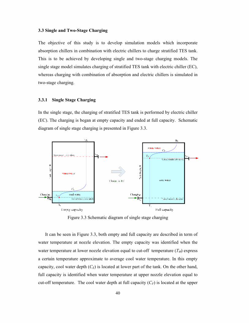
3.3.1 Single Stage Charging

In the single stage, the charging of stratified TES tank is performed by electric chiller

(EC). The charging is began at empty capacity and ended at full capacity. Schematic

diagram of single stage charging is presented in Figure 3.3.

Figure 3.3 Schematic diagram of single stage charging

It can be seen in Figure 3.3, both empty and full capacity are described in term of

water temperature at nozzle elevation. The empty capacity was identified when the

water temperature at lower nozzle elevation equal to cut-off temperature (TΘ) express

a certain temperature approximate to average cool water temperature. In this empty

capacity, cool water depth (CE) is located at lower part of the tank. On the other hand,

full capacity is identified when water temperature at upper nozzle elevation equal to

cut-off temperature. The cool water depth at full capacity (CF) is located at the upper

41

part of the tank. During charging, temperature distribution has an S-curve profile

which relates temperatures of cool, warm and thermocline regions. The cool and

warm water temperatures are designated as Tc and Th, respectively.

3.3.2 Two-Stage Charging

Two stage charging model is aimed to simulate charging of stratified TES tank

involve absorption and electric chillers sequentially. The first stage charging is

performed by using absorption chiller (SAC), while electric chiller (EC) is used on the

second stage. Schematic diagram of the two-stage charging is presented in Figure 3.4.

Figure 3.4 Schematic diagram of two-stage charging

In the first stage charging by absorption chiller, the charging is began at empty

capacity and ended at full capacity. Condition of empty is similar with that on the

single stage, whereas full capacity is identified when outlet charging temperature

equal to limit temperature of the absorption chiller. Cool water depths in the single

and two stage charging are (CE) and (CFT), respectively. This full capacity was

determined by equalizing water temperature at upper nozzle to limit temperature (Tr).

This condition was used as an initial state of the second stage charging. Determination

42

of empty capacity at the first stage and full capacity at the second stage was

performed based on cut-off temperature similar with that on the single stage charging.

In this study, both single and two-stage charging were developed using open and

close charging systems. The single stage charging model is first developed and

validated prior to enhancement for the two-stage charging.

3.4 Open Charging System Model

The open charging system model was developed based on temperature distribution

analysis in stratified TES tank. The temperature distribution analysis commence with

identification of temperature distribution profiles, determining the related parameters,

selection of temperature distribution function as well as formulating of charging

parameters. These steps were performed prior to establishing model type (I) both for

single and two-stage charging stratified TES tank.

3.4.1 Temperature Distribution

As discussed in the section 2.4, the charging of stratified TES tank is performed under

the condition that the TES tank is always full of water. The water comprises of three

layers i.e. the cool water in the lower part, the warm water in the upper part and

thermocline region in the middle part of the tank. Accordingly, water temperature

distribution form a specific S-curve reflecting cool, warm and transition temperatures

of the three layers. Along with additional cool water in the lower part of the TES tank,

the S-curve move upward from initial to final condition of charging cycles. The

typical S-curve temperature distribution is illustrated in Figure 2.1. The S-curve has a

slight inclined line of cool and warm water temperatures. In the modelling, however,

the cool and warm water temperatures were always generated at constant values [46].

Hence, the cool and warm water temperatures were exhibited as straight line of its

average value. The following discussion is focused on the S-curve shape with

constant values of cool and warm water temperatures.

43

3.4.1.1 Parameters of Temperature Distribution Profile

Determination of parameters affecting S-curve temperature distribution profile is

referred to Figure 2.1. The temperature distribution profile is schematically drawn

with respect to tank elevation as illustrated in Figure 3.5. The Figure 3.5 is used as a

basis for determination of temperature distribution parameters.

Tank E

levation (x)

Figure 3.5 Temperature profile in stratified TES tank

The parameters for temperature distribution profile were determined as follows:

i. Average cool temperature was described as Tc.

ii. Average of warm temperature was defined as Th.

iii. The thermocline profile was defined as

a. Position of midpoint of thermocline (C).

b. Slope gradient of thermocline profile (S).

iv. The thickness of thermocline (WTC).

v. Bottom limit point of thermocline (B) was defined as a point where bottom

edge of thermocline profiles located.

vi. Upper limit point of thermocline (U) was defined as position of upper edge of

thermocline profiles.

44

From Figure 3.5, it is shown that the temperature profile parameters are Tc, Th, C

and S. Cool and warm water exist at the lower and upper parts of storage tank. The

boundary line between cool and warm water was identified at C expressing the

position of midpoint of thermocline thickness. The C also indicated the cool water

depth in the TES tank. The thermocline thickness (WTC) was defined as the region

limited by bottom limit point (B) and upper limit point (U). Hence, the temperature

distribution were established as a function of parameters Tc, Th, C and S with variable

height of tank (x), as given in Equation 3.1.

),,,,()( xSCTTfxT hc= (3.1)

3.4.1.2 Selection of Temperature Distribution Function

Selection of the temperature distribution function was performed based on Equation

3.1. The function contained parameters in an independent equation. This was to

simplify the extension in formulating charging parameters. The selection of the

function was aimed to develop a mechanistic model representing the temperature

distribution profile. The criteria for the selection was based on capability in forming

the S-curve profile and contain parameters suitable to the requirement as illustrated in

Figure 3.5.

Selection of the temperature distribution function was conducted using non linear

regression fitting. A commercial software SIGMAPLOT was utilized as a tool to

solve non linear regression in the fitting the function [119]. Evaluation of the

goodness of fitting was evaluated using coefficient of determination (R2). The R

2

value approximate to unity indicates that the functions are capable of representing the

temperature distribution profile.

The function was selected based on historical data of temperature distribution. For

this purpose, six operating data sets were acquired namely IA, IB, IC, IIA, IIB and

IIC as described in section 3.2. The data sets were charging at 393 m3/hr and 524

m3/hr.

45

3.4.2 Formulation of Charging Parameters

This section is addressing on formulating the important charging parameters of the

models in open charging system, namely limit capacity and temperature transition.

Prior to define the charging parameters, determination of limits point of thermocline

and the thickness of thermocline were undertaken.

3.4.2.1 Limit Points

Limit points were defined as points at the edge of temperature profile that bounds the

thermocline thickness. Limit points were determined by utilizing cut-off water

temperature as reference points on the thermocline profile. Some concepts of limit

points have been reviewed in Section 2.3. Among them, dimensionless cut-off

temperature concept proposed by Musser [47] was adopted. The dimensionless cut-off

temperature takes the form of )/()( chc TTTT −−=Θ .

The limit points on the edges of thermocline profile namely bottom limit (B) and

upper limit (U) were determined by incorporating dimensionless cut-off temperature

to temperature distribution function as described in Equation 3.1. The B and U were

referred at a certain distance from C, therefore it was expressed as a function of

dimensionless cut-off temperature (Θ), position of midpoint of thermocline (C) and

slope gradient (S) and takes form as Equation 3.2.

),,(, SCfUB Θ= (3.2)

3.4.2.2 Thermocline Thickness

Thermocline thickness (WTC) was defined as the width of mixing region between cool

and warm water. The thermocline thickness (WTC) was a region limited by bottom and

upper limit points, (B) and (U), respectively. Thermocline thickness was established

by inserting dimensionless cut-off temperature into Equation 3.1.

46

Thermocline thickness was functionally derived as a function of dimensionless cut-off

temperature (Θ) and slope gradient (S) in Equation 3.3.

),( SfWTC Θ= (3.3)

3.4.2.3 Limit Capacity Criteria

Limit capacity criteria has significant role in developing charging model of stratified

TES tank. The limit capacity criteria were used to determine empty and full capacity,

where charging began or ended. The limit capacity were derived based on two criteria

namely water level limit and temperature limit.

i. Water level limit criteria

Using water limit criteria, limit capacity of the charging was determined based on

bottom limit point (B) elevation. It involves empty and full capacity in the charging of

stratified TES tank. When the bottom limit is located at the lower nozzle elevation,

the condition TES tank is at empty capacity. Full capacity, on the other hand, is

achieved when the bottom limit point at the same level with upper nozzle elevation.

The concept in defining empty and full capacity based on water level limit is

illustrated in Figure 3.6.

Figure 3.6(a) shows empty capacity condition that was obtained by positioning

bottom limit point (B) to lower nozzle elevation. Figure 3.6(b) illustrates the bottom

limit point (B) at upper nozzle elevation which indicates the full capacity in the

charging. Position of midpoint of thermocline which indicates cool water depth was

determined by equalizing based on limit point (B) Equation 3.2 to nozzle elevation.

47

(a) Empty capacity (b) Full capacity

Figure 3.6 Empty-full capacity based on water level limit criteria

The cool water depth at empty capacity (CE) was derived as Equations 3.4, and

cool water depth at full capacity (CF) was expressed in Equation 3.5.

Empty capacity (CE), LNSCfB =Θ= ),,( (3.4)

Full capacity (CF), TNSCfB =Θ= ),,( (3.5)

ii. Temperature limit criteria

In the case of charging using absorption chillers, the full capacity of the charging was

considered based on temperature limitation. The outlet charging temperature has to be

maintained above the limit temperature (Tr). Limit temperature is a value of a certain

temperature between cool and warm water temperature. Solution of the problem was

conducted using temperature limit criteria. Determination of empty and full capacities

based on temperature limit criteria is presented in Figure 3.7.

48

(a) Empty capacity (b) Full capacity

Figure 3.7 Empty-full capacity based on temperature limit criteria

Figure 3.7(a) shows empty capacity that was obtained on the condition of water

temperature at lower nozzle equal to a limit temperature (Tr). Determination of full

capacity was performed referring to Figure 3.7(b). From Figure 3.7(b), it can be seen

that full capacity was achieved when the water temperature at upper nozzle elevation

was equal to limit temperature (Tr). The cool water depth of these conditions was

determined by equalizing of temperature distribution function (Equation 3.1) to limit

temperature, while the x variable was referred to the nozzle elevations. Determination

of cool water depth at empty capacity (CET) is described in Equations 3.6, whereas

cool water depth at full capacity (CFT) is determined based on Equation 3.7.

Empty capacity, x=NL and ),,,,()( xSCTTfxT hc= = Tr (3.6)

Full capacity, x=NT and ),,,,()( xSCTTfxT hc= = Tr (3.7)

iii. Temperature transition point

Temperature transition is a point of charging temperature decreases from fairly

constant. It was achieved when the upper limit point of thermocline reach the upper

nozzle elevation. The temperature transition point condition is schematically drawn in

Figure 3.8.

49

Figure 3.8 Temperature transition point

The cool water depth at temperature transition point (CFR) was determined by

equalizing upper limit points (Equation 3.2) to upper nozzle elevation. Determination

of CFR was performed by equalizing upper limit point to upper nozzle elevation as in

Equation 3.8.

TNSCfU =Θ= ),,( (3.8)

Formulation of the charging parameters based on temperature distribution

analysis was used to develop models in open charging system. It was developed for

single stage charging model type (I).

3.4.3 Single Stage Charging Model Type (I)

In the single stage charging model type (I), the discussion is divided into three parts

namely development, verification and simulation of the model for single stage

charging of stratified TES tank.

50

3.4.3.1 Developing Single Stage Charging Model Type (I)

Charging model type (I) was developed by introducing cool water at lower nozzle and

withdrawing warm water from the upper nozzle. The outlet charging water was not

re-circulated into the lower nozzle, hence the model was called as open charging

system. The open charging system is schematically drawn in Figure 3.9.

CV&

Figure 3.9 Schematic flow of open charging system

As shown in Figure 3.9, cool water that is introduced from the lower nozzle has

inlet temperature of Tin and charging flow rate of CV& . The cool water depth is

indicated as hatch area in the lower part of the tank. The following sections explain

assumptions and charging parameters that were used in the model.

i. Assumptions of the single stage charging model type (I)

The assumptions made in the single stage charging model type (I) are as follows:

a. Constant inlet charging temperature at average cool water temperature (Tc).

b. Charging has flow rate of CV& .

c. Temperature distribution has similar profile during charging periods. Hence,

parameters of average cool and warm water temperatures as well as slope

gradient (Tc, Th and S) are constant.

51

d. Cool water depth (C) increases with respect to time and is proportional to

charging flow rate over cross sectional area of the tank. Hence, increasing of

cool water depth during charging was determined as Equation 3.9.

AVC C /&=∆ (3.9)

Based on the assumption, temperature distribution parameters could be

determined for charging stratified TES tank simulation. It is capable of generating

temperature distribution at observed time interval.

ii. Charging parameters of single stage charging model type (I)

Formulations as described in section 3.4.2 were used to determine charging

parameters of the model. The charging parameters were cool water depth, charging

duration as well as cumulative cooling capacity.

a. Cool water depth

Cool water depths were determined based on formulation from temperature

distribution analysis. Cool water depths were used to indicate the conditions of empty

capacity, temperature transition point as well as full capacity.

(i) Cool water depth at empty capacity (CE) was determined using water level

limit criteria in the solution of Equation 3.4. Optionally, it could also be

determined based on temperature limit criteria from the solution of

Equation 3.6.

(ii) Cool water depth at temperature transition point (CFR) was determined based

on solution of Equation 3.8.

(iii) Cool water at full capacity (CF) was determined by referring to water level

limit criteria in the solution of Equation 3.5. It could also be determined

based on temperature limit criteria in the solution of Equation 3.7.

52

b. Charging duration

Charging duration was defined as time required for performing charging from initial

to final state. It was determined based on cool water depth differences during the

charging to achieve temperature transition point as well as for full capacity.

(i) Charging duration to achieve transition temperature (tCFR) point was defined

as follows.

AV

CCt

C

EFRCFR .

&

−= (3.10)

(ii) Charging duration for full capacity (tCF) during the charging wass determined

as follows.

AV

CCt

C

EFCF .

&

−= (3.11)

With CE, CFR, CF are cool water depths at empty capacity, temperature transition

point and full capacity, respectively. CV& is charging flow rate and A is cross

sectional area of the tank.

c. Cumulative cooling capacity.

Cumulative cooling capacity was utilized to determine cooling energy stored in the

observed time interval during the charging. It was determined based on temperature

distribution consist of N slabs of the tank. The cumulative cooling capacity (Qcum) is

presented in Equation 3.12.

∑=

−=N

n

nrpncum TTCMQ1

)(.. (3.12)

Mn is mass of water at each slab, Cp is specific heat, Tr is reference temperature, Tn is

water temperature at each slab and N is number of slabs in TES tank.

53

3.4.3.2 Verification of Single Stage Charging Model Type (I)

The temperature distribution of the model was verified before implementing in the

simulation. The steps taken to verify the model are the follows.

i. Acquire observed data set which consists of hourly temperature distribution

within a certain charging period. The data set of IA was used consist six hours of

charging from 18.00 hours to 03.00 hours at flow rate of 393 m3/hr.

ii. Determination of parameters Tc, Th, C and S for the observed temperature

distribution data set. It was performed by using SIGMAPLOT package for non

linear regression fitting on the observed data.

iii. Generation of temperature distribution in the model. It was first carried out by

determining parameter values Tc, Th, C and S similar with that on initial condition

of the observed data. Increasing of cool water depth (∆C) was determined based

on Equation 3.9. The temperature distributions of the model were generated from

parameters of Tc, Th, C and S.

iv. Evaluation of temperature distribution of the observed data and model. The

evaluation used three criteria i.e temperature distribution similarity, temperature

parameters similarity and t-statistical test. The evaluations are explained as

follows:

a. Similarity of temperature distribution.

The evaluation was performed by determining the goodness relationship of the

temperature distribution. It was performed using coefficients of determination

(R2) of temperature distribution between the observed data and the model.

b. Similarity of temperature distribution parameters.

It was conducted by comparing parameters Tc, Th, C and S between the

observed data and model.

c. Statistical test.

Evaluation of significant similarity between the observed data and model was

performed using t statistical test [64]. The assessment was to see whether the

54

model can be accepted or not to represent temperature distribution on the

observed data. The Null hypothesis of the test is that temperature distribution

between observed data and model is similar. Therefore:

Null hypothesis Ho: 21

ii yy − = 0

Alternative hypothesis Ha: 21

ii yy − ≠ 0

t computed in the hypothesis test is the ratio of the mean data value ( y )

difference and its standard deviation (σ ). It was determined between the

observed data and model, designated as subscript 1 and 2, respectively. The t

computed takes form as in Equation 3.13.

2

2

2

1

21

σσ +

−=

yytcomp (3.13)

The standard deviation observed data and model were calculated using

Equations 3.14 and 3.15, respectively

1

)( 211

1 −−Σ

=n

yyiσ (3.14)

1

)( 222

2 −−Σ

=n

yyiσ (3.15)

With 1y and 2y are mean values of the observed data and model, 1σ and 2σ

are standard deviations of the observed data and model, whereas 1

iy and 2

iy are

temperature distributions of the observed data and model.

The region for null hypothesis acceptance is t computed < t critical. The t critical

value is equal to t(f,β/2) in the table t distribution with reference to significance level (β)

and value of the number of degree of freedom (f). The significance level indicates the

level of probability that the hypothesis would be rejected. The t distribution table is

presented in Appendix E.

55

3.4.3.3 Simulation of Single Stage Charging Model Type (I)

The steps taken in conducting simulation of the single stage charging model type (I) is

presented in Figure 3.10. The simulation of the single stage charging model type (I)

involve with input parameters and determination values of the charging parameter.

i. Input parameters of the simulation

a. Initial temperature distribution parameters.

Initial temperature was determined based on empty capacity as described in

the limit capacity criteria, hence require parameters of Th, Tc, S and

predetermined of dimensionless cut-off temperature (Θ). The parameter Θ

was used to determine cut-off water temperature, as stated in section 2.3.2.

b. TES tank configuration parameters.

TES tank configuration parameters required lower and upper nozzles

elevation, described as NL and NT, respectively. The other required parameters

were diameter (D), effective water depth (H) and number of slabs in the TES

tank.

c. Charging flow rate.

d. Observation time intervals

ii. Determining of charging parameter values in the simulation

Parameters that were determined in the simulation are cool water depth and

charging duration. All parameters were observed in term of empty capacity,

temperature transition and full capacity. The cool water depth at temperature

transition point (CFR) and full capacity (CF) were determined based on solution of

Equation 3.8 and 3.5, respectively. The charging duration to achieve transition

temperature (tCFR) and full capacity (tCF) were determined based on solution of

Equation 3.10 and 3.11, respectively.

iii. Temperature distribution of the simulation was generated by parameter

incorporated to temperature distribution function as described in Equation 3.1.

Cumulative cooling capacity was determined based on Equation 3.12.

56

Simulation of single stage charging model type (I) was performed in three cases

namely A1, B1 and D1. The cases of A1, B1 and D1 which involve variation of

charging flow rates of 524 m3/hr, 393 m

3/hr and 262 m

3/hr, were treated as having the

same initial temperature in the TES tank configuration. Simulation was performed

using TES tank configuration parameters as presented in Table 3.1, where chiller

parameter shown in Table 3.2. Initial temperature referred to parameter values of Tc,

Th, C and S. The TES tank configuration parameter as tabulated in Table 3.1 was

used for all simulation cases in this study.

CV&

CV&

Figure 3.10 Simulation steps in single stage charging model type (I)

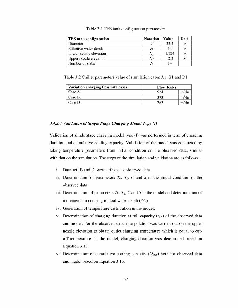
57

Table 3.1 TES tank configuration parameters

TES tank configuration Notation Value Unit

Diameter V 22.3 M

Effective water depth H 14 M

Lower nozzle elevation NL 1.824 M

Upper nozzle elevation NT 12.3 M

Number of slabs N 14

Table 3.2 Chiller parameters value of simulation cases A1, B1 and D1

Variation charging flow rate cases Flow Rates

Case A1 524 m3/hr

Case B1 393 m3/hr

Case D1 262 m3/hr

3.4.3.4 Validation of Single Stage Charging Model Type (I)

Validation of single stage charging model type (I) was performed in term of charging

duration and cumulative cooling capacity. Validation of the model was conducted by

taking temperature parameters from initial condition on the observed data, similar

with that on the simulation. The steps of the simulation and validation are as follows:

i. Data set IB and IC were utilized as observed data.

ii. Determination of parameters Tc, Th, C and S in the initial condition of the

observed data.

iii. Determination of parameters Tc, Th, C and S in the model and determination of

incremental increasing of cool water depth (∆C).

iv. Generation of temperature distribution in the model.

v. Determination of charging duration at full capacity (tCF) of the observed data

and model. For the observed data, interpolation was carried out on the upper

nozzle elevation to obtain outlet charging temperature which is equal to cut-

off temperature. In the model, charging duration was determined based on

Equation 3.13.

vi. Determination of cumulative cooling capacity (Qcum) both for observed data

and model based on Equation 3.15.

58

vii. Comparison of charging duration and cumulative cooling capacity between the

observed data and model.

3.4.4 Two-Stage Charging Model Type (I)

This section focuses on enhancing the single stage charging for two-stage charging

model type (I). The enhancement and simulation involved charging of the TES tank

by absorption and electric chillers sequentially.

3.4.4.1 Enhancement of Two-stage Charging Model Type (I)

The model was enhanced for implementation of two-stage charging stratified TES

tank. Absorption chiller was used at the first stage, whereas electric chiller was used

in the second stage of charging. The constraint in implementing absorption chillers in

the first stage charging was the occurrence of limit temperature. The limit temperature

in the absorption chillers was considered as a change state between the first and

second stage of charging. Hence, the full capacity in the first stage charging was due

to limitations on the outlet TES temperature.

Solution of temperature limitation was undertaken by utilizing limit capacity

criteria, as described in 3.4.2.3. Empty and full capacities in the simulation were

based on Equations 3.4 and 3.7, respectively. The steps taken for developing two-

stage charging simulation is presented in Figure 3.11.

The steps taken in the simulation of two-stage charging model type (I) is almost

similar with that on the single stage charging model, with additional charging flow

rates and full capacity in the second charging. Parameters that were determined in the

simulation namely cool water depth, charging duration as well as cumulative cooling

capacity.

i. Cool water depth

Cool water depths at empty capacity (CE) as well at temperature transition (CFR) in

the first charging were determined similar to that of the single stage simulation.

59

Cool water depths at empty capacity (CE) as well at temperature transition (CFR)

were determined using solution of Equation 3.4 and 3.8, respectively. The cool

water depth at full capacity at the first stage charging (CFT) was determined using

full capacity based on criteria temperature limit, using solution of Equation 3.7.

For the second stage charging, cool water depth at full capacity (CF) was

determined using full capacity on water level limit criteria, which was based on

solution of Equation 3.5.

ii. Charging duration

In the first stage, charging duration for temperature transition (tCFR) was

determined as follows.

AV

CCt

C

EFRCFR .

1&

−= (3.16)

Charging duration for full capacity at the first stage (tCFT) was determined as

follows.

AV

CCt

C

EFTCFT .

1&

−= (3.17)

In the second stage, charging duration for full capacity (tCF) was determined as in

Equation 3.18.

AV

CCt

C

FTFCF .

2&

−= (3.18)

60

1CV&

1CV&

2CV&

2CV&

Figure 3.11 Simulation steps in two-stage charging model type (I)

61

3.4.4.2 Simulation of Two-stage Charging Model Type (I)

Simulation of two-stage charging model was performed in two cases. In the first case,

charging flow rate variation of the second stage at 262 m3/hr, 393 m

3/hr and 524

m3/hr, as cases E1, F1 and G1, respectively. Whereas on the second case, charging

simulation was carried out with variation of limit temperature at 7oC, 9

oC and 11

oC,

as reflected in cases H1, J1 and K1. The flow rates at the first and second stage were

using flow rates at 504 m3/hr and 393 m

3/hr. Both cases were conducted at similar

TES tank configurations as described in Table 3.1. Description of chiller parameters

variation of the two-stage charging model type (I) cases are presented in Table 3.3

and 3.4 for flow rate and limit temperature, respectively.

Table 3.3 Chiller parameters for simulation cases E1, F1 and G1

Variation of charging flow rate (Cases E1, F1, G1) Notation Value Unit

Absorption chillers (1st stage)

Flow Rate 1CV& 504 m3/hr

Limit Temperature Tr 9 oC

Electric chillers (2nd stage)

Case E1 2CV& 524 m3/hr

Case F1 2CV& 393 m3/hr

Case G1 2CV& 262 m3/hr

Table 3.4 Chiller parameters for simulation cases H1, J1 and K1

Variation of limit temperature (Cases H1, J1, K1) Notation Value Unit

Absorption chiller (1st stage) Flow Rate

1CV& 504 m3/hr

Electric chiller (2nd stage) Flow Rate

2CV& 393 m3/hr

Case H1 Tr 7 oC

Case J1 Tr 9 oC

Case K1 Tr 11 oC

The simulation charging models as discussed in Section 3.2 were developed

considering temperature distribution profile analysis. In this model the charging was

assumed to have constant temperature parameters during charging periods. The

temperature profile movement was due to increasing of cool water volume in the

62

lower part of the tank. In the real cycles, however, charging is performed in close

system working at various operating conditions of TES tank and chillers. Related to

this, development and simulation models based on close charging system were

discussed in the next section.

3.5 Close Charging System

Selection of model in the simulation environment holds important role in achieving

accurate representation of system characteristic. In this study, selection of one-

dimensional flow model rather than two and a three-dimensional model is because of

two reasons. First, the one-dimensional flow model has capability in covering factors

that affect degradation of temperature distribution namely conduction through the

wall, conduction between cool and warm water, mixing effect in initial flow of

charging as well as heat loss to surroundings. The other main reason is that utilizing

one-dimensional model enables modelling of general configuration of the TES tank

system. Development and simulation of charging models using close system were

undertaken by utilizing convection and conduction equation. The models were

developed for single and two-stage charging in the stratified TES tank.

3.5.1 Single Stage Charging Model Type (II)

The models in close charging system were developed in a single stage charging model

type (II). The developed model was aimed to cover the fact that charging cycles was

operated as a close circulation system between the TES tank and chillers. Schematic

flow diagram of close charging system is illustrated in Figure 3.10.

As illustrated in Figure 3.12, chilled water was circulated in the close charging

system between TES tank and chillers. The chilled water was cooled in the chillers

prior to be flown in the lower part of the tank through lower nozzle. Adding of cool

chilled water increases the cool water volume in the tank and affected temperature

profile moves upward to the upper part of the tank. In addition, supplying cooler

chilled water also has an effect on the mixing temperature in the lower part of the TES

tank.

63

Hence, several factors affecting the charging cycles such as temperature distribution,

flow rate and working temperature of the chillers, mixing temperature and

temperature losses in the piping lines (∆T1 and ∆T2) have to be considered. These

factors were accommodated in the physical model of TES tank and the chillers in the

next section.

Figure 3.12 Schematic flow diagram of close charging system

3.5.1.1 Physical Model of Stratified TES Tank

Implementation of one-dimensional model was expressed in term of conduction and

convection cases that occur in the TES tank. Occurrence of conduction was caused by

cool and warm water temperature difference, whereas convection was due to flowing

of chilled water in the TES tank. The physical model of the stratified TES tank is

presented in Figure 3.13. Energy balance on elemental volume emerges in the form of

transient conduction and convection one-dimensional flow.

As shown in Figure 3.13, the charging cycle iss illustrated in a cylindrical TES

tank with diameter (D) and effective water depth (H). The cylindrical tank is assumed

has N equal slabs in the longitudinal direction. The TES tank is well insulated. Among

64

the factors affecting temperature distribution degradation, conduction between cool

and warm water, and mixing effects were emphasized. Heat losses to surrounding and

conduction through the tank wall were negligible. The heat loss to surrounding was

ignored in the installation of sufficient external insulation of the tank. Whereas

conducting wall effect was neglected due to internal coating of the tank.

1,Tm&

1, −nTm&

NTm,&

outTm,&

x

Tk

∂∂

− .

xx

Tk

∂∂

− .

dxxx

Tk

+∂∂

− .

x

Tk

∂∂

− .

inTm,&

nTm ,&

Figure 3.13 Physical model of stratified TES tank [4]

The energy balance of the water at a distance x from the bottom of the tank is

identified as a parabolic partial differential equation which as in Equation 3.19.

x

Tcm

x

TAk

t

TcA pp ∂

∂−

∂∂

=∂∂

.......2

2

&ρ (3.19)

Converting the mass flow rate, Avm ..ρ=& and thermal diffusivity )./( pck ρα = ,

reveal that Equation 3.19 was suitable to Equation 2.4, with the absence of last term

that express the heat loss to surrounding.

65

The effect of conduction across the thermocline was accounted for in term of

thermal diffusivity (α) that occurs due to conduction heat transfer between cool and

warm water in the tank. The mixing effect factor was emphasized by pronouncing

effective diffusivity factor [80]. The effective diffusivity factor form as

αεαε /)( Heff += , has value greater than unity in turbulent flow and for laminar flow the

value of εeff is equal to 1.

Accommodating the two aforementioned factors affecting the degradation of

stratification, Equation 3.19 became to Equation 3.20.

2

2

.x

T

x

Tv

t

Teff ∂

∂=

∂∂

+∂∂

εα (3.20)

Equation 3.20 was divided into two cases, i.e conduction and convection equation.

This was done to avoid any pseudo mixing in the numerical calculation as discussed

in Section 2.4.

The conduction equation takes the form of Equation 3.21.

2

2

.x

T

t

Teff ∂

∂=

∂

∂εα (3.21)

The convection equation form is as follow.

0=∂∂

+∂∂

x

Tv

t

T (3.22)

Since the assumption of a well insulated tank was used in this study, the

temperature gradient across the top and bottom boundaries of the tank was assumed to

be zero. It is expressed in Equation 3.23.

0=∂∂

x

Tat x = 1 and x = N (3.23)

The solution was carried out numerically based on finite difference method. As a

numerical solution, finite difference solves the equations as discrete solutions. This

was performed by subdividing the region into a number of small slabs (∆x) in the

66

height of TES tank and observed time interval (∆t). Each slab was assumed to

represent constant temperature at horizontal layer [67].

In this study, the finite difference solution was solved using explicit method. The

convergence stability of the explicit method was performed on the convection and

conduction equation. Using differentiating technique, conduction equation in

Equation 3.21 was described as Equation 3.24.

2

11

1 .2..

x

TTT

t

TT t

x

t

x

t

xeff

t

x

t

x

∆+−

=∆

− +−+

εα

)(..)....21( 1122

1 t

x

t

xeff

t

xeff

t

x TTx

tT

x

tT +−

+ +∆∆

+∆∆

−= εααε (3.24)

The convergence stability of Equation 3.24 requires limitation of α.εeff. (∆t/∆x2)

value designated as AMIX value. The stability occurred in the condition as described

in Equation 3.25 [74].

AMIX = α.εeff (∆t/∆x2) ≤ 0.5 (3.25)

Convection equation solution takes the form of Equation 3.26.

0)(

. 1

1

=∆−

+∆

− −+

x

TTv

t

TT t

x

t

x

t

x

t

x

)..1(.. 1

1 t

x

t

x

t

x Tx

tvT

x

tvT

∆∆

−+∆∆

= −+ (3.26)

On the stability criteria, the Courant number designated as FLOW = v.∆t/∆x must

not be greater than unity. Therefore, the time interval (∆t) and segmental element

(∆x) are chosen to fulfil the stability requirement as given by [74].

FLOW = v.∆t/∆x ≤ 1 (3.27)

The solution of boundary condition as described in Equation 3.23 of the tank was

calculated using Equation 3.28.

67

01 =∆

−+

x

TT t

x

t

x (3.28)

Solution of the combined conduction and convection equations is effectively

obtained using buffer tank concept [76]. The purpose of using buffer tank concept is

to eliminate pseudo mixing in the solution. Using the buffer concept, one fictitious

inlet buffer tank is placed at the bottom of the tank. The inlet buffer tank stores the

incoming flow of water and is evaluated at regular time intervals. If accumulated

water equals to one segment volume, the water is pulsed into the tank. Numerically

this indicates that the convection equation is derived using FLOW = 1. Referring to

Equation 3.26, condition of FLOW = 1 leads to Equation 3.29.

t

x

t

x TT 1

1

−+ = (3.29)

Solution of boundary condition in Equation 3.28 reveal that t

oT = tT1 at the bottom

of the tank and t

NT 1+ = t

NT at the top of the tank. t

oT is the temperature at inlet buffer

tank. The conduction equation was applied for each observed time interval, whereas

the convection was implemented only at FLOW = 1 that indicate of one filled

segment of the tank. The convection equation might be invoked occasionally, every

third and forth time, depending on the flow rate. Thus, convection and conduction

equation can be combined together without introducing pseudo-mixing through

numerical procedures.

3.5.1.2 Model of Chillers

As illustrated in Figure 3.10 chilled water is circulated in a close charging system

between TES tank and chillers. Outlet TES temperature, after accommodating

temperature losses (∆T1), chilled water flows into the chillers at temperature TinC. The

chilled water is cooled in the chillers and exit at temperature ToutC. The chilled water

is re-circulated into the TES tank, after accommodating temperature losses (∆T2) from

its connection piping.

68

Cooling capacity in the chillers is calculated based on temperature difference

between inlet and outlet temperature of chilled water as expressed in Equation 2.7.

This cooling capacity is equal to cooling capacity given by evaporator component of

the chillers, expressed as Equation 2.8 in Chapter 2.

The model of the chillers was developed as general equation to represent cooling

capacity for both vapor compression and absorption chillers. The chiller model was

also utilized to correlate inlet and outlet charging temperature. It was performed by

equalizing both Equations 2.7 and 2.8. The relationship between outlet and inlet

chilled water temperature takes form as Equation 3.30.

)../( pC CVUA

evCin

evCout

e

TTTT

ρ&

−+= (3.30)

The outlet temperature of the chillers (ToutEC), after having temperature losses

(∆T2) entering the TES tank at temperature at (TinTES). The entered volumes mix with

chilled water in the bottom part of TES tank and exist at mixing temperature (Tmix).

The refrigerant temperature is designated as working evaporator temperature, Tev. The

assumption is the evaporator works at a constant temperature [11].

Mixing temperature occurs due to mix condition of entered volume and chilled

water region at the lower part of TES tank. The chilled water influenced by mixing

has volume of VLC and temperature of TLC, whereas the entered charging volume is

multiplication of chillers flow rate ( CV& ) with time interval ∆t. Mixing temperature

was calculated based on energy balance as described by Equation 3.31. The mixing

temperature adopted concept of Wildin and Truman [79].

tVV

TtVTVT

CLc

inTESCLcLcmix ∆+

∆+=

.

...

&

&

(3.31)

3.5.1.3 Developing Single Stage Charging Model Type (II)

Developing single stage charging model type (II) was performed by integrating TES

tank and chillers models. The solution was carried out using finite difference in

69

explicit method, while buffer tank concept was involved in combining convection and

conduction equations in the TES tank. The steps taken for the solution is presented in

Figure 3.14.

The model was first carried out with initialization of the parameters, involving

determination of initial temperature, thermo-physical property of water in the tank

configuration parameter and chillers parameter. In addition, selecting εeff was also

undertaken.

The initialization parameters of the charging model type (II) are described as

follows.

i. Water temperature distribution in the initial charging condition.

Initial temperature was used as starting state for charging. It was obtained from

reading the temperature distribution or generated from empty capacity from the

limit capacity criteria. Using limit criteria, initial temperature was generated using

temperature distribution in Equation 3.1 with cool water depth at empty condition

(CE) as defined in Equation 3.4.

ii. Determination of average cool and warm water temperature.

These temperatures were used to determine the value of thermal diffusivity (α). It

was defined as average temperature of cool and warm water. The value of thermal

diffusivity (α) was obtained from Appendix F.

iii. TES tank configuration parameters.

TES tank configurations were used to determine parameters in the single charging

model type (II). The TES tank configuration parameters consist of D, H, NL, NT

and number of slabs (N).

a. Number of observed slabs in TES tank (N) indicate the position of temperature

sensors. Further, each slab was divided into small (L) numbers of ∆x segments

to cover parameter FLOW equal to 1 used in this method, hence observed

interval time ∆t was obtained accordingly using Equation 3.28.

70

b. TES tank configuration parameters were diameter (D), effective water depth

(H), lower and upper nozzle elevations, NL and NT, respectively. These data

were used to determine the mixing volume (VLC), mixing temperature (TLC),

and outlet charging TES temperature (ToutTES).

iv. Chillers parameters were flow rate ( )CV& , UA and evaporator temperature (Tev). In

addition, it was also required temperature losses at piping connection in the

upstream and downstream of the chillers, (∆T1) and (∆T2), respectively. Those

data were used to determine inlet and outlet chillers temperatures, TinC and ToutC,

respectively.

The other important parameter for identifying mixing effect was required prior to

parameters initialization. It was performed by selection of effective diffusivity (εeff).

The procedure in selection of εeff was discussed in section 3.5.1.4.

After initializing the parameters of the model, temperature distribution was

performed to determine the outlet charging temperature (ToutTES), cool water volume

influenced by mixing (VLC) and temperature in the mixing region (TLC). ToutTES was

determined from temperature distribution considering upper nozzle elevation in the

stratified TES tank. The volume VLC was obtained based on cool water volume in the

lower part of tank which was influenced by inlet flow. Temperature TLC was

determined as the average temperature of cool water volume in the VLC region.

Determination of these values was described in Section 3.5.3.

Next, the solution of the model followed the buffer concept based on finite

difference method. Prior to define mixing temperature (Tmix), several temperature

series have to be determined. Outlet charging temperature (ToutTES) was obtained

based on temperature distribution at upper nozzle elevation. Water mixing volume

temperature at (TLC) was determined as average temperature in the mixing region.

Inlet charging temperature (TinTES) was determined from Outlet charging temperature

(ToutTES) plus losses temperature (∆T1). Explanations of these formulae are described

in Equations 3.32 to 3.36.

71

Figure 3.14 Solution steps in integrating of TES tank and chiller models.

72

3.5.1.4 Selection of Effective Diffusivity

Prior to parameters initialization, effective diffusivity (εeff) were selected properly.

Selection of εeff was aimed to cover temperature distribution profile in the range of

working flow rate. The appropriate εeff was selected from various observations.

Higher value εeff indicates more slope gradient of thermocline profile. The other

purpose of selecting εeff was to observe whether the convergence criteria in Equation

3.25 were reached or not. If the model requires AMIX value less than 0.5, it indicates

that it can be solved using explicit method. On the other hand, if AMIX is observed

exceeding 0.5 means that finite difference should be solved in implicit method.

The selection of εeff was performed using data set IA for charging flow rate of

393 m3/hr. The mixing effect was selected from 0 to 250 in the range of AMIX lower

than 0.5. The evaluation in the selection utilized coefficient of determination, R2. The

selection of εeff involved TES tank configuration parameter and chillers parameter,

whereas initial temperature was taken from the observed data.

3.5.2 Verification of Single Stage Charging Model Type (II)

The single stage charging model type (II) developed in Section 3.5.1.3 has to be

verified prior to conduct simulation. The verification was performed in two charging

flow rate cases i.e 393 m3/hr and 524 m

3/hr. For flow rate of 393 m

3/hr, the

verification used data set of IB and IC. For the case of charging flow rate 524 m3/hr,

data sets of IIB and IIC were used.

Inputs of the model were initial water temperature distribution, TES tank

configuration and chillers parameters (flow rate, UA, Tev, ∆T1 and ∆T2) besides

thermo-physical properties of chilled water. The initial temperature was obtained

from the observed data and the parameters in TES tank configuration taken from

Table 3.1. Determination of chillers parameters is explained in the following section.

73

3.5.2.1 Chillers Parameters

The chiller parameters consist of flow rate, UA and evaporator temperature (Tev).

Parameters UA and Tev were determined based on Equations 2.7 and 2.8 incorporating

to designed data of the chillers namely inlet and outlet temperature (TinC,des, ToutC,des),

flow rate ( )CV& and designed chiller cooling capacity (QC,des).

In this study, design inlet and outlet water temperature were 13.5oC and 6

oC,

respectively. Chillers were assumed to have constant evaporator temperature (Tev) of

4oC. The obtained values of UA parameter are tabulated in Table 3.5.

Table 3.5 Values of UA parameter in the chillers

Flow rate ( )CV&

(m3/hr)

Cooling Capacity

(QC, des) UA (kW/

oC)

131 325 RT(1,142.75 kW) 238.14

262 650 RT (2,285.5 kW) 476.28

393 975 RT(3,428.25 kW) 714.41

524 1200 RT (4,571.0 kW) 952.55

504 1250 RT (4,395.2 kW) 916.19

3.5.2.2 Evaluation in Model Verification

The verification of the model was carried out by evaluating the temperature

distribution similarity and temperature profiles similarity. To endorse acceptance of

the model, the statistical test was also adopted. The evaluation of temperature values,

profile similarity as well as statistical test were similar to that of single charging

model type (I), described in section 3.4.3.2.

Since the operating TES tank data were available as hourly recorded, it is required

to divide each slabs of the TES tank to a numbers of small segment to get the

appropriate time interval. Selection of the segment numbers is performed to achieve

similar observed hourly interval. Hence, the multiplication of observed time interval

(∆t) is approximating similar to hourly interval.

74

3.5.3 Simulation of Single Stage Charging Model Type (II)

Simulations single stage charging model type (II) was conducted in variation of

chillers parameter. The simulation was treated using same initial temperature, TES

tank configuration parameter and the limit temperature (Tr) = 9oC. The TES tank

configuration parameter was similar on the charging model type (I) as in Table 3.1,

whereas chillers parameter is tabulated in Table 3.6, with all ∆T1 and ∆T2 are equal to

zero. The simulation was denoted as cases A2, B2 and D2.

Table 3.6 Chiller parameters value of simulation cases A2, B2 and D2.

Simulation cases Notation Value Unit

CV& 524 m3/hr

UA 952.5 kW/oC Case A2

Tev 4 oC

CV& 393 m3/hr

UA 714.4 kW/oC Case B2

Tev 4 oC

CV& 262 m3/hr

UA 476.3 kW/oC Case D2

Tev 4 oC

Simulation was extended to observe charging characteristics in term of

temperatures TinTES, ToutTES, Tmix and cumulative cooling capacity (Qcum). It was also

extended to perform observation of chiller cooling capacity (QC) and partial working

load of the chillers. Observation was carried out until reaching cumulative cooling

capacity exceeds its nominal holding capacity of 49,226.44 kWh.

For this purpose, the calculation of the aforementioned parameters was formed

based on temperature distribution in the TES tank, hence related to water slabs in the

TES tank. In this study, the TES elevation was divided into 14 slabs, which were

located serially as 1 to 14 from the bottom to the upper part. The slab temperature was

identified in the middle of the slab. Since the simulation involved temperature were

expressed accordingly. All equations were described in term of subscript t express

observation time intervals.

75

Outlet charging TES temperature was determined as water temperature at the

upper nozzle which is located at 12.3 m elevation. Determination of ToutTES was based

on interpolation of temperature slabs 12 and 13, therefore was calculated as Equation

3.32.

)(8.0 ,11,12,12, ttttoutTES TTTT −+= (3.32)

Inlet water temperature entering the chillers was calculated as in Equation 3.33.

TinC,t=ToutTES,t+∆T1 (3.33)

The outlet water temperature from the chillers was determined from Equation 3.31,

and takes form as Equation 3.34.

)../(

,

,, CpVUA

evtCin

evtCouttCe

TTTT

ρ&

−+= (3.34)

Inlet water temperature entering the TES tank was identified as in Equation 3.35

TinTES,t=ToutC,t+∆T2 (3.35)

Mixing temperature was calculated as a mixed temperature between the cool

water volume and the entering volume water from the chillers, as described in

Equation 3.36.

tVV

TtVTVT

ttCtLc

ttinCttCtLctLc

ttmix ∆+

∆+=

∆+

∆+∆+

∆+.

...

,,

,,

.

,,

, &

&

(3.36)

Determination of cool water volume influenced by mixing (VLC) was based on

assumption of two influenced slabs region. This considered lower nozzle elevation of

1.824 m. It was determined as the water volume at two slabs of TES tank, as Equation

3.37.

VLc,t = 2. A. ρ (3.37)

The temperature in the mixing region (TLC) was determined as average cool

water temperature of slabs 1 and 2 at the lower part of the tank, as in Equation 3.38.

76

TLC,t = (T1,t+T2,t)/2 (3.38)

On the other aspect, chillers working parameters were determined in term of

cooling capacity (QC) and percentage of partial working load (PL).

Cooling capacity of the chillers was calculated as in Equation 3.39.

).(. ,,., toutCtinCptCtC TTCVQ −= & (3.39)

Partial working load of the chillers was calculated as working cooling capacity over

the design cooling capacity of the chillers as Equation 3.40.

PLt=QC,t/QCdes (3.40)

3.5.4 Two-Stage Charging Model Type (II)

The single stage charging model type (II) was enhanced for two-stage charging

stratified TES tank. It was performed to cover charging with two types of chillers

sequentially, namely absorption and electric chiller. The special issue in two-stage

charging is the occurrence of limit temperature at outlet TES temperature, due to

temperature limitation of the absorption chillers is explained in the following section.

3.5.4.1 Enhancement of Two-Stage Charging Model Type (II)

As previously discussed, the two-stage charging simulation used the absorption

chillers in the first stage and electric chiller in the second stage. The first stage

charging is performed from empty to full capacity. The empty capacity is identified

from initial temperature distribution. The full capacity of the first stage charging is

determined in the condition of outlet charging temperature equal to limit temperature.

The simulation steps taken for the two-stage charging is presented in Figure 3.15.

77

Figure 3.15 Simulation steps in two-stage charging model type (II)

78

Inputs of the two-stage charging simulation were initial temperature, TES tank

configuration, chillers parameter and temperature losses in piping connection. In

addition, limit temperature of absorption chillers at the first stage charging was also

required. After parameter initialization, the simulation was performed in the first stage

charging. The full capacity of the first charging was reached when outlet charging

temperature equals to the limit temperature of the absorption chiller. The simulation

was then continued for the second stage charging which is served by electric chillers.

In the second stage charging, full capacity of the first charging was set as the initial

condition. The second stage charging could work either as the same or different

observed time interval as on the first stage charging. The full capacity of the second

stage charging is a condition of outlet TES tank temperature equals to the designated

cut-off temperature. Determinations of full capacities in the first and second stage of

charging were carried out by interpolation between two observed time intervals.

3.5.4.2 Simulation of Two-Stage Charging Model Type (II)

Simulation of two-stage charging model type (II) was performed using absorption

chillers in the first stage, whereas electric chiller was utilized in the second stage. The

simulations of two-stage charging were performed in two cases i.e variation of

chillers parameters and limit temperature.

i. Variation of chillers parameters

The input parameters of TES tank configuration are shown in Table 3.1. Temperature

losses ∆T1 and ∆T2 were taken as zero. Variation of chillers parameters were carried

out in the second stage charging, whereas the first stage charging used absorption

chillers at the flow rate of 504 m3/hr. The simulation was carried out for three cases

i.e E2, F2 and G2. Values of the chillers parameters in the simulation are tabulated in

Table 3.7.

79

Table 3.7 Chiller parameters value of simulation cases E2, F2 and G2

Chillers parameters Notation Value Units

1CV& 504 m3/hr

UA 952.5 kW/oC Absorption chiller (1

st stage)

Tev 4 oC

Tr 9 oC

Electric chiller (2nd stage)

2CV& 524 m3/hr

UA 952.5 kW/oC Case E2

Tev 4 oC

2CV& 393 m3/hr

UA 714.4 kW/oC Case F2

Tev 4 oC

2CV& 262 m3/hr

UA 476.3 kW/oC Case G2

Tev 4 oC

ii. Variation of limit temperature

The other simulation of the two-stage charging model type (II) was performed with

variation of limit temperature. The input parameters of initial temperature and TES

tank configuration were similar with that of the variation chillers parameter in the

two-stage charging model type (II). The simulation was carried out for three cases i.e

H2, J2 and K2. Variations of the chillers parameter in the simulation of the model is

tabulated in Table 3.8.

Table 3.8 Chiller parameters value of simulation cases H2, J2 and K2

Simulation cases H2, J2, K2 Notation Value Unit

Absorption chiller (1st stage)

UA = 916.2 kW/oC, Tev = 4

oC 1CV& 504 m

3/hr

Electric chiller (2nd stage)

UA = 714.4 kW/oC, Tev = 4

oC 2CV& 393 m3/hr

Variation limit temperature (Tr)

Case H2 Tr 7 oC

Case J2 Tr 9 oC

Case K2 Tr 11 oC

80

3.6 Comparison of Charging Models

Two different approaches were utilized for developing the models namely open and

close charging system. The simulation models were developed for single and two-

stage charging. In the open charging system, the models were designated as type (I)

whereas in the close charging system, the models were established as type (II).

Comparisons of the two models are discussed in the following section.

3.6.1 Comparison of Single Stage Charging Models

Comparison was carried out in the charging simulation cases on flow rate variation.

The comparisons were discussed in term of charging duration and cumulative cooling

capacity. The comparison between single stage charging model types (I) and (II) were

performed by comparing cases A1, B1, D1 and A2, B2, D2. The simulations were

treated to have similar parameters of initial temperature and TES tank configuration

parameters.

In addition, comparisons were also performed to observe additional cool water

temperature and charging parameters obtained from the simulations. Temperature of

additional cool water was carried out by comparing the average cool water

temperature (Tc) in the simulation model type (I) and mixing temperature (Tmix) in the

simulation model type (II). Comparisons were performed for the parameters values of

charging duration and cumulative cooling capacity.

3.6.2 Comparison of Two-stage Charging Models

Comparison between the two-stage of charging models were carried out for two cases

of flow rate and limit temperature variation. The simulation cases of E1, F1 and G1

were compared for flow rate variation. Limit temperature variation involves

comparisons of cases H1, J1, K1 and cases H2, J2, K2.

81

CHAPTER 4

RESULTS AND DISCUSSION

The main aim of the analysis and simulation undertaken in this study is to enable the

integration of absorption chillers to complement electric chillers for charging the

stratified TES tank. This was done by developing simulation models that have

capability in generating temperature distribution as well as determining charging

parameters. Development of the simulation models were performed into two different

approach namely open and close charging systems. Using open charging system, the

charging model for single stage type (I) was developed and then enhanced for two-

stage charging model type (I). Similarly for close system, the charging model for

single stage type (II) was developed and enhanced for two-stage charging model (II).

Both single stage charging model type (I) and type (II) were validated using historical

data obtained from district cooling plant at Universiti Teknologi PETRONAS. The

following section highlights the results of the development, validation and simulations

of the models.

4.1 Open Charging System

The main component in developing the models for open charging system is

determination of charging parameters based on temperature distribution function.

The temperature distribution function used for determination the parameters was

selected to represent temperature distribution profile.

4.1.1 Temperature Distribution

The temperature profile forms an S-curve shape containing parameters Th, Tc, C and

S. The important step that was undertaken to identify temperature profile was

82

selecting a function that represents the profile and having related parameters.

Identification of typical S-curve profile was performed utilizing operating

temperature distribution data of stratified TES tank.

4.1.1.1 Selection of Temperature Distribution Function

One data set of temperature distribution IA was used for the selection. The data

consist of serially temperature data recorded during the charging cycle from 18.00

hours to 03.00 hours in the following day with charging flow rate 393 m

3/hr. Plot of

the temperature data is presented in Figure 4.1.

4

6

8

10

12

14

16

0 2 4 6 8 10 12 14 16

Elevation (m)

Tem

per

atu

re (oC)

18:00

19:00

20:00

21:00

22:00

23:00

0:00

1:00

2:00

3:00

Figure 4.1 Temperature distribution of data set IA (September 9, 2008)

Data shown in Figure 4.1 were used for non linear curve fitting using commercial

software SIGMAPLOT. Selection of temperature distribution function was performed

on the fitting equation family which has S-curve profiles. The selection was

performed in three steps as follows.

i. Capability to represent S-curve profile.

ii. Contain four parameters of Tc, Th, C and S.

iii. Contain suitable parameters as described in Figure 3.3.

83

The selection of temperature distribution function is tabulated in Table 4.1. From

Table 4.1, it can be seen that there are 16 equations that have capability in

representing S-curve profile. The equations were obtained from sigmoidal and ligand

binding equation groups [115]. In the second step, equations numbered 1, 3, 4, 6, 8,

10, 11, 13 and 15 as per Table 4.1 failed to fulfil the four parameters criteria. In the

third step, one equation was found meeting the requirement namely sigmoid dose

response (variable slope) equation.

To achieve the requirement as described in Figure 3.3, the sigmoid dose response

(variable slope) equation was modified. The modification was performed by

replacing the term of logEC50 with C, min with Tc, max with Th and Hill Slope to S.

Table 4.1 Selection of temperature distribution function

Number Equation Types Results and Reasons

1 Three Parameter Sigmoid Not applicable, 3 parameters

2 Four Parameter Sigmoid Not suitable parameters

3 Five Parameter Sigmoid Not applicable, 5 parameters

4 Three Parameter Logistic Not applicable, 3 parameters

5 Four Parameter Logistic Not suitable parameters

6 Five Parameter Logistic Not applicable, 5 parameters

7 Four Parameter Weibull Not suitable parameters

8 Five Parameter Weibull Not applicable, 5 parameters

9 Four Parameter Gompertz Growth Not suitable parameters

10 Five Parameter Gompertz Growth Not applicable, 5 parameters

11 Three Parameter Chapman Not applicable, 3 parameters

12 Four Parameter Chapman Not suitable parameters

13 Three Parameter Hill Not applicable, 3 parameters

14 Four Parameter Hill Not suitable parameters

15 Sigmoid Dose Response Not applicable, 3 parameters

Accepted,

16 Sigmoid Dose Response (Variable Slope)HillSlopeXLogEC

Y)( 50101

minmaxmin −+

−+=

The modified equation is designated as sigmoid dose response (SDR) function

which takes the following form.

SXC

ch

c

TTTT

)(101 −+

−+= (4.1)

The SDR function relates temperature distribution to variable X and parameters

Tc, Th, C and S.

84

The parameters Tc and Th were temperature in oC. Parameter C is the dimensionless

mid point of thermocline thickness and S is related to slope gradient of the function.

The variable X expresses the dimensionless elevation, X= x.N/H. The x is elevation

of mid point of the slab, H is water effective depth of the tank , N is number of

slabs in the TES tank.

Evaluation of SDR function utilized temperature distribution data of charging

flow rate 393 m3/hr and 524 m

3/hr. This was performed by utilizing the whole

operating data sets of IA, IB, IC, IIA, IIB and IIC which are included in Appendices

A1 to A6.

One evaluation using temperature data set IA is discussed in this section. Fitting

SDR function to the data is presented in Figure 4.2. In Figure 4.2, temperature data

are shown as marked points, while curvature lines are the fitting function. It can be

seen that the temperature distribution resulted to more clear demarcation of the

temperature in the asymptotes curve region following the SDR function.

X (Dimensionless Elevation)

0 2 4 6 8 10 12 14 16

Tem

pera

ture

(oC

)

4

6

8

10

12

14

16

18.00

19.00

20.00

21.00

22.00

23.00

00.00

01.00

02.00

03.00

Figure 4.2 SDR fitting of temperature distribution data set IA

The fitting plot in Figure 4.2 was used to determine values of Tc, Th, C and S by

curve fitting method. The values of Tc, Th, C and S are tabulated in Table 4.1.

Coefficient determination (R2) for evaluation the goodness of fitting are also

presented in the table.

85

It is noted the R2 values in Table 4.2 are greater than 0.99, which indicate that the

temperature data fitted well to the SDR function. The function enabled to figure out

S-curve profile of temperature distribution.

Table 4.2 Parameters of SDR fitting on data set IA

Chrg. Hrs. Tc (oC) Th (

oC) C S R

2

18:00 6.9 13.6 2.7 1.6 0.999

19:00 6.9 13.6 3.6 1.4 0.999

20:00 6.9 13.6 4.6 1.4 1.000

21:00 6.9 13.5 5.5 1.5 1.000

22:00 6.9 13.5 6.5 1.4 1.000

23:00 6.9 13.5 7.5 1.7 1.000

0:00 6.9 13.5 8.4 2.0 1.000

1:00 6.8 13.5 9.4 1.8 1.000

2:00 6.8 13.5 10.3 1.8 1.000

3:00 6.8 13.5 11.3 1.6 1.000

SIGMAPLOT was also performed to fit data set of IA, IB, IC, IIA, IIB and IIC in

the Appendices A1-A6. Results of the fitting are included in Appendices G1-G6,

respectively. Summary of the curve fitting results is presented in Table 4.3.

Table 4.3 Summary results of SDR fitting

Data sets Charging Hours R2

Observation Results Remarks

IA 18.00 - 3.00 > 0.992 Passed Appendix G1

18.00 - 3.00 > 0.992 Passed

4.00 - 7.00 - In-corvergence

18.00 - 3.00 > 0.997 Passed

4.00 - 7.00 - In-corvergence

18.00 - 0.00 > 0.994 Passed

1.00 - 7.00 - In-corvergence

19.00 - 3.00 > 0.993 Passed

4.00 - 6.00 - In-corvergence

19.00 - 3.00 > 0.992 Passed

4.00 - 6.00 - In-corvergence

IIA

IIB

IIC

IB

IC

Appendix G5

Appendix G6

Appendix G2

Appendix G3

Appendix G4

From Table 4.3, it is shown that charging hours which has S-curve temperature

distribution could be fitted well to SDR function. Otherwise, it could not be covered

due to in-convergence fitting, since the SDR parameters values were not obtained in

the non linear fitting iteration. It is noted that R2 values for certain S-curve

temperature profile are higher than 0.992 which indicate that SDR function could fit

well to the temperature distribution.

86

This finding improved characterization of water temperature distribution in stratified

TES tank. Using SDR function, temperature distribution could be determined based

on Tc, Th, C and S parameters, hence offers benefits in determination of temperature

distribution based on functional relationship.

4.1.1.2 Characteristic of Sigmoid Dose Response Function

In order to identify changing effect of the parameters in SDR function,

characterization is required. It was performed by variation of Tc, Th, C and S.

i. Variation of average cool water temperature (Tc)

Characterization was carried out at constant Th = 13.5oC, C = 7 and S = 1, whereas Tc

varies from 1oC to 10

oC. The variation of Tc in SDR function is shown in Figure 4.3.

Th=13.5oC, C=7, S=1

0

2

4

6

8

10

12

14

16

0 2 4 6 8 10 12 14 16

X (Dimensionless Elevation)

Temperature (oC)

Tc=1

Tc=2

Tc=3

Tc=4

Tc=5

Tc=6

Tc=7

Tc=8

Tc=9

Tc=10

Figure 4.3 Variation of average cool water temperature (Tc) in SDR function

From Figure 4.3, it is noted that decreasing Tc affect changing of the asymptote

line. However, the midpoints of thermocline is still located fix at X values equal to 7,

this indicates that C values are not affected by changing of Tc. Slope gradient (S)

emerges as a connecting line from asymptote Tc and Th.

87

ii. Variation of average warm water temperature (Th)

Analysis was conducted at Tc = 6oC, C = 7 and S = 1 with variation Th at 7

oC, 8

oC,

9oC, 10

oC, 11

oC, 12

oC, 13

oC and 13.5

oC. The variation of Th in SDR function is

presented in Figure 4.4.

Tc = 6oC, C=7, S = 1

4

5

6

7

8

9

10

11

12

13

14

0 2 4 6 8 10 12 14 16

X (Dimensionless Elevation)

Tem

perature (oC)

Th=7

Th=8

Th=9

Th=10

Th=11

Th=12

Th=13

Th=13.5

Figure 4.4 Variation of average warm water temperature (Th) in SDR function

As seen in Figure 4.4, variation of Th values affect changing of asymptote line.

However, the values of Tc and C are not influenced by variation of Th. The midpoints

of thermocline fixed at X values equal to 7, which indicates that C values are

constant. Slope gradient (S) emerges as a connecting line from asymptote Tc and Th.

iii. Variation of midpoint of thermocline thickness (C)

Characterization was conducted at Tc = 6oC, Th = 13.5

oC, S = 1, with parameter C

varied from 0, 2, 4, 6, 8, 10, 12 and 14. The variation of C in the SDR function is

presented in Figure 4.5.

88

Tc = 6oC, Th = 13.5

oC, S = 1

4

6

8

10

12

14

16

0 2 4 6 8 10 12 14 16

X (Dimensionless Elevation)

Tem

perature (oC)

C=0

C=2

C=4

C=6

C=8

C=10

C=12

C=14

Figure 4.5 Variation of midpoint of thermocline (C) in SDR function

As shown in Figure 4.5, variation of C influences the temperature profile in SDR

function. The temperature profile move upward with increasing of C. Parameter C

reflects the midpoint of thermocline as the boundary limit between warm and cool

water. This is also used as identification of cool water depth in the TES tank.

iv. Variation of slope gradient (S)

Variation of parameter S was performed at constant parameters of Tc = 6oC,

Th = 13.5oC and C = 7. The variation of S is illustrated in Figure 4.6. From Figure

4.6, it is noted that changing of S values affected the slope gradient temperature

distribution. With S equal to 0, the temperature distribution profile is horizontal.

Increasing in values of S caused steeper thermocline profile, as shown for the range

values of S of 0<S<5. At the S values equal to 5 and above, similar temperature

profiles occurred at the steepest gradient.

Based on SDR function characteristics, it is shown that parameters Tc and Th

affect the asymptote value of the curve, C affect the midpoint of thermocline, whereas

S involves with slope gradient of temperature profile. In the implementation of SDR

function, Tc, Th and C values are selected to suit the water temperature condition in the

stratified TES tank. Values of Tc and Th reflect average cool and warm water

89

temperatures, whereas C indicates the cool water depth. The value of slope gradient of

thermocline profile (S) is recommended to be in the range of 0<S<5.

Tc = 6oC, Th = 13.5

oC, C = 7

4

6

8

10

12

14

16

0 2 4 6 8 10 12 14 16

X (Dimensionless Elevation)

Temperature (oC) S=0

S=0.1

S=0.5

S=1

S=2

S=3

S=4

S=5

S=10

S=15

Figure 4.6 Variation of slope gradient (S) in SDR function

4.1.2 Formulation of Charging Parameters

Formulations of charging parameters namely limit points, thermocline thickness, limit

capacity criteria and temperature transition points were performed utilizing SDR

function. The formulation was based on solutions of equations in Section 3.3.2.

4.1.2.1 Limit Points and Thermocline Thickness

The determination concept of thermocline thickness based on S-curve temperature

profile as illustrated in Figure 3.1. The formulation of limit points involves with

upper and bottom limit points (U) and (B), referred to Equation 3.2.

For this purposes, dimensionless cut-off temperature Θ=(T-Tc)/(Th-Tc), Musser

[28], was utilized to indicate the edge of thermocline profile. Hence, SDR function

is described as in Equation 4.2.

90

SXC )(1011 −+=Θ

(4.2)

Where the distance from C to X express the half-thickness of the thermocline.

SXC

)11

log( −Θ=− (4.3)

By predetermining the value of Θ at a certain value, X identifies the position of

bottom limit point (B) as described in Equation 3.2. Hence, bottom limit point (B)

takes the form of Equation 4.4.

SCB

)11

log( −Θ−= (4.4)

As described in Figure 3.1, upper limit point was obtained by adding half

thickness of thermocline to midpoint of thermocline. Therefore upper limit point (U)

of the thermocline can be expressed as in Equation 4.5.

SCU

)11

log( −Θ+= (4.5)

Accordingly, thermocline thickness (WTC) can be represented as twice the value

of half-thickness of thermocline as in Equation 4.6.

SWTC

)11

log(.2 −Θ= (4.6)

It is noted that SDR function is capable of formulating parameters of limit points

and thermocline thickness. This would enable accurate determination of parameters

rather than the estimation method [34], [36] and [40]. The improved method in the

formulation of the parameter based on SDR function was also utilized to evaluate

thermocline thickness [48, 49] and performance analysis [50] in stratified TES tank.

91

Parameters of the open charging system model were also developed based on

SDR function. The parameters were limit capacity criteria and temperature transition

point.

4.1.2.2 Limit Capacity Criteria

As described in the Section 3.3.2.3, limit capacity criteria can be defined based on

water level limit and temperature limit criteria. Both these criteria were used to

define empty and full capacities in the charging of stratified TES tank.

i. Water level limit criteria

Based on water level limit criteria, cool water depth at empty capacity was

determined by equalizing bottom limit point in Equation 4.4 with lower nozzle

elevation (NL). As a result, cool water depth on empty capacity (CE) was obtained as

the following.

SNC LE

−Θ+=

11

log

(4.7)

Full capacity, on the other hand, was defined by equalizing bottom limit point in

Equation 4.4 with upper nozzle elevation (NT). This was used to define cool water

depth at full capacity criteria (CF) as in Equation 4.8.

SNC TF

−Θ+=

11

log

(4.8)

ii. Temperature limit criteria

Based on temperature limit criteria, cool water depth on empty capacity (CET) was

formulated as in Equation 4.9.

92

−

−−

+= 1log.1

cr

chLET

TT

TT

SNC (4.9)

Equation (4.9) was obtained by equalizing temperature in SDR function to the

limit temperature (Tr), while variable X is equalized to the lower nozzle elevation

(NL). Full capacity based on temperature limit criteria was obtained by equalizing

temperature in SDR function with limit temperature (Tr) and variable X is referred to

upper nozzle elevation (NT). Hence, cool water depth on full capacity (CFT) was

obtained as defined by Equation 4.10.

−

−−

+= 1log.1

cr

chTFT

TT

TT

SNC (4.10)

4.1.2.3 Temperature Transition Point

As described in Section 3.3.2.3, temperature transition point can be defined by

utilizing upper limit point. The cool water depth at temperature transition point (CFR)

was obtained by equalizing upper limit point (U) in Equation 4.5 to the upper nozzle

elevation (NT). Hence, cool water depth at temperature transition point was obtained

as in equation 4.11.

SNC TFR

−Θ−=

11

log

(4.11)

From these results, it is noted that SDR function is capable of representing

formulation the important parameters in the charging of stratified TES tank. The

findings show that SDR function offer advantage of formulation parameters not only

limit points and thermocline thickness, but also limit capacity criteria and temperature

transition point in the charging of stratified TES tank.

93

4.1.2.4 Implementation of SDR Function

Prior to development of open charging model, the values of charging parameters

were specified. It involved determination of initial temperature and selection of limit

capacity criteria.

i. Determination of initial temperature distribution

Determination of initial condition during charging involves knowing how much cool

water temperature in the lower nozzle. It can be performed by utilizing parameters in

SDR function together with dimensionless cut-off temperature (Θ) and lower nozzle

elevation.

The parameter of dimensionless cut-off ratio values can be selected in the range of

0 to 0.5 covering minimum and maximum thermocline thickness. For Θ = 0 indicate

that the thermocline limit points are located at Tc and Th, therefore giving a maximum

thickness. At this condition cut-off temperature is equal to Tc. With Θ = 0.5, the value

of cut-off temperature is equal to (Tc + Th)/2 and the limit points are at midpoint of

thermocline region. It has zero values of the thermocline thickness. However,

calculation using SDR function at Θ equal to 0 and 0.5 revealed cool water depth at ∞

and 0 values, respectively. Therefore, the range of 0<Θ<0.5 can be chosen for its

implementation, depending on the appropriateness of the requirements. The smaller Θ

value indicates that the cut-off temperature is approximately at cool water

temperature, Tc.

One case for determining initial temperature is explained in this section is when

Tc = 6oC, Th = 13.5

oC, with lower nozzle elevation at 1.824 m. It was performed by

determining cool water depth at empty condition (CE) from selection of parameters S

andΘ. The value of cool water depth was determined based on Equation 4.7 with

various parameters of S and Θ is presented in Figure 4.7.

94

NL = 1.824 m, Tc=6oC, Th=13.5

oC

0

5

10

15

20

25

30

35

0.1 1 2 3 4 5

S

CE (m)

Θ = 0.001

Θ = 0.01

Θ = 0.1

Θ = 0.2

Θ = 0.3

Θ = 0.4

Θ = 0.49

Figure 4.7 CE in variation of S and Θ

From Figure 4.7, it can be seen that cool water depth at initial condition (CE)

depends on the parameters of S andΘ. Increasing value of S decreases the cool water

depth, since higher S identifies steeper thermocline profile in temperature distribution.

The values of CE is also affected by Θ, which reflects the required cut-off cool water

temperature in the lower nozzle. At value of S = 1 and Θ = 0.01, the cool water depth

was obtained at 3.84 m. Variation of cut-off water temperature in the lower nozzle

with respect to Θ is shown in Figure 4.8.

NL = 1.824 m, Tc=6oC, Th=13.5

oC

0

2

4

6

8

10

12

0.001 0.01 0.1 0.2 0.3 0.4 0.49

Θ Θ Θ Θ (dimensionless cut-off temperature)

T (oC)

Figure 4.8 Cut-off water temperatures in variation of Θ

95

It can be seen from Figure 4.8, cut-off water temperature at lower nozzle increase

with increasing value of Θ. At value Θ = 0.01, the cut-off water temperature obtained

equals to 6.075oC.

ii. Selection of limit capacity criteria

Limit capacity can be derived using two criteria namely water level and temperature

limit. Using water level limit criteria, empty and full capacity was derived using

Equations 4.7 and 4.8, whereas for temperature limit, were described in Equations

4.9 and 4.10.

Reviewing at the two criteria, it is noted that the related equations are similar. It is

shown by comparing empty capacity in the Equations 4.7 and 4.9, for water level

limit and temperature limit criteria, respectively. By transforming (Th-Tc)/(T-Tc) to the

term of 1/Θ , the two equations are equal. This is also shown in the comparison of

Equations 4.8 and 4.10 for full capacity as well. Hence, both criteria can be

implemented in the charging stratified TES tank. If Θ value is available, it is

recommended to use water limit criteria. On the other hand, if it is required to

determine based on limit temperature, it should be solved using temperature limit

criteria.

4.1.3 Single Stage Charging Model Type (I)

The open charging model was developed based on temperature distribution function.

Generation of temperature distribution of the model adopted SDR function. The

assumptions of the temperature distribution profile were constant for Tc, Th and S,

whereas cool water depth (C) increases proportionate in charging flow rate.

In the open model, charging parameters was determined from SDR function

formulation. Full capacity based on water level limit criteria in Equation 4.8 was used.

The duration of charging to achieve full capacity was calculated based on Equation

3.11, whereas charging duration to reach transition temperature was determined based

on Equation 3.10. Evaluation of the open model was performed by verification on the

temperature distribution and validation on the charging parameters.

96

4.1.3.1 Verification of Single Stage Charging Model Type (I)

To check the temperature distribution profile, the verification of the model was

required. Verification of the model was performed using (i) temperature data

similarity (ii) temperature parameters similarity and (iii) t-statistical test. Related to

this purpose, data set IA was taken for verification of model single stage charging

model type (I).

The observed data of temperature distribution is presented in Figure 4.1. The data

shows charging duration from 18.00 hours to 03.00 hours of the following day with

constant charging flow rate of 393 m3/hr. Fitting of SDR function to the data is

presented in Table 4.1. The model was developed with Tc, Th, S and C values at initial

temperature at 18.00 hours. The values of Tc, Th and S are 6.9, 13.6 and 1.6,

respectively, while the initial cool water depth (CE) was obtained equal to 2.7. At

observation interval time equal to 60 minutes, the increased cool water depth was

calculated based on Equation 3.9 with value of 1 m. Temperature distribution of the

model was generated using SDR function. The temperature distribution on the single

stage charging model type (I) is presented in Figure 4.9. Temperature distribution

profile as shown in Figure 4.9 was used to perform evaluation for single stage

charging model type (I).

4

6

8

10

12

14

16

0 2 4 6 8 10 12 14 16Elevation (m)

Temperature (oC) 0

60 min

120 min

180 min

240 min

300 min

360 min

420 min

480 min

540 min

Figure 4.9 Temperature distribution of charging model type (I) on data set IA

97

i. Temperature distribution data similarity

The verification was evaluated by comparing R2 value of temperature distribution

in Figures 4.1 and 4.9. The results are tabulated in Table 4.4. It is shown that all R2

values are higher than 0.95. This indicates that temperature distributions generated by

the model are similar with that on the observed data.

Table 4.4 R2 verification of charging model type (I)

Data Model

Chrg. Hrs. Chrg. time (min)

18:00 - 0 0.998

19:00 - 60 0.997

20:00 - 120 0.997

21:00 - 180 0.996

22:00 - 240 0.995

23:00 - 300 0.991

0:00 - 360 0.986

1:00 - 420 0.979

2:00 - 480 0.963

3:00 - 540 0.958

to R2

ii. Temperature distribution parameters similarity

The second evaluation was carried out by comparing temperature SDR parameters of

the observed data and model. Comparison of parameters Tc and Th are presented in

Figure 4.10, while parameters C and S are shown in Figure 4.11. Temperature

parameters deviation between the data and model is presented in Figure 4.12.

0

2

4

6

8

10

12

14

16

18:00 19:00 20:00 21:00 22:00 23:00 0:00 1:00 2:00 3:00

Charging time (hours)

Parameters Tc and T

h (oC)

Tc data

Tc model

Th data

Th model

Figure 4.10 Comparison of SDR parameters Tc and Th in verification of charging

model type (I)

98

0

2

4

6

8

10

12

14

18:00 19:00 20:00 21:00 22:00 23:00 0:00 1:00 2:00 3:00

Charging time (hours)

Parameters C and S

C data

C model

S data

S model

Figure 4.11 Comparison of SDR parameters C and S in verification of charging

model type (I)

0

2

4

6

8

10

18:00 19:00 20:00 21:00 22:00 23:00 0:00 1:00 2:00Charging time (hours)

Dev

iation (%

)

Dev. Tc

Dev. Th

Dev. C

Dev. S

Figure 4.12 Percentage deviations of SDR parameters in verification of charging

model type (I)

From Figures 4.10, it can be seen that parameters of Tc and Th have constant trend

within the charging periods. Both observed data and model have constant trend of

parameters Tc and Th. As shown in Figure 4.11, parameter C increases linearly while S

has constant trend during the charging. These trends are also indicated on both obser

99

data and model. Figure 4.12 shows smaller percentage deviation of Tc and Th, and

relatively higher deviations of C and S. The deviation of parameter S fluctuates and

parameter C increases as the charging progressing. Combination of these parameters

influences temperature distribution in the observed data and model. This influences to

decreasing of R2 temperature distribution with respect to charging duration as shown

in Table 4.4. It is noted that deviation of all the parameters are found to be below 5%.

Based on the results, it is highlighted that the assumption of constant Tc, Th and S

parameters in the single stage changing model type (I) is suitable for charging

stratified TES tank. This finding infers that thermocline profile of temperature

distribution during charging periods is relatively constant. This finding is consistent

with that of other research [56, 57]. In addition, it is also shown that SDR function

can be utilized as a means to evaluate temperature distribution in stratified TES tank.

iii. Statistical test

Statistical test was used to justify the acceptance similarity between the observed data

and the model. It was determined based on t statistical approaches that were described

in Section 3.3.51. The values of t computed are presented with respect to charging

time in Figure 4.13.

t critical = 2.145

0.001

0.0060.008

0.012

0.015

0.0170.019

0.022

0.025

0.031

0.000

0.005

0.010

0.015

0.020

0.025

0.030

0.035

18:00 19:00 20:00 21:00 22:00 23:00 0:00 1:00 2:00 3:00

Charging time (hours)

t co

mputed

t computed

Figure 4.13 t computed values in verification of charging model type (I)

100

It can bee seen from Figure 4.13 that t computed values are relatively small

compared to t critical (=2.145) that was obtained with confidence level of 95 % and

14 number of data. Determination t critical value was based on t distribution table in

Appendix E. It is shown that all t computed values are less than t critical, which

indicates that null hypothesis was accepted. It is noted that the two temperature

distribution data are similar, thus single stage charging model type (I) was statistically

accepted.

Based on the three evaluations result, it is shown that temperature distribution in

single stage charging model type (I) is capable of representing of charging

characteristic in the stratified TES tank. It is noted that the temperature distribution

has relatively constant parameters during charging periods, while cool water depth

increase proportionate to the charging flow rate.

4.1.3.2 Simulation of Single Stage Charging Model Type (I)

Simulation of single stage charging model type (I) was performed to determine the

charging parameters. It was carried out with flow rate variation of 524 m3/hr, 393

m3/hr and 262 m

3/hr, for cases A1, B1 and D1, respectively. Simulation was

performed using input parameters of initial temperature, TES tank configuration and

chillers parameter. The values of initial temperature parameter are tabulated in Table

4.5 and TES tank configuration is presented in Table 3.1.

Table 4.5 Initial temperature parameters of simulation charging model type (I)

Parameter Initial Temperature: Notation Value Units

Average cool water temperature Tc 6 oC

Average warm water temperature Th 13.5 oC

Slope gradient S 1

Dimensionless cut-off temperature Θ 0.01

Cut-off temperature 6.075

oC

The simulations were carried out using 60 minutes observation time. Temperature

distribution profile of the simulations with respect to charging duration are presented

in Figures 4.14, 4.15 and 4.16, for cases A1, B1 and D1, respectively. The observation

of charging parameters is carried out in term of cool water depth and charging

101

duration. The temperature distribution are presented with respect to tank elevation and

referred to 60 minute observation time interval. Cool water depths of initial condition

(CE), temperature transition point (CFR) and full capacity (CFT) are determined based

on equation 4.7, 4.11 and 4.10, respectively. Determination of charging duration to

reach temperature transition point and full capacity are based on equation 3.10 and

3.11, respectively. The charging durations for temperature transition points and full

capacity are written in the legend of the figures.

4

5

6

7

8

9

10

11

12

13

14

0 1 2 3 4 5 6 7 8 9 10 11 12 13 14 15 16

Elevation (m)

Tem

perature (oC)

0 (initial)

60.0 min

120.0 min

180.0 min

240.0 min

289.1 min (CFR)

300.0 min

360.0 min

420.0 min

467.5 min (CF)

Figure 4.14 Temperature distribution of simulation case A1 in single stage charging

model type (I) with flow rate 524 m3/hr.

From Figure 4.14, 4.15 and 4.16, it can be seen that each simulation case has

different span of temperature distribution profiles. Wider temperature profile span is

occurred for the higher charging flow rate. It indicates that increasing of cool water

depth is significantly affected by charging flow rate. It is also shown on that figures,

each simulation cases has different values of charging duration for temperature

transition point (CFR) and full capacity (CF). Comparing of the three figures, it is

noted that higher charging flow leads to reduce charging duration.

102

4

5

6

7

8

9

10

11

12

13

14

0 1 2 3 4 5 6 7 8 9 10 11 12 13 14 15 16

Elevation (m)

Temperature (oC)

0 (initial)

60.0 min

120.0 min

180.0 min

240.0 min

300.0 min

360.0 min

385.4 min (CFR)

420.0 min

480.0 min

540.0 min

600.0 min

623.3 min (CF)

Figure 4.15 Temperature distribution of simulation case B1 in single stage charging

model type (I) with flow rate 393 m3/hr.

4

5

6

7

8

9

10

11

12

13

14

0 1 2 3 4 5 6 7 8 9 10 11 12 13 14 15 16

Elevation (m)

Temperature (oC)

0 (initial)

60.0 min

120.0 min

180.0 min

240.0 min

300.0 min

360.0 min

420.0 min

480.0 min

540.0 min

578.1 min (CFR)

600.0 min

660.0 min

720.0 min

780.0 min

840.0 min

900.0 min

934.9 min (CF)

Figure 4.16 Temperature distribution of simulation case D1 in single stage charging

model type (I) with flow rate 262 m3/hr.

Cumulative cooling capacity (Qcum) is also determined based on Equation 3.12

which considers water mass (Mn) of each slab, diameter (D) and slab numbers of the

TES tank. Specific heat is calculated based on average of cool and warm water

temperature, whereas reference temperature (Tref) is taken to be equal to warm water

temperature (Th).

103

Hence, the cumulative cooling capacity is obtained as the following.

∑=

−=14

1

)(91.453n

nhcum TTQ kWh (4.12)

Cumulative cooling capacity comparison result in the simulation cases A1, B1 and D1

is also presented in Figure 4.17.

0

5000

10000

15000

20000

25000

30000

35000

40000

45000

50000

0 100 200 300 400 500 600 700 800 900 1000

Charging time (min)

Qcum (kWh)

Case A1 (524 m3/hr)

Case B1 (393 m3/hr)

Case D1 (262 m3/hr)

Figure 4.17 Cumulative cooling capacity of simulation cases A1, B1 and D1 in single

stage charging model type (I).

Based on Figure 4.17, it is shown that initial and full capacity of each simulation

has the same cumulative cooling capacity values. During the charging, increasing of

charging flow rates increases the cumulative cooling capacity values. These are

indicated at steeper cumulative cooling patterns in higher the charging flow rate.

The summary of the result for the single stage charging model type (I) simulation

is tabulated in Table 4.6. It contain of cool water depth, charging duration and

cumulative cooling capacity. All the observations are presented in term of initial

condition, temperature transition point and full capacity. From Table 4.6, it is shown

that charging duration to reach temperature transition has different values for each

simulation case. However, all cool water depths at temperature transition point (CFR)

are similar at 10.3 m. In term of charging duration to achieve full capacity, it was

104

found that increasing the values of flow rate also reduces the charging duration. Cool

water depths at full capacity (CF) for all cases are similar at 14.30 m.

Table 4.6 Parameter values of simulation cases A1, B1 and D1 in single stage

charging model type (I).

Variation Flow Rate Qcum (kWh) Charging Time (min) Remark

CE 3.84 13,033.70 0.00 Empty Capacity

CFR 10.30 35,041.48 289.06 Temperature Transition

CF 14.30 47,119.93 467.46 Full Capacity

CE 3.84 13,033.70 0.00 Empty Capacity

CFR 10.30 35,041.48 385.41 Temperature Transition

CF 14.30 47,119.93 623.29 Full Capacity

CE 3.84 13,033.70 0.00 Empty Capacity

CFR 10.30 35,041.48 578.11 Temperature Transition

CF 14.30 47,119.93 934.93 Full Capacity

Initial Condition, Tc = 6oC, Th = 13.5

oC, S = 1, ΘΘΘΘ = 0.01

Case D1, 262 m3/hr

Case B1, 393 m3/hr

C (m)

Case A1, 524 m3/hr

From Table 4.6, it is noted that cool water depth, charging duration as well as

cumulative cooling capacity could be determined exactly for the single stage charging

model type (I). Single stage charging model type (I) offers benefit in term of

capability to determine charging parameter values based on formulation from SDR

function.

4.1.3.3 Validation of Charging Duration in Single Stage Charging Model Type (I)

In order to ensure that the obtained values of charging parameter in the single stage

charging model type (I) simulation are relevant, validation of the charging duration

values was performed. It was carried out using data sets of IB and IC.

Initial condition of the two data sets IB and IC were fitted using SDR function.

The parameter values were obtained from SIGMAPLOT analysis report included in

Appendices G2 and G3. In data sets IB, the parameter values of Tc, Th, C and S are

7.32oC, 13.63

oC, 3.92 and 1.47, respectively. Data IC has parameter values of 7.73

oC,

13.54oC, 3.19 and 1.11 for Tc, Th, C and S, respectively. The data were obtained at R

2

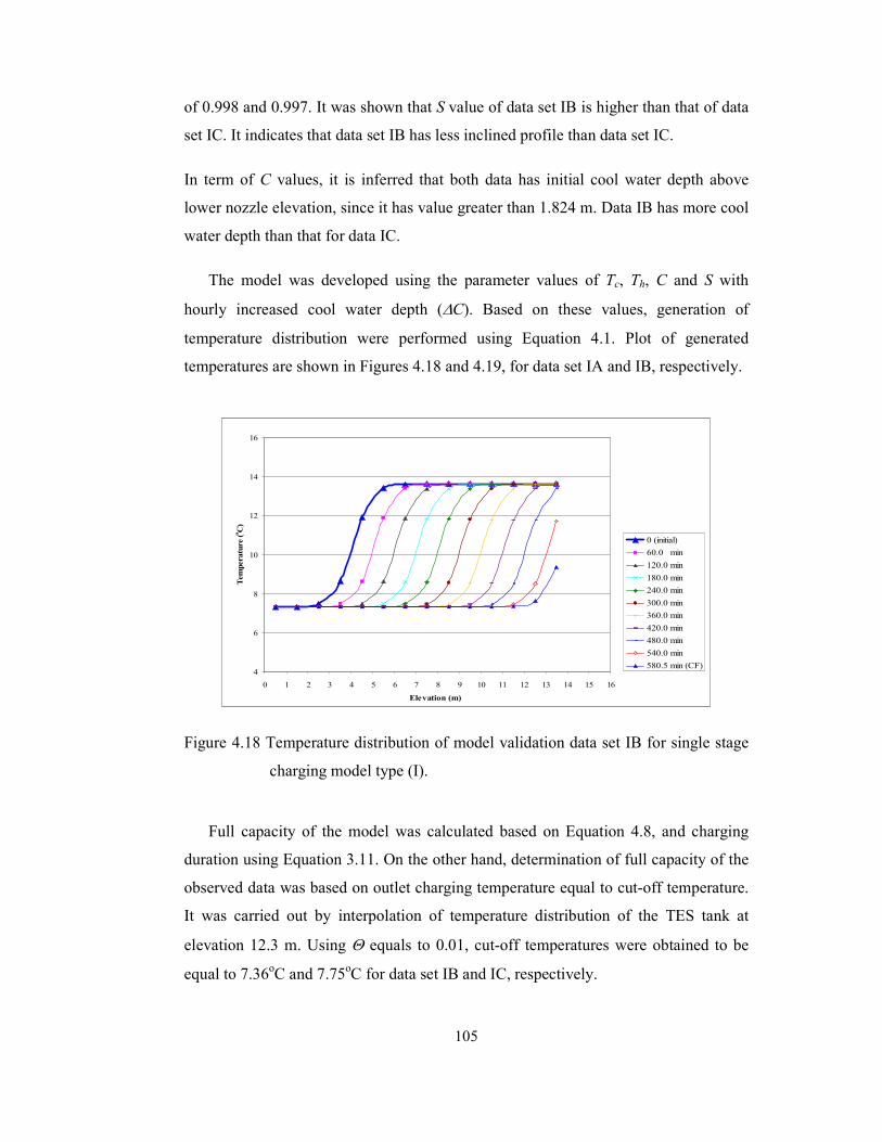
105

of 0.998 and 0.997. It was shown that S value of data set IB is higher than that of data

set IC. It indicates that data set IB has less inclined profile than data set IC.

In term of C values, it is inferred that both data has initial cool water depth above

lower nozzle elevation, since it has value greater than 1.824 m. Data IB has more cool

water depth than that for data IC.

The model was developed using the parameter values of Tc, Th, C and S with

hourly increased cool water depth (∆C). Based on these values, generation of

temperature distribution were performed using Equation 4.1. Plot of generated

temperatures are shown in Figures 4.18 and 4.19, for data set IA and IB, respectively.

4

6

8

10

12

14

16

0 1 2 3 4 5 6 7 8 9 10 11 12 13 14 15 16

Elevation (m)

Temperature (oC)

0 (initial)

60.0 min

120.0 min

180.0 min

240.0 min

300.0 min

360.0 min

420.0 min

480.0 min

540.0 min

580.5 min (CF)

Figure 4.18 Temperature distribution of model validation data set IB for single stage

charging model type (I).

Full capacity of the model was calculated based on Equation 4.8, and charging

duration using Equation 3.11. On the other hand, determination of full capacity of the

observed data was based on outlet charging temperature equal to cut-off temperature.

It was carried out by interpolation of temperature distribution of the TES tank at

elevation 12.3 m. Using Θ equals to 0.01, cut-off temperatures were obtained to be

equal to 7.36oC and 7.75

oC for data set IB and IC, respectively.

106

Validation results of the two data sets are tabulated in Tables 4.6 and 4.7 for data

sets IB and IC, respectively. Evaluation was performed in term of cumulative cooling

capacity and charging duration.

4

6

8

10

12

14

16

0 1 2 3 4 5 6 7 8 9 10 11 12 13 14 15 16

Elevation (m)

Temperature (oC)

0 (initial)

60.0 min

120.0 min

180.0 min

240.0 min

300.0 min

360.0 min

420.0 min

480.0 min

540.0 min

600.0 min

650.4 min (CF)

Figure 4.19 Temperature distribution of model validation data set IC for single stage

charging model type (I).

Table 4.7 Validation result on data set IB

Charging Time Cool Water Depth Qcum

(kWh) (minutes) (m) (kWh) (%)

18:00 11432.3 0 3.9 11675.21 2.1

19:00 14092.0 60 4.9 14557.53 3.2

20:00 16938.5 120 5.9 17439.93 2.9

21:00 19704.8 180 6.9 20322.34 3.0

22:00 22564.5 240 7.9 23204.75 2.8

23:00 25477.3 300 9.0 26087.16 2.3

0:00 28361.1 360 10.0 28969.46 2.1

1:00 31126.7 420 11.0 31850.67 2.3

2:00 34080.1 480 12.0 34720.86 1.8

3:00 37061.9 540 13.0 37483.68 1.1

4:00 40001.0 600 14.0 39486.54 1.3

Full Condition Full Condition (tCF)

Toutlet=7.36oC Θ=0.01, TΘ=7.36

oC 38212.02 tCF Deviation (%)

587.27 580.46 13.66 1.16

Qcum Deviation

Simulation Data

Charging Hours Qcum Tc=7.3

oC, Th=13.6

oC, S=1.5

107

It is shown in Tables 4.7 and 4.8; the values of parameters in the observed data

can only be exposed in term of cumulative cooling capacity and charging duration.

The charging duration was obtained using interpolation to obtain outlet temperature at

the upper nozzle elevation. Using the model, on the other hand, parameters of

charging duration as well cool water depth can be exactly determined based on

formulation.

From Tables 4.7 and 4.8, it is noted that all cumulative cooling capacity value

deviations are less than 6%. The difference was mainly due to sensitiveness of the

cumulative cooling capacity equation with respect to summation of temperature

distribution. Any small temperature difference leads to changes in the cumulative

cooling capacity. In the comparison, it was shown that cumulative cooling capacity of

the observed data is higher than that in the model. It was due to averaging of non

linear regression fitting as a part of model processing. The other reason, since inlet

temperatures were assumed constant in the model, the fluctuating temperature data

was ignored. Comparison of charging duration between the data and model are also

presented in Table 4.7 and 4.8. It was highlighted that charging duration values has

relatively similar deviation which is lower than 2%.

Table 4.8 Validation result on data set IC

Charging Time Cool Water Depth Qcum

(kWh) (minutes) (m) (kWh) (%)

18:00 8645.4 0 3.2 8554.60 1.1

19:00 11311.1 60 4.2 11224.75 0.8

20:00 14131.7 120 5.2 13895.35 1.7

21:00 16996.1 180 6.2 16566.01 2.6

22:00 19821.4 240 7.2 19236.67 3.0

23:00 22623.6 300 8.2 21907.34 3.3

0:00 25514.5 360 9.2 24578.00 3.8

1:00 28428.0 420 10.2 27248.52 4.3

2:00 31161.6 480 11.2 29917.61 4.2

3:00 33971.1 540 12.3 32572.16 4.3

4:00 36936.3 600 13.3 35087.55 5.3

5:00 38850.3 660 14.3 36730.03 5.8

Full Condition Full Condition (tCF)

Toutlet=7.75oC Θ=0.01, TΘ=7.75

oC 36577.80 tCF Deviation (%)

657.07 650.44 14.11 1.01

Qcum Deviation

Simulation Data

Qcum Tc=7.7

oC, Th=13.5

oC, S=1.1

Charging Hours

108

Based on the validation results, it is noted that the single stage charging model

type (I) is capable of determining charging duration in the stratified TES tank.

4.1.4 Two-Stage Charging Model Type (I)

Two-stage charging model was developed based on single stage charging model type

(I). The model development was explained in Section 3.3.6. The difference between

the two-stage to the single stage is the occurrence of limit temperature. Simulation of

the two-stage charging model type (I) was carried out into two main cases namely

variation of charging flow rate and limit temperature.

4.1.4.1 Simulation of Charging Flow Rate Variation

Simulation of two-stage charging model type (I) was carried out to cover charging

with absorption and electric chillers sequentially. The simulation used initial

temperature, TES tank configuration and variation of chillers parameter. The values

of initial temperature parameters are tabulated in Table 4.5, TES tank configuration

parameters were described in Table 3.1 and chiller parameter in Table 3.3.

Variation of charging flow rate for the first stage was performed using absorption

chiller at 504 m3/hr with limit temperature Tr = 9

oC. The second stage charging were

carried out using electric chiller with flow rate of 524 m3/hr, 393 m

3/hr and 262 m

3/hr,

for cases E1, F1 and G1, respectively. The simulations were performed based on 60

minutes time interval observation. Temperature distribution for two-stage charging

model type (I) are presented in Figures 4.20, 4.21 and 4.22 for cases E1, F1 and G1,

respectively. Cumulative cooling capacity in the three simulation cases is presented in

Figure 4.23.

The simulation was carried out to determine charging parameters in term of cool

water depth, charging duration and cumulative cooling capacity. Cool water depths

were determined for initial condition, transition temperature point and full capacity at

the first and second stage of charging. Cool water depth of initial condition (CE) and

temperature transition point (CFR) were referred to Equation 4.7 and 4.11. Cool water

109

depths at full capacity of the first and second stage, (CFT) and (CF) , were based on

Equations 4.10 and 4.8, respectively. Charging durations were determined in term of

temperature transition point, full capacity of the first and second stage which

designated as (tCFR), (tCFT) and (tCF) were referred to Equations 3.16. 3.17 and 3.18,

respectively. Cumulative cooling capacity (Qcum) was determined based on Equation

3.12. The results summary of the two-stage charging model type (I) simulation is

tabulated in Table 4.9.

4

6

8

10

12

14

16

0 2 4 6 8 10 12 14 16

Elevation (m)

Tem

perature (oC)

0 (initial)

60.0 min

120.0 min

180.0 min

240.0 min

300.0 min

300.5 min (CFR)

360.0 min

401.5 min (CFT)

461.5 min

482.8 min (CF)

Figure 4.20 Temperature distribution of simulation case E1 in two-stage charging

model type (I) with flow rate 504-524 m3/hr and limit temp. (Tr) = 9

oC.

4

6

8

10

12

14

16

0 2 4 6 8 10 12 14 16

Elevation (m)

Tem

perature (oC)

0 (initial)

60.0 min

120.0 min

180.0 min

240.0 min

300.0 min

300.5 min (CFR)

360.0 min

401.5 min (CFT)

461.5 min

509.9 min (CF)

Figure 4.21 Temperature distribution of simulation case F1 in two-stage charging

model type (I)with flow rate 504-393 m3/hr and limit temp. (Tr) = 9

oC.

110

4

6

8

10

12

14

16

0 2 4 6 8 10 12 14 16

Elevation (m)

Temperature (oC)

0 (initial)

60.0 min

120.0 min

180.0 min

240.0 min

300.0 min

300.5 min (CFR)

360.0 min

401.5 min (CFT)

461.5 min

521.5 min

564.1 min (CF)

Figure 4.22 Temperature distribution of simulation case G1 in two-stage charging

model type (I)with flow rate 504-262 m3/hr and limit temp. (Tr) = 9

oC.

0

5000

10000

15000

20000

25000

30000

35000

40000

45000

50000

0 100 200 300 400 500 600 700 800

Charging time (minutes)

Qcum (kW

h)

Case E1 (504-524 m3/hr)

Case F1 (504-393 m3/hr)

Case G1 (504-262 m3/hr)

Figure 4.23 Cumulative cooling capacity of simulation cases E1, F1 and G1 of two-

stage charging model type (I) in flow rate variation.

111

Table 4.9 Parameter values of simulation cases E1, F1 and G1

Variation Flow Rate Qcum (kWh) Charging Time (min) Remark

CE 3.84 13,033.70 0.00 Empty Capacity

CFR 10.30 35,041.48 300.53 Temperature Transition

CFT 12.48 42,402.86 401.45 Full capacity, 1st

stage

CF 14.30 47,119.93 482.79 Full capacity, 2nd

stage

CE 3.84 13,033.70 0.00 Empty Capacity

CFR 10.30 35,041.48 300.53 Temperature Transition

CFT 12.48 42,402.86 401.45 Full capacity, 1st

stage

CF 14.30 47,119.93 509.90 Full capacity, 2nd

stage

CE 3.84 13,033.70 0.00 Empty Capacity

CFR 10.30 35,041.48 300.53 Temperature Transition

CFT 12.48 42,402.86 401.45 Full capacity, 1st

stage

CF 14.30 47,119.93 564.12 Full capacity, 2nd

stage

C (m)

Initial Condition, Tc = 6oC, Th = 13.5

oC, S = 1, ΘΘΘΘ = 0.01 and Tr = 9

oC

Case G1, 504-262 m3/hr

Case F1, 504-393 m3/hr

Case E1, 504-524 m3/hr

It can be seen from Figures 4.20 to 4.22 and Table 4.9 that having limit

temperature of 9oC the full capacity of the first stage was obtained for charging

duration of tCFT = 401.45 minutes. In all cases, temperature transition temperatures of

the first stage was tCFR = 300.53 minutes, which indicates the condition of upper limit

points reaching the upper nozzle. It is also indicated that increasing charging flow rate

in the second stage of charging reduce the charging duration. Cumulative cooling

capacity at the initial condition and full capacity in the first stage was reached at

13,033.7 kWh and 35,041.48 kWh for cases E1, F1 and G1, respectively. Since all

cases were performed at same condition of total full capacity, therefore cumulative

cooling capacity of the second stage was similar at 47,119.93 kWh.

4.1.4.2 Simulation of Limit Temperature Variation

Simulation of two-stage charging model type (I) was carried out using absorption

chiller and electric chiller at the first and second stage of charging. The charging flow

rate of absorption chiller was 504 m3/hr, whereas electric chiller has flow rate of 393

m3/hr. The simulation was performed with variation of limit temperature (Tr) of 7

oC,

9oC and 11

oC, designated as cases H1, J1 and K1 in Table 3.4.

Temperature distribution of three simulation cases in the two-stage charging

model type (I) with variation of limit temperature are presented in Figures 4.24, 4.25

112

and 4.26 for cases H1, J1 and K1, respectively. Cumulative cooling capacity in the

three cases of simulation is presented in Figure 4.27. Simulation of limit temperature

variation was carried out for cool water depth, charging duration time as well as

cumulative cooling capacity. Summary of the results charging parameters values is

tabulated in Table 4.10.

4

6

8

10

12

14

16

0 2 4 6 8 10 12 14 16

Elevation (m)

Tem

perature (oC)

0 (initial)

60.0 min

120.0 min

180.0 min

240.0 min

300.0 min

300.5 min (CFR)

360.0 min

420.0 min

431.0 min (CFT)

491.0 min

501.5 min (CF)

Figure 4.24 Temperature distribution of simulation case H1 of two-stage charging

model type (I) with flow rate 504-393 m3/hr and limit temp. (Tr)=7

oC

4

6

8

10

12

14

16

0 2 4 6 8 10 12 14 16

Elevation (m)

Tem

perature (oC) 0 (initial)

60.0 min

120.0 min

180.0 min

240.0 min

300.0 min

300.5 CFR

360.0 min

401.5 min (CFT)

461.5 min

509.9 min (CF)

Figure 4.25 Temperature distribution of simulation case J1 of two-stage charging

model type (I) with flow rate 504-393 m3/hr and limit temp. (Tr)=9

oC

113

4

6

8

10

12

14

16

0 2 4 6 8 10 12 14 16

Elevation (m)

Tem

perature (oC)

0 (initial)

60.0 min

120.0 min

180.0 min

240.0 min

300.0 min

300.5 min (CFR)

360.0 min

379.3 min (CFT)

439.3 min

499.3 min

516.2 min (CF)

Figure 4.26 Temperature distribution of simulation case K1 of two-stage charging

model type (I) with flow rate 504-393 m3/hr and limit temp. (Tr)=11

oC

0

5000

10000

15000

20000

25000

30000

35000

40000

45000

50000

0 100 200 300 400 500 600 700 800

Charging time (minutes)

Qcu

m (kW

h)

Case H1(504-393 m3/hr),Tr=7oC

Case J1 (504-393 m3/hr),Tr=9oC

Case K1 (504-393 m3/hr),Tr=11oC

Figure 4.27 Cumulative cooling capacity of simulation cases H1, J1 and K1 of two-

stage charging model type (I) in limit temperature variation.

As shown in Figures 4.24, 4.25 and 4.26, it is noted that increasing the limit

temperature shown in cases H1, J1 and K1 reduces the cool water depth (CFT) at the

first stage of charging, hence reduces the charging duration as well as cumulative

cooling capacity. The full capacities of the second stage charging were obtained at the

same values of cool water depth as well as cumulative cooling capacity. It is also

114

highlighted that decreasing full capacity in the first stage reduces the change state

between the first and second stages. The consequence is that it takes longer charging

duration of the second stage.

The discussion shows the result of the two-stage charging model type (I)

simulation. These findings show that by utilizing SDR function has beneficial in

determining exact values of the parameter from the formulation.

The model type (I) were developed based on open charging system with

assumption of constant inlet water charging temperature. Using the assumptions, the

models could not cover variation of inlet charging temperature. Therefore, it is

required to develop another charging model enable covers variation of inlet charging

temperature. The next section involve with simulation charging models type (II)

which was developed based on a close charging system.

Table 4.10 Parameter values of simulation cases H1, J1 and K1

Variation Temperature Limit, Tr Qcum (kWh) Charging Time (min)

CE 3.84 13,033.70 0 Empty Capacity

CFR 10.30 35,041.48 300.53 Temperature Transition

CFT 13.11 44,457.82 431.05 Full capacity, 1st stage

CF 14.30 47,119.93 501.54 Full capacity, 2nd

stage

CE 3.84 13,033.70 0 Empty Capacity

CFR 10.30 35,041.48 300.53 Temperature Transition

CFT 12.48 42,402.86 401.45 Full capacity, 1st stage

CF 14.30 47,119.93 509.90 Full capacity, 2nd

stage

CE 3.84 13,033.70 0 Empty Capacity

CFR 10.30 35,041.48 300.53 Temperature Transition

CFT 12.00 40,802.65 379.28 Full capacity, 1st stage

CF 14.30 47,119.93 516.16 Full capacity, 2nd

stage

Case K1, Tr = 11oC

Case J1,Tr= 9oC

Initial Condition, Tc = 6oC, Th = 13.5

oC, S = 1, ΘΘΘΘ = 0.01 and Flow Rate 504-393 m

3/hr

Case H1, Tr = 7oC

C (m)

4.2 Close Charging System

As highlighted in the methodology section, the second type of charging models were

developed using close charging system. In the model, TES tank was integrated to

chillers equipment. The TES tank model adopted finite difference in explicit method,

whereas inlet and outlet charging temperature were correlated using energy balance in

115

the evaporator of the chillers. This method was aimed to generate temperature

distribution in the charging of stratified TES tank. The following section was

addressed on the simulation result of charging model type (II) for single and two-

stage charging of stratified TES tank. The single stage model was performed with

charging flow rate variation, whereas the two-stage was performed with variation of

flow rate and limit temperature.

4.2.1 Single Stage Charging Model Type (II)

Single stage charging model (II) was developed based on one-dimensional conduction

and convection equation. The model requires input of initial temperature, TES tank

configuration and chillers parameters. Development of the model was explained in

Section 3.4. This section discussed the result of verification and simulation of single

stage charging model type (II).

4.2.1.1 Verification of Single Stage Charging Model Type (II)

Prior to conduct verification, it requires initialization of parameters involved with

selection of effective diffusivity of the model. Using the selected effective diffusivity,

the temperature distribution of charging model type (II) was verified.

i. Selection of effective diffusivity

Selection of the effective diffusivity (εeff) was performed using temperature data at

charging flow rate of 393 m3/hr. For this purpose, data set IA was used. The selection

was performed using Tc = 6oC and Th = 13.5

oC, hence revealed an average

temperature of 9.75oC. Physical properties of water was obtained at average water

temperature involving thermal conductivity (k) = 0.568 W/m.oC, density (ρ) = 1,000

kg/m3 and specific heat (Cp) = 4,198 J/kg.K. These were obtained from table of

thermo-physical properties of water as in Appendix F. Accordingly, water thermal

diffusivity, α = k/ρ.Cp, was obtained at 0.000499 m2/hr.

116

Parameters of TES tank configuration based on Table 3.3 were used in the

selection. The dimension of the TES tank is diameter (D) of 22.3 m and effective

water depth (H) of 14 m. The observation numbers of slabs are 14. In this study, four

segments (∆x) were selected in each slab of the TES tank, resulting of ∆x equal to

0.25 m. Courant number, FLOW, in the models was equal to 1, hence observed time

interval (∆t) for charging flow rate at 393 m3/hr was obtained equal to 14.93 minutes.

Convergence stability of the conduction equation was observed by defining

AMIX not greater than 0.5. Utilizing Equation 3.25, the maximum of effective

diffusivity for 393 m3/hr was 251.67. In order to have suitable εeff representing flow

rate variations, selection of εeff values was performed in various values of 1; 10; 50;

100; 200 and 250.

The temperature distribution in the selection was evaluated using coefficient of

determination (R2). Plots of temperature distribution in the selection are attached in

Appendix B. Result summary of R2 value in the selection is presented in Figure 4.28.

0.5

0.6

0.7

0.8

0.9

1.0

1.1

0.0 59.7 119.4 179.1 238.8 298.5 358.2 417.9 477.6

Charging time (minutes)

R2

εeff = 1

εeff = 10

εeff = 50

εeff = 100

εeff = 200

εeff = 250

Figure 4.28 R2 in variation effective diffusivity

In Figures 4.28, the R2 of the temperature data is presented with respect to

charging time. Selection was performed at various εeff in the range of stabilities of

AMIX<0.5 identifies at εeff lower than 251.67. Referring to the figure, it can be seen

that R2 in the earlier charging time has values approximately equal to 1 which indicate

117

the temperature distribution data are almost similar. At lower εeff , the R2

closer to 1 is

occurred at all charging time. Along with increasing of εeff, the R2 value decrease

gradually with respect to charging time. This is due to the fact that increasing of εeff

revealed more inclined profile in the temperature distribution as shown in Appendix

B. It indicates that the stability is reached at the low of εeff and gradually decreases in

increasing value of effective diffusivity.

Thus, the model was suitable at low εeff values. It inferred that mixing factors does

not dominate degradations of temperature distribution, since it is not influenced by

mixing flow at its initial condition of the charging. Therefore, working εeff at 10 is

used in the charging model type (II).

The other indication from the results obtained is that the model single stage

charging model type (II) valid to be performed with explicit method. This is because

of effective diffusivity (εeff) stable at AMIX lower than 0.5.

ii. Verification of single stage charging model type (II)

Verification of the model was performed to ensure the similarity of temperature

distribution during charging. The verification of single stage charging model type (II)

was performed with three evaluation types, namely R2 between the observed and

simulated data, temperature parameter similarity and t-statistical test.

Verification of charging single stage type (II) was carried out with 4 operating

data sets of IB, IC, IIB and IIC. One of verification result at charging flow rate of 393

m3/hr using data IB is discussed in this section. Plot of temperature distribution data

set IB is shown in Appendix A2. Fitting SDR function of the data set IB is presented

in Figure 4.29, whereas the verification is presented in Figure 4.30.

The verification utilized TES tank configuration that has diameter (D) of 22.3 m

and effective water depth (H) of 14 m. It has 14 slabs which is provided with

temperature sensor in the mid point of the slab. The four segments (∆x) were selected

for each slab of the tank, resulting ∆x equal to 0.25 m. Courant number, FLOW, in the

model were selected equal to 1, hence reveals different observed time interval (∆t) for

various charging flow rate. In the case of charging flow rate at 393 m3/hr, resulting at

118

∆t = 14.93 minutes. The initial condition was taken at a similar value with of that in

observed data. The values of UA, Tev, ∆T1 and ∆T2 were equal to 714.4 W/oC; 4

oC;

0.2oC and 0.4

oC, respectively. Effective diffusivity εeff was taken equal to 10,

considering the result in its selection.

In Figures 4.29 and 4.30, both fitting temperature data are presented with respect

to dimensionless elevation of TES tank. Visually, both fitted temperature distributions

are similar. Some intensive evaluations, however, were conducted to ensure its

similarity. It was carried out by evaluating data distribution similarity, temperature

parameter similarity and statistical test.

X (dimensionless elevation)

0 2 4 6 8 10 12 14 16

Tem

per

atur

e (o

C)

6

8

10

12

14

16

18.00

19.00

20.00

21.00

22.00

23.00

00.00

01.00

02.00

Figure 4.29 SDR fitting on data set IB

119

X (Dimensionless Elevation)

0 2 4 6 8 10 12 14 16

Temperature (oC)

6

8

10

12

14

16

0.00

59.7 min

119.4 min

179.1 min

238.8 min

298.5 min

358.2 min

417.9 min

477.6 min

Figure 4.30 SDR fitting from charging model type (II) on data set IB

i. Temperature distribution similarity

The temperature data similarity was evaluated using R2 value. It was performed by

determining R2 of temperature distribution of data set 1B and charging model type

(II).

Table 4.11 R2 verification of charging model type (II)

Data to Model R2

Chrg. Hrs. Chrg. Time (min)

18:00 - 0.0 1.000

19:00 - 59.7 0.999

20:00 - 119.4 0.999

21:00 - 179.1 0.999

22:00 - 238.8 0.997

23:00 - 298.5 0.995

0:00 - 358.2 0.993

1:00 - 417.9 0.985

2:00 - 477.6 0.984

From Table 4.11, it can be seen that R2 between the two data approximately equal

to unity, indicating both data are similar. It was shown at all charging hours.

120

ii. Temperature parameters similarity

Temperature parameters similarity was carried out by comparing parameters obtained

from SDR function. It was performed by fitting of the observed and verified data

using SIGMAPLOT. The parameters of the observed data from SIGMAPLOT are

included in Appendix G2, and the verified data is presented in Appendix H1.

Verification of data set 1B is discussed in this section. Comparison SDR parameters

of Tc and Th is presented in Figure 4.31, while comparison of parameters C and S is in

Figure 4.32. Percentage parameter deviations of the two data sets are presented in

Figure 4.33.

From Figure 4.31 and 4.32, it can be seen that both observed and model has same

pattern of relatively constant at Tc and Th. Figure 4.32 shows that the parameter S is

constant during charging, while C has a linear increase with respect to charging hours.

From Figure 4.33, it is shown that fluctuated deviation occurred on the parameters Tc,

Th. and S. The parameters deviation of C increases during the charging hours. It can

be seen from Figure 4.32 that all parameters deviations are below than 5 %. The

highest deviation occurred for S parameter.

0

2

4

6

8

10

12

14

16

18:00 19:00 20:00 21:00 22:00 23:00 0:00 1:00 2:00

Charging time (hours)

Parameters T

c and T

h (oC)

Tc data

Tc model

Th data

Th model

Figure 4.31 Comparison of SDR parameters Tc and Th in verification of charging

model type (II)

121

0

2

4

6

8

10

12

14

18:00 19:00 20:00 21:00 22:00 23:00 0:00 1:00 2:00

Charging time (hours)

Parameters C and S

C data

C model

S data

S model

Figure 4.32 Comparison of SDR parameters C and S in verification of charging model

type (II)

0

2

4

6

8

10

18:00 19:00 20:00 21:00 22:00 23:00 0:00 1:00 2:00Charging time (hours)

Dev

iation (%

)

Dev. Tc

Dev. Th

Dev. C

Dev. S

Figure 4.33 Percentage deviations of SDR parameters in verification of charging

model type (II)

iii. Statistical test

Statistical analysis was performed to check the similarity acceptance of the model. It

was carried out using t statistic test. The t computed values of the verification are

122

presented in Figure 4.34. The t computed value was obtained from Equation 3.10,

whereas t critical was obtained from Appendix E, with 14 numbers of data at 95%

confidence level.

t critical = 2.145

0.009

0.0130.015

0.017

0.0270.028

0.000

0.019

0.008

0.000

0.004

0.008

0.012

0.016

0.020

0.024

0.028

0.032

18:00 19:00 20:00 21:00 22:00 23:00 0:00 1:00 2:00

Charging time (hours)

t co

mputed

t-computed

Figure 4.34 t computed values in verification of charging model type (II)

From Figure 4.34, it is shown that t computed value is very small compared to t

critical which indicates that the temperature distribution both verified and observed

data are similar. This finding shows that the null hypothesis was fulfilled, hence the

model of single stage charging model type (II) was statistically accepted.

Verification of single stage charging model type (II) were also performed with

other observed data for charging flow rate of 393 m3/hr and 524 m

3/hr. The other

verification for charging flow rate of 393 m3/hr was performed using data set IC,

whereas for charging flow rate 524 m3/hr was carried out using data set IIB and IIC.

Fitting SDR function of the verified data is attached in Appendix H. The three type of

evaluation results on the verification model are attached in Appendices C1, C2 and

C3, for data set IC, IIB and IIC, respectively. The results of the three evaluations are

summarized in Table 4.12, 4.13 and 4.14, for R2, parameter deviations and t-statistical

test, respectively.

123

Table 4.12 Summary of R2 in verification charging model type (II)

Data Charging Hours R2

Remarks

IB 18.00-2.00 > 0.984 Table 4.11

IC 18.00-2.00 > 0.993 Appendix C.1.3

IIB 18.00-2.00 > 0.989 Appendix C.2.3

IIC 18.00-2.00 > 0.935 Appendix C.3.3

Table 4.13 Summary of parameters deviation in verification charging model type (II)

Tc Th C S

IB 18.00-2.00 < 1.0 < 0.4 < 2.2 < 4.7 Figure 4.33

IC 18.00-2.00 < 1.5 < 0.2 < 1.5 < 5.0 Appendix C.1.6

IIB 18.00-2.00 < 1.7 < 0.2 < 1.6 < 5.2 Appendix C.2.6

IIC 18.00-2.00 < 2.7 < 0.9 < 2.5 < 5.1 Appendix C.3.6

Parameter Deviations (%)Data Charging Hours Remarks

From Table 4.12, it is shown that all R2 of the verification are higher than 0.936

which indicate that the temperature distribution between data and model are also

similar. Based on Table 4.13, it is noted that all parameters deviation for Tc, Th and C

are lower than 2% and deviation in the parameter C is less than 6%.

Table 4.14 Summary of t computed values in verification model type (II)

Data Charging Hours t-computed values Remarks

IB 18.00-2.00 < 0.028 Figure 4.34

IC 18.00-2.00 < 0.019 Appendix C.1.7

IIB 18.00-2.00 < 0.030 Appendix C.2.7

IIC 18.00-2.00 < 0.033 Appendix C.3.7

As shown in Table 4.14, all t-computed values are smaller than t-critical of 2.145.

Based on the results, it is noted that the simulation model single stage charging model

type (II) capable of generating temperature distribution as similar as the historical

data. The temperature distribution was statistically accepted.

124

4.2.1.2 Simulation of Single Stage Charging Model Type (II)

After being developed and verified, the single stage charging model type (II) was

utilized for simulation. The simulation was performed with variation of chillers

parameters in cases A2, B2 and D2. Inputs of the simulation are initial temperature,

TES tank configuration and chillers parameters. The TES tank configuration

parameters are described in Table 3.1, while chillers parameters are presented in

Table 3.6.

Initial temperature of the simulation was obtained from generation parameters of

Th = 13.5oC, Tc = 6

oC, C = 3.84, S = 1, and Θ = 0.01 using SDR function in Equation

4.1. The other parameters of effective diffusivity was taken at εeff = 10, whereas the

losses temperature uses ∆T1 = 0oC and ∆T2 = 0

oC.

For partial working load observation, simulation was performed exceeding that

full capacity which is approximately at 9,226.4 kWh. Temperature distribution in

single stage charging model type (II) of simulation cases A2, B2 and D2 are presented

in Figures 4.35, 3.36 and 3.37. All simulation in cases A2, B2 and D2 were carried

out with the same number of segments per slab and TES tank configuration. Four

segments in each slab were chosen in the simulation resulting in ∆x equals to 0.25 m.

Using FLOW = 1 described in Equation 3.25, the observed time interval obtained

were at 11.19 minutes, 14.93 minutes and 22.39 minutes, for cases A2, B2 and D2,

respectively. Simulation was carried out at approximately one hour observation time,

hence revealed at 56 minutes, 59.7 minutes and 111.9 minutes for cases A2, B2 and

D2, respectively. Determination of charging duration time as well as cumulative

cooling capacity was carried out by interpolation between the observed times interval.

Temperature distribution generated from simulation is presented in Figures 4.35,

4.36 and 4.37 for cases A2, B2 and D2, respectively. Cumulative cooling capacity

calculated using Equation 3.16 with reference temperature equal to Th = 13.5oC for

the three cases is presented in Figure 4.38.

As shown in Figures 4.35 to 4.37, decreasing in values of charging flow rate as shown

in cases A2, B2 and C2 reduce the span between temperature distributions. It

125

indicates that smaller flow rate decreases the additional cool water depth. It is also

shown that uniform temperatures of approximately 6oC at the whole elevation of the

tank were obtained at observation time of 503.8 minutes, 656.8 minutes and 985.1

minutes for cases A2, B2 and C2, respectively. It indicates that uniform temperature

at the whole elevation of the TES required shorter charging periods with higher

charging flow rate.

4

6

8

10

12

14

16

0 2 4 6 8 10 12 14 16

Elevation (m)

Tem

perature (oC)

0.0

56.0 min

111.9 min

167.9 min

223.9 min

279.9 min

335.8 min

391.8 min

447.8 min

503.8 min

559.7 min

615.7 min

671.7 min

Figure 4.35 Temperature distribution of simulation case A2 in single stage charging

model type (I) with flow rate 524 m3/hr.

4

6

8

10

12

14

16

0 2 4 6 8 10 12 14 16Elevation (m)

Tem

perature (oC)

0.0

59.7 min

119.4 min

179.1 min

238.8 min

298.5 min

358.2 min

417.9 min

477.6 min

537.3 min

597.1 min

656.8 min

716.5 min

776.2 min

835.9 min

895.6 min

955.3 min

Figure 4.36 Temperature distribution of simulation case B2 in single stage charging

model type (I) with flow rate 393 m3/hr.

126

4

6

8

10

12

14

16

0 2 4 6 8 10 12 14 16

Elevation (m)

Tem

perature (oC)

0.0

111.9 min

223.9 min

335.8 min

447.8 min

559.7 min

671.7 min

783.6 min

895.6 min

1007.5 min

1119.5 min

1231.4 min

1343.4 min

Figure 4.37 Temperature distribution of simulation case D2 in single stage charging

model type (I) with flow rate 262 m3/hr.

From the uniform temperature condition, charging still can be continued to have

more cooling capacity. However, due to decreased in cool water temperature entering

the chillers, the extended charging in stratified TES tank were carried out at partial

working load of the chillers. The partial working load yields smaller additional

cooling capacity in the tank.

Figure 4.38 shows a comparison of cumulative cooling capacity of the three cases

of A2, B2 and D2. It is shown that steeper cumulative cooling capacity curves

occurred at smaller charging flow rate. The smallest is in case D2. It shows that

smaller charging flow rate requires longer charging duration to achieve full capacity.

Initially, cumulative cooling capacity increase linearly and flattened after reaching the

full capacity. If the charging is continued, it generates less additional cooling

capacity. This is due to decreased outlet temperature in the charging.

127

0

10000

20000

30000

40000

50000

60000

0 300 600 900 1200 1500

Charging time (minutes)

Qcum (kWh)

Case A2 (524 m3/hr)

Case B2 (393 m3/hr)

Case D2 (262 m3/hr)

Figure 4.38 Cumulative cooling capacity of simulation cases A2, B2 and D2 of single

stage charging model type (II).

Determination the values of charging duration and cumulative cooling capacity

were also done in the simulation. Those values were determined based on initial

condition, temperature transition point and full capacity charging of the stratified TES

tank. Since the finite difference solution can only be performed using interval

observation time, therefore determination of the two parameters was carried out by

interpolation. Temperature transition was determined at time interval when the upper

nozzle has outlet temperature which equals to 13.425oC. Full capacity were

recognized when the outlet charging temperature at the upper nozzle equals to

6.075oC. The values of the charging duration as well as cumulative cooling capacity

are summarized in Table 4. 15.

From Table 4.15, it is shown that higher charging flow rate leads to shorter

charging duration in achieving temperature transition point as well as full capacity.

Hence, cumulative cooling capacity at temperature transition decrease with reduced

charging flow rate. This findings show that the close charging system capable of

determining charging duration and cumulative cooling capacity of the stratified TES

tank. It was performed by interpolation from temperature distribution generated by

simulation charging model type (II). In addition, simulation charging models type (II)

is capable of representing chillers partial working load characteristics. This is due its

128

capability in covering fluctuated inlet at outlet charging temperature. The following

section explains the results of partial working load analysis.

Table 4.15 Parameter values of simulation cases A2, B2 and D2

Variation Flow rate Qcum (kWh) Charging Time (min) Remark

13,033.7 0 Empty Capacity

35,294.1 293.1 Temperature Transition

47,564.9 479.3 Full Capacity

13,033.7 0 Empty Capacity

35,142.7 390.0 Temperature Transition

47,600.0 636.5 Full Capacity

13,033.7 0 Empty Capacity

35,332.9 587.2 Temperature Transition

47,697.6 951.0 Full Capacity

Initial Condition, Tc = 6oC, Th = 13.5

oC, S = 1, ΘΘΘΘ = 0.01

Case D2, 262 m3/hr

Case A2, 524 m3/hr

Case B2, 393 m3/hr

i. Partial working load of the chillers

Partial working load of the chillers during charging was carried out by observing

cooling capacity supplied by the chillers. Inlet, outlet and mixing charging

temperature were first discussed. Determination of these temperatures was discussed

in Section 3.4.4. The comparison of inlet, outlet and mixing temperature of cases A2,

B2 and D2 in the simulation are presented in Figures 4.39 to 4.41, respectively.

Chillers cooling capacity and percentage of partial load are presented in Figures 4.42

and 4.43.

Comparison of inlet and outlet charging temperatures in the simulation is

presented in Figures 4.39 and 4.40. It can be seen that initially charging temperature is

constant at a certain elevation, reduced incisively and finally stays constant at the

lower temperature. The inlet charging temperature also shows similar trends. Starting

time in reducing the temperature was due to commencing upper limit of thermocline

into the upper nozzle. The temperature decreases incisively when upper limit point

thermocline reaching the upper nozzle. The temperature finally stays constant at lower

limit temperature after the bottom limit point thermocline reaching the upper nozzle.

The high and low inlet temperatures are approximately at 6oC and 5

oC for all cases,

whereas high and low outlet temperatures are at 13.5oC and 6

oC for all cases. Those

129

inlet and outlet temperature are available in the range of two temperatures. This is due

to proportional cooling capacity of the chillers given as by Equation 3.31.

Mixing temperature of the three simulation cases is presented in Figure 4.41.

From Figure 4.41, it can be seen that initial mixing temperature stays fairly constant,

and then start to decrease gradually. The mixing temperature decrease after

thermocline profile commencing the upper nozzle. Thus mixing temperature affect the

charging characteristic in single stage charging model type (II) stratified TES tank.

The mixing temperature indicates additional cool water temperature in the lower part

of the TES tank. This makes it different from single charging model type (I).

4

5

6

7

0 300 600 900 1200 1500

Charging time (minutes)

Tem

pera

ture (oC)

Case A2 (524 m3/hr)

Case B2 (393 m3/hr)

Case D2 (262 m3/hr)

Figure 4.39 Inlet charging temperature of simulation cases A2, B2 and D2 in single

stage charging model type (II)

Accordingly, the trend also occurs in the cooling capacity supplied by chillers as

indicated in Figures 4.42. The high and low cooling capacities of cases A2, B2 and

D2 have different values. This is due to different charging flow rate that influence the

cooling capacity as described in Equation 2.7.

130

4

6

8

10

12

14

0 300 600 900 1200 1500

Charging time (minutes)

Tem

perature (oC)

Case A2 (524 m3/hr)

Case B2 (393 m3/hr)

Case D2 (262 m3/hr)

Figure 4.40 Outlet charging temperature of simulation cases A2, B2 and D2 in single

stage charging model type (II)

Chillers partial working load of the simulation cases is shown in Figure 4.42. It

can be seen that the trend of percentage partial load is similar with that on the inlet

and outlet charging temperatures. Initially, chillers work at full load and later at lower

partial load. In summarizing the charging characteristic, it is noted that the trend of

inlet and outlet temperatures significantly affect the cooling capacity supplied by

chillers.

.

4

5

6

7

0 300 600 900 1200 1500

Charging time (minutes)

Tem

perature (oC)

Case A2 (524 m3/hr)

Case B2 (393 m3/hr)

Case D2 (262 m3/hr)

Figure 4.41 Mixing temperatures of simulation cases A2, B2 and D2 in single stage

charging model type (II)

131

0

500

1000

1500

2000

2500

3000

3500

4000

4500

5000

0 300 600 900 1200 1500

Charging time (minutes)

Qchiller (kW

)

Case A2 (524 m3/hr)

Case B2 (393 m3/hr)

Case D2 (262 m3/hr)

Figure 4.42 Chillers cooling capacity of simulation cases A2, B2 and D2 of single

stage charging model type (II)

0.0

0.2

0.4

0.6

0.8

1.0

1.2

0 300 600 900 1200 1500

Charging time (minutes)

Partial Load (%

)

Case A2 (524 m3/hr)

Case B2 (393 m3/hr)

Case D2 (262 m3/hr)

Figure 4.43 Chillers partial working load of simulation cases A2, B2 and D2 of single

stage charging model type (II)

From the discussion, it is noted that the model is capable covering of partial

working analysis in the charging stratified TES tank. This takes advantage of its

capability to cover fluctuation of inlet charging temperature. The following

conclusions are drawn from partial working load analysis.

132

i. Two important charging parameters that affect the partial load charging

characteristic are temperature transition point and full capacity as predicted in

Figure 3.6 and 3.4 (b), respectively.

a. The temperatures transition point was obtained when the condition of

outlet temperature equal to warm cut-off water temperature.

b. Full capacity occurred at outlet temperature equal to cool cut-off water

temperature.

ii. The charging duration values both for temperature transition point and full

capacity is reduced by increasing of charging flow rate.

iii. The temperature transition and full capacity significantly affect the partial

working load characteristics during charging. This involves inlet, outlet and

mixing temperature as well as cooling capacity of the chillers.

4.2.2 Two-Stage Charging Model Type (II)

Two-stage of charging of stratified TES tank was enhanced from single stage

charging model type (II) as explained in Section 3.4.4. The two-stage charging model

type (II) was used to simulate absorption and electric chillers sequentially. The full

capacity of the first stage charging was bounded by limit temperature of the

absorption chillers that work at the first stage. The simulations were carried out with

variations of chillers parameters and limit temperature.

4.2.2.1 Simulation of Chiller Parameter Variation

Variation of the chillers parameter was performed similar to that of the model type (I).

The simulation involves several cases namely E2, F2 and G2. The first stage of

charging was absorption chiller at flow rate of 504 m3/hr and limit temperature was

9oC. Whereas electric chiller at the second was at flow rate 524 m

3/hr, 393 m

3/hr and

262 m3/hr, for cases E2, F2 and G2, respectively. The simulation used same initial

temperature and TES tank configuration parameters with that on the simulation single

stage, whereas chillers parameters are presented in Table 3.7.

133

All simulation in cases E2, F2 and G2 were carried out with four segments in each

slab, resulting in ∆x equals to 0.25 m. In the first stage, absorption chillers which

work at flow rate 504 m3/hr reveals time interval of 11.64 minutes. For the second

stage, the time interval was obtained at 11.19 minutes, 14.93 minutes and 22.39

minutes for chillers in the second stage of these cases. The observation time of the

simulation was approximately at hourly charging duration.

Temperature distribution generated from simulation in the first stage is presented

in Figures 4.44, whereas Figures 4.45, 4.46 and 4.47 presents temperature distribution

of the second stage of simulation for cases E2, F2 and G2, respectively. Cumulative

cooling capacity was calculated using Equation 3.12 with reference temperature at Th

= 13.5oC. Comparison of cumulative cooling capacity values is presented in Figure

4.48. Whereas simulation result in term of inlet and outlet charging temperatures,

mixing temperature, chillers cooling capacity, partial load of the chillers are attached

in Appendix D.

4

6

8

10

12

14

16

0 2 4 6 8 10 12 14 16

Elevation (m)

Temperature (oC)

0.0 (Initial)

58.2 min

116.4 min

174.6 min

232.8 min

291.0 min

349.2 min

407.4 min (Full)

Figure 4.44 Temperature distribution of first stage charging simulation cases E2, F2

and G2 in two-stage charging model type (II) with flow rate 504 m3/hr

and limit temp. (Tr)=9oC

134

4

6

8

10

12

14

16

0 2 4 6 8 10 12 14 16

Elevation (m)

Tem

per

atu

re (oC)

0.0 (initial)

56.0 min

86.9 min (Full)

Figure 4.45 Temperature distribution of second stage charging simulation case E2 in

two-stage charging model type (II) with flow rate 524 m3/hr

4

6

8

10

12

14

16

0 2 4 6 8 10 12 14 16

Elevation (m)

Tem

perature (oC)

0.0 (initial)

59.7 min

112.8 min (Full)

Figure 4.46 Temperature distribution of second stage charging simulation case F2 in

two-stage charging model type (II) with flow rate 393 m3/hr

135

4

6

8

10

12

14

16

0 2 4 6 8 10 12 14 16

Elevation (m)

Tem

per

atu

re (oC)

0.0 (Initial)

111.9 min

177.8 min (Full)

Figure 4.47 Temperature distribution of second stage charging simulation case G2 in

two-stage charging model type (II) with flow rate 262 m3/hr

Full capacity of the first stage in the simulation was determined by interpolation

between two interval times at limit temperature of 9oC as outlet charging temperature.

Temperature distribution at full capacity of the first stage charging was then set as

initial temperature in the second stage. The charging was continued for chillers

parameters at the second stage for cases E2, F2 and G2, respectively.

0

5000

10000

15000

20000

25000

30000

35000

40000

45000

50000

0 200 400 600 800

Charging Time (minutes)

Qcum (kWh)

Case E2 (504-524 m3/hr)

Case F2 (504-393 m3/hr)

Case G2 (504-262 m3/hr)

Figure 4.48 Cumulative cooling capacity of simulation cases E2, F2 and G2 in two-

stage charging model type (II) with chillers variation.

136

In the second stage of charging simulation, full capacity was determined by

interpolation to achieve outlet charging temperature equals to cut-off temperature at

6.075oC. It indicates that decreased charging duration occurred at higher charging

flow. Cumulative cooling capacity of the simulation is in Figure 4.48. It presents the

cumulative cooling capacity of the three cases with respect to charging time. It can be

seen that lower charging flow rate also lead to longer charging time.

Determination of the values of charging duration and cumulative cooling capacity

was also performed in the simulation. These values were determined based on initial

condition, temperature transition point and full capacity of charging the stratified TES

tank. Temperature transition was determined at time interval when the upper nozzle

has outlet temperatures equal to 13.425oC. Full capacity was recognized when the

outlet charging temperature at the upper nozzle is equal to 6.075oC. The result is

summarized in Table 4.16.

It is shown in Table 4.16, full capacity of the first charging for all simulation

cases were obtained at similar charging duration of 407.4 minutes, while temperature

transition was achieved at charging 305.2 minutes. At the second stage of charging, it

is shown that higher charging flow rate leads shorter charging duration. This finding

has similar pattern with that in the simulation charging models type (I).

Table 4.16 Parameters values of simulation cases E2, F2 and G2

Variation Flow rate Qcum (kWh) Charging Time (min) Remark

13,033.7 0.0 Empty Capacity

35,194.0 305.2 Temperature Transition

42,817.1 407.4 Full capacity, 1st stage

47,582.2 494.2 Full capacity, 2nd

stage

13,033.7 0.0 Empty Capacity

35,194.0 305.2 Temperature Transition

42,817.1 407.4 Full capacity, 1st stage

47,715.7 520.1 Full capacity, 2nd

stage

13,033.7 0.0 Empty Capacity

35,194.0 305.2 Temperature Transition

42,817.1 407.4 Full capacity, 1st stage

47,698.1 585.1 Full capacity, 2nd

stage

Case E2, 504-524 m3/hr

Case F2, 504-393 m3/hr

Case G2, 504-262 m3/hr

Initial Condition, Tc = 6oC, Th = 13.5

oC, S = 1, ΘΘΘΘ = 0.01, Tr = 9

oC

137

Partial working load analysis of the simulation is attached in Appendix D. Related

to partial working load analysis, it is shown that outlet transition point occurred at

smaller charging time than that at full capacity of the first stage of charging. This

shows that the outlet transition point was achieved before reaching full capacity for

both first and second charging. It indicates that full capacity in the first stage charging

occurred at partial working of the chillers.

4.2.2.2 Simulation of Limit Temperature Variation

Simulation on two-stage charging model type (II) was enhanced to observe variation

of limit temperature in the first stage charging. The first stage charging was with

absorption chillers, whereas the second stage utilizes electric chillers. The limit

temperature in the absorption chillers was varied at 7oC, 9

oC and 11

oC express as

cases H2, J2 and K2, respectively. The simulation used initial temperature as

described in Table 4.7 and TES tank configuration parameters as shown in Table 3.1.

The first stage charging flow rate was 504 m3/hr and for the second stage was 393

m3/hr, as presented in Table 3.7.

All simulation in cases H2, J2 and K2 were carried out with four segments in each

slab resulting in ∆x equals to 0.25 m. In the first stage, absorption chillers which work

at flow rate 504 m3/hr has time interval of 11.64 minutes whereas for the second stage

was 14.93 minutes for flow rate 393 m3/hr. The observation time of the simulation

was taken approximately at hourly charging duration.

Temperature distribution of the simulations are presented in Figures 4.49, 4,50

and 4.51, for first charging of cases H2, J2 and K2, respectively. Temperature

distributions in the second stage are presented in Figures 4.52, 4.53 and 4.54.

Comparison of cumulative cooling capacity of these cases is presented in Figure 4.55.

138

4

6

8

10

12

14

16

0 2 4 6 8 10 12 14 16

Elevation (m)

Tem

peratu

re (oC)

0.0 (Initial)

58.2 min

116.4 min

174.6 min

232.8 min

291.0 min

349.2 min

407.4 min

444.2 min (Full)

Figure 4.49 Temperature distribution of first stage charging simulation case H2 in

two-stage charging model type (II) with flow rate 504 m3/hr and limit

temperature 7oC

4

6

8

10

12

14

16

0 2 4 6 8 10 12 14 16

Elevation (m)

Temperature (oC)

0.0 (Initial)

58.2 min

116.4 min

174.6 min

232.8 min

291.0 min

349.2 min

407.4 min (Full)

Figure 4.50 Temperature distribution of first stage charging simulation case J2 in

two-stage charging model type (II) with flow rate 504 m3/hr and limit

temperature 9oC

139

4

6

8

10

12

14

16

0 2 4 6 8 10 12 14 16

Elevation (m)

Tem

peratu

re (oC)

0.0 (Initial)

58.2 min

116.4 min

174.6 min

232.8 min

291.0 min

349.2 min

385.4 min (Full)

Figure 4.51 Temperature distribution of first stage charging simulation case K2 in

two-stage charging model type (II) with flow rate 504 m3/hr and limit

temperature 11oC

4

6

8

10

12

14

16

0 2 4 6 8 10 12 14 16Elevation (m)

Tem

perature (oC)

0.0 (Initial)

59.7 min

78.0 min (Full)

Figure 4.52 Temperature distribution of second stage charging simulation case H2 in

two-stage charging model type (II) with flow rate 393 m3/hr and limit

temperature 7oC

140

4

6

8

10

12

14

16

0 2 4 6 8 10 12 14 16Elevation (m)

Tem

per

ature (oC)

0.0 (Initial)

59.7 min

112.8 min (Full)

Figure 4.53 Temperature distribution of second stage charging simulation case J2 in

two-stage charging model type (II) with flow rate 393 m3/hr and limit

temperature 9oC

4

6

8

10

12

14

16

0 2 4 6 8 10 12 14 16Elevation (m)

Tem

perature (oC)

0.0 (Initial)

59.7 min119.4 min

160.8 min (Full)

Figure 4.54 Temperature distribution of second stage charging simulation case K2

in two-stage charging model type (II) with flow rate 393 m3/hr and limit

temperature 11oC

Determination the values of charging duration and cumulative cooling capacity

was also performed based on initial condition, temperature transition point and full

capacity of charging the stratified TES tank. Temperature transition was determined at

141

time interval when the upper nozzle has outlet temperatures equal to 13.425oC. Full

capacities were calculated at outlet charging temperature at the upper nozzle equal to

6.075oC. The results are summarized in Table 4.17.

0

5000

10000

15000

20000

25000

30000

35000

40000

45000

50000

0 200 400 600Charging time (minutes)

Qcum (KWh)

Case H2 (504-393 m3/hr),7oC

Case J2 (504-393 m3/hr), 9oC

Case K2 (504-393 m3/hr),11oC

Figure 4.55 Cumulative cooling capacity of simulation cases H2, J2 and K2 of two-

stage charging model type (II) in limit temperature variation

Table 4.17 Parameters values of simulation cases H2, J2 and K2

Variation Temperature Limit, Tr Qcum (kWh) Charging time (min) Remarks

13,033.7 0 Empty Capacity

35,194.0 305.2 Temperature Transition

45,326.5 444.2 Full capacity, 1st stage

47,582.8 522.3 Full capacity, 2nd

stage

13,033.7 0 Empty Capacity

35,194.0 305.2 Temperature Transition

42,817.1 407.4 Full capacity, 1st stage

47,307.1 520.1 Full capacity, 2nd

stage

13,033.7 0 Empty Capacity

35,194.0 305.2 Temperature Transition

41,485.0 385.1 Full capacity, 1st stage

47,691.3 545.9 Full capacity, 2nd

stage

Case H2, Tr = 7oC

Case J2,Tr= 9oC

Case K2, Tr = 11oC

Initial Condition, Tc = 6oC, Th = 13.5

oC, S = 1, ΘΘΘΘ = 0.01, Flow Rate 504-393 m

3/hr, Variation Limit Temperature

As shown in Table 4.17, increased limit temperature lead to reducing of charging

duration as well as full capacity in the first stage. However, charging durations as well

as cumulative cooling capacity at temperature transition are constant, which indicates

that it was not influenced by variation in limit temperature during charging. In the

142

second stage charging, it is indicated that decreasing of limit temperature leads to

increasing charging duration in the second stage.

4.3 Comparison of Charging Models Type (I) and (II)

The simulation results of the charging models type (I) and (II) showed that both are

capable of simulation for single and two-stage charging stratified TES tank. As the

two models were developed based on different approach, comparison of the two

models was performed by equalizing input parameters. It was performed by

simulating at the same initial temperature, TES tank configuration as well as flow rate

parameters. Losses temperature in piping connection is assumed to be negligible.

The comparison was used to evaluate the values of charging duration as well as

cumulative cooling capacity. In the model type (I), the parameters were calculated

based on formulation. For model type (II), since utilizing finite difference in the

calculation, the parameter was obtained based on interpolation between interval time

observations. In the comparison, additional cool water temperature was considered. It

involved average cool water temperature (Tc) in model type (I) and mixing

temperature (Tmix) in model type (II). Comparison between the models was performed

for single and two-stage charging stratified TES tank.

4.3.1 Comparison of Single Stage Charging Models

In single stage charging model, the comparison was performed with cases of A1, B1,

D1 and A2, B2, D2 for model types (I) and (II), respectively.

i. Temperature of additional cool water

In the model type (I), additional cool water temperature presents as average cool

water temperature (Tc), whereas in model type (II) present as mixing temperature

(Tmix). Comparison of additional cool water temperature is presented in Figure 4.56.

143

From figure 4.56, it is shown that temperatures of additional temperature in model

type (I) are constant within charging time observation. In the model type (II), initially

temperature stays fairly constant until reaching temperature transition point and

decrease gradually. Decreasing temperature is less than 1oC. This trend difference was

due to open and close cycle considerations in the two models.

4

5

6

7

0 300 600 900 1200 1500

Charging time (minutes)

Tem

perature (oC)

Model (I), Case A1, B1, D1

Model (II), Case A2 (524 m3/hr)

Model (II), Case B2 (393 m3/hr)

Model (II), Case C2 (262 m3/hr)

Figure 4.56 Comparison of additional cool water temperature of single stage charging

model type (I) and (II).

ii. Values of Charging Parameters

Charging parameters values obtained from simulation model type (I) and (II) are

compared in this section. Deviations of the parameter value in the single stage

charging models are tabulated in Table 4.18.

From the parameters value deviation as tabulated in Table 4.18, it is shown

that any slightly deviation occurs between the parameters. In term of charging

durations, the deviation in temperature transition point is smaller than that in full

capacity. The higher deviation in full capacity is due to effect of mixing temperature

after reaching transition temperature. Charging duration in all simulation cases is

lower than 3%. In comparing cumulative cooling capacity, the deviation occurs less

than that on the charging duration. Deviation at cumulative cooling capacity at all

144

simulation cases are below than 2%. Based on these results, it is noted that the

charging parameter values both for models type (I) and (II) are approximately similar.

Table 4.18 Deviation parameter values of single stage charging models

Qcum (%) Charging Time (%)

0 0 Empty Capacity

0.7 1.4 Temperature Transition

0.9 2.5 Full Capacity

0 0 Empty Capacity

0.3 1.2 Temperature Transition

1.0 2.1 Full Capacity

0 0 Empty Capacity

0.8 1.6 Temperature Transition

1.2 1.7 Full Capacity

Deviation Simulation Cases Remark

A1-A2, 524 m3/hr

B1-B2, 393 m3/hr

D1-D2, 262 m3/hr

4.3.2 Comparison of Two-Stage Charging Models

Comparisons of two-stage charging cycle was performed in the variation charging

flow rate and limit temperature. In the charging flow rate variation, cases E1, F1 and

G1 were compared to cases E2, F2 and G2, whereas in the limit temperature variation

involves in comparisons between cases H1, J1, K1 and cases H2, J2, K2.

i. Flow rate variation

Comparison of the two models was carried out in term temperature of additional cool

water and charging parameters. Temperature of additional cool water comparison was

conducted by analysing mixing temperature of model type (II). This is due to constant

temperature of additional cool water of the model type (I). The mixing temperature of

model type (II) is presented in Figure 4.57.

From Figure 4.57, initially temperature stays fairly constant until reaching

temperature transition point, and decrease gradually to the full capacity of the first

charging. The mixing temperatures continue to decrease in the second stage of

charging. Decreasing temperature is approximately less than 1oC, which indicates that

the mixing temperature fluctuate slightly.

145

5.0

5.2

5.4

5.6

5.8

6.0

6.2

6.4

0 200 400 600 800Charging time (minutes)

Tem

perature (oC)

Case E2 (504-524 m3/hr)

Case F2 (504-393 m3/hr)

Case G2 (504-262 m3/hr)

Figure 4.57 Mixing temperatures of two-stage charging model type (II) with flow rate

variation

Deviation of the parameter values in the single stage charging models is tabulated

in Table 4.19. From Table 4.19, it can be seen that charging duration deviation

increases from temperature transition to full capacity. This is due to decreasing of

additional cool water after thermocline profile reaching temperature transitional point.

In all simulation cases charging duration deviation are smaller than 3% whereas

cumulative cooling capacities are below than 2%.

Table 4.19 Deviation parameters values of two-stage models with flow rate variation

Qcum (%) Charging Time (%)

0 0 Empty Capacity

0.4 1.6 Temperature Transition

1.0 1.5 Full capacity, 1st stage

0.6 2.4 Full capacity, 2nd

stage

0 0 Empty Capacity

0.4 1.6 Temperature Transition

1.0 1.5 Full capacity, 1st stage

0.4 2.0 Full capacity, 2nd

stage

0 0 Empty Capacity

0.4 1.6 Temperature Transition

1.0 1.5 Full capacity, 1st stage

0.2 1.7 Full capacity, 2nd

stage

Remarks

G1-G2,(504-262 m3/hr)

DeviationVariation Flow rate

E1-E2, (504-524 m3/hr)

F1-F2, (504-393 m3/hr)

146

ii. Limit temperature variation

Comparison of the two models was carried out in term temperature of additional cool

water and charging parameters. It was first carried out in reviewing the mixing

temperature of cases H2, J2 and K2 as presented in Figure 4.58.

4.0

4.5

5.0

5.5

6.0

6.5

7.0

0 200 400 600 800

Charging time (min)

Tem

perature (oC)

Case H2 (504-393 m3/hr),Tr=7oC

Case J2 (504-393 m3/hr),Tr=9oC

Case K2 (504-393 m3/hr),Tr=11oC

Figure 4.58 Mixing temperatures of two-stage charging model type (II) with limit

temperature variation

It can be seen in Figure 4.58, initial mixing temperature was found constant and

decrease after reaching temperature transition. In the second stage, the mixing

temperature also decreases as continuation from the first stage of charging.

Deviation of the parameters values between the two models is shown in Table

4.20. From Table 4.20, it can be seen that the charging duration deviation are smaller

than 4% whereas cumulative cooling capacity are below than 2%. Based on the

comparison results, it can be concluded that both simulation charging models (I) and

(II) are capable of determination parameters in the charging stratified TES tank.

Deviation in charging duration between the two models is below 4%, whereas

cumulative cooling capacity deviation is less than 2%.

147

Table 4.20 Deviation parameters values of two-stage models with limit temperature

variation

Remark

Qcum (%) Charging time (%)

0 0 Empty Capacity

0.4 1.6 Temperature Transition

2.0 3.1 Full capacity, 1st stage

1.0 3.1 Full capacity, 2nd

stage

0 0 Empty Capacity

0.4 1.6 Temperature Transition

1.0 1.5 Full capacity, 1st stage

0.4 2.0 Full capacity, 2nd

stage

0 0 Empty Capacity

0.4 1.6 Temperature Transition

1.7 1.5 Full capacity, 1st stage

1.2 3.8 Full capacity, 2nd

stage

K1-K2, (Tr=11oC)

Variation limit temperature Deviation

H1-H2, (Tr=7oC)

J1-J2, (Tr=9oC)

4.3.2 Evaluation of open and close charging system

In this study, two types of simulation charging models have been developed with

different approach. The simulation charging model type (I) was developed as an open

charging system incorporated to water temperature distribution analysis. The

simulation charging model type (II) was developed using close charging system by

integrating TES tank and chillers. Summary evaluation between the two approaches

that were used to develop the simulation models is presented in Table 4.21. The

evaluation was performed in term of basic concept, solution method, inputs

parameters, charging parameters and its capability in solving charging of stratified

TES tank.

148

Table 4.21 Evaluation summary of open and close charging system

No.

Description

Open Charging System

Close Charging System

1. Basic Concept based on temperature

distribution analysis

integrating TES tank

and chillers Models

2. Solution Equations SDR function conduction & convection Eq.

3. Temperature

Distribution generation

SDR function

constant Tc, Th, and S

C increase ~ flow rate

finite difference method

4. Input Parameters

4a. Initial Temperature SDR function parameters

(Tc, Th, C , S) and Θ

temperature distribution

water property (α), εeff

4b. Tank Configuration D,H,N,NT,NL D,H,N,NT,NL,∆T1, ∆T2

4c. Chillers parameter flow rate flow rate, UA, Tev

5. Charging parameter

5a. Cool water depth formulate using SDR function

CE,CF,CFR,CET,CFT

not capable

5b. Charging duration tCF, tCFR interpolation of temperature

values at nozzle elevation

5c. Cumulative Cooling

Capacity

capable capable

6. Inlet charging temperature constant temperature covers fluctuating temperature

7. Partial Load Analysis not capable capable

8. Simulation Single Stage

charging

capable

simulation single stage charging

model type (I)

capable

simulation single stage charging

model type (II)

9. Simulation Two-Stage

charging

capable

simulation two- stage charging

model type (I)

capable

simulation two-stage charging

model type (II)

Notation :

C : Midpoint of thermocline

CE : Cool water depth of empty capacity (m)

CF : Cool water depth of full capacity (m)

CET : Cool water depth of empty capacity (m)

CFT : Cool water depth of full capacity (m)

CFR : Cool water depth temp. transition (m)

D : Tank diameter (m)

H : Effective water depth (m)

N : Number of slabs

N : Upper nozzle elevation (m)

NL : Lower nozzle elevation (m)

S : Slope gradient parameter

Tr : Evaporator temperature (oC)

Tc : Average cool temperature (oC)

Th : Average warm temperature (oC)

tCF : Charging duration of full capacity (min)

tCET : Charging duration of temp. transition (min)

UA : Overall heat transfer times area (kW/oC)

∆T1: Upstream piping losses temperature (oC)

∆T2: Downstream piping losses temperature(oC)

εeff : Effective diffusivity factor

α : Thermal diffusivity (m2/sec)

Θ : Dimensionless cut-off temperature

From Table 4.21, it is noted that the open and close charging system are capable

of solving charging stratified TES tank with different basic concept and solution

methods. The input parameters in the two system models have some differences of

TES tank configuration and chillers parameters. They have also different approach to

determine charging parameters.

149

Sensitivity analysis of the charging models were performed on the single and two-

stage charging models for both open and close charging system. It was used to

determine how different values of charging parameters impact the charging duration

and cumulative cooling capacity on the charging of stratified TES tank. On the single

stage charging model, it was described in the simulation cases with variation of

charging flow rate. On the two-stage charging models, it was carried out by

simulating at variation of charging flow rate and limit temperature cases. The other

charging parameter were kept constant namely initial temperature and TES tank

configuration. The simulation result showed that charging duration and cumulative

cooling for both systems were found similar. In addition, both systems were capable

of solving temperature limitation in the absorption chillers.

The closing remarks from the evaluation of developing models in open and close

charging system are as follow.

i. Single stage and two-stage charging model type (I) that were developed

using open charging system has capability in determining charging

parameters exactly based on formulation.

ii. Single stage and two-stage charging model type (II) that were developed

using close charging system has capability of covering TES tank and chillers

parameters in the charging of stratified TES tank. These charging models are

capable covering of partial working load analysis.

4.4 Summary

Developing simulation models to overcome temperature limitation of charging

stratified TES tank using absorption chillers have been accomplished through several

comprehensive steps. It was developed for single stage and two-stage charging of

stratified TES tank which involved electric chiller solely and combination with

absorption chiller. The charging models were developed using open and close

charging systems.

150

In the open charging system, the charging models were developed based on

temperature distribution analysis. These models were designated as charging models

type (I). Development of the charging model type (I) involved selection of

temperature distribution function, formulation of charging parameters and simulation

of single stage charging model. Verification of temperature distribution in the

charging model type (I) was evaluated using three criteria namely temperature

distribution similarity, temperature parameters similarity and statistical test. In

addition, validation was performed in term of charging duration and cumulative

cooling capacity. On the model verification it was found that the temperature was

accepted to represent charging of stratified TES tank. It was described at R2 higher

than 0.95; parameters deviation less than 5% and accepted null hypothesis, for the

first, second and third criteria respectively. On the validation, it was found that the

deviation were less than 2% and 4%, for charging duration and cumulative cooling

capacity, respectively. Development of two-stage charging model type (I) was

performed by enhancing the single stage model. Simulation of two-stage charging

was performed through some cases involving absorption chiller and electric chiller in

sequence to charge the TES tank. Simulation results showed that the enhanced model

was capable of solving temperature limitation on the absorption chiller.

In the close charging system, the model was developed by integrating TES tank

and chillers parameters. Charging models solved using finite difference in explicit

method was designated as charging model type (II). The model was also developed

and simulated for single stage charging of stratified TES tank. Verification of

temperature distribution was also performed with similar criteria with that on the open

charging models. The model 8; parameters deviation less than 5% and accepted null

hypothesis, for the first, second and third criteria respectively. The developed model

was then enhanced for two-stage charging of stratified TES tank. The two-stage

charging model was used for simulation. The simulation results showed that the

model was also capable of solving temperature limitation in the absorption chiller.

Comparison between the open and close charging system were performed on the

single and two-stage charging simulation cases. It was found that the charging

duration and cumulative cooling capacity differences were less than 4% and 2%,

respectively.

151

It is noted that charging models both for open and close charging were capable of

simulation of charging of stratified TES tank using combination absorption and

electric chillers. The models in open charging system offer beneficial of solving

charging parameters based on formulation. The models in close charging system were

capable of covering fluctuated temperature for partial working load analysis.

152

CHAPTER 5

CONCLUSIONS AND RECOMMENDATIONS

The dissertation focused on the study of charging stratified TES tank utilizing

absorption chillers to complement electric chillers. This addresses the issue of

absorption chillers not being used for charging the TES tank due to temperature

limitation. The study was carried out by developing single and two-stage charging

models using open and close charging systems. Based on the simulations results of the

models, the following conclusions are arrived.

5.1 Conclusions

The conclusions in relation to the developed single and two-stage charging models

using open and close charging systems are:

i. The case for the single and two-stage charging models were developed based on

temperature distribution analysis in open charging system.

a. The water temperature distribution analysis shows significant findings.

Redefining parameters of an S-curve temperature distribution in term of

average cool temperature (Tc), average warm temperature (Th), cool water

depth (C) and slope gradient of thermocline profile (S). Based on these

parameters, the analysis reveals a function that could represent the

temperature distribution namely sigmoid dose response (SDR) function.

b. Charging parameters on the single and two-stage charging models in the

open charging system were developed based on formulation of SDR

function. The parameters are thermocline limit points, thermocline

153

thickness and temperature transition as well as limit capacity. The

parameters of limit capacity criteria enable determination of empty and full

capacities in the charging stratified TES tank.

c. The single stage charging models has been developed in open charging

system. Verification and validation was performed to the model using

historical data of the operating TES tank. Results reveal that the single

stage charging model is capable in determination of charging parameters in

stratified TES tank based on formulation.

d. The enhancement of the single stage model for two-stage charging with

absorption and electric chillers to charge the stratified TES tank

sequentially was performed in open charging system. Results show that the

model is capable of solving temperature limitation in the absorption

chillers. The two-stage charging model is able to determine charging

parameters based on formulation namely cool water depth, charging

duration, limit capacities as well as temperature transition.

ii. The case for the single and two-stage charging models using close system model

were developed by integrating TES tank and chillers.

a. The single stage charging models in close system was developed by

adopting finite difference method in solving conduction-convection

equation. The model was developed and verified using historical data of

operating stratified TES tank. Results show that the model capable of

covering fluctuated inlet charging temperature. In addition, the close

charging system model enable prediction of partial working load of the

chillers in the charging stratified TES tank.

b. The enhancement for the two-stage charging model was performed with

absorption chillers and electric chillers to charge stratified TES tank in

sequence. The simulations showed that the models also capable of solving

temperature limitation in the absorption chillers. Thus, the model can be

implemented for two-stage charging stratified TES tank using absorption

and electric chillers.

154

iii. Comparison between the single and two-stage charging models in open and

closes system was performed for evaluation of charging parameters, namely

charging duration, empty and full capacities and temperature transition. Even

though they have different features in the solution methods, the comparison

results reveal similar parameters. This indicated that single and two-stage

charging models for both systems could be implemented in the charging cycle of

stratified TES tank.

5.2 Contribution of Thesis

The contribution of the thesis is summarized as follows:

i. The implementation of the single and two-stage charging models either using

absorption chillers or combination with electric chillers could assist in shifting

of energy usage from off-peak to on-peak demand.

ii. The implementation of two-stage charging models that used absorption chillers

to complement electric chillers for charging of stratified TES tank could lead to

higher energy utilization in district cooling plant. Waste heat from gas turbine

can be effectively utilized by absorption chillers to charge the stratified TES

tank.

iii. The single and two-stage charging models for both open and close systems can

be used for assessing operation strategy in the charging of stratified TES tank.

iv. Development of single and two-stage charging models in close system that

integrates the TES tank and chillers parameters, enable covering charging

stratified TES tank under various operating condition. The models capable of

prediction charging of stratified TES tank in partial working load of the chillers.

v. Developing of simulation charging models in open charging system by utilizing

temperature distribution analysis, enabling determination of charging parameters

exactly based on formulation. These findings reveal an improved method in

characterization of temperature distribution for implementation in charging

stratified TES tank.

155

5.3 Recommendations for Future Works

Future works related to this study could be undertaken on the SDR function as well as

the charging models. Among the related works are as follows:

i. Temperature distribution parameters in stratified TES can be quantitatively

characterized using SDR function. This function could be expanded for

optimization of operation planning TES tank incorporated to district cooling

plant.

ii. The single and two-stage charging models using open charging system capable

of determination charging parameters exactly from formulation. Whereas in

close charging system, the two models capable of covering parameters of the

TES tank and the chillers. The models could be expanded for parametric

analysis on various stratified TES tank configurations.

iii. The single and two-stage charging models have been developed using open

and close system for charging of stratified TES tank. The two models could be

implemented for discharging of the stratified TES tank.

iv. The charging models in close charging system have been developed based on

one dimensional model. The models could be enhanced using two dimensional

models.

156

REFERENCES

[1] ASHRAE, HVAC Applications Handbook, 1999.

[2] K. Thirakomen, "Co-generation and the New Era of Absorption Chiller,"

[online] www.ashraethailand.org, 21st August 2010.

[3] N. L. Minh, "Modeling and Analysis of Cogeneration-based District Energy

System," Mechanical Engineering, MSc Thesis: University of Western

Ontario, 1996.

[4] D.P. Fiorino, "Case Study of a Large, Naturally Stratified Chilled-Water

Thermal Storage Systems," ASHRAE Transaction, vol. 2, pp. 1161-1169,

1991.

[5] D.P. Gatley, "Successful Thermal Storage," ASHRAE Transaction, vol. IB,

pp. 843-855, 1985.

[6] J.H. Horlock, Cogeneration-combined Heat and Power (CHP):

Thermodynamics and Economics, Pergamon, Oxford, England, 1987.

[7] B.F. Kolanovski, Small-scale Cogeneration Handbook, 3rd

ed., Fairmont Press

Inc, 2008.

[8] S. Collin, "The Perfect Match: Combined Cycles and District

Heating/Cooling," Power, vol. 135, pp. 117-120, 1991.

[9] Solar Energy Research Institute, "Economic Aspect of District Heating and

Cooling," Heating/Piping/Air Conditioning, vol. 59, no. 9, pp. 47-56, 1987.

[10] C. Gochenour, "District Energy Trend: Opportunities and Issues," World Bank

Technical Paper no. 493, 2001.

[11] M. Fallek, "Absorption Chillers for Cogeneration Applications," ASHRAE

Transactions SF 1B, vol. 92 (2), pp. 321-327, 1986.

[12] P. Kumar and S. Devotta, "Study of an Absorption Refrigeration System for

Simultaneous," ASHRAE Transactions, vol. 96, part 2, pp. 291-298, 1990.

[13] R.M. Tozer, "Absorption Refrigeration (Principles, Cycles and Applications to

Cogeneration)," Conference Cogeneration 92, Madrid 28-30, pp. 170-175,

1992.

157

[14] R.M. Tozer and R.W. James, "Absorption Chillers Applied to CHP Systems,"

Building Services Engineering Research and Technology, vol. 16 (4), pp.

175–188, 1995.

[15] P.E. Hufford, "Absorption Chillers Maximize Cogeneration Value," ASHRAE

Transactions, vol. 2(3), pp. 428-433, 1991.

[16] P.E. Hufford, "Absorption Chillers Improve Cogeneration Energy Efficiency,"

ASHRAE Journals, vol. 34, no. 3, pp. 46-53, 1992.

[17] Ainul Abedin, "Cogeneration: Balancing Heat Power Ratio," ASHRAE

Journals, pp. 23-37, 2003.

[18] O.E. Ataer, Storage of Thermal Energy, in Energy Storage Systems:

Encyclopedia of Life Support System (EOLSS), EOLSS Publishers, Oxford,

UK, 2006.

[19] I. Dincer and M.A. Rosen, "Energetic, Environmental and Economic Aspects

of Thermal Energy Storage System for Cooling Capacity," Applied Thermal

Engineering, vol. 21, pp. 1105-1107, 2001.

[20] The Kaleida Graph Guide to Curve Fitting, [Online]. Available:

http://www.synergy.com/Tools/curvefitting.pdf, 14th

July 2010.

[21] ASHRAE, Handbooks HVAC Applications, 2003.

[22] E. Macki and G. Reeves , "Stratified Chilled Water Storage Design Guide,"

Electric Power Research Institute, 1988.

[23] Y.H. Zurigat and A.J. Ghajar, Heat Transfer and Stratification in Sensible

Heat Storage System, in Thermal energy Storage System and Applications,

1st ed.: Dincer and M Rosen: John Willey and Sons, 2002.

[24] N. Tran and J.F. Kreider, "Field Measurement of Chilled Water Storage

Thermal Performance," ASHRAE, vol. 95 (1), pp. 1106-1112, 1989.

[25] Electric Power Research Institute, Commercial Cool Storage Design Guide

Springer-Verlag, 1987.

[26] M.W. Wildin, "Diffuser Design for Naturally Startified Thermal Storage,"

ASHRAE Transaction, vol. I, pp. 1094-1101, 1990.

[27] I. Dincer and M.A. Rosen, Thermal Energy Storage Systems and Applications,

John Wiley and Sons Ltd., 2001.

158

[28] A. Musser, "Field Measured and Modelled Performance of Full Scale

Cylindrical Stratified Chilled Water Storage Tanks," in Graduate School

PhD Thesis: The Pennsylvania State University, 1998.

[29] S.K. Wang, Handbook of Air Conditioning and Refrigeration, 2nd

ed.

Mc. Graw Hill Company, 2000.

[30] Dorgan, E. Charles, Elleson and S. James, Design Guide for Cool Thermal

Storage, Atlanta, GA, 1994.

[31] ASHRAE, HVAC Applications Handbook, 2007.

[32] M.W. Wildin and C.R. Truman, "Performance of Stratified Vertical

Cylindrical Thermal Storage Tanks-Part 1: Scale Model Tank," ASHRAE

Transactions vol. 95 (1), pp. 1086-1095, 1989.

[33] M.W. Wildin, E.I. Mackie and W.E. Harrison, "Thermal Storage Forum -

Stratified Thermal Storage: A New/Old Technology," ASHRAE Journal

vol. 32(4), pp. 29 - 39, 1990.

[34] A. Musser and W.P. Bahnfleth, "Evolution of Temperature Distributions in a

Full-Scale Stratified Chilled-Water Storage Tank with Radial Diffusers,"

ASHRAE Transaction, vol. 104 (1), pp. 55-67, 1998.

[35] A. Musser and W.P. Bahnfleth, "Field-Measured Performance of Four Full-

Scale Cylindrical Stratified Chilled-Water Thermal Storage Tanks," ASHRAE

Transaction vol. 105 (2), pp. 218-230, 1998.

[36] W.P. Bahnfleth, Jing Song and J.M. Cimbala, "Measured and Modeled

Charging of Stratified Chilled Water Thermal Storage Tank with Slotted Pipe

Diffusers," HVAC&R Research, vol. 9, no. 4, pp. 467-491, 2003.

[37] A. Musser and W.P. Bahnfleth, "Parametric Study of Charging Inlet Diffuser

Performance in Stratified Chilled Water Storage Tanks with Radial Diffusers:

Part 2-Dimensional Analysis, Parametric Simulations and simplified Model

Development," HVAC&R Research, vol. 7, no. 2, pp. 205-221, 2001.

[38] A. Musser and W.P. Bahnfleth, "Parametric Study of Charging Inlet Diffuser

Performance in Stratified Chilled Water Storage Tanks with Radial Diffusers:

Part 1-Model Development and Validation," HVAC&R Research vol. 7, no.1,

pp. 31-49, 2001.

159

[39] Jing Song and WP Bahnfleth, "Parametric Study of Single-Pipe Diffusers in

Stratified Chilled Water Storage Tanks," HVAC&R Research, vol. 10, no. 3,

pp. 345-364, 2004.

[40] Jing Song and W.P. Bahnfleth, "Constant Flowrate Charging Characteristics

of a Full-Scale Stratified Chilled Water Storage Tank with Double-Ring

Slotted Pipe Diffusers," Applied Thermal Engineering, pp. 3067-3082, 2005.

[41] J.S. Caldwell and W.P. Bahnfleth, "Identification of Mixing Effects in

Stratified Chilled-Water Storage Tanks by Analysis of Time Series

Temperature Data," ASHRAE Transaction, vol. 104 (2), pp. 366-376, 1998.

[42] J.E.B. Nelson, A.R. Balakhrishnan and S. Srinivasa Murthy, "Experiments on

Stratified Chilled-Water Tanks," International Journal of Refrigeration,

vol. 22, pp. 216-234, 1999.

[43] M. Karim, "Performance Evaluation of A Stratified Chilled-Water Thermal

Storage System," World Academy of Science Engineering and Technology,

vol. 53, pp. 328-334, 2009.

[44] M.R.W Walmsley, M.J. Atkins and J. Riley, "Thermocline Management of

Stratified Tanks for Thermal Storage," Proceedings of 12th

International

Conference on Process Integration, Modelling and Optimisation for Energy

Saving and Pollution Reduction. AIDIC, Rome, Italy; 10-13 May, pp. 231-236,

2009.

[45] J. Yoo, M.W. Wildin and C.R. Truman, "Initial Formation of Thermocline in

Stratified Thermal Storage Tanks," ASHRAE Transaction, vol. 92(2A),

pp. 280-292, 1986.

[46] K. Homan, Sohn and Soo, "Thermal Performance of Stratified Chilled Water

Storage Tanks," HVAC&R Research, vol. 2(2), pp. 158-170, 1996.

[47] W.P. Bahnfleth and A. Musser, "Thermal Performance of a Full Scale

Stratified Chilled Water Storage Tank," ASHRAE Transaction, vol. 104(2),

pp. 377-388, 1998.

[48] Joko Waluyo and M. Amin A. Majid, "Temperature Profile and Thermocline

Thickness Evaluation of a Stratified Thermal Energy Storage Tank,"

International Journal of Mechanical & Mechatronics Engineering IJMME-

IJENS, vol. 10, no. 1, pp. 7-12, 2010.

160

[49] M.A.A. Amin and Waluyo Joko, "Thermocline Thickness Evaluation on

Stratified Thermal Energy Storage Tank of Co-generated District Cooling

Plant," Journal of Energy and Power Engineering, vol. 4, no. 2, pp. 28-33,

2010.

[50] Joko Waluyo and M. Amin A. Majid, "Performance Evaluation of Stratified

TES using Sigmoid Dose Response Function," International Conference on

Plant Equipment and Reliability, 15-17 June 2010, Kuala Lumpur, Malaysia,

2010.

[51] J.E.B. Nelson, A.R Balakhrishnan and S. Srinivasa Murthy, "Parametric

Studies on Thermally Startified Chilled Water Storage Systems," Applied

Thermal Engineering, vol. 19, pp. 89-115, 1999.

[52] M.W. Wildin, "Flow Near the Inlet and Design Parameter for Stratified

Chilled Water Storage," ASME 91-HT-27, 1991.

[53] C.F. Hess and C.W. Miller, "An Experimental and Numerical Study on the

Effect of the Wall in a Cylindrical Exposure," Solar Energy, vol. 28,

pp. 145-152, 1982.

[54] Jaluria Y and Gupta SK, "Decay of of Thermal Stratification in water Body

for Solar Energy Storage," Solar energy, vol. 28, pp. 137-143, 1982.

[55] M.F. Lighstone, G.D. Raithby and K.G.T. Hollands, "Numerical Simulation

of the Charging of Liquid Storage Tanks; Comparison with Experiment,"

Journal of Solar Energy Engineering, vol. 111, pp. 225-231, 1989.

[56] K. Homan, Sohn and Soo, "Thermal Performance of Stratified Chilled Water

Storage Tanks " HVAC&R Research, vol. 2, pp. 158-170, 1996.

[57] Y.H. Zurigat, A.J Ghajar and P.M. Moretti, "A Comparison Study of One-

Dimensional Models for Stratified Thermal Storage Tanks," Transaction of

ASME, vol. 111, pp. 204-210, 1989.

[58] M. Wildin and C. Truman, "A Summary of Experience with Stratified Chilled

Water Tanks " ASHRAE Transactions vol. 91 (1b), pp. 956-976, 1985.

[59] Y. Jaluria and K.E. Torrance, Computational Heat Transfer, 2nd

ed., Taylor

and Francis, 2003.

[60] R.J. Gross, "An Experimental Study of Single Medium Thermocline Thermal

Energy Storage," ASME Paper 82-HT-53, 1982.

161

[61] E.M. Kleinback, W.A. Beckman and S.A. Klein, "Performance Study of One-

Dimensional Moels for Stratified Thermal Storage Tanks," Solar Energy,

vol. 50, pp. 155-166, 1993.

[62] V. Badescu, "Optimal Operation of Thermal Energy Storage Units Based on

Stratified and Fully Mixed Water Tanks," Applied Thermal Engineering 24,

pp. 2101-2116, 2004.

[63] S.P. Gretarsson, C.O. Pedersen and R.K. Strand, "Development of

Fundamentally Based Stratified Thermal Storage Tank Model for Energy

Calculations," ASHRAE Transaction, vol. 100, pp. 1213-1220, 1994.

[64] J. Devore and N. Farnum, Applied Statistics for Engineers and Scientist,

2nd

ed., Thomson Learning Inc, 2005.

[65] Y. Ji and K.O. Homan, "On Simplified Models for the Rate and Time

Dependent Performance of Stratified Thermal Storage," Transaction of ASME,

vol. 129, pp. 214-222, 2007.

[66] Y. Jaluria, Design and Optimization of Thermal Systems: CRC Press, 2008.

[67] F.P. Incropera and D.P. Dewitt, Introduction to Heat Transfer: John Wiley and

Sons, 2002.

[68] N.M. Al-Najem N.M. El-Refaee, "A Numerical Study for the Prediction of

Turbulent Mixing Factor in Thermal Storage Tank," Applied Thermal

Engineering, vol. 17, no. 12, pp. 1173-1181, 1997.

[69] M.N. Ozisick, Heat Conduction, 2nd

ed., John Wiley and Sons, Inc., 1993.

[70] S.C. Chapra and R.P. Canale, Numerical Methods for Engineers, 6th

ed., Mc

Graw Hill International Edition, 2009.

[71] J.P Holman, Heat Transfer, 10th

ed., Mc Graw Hill Higher Education, 2009.

[72] J.C. Tannehill, D.A. Anderson and R.H. Pletcher, Computational Fluid

Mechanics and Heat Transfer, 2nd

ed., Taylor and Francis, 2003.

[73] C.F. Gerald and P.O. Wheatly, Applied Numerical Analysis, 7th

ed., Addison-

Wesley Publishing Company, 2004.

[74] M.N. Ozisik, Finite Difference Methods in Heat Transfer, CRC Press Inc,

1994.

[75] J. Waluyo, M. Amin A. Majid and C. Rangkuti, "Analysis of Temperature

Distribution of Chilled-Water Thermal Storage Tank," National Postgraduate

162

Conference, Universiti Teknologi PETRONAS, 25-26 March 2009,

pp. 1-5, 2009.

[76] F.J.Oppel, A.J. Ghajjar and P.M. Moretti, "Computer Simulation of Stratified

Heat Storage," Applied Energy, vol. 23, pp. 293-, 1986.

[77] F.J. Oppel, A.J. Ghajjar and P.M. Moretti, "A Numerical and Experiment

Study of Stratified Thermal Storage," ASHRAE Transaction, vol. 92, no. 2,

pp. 293-309, 1986.

[78] Clint N. Dawson and Todd F. Dupont, "Explicit/implicit Conservative

Domain Decomposition Procedures for Parabolic Problems Based on Block-

Centered Finite Differences," SIAM Journal on Numerical Analysis, vol. 31.

no. 4, pp. 1045-1061, 1994.

[79] M.W. Wildin and C.R. Truman, "Evaluation of Stratified Chilled Water

Storage Technique," Electric Power Research Institute Report, 1985.

[80] Y.H. Zurigat, A.J. Ghajar and P.M. Moretti, "Stratified Thermal Storage Inlet

Mixing Characterization," Applied Energy, vol. 30, pp. 99-111, 1988.

[81] P.P. Votsis, S.A. Tasson, D.R. Wilson and C.J. Marquand, "Experimental and

Theoretical of Mixed and Stratified Water Storage Tanks," Proceedings of the

Institution of Mechanical Engineers, Part-C Journal of Mechanical

Engineering Science, vol. 202, pp. 187-193, 1988.

[82] M.W. Wildin, "Performance of Stratified Vertical Cylindrical Thermal

Storage tank, Part 2; Prototype Tank," ASHRAE Transaction 95(1),

pp. 1096-1105, 1989.

[83] W.C. Whitman, W.M. Johnson and J. Tomczyk, Refrigeration and Air

Conditioning Technology, 5th

ed.,Thompson Delmar Learning 2005.

[84] A.D. Althouse, C.H. Turnquist and A.F. Bracciano, Modern Refrigeration

and Air Conditioning, Goodheart-Willcox, 2004.

[85] I. Dincer, Refrigeration Systems and Applications: John Wiley and Sons,

2003.

[86] H.R. Colen, HVAC System Evaluation. New York: RS Means, 1990.

[87] J.F. Kreider, Handbook of Heating, Ventilating and Air Conditioning: CRC

Press, 2001.

163

[88] E.A. Koeppel, "The Modeling, Performance and Optimal Control of

Commercial Absorption Chillers," Mechanical Engineering Department,

MSc thesis: University of Wisconsin, 1994.

[89] ASHRAE, ASHRAE Refrigeration Handbook, 2002.

[90] K.E. Herold, R. Radermacher and S.A. Klein, Absorption Chillers and Heat

Pumps, CRC Press Inc., 1996.

[91] M. Izquierdo, M. Venegas, P. Rodriquez and A. Leucona, "Crystallization as

a Limit to Develop Solar Air-Cooled LiBr-H2O Absorption System using

Low-Grade Heat," Solar Energy Materials and Solar Cells, vol. 81,

pp. 205-216, 2004.

[92] G.A. Florides, S.A. Kalogirou, S.A. Tassou and L.C. Wrobel, "Design and

Construction of a LiBr-Water Absorption Machine," Energy Conversion and

Management, vol. 44, pp. 483-2508, 2003.

[93] Xiaohong Liao and R. Radermacher, "Absorption chiller crystallization

control strategies for integrated cooling heating and power systems,"

International Journal of Refrigeration, vol. 30, pp. 904-911, 2007.

[94] S.C. Sugarman, HVAC Fundamentals,Fairmont Press Inc, 2005.

[95] A.A. Bell, HVAC Equations, Data and Rule of Thumbs, 2nd

ed., Mc Graw

Hill, 2008.

[96] F. Kreith, Handbook of Thermal Engineering: Springer, 2000.

[97] C. Cecchini and F. Marshal, "Simulation of Refrigerating and Air

Conditioning Equipment Based on Experiment Data," ASHRAE Transaction,

vol. 97, pp. 388-393, 1991.

[98] J.M. Gordon and K.C. Ng, "Thermodynamic Modeling for Reciprocating

Chillers," Journal of Applied Physics, vol. 75 (6), pp. 2769-2774, 1994.

[99] R.K. Strand, C.O. Pederson and G.N. Coleman, "Development of Direct and

Indirect Ice-Storage for Energy Calculations," ASHRAE Transaction, vol. 100,

part. 1, pp. 1230-1244, 1994.

[100] L.E. Figuera, M.A. Madina, M. Cathey and D.W. Nutre, "Modification and

Validation of a Universal Thermodynamic Chiller Model Used to Evaluate

the Performance of Water Cooled Centrifugal Chillers," in The 11th

Symposium on Improving Building Systems in Hot and Humid Climates,

Texas, pp. 57-65,1998.

164

[101] D.I. Jahing, D.T. Reindl and S.A. Klein, "A Semi Empirical Method for

Representing Domestic Refrigerator/Freezer Compressor Calorimeter Test

Data," ASHRAE Transaction, vol. 106 (2), pp. 122-130, 2000.

[102] B.D. McIntosh, J.W. Mirchell and A. Beckman, "Fault Detection and

Diagnosis Part (I), Model Development and Application," ASHRAE

Transaction, vol. 106 (2), pp. 268-282, 2000.

[103] G. Grossman and Michelson, "A Modular Computer Simulation of

Absorption Systems," ASHRAE Transaction, vol. 91 (2B),

pp. 1808-1827, 1985.

[104] G. Grossman, K. Gommed and D. Gadoth, "Computer Model for Simulation

of Absorption Systems in Flexible and Modular Form," ASHRAE Transaction,

vol. 93 (2), pp. 1590-1598, 1987.

[105] K. Gommed and G. Grossman, "Performance of Staged Absorption Heat

Pumps: Water-Lithium Bromide Systems," ASHRAE Transaction, vol. 96 (1),

pp. 1590-1598, 1990.

[106] G. Grossman, M. Wilk and R.C. DeVault, "Simulation and Performance

Analysis of Triple-Effect Absorption Chiller Cycles," ASHRAE Transaction,

vol. 100, part.1, pp. 452-462, 1994.

[107] J.S. Seewald and H. Perez-Blanco, "Simple Model for Calculating

Performance of Lithium Bromide/Water Coil Absorber," ASHRAE

Transaction, vol. 100, part. 2, pp. 318-328, 1999.

[108] H.M. Hellman and F.F. Ziegler, "Simple Absorption Heat Pump Modules for

System Simulation Program," ASHRAE Transaction, vol. 105, part. 1, pp.

780-787, 1999.

[109] Joko Waluyo, M Amin A Majid and C. Rangkuti, "Simulation of Generated

Chilled Water of a Cogeneration Plant," International Conference on Plant

Equipment and Reliability, 27-28 March 2008, Selangor, Malaysia, 2008.

[110] ASHRAE, ASHRAE Fundamental Handbooks, 2005.

[111] N.V. Suryanarayana and O Arici, Design and Simulation of Thermal Systems,

Mc. Graw Hill, 2002.

[112] S.L. Arlinghaus, Practical Handbook of Curve Fitting: CRC Press, 1994.

[113] J.R. Hauser, Numerical Methods for Nonlinear Engineering Models:

Springer, 2009.

165

[114] E.N. Virtanen, Applied Mathematical Modeling, Nova Publishers, 2008.

[115] Systat Software Inc., "Regression Equation Library," in SIGMAPLOT User's

Guide, Systat Software Inc., 2008.

[116] G.A.F. Seber and C.J. Wild, Non Linear Regression, John Wiley and Sons,

2003.

[117] D.M. Bates and D.G. Watts, Non Linear Regression Analysis and Its

Applications, 2nd

ed., John Wiley and Sons Inc., 2007.

[118] D. Erdman and M. Little, Nonlinear Regression Analysis and Nonlinear

Simulation Models, SAS Institute Inc., 2004

[119] Systat Software, SigmaPlot 11 User's Guide, Systat Software Inc.2008.

166

PUBLICATIONS

Conference Papers:

1. M. Amin A Majid, C. Rangkuti, J. Waluyo, "Operating Modes of a Thermal

Energy Storage System of a Gas District Cooling Plant," Conference on

Applications and Design in Mechanical Engineering, 25-26 October 2007,

Kangar, Perlis, Malaysia.

2. J. Waluyo, M. Amin A Majid and C. Rangkuti, "Simulation of Generated

Chilled Water of Cogeneration Plant," International Conference on Plant

Equipment and Reliability, 27-28 March 2008, Selangor, Malaysia.

3. J. Waluyo, M. Amin A Majid and C. Rangkuti, "Analysis of Temperature

Distribution of Chilled-Water Thermal Storage Tank," National Postgraduate

Conference, 25-26 March 2009, Universiti Teknologi PETRONAS, Malaysia.

4. J. Waluyo and M. Amin A Majid, "Performance Evaluation of Stratified TES

using Sigmoid Dose Response Function," International Conference on Plant

Equipment and Reliability, 15-17 June 2010, Kuala Lumpur, Malaysia.

International Journals:

1. M Amin A Majid and J. Waluyo, "Thermocline Thickness Evaluation on

Stratified Thermal Energy Storage Tank of Co-generated District Cooling Plant,"

Journal of Energy and Power Engineering, vol. 4, no. 2, Serial no: 27, ISSN

1934-8975, 2010.

2. Joko Waluyo and M Amin A Majid, "Temperature and Thermocline Thickness

Evaluation of a Stratified Thermal Energy Storage," International Journal of

Mechanical & Mechatronics Engineering, vol. 10, no: 01, ISSN 2077-1207,

2010.

3. Joko Waluyo and M Amin A Majid, "Performance Evaluation of Stratified TES

using Sigmoid Dose Response Function," Journal of Applied Science, ISSN

1812-5654/DOI: 10.392/jas.2011, 2011.

167

4. J. Waluyo, M Amin A Majid and S. Anwar, "Development of Simulation Model

for Charging Stratified TES Tank utilizing Temperature Distribution Analysis,"

submitted to Journal of Energy Conversion and Management, Elsevier, 2010.

5. J. Waluyo, M Amin A Majid and S. Anwar, "Two-stage Simulation Model for

Charging Stratified TES Tank, " submitted to Journal of Energy Conversion and

Management, Elsevier, 2010.

168

APPENDICES

169

APPENDIX A

Operating Temperature Data of TES District Cooling

Universiti Teknologi PETRONAS

A1. Data set IA

September 9, 2008 ; flow rate 393 m3/hr.

4

6

8

10

12

14

16

0 2 4 6 8 10 12 14 16

Elevation (m)

Tem

per

atu

re (oC)

18:00

19:00

20:00

21:00

22:00

23:00

0:00

1:00

2:00

3:00

A2. Data set IB

September 11, 2008 ; flow rate 393 m3/hr.

4

6

8

10

12

14

16

0 2 4 6 8 10 12 14 16

Elevation (m)

Temperature (oC)

18:00

19:00

20:00

21:00

22:00

23:00

0:00

1:00

2:00

3:00

4:00

5:00

6:00

7:00

170

A3. Data set IC

September 19, 2008 ; flow rate 393 m3/hr.

4

6

8

10

12

14

16

0 2 4 6 8 10 12 14 16

Elevation (m)

Tem

per

atu

re (oC)

18:00

19:00

20:00

21:00

22:00

23:00

0:00

1:00

2:00

3:00

4:00

5:00

6:00

7:00

A4. Data set IIA

May 8, 2009 ; flow rate 524 m3/hr.

4

6

8

10

12

14

16

0 2 4 6 8 10 12 14 16

Elevation (m)

Tem

per

atu

re (oC)

18:00

19:00

20:00

21:00

22:00

23:00

0:00

1:00

2:00

3:00

4:00

5:00

6:00

7:00

171

A5. Data set IIB

June 22, 2009 ; flow rate 524 m3/hr.

4

6

8

10

12

14

16

0 2 4 6 8 10 12 14 16

Elevation (m)

Tem

per

atu

re (oC)

19:00

20:00

21:00

22:00

23:00

0:00

1:00

2:00

3:00

4:00

5:00

6:00

A6. Data set IIC

June 24, 2009 ; flow rate 524 m3/hr.

4

6

8

10

12

14

16

0 2 4 6 8 10 12 14 16

Elevation (m)

Tem

per

ature

(oC)

19:00

20:00

21:00

22:00

23:00

0:00

1:00

2:00

3:00

4:00

5:00

6:00

`

172

APPENDIX B

Selection of Effective Diffussivity (εεεεeff) for Single Stage Charging Model Type (II)

B1. Effective Diffussivity = 1

Data set IA, flow rate 393 m3/hr.

4

6

8

10

12

14

16

0 2 4 6 8 10 12 14 16

Elevation (m)

Tem

per

atu

re (oC)

0.0 min

59.7 min

119.4 min

179.1 min

238.8 min

298.5 min

358.2 min

417.9 min

477.6 min

B2. Effective Diffussivity = 10

Data set IA, flow rate 393 m3/hr.

4

6

8

10

12

14

16

0 2 4 6 8 10 12 14 16

Elevation (m)

Tem

per

atu

re (oC)

0.0 min

59.7 min

119.4 min

179.1 min

238.8 min

298.5 min

358.2 min

417.9 min

477.6 min

173

B3. Effective Diffussivity = 50

Data set IA, flow rate 393 m3/hr.

4

6

8

10

12

14

16

0 2 4 6 8 10 12 14 16

Elevation (m)

Tem

per

atu

re (oC)

0.0 min

59.7 min

119.4 min

179.1 min

238.8 min

298.5 min

358.2 min

417.9 min

477.6 min

B4. Effective Diffussivity = 100

Data set IA, flow rate 393 m3/hr.

4

6

8

10

12

14

16

0 2 4 6 8 10 12 14 16

Elevation (m)

Tem

per

atu

re (oC)

0.0 min

59.7 min

119.4 min

179.1 min

238.8 min

298.5 min

358.2 min

417.9 min

477.6 min

174

B5. Effective Diffussivity = 200

Data set IA, flow rate 393 m3/hr.

4

6

8

10

12

14

16

0 2 4 6 8 10 12 14 16

Elevation (m)

Tem

per

atu

re (oC)

0.0 min

59.7 min

119.4 min

179.1 min

238.8 min

298.5 min

358.2 min

417.9 min

477.6 min

B6. Effective Diffussivity = 250

Data set IA, flow rate 393 m3/hr.

4

6

8

10

12

14

16

0 2 4 6 8 10 12 14 16

Elevation (m)

Tem

per

atu

re (oC)

0.0 min

59.7 min

119.4 min

179.1 min

238.8 min

298.5 min

358.2 min

417.9 min

477.6 min

175

APPENDIX C Temperature Distribution Verification in Single Stage Charging Model Type (II)

C.1 Verification (Data set IC)

C1.1 SDR fitting Data set IC

X (Dimensionless Elevation)

0 2 4 6 8 10 12 14 16

Tem

per

atur

e (o

C)

6

8

10

12

14

16

18.00

19.00

20.00

21.00

22.00

23.00

00.00

01.00

02.00

C.1.2 SDR Fitting Verification Data set IC

X (Dimensionless Elevation)

0 2 4 6 8 10 12 14 16

Tem

per

atur

e (o

C)

6

8

10

12

14

16

0.0 min

59.7 min

119.4 min

179.1 min

238.8 min

298.5 min

358.2 min

417.9 min

477.6 min

176

C.1.3 Evaluation criteria 1

R2 verification (Data set IC)

Data to Model R2

Chrg. Hrs. Chrg. time (min)

18:00 - 0.0 1.000

19:00 - 59.7 0.999

20:00 - 119.4 0.999

21:00 - 179.1 0.999

22:00 - 238.8 0.998

23:00 - 298.5 0.997

0:00 - 358.2 0.997

1:00 - 417.9 0.995

2:00 - 477.6 0.993

C1.4 Evaluation criteria 2

C1.4.1 Comparison of parameters Tc and Th (Data set IC)

0

2

4

6

8

10

12

14

16

18:00 19:00 20:00 21:00 22:00 23:00 0:00 1:00 2:00

Charging time (hours)

Parameters T

c and T

h (

oC)

Tc data

Tc model

Th data

Th model

C.1.4.2 Comparison of parameters C and S (Data set IC)

0

2

4

6

8

10

12

18:00 19:00 20:00 21:00 22:00 23:00 0:00 1:00 2:00

Charging time (hours)

Para

meter

s C and S

C data

C model

S data

S model

177

C.1.4.3 Percentage Deviation of SDR Parameters (Data set IC)

0

2

4

6

8

10

18:00 19:00 20:00 21:00 22:00 23:00 0:00 1:00 2:00

Charging time (hours)

Deviation (%

)

Dev. Tc

Dev. Th

Dev. C

Dev. S

C.1.5 Evaluation criteria 3

Statistical Test (Data set IC)

t critical = 2.145

0.000

0.010

0.0120.013 0.014

0.0150.017

0.0180.019

0.000

0.004

0.008

0.012

0.016

0.020

0.024

0.028

0.032

18:00 19:00 20:00 21:00 22:00 23:00 0:00 1:00 2:00

Charging time (hours)

t computed

t-computed

178

C.2 Verification: Data set IIB

C.2.1 SDR Fitting Data set IIB

X (Dimensionless Elevation)

0 2 4 6 8 10 12 14 16

Tem

per

atur

e (o

C)

6

8

10

12

14

16

18.00

19.00

20.00

21.00

22.00

23.00

00.00

01.00

02.00

C.2.2 SDR Fitting Verification (Data set IIB)

X (Dimensionless Elevation)

0 2 4 6 8 10 12 14 16

Tem

per

atur

e (o

C)

6

8

10

12

14

16

0.0

59.7 min

119.4 min

179.1 min

238.8 min

298.5 min

358.2 min

417.9 min

477.6 min

179

C.2.3 Evaluation criteria 1

R2 verification (Data set IIB)

Data Model

Chrg. Hrs. Chrg. time (min)

18:00 - 0.0 1.000

19:00 - 59.7 0.999

20:00 - 119.4 0.996

21:00 - 179.1 0.996

22:00 - 238.8 0.995

23:00 - 298.5 0.994

0:00 - 358.2 0.992

1:00 - 417.9 0.992

2:00 - 477.6 0.989

R2to

C2.4 Evaluation criteria 2

C2.4.1 Comparison of parameters Tc and Th (Data set IIB)

0

2

4

6

8

10

12

14

16

18:00 19:00 20:00 21:00 22:00 23:00 0:00 1:00 2:00

Charging time (hours)

Para

meters T

c and T

h (

oC)

Tc data

Tc model

Th data

Th model

C.2.4.2 Comparison of parameters C and S (Data set IIB)

0

2

4

6

8

10

12

14

18:00 19:00 20:00 21:00 22:00 23:00 0:00 1:00 2:00

Charging time (hours)

Parameters C and S

C data

C model

S data

S model

180

C.2.4.3 Percentage Deviation of SDR Parameters (Data IIB)

0

2

4

6

8

10

18:00 19:00 20:00 21:00 22:00 23:00 0:00 1:00 2:00

Charging time (hours)

Dev

iation (%

)

Dev. Tc

Dev. Th

Dev. C

Dev. S

C.2.5 Evaluation criteria 3

Statistical Test (Data set IIB)

t critical = 2.145

0.000

0.0150.017

0.021

0.0240.025

0.0270.028

0.030

0.000

0.005

0.010

0.015

0.020

0.025

0.030

0.035

18:00 19:00 20:00 21:00 22:00 23:00 0:00 1:00 2:00

Charging time (hours)

t com

puted

t computed

181

C.3 Verification: Data set IIC

C.3.1 SDR Fitting Data set IIC

X (Dimensionless Elevation)

0 2 4 6 8 10 12 14 16

Tem

per

atur

e (o

C)

6

8

10

12

14

16

18.00

19.00

20.00

21.00

22.00

23.00

00.00

01.00

02.00

C.3.2 SDR Fitting Verification (Data set IIC)

X (Dimensionless Elevation)

0 2 4 6 8 10 12 14 16

Tem

per

atur

e (o

C)

6

8

10

12

14

16

0.0

59.7 min

119.4 min

179.1 min

238.8 min

298.5 min

358.2 min

417.9 min

477.6 min

182

C.3.3 Evaluation criteria 1

R2 verification (Data set II C) Data Model

Chrg. Hrs. Chrg. time (min)

18:00 - 0.0 1.000

19:00 - 59.7 0.998

20:00 - 119.4 0.983

21:00 - 179.1 0.961

22:00 - 238.8 0.960

23:00 - 298.5 0.950

0:00 - 358.2 0.940

0:01 - 417.9 0.936

0:02 - 477.6 0.932

to R2

C3.4 Evaluation criteria 2

C3.4.1 Comparison of parameters Tc and Th (Data set II C)

0

2

4

6

8

10

12

14

16

18:00 19:00 20:00 21:00 22:00 23:00 0:00 1:00 2:00

Charging time (hours)

Para

meters T

c and T

h (

oC)

Tc data

Tc model

Th data

Th model

C.3.4.2 Comparison of parameters C and S (Data set IIC)

0

2

4

6

8

10

12

14

18:00 19:00 20:00 21:00 22:00 23:00 0:00 1:00 2:00

Charging time (hours)

Para

met

ers C and S

C data

C model

S data

S model

183

C.3.4.3 Percentage Deviation of SDR Parameters (Data IIC)

0

2

4

6

8

10

18:00 19:00 20:00 21:00 22:00 23:00 0:00 1:00 2:00

Charging time (hours)

Dev

iation (%

)

Dev. Tc

Dev. Th

Dev. C

Dev. S

C.3.5 Evaluation criteria 3

Statistical Test (Data set IIC)

t critical = 2.145

0.000

0.008 0.0080.009

0.0110.012

0.023

0.027

0.033

0.000

0.005

0.010

0.015

0.020

0.025

0.030

0.035

18:00 19:00 20:00 21:00 22:00 23:00 0:00 1:00 2:00

Charging time (hours)

t computed

t computed

184

APPENDIX D

Partial Working Load Analysis of Two Stages Charging Model Type (II)

Simulation Cases E2, F2 and G2

D.1 Inlet charging temperature of simulation cases E2, F2 and G2:

4.0

4.5

5.0

5.5

6.0

6.5

0 200 400 600 800

Charging time (minutes)

Tem

perature (oC)

Case E2 (504-524 m3/hr)

Case F2 (504-393 m3/hr)

Case G2 (504-262 m3/hr)

D.2 Outlet Temperature of Simulation Cases E2, F2 and G2:

0

2

4

6

8

10

12

14

16

0 200 400 600 800

Charging time (minutes)

Tem

perature (oC)

Case E2 (504-524 m3/hr)

Case F2 (504-393 m3/hr)

Case G2 (504-262 m3/hr)

185

D.3. Mixing Temperature of Simulation Cases E2, F2 and G2:

5.0

5.2

5.4

5.6

5.8

6.0

6.2

6.4

0 200 400 600 800

Charging time (minutes)

Tem

perature (oC)

Case E2 (504-524 m3/hr)

Case F2 (504-393 m3/hr)

Case G2 (504-262 m3/hr)

D.4 Chiller Cooling Capacity of Simulation Cases E2, F2 and G2:

0

500

1000

1500

2000

2500

3000

3500

4000

4500

5000

0 200 400 600 800Charging time (minutes)

Qchiller (kWh)

Case E2 (504-524 m3/hr)

Case F2 (504-393 m3/hr)

Case G2 (504-262 m3/hr)

186

D.5. Percentage Partial Load of Simulation Cases E2, F2 and G2:

0.0

0.2

0.4

0.6

0.8

1.0

1.2

0 200 400 600 800

Charging time (minutes)

Partial Load (%)

Case E2 (504-524 m3/hr)

Case F2 (504-393 m3/hr)

Case G2 (504-262 m3/hr)

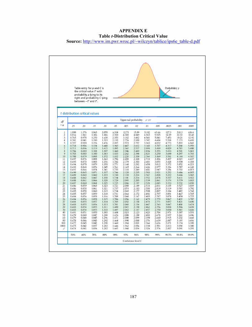
187

APPENDIX E

Table t-Distribution Critical Value

Source: http://www.im.pwr.wroc.pl/~wilczyn/tablice/ips6e_table-d.pdf

p= β/2 df =n

188

APPENDIX F

Thermophysical Properties of Water

189

190

APPENDIX G

Report of SIGMAPLOT Analysis (Data)

G.1 Data September 9, 2008

Result Summary of SIGMAPLOT Analysis Data (IA):

Charging Hour Tc (oC) Th (

oC) C S R

2 Remarks

18:00 6.91 13.58 2.71 1.60 0.9987 Passed

19:00 6.90 13.56 3.64 1.44 0.9994 Passed

20:00 6.93 13.55 4.61 1.42 0.9995 Passed

21:00 6.94 13.54 5.55 1.48 0.9995 Passed

22:00 6.91 13.54 6.51 1.41 0.9997 Passed

23:00 6.89 13.53 7.47 1.71 0.9996 Passed

0:00 6.87 13.51 8.44 2.01 0.9996 Passed

1:00 6.85 13.49 9.39 1.80 0.9997 Passed

2:00 6.83 13.46 10.31 1.83 0.9997 Passed

3:00 6.82 13.47 11.28 1.57 0.9996 Passed

Result of SIGMAPLOT processing: September 9, 2008 (Data IA)

Data set: 18.00 hours, data IA

Nonlinear Regression - Dynamic Fitting Thursday, July 22, 2010, 6:51:28 PM

Data Source: Data 1 in Notebook2

Equation: Ligand Binding, sigmoidal dose-response (variable slope)

f=Tc + (Th-Tc)/(1+10^((C-x)*S))

Dynamic Fit Options: Total Number of Fits 200

Maximum Number of Iterations 500

Parameter Ranges for Initial Estimates:

Minimum Maximum Tc -6.8210 20.4631

Th -13.7781 41.3343

C -2.8020 8.4059

S -1.0000 3.0000

Summary of Fit Results:

Converged 100.0%

Singular Solutions 55.5%

Results for the Overall Best-Fit Solution:

R Rsqr Adj Rsqr Standard Error of Estimate 0.9993 0.9987 0.9983 0.1068

Coefficient Std. Error t P

Tc 6.9070 0.0800 86.3819 <0.0001

Th 13.5758 0.0339 400.1587 <0.0001

C 2.7068 0.0259 104.5318 <0.0001

S 1.6024 0.1579 10.1492 <0.0001

191

Analysis of Variance: (Appendix G.1 cont.) Analysis of Variance:

DF SS MS Regression 4 2197.3200 549.3300

Residual 10 0.1141 0.0114

Total 14 2197.4341 156.9596

Corrected for the mean of the observations:

DF SS MS F P Regression 3 84.8045 28.2682 2476.6469 <0.0001

Residual 10 0.1141 0.0114

Total 13 84.9186 6.5322

Statistical Tests: Normality Test (Shapiro-Wilk) Passed (P = 0.9624)

W Statistic= 0.9781 Significance Level = 0.0500

Constant Variance Test Passed (P = 0.9637)

192

Data set: 19.00 hours, data IA (Appendix G.1 cont.)

Nonlinear Regression - Dynamic Fitting Thursday, July 22, 2010, 6:51:51 PM

Data Source: Data 1 in Notebook2

Equation: Ligand Binding, sigmoidal dose-response (variable slope) f=Tc + (Th-Tc)/(1+10^((C-x)*S))

Dynamic Fit Options: Total Number of Fits 200

Maximum Number of Iterations 500

Parameter Ranges for Initial Estimates:

Minimum Maximum Tc -6.8936 20.6807

Th -13.6709 41.0127

C -3.7123 11.1368

S -1.0000 3.0000

Summary of Fit Results:

Converged 100.0%

Singular Solutions 56.5%

Results for the Overall Best-Fit Solution:

R Rsqr Adj Rsqr Standard Error of Estimate 0.9997 0.9994 0.9992 0.0795

Coefficient Std. Error t P Tc 6.8987 0.0494 139.5154 <0.0001

Th 13.5601 0.0266 510.1241 <0.0001

C 3.6380 0.0171 212.4881 <0.0001

S 1.4428 0.1045 13.8040 <0.0001

Analysis of Variance:

Analysis of Variance:

DF SS MS Regression 4 2064.9120 516.2280

Residual 10 0.0632 0.0063

Total 14 2064.9752 147.4982

Corrected for the mean of the observations:

DF SS MS F P

Regression 3 105.4881 35.1627 5565.8055 <0.0001

Residual 10 0.0632 0.0063

Total 13 105.5513 8.1193

Statistical Tests: Normality Test (Shapiro-Wilk) Passed (P = 0.8736)

W Statistic= 0.9698 Significance Level = 0.0500

Constant Variance Test Passed (P = 0.4532)

193

Data set: 20.00 hours, data IA (Appendix G.1 cont.)

Nonlinear Regression - Dynamic Fitting Thursday, July 22, 2010, 6:52:08 PM

Data Source: Data 1 in Notebook2

Equation: Ligand Binding, sigmoidal dose-response (variable slope) f=Tc + (Th-Tc)/(1+10^((C-x)*S))

Dynamic Fit Options: Total Number of Fits 200

Maximum Number of Iterations 500

Parameter Ranges for Initial Estimates:

Minimum Maximum Tc -6.8720 20.6160

Th -13.6297 40.8890

C -4.6641 13.9924

S -1.0000 3.0000

Summary of Fit Results:

Converged 100.0%

Singular Solutions 59.5%

Results for the Overall Best-Fit Solution:

R Rsqr Adj Rsqr Standard Error of Estimate 0.9998 0.9995 0.9994 0.0740

Coefficient Std. Error t P

Tc 6.9329 0.0396 175.2703 <0.0001

Th 13.5536 0.0262 517.4668 <0.0001

C 4.6084 0.0154 298.3218 <0.0001

S 1.4204 0.0981 14.4774 <0.0001

Analysis of Variance:

Analysis of Variance:

DF SS MS

Regression 4 1933.3496 483.3374

Residual 10 0.0548 0.0055

Total 14 1933.4044 138.1003

Corrected for the mean of the observations:

DF SS MS F P Regression 3 121.4061 40.4687 7384.7919 <0.0001

Residual 10 0.0548 0.0055

Total 13 121.4609 9.3431

Statistical Tests: Normality Test (Shapiro-Wilk) Passed (P = 0.1035)

W Statistic= 0.8974 Significance Level = 0.0500

Constant Variance Test Passed (P = 0.6372)

194

Data set: 21.00 hours, data IA (Appendix G.1 cont.)

Nonlinear Regression - Dynamic Fitting Thursday, July 22, 2010, 6:52:23 PM

Data Source: Data 1 in Notebook2

Equation: Ligand Binding, sigmoidal dose-response (variable slope) f=Tc + (Th-Tc)/(1+10^((C-x)*S))

Dynamic Fit Options: Total Number of Fits 200

Maximum Number of Iterations 500

Parameter Ranges for Initial Estimates:

Minimum Maximum Tc -6.8633 20.5900

Th -13.6193 40.8578

C -5.5717 16.7150

S -1.0000 3.0000

Summary of Fit Results:

Converged 100.0%

Singular Solutions 62.5%

Results for the Overall Best-Fit Solution:

R Rsqr Adj Rsqr Standard Error of Estimate 0.9998 0.9995 0.9994 0.0805

Coefficient Std. Error t P Tc 6.9364 0.0385 180.2694 <0.0001

Th 13.5421 0.0301 449.6242 <0.0001

C 5.5474 0.0152 363.9671 <0.0001

S 1.4770 0.1289 11.4610 <0.0001

Analysis of Variance:

Analysis of Variance:

DF SS MS Regression 4 1804.3178 451.0794

Residual 10 0.0648 0.0065

Total 14 1804.3826 128.8845

Corrected for the mean of the observations:

DF SS MS F P

Regression 3 132.3713 44.1238 6807.4166 <0.0001

Residual 10 0.0648 0.0065

Total 13 132.4361 10.1874

Statistical Tests: Normality Test (Shapiro-Wilk) Passed (P = 0.3346)

W Statistic= 0.9329 Significance Level = 0.0500

Constant Variance Test Passed (P = 0.7499)

195

Data set: 22.00 hours, data IA (Appendix G.1 cont.)

Nonlinear Regression - Dynamic Fitting Thursday, July 22, 2010, 6:54:17 PM

Data Source: Data 1 in Sept9_DATA.JNB

Equation: Ligand Binding, sigmoidal dose-response (variable slope) f=Tc + (Th-Tc)/(1+10^((C-x)*S))

Dynamic Fit Options: Total Number of Fits 200

Maximum Number of Iterations 500

Parameter Ranges for Initial Estimates:

Minimum Maximum Tc -6.8498 20.5495

Th -13.6032 40.8095

C -6.5007 19.5021

S -1.0000 3.0000

Summary of Fit Results:

Converged 100.0%

Singular Solutions 64.0%

Results for the Overall Best-Fit Solution:

R Rsqr Adj Rsqr Standard Error of Estimate

0.9998 0.9997 0.9996 0.0678

Coefficient Std. Error t P Tc 6.9119 0.0297 232.9510 <0.0001

Th 13.5381 0.0272 498.0271 <0.0001

C 6.5089 0.0132 494.8539 <0.0001

S 1.4096 0.0948 14.8631 <0.0001

Analysis of Variance:

Analysis of Variance:

DF SS MS Regression 4 1671.0105 417.7526

Residual 10 0.0460 0.0046

Total 14 1671.0565 119.3612

Corrected for the mean of the observations:

DF SS MS F P

Regression 3 138.6039 46.2013 10042.3931 <0.0001

Residual 10 0.0460 0.0046

Total 13 138.6499 10.6654

Statistical Tests: Normality Test (Shapiro-Wilk) Passed (P = 0.2026)

W Statistic= 0.9175 Significance Level = 0.0500

Constant Variance Test Passed (P = 0.8201)

196

Data set: 23.00 hours, data IA (Appendix G.1 cont.)

Nonlinear Regression - Dynamic Fitting Thursday, July 22, 2010, 6:54:34 PM

Data Source: Data 1 in Sept9_DATA.JNB

Equation: Ligand Binding, sigmoidal dose-response (variable slope) f=Tc + (Th-Tc)/(1+10^((C-x)*S))

Dynamic Fit Options: Total Number of Fits 200

Maximum Number of Iterations 500

Parameter Ranges for Initial Estimates:

Minimum Maximum Tc -6.8313 20.4940

Th -13.5965 40.7894

C -7.4377 22.3131

S -1.0000 3.0000

Summary of Fit Results:

Converged 100.0%

Singular Solutions 68.0%

Results for the Overall Best-Fit Solution:

R Rsqr Adj Rsqr Standard Error of Estimate 0.9998 0.9996 0.9995 0.0704

Coefficient Std. Error t P

Tc 6.8936 0.0282 244.1950 <0.0001

Th 13.5286 0.0301 450.0203 <0.0001

C 7.4729 0.0119 626.8686 <0.0001

S 1.7054 0.1833 9.3050 <0.0001

Analysis of Variance:

Analysis of Variance:

DF SS MS

Regression 4 1539.0866 384.7717

Residual 10 0.0495 0.0050

Total 14 1539.1361 109.9383

Corrected for the mean of the observations:

DF SS MS F P Regression 3 140.7529 46.9176 9474.7526 <0.0001

Residual 10 0.0495 0.0050

Total 13 140.8024 10.8310

Statistical Tests: Normality Test (Shapiro-Wilk) Passed (P = 0.4704)

W Statistic= 0.9439 Significance Level = 0.0500

Constant Variance Test Passed (P = 0.8676)

197

Data set: 00.00 hours, data IA (Appendix G.1 cont.)

Nonlinear Regression - Dynamic Fitting Thursday, July 22, 2010, 6:54:51 PM

Data Source: Data 1 in Sept9_DATA.JNB

Equation: Ligand Binding, sigmoidal dose-response (variable slope) f=Tc + (Th-Tc)/(1+10^((C-x)*S))

Dynamic Fit Options: Total Number of Fits 200

Maximum Number of Iterations 500

Parameter Ranges for Initial Estimates:

Minimum Maximum Tc -6.8052 20.4157

Th -13.5845 40.7535

C -8.3635 25.0905

S -1.0000 3.0000

Summary of Fit Results:

Converged 99.5%

Singular Solutions 68.5%

Ill-Conditioned Solutions 0.5%

Iterations Exceeding 500 0.5%

Results for the Overall Best-Fit Solution:

R Rsqr Adj Rsqr Standard Error of Estimate 0.9998 0.9996 0.9995 0.0699

Coefficient Std. Error t P

Tc 6.8724 0.0262 262.2204 <0.0001

Th 13.5050 0.0322 419.0655 <0.0001

C 8.4357 0.0153 550.2128 <0.0001

S 2.0123 0.3301 6.0951 0.0001

Analysis of Variance:

Analysis of Variance:

DF SS MS

Regression 4 1405.4215 351.3554

Residual 10 0.0489 0.0049

Total 14 1405.4704 100.3907

Corrected for the mean of the observations:

DF SS MS F P Regression 3 136.1679 45.3893 9276.6728 <0.0001

Residual 10 0.0489 0.0049

Total 13 136.2169 10.4782

Statistical Tests: Normality Test (Shapiro-Wilk) Passed (P = 0.4997)

W Statistic= 0.9459 Significance Level = 0.0500

Constant Variance Test Passed (P = 0.6155)

198

Data set: 01.00 hours, data IA (Appendix G.1 cont.)

Nonlinear Regression - Dynamic Fitting Thursday, July 22, 2010, 6:55:07 PM

Data Source: Data 1 in Sept9_DATA.JNB

Equation: Ligand Binding, sigmoidal dose-response (variable slope) f=Tc + (Th-Tc)/(1+10^((C-x)*S))

Dynamic Fit Options: Total Number of Fits 200

Maximum Number of Iterations 500

Parameter Ranges for Initial Estimates:

Minimum Maximum Tc -6.7818 20.3455

Th -13.5606 40.6817

C -9.3032 27.9097

S -1.0000 3.0000

Summary of Fit Results:

Converged 99.5%

Singular Solutions 68.5%

Iterations Exceeding 500 0.5%

Results for the Overall Best-Fit Solution:

R Rsqr Adj Rsqr Standard Error of Estimate 0.9999 0.9997 0.9997 0.0574

Coefficient Std. Error t P

Tc 6.8456 0.0203 337.8586 <0.0001

Th 13.4917 0.0296 456.3355 <0.0001

C 9.3877 0.0133 707.5220 <0.0001

S 1.8037 0.1523 11.8448 <0.0001

Analysis of Variance: Analysis of Variance:

DF SS MS Regression 4 1271.4434 317.8609

Residual 10 0.0329 0.0033

Total 14 1271.4763 90.8197

Corrected for the mean of the observations:

DF SS MS F P

Regression 3 125.1448 41.7149 12668.5560 <0.0001

Residual 10 0.0329 0.0033

Total 13 125.1777 9.6291

Statistical Tests: Normality Test (Shapiro-Wilk) Passed (P = 0.6557)

W Statistic= 0.9559 Significance Level = 0.0500

Constant Variance Test Passed (P = 0.9637)

199

Data set: 02.00 hours, data IA (Appendix G.1 cont.)

Nonlinear Regression - Dynamic Fitting Thursday, July 22, 2010, 6:55:25 PM

Data Source: Data 1 in Sept9_DATA.JNB

Equation: Ligand Binding, sigmoidal dose-response (variable slope) f=Tc + (Th-Tc)/(1+10^((C-x)*S))

Dynamic Fit Options: Total Number of Fits 200

Maximum Number of Iterations 500

Parameter Ranges for Initial Estimates:

Minimum Maximum Tc -6.7544 20.2633

Th -13.5333 40.5998

C -10.2075 30.6225

S -1.0000 3.0000

Summary of Fit Results:

Converged 99.5%

Singular Solutions 70.5%

Iterations Exceeding 500 0.5%

Results for the Overall Best-Fit Solution:

R Rsqr Adj Rsqr Standard Error of Estimate

0.9998 0.9997 0.9996 0.0584

Coefficient Std. Error t P

Tc 6.8264 0.0195 349.8888 <0.0001

Th 13.4618 0.0344 391.0284 <0.0001

C 10.3062 0.0161 638.4681 <0.0001

S 1.8313 0.1236 14.8139 <0.0001

Analysis of Variance:

Analysis of Variance:

DF SS MS

Regression 4 1143.6628 285.9157

Residual 10 0.0341 0.0034

Total 14 1143.6969 81.6926

Corrected for the mean of the observations:

DF SS MS F P Regression 3 109.5495 36.5165 10708.5699 <0.0001

Residual 10 0.0341 0.0034

Total 13 109.5836 8.4295

Statistical Tests: Normality Test (Shapiro-Wilk) Passed (P = 0.5909)

W Statistic= 0.9519 Significance Level = 0.0500

Constant Variance Test Passed (P = 0.9517)

200

Data set: 03.00 hours, data IA (Appendix G.1 cont.)

Nonlinear Regression - Dynamic Fitting Thursday, July 22, 2010, 6:55:51 PM

Data Source: Data 1 in Sept9_DATA.JNB

Equation: Ligand Binding, sigmoidal dose-response (variable slope) f=Tc + (Th-Tc)/(1+10^((C-x)*S))

Dynamic Fit Options: Total Number of Fits 200

Maximum Number of Iterations 500

Parameter Ranges for Initial Estimates:

Minimum Maximum Tc -6.7315 20.1946

Th -13.5028 40.5084

C -11.1964 33.5891

S -1.0000 3.0000

Summary of Fit Results:

Converged 100.0%

Singular Solutions 75.5%

Results for the Overall Best-Fit Solution:

R Rsqr Adj Rsqr Standard Error of Estimate 0.9998 0.9996 0.9995 0.0585

Coefficient Std. Error t P

Tc 6.8156 0.0186 366.6265 <0.0001

Th 13.4697 0.0436 308.7311 <0.0001

C 11.2802 0.0146 772.1180 <0.0001

S 1.5701 0.0750 20.9257 <0.0001

Analysis of Variance:

Analysis of Variance:

DF SS MS

Regression 4 1008.3962 252.0991

Residual 10 0.0342 0.0034

Total 14 1008.4304 72.0307

Corrected for the mean of the observations:

DF SS MS F P Regression 3 85.3144 28.4381 8313.2956 <0.0001

Residual 10 0.0342 0.0034

Total 13 85.3486 6.5653

Statistical Tests: Normality Test (Shapiro-Wilk) Passed (P = 0.9845)

W Statistic= 0.9819 Significance Level = 0.0500

Constant Variance Test Passed (P = 0.5834)

201

G.2 Data September 11, 2008

Result Summary of SIGMAPLOT Analysis Data (IB):

Charging Hour Tc (oC) Th (

oC) C S R

2 Remarks

18:00 7.32 13.63 3.92 1.47 0.9985 Passed

19:00 7.36 13.61 4.87 1.57 0.9986 Passed

20:00 7.31 13.59 5.83 1.49 0.9987 Passed

21:00 7.27 13.59 6.77 1.34 0.9993 Passed

22:00 7.22 13.57 7.69 1.38 0.9995 Passed

23:00 7.17 13.54 8.63 1.42 0.9995 Passed

0:00 7.15 13.53 9.59 1.37 0.9996 Passed

1:00 7.12 13.50 10.49 1.26 0.9995 Passed

2:00 7.11 13.50 11.49 1.23 0.9990 Passed

3:00 7.09 13.83 12.55 1.10 0.9918 Passed

4:00 - - - - - In-convergence

5:00 - - - - - In-convergence

6:00 - - - - - In-convergence

7:00 - - - - - In-convergence

Result of SIGMAPLOT processing: September 11, 2008 (Data IB)

Data set: 18.00 hours, data IB

Nonlinear Regression - Dynamic Fitting Tuesday, June 29, 2010, 2:19:08 PM

Data Source: Data 1 in Notebook1

Equation: Ligand Binding, sigmoidal dose-response (variable slope)

f=Tc + (Th-Tc)/(1+10^((C-x)*S))

Dynamic Fit Options:

Total Number of Fits 200

Maximum Number of Iterations 500

Parameter Ranges for Initial Estimates:

Minimum Maximum Tc -3.7500 1.2500

Th -13.7848 41.3543

C -3.9603 11.8808

S -1.0000 3.0000

Summary of Fit Results:

Converged 100.0%

Singular Solutions 45.5%

Results for the Overall Best-Fit Solution:

R Rsqr Adj Rsqr Standard Error of Estimate 0.9993 0.9985 0.9981 0.1220

Coefficient Std. Error t P

Tc 7.3173 0.0727 100.6511 <0.0001

Th 13.6253 0.0410 332.0368 <0.0001

C 3.9220 0.0339 115.7509 <0.0001

S 1.4658 0.1001 14.6480 <0.0001

202

Analysis of Variance: (Appendix G.2 cont.) Analysis of Variance:

DF SS MS Regression 4 2070.4360 517.6090

Residual 10 0.1489 0.0149

Total 14 2070.5849 147.8989

Corrected for the mean of the observations:

DF SS MS F P Regression 3 101.1509 33.7170 2265.0673 <0.0001

Residual 10 0.1489 0.0149

Total 13 101.2998 7.7923

Statistical Tests: Normality Test (Shapiro-Wilk) Passed (P = 0.3123)

W Statistic= 0.9307 Significance Level = 0.0500

Constant Variance Test Passed (P = 0.2786)

203

Data set: 19.00 hours, data IB (Appendix G.2 cont.)

Nonlinear Regression - Dynamic Fitting Tuesday, June 29, 2010, 2:19:35 PM

Data Source: Data 1 in Notebook1

Equation: Ligand Binding, sigmoidal dose-response (variable slope) f=Tc + (Th-Tc)/(1+10^((C-x)*S))

Dynamic Fit Options: Total Number of Fits 200

Maximum Number of Iterations 500

Parameter Ranges for Initial Estimates:

Minimum Maximum Tc -3.6250 1.2083

Th -13.7332 41.1995

C -4.9275 14.7825

S -1.0000 3.0000

Summary of Fit Results:

Converged 100.0%

Singular Solutions 48.0%

Results for the Overall Best-Fit Solution:

R Rsqr Adj Rsqr Standard Error of Estimate 0.9993 0.9986 0.9982 0.1264

Coefficient Std. Error t P

Tc 7.3587 0.0644 114.2922 <0.0001

Th 13.6057 0.0450 302.3090 <0.0001

C 4.8698 0.0353 137.9451 <0.0001

S 1.5736 0.1255 12.5334 <0.0001

Analysis of Variance:

Analysis of Variance:

DF SS MS

Regression 4 1943.5365 485.8841

Residual 10 0.1597 0.0160

Total 14 1943.6962 138.8354

Corrected for the mean of the observations:

DF SS MS F P Regression 3 113.8312 37.9437 2376.2972 <0.0001

Residual 10 0.1597 0.0160

Total 13 113.9909 8.7685

Statistical Tests: Normality Test (Shapiro-Wilk) Passed (P = 0.0510)

W Statistic= 0.8760 Significance Level = 0.0500

Constant Variance Test Passed (P = 0.1476)

204

Data set: 20.00 hours, data IB (Appendix G.2 cont.)

Nonlinear Regression - Dynamic Fitting Tuesday, June 29, 2010, 2:19:49 PM

Data Source: Data 1 in Notebook1

Equation: Ligand Binding, sigmoidal dose-response (variable slope) f=Tc + (Th-Tc)/(1+10^((C-x)*S))

Dynamic Fit Options: Total Number of Fits 200

Maximum Number of Iterations 500

Parameter Ranges for Initial Estimates:

Minimum Maximum Tc -3.5000 1.1667

Th -13.7187 41.1561

C -5.8906 17.6717

S -1.0000 3.0000

Summary of Fit Results:

Converged 100.0%

Singular Solutions 50.0%

Results for the Overall Best-Fit Solution:

R Rsqr Adj Rsqr Standard Error of Estimate 0.9993 0.9987 0.9983 0.1272

Coefficient Std. Error t P

Tc 7.3107 0.0580 125.9718 <0.0001

Th 13.5934 0.0486 279.9471 <0.0001

C 5.8306 0.0344 169.6248 <0.0001

S 1.4949 0.1246 11.9986 <0.0001

Analysis of Variance:

Analysis of Variance:

DF SS MS

Regression 4 1809.9857 452.4964

Residual 10 0.1618 0.0162

Total 14 1810.1475 129.2963

Corrected for the mean of the observations:

DF SS MS F P Regression 3 123.2045 41.0682 2537.5107 <0.0001

Residual 10 0.1618 0.0162

Total 13 123.3664 9.4897

Statistical Tests: Normality Test (Shapiro-Wilk) Passed (P = 0.0218)

W Statistic= 0.8494 Significance Level = 0.0500

Constant Variance Test Passed (P = 0.1088)

205

Data set: 21.00 hours, data IB (Appendix G.2 cont.)

Nonlinear Regression - Dynamic Fitting Tuesday, June 29, 2010, 2:20:52 PM

Data Source: Data 1 in Notebook1

Equation: Ligand Binding, sigmoidal dose-response (variable slope) f=Tc + (Th-Tc)/(1+10^((C-x)*S))

Dynamic Fit Options: Total Number of Fits 200

Maximum Number of Iterations 500

Parameter Ranges for Initial Estimates:

Minimum Maximum Tc -3.3750 1.1250

Th -13.6939 41.0816

C -6.8324 20.4973

S -1.0000 3.0000

Summary of Fit Results:

Converged 100.0%

Singular Solutions 55.0%

Results for the Overall Best-Fit Solution:

R Rsqr Adj Rsqr Standard Error of Estimate 0.9997 0.9993 0.9991 0.0919

Coefficient Std. Error t P

Tc 7.2688 0.0386 188.2191 <0.0001

Th 13.5905 0.0381 356.6095 <0.0001

C 6.7725 0.0238 284.2982 <0.0001

S 1.3364 0.0822 16.2565 <0.0001

Analysis of Variance:

Analysis of Variance:

DF SS MS

Regression 4 1680.2753 420.0688

Residual 10 0.0845 0.0084

Total 14 1680.3598 120.0257

Corrected for the mean of the observations:

DF SS MS F P Regression 3 126.7783 42.2594 5001.1470 <0.0001

Residual 10 0.0845 0.0084

Total 13 126.8628 9.7587

Statistical Tests: Normality Test (Shapiro-Wilk) Passed (P = 0.1476)

W Statistic= 0.9080 Significance Level = 0.0500

Constant Variance Test Passed (P = 0.2715)

206

Data set: 22.00 hours, data IB (Appendix G.2 cont.)

Nonlinear Regression - Dynamic Fitting Tuesday, June 29, 2010, 2:21:05 PM

Data Source: Data 1 in Notebook1

Equation: Ligand Binding, sigmoidal dose-response (variable slope) f=Tc + (Th-Tc)/(1+10^((C-x)*S))

Dynamic Fit Options: Total Number of Fits 200

Maximum Number of Iterations 500

Parameter Ranges for Initial Estimates:

Minimum Maximum Tc -3.2500 1.0833

Th -13.6634 40.9902

C -7.7586 23.2757

S -1.0000 3.0000

Summary of Fit Results:

Converged 100.0%

Singular Solutions 61.5%

Results for the Overall Best-Fit Solution:

R Rsqr Adj Rsqr Standard Error of Estimate 0.9997 0.9995 0.9993 0.0818

Coefficient Std. Error t P

Tc 7.2158 0.0318 226.9532 <0.0001

Th 13.5667 0.0370 366.6422 <0.0001

C 7.6935 0.0201 383.4399 <0.0001

S 1.3793 0.0909 15.1799 <0.0001

Analysis of Variance:

Analysis of Variance:

DF SS MS

Regression 4 1548.7478 387.1869

Residual 10 0.0669 0.0067

Total 14 1548.8146 110.6296

Corrected for the mean of the observations:

DF SS MS F P Regression 3 126.8398 42.2799 6321.6759 <0.0001

Residual 10 0.0669 0.0067

Total 13 126.9067 9.7621

Statistical Tests: Normality Test (Shapiro-Wilk) Passed (P = 0.3852)

W Statistic= 0.9373 Significance Level = 0.0500

Constant Variance Test Passed (P = 0.3395)

207

Data set: 23.00 hours, data IB (Appendix G.2 cont.)

Nonlinear Regression - Dynamic Fitting Tuesday, June 29, 2010, 2:21:20 PM

Data Source: Data 1 in Notebook1

Equation: Ligand Binding, sigmoidal dose-response (variable slope) f=Tc + (Th-Tc)/(1+10^((C-x)*S))

Dynamic Fit Options: Total Number of Fits 200

Maximum Number of Iterations 500

Parameter Ranges for Initial Estimates:

Minimum Maximum Tc -3.1250 1.0417

Th -13.6447 40.9340

C -8.6874 26.0622

S -1.0000 3.0000

Summary of Fit Results:

Converged 100.0%

Singular Solutions 63.0%

Results for the Overall Best-Fit Solution:

R Rsqr Adj Rsqr Standard Error of Estimate

0.9998 0.9995 0.9994 0.0753

Coefficient Std. Error t P

Tc 7.1734 0.0275 261.2320 <0.0001

Th 13.5386 0.0378 358.2483 <0.0001

C 8.6282 0.0172 500.4156 <0.0001

S 1.4156 0.1016 13.9386 <0.0001

Analysis of Variance: Analysis of Variance:

DF SS MS Regression 4 1416.1622 354.0405

Residual 10 0.0568 0.0057

Total 14 1416.2190 101.1585

Corrected for the mean of the observations:

DF SS MS F P

Regression 3 121.2212 40.4071 7119.4173 <0.0001

Residual 10 0.0568 0.0057

Total 13 121.2780 9.3291

Statistical Tests: Normality Test (Shapiro-Wilk) Passed (P = 0.8699)

W Statistic= 0.9695 Significance Level = 0.0500

Constant Variance Test Passed (P = 0.5940)

208

Data set: 00.00 hours, data IB (Appendix G.2 cont.)

Nonlinear Regression - Dynamic Fitting Tuesday, June 29, 2010, 2:21:39 PM

Data Source: Data 1 in Notebook1

Equation: Ligand Binding, sigmoidal dose-response (variable slope) f=Tc + (Th-Tc)/(1+10^((C-x)*S))

Dynamic Fit Options: Total Number of Fits 200

Maximum Number of Iterations 500

Parameter Ranges for Initial Estimates:

Minimum Maximum Tc -6.0000 2.0000

Th -13.6248 40.8745

C -9.6302 28.8907

S -1.0000 3.0000

Summary of Fit Results:

Converged 100.0%

Singular Solutions 64.5%

Ill-Conditioned Solutions 0.5%

Results for the Overall Best-Fit Solution:

R Rsqr Adj Rsqr Standard Error of Estimate 0.9998 0.9996 0.9994 0.0690

Coefficient Std. Error t P

Tc 7.1491 0.0238 299.7888 <0.0001

Th 13.5251 0.0396 341.2610 <0.0001

C 9.5861 0.0154 621.2670 <0.0001

S 1.3707 0.0915 14.9809 <0.0001

Analysis of Variance: Analysis of Variance:

DF SS MS Regression 4 1284.7993 321.1998

Residual 10 0.0477 0.0048

Total 14 1284.8469 91.7748

Corrected for the mean of the observations:

DF SS MS F P

Regression 3 109.5347 36.5116 7661.4860 <0.0001

Residual 10 0.0477 0.0048

Total 13 109.5823 8.4294

Statistical Tests: Normality Test (Shapiro-Wilk) Passed (P = 0.5526)

W Statistic= 0.9495 Significance Level = 0.0500

Constant Variance Test Passed (P = 0.8676)

209

Data set: 01.00 hours, data IB (Appendix G.2 cont.)

Nonlinear Regression - Dynamic Fitting Tuesday, June 29, 2010, 2:21:58 PM

Data Source: Data 1 in Notebook1

Equation: Ligand Binding, sigmoidal dose-response (variable slope) f=Tc + (Th-Tc)/(1+10^((C-x)*S))

Dynamic Fit Options: Total Number of Fits 200

Maximum Number of Iterations 500

Parameter Ranges for Initial Estimates:

Minimum Maximum Tc -5.8750 1.9583

Th -13.5741 40.7224

C -10.4810 31.4430

S -1.0000 3.0000

Summary of Fit Results:

Converged 100.0%

Singular Solutions 66.0%

Results for the Overall Best-Fit Solution:

R Rsqr Adj Rsqr Standard Error of Estimate 0.9997 0.9995 0.9993 0.0685

Coefficient Std. Error t P

Tc 7.1248 0.0228 312.5994 <0.0001

Th 13.5008 0.0464 290.7041 <0.0001

C 10.4924 0.0159 658.6213 <0.0001

S 1.2565 0.0752 16.7130 <0.0001

Analysis of Variance:

Analysis of Variance:

DF SS MS

Regression 4 1158.8816 289.7204

Residual 10 0.0470 0.0047

Total 14 1158.9286 82.7806

Corrected for the mean of the observations:

DF SS MS F P Regression 3 92.6158 30.8719 6574.1408 <0.0001

Residual 10 0.0470 0.0047

Total 13 92.6628 7.1279

Statistical Tests: Normality Test (Shapiro-Wilk) Passed (P = 0.9674)

W Statistic= 0.9788 Significance Level = 0.0500

Constant Variance Test Passed (P = 0.6482)

210

Data set: 02.00 hours, data IB (Appendix G.2 cont.)

Nonlinear Regression - Dynamic Fitting Tuesday, June 29, 2010, 2:22:12 PM

Data Source: Data 1 in Notebook1

Equation: Ligand Binding, sigmoidal dose-response (variable slope) f=Tc + (Th-Tc)/(1+10^((C-x)*S))

Dynamic Fit Options: Total Number of Fits 200

Maximum Number of Iterations 500

Parameter Ranges for Initial Estimates:

Minimum Maximum Tc -5.7500 1.9167

Th -13.4152 40.2455

C -11.4564 34.3691

S -1.0000 3.0000

Summary of Fit Results:

Converged 100.0%

Singular Solutions 65.0%

Ill-Conditioned Solutions 0.5%

Results for the Overall Best-Fit Solution:

R Rsqr Adj Rsqr Standard Error of Estimate 0.9995 0.9990 0.9988 0.0814

Coefficient Std. Error t P

Tc 7.1128 0.0258 275.7624 <0.0001

Th 13.5007 0.0753 179.4107 <0.0001

C 11.4913 0.0205 560.7064 <0.0001

S 1.2285 0.0901 13.6330 <0.0001

Analysis of Variance: Analysis of Variance:

DF SS MS Regression 4 1025.2366 256.3092

Residual 10 0.0663 0.0066

Total 14 1025.3029 73.2359

Corrected for the mean of the observations:

DF SS MS F P

Regression 3 69.5151 23.1717 3497.5183 <0.0001

Residual 10 0.0663 0.0066

Total 13 69.5814 5.3524

Statistical Tests: Normality Test (Shapiro-Wilk) Passed (P = 0.7529)

W Statistic= 0.9618 Significance Level = 0.0500

Constant Variance Test Passed (P = 0.4532)

211

Data set: 03.00 hours, data IB (Appendix G.2 cont.)

Nonlinear Regression - Dynamic Fitting Tuesday, June 29, 2010, 2:22:27 PM

Data Source: Data 1 in Notebook1

Equation: Ligand Binding, sigmoidal dose-response (variable slope) f=Tc+ (Th-Tc)/(1+10^((C-x)*S))

Dynamic Fit Options:

Total Number of Fits 200

Maximum Number of Iterations 500

Parameter Ranges for Initial Estimates:

Minimum Maximum Tc -5.6250 1.8750

Th -13.2854 39.8561

C -12.4567 37.3702

S -1.0000 3.0000

Summary of Fit Results: Converged 99.0%

Singular Solutions 71.0%

Ill-Conditioned Solutions 0.5%

Iterations Exceeding 500 1.0%

Results for the Overall Best-Fit Solution:

R Rsqr Adj Rsqr Standard Error of Estimate 0.9991 0.9982 0.9977 0.0864

Coefficient Std. Error t P

Tc 7.0876 0.0265 267.3137 <0.0001

Th 13.8321 0.2039 67.8335 <0.0001

C 12.5525 0.0377 333.1423 <0.0001

S 1.1023 0.1038 10.6183 <0.0001

Analysis of Variance: Analysis of Variance:

DF SS MS Regression 4 892.0896 223.0224

Residual 10 0.0747 0.0075

Total 14 892.1642 63.7260

Corrected for the mean of the observations:

DF SS MS F P

Regression 3 41.8394 13.9465 1868.0823 <0.0001

Residual 10 0.0747 0.0075

Total 13 41.9140 3.2242

Statistical Tests: Normality Test (Shapiro-Wilk) Passed (P = 0.3859)

W Statistic= 0.9374 Significance Level = 0.0500

Constant Variance Test Passed (P = 0.3236)

212

G.3 Data September 19, 2008

Result Summary of SIGMAPLOT Analysis Data (IC)

Charging Hour Tc (oC) Th (

oC) C S R

2 Remarks

18:00 7.73 13.54 3.19 1.11 0.9968 Passed

19:00 7.58 13.53 4.10 1.03 0.9984 Passed

20:00 7.49 13.50 5.05 1.06 0.9983 Passed

21:00 7.40 13.49 6.01 1.05 0.9989 Passed

22:00 7.34 13.49 6.98 0.99 0.9994 Passed

23:00 7.30 13.46 7.91 1.03 0.9995 Passed

0:00 7.27 13.45 8.89 1.06 0.9994 Passed

1:00 7.24 13.41 9.86 1.09 0.9990 Passed

2:00 7.20 13.43 10.78 0.92 0.9995 Passed

3:00 7.20 13.51 11.80 0.93 0.9976 Passed

4:00 - - - - - In-convergence

5:00 - - - - - In-convergence

6:00 - - - - - In-convergence

7:00 - - - - - In-convergence

Result of SIGMAPLOT processing: September 19, 2008 (Data IC)

Data set: 18.00 hours, data IC

Nonlinear Regression - Dynamic Fitting Friday, July 23, 2010, 1:47:49 PM

Data Source: Data 1 in Notebook9

Equation: Ligand Binding, sigmoidal dose-response (variable slope) f=Tc + (Th-Tc)/(1+10^((C-x)*S))

Dynamic Fit Options: Total Number of Fits 200

Maximum Number of Iterations 500

Parameter Ranges for Initial Estimates:

Minimum Maximum

Tc -7.6479 22.9437

Th -13.7291 41.1874

C -3.1656 9.4968

S -1.0000 3.0000

Summary of Fit Results: Converged 100.0%

Singular Solutions 57.0%

Results for the Overall Best-Fit Solution:

R Rsqr Adj Rsqr Standard Error of Estimate 0.9984 0.9968 0.9959 0.1488

Coefficient Std. Error t P

Tc 7.7339 0.1161 66.5987 <0.0001

Th 13.5444 0.0484 279.5875 <0.0001

C 3.1921 0.0494 64.5568 <0.0001

S 1.1052 0.1101 10.0382 <0.0001

213

Analysis of Variance: (Appendix G.3 cont.) Analysis of Variance:

DF SS MS Regression 4 2161.9219 540.4805

Residual 10 0.2214 0.0221

Total 14 2162.1433 154.4388

Corrected for the mean of the observations:

DF SS MS F P Regression 3 69.7914 23.2638 1050.7709 <0.0001

Residual 10 0.2214 0.0221

Total 13 70.0128 5.3856

Statistical Tests: Normality Test (Shapiro-Wilk) Passed (P = 0.2816)

W Statistic= 0.9275 Significance Level = 0.0500

Constant Variance Test Passed (P = 0.8676)

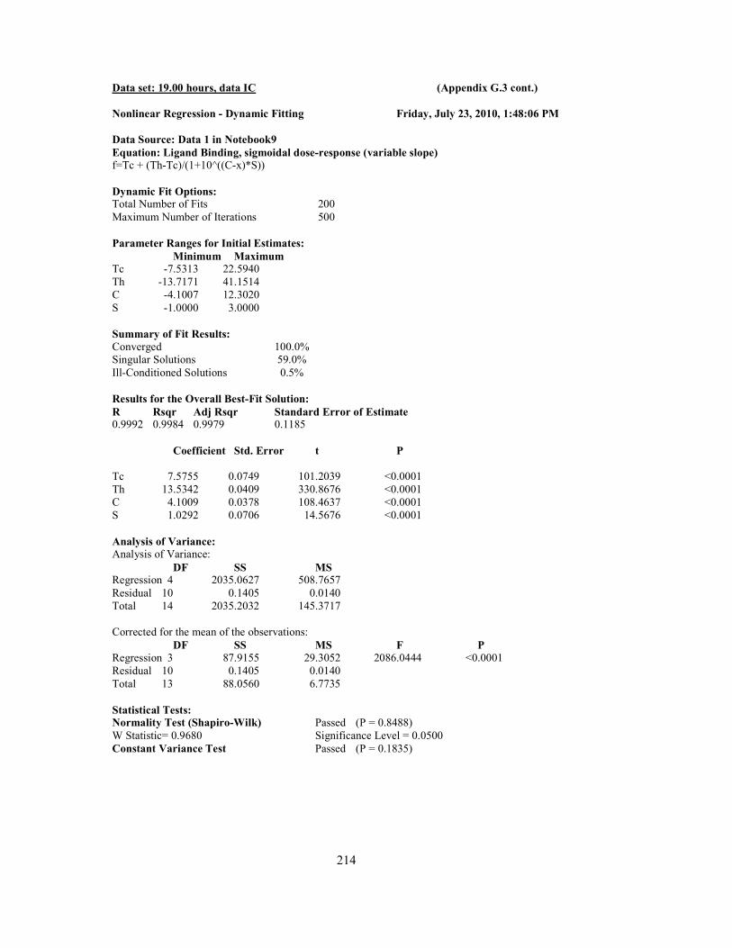
214

Data set: 19.00 hours, data IC (Appendix G.3 cont.)

Nonlinear Regression - Dynamic Fitting Friday, July 23, 2010, 1:48:06 PM

Data Source: Data 1 in Notebook9

Equation: Ligand Binding, sigmoidal dose-response (variable slope) f=Tc + (Th-Tc)/(1+10^((C-x)*S))

Dynamic Fit Options: Total Number of Fits 200

Maximum Number of Iterations 500

Parameter Ranges for Initial Estimates:

Minimum Maximum Tc -7.5313 22.5940

Th -13.7171 41.1514

C -4.1007 12.3020

S -1.0000 3.0000

Summary of Fit Results:

Converged 100.0%

Singular Solutions 59.0%

Ill-Conditioned Solutions 0.5%

Results for the Overall Best-Fit Solution:

R Rsqr Adj Rsqr Standard Error of Estimate 0.9992 0.9984 0.9979 0.1185

Coefficient Std. Error t P

Tc 7.5755 0.0749 101.2039 <0.0001

Th 13.5342 0.0409 330.8676 <0.0001

C 4.1009 0.0378 108.4637 <0.0001

S 1.0292 0.0706 14.5676 <0.0001

Analysis of Variance: Analysis of Variance:

DF SS MS Regression 4 2035.0627 508.7657

Residual 10 0.1405 0.0140

Total 14 2035.2032 145.3717

Corrected for the mean of the observations:

DF SS MS F P

Regression 3 87.9155 29.3052 2086.0444 <0.0001

Residual 10 0.1405 0.0140

Total 13 88.0560 6.7735

Statistical Tests: Normality Test (Shapiro-Wilk) Passed (P = 0.8488)

W Statistic= 0.9680 Significance Level = 0.0500

Constant Variance Test Passed (P = 0.1835)

215

Data set: 20.00 hours, data IC (Appendix G.3 cont.)

Nonlinear Regression - Dynamic Fitting Friday, July 23, 2010, 1:48:25 PM

Data Source: Data 1 in Notebook9

Equation: Ligand Binding, sigmoidal dose-response (variable slope) f=Tc + (Th-Tc)/(1+10^((C-x)*S))

Dynamic Fit Options: Total Number of Fits 200

Maximum Number of Iterations 500

Parameter Ranges for Initial Estimates:

Minimum Maximum Tc -7.4283 22.2849

Th -13.6765 41.0296

C -5.0582 15.1747

S -1.0000 3.0000

Summary of Fit Results:

Converged 100.0%

Singular Solutions 62.5%

Results for the Overall Best-Fit Solution:

R Rsqr Adj Rsqr Standard Error of Estimate 0.9992 0.9983 0.9978 0.1303

Coefficient Std. Error t P

Tc 7.4853 0.0694 107.8836 <0.0001

Th 13.5047 0.0476 283.5246 <0.0001

C 5.0521 0.0397 127.3729 <0.0001

S 1.0615 0.0764 13.8878 <0.0001

Analysis of Variance:

Analysis of Variance:

DF SS MS

Regression 4 1901.6078 475.4020

Residual 10 0.1697 0.0170

Total 14 1901.7775 135.8412

Corrected for the mean of the observations:

DF SS MS F P Regression 3 102.2105 34.0702 2007.9340 <0.0001

Residual 10 0.1697 0.0170

Total 13 102.3802 7.8754

Statistical Tests: Normality Test (Shapiro-Wilk) Passed (P = 0.7176)

W Statistic= 0.9597 Significance Level = 0.0500

Constant Variance Test Passed (P = 0.2786)

216

Data set: 21.00 hours, data IC (Appendix G.3 cont.)

Nonlinear Regression - Dynamic Fitting Friday, July 23, 2010, 1:48:44 PM

Data Source: Data 1 in Notebook9

Equation: Ligand Binding, sigmoidal dose-response (variable slope) f=Tc + (Th-Tc)/(1+10^((C-x)*S))

Dynamic Fit Options: Total Number of Fits 200

Maximum Number of Iterations 500

Parameter Ranges for Initial Estimates:

Minimum Maximum Tc -7.3205 21.9616

Th -13.6333 40.8998

C -6.0174 18.0522

S -1.0000 3.0000

Summary of Fit Results:

Converged 100.0%

Singular Solutions 64.5%

Results for the Overall Best-Fit Solution:

R Rsqr Adj Rsqr Standard Error of Estimate

0.9995 0.9989 0.9986 0.1093

Coefficient Std. Error t P

Tc 7.3960 0.0516 143.2224 <0.0001

Th 13.4908 0.0430 314.0624 <0.0001

C 6.0113 0.0327 183.8060 <0.0001

S 1.0454 0.0615 16.9855 <0.0001

Analysis of Variance: Analysis of Variance:

DF SS MS Regression 4 1768.7569 442.1892

Residual 10 0.1196 0.0120

Total 14 1768.8765 126.3483

Corrected for the mean of the observations:

DF SS MS F P

Regression 3 112.0716 37.3572 3124.6535 <0.0001

Residual 10 0.1196 0.0120

Total 13 112.1912 8.6301

Statistical Tests: Normality Test (Shapiro-Wilk) Passed (P = 0.4763)

W Statistic= 0.9443 Significance Level = 0.0500

Constant Variance Test Passed (P = 0.5520)

217

Data set: 22.00 hours, data IC (Appendix G.3 cont.)

Nonlinear Regression - Dynamic Fitting Friday, July 23, 2010, 1:49:04 PM

Data Source: Data 1 in Notebook9

Equation: Ligand Binding, sigmoidal dose-response (variable slope) f=Tc + (Th-Tc)/(1+10^((C-x)*S))

Dynamic Fit Options: Total Number of Fits 200

Maximum Number of Iterations 500

Parameter Ranges for Initial Estimates:

Minimum Maximum Tc -7.2489 21.7467

Th -13.5899 40.7697

C -6.9835 20.9506

S -1.0000 3.0000

Summary of Fit Results:

Converged 100.0%

Singular Solutions 67.0%

Results for the Overall Best-Fit Solution:

R Rsqr Adj Rsqr Standard Error of Estimate 0.9997 0.9994 0.9992 0.0818

Coefficient Std. Error t P

Tc 7.3402 0.0352 208.2555 <0.0001

Th 13.4863 0.0351 384.0484 <0.0001

C 6.9751 0.0247 282.7077 <0.0001

S 0.9927 0.0433 22.9193 <0.0001

Analysis of Variance:

Analysis of Variance:

DF SS MS

Regression 4 1638.3229 409.5807

Residual 10 0.0669 0.0067

Total 14 1638.3898 117.0278

Corrected for the mean of the observations:

DF SS MS F P Regression 3 115.7808 38.5936 5772.5606 <0.0001

Residual 10 0.0669 0.0067

Total 13 115.8476 8.9114

Statistical Tests: Normality Test (Shapiro-Wilk) Passed (P = 0.3812)

W Statistic= 0.9370 Significance Level = 0.0500

Constant Variance Test Passed (P = 0.4722)

218

Data set: 23.00 hours, data IC (Appendix G.3 cont.)

Nonlinear Regression - Dynamic Fitting Friday, July 23, 2010, 1:49:23 PM

Data Source: Data 1 in Notebook9

Equation: Ligand Binding, sigmoidal dose-response (variable slope) f=Tc + (Th-Tc)/(1+10^((C-x)*S))

Dynamic Fit Options: Total Number of Fits 200

Maximum Number of Iterations 500

Parameter Ranges for Initial Estimates:

Minimum Maximum Tc -7.2051 21.6152

Th -13.5493 40.6479

C -7.9295 23.7884

S -1.0000 3.0000

Summary of Fit Results:

Converged 100.0%

Singular Solutions 69.0%

Results for the Overall Best-Fit Solution:

R Rsqr Adj Rsqr Standard Error of Estimate 0.9998 0.9995 0.9994 0.0735

Coefficient Std. Error t P

Tc 7.3021 0.0290 251.3953 <0.0001

Th 13.4609 0.0346 388.9881 <0.0001

C 7.9114 0.0218 362.9134 <0.0001

S 1.0295 0.0412 25.0018 <0.0001

Analysis of Variance:

Analysis of Variance:

DF SS MS

Regression 4 1510.3494 377.5874

Residual 10 0.0540 0.0054

Total 14 1510.4034 107.8860

Corrected for the mean of the observations:

DF SS MS F P Regression 3 114.6559 38.2186 7079.0717 <0.0001

Residual 10 0.0540 0.0054

Total 13 114.7099 8.8238

Statistical Tests: Normality Test (Shapiro-Wilk) Passed (P = 0.2524)

W Statistic= 0.9242 Significance Level = 0.0500

Constant Variance Test Passed (P = 0.9396)

219

Data set: 00.00 hours, data IC (Appendix G.3 cont.)

Nonlinear Regression - Dynamic Fitting Friday, July 23, 2010, 1:49:42 PM

Data Source: Data 1 in Notebook9

Equation: Ligand Binding, sigmoidal dose-response (variable slope) f=Tc + (Th-Tc)/(1+10^((C-x)*S))

Dynamic Fit Options: Total Number of Fits 200

Maximum Number of Iterations 500

Parameter Ranges for Initial Estimates:

Minimum Maximum Tc -7.1631 21.4892

Th -13.5276 40.5829

C -8.9115 26.7345

S -1.0000 3.0000

Summary of Fit Results:

Converged 100.0%

Singular Solutions 68.0%

Ill-Conditioned Solutions 0.5%

Results for the Overall Best-Fit Solution:

R Rsqr Adj Rsqr Standard Error of Estimate 0.9997 0.9994 0.9993 0.0780

Coefficient Std. Error t P

Tc 7.2710 0.0286 254.0674 <0.0001

Th 13.4454 0.0413 325.2486 <0.0001

C 8.8882 0.0230 385.9494 <0.0001

S 1.0633 0.0462 23.0131 <0.0001

Analysis of Variance: Analysis of Variance:

DF SS MS Regression 4 1379.6746 344.9187

Residual 10 0.0609 0.0061

Total 14 1379.7355 98.5525

Corrected for the mean of the observations:

DF SS MS F P

Regression 3 108.3579 36.1193 5933.0644 <0.0001

Residual 10 0.0609 0.0061

Total 13 108.4188 8.3399

Statistical Tests: Normality Test (Shapiro-Wilk) Passed (P = 0.4880)

W Statistic= 0.9451 Significance Level = 0.0500

Constant Variance Test Passed (P = 0.3236)

220

Data set: 01.00 hours, data IC (Appendix G.3 cont.)

Nonlinear Regression - Dynamic Fitting Friday, July 23, 2010, 1:50:01 PM

Data Source: Data 1 in Notebook9

Equation: Ligand Binding, sigmoidal dose-response (variable slope) f=Tc + (Th-Tc)/(1+10^((C-x)*S))

Dynamic Fit Options: Total Number of Fits 200

Maximum Number of Iterations 500

Parameter Ranges for Initial Estimates:

Minimum Maximum Tc -7.1291 21.3872

Th -13.4859 40.4578

C -9.8879 29.6637

S -1.0000 3.0000

Summary of Fit Results:

Converged 100.0%

Singular Solutions 70.5%

Ill-Conditioned Solutions 0.5%

Results for the Overall Best-Fit Solution:

R Rsqr Adj Rsqr Standard Error of Estimate 0.9995 0.9990 0.9987 0.0968

Coefficient Std. Error t P

Tc 7.2404 0.0333 217.3203 <0.0001

Th 13.4130 0.0599 223.7675 <0.0001

C 9.8568 0.0289 340.8787 <0.0001

S 1.0928 0.0618 17.6733 <0.0001

Analysis of Variance: Analysis of Variance:

DF SS MS Regression 4 1248.1616 312.0404

Residual 10 0.0938 0.0094

Total 14 1248.2554 89.1611

Corrected for the mean of the observations:

DF SS MS F P

Regression 3 96.2368 32.0789 3420.1724 <0.0001

Residual 10 0.0938 0.0094

Total 13 96.3306 7.4100

Statistical Tests: Normality Test (Shapiro-Wilk) Passed (P = 0.1163)

W Statistic= 0.9009 Significance Level = 0.0500

Constant Variance Test Passed (P = 0.2311)

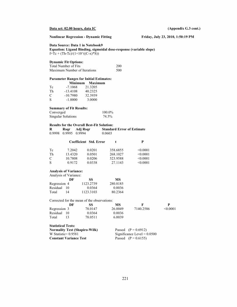
221

Data set: 02.00 hours, data IC (Appendix G.3 cont.)

Nonlinear Regression - Dynamic Fitting Friday, July 23, 2010, 1:50:19 PM

Data Source: Data 1 in Notebook9

Equation: Ligand Binding, sigmoidal dose-response (variable slope) f=Tc + (Th-Tc)/(1+10^((C-x)*S))

Dynamic Fit Options: Total Number of Fits 200

Maximum Number of Iterations 500

Parameter Ranges for Initial Estimates:

Minimum Maximum Tc -7.1068 21.3205

Th -13.4108 40.2325

C -10.7980 32.3939

S -1.0000 3.0000

Summary of Fit Results:

Converged 100.0%

Singular Solutions 74.5%

Results for the Overall Best-Fit Solution:

R Rsqr Adj Rsqr Standard Error of Estimate 0.9998 0.9995 0.9994 0.0603

Coefficient Std. Error t P

Tc 7.2042 0.0201 358.6855 <0.0001

Th 13.4320 0.0501 268.1027 <0.0001

C 10.7808 0.0206 523.9588 <0.0001

S 0.9172 0.0338 27.1143 <0.0001

Analysis of Variance:

Analysis of Variance:

DF SS MS

Regression 4 1123.2739 280.8185

Residual 10 0.0364 0.0036

Total 14 1123.3103 80.2364

Corrected for the mean of the observations:

DF SS MS F P Regression 3 78.0147 26.0049 7140.2586 <0.0001

Residual 10 0.0364 0.0036

Total 13 78.0511 6.0039

Statistical Tests: Normality Test (Shapiro-Wilk) Passed (P = 0.6912)

W Statistic= 0.9581 Significance Level = 0.0500

Constant Variance Test Passed (P = 0.6155)

222

Data set: 03.00 hours, data IC (Appendix G.3 cont.)

Nonlinear Regression - Dynamic Fitting Friday, July 23, 2010, 1:50:35 PM

Data Source: Data 1 in Notebook9

Equation: Ligand Binding, sigmoidal dose-response (variable slope) f=Tc + (Th-Tc)/(1+10^((C-x)*S))

Dynamic Fit Options: Total Number of Fits 200

Maximum Number of Iterations 500

Parameter Ranges for Initial Estimates:

Minimum Maximum Tc -7.0936 21.2807

Th -13.2870 39.8610

C -11.7941 35.3822

S -1.0000 3.0000

Summary of Fit Results:

Converged 99.5%

Singular Solutions 78.0%

Iterations Exceeding 500 0.5%

Results for the Overall Best-Fit Solution:

R Rsqr Adj Rsqr Standard Error of Estimate 0.9988 0.9976 0.9969 0.1152

Coefficient Std. Error t P

Tc 7.2021 0.0364 197.8757 <0.0001

Th 13.5131 0.1542 87.6516 <0.0001

C 11.8023 0.0471 250.7620 <0.0001

S 0.9292 0.0749 12.4117 <0.0001

Analysis of Variance: Analysis of Variance:

DF SS MS Regression 4 996.7135 249.1784

Residual 10 0.1327 0.0133

Total 14 996.8463 71.2033

Corrected for the mean of the observations:

DF SS MS F P

Regression 3 55.6822 18.5607 1398.5464 <0.0001

Residual 10 0.1327 0.0133

Total 13 55.8149 4.2935

Statistical Tests: Normality Test (Shapiro-Wilk) Passed (P = 0.2989)

W Statistic= 0.9294 Significance Level = 0.0500

Constant Variance Test Passed (P = 0.0276)

223

G.4 Data May 8, 2009

Result Summary of SIGMAPLOT Analysis Data (IIA):

Charging Hour Tc (oC) Th (

oC) C S R

2 Remarks

18:00 6.90 13.16 4.33 0.77 0.9952 Passed

19:00 6.95 13.12 5.65 0.84 0.9943 Passed

20:00 7.01 13.07 7.01 0.93 0.9962 Passed

21:00 7.01 12.97 8.34 1.12 0.9972 Passed

22:00 7.00 12.87 9.61 1.19 0.9978 Passed

23:00 6.98 12.71 10.84 1.12 0.9992 Passed

0:00 6.94 12.64 12.20 1.26 0.9989 Passed

1:00 - - - - - In-convergence

2:00 - - - - - In-convergence

3:00 - - - - - In-convergence

4:00 - - - - - In-convergence

5:00 - - - - - In-convergence

6:00 - - - - - In-convergence

7:00 - - - - - In-convergence

Result of SIGMAPLOT processing: May 8, 2009 (Data IIA)

Data set: 18.00 hours, data IIA

Nonlinear Regression - Dynamic Fitting Friday, July 23, 2010, 9:17:19 PM

Data Source: Data 1 in Notebook10

Equation: Ligand Binding, sigmoidal dose-response (variable slope) f=Tc + (Th-Tc)/(1+10^((C-x)*S))

Dynamic Fit Options: Total Number of Fits 200

Maximum Number of Iterations 500

Parameter Ranges for Initial Estimates:

Minimum Maximum Tc -6.9300 20.7901

Th -13.3201 39.9603

C -4.3175 12.9524

S -1.0000 3.0000

Summary of Fit Results:

Converged 100.0%

Singular Solutions 57.5%

Results for the Overall Best-Fit Solution:

R Rsqr Adj Rsqr Standard Error of Estimate

0.9976 0.9952 0.9938 0.2136

Coefficient Std. Error t P

Tc 6.9013 0.1429 48.2837 <0.0001

Th 13.1627 0.0776 169.5945 <0.0001

C 4.3311 0.0754 57.4418 <0.0001

S 0.7737 0.0911 8.4902 <0.0001

224

Analysis of Variance: (Appendix G.4 cont.) Analysis of Variance:

DF SS MS Regression 4 1860.7153 465.1788

Residual 10 0.4562 0.0456

Total 14 1861.1716 132.9408

Corrected for the mean of the observations:

DF SS MS F P Regression 3 95.1164 31.7055 694.9165 <0.0001

Residual 10 0.4562 0.0456

Total 13 95.5726 7.3517

Statistical Tests: Normality Test (Shapiro-Wilk) Passed (P = 0.0074)

W Statistic= 0.8137 Significance Level = 0.0500

Constant Variance Test Passed (P = 0.0873)

225

Data set: 19.00 hours, data IIA (Appendix G.4 cont.)

Nonlinear Regression - Dynamic Fitting Friday, July 23, 2010, 9:17:49 PM

Data Source: Data 1 in Notebook10

Equation: Ligand Binding, sigmoidal dose-response (variable slope) f=Tc + (Th-Tc)/(1+10^((C-x)*S))

Dynamic Fit Options: Total Number of Fits 200

Maximum Number of Iterations 500

Parameter Ranges for Initial Estimates:

Minimum Maximum Tc -6.7678 20.3033

Th -13.3014 39.9042

C -5.6581 16.9742

S -1.0000 3.0000

Summary of Fit Results:

Converged 100.0%

Singular Solutions 60.5%

Ill-Conditioned Solutions 0.5%

Results for the Overall Best-Fit Solution:

R Rsqr Adj Rsqr Standard Error of Estimate

0.9971 0.9943 0.9926 0.2494

Coefficient Std. Error t P

Tc 6.9476 0.1290 53.8505 <0.0001

Th 13.1195 0.0987 132.9801 <0.0001

C 5.6478 0.0808 69.9199 <0.0001

S 0.8388 0.1174 7.1427 <0.0001

Analysis of Variance:

Analysis of Variance:

DF SS MS

Regression 4 1691.6803 422.9201

Residual 10 0.6221 0.0622

Total 14 1692.3024 120.8787

Corrected for the mean of the observations:

DF SS MS F P Regression 3 108.5358 36.1786 581.5638 <0.0001

Residual 10 0.6221 0.0622

Total 13 109.1579 8.3968

Statistical Tests: Normality Test (Shapiro-Wilk) Passed (P = 0.0253)

W Statistic= 0.8542 Significance Level = 0.0500

Constant Variance Test Passed (P = 0.6047)

226

Data set: 20.00 hours, data IIA (Appendix G.4 cont.)

Nonlinear Regression - Dynamic Fitting Friday, July 23, 2010, 9:18:45 PM

Data Source: Data 1 in Notebook10

Equation: Ligand Binding, sigmoidal dose-response (variable slope) f=Tc + (Th-Tc)/(1+10^((C-x)*S))

Dynamic Fit Options: Total Number of Fits 200

Maximum Number of Iterations 500

Parameter Ranges for Initial Estimates:

Minimum Maximum Tc -6.9007 20.7020

Th -13.2685 39.8054

C -7.0181 21.0544

S -1.0000 3.0000

Summary of Fit Results:

Converged 100.0%

Singular Solutions 66.5%

Ill-Conditioned Solutions 0.5%

Results for the Overall Best-Fit Solution:

R Rsqr Adj Rsqr Standard Error of Estimate

0.9981 0.9962 0.9950 0.2070

Coefficient Std. Error t P

Tc 7.0086 0.0899 77.9645 <0.0001

Th 13.0669 0.0899 145.2717 <0.0001

C 7.0148 0.0652 107.5497 <0.0001

S 0.9332 0.1041 8.9628 <0.0001

Analysis of Variance:

Analysis of Variance:

DF SS MS

Regression 4 1521.4564 380.3641

Residual 10 0.4284 0.0428

Total 14 1521.8848 108.7061

Corrected for the mean of the observations:

DF SS MS F P Regression 3 111.4461 37.1487 867.0955 <0.0001

Residual 10 0.4284 0.0428

Total 13 111.8745 8.6057

Statistical Tests: Normality Test (Shapiro-Wilk) Passed (P = 0.0565)

W Statistic= 0.8792 Significance Level = 0.0500

Constant Variance Test Passed (P = 0.0262)

227

Data set: 21.00 hours, data IIA (Appendix G.4 cont.)

Nonlinear Regression - Dynamic Fitting Friday, July 23, 2010, 9:19:08 PM

Data Source: Data 1 in Notebook10

Equation: Ligand Binding, sigmoidal dose-response (variable slope) f=Tc + (Th-Tc)/(1+10^((C-x)*S))

Dynamic Fit Options: Total Number of Fits 200

Maximum Number of Iterations 500

Parameter Ranges for Initial Estimates:

Minimum Maximum Tc -6.9554 20.8662

Th -13.2423 39.7268

C -8.3084 24.9253

S -1.0000 3.0000

Summary of Fit Results:

Converged 99.5%

Singular Solutions 66.5%

Iterations Exceeding 500 0.5%

Results for the Overall Best-Fit Solution:

R Rsqr Adj Rsqr Standard Error of Estimate

0.9986 0.9972 0.9964 0.1713

Coefficient Std. Error t P

Tc 7.0148 0.0660 106.2604 <0.0001

Th 12.9740 0.0825 157.2291 <0.0001

C 8.3356 0.0477 174.7910 <0.0001

S 1.1167 0.1317 8.4780 <0.0001

Analysis of Variance:

Analysis of Variance:

DF SS MS

Regression 4 1351.1699 337.7925

Residual 10 0.2935 0.0294

Total 14 1351.4634 96.5331

Corrected for the mean of the observations:

DF SS MS F P Regression 3 105.9490 35.3163 1203.1272 <0.0001

Residual 10 0.2935 0.0294

Total 13 106.2425 8.1725

Statistical Tests: Normality Test (Shapiro-Wilk) Passed (P = 0.9023)

W Statistic= 0.9720 Significance Level = 0.0500

Constant Variance Test Passed (P = 0.0492)

228

Data set: 22.00 hours, data IIA (Appendix G.4 cont.)

Nonlinear Regression - Dynamic Fitting Friday, July 23, 2010, 9:19:34 PM

Data Source: Data 1 in Notebook10

Equation: Ligand Binding, sigmoidal dose-response (variable slope) f=Tc + (Th-Tc)/(1+10^((C-x)*S))

Dynamic Fit Options: Total Number of Fits 200

Maximum Number of Iterations 500

Parameter Ranges for Initial Estimates:

Minimum Maximum Tc -6.9380 20.8140

Th -13.1740 39.5221

C -9.6873 29.0619

S -1.0000 3.0000

Summary of Fit Results:

Converged 99.5%

Singular Solutions 69.5%

Iterations Exceeding 500 0.5%

Results for the Overall Best-Fit Solution:

R Rsqr Adj Rsqr Standard Error of Estimate

0.9989 0.9978 0.9971 0.1427

Coefficient Std. Error t P

Tc 6.9978 0.0497 140.8827 <0.0001

Th 12.8686 0.0839 153.3624 <0.0001

C 9.6102 0.0388 247.5425 <0.0001

S 1.1904 0.1410 8.4424 <0.0001

Analysis of Variance:

Analysis of Variance:

DF SS MS

Regression 4 1185.7017 296.4254

Residual 10 0.2037 0.0204

Total 14 1185.9054 84.7075

Corrected for the mean of the observations:

DF SS MS F P Regression 3 91.1672 30.3891 1491.7205 <0.0001

Residual 10 0.2037 0.0204

Total 13 91.3710 7.0285

Statistical Tests: Normality Test (Shapiro-Wilk) Passed (P = 0.0434)

W Statistic= 0.8710 Significance Level = 0.0500

Constant Variance Test Passed (P = 0.5015)

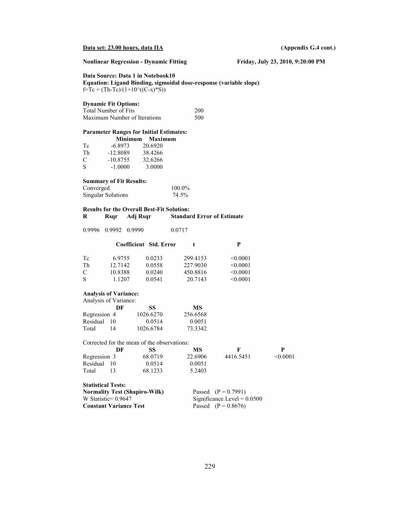
229

Data set: 23.00 hours, data IIA (Appendix G.4 cont.)

Nonlinear Regression - Dynamic Fitting Friday, July 23, 2010, 9:20:00 PM

Data Source: Data 1 in Notebook10

Equation: Ligand Binding, sigmoidal dose-response (variable slope) f=Tc + (Th-Tc)/(1+10^((C-x)*S))

Dynamic Fit Options: Total Number of Fits 200

Maximum Number of Iterations 500

Parameter Ranges for Initial Estimates:

Minimum Maximum Tc -6.8973 20.6920

Th -12.8089 38.4266

C -10.8755 32.6266

S -1.0000 3.0000

Summary of Fit Results:

Converged 100.0%

Singular Solutions 74.5%

Results for the Overall Best-Fit Solution:

R Rsqr Adj Rsqr Standard Error of Estimate

0.9996 0.9992 0.9990 0.0717

Coefficient Std. Error t P

Tc 6.9755 0.0233 299.4153 <0.0001

Th 12.7142 0.0558 227.9030 <0.0001

C 10.8388 0.0240 450.8816 <0.0001

S 1.1207 0.0541 20.7143 <0.0001

Analysis of Variance: Analysis of Variance:

DF SS MS Regression 4 1026.6270 256.6568

Residual 10 0.0514 0.0051

Total 14 1026.6784 73.3342

Corrected for the mean of the observations:

DF SS MS F P

Regression 3 68.0719 22.6906 4416.5451 <0.0001

Residual 10 0.0514 0.0051

Total 13 68.1233 5.2403

Statistical Tests: Normality Test (Shapiro-Wilk) Passed (P = 0.7991)

W Statistic= 0.9647 Significance Level = 0.0500

Constant Variance Test Passed (P = 0.8676)

230

Data set: 00.00 hours, data IIA (Appendix G.4 cont.)

Nonlinear Regression - Dynamic Fitting Friday, July 23, 2010, 9:20:22 PM

Data Source: Data 1 in Notebook10

Equation: Ligand Binding, sigmoidal dose-response (variable slope) f=Tc + (Th-Tc)/(1+10^((C-x)*S))

Dynamic Fit Options: Total Number of Fits 200

Maximum Number of Iterations 500

Parameter Ranges for Initial Estimates:

Minimum Maximum Tc -6.8509 20.5528

Th -12.5151 37.5453

C -12.1240 36.3719

S -1.0000 3.0000

Summary of Fit Results:

Converged 99.0%

Singular Solutions 80.0%

Ill-Conditioned Solutions 0.5%

Iterations Exceeding 500 1.0%

Results for the Overall Best-Fit Solution:

R Rsqr Adj Rsqr Standard Error of Estimate

0.9994 0.9989 0.9985 0.0675

Coefficient Std. Error t P

Tc 6.9431 0.0206 337.1417 <0.0001

Th 12.6413 0.0822 153.8631 <0.0001

C 12.2021 0.0233 524.2921 <0.0001

S 1.2635 0.0619 20.4007 <0.0001

Analysis of Variance: Analysis of Variance:

DF SS MS Regression 4 866.3026 216.5757

Residual 10 0.0455 0.0046

Total 14 866.3481 61.8820

Corrected for the mean of the observations:

DF SS MS F P

Regression 3 40.2662 13.4221 2949.2537 <0.0001

Residual 10 0.0455 0.0046

Total 13 40.3117 3.1009

Statistical Tests: Normality Test (Shapiro-Wilk) Passed (P = 0.8014)

W Statistic= 0.9649 Significance Level = 0.0500

Constant Variance Test Passed (P = 0.2064)

231

G.5 June 22, 2008

Result Summary of SIGMAPLOT Analysis Data (IIB):

Charging Hour Tc (oC) Th (

oC) C S R

2 Remarks

19:00 7.59 13.97 2.83 1.17 0.9994 Passed

20:00 7.31 13.86 3.86 1.17 0.9974 Passed

21:00 7.21 13.76 4.95 1.33 0.9934 Passed

22:00 7.10 13.69 6.08 1.32 0.9959 Passed

23:00 7.03 13.65 7.27 1.26 0.9979 Passed

0:00 6.97 13.61 8.45 1.25 0.9989 Passed

1:00 6.93 13.55 9.63 1.30 0.9992 Passed

2:00 6.90 13.46 10.79 1.19 0.9994 Passed

3:00 6.88 13.48 12.13 1.23 0.9974 Passed

4:00 - - - - - In-convergence

5:00 - - - - - In-convergence

6:00 - - - - - In-convergence

Result of SIGMAPLOT processing: June 22, 2008 (Data IIB)

Data set: 19.00 hours, data IIB

Nonlinear Regression - Dynamic Fitting Friday, July 23, 2010, 10:21:02 PM

Data Source: Data 1 in June22_DATA.JNB

Equation: Ligand Binding, sigmoidal dose-response (variable slope)

f=Tc + (Th-Tc)/(1+10^((C-x)*S))

Dynamic Fit Options: Total Number of Fits 200

Maximum Number of Iterations 500

Parameter Ranges for Initial Estimates:

Minimum Maximum Tc -7.5609 22.6827

Th -14.8668 44.6005

C -2.9831 8.9493

S -1.0000 3.0000

Summary of Fit Results:

Converged 100.0%

Singular Solutions 53.0%

Ill-Conditioned Solutions 0.5%

Results for the Overall Best-Fit Solution:

R Rsqr Adj Rsqr Standard Error of Estimate

0.9866 0.9994 0.9654 0.4581

Coefficient Std. Error t P

Tc 7.5888 0.3682 20.6114 <0.0001

Th 13.9653 0.1473 94.7931 <0.0001

C 2.8326 0.1310 21.6250 <0.0001

S 1.1682 0.3147 3.7121 0.0040

232

Analysis of Variance: (Appendix G.5 cont.) Analysis of Variance:

DF SS MS Regression 4 2327.1084 581.7771

Residual 10 2.0990 0.2099

Total 14 2329.2073 166.3720

Corrected for the mean of the observations:

DF SS MS F P Regression 3 76.7136 25.5712 121.8271 <0.0001

Residual 10 2.0990 0.2099

Total 13 78.8126 6.0625

Statistical Tests: Normality Test (Shapiro-Wilk) Passed (P = 0.6042)

W Statistic= 0.9528 Significance Level = 0.0500

Constant Variance Test Passed (P = 0.0941)

233

Data set: 20.00 hours, data IIB (Appendix G.5 cont.)

Nonlinear Regression - Dynamic Fitting Friday, July 23, 2010, 10:21:21 PM

Data Source: Data 1 in June22_DATA.JNB

Equation: Ligand Binding, sigmoidal dose-response (variable slope) f=Tc + (Th-Tc)/(1+10^((C-x)*S))

Dynamic Fit Options: Total Number of Fits 200

Maximum Number of Iterations 500

Parameter Ranges for Initial Estimates:

Minimum Maximum Tc -7.2990 21.8970

Th -14.5953 43.7859

C -3.9824 11.9472

S -1.0000 3.0000

Summary of Fit Results:

Converged 100.0%

Singular Solutions 56.0%

Ill-Conditioned Solutions 0.5%

Results for the Overall Best-Fit Solution:

R Rsqr Adj Rsqr Standard Error of Estimate 0.9937 0.9974 0.9836 0.3645

Coefficient Std. Error t P

Tc 7.3097 0.2277 32.0997 <0.0001

Th 13.8565 0.1238 111.9582 <0.0001

C 3.8590 0.0983 39.2575 <0.0001

S 1.1692 0.2319 5.0424 0.0005

Analysis of Variance: Analysis of Variance:

DF SS MS Regression 4 2138.5889 534.6472

Residual 10 1.3283 0.1328

Total 14 2139.9172 152.8512

Corrected for the mean of the observations:

DF SS MS F P

Regression 3 103.9228 34.6409 260.7967 <0.0001

Residual 10 1.3283 0.1328

Total 13 105.2510 8.0962

Statistical Tests: Normality Test (Shapiro-Wilk) Passed (P = 0.2474)

W Statistic= 0.9236 Significance Level = 0.0500

Constant Variance Test Passed (P = 0.0907)

234

Data set: 21.00 hours, data IIB (Appendix G.5 cont.)

Nonlinear Regression - Dynamic Fitting Friday, July 23, 2010, 10:21:37 PM

Data Source: Data 1 in June22_DATA.JNB

Equation: Ligand Binding, sigmoidal dose-response (variable slope) f=Tc + (Th-Tc)/(1+10^((C-x)*S))

Dynamic Fit Options: Total Number of Fits 200

Maximum Number of Iterations 500

Parameter Ranges for Initial Estimates:

Minimum Maximum Tc -7.1540 21.4621

Th -14.2428 42.7283

C -5.0182 15.0545

S -1.0000 3.0000

Summary of Fit Results:

Converged 100.0%

Singular Solutions 58.5%

Results for the Overall Best-Fit Solution:

R Rsqr Adj Rsqr Standard Error of Estimate 0.9967 0.9934 0.9914 0.2865

Coefficient Std. Error t P

Tc 7.2117 0.1480 48.7298 <0.0001

Th 13.7567 0.1028 133.8562 <0.0001

C 4.9539 0.0758 65.3563 <0.0001

S 1.3311 0.1951 6.8223 <0.0001

Analysis of Variance:

Analysis of Variance:

DF SS MS

Regression 4 1957.2087 489.3022

Residual 10 0.8205 0.0821

Total 14 1958.0292 139.8592

Corrected for the mean of the observations:

DF SS MS F P Regression 3 123.5860 41.1953 502.0490 <0.0001

Residual 10 0.8205 0.0821

Total 13 124.4066 9.5697

Statistical Tests: Normality Test (Shapiro-Wilk) Passed (P = 0.5579)

W Statistic= 0.9498 Significance Level = 0.0500

Constant Variance Test Passed (P = 0.0276)

235

Data set: 22.00 hours, data IIB (Appendix G.5 cont.)

Nonlinear Regression - Dynamic Fitting Friday, July 23, 2010, 10:21:54 PM

Data Source: Data 1 in June22_DATA.JNB

Equation: Ligand Binding, sigmoidal dose-response (variable slope) f=Tc + (Th-Tc)/(1+10^((C-x)*S))

Dynamic Fit Options: Total Number of Fits 200

Maximum Number of Iterations 500

Parameter Ranges for Initial Estimates:

Minimum Maximum Tc -7.0348 21.1045

Th -14.0339 42.1017

C -6.0882 18.2646

S -1.0000 3.0000

Summary of Fit Results:

Converged 100.0%

Singular Solutions 61.5%

Results for the Overall Best-Fit Solution:

R Rsqr Adj Rsqr Standard Error of Estimate 0.9980 0.9959 0.9947 0.2354

Coefficient Std. Error t P

Tc 7.1042 0.1078 65.9091 <0.0001

Th 13.6880 0.0907 150.9397 <0.0001

C 6.0811 0.0617 98.6205 <0.0001

S 1.3225 0.1599 8.2713 <0.0001

Analysis of Variance:

Analysis of Variance:

DF SS MS

Regression 4 1778.6205 444.6551

Residual 10 0.5539 0.0554

Total 14 1779.1744 127.0839

Corrected for the mean of the observations:

DF SS MS F P Regression 3 135.2982 45.0994 814.1903 <0.0001

Residual 10 0.5539 0.0554

Total 13 135.8521 10.4502

Statistical Tests: Normality Test (Shapiro-Wilk) Passed (P = 0.7448)

W Statistic= 0.9613 Significance Level = 0.0500

Constant Variance Test Passed (P = 0.0021)

236

Data set: 23.00 hours, data IIB (Appendix G.5 cont.)

Nonlinear Regression - Dynamic Fitting Friday, July 23, 2010, 10:22:13 PM

Data Source: Data 1 in June22_DATA.JNB

Equation: Ligand Binding, sigmoidal dose-response (variable slope) f=Tc + (Th-Tc)/(1+10^((C-x)*S))

Dynamic Fit Options: Total Number of Fits 200

Maximum Number of Iterations 500

Parameter Ranges for Initial Estimates:

Minimum Maximum Tc -6.9511 20.8533

Th -13.9287 41.7860

C -7.2356 21.7069

S -1.0000 3.0000

Summary of Fit Results:

Converged 100.0%

Singular Solutions 66.0%

Results for the Overall Best-Fit Solution:

R Rsqr Adj Rsqr Standard Error of Estimate 0.9990 0.9979 0.9973 0.1690

Coefficient Std. Error t P

Tc 7.0262 0.0702 100.0643 <0.0001

Th 13.6541 0.0716 190.8154 <0.0001

C 7.2703 0.0416 174.9612 <0.0001

S 1.2645 0.1353 9.3425 <0.0001

Analysis of Variance:

Analysis of Variance:

DF SS MS

Regression 4 1600.5018 400.1255

Residual 10 0.2856 0.0286

Total 14 1600.7874 114.3420

Corrected for the mean of the observations:

DF SS MS F P Regression 3 138.4284 46.1428 1615.8644 <0.0001

Residual 10 0.2856 0.0286

Total 13 138.7140 10.6703

Statistical Tests: Normality Test (Shapiro-Wilk) Passed (P = 0.8717)

W Statistic= 0.9696 Significance Level = 0.0500

Constant Variance Test Passed (P = <0.0001)

237

Data set: 00.00 hours, data IIB (Appendix G.5 cont.)

Nonlinear Regression - Dynamic Fitting Friday, July 23, 2010, 10:22:55 PM

Data Source: Data 1 in June22_DATA.JNB

Equation: Ligand Binding, sigmoidal dose-response (variable slope) f=Tc + (Th-Tc)/(1+10^((C-x)*S))

Dynamic Fit Options: Total Number of Fits 200

Maximum Number of Iterations 500

Parameter Ranges for Initial Estimates:

Minimum Maximum Tc -6.8984 20.6952

Th -13.8664 41.5993

C -8.4382 25.3147

S -1.0000 3.0000

Summary of Fit Results:

Converged 99.5%

Singular Solutions 66.0%

Ill-Conditioned Solutions 0.5%

Iterations Exceeding 500 0.5%

Results for the Overall Best-Fit Solution:

R Rsqr Adj Rsqr Standard Error of Estimate 0.9994 0.9989 0.9986 0.1213

Coefficient Std. Error t P

Tc 6.9700 0.0459 151.8796 <0.0001

Th 13.6089 0.0587 231.9354 <0.0001

C 8.4475 0.0266 317.1781 <0.0001

S 1.2528 0.1192 10.5136 <0.0001

Analysis of Variance:

Analysis of Variance:

DF SS MS

Regression 4 1424.6394 356.1598

Residual 10 0.1470 0.0147

Total 14 1424.7864 101.7705

Corrected for the mean of the observations:

DF SS MS F P Regression 3 132.0835 44.0278 2994.2366 <0.0001

Residual 10 0.1470 0.0147

Total 13 132.2305 10.1716

Statistical Tests: Normality Test (Shapiro-Wilk) Passed (P = 0.3730)

W Statistic= 0.9363 Significance Level = 0.0500

Constant Variance Test Passed (P = 0.0131)

238

Data set: 01.00 hours, data IIB (Appendix G.5 cont.)

Nonlinear Regression - Dynamic Fitting Friday, July 23, 2010, 10:23:11 PM

Data Source: Data 1 in June22_DATA.JNB

Equation: Ligand Binding, sigmoidal dose-response (variable slope) f=Tc + (Th-Tc)/(1+10^((C-x)*S))

Dynamic Fit Options: Total Number of Fits 200

Maximum Number of Iterations 500

Parameter Ranges for Initial Estimates:

Minimum Maximum Tc -6.8580 20.5741

Th -13.7175 41.1526

C -9.6937 29.0812

S -1.0000 3.0000

Summary of Fit Results:

Converged 99.5%

Singular Solutions 70.5%

Iterations Exceeding 500 0.5%

Results for the Overall Best-Fit Solution:

R Rsqr Adj Rsqr Standard Error of Estimate 0.9996 0.9992 0.9989 0.0976

Coefficient Std. Error t P

Tc 6.9349 0.0336 206.1837 <0.0001

Th 13.5477 0.0570 237.8016 <0.0001

C 9.6271 0.0227 424.6704 <0.0001

S 1.3004 0.1039 12.5118 <0.0001

Analysis of Variance: Analysis of Variance:

DF SS MS Regression 4 1251.4363 312.8591

Residual 10 0.0952 0.0095

Total 14 1251.5314 89.3951

Corrected for the mean of the observations:

DF SS MS F P

Regression 3 116.6008 38.8669 4084.2659 <0.0001

Residual 10 0.0952 0.0095

Total 13 116.6959 8.9766

Statistical Tests: Normality Test (Shapiro-Wilk) Passed (P = 0.9846)

W Statistic= 0.9820 Significance Level = 0.0500

Constant Variance Test Passed (P = 0.0977)

239

Data set: 02.00 hours, data IIB (Appendix G.5 cont.)

Nonlinear Regression - Dynamic Fitting Friday, July 23, 2010, 10:23:33 PM

Data Source: Data 1 in June22_DATA.JNB

Equation: Ligand Binding, sigmoidal dose-response (variable slope) f=Tc + (Th-Tc)/(1+10^((C-x)*S))

Dynamic Fit Options: Total Number of Fits 200

Maximum Number of Iterations 500

Parameter Ranges for Initial Estimates:

Minimum Maximum Tc -6.8115 20.4346

Th -13.4818 40.4454

C -10.8322 32.4965

S -1.0000 3.0000

Summary of Fit Results:

Converged 100.0%

Singular Solutions 73.5%

Ill-Conditioned Solutions 0.5%

Results for the Overall Best-Fit Solution:

R Rsqr Adj Rsqr Standard Error of Estimate 0.9997 0.9994 0.9992 0.0725

Coefficient Std. Error t P

Tc 6.8973 0.0235 293.3831 <0.0001

Th 13.4617 0.0552 243.8163 <0.0001

C 10.7925 0.0206 523.8101 <0.0001

S 1.1850 0.0544 21.7851 <0.0001

Analysis of Variance: Analysis of Variance:

DF SS MS Regression 4 1079.8695 269.9674

Residual 10 0.0526 0.0053

Total 14 1079.9220 77.1373

Corrected for the mean of the observations:

DF SS MS F P

Regression 3 90.9826 30.3275 5769.7938 <0.0001

Residual 10 0.0526 0.0053

Total 13 91.0352 7.0027

Statistical Tests: Normality Test (Shapiro-Wilk) Passed (P = 0.4298)

W Statistic= 0.9409 Significance Level = 0.0500

Constant Variance Test Passed (P = 0.6704)

240

Data set: 03.00 hours, data IIB (Appendix G.5 cont.)

Nonlinear Regression - Dynamic Fitting Friday, July 23, 2010, 10:23:54 PM

Data Source: Data 1 in June22_DATA.JNB

Equation: Ligand Binding, sigmoidal dose-response (variable slope) f=Tc + (Th-Tc)/(1+10^((C-x)*S))

Dynamic Fit Options: Total Number of Fits 200

Maximum Number of Iterations 500

Parameter Ranges for Initial Estimates:

Minimum Maximum Tc -6.7449 20.2347

Th -13.3459 40.0376

C -12.0684 36.2053

S -1.0000 3.0000

Summary of Fit Results:

Converged 99.5%

Singular Solutions 79.0%

Iterations Exceeding 500 0.5%

Results for the Overall Best-Fit Solution:

R Rsqr Adj Rsqr Standard Error of Estimate 0.9987 0.9974 0.9966 0.1215

Coefficient Std. Error t P

Tc 6.8752 0.0372 185.0389 <0.0001

Th 13.4839 0.1470 91.7554 <0.0001

C 12.1302 0.0380 319.2754 <0.0001

S 1.2332 0.0874 14.1054 <0.0001

Analysis of Variance: Analysis of Variance:

DF SS MS Regression 4 900.2102 225.0525

Residual 10 0.1477 0.0148

Total 14 900.3579 64.3113

Corrected for the mean of the observations:

DF SS MS F P

Regression 3 56.1792 18.7264 1267.9922 <0.0001

Residual 10 0.1477 0.0148

Total 13 56.3269 4.3328

Statistical Tests: Normality Test (Shapiro-Wilk) Passed (P = 0.0315)

W Statistic= 0.8611 Significance Level = 0.0500

Constant Variance Test Passed (P = 0.5520)

241

G.6 June 24, 2008

Result Summary of SIGMAPLOT Analysis Data (IIC):

Charging Hour Tc (oC) Th (

oC) C S R

2 Remarks

19:00 7.52 14.29 2.93 1.43 0.9942 Passed

20:00 7.30 14.25 4.01 1.36 0.9951 Passed

21:00 7.18 14.18 5.10 1.49 0.9968 Passed

22:00 7.05 14.14 6.18 1.31 0.9922 Passed

23:00 6.98 14.09 7.27 1.30 0.9949 Passed

0:00 6.94 14.00 8.36 1.37 0.9964 Passed

1:00 6.90 13.90 9.44 1.20 0.9986 Passed

2:00 6.87 13.77 10.52 1.25 0.9993 Passed

3:00 6.86 13.75 11.79 1.33 0.9968 Passed

4:00 - - - - - In-convergence

5:00 - - - - - In-convergence

6:00 - - - - - In-convergence

Result of SIGMAPLOT processing: June 24, 2008 (Data IIC)

Data set: 19.00 hours, data IIC

Nonlinear Regression - Dynamic Fitting Saturday, August 28, 2010, 6:10:48 PM

Data Source: Data 1 in Notebook1

Equation: Ligand Binding, sigmoidal dose-response (variable slope)

f=Tc + (Th-Tc)/(1+10^((C-x)*S))

Dynamic Fit Options:

Total Number of Fits 200

Maximum Number of Iterations 500

Parameter Ranges for Initial Estimates:

Minimum Maximum

Tc -7.4443 22.3328

Th -14.6580 43.9740

C -2.9869 8.9606

S -1.0000 3.0000

Summary of Fit Results: Converged 100.0%

Singular Solutions 55.0%

Results for the Overall Best-Fit Solution:

R Rsqr Adj Rsqr Standard Error of Estimate 0.9921 0.9842 0.9794 0.3867

Coefficient Std. Error t P

Tc 7.5210 0.2880 26.1163 <0.0001

Th 14.2918 0.1234 115.8335 <0.0001

C 2.9331 0.1033 28.4004 <0.0001

S 1.4334 0.2893 4.9547 0.0006

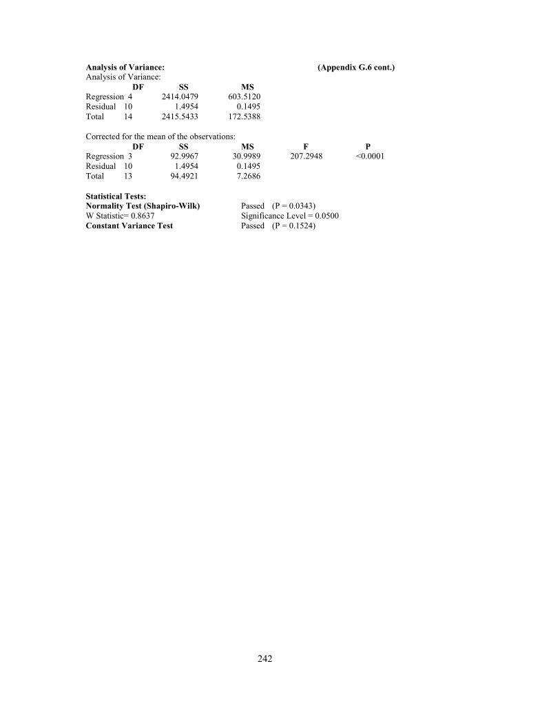
242

Analysis of Variance: (Appendix G.6 cont.) Analysis of Variance:

DF SS MS Regression 4 2414.0479 603.5120

Residual 10 1.4954 0.1495

Total 14 2415.5433 172.5388

Corrected for the mean of the observations:

DF SS MS F P Regression 3 92.9967 30.9989 207.2948 <0.0001

Residual 10 1.4954 0.1495

Total 13 94.4921 7.2686

Statistical Tests: Normality Test (Shapiro-Wilk) Passed (P = 0.0343)

W Statistic= 0.8637 Significance Level = 0.0500

Constant Variance Test Passed (P = 0.1524)

243

Data set: 20.00 hours, data IIC (Appendix G.6 cont.)

Nonlinear Regression - Dynamic Fitting Saturday, August 28, 2010, 6:11:08 PM

Data Source: Data 1 in Notebook1

Equation: Ligand Binding, sigmoidal dose-response (variable slope) f=Tc + (Th-Tc)/(1+10^((C-x)*S))

Dynamic Fit Options:

Total Number of Fits 200

Maximum Number of Iterations 500

Parameter Ranges for Initial Estimates:

Minimum Maximum Tc -7.2616 21.7848

Th -14.6206 43.8617

C -4.0404 12.1212

S -1.0000 3.0000

Summary of Fit Results: Converged 100.0%

Singular Solutions 54.5%

Results for the Overall Best-Fit Solution:

R Rsqr Adj Rsqr Standard Error of Estimate 0.9940 0.9881 0.9845 0.3854

Coefficient Std. Error t P

Tc 7.3021 0.2312 31.5889 <0.0001

Th 14.2510 0.1301 109.5615 <0.0001

C 4.0090 0.0983 40.7975 <0.0001

S 1.3640 0.2540 5.3704 0.0003

Analysis of Variance: Analysis of Variance:

DF SS MS Regression 4 2229.6780 557.4195

Residual 10 1.4851 0.1485

Total 14 2231.1630 159.3688

Corrected for the mean of the observations:

DF SS MS F P

Regression 3 123.2878 41.0959 276.7277 <0.0001

Residual 10 1.4851 0.1485

Total 13 124.7729 9.5979

Statistical Tests: Normality Test (Shapiro-Wilk) Passed (P = 0.0210)

W Statistic= 0.8482 Significance Level = 0.0500

Constant Variance Test Passed (P = 0.0778)

244

Data set: 21.00 hours, data IIC (Appendix G.6 cont.)

Nonlinear Regression - Dynamic Fitting Saturday, August 28, 2010, 6:11:32 PM

Data Source: Data 1 in Notebook1

Equation: Ligand Binding, sigmoidal dose-response (variable slope) f=Tc + (Th-Tc)/(1+10^((C-x)*S))

Dynamic Fit Options:

Total Number of Fits 200

Maximum Number of Iterations 500

Parameter Ranges for Initial Estimates:

Minimum Maximum Tc -7.1160 21.3479

Th -14.5652 43.6955

C -5.1016 15.3047

S -1.0000 3.0000

Summary of Fit Results: Converged 100.0%

Singular Solutions 59.5%

Results for the Overall Best-Fit Solution:

R Rsqr Adj Rsqr Standard Error of Estimate 0.9949 0.9898 0.9868 0.3861

Coefficient Std. Error t P

Tc 7.1800 0.1968 36.4929 <0.0001

Th 14.1823 0.1380 102.7524 <0.0001

C 5.1043 0.0969 52.6635 <0.0001

S 1.4875 0.2968 5.0119 0.0005

Analysis of Variance:

Analysis of Variance:

DF SS MS

Regression 4 2041.3813 510.3453

Residual 10 1.4906 0.1491

Total 14 2042.8719 145.9194

Corrected for the mean of the observations:

DF SS MS F P Regression 3 145.3496 48.4499 325.0388 <0.0001

Residual 10 1.4906 0.1491

Total 13 146.8402 11.2954

Statistical Tests:

Normality Test (Shapiro-Wilk) Passed (P = 0.0781)

W Statistic= 0.8890 Significance Level = 0.0500

Constant Variance Test Passed (P = 0.0108)

245

Data set: 22.00 hours, data IIC (Appendix G.6 cont.)

Nonlinear Regression - Dynamic Fitting Saturday, August 28, 2010, 6:11:55 PM

Data Source: Data 1 in Notebook1

Equation: Ligand Binding, sigmoidal dose-response (variable slope) f=Tc + (Th-Tc)/(1+10^((C-x)*S))

Dynamic Fit Options:

Total Number of Fits 200

Maximum Number of Iterations 500

Parameter Ranges for Initial Estimates:

Minimum Maximum Tc -6.9916 20.9748

Th -14.5542 43.6625

C -6.1690 18.5069

S -1.0000 3.0000

Summary of Fit Results: Converged 100.0%

Singular Solutions 62.0%

Results for the Overall Best-Fit Solution:

R Rsqr Adj Rsqr Standard Error of Estimate 0.9961 0.9922 0.9899 0.3517

Coefficient Std. Error t P

Tc 7.0490 0.1608 43.8350 <0.0001

Th 14.1433 0.1360 103.9868 <0.0001

C 6.1823 0.0841 73.5224 <0.0001

S 1.3129 0.2465 5.3253 0.0003

Analysis of Variance:

Analysis of Variance:

DF SS MS

Regression 4 1856.9392 464.2348

Residual 10 1.2372 0.1237

Total 14 1858.1764 132.7269

Corrected for the mean of the observations:

DF SS MS F P Regression 3 157.3073 52.4358 423.8205 <0.0001

Residual 10 1.2372 0.1237

Total 13 158.5445 12.1957

Statistical Tests: Normality Test (Shapiro-Wilk) Passed (P = 0.2751)

W Statistic= 0.9268 Significance Level = 0.0500

Constant Variance Test Passed (P = <0.0001)

246

Data set: 23.00 hours, data IIC (Appendix G.6 cont.)

Nonlinear Regression - Dynamic Fitting Saturday, August 28, 2010, 6:12:14 PM

Data Source: Data 1 in Notebook1

Equation: Ligand Binding, sigmoidal dose-response (variable slope) f=Tc + (Th-Tc)/(1+10^((C-x)*S))

Dynamic Fit Options: Total Number of Fits 200

Maximum Number of Iterations 500

Parameter Ranges for Initial Estimates:

Minimum Maximum Tc -6.9145 20.7436

Th -14.5437 43.6312

C -7.2512 21.7535

S -1.0000 3.0000

Summary of Fit Results:

Converged 100.0%

Singular Solutions 65.0%

Results for the Overall Best-Fit Solution:

R Rsqr Adj Rsqr Standard Error of Estimate 0.9974 0.9949 0.9934 0.2863

Coefficient Std. Error t P

Tc 6.9821 0.1188 58.7897 <0.0001

Th 14.0942 0.1209 116.6257 <0.0001

C 7.2708 0.0653 111.4152 <0.0001

S 1.3007 0.2253 5.7723 0.0002

Analysis of Variance:

Analysis of Variance:

DF SS MS

Regression 4 1676.6193 419.1548

Residual 10 0.8197 0.0820

Total 14 1677.4390 119.8171

Corrected for the mean of the observations:

DF SS MS F P Regression 3 159.8737 53.2912 650.1260 <0.0001

Residual 10 0.8197 0.0820

Total 13 160.6934 12.3610

Statistical Tests: Normality Test (Shapiro-Wilk) Passed (P = 0.5104)

W Statistic= 0.9467 Significance Level = 0.0500

Constant Variance Test Passed (P = <0.0001)

247

Data set: 00.00 hours, data IIC (Appendix G.6 cont.)

Nonlinear Regression - Dynamic Fitting Saturday, August 28, 2010, 6:12:30 PM

Data Source: Data 1 in Notebook1

Equation: Ligand Binding, sigmoidal dose-response (variable slope) f=Tc + (Th-Tc)/(1+10^((C-x)*S))

Dynamic Fit Options:

Total Number of Fits 200

Maximum Number of Iterations 500

Parameter Ranges for Initial Estimates:

Minimum Maximum Tc -6.8560 20.5681

Th -14.5254 43.5761

C -8.3495 25.0486

S -1.0000 3.0000

Summary of Fit Results: Converged 99.5%

Singular Solutions 69.0%

Iterations Exceeding 500 0.5%

Results for the Overall Best-Fit Solution:

R Rsqr Adj Rsqr Standard Error of Estimate 0.9982 0.9964 0.9953 0.2355

Coefficient Std. Error t P

Tc 6.9437 0.0896 77.5170 <0.0001

Th 14.0013 0.1102 127.0042 <0.0001

C 8.3607 0.0496 168.6173 <0.0001

S 1.3722 0.2447 5.6067 0.0002

Analysis of Variance: Analysis of Variance:

DF SS MS Regression 4 1494.8138 373.7035

Residual 10 0.5544 0.0554

Total 14 1495.3682 106.8120

Corrected for the mean of the observations:

DF SS MS F P

Regression 3 151.6885 50.5628 911.9806 <0.0001

Residual 10 0.5544 0.0554

Total 13 152.2429 11.7110

Statistical Tests: Normality Test (Shapiro-Wilk) Passed (P = 0.2699)

W Statistic= 0.9262 Significance Level = 0.0500

Constant Variance Test Passed (P = 0.0016)

248

Data set: 01.00 hours, data IIC (Appendix G.6 cont.)

Nonlinear Regression - Dynamic Fitting Saturday, August 28, 2010, 6:12:46 PM

Data Source: Data 1 in Notebook1

Equation: Ligand Binding, sigmoidal dose-response (variable slope) f=Tc + (Th-Tc)/(1+10^((C-x)*S))

Dynamic Fit Options:

Total Number of Fits 200

Maximum Number of Iterations 500

Parameter Ranges for Initial Estimates:

Minimum Maximum Tc -6.8270 20.4809

Th -14.2113 42.6338

C -9.4411 28.3234

S -1.0000 3.0000

Summary of Fit Results: Converged 100.0%

Singular Solutions 68.5%

Results for the Overall Best-Fit Solution:

R Rsqr Adj Rsqr Standard Error of Estimate 0.9993 0.9986 0.9982 0.1355

Coefficient Std. Error t P

Tc 6.8955 0.0482 143.1821 <0.0001

Th 13.9011 0.0752 184.8131 <0.0001

C 9.4354 0.0295 319.4640 <0.0001

S 1.2002 0.1137 10.5570 <0.0001

Analysis of Variance:

Analysis of Variance:

DF SS MS

Regression 4 1314.2690 328.5672

Residual 10 0.1836 0.0184

Total 14 1314.4526 93.8895

Corrected for the mean of the observations:

DF SS MS F P Regression 3 133.0627 44.3542 2416.1200 <0.0001

Residual 10 0.1836 0.0184

Total 13 133.2463 10.2497

Statistical Tests: Normality Test (Shapiro-Wilk) Passed (P = 0.0951)

W Statistic= 0.8949 Significance Level = 0.0500

Constant Variance Test Passed (P = 0.4254)

249

Data set: 02.00 hours, data IIC (Appendix G.6 cont.)

Nonlinear Regression - Dynamic Fitting Saturday, August 28, 2010, 6:13:17 PM

Data Source: Data 1 in Notebook1

Equation: Ligand Binding, sigmoidal dose-response (variable slope) f=Tc + (Th-Tc)/(1+10^((C-x)*S))

Dynamic Fit Options:

Total Number of Fits 200

Maximum Number of Iterations 500

Parameter Ranges for Initial Estimates:

Minimum Maximum Tc -6.7687 20.3061

Th -13.7930 41.3791

C -10.5286 31.5857

S -1.0000 3.0000

Summary of Fit Results: Converged 100.0%

Singular Solutions 72.5%

Results for the Overall Best-Fit Solution:

R Rsqr Adj Rsqr Standard Error of Estimate 0.9996 0.9993 0.9991 0.0877

Coefficient Std. Error t P

Tc 6.8694 0.0291 236.2324 <0.0001

Th 13.7730 0.0605 227.8397 <0.0001

C 10.5222 0.0191 551.3108 <0.0001

S 1.2516 0.0889 14.0771 <0.0001

Analysis of Variance:

Analysis of Variance:

DF SS MS Regression 4 1140.6142 285.1535

Residual 10 0.0770 0.0077

Total 14 1140.6911 81.4779

Corrected for the mean of the observations:

DF SS MS F P

Regression 3 107.7928 35.9309 4669.2430 <0.0001

Residual 10 0.0770 0.0077

Total 13 107.8697 8.2977

Statistical Tests: Normality Test (Shapiro-Wilk) Passed (P = 0.7553)

W Statistic= 0.9620 Significance Level = 0.0500

Constant Variance Test Passed (P = 0.5114)

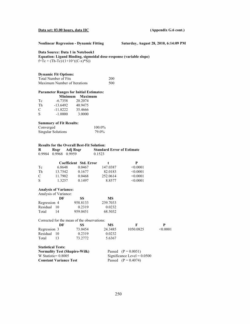
250

Data set: 03.00 hours, data IIC (Appendix G.6 cont.)

Nonlinear Regression - Dynamic Fitting Saturday, August 28, 2010, 6:14:09 PM

Data Source: Data 1 in Notebook1

Equation: Ligand Binding, sigmoidal dose-response (variable slope)

f=Tc + (Th-Tc)/(1+10^((C-x)*S))

Dynamic Fit Options: Total Number of Fits 200

Maximum Number of Iterations 500

Parameter Ranges for Initial Estimates:

Minimum Maximum Tc -6.7358 20.2074

Th -13.6492 40.9475

C -11.8222 35.4666

S -1.0000 3.0000

Summary of Fit Results:

Converged 100.0%

Singular Solutions 79.0%

Results for the Overall Best-Fit Solution:

R Rsqr Adj Rsqr Standard Error of Estimate 0.9984 0.9968 0.9959 0.1523

Coefficient Std. Error t P Tc 6.8648 0.0467 147.0387 <0.0001

Th 13.7542 0.1677 82.0183 <0.0001

C 11.7902 0.0468 252.0614 <0.0001

S 1.3257 0.1497 8.8577 <0.0001

Analysis of Variance:

Analysis of Variance:

DF SS MS

Regression 4 958.8133 239.7033

Residual 10 0.2319 0.0232

Total 14 959.0451 68.5032

Corrected for the mean of the observations:

DF SS MS F P Regression 3 73.0454 24.3485 1050.0825 <0.0001

Residual 10 0.2319 0.0232

Total 13 73.2772 5.6367

Statistical Tests: Normality Test (Shapiro-Wilk) Passed (P = 0.0051)

W Statistic= 0.8005 Significance Level = 0.0500

Constant Variance Test Passed (P = 0.4074)

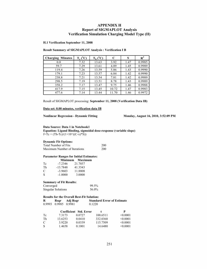
251

APPENDIX H

Report of SIGMAPLOT Analysis

Verification Simulation Charging Model Type (II)

H.1 Verification September 11, 2008

Result Summary of SIGMAPLOT Analysis : Verification I B

Charging Minutes Tc (oC) Th (

oC) C S R

2

0.0 7.32 13.63 3.92 1.47 0.9985

59.7 7.29 13.61 4.89 1.45 0.9989

119.4 7.26 13.59 5.86 1.43 0.9990

179.1 7.23 13.57 6.84 1.42 0.9990

238.8 7.21 13.54 7.81 1.42 0.9989

298.5 7.19 13.51 8.78 1.43 0.9989

358.2 7.17 13.47 9.75 1.46 0.9988

417.9 7.15 13.45 10.72 1.47 0.9983

477.6 7.14 13.44 11.70 1.46 0.9972 Result of SIGMAPLOT processing: September 11, 2008 (Verification Data IB)

Data set: 0.00 minutes, verification data IB

Nonlinear Regression - Dynamic Fitting Monday, August 16, 2010, 3:52:09 PM

Data Source: Data 1 in Notebook1

Equation: Ligand Binding, sigmoidal dose-response (variable slope) f=Tc + (Th-Tc)/(1+10^((C-x)*S))

Dynamic Fit Options:

Total Number of Fits 200

Maximum Number of Iterations 200

Parameter Ranges for Initial Estimates:

Minimum Maximum

Tc -7.2346 21.7037

Th -13.7848 41.3543

C -3.9603 11.8808

S -1.0000 3.0000

Summary of Fit Results: Converged 99.5%

Singular Solutions 56.0%

Results for the Overall Best-Fit Solution:

R Rsqr Adj Rsqr Standard Error of Estimate 0.9993 0.9985 0.9981 0.1220

Coefficient Std. Error t P Tc 7.3173 0.0727 100.6511 <0.0001

Th 13.6253 0.0410 332.0368 <0.0001

C 3.9220 0.0339 115.7509 <0.0001

S 1.4658 0.1001 14.6480 <0.0001

252

Analysis of Variance: (Appendix H.1 cont.) Analysis of Variance:

DF SS MS Regression 4 2070.4360 517.6090

Residual 10 0.1489 0.0149

Total 14 2070.5849 147.8989

Corrected for the mean of the observations:

DF SS MS F P Regression 3 101.1509 33.7170 2265.0673 <0.0001

Residual 10 0.1489 0.0149

Total 13 101.2998 7.7923

Statistical Tests: Normality Test (Shapiro-Wilk) Passed (P = 0.3123)

W Statistic= 0.9307 Significance Level = 0.0500

Constant Variance Test Passed (P = 0.2786)

253

Data set: 59.7 minutes, verification data IB (Appendix H.1 cont.)

Nonlinear Regression - Dynamic Fitting Monday, August 16, 2010, 3:52:30 PM

Data Source: Data 1 in Notebook1

Equation: Ligand Binding, sigmoidal dose-response (variable slope)

f=Tc + (Th-Tc)/(1+10^((C-x)*S))

Dynamic Fit Options:

Total Number of Fits 200

Maximum Number of Iterations 200

Parameter Ranges for Initial Estimates:

Minimum Maximum Tc -7.2029 21.6087

Th -13.7256 41.1768

C -4.9348 14.8045

S -1.0000 3.0000

Summary of Fit Results: Converged 100.0%

Singular Solutions 60.0%

Results for the Overall Best-Fit Solution:

R Rsqr Adj Rsqr Standard Error of Estimate 0.9994 0.9989 0.9985 0.1142

Coefficient Std. Error t P

Tc 7.2876 0.0586 124.3915 <0.0001

Th 13.6056 0.0408 333.4838 <0.0001

C 4.8925 0.0311 157.5381 <0.0001

S 1.4480 0.0948 15.2723 <0.0001

Analysis of Variance:

Analysis of Variance:

DF SS MS

Regression 4 1934.7563 483.6891

Residual 10 0.1304 0.0130

Total 14 1934.8868 138.2062

Corrected for the mean of the observations:

DF SS MS F P Regression 3 115.5992 38.5331 2953.9717 <0.0001

Residual 10 0.1304 0.0130

Total 13 115.7297 8.9023

Statistical Tests: Normality Test (Shapiro-Wilk) Passed (P = 0.1901)

W Statistic= 0.9156 Significance Level = 0.0500

Constant Variance Test Passed (P = 0.1251)

254

Data set: 119.4 minutes, verification data IB (Appendix H.1 cont.)

Nonlinear Regression - Dynamic Fitting Monday, August 16, 2010, 3:52:46 PM

Data Source: Data 1 in Notebook1

Equation: Ligand Binding, sigmoidal dose-response (variable slope)

f=Tc + (Th-Tc)/(1+10^((C-x)*S))

Dynamic Fit Options:

Total Number of Fits 200

Maximum Number of Iterations 200

Parameter Ranges for Initial Estimates:

Minimum Maximum Tc -7.1480 21.4440

Th -13.7085 41.1256

C -5.9109 17.7328

S -1.0000 3.0000

Summary of Fit Results: Converged 99.5%

Singular Solutions 63.0%

Iterations Exceeding 200 0.5%

Results for the Overall Best-Fit Solution:

R Rsqr Adj Rsqr Standard Error of Estimate 0.9995 0.9990 0.9986 0.1146

Coefficient Std. Error t P

Tc 7.2554 0.0524 138.4861 <0.0001

Th 13.5888 0.0438 310.0656 <0.0001

C 5.8637 0.0307 190.8044 <0.0001

S 1.4314 0.0974 14.6912 <0.0001

Analysis of Variance:

Analysis of Variance:

DF SS MS

Regression 4 1799.6890 449.9223

Residual 10 0.1313 0.0131

Total 14 1799.8203 128.5586

Corrected for the mean of the observations:

DF SS MS F P

Regression 3 124.9495 41.6498 3172.7174 <0.0001

Residual 10 0.1313 0.0131

Total 13 125.0808 9.6216

Statistical Tests: Normality Test (Shapiro-Wilk) Passed (P = 0.2285)

W Statistic= 0.9212 Significance Level = 0.0500

Constant Variance Test Passed (P = 0.4532)

255

Data set: 179.1 minutes, verification data IB (Appendix H.1 cont.)

Nonlinear Regression - Dynamic Fitting Monday, August 16, 2010, 3:53:00 PM

Data Source: Data 1 in Notebook1

Equation: Ligand Binding, sigmoidal dose-response (variable slope)

f=Tc + (Th-Tc)/(1+10^((C-x)*S))

Dynamic Fit Options: Total Number of Fits 200

Maximum Number of Iterations 200

Parameter Ranges for Initial Estimates:

Minimum Maximum Tc -7.1133 21.3399

Th -13.6944 41.0833

C -6.8891 20.6674

S -1.0000 3.0000

Summary of Fit Results:

Converged 100.0%

Singular Solutions 69.5%

Results for the Overall Best-Fit Solution:

R Rsqr Adj Rsqr Standard Error of Estimate 0.9995 0.9990 0.9987 0.1152

Coefficient Std. Error t P

Tc 7.2295 0.0480 150.6820 <0.0001

Th 13.5692 0.0477 284.5452 <0.0001

C 6.8355 0.0307 222.7768 <0.0001

S 1.4222 0.1021 13.9283 <0.0001

Analysis of Variance:

Analysis of Variance:

DF SS MS

Regression 4 1664.6981 416.1745

Residual 10 0.1327 0.0133

Total 14 1664.8308 118.9165

Corrected for the mean of the observations:

DF SS MS F P Regression 3 128.6467 42.8822 3230.7412 <0.0001

Residual 10 0.1327 0.0133

Total 13 128.7795 9.9061

Statistical Tests: Normality Test (Shapiro-Wilk) Passed (P = 0.3555)

W Statistic= 0.9348 Significance Level = 0.0500

Constant Variance Test Passed (P = 0.5729)

256

Data set: 238.8 minutes, verification data IB (Appendix H.1 cont.)

Nonlinear Regression - Dynamic Fitting Monday, August 16, 2010, 3:53:17 PM

Data Source: Data 1 in Notebook1

Equation: Ligand Binding, sigmoidal dose-response (variable slope)

f=Tc + (Th-Tc)/(1+10^((C-x)*S))

Dynamic Fit Options: Total Number of Fits 200

Maximum Number of Iterations 200

Parameter Ranges for Initial Estimates:

Minimum Maximum Tc -7.0841 21.2523

Th -13.6801 41.0403

C -7.8673 23.6020

S -1.0000 3.0000

Summary of Fit Results:

Converged 100.0%

Singular Solutions 66.0%

Results for the Overall Best-Fit Solution:

R Rsqr Adj Rsqr Standard Error of Estimate

0.9995 0.9989 0.9986 0.1154

Coefficient Std. Error t P Tc 7.2071 0.0444 162.2427 <0.0001

Th 13.5443 0.0524 258.2602 <0.0001

C 7.8070 0.0307 254.3794 <0.0001

S 1.4214 0.1088 13.0628 <0.0001

Analysis of Variance:

Analysis of Variance:

DF SS MS Regression 4 1529.7000 382.4250

Residual 10 0.1332 0.0133

Total 14 1529.8333 109.2738

Corrected for the mean of the observations:

DF SS MS F P

Regression 3 126.6381 42.2127 3168.6396 <0.0001

Residual 10 0.1332 0.0133

Total 13 126.7713 9.7516

Statistical Tests: Normality Test (Shapiro-Wilk) Passed (P = 0.3970)

W Statistic= 0.9383 Significance Level = 0.0500

Constant Variance Test Passed (P = 0.8438)

257

Data set: 298.5 minutes, verification data IB (Appendix H.1 cont.)

Nonlinear Regression - Dynamic Fitting Monday, August 16, 2010, 3:53:32 PM

Data Source: Data 1 in Notebook1

Equation: Ligand Binding, sigmoidal dose-response (variable slope)

f=Tc + (Th-Tc)/(1+10^((C-x)*S))

Dynamic Fit Options: Total Number of Fits 200

Maximum Number of Iterations 200

Parameter Ranges for Initial Estimates:

Minimum Maximum Tc -7.0590 21.1771

Th -13.6357 40.9072

C -8.8417 26.5250

S -1.0000 3.0000

Summary of Fit Results:

Converged 99.5%

Singular Solutions 68.0%

Results for the Overall Best-Fit Solution:

R Rsqr Adj Rsqr Standard Error of Estimate 0.9995 0.9989 0.9986 0.1142

Coefficient Std. Error t P

Tc 7.1876 0.0411 175.0665 <0.0001

Th 13.5104 0.0582 232.3235 <0.0001

C 8.7774 0.0305 287.4509 <0.0001

S 1.4324 0.1181 12.1286 <0.0001

Analysis of Variance:

Analysis of Variance:

DF SS MS

Regression 4 1394.7659 348.6915

Residual 10 0.1305 0.0130

Total 14 1394.8964 99.6355

Corrected for the mean of the observations:

DF SS MS F P Regression 3 118.8691 39.6230 3037.3894 <0.0001

Residual 10 0.1305 0.0130

Total 13 118.9995 9.1538

Statistical Tests: Normality Test (Shapiro-Wilk) Passed (P = 0.3454)

W Statistic= 0.9339 Significance Level = 0.0500

Constant Variance Test Passed (P = 0.6482)

258

Data set: 358.2 minutes, verification data IB (Appendix H.1 cont.)

Nonlinear Regression - Dynamic Fitting Monday, August 16, 2010, 3:53:47 PM

Data Source: Data 1 in Notebook1

Equation: Ligand Binding, sigmoidal dose-response (variable slope)

f=Tc + (Th-Tc)/(1+10^((C-x)*S))

Dynamic Fit Options: Total Number of Fits 200

Maximum Number of Iterations 200

Parameter Ranges for Initial Estimates:

Minimum Maximum Tc -7.0339 21.1016

Th -13.5203 40.5610

C -9.8062 29.4187

S -1.0000 3.0000

Summary of Fit Results:

Converged 98.5%

Singular Solutions 72.0%

Results for the Overall Best-Fit Solution:

R Rsqr Adj Rsqr Standard Error of Estimate 0.9994 0.9988 0.9984 0.1148

Coefficient Std. Error t P

Tc 7.1700 0.0389 184.4353 <0.0001

Th 13.4690 0.0677 198.9671 <0.0001

C 9.7469 0.0312 312.3017 <0.0001

S 1.4557 0.1353 10.7575 <0.0001

Analysis of Variance: Analysis of Variance:

DF SS MS Regression 4 1260.6976 315.1744

Residual 10 0.1319 0.0132

Total 14 1260.8295 90.0593

Corrected for the mean of the observations:

DF SS MS F P

Regression 3 105.5845 35.1948 2668.2835 <0.0001

Residual 10 0.1319 0.0132

Total 13 105.7164 8.1320

Statistical Tests: Normality Test (Shapiro-Wilk) Passed (P = 0.3969)

W Statistic= 0.9383 Significance Level = 0.0500

Constant Variance Test Passed (P = 0.1624)

259

Data set: 417.9 minutes, verification data IB

Nonlinear Regression - Dynamic Fitting Monday, August 16, 2010, 3:54:00 PM

Data Source: Data 1 in Notebook1

Equation: Ligand Binding, sigmoidal dose-response (variable slope)

f=Tc + (Th-Tc)/(1+10^((C-x)*S))

Dynamic Fit Options: Total Number of Fits 200

Maximum Number of Iterations 200

Parameter Ranges for Initial Estimates:

Minimum Maximum Tc -7.0124 21.0372

Th -13.4579 40.3737

C -10.7770 32.3310

S -1.0000 3.0000

Summary of Fit Results:

Converged 99.5%

Singular Solutions 72.0%

Ill-Conditioned Solutions 0.5%

Iterations Exceeding 200 0.5%

Results for the Overall Best-Fit Solution:

R Rsqr Adj Rsqr Standard Error of Estimate 0.9991 0.9983 0.9978 0.1231

Coefficient Std. Error t P

Tc 7.1540 0.0395 180.9786 <0.0001

Th 13.4457 0.0894 150.4034 <0.0001

C 10.7210 0.0347 309.0505 <0.0001

S 1.4677 0.1652 8.8872 <0.0001

Analysis of Variance: Analysis of Variance:

DF SS MS

Regression 4 1129.5320 282.3830

Residual 10 0.1516 0.0152

Total 14 1129.6836 80.6917

Corrected for the mean of the observations:

DF SS MS F P Regression 3 87.4852 29.1617 1923.6852 <0.0001

Residual 10 0.1516 0.0152

Total 13 87.6368 6.7413

Statistical Tests: Normality Test (Shapiro-Wilk) Passed (P = 0.3591)

W Statistic= 0.9351 Significance Level = 0.0500

Constant Variance Test Passed (P = 0.2064)

260

Data set: 477.6 minutes, verification data IB (Appendix H.1 cont.)

Nonlinear Regression - Dynamic Fitting Monday, August 16, 2010, 3:54:20 PM

Data Source: Data 1 in Notebook1

Equation: Ligand Binding, sigmoidal dose-response (variable slope)

f=Tc + (Th-Tc)/(1+10^((C-x)*S))

Dynamic Fit Options: Total Number of Fits 200

Maximum Number of Iterations 200

Parameter Ranges for Initial Estimates:

Minimum Maximum Tc -6.9839 20.9516

Th -13.3676 40.1028

C -11.7423 35.2269

S -1.0000 3.0000

Summary of Fit Results:

Converged 99.0%

Singular Solutions 75.0%

Iterations Exceeding 200 1.0%

Results for the Overall Best-Fit Solution:

R Rsqr Adj Rsqr Standard Error of Estimate 0.99448 0.9972 0.9964 0.1339

Coefficient Std. Error t P

Tc 7.1372 0.0410 173.8665 <0.0001

Th 13.4415 0.1397 96.1980 <0.0001

C 11.7695 0.0422 277.3351 <0.0001

S 1.4616 0.2120 6.8930 <0.0001

Analysis of Variance: Analysis of Variance:

DF SS MS Regression 4 999.5447 249.8862

Residual 10 0.1792 0.0179

Total 14 999.7239 71.4089

Corrected for the mean of the observations:

DF SS MS F P

Regression 3 64.3187 21.4396 1196.2674 <0.0001

Residual 10 0.1792 0.0179

Total 13 64.4979 4.9614

Statistical Tests: Normality Test (Shapiro-Wilk) Passed (P = 0.3158)

W Statistic= 0.9311 Significance Level = 0.0500

Constant Variance Test Passed (P = 0.5316)

261

H.2 Verification September 19, 2008

Result Summary of SIGMAPLOT Analysis : Verification IC

Charging Minutes Tc (oC) Th (

oC) C S R

2

0.0 7.32 13.54 3.19 1.11 0.9968

59.7 7.62 13.53 4.15 1.05 0.9983

119.4 7.56 13.51 5.12 1.00 0.9988

179.1 7.51 13.49 6.09 0.96 0.9987

238.8 7.47 13.47 7.06 0.92 0.9986

298.5 7.42 13.44 8.03 0.90 0.9985

358.2 7.39 13.42 9.00 0.87 0.9981

417.9 7.36 13.42 9.98 0.83 0.9974

477.6 7.33 13.46 10.95 0.76 0.9956 Result of SIGMAPLOT processing: September 19, 2008 (Verification Data IC)

Data set: 0.00 minutes, verification data IC

Nonlinear Regression - Dynamic Fitting Thursday, July 22, 2010, 7:45:15 PM

Data Source: Data 1 in Notebook5

Equation: Ligand Binding, sigmoidal dose-response (variable slope) f=Tc + (Th-Tc)/(1+10^((C-x)*S))

Dynamic Fit Options: Total Number of Fits 200

Maximum Number of Iterations 500

Parameter Ranges for Initial Estimates:

Minimum Maximum Tc -1.0000 1.0000

Th -13.7291 41.1874

C -3.1656 9.4968

S -1.0000 3.0000

Summary of Fit Results: Converged 100.0%

Singular Solutions 44.5%

Results for the Overall Best-Fit Solution:

R Rsqr Adj Rsqr Standard Error of Estimate 0.9984 0.9968 0.9959 0.1488

Coefficient Std. Error t P

Tc 7.7239 0.1161 66.5987 <0.0001

Th 13.5444 0.0484 279.5875 <0.0001

C 3.1921 0.0494 64.5568 <0.0001

S 1.1052 0.1101 10.0382 <0.0001

262

Analysis of Variance: (Appendix H.2 cont.)

Analysis of Variance:

DF SS MS Regression 4 2161.9219 540.4805

Residual 10 0.2214 0.0221

Total 14 2162.1433 154.4388

Corrected for the mean of the observations:

DF SS MS F P

Regression 3 69.7914 23.2638 1050.7709 <0.0001

Residual 10 0.2214 0.0221

Total 13 70.0128 5.3856

Statistical Tests: Normality Test (Shapiro-Wilk) Passed (P = 0.2816)

W Statistic= 0.9275 Significance Level = 0.0500

Constant Variance Test Passed (P = 0.8676)

263

Data set: 59.7 minutes, verification data IC (Appendix H.2 cont.)

Nonlinear Regression - Dynamic Fitting Thursday, July 22, 2010, 7:45:31 PM

Data Source: Data 1 in Notebook5

Equation: Ligand Binding, sigmoidal dose-response (variable slope)

f=Tc + (Th-Tc)/(1+10^((C-x)*S))

Dynamic Fit Options:

Total Number of Fits 200

Maximum Number of Iterations 500

Parameter Ranges for Initial Estimates:

Minimum Maximum Tc -7.5790 22.7369

Th -59.7053 179.1159

C -4.1426 12.4279

S -1.0000 3.0000

Summary of Fit Results: Converged 100.0%

Singular Solutions 49.0%

Ill-Conditioned Solutions 0.5%

Results for the Overall Best-Fit Solution:

R Rsqr Adj Rsqr Standard Error of Estimate 0.9992 0.9983 0.9978 0.1204

Coefficient Std. Error t P

Tc 7.6224 0.0753 101.2911 <0.0001

Th 13.5261 0.0416 325.4951 <0.0001

C 4.1537 0.0382 108.6343 <0.0001

S 1.0500 0.0761 13.7929 <0.0001

Analysis of Variance:

Analysis of Variance:

DF SS MS

Regression 4 2029.8281 507.4570

Residual 10 0.1449 0.0145

Total 14 2029.9730 144.9981

Corrected for the mean of the observations:

DF SS MS F P Regression 3 87.3295 29.1098 2008.8900 <0.0001

Residual 10 0.1449 0.0145

Total 13 87.4744 6.7288

Statistical Tests: Normality Test (Shapiro-Wilk) Passed (P = 0.7034)

W Statistic= 0.9588 Significance Level = 0.0500

Constant Variance Test Passed (P = 0.0977)

264

Data set: 119.4 minutes, verification data IC (Appendix H.2 cont.)

Nonlinear Regression - Dynamic Fitting Thursday, July 22, 2010, 7:45:57 PM

Data Source: Data 1 in Notebook5

Equation: Ligand Binding, sigmoidal dose-response (variable slope) f=Tc + (Th-Tc)/(1+10^((C-x)*S))

Dynamic Fit Options: Total Number of Fits 200

Maximum Number of Iterations 500

Parameter Ranges for Initial Estimates:

Minimum Maximum Tc -7.4466 22.3399

Th -119.4106 358.2318

C -5.1028 15.3084

S -1.0000 3.0000

Summary of Fit Results:

Converged 100.0%

Singular Solutions 46.5%

Ill-Conditioned Solutions 1.5%

Results for the Overall Best-Fit Solution:

R Rsqr Adj Rsqr Standard Error of Estimate 0.9994 0.9988 0.9984 0.1114

Coefficient Std. Error t P

Tc 7.5624 0.0597 126.6411 <0.0001

Th 13.5056 0.0411 328.5230 <0.0001

C 5.1216 0.0350 146.1490 <0.0001

S 1.0023 0.0638 15.7032 <0.0001

Analysis of Variance: Analysis of Variance:

DF SS MS Regression 4 1898.4411 474.6103

Residual 10 0.1241 0.0124

Total 14 1898.5652 135.6118

Corrected for the mean of the observations:

DF SS MS F P

Regression 3 99.3922 33.1307 2670.3582 <0.0001

Residual 10 0.1241 0.0124

Total 13 99.5162 7.6551

Statistical Tests: Normality Test (Shapiro-Wilk) Passed (P = 0.1235)

W Statistic= 0.9027 Significance Level = 0.0500

Constant Variance Test Passed (P = 0.2858)

265

Data set: 179.1 minutes, verification data IC (Appendix H.2 cont.)

Nonlinear Regression - Dynamic Fitting Thursday, July 22, 2010, 7:46:19 PM

Data Source: Data 1 in Notebook5

Equation: Ligand Binding, sigmoidal dose-response (variable slope)

f=Tc + (Th-Tc)/(1+10^((C-x)*S))

Dynamic Fit Options:

Total Number of Fits 200

Maximum Number of Iterations 500

Parameter Ranges for Initial Estimates:

Minimum Maximum Tc -7.3662 22.0987

Th -179.1159 537.3477

C -6.0729 18.2186

S -1.0000 3.0000

Summary of Fit Results: Converged 100.0%

Singular Solutions 52.5%

Ill-Conditioned Solutions 1.5%

Results for the Overall Best-Fit Solution:

R Rsqr Adj Rsqr Standard Error of Estimate 0.9994 0.9987 0.9984 0.1161

Coefficient Std. Error t P

Tc 7.5141 0.0554 135.5722 <0.0001

Th 13.4850 0.0463 291.0380 <0.0001

C 6.0915 0.0368 165.6649 <0.0001

S 0.9563 0.0616 15.5147 <0.0001

Analysis of Variance:

Analysis of Variance:

DF SS MS

Regression 4 1767.2386 441.8096

Residual 10 0.1349 0.0135

Total 14 1767.3735 126.2410

Corrected for the mean of the observations:

DF SS MS F P Regression 3 106.5051 35.5017 2631.7986 <0.0001

Residual 10 0.1349 0.0135

Total 13 106.6400 8.2031

Statistical Tests: Normality Test (Shapiro-Wilk) Passed (P = 0.0964)

W Statistic= 0.8953 Significance Level = 0.0500

Constant Variance Test Passed (P = 0.5316)

266

Data set: 238.8 minutes, verification data IC (Appendix H.2 cont.)

Nonlinear Regression - Dynamic Fitting Thursday, July 22, 2010, 7:46:39 PM

Data Source: Data 1 in Notebook5

Equation: Ligand Binding, sigmoidal dose-response (variable slope) f=Tc + (Th-Tc)/(1+10^((C-x)*S))

Dynamic Fit Options: Total Number of Fits 200

Maximum Number of Iterations 500

Parameter Ranges for Initial Estimates:

Minimum Maximum Tc -7.2981 21.8942

Th -238.8212 716.4637

C -7.0457 21.1370

S -1.0000 3.0000

Summary of Fit Results:

Converged 100.0%

Singular Solutions 55.0%

Ill-Conditioned Solutions 2.0%

Results for the Overall Best-Fit Solution:

R Rsqr Adj Rsqr Standard Error of Estimate 0.9993 0.9986 0.9982 0.1227

Coefficient Std. Error t P

Tc 7.4686 0.0533 140.1547 <0.0001

Th 13.4654 0.0536 251.0381 <0.0001

C 7.0608 0.0393 179.5224 <0.0001

S 0.9194 0.0616 14.9277 <0.0001

Analysis of Variance: Analysis of Variance:

DF SS MS Regression 4 1636.3791 409.0948

Residual 10 0.1507 0.0151

Total 14 1636.5297 116.8950

Corrected for the mean of the observations:

DF SS MS F P

Regression 3 108.9280 36.3093 2410.0620 <0.0001

Residual 10 0.1507 0.0151

Total 13 109.0787 8.3907

Statistical Tests: Normality Test (Shapiro-Wilk) Passed (P = 0.3112)

W Statistic= 0.9306 Significance Level = 0.0500

Constant Variance Test Passed (P = 0.1251)

267

Data set: 298.5 minutes, verification data IC (Appendix H.2 cont.)

Nonlinear Regression - Dynamic Fitting Thursday, July 22, 2010, 7:46:57 PM

Data Source: Data 1 in Notebook5

Equation: Ligand Binding, sigmoidal dose-response (variable slope) f=Tc + (Th-Tc)/(1+10^((C-x)*S))

Dynamic Fit Options: Total Number of Fits 200

Maximum Number of Iterations 500

Parameter Ranges for Initial Estimates:

Minimum Maximum Tc -7.2449 21.7346

Th -298.5265 895.5796

C -8.0155 24.0464

S -1.0000 3.0000

Summary of Fit Results:

Converged 96.0%

Singular Solutions 61.0%

Ill-Conditioned Solutions 0.5%

Iterations Exceeding 500 4.0%

Results for the Overall Best-Fit Solution:

R Rsqr Adj Rsqr Standard Error of Estimate 0.9993 0.9985 0.9981 0.1248

Coefficient Std. Error t P

Tc 7.4247 0.0500 148.6161 <0.0001

Th 13.4397 0.0608 221.1416 <0.0001

C 8.0303 0.0405 198.0570 <0.0001

S 0.8975 0.0609 14.7463 <0.0001

Analysis of Variance:

Analysis of Variance:

DF SS MS

Regression 4 1504.7623 376.1906

Residual 10 0.1557 0.0156

Total 14 1504.9181 107.4941

Corrected for the mean of the observations:

DF SS MS F P Regression 3 106.4821 35.4940 2279.4304 <0.0001

Residual 10 0.1557 0.0156

Total 13 106.6378 8.2029

Statistical Tests: Normality Test (Shapiro-Wilk) Passed (P = 0.9283)

W Statistic= 0.9743 Significance Level = 0.0500

Constant Variance Test Passed (P = 0.0663)

268

Data set: 358.2 minutes, verification data IC (Appendix H.2 cont.)

Nonlinear Regression - Dynamic Fitting Thursday, July 22, 2010, 7:48:42 PM

Data Source: Data 1 in Notebook5

Equation: Ligand Binding, sigmoidal dose-response (variable slope) f=Tc + (Th-Tc)/(1+10^((C-x)*S))

Dynamic Fit Options: Total Number of Fits 200

Maximum Number of Iterations 500

Parameter Ranges for Initial Estimates:

Minimum Maximum Tc -7.1997 21.5991

Th -358.2318 1074.6955

C -8.9766 26.9298

S -1.0000 3.0000

Summary of Fit Results:

Converged 98.0%

Singular Solutions 63.0%

Ill-Conditioned Solutions 3.0%

Iterations Exceeding 500 2.0%

Results for the Overall Best-Fit Solution:

R Rsqr Adj Rsqr Standard Error of Estimate 0.9991 0.9981 0.9976 0.1365

Coefficient Std. Error t P

Tc 7.3905 0.0510 144.7931 <0.0001

Th 13.4174 0.0765 175.3274 <0.0001

C 8.9996 0.0457 196.9107 <0.0001

S 0.8687 0.0649 13.3847 <0.0001

Analysis of Variance:

Analysis of Variance:

DF SS MS

Regression 4 1374.8958 343.7239

Residual 10 0.1862 0.0186

Total 14 1375.0820 98.2201

Corrected for the mean of the observations:

DF SS MS F P Regression 3 98.7436 32.9145 1767.2957 <0.0001

Residual 10 0.1862 0.0186

Total 13 98.9299 7.6100

Statistical Tests: Normality Test (Shapiro-Wilk) Passed (P = 0.9589)

W Statistic= 0.9777 Significance Level = 0.0500

Constant Variance Test Passed (P = 0.0018)

269

Data set: 417.9 minutes, verification data IC (Appendix H.2 cont.)

Nonlinear Regression - Dynamic Fitting Thursday, July 22, 2010, 7:49:04 PM

Data Source: Data 1 in Notebook5

Equation: Ligand Binding, sigmoidal dose-response (variable slope) f=Tc + (Th-Tc)/(1+10^((C-x)*S))

Dynamic Fit Options: Total Number of Fits 200

Maximum Number of Iterations 500

Parameter Ranges for Initial Estimates:

Minimum Maximum Tc -7.1664 21.4992

Th -417.9371 1253.8114

C -9.9561 29.8684

S -1.0000 3.0000

Summary of Fit Results:

Converged 98.0%

Singular Solutions 68.0%

Ill-Conditioned Solutions 1.5%

Iterations Exceeding 500 2.0%

Results for the Overall Best-Fit Solution:

R Rsqr Adj Rsqr Standard Error of Estimate 0.9987 0.9974 0.9966 0.1505

Coefficient Std. Error t P

Tc 7.3597 0.0531 138.6275 <0.0001

Th 13.4218 0.1031 130.1731 <0.0001

C 9.9753 0.0532 187.6238 <0.0001

S 0.8337 0.0702 11.8830 <0.0001

Analysis of Variance:

Analysis of Variance:

DF SS MS

Regression 4 1247.5134 311.8784

Residual 10 0.2264 0.0226

Total 14 1247.7398 89.1243

Corrected for the mean of the observations:

DF SS MS F P Regression 3 86.4320 28.8107 1272.6609 <0.0001

Residual 10 0.2264 0.0226

Total 13 86.6584 6.6660

Statistical Tests: Normality Test (Shapiro-Wilk) Passed (P = 0.8888)

W Statistic= 0.9709 Significance Level = 0.0500

Constant Variance Test Passed (P = 0.0907)

270

Data set: 477.6 minutes, verification data IC (Appendix H.2 cont.)

Nonlinear Regression - Dynamic Fitting Thursday, July 22, 2010, 7:49:22 PM

Data Source: Data 1 in Notebook5

Equation: Ligand Binding, sigmoidal dose-response (variable slope) f=Tc + (Th-Tc)/(1+10^((C-x)*S))

Dynamic Fit Options: Total Number of Fits 200

Maximum Number of Iterations 500

Parameter Ranges for Initial Estimates:

Minimum Maximum Tc -7.1332 21.3997

Th -477.6424 1432.9273

C -10.9207 32.7622

S -1.0000 3.0000

Summary of Fit Results:

Converged 94.5%

Singular Solutions 71.0%

Ill-Conditioned Solutions 1.0%

Iterations Exceeding 500 5.5%

Results for the Overall Best-Fit Solution:

R Rsqr Adj Rsqr Standard Error of Estimate 0.9978 0.9956 0.9943 0.1745

Coefficient Std. Error t P

Tc 7.3318 0.0589 124.4666 <0.0001

Th 13.4619 0.1702 79.0924 <0.0001

C 10.9513 0.0717 152.6749 <0.0001

S 0.7640 0.0794 9.6279 <0.0001

Analysis of Variance:

Analysis of Variance:

DF SS MS

Regression 4 1121.4815 280.3704

Residual 10 0.3044 0.0304

Total 14 1121.7859 80.1276

Corrected for the mean of the observations:

DF SS MS F P Regression 3 68.6134 22.8711 751.3597 <0.0001

Residual 10 0.3044 0.0304

Total 13 68.9178 5.3014

Statistical Tests: Normality Test (Shapiro-Wilk) Passed (P = 0.3320)

W Statistic= 0.9326 Significance Level = 0.0500

Constant Variance Test Passed (P = 0.5834)

271

H.3 Verification June 22, 2008

Result Summary of SIGMAPLOT Analysis : Verification II B

Charging Minutes Tc (oC) Th (

oC) C S R

2

0.0 7.59 13.97 2.83 1.17 0.9934

59.7 7.31 13.86 3.84 1.19 0.9977

119.4 7.20 13.76 4.94 1.36 0.9937

179.1 7.07 13.69 6.06 1.30 0.9959

238.8 7.01 13.66 7.25 1.25 0.9982

298.5 6.96 13.61 8.45 1.27 0.9989

358.2 6.91 13.55 9.62 1.27 0.9993

417.9 6.87 13.47 10.78 1.16 0.9994

477.6 6.86 13.50 12.12 1.20 0.9974 Result of SIGMAPLOT processing: June 22, 2008 (Verification Data IIB)

Data set: 0.0 minutes, verification data IIB

Nonlinear Regression - Dynamic Fitting Friday, July 30, 2010, 10:56:52 AM

Data Source: Data 1 in Notebook2

Equation: Ligand Binding, sigmoidal dose-response (variable slope)

f=Tc + (Th-Tc)/(1+10^((C-x)*S))

Dynamic Fit Options: Total Number of Fits 200

Maximum Number of Iterations 200

Parameter Ranges for Initial Estimates:

Minimum Maximum Tc -7.6000 22.8000

Th -14.8668 44.6005

C -2.9750 8.9251

S -1.0000 3.0000

Summary of Fit Results:

Converged 100.0%

Singular Solutions 54.5%

Results for the Overall Best-Fit Solution:

R Rsqr Adj Rsqr Standard Error of Estimate 0.9868 0.9934 0.9660 0.4524

Coefficient Std. Error t P

Tc 7.5888 0.3604 21.1368 <0.0001

Th 13.9653 0.1452 96.1647 <0.0001

C 2.8326 0.1276 22.0905 <0.0001

S 1.1682 0.3272 3.6698 0.0043

272

Analysis of Variance: (Appendix H.3 cont.) Analysis of Variance:

DF SS MS Regression 4 2331.3547 582.8387

Residual 10 2.0468 0.2047

Total 14 2333.4015 166.6715

Corrected for the mean of the observations:

DF SS MS F P Regression 3 76.1626 25.3875 124.0327 <0.0001

Residual 10 2.0468 0.2047

Total 13 78.2094 6.0161

Statistical Tests: Normality Test (Shapiro-Wilk) Passed (P = 0.4332)

W Statistic= 0.9411 Significance Level = 0.0500

Constant Variance Test Passed (P = 0.0690)

273

Data set: 59.7 minutes, verification data IIB (Appendix H.3 cont.)

Nonlinear Regression - Dynamic Fitting Friday, July 30, 2010, 10:57:05 AM

Data Source: Data 1 in Notebook2

Equation: Ligand Binding, sigmoidal dose-response (variable slope) f=Tc + (Th-Tc)/(1+10^((C-x)*S))

Dynamic Fit Options: Total Number of Fits 200

Maximum Number of Iterations 200

Parameter Ranges for Initial Estimates:

Minimum Maximum Tc -7.2990 21.8970

Th -14.5953 43.7859

C -4.0249 12.0748

S -1.0000 3.0000

Summary of Fit Results:

Converged 100.0%

Singular Solutions 56.0%

Ill-Conditioned Solutions 0.5%

Results for the Overall Best-Fit Solution:

R Rsqr Adj Rsqr Standard Error of Estimate

0.9955 0.9977 0.9845 0.3511

Coefficient Std. Error t P

Tc 7.3112 0.2243 32.8098 <0.0001

Th 13.8653 0.1202 115.3718 <0.0001

C 3.8218 0.1006 38.9846 <0.0001

S 1.1536 0.1938 5.4376 0.0003

Analysis of Variance:

Analysis of Variance:

DF SS MS

Regression 4 2135.9153 533.9788

Residual 10 1.2325 0.1232

Total 14 2137.1478 152.6534

Corrected for the mean of the observations:

DF SS MS F P Regression 3 102.2066 34.0689 276.4317 <0.0001

Residual 10 1.2325 0.1232

Total 13 103.4390 7.9568

Statistical Tests: Normality Test (Shapiro-Wilk) Passed (P = 0.3434)

W Statistic= 0.9337 Significance Level = 0.0500

Constant Variance Test Passed (P = 0.0610)

274

Data set: 119.4 minutes, verification data IIB (Appendix H.3 cont.)

Nonlinear Regression - Dynamic Fitting Friday, July 30, 2010, 10:57:17 AM

Data Source: Data 1 in Notebook2

Equation: Ligand Binding, sigmoidal dose-response (variable slope)

f=Tc + (Th-Tc)/(1+10^((C-x)*S))

Dynamic Fit Options:

Total Number of Fits 200

Maximum Number of Iterations 200

Parameter Ranges for Initial Estimates:

Minimum Maximum Tc -7.1540 21.4621

Th -14.2428 42.7283

C -5.0685 15.2055

S -1.0000 3.0000

Summary of Fit Results: Converged 100.0%

Singular Solutions 60.5%

Ill-Conditioned Solutions 0.5%

Results for the Overall Best-Fit Solution:

R Rsqr Adj Rsqr Standard Error of Estimate 0.9874 0.9937 0.9928 0.2618

Coefficient Std. Error t P

Tc 7.1958 0.1406 50.9548 <0.0001

Th 13.7614 0.0959 143.7906 <0.0001

C 4.9429 0.0732 68.4734 <0.0001

S 1.3563 0.1352 7.6399 <0.0001

Analysis of Variance:

Analysis of Variance:

DF SS MS

Regression 4 1947.6125 486.9031

Residual 10 0.6853 0.0685

Total 14 1948.2978 139.1641

Corrected for the mean of the observations:

DF SS MS F P Regression 3 122.6908 40.8969 596.7963 <0.0001

Residual 10 0.6853 0.0685

Total 13 123.3760 9.4905

Statistical Tests: Normality Test (Shapiro-Wilk) Passed (P = 0.5797)

W Statistic= 0.9512 Significance Level = 0.0500

Constant Variance Test Passed (P = 0.0131)

275

Data set: 179.1 minutes, verification data IIB (Appendix H.3 cont.)

Nonlinear Regression - Dynamic Fitting Friday, July 30, 2010, 10:57:28 AM

Data Source: Data 1 in Notebook2

Equation: Ligand Binding, sigmoidal dose-response (variable slope)

f=Tc + (Th-Tc)/(1+10^((C-x)*S))

Dynamic Fit Options:

Total Number of Fits 200

Maximum Number of Iterations 200

Parameter Ranges for Initial Estimates:

Minimum Maximum Tc -7.0000 21.0000

Th -14.0339 42.1017

C -6.1650 18.4949

S -1.0000 3.0000

Summary of Fit Results: Converged 100.0%

Singular Solutions 62.5%

Results for the Overall Best-Fit Solution:

R Rsqr Adj Rsqr Standard Error of Estimate 0.9918 0.9959 0.9962 0.1987

Coefficient Std. Error t P

Tc 7.0714 0.0943 74.7340 <0.0001

Th 13.6884 0.0796 172.5181 <0.0001

C 6.0589 0.0557 110.8098 <0.0001

S 1.3040 0.0973 9.8914 <0.0001

Analysis of Variance: Analysis of Variance:

DF SS MS Regression 4 1764.3900 441.0975

Residual 10 0.3950 0.0395

Total 14 1764.7849 126.0561

Corrected for the mean of the observations:

DF SS MS F P

Regression 3 134.1337 44.7112 1132.0499 <0.0001

Residual 10 0.3950 0.0395

Total 13 134.5287 10.3484

Statistical Tests: Normality Test (Shapiro-Wilk) Passed (P = 0.9554)

W Statistic= 0.9772 Significance Level = 0.0500

Constant Variance Test Passed (P = 0.0023)

276

Data set: 238.8 minutes, verification data IIB (Appendix H.3 cont.)

Nonlinear Regression - Dynamic Fitting Friday, July 30, 2010, 10:57:53 AM

Data Source: Data 1 in Notebook2

Equation: Ligand Binding, sigmoidal dose-response (variable slope) f=Tc + (Th-Tc)/(1+10^((C-x)*S))

Dynamic Fit Options: Total Number of Fits 200

Maximum Number of Iterations 200

Parameter Ranges for Initial Estimates:

Minimum Maximum Tc -6.9511 20.8533

Th -13.9287 41.7860

C -7.2937 21.8811

S -1.0000 3.0000

Summary of Fit Results:

Converged 99.5%

Singular Solutions 68.5%

Iterations Exceeding 200 0.5%

Results for the Overall Best-Fit Solution:

R Rsqr Adj Rsqr Standard Error of Estimate

0.9964 0.9982 0.9987 0.1197

Coefficient Std. Error t P

Tc 7.0144 0.0504 139.0987 <0.0001

Th 13.6616 0.0524 261.4633 <0.0001

C 7.2537 0.0311 235.3061 <0.0001

S 1.2489 0.0707 14.6654 <0.0001

Analysis of Variance:

Analysis of Variance:

DF SS MS

Regression 4 1598.8968 399.7242

Residual 10 0.1433 0.0143

Total 14 1599.0401 114.2171

Corrected for the mean of the observations:

DF SS MS F P Regression 3 138.1735 46.0578 3214.0145 <0.0001

Residual 10 0.1433 0.0143

Total 13 138.3168 10.6398

Statistical Tests: Normality Test (Shapiro-Wilk) Passed (P = 0.9221)

W Statistic= 0.9737 Significance Level = 0.0500

Constant Variance Test Passed (P = 0.0223)

277

Data set: 298.5 minutes, verification data IIB (Appendix H.3 cont.)

Nonlinear Regression - Dynamic Fitting Friday, July 30, 2010, 10:58:05 AM

Data Source: Data 1 in Notebook2

Equation: Ligand Binding, sigmoidal dose-response (variable slope) f=Tc + (Th-Tc)/(1+10^((C-x)*S))

Dynamic Fit Options: Total Number of Fits 200

Maximum Number of Iterations 200

Parameter Ranges for Initial Estimates:

Minimum Maximum Tc -6.8984 20.6952

Th -13.8664 41.5993

C -8.4255 25.2765

S -1.0000 3.0000

Summary of Fit Results:

Converged 99.5%

Singular Solutions 68.5%

Iterations Exceeding 200 0.5%

Results for the Overall Best-Fit Solution:

R Rsqr Adj Rsqr Standard Error of Estimate 0.9978 0.9989 0.9986 0.1178

Coefficient Std. Error t P

Tc 6.9635 0.0447 155.8355 <0.0001

Th 13.6144 0.0570 239.0816 <0.0001

C 8.4462 0.0263 320.1571 <0.0001

S 1.2737 0.1091 11.2678 <0.0001

Analysis of Variance: Analysis of Variance:

DF SS MS Regression 4 1426.8754 356.7188

Residual 10 0.1387 0.0139

Total 14 1427.0140 101.9296

Corrected for the mean of the observations:

DF SS MS F P

Regression 3 132.5909 44.1970 3186.7934 <0.0001

Residual 10 0.1387 0.0139

Total 13 132.7295 10.2100

Statistical Tests: Normality Test (Shapiro-Wilk) Passed (P = 0.5551)

W Statistic= 0.9496 Significance Level = 0.0500

Constant Variance Test Passed (P = 0.2248)

278

Data set: 358.2 minutes, verification data IIB (Appendix H.3 cont.)

Nonlinear Regression - Dynamic Fitting Friday, July 30, 2010, 10:58:17 AM

Data Source: Data 1 in Notebook2

Equation: Ligand Binding, sigmoidal dose-response (variable slope) f=Tc + (Th-Tc)/(1+10^((C-x)*S))

Dynamic Fit Options: Total Number of Fits 200

Maximum Number of Iterations 200

Parameter Ranges for Initial Estimates:

Minimum Maximum Tc -6.8580 20.5741

Th -13.7175 41.1526

C -9.5800 28.7399

S -1.0000 3.0000

Summary of Fit Results:

Converged 100.0%

Singular Solutions 71.5%

Results for the Overall Best-Fit Solution:

R Rsqr Adj Rsqr Standard Error of Estimate 0.9986 0.9993 0.9992 0.0876

Coefficient Std. Error t P

Tc 6.9117 0.0304 226.4536 <0.0001

Th 13.5502 0.0493 274.2570 <0.0001

C 9.6156 0.0175 545.0508 <0.0001

S 1.2748 0.1251 11.2779 <0.0001

Analysis of Variance:

Analysis of Variance:

DF SS MS

Regression 4 1254.2023 313.5506

Residual 10 0.0767 0.0077

Total 14 1254.2790 89.5914

Corrected for the mean of the observations:

DF SS MS F P Regression 3 118.9512 39.6504 5169.5965 <0.0001

Residual 10 0.0767 0.0077

Total 13 119.0279 9.1560

Statistical Tests: Normality Test (Shapiro-Wilk) Passed (P = 0.0738)

W Statistic= 0.8872 Significance Level = 0.0500

Constant Variance Test Passed (P = 0.0046)

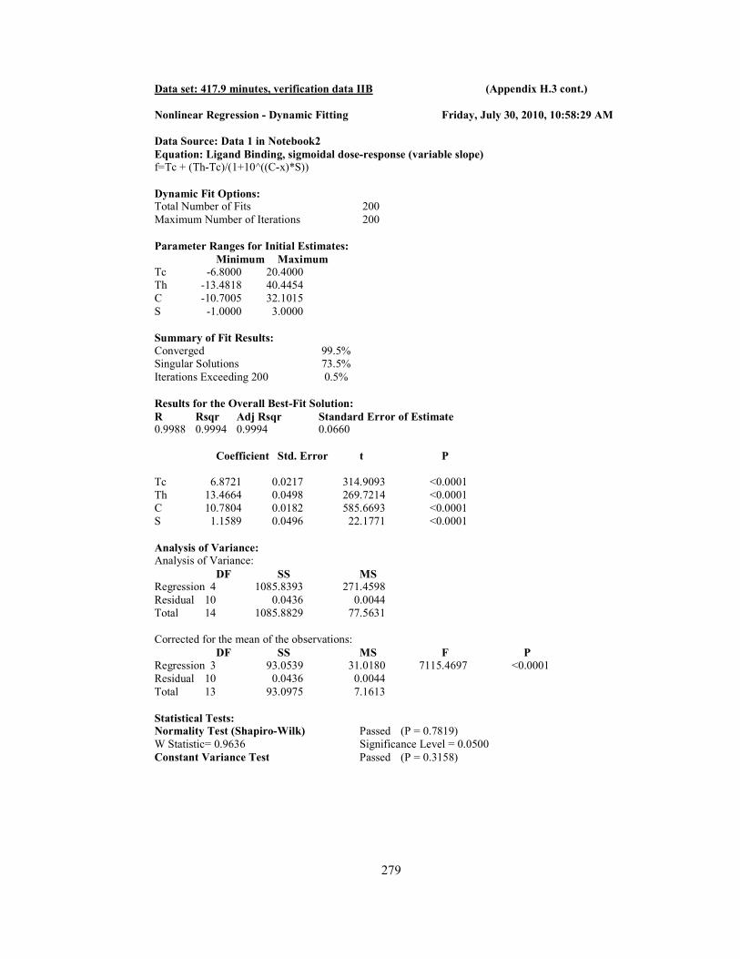
279

Data set: 417.9 minutes, verification data IIB (Appendix H.3 cont.)

Nonlinear Regression - Dynamic Fitting Friday, July 30, 2010, 10:58:29 AM

Data Source: Data 1 in Notebook2

Equation: Ligand Binding, sigmoidal dose-response (variable slope) f=Tc + (Th-Tc)/(1+10^((C-x)*S))

Dynamic Fit Options: Total Number of Fits 200

Maximum Number of Iterations 200

Parameter Ranges for Initial Estimates:

Minimum Maximum Tc -6.8000 20.4000

Th -13.4818 40.4454

C -10.7005 32.1015

S -1.0000 3.0000

Summary of Fit Results:

Converged 99.5%

Singular Solutions 73.5%

Iterations Exceeding 200 0.5%

Results for the Overall Best-Fit Solution:

R Rsqr Adj Rsqr Standard Error of Estimate 0.9988 0.9994 0.9994 0.0660

Coefficient Std. Error t P

Tc 6.8721 0.0217 314.9093 <0.0001

Th 13.4664 0.0498 269.7214 <0.0001

C 10.7804 0.0182 585.6693 <0.0001

S 1.1589 0.0496 22.1771 <0.0001

Analysis of Variance: Analysis of Variance:

DF SS MS Regression 4 1085.8393 271.4598

Residual 10 0.0436 0.0044

Total 14 1085.8829 77.5631

Corrected for the mean of the observations:

DF SS MS F P

Regression 3 93.0539 31.0180 7115.4697 <0.0001

Residual 10 0.0436 0.0044

Total 13 93.0975 7.1613

Statistical Tests: Normality Test (Shapiro-Wilk) Passed (P = 0.7819)

W Statistic= 0.9636 Significance Level = 0.0500

Constant Variance Test Passed (P = 0.3158)

280

Data set: 477.6 minutes, verification data IIB (Appendix H.3 cont.)

Nonlinear Regression - Dynamic Fitting Friday, July 30, 2010, 10:58:42 AM

Data Source: Data 1 in Notebook2

Equation: Ligand Binding, sigmoidal dose-response (variable slope) f=Tc + (Th-Tc)/(1+10^((C-x)*S))

Dynamic Fit Options: Total Number of Fits 200

Maximum Number of Iterations 200

Parameter Ranges for Initial Estimates:

Minimum Maximum Tc -6.7449 20.2347

Th -13.3459 40.0376

C -11.8566 35.5699

S -1.0000 3.0000

Summary of Fit Results:

Converged 98.5%

Singular Solutions 77.0%

Iterations Exceeding 200 1.5%

Results for the Overall Best-Fit Solution:

R Rsqr Adj Rsqr Standard Error of Estimate 0.9948 0.9974 0.9980 0.0960

Coefficient Std. Error t P

Tc 6.8640 0.0301 226.5246 <0.0001

Th 13.4981 0.1304 103.5095 <0.0001

C 12.1219 0.0370 320.9996 <0.0001

S 1.1972 0.0588 16.2284 <0.0001

Analysis of Variance: Analysis of Variance:

DF SS MS Regression 4 920.8469 230.2117

Residual 10 0.0922 0.0092

Total 14 920.9390 65.7814

Corrected for the mean of the observations:

DF SS MS F P

Regression 3 60.5516 20.1839 2190.0447 <0.0001

Residual 10 0.0922 0.0092

Total 13 60.6438 4.6649

Statistical Tests: Normality Test (Shapiro-Wilk) Passed (P = 0.8395)

W Statistic= 0.9674 Significance Level = 0.0500

Constant Variance Test Passed (P = 0.1524)

281

H.4 Verification June 24, 2008

Result Summary of SIGMAPLOT Analysis : Verification IIC

Charging Minutes Tc (oC) Th (

oC) C S R

2

0.0 7.52 14.29 2.93 1.43 0.9918

59.7 7.40 14.28 4.11 1.57 0.9969

119.4 7.37 14.28 5.15 1.37 0.9935

179.1 7.24 14.28 6.32 1.21 0.9960

238.8 7.01 14.18 7.42 1.19 0.9979

298.5 6.99 14.11 8.41 1.30 0.9989

358.2 6.81 14.00 9.47 1.29 0.9992

417.9 6.77 13.87 10.60 1.45 0.9994

477.6 6.74 13.70 11.65 1.07 0.9975 Result of SIGMAPLOT processing: June 24, 2008 (Verification Data IIC)

Data set: 0.0 minutes, verification data IIC

Nonlinear Regression - Dynamic Fitting Friday, July 30, 2010, 11:08:03 AM

Data Source: Data 1 in Notebook3

Equation: Ligand Binding, sigmoidal dose-response (variable slope) f=Tc + (Th-Tc)/(1+10^((C-x)*S))

Dynamic Fit Options:

Total Number of Fits 200

Maximum Number of Iterations 200

Parameter Ranges for Initial Estimates:

Minimum Maximum

Tc -7.5609 22.6827

Th -14.8668 44.6005

C -2.9990 8.9969

S -1.0000 3.0000

Summary of Fit Results: Converged 100.0%

Singular Solutions 53.5%

Ill-Conditioned Solutions 0.5%

Results for the Overall Best-Fit Solution:

R Rsqr Adj Rsqr Standard Error of Estimate 0.9837 0.9918 0.9634 0.4718

Coefficient Std. Error t P

Tc 7.5210 0.3810 19.9073 <0.0001

Th 14.2918 0.1519 91.8586 <0.0001

C 2.9331 0.1372 20.7822 <0.0001

S 1.4334 0.3114 3.6750 0.0043

282

Analysis of Variance: (Appendix H.4 cont.) Analysis of Variance:

DF SS MS Regression 4 2321.0688 580.2672

Residual 10 2.2257 0.2226

Total 14 2323.2945 165.9496

Corrected for the mean of the observations:

DF SS MS F P Regression 3 76.7556 25.5852 114.9521 <0.0001

Residual 10 2.2257 0.2226

Total 13 78.9813 6.0755

Statistical Tests: Normality Test (Shapiro-Wilk) Passed (P = 0.7339)

W Statistic= 0.9607 Significance Level = 0.0500

Constant Variance Test Passed (P = 0.1128)

283

Data set: 59.7 minutes , verification data IIC (Appendix H.4 cont.)

Nonlinear Regression - Dynamic Fitting Friday, July 30, 2010, 11:08:17 AM

Data Source: Data 1 in Notebook3

Equation: Ligand Binding, sigmoidal dose-response (variable slope) f=Tc + (Th-Tc)/(1+10^((C-x)*S))

Dynamic Fit Options: Total Number of Fits 200

Maximum Number of Iterations 200

Parameter Ranges for Initial Estimates:

Minimum Maximum Tc -7.2990 21.8970

Th -14.5953 43.7859

C -4.0572 12.1715

S -1.0000 3.0000

Summary of Fit Results:

Converged 100.0%

Singular Solutions 55.5%

Ill-Conditioned Solutions 0.5%

Results for the Overall Best-Fit Solution:

R Rsqr Adj Rsqr Standard Error of Estimate 0.9938 0.9969 0.9838 0.3629

Coefficient Std. Error t P

Tc 7.4021 0.2324 31.3809 <0.0001

Th 14.2810 0.1246 111.2514 <0.0001

C 4.1090 0.1044 37.8936 <0.0001

S 1.5720 0.1931 5.3516 0.0003

Analysis of Variance: Analysis of Variance:

DF SS MS Regression 4 2124.2701 531.0675

Residual 10 1.3173 0.1317

Total 14 2125.5874 151.8277

Corrected for the mean of the observations:

DF SS MS F P

Regression 3 104.4022 34.8007 264.1923 <0.0001

Residual 10 1.3173 0.1317

Total 13 105.7195 8.1323

Statistical Tests: Normality Test (Shapiro-Wilk) Passed (P = 0.2907)

W Statistic= 0.9285 Significance Level = 0.0500

Constant Variance Test Passed (P = 0.1383)

284

Data set: 119.4 minutes, verification data IIC (Appendix H.4 cont.)

Nonlinear Regression - Dynamic Fitting Friday, July 30, 2010, 11:08:50 AM

Data Source: Data 1 in Notebook3

Equation: Ligand Binding, sigmoidal dose-response (variable slope) f=Tc + (Th-Tc)/(1+10^((C-x)*S))

Dynamic Fit Options: Total Number of Fits 200

Maximum Number of Iterations 200

Parameter Ranges for Initial Estimates:

Minimum Maximum Tc -7.1540 21.4621

Th -14.2428 42.7283

C -5.1394 15.4183

S -1.0000 3.0000

Summary of Fit Results:

Converged 99.5%

Singular Solutions 60.0%

Iterations Exceeding 200 0.5%

Results for the Overall Best-Fit Solution:

R Rsqr Adj Rsqr Standard Error of Estimate 0.9870 0.9935 0.9929 0.2589

Coefficient Std. Error t P

Tc 7.3663 0.1397 51.3290 <0.0001

Th 14.2837 0.0957 144.0289 <0.0001

C 5.1539 0.0740 68.9963 <0.0001

S 1.3708 0.1291 7.5898 <0.0001

Analysis of Variance: Analysis of Variance:

DF SS MS Regression 4 1936.2331 484.0583

Residual 10 0.6705 0.0670

Total 14 1936.9035 138.3503

Corrected for the mean of the observations:

DF SS MS F P

Regression 3 122.7318 40.9106 610.1789 <0.0001

Residual 10 0.6705 0.0670

Total 13 123.4023 9.4925

Statistical Tests: Normality Test (Shapiro-Wilk) Passed (P = 0.7776)

W Statistic= 0.9633 Significance Level = 0.0500

Constant Variance Test Passed (P = 0.0306)

285

Data set: 179.1 minutes, verification data IIC (Appendix H.4 cont.)

Nonlinear Regression - Dynamic Fitting Friday, July 30, 2010, 11:09:33 AM

Data Source: Data 1 in Notebook3

Equation: Ligand Binding, sigmoidal dose-response (variable slope) f=Tc + (Th-Tc)/(1+10^((C-x)*S))

Dynamic Fit Options: Total Number of Fits 200

Maximum Number of Iterations 200

Parameter Ranges for Initial Estimates:

Minimum Maximum Tc -7.0496 21.1487

Th -14.0339 42.1017

C -6.2725 18.8176

S -1.0000 3.0000

Summary of Fit Results:

Converged 100.0%

Singular Solutions 63.0%

Results for the Overall Best-Fit Solution:

R Rsqr Adj Rsqr Standard Error of Estimate 0.9920 0.9960 0.9966 0.1861

Coefficient Std. Error t P

Tc 7.2412 0.0874 81.0862 <0.0001

Th 14.2756 0.0752 182.6895 <0.0001

C 6.3185 0.0513 122.6070 <0.0001

S 1.2110 0.0976 9.9022 <0.0001

Analysis of Variance:

Analysis of Variance:

DF SS MS

Regression 4 1753.9535 438.4884

Residual 10 0.3462 0.0346

Total 14 1754.2997 125.3071

Corrected for the mean of the observations:

DF SS MS F P Regression 3 133.6245 44.5415 1286.6595 <0.0001

Residual 10 0.3462 0.0346

Total 13 133.9707 10.3054

Statistical Tests: Normality Test (Shapiro-Wilk) Passed (P = 0.9850)

W Statistic= 0.9820 Significance Level = 0.0500

Constant Variance Test Passed (P = 0.0016)

286

Data set: 238.8 minutes, verification data IIC (Appendix H.4 cont.)

Nonlinear Regression - Dynamic Fitting Friday, July 30, 2010, 11:09:46 AM

Data Source: Data 1 in Notebook3

Equation: Ligand Binding, sigmoidal dose-response (variable slope) f=Tc + (Th-Tc)/(1+10^((C-x)*S))

Dynamic Fit Options: Total Number of Fits 200

Maximum Number of Iterations 200

Parameter Ranges for Initial Estimates:

Minimum Maximum Tc -6.9748 20.9245

Th -13.9287 41.7860

C -7.4092 22.2275

S -1.0000 3.0000

Summary of Fit Results:

Converged 99.5%

Singular Solutions 69.5%

Iterations Exceeding 200 0.5%

Results for the Overall Best-Fit Solution:

R Rsqr Adj Rsqr Standard Error of Estimate 0.9958 0.9979 0.9981 0.1407

Coefficient Std. Error t P

Tc 7.0130 0.0582 121.2273 <0.0001

Th 14.1836 0.0620 220.9694 <0.0001

C 7.4213 0.0340 218.2587 <0.0001

S 1.1859 0.1041 10.7244 <0.0001

Analysis of Variance: Analysis of Variance:

DF SS MS Regression 4 1585.4284 396.3571

Residual 10 0.1979 0.0198

Total 14 1585.6263 113.2590

Corrected for the mean of the observations:

DF SS MS F P

Regression 3 136.4210 45.4737 2298.3564 <0.0001

Residual 10 0.1979 0.0198

Total 13 136.6188 10.5091

Statistical Tests: Normality Test (Shapiro-Wilk) Passed (P = 0.6484)

W Statistic= 0.9555 Significance Level = 0.0500

Constant Variance Test Passed (P = 0.0560)

287

Data set: 298.5 minutes, verification data IIC (Appendix H.4 cont.)

Nonlinear Regression - Dynamic Fitting Friday, July 30, 2010, 11:09:59 AM

Data Source: Data 1 in Notebook3

Equation: Ligand Binding, sigmoidal dose-response (variable slope) f=Tc + (Th-Tc)/(1+10^((C-x)*S))

Dynamic Fit Options: Total Number of Fits 200

Maximum Number of Iterations 200

Parameter Ranges for Initial Estimates:

Minimum Maximum Tc -6.8984 20.6952

Th -13.8664 41.5993

C -8.5669 25.7008

S -1.0000 3.0000

Summary of Fit Results:

Converged 99.5%

Singular Solutions 70.0%

Iterations Exceeding 200 0.5%

Results for the Overall Best-Fit Solution:

R Rsqr Adj Rsqr Standard Error of Estimate 0.9978 0.9989 0.9985 0.1238

Coefficient Std. Error t P

Tc 6.9900 0.0461 150.4271 <0.0001

Th 14.1149 0.0607 224.0396 <0.0001

C 8.4086 0.0250 341.6492 <0.0001

S 1.3004 0.1537 8.8159 <0.0001

Analysis of Variance: Analysis of Variance:

DF SS MS Regression 4 1409.2612 352.3153

Residual 10 0.1534 0.0153

Total 14 1409.4146 100.6725

Corrected for the mean of the observations:

DF SS MS F P

Regression 3 133.8093 44.6031 2908.2366 <0.0001

Residual 10 0.1534 0.0153

Total 13 133.9626 10.3048

Statistical Tests: Normality Test (Shapiro-Wilk) Passed (P = 0.5816)

W Statistic= 0.9513 Significance Level = 0.0500

Constant Variance Test Passed (P = <0.0001)

288

Data set: 358.2 minutes, verification data IIC (Appendix H.4 cont.)

Nonlinear Regression - Dynamic Fitting Friday, July 30, 2010, 11:10:12 AM

Data Source: Data 1 in Notebook3

Equation: Ligand Binding, sigmoidal dose-response (variable slope) f=Tc + (Th-Tc)/(1+10^((C-x)*S))

Dynamic Fit Options: Total Number of Fits 200

Maximum Number of Iterations 200

Parameter Ranges for Initial Estimates:

Minimum Maximum Tc -6.8580 20.5741

Th -13.7175 41.1526

C -9.7146 29.1439

S -1.0000 3.0000

Summary of Fit Results:

Converged 99.5%

Singular Solutions 71.0%

Iterations Exceeding 200 0.5%

Results for the Overall Best-Fit Solution:

R Rsqr Adj Rsqr Standard Error of Estimate 0.9984 0.9992 0.9991 0.0897

Coefficient Std. Error t P

Tc 6.8110 0.0309 222.9880 <0.0001

Th 13.9957 0.0528 256.1377 <0.0001

C 9.4709 0.0215 449.6441 <0.0001

S 1.2934 0.0877 14.4428 <0.0001

Analysis of Variance: Analysis of Variance:

DF SS MS Regression 4 1240.9201 310.2300

Residual 10 0.0805 0.0081

Total 14 1241.0006 88.6429

Corrected for the mean of the observations:

DF SS MS F P

Regression 3 116.3536 38.7845 4815.1023 <0.0001

Residual 10 0.0805 0.0081

Total 13 116.4341 8.9565

Statistical Tests: Normality Test (Shapiro-Wilk) Passed (P = 0.3848)

W Statistic= 0.9373 Significance Level = 0.0500

Constant Variance Test Passed (P = 0.0101)

289

Data set: 417.9 minutes, verification data IIC (Appendix H.4 cont.)

Nonlinear Regression - Dynamic Fitting Friday, July 30, 2010, 11:10:26 AM

Data Source: Data 1 in Notebook3

Equation: Ligand Binding, sigmoidal dose-response (variable slope) f=Tc + (Th-Tc)/(1+10^((C-x)*S))

Dynamic Fit Options: Total Number of Fits 200

Maximum Number of Iterations 200

Parameter Ranges for Initial Estimates:

Minimum Maximum Tc -6.8000 20.4000

Th -13.4818 40.4454

C -10.8295 32.4886

S -1.0000 3.0000

Summary of Fit Results:

Converged 99.5%

Singular Solutions 73.5%

Iterations Exceeding 200 0.5%

Results for the Overall Best-Fit Solution:

R Rsqr Adj Rsqr Standard Error of Estimate 0.9988 0.9994 0.9995 0.0588

Coefficient Std. Error t P

Tc 6.7698 0.0191 360.1620 <0.0001

Th 13.8739 0.0447 300.4378 <0.0001

C 10.5960 0.0167 647.4669 <0.0001

S 1.4530 0.0446 26.7049 <0.0001

Analysis of Variance: Analysis of Variance:

DF SS MS Regression 4 1074.7832 268.6958

Residual 10 0.0346 0.0035

Total 14 1074.8178 76.7727

Corrected for the mean of the observations:

DF SS MS F P

Regression 3 91.3264 30.4421 8792.4139 <0.0001

Residual 10 0.0346 0.0035

Total 13 91.3610 7.0278

Statistical Tests: Normality Test (Shapiro-Wilk) Passed (P = 0.7367)

W Statistic= 0.9608 Significance Level = 0.0500

Constant Variance Test Passed (P = 0.4346)

290

Data set: 477.6 minutes, verification data IIC (Appendix H.4 cont.)

Nonlinear Regression - Dynamic Fitting Friday, July 30, 2010, 11:10:40 AM

Data Source: Data 1 in Notebook3

Equation: Ligand Binding, sigmoidal dose-response (variable slope) f=Tc + (Th-Tc)/(1+10^((C-x)*S))

Dynamic Fit Options: Total Number of Fits 200

Maximum Number of Iterations 200

Parameter Ranges for Initial Estimates:

Minimum Maximum Tc -6.7741 20.3224

Th -13.3459 40.0376

C -11.9525 35.8574

S -1.0000 3.0000

Summary of Fit Results:

Converged 99.0%

Singular Solutions 78.0%

Ill-Conditioned Solutions 0.5%

Iterations Exceeding 200 1.0%

Results for the Overall Best-Fit Solution:

R Rsqr Adj Rsqr Standard Error of Estimate 0.9975 0.9975 0.9990 0.0689

Coefficient Std. Error t P

Tc 6.7393 0.0211 323.6221 <0.0001

Th 13.6988 0.0820 163.8337 <0.0001

C 11.6542 0.0231 518.2881 <0.0001

S 1.0700 0.0492 24.2827 <0.0001

Analysis of Variance:

Analysis of Variance:

DF SS MS

Regression 4 914.2459 228.5615

Residual 10 0.0475 0.0047

Total 14 914.2934 65.3067

Corrected for the mean of the observations:

DF SS MS F P Regression 3 60.5753 20.1918 4253.2324 <0.0001

Residual 10 0.0475 0.0047

Total 13 60.6228 4.6633

Statistical Tests: Normality Test (Shapiro-Wilk) Passed (P = 0.0283)

W Statistic= 0.8577 Significance Level = 0.0500

Constant Variance Test Passed (P = 0.0338)

291

292

REFERENCES

[1] ASHRAE, HVAC Applications Handbook, 1999.

[2] T. K, "Co-generation and the New Era of Absorption Chiller," [online]

www.ashraethailand.org, August 2010.

[3] N. L. Minh, "Modeling and Analysis of Cogeneration-Based District Energy

System," in Mechanical Engineering. vol. MSc: University of Western

Ontario, 1996.

[4] F. DP, "Case Study of a Large, Naturally Stratified Chilled-Water Thermal

Storage Systems," ASHRAE Transaction, vol. II, pp. 1161-1169, 1991.

[5] G. DP, "Succesfull Thermal Storage," ASHRAE Transaction, vol. IB, pp. 843-

855, 1985.

[6] H. JH, Cogeneration--combined heat and power (CHP): thermodynamics and

economics: Pergamon, Oxford, England, 1987.

[7] K. BF, Small-scale Cogeneration Handbook, 3rd ed.: Fairmont Press Inc, 2008.

[8] C. S, "The Perfect Match: Combined Cycles and District Heating/Cooling,"

Power, vol. 135, pp. 117-120, 1991.

[9] S. E. R. Institute, "Economic Aspect of District Heating and Cooling," Heating/Piping/Air

Conditioning, vol. 59, No. 9, pp. 47-56, 1987.

[10] G. C, "District Energy Trend: Opportunities and Issues," World Bank Technical Paper

No. 493, 2001.

[11] M. Fallek, "Absorption Chillers for Cogeneration Applications," ASHRAE Transactions SF

1B, vol. 92 (2), pp. 321-327, 1986.

[12] P. K. a. S. Devotta, "Study of an Absorption Refrigeration System for Simultaneous "

ASHRAE Transactions, vol. 96 Part 2, pp. 291-298, 1990.

[13] R. M. Tozer, "Absorption Refrigeration (Principles, Cycles and Applications to

Cogeneration)," Conference Cogeneracion 92, Madrid 28-30, pp. 170-175, 1992.

[14] R. M. T. a. R. W. James, "Absorption Chillers Applied to CHP Systems," Building Services

Engineering Research and Technology vol. 16 (4), pp. 175–188, 1995.

[15] P. E. Hufford, "Absorption Chillers Maximize Cogeneration Value," ASHRAE

Transactions, vol. 2(3) pp. 428-433, 1991.

[16] P. Hufford, "Absorption Chillers Improve Cogeneration Energy Efficiency," ASHRAE

Journals, vol. 34, No.3, pp. 46-53

1992.

[17] A. Abedin, "Cogeneration : Balancing Heat Power ratio," ASHRAE Journals, pp. 23-37,

2003.

[18] A. OE, Storage of Thermal Energy, in Energy Storage Systems: Encyclopedia

of Life Support System (EOLSS), Eolss Publishers, Oxford, UK, 2006.

[19] I. D. a. M. A. Rosen, "Energetic, Environmental and Economic Aspects of

Thermal Energy Storage System for Cooling Capacity," Applied Thermal

Engineering, vol. 21, pp. 1105-1107, 2001.

[20] T. K. G. t. C. Fitting, [Online]. Available :

http://www.synergy.com/Tools/curvefitting.pdf, August 2009.

[21] ASHRAE, Handbooks HVAC Applications, 2003.

[22] E. M. a. G. Reeves, "Stratified Chilled Water Storage Design Guide," Electric

Power Research Institute 1988.

[23] Y. Z. a. A. Ghajar, Heat Transfer and Stratification in Sensible Heat Storage

System, in Thermal energy Storage System and Applications, Eds, I Dincer

and M Rosen: John Willey and Sons 2002.

293

[24] N. T. a. J. Kreider, "Field Measurement of Chilled Water Storage Thermal

Performance," ASHRAE, vol. 95 (1), pp. 1106-1112, 1989.

[25] EPRI, Commercial Cool Storage Design Guide Springer-Verlag, 1987.

[26] W. MW, "Diffuser Design for Naturally Startified Thermal Storage " ASHRAE

Transaction, vol. I, pp. 1094-1101, 1990.

[27] D. I. a. R. MA, Thermal Energy storage Systems and Applications: John

Wiley and Sons Ltd, 2001.

[28] A. Musser, "Field Measured and Modeled Performance of Full Scale

Cylindrical Sttratified Chilled Water Stoerage Tanks," in Graduate School.

vol. PhD: The Pennsylvania State University, 1998.

[29] W. SK, Handbook of Air Conditioning and Refrigeration, 2nd Edition ed.: Mc

Graw Hill Company, 2000.

[30] C. E. Dorgan, Elleson and James S, Design Guide for Cool Thermal Storage:

Atlanta, GA, 1994.

[31] ASHRAE, HVAC Applications Handbook, 2007.

[32] M. W. W. a. C. R. Truman., "Performance of Stratified Vertical Cylindrical

Thermal Storage Tanks—Part 1: Scale Model Tank," ASHRAE Transactions

vol. 95 (1), pp. 1086-1095, 1989.

[33] M. E. a. H. W. Wildin MW, "Thermal Storage Forum - Stratified Thermal

Storage : A New/Old Technology," ASHRAE Journal vol. 32(4), pp. 29 - 39,

1990.

[34] A. M. a. W. Bahnfleth, "Evolution of Temperature Distributions in a Full-

Scale Stratified Chilled-Water Storage Tank with Radial Diffusers," ASHRAE

Transaction, vol. 104 (1), pp. 55-67, 1998.

[35] A. M. a. W. P. Bahnfleth, "Field-Measured Performance of Four Full-Scale

Cylindrical Stratified Chilled-Water Thermal Storage Tanks," ASHRAE

Transaction vol. 105 (2), pp. 218-230, 1998.

[36] J. S. a. C. J. Bahnfleth WP, "Measured and Modeled Charging of Stratified

Chilled Water thermal Storage Tank with Slotted Pipe Diffusers," HVAC&R

Research, vol. 9, No. 4, pp. 467-491, 2003.

[37] A. M. a. W. Bahnfleth, "Parametric Study of Charging Inlet Diffuser

Performance in Stratified Chilled Water Storage Tanks with radial Diffusers:

Part 2-Dimensional Analysis, Parametric Simulations and simplified Model

Development," HVAC&R Research, vol. Vol. 7, No. 2, pp. 205-221, 2001.

[38] M. A. a. W. Bahnfleth, "Parametric Study of Charging Inlet Diffuser

Performance in Stratified Chilled Water Storage Tanks with Radial Diffusers:

Part 1-Model Development and Validation," HVAC&R Research vol. 7 No.1,

pp. 31-49, 2001.

[39] J. S. a. W. Bahnfleth, "Parametric Study of Single-Pipe Diffusers in Stratified

Chilled Water Storage Tanks," HVAC&R Research, vol. Vol. 10, No. 3, pp.

345-364, 2004.

[40] J. S. a. W. Bahnfleth, "Constant Flowrate Charging Characteristics of a Full-

Scale Stratified Chilled Water Storage Tank with Double-Ring Slotted pipe

Diffusers," Applied Thermal Engineering pp. 3067-3082, 2005.

[41] J. C. a. W. Bahnfleth, "Identification of Mixing Effects in Stratified Chilled-

Water Storage Tanks by Analysis of Time Series Temperature Data,"

ASHRAE Transaction, vol. 104 (2), pp. 366-376, 1998.

[42] A. B. a. S. S. M. JEB Nelson, "Experiments on Stratified Chilled-Water

Tanks," International Journal of Refrigeration, vol. 22, pp. 216-234, 1999.

294

[43] M. Karim, "Performance Evaluation of A Stratified Chilled-Water Thermal

Storage System," World Academy of Science Engineering and Technology,

vol. 53, pp. 328-334, 2009.

[44] M. J. A. a. J. R. M.R.W. Walmsley, "Thermocline Management of Stratified

Tanks for Thermal Storage," Proceedings of 12th International Conference on

Process Integration, Modelling and Optimisation for Energy Saving and

Pollution Reduction. AIDIC, Rome, Italy; 10-13 May, pp. 231-236, 2009.

[45] W. M. a. T. C. Yoo J, "Initial Formation of Thermocline in Stratified Thermal

Storage tanks," ASHRAE Transaction, vol. 92(2A), pp. 280-292, 1986.

[46] S. a. S. Homan K, "Thermal Performance of Stratified Chilled Water Storage

Tanks," HVAC&R Research, vol. 2, pp. 158-170, 1996.

[47] W. B. a. A. Musser, "Thermal Performance of a Full Scale Stratified Chilled

Water Storage Tank," ASHRAE Transaction vol. 104(2), pp. 377-388, 1998.

[48] J. W. a. M. A. A. Majid, "Temperature Profile and Thermocline Thickness

Evaluation of a Stratified Thermal Energy Storage Tank," International

Journal of Mechanical & Mechatronics Engineering IJMME-IJENS vol. 10,

No.1, pp. 7-12, 2010.

[49] M. A. a. W. Joko, "Thermocline Thickness Evaluation on Stratified Thermal

Energy Storage Tank of Co-generated District Cooling Plant," Journal of

Energy and Power Engineering, vol. 4, No.2 pp. 28-33, 2010.

[50] J. W. a. M. A. A. Majid, "Performance Evaluation of Stratified TES using

Sigmoid Dose Response Function," International Conference on Plant

Equipment and Reliability, 15-17 June 2010, Kuala Lumpur, Malaysia, 2010.

[51] A. B. a. S. S. M. JEB Nelson, "Parametric Studies on Thermally Startified

Chilled Water Storage Systems," Applied Thermal Engineering, vol. 19, pp.

89-115, 1999.

[52] W. MW, "Flow Near the Inlet and Design Parameter for Stratified Chilled

Water Storage," ASME 91-HT-27, 1991.

[53] H. C. a. M. CW, "An Experimental and Numerical Study on the Effect of the

Wall in a Cylindrical Exposure," Solar energy, vol. 28, pp. 145-152, 1982.

[54] J. Y. a. G. SK, "Decay of of Thermal Stratification in water Body for Solar

Energy Storage," Solar energy, vol. 28, pp. 137-143, 1982.

[55] R. G. a. H. K. Lighsone MF, "Numerical Simulation of the charging of Liquid

Storage Tanks; Comparison with experiment," Journal of Solar Energy

Engineering vol. Vol 111, pp. 225-231, 1989.

[56] S. C. a. S. S. Homan K, "Thermal Performance of Stratified Chilled Water

Storage Tanks " HVAC&R Research, vol. Vol. 2, pp. 158-170, 1996.

[57] A. G. a. P. M. YH Zurigat, "A Comparison Study of One-Dimensional Models

for Stratified Thermal Storage Tanks," Transaction of ASME, vol. 111, pp.

204-210, 1989.

[58] M. W. a. C. Truman, "A Summary of Experience with Stratified Chilled Water

Tanks " ASHRAE Transactions vol. 91 (1b), pp. 956-976, 1985.

[59] Y. J. a. K. Thomas, Computational Heat Transfer, 2nd ed., 2003.

[60] G. RJ, "An Experimental Study of Single Medium Thermocline Thermal

Energy Storage," ASME Paper 82-HT-53, 1982.

[61] W. B. a. S. K. EM Kleinback, "Performance Study of One-Dimensional Moels

for Stratified Thermal Storage Tanks," Solar Energy, vol. 50, pp. 155-166,

1993.

295

[62] V. Badescu, "Optimal Operation of Thermal Energy Storage Units Based on

Stratified and Fully Mixed Water Tanks," Applied Thermal Engineering 24,

pp. 2101-2116, 2004.

[63] P. C. a. S. R. Gretarsson SP, "Development of Fundamentally Based

Stratified Thermal Storage Tank Model for Energy Calculation," ASHRAE

Transaction, vol. Vol. 100 pp. 1213-1220, 1994.

[64] J. D. a. N. Farnum, Applied Statistics for Engineers and Scientist, 2nd ed.:

Thomson Learning Inc, 2005.

[65] Y. J. a. K. Homan, "On Simplified Models for the Rate and Time Dependent

Performance of Stratified Thermal Storage," Transaction of ASME, vol. 129,

pp. 214-222, 2007.

[66] J. Y, Design and Optimization of Thermal Systems: CRC Press, 2008.

[67] I. F. a. D. DP, Introduction to Heat Transfer: John Wiley and Sons, 2002.

[68] N. A.-N. N. El-Refaee, "A Numerical Study for the Prediction of Turbulent

Mixing factor in Thermal Storage Tank," Applied Thermal Engineering, vol.

Vol. 17, No. 12, pp. 1173-1181, 1997.

[69] O. MN, Heat Conduction, 2nd ed.: John Wiley and Sons, Inc., 1993.

[70] C. S. a. C. RP, Numerical Methods for Engineers, 6 ed.: Mc Graw Hill

International Edition, 2009.

[71] H. JP, Heat Transfer, 10 ed.: Mc Graw Hill Higher Education, 2009.

[72] J. Y. a. T. KE, Computational Heat Transfer, 2 ed.: Taylor and Francis, 2003.

[73] G. C. a. W. PO, Applied Numerical Analysis 7th ed.: Addison-Wesley

Publishing Company, 2004.

[74] O. MN, Finite Difference Methods in Heat Transfer: CRC Press Inc, 1994.

[75] M. A. A. M. a. C. R. J. Waluyo, "Analysis of Temperature Distribution of

Chilled-Water Thermal Storage Tank," National Postgraduate Conference,

Universiti Teknologi PETRONAS, 25-26 March 2009, pp. 1-5, 2009

[76] A. G. a. P. M. FJ Oppel, "Computer Simulation of Stratified Heat Storage,"

Applied Energy, vol. 23, pp. 293-, 1986.

[77] A. G. a. P. M. FJ Oppel, "A Numerical and Experiment Study of Stratified

Thermal Storage," ASHRAE Transaction, vol. 92, No. 2, pp. 293-309, 1986.

[78] C. N. D. a. T. F. Dupont, "Explicit/implicit Conservative Domain

Decomposition Procedures for Parabolic Problems Based on bBlock-Centered

Finite Differences," SIAM Journal on Numerical Analysis, vol. 31. no. 4, pp.

1045-1061, 1994.

[79] W. M. a. T. CR, "Evaluation of Stratified Chilled Water Storage Technique,"

EPRI Report 1985.

[80] A. G. a. P. M. YH Zurigat, "Stratified Thermal Storage Inlet Mixing

Characterization," Applied Energy, vol. 30, pp. 99-111, 1988.

[81] T. S. Votsis PP, Wilson DR and Marquand CJ, "Experimental and Theoretical

of Mixed and Stratified Water Storage Tanks," Proceedings of the Institution

of Mechanical Engineers, Part-C Journal of Mechanical Engineering Science

vol. Vol. 202, pp. 187-193, 1988.

[82] W. MW, "Performance of Stratifified Vertical Cylindrical Thermal Storage

tank, Part 2; Prototype Tank," ASHRAE Transaction 95(1), pp. 1096-1105,

1989.

[83] J. W. a. T. J. Whitman WC, Refrigeration and Air Conditioning Technology

5th ed.: Thompson Delmar Learning 2005.

296

[84] W. S. a. J. Jones, Refrigeration and Air Conditioning, 2 ed.: Mc Graw Hill

International Editions, 1982.

[85] D. Ibrahim, Refrigeration Systems and Applications: John Wiley and Sons

2003.

[86] C. HR, HVAC System Evaluation. New York: RS Means, 1990.

[87] K. JF, Handbook of Heating, Ventilating and Air Conditioning: CRC Press,

2001.

[88] K. EA, "The Modeling, Performance and Optimal Control of Commercial

Absorption Chillers," in Mechanical Department vol. MSc: University of

Wisconsin, 1994.

[89] ASHRAE, ASHRAE Refrigeration Handbook, 2002.

[90] R. R. a. S. K. KE Herold, Absorption Chillers and Heat Pumps: CRC Press.

Inc, 1996.

[91] V. M. Izquierdo M, Rodriquez P and Leucona A, "Crystallization as a Limit to

develop Solar Air-Cooled LiBr-H2O Absorption System Using Low-Grade

Heat," Solar Energy Materials and Solar Cells, vol. 81, pp. 205-216, 2004.

[92] K. S. GA Florides, Tassou SA and Wrobel LC, "Design and Construction of a

LiBr-Water Absorption Machine," Energy Conversion and management, vol.

Vol. 44, pp. 483-2508, 2003.

[93] R. R. Xiaohong Liaoa, "Absorption chiller crystallization control strategies for

integrated cooling heating and power systems," International Journal of

Refrigeration vol. 30, pp. 904-911, 2007.

[94] S. C. Sugarman, HVAC Fundamentals: Fairmont Press Inc, 2005.

[95] A. A. Bell, HVAC equations, data and ruleof thumbs, 2 ed.: Mc Graw Hill

Book

2008.

[96] F. Kreith, Handbook of Thermal Engineering: Springer, 2000.

[97] C. C. a. Marshal, "Simulation of Refrigerating and Air Conditioning

Equipment Based on Experiment Data," ASHRAE Transaction, vol. 97, pp.

388-393, 1991.

[98] G. J. a. N. KC, "Thermodynamic Modeling for Reciprocating Chillers,"

Journal of Applied Physics, vol. 75 (6), pp. 2769-2774, 1994.

[99] P. C. a. C. G. Strand RK, "Development of Direct and Indirect Ice-Storage for

Energy Calculations," ASHRAE Transaction, vol. 100, Part. 1, pp. 1230-1244,

1994.

[100] M. M. Figuera LE, Cathey M and Nutre DW, "Modification and Validation of

a Universal Thermodynamic Chiller Model Used to Evaluate the Performance

of Water Cooled Centrifugal Chillers," The Eleventh Symposium on Improving

Building Systems in Hot nd Humid Climates, Texas, pp. 57-65, 1998.

[101] R. D. a. K. S. Jahing DI, "A Semi Empirical Method for Representing

Domestic Refrigerator/Freezer Compressor Calorimeter Test Data," ASHRAE

Transaction, vol. 106 (2), pp. 122-130, 2000.

[102] M. J. a. B. A. McIntosh IIBD, "Fault Detection and Diagnosis Part (I), Model

Development and Application," ASHRAE Transaction, vol. 106 (2), pp. 268-

282, 2000.

[103] G. G. a. Michelson, "A Modular Computer Simiulation of Absorption

Systems," ASHRAE Transaction, vol. 91 (2B), pp. 1808-1827, 1985.

297

[104] G. K. a. G. D. Grossman G, "Computer Model for Simulation of Absorption

Systems in Flexible and Modular Form," ASHRAE Transaction, vol. 93 (2),

pp. 1590-1598, 1987.

[105] G. K. a. G. G, "Performance of Staged Absorption Heat Pumps : Water-

Lithium Bromide Systems," ASHRAE Transaction, vol. 96 (1), pp. 1590-1598,

1990.

[106] W. M. a. D. R. Grossman G, "Simulation and Performance Analysis of Triple-

Effect Absorption Chiller Cycles," ASHRAE Transaction, vol. 100 Part.1, pp.

452-462, 1994.

[107] S. J. a. P.-B. H, "Simple Model for Calculating Performance of Lithium

Bromide/Water Coil Absorber " ASHRAE Transaction, vol. 100 Part. 2, pp.

318-328, 1999.

[108] H. H. a. Z. FF, "Simple Absorption Heat Pump Modules for System

Simulation Program," ASHRAE Transaction, vol. 105 Part. 1, pp. 780-787,

1999.

[109] M. A. A. M. a. C. R. Joko Waluyo, "Simulation of Generated Chilled Water

of a Cogeneration Plant," International Conference on Plant Equipment and

Reliability, 27-28 March 2008, Selangor, Malaysia, 2008.

[110] ASHRAE, "ASHRAE Fundamental Handbooks," ASHRAE, 2005.

[111] W. Stoecker, Design of Thermal System, 3rd ed.: Mc. Graw Hill International

Editions, 1989.

[112] 1994, Practical Handbook of Curve Fitting: CRC Press, 1994.

[113] J. R. Hauser, Numerical Methods for Nonlinear Engineering Models:

Springer, 2009.

[114] E. N. Virtanen, Applied Mathematical Modeling: Nova Publishers, 2008.

[115] S. S. Inc, "Regression Equation Library," in SIGMAPLOT User's Guide,

Systat Software Inc. ed, 2008.

[116] S. G. a. W. CJ, Non Linear Regression John Wiley and Sons, 2003.

[117] B. D. a. W. DG, Non Linear Regression Analysis and Its Applications, 2nd

ed.: John Wiley and Sons Inc., 2007.

[118] D. E. a. M. Little, "Nonlinear Regression Analysis and Nonlinear Simulation

Models," SAS Institute Inc.

[119] S. S. Inc, "SigmaPlot 11 User's Guide," 2008.