
Chapter 1: Introduction
110
11 Chapter 1: Introduction 1.1. Notation SPC Statistical process control NSPC Nonparametric statistical process control pmf Probability mass function cdf Cumulative distribution function pgf Probability generating function mgf Moment generating function cgf Cumulant generating function n Sample size n X X X ,... , 2 1 Random variables in a sample n x x x ,... , 2 1 Observations in a sample 0 θ Target value / Known or specified in-control location parameter 1 CUSUM Cumulative sum EWMA Exponentially weighted moving average ARL Average run length 0 ARL In-control average run length δ ARL Out-of-control average run length SDRL Standard deviation of the run length MRL Median run length UCL Upper control limit CL Center line LCL Lower control limit FAR False alarm rate FAP False alarm probability VSI Variable sampling interval FSI Fixed sampling interval U a Upper action limit / Upper control limit U w Upper warning limit L w Lower warning limit L a Lower action limit / Lower control limit TPM Transition probability matrix A Absorbent NA Non-absorbent 1 The location parameter could be the mean, median or some percentile of the distribution. When the underlying distribution is known to be highly skewed, the median or some percentile is preferred to the mean.
-
Upload
khangminh22 -
Category
Documents
-
view
0 -
download
0
Transcript of Chapter 1: Introduction

11
Chapter 1: Introduction
1.1. Notation
SPC Statistical process control
NSPC Nonparametric statistical process control pmf Probability mass function cdf Cumulative distribution function pgf Probability generating function mgf Moment generating function cgf Cumulant generating function n Sample size
nXXX ,..., 21 Random variables in a sample
nxxx ,..., 21 Observations in a sample
0θ Target value / Known or specified in-control location parameter1 CUSUM Cumulative sum EWMA Exponentially weighted moving average
ARL Average run length
0ARL In-control average run length
δARL Out-of-control average run length SDRL Standard deviation of the run length MRL Median run length UCL Upper control limit CL Center line
LCL Lower control limit FAR False alarm rate FAP False alarm probability VSI Variable sampling interval FSI Fixed sampling interval
Ua Upper action limit / Upper control limit
Uw Upper warning limit
Lw Lower warning limit
La Lower action limit / Lower control limit TPM Transition probability matrix
A Absorbent NA Non-absorbent
1 The location parameter could be the mean, median or some percentile of the distribution. When the underlying distribution is known to be highly skewed, the median or some percentile is preferred to the mean.
12
1.2. Distribution of chance causes
One of the main goals of statistical process control (SPC) is to distinguish between
two sources of variability, namely common cause (chance cause) variability and assignable
cause (special cause) variability. Common cause variability is an inherent or natural (random)
variability that is present in any repetitive process, whereas assignable cause variability is a
result of factors that are not solely random. In SPC, the pattern of chance causes is usually
assumed to follow some parametric distribution (such as the normal). The charting statistic
and the control limits depend on this assumption and as such the properties of these control
charts are “exact” only if this assumption is satisfied. However, the chance distribution is
either unknown or far from being normal in many applications and consequently the
performance of standard control charts is highly affected in such situations. Thus there is a
need for some easy to use, flexible and robust control charts that do not require normality or
any other specific parametric model assumption about the underlying chance distribution.
Distribution-free or nonparametric control charts can serve this broader purpose. On this point
see for example, Woodall and Montgomery (1999) and Woodall (2000). These researchers
and others provide more than enough reasons for the development of nonparametric control
charts.
1.3. Nonparametric or distribution-free
The term nonparametric is not intended to imply that there are no parameters involved,
in fact, quite the contrary. While the term distribution-free seems to be a better description of
what we expect from these charts, that is, they remain valid for a large class of distributions,
nonparametric is perhaps the term more often used. In the statistics literature there is now a
rather vast collection of nonparametric tests and confidence intervals and these methods have
been shown to perform well compared to their normal theory counterparts. Remarkably, even
when the underlying distribution is normal, the efficiency of some nonparametric methods
relative to the corresponding (optimal) normal theory methods can be as high as 0.955 (see,
e.g., Gibbons and Chakraborti, 2003). In fact, for some heavy-tailed distributions like the
double exponential, nonparametric tests can be more efficient. It may be argued that
nonparametric methods will be “less efficient” than their parametric counterparts when one
has a complete knowledge of the process distribution for which that parametric method was
specifically designed. However, the reality is that such information is seldom, if ever,
13
available in practice. Thus it seems natural to develop and use nonparametric methods in SPC
and the quality practitioners will be well advised to have these techniques in their toolkits.
We only discuss univariate nonparametric control charts designed to track the location
of a continuous process since very few charts are available for monitoring the scale and
simultaneously monitoring the location and scale of a process. The field of multivariate
control charts is interesting and the body of literature on nonparametric multivariate control
charts is growing. However, in our opinion, it hasn’t yet reached a critical mass and a
discussion on this topic is better postponed for the future.
1.4. Nonparametric control charts
Chakraborti, Van der Laan and Bakir (2001) (hereafter CVB) provided a systematic
and thorough account of the nonparametric control chart literature. A nonparametric control
chart is defined in terms of its in-control run length distribution. If the in-control run length
distribution of a control chart is the same for every continuous distribution, the chart is called
nonparametric or distribution-free. CVB summarized the advantages of nonparametric control
charts as follows: (i) simplicity, (ii) no need to assume a particular parametric distribution for
the underlying process, (iii) the in-control run length distribution is the same for all
continuous distributions, (iv) more robust and outlier resistant, (v) more efficiency in
detecting changes when the true distribution is markedly non-normal, particularly with
heavier tails, and (vi) no need to estimate the variance to set up charts for the location
parameter. It is emphasized that from a technical point of view most nonparametric
procedures require the population to be continuous in order to be distribution-free and thus in
a SPC context we consider the so-called “variables control charts.” Some disadvantages of
nonparametric control charts are as follows: (i) they will be “less efficient” than their
parametric counterparts when one has a complete knowledge of the process distribution for
which that parametric method was specifically designed, (ii) one usually requires special
tables when the sample sizes are small, and (iii) nonparametric methods are not well-known
amongst all researchers and quality practitioners.
14
1.5. Terminology and formulation
Two important problems in usual SPC are monitoring the process mean and/or the
process standard deviation. In the nonparametric setting, we consider, more generally,
monitoring the center or the location (or a shift) parameter and/or a scale parameter of a
process. The location parameter represents a typical value and could be the mean or the
median or some percentile of the distribution; the latter two are especially attractive when the
underlying distribution is expected to be skewed. Also in the nonparametric setting, the
processes are implicitly assumed to follow (i) a location model, with a cdf )( θ−xF , where θ
is the location parameter or (ii) a scale model, with a cdf
τx
F , where )0(>τ is the scale
parameter. Even more generally, one might consider (iii) the location-scale model with cdf
−τ
θxF , where θ and τ are the location and the scale parameter, respectively. Under these
model assumptions, the problem is to track θ and τ (or both), based on random samples or
subgroups taken (usually) at equally spaced time points. In the usual (parametric) control
charting problems F is assumed to be the cdf Φ of the standard normal distribution whereas
in the nonparametric setting, for variables data, F is some unknown continuous cdf.
Although the location-scale model seems to be a natural model to consider paralleling the
normal theory case with mean and variance both unknown, most of what is currently available
in the nonparametric statistical process control (NSPC) literature deals mainly with the
location model.
As we noted earlier, a comprehensive survey of the literature until about 2000 can be
found in CVB. Here, we mention some of the key contributions and ideas and a few of the
more recent developments in the area; the literature on nonparametric methods continues to
grow at a rapid pace. In fact, Woodall and Montgomery (1999) stated: ‘There would appear to
be an increasing role for nonparametric methods, particularly as data availability increases’.
Most nonparametric charts, however, have been developed for Phase II applications. There
are generally two phases in SPC. In Phase I (also called the retrospective phase), typically,
preliminary analysis is done which includes planning, administration, data collection, data
management, exploratory work including graphical and numerical analysis, goodness-of-fit
analysis etc. to ensure that the process is in-control. This means that the process is managed to
operate at or near some acceptable target value along with some natural variation and no

15
special causes of concern are expected to be present. Once this is ascertained, SPC moves to
the next phase, Phase II, (or the prospective phase), where the control limits and/or the
estimators obtained in Phase I are used for process monitoring based on new samples of data.
When the underlying parameters of the process distribution are known or specified, this is
referred to as the “standard(s) known” case and is denoted case K. In contrast, if the
parameters are unknown and need to be estimated, it is typically done in Phase I, with in-
control data. This situation is referred to as the “standard(s) unknown” case and is denoted
case U. In this text we are going to consider decision problems under both Phase I and Phase
II. One of the main differences between the two phases is the fact that the FAR (or in-control
average run length 0ARL ) is typically used to construct and evaluate Phase II control charts,
whereas the false alarm probability (FAP) is used to construct and evaluate Phase I control
charts. The FAP is the probability of at least one false alarm out of many comparisons,
whereas the FAR is the probability of a single false alarm involving only a single comparison.
Various authors have studied the Phase I problem; see for example King (1954), Chou and
Champ (1995), Sullivan and Woodall (1996), Jones and Champ (2002), Champ and Chou
(2003), Champ and Jones (2004), Koning (2006) and Human, Chakraborti and Smit (2007).
Since not much is typically known or can be assumed about the underlying process
distribution in a Phase I setting, nonparametric Phase I control charts are of great use.
There are three main classes of control charts: the Shewhart chart, the cumulative sum
(CUSUM) chart and the exponentially weighted moving average (EWMA) chart and their
refinements. Relative advantages and disadvantages of these charts are well documented in
the literature (see, e.g., Montgomery, 2001). Analogs of these charts have been considered in
the nonparametric setting. We describe some of the charts under each of the three classes.
1.6. Shewhart-type charts
Shewhart-type charts are the most popular charts in practice because of their
simplicity, ease of application, and the fact that these versatile charts are quite efficient in
detecting moderate to large shifts. Both one-sided and two-sided charts are considered. The
one-sided charts are more useful when only a directional shift (higher or lower) in the median
is of interest. The two-sided charts, on the other hand, are typically used to detect a shift or
change in the median in any direction.
16
1.7. CUSUM-type charts
While the Shewhart-type charts are widely known and most often used in practice
because of their simplicity and global performance, other classes of charts, such as the
CUSUM charts are useful and sometimes more naturally appropriate in the process control
environment in view of the sequential nature of data collection. These charts, typically based
on the cumulative totals of a plotting statistic, obtained as data accumulate, are known to be
more efficient for detecting certain types of shifts in the process. The normal theory CUSUM
chart for the mean is typically based on the cumulative sum of the deviations of the individual
observations (or the subgroup means) from the specified target mean. It seems natural to
consider analogs of these charts using the nonparametric plotting statistics discussed earlier.
These lead to nonparametric CUSUM (NPCUSUM) charts.
1.8. EWMA-type charts
Another popular class of control charts is the exponentially weighted moving average
(EWMA) charts. The EWMA charts also take advantage of the sequentially (time ordered)
accumulating nature of the data arising in a typical SPC environment and are known to be
efficient in detecting smaller shifts but are easier to implement than the CUSUM charts.
17
Section A: Monitoring the location of a process when the target
location is specified (Case K)
Chapter 2: Sign control charts
2.1. The Shewhart-type control chart
2.1.1. Introduction
The sign test is one of the simplest and broadly applicable nonparametric tests (see, e.g.,
Gibbons and Chakraborti, 2003) that can be used to test hypotheses (or find confidence intervals)
for the median (or any specified percentile) of a continuous distribution. In this thesis, we will
only consider the 50th percentile, i.e. the median. The fact that the sign test is applicable for any
continuous population is an advantage to quality practitioners. Suppose that the median of a
continuous process needs to be maintained at a specified value 0θ . Amin et al. (1995) presented
Shewhart-type nonparametric charts for this problem using what are called “within group sign”
statistics. This is called a sign chart (also referred to as the SN chart).
2.1.2. Definition of the sign test statistic
Let inii XXX ,...,, 21 denote the thi ,...)2,1( =i sample or subgroup of independent
observations of size 1>n from a process with an unknown continuous distribution function F .
Let 0θ denote the known or specified value of the median when the process is in-control, then 0θ
is called the target value. Compare each ijx ),...,2,1( nj = with 0θ . Record the difference
between 0θ and each ijx by subtracting 0θ from ijx . There will be n such differences, 0θ−ijx
),...,2,1( nj = , in the thi sample. Let +n denote the number of observations with values greater
than 0θ in the thi sample. Let −n denote the number of observations with values less than 0θ in
the thi sample. Provided there are no ties we have that nnn =+ −+ .
18
Define
=
−=n
jiji xsignSN
10 )( θ (2.1)
where )(xsign = -1, 0, 1 if 0<x , 0= , 0> .
Then iSN is the difference between +n and −n in the thi sample, i.e. iSN is the
difference between the number of observations with values greater than 0θ and the number of
observations with values less than 0θ in the thi sample.
Define
2
nSNT i
i
+= , (2.2)
assuming there are no ties within a subgroup. The random variable iT is the number of sample
observations greater than or equal to 0θ in the thi sample. In (2.2) the statistic iT is expressed in
terms of the sign test statistic iSN . Using the relationship in (2.2), the sign test statistic iSN can
be expressed in terms of the statistic iT (if there are no ties within a subgroup) and we obtain
nTSN ii −= 2 . (2.3)
This relationship is evident from the fact that
( ) nTxxsignSN i
n
jij
n
jiji −=−−=−=
==
21)(2)(1
01
0 θψθ
where 0)( =xψ , 1 if 0≤x , 0> .
In the literature the statistic iT is also well-known under the name sign test statistic (see,
for example, Gibbons and Chakraborti (2003)). For the purpose of this study, iSN will be
referred to as the sign test statistic.
19
Zero differences
For a continuous random variable, X , the probability of any particular value is zero; thus,
0)( == aXP for any a . Since the distribution of the observations is assumed to be continuous,
0)0( 0 ==−θijXP . Theoretically, the case where 0)( 0 =−θijxsign should occur with zero
probability, but in practice zero differences do occur as a result of, for example, truncation or
rounding of the observed values. A common practice in such cases is to discard all the
observations leading to zero differences and to redefine n as the number of nonzero differences.
2.1.3. Plotting statistic
Sign control charts are based on the well-known sign test. A control chart is a graph
consisting of values of a plotting (or charting) statistic and the associated control limits. The
plotting statistic for the sign chart is =
−=n
jiji xsignSN
10 )( θ for ,...3,2,1=i .
Distributional properties of the charting statistic
The random variable iT has a binomial distribution with parameters n and
)( 0θ≥= ijXPp , i.e. ),(~ pnBINTi . Hence, we can find the distribution of iSN via the
relationship given in (2.3).
20
Table 2.1. Moments and the probability mass function of the iT and iSN statistics, respectively.
Ti SNi
Expected value npTE i =)(
)12(
)2(
)(
−=−=
pn
nTE
SNE
i
i
Variance ( ) )1(var pnpTi −=
)1(4
)2var(
)var(
pnp
nT
SN
i
i
−=−=
Standard deviation )1()( pnpTstdev i −= )1(2
)(
pnp
SNstdev i
−=
Probability mass function (pmf)
( ) ( ) tnti pp
t
ntTPtf −−
=== )1(
( )( )
+==
=−===
2
)2(
snTP
snTP
sSNP
sf
i
i
i
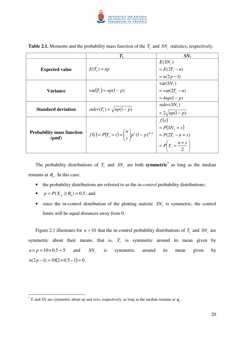
The probability distributions of iT and iSN are both symmetric* as long as the median
remains at 0θ . In this case:
• the probability distributions are referred to as the in-control probability distributions;
• 5.0)( 0 =≥= θijXPp ; and
• since the in-control distribution of the plotting statistic iSN is symmetric, the control
limits will be equal distances away from 0.
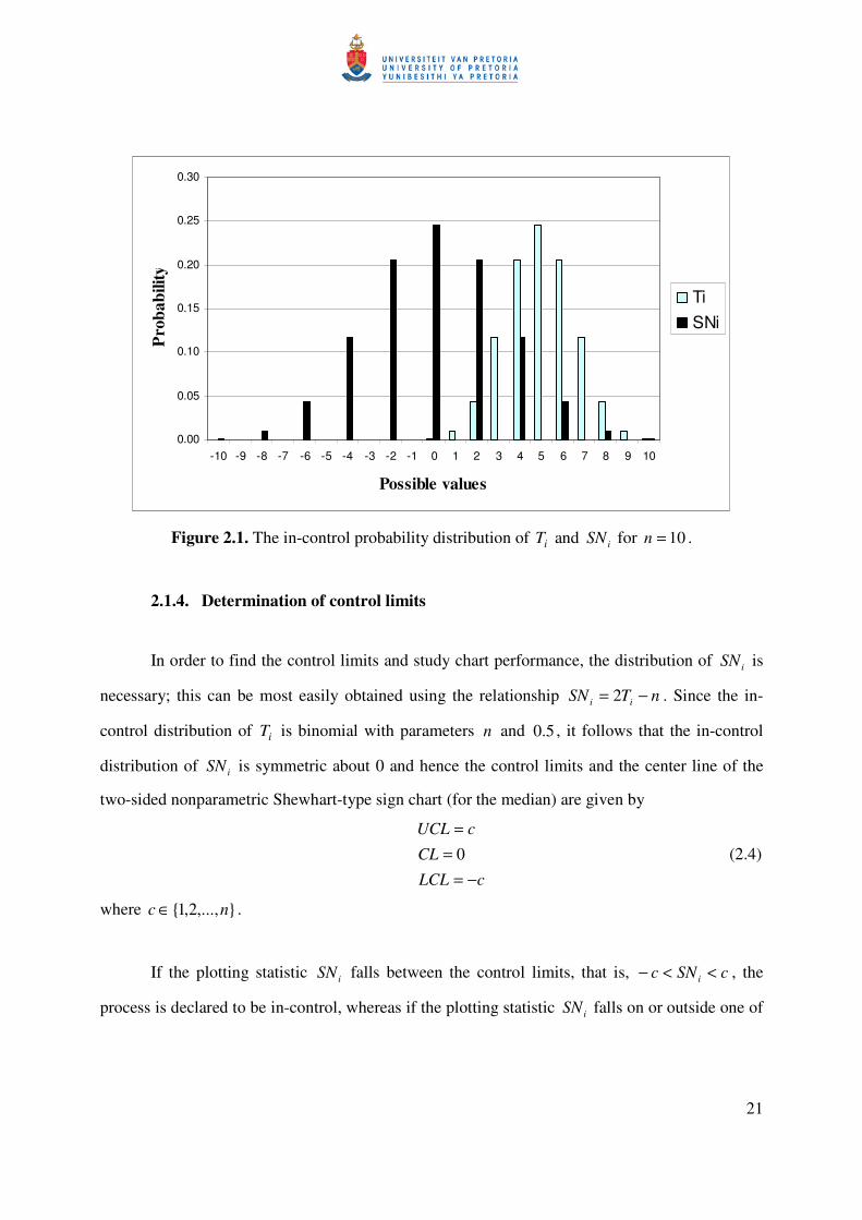
Figure 2.1 illustrates for 10=n that the in-control probability distributions of iT and iSN are
symmetric about their means, that is, iT is symmetric around its mean given by
55.010 =×=× pn and iSN is symmetric around its mean given by
( ) 015.0210)12( =−×=−pn .
* Ti and SNi are symmetric about np and zero, respectively, as long as the median remains at
0θ .
21
0.00
0.05
0.10
0.15
0.20
0.25
0.30
-10 -9 -8 -7 -6 -5 -4 -3 -2 -1 0 1 2 3 4 5 6 7 8 9 10
Possible values
Prob
abili
ty
TiSNi
Figure 2.1. The in-control probability distribution of iT and iSN for 10=n .
2.1.4. Determination of control limits
In order to find the control limits and study chart performance, the distribution of iSN is
necessary; this can be most easily obtained using the relationship nTSN ii −= 2 . Since the in-
control distribution of iT is binomial with parameters n and 5.0 , it follows that the in-control
distribution of iSN is symmetric about 0 and hence the control limits and the center line of the
two-sided nonparametric Shewhart-type sign chart (for the median) are given by
cLCL
CL
cUCL
−==
=0 (2.4)
where ,...,2,1 nc ∈ .
If the plotting statistic iSN falls between the control limits, that is, cSNc i <<− , the
process is declared to be in-control, whereas if the plotting statistic iSN falls on or outside one of
22
the control limits, that is, if cSN i −≤ or cSN i ≥ , the process is declared to be out-of-control. In
the latter case corrective action and a search for assignable causes is necessary.
Take note that iT can also be calculated and plotted against the control limits. This is
done by assuming that the LCL is equal to some constant a and that the UCL is equal to some
constant b , i.e. the control limits are given by: bUCL = and aLCL = . Since the in-control
probability distribution of iT is symmetric when working with the median, that is,
)()( anTPaTP ii −=== , a sensible choice for b is therefore an − .
The control limits and the center line of the nonparametric Shewhart chart (for the
median) using iT as the plotting statistic are given by
aLCL
npCL
anUCL
==
−=
where a denotes a positive integer which is selected such that UCLLCL < .
Although both iT and iSN can be calculated for each sample and be compared to the
control limits, the statistic iSN has the advantage of keeping the control limits symmetric around
zero. Therefore, the plotting statistic iSN is calculated and used as the plotting statistic. The
terms ‘plotting statistic’ and ‘charting statistic’ will be used interchangeably throughout this text.
The question arises: When using iSN as the plotting statistic, what should the values of
the control limits be set equal to? In other words, what is the value of the charting constant c ?
Specifying control limits is one of the critical decisions that must be made in designing a control
chart. By moving the control limits farther away from the center line, we decrease the risk of a
type I error – that is, the risk of a point falling beyond the control limits, indicating an out-of-
control condition when no assignable cause is present. However, widening the control limits will
also increase the risk of a type II error – that is, the risk of a point falling between the control
limits when the process is really out-of-control. If we move the control limits closer to the center
line, the opposite effect is obtained: The risk of type I error is increased, while the risk of type II
23
error is decreased. Consequently, the control limits are chosen such that if the process is in-
control, nearly all of the sample points will fall between them. In other words, the charting
constant c is typically obtained for a specified in-control average run length, which, in case K, is
equal to the reciprocal of the nominal FAR , α . Thus, using the symmetry of the binomial
distribution, c is the smallest integer such that ( )20
αθ ≤≥ cSNP i . For example, using Table G of
Gibbons and Chakraborti (2003) we give some ( )tTP ≥0θ values in Table 2.2 that may be
considered “small” in a SPC context. The charting constant c is obtained using ntc −= 2 (recall
that the sign test statistic iSN is expressed in terms of the statistic iT by the relationship
nTSN ii −= 2 ). The false alarm rate is obtained by adding the probability in the left tail,
( )tnTP −≤0θ , and the probability in the right tail, ( )tTP ≥
0θ , i.e. =FAR
( ) ( )tTPtnTP ≥+−≤00 θθ . Since the probability distribution of iT is symmetric (as long as the
median remains at 0θ ), the FAR is also obtained using ( )tTPFAR ≥=0
2 θ . For example, for
5=n we get 5=t and thus 5=c for a FAR of 0624.0)0312.0(2 = and this is the lowest FAR
achievable. However for 10=n the FAR drops to 0.0020 if 10=c . It should be noted that the
lowest attainable FAR is always obtained when tn = .
Table 2.2. FAR and 0ARL of a sign control chart for various values of n = t .
n 5 6 7 8 9 10 )(
0tTP ≥≥≥≥θθθθ 0.0312 0.0156 0.0078 0.0039 0.0020 0.0010 )(ααααFAR 0.0624 0.0312 0.0156 0.0078 0.0040 0.0020
0ARL 16.00 32.00 64.00 128.00 256.00 512.00
Looking at the attainable FAR and 0ARL values shown in Table 2.2, we see that unless
the sample size is at least 10, the sign chart would be somewhat unattractive (from an operational
point of view) in SPC applications, where one often stipulates a large in-control average run
length, as large as 370 or 500, and a small FAR , as small as 0.0027. If, for example, the FAR is
too ‘large’, which is the case for ‘small’ sample sizes, many false alarms will be expected by this
chart leading to a possible loss of time and resources. Then again, the sign chart is the simplest of
nonparametric charts that works under minimal assumptions. In fact, from the hypothesis testing
24
literature, it is known that the sign test (and so the chart) is more robust and efficient when the
chance distribution is symmetric like the normal but with heavier tails such as the double
exponential.
Example 2.1
A Shewhart-type sign chart for the Montgomery (2001) piston ring data
We illustrate the Shewhart-type sign chart using a set of data from Montgomery (2001;
Tables 5.1 and 5.2) on the inside diameters of piston rings manufactured by a forging process. A
part of this data, fifteen prospective samples (Table 5.2) each of five observations, is used here.
The rest of the data (Table 5.1) will be used later. We assume that the underlying distribution is
symmetric with a known median 740 =θ mm. From Table G (see Gibbons and Chakraborti
(2003)) we obtain 5=t (when 5=n ) for an achieved false alarm rate of 0624.0)0312.0(2 = .
Therefore, 5552 =−×=c and the control limits and the center line of the nonparametric
Shewhart sign chart are given by 5=UCL , 0=CL and 5−=LCL .
Panel a of Table 2.3 displays the sample number. The two rows of each cell in panel b
shows the individual observations and )( 0θ−ijxsign values, respectively. The iSN and iT values
are shown in panel c and panel d, respectively.
As an example, the calculation of 1SN (found in Table 2.3) is given.
)()()()()( 0150140130120111 θθθθθ −+−+−+−+−= xsignxsignxsignxsignxsignSN )7474()7473.986()7474.030()7474.015()7474.012( −+−+−+−+−= signsignsignsignsign
)0()014.0()03.0()015.0()012.0( signsignsignsignsign +−+++=
.201111
=+−++=
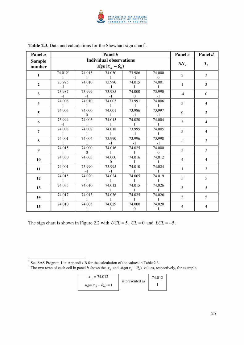
25
Table 2.3. Data and calculations for the Shewhart sign chart*.
Panel a Panel b Panel c Panel d Sample number
Individual observations )( 0θθθθ−−−−ijxsign iSN iT
1 74.012† 1
74.015 1
74.030 1
73.986 -1
74.000 0 2 3
2 73.995 -1
74.010 1
73.990 -1
74.015 1
74.001 1 1 3
3 73.987 -1
73.999 -1
73.985 -1
74.000 0
73.990 -1 -4 0
4 74.008 1
74.010 1
74.003 1
73.991 -1
74.006 1 3 4
5 74.003 1
74.000 0
74.001 1
73.986 -1
73.997 -1 0 2
6 73.994 -1
74.003 1
74.015 1
74.020 1
74.004 1 3 4
7 74.008 1
74.002 1
74.018 1
73.995 -1
74.005 1 3 4
8 74.001 1
74.004 1
73.990 -1
73.996 -1
73.998 -1 -1 2
9 74.015 1
74.000 0
74.016 1
74.025 1
74.000 0 3 3
10 74.030 1
74.005 1
74.000 0
74.016 1
74.012 1 4 4
11 74.001 1
73.990 -1
73.995 -1
74.010 1
74.024 1 1 3
12 74.015 1
74.020 1
74.024 1
74.005 1
74.019 1 5 5
13 74.035 1
74.010 1
74.012 1
74.015 1
74.026 1 5 5
14 74.017 1
74.013 1
74.036 1
74.025 1
74.026 1 5 5
15 74.010 1
74.005 1
74.029 1
74.000 0
74.020 1 4 4
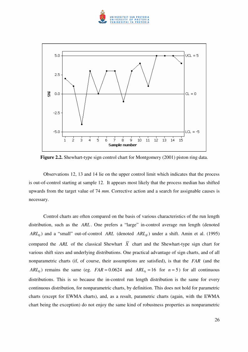
The sign chart is shown in Figure 2.2 with 5=UCL , 0=CL and 5−=LCL .
* See SAS Program 1 in Appendix B for the calculation of the values in Table 2.3. † The two rows of each cell in panel b shows the ijx and )( 0θ−ijxsign values, respectively, for example,
012.7411 =x
1)( 011 =− θxsign is presented as
74.012
1
26
Figure 2.2. Shewhart-type sign control chart for Montgomery (2001) piston ring data.
Observations 12, 13 and 14 lie on the upper control limit which indicates that the process
is out-of-control starting at sample 12. It appears most likely that the process median has shifted
upwards from the target value of 74 mm. Corrective action and a search for assignable causes is
necessary.
Control charts are often compared on the basis of various characteristics of the run length
distribution, such as the ARL . One prefers a “large” in-control average run length (denoted
0ARL ) and a “small” out-of-control ARL (denoted δARL ) under a shift. Amin et al. (1995)
compared the ARL of the classical Shewhart X chart and the Shewhart-type sign chart for
various shift sizes and underlying distributions. One practical advantage of sign charts, and of all
nonparametric charts (if, of course, their assumptions are satisfied), is that the FAR (and the
0ARL ) remains the same (eg. 0624.0=FAR and 160 =ARL for 5=n ) for all continuous
distributions. This is so because the in-control run length distribution is the same for every
continuous distribution, for nonparametric charts, by definition. This does not hold for parametric
charts (except for EWMA charts), and, as a result, parametric charts (again, with the EWMA
chart being the exception) do not enjoy the same kind of robustness properties as nonparametric

27
charts do. It should be noted that the EWMA control chart can be designed so that it is robust to
the normality assumption. On this point, Borror, Montgomery and Runger (1999) showed that the
0ARL of the EWMA chart is reasonably close to the normal-theory value for both skewed and
heavy-tailed symmetric non-normal distributions.
2.1.5. Run length distribution
The number of subgroups or samples that need to be collected (or, equivalently, the
number of plotting statistics that must be plotted) before the next out-of-control signal is given by
a chart is called the run length. The run length is a random variable denoted by N . A popular
measure of chart performance is the ‘expected value’ or the ‘mean’ of the run length distribution,
called the average run length ( ARL ). Various researchers, see for example, Barnard (1959) and
Chakraborti (2007), have suggested using other characteristics for assessment of chart
performance, for example, the standard deviation of the run length distribution ( SDRL ), the
median run length ( MRL ) and/or other percentiles of the run length distribution. This
recommendation is warranted seeing as (i) the run-length can only take on positive integer values
by definition, (ii) the shape of this distribution is significantly right-skewed and (iii) it’s known
that in a right-skewed distribution the mean is greater than the median and thus is usually not a
fair representation of a typical observation or the center.
Since the observations plotted on the control chart are assumed to be independent, the
number of points that must be plotted until the first plotted point plots on or exceeds a control
limit is a geometric random variable with parameter p , where p denotes the probability of a
success (or, equivalently, the probability of a signal). Therefore, Signal))((~ PGEON where
pP =Signal)( . The well-known properties of the geometric distribution are given in panel a of
Table 2.4 and we use the fact that if q denotes the probability of no signal then
1Signal) No(Signal)( =+=+ qpPP , i.e. pq −= 1 . The properties of the run length N are
derived using the well-known properties of the geometric distribution and they are displayed in
panel b of Table 2.4.
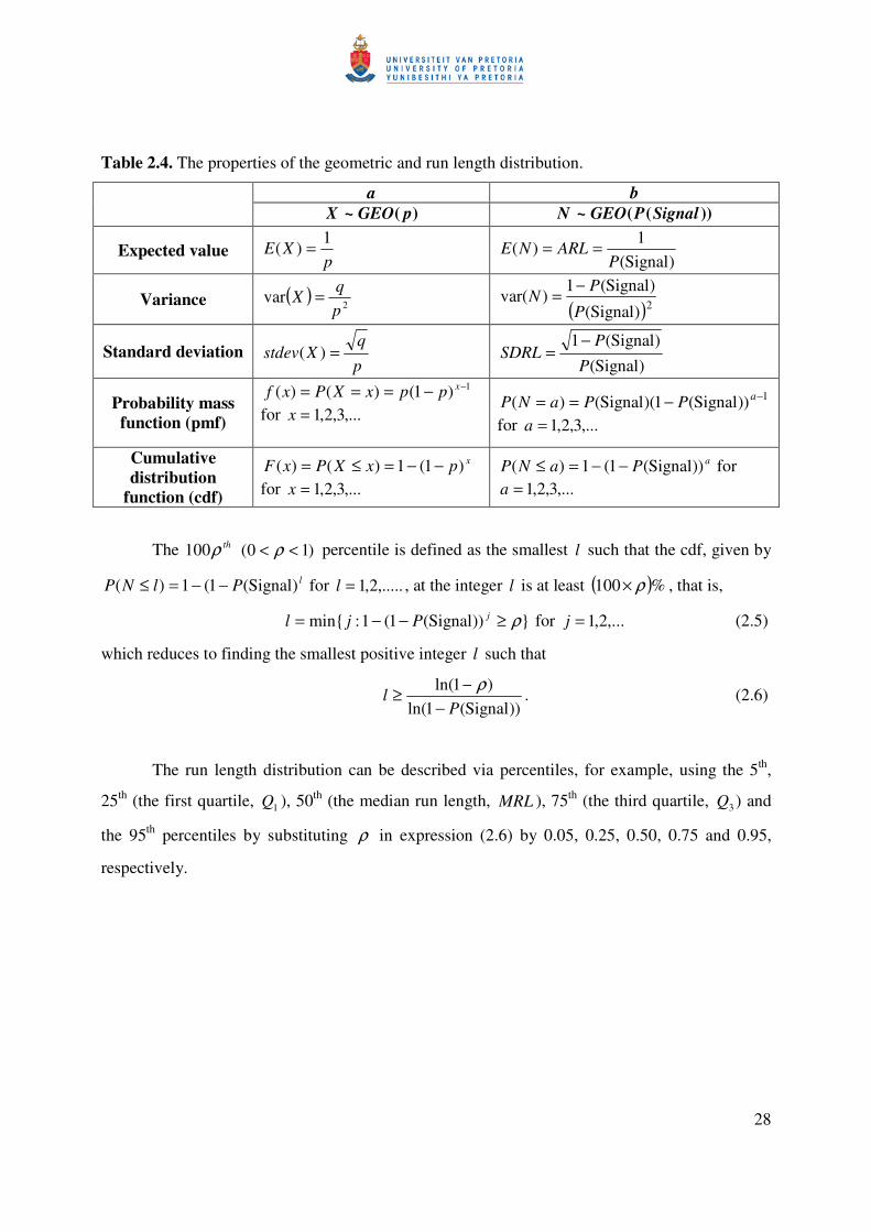
28
Table 2.4. The properties of the geometric and run length distribution.
a b )(~ pGEOX ))((~ SignalPGEON
Expected value p
XE1
)( = )Signal(
1)(
PARLNE ==
Variance ( )2var
pq
X = ( )2)Signal(
)Signal(1)var(
P
PN
−=
Standard deviation pq
Xstdev =)( )Signal(
)Signal(1P
PSDRL
−=
Probability mass function (pmf)
1)1()()( −−=== xppxXPxf for ,...3,2,1=x
1))Signal(1)(Signal()( −−== aPPaNP for ,...3,2,1=a
Cumulative distribution
function (cdf)
xpxXPxF )1(1)()( −−=≤= for ,...3,2,1=x
aPaNP ))Signal(1(1)( −−=≤ for ,...3,2,1=a
The thρ100 )10( << ρ percentile is defined as the smallest l such that the cdf, given by
lPlNP )Signal(1(1)( −−=≤ for ,.....2,1=l , at the integer l is at least ( )%100 ρ× , that is,
))Signal(1(1:min ρ≥−−= jPjl for ,...2,1=j (2.5)
which reduces to finding the smallest positive integer l such that
))Signal(1ln(
)1ln(P
l−
−≥ ρ. (2.6)
The run length distribution can be described via percentiles, for example, using the 5th,
25th (the first quartile, 1Q ), 50th (the median run length, MRL ), 75th (the third quartile, 3Q ) and
the 95th percentiles by substituting ρ in expression (2.6) by 0.05, 0.25, 0.50, 0.75 and 0.95,
respectively.
29
2.1.6. One-sided control charts
A lower one-sided chart will have a LCL equal to some constant value with no UCL ,
whereas an upper one-sided chart will have an UCL equal to some constant value with no LCL .
One-sided control charts are particularly useful in situations where only an upward (or only a
downward) shift in a particular process parameter is of interest. For example, we might be
monitoring the breaking strength of material used to make parachutes. If the breaking strength of
the material decreases it might tear at a critical time, whereas if the breaking strength of the
material increases it is beneficial to the user, since the material would, most likely, not tear while
being used. In such a scenario a lower one-sided chart will be sufficient, since we are only
interested in detecting a downward shift in a process parameter.
For the sign control chart, if we are only interested in detecting a downward shift we will
use a lower one-sided sign control chart with cLCL −= and no upper control limit.
Consequently, if the plotting statistic iSN falls on or below the LCL the process is declared to be
out-of-control. On the other hand, if we are only interested in detecting an upward shift we will
use an upper one-sided sign control chart with cUCL = and no lower control limit.
Consequently, if the plotting statistic iSN falls on or above the UCL the process is declared to be
out-of-control.
2.1.6.1. Lower one-sided control charts
Result 2.1: Probability of a signal
The probability that the control chart signals, that is, the probability that the plotting
statistic iSN is smaller than or equal to the lower control limit, can be expressed in terms of
)( 0θ≥= ijXPp , the sample size n and the constant c . Let )Signal(LP denote the probability of
a signal, where superscript L refers to the lower one-sided chart. The probability of a signal is
then given by
30
)()()Signal( cSNPLCLSNPP iL
iLL −≤=≤= )2( cnTP i
L −≤−=
−≤=2
cnTP i
L . (2.7)
Note that (2.7) can be solved by using the cdf of a Binomial distribution.
The probabilities, )Signal(LP ’s, were computed using Mathcad (see Mathcad Program 2
in Appendix B). In doing so, we kept in mind that we ultimately wanted to use the iT statistic in
the calculation of )Signal(LP , because then we could use the cdf of a Binomial distribution to
find )Signal(LP . Therefore, the probability of a signal for the lower one-sided sign chart was
computed using
inia
ii
Li
LL ppi
naTPLCLTPP −
=
−
=≤=≤= )1()()()Signal(
0
. (2.8)
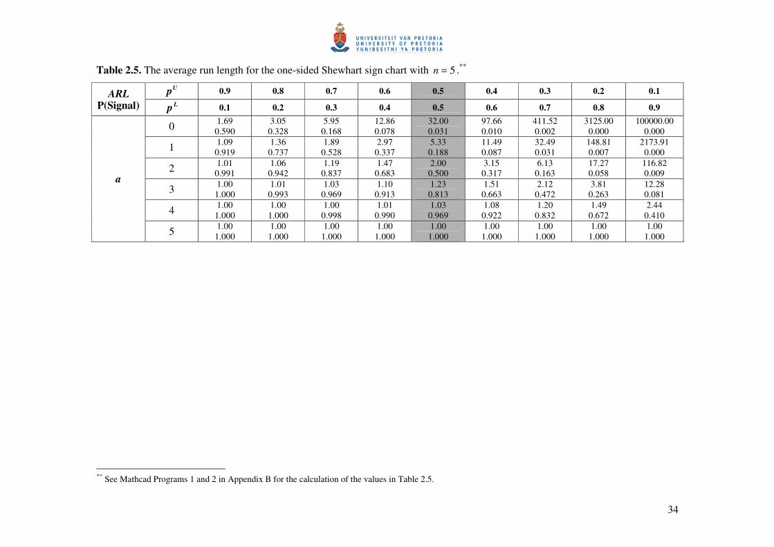
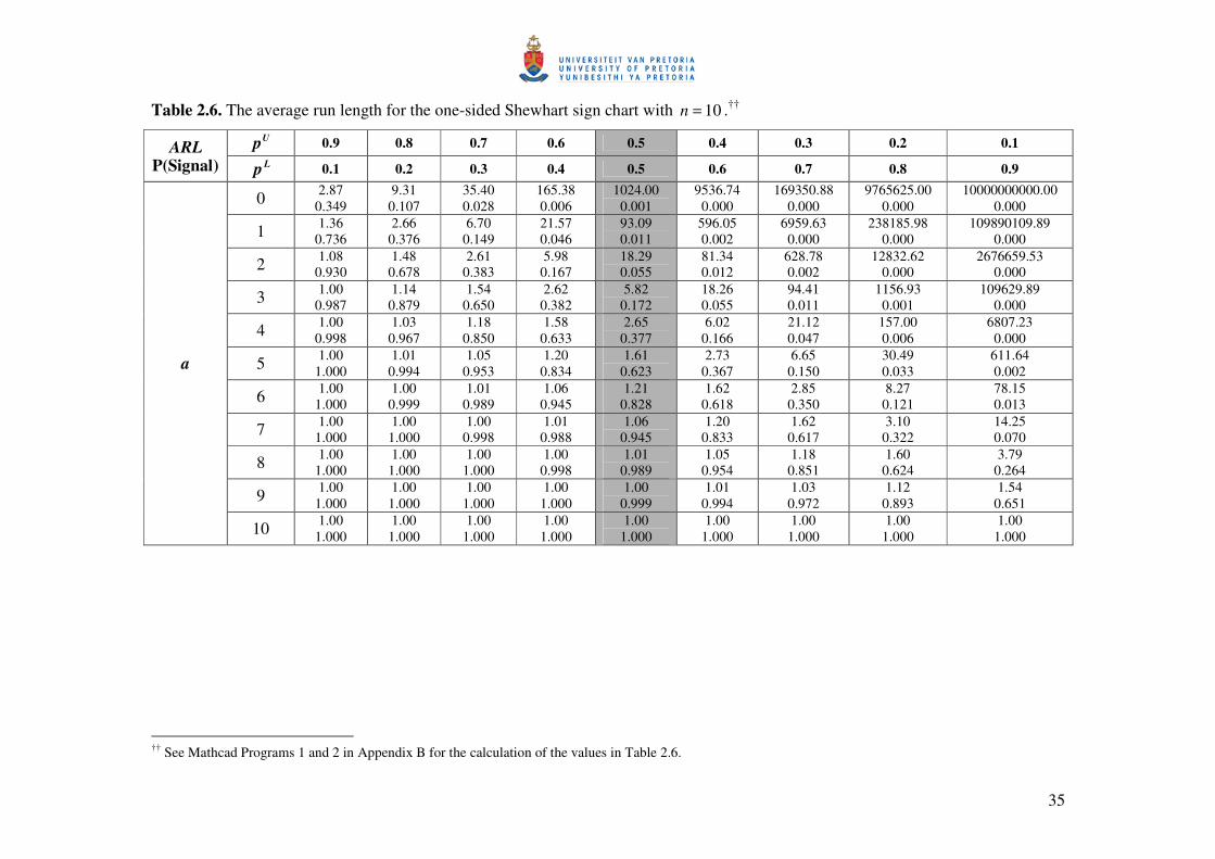
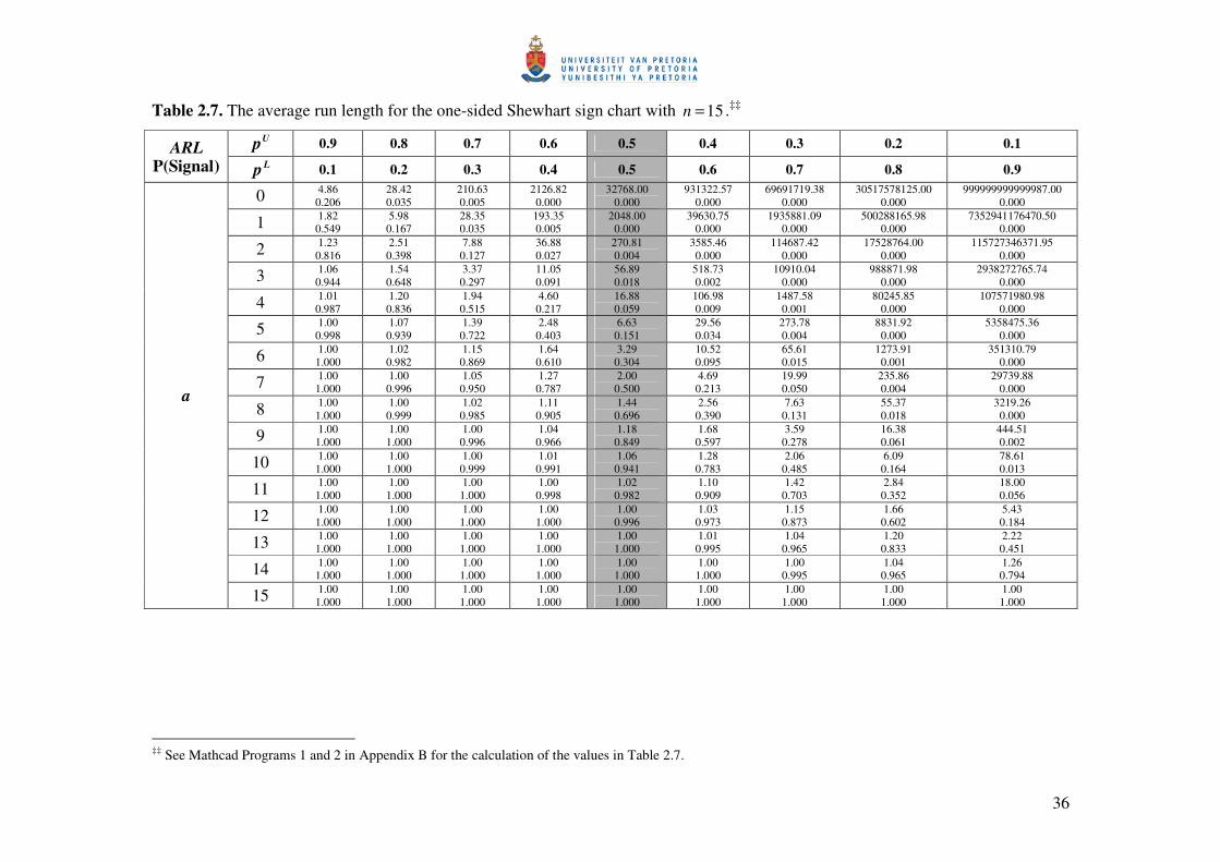
The results are given in Tables 2.5, 2.6 and 2.7 for 5=n , 10=n and 15=n , respectively, for
9.0)1.0(1.0=p and na )1(0= . The shaded column ( 5.0=p ) contains the value of the in-control
average run length ( 0ARL ) and the false alarm rate ( FAR ), whereas the rest of the columns
( 5.0≠p ) contain the values of the out-of-control average run length ( δARL ) and the probability
of a signal (when the process is considered to be out-of-control).
Result 2.2: Average run length
Since the run length has a geometric distribution (recall that ))Signal((~ LPGEON the
expected value of this specific geometric distribution will be equal to )Signal(
1LP
. The ARL is
the mean of the run length distribution. Therefore, we have that
)Signal(
1)(
LL
PNEARL == . (2.9)
31
Result 2.3: Standard deviation of the run length
Since the run length has a geometric distribution (see Result 2.2) the standard deviation
will be equal to )Signal(
)Signal(1L
L
P
P−. Therefore, we have that
)Signal(
)Signal(1)(
L
LL
P
PNSDRL
−= . (2.10)
Example 2.2
For a sample size of 10 ( 10=n ), 5.0=p and 2=a , we can calculate the probability of a
signal and the average run length using (2.8) and (2.9), respectively, and we obtain =)Signal(LP
055.0)5.01()5.0(10 10
2
0
=−
−
= ii
i i and 29.18
055.01 ==LARL .
2.1.6.2. Upper one-sided control charts
Result 2.4: Probability of a signal
The probability that the control chart signals, that is, the probability that the plotting
statistic iSN is greater than or equal to the upper control limit, can be expressed in terms of
)( 0θ≥= ijXPp , the sample size n and the constant c . Let )Signal(UP denote the probability
of a signal, where superscript U refers to the upper one-sided chart. The probability of a signal is
then given by
)()()Signal( cSNPUCLSNPP iU
iUU ≥=≥=
+≥=2
cnTP i
U
−+≤−= 12
1cn
TP iU . (2.11)
Note that (2.11) can be solved by using the cdf of a Binomial distribution.
The probabilities, )Signal(UP ’s, were computed using Mathcad (see Mathcad Program 1
in Appendix B). In doing so, we kept in mind that we ultimately wanted to use the iT statistic in
32
the calculation of )Signal(UP , because then we could use the cdf of a Binomial distribution to
find )Signal(UP . Therefore, the probability of a signal for the upper one-sided sign chart was
computed using
inin
anii
Ui
UU ppi
nanTPUCLTPP −
−=
−
=−≥=≥= )1()()()Signal( . (2.12)
The results are given in Tables 2.5, 2.6 and 2.7 for 5=n , 10=n and 15=n , respectively, for
9.0)1.0(1.0=p and na )1(0= . The shaded column ( 5.0=p ) contains the value of the in-control
average run length ( 0ARL ) and the false alarm rate ( FAR ), whereas the rest of the columns
( 5.0≠p ) contain the values of the out-of-control average run length ( δARL ) and the probability
of a signal (when the process is considered to be out-of-control).
Result 2.5: Average run length
Since the run length has a geometric distribution (recall that ))Signal((~ UPGEON the
expected value of this specific geometric distribution will be equal to )Signal(
1UP
. The ARL is
the mean of the run length distribution. Therefore, we have that
)Signal(
1)(
UU
PNEARL == . (2.13)
Result 2.6: Standard deviation of the run length
Since the run length has a geometric distribution (see Result 2.5) the standard deviation
will be equal to )Signal(
)Signal(1U
U
P
P−. Therefore, we have that
Signal)(
)Signal(1)(
U
UU
P
PNSDRL
−= . (2.14)
33
Example 2.3
For a sample size of 10 ( 10=n ), 5.0=p and 2=a , we can calculate the probability of a
signal and the average run length using (2.12) and (2.13), respectively, and we obtain
055.0)5.01()5.0(10
)Signal( 1010
210
=−
= −
−= ii
i
U
iP and 29.18
055.01 ==UARL .
Application
The average run length values for the lower and upper one-sided Shewhart sign charts are
calculated by evaluating expressions (2.8) and (2.9) for the lower one-sided chart and expressions
(2.12) and (2.13) for the upper one-sided chart using 10,5=n and 15 , respectively. These values
are shown in Table 2.5, Table 2.6 and Table 2.7, respectively.* As mentioned previously, the
shaded column ( 5.0=p ) contains the value of the in-control average run length ( 0ARL ) and the
false alarm rate ( FAR ), whereas the rest of the columns ( 5.0≠p ) contain the values of the out-
of-control average run length ( δARL ) and the probability of a signal (when the process is
considered to be out-of-control).
* Table 2.5, Table 2.6 and Table 2.7 should preferably be studied together.
34
Table 2.5. The average run length for the one-sided Shewhart sign chart with 5=n .** Up 0.9 0.8 0.7 0.6 0.5 0.4 0.3 0.2 0.1 ARL
P(Signal) Lp 0.1 0.2 0.3 0.4 0.5 0.6 0.7 0.8 0.9
0 1.69 0.590
3.05 0.328
5.95 0.168
12.86 0.078
32.00 0.031
97.66 0.010
411.52 0.002
3125.00 0.000
100000.00 0.000
1 1.09 0.919
1.36 0.737
1.89 0.528
2.97 0.337
5.33 0.188
11.49 0.087
32.49 0.031
148.81 0.007
2173.91 0.000
2 1.01 0.991
1.06 0.942
1.19 0.837
1.47 0.683
2.00 0.500
3.15 0.317
6.13 0.163
17.27 0.058
116.82 0.009
3 1.00 1.000
1.01 0.993
1.03 0.969
1.10 0.913
1.23 0.813
1.51 0.663
2.12 0.472
3.81 0.263
12.28 0.081
4 1.00 1.000
1.00 1.000
1.00 0.998
1.01 0.990
1.03 0.969
1.08 0.922
1.20 0.832
1.49 0.672
2.44 0.410
a
5 1.00 1.000
1.00 1.000
1.00 1.000
1.00 1.000
1.00 1.000
1.00 1.000
1.00 1.000
1.00 1.000
1.00 1.000
** See Mathcad Programs 1 and 2 in Appendix B for the calculation of the values in Table 2.5.
35
Table 2.6. The average run length for the one-sided Shewhart sign chart with 10=n .†† Up 0.9 0.8 0.7 0.6 0.5 0.4 0.3 0.2 0.1 ARL
P(Signal) Lp 0.1 0.2 0.3 0.4 0.5 0.6 0.7 0.8 0.9
0 2.87 0.349
9.31 0.107
35.40 0.028
165.38 0.006
1024.00 0.001
9536.74 0.000
169350.88 0.000
9765625.00 0.000
10000000000.00 0.000
1 1.36 0.736
2.66 0.376
6.70 0.149
21.57 0.046
93.09 0.011
596.05 0.002
6959.63 0.000
238185.98 0.000
109890109.89 0.000
2 1.08 0.930
1.48 0.678
2.61 0.383
5.98 0.167
18.29 0.055
81.34 0.012
628.78 0.002
12832.62 0.000
2676659.53 0.000
3 1.00 0.987
1.14 0.879
1.54 0.650
2.62 0.382
5.82 0.172
18.26 0.055
94.41 0.011
1156.93 0.001
109629.89 0.000
4 1.00 0.998
1.03 0.967
1.18 0.850
1.58 0.633
2.65 0.377
6.02 0.166
21.12 0.047
157.00 0.006
6807.23 0.000
5 1.00 1.000
1.01 0.994
1.05 0.953
1.20 0.834
1.61 0.623
2.73 0.367
6.65 0.150
30.49 0.033
611.64 0.002
6 1.00 1.000
1.00 0.999
1.01 0.989
1.06 0.945
1.21 0.828
1.62 0.618
2.85 0.350
8.27 0.121
78.15 0.013
7 1.00 1.000
1.00 1.000
1.00 0.998
1.01 0.988
1.06 0.945
1.20 0.833
1.62 0.617
3.10 0.322
14.25 0.070
8 1.00 1.000
1.00 1.000
1.00 1.000
1.00 0.998
1.01 0.989
1.05 0.954
1.18 0.851
1.60 0.624
3.79 0.264
9 1.00 1.000
1.00 1.000
1.00 1.000
1.00 1.000
1.00 0.999
1.01 0.994
1.03 0.972
1.12 0.893
1.54 0.651
a
10 1.00 1.000
1.00 1.000
1.00 1.000
1.00 1.000
1.00 1.000
1.00 1.000
1.00 1.000
1.00 1.000
1.00 1.000
†† See Mathcad Programs 1 and 2 in Appendix B for the calculation of the values in Table 2.6.
36
Table 2.7. The average run length for the one-sided Shewhart sign chart with 15=n .‡‡ Up 0.9 0.8 0.7 0.6 0.5 0.4 0.3 0.2 0.1 ARL
P(Signal) Lp 0.1 0.2 0.3 0.4 0.5 0.6 0.7 0.8 0.9
0 4.86 0.206
28.42 0.035
210.63 0.005
2126.82 0.000
32768.00 0.000
931322.57 0.000
69691719.38 0.000
30517578125.00 0.000
999999999999987.00 0.000
1 1.82 0.549
5.98 0.167
28.35 0.035
193.35 0.005
2048.00 0.000
39630.75 0.000
1935881.09 0.000
500288165.98 0.000
7352941176470.50 0.000
2 1.23 0.816
2.51 0.398
7.88 0.127
36.88 0.027
270.81 0.004
3585.46 0.000
114687.42 0.000
17528764.00 0.000
115727346371.95 0.000
3 1.06 0.944
1.54 0.648
3.37 0.297
11.05 0.091
56.89 0.018
518.73 0.002
10910.04 0.000
988871.98 0.000
2938272765.74 0.000
4 1.01 0.987
1.20 0.836
1.94 0.515
4.60 0.217
16.88 0.059
106.98 0.009
1487.58 0.001
80245.85 0.000
107571980.98 0.000
5 1.00 0.998
1.07 0.939
1.39 0.722
2.48 0.403
6.63 0.151
29.56 0.034
273.78 0.004
8831.92 0.000
5358475.36 0.000
6 1.00 1.000
1.02 0.982
1.15 0.869
1.64 0.610
3.29 0.304
10.52 0.095
65.61 0.015
1273.91 0.001
351310.79 0.000
7 1.00 1.000
1.00 0.996
1.05 0.950
1.27 0.787
2.00 0.500
4.69 0.213
19.99 0.050
235.86 0.004
29739.88 0.000
8 1.00 1.000
1.00 0.999
1.02 0.985
1.11 0.905
1.44 0.696
2.56 0.390
7.63 0.131
55.37 0.018
3219.26 0.000
9 1.00 1.000
1.00 1.000
1.00 0.996
1.04 0.966
1.18 0.849
1.68 0.597
3.59 0.278
16.38 0.061
444.51 0.002
10 1.00 1.000
1.00 1.000
1.00 0.999
1.01 0.991
1.06 0.941
1.28 0.783
2.06 0.485
6.09 0.164
78.61 0.013
11 1.00 1.000
1.00 1.000
1.00 1.000
1.00 0.998
1.02 0.982
1.10 0.909
1.42 0.703
2.84 0.352
18.00 0.056
12 1.00 1.000
1.00 1.000
1.00 1.000
1.00 1.000
1.00 0.996
1.03 0.973
1.15 0.873
1.66 0.602
5.43 0.184
13 1.00 1.000
1.00 1.000
1.00 1.000
1.00 1.000
1.00 1.000
1.01 0.995
1.04 0.965
1.20 0.833
2.22 0.451
14 1.00 1.000
1.00 1.000
1.00 1.000
1.00 1.000
1.00 1.000
1.00 1.000
1.00 0.995
1.04 0.965
1.26 0.794
a
15 1.00 1.000
1.00 1.000
1.00 1.000
1.00 1.000
1.00 1.000
1.00 1.000
1.00 1.000
1.00 1.000
1.00 1.000
‡‡ See Mathcad Programs 1 and 2 in Appendix B for the calculation of the values in Table 2.7.

37
2.1.7. Two-sided control charts
Result 2.7: Probability of a signal
The probability that the control chart signals, that is, the probability that the plotting
statistic iSN is greater than or equal to the UCL , or smaller than or equal to the LCL , can be
expressed in terms of )( 0θ≥= ijXPp , the sample size n and the constant c . The probability of
a signal is then given by
−≤+
−+≤−=<−<−−=2
12
1)2(1)Signal(cn
TPcn
TPcnTcPP iii . (2.15)
Note that (2.15) can be solved by using the cdf of a binomial distribution.
Result 2.8: Average run length
Since the run length has a geometric distribution we have that
)Signal(
1)(
PNEARL == . (2.16)
Compare expression (2.16) to expressions (2.9) and (2.13).
Result 2.9: Standard deviation of the run length
Since the run length has a geometric distribution we have that
Signal)(
)Signal(1)(
P
PNSDRL
−= . (2.17)
Compare expression (2.17) to expressions (2.10) and (2.14).
38
2.1.8. Summary
In Section 2.1 we have described and evaluated the nonparametric Shewhart-type sign
control chart. Generally speaking, when the underlying process distribution is either asymmetric
or symmetric with heavy tails, sign charts are more efficient while the reverse is true for normal
and normal-like distributions with light tails. One practical advantage of the nonparametric
Shewhart-type sign control chart is that there is no need to assume a particular parametric
distribution for the underlying process (see Section 1.4 for other advantages of nonparametric
charts).
2.2. The Shewhart-type control chart with warning limits
2.2.1. Introduction
It is known that standard Shewhart charts are efficient in detecting large process shifts
quickly, but are insensitive to small shifts (see, for example, Montgomery (2005)). Additional
supplementary rules have been suggested to increase the sensitivity of standard Shewhart charts
to small process shifts. Shewhart (1941) gave the first proposal in making the standard Shewhart
chart more sensitive to small process shifts by proposing that additional sensitizing tests should
be incorporated into the standard Shewhart chart. Various rules or ‘tests for special causes’ have
been considered in the literature for parametric control charts; see for example, the rules
associated with the Shewhart control chart in Nelson (1984) and in the Western Electric
handbook (1956). See also the discussion in Montgomery (2001).
Runs rules can be used to increase the sensitivity of standard Shewhart charts. Denote
each runs rule by ),,,( lknrR where a signal is given if r out of the last n points fall in the
interval ),( lk , where nr ≤ are integers and lk < . The well-known standardized Shewhart X
control chart is denoted by ),3,1,1()3,,1,1( ∞∪−−∞ RR , since the standardized Shewhart X
control chart signals if any charting statistic (1 out of 1 point) falls in the interval )3,( −−∞ or if
any charting statistic (1 out of 1 point) falls in the interval ),3( ∞ .

39
Page (1955) considered a Markov-chain approach for simple combinations of runs rules.
Amin et al. (1995) considered Shewhart-type sign charts with warning limits and runs rules. Page
(1962), Weindling, Littauer and Oliveira (1979) and Champ and Woodall (1987) studied the
properties of X charts with warning limits.
Incorporating the runs rules ),,1,1(),,1,1( ∞∪−∞ UL aRaR into the Shewhart sign chart is
similar to using action limits where action will be taken if any 1 point falls outside the action
limits. Incorporating the two runs rules ),,,(),,,( LLUU warrRawrrR ∪ into the Shewhart sign
chart is similar to using warning limits where action will be taken if r successive points fall
between the warning and action limits, that is, action will be taken if r successive points fall
between Uw and Ua or action will be taken if r successive points fall between La and Lw .
Hence, rule A follows: Action will be taken if r successive points fall between Uw and Ua , or
if r successive points fall between La and Lw , or if any point falls outside the action limits. Let
L denote the ARL of rule A . Assume that the upper action and upper warning limits are equal
to some constants represented by a and w , respectively, that is, aaU = and wwU = . In the case
of the Shewhart-type sign control chart with warning limits, sensible choices for the lower action
and lower warning limits are a− and w− , respectively, that is, aaL −= and wwL −= . The
latter choices are sensible, since the in-control distribution of iSN is symmetric about zero (see
Section 2.1.3).
In Section 2.2.3.1 two runs rules are incorporated into the upper one-sided Shewhart sign
chart. Similarly, in Section 2.2.3.2 two runs rules are incorporated into the lower one-sided
Shewhart sign chart. The average run lengths are computed for the upper and lower charts,
respectively. Finally, in Section 2.2.4 two runs rules are incorporated into the two-sided Shewhart
sign chart.
40
2.2.2. Markov chain representation
A Markov chain representation of a Shewhart chart supplemented with runs rules is used
for calculating the probability that any subset of runs rules will give an out-of-control signal. In
this section some basic concepts of matrices and transition probabilities are given and explained.
An illustrative example follows in the next section, i.e. Section 2.2.3.1.
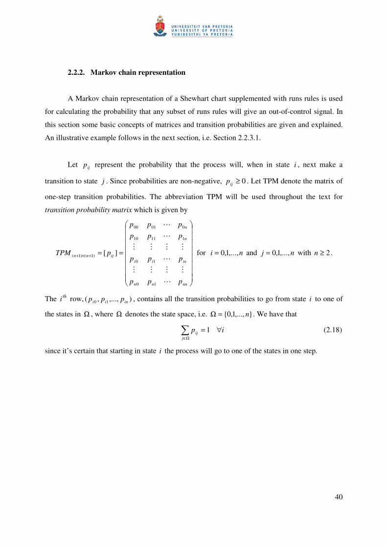
Let ijp represent the probability that the process will, when in state i , next make a
transition to state j . Since probabilities are non-negative, 0≥ijp . Let TPM denote the matrix of
one-step transition probabilities. The abbreviation TPM will be used throughout the text for
transition probability matrix which is given by
==+×+
nnnn
inii
n
n
ijnn
ppp
ppp
ppp
ppp
pTPM
10
10
11110
00100
)1()1( ][ for ni ,...,1,0= and nj ,...,1,0= with 2≥n .
The thi row, ),...,,( 10 inii ppp , contains all the transition probabilities to go from state i to one of
the states in Ω , where Ω denotes the state space, i.e. ,...,1,0 n=Ω . We have that
Ω∈
∀=j
ij ip 1 (2.18)
since it’s certain that starting in state i the process will go to one of the states in one step.
41
2.2.3. One-sided control charts
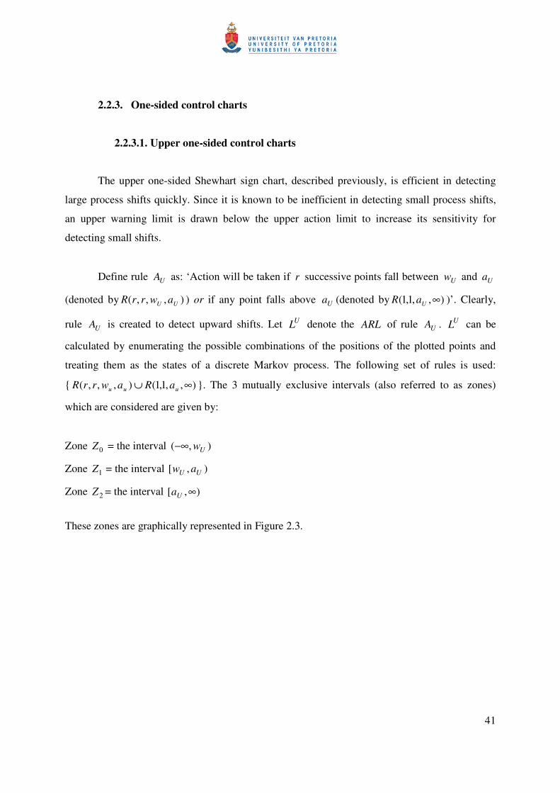
2.2.3.1. Upper one-sided control charts
The upper one-sided Shewhart sign chart, described previously, is efficient in detecting
large process shifts quickly. Since it is known to be inefficient in detecting small process shifts,
an upper warning limit is drawn below the upper action limit to increase its sensitivity for
detecting small shifts.
Define rule UA as: ‘Action will be taken if r successive points fall between Uw and Ua
(denoted by ),,,( UU awrrR ) or if any point falls above Ua (denoted by ),,1,1( ∞UaR )’. Clearly,
rule UA is created to detect upward shifts. Let UL denote the ARL of rule UA . UL can be
calculated by enumerating the possible combinations of the positions of the plotted points and
treating them as the states of a discrete Markov process. The following set of rules is used:
),,1,1(),,,( ∞∪ uuu aRawrrR . The 3 mutually exclusive intervals (also referred to as zones)
which are considered are given by:
Zone 0Z = the interval ),( Uw−∞
Zone 1Z = the interval ),[ UU aw
Zone 2Z = the interval ),[ ∞Ua
These zones are graphically represented in Figure 2.3.
42
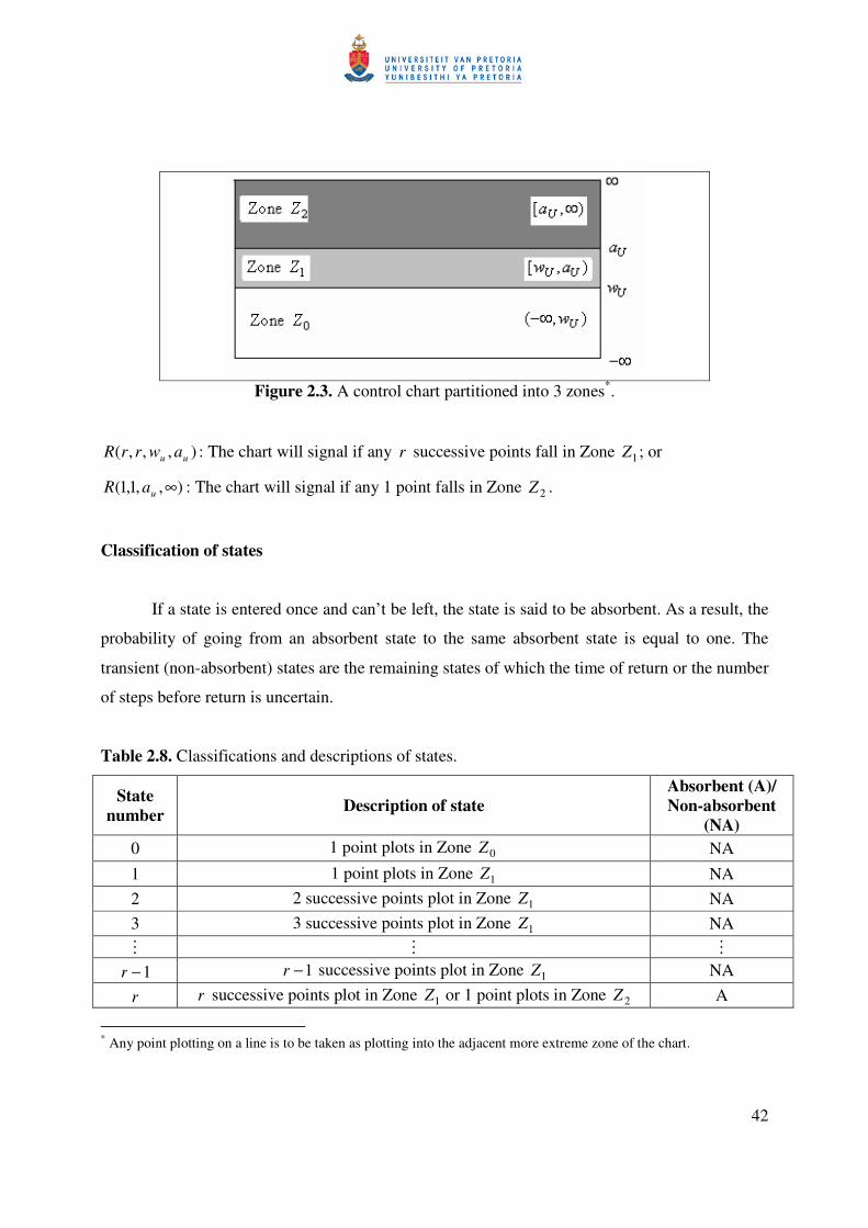
Figure 2.3. A control chart partitioned into 3 zones*.
),,,( uu awrrR : The chart will signal if any r successive points fall in Zone 1Z ; or
),,1,1( ∞uaR : The chart will signal if any 1 point falls in Zone 2Z .
Classification of states
If a state is entered once and can’t be left, the state is said to be absorbent. As a result, the
probability of going from an absorbent state to the same absorbent state is equal to one. The
transient (non-absorbent) states are the remaining states of which the time of return or the number
of steps before return is uncertain.
Table 2.8. Classifications and descriptions of states.
State number Description of state
Absorbent (A)/ Non-absorbent
(NA) 0 1 point plots in Zone 0Z NA 1 1 point plots in Zone 1Z NA 2 2 successive points plot in Zone 1Z NA 3 3 successive points plot in Zone 1Z NA
1−r 1−r successive points plot in Zone 1Z NA
r r successive points plot in Zone 1Z or 1 point plots in Zone 2Z A
* Any point plotting on a line is to be taken as plotting into the adjacent more extreme zone of the chart.
43
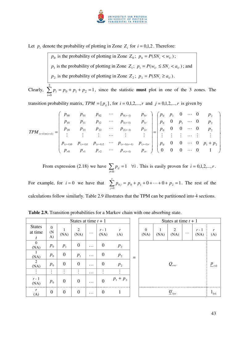
Let ip denote the probability of plotting in Zone iZ for 2,1,0=i . Therefore:
0p is the probability of plotting in Zone 0Z ; )(0 Ui wSNPp <= ;
1p is the probability of plotting in Zone 1Z ; )(1 UiU aSNwPp <≤= ; and
2p is the probability of plotting in Zone 2Z ; )(2 Ui aSNPp ≥= .
Clearly, =
=++=2
0210 1
ii pppp , since the statistic must plot in one of the 3 zones. The
transition probability matrix, ][ ijpTPM = , for ri ,...,2,1,0= and rj ,...,2,1,0= is given by
.
10000000
0000000
210
20
210
210
)1(210
)1()1)(1(2)1(1)1(0)1(
2)1(2222120
1)1(1121110
0)1(0020100
)1()1(
+
=
=
−
−−−−−−
−
−
−
+×+
ppp
pp
ppp
ppp
ppppp
ppppp
ppppp
ppppp
ppppp
TPM
rrrrrrr
rrrrrrr
rr
rr
rr
rr
From expression (2.18) we have Ω∈
∀=j
ij ip 1 . This is easily proven for ri ,...,2,1,0= .
For example, for 0=i we have that 100 2100
0 =+++++==
ppppr
jj . The rest of the
calculations follow similarly. Table 2.9 illustrates that the TPM can be partitioned into 4 sections.
Table 2.9. Transition probabilities for a Markov chain with one absorbing state.
States at time t + 1 States at time t + 1 States at time
t
0 (NA)
1 (NA)
2 (NA) … r - 1
(NA) r
(A) 0
(NA) 1
(NA) 2
(NA) … r - 1 (NA)
r (A)
0 (NA) 0p 1p 0 … 0 2p
1 (NA) 0p 0 1p … 0 2p
2 (NA) 0p 0 0 … 0 2p
… r - 1 (NA) 0p 0 0 … 0 21 pp +
rrQ × 1×rp
r (A) 0 0 0 … 0 1
=
r×1'0 111 ×
44
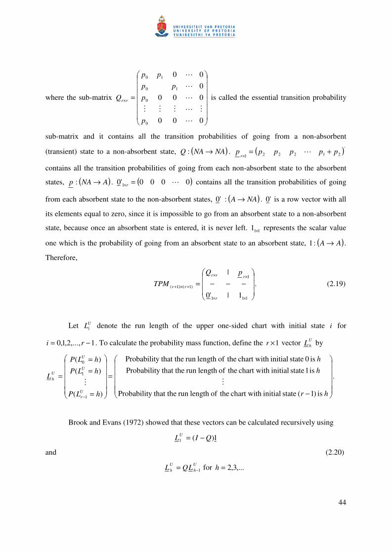
where the sub-matrix rrQ ×
=
000
000000
0
0
10
10
p
p
pp
pp
is called the essential transition probability
sub-matrix and it contains all the transition probabilities of going from a non-absorbent
(transient) state to a non-absorbent state, Q ( )NANA →: . 1×r
p ( )'21222 ppppp +=
contains all the transition probabilities of going from each non-absorbent state to the absorbent
states, p ( )ANA →: . r×1'0 ( )0000 = contains all the transition probabilities of going
from each absorbent state to the non-absorbent states, '0 ( )NAA →: . '0 is a row vector with all
its elements equal to zero, since it is impossible to go from an absorbent state to a non-absorbent
state, because once an absorbent state is entered, it is never left. 111 × represents the scalar value
one which is the probability of going from an absorbent state to an absorbent state, 1 ( )AA →: .
Therefore,
=+×+ )1()1( rrTPM
−−−
××
××
111
1
1|'0
|
r
rrr pQ
. (2.19)
Let UiL denote the run length of the upper one-sided chart with initial state i for
1,...,2,1,0 −= ri . To calculate the probability mass function, define the 1×r vector UhL by
−
=
=
==
=
− hr
h
h
hLP
hLP
hLP
L
Ur
U
U
Uh
is )1( state initial chart with theoflength run y that theProbabilit
is 1 state initial chart with theoflength run y that theProbabilit is 0 state initial chart with theoflength run y that theProbabilit
)(
)()(
1
1
0
.
Brook and Evans (1972) showed that these vectors can be calculated recursively using
1)(1 QILU −=
and (2.20)
Uh
Uh LQL 1−= for ,...3,2=h
45
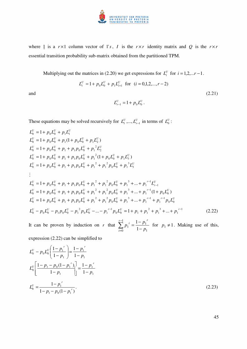
where 1 is a 1×r column vector of s'1 , I is the rr × identity matrix and Q is the rr ×
essential transition probability sub-matrix obtained from the partitioned TPM.
Multiplying out the matrices in (2.20) we get expressions for UiL for 1,...2,1 −= ri .
Ui
UUi LpLpL 11001 +++= for )2,...,2,1,0( −= ri
and (2.21)
UUr LpL 001 1+=− .
These equations may be solved recursively for Ur
U LL 11 ,..., − in terms of UL0 :
UUUUU
UUUUU
UUUU
UUUU
UUU
LpLpppLpppLpL
LpLppLpppLpL
LpLpppLpL
LpLppLpL
LpLpL
33
1002
12
10011000
31002
10011000
22
10011000
21001000
11000
1
)1(1
1
)1(1
1
++++++=
++++++=
++++=
++++=
++=
UrrUUUU
UrUUUU
Ur
rUUUU
LppppLpppLpppLpL
LpppLpppLpppLpL
LppLpppLpppLpL
001
11
13
1002
12
10011000
001
13
1002
12
10011000
11
13
1002
12
10011000
...1
)1(...1
...1
−−
−−
−
+++++++++=
+++++++++=
++++++++=
11
31
21100
1100
21001000 ...1... −− +++++=−−−−− rUrUUUU ppppLppLppLppLpL (2.22)
It can be proven by induction on r that 1
11
01 1
1pp
prr
i
i
−−=
−
= for 11 ≠p . Making use of this,
expression (2.22) can be simplified to
1
1
1
1010
1
1
1
1000
11
1)1(1
11
11
pp
pppp
L
pp
pp
LpL
rrU
rrUU
−−
=
−−−−
−−
=
−−
−
.)1(1
1
101
10 r
rU
pppp
L−−−
−= (2.23)
46
Expression (2.23) of this thesis is given in Amin et al. (1995) and determined in Page
(1962). Expression (2.23) is a closed form expression of the in-control average run length of a
one-sided chart with warning and action limits in the positive direction only.
Therefore, the in-control average run length of the one-sided (upper or positive direction)
chart with warning limit Uw and control limit (action limit) at Ua is given by (2.23) where
−+
=
−−
=<=
22
00 )1()(
nw
i
iniUi pp
i
nwSNPp (2.24)
and
−+
=
−
−+
=
− −
−−
=<≤=
22
0
22
01 )1()1()(
nw
i
ini
na
i
iniUiU pp
i
npp
i
naSNwPp . (2.25)
The derivations of (2.24) and (2.25) are given below. Derivation of expression (2.24):
)(0
Ui wSNP
p
<=
by using the relationship between iSN and iT (recall that nTSN ii −= 2 ) we obtain
+<=
<−=
2
)2(
nwTP
wnTP
Ui
Ui
−+≤=
22nw
TP Ui
given that iT is binomially distributed with parameters n and )( 0θ≥= ijXPp we obtain
−+
=
−−
=
22
0
)1(
nw
i
ini
U
ppi
n
since the upper warning limit is equal to some constant w , i.e. wwU = (see Section 2.2.1) we obtain
−+
=
−−
=
22
0
)1(
nw
i
ini ppi
n.
47
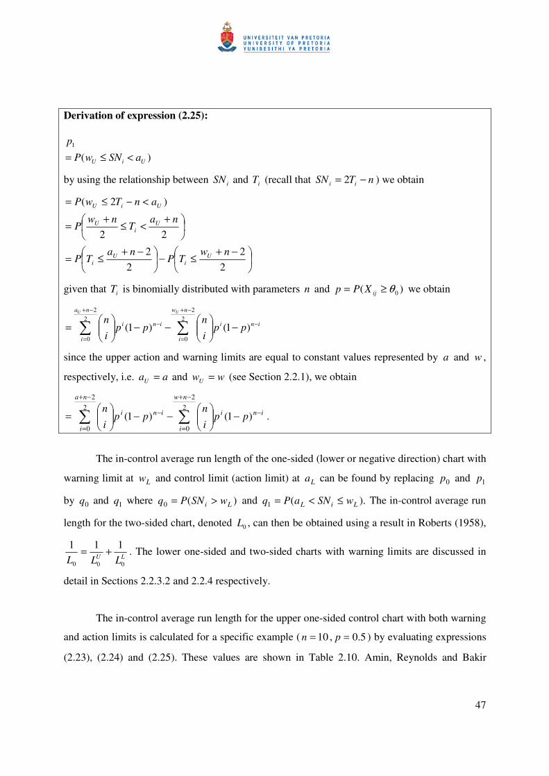
Derivation of expression (2.25):
)(1
UiU aSNwP
p
<≤=
by using the relationship between iSN and iT (recall that nTSN ii −= 2 ) we obtain
−+≤−
−+≤=
+<≤
+=
<−≤=
22
22
22
)2(
nwTP
naTP
naT
nwP
anTwP
Ui
Ui
Ui
U
UiU
given that iT is binomially distributed with parameters n and )( 0θ≥= ijXPp we obtain
−+
=
−
−+
=
− −
−−
=
22
0
22
0
)1()1(
nw
i
ini
na
i
ini
UU
ppi
npp
i
n
since the upper action and warning limits are equal to constant values represented by a and w ,
respectively, i.e. aaU = and wwU = (see Section 2.2.1), we obtain
−+
=
−
−+
=
− −
−−
=
22
0
22
0
)1()1(
nw
i
ini
na
i
ini ppi
npp
i
n.
The in-control average run length of the one-sided (lower or negative direction) chart with
warning limit at Lw and control limit (action limit) at La can be found by replacing 0p and 1p
by 0q and 1q where )(0 Li wSNPq >= and ).(1 LiL wSNaPq ≤<= The in-control average run
length for the two-sided chart, denoted 0L , can then be obtained using a result in Roberts (1958),
LU LLL 000
111 += . The lower one-sided and two-sided charts with warning limits are discussed in
detail in Sections 2.2.3.2 and 2.2.4 respectively.
The in-control average run length for the upper one-sided control chart with both warning
and action limits is calculated for a specific example ( 10=n , 5.0=p ) by evaluating expressions
(2.23), (2.24) and (2.25). These values are shown in Table 2.10. Amin, Reynolds and Bakir
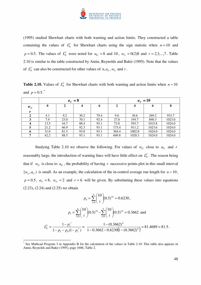
48
(1995) studied Shewhart charts with both warning and action limits. They constructed a table
containing the values of UL0 for Shewhart charts using the sign statistic when 10=n and
5.0=p . The values of UL0 were noted for 10 and 8=Ua , 8)2(0=Uw and 7,...,3,2=r . Table
2.10 is similar to the table constructed by Amin, Reynolds and Bakir (1995). Note that the values
of UL0 can also be constructed for other values of rwan UU and ,, .
Table 2.10. Values of UL0 for Shewhart charts with both warning and action limits when 10=n
and 5.0=p .*
8====Ua 10====Ua
Uw
r
0 2 4 6 2 4 6 8
2 4.1 9.2 30.2 79.4 9.6 38.6 269.2 933.7 3 7.9 23.0 70.1 92.4 27.8 194.7 890.3 1023.0 4 13.5 44.7 88.4 93.1 73.0 593.7 1015.8 1024.0 5 21.2 66.9 92.3 93.1 175.4 911.2 1023.6 1024.0 6 31.0 81.5 93.0 93.1 364.4 1002.8 1024.0 1024.0 7 42.2 88.5 93.1 93.1 609.8 1020.3 1024.0 1024.0
Studying Table 2.10 we observe the following. For values of Uw close to Ua and r
reasonably large, the introduction of warning lines will have little effect on UL0 . The reason being
that if Uw is close to Ua , the probability of having r successive points plot in this small interval
),[ Uu aw is small. As an example, the calculation of the in-control average run length for 10=n ,
5.0=p , 8=Ua , 2=Uw and 6=r will be given. By substituting these values into equations
(2.23), (2.24) and (2.25) we obtain
=0p 6230.0)5.0(105
0
10 =
=i i,
=1p 3662.0)5.0(10
)5.0(10 5
0
108
0
10 =
−
== ii ii and
=UL0 )1(11
101
1r
r
pppp
−−−−
= ( ) 5.814689.81)3662.0(16230.03662.01
)3662.0(16
6
≈=−−−
−.
* See Mathcad Program 3 in Appendix B for the calculation of the values in Table 2.10. This table also appears in Amin, Reynolds and Bakir (1995), page 1606, Table 2.
49
2.2.3.2. Lower one-sided control charts
The lower one-sided Shewhart sign chart, described previously, is efficient in detecting
large process shifts quickly. Since it is known to be inefficient in detecting small process shifts, a
lower warning limit is drawn above the lower action limit to increase its sensitivity for detecting
small shifts.
Define rule LA as: ‘Action will be taken if r successive points fall between La and Lw
(denoted by ),,,( LL warrR ) or if any point falls below La (denoted by ),,1,1( LaR −∞ )’. Clearly,
rule LA is created to detect downward shifts. Let LL denote the ARL of rule LA . LL0 can be
computed similarly as UL0 (see equation (2.23)) with 0p and 1p being replaced by 0q and 1q ,
where 0q denotes the probability that a given sample point falls above Lw and 1q denotes the
probability that a given sample point falls between La and Lw . Therefore, we have that
)1(1
1
101
10 r
rL
qqq
qL
−−−−= (2.26)
where
−
=
−−
−=>=
2
00 )1(1)(
wn
i
iniLi pp
i
nwSNPq (2.27)
and
−
=
−
−
=
− −
−−
=≤<=
2
0
2
01 )1()1()(
an
i
ini
wn
i
iniLiL pp
i
npp
i
nwSNaPq . (2.28)
Compare expressions (2.27) and (2.28) to (2.24) and (2.25).
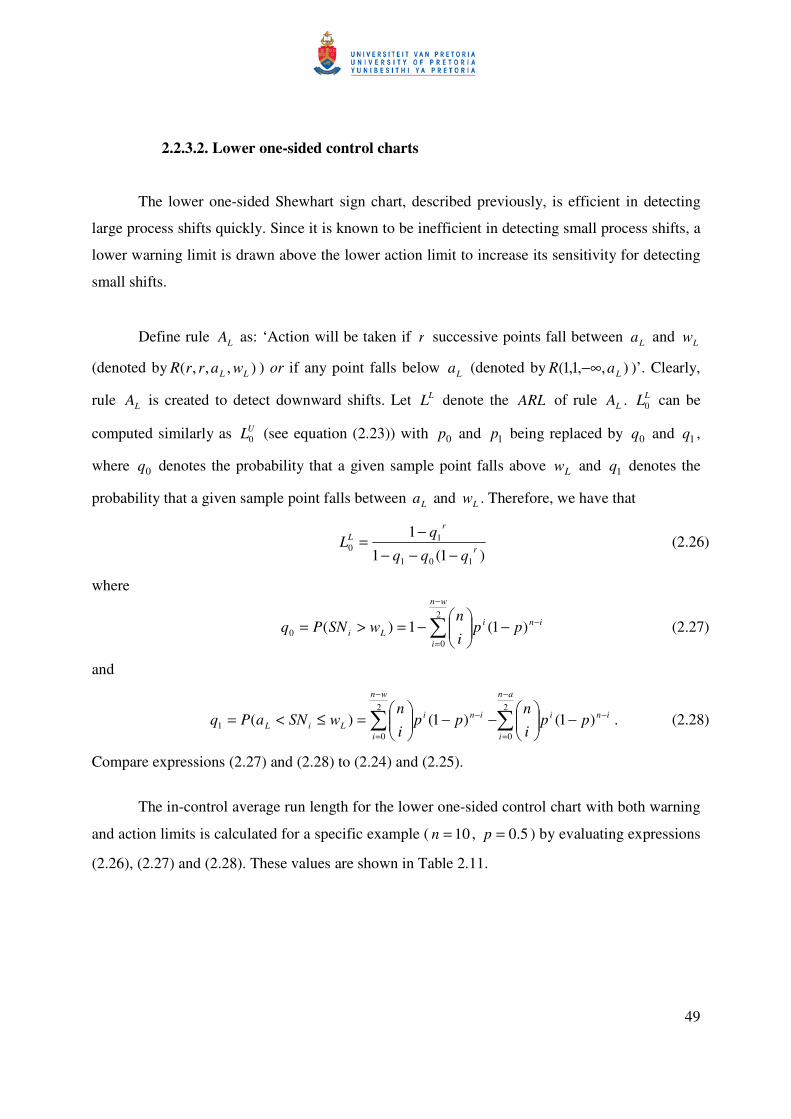
The in-control average run length for the lower one-sided control chart with both warning
and action limits is calculated for a specific example ( 10=n , 5.0=p ) by evaluating expressions
(2.26), (2.27) and (2.28). These values are shown in Table 2.11.
50
Table 2.11. Values of LL0 for Shewhart charts with both warning and action limits when 10=n
and 5.0=p .*
8====La 10====La
Lw r
0 2 4 6 2 4 6 8
2 4.1 9.2 30.2 79.4 9.6 38.6 269.2 933.7 3 7.9 23.0 70.1 92.4 27.8 194.7 890.3 1023.0 4 13.5 44.7 88.4 93.1 73.0 593.7 1015.8 1024.0 5 21.2 66.9 92.3 93.1 175.4 911.2 1023.6 1024.0 6 31.0 81.5 93.0 93.1 364.4 1002.8 1024.0 1024.0 7 42.2 88.5 93.1 93.1 609.8 1020.3 1024.0 1024.0
Studying Table 2.11 we observe the following. For values of Lw close to La and r
reasonably large, the introduction of warning lines will have little effect on LL0 . The reason being
that if Lw is close to La , the probability of having r successive points plot in this small interval
],( LL wa is small. As stated earlier, due to the symmetry of the Binomial distribution we have
that if aaU = then let aaL −= and if wwU = then let wwL −= . As a result the values of LL0
and the values of UL0 are equal.
As an example, the calculation of the in-control average run length for 10=n , 5.0=p ,
8=La , 2=Lw and 6=r will be given. By substituting these values into equations (2.26),
(2.27) and (2.28) we obtain
6230.0)5.0(10
14
0
100 =
−=
=i iq ,
3662.0)5.0(10
)5.0(10 1
0
104
0
101 =
−
=
== ii iiq and
)1(1
1
101
10 r
rL
qqq
qL
−−−−= = ( ) 5.814689.81
)3662.0(16230.03662.01)3662.0(1
6
6
≈=−−−
−.
* See Mathcad Program 3 in Appendix B for the calculation of the values in Table 2.11.
51
2.2.4. Two-sided control charts
Roberts (1958) provided a method of approximating the ARL of the two-sided Shewhart
chart with both warning and action limits. The ARL for each separate one-sided Shewhart chart
was calculated and then combined by applying equation (2.29)
LU LLL 000
111 += . (2.29)
(See Appendix A Theorem 1 for a step-by-step derivation of equation (2.29)). Equation (2.29)
can be re-written as
UL
UL
LLLL
L00
000 +
= (2.30)
where 0L denotes the ARL of a two-sided chart. In practice some observations can be tied with
the specified median. If the number of such cases, within a sample, is small (relative to n) one can
drop the tied cases and reduce n accordingly. On the other hand, if the number of ties is large,
more sophisticated analysis might be necessary.
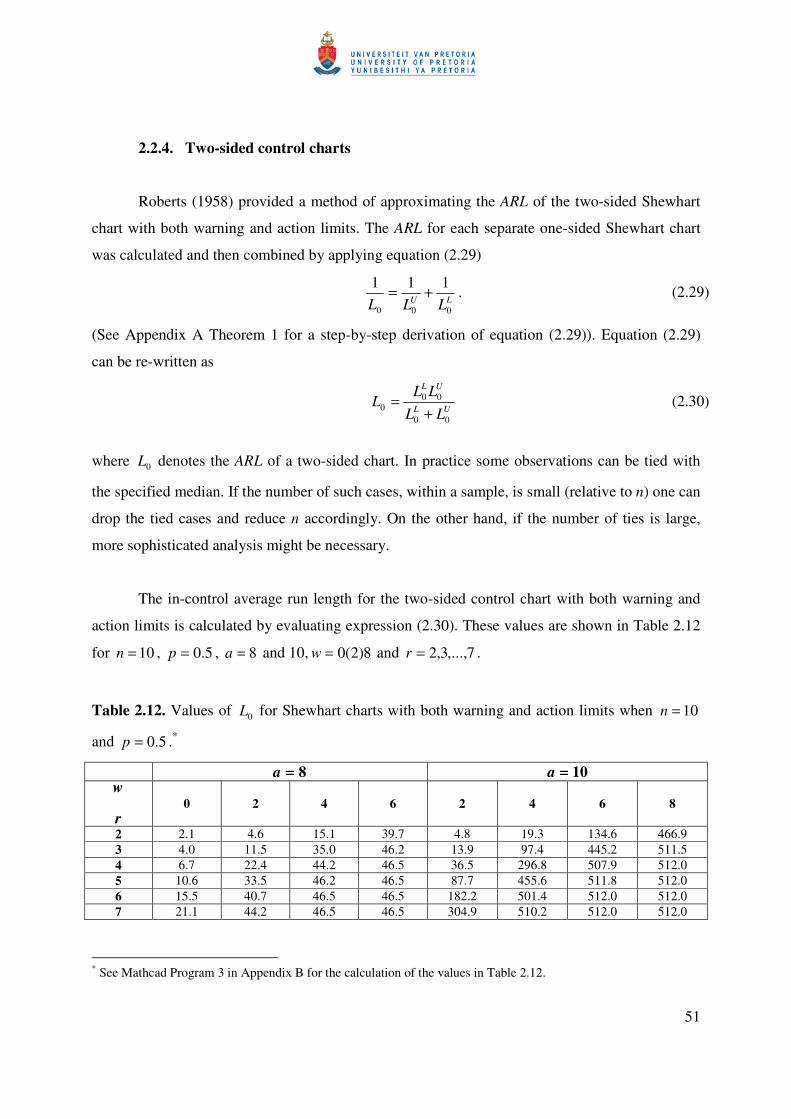
The in-control average run length for the two-sided control chart with both warning and
action limits is calculated by evaluating expression (2.30). These values are shown in Table 2.12
for 10=n , 5.0=p , 8=a and 10, 8)2(0=w and 7,...,3,2=r .
Table 2.12. Values of 0L for Shewhart charts with both warning and action limits when 10=n
and 5.0=p .*
8====a 10====a w r
0 2 4 6 2 4 6 8
2 2.1 4.6 15.1 39.7 4.8 19.3 134.6 466.9 3 4.0 11.5 35.0 46.2 13.9 97.4 445.2 511.5 4 6.7 22.4 44.2 46.5 36.5 296.8 507.9 512.0 5 10.6 33.5 46.2 46.5 87.7 455.6 511.8 512.0 6 15.5 40.7 46.5 46.5 182.2 501.4 512.0 512.0 7 21.1 44.2 46.5 46.5 304.9 510.2 512.0 512.0
* See Mathcad Program 3 in Appendix B for the calculation of the values in Table 2.12.
52
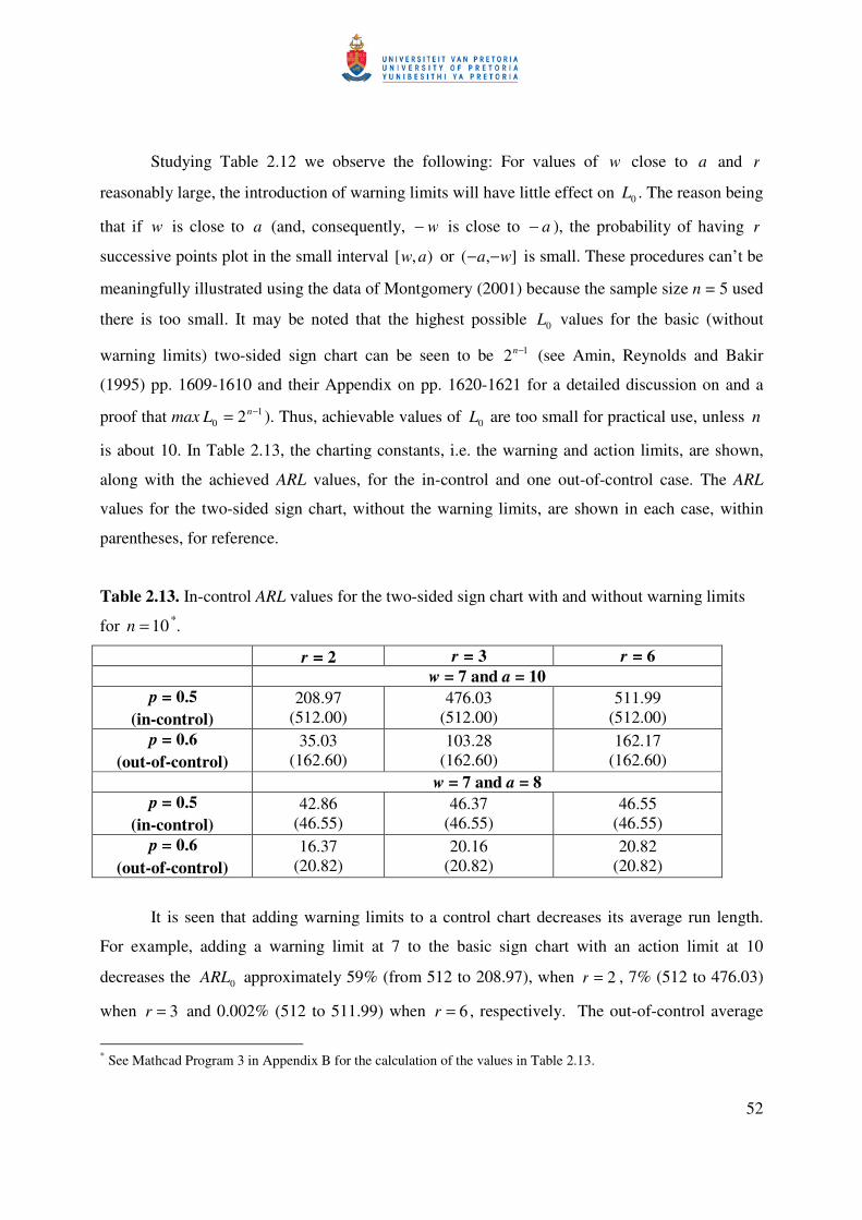
Studying Table 2.12 we observe the following: For values of w close to a and r
reasonably large, the introduction of warning limits will have little effect on 0L . The reason being
that if w is close to a (and, consequently, w− is close to a− ), the probability of having r
successive points plot in the small interval ),[ aw or ],( wa −− is small. These procedures can’t be
meaningfully illustrated using the data of Montgomery (2001) because the sample size n = 5 used
there is too small. It may be noted that the highest possible 0L values for the basic (without
warning limits) two-sided sign chart can be seen to be 12 −n (see Amin, Reynolds and Bakir
(1995) pp. 1609-1610 and their Appendix on pp. 1620-1621 for a detailed discussion on and a
proof that max 10 2 −= nL ). Thus, achievable values of 0L are too small for practical use, unless n
is about 10. In Table 2.13, the charting constants, i.e. the warning and action limits, are shown,
along with the achieved ARL values, for the in-control and one out-of-control case. The ARL
values for the two-sided sign chart, without the warning limits, are shown in each case, within
parentheses, for reference.
Table 2.13. In-control ARL values for the two-sided sign chart with and without warning limits
for 10=n *.
2====r 3====r 6====r w = 7 and a = 10
5.0====p (in-control)
208.97 (512.00)
476.03 (512.00)
511.99 (512.00)
6.0====p (out-of-control)
35.03 (162.60)
103.28 (162.60)
162.17 (162.60)
w = 7 and a = 8 5.0====p
(in-control) 42.86
(46.55) 46.37
(46.55) 46.55
(46.55) 6.0====p
(out-of-control) 16.37
(20.82) 20.16
(20.82) 20.82
(20.82)
It is seen that adding warning limits to a control chart decreases its average run length.
For example, adding a warning limit at 7 to the basic sign chart with an action limit at 10
decreases the 0ARL approximately 59% (from 512 to 208.97), when 2=r , 7% (512 to 476.03)
when 3=r and 0.002% (512 to 511.99) when 6=r , respectively. The out-of-control average
* See Mathcad Program 3 in Appendix B for the calculation of the values in Table 2.13.
53
run length is decreased by approximately 79% (from 162.6 to 35.03) when 2=r , 36% (from
162.6 to 103.28) when 3=r and 0.26% (from 162.6 to 162.17) when 6=r , respectively. Note
that although the out-of-control average run length is reduced significantly (which means a
quicker detection of shift) by the addition of warning limits, the 0ARL is also reduced
significantly. This poses a dilemma in practice, since it is desirable to have a high 0ARL and a
low FAR, so one would need to strike a balance. One possibility is to use warning limits closer to
the action limits. For example, from the second panel of Table 2.13, we see that adding a warning
limit at 7 to the sign chart with an action limit of 8, decreases the 0ARL by only 8% (from 46.55
to 42.86) when 2=r and has little effect on 0ARL when r is reasonably large. Amin et al.
(1995) concluded that for the upper one-sided Shewhart-type sign chart, introduction of warning
limits will have little effect on the in-control average run length, but can significantly reduce the
out-of-control average run length for small shifts when the warning limits are chosen close to the
action limits and r is reasonably large. Similar conclusions are expected to hold for two-sided
charts.
Up to this point we have discussed methods to increase the sensitivity of standard
Shewhart control charts to small process shifts. Another method is to extend the existing charts
by incorporating various signaling rules involving runs of the plotting statistic. The signaling
rules considered include the following: A process is declared to be out-of-control when (a) a
single point (charting statistic) plots outside the control limit(s) (1-of-1 rule) (b) k consecutive
points (charting statistics) plot outside the control limit(s) (k-of-k rule) or (c) exactly k of the last
w points (charting statistics) plot outside the control limit(s) (k-of-w rule). We can consider these
signaling rules where both k and w are positive integers with wk ≤≤1 and 2≥w . Rule (a) is
the simplest and is the most frequently used in the literature. Thus, the 1-of-1 rule corresponds to
the usual control chart, where a signal is given when a plotting statistic falls outside the control
limit(s). Rules (a) and (b) are special cases of rule (c); rules (b) and (c) have been used in the
context of supplementing the Shewhart charts with warning limits and zones.
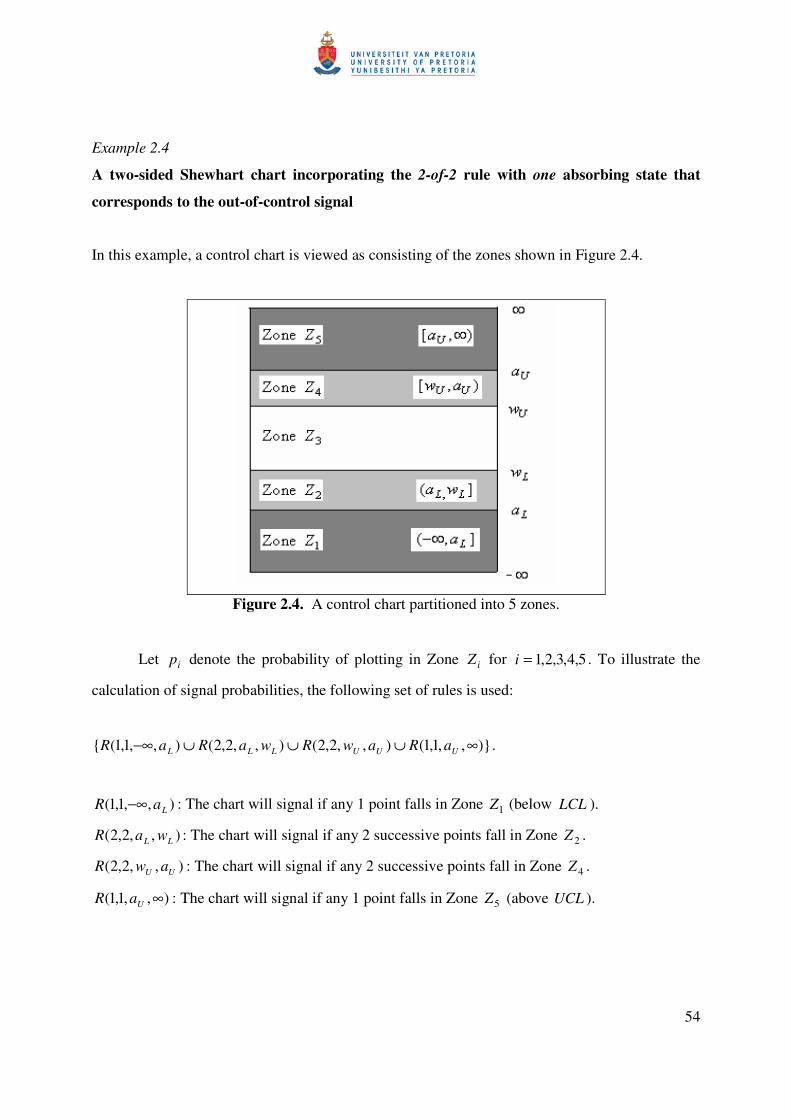
54
Example 2.4
A two-sided Shewhart chart incorporating the 2-of-2 rule with one absorbing state that
corresponds to the out-of-control signal
In this example, a control chart is viewed as consisting of the zones shown in Figure 2.4.
Figure 2.4. A control chart partitioned into 5 zones.
Let ip denote the probability of plotting in Zone iZ for 5,4,3,2,1=i . To illustrate the
calculation of signal probabilities, the following set of rules is used:
),,1,1(),,2,2(),,2,2(),,1,1( ∞∪∪∪−∞ UUULLL aRawRwaRaR .
),,1,1( LaR −∞ : The chart will signal if any 1 point falls in Zone 1Z (below LCL ).
),,2,2( LL waR : The chart will signal if any 2 successive points fall in Zone 2Z .
),,2,2( UU awR : The chart will signal if any 2 successive points fall in Zone 4Z .
),,1,1( ∞UaR : The chart will signal if any 1 point falls in Zone 5Z (above UCL ).
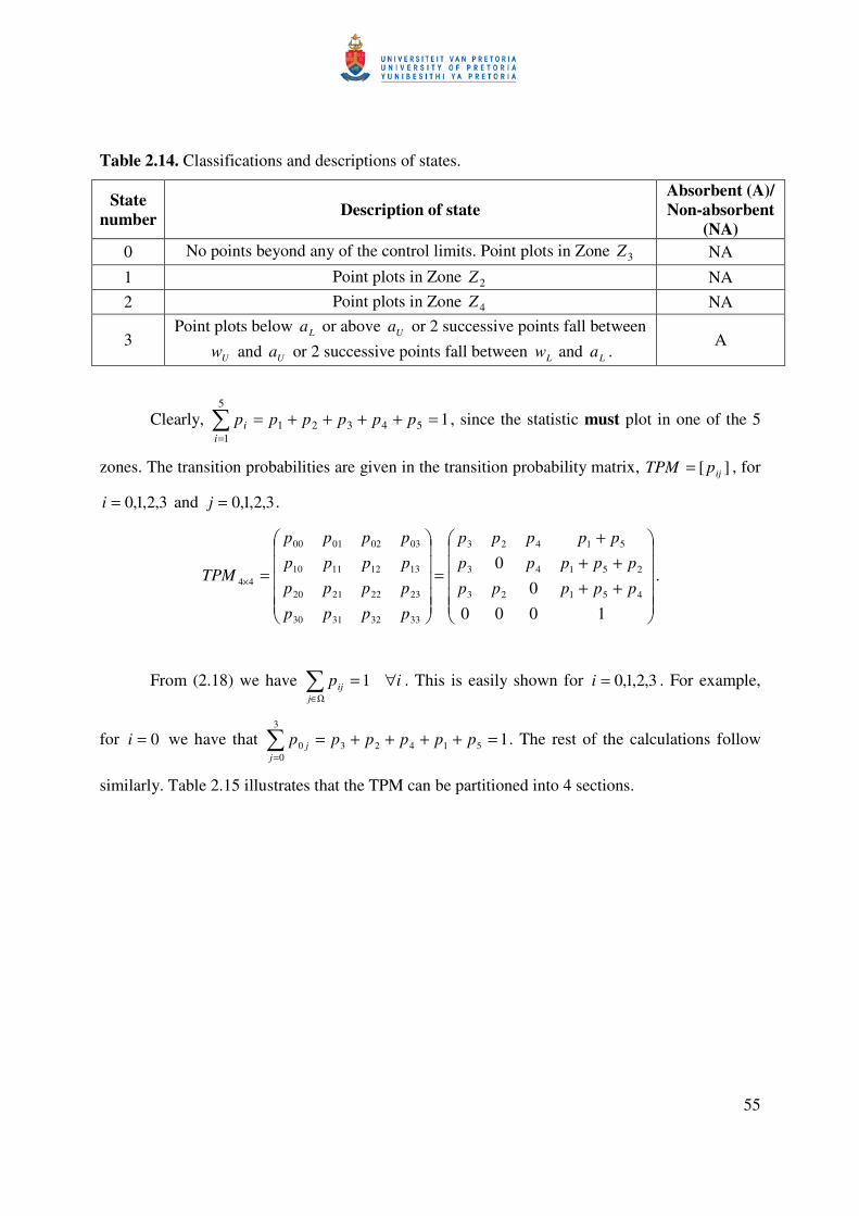
55
Table 2.14. Classifications and descriptions of states.
State number Description of state
Absorbent (A)/ Non-absorbent
(NA) 0 No points beyond any of the control limits. Point plots in Zone 3Z NA
1 Point plots in Zone 2Z NA 2 Point plots in Zone 4Z NA
3 Point plots below La or above Ua or 2 successive points fall between
Uw and Ua or 2 successive points fall between Lw and La . A
Clearly, 154321
5
1
=++++==
ppppppi
i , since the statistic must plot in one of the 5
zones. The transition probabilities are given in the transition probability matrix, ][ ijpTPM = , for
3,2,1,0=i and 3,2,1,0=j .
++++
+
=
=×
10000
0
45123
25143
51423
33323130
23222120
13121110
03020100
44 ppppp
ppppp
ppppp
pppp
pppp
pppp
pppp
TPM .
From (2.18) we have Ω∈
∀=j
ij ip 1 . This is easily shown for 3,2,1,0=i . For example,
for 0=i we have that 151423
3
00 =++++=
=
ppppppj
j . The rest of the calculations follow
similarly. Table 2.15 illustrates that the TPM can be partitioned into 4 sections.
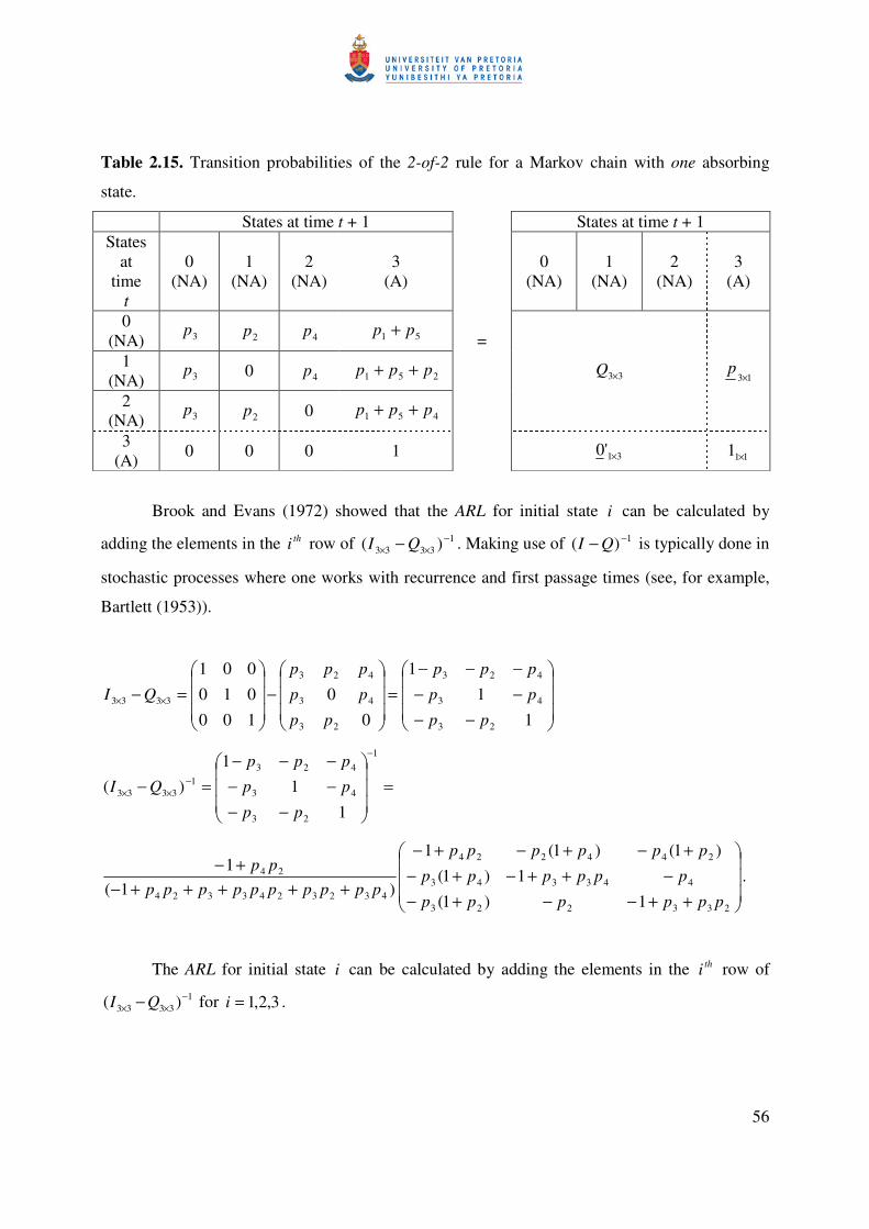
56
Table 2.15. Transition probabilities of the 2-of-2 rule for a Markov chain with one absorbing
state.
States at time t + 1 States at time t + 1 States
at time
t
0 (NA)
1 (NA)
2 (NA)
3 (A)
0 (NA)
1 (NA)
2 (NA)
3 (A)
0 (NA) 3p 2p 4p 51 pp +
1 (NA) 3p 0 4p 251 ppp ++
2 (NA) 3p 2p 0 451 ppp ++
33×Q 13×
p
3 (A) 0 0 0 1
=
31'0 × 111 ×
Brook and Evans (1972) showed that the ARL for initial state i can be calculated by
adding the elements in the thi row of 13333 )( −
×× − QI . Making use of 1)( −− QI is typically done in
stochastic processes where one works with recurrence and first passage times (see, for example,
Bartlett (1953)).
−−−−−−−
=
−
=− ××
11
1
00
100010001
23
43
423
23
43
423
3333
pp
pp
ppp
pp
pp
ppp
QI
=
−−−−−−−
=−
−
−××
1
23
43
4231
3333
11
1)(
pp
ppppp
QI
++−−+−−++−+−
+−+−+−
+++++−+−
233223
443343
244224
4323243324
24
1)1(1)1(
)1()1(1
)1(1
pppppp
pppppp
pppppp
pppppppppppp
.
The ARL for initial state i can be calculated by adding the elements in the thi row of 1
3333 )( −×× − QI for 3,2,1=i .
57
Example 2.5
A two-sided Shewhart chart incorporating the 2-of-2 rule with more than one absorbing
state that corresponds to an out-of-control signal.
This example is similar to the previous example in having three transient states, but
differs from the previous example by having more than one absorbing state. By changing the
classification of the states, the generalization to more than one absorbing state is considered. We
need to introduce a rule number and this is done by adding a subscript to each rule, i.e. in general
we have that ),,,( lknrR which now becomes ),,,( lknrR j where j denotes the rule number. This
modification allows for a separate absorbing state, jA , that is associated with each of the runs
rules, ),,,( lknrR j . This modification of Champ and Woodall’s (1987) method was done by
Champ and Woodall (1997). As a result, we have the following rules with the corresponding
absorbing states (see Figure 2.4 for the partitioning of the control chart into 5 zones):
• ),,1,1(1 LaR −∞ associated with absorbing state 1A : The chart will signal if any 1 point
falls in Zone 1Z (below LCL ).
• ),,2,2(2 LL waR associated with absorbing state 2A : The chart will signal if any 2
successive points fall in Zone 2Z .
• ),,2,2(3 UU awR associated with absorbing state 3A : The chart will signal if any 2
successive points fall in Zone 4Z .
• ),,1,1(4 ∞UaR associated with absorbing state 4A : The chart will signal if any 1 point falls
in Zone 5Z (above UCL ).
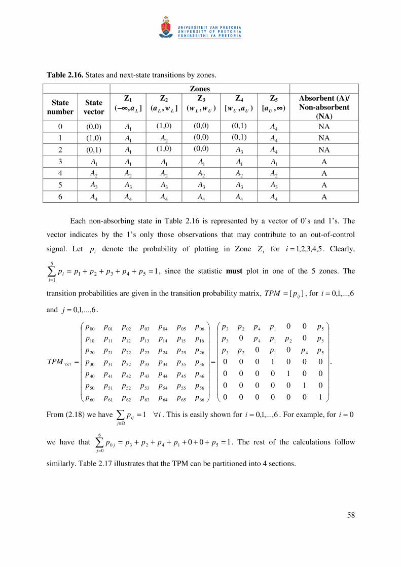
58
Table 2.16. States and next-state transitions by zones.
Zones
State number
State vector
Z1 ],( La−∞−∞−∞−∞
Z2 ],( LL wa
Z3 ),( UL ww
Z4 ),[ UU aw
Z5 ),[ ∞∞∞∞Ua
Absorbent (A)/ Non-absorbent
(NA) 0 (0,0) 1A (1,0) (0,0) (0,1) 4A NA 1 (1,0) 1A 2A (0,0) (0,1) 4A NA 2 (0,1) 1A (1,0) (0,0) 3A 4A NA 3 1A 1A 1A 1A 1A 1A A 4 2A 2A 2A 2A 2A 2A A 5 3A 3A 3A 3A 3A 3A A 6 4A 4A 4A 4A 4A 4A A
Each non-absorbing state in Table 2.16 is represented by a vector of 0’s and 1’s. The
vector indicates by the 1’s only those observations that may contribute to an out-of-control
signal. Let ip denote the probability of plotting in Zone iZ for 5,4,3,2,1=i . Clearly,
154321
5
1
=++++==
ppppppi
i , since the statistic must plot in one of the 5 zones. The
transition probabilities are given in the transition probability matrix, ][ ijpTPM = , for 6,...,1,0=i
and 6,...,1,0=j .
=
=×
100000001000000010000
000100000
0000
54123
52143
51423
66656463626160
56555453525150
46454443424140
36353433323130
26252423222120
16151413121110
06050403020100
77
ppppp
ppppp
ppppp
ppppppp
ppppppp
ppppppp
ppppppp
ppppppp
ppppppp
ppppppp
TPM .
From (2.18) we have Ω∈
∀=j
ij ip 1 . This is easily shown for 6,...,1,0=i . For example, for 0=i
we have that 100 51423
6
00 =++++++=
=
ppppppj
j . The rest of the calculations follow
similarly. Table 2.17 illustrates that the TPM can be partitioned into 4 sections.
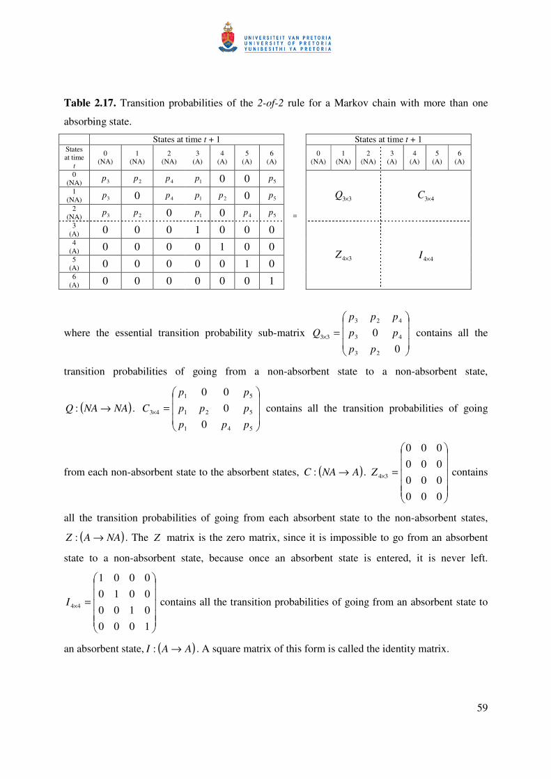
59
Table 2.17. Transition probabilities of the 2-of-2 rule for a Markov chain with more than one
absorbing state.
States at time t + 1 States at time t + 1 States at time
t
0 (NA)
1 (NA)
2 (NA)
3 (A)
4 (A)
5 (A)
6 (A)
0 (NA)
1 (NA)
2 (NA)
3 (A)
4 (A)
5 (A)
6 (A)
0 (NA) 3p 2p 4p 1p 0 0 5p
1 (NA) 3p 0 4p 1p 2p 0 5p
2 (NA) 3p 2p 0 1p 0 4p 5p
33×Q 43×C
3 (A) 0 0 0 1 0 0 0 4
(A) 0 0 0 0 1 0 0 5
(A) 0 0 0 0 0 1 0 6
(A) 0 0 0 0 0 0 1
=
34×Z 44×I
where the essential transition probability sub-matrix
=×
00
23
43
423
33
pp
pp
ppp
Q contains all the
transition probabilities of going from a non-absorbent state to a non-absorbent state,
( )NANAQ →: .
=×
541
521
51
43
0000
ppp
ppp
pp
C contains all the transition probabilities of going
from each non-absorbent state to the absorbent states, ( )ANAC →: .
=×
000000000000
34Z contains
all the transition probabilities of going from each absorbent state to the non-absorbent states,
( )NAAZ →: . The Z matrix is the zero matrix, since it is impossible to go from an absorbent
state to a non-absorbent state, because once an absorbent state is entered, it is never left.
=×
1000010000100001
44I contains all the transition probabilities of going from an absorbent state to
an absorbent state, ( )AAI →: . A square matrix of this form is called the identity matrix.
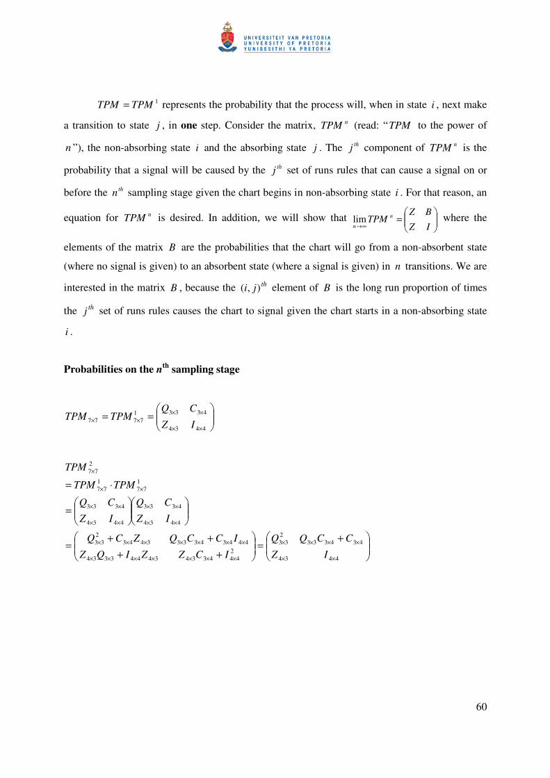
60
1TPMTPM = represents the probability that the process will, when in state i , next make
a transition to state j , in one step. Consider the matrix, nTPM (read: “TPM to the power of
n ”), the non-absorbing state i and the absorbing state j . The thj component of nTPM is the
probability that a signal will be caused by the thj set of runs rules that can cause a signal on or
before the thn sampling stage given the chart begins in non-absorbing state i . For that reason, an
equation for nTPM is desired. In addition, we will show that
=
∞→ IZ
BZTPM n
nlim where the
elements of the matrix B are the probabilities that the chart will go from a non-absorbent state
(where no signal is given) to an absorbent state (where a signal is given) in n transitions. We are
interested in the matrix B , because the thji ),( element of B is the long run proportion of times
the thj set of runs rules causes the chart to signal given the chart starts in a non-absorbing state
i .
Probabilities on the nth sampling stage
==
××
××××
4434
433317777 IZ
CQTPMTPM
+=
++++
=
=
⋅=
××
××××
×××××××
×××××××
××
××
××
××
××
×
4434
4343332
332
44433434443334
4443433334432
33
4434
4333
4434
4333
177
177
277
IZ
CCQQ
ICZZIQZ
ICCQZCQ
IZ
CQ
IZ
CQ
TPMTPM
TPM
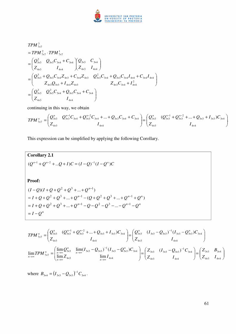
61
++=
++++++
=
+=
⋅=
××
××××××
×××××××
×××××××××××××
××
××
××
××××
××
×
4434
434333432
333
33
244433434443334
4443444333432
3334433443333
33
4434
4333
4434
4343332
33
177
277
377
IZ
CCQCQQ
ICZZIQZ
ICICQCQZCZCQQ
IZ
CQ
IZ
CCQQ
TPMTPM
TPM
continuing in this way, we obtain
.)...(...
4434
4333332
3313333
4434
434333432
334313333
77
++++=
++++=
××
×××−
×−
××
××
××××−
××−
××× IZ
CIQQQQ
IZ
CCQCQCQQTPM
nnnnnnn
This expression can be simplified by applying the following Corollary.
Corollary 2.1
CQIQICIQQQ nnn )()()...( 121 −−=+++ −−−
Proof:
n
nnn
nnn
n
QI
QQQQQQQQQI
QQQQQQQQQI
QQQQIQI
−=
−−−−−−+++++=
+++++−+++++=
+++++−
−−
−−
−
132132
132132
132
......
)...(...
)...)((
−−=
++++=
××
×××−
×××
××
×××−
×−
×××
4434
4333331
333333
4434
4333332
3313333
77
)()()...(IZ
CQIQIQ
IZ
CIQQQQTPM
nnnnnn
=
−=
−−=
××
××
××
×−
×××
×∞→×∞→
×××−
××∞→×∞→×∞→
4434
4333
4434
431
333333
4434
4333331
33333377
)(limlim
)()(limlimlim
IZ
BZ
IZ
CQIZIZ
CQIQIQTPM
nn
n
n
n
nn
n
where ( ) 431
333343 ×−
××× −= CQIB .
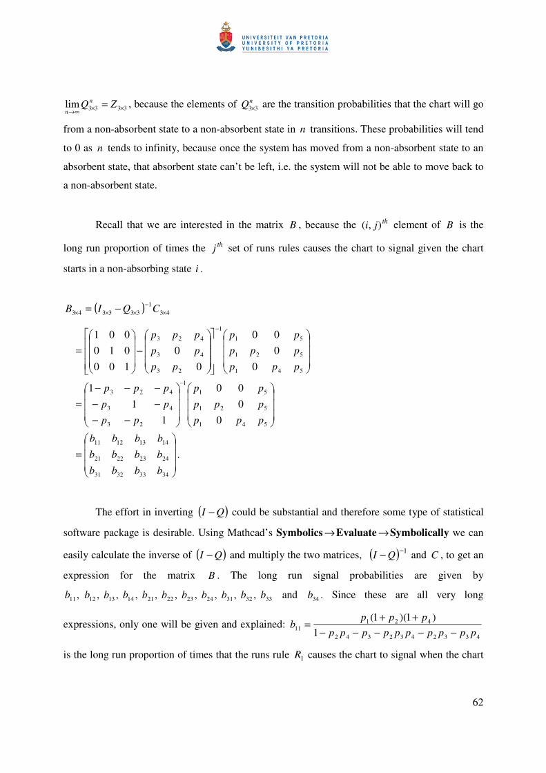
62
3333lim ××∞→= ZQ n
n, because the elements of nQ 33× are the transition probabilities that the chart will go
from a non-absorbent state to a non-absorbent state in n transitions. These probabilities will tend
to 0 as n tends to infinity, because once the system has moved from a non-absorbent state to an
absorbent state, that absorbent state can’t be left, i.e. the system will not be able to move back to
a non-absorbent state.
Recall that we are interested in the matrix B , because the thji ),( element of B is the
long run proportion of times the thj set of runs rules causes the chart to signal given the chart
starts in a non-absorbing state i .
( ) 431
333343 ×−
××× −= CQIB
.
0000
11
1
0000
00
100010001
34333231
24232221
14131211
541
521
511
23
43
423
541
521
51
1
23
43
423
=
−−−−−−−
=
−
=
−
−
bbbb
bbbb
bbbb
ppp
ppp
pp
pp
pp
ppp
ppp
ppppp
pp
ppppp
The effort in inverting ( )QI − could be substantial and therefore some type of statistical
software package is desirable. Using Mathcad’s Symbolics →Evaluate →Symbolically we can
easily calculate the inverse of ( )QI − and multiply the two matrices, ( ) 1−− QI and C , to get an
expression for the matrix B . The long run signal probabilities are given by
3332312423222114131211 ,,,,,,,,,, bbbbbbbbbbb and 34b . Since these are all very long
expressions, only one will be given and explained: 4332432342
42111 1
)1)(1(pppppppppp
pppb
−−−−−++
=
is the long run proportion of times that the runs rule 1R causes the chart to signal when the chart
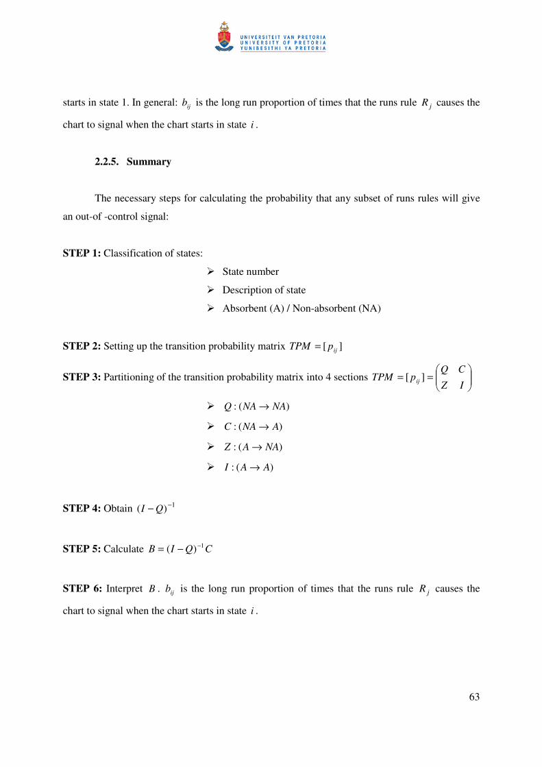
63
starts in state 1. In general: ijb is the long run proportion of times that the runs rule jR causes the
chart to signal when the chart starts in state i .
2.2.5. Summary
The necessary steps for calculating the probability that any subset of runs rules will give
an out-of -control signal:
STEP 1: Classification of states:
State number
Description of state
Absorbent (A) / Non-absorbent (NA)
STEP 2: Setting up the transition probability matrix ][ ijpTPM =
STEP 3: Partitioning of the transition probability matrix into 4 sections
==
IZ
CQpTPM ij ][
)(: NANAQ →
)(: ANAC →
)(: NAAZ →
)(: AAI →
STEP 4: Obtain 1)( −− QI
STEP 5: Calculate CQIB 1)( −−=
STEP 6: Interpret B . ijb is the long run proportion of times that the runs rule jR causes the
chart to signal when the chart starts in state i .
64
2.3. The tabular CUSUM control chart
2.3.1. Introduction
Cumulative sum (or CUSUM) control charts were first introduced by Page (1954)
(although not in its present form) and have been studied by many authors, for example,
Barnard (1959), Ewan and Kemp (1960), Johnson (1961), Goldsmith and Whitfield (1961),
Page (1961), Ewan (1963), Van Dobben de Bruyn (1968), Woodall and Adams (1993) and
Hawkins and Olwell (1998). Montgomery (2005) related CUSUM ideas to other SPC
methodologies.
The statistical design of CUSUM charts
While the Shewhart-type charts are widely known and most often used in practice
because of their simplicity and global performance, other classes of charts, such as the
CUSUM charts are useful and sometimes more naturally appropriate in the process control
environment in view of the sequential nature of data collection. The CUSUM chart
incorporates all the information in the sequence of sample values by plotting a function of the
cumulative sums of the deviations of the sample values from a target value. For example,
suppose that samples of size 1=n are collected and let jx denote the thj observation. The
case of individual observations occurs very often in practice, so that situation will be treated
first. Later we will see how to modify these results for subgroups. Then if 0θ is the target
value, the CUSUM chart is formed by plotting iC where
.)()()()( 100
1
100
1−
−
==
+−=−+−=−= ii
i
jji
i
jji CxxxxC θθθθ
The upper one-sided CUSUM works by accumulating deviations from K+0θ that are
above target. For the upper one-sided CUSUM chart we use
])(,0max[ 01 KxCC iii −−+= +−
+ θ for ,...3,2,1=i (2.31)
to detect positive deviations from 0θ . A signaling event occurs for the first i such that
HCi ≥+ .
65
The lower one-sided CUSUM works by accumulating deviations from K−0θ that are
below target. For the lower one-sided CUSUM chart we use
])(,0min[ 01 KxCC iii +−+= −−
− θ for ,...3,2,1=i (2.32)
or
])(,0max[ 0
*
1
*KxCC iii −−−= −
−− θ for ,...3,2,1=i (2.33)
to detect negative deviations from 0θ . A signaling event occurs for the first i such that
HCi −≤− (if expression (2.32) is used) or HCi ≥−* (if expression (2.33) is used). For a
visually appealing chart, expression (2.32) will be used to construct the lower one-sided
CUSUM.
The two-sided CUSUM chart signals for the first i at which either one of the two
inequalities is satisfied, that is, either HCi ≥+ or HCi −≤− . Both K and H are non-
negative integers and they are needed in order to implement the CUSUM chart. Details
regarding how to choose these constants are given in Section 2.3.1 in the sub-section called
Recommendations for the design of the CUSUM control chart.
Note that both +iC and −
iC accumulate deviations from the target value 0θ that are
greater than K . Originally, Page (1954) set the starting values equal to zero, that is, 00 =+C
and 00 =−C . Later on, Lucas and Crosier (1982) recommended setting the starting values
equal to some nonzero value to improve the sensitivity of the CUSUM at process start-up.
This is referred to as the fast initial response (FIR) or head start feature.
The standardized CUSUM
The variable ix can be standardized by subtracting its mean and dividing by its
standard deviation, that is,
( )
σθ0−
= ii
xy . (2.34)
The resulting standardized upper one-sided CUSUM is given by
],0max[ 1 kySS iii −+= +−
+ for ,...3,2,1=i (2.35)
while the resulting standardized lower one-sided CUSUM is given by
66
],0min[ 1 kySS iii ++= −−
− for ,...3,2,1=i (2.36)
or
],0max[*
1
*kySS iii −−= −
−− for ,...3,2,1=i (2.37)
The two-sided standardized CUSUM is constructed by running the upper and lower
one-sided standardized CUSUM charts simultaneously and signals at the first i such that
si HS ≥+ or si HS −≤− *. Both k and sH are non-negative integers and they are needed in
order to implement the standardized CUSUM chart. As mentioned previously, details
regarding how to choose these constants are given in Section 2.3.1 in the sub-section called
Recommendations for the design of the CUSUM control chart.
The unstandardized CUSUM iC and the standardized CUSUM iS contains the same
information. The question arises: Should unstandardized or standardized data be used?
Unstandardized data has the advantage that the units of the vertical axis are in their original
measurements which makes interpretation easier. Standardized data has the advantage that
different CUSUM charts can be compared.
The CUSUM for monitoring the process mean and other sample statistics
A CUSUM chart for monitoring the process mean can be obtained by replacing ix in
expression (2.34) with the sample average ix and by replacing σ by nσ . It is also
possible to develop CUSUM charts for other sample statistics, for example, standard
deviations and defects. These CUSUM charts for other sample statistics have been studied by
many authors, for example, Lucas (1985), Gan (1993) and White, Keats and Stanley (1997).
Recommendations for the design of the CUSUM control chart
Phase II CUSUM charts should be designed on the basis of ARL performance. The
parameters K and H are obtained for a specified in-control average run length. Both
* The vertical axis of the standardized CUSUM will be measured in multiples of the standard deviation ( σ ) of the data, whereas the vertical axis of the unstandardized data will be measured in the same units of X, for example, in meters, millimeters, ect. To avoid confusion, H and Hs will be used to denote the decision intervals for the unstandardized and standardized CUSUM charts, respectively.
67
parameters are non-negative integers. Let σ denote the standard deviation of the sample
variable used in forming the cumulative sum. Parametric CUSUM charts (see Page (1954))
are used for detecting shifts in a normal mean based on the cumulative sum of differences
from target. Let σhH = and σkK = where h is usually taken to be equal to 4 or 5 and k is
usually taken to equal 0.5 (see Montgomery (2005) page 395). By choosing 4=h or 5=h
and 5.0=k (the values most commonly used in practice) we generally get a good average run
length performance for parametric CUSUM charts. In the next section we will show that
choosing 4=h or 5=h and 5.0=k is not recommended for nonparametric CUSUM charts,
since it usually gives a poor in-control average run length performance. Since we will not be
using σ4=H or σ5 and σ5.0=K for nonparametric control charts, we will denote the
decision interval and reference value by h and k, respectively, from this point forward.
The proposed nonparametric CUSUM chart
Amin, Reynolds and Bakir (1995) proposed a nonparametric CUSUM chart for the
median (or any other percentile) of any continuous population based on sign statistics. Recall
that for the thi random sample the plotting statistic in the Shewhart-type chart was
=
−=n
jiji xsignSN
10 )( θ . The chart proposed by Amin et al. (1995) instead uses the cumulative
sum of the statistic iSN with a stopping rule. They also calculated the ARL of the chart using
a Markov chain approach where the transition probabilities are calculated via the distribution
of the sign statistic, which is of course binomial. The procedure is distribution-free since the
in-control distribution of iSN does not depend on the underlying distribution for all
continuous distributions. A CUSUM sign chart can be obtained by replacing iy in
expressions (2.35), (2.36) and (2.37) with iSN . In other words, for the upper one-sided
CUSUM sign chart we use
],0max[ 1 kSNSS iii −+= +−
+ for ,...3,2,1=i (2.38)
to detect positive deviations from the known target value 0θ . A signaling event occurs for the
first i such that hS i ≥+ .
For a lower one-sided CUSUM sign chart we use
],0min[ 1 kSNSS iii ++= −−
− for ,...3,2,1=i (2.39)
68
or
],0max[*
1
*kSNSS iii −−= −
−− for ,...3,2,1=i (2.40)
to detect negative deviations from the known target value 0θ . A signaling event occurs for the
first i such that hS i −≤− (if expression (2.39) is used) or hS i ≥−* (if expression (2.40) is
used).
The corresponding two-sided CUSUM chart signals for the first i at which either one
of the two inequalities is satisfied, that is, either hS i ≥+ or hS i −≤− . Starting values are
typically chosen to equal zero, that is, 000 == −+ SS .
The constants k and h are obtained for a specified in-control average run length. In-
control average run length ( 0ARL ), standard deviation of the run length ( 0SDRL ), th5 , th25
(the first quartile, 1Q ), th50 (the median run length, 0MRL ), th75 (the third quartile, 3Q ) and
th95 percentile values will be computed and tabulated for various values of h and k later on.
2.3.2. One-sided control charts
2.3.2.1. Upper one-sided control charts
Various expressions for the exact run length distribution and its parameters have been
given for the normal theory one-sided CUSUM procedure by, for example, Ewan and Kemp
(1960), Brook and Evans (1972), Woodall (1983) and Hawkins and Olwell (1998). Many
authors have presented various approximations for the run length distribution and its
parameters for the one-sided CUSUM procedure. A Markov chain representation of the one-
sided CUSUM procedure based on integer-valued cumulative sums is presented in this
section. The number of states included in the Markov chain is minimized in order to make the
methods as efficient as possible.
69
Markov chain approach
Brook and Evans (1972) and Amin et al. (1995) considered a method for evaluating
the exact average run length and its moments for the upper one-sided CUSUM chart by
treating the cumulative sum as a Markov chain with the state space a subset of ,...,2,1,0 h .
Markov techniques have a great advantage as they are adjustable to many runs related
problems and they often simplify the solutions to the specific problems they are applied on.
Fu, Spiring and Xie (2002) presented three results that must be satisfied before implementing
the finite-state Markov chain approach.
Let +tS be a finite-state homogenous Markov chain on the state space +Ω with a TPM
such that (i) ,...,, 110 −++ =Ω srςςς where hsr =<<<= −+ 110 ...0 ςςς and 1−+srς is an
absorbent state; (ii) the TPM is given by ][ ijpTPM = for 1,...,1,0 −+= sri and
1,...,1,0 −+= srj where r denotes the number of non-absorbent states and s the number of
absorbent states, respectively, and (iii) the starting value should be in the “dummy” state with
probability one, that is, 1)( 00 ==+ ςSP , to ensure the process starts in-control . Assume that
the Markov chain +tS satisfies conditions (i), (ii) and (iii), then from Fu, Spiring and Xie
(2002) and Fu and Lou (2003) we have
1)()0|( 10 QIQSnNP n −=== −+ ξ (2.41)
( ) ( ) 11−−= QINE ξ (2.42)
( ) ( )( ) 122 −−+= QIQINE ξ (2.43)
( ) ( ) ( )( ) ( )( )21222 11)()var( −− −−−+=−= QIQIQINENEN ξξ (2.44)
( )( ) ( )( )212 11)var( −− −−−+== QIQIQINSDRL ξξ (2.45)
where the essential transition probability sub-matrix Q is the rr × matrix that contains all the
transition probabilities of going from a non-absorbent state to a non-absorbent state, I is the
rr × identity matrix, ξ is a r×1 row vector with 1 at the st1 element and zero elsewhere and
1 is an 1×r column vector with all elements equal to unity. See Theorem 2 in Appendix A
for the derivations done by Fu, Spiring and Xie (2002) and Fu and Lou (2003).
70
The time that the procedure signals is the first time such that the finite-state Markov
chain +tS enters one of the absorbent states where the state space is given by
,...,, 110 −++ =Ω srςςς , 00 =+S and
kSNShS ttt −+= +−
+1,0max,min . (2.46)
The state corresponding to a signal by the CUSUM chart is called an absorbent state.
Clearly, there is only one absorbent state, since the chart signals when +tS falls on or above h,
i.e. 1=s .
The distribution of tSN can easily be obtained from the binomial distribution (recall
that nTSN ii −= 2 i∀ , where iT is binomially distributed with parameters n and
)( 0θ≥= ijXPp ) . The binomial probabilities are given in Table G of Gibbons and
Chakraborti (2003) and can easily be calculated using some type of statistical software
package, for example, Excel or SAS.
Example 2.6
An upper one-sided CUSUM sign chart where the sample size is odd ( 5====n )
The statistical properties of an upper one-sided CUSUM sign chart with a decision
interval of 4 ( 4=h ), a reference value of 1 ( 1=k ) and a sample size of 5 ( 5=n ) is
examined. For n odd, the reference value is taken to be odd, because this leads to the sum
( ) − kSN i being equal to even values which reduces the size of the state space for the
Markov chain. This will halve the size of the matrices of transition probabilities. For 4=h
we have that the state space is 4,2,0,, 210 ==Ω+ ςςς with h=<<= 2100 ςςς . The state
space is calculated using equation (2.46) and the calculations are shown in Table 2.18.
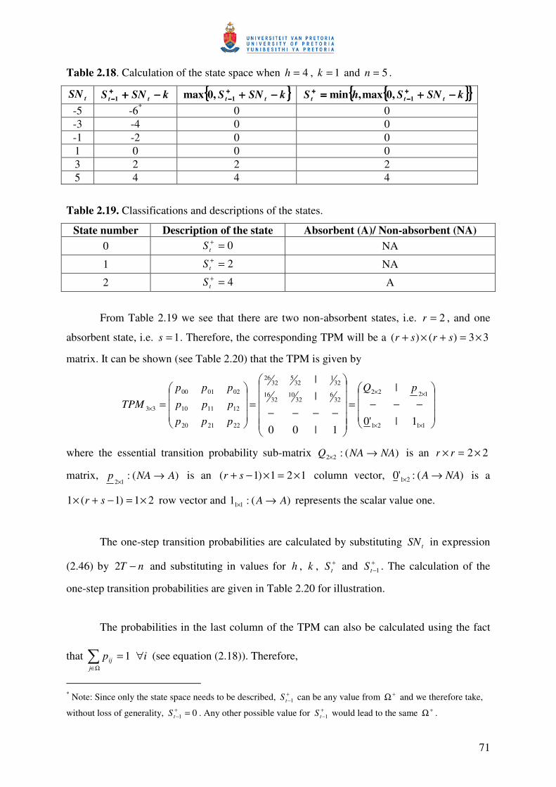
71
Table 2.18. Calculation of the state space when 4=h , 1=k and 5=n .
tSN kSNS tt −−−−++++++++−−−−1 kSNS tt −−−−++++++++
−−−−1,0max kSNShS ttt −−−−++++==== ++++−−−−
++++1,0max,min
-5 -6* 0 0 -3 -4 0 0 -1 -2 0 0 1 0 0 0 3 2 2 2 5 4 4 4
Table 2.19. Classifications and descriptions of the states.
State number Description of the state Absorbent (A)/ Non-absorbent (NA) 0 0=+
tS NA
1 2=+tS NA
2 4=+tS A
From Table 2.19 we see that there are two non-absorbent states, i.e. 2=r , and one
absorbent state, i.e. 1=s . Therefore, the corresponding TPM will be a 33)()( ×=+×+ srsr
matrix. It can be shown (see Table 2.20) that the TPM is given by
−−−=
−−−−=
=
××
××
×
1121
122232
632
1032
16
321
325
3226
222120
121110
020100
33
1|'0
|
1|00
||
pQ
ppp
ppp
ppp
TPM
where the essential transition probability sub-matrix )(:22 NANAQ →× is an 22 ×=× rr
matrix, )(:12
ANAp →×
is an 121)1( ×=×−+ sr column vector, )(:'0 21 NAA →× is a
21)1(1 ×=−+× sr row vector and )(:1 11 AA →× represents the scalar value one.
The one-step transition probabilities are calculated by substituting tSN in expression
(2.46) by nT −2 and substituting in values for h , k , +tS and +
−1tS . The calculation of the
one-step transition probabilities are given in Table 2.20 for illustration.
The probabilities in the last column of the TPM can also be calculated using the fact
that Ω∈
=j
ijp 1 i∀ (see equation (2.18)). Therefore,
* Note: Since only the state space needs to be described, +
−1tS can be any value from +Ω and we therefore take,
without loss of generality, 01 =+−tS . Any other possible value for +
−1tS would lead to the same +Ω .
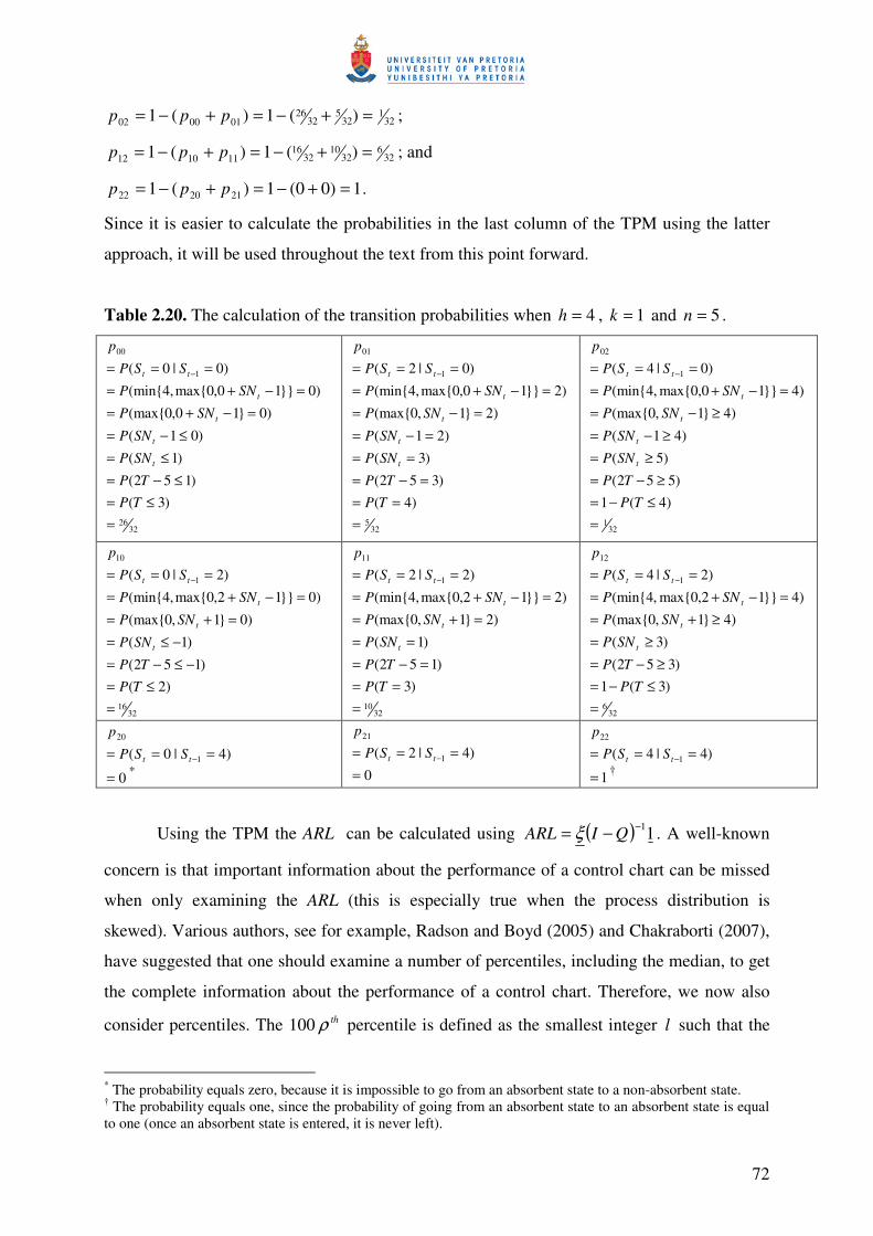
72
321
325
3226
010002 )(1)(1 =+−=+−= ppp ;
326
3210
3216
111012 )(1)(1 =+−=+−= ppp ; and
1)00(1)(1 212022 =+−=+−= ppp .
Since it is easier to calculate the probabilities in the last column of the TPM using the latter
approach, it will be used throughout the text from this point forward.
Table 2.20. The calculation of the transition probabilities when 4=h , 1=k and 5=n .
3226
1
00
)3()152(
)1(
)01(
)010,0(max
)010,0max,4(min
)0|0(
=≤=
≤−=≤=
≤−==−+=
=−+==== −
TP
TP
SNP
SNP
SNP
SNP
SSP
p
t
t
t
t
tt
325
1
01
)4()352(
)3(
)21(
)21,0(max
)210,0max,4(min
)0|2(
===
=−===
=−==−=
=−+==== −
TP
TP
SNP
SNP
SNP
SNP
SSP
p
t
t
t
t
tt
321
1
02
)4(1)552(
)5(
)41(
)41,0(max
)410,0max,4(min
)0|4(
=≤−=
≥−=≥=
≥−=≥−=
=−+==== −
TP
TP
SNP
SNP
SNP
SNP
SSP
p
t
t
t
t
tt
3216
1
10
)2()152(
)1(
)01,0(max
)012,0max,4(min
)2|0(
=≤=
−≤−=−≤=
=+==−+=
=== −
TP
TP
SNP
SNP
SNP
SSP
p
t
t
t
tt
3210
1
11
)3()152(
)1(
)21,0(max
)212,0max,4(min
)2|2(
===
=−===
=+==−+=
=== −
TP
TP
SNP
SNP
SNP
SSP
p
t
t
t
tt
326
1
12
)3(1)352(
)3(
)41,0(max
)412,0max,4(min
)2|4(
=≤−=
≥−=≥=
≥+==−+=
=== −
TP
TP
SNP
SNP
SNP
SSP
p
t
t
t
tt
)4|0( 1
20
=== −tt SSP
p
0= * 0
)4|2( 1
21
==== −tt SSP
p
)4|4( 1
22
=== −tt SSP
p
1= †
Using the TPM the ARL can be calculated using ( ) 11−−= QIARL ξ . A well-known
concern is that important information about the performance of a control chart can be missed
when only examining the ARL (this is especially true when the process distribution is
skewed). Various authors, see for example, Radson and Boyd (2005) and Chakraborti (2007),
have suggested that one should examine a number of percentiles, including the median, to get
the complete information about the performance of a control chart. Therefore, we now also
consider percentiles. The 100 thρ percentile is defined as the smallest integer l such that the
* The probability equals zero, because it is impossible to go from an absorbent state to a non-absorbent state. † The probability equals one, since the probability of going from an absorbent state to an absorbent state is equal to one (once an absorbent state is entered, it is never left).

73
cdf is at least ( )%100 ρ× . Thus, the 100 thρ percentile l is found from ρ≥≤ )( lNP . The
median ( th50 percentile) will be considered, since it is a more representative performance
measure than the ARL (see the discussion in Section 2.1.5). The first and third quartiles ( th25
and th75 percentiles) will also be considered, since it contains the middle half of the
distribution. The ‘tails’ of the distribution should also be examined and therefore the th5 and th95 percentiles are calculated. The calculation of these percentiles is shown in Table 2.21 for
illustration purposes. The first column of Table 2.21 contains the values that the run length
variable ( N ) can take on.
Table 2.21. Calculation of the percentiles when 4=h , 1=k and 5=n *.
N )( lNP ≤≤≤≤ The 5th, 25th, 50th, 75th and 95th percentiles 1 0.0313 2 0.0859 =05.0ρ 2 (smallest integer such that the cdf is at least 0.05) 3 0.1420 4 0.1954 5 0.2456 6 0.2928 =25.0ρ 6 (smallest integer such that the cdf is at least 0.25) 7 0.3370 8 0.3784 9 0.4173
10 0.4537 11 0.4878 12 0.5198 =5.0ρ 12 (smallest integer such that the cdf is at least 0.5) 13 0.5499 14 0.5780 15 0.6044 16 0.6291 17 0.6523 18 0.6740 19 0.6944 20 0.7135 21 0.7314 22 0.7482 23 0.7639 =75.0ρ 23 (smallest integer such that the cdf is at least 0.75) 24 0.7787 25 0.7925 26 0.8055 27 0.8176 28 0.8290 29 0.8397 30 0.8497
48 0.9530 =95.0ρ 48 (smallest integer such that the cdf is at least 0.95) 49† 0.9559
* See SAS Program 2 in Appendix B for the calculation of the values in Table 2.21. † The value of the run length variable is only shown for some values up to N=49 for illustration purposes.
74
The formulas of the moments and some characteristics of the run length distribution
have been studied by Fu, Spiring and Xie (2002) and Fu and Lou (2003) – see equations
(2.41) to (2.45). By substituting )01(21
=×
ξ ,
=× 1016
526
321
22Q and
=× 1
11 12 into these
equations, we obtain the following:
( ) ( ) 62.1611 =−== −QINEARL ξ
( ) ( )( ) 59.516122 =−+= −QIQINE ξ
( ) ( ) 51.15)()( 22 =−== NENENVarSDRL
2 percentile 5 05.0 == ρth
6 percentile 25 25.0 == ρth
12 percentile 50 Median 5.0 === ρth
23 percentile 75 75.0 == ρth
48 percentile 95 95.0 == ρth
Other values of h, k and n were also considered and the results are given in Table 2.22.
Table 2.22. The in-control average run length ( +0ARL ), standard deviation of the run length
( SDRL ), th5 , th25 , th50 , th75 and th95 percentile* values for the upper one-sided CUSUM
sign chart when 5=n †.
h k 2 3 or 4
1 5.33 4.81
(1, 2, 4, 7, 15)
16.62 15.51
(2, 6, 12, 23, 48)
3 32.00 31.50
(2, 10, 22, 44, 95)
‡
* The three rows of each cell shows the +
0ARL , the SDRL , and the percentiles ( 5ρ , 25ρ , 50ρ , 75ρ , 95ρ ), respectively. † See SAS Program 2 in Appendix B for the calculation of the values in Table 2.22. ‡ Since the decision interval is taken to satisfy knh −≤ there are open cells in Table 2.22.
75
Note that the summary measures for odd values of h will be equal to the summary
measures of the subsequent even integer. More on this later (refer to example (2.8)). Values of
k and h are restricted to be integers so that the Markov chain approach could be employed to
obtain expressions for the exact run length distribution and its parameters. In order to allow
for the possibility of stopping after one sample, i.e. issuing a signal, the values of h is taken
to satisfy knh −≤ .
The five percentiles (given in Table 2.22) are displayed in boxplot-like graphs for
various h and k values in Figure 2.5. It should be noted that these boxplot-like graphs differ
from standard box plots. In the latter case the whiskers are drawn from the ends of the box to
the smallest and largest values inside specified limits, whereas, in the case of the boxplot-like
graphs, the whiskers are drawn from the ends of the box to the 5th and 95th percentiles,
respectively. In this thesis “boxplot” will refer to a boxplot-like graph from this point forward.
Figure 2.5 clearly shows the effects of h and k on the run length distribution and it
portrays the run length distribution when the process is in-control. We would prefer a
“boxplot” with a high valued (large) in-control average run length and a small spread.
Applying this criterion, we see that the “boxplot” corresponding to the )3,2(),( =kh
combination has the largest in-control average run length, which is favorable, but it also has
the largest spread which is unattractive. The “boxplot” furthest to the right is exactly opposite
from the “boxplot” furthest to the left. The latter has the smallest spread, which is favorable,
but it also has the smallest in-control average run length, which is unattractive. In conclusion,
no “boxplot” is optimal relative to the others.
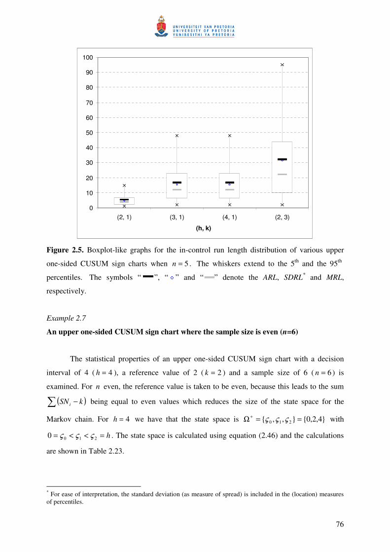
76
0
10
20
30
40
50
60
70
80
90
100
(2, 1) (3, 1) (4, 1) (2, 3)
(h, k)
Figure 2.5. Boxplot-like graphs for the in-control run length distribution of various upper
one-sided CUSUM sign charts when 5=n . The whiskers extend to the 5th and the 95th
percentiles. The symbols “ ”, “ ” and “ ” denote the ARL, SDRL* and MRL,
respectively.
Example 2.7
An upper one-sided CUSUM sign chart where the sample size is even (n=6)
The statistical properties of an upper one-sided CUSUM sign chart with a decision
interval of 4 ( 4=h ), a reference value of 2 ( 2=k ) and a sample size of 6 ( 6=n ) is
examined. For n even, the reference value is taken to be even, because this leads to the sum
( ) − kSN i being equal to even values which reduces the size of the state space for the
Markov chain. For 4=h we have that the state space is 4,2,0,, 210 ==Ω+ ςςς with
h=<<= 2100 ςςς . The state space is calculated using equation (2.46) and the calculations
are shown in Table 2.23.
* For ease of interpretation, the standard deviation (as measure of spread) is included in the (location) measures of percentiles.
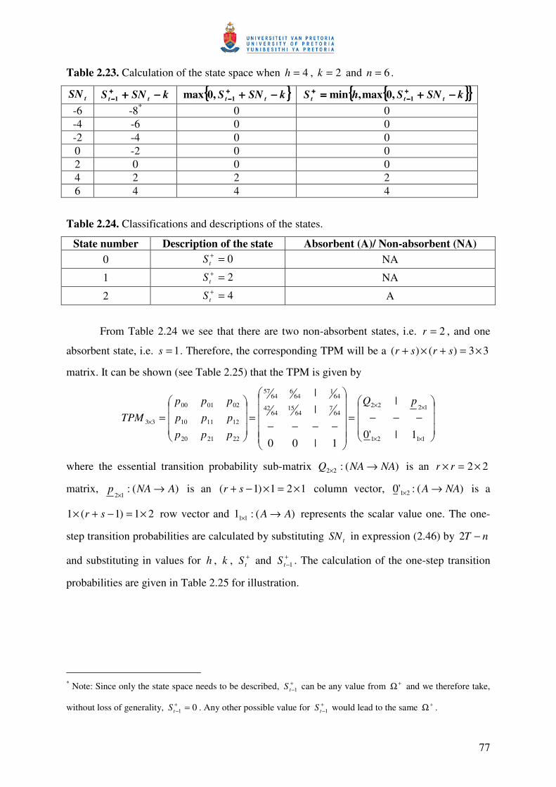
77
Table 2.23. Calculation of the state space when 4=h , 2=k and 6=n .
tSN kSNS tt −−−−++++++++−−−−1 kSNS tt −−−−++++++++
−−−−1,0max kSNShS ttt −−−−++++==== ++++−−−−
++++1,0max,min
-6 -8* 0 0 -4 -6 0 0 -2 -4 0 0 0 -2 0 0 2 0 0 0 4 2 2 2 6 4 4 4
Table 2.24. Classifications and descriptions of the states.
State number Description of the state Absorbent (A)/ Non-absorbent (NA) 0 0=+
tS NA
1 2=+tS NA
2 4=+tS A
From Table 2.24 we see that there are two non-absorbent states, i.e. 2=r , and one
absorbent state, i.e. 1=s . Therefore, the corresponding TPM will be a 33)()( ×=+×+ srsr
matrix. It can be shown (see Table 2.25) that the TPM is given by
−−−=
−−−−=
=
××
××
×
1121
122264
764
1564
42
641
646
6457
222120
121110
020100
33
1|'0
|
1|00
||
pQ
ppp
ppp
ppp
TPM
where the essential transition probability sub-matrix )(:22 NANAQ →× is an 22 ×=× rr
matrix, )(:12
ANAp →×
is an 121)1( ×=×−+ sr column vector, )(:'0 21 NAA →× is a
21)1(1 ×=−+× sr row vector and )(:1 11 AA →× represents the scalar value one. The one-
step transition probabilities are calculated by substituting tSN in expression (2.46) by nT −2
and substituting in values for h , k , +tS and +
−1tS . The calculation of the one-step transition
probabilities are given in Table 2.25 for illustration.
* Note: Since only the state space needs to be described, +
−1tS can be any value from +Ω and we therefore take,
without loss of generality, 01 =+−tS . Any other possible value for +
−1tS would lead to the same +Ω .
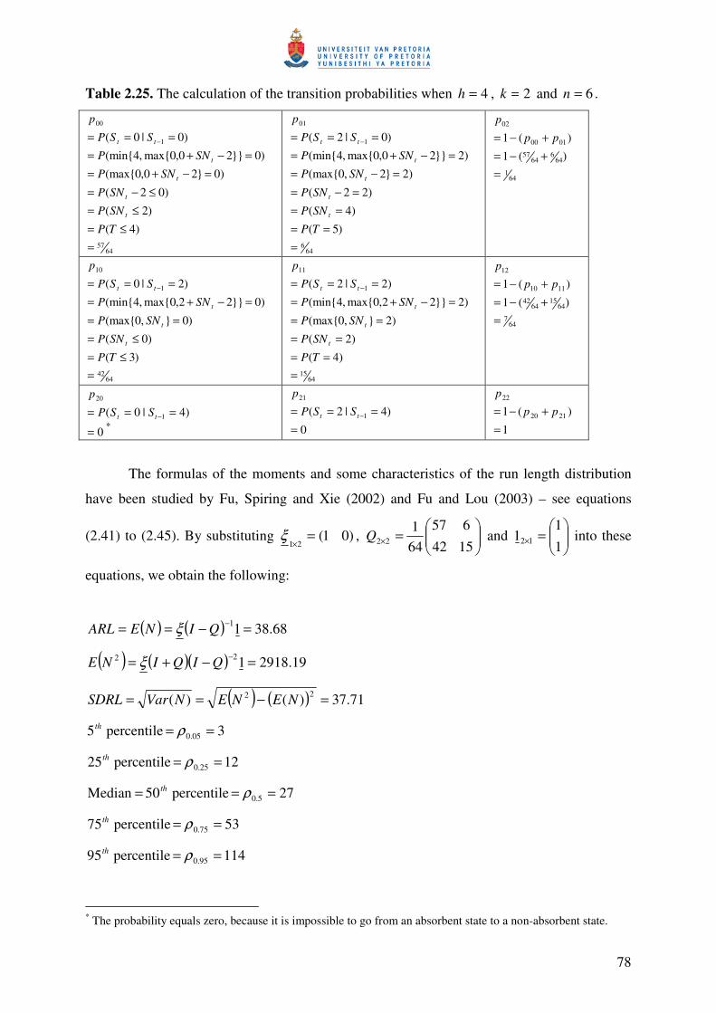
78
Table 2.25. The calculation of the transition probabilities when 4=h , 2=k and 6=n .
6457
1
00
)4(
)2(
)02(
)020,0(max
)020,0max,4(min
)0|0(
=≤=
≤=≤−=
=−+==−+=
=== −
TP
SNP
SNP
SNP
SNP
SSP
p
t
t
t
t
tt
646
1
01
)5(
)4(
)22(
)22,0(max
)220,0max,4(min
)0|2(
===
===−=
=−==−+=
=== −
TP
SNP
SNP
SNP
SNP
SSP
p
t
t
t
t
tt
641
646
6457
0100
02
)(1
)(1
=+−=+−= pp
p
6442
1
10
)3(
)0(
)0,0(max
)022,0max,4(min
)2|0(
=≤=
≤===
=−+==== −
TP
SNP
SNP
SNP
SSP
p
t
t
t
tt
6415
1
11
)4(
)2(
)2,0(max
)222,0max,4(min
)2|2(
===
====
=−+==== −
TP
SNP
SNP
SNP
SSP
p
t
t
t
tt
647
6415
6442
1110
12
)(1
)(1
=+−=+−= pp
p
)4|0( 1
20
=== −tt SSP
p
0= * 0
)4|2( 1
21
==== −tt SSP
p
1
)(1 2120
22
=+−= pp
p
The formulas of the moments and some characteristics of the run length distribution
have been studied by Fu, Spiring and Xie (2002) and Fu and Lou (2003) – see equations
(2.41) to (2.45). By substituting )01(21
=×
ξ ,
=× 1542
657
641
22Q and
=× 1
11 12 into these
equations, we obtain the following:
( ) ( ) 68.3811 =−== −QINEARL ξ
( ) ( )( ) 19.2918122 =−+= −QIQINE ξ
( ) ( ) 71.37)()( 22 =−== NENENVarSDRL
3 percentile 5 05.0 == ρth
12 percentile 25 25.0 == ρth
27 percentile 50 Median 5.0 === ρth
53 percentile 75 75.0 == ρth
114 percentile 95 95.0 == ρth
* The probability equals zero, because it is impossible to go from an absorbent state to a non-absorbent state.
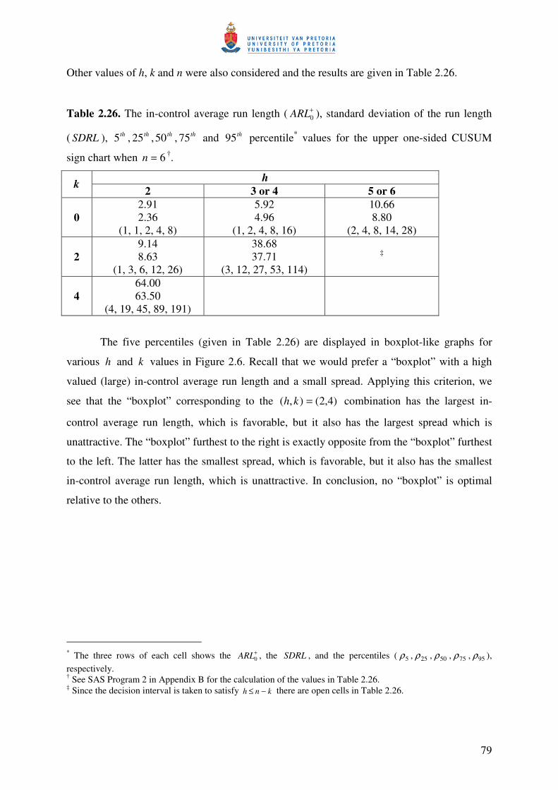
79
Other values of h, k and n were also considered and the results are given in Table 2.26.
Table 2.26. The in-control average run length ( +0ARL ), standard deviation of the run length
( SDRL ), th5 , th25 , th50 , th75 and th95 percentile* values for the upper one-sided CUSUM
sign chart when 6=n †.
h k 2 3 or 4 5 or 6
0 2.91 2.36
(1, 1, 2, 4, 8)
5.92 4.96
(1, 2, 4, 8, 16)
10.66 8.80
(2, 4, 8, 14, 28)
2 9.14 8.63
(1, 3, 6, 12, 26)
38.68 37.71
(3, 12, 27, 53, 114)
‡
4 64.00 63.50
(4, 19, 45, 89, 191)
The five percentiles (given in Table 2.26) are displayed in boxplot-like graphs for
various h and k values in Figure 2.6. Recall that we would prefer a “boxplot” with a high
valued (large) in-control average run length and a small spread. Applying this criterion, we
see that the “boxplot” corresponding to the )4,2(),( =kh combination has the largest in-
control average run length, which is favorable, but it also has the largest spread which is
unattractive. The “boxplot” furthest to the right is exactly opposite from the “boxplot” furthest
to the left. The latter has the smallest spread, which is favorable, but it also has the smallest
in-control average run length, which is unattractive. In conclusion, no “boxplot” is optimal
relative to the others.
* The three rows of each cell shows the +
0ARL , the SDRL , and the percentiles ( 5ρ , 25ρ , 50ρ , 75ρ , 95ρ ), respectively. † See SAS Program 2 in Appendix B for the calculation of the values in Table 2.26. ‡ Since the decision interval is taken to satisfy knh −≤ there are open cells in Table 2.26.
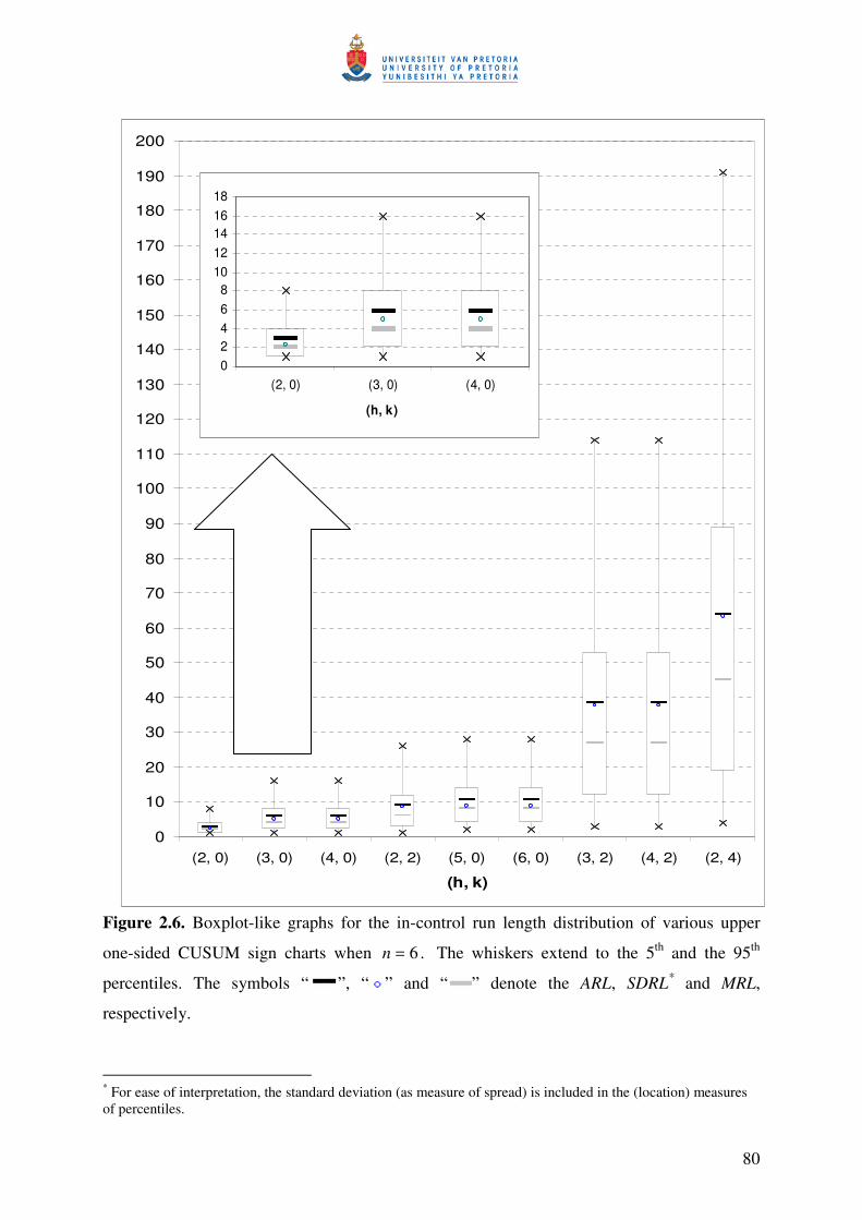
80
0
10
20
30
40
50
60
70
80
90
100
110
120
130
140
150
160
170
180
190
200
(2, 0) (3, 0) (4, 0) (2, 2) (5, 0) (6, 0) (3, 2) (4, 2) (2, 4)
(h, k)
02468
1012141618
(2, 0) (3, 0) (4, 0)
(h, k)
Figure 2.6. Boxplot-like graphs for the in-control run length distribution of various upper
one-sided CUSUM sign charts when 6=n . The whiskers extend to the 5th and the 95th
percentiles. The symbols “ ”, “ ” and “ ” denote the ARL, SDRL* and MRL,
respectively.
* For ease of interpretation, the standard deviation (as measure of spread) is included in the (location) measures of percentiles.
81
On the performance side, note that the largest in-control average run length that the
upper one-sided CUSUM sign chart can obtain is n2 . Therefore, for a sample size of 6 the
largest +0ARL equals 6426 = (this is obtained when 2=h and 4=k ). For this case we find
the
=
1064
164
63
TPM and as a result the in-control average run length equals
( ) 641)1(11 164
6310 =×−×=−= −−+ QIARL ξ . Since the largest +
0ARL is only 64 for 6=n ,
many false alarms will be expected by this chart leading to a possible loss of time and
resources. Larger sample sizes should therefore preferably be taken when implementing the
upper one-sided CUSUM sign chart.
.......................................................................................................................................................
Example 2.8
An upper one-sided CUSUM sign chart with a decision interval of 4 (h=4), a reference
value of 1 (k=1) and a sample size of 5 (n=5)
In the previous two examples it can be seen that summary measures for odd values of
h will be equal to the summary measures of the subsequent even integer. This will be
illustrated by the use of an example.
For the upper one-sided CUSUM sign chart with a decision interval of 4 ( 4=h ), a
reference value of 1 ( 1=k ) and a sample size of 5 ( 5=n ) the TPM was given by
=10032
632
1032
16
321
325
3226
TPM (see example (2.6). By keeping the reference value and the sample
size fixed and changing h to an odd integer ( 3=h ) we obtain the same TPM and therefore
we obtain the same summary measures. Stated differently, the summary measures of h odd
( 3=h ) will be equal to the summary measures of the subsequent even integer ( 4=h ).
……………………………………………………………………………………………...........
We’ve considered sample sizes of 5=n and 6 and established that larger sample sizes
should preferably be taken when implementing the upper one-sided CUSUM sign chart.
Therefore, a larger sample size ( 10=n ) is considered and the results are given in Table 2.27.
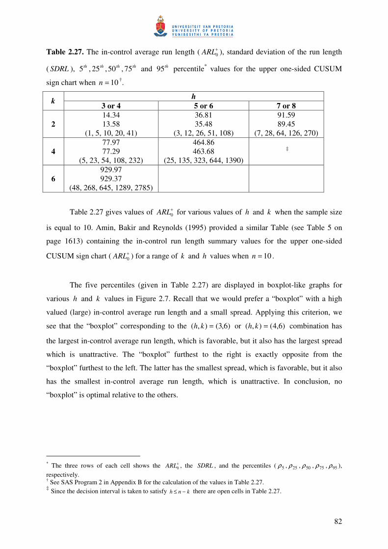
82
Table 2.27. The in-control average run length ( +0ARL ), standard deviation of the run length
( SDRL ), th5 , th25 , th50 , th75 and th95 percentile* values for the upper one-sided CUSUM
sign chart when 10=n †.
h k 3 or 4 5 or 6 7 or 8
2 14.34 13.58
(1, 5, 10, 20, 41)
36.81 35.48
(3, 12, 26, 51, 108)
91.59 89.45
(7, 28, 64, 126, 270)
4 77.97 77.29
(5, 23, 54, 108, 232)
464.86 463.68
(25, 135, 323, 644, 1390) ‡
6 929.97 929.37
(48, 268, 645, 1289, 2785)
Table 2.27 gives values of +0ARL for various values of h and k when the sample size
is equal to 10. Amin, Bakir and Reynolds (1995) provided a similar Table (see Table 5 on
page 1613) containing the in-control run length summary values for the upper one-sided
CUSUM sign chart ( +0ARL ) for a range of k and h values when 10=n .
The five percentiles (given in Table 2.27) are displayed in boxplot-like graphs for
various h and k values in Figure 2.7. Recall that we would prefer a “boxplot” with a high
valued (large) in-control average run length and a small spread. Applying this criterion, we
see that the “boxplot” corresponding to the )6,3(),( =kh or )6,4(),( =kh combination has
the largest in-control average run length, which is favorable, but it also has the largest spread
which is unattractive. The “boxplot” furthest to the right is exactly opposite from the
“boxplot” furthest to the left. The latter has the smallest spread, which is favorable, but it also
has the smallest in-control average run length, which is unattractive. In conclusion, no
“boxplot” is optimal relative to the others.
* The three rows of each cell shows the +
0ARL , the SDRL , and the percentiles ( 5ρ , 25ρ , 50ρ , 75ρ , 95ρ ), respectively. † See SAS Program 2 in Appendix B for the calculation of the values in Table 2.27. ‡ Since the decision interval is taken to satisfy knh −≤ there are open cells in Table 2.27.
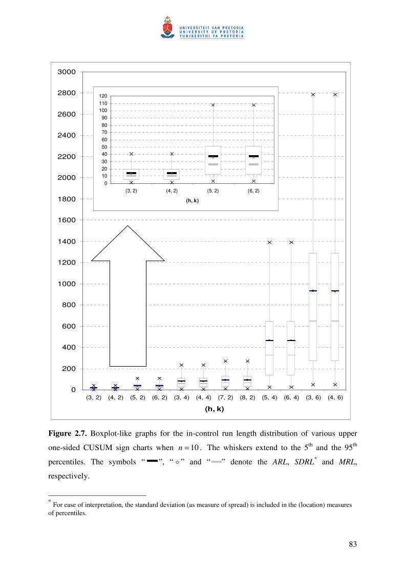
83
0
200
400
600
800
1000
1200
1400
1600
1800
2000
2200
2400
2600
2800
3000
(3, 2) (4, 2) (5, 2) (6, 2) (3, 4) (4, 4) (7, 2) (8, 2) (5, 4) (6, 4) (3, 6) (4, 6)
(h, k)
0102030405060708090
100110120
(3, 2) (4, 2) (5, 2) (6, 2)
(h, k)
Figure 2.7. Boxplot-like graphs for the in-control run length distribution of various upper
one-sided CUSUM sign charts when 10=n . The whiskers extend to the 5th and the 95th
percentiles. The symbols “ ”, “ ” and “ ” denote the ARL, SDRL* and MRL,
respectively.
* For ease of interpretation, the standard deviation (as measure of spread) is included in the (location) measures of percentiles.
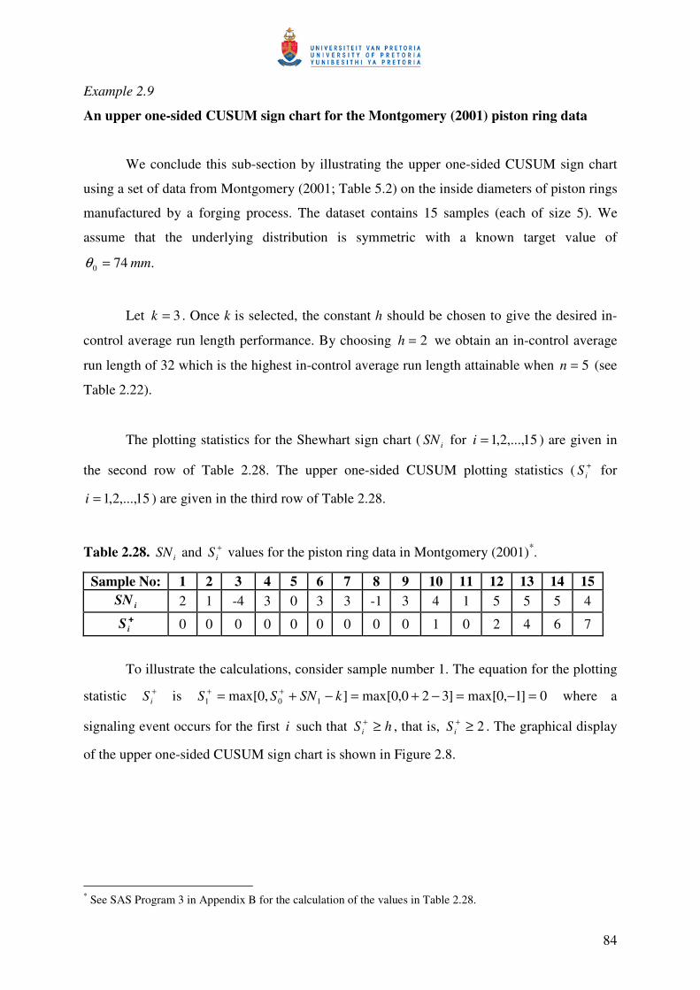
84
Example 2.9
An upper one-sided CUSUM sign chart for the Montgomery (2001) piston ring data
We conclude this sub-section by illustrating the upper one-sided CUSUM sign chart
using a set of data from Montgomery (2001; Table 5.2) on the inside diameters of piston rings
manufactured by a forging process. The dataset contains 15 samples (each of size 5). We
assume that the underlying distribution is symmetric with a known target value of
740 =θ mm.
Let 3=k . Once k is selected, the constant h should be chosen to give the desired in-
control average run length performance. By choosing 2=h we obtain an in-control average
run length of 32 which is the highest in-control average run length attainable when 5=n (see
Table 2.22).
The plotting statistics for the Shewhart sign chart ( iSN for 15,...,2,1=i ) are given in
the second row of Table 2.28. The upper one-sided CUSUM plotting statistics ( +iS for
15,...,2,1=i ) are given in the third row of Table 2.28.
Table 2.28. iSN and +iS values for the piston ring data in Montgomery (2001)*.
Sample No: 1 2 3 4 5 6 7 8 9 10 11 12 13 14 15 iSN 2 1 -4 3 0 3 3 -1 3 4 1 5 5 5 4
++++iS 0 0 0 0 0 0 0 0 0 1 0 2 4 6 7
To illustrate the calculations, consider sample number 1. The equation for the plotting
statistic +iS is 0]1,0max[]320,0max[],0max[ 101 =−=−+=−+= ++ kSNSS where a
signaling event occurs for the first i such that hS i ≥+ , that is, 2≥+iS . The graphical display
of the upper one-sided CUSUM sign chart is shown in Figure 2.8.
* See SAS Program 3 in Appendix B for the calculation of the values in Table 2.28.
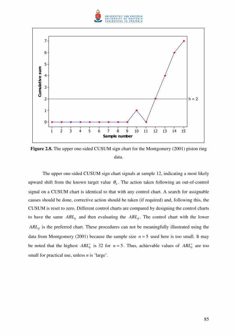
85
Figure 2.8. The upper one-sided CUSUM sign chart for the Montgomery (2001) piston ring
data.
The upper one-sided CUSUM sign chart signals at sample 12, indicating a most likely
upward shift from the known target value 0θ . The action taken following an out-of-control
signal on a CUSUM chart is identical to that with any control chart. A search for assignable
causes should be done, corrective action should be taken (if required) and, following this, the
CUSUM is reset to zero. Different control charts are compared by designing the control charts
to have the same 0ARL and then evaluating the δARL . The control chart with the lower
δARL is the preferred chart. These procedures can not be meaningfully illustrated using the
data from Montgomery (2001) because the sample size 5=n used here is too small. It may
be noted that the highest +0ARL is 32 for 5=n . Thus, achievable values of +
0ARL are too
small for practical use, unless n is ‘large’.
86
2.3.2.2. Lower one-sided control charts
Analogous to the previous section, a Markov chain representation of the one-sided
CUSUM procedure based on integer-valued cumulative sums is presented in this section. The
number of states included in the Markov chain is minimized in order to make the methods as
efficient as possible. The time that the procedure signals is the first time such that the finite-
state Markov chain −tS enters the state 0ς where the state space is given by
,...,, 110 −+− =Ω srςςς with 0... 10 =<<=− −+srh ςς , 00 =−S and
kSNShS ttt ++−= −−
−1,0min,max . (2.47)
Clearly, there is only one absorbent state, since the chart signals when −tS falls on or below
h− , i.e. 1=s .
The distribution of tSN can easily be obtained from the binomial distribution (recall
that nTSN ii −= 2 i∀ , where iT is binomially distributed with parameters n and
)( 0θ≥= ijXPp ) . The binomial probabilities are given in Table G of Gibbons and
Chakraborti (2003) and can easily be calculated using some type of statistical software
package, for example, Excel or SAS.
Example 2.10
A lower one-sided CUSUM sign chart where the sample size is odd ( 5====n )
The statistical properties of a lower one-sided CUSUM sign chart with a decision
interval of 4 ( 4=h ), a reference value of 1 ( 1=k ) and a sample size of 5 ( 5=n ) is
examined. For n odd, the reference value is taken to be odd, because this leads to the sum
( ) − kSN i being equal to even values which reduces the size of the state space for the
Markov chain. For 4=h we have =Ω− =,, 210 ςςς 0,2,4 −− with 0210 =<<=− ςςςh .
The state space is calculated using equation (2.47) and the calculations are shown in Table
2.29.
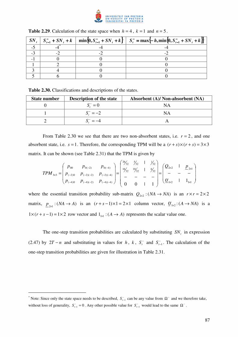
87
Table 2.29. Calculation of the state space when 4=h , 1=k and 5=n .
tSN kSNS tt ++++++++−−−−−−−−1 kSNS tt ++++++++−−−−
−−−−1,0min kSNShS ttt ++++++++−−−−==== −−−−−−−−
−−−−1,0min,max
-5 -4* -4 -4 -3 -2 -2 -2 -1 0 0 0 1 2 0 0 3 4 0 0 5 6 0 0
Table 2.30. Classifications and descriptions of the states.
State number Description of the state Absorbent (A)/ Non-absorbent (NA) 0 0=−
tS NA
1 2−=−tS NA
2 4−=−tS A
From Table 2.30 we see that there are two non-absorbent states, i.e. 2=r , and one
absorbent state, i.e. 1=s . Therefore, the corresponding TPM will be a 33)()( ×=+×+ srsr
matrix. It can be shown (see Table 2.31) that the TPM is given by
−−−=
−−−−=
=
××
××
−−−−−
−−−−−
−−
×
1121
122232
632
1032
16
321
325
3226
)4)(4()2)(4(0)4(
)4)(2()2)(2(0)2(
)4(0)2(000
33
1|'0
|
1|00
||
pQ
ppp
ppp
ppp
TPM
where the essential transition probability sub-matrix )(:22 NANAQ →× is an 22 ×=× rr
matrix, )(:12
ANAp →×
is an 121)1( ×=×−+ sr column vector, )(:'0 21 NAA →× is a
21)1(1 ×=−+× sr row vector and )(:1 11 AA →× represents the scalar value one.
The one-step transition probabilities are calculated by substituting tSN in expression
(2.47) by nT −2 and substituting in values for h , k , −tS and −
−1tS . The calculation of the
one-step transition probabilities are given for illustration in Table 2.31.
* Note: Since only the state space needs to be described, −
−1tS can be any value from −Ω and we therefore take,
without loss of generality, 01 =−−tS . Any other possible value for −
−1tS would lead to the same −Ω .
88
Table 2.31. The calculation of the transition probabilities when 4=h , 1=k and 5=n .
3226
1
00
)1(1)2(
)152(
)1(
)01(
)010,0(min
)010,0min,4(max
)0|0(
=≤−=
≥=−≥−=
−≥=≥+=
=++==++−=
=== −
TP
TP
TP
SNP
SNP
SNP
SNP
SSP
p
t
t
t
t
tt
325
1
)2(0
)1()352(
)3(
)21(
)21,0(min
)210,0min,4(max
)0|2(
===
−=−=−==
−=+=−=+=
−=++−==−== −
−
TP
TP
SNP
SNP
SNP
SNP
SSP
p
t
t
t
t
tt
321
325
3226
)2(000
)4(0
)(1
)(1
=+−=
+−= −
−
pp
p
3216
1
0)2(
)2(1)3(
)152(
)1(
)01(
)012,0(min
)012,0min,4(max
)2|0(
=≤−=
≥=≥−=
≥=≥−=
=++−==++−−=
−=== −
−
TP
TP
TP
SNP
SNP
SNP
SNP
SSP
p
t
t
t
t
tt
3210
1
)2)(2(
)2()152(
)1(
)21(
)212,0(min
)212,0min,4(max
)2|2(
===
−=−=−==
−=−=−=++−=
−=++−−=−=−== −
−−
TP
TP
SNP
SNP
SNP
SNP
SSP
p
t
t
t
t
tt
326
3210
3216
)2)(2(0)2(
)4)(2(
)(1
)(1
=+−=
+−= −−−
−−
pp
p
)4|0( 1
0)4(
−=== −
−
tt SSP
p
0= * 0
)4|2( 1
)2)(4(
=−=−== −
−−
tt SSP
p
1)00(1
)(1 )2)(4(0)4(
)4)(4(
=+−=
+−= −−−
−−
pp
p
The formulas of the moments and some characteristics of the run length distribution
have been studied by Fu, Spiring and Xie (2002) and Fu and Lou (2003) – see equations
(2.41) to (2.45). By substituting )01(21
=×
ξ ,
=×
3210
3216
325
3226
22Q and
=× 1
11 12 into these
equations, we obtain the following:
( ) ( ) 62.1611 =−== −QINEARL ξ
( ) ( )( ) 59.516122 =−+= −QIQINE ξ
( ) ( ) 51.15)()( 22 =−== NENENVarSDRL
2 percentile 5 5 == ρth
6 percentile 25 25 == ρth
* The probability equals zero, because it is impossible to go from an absorbent state to a non-absorbent state.

89
12 percentile 50 Median 50 === ρth
23 percentile 75 75 == ρth
48 percentile 95 95 == ρth
The in-control average run length values, standard deviation of the run length values
and percentiles for the lower one-sided CUSUM sign chart are exactly the same as for the
upper one-sided CUSUM sign chart, since the one-step transition probabilities matrices are
the same (compare the transition probabilities matrices of examples 2.6 and 2.10). Therefore,
we obtain Result 2.10:
Result 2.10:
The in-control average run length ( +0ARL ), standard deviation of the run length ( SDRL ),
th5 , th25 , th50 , th75 and th95 percentile values tabulated for the upper one-sided CUSUM sign
chart will also hold for the lower one-sided CUSUM sign chart.
Example 2.11
A lower one-sided CUSUM sign chart for the Montgomery (2001) piston ring data
We conclude this sub-section by illustrating the lower one-sided CUSUM sign chart
using a set of data from Montgomery (2001; Table 5.2) on the inside diameters of piston rings
manufactured by a forging process. The dataset contains 15 samples (each of size 5). We
assume that the underlying distribution is symmetric with a known target value of
740 =θ mm.
From Table 2.22 it can be seen that the in-control average run length equals 32 when
2=h and 3=k (recall that this is the largest possible in-control average run length value
that the chart can obtain, since 3225 = ). The plotting statistics for the Shewhart sign chart
( iSN for 15,...,2,1=i ) are given in the second row of Table 2.32. The lower one-sided
CUSUM plotting statistics ( −iS for 15,...,2,1=i ) are given in the third row of Table 2.32.
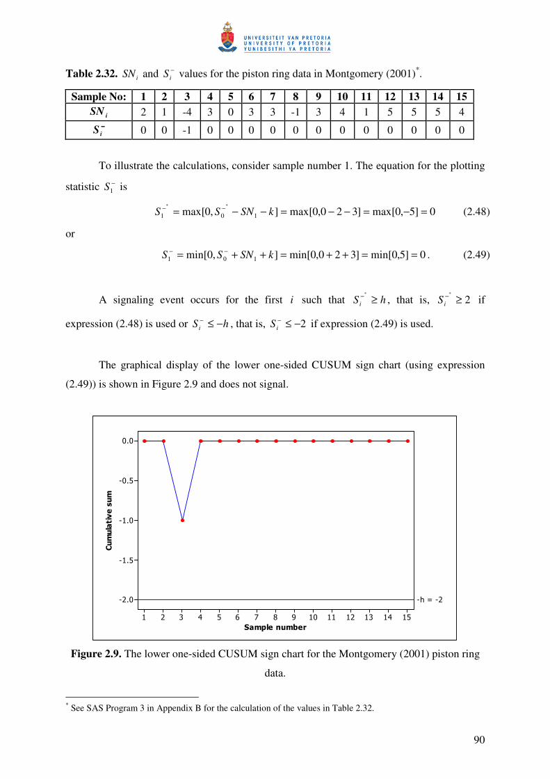
90
Table 2.32. iSN and −iS values for the piston ring data in Montgomery (2001)*.
Sample No: 1 2 3 4 5 6 7 8 9 10 11 12 13 14 15 iSN 2 1 -4 3 0 3 3 -1 3 4 1 5 5 5 4
−−−−iS 0 0 -1 0 0 0 0 0 0 0 0 0 0 0 0
To illustrate the calculations, consider sample number 1. The equation for the plotting
statistic −1S is
0]5,0max[]320,0max[],0max[ 101
**
=−=−−=−−= −− kSNSS (2.48)
or
0]5,0min[]320,0min[],0min[ 101 ==++=++= −− kSNSS . (2.49)
A signaling event occurs for the first i such that hS i ≥−*
, that is, 2*
≥−iS if
expression (2.48) is used or hS i −≤− , that is, 2−≤−iS if expression (2.49) is used.
The graphical display of the lower one-sided CUSUM sign chart (using expression
(2.49)) is shown in Figure 2.9 and does not signal.
Figure 2.9. The lower one-sided CUSUM sign chart for the Montgomery (2001) piston ring
data.
* See SAS Program 3 in Appendix B for the calculation of the values in Table 2.32.
91
2.3.3. Two-sided control charts
Various authors have studied the two-sided CUSUM scheme, for example, Kemp
(1971) gives the average run length of the two-sided CUSUM scheme in terms of the average
run lengths of the two corresponding one-sided schemes. Lucas and Crosier (1982) used a
Markov chain representation of the two-sided CUSUM scheme to determine the run length
distribution and the average run length. In this thesis, the approach taken by Brook and Evans
(1972) for the one-sided CUSUM scheme is extended to the two-sided CUSUM scheme. A
Markov chain representation of the two-sided CUSUM scheme based on integer-valued
random variables will be presented. This is done since the nonparametric statistics that are the
building blocks of the CUSUM scheme are discrete random variables. The number of states
included in the Markov chain is minimized by taking the reference value k so that the state
space of the Markov chain is a set of even numbers. This reduces the size of the TPM and
thus eliminates unnecessary calculations in order to make the methods as efficient as possible.
Recall that for the upper one-sided CUSUM sign chart we use
,0max,min 1+−
+ +−= ttt SkSNhS for ,...2,1=n (2.50)
For a lower one-sided CUSUM sign chart we use
,0min,max 1−−
− ++−= ttt SkSNhS for ,...2,1=n (2.51)
For the two-sided scheme the two one-sided schemes are performed simultaneously. The
corresponding two-sided CUSUM chart signals for the first t at which either one of the two
inequalities is satisfied, that is, either hSt ≥+ or hSt −≤− . Starting values are typically chosen
to equal zero, that is, 000 == −+ SS . The two-sided scheme signals at
hShStN ttt−≤≥= −+ or:min where h is a positive integer.
The two-sided CUSUM scheme can be represented by a Markov chain with states
corresponding to the possible combinations of values of +tS and −
tS . The states corresponding
to values for which a signal is given by the CUSUM scheme are called absorbent states.
Clearly, there are two absorbent states since the chart signals when +tS falls on or above h or
when −tS falls on or below h− , i.e. 2=s . Recall that r denotes the number of non-absorbent
92
states and, consequently, the corresponding TPM is an )()( srsr +×+ , i.e. an
)2()2( +×+ rr matrix.
The time that the procedure signals is the first time such that the finite-state Markov
chain enters the state 0ς or 1−+srς where the state space is given by Ω = −+ Ω∪Ω =
,...,, 110 −+srςςς with hh sr =<<=− −+ 10 ... ςς .
Example 2.12
A two-sided CUSUM sign chart where the sample size is odd ( 5====n )
The statistical properties of a two-sided CUSUM sign chart with a decision interval of
4 ( 4=h ), a reference value of 1 ( 1=k ) and a sample size of 5 ( 5=n ) is examined. For n
odd, the reference value k is taken to be odd, because this leads to the sum ( ) − kSN i being
equal to even values which reduces the size of the state space for the Markov chain. This
reduces the size of the TPM and thus eliminates unnecessary calculations in order to make the
methods as efficient as possible. Let Ω denote the state space for the two-sided chart. Ω is
the union of the state space for the upper one-sided chart 4,2,0=Ω+ and the state space for
the lower one-sided chart 0,2,4 −−=Ω− . Therefore, Ω = −+ Ω∪Ω = 4,2,00,2,4 ∪−− =
4,2,0,2,4 −− = ,,,, 43210 ςςςςς with hh =<<<<=− 43210 ςςςςς .
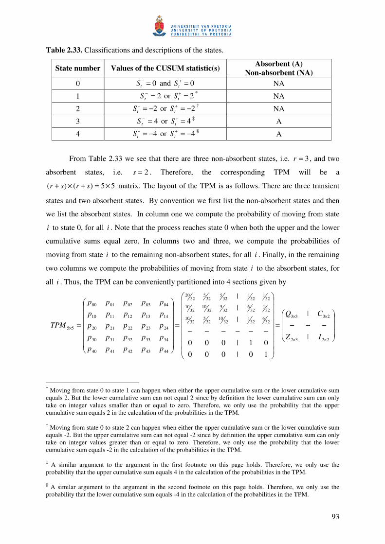
93
Table 2.33. Classifications and descriptions of the states.
State number Values of the CUSUM statistic(s) Absorbent (A) Non-absorbent (NA)
0 0=−tS and 0=+
tS NA
1 2=−tS or 2=+
tS * NA
2 2−=−tS or 2−=+
tS † NA
3 4=−tS or 4=+
tS ‡ A
4 4−=−tS or 4−=+
tS § A
From Table 2.33 we see that there are three non-absorbent states, i.e. 3=r , and two
absorbent states, i.e. 2=s . Therefore, the corresponding TPM will be a
55)()( ×=+×+ srsr matrix. The layout of the TPM is as follows. There are three transient
states and two absorbent states. By convention we first list the non-absorbent states and then
we list the absorbent states. In column one we compute the probability of moving from state
i to state 0, for all i . Note that the process reaches state 0 when both the upper and the lower
cumulative sums equal zero. In columns two and three, we compute the probabilities of
moving from state i to the remaining non-absorbent states, for all i . Finally, in the remaining
two columns we compute the probabilities of moving from state i to the absorbent states, for
all i . Thus, the TPM can be conveniently partitioned into 4 sections given by
−−−=
−−−−−−=
=
××
××
×
2232
233332
632
132
1032
532
10
321
326
325
3210
3210
321
321
325
325
3220
4443424140
3433323130
2423222120
1413121110
0403020100
55
|
|
10|00001|000
|||
IZ
CQ
ppppp
ppppp
ppppp
ppppp
ppppp
TPM
* Moving from state 0 to state 1 can happen when either the upper cumulative sum or the lower cumulative sum equals 2. But the lower cumulative sum can not equal 2 since by definition the lower cumulative sum can only take on integer values smaller than or equal to zero. Therefore, we only use the probability that the upper cumulative sum equals 2 in the calculation of the probabilities in the TPM. † Moving from state 0 to state 2 can happen when either the upper cumulative sum or the lower cumulative sum equals -2. But the upper cumulative sum can not equal -2 since by definition the upper cumulative sum can only take on integer values greater than or equal to zero. Therefore, we only use the probability that the lower cumulative sum equals -2 in the calculation of the probabilities in the TPM. ‡ A similar argument to the argument in the first footnote on this page holds. Therefore, we only use the probability that the upper cumulative sum equals 4 in the calculation of the probabilities in the TPM. § A similar argument to the argument in the second footnote on this page holds. Therefore, we only use the probability that the lower cumulative sum equals -4 in the calculation of the probabilities in the TPM.
94
where the essential transition probability sub-matrix )(:33 NANAQ →× is an 33×=× rr
matrix, )(:23 ANAC →× is an 23×=× sr matrix, )(:32 NAAZ →× is an 32 ×=× rs matrix
and )(:22 AAI →× is a 22 ×=× ss matrix.
The calculation of the elements of the TPM is illustrated next. Note that this
essentially involves the calculation of the matrices Q and C . First consider the transient
states. Note that the process moves to state 0, i.e., 0=j , when both the upper and the lower
cumulative sums equal 0. Thus the required probability of moving to 0, from any other
transient state, is the probability of an intersection of two sets involving values of the upper
and the lower CUSUM statistics, respectively. On the other hand, the probability of moving to
any state 0≠j , from any other state, is the probability of a union of two sets involving values
of the upper and the lower CUSUM statistics, respectively. However, one of these two sets is
empty so that the required probability is the probability of only the non-empty set.
The calculation of the entry in the first row and the first column of the matrix Q , 00p ,
will be discussed in detail. This is the probability of moving from state 0 to state 0 in one step.
As we just described, this can happen only when the upper and the lower cumulative sums
both equal 0 at time t . For the upper one-sided CUSUM 00p is the probability that the upper
CUSUM equals 0 at time t , given that the upper CUSUM equaled 0 at time 1−t , that is,
)0|0( 1 == +−
+tt SSP . For the lower one-sided procedure 00p is the probability that the lower
CUSUM equals 0 at time t , given that the lower CUSUM equaled 0 at time 1−t , that is,
)0|0( 1 == −−
−tt SSP . For the two-sided procedure the two one-sided procedures are performed
simultaneously. Therefore we have that ( )0|00|0 1100 ==∩=== −−
−+−
+tttt SSSSPp .
95
We have that
( )0|00|0 11
00
==∩=== −−
−+−
+tttt SSSSP
p
this is computed by substituting in values for h , k , +tS , +
−1tS , −tS and −
−1tS into equations
(2.50) and (2.51)
( ) ( )( ) ( )( )( ) ( )( )11
00101
001,0min001,0max
001,0min,4max001,0max,4min
−≥∩≤=≥++∩≤−=
=++∩=+−==++−∩=+−=
tt
tt
tt
tt
SNSNP
SNSNP
SNSNP
SNSNP
recall that nTSNt −= 2 where T is binomially distributed with parameters n and )( 0θ≥= ijXPp
( ) ( )( )( ) ( )( )23
152152≥∩≤=
−≥−∩≤−=TTP
TTP
( )32
20
32102
)2(2)3()2(
=×=
===+==
TP
TPTP
since T is binomially distributed with parameters 5=n and 5.0=p .
The remaining entries in the first column of the matrix Q can be calculated similarly
and we find that 3210
10 =p and 3210
20 =p .
Next we discuss the calculation of the entry in the first row and the second column of
the matrix Q , 01p , in detail. This is the probability of moving from state 0 to state 1 in one
step. This can happen when either the upper cumulative sum or the lower cumulative sum
equals 2. But the lower cumulative sum can not equal 2 since by definition the lower
cumulative sum can only take on integer values smaller than or equal to zero. Therefore
although the required probability is the probability of the union of two sets involving values
of the upper and the lower CUSUM statistics, one of these sets is empty so that the required
probability is the probability of only the non-empty set. Hence, in this case, we will only have
to calculate the upper one-sided probability. For the upper one-sided CUSUM, 01p is the
probability that the upper cumulative sum equals 2 at time t , given that the upper cumulative
sum equaled 0 at time 1−t , that is, )0|2( 1 == +−
+tt SSP . We have that
96
)0|2( 1
01
=== +−
+tt SSP
p
( )( )( )( )3
21
201,0max
201,0max,4min
===−=
=+−==+−=
t
t
t
t
SNP
SNP
SNP
SNP
( )( )4
352==
=−=TP
TP
325= .
The remaining entries in the second column of the matrix Q can be calculated
similarly and we find that 3210
11 =p and 325
21 =p .
Next we discuss the calculation of the entry in the first row and the third column of the
matrix Q , 02p , in detail. This is the probability of moving from state 0 to state 2 in one step.
This happens when only the lower cumulative sum moves to -2, since the upper cumulative
sum can not move to -2. Recall that the upper cumulative sum can only take on integer values
greater than or equal to zero. As in the case of 01p , this probability is also the probability of
the union of two sets, involving values of the CUSUM statistics, one of which is empty, so
that the required probability is the probability of only the non-empty set. Hence, in this case
since the lower CUSUM is involved, we will only have to calculate the probability associated
with the lower one-sided procedure. Now, for the lower one-sided procedure 02p is the
probability that the lower cumulative sum equals -2 at time t , given that the lower cumulative
sum equaled 0 at time 1−t , that is, )0|2( 1 =−= −−
−tt SSP . We have that
)0|2( 1
02
=−== −−
−tt SSP
p
( )( )( )( )3
21
201,0min
201,0min,4max
−==−=+=
−=++=−=++−=
t
t
t
t
SNP
SNP
SNP
SNP
( )( )1
352==
−=−=TP
TP
325= .
97
The remaining entries in the third column of the matrix Q can be calculated similarly
and we find that 325
12 =p and 3210
22 =p .
Next we discuss the calculation of the entry in the first row and the first column of the
matrix C , 03p , in detail. This is the probability of moving from state 0 to an absorbent state,
state 3, in one step. Again, this can happen when only the upper cumulative sum moves to 4,
since the lower cumulative sum can not move to 4. Recall that the lower cumulative sum can
only take on integer values smaller than or equal to zero. Therefore, once again the required
probability is the probability of the union of two sets involving values of the CUSUM
statistics, one of which is empty so that the probability is the probability of only the non-
empty set. Therefore we will only have to calculate the upper one-sided probability in this
case. For the upper one-sided procedure 03p is the probability that the upper cumulative sum
equals 4 at time t , given that the upper cumulative sum equaled 0 at time 1−t , that is,
)0|4( 1 == +−
+tt SSP . We have that
)0|4( 1
03
=== +−
+tt SSP
p
( )( )( )( )( )5
552
5
41
401,0max,4min
≥=≥−=
≥=≥−=
=+−=
TP
TP
SNP
SNP
SNP
t
t
t
321= .
The remaining entries in the first column of the matrix C can be calculated similarly
and we find that 326
13 =p and 321
23 =p .
Next we discuss the calculation of the entry in the first row and the last column of the
matrix C , 04p , in detail. This is the probability of moving from state 0 to state 4 in one step.
This can happen when only the lower cumulative sum moves to -4, since the upper cumulative
sum can not move to -4. Recall that the upper cumulative sum can only take on integer values
greater than or equal to zero. Therefore although the required probability is the probability of
the union of two sets involving values of the upper and the lower CUSUM statistics, one of
these sets is empty so that the required probability is the probability of only the non-empty
98
set. Therefore we will only have to calculate the lower one-sided probability. For the lower
one-sided procedure 04p is the probability that the lower cumulative sum equals -4 at time t ,
given that the lower cumulative sum equaled 0 at time 1−t , that is, )0|4( 1 =−= −−
−tt SSP . We
have that
)0|4( 1
04
=−== −−
−tt SSP
p
( )( )( )( )( )0
552
5
41
401,0min,4max
≤=−≤−=
−≤=−≤+=
−=++−=
TP
TP
SNP
SNP
SNP
t
t
t
321= .
The remaining entries in the last column of the matrix C can be calculated similarly
and we find that 321
14 =p and 326
24 =p .
The run length distribution and its parameters
The run length distribution and its parameters are calculated using the matrix Q . The
ARL is given by ( ) 11−− QIξ where )001(31
=×
ξ ,
=×
1051051010
5520
321
33Q and
=×
11
1
1 13 .
As a result, ( ) ( ) 31.811 =−== −QINEARL ξ .
Let +ARL and −ARL denote the average run lengths of the upper and lower one-sided
charts, respectively. The ARL of the two-sided chart can be expressed as a function of the
average run lengths of the one-sided charts through the expression
( )−+
−+
+=
ARLARLARLARL
ARL))((
(2.52)
(see Theorem 1 in Appendix A for the proof of result (2.52)).
99
From the lower- and upper CUSUM sign sections we have that 62.16=+ARL and
62.16=−ARL . Using equation (2.52) we have that ( ) 31.862.1662.16
)62.16)(62.16( =+
=ARL .
Table 2.34. The in-control average run length ( 0ARL ), standard deviation of the run length
( SDRL ), th5 , th25 , th50 , th75 and th95 percentile* values for the two-sided CUSUM sign chart
when 5=n †.
h k 2 3 or 4
1 2.67 2.11
(1, 1, 2, 3, 7)
8.31 7.16
(1, 3, 6, 11, 23)
3 16.00 15.50
(1, 5, 11, 22, 47)
‡
Analogous to what was done for the upper one-sided chart, the five percentiles (given
in Table 2.34) are displayed in boxplot-like graphs for various h and k values in Figure 2.10.
Recall that we would prefer a “boxplot” with a high valued (large) in-control average run
length and a small spread. Applying this criterion, we see that the “boxplot” corresponding to
the )3,2(),( =kh combination has the largest in-control average run length, which is
favorable, but it also has the largest spread which is unattractive. The “boxplot” furthest to the
right is exactly opposite from the “boxplot” furthest to the left. The latter has the smallest
spread, which is favorable, but it also has the smallest in-control average run length, which is
unattractive. In conclusion, no “box plot” is optimal relative to the others.
* The three rows of each cell shows the ARL0, the SDRL , and the percentiles ( 5ρ , 25ρ , 50ρ , 75ρ , 95ρ ), respectively. † See SAS Program 2 in Appendix B for the calculation of the values in Table 2.34. ‡ Since the decision interval is taken to satisfy knh −≤ there are open cells in Table 2.34.
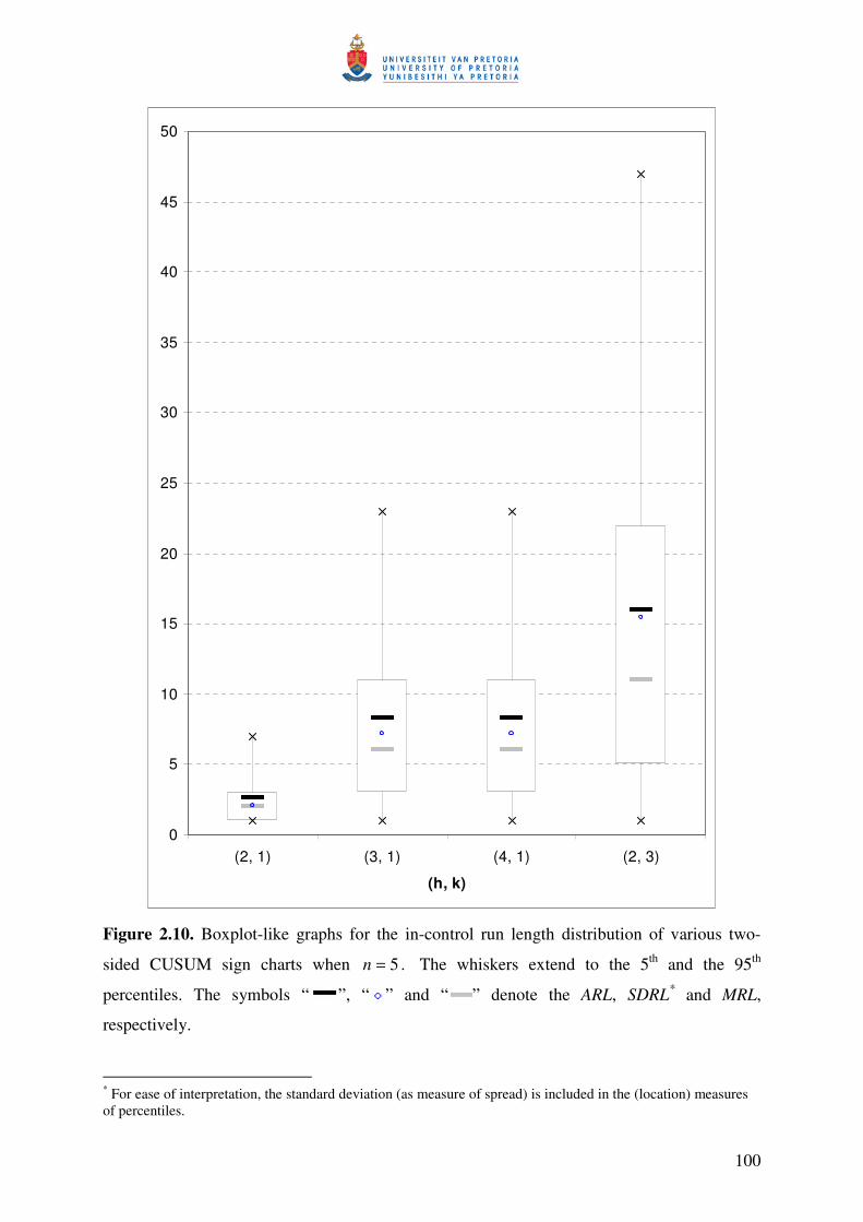
100
0
5
10
15
20
25
30
35
40
45
50
(2, 1) (3, 1) (4, 1) (2, 3)
(h, k)
Figure 2.10. Boxplot-like graphs for the in-control run length distribution of various two-
sided CUSUM sign charts when 5=n . The whiskers extend to the 5th and the 95th
percentiles. The symbols “ ”, “ ” and “ ” denote the ARL, SDRL* and MRL,
respectively.
* For ease of interpretation, the standard deviation (as measure of spread) is included in the (location) measures of percentiles.
101
Other values of h, k and n were also considered and the results are given in Table 2.35.
Table 2.35. The in-control average run length ( 0ARL ), standard deviation of the run length
( SDRL ), th5 , th25 , th50 , th75 and th95 percentile* values for the two-sided CUSUM sign chart
when 6=n †.
h k 2 3 or 4 5 or 6
0 1.45 0.81
(1, 1, 1, 2, 3)
2.96 1.88
(1, 2, 3, 4, 7)
5.33 4.22
(1, 2, 4, 7, 14)
2 4.57 4.04
(1, 2, 3, 6, 13)
19.34 18.36
(2, 6, 14, 26, 56)
‡
4 32.00 31.50
(2, 10, 22, 44, 95)
** The three rows of each cell shows the ARL0, the SDRL , and the percentiles ( 5ρ , 25ρ , 50ρ , 75ρ , 95ρ ), respectively. † See SAS Program 2 in Appendix B for the calculation of the values in Table 2.35. ‡ Since the decision interval is taken to satisfy knh −≤ there are open cells in Table 2.35.
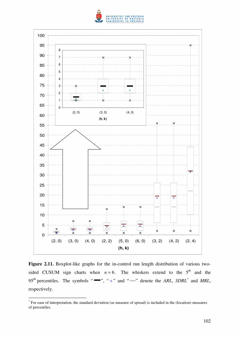
102
0
5
10
15
20
25
30
35
40
45
50
55
60
65
70
75
80
85
90
95
100
(2, 0) (3, 0) (4, 0) (2, 2) (5, 0) (6, 0) (3, 2) (4, 2) (2, 4)
(h, k)
0
1
2
3
4
5
6
7
8
(2, 0) (3, 0) (4, 0)
(h, k)
Figure 2.11. Boxplot-like graphs for the in-control run length distribution of various two-
sided CUSUM sign charts when 6=n . The whiskers extend to the 5th and the
95th percentiles. The symbols “ ”, “ ” and “ ” denote the ARL, SDRL* and MRL,
respectively.
* For ease of interpretation, the standard deviation (as measure of spread) is included in the (location) measures of percentiles.
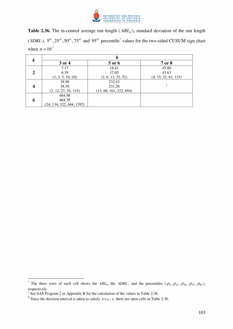
103
Table 2.36. The in-control average run length ( 0ARL ), standard deviation of the run length
( SDRL ), th5 , th25 , th50 , th75 and th95 percentile* values for the two-sided CUSUM sign chart
when 10=n †.
h k 3 or 4 5 or 6 7 or 8
2 7.17 6.39
(1, 3, 5, 10, 20)
18.41 17.05
(2, 6, 13, 25, 52)
45.80 43.63
(4, 15, 32, 63, 133)
4 38.98 38.30
(3, 12, 27, 54, 115)
232.43 231.26
(13, 68, 161, 322, 694)
‡
6 464.98 464.39
(24, 134, 322, 644, 1392)
* The three rows of each cell shows the ARL0, the SDRL , and the percentiles ( 5ρ , 25ρ , 50ρ , 75ρ , 95ρ ), respectively. † See SAS Program 2 in Appendix B for the calculation of the values in Table 2.36. ‡ Since the decision interval is taken to satisfy knh −≤ there are open cells in Table 2.36.
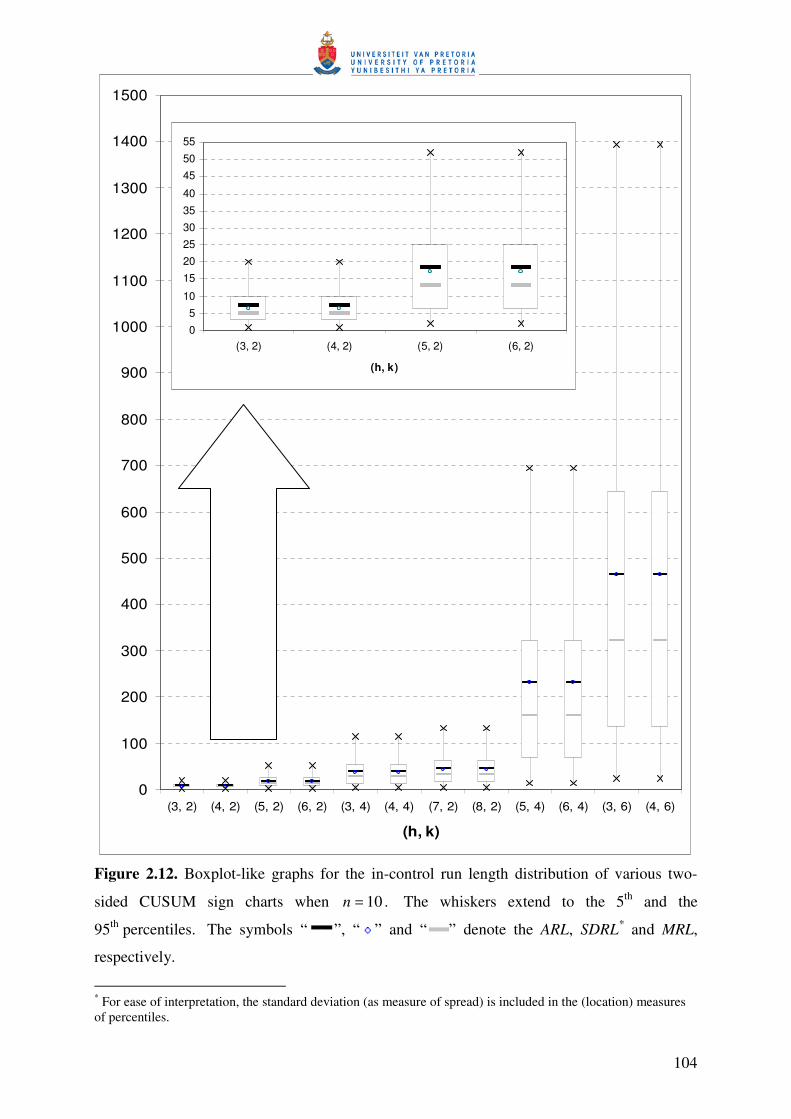
104
0
100
200
300
400
500
600
700
800
900
1000
1100
1200
1300
1400
1500
(3, 2) (4, 2) (5, 2) (6, 2) (3, 4) (4, 4) (7, 2) (8, 2) (5, 4) (6, 4) (3, 6) (4, 6)
(h, k)
05
10
1520253035
40
4550
55
(3, 2) (4, 2) (5, 2) (6, 2)
(h, k)
Figure 2.12. Boxplot-like graphs for the in-control run length distribution of various two-
sided CUSUM sign charts when 10=n . The whiskers extend to the 5th and the
95th percentiles. The symbols “ ”, “ ” and “ ” denote the ARL, SDRL* and MRL,
respectively.
* For ease of interpretation, the standard deviation (as measure of spread) is included in the (location) measures of percentiles.
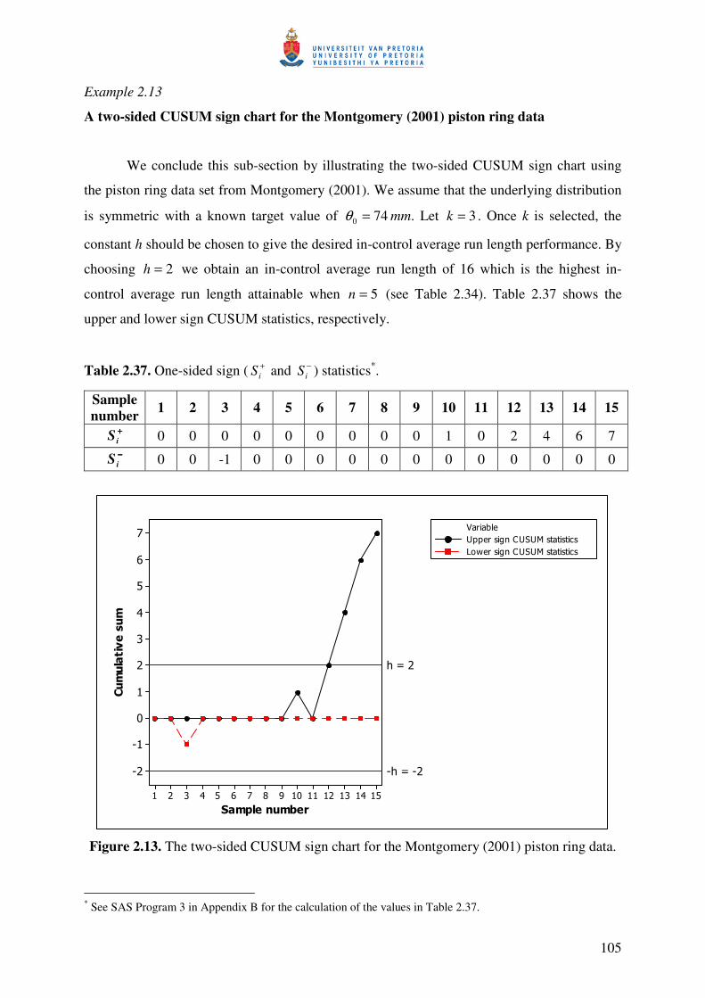
105
Example 2.13
A two-sided CUSUM sign chart for the Montgomery (2001) piston ring data
We conclude this sub-section by illustrating the two-sided CUSUM sign chart using
the piston ring data set from Montgomery (2001). We assume that the underlying distribution
is symmetric with a known target value of 740 =θ mm. Let 3=k . Once k is selected, the
constant h should be chosen to give the desired in-control average run length performance. By
choosing 2=h we obtain an in-control average run length of 16 which is the highest in-
control average run length attainable when 5=n (see Table 2.34). Table 2.37 shows the
upper and lower sign CUSUM statistics, respectively.
Table 2.37. One-sided sign ( +iS and −
iS ) statistics*.
Sample number 1 2 3 4 5 6 7 8 9 10 11 12 13 14 15
++++iS 0 0 0 0 0 0 0 0 0 1 0 2 4 6 7 −−−−iS 0 0 -1 0 0 0 0 0 0 0 0 0 0 0 0
!"#
Figure 2.13. The two-sided CUSUM sign chart for the Montgomery (2001) piston ring data.
* See SAS Program 3 in Appendix B for the calculation of the values in Table 2.37.
106
The two-sided CUSUM sign chart signals at sample number 12, indicating a most like
upward shift in the process median. The action taken following an out-of-control signal on a
CUSUM chart is identical to that with any control chart. A search for assignable causes
should be done, corrective action should be taken (if required) and, following this, the
CUSUM is reset to zero.
2.3.4. Summary
While the Shewhart-type charts are widely known and most often used in practice
because of their simplicity and global performance, other classes of charts, such as the
CUSUM charts are useful and sometimes more naturally appropriate in the process control
environment in view of the sequential nature of data collection. In this section we have
described the properties of the CUSUM sign chart and given tables for its implementation.
Detailed calculations have been given to help the reader to understand the subject more
thoroughly.
2.4. The EWMA control chart
2.4.1. Introduction
The exponentially weighted moving average (EWMA) scheme was first introduced by
Roberts (1959). In a subsequent article, Roberts (1966) compared the performance of EWMA
charts to Shewhart and CUSUM charts. Various authors have studied EWMA charts (see for
example Robinson and Ho (1978) and Crowder (1987)). EWMA charts have become very
popular over the last few years. It is one of several charting methods aimed at correcting a
deficiency of the Shewhart chart – insensitivity to small process shifts.
An EWMA control chart scheme accumulates statistics ,...,, 321 XXX with the plotting
statistics defined as
1)1( −−+= iii ZXZ λλ (2.53)
where 10 ≤< λ is a constant called the weighting constant. The starting value 0Z is often
taken to be the process target value, i.e. 00 θ=Z .
107
The EWMA chart is constructed by plotting iZ against the sample number i (or
time). If the plotting statistic iZ falls between the two control limits, that is,
UCLZLCL i << , the process is considered to be in-control. If the plotting statistic iZ falls on
or outside one of the control limits, that is LCLZ i ≤ or UCLZ i ≥ , the process is considered
to be out-of-control.
To illustrate that the plotting statistic iZ is a weighted average of all the previous
statistics, 1−iZ may be substituted by 211 )1( −−− −+= iii ZXZ λλ in equation (2.53) to obtain
( )
( ).)1()1()1(
)1()1()1(
)1()1(
)1()1(
33
22
1
322
1
22
1
21
−−−
−−−
−−
−−
−+−+−+=
−+−+−+=
−+−+=
−+−+=
iiii
iiii
iii
iiii
ZXXX
ZXXX
ZXX
ZXXZ
λλλλλλλλλλλλ
λλλλλλλλ
This method of substitution is called recursive substitution. By continuing the process
of recursive substitution for piZ − , tp ,...,3,2= , we obtain
0
1
0
)1()1( ZXZ ipi
i
p
pi λλλ −+−= −
−
= . (2.54)
We can see from expression (2.54) that iZ can be written as a moving average of the current
and past observations which has geometrically decreasing weights p)1( λλ − associated with
increasingly aged observations piX − ( ,...2,1=p ). Therefore, the EWMA has been referred to
as a geometric moving average (see, for example, Montgomery (2005)).
If the observations ,...2,1, =iX i are independent identically distributed variables
with mean µ and variance 2σ , then the mean and the variance of the plotting statistic iZ are
given by
µµ == )( iZ ZEi
for ,...2,1=i
and
( )iZ i
222 )1(12
λλ
λσσ −−
−= for ,...2,1=i .
108
The exact control limits and the center line of the EWMA control chart are given by
( )
( )i
i
LLCL
CL
LUCL
20
0
20
)1(12
)1(12
λλ
λσθ
θ
λλ
λσθ
−−
−−=
=
−−
−+=
. (2.55)
From (2.55) we see that we have two design parameters of interest, namely the
multiplier L , ( 0>L ) and the smoothing constant λ . We also see that ( ) 1)1(1 2 →−− iλ as i
increases. Therefore, as i increases the control limits will approach steady-state values given
by
−−=
−+=
λλσθ
λλσθ
2
2
0
0
LLCL
LUCL
. (2.56)
The above-mentioned control limits are called steady-state control limits.
Various authors recommend choosing the EWMA constants L and λ by minimizing
the average run length at a specified shift for a desired in-control average run length. In
general, values of λ in the interval 25.005.0 ≤≤ λ work well in the normal theory case with
05.0=λ , 1.0=λ and 2.0=λ being popular choices. The 0ARL , standard deviation of the
run length ( SDRL ), th5 , th25 (the first quartile, 1Q ), th50 (the median run length, MRL ),
th75 (the third quartile, 3Q ) and th95 percentile values can be computed and tabulated for
various values of L and λ .
Lucas and Saccucci (1990) have investigated some properties of the EWMA chart
under the assumption of independent normally distributed observations. Lucas and Saccucci’s
most important contribution is the use of a Markov-chain approach to evaluate the run-length
properties of the EWMA chart. It is important to note that the successive observations are
assumed to be independent over time in their evaluation. Lucas and Saccucci (1990) used a
procedure similar to that described by Brook and Evans (1972) to approximate the properties
of an EWMA scheme. They evaluate the properties of the continuous state Markov chain by
109
discretizing the infinite state transition probability matrix (TPM). This procedure entails
dividing the interval between the upper control limit and the lower control limit into N
subintervals of width δ2 . Then the plotting statistic, iZ , is said to be in the non-absorbing
state j at time i if
δδ +≤<− jij SZS for 1,...,2,1 −= Nj
and
δδ +<<− jij SZS for Nj =
where jS denotes the midpoint of the thj interval. Let r denote the number of non-absorbing
states. iZ is said to be in the absorbing state if iZ falls on or outside one of the control limits,
that is, LCLZ i ≤ or UCLZ i ≥ . Clearly, there are 1+r states, since there are r non-
absorbing states and one absorbing state. Lucas and Saccucci (1990) have done a thorough
job of evaluating the run length properties of the EWMA chart and provided helpful tables for
the design of the EWMA chart. Additional tables are provided in the technical report by
Lucas and Saccucci (1987). In their 1990 paper they concentrate on the average run length
characteristics of various charting combinations. The authors conclude that EWMA
procedures have average run length properties similar to those for CUSUM procedures. This
point has also been made by various authors, for example, Ewan (1963), Roberts (1966) and
Montgomery, Gardiner and Pizzano (1987). In this thesis, the approach taken by Lucas and
Saccucci (1990) is extended to the use of the sign statistic resulting in an EWMA sign chart
that accumulates the statistics ,...,, 321 SNSNSN .
2.4.2. The proposed EWMA sign chart
A nonparametric EWMA-type of control chart based on the sign statistic can be
obtained by replacing iX in expression (2.53) with iSN (recall that =
−=n
jiji xsignSN
10 )( θ ).
The EWMA sign chart accumulates the statistics ,...,, 321 SNSNSN with the plotting statistics
defined as
1)1( −−+= iii ZSNZ λλ (2.57)
where 10 ≤< λ and the starting value 0Z is usually taken to equal zero, i.e. 00 =Z .
110
The expected value, variance and standard deviation of iSN are found from the fact
that the distribution of iSN can easily be obtained from the distribution of the binomial
distribution (recall that nTSN ii −= 2 if there are no ties within a subgroup, where iT has a
binomial distribution with parameters n and )( 0θ≥= ijXPp ). The formulas for the
expected value, variance and standard deviation of iSN was derived in Section 2.1 and we
obtained )12()( −= pnSNE i , )1(4)var( pnpSN i −= and )1(2)( pnpSNstdeviSNi −== σ ,
respectively. The starting value 0Z can also be taken to be the expected value of iSN ,
therefore ( ) )12(0 −== pnSNEZ i and in the in-control case where 5.0=p we have
0)15.02(0 =−×= nZ for all n .
From the similarity between the definitions of the normal EWMA scheme and the sign
EWMA scheme, it follows that the exact control limits and the center line of the EWMA sign
control chart can be obtained by replacing σ in (2.55) with iSNσ which yields
( )
( )iSN
iSN
i
i
LLCL
CL
LUCL
2
2
)1(12
0
0
)1(12
0
λλ
λσ
λλ
λσ
−−
−−=
=
−−
−+=
. (2.58)
It is important to note 0θ in (2.55) is replaced by 0 in (2.58). This is because the
EWMA sign chart is designed for the sign test statistic and not for the observations (the
iX ’s).
Similarly, the steady-state control limits can be obtained by replacing σ in (2.56)
with iSNσ and 0θ by zero which yields
−−=
−=
λλσ
λλσ
2
2
i
i
SN
SN
LLCL
LUCL
. (2.59)
111
2.4.3. Markov-chain approach
Lucas and Saccucci (1990) evaluated the properties of the continuous state Markov
chain by discretizing the infinite state TPM. This procedure entails dividing the interval
between the UCL and the LCL into N subintervals of width δ2 . The width of each
subinterval can be obtained by setting ( )
NLCLUCL −×=
21δ and we get that the width of an
interval equals ( )
NLCLUCL −=δ2 . Thus, the endpoints of the subintervals will be given by
,LCL ( )
NLCLUCL
LCL−+ ,
( ),2
NLCLUCL
LCL−+ …,
( ),)1(
NLCLUCL
NLCL−−+ UCL ,
respectively (see Figure 2.14). In general, the endpoints of the thj interval will be given by
( ) ( ) ( ).,)1(,
−×+−×−+=N
LCLUCLjLCL
NLCLUCL
jLCLUCLLCL jj
The midpoint of the thj interval, jS , is easily obtained by taking the sum of the two
endpoints of the thj interval and dividing it by 2. Thus, we obtain
jS
2jj UCLLCL +
=
( ) ( )
2
)1(
−++
−−+= N
LCLUCLjLCL
NLCLUCLj
LCL
( ).
2)12(
NLCLUCLj −−=
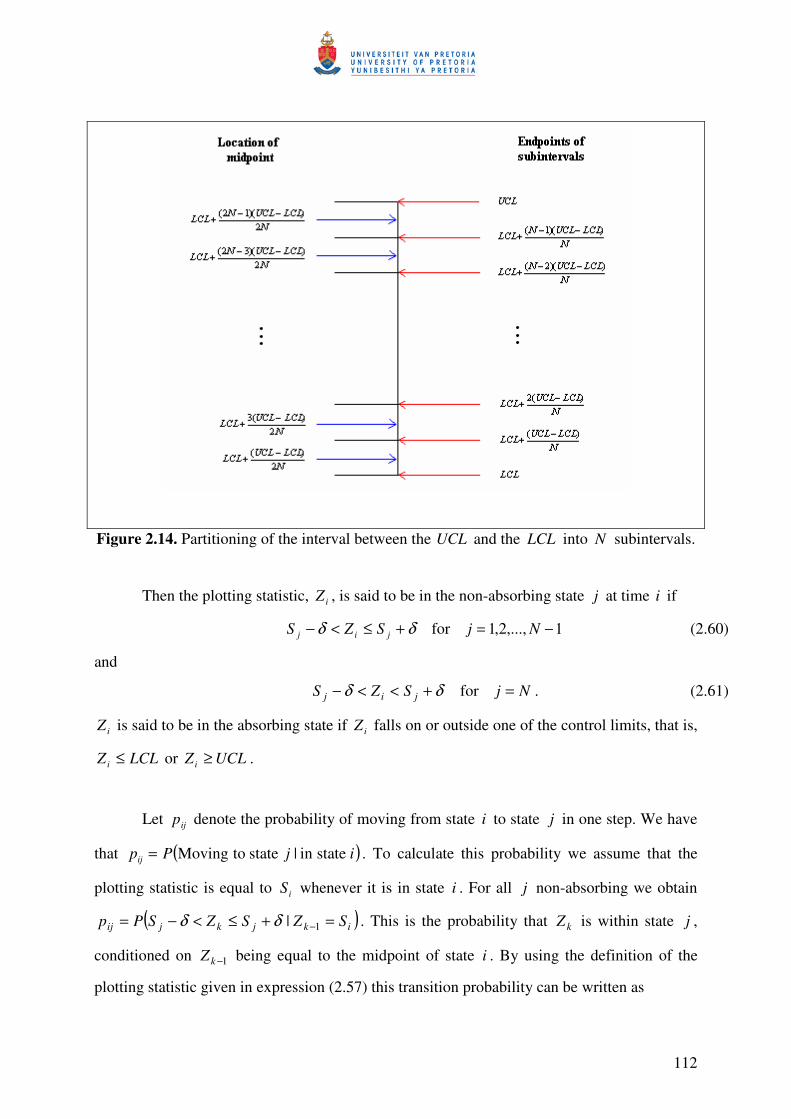
112
Figure 2.14. Partitioning of the interval between the UCL and the LCL into N subintervals.
Then the plotting statistic, iZ , is said to be in the non-absorbing state j at time i if
δδ +≤<− jij SZS for 1,...,2,1 −= Nj (2.60)
and
δδ +<<− jij SZS for Nj = . (2.61)
iZ is said to be in the absorbing state if iZ falls on or outside one of the control limits, that is,
LCLZ i ≤ or UCLZ i ≥ .
Let ijp denote the probability of moving from state i to state j in one step. We have
that =ijp ( )ijP statein|statetoMoving . To calculate this probability we assume that the
plotting statistic is equal to iS whenever it is in state i . For all j non-absorbing we obtain
( )ikjkjij SZSZSPp =+≤<−= −1|δδ . This is the probability that kZ is within state j ,
conditioned on 1−kZ being equal to the midpoint of state i . By using the definition of the
plotting statistic given in expression (2.57) this transition probability can be written as
113
( )ikjkkjij SZSZSNSPp =+≤−+<−= −− 11 |)1( δλλδ
( )δλλδ +≤−+<−= jikj SSSNSP )1(
−−+≤<
−−−=
λλδ
λλδ ij
kij SS
SNSS
P)1()()1()(
.
Recall that nTSN kk −= 2 where kT is binomially distributed with parameters n and
)( 0θ≥= ijXPp
−−+≤−<
−−−=
λλδ
λλδ ij
kij
ij
SSnT
SSPp
)1()(2
)1()(
+
−−+
≤<
+
−−−
=2
)1()(
2
)1()(n
SS
T
nSS
P
ij
k
ij
λλδ
λλδ
. (2.62)
The probability of transition to the out-of-control state can be determined similarly.
For all j absorbing we obtain
( ) ( )( ) ( )( ) ( )
−−≥−+
−−≤−=
−−≥+
−−≤=
≥−++≤−+==≥−++=≤−+=
=≥+=≤=
−−−−
−−
λλ
λλ
λλ
λλ
λλλλλλλλ
ik
ik
ik
ik
ikik
ikkkikkk
ikkikkij
SUCLnTP
SLCLnTP
SUCLSNP
SLCLSNP
UCLSSNPLCLSSNP
SZUCLZSNPSZLCLZSNP
SZUCLZPSZLCLZPp
)1(2
)1(2
)1()1(
)1()1(
|)1(|)1(
||
1111
11
+−−
≥+
+−−
≤=2
)1(
2
)1(n
SUCL
TPn
SLCL
TP
i
k
i
kλ
λλ
λ
. (2.63)
Since the values δ , λ , n , iS and jS are known constants the binomial probabilities
in expressions (2.62) and (2.63) can easily be calculated using some type of statistical
software package, for example, Excel or SAS.
114
Once the one-step transition probabilities are calculated, the TPM can be constructed
and is given by
−−−=1|'0
| pQ
TPM (written in partitioned form) where Q is the matrix that
contains all the transition probabilities of going from a non-absorbing state to a non-absorbing
state. In other words, Q is the transition matrix among the in-control states, Q ( )NANA →: .
p contains all the transition probabilities of going from each non-absorbing state to the
absorbing states, p ( )ANA →: . '0 ( )0000 = contains all the transition
probabilities of going from the absorbing state to each non-absorbing state, '0 ( )NAA →: . 1
represents the scalar value one which is the probability of going from the absorbing state to
the absorbing state, 1 ( )AA →: .
Lucas and Saccucci (1990) have investigated some properties of the EWMA chart
under the assumptions of independent normally distributed observations. From the similarity
between the definitions of the normal EWMA scheme and the sign EWMA scheme, it follows
that the formulas derived by Lucas and Saccucci (1990) can be extended to the use of the sign
EWMA scheme. The formulas derived by Lucas and Saccucci (1990) have been studied by
other authors, for example, Fu, Spiring and Xie (2002) and Fu and Lou (2003). The latter two
used the moment generating function and the probability generating function, respectively, to
derive expressions for the first and second moments of the run length variable N . See
Theorem 2 in Appendix A for the derivations done by Fu, Spiring and Xie (2002) and Fu and
Lou (2003). For the formulas refer to equations (2.41) to (2.45) of this thesis.
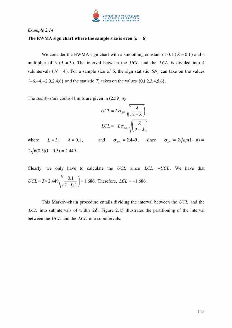
115
Example 2.14
The EWMA sign chart where the sample size is even (n = 6)
We consider the EWMA sign chart with a smoothing constant of 0.1 ( 1.0=λ ) and a
multiplier of 3 ( 3=L ). The interval between the UCL and the LCL is divided into 4
subintervals ( 4=N ). For a sample size of 6, the sign statistic iSN can take on the values
6,4,2,0,2,4,6 −−− and the statistic iT takes on the values 6,5,4,3,2,1,0 .
The steady-state control limits are given in (2.59) by
−−=
−=
λλσ
λλσ
2
2
i
i
SN
SN
LLCL
LUCL
where 3=L , 1.0=λ , and 449.2=iSNσ , since =
iSNσ =− )1(2 pnp
449.2)5.01)(5.0(62 =− .
Clearly, we only have to calculate the UCL since UCLLCL −= . We have that
686.11.02
1.0449.23 =
−×=UCL . Therefore, 686.1−=LCL .
This Markov-chain procedure entails dividing the interval between the UCL and the
LCL into subintervals of width δ2 . Figure 2.15 illustrates the partitioning of the interval
between the UCL and the LCL into subintervals.
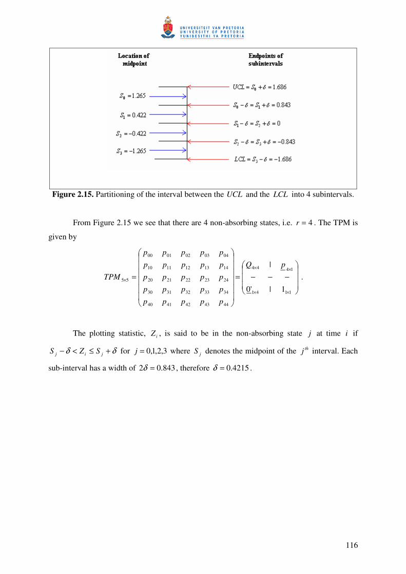
116
Figure 2.15. Partitioning of the interval between the UCL and the LCL into 4 subintervals.
From Figure 2.15 we see that there are 4 non-absorbing states, i.e. 4=r . The TPM is
given by
−−−=
=
××
××
×
1141
1444
4443424140
3433323130
2423222120
1413121110
0403020100
55
1|'0
| pQ
ppppp
ppppp
ppppp
ppppp
ppppp
TPM .
The plotting statistic, iZ , is said to be in the non-absorbing state j at time i if
δδ +≤<− jij SZS for 3,2,1,0=j where jS denotes the midpoint of the thj interval. Each
sub-interval has a width of 843.02 =δ , therefore 4215.0=δ .
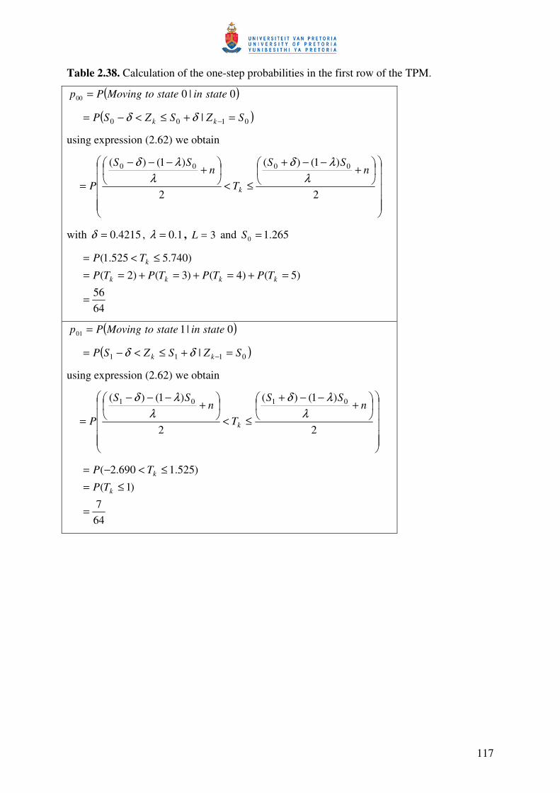
117
Table 2.38. Calculation of the one-step probabilities in the first row of the TPM.
( )0|000 stateinstatetoMovingPp =
( )0100 | SZSZSP kk =+≤<−= −δδ
using expression (2.62) we obtain
+−−+
≤<
+−−−
=2
)1()(
2
)1()( 0000 nSS
Tn
SS
P kλ
λδλ
λδ
with 4215.0=δ , 1.0=λ , 3=L and 265.10 =S
6456
)5()4()3()2(
)740.5525.1(
=
=+=+=+==≤<=
kkkk
k
TPTPTPTP
TP
( )0|101 stateinstatetoMovingPp =
( )0111 | SZSZSP kk =+≤<−= −δδ
using expression (2.62) we obtain
+−−+
≤<
+−−−
=2
)1()(
2
)1()( 0101 nSS
Tn
SS
P kλ
λδλ
λδ
647
)1(
)525.1690.2(
=
≤=≤<−=
k
k
TP
TP
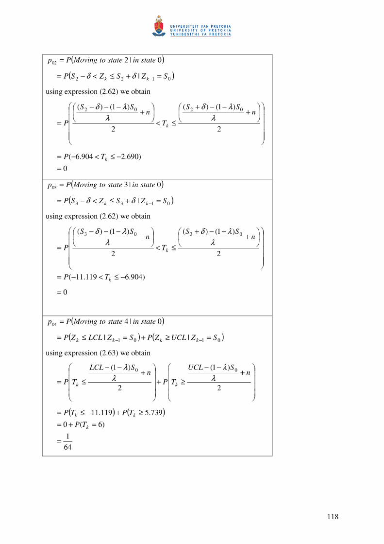
118
( )0|202 stateinstatetoMovingPp =
( )0122 | SZSZSP kk =+≤<−= −δδ
using expression (2.62) we obtain
+−−+
≤<
+−−−
=2
)1()(
2
)1()( 0202 nSS
Tn
SS
P kλ
λδλ
λδ
0
)690.2904.6(
=−≤<−= kTP
( )0|303 stateinstatetoMovingPp =
( )0133 | SZSZSP kk =+≤<−= −δδ
using expression (2.62) we obtain
)904.6119.11(
2
)1()(
2
)1()( 0303
−≤<−=
+−−+
≤<
+−−−
=
k
k
TP
nSS
Tn
SS
Pλ
λδλ
λδ
0=
( )0|404 stateinstatetoMovingPp =
( ) ( )0101 || SZUCLZPSZLCLZP kkkk =≥+=≤= −−
using expression (2.63) we obtain
+−−
≥+
+−−
≤=2
)1(
2
)1( 00 nSUCL
TPn
SLCL
TP kkλ
λλ
λ
( ) ( )
641
)6(0
739.5119.11
=
=+=≥+−≤=
k
kk
TP
TPTP
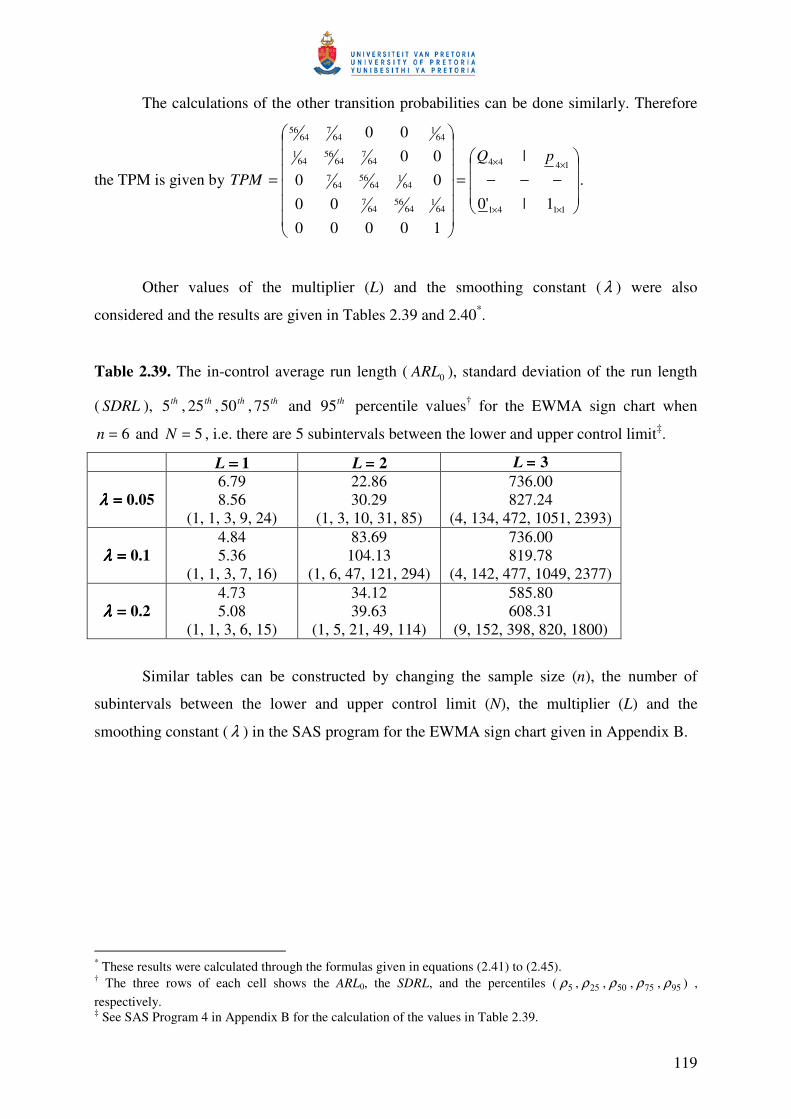
119
The calculations of the other transition probabilities can be done similarly. Therefore
the TPM is given by
−−−=
=
××
××
1141
1444
641
6456
647
641
6456
647
647
6456
641
641
647
6456
1|'0
|
1000000
0000
00pQ
TPM .
Other values of the multiplier (L) and the smoothing constant ( λ ) were also
considered and the results are given in Tables 2.39 and 2.40*.
Table 2.39. The in-control average run length ( 0ARL ), standard deviation of the run length
( SDRL ), th5 , th25 , th50 , th75 and th95 percentile values† for the EWMA sign chart when
6=n and 5=N , i.e. there are 5 subintervals between the lower and upper control limit‡.
1====L 2====L 3====L
05.0====λλλλ 6.79 8.56
(1, 1, 3, 9, 24)
22.86 30.29
(1, 3, 10, 31, 85)
736.00 827.24
(4, 134, 472, 1051, 2393)
1.0====λλλλ 4.84 5.36
(1, 1, 3, 7, 16)
83.69 104.13
(1, 6, 47, 121, 294)
736.00 819.78
(4, 142, 477, 1049, 2377)
2.0====λλλλ 4.73 5.08
(1, 1, 3, 6, 15)
34.12 39.63
(1, 5, 21, 49, 114)
585.80 608.31
(9, 152, 398, 820, 1800)
Similar tables can be constructed by changing the sample size (n), the number of
subintervals between the lower and upper control limit (N), the multiplier (L) and the
smoothing constant ( λ ) in the SAS program for the EWMA sign chart given in Appendix B.
* These results were calculated through the formulas given in equations (2.41) to (2.45). † The three rows of each cell shows the ARL0, the SDRL, and the percentiles ( 5ρ , 25ρ , 50ρ , 75ρ , 95ρ ) , respectively. ‡ See SAS Program 4 in Appendix B for the calculation of the values in Table 2.39.
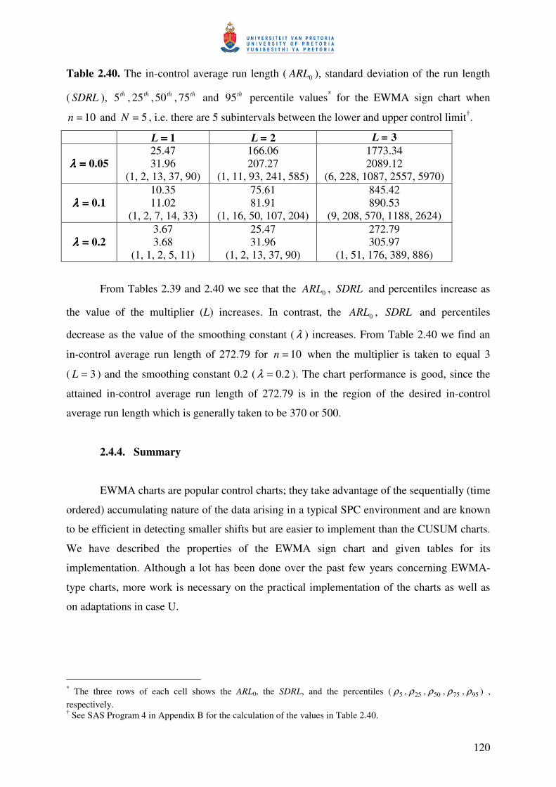
120
Table 2.40. The in-control average run length ( 0ARL ), standard deviation of the run length
( SDRL ), th5 , th25 , th50 , th75 and th95 percentile values* for the EWMA sign chart when
10=n and 5=N , i.e. there are 5 subintervals between the lower and upper control limit†.
1====L 2====L 3====L
05.0====λλλλ 25.47 31.96
(1, 2, 13, 37, 90)
166.06 207.27
(1, 11, 93, 241, 585)
1773.34 2089.12
(6, 228, 1087, 2557, 5970)
1.0====λλλλ 10.35 11.02
(1, 2, 7, 14, 33)
75.61 81.91
(1, 16, 50, 107, 204)
845.42 890.53
(9, 208, 570, 1188, 2624)
2.0====λλλλ 3.67 3.68
(1, 1, 2, 5, 11)
25.47 31.96
(1, 2, 13, 37, 90)
272.79 305.97
(1, 51, 176, 389, 886)
From Tables 2.39 and 2.40 we see that the 0ARL , SDRL and percentiles increase as
the value of the multiplier (L) increases. In contrast, the 0ARL , SDRL and percentiles
decrease as the value of the smoothing constant ( λ ) increases. From Table 2.40 we find an
in-control average run length of 272.79 for 10=n when the multiplier is taken to equal 3
( 3=L ) and the smoothing constant 0.2 ( 2.0=λ ). The chart performance is good, since the
attained in-control average run length of 272.79 is in the region of the desired in-control
average run length which is generally taken to be 370 or 500.
2.4.4. Summary
EWMA charts are popular control charts; they take advantage of the sequentially (time
ordered) accumulating nature of the data arising in a typical SPC environment and are known
to be efficient in detecting smaller shifts but are easier to implement than the CUSUM charts.
We have described the properties of the EWMA sign chart and given tables for its
implementation. Although a lot has been done over the past few years concerning EWMA-
type charts, more work is necessary on the practical implementation of the charts as well as
on adaptations in case U.
* The three rows of each cell shows the ARL0, the SDRL, and the percentiles ( 5ρ , 25ρ , 50ρ , 75ρ , 95ρ ) , respectively. † See SAS Program 4 in Appendix B for the calculation of the values in Table 2.40.