1

Chapter 1 Introduction

1.1 Solar heating systems overview Since the 1970’s, residential solar technology has emerged as a result of the increasing cost of energy. The true cost of a house includes construction and operational costs. Energy consumption, which in most cases is used for heating and cooling, is typically the most significant operational cost in residential buildings. Many attempts have been made thereafter to save space heating and cooling energy. Although the features of each specific solar heating system vary, the basic components of a solar heating system are the same. It should at least include: a collector, where heat is collected from the solar energy; heat storage and a heat circulation system. The solar collector is typically installed on the roof and mounted on the south-facing slope. Normally, the solar heating system cannot support the house’s heating demand in extreme weather conditions. For this, a conventional backup heating system is usually installed. The investment in two heating systems increases the cost/benefit ratio of the solar system. A balance between maximizing solar collection and cost must be achieved. There are at least three concerns for the cost effective integration of thermal-solar systems. First, what type of system should be used? Second, what size collector is most economical? And third, can costs be reduced to maximize the return-on-investment for the system? It is this last question that is of concern for this thesis. Most thermal-solar systems are added to a pre-constructed roof or wall. If the collector is integrated with the roof or wall, then both material and installation costs can be saved. The system investigated through this thesis is a demonstration of this integrated approach. For thermal-solar collectors two collection and transport media are common: water and air. In water-media collectors, water circulates through copper tubing attached to an absorptive surface. The circulating water takes the heat that is being captured by the blacken surface and transfers the heat to the storage tank. The air-media collector is less expensive and less efficient in terms of carrying heat. However, it is easier to install and is nearly a maintenance-free system. Without water, the collector does not have rust and freezing problems. By using the air-media collector, the water-to-air heat exchange can be eliminated because the heated air can be directly used in the house. Since the 70’s, solar heating systems both using air and water have been used. Examples can be found in most states including Virginia, the target market of this research. In general, the solar heating system can provide at least 50 percent of the heating demand. In the NASA Technology Utilization House (Hampton, Virginia 1976), with a two-collector water-media solar heating system and a heat pump, 100 percent of the heating demand was met. The building is one-story, 1500 square feet footage. Collector area is 370 square feet with a storage volume of 1900 gallons of water. (Shurcliff, 1979) An integrated approach can result in a more cost effective system. During the 1970’s, there was some effort made to design integrated solar collection systems, which is, combining the collector system with the roof structure. With this integrated approach, the collector itself can function as

2

the roof structure instead of merely a mounted-on system. As stated by Bruce Anderson, “It makes more sense to build the collector to the full dimension of a roof, using it for heating both the building and the domestic hot water.” (Anderson, 1977). In the late 80’s, OM Solar (2003) developed an integrated air-media solar collector. OM Solar has several projects built using this approach. For example, the Silberstein residence, in Sacramento, California, has a conventional light timber frame with 1636-square-foot living space and 432 square feet of studio area. The house has an air-media solar heating system integrated with the roof structure and an auxiliary gas heater. According to their data, in heating season for each year, there are 121 Days when no auxiliary heating is required; 19 days when the house may need some gas heating in the early morning; 13 days when the house may need some gas heating in the early morning and early evening; 23 days when the house may need some gas heating during the day. This suggests the potential values for this approach. Figure 1 shows the OM solar roof system. The photovoltaic panels in the picture supply the power of the air-handling unit. The external ridge duct collects the heated air and sends it to the air-handling unit.

Figure2. Solar Roof Collector System and a house section (Graph courtesy of OM Solar)

Figure1. OM Solar roof system (Graph courtesy of OM Solar)

3

Figure 3. The Silberstein house model in Sacramento, California (Graph courtesy of Sora Design, 2004 ) In the OM Solar collector roof system, the sun heats air drawn up from under the eaves. The roof system absorbs most of the incident solar energy, which warms the air. This warmed air is used for either domestic hot water or space heating, as shown in Figure 2. Unlike most solar collectors, the integration of the heat exchanger results in year-round utilization of the solar energy. In order to obtain an understanding of the performance of the integrated solar collector roof system and answer some remaining performance questions, an experimental solar roof assembly was previously constructed at the Research and Demonstration Facilities on the campus of Virginia Polytechnic Institute and State University in Blacksburg, Virginia.

1.2 Objectives Monitoring the experimental setup for the OM Solar integrated thermal-solar system the following objectives were met. For marketing purpose, the goal is to give potential customers a clear idea concerning how much energy can be saved and how much financial benefit can thus be achieved by an integrated system. Obviously it is not a clear yes-or-no answer; the advantages and disadvantages on both sides will be brought up for consideration through monitoring the experimental setup for the OM Solar integrated thermal-solar system. In terms of energy saving, there are three goals to this research:

1) Estimate the percentage of annual space heating demand that can be met by the integrated solar collector roof system for typical residential construction in Roanoke, Virginia.

2) Estimate the amount of heat that can be transferred to hot water heating system and its annual saving for typical residential construction in Roanoke, Virginia.

3) Compare the heat collection potential from the three systems: Collector one, which is the all-metal roof; Collector two, which is the 50% glass coverage roof; and Collector three, which is the all-glass-covered roof.

4

1.3 Assumptions This research is based on a number of assumptions. These include the following: 1). The fundamental assumption is that the experimental collectors will possess similar Solar Energy Collecting Ratio (Btu/ Sq. ft) to those in real situations. Based upon this assumption, we can use the Solar Energy Collecting Ratio times the collectable area of the roof surface in real cases to estimate the amount of solar energy that can be collected from this kind of roof installations. 2). Another assumption is that in the experimental setup, the roof angle was set at 40 degrees and this angle is a compromise between desirable winter and summer’s extreme cases. According to support research conducted by Tom Miller the ideal tilt angle in coldest month would be 52 degrees for locations at 37 degrees north latitude. Whereas in summer, when the sun’s position is high, the optimal performance of the heat collecting for domestic hot water heating would require a rather small angle of about 15 degrees. Intermediate between these two cases, plus giving consideration for headroom in the second floor bedroom spaces, the roof angle was fixed at 40 degrees. By this setup we assume that those roofing systems in the houses used in this study for cost benefit assessment in our estimation will use the same angle. 3). We also assume that the south-facing roof area of the case study houses would be clear of interference with the sun. By careful design, this goal can be achieved. The shade that the roofing system’s structure may cast on the collector’s surface can be neglected because in this experimental setup the shading factor has been included. 4). The heat calculation is based on the assumption of constant airflow, whereas in the experiment, the airflow may not be constant because of wind affects. Part of the calculation error may come from this assumption. 5). The temperature of incoming water for the domestic hot water tank is assumed to be 50°F. 6) Heat recover efficiency in preheating the hot water is assumed to be 50%. 7) Assuming the estimated houses use natural gas heating in the heating season. 8) A cubic foot of natural gas on average gives off 1,000 Btu heat.

1.4 Hypotheses This research tests the following hypotheses. 1.4.1 Hypothesis One In an effort to extrapolate the experimental results to other roof geometries the following model could be used. The temperature at different locations on the collector can be predicted by a multi-linear regression with the dependent variable Tx and four independent variables, including solar radiation intensity, incident angle, inlet temperature, and distance from the inlet. This hypothesis is applied to all three collectors. It can be expressed as following:

Tx-C1= b0 + b1*Sol.Rad. + b2*Inci. + b3*InletTemp + b4*Distance Equation 1 Tx-C2= b0 + b1*Sol.Rad. + b2*Inci. + b3*InletTemp + b4*Distance Equation 2 Tx-C3= b0 + b1*Sol.Rad. + b2*Inci. + b3*InletTemp + b4*Distance Equation 3

5

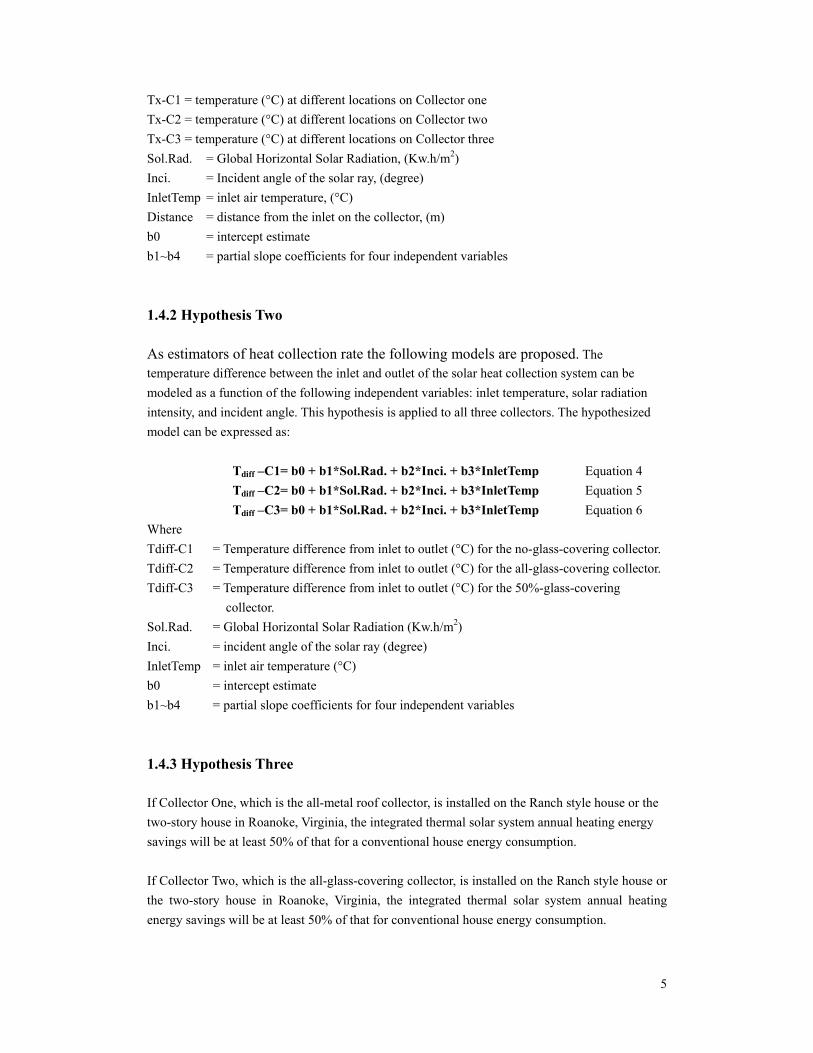
Tx-C1 = temperature (°C) at different locations on Collector one Tx-C2 = temperature (°C) at different locations on Collector two Tx-C3 = temperature (°C) at different locations on Collector three Sol.Rad. = Global Horizontal Solar Radiation, (Kw.h/m2) Inci. = Incident angle of the solar ray, (degree) InletTemp = inlet air temperature, (°C) Distance = distance from the inlet on the collector, (m) b0 = intercept estimate b1~b4 = partial slope coefficients for four independent variables 1.4.2 Hypothesis Two As estimators of heat collection rate the following models are proposed. The temperature difference between the inlet and outlet of the solar heat collection system can be modeled as a function of the following independent variables: inlet temperature, solar radiation intensity, and incident angle. This hypothesis is applied to all three collectors. The hypothesized model can be expressed as: Tdiff –C1= b0 + b1*Sol.Rad. + b2*Inci. + b3*InletTemp Equation 4 Tdiff –C2= b0 + b1*Sol.Rad. + b2*Inci. + b3*InletTemp Equation 5 Tdiff –C3= b0 + b1*Sol.Rad. + b2*Inci. + b3*InletTemp Equation 6 Where Tdiff-C1 = Temperature difference from inlet to outlet (°C) for the no-glass-covering collector. Tdiff-C2 = Temperature difference from inlet to outlet (°C) for the all-glass-covering collector. Tdiff-C3 = Temperature difference from inlet to outlet (°C) for the 50%-glass-covering collector. Sol.Rad. = Global Horizontal Solar Radiation (Kw.h/m2) Inci. = incident angle of the solar ray (degree) InletTemp = inlet air temperature (°C) b0 = intercept estimate b1~b4 = partial slope coefficients for four independent variables 1.4.3 Hypothesis Three If Collector One, which is the all-metal roof collector, is installed on the Ranch style house or the two-story house in Roanoke, Virginia, the integrated thermal solar system annual heating energy savings will be at least 50% of that for a conventional house energy consumption.

If Collector Two, which is the all-glass-covering collector, is installed on the Ranch style house or the two-story house in Roanoke, Virginia, the integrated thermal solar system annual heating energy savings will be at least 50% of that for conventional house energy consumption.

6

If Collector Three, which is the 50%-glass-covering collector, is installed on the Ranch style house or the two-story house in Roanoke, the integrated thermal solar system annual heating energy savings will be at least 50% of that for conventional house energy consumption. The testing of these hypotheses follows.

7

Chapter 2 Literature Review

2.1 Solar Technology Solar energy utilization can be categorized in two ways: passive solar and active solar systems. Passive solar, in terms of investment, is typically the most economical approach to solar energy utilization. By carefully arranging the building orientation, shape and envelope, the sun’s energy can be captured to offset the need for mechanical heating. The active solar system includes solar electric and solar thermal systems. Solar electric systems use photovoltaic panels to produce electricity. Because of the high cost of the photovoltaic panels and the electric storage sub-systems it is not widely used in residential buildings. BP Solar (2004) for example, has panels with nominal voltage of 12V, with 3.88, 4.45, 4.72 amps, with 64, 75, and 85 watts of power but with cost of $419, $495, and $409 respectively. Solar electric systems are usually limited on residential building practice. (BP Solar,2004) Solar thermal systems use the heat collected from solar energy for domestic heating, e.g., for space heating in the winter, or hot water in the summer. In this system, as distinguished from passive systems, a chosen media is heated by the solar energy. Fans or pumps and necessary pipe work are installed to transport the heat collected from the collector. Active solar systems are typically not totally integrated into the building envelope.

2.2 Past investigations and relevant research 2.2.1 Case studies of solar heating systems In his book New Inventions In Low Cost Solar Heating, William A.Shurcliff explored low-cost solar heating systems; some have been built while others have not. The inventions described in his book include passive systems, active systems, and combinations of passive-and-active systems. Most of the inventions deal with the design and sizing of the collector system. Some are concerned with the thermal storage system. Most examples in his book are for space heating while a few are for domestic hot water heating. The book presents the fundamental principles of each system but presents little quantitative performance results. (Shurcliff, 1979) In his other book Solar Heated Buildings of North America, Mr. Shurcliff quantitatively described 120 existing buildings and their heating and cooling systems. Instead of theory, the book emphasized practice. The exploration of this book includes systems applicable for all typical weather conditions within the United States. The percentage of heating and cooling energy provided by solar systems is either recorded from operational data or predicted. However, the predicting method is not explained in this book. Judgments, problems and modifications were stated on each building’s performance to give later researchers a preliminary understanding of each specific system performance. No life cycle cost analysis is presented. (Shurcliff, 1978) In Solar Heated Houses by MASSDESIGN, the solar heating system’s impact on prototypical single-family houses in the Boston region was studied. This research is mostly concentrated on water/roof collector systems. The design implications of solar heating system meeting 20, 40, 60,

8

80, and 100 percent of the total heating demand were evaluated. Each prototype is analyzed with the aid of a computer program for daily performance throughout a typical year. The cost of each system was estimated with current fuel prices. Of the several typical houses studied, in the conclusion section, the townhouse seems to be particularly appropriate for solar heating. (MASSDESIGN, 1975) 2.2.2 Solar system practice and theory In S. A. Klein, W. A. Beckman and J. A. Duffie’s article, A design procedure for solar heating systems, simulation is used to estimate the thermal performance of the solar heating system. The necessary meteorological parameters included in the simulation are investigated. The information from the simulation is developed into a design process for solar heating systems. After “Why to use the solar heating system” has been answered, this research is relevant for the “How to use the solar heating system” question. In addition, the simulation method can be of a reference for energy performance estimation. It gives architects and engineers a simple graphic method to design economical solar heating systems by using monthly average meteorological data. (Solar Energy, 1976) In their paper titled, Experimental study of a roof solar collector towards the natural ventilation of new houses, Joseph Khedari, Jongjit Hirunlabh, * and Tika Bunnag, discussed a passive method to deal with solar radiation to induce natural ventilation for houses in tropical area to reduce the cooling load. The indication from this paper is that solar energy can be exploited in an inexpensive way by modification of the constructive method. (Energy and Buildings, 1997) In their paper, A solar energy collector for heating air, V. D. Bevill and H. Brandt, studied an alternative air-media solar heating system. Their paper is related to a solar collector model for an air media system. For this, 96 parallel aluminum fins, 0.635 cm each apart, are installed in a glass cover box. Air is pumped through the box so the heat accumulated in the aluminum fins can be transferred. The specular reflectance parameter of the aluminum fins is studied in order to determine the efficiency of the collector. In addition, the efficiency of the collector when some parts of the fins are made diffuse is evaluated. From the measurement of the solar energy received by the collector and the temperature difference between inlet and outlet, a data set was formed to calculate the efficiency of the collector. The result shows that when the ambient air is calm, with the specular fins, the collector can capture 80 percent of the energy. When the fins are made diffuse, the collector efficiency will decrease by about 50 percent. (Solar Energy, 1968) Still, the system being studied is an add-on system rather than an integrated one. The installation of the parallel aluminum fins may increase the complexity of its construction process. 2.2.3 Efficiency analysis In their paper titled Cost of house heating with solar energy, G. O. G. Löf, and R. A. Tybout analyzed solar heating cost and the solar system optimization in eight US cities under particular climatic, geographic, and residential characteristics. Six variables, which are solar radiation, temperature, wind, solar altitude, cloud cover, and humidity, are treated as weather variables. Eight design parameters, which are house size, collector size, storage size, collector tilt, number of

9

transparent surfaces in collector, hot water demand, insulation on storage unit, and thermal capacity of collector are treated as design parameters. Both the weather variables and the design parameters are included to develop a performance equation for a flat plate solar collector and heat storage systems. (Solar Energy, 1973) The relationship between the design parameters and the capital and operating cost are described quantitatively. The values of the design parameters, which yield the lowest heating cost in each of the eight cities, are described. The relative importance of each parameter is discussed. Comparisons were made between the conventional system and the solar heating systems in each location. The findings are expressed by two tables and ten graphs, showing heating costs as functions of various design and location factors, which is indicative to this study. 2.2.4 Estimation and simulation In their paper, Simulation of a solar heating and cooling system, L. W. Butz, W. A. Beckman and J. A. Duffie, performed thermal and economic analysis of a water-heating collector. Except for the water heating system, the system also includes a water storage unit, a hot water service facility, a lithium bromide-water air conditioner (with cooling tower), an auxiliary energy source, and associated controls. The result indicates the dependence of the thermal output on the area of the collector. The annual efficiency decreases as the collector area increases. (Solar Energy,1974) In their paper titled Simulation and optimization of solar collector and storage for house heating, by H. Buchberg and J. R. Roulet, a combined solar collector and storage performance was evaluated. The parameters include: the house, a flat plate solar collector, a water heat storage unit and an auxiliary heater. The combined performance was studied to decide the maximum allowable collector cost. This study suggested that the design optimization study using annual weather data for the Fresno, California area showed a maximum allowable cost of approximately $1.00/ft2 for the solar collector. It also suggested the necessity of a supplemental heater to provide heat during long overcast and peak heat load periods. Some savings in auxiliary heater capacity are possible by using the storage system to suppress peak heating loads through distribution over longer periods. (Solar Energy,1968) 2.2.5 OM Solar: its research and questions remain unanswered OM Solar, since the 80’s, has installed an integrated solar roof collector system with a combination of heat distribution and heat storage systems. Performance records for built projects have been analyzed. Unfortunately, the detailed data is not published. The main features of the OM Solar system include: the air handling unit, which is the solar roof collector being called in this research; the vertical duct, which is the media transportation system; the heat storing concrete slab; and an air-to-water heat exchanger. In the heating mode, the vertical air duct carries the heated air to the heat storage concrete slab to take advantage of its thermal mass. At night, the heated concrete slab will slowly give off the heat that has been stored during the day and warms the house. While OM Solar has presented some performance data some questions remain unanswered. For example, what is the year-round energy performance of the OM Solar roof system? What is the

10

optimal length of the collector? What proportion of the glass area is optimal for the collector system? Or, is it the glass cover over the top of the sheet metal necessary at all? This research sets its objectives, as stated in Section 1.2, on the quantitative aspect of the collector. In the end, the annual energy saving percentage for those three collector types and the inter-comparison of three collectors are concluded. The three types of collectors constructed at the Research Demonstration Facility in Virginia Polytechnic Institute and State University will allow this research to obtain an understanding of the glass cover’s role in its energy collecting performance. The three collectors are, Collector One without glass cover, Collector Three with half area covered with glass, and Collector Two with 100% area cover glass. A subsequent study after this research would focus on the optimal proportion of the glass cover area to maximize the performance of the solar roof collector.

2.3 Solar roof system operational fundamentals and heat calculation

The transport media for the OM Solar system is air. The collector surfaces are painted black to maximize the absorption of solar radiation. Airflow transports the collected heat either through an air-to-water heat exchanger or directly to the occupied space, as shown in Figure 2. An important difference between a typical air-media solar collector and the OM Solar roof system is that an air-media collector usually blows air between the glass cover and an absorptive surface while in the OM Solar roof system, a more integrated method, airflow travels in the air cavity below the sheet roofing which is the upper side of the heated air route. The air cavity is located beneath the black-painted sheet metal roofing. Therefore, the glass cover is not exposed to large convective heat transference at the inside surface. The glass keeps the heat on the sheet metal surface from reradiating. The optimal percentage of coverage of the sheet glass and its optimal position will be explored in this study.

Figure 4. Section of a typical solar roof collector system

2.3.1 Heat transfer fundamentals In order to better understand the operation of the OM Solar roof system, several fundamental heat transfer concepts must also be understood. The amount of heat collected in a solar collector will depend on conduction, convection and radiation. Conduction is the heat transfer from solid to solid. Generally for a solar collector the goal is to minimize the conductive losses out of the upper and lower surfaces of the collector. The

11

conductivity of the corrugated sheet metal is 0.029w/m.k. The insulation layer (the extruded polystyrene panel) under the corrugated sheet metal slows down the conductive heat loss through the collector. Convection is the transfer of heat to and from a fluid to a solid or within a fluid. For the OM Solar system, heat is transferred to the transport fluid (air) at the inside surface of the metal panel to the air. Heat flow is caused by temperature difference. That is, wherever there is temperature difference within a conductive media, there is heat flow. Heated air tends to flow from areas of high density to areas of low density, high temperature. With a fan installed as a pressure driving force, the outdoor air at the inlet of the collector is drawn through a screened opening along the eave to the ductwork (shown in Figure 5 & 6). Then the heated air is either sent to the heat exchanger to preheat the hot water or sent vertically down under the raised floor for occupancy heating. For the purpose of capturing solar radiation, the corrugated sheet metal is painted with black acrylic latex paint (See Figure 5), with emissivity value ranges from 0.84 to 0.90 and absorption rate ranges from 0.92 to 0.97. All of the materials used in the experimental setup are accessible in the local construction market.

Figure 5. Front, south view of the solar roof collector

12

Figure 6. Interior side of the collector (The heated air is collected in the ductwork) 2.3.2 Thermal radiant properties Thermal radiation happens whenever there is temperature difference between two regions in view of each other. The transfer of heat in this way does not depend on any intermediate material. In the OM Solar Roof Collector, the heated corrugated sheet metal will radiate its heat to its surroundings, including the air cavity above it and airflow cavity below it. Emmisivity is a property of the surface characterizing how effectively the surface radiates when compared to a "blackbody". It is the ratio of the emission of thermal radiant flux from the surface to the flux that would be emitted by a blackbody at the same temperature. The value is always between 0 and 1. The blackbody is an ideal surface that emits the maximum possible thermal radiation at a given temperature. Solar radiation incident on a glazing system is partly transmitted and partly reflected, and partly absorbed by the system. Reflectance is the fraction of the reflected part of the incident flux. It means that the less the amount of solar radiation is reflected, the more the amount of solar radiation is being absorbed or transmitted by the surface. Absorptance is the ratio between the amount of radiation absorbed by a surface to the total incident flux on the surface. In the case of Solar Roof Collector, the less reflectance the corrugated sheet metal has, the better. (ASHREA,1999) After the solar radiation strikes an opaque surface, which in this case is the corrugated sheet metal roofing, some radiation is reflected off the surface. The amount of reflection is determined by both the incident angle and the reflectance of the surface. Assuming little absorption happens in the air, the rest of the incident solar radiation is absorbed by the surface. How much of the heat being absorbed by the surface depends on the absorptance of the surface. In this case, high absorptance and low reflectance will make the system reach its optimal performance. The heat being absorbed will be stored and conducted through surface materials. When the

13

temperature of the surface material is higher than its surroundings, it will emit heat to the surroundings. The higher the emissivity of the material, the more heat it will give off. The air cavity below the heated surface is heated by both convection and emittance. The net rate of radiation heat exchange between a surface and its surroundings can be expressed as Equation 7:

q = ε Aσ (Ts4 – Tsur4) Equation 7 q = heat exchange (W) ε = the emmisivity of the surface A = surface area (m2)

σ = Stefan-Boltzmann constant (σ = 5.67×10-8 W/m2.K4)

Ts = the absolute temperature of the surface (K) Tsur = the temperature of the surroundings (K) (Frank P. Incropera, David P. Dewitt, 1990) The use of a corrugated sheet metal collector plate has its advantage. The corrugated shape helps the solar heat absorption because direct solar radiation strikes the surface and is reflected several times on the surface, and therefore increases the amount of absorption. When the air is heated by solar radiation, it becomes less dense and rises toward the outlet. During the process, it continues to be heated through the collector. The result is heated air at the outlet and a temperature difference between the inlet and outlet. 2.3.3 Heat collection rate To determine the amount of heat collected within the system, two variables must be known: 1) The temperature difference between the inlet and outlet 2) The air flow rate through the collector When these are known, the energy collected can be calculated according to Equation 8. The sensible heat gain is calculated as following:

Qv=1.08*Tdiff* V Equation 8 Qv = sensible heat collected (Btu) Tdiff = temperature difference between outlet and inlet (°F) V = air flow rate through the collector, in cubic feet per minute (cfm) 1.08 = a constant, whose units are Btu-min/ft3h °F. The air density is 0.075lb/ft3 under normal temperature and pressure, which is 60°F and 30 inch Hg). The specific heat of air is 0.24Btu / lb°F. 1.08 equals air density multiplied by air specific heat, and then multiplied by 60min/h. (Note: this value may vary slightly and be lower for low density conditions) (Benjamin Stein and John S. Reynolds, 1999) The air flow section area in the experimental setup = 45.75in2 (the rectangle part in the shaded area in Figure 9) + 22.8594in2 (the accumulation of the 7 trapezoid shapes in the shaded area in Figure 9) = 68.6094in2 = 0.4765 ft2 The measured airflow speed is 35-40ft/min, therefore, Volumetric flow rate = 16.68~19.06ft3/min ≈ 17.87 ft3/min

14

2.3.4 Solar Radiation and Heat Collection The amount of heat collected will depend on the intensity of incident solar radiation. Thus solar radiation is included as a parameter to observe its relationship with the heat that can be collected from the roof system. In the ideal case, solar radiation and heat collected from the roof system should have a directly proportional relationship. But in real case situations, clouds and particles in the sky, the wind speed, and other factors may effect the solar radiation. The relationship may turn out to be less than proportional. Global Horizontal Radiation: Total amount of direct and diffuse solar radiation in Wh/m2 received on a horizontal surface during the 60 minutes preceding the hour indicated. (NREL, 2004) The solar energy flux is composed of two parts: that due to incident beam radiation (b) and that due to incident diffuse radiation (d). The diffuse radiation includes both diffuse sky radiation and radiation reflected from the ground. Their relationship can be expressed by Equation 9.

Qs= Qb+Qd Equation 9 Qs= Total amount of solar energy flux, Wh/m2 Qb= Incident beam radiation, Wh/m2 Qd= Incident diffuse radiation, Wh/m2 (ASHREA, 1999) 2.3.5 Wind Speed and Heat Collection Wind speed will affect both the airflow rate through the collection cavity and the collector’s exterior surface heat loss by convection. Under conditions of high solar radiation and low ambient temperature, high wind speeds will adversely affect the performance of the solar collector. Wind can increase the airflow rate over the corrugated sheet metal roofing therefore accelerating the convective heat loss of the collector’s exterior surface. The more convective heat loss on the sheet metal surface, the more convective heat loss happens from the warmed air to the underside surface of the sheet metal. At the same time, high wind speeds can change the airflow value in Equation 8, and compromise the assumption of constant heat flow. It contributes to the overall error of the heat collecting prediction. 2.3.6 Incident Angle and Heat Collection Part of the solar radiation incident on a solar collector surface is absorbed by the surface and part is reflected. For many materials, glass in particular, the proportion of the amount being reflected and being absorbed depends on the angle of incidence between the surface and the sun. The incident angle is defined as the angle between the incoming solar rays and a line normal to that surface. When the incident angle is 0 degree, the solar radiation absorption is maximal. When the incident angle value increases, the amount of reflection is greater accordingly and the absorption is gradually reduced. For typical clear glass, for incident angles over 60 degrees, the absorption rate drops while the reflectance rises dramatically. Figure 7 shows the relationship between the incident angle and the reflection and the absorption for a typical transparent surface.

15

2.3.7 Inlet Temperature and Heat Collection The inlet temperature is the temperature of the air entering the collector. The relationship between the inlet temperature and the heat collection is twofold: in a certain range, when the inlet temperature rises, it is possible that the outlet temperature may not rise at the same rate. Therefore, the temperature difference (Tdiff) between the inlet and the outlet may actually go down. The heat collected at the outlet can be reduced because of the lower Tdiff value. From observation, this situation happens normally in the morning when the ambient temperature begins to rise. The solar angle is still low and thus a large proportion of the solar radiation is reflected off the surface, while the ambient temperature is heated by the sun faster than the air flowing through the cavity of the collector.

2.4 Conclusion It is through the fundamental understanding of solar collection processes and performance that Hypotheses One and Two are developed.

Figure 7. Relationship between the incident angle and the transmittance for a transparent surface (ASHRAE, 1999)

16

Chapter 3 Methodology

3.1 Overview of methodology To test the research hypotheses, a two–step methodology was applied. First the experimental data was statistically analyzed and regression models were derived (Hypotheses One and Two). Second, the regression models were applied to an analytical method to estimate the energy savings from the integrated system (Hypothesis Three). These two procedures are described in the following chapter.

3.2 Experimental setup The two evaluation methods are applied to data collected under actual operating conditions for a full-scale experimental setup. 3.2.1 The integrated roof construction According to Edward Allen, a steep roof is defined as a roof with a pitch of 3:12 or greater. A conventional residential steep roof structure, if the under side of the deck is left to be the finishing surface, typically includes: a wood deck, vapor retarder, insulation layers, roofing shingles, venting cap and ridge. Otherwise, the insulation layers and the vapor retarder are left under the wood deck. In the case of the solar collector roof system, an attic space is required to install a fan and possibly the heat exchanging systems. In addition, the insulation layers and the vapor retarder together are needed to form the air channel because the insulation layer will prevent the heat from escaping to the attic. They are preferably located above the roof deck. When designing the roof details, these factors should be taken into consideration. (Edward Allen,1999) The layering of the roof structure from bottom to top in this experimental setup is as following: Roof deck (OSB board), vapor retarder, insulation panel, airflow cavity, corrugated sheet metal, air cavity, and glass cover (for Collector Two and Three). In the normal practice of light timber roof systems, the roof deck is nailed down to the roof beams, and roof shingles are nailed on the wood deck, which is rather labor intensive. In the solar collector roof system, where corrugated sheet metal is used, construction speed is greatly improved. The wood beam that supports the sheet metal needs to be detailed to provide a ridge cap above the seam of two adjacent metal sheets. If carefully detailed, the cap will not stick out of the surface too much. This way, the chance of casting a shadow is reduced. The performance of the solar collector roof is maximized. In conventional steep roof systems, chimneys and skylights are common. These elements can cast shadows thus reducing the efficiency of the collector. By careful architectural design, the chimney can be located on the perimeter of the roof area and the skylights can be located along the ridge of the roof without sacrificing the aesthetics. The goal is to maximize the south facing roof area and thus collect as much solar energy as possible.

17

Figure 8. Solar Roof Collector model with glazing (Collector Two), the glass sheet can be designed as a sliding-in panel (Note: the shading area is the airflow cavity)

Figure 9. Section of Collector One (Note: the shading area is the airflow cavity)

Figure 10. View of the Solar Roof Collector model (Drawing courtesy of Thomas Miller) The layering and geometry of the experimental setup is shown in Figure 10.

18

Figure 11. Southeast corner view of the solar roof collector Three configurations have been set up for a comparative study, the all-metal without glass cover collector (C1), the all-glass cover collector (C2), and the 50%-glass cover collector (C3). They are all based on the duplication of a south facing residential roof. The roof originates from a 24 inch-height wall and rises to the plate of a 10-foot high wall on the north side. The resulting roof deck is at a 40-degree angle. This deck is 10 feet by 14 feet. (Figure 5 and Figure 11) (Thomas Miller, 2003) On top of the roof deck, the three collectors are installed. The three collectors are: C1, constructed with all standing seam sheet metal roofing without any glass cover; C2, corrugated sheet metal totally covered with glass; and C3, it leaves the lower half sheet metal roofing outside and the upper 6 feet covered with glass. Each collector measures 11.5 feet in length by 30 inches in width, by 1.5 inches in depth. The corrugated metal roof panel, which is a 26-gauge Galvalume panel painted with black acrylic latex paint functions as an absorber. The absorbers are separated from the roof deck by a layer of reflective foil and another 1.5-inch thick layer of Dow’s extruded polystyrene (R value = 4.8 per inch thickness). All the material used in this study is easily accessible from local construction markets in order to make the experiment easy to repeat. 3.2.2 The integrated roof operation In the Solar Roof Collector, the outdoor air is drawn through the eave then heated by the solar radiation while it travels through the airflow cavity under the blackened corrugated sheet metal. Normally, when the air reaches the outlet of the collector, there is a positive temperature difference between inlet and outlet and therefore heat is collected. At the top of the collector, there is a

19

ductwork manifold connected with the collector and the heat control unit. When the outside air temperature is below the balance point temperature (discussed in Section 3.4.2), the house is in the heating mode. If the heated air temperature is above 70 °F, which is the designed room temperature, the heated air is transferred through a vertical duct down to the heat storing concrete slab. The concrete slab acts as a thermal mass releasing the heat stored inside it slowly to heat the house. The heat stored in the concrete slab during daytime may help to heat the house at night while there is no solar energy available. If the heated air temperature is below 70 °F, the designed room temperature, but above 50 °F, which is the incoming water temperature, it could be sent to the domestic hot water heat exchange system to preheat the hot water. (Note: 50 °F is set as the incoming domestic water temperature for pre-heating the hot water) When the outside air temperature is above the balance point temperature, the house is in the cooling mode. The heated air is sent to the domestic hot water heat exchange system to preheat the hot water. 3.2.3 The data collection system Seven thermocouples were placed at regular intervals in each of the three collectors. The first point is under the eave and is deemed the ambient temperature. The second is at a distance of 20 inches toward the ridge from the inlet. The third to the sixth sensors are evenly spaced at distances of 20 inches. The seventh point is the outlet temperature of the collector. It is located at the top of the collector joining the horizontal duct. The sensors have been wired to two “Campbell Scientific, Model 21” data loggers. Every 15 minutes, the data is read into the data loggers. Both instantaneous and 15-minute-averages are recorded. The data is transferred to computer files each week. Then the software Excel and StatView analyze the data statistically.

Figure 12. Interior side of the solar roof collector mock-up (wires from the sensors are connected with the two “Campbell Scientific, Model 21” data loggers)

20

Figure 13. Solar Roof Collector section with thermal couple locations 3.2.4 The data collection period The data were collected during the following time periods: May 10, 2003 to July 4, 2003, Sept.16, 2003 to Oct.15, 2003, Oct.24 to Nov.25, 2003 and Dec.1 to Dec.10, 2003. The data were partitioned using selective criteria. By these criteria, certain periods are excluded from the analysis. These criteria include: 1) Nighttime and conditions with solar radiation less than 0.008 Kw/m2 were partitioned and removed from the analysis. From observation of the dataset, when solar radiation is less than 0.008 Kw/m2, it is either early in the morning or late in the afternoon when solar radiation has a negligible impact on the roof. These are conditions when the collector should not be operated. 2) When the outlet temperature of the collector (Tout) is lower than 50°F, the solar collector system will be shut down. These data are excluded. 3) When the incident angle is greater than 60 degrees and the ambient temperature is between 30ºF to 50ºF, the data are excluded from the data set because after the incident angle is over 60 degrees, most incident solar radiation will be reflected off the collector surface. The heat collected in this condition is assumed to be negligible. In addition, for this situation the prediction of the collector’s performance is not reliable. 3.2.5 Calculation of incident angle As discussed in section 2.3.6, the collection of solar energy will depend on the angle of incidence. The calculation of the incident angle (θ) is through its relationship with solar altitude (β), surface azimuth (γ), and the tilt angle of the surface (Σ). In addition to the temperature data, the angle of incidence should be included as a variable in the data set. It is expressed by the following equation.

21

cosθ=(cosβ)*(cosγ)*(sinΣ)+(sinβ)*(cosΣ) (ASHRA,1999) Equation 10 where: θ is the incident angle; β is the solar altitude; γ is the surface azimuth, which is 0 degree in this experiment; Σ is the tilt angle of the surface, which is 40 degrees in this experiment. In order to determine solar altitude, which is ever changing, we apply the following formula: sinβ= (cosL )*(cosδ)*(cosH) + (sinL)*(sinδ) (ASHRA,1999) Equation 11 L = local latitude, which in our case is 37.23 degrees δ = solar declination, which is a function of the Jullien day of the year H = the hour angle In order to get δand H, there are two formulas introduced as following: δ = 23.45*sin((360*(284+η))/365) (ASHRA,1999) Equation 12 η = the Jullien day H = 15*(AST-12) (ASHRA,1999) Equation 13 AST = LST+ET/60+(LSM-LON)/15 (ASHRA,1999) Equation 14 AST = apparent solar time, decimal hours LST = local standard time, decimal hours ET = equation of time due to the earth’s varying orbital velocity. Table 3.1 Equation of time (ASHRA,1999) Month Jan. Feb. Mar. Apr. May Jun. Jul. Aug. Sep. Oct. Nov. Dec. ET(min) -11.2 -13.9 -7.5 1.1 3.3 -1.4 -6.2 -2.4 7.5 15.4 13.8 1.6 LSM =Local standard time, decimal degree of arc, which is 75 degrees west, Eastern Standard Time in this experiment LON =Local longitude, decimal degrees of an arc, which in our experiment is 80.41 degrees (ASHRAE,1999) Using these equations, the angle of incidence can be calculated at selected days and times. From the above formulas, the solar incident angle of each 15 minutes was calculated. The 15-minute interval will allow the incident angle data set to match the data collected from the mock-up, which is based on 15-minute intervals also.

3.3 Statistical Analysis

When the data from the mock-up has been organized (see original data structure in Table 3.2) and prepared, statistical analyses were used to analyze the data. The StatView software was used to execute the analysis. By setting criteria (described in Section 3.2.4) in StatView, the unwanted data, for example, the nighttime data, was excluded from the dataset when performing the regression analysis. Two statistical models of each collector are tested for each collector. The first one, Model One, includes four independent variables as suggested by Hypothesis One, solar radiation, incident angle, inlet temperature, and distance from a certain tested point to the inlet. The second model, as suggested by Hypothesis Two, is tested after testing the validation of the first model. It includes three independent variables: solar radiation, incident angle, and inlet temperature.

22

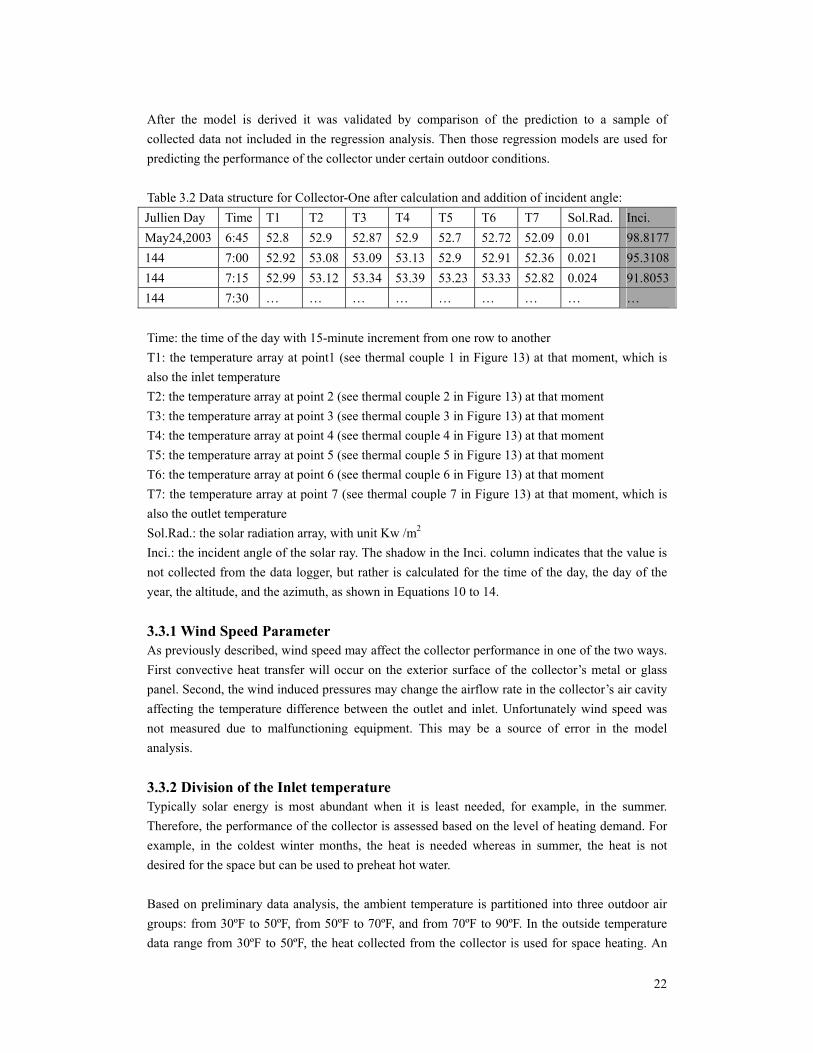
After the model is derived it was validated by comparison of the prediction to a sample of collected data not included in the regression analysis. Then those regression models are used for predicting the performance of the collector under certain outdoor conditions. Table 3.2 Data structure for Collector-One after calculation and addition of incident angle: Jullien Day Time T1 T2 T3 T4 T5 T6 T7 Sol.Rad. Inci. May24,2003 6:45 52.8 52.9 52.87 52.9 52.7 52.72 52.09 0.01 98.8177144 7:00 52.92 53.08 53.09 53.13 52.9 52.91 52.36 0.021 95.3108144 7:15 52.99 53.12 53.34 53.39 53.23 53.33 52.82 0.024 91.8053144 7:30 … … … … … … … … … Time: the time of the day with 15-minute increment from one row to another T1: the temperature array at point1 (see thermal couple 1 in Figure 13) at that moment, which is also the inlet temperature T2: the temperature array at point 2 (see thermal couple 2 in Figure 13) at that moment T3: the temperature array at point 3 (see thermal couple 3 in Figure 13) at that moment T4: the temperature array at point 4 (see thermal couple 4 in Figure 13) at that moment T5: the temperature array at point 5 (see thermal couple 5 in Figure 13) at that moment T6: the temperature array at point 6 (see thermal couple 6 in Figure 13) at that moment T7: the temperature array at point 7 (see thermal couple 7 in Figure 13) at that moment, which is also the outlet temperature Sol.Rad.: the solar radiation array, with unit Kw /m2 Inci.: the incident angle of the solar ray. The shadow in the Inci. column indicates that the value is not collected from the data logger, but rather is calculated for the time of the day, the day of the year, the altitude, and the azimuth, as shown in Equations 10 to 14. 3.3.1 Wind Speed Parameter As previously described, wind speed may affect the collector performance in one of the two ways. First convective heat transfer will occur on the exterior surface of the collector’s metal or glass panel. Second, the wind induced pressures may change the airflow rate in the collector’s air cavity affecting the temperature difference between the outlet and inlet. Unfortunately wind speed was not measured due to malfunctioning equipment. This may be a source of error in the model analysis. 3.3.2 Division of the Inlet temperature Typically solar energy is most abundant when it is least needed, for example, in the summer. Therefore, the performance of the collector is assessed based on the level of heating demand. For example, in the coldest winter months, the heat is needed whereas in summer, the heat is not desired for the space but can be used to preheat hot water. Based on preliminary data analysis, the ambient temperature is partitioned into three outdoor air groups: from 30ºF to 50ºF, from 50ºF to 70ºF, and from 70ºF to 90ºF. In the outside temperature data range from 30ºF to 50ºF, the heat collected from the collector is used for space heating. An

23

extreme weather event would need both the solar and the supplemental heating systems. When the heat from the solar system can suffice the house heating demand, the conventional heating system is turned off. In the temperature range from 50ºF to 70ºF, the weather is normally mild and conditions are above the balance point temperature. The house may need heating in early morning and in the evening. Sometimes during the day, the solar energy may overheat the house. The control system is set to transfer the heat to the domestic hot water tank in this situation. 3.3.3 Model 1: temperature prediction at different locations The multiple-linear-regression model expresses the relationship between a dependent variable y to a set of quantitative independent variables by using a method of least squares. The dependent variable is assumed to be a normally distributed variable with its mean falling on the regression line. It would be ideal if the temperature at different locations on the collector could be predicted by a reliable linear regression model. Model 1, as introduced in Chapter One, has four parameters including the distance from the inlet, is a regression model with temperature at one of the seven thermal couple locations as a dependent variable and solar radiation, incident angle, inlet temperature and distance from the inlet as independent variables.

Tx –C1= b0 + b1*SolRad + b2*Inci. + b3*Inlet + b4 *Distance Tx –C2= b0 + b1*SolRad + b2*Inci. + b3*Inlet + b4 *Distance Tx –C3= b0 + b1*SolRad + b2*Inci. + b3*Inlet + b4 *Distance

Tx-C1 = temperature at one of the seven points on the collector C1 Tx-C2 = temperature at one of the seven points on the collector C2 Tx-C3 = temperature at one of the seven points on the collector C3 Distance = the distance between the inlet and certain one of the seven points on the collector SolRad. = solar radiation value, Kw/m2 Inci. = the incident angle, degree Inlet = inlet temperature, which equals the ambient temperature, ºC 3.3.4 Test of Model 1’s assumption Model 1 is based on the assumption that each of the four independent variables is linearly related to the dependent variable. In order to prove the linear relationship between the distance independent variable and the temperature dependent variable, for each collector, a binary regression for each collector is proposed. They are:

Tdiff-C1 = b0 + b1 * Lcn2_3 + b2 * Lcn 3_4 + b3* Lcn 4_5 + b4 * Lcn 5_6 + b5 * Lcn 6_7 Equation 15

Tdiff-C2 = b0 + b1 * Lcn2_3 + b2 * Lcn 3_4 + b3* Lcn 4_5 + b4 * Lcn 5_6 + b5 * Lcn 6_7

Equation 16

Tdiff-C4 = b0 + b1 * Lcn2_3 + b2 * Lcn 3_4 + b3* Lcn 4_5 + b4 * Lcn 5_6 + b5 * Lcn 6_7

24

Equation 17 Tdiff-C1 = temperature differential between two successive monitoring locations on collector C1,

ºC Tdiff-C2 = temperature differential between two successive monitoring locations on collector C2,

ºC Tdiff-C3 = temperature differential between two successive monitoring locations on collector C3,

ºC Lcn2-3 =Location2-3, which is the temperature difference per unit length from monitoring point 2 to point 3 Lcn3-4 =Location3-4, which is the temperature difference per unit length from monitoring point 3 to point 4 Lcn4-5 =Location4-5, which is the temperature difference per unit length from monitoring point 4 to point 5 Lcn5-6 =Location5-6, which is the temperature difference per unit length from monitoring point 5 to point 6 Lcn6-7 =Location6-7, which is the temperature difference per unit length from monitoring point 6 to point 7 The goal of this regression analysis is to test the linearity of the incremental temperature difference throughout the collector length. For statistical purposes, one segment, Lcn1-2, is excluded. The five independent variables represent the segments between each two sensors on each collector. Depending on the situation, the independent variable equals either 1 or 0. When the value of the dependent variable, Tdiff, is from a certain segment on the collector, the independent variable Lcn. that represents that segment equals 1 and the other Lcn. (location) values are 0. Their relationship can be expressed in the following simplified table (Table 3.3). Figure 14 indicates the physical location of each segment. Each segment has its corresponding Tdiff value. Table 3.3 The relationship between the dependent variable and the independent variable in the binary regression table for collector C1 Tdiff-C1 Lcn1-2 Lcn2-3 Lcn3-4 Lcn4-5 Lcn5-6 Lcn6-7 ∆(T2-T1) 1 0 0 0 0 0 ∆(T3-T2) 0 1 0 0 0 0 ∆(T4-T3) 0 0 1 0 0 0 ∆(T5-T4) 0 0 0 1 0 0 ∆(T6-T5) 0 0 0 0 1 0 ∆(T7-T6) 0 0 0 0 0 1

25

Figure 14. Section of the collector with labels in length The result of this regression analysis is a multinomial with five parameters. Each parameter has its coefficient and test for significance (“t” value). By comparing the five coefficients, a conclusion can be made as to whether or not the temperature differential over each location is the same. In other words, the distance linearity can be judged in this way. The results are presented in Chapter 4. 3.3.5 Model 3 linearity test - analysis of the scatter plots of the independent variables The assumption of a multiple linear regression model is that each independent variable has a linear relationship with the dependent variable. The judgment of the linear assumption can be obtained from the X-Y scatter plot. To avoid the gathering of outliers of all the collecting time period, it is reasonable to observe the x-y relationship over several typical week periods. Two time slots are chosen to judge the assumption: From June 28, 2003 to July 4, 2003 and from Nov.19, 2003 to Nov.25, 2003. They represent typical summer and winter conditions. There are altogether 45 X-Y plots showing the relationship between the independent variables and the dependent variable. They are all in Appendix II. The following (Figure II-2) is an example from the time slot June28, 2003-July 4, 2003. The result of the 45 X-Y plots show no obvious parabolic or hyperbolic shape, therefore, the linear relationship between the dependent variable and the independent variables is proved. The detail of the X-Y plots and its contribution to the regression

26

error are discussed in Chapter 4.

5

10

15

20

25

30

35

40

45

50

55Td

iff-C

1

25 30 35 40 45 50 55 60 65Incident Angle

Bivariate Scattergram with SupersmootherInclusion criteria: C1-Criteria 2 from June28-July4-2003.svd

Figure II-2 Incident angle versus Tdiff for C1 in the temperature range from 70ºF to 90ºF

June28, 2003-July 4, 2003

3.3.6 Regression analysis As discussed in Section 3.3.2, the outside air temperature has been partitioned into three groups: from 30ºF to 50ºF; from 50ºF to 70ºF; from 70ºF to 90ºF. Therefore, for each collector, there are three regression models according to each of the three temperature ranges. Altogether, there are nine regressions analyses. The regression reports are shown in Appendix II. A stepwise regression method was used to decide which of the three independent variables are statistically significant and should be included in the regression model. The stepwise regression report is included in Appendix III. The following table shows the relationship between the regression analyses and the corresponding conditions being included. Table 3.4 Regression analyses and corresponding temperature range 30°F ≤ Inlet temperature

< 50°F 50°F ≤ Inlet temperature < 70°F

70°F ≤ Inlet temperature < 90°F

C1 RegressionC1-1 RegressionC1-2 RegressionC1-3 C2 RegressionC2-1 RegressionC2-2 RegressionC2-3 C3 RegressionC3-1 RegressionC3-2 RegressionC3-3

Criteria for the regression As explained in the X-Y plot in the temperature range from 30°F to 50°F, the Tdiff is almost zero when the incident angle is over 50 degrees. In addition, the heat collected under these conditions is negligible. Therefore, a criterion is set to exclude that part of the data with an incident angle over 50 degrees.

27

Another criterion is set to exclude data with solar radiation values lower than 0.008 Kw/m2. Therefore when there is no solar radiation available this data is excluded. The third criterion is set to exclude data with collector outlet temperature lower than 55°F. The solar collector system will be shut down in this situation. 3.3.7 Test of the regression and its predictability A common way to test the predictability of a regression model is to try the predicted value in real case data and compare with the dependent variable with those from the experimental data. The data have been used to derive the regression models. The validation data are excluded from the regression analysis (from May 10, 2003 to Nov.25, 2003). They were used to test the predictability of the regression. Then a simple linear regression is conducted and plotted. If the slope of the simple linear regression is about 45 degrees, it means that the prediction is generally in agreement with the real case conditions. The following table shows the time slot for testing each of the regressions. Table 3.5 The prediction checking time slot 30°F≤Inlet

temperature < 50°F 50°F ≤ Inlet

temperature < 70°F 70°F ≤ Inlet

temperature < 90°F C1 Jun.7 – Jun. 13 Sep. 16-19

Oct. 24-29 Dec.01-08

Sep. 16-19 Oct. 24-29 Dec.01-08

C2 Jun.7 – Jun. 13 Sep. 16-19 Oct. 24-29 Dec.01-08

Sep. 16-19 Oct. 24-29 Dec.01-08

C3 Jun.7 – Jun. 13 Sep. 16-19 Oct. 24-29 Dec.01-08

Sep. 16-19 Oct. 24-29 Dec.01-08

3.4 Analytical analysis After the regression models for each collector are derived and tested according to the three temperature ranges, they can be used as an input to the analytical analysis. The analytical analysis is carried out in the following steps: 1). Select typical houses in Roanoke area and calculate the annual heating energy demand by using Energy 10. A ranch house, with floor area of 1,560 sq.ft., and a two-story house, with 2000-sq.ft. floor area, are selected as the estimate houses. Assuming the solar roof structure is applied on the two houses, estimate the collectable area from the solar roof collector installed on the two houses. (This part of work is explained in Section 3.4.1.) 2). Calculate the balance point temperature for both the ranch house and the two-story house to decide the heating season and cooling season. (This part of work is explained in Section 3.4.2.)

28

3). Separate the interpolated 15-minute-interval TMY2 data into heating season data and cooling season data according to their balance point temperature for both the ranch house and the two-story house. (Note: A TMY weather file is a set of hourly data of solar radiation and other meteorological elements for a 1-year period. Months selected from individual years are concatenated to form a complete year. It can be used for computer simulations of solar energy conversion systems and building systems. TMY files are not appropriate for simulations of wind energy conversion systems because of its selection criteria.) A TMY file provides a standard for hourly data for solar radiation and other meteorological elements. A TMY file represents conditions judged to be typical over a long period of time, such as 30 years. TMY files are not intended for designing systems and their components to meet the worst-case scenarios occurring at a location because the TMY file represent typical instead of extreme conditions. In this research, the TMY2 file is interpolated from hourly data to 15-minute-interval data, which is agreement with the experiment of the tested solar roof collector. (NREL,2004) 4). Input the regression models into the modified TMY2 weather data file to estimate the yearly accumulated heating energy saving and collectable energy for preheating hot water from each collector on both houses. As the result, an annual heat collection rate is calculated for each collector with the unit Btu/sq.ft. to estimate the energy performance of each collector, as stated by Hypothesis Three in Section 1.4.3 and Objectives in Section 1.2. 3.4.1 Typical House selection Based on the reasons mentioned in Section 4.6, a ranch house with net occupied floor areas of about 1,560 sq.ft.(not including garage) and a two-story house with net occupied floor areas of about 2,000 sq.ft. (not including garage) are assumed for estimation purpose: one is a ranch style house common in rural or suburban areas; the other is two-story-house style that is often found in more urban areas in the Blue Ridge Valley. The two houses presented here for the energy evaluation is based on the description of James W. Wentling, (James W. Wentling,1995)

Figure 15-a. Typical Ranch style house (Modified from a ranch house prototype by James W. Wentling) (James W. Wentling,1995)

29

Figure 15-b. Typical Ranch style house (Modified from a ranch house prototype by James W. Wentling) (James W. Wentling,1995)

Figure16-a. Typical two-story house (Modified from a two-story house prototype by James W. Wentling) (James W. Wentling,1995)

Figure16-b. Typical two-story house (Modified from a two-story house prototype by James W. Wentling) (James W. Wentling,1995)

TWO-STORY HOUSE

30

Figure16-c. Typical two-story house (Modified from a two-story house by James W. Wentling) (James W. Wentling,1995) 3.4.2 Balance Point temperature estimation Balance point temperature is the outside air temperature when the total internal heat gain equals the heat loss through the envelope to the ambient environment. The balance point temperature determines the operation mode of a house, either heating mode or cooling mode. After determining the balance point temperature, the analysis determines where the heat from the solar roof collector goes. For example, if the outdoor air temperature is below the balance point temperature the house is in the heating mode. When the outdoor air temperature is above the balance point temperature the house should be in the cooling mode. In order to predict the performance of the collector, it is necessary to estimate the balance point temperature for the two test houses. When the outside air temperature is lower than the balance point temperature, the system is in heating mode and the heat collected from the solar roof collector is used to warm the space (if the outlet temperature is above the designed room temperature). Otherwise, it is either neutral or in cooling mode and the heat collected from the solar collector roof is sent to the domestic hot water tank to pre-heat the hot water. The equation of the balance point temperature can be expressed as follow: ∑ internal heat gains plus solar radiation= ∑ Ui Ai*(Ti-Tb) Equation 18

or alternatively as : Q balance point = (UA )total*(Ti-Tb)=Q internal + Q solar Tb = balance point temperature Ti = average interior temperature over 24 hour period, winter

UA total = total heat loss rate, which includes envelope heat loss plus infiltration (Btu/h. ºF)

Q internal = heat from people, equipment, and electric light Q solar = heat from the sun

Tb = Ti - Q internal / UA total Equation 19 The balance point temperature is a function of the internal heat gain and the total heat loss rate, which are ever changing. Therefore, the balance point temperature is typically not a fixed value. To simplify this problem, a technique by G.Z.Brown and Mark Dekay provide an approximation for the balance point temperature. The procedure is as follows. (G.Z.Brown and Mark Dekay, 2000)

31

3.4.2.1. The ranch house balance point temperature 1) Heat gain from people and equipment Assume occupancy of four people, according to G.Z.Brown, (G.Z.Brown and Mark Dekay, 2000) the middle value of the heat gain from people and equipment is 3.0 Btu/hr.ft2 Table 3.6 Sensible heat gain from people and equipment for residential building (G.Z.Brown and Mark Dekay, 2000)

Total: People + Equipment (Btu/hr, ft2 of Floor Area) People

Equipment Low (Efficient Equip.

+ Ave. Occupancy) Mid High (Average Equip. +

Peak Occupancy) 1-2 1-2 2 3 4

2) Heat gain from electric light Take the ranch style house in Figure 15-a and Figure 15-b for example; there are 15 windows altogether. Each window has an area of 15 ft2, with a total window area of 225 ft2,

DF *100% = 0.2 × (window area/floor area) Equation 20

= 0.2 × (225 / 1560) = 0.02885 ≈ 3%

Therefore, the DF value is 3. DF- Daylight Factor. It is expressed as a percentage between the available indoor lights and outdoor light under the overcast skies. (Benjamin Stein and John S. Reynolds, 1999) The floor area excludes the 440 ft2 garage area, which leaves 1560 ft2. Therefore, the DF factor for the ranch house is about 3%. According to G.Z.Brown and Mark Dekay (G.Z.Brown and Mark Dekay, 2000) the electric lighting load is approximately 1.5 Btu/hr, ft2.So, the total heat gain from electric light for the ranch house is 3.0 +1.5 = 4.5 Btu/hr . ft2 3) Heat Loss Rate- UAtotal Envelope heat loss is through the exposed non-south-glass envelope. - Heat loss through the roof Take the ranch style house in Figure 15-a and Figure 15-b for example, the roof area is: 1560 ft2, U value 0.034 Btu/hr. ft2. ºF (calculated from Energy10). Details of the assembly are: outside air film, plywood about 0.75 inches, ceiling air space, fiberglass 10 inches, gypsum board 0.38 inches, and inside air film)

Figure 17. Section of the roof structure in balance point temperature calculation

32

Therefore the UA value is 1560*0.034=53.04 Btu/hr. ºF - Heat loss through the wall Exterior opaque walls area is: 2130 ft2, with U value 0.044 Btu/hr. ft2. ºF, as indicated in Figure 18, the UA value is 2130*0.044=93.72 Btu/hr. ºF

- North window heat loss North windows area is: 90 ft2, assuming the value of 0.5 inches air space double-glazing with reinforced vinyl has U the value 0.5284 Btu/hr. ft2. ºF, the UA value is 90*0.5284 = 47.55 Btu/hr. ºF (ASHRAE, 1999, Chapter30.8). 4) Infiltration Heat Loss The infiltration heat loss is calculated from Energy10. The Effective Leakage Area according to Energy 10 calculation is 255.4-square inch in reference case and 69.1-square inch in low energy case. Taking the average of the reference case value and low energy case as the input to Equation 21. (162.25-square inch = 1046.77cm2) Air flow rate due to infiltration = (AL/1000)*Square root (CS∆t+CwU2) Equation 21

(ASHRAE, 1999, Chapter 26.21) AL = Effective air leakage area, cm2 CS = Stack coefficient, (L/s) 2 / (cm4. K) ∆t = average indoor-outdoor temperature difference for time interval of calculation, K. The temperature difference between design room temperature and the design outside lowest temperature is 70°F - 30°F = 40°F = 22.2°C=22.2 K Cw = wind coefficient, (L/s) 2 / [cm4. (m / s)2] U = average wind speed measured at local weather station for time interval of calculation, m/s Cs = taking the value 0.000145 for one story house in ASHRAE Fundamentals chapter 26.22 Cw = taking the shelter class 2 with one story house height, the value is 0.000246 in ASHRAE Fundamentals chapter 26.22 because it is a typical shelter for an isolated rural house

U = calculated from January data from the TMY2 file, the average wind speed of January is 4.69 m/s

Figure 18. Section of the wall structure in balance point temperature calculation (Benjamin Stein and John S. Reynolds, 1999, P.131)

33

Airflow rate due to infiltration = (850/1000)* Square-root (0.000145*22.2 + 0.000246* 4.69*4.69) = 0.04138 m3 / s = 7674.9ft3 / Hr. UAinfiltration= 7674.9*0.018=138.15 Btu/hr. ºF Altogether, the heat loss rate for ranch house is (53.04+93.72+47.55+138.15)/1560=0.2131Btu/hr. ft2. ºF. Therefore, by the balance point temperature formula

Tb = Ti - Q internal / UA total

We get T b = 70 － (4.5 / 0.2131) = 48.88ºF Assume average indoor temperature 70ºF is to be

kept, the balance point temperature is therefore 48.88ºF. 3.4.2.2 The two-story house balance point temperature 1) Heat gain from people and equipment Using the same table (Table 3.6) as the ranch house, the two-story house choose a middle value of heat gain from people and equipment, 3.0 Btu/hr, ft2. 2) Heat gain from electric light As shown in Figure 16-a, Figure 16-b, and Figure 16-c, there are 19 windows, with 15 ft2 each. Altogether the windows area is 285 ft2.

DF *100%= 0.2 * (285 ft2 / 2000 ft2) = 0.0285≈3%, therefore, the DF value for the two-story

house is 3%. The electric lighting load is about 1.5 Btu/hr also. Therefore, the total heat gain from electric light is 4.5 Btu / hr . ft2 3) Heat Loss Rate- UAtotal - Heat loss through the roof The roof area for the two-story house is 1054 ft2, With the same U-value 0.034 Btu/hr. ft2. ºF (calculated from Energy10), the UA value = 0.034 * 1054 = 35.84 Btu/hr. ºF - Heat loss through the wall Exterior opaque walls area is: 2315 ft2, with U value 0.044 Btu/hr. ft2. ºF, the UA value is 2315 * 0.044 = 101.86 Btu/hr. ºF. (Benjamin Stein and John S. Reynolds, 1999) - North window heat loss North windows area is: 120 ft2, with U value 0.5284 Btu/hr. ft2. ºF, the UA value is 120*0.5284=63.41 Btu/hr. ºF, assuming the value of the window with 0.5 inches air space double-glazing and with reinforced vinyl. (ASHRAE, 1999, Chapter30.8) 4) Infiltration Heat Loss

34

The Effective Leakage Area according to Energy 10 calculation for the two-story house is -square inch in reference case and 170.2 square-inch 46.1 square-inch in low energy case. Taking an average value of the average of the reference case value and the low energy case as the input to Equation 21. (108.15-square inch = 697.1cm2) Using Equation 21, Cs – taking the value 0.00029 for two story house in ASHRAE Fundamentals Chapter 26.22 Cw – taking the shelter class 3, the value is 0.000174 in ASHRAE Fundamentals chapter 26.22 because it is a “typical shelter caused by other buildings across the street from the building under study” Air flow rate due to infiltration = (697.1/1000) * Square-root (0.00029* 22.2 + 0.000174* 4.69*4.69) = 0.07062 m3 / s = 8978.13 ft3 / Hr UAinfiltration = 8978.13*0.018 = 161.61 Btu/hr. ºF Altogether, the heat loss rate for the 2-story-house is (35.84 + 101.86 + 161.61 + 63.41) / 2000 = 0.1814 Btu/hr. ft2. ºF Tb = 70 – 4.5/0.1814= 45.19 ºF 3.4.3. Collectable area of the Solar Roof Collector Because of the complicated roofline of the ranch style house, not all the south facing roof area can be counted as collectable area. From Figure 19, the shaded area, including Area 1, Area 2, Area 3, Area 1a, Area 2a, and Area 3a (refer to Figure 19) are collectable area. Among those six areas, Area 1, Area 2, and Area 3 can receive solar radiation without obstruction from the pitched rooflines below them. Area 1a, Area 2a, and Area 3a will experience some shade from the lower roofline when the solar angle is low. Therefore, the collectable area calculation should be divided into two categories: one without possibility of shading from itself; and one with possible shading from itself, which should be counted with a coefficient. Assuming the coefficient is 0.5 for the area calculation because roughly half of the time the solar ray coming to 1a, 2a, and 3a will be partly obstructed by the lower roofline. Therefore, the collectable area is:

9.6” ×40”+ 6.2” ×40×50%=508.4 square feet (refer to Figure 19 & 20)

Figure 19. Area calculation method illustration of the ranch house

35

Figure 20. Section - area calculation method illustration of the ranch house Therefore, the roof collector area is: RCA-1 = roof collector area for the ranch house = 508.4 square feet The 2-story house has a simple roofline. See Figure 16-a, b, and c. RCA-2 = roof collector area for the 2-story house = 527 square feet 3.4.4. TMY 2 file alteration for annual energy saving estimation In order to apply the regression models to predict the collector’s performance under certain weather conditions, the yearly TMY2 weather file obtained from U.S. Department of Energy website was partitioned. The data from the TMY2-Roanoke file is reported hourly. To correspond to the measured data, it was interpolated into data for each 15 minutes. By the sifting function in Excel, criteria were set to skip those unwanted data mentioned in Section 3.3.6. The base file also includes the incident angle, which was calculated every 15 minutes and attached to the base file. The modifications to the TMY2 weather file are as follows: 1) Interpolate the hourly outside dry bulb temperature provided by the station to 15 minutes

increments. 2) The TMY2 file was partitioned into temperatures above and below the calculated balance point temperature. 3.4.5. Set criteria and apply Tdiff model 3.4.5.1. Heating season analysis When the outside air temperature is lower than the balance point temperature, the house is in the heating mode. Three criteria are set to separate the heated air into two usages. 1) When the outlet temperature of the collector is over 70ºF, the designed room temperature, the

heated air can be directly used for space heating. Therefore, the system will transfer the air through the vertical air duct down to the concrete slab.

2) When the outlet temperature of the collector is below 70ºF but higher than 55ºF, it can be transferred into the heat exchanger in the hot water tank to preheat the water. It is assumed that the incoming water temperature for the hot water tank is 50ºF.

36

3) When the outlet temperature of the collector is below 55ºF, the system is shutdown. 3.4.5.2. Cooling season analysis When the outlet temperature of the collector is higher than 55ºF, it can be transferred into the heat exchanger in the hot water tank to preheat the water. 50ºF is assumed to be the incoming water temperature. The accumulated energy collection in cooling season is for preheating the domestic hot water tank. 3.4.6. Heating season energy-collecting calculation method of the two houses 3.4.6.1. The ranch house energy collecting calculation in heating season After modifying the TMY2 base file, the TMY2 sub-files are applied to the regression model for temperature range from 30ºF to 50ºF. A sub-file is created as following: Sub-file-1: Inlet temperature range from 30°F to 48.88°F, using regression model C1-1; For the Ranch house in heating season, the criteria can be expressed in the following logical way: If Outdoor Air Temperature < Balance Point Temperature (48.88°F), For Tout = (Tinlet +Tdiff ) > 70ºF,

Usable Energy = {Σannual[1.08 ×17.87×(Tout - 70ºF)×0.25×70%]/ collector area}× RCA-1-ranch

Equation 22 For 55ºF < Tout <=70ºF, Usable Energy =

{Σannual[1.08 ×17.87× (Tout - 55ºF)×0.25 ×50%]/ collector area}× RCA-1-ranch Equation 23

Note: 1). 0.25 in the above calculation converts hourly heat flow to 15-minute intervals.

2). 17.87 is the assumed constant airflow rate through the experimental air cavity in the roof assembly defined in Section 3.2.1.

3). RCA-1-ranch is the Roof Collector Area for Collector 1 for the typical ranch house. 4). Collector area = area of the experimental collector=28.75 sq.ft. 5). 70% is assumed to be the efficiency of the space heat transfer system. 6). 50% is assumed to be the efficiency of the hot water tank heat exchanger system.

3.4.6.2. The two-story house energy collecting calculation in heating season After the modified TMY2 base file is ready, the heating season part is one TMY2 sub-file according to the following condition: Sub-file-1: Inlet temperature range from 30°F to 45.19°F; Same logical approach as for the ranch house, the criteria of the two-story house in heating season can be expressed in the following way:

37

For Tout = (Tinlet +Tdiff ) > 70ºF Usable Energy = {Σannual[1.08 ×17.8×(Tout - 70ºF)×0.25×70%]/ collector area}×RCA-1-two-story

Equation 24 For 55ºF < Tout ≤70ºF, Usable Energy =

{Σannual[1.08×17.87×(Tout - 55ºF)×0.25×50%]/ collector area}× RCA-1- two-story Equation 25

Note: 1). 0.25 in the above calculation converts hourly heat flow to 15-minute intervals.

2). 17.87 is the assumed constant airflow rate through the experimental air cavity in the roof assembly defined in Section 3.2.1

3). RCA-1-two-story is the Roof Collector Area for Collector 1 for the typical two-story house.

4). Collector area = area of the experimental collector=28.75 sq.ft. 5). 70% is assumed to be the efficiency of the space heat transfer system. 6). 50% is assumed to be the efficiency of the hot water tank heat exchanger system.

According to Lawrence Berkeley National Laboratory’s Home Energy advisor, the most energy efficient gas fired hot water tank would have an Energy Factor (EF) of 0.63 or higher. An EF of 1 would indicate that 100 percent of the energy to the heater is converted into the hot water. Therefore, 50 percent of the heat exchange efficiency is assumed for the air-to-water heat exchanger.

3.4.7. Heating season energy collecting calculating procedure of the two houses 3.4.7.1. The ranch house heating season energy collection calculation The ranch house has its balance point temperature at 48.88°F. The TMY2 file is divided into heating season and cooling season according to this temperature. The ranch house roof has collectable area of 508.4 square feet. The regression models (in temperature range from 30°F to 50°F) were applied into the modified TMY2 data file to obtain the temperature increment value and the outlet temperature. The outlet temperature value was input into either Equation 22 or Equation 23, depending on its value, and obtained the usable energy amount for one time interval (15 minutes). After taking the accumulated usable energy collection in heating season, the annual energy collection ratio of each collector was calculated by dividing the energy collection by the experimental collector area (28.75 Sq.Ft.). The annual energy collection for the ranch house was then calculated by multiplying the ratio by both the collectable area of the ranch house (508.4 sq.ft.) and the assumed efficiency of the system. 3.4.7.1.1. Calculation procedure for Collector 1 on the ranch house in the heating season Space Heating When the regression models are applied to the modified heating season TMY2 data file, the temperature increment was calculated according to the regression model. The heat collection of each time interval was then calculated according to Equation 8, using the calculated temperature

38

increment value. The accumulated heat collection from each experimental collector in the heating season is calculated thereafter. Divided by the area of the experimental collector, a heat collection ratio for each collector in heating season was calculated. Assuming the roof collector installed on the estimated ranch house has the same heat collection performance as the experimental collectors, the collectable heat for the ranch house is calculated by multiplying the ratio and the collectable area for the ranch house. The following are the steps: 1). Input Regression-C1-1 in Sub-1 file (see Table 3.7). Select from Sub-1 whose predicted outlet temperature is greater than 70°F and set them as Sub-1-space. This part of energy can be directly used for space heating. Table 3.7 The ranch house usable energy calculating sub-files

Sub-1-space (Toutlet>70°F) Space Heating Sub- 1 (30°F<Tinlet ≤48.88°F) Sub-1-tank (55°F<Toutlet ≤70°F) Preheat Hot Water tank

Sub-2 (48.88°F<Tinlet ≤50°F)

Sub-2- tank (Toutlet >55°F) Preheat Hot Water tank

Sub-3 (50°<Tinlet ≤70°F)

Sub-3-tank Preheat Hot Water tank

Sub-4 (70°<Tinlet ≤90°F)

Sub-4-tank Preheat Hot Water tank

2). According to Equation 8 in Section 2.3, the collector heat flow is, Qv=1.08*∆T* V, in which case the average flow rate of the experimental collector is 17.87 ft3/min according to Section3.2.1. Therefore, Qexperimental = 1.08×17.87 × (Tout - 70ºF) × 0.25 Note: 0.25 is the 15-minute time interval 3). Calculate the yearly-accumulated heat in Sub-1-space. The result is:

421195.74 Btu / year (from Sub-file 1-space) This is a prediction of part for the heat that can be collected from Collector 1 for space heating in the heating season with a balance point temperature of 48.88°F. 4). The Collector 1’s annual collected heat directly for space heating heat/area ratio is:

421195.74 Btu / 28.75ft2 = 14650.3 Btu / ft2.year Note: 28.75 ft2 is the area of the experimental collector 5). The annual collectable heat for the ranch house from Collector 1 is:

14650.3 Btu / ft2.year× 508.4 ft2 (ranch house collectable area)×70% = 5213744 Btu/year

Note: ①. 70% is the assumed efficiency of the collector system.

②. 508.4 ft2 is the collectable area for the ranch house (refer to section 3.4.3).

Preheating hot water tank 1). Input Regression-C1-1 in Sub-1 file (see Table 3.7). Select from Sub-1 whose predicted outlet

39

temperature is greater than 55°F but lower than 70°F and set them as Sub-1-tank. This part of energy can be used to preheat the hot water. 2). According to Equation 8 in Section 2.3, the collector heat flow is, Qv=1.08×∆T×V×0.25, in which case the average flow rate of the experimental collector is 17.87 ft3/min according to Section 3.2.1. Therefore, Q = 1.08 × 17.87 × (Tout - 55ºF)× 0.25 3). Calculate the yearly-accumulated heat in Sub-1-tank (See Table 3.7). The result is:

275834.16Btu (from Sub-file 1-tank) / year This heat is applied to the hot water tank in the heating season while the outlet temperature from the collector is below the designed room temperature but higher than 55°F. 4). For Collector 1 the annual collected heat for preheating the hot water’s heat/area ratio is: (275834.16 Btu /year) / 28.75ft2 = 9594.23Btu / ft2.year 5). The annual collectable heat for the ranch house from Collector 1 is: 9594.23Btu / ft2.year× 508.4 ft2 (ranch house collectable area)×50% = 2438853.3Btu / year Note:

①. 50% is the assumed efficiency of the heat exchanger system in hot water tank.

②. 508.4 ft2 is the collectable area for the ranch house (refer to section 3.4.3).

3.4.7.1.2. Calculation procedure for Collector 2 on the ranch house in the heating season Space Heating The same procedure is followed as in section 3.4.7.1.1. 1). The yearly-accumulated heat in Sub-1-space (See Table 3.7) is:

3336593.4Btu / year (from Sub-file 1-space) This result is a prediction for the heat can be collected from Collector 2 for space heating in the heating season with balance point temperature 48.88°F. 2). For Collector 2 the annual energy/area ratio for space heating is:

(3336593.4 Btu / year) / 28.75ft2 = 116055.4 Btu / ft2.year 3). The annual collectable heat for the ranch house from Collector 2 is:

116055.4Btu / ft2.year× 508.4 ft2 (ranch house collectable area)×70% = 41301795.8 Btu / year Note:

①. 70% is the assumed efficiency of the collector system.

②. 508.4 ft2 is the collectable area for the ranch house (refer to section 3.4.3).

40

Preheat the hot water tank 1). Calculate the yearly-accumulated heat in Sub-1-tank (See Table 3.7). The result is:

128568.61Btu / year (from Sub-file 1-tank) The heat from Collector 2 is applied to the hot water tank in heating season while the outlet temperature from the collector is below the designed room temperature while above 55°F. 2). The Collector 2’s annual collected heat for preheat the hot water’s heat/area ratio is:

(128568.61 Btu /year) / 28.75ft2 = 4471.95 Btu / ft2.year

3). The annual collectable heat for the ranch house from Collector 2 is:

2235.98Btu / ft2.year× 508.4 ft2 (ranch house collectable area)×50% = 1136770.1Btu / year Note:

①. 50% is the assumed efficiency of the heat exchanger system in hot water tank.

②. 508.4 ft2 is the collectable area for the ranch house (refer to section 3.4.3).

3.4.7.1.3. Calculation procedure for Collector 3 on the ranch house in the heating season Space Heating The same procedure is followed as in section 3.4.7.1.1. 1). The accumulated heat in Sub-1-space (See Table 3.7) is:

3499005.37Btu / year (from Sub-1-space) This result is a prediction for the heat can be collected from Collector 3 in the heating season with balance point temperature 48.88°F. 2). The Collector 3’s annual energy/area ratio for space heating is:

(3499005.37 Btu / year) / 28.75ft2 = 121704.5Btu / ft2.year

3). The annual collectable heat for the ranch house from Collector 3 is: 121704.5Btu / ft2.year × 508.4 ft2 (ranch house collectable area) × 70% = 43312197.5 Btu / year Note:

①. 70% is the assumed efficiency of the collector system.

②. 508.4 ft2 is the collectable area for the ranch house (refer to section 3.4.3).

Preheat the hot water tank 1). Calculate the accumulated heat in Sub-1-tank (See Table 3.7). The result is:

105684.79Btu (from Sub-file 1-tank) / year This heat from Collector 3 is applied to the hot water tank in heating season while the outlet temperature from the collector is below the designed room temperature but above 55°F. 2). The Collector 3’s annual collected heat for preheat the hot water’s heat/area ratio is:

41

(105684.79Btu /year) / 28.75ft2 = 3676 Btu / ft2.year 3). The annual collectable heat for the ranch house from Collector 3 is:

3676Btu / ft2.year× 508.4 ft2 (ranch house collectable area)×50% = 934439.2Btu / year Note:

①. 50% is the assumed efficiency of the heat exchanger system in hot water tank.

②. 508.4 ft2 is the collectable area for the ranch house (refer to section 3.4.3).

3.4.7.2 The two-story house heating season energy collection calculation The two-story house has its balance point temperature at 45.19°F.The TMY2 file is divided into heating season and cooling season according to this temperature. The two-story house roof has collectable area of 527 square feet. The regression models (in temperature range from 30°F to 50°F) were applied into the modified TMY2 data file to obtain the temperature increment value and the outlet temperature. The outlet temperature value was input into either Equation 24 or Equation 25, depending on its value, and obtained the usable energy amount for one time interval (15 minutes). After taking the accumulated usable energy collection in heating season, the annual energy collection ratio of each collector was calculated by dividing the energy collection by the experimental collector area (28.75 sq.ft.). The annual energy collection for the two-story house was then calculated by multiplying the ratio by both the collectable area of the ranch house (508.4 sq.ft.) and the assumed efficiency of the system. Table 3.8 Two-story house usable energy calculating sub-files

Sub-1-space (Toutlet>70°F) Space Heating Sub- 1 (30°F<Tinlet ≤45.19°F) Sub-1-tank (55°F<Toutlet ≤70°F) Preheat Hot Water tank

Sub-2 (45.19°F<Tinlet ≤50°F)

Sub-2- tank (Toutlet >55°F) Preheat Hot Water tank

Sub-3 (50°<Tinlet ≤70°F)

Sub-3-tank Preheat Hot Water tank

Sub-4 (70°<Tinlet ≤90°F)

Sub-4-tank Preheat Hot Water tank

3.4.7.2.1. Calculation procedure for Collector 1 on the two-story house in the heating season Space Heating 1). Input Regression-C1-1 into Sub-1 file (see Table 3.8). Select from Sub-1 whose predicted outlet temperature is greater than 70°F and set them as Sub-1-space. This part of energy can be directly used for space heating. 2). According to Equation 8 in Chapter 2.3, Solar roof system operational fundamental and heat calculation, Qv=1.08*∆T* V*0.25, in which case the average flow rate is 17.87 ft3/min according to Chapter 3.2.1.

Therefore, Q = 1.08 * 17.87 * (Tout - 70ºF)*0.25

42

3). The yearly-accumulated heat in Sub-1-space (See Table 3.8) is: 315103.17 Btu / year (from Sub-1-space)

This is a prediction of part of the heat that can be collected from Collector 1 for space heating in heating season with a balance point temperature of 45.19°F. 4). The Collector 1’s annual collected heat directly for space heating heat/area ratio is:

(315103.17Btu/ year) / 28.75ft2 = 10960.11Btu / ft2.year 5). The annual collectable heat for the two-story house from Collector 1 is: 10960.11Btu / ft2.year× 508.4 ft2 (ranch house collectable area)×70% = 3900444.8 Btu / year Note:

①. 70% is the assumed efficiency of the collector and heat transfer system.

②. 508.4 ft2 is the collectable area for the ranch house (refer to section 3.4.3).

Preheat the hot water tank 1). Calculate the accumulated heat in Sub-1-tank (See Table 3.8). The result is:

236378.74 Btu / year (from Sub-file 1-tank) 2). For the 2-story house, in heating season, the Collector 1’s annual collected heat for preheat the hot water’s heat/area ratio is:

(236378.74 Btu/ year) / 28.75ft2 = 8221.87Btu / ft2.year

3). The annual collectable heat for the two-story house from Collector 1 is: 8221.87 Btu / ft2.year× 508.4 ft2 (two-story house collectable area)×50% = 2089999.16 Btu / year Note:

①. 50% is the assumed efficiency of the heat exchanger system in hot water tank.

②. 508.4 ft2 is the collectable area for the ranch house (refer to section 3.4.3).

3.4.7.2.2. Calculation procedure for Collector 2 on the two-story house in the heating season Space Heating 1). The accumulated heat in Sub-1-space (See Table 3.8) is:

2737361.59Btu / year (from Sub-1-space) 2). The Collector 2’s annual collected heat directly for space heating heat/area ratio is:

(2737361.59Btu / year) / 28.75ft2 = 95212.58Btu / ft2.year

3). The annual collectable heat for the two-story house from Collector 1 is: 95212.58Btu / ft2.year× 508.4 ft2 (ranch house collectable area)×70% = 33884252.97 Btu / year Note:

①. 70% is the assumed efficiency of the collector and heat transfer system.

②. 508.4 ft2 is the collectable area for the ranch house (refer to section 3.4.3).

43

Preheat the hot water tank 1). Calculate the accumulated heat in Sub-1-tank (See Table 3.8). The result is:

113748.81Btu (from Sub-file 1-tank) / year 2). For the two-story house, the Collector 2’s annual collected heat for preheat the hot water’s heat/area ratio is:

(113748.81Btu / year) / 28.75ft2 = 3956.48Btu / ft2.year 3). The annual collectable heat for the two-story house from Collector 2 is: 3956.48Btu / ft2.year× 508.4 ft2 (two-story house collectable area)×50% = 1005737.3Btu / year Note:

①. 50% is the assumed efficiency of the heat exchanger system in hot water tank.

②. 508.4 ft2 is the collectable area for the ranch house (refer to section 3.4.3).

3.4.7.2.3 Calculation procedure for Collector 3 on the two-story house in the heating season Space Heating 1). The accumulated heat in Sub-1-space (See Table 3.8) is:

2873603.57Btu / year (from Sub-1-space) 2). The Collector 3’s annual collected heat directly for space heating heat/area ratio is:

(2873603.57Btu/ year) / 28.75ft2 = 99951.43Btu / ft2.year

3). The annual collectable heat for the two-story house from Collector 3 is: 99951.43Btu / ft2.year× 508.4 ft2 (ranch house collectable area)×70% = 35570714.91 Btu / year Note:

①. 70% is the assumed efficiency of the collector and heat transfer system.

②. 508.4 ft2 is the collectable area for the ranch house (refer to section 3.4.3)

Preheat the hot water tank 1). Calculate the accumulated heat in Sub-1-tank (See Table 3.8). The result is:

94249.94Btu (from Sub-file 1-tank) / year 2). For the two-story house, the Collector 3’s annual collected heat for preheating the hot water’s heat / area ratio is:

(94249.94Btu / year) / 28.75ft2 = 3278.26Btu / ft2 3). The annual collectable heat for the two-story house from Collector 3 is: 3278.26Btu / ft2.year× 508.4 ft2 (two-story house collectable area)×50% = 833333.69Btu / year Note:

①. 50% is the assumed efficiency of the heat exchanger system in hot water tank.

②. 508.4 ft2 is the collectable area for the ranch house (refer to section 3.4.3).

44

3.4.8. Cooling season energy-collecting calculation method of the two houses 3.4.8.1. The ranch house energy collecting calculation in the cooling season After modifying the TMY2 base file, the TMY2 sub-files are applied to the regression model for

temperature range from 48.88ºF to 50ºF, from 50ºF to 70ºF, and from 70ºF to 90ºF. The sub-files

are created as following: Sub-2: Inlet temperature range from 48.88°F to 50°F, using regression model C1-1; Sub-3: Inlet temperature range from 50°F to 70°F, using regression model C1-2; Sub-4: Inlet temperature range from 70°F to 90°F, using regression model C1-3. For the Ranch house in cooling season, the criteria can be expressed in the following logical way: If Outdoor Air Temperature > Balance Point Temperature (48.88°F),

For Tout >50ºF,

Usable Energy = {Σannual[1.08 ×17.87× (Tout - 55ºF)×0.25 ×50%]/ collector area}× RCA-1-ranch

Equation 26 Note:

1). 0.25 in the above calculation converts hourly heat flow to 15-minute intervals. 2). 17.87 is the assumed constant airflow rate through the experimental air cavity in the

roof assembly defined in Section 3.2.1. 3). RCA-1-ranch is the Roof Collector Area for Collector 1 for the typical ranch house.

4). Collector area = area of the experimental collector=28.75 sq.ft. 5). 50% is assumed to be the efficiency of the hot water tank heat exchanger system.

3.4.8.2. The two-story house energy collecting calculation in the cooling season After modifying the TMY2 base file, the TMY2 sub-files are applied to the regression model for

temperature range from 45.19ºF to 50ºF, from 50ºF to 70ºF, and from 70ºF to 90ºF. The sub-files

are created as following: Sub- 1: Inlet temperature range from 45.19°F to 50°F; Sub- 2: Inlet temperature range from 50°F to 70°F; Sub- 3: Inlet temperature range from 70°F to 90°F. Same logical approach as for the ranch house, the criteria of the two-story house in cooling season can be expressed in the following way:

For Tout = (Tinlet +Tdiff ) > 55ºF

Usable Energy = {Σannual[1.08×17.87×(Tout - 55ºF)×0.25×50%]/ collector area}× RCA-1- two-story

Equation 27

45

Note: 1). 0.25 in the above calculation converts hourly heat flow to 15-minute intervals.

2). 17.87 is the assumed constant airflow rate through the experimental air cavity in the roof assembly defined in Section 3.2.1

3). RCA-1-two-story is the Roof Collector Area for Collector 1 for the typical two-story house.

4). Collector area = area of the experimental collector=28.75 sq.ft. 5). 50% is assumed to be the efficiency of the hot water tank heat exchanger system. According to Lawrence Berkeley National Laboratory’s Home Energy advisor, the most energy efficient gas fired hot water tank would have an Energy Factor (EF) of 0.63 or higher. An EF of 1 would indicate that 100 percent of the energy to the heater is converted into the hot water. Therefore, 50 percent of the heat exchange efficiency is assumed for the air-to-water heat exchanger.

3.4.9. Cooling season energy collecting calculating procedure of the two houses 3.4.9.1. The ranch house cooling season energy collection procedure The ranch house has its balance point temperature at 48.88°F. The cooling season TMY2 file is those data with temperature above 48.88°F. The ranch house roof has collectable area of 508.4 square feet. The regression models (in temperature range from 48.88°F to 50°F, from 50°F to 70°F, and from 70°F to 90°F) were applied into the modified TMY2 data file to obtain the temperature increment value and the outlet temperature. The outlet temperature value was input into either Equation 26, and obtained the usable energy amount for one time-interval (15 minutes). After taking the accumulated usable energy collection in the cooling season, the yearly energy collection ratio of each collector was calculated by dividing the energy collection by the experimental collector area (28.75 sq.ft.). The annual energy collection for the ranch house was then calculated by multiplying the ratio by both the collectable area of the ranch house (508.4 sq.ft.) and the assumed efficiency of the heat exchanger system. 3.4.9.1.1. Calculation procedure for Collector 1 on the ranch house in the cooling season 1). Calculate the sum of yearly-accumulated heat in Sub-2-tank, Sub-3-tank, and Sub-4-tank (See Table 3.7) according to Equation 26. The result is: 3492598.26Btu / year (from sub-2-tank and sub-3-tank) + 4973095.64Btu /year (from sub-4-tank)

= 8465693.9 Btu / year 2). For the ranch house, the Collector 1’s annual collected heat for preheating the hot water’s heat / area ratio is:

(8465693.9Btu / year) / 28.75ft2 = 294458.92 Btu / ft2.year 3). The annual collectable heat for the ranch house from Collector 1 is:

294458.92Btu / ft2.year× 508.4 ft2 (two-story house collectable area)×50% = 74851457.46Btu / year

Note:

①. 50% is the assumed efficiency of the heat exchanger system in hot water tank.

②. 508.4 ft2 is the collectable area for the ranch house (refer to section 3.4.3).

46

3.4.9.1.2. Calculation procedure for Collector 2 on the ranch house in the cooling season 1). Calculate the sum of yearly-accumulated heat in Sub-2-tank, Sub-3-tank, and Sub-4-tank (See Table 3.7) according to Equation 26. The result is: 6072338.93Btu / year (from sub-2-tank and sub-3-tank) + 9453991.55Btu /year (from sub-4-tank)

=15526330.48 Btu / year 2). For the ranch house, the Collector 1’s annual collected heat for preheating the hot water’s heat / area ratio is:

15526330.48 (Btu / year) / 28.75ft2 = 540046.28 Btu / ft2.year 3). The annual collectable heat for the ranch house from Collector 2 is:

540046.28Btu / ft2.year× 508.4 ft2 (two-story house collectable area)×50% = 137279763.8 Btu / year

Note:

①. 50% is the assumed efficiency of the heat exchanger system in hot water tank.

②. 508.4 ft2 is the collectable area for the ranch house (refer to section 3.4.3).

3.4.9.1.3. Calculation procedure for Collector 3 on the ranch house in the cooling season 1). Calculate the sum of yearly-accumulated heat in Sub-2-tank, Sub-3-tank, and Sub-4-tank (See Table 3.7) according to Equation 26. The result is: 5712208.65Btu / year (from sub-2-tank and sub-3-tank) + 9405651.26Btu /year (from sub-4-tank)

= 15117859.91Btu / year 2). For the ranch house, the Collector 1’s annual collected heat for preheating the hot water’s heat / area ratio is:

15117859.91 (Btu / year) / 28.75ft2 = 525838.61 Btu / ft2.year 3). The annual collectable heat for the ranch house from Collector 3 is:

525838.61 Btu / ft2.year× 508.4 ft2 (two-story house collectable area)×50% = 133668173.5 Btu / year

Note:

①. 50% is the assumed efficiency of the heat exchanger system in hot water tank.

②. 508.4 ft2 is the collectable area for the ranch house (refer to section 3.4.3).

3.4.9.2. Procedure of the two-story house energy-collecting rate in cooling season The two-story house has its balance point temperature at 45.19°F. The cooling season TMY2 file is those data with temperature above 45.19°F. The ranch house roof has collectable area of 508.4 square feet. The regression models (in temperature range from 45.19°F to 50°F, from 50°F to 70°F, and from 70°F to 90°F) were applied into the modified TMY2 data file to obtain the temperature increment value and the outlet temperature. The outlet temperature value was input into either Equation 27, and obtained the usable energy amount for one time-interval (15 minutes). After taking the accumulated usable energy collection in the cooling season, the yearly energy collection ratio of each collector was calculated by dividing the energy collection by the experimental

47

collector area (28.75 sq.ft.). The annual energy collection for the two-story house was then calculated by multiplying the ratio by both the collectable area of the two-story house (508.4 sq.ft.) and the assumed efficiency of the heat exchanger system. 3.4.9.2.1. Calculation procedure for Collector 1 on the two-story house in cooling season 1). Calculate the sum of yearly-accumulated heat in Sub-2-tank, Sub-3-tank, and Sub-4-tank (See Table 3.8) according to Equation 27. The result is: 4145268.7 Btu / year (from sub-2-tank and sub-3-tank) + 4973095.64 Btu /year (from sub-4-tank)

= 9118364.34 Btu / year 2). For the ranch house, the Collector 1’s annual collected heat for preheating the hot water’s heat / area ratio is:

9118364.34 (Btu / year) / 28.75ft2 = 317160.5 Btu / ft2.year 3). The annual collectable heat for the ranch house from Collector 1 is:

317160.5 Btu / ft2.year× 508.4 ft2 (two-story house collectable area)×50% = 80622198.79 Btu / year

Note:

①. 50% is the assumed efficiency of the heat exchanger system in hot water tank.

②. 508.4 ft2 is the collectable area for the ranch house (refer to section 3.4.3).

3.4.9.2.2. Calculation procedure for Collector 2 on the two-story house in cooling season 1). Calculate the sum of yearly-accumulated heat in Sub-2-tank, Sub-3-tank, and Sub-4-tank (See Table 3.8) according to Equation 27. The result is: 798464.73+6971915.89Btu / year (from sub-2-tank and sub-3-tank) + 9453991.55Btu /year (from

sub-4-tank) = 17224372.17 Btu / year 2). For the ranch house, the Collector 1’s annual collected heat for preheating the hot water’s heat / area ratio is:

(17224372.17 Btu / year) / 28.75ft2 = 599108.6 Btu / ft2.year 3). The annual collectable heat for the ranch house from Collector 2 is:

599108.6 Btu / ft2.year× 508.4 ft2 (two-story house collectable area)×50% = 152293405.4 Btu / year

Note:

①. 50% is the assumed efficiency of the heat exchanger system in hot water tank.

②. 508.4 ft2 is the collectable area for the ranch house (refer to section 3.4.3).

3.4.9.2.3. Calculation procedure for Collector 3 on the two-story house in cooling season 1). Calculate the sum of yearly-accumulated heat in Sub-2-tank, Sub-3-tank, and Sub-4-tank (See Table 3.8) according to Equation 27. The result is: 7342920.91Btu / year (from sub-2-tank and sub-3-tank) + 9405615.26Btu /year (from sub-4-tank)

= 16748536.17Btu / year 2). For the ranch house, the Collector 1’s annual collected heat for preheating the hot water’s heat /

48

area ratio is: (16748536.17Btu / year) / 28.75ft2 = 582557.78 Btu / ft2.year

3). The annual collectable heat for the ranch house from Collector 3 is: 582557.78Btu / ft2.year× 508.4 ft2 (two-story house collectable area)×50%

= 148086187.6 Btu / year Note:

①. 50% is the assumed efficiency of the heat exchanger system in hot water tank.

②. 508.4 ft2 is the collectable area for the ranch house (refer to section 3.4.3).

49

Chapter 4 Results and Conclusion Through the statistical analysis and the analytical analysis in Chapter 3, the three objectives stated in Section 1.2 can be concluded. The objectives are, the percentage saving on annual space heating for typical residential constructions in Roanoke, Virginia; the amount of energy collectable for preheating the hot water; and the energy performance comparison of the three collectors. Under these three objectives, there are three hypotheses. The first two hypotheses are tested during the experimental analysis. The third hypothesis is tested in the analytical analysis, which is based on the statistical models of the experimental analysis. The following are the conclusions of the hypotheses and objectives.

4.1 Hypothesis One conclusion A multi-linear regression model, Model One, as follow, expresses hypothesis One for each collector.

Tx-C1= b0 + b1*Sol.Rad. + b2*Inci. + b3*InletTemp + b4*Distance Tx-C2= b0 + b1*Sol.Rad. + b2*Inci. + b3*InletTemp + b4*Distance Tx-C3= b0 + b1*Sol.Rad. + b2*Inci. + b3*InletTemp + b4*Distance

One of the initial goals of this research is a dynamic multi-linear regression model that can predict the temperature increment of each collector. The model is based not only on solar radiation, incident angle, and inlet temperature, but also on the distance from the inlet and outlet of the collector. In this way the collector’s geometric factor, the distance is included. The temperature at different locations on the collector was expressed by a multi-linear regression with the dependent variable Tx –Cx and four independent variables, including solar radiation, incident angle, inlet temperature, and distance from the inlet. In order to test the linearity of the independent variable, which is the assumption of a multi-linear regression model, Model Two was introduced for each collector. It is a binary regression.

Tdiff-C1 = b0 + b1 * Lcn2_3 + b2 * Lcn 3_4 + b3* Lcn 4_5 + b4 * Lcn 5_6 + b5 * Lcn 6_7 Tdiff-C2 = b0 + b1 * Lcn2_3 + b2 * Lcn 3_4 + b3* Lcn 4_5 + b4 * Lcn 5_6 + b5 * Lcn 6_7 Tdiff-C3 = b0 + b1 * Lcn2_3 + b2 * Lcn 3_4 + b3* Lcn 4_5 + b4 * Lcn 5_6 + b5 * Lcn 6_7

By comparing the five coefficients, a conclusion can be made as to whether or not the temperature differential over each section between two sensor points is the same.

As shown in Appendix I, the greatly varying location coefficients in each temperature range of all the three collectors mean that the temperature increment over each of the two evenly distributed points along the collector varies dramatically. For example, Collector Two in temperature range

50

from 30ºF to 50ºF has the binary regression report as shown in Figure I-4. The coefficient of the six segments along the length of the collector varies from 0.330 (minimum) to 12.207(maximum). That means the temperature difference of Segment 3-4 (from point 3 to 4) is 0.330 while Segment 6-7 (from point 6 to 7) is 12.207. Obviously it can be concluded that the temperature increment along the unit length of the collector is nonlinear. A linear relationship between the distance from the collector inlet and the temperature increment over unit length does not exist. Therefore, the linearity assumption of the distance variable is overthrown. Model Two is invalid. Consequently, the linearity assumption of Hypothesis One is overthrown. Hypothesis One is invalid. Hypothesis Two was tested thereafter assuming that the real case solar collector roof system has the similar performance with the roof collectors being tested in this experiment.

30060

.540

.292

.2916.774

CountNum. MissingRR SquaredAdjusted R SquaredRMS Residual

Regression SummaryTdiff vs. 5 IndependentsInclusion criteria: Criteria 1 from Lcn-C2.svd

5 56756.974 11351.395 247.352 <.00013000 137675.245 45.8923005 194432.218

DF Sum of Squares Mean Square F-Value P-ValueRegressionResidualTotal

ANOVA TableTdiff vs. 5 IndependentsInclusion criteria: Criteria 1 from Lcn-C2.svd

1.022 .303 1.022 3.376 .00071.115 .428 .052 2.606 .0092.330 .428 .015 .771 .4409

5.564 .428 .258 12.999 <.00011.202 .428 .056 2.809 .0050

12.207 .428 .566 28.521 <.0001

Coefficient Std. Error Std. Coeff. t-Value P-ValueInterceptLcn2-3Lcn3-4Lcn4-5Lcn5-6Lcn6-7

Regression CoefficientsTdiff vs. 5 IndependentsInclusion criteria: Criteria 1 from Lcn-C2.svd

Figure I-4 regression results for test of linearity for incremental temperature differences for Collector Two in the temperature range 30ºF to 50ºF

4.2 Hypothesis Two conclusion

After Hypothesis One was overthrown, Hypothesis Two was tested to verify if a multi-linear regression relationship exists between the temperature increment of each collector and the three independent variables. The three independent variables are: solar radiation, incident angle of the

51

solar ray, and the inlet temperature of the collector. The regression model for each collector, expressed as the following, predicts the temperature increment between the inlet and outlet based on the three independent variables.

Tx-C1= b0 + b1*Sol.Rad. + b2*Inci. + b3*InletTemp Tx-C2= b0 + b1*Sol.Rad. + b2*Inci. + b3*InletTemp Tx-C3= b0 + b1*Sol.Rad. + b2*Inci. + b3*InletTemp

There are altogether nine regressions for the three collectors with each of the three temperature ranges. After the X-Y plots between each independent variable and dependent variable are checked, the nine regressions are reported. The details of the regression report and its criteria are in Appendix IV. The analysis of the X-Y plot is in section 4.6.1. The nine regressions are: RegressionC1-1 with 30°F ≤ Inlet temperature < 50°F

Tdiff = 2.769 –0.089*Incident Angle + 120.791*Sol.Rad. Equation 28 It turns out that for the three parameters, only solar radiation (t-value= 25.64) and incident angle (t-value= –6.429) were statistically significant. The other parameter, the inlet temperature, is deemed not significant by the stepwise regression method. RegressionC1-2 with 50°F ≤ Inlet temperature < 70°F

Tdiff = -1.907 + 44.828*Sol.Rad. – 0.181*Incident Angle + 0.287* Inlet Equation 29 Sol.Rad.’s t-value: 29.99 Incident Angle’s t-value: -22.11 Inlet’s t-value: 8.63 RegressionC1-3 with 70°F ≤ Inlet temperature < 90°F Tdiff = -27.814-0.447 *Incident Angle +0.984*Inlet Temperature + 5.082*SolRad. Equation 30 Sol.Rad.’s t-value: 2.17 Incident Angle’s t-value: -31.66 Inlet’s t-value: 13.88 RegressionC2-1 with 30°F ≤ Inlet temperature < 50°F

Tdiff = 26.151 –0.181* Incident Angle – 0.421*Inlet Temperature + 246.806*SolRad. Equation 31

Sol.Rad.’s t-value: 37.49 Incident Angle’s t-value: -9.03 Inlet’s t-value: -4.98 Regression C2-2 with 50°F ≤ Inlet temperature < 70°F

Tdiff = 23.013 –0.417* Incident Angle + 0.213* Inlet Temperature + 93.93 * SolRad. Equation 32

Sol.Rad.’s t-value: 36.17 Incident Angle’s t-value: -28.24 Inlet’s t-value: 3.63

52

Regression C2-3 with 70°F ≤ Inlet temperature < 90°F Tdiff = -2.086 –0.829*Incident Angle + 1.153* Inlet Temperature +29.177*SolRad.

Equation 33 Sol.Rad.’s t-value: 6.34 Incident Angle’s t-value: -30.35 Inlet’s t-value: 7.01 Regression C3-1 with 30°F ≤ Inlet temperature < 50°F

Tdiff = 26.289 –0.199* Incident Angle – 0.404*Inlet Temperature + 247.06* SolRad. Equation 34

Sol.Rad.’s t-value: 35.77 Incident Angle’s t-value: -9.88 Inlet’s t-value: -4.6 Regression C3-2 with 50°F ≤ Inlet temperature < 70°F

Tdiff = 20.688 – 0.448* Incident Angle + 0.307*Inlet Temperature + 87.018*SolRad. Equation 35

Sol.Rad.’s t-value: 33.19 Incident Angle’s t-value: -29.82 Inlet’s t-value: 5.15 Regression C3-3 with 70°F ≤ Inlet temperature < 90°F

Tdiff = -0.422-0.85* Incident Angle +1.166*Inlet Temperature +24.264* SolRad. Equation 36

Sol.Rad.’s t-value: 5.507 Incident Angle’s t-value: -32.9 Inlet’s t-value: 7.45 R2- Coefficient of determination and RMS value Coefficient of determination (R2) is always a value between 0 and 1. When it equals 0 indicates no relationship between the independent variables and the dependent variable. When it equals 1, which is the ideal case, indicates perfect linear relationship between the independent variables and the dependent variable. R2 is a descriptive statistics for measuring the strength of relationship, but not a test statistics for determining statistical significance. A high R2 value with low RMS value would show a strong relationship between the independent variables and the dependent variable. RMS value is the residue mean square. A high RMS value indicates a high level of errors for the regression. For those reasons mentioned in Section 4.5.2 that contribute to the imprecision of the regressions models, the R2 values of the nine regression analyses are not ideal, from 0.498 (in regression C1-2) to 0.734 (in regression C2-1). The RMS value is not negligible, from 7.293 (in regression C1-1) to 18.003 (in regression C2-2). That indicates the imprecision of the regression prediction. “t” value and “p” value “t” value is the test statistics to determine whether or not a independent variable is significant in

53

the regression. The default rejection region in Statview software is 5%. With the F0.05 value setting the test statistics, any value goes beyond that value will fall into the rejection area and therefore the null hypothesis will be rejected. That means there does exist a structure. “p” value is the smallest fixed level at which the null hypothesis can be rejected. With the “p” value, it is easy to make a statistical judgment with changing rejection region. The nine regressions in Appendix IV showed all the three independent variables are statistically significant by looking at their “p” values, except for one case, - the incident angle variable in temperature range from 30°F to 50°F for Collector One. Further more, some of the regressions’ intercepts are not significant and therefore brought error to the precision of the prediction. (R. Lyman Ott and Michael Longnecker, 2000) Interpretation of the regression model From those tables above, we can tell from the inter-comparison of the three collectors that in all 3 temperature-ranges, the all-metal solar roof collector has the mildest reaction to the changing of solar radiation, inlet temperature (outside air temperature), and the incident angle. Collector Two has the best energy collecting performance, but with only a slight difference from Collector Three. It should be noticed that the physical position of Collector Three in the testing model is in between the other two models. It is possible that Collector Three has less heat loss than the other two collectors, which are located on the perimeter of the mock-up. Still, a conclusion can be drawn that the bottom half of the glass cover does not help Collector Two to collect much more heat than Collector Three, the half-glass-covered collector. But the glass cover does enhance the energy collecting performance of the collector when compared with the no-glass-cover collector. The coefficient of each independent variable shows the different level of reaction of the temperature increment, which is the independent variable, to each of the three independent variables, which are solar radiation, incident angle of the solar radiation, and the inlet temperature. They are summarized in Table 4.1. It can been also seen in Table 4.1 that in temperature range 30°F ≤ Inlet temperature < 50°F, the three collectors have the strongest reaction to solar radiation independent variable. Table 4.1 Coefficients for the regressions of the three collectors in different temperature range

Collector One Collector Two Collector Three Temp. 30-50°F

Temp. 50-70°F

Temp. 70-90°F

Temp. 30-50°F

Temp. 50-70°F

Temp. 70-90°F

Temp. 30-50°F

Temp. 50-70°F

Temp. 70-90°F

Solar Radiation

120.791 44.828 5.082 246.806 93.93 29.177 247.06 87.018 24.264

Incident Angle

-0.089 -0.181 -0.447 -0.181 -0.417 -0.829 -0.199 -0.448 -0.85

Inlet Temp.

N/A 0.287 0.984 -0.421 0.213 1.153 -0.404 0.307 1.166

4.3 Space heating energy savings

From the calculation results in Section 3.4.7, the annual space heating energy saving is summarized in Table 4.2. From calculation of Energy 10, the annual space heating demand is

54

57876000 Btu for the ranch house and 46600000 Btu for the two-story house. Accordingly, the annual space heating energy percentage savings are shown in Table 4.3. The space heating energy dollar saving of each collector are shown in Table 4.4 assuming the space heating energy for the house is provided by natural gas with a price of $10.27/Mcf. (Mcf: thousand cubic feet) and a cubic foot of natural gas on average gives off 1,000 Btu’s energy. Collector One’s annual space heating energy saving for ranch house is 9% (Figure 22). For the two-story house, the space heating energy saving from Collector One is about 8.37% (Figure 25). The annual space heating energy saving for both house types are far less than 50%. Therefore, Hypothesis Three for Collector One is not valid. In heating season, the energy collected from Collector One is much lower than the other two collectors. The energy collecting rate for space heating from Collector Two and Three for both houses are 70% or so. The annual dollar saving of this amount of energy is about $124 for the ranch house, and $102 for the two-story house. Hypothesis Three for Collector Two and Three are valid. If the installation costs of these two systems are comparable to a typical conventional roof, it should have a short payback period. Table 4.2 Annual heating energy saving for the three collectors

For the Ranch house For the two story house Collector One 5123744 Btu / year 3900444.8 Btu / year Collector Two 41301795.8 Btu / year 33884252.97 Btu / year

Collector Three 43312197.5 Btu / year 35570714.91 Btu / year

Annual space heating energy collection from the three collectors

05000

100001500020000250003000035000400004500050000

Collector One Collector Two CollectorThree

KB

tu's

For the Ranch house

For the Two-storyhouse

Figure 21. The space heating energy collected from the three collectors Table 4.3 The annual space heating percentage saving Annual ranch house space

heating percentage saving Annual two-story house space

heating percentage saving

55

Collector One 9% 8.37% Collector Two 71% 72.71%

Collector Three 74.8% 76.33% Table 4.4 Heating energy dollar savings for the three collectors

For the ranch house For the two-story house Collector One $ 15.42 $11.74 Collector Two $124 $102

Collector Three $130.38 $107.07

Collector One for the ranch house

9%

91%

Annual space heatingpercentage savingUnmet space heatingdemand

Figure 22. Space heating energy saving from Collector One on the Ranch house

Collector Two for the ranch house

71%

29% Annual space heatingpercentage savingUnmet space heatingdemand

Figure 23. Space heating energy saving from Collector Two on the Ranch house

Collector Three for the ranch house

74.80%

25% Annual space heatingpercentage savingUnmet space heatingdemand

Figure 24. Space heating energy saving from Collector Three on the Ranch house

56

Collector One for the two-story house

8.37%

91.63%

Annual space heatingpercentage savingUnmet space heatingdemand

Figure 25. Space heating energy saving from Collector One on the two-story house

Collector Two for the two-story house

72.71%

27.29% Annual space heatingpercentage savingUnmet space heatingdemand

Figure 26. Space heating energy saving from Collector Two on the two-story house

Collector Three for the two-story house

76.33%

23.67% Annual space heatingpercentage savingUnmet space heatingdemand

Figure 27. Space heating energy saving from Collector Three on the two-story house From the space heating energy collection pie chart, it can be concluded that Collector Two and Three have similar energy collecting performance. Both of their performances are much better than Collector One. In terms of energy collection amount Collector Two has the maximum performance. However, its 100% glass coverage of the collector compromises its cost-benefit ratio. Therefore, Collector Three has the maximum cost-efficient ratio.

4.4 Conclusions on preheating the hot water 4.4.1 Savings on preheating the hot water in heating season The heat collected from the collector can be used to preheat the hot water. In heat season, when

57

the outlet airflow temperature from the collector is lower than 70°F, it is transferred to preheat the domestic hot water tank. This part of heat is shown in Table 4.5. According to the reports of heat collected to preheat the hot water from the three collectors, Collector One has the highest heat-collecting rate among the three collectors. The reason is that the airflow temperature from the outlet of Collector One is usually lower than Collector Two and Three. More often than Collector Two and Three, the outlet airflow temperature from Collector One is lower than 70°F. Therefore, it is more often to be sent to preheat the domestic hot water rather than to heat the space. The heating season collectable energy for the hot water tank is illustrated in Figure 28. Table 4.5 Domestic hot water preheating energy from the three collectors in heating season

For the ranch house For the two-story house Collector One 2438853.3 Btu 2089999.16 Btu Collector Two 1136770.1 Btu 1005737.3 Btu

Collector Three 934439.2 Btu 833333.69 Btu

0500

100015002000

25003000

Collect

or One

Collect

or Two

Collect

or Thre

e

KB

tu's For the ranch house

For the two-storyhouse

Figure 28. The hot water preheating energy collected from the three collectors 4.4.2 Savings on preheating the hot water in cooling season In cooling season, all collectable heat from the collector is sent to preheat the hot water. According to calculation result in Section 3.4.9, although the total amount of energy collected for preheating the hot water exceeds the hot water demand for each year, it does not mean that the collected energy covers the hot water heating demand. For example, assuming daily hot water demand is 75 Gallon, incoming and out coming water temperature are 50 °F and 120 °F respectively, daily heat demand for the hot water is:

75gallon * 8.31 lb/gallon * (120-50)*1Btu/lb. °F = 43627.5 Btu Follow the same calculation procedure explained in Section 3.4.8, a summer day (July 27) in TMY2 file is picked up and the predicted collectable heat from the three collectors are calculated for the ranch house. (See Table 4.6). Although the heat from Collector Two and Three exceeds the amount of demand on that specific day, only about four hours when the outlet temperature is over 120°F. That means mostly the collected heat will be used to offset the standby heat loss. A

58

supplemental heating device for the domestic hot water tank cannot be omitted in order to reach 120°F. Table 4.6 Preheating hot water heat from the three collectors on the ranch house on a summer day Collector One Collector Two Collector Three

Ranch house 24835.4 Btu 48585.3 Btu 48279.4 Btu When hot water heating energy is mostly needed does not usually meet with the time when heat can be collected. This makes the estimation of domestic hot water heating saving complicated. A further study is required on this subject.

4.5 Conclusions of findings in the statistical and analytical analysis

4.5.1 the X-Y plots 4.5.1.1 The incident angle versus Tdiff X-Y plot From the X-Y plot of the period from June 28 to July 4, we can see that for the collectors in the temperature range from 50ºF to 70ºF, although we can see a generally declining trend, the outlier spots in the upper right corner make the trend unclear (see Figure II-1, II-3, and II-5) . For a typical summer period, the temperature slot from 50ºF to 70ºF is relatively low. It means cloudy weather conditions might occur and therefore make the relationship between the incident angle and the temperature increment unclear. Thus the relationship between the dependent variable, which is the temperature increment, and the independent variable, which is the incident angle is less predictable in this situation. This may contribute to the error of the regression.

-202468

101214161820

Tdiff

-C1

25 30 35 40 45 50 55 60 65Incident Angle

Bivariate Scattergram with SupersmootherInclusion criteria: C1-Criteria 1 from June28-July4-2003.svd

For those X-Y plots in the same temperature range from 50ºF to 70ºF but only in the Nov.19 to Nov.25 time period (see Figure II-8, II-11, and II-14), there are clusters of spots closely parallel with the X-axis. It shows that the changing independent variable, the incident angle, does not affect the dependent variable, Tdiff.

Figure II-1 Incident angle versus Tdiff for C1 at temperature range from 50ºF to 70ºF, June28, 2003-July 4,2003

59

0

10

20

30

40

50

60

Tdiff

-C2

25 30 35 40 45 50 55 60 65Incident Angle

Bivariate Scattergram with SupersmootherInclusion criteria: C2-Criteria 1 from June28-July4-2003.svd

0

10

20

30

40

50

60

Tdiff

-C3

25 30 35 40 45 50 55 60 65Incident Angle

Bivariate Scattergram with SupersmootherInclusion criteria: C3-Criteria 1 from June28-July4-2003.svd

-10

0

10

20

30

40

50

60

70

Tdiff

-C1

10 20 30 40 50 60 70 80 90inci-?(degree)

Bivariate Scattergram with SupersmootherInclusion criteria: C1-Criteria 2 from Nov19-Nov25-2003.svd

Figure II-8 Incident angle versus Tdiff for C1 at temperature range from 50ºF to 70ºF, Nov 19, 2003-Nov.25, 2003

Figure II-3 Incident angle versus Tdiff

for C2 at temperature range from 50ºF to 70ºF, June 28, 2003-July 4,2003

Figure II-5 Incident angle versus Tdiff for C3 at temperature range from 50ºF to 70ºF, June28, 2003-July 4,2003

60

-20

0

20

40

60

80

100

120

Tdiff

-C2

10 20 30 40 50 60 70 80 90inci-(degree)

Bivariate Scattergram w ith SupersmootherInclusion criteria: C2-Criteria2 from Nov19-Nov25-2003.svd

-100

102030405060708090

100

Tdiff

-C3

10 20 30 40 50 60 70 80 90inci-(degree)

Bivariate Scattergram with SupersmootherInclusion criteria: C3-Criteria 2 from Nov19-Nov25-2003.svd

Comparisons of Figure II-1 with II-8, Figure II-3 with II-11, and Figure II-5 with II-14, which are pairs of typical summer and winter X-Y plots in the same temperature range from 50ºF to 70ºF, a conclusion can be made that in this temperature range throughout the four seasons, the relationship between the incident angle and the Tdiff is not stable. Because the temperature from 50ºF to 70ºF in winter is probably sunny and clear whereas the same temperature range in summer it is probably cloudy. It can be observed from the graphs that in the summer case, the data spots are more widely distributed and have more varieties. While in the winter case, the data spots tend to be clustered along the best-fit line tighter. Again, the cloud coverage is one of the factors contributing to the error. Usually, the temperature difference from inlet to outlet in the winter case is higher than in the summer case probably because of sunny weather conditions. This inconsistency of relationship between the independent and dependent variables may explain the poor prediction area in the lower left corner in Figure IV-4, IV-10, and IV-16 (More details see Appendix IV). In the winter X-Y plots in the temperature range from 30ºF to 50ºF, the Tdiff value is almost zero when the incident angle is greater than 50 degrees, as can be seen in the following graphs (Figure II-7,II-10,and II-13). There is more reflection than in other temperature ranges. Therefore, in the temperature range from 30ºF to 50ºF, the part of the data with its incident angle greater than 50

Figure II-11 Incident angle versus Tdiff for C2 at temperature range from 50ºF to 70ºF, Nov 19, 2003-Nov.25, 2003

Figure II-14 Incident angle versus Tdiff for C3 at temperature range from 50ºF to 70ºF, Nov 19, 2003-Nov.25, 2003

61

degrees is excluded from the data set.

-10

0

10

20

30

40

50

60

70Td

iff-C

1

10 20 30 40 50 60 70 80 90inci-?(degree)

Bivariate Scattergram with SupersmootherInclusion criteria: C1-Criteria 1 from Nov19-Nov25-2003.svd

-20

0

20

40

60

80

100

120

Tdiff

-C2

10 20 30 40 50 60 70 80 90inci-(degree)

Bivariate Scattergram with SupersmootherInclusion criteria: C2-Criteria 1 from Nov19-Nov25-2003.svd

-20

0

20

40

60

80

100

120

Tdiff

-C3

10 20 30 40 50 60 70 80 90inci-(degree)

Bivariate Scattergram with SupersmootherInclusion criteria: C3-Criteria 1 from Nov19-Nov25-2003.svd

Figure II-7 Incident angle versus Tdiff for C1 at temperature range from 30ºF to 50ºF, Nov 19, 2003-Nov.25, 2003

Figure II-10 Incident angle versus Tdiff for C2 at temperature range from 30ºF to 50ºF, Nov 19, 2003-Nov.25, 2003

Figure II-13 Incident angle versus Tdiff for C3 at temperature range from 30ºF to 50ºF, Nov 19, 2003-Nov.25, 2003

62

Another phenomenon worth attention is that there is an increasing variability along with the dropping of the incident angle. This question can also be explained by the sky coverage factor. The high incident angle always happens in the early morning or late afternoon, with most of the incoming solar energy reflected back into space, there is not much left to fluctuate. When the solar angle is normal to the surface, the sky coverage factor may again affect incoming solar radiation more than in the higher angles. For example, on a cloudy noon, when the solar angle is normal to the roof surface, clouds can greatly reduce the radiant solar energy striking the surface. Without a sky coverage parameter, this experiment cannot separate its mixed effect from incident angle. Further research is required to determine the extent of this effect. The slope is steeper in all the temperature ranges of Collector Two and Collector Three than Collector One. Collector Two and Collector Three have similar slopes. It can be concluded that C1, the collector with an all-metal surface, is less sensitive to the incident angle changing than the other two collectors and may have more thermal radiation heat change with the ambient than the other two collectors. 4.5.1.2 The solar radiation versus Tdiff X-Y plot The fifteen X-Y plots of the solar radiation versus temperature difference between inlet and outlet are mostly linear. Therefore the preliminary linearity test for solar radiation versus temperature difference between inlet and outlet can be proved by these X-Y plots. In all temperature ranges, C2 and C3 always cluster along the best-fit lines tighter than C1. It can be explained by the all-metal-surface of Collector One again. The metal has more thermal radiance heat exchange with the atmosphere than the collectors with glass covers. 4.5.1.3 The inlet temperature versus Tdiff X-Y plot In general, the slope of the unit increment of the Tdiff tends to be greater when the ambient temperature rises up over 50 degrees, but there does exist some drops over some small segments. For example, C2 in temperature range from 30ºF to 50ºF in November (see Figure II-40 in Appendix II), when the ambient temperature rises from about 31ºF to 35ºF, the temperature difference between inlet and outlet actually goes down. It could be because of the temperature of the ambient air heated by the sun is rising at a faster pace than the air traveling inside the air channel under the collector surface. Since the criteria are set to exclude those data with its Tout lower than 55ºF, therefore, some part of those clusters of spot parallel the X-axis in Figure II-37,II-38,II-40,II-41,II-43,and II-44 will not be taken into account into the regression analysis. There are still some of those spots left which contribute to the overall error of the regressions. 4.5.2 Conclusions of the imprecision of the regression model prediction It is observed that the prediction for C1-1, C1-2, C2-1, C2-2, C3-1, and C3-2 have clusters of spots near the origin paralleling with the X-axis. That means that the actual temperature difference between the inlet and the outlet is zero while the regression models predict a higher positive number. It can be explained by the selective criteria that have been set up for the regressions. As

63

observed in the X-Y plots, such as Figure II-1, II-3, II-5, II-8, II-11, and II-14, there are some clusters of spots parallel with the X-axis. They show the temperature differences between the inlet and the outlet (Tdiff) do not change with the increasing X-values. However, by setting selective criteria, such as excluding those data with their outlet temperature lower than 55°F, those data are excluded from the data set for the regression analysis. Therefore, the regression models were conducted under more or less idealized situation. That is why when we re-input the regression model into the testing sample data set, which does not exclude the part of the data with which the outlet temperature is lower than 55°F, the clusters of spots will be gathered along the X-axis. It means that the actual Tdiff is almost zero while the prediction is higher. Because the selective criteria applies mostly to the conditions with ambient temperature ranges from 30°F to 50°F and from 50°F to 70°F, the prediction test graph for C1-3, C2-3, and C3-3, which belong to the temperature range from 70°F to 90°F, do not show this imprecision.

4.6 Conclusion about typical house selection From Bureau of the Census’ report in 2000, the median age of the population in Roanoke, VA area is 37.6, with 24.7 percent of the population age under 19 and 36.6 percent between 20 and 44. The par capita income of this area in 1999 is $24,637. It makes sense to aim the affordable and energy efficient housing market target to this group of population. The area’s population includes over 50 percent of young adults whose earnings are likely to be less than the reported averages. Energy efficient, starter homes for these young adults would be an important asset to the region and particularly so given the recent rapidly increasing cost of fossil fuels. The incorporation of solar collectors into roof systems may provide an economical and efficient way of both constructing and heating these homes. For a variety of reasons, new homes in America are expected to be smaller in the future. According to Lawrence Home Builder’s association, “The demographics of new-home buyers have changed substantially over three decades. In 1970, for example, 40 percent of U.S. households consisted of couples with children. By 2000, that had fallen to 24 percent. In those 30 years, however, the share of single-person households rose to 26 percent from 17 percent. Single-parent households rose to 16 percent from 5 percent.” It makes sense to direct the market to affordable small houses with energy efficient features. Therefore, two house models are established and the solar roof collector is applied to them to estimate the energy benefit on those two houses. The details of the two houses are illustrated in Section 3.4.1.

4.7 Final summaries Conclusions from Section 4.1 to Section 4.4 suggest that the space heating energy saving from the all-metal surface collector (Collector One) is much lower than those from the collectors with glass cover (Collector Two and Three). In addition, because Collector Three has the half glass coverage instead of total glass coverage, it has the best cost-benefit ratio among the three collectors. A further study can concentrate on the glass coverage percentage to decide if the glass coverage can

64

be further reduced and what is the most cost-benefit glass coverage factor.