CHAPTER ONE INTRODUCTION

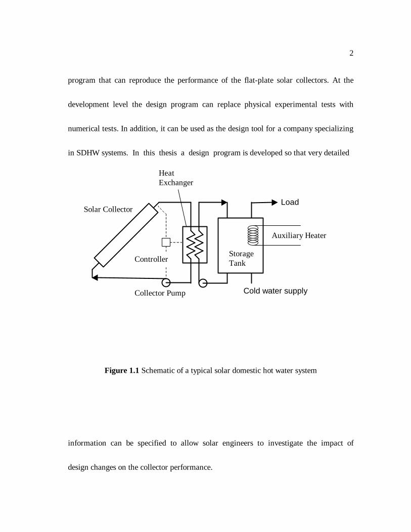
1

CHAPTER ONE

INTRODUCTION

A solar domestic hot water (SDHW) system consists of solar collectors, heat

exchangers, storage tanks, auxiliary heaters, pipes, pumps, valves, and controllers. It

absorbs solar radiation in collectors, delivers the collected energy to the thermal storage

tank with or without heat exchangers, and then provides hot water for domestic usage.

Excess thermal energy is stored in one or two thermal storage tanks. When the solar

energy is insufficient to meet the heating load, an auxiliary heater will provide the

thermal energy. Figure 1.1 shows a schematic diagram of a typical one-tank forced-

circulation SDHW system.

To evaluate the performance of solar heating systems, experimental or numerical

testing methods can be used. While experiments yield valuable information, numerical

modeling allows differentiating between designs at reasonable costs. A simulation

program like TRNSYS [7] needs performance equations or data for each component to

perform system simulation. The main objective of this study is to develop a design

2

program that can reproduce the performance of the flat-plate solar collectors. At the

development level the design program can replace physical experimental tests with

numerical tests. In addition, it can be used as the design tool for a company specializing

in SDHW systems. In this thesis a design program is developed so that very detailed

Figure 1.1 Schematic of a typical solar domestic hot water system

information can be specified to allow solar engineers to investigate the impact of

design changes on the collector performance.

Load

Cold water supplyCollector Pump

ControllerStorageTank

Auxiliary Heater

Solar Collector

HeatExchanger

3

1.1 Flat-Plate Solar Collectors

Flat-plate solar collectors have potential applications in many space-heating

situations, air conditioning, industrial process heat, and also for heating domestic water

[3]. These collectors use both beam and diffuse radiation. A well-designed collector can

produce hot water at temperature up to the boiling point of water [3]. They are usually

fixed in position permanently, have fairly simple construction, and require little

maintenance. To keep costs at a level low enough to make solar heating more attractive

than other sources of heat, the materials, dimensions, and method of fabrication must be

chosen with care.

A flat-plate solar collector consists of a radiation-absorbing flat plate beneath

one or more transparent covers, tubes attached to the plate to transport the circulating

fluid and back and edge insulation to reduce heat loss. Water or an anti-freeze fluid

circulates through the collector by a pump or by natural convection to remove the

absorbed heat.

4

Even though the theory of flat-plate solar collectors is well established, accurate

design programs, which have an easy-to-use graphic interface and include all the design

factors, are not available. In this thesis a detailed model is developed that includes all of

the design features of the collector such as: plate material and thickness, tube diameters

and spacing, number of covers and cover material, back and edge insulation dimensions,

etc. The program is useful for collector design and for detailed understanding of how

collectors function. For system simulation programs such as TRNSYS [7], simple

models such as instantaneous efficiency and incident angle modifier are usually

adequate. The detailed model developed in this study can provide these simple

parameters.

1.2 Engineering Equation Solver

Engineering Equation Solver (EES) is a program developed by Professor

Sanford A. Klein of the Solar Energy Laboratory, University of Wisconsin – Madison

5

[6]. It can solve a system of algebraic, differential, and complex equations. It can also

perform optimization, provide linear and nonlinear regression, and generate publication-

quality plots. Since it automatically identifies and groups equations to be solved

simultaneously, the solver always operates at optimum efficiency. Many mathematical

functions, thermophysical properties, and transport properties are also provided by

built-in functions that are helpful in solving engineering problems in thermodynamics,

fluid mechanics, and heat transfer. With these features, the user is able to concentrate

more on his/her own problem. EES is particularly useful for design problems in which

the impacts of one or more parameters need to be investigated.

The professional version of EES provides multiple diagram windows and

additional features by which a programmer can develop graphic user interface. One

valuable feature of the professional version is “make distributable.” Once a program is

developed, a compiled version can be created. This compiled version can be freely

distributed among students and the solar engineers. The design programs of this study

will be developed with EES.

6

1.3 Objectives

The objective of this thesis is to develop a new analytical and modeling tool to

evaluate the performance of components in order to reduce the cost of solar domestic

hot water (SDHW) systems. The new design tool will allow engineers to make design

changes and determine their effects on the thermal performance at a reasonable cost.

The program will be arranged so that very detailed information can be specified. It will

allow a company specializing in SDHW systems to investigate the impact of design

changes in their equipment on the thermal performance. For the task to be useful to the

SDHW industry, the design program will have to provide performance equations and

data that can be used a system simulation program like TRNSYS [7]. The program

should also provide comparisons of the analytical results from EES with experiments

following SRCC [17] practice that are normally performed on solar collector.

Throughout the project, it is necessary to ensure that EES is capable of modeling and

analyzing innovative designs.

7

CHAPTER TWO

FLAT-PLATE SOLAR COLLECTORS

A solar collector is a very special kind of heat exchanger that uses solar radiation

to heat the working fluid. While conventional heat exchangers accomplish a fluid-to-

fluid heat exchange with radiation as a negligible factor, the solar collector transfers the

energy from an incoming solar radiation to a fluid. The wavelength range of importance

for flat-plate solar collectors is from the visible to the infrared [3]. The radiation heat

transfer should be considered thoroughly in the calculation of absorbed solar radiation

and heat loss. While the equations for collector performance are reduced to relatively

simple forms in many practical cases of design calculations, they are developed in detail

in this thesis to obtain a thorough understanding of the performance of flat-plate solar

collectors.

8

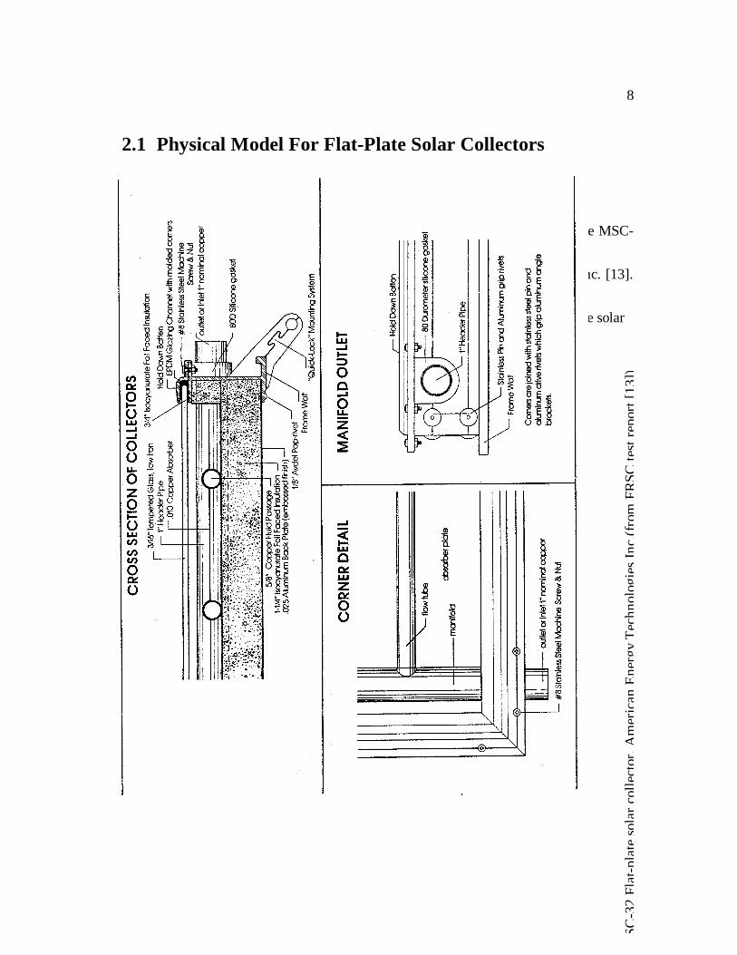
2.1 Physical Model For Flat-Plate Solar Collectors

A flat-plate solar collector is illustrated in detail in Figure 2.1.1. It is the MSC-

32 flat-plate solar collector manufactured by American Energy Technologies, Inc. [13].

Figure 2.1.2 shows a schematic diagram of a typical liquid heating flat-plate solar

MSC

-32

Flat

-pla

te s

olar

col

lect

or, A

mer

ican

Ene

rgy

Tech

nolo

gies

Inc.

(fro

m F

RSC

test

repo

rt [1

3])

9

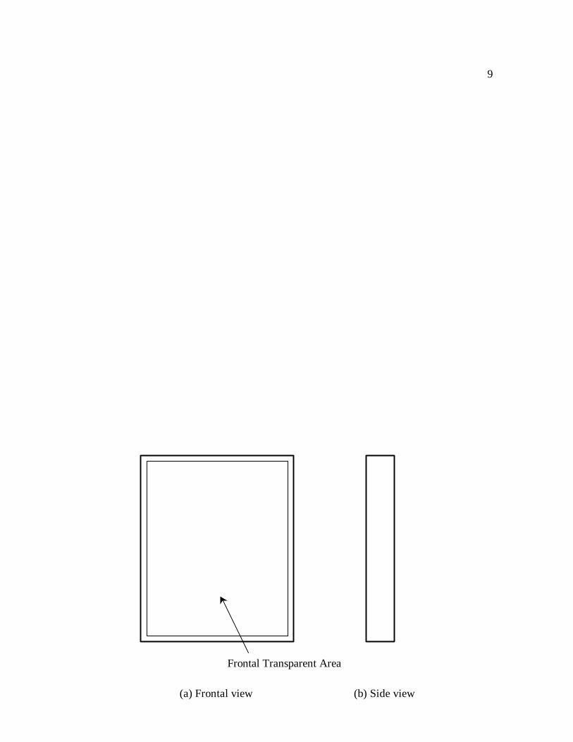
Frontal Transparent Area

(a) Frontal view (b) Side view

10

Figure 2.1.2 Physical flat-plate collector model

collector. Important parts are the cover system with one or more glass or plastic covers,

a plate for absorbing incident solar energy, parallel tubes attached to the plates, and

11

edge and back insulation. The detailed configuration may be different from one

collector to the other. However, the basic geometry is similar for almost flat-plate solar

collectors. The analysis of the flat-plate solar collector in this chapter is performed

based on the configuration shown in Figure 2.1.2.

Some assumptions made to model the flat-plate solar collectors are as follows:

1. The collector operates in steady state.

2. Temperature gradient through the covers is negligible.

3. There is one-dimensional heat flow through the back and side insulation and

through the cover system.

4. The temperature gradient around and through tubes is negligible.

5. The temperature gradient through the absorber plate is negligible.

6. The collector may have zero to two covers.

7. The semi-gray radiation model is employed to calculate radiation heat transfer in the

solar and infrared spectrum.

8. In calculating instantaneous efficiency, the radiation is incident on the solar

collector with fixed incident angle.

12

9. The collector is free-standing.

10. The area of absorber is assumed to be the same as the frontal transparent area.

13

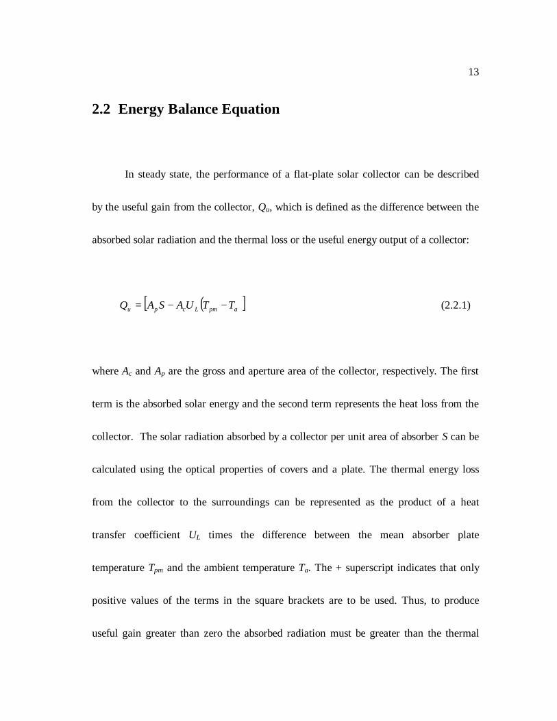
2.2 Energy Balance Equation

In steady state, the performance of a flat-plate solar collector can be described

by the useful gain from the collector, Qu, which is defined as the difference between the

absorbed solar radiation and the thermal loss or the useful energy output of a collector:

( )[ ]+−−= apmLcpu TTUASAQ (2.2.1)

where Ac and Ap are the gross and aperture area of the collector, respectively. The first

term is the absorbed solar energy and the second term represents the heat loss from the

collector. The solar radiation absorbed by a collector per unit area of absorber S can be

calculated using the optical properties of covers and a plate. The thermal energy loss

from the collector to the surroundings can be represented as the product of a heat

transfer coefficient UL times the difference between the mean absorber plate

temperature Tpm and the ambient temperature Ta. The + superscript indicates that only

positive values of the terms in the square brackets are to be used. Thus, to produce

useful gain greater than zero the absorbed radiation must be greater than the thermal

14

losses. Two collector areas appear in Equation 2.2.1; gross collector area Ac is defined

as the total area occupied by a collector and the aperture collector area Ap is the

transparent frontal area.

ASHRAE Standard [1] employs the gross area as a reference collector area in

the definition of thermal efficiency of the collector. The useful gain from the collector

based on the gross collector area becomes

( )[ ]+−−= apmLccu TTUSAQ (2.2.2)

where Sc is the absorbed solar radiation per unit area based on the gross collector area,

defined as

c

pc A

ASS = . (2.2.3)

Since the radiation absorption and heat loss at the absorber plate is considered

based on the aperture area in this study, it is convenient to make the aperture collector

area the reference collector area of the useful gain. Then Equation 2.2.1 becomes

15

( )[ ]+−′−= apmLpu TTUSAQ (2.2.4)

where U′L is the overall heat loss coefficient based on the aperture area given by

p

cLL A

AUU =′ . (2.2.5)

2.3 Solar Radiation Absorption

The prediction of collector performance requires knowledge of the absorbed

solar energy by the collector absorber plate. The solar energy incident on a tilted

collector consists of three different distributions: beam radiation, diffuse radiation, and

ground-reflected radiation. The details of the calculation depend on which diffuse-sky

model is used. In this study the absorbed radiation on the absorber plate is calculated by

isotropic sky model [8]:

16

( ) ( ) ( )( )

+++

++=

2cos1

2cos1 βρτ αβτ ατ α ggdbddbbb IIIRIS (2.3.1)

where the subscripts b, d, and g represent beam, diffuse, and ground-reflected radiation,

respectively. I is intensity of radiation on a horizontal surface, (τ α ) the transmittance-

absorptance product that represents the effective absorptance of the cover-plate system,

and β the collector slope. ρ g is the diffuse reflectance of ground and the geometric

factor Rb is the ratio of beam radiation on the tilted surface to that on a horizontal

surface. This section treats the way to calculate the transmittance-absorptance product

of beam, diffuse, ground-reflected radiation for a given collector configuration and

specified test conditions.

θ 1

Ii

It2

Ir

Medium 1 (n1)

Medium 2 (n2)

θ 2

It1

θ 1

Lτ a

17

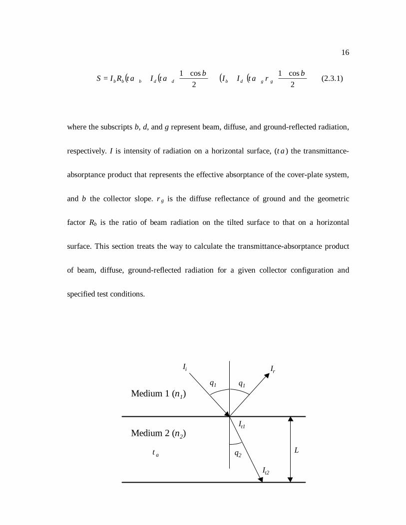
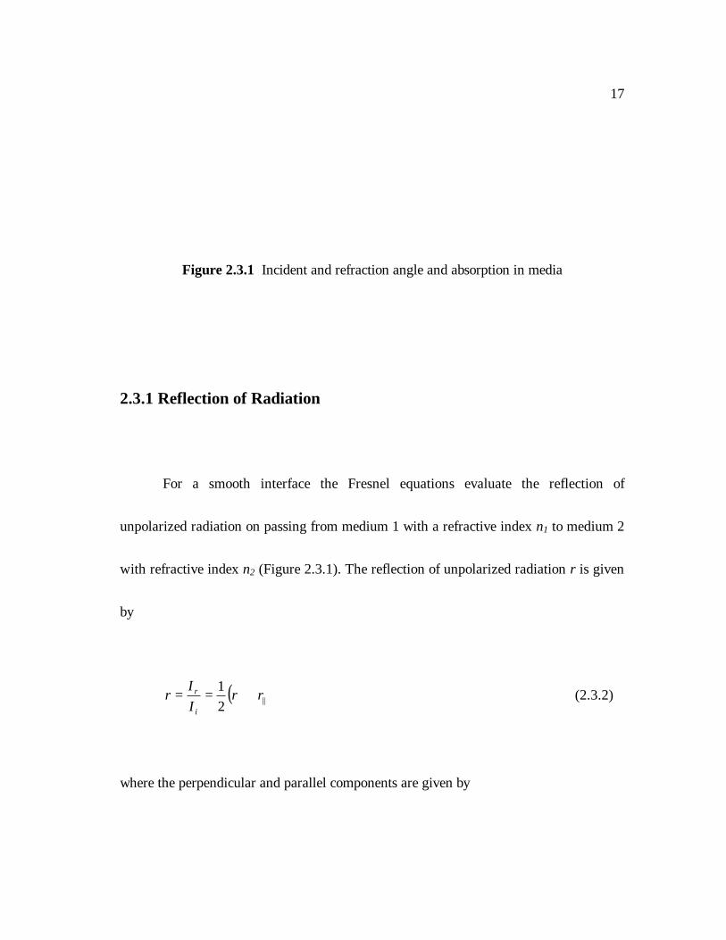
Figure 2.3.1 Incident and refraction angle and absorption in media

2.3.1 Reflection of Radiation

For a smooth interface the Fresnel equations evaluate the reflection of

unpolarized radiation on passing from medium 1 with a refractive index n1 to medium 2

with refractive index n2 (Figure 2.3.1). The reflection of unpolarized radiation r is given

by

( )||21 rr

II

ri

r +== ⊥ (2.3.2)

where the perpendicular and parallel components are given by

18

( )( )12

212

2

sinsin

θθθθ

+−=⊥r (2.3.3)

( )( )12

212

2

|| tantan

θθθθ

+−=r (2.3.4)

where θ 1 and θ 2 are the incident and refraction angles, respectively, that are related to

the refraction indices by Snell’s law:

1

2

2

1

sinsin

θθ=

nn

. (2.3.5)

If the angle of incidence and refractive indices of media are known, the reflectance of a

surface can be calculated by using Equations 2.3.2-2.3.5.

2.3.2 Absorption by Glazing

Bouguer’s law [3] describes the absorption of radiation in a partially transparent

medium. With the assumption that the absorbed radiation is proportional to the local

intensity in the medium and the distance x the radiation has traveled in the medium, the

19

transmittance of the medium can be represented as (Figure 2.3.1)

−==

21

2

cosexp

θτ KL

II

t

ta (2.3.6)

where K is the extinction coefficient and L the thickness of the medium (Figure 2.3.1).

The subscript a is a reminder that only absorption has been considered.

2.3.3 Optical Properties of Cover Systems

In the case of collector covers and windows, the solar radiation travels through a

slab of materials. A cover or a window has two interfaces per cover causing reflection

losses. At an off-normal incident angle, reflection is different for each component of

polarization so that the transmitted and reflected radiation will be polarized. Ray tracing

techniques [12] for each component of polarization yields the transmittance of initially

unpolarized radiation.

20

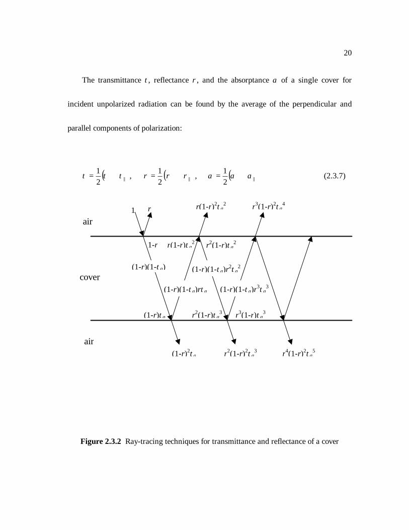
The transmittance τ , reflectance ρ , and the absorptance α of a single cover for

incident unpolarized radiation can be found by the average of the perpendicular and

parallel components of polarization:

( )||21 τττ += ⊥ , ( )||2

1 ρρρ += ⊥ , ( )||21 ααα += ⊥ (2.3.7)

Figure 2.3.2 Ray-tracing techniques for transmittance and reflectance of a cover

1 r

1-r

air

cover

air

(1-r)τ a

(1-r)2τ a

r(1-r)τ a2 r2(1-r)τ a

2

r(1-r)2τ a2

r2(1-r)τ a3

r2(1-r)2τ a3

r3(1-r)τ a3

r3(1-r)2τ a4

r4(1-r)2τ a5

(1-r)(1-τ a)

(1-r)(1-τ a)rτ a

(1-r)(1-τ a)r2τ a2

(1-r)(1-τ a)r3τ a3

21

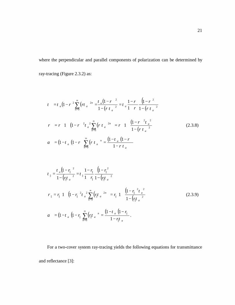
where the perpendicular and parallel components of polarization can be determined by

ray-tracing (Figure 2.3.2) as:

( ) ( ) ( )( )

( )( )2

2

2

2

0

22

11

11

11

1a

aa

a

n

naa r

rrr

rr

rrτ

ττ

ττττ⊥

⊥

⊥

⊥

⊥

⊥∞

=⊥ −

−+−=

−−=−= ∑

( ) ( ) ( )( )

−−+=

−+=

⊥

⊥⊥

∞

=⊥⊥⊥⊥ ∑ 2

22

0

222

11

111a

a

n

naa r

rrrrr

ττττρ (2.3.8)

( )( ) ( ) ( )( )a

a

n

naa r

rrr

ττττα

⊥

⊥∞

=⊥⊥⊥ −

−−=−−= ∑ 111

110

( )( )

( )( )2

||

2||

||

||||2

||

2||

|| 1

111

1

1

aa

a

r

rrr

r

r

ττ

ττ

τ−

−+−

=−

−=

( ) ( ) ( )( )

−−

+=

−+= ∑

∞

=2

||

22||

||0

2||

22|||||| 1

1111

a

a

n

naa r

rrrrr

ττ

ττρ (2.3.9)

( )( ) ( ) ( )( )a

a

n

naa r

rrr

ττ

ττα||

||

0|||| 1

1111

−−−

=−−= ∑∞

=⊥ .

For a two-cover system ray-tracing yields the following equations for transmittance

and reflectance [3]:

22

( )

−+

−=+=

⊥⊥

||12

12

12

12|| 112

121

ρρττ

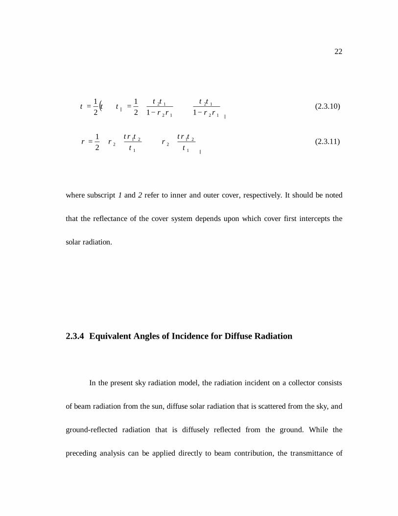
ρρτττττ (2.3.10)

++

+=

⊥ ||1

212

1

2122

1τ

ττ ρρτ

ττ ρρρ (2.3.11)

where subscript 1 and 2 refer to inner and outer cover, respectively. It should be noted

that the reflectance of the cover system depends upon which cover first intercepts the

solar radiation.

2.3.4 Equivalent Angles of Incidence for Diffuse Radiation

In the present sky radiation model, the radiation incident on a collector consists

of beam radiation from the sun, diffuse solar radiation that is scattered from the sky, and

ground-reflected radiation that is diffusely reflected from the ground. While the

preceding analysis can be applied directly to beam contribution, the transmittance of

23

cover systems for diffuse and ground-reflected radiation must be calculated by

integrating the transmittance over the appropriate incidence angles with an assumed sky

model. The calculation can be simplified by defining equivalent angles that give the

same transmittance as for diffuse and ground-reflected radiation [3].

Brandemuehl and Beckman [2] have performed the integration of the

transmittance over the appropriate incident angle with an isotropic sky model and

suggested the equivalent angle of incidence for diffuse radiation:

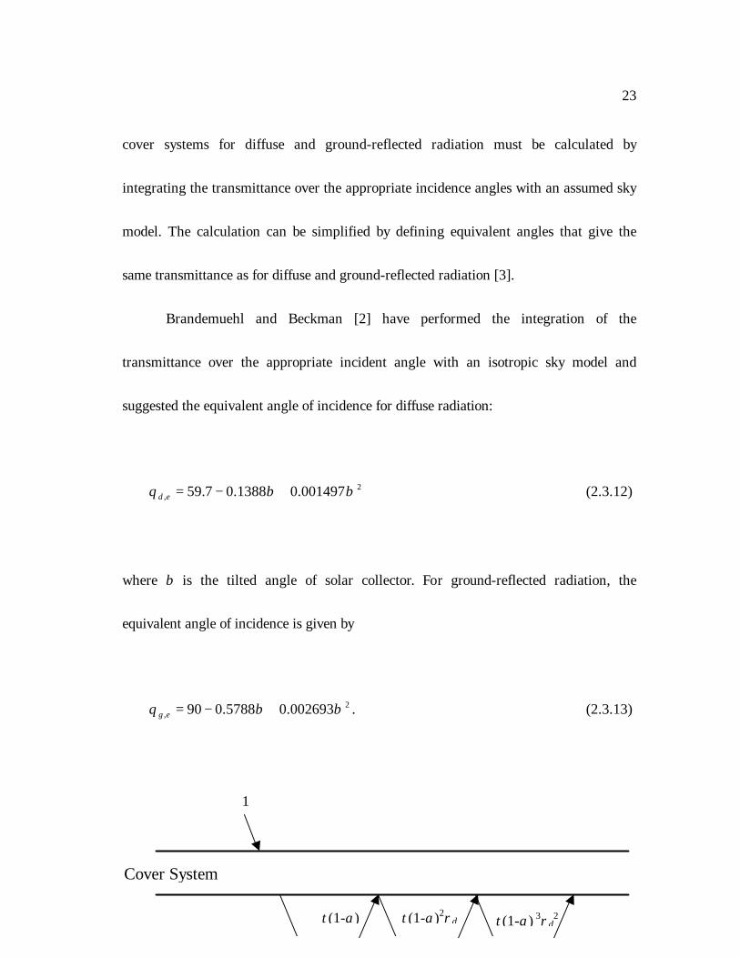
2, 001497.01388.07.59 ββθ +−=ed (2.3.12)

where β is the tilted angle of solar collector. For ground-reflected radiation, the

equivalent angle of incidence is given by

2, 002693.05788.090 ββθ +−=eg . (2.3.13)

1

Cover System

τ (1-α ) τ (1-α )2ρ d τ (1-α ) 3ρ d2

24

Figure 2.3.3 Absorbed solar radiation at the absorber plate

2.3.5 Transmittance-Absorptance Product (τ α )

Some of the radiation passing through the cover system is reflected back to the

cover system while the remainder is absorbed at the plate. In turn, the reflected radiation

from the plate will be partially reflected at the cover system and back to the plate as

illustrated in Figure 2.3.3. In this figure, τ is the transmittance of the cover system at the

desired angle, α is the angular absorptance of the absorber plate, and ρ d refers to the

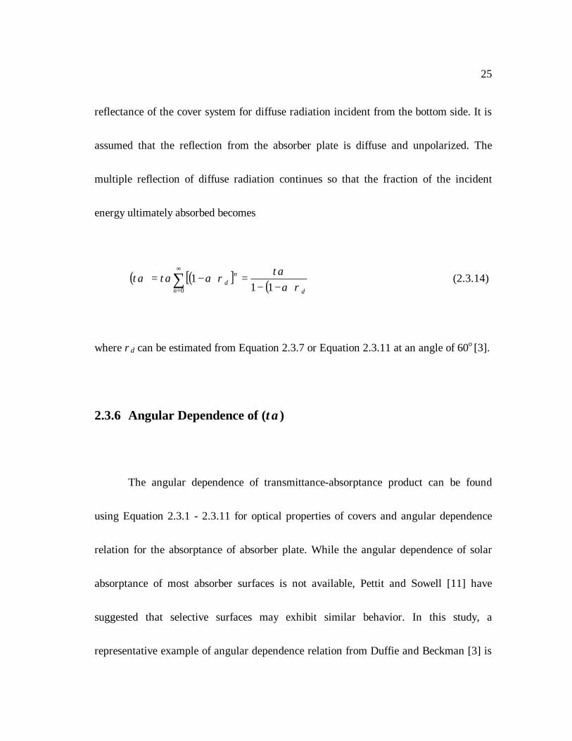
25

reflectance of the cover system for diffuse radiation incident from the bottom side. It is

assumed that the reflection from the absorber plate is diffuse and unpolarized. The

multiple reflection of diffuse radiation continues so that the fraction of the incident

energy ultimately absorbed becomes

( ) ( )[ ] ( ) dn

nd ρα

τ αρατ ατ α−−

=−= ∑∞

= 111

0

(2.3.14)

where ρ d can be estimated from Equation 2.3.7 or Equation 2.3.11 at an angle of 60o [3].

2.3.6 Angular Dependence of (τ α )

The angular dependence of transmittance-absorptance product can be found

using Equation 2.3.1 - 2.3.11 for optical properties of covers and angular dependence

relation for the absorptance of absorber plate. While the angular dependence of solar

absorptance of most absorber surfaces is not available, Pettit and Sowell [11] have

suggested that selective surfaces may exhibit similar behavior. In this study, a

representative example of angular dependence relation from Duffie and Beckman [3] is

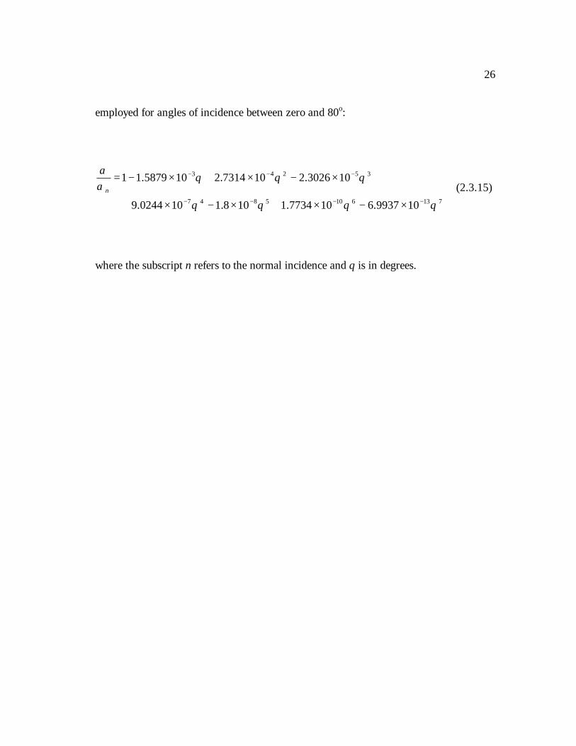
26

employed for angles of incidence between zero and 80o:

7136105847

35243

109937.6107734.1108.1100244.9

103026.2107314.2105879.11

θθθθ

θθθαα

−−−−

−−−

×−×+×−×+

×−×+×−=n (2.3.15)

where the subscript n refers to the normal incidence and θ is in degrees.

27

2.4 Heat Loss From The Collector

In solar collectors, the solar energy absorbed by the absorber plate is distributed

to useful gain and to thermal losses through the top, bottom, and edges [3]. In this

section the equations for each loss coefficient are derived for a general configuration of

the collector. The semi-gray model is employed for radiation heat transfer. All the

optical properties in this section are for infrared radiation while Section 2.3 deals with

the visible radiation.

2.4.1 Collector Overall Heat Loss

Heat loss from a solar collector consists of top heat loss through cover systems

and back and edge heat loss through back and edge insulation of the collector. With the

assumption that all the losses are based on a common mean plate temperature Tpm, the

overall heat loss from the collector can be represented as

28

( )apmcLloss TTAUQ −= (2.4.1)

where UL is the collector overall loss coefficient. The overall heat loss is the sum of the

top, back, and edge losses:

ebtloss QQQQ ++= . (2.4.2)

where the subscripts t, b, and e represent for the top, back, and edge contribution,

respectively.

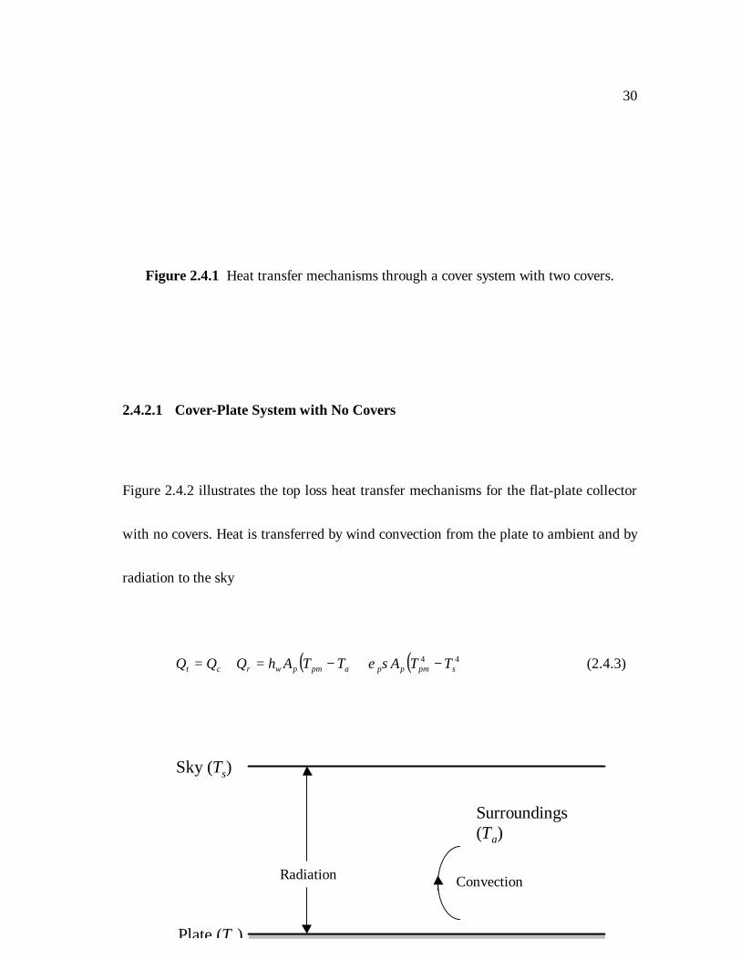
2.4.2 Top Heat Loss through the Cover System

To evaluate the heat loss through the cover systems, all of the convection and

radiation heat transfer mechanisms between parallel plates and between the plate and

the sky must be considered as shown in Figure 2.4.1. The collector model may have up

to two covers and the cover system have 9 different combinations of covers: no covers,

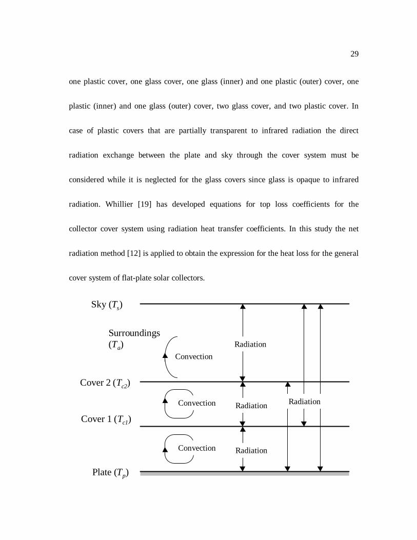
29

one plastic cover, one glass cover, one glass (inner) and one plastic (outer) cover, one

plastic (inner) and one glass (outer) cover, two glass cover, and two plastic cover. In

case of plastic covers that are partially transparent to infrared radiation the direct

radiation exchange between the plate and sky through the cover system must be

considered while it is neglected for the glass covers since glass is opaque to infrared

radiation. Whillier [19] has developed equations for top loss coefficients for the

collector cover system using radiation heat transfer coefficients. In this study the net

radiation method [12] is applied to obtain the expression for the heat loss for the general

cover system of flat-plate solar collectors.

Sky (Ts)

Plate (Tp)

Convection

Cover 2 (Tc2)

Cover 1 (Tc1)

Radiation

Convection Radiation

Radiation

RadiationConvection

Surroundings(Ta)

30

Figure 2.4.1 Heat transfer mechanisms through a cover system with two covers.

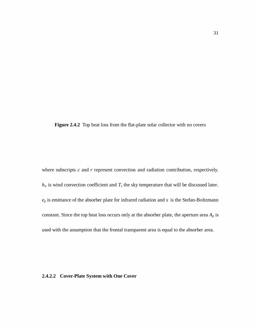
2.4.2.1 Cover-Plate System with No Covers

Figure 2.4.2 illustrates the top loss heat transfer mechanisms for the flat-plate collector

with no covers. Heat is transferred by wind convection from the plate to ambient and by

radiation to the sky

( ) ( )44spmppapmpwrct TTATTAhQQQ −+−=+= σε (2.4.3)

Sky (Ts)

Plate (Tp)

Radiation Convection

Surroundings(Ta)

31

Figure 2.4.2 Top heat loss from the flat-plate solar collector with no covers

where subscripts c and r represent convection and radiation contribution, respectively.

hw is wind convection coefficient and Ts the sky temperature that will be discussed later.

ε p is emittance of the absorber plate for infrared radiation and σ is the Stefan-Boltzmann

constant. Since the top heat loss occurs only at the absorber plate, the aperture area Ap is

used with the assumption that the frontal transparent area is equal to the absorber area.

2.4.2.2 Cover-Plate System with One Cover

32

For a flat-plate solar collector with one cover, the top heat loss from the collector plate

to the ambient can be obtained by applying the net-radiation method [12]. In Figure

Figure 2.4.3 Net-radiation method applied to one cover-plate

Figure 2.4.3, the outgoing radiation flux from the cover can be written in terms of

incoming fluxes as

Sky (Ts)

Plate (Tp)

Cover (Tc)

Natural Convection

Convection

Surroundings (Ta)

12

q1,i q1,o

q2,i q2,o

ρ p, ε p

τ c, ρ c, ε c

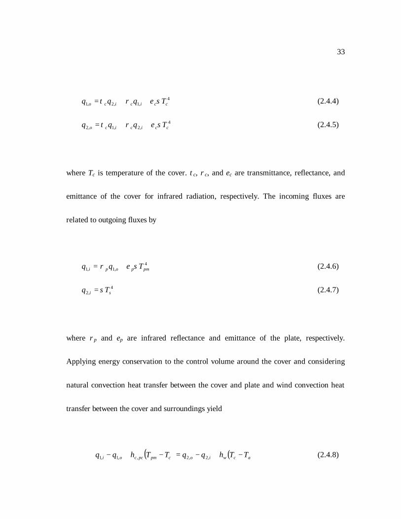
33

4,1,2,1 ccicico Tqqq σερτ ++= (2.4.4)


where Tc is temperature of the cover. τ c, ρ c, and ε c are transmittance, reflectance, and

emittance of the cover for infrared radiation, respectively. The incoming fluxes are

related to outgoing fluxes by

4,1,1 pmpopi Tqq σερ += (2.4.6)

4,2 si Tq σ= (2.4.7)

where ρ p and ε p are infrared reflectance and emittance of the plate, respectively.

Applying energy conservation to the control volume around the cover and considering

natural convection heat transfer between the cover and plate and wind convection heat

transfer between the cover and surroundings yield

( ) ( )acwiocpmpccoi TThqqTThqq −+−=−+− ,2,2,,1,1 (2.4.8)

34

where hc,pc is natural convection heat transfer coefficient between the absorber plate and

cover that will be discussed later. By solving Equations 2.4.4-2.4.8 simultaneously, heat

fluxes and cover temperature can be obtained for the given temperatures of plate and

sky and optical properties of cover-plate system. Top heat loss is the heat flux at the

control surface times absorber area given by

( )[ ]cpmpccoipt TThqqAQ −+−= ,,1,1 . (2.4.9)

35

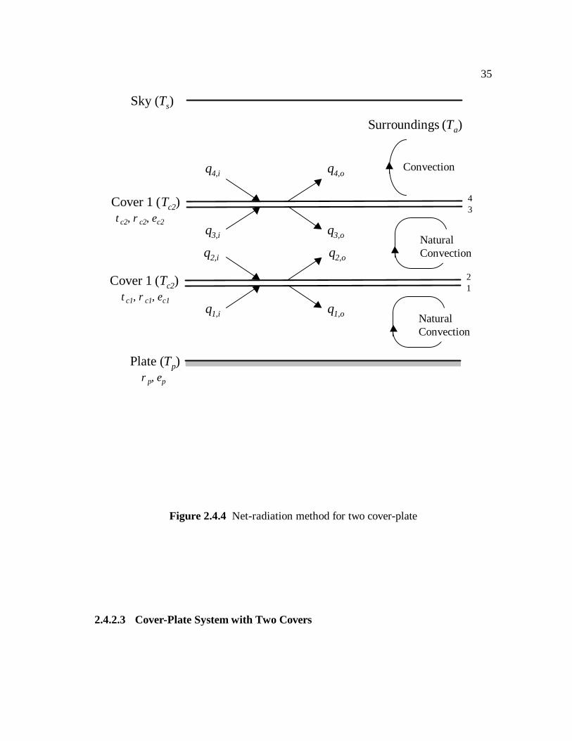
Figure 2.4.4 Net-radiation method for two cover-plate

2.4.2.3 Cover-Plate System with Two Covers

Sky (Ts)

Cover 1 (Tc2)

Natural Convection

Convection

Surroundings (Ta)

34

q2,i q2,o

τ c2, ρ c2, ε c2

Plate (Tp)

Cover 1 (Tc2)

Natural Convection

12

q1,i q1,o

ρ p, ε p

τ c1, ρ c1, ε c1

q3,i q3,o

q4,i q4,o

36

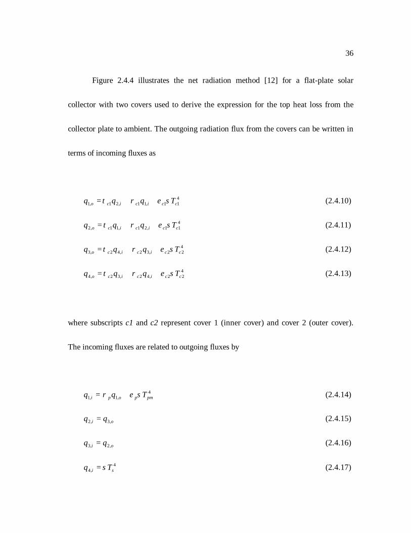
Figure 2.4.4 illustrates the net radiation method [12] for a flat-plate solar

collector with two covers used to derive the expression for the top heat loss from the

collector plate to ambient. The outgoing radiation flux from the covers can be written in

terms of incoming fluxes as





where subscripts c1 and c2 represent cover 1 (inner cover) and cover 2 (outer cover).

The incoming fluxes are related to outgoing fluxes by

4,1,1 pmpopi Tqq σερ += (2.4.14)

oi qq ,3,2 = (2.4.15)

oi qq ,2,3 = (2.4.16)

4,4 si Tq σ= (2.4.17)

37

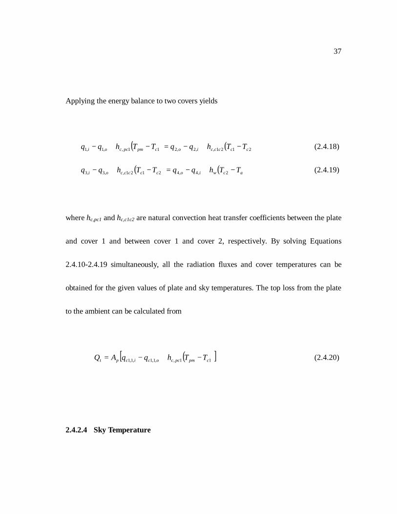
Applying the energy balance to two covers yields

( ) ( )2121,,2,211,,1,1 ccccciocpmpccoi TThqqTThqq −+−=−+− (2.4.18)

( ) ( )acwiocccccoi TThqqTThqq −+−=−+− 2,4,42121,,3,3 (2.4.19)

where hc,pc1 and hc,c1c2 are natural convection heat transfer coefficients between the plate

and cover 1 and between cover 1 and cover 2, respectively. By solving Equations

2.4.10-2.4.19 simultaneously, all the radiation fluxes and cover temperatures can be

obtained for the given values of plate and sky temperatures. The top loss from the plate

to the ambient can be calculated from

( )[ ]11,,1,1,1,1 cpmpccocicpt TThqqAQ −+−= (2.4.20)

2.4.2.4 Sky Temperature

38

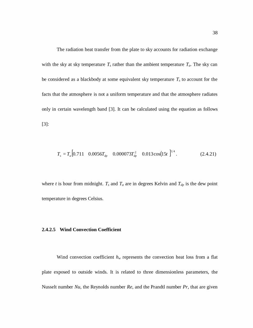
The radiation heat transfer from the plate to sky accounts for radiation exchange

with the sky at sky temperature Ts rather than the ambient temperature Ta. The sky can

be considered as a blackbody at some equivalent sky temperature Ts to account for the

facts that the atmosphere is not a uniform temperature and that the atmosphere radiates

only in certain wavelength band [3]. It can be calculated using the equation as follows

[3]:

( )[ ] 412 15cos013.0000073.00056.0711.0 tTTTT dpdpas +++= . (2.4.21)

where t is hour from midnight. Ts and Ta are in degrees Kelvin and Tdp is the dew point

temperature in degrees Celsius.

2.4.2.5 Wind Convection Coefficient

Wind convection coefficient hw represents the convection heat loss from a flat

plate exposed to outside winds. It is related to three dimensionless parameters, the

Nusselt number Nu, the Reynolds number Re, and the Prandtl number Pr, that are given

39

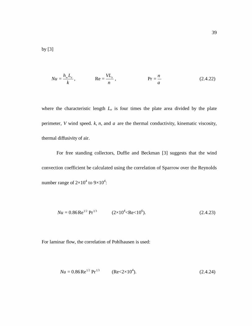
by [3]

kLh

Nu ew= , ν

eVL=Re , αν=Pr (2.4.22)

where the characteristic length Le is four times the plate area divided by the plate

perimeter, V wind speed. k, ν , and α are the thermal conductivity, kinematic viscosity,

thermal diffusivity of air.

For free standing collectors, Duffie and Beckman [3] suggests that the wind

convection coefficient be calculated using the correlation of Sparrow over the Reynolds

number range of 2×104 to 9×104:

3121 PrRe86.0=Nu (2×104<Re<106). (2.4.23)

For laminar flow, the correlation of Pohlhausen is used:

3121 PrRe86.0=Nu (Re<2×104). (2.4.24)

40

2.4.2.6 Natural Convection between Parallel Plates

For the prediction of the top loss coefficient, the evaluation of natural

convection heat transfer between two parallel plates tilted at some angle to the horizon

is of obvious importance. The natural convection heat transfer coefficient hc is related to

three dimensionless parameters, the Nusselt number Nu, the Rayleigh number Ra, and

the Prandtl number Pr, that are given by

kLh

Nu c= , ν α

β 3TLgRa v ∆= ,

αν=Pr (2.4.25)

where L is the plate spacing, g the gravitational constant, ∆ T the temperature difference

between plates, and β v is the volumetric coefficient of expansion of air.

Hollands et al. [4] suggested the relationship between the Nusselt number and

Rayleigh number for tilt angle β from 0 to 75o as

( )[ ] ++

−

+

−

−+= 1

5830cos

cos17081

cos8.1sin1708144.11

316.1 βββ

β RaRaRa

Nu (2.4.26)

41

While Equation 2.4.26 is for the isothermal plates, plastic covers are thin and have low

values of conductivity. Thus, the convection cells cause small temperature gradients

along the covers. Yiqin et al. [21] suggested the following relationship for the natural

convection for a two-cover system with the inner cover made from plastic:

( )[ ] ++

−

+

−

−+= 1

5830cos

cos12961

cos8.1sin1296144.11

316.1 βββ

β RaRaRa

Nu . (2.4.27)

2.4.3 Back and Edge Heat Loss

The energy loss through the back of the collector is the result of the conduction

through the back insulation and the convection and radiation heat transfer from back of

the collector to surroundings. Since the magnitudes of the thermal resistance of

convection and radiation heat transfer are much smaller than that of conduction, it can

be assumed that all the thermal resistance from the back is due to the insulation [3]. The

back heat loss, Qb, can be obtained from

42

( )apmcb

bb TTA

Lk

Q −= (2.4.28)

where kb and Lb are the back insulation thermal conductivity and thickness, respectively.

While the evaluation of edge losses is complicated for most collectors, the edge

loss in a well-constructed system is intended to be so small that it is not necessary to

predict it with great accuracy [3]. With the assumption of one-dimensional sideways

heat flow around the perimeter of the collector, the edge losses can be estimated by

( )apmee

ee TTA

Lk

Q −= (2.4.29)

where ke and Le are the edge insulation thermal conductivity and thickness and Ae is

edge area of the collector.

2.4.4 Overall Heat Loss Coefficient

43

The overall loss coefficient UL based on the gross collector area can be

calculated from Equation 2.4.1 with the known values of the overall heat loss Qloss and

the plate temperature Tpm. To derive an expression for the mean temperature of the

absorber plate, it is necessary to know the overall heat loss coefficient based on the

absorber area. Since of heat transfer coefficient-area product is constant, it can be

calculated from

cLpL AUAU =′ . (2.4.30)

where U′L is the modified overall heat loss coefficient whose base area is the aperture

area of the collector.

2.5 The Mean Absorber Plate Temperature*

To calculate the collector useful gain using Equation 2.2.1, it is necessary to

know the mean temperature of absorber plate that is a complicated function of the

temperature distribution on the absorber plate, bond conductivity, heat transfer inside of

44

tubes and geometric configuration. To consider these factors along with the energy

collected at the absorber plate and heat loss, the collector efficiency factor and the

collector heat removal factor are introduced.

2.5.1 Collector Efficiency Factor

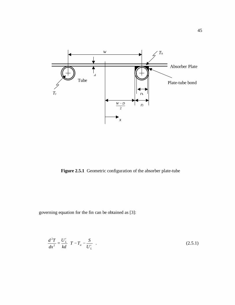
The collector efficiency factor, F′, represents the temperature distribution along

the absorber plate between tubes. Figure 2.5.1 illustrates the absorber plate-tube

configuration of the present collector model. With the assumption of negligible

temperature gradient in the fin in the flow direction, the collector efficiency factor can

be obtained by solving the classical fin problem [3]. Figure 2.5.2(a) shows the fin with

insulated tip that is to be analyzed. The plate just above the tube is assumed to be at

some local base temperature Tb. The fin is (W-D)/2 long and has unit depth in the flow

direction. By applying energy balance on the element shown in Figure 2.5.2(b), the

* The analysis follows the book, Solar Engineering of Thermal Processes, Duffie and Beckman, 1991 [3].

45

Figure 2.5.1 Geometric configuration of the absorber plate-tube

governing equation for the fin can be obtained as [3]:

′−−′=L

aL

US

TTkU

dxTd

δ2

2

. (2.5.1)

Absorber Plate

Tube Plate-tube bond

Di

W

D

x

Tf

2DW −

δ

Tb

46

where U′L is the overall loss coefficient based on the aperture area. The two boundary

conditions are the insulated tip condition and the known base temperature Tb:

00

==xdx

dT , bDWx

TT =−=2

. (2.5.2)

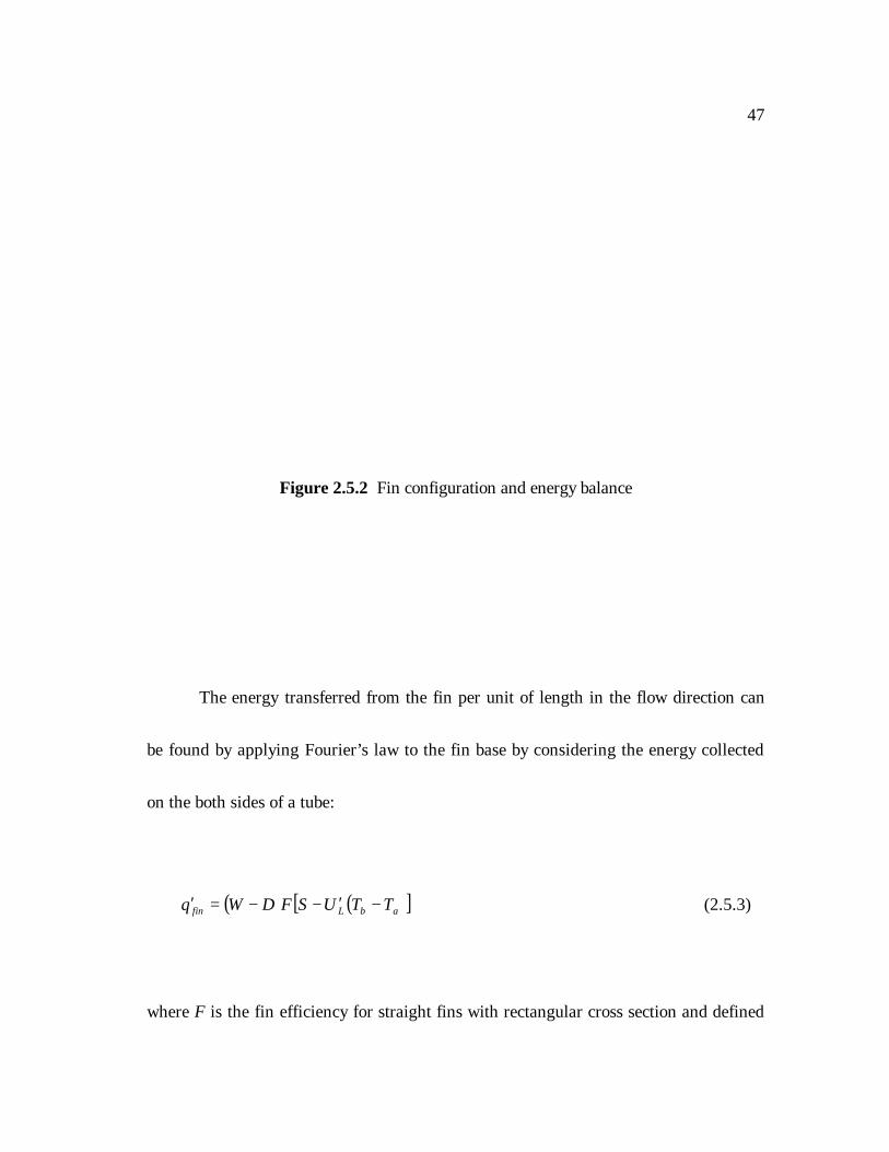
(a) fin with insulated tip

Insulated tipδ

2DW −

Tbx ∆ x

S

S∆ x

xdxdT

kδ−

U′L∆ x(Tx-Ta)

(b) energy balance on finite element

xxdxdTk

∆+− δ

x∆ x

47

Figure 2.5.2 Fin configuration and energy balance

The energy transferred from the fin per unit of length in the flow direction can

be found by applying Fourier’s law to the fin base by considering the energy collected

on the both sides of a tube:

( ) ( )[ ]abLfin TTUSFDWq −′−−=′ (2.5.3)

where F is the fin efficiency for straight fins with rectangular cross section and defined

48

as

( )[ ]( ) 2

2tanhDWm

DWmF

−−= (2.5.4)

and m is a parameter of the fin-air arrangement defined as

δkU

m L′= (2.5.5)

The solar energy absorbed just above the tube per unit of length in the flow

direction can be calculated by

( )[ ]abLtube TTUSDq −′−=′ . (2.5.6)

Then the useful gain q′u per unit of depth in the flow direction is the sum of q′fin and

q′tube :

( )[ ] ( )[ ]abLu TTUSDFDWq −′−+−=′ (2.5.7)

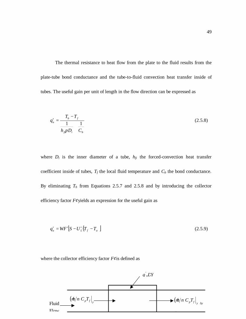
49

The thermal resistance to heat flow from the plate to the fluid results from the

plate-tube bond conductance and the tube-to-fluid convection heat transfer inside of

tubes. The useful gain per unit of length in the flow direction can be expressed as

bifi

fbu

CDh

TTq

11 +

−=′

π

(2.5.8)

where Di is the inner diameter of a tube, hfi the forced-convection heat transfer

coefficient inside of tubes, Tf the local fluid temperature and Cb the bond conductance.

By eliminating Tb from Equations 2.5.7 and 2.5.8 and by introducing the collector

efficiency factor F′ yields an expression for the useful gain as

( )[ ]afLu TTUSFWq −′−′=′ (2.5.9)

where the collector efficiency factor F′ is defined as

q’u∆ Y

( )yfpTCnm& ( )

yyfpTCnm∆+

&Fluid Flow

50

Figure 2.5.3 Energy balance of a control volume of the tube

( )[ ]

++

−+′

′=′

fiibL

L

hDCFDWDUW

UF

π111

1. (2.5.10)

2.5.2 Temperature Distribution in Flow Direction

The fluid temperature of fluid varies along the tube with a certain temperature

profile. Equation 2.5.9 expresses the useful gain per unit length in the flow direction as

51

a function of local fluid temperature that is a function of a position y along the flow

direction. Applying the energy conservation to the control volume shown in Figure 2.5.3

and substituting Equation 2.5.9 for q′u yield energy balance equation:

( )[ ] 0=−′−−′ afLfp TTUS

dy

dT

FnW

Cm& (2.5.11)

where m& is the total collector flow rate, n the number of tubes, and Tf the temperature

of fluid at any location y. With the assumption that F′ and UL are independent of

position the fluid temperature at any position y can be calculated from

′′−=′−−′−−

p

L

Lai

Laf

CmyFnWU

USTTUSTT

&exp . (2.5.12)

where Ti is fluid inlet temperature.

52

2.5.3 Collector Heat Removal Factor

The collector heat removal factor, FR, is the ratio of the actual useful energy gain

of a collector to the maximum possible useful gain if the whole collector surface were at

the fluid inlet temperature. It is defined as

( )( )[ ]aiLp

iopR TTUSA

TTCmF

−′−−

=&

(2.5.13)

where the aperture area Ap is used as a reference area for the useful gain from the

collector. The exit temperature To can be calculated using Equation 2.5.12 by

substituting tube length L for y. Then Equation 2.5.13 can be expressed as [3]

′′−′=

p

Lp

Lp

pR Cm

FUAUACm

F &&

exp1 (2.5.14)

Physically the collector heat removal factor is equivalent to the effectiveness of

a conventional heat exchanger. By introducing the collector heat removal factor and the

53

modified overall heat transfer coefficient into Equation 2.2.4, the actual useful energy

gain Qu can be represented as

( )[ ]+−′−= aiLRpu TTUSFAQ . (2.5.15)

Introducing Equation 2.2.3 and 2.2.5 into Equation 2.5.15 yields

( )[ ]+−−= aiLcRcu TTUSFAQ (2.5.16)

Using Equations 2.5.15 and 2.5.16, the useful energy gain can be calculated as a

function of the inlet fluid temperature not the mean plate temperature.

2.5.4 Mean Fluid and Plate Temperatures

For accurate the prediction of collector performance, it is necessary to evaluate

properties of the working fluid to calculate the forced convection heat transfer

coefficients inside of tubes and the overall loss coefficient. The mean fluid temperature

Tfm at which the fluid properties are evaluated can be obtained by [3]:

54

( )FUFAQ

TTLR

puifm ′′−′+= 1 . (2.5.17)

where the collector flow factor F′′, defined as the ratio of FR to F′, are given by

′′−′′=′=′′

p

Lp

Lp

pR

CmFUA

FUACm

FF

F &&

exp1 (2.5.18)

The collector flow factor is a function of the dimensionless collector capacitance rate

m&Cp/ApULF′.

The mean plate temperature, Tpm, is always greater than the mean fluid

temperature due to the heat transfer resistance between the absorbing surface and the

fluid. Equating Equations 2.2.4 and 2.5.15 and solving for the mean plate temperature

Tpm yields

( )RLR

puipm F

UF

AQTT −′+= 1 (2.5.19)

55

2.5.5 Forced Convection inside of Tubes

For fully developed turbulent flow inside of tubes (Re>2300), the Nusselt

number can be obtained from Gnielinsky correlation [5]:

( )( )( )18712110008

32 −+−=

Prf.PrRef

Nu tubelong (2.5.20)

where Darcy friction factor f for smooth surface is calculated from Petukhov relation [5]

given by

( ) 264.1Reln0790.0 −−= tubef . (2.5.21)

For short tubes with a sharp-edged entry, the developing thermal and hydrodynamic

boundary layers will result in a significant increase in the heat transfer coefficient near

entrance. To consider this phenomena Duffie and Beckman [3] suggests that the

56

McAdams relation be used:

+=

7.0

1LDNuNu long (2.5.22)

where D and L is inner diameter and length of a tube.

For laminar flow inside of tubes the local Nusselt number for the case of short

tubes and constant heat flux is given by [3]

( )( )n

m

long LRePrDbLRePrDa

NuNu/1

/+

+= . (2.5.23)

With the assumption that the flow inside of tubes is fully developed, the values of Nulong,

a, b, m, and n are 4.4, 0.00172, 0.00281, 1.66, and 1.29, respectively, for the constant

heat flux boundary condition.

The friction factor f for fully developed laminar flow inside of a circular tube

can be calculated from

57

D

fRe64= . (2.5.24)

Generally the straight tubes are connected headers on both ends that provide

pipe entrance and exit with sharp edges. The friction coefficients for those minor losses

are approximated by

KDLf eqor =min (2.5.25)

where Leq is equivalent length and K loss coefficient. The value of loss coefficient is 0.5

for entrance with sharp edge and 1.0 for pipe exit [20]. Then the pressure drop through a

pipe and header can be calculated by

∑

+

=∆

22

22 UKL

DU

fP ffpipe

ρρ (2.5.26)

where U represents the mean fluid velocity inside of the tube and ρ f is fluid density.

59

2.6 Thermal Performance Of The Collectors

Based on the analysis in the previous sections, the thermal performance of the

flat-plate collector can be calculated. The thermal performance of the collector can be

represented by the instantaneous efficiency and the incidence angle modifier. The

stagnation temperature is also needed to ensure that the collector materials do not

exceed their thermal limit.

2.6.1 Instantaneous Efficiency

The instantaneous collector efficiency, η i, is a measure of collector performance

that is defined as the ratio of the useful gain over some specified time period to the

incident solar energy over the same time period:

∫∫=

dtGA

dtQ

Tc

uiη . (2.6.1)

60

where GT is the intensity of incident solar radiation. According to ASHRAE Standard

93-86 [1], the gross area Ac is used as a reference collector area in the definition of

instantaneous efficiency. By introducing the Equation 2.5.16, the instantaneous

efficiency becomes

( ) ( ) +

−−==

T

aiLRR

Tc

ui G

TTUFF

GAQ τ αη . (2.6.2)

where the absorbed energy Sc based on the gross collector area has been replaced by

( )τ αTc GS = . (2.6.3)

(τ α ) is the effective transmittance-absorptance product based on the collector gross area

defined as

( ) ( )c

pavg

cT

p

A

A

AG

SAτ ατ α == (2.6.4)

61

where (τ α )avg is the transmittance-absorptance product averaged for beam, diffuse, and

ground-reflected irradiation. SAp is the solar energy absorbed at absorber surface and

GTAc is the total solar energy incident on the gross area of the collector. In Equation

2.6.2, two important parameters, FR(τ α ) and FRUL, describe how the collector works.

FR(τ α ) indicates how energy is absorbed by the collector while FRUL is an indication of

how energy is lost from the collector.

2.6.2 Incidence Angle Modifier

To express the effects of the angle of incidence of the radiation on thermal

performance of the flat-plate solar collector, an incidence angle modifier Kτ α is

employed [1]. It describes the dependence of (τ α ) on the angle of incidence of radiation

on the collector and is a function of the optical characteristics of covers and the

absorber plate. It is defined as

62

( )( )n

Kτ ατ α

τ α = (2.6.5)

where subscript n indicates that the transmittance-absorptance product is for the normal

incidence of solar radiation.

2.6.3 Stagnation Temperatures

A plastic cover will melt when the temperature of the cover exceeds its melting

point. To ensure the thermal tolerance of the collector, the highest temperature in the

collector should be less than the melting point of the plastic covers. Stagnation

temperatures are the highest temperatures of the covers and absorber plate that can be

obtained from the collector. They occur when the collector is not working, that is, when

the working fluid does not circulate. In this case, the useful gain from the collector is

zero in Equation 2.2.1 and then the energy balance equation becomes

( )apmLcp TTUASA −= (2.6.6)

63

By solving this equation with the constitutive equations provided in this chapter, the

stagnation temperatures can be obtained.

2.7 Collector Test And Thermal Performance Models

In this study the thermal performance test of flat-plate collector consists of three

parts. The first is to determine instantaneous efficiency with beam radiation nearly

normal to the absorber surface. The second is determination of incident angle modifier.

The last is determination of the stagnation temperature. This section briefly reviews the

standard test procedure and introduces the thermal performance models for the

instantaneous efficiency and incidence angle modifier.

64

2.7.1 Instantaneous Efficiency

The ASHRAE Standard 93-86 [1] and SRCC document RM-1 [17] provide the

standard test methods for flat-plate solar collectors. The general test procedure is to

operate the collector in a test facility under nearly steady conditions and measure the

data that are needed for analysis. Although details differ, the essential features of all of

the procedures can be summarized as below [3]:

1. Solar radiation is measured by a pyranometer in the plane of the collector.

2. Flow rate of working fluid, inlet and outlet fluid temperatures, ambient temperature,

and wind speed) are measured.

3. Tests are made over a range of inlet temperatures.

4. The inlet pressure and pressure drop in the collector are measured.

Information available from the test is data on the thermal input, data on the thermal

output, and data on the ambient conditions. These data characterize a collector by

parameters, FR(τ α ), and FRUL, that indicate absorption of solar energy and energy loss

65

from the collector.

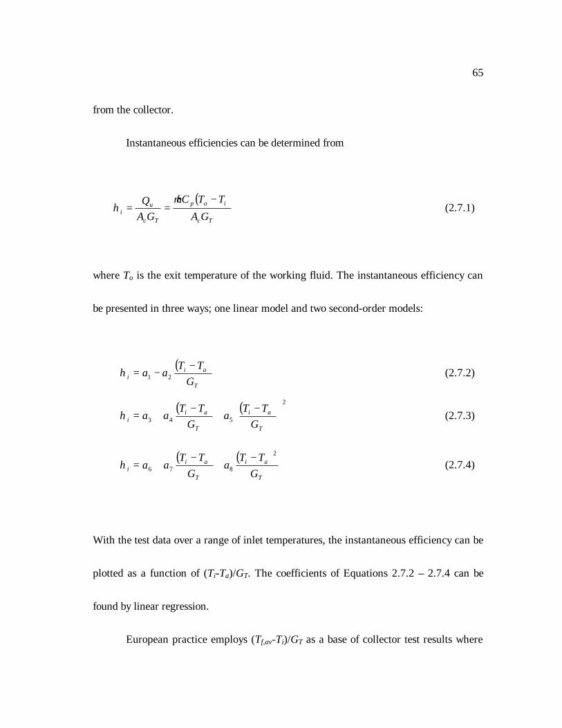
Instantaneous efficiencies can be determined from

( )Tc

iop

Tc

ui GA

TTCmGA

Q −==&

η (2.7.1)

where To is the exit temperature of the working fluid. The instantaneous efficiency can

be presented in three ways; one linear model and two second-order models:

( )T

aii G

TTaa

−−= 21η (2.7.2)

( ) ( ) 2

543

−+−+=

T

ai

T

aii G

TTa

GTT

aaη (2.7.3)

( ) ( )T

ai

T

aii G

TTa

GTT

aa2

876

−+−+=η (2.7.4)

With the test data over a range of inlet temperatures, the instantaneous efficiency can be

plotted as a function of (Ti-Ta)/GT. The coefficients of Equations 2.7.2 – 2.7.4 can be

found by linear regression.

European practice employs (Tf,av-Ti)/GT as a base of collector test results where

66

Tf,av is the arithmetic average of the fluid inlet and outlet temperature

2.7.2 Incidence Angle Modifier

The second important aspect of collector testing is the determination of effects

of incident angle of the solar radiation. The standard test methods [1,17] include

experimental estimation of this effect and require a clear test day so that the

experimental value of (τ α ) is essentially the same as (τ α )b. ASHRAE Standard 93-86

[1] recommends that experimental determination of Kτ α be done with the incidence

angles of beam radiation of 0, 30, 45, 60o.

For flat-plate solar collector Souka and Safwat [16] have suggested an

expression for angular dependence of Kτ α as

−+= 1

cos1

1 0 θτ α bK (2.7.5)

where θ is angle of incidence of beam radiation and b0 is the incidence angle modifier

67

coefficient. The incidence angle modifier coefficient can be determined using linear

regression with the test data of Kτ α over several values of incident angles.

68

CHAPTER THREE

RESULTS AND DISCUSSION

Provided that the calculation predicts the experimental results accurately, the

design program for flat-plate solar collectors might substitute for the experimental test

at the development level and enable the solar industries to make well-designed

economical solar collectors. In this chapter the comparisons with the experimental test

are performed and the effects of parameters are investigated.

3.1 Natural Convection Between Parallel Plates

The natural convection between the cover and plate and between covers plays an

important role in top heat loss through a cover system. As explained in Section 2.4.2.6,

the natural convection coefficients between two parallel plates can be calculated using

two equations: Equation 2.4.26 for glass cover system and Equation 2.4.27 for the cover

system with plastic as the inner cover.

69

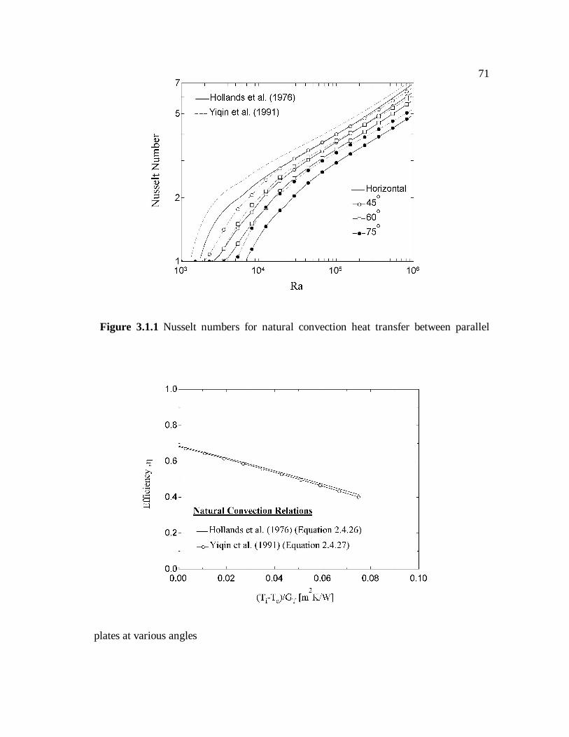
Figure 3.1.1 shows Nusselt numbers as a function of Rayleigh number for

natural convection heat transfer between parallel plates at various slopes. Solid curves

are the calculation result from the equation of Hollands et al. [4] (Equation 2.4.26) and

dotted curves are from Yiqin et al. [21] (Equation 2.4.27). Curves without symbols are

for horizontal plates, Curves with hollow circles, hollow squares, solid circles are for

the parallel plates tilted at 45o, 60o, and 75o with respect to horizon, respectively. As

shown in this figure the Nusselt number from Equation 2.4.13 is always larger than that

from Equation 2.4.12. These results show that the small temperature gradient along the

plastic cover caused by the convection cells enhances the natural convection heat

transfer.

Figure 3.1.2 shows a comparison of collector efficiencies calculated with the

two relations for natural convection heat transfer between the cover and plate and

between covers. The collector configuration and test conditions are based on the FSEC

solar collector test report for MSC-32 flat plate solar collector [13]. To investigate the

effect of natural convection correlation, a polyvinylfluoride (tedlar) cover is used for the

inner cover of the collector and the cover-to-cover air spacing is set to 0.5 cm. The

optical properties of the plastic covers are given by

70

Solar Spectrum : Refractive Index =1.45

Transmittance = 0.9

Infrared Spectrum : transmittance = 0.3

Absorptance = 0.63

The equation of Yiqin et al. always yields a higher Nusselt number and thus its

heat transfer coefficient exceeds that from Hollands et al. It causes the higher top loss

coefficient and lower collector efficiency. Even though the difference in the two Nusselt

71

Figure 3.1.1 Nusselt numbers for natural convection heat transfer between parallel

plates at various angles

72

Figure 3.1.2 Comparison of Instantaneous efficiencies of the collector with different

natural convection relations

numbers decreases with an increase of Rayleigh number (Figure 3.1.1), the difference in

instantaneous efficiencies increases as the temperature difference increases (Figure

3.1.2). This indicates that the proportion of the total heat loss that is natural convection

becomes larger as the absorber plate temperature increases. The Hollands et al. equation

overpredicts the instantaneous efficiency of the collector.

3.2 Comparison With Experiments

The calculation results were compared with the experimental results from three

flat-plate solar collectors. The experimental tests were performed by the Testing and

Laboratories Division, Florida Solar Energy Center (FSEC) according to the SRCC

testing method [17]. The calculations were performed with the test conditions and

collector configuration provided by the test reports [13-15].

73

3.2.1 MSC-32 (American Energy Technologies, Inc.)

Figure 2.1.1 shows the detailed geometric configuration of the MSC-32 flat-

plate solar collector [13]. Even though the detailed plate-tube configuration is different

from that of Figure 2.2.2, the overall geometric configuration is similar to the general

model. Test conditions and collector configurations provided by the FSEC test report

are summarized at Table 3.2.1 [13]. The test conditions are averaged values of the

experimental measurement.

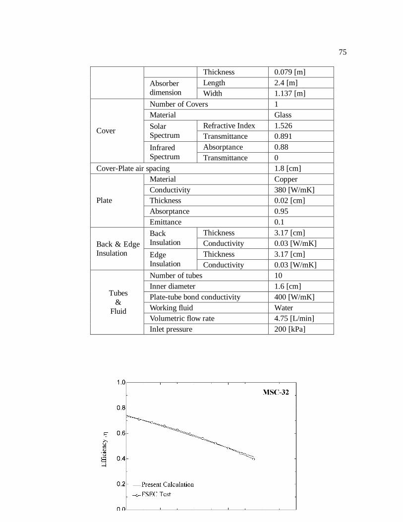
A plot of the instantaneous efficiency of the MSC-32 collector as a function of

(Ti-Ta)/GT is shown in Figure 3.2.1. The predicted instantaneous efficiency is compared

to the experimental results from the test report. As shown in this figure, the calculation

can predict the experimental results very well. The linear and 2nd-order polynomial

efficiency equations with the calculated coefficients are

74

( )T

aii G

TT −−= 33.4746.0η , ( ) ( ) 2

99.498.3743.0

−−−−=

T

ai

T

aii G

TTG

TTη

while those from experimental test [13] are given by

( )T

aii G

TT −−= 45.4751.0η , ( ) ( ) 2

65.2096.2736.0

−−−−=

T

ai

T

aii G

TTG

TTη .

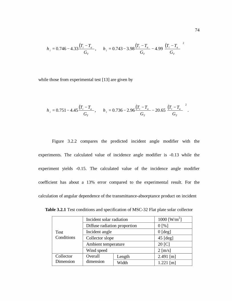
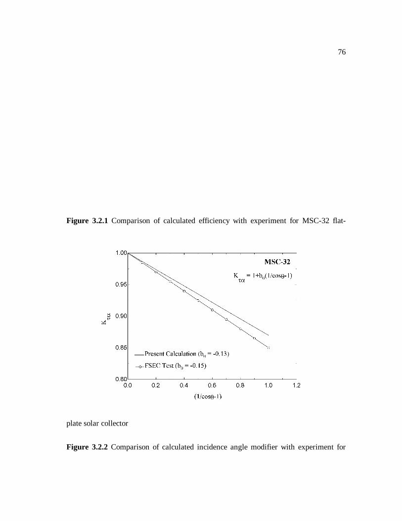
Figure 3.2.2 compares the predicted incident angle modifier with the

experiments. The calculated value of incidence angle modifier is -0.13 while the

experiment yields -0.15. The calculated value of the incidence angle modifier

coefficient has about a 13% error compared to the experimental result. For the

calculation of angular dependence of the transmittance-absorptance product on incident

Table 3.2.1 Test conditions and specification of MSC-32 Flat plate solar collector

Incident solar radiation 1000 [W/m2] Diffuse radiation proportion 0 [%] Incident angle 0 [deg] Collector slope 45 [deg] Ambient temperature 20 [C]

Test Conditions

Wind speed 2 [m/s] Length 2.491 [m] Collector

Dimension Overall dimension Width 1.221 [m]

75

Thickness 0.079 [m] Length 2.4 [m]

Absorber dimension Width 1.137 [m] Number of Covers 1 Material Glass

Refractive Index 1.526 Solar Spectrum Transmittance 0.891

Absorptance 0.88

Cover

Infrared Spectrum Transmittance 0

Cover-Plate air spacing 1.8 [cm] Material Copper Conductivity 380 [W/mK] Thickness 0.02 [cm] Absorptance 0.95

Plate

Emittance 0.1 Thickness 3.17 [cm] Back

Insulation Conductivity 0.03 [W/mK] Thickness 3.17 [cm]

Back & Edge Insulation Edge

Insulation Conductivity 0.03 [W/mK] Number of tubes 10 Inner diameter 1.6 [cm] Plate-tube bond conductivity 400 [W/mK] Working fluid Water Volumetric flow rate 4.75 [L/min]

Tubes &

Fluid

Inlet pressure 200 [kPa]

76

Figure 3.2.1 Comparison of calculated efficiency with experiment for MSC-32 flat-

plate solar collector

Figure 3.2.2 Comparison of calculated incidence angle modifier with experiment for

77

MSC-32 flat-plate solar collector

angle, Equation 2.3.15 is employed as a model for the angular dependence of the

absorptance of the absorber plate. Even though almost all selective surfaces may exhibit

similar behavior, there might be difference between this generalized equation and the

actual plates. This difference may cause the error in the predicted value of incidence

angle modifier coefficient.

3.2.2 SX-600 (Solmax Inc.)

Table 3.2.2 shows test conditions and collector configurations for the Solmax

SX-600 flat-plate solar collector based on the FSEC solar collector test report [15].

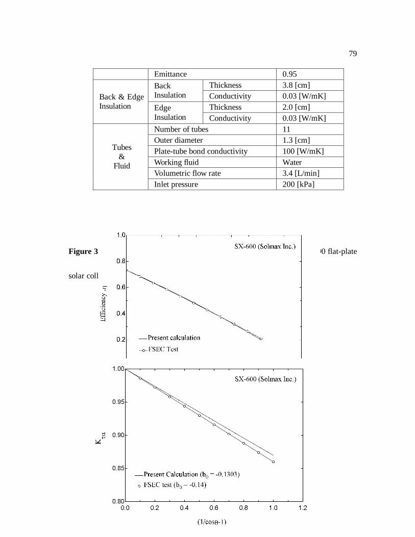
Figure 3.2.3 illustrates comparison of the predicted and experimental instantaneous

efficiencies. As shown in the figure, the calculation can predict the experimental results

very accurately. The calculated efficiency equations are

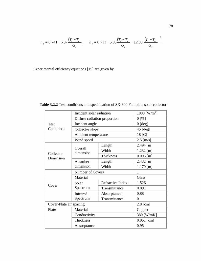
78

( )T

aii G

TT −−= 87.6741.0η , ( ) ( ) 2

83.1295.5733.0

−−−−=

T

ai

T

aii G

TTG

TTη .

Experimental efficiency equations [15] are given by

Table 3.2.2 Test conditions and specification of SX-600 Flat plate solar collector


Test Conditions

Wind speed 2.5 [m/s] Length 2.494 [m] Width 1.232 [m] Overall

dimension Thickness 0.095 [m] Length 2.432 [m]

Collector Dimension



Absorptance 0.88

Cover


Cover-Plate air spacing 2.8 [cm] Material Copper Conductivity 380 [W/mK] Thickness 0.051 [cm]

Plate

Absorptance 0.95

79




Insulation Conductivity 0.03 [W/mK] Number of tubes 11 Outer diameter 1.3 [cm] Plate-tube bond conductivity 100 [W/mK] Working fluid Water Volumetric flow rate 3.4 [L/min]

Tubes &

Fluid


Figure 3.2.3 Comparison of calculated efficiency with experiment for SX-600 flat-plate

solar collector

80


SX-600 flat-plate solar collector

( )T

aii G

TT −−= 77.6737.0η , ( ) ( ) 2

82.628.6733.0

−−−−=

T

ai

T

aii G

TTG

TTη .

Figure 3.2.4 shows the comparison of incidence angle modifier. The calculated value of

incidence angle modifier is -0.13 while the experimental test yields -0.14, in good

agreement with the experiment. However, the calculated value of incidence angle

modifier is almost the same as the value of MSC-32. This similar values result from the

fact that the fact that the calculations for both collectors employ the same model for the

angular dependence of the optical property of the plate.

3.2.3 STG-24 (Sun Trapper Solar Systems, Inc.)

Table 3.2.3 summarizes test conditions and collector configurations of STG-24

81

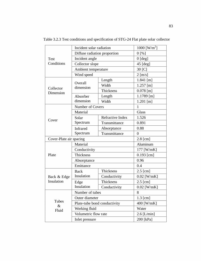
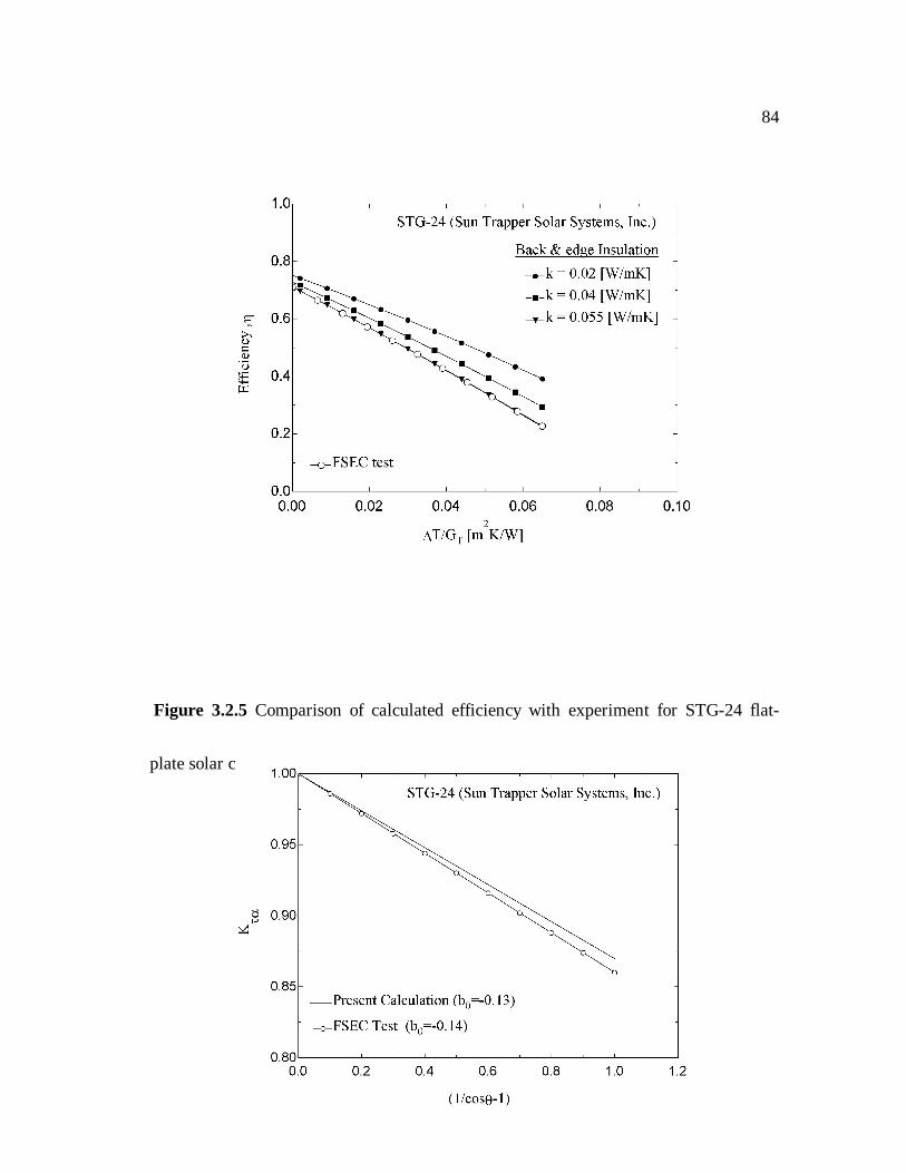
flat-plate solar collector that is produced by Sun Trapper Solar Systems, Inc [14]. Figure

3.2.5 shows the calculated and experimental instantaneous efficiencies of the collector

as a function of (Ti-Ta)/GT. The curve with the conductivity of the back and edge

insulation labeled k = 0.02 W/mK is the result of calculation with the values of Table

3.2.3. In this case, the instantaneous efficiency is overpredicted compared to the

experimental results. However, as the value of the insulation conductivity increases, the

predicted curve approaches the experimental result. The calculation yields the accurate

experimental collector performance when k = 0.055 W/mK. There are two possibilities

that cause this result. The first is that the value of back and edge insulation conductivity

provided by manufacturer may be different from the actual value. The other possibility

is that there might be a thermal leakage in this collector. The increase in back and edge

thermal conductivity causes an increase in the heat loss from the collector and is

equivalent to the increase of thermal leakage from the collector. This indicates that this

flat-plate collector may not be a well-constructed collector. Figure 3.2.6 shows the

incidence angle modifier as a function of (1/cosθ -1). It also shows a good agreement of

the calculation with the experiment.

82

From the comparison of the calculation results with the experimental results, it

can be concluded that the flat-plate solar collector design program can accurately

predict the thermal performance of flat-plate collectors with one glass cover. Since the

test reports of the collector with two covers or plastic covers are not available, a direct

comparison was not made. Since the analytical base of the solar collector design

program developed in Chapter 2 has been verified by substantial experimental evidence

[3], it can be concluded that the flat-plate solar collector design program developed in

this study has an ability to predict the accurate performance of the collector.

83

Table 3.2.3 Test conditions and specification of STG-24 Flat plate solar collector


Test Conditions

Wind speed 2 [m/s] Length 1.841 [m] Width 1.257 [m] Overall

dimension Thickness 0.078 [m] Length 1.1789 [m]

Collector Dimension



Absorptance 0.88

Cover


Cover-Plate air spacing 2.8 [cm] Material Aluminum Conductivity 177 [W/mK] Thickness 0.193 [cm] Absorptance 0.96

Plate




Insulation Conductivity 0.02 [W/mK] Number of tubes 8 Outer diameter 1.3 [cm] Plate-tube bond conductivity 400 [W/mK] Working fluid Water Volumetric flow rate 2.6 [L/min]

Tubes &

Fluid


84

Figure 3.2.5 Comparison of calculated efficiency with experiment for STG-24 flat-

plate solar collector

85


STG-24 flat-plate solar collector

3.3 Effects Of Design Parameters

The design program was successfully verified in the last section. As a result it is

possible to investigate the effect of design parameters by numerical simulation. In this

section the effects of three design parameters on the collector efficiency are investigated.

The test conditions and the collector configuration are based on those of MSC-32 test

report (Table 3.2.1) [13].

3.3.1 Number of Covers

86

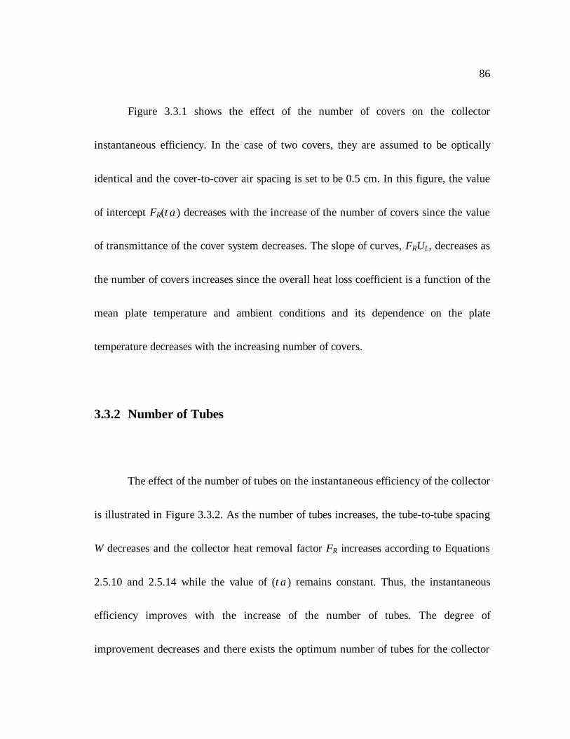
Figure 3.3.1 shows the effect of the number of covers on the collector

instantaneous efficiency. In the case of two covers, they are assumed to be optically

identical and the cover-to-cover air spacing is set to be 0.5 cm. In this figure, the value

of intercept FR(τ α ) decreases with the increase of the number of covers since the value

of transmittance of the cover system decreases. The slope of curves, FRUL, decreases as

the number of covers increases since the overall heat loss coefficient is a function of the

mean plate temperature and ambient conditions and its dependence on the plate

temperature decreases with the increasing number of covers.

3.3.2 Number of Tubes

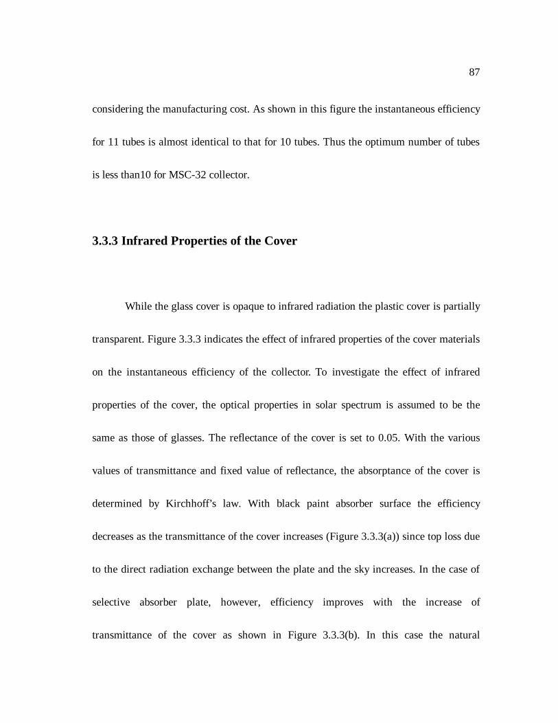
The effect of the number of tubes on the instantaneous efficiency of the collector

is illustrated in Figure 3.3.2. As the number of tubes increases, the tube-to-tube spacing

W decreases and the collector heat removal factor FR increases according to Equations

2.5.10 and 2.5.14 while the value of (τ α ) remains constant. Thus, the instantaneous

efficiency improves with the increase of the number of tubes. The degree of

improvement decreases and there exists the optimum number of tubes for the collector

87

considering the manufacturing cost. As shown in this figure the instantaneous efficiency

for 11 tubes is almost identical to that for 10 tubes. Thus the optimum number of tubes

is less than10 for MSC-32 collector.

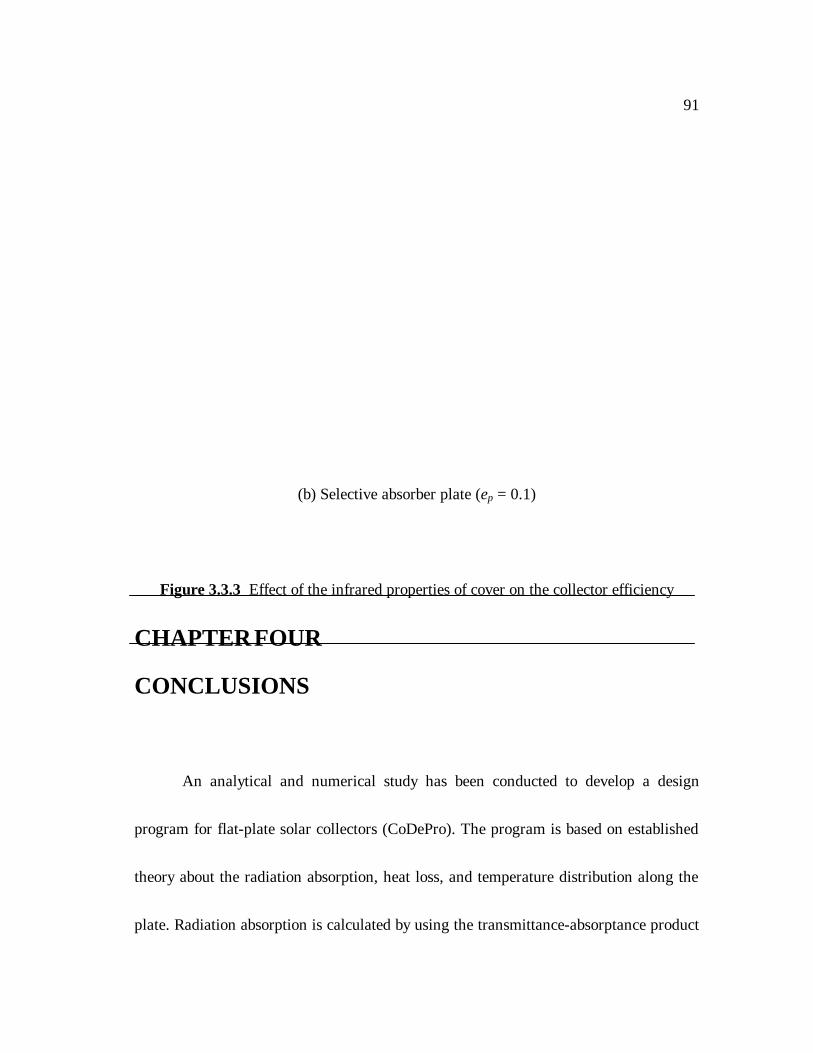
3.3.3 Infrared Properties of the Cover

While the glass cover is opaque to infrared radiation the plastic cover is partially

transparent. Figure 3.3.3 indicates the effect of infrared properties of the cover materials

on the instantaneous efficiency of the collector. To investigate the effect of infrared

properties of the cover, the optical properties in solar spectrum is assumed to be the

same as those of glasses. The reflectance of the cover is set to 0.05. With the various

values of transmittance and fixed value of reflectance, the absorptance of the cover is

determined by Kirchhoff’s law. With black paint absorber surface the efficiency

decreases as the transmittance of the cover increases (Figure 3.3.3(a)) since top loss due

to the direct radiation exchange between the plate and the sky increases. In the case of

selective absorber plate, however, efficiency improves with the increase of

transmittance of the cover as shown in Figure 3.3.3(b). In this case the natural

88

convection between the cover and the plate plays a more important role in top heat loss

than radiation exchanger between them. As the infrared transmittance of the cover

increases, the radiation heat transfer increases and the natural convection decreases.

Since the degree of increase in radiation heat transfer between the cover and the plate is

small compared to that of the natural convection heat transfer, the top loss from the

plate decreases and the instantaneous efficiency improves. The infrared properties has

an impact on the values of intercept, FR(τ α ), since FR is a function of loss coefficient by

Equation 2.5.14. The infrared radiation properties of the cover do not have much effect

on efficiency when the infrared transmittance of the cover is less than 0.7 with selective

absorber plate. More study is required to understand the exact physical mechanism

related to the effect of infrared properties of the cover on the collector performance.

89

Figure 3.3.1 Effect of the number of covers on the collector efficiency

90

Figure 3.3.2 Effect of the number of tubes on the collector efficiency

(a) Black absorber plate (ε p = 0.95)

91

(b) Selective absorber plate (ε p = 0.1)

Figure 3.3.3 Effect of the infrared properties of cover on the collector efficiency

CHAPTER FOUR

CONCLUSIONS

An analytical and numerical study has been conducted to develop a design

program for flat-plate solar collectors (CoDePro). The program is based on established

theory about the radiation absorption, heat loss, and temperature distribution along the

plate. Radiation absorption is calculated by using the transmittance-absorptance product

92

of the cover and plate system. In the evaluation of heat loss from the collector, the net

radiation method was employed to calculate top loss for a general cover system. The

correlation of Yiqin et al. [21] was employed for natural convection heat transfer for the

cover system with plastic as the inner cover. For other cover configurations the

correlation of Hollands et al. [4] was used. The temperature distribution along the plate

was represented by the collector heat removal factor. In the analysis the aperture area of

the collector is used to consider the effect of the edge of collector frontal surface.

In this study, the semi-gray radiation model was employed for the optical

properties of the collector covers. The optical properties of the cover system for infrared

radiation were assumed to be diffuse radiation properties that can be obtained by using

ray-tracing techniques.

Comparisons of the calculated results with the experiments indicate that the

design program developed in this study has an ability to predict the thermal

performance of the collector. The predicted instantaneous efficiency of the collector is

almost the same as the experimental results while there is a little discrepancy between

the calculated and experimental values of incidence angle modifier coefficient. The

error in incidence angle modifier may come from the lack of information about the

93

optical properties of the absorber plate.

Through this study a design program for flat-plate solar collector has been

developed so that very detailed information can be specified to allow solar engineers to

investigate the impact of various design changes on collector performance. The program

has been distributed to solar engineers and modified according to their suggestions. It

has an easy-to-use graphical interface and provides an accurate prediction of the thermal

performance of the collector. Thus, it can be concluded that the program can be used as

a design tool for a company specializing in solar systems to investigate the impact of

design parameters. It can also be used as a tool for identifying design problems.

CHAPTER ONE INTRODUCTION

Documents

Transcript of CHAPTER ONE INTRODUCTION