
Title of Thesis Study on Three-dimensional Flows in the ...
100
Graduate School of Engineering, Mie University Doctor of Engineering Title of Thesis Study on Three-dimensional Flows in the Vicinity of the Horizontal Axis Wind Turbine Blade (水平軸風車翼近傍の 3 次元流れに関する研究) Tinnapob PHENGPOM Division of System Engineering Graduate School of Mechanical Engineering Mie University Tsu, Mie, JAPAN 2016
-
Upload
khangminh22 -
Category
Documents
-
view
0 -
download
0
Transcript of Title of Thesis Study on Three-dimensional Flows in the ...
Graduate School o f Engineer ing , Mie Univers i ty
Doctor of Engineering
Title of Thesis
Study on Three-dimensional Flows in the Vicinity of the
Horizontal Axis Wind Turbine Blade
(水平軸風車翼近傍の 3 次元流れに関する研究)
Tinnapob PHENGPOM
Division of System Engineering
Graduate School of Mechanical Engineering
Mie University
Tsu, Mie, JAPAN
2016

Graduate School of Engineer ing , Mie Univers i ty
Table of Contents Chapter 1 Introduction………………………………………………………………………………..1
1.1 Renewable energy and wind energy…………………………………………………………………………………1
1.1.1 Wind power generation……………………….…………………………………………………………..……2 1.1.2 Historical development of wind energy……….……………………………………………………………….3 1.1.3 Worldwide installed wind power capacity by country…….……………………………………………….......3
1.2 Current status of wind power in Japan……………………………………………………………………………….4 1.2.1 Wind energy resources in Japan…………………………….……………………………………………...…..5 1.2.2 Current status of wind energy in Japan………………………………………………………………………...5 1.2.3 Future perspective of wind energy in Japan…………..………………………………………………………..5
1.3 Basic concepts of wind energy converters…………………………………………………………………………6 1.3.1 Vertical Axis Wind Turbine (VAWT)………………………………..…………………………………………6 1.3.2 Horizontal Axis Wind Turbine (HAWT)…………………………...………………………………………….6 1.3.3 Comparison between HAWT VS VAWT………………………………………………………………………7
1.3.3.1 Structural features……..…………………………………………………………………………………7 1.3.3.2 Environmental problems………...……………………………………………………………………….7
1.4 Literature survey of Horizontal Axis Wind Turbine (HAWT)………………………………………………….......7 1.5 Motivation and purpose of dissertation…………………………………………………………………………..…9
Chapter 2 Nomenclature…………………………………………………………………………………………….17
Chapter 3 Physical principles of wind turbines……….....…………………...…………………………………19
3.1 Momentum theory…………………………………………………………………………………………………19 3.2 Blade Element Theory……………………………………………………………………………………………..21
Chapter 4 Experimental apparatus and methods………………….…………………………………………25
4.1 Experimental apparatus…………………………………………………………………………………………..25
4.1.1 Wind tunnel…………………………………………………………………………………………………..25 4.1.2 Test wind turbine model……………………………………………………………………………………25 4.1.3 Laser Doppler Velocimetry (LDV)…………………………………………………………………………..26
4.2 Experimental methods…………………………………………………………………………………………......27 4.2.1 Experiment conditions……….……………………………………………………………………………….27 4.2.2 Method for measuring the velocity distribution in the vicinity of the blade surface……..………………........28
4.2.2.1 LDV probe placement……….………………………………………………………………………….28 4.2.2.2 Precision positioning traverse………………………………………………………………………......28 4.2.2.3 Blade displacement correction method with respect to the measurement point…………...…………….28 4.2.2.4 Method to calculate three-dimensional velocity components in the rotor blade coordinate…………….29
Chapter 5 Results and Discussion……………….…………………......………………...……...……….56
5.1 Preliminary experiments………………………….………………………………………………………………..56
5.1.1 Power output performance…………………………………………………………………………………...56 5.1.2 Blade surface displacement………………………………………………………………….……………….56
5.2 Angle of attack considering induction factors…………………………………………………….………………..57 5.3 Three-dimensional flow characteristics on the blade sections…………………………………...…………………59
5.3.1 Three-dimensional flow characteristics for the optimum tip speed ratio (λ = 5.2)……...…………………59 5.3.2 Three-dimensional flow characteristics for the low tip speed ratio (λ = 3.7)…………...…………………60
5.4 Pressure distribution on the blade sections…………………………………………………………………………61 5.5 Boundary layer………………………………………………….………………………………………………….62 5.6 Viscous effects on the blade sections……………………………………………………………………………….63 5.7 Circulation on the blade sections………………………………..…………………………………………….........64 5.8 Three-dimensional flow trajectory on the rotor blade sections……….…………………………………………….65

Graduate School of Engineer ing , Mie Univers i ty
Chapter 6 Conclusion……….……………………………….…………………………………………..………….92
Acknowledgments…………………………………………………………………………………………………......94
References…………………………………………………………………………………………………....…………95

Study on Three-dimensional Flows in the Vicinity of the Horizontal Axis Wind Turbine Blade
1 Graduate School of Engineering, Mie University
Chapter 1 Introduction
1.1 Renewable energy and wind energy The energy production has been based on imported fossil fuels such as coal, oil, and natural gas in Japan. The
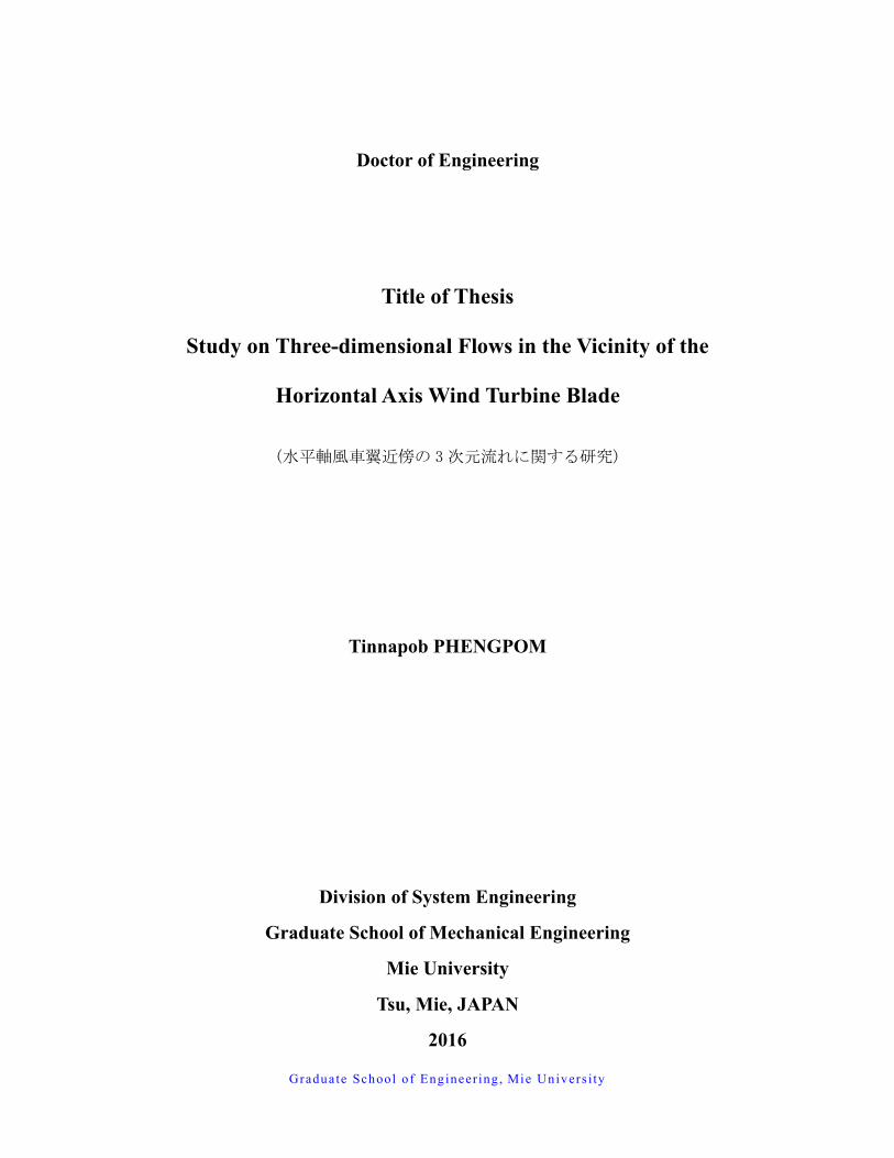
humans remain to face the problems with major challenges in the environmental pollution, energy shortage and greenhouse gas emission. The main disadvantages of fossil fuels are not renewable, and they also pollute the environment. The air pollution has a distressing impact on human health that more than 200 million people are worldwide affected. Carbon dioxide (CO2) is also the major greenhouse gas that results from human activities and causes global warming and climate change. Figure 1.1 presents the data for atmospheric carbon dioxide measurements by the Scripps Carbon Dioxide program at Mauna Loa Observatory in Hawaii [1]. As shown in Fig. 1.1, carbon dioxide was measured from Jan 1960 until May 2015. The trend of carbon dioxide concentration in the atmosphere is gradual increasing exponentially at an accelerating rate from decade to decade. To solve these issues, a sustainable energy becomes an important key solution. The energy production will become more self-sufficient by using alternatives such as renewable energy. The renewable energy continued to grow in the year 2014 that parallel with global energy consumption [2]. In the present, many researchers have been interesting in using renewable energy to reduce the amount of fossil fuel uses. There are many kinds of renewable energy such as
1) Solar power: This energy relies on the nuclear fusion reaction of the sun which converts the sunlight into the electricity. It can be collected and converted in a few different ways. In the present, the solar energy is popularly used in the form of photovoltaic (PV) solar cells for converting the sunlight into the electricity directly. While the indirect method is normally known as concentrated solar power (CSP). This method generates the solar power by using mirrors or lenses to concentrate a large area of the sunlight onto a small area. And then, the electricity is generated when the concentrated light is converted to heat that drives a heat engine (usually a steam turbine) connected to an electrical power generator. Unfortunately, their capacities are insufficient to supply the fully energy consumption of the modern life.
2) Hydroelectric energy: This form uses the gravitational potential of elevated water that was lifted from the oceans by the sunlight. It is not strictly speaking renewable since all reservoirs eventually fill up and require very expensive excavation to become useful again. At this time, most of the available locations for hydroelectric dams are already used in the developed world.
3) Biomass energy: This source comes from plants such as crop, residues, stalks, grasses, etc. The energy in this form is very commonly used throughout the world. Biomass can be converted in different ways to produce the energy. Biomass can be burned in power plants to produce heat or electricity that the carbon dioxide from this method is thought as carbon neutral. The carbon monoxide pollution causes the incomplete combustion equipment, burning fossil fuel and poorly designed cooking equipment. Biomass can be fermented to produce fuels like ethanol for cars and biomass can be digested to create methane gas by bacteria.
4) Hydrogen and fuel cells: Hydrogen can be combined with oxygen to produce energy as an electrical fuel, typically in a vehicle, with only water as the combustion product. This clean burning fuel can mean a significant reduction of pollution in cities. The hydrogen can be used in fuel cells, which are similar to batteries, to power an electric motor. In either case, significant production of hydrogen requires abundant power. There are several promising methods to produce hydrogen, such as solar power, that may alter this picture drastically. These energy sources are also not strictly renewable energy resources but are very abundant in availability and are very low in pollution when utilized.
5) Geothermal power: This energy left over from the original accretion of the planet and augmented by the heat from radioactive decay seeps out slowly everywhere. Another form of geothermal energy is the earth energy, a result of the heat storage in the Earth's surface. Soil everywhere tends to stay at a relatively constant temperature,

Study on Three-dimensional Flows in the Vicinity of the Horizontal Axis Wind Turbine Blade
2 Graduate School of Engineering, Mie University
the yearly average, and can be used with heat pumps to heat a building in winter and cool a building in summer. This form of energy can lessen the need for other power to maintain comfortable temperatures in buildings, but cannot be used to produce electricity.
6) Wind power: It is the kinetic energy that extracted from the airflow to produce mechanical or electrical power. Many devices can convert the kinetic energy of wind into various forms of the energy to utilize in everyday life such as wind pumps are used for water pumping, sails are used for propelling ships, wind turbines or windmills used for mechanical power, etc. Wind turbines are popularly utilized for wind energy as an alternative to fossil fuels.
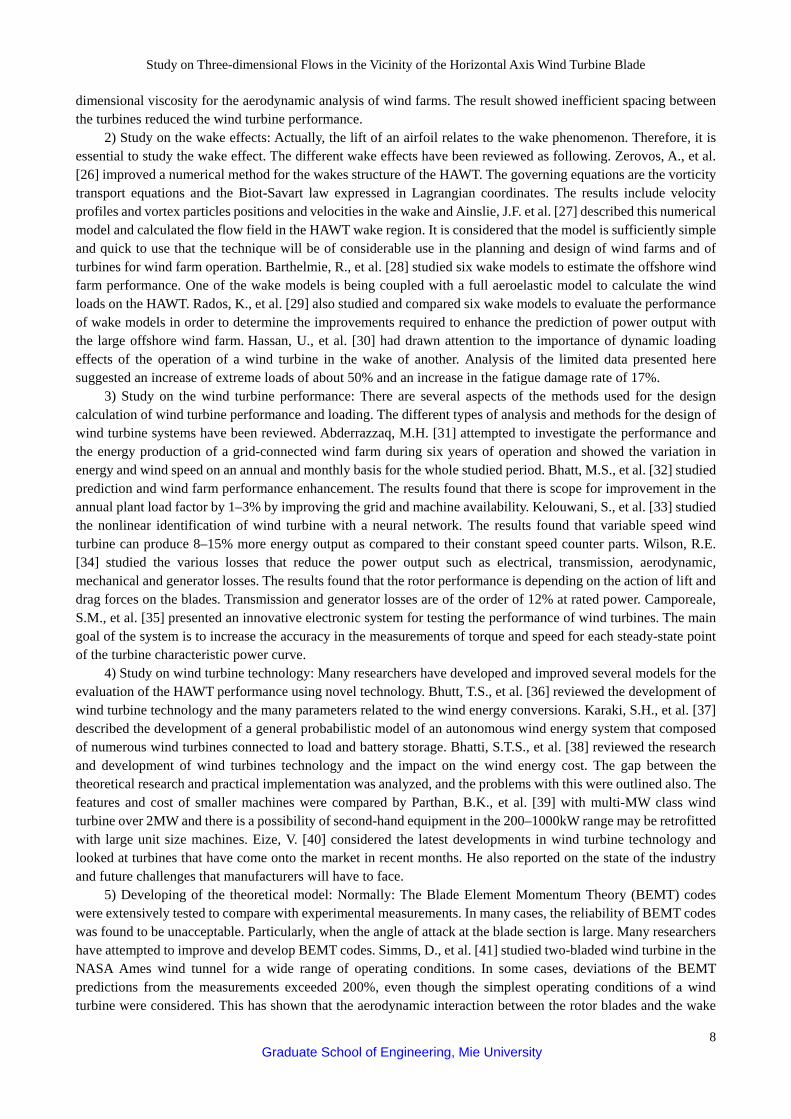
Figure 1.2 shows the average annual growth rates of renewable energy and biofuels production during 2009-2014. The modern renewable energy can be classified three types according to sectoral targets. They comprise the renewable energy for power, heating, and transport. As shown in Fig. 1.2, modern renewable energy overall expanded significantly in the terms of capacity installation and energy production in the year 2014. Some technologies found that more rapid growth in deployment in 2014 than they have averaged over the past five years. In the heating sector, capacity installations continued at a steady pace. The production of biofuels for transport was shown to growth for the second consecutive year. The most rapid growth and the largest increasing renewable energy in capacity occurred in the power sector. Although many renewable energy technologies have a rapid expansion, the bulk of new capacity and investment has just three technologies: solar photovoltaic system (solar PV), concentrating solar power (CSP) and the wind. The average annual growth rate in the year 2014 showed solar PV of 30%, CSP of 27% and wind power of 16%.
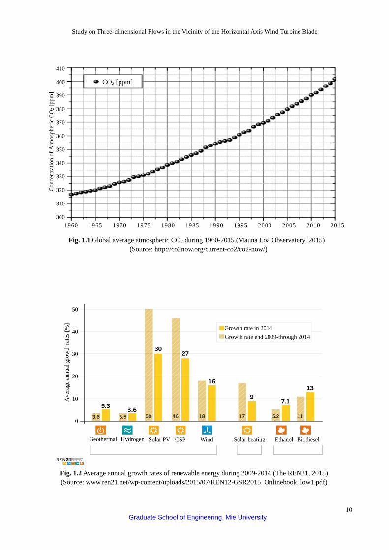
In the year 2014, the wind power is the most attractive renewable energy. Figure 1.3 shows the power capacities from renewable energy in the world, EU-28, BEICS and top seven countries. Although, the average annual growth rate for the wind power is less than solar PV and CSP technologies, the wind power is a renewable energy that has the highest power capacity to produce the electric power. As shown in Fig. 1.3, the wind power capacity can roughly estimate of 380 GW from the total renewable energy capacity in the world of 657 GW. The wind power accounted for 56.31% of the total renewable energy capacity. Therefore, the wind power is the most attractive renewable in this decade.
1.1.1 Wind power generation
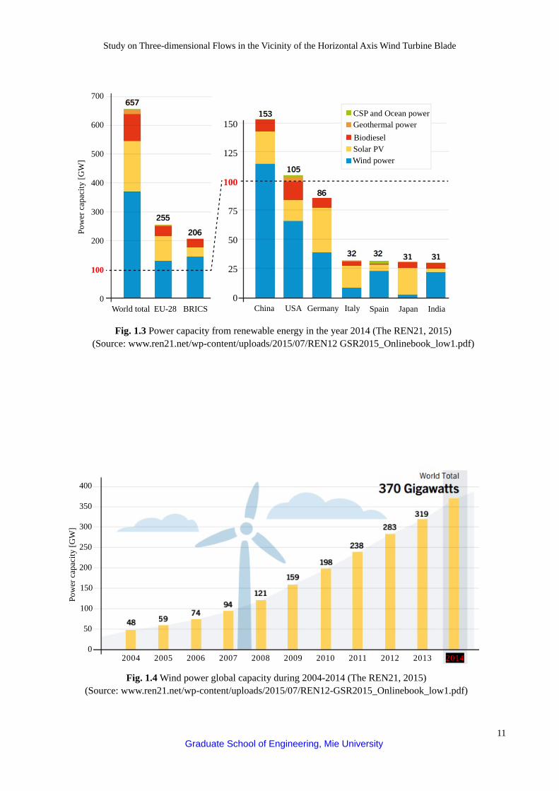
The wind power is clean and inexhaustible energy source. Currently, many researchers in the world would like to use maximizing the benefits of wind power. The growth rate of wind energy in order to use as a renewable energy is increasing every year. The wind turbine installation is increasing every year at an annual rate of 20% [3]. Nowadays, a wind turbine is installed around the world around 370 GW for generating electrical power. Figure 1.4 shows the wind turbine global capacity during 2004-2014. Following a slowdown in the year 2013, the wind power market resumed its advance in the year 2014. Over 51 GW was added representing a 44% increase over the year 2013 and bringing the global total to approximately 370 GW.
In addition, the wind energy has attractive advantages as the following; 1) It is a clean fuel source and friendly to the surrounding environment. Wind energy does not pollute the air
and atmospheric emissions that cause acid rain or greenhouse gasses. 2) It takes up less space than the average power station. Windmills or wind turbines only have to occupy a few
square meters for the base. This allows the land around the turbine to be used for many purposes such as an agriculture.
3) The wind is free. Newer technologies are making the extraction of wind energy much more efficient. 4) Wind turbines are a great resource to generate energy in remote locations, such as mountain communities
and remote countryside. 5) Wind energy is that when combined with solar electricity, this energy source is great for developed and
developing countries to provide a steady, reliable supply of electricity. However, the wind energy has disadvantages as the following; 1) The main disadvantage regarding wind power is down to the wind unreliability factor. In many areas, the
wind strength is too low to support a wind turbine or wind farm.

Study on Three-dimensional Flows in the Vicinity of the Horizontal Axis Wind Turbine Blade
3 Graduate School of Engineering, Mie University
2) Wind turbine construction can be very expensive and costly to surrounding wildlife during the build process. 3) The noise pollution from commercial wind turbines is sometimes similar to a small jet engine.
1.1.2 Historical development of wind energy
The utilization of wind energy is not a novel technology but draws on the rediscovery of a long tradition of wind power technology. For at least 3000 years, the wind energy has been used for grinding grain or pumping water as wind turbines or windmills in Egypt but there is no believable evidence [4]. The first believable evidence about the existence of windmills from ancient sources that the first windmill originates for milling grain in the year 644 A.D. [5]. It found in Persian and windmills had a vertical axis of rotation. Centuries later, the Chinese was also using wind wheels for draining rice fields. However, Chinese wind wheels were too simple structures made of bamboo sticks and fabric sails. Chinese wind wheels had a vertical axis of rotation. Meanwhile, the traditional windmill with a horizontal axis of rotation was invented in Europe. The first believable evidence has its beginning in the year 1180 in the Duchy of Normandy (France). The windmills were made completely from wood. In the 16th century, several decisive improvements were made on windmills in Holland leading to a new type of windmill. They are so-called “Dutch windmill”. The historical windmill reached its perfection towards the middle of the 19th century. The development of windmill from medieval times to the 17th century can be considered the result of research and development.
The designs of windmills were raised in the Renaissance period. Gottfried Wilhelm Leibniz provided numerous impulses for the construction of windmills and also proposed new designs. Daniel Bernoulli applied basic laws of fluid mechanics to the design of windmill sails. Leonhard Euler was the first to calculate the twist of sail correctly. Important technical improvements came from Meikle and Lee invented the fantail that permitted automatic yawing for the windmill in the year 1750. However, the aerodynamic efficiency of sail was not high. After the aerodynamicist, Albert Betz had formulated the modern physical principles of wind energy conversion in the year 1920, and modern airfoil designs had been developed, Major Kurt Bilau applied this knowledge to design of modern windmills. He developed modern windmills in co-operation with Albert Betz that the same as an aircraft airfoil and the modern windmill can adjust a speed regulation of windmill.
When windmill technology was reaching its peak in Europe in the 19th century, horizontal axis windmills were an essential part of the countryside economy. The use of wind turbines to generate electricity can be traced back to the late 19th century with the 12 kW direct current wind turbine generator [6]. One important development was the Smith-Putnam wind turbine of 1,250 kW in USA and constructed in the year 1941. This wind turbine has a steel rotor diameter of 53 m with full span pitch control and flapping blades to reduce loads. It remained the largest wind turbine constructed in the middle of the 19th century [7].
Figure 1.5 shows the evolution of wind turbine technology. As shown in Fig. 1.5, manufacturers are currently working to develop large wind turbines capable of generating significantly more electricity than traditional wind turbines. Wind turbines for commercial scale typically have a rated capacity between 1.5 and 3 MW. The wind turbine has a rotor diameter in the range from 70 to 120 m and stand on towers with a hub height typically in the range from 70 to 80 m. However, offshore wind turbines have a bigger rotor size. Generally, offshore wind turbines typically have a rated capacity ranging from 3 to 6 MW with wind turbine rotor size more than 120 m in diameter, and standing with hub heights of 70 to 100 m. In the future, numerous manufacturers are now considering 10 to 20 MW turbine designs for future offshore wind facilities.
Nowadays, the largest wind turbine in the world is Vestas V164 8 MW in Denmark, and the first prototype unit was installed in January 2014 for generating electricity [8]. The first industrial units will install in the year 2016 at off the coast of the UK [9]. The Vestas V164-8 MW is a three bladed offshore horizontal axis wind turbine (HAWT) with diameter rotor of 164 m, swept area of 21,124 m2 and the hub height of 220 m. 1.1.3 Worldwide installed wind power capacity by country
In the year 2014, the wind industry was a first time record year for the 50 GW installations around the world. Global Wind Energy Council (GWEC) reported “Global status of wind power in 2014” that the wind power market

Study on Three-dimensional Flows in the Vicinity of the Horizontal Axis Wind Turbine Blade
4 Graduate School of Engineering, Mie University
has the growth rate with the installed capacity. The global wind power circumstances in the year during 1997-2014 [10]. Figure 1.6 shows the newly installed and total installed global status of wind power capacity during the period 1997–2014. As shown in Fig. 1.6, the cumulative installed capacity in the year 1997 is only 7,600 MW while annual installed capacity has been around 1,530 MW. Due to the demand for consuming energy increases every year, the trend of the global annual installed capacity increases gradually every year. The global wind power market resumed its advance in the year 2014. Following a slowdown in 2013, the wind power market resumed its advance with a new record in the year 2014. The global annual installed wind capacity was added 51,473 MW representing a 44% increase over the year 2013 market and bringing the global total to around 369,597 MW. Obviously, the global annual installed capacity rises 44,929 MW in the year 2012 but the global annual installed capacity decreased quickly in 2013. The global annual installed capacity drops in the year 2013 because the political uncertainty in USA and economic slowdown in Europe. The wind power market growth turned out to be a difficult in the year 2013 for the manufacturing business [11].
Figure 1.7 shows the top 10 countries of cumulative and newly installed capacity in 2014. China remains the number one of the cumulative and annual installed capacity. China still continuous to lead the global wind power market since 2009. Installations in Asia again led global markets, with Europe reliably in the second spot, and North America a distant third. In the end of year 2014, the top 10 annual installed capacity comprises 1) China (23,352 MW), 2) Germany (5,279 MW), 3) USA (4,854 MW), 4) Brazil (2,472 MW), 5) India (2,315 MW), 6) Canada (1,871 MW), 7) UK (1,736 MW), 8) Sweden (1,050 MW), 9) France (1,042 MW) and 10) Turkey (804 MW) that accounted for 45.36%, 10.26%, 9.43%, 4.80%, 4.50%, 3.63% 3.37%, 2.04%, 2.02% and 1.56% of the global new installed capacity, respectively. The global wind power accumulative installed capacity in the top 10 countries amounts to 84.23%, while the annual installed capacity amounts to 86.98% in the year 2014.
The global demand for the wind power is gradually rising because of the global economic growth. So, the global wind power market can conclude as the following:
1) The Asian wind power market becomes the world’s largest regional market for the wind energy. The annual installed capacity added over than 250,000 MW in the year 2014 because China and India have a fast growth of wind power market.
2) The European wind power market has the total cumulative capacity of 92,540 MW in 2014 that still the leader in the global market and has a sustainable development.
3) The situation of the North American wind power market showed that the USA had strongest annual installed the wind power capacity in the year 2012. However, the annual installed wind power capacity in the year 2013 saw a precipitous drop over 92% with just 1,084 MW in new installations. Uncertain federal policies in the USA continue to inflict a ‘boom-bust’ cycle of the country’s wind industry. The new wind power capacity from Canada of 1,871 MW in the year 2014 illustrates Canada’s wind power market saw significant growth up. 1.2 Current status of wind power in Japan
Japan is an island country in East Asia and located in the Pacific Ocean. The four largest are Honshu, Hokkaido, Kyushu, and Shikoku, respectively. Japan has an area of 377,930 km2 that comprise the land area of 364,485 km2 (96.44%) and the water area of 13,430 km2 (3.56%). The population of Japan is estimated at 126,249,215 as of September 2015 [12]. The energy policy and the status of renewable energy in Japan are about to change significantly after the Fukushima nuclear accident in the year 2011. It is pushing wind power to the forefront as a safer and more reliable alternative to meet the country's future electricity requirements. The wind power sector of Japan's electricity generates a small electrical capacity, but increasing proportion of the country's electricity as the installed wind power capacity has been growing in recent years. In the year 2014, the wind power has several issues caused by excessive regulations or limitations of the power system in Japan. However, the offshore wind power has an enormous potential in Japan. Ambitious targets and clear policies for each technology of the renewable energy are needed and especially for the wind. Japan has wide sea area. The wind streams from the Pacific Ocean in summer, the wind streams from the Sea of Japan in winter and typhoons in autumn are the major source. It can be estimated that Japan has the potential of onshore wind energy resources for 144 GW and the potential of offshore wind energy resources for 608 GW [13]. There is more than 6.5 times the value of Japan's

Study on Three-dimensional Flows in the Vicinity of the Horizontal Axis Wind Turbine Blade
5 Graduate School of Engineering, Mie University
total current power generation capacity [14]. 1.2.1 Wind energy resources in Japan
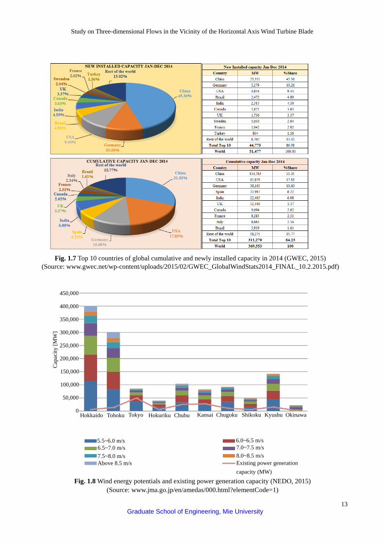
Figure 1.8 shows the wind energy potentials and the existing power generation capacity in Japan. As shown in Fig. 1.8, the wind energy resources are concentrated in Hokkaido, Tohoku, and Kyushu regions. While the demand centers indicated by the existing power generation capacity are in the areas supplied by the Tokyo, Kansai, and Chubu [15]. The regions with excellent wind energy resources do not have strong demands. Also, good wind energy resources are remotely located areas with no transmission lines or tiny capacity lines, making it very difficult to connect large-scale wind energy projects without the fortification of transmission line capacity within each region. This regional discrepancy of market demand and wind energy supply creates the necessity for a strong transmission grid between regions in order to transmit wind-generated electricity from Hokkaido, Tohoku, and Kyushu to the demand centers such as Tokyo, Kansai, and Chubu regions.
The notable project is the Shin Izumo wind farm owned by Eurus Energy. This wind farm is the largest wind farm in Japan that comprises 26 wind turbines with a total wind power capacity of 78 MW. Japan plans to build a pilot floating wind farm, with six wind turbines of 2 MW off the Fukushima coast. The evaluation phase is complete in the year 2016; Japan plans to build more than 80 floating wind turbines off Fukushima by 2020 [16]. In 2013, a floating offshore wind turbine was tested about 1 km off the coast of the island of Kabajima in Nagasaki Prefecture. It was a part of a Japanese government test project [17]. 1.2.2 Current status of wind energy in Japan
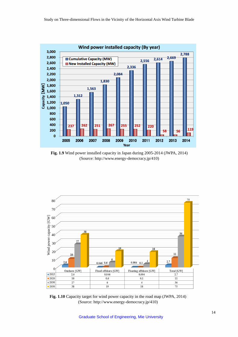
Japan Wind Power Association (JWPA) reported the cumulative installed capacity of wind power generation in Japan as of December 2014 [18]. Figure 1.9 shows the wind power installed capacity in Japan during 2005-2014. As can be seen in this figure, the cumulative installed capacity of wind energy was 2,788 MW and the annual installed capacity was 119 MW in the year 2014. The rate of the annual installed capacity was sluggish because of various constraints in the year 2012 and 2013. Nevertheless, the cumulative installed wind energy capacity will reach 3,700 MW after the installation of the current FIT certified projects in a few years. Many of these projects are proceeding the process of Environmental Impact Assessment (EIA). The cumulative installed wind energy capacity of wind farms in the EIA process will reach 58 GW. If all wind projects are successful through the EIA process. The cumulative installed wind energy capacity would be expected to reach 9.5 GW in the next several years in Japan.
One of the reasons for wind power generation is not growing faster in Japan because it has difficult to build large scale wind generation facilities on land. Due to the limited availability of flat land, the limited amount of suitable land also limits the quota of wind turbines that can install per wind farm. So, it leads to high costs compared to projects overseas. 1.2.3 Future perspective of wind energy in Japan
The Japanese government has still not decided on the goal of the renewable energy capacity in this year (2015), but the Japan Wind Power Association (JWPA) already released the scenarios and roadmap for the wind energy. This road map includes offshore based on calculations of wind energy resources and availability in Japan. The wind power capacity target in the road map by JWPA is shown in Fig. 1.10. The annual installed wind power capacity is estimated to grow to 3GW per year until the year 2030, and the wind power market will keep adding more than 3.5GW per year after the year 2030.
Nowadays, Japan endeavors to maximize the benefits of floating offshore wind farms. The Fukushima offshore wind consortium is proceeding with Fukushima floating offshore wind farm demonstration project funded by the Ministry of Economy, Trade and Industry. This project cooperated with ten companies, University of Tokyo and Marubeni Corporation. The Fukushima offshore wind consortium is implementing the floating offshore wind farm project off the coast of Fukushima Prefecture. The purposes of this demonstration project are to overcome

Study on Three-dimensional Flows in the Vicinity of the Horizontal Axis Wind Turbine Blade
6 Graduate School of Engineering, Mie University
various technical challenges, secure marine navigation safety, ensure collaboration with the fishing industry and establish a method for environmental impact assessment. Moreover, the project also has developed floating offshore wind farms into one of Japan's main export industries by accumulating expertise and transferring that expertise to projects abroad. 1.3 Basic concepts of wind energy converters
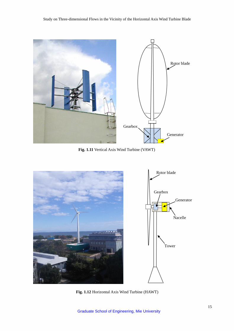
A force in a wind stream can be made to rotate, translate and oscillate an object, and a power can be extracted from the wind. There are many different devices to convert the kinetic energy contained in a wind stream into the mechanical work. A wind turbine is a one of the power generating devices that it is driven by the kinetic energy of wind. Generally, wind turbines can be divided into two major categories: Horizontal axis wind turbines (HAWTs) and vertical axis wind turbines (VAWTs) according to the direction of the rotor axis [19]. 1.3.1 Vertical Axis Wind Turbine (VAWT)
Figure 1.11 shows the vertical axis wind turbine (VAWT). The rotor of the vertical axis wind turbine rotates around a vertical axis. The generator and other primary components can be placed near the ground, so the tower does not need to support it, also makes maintenance easier wind and always be used in city areas. The VAWT can obtain the wind stream from every direction. When the wind direction changes, the VAWT has no need to initiate the steering device to deviate the rotor to face the wind. Because the VAWT is no need of the steering device and the structure of the VAWT is simplified. The gearbox and the generator of the VAWT can be installed on the ground [20].
The main advantages of the vertical axis wind turbines are shown as the following: 1) Vertical axis wind turbines can reduce the transmission losses due to proximity to the demand center. 2) Vertical axis wind turbines can be applied in the remote areas, street lighting and general families, etc.
because of its independent power generation system. It also can provide power for portable device, crisis evacuation indicator in disaster events, etc.
3) Vertical axis wind turbines can be located nearer the ground, making it easier to maintain the moving parts. 4) No yaw mechanisms are needed. The main disadvantages of VAWT are shown as the following: 1) Most vertical axis wind turbines have a low efficiency compared with HAWTs, mainly because of the
additional drag that they have as their blades rotate into the wind. 2) Vertical axis wind turbines located close to the ground where wind speeds are lower and do not take
advantage of higher wind speeds above.
1.3.2 Horizontal Axis Wind Turbine (HAWT)
Figure 1.12 shows the horizontal axis wind turbine (HAWT). The rotor of the horizontal axis wind turbine rotates around a horizontal axis. The rotating plane is vertical to the wind direction during operation. The Horizontal Axis Wind Turbines have the main rotor shaft and electrical generator at the top of a tower, and they must be pointed into the wind. The blades of the HAWT are installed perpendicularly to the rotating axis. The number of wind turbine blade depends on the function of wind turbine. The technology of the HAWT is more mature, and it is easy to produce high power wind turbines, but the structure is complicated.
The main advantages of HAWT are shown as the following: 1) The HAWT has a high efficiency since the blades always move perpendicularly to the wind receiving power
through the whole rotation, unlike vertical axis wind turbines. 2) The tall tower base of the horizontal axis wind turbine allows access to the strong wind in sites with wind
shear. In some wind shear sites, every ten meters up the wind speed can increase by 20% and the power output by 49%.
The main disadvantages of HAWT are shown as the following:

Study on Three-dimensional Flows in the Vicinity of the Horizontal Axis Wind Turbine Blade
7 Graduate School of Engineering, Mie University
1) The HAWT require an additional yaw control mechanism to turn the blades toward the wind. 2) The strong tower construction is required to support the heavy blades, generator, and gearbox.
1.3.3 Comparison between HAWT VS VAWT 1.3.3.1 Structural features
As the HAWT, the wind turbine blades receive the combined effects of the inertial force and the gravity during the process of one circle of the blade rotation. The inertial force direction is subject to change while the gravity is stable ever. The wind turbine blades suffer an alternating load that is very baneful to the fatigue strength of wind turbine blades. Besides, the generator of the HAWT is approximately several tens of meters far away from the ground that brings many troubles to maintain and repair the generator.
As the VAWT, the wind turbine blades receive the combined effects of the inertial force and gravity is better than the HAWT during the wind turbine blade rotation. The inertial force direction and gravity keep stable ever. Consequently, the wind turbine blades obtain a fixed load and accordingly the fatigue longevity is longer than the HAWT. Simultaneously, the VAWT generator is often placed below the rotor or on the ground. It is easy to repair and maintenance. 1.3.3.2 Environmental problems
Even though the wind energy is known as the clean energy, and can be friendly to the environment. More large scale wind farms being constructed and ecological problems caused by the wind turbines. These problems are mainly reflected in two aspects:
1) The noise problem. 2) The negative impact on the local ecological environment. The tip speed ratio of the HAWT is generally in the range of 5 < λ < 7 as a high rotational speed. The wind
turbine blades passing the wind flow will produce loud noise, and meanwhile many birds through are difficult to escape.
The tip speed ratio of the VAWT is generally in the range of 1.5 < λ < 2 that it is much lower than that of the HAWT. Low rotating speed mostly cannot produce noise, and completely mute the noise.
The comparison of general performance between the HAWT and the VAWT are shown as Tab. 1.1. 1.4 Literature survey of Horizontal Axis Wind Turbine (HAWT)
The Horizontal Axis Wind Turbine (HAWT) has been improved and developed until now. Many researchers have attempted to improve the efficiency of The HAWTs. Although the wind turbine efficiency topic has been studied in the many kinds of literature, there are can be classified the main aspects to consider: Study on aerodynamic enhancement, study on the wake effects, study on wind turbine performance and development of theoretical models.
1) Study on aerodynamic enhancement: Many universities, industries and researchers have studied in the wind turbine aerodynamics. Different models of wind turbine aerodynamic analysis have been reviewed. Miller, R.H., et al. [21] presented The HAWT aerodynamics and also highlighted the requirement for a comprehensive design theory. The aerodynamic loads resulting from the wind shear estimated from momentum theory. Bak, C., et al. [22] modified the NACA 622-415 leading part for aerodynamic performance enhancement and suggested numerous causes for the double stall. The HAWT is extremely dynamic structures that are subject to complex distribution of aerodynamic load. Schreck, S., et al. [23] analyzed rotational augmentation of horizontal axis wind turbine blade aerodynamics response and concluded that rotational augmentation was associated with chord wise and span wise pressure distribution. Mayda, E.A., et al. [24] analyzed the NREL S809 airfoil for controlled stall for all flow conditions including laminar separation, bubble-induced vortex shedding. This flow phenomenon causes oscillations in the airfoil surface generates aerodynamic forces. Ammara, I., et al. [25] presented a three-
Study on Three-dimensional Flows in the Vicinity of the Horizontal Axis Wind Turbine Blade
8 Graduate School of Engineering, Mie University
dimensional viscosity for the aerodynamic analysis of wind farms. The result showed inefficient spacing between the turbines reduced the wind turbine performance.
2) Study on the wake effects: Actually, the lift of an airfoil relates to the wake phenomenon. Therefore, it is essential to study the wake effect. The different wake effects have been reviewed as following. Zerovos, A., et al. [26] improved a numerical method for the wakes structure of the HAWT. The governing equations are the vorticity transport equations and the Biot-Savart law expressed in Lagrangian coordinates. The results include velocity profiles and vortex particles positions and velocities in the wake and Ainslie, J.F. et al. [27] described this numerical model and calculated the flow field in the HAWT wake region. It is considered that the model is sufficiently simple and quick to use that the technique will be of considerable use in the planning and design of wind farms and of turbines for wind farm operation. Barthelmie, R., et al. [28] studied six wake models to estimate the offshore wind farm performance. One of the wake models is being coupled with a full aeroelastic model to calculate the wind loads on the HAWT. Rados, K., et al. [29] also studied and compared six wake models to evaluate the performance of wake models in order to determine the improvements required to enhance the prediction of power output with the large offshore wind farm. Hassan, U., et al. [30] had drawn attention to the importance of dynamic loading effects of the operation of a wind turbine in the wake of another. Analysis of the limited data presented here suggested an increase of extreme loads of about 50% and an increase in the fatigue damage rate of 17%.
3) Study on the wind turbine performance: There are several aspects of the methods used for the design calculation of wind turbine performance and loading. The different types of analysis and methods for the design of wind turbine systems have been reviewed. Abderrazzaq, M.H. [31] attempted to investigate the performance and the energy production of a grid-connected wind farm during six years of operation and showed the variation in energy and wind speed on an annual and monthly basis for the whole studied period. Bhatt, M.S., et al. [32] studied prediction and wind farm performance enhancement. The results found that there is scope for improvement in the annual plant load factor by 1–3% by improving the grid and machine availability. Kelouwani, S., et al. [33] studied the nonlinear identification of wind turbine with a neural network. The results found that variable speed wind turbine can produce 8–15% more energy output as compared to their constant speed counter parts. Wilson, R.E. [34] studied the various losses that reduce the power output such as electrical, transmission, aerodynamic, mechanical and generator losses. The results found that the rotor performance is depending on the action of lift and drag forces on the blades. Transmission and generator losses are of the order of 12% at rated power. Camporeale, S.M., et al. [35] presented an innovative electronic system for testing the performance of wind turbines. The main goal of the system is to increase the accuracy in the measurements of torque and speed for each steady-state point of the turbine characteristic power curve.
4) Study on wind turbine technology: Many researchers have developed and improved several models for the evaluation of the HAWT performance using novel technology. Bhutt, T.S., et al. [36] reviewed the development of wind turbine technology and the many parameters related to the wind energy conversions. Karaki, S.H., et al. [37] described the development of a general probabilistic model of an autonomous wind energy system that composed of numerous wind turbines connected to load and battery storage. Bhatti, S.T.S., et al. [38] reviewed the research and development of wind turbines technology and the impact on the wind energy cost. The gap between the theoretical research and practical implementation was analyzed, and the problems with this were outlined also. The features and cost of smaller machines were compared by Parthan, B.K., et al. [39] with multi-MW class wind turbine over 2MW and there is a possibility of second-hand equipment in the 200–1000kW range may be retrofitted with large unit size machines. Eize, V. [40] considered the latest developments in wind turbine technology and looked at turbines that have come onto the market in recent months. He also reported on the state of the industry and future challenges that manufacturers will have to face.
5) Developing of the theoretical model: Normally: The Blade Element Momentum Theory (BEMT) codes were extensively tested to compare with experimental measurements. In many cases, the reliability of BEMT codes was found to be unacceptable. Particularly, when the angle of attack at the blade section is large. Many researchers have attempted to improve and develop BEMT codes. Simms, D., et al. [41] studied two-bladed wind turbine in the NASA Ames wind tunnel for a wide range of operating conditions. In some cases, deviations of the BEMT predictions from the measurements exceeded 200%, even though the simplest operating conditions of a wind turbine were considered. This has shown that the aerodynamic interaction between the rotor blades and the wake

Study on Three-dimensional Flows in the Vicinity of the Horizontal Axis Wind Turbine Blade
9 Graduate School of Engineering, Mie University
are non‐linear and more three-dimensional flow effect. Certainly, the aerodynamic phenomena associated with wind turbine blades are still poorly known and are challenging. Rooij, R.P.O.M, et. al. [42] discussed that a correction has to be applied to estimate the angle of attack from the inflow angle. Another method to determine the angle of attack is the so‐called inverse BEMT method. Snel, H., et al. [43], Bruining, A., et al. [44] and Laino, D.J., et al. [45] applied this method to estimate the axial and rotation induction factors from the known blade loading, thereby finding the angle of attack. The accuracy of the method was limited by the capability of the BEMT in predicting the induction factors. Especially, this method would not always be dependable in yawed and high loading conditions. 1.5 Motivation and purpose of dissertation
The motivation for this dissertation that need to the insight of the three-dimensional flows. Nowadays, this issue still under pending. Deeply understanding in the phenomena of three-dimensional flows will allow to design high efficiency of wind turbine.
An efficiency of a wind turbine is largely determined by the aerodynamics of the turbine blades. There are many ways to increase wind turbine efficiency. Generally, the shape of airfoil section in wind turbine blade has been designed by the sectional performance. The sectional performance depends on flow around a wind turbine rotating blade. Many researchers have attempted to improve a rotor blade for increasing a wind turbine performance [46]. Different approaches exist to predict wind turbine rotor performance. One of the most effective approaches is the classical Blade Element Momentum Theory (BEMT) [47]. This theory divides the blade into element sections in the span-wise direction, and each section is assumed to be operated independently [48]. Much research has been done to improve the aerodynamic performance of Horizontal Axis Wind Turbine (HAWT) rotor blades by using BEMT. However, the prediction of BEMT is different from experimental results because this theory considers only two-dimensional directions (axial and tangential directions). In fact, the blade surface has a flow effect from a span-wise direction due to the rotational effect [49]. The effects of rotation on HAWT blade aerodynamics have been extensively studied. A span-wise flow is always generated from centrifugal force, which play an important role in the 3D stall delay and increasing lift coefficient [50]. The separation point on the surface of the blade is postponed slightly due to rotational effect. This delayed separation has the beneficial effect of giving rise to higher lift and lower drag as compared with 2D conditions [51]. Pressure distribution on a test wind turbine rotor blade for non- rotating and rotating conditions was examined, and the result exposed significant differences in lift behavior at the inboard region of the rotor blade [52]. The aerodynamic performance of blade sections also depends on the boundary layer around the airfoil surface [53]. A span-wise flow velocity from rotating blades can change the boundary layer thickness and the rotational effect shows that three-dimensional flows have a significant effect on separation as compared with two-dimensional flows [54]. Three-dimensional flow phenomena are complicated and difficult to understand well. However, many researchers have attempted to describe span-wise flow in a rotating blade condition. For example, the characteristics of three-dimensional flows near a HAWT rotor have been described using Stereo Particle Image Velocimetry (SPIV), showing that strong three-dimensional relative velocities and a span-wise velocity had been observed at the inboard section of the rotor blades [55]. Three-dimensional flow greatly affects the boundary layer when the relative velocity has a high angle of attack (AOA). Our previous research also attempted to study three-dimensional flow near a HAWT rotor [56, 57, 58]. Laser Doppler Velocimetry (LDV) was carried out to detect three-dimensional velocity components. The three-dimensional velocity components (axial, tangential and radial) were measured by two LDV probes, which were set separately in vertical and horizontal directions. However, the problem of the measuring volume layout was a point of concern. It was diagnosed that the high deviation of the velocity at the leading edge was due to the larger measuring volume found in detecting the span-wise velocity component.
The purpose of dissertation focused on a rotor blade shape to improve the performance of Horizontal Axis Wind Turbine (HAWT) by considering the effect of three-dimensional flows. The new method that simultaneously measures these components using an LDV system. Characteristics of three-dimensional flow were investigated and visualized.
Study on Three-dimensional Flows in the Vicinity of the Horizontal Axis Wind Turbine Blade
10 Graduate School of Engineering, Mie University
Fig. 1.1 Global average atmospheric CO2 during 1960-2015 (Mauna Loa Observatory, 2015) (Source: http://co2now.org/current-co2/co2-now/)
Con
cent
ratio
n of
Atm
osph
eric
CO
2 [pp
m]
CO2 [ppm]
1960 1965 1970 1975 1980 1985 1990 1995 2000 2005 2010 2015
410
400
390
380
370
360
350
340
330
320
310
300
Power Heating Transport
Geothermal Hydrogen Solar PV CSP Wind Solar heating Ethanol Biodiesel
Growth rate in 2014 Growth rate end 2009-through 2014
50
40
30
20
10
0
Ave
rage
ann
ual g
row
th ra
tes [
%]
Fig. 1.2 Average annual growth rates of renewable energy during 2009-2014 (The REN21, 2015) (Source: www.ren21.net/wp-content/uploads/2015/07/REN12-GSR2015_Onlinebook_low1.pdf)
Study on Three-dimensional Flows in the Vicinity of the Horizontal Axis Wind Turbine Blade
11 Graduate School of Engineering, Mie University
World total
Pow
er c
apac
ity [G
W]
CSP and Ocean power Geothermal power Biodiesel Solar PV Wind power
700
600
500
400
300
200
100
0
150
125
100
75
50
25
0 EU-28 BRICS China USA Germany Italy Spain Japan India
Fig. 1.3 Power capacity from renewable energy in the year 2014 (The REN21, 2015) (Source: www.ren21.net/wp-content/uploads/2015/07/REN12 GSR2015_Onlinebook_low1.pdf)
Fig. 1.4 Wind power global capacity during 2004-2014 (The REN21, 2015) (Source: www.ren21.net/wp-content/uploads/2015/07/REN12-GSR2015_Onlinebook_low1.pdf)
2004 2005 2006 2007 2008 2009 2010 2011 2012 2013 2014
400
350
300
250
200
150
100
50
0
Pow
er c
apac
ity [G
W]

Study on Three-dimensional Flows in the Vicinity of the Horizontal Axis Wind Turbine Blade
12 Graduate School of Engineering, Mie University
Fig. 1.5 Evolution of wind turbine technology over time (NREL, 2014) (Source: http://esm.versar.com/pprp/ceir17/HTML/Chapter5-5-1.html)
320
280
240
200
160
120
80
40
0
Hub
hei
ght [
m]
1997 1998 1999 2000 2001 2002 2003 2004 2005 2006 2007 2008 2009 2010 2011 2012 2013 2014
400,000
350,000
300,000
250,000
200,000
150,000
100,000
50,000
0
Global annual installed wind capacity 1997-2014
Global cumulative installed wind capacity 1997-2014
Fig. 1.6 Global cumulative and newly installed wind capacity during 1997-2014 (GWEC, 2015) (Source: www.gwec.net/wpcontent/uploads/2015/02/GWEC_GlobalWindStats2014_FINAL_10.2.2015.pdf)
Inst
alle
d C
apac
ity [M
W]
Study on Three-dimensional Flows in the Vicinity of the Horizontal Axis Wind Turbine Blade
13 Graduate School of Engineering, Mie University
Fig. 1.7 Top 10 countries of global cumulative and newly installed capacity in 2014 (GWEC, 2015) (Source: www.gwec.net/wp-content/uploads/2015/02/GWEC_GlobalWindStats2014_FINAL_10.2.2015.pdf)
Fig. 1.8 Wind energy potentials and existing power generation capacity (NEDO, 2015) (Source: www.jma.go.jp/en/amedas/000.html?elementCode=1)
Hokkaido Tohoku
5.5~6.0 m/s 6.5~7.0 m/s 7.5~8.0 m/s Above 8.5 m/s
6.0~6.5 m/s 7.0~7.5 m/s 8.0~8.5 m/s Existing power generation capacity (MW)
Hokuriku Chubu Kansai Chugoku Shikoku Kyushu Okinawa Tokyo
450,000
400,000
350,000
300,000
250,000
200,000
150,000
100,000
50,000
0
Cap
acity
[MW
]
Study on Three-dimensional Flows in the Vicinity of the Horizontal Axis Wind Turbine Blade
14 Graduate School of Engineering, Mie University
Fig. 1.9 Wind power installed capacity in Japan during 2005-2014 (JWPA, 2014) (Source: http://www.energy-democracy.jp/410)
Fig. 1.10 Capacity target for wind power capacity in the road map (JWPA, 2014) (Source: http://www.energy-democracy.jp/410)
80
70
60
50
40
30
20
10
0
Win
d po
wer
cap
acity
[GW
]
Study on Three-dimensional Flows in the Vicinity of the Horizontal Axis Wind Turbine Blade
15 Graduate School of Engineering, Mie University
Fig. 1.12 Horizontal Axis Wind Turbine (HAWT)
Fig. 1.11 Vertical Axis Wind Turbine (VAWT)
Rotor blade
Gearbox
Generator
Nacelle
Tower
Generator
Gearbox
Rotor blade

Study on Three-dimensional Flows in the Vicinity of the Horizontal Axis Wind Turbine Blade
16 Graduate School of Engineering, Mie University
Table 1.1 Comparison of general performance between HAWT and VAWT
Performance HAWT VAWT Power generation efficiency 50%-60% Above 70% Electromagnetic interference Yes No Steering mechanism of wind Yes No
Gear box Above 10KW No Blade rotation space Quite large Quite small
Wind-resistance capability Weak Strong Noise 5-60dB 0-10dB
Starting wind speed High (2.5-5 m/s) Low (1.5-3 m/s) Ground projection effects Dizziness No effect
Failure rate High Low Maintenance Complicated Convenient
Rotational speed High Low Effect on birds Big Small
Cable stranding problem Yes No Power curve Depressed Full

Study on Three-dimensional Flows in the Vicinity of the Horizontal Axis Wind Turbine Blade
17 Graduate School of Engineering, Mie University
Chapter 2 Nomenclature
A2 Control volume area at the rotor [m2] Ad Rotor swept area [m2] a Axial induction factor [-] a' Tangential induction factor [-] CD Drag coefficient [-] Cf Skin friction coefficient [-] CL Lift coefficient [-] Cp Power coefficient [-] Cp_LDV Pressure coefficient from LDV [-] Cp_Xfoil Pressure coefficient from Xfoil [-] Cp_tap Pressure coefficient from pressure tap [-] c Local chord length [m] D Sectional drag [N] FN Normal force [N] FT Tangential force [N] H Shape factor [-] L Sectional lift [N] ṁ Mass flow rate [kg/s] P Power [W] pd Dynamic pressure [Pa] pi Static pressure at a i-th pressure tap on the measured blade section [Pa] p0 Reference static pressure [Pa] p1 Static pressure at far away upstream from the wind turbine [Pa] p2 Static pressure at just before the blade [Pa] p3 Static pressure at just after the blade [Pa] p4 Static pressure at far away downstream from the wind turbine [Pa] T Torque [Nm] R Rotor radius (= 1.2) [m] R2 Correlation [-] r Local blade radius [m] t Time [s] U0 Mainstream velocity (= 7.0) [m/s] U1 Axial velocity at far away upstream from the wind turbine [m/s] U2 Axial velocity at just before the blade [m/s] U2D Two-dimensional relative velocity [m/s] U3 Axial velocity at just after the blade [m/s] U4 Axial velocity at far away downstream from the wind turbine [m/s] Ue Velocity at the outer edge of the boundary layer [m/s] Uparallel Velocity vector parallel to the blade surface [m/s] Uref Geometrical inflow velocity [m/s] u Axial velocity component [m/s] u1 u1 velocity component from 1st probe [m/s] u2 u2 velocity component from 1st probe [m/s] u3 u3 velocity component from 2nd probe [m/s] v Tangential velocity component [m/s] w Radial velocity component [m/s] w0 Span-wise velocity component [m/s] x Axial position [mm] x* Distance from blade surface [mm] y Chord position [mm]

Study on Three-dimensional Flows in the Vicinity of the Horizontal Axis Wind Turbine Blade
18 Graduate School of Engineering, Mie University
Greek symbols
ɸ Inflow angle [°] α Angle of attack [°] λ Tip speed ratio (= ΩR/U0) [-] Ψ Azimuth angle [°] β Pitch angle [°] θ Momentum thickness [mm] θtwist Twist angle [°] θvector Direction of local velocity in the sectional plane [°] θ1 Tilted angle between u1 and rotor axis [°] θ2 Tilted angle between u2 and rotor axis [°] θ3 Tilted angle between 2nd probe and rotor axis [°] θ4 Tilted angle between 1st probe and rotor axis [°] ω Angular velocity [1/s] δ Boundary layer thickness [mm] δ* Displacement thickness [mm] µ Dynamic viscosity [m2/s] τw Wall shear stress [Pa] Γ Bound circulation [m/s2] Ω Rotational speed of wind turbine rotor [1/s]
Study on Three-dimensional Flows in the Vicinity of the Horizontal Axis Wind Turbine Blade
19 Graduate School of Engineering, Mie University
Chapter 3 Physical principles of wind turbines
The wind turbine rotors aerodynamic design needs more than knowledge of elementary physical laws of
energy conversion. Many researchers confront with the problems such as finding the relationship between the actual shape of the rotor, the number of rotor blades, its aerodynamic properties and the airfoil shape of its blades.
The design of the horizontal axis wind turbine rotor blade is generally based on the blade element momentum theory (BEMT). The BEMT was initially developed to treat propeller and helicopter aerodynamics, but it is easily adapted to use with a HAWT model. The BEMT is a hybrid method that combines the momentum theory and the blade element theory. These methods examine how a wind turbine operates. The momentum theory applies a momentum on a rotating annular stream tube passing through a wind turbine, while the blade element theory examines the forces produced by the lift and drag coefficients at various airfoil sections along the blade span. The BEMT provides a series of equations that can be solved iteratively.
3.1 Momentum theory
This theory is to use a momentum balance on a rotating annular stream tube passing through a turbine. The momentum theory is useful in predicting ideal efficiency and flow velocity. It can determine the forces acting on the rotor to produce the motion of the fluid. This theory has no connection to the geometry of the blade, thus is not able to provide optimal blade parameters.
The following assumptions are made for momentum theory: • Each blade operates without frictional drag. • A slipstream that is well defined separates the flow passing through the rotor disc from that outside disc. • Thrust loading is uniform over the rotor disc. • No rotation is imparted to the flow by the disc. • The static pressure far away upstream and far away downstream from the wind turbine rotor is equal to
undisturbed ambient static pressure. A static pressure variation occurs across the wind turbine rotor. Figure 3.1 shows the rotating annular stream
tube. Four stations comprise 1) far away upstream from the wind turbine, 2) just before the blade, 3) just after the blade and 4) far away downstream from the wind turbine. The energy between station 2 and station 3 is extracted from the wind and there is a change in pressure. This theory assumes p1 = p4 and U2 = U3. Therefore, the flow is frictionless between station 1 and station 2 and between station 3 and station 4. It can apply Bernoulli’s equation to be expressed as,
2 2
2 3 1 40.5 ( )p p U Uρ− = − (3.1) Where p2 is the static pressure at just before the blade, p3 is the static pressure at just after the blade, ρ is the density of air, U1 is the axial velocity at far away upstream from the wind turbine and U4 is the axial velocity at far away upstream from the wind turbine. Noting that force is the pressure times area and find that:
2 2N 2 3 2 1 4 2d = ( - )d = 0.5 ( - )dF p p A U U Aρ (3.2)
Where FN is the normal force and A2 is the control volume area at the rotor. The axial induction factor a is defined as the fractional decrease in wind velocity between the mainstream velocity and the wind turbine rotor. So,
1 2 1( / )a U U U= − (3.3)

Study on Three-dimensional Flows in the Vicinity of the Horizontal Axis Wind Turbine Blade
20 Graduate School of Engineering, Mie University
Where U2 is the axial velocity at just before the blade. It can also be shown that:
2 1= (1- )U U a (3.4)
4 1= (1- 2 )U U a (3.5)
Thus, the normal force FN can be expressed as Eq. (3.6)
2N 1d = 0.5 [4 (1- )]2 dF U a a r rρ π (3.6)
Where r is the local radius of the rotor blade. The power output P is equal to the thrust times the velocity at the wind turbine.
2 22 1 4 2= 0.5 ( - )P A U U Uρ (3.7)
Thus, substituting for U2 and U3 from Eq. (3.4) and (3.5) gives
3 22 1= 0.5 4 (1- )P A U a aρ (3.8)
Where the control volume area at the rotor A2 is replaced with the Rotor swept area Ad and the free stream velocity U1 is replaced by the mainstream velocity of wind tunnel U0. Wind turbine rotor performance is usually characterized by power coefficient Cp
p 30 d
=0.5
PCU Aρ
(3.9)
The non-dimensional power coefficient represents the fraction of the power in the wind that is extracted by the rotor. From Eq. (3.8), the power coefficient is:
2p = 4 (1- )C a a (3.10)
In the Fig. 3.1, the linear momentum theory is assumed that no rotation is imparted to the flow. The linear
momentum theory can be extended to the case where the rotating rotor generates angular momentum, which can be related to rotor torque.
In the case of a rotating wind turbine, the flow behind the rotor rotates in the opposite direction to the rotor, in reaction to the torque exerted by the flow on the rotor. An annular stream tube model of this flow illustrational of the wake is shown as Fig. 3.2. The rotation of the turbine imparts a rotation onto the blade wake between station 2 and station 3. The conservation of angular momentum in this annular stream tube is shown in Fig. 3.3. The blade wake rotates with an angular velocity ω and the blades rotate with an angular velocity Ω. So for a small element the corresponding torque will be:
2d = dT m rω (3.11)
Where m is the mass flow rate for the rotating annular element.
d 2 2d 2 dm A U r rUρ ρ π= = (3.12)

Study on Three-dimensional Flows in the Vicinity of the Horizontal Axis Wind Turbine Blade
21 Graduate School of Engineering, Mie University
So, substituting mass flow from Eq. (3.11) gives
22d 2 dT U r r rρ ω π= (3.13)
The tangential induction factor a' is defined as the fractional decrease in the rotational direction.
/ 2a Ωω′ = (3.14) 3.2 Blade Element Theory
This theory is to examine the forces generated by the airfoil lift and drag coefficients at each blade section along the blade. The blade element theory determines the forces on the blade as a result of the motion of the fluid in terms of the blade geometry. By combining the two theories, Blade element theory, also known as strip theory, relates rotor performance to rotor geometry.
The blade element theory relies on two key assumptions: • There are no aerodynamic interactions between different blade elements • The forces on the blade elements are solely determined by the lift and drag coefficients Figure 3.4 shows the wind turbine blade divided up into N elements. Each of the blade elements will
experience a slightly different flow as they have a different rotational speed ωr, a different chord length c and a different twist angle θtwist. The blade element theory involves dividing up the blade into a sufficient number (usually between ten and twenty) of elements and calculating the flow at each one. Overall performance characteristics are determined by numerical integration along the blade span.
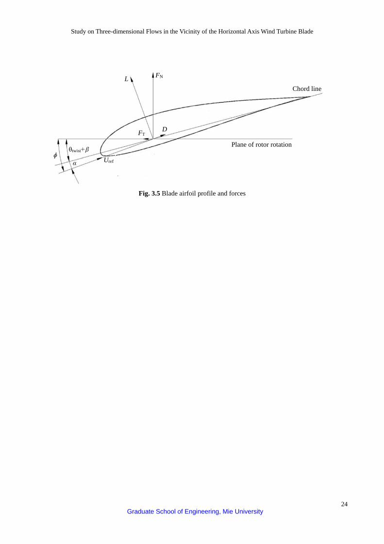
The forces on the blade element are shown in Fig. 3.5. It notes that by definition the lift and drag forces are perpendicular and parallel to the incoming flow. For each blade element one can see:
Td d cos d sinF L Dα α= − (3.15)
Nd d sin d sinF L Dα α= + (3.16)
Where FT, L and D are the tangential force, the lift and drag on the blade element, respectively. L and D can be found from the definition of the lift and drag coefficients as follows:
2L 0d 0.5 dL C U c rρ= (3.17)
2
D 0d 0.5 dD C U c rρ= (3.18) Where CL is the lift coefficient, CD is the drag coefficient and c is the chord length.

Study on Three-dimensional Flows in the Vicinity of the Horizontal Axis Wind Turbine Blade
22 Graduate School of Engineering, Mie University
Hub
1
3
Wind turbine blade
2
4
4 3 2 1
Fig. 3.1 Stream tube around a wind turbine in the axial direction (Non- rotating)
Fig. 3.2 Stream tube around a wind turbine in the axial direction (Rotating)
U1
Wind turbine blade
U4 U2 U3
Hub
1
3 2
4

Study on Three-dimensional Flows in the Vicinity of the Horizontal Axis Wind Turbine Blade
23 Graduate School of Engineering, Mie University
dr
c
r
R
Fig. 3.3 Conservation of angular momentum in the annular stream tube
Fig. 3.4 Blade element model
dr
r
ω
Ω
Study on Three-dimensional Flows in the Vicinity of the Horizontal Axis Wind Turbine Blade
24 Graduate School of Engineering, Mie University
Plane of rotor rotation
D
L
FT
FN
Uref α
Chord line
θtwist+β ɸ
Fig. 3.5 Blade airfoil profile and forces

Study on Three-dimensional Flows in the Vicinity of the Horizontal Axis Wind Turbine Blade
25 Graduate School of Engineering, Mie University
Chapter 4 Experimental apparatus and methods
4.1 Experimental apparatus
In this dissertation, the three-bladed horizontal axis wind turbine was performed in the wind tunnel. The three-dimensional velocity components in the vicinity of the blade surfaces were experimentally investigated through Laser Doppler Velocimetry (LDV) system. Table 4.1 shows the types of equipment using in this dissertation.
The details of main experimental apparatus have been explained as below. 4.1.1 Wind tunnel
Figures 4.1 (a) and (b) show the photo and the schematic view of a test section of a Göttingen type wind tunnel in the Department of Mechanical Engineering at Mie University. Figures 4.2 (a) and (b) show the wind tunnel in the two-dimensional sketch and the experimental setup for the wind turbine model respectively. This the wind tunnel has an open test section. The experiments were performed with the mainstream wind speed of U0 = 7 m/s. A test wind turbine was set in the test section, at a distance 1.85 m from the outlet section. A pitot tube and a thermometer were installed at the outlet of a wind tunnel to measure mainstream velocity and temperature. The test section is a diameter of 3.6 m, and a length of 4.5 m. The corrector inlet is 4.5 x 4.5 m. The wind tunnel is driven by a 400 kW variable speed fan set at the return passage. The maximum velocity is 30 [m/s]. The turbulence intensity is less than 0.5%. The radius of wind turbine wake can be estimated as 1.47 m for the optimum operation. The radius of uniform wind region is 1.7 m, so the flow affected by wind turbine rotor can stay in a uniform wind region.
In the wind tunnel experiment, the blockage effect must be checked. The blockage ratio is the ratio between the rotor swept area and the wind tunnel uniform flow area. Typically, the blockage ratio should less than 30% for the wind tunnel test. The high blockage ratio might affect to the wake expansion and give influence on the span-wise flow. So, the generalized result as a power curve is checked to make sure that the blockage ratio do not affect to measured results. 4.1.2 Test wind turbine model
The test HAWT is composed of wind turbine rotor, nacelle, tower, and base. The test HAWT is an upwind turbine rotor with three blades. The rotor radius is 1.2 m. The wind turbine blades are made from Polyurethane (PUR) plastic. The shape of the test blade is designed by the blade element momentum theory (BEMT). The blade is twisted and tapered like a general commercial wind turbine blade. The wind turbine rotation could be controlled by using a servomotor that is set at the nacelle. This nacelle consists of a servomotor, an encoder, a slip-ring and a coupling as shown in Fig. 4.3. In this dissertation, the servomotor provides the precise rotational speed controller for the wind turbine rotor through the coupling. The torque generated by the rotor is absorbed by the braking operation of the servomotor. So, the wind turbine during the operation can maintain the rotational speed. The photo sensor and the encoder are installed on the rotating shaft for detecting the rotational angle of wind turbine rotor. The slip-ring installed in the main shaft can pass electrical signals between the stationary system and the rotational system.
Figure 4.4 shows the definition of the azimuth angle. The azimuth angle represents the angle of the blade rotation. The azimuth angle ψ = 0 [°] is set at the vertical upward position. The rotational direction is the clockwise direction when seen from upstream. The wind turbine rotor axis is set in the mainstream direction.
Figure 4.5 shows the definition of the pitch angle β. The pitch angle is defined as the angle between the rotor
Study on Three-dimensional Flows in the Vicinity of the Horizontal Axis Wind Turbine Blade
26 Graduate School of Engineering, Mie University
plane and the chord line of the blade tip. The positive pitch angle is the direction in which the blade leading edge inclines to the mainstream direction upstream side.
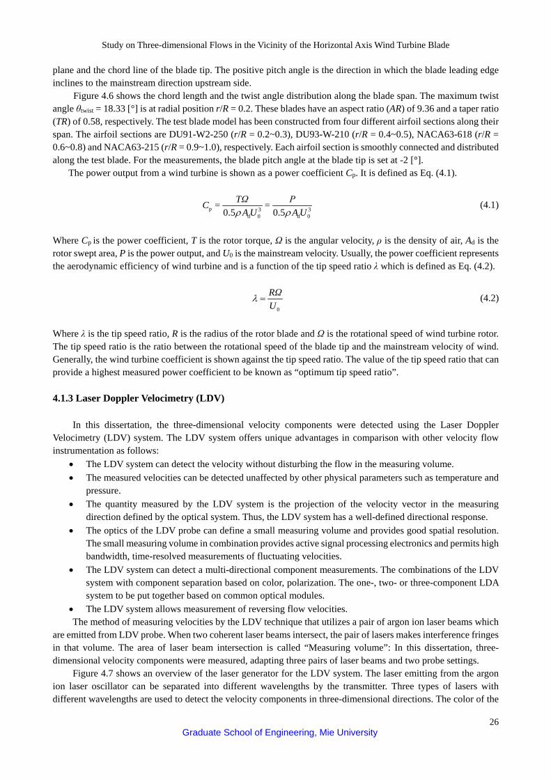
Figure 4.6 shows the chord length and the twist angle distribution along the blade span. The maximum twist angle θtwist = 18.33 [°] is at radial position r/R = 0.2. These blades have an aspect ratio (AR) of 9.36 and a taper ratio (TR) of 0.58, respectively. The test blade model has been constructed from four different airfoil sections along their span. The airfoil sections are DU91-W2-250 (r/R = 0.2~0.3), DU93-W-210 (r/R = 0.4~0.5), NACA63-618 (r/R = 0.6~0.8) and NACA63-215 (r/R = 0.9~1.0), respectively. Each airfoil section is smoothly connected and distributed along the test blade. For the measurements, the blade pitch angle at the blade tip is set at -2 [°].
The power output from a wind turbine is shown as a power coefficient Cp. It is defined as Eq. (4.1).
p 3 3d 0 d 0
= =0.5 0.5
TΩ PCA U A Uρ ρ
(4.1)
Where Cp is the power coefficient, T is the rotor torque, Ω is the angular velocity, ρ is the density of air, Ad is the rotor swept area, P is the power output, and U0 is the mainstream velocity. Usually, the power coefficient represents the aerodynamic efficiency of wind turbine and is a function of the tip speed ratio λ which is defined as Eq. (4.2).
0
RΩU
λ = (4.2)
Where λ is the tip speed ratio, R is the radius of the rotor blade and Ω is the rotational speed of wind turbine rotor. The tip speed ratio is the ratio between the rotational speed of the blade tip and the mainstream velocity of wind. Generally, the wind turbine coefficient is shown against the tip speed ratio. The value of the tip speed ratio that can provide a highest measured power coefficient to be known as “optimum tip speed ratio”. 4.1.3 Laser Doppler Velocimetry (LDV)
In this dissertation, the three-dimensional velocity components were detected using the Laser Doppler Velocimetry (LDV) system. The LDV system offers unique advantages in comparison with other velocity flow instrumentation as follows:
• The LDV system can detect the velocity without disturbing the flow in the measuring volume. • The measured velocities can be detected unaffected by other physical parameters such as temperature and
pressure. • The quantity measured by the LDV system is the projection of the velocity vector in the measuring
direction defined by the optical system. Thus, the LDV system has a well-defined directional response. • The optics of the LDV probe can define a small measuring volume and provides good spatial resolution.
The small measuring volume in combination provides active signal processing electronics and permits high bandwidth, time-resolved measurements of fluctuating velocities.
• The LDV system can detect a multi-directional component measurements. The combinations of the LDV system with component separation based on color, polarization. The one-, two- or three-component LDA system to be put together based on common optical modules.
• The LDV system allows measurement of reversing flow velocities. The method of measuring velocities by the LDV technique that utilizes a pair of argon ion laser beams which
are emitted from LDV probe. When two coherent laser beams intersect, the pair of lasers makes interference fringes in that volume. The area of laser beam intersection is called “Measuring volume”: In this dissertation, three-dimensional velocity components were measured, adapting three pairs of laser beams and two probe settings.
Figure 4.7 shows an overview of the laser generator for the LDV system. The laser emitting from the argon ion laser oscillator can be separated into different wavelengths by the transmitter. Three types of lasers with different wavelengths are used to detect the velocity components in three-dimensional directions. The color of the

Study on Three-dimensional Flows in the Vicinity of the Horizontal Axis Wind Turbine Blade
27 Graduate School of Engineering, Mie University
nD = Vf
d
laser beams after laser spectroscopy are violet (wavelength = 476.5 nm), blue (wavelength = 488.0 nm), and green (wavelength = 514.5 nm). Then the spectroscopic laser passes through the optical regulators, optical fibers, and into the LDV probes.
Figures 4.8 (a)-(c) show the focal length, the distance between each interference fringe, and the LDV measuring volume dimension for one pair of laser beams, respectively. As shown in Fig. 4.8 (a), the pair of laser beams pass the lens of the LDV probe. The pair of laser beams will make the interference fringes at the focal point. The focal length is defined as the distance between the focal point and the lens of LDV probe. The extent of interference fringes occurs that it is called the measurement volume as shown in Fig. 4.8 (b). Figure 4.8 (c) shows a schematic drawing of the LDV measuring volume size from one pair of laser beams. The distance between each interference fringes d is expressed by the following equation.
w
cross
=2sin( / 2)
d λθ
(4.3)
Where λw is the wavelength of the laser. θcross is the crossing angle between pairs of laser beams. When seeding particles flow through this volume, the frequency of the reflected light from seeding particles is used to compute the velocities by using Dantec BSA flow software. The seeding particles are strongly reflected laser light with the bright parts of the interference fringes. While the seeding particles are weakly reflected the laser light with the dark parts of the interference fringes. It is called the intensity of the reflected light and the Doppler frequency that is detected by the light detector. The Doppler frequency fD is proportional to the seeding particle velocity Vn, and the distance between each interference fringes d. It is expressed by the following equation.
(4.4)
Eq. (4.3) can be replaced by Eq. (4.5).
w D
ncross
=2sin( / 2)
fV λθ
(4.5)
Figure 4.9 shows a shape of the LDV measuring volume for six laser beams. The three pairs of laser beams
were used with two LDV probes. The measuring volume for one velocity component has a diameter with a certain length. The properties of laser beams are shown in Tab. 4.2. In this dissertation, the synchronized mode was selected for the three velocity components. The three-dimensional velocity components from each measuring volume can be detected from the single seeding particle. The measuring volume of the three-dimensional directions is smaller than the measuring volume of the one-dimensional measurement. Thus, three-dimensional measurement can be done at a higher spatial resolution than the one-dimensional measurement.
The measuring volume is limited to the intersection area for six laser beams as oval sphere shape, with the length of 0.15 mm and the width of 0.14 mm. The focus point of each laser is aligned by using a pinhole with a diameter of 50 µm as shown in Fig. 4.10. Achieving small measuring volume made possible detect complex flow on the blade surface in this dissertation. 4.2 Experimental methods 4.2.1 Experiment conditions
In this dissertation, the operating conditions for the velocity measurement were set as follows: • Mainstreams velocity U0 = 7.0 [m/s] • Blade pitch angle β = -2.0 [°]

Study on Three-dimensional Flows in the Vicinity of the Horizontal Axis Wind Turbine Blade
28 Graduate School of Engineering, Mie University
• Tip speed ratio λ = 5.2 (Optimum tip speed ratio) and λ = 3.7 (Low tip speed ratio) • Radial position r/R = 0.3000, 0.3042, 3083, 0.3125, 0.5000, 0.7000, 0.7017, 0.7033
4.2.2 Method for measuring the velocity distribution in the vicinity of the blade surface 4.2.2.1 LDV probe placement
Two probes with three pairs of laser beams were conducted to detect the three-dimensional velocity components in the vicinity of the blade surface. Figure 4.11 shows the wind turbine and the LDV probes layout for this dissertation. The coordinate system for the LDV measurement was set as the three-dimensional Cartesian coordinate system: the X-axis was set on the rotor axis, the Y-axis was set vertically downward, and the Z-axis was set horizontally sideward. The measuring volume was obtained on the horizontal plane at the rotor axis height. The target blade passed the measurement plane at the azimuth angle of 270 [°]. The two probes were set on the X-Z traversing device. The blade sections at the inboard (r/R = 0.3000, 0.3042, 0.3083 and 0.3125), the midspan (r/R = 0.5) and the outboard (r/R = 0.7000, 0.7017 and 0.7033) were chosen to study the characteristics of the three-dimensional flows. The yaw condition was fixed and the yaw angle was set at 0 [°]. The 1st LDV probe was set horizontally at the rotor axis height, and the 2nd LDV probe was set vertically seeing from the upstream side. The focal lengths were 1.0 m for the 1st probe and 1.6 m for the 2nd probe. The 1st probe detected u1 and u2 velocity components. The 2nd probe detected u3 velocity component. Finally, the three-dimensional velocity components (u1, u2 and u3) on the LDV coordinate will be converted to the three-dimensional velocity components (u, v and w) on the rotor coordinates by using vector calculation. Figure 4.12 shows a side view of two LDV probe settings. The 1st probe detected u1 and u2 velocity components that u1 and u2 velocity components have the difference between the angle of 90 [°]. To keep the distance between the laser beam and the blade surface, the azimuthal orientation of the 1st probe was set to 45 [°] between the rotor axis and one velocity component. Thus, the u1 and u2 velocity components had a tilted angle θ1 = 45 [°] and θ2 = -45 [°] to the rotor axis. The 2nd probe detected u3 velocity component, and laser beams were inclined θ4 = 70 [°] with the rotor axis to avoid the interference by the blade. Figure 4.13 shows the top view of the two LDV probe setting. The 1st probe was set at a tilted angle of 10 [°] from the rotor plane to avoid interference by the blade. The azimuthal orientation of 2nd probe was set to detect u3 velocity component. 4.2.2.2 Precision positioning traverse
The precision positioning traverse is used to change the position of the LDV measuring point in the XZ plane. Figure 4.14 shows the precision positioning traverse. The LDV measuring point at the rotor axis height can move in the X-axis direction and Z-axis direction independently. The azimuth angle and measured velocities are simultaneously obtained from the photoelectric sensor in the nacelle and the LDV system respectively to determine the relative measurement position. The radial position can be measured arbitrarily by the movement of the Z-axis direction. 4.2.2.3 Blade displacement correction method with respect to the measurement point
In order to detect the velocity distribution in the vicinity of the blade surface precisely, it is important for understanding the relative blade surface position to the measurement point. The wind turbine blade during operation is displaced in the mainstream direction by the fluid force. Figure 4.15 shows the positional relationship of the blade section in the stationary condition and the operating condition. As shown in Fig. 4.15, the measurement point A on the blade section surface without the fluid force is displaced to the measurement point A' with the fluid force at the operating condition. The relative position on the blade surface di can be calculated from the difference between the amount of measurement point A and A' displacement. Therefore, it is necessary to correct the measured position. A Laser Displacement Sensor (LDS) was conducted to detect the position of the blade section on the

Study on Three-dimensional Flows in the Vicinity of the Horizontal Axis Wind Turbine Blade
29 Graduate School of Engineering, Mie University
suction surface. The position of the blade section without fluid force was set as a reference while the relative position of the blade section was measured in the operating condition. The relative position of the blade section is clarified and subjected to correction of the measuring position of the blade suction surface.
The LDS is a device that can detect the displacement of the measured object in a non-contact manner. The measurement principle is a method that applies the triangulation and a combination of a laser oscillator and a laser beam position detector. The laser beam from the laser oscillator is emitted into the measured object and diffuse reflected by the object surface. Some of the laser light that is diffusely reflected passes through a light-receiving lens and is projected on the laser beam position detector. As the measured object moves, the laser beam proportionally moves on the detector. The LDS in this dissertation is focused on the measurement distance 100 mm, and it can be detected within the range of the laser irradiation direction ± 40 mm. Figure 4.16 shows the installation position of the LDS.
The installation position of the LDS was set at the same height of the rotor shaft and was placed in the position of 100 mm from the blade surface in the X-axis direction downstream side. The laser beam was emitted to measure the blade surface displacement in the X-axis direction. The blade surface displacement was measured for all azimuth position of the rotor with the reset signal of the rotor axis. The 0.05 degree azimuth BIN was used for detecting the rotor azimuth. The measurement of the blade surface displacement is performed 40 rotations to calculate the average value.
Figure 4.17 shows the positional relationship between the blade section and the LDV measuring point. The LDV measuring point was fixed to the stationary system. During measurement, LDV can detect the local velocity and the azimuthal position of wind turbine rotor. For one local measuring point, the number of samples was 1.0 x 10⁵. A 0.1 degree azimuth BIN was used for cyclic flow phenomena.
Figures 4.18 (a) - (h) show the axial measurement range of the LDV measuring point at the radial position. The three-dimensional velocity field around the wind turbine blade was detected by moving axial position. The minimum distance between two axial lines is 0.2 mm. 4.2.2.4 Method to calculate three-dimensional velocity components in the rotor blade coordinate
Figure 4.19 shows the direction of the three-dimensional velocity components (u1, u2 and u3) on the LDV coordinate and the three-dimensional velocity components (u, v and w) on the rotor coordinate. The u1, u2, and u3 velocity components were measured from the arrangement of the LDV probe and these velocity components obtained as a projection of the three-dimensional velocity components in the rotor coordinate. The u1, u2, and u3 velocity components are defined in Eqs. (4.6), (4.7) and (4.8).
1 1 3 1 1 3cos cos sin cos sinu u v wθ θ θ θ θ= + + (4.6)
2 2 3 2 2 3cos cos sin cos sinu u v wθ θ θ θ θ= + + (4.7)
3u w= (4.8) Where u is the axial velocity component that stand on the X-axis, v is the tangential velocity component that stand on the Y-axis and w is the radial velocity component that stand on the Z-axis. The formula can be expressed in the form of the velocity conversion matrix as shown in Eq. (4.9).
1 1 3 1 1 3
2 2 3 2 2 3
3
cos cos sin cos sincos cos sin cos sin
0 0 1
u uu vu w
θ θ θ θ θθ θ θ θ θ
=
(4.9)
The tilted angles θ1, θ2 and θ3 are substituted by 45 [°], -45 [°] and 10 [°], respectively. Thus, the velocity
conversion matrix can be expressed as Eq. (4.10).

Study on Three-dimensional Flows in the Vicinity of the Horizontal Axis Wind Turbine Blade
30 Graduate School of Engineering, Mie University
1
2
3
0.696 0.707 0.1230.696 0.707 0.123
0 0 1
u uu v
wu
= −
(4.10)
As shown in Eq. (4.10), the ingredients of each velocity component obtaining from the LDV probe
comprised breaking vectors of velocity components on the X, Y and Z axes. Finally, the axial, tangential and radial velocity components can find from the property of inverse matrix as shown in Eq. (4.11).
1
2
3
0.718 0.718 0.1770.707 0.707 0
0 0 1
uuv uw u
− = −
(4.11)
In this dissertation, the measuring point was stationary at an azimuth angle of 270 [°]. When the rotor is
rotating, the relative measuring point to the blade surface can be detected by the rotor azimuth angle. The local three-dimensional velocity components around blade surface are discussed. In addition, the effects of span-wise velocity w0 was investigated also. The direction of span-wise velocity is set on the pitch axis for each blade. Therefore, the span-wise velocity component for each azimuth angle can be calculated as Eq. (4.12).
( ) ( ) ( )0 ref refsin cosw v Ωr wΨ Ψ Ψ Ψ= + − + − (4.12)
Here w0 is the span-wise velocity, Ω is the angular velocity of the blade’s rotation, r is the local blade radius, Ψ is the azimuth angle, and Ψref is the azimuth angle reference that equals 270 [°]. Figure 4.20 shows the measured velocity components at the certain azimuth angle Ψ on the YZ plane. This figure shows an example of the measured velocity components when the target blade is rotating to the azimuth angle 280 [°]. The vectors at the measuring point show the direction of the measured velocity components. The axial velocity component u has a direction toward the upstream side. The tangential velocity component v has a direction toward the Y-axis. The radial velocity component w has a direction toward the Z-axis. The span-wise velocity component w0 has a parallel direction with pitch axis and has a direction toward the blade tip. The span-wise velocity component w0 can be calculated from the sum of the vector calculation between measured velocity components in the tangential direction and the radial direction.
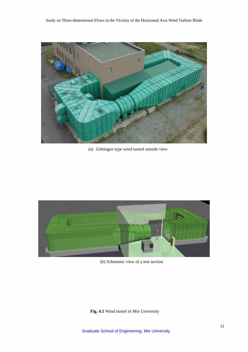
Study on Three-dimensional Flows in the Vicinity of the Horizontal Axis Wind Turbine Blade
31 Graduate School of Engineering, Mie University
(a) Göttingen type wind tunnel outside view
(b) Schematic view of a test section
Fig. 4.1 Wind tunnel in Mie University

Study on Three-dimensional Flows in the Vicinity of the Horizontal Axis Wind Turbine Blade
32 Graduate School of Engineering, Mie University
Inlet Outlet
4.5 m
Fan
Open test section 9.5 m
U0
31 m
Wind tunnel outlet
3.6
m
U0
Rotor
Inlet
4.5
m
R =
1.2
m
Thermometer
Pitot tube
0.15 m
Base 1.85 m
4.5 m
Nacelle
Tower
Fig. 4.2 Experimental setup for the wind turbine model
(a) Wind tunnel in two-dimensional sketch
(b) Test section
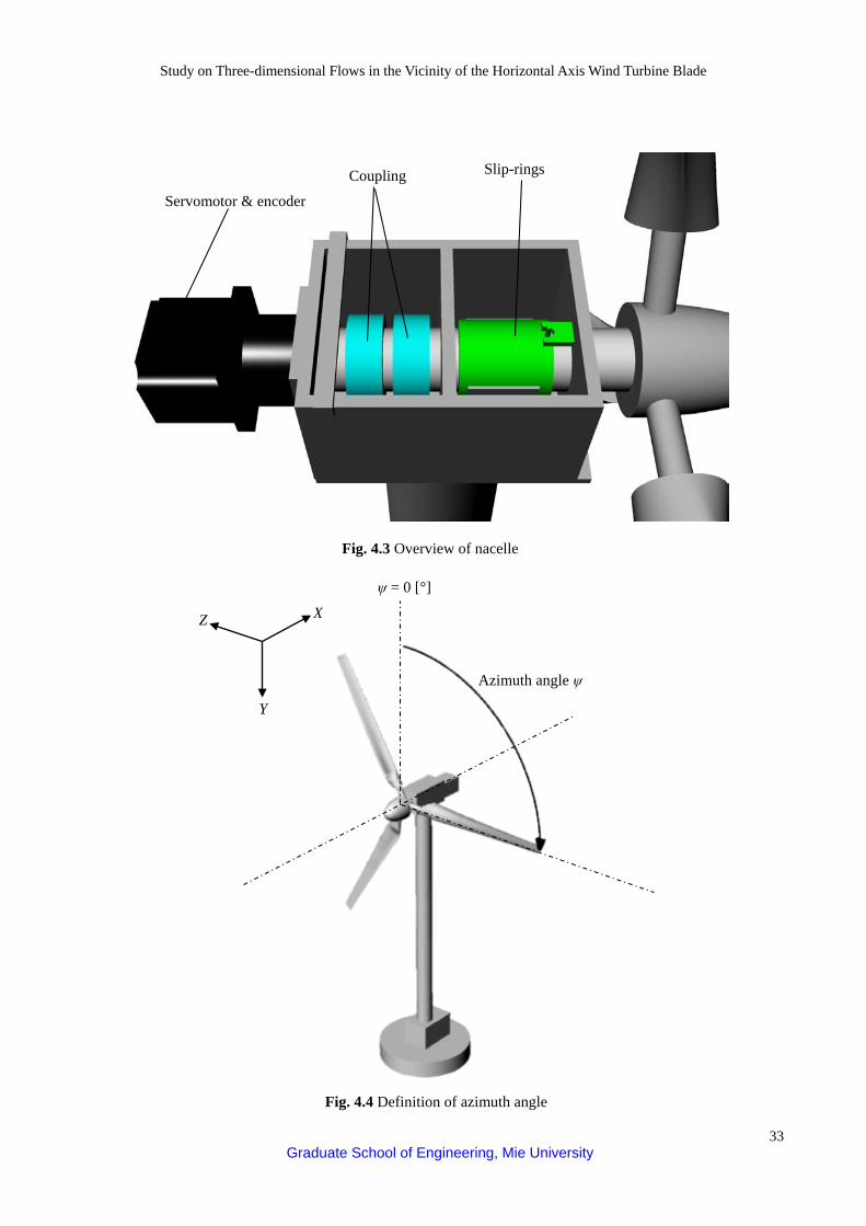
Study on Three-dimensional Flows in the Vicinity of the Horizontal Axis Wind Turbine Blade
33 Graduate School of Engineering, Mie University
X Z
Y
ψ = 0 [°]
Azimuth angle ψ
Servomotor & encoder
Slip-rings
Fig. 4.3 Overview of nacelle
Coupling
Fig. 4.4 Definition of azimuth angle
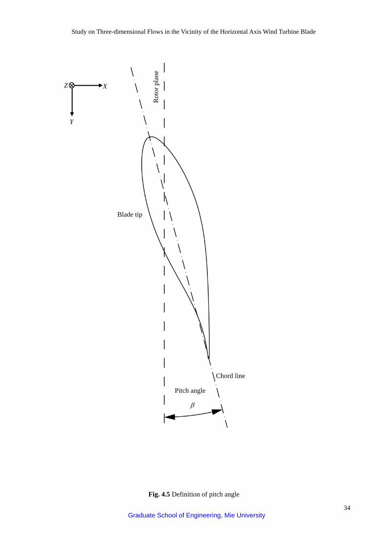
Study on Three-dimensional Flows in the Vicinity of the Horizontal Axis Wind Turbine Blade
34 Graduate School of Engineering, Mie University
Blade tip
Rot
or p
lane
Pitch angle
β
Chord line
Y
Z
X
Fig. 4.5 Definition of pitch angle

Study on Three-dimensional Flows in the Vicinity of the Horizontal Axis Wind Turbine Blade
35 Graduate School of Engineering, Mie University
r/R=1.0(r=1200[mm])
0.4(r = 480[mm])
0.5(r = 600[mm])
0.2(r = 240[mm])
0.3(r = 360[mm])
0.6(r = 720[mm])
0.7(r = 840[mm])
0.8(r =960[mm])
0.9(r = 1080[mm])
0.1(r = 120[mm])
c =85.0 [mm]
c =92.8 [mm]
c =100.6 [mm]
c =108.4 [mm]
c =116.2 [mm]
c =139.6 [mm]
c =124.0 [mm]
c =131.8 [mm]
c =147.4 [mm]
d =70.0 [mm]
Radial position r/R Chord length c Rotational direction
Twist angle θ twist
NA
CA63
-215
NA
CA63
-618
DU
93-W
-210
DU
91-W
2-25
0
Fig. 4.6 Chord length and twist angle distribution
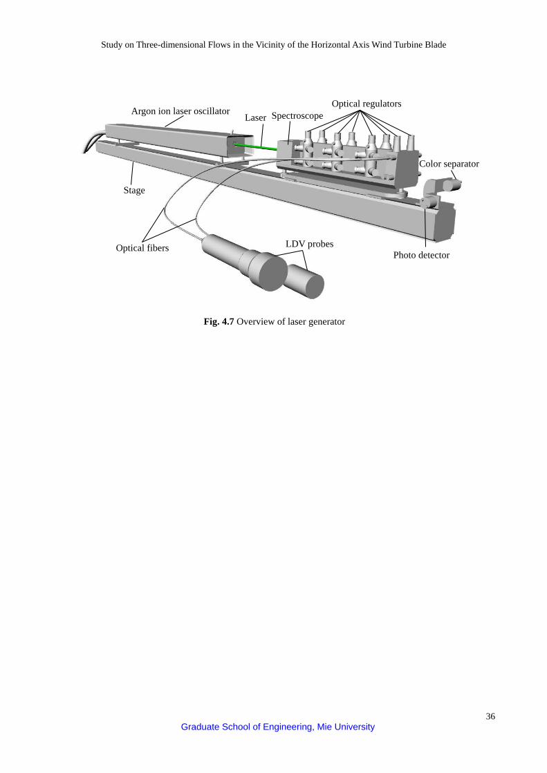
Study on Three-dimensional Flows in the Vicinity of the Horizontal Axis Wind Turbine Blade
36 Graduate School of Engineering, Mie University
Optical regulators
Color separator
Spectroscope Laser Argon ion laser oscillator
Stage
Optical fibers LDV probes Photo detector
Fig. 4.7 Overview of laser generator

Study on Three-dimensional Flows in the Vicinity of the Horizontal Axis Wind Turbine Blade
37 Graduate School of Engineering, Mie University
(c) LDV measuring volume dimension
(b) LDV measuring volume
Laser
dx
Focal point
Optical axis Crossed axes angle
of laser
Laser
Vn
Seeding particle
Optical axis
dz
Optical axis
d
θ
(a) LDV probe
Focal length
Interference fringe
Fig. 4.8 Measuring volume (One pair laser beams from one probe)
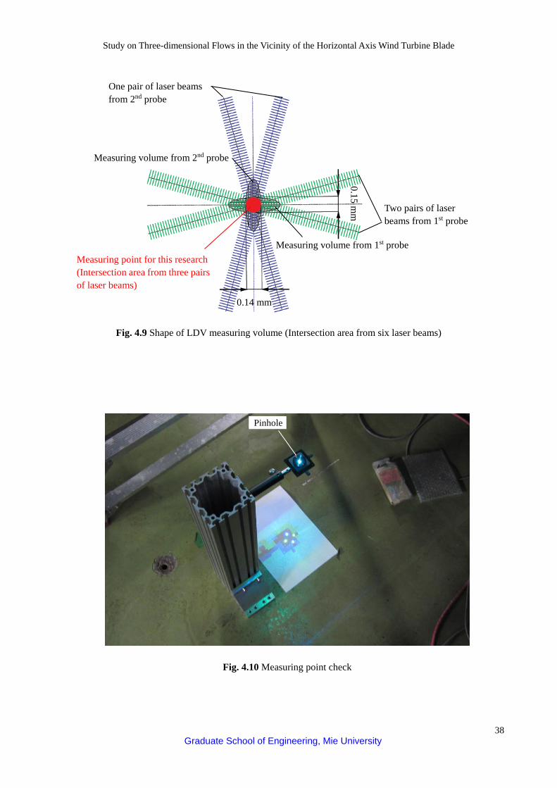
Study on Three-dimensional Flows in the Vicinity of the Horizontal Axis Wind Turbine Blade
38 Graduate School of Engineering, Mie University
One pair of laser beams from 2nd probe
Measuring volume from 2nd probe
Measuring volume from 1st probe
Two pairs of laser beams from 1st probe
0.15 mm
0.14 mm
Measuring point for this research (Intersection area from three pairs of laser beams)
Fig. 4.9 Shape of LDV measuring volume (Intersection area from six laser beams)
Fig. 4.10 Measuring point check
Pinhole

Study on Three-dimensional Flows in the Vicinity of the Horizontal Axis Wind Turbine Blade
39 Graduate School of Engineering, Mie University
Violet laser beams
Focus point
2nd probe
Green laser beams
X-Z traverse device
w Blue laser beams
u
1st probe v
Z X
Y
r/R
Upstream
U0
Downstream
Fig. 4.11 Wind turbine and LDV probes layout
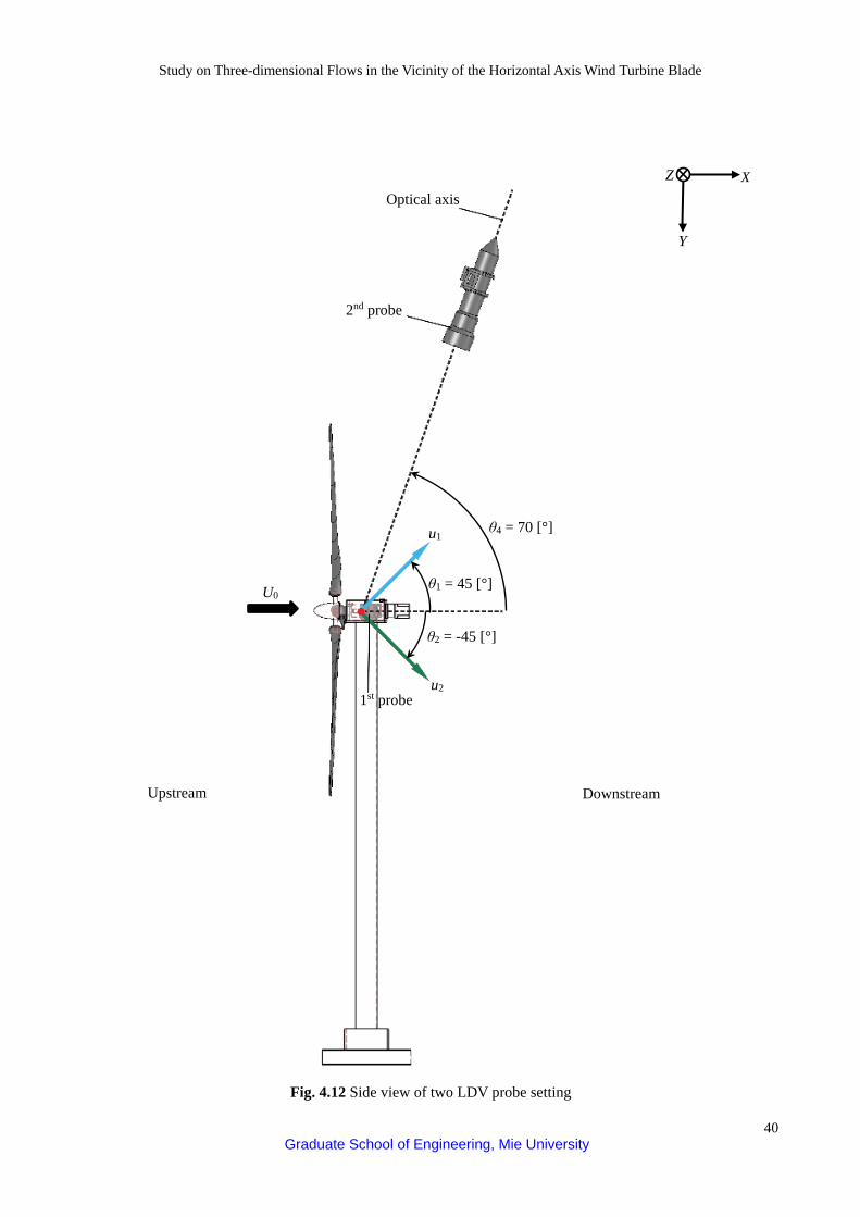
Study on Three-dimensional Flows in the Vicinity of the Horizontal Axis Wind Turbine Blade
40 Graduate School of Engineering, Mie University
X
Y
Z
θ4 = 70 [°]
θ2 = -45 [°]
θ1 = 45 [°]
u1
1st probe u2
2nd probe
Optical axis
U0
Upstream Downstream
Fig. 4.12 Side view of two LDV probe setting

Study on Three-dimensional Flows in the Vicinity of the Horizontal Axis Wind Turbine Blade
41 Graduate School of Engineering, Mie University
Z
X Y
Upstream Downstream
Fig. 4.13 Top view of two LDV probe setting
1st probe
Optical axis
u3
Violet laser beams 2nd probe Optical axis
1.6 m
1.0 m
U0
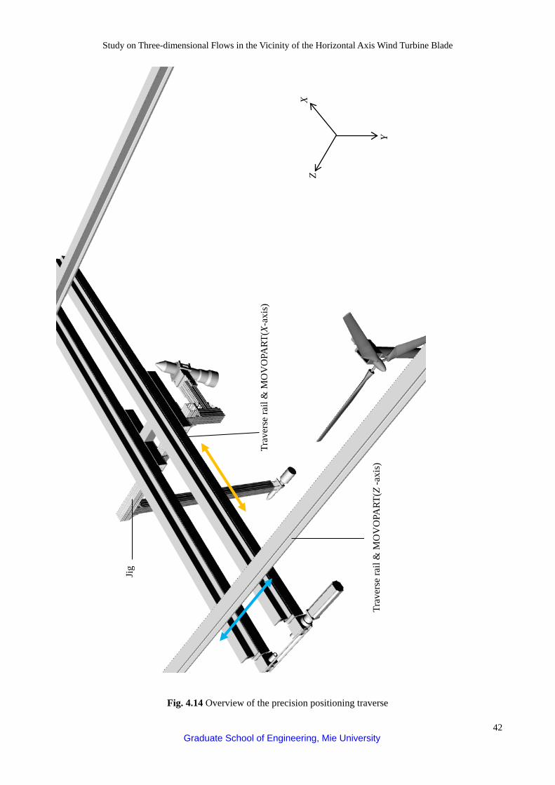
Study on Three-dimensional Flows in the Vicinity of the Horizontal Axis Wind Turbine Blade
42 Graduate School of Engineering, Mie University
Fig. 4.14 Overview of the precision positioning traverse
Y
Z X
Trav
erse
rail
& M
OV
OPA
RT(X
-axi
s)
Jig
Trav
erse
rail
& M
OV
OPA
RT(Z
-axi
s)

Study on Three-dimensional Flows in the Vicinity of the Horizontal Axis Wind Turbine Blade
43 Graduate School of Engineering, Mie University
Fig. 4.15 Positional relationship of the blade section
Rot
atio
nal d
irect
ion
Y
Z X
Blade section at the stationary
Main stream
Measurement point A di Measurement point A’
Blade section in operation
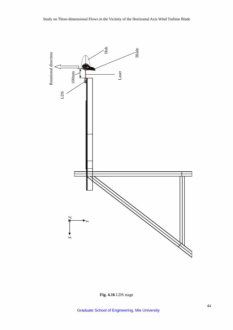
Study on Three-dimensional Flows in the Vicinity of the Horizontal Axis Wind Turbine Blade
44 Graduate School of Engineering, Mie University
Fig. 4.16 LDS stage
Y
X Z
Lase
r
Rot
atio
nal d
irect
ion
LDS
Hub
Bla
de
100m
m
Y

Study on Three-dimensional Flows in the Vicinity of the Horizontal Axis Wind Turbine Blade
45 Graduate School of Engineering, Mie University
Fig. 4.17 Blade section and LDV measuring point
Rot
atio
nal d
irect
ion
LDV measuring point
(a) t = t0-∆t (b) t = t0
(c) t = t0+∆t
Main stream
Z
Y
X
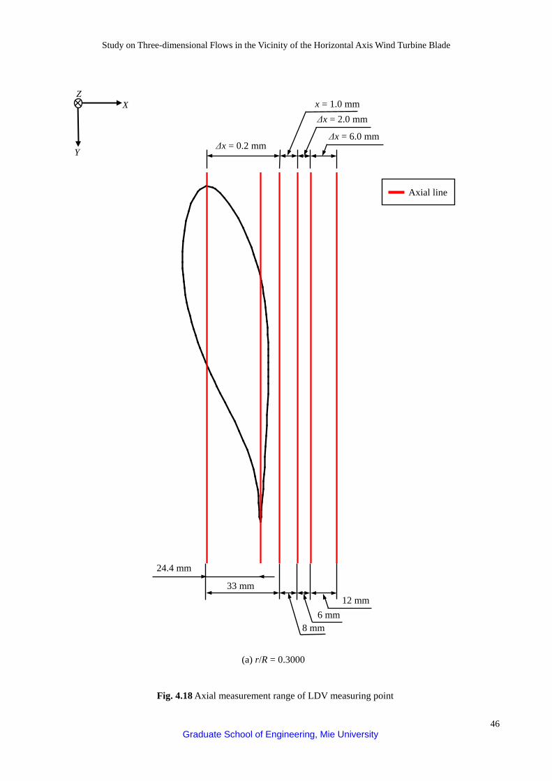
Study on Three-dimensional Flows in the Vicinity of the Horizontal Axis Wind Turbine Blade
46 Graduate School of Engineering, Mie University
24.4 mm
(a) r/R = 0.3000
33 mm
6 mm 8 mm
12 mm
Y
Z X
Fig. 4.18 Axial measurement range of LDV measuring point
Axial line
Δx = 1.0 mm
Δx = 2.0 mm
Δx = 0.2 mm Δx = 6.0 mm

Study on Three-dimensional Flows in the Vicinity of the Horizontal Axis Wind Turbine Blade
47 Graduate School of Engineering, Mie University
(b) r/R = 0.3042
32.6 mm
6 mm 8 mm
12 mm
25.5 mm
Δx = 0.2 mm
Y
Z X
Δx = 1.0 mm
Δx = 2.0 mm Δx = 6.0 mm
Axial line
Fig. 4.18 Axial measurement range of LDV measuring point

Study on Three-dimensional Flows in the Vicinity of the Horizontal Axis Wind Turbine Blade
48 Graduate School of Engineering, Mie University
(c) r/R = 0.3083
Y
Z X
32.6 mm
6 mm 8 mm
12 mm
25.5 mm
Axial line
Δx = 1.0 mm
Δx = 2.0 mm
Δx = 0.2 mm Δx = 6.0 mm
Fig. 4.18 Axial measurement range of LDV measuring point
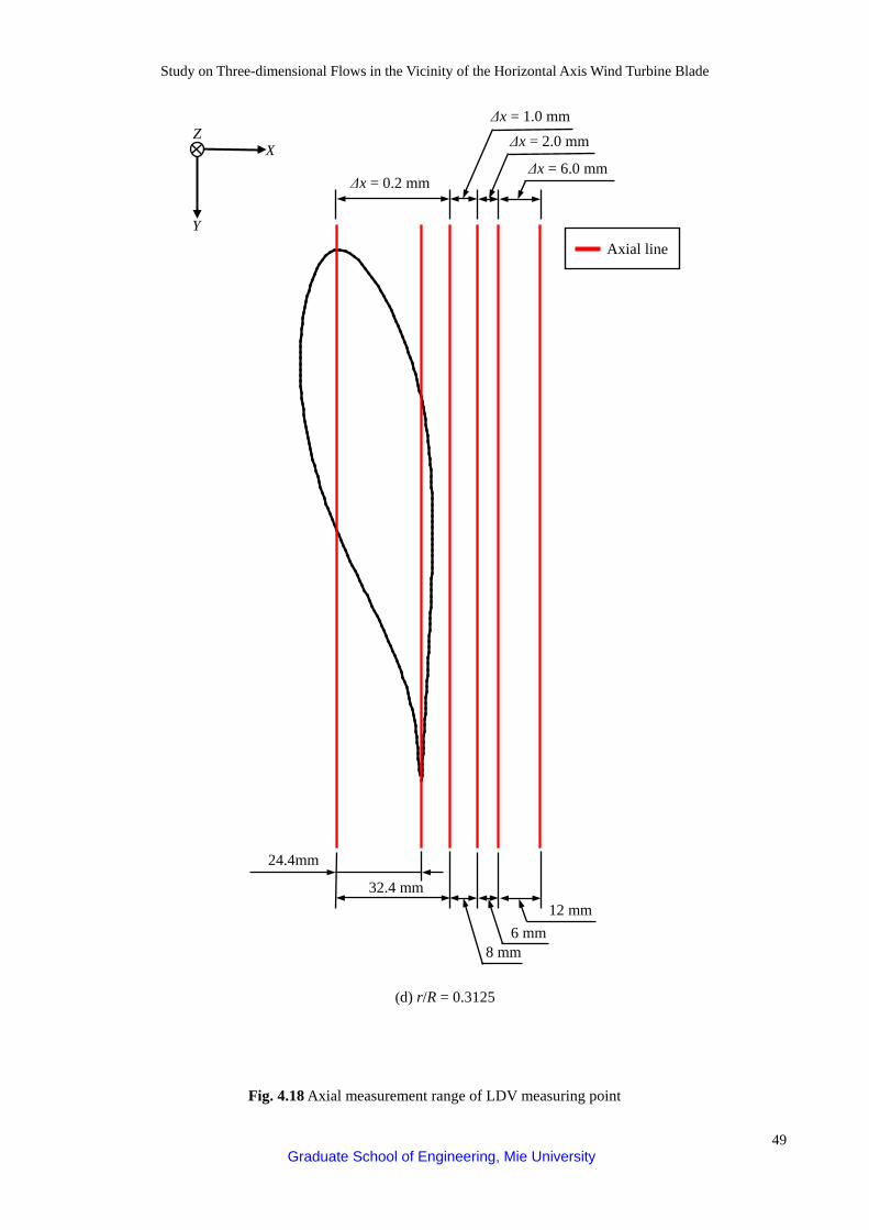
Study on Three-dimensional Flows in the Vicinity of the Horizontal Axis Wind Turbine Blade
49 Graduate School of Engineering, Mie University
(d) r/R = 0.3125
Δx = 1.0 mm Δx = 2.0 mm
Δx = 0.2 mm Δx = 6.0 mm
32.4 mm
6 mm 8 mm
12 mm
24.4mm
Y
Z X
Axial line
Fig. 4.18 Axial measurement range of LDV measuring point
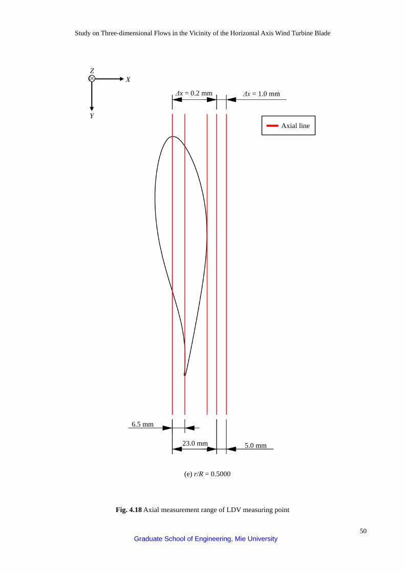
Study on Three-dimensional Flows in the Vicinity of the Horizontal Axis Wind Turbine Blade
50 Graduate School of Engineering, Mie University
Y
Z X
(e) r/R = 0.5000
Δx = 1.0 mm
Axial line
Fig. 4.18 Axial measurement range of LDV measuring point
Δx = 0.2 mm
6.5 mm
23.0 mm 5.0 mm

Study on Three-dimensional Flows in the Vicinity of the Horizontal Axis Wind Turbine Blade
51 Graduate School of Engineering, Mie University
Δx = 6.0 mm Δx = 2.0 mm
Δx = 1.0 mm Δx = 0.2 mm
Y
Z X
18.8 mm
6 mm 8 mm
12 mm
1.7mm
(f) r/R = 0.7000
Axial line
Fig. 4.18 Axial measurement range of LDV measuring point
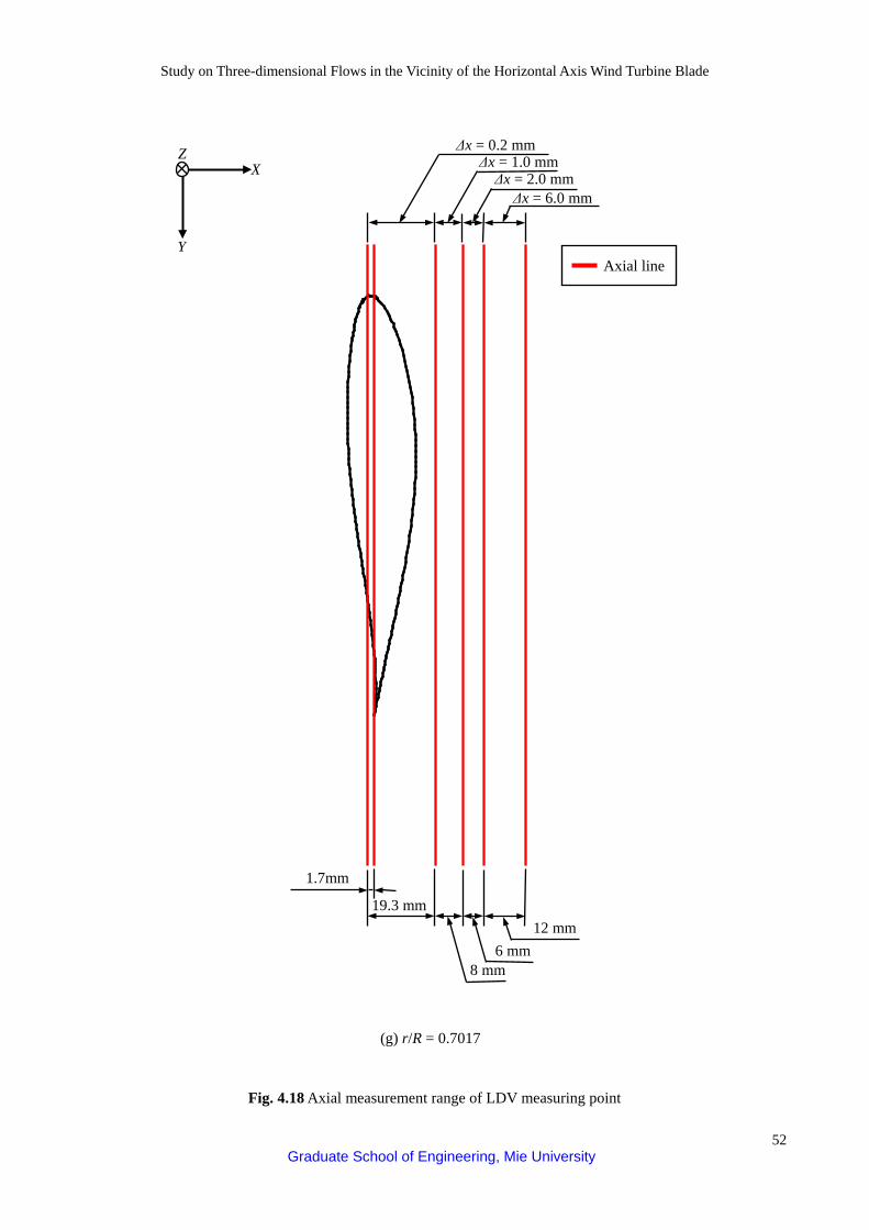
Study on Three-dimensional Flows in the Vicinity of the Horizontal Axis Wind Turbine Blade
52 Graduate School of Engineering, Mie University
(g) r/R = 0.7017
19.3 mm
6 mm 8 mm
12 mm
1.7mm
Δx = 6.0 mm Δx = 2.0 mm
Δx = 1.0 mm Δx = 0.2 mm
Y
Z X
Axial line
Fig. 4.18 Axial measurement range of LDV measuring point

Study on Three-dimensional Flows in the Vicinity of the Horizontal Axis Wind Turbine Blade
53 Graduate School of Engineering, Mie University
(h) r/R = 0.7033
19.3 mm
6 mm 8 mm
12 mm
1.7mm
Δx = 6.0 mm Δx = 2.0 mm
Δx = 1.0 mm Δx = 0.2 mm
Y
Z X
Axial line
Fig. 4.18 Axial measurement range of LDV measuring point
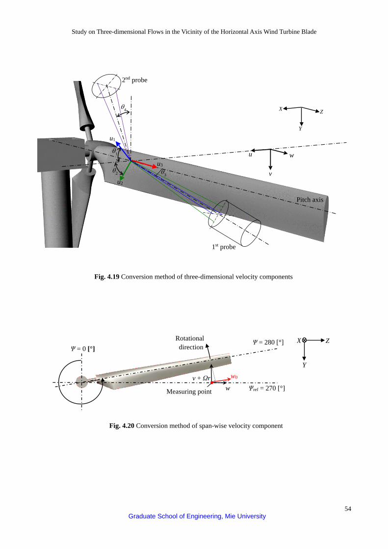
Study on Three-dimensional Flows in the Vicinity of the Horizontal Axis Wind Turbine Blade
54 Graduate School of Engineering, Mie University
v
w
1st probe
2nd probe
u
X
Y
Z
Pitch axis
θ4
u1
X
Y
Z Ψ = 0 [°]
Rotational direction
Ψref = 270 [°]
Ψ = 280 [°]
Measuring point
v + Ωr
w
w0
Fig. 4.20 Conversion method of span-wise velocity component
u2
u3 θ3
θ1
θ2
Fig. 4.19 Conversion method of three-dimensional velocity components

Study on Three-dimensional Flows in the Vicinity of the Horizontal Axis Wind Turbine Blade
55 Graduate School of Engineering, Mie University
Table 4.1 The types of equipment using in this dissertation Equipment Model number Manufacturer
Digital manometer DM-5031 COSMO Platinum resistance temperature E52-P10GR OMRON
Panel meter K3HB-H OMRON Servomotor SGMPH-15AAAH121 YASUKAWA electronic Servopack SGDH-15AE YASUKAWA electronic
Power regeneration unit VARISPEED 656RC5 YASUKAWA electronic Photosensor EE-SPX403 OMRON
CPU unit KV-5500 KEYENCE Fast counter unit KV-SC20V KEYENCE A/D transfer unit KV-AD40V KEYENCE D/A transfer unit KV-DA40V KEYENCE
Positioning motion unit KV-MC40V KEYENCE Personal computer Vostro 260 Dell Inc.
Laser oscillator Stabilite2017 Spectra-Physics Signal processing unit BSA F60 DANTEC
Fog generator Home made Tracer SAFEX INSIDE FOG FLUDE DANTEC
Laser Displacement Sensor Z4M-S100RA OMRON LDS amplifier Z4M-W100R OMRON
A/D conversion terminal AIO-160802AY-USB CONTEC
Table 4.2 LDV measuring volume Wave length λopt [nm] 476.5 488.0 514.5 Focal length F [mm] 1600 1000 1000
Diameter dx [mm] 0.149 0.143 0.150 Width dz [mm] 4.29 3.81 4.01
Crossed angle θcross [º] 3.98 4.36 4.36

Study on Three-dimensional Flows in the Vicinity of the Horizontal Axis Wind Turbine Blade
56 Graduate School of Engineering, Mie University
Chapter 5 Results and Discussion
In this chapter, the experimental results of the test HAWT in the wind tunnel were explained. The first results
are the rotor power curve test. When the model wind turbine shows the low power coefficient, the model wind turbine does not show the general result for wind turbines. For the preparation of surface flow measurements, the blade surface displacement is measured in the rotating condition. These results must check before starting velocity measurements. The next step is the LDV measurement. The results and discussion are shown as follows:
5.1 Preliminary experiments 5.1.1 Power output performance
The test wind turbine rotor of 1.2 m was chosen to perform in the wind tunnel to detect a more detailed measurement on the blade surface. The high blockage effect in the wind tunnel experiment may affect the flow on the blade surface. The test wind turbine rotor has a blockage ratio of 44%. Therefore, the impact of a high blockage ratio should be examined. Generally, the effect of the blockage ratio is verified by a power coefficient curve.
Figure 5.1 shows the power coefficients for this test wind turbine rotor and a small wind turbine rotor in the same wind tunnel. The power coefficient of a small wind turbine rotor refers to the previous experiment. The small wind turbine has a rotor radius of 0.563 m, and the mainstream is a set constant of 6 m/s. As shown in Fig. 5.1, the black solid circle indicates the power coefficient for test wind turbine (R = 1.2 m). The black triangle indicates the power coefficient for the small wind turbine (R = 0.563 m). The black line indicates the results using the blade element momentum theory (BEMT R = 1.2 m) for test wind turbine. The results of the wind turbine rotor of 1.2 m (Solidity = 0.10) show the maximum power coefficient of 0.43 at tip speed ratio of 5.2. The measured power coefficient almost fit well with the BEMT prediction. The results of the small wind turbine rotor of 0.563 m (Blockage ratio = 9.8%, Solidity = 0.15) show the maximum power coefficient of 0.44 at the tip speed ratio of 4.62. The optimum tip speed ratio for the smaller rotor is smaller than that of this test wind turbine because of higher solidity. The results from both wind turbine rotors show almost similar power curve. Although the test wind turbine rotor radius of 1.2 m has a high blockage ratio, it is sure that the high blockage ratio has not affected this experimental study.
5.1.2 Blade surface displacement
As the rotor blades during operation, a wind turbine blade will be transformed a position in axial and tangential directions due to the fluid force. Therefore, the displacement from the transformation of the rotor blade was correctly detected by using the laser displacement sensor (LDS). The displacement data during the rotation will apply to set correctly the axial position x/c for the LDV measurement.
The shape of blade sections can be detected by the LDS. The designed airfoil shape and the measured blade section shape are different at the same radial position r/R. The measured blade section at the same radial position r/R is not perpendicular to the pitch axis. Figure 5.2 shows a cross-section comparison between the designed airfoil section and the measured blade section at a certain radial position r/R. The red and blue lines indicate designed airfoil and measured blade cross-section shapes, respectively. The radial position r/R is defined as a distance from the rotational axis of the wind turbine rotor. Therefore, measured velocities data have a slight discrepancy between the designed airfoil section and the measured blade section due to the azimuth position.
Figures 5.3, 5.4 and 5.5 show the comparison of a designed airfoil and measured blade section shapes at radial position r/R = 0.3, 0.5 and 0.7, respectively. In these figures, the horizontal axis indicates the mainstream position
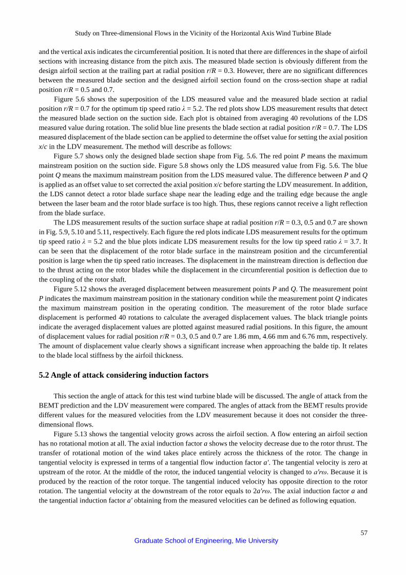
Study on Three-dimensional Flows in the Vicinity of the Horizontal Axis Wind Turbine Blade
57 Graduate School of Engineering, Mie University
and the vertical axis indicates the circumferential position. It is noted that there are differences in the shape of airfoil sections with increasing distance from the pitch axis. The measured blade section is obviously different from the design airfoil section at the trailing part at radial position r/R = 0.3. However, there are no significant differences between the measured blade section and the designed airfoil section found on the cross-section shape at radial position r/R = 0.5 and 0.7.
Figure 5.6 shows the superposition of the LDS measured value and the measured blade section at radial position r/R = 0.7 for the optimum tip speed ratio λ = 5.2. The red plots show LDS measurement results that detect the measured blade section on the suction side. Each plot is obtained from averaging 40 revolutions of the LDS measured value during rotation. The solid blue line presents the blade section at radial position r/R = 0.7. The LDS measured displacement of the blade section can be applied to determine the offset value for setting the axial position x/c in the LDV measurement. The method will describe as follows:
Figure 5.7 shows only the designed blade section shape from Fig. 5.6. The red point P means the maximum mainstream position on the suction side. Figure 5.8 shows only the LDS measured value from Fig. 5.6. The blue point Q means the maximum mainstream position from the LDS measured value. The difference between P and Q is applied as an offset value to set corrected the axial position x/c before starting the LDV measurement. In addition, the LDS cannot detect a rotor blade surface shape near the leading edge and the trailing edge because the angle between the laser beam and the rotor blade surface is too high. Thus, these regions cannot receive a light reflection from the blade surface.
The LDS measurement results of the suction surface shape at radial position r/R = 0.3, 0.5 and 0.7 are shown in Fig. 5.9, 5.10 and 5.11, respectively. Each figure the red plots indicate LDS measurement results for the optimum tip speed ratio λ = 5.2 and the blue plots indicate LDS measurement results for the low tip speed ratio λ = 3.7. It can be seen that the displacement of the rotor blade surface in the mainstream position and the circumferential position is large when the tip speed ratio increases. The displacement in the mainstream direction is deflection due to the thrust acting on the rotor blades while the displacement in the circumferential position is deflection due to the coupling of the rotor shaft.
Figure 5.12 shows the averaged displacement between measurement points P and Q. The measurement point P indicates the maximum mainstream position in the stationary condition while the measurement point Q indicates the maximum mainstream position in the operating condition. The measurement of the rotor blade surface displacement is performed 40 rotations to calculate the averaged displacement values. The black triangle points indicate the averaged displacement values are plotted against measured radial positions. In this figure, the amount of displacement values for radial position r/R = 0.3, 0.5 and 0.7 are 1.86 mm, 4.66 mm and 6.76 mm, respectively. The amount of displacement value clearly shows a significant increase when approaching the balde tip. It relates to the blade local stiffness by the airfoil thickness. 5.2 Angle of attack considering induction factors
This section the angle of attack for this test wind turbine blade will be discussed. The angle of attack from the BEMT prediction and the LDV measurement were compared. The angles of attack from the BEMT results provide different values for the measured velocities from the LDV measurement because it does not consider the three-dimensional flows.
Figure 5.13 shows the tangential velocity grows across the airfoil section. A flow entering an airfoil section has no rotational motion at all. The axial induction factor a shows the velocity decrease due to the rotor thrust. The transfer of rotational motion of the wind takes place entirely across the thickness of the rotor. The change in tangential velocity is expressed in terms of a tangential flow induction factor a'. The tangential velocity is zero at upstream of the rotor. At the middle of the rotor, the induced tangential velocity is changed to a'rω. Because it is produced by the reaction of the rotor torque. The tangential induced velocity has opposite direction to the rotor rotation. The tangential velocity at the downstream of the rotor equals to 2a'rω. The axial induction factor a and the tangential induction factor a' obtaining from the measured velocities can be defined as following equation.

Study on Three-dimensional Flows in the Vicinity of the Horizontal Axis Wind Turbine Blade
58 Graduate School of Engineering, Mie University
m
0
1 uaU
= − (5.1)
Where um is the average of the local axial velocity component from azimuth angle 0 [°] to 360 [°] near the airfoil suction surface. From Eq. (5.1), the tangential induction factor a' can thus be found from .
20(1 )( )Ua a aΩr
′ = − (5.2)
Figures 5.14 and 5.15 show the axial induction factor a and the tangential induction factor a' from the BEMT
prediction and the LDV measurement. The red line indicates the induction factor from the BEMT prediction for the optimum tip speed ratio λ = 5.2. The blue line indicates the results for the low tip speed ratio λ = 3.7. The red triangle point indicates the induction factor calculating from the LDV measurement for the optimum tip speed ratio. The blue circle point indicates the results for the low tip speed ratio λ = 3.7. From Fig. 5.14, obviously, the axial induction factors at radial position r/R = 0.5 and 0.7 for the optimum tip speed ratio λ = 5.2 are almost no difference between the BEMT prediction and experiment data from the LDV measurement. On the other hand, the axial induction factors at radial position r/R = 0.3 for the low tip speed ratio λ = 3.7 shows more difference between the BEMT prediction and the LDV measurement. From Fig. 5.15, the tangential induction factor a' from the BEMT prediction and the LDV measurement are few different value at radial position r/R = 0.3 for the low tip speed ratio λ = 3.7.
From Figs. 5.14 and 5.15, the reason why has a more different axial and tangential induction factors between the BEMT prediction and the LDV measurement at radial position r/R = 0.3. It is considered that the flow near the blade root has three-dimensional flows substantially. While the axial and tangential induction factors from the BEMT prediction and experiment data at radial position r/R = 0.5 and 0.7 agrees well because blade sections approaching the blade tip exhibit only two-dimensional velocity.
Figure 5.16 shows a velocity diagram in a blade section. It illustrates the relationship between the angle of attack and the velocity triangle. Uref is composed of the axial velocity U0(1–a), and the tangential velocity Ωr(1+a'). The angle of attack α becomes the difference between the inflow angleφ , the blade’s pitch β and twist angle θtwist.
twist( )α φ β θ= − + (5.3) From Eq. (5.3), the angle of attack can be calculated as follows:
1 0twist
(1 )tan ( )(1 )
a U+ a Ωr
α θ β− − = − + ′
(5.4)
Figure 5.17 shows the angle of attack distribution for each radial position. The horizontal axis indicates the
radius position r/R, and the vertical axis indicates the angle of attack α. The red triangle point means the angle of attack calculating from the LDV measurement for the optimum tip speed ratio λ = 5.2, while the blue circle point means the angle of attack calculating from experiment data for the low tip speed ratio λ = 3.7. The red line indicates the angle of attack from BEMT prediction for the optimum tip speed ratio λ = 5.2, and the blue line indicates that for the low tip speed ratio λ = 3.7. From Fig. 5.17, obviously, the angle of attack for the low tip speed ratio shows higher than the angle of attack for the optimum tip speed ratio. It causes stall phenomena on the blade section for the low tip speed ratio. The angle of attack from BEMT prediction and calculating from the LDV measurement does not show significantly different value at radial position r/R = 0.5 and 0.7. Thus, The BEMT can roughly predict the angle of attack for each blade section. However, the angle of attack from BEMT is excessive angle of attack with comparing with the angle of attack from experiment data at radial position r/R = 0.3. Because at blade root has a complicated effect from three-dimensional flows at the inboard of the wind turbine blade.

Study on Three-dimensional Flows in the Vicinity of the Horizontal Axis Wind Turbine Blade
59 Graduate School of Engineering, Mie University
5.3 Three-dimensional flow characteristics on the blade sections
In this section, three-dimensional velocities measured from the LDV system are presented. It must be emphasized that in the three-dimensional flow characteristics near the blade surface downstream (suction side) was investigated. Measurements were performed for blade sections located at radial positions r/R = 0.3 (inboard) and 0.7 (outboard). The results contribute to a better understanding of the flow characteristics for different radial positions. The rotor tip speed ratio was chosen at the optimum condition (λ = 5.2) and the stall condition (λ = 3.7). 5.3.1 Three-dimensional flow characteristics for the optimum tip speed ratio (λ = 5.2)
In this section, velocity distribution on the blade sections for the optimum tip speed ratio will be discussed, taking into account two-dimensional relative velocity U2D. Local velocity will be described as the velocity vector with color. The two-dimensional relative velocity U2D can be defined as a vector quantity in Eq. (5.5).
2D ( )U ui + v+ Ωr j=
(5.5) Here 2DU
is the vector quantity of the two-dimensional relative velocity to the blade section; i
and j
are the unit vectors on the axial direction and the tangential direction, respectively. The color of vector shows the magnitude of the local velocity. It can be calculated by using Eq. (5.6).
2 22D ( )U u v Ωr= + + (5.6)
The direction of local velocity in a sectional plane is exhibited by the angle of vector, which can be calculated using the local axial velocity component and the local tangential velocity component. It can be defined as Eq. (5.7).
1vector tan ( )u
v+ Ωrθ −= (5.7)
Here θvector is the angle of the velocity vector. The local velocity is normalized by dividing it by the geometrical inflow velocity Uref which is defined in Eq. (5.8).
2 2ref 0= [ (1- )] +[ (1+ )]U U a Ωr a′ (5.8)
Here Uref is the geometrical inflow velocity, U0 is the mainstream velocity. The Uref depends on the radial position. It is enhanced for the outer radial positions.
Figure 5.18 (a) shows the velocity distribution at radial position r/R = 0.3 for the optimum tip speed ratio. The colored vectors show the local velocity on the blade section. The color of vector expresses the two-dimensional relative speed. The color bar indicates the two-dimensional relative flow speed (U2D/Uref). The yellow point inside the blade section indicates the position of the pitch axis, which is located at 25% of the chord length. The velocity vector at pitch axis indicates direction and magnitude of blade's rotational speed. This speed is the same scale with the two-dimensional relative flow speed. The white line above the blade section shows the contour of the area of the maximum value of the two-dimensional relative speed at each chord station y/c. The distance from the wall surface to a white line can assume to represent the boundary layer thickness for the region of non-separated flow. From this figure, the boundary layer thickness increases gradually along the blade surface from leading edge to the trailing edge. The boundary layer thickness above leading part can be observed as a thin layer. The boundary layer thickness depends on the viscosity effect, the airfoil shape and the pressure gradient. The velocity vectors at the chord position of 0.05 < y/c < 0.2 exhibit a high two-dimensional relative velocity area in the range of 1.8 < U2D/Uref
< 1.9. However, these flows are gradually reduced in speed approaching the trailing edge because the pressure is
Study on Three-dimensional Flows in the Vicinity of the Horizontal Axis Wind Turbine Blade
60 Graduate School of Engineering, Mie University
recovered close to the trailing edge. Obviously, most of the colored vectors on the velocity map seem like the color of rotational velocity. On the other hand, the rotational velocity is greatly influenced by two-dimensional flows. This blade section rotates at a constant speed Ωr/Uref of 0.85. At chord positions of 0.7 < y/c < 1.0, velocity vectors inside the boundary layer show low speed in the range of 0.2 < U2D/Uref < 0.4 and the direction of vectors are not parallel to the blade surface due to the formation of separated flow.
Figure 5.18 (b) shows the velocity distribution at radial position r/R = 0.7 for the optimum tip speed ratio. This blade section operates at a constant rotational speed Ωr/Uref of 0.97. The boundary layer thickness grows gradually along the blade section. The velocity vectors are fully attached to the suction surface as well. The high two-dimensional relative velocity area in the range of 1.6 < U2D/Uref < 1.7 occurs above the chord position of 0 < y/c < 0.2. The velocity vectors on the suction surface at y/c > 0.2 show deceleration close to the trailing edge.
Figure 5.19 (a) shows the span-wise velocity contour at radial position r/R = 0.3 for the optimum tip speed ratio. The colors of the figure refer to the local flow speed in the span-wise direction. The black area shows the lack of data due to the insufficient number of measured particles. The color bar indicates the span-wise flow speed (w0/Uref). The sign of values represents the direction of the span-wise flow. The positive value indicates the direction of the span-wise flow from root to tip, and a negative value is the opposite direction. The outer region of the boundary layer thickness indicates that the low positive span-wise velocity in the range of 0 < w0/Uref < 0.03 is observed above the chord station of 0 < y/c < 0.3. The positive span-wise velocity will be increased gradually until w0/Uref = 0.12 along the chord station of 0.4 < y/c < 1. Obviously, the direction of span-wise velocity gradually changes to towards the outside blade. When considering the span-wise velocity inner region of boundary layer thickness, the low span-wise velocity of w0/Uref < -0.03 is located at the chord position of 0 < y/c < 0.1, while the strong span-wise velocity of w0/Uref > 0.18 is located at the chord position of 0.6 < y/c < 1. It has been found that the area that exhibits the maximum span-wise velocity in Fig. 5.19 (a) is quite different from the area with the maximum two-dimensional relative velocity U2D/Uref observed in Fig. 5.18 (a). The two-dimensional relative velocity has a strong effect on the leading part, while the span-wise velocity seems to have a high effect on the trailing part where the velocity vector has a high fluctuation in direction.
Figure 5.19 (b) shows the span-wise velocity contour at radial position r/R = 0.7 for the optimum tip speed ratio. The observed value of the span-wise velocity approximately equals to w0/Uref = 0.06 at the chord station of 0 < y/c < 0.7, and then span-wise flow reaches the value w0/Uref = 0.12 at the chord station of 0.7 < y/c < 1 on the blade surface. It is assumed that blade sections approaching the blade tip exhibit only two-dimensional velocity U2D
5.3.2 Three-dimensional flow characteristics for the low tip speed ratio (λ = 3.7)
Figure 5.20 (a) shows the velocity distribution at radial position r/R = 0.3 for the low tip speed ratio. This blade section has a constant rotational speed Ωr/Uref of 0.75. Obviously, the high two-dimensional relative velocity area in the range of 1.8 < U2D/Uref < 1.9 occurs at the outer region of the boundary layer and above chord position 0.1 < y/c < 0.2. While the low two-dimensional relative velocity area in the range of 0.3 < U2D/Uref < 0.4 occurs at the inner region of the boundary layer along chord position 0 < y/c < 1. The velocity vectors near the suction surface show high fluctuation in direction, and the flow is not attached to the suction surface due to the high angle of attack.
Figure 5.20 (b) shows the velocity distribution at radial position r/R = 0.7 for the low tip speed ratio. This blade section has a constant rotational speed Ωr/Uref of 0.93. The high two-dimensional relative velocity area in the range of 1.7 < U2D/Uref < 1.8 occurs at the outer region of the boundary layer and chord position 0.1 < y/c < 0.3, and flow speed is reduced gradually until U2D/Uref = 1 at the trailing part. The swirling of the velocity vectors near the suction surface can be observed, and the white line becomes detached from the suction surface at the trailing part 0.5 < y/c < 1 due to the phenomena of flow separation. The low tip speed ratio condition indicates that the flow is not attached to the suction surface because the critical angle of attack for the blade section is exceeded and the flow on the suction surface will separate.
Figure 5.21 (a) shows the span-wise velocity contour at radial position r/R = 0.3 for the low tip speed ratio. The span-wise velocity near the suction surface indicate the negative value of w0/Uref = -0.03 at chord positions of 0 < y/c < 0.1, and the span-wise velocity rapidly increases to positive value w0/Uref > 0.18 at chord positions of 0.4

Study on Three-dimensional Flows in the Vicinity of the Horizontal Axis Wind Turbine Blade
61 Graduate School of Engineering, Mie University
< y/c < 1 on the suction surface. The high speed region for the XY component of relative velocity is different from that of the span-wise velocity component. The span-wise velocity component is low at the region where the XY component of relative velocity is high. The two-dimensional relative velocity shows a high value while the span-wise velocity shows a low value on the leading part at the chord position of 0 < y/c < 0.2. In addition, the span-wise velocity shows a high value, while the two-dimensional relative velocity shows a low value on the trailing part, where velocity vectors show a strong fluctuation. Obviously, the direction of the span-wise flow near the blade surface gradually changes towards the outside blade. A negative value of the span-wise velocity occurs near the leading part. It is caused by the span-wise component of rotational speed. This flow has a direction toward the blade root. The span-wise velocity gradually changed the sign of value due to the formation of the centrifugal force. The centrifugal force has a direction toward the blade tip.
Figure 5.21 (b) shows the span-wise velocity contour at the radial position r/R = 0.7 for the low tip speed ratio. The outer region of boundary layer thickness shows span-wise velocity in the range of 0 < w0/Uref < 0.03 at the chord position of 0 < y/c < 0.2, and then they are gradually increased until w0/Uref = 0.09 when approaching the trailing edge. However, the inner region of the boundary layer thickness at chord positions of 0.8 < y/c < 1 shows high span-wise velocity of w0/Uref > 0.18.
From this study, a high span-wise velocity substantially coincides with the region of two-dimensional relative velocity deceleration, the same as the optimum tip speed case, but the low speed ratio has a large region of high span-wise flow along the vicinity of the blade surface. 5.4 Pressure distribution on the blade sections
In this section, the blade surface pressure distribution at the inboard and outboard sections (r/R = 0.3 and 0.7) from the LDV measurement were investigated comparing with the pressure distributions from pressure measurement and prediction from Xfoil software. The blade surface pressure distribution from the pressure measurement is measured from the previous thesis [59]. The pressure distribution is expressed in dimensionless form by using the pressure coefficient. In the case of a rotating blade, the pressure coefficient from pressure measurements Cp_tap can be defined as the ratio between the total pressure measured on the blade surface and the dynamic pressure of the geometrical inflow velocity. It can be indicated in Eq. (5.9)
i 0 i 0p_tap 2
d ref0.5p p p pC
p Uρ− −
= = (5.9)
Where pi is the measured surface pressure at the i-th pressure tap on the measurement section, p0 is the reference static pressure and pd is the dynamic pressure of geometrical inflow velocity.
The pressure coefficient also can be calculated from measured velocities. The pressure coefficient from LDV measurement Cp_LDV can be derived as Eq. (5.10).
2
p_LDVref
1 eUCU
≡ −
(5.10)
Where Ue is the relative velocity at the outer edge of the boundary layer.
Figures 5.22 (a) and (b) show the pressure distributions from the pressure measurement, velocity measurement, and Xfoil prediction. The green solid circle indicates the pressure coefficient from pressure measurement Cp_tap. The red solid circle indicates the results from velocity measurement Cp_LDV. The black solid line indicates the results from Xfoil prediction Cp_Xfoil. The pressure coefficient Cp_tap at radial position r/R = 0.3 and 0.7 clearly shows that the Cp_tap = 1.0 is at the stagnation point near the leading edge. And then, the Cp_tap on pressure surface decreases. Cp_tap on the suction surface shows minimum near around the leading edge and then it rises as close to the trailing edge. Finally, the Cp_tap recovers to a small positive value near the trailing edge.
As shown in Fig. 5.22 (a), the pressure coefficient Cp_Xfoil seems more different from the pressure coefficients

Study on Three-dimensional Flows in the Vicinity of the Horizontal Axis Wind Turbine Blade
62 Graduate School of Engineering, Mie University
obtaining from pressure taps and LDV measurement due to the rotational effects. The pressure coefficients Cp_tap and Cp_LDV were measured in rotating blade condition while the pressure coefficient Cp_Xfoil was simulated in non-rotating condition. Generally, the aerodynamic characteristics extracted from a rotating blades commonly present evidence of rotational effects, such as stall delay and lift enhancement. Especially, the radial positions are close to the blade root. The pressure coefficient Cp_Xfoil predicts a transition point near the chord station y/c = 0.15 while transition points from the pressure taps and LDV measurement delay to the chord station y/c = 0.3. For the chord station 0.15 < y/c < 0.5, the pressure coefficient Cp_Xfoil increases rapidly while the pressure coefficients Cp_tap and Cp_LDV increase gradually. The pressure coefficients Cp_tap and Cp_LDV show quite stable values which phenomena is known as laminar separation bubble at the chord station 0.25 < y/c < 0.3. The different pressure coefficient results between the rotating and non-rotating conditions correspond to the span-wise flow effect. Span-wise flow makes slow slope of the pressure recovery on the suction surface and delays the transition point.
In Fig. 5.22 (b), the pressure coefficient Cp_Xfoil shows very similar to the pressure coefficients obtaining from pressure taps and LDV measurements. It seems that the rotational effects can not affect the position near the blade tip. The slope of pressure coefficients Cp_tap, Cp_LDV and Cp_Xfoil show approaching a zero slope and few different values on the suction surface at the chord station 0.4 < y/c < 0.5. It seems like laminar separation bubble. The chord station y/c = 0.5 is presented as a transition point, and then the pressure coefficients are rapidly increased close to the trailing edge at the chord station 0.5 < y/c < 0.6. 5.5 Boundary layer
In this section, the boundary layer on the rotating blade for the optimum tip speed ratio will be discussed. Generally, three parameters used to measure the properties of boundary layers are comprised as follows: 1.) The boundary layer thickness δ, 2.) The displacement thickness δ* and 3.) The momentum thickness θ. In the previous section, the boundary layer thickness δ was discussed by using the velocity of local flow. It was found that the boundary layer thickness was gradually increased along the blade surface from leading edge to the trailing edge. The boundary layer thickness for the low tip speed ratio always becomes thicker than the optimum tip speed ratio due to stall phenomenon. In this section, the displacement thickness and momentum thickness of the boundary layer will be discussed.
Figure 5.23 (a) shows the shape factor, displacement thickness and momentum thickness of the boundary layer for the local chord wise position. The radial position is r/R = 0.3, and the tip speed ratio is optimal. The horizontal axis indicates the chord position y/c. The right vertical axis indicates the distance from the airfoil suction surface in unit mm, and the left vertical axis indicates the value of the shape factor. From this figure, the blue dots represent the displacement thickness, which is defined in Eq. (5.11). The green dots represent the momentum thickness, which is defined in Eq. (5.12), and the red dot represents the shape factor, which is defined in Eq. (5.13).
0e
1 dUU
xδ
δ ∗ ∗= −
∫ (5.11)
0e e
1 dU U xU U
δθ ∗
= −
∫ (5.12)
H δθ
∗
= (5.13)
Here δ* is the displacement thickness, θ is the momentum thickness, H is the shape factor and x* is the distance from the blade surface. The x* stands on a special coordinate that set on the blade surface and has a direction outward blade surface. U is the two-dimensional relative velocity on the blade surfaces at each chord position y/c and Ue is the velocity at the outer edge of the boundary layer. However, the free stream velocity on the blade
Study on Three-dimensional Flows in the Vicinity of the Horizontal Axis Wind Turbine Blade
63 Graduate School of Engineering, Mie University
changes given the effect of circulation and surface pressure distribution. Therefore, Ue was selected from two-dimensional relative velocity, where the maximum speed for each chord position was taken into account.
The shape factor H is an index to know the boundary layer transition. Several criteria exist for predicting transition point. Conventionally, a shape factor criterion that predicts transition point when H reaches a value between 1.3 and 1.4 (Blasius boundary layer). However, this thesis considers the rotational effects also. Thus, the shape factor criterion predicts transition point when H reaches a value between 1.7 and 1.8 [60] that this area is indicated by brown color in Figs. 5.23 (a) and 5.23 (b).
From Fig. 5.23 (a), the displacement and momentum thickness shows a significant increasing trend from the leading edge to the trailing edge. The shape factor sharply reduces at the chord positions of 0.2 ≤ y/c ≤ 0.5, and then it becomes a minimum at the chord position of y/c = 0.5. However, the shape factor increases gradually at the chord positions of 0.5 ≤ y/c ≤ 0.9. The increase of the shape factor from the middle chord station to the trailing edge has been influenced by an adverse pressure gradient on the blade surface. The increasing of shape factor H shows the possibility of flow separation. The low value of H indicates that this location is near the transition point from laminar to turbulent.
Figure 5.23 (b) shows the boundary layer at radial position r/R = 0.7 for the optimum tip speed ratio. The shape factor is relatively stable around H = 2.6 at chord stations of 0.2 ≤ y/c ≤ 0.4, and then the shape factor sharply reduces at chord positions of 0.4 ≤ y/c ≤ 0.5. The shape factor becomes a minimum at the chord position of y/c = 0.5. In addition, the shape factor increases again at the chord positions of 0.5 ≤ y/c ≤ 0.9. Obviously, the flow on the rotating blade surface has a laminar flow for chord positions of 0 ≤ y/c < 0.5 at both radial positions r/R = 0.3 and 0.7. The transition point is close to the chord position y/c = 0.5. 5.6 Viscous effects on the blade sections
This section focuses on skin friction effects on blade section. The blade surface at radial position r/R = 0.7 was chosen to study the skin friction effects for the outboard. The wall shear stress can be calculated from
w parallel 0(d / d )
xU xτ µ ∗
∗
== (5.14)
Where τw is the shear stress, µ is the dynamic viscosity, dUparallel/dx* is the velocity gradient, Uparallel is the velocity vector parallel to the airfoil surface and x* is the distance from the blade surface.
Fig. 5.24 shows the velocity distribution for radial position r/R = 0.7, chord position y/c = 0.8 at the optimum tip speed ratio. An approximate curve of the velocity profile, obtained from the least square method, shows reasonable good agreement with LDV data. The exponential function curve of x* = 0.022e0.2362U
parallel gives a good correlation R2 = 0.86. By using this approximate curve, the velocity gradient near the surface can be calculated. The shear stress is normalized by Eq. (5.15), and is called, “The wall skin coefficient”.
wf 2
ref0.5C
Uτρ
= (5.15)
Fig. 5.25 describes the skin friction coefficient for radial position r/R = 0.7. The solid circle and triangle
indicate the skin friction coefficient for the optimum and low tip speed operations, respectively. In the case of the optimum tip speed ratio, leading part at the chord position y/c = 0.05 shows the highest friction coefficient. However, the local skin friction distribution is decreased rapidly at the chord position 0.1 < y/c < 0.4. The skin friction becomes close to Cf = 0 at the chord position 0.4 < y/c < 0.5. The zero velocity gradient near the surface is thought that this region corresponds to the laminar separation bubble. It frequently occurs at a low Reynolds number airfoil. The region where the turbulent flow touches the blade surface again is called reattachment point (y/c ≈ 0.5), and the turbulent flow is started (as indicated by the rise in skin friction). Its friction coefficient is raised again until Cf = 0.004 at the chord position y/c = 0.7. Nevertheless, the local skin friction coefficient distribution reduces gradually again when approaching the trailing edge.

Study on Three-dimensional Flows in the Vicinity of the Horizontal Axis Wind Turbine Blade
64 Graduate School of Engineering, Mie University
In the case of low tip speed, the transition point is moved closer to the leading edge, and turbulent region is located at the chord position 0.1 < y/c < 1. The negative value of Cf at 0.6 < y/c < 1 is due to inverse velocity on the suction surface. The separated region is located at the chord position y/c > 0.6. 5.7 Circulation on the blade sections
In previous sections, the sectional flow on blade sections was discussed. Of further interest is the circulation of bound vortex. Usually, the circulation can be calculated from the tangentially induced velocity ∆v, induced velocity defined by:
Γvxπ
∆ =2
(5.16)
Where Γ is the circulation and x is the distance from vortex center. The distance from vortex center is difficult
to measure. Various authors such as Vermeer, L.J. et al [61] presented an analytical approach to calculate the bound circulation by Eq. (5.17).
vΓx
π −∂ ∆=
∂( / )( ) 112 (5.17)
In order to calculate the circulation of the bound vortex, the measuring mesh is set around a blade section as
shown in Fig. 5.26. The solid black circles represent the measuring points. Red lines indicate the measuring points for calculating the circulation. The circulation can be calculated accurately from local measured tangential velocity.
Fig. 5.27 shows tangential velocities in axial direction of x/R = 0.0285 for the radial position of r/R = 0.7. From this figure, the horizontal axis shows azimuth angle, the vertical axis shows the tangential velocity. The tangential velocities for the optimum and low tip speed ratio are shown in blue and red lines, respectively. Both tangential velocities show a stable positive value at a distance far from blade surface. This positive tangential velocity is related to the rotor wake rotation by the reaction of rotor torque. The tangential velocity significantly increases when measuring point is near the blade. It is caused by the bound vortex of the rotating blade. However, tangential velocity shows a rapid decrease after blade passing. When a distance is far from the blade surface again, the tangential velocity will be recovered values and shows a stable value again. In addition, the tangential velocity for low tip speed ratio shows bigger fluctuation at trailing part.
The results of the circulation are indicated in Fig. 5.28. The horizontal axis shows radial position r/R and the vertical axis shows the dimensionless strength of circulation. The circulation at radial positions r/R = 0.3, 0.5 and 0.7 are calculated by using LDV data measured at two axial positions of x/R = 0.0283 and 0.0285. The circulation by BEMT for the optimum case is also shown in the fig.
From Fig. 5.28, the BEMT predicts circulation along the blade span. The BEMT for the optimum tip speed ratio shows the circulation increasing until radial position r/R = 0.8, and then decreases considerably at the blade tip. The decreasing of circulation at the blade tip is due to the generation of the tip vortex. The measured circulation for the optimum tip speed ratio increases with the increase of radial position. It also agrees well with the BEM results. On the other hand, the circulations for the low tip speed case are smaller than that of the optimum case, except r/R = 0.3. The angle of attack for r/R = 0.5, 0.7 is too large: lift force is lost, the drag force is increased, so the stall occurs. However, the circulation for radial position r/R = 0.3 for the low tip speed case is higher than the optimum case.
Thus, it is presumed that the blade section at r/R = 0.3 does not stall. Because the radial position r/R = 0.3 has a thick airfoil section and blunt leading edge. Furthermore, the strong span-wise flow suppresses the flow separation on some level. So the flow near leading edge maintains bound vortex.
Study on Three-dimensional Flows in the Vicinity of the Horizontal Axis Wind Turbine Blade
65 Graduate School of Engineering, Mie University
5.8 Three-dimensional flow trajectory on the rotor blade sections
This section introduces a fluid flow trajectory by including the span-wise velocity effect. The shape difference between airfoil and measured blade sections affects the path of an individual particle in a moving fluid. In addition, the effects of three-dimensional flow cause the fluid particle trajectory to bend from the arc line of a certain radial position r/R. The trajectory of a fluid flow will be discussed as a pathline. The pathline can be calculated using an integration of the relationship between velocity and displacement in three-dimensional directions; this is defined by the following equation;
00( ) ( ) ( )dt
t
tX t X t V t= + ∫
(5.18)
Where t0 is the initial time to consider flow trajectory, t is the passage of time that needs to consider flow trajectory,
0( )X t
is the initial point to calculate the trajectory line, ( )V t
is the velocity in three-dimensional directions that consists of axial, tangential and radial velocity components.
To study the flow trajectory at radial position r/R = 0.3 and 0.7, the four initial points 0( )nX t
are set on the blade
section. The initial point can be defined as a position in the three-dimensional Cartesian coordinate 0( )nX t
= (x*/c, y/c, r/R). Here, x*/c is the distance from the wall surface, y/c is the chord position and the radial position r/R, respectively. Subscript n is the numbering pathlines. The four initial points at the radial position r/R = 0.3 are located at 1 0( )X t
= (0.10, 0.00, 0.3), 2 0( )X t
= (0.10, 0.25, 0.3), 3 0( )X t
= (0.01, 0.90, 0.3) and 4 0( )X t
= (0.10, 0.90,
0.3), respectively. The four initial points at the radial position r/R= 0.7 are located at 5 0( )X t
= (0.10, 0.00, 0.7), 6 0( )X t
= (0.10, 0.25, 0.7), 7 0( )X t
= (0.01, 0.90, 0.7) and 8 0( )X t
= (0.10, 0.90, 0.7), respectively. To draw the flow trajectory line, three-dimensional velocity components near the radial position r/R = 0.3 and
0.7 were measured also, because a particle at the initial point will move obliquely from the arc line of a certain radial position (r/R = 0.3 and 0.7) due to the effect of the span-wise velocity. Therefore, the measured velocities for drawing the trajectory line should cover the movement of the particle in the radial direction. The measured velocities at radial position r/R = 0.3, 0.3042, 0.3083, 0.3125, 0.7, 0.7017 and 0.7033 were measured to study the flow trajectory. The flow trajectory line is presented on the XY plane and the YZ plane as well. The flow trajectory line from three-dimensional flow field data can be projected to Cartesian coordinates and shown on the XY and YZ planes. For the XY plane, the shape of the flow trajectory line draws the relationship between velocity and displacement in axial and tangential directions. For the YZ plane, this figure shows the shape of the measured blade section comparing with the flow trajectory line. This flow trajectory line draws the relationship between velocity and displacement in tangential and span-wise directions. The shape of the blade span on the YZ plane refers to the actual test blade geometry.
Figures 5.29 (a) and (b) show the flow trajectory lines on the rotor blade at radial position r/R = 0.3 for the optimum tip speed ratio. Figure 5.29 (a) shows the flow trajectory lines on the XY plane. The four red points indicate the initial points to calculate the flow trajectory lines on the blade section. The green, violet, brown, and yellow colored lines in the figure indicate the trajectory line. The black line indicates the boundary layer thickness. Initial points are located in 1 0( )X t
, 2 0( )X t
, 3 0( )X t
and 4 0( )X t
, respectively. These flow trajectory lines show a similar shape to the blade suction surface curvature. However, these flow trajectory lines become vastly detached from the blade surface at the trailing part. Figure 5.29 (b) shows two flow trajectory lines 1( )X t
and 2 ( )X t
on the YZ plane. The
gray color indicates the blade span geometry referring shape from the actual test blade drawing. From this figure, the vertical scale indicates the position of the leading edge (y/c = 0.00), the pitch axis (y/c = 0.25), and the trailing edge (y/c = 1.00). The black arc lines indicate arc lines of radial position in the range of 0.25 < r/R < 0.35. The red points indicate the initial points. The blue line indicates the arc line of the measured blade section. Two trajectory lines 1( )X t
and 2 ( )X t
begin to incline from the arc line of radial position r/R = 0.3 when the flow
passes through the pitch axis because the flow velocity near the leading edge has a low influence on the span-wise

Study on Three-dimensional Flows in the Vicinity of the Horizontal Axis Wind Turbine Blade
66 Graduate School of Engineering, Mie University
velocity w0. In addition, two flow trajectory lines gradually move obliquely from the arc line of the radial position until the flow passes the trailing edge.
Figures 5.30 (a) and (b) show the flow trajectory lines on the blade surface at radial position r/R = 0.7 for the optimum tip speed ratio. Figure 5.30 (a) shows the flow trajectory lines on the XY plane. The initial points are located in 5 0( )X t
, 6 0( )X t
, 7 0( )X t
and 8 0( )X t
, respectively. All of the flow trajectory lines show a similar shape to the
blade suction surface curvature as well. Figure 5.30 (b) shows two flow trajectory lines 5( )X t
and 6 ( )X t
on the YZ plane. The black arc lines indicate arc lines of radial position in the range of 0.65 < r/R < 0.75. Two trajectory lines,
5( )X t
and 6( )X t
arise to incline significantly from the arc line of radial position r/R = 0.7 when the flow passes through chord station y/c = 0.25.
Obviously, this blade section is the same without the influence of the span-wise velocity as radial position r/R = 0.3 at the chord position 0 < y/c < 0.25. However, the flow trajectory lines incline slightly out of arc line of radial position r/R = 0.7 due to low span-wise velocity for this blade section. In addition, the difference also depends a little on the airfoil shape, span-wise slope on the twisted angles.
Figure 5.31 (a) shows the enlarged view of two flow trajectory lines 3( )X t
and 4( )X t
near the trailing edge at
radial position r/R = 0.3 for the optimum tip speed ratio. The initial points 3 0( )X t
and 4 0( )X t
are located inside and
outside the boundary layer thickness, respectively. The flow trajectory 3( )X t
tilts more than 4 ( )X t
near the trailing edge ( y/c = 1.00) because the inner region of the boundary layer thickness has the high span-wise velocity at the trailing part. However, both lines show parallel when the flow passes through the trailing edge (y/c > 1.00) due to low span-wise flow effect. The enlarged view of two flow trajectory lines 7 ( )X t
and 8( )X t
near the trailing edge at
radial position r/R = 0.7 for the optimum tip speed ratio is shown in Fig. 5.31 (b). The initial points 7 0( )X t
and 8 0( )X t
are located inside and outside the boundary layer thickness, respectively. The flow trajectory lines 7 ( )X t
and 8( )X t
show no significant difference due to small span-wise velocity for both inner and outer regions of boundary layer thickness at radial position r/R = 0.7. In addition, both trajectory lines tilt from the arc line of radial position less than radial position r/R = 0.3 case due to low span-wise velocity at radial position r/R = 0.7.
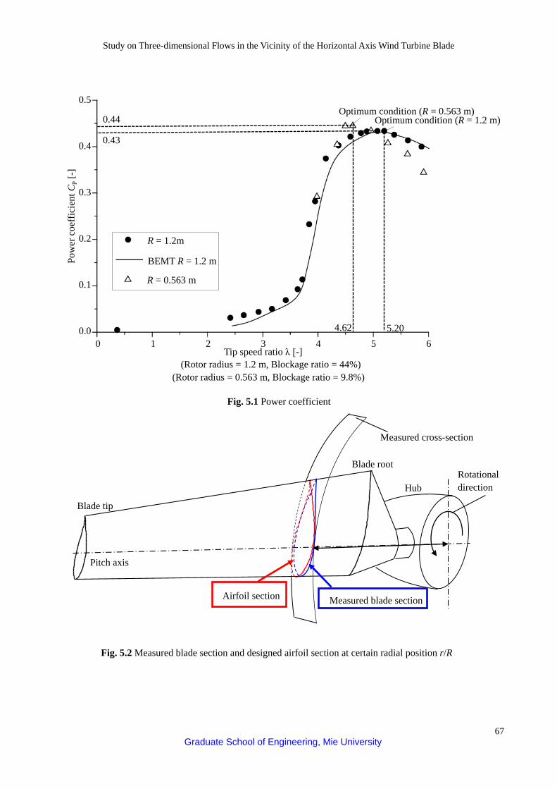
Study on Three-dimensional Flows in the Vicinity of the Horizontal Axis Wind Turbine Blade
67 Graduate School of Engineering, Mie University
Tip speed ratio λ [-] (Rotor radius = 1.2 m, Blockage ratio = 44%)
(Rotor radius = 0.563 m, Blockage ratio = 9.8%)
0.5
0.4
0.3
0.2
0.1
0.0
Pow
er c
oeffi
cien
t Cp [
-]
BEMT R = 1.2 m
R = 0.563 m
R = 1.2m
5.20 4.62
Optimum condition (R = 1.2 m) Optimum condition (R = 0.563 m)
0.43
0.44
0 1 2 3 4 5 6
Fig. 5.1 Power coefficient
Measured cross-section
Blade root
Blade tip
Pitch axis
Hub
Airfoil section Measured blade section
Rotational direction
Fig. 5.2 Measured blade section and designed airfoil section at certain radial position r/R

Study on Three-dimensional Flows in the Vicinity of the Horizontal Axis Wind Turbine Blade
68 Graduate School of Engineering, Mie University
Fig. 5.3 Airfoil section and measured blade section (r/R = 0.3)
Z
Y
X
Designed airfoil 2D section Measured blade section
-40
-30
-20
-10
0
10
20
30
40
50
60
70
80
90
100
110
-20 -10 +00 +10 +20 +30
Pitch axis
Mainstream position [mm]
Circ
umfe
rent
ial p
ositi
on [m
m]
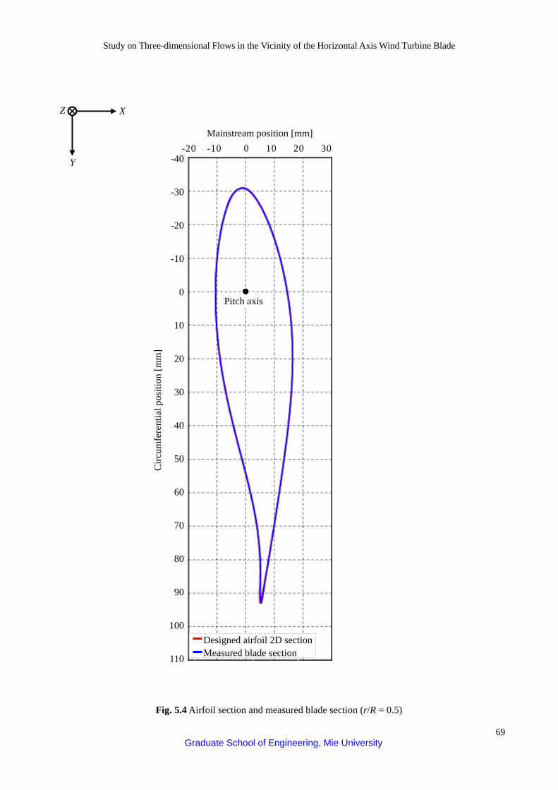
Study on Three-dimensional Flows in the Vicinity of the Horizontal Axis Wind Turbine Blade
69 Graduate School of Engineering, Mie University
Fig. 5.4 Airfoil section and measured blade section (r/R = 0.5)
Z
Y
X
-40
-30
-20
-10
0
10
20
30
40
50
60
70
80
90
100
110
-20 -10 +00 +10 +20 +30
Designed airfoil 2D section Measured blade section
Pitch axis
Mainstream position [mm]
Circ
umfe
rent
ial p
ositi
on [m
m]
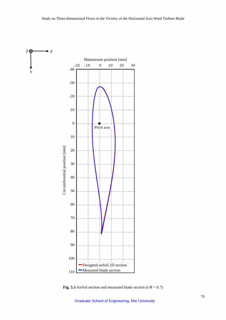
Study on Three-dimensional Flows in the Vicinity of the Horizontal Axis Wind Turbine Blade
70 Graduate School of Engineering, Mie University
Z
Y
X
Fig. 5.5 Airfoil section and measured blade section (r/R = 0.7)
Designed airfoil 2D section Measured blade section
-40
-30
-20
-10
0
10
20
30
40
50
60
70
80
90
100
110
-20 -10 +00 +10 +20 +30
Pitch axis
Mainstream position [mm] C
ircum
fere
ntia
l pos
ition
[mm
]
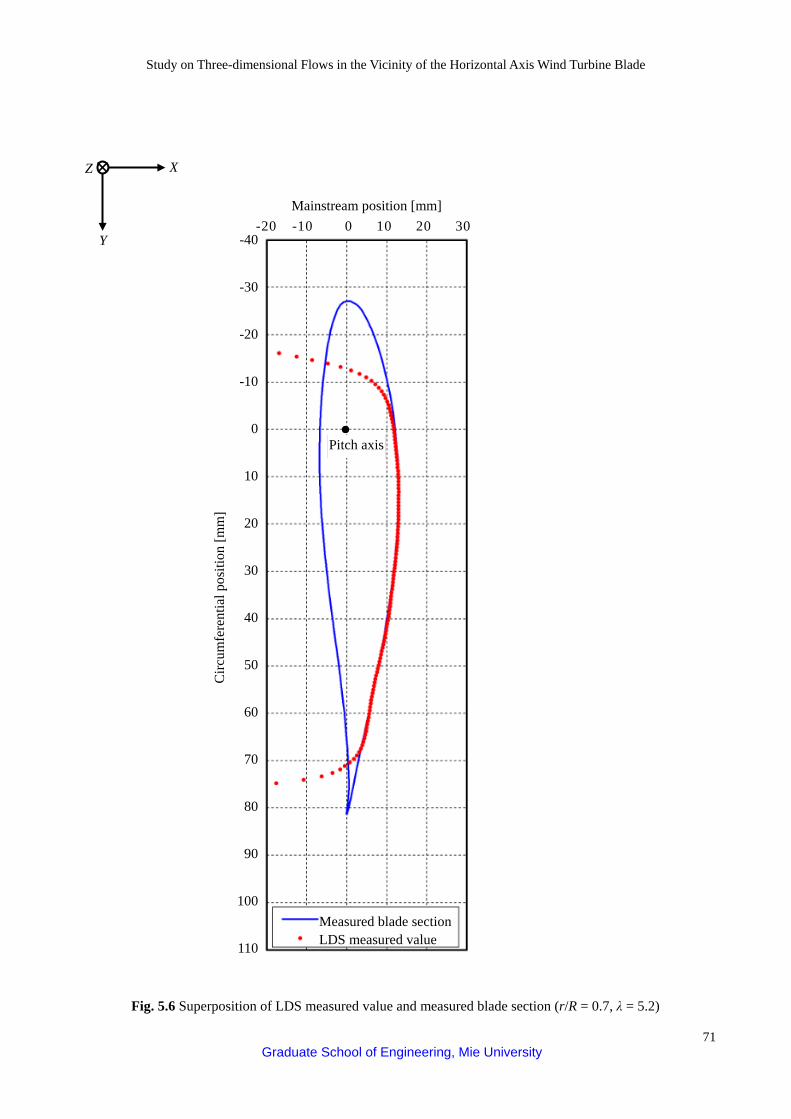
Study on Three-dimensional Flows in the Vicinity of the Horizontal Axis Wind Turbine Blade
71 Graduate School of Engineering, Mie University
Fig. 5.6 Superposition of LDS measured value and measured blade section (r/R = 0.7, λ = 5.2)
Z
Y
X
Measured blade section LDS measured value
-40
-30
-20
-10
0
10
20
30
40
50
60
70
80
90
100
110
-20 -10 +00 +10 +20 +30
Pitch axis
Mainstream position [mm] C
ircum
fere
ntia
l pos
ition
[mm
]
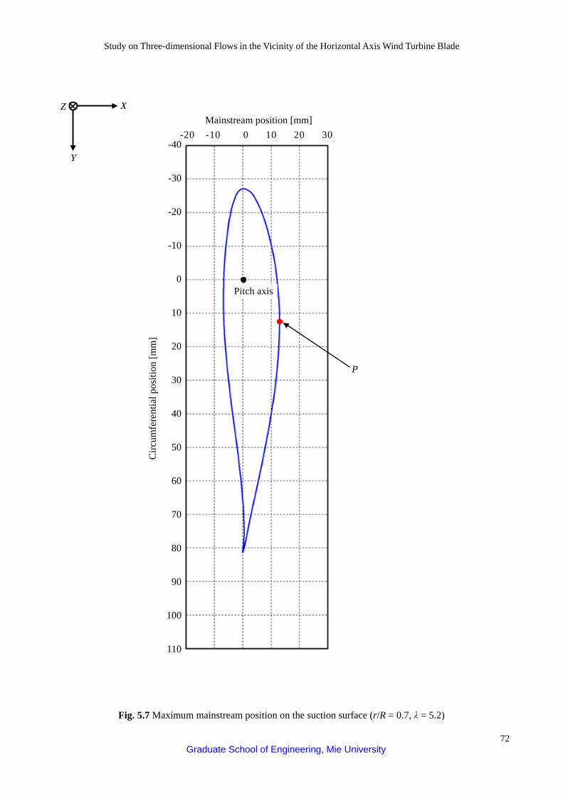
Study on Three-dimensional Flows in the Vicinity of the Horizontal Axis Wind Turbine Blade
72 Graduate School of Engineering, Mie University
Circ
umfe
rent
ial p
ositi
on [m
m]
-40
-30
-20
-10
0
10
20
30
40
50
60
70
80
90
100
110
-20 -10 +00 +10 +20 +30
Pitch axis
Mainstream position [mm]
P
Z
Y
X
Fig. 5.7 Maximum mainstream position on the suction surface (r/R = 0.7, λ = 5.2)

Study on Three-dimensional Flows in the Vicinity of the Horizontal Axis Wind Turbine Blade
73 Graduate School of Engineering, Mie University
Circ
umfe
rent
ial p
ositi
on [m
m]
-40
-30
-20
-10
0
10
20
30
40
50
60
70
80
90
100
110
-20 -10 +00 +10 +20 +30
Pitch axis
Mainstream position [mm]
Q
Z
Y
X
Fig. 5.8 Maximum mainstream position for the LDS measurement (r/R = 0.7, λ = 5.2)
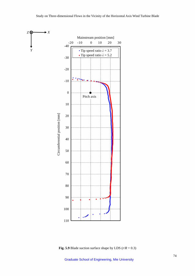
Study on Three-dimensional Flows in the Vicinity of the Horizontal Axis Wind Turbine Blade
74 Graduate School of Engineering, Mie University
Z
Y
X
Fig. 5.9 Blade suction surface shape by LDS (r/R = 0.3)
Tip speed ratio λ = 3.7 Tip speed ratio λ = 5.2
-40
-30
-20
-10
0
10
20
30
40
50
60
70
80
90
100
110
-20 -10 +00 +10 +20 +30
Pitch axis
Mainstream position [mm]
Circ
umfe
rent
ial p
ositi
on [m
m]
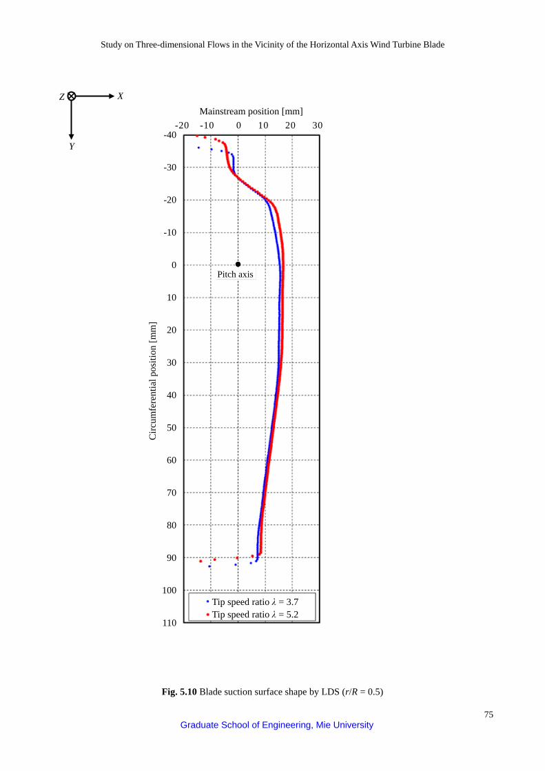
Study on Three-dimensional Flows in the Vicinity of the Horizontal Axis Wind Turbine Blade
75 Graduate School of Engineering, Mie University
Z
Y
X
Fig. 5.10 Blade suction surface shape by LDS (r/R = 0.5)
Tip speed ratio λ = 3.7 Tip speed ratio λ = 5.2
-40
-30
-20
-10
0
10
20
30
40
50
60
70
80
90
100
110
-20 -10 +00 +10 +20 +30
Pitch axis
Mainstream position [mm]
Circ
umfe
rent
ial p
ositi
on [m
m]

Study on Three-dimensional Flows in the Vicinity of the Horizontal Axis Wind Turbine Blade
76 Graduate School of Engineering, Mie University
Z
Y
X
Fig. 5.11 Blade suction surface shape by LDS (r/R = 0.7)
Tip speed ratio λ = 3.7 Tip speed ratio λ = 5.2
-40
-30
-20
-10
0
10
20
30
40
50
60
70
80
90
100
110
-20 -10 +00 +10 +20 +30
Pitch axis
Mainstream position [mm]
Circ
umfe
rent
ial p
ositi
on [m
m]
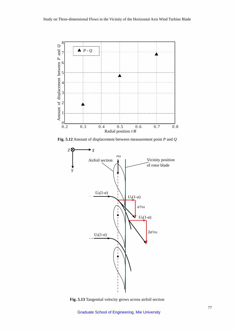
Study on Three-dimensional Flows in the Vicinity of the Horizontal Axis Wind Turbine Blade
77 Graduate School of Engineering, Mie University
8
7
6
5
4
3
2
1
0 0.2 0 .3 0 .4 0 .5 0 .6 0 .7 0 .8
Am
ount
of
disp
lace
men
t be
twee
n P
and
Q
Radial position r/R
P - Q
U0(1-a)
a'rω
rω
U0(1-a)
U0(1-a) 2a'rω
U0(1-a)
Airfoil section Vicinity position of rotor blade
Z
Y
X
Fig. 5.13 Tangential velocity grows across airfoil section
Fig. 5.12 Amount of displacement between measurement point P and Q
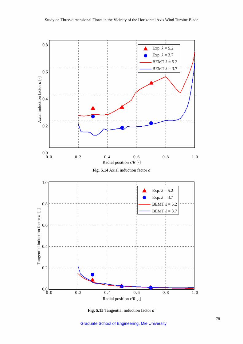
Study on Three-dimensional Flows in the Vicinity of the Horizontal Axis Wind Turbine Blade
78 Graduate School of Engineering, Mie University
Fig. 5.15 Tangential induction factor a'
Fig. 5.14 Axial induction factor a
Exp. λ = 5.2 Exp. λ = 3.7 BEMT λ = 5.2 BEMT λ = 3.7
0 .0 0 .2 0 .4 0 .6 0 .8 1 .0
0.8
0.6
0.4
0.2
0.0
Axi
al in
duct
ion
fact
or a
[-]
Radial position r/R [-]
Exp. λ = 5.2 Exp. λ = 3.7 BEMT λ = 5.2 BEMT λ = 3.7
0 .0 0 .2 0 .4 0 .6 0 .8 1 .0
1.0
0.8
0.6
0.4
0.2
0.0
Tang
entia
l ind
uctio
n fa
ctor
a' [
-]
Radial position r/R [-]

Study on Three-dimensional Flows in the Vicinity of the Horizontal Axis Wind Turbine Blade
79 Graduate School of Engineering, Mie University
Fig. 5.17 Angle of attack α
X
Y Z
(1-a)U0 Surface of rotation
Chord line Blade section
(1+a')Ωr
α θtwist+β
Uref
Fig. 5. 16 Velocity diagram
Exp. λ = 5.2
Exp. λ = 3.7
BEMT λ = 5.2
BEMT λ = 3.7
0 .0 0 .2 0 .4 0 .6 0 .8 1 .0
35
30
25
20
15
10
5
0
Ang
le o
f atta
ck α
[°]
Radial position r/R [-]
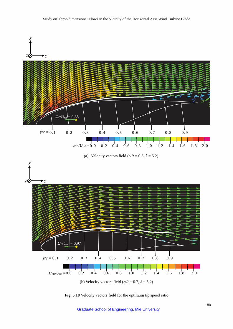
Study on Three-dimensional Flows in the Vicinity of the Horizontal Axis Wind Turbine Blade
80 Graduate School of Engineering, Mie University
Y
Z
X
(a) Velocity vectors field (r/R = 0.3, λ = 5.2)
U2D/Uref = 0.0 0 .2 0 .4 0 .6 0 .8 1 .0 1 .2 1 .4 1 .6 1 .8 2 .0
0 .1 0 .2 0 .3 0 .4 0 .5 0 .6 0 .7 0 .8 0 .9 y/c =
Ωr/Uref = 0.85
Fig. 5.18 Velocity vectors field for the optimum tip speed ratio
Y
Z
X
(b) Velocity vectors field (r/R = 0.7, λ = 5.2)
U2D/Uref =
y/c = 0 . 1 0 . 2 0 . 3 0 . 4 0 . 5 0 . 6 0 . 7 0 . 8 0 . 9
Ωr/Uref = 0.97
0.0 0.2 0.4 0.6 0.8 1.0 1.2 1.4 1.6 1.8 2.0

Study on Three-dimensional Flows in the Vicinity of the Horizontal Axis Wind Turbine Blade
81 Graduate School of Engineering, Mie University
(a) Span-wise velocity contour (r/R = 0.3, λ = 5.2)
y/c = 0 .1 0 .2 0 .3 0 .4 0 .5 0 .6 0 .7 0 .8 0 . 9
Ωr/Uref = 0.85
w0/Uref =
(b) Span-wise velocity contour (r/R = 0.7, λ = 5.2)
w0/Uref =
y/c = 0 .1 0 .2 0 .3 0 .4 0 .5 0 .6 0 .7 0 .8 0 .9
Ωr/Uref = 0.97
Y
Z
X
Fig. 5.19 Span-wise velocity contour for the optimum tip speed ratio
Y
Z
X
-0.03 +0.00 +0.03 +0.06 +0.09 +0.12 +0.15 +0.18
-0 .03 +0 .00 +0 .03 +0 .06 +0 .09 +0 .12 +0 .15 +0 .18

Study on Three-dimensional Flows in the Vicinity of the Horizontal Axis Wind Turbine Blade
82 Graduate School of Engineering, Mie University
Y
Z
X
(a) Velocity vectors field (r/R = 0.3, λ = 3.7)
U2D/Uref = 0.0 0.2 0.4 0.6 0.8 1.0 1.2 1.4 1.6 1.8 2.0
y/c = 0.1 0.2 0.3 0.4 0.5 0.6 0.7 0.8 0.9
Ωr/Uref = 0.75
Y
Z
X
(b) Velocity vectors field (r/R = 0.7, λ = 3.7)
U2D/Uref = 0 . 0 0 . 2 0 . 4 0 . 6 0 . 8 1 . 0 1 . 2 1 . 4 1 . 6 1 . 8 2 . 0
y/c = 0.1 0.2 0.3 0.4 0.5 0.6 0.7 0.8 0.9
Ωr/Uref = 0.93
Fig. 5.20 Velocity vectors field for the low tip speed ratio

Study on Three-dimensional Flows in the Vicinity of the Horizontal Axis Wind Turbine Blade
83 Graduate School of Engineering, Mie University
Ωr/Uref = 0.75
w0/Uref = -0.03 +0.00 +0.03 +0.06 +0.09 +0.12 +0.15 +0.18
0.1 0.2 0.3 0.4 0.5 0.6 0.7 0.8 0.9
(a) Span-wise velocity contour (r/R = 0.3, λ = 3.7)
y/c =
Y
Z
X
(b) Span-wise velocity contour (r/R = 0.7, λ = 3.7)
w0/Uref =
y/c= 0.1 0.2 0.3 0.4 0.5 0.6 0.7 0.8 0.9
Ωr/Uref = 0.93
Y
Z
X
Fig. 5.21 Span-wise velocity contour for the low tip speed ratio
-0.03 +0.00 +0.03 +0.06 +0.09 +0.12 +0.15 +0.18

Study on Three-dimensional Flows in the Vicinity of the Horizontal Axis Wind Turbine Blade
84 Graduate School of Engineering, Mie University
Fig. 5.22 Pressure coefficient for the optimum tip speed ratio
Chord position y/c [-]
Cp_LDV
Cp_tap
Cp_Xfoil
0.0 0.1 0.2 0.3 0.4 0.5 0.6 0.7 0.8 0.9 1.0
-4.0
-3.0
-2.0
-1.0
0.0
1.0
2.0
Pres
sure
coe
ffici
ent C
p_ta
p, C
p_LD
V a
nd C
p_BE
MT
[-]
(b) Pressure distribution (r/R = 0.7, λ = 5.2)
0.0 0.1 0.2 0.3 0.4 0.5 0.6 0.7 0.8 0.9 1.0
-4.0
-3.0
-2.0
-1.0
0.0
1.0
2.0
Cp_LDV
Cp_tap
Cp_Xfoil
Pres
sure
coe
ffici
ent C
p_ta
p, C
p_LD
V a
nd C
p_BE
MT
[-]
Chord position y/c [-]
(a) Pressure distribution (r/R = 0.3, λ = 5.2)

Study on Three-dimensional Flows in the Vicinity of the Horizontal Axis Wind Turbine Blade
85 Graduate School of Engineering, Mie University
4.00
3.00
2.00
1.00
0.00
2.50
2.25
2.00
1.75
1.50
Chord position y/c [-]
Shap
e Fa
ctor
H [-
]
Dis
plac
emen
t thi
ckne
ss δ
* [m
m]
Mom
entu
m th
ickn
ess θ
[mm
]
0 .2 0 .4 0 .6 0 .8 1 .0
(a) Boundary layer (r/R = 0.3, λ = 5.2)
Chord position y/c [-]
Dis
plac
emen
t thi
ckne
ss δ
* [m
m]
Mom
entu
m th
ickn
ess θ
[mm
]
Shap
e Fa
ctor
H [-
]
3.00
2.50
2.00
1.50 0.2 0 .4 0 .6 0 .8 1 .0
(b) Boundary layer (r/R = 0.7, λ = 5.2)
3.00
2.00
1.00
0.00
Fig. 5.23 Boundary layer for the optimum tip speed ratio
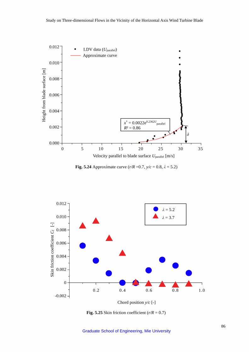
Study on Three-dimensional Flows in the Vicinity of the Horizontal Axis Wind Turbine Blade
86 Graduate School of Engineering, Mie University
Fig. 5.25 Skin friction coefficient (r/R = 0.7)
0.012
0.010
0.008
0.006
0.004
0.002
0
-0.002 Chord position y/c [-]
Skin
fric
tion
coef
ficie
nt C
f [
-]
0 .2 0.4 0.6 0.8 1.0
λ = 5.2 λ = 3.7
δ
0 5 10 15 20 25 30 35 Velocity parallel to blade surface Uparallel [m/s]
Hei
ght f
rom
bla
de su
rfac
e [m
]
0.012
0.010
0.008
0.006
0.004
0.002
0.000
LDV data (Uparallel) Approximate curve
Fig. 5.24 Approximate curve (r/R =0.7, y/c = 0.8, λ = 5.2)
x* = 0.0022e0.2362Uparallel
R² = 0.86

Study on Three-dimensional Flows in the Vicinity of the Horizontal Axis Wind Turbine Blade
87 Graduate School of Engineering, Mie University
225 240 255 270 285 300 315
40
35
30
25
20
15
10
5
0
λ= 5.2 λ= 3.7
Tang
entia
l vel
ocity
v [m
/s]
Azimuth angle ψ [°]
Fig. 5.27 Tangential velocities in the axial direction (x/R = 0.0285, r/R = 0.7)
Fig. 5.26 Control volume around the blade section
Axi
al d
irect
ion
Measuring point for calculating the bound circulation
Azimuth direction
∆x

Study on Three-dimensional Flows in the Vicinity of the Horizontal Axis Wind Turbine Blade
88 Graduate School of Engineering, Mie University
Non
dim
ensi
onal
circ
ulat
ion
Γ/U
0R [-
]
Experiment (λ=5.2) BEMT (λ=5.2)
Experiment (λ=3.7)
0.25
0.20
0.15
0.10
0.05
0 0.0 0.1 0.2 0.3 0.4 0.5 0.6 0.7 0.8 0.9 1.0 Radial position r/R [-]
Fig. 5.28 Circulation along the blade span

Study on Three-dimensional Flows in the Vicinity of the Horizontal Axis Wind Turbine Blade
89 Graduate School of Engineering, Mie University
0.1 0.2 0.3 0.4 0.5 0.6 0.7 0.8 0.9
δ
Y
Z
Y
Z
X
y/c =
1.00
0.00
0.25
Fig. 5.29 Three-dimensional flow trajectory on the rotor blade surface (r/R = 0.3, λ = 5.2)
Chord station y/c [-]
(a) Flow trajectory on the XY plane (r/R = 0.3, λ = 5.2)
(b) Flow trajectory on the YZ plane (r/R = 0.3, λ = 5.2)
1 0( )X t
Pitch Axis
0.25 0.30 0.35
Leading Edge
Trailing Edge
4 0( )X t
2 0( )X t
3 0( )X t
1( )X t
2 ( )X t
3 ( )X t
4 ( )X t
2 ( )X t
Measured blade section
1( )X t
2 0( )X t
1 0( )X t
X

Study on Three-dimensional Flows in the Vicinity of the Horizontal Axis Wind Turbine Blade
90 Graduate School of Engineering, Mie University
δ
Y
Z
X
Y
Z
X
(a) Flow trajectory on the XY plane (r/R = 0.7, λ = 5.2)
Chord station y/c [-] 0.1 0 .2 0 .3 0.4 0.5 0 .6 0 .7 0 .8 0.9 y/c=
Measured blade section
Fig. 5.30 Three-dimensional flow trajectory on the rotor blade surface (r/R = 0.7, λ = 5.2)
(b) Flow trajectory on the YZ plane (r/R = 0.7, λ = 5.2)
1.00
0.00
0.25 Pitch Axis
0.65 0.70 0.75
Leading Edge
Trailing Edge
8 0( )X t
6 0( )X t
5 0( )X t 7 0( )X t
8 ( )X t
6 ( )X t
5 ( )X t
7 ( )X t
5 0( )X t
6 0( )X t
6 ( )X t 5 ( )X t
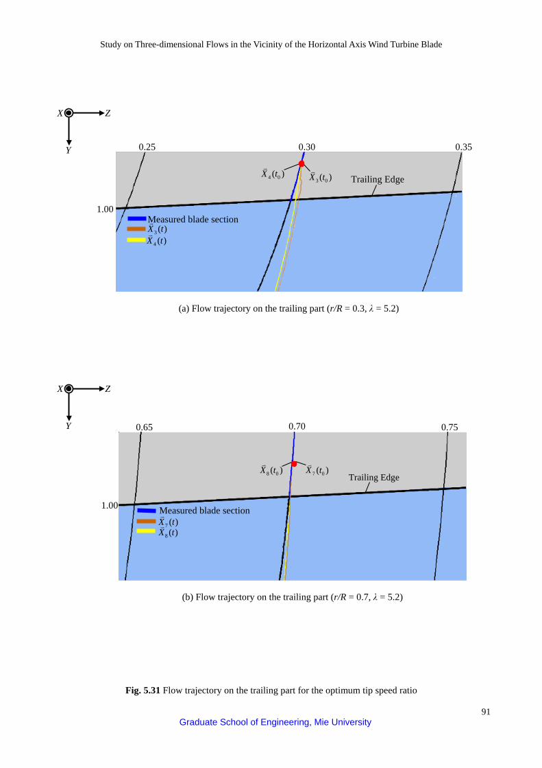
Study on Three-dimensional Flows in the Vicinity of the Horizontal Axis Wind Turbine Blade
91 Graduate School of Engineering, Mie University
Trailing Edge
0.25 0.30 0.35
1.00
Measured blade section
1.00 Measured blade section
Trailing Edge
0.65 0.70 0.75
Y
Z
X
Y
Z
X
Fig. 5.31 Flow trajectory on the trailing part for the optimum tip speed ratio
(a) Flow trajectory on the trailing part (r/R = 0.3, λ = 5.2)
(b) Flow trajectory on the trailing part (r/R = 0.7, λ = 5.2)
8 0( )X t
4 0( )X t
3 0( )X t
3 ( )X t
4 ( )X t
7 0( )X t
8 ( )X t7 ( )X t

Study on Three-dimensional Flows in the Vicinity of the Horizontal Axis Wind Turbine Blade
92 Graduate School of Engineering, Mie University
Chapter 6 Conclusion
This dissertation attempted to study the span-wise flow effects on the rotating blade of the horizontal axis wind turbine. The general blade design by BEMT bases on a sectional airfoil performance in the two-dimensional flow without any span-wise flow. The power prediction of the HAWT neglects the aerodynamic interactions between span-wise positions. The predicted power output does not agree with the measured one due to the span-wise flow effects on the rotating blade. The actual rotating blades have the span-wise flow on the blade surface by the centrifugal force in the boundary layer.
For the further improvement of the rotor blade design, it is necessary to clarify the surface flow on the blade surface which includes the span-wise flow effect. In this study, the surface flow velocities were detected through Laser Doppler Velocimetry (LDV) system in the wind tunnel. In this dissertation, a new approach of simultaneously measuring three-dimensional velocity components by the LDV system was implemented to maximize the spatial resolution of the measurements. Two LDV probes were set in both horizontal and vertical directions for a measuring volume. Consequently, the measuring volume was limited in the crossing point of three pair laser beams. The three-dimensional velocity was detected concurrently by single seeding particle. Based on the experimental analysis, the following conclusion can be obtained: I. Power curve of the test HAWT
This test wind turbine rotor shows almost similar power curve with other small wind turbine rotor. The power curve of test wind turbine rotor shows accuracy data, and the blockage ratio does not make an effect on this wind turbine performance.
II. Three-dimensional flow characteristics on the blade sections 1) The two-dimensional relative flow (U2D/Uref) for inboard is higher than outboard at the leading part. 2) The span-wise flow (w0/Uref) inside boundary layer is high positive at the trailing part. 3) The span-wise flow (w0/Uref) is a little at the leading edge and increases rapidly when approaching the
trailing edge. III. Pressure distribution on the blade sections
1) The rotational effects are high influence on the inboard such as delayed transition point and pressure distribution pattern changes.
2) The rotational effects take less impact on the outboard.
IV. Angle of attack 1) The attack angle for low tip speed ratio is higher than that of optimum tip speed ratio due to stall
phenomena. 2) The measured attack angle at outboard agrees with BEMT prediction as well. However, the attack angle
at inboard is more different due to three-dimensional complicated flow.
V. Boundary layer 1) The transition point for blade root section delays due to span-wise flow effect. 2) The shape factor increasing from the middle chord position to the trailing edge has been influenced by an
adverse pressure gradient on the blade surface.

Study on Three-dimensional Flows in the Vicinity of the Horizontal Axis Wind Turbine Blade
93 Graduate School of Engineering, Mie University
VI. Viscous effects on the blade sections 1) The skin friction for low tip speed ratio is higher than that of optimum tip speed ratio due to strong shear
near surface. 2) Negative skin friction is occurred due to reversed flow on the blade surface.
VII. Circulation on the blade sections
1) The measured circulation for optimum tip speed ratio increases with increase of radial position. 2) The circulation for optimum tip speed ratio is higher than that of low tip speed ratio except near the blade
root. VIII. Three-dimensional flow trajectory on the blade sections
1) The span-wise flow does not affect the flow trajectory on the suction surface from leading edge to pitch axis (0 < y/c < 0.25).
2) The span-wise flow affects the flow trajectory from pitch axis to trading edge (y/c > 0.25). 3) There is a greater deviation of the flow trajectory at inboard from two dimensional flow assumption.

Study on Three-dimensional Flows in the Vicinity of the Horizontal Axis Wind Turbine Blade
94 Graduate School of Engineering, Mie University
Acknowledgments
I compare Ph.D. work to a journey. As in many journeys, you do not travel alone. There have been many stories throughout the three years that I have worked on this Ph.D. My Ph.D. dissertation would not have been possible without the support and help I've received.
First of all, I would like to give a big thank you to those persons who gave me the greatest love in the world, my family: my father Phachern PHENGPOM, my mother Ratchanee PHENGPOM, and my younger brother Sittichai PHENGPOM. They have given me everything. It was their encouragement and support that made all of my accomplishments throughout life possible. This Ph.D. is theirs as much as it is mine. They have created a solid family and given me life values that I will cherish forever.
I would like to express my heartfelt thanks to my associate professor, Yasunari KAMADA, my supervisor, who helped me to come back to Japan, who always walked beside me when I needed some advice, and who has walked me through all the stages of the writing of this dissertation. This dissertation would not have been possible without his good suggestions, insightful advice, and professional guidance. I would like to express my heartfelt thanks to Professor Takao MAEDA for the guidance and invaluable advice given to me during my research. I also would like to thank my assistant Professor Dr. Junsuke MURATA, who always provides valuable assistance.
Specifically, I would like to thank Profs. Koichi TSUJIMOTO and Masafumi HIROTA for their kind review of my dissertation.
I also would like to say thanks and express the pleasure of working with a great group of individuals in the Energy - environment engineering laboratory (ENEKAN). In addition, my sincere appreciation also goes to my team members: Yosuke KAGISAKI, Nishimura SHOGO, Tasuku MATSUNO, Noriaki SUGIMOTO and Yutaro TOTSUKA for your helpful assistance during the experiment.
Thanks to all those not mentioned here but who have made this Ph.D. a reality. Thank you for all you have done for me. I will never forget those who helped me. Thank you to those who will be reading about my work; I hope that you will enjoy reading it as much as I enjoyed writing it.
Tinnapob PHENGPOM March 2016
Study on Three-dimensional Flows in the Vicinity of the Horizontal Axis Wind Turbine Blade
95 Graduate School of Engineering, Mie University
References
[1] CO2now, http://co2now.org/current-co2/co2-now/, Access 2015. 09. 8. [2] Renewable Energy Policy Network for the 21st Century (REN21)-Renewables Global Status Report,
http://www.ren21.net/wp-content/uploads/2015/07/REN12-GSR2015_Onlinebook_low1.pdf, Access 2015. 09. 8. [3] National Renewable Energy Laboratory (NREL), www.nrel.gov/docs/fy09osti/42864.pdf, Access 2015. 09. 8. [4] König, F.v., Windenergie in praktischer Nutzung, Udo Pfriemer Verlag, Munich, (1978). [5] Fröde, E.u.F., Windmühlen, Du Mont Buchverlag, Cologne, (1981). [6] Musgrove, P., Wind Power, Cambridge University Press, Cambridge, (2010). [7] Putnam, G.C., Power from the Wind, Van Nostrand Rheinhold, New York, (1948). [8] MHI Vestas Offshore Wind A/S, http://www.mhivestasoffshore.com/v164-8-0-mw-breaks-world-record-for-wind-
energy-production/, Access 2015. 09. 8. [9] MHI Vestas Offshore Wind A/S, http://www.mhivestasoffshore.com/mhi-vestas-offshore-wind-receives-
breakthrough-first-order-for-the-v164-8-0-mw/, Access 2015. 09. 8. [10] GWEC Global Wind Outlook 2013, http://www.gwec.net/wp-content/uploads/2015/03/GWEC_Global_ Wind_
2014_Report_LR.pdf, Access 2015. 09. 8. [11] EWEA, http://www.linkedin.com/groups?gid=2391932, Access 2015. 09. 8. [12] Statistics bureau, http://www.stat.go.jp/data/jinsui/new.htm, Access 2015. 09. 8. [13] Japan Wind Power Association, http://jwpa.jp/index_e.html, Access 2015. 09. 8. [14] Tanabe, N., Japan's First Floating Offshore Wind Power Project Making Progress, Addressing Challenge. JFS
Newsletter No.138, p.6, March 4, 2014. [15] Japan Meteorological Agency, http://www.jma.go.jp/en/amedas/000.html?elementCode=1, Access 2015. 09. 8. [16] Japan Plans Floating Wind Power Plant, Breakbulk 2011-09-16, Retrieved 2011-10-12. [17] Project tests viability of offshore floating wind turbines, Japan Times. 4 April 2013, retrieved 2013-4-30. [18] Japan Wind Power Association, http://jwpa.jp/pdf/JapanWindPowerInstallation2014.pdf, Access 2015. 09. 8. [19] Maeda, T., Kamada, Y., Murata, J., Li, Q.A., Kawabata, T. and Kogaki, T., Measurements of flow field and pressure
distribution of straight-bladed vertical axis wind turbine, Proc. European Wind Energy Association Conference and Exhibition, 8p, Vienna, Austria, (2013).
[20] Li, Q.A., Maeda, T., Kamada,Y., Murata, J., Kawabata, T., Furukawa K. and Kogaki T., Study on power performance for straight-bladed vertical axis wind turbine by field experiment and wind tunnel, Proceedings of 5th Asian Joint Workshop on Thermophysics and Fluid Science, Paper No. JP03, (2014).
[21] Miller, R.H., The aerodynamics and dynamic analysis of horizontal axis wind turbines, J Wind Eng Ind Aerodyn, Vol.15, pp.329–340, (1983).
[22] Bak, C. and Fuglsang, P., Modification of the NACA 622-415 leading edge for better aerodynamic performance, J Sol Energy Eng, Vol.124, pp.327–34, (2002).
[23] Schreck. S. and Robinson., M., Rotational augmentation of horizontal axis wind turbine blade aerodynamics response, J Wind Eng, Vol.5, pp.133–150. (2002).
[24] Mayda, E.A. and Van Dam, C.P., Bubble-induced unsteadiness on a wind turbine airfoil, J Sol Energy Eng, Vol.124, pp.335-344. (2002).
[25] Ammara. I., Leclerc, C. and Masson, C., A viscous three-dimensional differential/actuator-disk method for the aerodynamic analysis of wind farms, J Sol Energy Eng, Vol.124, 345–356. (2002).
[26] Zerovos, A., Huberson, S. and Hemon, A., Three-dimensional free wake calculation of wind turbine wakes, J Wind Eng Ind Aerodyn, Vol.27, pp.65–76, (1988).
[27] Ainslie, J.F., Calculating the flow field in the wake of wind turbines, J Wind Eng Ind Aerodyn, Vol.27, pp.213–24, (1988).
[28] Barthelmie, R. and Larsen, G., ENDOW: Efficient Development of Offshore Windfarms, Wind Eng Vol.25, No.5, pp.263–270, (2001).

Study on Three-dimensional Flows in the Vicinity of the Horizontal Axis Wind Turbine Blade
96 Graduate School of Engineering, Mie University
[29] Rados, K., Larsen, G. and Lange, B., Comparison of wake models with data for offshore wind farms, Wind Eng Vol.25, No.5, pp.271–280, (2001).
[30] Hassan, U., Taylor, G.J., Garrad, A.D., The dynamic response of wind turbine operating in a wake flow, J Wind Eng Ind Aerodyn, Vol.27, pp.113–126, (1988).
[31] Abderrazzaq, M.H., Energy production assessment of small wind farms, J Renewable Energy. Vol.29, Issue 15, pp. 2261–2272, (2004).
[32] Bhatt, M.S. and Jothibasu, S., Prediction and enhancement of performance of wind farm in India, J Sci Ind Res, Vol.61, No.12, pp.1056–1062, (2002).
[33] Kelouwani, S. and Agbossou K., Non-linear model identification of wind turbine with a neural network IEEE Trans Energy Convers, Vol.19, Issue 3, pp.607-612, (2004).
[34] Wilson, R.E., Wind-turbine aerodynamics, J Ind Aerodyn, Vol.5, pp.357–372, (1980), [35] Camporeale, S.M., Fortunato B. and Marilli, G., Automatic System for Wind Turbine Testing, Journal of Solar
Energy Engineering, Vol.123, Issue 4, pp.333-338, (2001). [36] Bhatt, T.S. and Kothari, D.P., The evolution of wind power technology a review, IE (I) JID, Vol.84, pp.4–9, (2003). [37] Karaki, S.H., Chedid, R.B. and Ramadan, R., Probabilistic performance assessment of wind energy conversion
systems, IEEE Trans Energy Convers, Vol.14, Issue 2, 217–24, (1999). [38] Bhatti, S.T.S. and Kothari, D.P., Aspects of technological development of wind turbines, J Energy Eng ASCE,
Vol.129, Issue 3, pp.81–95, (2003). [39] Parthan, B.K. and Gebbonn, P.F., Multi megawatt class wind turbines, REDA News, Vol.14, Issue 2, pp.25–28,
(2003). [40] Eize, V., Wind turbine technology trends review, Windpro 2003, pp.23–28, (2003). [41] Simms, D., Schreck, S., Hand, M., and Fingersh, L.J., NREL Unsteady Aerodynamics Experiment in the NASA-
Ames Wind Tunnel: A Comparison of Predictions to Measurements, NREL Tech Report NREL/TP-500-29494, Golden, Colorado, (2001).
[42] van Rooij, R.P.O.M., Timmer W.A. and Bruining A., Determination of The Local Flow Angle on Rotating Blades, Proceedings of the World Wind Energy Conference and Exhibition, 2-6 July 2002, 4p, Berlin, Germany, (2002).
[43] Snel, H., Houwink, R., Bosschers, J., Piers, W.J., van Bussel, G.J.W. and Bruining, A., Sectional Prediction 3D Effects for Stalled Flow on Rotating Blades and Comparison with Measurements, Netherlands Energy Research Foundation ECN, Vol.93, Issue 28, pp.1381-1495, (1993).
[44] Bruining, A., van Bussel, G.J.W., Corten, C.P., and Timmer, W.A., Pressure Distributions from a Wind Turbines Blade: Field Measurements Compared to a 2-dimensional Wind Tunnel Data, DUT-IVW-93065R, Delft University of Technology, (1993).
[45] Laino, D.J., Hansen, A.C. and Minnema, J.E., Validation of the Aerodyn Subroutines Using NREL Unsteady Aerodynamics Experiment Data, Wind Energy, Vol.5, pp.227-244, (2002).
[46] João, P., Monteiro, M.R., Hugh, P. and Jorge, C.A., Wind tunnel testing of a horizontal axis wind turbine rotor and comparison with simulations from two Blade Element Momentum code, Journal of Wind Engineering and Industrial Aerodynamics, Vol.123, No.1, pp.99–106, (2013).
[47] Ronsten, G., Static pressure measurements on a rotating and a non-rotating 2.375 m wind turbine blade. Comparison with 2D calculations, Wind Eng. Ind. Aerodyn., Vol.39, Issues 1-3, pp.105–118, (1992).
[48] Burton, T., Sharpe, D., Jenkins, N. and Bossanyi, E., Wind Energy Handbook, John Wiley and Sons, New York, (2012).
[49] Dua, Z. and Seligb, M. S., The effect of rotation on the boundary layer of a wind turbine blade, Renewable Energy, Vol.20, No.2, pp.167-181, (2000).
[50] Hansen, M., Aerodynamics of wind turbines 2nd edition, James & James, London, (2000). [51] Wood, D.H., Three dimensional analysis of stall delay on a horizontal axis wind turbine, Journal of Wind
Engineering and Industrial Aerodynamics, Vol.37, Issue 1, pp.1–14, (1991). [52] Ronsten, G., Static pressure measurements on a rotating and a non-rotating 2.375 m wind turbine blade. Comparison
with 2D calculations, Wind Eng. Ind. Aerodyn., Vol.39, Issues 1-3, pp.105–118. (1992). [53] Johansen, J., Madsen H., Gaunaa, M. and Bak, C., Design of a wind turbine rotor for maximum aerodynamic
Efficiency, Wind Energy, Vol.12, Issue 3, pp.261-273, (2009). [54] Martínez, G.G., Sørensen, N. J. H. and Shen, Z. W., 3D Boundary layer study on a rotating wind turbine blade,

Study on Three-dimensional Flows in the Vicinity of the Horizontal Axis Wind Turbine Blade
97 Graduate School of Engineering, Mie University
Journal of Physics: Conference Series (Online), Vol.75, No. 012032, pp.1-8, (2007). [55] Micallef, D., van Bussell, G., Ferreira, C.S., and Sant, T., An investigation of radial velocities for a horizontal axis
wind turbine in axial and yawed flows, Wind Energy, Vol.16, Issue 4, pp.529-544, (2013). [56] Suzuki, D., Kamada, Y., Maeda, T., Murata, J., Kagisaki, Y. and Nishimura, S., Experimental study on flow over
surface of horizontal axis wind turbine blades, Proceeding of the 2nd International Symposium for Sustainability by Engineering, pp.163-166, 82012).
[57] Kamada, Y., Phengpom, T., Maeda, T., Murata, J., Kagisaki,Y. and Nishimura, S., LDV measurement of boundary layer on wind turbine blade, Proceedings of the Japan Society of Mechanical Engineers Annual Meeting, Paper No. J056032 (in Japanese), 5p, Okayama, Japan (2013).
[58] Kamada, Y., Phengpom, T., Maeda, T., Murata, J., Kagisaki, Y. and Nishimura, S., Boundary layer study on rotating blade surface of horizontal axis wind turbine blade, Proceedings of the 12th International Symposium on Fluid Control, Measurement and Visualization, Paper No. OS18-03-1, 7p, Nara, japan, (2013).
[59] Okada, N., Study on boundary layer on the blade surface of horizontal axis wind turbine, Master thesis, Mie University, Mie, Japan, (2009). (in Japanese)
[60] Zingg, D.W., An approach to the design of airfoils with high lift to drag ratios, UTIAS, Toronto, (1983). [61] Vermeer, L.J. and van Bussel, G.J.W., Velocity measurements in the near wake of a model rotor and comparison
with theoretical results, Proceedings of 1990 European Community Wind Energy Conference, Madrid, Spain, pp.218–222, (1990).