Time series Report
61
TECHNICAL REPORT 1 A STUDY OF THE INTER-RELATIONSHIP BETWEEN PRICES OF GOLD, SILVER, CRUDE OIL, SENSEX AND EXCHANGE RATE: APPLICATION OF ADVANCED TIME SERIES MODELS ANIL KUMAR GV AND SANTOSH KUMAR REDDY MBA in Food and Dairy Business DEPARTMENT OF DAIRY ECONOMICS AND BUSINESS MANAGEMENT DAIRY SCIENCE COLLEGE, HEBBAL, BANGALORE KARNATAK VETERINARY ANIMAL AND FISHERIES SCIENCES UNIVERSITY, BIDAR AUGUST 2012
Transcript of Time series Report

TECHNICAL REPORT 1
A STUDY OF THE INTER-RELATIONSHIP BETWEEN PRICES OFGOLD, SILVER, CRUDE OIL, SENSEX AND EXCHANGE RATE:
APPLICATION OF ADVANCED TIME SERIES MODELS
ANIL KUMAR GV AND SANTOSH KUMAR REDDYMBA in Food and Dairy Business
DEPARTMENT OF DAIRY ECONOMICS AND BUSINESS MANAGEMENTDAIRY SCIENCE COLLEGE, HEBBAL, BANGALORE
KARNATAK VETERINARY ANIMAL AND FISHERIES SCIENCES UNIVERSITY, BIDAR
AUGUST 2012
FOREWORD
In this report a step by step analysis of selected
commodity prices have been undertaken using advanced time
series models like ARIMA, Transfer function, ARCH/GARCH and
Vector Auto Regressive Models. The report also gives the SAS
codes and SAS output at every step of the analysis. Time
series analysis of commodity prices is important as one wants
to understand its behavior use it for forecasting. There are
four components embedded in a time series model, viz., Trend,
Seasonal, Cyclical and Random variation. The first three are
deterministic and can be easily estimated while the last one
is probabilistic. Once the underlying relationship is
understood, then we can use it for quantifying it and
forecasting the same. This is most relevant in the case of
commodity prices.
The challenge when one study’s commodity price is that it
can vary and these components are dynamic. Thus forecasts and
predictions made out of these series may not hold for all
situations. Further these series may have an underlying
relationship. This is captured through a variety of techniques
in the time series framework. In this study certain price
series which are of macro-economic significance like gold
prices, silver prices, crude oil prices, stock market index
and exchange rate have been modeled and the results are
discussed herein.
Anilkumar G.V and Santosh Kumar Reddy have worked very
hard in preparing this report, which included collection of
data, conceptualization of the methodology, carrying out the

analysis and finally preparing the Report. They gave
demonstrated their ability to carry out a study using
sophisticated analytical techniques. I wish them all success
in all their future endeavours.
Lalith Achoth
Co-ordinator, MBA Programme
MODELLING COMMODITY PRICES: A STUDY OF THE INTER-RELATIONSHIP BETWEEN PRICES OF
GOLD, SILVER, CRUDE OIL AND EXCHANGE RATE:APPLICATION OF ADVANCED TIME SERIES MODELS
ANIL KUMAR G.V AND SANTOSH KUMAR REDDYMBA (FOOD BUSINESS)

DEPARTMENT OF DAIRY ECONOMICS AND BUSINESS MANAGEMENTDairy Science College,
Karnataka Veterinary Animal and Fisheries SciencesUniversity,
Hebbal campus, Bangalore 560 024
August 2012
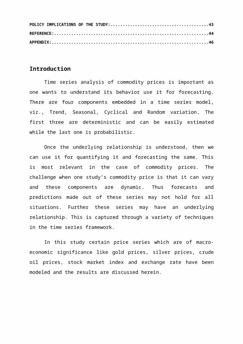
ContentsINTRODUCTION..............................................................5
OBJECTIVE OF THE STUDY:....................................................5GOLD....................................................................5EXCHANGE RATE:............................................................6SILVER PRICES:............................................................6CRUDE OIL:...............................................................7BOMBAY STOCK EXCHANGE INDEX:................................................7
RESULTS AND DISCUSSION....................................................8
TECHNIQUES FOR FORECASTING TIME SERIES DATA OF COMMODITIES.......................8THE ARMA PROCESS IN FORECASTING............................................10STAGES IN ARIMA MODELING..................................................11MODEL IDENTIFICATION......................................................12
Stationarity and Seasonality................................................................................................................ 12Seasonal differencing........................................................................................................................... 12Identifying p and q................................................................................................................................ 13Autocorrelation and Partial Autocorrelation Plots.............................................................................13Order of Autoregressive Process (p).....................................................................................................13Order of Moving Average Process (q)..................................................................................................13Shape of Autocorrelation Function......................................................................................................14
MODEL ESTIMATION:........................................................15Model Validation:.................................................................................................................................. 15
DIAGNOSTIC CHECKING:......................................................19FORECASTING:.............................................................19
Gold:....................................................................................................................................................... 19Silver prices:........................................................................................................................................... 20Crude oil:................................................................................................................................................ 22Exchange Rate:...................................................................................................................................... 23Bombay stock exchange:......................................................................................................................24
TRANSFER FUNCTION........................................................26
EXAMPLE1:...............................................................27EXAMPLE 2:..............................................................29
ARCH AND GARCH...........................................................31
LINEAR GARCH VARIATIONS...................................................32Example for ARCH/ GARCH:.................................................................................................................. 33
VECTOR AUTO REGRESSION MODEL (VAR).......................................38
Example for VARMAX............................................................................................................................. 39
POLICY IMPLICATIONS OF THE STUDY:........................................43
REFERENCE:...............................................................44
APPENDIX:................................................................46
Introduction
Time series analysis of commodity prices is important as
one wants to understand its behavior use it for forecasting.
There are four components embedded in a time series model,
viz., Trend, Seasonal, Cyclical and Random variation. The
first three are deterministic and can be easily estimated
while the last one is probabilistic.
Once the underlying relationship is understood, then we
can use it for quantifying it and forecasting the same. This
is most relevant in the case of commodity prices. The
challenge when one study’s commodity price is that it can vary
and these components are dynamic. Thus forecasts and
predictions made out of these series may not hold for all
situations. Further these series may have an underlying
relationship. This is captured through a variety of techniques
in the time series framework.
In this study certain price series which are of macro-
economic significance like gold prices, silver prices, crude
oil prices, stock market index and exchange rate have been
modeled and the results are discussed herein.

Objective of the study:
1. To identify suitable models for studying the structure of
commodities in general, and gold, silver, nymex and
sensex in particular.
2. To study interrelationships between these series using
sophisticated time series models.
3. Developing and validating forecasting models for
commodities.
Gold: Many researchers believed that gold is the best
preserving purchasing power in the long run. Gold is also
providing high liquidity; it can be exchanged for money
anytime the holders want. Gold investment can also be used as
a hedge against inflation and currency depreciation. However,
in high volatility situation the change in gold price
fluctuation is common. The investors hesitate to execute
decision because only their intuition is not enough and can
lead to loss. To provide better view of gold investment,
forecasting models should be formed to support the decision.
Many researchers suggest that Box-Jenkins’ ARIMA is
the most accurate forecasting model. ARIMA wins over other
models; Holt’s Forecast model and a combination of Box-
Jenkins’ and Holt’s in regression, by providing lowest MAPE
(Mean Absolute Percent Error), (Wararit, 2006) the idea that
Box and Jenkin’s ARIMA model has predictability in Gold Price
is accepted in many countries including India.
Exchange Rate: The exchange rate in India under the
current regime is by and large market determined. Even while

intervening, RBI takes care that through its operation, the
basic market forces are not out of place. The market players,
while always keeping an eye on what could be the possible move
by RBI, broadly agree that the exchange rate moves based on
the demand and supply forces. Therefore, the Indian forex
market could perhaps be studied by the regular supply demand
models of price determination.
Silver prices: Silver is one of the most precious
metals, valued both as a form of currency and store of value.
The major components of silver demand1 are Industrial use
(54%), Photography (15%), Jewellery and Silverware (26%) and
Coins (5%). Twenty countries together produce 96% of the
silver mined globally2. Mexico is the largest producer
followed closely by Peru3. The main consumer countries for
silver are the US, India, Canada, Mexico, UK, France, Germany,
Italy and Japan.
The key factors that affect the volatility of
silver are fluctuating industrial demand and store of value
demand, geo-political uncertainties, rising crude oil prices,
depreciating dollar, government policies on major export and
import destinations, sales by China and other central banks,
direction of gold prices and direction of other commodity
prices.
Crude oil: Economic development closely relates to
energy acquisition, and today, crude oil is the primary energy
source worldwide. Crude oil’s price changes directly influence
the price of commodities worldwide, as well as the economic

growth of every country. Before 1999, oil prices declined only
in times of economic downturn. The price of crude oil,
however, started rising in 2007 and, as a result, global
prices have been rising drastically since then. The price of
oil exceeded $100US per barrel for the first time, in February
2008; it later peaked at $145.66US in July of the same year.
This caused the prices of commodities to rise continuously,
prompting an unstable global economy that showed a downward
trend. However, by
December 2008, the oil price had fallen back to $31.12US
per barrel. Hamilton (2009) explains that the high oil prices
in 2008 were part of a bubble, and that three key variables
were responsible for them in the summer of 2008: oil’s low
price elasticity of demand; the strong growth in demand for
oil from China, the Middle East, and various newly
industrialized nations; and the failure of global oil
production to increase. Today’s international markets and
global economic data suggest the presence of slight inflation
and stagnant growth, and oil prices rose from $84US per barrel
in February 2011 to $98US in November 2011
Bombay stock exchange index: BSE is the world's number 1exchange in the world in terms of the number of listed
companies (over 4900). It is the world's 5th most active in
terms of number of transactions handled through its electronic
trading system. And it is in the top ten of global exchanges
in terms of the market capitalization of its listed companies
(as of December 31, 2009). The companies listed on BSE command
a total market capitalization of USD Trillion 1.28 as of Feb,
2010.
RESULTS AND DISCUSSION
In this project we collected data from different websites. Forthat data we done first
1. Data cleaning techniques like: Sorting, Merging, Findingmissing values, Convert character to numeric.
2. Test data for stationarity.3. ARIMA4. Transfer function5. GARCH and ARCH 6. VARMAX
Techniques for forecasting Time Series data of commodities
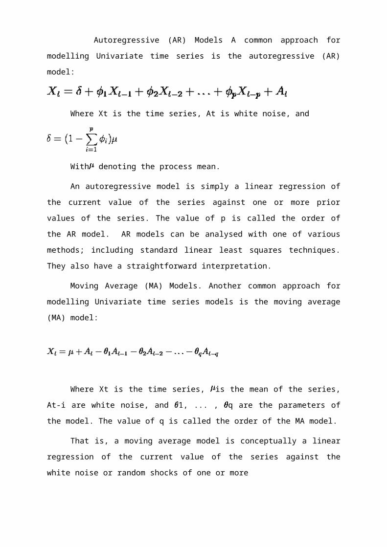
Autoregressive (AR) Models A common approach for
modelling Univariate time series is the autoregressive (AR)
model:
Where Xt is the time series, At is white noise, and
With denoting the process mean.
An autoregressive model is simply a linear regression of
the current value of the series against one or more prior
values of the series. The value of p is called the order of
the AR model. AR models can be analysed with one of various
methods; including standard linear least squares techniques.
They also have a straightforward interpretation.
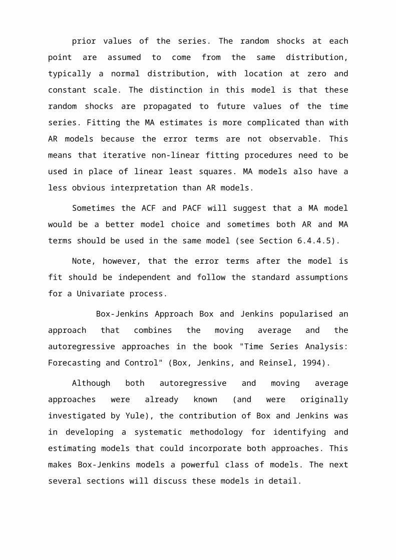
Moving Average (MA) Models. Another common approach for
modelling Univariate time series models is the moving average
(MA) model:
Where Xt is the time series, is the mean of the series,
At-i are white noise, and 1, ... , q are the parameters of
the model. The value of q is called the order of the MA model.
That is, a moving average model is conceptually a linear
regression of the current value of the series against the
white noise or random shocks of one or more
prior values of the series. The random shocks at each
point are assumed to come from the same distribution,
typically a normal distribution, with location at zero and
constant scale. The distinction in this model is that these
random shocks are propagated to future values of the time
series. Fitting the MA estimates is more complicated than with
AR models because the error terms are not observable. This
means that iterative non-linear fitting procedures need to be
used in place of linear least squares. MA models also have a
less obvious interpretation than AR models.
Sometimes the ACF and PACF will suggest that a MA model
would be a better model choice and sometimes both AR and MA
terms should be used in the same model (see Section 6.4.4.5).
Note, however, that the error terms after the model is
fit should be independent and follow the standard assumptions
for a Univariate process.
Box-Jenkins Approach Box and Jenkins popularised an
approach that combines the moving average and the
autoregressive approaches in the book "Time Series Analysis:
Forecasting and Control" (Box, Jenkins, and Reinsel, 1994).
Although both autoregressive and moving average
approaches were already known (and were originally
investigated by Yule), the contribution of Box and Jenkins was
in developing a systematic methodology for identifying and
estimating models that could incorporate both approaches. This
makes Box-Jenkins models a powerful class of models. The next
several sections will discuss these models in detail.

The ARMA Process in Forecasting Box-Jenkins Approach
The Box-Jenkins ARMA model is a combination of the AR andMA models (described on the previous page):
Where the terms in the equation have the same meaning as
given for the AR and MA model.
Comments on Box-Jenkins Model a couple of notes on this model.
1. The Box-Jenkins model assumes that the time series is
stationary. Box and Jenkins recommend differencing non-
stationary series one or more times to achieve
stationarity. Doing so produces an ARIMA model, with the
"I" standing for "Integrated".
2. Some formulations transform the series by subtracting
the mean of the series from each data point. This yields a
series with a mean of zero. Whether you need to do this or not
is dependent on the software you use to estimate the model.
3. Box-Jenkins models can be extended to include seasonal
autoregressive and seasonal moving average terms. Although
this complicates the notation and mathematics of the model,
the underlying concepts for seasonal autoregressive and

seasonal moving average terms are similar to the non-seasonal
autoregressive and moving average terms.
4. the most general Box-Jenkins model includes difference
operators, autoregressive terms, moving average terms,
seasonal difference operators, seasonal autoregressive terms,
and seasonal moving average terms. As with modelling in
general, however, only necessary terms should be included in
the model. Those interested in the mathematical details can
consult Box, Jenkins (1986).
Stages in ARIMA Modeling
There are three primary stages in building a Box-Jenkins
time series model.
1. Model Identification
2. Model Estimation
3. Model Validation
4. Forecasting
The following remarks regarding Box-Jenkins models
should be noted.
a) Box-Jenkins models are quite flexible due to the
inclusion of both autoregressive and moving average terms.
b) Based on the Wold decomposition theorem, a stationary
process can be approximated by an ARMA model. In practice,
finding that approximation may not be easy.
c) Chatfield (1996) recommends decomposition methods for
series in which the trend and seasonal components are
dominant.
d) Building good ARIMA models generally requires more
experience than commonly used statistical methods such as
regression.
e) Sufficiently Long Series required typically,
effective fitting of Box-Jenkins models requires at least a
moderately long series. Chatfield (1996) recommends at least
50 observations. Many others would recommend at least 100
observations.
Model Identification
Stationarity and Seasonality
The first step in developing a Box-Jenkins model is to
determine if the series is stationary and if there is any
significant seasonality that needs to be modelled.
Detecting stationarity
Stationarity can be accessed from a run sequence plot.
The run sequence plot should show constant location and scale.
It can also be detected from an autocorrelation plot.
Specifically, non-stationarity is often indicated by an
autocorrelation plot with very slow decay.
Detecting seasonality
Seasonality (or periodicity) can usually be assessed from
an autocorrelation plot, a seasonal subseries plot, or a
spectral plot. Differencing to achieve stationarity Box and
Jenkins recommend the differencing approach to achieve

stationarity. However, fitting a curve and subtracting the
fitted values from the original data can also be used in the
context of Box-Jenkins models.
Seasonal differencing
At the model identification stage, our goal is to detect
seasonality, if it exists, and to identify the order for the
seasonal autoregressive and seasonal moving average terms. For
many series, the period is known and a single seasonality term
is sufficient. For example, for monthly data we would
typically include either a seasonal AR 12 term or a seasonal
MA 12 term. For Box-Jenkins models, we do not explicitly
remove seasonality before fitting the model. Instead, we
include the order of the seasonal terms in the model
specification to the ARIMA estimation software. However, it
may be helpful to apply a seasonal difference to the data and
regenerate the autocorrelation and partial autocorrelation
plots. This may help in the model identification of the non-
seasonal component of the model. In some cases, the seasonal
differencing may remove most or all of the seasonality effect.
Identifying p and q
Once stationarity and seasonality have been addressed,
the next step is to identify the order (i.e., the p and q) of
the autoregressive and moving average terms.
Autocorrelation and Partial Autocorrelation Plots
The primary tools for doing this are the autocorrelation
plot and the partial autocorrelation plot. The sample
autocorrelation plot and the sample partial autocorrelation
plot are compared to the theoretical behaviour of these plots
when the order is known.
Order of Autoregressive Process (p)
Specifically, for an AR (1) process, the sample
autocorrelation function should have an exponentially
decreasing appearance. However, higher-order AR processes are
often a mixture of exponentially decreasing and damped
sinusoidal components.
For higher-order autoregressive processes, the sample
autocorrelation needs to be supplemented with a partial
autocorrelation plot. The partial autocorrelation of an AR (p)
process becomes zero at lag p+1 and greater, so we examine the
sample partial autocorrelation function to see if there is
evidence of a departure from zero. This is usually determined
by placing a 95% confidence interval on the sample partial
autocorrelation plot (most software programs that generate
sample autocorrelation plots will also plot this confidence
interval). If the software program does not generate the
confidence band, it is approximately, with N denoting the
sample size.
Order of Moving Average Process (q)
The autocorrelation function of a MA (q) process becomes
zero at lag q+1 and greater, so we examine the sample
autocorrelation function to see where it essentially becomes
zero. We do this by placing the 95% confidence interval for
the sample autocorrelation function on the sample
autocorrelation plot. Most software that can generate the
autocorrelation plot can also generate this confidence
interval.
The sample partial autocorrelation function is generally
not helpful for identifying the order of the moving average
process.
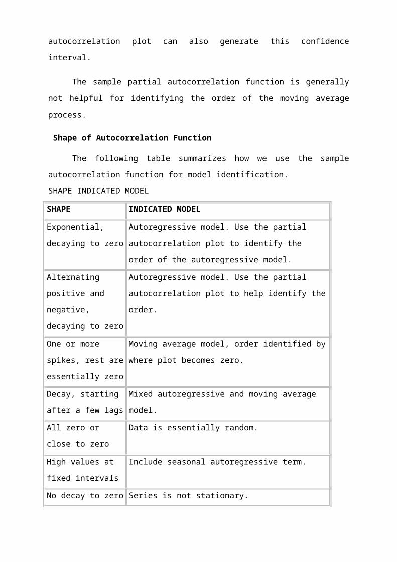
Shape of Autocorrelation Function
The following table summarizes how we use the sample
autocorrelation function for model identification.
SHAPE INDICATED MODEL
SHAPE INDICATED MODEL
Exponential,
decaying to zero
Autoregressive model. Use the partial
autocorrelation plot to identify the
order of the autoregressive model.
Alternating
positive and
negative,
decaying to zero
Autoregressive model. Use the partial
autocorrelation plot to help identify the
order.
One or more
spikes, rest are
essentially zero
Moving average model, order identified by
where plot becomes zero.
Decay, starting
after a few lags
Mixed autoregressive and moving average
model.
All zero or
close to zero
Data is essentially random.
High values at
fixed intervals
Include seasonal autoregressive term.
No decay to zero Series is not stationary.
Mixed models Difficult to Identify. In practice, the
sample autocorrelation and partial autocorrelation functions
are random variables and will not give the same picture as the
theoretical functions. This makes the model identification
more difficult. In particular, mixed models can be
particularly difficult to identify.
Although experience is helpful, developing good models
using these sample plots can involve much trial and error. For
this reason, in recent years information-based criteria such
as FPE (Final Prediction Error) and AIC ( Aikake Information
Criterion) and others have been preferred and used. These
techniques can help automate the model identification process.
These techniques require computer software to use.
Fortunately, these techniques are available in many commercial
statistical software programs that provide ARIMA modelling
capabilities.
Model Estimation:Having tentatively identified the model the next step is
to estimate the parameters of the tentatively identified
model. The parameters are estimated using the maximum
likelihood estimator (MLE).
Model Validation:
Since the model identification is tentative the next step
is to examine whether the tentatively identified is correct or
not. This step is called diagnostic checking. In diagnostic
checking the autocorrelation of the residuals is done to see
whether the residuals of the estimated model are a random
white noise process. This is confirmed if the residuals do not
have any significant autocorrelations or if the Box_Ljung test
which is a test of the overall significance of the
autocorrelation function is non-significant. The Box_Ljung
test follows a chi square test with
(N-p-q) degrees of freedom.
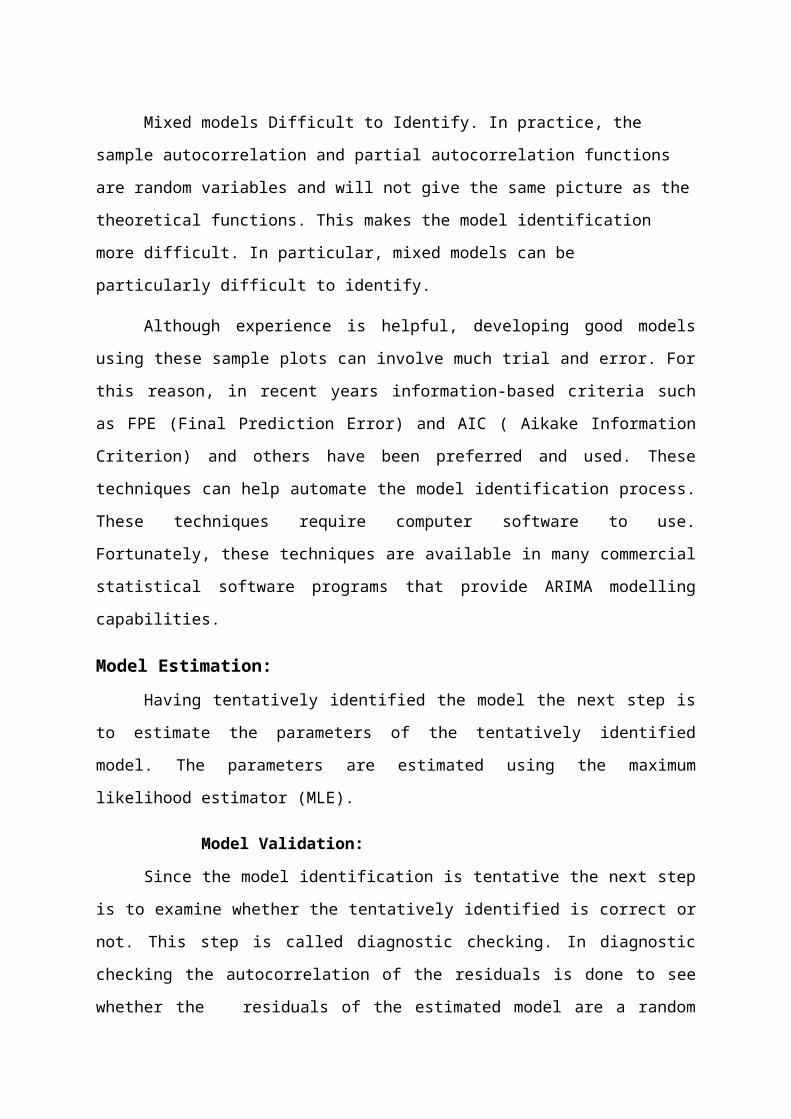
EXAMPLE:
ARIMA model output for gold prices ARIMA method
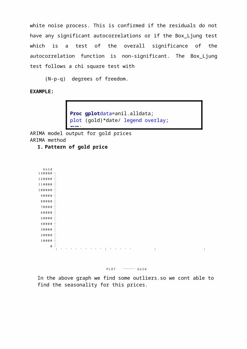
1. Pattern of gold price
P L O T G o l d
G o l d
01 0 0 0 02 0 0 0 03 0 0 0 04 0 0 0 05 0 0 0 06 0 0 0 07 0 0 0 08 0 0 0 09 0 0 0 0
1 0 0 0 0 01 1 0 0 0 01 2 0 0 0 01 3 0 0 0 0
In the above graph we find some outliers.so we cont able to find the seasonality for this prices.
Proc gplotdata=anil.alldata;plot (gold)*date/ legend overlay;run;

After removed the outliers we find the trend in gold prices as shown in below graph.
P L O T G o l d
G o l d
0
1 0 0 0 0
2 0 0 0 0
3 0 0 0 0
4 0 0 0 0
D a t e
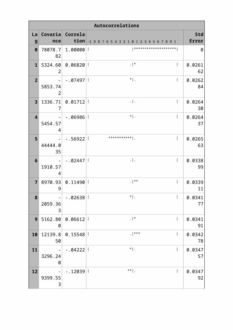
1. Autocorrelation:
AutocorrelationsLag
Covariance
Correlation -1 9 8 7 6 5 4 3 2 1 0 1 2 3 4 5 6 7 8 9 1
StdError
0 78078.782
1.00000 | |********************| 0
1 5324.602
0.06820 | .|* | 0.026162
2 -5853.74
2
-.07497 | *|. | 0.026284
3 1336.717
0.01712 | .|. | 0.026430
4 -5454.57
4
-.06986 | *|. | 0.026437
5 -44444.0
35
-.56922 | ***********|. | 0.026563
6 -1910.57
4
-.02447 | .|. | 0.033899
7 8970.939
0.11490 | .|** | 0.033911
8 -2059.36
3
-.02638 | *|. | 0.034177
9 5162.800
0.06612 | .|* | 0.034191
10 12139.850
0.15548 | .|*** | 0.034278
11 -3296.24
0
-.04222 | *|. | 0.034757
12 -9399.55
3
-.12039 | **|. | 0.034792

AutocorrelationsLag
Covariance
Correlation -1 9 8 7 6 5 4 3 2 1 0 1 2 3 4 5 6 7 8 9 1
StdError
13 3630.489
0.04650 | .|* | 0.035076
14 -958.884
-.01228 | .|. | 0.035119
15 -9864.44
8
-.12634 | ***|. | 0.035122
16 2672.044
0.03422 | .|* | 0.035431
17 8705.872
0.11150 | .|** | 0.035454
18 -3572.31
8
-.04575 | *|. | 0.035693
19 -1709.91
6
-.02190 | .|. | 0.035733
20 3884.195
0.04975 | .|* | 0.035742
21 2237.078
0.02865 | .|* | 0.035790
22 -5149.61
3
-.06595 | *|. | 0.035805
23 4808.076
0.06158 | .|* | 0.035888
24 2652.068
0.03397 | .|* | 0.035961
In the above table we identified a ‘q’ value. In this there are 1,2,5 are significant so that form these values will help for forecasting the future values.
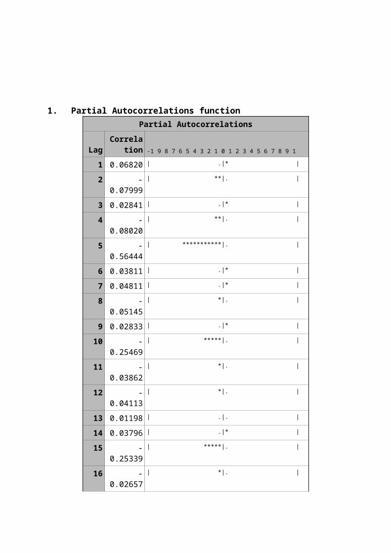
1. Partial Autocorrelations functionPartial Autocorrelations
LagCorrela
tion -1 9 8 7 6 5 4 3 2 1 0 1 2 3 4 5 6 7 8 9 1
1 0.06820 | .|* |
2 -0.07999
| **|. |
3 0.02841 | .|* |
4 -0.08020
| **|. |
5 -0.56444
| ***********|. |
6 0.03811 | .|* |
7 0.04811 | .|* |
8 -0.05145
| *|. |
9 0.02833 | .|* |
10 -0.25469
| *****|. |
11 -0.03862
| *|. |
12 -0.04113
| *|. |
13 0.01198 | .|. |
14 0.03796 | .|* |
15 -0.25339
| *****|. |
16 -0.02657
| *|. |

Partial Autocorrelations
LagCorrela
tion -1 9 8 7 6 5 4 3 2 1 0 1 2 3 4 5 6 7 8 9 1
17 0.03382 | .|* |
18 -0.03253
| *|. |
19 0.01600 | .|. |
20 -0.21152
| ****|. |
21 0.06570 | .|* |
22 0.00916 | .|. |
23 0.02482 | .|. |
24 0.04699 | .|* |
In this table we identified a ‘p’ values. It means partial autocorrelation function values.The p values in this table are p= (1, 5, 10, 15, and 20)
Diagnostic Checking:In the estimation and diagnostic checking stage, we can use
the ESTIMATE statement to specify the ARIMA model to fit to
the variable specified in the previous IDENTIFY statement, and
to estimate the parameters of that model. The ESTIMATE
statement also produces diagnostic statistics to help you
judge the adequacy of the model.
Significance tests for parameter estimates indicate whether
some terms in the model may be unnecessary. Goodness-of-fit
statistics aid in comparing this model to others. Tests for
white noise residuals indicate whether the residual series
contains additional information that might be utilized by a
more complex model. If the diagnostic tests indicate problems
with the model, you try another model, then repeat the
estimation and diagnostic checking stage.
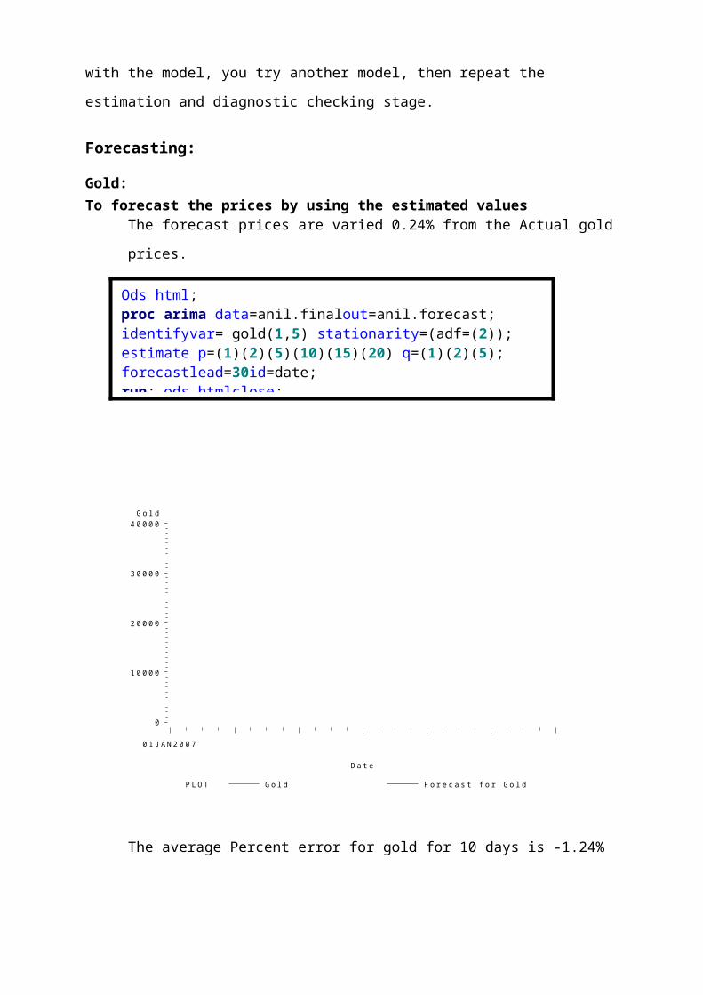
Forecasting:
Gold:To forecast the prices by using the estimated values
The forecast prices are varied 0.24% from the Actual gold
prices.
P L O T G o l d F o r e c a s t f o r G o l d
G o l d
0
1 0 0 0 0
2 0 0 0 0
3 0 0 0 0
4 0 0 0 0
D a t e
0 1 J A N 2 0 0 7
The average Percent error for gold for 10 days is -1.24%
Ods html;proc arima data=anil.finalout=anil.forecast;identifyvar= gold(1,5) stationarity=(adf=(2));estimate p=(1)(2)(5)(10)(15)(20) q=(1)(2)(5);forecastlead=30id=date;run; ods htmlclose;
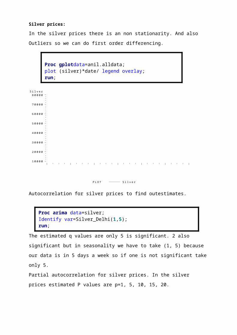
Silver prices:
In the silver prices there is an non stationarity. And also
Outliers so we can do first order differencing.
P L O T S i l v e r
S i l v e r
1 0 0 0 0
2 0 0 0 0
3 0 0 0 0
4 0 0 0 0
5 0 0 0 0
6 0 0 0 0
7 0 0 0 0
8 0 0 0 0
Autocorrelation for silver prices to find outestimates.
The estimated q values are only 5 is significant. 2 also
significant but in seasonality we have to take (1, 5) because
our data is in 5 days a week so if one is not significant take
only 5.
Partial autocorrelation for silver prices. In the silver
prices estimated P values are p=1, 5, 10, 15, 20.
Proc gplotdata=anil.alldata;plot (silver)*date/ legend overlay;run;
Proc arima data=silver;Identify var=Silver_Delhi(1,5);run;

For forecasting of silver prices we use the estimated values
what we find out in the autocorrelation and partial
autocorrelation functions
.
P L O T S i l v e r F o r e c a s t f o r S i l v e r
S i l v e r
1 0 0 0 0
2 0 0 0 0
3 0 0 0 0
4 0 0 0 0
5 0 0 0 0
6 0 0 0 0
7 0 0 0 0
8 0 0 0 0
The average Percent error for silver for 10 days is -2.07%
Crude oil: The nymex oil prices are plotted the graph. As we observed in
the graph there is a trend in the crude oil prices. it means
it’s a non stationarity in this series.
Odshtml;procarimadata=anil.finalout=anil.forecast;identifyvar= silver(1,5) stationarity=(adf=(2));estimatep=(1)(2)(5)(10)(15)(20) q=(5);forecastlead=30id=date;run;odshtmlclose;
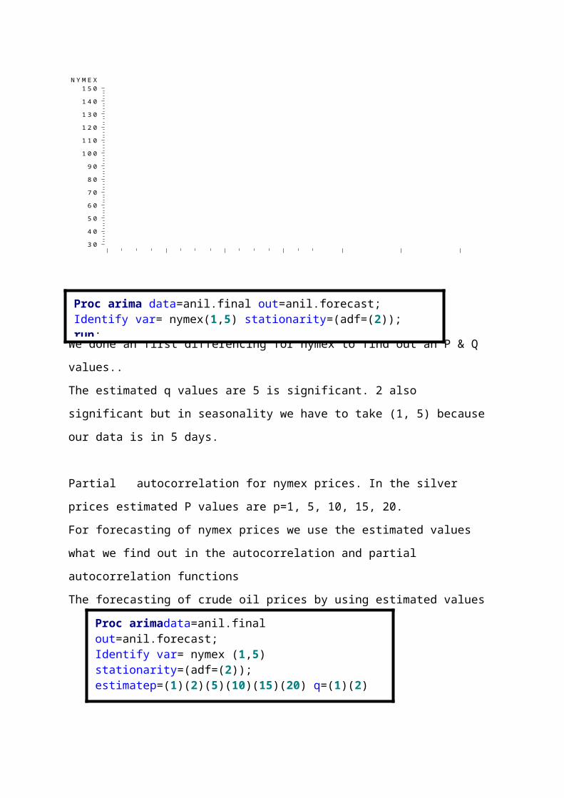
P L O T N Y M E X
N Y M E X
3 0
4 0
5 0
6 0
7 0
8 0
9 0
1 0 0
1 1 0
1 2 0
1 3 0
1 4 0
1 5 0
We done an first differencing for nymex to find out an P & Q
values..
The estimated q values are 5 is significant. 2 also
significant but in seasonality we have to take (1, 5) because
our data is in 5 days.
Partial autocorrelation for nymex prices. In the silver
prices estimated P values are p=1, 5, 10, 15, 20.
For forecasting of nymex prices we use the estimated values
what we find out in the autocorrelation and partial
autocorrelation functions
The forecasting of crude oil prices by using estimated values
Proc arimadata=anil.final out=anil.forecast;Identify var= nymex (1,5) stationarity=(adf=(2));estimatep=(1)(2)(5)(10)(15)(20) q=(1)(2)(5);
Proc arima data=anil.final out=anil.forecast;Identify var= nymex(1,5) stationarity=(adf=(2));run;
P L O T N Y M E X F o r e c a s t f o r N Y M E X
N Y M E X
3 0
4 0
5 0
6 0
7 0
8 0
9 0
1 0 0
1 1 0
1 2 0
1 3 0
1 4 0
1 5 0
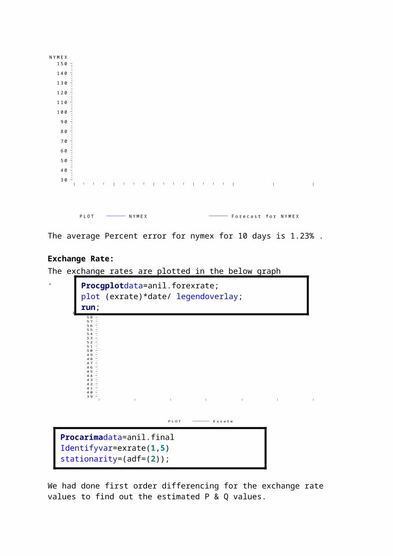
The average Percent error for nymex for 10 days is 1.23% .
Exchange Rate:The exchange rates are plotted in the below graph.
P L O T E x r a t e
E x r a t e
3 94 04 14 24 34 44 54 64 74 84 95 05 15 25 35 45 55 65 75 8
Procarimadata=anil.finalIdentifyvar=exrate(1,5) stationarity=(adf=(2));run;
We had done first order differencing for the exchange rate values to find out the estimated P & Q values.
Procgplotdata=anil.forexrate;plot (exrate)*date/ legendoverlay;run;

The autocorrelation values (q) are 1,2,5 .when we done an first order differencing for exchange rate values.Partial autocorrelation gives an p values in the nymex P estimated values are 1,5,10,15,20. The forecasting for an exchange rate by using estimated p & q values.
Procarimadata=anil.finalout=anil.exforecast;Identifyvar= exrate(1,5) stationarity=(adf=(2));Estimatep=(1)(2)(5)(10)(15)(20) q=(1)(2)(5);Forecastlead=30id=date;run;
The bellowed graph is showing actual values and forecasting values for the exchange rate.
P L O T E x r a t e F o r e c a s t f o r E x r a t e
E x r a t e
3 94 04 14 24 34 44 54 64 74 84 95 05 15 25 35 45 55 65 75 8
The average Percent error for exrate for 10 days is -0.062%.
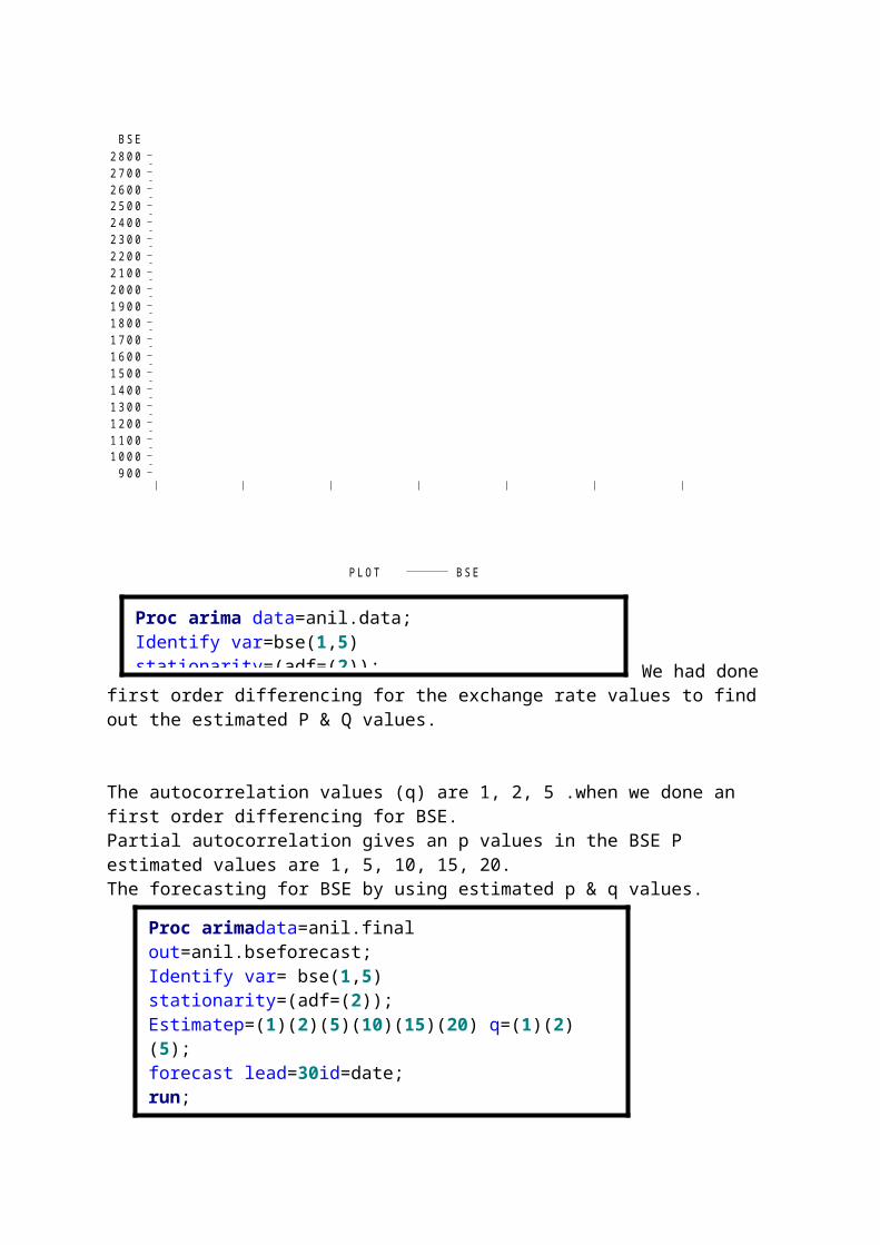
Bombay stock exchange:
We had taken data from Jan 2007 to July 2012 for forecasting. For that data we done cleaning and done a arima model.
Procgplotdata=anil.bse;plot (bse)*date/ legendoverlay;run;
P L O T B S E
B S E
9 0 01 0 0 01 1 0 01 2 0 01 3 0 01 4 0 01 5 0 01 6 0 01 7 0 01 8 0 01 9 0 02 0 0 02 1 0 02 2 0 02 3 0 02 4 0 02 5 0 02 6 0 02 7 0 02 8 0 0
Proc arima data=anil.data;Identify var=bse(1,5) stationarity=(adf=(2)); We had done
first order differencing for the exchange rate values to find out the estimated P & Q values.
The autocorrelation values (q) are 1, 2, 5 .when we done an first order differencing for BSE.Partial autocorrelation gives an p values in the BSE P estimated values are 1, 5, 10, 15, 20.The forecasting for BSE by using estimated p & q values.
Proc arimadata=anil.final out=anil.bseforecast;Identify var= bse(1,5) stationarity=(adf=(2));Estimatep=(1)(2)(5)(10)(15)(20) q=(1)(2)(5);forecast lead=30id=date;run;

P L O T B S E F o r e c a s t f o r B S E
B S E
9 0 01 0 0 01 1 0 01 2 0 01 3 0 01 4 0 01 5 0 01 6 0 01 7 0 01 8 0 01 9 0 02 0 0 02 1 0 02 2 0 02 3 0 02 4 0 02 5 0 02 6 0 02 7 0 02 8 0 0
The average Percent error for BSE for 10 days is -1.45% .
Transfer function
A Transfer function approach to modeling a time series is
a multivariate way of modeling the various lag structures
found in the data. It is similar to a distributed lag model in
traditional econometrics. The transfer function model,
however, makes use of the ratio between what are called
Numerator and Denominator polynomials. The Numerator
polynomials are the different lags of the exogenous variables.
The Denominator polynomials are the coefficients associated
with lags of the forecast itself (i.e. the traditional
dependent variable). Something called a Delay Factor or "dead
time" is associated with the exogenous variables. This is the
amount of time elapsed before the numerator polynomial begins
to impact the forecasted series. The error term is modeled
simultaneously as an ARMA process. Stationarity requirements

hold the same for each exogenous series as in the Univariate
endogenous case. Difference operations must be used if the
autocorrelation function of each series is to exhibit
stationarity. These difference operations need not be exactly
the same across all variables.
There may seem to be a close relationship between the Transfer
Function models and multiple regressions (OLS). At a glance,
one might think that the regression models are a special case
of the transfer function. However, they are quite different.
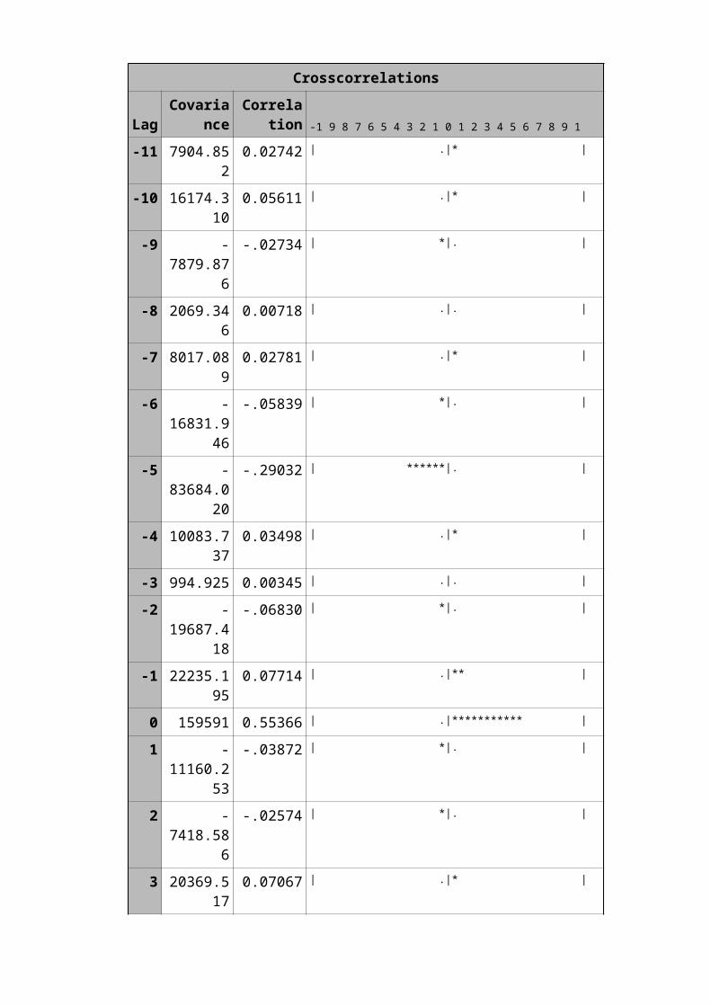
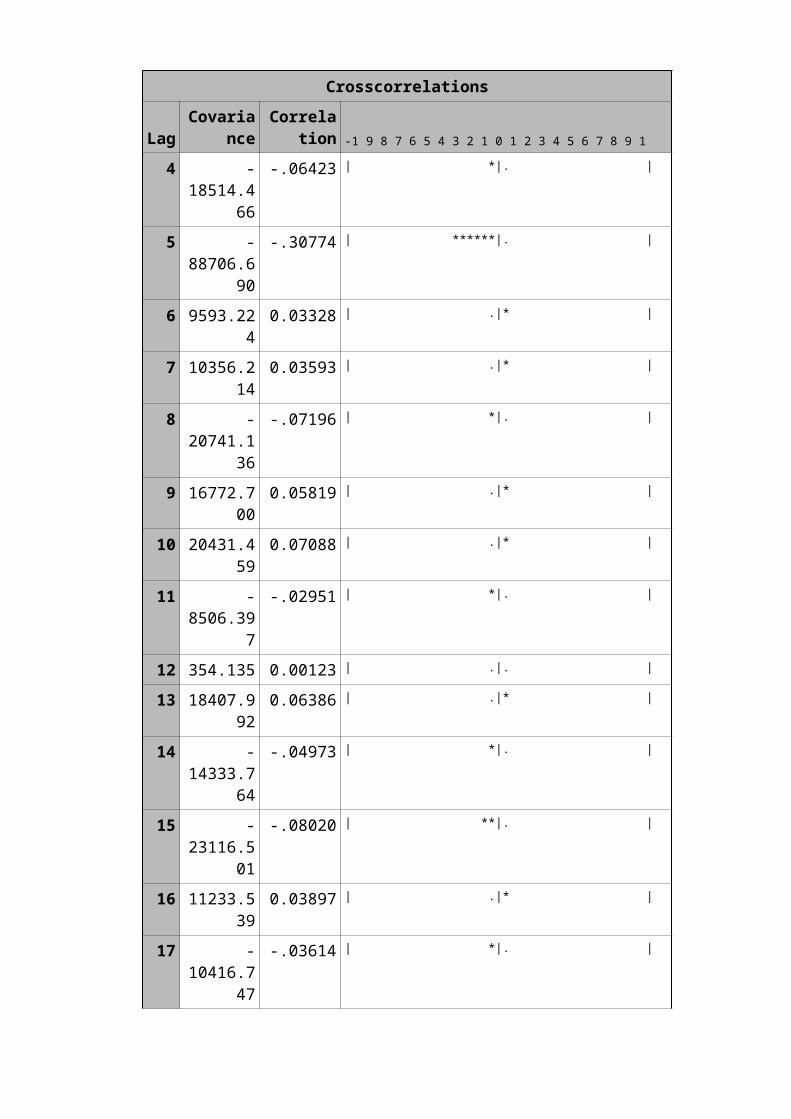
Example1:In this example, Silver is dependent on Gold. As we taken data
from Jan 2007 to July 2012. For our data we taken y=silver
(dependent variable) and x=gold (independent variable). We
will model the silver prices regression against the gold
prices. We can use Proc ARIMA to carry simple transfer
function. This is illustrated by using SAS codes
The following is SAS output
Proc arima data=anil.transall1;Identify var=silver(1,5) crosscorr=gold(1,5);Estimate p=(1)(2)(5)(10)(15)(20) q=(1)(2)(5) input=((0,3,5)gold);run;
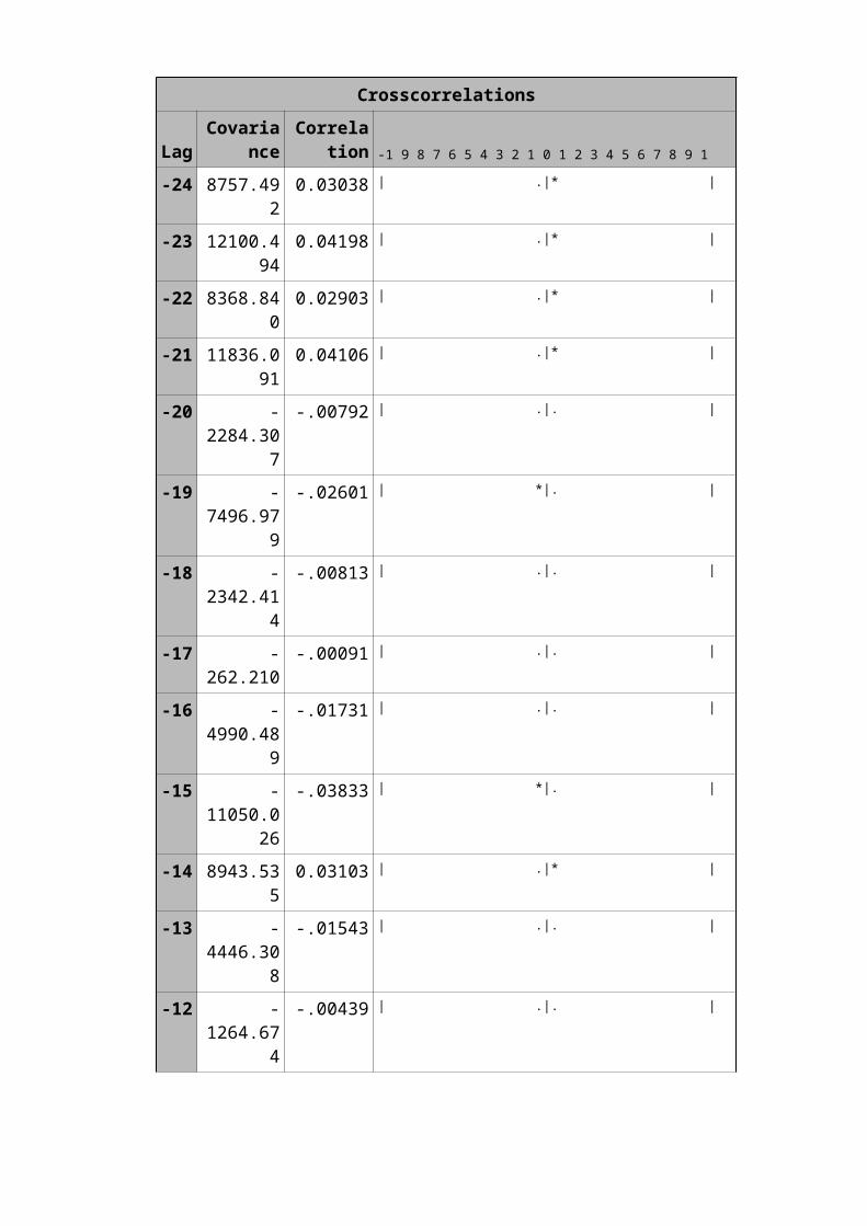
Crosscorrelations
LagCovaria
nceCorrela
tion -1 9 8 7 6 5 4 3 2 1 0 1 2 3 4 5 6 7 8 9 1
-24 8757.492
0.03038 | .|* |
-23 12100.494
0.04198 | .|* |
-22 8368.840
0.02903 | .|* |
-21 11836.091
0.04106 | .|* |
-20 -2284.30
7
-.00792 | .|. |
-19 -7496.97
9
-.02601 | *|. |
-18 -2342.41
4
-.00813 | .|. |
-17 -262.210
-.00091 | .|. |
-16 -4990.48
9
-.01731 | .|. |
-15 -11050.0
26
-.03833 | *|. |
-14 8943.535
0.03103 | .|* |
-13 -4446.30
8
-.01543 | .|. |
-12 -1264.67
4
-.00439 | .|. |
Crosscorrelations
LagCovaria
nceCorrela
tion -1 9 8 7 6 5 4 3 2 1 0 1 2 3 4 5 6 7 8 9 1
-11 7904.852
0.02742 | .|* |
-10 16174.310
0.05611 | .|* |
-9 -7879.87
6
-.02734 | *|. |
-8 2069.346
0.00718 | .|. |
-7 8017.089
0.02781 | .|* |
-6 -16831.9
46
-.05839 | *|. |
-5 -83684.0
20
-.29032 | ******|. |
-4 10083.737
0.03498 | .|* |
-3 994.925 0.00345 | .|. |
-2 -19687.4
18
-.06830 | *|. |
-1 22235.195
0.07714 | .|** |
0 159591 0.55366 | .|*********** |
1 -11160.2
53
-.03872 | *|. |
2 -7418.58
6
-.02574 | *|. |
3 20369.517
0.07067 | .|* |
Crosscorrelations
LagCovaria
nceCorrela
tion -1 9 8 7 6 5 4 3 2 1 0 1 2 3 4 5 6 7 8 9 1
4 -18514.4
66
-.06423 | *|. |
5 -88706.6
90
-.30774 | ******|. |
6 9593.224
0.03328 | .|* |
7 10356.214
0.03593 | .|* |
8 -20741.1
36
-.07196 | *|. |
9 16772.700
0.05819 | .|* |
10 20431.459
0.07088 | .|* |
11 -8506.39
7
-.02951 | *|. |
12 354.135 0.00123 | .|. |
13 18407.992
0.06386 | .|* |
14 -14333.7
64
-.04973 | *|. |
15 -23116.5
01
-.08020 | **|. |
16 11233.539
0.03897 | .|* |
17 -10416.7
47
-.03614 | *|. |

Crosscorrelations
LagCovaria
nceCorrela
tion -1 9 8 7 6 5 4 3 2 1 0 1 2 3 4 5 6 7 8 9 1
18 -18154.0
95
-.06298 | *|. |
19 13639.149
0.04732 | .|* |
20 8077.267
0.02802 | .|* |
21 -9916.79
9
-.03440 | *|. |
22 7506.528
0.02604 | .|* |
23 27411.793
0.09510 | .|** |
24 -10879.9
33
-.03774 | *|. |
Conditional Least Squares Estimation
Parameter Estimate
Standard Error
t Value
ApproxPr > |
t| LagVariable
Shift
MU -0.10971 0.21055 -0.52
0.6024 0 Silver
0
MA1,1 0.99021 0.0037712
262.57
<.0001 5 Silver
0
AR1,1 0.02043 0.02663 0.77 0.4431 5 Silver
0
AR2,1 -0.07124 0.02666 -2.67
0.0076 10 Silver
0
AR3,1 -0.02669 0.02664 -1.00
0.3166 15 Silver
0
AR4,1 0.02629 0.02683 0.98 0.3273 20 Silver
0
Crosscorrelations
LagCovaria
nceCorrela
tion -1 9 8 7 6 5 4 3 2 1 0 1 2 3 4 5 6 7 8 9 1
NUM1 2.09657 0.08291 25.29
<.0001 0 Gold 0
NUM1,1 -0.004502
7
0.08289 -0.05
0.9567 5 Gold 0
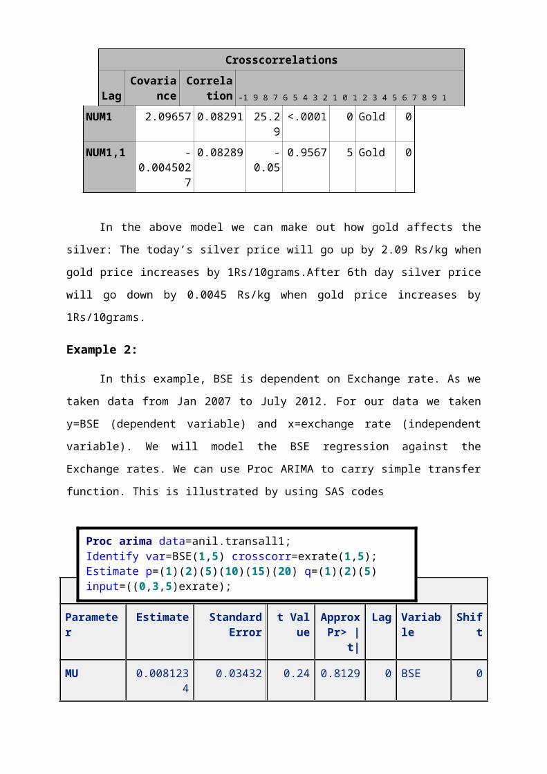
In the above model we can make out how gold affects the
silver: The today’s silver price will go up by 2.09 Rs/kg when
gold price increases by 1Rs/10grams.After 6th day silver price
will go down by 0.0045 Rs/kg when gold price increases by
1Rs/10grams.
Example 2:
In this example, BSE is dependent on Exchange rate. As we
taken data from Jan 2007 to July 2012. For our data we taken
y=BSE (dependent variable) and x=exchange rate (independent
variable). We will model the BSE regression against the
Exchange rates. We can use Proc ARIMA to carry simple transfer
function. This is illustrated by using SAS codes
Conditional Least Squares Estimation
Parameter
Estimate StandardError
t Value
ApproxPr> |
t|
Lag Variable
Shift
MU 0.0081234
0.03432 0.24 0.8129 0 BSE 0
Proc arima data=anil.transall1;Identify var=BSE(1,5) crosscorr=exrate(1,5);Estimate p=(1)(2)(5)(10)(15)(20) q=(1)(2)(5) input=((0,3,5)exrate);run;
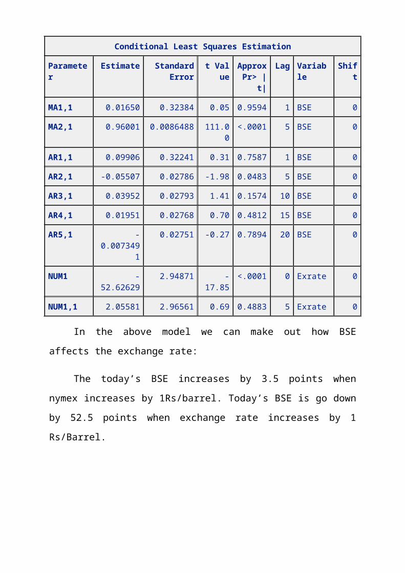
Conditional Least Squares Estimation
Parameter
Estimate StandardError
t Value
ApproxPr> |
t|
Lag Variable
Shift
MA1,1 0.01650 0.32384 0.05 0.9594 1 BSE 0
MA2,1 0.96001 0.0086488 111.00
<.0001 5 BSE 0
AR1,1 0.09906 0.32241 0.31 0.7587 1 BSE 0
AR2,1 -0.05507 0.02786 -1.98 0.0483 5 BSE 0
AR3,1 0.03952 0.02793 1.41 0.1574 10 BSE 0
AR4,1 0.01951 0.02768 0.70 0.4812 15 BSE 0
AR5,1 -0.007349
1
0.02751 -0.27 0.7894 20 BSE 0
NUM1 -52.62629
2.94871 -17.85
<.0001 0 Exrate 0
NUM1,1 2.05581 2.96561 0.69 0.4883 5 Exrate 0
In the above model we can make out how BSE
affects the exchange rate:
The today’s BSE increases by 3.5 points when
nymex increases by 1Rs/barrel. Today’s BSE is go down
by 52.5 points when exchange rate increases by 1
Rs/Barrel.

ARCH and GARCHWHY ARCH/GARCH?
The ARCH/GARCH framework proved to be very successful in
predicting volatility changes. Empirically, a wide range of
financial and economic phenomena exhibit the clustering of
volatilities. As we have seen, ARCH/GARCH models describe the
time evolution of the average size of squared errors, that is,
the evolution of the magnitude of uncertainty. Despite the
empirical success of ARCH/GARCH models, there is no real
consensus on the economic reasons why uncertainty tends to
cluster. That is why models tend to perform better in some
periods and worse in other periods. It is relatively easy to
induce ARCH behavior in simulated systems by making
appropriate assumptions on agent behavior. For example, one
can reproduce ARCH behavior in artificial markets with simple
assumptions on agent decision-making processes. The real
economic challenge, however, is to explain ARCH/GARCH behavior
in terms of features of agents behavior and/or economic
variables that could be empirically ascertained. In classical
physics, the amount of uncertainty inherent in models and
predictions can be made arbitrarily low by increasing the
precision of initial data. This view, however, has been
challenged in at least two ways. First, quantum mechanics has
introduced the notion that there is a fundamental uncertainty
in any measurement process. The amount of uncertainty is
prescribed by the theory at a fundamental level. Second, the
theory of complex systems has shown that nonlinear complex
systems are so sensitive to changes in initial conditions
that, in practice, there are limits to the accuracy of any
model. ARCH/GARCH models describe the time evolution of
uncertainty in a complex system.
In financial and economic models, the future is always
uncertain but over time we learn new information that helps us
forecast this future. As asset prices reflect our best
forecasts of the future profitability of companies and
countries, these change whenever there is news .ARCH/GARCH
models can be interpreted as measuring the intensity of the
news process. Volatility clustering is most easily understood
as news clustering. Of course, many things influence the
arrival process of news and its impact on prices. Trades
convey news to the market and the macro economy can moderate
the importance of the news. These can all be thought of as
important determinants of the volatility that is picked up by
ARCH/GARCH.
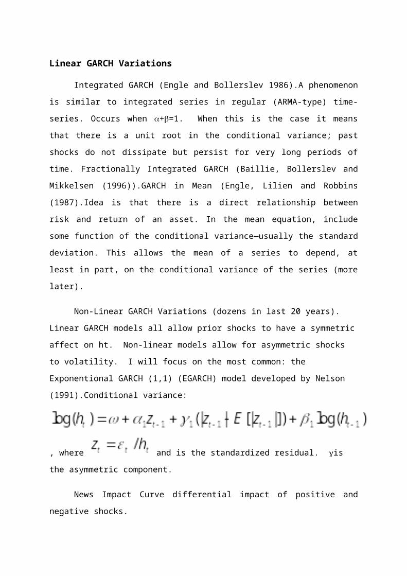
Linear GARCH Variations
Integrated GARCH (Engle and Bollerslev 1986).A phenomenon
is similar to integrated series in regular (ARMA-type) time-
series. Occurs when +=1. When this is the case it means
that there is a unit root in the conditional variance; past
shocks do not dissipate but persist for very long periods of
time. Fractionally Integrated GARCH (Baillie, Bollerslev and
Mikkelsen (1996)).GARCH in Mean (Engle, Lilien and Robbins
(1987).Idea is that there is a direct relationship between
risk and return of an asset. In the mean equation, include
some function of the conditional variance—usually the standard
deviation. This allows the mean of a series to depend, at
least in part, on the conditional variance of the series (more
later).
Non-Linear GARCH Variations (dozens in last 20 years).
Linear GARCH models all allow prior shocks to have a symmetric
affect on ht. Non-linear models allow for asymmetric shocks
to volatility. I will focus on the most common: the
Exponentional GARCH (1,1) (EGARCH) model developed by Nelson
(1991).Conditional variance:
, where and is the standardized residual. is
the asymmetric component.
News Impact Curve differential impact of positive and
negative shocks.
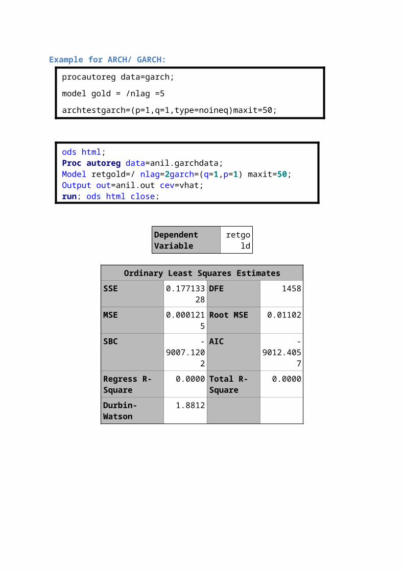
Example for ARCH/ GARCH:
procautoreg data=garch;
model gold = /nlag =5
archtestgarch=(p=1,q=1,type=noineq)maxit=50;
ods html;Proc autoreg data=anil.garchdata; Model retgold=/ nlag=2garch=(q=1,p=1) maxit=50; Output out=anil.out cev=vhat; run; ods html close;
Dependent Variable
retgold
Ordinary Least Squares EstimatesSSE 0.177133
28DFE 1458
MSE 0.0001215Root MSE 0.01102
SBC -9007.120
2
AIC -9012.405
7Regress R-Square
0.0000 Total R-Square
0.0000
Durbin-Watson
1.8812
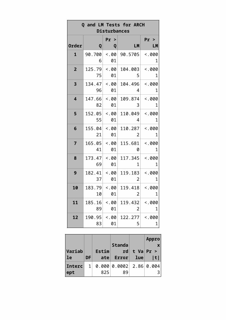
Q and LM Tests for ARCHDisturbances
Order QPr >
Q LMPr >
LM1 90.700
6<.0001
90.5705 <.0001
2 125.7975
<.0001
104.0035
<.0001
3 134.4796
<.0001
104.4964
<.0001
4 147.6682
<.0001
109.8743
<.0001
5 152.0555
<.0001
110.0494
<.0001
6 155.0421
<.0001
110.2872
<.0001
7 165.0541
<.0001
115.6810
<.0001
8 173.4769
<.0001
117.3451
<.0001
9 182.4137
<.0001
119.1832
<.0001
10 183.7910
<.0001
119.4182
<.0001
11 185.1689
<.0001
119.4322
<.0001
12 190.9583
<.0001
122.2775
<.0001
Variable DF
Estimate
Standard
Errort Value
Approx
Pr > |t|
Intercept
1 0.000825
0.000289
2.86 0.0043
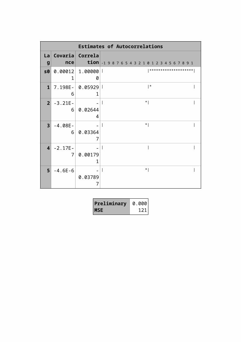
Estimates of AutocorrelationsLag
Covariance
Correlation -1 9 8 7 6 5 4 3 2 1 0 1 2 3 4 5 6 7 8 9 1
s0 0.000121
1.000000
| |********************|
1 7.198E-6
0.059291
| |* |
2 -3.21E-6
-0.02644
4
| *| |
3 -4.08E-6
-0.03364
7
| *| |
4 -2.17E-7
-0.00179
1
| | |
5 -4.6E-6 -0.03789
7
| *| |
PreliminaryMSE
0.000121
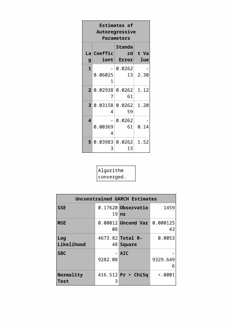
Estimates ofAutoregressiveParameters
LagCoeffic
ient
Standard
Errort Value
1 -0.06025
1
0.026213
-2.30
2 0.0293870.0262
611.12
3 0.0315840.0262
591.20
4 -0.00369
4
0.026261
-0.14
5 0.0398330.0262
131.52
Algorithm converged.
Unconstrained GARCH EstimatesSSE 0.17620
19Observations
1459
MSE 0.0001208
Uncond Var 0.00012543
Log Likelihood
4673.8248
Total R-Square
0.0053
SBC -9282.08
AIC -9329.649
6Normality Test
416.5123Pr > ChiSq <.0001
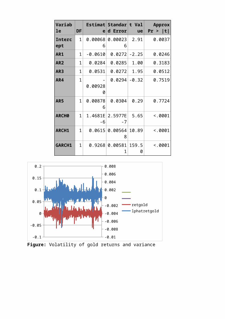
Variable DF
EstimateStandard Error
t Value
ApproxPr > |t|
Intercept
1 0.0006860.00023
62.91 0.0037
AR1 1 -0.0610 0.0272 -2.25 0.0246AR2 1 0.0284 0.0285 1.00 0.3183AR3 1 0.0531 0.0272 1.95 0.0512AR4 1 -
0.009280
0.0294 -0.32 0.7519
AR5 1 0.008786
0.0304 0.29 0.7724
ARCH0 1 1.4681E-6
2.5977E-7
5.65 <.0001
ARCH1 1 0.0615 0.00564810.89 <.0001
GARCH1 1 0.9268 0.005811159.5
0<.0001
-0.1
-0.05
0
0.05
0.1
0.15
0.2
-0.01
-0.008
-0.006
-0.004
-0.002
0
0.002
0.004
0.006
0.008
retgoldlphatretgold
Figure: Volatility of gold returns and variance

-0.3
-0.25
-0.2
-0.15
-0.1
-0.05
0
0.05
0.1
-0.02
-0.01
0
0.01
0.02
0.03
0.04
retsilverlphatretsilver
Figure: Volatility of silver returns and variance
-0.005
0
0.005
0.01
0.015
lphatretexrateuretexrate
Figure: Volatility of Exrate returns and variance
-0.008-0.006-0.004-0.002
00.0020.0040.0060.0080.010.012
-0.15-0.13-0.11-0.09-0.07-0.05-0.03-0.010.009999999999999980.030.05
lphatretnymexretnymex

Figure: Volatility of Nymex returns and variance
-0.04
-0.02
0
0.02
0.04
0.06
0.08
0.1
-0.15
-0.1
-0.05
2.77555756156289E-17
0.05
0.1
lphatretbseretbse
SFigure: Volatility of BSE returns and variance
Vector Auto Regression Model (VAR)Transfer functions assume that the independent variables and
associated lags influence the direction and magnitude of the
forecast series. These models are said NOT to allow for what
is termed “feedback”. A system is said to include feedback if
values of the input variable X depend in some fashion on the
past or current levels of the dependent variable. Vector ARIMA
models allow for this feedback process to occur. Being able to
describe the duality relationship between autoregressive
processes and moving average processes enables the forecaster
to use the autocorrelation and partial autocorrelation
functions to identify potential forms of Univariate models.
This is not the case in Vector ARIMA. The vector model does
not allow us to move from the infinite representation of one
process to the finite representation of the other. Therefore,
we need different tools to help us identify these processes
than what is generally used in Univariate ARIMA modeling. This
tool is called a CCF.
VARMAX models are defined in terms of the orders of the
autoregressive or moving-average process (or both). When you
use the VARMAX procedure, these orders can be specified by
options or they can be automatically determined. Criteria for
automatically determining these orders include
Akaike Information Criterion (AIC)
Corrected AIC (AICC)
Hannan-Quinn (HQ) Criterion
Final Prediction Error (FPE)
Schwarz Bayesian Criterion (SBC), also known as Bayesian
Information Criterion (BIC)
For situations where the stationarity of the time series
is in question, the VARMAX procedure provides tests to
aid in determining the presence of unit roots and
Cointegration. These tests include
Dickey-Fuller test
Johansen Cointegration test for non-stationary vector
processes of integrated order one
Stock-Watson common trends test for the possibility of
Cointegration among non-stationary vector processes of
integrated order one
Johansen Cointegration test for non-stationary vector
processes of integrated order two.
The VARMAX procedure provides a Granger-Causality test to
determine the Granger-causal relationships between two
distinct groups of variables. It also provides
infinite order AR representation
impulse response function (or infinite order MA
representation)
decomposition of the predicted error co variances
roots of the characteristic functions for both the AR and
MA parts to evaluate the proximity of the roots to the
unit circle
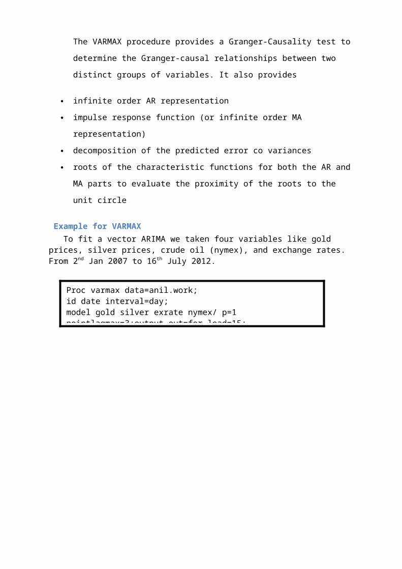
Example for VARMAX To fit a vector ARIMA we taken four variables like gold prices, silver prices, crude oil (nymex), and exchange rates. From 2nd Jan 2007 to 16th July 2012.
Proc varmax data=anil.work;id date interval=day;model gold silver exrate nymex/ p=1 nointlagmax=3;output out=for lead=15;
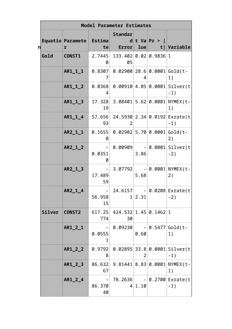
Model Parameter Estimates
Equation
Parameter
Estimate
Standard
Errort Value
Pr > |t| Variable
Gold CONST1 2.74450
133.40205
0.02 0.9836 1
AR1_1_1 0.83077
0.02900 28.640.0001 Gold(t-
1)AR1_1_2 0.0368
40.00910 4.05 0.0001 Silver(t
-1)AR1_1_3 17.328
193.08401 5.62 0.0001 NYMEX(t-
1)AR1_1_4 57.656
9324.5930
22.34 0.0192 Exrate(t
-1)AR2_1_1 0.1655
00.02902 5.70 0.0001 Gold(t-
2)AR2_1_2 -
0.03510
0.00909 -3.86
0.0001 Silver(t-2)
AR2_1_3 -17.489
59
3.07792 -5.68
0.0001 NYMEX(t-2)
AR2_1_4 -56.958
15
24.61571
-2.31
0.0208 Exrate(t-2)
Silver CONST2 617.25774
424.53230
1.45 0.1462 1
AR1_2_1 -0.0555
1
0.09230 -0.60
0.5477 Gold(t-1)
AR1_2_2 0.97928
0.02895 33.820.0001 Silver(t
-1)AR1_2_3 86.632
679.81441 8.83 0.0001 NYMEX(t-
1)AR1_2_4 -
86.37040
78.26364
-1.10
0.2700 Exrate(t-1)
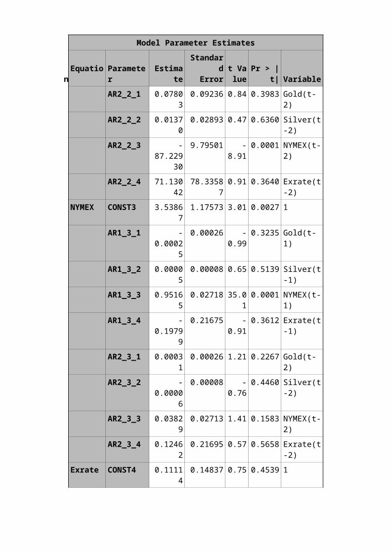
Model Parameter Estimates
Equation
Parameter
Estimate
Standard
Errort Value
Pr > |t| Variable
AR2_2_1 0.07803
0.09236 0.84 0.3983 Gold(t-2)
AR2_2_2 0.01370
0.02893 0.47 0.6360 Silver(t-2)
AR2_2_3 -87.229
30
9.79501 -8.91
0.0001 NYMEX(t-2)
AR2_2_4 71.13042
78.335870.91 0.3640 Exrate(t
-2)NYMEX CONST3 3.5386
71.17573 3.01 0.0027 1
AR1_3_1 -0.0002
5
0.00026 -0.99
0.3235 Gold(t-1)
AR1_3_2 0.00005
0.00008 0.65 0.5139 Silver(t-1)
AR1_3_3 0.95165
0.02718 35.010.0001 NYMEX(t-
1)AR1_3_4 -
0.19799
0.21675 -0.91
0.3612 Exrate(t-1)
AR2_3_1 0.00031
0.00026 1.21 0.2267 Gold(t-2)
AR2_3_2 -0.0000
6
0.00008 -0.76
0.4460 Silver(t-2)
AR2_3_3 0.03829
0.02713 1.41 0.1583 NYMEX(t-2)
AR2_3_4 0.12462
0.21695 0.57 0.5658 Exrate(t-2)
Exrate CONST4 0.11114
0.14837 0.75 0.4539 1

Model Parameter Estimates
Equation
Parameter
Estimate
Standard
Errort Value
Pr > |t| Variable
AR1_4_1 0.00000
0.00003 0.13 0.9000 Gold(t-1)
AR1_4_2 0.00000
0.00001 0.13 0.8936 Silver(t-1)
AR1_4_3 -0.0050
4
0.00343 -1.47
0.1422 NYMEX(t-1)
AR1_4_4 1.01326
0.02735 37.050.0001 Exrate(t
-1)AR2_4_1 0.0000
00.00003 0.07 0.9420 Gold(t-
2)AR2_4_2 -
0.00000
0.00001 -0.26
0.7923 Silver(t-2)
AR2_4_3 0.00546
0.00342 1.59 0.1110 NYMEX(t-2)
AR2_4_4 -0.0177
4
0.02738 -0.65
0.5171 Exrate(t-2)
Proc gplot data=data;plot (gold gforecast)*date/overlay legend;run;
P L O T G o l d F o r e c a s t s f o r G o l d
G o l d
0
1 0 0 0 0
2 0 0 0 0
3 0 0 0 0
4 0 0 0 0
D a t e
0 1 J A N 2 0 0 7
P L O T S i l v e r F o r e c a s t s f o r S i l v e r
S i l v e r
1 0 0 0 0
2 0 0 0 0
3 0 0 0 0
4 0 0 0 0
5 0 0 0 0
6 0 0 0 0
7 0 0 0 0
8 0 0 0 0
Proc gplot data=data;plot (silver sforecast)*date/overlay
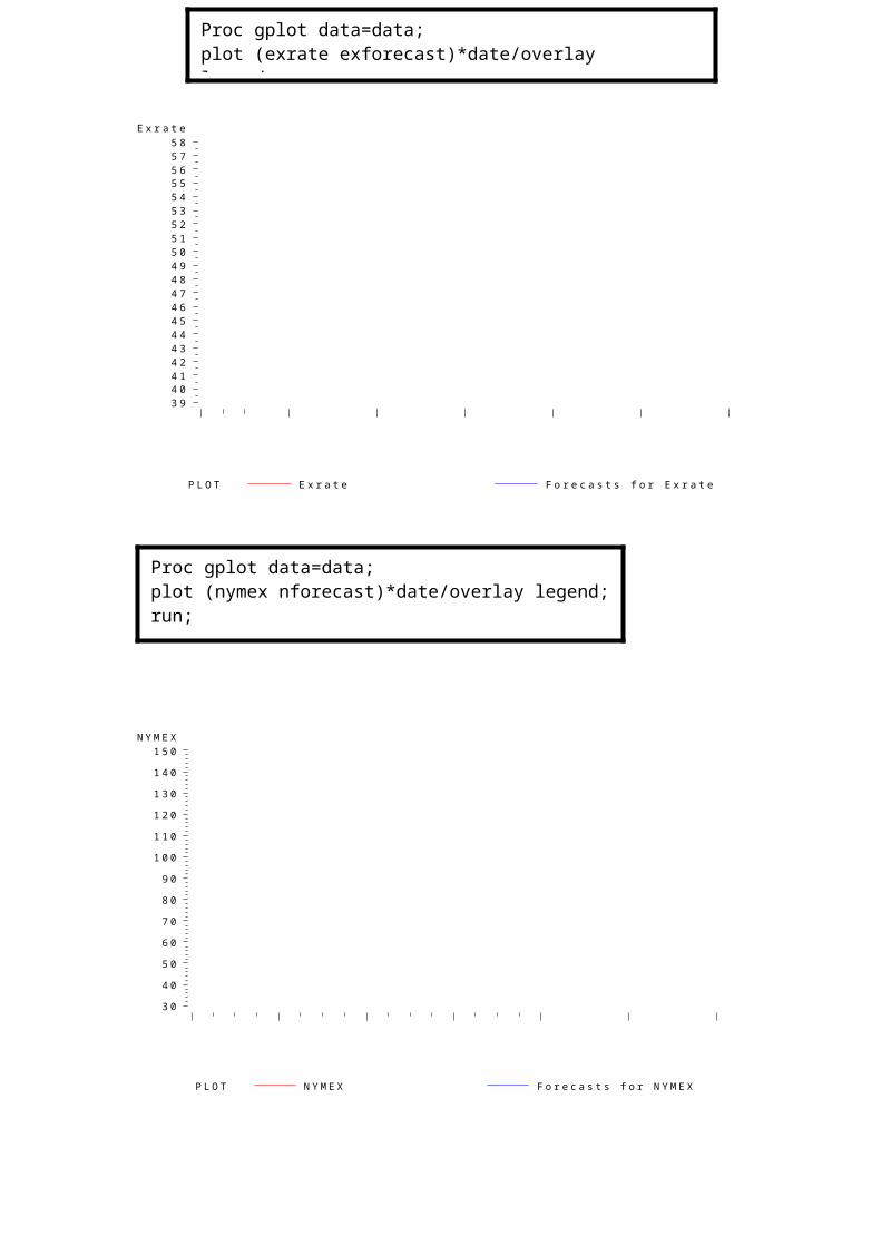
P L O T E x r a t e F o r e c a s t s f o r E x r a t e
E x r a t e
3 94 04 14 24 34 44 54 64 74 84 95 05 15 25 35 45 55 65 75 8
P L O T N Y M E X F o r e c a s t s f o r N Y M E X
N Y M E X
3 0
4 0
5 0
6 0
7 0
8 0
9 0
1 0 0
1 1 0
1 2 0
1 3 0
1 4 0
1 5 0
Proc gplot data=data;plot (exrate exforecast)*date/overlay legend;run;
Proc gplot data=data;plot (nymex nforecast)*date/overlay legend;run;
Policy Implications of the study:
1. Seasonal ARIMA models can effectively capture the structure
of commodity prices.
2. These models produced forecast of reasonably good accuracy
in the range of 0.8% to 5% RMSE baring crude oil the
accuracy in commodity prices was very high.
3. The study demonstrated that transfer function can be used to
study interrelation ship between commodities. For instance
gold prices are influenced by changes in exchange rate with
delay of 5 days. Changes in crude oil prices adversely affect
the sensex after about week.
4. VAR models produce better forecast of commodity prices
probably because of the use of independent variable.
5. Commodity prices are fraught with high degree of volatility
which has to be captured to get better forecast.
6. GARCH/ARC showed that news influenced commodity price
volatility which is an indication of the efficiency of
markets for these commodities.
REFERENCE:
1. http://www.ncdex.com/MarketData/SpotPrice.aspx
2. www.bseindia.com
3. http://www.exchange-rates.org/history/INR/USD/T
4. www.eia.gov/dnav/pet/hist/LeafHandler.ashx?
n=PET&s=RCLC1&f=D

5. ROBERT F. ENGLE, PhD Leonard N. Stern School of Business,New York University, ARCH/GARCH Models in Applied Financial Econometrics
6. John J. Sparks and Yuliya V. Yurova, University of
Illinois at Chicago Comparative Performance of ARIMA and
ARCH/GARCH Models on Time Series of Daily Equity Prices
for Large Companies
7. James D. Hamilton, Applied time series analysis,
Princstion university Press 1994
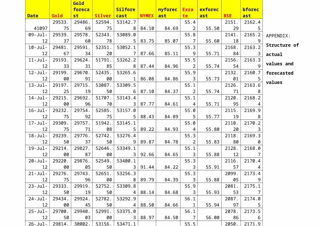
APPENDIX:
Structure of
actual
values and
forecasted
values
Date Gold
Gold forecast Silver
Silforecast NYMEX
nyforecast
Exrate
exforecast BSE
bforecast
4109729533.
7529486.
6952594.
7553142.7
8 84.10 84.6955.4
2 55.502151.
292162.4
509-Jul-
1229539.
3729578.
6052343.
7853089.0
5 83.75 85.0755.8
7 55.602141.
182165.2
910-Jul-
1229481.
6729591.
3452351.
2053052.1
7 87.66 85.1155.3
9 55.712168.
842163.2
311-Jul-
1229193.
3329624.
3151791.
8553262.2
8 87.44 84.9655.5
2 55.742156.
542163.3
912-Jul-
1229199.
0029670.
9152435.
0053265.6
1 86.08 84.8655.9
3 55.732132.
012160.7
513-Jul-
1229197.
2529715.
1953087.
5053309.5
6 87.10 84.3755.1
2 55.742126.
712163.6
814-Jul-
1229215.
0029692.
9651707.
7053143.4
3 87.77 84.6155.1
4 55.712120.
952168.2
416-Jul-
1229232.
7529754.
9252585.
7553157.0
5 88.43 84.8955.0
5 55.772115.
192169.9
817-Jul-
1229309.
7529757.
7151942.
0853145.1
5 89.22 84.9355.0
4 55.802110.
202170.2
318-Jul-
1229239.
5029776.
3752742.
5053276.4
9 89.87 84.7855.3
2 55.832118.
802169.3
019-Jul-
1229214.
0029827.
8752646.
0053349.1
3 92.66 84.6555.1
3 55.882128.
122168.0
720-Jul-
1229220.
0029876.
0552549.
5053400.1
3 91.44 84.2255.3
3 55.912116.
572170.4
421-Jul-
1229276.
7529743.
9652651.
0053256.3
8 89.79 84.3955.3
3 55.882099.
052173.4
923-Jul-
1229333.
5029919.
1952752.
5053309.8
4 88.14 84.6855.9
3 55.932081.
532175.1
724-Jul-
1229434.
0029924.
4552782.
5053292.9
4 88.50 84.6656.1
1 55.942087.
972174.0
525-Jul-
1229700.
5029940.
0352991.
0053375.0
3 88.97 84.5056.1
7 56.002078.
862173.5
626-Jul- 29814. 30002. 53156. 53471.1 55.5 2050. 2171.9