
Time estimation for large scale of data processing in Hadoop ...
65
This Master’s Thesis is carried out as a part of the education at the University of Agder and is therefore approved as a part of this education. University of Agder, 2011 May Faculty of Engineering and Science Department of Information and Communication Technology Time estimation for large scale of data processing in Hadoop MapReduce scenario Li Jian Supervisors Anders Aasgaard , Jan Pettersen Nytun brought to you by CORE View metadata, citation and similar papers at core.ac.uk provided by Agder University Research Archive
-
Upload
khangminh22 -
Category
Documents
-
view
3 -
download
0
Transcript of Time estimation for large scale of data processing in Hadoop ...

This Master’s Thesis is carried out as a part of the education at the
University of Agder and is therefore approved as a part of this education.
University of Agder, 2011 May
Faculty of Engineering and Science
Department of Information and Communication Technology
Time estimation for large scale of data
processing in Hadoop MapReduce scenario
Li Jian
Supervisors
Anders Aasgaard , Jan Pettersen Nytun
brought to you by COREView metadata, citation and similar papers at core.ac.uk
provided by Agder University Research Archive

Abstract
The appearance of MapReduce technology gave rise to a strong blast in IT industry. Largecompanies such as Google, Yahoo and Facebook are using this technology to facilitatetheir data processing[12]. As a representative technology aimed at processing large datasetin parallel, MapReduce received great focus from various organizations. Handling largeproblems, using a large amount of resources is inevitable. Therefore, how to organize themeffectively becomes an important problem. It is a common strategy to obtain some learningexperience before deploying large scale of experiments. Following this idea, this materthesis aims at providing some learning models towards MapReduce. These models help usto accumulate learning experience from small scale of experiments and finally lead us toestimate execution time of large scales of experiment.

Preface
This report is the master thesis report in spring semester 2011. The topic derived fromDevoteam, a well-known IT consulting company in south Norway. The main goal of thisthesis is to discover how we can use cloud computing effectively. We choose the represen-tative technology MapReduce as our research target.
Both cloud computing and MapReduce are complicated concepts. Through one semester’sstudy and experiment, we came up with some learning models to make MapReduce serveus in a better way. MapReduce is truly a useful and practical technology to process largescale of data. It can solve some complicated enterprise level problems in an elegant way.
Last but not the least,I would like to thank my supervisors Anders Aasgaard and Jan P.Nytun for their careful and patient supervision. Due to their efforts, I got a lot of construc-tive ideas in doing experiments and academic report writing. Big thanks to them.
Grimstad NorwayJanuary 2011Li Jian
1

Contents
Contents 2
List of Figures 4
List of Tables 6
1 Introduction 71.1 Problem definition . . . . . . . . . . . . . . . . . . . . . . . . . . . . . . 71.2 Research goals and facilities . . . . . . . . . . . . . . . . . . . . . . . . . 81.3 Thesis outline . . . . . . . . . . . . . . . . . . . . . . . . . . . . . . . . . 91.4 Constraints and limitations . . . . . . . . . . . . . . . . . . . . . . . . . . 9
2 Prior research 102.1 Methodology . . . . . . . . . . . . . . . . . . . . . . . . . . . . . . . . . 102.2 Parallel computing . . . . . . . . . . . . . . . . . . . . . . . . . . . . . . 11
2.2.1 Common network topologies . . . . . . . . . . . . . . . . . . . . . 112.2.2 Granularity . . . . . . . . . . . . . . . . . . . . . . . . . . . . . . 132.2.3 Speedup . . . . . . . . . . . . . . . . . . . . . . . . . . . . . . . . 13
2.2.3.1 Compute speedup by execution time . . . . . . . . . . . 132.2.3.2 Compute speedup by Amdahl’s Law . . . . . . . . . . . 142.2.3.3 Scaling behavior . . . . . . . . . . . . . . . . . . . . . . 16
2.2.4 Data synchronization . . . . . . . . . . . . . . . . . . . . . . . . . 16
3 Research target:Hadoop MapReduce 173.1 Mechanism . . . . . . . . . . . . . . . . . . . . . . . . . . . . . . . . . . 17
3.1.1 Job hierarchy . . . . . . . . . . . . . . . . . . . . . . . . . . . . . 183.1.2 Job execution workflow . . . . . . . . . . . . . . . . . . . . . . . 193.1.3 Hadoop cluster hierarchy . . . . . . . . . . . . . . . . . . . . . . . 213.1.4 Traffic pattern . . . . . . . . . . . . . . . . . . . . . . . . . . . . . 22
2

CONTENTS
3.2 Supportive platform:Hadoop Distributed File System . . . . . . . . . . . . 243.3 Key feature:speculative execution . . . . . . . . . . . . . . . . . . . . . . 243.4 Hadoop MapReduce program structure . . . . . . . . . . . . . . . . . . . . 253.5 MapReduce applications . . . . . . . . . . . . . . . . . . . . . . . . . . . 263.6 Experiment plan . . . . . . . . . . . . . . . . . . . . . . . . . . . . . . . . 27
4 Proposed models and verification 284.1 Assumptions . . . . . . . . . . . . . . . . . . . . . . . . . . . . . . . . . 284.2 Key condition:execution time follows regular trend . . . . . . . . . . . . . 29
4.2.1 The effect of increasing total data size . . . . . . . . . . . . . . . . 304.2.2 The effect of increasing nodes . . . . . . . . . . . . . . . . . . . . 31
4.2.2.1 Speedup bottleneck due to network relay device . . . . . 334.2.2.2 Speedup bottleneck due to an Http server’s capacity . . . 354.2.2.3 Decide boundary value . . . . . . . . . . . . . . . . . . 364.2.2.4 Summary . . . . . . . . . . . . . . . . . . . . . . . . . . 37
4.3 Wave model . . . . . . . . . . . . . . . . . . . . . . . . . . . . . . . . . . 384.3.1 General form . . . . . . . . . . . . . . . . . . . . . . . . . . . . . 394.3.2 Slowstart form . . . . . . . . . . . . . . . . . . . . . . . . . . . . 414.3.3 Speedup bottleneck form . . . . . . . . . . . . . . . . . . . . . . . 424.3.4 Model verification for general form . . . . . . . . . . . . . . . . . 444.3.5 Model verification for slowstart form . . . . . . . . . . . . . . . . 46
4.4 Sawtooth model . . . . . . . . . . . . . . . . . . . . . . . . . . . . . . . . 474.4.1 General form . . . . . . . . . . . . . . . . . . . . . . . . . . . . . 484.4.2 Model verification for general form . . . . . . . . . . . . . . . . . 49
4.5 Summary . . . . . . . . . . . . . . . . . . . . . . . . . . . . . . . . . . . 50
5 Discussion 515.1 Scalability analysis . . . . . . . . . . . . . . . . . . . . . . . . . . . . . . 515.2 The essence of wave model and sawtooth model . . . . . . . . . . . . . . . 535.3 Extend models to more situations . . . . . . . . . . . . . . . . . . . . . . . 535.4 Deviation analysis . . . . . . . . . . . . . . . . . . . . . . . . . . . . . . . 545.5 Summarize learning workflow . . . . . . . . . . . . . . . . . . . . . . . . 56
6 Conclusion 57
A Raw experiment results 58
Bibliography 62
3

List of Figures
2.1 Problem abstraction. . . . . . . . . . . . . . . . . . . . . . . . . . . . . . 102.2 A star network:each circle represents a node. . . . . . . . . . . . . . . . . 122.3 Typical two-level tree network for a Hadoop Cluster [30] . . . . . . . . . . 122.4 Speedup computation example[1] . . . . . . . . . . . . . . . . . . . . . . 142.5 Parallelizable and non-Parallelizable work . . . . . . . . . . . . . . . . . . 152.6 Amdahl’s Law limits speedup [1] . . . . . . . . . . . . . . . . . . . . . . . 152.7 Scaling behavior . . . . . . . . . . . . . . . . . . . . . . . . . . . . . . . 16
3.1 Google use mapreduce . . . . . . . . . . . . . . . . . . . . . . . . . . . . 173.2 Job Hierarchy . . . . . . . . . . . . . . . . . . . . . . . . . . . . . . . . . 183.3 map and reduce function [6] . . . . . . . . . . . . . . . . . . . . . . . . . 183.4 The workflow of WordCount . . . . . . . . . . . . . . . . . . . . . . . . . 183.5 MapReduce cluster execution workflow [6] . . . . . . . . . . . . . . . . . 193.6 MapReduce partitioner[18] . . . . . . . . . . . . . . . . . . . . . . . . . . 203.7 Disambiguate concepts in reduce phase . . . . . . . . . . . . . . . . . . . 213.8 Hadoop cluster hierarchy . . . . . . . . . . . . . . . . . . . . . . . . . . . 223.9 Traffic pattern:servers and fetchers are the same set of nodes. . . . . . . . . 223.10 Intermittent copy . . . . . . . . . . . . . . . . . . . . . . . . . . . . . . . 233.11 Speculative execution . . . . . . . . . . . . . . . . . . . . . . . . . . . . . 253.12 MapReduce program structure . . . . . . . . . . . . . . . . . . . . . . . . 253.13 Distributed sort scenario: the vertical bar stands for a key. . . . . . . . . . . 27
4.1 Simplified MapReduce workflow: a grid represents a task . . . . . . . . . . 284.2 Scenario of expanding the network . . . . . . . . . . . . . . . . . . . . . . 324.3 Models to describe a MapReduce job . . . . . . . . . . . . . . . . . . . . . 324.4 Bottleneck due to limitation on shared resources . . . . . . . . . . . . . . . 324.5 Three data fetching behaviors . . . . . . . . . . . . . . . . . . . . . . . . . 344.6 Expand two-level network . . . . . . . . . . . . . . . . . . . . . . . . . . 35
4
LIST OF FIGURES
4.7 Boundary detection experiment illustration . . . . . . . . . . . . . . . . . . 364.8 The illustration of concept “wave” . . . . . . . . . . . . . . . . . . . . . . 394.9 General form of wave model . . . . . . . . . . . . . . . . . . . . . . . . . 394.10 Slowstart . . . . . . . . . . . . . . . . . . . . . . . . . . . . . . . . . . . 414.11 Slowstart analysis model . . . . . . . . . . . . . . . . . . . . . . . . . . . 414.12 Partial copy . . . . . . . . . . . . . . . . . . . . . . . . . . . . . . . . . . 434.13 Downgraded full copy . . . . . . . . . . . . . . . . . . . . . . . . . . . . 434.14 Map wave of WordCount. . . . . . . . . . . . . . . . . . . . . . . . . . . . 454.15 Reduce wave of WordCount. . . . . . . . . . . . . . . . . . . . . . . . . . 454.16 Once-and-for-all copy[23] . . . . . . . . . . . . . . . . . . . . . . . . . . 464.17 Current slowstart copy pattern . . . . . . . . . . . . . . . . . . . . . . . . 474.18 Proposed new copy pattern . . . . . . . . . . . . . . . . . . . . . . . . . . 474.19 Sawtooth model . . . . . . . . . . . . . . . . . . . . . . . . . . . . . . . . 484.20 Map sawtooth of WordCount. . . . . . . . . . . . . . . . . . . . . . . . . . 494.21 Reduce sawtooth of WordCount. . . . . . . . . . . . . . . . . . . . . . . . 49
5.1 Periodical workload . . . . . . . . . . . . . . . . . . . . . . . . . . . . . . 545.2 A deviation situation. . . . . . . . . . . . . . . . . . . . . . . . . . . . . . 555.3 Not all tasks are launched at the same time[23] . . . . . . . . . . . . . . . 55
5

List of Tables
4.1 Notations for general form of wave model . . . . . . . . . . . . . . . . . . 404.2 Notations for slowstart form of wave model . . . . . . . . . . . . . . . . . 424.3 Verify wave model for WordCount program . . . . . . . . . . . . . . . . . 454.4 Verify wave model for Terasort program . . . . . . . . . . . . . . . . . . . 454.5 Verify wave model for slowstart form . . . . . . . . . . . . . . . . . . . . 464.6 Verify sawtooth model for WordCount program . . . . . . . . . . . . . . . 494.7 Verify sawtooth model for Terasort program . . . . . . . . . . . . . . . . . 49
5.1 Execution time for WordCount program(unit:sec) . . . . . . . . . . . . . . 525.2 Execution time for Terasort program(unit:sec) . . . . . . . . . . . . . . . . 52
A.1 WordCount,929MB,4nodes . . . . . . . . . . . . . . . . . . . . . . . . . . 58A.2 WordCount,1.86GB,4nodes . . . . . . . . . . . . . . . . . . . . . . . . . . 58A.3 WordCount,929MB,8nodes . . . . . . . . . . . . . . . . . . . . . . . . . . 58A.4 WordCount,1.86GB,8nodes . . . . . . . . . . . . . . . . . . . . . . . . . . 59A.5 WordCount,3.72GB,16nodes . . . . . . . . . . . . . . . . . . . . . . . . . 59A.6 Terasort,2GB,4nodes . . . . . . . . . . . . . . . . . . . . . . . . . . . . . 59A.7 Terasort,4GB,4nodes . . . . . . . . . . . . . . . . . . . . . . . . . . . . . 60A.8 Terasort,2GB,8nodes . . . . . . . . . . . . . . . . . . . . . . . . . . . . . 60A.9 Terasort,4GB,8nodes . . . . . . . . . . . . . . . . . . . . . . . . . . . . . 60A.10 Terasort,8GB,16nodes . . . . . . . . . . . . . . . . . . . . . . . . . . . . 61
6

Chapter 1
Introduction
The advent of cloud computing has triggered a tremendous trend on its research and prod-ucts development. Basically, it is a network-based computing [5]. It combines technologiessuch as virtualization, Distributed File System, Distributed computing and so on to makeit a very powerful resource pool. As a representative technology in cloud computing er-a, MapReduce also attracted great attention from both industry and academic institutions.Simply speaking, MapReduce is a programming model targeted at processing large scaleof data in a parallel manner. “Large scale” refers to a dataset that may exceed terabyte oreven petabyte. Facing with such a huge dataset, how to estimate its execution time undercertain amount of hardware and how to customize just-enough hardware under certain bot-tleneck is quite important . As data size and computing nodes grow, how is the executiontime curve like and how we tune our program to make it predictable are also importantquestions.
1.1 Problem definition
Based on the knowledge above, we describe our research problem to be estimating theexecution time for large scale of dataset processing through small scale of experiment.Namely, given a huge dataset and sufficient machines, we aim to estimate its executiontime by sampling a part of data and using a part of available machines.
Basically, our work is a practice of learning theory. We learn from completed experi-ments and apply this learning experience to new experiments. Our main problem generatesthe following subproblems:
7

CHAPTER 1. INTRODUCTION
• How does MapReduce parallelize a problem?
• What effect comes into being once we increase total data size and computing nodes?And how does MapReduce handle these effect?
• What approximation and assumptions do we need to achieve our estimation?
In parallel computing, communication and data synchronization are complicated prob-lems, so it is the same with scheduling and coordination. Unlike traditional parallel pro-gramming model MPI(Message Passing Interface) [21], MapReduce shifts its focus fromparallelizing a problem via point-to-point communication to designing basic task unit. HowMapReduce simplifies parallel programming will be illustrated in Chapter 3. Further more,what factors may bring about bottleneck for parallelism will also be revealed.
1.2 Research goals and facilities
Our main goal is to propose convenient models to learn Hadoop MapReduce effectively.These models guide us on what to learn and how to apply learning experience on newexperiments.
We use Amazon’s cloud service Elastic Computing Cloud(EC2)[7] to accomplish ourexperiments. EC2 is an infrastructure service which provides virtual machines for cus-tomers. All virtual machines we use are 1.7 GB of memory, 1 EC2 Compute Unit,whichis equivalent to 1.0-1.2 GHz 2007 Opteron or 2007 Xeon processor [15]. Except virtualmachine’s performance, Amazon also has guarantee on the network connection and point-to-point bandwidth [3].
We use on-demand virtual servers from Amazon. This service allows us to terminatevirtual servers immediately after we finish our computation tasks. Standing at customer’sview, it saves cost. But one problem is each time we start a new cluster environment, thenetwork topology can not stay the same with the previous network. As servers are virtual-ized, network is also virtualized, therefore changes to virtual servers introduces change tonetwork. Because of various concerns, cloud providers normally prohibit customers prob-ing network topology. But their ensurance on point-to-point bandwidth provides a goodreason to divert customers’ attention away from this aspect.
8

CHAPTER 1. INTRODUCTION
1.3 Thesis outline
Up till here, we have described research problem and experiment environment in detail.Chapter 2 will mainly introduce necessary theories that will help us solve our researchproblem. Chapter 3 gives a detailed introduction about our research target Hadoop MapRe-duce. It’s mechanism will be elaborated. In Chapter 4, we deepen our understanding ofHadoop MapReduce by proving a key proposition. Then we propose two models to solveour research problem. Chapter 5 is Discussion chapter, which gives a detailed analysis ofour experiment results. Chapter 6 is Conclusion chapter, which can be seen as a summaryof our research work.
1.4 Constraints and limitations
MapReduce is a network based programming model. The more computing nodes, the morecomplex the network is. In order to simplify our problem, we limit computing nodes to beless than 1024. The reasons that we choose 1024 as our boundary include:(1) According toIEEE 802.3i standard(10BASE-T)[14] , a star network can accommodate 1024 nodes. (2)Star network is simple to achieve and a network of 1024 nodes can do a great many thingsfor an enterprise. Further more, Yahoo has experimented Terabyte sort program on morethan 1406 nodes[24]. As of 15 May 2010, Yahoo has used 3452 nodes to finish 100TB’ssort within 173 minutes[10]. Because most of our research is based on star network, wesuppose limiting the number of nodes to be 1024 is necessary and reasonable.
This thesis is not working on actual enterprise problems. Therefore, the experimentdata is generated by some tools. Because of budget limitation, we are not able to work on areal “huge” dataset and a very big number of machines. We just use our current experimentand theoretical analysis to prove our models and other conclusions are reasonable.
Since we use virtual servers from Amazon, the network is maintained by Amazon. Dueto the limitation set by Amazon ,we couldn’t configure proper experiment environment forsome special situations. In other words, our experiments can only support a part of analysisand conclusions. But we will use proper assumptions, math and other knowledge to supportother analysis and conclusions.
9

Chapter 2
Prior research
2.1 Methodology
Before stepping into our problem, we present a further problem abstraction. This abstrac-tion is shown in the following Figure 2.1. Right now, our problem becomes experimenting
Figure 2.1: Problem abstraction.
the dark area in Figure 2.1 and then estimating T (m,n), where m represents the number ofcomputing nodes and n denotes data size, eg. we can define n = 1 as 1GB’s data.
Figure 2.1 gives us hint that execution time T can be expressed as a function T (nodes,
size), where variable nodes stands for the number of parallel nodes and size stands for thesize of input data . If T (size, nodes) can be generated through small scale of experiment,and most importantly the trend of T is regular, then we can use it to estimate execution timegiven a certain size and nodes. Our strategy is to fix nodes and then compute T (size).Similarly, we attempt to get T (nodes) by fixing size. Finally, we combine these twofunctions together to form T (size, nodes).
In fact, T (size) here is another format of time complexity. T (nodes) measures whennodes changes how execution time T changes. This change is often described by speedup.
10

CHAPTER 2. PRIOR RESEARCH
We assume readers to this thesis already have some knowledge about time complexity.Therefore, we only introduce speedup theory in the following section.
2.2 Parallel computing
Parallel computing aims at shortening the execution time of a problem by distributing com-putation tasks to multiple computing nodes. Parallel algorithms must be designed to makeit work. The designers must consider communication, load balancing, scheduling and da-ta synchronization across nodes. Comparing with sequential execution, these complicatedproblems often cause headache for designers. How Hadoop MapReduce solves these prob-lems will be covered in Chapter 3.
The performance of a parallel system is measured by speedup. Mature theories suchas Amdahl’s Law[1] and Gustafson’s Law[11] provide useful guidance for our research.Similar to any parallel architectures, data synchronization is also a big problem for HadoopMapReduce. The next few sections will cover speedup,data synchronization and otherimportant issues in detail.
2.2.1 Common network topologies
Parallel computing can be classified into many categories. A distributed cluster environ-ment is a way of achieving parallel computing, where each node has independent processorand memory and they communicate through network. Data exchange is a very frequen-t activity over the network. Therefore, network topology plays a very important role forcluster-based parallel computing.
In order to facilitate the following description, we emphasize an important concept:point-to-point bandwidth. It describes the transmission speed between one computer andanother computer.
Topologies such as star network, tree network and mesh network can be used for parallelcomputing. The simplest star network showed in Figure 2.2 is that each node is directlyconnected to a central device such as a switch or router but no pair of nodes has directconnection. In such a network, data communication between nodes is handled by a centraldevice. Its performance decides the performance of the network.
In fact, data centers often organize a group of servers on a rack and one rack normally
11

CHAPTER 2. PRIOR RESEARCH
Figure 2.2: A star network:each circle represents a node.
contains 30-40 servers. One rack has a centralized switch in connection with those servers.This topology on a rack is a star topology. Different racks are connected via anther level ofswitch. Thus several star networks compose a tree network, which is shown in Figure 2.3.
Figure 2.3: Typical two-level tree network for a Hadoop Cluster [30]
Considering this two-level tree network, the point-to-point bandwidth available for eachof the following scenarios becomes progressively less[30]: (1) Different nodes on the samerack; (2) Nodes on different racks in the same data center.
For an infrastructure owner, he can build a star, mesh or tree network according to hiswill. But in a public cloud1, different vendors may adopt different topologies. Due to vari-ous concerns such as security, commercial secrets and so on, they often don’t let customersknow what exact physical topologies they use. For example, Amazon Web Service allowsusers to build a virtual cluster, but it is banned to trace its network topology. Amazon justhas a guarantee to customers that it ensures a certain point-to-point bandwidth. How thebandwidth is allocated and its relationship to network topology are unknown to customers.
1Public cloud is a form of cloud computing that vendors provide computing service to customers but hidetechnology details.
12

CHAPTER 2. PRIOR RESEARCH
2.2.2 Granularity
Granularity means the size of a basic operation unit that we take into consideration. Coarse-grained systems consist of fewer, larger units than fine-grained systems [9]. For a parallelalgorithm, a basic operation such as addition, subtraction and multiplication can be seen asa basic computing unit. For data parallelism, the size of evenly partitioned data unit canserve as a granularity unit. The larger a data split is, the coarse-grained it is.
2.2.3 Speedup
Speedup is an important measurement criteria to the performance of a parallel system. Itmeasures how faster a parallel system performs than a sequential execution scheme[8]. Itis widely applied to describe the scalability of a parallel system [17, 29]. Amdahl’s Law[2]provides a method to compute speedup by workload, but it can also be computed throughexecution time. This section gives a detailed introduction of speedup and its relationshipwith our research.
2.2.3.1 Compute speedup by execution time
Speedup is a concept that only applies to parallel system. Its original definition is the ratioof sequential execution time to parallel execution time[8] which is defined by the followingformula:
S(n) =T (1)
T (n)(2.1)
where:
• n is the number of processors. We assume one node has one processor, thus thenumber of computing nodes equals processors.
• T (1) is sequential execution time, namely using one node. T(1) is the referencestandard or baseline to compute speedup.
• T (n) is the parallel execution time when running n nodes.
Theoretically, T (1) is a necessary component to compute speedup, however, as far asenormous computation work is concerned, we normally don’t do such a heavy experimenton a single machine. There are two strategies to handle this: (1) use a bundle of machinesand take the bundle as baseline; (2) estimate T (1) by small scale of experiment on onenode.
13

CHAPTER 2. PRIOR RESEARCH
Considering several consecutive phases and each phase is parallelizable, we shouldcompute speedup for each phase separately and then merge them to be the final speedup.Denote Tpi as execution time for the ith phase, we can use the following equation to com-pute speedup:
if T (1) = Tp1 + Tp2 + ... + Tpk
then T (n) =Tp1
S1(n)+
Tp2
S2(n)+ ... +
Tpk
Sk(n)
S(n) =T (1)
T (n)=
Tp1 + Tp2 + ... + Tpk
Tp1
S1(n)+ Tp2
S2(n)+ ... +
Tpk
Sk(n)
(2.2)
Equation 2.2 tells us the final speedup is computed through subcomponents (S1(n),
S2(n), .., Sk(n)). We can view the vector (Tp1, Tp2, .., Tpk) as the weight of vector (S1(n),
S2(n), .., Sk(n)).
In order to enhance our readers’ understanding, we provide an example in Figure 2.4[1].Assume part A and B must be executed sequentially, part A takes 80% of the whole timeand part B only occupies 20%. If we accelerate part A 4 times and part B 2 times ,the final
speedup is (0.8 + 0.2)/(0.8
5+
0.2
2) = 3.8. From this example we see that, the larger the
weight of a phase is, the more influence it has on the final speedup.
Figure 2.4: Speedup computation example[1]
2.2.3.2 Compute speedup by Amdahl’s Law
Functioning the same as the formula 2.1, Amdahl’s Law defines speedup from anotherangle. This law describes speedup S as follows:
S =Ws + Wp
Ws + Wp/n(2.3)
where:
• n is the number of computing nodes;
• Ws represents the non-parallelizable work of the total work.
• Wp refers to the parallelizable work of the whole work;
14
CHAPTER 2. PRIOR RESEARCH
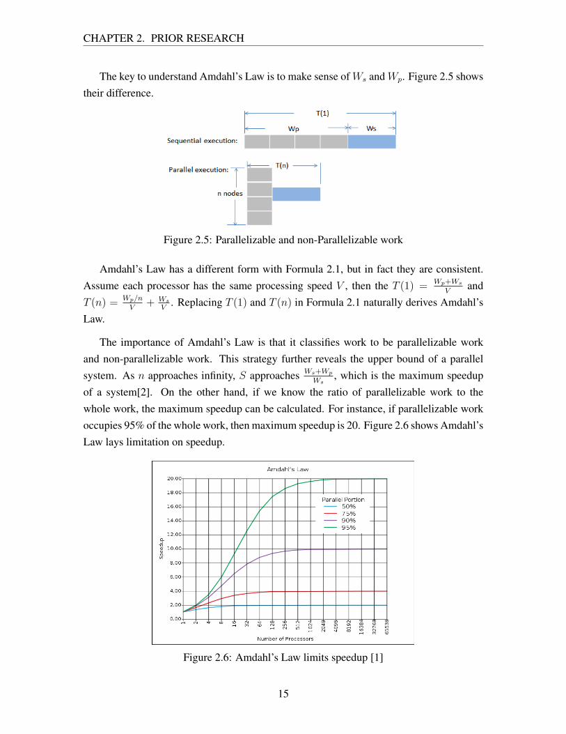
The key to understand Amdahl’s Law is to make sense of Ws and Wp. Figure 2.5 showstheir difference.
Figure 2.5: Parallelizable and non-Parallelizable work
Amdahl’s Law has a different form with Formula 2.1, but in fact they are consistent.Assume each processor has the same processing speed V , then the T (1) = Wp+Ws
Vand
T (n) = Wp/n
V+ Ws
V. Replacing T (1) and T (n) in Formula 2.1 naturally derives Amdahl’s
Law.
The importance of Amdahl’s Law is that it classifies work to be parallelizable workand non-parallelizable work. This strategy further reveals the upper bound of a parallelsystem. As n approaches infinity, S approaches Ws+Wp
Ws, which is the maximum speedup
of a system[2]. On the other hand, if we know the ratio of parallelizable work to thewhole work, the maximum speedup can be calculated. For instance, if parallelizable workoccupies 95% of the whole work, then maximum speedup is 20. Figure 2.6 shows Amdahl’sLaw lays limitation on speedup.
Figure 2.6: Amdahl’s Law limits speedup [1]
15

CHAPTER 2. PRIOR RESEARCH
2.2.3.3 Scaling behavior
Generally speaking, there are three types of scaling behaviors. They are super-linear scal-ing, linear scaling and sub-linear scaling. These three scaling behaviors are described inFigure 2.7. They actually described three speedup patterns. Speedup is calculated by hegradient of each line in Figure 2.7. Super-linear scaling means speedup is growing up, andsub-linear scaling means speedup is decreasing and linear scaling means speedup is keptthe same.
Figure 2.7: Scaling behavior
2.2.4 Data synchronization
Data synchronization aims at keeping consistency among different parts of data[28]. Weuse traditional WordCount algorithm to illustrate this. Assume there is a huge dataset, thesize of which is much greater than the memory of our available computer. In a typicaltraditional WordCount algorithm, we make key/value pair (wordi, 1) for wordi that weencounter for the first time. Then we store it on hard disk. When we meet wordi for thesecond time, we query the position of wordi on hard disk and then load it to memory andplus one to its value. Thus its key/value pair becomes (wordi, 2). Similarly, the kth timewe meet wordi, its key/value pair becomes (wordi, k). That is to say, pairs (wordi, value1)
and (wordi, value2) are put together and merged to be (wordi, value1 + value2). In thisscenario, placing the pairs with the same key together is data synchronization. It helps usmerge data. The problem with this traditional algorithm is there are too many queries. Thisdata synchronization gives rise to a large amount of workload. In Hadoop MapReduce,how this heavy workload is relived is covered in Chapter 3 Section 3.1.2 Job executionworkflow.
16

Chapter 3
Research target:Hadoop MapReduce
MapReduce is programming model aimed at large scale of dataset processing. It originatedfrom functional language Lisp. Its basic idea is to connect a large number of servers toprocess dataset in a parallel manner. Google started using this technology from the year2003. Thousands of commodity servers can be connected through MapReduce to run acomputation task. Figure 3.3 shows Google’s use of MapReduce in 2004.
Figure 3.1: Google use mapreduce
3.1 Mechanism
The execution workflow of MapReduce has been elaboratively described in Jeffrey Dean’spaper [6]. Although it covered the core workflow, it didn’t cover the architecture anddeployment. Therefore, we choose a bottom-to-top strategy to show the whole view ofHadoop MapReduce. However, we should emphasize that Google MapReduce and HadoopMapReduce are not the same in every aspect. As an open source framework inspiredby Google MapReduce, Hadoop MapReduce implemented most of the characteristics de-scribed in Jeffrey Dean’s paper [6], but it still has some features of its own.
17

CHAPTER 3. RESEARCH TARGET:HADOOP MAPREDUCE
3.1.1 Job hierarchy
Figure 3.2: Job Hierarchy Figure 3.3: map and reduce function [6]
Figure 3.2 shows the sketch of a basic working unit job for MapReduce. A job issimilar to the term project in C++ or Java development environment. As shown in Figure3.2, a job contains multiple tasks, and each task should either be a MapTask or ReduceTask.The functions map() and reduce() are user-defined functions. They are the most importantfunctions to achieve a user’s goal.
Map function transforms a key/value pair into a list of key/value pairs; while reducefunction aggregates all the pairs sharing the same key and processes their values. Figure3.3 shows the function of map and reduce.
The combination of map and reduce simplifies some traditional algorithms. We use theprogram WordCount to illustrate this. By default, the input of a map function is (key,value)pairs, in which key is line content of a text file, and value is line number. The map functionof WordCount splits the line content to be words list, each word is key and its value is1. Then reduce function aggregates all the pairs which have the same key and adds theirvalues together. The sum of these values sharing the same key is the total number of itscorrespondent word. The workflow of WordCount is shown in Figure 3.4.
Figure 3.4: The workflow of WordCount
18

CHAPTER 3. RESEARCH TARGET:HADOOP MAPREDUCE
3.1.2 Job execution workflow
Based on the knowledge of map and reduce function, now let’s look at their executionworkflow in a cluster environment. Figure 3.5 shows Google’s MapReduce cluster execu-tion workflow. Hadoop MapReduce’s workflow is the same with it.
Figure 3.5: MapReduce cluster execution workflow [6]
Jeffrey Dean’s paper [6] illustrated this workflow elaboratively. Here We just interpret itby decoupling this workflow in our own words. Nevertheless, our logic is similar to JeffreyDean. Since Hadoop MapReduce was inspired by Google MapReduce, here we just usethe mechanism of Google MapReduce to illustrate Hadoop MapReduce.
Before we start out, it is necessary to explain the key words appeared in Figure 3.5:
master Master is a computer that handles the management work such as scheduling tasksand resource allocation for tasks. There is only one master node in a Hadoop cluster,and the other nodes serve as slave nodes. Sometimes, we use one node to be a backupnode for master. The backup node doesn’t participate any actual management job. Itonly backup the most important information for the running master node.
fork It is the process of distributing user program to all machines in the cluster.
split A big file is divided into many splits and each split is usually customized to be 64MB.Splits facilitates data parallelism and backup. They are distributed to slave nodes forprocessing. Each split can be replicated to other machines as backup.
19

CHAPTER 3. RESEARCH TARGET:HADOOP MAPREDUCE
worker The worker in the figure is a logical concept, not a physical machine. A workerhas the same meaning with a task. A node can have many workers to execute basicmap or reduce operations. A map worker is also named as a mapper or a map taskand a reduce worker is named as a reducer or a reduce task.
Basically, a job contains two sequential phases:map and reduce phase. The map phasein Figure 3.5 is simple. It takes file splits as input and writes intermediate results to localdisks. The reduce phase is a bit complicated. Mappers and reducers have many-to-manyrelationship. One reducer fetches data from all mappers; and one mapper partitions itsoutput to all reducers. This action is performed by partition function. In Hadoop, parti-tion function is allowed to be overwritten by users . Partition function plays the role ofa connector between map and reduce phase. It decides which key goes to which specificreducer and achieves data synchronization. The partition function for WordCount programis hash(key) mod R ,where R is the number of reducers. This partition function achievesdata synchronization in an elegant way. It doesn’t need any query to put the same word tothe same reducer.
The result of partition function is a reducer gets a lot of pairs (wordi, 1) and the samepair (wordi, 1) may appear multiple times. For example, a reducer might get such pairssequentially: (wordi, 1), (wordj, 1), (wordi, 1), (wordk, 1).... In Hadoop MapReduce, areducer doesn’t merge pair (wordi, 1) with its previous occurrence immediately after itfetches one more (wordi, 1). The strategy is after a reducer obtains all its pairs and thenit sorts all of them by key so that the pairs sharing the same key are naturally groupedtogether.
Figure 3.6: MapReduce partitioner[18]
20

CHAPTER 3. RESEARCH TARGET:HADOOP MAPREDUCE
The details of partition function and reduce phase is explained via Figure 3.6. Thisfigure shows that partitioner is executed in between a mapper and reducer. It is executed inthe same machine with its mapper. Partitioner is a bridge between a mapper and a reducer.In Figure 3.6, “copy1” means reducers fetch intermediate results from mappers though Httpprotocol. “Sort” achieves aggregation for reducers. In Hadoop MapReduce, each reducetask has three subphases:copy, sort and reduce. The subphase reduce fulfils user-definedfunction. In WordCount program, the reduce operation is to sum the values sharing thesame key.
Notice that we use “reduce phase”,“reduce tasks(reducers)”, “subphase reduce(or sub-reduce)” and “reduce operation(reduce function)” to distinguish their differences. Similar-ly, “map phase”,“map tasks(mappers)” and “map operation(map function)” are also used todifferentiate them. The hierarchy and multiplicity relationship among them are important.Figure 3.7 shows the relationship among these reduce-related concepts.
Figure 3.7: Disambiguate concepts in reduce phase
3.1.3 Hadoop cluster hierarchy
Figure 3.8 shows Hadoop cluster hierarchy. It shows us how a job and its tasks are arrangedamong physical machines. Master node is also named as job tracker, which manages all thenodes. It needs an IP address table containing all IP addresses of all nodes. The slave nodesare also called datanode or task tracker. They contribute their local hard disk to form aHadoop Distributed File System(HDFS). They process data directly. From the perspectiveof a master node, all the slave nodes are dummy nodes. Except configuring slave nodesto be able to run Hadoop MapReduce program, we just use master node to control jobexecution and manage slaves.
1The operation is actually moving data, rather than copying data. In order to be in line with the descriptionof Hadoop’s official documents, we still use the term copy.
21

CHAPTER 3. RESEARCH TARGET:HADOOP MAPREDUCE
Figure 3.8: Hadoop cluster hierarchy
3.1.4 Traffic pattern
In parallel computing, data exchange is inevitable, therefore making sense of traffic patternis of great importance. Large scale of data exchange over the cluster often reveals somebottlenecks. In Hadoop MapReduce, large scale of data exchange happens after the com-pletion of map phase. This data exchange process refers to subphase “copy” in Figure 3.6.From the perspective of a reducer, it is executed on an individual node but its input data isconstructed from multiple mappers. From the perspective of a mapper, it partitions data tomultiple reducers and it is likely to produce a part of input data dedicated to any reducer.Thus, from the perspective of tasks, data transmission between mappers and reducers is amany-to-many relationship. Correspondingly, from the perspective of computing nodes, itis a multipoint-to-multipoint transmission relationship, because every node contains bothmappers and reducers. Thus, if all nodes are executing copy operation simultaneously, ev-ery node is transmitting data bidirectionally. Under this situation, the reducer of a node isdownloading data from all nodes including itself, and the mappers of that node are upload-ing their results to all nodes. Therefore, referring to Figure 3.5 we see that one mapperspills data to multiple reducers and one reducer fetches data from multiple mappers. Thisbidirectional multipoint-to-multipoint data exchange process is described in Figure 3.9.
Figure 3.9: Traffic pattern:servers and fetchers are the same set of nodes.
22

CHAPTER 3. RESEARCH TARGET:HADOOP MAPREDUCE
After map phase is finished, data exchange is not fulfilled once and for all. Every re-ducer always follows such an execution seqence:copy and then sort and finally reduce. Inother words, copy is bound with sort and reduce operation so that copy operation is exe-cuted intermittently. Between one reducer’s copy operation and its subsequent reducer’scopy operation, there is a time interval for sort and reduce operation. Figure 3.10 pro-vides a graphical description of this intermittent copy. We emphasize this intermittent copybecause in previous Hadoop version pre-0.18.0[23], it is once-and-for-all copy. Withoutexplicit explanation, it is very confusing.
Figure 3.10: Intermittent copy
Even though we mentioned it’s a multipoint-to-multipoint data exchange process, thedata fetching pattern is not very complicated. We view this data fetching activity from twoperspectives: an individual reducer and a set of parallel reducers.
Hadoop has a property mapred.reduce.parallel.copies, which is set to be 20 by default.It means that a reducer can fetch data from 20 mappers simultaneously. This value is fixedduring the execution of a MapReduce job. Therefore, if the total number of mappers islarger than 20, from the perspective of an individual reducer, its data fetching can be seenas a sequential process. Thus, once the input data size of a reducer is fixed, no matter theinput data is constructed from n nodes or 2n nodes, the number of mappers to that reduceris almost the same and the data volume from every mapper of them also doesn’t change,thus the fetching time is the same. For simplicity reason we ignore the time delay due toHttp connection setup and teardown. It is obvious that fetching data from 2n nodes needsmore Http connection setup and teardown than n nodes. From the perspective of a set ofparallel reducers, data fetching is parallelized. One reducer’s data fetching activity happenssimultaneously with other reducers’ data fetching.
From this introduction we see that Hadoop lays more focus on logical entities suchas mappers and reducers than physical entities computing nodes. According to commonknowledge, the total input data is more associated to the number of mappers than the num-ber of nodes, thus removing the concern about the number of nodes simplifies our problem.Facing with the same problem, the number of mappers will not change even if the numberof nodes increases. That is to say, a MapReduce program is adaptive to different numberof nodes without any necessity to change its code.
23

CHAPTER 3. RESEARCH TARGET:HADOOP MAPREDUCE
3.2 Supportive platform:Hadoop Distributed File System
MapReduce was originally designed to solve large dataset problems. The “large” datasetmay exceed several terabytes. Storage is a challenge for such big datasets. Google designedGoogle File System(GFS) to solve this problem and accordingly Hadoop has Hadoop Dis-tributed File System(HDFS). The details of GFS is unknown to public, here we just intro-duce HDFS. As Figure 3.8 shows, a lot of slaves are under the control of a master machine.The master uses Secure Shell(SSH) to start HDFS daemon on every slave. HDFS calcu-lates the storage space on every slave and combine them to be a big storage system. Unliketraditional file system, HDFS doesn’t have partitions. The master node and any slave nodecan upload files to HDFS and download them. Similar to GFS, users can define the size ofsplit, typically 64MB. This value 64MB means that an uploaded file is partitioned by thebasic unit 64MB. Therefore, a big file usually have multiple splits.
In order to facilitate data fetching, HDFS distributes splits to all slaves. Local split-s have higher processing priority than remote splits, so that in some cases, slaves do nothave to fetch remote data to accomplish distributed computing. This mechanism reducesnetwork burden for distributed computing. Further more, considering the failure of ma-chines, HDFS allows users to define a replica value. Its default value is 3, which meansevery split has three copies(including itself), and they are also distributed over the network.Hence, the failure of a single machine does not cause data loss and computation failure fora computation task. In a word, HDFS is a scalable and fault-tolerant distributed file system.
3.3 Key feature:speculative execution
Speculative execution[27] is a feature of Hadoop MapReduce. It computes the executionprogress of tasks and speculates whether they are slow. Slow tasks are re-executed byanother node. This mechanism avoids slow tasks from lasting too long, and reduces thegap among tasks’ execution time. In other words, it boosts the balance of the executiontime of tasks. An example of speculative execution is shown in Figure 3.11.
24

CHAPTER 3. RESEARCH TARGET:HADOOP MAPREDUCE
Figure 3.11: Speculative execution
3.4 Hadoop MapReduce program structure
Up till now MapReduce has many implementations. Its libraries have been written in C++,C#, Erlang, Java[19] and so on. Hadoop MapReduce is written in Java, hence we onlyprovide the program structure for Hadoop MapReduce. Figure 3.12 shows its programstructure.
Figure 3.12: MapReduce program structure
Basically, Figure 3.12 is consistent with job hierarchy showed in Figure 3.2. The onlydifference is this figure is at the standpoint of a programmer. The entrance class is MyDriver
class, in which a programmer defines which mapper/reducer class he uses. The wholeworkflow such as the number of total chained jobs and when to submit them is also definedin this class. Map and Reduce class rewrite the inherited method map() and reduce() todefine how to process a task unit. Communication, coordination and task scheduling areembedded into Hadoop’s library file. Thus, a programmer is exempt from this tough andheavy work. A mapper class is instantiated when it gets the command of processing onedata split. In text processing programs, it’s map method is invoked when it reads in aline. Normally, a mapper instance does not communicate with another map instance. Theirstatus information is reported to master node and handled by embedded library. Namely,a programmer doesn’t have to define which node processes which map tasks and he alsodoesn’t have to define any communication rule for any two map tasks. These details aboutmap task are the same as reduce tasks.
25

CHAPTER 3. RESEARCH TARGET:HADOOP MAPREDUCE
A sample WordCount program written in pseudo code is shown as follows:
Program 1 WordCount pseudo codeclass MyDriver:
main():Define a jobset input/output format for that jobAssociate a mapper class to that jobAssociate a reducer class to that jobSet the number of reducersRun this job
class MyMapper:map(String key,String value)://key:document line number//value:line content
for each word w in value:store key/value pair (w,1);
class MyReducer:reduce(String word,Iterator values)://key:a word//values: a list of counts
count=0;for each v in values:
count=count+1;store key/value pair (word,count)
We need to emphasize that it is required to set the number of reducers, but not requiredto set the number of mappers. The number of mappers equals the number of splits. Up tillnow, the current Hadoop MapReduce is not smart enough to do everything for users. Usershave to set the number of reducers according to their own requirement.
3.5 MapReduce applications
MapReduce is extensively used by Google, Yahoo,Facebook and so on. The applicationarea mainly covers: distributed search, log batch processing ,sorting[6] and so on. Webriefly describe some examples as follows:
Distributed search[6] The map operation returns a line when it matches a user-definedpattern. Since there is no use of reduce function, we don’t have to set a reduce classand write its function.
26

CHAPTER 3. RESEARCH TARGET:HADOOP MAPREDUCE
Distributed sort A typical example is Terasort [23], where results are sorted by keys.The map phase does nothing but distributes data to reducers. Assume user sets N
reducers. User’s Driver program selects N−1 sampled keys from map and sort them.According to these N − 1 sorted keys, a user-defined partition function partitions(key, value) pairs to the intervals of N−1 sorted keys. This measure guarantees thatthe keys distributed to ith reducers are always within the range of sorted (i − 1)th
key and ith key. The scenario is shown in Figure 3.13.
Figure 3.13: Distributed sort scenario: the vertical bar stands for a key.
File format batch conversion It’s reported that New York times converted 4TB’s scannedpicture format files into PDF format [22]. This application only uses map phase toparallelize batch processing work.
3.6 Experiment plan
Previous research [25, 31, 18, 16, 12, 13] have customized several experiments on HadoopMapReduce. These experiments include WordCount, matrix multiplication, Bayesian Clas-sification, Sorting, Page rank ,K-means clustering and so on. Among all the experiments,WordCount and Sorting are widely adopted benchmarks [13]. We choose these two exper-iments to fulfil our needs. The reasons are that they are easy to parallelize by MapReduceand they are the basic ingredients for many other experiments.
27

Chapter 4
Proposed models and verification
According to the execution workflow of Hadoop MapReduce , we abstracted a more un-derstandable model to describe it. This model is shown in 4.1. In our context, the termmodel refers to a simplified description of a problem, which leads to a solution directly.However, Figure 4.1 is an ideal situation, which must be based on certain assumptions andconditions. Therefore, it is important to clarify those important assumptions and conditionsfirst. After that, we propose two models to estimate the execution time of a MapReducejob.
Figure 4.1: Simplified MapReduce workflow: a grid represents a task
4.1 Assumptions
Establishing a model is not an easy thing, questions like why a model is reasonable, whatconditions it must satisfy and does it really match the real situation are very important. Inorder to remove those suspicion, we made some necessary assumptions and conditions inthis section. The most important assumptions and conditions are listed as follows:
Homogeneous computing environment and stability Computers have the same perfor-mance. They are running the same type of operating system. The network is stableso that the bandwidth will not shrink during our program running time.
28
CHAPTER 4. PROPOSED MODELS AND VERIFICATION
No severe workload imbalance We assume that each task handles almost the same work-load. That is to say, the computation density is evenly distributed for data splits.
Granularity unit:a task A job may contain tens of thousands of map and reduce tasks,taking one map/reduce task as granularity unit can simplify our analyzing work [6].In map phase, granularity unit is a map task and in reduce phase it is a reduce task.
Ignore management cost It is the master machine that mainly handles scheduling andother coordination work. We normally use a very powerful machine to be mastermachine, and its management work is normally far less than slaves’ workload, there-fore we assume master’s management doesn’t bring about explicit time delay for thewhole job.
One node has one processor Current computers normally have multiple processors, welimit that one computer node has only one processor. Thus, the number of nodes isthe same as the number of processors. This limitation just simplifies our explanation.
No node failure Hadoop MapReduce can handle node failures by diverting workload toother nodes. In our case, we don’t consider node failure. We just use experimentsthat have no node failures for analysis.
Condition of approximate equality In the process of experiment verification, we are sup-pose to check whether value A and B are equal. For instance, A could be a measuredvalue and B could be an estimated value. We use the following expression to judgewhether they are equal:
|A−B| ≤ 1
10min{A,B} (4.1)
4.2 Key condition:execution time follows regular trend
Before we propose our models, one critical proposition must be proved: the execution timeof tasks obeys regular trend under certain conditions even if the number of nodes and theinput data size change. We focus on the influence on two aspects: (1) the behaviors of anindividual node, (2) the behaviors of a set of parallel nodes.
Individual behavior mainly refers to the time consumption of the same type of taskswithin an individual node. In terms of group behavior, we mainly focus on the followingtwo aspects:
29

CHAPTER 4. PROPOSED MODELS AND VERIFICATION
• When the number of nodes increases, is there any change to the parallel behavior ofall parallel nodes?
• When the total data size changes, is there any change to the workload of a task, anddoes it affect parallel behavior?
Assume we have n nodes, parallel behavior refers to whether n parallel tasks can byrunning simultaneously. It is in contrast with such a scenario: when the number of nodesreaches a certain value, because of some bottleneck, the growth of nodes couldn’t give riseto the growth of parallel tasks. That is to say, parallelism is limited to a bottleneck.
The following subsection will give a detailed analysis on the influence of increasingcomputing nodes and total input data size.
4.2.1 The effect of increasing total data size
Assume we keep the number of nodes fixed, we analyze the effect of increasing total datasize for map and reduce phase separately.
Considering map phase, the input data is a number of evenly partitioned data splits(onlyone split is an exception). This partition process is performed before any MapReduceprogram is running. Once we upload any data to Hadoop Distributed File System, datais automatically partitioned to multiple splits according to a certain split size. Because ofthis, the number of unique splits equals the number of map tasks and they form a queuewaiting to be processed. If we keep the split size fixed, increasing the total data size willnot affect the size and workload of such a working unit. It just increases the total numberof map tasks. Further more, Hadoop MapReduce only allows us to load a certain numberof map tasks into the memory of one node each time, eg. two map tasks. This thresholdvalue makes sure memory and CPU are utilized regularly.
As for reduce phase, its input is constructed from many map tasks’ intermediate results.These results are stored in local disks. because before map phase is finished the size ofintermediate results is unknown, the number of reduce tasks is a user-defined value. That isto say Hadoop MapReduce does not automatically increase the number of reducers. If weincrease this value proportionally while increasing total data size, the input data size for areducer also doesn’t change.
According to the analysis of above, if we keep the split size fixed and tune the numberof reducers proportional to total data size, both the workload of a map and reduce task are
30

CHAPTER 4. PROPOSED MODELS AND VERIFICATION
not affected by increasing total data size.
4.2.2 The effect of increasing nodes
A direct effect of changing the number of nodes is the change to the arrangement of datasplits. More nodes means more splits can be processed in parallel. Its negative effect iswhen the number of nodes reaches a certain value, increasing nodes couldn’t bring aboutany speedup. Namely, it exposes the speedup bottleneck. This bottleneck might comefrom the problem itself, or the limitation of shared resources. As mentioned before, if aproblem’s non-parallelizable workload occupies 5% of the whole workload, the maximumspeedup is 20 [1]. More nodes means more traffic and heavier burden to the network. In factmany resources can be seen as shared resources, for instance, when a node serves as an Httpserver for all the nodes in the network, then the node itself is a shared resource. Anothertype of shared resource is the network relay device. Such devices are hubs,switches routersand so on. They are shared by a set of nodes. We also took the same analyzing strategy asbefore: fix the total data size, just increase nodes.
Considering map phase, the only process might be affected is partition function. Butpartition function just partitions a map task’s results to reducers and the number of them isnot related to the number of parallel nodes, for example, partition function for WordCountprogram is hash(key) mod R, where R is the number of reducers, hence partition functionis not affected. Further more there is no communication between any pair of map tasks.Hence, the whole map phase is not affected by the number of nodes.
Considering reduce phase, which has three subphases:copy,sort and reduce. Both sortand reduce operation are handled independently inside a node, thus from the perspectiveof parallel nodes, more nodes will surely accelerate sort and reduce operation. But fromthe perspective of an individual node, there is no impact on the processing time of sortand reduce operation. As for copy operation, it is involved with the utilization of sharedresources such as the network and other nodes. On the other hand, increasing the nodeswill evidently result in more reducers run in parallel. Thus, they will put heavier burden onthe shared resources. This scenario is shown in Figure 4.2.
Figure 4.2 gives us hint that increasing nodes but not increasing the capacity of sharedresources will give rise to speedup bottleneck to subphase copy. Figure 4.3 can help usunderstand what this bottleneck means. The lower part of the figure shows intermittentcopy, which represents current MapReduce’s actual workflow. If we extract all the copy
31

CHAPTER 4. PROPOSED MODELS AND VERIFICATION
Figure 4.2: Scenario of expanding the network
operation from reduce phase and connect them together, we have the three-phase modelshown in the upper part in Figure 4.3. We name this centralized copy as once-and-for-all
copy. The meaning of bottleneck is that, the time consumption of copy phase shown inthree-phase model couldn’t be reduced even if we increase the number of nodes. Becauseof this, the speedup of copy phase couldn’t grow. This speedup behavior is roughly shownin Figure 4.4. Even though copy speedup doesn’t affect map speedup and other phases’speedup, as a part of the whole job, according to Equation 2.2, it does affect the finalspeedup.
Figure 4.3: Models to describe a MapReduce job
Figure 4.4: Bottleneck due to limitation on shared resources
32

CHAPTER 4. PROPOSED MODELS AND VERIFICATION
In a word, two types of physical entities may cause speedup bottleneck for copy phase.Both a network relay device and any individual node may cause speedup bottleneck forcopy phase.
4.2.2.1 Speedup bottleneck due to network relay device
As mentioned before, a reducer fetches data from the network sequentially, but a batch ofreducers fetch data in a parallel manner. There is no doubt that data exchange must bebased on the most important shared resource:network. Therefore, due to the limitation ofnetwork bandwidth, the speedup of data fetching couldn’t grow all the time. For instance,if one reducer is supposed to fetch 100MB data from 10 parallel nodes, then 10 parallelreducers require to fetch 100*10=1000MB data simultaneously from the network. Thus1000 nodes requires to fetch 1000*100=97.7GB of data simultaneously. It is obvious thattransmitting 97.7GB of data lays much more burden on network than 1000MB. It is hardto guarantee that 97.7GB and 1000MB of data finish their transmission within the sameamount of time.
The ideal situation of such data parallelism has the following characteristics:(1) onereducer fetches d bytes of data from a network consumes the same time with n parallelreducers fetching nd bytes of data; (2) if one node fetches data from the network withtransmission speed s, k nodes should have transmission speed ks.
Considering a star network, all the nodes are connected to a centralized switch or otherdevices. The switch helps nodes achieve point-to-point communication. Normally, theswitch has a certain processing capacity. We denote it as h (bytes per sec), which is also aconstraint for data transmission. The h means that at most h bytes of data can be processedsimultaneously by the switch every second. we consider such a scenario:
Suppose we have a MapReduce job, which has D bytes of data to transmit aftermap phase. We use n nodes and 2n nodes to run the job separately. DenoteTc(n) as its total data fetching time by use of n nodes. Accordingly, denoteTc(2n) as the total data fetching time for 2n nodes. Denote tc(n) as one reduc-er’s data fetching time from n nodes, accordingly tc(2n) is used for 2n nodes.Denote s0 as point-to-point transmission speed. Therefore, n nodes require tohave transmission speed ns0 and 2n nodes require transmission speed 2ns0.Assume for both n nodes and 2n nodes, we use r reducers, therefore, each
reducer is supposed to fetch data d =D
rbytes. We ignore time delay due to
33
CHAPTER 4. PROPOSED MODELS AND VERIFICATION
Http connection setup and teardown.
We analyze the following situations:
1. ns0 < 2ns0 ≤ h. Since each reducer fetches d bytes of data sequentially, natu-
rally tc(n) = tc(2n) =d
s0. According to D = Tc(2n) · 2ns0 = Tc(n) · ns0, we
have Tc(2n) =1
2Tc(n). Under this situation, both n nodes and 2n nodes fetch data
simultaneously.
2. h ≤ ns0 < 2ns0. Under this situation, h causes speedup bottleneck. Following thesame logic as the item above, we have D = Tc(2n) · h = Tc(n) · h, thus Tc(2n) =
Tc(n). Under this situation, even if we have n or 2n nodes, actually onlyh
s0nodes
fetch data simultaneously or the transmission speed of each node decreases from s0 toh
nand
h
2n. These two situations are accordingly manifested by: (1) tc(n) = tc(2n);
(2) tc(n) < tc(2n).
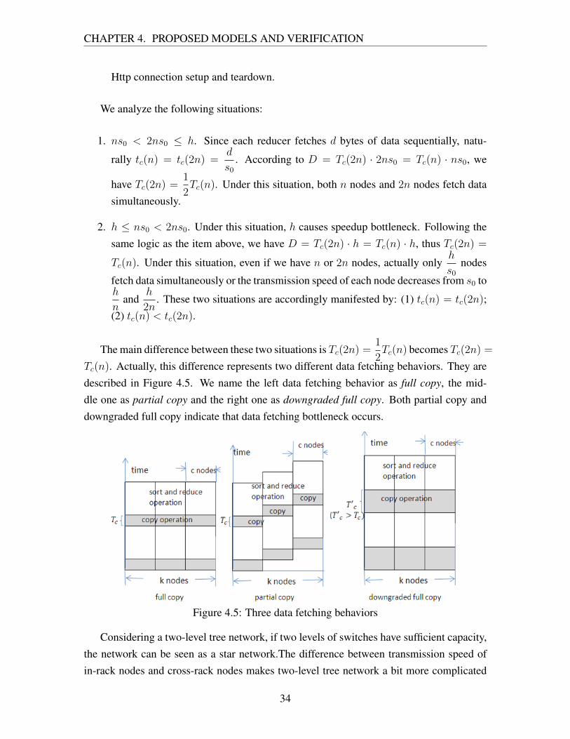
The main difference between these two situations is Tc(2n) =1
2Tc(n) becomes Tc(2n) =
Tc(n). Actually, this difference represents two different data fetching behaviors. They aredescribed in Figure 4.5. We name the left data fetching behavior as full copy, the mid-dle one as partial copy and the right one as downgraded full copy. Both partial copy anddowngraded full copy indicate that data fetching bottleneck occurs.
Figure 4.5: Three data fetching behaviors
Considering a two-level tree network, if two levels of switches have sufficient capacity,the network can be seen as a star network.The difference between transmission speed ofin-rack nodes and cross-rack nodes makes two-level tree network a bit more complicated
34

CHAPTER 4. PROPOSED MODELS AND VERIFICATION
than a star network. We denote s0 as in-rack point-to-point transmission speed, and s1 ascross-rack point-to-point transmission speed. We denote d = d0 + d1, where d representsa reducer’s input data and d0 is the part of data distributed within the same rack with thatreducer, and d1 represents the data distributed outside the reducer’s rack. Figure 4.6 showsthese notations in detail. Obviously, s0 is greater than s1.
Figure 4.6: Expand two-level network
For a large cluster, expanding the network is mainly done through increasing the num-ber of racks. Thus the bottleneck is often caused by the first-level switch, rather than the
second-level switch. Similar to the analysis above, we have tc(n) =d0s0
+d1s1
. Without
considering any bottleneck, the two-level tree network can actually be approximate to a
star network, therefore Tc(2n) =1
2Tc(n).
Under the premise of d = d0 + d1, we have tc(n) =d0s0
+d1s1
, where d is fixed all the
time. The increase of n or rather the increase of racks will increase d1 and decrease d0.
Since s0 > s1, the increase ofd1s1
is greater than the decrease ofd0s0
. As a result, tc(n) will
increase when we increase n, even if there is no bottleneck.
4.2.2.2 Speedup bottleneck due to an Http server’s capacity
The capacity of an Http server can cause speedup bottleneck. In Hadoop MapReduce ,every node serves as a server. An Http server’s capacity depends on a server’s memory andCPU capacity. Denote this maximum Http connections as c. Similar to the analysis abovewe list the following situations:
1. c ≥ 2n. This situation is similar to the first situation of our previous analysis on thebottleneck caused by network relay device . It is not difficult to get tc(2n) = tc(n)
35

CHAPTER 4. PROPOSED MODELS AND VERIFICATION
and Tc(2n) =1
2Tc(n). Both n nodes and 2n nodes fetch data simultaneously
2. c ≤ n. Under this situation, n nodes are divided into [n
c] + 1 groups. The operation
[n
c] means calculating integer part of
n
c. Data transmission is handled sequentially
among these groups. Under this situation, only c nodes can fetch data simultaneously.Therefore, tc(n) = tc(2n) and Tc(n) = Tc(2n).
Obviously, the situation of c ≤ n causes speedup bottleneck. even though we have n or2n parallel nodes, it only allows c nodes fetch data in parallel.
4.2.2.3 Decide boundary value
Our previous analysis shows that once we meet any bottleneck, full copy will either turn topartial copy or downgraded full copy. It is important to find out when this change happens.We denote b as the boundary value to describe this copy behavior change. When the numberof nodes is less than b, the copy behavior is full copy, when it surpasses b, it turns to beeither partial copy or downgraded full copy. As for which exact copy behavior it turnsto be, it depends on how the infrastructure program configure the switch. We can use anempty MapReduce program to detect whether our customized number of nodes is withinboundary b. We design such a MapReduce program that the map operation does nothingbut transmits data directly to reduce phase, and the reduce operation also does nothing. Weillustrate this experiment by use of Figure 4.7.
Figure 4.7: Boundary detection experiment illustration
Figure 4.7 shows that k is less than boundary b. T (k) represents the execution timeof the whole MapReduce job by use of k nodes; Ti stands for the ith reducer’s executiontime and tc(k) represents average copy time of a reducer. We do an experiment by use of knodes at first. Then we increase k to be k′. We aim at detecting whether k′ nodes exceedsboundary b. In both experiments, the input data is the same. Further more, the number ofmappers and reducers are kept the same. The judgement steps are described as follows:
36

CHAPTER 4. PROPOSED MODELS AND VERIFICATION
1. Firstly, compare T (k) with T (k′) first, if T (k) = T (k′) then the copy behavior of k′
nodes is full copy, otherwise it is either downgraded full copy or partial copy.
2. If T (k) 6= T (k′), compare tc(k) with tc(k′). If tc(k) = tc(k
′), the copy behavior ispartial copy, otherwise it is downgraded full copy.
Actually, this experiment is not every efficient, because it requires to test the same setof data on both k and k′ nodes. Once k is far less than k′, the experiment on k nodes willstill consume a large amount of time. But this experiment does give us hint to proposeanother more efficient experiment. This experiment scheme is described as follows:
Make an empty MapReduce program as described before. Test small amountof data by use of k nodes and compute tc(k). Test proper amount of data onk′ nodes. This data is larger than previous data on k nodes. Accumulate allreducers’ execution time in the experiment of k′ nodes as T . The ith reduc-er’s execution time is marked as Ti in Figure 4.7. The judgement steps aredescribed as follows:
1. CompareT
k′ with T (k′), where T (k′) is the execution time for the whole
MapReduce job. IfT
k′ = T (k′), then the copy behavior is either full copyor downgraded full copy.
2. IfT
k′ = T (k′), compare tc(k) with tc(k′), if tc(k) = tc(k
′) then the copybehavior is full copy, otherwise it is downgraded full copy.
4.2.2.4 Summary
We mainly analyzed the effect of increasing nodes in a star network. Its negative effect isfull copy may become partial copy and downgraded full copy. We suppose partial copy anddowngraded full copy are two forms of bottleneck. The conditions of full copy are listedas follows:
1. ns0 < h , where h represents capacity of central switch and s0 represents point-to-point transmission speed.
2. c ≥ n , where c represents the maximum Http connections to a server and n repre-sents the number of servers.
These two conditions are manifested in two aspects:
37

CHAPTER 4. PROPOSED MODELS AND VERIFICATION
1. One reducer’s fetching time tc(n) is fixed, even if n grows.
2. When n grows, the data fetching time of a parallel group Tc(n) will decrease.
In fact, those two conditions essentially stand for the same thing: the limitation onshared resources. A server node has connections with all other nodes. It means it is con-sumed or shared by all other nodes. Its Network Interface Card(NIC), CPU and memoryare shared resources. Data exchange must make use of the network, thus the replay deviceson network become shared resources. As we increase nodes, the limitation on any sharedresources can bring about bottleneck to subphase copy. Once shared resources meet theirlimitation, copy cannot speed up, but other phases can still speed up. Even if we meet anyform of bottleneck, previous experience is still useful.
Our analysis ignored time delay caused by Http connection setup and teardown. Con-sidering this effect, one reducer’s data fetching time tc(n) is not always fixed. As theincrease of n, tc(n) will have slight increase. We also did a short analysis on a two-leveltree network. From a certain angle, it can be seen as a star network. The increase of n willalso cause slight increase of tc(n) even if no bottleneck occurs. However, within a certainallowable range, we can ignore this slight increase.
The conclusion that one reducer’s fetching time tc(n) is fixed is of great significance.It leads to the conclusion that one reducer’s processing time Tr is fixed. This is becausea reducer is composed of three operations: copy, sort and reduce and none of their timeconsumption is affected by n. Considering one mapper’s processing time Tm is also fixed,Tm and Tr can be seen as useful learning experience. That is to say, they can be used toestimate the execution time of a MapReduce job, which aims at handling a larger scale ofdata on larger scale of nodes.
4.3 Wave model
Our previous analysis gives us some hint to propose a computation model to estimate ex-ecution time for a MapReduce job. In order to facilitate our description we define a termwave.
Definition: A wave is a group of parallel tasks, the length of which is the number ofparallel nodes n. There is map wave in map phase and reduce wave in reduce phase. The
38

CHAPTER 4. PROPOSED MODELS AND VERIFICATION
number of waves is computed by:
Nwave = [Ntask
n] + 1
where Ntask represents the number of tasks. The operation [Ntask
n] means obtaining the
integer part ofNtask
n. The number of waves Nwave indicates that roughly Nwave tasks
will be allocated to one node. Figure 4.8 shows that three tasks form a wave, which arerepresented by three vertical grids in the figure. Further more, in order to facilitate ourdescription, we name the series of tasks executed by an individual node as a task chain.Figure 4.8 shows that three nodes have three task chain.
Figure 4.8: The illustration of concept “wave”
4.3.1 General form
Figure 4.9: General form of wave model
This model is described in Figure 4.9. This figure shows that we apply the learningexperience on p nodes to q nodes(p < q). The most important condition for this model isq is less or equal than boundary b. How to test whether q is within boundary b has beenillustrated in subsection 4.2.2.3 Decide boundary value.
39

CHAPTER 4. PROPOSED MODELS AND VERIFICATION
This model derives the following expression to estimate execution time:
T̂ = T̂M + T̂R (4.2)
= TmNmw + TrNrw (4.3)
where Nmw is computed by [Nm
n] + 1 and Nrw is computed by [
Nr
n] + 1.
The meanings of notations are described in Table 4.1:
T̂ estimation of execution timeT̂M the estimated time consumption for map phaseT̂R the estimated time consumption for reduce phaseTm the time consumption of a map taskTr the time consumption of a reduce taskNmw the number of map wavesNrw the number of reduce wavesn the number of parallel nodesNm the number of map tasksNr the number of reduce tasks
Table 4.1: Notations for general form of wave model
Assume we have verified q is within the boundary b. The steps of how to accumulatelearning experience and how to apply the learning experience on p nodes to q nodes aredescribed as follows:
1. Do training experiment on p nodes by use of small sale of data, obtain Tm and Tr.
2. When it comes to large scale of data, according to the total input size and split sizeset in HDFS, compute the number of map tasks Nm and the number of reduce tasksNr.
3. Compute the number of map waves Nmw and the number of reduce waves Nrw ac-
cording to Nwave = [Ntask
n] + 1.
4. Use Tm and Tr obtained in training experiment, Nm and Nr to compute T̂ = TmNmw+
TrNrw. T̂ is our estimated value for large scale of data on q nodes.
From the step description above, we see that our useful experience information is Tm
and Tr. From now on we will not provide detailed step description unless it’s necessary.Pointing out what is experience information is enough for readers to catch our ideas.
40

CHAPTER 4. PROPOSED MODELS AND VERIFICATION
4.3.2 Slowstart form
The model shows in Figure 4.9 just presents the ideal situation that reduce phase waits forthe completion of all mappers. But Hadoop MapReduce has a slowstart mechanism, whichneeds special treatment. Slowstart value indicates that a part of reducers can be launchedafter the a fraction of mappers are completed[26]. Comparing with reducers wait for thecompletion of all mappers, this slowstart mechanism appears to be more efficient. Figure4.10 shows the effect of slow start. As long as some map tasks are finished, their results canbe copied to reducers. The whole copy phase for a reduce task occupies 33.3% 1 progressin that reduce task.
Figure 4.10: Slowstart
Even though Hadoop MapReduce utilizes slowstart to warm up reduce tasks, only thefirst wave of reduce tasks are affected. Further more, slowstart only performs copy op-eration earlier. This is because sort and reduce operation couldn’t start until the data iscompletely copied from all mappers. Reducers have to start sort and reduce operation afterthe arrival of the last (key,value) pair from the last mapper. Therefore, although the firstwave of reduce tasks starts early, they are actually in an “idle” state, which means they oc-cupy computation resources by fetching data, but couldn’t start sort and reduce operation.The math computation process of slowstart form is illustrated under the help of Figure 4.11.
Figure 4.11: Slowstart analysis model
A part of the notations can be found in Table 4.1, and the same notation stands for thesame meaning. New notations are described in the following Table 4.2:
1This value is obtained from Hadoop MapReduce runtime monitoring webpage.
41

CHAPTER 4. PROPOSED MODELS AND VERIFICATION
T̂ the estimation of completion timeT0 the start time of jobT1 the start time of reduce phaseT2 the end time of map phaseT3 the end time of first reduce wave∆ equals T3− T2Tov overlapped time,equals Tr −∆
Table 4.2: Notations for slowstart form of wave model
The goal here is to compute T̂ . Estimating TM is easy, which is achieved by T̂M =
NmwTm, however because of the abnormal behavior of the first reduce wave, T̂R couldn’tbe simply computed by NrwTr.
Let T ′R = NrwTr, refer to Figure 4.11, we have:
T̂ = TM + T ′R − Tov (4.4)
= TmNmw + TrNrw − (Tr −∆) (4.5)
= TmNmw + TrNrw − (Tr − T3 + T2) (4.6)
An important question here is as long as Tm and Tr are fixed, ∆ doesn’t change evenif scaling plan changes. As we mentioned before, reduce phase couldn’t start sorting andreduce until map phase is completely finished, therefore it is reasonable to treat Tov as thetime consumption for copy operation of the first reduce wave. We see from the expressionabove that our experience information is Tm, Tr and Tov.
Figure 4.11 shows that slowstart only saves time Tov, which is less than Tr. Consideringhuge amount of reduce tasks, this amount of time is ignorable. Therefore, the followingmodels will not consider slowstart situation, even if Hadoop MapReduce has provided sucha mechanism.
4.3.3 Speedup bottleneck form
We analyzed several possible situations which might cause speedup bottleneck. Becausespeedup bottleneck just happens in subphase copy, if we treat it differently, we can still findproper models to estimate execution time. According to Equation 2.2, as long as subphasecopy doesn’t occupy a great percentage in the whole job, it is still meaningful to intensifyparallelism for other phases by increasing nodes.
42

CHAPTER 4. PROPOSED MODELS AND VERIFICATION
Figure 4.12: Partial copy
Our previous analysis has revealed two copy behaviors caused by copy bottleneck.These two copy behaviors are partial copy and downgraded full copy. By use of Figure4.12, we can use the following expression to estimate execution time:
T̂ = T̂M + T̂R + Toffset (4.7)
= TmNmw + TrNrw + Toffset (4.8)
where Tm, Tr and Toffset are experience information.
Considering downgraded full copy, we concluded that one reducer’s data fetching timetc(n) will increase if n increases. Figure 4.13 described this phenomenon clearly. Actually,even if we don’t consider this bottleneck, considering time delay brought by Http connec-tion setup and teardown will also have some slight impact on tc(n). Further more, ouranalysis on two-level tree network also revealed that the increase of n will increase tc(n).This side-effect of increasing n is not so severe as the effect of bottleneck, but they behavevery similarly. Thus, we don’t aim to distinguish them here.
Figure 4.13: Downgraded full copy
43

CHAPTER 4. PROPOSED MODELS AND VERIFICATION
On the basis of the empty MapReduce program we proposed to test whether it is fullcopy or downgraded full copy in Subsection 4.2.2.3 Decide boundary value, we propose asolution to estimate execution time when we meet tc(m) > tc(n) where m > n.
Assume we aim to estimate the execution time of a practical problem on m nodes. Weuse three experiments to achieve our goal:(1) empty MapReduce experiment on n nodeswhere n is far less than m; (2) empty MapReduce experiment on m nodes; (3) practicalproblem-solving experiment on n nodes. From Figure 4.13 we see that the execution timeon sort and reduce operation do not change, no matter we use n or m nodes. Therefore,our main goal is to estimate the copy time of practical experiment on m nodes, which isdenoted as t′c(m). Similarly, we denote the copy time of practical experiment on n nodesas t′c(n). We estimate t′c(m) by the following expression:
t′c(m) = t′c(n) ∗ tc(m)
tc(n)
According to the execution workflow of a reduce task. Its execution time Tr is com-posed of three parts:Tcopy, Tsort and Treduce. Comparing the experiment on n and m nodes,only the value of Tcopy is changed from t′c(n) to t′c(m). Therefore, we just replace t′c(n)
with t′c(m) to compute the execution time of a reduce task and finally compute the wholeexecution time by T̂ = TmNmw + TrNrw (Expression 4.3).
4.3.4 Model verification for general form
We mainly did experiments on WordCount and Terasort program. We have two types ofexperiments:traning experiments and test experiments. Training experiments are used toaccumulate experience, while test experiments are used to verify the correctness of ourmodel. We obtained the start time and end time of every task. The duration is representedby their gap. We gathered them to form task chains and traced their execution time.
In stead of executing a job several times to compute its average execution time, wemeasure it by computing the expectancy from task chains. The advantage of this is we canreduce the number of experiment time.
We first present the behavior of map and reduce wave. Figure 4.14 and 4.15 showmap and reduce wave separately. This result shows the experiment of 4 nodes processing1.86GB data. For WordCount and Terasort program, we customized five experiments foreach program. The verification results are shown in Table 4.3 and Table 4.4.
44

CHAPTER 4. PROPOSED MODELS AND VERIFICATION
Figure 4.14: Map wave of WordCount. Figure 4.15: Reduce wave of WordCount.
4nodes 8nodes 16nodesTmeasure T̂ gap Tmeasure T̂ gap Tmeasure T̂ gap
929MB learn learn - 185.375 172.26 13.115 - - -1.86G 702.25 689.4 12.85 360.75 344.52 16.23 - - -
1.86G*2 - - - - - - 363.63 344.52 19.11
Table 4.3: Verify wave model for WordCount program
4nodes 8nodes 16nodesTmeasure T̂ gap Tmeasure T̂ gap Tmeasure T̂ gap
2GB learn learn - 161 156.12 4.88 - - -4GB 657.5 624.48 33.02 313 312.24 0.76 - - -8GB - - - - - - 318.9 312.24 6.66
Table 4.4: Verify wave model for Terasort program
These two tables show that the gaps are within 10% of min{Tmeasure, T̂}. It meansour measured values are consistent with estimated values. Theoretically speaking, if Tm
and Tr in our learning experiment are closer to Tm and Tr in new experiments, the gapshould be smaller. However, the fact is Tm and Tr are just average of a set of values. Itis the fluctuation or deviation of this set of values decides whether estimated value arecloser to measured value. From this point of view, we see that wave model requires a stricthomogeneous computing environment. But on the other hand, if accuracy requirement isnot very high, the simplicity of wave model is a good reason of choosing it.
45

CHAPTER 4. PROPOSED MODELS AND VERIFICATION
4.3.5 Model verification for slowstart form
The verification for slowstart form is shown in Table 4.5. This experiment result verifiesthat our computation method for slowstart situation is reasonable. The gaps are still within10% of min{Tmeasure, T̂}. Even though slowstart doesn’t really save too much time, it doesintroduce an interesting problem: the current slowstart just serves the first reduce wave,why designers don’t let it serve all the reduce waves is an interesting problem. Logicallyspeaking, after a map task is finished, which part of its result belongs to which reduceris fixed by partition function, then the system knows which result should be delivered towhich target machine.
8 nodes(Terasort) 8 nodes(WordCount)Tmeasure T̂ gap Tmeasure T̂ gap
2 GB - - - - - -4 GB 384.375 382.956 1.419 548.05 538 10.05
Table 4.5: Verify wave model for slowstart form
Essentially, this problem is about the argument between intermittent data exchange andonce-and-for-all data exchange. We noticed that in previous version Hadoop pre-0.18.0,once-and-for-all data exchange was used. Yahoo’s One Terabyte Sort experiment showsthis clearly. The task execution details is shown in Figure 4.16[23].
Figure 4.16: Once-and-for-all copy[23]
From our point of view,once-and-for-all copy is a bandwidth intensive process. Dataexchange is straightforward, but it also shows that CPU and memory are not fully utilizedin this process. Thus, recent Hadoop versions(our experiment version is 0.20.2) use inter-mittent copy to replace it. For intermittent copy if a part of reducers take less copy timethan others,they can start sort and reducer operation earlier, thus less parallel nodes are
46

CHAPTER 4. PROPOSED MODELS AND VERIFICATION
using the network. That is to say not all the nodes utilize network simultaneously. This al-ternate utilization of network relieves the burden on network. Figure 4.17 shows slowstartcopy pattern used in Hadoop 0.20.2.
Figure 4.17: Current slowstart copy pattern
The problem with this slowstart copy pattern is during map phase copy operation justserves the first wave, comparing with once-and-for-all copy it is quite slow. Combiningintensive copy in previous pattern with current intermittent copy, we propose a new copypattern. This copy pattern is shown in the Figure 4.18. This copy pattern combines thebenefits of intermittent copy and intensive copy.
Figure 4.18: Proposed new copy pattern
4.4 Sawtooth model
The previous section described wave model, which focuses on the group behavior of allparallel nodes. In fact, we can also focus on the individual behavior of every node. Basedon this idea, we come up with a Sawtooth model. We suppose that slowstart just reduce theprocessing time for first reduce wave. We do not provide the slowstart form in this section.
47

CHAPTER 4. PROPOSED MODELS AND VERIFICATION
4.4.1 General form
This model is described in Figure 4.19.
Figure 4.19: Sawtooth model
Basically, from each machine’s view, as tasks are gradually processed by itself, theirexecution time forms a trend line. Therefore, we can use some math tools such as linearregression to generate its trend function and finally estimate the whole execution time fora job by collecting each machine’s trend function. An important thing is this model shouldbe applied to map and reduce phase separately. We add their estimation value together tobe the execution time for a job. In order to make our results more accurate, it is better toaccomplish more waves to draw trend line.
The details of our ideas are summarized to be the following steps, we just use mapphase as our illustration example:
1. Accumulate experience by generating linear function for every experiment node:fi(x) = aix + bi, where 1 ≤ i ≤ n, n is the number of our experiment nodes. Thegradient ai represents the average execution time of a map task on nodei.
2. Facing with large scale of data, estimate the number of waves Nmw. Assume we haveincreased computing nodes from n to m;
3. Compute fi(Nmw), where 1 ≤ i ≤ n;
4. Sort fi(Nmw), and balance them. This balanced value is our estimated value. Thereason for this step is there might be a big gap between the biggest fj(Nmw) andthe smallest fk(Nmw). If this gap exceeds execution time of a map task aj and ak,then we should amend this by deducting one task from nodej and adding one taskto nodek. This goal is achieved by computing fj(Nmw − 1) and fk(Nmw + 1). Thisprocedure is performed recursively until the gap is small enough.
48

CHAPTER 4. PROPOSED MODELS AND VERIFICATION
The estimation for reduce phase is the same as map phase. After this is done, we addthese two estimated value together to be our final estimation.
4.4.2 Model verification for general form
We first present the behavior of map and reduce sawtooth. Figure 4.20 and 4.21 show mapand reduce sawtooth separately. This result shows the experiment of 4 nodes processing1.86GB data. These two figures match our model very well.
Figure 4.20: Map sawtooth of WordCount. Figure 4.21: Reduce sawtooth of WordCount.
The verification of our computation method is shown in the Table 4.7 and 4.6. Theresults show that the gap is within 10% of min{Tmeasure, T̂}. It means our measuredvalues are consistent with estimated values.
4nodes 8nodes 16nodesTmeasure T̂ gap Tmeasure T̂ gap Tmeasure T̂ gap
929MB - - - 185.375 173.935 gap - - -1.86G learn learn - 360.75 371.42 10.67 - - -
1.86G*2 - - - - - - 363.63 371.42 7.79
Table 4.6: Verify sawtooth model for WordCount program4nodes 8nodes 16nodes
Tmeasure T̂ gap Tmeasure T̂ gap Tmeasure T̂ gap2GB - - - 161 161.6 0.6 - - -4GB learn learn - 313 323.26 10.26 - - -8GB - - - - - 318.9 323.26 4.36
Table 4.7: Verify sawtooth model for Terasort program
49

CHAPTER 4. PROPOSED MODELS AND VERIFICATION
4.5 Summary
This chapter is the most important chapter of all. We started from describing key assump-tions and conditions. The proposition that execution time follows regular trend is the basisof our proposed models. The analysis on the effect of increasing total data size and increas-ing nodes revealed possible bottlenecks to copy operation. We name the two possible bot-tleneck behaviors as partial copy and downgraded full copy. Then, based on this analysisresult we proposed two models to estimate execution time of a MapReduce job. These twomodels are named as wave model and sawtooth model. They mainly address two problem-s:(1) what experience information should be learned from training experiment; (2) Whatformula or expression should be used to compute the estimated value. In sawtooth mod-el, we just provided the general form. Under the guidance of slowstart form and speedupbottleneck form of wave model, it is not difficult to adapt current sawtooth model to thesesituations. Due to budget limitation, we just provided possible bottleneck behaviors andconditions but didn’t do practical experiment to verify them.
50

Chapter 5
Discussion
5.1 Scalability analysis
For a parallel system, scalability analysis is a necessary step. Scalability often covers twoaspects: (1) scaling input data (2) scaling computing nodes. Scaling computing nodes isoften analyzed via speedup, which is an important performance evaluation criteria. It aimsat studying how much faster can a system achieves after expanding the number of nodes.In a multi-phase process, Equation 2.2 can facilitate our analysis quite a lot. In this aspect,MapReduce divides its process to be a map phase and reduce phase, which simplified ouranalysis. Even if when facing with a job chain, the speedup for the whole process can becomputed easily by analyzing every job separately. Consider map phase individually, itsscaling behavior is linear scaling, if no bottleneck occurs reduce phase also scales linearly.After combining them together, the scaling behavior is also linear scaling, which meansspeedup is linear.
Considering the effect of scaling data size on execution time, the ideal situation is in-creasing the data size just linearly increases its workload. In such case, the time consump-tion on (n nodes, d megabyte) is the same with (2n nodes, 2d megabyte). However, formany algorithms, workload is not proportional to their data size. For instance, consideringbubble sort[4], whose average time complexity is O(n2). Increasing data size n to be 2n
results in increasing workload approximately(2n)2
n2= 4 times. Therefore, assuming it’s
parallelizable, simply doubling computing nodes while doubling data size will not keepthe execution time the same. Considering MapReduce programming model, when taking atask as granularity unit, linear scaling on total data size also brings about linear scaling on
51

CHAPTER 5. DISCUSSION
total workloads. However, one thing we should notice is the scaling of total data size canautomatically scale the number of mappers, but it doesn’t scale the number of reducers ac-cordingly. Therefore in order to make the learning experience of one experiment consistentwith another experiment, it is necessary to make sure the execution time of each reducetask is the same in both of the experiments. An easy strategy is to make the number ofreducers proportional to the total data size. If we use 6 reducers for 1GB’s data(the inputsize for map), then we use 12 reducers for 2GB’s data.
4nodes 8nodes 16nodes929M 368.5 185.375 -1.86G 702.25 360.75 -
1.86G*2 - - 363.63
Table 5.1: Execution time for WordCount program(unit:sec)
4nodes 8nodes 16nodes2GB 318.5 161 -4GB 657.5 313 -8GB - - 318.9
Table 5.2: Execution time for Terasort program(unit:sec)
Due to the analysis above we conclude that by use of Hadoop MapReduce if workloadis balanced and no bottleneck affects parallelism, execution time is proportional to data sizeand inverse proportional to the number of computing nodes. We describe this conclusionby the following expression:
T (nodes, datasize) ∝ datasize
nodes
The experiment results in Table 5.1 and 5.2 are consistent with this expression. On theother hand, assume T (1) is execution time on a single node, we have:
speedup =T (1)
T (nodes, size)∝ nodes
datasize
This expression tells that once we fix datasize, we can achieve linear scaling undercertain conditions.
52

CHAPTER 5. DISCUSSION
5.2 The essence of wave model and sawtooth model
In Chapter 2 we mentioned that our main method is to find out a function T (nodes, datasize)
and its valid boundary to estimate the execution time of a larger problem. Readers maywonder why we turned to wave model and sawtooth model afterwards. Actually, theystand for the same idea.
The key factor in wave model is the number of map waves Nmw and reduce waves Nrw.Nmw and Nrw are decided by both the number of nodes and total data size. In other words,instead of study T (nodes, datasize) directly, we use a middle ware Nmw(nodes, datasize)
and Nrw(nodes, datasize) to study it. We have a more simplified understanding: assume
one node needs t time units to finish a MapReduce job, then n nodes needt
ntime units. It’s
like a string with length t is folded n times, then its folded length becomest
n. The strategy
of wave model is to compute the unit length of a string Tm, and then multiply it with thetotal number of units Nm and finally divide it by the number of parallel strings n. That is
to say the folded length is expressed by TmNm1
n, where
Nm
nequals the number of waves.
The idea behind sawtooth model is similar to wave model. Sawtooth model generatestrend line function fi(x) = aix+bi, and finally merge the value of every fi(x). The numberof waves is used to replace x. Wave model computes the average value for a task unit firstand then multiply it by number of waves Nwave. This multiplication is similar to replacingx with Nwave. Further more, in the expression fi(x) = aix + bi, the gradient ai actuallymeans the execution time of a task unit. If every trend function fi(x) = aix + bi are thesame, this particular case of sawtooth model can be seen as wave model. That is to say,wave model is actually a special case of sawtooth model.
The focus of wave model is the group behavior of all parallel nodes, but the focus ofsawtooth model is every individual node. Therefore, wave model requires a heterogeneouscomputing environment more than sawtooth model. But on the other hand, wave modelis obviously easier to perform. When the requirement of estimation accuracy is not verystrict, the simplicity of wave model is a good reason for us to choose it.
5.3 Extend models to more situations
Even though our proposed models must satisfy certain conditions, in fact they can be ex-tended to more situations. In some cases, small modification can adapt them to new situa-
53
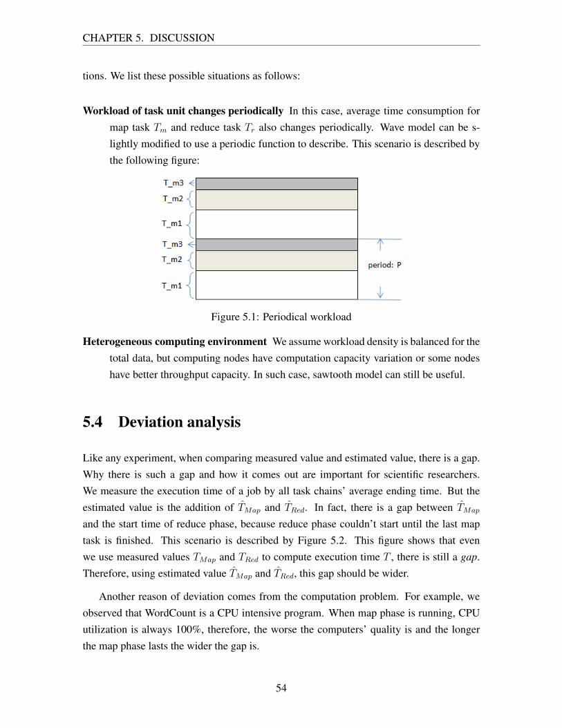
CHAPTER 5. DISCUSSION
tions. We list these possible situations as follows:
Workload of task unit changes periodically In this case, average time consumption formap task Tm and reduce task Tr also changes periodically. Wave model can be s-lightly modified to use a periodic function to describe. This scenario is described bythe following figure:
Figure 5.1: Periodical workload
Heterogeneous computing environment We assume workload density is balanced for thetotal data, but computing nodes have computation capacity variation or some nodeshave better throughput capacity. In such case, sawtooth model can still be useful.
5.4 Deviation analysis
Like any experiment, when comparing measured value and estimated value, there is a gap.Why there is such a gap and how it comes out are important for scientific researchers.We measure the execution time of a job by all task chains’ average ending time. But theestimated value is the addition of T̂Map and T̂Red. In fact, there is a gap between T̂Map
and the start time of reduce phase, because reduce phase couldn’t start until the last maptask is finished. This scenario is described by Figure 5.2. This figure shows that evenwe use measured values TMap and TRed to compute execution time T , there is still a gap.Therefore, using estimated value T̂Map and T̂Red, this gap should be wider.
Another reason of deviation comes from the computation problem. For example, weobserved that WordCount is a CPU intensive program. When map phase is running, CPUutilization is always 100%, therefore, the worse the computers’ quality is and the longerthe map phase lasts the wider the gap is.
54

CHAPTER 5. DISCUSSION
Figure 5.2: A deviation situation.
Figure 5.3: Not all tasks are launched at the same time[23].
For a large amount of parallel tasks for instance 1024 mappers, they cannot be launchedcompletely at the same time. From Yahoo’s experiment result of One Terabyte Sort showedin Figure 5.3 we see that approximately 1800 mappers are supposed to run in parallel. Thisfigure roughly shows that the gap between the start time of the first mapper and 1800thmapper is within 25 seconds. Accordingly, the gap between the first reducer and the 1800this also within 25 seconds. This fact tells us that if we don’t count this offset, we will have adeviation of 25 seconds. If a MapReduce job runs several hours, this 25 seconds could beignored. In our experiments, we did’t consider this offset, because our maximum numberof nodes is 16. This small number didn’t give rise to evident deviation.
Further more, we mentioned that the increase of number of nodes n will result in slightincrease of copy time tc(n) because of more Http connection setup and teardown. If wedon’t treat it the same as the handling of downgraded partial copy, it brings about deviation.As for our experiment, the gap between 4 nodes and 16 nodes is too small, so that there isalmost no change on tc(n) when n is increased from 4 to 16. Therefore, this is not a good
55
CHAPTER 5. DISCUSSION
reason that bring about deviation for our experiment. But for large scale of increasing n,for example changing n from 32 to 1024, the change on tc(n) is not ignorable.
5.5 Summarize learning workflow
A complete learning process should achieve at least two goals: (1) accumulate learningexperience; (2) decide the valid boundary of this learning experience. We need at leastthree experiments to estimate the execution time of a big problem:
1. An experiment using customized MapReduce program on small scale of data andsmall scale of computing nodes.
2. An experiment using empty MapReduce program on small scale of data and smallscale of computing nodes.
3. An experiment using empty MapReduce program on all available nodes.
The first experiment aims at obtaining the main experience information. The secondand the third experiment are used to detect the boundary of learning experience. If anybottleneck occurs, special form of models must be used. Based on these knowledge, wesummarize the learning workflow as follows:
1. Fairly sample a part of nodes and data.
2. Apply an empty MapReduce program and customized MapReduce program to sam-pled nodes. Empty program is used to detect whether copy subphase meets anybottleneck and customized program is used to accumulate main learning experience.
3. Apply an empty MapReduce program to all available nodes. Compare the resultsof previous empty program experiment and current one. Judge whether we meetbottleneck according to this comparison.
4. Decide which model to use according to the step3’s test result and accuracy require-ment.
56

Chapter 6
Conclusion
We started this thesis report by describing the research problem. Then we gradually re-vealed the mechanism of Hadoop MapReduce. Review our whole report, we mainly didthree things:(1) proved execution time of map/reduce tasks follow regular trend under cer-tain conditions;(2) proposed two models to estimate execution time of a MapReduce job;(3)fulfilled scalability analysis.
MapReduce is essentially a parallel programming model, thus we use speedup to mea-sure its performance. We emphasized that the utilization of shared resources is the causeof speedup bottleneck. For a MapReduce job, speedup bottleneck only occurs to copyoperation. We name the two copy behaviors which manifest bottleneck as partial copy
and downgraded full copy. An empty MapReduce program is proposed to handle thesebottlenecks. If bottleneck is detected, bottleneck form of proposed models has to be usedto estimate execution time. In order to address how learning process is performed, weproposed a learning workflow. It serves as a guidance of how to carry out a streamlinedlearning. Based on the virtual infrastructure service provided by Amazon Web Service, wefulfilled experiment verification for some models. The experiment result further boosts usto fulfil scalability analysis. It reveals the most important conclusion in this thesis: under
certain conditions, we can tune MapReduce to achieve T (nodes, datasize) ∝ datasize
nodes.
This expression further reveals that, MapReduce can be tuned to achieve linear scaling.
From our research we see that MapReduce is a simple and powerful parallel program-ming framework. Grasping the discipline of MapReduce can greatly help us carry out largescale of experiment on MapReduce.
57

Appendix A
Raw experiment results
Our raw experiment results are shown in the following tables. The first row of each tablerepresents the start time of first wave of tasks. The second row represents the end time offirst wave of tasks, and it also represents the start time of second wave of tasks. The timeunit of the following results is second.
map chain0 map chain1 map chain2 map chain3 red chain0 red chain1 red chain2 red chain31 1 0 3 345 343 344 34677 83 83 84 357 356 356 358
156 167 169 169 367 368 368 371239 250 252 253315 340 299
Table A.1: WordCount,929MB,4nodes
map chain0 map chain1 map chain2 map chain3 red chain0 red chain1 red chain2 red chain34 0 4 4 654 653 654 65382 81 82 84 667 665 667 671
165 163 162 165 672 677 679 684247 245 243 242 685 689 690 695330 327 326 322 697 701 703 708411 410 407 402489 492 487 483568 575 570 564650
Table A.2: WordCount,1.86GB,4nodes
map chain0 main chain1 map chain2 map chain3 map chain4 main chain5 map chain6 map chain71 1 0 1 1 2 1 180 80 81 82 83 84 86 88
158 160 160 165 170 169 133
red chain0 red chain1 red chain2 red chain3 red chain4 red chain5 red chain6 red chain7172 173 173 174 171 173 174 174184 185 185 185 186 186 186 186
Table A.3: WordCount,929MB,8nodes
58

APPENDIX A. RAW EXPERIMENT RESULTS
map chain0 map chain1 map chain2 map chain3 map chain4 map chain5 map chain6 map chain71 1 2 3 0 2 1 2
79 79 81 81 83 83 86 84157 158 159 161 163 168 168 170237 237 239 243 246 248 254 257316 317 319 323 310 332
red chain0 red chain1 red chain2 red chain3 red chain4 red chain5 red chain6 red chain7333 333 334 333 334 335 335 334345 345 347 348 349 348 348 349357 358 359 360 361 363 364 364
Table A.4: WordCount,1.86GB,8nodes
map chain0 map chain1 map chain2 map chain3 map chain4 map chain5 map chain6 map chain70 1 1 4 1 7 7 177 81 78 79 82 84 85 81
157 157 156 161 161 163 161 164234 235 236 239 241 241 243 243313 317 315 318 322 321 324 304
map chain8 map chain9 map chain10 map chain11 map chain12 map chain13 map chain14 map chain151 1 1 4 7 1 5 4682 84 83 87 84 81 94 123
166 166 164 168 168 169 186 201249 250 251 251 252 268 279 283333 334 333 319
red chain0 red chain1 red chain2 red chain3 red chain4 red chain5 red chain6 red chain7337 337 337 337 338 338 338 338349 349 349 349 349 350 350 350361 362 362 362 362 362 362 362
red chain8 red chain9 red chain10 red chain11 red chain12 red chain13 red chain14 red chain15338 339 339 339 341 337 339 340351 351 351 352 353 352 355 355363 363 363 364 365 366 369 370
Table A.5: WordCount,3.72GB,16nodes
map chain0 map chain1 map chain2 map chain3 red chain0 red chain1 red chain2 red chain30 1 0 1 157 158 158 15616 18 19 18 197 197 198 19935 36 40 36 237 240 237 24252 54 61 54 273 279 280 28473 73 81 73 307 319 322 32691 91 98 94
111 112 115 112130 131 134 133148 152 152 154
Table A.6: Terasort,2GB,4nodes
59

APPENDIX A. RAW EXPERIMENT RESULTS
map chain0 map chain1 map chain2 map chain3 red chain0 red chain1 red chain2 red chain31 3 0 1 329 329 334 33118 21 20 20 372 372 377 37537 42 40 41 415 417 420 42157 64 62 62 454 460 462 46676 83 83 83 496 500 504 51493 105 102 102 538 545 547 562
112 126 123 125 581 588 589 609130 149 144 146 624 632 632 657148 168 165 166 670 677 679 700167 187 185 187189 210 204 206211 230 223 225222 248 239 244250 268 259 264269 291 285 285290 309 304 304312 321 324 327
Table A.7: Terasort,4GB,4nodes
map chain0 map chain1 thread2 thread3 thread4 thread5 thread6 thread71 3 2 2 3 3 0 3
18 18 19 18 19 20 18 1935 36 36 35 37 37 36 3852 54 55 53 54 55 54 5572 72 72 73 73 73 75 75
red chain0 red chain1 thread2 thread3 thread4 thread5 thread6 thread778 79 80 78 79 80 80 81119 122 123 122 122 123 124 123161 162 162 163 164 165 166 169
Table A.8: Terasort,2GB,8nodes
map chain0 map chain1 map chain2 map chain3 map chain4 map chain5 map chain6 map chain70 1 0 2 1 2 2 2
16 17 16 17 17 19 19 1935 35 35 36 35 36 37 3753 53 53 54 53 54 55 5470 72 71 72 71 72 74 7490 91 89 91 90 92 92 92108 108 109 109 109 110 110 110126 126 126 127 126 128 128 129144 144 144 145 146 146 147 147
red chain0 red chain1 red chain2 red chain3 red chain4 red chain5 red chain6 red chain7149 149 148 150 149 149 150 151195 192 192 196 191 192 193 197240 235 236 236 237 237 235 240276 277 278 279 283 283 281 286312 320 321 326 328 328 330 335
Table A.9: Terasort,4GB,8nodes
60

APPENDIX A. RAW EXPERIMENT RESULTS
map chain0 map chain1 map chain2 map chain3 map chain4 map chain5 map chain6 map chain71 1 1 1 1 0 2 118 18 18 18 18 17 19 1936 37 35 36 35 35 37 3654 54 53 56 53 53 56 5772 72 74 73 73 72 75 7589 90 90 90 91 91 93 93
107 108 108 108 109 109 110 111125 126 126 126 127 128 129 129144 144 144 145 145 146 147 147
map chain8 map chain9 map chain10 map chain11 map chain12 map chain13 map chain14 map chain153 0 0 2 2 3 3 119 20 19 22 20 20 20 2039 38 36 42 39 39 40 3955 57 56 61 58 60 59 5874 75 76 80 76 79 78 7793 93 94 97 94 96 95 95
111 112 112 115 113 114 115 114129 130 131 135 131 133 132 131148 148 149 149 150 151 152 153
Table A.10: Terasort,8GB,16nodes
61

Bibliography
[1] Amdahl’s law. [Online]. Available: http://en.wikipedia.org/wiki/Amdahl’s law
[2] G. M. Amdahl, “Validity of the single processor approach to achieving large scalecomputing capabilities,” in Proceedings of the April 18-20, 1967, spring joint com-puter conference, ser. AFIPS ’67 (Spring). New York, NY, USA: ACM, 1967, pp.483–485.
[3] Amazon web service. [Online]. Available: http://aws.amazon.com/
[4] Bubble sort. [Online]. Available: http://en.wikipedia.org/wiki/Bubble sort
[5] Cloud computing. [Online]. Available: http://en.wikipedia.org/wiki/Cloudcomputing
[6] J. Dean, S. Ghemawat, and G. Inc, “Mapreduce: simplified data processing on largeclusters,” in In OSDI04: Proceedings of the 6th conference on Symposium on Opeart-ing Systems Design & Implementation. USENIX Association, 2004.
[7] Elastic computing cloud. [Online]. Available: http://aws.amazon.com/ec2/
[8] A. Y. Grama, A. Gupta, and V. Kumar, “Isoefficiency: Measuring the scalability ofparallel algorithms and architectures,” IEEE Parallel Distrib. Technol., vol. 1, pp. 12–21, August 1993.
[9] granularity. [Online]. Available: http://en.wikipedia.org/wiki/Granularity
[10] graysort. [Online]. Available: http://sortbenchmark.org/
[11] Gustafson’s law. [Online]. Available: http://en.wikipedia.org/wiki/Gustafson’s law
[12] S. Huang, J. Huang, J. Dai, T. Xie, and B. Huang, “The hibench benchmark suite:Characterization of the mapreduce-based data analysis,” in Data Engineering Work-shops (ICDEW), 2010 IEEE 26th International Conference on, march 2010, pp. 41–51.
[13] S. Ibrahim, H. Jin, L. Lu, L. Qi, S. Wu, and X. Shi, “Evaluating mapreduce on virtualmachines: The hadoop case,” in Proceedings of the 1st International Conference onCloud Computing, ser. CloudCom ’09. Berlin, Heidelberg: Springer-Verlag, 2009,pp. 519–528.
62

BIBLIOGRAPHY
[14] IEEE 802.3i(10BASE-T), IEEE Std.
[15] Amazon instance. [Online]. Available: http://aws.amazon.com/ec2/#instance
[16] K. Kim, K. Jeon, H. Han, S.-g. Kim, H. Jung, and H. Y. Yeom, “Mrbench: A bench-mark for mapreduce framework,” in Proceedings of the 2008 14th IEEE InternationalConference on Parallel and Distributed Systems. Washington, DC, USA: IEEEComputer Society, 2008, pp. 11–18.
[17] V. Kumar and A. Gupta, “Analyzing scalability of parallel algorithms and architec-tures,” J. Parallel Distrib. Comput., vol. 22, pp. 379–391, September 1994.
[18] J. Lin and C. Dyer, Data-Intensive Text Processing with MapReduce, 2010.
[19] Mapreduce. [Online]. Available: http://en.wikipedia.org/wiki/MapReduce
[20] mesh network. [Online]. Available: http://en.wikipedia.org/wiki/Mesh networking
[21] Message passing interface(mpi). [Online]. Available: http://en.wikipedia.org/wiki/Message Passing Interface
[22] Newyork. [Online]. Available: http://open.blogs.nytimes.com/2007/11/01/self-service-prorated-super-computing-fun/
[23] O. O’Malley, “Terabyte sort on apache hadoop,” May 2008.
[24] ——, “Winning a 60 second dash with a yellow elephant,” April 2009.
[25] W.-C. Shih, S.-S. Tseng, and C.-T. Yang, “Performance study of parallel program-ming on cloud computing environments using mapreduce,” in Information Scienceand Applications (ICISA), 2010 International Conference on, april 2010, pp. 1–8.
[26] Hadoop mapreduce configuration file. [Online]. Available: http://hadoop.apache.org/mapreduce/docs/current/mapred-default.html
[27] speculative execution. [Online]. Available: http://developer.yahoo.com/hadoop/tutorial/module4.html
[28] Data synchronization. [Online]. Available: http://en.wikipedia.org/wiki/Data synchronization
[29] E. Tambouris and P. v. Santen, “A methodology for performance and scalability anal-ysis,” in Proceedings of the 22nd Seminar on Current Trends in Theory and Practiceof Informatics, ser. SOFSEM ’95. London, UK: Springer-Verlag, 1995, pp. 475–480.
[30] T. White, Hadoop:The definitive guide, M. Loukides, Ed. O’Reilly Media, 2009.
[31] M. Zaharia, A. Konwinski, A. D. Joseph, R. Katz, and I. Stoica, “Improving mapre-duce performance in heterogeneous environments,” in Proceedings of the 8th USENIXconference on Operating systems design and implementation, ser. OSDI’08. Berke-ley, CA, USA: USENIX Association, 2008, pp. 29–42.
63