Array Processing Techniques for Estimation and Tracking of ...

ARRAY PROCESSING TECHNIQUES FOR ESTIMATIONAND TRACKING OF AN ICE-SHEET BOTTOM

By

Mohanad Ahmed Abdulkareem Al-Ibadi

Submitted to the Department of Electrical Engineering and Computer Science and theGraduate Faculty of the University of Kansas

in partial fulfillment of the requirements for the degree ofDoctor of Philosophy

Committee members

Shannon Blunt, Chairperson

John Paden, Co-chair

James Stiles

Erik Perrins

Christopher Allen

Huazhen Fang

Date defended: May 10, 2019

The Dissertation Committee for Mohanad Ahmed Abdulkareem Al-Ibadi certifiesthat this is the approved version of the following dissertation :

ARRAY PROCESSING TECHNIQUES FOR ESTIMATION AND TRACKING OF ANICE-SHEET BOTTOM

Shannon Blunt, Chairperson

John Paden, Co-chair

Date approved:

ii

Abstract

Ice bottom topography layers are an important boundary condition required to model

the flow dynamics of an ice sheet. In this work, using low frequency multichannel

radar data, we locate the ice bottom using two types of automatic trackers.

First, we use the multiple signal classification (MUSIC) beamformer to determine the

pseudo-spectrum of the targets at each range-bin. The result is passed into a sequen-

tial tree-reweighted message passing belief-propagation algorithm to track the bottom

of the ice in the 3D image. This technique is successfully applied to process data

collected over the Canadian Arctic Archipelago ice caps in 2014, and produce dig-

ital elevation models (DEMs) for 102 data frames. We perform crossover analysis

to self-assess the generated DEMs, where flight paths cross over each other and two

measurements are made at the same location. Also, the tracked results are compared

before and after manual corrections. We found that there is a good match between the

overlapping DEMs, where the mean error of the crossover DEMs is 38±7 m, which

is small relative to the average ice-thickness, while the average absolute mean error of

the automatically tracked ice-bottom, relative to the manually corrected ice-bottom, is

10 range-bins.

Second, a direction of arrival (DOA)-based tracker is used to estimate the DOA of

the backscatter signals sequentially from range bin to range bin using two methods:

a sequential maximum a posterior probability (S-MAP) estimator and one based on

the particle filter (PF). A dynamic flat earth transition model is used to model the

flow of information between range bins. A simulation study is performed to evalu-

ate the performance of these two DOA trackers. The results show that the PF-based

iii

tracker can handle low-quality data better than S-MAP, but, unlike S-MAP, it saturates

quickly with increasing numbers of snapshots. Also, S-MAP is successfully applied

to track the ice-bottom of several data frames collected over Russell glacier in 2011.

Several tracker bounding models with uniform and Gaussian priors are proposed and

compared as well. The results show that uniform prior pdf with not-too-tight bounds

give the best tracking results. The results of the DOA-based techniques are the final

tracked surfaces, so there is no need for an additional tracking stage as there is with

the beamformer technique.

In addition, a machine learning (ML) based solution to the wideband model order esti-

mation (MOE) problem is proposed and compared to six other standard MOE methods

as well as a numerically tuned method. The results show a substantial improvement

in the percentage of estimating the correct number of targets, especially in the more

challenging scenario of wideband data with large number of targets relative to the

number of sensors. Also, we found that the standard MOE methods work well on real

wideband if the log-likelihood term of the cost function is corrected to account for the

narrowband model mismatch when the number of targets is small.

iv

Acknowledgements

I would like to thank my wife, Dumooa, for her love and support during the many

years of my PhD, and for taking care of my two little daughters as well. She was, and

still is, the source of joy and happiness in the family all the time. I also would like

to thank my great mother for her encouragement and support and for her smile and

reassuring words whenever I feel homesick. Many thanks to my father as well for his

big love and support.

I am indebted to my advisor, Dr. John Paden, for his help and patience with my slow

learning process and for the too much time he dedicated to me and the data processing

group. All the words can’t express my deep gratitude to him.

I’m also grateful to Dr. Shannon Blunt and Dr. James Stiles for the great courses that I

took with them. These courses increased my love to the radar signal processing field.

I also want to thank my dearest friends in the data processing group in CReSIS. Many

thanks to Victor Berger and Sravya Athinarapu for the long discussions we had about

different parts of our research. I’m really proud of being surrounded by such a great

colleagues, friends, and collaborators.

I also acknowledge my sponsor, the Higher Committee for Education Development in

Iraq (HCED), NSF (ACI-1443054), and NASA (NNX16AH54G).

v

Contents

1 Introduction and Literature Review 1

1.1 Motivation and Literature Review . . . . . . . . . . . . . . . . . . . . . . . . . . 1

1.2 Thesis Outline . . . . . . . . . . . . . . . . . . . . . . . . . . . . . . . . . . . . . 5

2 Array Signal Processing for Ice-Sheet Imaging: Theory and Background 6

2.1 Introduction . . . . . . . . . . . . . . . . . . . . . . . . . . . . . . . . . . . . . . 6

2.2 SAR Tomography . . . . . . . . . . . . . . . . . . . . . . . . . . . . . . . . . . . 8

2.2.1 Ground Range Resolution and Number of Snapshots . . . . . . . . . . . . 10

2.3 Narrowband Signal Model . . . . . . . . . . . . . . . . . . . . . . . . . . . . . . 16

2.4 Wideband Signal Model . . . . . . . . . . . . . . . . . . . . . . . . . . . . . . . 21

2.5 Cramer-Rao Lower Bound (CRLB) . . . . . . . . . . . . . . . . . . . . . . . . . 22

2.6 Direction of Arrival Estimation (DOA) . . . . . . . . . . . . . . . . . . . . . . . . 24

2.6.1 Multiple Signal Classification (MUSIC) . . . . . . . . . . . . . . . . . . . 24

2.6.2 Maximum Likelihood Estimation (MLE) . . . . . . . . . . . . . . . . . . 26

2.6.3 Wideband MLE (WBMLE) . . . . . . . . . . . . . . . . . . . . . . . . . 27

2.6.4 Focusing Matrices . . . . . . . . . . . . . . . . . . . . . . . . . . . . . . 28

2.6.5 Sequential DOA Estimation . . . . . . . . . . . . . . . . . . . . . . . . . 29

2.6.5.1 Particle Filter (PF) . . . . . . . . . . . . . . . . . . . . . . . . . 34

2.6.5.2 Sequential Maximum A Posteriori Estimation (S-MAP) . . . . . 49

2.7 Steering Vectors Estimation and Array Calibration . . . . . . . . . . . . . . . . . . 51

vi

2.8 Specifications of the Radars Used in This Work . . . . . . . . . . . . . . . . . . . 57

2.9 Processing Phase Centers . . . . . . . . . . . . . . . . . . . . . . . . . . . . . . . 61

3 Wideband Model Order Estimation Using Machine Learning 63

3.1 Introduction . . . . . . . . . . . . . . . . . . . . . . . . . . . . . . . . . . . . . . 63

3.2 MOE Based on Logistic Regression (LR-MOE) . . . . . . . . . . . . . . . . . . . 66

3.2.1 Logistic Regression Model . . . . . . . . . . . . . . . . . . . . . . . . . . 67

3.2.2 Logistic Regression Cost Function . . . . . . . . . . . . . . . . . . . . . . 69

3.2.3 Testing and Training Modes . . . . . . . . . . . . . . . . . . . . . . . . . 70

3.2.4 LR-MOE Algorithm . . . . . . . . . . . . . . . . . . . . . . . . . . . . . 70

3.2.5 Results: Comparison Between LR-MOE and Other Methods . . . . . . . . 71

4 Comparison Between Particle Filter and Sequential MAP for Surface Tracking 79

4.1 Introduction . . . . . . . . . . . . . . . . . . . . . . . . . . . . . . . . . . . . . . 79

4.2 Simulation Setup . . . . . . . . . . . . . . . . . . . . . . . . . . . . . . . . . . . 79

4.3 Particle Filter As a Surface Tracker . . . . . . . . . . . . . . . . . . . . . . . . . . 81

4.3.1 DOA estimation under the PF framework . . . . . . . . . . . . . . . . . . 83

4.3.2 PF vs MLE and MUSIC: a Qualified Validation . . . . . . . . . . . . . . . 85

4.3.3 Surface Tracking: Step by Step Explanation . . . . . . . . . . . . . . . . . 89

4.4 Sequential MAP Filter As a Surface Tracker . . . . . . . . . . . . . . . . . . . . . 97

4.4.1 Surface Tracking: Step By Step Explanation . . . . . . . . . . . . . . . . 97

4.5 Performance Comparison of PF vs S-MAP . . . . . . . . . . . . . . . . . . . . . . 99

4.6 Discussion . . . . . . . . . . . . . . . . . . . . . . . . . . . . . . . . . . . . . . . 105

5 3D Image Formation Results of Ice-Sheets 113

5.1 Introduction . . . . . . . . . . . . . . . . . . . . . . . . . . . . . . . . . . . . . . 113

5.2 Ice-Bottom Tracking Using MUSIC and TRWS . . . . . . . . . . . . . . . . . . . 114

5.2.1 MUSIC: Ice-Bottom Tracking Algorithm and DEM Generation Process . . 119

5.2.2 MUSIC: DEM Generation Results . . . . . . . . . . . . . . . . . . . . . . 125

vii

5.2.3 MUSIC: DEM Crossover Analysis . . . . . . . . . . . . . . . . . . . . . . 126

5.2.4 MUSIC: Layer Tracking Assessment . . . . . . . . . . . . . . . . . . . . 131

5.3 Ice-Bottom Tracking Using Sequential MAP . . . . . . . . . . . . . . . . . . . . . 134

5.3.1 S-MAP Tracker: Bounding Models and Prior pdf . . . . . . . . . . . . . . 135

5.3.2 S-MAP Tracker: Layer Tracking Assessment . . . . . . . . . . . . . . . . 150

5.3.2.1 Tracking Assessment: MOE . . . . . . . . . . . . . . . . . . . . 150

5.3.2.2 Tracking Assessment: S-MAP tracked layers vs ground truth . . 154

5.3.3 S-MAP Tracker: DEM Generation Results and Assessments . . . . . . . . 156

6 Conclusions and Future Work 161

6.1 Concluding Remarks . . . . . . . . . . . . . . . . . . . . . . . . . . . . . . . . . 161

6.2 Future Work . . . . . . . . . . . . . . . . . . . . . . . . . . . . . . . . . . . . . . 162

viii

List of Figures

2.1 SAR data processing steps . . . . . . . . . . . . . . . . . . . . . . . . . . . . . . 7

2.2 Cross-track slice . . . . . . . . . . . . . . . . . . . . . . . . . . . . . . . . . . . . 8

2.3 Ground range resolution of a flat surface . . . . . . . . . . . . . . . . . . . . . . . 12

2.4 Ground-range resolution of non-flat surface . . . . . . . . . . . . . . . . . . . . . 12

2.5 Deriving the change in DOA with range . . . . . . . . . . . . . . . . . . . . . . . 13

2.6 Ground-range resolution vs incident angle . . . . . . . . . . . . . . . . . . . . . . 13

2.7 Change in DOA vs incident angle . . . . . . . . . . . . . . . . . . . . . . . . . . 14

2.8 Section of a 3D image showing near-nadir point cloud . . . . . . . . . . . . . . . . 15

2.9 Ground-range resolution vs incident angle for a wideband case . . . . . . . . . . . 16

2.10 Elevation angle vs CRLB . . . . . . . . . . . . . . . . . . . . . . . . . . . . . . . 24

2.11 Geometric presentation of the parameters of the DOA prior pdf . . . . . . . . . . . 32

2.12 ∆θ vs f (∆θ) defined in equation 2.32 . . . . . . . . . . . . . . . . . . . . . . . . 33

2.13 Example of an importance sampling region. . . . . . . . . . . . . . . . . . . . . . 36

2.14 Sequential importance sampling resampling (SISR) . . . . . . . . . . . . . . . . . 44

2.15 Sensors gain pattern . . . . . . . . . . . . . . . . . . . . . . . . . . . . . . . . . . 56

2.16 Sensors phase deviation pattern . . . . . . . . . . . . . . . . . . . . . . . . . . . . 57

2.17 Transmit configuration of the P-3 radar . . . . . . . . . . . . . . . . . . . . . . . . 58

2.18 Phase centers of the three subarrays mounted on the P-3 radar . . . . . . . . . . . 59

2.19 Monostatic equivalent measurement phase center for a bistatic radar geometry . . . 62

3.1 The sigmoid function . . . . . . . . . . . . . . . . . . . . . . . . . . . . . . . . . 68

ix

3.2 Geometric means of the eigenvalues of the data covariance matrix . . . . . . . . . 72

3.3 Arithmetic means of the eigenvalues of the data covariance matrix . . . . . . . . . 72

3.4 Logistic regression-based MOE results for narrowband scenario . . . . . . . . . . 74

3.5 Model order estimation results of seven compared methods for a narrowband scenario 75

3.6 Logistic regression-based MOE results for wideband scenario . . . . . . . . . . . 75

3.7 Results of seven compared methods for wideband scenario [1]. . . . . . . . . . . . 76

3.8 Model order estimation results of seven compared methods for a wideband scenario 77

3.9 Logistic regression-based MOE results for wideband scenario using wide dynamic

range of training SNRs . . . . . . . . . . . . . . . . . . . . . . . . . . . . . . . . 77

3.10 Logistic regression-based MOE results for wideband scenario for 50 dB SNR . . . 78

4.1 Elevation angle vs√

CRLB, in degrees, for 3 SNRs with M = 21 snapshots. . . . . 82

4.2 RMSE vs number of particles: single range-bin scenario . . . . . . . . . . . . . . 84

4.3 RMSE vs number of particles: multiple range-bins scenario . . . . . . . . . . . . . 85

4.4 PF vs MLE and MUSIC: RMSE vs SNR for narrowband scenario . . . . . . . . . 87

4.5 PF vs MLE and MUSIC: RMSE vs number of snapshots for narrowband scenario . 87

4.6 PF vs MLE and MUSIC: RMSE vs SNR for wideband scenario . . . . . . . . . . . 88

4.7 PF vs MLE and MUSIC: RMSE vs number of snapshots for wideband scenario . . 88

4.8 PF vs MLE and MUSIC: RMSE vs SNR for narrowband scenario at Low snapshots

regime . . . . . . . . . . . . . . . . . . . . . . . . . . . . . . . . . . . . . . . . . 89

4.9 Tracking the importance sampling region: 3D scatter plots . . . . . . . . . . . . . 93

4.10 Tracking the importance sampling region: 2D histogram-like plots plots . . . . . . 96

4.11 S-MAP surface for 3 different SNR scenarios . . . . . . . . . . . . . . . . . . . . 98

4.12 S-MAP: RMSE for wide range of SNRs vs range-bin . . . . . . . . . . . . . . . . 101

4.13 FP: RMSE for wide range of SNRs vs range-bin . . . . . . . . . . . . . . . . . . . 101

4.14 S-MAP: RMSE for wide range of number of snapshots vs range-bin . . . . . . . . 102

4.15 PF: RMSE for wide range of number of snapshots vs range-bin . . . . . . . . . . . 102

4.16 S-MAP vs PF: average RMSE vs SNR for narrowband scenario . . . . . . . . . . 103

x

4.17 S-MAP vs PF: average RMSE vs number of snapshots for narrowband scenario . . 103

4.18 S-MAP vs PF: average RMSE vs SNR for wideband scenario . . . . . . . . . . . . 104

4.19 S-MAP vs PF: average RMSE vs number of snapshots for wideband scenario . . . 104

4.20 Mean and variance of the DOA from geostatistical analysis of the CAA 2014 data

set . . . . . . . . . . . . . . . . . . . . . . . . . . . . . . . . . . . . . . . . . . . 106

4.21 Eigenvalues of a data covariance matrix generated by simulating M = 21 snapshots

and p = 7 sensors for the 15% fractional bandwidth scenario. . . . . . . . . . . . . 109

4.22 Percentage correct plots of the estimated number of targets for the 15% fractional

bandwidth scenario. . . . . . . . . . . . . . . . . . . . . . . . . . . . . . . . . . . 110

4.23 Number of estimated targets per range-bin for each of the 7 tested MOE methods,

in addition to the actual number of targets, Q, for the 15% fractional bandwidth

scenario with SNR = 30 dB. . . . . . . . . . . . . . . . . . . . . . . . . . . . . . 111

5.1 Canadian Arctic Archipelago islands along with the flight paths . . . . . . . . . . . 117

5.2 Example of a beamformer output . . . . . . . . . . . . . . . . . . . . . . . . . . . 118

5.3 Example of a merged image composed of three separate images with Gaussian

weighting . . . . . . . . . . . . . . . . . . . . . . . . . . . . . . . . . . . . . . . 118

5.4 Along-track slices shown in cylindrical coordinates. . . . . . . . . . . . . . . . . . 119

5.5 Input/output of the automatic ice-layer tracker . . . . . . . . . . . . . . . . . . . . 120

5.6 Flow diagram showing how TRW-S algorithm works . . . . . . . . . . . . . . . . 125

5.7 DEM crossovers example . . . . . . . . . . . . . . . . . . . . . . . . . . . . . . . 128

5.8 DEM crossovers: change of the average RMSE as we remove a percentage of the

largest errors . . . . . . . . . . . . . . . . . . . . . . . . . . . . . . . . . . . . . 129

5.9 DEM crossovers: RMSE (m) before and after trimming the largest errors . . . . . . 130

5.10 DEM crossovers: CDF plot . . . . . . . . . . . . . . . . . . . . . . . . . . . . . . 133

5.11 DEM crossovers: RMSE (m) of all tracked data frames . . . . . . . . . . . . . . . 133

5.12 Geometry for deriving the geometry-based S-MAP bounds . . . . . . . . . . . . . 136

5.13 S-MAP result for Scenario 1 . . . . . . . . . . . . . . . . . . . . . . . . . . . . . 138

xi







5.20 Uniform and Gaussian priors of S-MAP for a specific range-bin . . . . . . . . . . 147

5.21 Bad S-MAP tracking example . . . . . . . . . . . . . . . . . . . . . . . . . . . . 149

5.22 Ice-top and ice-bottom examples when MLE is used to estimate DOA . . . . . . . 150

5.23 Model order estimation using MDL with S-MAP (real data) . . . . . . . . . . . . . 152

5.24 Model order estimation using MDL with MLE (real data) . . . . . . . . . . . . . . 152

5.25 Eigen analysis of range-bin: example 1 . . . . . . . . . . . . . . . . . . . . . . . . 153



5.28 CDF of the error in S-MAP layer tracking . . . . . . . . . . . . . . . . . . . . . . 155

5.29 S-MAP tracked slice along with ground truth surface . . . . . . . . . . . . . . . . 155

5.30 S-MAP DEM example 1 . . . . . . . . . . . . . . . . . . . . . . . . . . . . . . . 157

5.31 S-MAP DEM example 2 . . . . . . . . . . . . . . . . . . . . . . . . . . . . . . . 158

5.32 S-MAP DEM error example 1 . . . . . . . . . . . . . . . . . . . . . . . . . . . . 159

5.33 S-MAP DEM error example 2 . . . . . . . . . . . . . . . . . . . . . . . . . . . . 159

5.34 CDF of the S-MAP elevation errors . . . . . . . . . . . . . . . . . . . . . . . . . 160

5.35 RMSE of the trimmed S-MAP largest elevation errors . . . . . . . . . . . . . . . . 160

xii

List of Tables

2.1 P-3 radar system parameters . . . . . . . . . . . . . . . . . . . . . . . . . . . . . 59

2.2 P-3 radar beam parameters for CAA data . . . . . . . . . . . . . . . . . . . . . . 60

5.1 Statistics of the errors of the overlapped DEMs in figure 5.7. . . . . . . . . . . . . 131

5.2 Statistics of the errors of the overlapped DEMs in figure 5.7 when the largest 10%

of the errors were removed. . . . . . . . . . . . . . . . . . . . . . . . . . . . . . . 131

5.3 Statistics of the layer-tracker errors (measured in range-bins). . . . . . . . . . . . . 133

xiii

Chapter 1

Introduction and Literature Review

1.1 Motivation and Literature Review

The increased melting rate of ice-sheets has been a major concern to scientists over the last couple

of decades due to several reasons including their contribution to the mean sea-level rise [2, 3, 4]

and their role in climate change [5]. The ice mass measurements from the National Aeronautics

and Space Administration (NASA) GRACE satellite have revealed that both the Antarctic and

Greenland ice sheets have accelerating ice mass loss since 2009, where the rate of change in ice

mass was reported as 127± 39 Gt in Antarctica and 286± 21 Gt in Greenland based on data

collected between April 2002 and June 2017 [6].

The ice mass loss varies over time due to ice flow and discharge dynamics. Since the time over

which ice-sheet measurements are taken is small compared to the response times of the ice-sheet

dynamics, ice-sheet models provide the ability to decipher between short and long-term trends

and identify feedback mechanisms, and thereby predict future mass balance changes [7] as well as

understand present ice dynamics. The input boundary conditions to these ice-dynamics models are

the ice-surface (i.e. air-ice interface) and ice-bottom (i.e. ice-bed interface). We use multichannel

sounding radars [8] to collect data to estimate these boundaries and map the basal topography of the

glaciers and ice sheets to produce a digital elevation model (DEM) that shows the location of the

1

ice-surface and ice-bottom for the areas where the data were collected. Ice-surface measurements

are available from satellite data, but ice-bottom measurements are not due to the large attenuation

of the high-frequency satellite signals when they propagate through the ice. Thus, in this work

we focus on estimating the ice-bottom DEMs only and use the available ice-surface DEMs for

validation and algorithm training purposes.

Several methods have been proposed in the literature to estimate the bed of ice-sheets. In [9],

the ice thickness was estimated using an estimate of the ice flux, where the continuity equation is

solved between adjacent flow lines, and the method was tested on data from Colombia Glacier in

Alaska, USA. This method works only for glaciers for which ice-surface data are available, and

tracking the ice-bed in the cross-track dimension is not studied. In [10], the authors developed

a method for estimating the ice thickness along glacier flow lines using the “perfect-plasticity”

rheological assumption that relates the thickness and surface slope to yield stress. The method

was tested on five glaciers in northwest China where thickness data are available from radio echo

soundings, but no DEMs were generated.

Another approach to generate the DEMs is to digitally process the radar data collected in along-

track, range, and elevation angle dimensions using signal processing techniques to resolve the

ground targets along each of these three dimensions. Then a tracker is applied to extract the surface

and bottom of the ice-sheet. The combination of these 2D images constitutes the final 3D image

of the scene.

Several DoA estimation techniques can be applied to resolve the elevation angle of targets

and generate tomographic SAR images. In [11], the multiple signal classification (MUSIC) was

applied for ice-bed mapping using data collected by the Center for Remote Sensing of Ice-Sheets

(CReSIS) radars. In [12], MUSIC was compared against interferometric SAR (InSAR) technique

for tomographic DEM generation and it was shown that applying MUSIC to resolve near-nadir

targets would give better results owing to the difficulty in separating the returns by beam steering

near nadir in the case of InSAR. Other narrowband and wideband methods, such as maximum

likelihood estimation (MLE) and wideband MLE, have also been discussed in [13, 14, 15]. It

2

is worth noting that compressive sensing has also been used for tomographic imaging purposes

in several applications, such as resolving two targets in a SAR pixel using orbital information

from RADARSAT-2 [16], exploring the potentials of very high resolution SAR data for urban

infrastructure mapping [17], and for spaceborne tomographic reconstruction [18].

After estimating the direction of arrival (DoA) of the received signals, the surface and bottom

of the ice-sheets can be estimated. This problem can be formulated as a target tracking problem,

where different tracking and learning algorithms can be used to estimate the ice-sheet boundaries.

In [19], the authors proposed an automatic technique for identifying the ice boundaries by pos-

ing the problem as a Hidden Markov Model (HMM) inference problem and solving it using the

Viterbi algorithm. The input tensor to this method is the result of the MUSIC beamformer, where

each pixel in the DoA-range grid is the pseudo-spectrum of the corresponding DoA bin center

[11]. This work was extended in [20], where a Markov-Chain Monte Carlo (MCMC) method was

used to sample from the joint distribution over all possible layers conditioned on an image, and

then estimate the ice-layers boundaries by taking the expectation over this distribution. Another

extension to [19] was also published in [21] to extract 3D ice-bottom surfaces using Sequential

Tree-reweighted Message Passing (TRW-S) algorithm, which is a belief propagation based tech-

nique. The authors in [22] proposed a semi-automatic approach for tracing near surface internal

layers in snow radar echogram imagery, where curve point classification was used for this purpose,

followed by a refining step. Further improvements were applied in [23] to the TRW-S and Viterbi

algorithms used in the aforementioned references by incorporating domain-specific knowledge to

the cost-functions. Even though these methods have produced acceptable results so far in terms

of tracking accuracy, the main drawback is that the trackers work on an intensity image where the

continuous spacial field of view of the radar is discretized into a small set of bins to form image

pixels (or voxels) rather than working on the continuous space directly.

A point cloud based surface tracker is also possible, where the arrival angles of the received

signals are estimated adaptively so that there is no need for the tracking step. However, for the

ice-sheet airborne radar imaging application, there is very little about this approach in the litera-

3

ture relative to the voxel-based approaches mentioned previously. Also, this method requires the

number of targets in each range-bin to be estimated beforehand, which is a problem known as the

model order estimation (MOE) problem in signal processing literature. Errors in the model order

(or number of targets) can change the tracker decision about the best surface that fits the estimated

DoAs. Another issue with these approaches is that they are more sensitive to array errors, such as

phase, location, and gain errors, than voxel based methods (e.g. MUSIC beamformer). In [13],

an MLE-based method was used to sequentially track the elevation angles of the signals received

from the surface and bottom of the ice-sheet, but there are no details about the technique. However,

from a personal communication with the first author, X. Wu, they have imposed some constraints

on the estimated signal directions in one range-bin based on the previous range-bin. In spaceborne

SAR tomography literature, there is some work on using neural networks to fit surfaces to 3D SAR

tomography point clouds, such as [24, 25, 26, 27]. In this thesis we will explore more about the

point cloud trackers and suggest new solutions to the ice boundaries estimation problem.

Multiple other approaches were also presented in the literature recently. A level-set approach

was used in [28] to detect the ice-layer topology by evolving an initial curve using distance-

regularized level set. The main idea is that the algorithm is fed by an initial surface (zero-level

surface or contour at a given time, t), then the changes in the surface are tracked as the 3D shape

evolves at each iteration. In [29], the authors used a multi-task spatiotemporal neural network that

combines 3D ConvNets and Recurrent Neural Networks (RNN) to estimate ice surface boundaries

from sequences of tomographic radar images. This approach has the ability to estimate ice-surface

and ice-bottom simultaneously with higher speed relative to the belief propagation based tech-

niques mentioned above. Another neural network (NN) based detection approach was proposed in

[30], where surface boundaries are tracked using a convolutional NN model that takes advantage

of an undecimated Wavelet transform to provide the highest level of information from radar im-

ages, as well as a multilayer and multi-scale optimized architecture. These recent approaches are

promising directions for better ice-layer detection results although both are only demonstrated on

2D imagery with no elevation angle dimension.

4

The algorithms and methods discussed in the subsequent chapters are used to process data

collected by CReSIS radars. These radars operate on a wide range of frequencies ranging from

VHF to SHF [8]. The higher frequency radars, such as the Snow Radar and Accumulation Radar,

are used for near-surface radar imaging. The lower frequency radars, such as MCoRDS radar, are

used for surface and basal ice-sheet imaging. Since our purpose in this work is to generate 3D ice-

bed tomography images, we use the MCoRDS radar data collected from Greenland and Antarctica.

Specifically, we have processed several missions collected by the P-3 airborne radar from the 2014

Greenland mission (102 data frames) [31]. Also, we processed data collected over Russell glacier

during the 2011 arctic campaign.

1.2 Thesis Outline

In the following chapters, we study the ice-bottom tracking problem from different perspectives. In

chapter 2, we lay the ground for the following three chapters by providing a necessary theoretical

background that covers the basic theory of synthetic aperture radar (SAR) tomography imaging,

narrowband and wideband signal models, and multiple direction finding techniques, among other

topics.

In chapter 3, we explore the problem of estimating the signal subspace dimension (or number

of targets). We propose a machine learning-based method to solve this problem in the case of

wideband data with large number of targets relative to the number of sensors.

Particle filter (PF) and sequential maximum a posterior estimation (S-MAP) algorithms are

studied and compared for the ice-surface tracking problem using 2D simulation data in chapter 4.

Chapter 5 is dedicated to the application of beamformer-based and direction of arrival (DOA)-

based trackers into real wideband radar data, where we elaborate on the steps that led to the gener-

ation of tracked surfaces and, eventually, digital elevation models (DEMs).

We conclude this work in chapter 6 and we list few possible future research directions that can

be extended from this work.

5

Chapter 2

Array Signal Processing for Ice-Sheet

Imaging: Theory and Background

2.1 Introduction

In airborne radar sounder signal processing, the collected data are most naturally represented in a

cylindrical coordinate system: along-track (or slow-time dimension), range (or fast-time dimen-

sion), and elevation angle. Generally, the data are processed in each of these dimensions sequen-

tially using proper signal processing techniques [32, 33], as shown in figure 2.1. The goal of

each step is to focus or resolve the data in the corresponding dimension such that a 3D image

of the scene can be formulated. SAR processing algorithms, such as the frequency-wavenumber

(f-k) migration algorithm [34], are used to process the data in along-track, pulse-compression or

matched filtering is used to process the range dimension, and array-processing techniques are used

for the elevation angle dimension.

After the first two steps, the 3D scene is dissected into toroids parallel to the cross-track di-

mension, where the common-range targets need to be resolved using their arrival direction. In this

work, we focus on the array processing step, with the goal of using these results to form 3D im-

ages of the ice-bed. Several direction of arrival (DOA) estimation methods can be used to resolve

6

the elevation angle of the targets, such as MUltiple Signal Classification (MUSIC) and maximum-

likelihood estimation (MLE), which are two techniques, among others, utilized in this work. Other

wideband DOA estimators are also possible, such as wideband MLE. A class of adaptive DOA es-

timators is also discussed in this chapter. These array processing techniques are detailed in Section

2.6. Sections 2.2 to 2.5 will be dedicated to the general background theory needed to understand

the following sections.

In section 2.7, we discuss another practical issue with DOA estimation, which is the array

calibration problem, where we account for the mismatch between the ideal and actual beam pattern

of the sensors and the array. The types of the radars and data used in this work are introduced in

section 2.8. The chapter ends in section 2.9, where we explain the way we calculate the phase

centers of the array sensors.

Figure 2.1: SAR data processing steps. After data preconditioning, three processing steps areapplied, one for each cylindrical dimension of the collected data.

7

2.2 SAR Tomography

In this section we introduce the radar processing steps that lead to the formation of the 2D images

of the scene. The scene in our case is an ice-sheet with thickness between 0 km (e.g. over the

ocean where there is no ice) to several kilometers.

SAR images are 2D images of the scene, where the first axis represents the range dimension

and the second axis represents the along-track dimension, and each pixel in the image contains the

intensity information of the ground targets that are resolvable, in both these two dimensions. Figure

2.2 shows a three range-bin cross-track slice that illustrates the contents of a single range-line. The

combination of the 2D slices will then produce the final 3D image of the scene. At a specific

along-track location (i.e. range-line), the targets in each range-bin contain scattering from multiple

targets that share the same range to the radar. These targets are resolved in the array processing

step. There are typically up to four separable signals in a single range-bin: left/right ice-surface

and left/right ice-bottom. However, with transmit beamforming, the beam can be steered to one

side or the other so that usually only two signals dominate. For example, in the left transmit beam,

the left ice-surface and left ice-bottom targets would tend to dominate.

Figure 2.2: Cross-track slice that illustrates the contents of a single range line, composed of threerange-bins. Array processing is then applied to resolve the ground targets. θmax is the maximumelevation angle of the targets in the array field of view.

8

In the range dimension, closely-spaced targets in each pixel in the SAR image can be resolved

by matched-filtering the preconditioned data followed by frequency-domain windowing to reduce

the side lobes of the resulting image in the range dimension. In this work, we use a fast-time

Hanning window. A good example to explain the need for windowing is when there are two close

targets in the scene, where one is strong and the other is weak, and we want to see them both.

In this case windowing helps to reduce the correlation between these two targets by suppressing

the sidelobes of the strong target’s impulse response below the main lobe of the second target’s

impulse response.

Also, for a transmitted signal bandwidth B and pulse duration τ , the compression gain is

τ/τc = τB, where τc is the compressed-pulse duration. Another important parameter here is the

range resolution σr, defined as the smallest distance between two resolvable targets in the range

dimension, which is given by σr = αc/2B, where c is the speed of light, and α is a scaling factor

that accounts for the windowing step.

The pulse-compressed data are then SAR-processed to focus the data in the slow-time di-

mension, where an FFT-implemented frequency-wavenumber (f-k) migration algorithm is applied

[34]. The azimuth resolution σx, defined as the smallest distance between two resolvable targets

on the ground in the azimuth dimension, greatly improves after SAR processing, and the effects

of the azimuth clutter are reduced. The SAR resolution is mostly limited by the backscatter in the

along-track dimension which is strongest around the nadir direction where the incidence angle of

the scattering is near zero or normal to the surface.

Fluctuations in the platform trajectory relative to the nominal SAR aperture length are com-

pensated for by time delaying signals along the aperture to mimic a smooth flight trajectory with

a squint angle of nadir (these time delays are removed after SAR processing to preserve the actual

phase centers of the measurements), while fluctuations in platform velocity are handled by uni-

formly re-sampling the radar data in the along-track dimension using a sinc-interpolation kernel

[33].

9

2.2.1 Ground Range Resolution and Number of Snapshots

The relationship between the flatness of the surface and the number of snapshots used to estimate

the data covariance matrix can be used to estimate the prior distribution of the targets (i.e. the

ground targets), which makes it possible to use Bayesian DOA estimation, such as sequential MLE

and the particle filter, rather than classical DOA estimation, such as MLE. Figure 2.3 shows the

ground-range resolution, σg, defined as the distance on the ground between the intersection of two

consecutive range bins with the surface, of a perfectly flat surface. Flat surfaces make it possible to

use neighboring pixels as snapshots. For example, in figure 2.4, if the surface was flat, the ground-

range resolution would have been σg1, but due to the surface undulations, the ground-range has

increased to σg2 > σg1, which makes the neighboring targets further apart and thus have different

statistics. Even for smooth surfaces, there is a limit to using the snapshots because the ice-surface

is usually not perfectly flat, and the range dimension, especially at nadir, is worse than the along-

track dimension for collecting snapshots.

The flatness of the surface can help us do the following: 1) use prior DOA estimates to help

improve future DOA estimates, and 2) track the ice-bed using simple models. To track a flat

surface, we can use the position of the targets at one location to predict the position of the targets

at another location with high accuracy due to the high stationarity or stability of the snapshots.

This is a more different problem than tracking a single target whose angle of arrival is slowly

changing, such as a rocket tracking problem where we can use the prior locations of the target to

predict its future location. In other words, tracking the ice-bed is a multi-target tracking problem,

where the degree of correlation between the tracked targets depend on their arrival angle and on

the flatness of the surface they belong to. Additionally, for flat surfaces, it is easier to couple the

DOA estimation problem with the tracking problem, as both can be formulated under Bayesian

approaches, relative to very rough surfaces, which require more complex models.

The ground range resolution changes with the incident angle (θ ). For a flat surface, its max-

imum occurs at nadir or more generally anywhere the surface is normal to the range vector, and

decreases as θ increases. In other words, for a flat surface, the ground range resolution improves

10

as incidence angle increases.

Mathematically, let σr = c/2B be the range-resolution (ignoring the effect of windowing).

Also, let h be the radar height, and r be the distance from the radar to the ground level where

the two range-bins intersect with the ground, as shown in figure 2.5. Then, for a flat surface, the

ground-range resolution can be calculated as follows:

σg =√

(r+σr)2−h2− r sin(θ1) (2.1)

where r = h/cos(θ1).

The two extremes of σg are:

• At nadir, θ1 = 0◦ (i.e. r = h), and thus the ground range is σg =√

2σrr+σ2r . For example,

if h = 1000m and B = 30MHz, then σg ≈ 100m.

• When θ1 = 90◦, it can be shown that σg = σr.

Figure 2.6 shows how the ground-range changes with the incident angle for θ = 0◦ to 30◦ for

the same parameters given above.

Note that the angle between two targets (∆θ ) on the ground also reduces as the incidence angle

increases, as shown in figure 2.7. Using trigonometry and algebraic manipulations, ∆θ can be

expressed as:

∆θ = θ2−θ1 = cos−1(h

r+σr)− cos−1(

hr) (2.2)

11

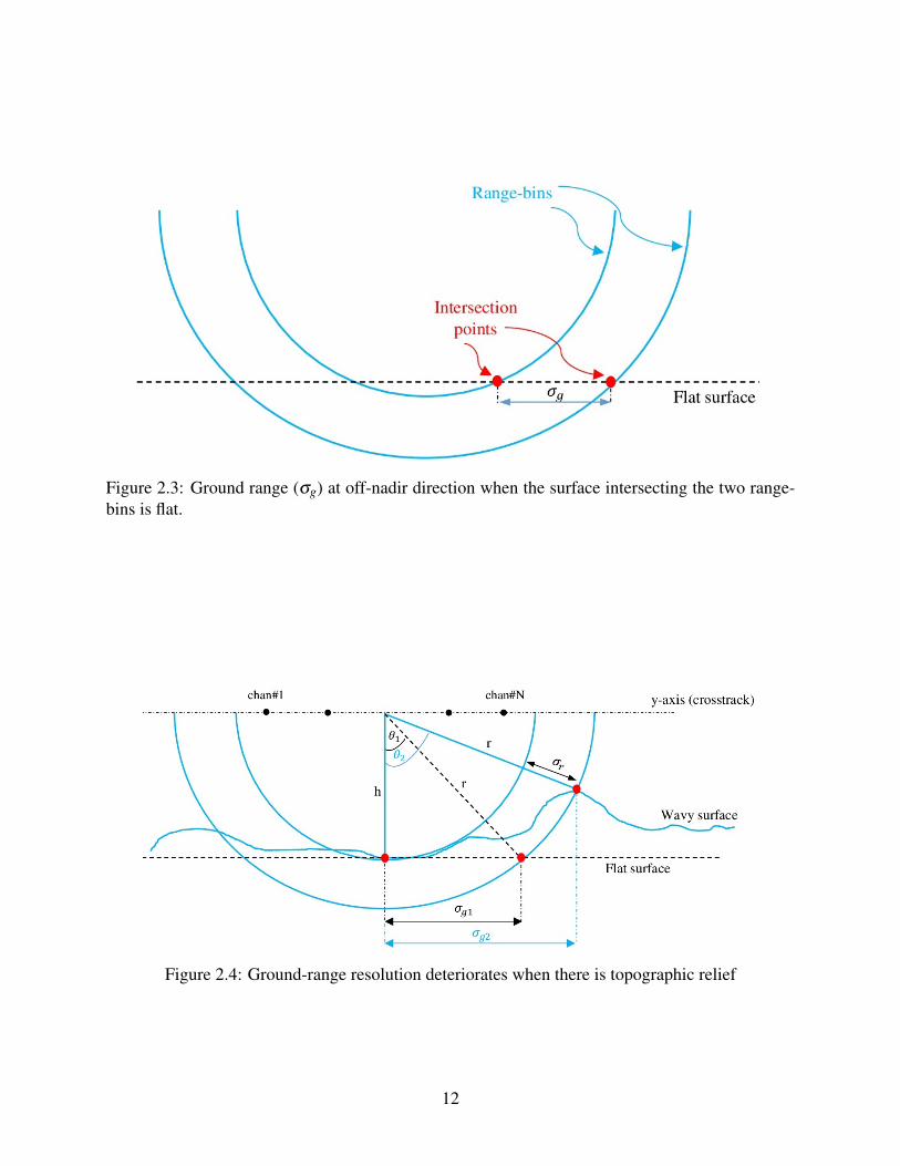
Figure 2.3: Ground range (σg) at off-nadir direction when the surface intersecting the two range-bins is flat.

Figure 2.4: Ground-range resolution deteriorates when there is topographic relief

12

Figure 2.5: Problem geometry

Figure 2.6: Ground-range resolution improves as the incident angle increases

13

Figure 2.7: Change in angle between two targets separated by the ground range resolution as afunction of the change in the incidence angle

From the above discussion, we can see that near nadir there is wide angular separation between

targets in close range proximity, which has two main effects:

a. It is not recommended to use the range snapshots from near-by targets to estimate the data

covariance matrix (DCM) because the snapshots are coming from targets at distinct inci-

dence angles, especially at nadir. This makes DOA estimation worse and suggests the use of

along-track snapshots rather than range snapshots for this purpose. Note that the snapshots

are assumed to be uncorrelated because the noise samples are uncorrelated, but they are spa-

tially correlated across the array. Ideal pulse compression and SAR processing should make

the snapshots completely independent along the range and azimuth dimensions, but this is

not true in practice due to sidelobes of the targets’ response (frequency leakage).

b. Due to the large ground range resolution at nadir, the signals received from the angular-bins

around nadir will appear as a distributed target in the final 3D image of the scene, which

makes it difficult to recognize the exact range-bins of the ice-surface corresponding to these

14

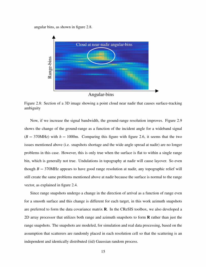
angular bins, as shown in figure 2.8.

Figure 2.8: Section of a 3D image showing a point cloud near nadir that causes surface-trackingambiguity

Now, if we increase the signal bandwidth, the ground-range resolution improves. Figure 2.9

shows the change of the ground-range as a function of the incident angle for a wideband signal

(B = 370MHz) with h = 1000m. Comparing this figure with figure 2.6, it seems that the two

issues mentioned above (i.e. snapshots shortage and the wide angle spread at nadir) are no longer

problems in this case. However, this is only true when the surface is flat to within a single range

bin, which is generally not true. Undulations in topography at nadir will cause layover. So even

though B = 370MHz appears to have good range resolution at nadir, any topographic relief will

still create the same problems mentioned above at nadir because the surface is normal to the range

vector, as explained in figure 2.4.

Since range snapshots undergo a change in the direction of arrival as a function of range even

for a smooth surface and this change is different for each target, in this work azimuth snapshots

are preferred to form the data covariance matrix R. In the CReSIS toolbox, we also developed a

2D array processor that utilizes both range and azimuth snapshots to form R rather than just the

range snapshots. The snapshots are modeled, for simulation and real data processing, based on the

assumption that scatterers are randomly placed in each resolution cell so that the scattering is an

independent and identically distributed (iid) Gaussian random process.

15

Figure 2.9: Ground-range resolution as a function of the incident angle in a wideband system with370 MHz bandwidth

2.3 Narrowband Signal Model

In our work, we have made the following assumptions:

• There are P sensors.

• There are Q targets (aka scattering sources or targets for radar).

• The scatterers are in the far field so that only the direction of arrival matters and not the range

to the target when determining the relative delays between sensors.

• The targets obey the principle of superposition or Born approximation. This allows us to

neglect interactions between the targets.

• The target signals are band limited signals with a center frequency of ωc

In general, a target’s complex baseband representation, Sw(t), received at a sensor with time

16

delay, td , can be written in the following form:

Sw(t− td) = S(t− td) exp(− jωctd) (2.3)

where S(t) is the complex baseband target signal.

The signal received at sensor p, xp(t), is a linear combination of all Q targets, and is given by

the following equation:

xp(t) =Q

∑q=1

Sw,q(t− τp(θq))+np(t) =Q

∑q=1

Sq(t− τp(θq)) exp(− jωcτp(θq))+np(t) (2.4)

where, θq is the direction of arrival of the target q, τp(θq) is the signal delay to sensor p for a

direction of arrival of θq, and np(t) is an additive noise at sensor p.

The signal model in equation 2.3 is valid for both narrow and wide bandwidths, where the

received signal’s envelope is not assumed to be constant across the array. This model is cumber-

some to deal with because it deals with time shifted versions of the signal, Sq(t−τp(θq)). Because

of the dependence on p, we cannot write the summation as a matrix equation. Under the nar-

rowband approximation, we assume that the signal is narrowband enough (i.e. complex envelope

changes slowly enough with time) so that the variation in τp(θq) over the whole array allows for

the following approximation:

Sw,q(t− τp(θq))≈ Sq(t)exp(− jωcτp(θq)) (2.5)

Note that we are only requiring that the relative delays between sensors be small enough so that if

we look at the signals received by the array at a particular instance in time, they can be modeled

across the array in this way.

Now apply the narrowband signal model discussed above on the data collected by the radar.

Given a SAR image pixel at range ρ , and along-track position x, the pixel’s received signal x(x,ρ)

17

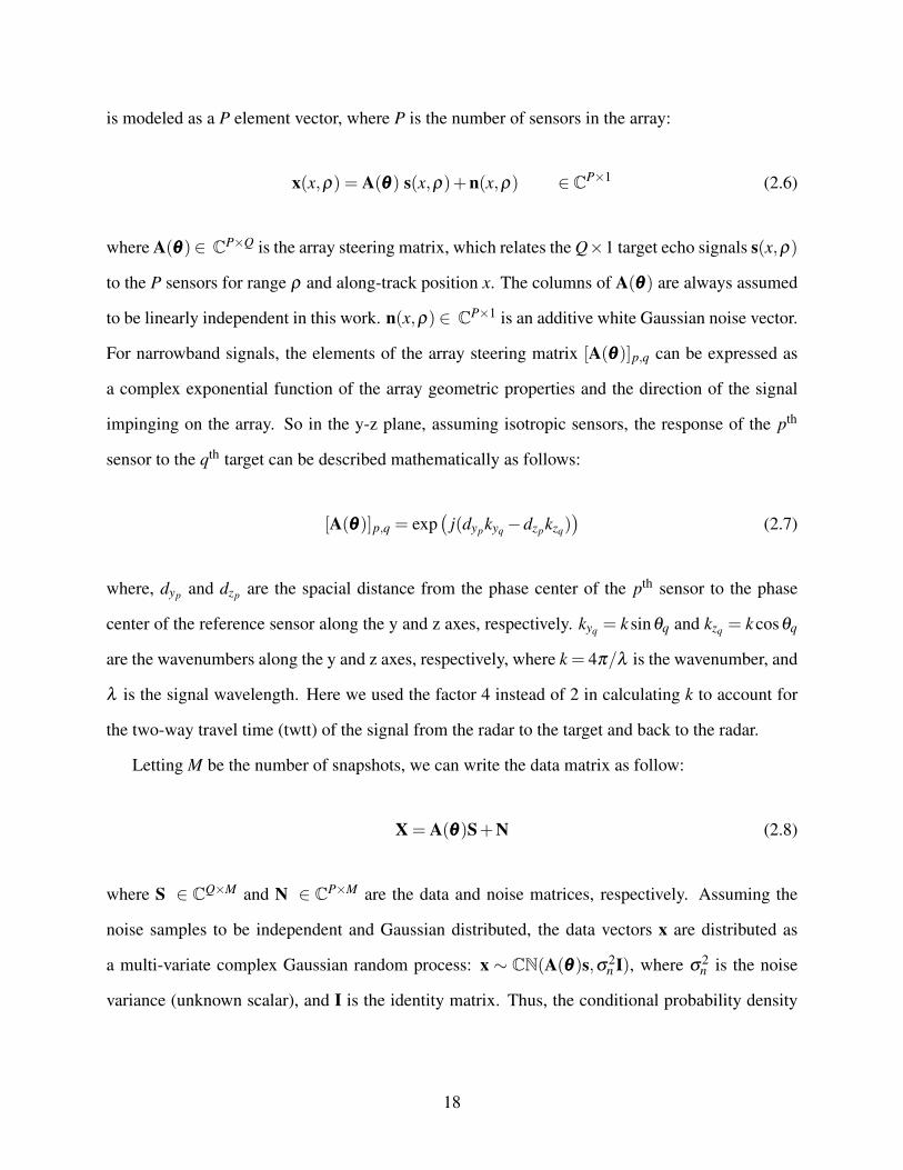
is modeled as a P element vector, where P is the number of sensors in the array:

x(x,ρ) = A(θθθ) s(x,ρ)+n(x,ρ) ∈ CP×1 (2.6)

where A(θθθ)∈ CP×Q is the array steering matrix, which relates the Q×1 target echo signals s(x,ρ)

to the P sensors for range ρ and along-track position x. The columns of A(θθθ) are always assumed

to be linearly independent in this work. n(x,ρ)∈ CP×1 is an additive white Gaussian noise vector.

For narrowband signals, the elements of the array steering matrix [A(θθθ)]p,q can be expressed as

a complex exponential function of the array geometric properties and the direction of the signal

impinging on the array. So in the y-z plane, assuming isotropic sensors, the response of the pth

sensor to the qth target can be described mathematically as follows:

[A(θθθ)]p,q = exp(

j(dypkyq−dzpkzq))

(2.7)

where, dyp and dzp are the spacial distance from the phase center of the pth sensor to the phase

center of the reference sensor along the y and z axes, respectively. kyq = k sinθq and kzq = k cosθq

are the wavenumbers along the y and z axes, respectively, where k = 4π/λ is the wavenumber, and

λ is the signal wavelength. Here we used the factor 4 instead of 2 in calculating k to account for

the two-way travel time (twtt) of the signal from the radar to the target and back to the radar.

Letting M be the number of snapshots, we can write the data matrix as follow:

X = A(θθθ)S+N (2.8)

where S ∈ CQ×M and N ∈ CP×M are the data and noise matrices, respectively. Assuming the

noise samples to be independent and Gaussian distributed, the data vectors x are distributed as

a multi-variate complex Gaussian random process: x ∼ CN(A(θθθ)s,σ2n I), where σ2

n is the noise

variance (unknown scalar), and I is the identity matrix. Thus, the conditional probability density

18

function of X given θθθ can be stated as:

p(X|θθθ) =M

∏i=1

(πσ2n )−M exp

(− ||x(i)−A(θθθ)s(i)||2

σ2n

)(2.9)

where ||.|| is the 2-norm operator.

We define R to be the covariance matrix of X. Since the signals received from nearby SAR

image pixels have approximately the same direction of arrival under the assumption of a smooth

surface (and hence the same statistics), they can be used as independent snapshots for estimating

the data covariance matrix R as follows:

R =1M

XXH (2.10)

where H represents the complex-conjugate transpose operation. Using R we can estimate the

DOA, which is done for every pixel in the SAR image. As discussed in Section 2.2.1, neighboring

pixels will likely have slightly different incidence angles. Also noted is that a greater spread is

expected near nadir and when taking neighboring pixels in range rather than in the along-track

dimension.

The true data covariance matrix RRR can be written as follows:

RRR = E(xxxxxxH) =AAA(θθθ)RRRssAAAH(θθθ)+RRRnn (2.11)

where E is the expectation operator. The matrices RRRss = E(ssssssH) and RRRnn = E(nnnnnnH) are the corre-

lation matrices for signal and noise, respectively. RRRss and RRRnn are positive definite matrices, where

the rank of RRRss is Q and the rank of RRRnn is P−Q [35]. The rank of RRR is P, which can be shown

using the positive definite properties of the constituent matrices and the linear Independence of the

columns of A..

19

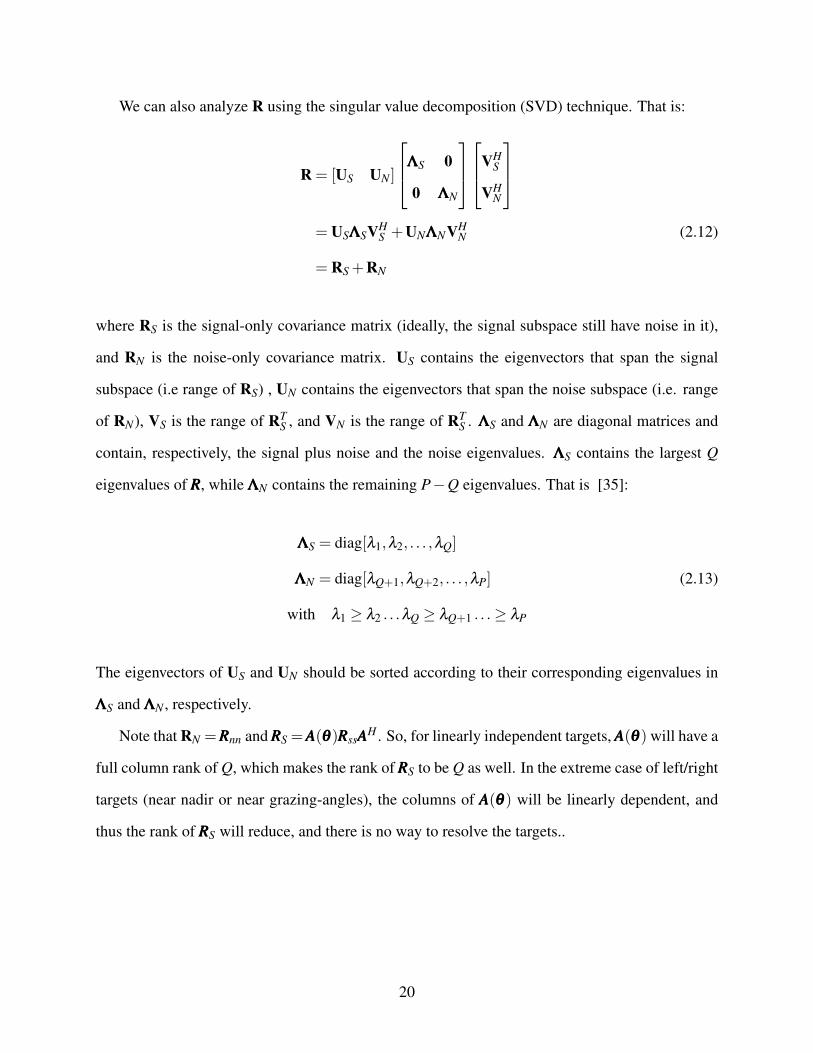
We can also analyze R using the singular value decomposition (SVD) technique. That is:

R = [US UN ]

ΛΛΛS 0

0 ΛΛΛN

VH

S

VHN

= USΛΛΛSVH

S +UNΛΛΛNVHN (2.12)

= RS +RN

where RS is the signal-only covariance matrix (ideally, the signal subspace still have noise in it),

and RN is the noise-only covariance matrix. US contains the eigenvectors that span the signal

subspace (i.e range of RS) , UN contains the eigenvectors that span the noise subspace (i.e. range

of RN), VS is the range of RTS , and VN is the range of RT

S . ΛΛΛS and ΛΛΛN are diagonal matrices and

contain, respectively, the signal plus noise and the noise eigenvalues. ΛΛΛS contains the largest Q

eigenvalues of RRR, while ΛΛΛN contains the remaining P−Q eigenvalues. That is [35]:

ΛΛΛS = diag[λ1,λ2, . . . ,λQ]

ΛΛΛN = diag[λQ+1,λQ+2, . . . ,λP] (2.13)

with λ1 ≥ λ2 . . .λQ ≥ λQ+1 . . .≥ λP

The eigenvectors of US and UN should be sorted according to their corresponding eigenvalues in

ΛΛΛS and ΛΛΛN , respectively.

Note that RN =RRRnn and RRRS =AAA(θθθ)RRRssAAAH . So, for linearly independent targets, AAA(θθθ) will have a

full column rank of Q, which makes the rank of RRRS to be Q as well. In the extreme case of left/right

targets (near nadir or near grazing-angles), the columns of AAA(θθθ) will be linearly dependent, and

thus the rank of RRRS will reduce, and there is no way to resolve the targets..

20

2.4 Wideband Signal Model

The time-bandwidth product (TBP) of the array is usually used as a metric to determine whether

the system is narrowband or wideband. For small enough TBP, the envelope of the signal may be

assumed constant across the entire array at any given instant in time. TBP is defined as: τmaxB,

where τmax is the maximum difference in the time delays across the array taken over all the possible

angles of arrival within the field of view (FOV). τ can be expressed as τ = La(θ)/c, where La(θ)

is the length of the array projected onto the range vector in the direction of (θ). Note that La is a

function of the DOA, where, for a linear array, the minimum array-length is for a target broadside

to the array since the wavefront will impinge on all elements simultaneously, and the maximum

array length is for an end fire target. Also, FOV affects whether the system is narrowband or

wideband. Reducing the FOV reduces the maximum difference in time delays across the array and

therefore makes the measured array signals more narrowband.

In summary, the size of the array, the bandwidth, and the FOV are the three main parameters

that decide whether the system is wideband or narrowband. Van Trees [35] states that the narrow-

band assumption is valid when τmaxB << 1. Based on simulations and real data using parameters

which match one of the CReSIS radar systems, we noticed some degradation for a 0.4 TBP when

MUSIC was used to estimate the DOAs of the received signals (due to the inherent narrowband

assumption in this technique) for a 7 sensors array with B f ≈ 0.164 assuming FOV=±90◦ , but it

is not severe.

In case of wideband systems, the array steering matrix will be frequency-dependent. Thus,

equation 2.7 now becomes:

[A(θθθ , fi)]p,q = exp(

j(dypkyq( fi)−dzpkzq( fi)

))(2.14)

where fi is the ith frequency within the signal bandwidth. kyq( fi) and kzq( fi) have the same def-

initions given in the previous section, except that now the wavenumber is frequency-dependent:

21

ki = 4π fi/c. Thus, the wideband data model can be written, similar to equation 2.6, as follows:

xi(x,ρ) = A(θθθ , fi) si(x,ρ)+ni(x,ρ) ∈ CP×1 (2.15)

The frequency dependence of the data model makes the array processing methods more com-

plex as we now have an additional degree of freedom. For each application of wideband array

processing using subbanding, we will need to choose the number of subbands that is optimal for

the specific application. This is because increased subbands leads to reduced snapshots per sub-

band and coarser ground range resolution.

2.5 Cramer-Rao Lower Bound (CRLB)

Cramer-Rao Lower Bound (CRLB) is a measure of the amount of uncertainty in the observed data

about some unknown embedded in the observation. In our case, we use the CRLB to quantify

the quality of the estimated DOAs from our measured data. CRLB is independent of the type of

estimator, and depends on several parameters, such as the number of sensors, the quality of the

sensors, the number of targets, the number of snapshots, the degree of correlation between the

targets, the amount of noise in the data, and the array imperfections (e.g. uncalibrated arrays).

The CRLB is calculated as follows [36]:

CRLB(θ)θ)θ) =σ2

n2N

[Re{

D�(Rs−

(R−1

s +1

σ2n

AAAH(θθθ)AAA(θθθ))−1)T

}]−1(2.16)

where, � is the Hadamard product (i.e. element-wise product). D = AAAH(θθθ)P⊥AAAA(θθθ) , and AAA(θθθ) is

the derivative of AAA(θθθ) w.r.t θθθ , where the qth column of AAAH(θθθ) is given by the following expression:

AAAq(θθθ) = dddq�AAAq(θθθ) (2.17)

where dddq = [ jd1q, . . . jdPq]T ∈CP×1, where dpq = dypkyq−dzpkzq, and these variables were defined

22

in Section 2.3. Also, P⊥A = III−AAA(θθθ)(AAAH(θθθ)AAA(θθθ))−1AAA(θθθ)H is the complementary projection matrix

(i.e. projects onto the noise subspace, which is orthogonal to the subspace spanned by the columns

of the steering-vectors).

Figure 2.10 shows the square-root of CRLB as a function of the direction of arrival for ice-

bottom targets, where 2 equal-power and uncorrelated targets were assumed, with 11 snapshots

and 7 sensors. The SNR was estimated from the collected data: the data at the very end of the

ice-bottom were used to estimate the noise variance, while the data around the ice-bottom layer

were used to estimate the signal variance, then the SNR was estimated as follows:

SNR =Ex(||x||2)En(||n||2)

−1 (2.18)

where the expectation is approximated by averaging over a large number of data points. x repre-

sents the data within ±10 range-bins of the ice-bottom, and n represents the data from the last 50

range-bins, where there is no signal. Data from multiple frames (10 frames) were used to increase

the accuracy of the estimated SNR, which was 14 dB for a nadir bottom target.

The DOA standard deviation is larger near nadir and near grazing angles. The first case (i.e.

near nadir) is due to the small angular separation between the two targets, which results in cor-

related steering vectors, while the second case (near grazing angle) is due to the fact that as the

arrival angle approaches ±90◦, the steering vectors (for a uniform linear array with quarter wave-

length spaced phase centers) also become equal and the effective aperture size reduces significantly

because of the end fire geometry.

23

0 10 20 30 40 50 60 70

Elevation angle (deg)

0

0.2

0.4

0.6

0.8

√

CRLB

(deg)

Figure 2.10: Square-root of CRLB as a function of the arrival angle for a target at the bottom of anice-sheet assuming 2 equal-power targets with 11 along-track snapshots. One target is assumed tobe on the left of the nadir and the other target is on the right of nadir.

2.6 Direction of Arrival Estimation (DOA)

After range and azimuth processing, 2D echogram images of the scene can be formulated as along-

track position versus travel time or range. To obtain a 3D tomographic image of the ice-bottom, the

elevation angles of the targets in each pixel need to be estimated. This problem can be formulated

as a direction of arrival (DOA) estimation problem. We have applied and tested several narrowband

and wideband elevation angle estimation techniques, such as MUSIC, MLE, and wideband MLE,

in addition to other adaptive methods, on real and simulation data to resolve the targets in each

pixel of the 2D SAR image. The theory behind these methods is introduced in this section.

2.6.1 Multiple Signal Classification (MUSIC)

MUSIC is a parametric DOA estimation technique that relies on the projection of the array steer-

ing vector at a given DOA, a(θθθ), onto the noise subspace, UUUN . Ideally, a(θθθ) is orthogonal to

UUUN . Within the field of view, θθθ that corresponds to the minimum projection result represents the

24

estimated DOA.

The MUSIC cost function is defined as [35]:

Jmusic(θθθ) =1

P∑

j=Q+1|aH(θθθ)u j|2

(2.19)

where uuu j is the jth eigenvector of the noise subspace, which can be determined from the SVD

of the data covariance matrix RRR, as shown in Section 2.3. The MUSIC cost function utilizes the

orthogonality between the noise subspace and the array steering vectors at the true DOAs [37].

This means that MUSIC, if used as a DOA estimator, gives the θθθ ’s which result in the steering

vectors with the lowest inner products with the noise subspace (i.e. θθθ that maximizes Jmusic(θθθ)).

In this work, we use MUSIC as a beamformer (grid scan over entire field of view) rather than

an estimator (returning just the peak location for each target). The latter requires the exact number

of targets or targets in the range shell to be known otherwise the tracker may track false targets or

miss targets all together. Note that we have fixed the dimension of the signal subspace as this is

required by MUSIC to produce the output. However, there is more information in this beamformer

output because it returns the result for angles spanning the whole field of view rather than just the

positions of the peaks. Current efforts to estimate the model order using standard eigen-analysis

of the data covariance matrices have failed due to the complicated eigen-structure of our data that

may be due to issues such as the relatively large time-bandwidth product of the array and multipath

effects. The output of the beamformer is a 3D image where the dimensions are along-track, range,

and elevation angle. The beamformer has the advantage that even when the signal eigenspace is not

precisely estimated, there is still likely to be some reduction in the null-space’s correlation with

the actual target’s steering vector. Since MUSIC’s output is based on the reduction in the null-

space correlation with the steering vectors, this can aid the ice bottom tracker even though it is not

the steering vector with the lowest correlation due to errors in the steering vectors or eigenspace

estimation.

25

2.6.2 Maximum Likelihood Estimation (MLE)

MLE, for the DOA estimation problem, is an asymptotically consistent and efficient estimation

technique, and is optimal to MUSIC. However, this method is more time-consuming because it

requires a non-linear multidimensional search to obtain its estimates [38, 39].

Assuming that the noise variance and the target signal are unknown, but non-random, the de-

terministic MLE cost function to be maximized can be written as [39]:

Jmle = Tr(PAR) (2.20)

where,Tr is the trace operator, and PA = A(θθθ)(AH(θθθ)A(θθθ)

)−1AH(θθθ) is the projection matrix of

the steering matrix. Thus, we seek the value of θθθ that maximizes Jmle. That is:

θθθ = argmaxθθθ

Jmle (2.21)

Taking the SVD of RRR, as shown in equation 2.12, and using the trace and projection properties,

equation 2.20 can be re-written as [39]:

Jmle =P

∑p=1

λp||PPPAuuup||2 (2.22)

where uuup is the pth eigenvector of RRR that corresponds to the eigenvalue λp, for p ∈ {1, . . .P}. Note

that the MLE cost function utilizes the eigen-structure of the signal and noise subspaces, which is

unlike MUSIC that only uses the noise or signal eigen-structure. The amount of contribution any

eigenvector makes depends on how big its corresponding eigenvalue is.

Stochastic MLE can also be used for DOA estimation [40]. However, in this work we only use

deterministic MLE due to its mathematical simplicity and the ability to estimate targets’ signals

(and therefore targets’ power) in a straight forward method [39].

26

2.6.3 Wideband MLE (WBMLE)

MLE and MUSIC, as described in the previous two sections, are suitable for narrowband systems,

where the time-bandwidth product is much less than 1, that is τB << 1. From an array process-

ing stand point, wideband systems have some problems that need special treatment. For example,

the narrowband array-processing techniques produce larger errors as the bandwidth of the system

increases [41]. Model-order estimation is a good example of this problem, where wideband sys-

tems induce false targets [42], producing an overestimated number of targets because the signal

subspace dimension is not equal to the number of targets as it is for narrowband arrays. Also,

wideband systems have lower SNR relative to narrowband systems for area distributed scattering.

This is due to the concomitant refinement in the resolution which results in a smaller scattering

area for each radar image pixel and hence less scattered energy.

Wideband MLE (WBMLE) is a DOA estimation technique, where the signal bandwidth is

sub-divided into N f sub-bands, and then MLE is applied to all subbands at once and that for

independent subbands this is just the product of the individual likelihood density functions or the

sum of the individual log likelihood functions [43].

Wideband MLE has the following cost function:

Jwbmle =N f

∑n=1

Jmle(wn) (2.23)

where, Jmle(wn) is the MLE cost function given in equation 2.20 as a function of frequency wn.

Thus, the optimization problem can be written as:


Jwbmle (2.24)

The WBMLE method has a disadvantage [14]: it degrades the range resolution of the SAR

image (due to subbanding) in order to obtain an estimate of the DOA, allowing more targets over a

wider angular spread to be illuminated. The increased signal subspace and angular spread of targets

27

within each ground range bin will result in reduced performance for our specific SAR tomography

application especially for targets near nadir.

2.6.4 Focusing Matrices

Another coherent DOA estimation method is to use a focusing matrix to focus the DOA from dif-

ferent frequencies into the center frequency of the signal bandwidth using signal-subspace trans-

formation matrices TTT ( f ) such that the narrowband DOA estimation techniques can be used. Even

though we still have not applied the focusing matrices method to any of our data yet, we mention

it here briefly for completeness.

There are several classes of this method in the literature, and here we describe the general

framework given by [44], which can be summarized as follow:

1. Define TTT i as the focusing matrix associated with frequency fi, for i ∈ {1,2, . . . ,N f }. The

main characteristics of TTT i are described in [45]. Note that TTT i transforms the array steering

matrix at frequency fi into an array steering matrix at another reference frequency, f0, which

is usually the center frequency. Thus, we can determine TTT i as follow:

TTT i = argminTTT i||AAA0(θθθ f )−TTT iAAAi(θθθ f )||F (2.25)

where ||.||F is the Frobenius-norm operator, and AAA0 is the array steering matrix at the refer-

ence frequency. θθθ f is the set of focusing angles, which need to be estimated a priori.

2. Using TTT i, determine the focused data covariance matrix RRR f oc as follow:

RRR f oc =N f−1

∑i=0

wiTTT iRRRiTTT Hi (2.26)

where wi is a weighting factor and RRRi is the data covariance matrix associated with frequency

fi.

28

3. Using RRR f oc and AAA0, estimate the DOAs using the narrowband estimation methods, such as

MLE and MUSIC.

Note that the main drawback of this method is that the set of focusing angles θθθ f needs to

be prepared a priori, which is not always possible. Thus, other methods were introduced in the

literature to get around this problem, such as the test of orthogonality of projected sources (TOPS)

introduced in [44]. On the other hand, one advantage of this method is that the subbands are used

to generate more snapshots, one for each subband.

2.6.5 Sequential DOA Estimation

Unlike standard DOA estimation methods discussed above, sequential DOA estimation techniques

utilize the surface geometry information to relate the estimated DOAs from neighboring pixels.

This can be done by mathematically modeling the relationship between the DOAs of the neighbor-

ing range-bins. The model can also include other important prior information about the surface,

such as the slope of the surface and the number of dead range-bins (i.e. range-bins that do not have

targets). This model is called the transition model, the dynamics model, or the process model, and

can be data-independent (i.e. only a function of the geometry of the surface).

Another important aspect of the Sequential DOA estimation is the adaptive prior probability

density function or pdf. One way of updating the prior pdf is to derived it from the transition model

such that it is updated at each state or range-bin based on the results from the previous range-bins.

The prior pdf parameters can also be obtained from training data and then feeding the inferred

parameters to the filter at each range-bin.

The bounds of the estimated DOAs should also be adaptively changing. This can be done by

using the estimated DOAs from one range-bin to bound (and may be to initialize) the DOAs at the

following range-bin. Accurate and tight bounds make it possible to eliminate DOA outliers and

form a smooth surface in the end, but it makes the prior pdf less important to the results. Also,

making an error at one range-bin may cause the following range-bins to have wrong DOAs. So,

setting the tolerance in the bounds should be dependent on the geometry/flatness of the surface to

29

be tracked, the amount of change in the DOA as a function of range-bin, and a few other physically-

imposed constraints.

The results from DOA-based tracking methods can be used directly to reconstruct the ice-

bottom surface, which is usually not realizable if non-sequential techniques were used to estimate

the elevation angles because these techniques require a tracker to be used to extract the surface

information from the estimated DOAs. Thus, here we attempt to eliminate the need for the extra

tracking step by utilizing the surface geometry as a prior information.

The flat earth transition model:

In the following two sub-sections we will use the flat-earth approximation model to have an

initial estimate of the change in DOA as a function of range-bin, which is defined in equation 2.2

and depicted in figure 2.5. So, the flat-earth surface will serve as the mean for estimating the actual

surface.

Define Nt as the total number of range-bins and Nt ≤ Nt as the last range-bin index where

the DOA, θNt, reaches the edges of the FOV. Also, let m and k be the range bin indices where

m,k ∈ {1, . . . , Nt} and m > k. So, proceeding from equation 2.2, we can calculate θm as a function

of θk and rk, which is the range associated with range-bin index k, for a perfectly flat surface in the

following way:

θm =±cos−1 ( rk

rmcos(θk)

)(2.27)

where rm = rk +(m− k)σr. If we let θre f represent the reference DOA, which is the nadir DOA in

our case, that divides the surface into two halves or modes, left and right, then +θm belongs to the

right portion of the surface and −θm belongs to the left portion. Same thing holds for ∆θ .

To properly bound the estimated DOA of range-bin m, we model the prior pdf of the DOA as

a truncated Gaussian random variable: T N (µθm,σ2θm,θ

(lb)m ,θ

(ub)m ), where µθm is the mean, σ2

θm

is the variance, θ(lb)m is the lower bound, and θ

(ub)m is the upper bound. These four parameters

are derived as follows, where we show the math for the right surface mode only, which is the

same for the left mode except for the sign conventions. Figure 2.11 shows a graphical view of the

relationship between these four parameters.

30

1. Mean: let θk be the estimated DOA at range-bin k. Propagating θk through the transition

model in equation 2.27, we can calculate the mean of the prior pdf as follows:

µθm = cos−1 ( rk

rmcos(θk)

)(2.28)

Note that equation 2.28 implies that the mean surface is the one produced by propagating

the estimated DOAs at each range-bin to the next, and not the exact flat surface. In other

words, the mean surface may not necessarily be that of the flat surface, and is usually not.

This makes the tracker capable of tracking non-perfectly flat surfaces and makes the quality

of the estimated surface more dependent on the quality of the data, such as SNR, than the

transition model.

2. Standard deviation: define ∆θm = µθm− θk, then the standard deviation can be calculated as

follows:

σθm = ∆θm = µθm− θk (2.29)

3. Lower bound: let a1 be a fractional number that is close to 0, but not 0 (e.g. a1 = 0.1), then

the lower bound on the estimated DOA is the previously estimated DOA plus a small guard:

θ(lb)m = θk +a1∆θm (2.30)

So a1∆θm is a guard that guarantees that the estimated DOA does not turn back towards the

previously estimated DOA and only expands outwards from the center (in the case of the

particle filter this is true for each particle, but not for the final result). a1 can be set to a

negative value to relax this constraint.

4. Upper bound: the upper bound can be calculated as follows:

θ(ub)m = µθm + f (∆θm) (2.31)

31

where

f (∆θm) =−0.5569∆θ2m +0.7878∆θm +0.0071 (2.32)

The coefficients in equation 2.32 were derive by fitting a curve into a few reasonable points,

as shown in figure 2.12. Note that the definition of f (∆θm) here is an example of how the

upper guard can be st, but f (∆θm) can take any other forms, as we will see in Chapter 5.

Figure 2.11: Geometric presentation of the parameters of the DOA prior pdf, which is truncatedGaussian. This figure is plotted for a perfectly flat surface for the purpose of demonstration, butthis is not necessarily the case in reality.

32

0 2 4 6 8 10∆θ (in degrees)

0

0.05

0.1

0.15

g(∆θ)

Fitted pointsFitting curve

Figure 2.12: ∆θ vs f (∆θ) defined in equation 2.32

To summarize, here we assume that the mean surface follows the flat earth model, where the

estimated DOAs from the previous range-bin are propagated through the model in equation 2.27

to calculate the mean DOA at the next range-bin. Then, the variance and bounds of the prior pdf,

which is truncated Gaussian, are calculated based on the angular distance between the mean DOA

and the previously estimated DOA. In this way, the tracker can track the left and right surface

modes simultaneously, but independently. Also, since the DOA bounds are determined based

on ∆θ , the near-nadir DOAs (first few range-bins) will have much wider bounds than far-from-

nadir DOAs (last few range-bins), which matches the physical realty, where the change in DOA

reduces as a function of range (see figure 2.6). Another important point to mention here is that

the suggested model can handle very low quality data scenarios (e.g. very low SNR), where the

worst case scenario is that the tracker would produce a surface that is exactly the mean surface,

such as in the extreme case of SNR=−∞. This case is almost impossible to deal with in the case

of non-iterative filters.

Note that since each range-bin has Q ∈ {0, . . . ,P− 1} targets that share the same measure-

ments, the ice-bottom tracking problem is an inseparable multi-target tracking problem, which

is, due to the nonlinear nature of the models, a highly nonlinear problem with multimodal non-

Gaussian posterior distributions. In the standard object tracking problems, each object is assumed

33

to send its own narrowband signal, so it is possible to decompose the problem into smaller sub-

problems, which is not possible in our ice-bottom tracking problem. In other words, the Q targets in

each range-bin are connected via the measurements model, but separable in the transition model.

In the following two subsections, equations 2.27 through 2.32, in addition to equation 2.8,

will be used to model two Bayesian filters: the particle filter (PF) and the sequential maximum

a posterior (S-MAP) filter, to estimate a radar-imaged surface at each range-line along the flight

path.

2.6.5.1 Particle Filter (PF)

The Kalman filter (KF) is known for its optimality, in the mean squared-error (MSE) sense, for lin-

ear systems with a Gaussian noise distribution [46]. However, for non-linear systems, the standard

KF is not guaranteed to converge due to several reasons, such as a multimodal posterior distribution

that may arise from the non-linear nature of the system. The Extended Kalman filter (EKF) was

introduced to handle non-linear systems, but the EKF still has the (unimodal) Gaussian noise as-

sumption and uses a linear approximation to the non-linear system model. Because of this, it may

not be able to accurately handle tracking problems for highly non-linear systems. The Unscented

Kalman filter (UKF), on the other hand, can handle the non-linear systems in a better way than

EKF by numerically fitting a Gaussian distribution into pregenerated samples, but it only works

for unimodal noise distributions [47].

The particle filter (PF) is the most general form of a sequential filter and is capable of dealing

with any mathematically defined system (i.e. linear and non-linear) and any type of posterior

distribution (i.e. Gaussian and non-Gaussian, unimodal and multimodal) [48, 49]. However, unlike

KF, PF approximates the posterior distribution using N samples (called particles) generated from a

proposal or instrumental distribution that shares the same sample support as the actual distribution,

but that is easier to draw samples from. Also, unlike the EKF, the PF uses the exact non-linear

system model, which is a big advantage because it makes it possible to deal with very complex

and rich dynamic models. The idea of the PF is similar to that of the UKF, but here the sample

34

space and grid size can change adaptively over time rather than using a deterministic grid as in the

case of the UKF. So, the PF sacrifices the accuracy of the posterior distribution for a better (exact)

non-linear system that captures as many aspects of the problem as we want.

The PF is a sequential Monte Carlo (SMC) technique for solving the nonlinear/non-Gaussian

filtering problems numerically (i.e. simulation-based method). Generally, the SMC methods are

numerical solvers for integration and optimization problems [49]. But, as a sequential filter, it

can also be used to adaptively track a probability distribution of a random variable, x, in signal

processing problems. Given g(x), x ∈ Rnx for some positive integer nx, we would like to calculate

the following multidimensional integration numerically [49]:

I =ˆ

g(x)dx (2.33)

Now, if g(x) = f (x)p(x) such that p(x) is interpreted as a probability distribution (i.e. p(x) ≥ 0

and´

∞

−∞p(x)dx = 1), then equation 2.33 can be rewritten as follows:

I =ˆ

g(x)dx =ˆ

f (x)p(x)dx = Ep(x){ f (x)}. (2.34)

The Monte-Carlo (MC) estimation of the integral above is the sample mean of f (x):

IN =1N

N

∑i=1

f (x(i)), s.t. {x(i) : i = 1 : N} ∼ p(x), (2.35)

where the symbol ∼ means ’distributed as’, and i is the sample or particle index. This expression

implies that p(x) has the following form:

p(x) =1N

N

∑i=1

δ (x− x(i)), (2.36)

where δ (x) is the Dirac function.

An accurate MC estimation of the integral requires that the particles, x(i), be primarily drawn

35

from regions in f (x) that correspond to the high probability regions in p(x). These attractive

regions are called the importance sampling regions. Figure 2.13 illustrates the importance sampling

region with a simple example.

Figure 2.13: Example of an importance sampling region.

If the particles are independent, then IN is unbiased and converges to IN almost surely as N→∞

[49, 50]. Also, the error of MC estimates is of order O(N−1/2). This means that the rate of

convergence is independent of the dimension of the integrand, nx. This is because the particles,

x(i), are drawn from regions of high importance to the integration result, as mentioned previously.

We separate the different concepts of the PF into sections to make the problem more tractable.

We follow [49, 50] for the necessary background.

1. Importance Sampling (IS):

In the Bayesian estimation context, p(x) represents the posterior density. However, it is not

always possible to sample effectively from p(x) if it is multivariate, nonstandard, or only

partially known. To solve this problem, the importance sampling (IS) technique can be used.

IS suggests drawing the samples from an easy-to-sample-from proposal density q(x). q(x)

must satisfy the following two conditions:

(a) q(x) shares the same sample support with p(x) so that q(x)> 0 ∀x ∈ Rnx : p(x)> 0.

36

(b) q(x) has a heavier tail than p(x).

Starting from equation 2.33, we can proceed mathematically as follows:

I =ˆ

g(x)dx

=

ˆf (x)p(x)dx

=

ˆf (x)

p(x)q(x)

q(x)dx

=

ˆf (x)w(x)q(x)dx

=

ˆf (x)q(x)dx

= Eq(x){ f (x)} (2.37)

such that the importance weight 0 ≤ w(x) =p(x)q(x)

< ∞, which can be guaranteed if the

conditions on q(x) are met.

Since´

w(x)q(x)dx = 1, we can estimate I and p(x) as follow:

• First, rewrite I in equation 2.37 as follows:

I =

´f (x)w(x)q(x)dx´

w(x)q(x)dx(2.38)

• Second, estimate the numerator and denominator:

IN =

1N

∑Ni=1 f (x(i))w(x(i))

1N

∑Ni=1 w(x(i))

=N

∑i=1

f (x(i))w(x(i)), s.t. {x(i) : i = 1 : N} ∼ q(x) (2.39)

37

where, the normalized weight w(x(i)) is defined as:

w(i) =w(x(i))

∑Ni=1 w(x(i))

(2.40)

Note that since it is the ratio of two estimates, IN is a biased estimate of IN if N is finite,

but asymptotically IN converges to IN almost surely.

• From equation 2.39, we can infer that the approximate (discrete) posterior density is

given by the following expression:

p(x) =N

∑i=1

w(i)δ (x− x(i)) (2.41)

2. Sequential Importance Sampling (SIS)

To apply the MC estimation method to solve nonlinear filtering problems under the Bayesian

framework, the IS needs to be performed sequentially such that the particle weights at the

current state are a function of the particle weights of the previous state, otherwise the filter

complexity grows with each iteration. A state can be defined as the representation of our

knowledge about tracked variables up to and including the current time step where the last

received measurements are incorporated in the processing. The possible values the state vari-

ables can take are called the state space. Generally, every time new measurements become

available, the state index is incremented by one, and the state can be updated, and thus our

knowledge about the tracked variables is also updated. In our ice-bottom tracking problem,

we use the PF to track the posterior density of the elevation angles given the measurements

and the elevation angles estimated at the previous states. We then use this posterior density to

estimate the DOAs for the current range-bin. So, these angles of arrival represent the state,

which is updated over range-bins because each range bin has its own measurements and

DOAs. The range-bin index is the state index. The state space, on the other hand, represents

all the possible DOAs within predefined bounds (i.e. the sample support) in a given range-

bin. From now on we will work on posterior probability distributions rather than general

38

probability distributions and we will tune our discussion to our specific problem of tracking

the bottom of an ice-sheet.

Let x0:K = {x0, . . . ,xK} represent the sensor measurements up to and including state index

(or range-bin) K. x0 is the null measurement. Also, let θ0:K = {θ0, . . . ,θK} represent the

sequence of target states up to and including time K. θk is a hidden parameter inside the

measurements xk (see equation 2.6) and needs to be estimated. Then the posterior density of

the target’s trajectory, p(θ0:K|x0:K) can be characterized by {θ (i)0:K,w(θ

(i)0:K), i = 1, . . . ,N}:

p(θ0:K|x0:K) =N

∑i=1

w(θ (i)0:K) δ (θ0:K−θ

(i)0:K) (2.42)

where w(θ (i)0:K) ∝

p(θ0:K|x0:K)

q(θ0:K|x0:K), and ∝ means proportional to.

If the proposal density is chosen such that

q(θ0:K|x0:K) = q(θK|θ0:K−1,x0:K)q(θ0:K−1|x0:K−1) (2.43)

then one can obtain samples θ0:K ∼ q(θ0:K|x0:K) by augmenting each of the existing samples

θ(i)0:K−1 ∼ q(θ0:K−1|x0:K−1) with the new state particles θ

(i)K ∼ q(θK|θ0:K−1x0:K).

The actual posterior density can also be factorized in the following way:

p(θ0:K|x0:K) =p(θ0:K,x0:K)

p(x0:K)

∝ p(xK|θK) p(θK|θK−1) p(θ0:K−1|x0:K−1) (2.44)

where the normalizing constant, p(x0:K), has been dropped. Now, by substituting the new

expressions of q(θ0:K|x0:K) and p(θ0:K|x0:K) into w(θK) we obtain the following recursive

update equation for the particle weights:

w(θ (i)0:K) ∝ w(θ (i)

0:K−1)p(xK|θ (i)

K ) p(θ (i)K |θ

(i)K−1)

q(θ (i)K |θ

(i)0:K−1,x0:K)

(2.45)

39

If we impose the Markov property, then we can assume that:

q(θ (i)K |θ

(i)0:K−1,x0:K) = q(θ (i)

K |θ(i)K−1,xK) (2.46)

In this case, the posterior density, equation 2.42, becomes:

p(θK|x0:K) =N

∑i=1

w(θ (i)0:K) δ (xK− x(i)K ) (2.47)

and the importance weight, equation 2.45, becomes:

w(θ (i)0:K) ∝ w(θ (i)

0:K−1)p(xK|θ (i)

K ) p(θ (i)K |θ

(i)K−1)

q(θ (i)K |θ

(i)K−1,xK)

(2.48)

Equations 2.47 and 2.48 will be used from now on (i.e. we impose Markov assumption).

Using these two equations, we can perform maximum a posterior estimation (MAP) or min-

imum mean squared-error (MMSE) estimation. We also consider a mixture of the two which

we call quasi-MAP estimation. Note that the particles are vectors of length Q (DOAs for the

number of targets in the considered range-bin) so that operations on particles by an estimator,

operate on the whole vector.

• MMSE estimation:

The MMSE estimator is the expected value (or weighted sum) over the sample support.

Mathematically, it can be stated as follows:

θK = Ep(θK |x0:K)(θK) =N

∑i=1

θ(i)K w(θ (i)

0:K) (2.49)

Since MMSE estimation is the weighted sum of N particles, its result is not guaran-

teed to be in the sample space if the space is noncontiguous. This is not an issue for

our problem because the space is contiguous. Also, if the posterior density has a multi-

modal nature, MMSE may give an answer that is not in the importance sampling region

40

(low probability answer).

• MAP estimation:

The MAP estimator chooses the particle that corresponds to the maximum weight

among all particles of the sample support. This is equivalent to the particle with DOAs

that maximize the posterior density, and can be stated as follows:

θK = argmaxθ(i)K

p(θK|x0:K), i ∈ {1, . . . ,N} (2.50)

Since only one particle is chosen out of the N particles, MAP estimation can result in

a poorer answer than MMSE. However, the answer is always a sample in the sample

support (i.e. it is not possible for the answer to be outside the predefined sample space

because the answer is a valid particle). Also, the MAP estimator handles multimodal

posterior distributions well.

• Quasi-MAP estimation:

Since there are usually several particles that have large weights relative to the other

particles, involving all of these highly-weighted particles in the estimation process is

expected to produce a better result than MAP. We introduce the quasi-MAP estimation

as a way to improve the estimated DOA of MAP and as a solution to the modal problem

that MMSE estimation has. This is a very simple solution that may fail for equally

weighted modal posterior distributions because it takes the (non-weighted) average of

the particles that correspond to the largest n percent of the weights, where n could be

any reasonably small value, such as 5 or 10.

In summary, in the PF framework, we draw samples (or particles) from a proposal distri-

bution, then assign weights to each particle based on how important this particle is to the

estimation result. As new data arrive, we update our beliefs on the importance of these par-

ticles by updating their associated weights.

41

Note about MAP vs MMSE for DOA estimation under the PF framework:

Since each particle has its own truncated Gaussian pdf and is propagated separately through

a nonlinear dynamics model, the particles usually span a wide angular window around the

mean surface, which makes it difficult or impossible to set a single DOA bound that is shared

among all the particles. Because of this, the probability of having outlier particles is non-

trivial. Also, it is possible that the estimated DOAs for one step could be lower in magnitude

than the previously estimated DOAs (which we generally consider to be physically unreal-

istic since it suggests that a target is in the radar shadow of a previous target. Using S-MAP

(next section), it is possible . Since in the case of MMSE all the particles participate, each

based on its weight, in the calculation of the final answer, MMSE is the best option for

DOA estimation with PF for our application, which will also be confirmed by the simulation

results presented in Chapter 4.

Another important point to mention is that if the posterior pdf has a multimodal nature,

where there is more than one peak in the pdf, then MAP is a better choice than MMSE for

PF parameter estimation. This is because the MMSE estimator may give a solution that

has low probability (e.g. average of two peaks). For this reason, the literature generally

recommends MAP over MMSE in the PF context since PFs are often used for multimodal

distributions. Although, our distribution can be multimodal, the particular parameters chosen

result in distributions which are unimodal. This could be due to our specific choice of the

Gaussian prior pdf and/or the angular bounds over which the posterior pdf fits are small.

3. Sequential Importance Sampling Resampling (SISR):

With SIS, the high-weight particles tend to be rewarded and gain more weight over time.

However, low-weight particles tend to be penalized and lose weight over time until they

are effectively zero weight. The extreme case is when one particle survives and all other

particles die. That is w(θ (i)K ) = 1 and w(θ ( j)

K ) = 0 ∀i 6= j. This degeneracy problem is

generally impossible to avoid in the SIS framework.

42

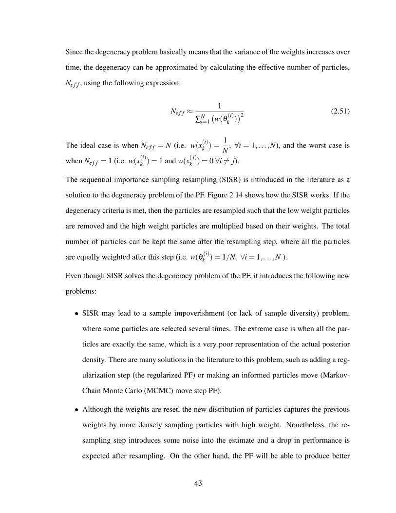
Since the degeneracy problem basically means that the variance of the weights increases over

time, the degeneracy can be approximated by calculating the effective number of particles,

Ne f f , using the following expression:

Ne f f ≈1

∑Ni=1(w(θ (i)

k ))2 (2.51)

The ideal case is when Ne f f = N (i.e. w(x(i)k ) =1N, ∀i = 1, . . . ,N), and the worst case is

when Ne f f = 1 (i.e. w(x(i)k ) = 1 and w(x( j)k ) = 0 ∀i 6= j).

The sequential importance sampling resampling (SISR) is introduced in the literature as a

solution to the degeneracy problem of the PF. Figure 2.14 shows how the SISR works. If the

degeneracy criteria is met, then the particles are resampled such that the low weight particles

are removed and the high weight particles are multiplied based on their weights. The total

number of particles can be kept the same after the resampling step, where all the particles

are equally weighted after this step (i.e. w(θ (i)k ) = 1/N, ∀i = 1, . . . ,N ).

Even though SISR solves the degeneracy problem of the PF, it introduces the following new

problems:

• SISR may lead to a sample impoverishment (or lack of sample diversity) problem,

where some particles are selected several times. The extreme case is when all the par-

ticles are exactly the same, which is a very poor representation of the actual posterior

density. There are many solutions in the literature to this problem, such as adding a reg-

ularization step (the regularized PF) or making an informed particles move (Markov-

Chain Monte Carlo (MCMC) move step PF).

• Although the weights are reset, the new distribution of particles captures the previous

weights by more densely sampling particles with high weight. Nonetheless, the re-

sampling step introduces some noise into the estimate and a drop in performance is

expected after resampling. On the other hand, the PF will be able to produce better

43

estimates in future iterations because the particles should be more densely sampled in

the importance sampling region.

Figure 2.14: Sequential importance sampling resampling (SISR) [50]

44

4. PF algorithm:

We now introduce the PF algorithm in Algorithm 1.

Algorithm 1: PF steps

Given the resampling threshold, Nthr, and the initial posterior density, p(θ0).

(a) Initialization: k = 0

For i = 1 : N

Sample θ(i)0 ∼ p(θ0)

End for

(b) IS step:

For i = 1 : N

- Draw θ(i)0 ∼ q(θ (i)

k |θ(i)k−1,xk)

- Evaluate w(θ (i)k ) = w(θ (i)

k−1)p(xk|θ

(i)k ) p(θ (i)

k |θ(i)k−1)

q(θ (i)k |θ

(i)k−1,xk)

End For

(c) Normalize the importance weights:

For i = 1 : N

w(θ (i)k ) =

w(θ (i)k )

∑Nj=1 w(θ ( j)

k )End For

(d) Resampling step:

If Ne f f < Nthr, resample the N particles with replacement according to their im-

portance weights.

(e) Set k→ k+1 and go to step 2.

45

5. Other versions of the PF:

There are two main extensions to the PF in the literature. These are the regularized PF (RPF)

and the Markov-Chain Monte Carlo (MCMC) move-step PF. They differ from the main PF

framework in the resampling step. In both extensions, a random set of samples is generated

from a predefined kernel and added to the previous particle’s system to generate the new one

(i.e. jittering). This jittering step is called regularization. In MCMC move-step PF there is an

additional step: accept the new particle only if its associated acceptance probability meets

a certain threshold. The goal is to improve the sample diversity of the particle’s system,

where loss of diversity could happen due to the resampling step. MCMC move-step PF is,

theoretically, guaranteed to converge to the true posterior, while the RPF is not. For our

surface-tracking application, we use the standard PF because, by doing some tests, we did

not see a noticeable difference when the modified PF is used.

6. PF model for DOA tracking problem:

Like any Sequential Bayesian filtering problem, the PF requires a model for the measured

data, which relates the measurements to the tracked parameter, and another model for the

dynamics of the states, which relates the results of one state to the next. These equations can

be described as follows:

• The measurements model :

The measurements model is given in equation 2.8, but we restate it here for a single

range-bin, k, case:

Xk = A(θθθ k)Sk +Nk (2.52)

where θθθ k is bold faced to emphasize that it is a vector of length Qk. The MLE (and also

the least squares) estimation of the target’s backscatter signal is given by the following

expression [39]:

sk(m) =(

A(θθθ k)H A(θθθ k)

)−1A(θθθ k)

H xk(m) (2.53)

46

where m∈ 1,2, . . .M is the mth snapshot. The noise variance can be estimated as the av-

erage of the noise subspace eigenvalues [39]. From Section 2.3 we know that the noise

has a complex Gaussian distribution. So, using equation 2.53, the complex likelihood

density function can now be written as follows:

p(Xk|θθθ k) =M

∏m=1

(πσ2n )−P exp

{−||P⊥A(θθθ k)

xk(m)||2

σ2n

}(2.54)

Since the likelihood value is always≤ 1, p(Xk|θθθ k) can be extremely small if M is large.

Although it is possible to represent the PF in the log domain, we take the mean of the

likelihood densities for each snapshot rather than the product as follows to deal with

the dynamic range problem:

p(Xk|θθθ k) =1M

M

∑m=1

(πσ2n )−P exp

{−||P⊥A(θθθ k)

xk(m)||2

σ2n

}(2.55)

• The transition model:

The transition model was described previously in equations 2.27 through 2.32 and fig-

ure 2.11.

The PF multi-target transition algorithm:

Since the maximum number of targets is assumed to be 2 (maximum of 1 target on each side

of the surface), the transition model should be able to handle the transition from 0, 1, or 2

DOAs at one state to 0, 1, or 2 DOAs at the next state. This is done using Algorithm 2, which

is implemented as part of the SIS step. The main issues are 1) how to determine which side

has a target when there is only one target, 2) how to update the active side (target), and 3)

how to update the inactive side (no target).

47

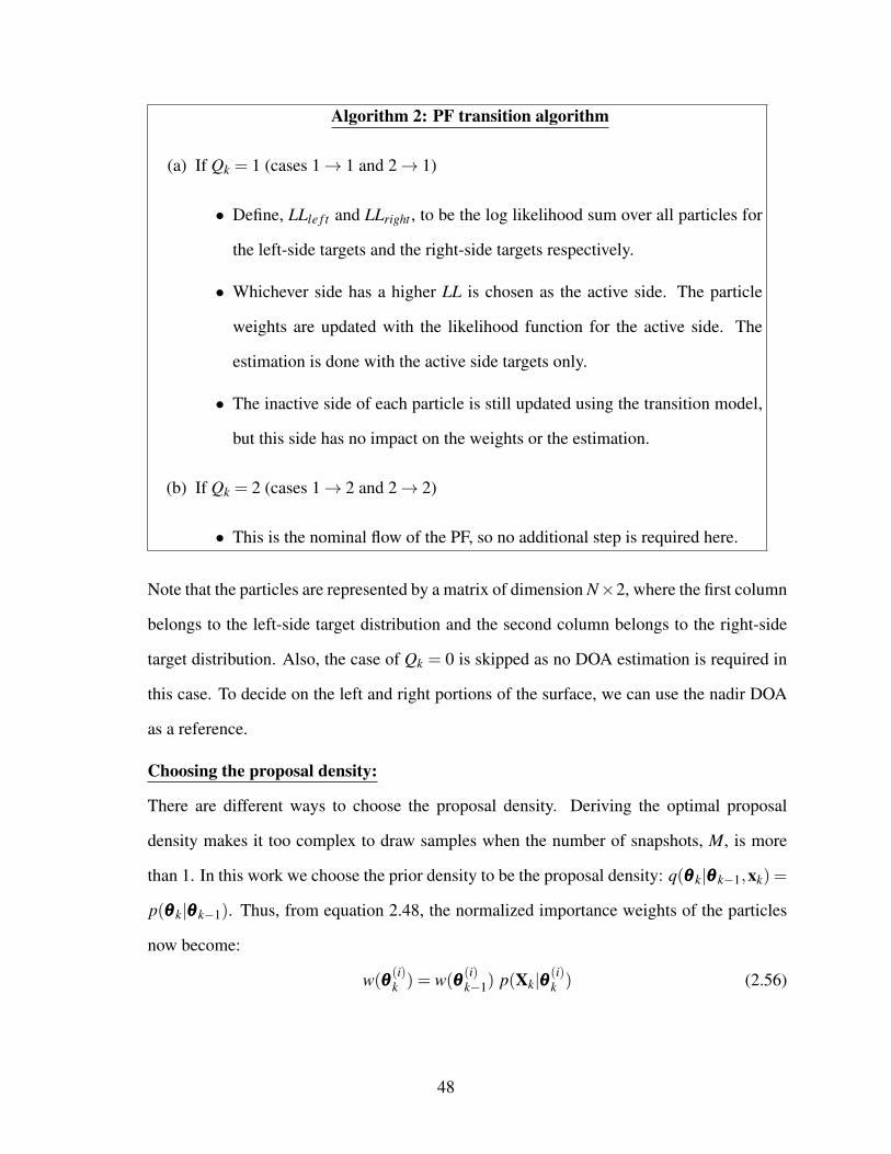
Algorithm 2: PF transition algorithm

(a) If Qk = 1 (cases 1→ 1 and 2→ 1)

• Define, LLle f t and LLright , to be the log likelihood sum over all particles for

the left-side targets and the right-side targets respectively.

• Whichever side has a higher LL is chosen as the active side. The particle

weights are updated with the likelihood function for the active side. The

estimation is done with the active side targets only.

• The inactive side of each particle is still updated using the transition model,

but this side has no impact on the weights or the estimation.

(b) If Qk = 2 (cases 1→ 2 and 2→ 2)

• This is the nominal flow of the PF, so no additional step is required here.

Note that the particles are represented by a matrix of dimension N×2, where the first column

belongs to the left-side target distribution and the second column belongs to the right-side

target distribution. Also, the case of Qk = 0 is skipped as no DOA estimation is required in

this case. To decide on the left and right portions of the surface, we can use the nadir DOA

as a reference.

Choosing the proposal density:

There are different ways to choose the proposal density. Deriving the optimal proposal

density makes it too complex to draw samples when the number of snapshots, M, is more

than 1. In this work we choose the prior density to be the proposal density: q(θθθ k|θθθ k−1,xk) =

p(θθθ k|θθθ k−1). Thus, from equation 2.48, the normalized importance weights of the particles

now become:

w(θθθ (i)k ) = w(θθθ (i)

k−1) p(Xk|θθθ(i)k ) (2.56)

48

2.6.5.2 Sequential Maximum A Posteriori Estimation (S-MAP)

Sequential MAP (S-MAP) is another type of sequential filters that we used to estimate the ice-

bottom surface. Unlike PF, here we track the DOAs directly (in the case of PF we track the

posterior pdf of the DOAs, and then estimate the DOAs using the estimated pdf) using a cost

function that has two components: the MLE cost function (discussed in section 2.6.2) and the

truncated Gaussian prior pdf, where the truncation of the Gaussian pdf is performed as part of a

bounded minimization problem. The parameters of the truncated Gaussian pdf were discussed in

equations 2.27 through 2.32 and depicted in figure 2.11. The S-MAP optimizer is initialized by the

mean DOA, µθm , which is defined in equation 2.28.

The multivariate prior Gaussian pdf is given by the following expression:

f (θθθ) =1√

det(2πRθ )exp(− 1

2(θθθ −µµµθ )

T R−1θ(θθθ −µµµθ )

)(2.57)

where Rθ ∈RQ×Q is the covariance matrix of the DOA vector, and it is diagonal because the targets

are assumed to be independent in the transition model (in the measurements model, the targets of

the same range-bin are not independent). Taking the natural logarithm of equation 2.57, we get the

following log-prior cost function:

Jθ =−Q log(2π)−Q

∑q=1

log(σ2θq)− 1


T R−1θ(θθθ −µµµθ ) (2.58)

The log-likelihood cost function can be obtained by taking the natural logarithm of equation 2.9 as

follows:

Jx =−M log(π)−Mp log(σ2n )−

1σ2

n

M

∑i=1||xi−AAA(θθθ)si||2 (2.59)

Now, the MAP cost function is the sum of the log-prior and log likelihood cost functions. Mathe-

49

matically, this can be written as follows:

J = Jx +Jθ

= c1−Mp log(σ2n )−

1σ2

n

M

∑i=1||xi−A(θθθ)si||2−



where c1 = −M log(π)−Q log(2π)−Q∑

q=1log(σ2

θq) lumps together all the constants that are not

function of θθθ .

Fixing θθθ and s, the noise variance, σ2n , that maximizes the cost function in equation 2.60 can

be estimated as follows:

σ2n =

1MP

M

∑i=1||xi−A(θθθ)si||2 (2.61)

Now to estimate the backscatter signal, s, we substitute σ2θ

back into equation 2.60, and we fix θθθ

and minimize the MAP cost function with respect to s. The result is as follows:

si =(AH(θθθ)A(θθθ)

)−1AH(θθθ)xi (2.62)

Note that equations 2.61 and 2.62 were also derived in [39] for the case of deterministic MLE

estimation. Now our derivation and the MLE derivation starts to diverge.

Substituting equations 2.61 and 2.62 back into equation 2.60, we get the following expression:

J = c−Mp log( 1

Mp

M

∑i=1||xi−PAxi||2

)− 1



where c = c1−Mp. So, the S-MAP optimization problem can be stated as follows:


(J)

s.t. θθθ(lb) ≤ θθθ ≤ θθθ

(ub) (2.64)

where the bounds are updated sequentially at each state. The first part of the above equation can

50

also be written as follows:


(J)

= argminθθθ

(−J)

= argminθθθ

{Mp log

( 1Mp

M

∑i=1||P⊥A xi||2

)+



}= argmin

θθθ

{Mp log

(1p

Tr(P⊥A R))+



}= argmin

θθθ

{Mp log

(Tr(P⊥A R)

)+



}(2.65)

The first term in equation 2.65 is equivalent to the MLE cost function, Jmle, which was defined

in equation 2.20, while the second term is the prior cost function, Jprior. So, the estimated DOA

is the one that balances 1) the minimization of the projection of the measurements onto the null

of the subspace spanned by the steering vectors and 2) the minimization of the angular distance

between the estimated DOA and the mean DOA. Roughly speaking, JJJprior dominates the result

when the data quality are low and JJJmle is a weak function of θθθ . In the extreme case of no signal,

θθθ ≈ µµµθ . If the data quality are high enough, JJJmle will likely have a large Hessian and dominate the

cost function.

There are a few other points worth mentioning. First, we assume that there is a maximum of

2 sources in each range-bin, one on the left ice-bed interface and the other on the right ice-bed

interface. Second, the posterior pdf is not Gaussian in θθθ so that the S-MAP and the MMSE PF

results in Chapter 4 will potentially give different optimal answers from each other.

2.7 Steering Vectors Estimation and Array Calibration

Array imperfections can be divided into three categories: phase, gain, and array sensor location er-

rors. Each of these types can have different effect on the performance of the beamformer/estimator,

51

and thus there are different ways of handling each type. Also, different beamformers/estimators

react differently to these errors. For example, the linearly-constrained minimum variance (LCMV)

beamformer is very sensitive to the three types of errors [51]. For this reason, in addition to

their simplicity, the performance of the LCMV-like beamformers have been extensively studied

in the literature and several approaches have been presented to alleviate the effects of these errors

[35, 52].

Since all of the beamformers and estimators discussed this dissertation depend on the eigen-

structure of the data covariance matrix, which is a function of the array manifold matrix, these

methods are affected by perturbations in the sensors and the following circuitry. So, these errors

should be compensated for to improve the DOA estimation.

Most of the literature that tackles the array calibration problem focuses only on a beamformer

and/or an estimator performance and behavior in the presence of array and system perturbations.

Very few references address how to estimate these errors and compensate for them. Here, we

classify previous work and give a summary on some example references:

1. Estimation of (and compensation for) the perturbation errors:

a) [53]: Here, the authors suggest a way to estimate the array phase and gain errors,

but they do not treat sensor location errors separately (i.e. treated as phase errors),

and require the DOA and number of targets to be known a priori. To estimate the

actual steering matrix, the authors solve the following least-squares (LS) optimization

problem:

minθθθ

||PUSA(θθθ)−A(θθθ)||2 (2.66)

where PUS = US(UHS US)

−1UHS . Also, the authors claim that the phase and gain errors

can lead to the cancellation of the desired signal rather than the interference signal in

the case of the LCMV beamformer.

b) [54]: Here, the authors suggest a way to estimate the phase and gain errors and sensor

location errors simultaneously through an iterative 2-step algorithm and an additional

52

step that takes care of the residual errors. The cost function to be minimized is:

J = AH(θθθ)UNUHN A(θθθ) (2.67)

The algorithm steps are :

1. Define the position error vector as ∆X . The estimation algorithm comprises two

steps. In the first step, fixing ∆X (initial value is zero), we estimate the gain and

phase errors of each array element. In the second step, using the results from

the first step, i.e., holding the gain and phase errors fixed, ∆X is estimated. The

algorithm iterates alternatively between the two steps until it converges.

2. Once the steering matrix, A(θθθ), is estimated, project it onto US to reduce the

effects of the residual errors due to the inaccurate noise subspace estimation.

As explained in section 2.6.2, MLE cost function does the projection onto the

signal subspace and away from the noise subspace simultaneously rather than sep-

arately here.

c) [55]: Here the authors suggest a self-calibration algorithm based on MLE. It estimates

both the DOAs and the sensor locations simultaneously. Here is how this method

works: In the first step, the DOAs are estimated using the nominal sensor locations.

Then using these DOAs, the sensor locations are estimated, and the process repeats

until the algorithm converges.

Note that this algorithm is more robust and more complicated than the algorithms given

above. However, it neglects the phase and gain errors. Also, the number of targets is

assumed to be known. In addition, the algorithm is computationally expensive because

for each set of sensor locations we need to iterate until the convergence condition is

satisfied. Then we need to use these DOAs to iteratively estimate the sensors locations,

and the process repeats. Each step in each iteration is generally a multidimensional

nonlinear search.

53

2. Optimal diagonal loading to handle the effect of random steering errors:

a) [56]: Here the authors suggest a negative diagonal loading to reduce the effects of

array steering errors for the beamformers of the form:

w = (R+ γI)−1a(θ) (2.68)

where w is the weight vector and I is the identity matrix. LCMV beamformers are of

this type. The optimal diagonal loading is:

γopt =−(σ2n +σ

2s ||a(θ)||2) =−(σ2

n +σ2s P) (2.69)

where σ2n is the noise power, and σ2

s is the signal power. γopt provides a rough order of

magnitude of the optimal loading level.

b) [35]: Van Trees also suggests the use of diagonal loading to improve the sensitivity

of the minimum power distortionless response (MPDR) beamformer to array perturba-

tions. But the problem is that this loading can reduce the SINR as well.

3. Study of the effect of array errors onto SINR and array weights (for MVDR/MPDR

beamformers):

References [57, 58, 59], among many others, give a detailed analysis for the effect of system

and array imperfections on the performance of MVDR-like beamformers. They are good for

understanding the problem, but they do not offer solutions to the problem.

Note that using the MLE cost function (equation 2.19) can alleviate some of the array imper-

fections. This is because it does simultaneously two projections: onto the signal subspace and

away from the noise subspace. Thus, we use MLE cost function not only for DOA estimation,

but also for array calibration. Note that MLE is superior to MUSIC in this regard. For MUSIC,

we only seek the DOAs that make the noise subspace orthogonal to the steering vectors. MUSIC

54

cost function doesn’t utilize the signal subspace and noise subspace simultaneously as MLE does.

Thus, MLE is more robust to array-errors than MUSIC [55].

We have developed an MLE-based cost function to estimate the gain, phase, and location errors

from the 2D data of the SAR imagery. [1] has good details on the technique, but here we will

explain the method briefly and elaborate on the modifications we added to the model.

The sensors gain error is modeled as a function of the DOA using three parameters that control

the shape, size, and orientation of the gain pattern of each sensor. So, the gain model for sensor p

can be written, in dB, as follows:

g(dB)p (θq) = αpS

(sin(θq)− sin(αpθ )

)2+αpD (2.70)

where αpS controls the size of the gain pattern, αpθ , measured in radians, controls the shape and

orientation (or peak location) of the gain pattern, and αpD controls the deviation (up or down) of

the gain pattern of the pth sensor relative to the other sensors. The nominal values of these three

parameters are zeros. However, to estimate αpθ , then αpS should not be set to zero and its nominal

value becomes αpS = 1. In linear scale, the gain error becomes gp(θq) = 10g(dB)

p (θq)20 .

The sensors location and phase offset (DC) errors for sensor p are modeled as a phase term in

the following way (also a function of the DOA):

φφφ p(θq) = exp{− j(k∆py sin(θq)− k∆pz cos(θq)+∆pθ

)}(2.71)

where ∆py and ∆pz are the location errors along y and z dimensions, respectively. ∆pθ is the phase

deviation or DC phase offset.

Combining the gain and phase error models, the final error model of the pth sensor in the

direction θq now becomes as follows:

ðp(θq) = gp(θq)×φφφ p(θq) (2.72)

55

The new steering matrix can be written as the Hadamard product (i.e. element-wise product)

between the ideal steering matrix, which is defined in equation 2.7, and the error matrix, which is

defined above.

The cost function to be maximized is a superposition of the log-likelihood cost functions of

the Nt range-bins in a given range-line. So, we seek the array errors that maximizes the following

MLE-based cost function:

ð= argmaxð

Nt

∑t=1

Tr(PA(θθθ t)Rt

)(2.73)

where Tr is the trace operator. Note that A(θθθ t) is now the perturbed steering matrix, not the ideal.

Figures 2.15 and 2.16 show, respectively, an example of the gain and phase deviation patterns

from simulation data for a practical error values of 7 linearly spaced sensors receiving 100 snap-

shots with 30dB SNR. Note that these errors are measured relative to the first sensor.

The gain errors represent the amount of mismatch between the isotropic pattern of the ideal

sensors and the actual patters. On the other hand, the phase errors don’t affect the gain pattern of

the individual sensors, but rather affect the array factor.

-30 -20 -10 0 10 20 30

θ°

-3

-2.5

-2

-1.5

-1

-0.5

0

Pow

er (

dB)

Ant 1Ant 2Ant 3Ant 4Ant 5Ant 6Ant 7

Figure 2.15: Sensors gain pattern

56

−30 −20 −10 0 10 20 30−4

−3

−2

−1

0

1

2

3

θ°

Pha

se (

deg.

)

Ant 1Ant 2Ant 3Ant 4Ant 5Ant 6Ant 7

Figure 2.16: Sensors phase deviation pattern

2.8 Specifications of the Radars Used in This Work

In this section we describe the properties and parameters of the radar data used in this work.

The airborne Multichannel Coherent Radar Depth Sounder (MCoRDS), developed at the Uni-

versity of Kansas, was used to collect data for several of the results presented in this work. The

MUSIC results in Chapter 5 were collected over the Canadian Arctic Archipelago (CAA), in 2014.

Figure 2.17 a shows the transmit configuration for the CAA data collection. Three time division

multiplexed beams are formed and a separate SAR image is formed for each beam. The S-MAP

results in Chapter 5 are collected in a nadir-only beam configuration. Figure 2.17 b shows the 3D

SAR resolution. The antenna system is composed of 15 sensors divided into three subarrays: 1)

the center subarray, which is mounted on the fuselage, is composed of 7 sensors used for transmit

and receive, 2) the left/right subarrays, which are mounted on the left/right wings respectively,

are each composed of 4 receive-only sensors. These three subarrays are separated by substantial

baselines. So, to avoid the grating lobes or ambiguities that occur when using all 15 elements, we

only make use of the 7 receive elements of the center subarray, which has a length of 4.5 m. Figure

57

2.18 shows the geometry of this array in the y-z plane.

Figure 2.17: Transmit configuration of the P-3 radar. a) Shows the time multiplexed multi-beammode of the radar, which results in a large imaged swath. b) Shows a single SAR image pixel afterpulse compression and SAR processing, where the 3D scene is resolved into toroids with constantalong-track and constant range that are centered on the flight path. The targets lying in a particulartoroid need to be resolved by estimating their respective elevation angles.

58

Figure 2.18: Phase centers of the three subarrays mounted on the P-3 radar plotted in the y-z plane.Each star ’*’ represents one sensor of the array. The y-axis points starboard/right and the z-axispoints down relative to the aircraft.

MCoRDS [8] consists of three main subsystems: digital, RF, and antennas. Table 2.1 shows

the radar system parameters. To increase the imaged swath for the CAA data collection, the radar

was set to a multibeam transmission mode with three transmit beams steered to the left −30◦,

nadir 0◦, and right 30◦. The beam parameters are given in Table 2.2. The transmit beamwidth with

the Hanning window taper produces a beam with most of the power concentrated in a 30◦ wide

beamwidth.

Table 2.1: P-3 radar system parameters

Parameter ValueRadar carrier-frequency 195 MHz

Signal bandwidth 30 MHzTransmit pulse duration CAA 3 µs

Transmit pulse duration S-MAP 1 µs, 10 µsTX antennas 7 DipolesRX antennas 15 Dipoles

PRF 12 KHzEffective Storage PRF CAA

3 Beams Multiplexed, 13 stacked pulses each 307 HzEffective Storage PRF S-MAP

2 Nadir Beams, 32 stacked pulses total 375 Hz

The digital section consists of a waveform generator for each transmit antenna and an analog-

59

Table 2.2: P-3 radar beam parameters for CAA data

Waveform Look Angle Attenuation Weights1 −30◦ (left) 15 dB Hanning2 0◦ (nadir) 20 dB Hanning3 +30◦ (right) 15 dB Hanning

to-digital-converter (ADC) for each receive antenna. The waveform generators are individually

amplitude, phase, and time-shifted to produce a 10% Tukey-weighted linear-FM chirp, beam

steered in the desired direction using true time delays. For the CAA data collection, the sys-

tem cycles every 13 pulses between left, nadir, and right beams. Each batch of 13 pulses captured

by an ADC, is averaged in hardware, and then stored to disk, creating 45 independent streams of

data (15 ADCs × 3 beams), one for each receive-antenna and beam pairing.

The RF transmit section consists of power amplifiers, bandpass filters, and switches needed to

precondition the generated pulses before radiating them into the air through the transmit antenna

elements.

The duration of the transmitted pulse for the CAA data collection, 3 µs, was chosen as the

longest pulse duration that would guarantee capture of the ice-surface. The minimum altitude was

about 2250 ft above ground level (AGL) which allows 1.5 µs for the center 7 elements to switch

from transmitting to receiving. Due to the thin ice (<1000m), the radar was operated with a single

receiver gain setting for the entire range line and chose the gain to be the highest setting that still

ensured that the surface return from ice would not saturate the receiver.

For a platform speed of v=124 m/s, the Nyquist criterion requires PRF=4v/λc =322 Hz. The

actual recording rate of 307 Hz leads to some ambiguity between forward and reverse grazing

angles in the along-track dimension. However, these look angles are not used because basal ice

scattering is very weak at these angles.

60

2.9 Processing Phase Centers

Since the transmit phase center and receive phase centers rarely align for all measurement phase

centers, then by definition, CReSIS radars are bistatic even though the transmit and receive an-

tennas are either the same or co-located. However, because monostatic geometry is much simpler

than bistatic geometry, we use the monostatic radar equivalent phase centers to a bistatic radar

when processing our data.

Figure 2.19 shows a graphical view of the measurement phase center calculation for a bistatic

radar. The phase centers are calculated as follows. Define the following variables:

• xtxp ,y

txp ,z

txp : location of the pth transmit array sensor in the x, y, and z dimensions.

• xtxpc,y

txpc,z

txpc: transmit phase center (for the particular configuration) in the x, y, and z dimen-

sions.

• xrxp ,y

rxp ,z

rxp : location of the pth receive array sensor in the x, y, and z dimensions.

• xpc,ypc,zpc: phase center for the ith monostatic equivalent measurement in the x, y, and z

dimensions.

• wtx: transmit weights vector.

Then, we can calculate the phase centers of the transmit sensors as the inner product between the

transmit sensors location and their preassigned weight, as shown in the following equation:

btxpc =

1P∑

p=1wtx

p

P

∑i=p

btxp wtx

p , where b ∈ {x,y,z} (2.74)

The phase centers of the receive sensors can be calculated as the average of the phase centers of

the transmit sensors and the location of the receive sensors. This can be written mathematically as

follows:

bpc =(brx +btx

pc)

2, where b ∈ {x,y,z} (2.75)

61

Figure 2.19: Monostatic equivalent measurement phase center for a bistatic radar geometry involv-ing a single transmit and single receive antenna.

62

Chapter 3

Wideband Model Order Estimation Using

Machine Learning

3.1 Introduction

Model order estimation (MOE) is the problem of estimating the number of targets, Q, that con-

tribute to a measurement. Parametric direction of arrival (DOA) estimation techniques require the

number of targets to be known a priori. Overestimating Q leads to estimating false targets, which

reduces the accuracy of the estimated DOAs due to the noise being modeled incorrectly as a sig-

nal source. Similarly, underestimating Q means that the signal energy is modeled inaccurately as

noise, which generally has a much more detrimental effect on the estimation accuracy than overes-

timation. Although overestimation does not affect the DOA as much, in the DOA-based tracking

problem, such as tracking the bottom of an ice-sheet [33], overestimating Q usually leads to poor

tracking results because the false targets affect the tracker’s decision. Thus, it is important that Q

is estimated as accurately as possible.

The classic MOE problem is solved by formulating a cost function and choosing the model

order (number of targets) that minimizes the cost function. The cost function is composed of two

terms: a negative log-likelihood term and a penalty term [60]. The log-likelihood term depends

63

on the signal model used, but is always a monotonically decreasing function with model order.

The reason for this is that as the model order is increased, the likelihood function is better able

to match the data and so the likelihood goes up and the negative log likelihood goes down. The

penalty term is a monotonically increasing function to counteract this trend so that the minimum

of the combined terms occurs at the actual model order. Classic methods use analytical forms of

the penalty term that are convenient because the signal model parameters are usually parameter-

ized, which makes it easy to apply them to different scenarios (varying snapshots and number of

sensors). However, in situations where the parameters are known ahead of time, [42] found that

a numerically tuned penalty function outperforms all the classic methods considered in [60]. [1]

has more details about this method, where optimal (number of targets and their directions are es-

timated jointly) and suboptimal (number of targets and their directions are estimated separately)

signal models [38] are compared with each of the MOE techniques including the new numerically

tuned penalty term. For the narrowband case, their results show a substantial improvement over

standard methods, especially with the optimal signal model. Note that both the suboptimal and

optimal signal models that the MOE techniques use are based on the narrowband signal model and

they exploit the structure of the signal model’s data covariance matrix (R) to estimate the number

of targets.

For wideband signals, neither the standard MOE methods nor the numerically tuned method

(NT) have good performance, especially beyond the low SNR regime and/or for large model orders

up to one less than the number of sensors, P. For example, if we must estimate the number of

targets, then Q ∈ {0, . . . ,P− 1}. This is because, for wideband data, the signal subspace is no

longer equal in dimension to the number of targets. It is worth noting here that higher signal-to-

noise ratio (SNR) makes the MOE results worse in the wideband case because the spreading of

signal energy into all the eigenvalues will be more prominent in this case. The additional signal

energy in all the eigenvalues can cause a model order estimator designed around a narrowband

signal model to decide these are distinct targets.

At the Center for Remote Sensing of Ice-Sheets (CReSIS), we process wideband data collected

64

by CReSIS radars from different regions in Greenland and Antarctica with the goal of producing

digital elevation models (DEMs) of the surveyed areas. But to generate these DEMs, the location

of the top and bottom of the ice-sheets need to be known. The ice-top is given from the satellite

imagery, but the ice-bottom should be estimated from the wideband radar data. To perform this

task, the number of targets needs to be estimated per range-bin. The simple narrowband model

is not effective with CReSIS radar data because the has a complicated eigen-structure for the data

covariance matrix, R, where the dynamic range of the eigenvalues of R can be very large and the

noise eigenvalues do not show proper multiplicity in cases where the radar scene is simple enough

to enable determination of the correct model order by inspection. This suggests that there could be

a violation of the narrowband assumption caused by multipath or the wider bandwidth, potential

electromagnetic interference (EMI), or some combination of these. Regardless, standard MOE

performs poorly.

Due to the complexity of the eigenspace for wideband data and the further complexity of the

CReSIS data, we introduce a machine learning-based replacement for the simple numerical tuning

model, where we apply a logistic regression method (LR-MOE) to estimate the model order under

narrowband and wideband scenarios. Also, using the narrowband signal model presented in Sec-

tion 2.3, we compare our results against six standard MOE methods and the former numerically

tuned method (NT) compared in [1, 42]. Based on these simulations, the machine learning based

MOE is able to do as well on narrowband data as the above mentioned methods and substantially

outperforms all of them on wideband data.

To the best of our knowledge, this type of method and comparison are not explored in the

literature and are introduced for the first time in this work. However, there are some attempts in the

literature to perform this task by dividing the field of view (FOV) into multiple sectors and detect

the presence of targets in each sector using NN techniques, and then apply DOA estimation at the

sectors that have targets detected [61, 62]. A similar idea was also presented in [63] to estimate

the DOA of a sound source after uniformly sampling the field of view in the elevation and azimuth

dimensions and detect the presence of a source in each sampled direction. It is worth noting that

65

none of these research articles dealt with the MOE problem as a multi-class classification problem

or made a comparison with several other MOE methods, especially in regards to radar imagery

applications, which is the focus of this work.

Although this logistic regression based technique is explored here, the MOE technique used

in the remaining chapters of the dissertation is based on the minimum description length (MDL)

using the optimal signal model with log-likelihood normalization method as introduced by [1, 42].

We abbreviate this method as N-MDL in this and later chapters. The log-likelihood normalization

term accounts for the spread in the estimated noise subspace that occurs because a finite number of

snapshots are used. Also, the standard MOE methods use the narrowband signal model, so in the

wideband case, such as our application, the normalization term corrects for this model mismatch

in the log-likelihood term of the cost function as well. By accounting for these effects, the standard

algorithms perform much better. Note that the wideband results presented in [1] assume the max-

imum number targets is 6 for 7 sensors uniform linear array, which is why their results show that

optimal and suboptimal MOE methods as well the NT method fail on wideband data, even with

normalization. As we will will see in chapter 5, N-MDL works well on real wideband data when

Q = 2 (i.e. small number targets relative to the number of sensors).

3.2 MOE Based on Logistic Regression (LR-MOE)

MOE can be viewed as a mutually exclusive multinomial classification problem, where each class

represents a specific number of targets and the total number of classes is the maximum number

of targets, Q, that we expect to have contributed to the measured data. Generally, for a uniform

linear array, Q = P− 1, where P is the number of array sensors. So, in this case, there are P

classes that the MOE needs to choose from, which are Q = 0,1, . . . ,P− 1. Each of these classes

has a probability or cost associated with it and the final answer is the class that has the maximum

probability or minimum cost among all other classes.

66

3.2.1 Logistic Regression Model

We use one versus all logistic regression to perform the classification task. Here we give a brief

background on the theory of LR [64] and customize the discussion for our specific MOE problem.

We start by mathematically defining the LR hypothesis model (also called sigmoid or logistic

function) as follows:

hΘk(x) =1

1+ exp(−ΘTk x)

(3.1)

0≤ hΘk(x)≤ 1

where Θk is the LR parameter vector that is learned or optimized using the training dataset for

class k, and x is the feature or input vector. Figure 3.1 shows a plot of the LR hypothesis function.

hΘ(x) maps z = ΘT x to a probability distribution such that we can calculate the probability of each

of the P classes, given z, and choose the one that has the maximum probability.

In our MOE application, we choose the features, x, to be the log of the geometric mean, λλλ g(k),

and the scaled log of the arithmetic mean, λλλ a(k), of the eigenvalues of the data covariance matrix

for k = 0,1 . . . ,P− 1 targets or classes. Considering this, there are a total of 2P features for each

binary classifier. We define the ith eigenvalue as λλλ (i) and sort the eigenvalues in descending order

so that λλλ (1) is the largest. λλλ g and λλλ a are then defined as follows:

λλλ g(k) =P

∑i=k+1

log(λλλ (i)

)(3.2)

λλλ a(k) = (P− k) log( 1

p− k

P

∑i=k+1

λλλ (i))

(3.3)

Note that M(λλλ g−λλλ a

)is the log-likelihood term of the standard suboptimal MOE methods where

the scaling factor M is the number of snapshots. The unscaled feature vector can now be defined

as follows:

xno−scale = [λλλ g(0), . . . ,λλλ g(P−1),λλλ a(0), . . . ,λλλ a(P−1)]T (3.4)

67

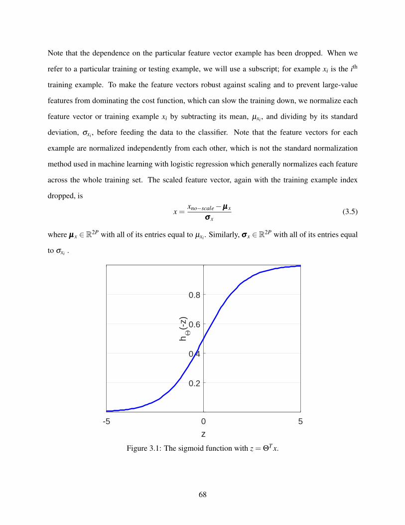
Note that the dependence on the particular feature vector example has been dropped. When we

refer to a particular training or testing example, we will use a subscript; for example xi is the ith

training example. To make the feature vectors robust against scaling and to prevent large-value

features from dominating the cost function, which can slow the training down, we normalize each

feature vector or training example xi by subtracting its mean, µxi , and dividing by its standard

deviation, σxi , before feeding the data to the classifier. Note that the feature vectors for each

example are normalized independently from each other, which is not the standard normalization

method used in machine learning with logistic regression which generally normalizes each feature

across the whole training set. The scaled feature vector, again with the training example index

dropped, is

x =xno−scale−µµµx

σσσ x(3.5)

where µµµx ∈ R2P with all of its entries equal to µxi . Similarly, σσσ x ∈ R2P with all of its entries equal

to σxi .

-5 0 5

z

0.2

0.4

0.6

0.8

hΘ

(-z)

Figure 3.1: The sigmoid function with z = ΘT x.

68

3.2.2 Logistic Regression Cost Function

In our classification problem we are seeking the parameter Θk, which is obtained by minimizing a

cost function, JLR,k, that has two main terms: the first is the cost when the training example is in

the class and the second is the cost when the training example is not in the class. For m training

examples, this can be written as follows [64]:

JLR,k =−1m

m

∑i=1

(1k1k1k(yi) log

(hΘk(xi)

)+1not k1not k1not k(yi) log

(1−hΘk(xi)

))+αΘ

Tk Θk (3.6)

where xi is the ith example (or feature vector) and yi is the corresponding label or class (the model

order). Here we use indicator functions to control the first two terms. 1k1k1k(yi) is 1 when yi is equal

to k and is zero otherwise. Conversely, 1not k1not k1not k(yi) is 1 when y1 is not equal to k and zero otherwise.

α is the learning rate and αΘTk Θk is the regularization term that is added to avoid overfitting on

the training set, which is an issue that usually arises from having too many features relative to the

training set size. In other words, α can be used to keep all the features in the model by reducing

the variability of the parameter vector Θk. In our application, we found through a grid search that

setting α = 10−5 helps to slightly improve the percentage of correctly estimating the true number

of targets.

The optimization problem can now be stated, for each class k, as follows:

Θk = argminΘk

JLR,k (3.7)

Because the logistic regression cost function is convex, we use a steepest gradient based algo-

rithm to minimize the cost function to find the MOE classification parameters. A grid search on

the regularization coefficient was also performed to find the optimal regularization constant.

69

3.2.3 Testing and Training Modes

In supervised machine learning, we first train the algorithm using a training data set to obtain

the parameters, Θ. Once we are satisfied with the results, usually based on some application-

dependent metrics, we take Θ associated with the best or lowest cost and apply this to a test set,

which is mutually exclusive of the training set, to obtain the final results and can then move on to

actual operation.

For our MOE application, we train and test for a given number of snapshots, M, and sensors,

P. This implies that if either the number snapshots or sensors change, then we should again re-

train to obtain the best possible results. For a particular number of snapshots and sensors, we

generate training and testing data sets for a range of SNR scenarios and for all possible numbers

of targets, Q = 0,1, . . . ,P−1, using a one dimensional (1D) DOA simulator, where the snapshots

are generated along the azimuth (along-track) dimension only and are assumed to be temporally

independent, which simulates an ideal synthetic aperture radar (SAR) processor. The number of

training examples for each possible combination of SNR and number of targets is 10000. There-

fore, if there are 3 SNRs and P = 7, there are 3×7×10000 = 210,000 training examples in total.

Similarly, we used 105,000 testing examples. The generated data snapshots used in each training

and test example are independent.

3.2.4 LR-MOE Algorithm

The LR-MOE problem is a multi-class classification problem, where each class has its own pa-

rameter vector Θk ∈ R2P, and the parameters of the P classes are arranged in a single parameter

matrix, ΘΘΘ ∈ R2P×P, that is then fed into the testing phase along with the testing dataset. In the

training phase, the optimizer considers each class independently, where the label vector, y, has m

entries with individual values yi ∈ {0, . . . ,P−1}.

In the testing phase, we apply the estimated parameters of the P classes, one class at a time, to

the testing dataset, and the final answer for the estimated number of targets, q (i.e. the estimated

class) corresponds to the binary class function that has minimum cost. Mathematically, this can be

70

written as follows:

q = argmaxk

hΘk(x) (3.8)

where hΘk(x) is the sigmoid function for class k.

We use the percentage correct metric to evaluate our results. This metric represents the aver-

age number of times the model order is estimated correctly relative to the total number of input

examples. We use this metric to compare the LR-MOE results to seven other MOE methods.

3.2.5 Results: Comparison Between LR-MOE and Other Methods

Now we present our results of the LR-MOE. The training and testing data were generated from

a P = 7 sensor uniform linear array with M = 11 snapshots and different SNR values. We are

particularly interested in the low snapshots case because the radar scene often allows for only

a small number of snapshots because of the requirement that the snapshots are stationary. The

data were generated for narrowband and wideband scenarios with fractional bandwidths of ∼ 0%

and ∼ 15%, respectively, and for Q = 0,1, . . . ,6 targets. Figures 3.2 and 3.3 show the normalized

geometric and arithmetic means of the eigenvalues of a wideband data covariance matrix (averaged

over 5000 Monte Carlo runs). We can see that there is good separation between the different

curves (each belongs to a specific number of targets), which justifies choosing the geometric and

arithmetic means of the eigenvalues as features to perform classification. But the boundary between

the different classes becomes less clear as the number of targets increases. As we will see next,

the LR-MOE method performs better in the narrowband case than in the wideband case, especially

when the number of targets is large, due to the clearer boundary between the different classes in

the narrowband case. For the wideband case, the LR-MOE outperforms all the other methods even

though all methods, including the LR-MOE method, use the arithmetic and geometric means of

the eigenvalues as the main component in their cost functions. The following results demonstrate

this.

71

1 2 3 4 5 6 7Eigenvalue index

-1

-0.5

0

0.5

1

Nor

mal

ized

λg

q=0q=1q=2q=3q=4q=5q=6

Figure 3.2: Normalized geometric means of the eigenvalues of the data covariance matrix averagedover 5000 Monte Carlo runs.

1 2 3 4 5 6 7Eigenvalue index

-1

-0.5

0

0.5

1

Nor

mal

ized

λa

Figure 3.3: Normalized arithmetic means of the eigenvalues of the data covariance matrix averagedover 5000 Monte Carlo runs. The legend matches the previous plot.

Seven MOE methods were used to compare against the suggested logistic regression MOE

method, which are [42, 1]: Akaike Information Criterion (AIC), Hannan and Quinn Criterion

(HQ), Minimum Description Length (MDL), Corrected AIC (AICc), Vector Corrected Kullback

Information Criterion (KICvc), Weighted-Average Information Criterion (WIC), and numerical

tuning (NT). In the plot results presented below we present the LR-MOE results in a separate plot

while keeping all other methods in a single plot for better visualization.

We start the comparison with the narrowband case. Figures 3.4 and 3.5 show the percentage

correct results of the LR-MOE method and the other compared methods, respectively. The data

72

is a mix of 3 SNRs: 10 dB, 20 dB, and 30 dB. The suboptimal signal model is used in all these

methods. The results are evaluated for each SNR separately and with all SNRs at once, including

the LR method.

We can conclude from these results that the LR-MOE method has better performance than all

other methods at low SNRs and at large numbers of targets, which is a more challenging scenario

in the narrowband case. It is worth noting that the log-likelihood term, in all of the compared

methods except the LR method, is normalized using the method described in [1]. Without the

normalization, the results are much worse. Note that the percentage correct of the WIC and KICvc

methods is 0 for some numbers of targets because the penalty term of their cost function has a

denominator that is not positive due to our specific choice of the number of snapshots and number

of sensors, which causes these methods to give nonphysical values for the model order.

Now we perform the same comparison as before, but for the wideband scenario. Figures 3.6

and 3.7 show the percentage correct results of the compared methods. As expected, all the standard

MOE methods as well as the NT method fail almost completely at medium and high SNRs even

when the measurement snapshots result from a small number of targets. Increasing the number of

snapshots from 11 to 101 does not help improve the performance of these methods, as shown in

figure 3.8. These results are discussed in [1]. However, the logistic regression results are much

more robust and have comparable performance at all SNRs and numbers of targets and with a

small number of snapshots, which is the main conclusion from this study. Note that we did not

include the machine learning results for the 101 snapshots because it already performs well with

only 11 snapshots and increasing snapshots increases the performance since it reduces the noise in

the estimation of the eigenvalues.

To test the SNR range over which the LR-MOE method still performs well, we did a separate

experiment where we trained and tested the machine learning algorithm on 1D wideband data

generated for 3 dB, 40 dB and 50 dB SNRs (i.e. skipped medium SNR). The percentage correct

results are shown in figure 3.9. Also, figure 3.10 shows the results for the case of SNR = 50

dB narrowband and wideband data (the LR algorithm is trained and tested separately for each

73

bandwidth scenario). We can see that the LR-MOE method still has acceptable performance,

where the percentage correct is more that 80% in all test cases, given the wide dynamic range

of the SNRs with no mid-range SNRs used in tuning for figure 3.9. These results support our

conclusions regarding the robustness of the machine learning technique when applied to the MOE

problem. Also, the results of this section unveil a promising solution for the MOE problem in the

case of wideband data, especially in the high SNR regime and high model order applications.

0 1 2 3 4 5 6Number of targets

98

99

100

% C

orre

ct

All SNRsSNR=10 dBSNR=20 dBSNR=30 dB

Figure 3.4: LR-MOE results for narrowband scenario. It shows the number of times the modelorder is estimated correctly relative to the total number of examples contributed in the test.

74

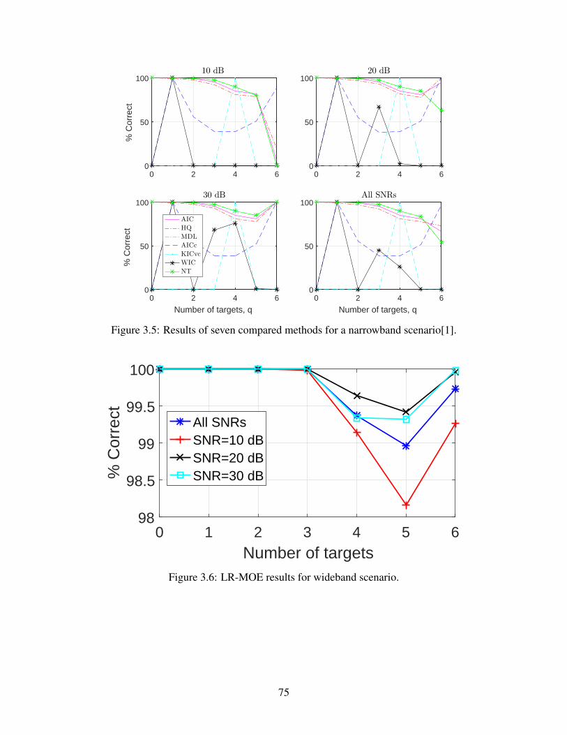
0 2 4 60

50

10020 dB

0 2 4 6

Number of targets, q

0

50

100

% C

orre

ct

30 dB

AIC

HQ

MDL

AICc

KICvc

WIC

NT

0 2 4 6

Number of targets, q

0

50

100All SNRs

0 2 4 60

50

100

% C

orre

ct

10 dB

Figure 3.5: Results of seven compared methods for a narrowband scenario[1].


98

98.5

99

99.5

100

% C

orre

ct


Figure 3.6: LR-MOE results for wideband scenario.

75

0 2 4 60

50

10020 dB

0 2 4 6Number of targets, q

0

50

100

% C

orre

ct

30 dB

AIC

HQ

MDL

AICc

KICvc

WIC

NT

0 2 4 6Number of targets, q

0

50

100All SNRs

0 2 4 60

50

100

% C

orre

ct

10 dB

Figure 3.7: Results of seven compared methods for wideband scenario [1].

76

Figure 3.8: Results of seven compared methods for wideband scenario with 101 snapshots [1]. Thelegend matches the previous plot.


80

90

100

% C

orre

ct


Figure 3.9: LR-MOE results for wideband scenario using wide dynamic range of training SNRs.

77


98

99

100

% C

orre

ct

NarrowbandWideband

Figure 3.10: LR-MOE results for narrowband and wideband scenarios for 50 dB SNR.

78

Chapter 4

Comparison Between Particle Filter and

Sequential MAP for Surface Tracking

4.1 Introduction

In this chapter we perform a 2D simulation-based study to evaluate the sequential surface track-

ers suggested and discussed in chapter 2 (namely, the PF and S-MAP). First, we investigate the

performance of each of the two filters separately, and then compare them together and draw some

conclusions. So, the goal here is to form a more in-depth understanding of the theoretical bounds

of these filters when applied to the problem under consideration (surface tracking). For the best

of our knowledge, this is the first study that is performed for this type of application, which we

think that it will open the door for a new research direction to where these sequential filters can be

applied, including the point cloud-based ice-bottom tracking problem.

4.2 Simulation Setup

The results presented in the following sections are produced using a 2D simulator, where the data

are generated for each range-bin and each range-line as opposed to the standard 1D simulator

that works along one dimension only. The 2D simulator is built to generate surfaces and evaluate

79

the performance of different DOA estimation methods. All simulations assume a flat earth and

point targets (a target that can be characterized by its radar cross section, RCS, only). Since

we are interested in cross-track slices, no interaction between the data collected across range-

lines is assumed, which mimics an ideal SAR processor. All snapshots are along-track snapshots,

and thus independent. However, the frequency leakage between range-bins is captured in the 2D

simulator, where the range to each target is calculated with respect to each phase center of the radar

array sensors and a received sinusoidal signal is generated for that target at the predefined center

frequency and bandwidth. The signals from the different targets are then combined together after

being multiplied by their radar cross-section, which is modeled as a complex Gaussian random

variable with predefined mean and variance. A Hanning window is then applied to reduce the

interaction between neighboring range-bins. Thus, targets that share the same range to the radar

are added together to form the measurements data received from their respective range-bin. The

different relative delays from each target to the array sensors are then utilized by the DOA estimator

to estimate the elevation angle of the targets.

We simulate a 7 sensor uniform linear array (ULA) in this chapter. The transmit beamforming

and array perturbations can also be incorporated in the data generation, but for the simulations in

this chapter we assume the array is ideal and no transmit beamforming is applied. So, all targets are

assumed to have the same SNR (omni-directional array) to avoid averaging high SNR results (near

nadir) with low SNR results (outside the 3 dB beamwidth of the radiation pattern). The FOV is

restricted to be±30◦. Also, SNR is defined to be per channel everywhere in this chapter. Note that

there is an SNR gain of 8.5 dB from the 7 sensors, assuming coherent integration of the returns.

We do our simulations for 2 fractional bandwidth scenarios: fc = 195 GHz at B = 30 MHz

(narrowband case) and fc = 195 MHz at B = 30 MHz (wideband case, which matches real data

fractional bandwidth). 1000 Monte Carlo runs are used in both simulation scenarios.

The model order, Q, is assumed to be known exactly, even though we will discuss the case

of the estimated model order at the end of the chapter. Also, for the sequential trackers to work

properly, tight initial bounds are necessary. But, for the purpose of this theoretical study, we

80

relax this requirement and set the bounds to be ±15◦ (for the first active range-bin only) to better

understand the behavior of the sequential trackers under unfavorable conditions. One issue withe

these loose initial bounds is the possibility that the tracker may diverge and not be able to recover

and come back on track. We found issue is less sever in the case of the PF than S-MAP, as we will

see later in this chapter.

We use the root mean squared-error (RMSE) as a qualitative statistic to evaluate the perfor-

mance of the studied DOA estimation methods. We chose the RMSE because it is a combination

of the variance and the bias of the estimator. Note that the RMSE curves in this chapter are av-

eraged over the number of simulated targets and number of active range-bins, so it is the average

RMSE. Also, to measure the quality of the RMSE results, we use√

CRLB as a reference. Figure

4.1 shows a plot of the√

CRLB as a function of DOA for 3 different SNRs (3 dB, 10 dB, and

20 dB) and 21 snapshots for the case of a single range-bin with 2 equal SNR targets. The higher

the SNR is, the more linear the√

CRLB curve becomes over the considered FOV, and also less

dependent on the elevation angle of the target. Also, as the two targets both approach nadir, there

angular separation decreases, making it harder to distinguish the two targets, and thus higher SNR

is important to separate them. Note that figure 4.1 is the only CRLB curve in this chapter and we

put it separate for better visualization.

4.3 Particle Filter As a Surface Tracker

In this section we evaluate the performance of the PF, where we use the sequentially tracked (ap-

proximate) posterior pdf to perform Bayesian DOA estimation. One of the important parameters

in the PF implementation is the resampling threshold, Nthr, where, as mentioned in chapter 2, if the

effective number of particles, Ne f f , is less than Nthr, then resampling is performed. This parameter

is application-dependent. Setting the threshold too low makes the resampling happens more often,

which leads to a loss of the information that is accumulated over time. Also, setting the threshold

too high can lead to the degeneracy problem. In our PF simulations, we set Nthr = 0.2N (or 20%

81

5 10 15 20 25 30 35


0

0.2

0.4

0.6

0.8

1√

CRLB

(deg)

SNR = 3 dBSNR = 10 dBSNR = 20 dB

Figure 4.1: Elevation angle vs√

CRLB, in degrees, for 3 SNRs with M = 21 snapshots.

of the total number of particles), and use the ’systematic’ resampling method [47].

The PF algorithm is initialized with a uniform prior pdf within the predefined initial DOA

bounds. For the following states, the particles are drawn from a truncated Gaussian pdf, as detailed

in chapter 2. Also, to calculate the likelihood of each particle from the measured data, the noise

variance is estimated using the measurement model for each particle separately, which requires the

model order to be known a priori.

The PF is setup to start from the center of the surface, which is nadir for the case of a flat

surface, and tracks outwards one range-bin or state at a time, until it reaches the limits of the FOV.

After the forward PF tracking, a smoothing step can be applied in the backward direction to refine

the results. One of the optimal backward smoothing methods is the Viterbi smoother [65], which

is based on the MAP trajectory estimation. However, since we use the minimum mean-squared

error (MMSE) estimator for DOA estimation under the PF framework, the Viterbi smoother is not

relevant for our application. Other forms of PF smoothers are also available in the literature. But,

smoothing, in general, is more suited for low quality data, so it is better applied for real data with

low SNR. Also, for a large number of particles, smoothing is time consuming and requires extra

82

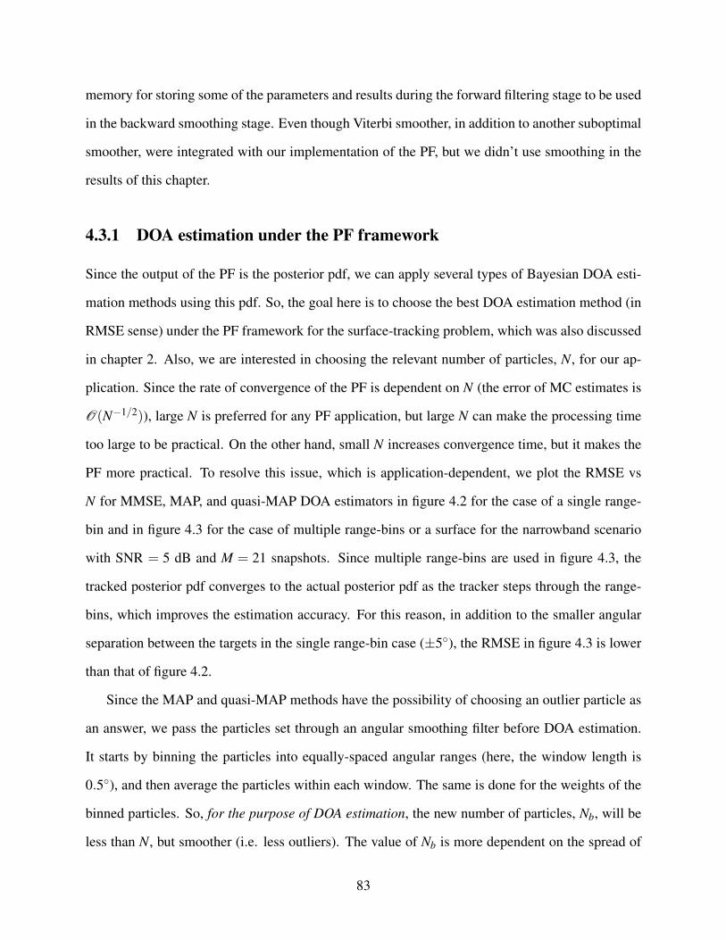
memory for storing some of the parameters and results during the forward filtering stage to be used

in the backward smoothing stage. Even though Viterbi smoother, in addition to another suboptimal

smoother, were integrated with our implementation of the PF, but we didn’t use smoothing in the

results of this chapter.

4.3.1 DOA estimation under the PF framework

Since the output of the PF is the posterior pdf, we can apply several types of Bayesian DOA esti-

mation methods using this pdf. So, the goal here is to choose the best DOA estimation method (in

RMSE sense) under the PF framework for the surface-tracking problem, which was also discussed

in chapter 2. Also, we are interested in choosing the relevant number of particles, N, for our ap-

plication. Since the rate of convergence of the PF is dependent on N (the error of MC estimates is

O(N−1/2)), large N is preferred for any PF application, but large N can make the processing time

too large to be practical. On the other hand, small N increases convergence time, but it makes the

PF more practical. To resolve this issue, which is application-dependent, we plot the RMSE vs

N for MMSE, MAP, and quasi-MAP DOA estimators in figure 4.2 for the case of a single range-

bin and in figure 4.3 for the case of multiple range-bins or a surface for the narrowband scenario

with SNR = 5 dB and M = 21 snapshots. Since multiple range-bins are used in figure 4.3, the

tracked posterior pdf converges to the actual posterior pdf as the tracker steps through the range-

bins, which improves the estimation accuracy. For this reason, in addition to the smaller angular

separation between the targets in the single range-bin case (±5◦), the RMSE in figure 4.3 is lower

than that of figure 4.2.

Since the MAP and quasi-MAP methods have the possibility of choosing an outlier particle as

an answer, we pass the particles set through an angular smoothing filter before DOA estimation.

It starts by binning the particles into equally-spaced angular ranges (here, the window length is

0.5◦), and then average the particles within each window. The same is done for the weights of the

binned particles. So, for the purpose of DOA estimation, the new number of particles, Nb, will be

less than N, but smoother (i.e. less outliers). The value of Nb is more dependent on the spread of

83

the particles than on the actual number of particles, N. It is worth noting that applying the MMSE

estimator within each angular window is not possible here because the result could be outside the

window limits (MMSE is a weighted sum over all the N particles in the sample space). Choosing

the length of the smoothing window is a compromise between smoothness and number of particles

that should efficiently represent the posterior pdf in the DOA estimation step.

Figures 4.2 and 4.3 confirm our conclusion in chapter 2 that the MMSE DOA estimator per-

forms much better than MAP and quasi-MAP estimators under the PF framework in terms of

RMSE. We can also see that the MMSE is more stable and steady than the other two methods.

In addition, both the single and multiple range-bin simulations show that, for MMSE estimator,

N > 100 is sufficient for our application. But, to keep the PF more stable and to avoid resampling

at each state, we choose N = 1000 and Nthr = 200 for all the simulations in this chapter. We think

that this choice is a good compromise between accuracy, convergence speed, and efficiency.

101 102 103 104

Number of particles (N)

0

1

2

3

RM

SE

(de

g)

MAPquasi-MAPMMSE

Figure 4.2: RMSE vs number of particles for 3 DOA estimation methods under the PF framework.0.5◦ window length is used for the angular smoothing filter applied on the particles before MAPand quasi-MAP DOA estimation. These curves were generated for the narrowband case with SNR= 5 dB, M = 21 snapshots, and actual DOAs are [−5◦ +5◦] (i.e. single range-bin).

84

101 102 103 104

Number of particles (N)

0

0.5

1

1.5

2

RM

SE

(de

g)

MAPquasi-MAPMMSE

Figure 4.3: Same as figure 4.2, but here we simulate a flat surface with several range-bins. Therange of the actual DOAs extends over the whole FOV, which is ±30◦.

4.3.2 PF vs MLE and MUSIC: a Qualified Validation

The PF framework is set to work as a tracker, where the posterior pdf is updated sequentially and

adaptively over time. But, before running the whole PF, we want to test the PF for the single-

state case and compare its performance against MLE and MUSIC because the performance of

these methods is well studied in the literature, so they can serve as a reference for validation or

comparison against the MMSE PF. Figures 4.4 and 4.5 show, respectively, the RMSE vs SNR and

RMSE vs number of snapshots for MLE, MUSIC, and PF for the narrowband scenario. Figures 4.6

and 4.7 show the same curves for the wideband scenario. The 1D simulator curves of the MLE and

MUSIC are also included for reference against the MLE and MUSIC curves of the 2D simulator.

It is also worth noting that due to outliers, some of the SNR curves seem to be increasing between

SNR = 5 dB and SNR = 10 dB. Removing these outliers (e.g. using 3σ rule) makes the curves

smoother, but we did not investigate this further.

1D and 2D simulator curves don’t exactly match because in the 2D simulator case we simulate

Nt = 300 range-bins, but in the 1D simulator case there is no sense of range bins. But we can

consider the number of snapshots as the number of range-bins in the 1D simulator case. Thus, in

the 2D simulator case the fast time Hanning window has a length of Nt = 300 here, but in the 1D

85

simulator case it is Nt = M = 21.

From these results, we can observe that the PF is better than MLE at the low SNR and/or

low snapshots regimes because the PF solution is a brute force solution in this case, where the

likelihood of each of the N particles is calculated and either the best particle is chosen (in case of

MAP) or all the particles participate, each based on its own weight, in the final answer (in case of

MMSE). However, in the case of MLE, an optimizer walks towards the answer in steps starting

from some initial point. Also, the shape of the cost function, which is dependent on the quality of

the data, is a key factor in the optimizer’s decision. To further support our conclusion, we plot the

PF vs MLE and MUSIC in figure 4.8 for the 2D narrowband scenario when M = 3 (low snapshots

regime). We can see that the PF is performing much better than MLE in this scenario.

The results of the wideband scenario (B f = B/ fc = 0.1538≈ 15%) have almost no difference

from the narrowband scenario (B f = B/ fc = 0.1538×10−3 ≈ 0%). To see a difference, we need

to increase the fractional bandwidth to B f > 15% (from simulations, we noticed a difference at

B f ≥ 30%). This seems to be the case for many subspace-based DOA estimation and beamforming

methods [66], but still more investigation is required to generalize this fact. Interestingly, for model

order estimation problem, B f = 15% is large enough to make almost all the standard model order

estimation techniques fail when the number of targets is large relative to the number of array

sensors, as shown in [1], because this is a classification or detection problem rather than estimation

problem.

86

-5 0 5 10 15 20 25

SNR (dB)

0

1

2

3

4

5

6R

MS

E (

deg)

2D: MUSIC2D: MLE1D: MUSIC1D: MLEPF: MMSE

Figure 4.4: Two equal SNR targets, located at ±5◦, are simulated for a narrowband scenario withM = 21 snapshots.

101 102 103

Number of snapshots (M)

0

0.5

1

1.5

2

2.5

3

RM

SE

(de

g)


Figure 4.5: Same scenario as in figure 4.4. SNR = 5 dB.

87

-5 0 5 10 15 20 25

SNR (dB)

0

1

2

3

4

5

6R

MS

E (

deg)


Figure 4.6: Same scenario as in figure 4.4, but for wideband case.

101 102 103


0

0.5

1

1.5

2

2.5

3

RM

SE

(de

g)


Figure 4.7: Same scenario as in figure 4.6. SNR = 5 dB.

88

-5 0 5 10 15 20 25

SNR (dB)

0

2

4

6

8

10

RM

SE

(de

g.)

MUSICMLEPF: MMSE

Figure 4.8: Same scenario as in figure 4.4. Low snapshots support, M = 3.

4.3.3 Surface Tracking: Step by Step Explanation

Here we explain the sequential part of the PF and how it starts and converges to the true posterior

pdf as it passes from one range-bin to the next. The simulation scenarios are the same as those

presented in Section 4.3.2, except that here we simulate a flat surface with multiple range-bins,

each has either 2 targets (one on the left and one on the right) or no targets.

Figure 4.9 shows the estimated posterior pdf in a 3D scatter plot, where the particles are plotted

on the x-and-y axes (each particle is a vector of length 2) and the weights are color coded. Two

scenarios are simulated : a) low/medium number of snapshots (the left sub-figures), and b) high

number of snapshots (the right sub-figures). Another view of the same plots is also presented

in figure 4.10 in the form of empirical density plots. Five states were skipped in between the

presented states (total of 21 states were simulated). These plots represent the outputs of the labeled

states, which are then propagated into the next state after the DOAs are estimated. In other words,

these plots show how the importance sampling work, which is the heart of the PF algorithm. The

actual DOAs are also shown in the scatter plots as a red ‘+’ symbol. We can see that even though

the particles are initially uniformly distributed (two dimensional), the importance region of the

posterior density is quickly approached after few iterations, which improves the estimation of the

89

DOA by a large amount relative to the first few states. It is worth noting that ‘state 1’ here is not

the initial state, which is state 0 (initially, all the weights are 1/N).

The purpose of presenting low and high sample support scenarios is to show an interesting

fact about the PF, where in the case of M = 1001 the high-quality particles (i.e. particles with

high weight) quickly accumulate around the true solution starting from the first state (i.e. smaller

uncertainty region). After passing through the few following states, the high-weight particles start

to collapse into a very small region, and thus very small importance sampling area. This behavior

can be confusing and might lead to wrong conclusions because we might think that there is a

degeneracy problem (particles collapse into a very small importance region, which results in a bad

representation of the actual posterior pdf). However, in our application, due to the fast decrease

of the change in DOA over range (see figure 2.7 in Chapter 2), the region over which the actual

posterior pdf fits narrows down as the tracker steps through the range-bins. In addition to this,

increasing the number of snapshots improves the estimation of the data covariance matrix, which

makes the particles less noisy (smaller spread around the true solution). Thus the PF performance

saturates with increasing number of snapshots, and to get out of this situation we need to either

re-distribute the particles, which may only work for the first few states, or expand the region over

which the particles are distributed, which means losing some prior information. Also, note that this

issue was not very clear from the results of the previous section because we estimated the DOA for

a single range-bin with±20◦ initial bounds (i.e. the posterior pdf is fit into a wide region) It is also

worth noting that the PF does not saturate with increasing SNR because the noise variance will go

down, which improves the selection of the particles that most contribute to the final results. This

fact will be elaborated on in section 4.5.

Moreover, because the particles are sequentially accumulating around a single mode that is

the true solution, MMSE makes more sense than MAP and quasi-MAP for our surface-tracking

application. Another thing to note here is that if the number of states is large, the PF will soon

run into the sample impoverishment problem, which means two things: 1) a more sophisticated PF

needs to be used, such as MCMC move-step, and 2) because, generally, there are more range-lines

90

than range-bins in SAR imaging problems, tracking along the azimuth direction is not practical

on a large scale, especially when the PF will need to resample every few states to stay stable

(resampling means loss of the previously accumulated information represented by the sequentially-

updated weights).

91

-14 -12 -10 -8 -6 -4 -2θ

1 (deg)

2

4

6

8

10

12

14θ

2 (de

g)

0.0000

0.5000

1

Nor

mal

ized

par

ticle

wei

ght

a) State 1: M = 21

-14 -12 -10 -8 -6 -4 -2θ

1 (deg)

2

4

6

8

10

12

14

θ2 (

deg)

0.0000

0.5000

1

Nor

mal

ized

par

ticle

wei

ght

b) State 1: M = 1001

-30 -25 -20 -15 -10θ

1 (deg)

10

15

20

25

30

35

40

θ2 (

deg)

0.0000

0.5000

1

Nor

mal

ized

par

ticle

wei

ght

c) State 5: M = 21

-30 -25 -20 -15 -10θ

1 (deg)

10

15

20

25

30

35

40

θ2 (

deg)

0

0.5

1

Nor

mal

ized

par

ticle

wei

ght

d) State 5: M = 1001

-30 -28 -26 -24 -22 -20 -18θ

1 (deg)

20

25

30

35

40

θ2 (

deg)

0.0000

0.5000

1

Nor

mal

ized

par

ticle

wei

ght

e) State 10: M = 21

-30 -28 -26 -24 -22 -20 -18θ

1 (deg)

20

25

30

35

40

θ2 (

deg)

0

0.5

1

Nor

mal

ized

par

ticle

wei

ght

f) State 10: M = 1001

92

-35 -30 -25θ

1 (deg)

22

24

26

28

30

32

34

36θ

2 (de

g)

0.0000

0.5000

1

Nor

mal

ized

par

ticle

wei

ght

g) State 15: M = 21

-35 -30 -25θ

1 (deg)

22

24

26

28

30

32

34

36

θ2 (

deg)

0.0000

0.5000

1

Nor

mal

ized

par

ticle

wei

ght

h) State 15: M = 1001

-80 -70 -60 -50 -40 -30θ

1 (deg)

30

40

50

60

70

80

θ2 (

deg)

0

0.5

1

Nor

mal

ized

par

ticle

wei

ght

i) State 20: M = 21

-80 -70 -60 -50 -40 -30θ

1 (deg)

30

40

50

60

70

80

θ2 (

deg)

0

0.5

1

Nor

mal

ized

par

ticle

wei

ght

j) State 20: M = 1001

Figure 4.9: Tracking the importance sampling region using PF: 3D scatter plots, which show thetwo dimensional posterior pdf. Two scenarios are presented here: M = 21 snapshots (left sub-figures) and M = 1001 snapshots (right sub-figures). These plots are the outputs of the labeledstates, which are passed into the DOA estimator and then to the input of the following state. Thered ‘+’ symbol represents the location of the actual DOA. Note that the weights of the particles arenormalized relative to the maximum weight for better visualization.

93

a) State 1: M = 21 b) State 1: M = 1001

c) State 5: M = 21 d) State 5: M = 1001

94

e) State 10: M = 21 f) State 10: M = 1001

g) State 15: M = 21 h) State 15: M = 1001

95

i) State 20: M = 21 j) State 20: M = 1001

Figure 4.10: Tracking the importance sampling region using PF: 2D empirical density plots. Samesimulation scenarios as in figure 4.9, but here we show the bi-modal empirical posterior pdf in ahistogram-like plots.

96

4.4 Sequential MAP Filter As a Surface Tracker

The details of the S-MAP surface-tracker were presented in Chapter 2. So, here we look closely at

the operation of the S-MAP as it steps through the range-bins of each cross-track slice, following

a similar approach to that introduced in section 4.3.3.

4.4.1 Surface Tracking: Step By Step Explanation

Unlike PF, S-MAP has an analytical form, which was given by equation 2.64. So, here we plot

the actual surface, the estimated surface, the mean surface, and the bounds in figure 4.11 for three

SNR scenarios: −100 dB, 100 dB, and 5 dB, with 21 snapshots for the narrowband case. These

specific examples are chosen to show the main tracking habits, and they all share the exact same

input data set, but different SNRs. We can see that when the SNR is very low (-100 dB here), the

estimated surface is the mean surface because the data quality is too low and, thus, the prior cost

function dominates the MAP cost function, which is an expected result. Thus, the worst result we

could get in the case of S-MAP is the mean surface. This is not necessarily true for PF. However,

when the SNR is very high (100 dB here), the estimated surface matches the actual surface almost

exactly, where the likelihood cost function dominates the MAP cost function in this case. Finally,

when the SNR is in between these two extremes (5 dB here), the estimated surface results from

a combination of the prior information and the measurements data. These conclusions match our

expectations based on the mathematical equation of the S-MAP cost function in chapter 2. Also,

note that there is no mean DOA in the first range-bin, but there are initial DOA bounds, because

the DOAs are assumed to be initially uniformly distributed (see the dynamics model in chapter

2). In addition, S-MAP tracker (as well as PF) put a heavy weight on the results of the first state,

where if the estimated DOA of the first state is far from the actual DOA, the estimated surface may

not match the actual surface, as seen by figure 4.11-a. The probability of this event is inversely

proportional to the SNR. However, PF is more robust to this problem than S-MAP because its

mathematical model is built to handle randomness.

97

-30 -20 -10 0 10 20 30θ (deg)

100

110

120

130

140

Ran

ge-b

in in

dex

Actual DOAEst. DOAMean DOALower boundUpper bound

a) SNR =−100 dB

-30 -20 -10 0 10 20 30θ (deg)

100

110

120

130

140

Ran

ge-b

in in

dex


b) SNR = 5 dB

-30 -20 -10 0 10 20 30θ (deg)

100

110

120

130

140

Ran

ge-b

in in

dex


c) SNR = 100 dB

Figure 4.11: S-MAP surface for 3 different SNR scenarios: -100 dB, 5 dB, and 100 dB. M = 21snapshots. 98

4.5 Performance Comparison of PF vs S-MAP

In this section we compare the performance of S-MAP vs PF as surface-trackers for narrowband

and wideband scenarios. The simulation setup is the same as that of section 4.3.2, but here we

simulate a surface that has 21 active range-bins, each has 2 targets (one on each side of the surface).

Figures 4.12 through 4.15 show the performance of these two sequential trackers, measured by

the color-coded RMSE (deg), over a wide range of SNR and snapshots support for the narrowband

scenario. The SNR plots are generated with M = 21 snapshots, while the snapshots plots are

generated with SNR = 5 dB. The following main points can be drawn from these plots:

• The PF converges, over range, SNR, and number of snapshots, faster than S-MAP. This is

due to two reasons:

a. The PF has a brute force-like nature, and thus it is not limited by the shape of the cost

function and/or the performance of the optimization method used to solve the problem.

b. The PF is limited by the number and the spread of the particles over the importance

sampling region, as well as the bounds of the DOAs (remember (the error of Monte

Carlo-based estimates of the pdf is O(N−1/2), which is 0.0316 in our case, but increases

to 0.0707 when PF enters into a resampling mode) .

• Unlike S-MAP, the PF performance saturates with high number of snapshots.

• For both trackers, the main source of the high RMSE is the first 1 or 2 range-bins, which

shows how much these trackers rely on the initial states and on the initial DOA bounds. The

tighter the initial DOA bounds, the better the performance of the S-MAP and PF is, given

that there is good-quality data within the preset initial bounds.

• On average, the PF has a better performance, in terms of RMSE, than S-MAP due to the

same reasons mentioned in the first point above.

Also, to provide an average look at the performance of the compared trackers, we plot the

average RMSE vs SNR in figures 4.16 and 4.18 and the average RMSE vs number of snapshots

99

in figures 4.17 and 4.19 for the narrowband and wideband cases, respectively. As we have seen

in section 4.3.2, wideband scenario has almost the same results as the narrowband scenario. In

addition, the PF is much better than the S-MAP at low SNR and/or low snapshots support regions,

and the reason for this was discussed when we compared the PF against MLE.

The saturation of the PF with increasing M is also clear in figures 4.17 and 4.19, which was

discussed in section 4.3.2. The PF is, again, limited by N, angular spread of the particles, and

the bounds of the DOA, and not by M. Higher SNR decreases the noise variance relative to the

signal power, which improves the selection of the important region within the posterior pdf, and

so result in better importance sampling. However, increasing M improves the estimation of the

noise variance, but does not necessarily make it smaller as in the case of increasing SNR. So, since

the particles are concentrate around the true solution over time, small improvements in the noise

variance estimation become less important for the final result. In the case of S-MAP (and MLE and

MUSIC), we set the tolerance of the optimizer to 10−6, so any improvement in the data covariance

matrix (or the estimation of the noise variance) matters. But in the case of PF, there is no way to

set a tolerance on the accuracy of the estimated DOA in this way. In summary, the PF is better

suited for the case of limited data quality, where the SNR is very low and/or with low snapshots

support.

100

-5 0 5 10 15 20 25

SNR (dB)

100

110

120

130

140

Ran

ge-b

in

0.02

3.25

6.45

RM

SE

(de

g)

Figure 4.12: S-MAP: surface tracking assessment result. Narrowband scenario with M = 21 snap-shots.

-5 0 5 10 15 20 25

SNR (dB)

100

110

120

130

140

Ran

ge-b

in

0.05

2.2

4.32

RM

SE

(de

g)

Figure 4.13: PF (MMSE): surface tracking assessment result. Narrowband scenario with M = 21snapshots.

101

0 200 400 600 800 1000


100

110

120

130

140

Ran

ge-b

in

0.021

1.55

3.08

RM

SE

(de

g)

Figure 4.14: S-MAP: surface tracking assessment result. Narrowband scenario with SNR = 5 dB.

0 200 400 600 800 1000


100

110

120

130

140

Ran

ge-b

in

0.08

1.45

2.82

RM

SE

(de

g)

Figure 4.15: PF (MMSE): surface tracking assessment result. Narrowband scenario with SNR= 5 dB.

102

-5 0 5 10 15 20 25

SNR (dB)

0

1

2

3

RM

SE

(de

g)

S-MAPPF: MMSE

Figure 4.16: Surface tracking assessment result: narrowband scenario with M = 21 snapshots.

101 102 103


0.2

0.4

0.6

0.8

1

RM

SE

(de

g)

S-MAPPF: MMSE

Figure 4.17: Surface tracking assessment result: narrowband scenario with SNR = 5 dB.

103

-5 0 5 10 15 20 25

SNR (dB)

0

1

2

3

RM

SE

(de

g)

S-MAPPF: MMSE

Figure 4.18: Surface tracking assessment result: wideband scenario with M = 21 snapshots.

101 102 103


0.2

0.4

0.6

0.8

1

RM

SE

(de

g)

S-MAPPF: MMSE

Figure 4.19: Surface tracking assessment result: wideband scenario with SNR = 5 dB.

104

4.6 Discussion

The goal of this section is to answer three questions about the two trackers discussed in this chapter:

• Can PF and S-MAP track non-flat surfaces?

• How do PF and S-MAP perform if the model order is not exactly known?

• Can PF and S-MAP track distributed targets surface?

We now discuss these three questions separately with a reasonable amount of details, but leave a

more comprehensive study for future work.

1. Can PF and S-MAP track non-flat surfaces? Since all the tracking results in this sec-

tion are generated for a perfectly-flat surface, here we discuss the case of tracking non-flat

surfaces. Generally, the ability to track moving targets using any tracking technique relies

heavily on the dynamics model, which connects, mathematically, the different states of the

state space of the problem based on our understanding of the physical world. For our surface

tracking problem, even though we use the flat-earth assumption as our transition model to

estimate the mean surface, this estimated mean surface is dynamic and does not represent a

perfect surface (i.e. not static). This is because the mean surface is obtained from the mean

DOAs based on a posterior pdf that is sequentially updated over time. In other words, how

well it matches the actual surface depends on the quality of the measurements (e.g. SNR and

M).

The bounds of the search region is another important factor. Tracking surfaces that are

narrower or wider than a flat surface is possible if we can set the DOA bounds appropriately

to be around the mean DOA at each state. This is a design problem that is surface geometry

dependent. So, the mathematical model of the bounds introduced in equations 2.30 and 2.31

can still be applied to any surface geometry, but the limits of the DOA bounds need to be

adapted to allow for different types of surfaces (e.g. change a1 in equation 2.30 and f (∆θm)

105

in equation 2.31). We will present several bounding models in Chapter 5 when we apply

S-MAP to real radar data.

Statistics and mean surfaces drawn from geostatistical analysis of real tracked surfaces can

also be used to modify the transition model and the bounds. For example, figure 4.20 shows

the mean and variance of the DOAs from the 2014 Canadian Arctic Archipelago (CAA)

training data set. The FOV (±90◦) is quantized into 64 bins (here we clipped the first and

last DOA bins), where bin 1 corresponds to the far right DOA, bin 64 corresponds to the far

left DOA, and nadir corresponds bin 33. The horizontal axis is the index of the DOA bin and

the vertical axis is the DOA step size per range-bin measured in DOA bins. These means and

variances can be used to calculate the prior pdf of the DOA, the search bounds, and assign

costs to separate left from right DOAs in case the model order is Q = 1. Other information

about the use of geostatistical analysis to help in tracking surfaces can be found in [67].

0 10 20 30 40 50 60

DoA bins

-0.2

0

0.2

0.4

0.6

Ste

p si

ze (

in D

oA b

ins)

MeanVariance

Figure 4.20: Mean and variance of the quantized DOA range (64 bins) generated from the 2014Canadian Arctic Archipelago (CAA) training data set.

2. How do PF and S-MAP perform if MOE is not exactly known?

The main assumption in this work is that there is a maximum of Q = 2 DOAs per range-bin,

one on each side of the surface. With MLE and MUSIC, we assume that there is either Q = 0

106

or Q = 2 targets per range-bin. But, S-MAP and PF have a transition model that can handle

the transition between range-bins that have different numbers of targets (for example, see

Algorithm 2 in Section 2.6.5.1). The main idea of these multi-target transition algorithms

is that we use a transition model to keep track of the DOAs such that there is always Q = 2

DOAs at each state. These DOAs need not represent an actual target. This is useful in the

case of Q = 1, where we should know whether this target is on the left or on the right side

of the surface. If the model order is completely unknown, then MUSIC beamformer is our

next option. However, for point-cloud trackers, the model order must be provided, even if it

is not very accurate.

Since our real data are relatively wideband (about 15% fractional bandwidth), non of the

standard model order estimation (MOE) methods can give a reasonable performance in the

case of large number of targets relative to the number of array sensors. This problem was

discussed in Chapter 3. The results in [1, 42] confirmed that the numerical tunning (NT)

method also fails to handle the MOE problem in wideband systems. In addition, the authors

in [1, 42] conducted all of their experiments for the case of Q= 6 targets. However, repeating

the same experiments on the case of Q = 2 targets showed very satisfactory performance of

the NT method in the wideband case. Moreover, normalizing the log-likelihood function

with respect to the case of SNR = −∞ (effectively, this is a no-target scenario) does help

make most of the standard MOE methods perform as well as the NT method in the wideband

case.

Figure 4.21 shows the eigenvalues of a data covariance matrix for the 15% fractional band-

width scenario for q = 0, q = 1, and q = 2 targets. The simulation parameters are: M = 21,

100 Monte Carlo runs, and the training and testing data were generated for three SNRs: 10

dB, 20 dB, and 30 dB. We can see that the eigenvalue spread starts to show up at q = 2, espe-

cially at high SNR, which is why most of the standard MOE methods fail in these scenarios.

Also, figure 4.22 shows the percentage correct (i.e. number of times the MOE is estimated

correctly relative to the total number of simulated examples) plots of 7 MOE methods, which

107

are: Akaike Information Criterion (AIC), Hannan and Quinn Criterion (HQ), Minimum De-

scription Length (MDL), Corrected AIC (AICc), Vector Corrected Kullback Information

Criterion (KICvc), Weighted-Average Information Criterion (WIC), and numerical tuning

(NT). In the case of optimal MOE, the number of targets and their directions are estimated

simultaneously. Color-coded plots are also shown in figure 4.23 for the estimated number

of targets at each simulated range-bin for each of the 7 MOE methods, in addition to the

actual number of targets, Q, in the worst simulated case scenario , which is when SNR = 30

dB and the data is wideband. All of these plots show that most of the tested MOE methods

can be used successfully for MOE in the wideband scenario if the log-likelihood values are

normalized and the number of targets is small relative to the number of sensors. Also, AICc

and KIVvc methods failed here due to our specific choice of M = 21 and p= 7, which makes

the denominator of their mathematical formula go to 0 in some cases.

In the next chapter, we will apply the MDL method with normalized log-likelihood values

(N-MDL) under the optimal MOE formulation to estimate the number of targets and their

direction, which will be integrated with the sequential surface-tracking methods introduced

in this chapter, at each range-bin of the real radar-collected wideband data.

108

0 2 4 6

-4

-2

0

2

Eig

enva

lue

(dB

)

q = 0

10dB20dB30dB

0 2 4 6

Eigenvalue index

0

10

20

30

Eig

enva

lue

(dB

)

q = 2

0 2 4 6

Eigenvalue index

0

10

20

30

q = 1

Figure 4.21: Eigenvalues of a data covariance matrix generated by simulating M = 21 snapshotsand p = 7 sensors for the 15% fractional bandwidth scenario.

109

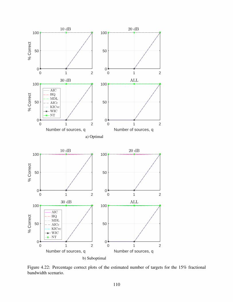
0 1 20

50

10020 dB

0 1 2

Number of sources, q

0

50

100

% C

orre

ct

30 dB

AIC

HQ

MDL

AICc

KICvc

WIC

NT

0 1 2


0

50

100ALL

0 1 20

50

100%

Cor

rect

10 dB

a) Optimal

0 1 20

50

10020 dB

0 1 2


0

50

100ALL

0 1 20

50

100

% C

orre

ct

10 dB

0 1 2


0

50

100

% C

orre

ct

30 dB

AIC

HQ

MDL

AICc

KICvc

WIC

NT

b) Suboptimal

Figure 4.22: Percentage correct plots of the estimated number of targets for the 15% fractionalbandwidth scenario.

110

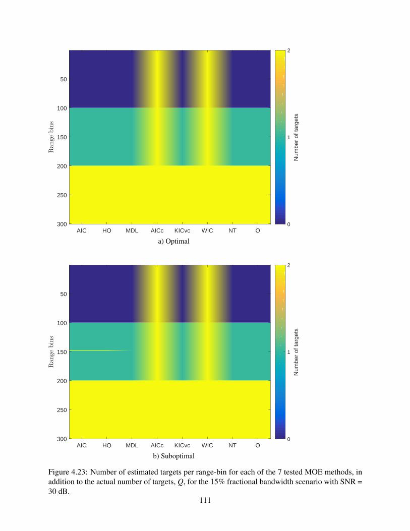
AIC HQ MDL AICc KICvc WIC NT Q

50

100

150

200

250

300

Rangebins

0

1

2

Num

ber

of ta

rget

s

a) Optimal

AIC HQ MDL AICc KICvc WIC NT Q

50

100

150

200

250

300

Rangebins

0

1

2

Num

ber

of ta

rget

s

b) Suboptimal

Figure 4.23: Number of estimated targets per range-bin for each of the 7 tested MOE methods, inaddition to the actual number of targets, Q, for the 15% fractional bandwidth scenario with SNR =30 dB.

111

3. Can PF and S-MAP track distributed targets surface?

All of the simulations above assume point targets. But, for a distributed target scenario,

where ND point targets are collocated and separated by a small angular distance, ∆θD, we

expect ∆θD to be a new limiting factor of the tracking performance. Because our PF and S-

MAP trackers are built around the assumption of having a maximum of Q = 1 target on each

side of the surface, the larger ∆θD gets, the worse the estimation. So, this is a limitation of

the mathematical model, and not of the estimation techniques. A more general mathematical

model would either deal with more than just 2 sides of the surface (left and right) or relax the

assumption of having a maximum of 1 target per surface side. But, these types of general-

izations require first solving the wideband MOE problem for the distributed target scenario,

which is not available at this point (open research problem). Also, dealing with distributed

targets might require a new measurements model than that used in this dissertation, which

is the standard model used in the literature. Thus, we do not tackle the distributed targets

problem in this work and leave it as a future project.

112

Chapter 5

3D Image Formation Results of Ice-Sheets

5.1 Introduction

In this chapter, we describe the processing steps that led to the generation of the digital elevation

models (DEMs) of the ice-bottom from the different data sets that were collected using CReSIS

radars. We applied MUSIC to generate a 3D image and tracked the ice bottom in this image with

the sequential tree reweighted (TRW-S) belief propagation algorithm to generate DEMs of the

CAA. We also used the S-MAP algorithm to generate a few sample results for sea ice near Thule,

Greenland and for ice-free land near Russell Glacier.

The quality of the MUSIC/TRW-S tracking algorithm is statistically evaluated by comparing

the tracked ice-bottom layers from each range-line before and after applying manual corrections.

In addition, the generated DEMs are self-assessed using crossover analysis where two flight paths

intersect. The ice-surface DEMs, which are already available from the satellite imagery, were also

used to provide a simple calibration of the steering vectors and to aid the tracker.

The collected data are partitioned into segments, where each data segment corresponds to the

data collected over the time from turning the radar on until turning it off again. Then each segment

is divided into frames, where each frame is, roughly, 50 km along the flight path. Each frame has

an identifier or ID associated with it, which has the following format: yyyymmdd_ss_fff, which

113

refers to the year (yyyy), month (mm), day (dd), segment number (ss), and frame number (fff). For

example, the frame ID 20140401_03_037 provides the following information about the DEM: the

DEM is created using the data collected on April 1st, 2014 from the 37th frame in segment 3. This

naming style will be used from now on.

The DEMs were generated per frame in the following way. Assuming the dielectric constant

of the ice to be 3.15 and using the derived surface range to determine the point of refraction, each

tracked ice-bottom point is geolocated. Then, we perform Delaunay triangulation to tessellate the

ice-bottom points. The final gridded product is a linear interpolation of all the points in the swath

after removing the gridded points outside the boundary of the valid SAR pixels.

5.2 Ice-Bottom Tracking Using MUSIC and TRWS

The Canadian Arctic Archipelago (CAA) contains one-third of the global volume of land ice out-

side the ice sheets. But the basal topography of the outlet glaciers draining the CAA ice caps

and its contribution to sea-level change is largely unknown. To measure the basal topography, the

MCoRDS radar was used to collect data over the CAA islands (Ellesmere, Axel Heiberg, and De-

von) during the NASA Operation IceBridge 2014 arctic campaign. Figure 5.1 shows the location

of the CAA islands and the flight-paths of this mission.

To create the DEMs, we use MUSIC array processing to estimate the pseudo-spectrum (a value

loosely related to the scattering intensity for the corresponding DOA) for a uniform grid of 64

cross-track wavenumbers that correspond to DOAs from −90◦ to +90◦ [11]. Figure 5.2 illustrates

the beamformer output at one along-track location for 5 range-bins, Q = 2 targets per range-bin,

and the FOV is quantized into 10 angular-bins. In this example, the beamformer output is a 5×10

matrix, where each row contains the pseudo-spectrum information from a single range-bin. The

pseudo-spectrum is the inverse of the correlation between the array steering vector and the noise

subspace at each angular-bin and is roughly related to the scattered energy. Then, the ice-bottom

tracker tracks or estimates the row corresponding to the surface in each column. The estimate

114

balances a cost function that considers a number of inputs including the pseudo-spectrum and the

smoothness of the surface.

The characteristics of this work can be summarized as follow:

• We used the narrowband signal model.

• Only the center subarray of the P-3 radar array was used.

• We used a fixed model order for each range bin (i.e. number of targets) of 2.

• We applied a simple array calibration step to calibrate the center subarray using the surface

DEMs.

• The ice-bottom tracker is used to track the surface from one elevation angle bin to the next

(64 bins total) rather than tracking targets from one range bin to the next. In this way,

solutions are forced to be single valued with respect to elevation angle.

• Three array beams were collected (left, center, and right). They were array processed sepa-

rately, but then combined before tracking.

• The tracking is based on computer vision algorithms and not coupled with DoA estimation.

After array processing is done, we have a 3D image for each of the 3 beams, as shown in figure

5.3. Then, the three images are merged using a Gaussian-weighted sum of the three images to

synthesize a single wide swath beam. The Gaussian weights are proportioned according to the

transmit beam direction of the particular image. We call the image formed by taking the 3D pixels

at a constant along-track position, a "slice". A slice contains information about the surface and

bottom of the ice at a single range-line (i.e. along-track position), making it possible to visualize

the ice surface and bottom simultaneously. An example slice is shown in figure 5.3. Note that

the slices are in cylindrical coordinates with the vertical axis corresponding to the range and the

horizontal axis corresponding to the elevation angle. Figure 5.4 illustrates the actual (Cartesian)

geometry of a sequence of slices.

115

To improve the accuracy of the steering vectors, the ice-surface DEM, which is obtained from

the ArcticDEM [68], was used to calibrate the steering vectors by adjusting the angular dependence

using a low-order polynomial least squares fit between the radar-derived ice-surface and the ice-

surface DEM [33, 69]. A region of data was used where the radar surface returns were very clear

and the ice-surface scattering could be tracked accurately with a simple routine and then compared

to the ArcticDEM surface elevation. The polynomial fit adjustment from the surface is then applied

to the ice bottom for which there is no similar a priori information.

116

-1000 -800 -600 -400 -200 0 200 400 600 800

-3000

-2500

-2000

-1500

-1000

-500

X (km)

Y (

km

)

Ellesmere, Axel Heiberg, and Devon Islands

Figure 5.1: Canadian Arctic Archipelago islands along with the flight paths (the blue curve) forthe radar data used in this work. Background raster image from NASA Natural Earth.

117

Figure 5.2: Illustration of the beamformer output for a single range line. In this example, wegrid the FOV into 10 angular-bins and, assuming Q = 2 targets per range-bin, we use the MUSICpseudospectrum from all these angular-bins to form an image, where each square represents oneimage pixel. The red squares are the pixels where the pseudo spectrum is highest. The trackedsurface (the black curve) is formed by connecting these pixels such that the surface is smooth.

Figure 5.3: The merged image composed of three separate left-beam, nadir-beam, and right-beamimages. The red curves represent the Gaussian weighting associated with each input image. Thelabeled output is shown on the right.

118

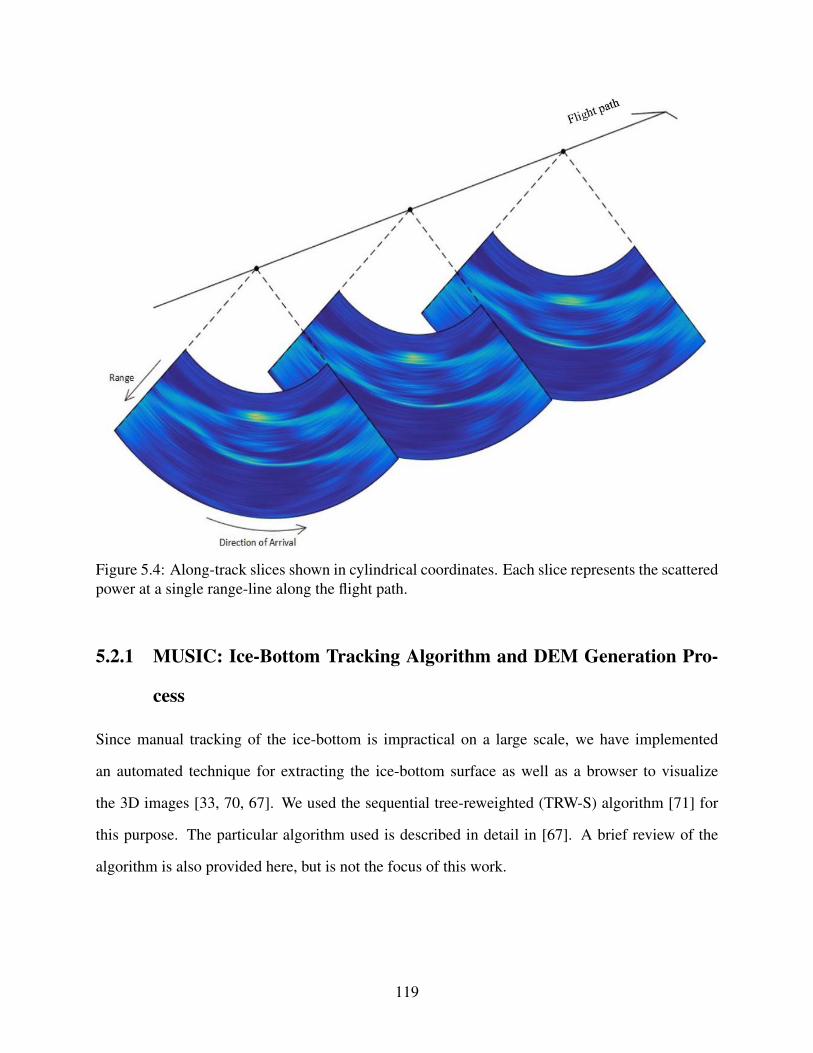
Figure 5.4: Along-track slices shown in cylindrical coordinates. Each slice represents the scatteredpower at a single range-line along the flight path.

5.2.1 MUSIC: Ice-Bottom Tracking Algorithm and DEM Generation Pro-

cess

Since manual tracking of the ice-bottom is impractical on a large scale, we have implemented

an automated technique for extracting the ice-bottom surface as well as a browser to visualize

the 3D images [33, 70, 67]. We used the sequential tree-reweighted (TRW-S) algorithm [71] for

this purpose. The particular algorithm used is described in detail in [67]. A brief review of the

algorithm is also provided here, but is not the focus of this work.

119

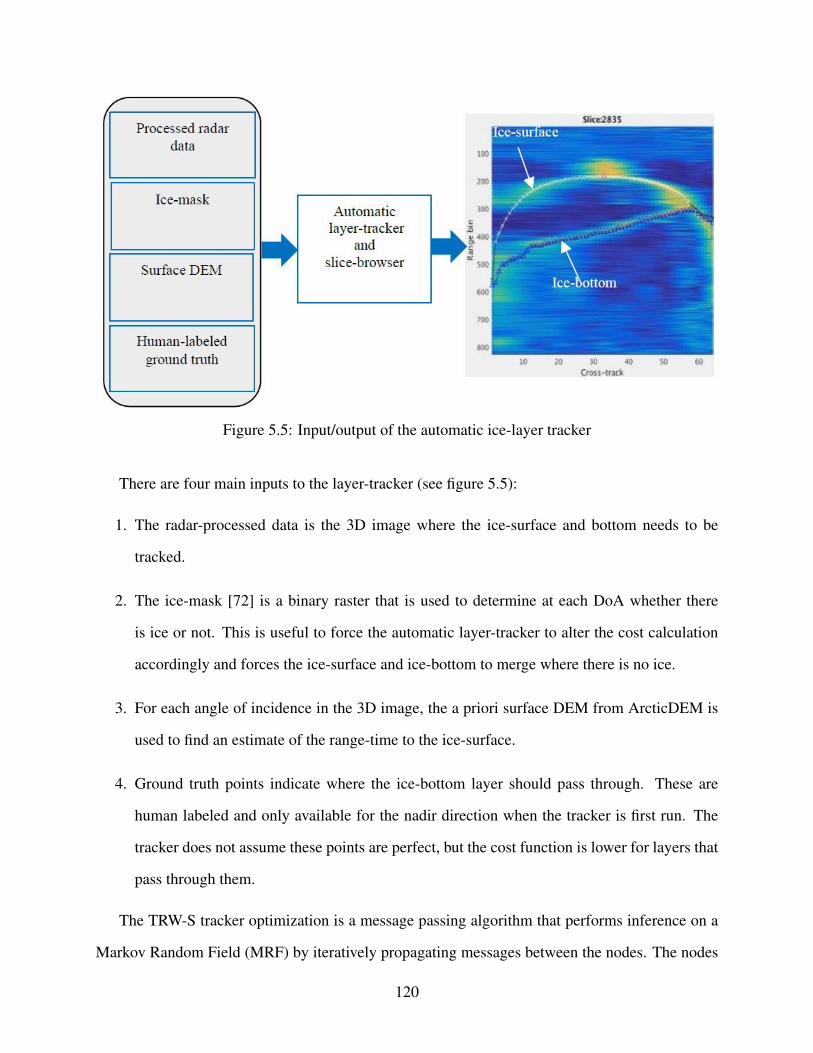
Figure 5.5: Input/output of the automatic ice-layer tracker

There are four main inputs to the layer-tracker (see figure 5.5):

1. The radar-processed data is the 3D image where the ice-surface and bottom needs to be

tracked.

2. The ice-mask [72] is a binary raster that is used to determine at each DoA whether there

is ice or not. This is useful to force the automatic layer-tracker to alter the cost calculation

accordingly and forces the ice-surface and ice-bottom to merge where there is no ice.

3. For each angle of incidence in the 3D image, the a priori surface DEM from ArcticDEM is

used to find an estimate of the range-time to the ice-surface.

4. Ground truth points indicate where the ice-bottom layer should pass through. These are

human labeled and only available for the nadir direction when the tracker is first run. The

tracker does not assume these points are perfect, but the cost function is lower for layers that

pass through them.

The TRW-S tracker optimization is a message passing algorithm that performs inference on a

Markov Random Field (MRF) by iteratively propagating messages between the nodes. The nodes

120

in the MRF are the columns of the 3D image. Columns are aligned with the range dimension.

Therefore, for every range line and elevation angle pair, there is a node and associated column of

range bins. The estimated surface is single valued for each node so that the surface is only allowed

to pass through a node once and the tracker’s job is to determine which range bin this occurs at.

For each node, connections are made to each of the four neighboring nodes. These connections

are left and right (elevation angle dimension) and forward and backward (along-track dimension)

as shown in figure 5.6. Each node stores a unary cost for each range bin and a set of four binary

messages for each range bin. The four binary messages are the last messages passed to that range

bin from the four neighboring nodes. A new cost message, JTRWS, from range bin di of node i to

range bin d j of a neighboring node j is given by:

JTRWS = JU + JB + JI. (5.1)

JU is the unary cost for range bin di of node i that is sending the message. It is composed of three

terms:

JU = JUi + JUg + JUb, (5.2)

where JUi is a pixel intensity related cost, JUg is a ground-truth related cost, and JUb ensures that

the bottom does not go above the surface. The unary cost for each pixel is only computed one time

and is not updated. JB is the binary cost and depends on how the surface transitions from one node

to the next and is used to control the smoothness of the surface. This allows the tracker to work

through low quality regions where several pixel choices might be equally likely based on the unary

cost only. The binary cost increases the likelihood that the range bin that produces the smoothest

surface overall will have the lowest cost by applying a quadratic distance cost. The distance is

the absolute value of the change in range bins, |di− d j|. JI is the summation of the most recent

incoming messages to range bin di of node i from the other three nodes that are connected to node i

(so not including from node j). The messages are updated on each iteration of the algorithm. They

are a mix of unary and binary costs. The incoming messages are all initialized to the prior.

121

In general, the cost message to bin d j of node j from node i is taken to be the minimum cost

message from node i where the minimum is taken over all of the range bins di of node i. Therefore,

many cost messages to bin d j on node j are computed, but only the minimum cost message will be

used. Due to symmetry properties of the quadratic distance used in the binary cost, only a subset

of the possible transitions require the cost messages to be computed. As the algorithm iterates, the

most recent cost messages, JTRWS, are stored and they represent the state of inference.

In our implementation, once a fixed number of iterations have been reached, the algorithm is

stopped and the final answer for any node i is taken to be the range bin, di, with the lowest cost.

This cost is defined as JU+JI where JU is the unary cost for bin di of node i and JI is the summation

of the most recent messages from the (four) neighboring nodes of node i for range bin di.

The tracker [70] was modified in several ways to improve its performance. In [70], although

messages are passed in all directions on each iteration, there is a preferential direction where the

most recent message is taken from the current iteration rather than the previous iteration. The

message costs in the preferential direction propagate across the entire field or graph in a single

iteration. This causes a strong bias towards the side of the image that the preferential direction

starts from. For example, when the preferential direction is left to right, the left-most side of the

image has a stronger effect on the updated messages than all other columns because its message

would be passed to all nodes in a single iteration. [70] dealt with this by alternating the preferential

direction on each loop from left to right and then right to left and from up to down and then

down to up. The issue with this solution was that the most extreme directions of arrival (far-left

and far-right), where the signal quality is worst, were being given too much influence. Since we

have ground truth at nadir and the signal quality is often best at nadir, the preferential direction

was changed to be always outward from nadir. So on the left side of the image, the preferential

direction is always toward the left and on the right side of the image, the preferential direction is

always toward the right. These are shown by the green arrows in figure 5.6). In this way, the nadir

column asserts the greatest influence. No change was made to the alternation between up and down

directions so that each is the preferential direction 50% of the time.

122

The cost function has been updated from [70]. The unary term includes several components

that we modified to improve the tracking. The first term is the template energy which was set by the

mean squared difference between a template peak waveform and the image intensity surrounding

the pixel in question. A single template was used on all pixels and was not scaled with the pixel

intensity: a peak waveform that exactly matches the template intensity scores the lowest cost of

zero while a peak waveform with a larger peak value than the template (and presumably higher

quality) would score a higher cost because the mean squared difference is used. Instead of using

the mean squared difference, we now use the negative of the correlation between the template and

the waveform around the image pixel to set the cost.

Another term in the unary cost is the bottom location or bin in the nadir direction which is a

priori information available at each along-track position. In [70] this was constructed to ensure the

ice bottom layer passed beneath this bottom bin. The bottom bin cost was modified to force the ice

bottom layer to pass within a 20-pixel neighborhood of the bottom bin rather than strictly beneath.

This improved results when the bottom bin was too low due to errors in the human labeling of

the nadir bottom bin. Although the bottom bin tends to be fairly accurate, the previous tracker

implementation would allow the bottom layer to pass far beneath the bottom bin with no cost

penalty.

The final term that was modified is a surface repulsion term that increases the ice bottom layer

cost if it approaches the ice surface. This was necessary because the ice surface is often stronger

and more consistent than the bottom and there is no other mechanism in the cost function to keep

the tracker from choosing the surface instead of the bottom. Combined in this term, but not fully

described in [70], was an ice mask term that overrode this term when there was no ice present. In

this case the ice bottom was forced to be equal to the ice surface to indicate zero ice thickness.

The issue is that at the boundaries between ice and no-ice, the ice bottom often gradually separates

from the ice surface. To accommodate this, the surface repulsion term was modified to gradually

increase away from no ice edges and another term was added to attract the layers together as

they approach a no ice region. This modification helped remove artificial discontinuities at the

123

no-ice/ice transitions.

The binary cost was also improved, where in [70], the smoothing was set to produce a constant

range layer in the cylindrical coordinate system of the image. The problem is that a constant range

layer in the cylindrical coordinate system is a circle in Cartesian space. The smoothing term was

modified to set to lowest cost an ice bottom layer with the same range-slope as the ice surface.

Although this is still not a flat surface, it is generally flatter and more realistic than the circle

and was simpler computationally than calculating a flat ice bottom in Cartesian space which must

account for ice refraction from a non-flat ice surface layer.

After the layer tracker is run, the layers are visualized by viewing the layer overlaid on the

radar image in three dimensions along with a corresponding satellite image map and ice mask map

that shows the flight track and image pixel locations. Where needed, the bottom layer is manually

corrected by adding additional ground truth points to the 3D image and corrections are made to the

ice mask. The tracker is then rerun in small neighborhoods with this new information to correct

issues. Poor data quality areas are also tagged so that they are not included in the final output.

124

Figure 5.6: Flow diagram showing how TRW-S algorithm works by passing cost messages to andfrom neighboring pixels. The arrows represent the preferred direction of information flow. Thecolors of the arrows indicate the frequency of the preferred direction aligning with the arrow.

5.2.2 MUSIC: DEM Generation Results

After the cross-track slices have been processed and tracked at every range-line along the flight-

path, we are ready to combine them to form the ice-bed tomography images of the scene, where

the x-axis and y-axis represent the location of the imaged ice-bottom, and the z-axis is color-coded

125

to convey the elevation information referenced to the WGS-84 ellipsoid.

Using MUSIC and TRW-S, we have processed 102 DEMs from the Canadian Arctic Archipelago

in Greenland from 5 segments: 20140325_05 (2 DEMs), 20140325_06 (1 DEM), 20140325_07 (5

DEMs), 20140401_03 (48 DEMs), and 20140506_01 (46 DEMs). The complete set of the gener-

ated DEMs can be found here [31], which contains all the ice-surface and ice-bottom DEMs that

we have processed. An example DEMs are shown in figure 5.7.

In the next two sub-sections, we will assess the quality of the generated DEMs from two per-

spectives. First, we self-assess our results by generating the DEMs of the overlapped areas from

the crossing tracks (crossovers), and second, we present and discuss several statistics of the error

between the output of the automatic layer-tracker before and after manual corrections (MC) are

applied. By MC we mean the manual correction by adding more ground truth, fixing the ice mask,

and the data quality labeling step.

5.2.3 MUSIC: DEM Crossover Analysis

Here, we evaluate the self-consistency of the generated DEMs where flight paths cross over each

other and two measurements are made at the same location. Quality control has been applied to all

the results in this section; most importantly this includes the manual corrections.

We have a total of 20 crossovers from this data set, but here we have only illustrated two, and

the complete set of crossovers can be found here [31]. Figure 5.7 shows two crossover examples

over ice, which are also representative of the types of error patterns seen in the 20 crossovers. Each

example has four plots, which are the zoomed version of the original DEMs with the intersection

marked in red along with an inset showing the error map, and a sample slice from each DEM at

the intersection of the two flight lines showing the ice-surface and ice-bottom after applying the

automatic tracker (detailed in the previous subsection) in addition to manual corrections. The flight

line for each DEM is shown in black. The location of the 3D slice at the intersection of the flight

lines is shown in the error map and marked to indicate the left and right DoA portions. In the slice

view, the left and right DoA portions are marked in red and white, respectively. The difference

126

between the DEMs is the crossover error since, from a self-consistency standpoint, the two DEMs

would ideally be the same and the difference would be zero. Table 5.1 shows the statistics of the

overlapped DEM errors for the crossovers in figure 5.7. Over all 20 crossovers, the mean absolute

error is 23 m, the median absolute error is 11 m, and the root mean square-error (RMSE) is 38±7

m (average RMSE±√

σ2rmse/N, where σ2

rmse is the variance of the RMSEs and N = 20). If we

assume Gaussian statistics for the errors in each of the individual DEMs, then the RMSE for the

crossovers that are shown here should be√

2 larger than the RMSE of the individual images. This

accuracy is acceptable since the ice thickness is about 1000 m.

Figure 5.8 shows the change of the average RMSE over all 20 crossovers as the largest errors

are removed. This plot shows that the lower 70% of the errors have an RMSE of 10m. Table 5.2

gives the same results as in Table 5.1, but with the largest 10% of errors removed. The resultant

reduction in error statistics is larger than what would be expected for Gaussian distributed errors.

Also, in figure 5.9 we plot the RMSE of the errors of the 20 DEM crossovers before and after

trimming the largest 10% of the errors. The RMSE values were sorted in a descending order for

better visualization. We see that 15 of the 20 crossovers have an RMSE < 50m before trimming,

which goes down to less than 25m after trimming. Also, there are 5 crossovers with RMSE <

5m before and after trimming. The main source of the larger error statistics comes from the 5

crossovers with RMSE > 60m, including the crossover example presented in figure 5.7-B, which

is the one with the largest RMSE error among all the 20 crossovers. These results tell us that

there is usually a good match between the overlapped DEMs, but there are few large errors that

are causing the mean statistics to be large (i.e. a heavy tail distribution due to outliers). From

examining figure 5.7-B, if the tracker fails to track the correct surface, a whole region may have a

very large error and creates a heavy tail distribution.

127

Figure 5.7: Examples of a consistent (A) and inconsistent (B) crossovers. The inconsistentcrossover is caused by weak basal scattering for which the tracker fails. The DEM for each flightline is shown along with the difference between the two. Example slices from the 3D images usedto construct the DEMs are also given. 128

0 20 40 60 80

10

20

30

Percentage of the removed largest errors

RM

SE

(m

)

Figure 5.8: Change of the average RMSE as we remove a percentage of the largest errors.

129

5 10 15 200

50

100

DEM crossover index

RM

SE

(m

)

No error trimLargest 10% errors trimmed

Figure 5.9: Sorted RMSE of the differences of the 20 DEM crossovers before and after trimmingthe largest 10% of the errors.

The DEM errors can result from several causes. We divide these into four categories:

1. Poor data quality: This is the most severe type of errors. It is due to shadowing and weak

backscatter, or data recording issues. Different flight paths and improved instrument param-

eters may improve this category, but these causes cannot be changed in post processing. For

example, in figure 5.7-B, there seems to be no bottom data in the rightmost angular bins of

the 3D slice example of frame 10. In this case, there is no guarantee that this portion of the

ice-bottom layer is correct.

2. Errors due to suboptimal array processing: The MUSIC method is known to be subopti-

mal to MLE [73] and we assume a fixed model order of 2 even though the scene in general

may have more or less than 2 scattering sources. The beamformer was setup to scan through

64 DoA bins with uniform sampling in wavenumber domain. This DoA sample spacing lim-

its the accuracy of the DoA resolution. For example, in figure 5.7-B we can see that there

130

are several targets near the first half of the bottom layer of frame 21.

3. Tracking errors: The tracker does not perform an exhaustive search of all paths (NP-hard

problem) and therefore the ice-bottom result may not be the best regardless of other deficien-

cies. In areas where there are no data, even a trained analyst cannot predict for sure where

the ice-bottom layer should pass through. This problem is clearly evident in figure 5.7-B.

4. Radar view angles: The radar look angle or view is different for the two overlapped DEMs,

which makes the imaged surface look different to the radar in each case.

As a sanity check, we have also performed the crossover analysis on the surface DEMs that

were generated using the radar collected data and found that the error statistics are almost zero for

all the tested crossovers. This is expected because the surfaces are all pulled from the ArcticDEM

and should be the same within the interpolation errors of the software (the surface is linearly

interpolated onto the radar data and then linearly interpolated again to form the crossover DEMs

used to check the software).

Table 5.1: Statistics of the errors of the overlapped DEMs in figure 5.7.

Figure 5.7 A BMean error [m] 29 86

Median error [m] 16 45RMSE [m] 47 127

Table 5.2: Statistics of the errors of the overlapped DEMs in figure 5.7 when the largest 10% ofthe errors were removed.

Figure 5.7 A BMean error [m] 19 62

Median error [m] 13 37RMSE [m] 25 87

5.2.4 MUSIC: Layer Tracking Assessment

Here we assess the ice-bottom tracking results by looking at statistics of the difference (measured

in range-bins) between the MC output, which has been manually corrected, and the result with

131

no MC (NMC), which is the direct output from the automatic layer-tracker. Results are averaged

over all 102 frames in this CAA data set, where each frame contains approximately 3332 slices.

The reference layer is the MC ice-bottom layer. Thus, when the error is positive it represents the

number of range-bins the NMC tracking result is above the MC tracking result. Note that the

layer data from the first and last 5 DOA-bins, which correspond to the near-grazing angles, were

removed in this comparison and in the generated DEM crossovers, as shown in the slice plots in

figure 5.7. At these angles, the effective array aperture is very small and the received echoes are

weak, which can reduce the quality of the data.

Table 5.3 shows the average mean, median, and RMSE of the absolute error. Based on our

previous published results [70], the old algorithm had an average mean error of 11.9 range bins

over seven test frames, whereas the new algorithm has an average mean error of 4.5 range bins

over the same test frames. Figure 5.10 shows the cumulative distribution function of these errors.

We see that ∼ 52% of the errors are 0 (i.e. identical), ∼ 85% of the errors are within 5 range-bins

from the MC results, and ∼ 95% of the errors are within 25 range-bins from the MC results. Also,

figure 5.11 shows the RMSE of the 102 frames that we have in the CAA data set. The RMSE

values were sorted in a descending order for better visualization. We see that there are 89 frames

of the 102 frames with RMSE < 30 range-bins, 46 frames with RMSE < 10 range-bins, and 26

frames with RMSE < 5 range-bins.

These errors arise from different factors related to the error types mentioned in the previous

subsection. From a qualitative inspection, the largest errors occur when the wrong layer is tracked,

which often means a few manually placed ground truth points allow the algorithm to track the

correct layer.

The error statistics discussed in this section show a good tracking capability, but with limi-

tations where data quality is poor. In some cases, the MC result will also have errors, even for

a trained analyst, especially in the places where the data quality is low (e.g. due to weak target

echoes).

132

Table 5.3: Statistics of the layer-tracker errors (measured in range-bins).

Average mean error Average median error Average RMSE10 6 19.5

0 5 10 15 20 250

0.5

1

|Error| (range−bins)

F(|

Err

or|)

Figure 5.10: Cumulative distribution function of the distance, measured in range-bins, between thetracked ice-bottom layers before and after manual corrections have been applied.

20 40 60 80 1000

20

40

60

Frame index

RM

SE

(ra

nge−

bins

)

Figure 5.11: Sorted RMSE of all the frames in the CAA data set that we processed.

133

5.3 Ice-Bottom Tracking Using Sequential MAP

In this section we present our results of the S-MAP tracker applied to real wideband data collected

by the MCoRDS CReSIS radar from Russell glacier in Greenland during the 2011 arctic campaign.

As we did in the beamforming-based tracker, we only process the data collected by the center 7

sensors (i.e. the middle subarray) mounted on the fuselage of the P-3 aircraft used in this campaign.

Signal bandwidth and center frequency are same as before as well. However, rather than operating

the radar in a 3-beam mode (left/center/right) with a single medium-gain setting as in the CAA

2014 campaign, here the radar was operated in a single beam mode with two receiver gain settings:

a low gain mode for imaging the ice-top and a high gain mode for imaging the ice-bottom. Thus,

here we do a vertical fusing of the two tracked images as opposed to a horizontal fusing in the case

of the CAA 2014 dataset.

The S-MAP tracker tracks the ice-bottom along range-bins and no tracking information is

passed from one range-line to the next (i.e. 1D tracker). From now on we will use the term ’slice’

to refer to the 2D cross-section at one specific range-line. (The tracker tracks one slice at a time.)

The initial range-bin in each slice comes from a nadir ground truth, which are obtained by expert

human annotators aided by automatic tracking methods [67]. Since these ground truth points are

not always accurate to the pixel level, the tracker is set to start searching for the initial point three

range-bins before the ground truth point.

Each range-bin is assumed to have a maximum of Q = 2 targets, one on each side of nadir. The

continuous FOV is restricted to ±70◦. The number of targets and their directions are estimated

jointly (i.e. optimal model order estimation) using optimal normalized MDL (N-MDL), which

was explained in Chapter 3. Since, usually, nadir data have the best quality (unless the receiver is

saturated by the strong nadir echoes), we start the tracker at ±2◦ around nadir at the initial range-

bin. The tracker decides that the tracking task is complete for each slice once it reaches either end

of the FOV.

In the following sections, we present and assess the quality of our S-MAP tracking results from

different perspectives.

134

5.3.1 S-MAP Tracker: Bounding Models and Prior pdf

The first piece of prior information that is given to the S-MAP tracker is the bounds over which the

optimizer searches for the answer. Here we suggest four methods (models) to perform this task.

1. Model 1: Default bounds:

Here, we use the flat-earth model given in Section 2.6.5. This is the basic model used in all

the simulations of Chapter 4. So, applying this model to real data helps us to understand how

practical our tracking results and conclusions are that were presented in the Chapter 4.

2. Model 2: Fixed wide bounds:

Here, we fix the bounds to be±5◦ around the mean DOA defined in equation 2.28. The goal

of this model is to test the tracker’s behavior in too wide bounds scenarios.

3. Model 3: Slightly wider bounds:

Here, we set the the upper bound (or lower bound for left targets),θ ub, to 3 times the default

value whenever it drops below some threshold. In other words, for right the hand side of

the surface, θ ubnew = µθ + 3 f (∆θ) if f (∆θ) ≤ θ ub

t , where θ ubnew is the new upper bound and

θ ubt is the threshold value, which is 0.5◦ in our case. Usually, the DOA bounds drop to a

fraction of a degree soon after the tracker starts in case of high altitude radar imaging as well

as far-from-nadir elevation angles. A continuous version of this model is also implemented

based on a heuristic mathematical formula.

4. Model 4: Geometry-based bounds:

This model is derived from the geometry shown in figure 5.12 and the bounds, around the

mean value, are given as follows:

θgeom = π/2−θ − sin−1(r1

r2sin(π/2+θ)

)(5.3)

where all the symbols are defined in figure 5.12. The effect of refraction of ice-bottom targets

is accounted for in the implementation of this model.

135

Figure 5.12: Geometry of Model 5 for bounding the S-MAP tracker (used for deriving equation5.3).

These models sever as an upper bound for the right target and a lower bound for the left target.

These models are meant to study the effect of the bounds on the quality of the tracked slices.

The tracked layers in all of the following results are laid over a MUSIC pseudo-spectrum

background (64 DOA bins and fixed Q = 2 targets are assumed) to better visualize and understand

the traced layers and to guide us in our visual assessments. We generated results for two layers:

ice-top, where we used sea ice data frame 20110417_04_001 (this is high altitude relative to other

some frames), and ice-bottom, where we used data frame 20110313_01_001. We chose these

two specific frames among others to generate our results and do our assessments because the data

of image 2 are not affected by receiver saturation in almost all of the slices, which is a major

problem in this 2011 campaign data, and also have reasonably good data quality. However, here

we present sample results for an ice-bottom only since it is the focus of this work. Note that the

tracked surfaces are plotted in the DOA-range domain, where the elevation angle axis (the x-axis)

is restricted to ±70◦ and the range axis (y-axes) are forced to be matched for each plot for fair

assessment even though the curves may start and end at different range-bins depending on the

136

bounding and prior pdf used in generating these plots. Thus, we stamp the DOA tracking results

with the used bounding model and prior pdf for storage and for comparison against other tracking

techniques or ground truth.

N-MDL is used for model order estimation. Few examples will be presented at the end of this

section to show the performance of N-MDL on real data, which is not presented in [1] where this

method was first suggested (the N-MDL is tested using 1D and 2D simulation data only and for 0

to 6 targets in [1]).

From the many tests we performed, we realized that the geometry-based model (Model 4) is

the best in most scenarios. Thus, here we presents our tracking results using Model 4 and two types

of prior pdfs, Gaussian and uniform. The results are intended to show different tracking behaviors

based on the prior information, which includes both of the prior bounds and the prior pdf. These

results are presented in figures 5.13 to 5.19 for 7 different scenarios. In each example, there are

two plots: the one plot shows the whole tracked slice and the other plot shows a zoomed-in cross-

section of the slice to show the tracking behavior at different stages of the tracking process.

Define σθ as the standard deviation of the prior Gaussian pdf, kσ as a scaling factor of σθ to

test the effect of larger and smaller values of σθ , and kb as a scaling factor of the bounds to test the

effect of wider and narrower bounds on the tracking performance. Default values are kσ = 1 and

kb = 1. Now we list the different tested scenarios and give our observations and conclusions in the

end.

137

1. Scenario 1: Gaussian prior pdf with default bounds and default standard deviation. In this

scenario, we use the default values of the bounds and σθ defined in equations 5.3 and 2.29,

respectively. Figure 5.13 shows the result of this scenario.

Figure 5.13: S-MAP result for Scenario 1: Gaussian prior pdf with default bounds and defaultstandard deviation.

138

2. Scenario 2: Gaussian prior pdf with narrow bounds and default standard deviation. In this

scenario, we scale the default value of the bound down by kb = 1/2, but kept the default

value of σθ . Figure 5.14 shows the result of this scenario.

Figure 5.14: S-MAP result for Scenario 2: Gaussian prior pdf with narrow bounds and defaultstandard deviation.

139

3. Scenario 3: Gaussian prior pdf with wide bounds and narrow standard deviation. In this

scenario, we set the bounds to be ±5◦ around the mean, and we scale σθ down by kσ = 1/4.

Note that ±5◦ bounds are much more than the standard values of the bounds, especially far

from nadir where σθ drops to a fraction of a degree. Figure 5.15 shows the result of this

scenario.

Figure 5.15: S-MAP result for Scenario 3: Gaussian prior pdf with wide bounds and narrowstandard deviation.

140

4. Scenario 4: Gaussian prior pdf with wide bounds and wide standard deviation. In this sce-

nario, we set the bounds to be ±5◦ around the mean, and we scale σθ up by kσ = 4. Figure

5.16 shows the result of this scenario.

Figure 5.16: S-MAP result for Scenario 4: Gaussian prior pdf with wide bounds and wide standarddeviation.

141

5. Scenario 5: Uniform prior pdf with default bounds. In this scenario, we use the default

values of the bounds defined in equation 5.3. Figure 5.17 shows the result of this scenario.

Figure 5.17: S-MAP result for Scenario 5: Uniform prior pdf with default bounds.

142

6. Scenario 6: Uniform prior pdf with narrow bounds. In this scenario, we scale the default

value of the bound down by kb = 1/2. Figure 5.18 shows the result of this scenario.

Figure 5.18: S-MAP result for Scenario 6: Uniform prior pdf with narrow bounds.

143

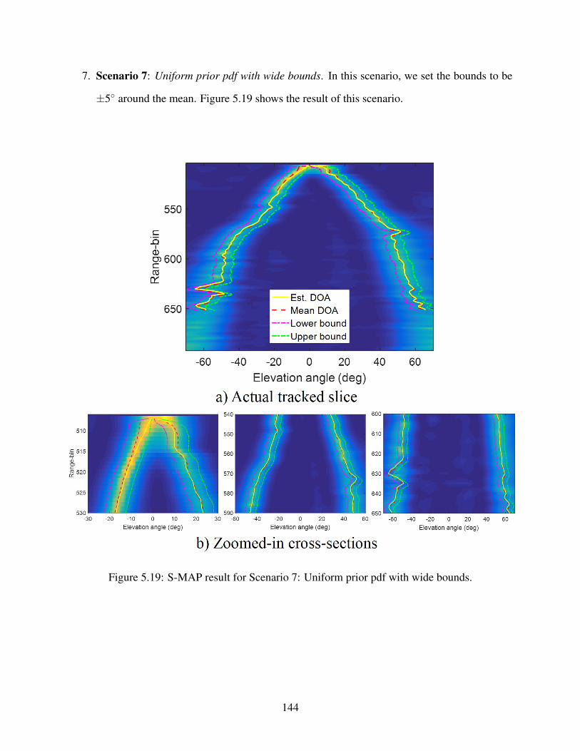
7. Scenario 7: Uniform prior pdf with wide bounds. In this scenario, we set the bounds to be

±5◦ around the mean. Figure 5.19 shows the result of this scenario.

Figure 5.19: S-MAP result for Scenario 7: Uniform prior pdf with wide bounds.

144

Main observations:

The main observations and conclusions from these examples are listed below:

1. Effect of bounds:

Choosing the right bounds depends mainly on the ice-surface topography and the quality of

the data. Narrowing the bounds down serves as a smoother to the tracked slice. But it doesn’t

give the tracker a good chance to make a good use of the measured data to guide its decision

(i.e. the narrower the bounds are, the less the tracker relies on the measured data). Figures

5.13, 5.14, 5.17, and 5.18 confirm this observation.

Wide bounds, on the other hand, give the tracker the chance to rely more on the log-

likelihood part of the cost function. Also, tight bounds make the prior pdf less important

for the answer.

But wide bounds also make the tracker behave in a strange way in regions of low quality

data. The blips around range-bins 550 and 635 on the left side of the slice and range-bin 575

on right side of the slice in figures 5.16 and 5.19 show this observation.

In addition, making the bounds too wide or leaving the bounds open mean that the tracker

is loosing an important piece of prior information that can be efficiently used to improve the

results.

2. Effect of the prior pdf:

Gaussian prior pdf has an extra benefit over uniform prior pdf, which is the possibility of

adjusting the standard deviation to improve the tracking results. Figure 5.15 shows an inter-

esting example if the effect of narrowing the standard deviation down. We can see that the

blips near range-bins 575 and 635 are almost completely gone and that near range-bin 550

is greatly reduced when the standard deviation is reduced, even though the bounds are too

wide.

Figure 5.20 shows an ice-bottom example of a uniform prior pdf and another example of

a Gaussian prior pdf aligned with the corresponding range-bin for which these priors are

145

calculated as well as the log-likelihood cost for. The location of the estimated targets and

bounds are different in the two examples because the priors are not exactly the same, even

though both of them use Model 4 to bound the DOA. These plots show, visually, the effect

of the prior pdf on the tracking performance.

In the case of uniform prior pdf, the decision is completely made based on the measured

data within the bounds. However, in the case of Gaussian prior, the prior pdf also affects

the trackers decision, even though the Gaussian pdf is acting similar to a uniform pdf in the

presented example because the standard deviation is wide.

146

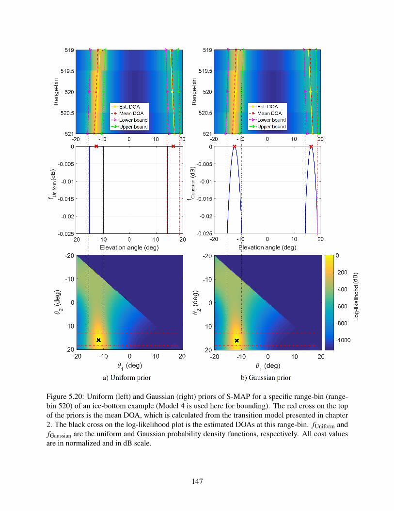
Figure 5.20: Uniform (left) and Gaussian (right) priors of S-MAP for a specific range-bin (range-bin 520) of an ice-bottom example (Model 4 is used here for bounding). The red cross on the topof the priors is the mean DOA, which is calculated from the transition model presented in chapter2. The black cross on the log-likelihood plot is the estimated DOAs at this range-bin. fUniform andfGaussian are the uniform and Gaussian probability density functions, respectively. All cost valuesare in normalized and in dB scale.

147

The net conclusion from this discussion is that Gaussian prior pdf is always a better option

for our application than uniform prior because it has an extra degree of freedom that comes from

controlling its standard deviation. Also, since the prior and standard deviation are both important

to the tracking result, the best solution is the one that uses them both. Our recommendation is to

use wider bounds than the default, but narrower standard deviation than the default.

Bad tracking example:

In Figure 5.21 we show a bad-tracking example of an ice-bottom layer using uniform prior pdf

with bounding Model 3. We can see that the tracking is good over elevation angles ∼ 10◦ to 60◦,

but it didn’t track anything on the left side of the slice. The reason for this is a) the starting range

bin comes too early (around 510 instead of 525), b) the confusing nadir data, which extends from

about range-bins 520 to 540, and c) the weak-scattering region (most severe on the left) centered

on range bin 540, which makes the model order estimator estimate zero targets, and thus no DOA

is estimated by the tracker. Possible solutions in this case include the use of wider bounds (e.g.

±20◦) on the left side of the slice, or having a human annotator add a few ground truth points on

the edge between the bad-data zone and the following good-data zone and force the tracker to start

from these points rather than from its default nadir point.

148

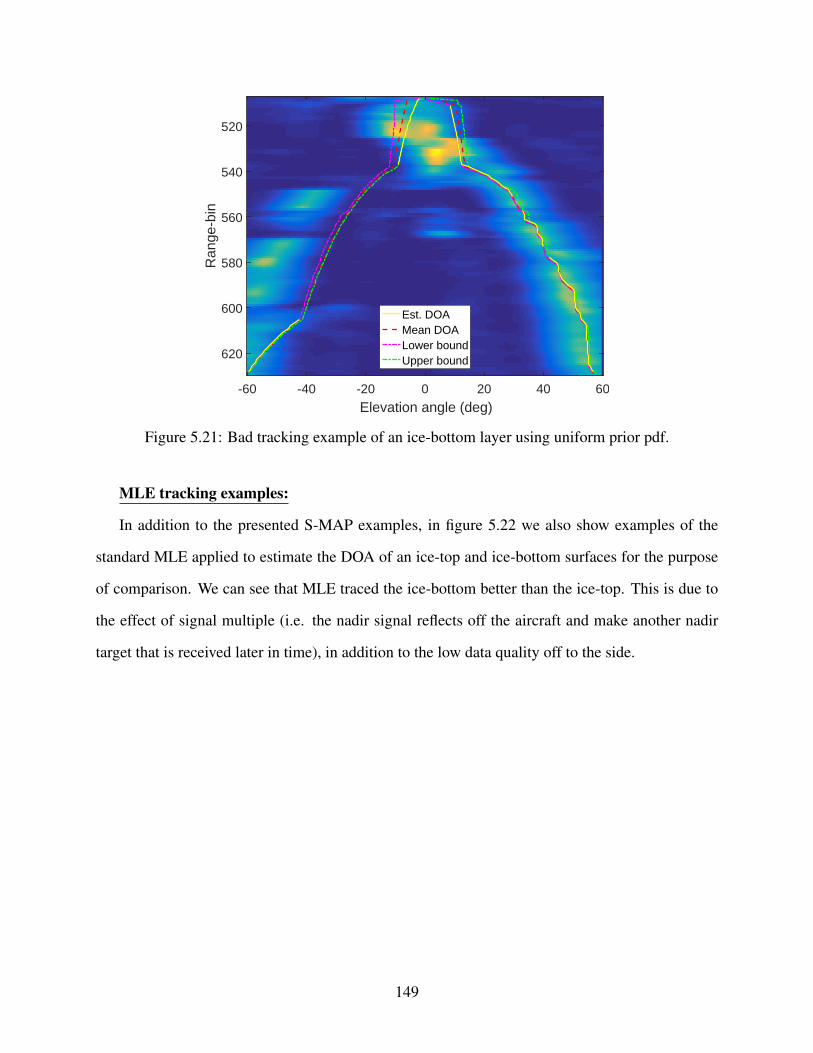
-60 -40 -20 0 20 40 60


520

540

560

580

600

620

Ran

ge-b

in

Est. DOAMean DOALower boundUpper bound

Figure 5.21: Bad tracking example of an ice-bottom layer using uniform prior pdf.

MLE tracking examples:

In addition to the presented S-MAP examples, in figure 5.22 we also show examples of the

standard MLE applied to estimate the DOA of an ice-top and ice-bottom surfaces for the purpose

of comparison. We can see that MLE traced the ice-bottom better than the ice-top. This is due to

the effect of signal multiple (i.e. the nadir signal reflects off the aircraft and make another nadir

target that is received later in time), in addition to the low data quality off to the side.

149

Figure 5.22: Ice-top and ice-bottom examples when MLE is used to estimate the DOA (i.e. nobounds and no prior information).

5.3.2 S-MAP Tracker: Layer Tracking Assessment

In addition to the basic tracking evaluation presented in the previous section, in this section we

assess the performance of the proposed DOA tracker in two ways. First, we evaluate the effect of

the model order estimation on the S-MAP tracking results and compare that to a reference MLE

DOA estimator. Second, we compare our tracked surfaces against the surface data provided by the

satellite imagery, which are usually very accurate. We use sea-ice data frames 20110417_03_001

and 20110417_04_001 in this evaluation study.

5.3.2.1 Tracking Assessment: MOE

Unlike beamformer-based trackers, DOA-based trackers require a good estimation of the model

order in most of the tracked range-bins. The tracker can loose track of the ice-surface if there are

big chunks of data missing or have 0 model order, unless the bounds are set too wide, which means

loosing a great deal of prior information.

In this section we apply the MLE and S-MAP to a sea-ice example (i.e. ice-top surface)

and investigate the performance of the MOE method (N-MDL) under both processors. The log-

150

likelihood is normalized using data generated from a 1D simulator, following the method described

in [1]. Figures 5.23 and 5.24 show a processed slice (the left figure) and a zoomed-in cross-section

of the processed slice (the right figure) for MLE and S-MAP, respectively.

The eigen-analysis of three specific range-bins from this example are shown in figures 5.25,

5.26, and 5.27. The data covariance matrix, RRR, is estimated using 63 snapshots (±10 range-lines

and ±1 range-bins). Also, the eigenvalues are normalized by subtracting their mean and dividing

by their standard deviation. However, the eigenvectors pseudo-spectrum and |RRR| are normalized

relative to their maximum values (i.e. maximum relative value is 1). Now we look closely into

each of these range-bins:

• Figure 5.25: This range-bin has two targets with similar SNR and are both inside the bounds

of the S-MAP. So the model order is estimated correctly as 2 in S-MAP as well as MLE

cases. The two big peaks in the MUSIC pseudo-spectrum and the first two eigenvalues

confirm this observation.

• Figure 5.26: This range bin is at the beginning of a nadir multiple, which is clear in the nadir

peak of the MUSIC pseudo-spectrum and the second biggest eigenvalue. But this nadir target

is outside the S-MAP bounds. The other target, ∼−38◦, is inside the S-MAP bounds. Thus

the model order should be 1 in the case of S-MAP and 2 in the case of MLE, which is what

the model order estimated.

• Figure 5.27: This range-bin is right at the strong nadir multiple, which dominates the other

targets in this range-bin. This is clear in the sharp nadir peak of the MUSIC pseudo-

spectrum. Again, since this target is outside the S-MAP bounds, then the model order is

correctly estimated as 0. However, it is 2 in the case of MLE since it is not bounded.

151

Figure 5.23: Sea-ice example showing the behavior of N-MDL when used with MLE DOA esti-mator, applied to real data. DOA 1 (yellow) and DOA 2 (red) are the elevation angles of the leftand right targets, respectively.

Figure 5.24: Sea-ice example showing the behavior of N-MDL when used with S-MAP tracker(Gaussian prior pdf and bounding Model 1 are used here), applied to real data. DOA 1 and DOA 2are defined in figure 5.23.

152

Figure 5.25: Eigen analysis of range-bin 1706 of the sea-ice example shown in figures 5.23 and5.24.



153

5.3.2.2 Tracking Assessment: S-MAP tracked layers vs ground truth

In this section, we compare S-MAP tracking results against ground truth for two sea-ice frames

20110417_03_001 and 20110417_04_001 (i.e. no ice-bottom, just ice-top), which are ideal frames

for assessment and calibration. The first frame has 2012 slices, while the second frame has 2929

slices. The FOV is restricted to ±25◦. Also, S-MAP bounding Model 3 with uniform prior pdf is

used in generating the results of this section.

Figure 5.28 shows the empirical cumulative distribution function (CDF) of the absolute dif-

ference between the S-MAP tracked ice-top layer data and the ground-truth layer data. We can

see that 73% of the errors are less than 5 range-bins and 85% are less than 10 range-bins. Over

all range-bins and range-lines of the testing data frames, the mean of the absolute error is 4.65

range-bins and the root mean-squared error (RMSE) is 6.5 range-bins.

The reason for these errors, as well as the elevation errors in the next section, can be attributed

to the following reasons:

1. S-MAP tracker doesn’t usually start from the same initial point provided by the nadir ground

truth (i.e. it could start before, after, or at the nadir ground-truth). As we mentioned before,

S-MAP searches for the initial range-bin around the ground truth point because the ground

truth points are usually provided by human annotators, which makes the ground truth not

accurate to the pixel level. However, the ground-truth surfaces start exactly at the nadir

ground truth. Since nadir strong echo signals may contaminate the near-by range-bins, the

S-MAP initial range-bin is usually difficult to determine exactly. Thus, large percentage of

these error statistics are attributed to this initial point mismatch.

2. Unlike S-MAP surface, the ground truth surface doesn’t depend on the quality of the mea-

sured data. This fact is clear in figure 5.29, which shows a slice example of an S-MAP

surface and the corresponding ground truth surface.

So, these statistics show a good S-MAP tracking performance.

154

0 5 10 15 20|Error|(range-bins)

0

0.2

0.4

0.6

0.8

1

F(|

Err

or|)

Figure 5.28: CDF of the error in S-MAP layer tracking relative to the ground truth.

-20 -10 0 10 20


1500

1520

1540

1560

1580

1600

Ran

ge-b

in

Est. DOAMean DOALower boundUpper boundGround truth

Figure 5.29: A slice example from data frame 20110417_03_001. It shows the S-MAP trackedsurface (yellow) as well as the ground truth surface (black). Clearly, S-MAP surface if trackingcorrectly based on its bounds, prior pdf, and the quality of the measured data. However, the groundtruth surface is not affected by these parameters.

155

5.3.3 S-MAP Tracker: DEM Generation Results and Assessments

The goal of tracking the bottom of an ice-sheet is to generate a DEM by geocoding and gridding

the DOA points of the tracked slices.

Figures 5.30 and 5.31 show two versions of the DEM for each of the testing frames used in

Section 5.3.2.2: the upper plot is the DEM generated from the ground truth layers (i.e. ground-

truth DEM), and the lower plot shows the DEM generated from the S-MAP tracked slices. The

ice-top elevation information are color-coded and referenced to the WGS-84 ellipsoid.

To assess the quality of the S-MAP DEM, we present the error DEMs for the same considered

testing frames in figures 5.32 and 5.33. These error DEMs represent the error between the S-

MAP DEM and the ground-truth DEM, which is the reference (i.e. negative errors mean that the

elevation value from S-MAP is less than that of the ground truth).

Also, figure 5.34 shows the CDF of the elevation absolute error. We can see that 56% of the

errors are less than 10 m and 80% of the errors are less than 20 m. In addition, over all the points

in the error DEM, the mean absolute error is 15.2 m and the RMSE is 21.76 m. No error outliers

were removed in these statistics. In addition, figure 5.35 shows the RMSE of the elevation errors

after trimming the largest n% of the errors, where n is a number between 0 and 95 with steps of

5. This plot shows that trimming the largest 20% of the errors reduces the RMSE from 21.76 m

to 9.83 m (i.e. 57% reduction in the RMSE). The reasons for these errors were discussed in the

previous section. These results show good S-MAP tracking performance, but there seems to be a

systematic tracking or steering vector error that is affecting one side of both the swaths.

156

Figure 5.30: Digital elevation models of the ice-top of sea-ice frame 20110417_03_001. a) is theground truth DEM and b) is the DEM resulting from S-MAP tracker. Nadir is right at the flightline, negative elevation angles extend from nadir towards positive x-axis, and positive elevationangles extend from nadir towards negative x-axis.

157

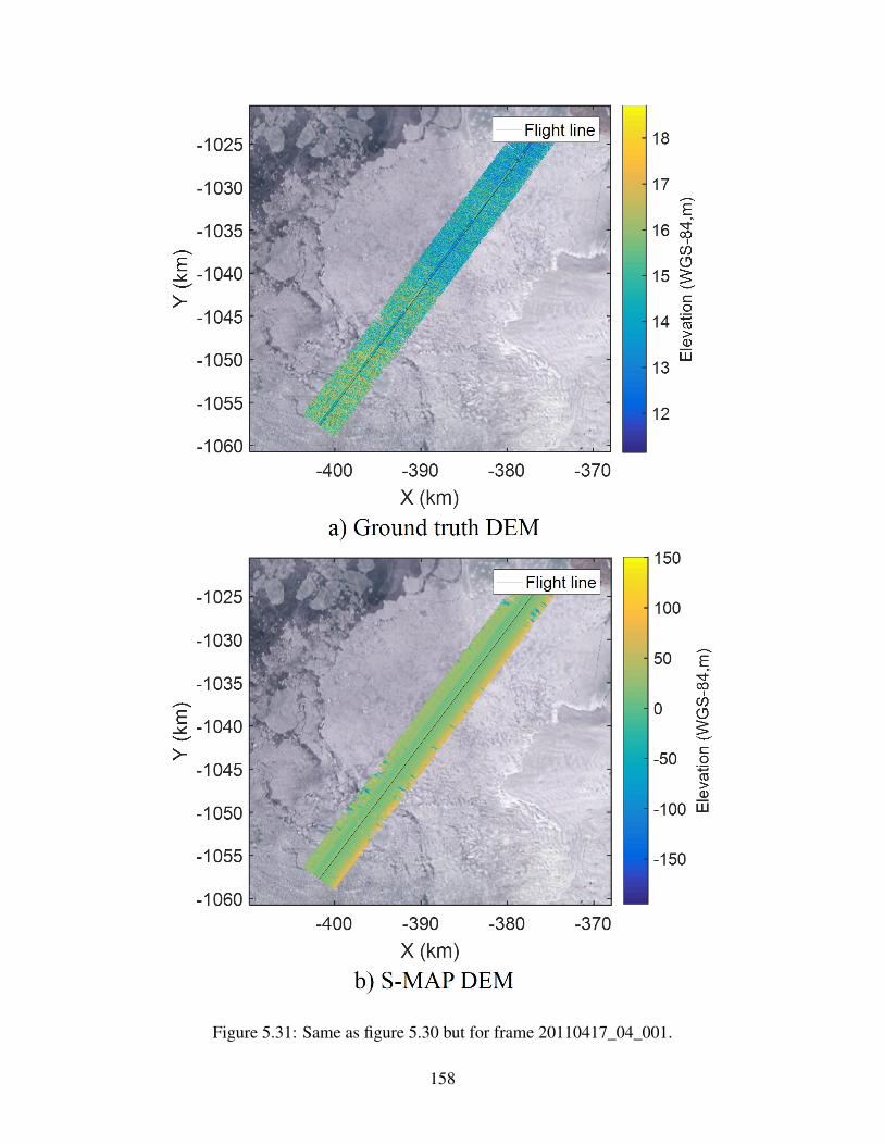
Figure 5.31: Same as figure 5.30 but for frame 20110417_04_001.

158

Figure 5.32: Digital elevation model of the error between S-MAP DEM and the ground-truth DEMfor data frame 20110417_03_001.

Figure 5.33: Digital elevation model of the error between S-MAP DEM and the ground truth DEMfor data frame 20110417_04_001.

159

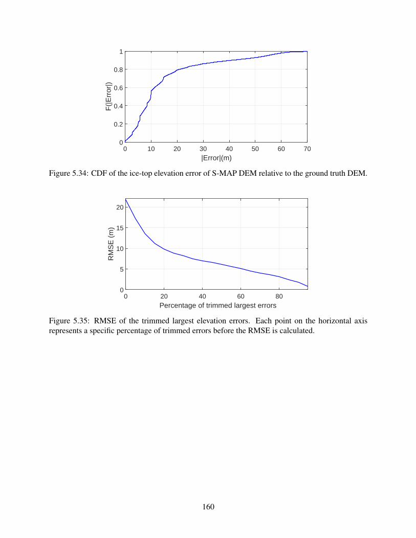
0 10 20 30 40 50 60 70|Error|(m)

0

0.2

0.4

0.6

0.8

1

F(|

Err

or|)

Figure 5.34: CDF of the ice-top elevation error of S-MAP DEM relative to the ground truth DEM.

0 20 40 60 80Percentage of trimmed largest errors

0

5

10

15

20

RM

SE

(m

)

Figure 5.35: RMSE of the trimmed largest elevation errors. Each point on the horizontal axisrepresents a specific percentage of trimmed errors before the RMSE is calculated.

160

Chapter 6

Conclusions and Future Work

6.1 Concluding Remarks

In this work, we addressed the problem of estimating the location of the ice-bottom of an ice-

sheet. We started by investigating the problem of estimating the signal subspace dimension, which

is an essential part of our tracking model. Seven methods were tested in this work and compared

against a machine learning (ML) based technique. We found that the ML method outperforms

all other compared methods, especially in the more challenging scenario of wideband data with

a large number of targets. Also, we found that normalizing the log-likelihood term of the MOE

cost function can make the standard methods, such as MDL, work well in the wideband case

with Q = 2 maximum number of targets. The normalized MDL was applied successfully to real

wideband radar data.

Several methods were studied to solve the problem of surface tracking in the radar imaging

application. This problem was formulated as an ice-bottom tracking problem and two main cate-

gories of solutions were proposed.

The first solution was beamforming-based, where we used the MUSIC beamformer to create

images of the radar scene (in the elevation angle-range domain) that are fed into a sequential tree-

reweighted message passing (TRW-S) belief propagation tracker to estimate the location of the

161

bottom of the ice-sheet. This technique was successfully applied to process 102 frames collected

from the Canadian Arctic Archipelago during the 2014 Arctic campaign.

The second category of solutions to the ice-bottom tracking problem is DOA-estimator based.

Here, two types of trackers were proposed: one is based on the particle filter (PF) and the other is

based on the sequential maximum a posterior (S-MAP) which is numerically solved the maximum

likelihood estimator with a prior added. These two algorithms were compared using a 2D sim-

ulator under narrowband and wideband scenarios. In performing these simulations we assumed

equal power point targets and a flat surface. We found that the PF solution is more suitable for

low snapshots and/or low SNR scenarios than S-MAP. Also, the PF, in our specific application,

saturates quickly with increasing number of snapshots relative to S-MAP. The model order was

assumed to be known in this comparison. In addition, we discussed the performance of these two

methods in other scenarios, such as estimating model order (i.e. effect of model order errors) and

tracking non-flat surfaces.

We successfully applied the S-MAP tracker to process real wideband data collected from Rus-

sell glacier collected during the 2011 Arctic campaign. Also, we proposed several models to

bound the S-MAP tracker and compared these models under different scenarios with uniform and

Gaussian prior distributions. We found that the prior bounds and pdf affect the tracking results

in different ways, where the best option is to use relatively wide bounds with narrow standard

deviation with the Gaussian prior.

6.2 Future Work

The DOA-based ice-bottom tracking problem presented in this dissertation is still in its early

stages. We laid the groundwork for this problem, but there are still several open problems that

are not covered.

In this work we assumed that there are Q = 2 maximum number of targets in each range-bin;

one on the left side of the platform and the other on the right side of the platform, with nadir being

162

the reference. This could be extended to a more general framework that can handle an arbitrary

number of targets, arbitrary starting angles, and the ability to handle the birth and death of targets.

This proposal also opens a new problem, which is how to accurately estimate the model order

in the high order wideband scenario with real data. Machine learning is a powerful solution, but

preparing training and testing datasets from real data is a major bottleneck.

Also, some of the S-MAP bounding models tested in this work were not chosen based on math-

ematically rigorous derivations or tuning. It is difficult to choose one set of parameters that works

for all scenarios. Machine learning may be used here to learn some of the parameters of S-MAP,

such as the standard deviation of the Gaussian prior. This is another promising research direction.

In addition, we did not apply the particle filter-based DOA tracker to process real data in this

work. So, exploring this ice-bottom tracking solution with real data along with other Kalman

filter-based solutions are good research problems that should be addressed in the future. From our

analysis in this dissertation, we expect that the particle filter based solution will be a competitive

solution to the S-MAP tracker because it can handle low quality data scenarios and difficult surface

shapes better.

163

References

[1] Sravya Athinarapu. Model order estimation and array calibration for synthetic aperture

radar tomography. Master’s thesis, University of Kansas, 2018.

[2] Bruce C. Douglas, Michael S. Kearney, and Stephen P. Leatherman. Sea level rise: History

and consequences. International Geophysics Series, 75(34), 2001.

[3] Bruce C. Douglas and W. Richard Peltier. The puzzle of global sea-level rise. Physics Today,

55(3):35–40, May 2002.

[4] Wesley Van Wychen, Jamie Davis, David O. Burgess, Luke Copland, Laurence Gray, Martin

Sharp, and Colleen Mortimer. Characterizing interannual variability of glacier dynamics

and dynamic discharge (1999–2015) for the ice masses of Ellesmere and Axel Heiberg Is-

lands, Nunavut, Canada. Journal of Geophysical Research: Earth Surface, 121(1):39–63,

2016.

[5] Climate Change IPCC. The scientific basis. IPCC, Geneva, Switzerland, 2001.

[6] Ice bottom DEMs, 2018. https: // climate. nasa. gov/ vital-signs/ ice-sheets/

[Accessed: 2018-08-07].

[7] John Paden. Synthetic aperture radar for imaging the basal conditions of the polar ice sheets.

PhD thesis, University of Kansas, 2006.

[8] F. Rodriguez-Morales, S. Gogineni, C. J. Leuschen, J. D. Paden, J. Li, C. C. Lewis, B. Panzer,

D. Gomez-Garcia Alvestegui, A. Patel, K. Byers, R. Crowe, K. Player, R. D. Hale, E. J.

164

Arnold, L. Smith, C. M. Gifford, D. Braaten, and C. Panton. Advanced multifrequency radar

instrumentation for polar research. IEEE Transactions on Geoscience and Remote Sensing,

52(5):2824–2842, May 2014.

[9] R.W. MCNABB, R. HOCK, S. O’NEEL, L.A. RASMUSSEN, Y. AHN, M. BRAUN, H. CON-

WAY, S. HERREID, I. JOUGHIN, W.T. PFEFFER, B.E. SMITH, and M. TRUFFER. Using

surface velocities to calculate ice thickness and bed topography: a case study at Columbia

Glacier, Alaska, Usa. Journal of Glaciology, 58(212):1151–1164, 2012.

[10] Huilin Li, Felix Ng, Zhongqin Li, Dahe Qin, and Guodong Cheng. An extended “perfect-

plasticity” method for estimating icethickness along the flow line of mountain glaciers. OUR-

NAL OF GEOPHYSICAL RESEARCH, 17, 2012.

[11] J. Paden, T. Akins, D. Dunson, C. Allen, and P. Gogineni. Ice-sheet bed 3D tomography.

Journal of Glaciology, 56(195):3–11, 2010.

[12] W. A. Blake. Interferometric synthetic aperture radar (INSAR) for fine-resolution basal

icesheet imaging. PhD thesis, University of Kansas, 2010.

[13] X. Wu, K. C. Jezek, E. Rodriguez, S. Gogineni, F. Rodriguez-Morales, and A. Freeman. Ice

sheet bed mapping with airborne SAR tomography. IEEE Transactions on Geoscience and

Remote Sensing, 49(10):3791–3802, Oct 2011.

[14] Theresa Stumpf. A wideband direction of arrival technique for multibeam, wide-swath imag-

ing of ice sheet basal morphology. Master’s thesis, University of Kansas, 2015.

[15] U. Nielsen. Tomographic techniques for radar ice sounding. PhD thesis, Technical University

of Denmark, 2015.

[16] D. Kirkland. Compressive sensing for RADARSAT-2 tomography. In 3rd International Work-

shop on Compressed Sensing Theory and its Applications to Radar, Sonar, and Remote Sens-

ing (CoSeRa), Pisa, Italy. IEEE, July 2015.

165

[17] X. X. Zhu and R. Bamler. Superresolving SAR tomography for multidimensional imaging

of urban areas: Compressive sensing-based tomosar inversion. IEEE Signal Processing

Magazine, 31(4):51–58, July 2014.

[18] X. X. Zhu and R. Bamler. Tomographic SAR inversion by l1-norm regularization—the

compressive sensing approach. IEEE Transactions on Geoscience and Remote Sensing,

48(10):3839–3846, Oct 2010.

[19] D. J. Crandall, G. C. Fox, and J. D. Paden. Layer-finding in radar echograms using prob-

abilistic graphical models. In Proceedings of the 21st International Conference on Pattern

Recognition (ICPR2012), pages 1530–1533, Nov 2012.

[20] S. Lee, J. Mitchell, D. J. Crandall, and G. C. Fox. Estimating bedrock and surface layer

boundaries and confidence intervals in ice sheet radar imagery using MCMC. In 2014 IEEE

International Conference on Image Processing (ICIP), pages 111–115, Oct 2014.

[21] M. Xu, D. J. Crandall, G. C. Fox, and J. D. Paden. Automatic estimation of ice bottom

surfaces from radar imagery. In 2017 IEEE International Conference on Image Processing

(ICIP), pages 340–344, Sept 2017.

[22] J. E. Mitchell, D. J. Crandall, G. C. Fox, and J. D. Paden. A semi-automatic approach for

estimating near surface internal layers from snow radar imagery. In 2013 IEEE International

Geoscience and Remote Sensing Symposium - IGARSS, pages 4110–4113, July 2013.

[23] Victor Berger, Mingze Xu, Shane Chu, David Crandall, John Paden, and Geoffrey C. Fox.

Automated tracking of 2D and 3D ice radar imagery using Viterbi and TRW-S. In 2018 IEEE

International Geoscience and Remote Sensing Symposium - IGARS, July 2018.

[24] X. X. Zhu and M. Shahzad. Facade reconstruction using multiview spaceborne TomoSAR

point clouds. IEEE Transactions on Geoscience and Remote Sensing, 52(6):3541–3552,

June 2014.

166

[25] M. Shahzad and X. X. Zhu. Robust reconstruction of building facades for large areas using

spaceborne TomoSAR point clouds. IEEE Transactions on Geoscience and Remote Sensing,

53(2):752–769, Feb 2015.

[26] M. Shahzad, M. Maurer, F. Fraundorfer, Y. Wang, and X. X. Zhu. Extraction of buildings in

vhr sar images using fully convolution neural networks. In 2018 IEEE International Geo-

science and Remote Sensing Symposium - IGARS, July 2018.

[27] X. X. Zhu, F. Fraundorfer, F. Kurz, and P. Reinartz. Building detection and segmentation using

a CNN with automatically generated training data. In 2018 IEEE International Geoscience

and Remote Sensing Symposium - IGARS, July 2018.

[28] M. Rahnemoonfar, G. C. Fox, M. Yari, and J. Paden. Automatic ice surface and bottom

boundaries estimation in radar imagery based on level-set approach. IEEE Transactions on

Geoscience and Remote Sensing, 55(9):5115–5122, Sept 2017.

[29] Mingze Xu, Chenyou Fan, John D. Paden, Geoffrey C. Fox, and David J. Crandall. Multi-

task spatiotemporal neural networks for structured surface reconstruction. IEEE Winter

Conference on Applications of Computer Vision (WACV), March 2018.

[30] Hamid Kamangir, Maryam Rahnemoonfar, Dugan Dobbs, John Paden, and Geoffrey Fox.

Deep hybrid wavelet network for ice boundary detection in radra imagery. In 2018 IEEE

International Geoscience and Remote Sensing Symposium - IGARS, July 2018.

[31] Ice bottom DEMs, 2018. https: // data. cresis. ku. edu/ data/ rds/ 2014_

Greenland_ P3/ CSARP_ DEM/ [Accessed: 2018-08-12].

[32] Z. Wang, S. Gogineni, F. Rodriguez-Morales, J. B. Yan, J. Paden, C. Leuschen, R. D. Hale,

J. Li, C. L. Carabajal, D. Gomez-Garcia, B. Townley, R. Willer, L. Stearns, S. Child, and

D. Braaten. Multichannel wideband synthetic aperture radar for ice sheet remote sensing:

Development and the first deployment in antarctica. IEEE Journal of Selected Topics in

Applied Earth Observations and Remote Sensing, 9(3):980–993, March 2016.

167

[33] M Al-Ibadi, J Sprick, S Athinarapu, T Stumpf, J Paden, C Leuschen, F Rodríguez, M Xu,

D Crandall, G Fox, D Burgess, M Sharp, L Copland, and W Van Wychen. DEM extraction of

the basal topography of the Canadian Archipelago ice caps via 2D automated layer-tracker.

In International Geoscience and Remote Sensing Symposium (IGARSS), pages 965–968.

IEEE, July 2017.

[34] C. Leuschen, S. Gogineni, and D. Tammana. SAR processing of radar echo sounder data. In

International Geoscience and Remote Sensing Symposium (IGARSS), 2000.

[35] H. Van Trees. Optimum Array Processing. Part IV of Detection, Estimation, and Modulation

Theory. John Wily and Sons Inc., 2002.

[36] M. A. Doron and E. Doron. Wavefield modeling and array processing,Part III-resolution

capacity. IEEE Transactions on Signal Processing, 42(10):2571–2580, Oct 1994.

[37] T. B. Lavate, V. K. Kokate, and A. M. Sapkal. Performance analysis of MUSIC and ESPRIT

DOA estimation algorithms for adaptive array smart antenna in mobile communication. In

2010 Second International Conference on Computer and Network Technology, pages 308–

311, April 2010.

[38] Mati Wax. Detection and Estimation of Superimposed Signals. PhD thesis, Stanford Univer-

sity, 1985.

[39] I. Ziskind and M. Wax. Maximum likelihood localization of multiple sources by alternating

projection. IEEE Transactions on Acoustics, Speech, and Signal Processing, 36(10):1553–

1560, Oct 1988.

[40] M Wax, T. J. Shan, and T. Kailath. Location and the spectral density estimation of multiple

sources. In Proc. 16th Asiloma conference on signals, systems, and computers, 1982.

[41] J. Paden, T. Stumpf, and M. Al-Ibadi. Wideband DOA estimation for ice sheet bed mapping. In

168

IEEE International Symposium on Phased Array Systems and Technology (PAST), October

2016.

[42] S. Athinarapu, J. Paden, M. Al-Ibadi, and T. Stumpf. Model order estimators using optimal

and suboptimal methods with numerical tuning. In IEEE Radar Conference, 2018.

[43] M. A. Doron, A. J. Weiss, and H. Messer. Maximum-likelihood direction finding of wide-band

sources. IEEE Transactions on Signal Processing, 41(1):411–, Jan 1993.

[44] Yeo-Sun Yoon, L. M. Kaplan, and J. H. McClellan. TOPS: new DOA estimator for wideband

signals. IEEE Transactions on Signal Processing, 54(6):1977–1989, June 2006.

[45] M. A. Doron and A. J. Weiss. On focusing matrices for wide-band array processing. IEEE

Transactions on Signal Processing, 40(6):1295–1302, Jun 1992.

[46] Steven M. Kay. Fundamentals of Statistical Signal Processing: Estimation Theory. Prentice-

Hall Inc., 1993.

[47] F. Gustafsson. Particle filter theory and practice with positioning applications. IEEE

Aerospace and Electronic Systems Magazine, 25(7):53–82, July 2010.

[48] A. Doucet and A. Johansen. A tutorial on particle filters for online nonlinear/non-gaussian

bayesian tracking. in The Oxford Handbook of Nonlinear Filtering. New York: Oxford Univ.

Press, 2009.

[49] B. Ristic, S. Arulampala, and N. Gordon. Beyond the Kalman Filter: Particle Filters for

Tracking Applications. Artech House, 2004.

[50] A. Doucet, N. de Freitas, and N. Gordon. Sequential Monte Carlo Methods in Practice.

Springer, 2001.

[51] Won Sik Youn and Chong Kwan Un. Robust adaptive beamforming based on the eigenstruc-

ture method. IEEE Transactions on Signal Processing, 42(6):1543–1547, Jun 1994.

169

[52] A. Young, M. V. Ivashina, R. Maaskant, O. A. Iupikov, and D. B. Davidson. Improving the

calibration efficiency of an array fed reflector antenna through constrained beamforming.

IEEE Transactions on Antennas and Propagation, 61(7):3538–3545, July 2013.

[53] Won Sik Youn and Chong Kwan Un. Robust adaptive beamforming based on the eigenstruc-

ture method. IEEE Transactions on Signal Processing, 42(6):1543–1547, Jun 1994.

[54] L. Ma, Z.F. Li, and G.S. Liao. System error analysis and calibration methods for multi-

channel SAR. Progress In Electromagnetics Research, 112(6):309–327, 2011.

[55] A. J. Weiss and B. Friedlander. Array shape calibration using sources in unknown locations-a

maximum likelihood approach. IEEE Transactions on Acoustics, Speech, and Signal Process-

ing, 37(12):1958–1966, Dec 1989.

[56] F. Vincent and O. Besson. Steering vector errors and diagonal loading. IEE Proceedings -

Radar, Sonar and Navigation, 151(6):337–343, Dec 2004.

[57] M. Wax and Y. Anu. Performance analysis of the minimum variance beamformer in the

presence of steering vector errors. IEEE Transactions on Signal Processing, 44(4):938–947,

Apr 1996.

[58] Azizul H. Quazi. Array beam response in the presence of amplitude and phase fluctuations.

The Journal of the Acoustical Society of America, 72(1):171–180, June 1998.

[59] B. Friedlander. Sensitivity analysis of the maximum likelihood direction finding algorithm.

In Twenty-Third Asilomar Conference on Signals, Systems and Computers, 1989., volume 2,

pages 594–598, Oct 1989.

[60] P. Chen, T. J. Wu, and J. Yang. A comparative study of model selection criteria for the number

of signals. IET Radar, Sonar and Navigation, 2(3):180–188, 2008.

[61] S. Caylar. A novel neural network based approach for direction of arrival estimation. PhD

thesis, Middle East Technical University, 2007.

170

[62] M. Agatonovic, Z. Stankovic, N. Doncov, L. Sit, B. Milovanovic, and T. Zwick. Application of

artificial neural networks for efficient high-resolution 2d doa estimation. Radioengineering,

21(4):1178–1186, 2012.

[63] S. Adavanne, A. Politis, and T. Virtanen. Direction of arrival estimation for mul-

tiple sound sources using convolutional recurrent neural networ. [Online]. available:

https://arxiv.org/abs/1710.10059, Aug 2018.

[64] Kevin P Murphy. Machine learning: a probabilistic perspective. MIT press, 2012.

[65] A. Doucet and A. Johansen. A tutorial on particle filtering and smoothing: Fifteen years

later. Handbook of Nonlinear Filtering, Oxford Univ. Press, 2009.

[66] M. Zatman. How narrow is narrowband? Proc. IEEE-Radar, Sonar and Navin, 145(2), 1998.

[67] Victor Berger, Mingze Xu, Mohanad Al-Ibadi, Shane Chu, David Crandall, John Paden, and

Geoffrey Fox. Automated tracking of 2D and 3D ice radar imagery using Viterbi and TRW-S.

Submitted to IEEE J. Sel. Topics Appl. Earth Observ (JSTARS), 2019.

[68] ArcticDEM, 2018. https: // www. pgc. umn. edu/ data/ arcticdem/ .

[69] Jérôme Korona, Etienne Berthier, Marc Bernard, Frédérique Rémy, and Eric Thouvenot.

SPIRIT. SPOT 5 stereoscopic survey of polar ice: Reference images and topographies during

the fourth international polar year (2007–2009). ISPRS Journal of Photogrammetry and

Remote Sensing, 64(2):204 – 212, 2009.

[70] M.Xu, D.Crandall, G.Fox, and J.Paden. Automatic estimation of ice bottom surfaces from

radar imagery. In IEEE International Conference on Image Processing (ICIP) 2017, 2017.

[71] V. Kolmogorov. Convergent tree-reweighted message passing for energy minimization. IEEE

Transactions on Pattern Analysis and Machine Intelligence, 28(10):1568–1583, Oct 2006.

[72] A. Arendt and et.al. Randolph glacier inventory [v2.0]: A dataset of global glacier outlines.

Global Land Ice Measurements from Space, Boulder Colorado, USA, Digital Media, 2012.

171

[73] P. Stoica and A. Nehorai. Music, maximum likelihood, and cramer-rao bound. IEEE Trans-

actions on Acoustics, Speech, and Signal Processing, 37(5):720–741, May 1989.

172

Array Processing Techniques for Estimation and Tracking of ...

Documents

Transcript of Array Processing Techniques for Estimation and Tracking of ...