This article appeared in a journal published by Elsevier. The attachedcopy is furnished to the author for internal non-commercial researchand education use, including for instruction at the authors institution

and sharing with colleagues.

Other uses, including reproduction and distribution, or selling orlicensing copies, or posting to personal, institutional or third party

websites are prohibited.

In most cases authors are permitted to post their version of thearticle (e.g. in Word or Tex form) to their personal website orinstitutional repository. Authors requiring further information

regarding Elsevier’s archiving and manuscript policies areencouraged to visit:

http://www.elsevier.com/copyright

Author's personal copy

Inverse combustion force estimation based on responsemeasurements outside the combustion chamberand signal processing

Mohammad Hosseini Fouladi �, Mohd. Jailani Mohd. Nor, Ahmad Kamal Ariffin,Shahrir Abdullah

Department of Mechanical and Materials Engineering, Faculty of Engineering, Universiti Kebangsaan Malaysia, 43600 Bangi, Selangor, Malaysia

a r t i c l e i n f o

Article history:

Received 11 December 2008

Received in revised form

3 April 2009

Accepted 21 May 2009Available online 29 May 2009

Keywords:

Vibration source reconstruction

Experimental and numerical modal analysis

Non-accessible sources

Inverse technique

Tikhonov regularization

L-curve

GCV

a b s t r a c t

Exposure to vibration has various physiological effects on vehicle passengers. Engine is

one of the main sources of vehicle vibration. The major causes of engine vibration are

combustion forces transmitted through the pistons and connection rods. Evaluation of

sources is the first step to attenuate this vibration. Assessment of these sources is not an

easy task because internal parts of machinery are not accessible. Often, instrumentation

for such systems is costly, time consuming and some modifications would be necessary.

Aim of the first part of this paper was to validate an inverse technique and carry out

mobility analysis on a vehicle crankshaft to achieve matrix of Frequency Response

Functions (FRFs). Outcomes were implemented to reconstruct the applied force for

single and multiple-input systems. In the second part, the validated inverse technique

and FRFs were used to estimate piston forces of an operating engine. Bearings of

crankshaft were chosen as nearest accessible parts to piston connecting rods.

Accelerometers were connected to the bearings for response measurement during an

ideal engine operation. These responses together with FRFs, which were estimated in

the previous part, were utilised in the inverse technique. Tikhonov regularization was

used to solve the ill-conditioned inverse system. Two methods, namely L-curve criterion

and Generalized Cross Validation (GCV), were employed to find the regularization

parameter for the Tikhonov method. The inverse problem was solved and piston forces

applied to crankpins were estimated. Results were validated by pressure measurement

inside a cylinder and estimating the corresponding combustion force. This validation

showed that inverse technique and measurement outcomes were roughly in agreement.

In presence of various noise, L-curve criterion conduces to more robust results

compared to the GCV method. But in the absence of high correlation between sources

(f4600 HzHz), the GCV technique leads to more accurate results. This research shows

that inverse techniques have great ability to estimate vibration sources inside the

machinery.

& 2009 Elsevier Ltd. All rights reserved.

Contents lists available at ScienceDirect

journal homepage: www.elsevier.com/locate/jnlabr/ymssp

Mechanical Systems and Signal Processing

ARTICLE IN PRESS

0888-3270/$ - see front matter & 2009 Elsevier Ltd. All rights reserved.

doi:10.1016/j.ymssp.2009.05.008

� Corresponding author. Tel.: +60 0389216015; fax: +60 0389216016.

E-mail address: mfoolady@gmail.com (M. Hosseini Fouladi).

Mechanical Systems and Signal Processing 23 (2009) 2519–2537

Author's personal copy

1. Introduction

A comprehensive understanding of structural dynamics is essential for solving noise and vibration problems. Modalanalysis is an efficient tool for describing, understanding and modeling structural dynamics [1]. Wamsler and Rose [2]demonstrated the use of a graphical energy method to find the mode shapes and to study the dynamic behavior ofstructure in automotive applications. Mancosu et al. [3] implemented a modal model to study dynamics of rolling tyre andsimulated the interaction between road, tyre and vehicle. Seidlitz [4] conducted torsional modal tests on a diesel generatorto verify a mass-elastic model. Okamura and Arai [5] utilised experimental modal analysis to investigate vibration behaviorand excitation force transmission for a diesel engine. Guan et al. [6] evaluated the modal parameters of a dynamic tyre thencarried out the dynamic responses of tyre running over cleats with different speeds. Xingguo et al. [7] simulated themechanical behavior of engine crankshaft in real working condition. Mobility measurement is a kind of modal analysis thatis based on classical input/output measurements. It can be implemented in simple dual-channel measurements using animpact hammer or multi-channel Multiple-Input Multiple-Output (MIMO) measurements using more excitations. Modalparameters are extracted from FRFs using curve-fitting algorithms. The FRFs are referred as mobility because theydetermine how ‘‘mobile’’ the structure is [1]. Structure is assumed to behave as a linear, time-invariant system. Structuresgenerally behave linearly for small deflections (small forces). The linearity assumption reveals that response is alwaysproportional to excitation. Structure should be causal, stable and time-invariant, as the characteristics of some structuresmay be altered during the test by temperature or other environmental changes. Parameters that describe each mode arenatural frequency, modal damping and mode shape. The modal parameters of all the modes, within the frequency range ofinterest, constitute a complete dynamic description of the structure.

Methods that are commonly used for noise source identification (NSI) can be considered as inverse input problems; theyestimate the source of perturbation according to the type of measured field data. Differences among these methods arebased on the type of data and methods of data collection that are used to estimate the solution. Three most popularmethods are sound intensity, sound pressure and acoustic holography (AH) [8]. Sound intensity is a vector quantity thatmeasures the energy flow. It may be measured in the near or far field and has a very specific use in machine conditionmonitoring [9]. Moschioni et al. [10] used an intensity-based method to find the sound sources existing in environmentand industrial areas. In sound intensity mapping, an imaginary grid is placed over a surface of a stationary source (the gridshould cover the area of interest). The intensity probe is moved over the surface and the measured intensity was mappedwith a good resolution. Kang et al. [11] implemented intensity mapping in order to find the sound sources of a hard diskdrive. In sound pressure mapping, a single microphone is enough to measure and map the sound pressure at a number ofpoints on a surface. However, it does not represent any sound power or energy flow and the resolution is poor (low cost).The basis of acoustic holography method is to use an array of microphones for field measurements. In Spatial Transformof Sound Fields (STSF), the array of microphones is moved over parallel planes to map the sound field [12,13] but in non-stationary STSF (NS-STSF), a full-size microphone array is used that covers the object. Highly transient sounds can bemapped very well using the STSF method [14].

In beamforming, a full-size wheel microphone array (looks as a spider grid) focuses acoustic measurements on aparticular source. Using this method, large objects and high frequencies could be mapped very quickly [15]. Fieldhouse andNewcomb [16] implemented special holography technique to study the vibration characteristics of a disk brake. Again,Ruhala and Burroughs [17] used Nearfield Acoustic Holography (NAH) to investigate the radiated noise from different areasof a tyre while it is rolling on the pavement. Moreover, Hald [18] performed time domain acoustical holography to measurespectral emissions of a squealing brake. Fischer and Simmerb [19] showed that beamforming was an effective tool forspeech acquisitions in noisy area. Lastly, Choi and Kim [20] proposed a new method based on beamforming to find theimpulsive noise sources of fault machinery.

The above-mentioned methods are used not only to estimate noise sources but also to identify vibration sources. Kimand Ih [21] and Schuhmacher [22] reconstructed vibration sources of sound based on data collected in the nearfield.The exterior domain was designed by means of a boundary element model and the acoustic field was expressed by theboundary vibration variables. Therefore, based on the measured acoustic field, the inverse problem of estimating vibrationof the surface was solved. The critical part was to define transfer function of the system, which acted as a transformerbetween the sound and vibration. Visser [23] described how the nearfield particle velocities can be used instead ofpressures to reconstruct the original source vibrations. In another research, Gerard et al. [24] evaluated the unsteadyrotating forces acting by a fan on the fluid from the far-field acoustic pressure measurements. Jacobsen et al. [25] usedthe NAH coupled with an inverse boundary element method to measure the surface vibration on a solid concrete tub.The results were in agreement with the solutions obtained by Laser Doppler Vibrometry (LDV), which is a non-contactmeasurement technique. A beam is sent onto a vibrating surface, and the reflected beam is recombined with the referenceinternal beam. The slight intensity change is the key for analysing the vibration of the surface. In addition, LDV is useful forvery high frequency changes.

The above-mentioned methods are useful in problems where the object is accessible. They are not practical for installingthe measurement equipments in internal parts of machinery. Distances and angles play important roles in accuracy ofresults. For instance, in the LDV method the laser beam should collide the vibrating surface and be captured by the deviceafter reflection. Nam and Kim [26] and Schuhmacher [27] showed that the distance between the field microphones, theiralignment and their distance from the excitation surface had huge influence on the accuracy of solutions.

ARTICLE IN PRESS

M. Hosseini Fouladi et al. / Mechanical Systems and Signal Processing 23 (2009) 2519–25372520

Author's personal copy

There are other methods to find sources of noise, which are classified under Noise Path Analysis (NPA) [28]. They havefrequently been implemented in automotive industries since the last decade. All of them are based on finding the transferfunction between the source and the receiver. Three most important methods are coherence [29,30], complex stiffness andmatrix inversion methods [31,32]. The difficulty associated with the last two methods is to separate the observation partfrom the system. A predefined force is applied and transfer function was calculated by measuring the response. However,coherence method is not very practical in low-frequency analysis of engine (because of high coherency between theoscillations) but there is no need to separate the part from the system. It is well established with digital signal processingmethods [33]. The coherence-based methods are only useful when the output and inputs of system are measurable and thegoal is to find the contribution of each input to the output. They are not useful for problems with missing inputs andoutputs.

Explosions of an internal combustion engine produce powerful pulses of energy, which cause the engine vibration as aresponse. Attenuation of engine vibration is one of the important problems for NVH engineers. It has effects on wholechassis vibration and interior noise emissions. Hosseini Fouladi et al. [30] showed that below 200 Hz, vibration of enginecomponents is the dominant and highly coherent sources of noise emissions inside the vehicle compartment. Junhong andJun [34] implemented CAE approach and simulated the dynamic and acoustic behavior of a whole engine. Computer-aidedmethod has this advantage that no prototype is necessary and models can be used for further design development. Butmodeling is not an easy task and usually they have shortcomings due to preliminary assumptions. Modeling of joint,components and their interactions has also difficulties.

Mas et al. [35] showed that conditioning of matrix of transfer functions has great influence on indirect forceidentification in highly damped systems such as vehicles. Busby and Trujillo [36] solved inverse dynamic problemof a cantilever beam by Tikhonov regularization. Generalized Cross Validation (GCV) and L-curve technique wereimplemented to obtain the optimum regularization parameter. They suggested using L-curve in computer programsthat are to be used for large models. Kromulski and Hojan [37] integrated modal analysis and inverse techniquesto determine the operational deflection shapes of machinery. Thite and Thompson [38,39] focused on the transferpath of structure-borne noise using inverse methods. They discussed different techniques and strategies for over-determination and singular values rejection. Thereafter, alternative methods were studied to regularize the inverted matrixof transfer functions. Tikhonov regularization together with ordinary cross-validation method was used to select theregularization parameter. Leclere et al. [40] implemented inverse techniques to evaluate internal vibration sourcesexciting engine block during operation. Forces exciting the diesel engine were not directly measurable, so they wereassessed from dynamic deformation of the structure. Transfer functions between excitations and responses weremeasured by modal analysis. Later, two approaches based on truncated singular value decomposition and the L-curveprinciple were suggested for inverse problem resolution. In the other study [41], they compared two least squareapproaches, namely weighted least square and weighted total least square, to identify dynamic forces acting on anengine cylinder block. The literature regarding the utilisation of inverse techniques for vibration source reconstruction ofvehicles is rather limited. However, the main concept behind inverse techniques is the same for noise or vibrationproblems.

This research was initiated to implement inverse techniques in operating conditions of machinery. Hence it mayilluminate the application of these methods in real world rather than a controlled test rig situation. Signal processing wasintegrated with inverse techniques to solve inverse problem for internal parts of machinery in which amounts of sourcesare unknown and they are inaccessible. Tikhonov regularization was carried out to stabilize the solution of ill-posedproblem. For the first time, GCV was utilised for vibration source reconstruction inside the machinery and compared toL-curve as two methods to estimate the regularization parameter. The same methods are also applicable for noisesource evaluation of machinery. FRFs of such systems may be estimated experimentally in an anechoic chamber ornumerically using the model. Thereafter, responses can be recorded by microphones in operational condition. HavingFRFs and operational responses will lead to quantification of the operational noise sources using the same inversetechnique.

1.1. System response model

The relationship between input (excitation) and output (vibration response) of a linear system is given by Eq. (1) asfollows:[1]

Yi ¼X

j

HijXj (1)

where Yi is the output spectrum at Degree Of Freedom (DOF) i, Xj is the input spectrum at DOF j, and Hij is the FRF betweenDOF j and DOF i. Most of the test cases require measurements with more than one reference DOF, i.e., measurements ofmore than one row or more than one column of the FRF matrix [H]. It enables calculation of linear combinations of theserows or columns to enhance different modes. In a roving hammer test, more rows may be obtained by including moreresponse DOFs. In order to optimise data consistency and reduce measurement time, response and reference DOFs shouldbe measured simultaneously by using more accelerometers (more measurement channels), i.e., single-input multiple-output (SIMO) system.

ARTICLE IN PRESS

M. Hosseini Fouladi et al. / Mechanical Systems and Signal Processing 23 (2009) 2519–2537 2521

Author's personal copy

1.2. Inverse problems and ill conditioning

Inverse techniques are very beneficial in automotive applications. It is usually difficult to measure the input, output orthe boundary conditions in such complex systems. Hence the indirect formulation coupled with an experimental trial ofthe process can lead to finding a close estimate to the unknown information. For an inverse input problem, the output andparameters of the system are known and the goal is to find the input of the problem. Consider Eq. (1), an inverse inputproblem is to estimate the input spectrum Xj from the output spectrum Yi and matrices of FRFs; Hij. At the first glance, itseems to be an easy task that can be carried out by multiplying the inverse of FRFs by the output spectrum. This is the casein single-input problems but some precautions should be considered before inverting the FRFs in multiple-input problems.For a square and symmetric transfer matrix of size n�n, the condition number is defined as follows [42]:

k ¼maxðl1; l2; . . . ; lnÞ

minðl1;l2; . . . ; lnÞ(2)

where l1,l2,y, ln are singular values of the transfer matrix and can be derived by implementing the singular valuedecomposition (SVD) technique as follows:

½H� ¼ ½U�½S�½V �T (3)

where [U] and [V] are unitary matrices such that [U]*[U] ¼ [I] and [S] is the diagonal matrix of singular values, wherel1,l2,y,ln are the elements on the main diagonal. If the matrix is singular, the smallest eigenvalue will be zero and thecondition number will become infinity. In practical numerical analysis, the smallest eigenvalue for a singular matrix willusually be a very small number, which leads to a large condition number. Therefore, the larger the condition number, theworse the conditioning of the matrix. A very large condition number in a system indicates that outputs of the system arenot sensitive to at least one of the inputs. Other reason may be the existence of linear dependencies between columns ofthe transfer matrix. This system is called ill-conditioned and solutions are unstable, where a slight change in the input dataresults in a large change in the solution [43].

Because SVD does compute the singular values of the matrix, condition number can be very easily obtained once SVD isapplied [44]. If responses are only partially coherent (as most cases), it means that several incoherent phenomena arecontributing to the deformation of the structure. Therefore, special techniques should be utilised to extract the deflectionshapes characterizing each incoherent phenomena. They can be achieved through the cross-spectral matrix of responses[45]:

½Sðf Þ� ¼ ½U�½S�½U�n (4)

where [S(f)] is cross-spectral matrix of responses, [U] is the matrix of eigenvectors and [U]* is conjugate transpose of [U].The quantity of non-negligible eigenvalues is equal to the quantity of incoherent phenomena join in the deformationof structure. Consider [X]nk as the matrix of virtual sources, n the total number of responses and [s]kk as a diagonal matrix,whose elements of its main diagonal are square roots of the corresponding k non-negligible eigenvalues. So it can bewritten as follows:

½X�nk ¼ ½U�nk½s�kk (5)

This kind of decomposition is called principal component analysis [Y] ¼ [H][X] because each column of [X]nk

characterizes one of the k incoherent phenomena (deflection shape). Hosseini Fouladi et al. [30] utilised this techniqueto reconstruct vibro-acoustical sources of vehicle interior noise.However, methods (regularization) are needed to avoidunstable solutions and will be discussed particularly.

1.3. Tikhonov regularization

The origin of regularization methods is to add a choice criterion based on the norm of the solution. Tikhonovregularization is the most commonly used method of regularization of ill-posed problems. Consider Eq. (6) as anill-conditioned linear system:

½Y� ¼ ½H�½X� (6)

This system can be replaced by a problem of looking for an x to minimize Eq. (7) [46]:

½H�½X� � ½Y ��� ��2

2þ l2

½X��� ��2

2(7)

This is the standard form of Tikhonov regularization where || � ||2 is the Euclidean norm and l40 is the regularizationparameter. The solution to this problem [Xreg] is called the regularized solution [47]. It is based on tuning the regularizingparameter l, which adjusts the importance given to the minimization of the residue norm ||[H][X]�[Y]||2, on the one hand,and the solution norm ||X||2 on the other hand. The most suitable graphical tool for such analysis is the L-curve thatdisplays the compromise between minimization of these two quantities. It is plotted in log–log scale, where the verticalaxis is norm of the regularized solution and the horizontal axis is the residual norm. Then it is possible to find an estimation

ARTICLE IN PRESS

M. Hosseini Fouladi et al. / Mechanical Systems and Signal Processing 23 (2009) 2519–25372522

Author's personal copy

to the optimum regularization parameter by locating the corner of the L-curve (point with maximum curvature) [48].Interesting discussions in inverse techniques may be found in [36,38,39,49,50].

1.4. Conditioning of system of equations

By including more response data, accuracy of the calculation can be enhanced. Over-determination can improve thecondition number of the FRF matrix by reducing the extreme sensitivity of inverse technique to measurement errors as it isdescribed by Thite and Thompson [38,39]. They showed that many of the peaks in the condition numbers were removed asthe number of responses increased. But it should be noticed that sensors cannot be placed very close to each other. This isrelated to the conditioning of the FRF matrix that is to be inverted. Two sensors at the same position give two dependentrows in the FRF matrix. Another way to improve the condition number is implementing a weighting matrix. Eq. (8)describes the relation between operating forces [F] and responses [X] in a linear system of equations [35]:

½X�nk ¼ ½H�nm½F�mk (8)

where [H]nm is the measured FRF matrix between m excitations and n response points. By using a weighting method, everysensor may be given the same importance with respect to the force estimation. To describe the weighting principle, Eq. (8)can be written as follows:

½W�nn½X�nk ¼ ½W�nn½H�nm½H�mk (9)

where [W] is the weighting matrix:

½W� ¼

w1 0 . . . 0

0 w2 . . . 0

. . . . . . . . . . . .

0 0 . . . wn

26664

37775 (10)

The weighting method is only helpful when over-determination is achieved (a rectangular matrix is to be inverted)because the inverse of square matrix is independent of the values in the weighting matrix. Leclere et al. [41] showed that avector of unitary uncorrelated forces should give a vector of unitary accelerations and deduced a weighting matrix asfollows:

WðoÞi;i ¼

ffiffiffiffiffiffiffiffiffiffiffiffiffiffiffiffiffiffiffiffiffiffiffiffiffiffiffiffiffiffiffiffiffiffiffiffiffiffiffiffiffiXn

j¼1

HðoÞi;j�� ��2

0@

1A�1

vuuut (11)

1.5. GCV technique

Another widely accepted criterion to choose the regularization parameter is GCV, which was first introduced by GraceWahba [51,52]. A regularization parameter is chosen which minimizes the GCV function as mentioned thoroughly byWahba [51] and Yoon and Nelson [53]:

G ¼½H�½X� � ½Y ��� ��2

2

ðtraceðIm � HH�1ÞÞ

2(12)

where H�1 is the inverse of the coefficient matrix H and trace is sum of diagonal entries of a matrix. The numerator is thesquared residual norm and the denominator is a squared effective number of degrees of freedom, which can be written interms of filter factors [54]. Hansen [55] mentioned that GCV balances the perturbation and regularization errors, thus it isrelated to the L-curve corner. The GCV method can be used with confidence only if errors are characterized as white noise.Also Wahba [51] stated that GCV was quite likely to produce unsatisfactory result if noise components contaminating themeasured data are highly correlated.

2. Methodology

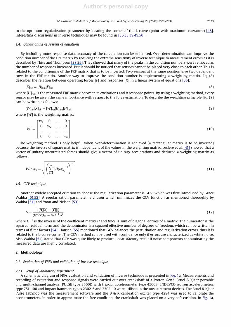
2.1. Evaluation of FRFs and validation of inverse technique

2.1.1. Setup of laboratory experiment

A schematic diagram of FRFs evaluation and validation of inverse technique is presented in Fig. 1a. Measurements andrecording of excitation and response signals were carried out over crankshaft of a Proton Gen2. Bruel & Kjaer portableand multi-channel analyzer PULSE type 3560D with triaxial accelerometer type 4506B, ENDEVCO isotron accelerometerstype 751-100 and impact hammers types 2302-5 and 2302-10 were utilised in the measurement devices. The Bruel & KjaerPulse LabShop was the measurement software and the B & K calibration exciter type 4294 was used to calibrate theaccelerometers. In order to approximate the free condition, the crankshaft was placed on a very soft cushion. In Fig. 1a,

ARTICLE IN PRESS

M. Hosseini Fouladi et al. / Mechanical Systems and Signal Processing 23 (2009) 2519–2537 2523

Author's personal copy

‘‘measured excitation’’ is the output of force transducer connected to the head of the impact hammer. Hammer signals areacquired by analyzer PULSE and kept as a reference to be compared with the inverse technique results. As shown in Fig. 2,the triaxial accelerometer was connected at position A to measure vibration in three directions. One uni-axialaccelerometer was attached alongside the z direction (position B) and four uni-axial accelerometers measured vibrationalong the x direction of the crankshaft (along the crankpins, positions C–F).

The weights of accelerometers were 7.8 and 15 g for uni-axial (Endevco ISOTRON 751-100) and triaxial (B&K 4506B)transducers, respectively. The weight of crankshaft was 12 kg, which was made of alloy steel, and despite the size, it wasmuch heavier than the accelerometers. The total weight of accelerometers was 0.5% of the crankshaft and had negligibleeffects on the measurement.

2.1.2. Impact excitations

In a single-input experiment, the crankshaft was impacted with one hammer along the x-axis at the crankpin position 2as shown in Fig. 2. It was a SIMO system and the system response model can be written as follows:

y1

:

:

yn

266664

377775

n�1

¼

H1

:

:

Hn

26664

37775

n�1

½F�1�1 (13)

where n is the number of response channels along the object. An extra hammer would be used for a multiple-input system;they impacted the crankshaft simultaneously in the same direction along the x-axis at crankpin positions 1 and 2. In this

ARTICLE IN PRESS

Analyser PULSE

Accelerometers Connected to

bearings inside the engine

Estimation of combustion

forces

Measuredresponses in

operatingcondition

Validation of results by

comparing to real forces

WeightedFRF

matrices

Checkingthe

conditionnumber

Regularizationis needed

Regularizationapplied

Yes

No

Weighting

Comparison of results and

validation of technique

MSC Nastran/Patran Analyser PULSE

Impact hammer

Exp. FRF calculation

Num. FRF calculation

Comparison

Num. model

Evaluationof FRF

matrices

Measuredexcitation

Excitation evaluation

Accelerometers connected to

bearing positions of crankshaft in

the lab

Fig. 1. Schematic diagram of the research effort: (a) mobility analysis and validation of inverse technique and (b) inverse reconstruction of combustion

forces.

M. Hosseini Fouladi et al. / Mechanical Systems and Signal Processing 23 (2009) 2519–25372524

Author's personal copy

example, the system response model is written as

y1

y2

:

:

yn

26666664

37777775

n�1

¼

H11 H12

H21 H22

: :

: :

Hn1 Hn2

26666664

37777775

n�2

F1

F2

" #2�1

(14)

where Hpq is FRF between excitation degree of freedom q and response degree of freedom p. Transient windows with 50 mslength were chosen for time sampling of impact forces. Time domain responses of accelerometers were captured withexponential type of window. An FFT analyser sampled the frequency domain data with a sampling frequency of 8.2 kHzthrough the frequency span of 3.2 kHz. The frequency range of interest was 0–3 kHz, equal to the minimum dynamic rangeof accelerometers that were implemented in the experiment (corresponding to the dynamic frequency range of y- andz-axis of the triaxial accelerometer). The excitation waveform was generally chosen to have an ideally flat spectrum, andthen it follows that the response spectrum would have the same large dynamic range as the FRF. The aluminum hammertip could produce a relatively flat spectrum over the frequency range of interest.

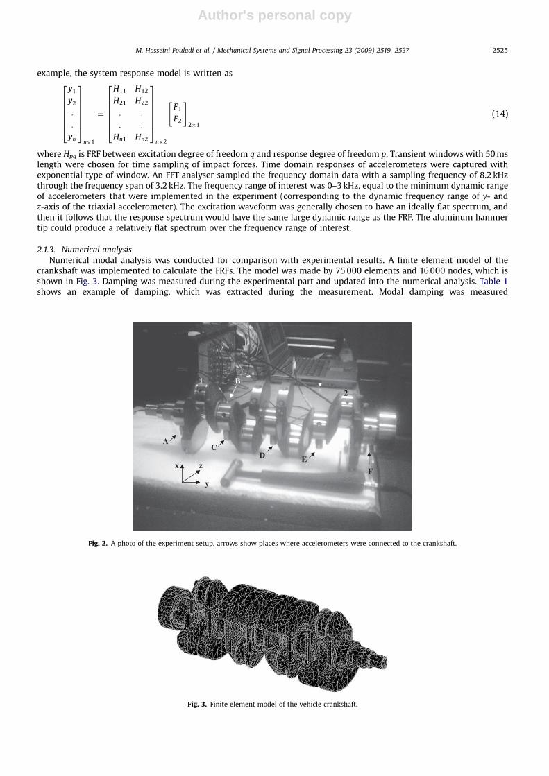
2.1.3. Numerical analysis

Numerical modal analysis was conducted for comparison with experimental results. A finite element model of thecrankshaft was implemented to calculate the FRFs. The model was made by 75 000 elements and 16 000 nodes, which isshown in Fig. 3. Damping was measured during the experimental part and updated into the numerical analysis. Table 1shows an example of damping, which was extracted during the measurement. Modal damping was measured

ARTICLE IN PRESS

Fig. 3. Finite element model of the vehicle crankshaft.

AC

D E

B

F

2

1

y

x z

Fig. 2. A photo of the experiment setup, arrows show places where accelerometers were connected to the crankshaft.

M. Hosseini Fouladi et al. / Mechanical Systems and Signal Processing 23 (2009) 2519–2537 2525

Author's personal copy

automatically by the analyzer PULSE at each resonance through identifying the half power (�3 dB) points of the magnitudeof the frequency response function. For a particular mode, damping ratio Br is calculated by

Br ¼Df

2f r

(15)

where Df is the frequency bandwidth between the two half power points and fr is the resonance frequency. PULSE type3560 contains a built-in standard cursor reading, which calculates the modal damping. The accuracy of this method isdependent on the frequency resolution (1 Hz for this measurement) used for the measurement because this determineshow accurately the peak magnitude can be measured. Lumped mass characteristic was used for modeling the structure tosave memory and time needed for analysis. The Lanczos method was utilised to extract eigenvalues of all the modes forsuch a large model in the frequency span of 2 kHz. Traditionally, results are useful to check characteristics of the structureup to half of the frequency span that modes are calculated (1 kHz for this calculation).

2.2. Inverse estimation of piston forces

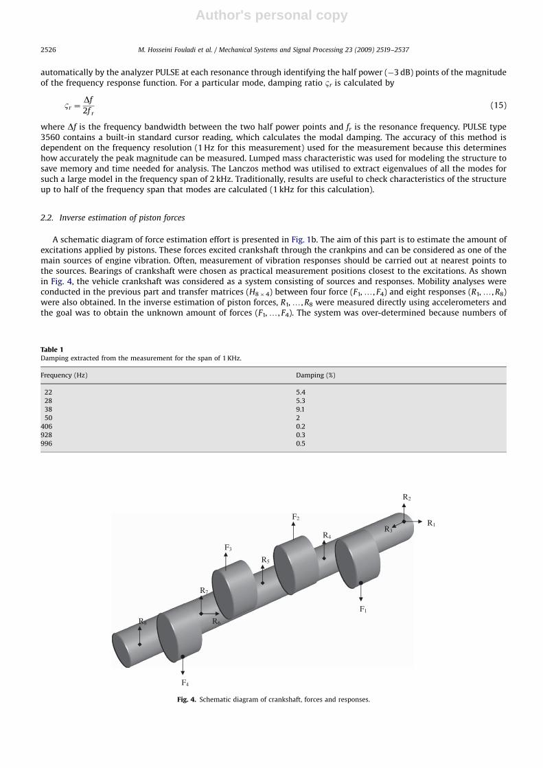
A schematic diagram of force estimation effort is presented in Fig. 1b. The aim of this part is to estimate the amount ofexcitations applied by pistons. These forces excited crankshaft through the crankpins and can be considered as one of themain sources of engine vibration. Often, measurement of vibration responses should be carried out at nearest points tothe sources. Bearings of crankshaft were chosen as practical measurement positions closest to the excitations. As shownin Fig. 4, the vehicle crankshaft was considered as a system consisting of sources and responses. Mobility analyses wereconducted in the previous part and transfer matrices (H8�4) between four force (F1,y, F4) and eight responses (R1,y, R8)were also obtained. In the inverse estimation of piston forces, R1,y, R8 were measured directly using accelerometers andthe goal was to obtain the unknown amount of forces (F1,y, F4). The system was over-determined because numbers of

ARTICLE IN PRESS

F1

F2

F3

F4

R1R3

R4

R5

R6

R7

R8

R2

Fig. 4. Schematic diagram of crankshaft, forces and responses.

Table 1Damping extracted from the measurement for the span of 1 KHz.

Frequency (Hz) Damping (%)

22 5.4

28 5.3

38 9.1

50 2

406 0.2

928 0.3

996 0.5

M. Hosseini Fouladi et al. / Mechanical Systems and Signal Processing 23 (2009) 2519–25372526

Author's personal copy

responses were more than unknown forces. This over-determination should be achieved in inverse problems to improvethe condition number and result in better solutions.

2.2.1. Setup of operational response measurement

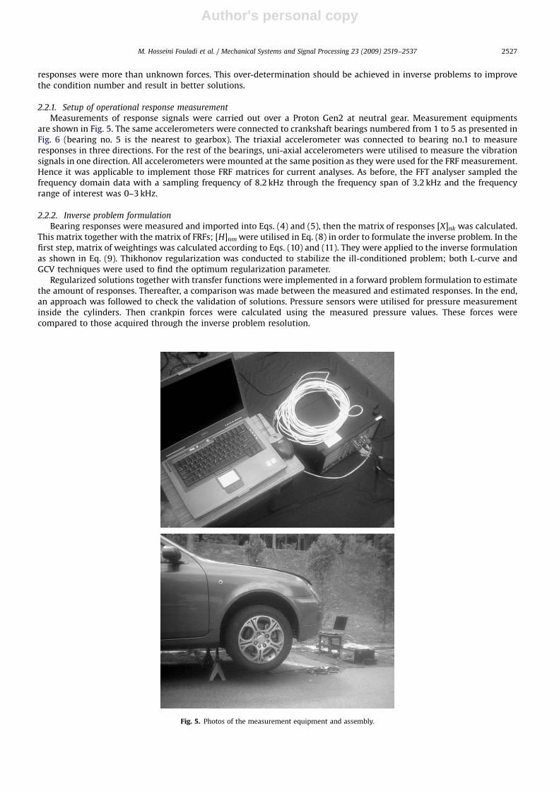
Measurements of response signals were carried out over a Proton Gen2 at neutral gear. Measurement equipmentsare shown in Fig. 5. The same accelerometers were connected to crankshaft bearings numbered from 1 to 5 as presented inFig. 6 (bearing no. 5 is the nearest to gearbox). The triaxial accelerometer was connected to bearing no.1 to measureresponses in three directions. For the rest of the bearings, uni-axial accelerometers were utilised to measure the vibrationsignals in one direction. All accelerometers were mounted at the same position as they were used for the FRF measurement.Hence it was applicable to implement those FRF matrices for current analyses. As before, the FFT analyser sampled thefrequency domain data with a sampling frequency of 8.2 kHz through the frequency span of 3.2 kHz and the frequencyrange of interest was 0–3 kHz.

2.2.2. Inverse problem formulation

Bearing responses were measured and imported into Eqs. (4) and (5), then the matrix of responses [X]nk was calculated.This matrix together with the matrix of FRFs; [H]nm were utilised in Eq. (8) in order to formulate the inverse problem. In thefirst step, matrix of weightings was calculated according to Eqs. (10) and (11). They were applied to the inverse formulationas shown in Eq. (9). Thikhonov regularization was conducted to stabilize the ill-conditioned problem; both L-curve andGCV techniques were used to find the optimum regularization parameter.

Regularized solutions together with transfer functions were implemented in a forward problem formulation to estimatethe amount of responses. Thereafter, a comparison was made between the measured and estimated responses. In the end,an approach was followed to check the validation of solutions. Pressure sensors were utilised for pressure measurementinside the cylinders. Then crankpin forces were calculated using the measured pressure values. These forces werecompared to those acquired through the inverse problem resolution.

ARTICLE IN PRESS

Fig. 5. Photos of the measurement equipment and assembly.

M. Hosseini Fouladi et al. / Mechanical Systems and Signal Processing 23 (2009) 2519–2537 2527

Author's personal copy

3. Results and observations

The applied force DOFs (also response measurement DOFs) are identical in experimental modal analysis and realcondition, which make it possible to use the measured FRFs (by modal analysis) in force reconstruction process. Thedifference is that crankshaft has less degree of freedom while it is positioned in the car rather than in the free condition.Then in real condition some modes may not be excited and the corresponding responses are zero. The additional modesincluded in the experimental FRF (free condition) will be mapped to zero forces by these zero responses, which willnot affect the overall estimations. The gyroscopic effects are mostly important in high revolution speed and huge rotordeflections. This engine was working at neutral gear and low revolution of 1500 rpm; therefore those effects wereneglected.

3.1. Mobility analysis and evaluation of FRFs

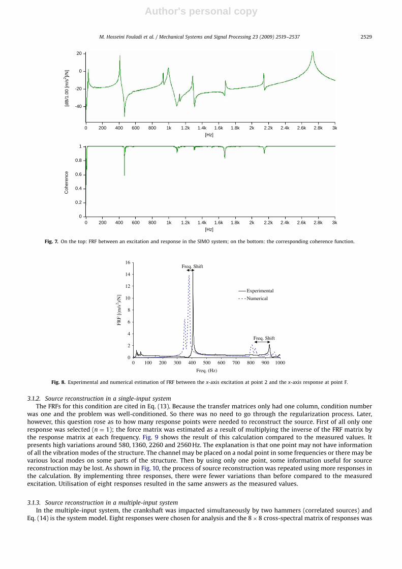
Linearity between excitation and response is the basis of frequency response analysis. Coherence function between anexcitation and response in a SIMO system is shown in Fig. 7. As expected for such a system, coherence function is perfectly1 unless around an antiresonance where signal to noise ratio is rather low. In a MIMO system with partially coherentsources, linearity between one of the sources and any response channel is not a point of interest; the coherence function isoscillating, which shows effects of the other sources.

3.1.1. Numerical and experimental FRF comparison

Reliability of calculated FRFs highly depends on accuracy of the model. Mass of the numerical model was more than thereal one because it was prepared beforehand for the same crankshaft with more counterweights. Resonances were shiftedto lower frequencies by increasing the mass of the object (traditionally it is a way of structural modification for preventingmechanical amplification). Then as shown in Fig. 8, the first natural frequency was shifted from 406 to 380 Hz. Amplitudesonly changed a little and other differences were due to imperfections in the model. Another interesting point was the valueof first natural frequency (406 Hz). It showed that the first resonance may occur at 24 000 rpm, which was much more thanthe operational crankshaft revolutions and never can be reached. The lower peak that occurred around 30 Hz was related tothe rigid-body mode, which was much lower than the amplitude of the first flexible mode (at 406 Hz) and had negligibleeffects.

ARTICLE IN PRESS

Fig. 6. Photos showing the accelerometers mounting on the crankshaft bearings.

M. Hosseini Fouladi et al. / Mechanical Systems and Signal Processing 23 (2009) 2519–25372528

Author's personal copy

3.1.2. Source reconstruction in a single-input system

The FRFs for this condition are cited in Eq. (13). Because the transfer matrices only had one column, condition numberwas one and the problem was well-conditioned. So there was no need to go through the regularization process. Later,however, this question rose as to how many response points were needed to reconstruct the source. First of all only oneresponse was selected (n ¼ 1); the force matrix was estimated as a result of multiplying the inverse of the FRF matrix bythe response matrix at each frequency. Fig. 9 shows the result of this calculation compared to the measured values. Itpresents high variations around 580, 1360, 2260 and 2560 Hz. The explanation is that one point may not have informationof all the vibration modes of the structure. The channel may be placed on a nodal point in some frequencies or there may bevarious local modes on some parts of the structure. Then by using only one point, some information useful for sourcereconstruction may be lost. As shown in Fig. 10, the process of source reconstruction was repeated using more responses inthe calculation. By implementing three responses, there were fewer variations than before compared to the measuredexcitation. Utilisation of eight responses resulted in the same answers as the measured values.

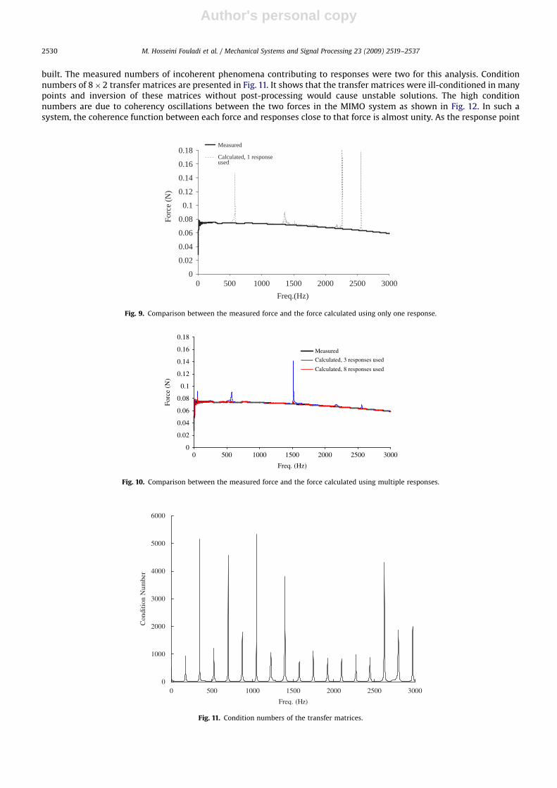
3.1.3. Source reconstruction in a multiple-input system

In the multiple-input system, the crankshaft was impacted simultaneously by two hammers (correlated sources) andEq. (14) is the system model. Eight responses were chosen for analysis and the 8�8 cross-spectral matrix of responses was

ARTICLE IN PRESS

20

0

-20

-40

1

0.8

0.6

0.4

0.2

0

0 200 400 800

600

600 1k 1.2k 1.4k 1.6k 1.8k 2k 2.2k 2.4k 2.6k 2.8k 3k[Hz]

0 200 400 800 1k 1.2k 1.4k 1.6k 1.8k 2k 2.2k 2.4k 2.6k 2.8k 3k[Hz]

[dB

/1.0

0 [m

/s2 ]/N

]C

oher

ence

Fig. 7. On the top: FRF between an excitation and response in the SIMO system; on the bottom: the corresponding coherence function.

0

2

4

6

8

10

12

14

16

0

Freq. (Hz)

FRF

[(m

/s2 )/

N]

Experimental

Numerical

Freq. Shift

Freq. Shift

100 200 300 400 500 600 700 800 900 1000

Fig. 8. Experimental and numerical estimation of FRF between the x-axis excitation at point 2 and the x-axis response at point F.

M. Hosseini Fouladi et al. / Mechanical Systems and Signal Processing 23 (2009) 2519–2537 2529

Author's personal copy

built. The measured numbers of incoherent phenomena contributing to responses were two for this analysis. Conditionnumbers of 8�2 transfer matrices are presented in Fig. 11. It shows that the transfer matrices were ill-conditioned in manypoints and inversion of these matrices without post-processing would cause unstable solutions. The high conditionnumbers are due to coherency oscillations between the two forces in the MIMO system as shown in Fig. 12. In such asystem, the coherence function between each force and responses close to that force is almost unity. As the response point

ARTICLE IN PRESS

0

0.02

0.04

0.06

0.08

0.1

0.12

0.14

0.16

0.18

0

Freq. (Hz)

Forc

e (N

)

Measured

Calculated, 3 responses used

Calculated, 8 responses used

500 1000 1500 2000 2500 3000

Fig. 10. Comparison between the measured force and the force calculated using multiple responses.

0 500 1000 1500 2000 2500 30000

1000

2000

3000

4000

5000

6000

Freq. (Hz)

Con

ditio

n N

umbe

r

Fig. 11. Condition numbers of the transfer matrices.

0

0.02

0.04

0.06

0.08

0.1

0.12

0.14

0.16

0.18

0Freq.(Hz)

Forc

e (N

)

Measured

Calculated, 1 responseused

30002500200015001000500

Fig. 9. Comparison between the measured force and the force calculated using only one response.

M. Hosseini Fouladi et al. / Mechanical Systems and Signal Processing 23 (2009) 2519–25372530

Author's personal copy

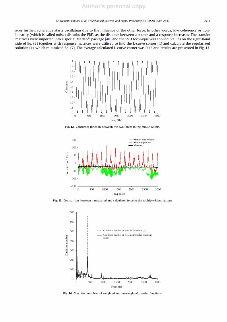
goes further, coherency starts oscillating due to the influence of the other force. In other words, low coherency or non-linearity (which is called noise) disturbs the FRFs as the distance between a source and a response increases. The transfermatrices were imported into a special Matlabs package [48] and the SVD technique was applied. Values on the right-handside of Eq. (3) together with response matrices were utilised to find the L-curve corner (l) and calculate the regularizedsolution (x), which minimized Eq. (7). The average calculated L-curve corner was 0.42 and results are presented in Fig. 13.

ARTICLE IN PRESS

0

0.1

0.2

0.3

0.4

0.5

0.6

0.7

0.8

0.9

1

Freq. (Hz)

Coh

eren

ce

0 500 1000 1500 2000 2500 3000

Fig. 12. Coherence function between the two forces in the MIMO system.

-150

-100

-50

0

50

100

150

Freq. (Hz)

Forc

e (d

B r

ef: 1

N2 )

without post process.with post process.Measured

0 500 1000 1500 2000 2500 3000

Fig. 13. Comparison between a measured and calculated force in the multiple-input system.

0

100

200

300

400

500

600

700

Freq. (Hz)

Con

ditio

n nu

mbe

r

Condition number of transfer functions (H)

Condition number of weighted transfer functions(wH)

0 500 1000 1500 2000 2500 3000

Fig. 14. Condition numbers of weighted and un-weighted transfer functions.

M. Hosseini Fouladi et al. / Mechanical Systems and Signal Processing 23 (2009) 2519–2537 2531

Author's personal copy

It can be seen that solutions without post-processing were highly unstable, resulting in strong peaks that show largedeviations from the measured excitation. Regularization has highly improved the quality of reconstructed excitation,although there are still some deviations around the strong resonance frequencies of the structure.

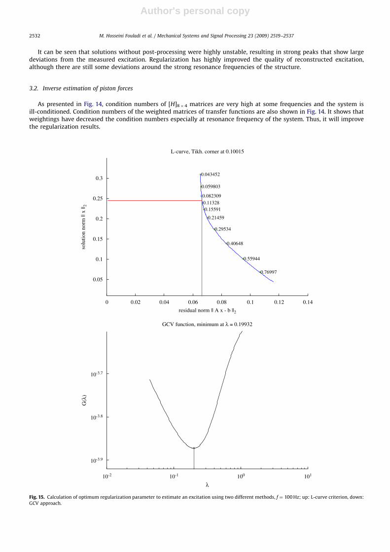
3.2. Inverse estimation of piston forces

As presented in Fig. 14, condition numbers of [H]8�4 matrices are very high at some frequencies and the system isill-conditioned. Condition numbers of the weighted matrices of transfer functions are also shown in Fig. 14. It shows thatweightings have decreased the condition numbers especially at resonance frequency of the system. Thus, it will improvethe regularization results.

ARTICLE IN PRESS

0 0.02 0.04 0.06 0.08 0.1 0.12 0.14

0.05

0.1

0.15

0.2

0.25

0.3

0.76997

0.55944

0.40648

0.29534

0.21459

0.155910.113280.082309

0.059803

0.043452

residual norm || A x - b ||2

solu

tion

norm

|| x

||2

L-curve, Tikh. corner at 0.10015

10-2 10-1 100 101

10-3.9

10-3.8

10-3.7

λ

G(λ

)

GCV function, minimum at λ = 0.19932

Fig. 15. Calculation of optimum regularization parameter to estimate an excitation using two different methods, f ¼ 100 Hz; up: L-curve criterion, down:

GCV approach.

M. Hosseini Fouladi et al. / Mechanical Systems and Signal Processing 23 (2009) 2519–25372532

Author's personal copy

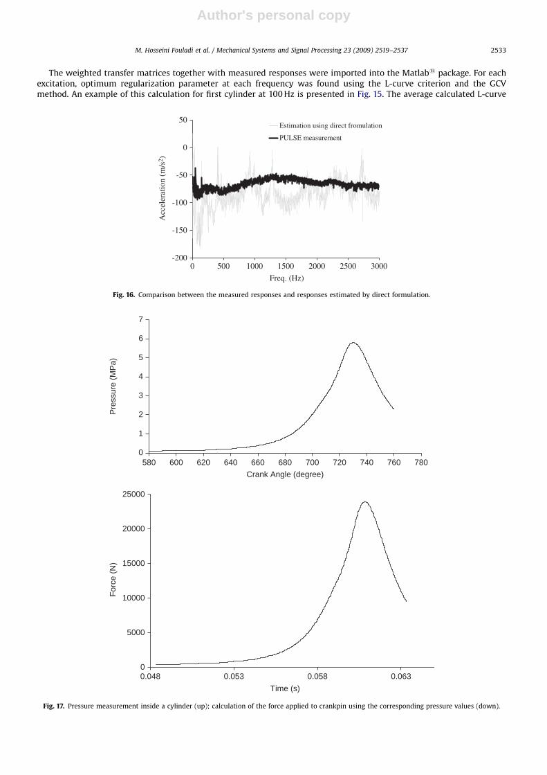
The weighted transfer matrices together with measured responses were imported into the Matlabs package. For eachexcitation, optimum regularization parameter at each frequency was found using the L-curve criterion and the GCVmethod. An example of this calculation for first cylinder at 100 Hz is presented in Fig. 15. The average calculated L-curve

ARTICLE IN PRESS

0

1

2

3

4

5

6

7

580Crank Angle (degree)

Pre

ssur

e (M

Pa)

0

5000

10000

15000

20000

25000

0.048Time (s)

Forc

e (N

)

600 620 640 660 680 700 720 740 760 780

0.053 0.058 0.063

Fig. 17. Pressure measurement inside a cylinder (up); calculation of the force applied to crankpin using the corresponding pressure values (down).

-200

-150

-100

-50

0

50

Freq. (Hz)

Acc

eler

atio

n (m

/s2 )

Estimation using direct fromulation

PULSE measurement

0 500 1000 1500 2000 2500 3000

Fig. 16. Comparison between the measured responses and responses estimated by direct formulation.

M. Hosseini Fouladi et al. / Mechanical Systems and Signal Processing 23 (2009) 2519–2537 2533

Author's personal copy

corner was l ¼ 0.1 and the minimum value for GCV function was at l ¼ 0.2. Each value was implemented in the Tikhonovformulation to find the corresponding regularized solution. As a preliminary utilisation of results, the regularized solutionstogether with transfer matrices were imported into a forward formulation to estimate the responses as presented in Fig. 16.It should not be misunderstood with the combustion force estimation results as the main outcomes of the research. Fig. 16presents the residue error to the reader. This graph shows that estimated and measured responses outside the chamber aredifferent at many frequencies. They are not expected to be wholly the same because the Tikhonov regularization is acompromise between the solution norm and residue norm for achieving the best results. Differences are due to residuenorm, which was adjusted in order to obtain the combustion forces as the regularized solution; it does not convey theinaccuracy of the inverse estimation of combustion forces.

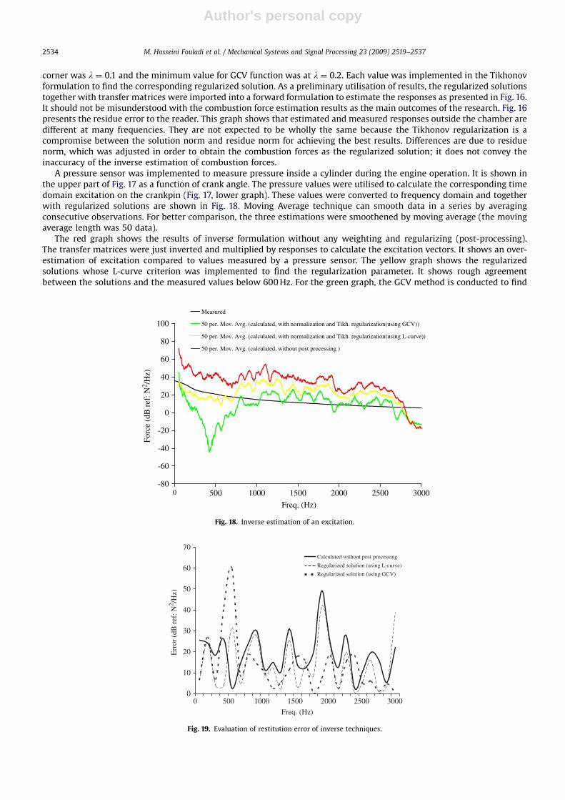
A pressure sensor was implemented to measure pressure inside a cylinder during the engine operation. It is shown inthe upper part of Fig. 17 as a function of crank angle. The pressure values were utilised to calculate the corresponding timedomain excitation on the crankpin (Fig. 17, lower graph). These values were converted to frequency domain and togetherwith regularized solutions are shown in Fig. 18. Moving Average technique can smooth data in a series by averagingconsecutive observations. For better comparison, the three estimations were smoothened by moving average (the movingaverage length was 50 data).

The red graph shows the results of inverse formulation without any weighting and regularizing (post-processing).The transfer matrices were just inverted and multiplied by responses to calculate the excitation vectors. It shows an over-estimation of excitation compared to values measured by a pressure sensor. The yellow graph shows the regularizedsolutions whose L-curve criterion was implemented to find the regularization parameter. It shows rough agreementbetween the solutions and the measured values below 600 Hz. For the green graph, the GCV method is conducted to find

ARTICLE IN PRESS

-80

-60

-40

-20

0

20

40

60

80

100

Freq. (Hz)

Forc

e (d

B r

ef: N

2 /Hz)

Measured

50 per. Mov. Avg. (calculated, with normalization and Tikh. regularization(using GCV))

50 per. Mov. Avg. (calculated, with normalization and Tikh. regularization(using L-curve))

50 per. Mov. Avg. (calculated, without post processing )

0 500 1000 1500 2000 2500 3000

Fig. 18. Inverse estimation of an excitation.

0

10

20

30

40

50

60

70

Freq. (Hz)

Err

or (

dB r

ef: N

2 /Hz)

Calculated without post processing

Regularized solution (using L-curve)

Regularized solution (using GCV)

0 500 1000 1500 2000 2500 3000

Fig. 19. Evaluation of restitution error of inverse techniques.

M. Hosseini Fouladi et al. / Mechanical Systems and Signal Processing 23 (2009) 2519–25372534

Author's personal copy

the optimum regularization parameter for the Tikhonov technique. These results are closer to measured excitations unlessfor frequencies lower than 600 Hz. One reason is that noise sources of automobile engine are highly correlated in lowfrequencies. The other reason may be the existence of other kinds of noise rather than white noise, which extremely affectsthe GCV results. For better comparison of techniques, absolute difference between each estimation and the measured forcewas calculated and the above outcomes confirmed as shown in Fig. 19.

Although the regularization technique calculated reasonable values, still there were differences between the estimationand experimental results. One explanation was that for operational response measurement in a real car, accelerometerswere not mounted exactly at the same positions as they were used for modal analysis in the laboratory. In modal analysis,these transducers were mounted on crankshaft at the bearing positions. But in real response measurements, only theycould be attached to the outer area of bearing housing. The linearity assumption of modal analysis was an important reasonof source estimation errors. In modal analysis, objects were impacted by small forces to keep the system in linear behavior.But response measurement was accomplished in real engine mechanism with great forces. Thus it was infeasible toconsider the system operation as fully linear.

4. Conclusions and recommendations

Modal analysis was utilised as a unique method to estimate the characteristics of structure. For the sourcereconstruction, number and position of response channels were important. They were needed to expand over the object toreceive information of all the modes. Firstly, this information was used to reconstruct the excitation in a single-inputsystem. It was shown that increasing the number of response channels improved the accuracy of reconstructed force untilthe measured and calculated values were overlapped. For the single-input system, condition number was equal to one andthe system was well-conditioned. But the multiple-input systems would be treated carefully. Transfer matrices with highcondition number were ill-conditioned and inversion of these matrices would result in extreme errors. Therefore, theTikhonov method was implemented to calculate the regularized solutions. The accuracy of reconstructed forces wasextremely improved, although there were some deviations around the strong resonance frequencies of the structure.Furthermore, other techniques such as weighting method can be utilised to improve the results.

Engine internal vibration sources were estimated very well using the verified inverse formulation and measured FRFs.The Tikhonov technique was conducted to estimate the regularized solutions in such an ill-conditioned system. The L-curvecriterion and the GCV method were utilised to get the optimum regularization parameter. In real-world applications,different kinds of error are available. Hence, the L-curve criterion is more robust than the GCV method. Nevertheless, in theregion that engine vibrations normally have lower correlations f4600 Hz, GCV results were much better and closer to themeasurement values. Thus it can be concluded that to achieve consistent results in engine vibration source reconstruction,L-curve is appropriate up to 600 Hz and after that GCV may be utilised to estimate the optimum regularization parameter.

It is the first time that the GCV technique is utilised for combustion force reconstruction based on the measuredresponses outside the combustion chamber. A direct comparison of these results with others is not applicable as previousstudies are only conducted on basic models or test bench in laboratory. Leclere et al. [41] utilised truncated singularvalue decomposition as the regularization technique and the L-curve method to estimate the regularization parameter.They estimated the main bearing loads in a diesel engine test bench. Their indirect estimations were 25 dB greater than themeasured values above 200 Hz. Implementation of L-curve and GCV techniques below and after 600 Hz, respectively, assuggested by this paper, will reduce the error mainly below 20 dB throughout the spectrum in operational condition of realengine.

This inverse formulation can be considered as the basis of a whole approach to find the internal forces of machinery. Theentire mathematical model of the system can be achieved by modeling all the engine parts through their transfer functions.An accessible point should be used for response measurement. Then these responses may be related to any internalexcitation (near or far) by a series of transfer functions. Non-linearities corresponding to non-coherent output power ofsystems may be cited as the shortcoming of this method.

Acknowledgment

Authors greatly appreciate Mr. Azizan and Mr. Arif from Engine Workshop, Faculty of Engineering, UniversitiKebangsaan Malaysia for their kind assistance during the engine experiment.

References

[1] H. Herlufsen, Modal analysis using multi-reference and multiple-input multiple output techniques, Bruel & Kjær Application Note BO 0505-12,no date.

[2] M. Wamsler, T. Rose, Advanced mode shape identification method for automotive application via modal kinetic energy plots assisted by numerousprinted outputs, Presented at the MSC Americas Users’ Conference Sheraton Universal Hotel, Universal City, California, 1998.

[3] F. Mancosu, D. Da Re, D. Minen, Non-linear modal rolling tyre model for dynamic simulation with ADAMS, Presented at European Adams Users’Conference, Paris, 1998.

ARTICLE IN PRESS

M. Hosseini Fouladi et al. / Mechanical Systems and Signal Processing 23 (2009) 2519–2537 2535

Author's personal copy

[4] S. Seidlitz, Using modal analysis to verify a torsional mass elastic model, in: Proceedings of the 16th International Modal Analysis Conference (SPIE),vol. 3243, 1998.

[5] H. Okamura, S. Arai, Experimental modal analysis for cylinder block-crankshaft substructure systems of six-cylinder in-line diesel engines, SAE Paper2001-01-1421, 2001.

[6] D. Guan, C. Fan, X. Xie, A dynamic tyre model of vertical performance rolling over cleats, Vehicle System Dynamics 43 (1) (2005) 209–222.[7] M. Xingguo, Y. Xiaomei, W. Bangchun, Multi-body dynamics simulation on flexible crankshaft system, in: Proceedings of the 12th IFToMM World

Congress, Besancon, France, 2007.[8] R. Upton, Advanced acoustic solutions, Bruel & Kjær Technical Workshop, Selangor, Malaysia, 2006.[9] M.J. Mohd. Nor, 1996, A machine component monitoring system using audio acoustic signals, Ph.D. Thesis, The University of Sheffield Hallam, School

of Engineering, 1996.[10] G. Moschioni, B. Saggin, M. Tarabini, Sound source identification using coherence and intensity based methods, in: Proceedings of the

Instrumentation and Measurement Technology Conference, IMTC 2004, Como, Italy, 2004.[11] S.W. Kang, Y.S. Han, T.Y. Hwang, Y. Son, J.C. Koo, Noise source identification of hard disk drives using sound intensity and its control, in: Proceedings of

the Asia-Pacific Magnetic Recording Conference, APMRC 2000, Tokyo, Japan, 2000.[12] S. Gade, P. Rasmussen, J. Deel, STSF, a unique technique for near-field acoustic holography and exterior noise measurements, Journal of Society of

Automotive Engineers of Japan 16 (3) (1995), 325–325(1).[13] X.D. Li, S. Zhou, Spatial transformation of the discrete sound field from a propeller, Journal of American Institute of Aeronautics and Astronautics 34

(6) (1995) 1097–1102.[14] J. Hald, Use of non-stationary STSF for the analysis of transient engine noise radiation, Bruel & Kjær Technical Review, Denmark, 1999.[15] Bruel & Kjær Magazine, Central Japan railway company—advanced noise measurement techniques for new Shinkansen & want a quieter life? The

latest acousitc solutions will help, No. 1, 2006.[16] J.D. Fieldhouse, T.P. Newcomb, Double pulsed holography used to investigate noisy brakes, Journal of Optics and Lasers in Engineering 25 (6) (1996)

455–494.[17] R.J. Ruhala, C.B. Burroughs, Tire/pavement interaction noise source identification using multi-planar nearfield acoustic holography, SAE Paper 1999-

01-1733, Noise and Vibration Conference and Exposition, Traverse City, Michigan, 1999.[18] J. Hald, Time domain acoustical holography and its applications, Journal of Sound and Vibration 35 (2) (2001) 16–25.[19] S. Fischer, K.U. Simmerb, Beamforming microphone arrays for speech acquisition in noisy environments, Journal of Speech Communication 20 (3–4)

(1996) 215–227.[20] Y.C. Choi, Y.H. Kim, Impulsive sources localisation in noisy environment using modified beamforming method, Journal of Mechanical Systems and

Signal Processing 20 (6) (2006) 1473–1481.[21] B.K. Kim, J.G. Ih, On the reconstruction of the vibro-acoustic field over the surface enclosing an interior space using the boundary element method,

Journal of Acoustical Society of America 100 (5) (1996) 3003–3016.[22] A. Schuhmacher, On the use of inverse BEM for driving equivalent acoustical source models, in: Proceedings of the International Congress and

Exposition on Noise Control Engineering, Dearborn, MI, USA, 2002.[23] R. Visser, Inverse source identification based on acoustic particle velocity measurements, in: Proceedings of the International Congress and

Exposition on Noise Control Engineering, Dearborn, MI, USA, 2002.[24] A. Gerard, A. Berry, P. Masson, Control of tonal noise from subsonic axial fan. Part 1: reconstruction of aeroacoustic sources from far-field sound

pressure, Journal of Sound and Vibration 288 (2005) 1049–1075.[25] N.J. Jacobsen, J. Morkholt, A. Schuhmacher, Surface vibration reconstruction using the inverse boundary element method and planar near-field

acoustical holography, in: Proceedings of the Twelfth International Congress on Sound and Vibration, Lisbon, Portugal, 2005.[26] K.U. Nam, Y.H. Kim, Errors due to sensor and position mismatch in planar acoustic holography, Journal of Acoustical Society of America 106 (4) (1999)

1655–1665.[27] A. Schuhmacher, Sound source reconstruction using inverse sound field calculation, Ph.D. Thesis, The Technical University of Denmark, Department

of Acoustic Technology, 2000.[28] M. Harrison, Vehicle Refinement-Controlling Noise and Vibration in Road Vehicles, Elsevier Butterworth-Heinemann Publication, ISBN 0750661291,

2004.[29] W.G. Halvorsen, J.S. Bendat, Noise source identification using coherent output power spectra, Journal of Sound and Vibration 9 (1975) 15–24.[30] M. Hosseini Fouladi, M.J. Mohd. Nor, A. Kamal Ariffin, Spectral analysis methods for vehicle interior vibro-acoustics identification, Mechanical

Systems and Signal Processing 23 (2) (2009) 489–500.[31] M.G. Kim, J.S. Jo, J.H. Sohn, W.S. Yoo, Reduction of road noise by the investigation of contributions of vehicle components, SAE Paper 2003-01-1718,

Noise & Vibration Conference and Exhibition, Grand Traverse, MI, USA, 2003.[32] G. Koners, Panel noise contribution analysis: An experimental method for determining the noise contribution of panels to an interior noise, SAE

Paper 2003-01-1410, Noise & Vibration Conference and Exhibition, Grand Traverse, MI, USA, 2003.[33] J.S. Bendat, A.G. Piersol, Engineering Application of Correlation and Spectral Analysis, Wiley-Interscience, New York, 1980.[34] Z. Junhong, H. Jun, CAE process to simulate and optimise engine noise and vibration, Mechanical Systems and Signal Processing 20 (6) (2006)

1400–1409.[35] P. Mas, P. Sas, K. Wyckaert, Indirect force identification based upon impedance matrix inversion: a study on statistical and deterministical accuracy,

in: Proceedings of the International Seminar on Modal Analysis, Leuven, 1994.[36] H.R. Busby, D.M. Trujillo, Optimal regularization of an inverse dynamics problem, Computers & Structures 63 (2) (1997) 243–248.[37] J. Kromulski, E. Hojan, An application of two experimental modal analysis methods for the determination of operational deflection shapes, Journal of

Sound and Vibration 196 (4) (1996) 429–438.[38] A.N. Thite, D.J. Thompson, The quantification of structure-borne transmission paths by inverse methods. Part 1: Improved singular value rejection

methods,, Journal of Sound and Vibration 264 (2003) 411–431.[39] A.N. Thite, D.J. Thompson, The quantification of structure-borne transmission paths by inverse methods. Part 2: Use of regularization techniques,

Journal of Sound and Vibration 264 (2003) 433–451.[40] Q. Leclere, C. Pezerat, B. Laulagnet, L. Polac, Indirect measurement of main bearing loads in an operating diesel engine, Journal of Sound and Vibration

286 (2005) 341–361.[41] Q. Leclere, C. Pezerat, B. Laulagnet, L. Polac, Different least square approaches to identify dynamic forces acting on an engine cylinder block, Acta

Acoustica 90 (2004) 285–292.[42] W.H. Press, B.P. Flannery, S.A. Teukolsky, W.T. Vetterling, Numerical Recipes. The Art of Scientific Computing (FORTRAN version), Cambridge

University Press, Cambridge, 1989.[43] K.A. Woodbury, Inverse Engineering Handbook, CRC Press, Boca Raton, FL, ISBN 0849308615, 2002.[44] G.R. Liu, X. Han, Computational Inverse Techniques in Nondestructive Evaluation, CRC Press, Boca Raton, FL, 2003.[45] S.M. Price, R.J. Bernhard, Virtual coherence: a digital signal processing technique for incoherent source identification, in: Proceedings of IMAC 4,

Schenectady, NY, USA, 1986.[46] A.N. Tikhonov, Solution of incorrectly formulated problems and the regularization method, Soviet Math. Dokl. 4 (1963) 1035–1038.[47] M.W. Andersen, J. Pedersen, Localized solutions in inverse sound source reconstructions, Polytechnic midway project at IMM, Technical University of

Denmark, 2003.[48] P.C. Hansen, Regularization tools: a Matlab package for analysis and solution of discrete ill-posed problems, Numerical Algorithms 6 (1994) 1–35.

ARTICLE IN PRESS

M. Hosseini Fouladi et al. / Mechanical Systems and Signal Processing 23 (2009) 2519–25372536

Author's personal copy

[49] X. Chiementin, F. Bolaers, L. Rasolofondraibe, J.P. Dron, Localization and quantification of vibratory sources, Application to the predictive maintenanceof rolling bearings, Journal of Sound and Vibration, doi:10.1016/j.jsv.2008.02.029, 2008.

[50] J.A. Fabunmi, Effects of structural modes on vibratory force determination by the pseudo-inverse technique, AIAA Journal 24 (3) (1986) 504–509.[51] G. Wahba, Spline methods for observational data, in: CBMS-NSF Regional Conference Series in Applied Mathematics, vol. 59, SIAM, Philadelphia,

1990.[52] G.H. Golub, M. Heath, G. Wahba, Generalized cross-validation as a method for choosing a good ridge parameter, Technometrics 21 (2) (1979)

215–223.[53] S.H. Yoon, P.A. Nelson, Estimation of acoustic source strength by inverse methods: Part II, Experimental investigation of methods for choosing

regularization parameters, Journal of Sound and Vibration 233 (4) (2000) 669–705.[54] P.C. Hansen, Rank-Deficient and Discrete Ill-Posed Problems: Numerical Aspects of Linear Inversion, Society for Industrial and Applied Mathematics,

Philadelphia, 1998.[55] P.C. Hansen, Analysis of discrete ill-posed problems by means of the L-curve, SIAM Review 34 (1992) 561–580.

ARTICLE IN PRESS

M. Hosseini Fouladi et al. / Mechanical Systems and Signal Processing 23 (2009) 2519–2537 2537