A Comparative Study of Hadoop MapReduce,

Apache Spark & Apache Flink for Data Science

Bilal Akil

Supervised by: A/Prof. Uwe Rohm

Faculty of Engineering and IT

School of Information Technology

The University of Sydney, Australia

bilal.akil@sydney.edu.au

A thesis submitted in fulfilment of the requirements

for the degree of Master of Philosophy

March 2018

brought to you by COREView metadata, citation and similar papers at core.ac.uk

provided by Sydney eScholarship

I’ll take this opportunity to express my deepest gratitude to Joy, my fam-

ily, and Uwe Rohm, for your support and faith in my ability to persevere

through this candidature. Without such, I surely would not have made it.

Furthermore, I’d like to thank Uwe Rohm again, and Ying Zhou, Alan

Fekete, and the school’s Database Research Group, for the critical feedback

and tutelage that kept this research on track and helped me to present at an

international conference – a feat I was doubtful of being able to achieve.

I also acknowledge and appreciate the quality research of Veiga et al.

[36], whose performance comparison data was used to accommodate the per-

formance dimension of this multidimensional comparison. This has been

further acknowledged within the thesis text wherever their research has been

utilised.

Ying Zhou provided great assistance in updating the cluster and software

for the usability study, as well as the Flickr data, problems, and solutions

for assignment 1.

Uwe Rohm, the supervisor for my Master’s candidature, developed new,

and updated existing learning materials for the course, which were depended

on by the usability study, and helped immensely through all stages of its

execution.

They both provided invaluable feedback and support as I devised the

usability study and compiled its results, as well as in reviewing and editing

my writing of the below publications.

i

Related Publications

The following publications arose from work related to this thesis, including

some content from the introduction and conclusion, as well as from Chap-

ters 2 and 3:

• Bilal Akil, Ying Zhou, and Uwe Rohm. “On the Usability of Hadoop

MapReduce, Apache Spark & Apache Flink for Data Science”. In:

2017 IEEE International Conference on Big Data. IEEE Big Data’17.

2017, pp. 303–310

• Bilal Akil, Ying Zhou, and Uwe Rohm. Technical Report: On the

Usability of Hadoop MapReduce, Apache Spark, & Apache Flink for

Data Science. Tech. rep. 709. School of IT, University of Sydney,

2018

Statement of Originality

This is to certify that to the best of my knowledge, the content of this thesis

is my own work. This thesis has not been submitted for any degree or other

purposes.

I certify that the intellectual content of this thesis is the product of my

own work and that all the assistance received in preparing this thesis and

sources have been acknowledged.

Bilal Akil

Human Ethics

Ethics approval was attained prior to commencement of the usability study

described in Chapter 3, from the University of Sydney’s Human Research

Ethics Committee under project number 2017/212. This application was

supported by the university’s Research Cluster for Human-centred Technol-

ogy.

ii

Abstract

Distributed data processing platforms for cloud computing are impor-

tant tools for large-scale data analytics. Apache Hadoop MapReduce has

become the de facto standard in this space, though its programming interface

is relatively low-level, requiring many implementation steps even for simple

analysis tasks. This has led to the development of advanced dataflow ori-

ented platforms, most prominently Apache Spark and Apache Flink. Those

not only aim to improve performance, but also provide high-level data pro-

cessing functionality, such as filtering and join operators, which should make

data analysis tasks easier to develop. But with limited comparison data, how

would data scientists know which system they should choose?

This research compares: Apache Hadoop MapReduce; Apache Spark;

and Apache Flink, from the perspectives of performance, usability and prac-

ticality, for batch-oriented data analytics. We propose and apply a method-

ology which guides the preparation of multidimensional software compar-

isons and the presentation of their results. The methodology was effective,

providing direction and structure to the comparison, and should serve as

helpful for future comparisons. The comparison results confirm that Spark

and Flink are superior to Hadoop MapReduce in performance and usability.

Spark and Flink were similar in all three perspectives, however as per the

methodology, readers have the flexibility to adjust weightings to their needs,

which could differentiate them on a case-by-case basis.

We also report on the design, execution and results of a large-scale us-

ability study with a cohort of masters students, who learn and work with

all three platforms, solving different use cases in data science contexts. Our

findings show that Spark and Flink are preferred platforms over MapReduce.

Among participants, there was no significant difference in perceived prefer-

ence or development time between both Spark and Flink. These results were

included in the usability component of the multidimensional comparison.

iii

Contents

1 Introduction 1

1.1 Study Conception . . . . . . . . . . . . . . . . . . . . . . . . . 5

1.2 Systems . . . . . . . . . . . . . . . . . . . . . . . . . . . . . . 7

1.2.1 Apache Hadoop MapReduce . . . . . . . . . . . . . . . 8

1.2.2 Apache Spark . . . . . . . . . . . . . . . . . . . . . . . 11

1.2.3 Apache Flink . . . . . . . . . . . . . . . . . . . . . . . 13

2 Literature Review 16

2.1 System Comparisons . . . . . . . . . . . . . . . . . . . . . . . 16

2.2 Usability Studies . . . . . . . . . . . . . . . . . . . . . . . . . 18

2.3 Comparison Methodologies . . . . . . . . . . . . . . . . . . . 19

2.4 Interdisciplinary Usage . . . . . . . . . . . . . . . . . . . . . . 20

2.4.1 Web Scraper . . . . . . . . . . . . . . . . . . . . . . . 22

3 Usability Study 29

3.1 Background . . . . . . . . . . . . . . . . . . . . . . . . . . . . 29

3.2 Design . . . . . . . . . . . . . . . . . . . . . . . . . . . . . . . 31

3.2.1 Assignment Tasks . . . . . . . . . . . . . . . . . . . . 32

3.2.2 Data Analysis Scenarios . . . . . . . . . . . . . . . . . 33

3.2.3 Self-Reflection Surveys . . . . . . . . . . . . . . . . . . 34

3.2.4 System Usability Scale (SUS) . . . . . . . . . . . . . . 35

3.3 Execution . . . . . . . . . . . . . . . . . . . . . . . . . . . . . 37

3.3.1 Self-Reflection Surveys . . . . . . . . . . . . . . . . . . 40

3.4 Analysis . . . . . . . . . . . . . . . . . . . . . . . . . . . . . . 41

3.4.1 Method . . . . . . . . . . . . . . . . . . . . . . . . . . 41

iv

3.4.2 Background of Participants . . . . . . . . . . . . . . . 44

3.4.3 Preferences and SUS Scores . . . . . . . . . . . . . . . 45

3.4.4 Influence of Assignments . . . . . . . . . . . . . . . . . 46

3.4.5 Programming Duration versus System . . . . . . . . . 48

3.4.6 Influence of Programming Experience . . . . . . . . . 49

3.4.7 Influence of Programming Language . . . . . . . . . . 51

3.4.8 Individual SUS Statements . . . . . . . . . . . . . . . 54

3.4.9 Free-text Feedback and Other Impressions . . . . . . . 55

4 Comparison and Methodology 58

4.1 Methodology . . . . . . . . . . . . . . . . . . . . . . . . . . . 59

4.1.1 Outline . . . . . . . . . . . . . . . . . . . . . . . . . . 59

4.1.2 Design and Justification . . . . . . . . . . . . . . . . . 62

4.2 Result . . . . . . . . . . . . . . . . . . . . . . . . . . . . . . . 68

4.2.1 Step 1: Context and audience . . . . . . . . . . . . . . 68

4.2.2 Step 2: High-level considerations . . . . . . . . . . . . 69

4.2.3 Steps 3 & 5: Breakdown and results . . . . . . . . . . 71

5 Conclusion 85

Bibliography 92

v

Chapter 1

Introduction

Across many scientific disciplines, automated scientific experiments have fa-

cilitated the gathering of unprecedented volumes of data, well into the ter-

abyte and petabyte scale [24]. Big data analytics is becoming an important

tool in these disciplines, and consequently more and more non-computer sci-

entists require access to scalable distributed computing platforms. However,

distributed data processing is a difficult task requiring specialised knowledge.

Distributed computing platforms were created to abstract away distri-

bution challenges. One of the most popular systems is Apache Hadoop

which provides a distributed file system, resource negotiator, scalable pro-

gramming environment named MapReduce, and other features to enable or

simplify distributed computing [6, 14]. While a tremendous step in the right

direction, effective use of this environment still requires familiarity with the

functional programming paradigm and with a relatively low-level program-

ming interface.

Following the success of Hadoop MapReduce, several newer systems were

created introducing higher levels of abstraction. MapReduce addresses the

main challenges of parallelising distributed computations – including high

scalability, built-in redundancy, and fail safety. Newer systems including

Apache Flink [5, 13] and Apache Spark [7, 38] extend their focus to the

needs of efficient distributed data processing: dataflow control (including

support for iterative processing), efficient data caching, and declarative data

processing operators.

1

Scientists have now a choice between several distributed computing plat-

forms, and to guide their decision several comparison studies have been pub-

lished recently [9, 28, 29]. The focus of those studies was performance, which

is perhaps not the primary problem for platforms built from the ground up

with scalability in mind. More interesting is the question of the usability

of those platforms, given that they will be used by non-computer scientists.

Here we define usability as the ease of learning the concepts and usage of,

and becoming proficient with a given system. But there are no reliable

comparisons or large-scale usability studies so far.

Furthermore, users would need to consider the practicality of the systems

given their individual circumstances. For instance, is their existing cluster

configuration supported by the system, and could they use a programming

language for which they have already got a workflow and development en-

vironment setup? These real-world considerations are often left behind in

system comparisons, but would be an important part of the decision mak-

ing process for a potential user. The user may not have the know-how, or

even permission, to enact changes on cluster configurations or install and

configure new programming languages and environments.

We have now described three factors that potential users tend to consider

before deciding on a system to use: performance; usability; and practicality.

While some may have the resources available to investigate these factors

themselves, this will not be an option for many, who for the lack of other

options, will instead resort to utilising software as described in previous

research.

This is often not a bad choice. However, it could sometimes lead to the

usage of an inappropriate system, in turn increasing cost or reducing poten-

tial impact, for instance where a more appropriate system could have been

used to run more experiments given the same amount of time and resources.

In more extreme cases however, where too small a portion of research is

conducted utilising modern or experimental technology in a particular dis-

cipline, it can be considered as slowing the technological progression of that

discipline as a whole. As an example, we observed that when distributed

computing is used in the bioinformatics discipline, MapReduce remains the

dominant computational engine, which is strange considering both the per-

2

formance and usability benefits of MapReduce’s modern competitors – see

Chapter 1.2 Section 2.4 for this discussion. This could indeed be due to

the repeated following of past practices, as the more modern options remain

largely unexplored there.

Thus we aim to provide a succinct, reliable multidimensional comparison

of distributed computing engines that will help data scientists identify the

system which would best suit their research, instead of potentially resorting

to suboptimal tooling which could increase their effort and reduce their

reward. The comparison must be suitable for viewers of differing technical

backgrounds, as a data scientist or bioinformatician, for instance, would

likely not be as familiar with the deeper concepts of distributed computing

than a computer scientist would. And while all this will be useful in the

present, the distributed computing space will continue to evolve, and these

comparisons would need to be adjusted and repeated considering the major

systems of the times, helping disciplines who utilise these tools to not fall

behind – which is similarly the case in contexts other distributed computing

and data science, as the rapid development of technology is a somewhat

universal challenge across both sciences and in the industry.

To address these needs we propose a methodology for conceiving and dis-

playing the results of multidimensional software comparisons, and employ it

for the first time in this thesis. We present a comparison of Apache Hadoop

MapReduce; Apache Spark; and Apache Flink, considering performance, us-

ability and practicality, in a batch-oriented data analytics context. The per-

formance component of the methodology will utilise an existing performance

comparison (Veiga et al. [36]) between the three systems; the practicality

component consists of various static analyses; and to complete the usabil-

ity component we combine static analysis with the results of a large-scale

usability study that we performed as part of this thesis.

The usability study was conducted within a cloud computing course at

The University of Sydney. The course was targeted at masters students from

various backgrounds, including IT and data science. It is, to the best of our

knowledge, the largest usability study of modern data processing platforms.

Participants of the study had to implement three different data analysis

tasks with use cases involving social media, immunology and genomics. The

3

first task was implemented using MapReduce, while the last two tasks were

implemented in a crossed A/B test with half the class first using Flink and

the other half Spark.

All in all, this thesis details the following contributions:

Chapter 2 A literature review of related works considering existing com-

parisons, usability studies, and comparison methodologies, all in the

context of distributed computing systems or software in general.

Chapter 2 Section 2.4 A survey of the types of software developed for

large-scale DNA analysis in recent research from the BMC Bioinfor-

matics journal (as performed using a custom web scraper) and the

IEEE BigData conference.

Chapter 3 Details on the design, execution, data analysis method and re-

sults of what is, to the best of our knowledge, the largest usability

study of modern data processing platforms. We find that in-class us-

ability studies are very effective and surprisingly underutilised (at least

in the computer science space), and believe that our learnings in exe-

cution will prove useful in guiding others, thus discussing the successes

and challenges met throughout our experience.

Chapter 4 The initial proposal of a methodology to conceive and display

the results of multidimensional system comparisons, and its first appli-

cation – comparing Apache Hadoop MapReduce, Apache Spark and

Apache Flink, from the perspectives of performance, usability and

practicality, in a batch-oriented data analytics context.

Further in this chapter, you will find:

Section 1.1 The background of what led to this research, and its initial

focus on bioinformatics.

Chapter 1.2 Descriptions of the architecture and usage patterns of the

compared systems.

4

1.1 Study Conception

This research was originally focused on the bioinformatics discipline, where

we heard from colleagues that new research was being conducted using

Apache Hadoop MapReduce. With our knowledge of various modern dis-

tributed computing engines and the benefits they had, especially in terms

of usability, we found it strange that Hadoop MapReduce was still being

considered and used in new research.

Looking further in to it, we got the impression that very little bioin-

formatics research was being conducted with MapReduce’s modern descen-

dants. Thus our initial project was to try and develop a better understanding

of why this was the case (without going into the psychology or sociology of

it), which involved exploring the strengths and weaknesses that the modern

systems have in bioinformatics contexts. We found that the strengths did

indeed outweigh the weaknesses, and so proceeded to investigate methods to

increase awareness and adoption of these systems, with the goal of helping

to lower their barriers to entry.

Moving forward, we first performed a preliminary literature review and

then a more thorough examination of recent bioinformatics research in an

attempt to validate our intuition – that the more modern systems were

in fact being underutilised. The examination is presented in Chapter 1.2

Section 2.4 of this thesis, including details on the custom web scraper that

was made to traverse, scrape and filter articles from the BMC Bioinformatics

journal.

Thus validated, we considered that a reliable, multidimensional system

comparison in a bioinformatics context would serve as effective, and de-

cided that this would become our goal. We then selected prominent dis-

tributed computing engines – Apache Hadoop MapReduce; Apache Spark;

and Apache Flink – and worked to identify bioinformatics algorithms or

tasks which both involve significant amounts of data, and present a variety

of challenges in implementation or scalability. From that point we planned

to implement each of the decided algorithms on each of the selected systems,

thus providing the data for a comparison of the systems in terms of usability,

performance, and the development experience as a whole.

5

However before getting started with the implementations, we realised

that there had to be more structure in the comparison and implementations

such to reduce potential biases and increase the comparison’s integrity. The

first decision made was that instead of proceeding immediately to imple-

menting an algorithm on each system, we should instead initially create a

‘blueprint implementation’ for each task in an unrelated, non-distributed en-

vironment, such as plain Python, and then work on mapping that blueprint

implementation to each of the individual systems. This would separate

any difficulties in understanding and implementing the algorithm itself from

struggles with the distributed computing systems.

Secondly, some details for the comparison needed to be decided up front

so we would know what to keep track of or look out for during the im-

plementation process. It was this hurdle that led to the proposal of the

methodology that will be discussed in Chapter 4. We realised the proposed

methodology would need to be flexible enough to handle the different use

cases and systems, and with a bigger picture in mind, also different com-

parison dimensions and audiences – otherwise there would be little benefit

in proposing a methodology at all.

Following completion of the first blueprint, where the use case was DNA

short-read correction based on the Blue algorithm [20], we presented our

project and an early draft of the methodology to The University of Syd-

ney’s Database Research Group, of which we were members of, and received

important feedback which resulted in our research changing direction to-

wards what it is now. The group emphasised that while the methodology is

conceptually sound, the usability component of the comparison would suffer

greatly from the subjectivity in having a single person (myself) implement

the use cases across the systems – especially considering that we are not

members of the target audience.

Instead they strongly suggested performing a usability study, and fortu-

nately we had the opportunity to do so. Thus the direction of the research

changed: with a cloud computing course starting in the coming months, we

switched focus to attaining ethics approval and developing a usability study

to be run as part of that class. The design, execution, data analysis method

and results of the usability study are discussed in Chapter 3. Data from the

6

usability study corresponded with the usability component of the compari-

son, alongside some additional static analyses. The performance component

was covered using existing research between the systems, of which we found

plenty to exist, and ‘static’ research was performed to complete the practi-

cality component by examining the characteristics of each system.

1.2 Systems

Apache Hadoop MapReduce [14] has long been the de facto standard for

large-scale data analytics, being one of the earliest systems available to ab-

stract the challenges of distributed computing and fault tolerance away from

its users, significantly reducing the barrier to entry that was present in the

big data space.

Its success led to the creation of systems which provided higher-level

approaches to distributed computing. Apache Spark [38] and Apache Flink

(formerly Stratosphere) [13] are two prominent examples of such systems.

Spark and Flink are seen as common rivals, and have had much attention

paid to their performance merits and pitfalls [28, 31, 36]. However, these

comparisons focus primarily on the systems’ performance, while this com-

parison is also to consider usability and practicality.

Due to their prominence and competitiveness, Spark and Flink will be

the subject of this study’s comparison. Hadoop MapReduce will also be part

of the comparison, acting more as a control of sorts, allowing examination

of the relative advantages or disadvantages of each newer system compared.

We examined data from Google Scholar, the IEEE BigData Conference and

the BMC Bioinformatics journal, in an attempt to confirm that MapReduce

did indeed remain the dominant choice for distributed computing in bioin-

formatics and likely other scientific disciplines, as discussed in this chapter’s

interdisciplinary usage section.

For the purpose of the usability study in Chapter 3, all three systems

were run using Apache Hadoop YARN for resource management [35] and

HDFS as the distributed file system [33]. The following versions were used

in the usability study: Apache Hadoop MapReduce v2.7.2; Apache Spark

v2.1.1; Apache Flink v1.2.1. These were all the stable or highest non-beta

7

versions at the time of the study’s preparation.

The three following sections will describe the background and architec-

ture of each system, as well as a high-level description of their usage. Then

Section 2.4 will discuss the apparent prevalence of each system in scientific

disciplines like bioinformatics.

1.2.1 Apache Hadoop MapReduce

This brief history of Apache Hadoop is paraphrased and summarised from

an enjoyable article by Bonaci [11].

Hadoop has a long history, having been given a name by Doug Cutting

in 2006 but in development much earlier. Cutting was working with Mike

Cafarella from the University of Washington with the aim of indexing the

entire web, and also running Google’s PageRank algorithm against it. Of

course this proved an immense challenge in distribution and scalability –

hence the creation of Hadoop’s HDFS, MapReduce, and then YARN and

MapReduce 2. The former two were born with inspiration from Google

publications including The Google File System [19] and MapReduce [14].

Following Hadoop’s initial success at Google, Yahoo! took guidance

from Cutting to get themselves on-board with Hadoop, which proved to be

a great decision for the company. Later, newer web-scale companies like

Twitter, Facebook and LinkedIn started using Hadoop and contribute to

its open source codebase and tooling, thus continuing to grow the software’s

ecosystem. In 2008 Hadoop transitioned from a subproject of Apache Lucene

to the top level Apache Hadoop where it still remains, now with many

subprojects of its own.

A large part of its success was due to how it abstracted away many

distributed computing challenges from its users, being one of the earliest

systems to do so. HDFS was presented as a single reliable file system, when

in fact it handled the tasks of monitoring for failures and rebalancing the

distribution of blocks, while itself not imposing any restrictions on schema

or structure. Its acceptance of failure promoted a shift from expensive, spe-

cialised hardware to commodity hardware: if your scale is large enough,

there are inevitably going to be hardware failures, so why not expect them

8

instead of treating them as an exception? MapReduce further solved the

problems of parallelisation, distribution and fault tolerance in program ex-

ecution.

However, the original MapReduce had a flaw in the sense that it prac-

tically handled all responsibilities (other than the distributed file system),

including scheduling, managing job execution, interfacing towards clients,

and of course actually executing the provided code and managing the flow

of data. As a growing number of specialised applications requiring differ-

ent processing models demanded attention, newer distributed computing

engines to support them had to either be build atop MapReduce itself, or

face the challenge of reimplementing the surrounding tooling like scheduling

and managing job execution. This was a problem because MapReduce’s

batch processing model is not suitable for all applications, being especially

problematic for those requiring iterative execution like machine learning or

graph processing.

Thus YARN (Yet Another Resource Negotiator) was born, separating

the resource management, workflow management and fault-tolerance from

MapReduce, and allowing other frameworks to be built atop it. MapReduce

was modified to use YARN, becoming MapReduce 2.

Usage

As the name suggests, Apache Hadoop MapReduce is executed in the Hadoop

ecosystem, typically utilising YARN for cluster management [35] and HDFS

as a distributed file system [33]. Specifically, Hadoop MapReduce is a soft-

ware framework which is managed by Hadoop YARN, a resource negotiator.

HDFS is separate in the sense that it does not run on YARN, however the

software is distributed as a part of the Hadoop ecosystem.

MapReduce jobs usually utilise HDFS for input and output, often on

the same nodes to minimise data transportation. MapReduce communi-

cates with YARN for resource negoitation and scheduling, and monitors the

running jobs in case it needs to request re-execution from YARN.

The architecture of YARN and HDFS will not be described here, as

they are shared between the comparison of the three distributed computing

9

systems. You can learn more about YARN and HDFS from the Hadoop

website [6], which provides great descriptions of their architectures.

MapReduce facilitates the fault-tolerant, distributed execution of ‘jobs’

or applications, which encompasses the following processing steps:

1. Read input from HDFS blocks and split to mappers.

2. Map, applying a user-defined function (UDF) in a completely parallel

manner.

3. If there is no reducer specified: output one file per mapper, typically

to HDFS, and finish.

4. Optionally combine output from mappers using a UDF.

5. Partition, shuffle, sort and merge data into reducers. Default partition

and sort behaviour can be overridden.

6. Reduce using a UDF, turning multiple values per key into a single

value, also in a completely parallel manner (per key).

7. Output one file per reducer, typically to HDFS.

In MapReduce, the user provides a driver Java class which utilises the

MapReduce package to configure, start and interact with jobs. It can access

written data between jobs by reading their output, for instance from HDFS.

Alternatively, in streaming mode, the driver is instead a set of shell

commands, where scripts are specified to act as the mapper, combiner and

reducer, each operating via standard input and output. This allows any

method of programming available throughout the cluster to be used, and

may present other contextual advantages or disadvantages [15]. Chaining

jobs would then become a matter of chaining shell commands.

The mapper and reducer are classes or scripts that operate on key value

pairs. A single mapper receives an iterator of key value pairs and can output

zero or more key value pairs. A single reducer receives one key and an

iterator of values – or an iterator of key value pairs in sorted key order

in Hadoop Streaming – and can output zero or more key value pairs. A

combiner is a reducer that is executed on each mapper following mapping

10

but prior to data being shuffled over the network, primarily used to reduce

communication overhead.

Other distributed computing operations are implemented in terms of

mapping and reducing. For instance, filter is usually performed in the map

step, while joining and aggregation would be in one or both of the mapper

and reducer, presenting different trade-offs [10]. Iteration can be imple-

mented using a loop in the driver, and in that loop configuring and starting

new jobs that use the previous completed jobs’ output. Higher level systems

have been created to improve support for or simplify iteration in MapRe-

duce, such as Twister [16].

1.2.2 Apache Spark

Spark was born in 2012 by the need for improvement for iteration and

data mining algorithms, with its initial publication of Resilient Distributed

Datasets (RDDs) which “lets programmers perform in-memory computa-

tions on large clusters in a fault-tolerant manner” [37].

Soon after, Zaharia et al. announced Discretized Streams, providing a

“high-level programming API, strong consistency, and efficient fault recov-

ery” to distributed stream computation, in the Spark environment. Thus

Spark became one of the earliest high-level systems supporting both dis-

tributed batch and stream computation, as well as iterative querying.

Its high-level API was a breath of fresh air compared to the verbosity of

Apache Hadoop MapReduce, and while initially available in Scala, its APIs

soon became available in Java and Python, and later R.

Open source at its inception, the project was later donated to the Apache

Foundation, whence it became the top level Apache Spark in 2014. By then

the project already had a significant contributor and user base, which contin-

ued to grow to today’s staggering levels – considerably Hadoop MapReduce’s

top competitor, as explored in Section 2.4.

Usage

Apache Spark turns input data into RDDs, and then applies lazy transforma-

tions to them, creating new RDDs, where execution of said transformations

11

Listing 1.1: Apache Spark Python word count example as shown at: https://spark.apache.org/examples.html

text_file = sc.textFile("hdfs ://...")

counts = text_file.flatMap(lambda line: line.split(" ")) \

.map(lambda word: (word , 1)) \

.reduceByKey(lambda a, b: a + b)

counts.saveAsTextFile("hdfs ://...")

do not occur until necessary for consumption by an ‘action’ – for instance

for collection onto the driver or for storage into HDFS.

Spark has resource requests fulfilled by one of three resource managers:

Spark Standalone; YARN; or Apache Mesos. Its core API features various

generic transformations and actions, and additional APIs have been built

atop the core API to provide higher-level support for various contexts. API

libraries are provided for different programming languages, with the core

API currently supporting Scala, Java, Python and R.

The driver is any program which utilises the core API and optionally the

other more specialised APIs. It creates RDDs from various input sources,

including the local file system or HDFS, and applies lazy transformations

and actions to those RDDs. The driver can also be an interpreter, which is

often useful for exploration or debugging.

Iteration can be performed similarly to Apache Hadoop MapReduce;

using a loop in the driver. However, instead of configuring, starting and

blocking on new jobs which write to and from HDFS, Spark would simply

apply additional lazy transformations, collect them into a variable when

necessary, and repeat.

Spark predominantly performs in-memory computation in an attempt to

minimise disk communication. This has the potential to provide speed im-

provements compared to MapReduce in many situations, including iteration,

but can also degrade performance if memory is insufficient [21]. More effort

is being dedicated to improving memory management to improve resiliency

and performance [28].

The core API operates on either key value pairs or arbitrary objects.

It includes transformations such as: map, filter, reduceByKey, distinct,

12

union, intersection, sortByKey, aggregateByKey, join, and so forth.

Actions include saveAsTextFile, collect, count, countByKey, first, foreach,

takeSample, and so forth. Some transformations or operations can only op-

erate on key value pairs – not on arbitrary objects.

With thanks to its high-level APIs, Apache Spark programs can end

up looking quite simple, such as in the word count example in Listing 1.1.

However, in reality users will need to understand various system internals,

such as when data is shuffled, to support the design of efficient and scalable

programs.

Fault tolerant, distributed stream processing is achieved in Apache Spark

by using the Spark Streaming extension of the core API. It works by dividing

or ‘micro-batching’ live input data streams into a ‘discretized stream’ or

DStream [39], which is a sequence of RDDs that can be operated on by the

core API and with additional streaming operations such as window. Other

Spark API libraries, including MLlib and GraphX, also provide DStream

support. Spark’s method of micro-batching has been found to be slower,

but more resilient to failure than native streaming in Apache Storm and

Apache Flink [27].

Spark’s core APIs have been revamped in more recent versions. Looking

at the documentation for Spark v2.2.1 – the stable version at the time of

performing the comparison in Chapter 4 – we can see that usage of DataSet

and DataFrame APIs are recommended for working with RDDs, or Spark

SQL for relational data.

1.2.3 Apache Flink

In 2014, Alexandrov et al. presented Stratosphere [4], an “open-source soft-

ware stack for parallel data analysis” which included a program optimiser,

and at the time its own query language named Meteor, and much more. It

claimed a major point of differentiation from competing systems was in its

support for efficient incremental iteration.

In one year’s time the engine received a great amount of attention and

development. While it maintained most of its architectural and conceptual

features, much of its implementation changed, and even its name changed

13

as it become the top level Apache Flink [13].

For instance, the Meteor query language was no longer mentioned. In-

stead, Flink featured a DataSet API for batch processing, and a DataStream

API for stream processing, which would both execute against a ‘common

fabric’ of streaming dataflows.

Thus was one of Flink’s highlights: the unification of stream and batch

processing. In fact, Flink treated a batch process as a special case of a stream

process – where the stream is finite. Furthermore, the project boasted a

strong, wide set of features, supporting incremental asynchronous stream

iterations, query optimisation, its own memory management to support

spilling to disk in memory intensive applications, and more.

Usage

Apache Flink has changed much since its Stratosphere days. Thus, the

information here is based on the Apache Flink v1.2 documentation found at

https://flink.apache.org.

Flink is natively a stream processor where batch processing is repre-

sented as a special case of steaming – more specifically, bounded streaming

with some adjustments to features such as fault tolerance and iteration. In

Flink, users specify lazy streams and transformations which the engine then

maps to a streaming dataflow using a cost-based optimiser. This dataflow

is a directed acyclic graph (DAG) from sources to sinks, with transforma-

tion operators in between. Sinks trigger the execution of necessary lazy

transformations.

The engine can be run in standalone, Hadoop YARN, or Apache Mesos

cluster modes, similar to Apache Spark. It provides APIs with different

levels of abstraction. The core DataSet (batch) and DataStream APIs are

the most commonly used, with table and SQL APIs sitting at atop them.

Other libraries are provided to directly support various specific contexts.

Core API libraries are provided for Java and Scala, with the DataSet API

additionally supporting Python.

Similar to Apache Spark, the driver is any program which utilises the

Flink APIs. It creates DataSets or DataStreams from various input sources

14

and applies lazy transformations to them, creating new DataSets or DataStreams,

until eventually directing them all various sinks.

Iteration can be achieved either using a loop in the driver, or via the

IterativeStream or IterativeDataSet classes. Using a loop is technically

not iteration, but rather the driver continuously extending the DAG as nec-

essary, which is limited in its scalability. The provided classes, on the other

hand, can be thought to add a single node in the DAG which performs a set

of transformations iteratively (given exit conditions), either using the last

computed value or a solution set state that is modifiable in each iteration.

Flink also primarily utilises in-memory computation to minimise disk

communication. For robustness it implements its own memory management

within the JVM, attempting to reduce garbage collection pressure, prevent

out of memory errors by spilling to disk, and more.

The system does not operate on key value pairs, but requires ‘virtual’

keys for some operators like grouping. Instead, it operates on arbitrary data

types, and provides additional support for tuples and ‘plain old Java objects’

(POJOs) by simplifying keying – allowing specification of ‘virtual’ keys as a

tuple index or object property.

Its core API supports a set of transformations that is largely similar to

those in Spark’s core API. As a result, Flink programs can also appear quite

simple upon completion, but its users also will need to understand various

system internals, such as when data is shuffled, to support the design of

efficient and scalable programs.

15

Chapter 2

Literature Review

The first section of this literature review searches for related work compar-

ing the subject distributed computing systems, considering performance and

other factors. The second examines usability studies which compared pro-

gramming systems and were set in university class contexts, and the third

attempts to find existing methodologies or other relevant information on

multidimensional software comparisons.

2.1 System Comparisons

There have been several comparison studies of distributed computing engines

in the context of scientific applications before, which however typically focus

on the performance and scalability of the systems, somewhat neglecting us-

ability metrics. For example, Bertoni et al. are comparing Apache Flink and

Apache Spark with regard to genomics applications [9], but only report on

differences in implementation techniques and runtime performance. Similar

performance comparison studies of Spark and Flink with varying analytical

workloads have been done by Marcu et al. [28], Perera et al. [31], Veiga et al.

[36], and likely others.

We will in fact be utilising experimental results from the last mentioned

paper by Veiga et al. [36] to accommodate the performance component of

our multidimensional comparison. This decision was made considering that

this thesis involves performing a broad and comprehensive comparison of the

16

systems – not specific only to performance. Being a Master’s candidature,

and with effort needing to be devoted to the other aspects of the comparison

and development of a methodology, we would not be able to perform as

thorough and diligent a performance comparison as Veiga et al. have.

We choose this research because it compares the same systems as ours,

exercising the three systems against six tasks – some characterised as CPU

bound, one I/O bound, and three iterative algorithms – on common big

data benchmarks including as TeraSort, PageRank, and k-means. Careful

attention was paid to the configuration of each system, and one section of

the comparison was even devoted to the impact of parameter tuning. For the

purpose of our research, we use their execution speed results in completing

the six tasks, and also look at how the speed changes as the number of nodes

used increases. The application of this paper’s findings in our comparison

can be found in Chapter 4.

It is clear that plentiful research is available in regards to the perfor-

mance of these distributed computing engines. However, there were far fewer

options when it came to multidimensional comparisons, and especially com-

parisons focusing on non-performance related comparisons like usability or

practicality.

• Mehta et al. present a study comparing five big data processing sys-

tems (Apache Spark; SciDB; Myria; Dask; and TensorFlow) with re-

gard to their suitability and performance for scientific image analysis

workflows [29]. This paper also gives a brief qualitative assessment of

each system, considering the ease of use and overall implementation

complexity, however based on measuring lines of code and observing

issues experienced during implementation – not quite capturing the

usability of the systems.

• Richter et al. present a multidimensional comparison of Apache Hadoop

MapReduce, Apache Storm and Spark via some of their higher level

APIs, like MlLib for Spark, in the context of various distributed com-

puting algorithms such as k-means and linear regression [32]. The

dimensions of the comparison include four performance or ‘capability’

related metrics – speed, fault tolerance, scalability and extensibility

17

– and also usability. However, the usability dimension appears to

primarily be based on static analyses, for instance of the available

interface features or programming language support, providing little

information on the ease of use or human interaction aspect, and how

the final scores were actually decided. This is yet another a good

performance comparison, however lacking depth in the usability di-

mension.

• Galilee et al. present a poster comparing Hadoop MapReduce, Spark

and Flink on the grounds of performance, understandability, usability

and practicality [18]. It is refreshing to see a focus on these non-

performance related factors, however considering the nature of the

publication, there is lacking detail in how the scores were compiled,

and concern over the subjectivity in having been performed all from a

single researcher’s perspective.

We can see that performance comparisons are plentiful, and that what

we have found will be sufficient in accommodating the performance aspect

of our multidimensional comparison – specifically by using the data from

Veiga et al. [36] which provides both the system coverage we require at

a level of quality that consider reliable. Now we will shift focus to the

important factors of usability and practicality, which was notably lacking in

the above articles. Without this information available, potential users will

find it difficult to accurately and efficiently judge the applicability of these

systems to their use cases. This is especially a problem for users without a

strong technical background, as they perhaps would not be able to compare

and judge these factors themselves.

2.2 Usability Studies

We found no usability studies comparing the exact set of distributed systems

in this paper, or in fact any distributed systems at all. Thus we had to

broaden our search in an attempt to learn what challenges laid ahead of us,

and of any useful techniques that could improve the quality of our usability

study. Particularly, we were looking for usability studies which compared

18

two or more programming systems, and was set in a university class or course

environment.

The usability study by Nanz et al. [30] compared concurrent program-

ming languages, and while similar in how it subjected a university class

to two different programming languages and compared the results, it had

spanned only four hours and was set in a more controlled environment – in

that participants utilised self-study material under supervision, and contin-

ued to the measured exercise session later on the same day – and thus would

not face many of the challenges that our semester-long study would. With

that being said, this research was excellently composed and executed, so

despite it not being especially applicable to our situation as just described,

it still contained helpful advice and techniques that we tried to implement

in our study such to increase its reliability and reduce potential biases.

The usability study by Hochstein et al. [25] compared the programming

effort of two parallel programming models. While being roughly similar to

the previous paper in terms of comparative nature and participant base, it

had a time-frame of two weeks, which is notably closer to our intentions

than the previous paper’s four hours. However, this one heavily utilised

instrumented compilers in producing its data, which in our case would be

impractical considering time restraints and system complexity. It also was

focused on comparing effort in the form of development time and correctness,

which we felt would not be sufficient to describe and compare the broader

usability of a system.

In both of these studies, participants were grouped and only used one

of the two compared systems, with data being compared across the groups.

Our study differs in that participants would use each of the three systems and

provide feedback on them all. This would present a series of challenges for

us, such as dealing with potential first-used biases, which we unfortunately

did not manage to find any guidance on via literature review.

2.3 Comparison Methodologies

Our research aims to compare multiple systems, considering multiple dimen-

sions, and faced the challenge of devising, collecting and portraying those

19

results effectively. The display of the results must be suitable for audi-

ences of differing technical ability. Before deciding to propose a comparison

methodology that meets these requirements, we of course searched for any

existing methodologies that could be used or learned from.

Interestingly, none were found. The search was continually broadened,

from being for multidimensional comparisons of software or programming

systems, to multidimensional comparisons in any context, to comparison

methodologies in general, and yet nothing relevant could be found.

Comparisons do indeed need to be context appropriate in how they

are performed and displayed, perhaps explaining the lack of a developed

methodology. Particularly in regards to the display, there are many cre-

ative approaches that could be more suitable to given audiences, and so

authors would likely do what seems best for them rather than using a stan-

dard methodology. For instance, it is common to see infographics used to

display comparison results online – to a non-technical audience – but it is

not always appropriate, and so would likely not be found in any particular

methodology.

With that being said, we still aim to apply a well-thought methodology

to this thesis’ comparison, and so have taken the step to propose one in

Chapter 4 considering the lack thereof. This methodology will be quite high-

level or generalised, allowing it to guide researchers with different contexts

or needs instead of only being useful in very similar circumstances to ours.

2.4 Interdisciplinary Usage

The hypothesis that led to us starting this research project was specific to the

bioinformatics discipline – that Apache Hadoop MapReduce remained the

dominant distributed computing engine despite the recent development of

more modern dataflow-oriented platforms such as Apache Spark or Apache

Flink. We took some steps to validate this hypothesis on a larger scale by

surveying the literature, however still within the context of bioinformatics.

We believe that if the problem exists in the bioinformatics discipline,

it would likely exist in other scientific disciplines where big data plays a

similarly critical role, such as in astronomy, chemistry, and likely many

20

Table 2.1: Google Scholar search results

Query 2015/06/22 2016/04/26 2016/09/15 2018/01/30

“hadoop” dna alignment OR assembly OR searching 1220a 1520a 1740a 2690a

“apache spark” dna alignment OR assembly OR searching 46a 104a 163a 444a

“apache storm” dna alignment OR assembly OR searching -b 18 33a 68a

“apache flink” dna alignment OR assembly OR searching 1 9 18a 52a

“apache hama” dna alignment OR assembly OR searching -b 6 8 10“apache apex” dna alignment OR assembly OR searching -b 0 1 2

a Result is approximate, indicated as “About 46 results” instead of “46 results” (for instance)on the search results page.

b That particular query was not performed at that time.Source: https://scholar.google.com/ – The raw number of search results given a par-

ticular search query, with numbers collected at 2015/06/22, 2016/04/26, 2016/09/15 and2018/01/30. Note that the query dates are not evenly separated.

other natural sciences. As these disciplines continue to collect significantly

more data from significantly more numerous and powerful sensors, they face

a similar challenge to bioinformatics, in that they grow increasingly reliant

on distributed computing systems despite their practitioners often lacking

the traditional computing background necessary to operate them without

great difficulty.

The intention in this section is to give an overview and to highlight

any trends that may be present in the usage of distributed data science

platforms, rather than to provide a fine-grained measurement of the system

usage in each individual disciplines, which would be a very difficult task.

Considering this, we concentrated on one specific application area of data

science, namely bioinformatics.

Our first attempt at gauging usage trends for each system, in the mid-

dle of 2015, was to compare the number of Google Scholar query results

between each system, as portrayed in Table 2.1. To this end, we issued

several search queries to Google Scholar, each looking for the mentioning

of a different data processing platform in the context of a research paper

on DNA alignment, sequencing or searching. Indeed, this is not a precise

measurement, as there would likely be many false-positives. However after

cross-checking a sample of these papers (see below in Section 2.4.1), we are

positive that simply observing differences in the order of magnitude between

the systems provides a good indication of an apparent trend. For instance,

21

in the first measurement in June 2015 it was clear that Hadoop was almost

the only compared system being compared at all, with Apache Spark only

beginning to emerge with 3.77% of Hadoop’s occurrences.

It is interesting to see that trend change over time, as other systems

begin to emerge. However, they all remain mostly negligible in comparison

to Hadoop and Spark, as the number of articles for both continue to grow,

with Spark amounting to 16.51% of Hadoop’s occurrences by the beginning

of 2018 – a substantial improvement from 3.77%, and almost seven times

more than any other compared system.

Thus this rough observation supports the hypothesis that Hadoop MapRe-

duce remains the dominant choice, but by a shortening margin, with Spark

particularly on the rise. The following subsections will attempt to provide

more specific measurements to support this hypothesis.

2.4.1 Web Scraper

Our look at Google Scholar for trends yielded interesting numbers, however

at that point we still had not seen first-hand an imbalance in actual research

being performed – we wanted to look at the actual papers being published

to validate this hypothesis.

To achieve this, we selected a major bioinformatics journal and examined

a sample of its papers to see which systems were being used. Specifically, we

wanted to look at DNA analysis articles, as that was the main bioinformatics

topic which we, at the time, had the ability judge confidently for the survey’s

purpose. This approach does of course not consider many bioinformatics

articles solving other problems, however DNA analysis is well known to be

a big data problem – which is perhaps not the case with other topics like

microbial or transcriptome analysis. It also provided a well-defined scope

for the sampling of the articles, as otherwise there would be far too many

articles to handle if we tried to do them all.

We selected BMC Bioinformatics as it was a high quality, open access

journal, and had a relatively straight forward web portal including the full

content of the articles in HTML (not requiring a PDF download) – an im-

portant trait as we were planning on implementing a web scraper to traverse

22

its web pages and scrape relevant papers to be part of our survey. Although

we have no intention of abusing their service, we were careful to also look

at the journal’s policies, where we found no clause mentioning restrictions

on programmatic access or scraping of its articles.

The web scraper we implemented is a Python 3 script utilising standard

HTTP modules to download the pages, and the BeautifulSoup4 module

for parsing them. While we provided a Docker container to promote repro-

ducibility, the BMC Bioinformatics website itself is frequently updated, so it

is unlikely that the script would work in future without adjustment. Consid-

ering this, we tried to make the parsing process easily adjustable, however

only on a shallow level – significant changes to the website’s structure would

understandably require more substantial changes to the parsing process. In

application, it took about 30 minutes to adjust the scraper to function in

2018 compared to when it was first used in 2016. You can view or download

the web scraper code from https://www.github.com/bilalakil/mphil.

The scraper performs a binary search through the online journal, looking

for the first and last page with articles in the provided search range, and

then proceeds through all pages in between collecting relevant articles’ DOIs.

It then accesses each article via their DOI and categorises it as a match if

any provided regular expressions are matched within the article’s contents

(excluding attachments and the bibliography). Although the web scraper is

single-threaded, it does not take too long to do its job, considering that it is

more or less a one-off operation. If being expanded to a larger search, then

multi-threaded execution would be a natural optimisation.

The inputs provided to the web scraper when working to validate our

hypothesis were:

Date range From 2015/09/01 to 2016/08/31 (inclusive).

Sections Which article sections (as visible at https://bmcbioinformatics.

biomedcentral.com/articles/sections/) to search through. The

provided parameters were “Sequence analysis (applications)” and “Se-

quence analysis (methods)”.

Keywords Keywords, in the form of regular expressions, that articles must

23

contain (at least one of) to be considered a match. The provided key-

words were fasta|fastq| embl|gcg|genbank| sam[ .,] (in sepa-

rate regular expressions). These keywords each refer to a popular

DNA read file format, at least one of which would likely be used and

mentioned in any paper detailing a process of performing DNA anal-

ysis.

Article Types The scraper could be made more efficient by skipping ar-

ticles which did not match a provided type, however this ended up

being unnecessary – all article types were allowed.

Note some the spaces in keyword regular expressions, such as " embl"

and " sam[ .,]". These were necessary to avoid matching in the middle

common words, such as ‘sample’ or ‘assemble’.

The scraper outputs the DOIs of the matches along with which key-

words were matched. From there we manually looked through each article

to determine whether it was suitable, and if it was suitable, what software

was being used, the result of which is visible in Table 2.2. Considering that

we were particularly searching for DNA analysis articles involving big data

processing, the values in the suitable column were derived as follows:

YES Suitable – none of the below points apply, and this article should be

considered for the purpose of testing the hypothesis.

NOMATCH The keyword that was matched was not actually relevant to

the research being performed. For instance: “We created a new format

for ..., as inspired by the FASTA format...”

SMALLSCALE The nature of the analysis was too small – in terms of

the data or processing involved – to warrant usage of a distributed

computing engine.

PIPELINE/PLATFORM The article discussed a platform or pipeline

which would support the execution of existing DNA analysis and other

bioinformatics tools, instead of a tool or process for analysing DNA

itself. There were surprisingly many of these articles.

24

MICROBIAL or TRANSCRIPTOME or MEDIP-SEQ or CHIP-SEQ

Other kinds of analyses were being performed, outside of our areas of

expertise.

NOTANALYSIS The software itself does not analyse the DNA. For in-

stance, it might be a specialised storage layer to improve the efficiency

of downstream tools.

NOTSOFTWARE The article discusses DNA analysis algorithms or the-

ory – not presenting any new software or processes.

OTHER Not categorisable to any of the above, yet still not relevant. These

articles were typically far beyond our areas of expertise (considering

that we are not bioinformaticians).

The web scraper returned 49 articles which matched at least one of the

provided keywords, of which 16 were deemed suitable. Of those 16, only

three used any form of distributed computing – the rest executing on a single

machine. Of the three distributed solutions, one involved Apache Hadoop

MapReduce, one involved Apache Spark, and the last involved Celery – a

distributed task queue.

Unfortunately, the dominance of non-distributed tools was too great in

this set of articles from BMC Bioinformatics, and so we were not able to

collect enough data to meaningfully validate or invalidate our hypothesis.

This is an interesting result in itself however: the tools of choice for BMC

Bioinformatic’s authors appear to primarily be scripting languages. Perhaps

we will see this change following further improvement in the usability and

on-boarding processes in modern engines, as the performance gain trumps

the lowering barrier to entry.

We then decided to examine the IEEE BigData conference, a conference

that is not specific to bioinformatics, but undoubtedly includes more solu-

tions utilising distributed computing engines – hopefully providing us with

enough data to challange or support our hypothesis. We filtered our search

within the conference only to DNA analysis articles, for the same reasons as

with BMC Bioinformatics.

25

After a quick look, we found that we could not apply the same keywords

to the conference’s articles, as practically no results were returned. This

made sense considering that the conference was not targeted at bioinfor-

maticians, so submissions would likely not contain such specific details in a

shorter conference paper format. Instead, we applied the more general terms

“genomics” and “bioinformatics”, and this returned a manageable amount

of results: 44 papers that we looked through in a similar manner to the BMC

Bioinformatics paper for classification, whose results are shown in Table 2.3.

Of the 44 relevant articles found in the three IEEE BigData conferences,

12 were deemed suitable. Of those 12, 6 involved Hadoop MapReduce, 1

involved Spark, and 1 involved both Apache Flink and Spark – itself an

evaluation of the two.

We found this result particularly interesting considering the venue – the

bleeding edge of big data. While we expected that to provide bias to newer

systems, MapReduce remained the dominant choice in the DNA analysis

papers found. Although not quite a substantial amount of supporting data,

we felt it sufficed as a direct look at the research being performed to validate

our hypothesis.

26

Table 2.2: BMC Bioinformatics system usage web scraper results

DOI Keywords Suitable? Software

10.1186/s12859-016-1179-2 (’fasta’,) YES Vaadin (Java), R10.1186/s12859-016-0904-1 (’fastq’, ’ sam[ .,]’) YES SparkSQL (mod.)10.1186/s12859-015-0812-9 (’fasta’, ’fastq’, ’genbank’, ’ sam[ .,]’) YES SAS, Perl10.1186/s12859-016-0915-y (’fasta’, ’fastq’) YES Python210.1186/s12859-016-1014-9 (’fasta’, ’fastq’, ’ sam[ .,]’) YES Python210.1186/s12859-015-0705-y (’fasta’, ’ sam[ .,]’) YES Python210.1186/s12859-016-0967-z (’fastq’,) YES Perl, R10.1186/s12859-015-0800-0 (’fasta’, ’fastq’) YES Perl, R10.1186/s12859-016-0969-x (’fasta’,) YES Perl10.1186/s12859-016-1159-6 (’fasta’, ’fastq’, ’genbank’) YES MapReduce, C++, Ruby, ...10.1186/s12859-015-0744-4 (’genbank’,) YES CUDA10.1186/s12859-016-0887-y (’fasta’,) YES Celery, RabbitMQ, Django, ...10.1186/s12859-016-1069-7 (’fastq’,) YES C++10.1186/s12859-015-0798-3 (’fasta’,) YES C, Java10.1186/s12859-016-0930-z (’fasta’, ’fastq’) YES C10.1186/s12859-015-0736-4 (’fastq’, ’ sam[ .,]’) YES Unknown...10.1186/s12859-016-0881-4 (’fasta’, ’fastq’, ’ sam[ .,]’) TRANSCRIPTOME10.1186/s12859-015-0698-6 (’gcg’,) TRANSCRIPTOME10.1186/s12859-015-0826-3 (’fasta’,) SMALLSCALE10.1186/s12859-016-1057-y (’fasta’,) SMALLSCALE10.1186/s12859-015-0785-8 (’fasta’,) SMALLSCALE10.1186/s12859-015-0711-0 (’fasta’,) SMALLSCALE10.1186/s12859-016-1146-y (’fasta’,) SMALLSCALE10.1186/s12859-015-0840-5 (’fastq’, ’genbank’) PIPELINE/PLATFORM10.1186/s12859-015-0795-6 (’fasta’, ’fastq’) PIPELINE/PLATFORM10.1186/s12859-016-1104-8 (’fastq’,) PIPELINE/PLATFORM10.1186/s12859-016-0892-1 (’fasta’, ’fastq’) PIPELINE/PLATFORM10.1186/s12859-016-0879-y (’fasta’, ’fastq’, ’ sam[ .,]’) PIPELINE/PLATFORM10.1186/s12859-015-0837-0 (’fasta’,) PIPELINE/PLATFORM10.1186/s12859-016-0966-0 (’fasta’, ’fastq’) PIPELINE/PLATFORM10.1186/s12859-015-0726-6 (’genbank’, ’ sam[ .,]’) NOTSOFTWARE10.1186/s12859-015-0778-7 (’fastq’, ’ sam[ .,]’) NOTSOFTWARE10.1186/s12859-016-1052-3 (’fastq’,) NOTSOFTWARE10.1186/s12859-015-0709-7 (’fasta’, ’fastq’) NOTANALYSIS10.1186/s12859-016-1108-4 (’fastq’,) NOMATCH10.1186/s12859-015-0827-2 (’fasta’,) NOMATCH10.1186/s12859-015-0748-0 (’fasta’,) NOMATCH10.1186/s12859-015-0747-1 (’gcg’,) NOMATCH10.1186/s12859-015-0829-0 (’fasta’,) NOMATCH10.1186/s12859-016-0976-y (’gcg’,) NOMATCH10.1186/s12859-015-0742-6 (’fastq’, ’ sam[ .,]’) NOMATCH10.1186/s12859-015-0811-x (’ embl’,) NOMATCH10.1186/s12859-015-0727-5 (’fastq’,) NOMATCH10.1186/s12859-016-0958-0 (’fasta’, ’fastq’) NOMATCH10.1186/s12859-016-1061-2 (’fastq’,) NOMATCH10.1186/s12859-016-0959-z (’fasta’,) NOMATCH10.1186/s12859-016-1158-7 (’fastq’,) MEDIP-SEQ10.1186/s12859-015-0797-4 (’fasta’, ’gcg’) CHIP-SEQ10.1186/s12859-016-1125-3 (’fastq’, ’ sam[ .,]’) CHIP-SEQ

Source: https://bmcbioinformatics.biomedcentral.com/articles/sections/ - OurPython web scraper was executed on the “Sequence analysis (applications)” and “Sequenceanalysis (methods)” sections of BMC Bioinformatics’ online list of articles, scraping all articlespublished in the one year period from 2015/09/01 to 2016/08/31. Only articles containing amatch of the following regular expression were included: fasta|fastq| embl|gcg|genbank|

sam[ .,].

27

Table 2.3: IEEE BigData 2013–2015 bioinformatics system usage searchresults

DOI Keywords Suitable? Software

10.1109/BigData.2015.7364056 (’genomics’, ’bioinformatics’) YES SPARQL, Urika-GD, Apache Jena Fuseki10.1109/BigData.2015.7363756 (’genomics’, ’bioinformatics’) YES Spark, SparkSQL, Flink10.1109/BigData.2015.7363853 (’genomics’, ’bioinformatics’) YES Spark, GraphX10.1109/BigData.2015.7363750 (’genomics’, ’bioinformatics’) YES MapReduce, Giraph10.1109/BigData.2015.7363891 (’genomics’, ’bioinformatics’) YES MapReduce10.1109/BigData.2014.7004306 (’genomics’, ’bioinformatics’) YES MapReduce10.1109/BigData.2014.7004395 (’genomics’, ’bioinformatics’) YES MapReduce10.1109/BigData.2014.7004271 (’genomics’,) YES CUDA10.1109/BigData.2014.7004291 (’genomics’, ’bioinformatics’) YES Unknown...10.1109/BigData.2014.7004389 (’genomics’, ’bioinformatics’) YES Unknown...10.1109/BigData.2013.6691642 (’genomics’, ’bioinformatics’) YES MapReduce10.1109/BigData.2013.6691694 (’genomics’, ’bioinformatics’) YES MapReduce10.1109/BigData.2015.7364129 (’genomics’,) PIPELINE/PLATFORM10.1109/BigData.2014.7004485 (’genomics’, ’bioinformatics’) PIPELINE/PLATFORM10.1109/BigData.2013.6691638 (’genomics’, ’bioinformatics’) PIPELINE/PLATFORM10.1109/BigData.2013.6691723 (’genomics’, ’bioinformatics’) PIPELINE/PLATFORM10.1109/BigData.2015.7363806 (’genomics’, ’bioinformatics’) OTHER10.1109/BigData.2015.7363832 (’genomics’,) OTHER10.1109/BigData.2015.7363841 (’genomics’,) OTHER10.1109/BigData.2015.7363917 (’genomics’, ’bioinformatics’) OTHER10.1109/BigData.2015.7363784 (’bioinformatics’,) OTHER10.1109/BigData.2015.7363896 (’bioinformatics’,) OTHER10.1109/BigData.2015.7363981 (’bioinformatics’,) OTHER10.1109/BigData.2015.7364055 (’bioinformatics’,) OTHER10.1109/BigData.2015.7364064 (’bioinformatics’,) OTHER10.1109/BigData.2015.7364130 (’bioinformatics’,) OTHER10.1109/BigData.2015.7364117 (’genomics’, ’bioinformatics’) NOTSOFTWARE10.1109/BigData.2014.7004392 (’genomics’, ’bioinformatics’) NOTSOFTWARE10.1109/BigData.2014.7004394 (’genomics’, ’bioinformatics’) NOTSOFTWARE10.1109/BigData.2014.7004385 (’genomics’, ’bioinformatics’) NOTANALYSIS10.1109/BigData.2013.6691572 (’genomics’, ’bioinformatics’) NOTANALYSIS10.1109/BigData.2014.7004213 (’bioinformatics’,) NOMATCH10.1109/BigData.2014.7004301 (’bioinformatics’,) NOMATCH10.1109/BigData.2014.7004341 (’bioinformatics’,) NOMATCH10.1109/BigData.2014.7004387 (’bioinformatics’,) NOMATCH10.1109/BigData.2014.7004391 (’bioinformatics’,) NOMATCH10.1109/BigData.2014.7004396 (’bioinformatics’,) NOMATCH10.1109/BigData.2013.6691757 (’genomics’, ’bioinformatics’) NOMATCH10.1109/BigData.2013.6691789 (’genomics’,) NOMATCH10.1109/BigData.2013.6691734 (’bioinformatics’,) NOMATCH10.1109/BigData.2013.6691751 (’bioinformatics’,) NOMATCH10.1109/BigData.2013.6691755 (’bioinformatics’,) NOMATCH10.1109/BigData.2013.6691783 (’bioinformatics’,) NOMATCH10.1109/BigData.2015.7364124 (genomics’,) MICROBIAL

Source: Publications displayed from searching the terms “genomics” and “bioinformatics” (separately)from the IEEE Xplore listings for the IEEE BigData conferences run in 2013, 2014 and 2015.

28

Chapter 3

Usability Study

The aim of this usability study is to compare the usability of three pop-

ular distributed computing systems: Apache Hadoop MapReduce; Apache

Spark; and Apache Flink, thus providing data for the usability component

of the systems’ multidimentional comparison. The participants of this us-

ability study were masters students from a cloud computing class at the

University of Sydney, where the mentioned systems were taught. The focus

of that course is on data processing in the cloud, assessed with practical

programming assignments. Stream processing is not covered in this course

or the usability study – all exercises are in the form of batch processing.

As highlighted in the related work section, our study is quite novel and

unique as the two closest existing usability studies of similar circumstance

still differed fundamentally in scope and study duration. We adapted effec-

tive study design considerations from those and other papers where possible,

and otherwise applied our knowledge and best judgment in designing this

usability study. This section will describe the background of the study, the

study design and decisions that were made in its regard, and the strengths

and challenges in its execution.

3.1 Background

The usability study was conducted as part of a regular master’s level class

on cloud computing at the University of Sydney. This class attracts a di-

29

verse student cohort because it is available for selection in several different

degrees, most prominently including students studying computer science at

either master’s or undergraduate (4th year) level, or studying a Master of

Data Science – which does not require a computer science background. Par-

ticipation in this study was voluntary, so it was paramount to design and

organise the usability study in such a way that students who did not opt-in

to participate were not at an advantage or disadvantage.

The class of 2017 was scheduled to start in early March, and consider-

ation and preparation for this usability study began in early-mid February.

Topics relevant to the usability study began being taught in early April

through to late June, with the earlier weeks dedicated to general concepts

like the cloud and data centres. Thus the time-frame for the usability study

was 2.5 months, with 1.5 months preparation.

The author of this thesis and his supervisor both held roles in execution

of the unit of study while the study was being performed. A. Prof. Uwe

Rohm was the unit of study coordinator and lecturer. Bilal Akil was the unit

of study teaching assistant and one of its five tutors. Thus, once granted

ethics approval, we had the means to reshape the class to better fit the

usability study – bearing in mind the students who may not have opted-in.

In previous years, this course covered Apache Hadoop MapReduce and

Apache Spark, and this year a third system – Apache Flink – was taught too.

A YARN enabled cluster was available to this course’s students, and needed

Apache Flink installed and all relevant systems updated. Teaching mate-

rial and exercises were prepared for all three systems and updated where

necessary. Because of the diversity of the student cohort, this course sup-

ports both the Java and Python programming languages, which individual

students can select as they prefer. This means six variants of exercise and

assignment solutions (3 systems × 2 programming languages) were prepared.

We realised that the preparation time was not long enough to address

everything before the usability study commenced. Assignments and learning

materials would need to be developed and the cluster would need to be

updated as the usability study was being executed. With this in mind, time

being a scarce resource was a factor that had to be considered in the study’s

design.

30

The assessment component of the class comprised three practical pro-

gramming assignments that students worked on in pairs, plus a written final

exam that is not part of this study. Students were provided with between

three and four weeks to complete assignments, each of which were an in-

creasingly complex series of distributed computing tasks in some domain.

3.2 Design

To be fair to all the class’ students, we decided that they would all learn and

use each of the three distributed computing engines, as opposed to dividing

usage among them. This choice was made to avoid circumstances such as:

“Why did (s)he use System X but I had to use System Y?”

Each assignment was targeted at different distributed computing engines

(cf. Table 3.1), and provided students with an experience which they could

then reflect upon to consider the usability of each system. The first assign-

ment covered the lower level framework, Apache Hadoop MapReduce. This

placed participants on an equal starting point for comparison to the more

modern, higher level data processing frameworks to come. This decision

also complemented the existing course structure, where the fundamental

and lower level distributed computing concepts are taught first. We sus-

pected that the majority of participants would not prefer to use Hadoop

MapReduce compared to the other systems (and you can see in Section 3.4

that this was indeed the case), and thus were not concerned by the possibil-

ity of slight biases in favour of it that may be introduced by having used it

first.

On the other hand, we were concerned that the order of usage for the

next two systems could have an effect on their comparison results – or at

least that it would be difficult to be confident that they would not. To

account for this, we decided to employ a crossed A/B test for the remaining

two assignments: half of the participants used Apache Spark for assignment

2 and Apache Flink for assignment 3, and the other half did the opposite.

Therefore teaching and learning resources for both systems were to be made

available at the roughly same time and depth.

31

3.2.1 Assignment Tasks

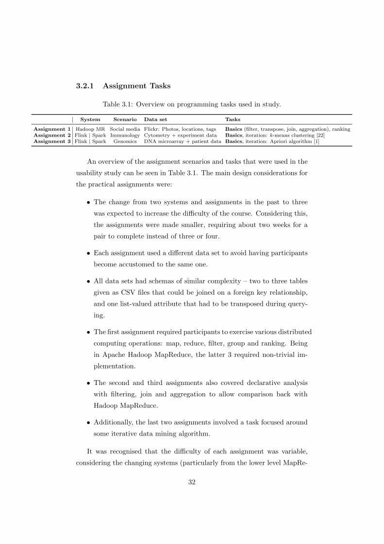
Table 3.1: Overview on programming tasks used in study.

System Scenario Data set Tasks

Assignment 1 Hadoop MR Social media Flickr: Photos, locations, tags Basics (filter, transpose, join, aggregation), rankingAssignment 2 Flink | Spark Immunology Cytometry + experiment data Basics, iteration: k-means clustering [22]Assignment 3 Flink | Spark Genomics DNA microarray + patient data Basics, iteration: Apriori algorithm [1]

An overview of the assignment scenarios and tasks that were used in the

usability study can be seen in Table 3.1. The main design considerations for

the practical assignments were:

• The change from two systems and assignments in the past to three

was expected to increase the difficulty of the course. Considering this,

the assignments were made smaller, requiring about two weeks for a

pair to complete instead of three or four.

• Each assignment used a different data set to avoid having participants

become accustomed to the same one.

• All data sets had schemas of similar complexity – two to three tables

given as CSV files that could be joined on a foreign key relationship,

and one list-valued attribute that had to be transposed during query-

ing.

• The first assignment required participants to exercise various distributed

computing operations: map, reduce, filter, group and ranking. Being

in Apache Hadoop MapReduce, the latter 3 required non-trivial im-

plementation.

• The second and third assignments also covered declarative analysis

with filtering, join and aggregation to allow comparison back with

Hadoop MapReduce.

• Additionally, the last two assignments involved a task focused around

some iterative data mining algorithm.

It was recognised that the difficulty of each assignment was variable,

considering the changing systems (particularly from the lower level MapRe-

32

duce in assignment 1 to the higher level systems), scenarios, data sets, and

algorithms. However, these were all necessary either for the reduction of

bias towards any particular system, or for the general flow of the course.

Effects that assignment difficulty may have had on perceived usability has

been explored in Section 3.4.

We intended to include assignment marks in the usability study data.

Since the unit of study had multiple tutors to teach classes and mark assign-

ments, it was necessary (more than otherwise) to implement some form of

marking that would reduce subjectivity and thus potential bias from indi-

vidual markers. We tried taking on the approach described in section 6.4 of

the study by Nanz et al. [30]: to identify a set of mistakes and their weight-

ings, and then to perform marking backwards, so to speak. However we

faced a challenge when trying to implement this, wherein our course struc-

ture required the release of a marking rubric for students to access prior to

completion of the assignment, inferring that the set of potential mistakes

had to be compiled beforehand, as opposed to after scanning submissions

and categorising the mistakes that actually were made – as performed in

the reference paper. Ultimately it was decided to exclude assignment marks

from the study.

3.2.2 Data Analysis Scenarios

Each assignment was set in a different scenario to avoid any potential bias

due to familiarity with a data set (cf. Table 3.1). As our aim is to study

the usability of the distributed data processing platforms for non-computer

scientists (those who would have difficulty judging usability and such on their

own), we chose data analysis scenarios from social media, bioinformatics,

and genomics.

Assignment 1 involved data analysis of Flickr data. The data set is an

excerpt of real-world Flickr data including a hierarchical location attribute

and multiple tags per photo given as a multivalued attribute. Students were

asked to implement different analytical queries to identify: the number of

photos taken at a certain locality level; the top 50 localities by number of

photos; and the top 10 tags used for those photos.

33

Assignment 2 considered a scenario from immunology, involving real cy-

tometry data from a study of infections with the West Nile Virus. We also

attached fabricated metadata to the real cytometry data, for instance infor-

mation about the imaginary researcher who collected the data, to facilitate

examination of particular skills. This assignment had two subtasks. Firstly,

students had to determine the number of valid measurements per researcher,

involving: filter; transpose; join; and aggregation operations, similar to as-

signment 1. Secondly, students had to complete a clustering task to iden-

tify similar cell measurements with regard to some given 3-dimensional cell

markers using the k-means clustering algorithm [22].

Assignment 3 presents a genomics scenario requiring the analysis of a

DNA microarray data set and patient metadata. This data set was syn-

thetic – generated using the schema and data generator from the GenBase

benchmark [34]. We modified the GenBase schema to allow the application

of multiple disease codes per patient (instead of a single one) via a mul-

tivalued attribute. Students were first asked to find the number of cancer

patients with certain active genes, covering the filter, transpose, join, and

aggregation operations as in the previous two assignments. They further had

to mine the microarray data in search of frequent combinations of expressed

genes for certain cancer types using the Apriori algorithm [1].

3.2.3 Self-Reflection Surveys

We included a short survey as part of the assignment submission process,

acting as a method of self-reflection for students after completing the assign-

ment, and also as a primary source of the usability study’s data. The survey

was only available for completion following the submission of source code,

thus capturing their view of each system upon completion of the relevant

assignment, as opposed to say halfway through.

Although the assignments were completed in pairs, and thus only one

source code submission was necessary for a pair of students, we emphasized

that the self-reflection surveys were to be completed individually.

The surveys for each assignment included:

• A simple and standard usability survey: the System Usability Scale

34

survey [12], as discussed in Section 3.2.4.

• A question directly asking which is their preferred system. This ques-

tion does not apply to assignment 1.

• A question asking approximately how much time was spent working

on the assignment. Options were separated into seven 4 hour bins,

from 0-4 hours, to 20-24 hours and then 24+ hours.

• A text area to provide any textual feedback.

The first survey also included four questions to gauge students’ prior pro-

gramming experience. It asked how many years of programming experience

the students considered themselves to have, from 0 to 9 and then 10+, and

three Likert scale questions asking students for their perceived proficiency

with Java, Python and shell environments, from “No proficiency” to “Very

high proficiency”.

We required all students to complete the survey as part of their learning

outcomes, as we considered it a form of self-reflection. However, all questions

were optional, allowing students to omit any if uncomfortable. Only partic-

ipating students’ survey data was included for the purpose of the usability

study. We made sure to keep the survey brief and simple to reduce load

on students and, perhaps optimistically, reduce fake responses and increase

usability study participation.

3.2.4 System Usability Scale (SUS)

The SUS [12] was used to provide a score for the usability of each system

to be used for comparison. While programming frameworks or distributed

systems may not be the intended application of this survey, we were unable

to find anything more specifically targeted to this use case, and found that

the SUS was general enough to be applied nonetheless, considering that our

survey was explicitly focused on usability. In this regard we were trying

something seemingly rare, and thus could not be sure of the applicability of

the results.

The SUS is comprised of ten Likert scale questions. Odd numbered

questions are positively natured, while even numbered are negative. The

35

final score is compiled adding or subtracting those scores and applying a

multiplier, becoming a single score between 0 and 100. Note that SUS scores

are interval level – not ratio – meaning a SUS score of 80 is not necessarily

twice as good as 40.

We decided to use this survey as it presented a good balance of ease

and generality. Ease here refers to the survey only having ten questions

of a simple nature. Generality is in how the survey only presents rather

general statements about the ‘system’, making it applicable to a variety of

systems even with significant differences between them, and avoiding ref-

erences which would not apply or would be confusing in a programming

context, such as ‘scenario’ in the After Scenario Questionnaire (ASQ) [26],

or ‘information’ and ‘interface’ in the Computer System Usability Question-

naire (CSUQ) [26].

Despite the availability of more succinct questionnaires, we found the

SUS to be of a good balance. While not requiring much time or effort to be

conducted overall, its questions may have the potential to provide additional

information about the systems that could be used to make recommendations.

For instance, “I needed to learn a lot of things before I could get going

with this system” and “I thought there was too much inconsistency in this

system” both provide insight into specific strengths or weaknesses of the

system in question.

The SUS is also a well-established, widely used and scrutinised method.

An empirical study of the SUS used nearly 10 years of data to conclude that

the survey does effectively fulfil its purpose of attaining a user’s subjective

rating of a product’s usability [8].

A study of SUS usage with non-native English speaking participants

recommended adjusting a single question to reduce confusion [17], namely

changing the 8th statement from ‘I found the system very cumbersome to

use’ to ‘I found the system very cumbersome/awkward to use’, and we chose

to adopt this for our usability study. Finally, we modified the fourth ques-

tion by changing ‘technical person’ to ‘tutor/technical person’, hopefully

reducing potential confusion as the context in this usability study does not

have an obvious definition of who a technical person is.

36

3.3 Execution

By designing the usability study with the course and students’ learning out-

comes as the top priority, we were able to frame the usability study as an

application of existing data for the purposes of attaining ethics approval.

Specifically, the self-reflection survey was to be performed regardless of the

usability study, as a part of the students’ learning outcomes. Additionally,

the crossed A/B test was to be performed as a way for the course to com-

pare students’ feedback on Apache Spark and Apache Flink, to determine

which systems are most appropriate for usage in future semesters – again

irrespective of this usability study.

Thus the data was already being collected for the course itself. For

the purpose of this usability study, we were to attain ethics approval to

use that existing data in performing this analysis and for disseminating

any publications. This approach was very effective considering the time

limitations in place, and served the needs of the students, the university,

and our research, as we were able to implement most changes to the course

structure without having to wait for ethics approval. By the time the first

self-reflection survey was executed, which included the option to opt-in to

this usability study, we had successfully attained ethics approval.

Students of the cloud computing class had access to a dedicated teaching

cluster of 30 nodes for developing and testing their solutions. This cluster

was shared among all students and had all systems installed using the same

HDFS file system and YARN resource manager. The distributed comput-

ing engine versions used were: Apache Hadoop MapReduce v2.7.2; Apache

Spark v2.1.1; Apache Flink v1.2.1. Configuration changes from default set-

tings were kept to a minimum. During the installation and testing process,

where we tried to ensure that the systems would work from a the perspec-

tive of a logged-in student, we experienced cluster multitenancy issues and

found little documentation to assist, ultimately requiring a large amount of

our time to work around.

We aimed to support both Java and Python as implementation lan-

guages, and consequently lecture and tutorial materials were provided in

both languages. However, despite our best efforts, we did not succeed in

37

creating exercise materials for Flink with Python that worked well enough

that we could instruct students on. We found that some simple operations

were behaving unpredictably or producing overly complicated and computa-

tionally expensive dataflows, making it very difficult to solve even basic tasks

efficiently. There was limited documentation on the matter and the whole

experience felt rather immature. Ultimately we did not provide teaching

materials for Flink in Python, and recommended that students avoid using

it for their assignments. This recommendation was followed as all Flink

submissions were written in Java. An exploration of the potential biases

this may have introduced was performed in Section 3.4.7.

Due to the delays caused by this struggle, we were forced to release Flink

tutorial exercises (only in Java) one week after Spark’s, as opposed to the

desired synchronised release. This remained prior to release of assignment 2,

and lectures still covered both systems in parallel.

We designed the usability study such that the comparisons of Flink and

Spark were done in a crossed A/B test to avoid potential bias for or against

the first system used after MapReduce. To this end, student pairs were

randomly assigned to use Spark or Flink for assignment 2, with an even

split.

However, some students requested to change their assigned system for

assignment 2 from Flink to Spark. We suspect that this was due to Flink’s

tutorial exercises having been delayed while working on Python support,

meaning students had less experience with it than Spark when assignment 2

was to come around. We did not deny their requests, and instead offered

other Spark groups to transfer to Flink in an effort to restore balance. Ul-

timately there were more students using Spark than Flink for assignment 2;

specifically 39 for Spark compared to 30 for Flink. All students cooperated in

using the alternate system for assignment 3, which meant that assignment 3

had more Flink users.

Students were instructed not to use higher level APIs like FlinkML or

Spark’s MLlib in their assignment solutions. This instruction was adhered

to by all students.

Standard iterative algorithms relevant to big data contexts were selected

to be the focus of the final two assignments. These algorithms were k-means

38

clustering [22] for assignment 2, and the Apriori algorithm [1] for assign-

ment 3. Example implementations of these algorithms are available online

for both Spark and Flink, however for different use cases and data sets. De-

spite this, we decided not to change the algorithms, as the examples did not

include accompanying guides or tutorials, and thus participants still had to

put a significant amount of effort into understanding and adapting those

implementations to solve the assignment tasks. As expected, some students

did find these existing implementations and did reference and adapt them in

solving the assignments. Considering this, we decided not to include metrics

such as their solutions’ number of lines of code or other code related meta-

data in the usability study data set, as a notable portion of such data would

have come from online examples instead of the actual work of participants.

Our attempt to reduce bias in marking was not successful. We attempted

to define a covering set of mistake categories and penalties in advance – as

the course required the marking rubric to be available prior to completion of

the assignment – but students made many mistakes that did not fall beneath

these categories. Thus the approach was not highly effective in reducing the

requiring judgement in marking, and the end result was that two markers

provided a significantly lower average mark than the other two; namely 10.5

compared to 13 where the maximum mark was 15. Considering this, it was

decided that assignment marks should not be included in the usability study.

Despite the various mentioned setbacks: the usability study had a high

participation level of over 80%; all students were cooperative with the crossed

A/B test and in completing the surveys; and the end-of-semester course sat-

isfaction feedback was high overall. The usability study had 72 participants,

reduced to 69 after removing three with incomplete course participation.

Following completion of the semester, participants’ three assignment sur-

veys, and some metadata such as their degree code, was linked, recorded and

anonymised. All feedback from surveys was checked and any personal infor-

mation was removed. The survey data can be viewed or downloaded from

https://www.github.com/bilalakil/mphil.

39

3.3.1 Self-Reflection Surveys

Self-reflection surveys were available for individuals to complete immediately

following the submission of each assignment. As the submission system pro-

vided no mechanism to enforce the surveys’ completion, we instead reminded

students to complete them during lectures and tutorials, and by direct email.

Eventually all students completed the surveys, however the delay between

assignment and survey completion is something we would have preferred to

avoid. Approximately 60% of students submitted the self-reflection survey

on the same day that they submitted the assignment.

However, due to a discovered limitation of our learning management

system (LMS – where the surveys were being executed), we were forced to

recreate and repeat the execution of the first survey. This was discovered

and performed soon after releasing the initial survey, so a few participants

had to repeat their submissions. The specific problem was that a ‘survey’

as defined by the LMS was completely anonymous, but we intended on

linking the results of participants’ surveys across each assignment before

anonymising the data, and importantly removing any data for students who

did not opt-in to the usability study. The LMS had no feature to support

this, and thus the data collected from the first survey was not useful as it

could not be put into context. We instead had to create a ‘test’ in the LMS

and perform anonymisation manually following all necessary data linking.

Also, the question about how much time was spent working on the as-

signment was updated following inspection of assignment 1 survey results,

where we found that about half of the responses were 24+ hours. The

question was updated to use thirteen 4 hour bins (instead of seven) in the

assignment 2 and 3 surveys, from 0-4 hours to 44-48 hours and then 48+.

Despite all survey questions being optional, the four programming expe-

rience questions in the first survey, and all of the system preference questions,

were answered by all students. Two out of 207 time questions were left unan-

swered, along with some SUS statement responses preventing calculation of

7 individual SUS scores out of 207 in total.

40

3.4 Analysis

3.4.1 Method

Listing 3.1: Exclusion of Python data using pandas DataFrame overloadedoperators and slicing.

# Remove Python data?

if True:

a1, a2 , a3 = [data[’A’ + str(n) + ’ Language Used’] == ’Python ’

for n in range(1, 3 + 1)]

python = a1 | a2 | a3

s = ’Removing {}/{} ({:.1f}%) Python records.’

print(s.format(python.sum(),

python.count(),

python.sum() / python.count () * 100))

data = data[~ python]

else:

print(’Retaining Python records.’)

Listing 3.2: Usage of pandas and custom plotting functions in drawing adiverging stacked bar chart – specifically that for Figure 3.2.

envs = [’Java’, ’Python ’, ’Shell ’]

plot_data = pd.DataFrame ([data[env + ’ Experience ’]. value_counts ()

for env in envs],

index=envs)

plot_data.columns = [’None’, ’Limited ’, ’Average ’, ’High’, ’Very high’]

cust.plot (). likert(plot_data )\

.legend(columnspacing =1)\

.label(’Programming Environment Proficiency ’, ’Count’)\

.show()

As aforementioned, self-reflection surveys created within the LMS were

configured to not be fully anonymous, as if they were we would not be able

to: correlate participant responses across multiple surveys; include other

metadata such as the systems and programming languages used per assign-

ment; or remove the data for students who opted not to participate in the

study. Thus student identifiers were included with survey responses and

were later removed.

41

Listing 3.3: Usage of pandas and custom plotting functions in drawing apair of box and whisker plots – specifically that for Figure 3.8.

a2spark = data[’A2 System Used’] == ’Spark ’

a3spark = ~a2spark

a2_plot_data = [data[’A2 Time Spent ’][ a2spark ]. dropna(),

data[’A2 Time Spent ’][~ a2spark ]. dropna ()]

a3_plot_data = [data[’A3 Time Spent ’][ a3spark ]. dropna(),

data[’A3 Time Spent ’][~ a3spark ]. dropna ()]

kwargs = {’labels ’: [’Spark ’, ’Flink ’], ’widths ’: 0.4}

cust.plot ()\

.subplots(2, 1, 1). boxplot(a2_plot_data , ** kwargs )\

.label(’System Time Spent Comparison\nAssignment 2’)\

.subplots(2, 1, 2). boxplot(a3_plot_data , ** kwargs )\

.label(’Assignment 3’, ’Time Spent (4 hour bins)’)\

.show()

Data was initially exported from the LMS in Excel format following

completion of the unit of study. The exported files contained many ex-

cess columns such as question IDs and labels, all of which were manually

removed. The remaining columns contained only relevant metadata or an-

swers to survey questions, and the column headers were renamed to reflect

that, for instance from “Question 4 answer” to “Python Experience”. Data

for each of the three surveys had to be exported separately, creating multiple

files, which were then joined to a single file using student identifiers as the

join key. The file was then converted to a tab-separated values file, and rows

for students who opted not to participate in the study were removed. Ad-

ditional columns of data including participants’ system and language used

per assignment were added. Once all necessary data was removed, added,

and double-checked, all student identifiers were removed. Then all textual

feedback was manually checked for any personal information for removal,

of which none was found. From this point the survey data was entirely

anonymised – the point of no return.

With the data ready for analysis, it was then copied into a directory

where a Python Jupyter Notebook was created and executed, performing

various analyses and producing the diagrams seen throughout this thesis.

A Jupyter notebook is a common choice for exploratory data analysis and

42

among data scientists. It is very flexible and ‘freestyle’, so to speak, and

thus seemed appropriate for the task of analysing the usability study data.

The following Python modules and libraries were used in performing the

exploration and analysis: NumPy, a “fundamental package for scientific

computing with Python”; Matplotlib for creation of charts and plots to be

both displayed in-line in the notebook and saved to files (most of which were

included in this thesis); pandas to simplify data usage and manipulation; and

SciPy for its library of statistical functions.

The pandas DataFrame and Series implementations contain many over-

loaded operators, including the slice operator, which all serve to streamline

usage of the class, but can seem unintuitive for programmers who do not

have prior experience with such overloading techniques. Many of these op-

erators – including ==, <, and so forth – produce a DataFrame or Series

of boolean values, which can then be used to slice the original set, easily

excluding irrelevant data. An example of how these features have been used

in the analysis can be seen in Listing 3.1.

We created a custom plot class to enable succinct, simple and consis-

tent usage of Matplotlib throughout the study. The class was updated as the

study progressed and its needs evolved, and is how the charts and plots seen

throughout this paper are mostly consistent in their appearance. Most of

the class’ functions returned the instance of the class itself, allowing chained

function execution, such as cust.plot().boxplot(data).legend().show().

We also created a function for drawing the diverging stacked bar charts seen

throughout the paper – a chart that at the time did not have a correspond-

ing Matplotlib function – and to simply and consistently work with subplots

when we needed to include multiple simple charts in the same figure. List-

ing 3.2 shows how Likert scale data was displayed in a diverging stacked bar

chart, and Listing 3.3 shows how the custom class handles subplots.

Combining pandas data manipulation and the custom plot class with

one-line statistical tests available in SciPy provided a means for efficient

data exploration and analysis. The notebook was easily transferable be-

tween collaborators, and the mix of descriptive writing (via Markdown),

Python code and output, and in-line charts assisted with navigation and

comprehension of the notebook.

43

Exclusion of Python user data from the usability study, as for Sec-

tion 3.4.7, was performed using a single conditional statement close to the

beginning of the notebook. This statement could easily be toggled (by

changing True to False), followed by a restart and full run of the note-

book, to quickly compare analyses with and without including Python data.

The corresponding code can be seen in Listing 3.1.

3.4.2 Background of Participants

Figure 3.1: Frequency histogram displaying all 69 responses for the pro-gramming experience question. A value of 10 means 10 or more years.

Figure 3.2: Diverging stacked bar chart [23] displaying all 69 Likert scaleresponses for questions on perceived programming proficiency.

Of the 69 participants: 55 were graduate computing students; 7 were

Master of Data Science students, who do not necessarily have a computer

science background; 6 were final-year undergraduate students; and 1 was a

44

master’s student of a different degree.

Figure 3.1 shows that most (78.3%) participants reported having 1 to

4 years of programming experience. Reflecting the diversity of the student

cohort, around half of the participants reported to have limited or no pro-

ficiency in shell and Python environments, compared to around a third for

Java, as seen in Figure 3.2. There is a slightly negative correlation between

Java and Python proficiency, with a Spearman’s rank correlation coefficient

of -0.128. The Pearson correlation coefficient was not used because the data

is ordinal level, failing the test’s ratio level assumption.

3.4.3 Preferences and SUS Scores

Figure 3.3: Frequency histogram comparing all 69 SUS scores per system(minus 7 individual incomplete responses).

Following the completion of the third survey, participants reported their

system preference as: 8 (11.6%) for Apache Hadoop MapReduce; 29 (42.0%)

for Apache Spark; and 32 (46.4%) for Apache Flink. This is strong evidence

that Spark and Flink were preferred over Hadoop MapReduce.

The difference was similarly pronounced among data science students

where 5 of 7 preferred Flink over Spark or MapReduce. However we note

that four of those five students did use Flink in assignment 2 before using

Spark, which could have an influence, as Section 3.4.4 will show. Due to the

small amount of data in this context there was no applicable significance

test.

The SUS scores reveal little information, with all systems sharing similar

45

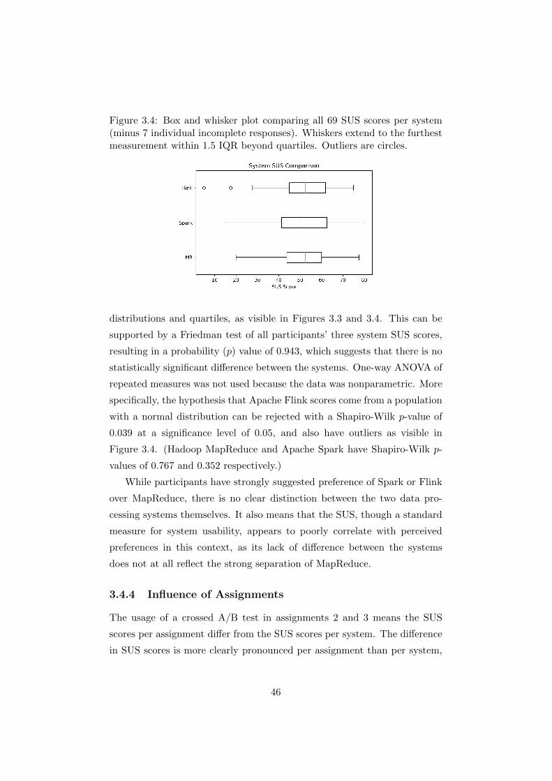
Figure 3.4: Box and whisker plot comparing all 69 SUS scores per system(minus 7 individual incomplete responses). Whiskers extend to the furthestmeasurement within 1.5 IQR beyond quartiles. Outliers are circles.

distributions and quartiles, as visible in Figures 3.3 and 3.4. This can be

supported by a Friedman test of all participants’ three system SUS scores,

resulting in a probability (p) value of 0.943, which suggests that there is no

statistically significant difference between the systems. One-way ANOVA of

repeated measures was not used because the data was nonparametric. More

specifically, the hypothesis that Apache Flink scores come from a population

with a normal distribution can be rejected with a Shapiro-Wilk p-value of

0.039 at a significance level of 0.05, and also have outliers as visible in

Figure 3.4. (Hadoop MapReduce and Apache Spark have Shapiro-Wilk p-

values of 0.767 and 0.352 respectively.)

While participants have strongly suggested preference of Spark or Flink

over MapReduce, there is no clear distinction between the two data pro-

cessing systems themselves. It also means that the SUS, though a standard

measure for system usability, appears to poorly correlate with perceived

preferences in this context, as its lack of difference between the systems

does not at all reflect the strong separation of MapReduce.

3.4.4 Influence of Assignments

The usage of a crossed A/B test in assignments 2 and 3 means the SUS

scores per assignment differ from the SUS scores per system. The difference

in SUS scores is more clearly pronounced per assignment than per system,

46

Figure 3.5: Box and whisker plot comparing all 69 SUS scores per assignment(minus 7 individual incomplete responses). Whiskers extend to the furthestmeasurement within 1.5 IQR beyond quartiles. Outliers are circles.

as visible by comparing Figure 3.5 to Figure 3.4. It appears as though as-

signment 2 had the highest relative SUS scores, and assignment 3 the lowest.

This is supported by a Friedman test of all participants’ three assignment

SUS scores, resulting in a p-value of 0.025, which suggests a statistically

significant difference at a significance level of 0.05.

More than half of the participants (39 participants or 56.5%) preferred

the system they used in assignment 2, compared to 22 (31.9%) for assign-

ment 3 (with the other 8 (11.6%) preferring Apache Hadoop MapReduce),

which is quite a noteworthy difference. However, it is difficult to reason

about this difference, as there is no clear distinction as to whether the dif-

ference is due to some form of a first-system-used bias or differences in

assignment difficulty (as described in Section 3). Figure 3.6 shows the time

spent working on assignments, which provides a hint as to potential dif-

ferences in assignment difficulty, wherein assignment 3 appeared to require

slightly more time than assignment 2. However, this claim is not supported

by a one-sided sign test with plus representing participants who spent more

time on assignment 3 than 2, and minus otherwise, resulting in a p-value of

0.358. The sign test is used because the data is non-normal and asymmet-

rical, as clearly visible in Figure 3.7, ruling out the paired t-test due to it

being a parametric test, and the Wilcoxon signed-rank test due to it having

high Type I error rates when used with asymmetric data.

While we suspect assignment difficulty and ‘first-used advantages’ could

47

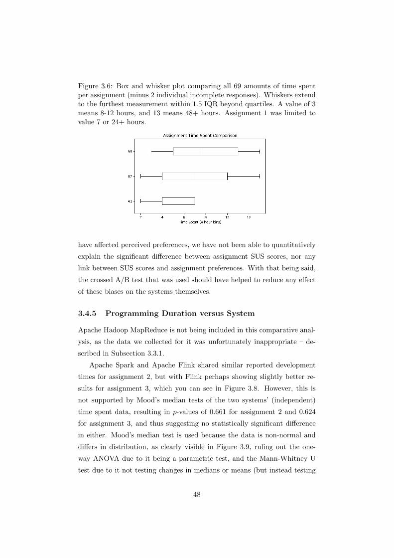
Figure 3.6: Box and whisker plot comparing all 69 amounts of time spentper assignment (minus 2 individual incomplete responses). Whiskers extendto the furthest measurement within 1.5 IQR beyond quartiles. A value of 3means 8-12 hours, and 13 means 48+ hours. Assignment 1 was limited tovalue 7 or 24+ hours.

have affected perceived preferences, we have not been able to quantitatively

explain the significant difference between assignment SUS scores, nor any

link between SUS scores and assignment preferences. With that being said,

the crossed A/B test that was used should have helped to reduce any effect

of these biases on the systems themselves.

3.4.5 Programming Duration versus System

Apache Hadoop MapReduce is not being included in this comparative anal-

ysis, as the data we collected for it was unfortunately inappropriate – de-

scribed in Subsection 3.3.1.

Apache Spark and Apache Flink shared similar reported development

times for assignment 2, but with Flink perhaps showing slightly better re-

sults for assignment 3, which you can see in Figure 3.8. However, this is

not supported by Mood’s median tests of the two systems’ (independent)

time spent data, resulting in p-values of 0.661 for assignment 2 and 0.624

for assignment 3, and thus suggesting no statistically significant difference

in either. Mood’s median test is used because the data is non-normal and

differs in distribution, as clearly visible in Figure 3.9, ruling out the one-

way ANOVA due to it being a parametric test, and the Mann-Whitney U

test due to it not testing changes in medians or means (but instead testing

48

Figure 3.7: Frequency histogram comparing all 69 amounts of time spent perassignment (minus 2 individual incomplete responses). A value of 3 means8-12 hours, and 13 means 48+ hours. Assignment 1 was limited to value 7or 24+ hours.

changes in distribution) when used with data of differing distributions.

Spark and Flink do not present a significant difference in the amount of

time that was required to complete either of the assignments. This shows

that both systems are similarly suitable for completion of data analysis tasks

like those in assignments 2 and 3.

3.4.6 Influence of Programming Experience

As previously mentioned, Figure 3.1 shows that most (78.3%) participants

reported having 1 to 4 years of programming experience. In this subsection

we will consider the 12 (17.4%) participants who reported having more than

4 years experience as being of relatively ‘high experience’. Their experience

is distributed as so: 6 with 5 years experience, and 2 with each of 6, 8 and

10+ years experience. Is there any difference in the reported preferences or

SUS scores for high experience participants compared to the majority?

A comparison between the two groups’ system SUS scores is shown in

Figure 3.10, which does not tell much of any preference or skew. The ranges

of all three systems are more dense and perhaps slightly higher overall in the

high experience group, and also particularly lacking the long tail towards

lower scores. However, it is difficult to indicate that it is not due to coin-

cidence. These observations still apply, perhaps with a slight reduction in

density, when moving the threshold from 5 years to 3 years and thus placing

49

Figure 3.8: Box and whisker plots for assignments 2 and 3 comparing all69 amounts of time spent per assignment (minus 1 individual incompleteresponse). Whiskers extend to the furthest measurement within 1.5 IQRbeyond quartiles. A value of 3 means 8-12 hours, and 13 means 48+ hours.

Figure 3.9: Frequency histograms for assignments 2 and 3 comparing all 69amounts of time spent per system (minus 1 individual incomplete response).A value of 3 means 8-12 hours, and 13 means 48+ hours.

34 (49.3%) participants in the high experience tier.

A comparison between the two groups’ reported preferences is shown in

Figure 3.11, which also does not tell much of any preference or skew. Hadoop

MapReduce remains behind the dataflow engines, but it is difficult to reason

much further. For instance, the difference in Apache Flink and Apache Spark

looks quite pronounced, with Flink appearing to be less preferred to Spark

in comparison to the low experience group. However, in actual fact it is

only a difference of two individual preferences, which is difficult to claim as

being anything other than coincidence. When moving the threshold from

5 years to 3 years and thus placing 34 (49.3%) participants in the high

50

Figure 3.10: Box and whisker plots for high (>=5 years) and low program-ming experience participants comparing all 69 SUS scores per system (minus7 individual incomplete responses). Whiskers extend to the furthest mea-surement within 1.5 IQR beyond quartiles. Outliers are circles.

experience tier, the two charts end up look nearly identical, also with very

similar Preference Count scales.

It was good to have collected the programming experience data as part

of the survey, especially with full participation in that regard, having pro-

vided information regarding the background of participants and the diver-

sity present in the study. However, this information did not turn out to be

indicative of any pattern in reported preferences or system SUS scores.

3.4.7 Influence of Programming Language

In the analysis thus far, participants’ usage of Python or Java for each system

or assignment has not been taken into account. However, it is mentioned

in Section 3.3 that learning materials, or more specifically tutorial exercises

and sample assignment solutions, were not successfully created for Apache

Flink; that students were recommended not to use Python for Flink; and

that this recommendation was followed by all students. Unfortunately, this

presents an inconsistency in the experiment which could bias some of the

findings. This subsection will explore said biases by comparing the previous

analyses with a repetition of them that excluded all Python user data.

Of the 69 participants whose data was used in the above analyses, 32

(46.4%) had used Python for either or both of assignment 1 (Hadoop MapRe-

duce) or the assignment in which they used Apache Spark. Excluding this

51

Figure 3.11: Bar charts for high (>=5 years) and low programming experi-ence participants comparing reported system preference counts upon com-pletion of assignment 3. There are 69 preferences measured in total. Chartshave differing Preference Count scales.

data leaves 37 records to work with. Furthermore, the crossed A/B test

that was employed did not take programming language usage into account,

and thus the Python records removed could have further produced skew in

that regard. With 69 records the Spark vs. Flink usage split for assign-

ment 2 (and conversely for assignment 3) is 39 vs. 30 (56.5% vs. 43.5%)

respectively, skewed due to students’ requests to switch to Apache Spark

as described in Section 3.3, whereas with 37 records it is 23 vs. 14 (62.2%

vs. 37.8%) respectively. Flink is 9 users behind Spark (for assignment 2) in

both cases, however this difference is more pronounced as a percentage in

the latter case.

Of the subsections that were analysed earlier, noteworthy differences

were only apparent in relation to the background of participants, and their

reported system preferences.

Background of Participants

Of the 37 participants: 33 were graduate computing students; 1 (compared

to 7) was a Master of Data Science student; 2 were final-year undergraduate

students; and 1 was a master’s student of a different degree. Furthermore,

Figure 3.12 (compared to Figure 3.2) shows the dominance of Java among

the cohort, also with substantially more participants reporting having lim-

ited or no Python proficiency than average or higher.

52

Figure 3.12: Diverging stacked bar chart [23] displaying all 37 (Python userdata excluded) Likert scale responses for questions on perceived program-ming proficiency.

This apparent reduction in diversity may be due to individuals in this

cohort having been more likely to have come from a computer science back-

ground, where compiled and object-oriented programming languages would

be of a larger focus than scripting languages – which is what we observe

Python to be commonly taught as, despite it also being object-oriented. Un-

fortunately, this representation may not effectively capture the experiences

of interdisciplinary users, as has been one of our intentions in conducting

this study.

Preferences

Following completion of the third survey, participants reported their system

preference as: 4 (10.8%) for Hadoop MapReduce; 12 (32.4%) for Apache

Spark; and 21 (56.8%) for Apache Flink. While this result is similar to the

full (Python included) data set in how MapReduce is behind in comparison

to the dataflow engines, it differs from having Spark and Flink on a very close

footing to instead placing Flink quite noticeably ahead as the participants’

preferred system.

This difference seems to make sense considering that Python users likely

felt inconvenienced by the inability to use Python for Flink in compari-

son to Spark or MapReduce, thus reducing Flink’s popularity among the

full cohort. With Python users excluded from analysis, it has now become

53

apparent that Flink is preferred over Spark among Java users.

Unfortunately, as described in Section 3.3.1, there is little information

available from participants to justify these reported preferences, and so we

can make no conclusion as to why Java users may have preferred Flink

over Spark, especially considering the similarities in their usage as described

in Section 1.2. The key difference in usage that we could think of was in

Flink’s availability of IterativeDataSet, which could have been used in

solving both assignments 2 and 3.

With the full data set it was apparent that participants tended to prefer

the system they used for assignment 2 more than assignment 3, as described

in Section 3.4.4. With Python data excluded, this changes to having 17

(45.9%) participants preferring the system used for assignment 2 compared

to 16 (43.2%) for assignment 3 (with the other 4 (10.8%) preferring MapRe-

duce). It makes sense that assignment 3 gained preference considering the

skewed crossed A/B test distribution, where more participants used Flink for

assignment 3, in combination with participants’ higher preference of Flink.

This means that although reported preferences put assignments 2 and 3

on similar proportions, it remains likely that assignment 3 was somehow

disadvantaged.

3.4.8 Individual SUS Statements

This subsection will discuss Figure 3.13, which displays all participants’

responses to all ten SUS statements. The figure has been organised in a

particular way considering the nature of the SUS. Its caption describes the

intended interpretation.

The first takeaway is that, for all ten questions, there is little difference in

response distribution between the three systems. This explains why the SUS

scores were very similar, as discussed in Section 3.4.3. It shows that in terms

of usability as examined by the System Usability Scale, these three systems

apparently share the same strengths and weaknesses, which is unintuitive

considering that Apache Spark and Flink feature much higher level APIs.

Furthermore, most questions had a good response as either a slight or

strong majority – a good sign for the usability of these systems. There

54

are three exceptions: “Q4: I think that I would need the support of a tu-

tor/technical person to be able to use this system”, which most participants

agreed with; “Q7: I would imagine that most people would learn to use this

system very quickly”, which a slight majority of participants disagreed with;

and “Q10: I needed to learn a lot of things before I could get going with

this system”, which participants overwhelmingly agreed or strongly agreed

with.

These three questions with bad responses cover the topics of learning

and support, and are the only questions in the set of ten concerning them.

The other seven questions with good responses covered topics such as ease

of use and system design and complexity. Is it normal that participants

perceived the systems to be well designed, non-complex and usable, and yet

hard to learn and in need of support to be used? One interpretation of

this result is that participants felt that the systems were to be complex by

design, considering their function as distributed computing engines, and in

that context perceived them to be usable and such.

However, the steep learning curve still needed to be addressed for them

to use the system. We believe this is indicative of a prominent barrier to

adoption of data science systems – although they effectively abstract vari-

ous distributed computing and dataflow challenges away, without simplifying

the process of learning to use and overcoming difficulties with these systems,

users with non-computing backgrounds will have significant trouble adopt-

ing them. From our experience and from the feedback of participants, we

found the key areas for improvement to be first-party documentation and

the process of debugging programs.

3.4.9 Free-text Feedback and Other Impressions

Considering the participants’ free-text feedback, and the experiences of in-

structors throughout execution of the study and teaching of its materials,

we are able to highlight several areas of potential future improvement of the

evaluated systems:

• Debugging in MapReduce was particularly difficult.

• MapReduce code tended to be overly verbose.

55

• Flink development environment setup was troublesome.

• Python support in Flink 1.2 felt immature.

• Spark and Flink felt quite similar to work with.

• Spark and Flink documentation covered basic usage quite well, but

was limited for non-standard operations. Consequently, both Spark

and Flink involved significant trial and error.

• Spark community support was good, but first-party documentation

was lacking. Flink was described inversely.

We note that these points represent anecdotal observations only, but be-

lieve they are a good indicator of the general struggles faced by new users of

these systems. Considering them, we would recommend that developers of

these newer dataflow engines work to excel in regards to the on-boarding ex-

perience, the process of debugging, and the documentation of these systems

– especially for non-standard operations, perhaps by providing a very wide

range of examples as opposed to focusing on canonical ones. Work in these

suggested areas would complement the already greatly improved usability

that these systems provide, giving new users a streamlined experience of

adoption, which is especially beneficial for individuals from non-distributed

computing backgrounds.

56

Figure 3.13: Diverging stacked bar charts [23] displaying all 69 Likert scaleresponses for each SUS statement, however minus some missing individualresponses. The five odd numbered statements on the left are ‘positivelynatured’, such as “Q3: I thought the system was easy to use” – agreeingwith this statement is good in terms of the system’s usability. The five evennumbered statements on the right are ‘negatively natured’, such as “Q2: Ifound the system unnecessarily complex” – agreeing with this statement isbad in terms of the system’s usability. To display this effectively, the legendson the left and right have their colours inverted – blue is used to highlightgood responses (regardless of a statements’ positive/negative nature) andred for bad responses.

57

Chapter 4

Comparison and

Methodology

Performing a comparison of multiple technologies, considering multiple fac-

tors, and having to communicate the results to users of differing technical

backgrounds, is a challenge. Consideration needs to be taken in reducing

biases between technologies. The chosen factors need to be of interest to the

target audience. The communication method needs to be suitable for read-

ers who want to know the technical details of the comparison, but also for

those who may not be able to understand that detail and need a more dis-

tilled presentation. There are plenty more needs to consider, and this is why

some methodology or theoretical framework is necessary before engaging in

a comparison.

However, we were unable to find any existing methodologies or frame-

works to employ in our comparison, or even to apply principles or techniques

from in the development of a new methodology. Thus we present an initial

proposal of a multidimensional software comparison methodology to pro-

vide structure in considering all of these needs. The methodology provides

guidance in the setup, execution and display of results for comparisons, in

a way that is suitable for comparisons in different contexts, and intended

for different audiences. In this sense it is not a very controlling or spe-

cific methodology, as that would largely restrict its applicability. Instead it

seeks to guide the decision making process that occurs before commencing

58

these comparisons, with the purpose of increasing comparison reliability and

usefulness for the target audience.

The following section will describe the proposed methodology and jus-

tify its design. The results section following that will apply the proposed

methodology in performing a multidimensional comparison of Apache Hadoop

MapReduce, Apache Spark and Apache Flink, considering each system’s

performance, usability and practicality.

4.1 Methodology

We will describe the methodology, as introduced at the beginning of the

chapter, in two parts. First, we provide an outline of the methodology, set-

ting it out as a series of steps and touching on its intended outcomes for the

readers of resulting comparisons – useful as a quick reference during usage.

This will be followed by an explanation of the design of the methodology

and our justification of each step.

4.1.1 Outline

Figure 4.1: (Example) Kiviat dia-gram for a system Z

PerformanceUsability

Practicality

(Example) Larger measurementsare better. See Table 4.1 for more

details.

Figure 4.2: (Example) Kiviat dia-gram comparing X, Y and Z

PerformanceUsability

Practicality

(Example) Larger measurementsare better. See Figures A, B and Cfor individual plots, and Table 4.1

for more details.

This methodology guides the conception and display of results for multi-

dimensional software comparisons. It requires the definition of an intended

audience and context, as it emphasises the need to consider them throughout

59

Table 4.1: (Example) Comparison measurements for systems X, Y and Z

Weight System X System Y System Z

PerformanceSpeed 100% 0.6 0.9 0.5

Usability 0.6 0.4 1Community answers 10% 0.4 1 1Complexity 30% 0.8 0.2 1Documentation 20% 1 0.5 1Examples 20% 0.6 0.7 1

Practicality 0.4 0.7 0.9License type 40% 1 1 1Shared environment 20% 0 0.5 1Security settings 40% 0 0.5 0.75

(Example) Higher values are better. Weightings have been providedas sensible defaults. You can adjust them better consider your circum-stances.

Source: Direct the reader to the section of text which describes these mea-surements in detail, including how they were measured and normalised.

the design of the comparison and display of its results. The methodology

aims to improve the structure and reliability of applied comparisons and

their results.

1. Select a context and audience.

• For instance: a comparison of databases, with an audience of

database researchers. This audience typically would be interested

in different (more technical) considerations than an audience of,

say, application developers.

2. Identify the key, high-level considerations for that context and audi-

ence.

• For instance: read throughput; write throughput; scalability; and

fault tolerance.

• A less technical audience, say an application developer, may have

less specific considerations: performance (as a whole); usability

(the ease of learning the concepts and usage of a system, and

60

becoming proficient with it); and practicality (the ease of a sys-

tem’s adoption into existing clusters, development environments

and workflows).

3. Break down the identified considerations into one or more weighted,

objective, normalised (to range from 0 to 1) measurements that are

important to the audience.

• Explain each measurement and why it’s being measured as part

of its higher-level consideration.

• Explain the exact method of measurement and normalisation.

• Decide on each measurement’s weighting as a percentage of its

consideration’s overall value, and explain the decisions.

4. Do your best to identify potential biases for these measurements and

take steps to avoid them. Then perform the measurements.

5. Present the results in three ‘tiers’:

(a) A set of Kiviat diagrams, also known as radar charts, comparing

the values of the high-level considerations (cf. Figure 4.1), as

a sum of their weighted measurements. Optionally, a combined

Kiviat diagram overlaying each system (cf. Figure 4.2) can addi-

tionally – not exclusively – be presented. The combined Kiviat

diagram should not be presented exclusively to avoid dependence

on colour for interpretation, as this may not always be available

to the reader.

(b) A table breaking down each high-level consideration into their

individual measurements and weightings (cf. Table 4.1).

(c) A section of text describing each measurement in technical detail,

including how their values were derived. The explanations from

step 3 should be included here, as well as any details of steps

taken to reduce potential biases.

• The intention here is that readers would start with the Kiviat diagrams

for an overview, requiring less technical depth and understanding (rel-

61

atively), but quickly covering what you identified to be their primary

considerations.

• For more information they can resort to the table, which breaks down

the derived values into their individual measurements and weightings.

• If unsure about any particular measurements or in search of more

detail, they can resort to the full, technical descriptions provided.

• Additionally, readers are free to adjust the provided weightings based

on the importance of each measurement given the their individual

circumstance.

4.1.2 Design and Justification

We realised that when it came to the design of a comparison methodology,

it would be easy to fall into a trap where the methodology is too specific,

such that it would primarily be useful for our research and other very sim-

ilar comparisons – say of other distributed computing engines – only. In

that sense we would not really be proposing a methodology at all, but just

developing one for usage in our current research.

However, we believe that while the situation described throughout this

thesis – data scientists lacking clear, reliable comparisons to support their

selection of a distributed computing engine – is indeed one which could ben-

efit by these comparisons, there are undoubtedly many other contexts would

be better off had it a stream of regular system comparisons. So, instead of

focusing only on our context, we decided to try and provide guidance in the

performance of multidimensional system comparisons to researchers looking

to go down that path in other contexts too, as we experienced first-hand

how little guidance already exists.

System comparisons tend to be very specific though. Distributed sys-

tems need to consider fault tolerance and scalability, for instance, while the

concept does not exist in programming languages on their own. A com-

parison of image compression libraries would consider the file size of the

output images as one of its key metrics. Video streaming analysis systems

would need to consider not only throughput, but also result latency. The

62

list goes on, and we are using it to illustrate the challenge in developing a

methodology that can be useful in all these contexts.

It is for this reason that the methodology itself is rather high-level. It

tries to guide the decision making process of the researchers who are con-

ducting the comparison, such to help them avoid pitfalls that could damage

the integrity of their comparison factors – such as not empathising with the

audience of the comparison (which we almost fell into ourselves) – while still

providing them the power necessary to tailor the comparison to the needs

of their chosen systems and audiences.

With different contexts in mind, another major theme we thought the

methodology must consider is the differing audiences, and their level of con-

textual understanding, that can and should be considered when performing

a comparison. As described in Chapter 1 Section 1.1, we started off with

the intention of performing this multidimensional comparison for a bioin-

formatics context, but considered what we thought to be important in that

comparison instead of the needs that bioinformaticians themselves would

consider. Having a computer science background myself, and a supervisor

with extensive knowledge in databases and distributed systems, one might

think that our interpretation of what a distributed system comparison needs

to consider may be more “authoritative”, and that the bioinformaticians

considerations are somehow “wrong”. However, we do not believe this to

be the case. Instead it is us who must empathise with the changing needs

of different audiences. Perhaps one system is more “cutting edge” or tech-

nically impressive, and while that may excite researchers in a related field,

it could be largely irrelevant to data scientists or bioinformaticians who are

looking for systems that they could use, given their less specialised technical

knowledge, to increase the potential of their domain specific algorithms.

Thus the two major themes coming into the design of this methodology

were its applicability in a variety of technical contexts, and the consideration

of a specific audience and their needs when performing a comparison. With

this as a foundation, we attempt to explain and justify each step from the

outline:

Step 1: Select a context and audience We place this at the forefront

63

because it should be in the researcher’s mind as they are making all of

their decisions regarding the comparison. The comparison is for a spe-

cific context and audience, and if that is forgotten then the usefulness

or applicability of the comparison is in danger.

The context can be as specific or as general as the researcher thinks

is useful for that audience. In our case, a general context such as

“distributed data analysis tasks” is sufficient, but for more technical

audiences that would likely be too vague.

Application of the methodology should be repeated and reconsidered

even just for different audiences, to ensure their differing needs are

being met, but of course measurements can be reused if present in

both.

Step 2: Identify high-level considerations The high-level considerations

will each be assigned a value that can be compared between systems.

A good rule of thumb in deciding on these high-level considerations

is: if you asked a member of your audience what they think is im-

portant given a certain circumstance, without going into significant

detail, what would they say? For instance, if you asked an application

developer what they thought was important in comparing database

engines, they might say performance; ease of use; and whether or not

it could connect to their given application stack off the shelf. On the

other hand, if you asked a database researcher the same question, they

would likely refer to more technical considerations such as read/write

throughput; scalability; and fault tolerance. Try talking to members of

your intended audience to find out what they consider to be important

– you may be surprised.

We label these considerations “high-level” because they are often not

clearly measurements in themselves – like usability or performance –

but are still an important consideration for a given audience. Just as

these are ideally some of the first things to come to the reader’s mind

when they think of comparing the systems, we want them to be the

first result they see in the comparison, providing a quick and useful

high-level view of each system.

64

By keeping these considerations and their values seperate instead of

providing one overall value for each system, readers can judge the

importance of each consideration given their individual circumstance.

For instance, one user may be willing to put in significantly more effort

to attain maximum performance, and thus values performance more

greatly than usability, whereas others may be the opposite. If the

values were compressed into one then this judgement would be harder

to make.

Step 3: Break down considerations Considerations should be broken

down into measurements that are clearly related, and include an ex-

planation where that relation is not immediately obvious.

They should also be as objective as possible. In our case, recognising

that usability is an inherently subjective measure, we opted to perform

a large-scale usability study and use an aggregated measurement of the

participants’ preferences.

The measurements must then be normalised from 0 to 1 by some mea-

sure. Discrete measurements can simply have values assigned – for

instance, open source means 1, free community edition means 0.5, pro-

prietary means 0 – but be sure to justify any employed normalisation

strategy.

Finally, for considerations which have been broken down into multiple

measurements, you must consider the weighting of each measurement.

Note that this is simply a ‘default’ weighting, as readers are encouraged

to adjust the weightings to their individual circumstance, however it

is important to provide sensible defaults considering that not all read-

ers will do this. Again, you should provide justification for provided

weightings.

This arrangement provides readers with traceability and understand-

ing, where sought after, and additionally flexibility in that they can

adjust the weightings as they require. By exposing the thought pro-

cesses behind these measurements, it hopefully also serves to increase

the integrity of the comparison. It is important to be clear and ob-

65

jective to avoid a common concern in comparisons: that they are per-

formed with a goal of skewing its results towards a particular system.

Readers that may be suspicious should be able to read and understand

how your measurements are being performed in a manner that indeed

does not have this problem.

Step 4: Identify biases and perform measurements Some measurements

may be susceptible to biases in the process of being measured, so it

is important to consider these potential biases prior to commencing

measurements. There is not much guidance that can be provided here

as it is very specific to the individual measurements, but as an example

we identified a potential marking bias in our usability measurement

– where biases in the marking process could skew analysis results –

and while we attempted to reduce this bias, we ultimately ended up

removing assignment marks from the analysis to be careful. If we had

not taken the time to think of it as a potential bias, then it indeed

could have ended up skewing the analysis results.

Step 5: Present the results in three tiers We introduce the concept of

‘tiers’ in terms of displaying the comparison results with the goal of

assisting the reader in both navigating the multiple dimensions of re-

sults, and comprehending them. Three tiers are employed here, which

grow more complicated from the ‘top’ tier to the ‘bottom’ tier. Each

tier should be clearly linked for readers who seek more information

on particular parts of the comparison. Definitions of the three tiers

follows.

The bottom tier is the most verbose, intended to provide the full story

on how the considerations and measurements were decided upon and

executed in a reliable manner. It should be a section of text that is

referenced by the other tiers. All explanations and justifications from

the previous methodology steps should be included here, and enough

technical detail should be provided to clarify any potential misunder-

standings or misinterpretations of your comparison. This tier may not

be suitable for readers with more a shallow technical understanding,

but that is ok – they will have access to the other two tiers and can

66

request further assistance if required. It is suggested that this sec-

tion includes a breakdown of all measurements, their definitions and

method of normalisation.

Above this verbose textual tier, you should provide a table of mea-

surements and their weightings, with Table 4.1 acting as an example.

The table’s purpose is to quick provide a breakdown of the high-level

considerations, for instance showing performance as a combination of

throughput and scalability, and to separate the considerations’ values

into individual measurements and weightings. This provides slightly

more technical detail than the high-level considerations, and should

direct the reader to the section of text describing the measurements

in full detail. It should also highlight that the weightings have been

provided as ‘defaults’, and recommend that the reader adjust them to

their individual needs. This arrangement provides readers with a good

level of flexibility without requiring significant technical knowledge or

a large investment of time, but also the ability to dig in deeper if they

require.

Finally, at the top tier lies a visual overview of the systems comparison

results, based on their high-level considerations. We suggest using

Kiviat diagrams, also known as radar charts, as they can provide a

clear and concise display of the multidimensional comparisons, with

Figure 4.1 as an example. The diagrams should refer to the table of

measurements for further details.

We recommend presenting the systems’ diagrams in close proximity to

support easy visual comparison. To this end, you could also present

multiple systems in a single diagram, as shown in Figure 4.2. However,

it is important that this is not the only displayed chart as, if it is

displayed depending on colour to separate each system, there may be

accessibility issues for readers suffering from vision impairment. Thus,

if you choose to include such a diagram with multiple systems overlayed

and identified by colour, be sure to provide it in a complementary

manner, referring to the individual diagrams which do not depend on

colour, as we have done in Figure 4.2.

67

Note that Kiviat diagrams require a minimum of three dimensions (or

variables), so a different choice of visualisation would be necessary in

two-dimensional comparisons – perhaps a bar chart.

With all of this in place, readers would be able to easily navigate the

multidimensional comparison, starting from a concise, high-level visual rep-

resentation, with directions to focus on the details that are important to

them and easily being able to dig deeper to learn more. Naturally, the level

of technical understanding required will increase as they descend the tiers

of detail. A simple mechanism is provided to give readers some flexibility in

adjusting measurement weighting.

Researchers performing comparisons will have a structured approach to

devising their comparison, and hopefully have the intended context and au-

dience in mind throughout the decision making process. Yet, the methodol-

ogy doesn’t take away the flexibility researchers need to produce compelling

comparisons in their specific contexts.

4.2 Result

In this section we apply the methodology that was previously defined to

the comparison of Apache Hadoop MapReduce, Apache Spark, and Apache

Flink, in comparing their performance, usability, and practicality for data

science. We present the application of the methodology in the series of steps

as per its definition, however with the breakdown of individual measure-

ments (step 3) and comparison results (step 5) combined into one – because

the full description of measurements needs to be included in the bottom tier

of the comparison results, as per the definition in Subsection 4.1.2.

4.2.1 Step 1: Context and audience

The comparison will be evaluating the suitability of Apache Hadoop MapRe-

duce; Apache Spark; and Apache Flink, in the context of general, large-scale,

batch data science or data analysis tasks. It is important to remember that

stream processing is not being compared here. We consider the audience to

be data scientists or researchers from varying disciplines who need to per-

68

form such large-scale batch analyses, but are not equipped with a traditional

computer science or distributed computing background.

Often these users are not in direct control of their distributed computing

or cluster environments, and may be forced to utilise whatever communi-

cation layers have been made available to them from their institution or

organisation – perhaps Hadoop YARN or Apache Mesos. If a system is

not compatible with said communication layers, then it could be too costly

(perhaps in time) for the organisation to update the cluster to support it,

and thus the system may not be a practical choice for this user’s work.

We observe that data scientists commonly have moderate to high expe-

rience with scripting or scientific programming languages such as Python or

R, which are common tools in many scientific disciplines. While they may

range from little or no to plenty of experience in distributed computing,

they usually do not hold a deep understanding of the underlying concepts,

because attaining a working knowledge of the systems is more often relevant

to them than studying distributed computing principles.

While these descriptions of the audience are speculative in nature, they

represent our understanding of the problems faced by data scientists based

on our observations and interactions with members of such communities,

which we want to be particularly mindful of. Of course not everybody will

face the same challenges, however we are trying to highlight that these users

usually will often not possess the technical ability, understanding or the

power to make technical changes, of an individual with a computer science

or distributed computing background, and that we will be considering this

throughout the comparison.

4.2.2 Step 2: High-level considerations

Performance This is essential given the context of large-scale data science

or data analysis. Poor performance may rule out the applicability of a

system for especially demanding experiments, where being an order of

magnitude slower than another system could take computation time

from hours to days, or days to weeks. Great performance, on the

other hand, reduces incurred costs by improving resource utilisation

69

and efficiency (noting that we are comparing the systems on the same

underlying hardware), and also is able to facilitate performing more

experiments in less time, increasing the potential of the research.

Usability A computer scientist or distributed computing specialist can be

especially focused on the technical advantages of one system over an-

other, for instance prioritising higher scalability or cutting edge per-

formance – they are often not concerned about the difficulty to learn

or use the system, as with a deeper understanding of the underlying

concepts, learning in such topics is something they are accustomed to.

However, our audience of data scientists may struggle to learn and

become proficient with more complex or verbose distributed computing

engines – it is a challenging topic, and a departure from their usual area

of learning and research. While performance is undeniably important,

this audience may be willing to sacrifice some of that in the interests

of a system that they could learn to use more quickly, and thus work

more effectively with.

Systems with greater usability would support their users to focus more

on their algorithms and analyses, rather than struggling to understand

or implement a solution, or debug a problem. This difference may be

worth significantly more to some users than, say, a 10% performance

boost on a less usable system. With that being said, we recognise

that not all users have the same priorities, and the clear separation of

usability and performance in this comparison will allow the individual

reader to easily make a decision that suits their needs and preferences.

Practicality Another problem we described our audience was likely to have

was the limited control over their technical environment. They may

not have the know-how, or even the permissions necessary to imple-

ment cluster or development environment changes, as may be neces-

sary with different programming languages or cluster managers. This

is why we consider practicality, which tries to capture the likelihood

that a given dataflow engine will work without a requiring a user to

change their development practices or environment.

70

For instance, in an institution or organisation which provides an Mesos

cluster to its data scientists, a request to install an additional custom

resource negotiator such to use a particular distributed computing en-

gine may be refused, deeming the system ‘impractical’ in this case,

compared to one which happens to support Mesos out of the box. In

a similar situation, an organisation may already have a wide range of

useful modules installed across a cluster for the Python programming

language, which its practitioners may have become accustomed to us-

ing. Being required to deviate from established workflows could be

difficult for many users.

These three high-level considerations are clearly separate, and provide

what we believe to be a good coverage of potential measurements for com-

parison, in the sense that all the useful measurements we have been able to

think of clearly fall beneath one of these three.

4.2.3 Steps 3 & 5: Breakdown and results

An overview of the comparison results, quickly comparing the value for each

consideration, is presented in Figure 4.3. An overview of the individual

measurements and how they contribute to their considerations’ values is

presented in Table 4.2.

What follows is the elaboration of each measurement, including how they

were decided, measured and normalised.

The stable versions at the time of conducting measurement were: Apache

Hadoop MapReduce v2.9.0; Apache Spark v2.2.1; Apache Flink v1.4.1.

The performance measurements, which utilised external research, were per-

formed with versions: Apache Hadoop MapReduce v2.7.2; Apache Spark

v1.6.1; and Apache Flink v1.0.1. The usability study was performed with

versions: Apache Hadoop MapReduce v2.7.2; Apache Spark v2.1.1; Apache

Spark v1.2.1 – the stable versions at the time.

Performance – Speed (50%) Summary (based on data from Veiga et al.

[36]): How does the execution speed of each system, given a set of

6 tasks in a consistent environment, compare to the other systems?

71

Figure 4.3: Kiviat diagram compar-ing the high-level consideration val-ues of Apache Hadoop MapReduce,Apache Spark and Apache Flink

PerformanceUsability

Practicality

Larger measurements are better.Performance measurements derivedusing data from Veiga et al. [36].See Figures 4.4, 4.5 and 4.6 for

individual plots, and Table 4.2 formore details. If it looks like thereare only two systems in the abovediagram, that is because ApacheSpark and Apache Flink are very

close to overlapping in allconsiderations.

Figure 4.4: Kiviat diagram show-ing the high-level consideration val-ues for Apache Hadoop MapReduce

PerformanceUsability

Practicality

Larger measurements are better.Performance measurement derivedusing data from Veiga et al. [36].See Table 4.2 for more details.

Figure 4.5: Kiviat diagram show-ing the high-level consideration val-ues for Apache Spark

PerformanceUsability

Practicality

Larger measurements are better.Performance measurement derivedusing data from Veiga et al. [36].See Table 4.2 for more details.

Figure 4.6: Kiviat diagram show-ing the high-level consideration val-ues for Apache Flink

PerformanceUsability

Practicality

Larger measurements are better.Performance measurement derivedusing data from Veiga et al. [36].See Table 4.2 for more details.

72

Table 4.2: Comparison high-level considerations and their measurements forsystems Apache Hadoop MapReduce, Apache Spark and Apache Flink

Weight Apache Hadoop MapReduce Apache Spark Apache Flink

Performance 0.451 0.764 0.767Speed 50% 0.215 0.883 0.695Scalability 50% 0.688 0.644 0.838

Usability 0.175 0.934 0.883From usability study 70% 0.25 0.905 1REPL availability 10% 0 1 0.5Specialised APIs 20% 0 1 0.667

Practicality 0.75 0.7 0.65Programming languages 50% 1 0.4 0.3Cluster/deployment options 50% 0.5 1 1

Higher values are better. Weightings have been provided as sensible defaults. You can adjustthem better consider your circumstances.

Source: Performance values derived using data from Veiga et al. [36]. Each of these measurementsare elaborated under Subsection 4.2.3.

Table 4.3: Performance: Raw data

Execution time (seconds)Task Cluster size Apache Hadoop MapReduce Apache Spark Apache Flink

WordCount 13 483.21 136.25 326.6825 244.96 64.39 183.3237 171.54 58.86 138.2449 131.21 56.71 114.27

Grep 13 1737.32 32.39 45.1825 1671.03 35.86 41.8937 1139.02 36.96 45.3849 878.31 39.48 48.21

TeraSort 13 838.12 449.83 467.7725 339.07 139.35 186.0637 202.64 100.17 106.7549 119.53 85.70 76.68

Connected Components 13 1414.46 242.44 301.0725 1081.13 184.82 162.0937 855.96 135.64 138.6849 759.12 114.95 110.81

PageRank 13 1716.19 944.07 280.8525 1106.48 593.74 177.8337 905.71 398.71 134.6849 773.73 287.98 112.79

k-means 13 2501.97 309.50 1204.3825 1705.36 225.47 652.3337 1377.72 177.12 501.4549 1373.56 182.62 396.95

Source: Veiga et al. [36] responded to our request for the numbers pertaining to Figure 1in their performance comparison paper – shown in this table.

73

Table 4.4: Performance: Task execution time comparison

Execution time with 13 nodes (seconds), and normalised valuea

Task Apache Hadoop MapReduce Apache Spark Apache Flink

WordCount 483.21 0.28 136.25 1 326.68 0.42Grep 1,737.32 0.02 32.39 1 45.18 0.72TeraSort 838.12 0.54 449.83 1 467.77 0.96Connected Components 1,414.46 0.17 242.44 1 301.07 0.81PageRank 1,716.19 0.16 944.07 0.30 280.85 1k-means 2,501.97 0.12 309.50 1 1,204.38 0.26

Average 0.215 0.883 0.695

a Higher values are better. The normalised value is the lowest execution time acrossthe task divided by the system’s individual execution time for that task.

Source: Execution speeds from Veiga et al. [36], as visible in Table 4.3. This mea-surement is elaborated in Subsection 4.2.3 under “Performance – Speed”.

Table 4.5: Performance: Task execution scalability comparison

Execution speedup from 13 to 49 nodes, and normalised valuea

Task Apache Hadoop MapReduce Apache Spark Apache Flink

WordCount 268% 1 140% 0.52 186% 0.69Grep 98% 1 -18% -0.18 -6% -0.06TeraSort 601% 1 425% 0.71 510% 0.85Connected Components 86% 0.50 111% 0.65 172% 1PageRank 122% 0.54 228% 1 149% 0.65k-means 82% 0.40 69% 0.34 203% 1

Averageb 0.688 0.644 0.838

a Higher values are better. The normalised value is the system’s individual speedupfor the task divided by the maximum speedup across that task.

b The Grep task was not included in calculating this average, as described in Sub-section 4.2.3 under “Performance – Scalability”.

Source: Speedup derived using execution speeds from Veiga et al. [36], as visible inTable 4.3. This measurement is elaborated in Subsection 4.2.3 under “Performance– Scalability”.

74

Apache Hadoop MapReduce: 0.215; Apache Spark: 0.883; Apache

Flink: 0.695. Higher values represent lower execution times. The

tasks included in the comparison are WordCount, Grep, TeraSort,

Connected Components, PageRank and k-means – the latter three

of which are iterative algorithms.

Details: During literature review we found a rich collection of research

evaluating the performance of distributed computing engines. Consid-

ering this, we have decided to incorporate research by Veiga et al. [36],

which compares all three of the subject systems reliably. As discussed

in Chapter 2 Subsection 2.1, there is little benefit to be found in re-

peating similar studies over utilising this quality, existing evaluation.

Please refer to that paper for full performance evaluation details, es-

pecially including Section IV of the paper, where the hardware and

software configuration used in the experiments is described – different

configurations would provide different comparison results.

For the purpose of measurement, we contacted the author of the paper

requesting the data behind what had been presented in Figure 1 of

the performance comparison – as the figure did not show the exact

numbers, only bars for comparison. The author kindly provided the

data, which we display in Table 4.3.

For each of the six compared tasks, using the measurement at the

lowest (13) node configuration, the system with the lowest execution

time is assigned a value of 1, and the other systems’ a value inversely

proportional to that – so a system that took double the time to com-

plete the task would have a value of 0.5. This also serves to normalise

the values. The final value used for this measurement is each of the

systems’ average across the six normalised values.

This approach is has been chosen considering that systems may be

strong at certain tasks, but weak at others, so picking a single task for

comparison is inappropriate. Taking the average of the tasks’ values

is approximate, as it may be the case that a particular user will value

the performance of a given task more often than some other, however

we cannot be sure of each reader’s priorities and so will not attempt to

75

provide weight to these tasks ourselves – readers can apply individual

weightings to the tasks if they know that a particular one is more

important to them. Furthermore, the lowest (13) node configuration

is examined as opposed to those with more machines in an attempt

to minimise the effect of improved scalability and instead focus on

more direct system performance. Scalability is covered in a separate

measurement, immediately below.

Table 4.4 presents the execution times for each task, and the average.

Performance – Scalability (50%) Summary (based on data from Veiga

et al. [36]): How does the speedup of each system compare, given a

set of 5 tasks, as the size of the cluster increases from 13 nodes to

49 nodes? Apache Hadoop MapReduce: 0.688; Apache Spark: 0.644;

Apache Flink: 0.838. Higher values represent greater speedups. The

tasks included in the comparison are WordCount, TeraSort, Connected

Components, PageRank and k-means – the latter three of which are

iterative algorithms.

Details: During literature review we found a rich collection of research

evaluating the performance of distributed computing engines. Consid-

ering this, we have decided to incorporate research by Veiga et al. [36],

which compares all three of the subject systems reliably. As discussed

in Chapter 2 Subsection 2.1, there is little benefit to be found in re-

peating similar studies over utilising this quality, existing evaluation.

Please refer to that paper for full performance evaluation details, es-

pecially including Section IV of the paper, where the hardware and

software configuration used in the experiments is described – different

configurations would provide different comparison results.

We use the same dataset as in the speed comparison, Figure 1 in the

performance comparison paper (presented in Table 4.3 here), in per-

forming this measurement, however this time looking at the speedup

from the minimal 13 node cluster to the maximal 49 node cluster.

This limits the applicability of our measurement to a context where

cluster growth is from 13 to 49 nodes – please bear this in mind, as

76

the results may not be applicable if your situation involves the usage

of substantially more nodes.

Specifically, for each system and each of the six compared tasks, the

‘speedup’ is the execution time at the minimal 13 nodes divided by

the execution time at the maximal 49 nodes, minus 1, displayed as a

percentage. The final value for this measurement was intended to be

the systems’ average across all six tasks. However, the Grep task was

completed very quickly by both Spark and Flink even at the smallest

cluster size, resulting in a slowdown as the scale increased and addi-

tional overheads were imposed unnecessarily. We believe that in this

particular case, the scalability of the systems is not accurately rep-

resented, and thus will exclude it – the Grep task – from the final

calculation.

Table 4.5 presents the speedup for each task, and the average excluding

Grep.

Usability – From usability study (70%) Summary: This value is based

on how many participants from our usability study prefer to use a

given system, considering the entire participant pool (rather than the

Java-only pool from Chapter 3 Subsection 3.4.7). Apache Hadoop

MapReduce: 0.25; Apache Spark: 0.905; Apache Flink: 1. Higher

values represent a higher proportion of reported preferences.

Details: The usability study performed and detailed in Chapter 3

compared multiple usability factors between the subject systems – pri-

marily: reported system preference, System Usability Scale (SUS) val-

ues, and reported time spent. However, we decided this measurement

would only consider reported system preference, for various reasons

specific to this usability study’s execution:

1. Our intention was to use the SUS score as a usability value, as

that is the purpose of the survey. However, our usage of the SUS

was experimental – as described in Chapter 3 Subsection 3.2.4

– and, we believe, ultimately unsucessful. Specifically, the three

systems turned out very similar in all measures related to the

77

SUS, as explored in Chapter 3 Subsections 3.4.3 and 3.4.8. Tech-

nically, this could mean the three systems indeed are similar in

usability, but we find this unlikely considering the very large dif-

ference in preference when looking at Apache Hadoop MapRe-

duce, and also our personal experiences with the systems. Thus

due to a lack of understanding, we choose not to rely on SUS

data in this comparison.

2. Discluding the SUS, we were left with the reported system prefer-

ences and time spent working on the assignments. Unfortunately,

a mishap in the collection of assignment 1 time spent data, as de-

scribed in Chapter 3 Subsection 3.3.1, prevented us from being

able to reliably compare the three systems’ with that data. Al-

though we may have come to the same decision to not use this

data even if it had been appropriate, as the reported system pref-

erence could be considered more relevant.

Thus, to utilise the performed large-scale usability study, we are left

with reported system preferences as our means of comparison. Here

we must decide which participant pool to consider: the full pool, or

the Java-only pool. This decision is necessary considering the lack of

Python support for Apache Flink in our usability study, as described

in Chapter 3 Section 3.3, which could have introduced biases to the

experiment. The analyses in Chapter 3 Subsection 3.4.7 found that all

of our initial conclusions remained consistent in the Java-only pool,

indicating that little bias was introduced. The only exception here

was in the reported system preferences, which changed notably, and

understandably – Python users may have felt disappointed by the fact

that they could use Apache Spark with Python, but not Flink, and

this could have affected their reported preference. However, this would

have had no effect on Java users.

Our audience for this comparison is data scientists, and in that sense

it would be wrong to exclude Python users from the pool, as Python

is a very common tool among data scientists and for general purpose

data analytics. Including the Python users would mean that any of

78

the aforementioned biases will be represented in the comparison results

here. However, trying to exclude them could be considered inaccurate,

as they were resultant of Flink’s immature Python support at the time,

as opposed to some error in the design or execution of the usability

study. Thus, we will be considering the reported preference from the

full pool of participants.

Therefore, a system’s value is simply the percentage of participants

who preferred that system, as reported in Chapter 3 Subsection 3.4.3,

divided by the percentage of the most preferred system for normalisa-

tion.

Usability – REPL availability (10%) Summary: This represents whether

or not each system provides first-party REPL (Read-Eval-Print Loop)

support. Apache Hadoop MapReduce: 0; Apache Spark: 1; Apache

Flink: 0.5.

Details: We believe being able to utilise a REPL environment is very

useful when writing and debugging distributed programs. It assists

in debugging and understanding the workings of a program, by being

able to interactively inspect the data at its various steps through the

distributed computation – a graph of operations in Spark and Flink.

It can help users become proficient with a system faster than had it

not been available.

REPL availability is linked to whether the programming language itself

includes a REPL, and whether or not a first-party connector has been

provided, as it is non-trivial to connect the language’s standard REPL

environment to a cluster for the given system.

Looking at Hadoop MapReduce, abitrary programming languages are

supported via Hadoop Streaming, which utilises arbitrary executables,

but this does not mean that there is REPL support. Hadoop’s APIs

are only available in Java which does not include REPL support, and

we find no indication of any other first-party mechanism. Thus its

value is 0.

Spark and Flink provide APIs in Scala and Python (and R for Spark),

79

all of which are languages with REPL support. Spark provides con-

nectors for all three of these languages, giving it a value of 1 for this

measurement. Flink provides a connector for Scala – one of its two

applicable languages, giving it a value of 0.5 for this measurement.

Usability – Specialised APIs (20%) Summary: How many first-party

specialised API packages or libraries are provided for each system,

compared to the other systems? Apache Hadoop MapReduce: 0;

Apache Spark: 1; Apache Flink: 0.667.

Details: Spark and Flink provide higher-level, specialised APIs for cer-

tain use cases, for instance including graph computation and machine

learning. Such APIs are very useful for practitioners performing re-

lated work, reducing the need for low-level learning and often improv-

ing execution speed and performance with thanks to their specialised

implementations. Note that here we are focused on batch computing,

so streaming libraries will not be considered.

Working without such APIs can be difficult – I for one am not sure

how I would go about graph computation in Spark or Flink without

using their higher-level APIs. This difficulty would be exaggerated for

our audience, who likely have more limited technical ability compared

to a distributed computing specialist or computer scientist.

MapReduce does not appear to have any such high-level APIs itself.

Sometimes it is the foundation of higher-level systems or frameworks

which may compile down to it, such as Apache Pig or Apache Hive,

however we do not consider those in this measurement, as the user is

not actually using MapReduce in these cases. In contrast, users can

interchange between the standard DataSet, SQL, and the Gelly graph

processing APIs easily, within the same Flink program. Considering

this, MapReduce has a value of 0 for this measurement.

Interestingly, both Spark and Flink provide: a higher level SQL API

to enable SQL-like querying over relational data, however still in beta

in Flink; a machine learning library (MLlib for Spark and FlinkML for

Flink); and a graph processing library (GraphX for Spark and Gelly

80

for Flink). As the SQL API is still in beta for Flink, it will not be

considered in this measurement. Thus Spark achieves a value of 1,

and Flink a value one-third lower, considering that its beta SQL API

is not being included: 0.667.

Practicality – Programming languages (50%) Summary: How many

programming languages have first-party support in all of each sys-

tems’ core APIs? Apache Hadoop MapReduce: 1; Apache Spark: 0.4;

Apache Flink: 0.3.

Details: This measurement is appropriate considering our definition

of practicality, the ease of a system’s adoption into existing clusters,

development environments and workflows. This could be especially

relevant to our audience, as described in Subsection 4.2.1.

MapReduce includes a feature named Hadoop Streaming, which facil-

itates the usage of arbitrary executables to act as mappers, reducers

and combiners. Through this mechanism, any programming language

installed on the cluster can be used. Fine-tuning implementations by

customising partitioners or comparators, for instance, must still be

done via Java, however often the majority of work will be completed

in the mapper, reducer and driver, and so Hadoop Streaming pro-

vides a great level of flexibility here. In that sense, its value for this

measurement is 1, as it supports artbitrary programming languages.

Since MapReduce supports arbitrary languages, the values for the

other systems cannot be relative to MapReduce. But then what should

they be relative to? We can make an estimate that if 10 languages were

supported, then it is very likely that there will exist at least one lan-

guage in which a given user will be familiar with. Thus supporting

10 languages, for the purpose of assigning values for this measure-

ment, is equivelant to supporting an arbitrary number of languages

like MapReduce. Therefore each supported language adds 0.1 to the

measurement’s value, up to a maximum of 1. We realise that this is

not quite a precise method of measurement, however it should suf-

fice in providing an approximate value here, for the lack of a better

81

techinque.

Spark’s core batch processing APIs can be considered as the ‘classic’

RDD API, as well as the ‘modernised’ DataFrame and DataSet APIs.

All of these APIs are supported in the Scala, Java, Python and R

programming languages. Accordingly, Spark has a value of 0.4 for this

measurement.

Flink’s core batch processing API is the DataSet API, which pro-

vides support to the Scala, Java and Python programming languages,

thus earning a value of 0.3 for this measurement. While feature par-

ity across these three languages is not complete (which is not at all

unexpected), it is quite significantly behind for Python. Although

we experienced significant difficulty working with the Python API in

Flink v1.2.1, we are unaware of its state now, in v1.4.1. Python users

should especially consider performing some exercises with the system

before deciding to commit to it.

Practicality – Cluster/deployment options (50%) Summary: How does

the number of first-party supported cluster deployment options com-

pare between each system? Apache Hadoop MapReduce: 0.5; Apache

Spark: 1; Apache Flink: 1.

Details: We consider this measurement as our audience will often not

be in direct control of their cluster environment, perhaps having to

request cluster changes from their institution or organisation, which

could be a time-consuming or, in the worst case, fruitless undertaking.

Thus a system that provides support for more cluster configurations

has a higher chance of being practical for a given user.

We must consider the provider of a cluster deployment option for the

purposes of this measurement: should we only consider clusters with

first-party support, like how Spark itself provides Apache Mesos sup-

port (new SparkConf().setMaster("mesos://HOST:5050"))? What

about cases where the deployment target itself advertises support for

the distributed computing engine, like how Mesos provides instructions

on how to run MapReduce applications within (and not vice versa)?

82

Firstly, it is impractical to check ‘all’ cluster deployment options to

see if they provide support to the compared systems. Furthermore,

it may be risky to do so, considering that the methods they provide

may have fallen out of date – it is not the cluster’s obligation to pro-

vide support to specific distributed computing engines, but rather to

provide interfaces for arbitrary systems to connect to.

While it is also not the engine’s obligation to provide support to the

given clusters, it is more likely that if some cluster management soft-

ware is being advertised in an engine’s first-party documentation as a

deployment option, that they will in fact maintain support for that –

bearing in mind that these are not experimental systems or deployment

options; they are intended for usage in production environments. Af-

ter all, cluster managers or resource negotiators like Mesos and YARN

are purposefully ‘pluggable’, in the sense that arbitrary systems can

connect to it and request resources, whereas distributed computing

engines are not.

Thus we will only consider cluster deployment options with first-party

support.

How are standalone cluster configurations related to this measure-

ment? Standalone deployment options make it significantly easier to

use a system on one’s local machine, perhaps for development or ex-

perimental purposes. On the other hand, they certainly will not be

an existing cluster configuration that can be utilised without needing

to directly modify or request modification to a user’s cluster (unless

the system is already being used), which means that these are not re-

lated to our definition of practicality. So we will not consider them in

this measurement – but note that all three of the compared systems

are capable of executing locally, without a cluster manager installed.

Spark and Flink also include standalone cluster managers which can

be used instead of dedicated ones like Mesos or YARN.

With all this in mind, we observe that MapReduce only supports

YARN, while Spark and Flink support both YARN and Mesos. Thus

this measurement’s value is 0.5 for MapReduce, and 1 for Spark and

83

Flink.

Practicality – Software licensing (N/A) We considered this to be a

measure of practicality as incompatible software licensing could be

prohibitive under some circumstances. However all three of the sub-

ject systems are top-level Apache projects, and thus feature identical

licensing models, making the measurement useless in this particular

case.

Looking again at Figure 4.3, we can see that in comparison to Apache

Spark and Apache Flink, Apache Hadoop MapReduce is quite far behind

in both performance and especially usability, but similar on the grounds of

practicality – with its support for arbitrary programming languages com-

pensating for its lack of Apache Mesos deployment support.

The three high-level considerations for Spark and Flink reached very sim-

ilar values. Spark’s performance was slightly superior in terms of speed, but

inferior in scalability (in the scope of scaling from 13 to 49 nodes) compared

to Flink. We recommended that readers explore the individual measure-

ments and adjust their weightings to more closely match your individual

requirements and preferences, which map help to differentiate between the

two systems. However, even after doing this they may end up similar, as we

found that they both included many of the same features and characteristics.

We are very happy with the experience of using our proposed multidi-

mensional comparison methodology. It provided a structured approach to

devising, performing, and presenting the results of the comparison. Contin-

ued improvement of the methodology following further application in other

contexts should see it grow to be an excellent tool in future software com-

parisons.

84

Chapter 5

Conclusion

We observed that Apache Hadoop MapReduce [6] remained a dominant

choice for distributed computing in the bioinformatics field – and likely in

other scientific disciplines – in comparison to the newer, more dataflow ori-

ented Apache Spark [7, 38] and Apache Flink [5, 13]. Our impression was

that in these disciplines where practitioners are not generally equipped with

deep distribution computing knowledge, it is difficult to keep up with the

rapid pace of innovation in dataflow engines, especially where there exists a

lack of academic guidance in matters other than performance. While per-

formance is indeed always a concern, we argue that it is less so within fields

where users of these distributed systems are not distributed computing ex-

perts themselves. Other concerns including usability, which we define as the

ease of learning to use and becoming proficient with a system, and practi-

cality, which we define as the flexibility of a system in terms of adopting

or fitting it into one’s existing development environment and workflow, be-

come very important for users who do not have the ability to learn complex

distributed computing topics on a whim, or configure clusters or computing

environments as they please.

Thus our research firstly investigated this hypothesis – that Hadoop

MapReduce was indeed a dominant choice in bioinformatics and other scien-

tific disciplines, over newer, more performant and dataflow oriented systems.

With that validated, we proceeded to both confirm that these newer sys-

tems are indeed more suitable for problem solving in these sub-disciplines,

85

and then to explore potential solutions that could increase adoption of these

newer systems in consideration of that. Effectively, we have bridged the

gap which we identified as missing non-performance related comparisons be-

tween these engines, in the hope that this information will provide guidance

to practitioners in said disciplines, granting them the confidence to work

with the systems most suitable for them, rather than resorting to MapRe-

duce by default – ultimately helping the disciplines to reap the benefits of

the unending innovations of the distributed computing field.

In summary, to achieve these goals we:

• Performed a thorough literature review, and created a web scraper

to analyse a large number of bioinformatics related research – thus

validating our hypothesis that this problem in fact existed.

• Performed a novel large-scale usability study to confirm that Apache

Spark and Apache Flink were indeed more suitable for distributed

computing tasks within scientific disciplines like bioinformatics. This

doubled up as a large part of the multidimensional software comparison

that was developed.

• Proposed a methodology for developing multidimensional software com-

parisons (considering the lack of an already well-developed one). The

output comparisons are intended to facilitate effective communication

of a wide range of considerations, and provide the individual reader the

ability to conveniently navigate and even appropriate the comparison

results based on their specific use case.

• Applied this proposed methodology, along with usability data from

the large-scale usability study, performance data from Veiga et al.

[36], and researched practicality data, to produce a multidimensional

comparison of Hadoop MapReduce, Spark and Flink – thus bridging

the identified gap in knowledge.

In more detail, we implemented a web scraper that was used to scrape

one year of data from the BMC Bioinformatics journal, which we combined

with an analysis of papers from three years of more sparse bioinformatics

86

research presented within the IEEE BigData conference. With this informa-

tion we examined the systems being used in recent bioinformatics research,

considering both purely bioinformatics perspectives (within the BMC Bioin-

formatics journal), as well as from a more distributed computing perspective

but with bioinformatics applications (within the IEEE BigData conference).

This practice was effective, successfully providing a holistic view of the tech-

nical landscape in the bioinformatics field (at least pertaining to distributed

computing), and accordingly validating our hypothesis that newer dataflow

engines were struggling to gain traction within the field. With more time,

it could be valuable to negotiate with other representative journals which

may not be open access like BMC Bioinformatics, to facilitate scraping of

a wider range of data – however even without doing so, we consider our

findings quite reliable.

We performed a large-scale usability study with students in a cloud com-

puting class, which addressed the lack of usability data concerning modern

distributed data processing platforms, and act as the dominant part of the

usability consideration in our multidimensional comparison. The usability

study primarily involved survey data collected from three surveys – one

following completion of each of three data analysis assignments. The first

assignment used MapReduce, and the latter two employed a crossed A/B

test with Spark and Flink. To the best of our knowledge, this usability study

was the first of its kind, and so substantial effort was placed into ensuring

its reliability and making it a quality contribution to this research.

The usability study worked well: study participation was high; students

cooperated in the crossed A/B test with perhaps surprisingly little organi-

sational difficulty; only a small portion of survey data was left unfilled; and

student course satisfaction levels remained high (data not shown). Catering

for the diversity of a class with both IT and data science students is a chal-

lenge, and we see the learned lessons and careful design of our study as one

of our contributions.

We found that participants’ perceived preferences were strongly in favour

of either Spark or Flink in comparison to MapReduce, however there was

little difference between the two modern systems themselves. There was also

87

no significant difference in the amount of time participants reported they

required to complete the assignments using either of the modern systems.

Thus from a usability point of view and without a more specific use case

in mind, both Spark and Flink seem to be equally suitable choices over

MapReduce, most likely due to the high-level nature of these data processing

platforms.

In performing our usability study, we experimented with using the Sys-

tem Usability Scale (SUS) [12] to measure and compare the usability of the

three systems, which we have not seen used in programming contexts de-

spite being found effective elsewhere [8]. However despite its convenience,

we ultimately did not find it highly effective, as it did not provide much

insight into the usability of each system, nor did it correlate with perceived

preferences. Looking in detail at responses to individual SUS questions

highlighted weaknesses in the learn-ability and need for support in all three

systems, supporting what we believe to be key areas for improvement in data

science systems which would greatly support their adoption by users with

non-computing backgrounds: first-party documentation and the process of

debugging programs.

A further finding when performing the usability study was that partici-

pants preferred the first of the data processing engines that they encountered

in the class – either Spark or Flink. Interestingly, there was also a signif-

icant difference in SUS scores between the assignments, however there was

no suitable data to highlight the cause of this difference. We suspect that

it is a combination of a first-used advantage and differences in assignment

difficulty.

However, Python with Flink was not working to an acceptable degree

and we thus could not provide support and learning resources for them. We

recognise that this would have introduced some bias to the study, and to

account for this analyses were repeated with Python user data excluded,

where it became apparent that among Java users Flink was more often

reported as preferred than Spark. A subsection of the usability study’s

analysis was dedicated to examining these potentially introduced biases,

where we found that all of our initial conclusions remained consistent in the

Java-only pool, indicating that little bias was introduced.

88

Overall, we consider the usability study a success in that we could mea-

sure meaningful differences between big data processing systems in their

usability, which might contribute to their adoption as much as technical

aspects or raw performance – especially considering that all of them scale

well when adding more virtual machines. There were indeed some chal-

lenges faced during execution of the study, leading us to advise allowing

a generous amount of time for preparation, and if at all possible to avoid

having to continue preparation after the usability study’s commencement

– but that was the nature of our situation and we believe we executed it

well, all things considered. With experience, we now hold the opinion that

the medium of university classes is an excellent one for performing software

comparisons, and recommend other researchers to consider doing the same

if that is indeed an option.

We then continued to produce a clear, reliable comparison of these three

systems, helping to highlight the strengths and weaknesses of each, and

guiding practitioners in making informed decisions regarding the system that

would best fit a given project. The comparison did not solely consider the

context of bioinformatics, but of data science and distributed data analysis in

general, because this phenomenon is likely not limited to the single scientific

field.

The comparison was multidimensional because performance is not the

only factor necessary to consider when deciding which system to use – as

is especially the case for less technical audiences, such as data scientists,

who may struggle to adopt cutting edge systems substantially more than,

say, a computer scientist or distributed computing researcher. The need

grows further considering the compared software, wherein by their nature,

all distributed systems will be able to scale and achieve immense speeds by

adding more virtual machines; so it would take more than only performance

to differentiate or decide between these systems.

On a larger scale, the presence of regular, high quality multidimensional

comparisons would improve the pace of innovation in scientific fields, which

are not naturally focused on keeping up with the cutting edge of the soft-

ware they may be using. Thus this particular comparison is useful now,

89

considering the lack of related research, but needs to be kept relevant with

more comparisons that follow the ongoing developments of the distributed

computing field.

To facilitate both this research, and to promote and assist in the conduct

of ongoing comparisons of software in general, we proposed a methodology

for performing multidimensional software comparisons – which we were un-

able to find an existing standard for. This research also features its first

application: the comparison of MapReduce, Spark and Flink, in considera-

tion of performance, usability and practicality for data science.

The methodology was highly effective in this application, where it pro-

vided both guidance and structure in devising, performing, and displaying

the multidimensional comparison results. Already a valuable contribution,

we are excited to follow the growth of the methodology as it is applied in

varying contexts. We found that it was indeed general enough to be applied

to a variety of situations, while still providing useful guidance in how we

could massage our collected data into a format navigable by readers with

a variety of needs. We found that our choice of performance, usability and

practicality as high-level considerations was effective, as all relevant met-

rics seemed to naturally fall into one of those three. If repeated, we would

consider doing more case studies relating to the practicality consideration,

perhaps by visiting actual researchers within relevant sub-disciplines, and

learning what the prohibiting factors are in trying to adopt a new system

in reality as opposed to anecdotally.

The performed multidimensional comparison itself combined existing re-

search from Veiga et al. [36] for the performance consideration, with both our

large-scale usability study and more simple static analyses for the usability

and practicality considerations.

The results align with our hypothesis that Spark and Flink are indeed

superior to MapReduce both in terms of performance and usability – in

fact being significantly so. While MapReduce exhibited slightly improved

scalability to Spark, its speed of execution was far behind the other sys-

tems. Owing to MapReduce’s support of arbitrary programming languages,

it scored similar to Spark and Flink in consideration of practicality.

Spark and Flink turned out similar across all three considerations. With

90

that being said, one of the proposed methodology’s goals is to provide the

output comparison’s readers with the flexibility to adjust the weighting of

involved measurements. We especially recommend doing so here, in the

hopes of providing differentiation between the two systems to better suit

the reader’s individual circumstances. Notably, Spark exhibited superior

performance in the form of speed, but inferior in the form of scalability,

compared to Flink. We believe this comparison achieves our goal of empow-

ering readers to understand the differences between these systems, not only

in consideration of performance, and thus hopefully provide confidence in

making the switch more appropriate systems where applicable.

Overall we consider this research a success, as none of its hypotheses were

invalidated, and all of its goals were reasonably met. It forms the first step by

our group, and an early step in the field as a whole, to better understand the

usability and adoption of big data processing systems for data science. Our

long-term goal is to identify factors and to develop techniques for improving

the usability and impact of the next generation of big data systems. The

proposed methodology will hopefully grow and serve an even wider goal, of

promoting ongoing execution of software comparisons. This is necessary to

assist the many scientific disciplines, such as bioinformatics, in using the

most appropriate software for their research, and thus increasing their pace

of innovation.

91

Bibliography

[1] Rakesh Agrawal, Ramakrishnan Srikant, et al. “Fast algorithms for

mining association rules”. In: Proceedings of the 20th International

Conference on Very Large Data Bases. Vol. 1215. VLDB’94. 1994,

pp. 487–499.

[2] Bilal Akil, Ying Zhou, and Uwe Rohm. “On the Usability of Hadoop

MapReduce, Apache Spark & Apache Flink for Data Science”. In:

2017 IEEE International Conference on Big Data. IEEE Big Data’17.

2017, pp. 303–310.

[3] Bilal Akil, Ying Zhou, and Uwe Rohm. Technical Report: On the Us-

ability of Hadoop MapReduce, Apache Spark, & Apache Flink for Data

Science. Tech. rep. 709. School of IT, University of Sydney, 2018.

[4] Alexander Alexandrov, Rico Bergmann, Stephan Ewen, Johann-Christoph

Freytag, Fabian Hueske, Arvid Heise, Odej Kao, Marcus Leich, Ulf

Leser, Volker Markl, Felix Naumann, Mathias Peters, Astrid Rheinlander,

Matthias J. Sax, Sebastian Schelter, Mareike Hoger, Kostas Tzoumas,

and Daniel Warneke. “The Stratosphere platform for big data analyt-

ics”. In: The VLDB Journal 23.6 (2014), pp. 939–964.

[5] Apache Flink. url: https://flink.apache.org.

[6] Apache Hadoop. url: https://hadoop.apache.org.

[7] Apache Spark. url: https://spark.apache.org.

[8] Aaron Bangor, Philip T. Kortum, and James T. Miller. “An Empirical

Evaluation of the System Usability Scale”. In: International Journal

of Human-Computer Interaction 24.6 (2008), pp. 574–594.

92

[9] Michele Bertoni, Stefano Ceri, Abdulrahman Kaitoua, and Pietro Pinoli.

“Evaluating Cloud Frameworks on Genomic Applications”. In: 2015

IEEE International Conference on Big Data. IEEE Big Data’15. 2015,

pp. 193–202.

[10] Spyros Blanas, Jignesh M. Patel, Vuk Ercegovac, Jun Rao, Eugene J.

Shekita, and Yuanyuan Tian. “A Comparison of Join Algorithms for

Log Processing in MapReduce”. In: Proceedings of the 2010 ACM SIG-

MOD International Conference on Management of Data. SIGMOD’10.

2010, pp. 975–986.

[11] Marko Bonaci. The history of Hadoop. url: https://medium.com/

@markobonaci/the-history-of-hadoop-68984a11704 (visited on

01/29/2018).

[12] John Brooke. “SUS - A quick and dirty usability scale”. In: Usability

evaluation in industry. 1996. Chap. 21, pp. 189–194.

[13] Paris Carbone, Asterios Katsifodimos, Stephan Ewen, Volker Markl,

Seif Haridi, and Kostas Tzoumas. “Apache FlinkTM: Stream and Batch

Processing in a Single Engine”. In: IEEE Data Engineering Bulletin

38.4 (2015), pp. 28–38.

[14] Jeffrey Dean and Sanjay Ghemawat. “MapReduce: Simplified Data

Processing on Large Clusters”. In: 6th Symposium on Operating Sys-

tem Design and Implementation. OSDI’04. 2004, pp. 137–150.

[15] Mengwei Ding, Long Zheng, Yanchao Lu, Li Li, Song Guo, and Minyi

Guo. “More Convenient More Overhead: The Performance Evaluation

of Hadoop Streaming”. In: Proceedings of the 2011 ACM Symposium

on Research in Applied Computation. RACS’11. 2011, pp. 307–313.

[16] Jaliya Ekanayake, Hui Li, Bingjing Zhang, Thilina Gunarathne, Seung-

Hee Bae, Judy Qiu, and Geoffrey Fox. “Twister: A Runtime for It-

erative MapReduce”. In: Proceedings of the 19th ACM International

Symposium on High Performance Distributed Computing. HPDC’10.

2010, pp. 810–818.

[17] Kraig Finstad. “The System Usability Scale and Non-native English

Speakers”. In: Journal of Usability Studies 1.4 (2006), pp. 185–188.

93

[18] Jack Galilee and Ying Zhou. A study on implementing iterative al-

gorithms using big data frameworks. url: https://web.archive.

org/web/20160602063912/http://sydney.edu.au/engineering/

it/research/conversazione-2014/Galilee-Jack.pdf (visited on

08/19/2017).

[19] Sanjay Ghemawat, Howard Gobioff, and Shun-Tak Leung. The Google

file system. SOSP’03. 2003, pp. 29–43.

[20] Paul Greenfield, Konsta Duesing, Alexie Papanicolaou, and Denis C.

Bauer. “Blue: correcting sequencing errors using consensus and con-

text”. In: Bioinformatics 30.19 (2014), pp. 2723–2732.

[21] Lei Gu and Huan Li. “Memory or Time: Performance Evaluation for

Iterative Operation on Hadoop and Spark”. In: 2013 IEEE 10th In-

ternational Conference on High Performance Computing and Com-

munications 2013 IEEE International Conference on Embedded and

Ubiquitous Computing. HPCC EUC’13. 2013, pp. 721–727.

[22] John A Hartigan and Manchek A Wong. “Algorithm AS 136: A k-

means clustering algorithm”. In: Journal of the Royal Statistical Soci-

ety. Series C (Applied Statistics) 28.1 (1979), pp. 100–108.

[23] Richard Heiberger and Naomi Robbins. “Design of Diverging Stacked

Bar Charts for Likert Scales and Other Applications”. In: Journal of

Statistical Software 57.5 (2014), pp. 1–32.

[24] Tony Hey, Stewart Tansley, and Kristin Tolle. The Fourth Paradigm:

Data-intensive Scientific Discovery. Microsoft Research, 2009.

[25] Lorin Hochstein, Victor R. Basili, Uzi Vishkin, and John Gilbert.

“A pilot study to compare programming effort for two parallel pro-

gramming models”. In: Journal of Systems and Software 81.11 (2008),

pp. 1920–1930.

[26] James R. Lewis. “IBM computer usability satisfaction questionnaires:

psychometric evaluation and instructions for use”. In: International

Journal of Human-Computer Interaction 7.1 (1995), pp. 57–78.

94

[27] Martin Andreoni Lopez, Antonio Gonzalez Pastana Lobato, and Otto

Carlos M. B. Duarte. “A Performance Comparison of Open-Source

Stream Processing Platforms”. In: 2016 IEEE Global Communica-

tions Conference: Selected Areas in Communications: Cloud Networks.

GLOBECOM’16. 2016, pp. 1–6.

[28] Ovidiu-Cristian Marcu, Alexandru Costan, Gabriel Antoniu, and Marıa

S. Perez-Hernandez. “Spark Versus Flink: Understanding Performance

in Big Data Analytics Frameworks”. In: 2016 IEEE International Con-

ference on Cluster Computing. CLUSTER’16. 2016, pp. 433–442.

[29] Parmita Mehta, Sven Dorkenwald, Dongfang Zhao, Tomer Kaftan,

Alvin Cheung, Magdalena Balazinska, Ariel Rokem, Andrew J. Con-

nolly, Jacob VanderPlas, and Yusra AlSayyad. “Comparative Evalu-

ation of Big-Data Systems on Scientific Image Analytics Workloads”.

In: Proceedings of the 43rd International Conference on Very Large

Data Bases 10.11 (2017), pp. 1226–1237.

[30] Sebastian Nanz, Faraz Torshizi, Michela Pedroni, and Bertrand Meyer.

“Design of an empirical study for comparing the usability of concurrent

programming languages”. In: Information and Software Technology

55.7 (2013), pp. 1304–1315.

[31] Shelan Perera, Ashansa Perera, and Kamal Hakimzadeh. “Reproducible

Experiments for Comparing Apache Flink and Apache Spark on Public

Clouds”. In: Computing Research Repository abs/1610.04493 (2016).

[32] Aaron N. Richter, Taghi M. Khoshgoftaar, Sara Landset, and Tawfiq

Hasanin. “A Multi-dimensional Comparison of Toolkits for Machine

Learning with Big Data”. In: 2015 IEEE International Conference on

Information Reuse and Integration. IRI’15. 2015, pp. 1–8.

[33] Konstantin Shvachko, Hairong Kuang, Sanjay Radia, and Robert Chansler.

“The Hadoop Distributed File System”. In: 2010 IEEE 26th Sym-

posium on Mass Storage Systems and Technologies. MSST’10. 2010,

pp. 1–10.

[34] Rebecca Taft, Manasi Vartak, Nadathur Rajagopalan Satish, Narayanan

Sundaram, Samuel Madden, and Michael Stonebraker. “GenBase: a

95

complex analytics genomics benchmark”. In: International Conference

on Management of Data. SIGMOD’14. 2014, pp. 177–188.

[35] Vinod Kumar Vavilapalli, Arun C. Murthy, Chris Douglas, Sharad

Agarwal, Mahadev Konar, Robert Evans, Thomas Graves, Jason Lowe,

Hitesh Shah, Siddharth Seth, Bikas Saha, Carlo Curino, Owen O’Malley,

Sanjay Radia, Benjamin Reed, and Eric Baldeschwieler. “Apache Hadoop

YARN: Yet Another Resource Negotiator”. In: Proceedings of the 4th

Annual Symposium on Cloud Computing. SOCC’13. 2013, 5:1–5:16.

[36] Jorge Veiga, Roberto R. Exposito, Xoan C. Pardo, Guillermo L. Taboada,

and Juan Tourino. “Performance Evaluation of Big Data Frameworks

for Large-Scale Data Analytics”. In: 2015 IEEE International Confer-

ence on Big Data. IEEE Big Data’15. 2015, pp. 193–202.

[37] Matei Zaharia, Mosharaf Chowdhury, Tathagata Das, Ankur Dave,

Justin Ma, Murphy McCauley, Michael J. Franklin, Scott Shenker,

and Ion Stoica. “Resilient Distributed Datasets: A Fault-tolerant Ab-

straction for In-memory Cluster Computing”. In: Proceedings of the

9th USENIX Conference on Networked Systems Design and Imple-

mentation. NSDI’12. 2012, pp. 2–2.

[38] Matei Zaharia, Mosharaf Chowdhury, Michael J. Franklin, Scott Shenker,

and Ion Stoica. “Spark: Cluster Computing with Working Sets”. In:

2nd USENIX Workshop on Hot Topics in Cloud Computing. Hot-

Cloud’10. 2010.

[39] Matei Zaharia, Tathagata Das, Haoyuan Li, Scott Shenker, and Ion

Stoica. “Discretized Streams: An Efficient and Fault-tolerant Model

for Stream Processing on Large Clusters”. In: Proceedings of the 4th

USENIX Conference on Hot Topics in Cloud Ccomputing. HotCloud’12.

2012, pp. 10–10.

96