IEEE TRANSACTIONS ON ANTENNAS AND PROPAGATION, VOL. 48, NO. 3, MARCH 2000 345

Estimation of Radio Refractivity Structure UsingMatched-Field Array Processing

Peter Gerstoft, Donald F. Gingras, Member, IEEE, L. Ted Rogers, and William S. Hodgkiss, Member, IEEE

Abstract—In coastal regions the presence of the marineboundary layer can significantly affect RF propagation. Therelatively high specific humidity of the underlying “marine layer”creates elevated trapping layers in the radio refractivity structure.While direct sensing techniques provide good data, they arelimited in their temporal and spatial scope. There is a need forassessing the three-dimensional (3-D) time-varying refractivitystructure. Recently published results (Gingraset al. [1]) indicatethat matched-field processing methods hold promise for remotelysensing the refractive profile structure between an emitter andreceive array. This paper is aimed at precisely quantifying theperformance one can expect with matched-field processingmethods for remote sensing of the refractivity structure usingsignal strength measurements from a single emitter to an array ofradio receivers. The performance is determined via simulation andis evaluated as a function of: 1) the aperture of the receive array;2) the refractivity profile model; and 3) the objective functionused in the optimization. Refractivity profile estimation resultsare provided for a surface-based duct example, an elevated ductexample, and a sequence of time-varying refractivity profiles. Therefractivity profiles used were based on radiosonde measurementscollected off the coast of southern California.

Index Terms—Antenna arrays, electromagnetic propagation innonhomogeneous media, refractivity estimation, signal processing,UHF radio propagation.

I. INTRODUCTION

T HE ability to predict variation of the received signal levelin the troposphere at microwave frequencies due to terrain

and refractive index effects is an important aspect of predictingthe performance of modern radar and communications systems.Currently, there are a number of well-established propagationprediction models, c.f. [2]–[5]. The major issue with respect topropagation prediction, especially in coastal environments, isknowledge of the atmospheric parameters that determine the re-fractivity structure as a function of time and space. Efforts areunderway to improve the quality of the refractivity inputs, in-cluding improving meso-scale weather models and developingor improving direct and remote sensing of the refractivity struc-ture (a survey can be found in [6]).

Two important and variable atmospheric features found in thecoastal region are the surface-layer evaporation duct and the el-evated refractive layers at the top of the marine boundary layer.

Manuscript received April 13, 1998; revised October 12, 1999. This work wassupported by the Office of Naval Research.

P. Gerstoft and W. S. Hodgkiss are with the Marine Physical Laboratory, Uni-versity of California, San Diego, CA 92093-0701 USA.

D. F. Gingras and L. T. Rogers are with the Propagation Division, Space andNaval Warfare Systems Center, San Diego, CA 92152-7385 USA.

Publisher Item Identifier S 0018-926X(00)02462-5.

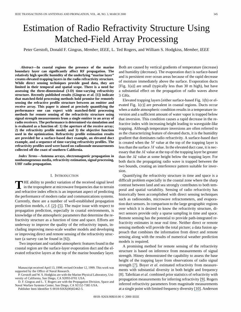
Both are caused by vertical gradients of temperature (increase)and humidity (decrease). The evaporation duct is surface-basedand is persistent over ocean areas because of the rapid decreaseof moisture immediately above the surface. Evaporation ducts[Fig. 1(a)] are small (typically less than 30 m high), but havea substantial effect on the propagation of radio waves above3 GHz.

Elevated trapping layers [either surface-based Fig. 1(b) or el-evated Fig. 1(c)] are prevalent in coastal regions. Ducts occurwhen a stable atmospheric condition results in a temperature in-version and a sufficient amount of water vapor is trapped belowthat inversion. This condition causes a rapid decrease in the re-fractive index with increasing height leading to waveguide-liketrapping. Although temperature inversions are often referred toas the characterizing feature of elevated ducts, it is the humiditygradient that dominates radio refractivity. A surface-based ductis created when the value at the top of the trapping layer isless than the surface value. In the elevated duct case, it is nec-essary that the value at the top of the trapping layer be greaterthan the value at some height below the trapping layer. Forboth ducts the propagating radio wave is trapped between thetwo bounds, creating an interference pattern suitable for inver-sion.

Quantifying the refractivity structure in time and space is adifficult problem especially in the coastal zone where the sharpcontrast between land and sea strongly contributes to both tem-poral and spatial variability. Sensing of radio refractivity hashistorically been accomplished with direct sensing techniquessuch as radiosondes, microwave refractometers, and evapora-tion duct sensors. In comparison to the large geographic regionsover which it is desired to know the refractivity structure, di-rect sensors provide only a sparse sampling in time and space.Remote sensing has the potential to provide path-integrated re-fractivity estimates in near real time. Neither direct or remotesensing methods will provide the total picture; a data fusion ap-proach that combines the information from direct and remotesensing along with the results of numerical weather predictionmodels is required.

A promising method for remote sensing of the refractivitystructure is based on inference from measurements of signalstrength. Hitney demonstrated the capability to assess the baseheight of the trapping layer from observations of radio signalstrength [7]. Boyeret al. estimated refractivity from measure-ments with substantial diversity in both height and frequency[8]. Tabrikianet al.combined prior statistics of refractivity withpropagation measurements for inferring refractivity [9]. Rogersinferred refractivity parameters from magnitude measurementsat a single point with limited frequency diversity [10]. Anderson

0018–926X/00$10.00 © 2000 IEEE

346 IEEE TRANSACTIONS ON ANTENNAS AND PROPAGATION, VOL. 48, NO. 3, MARCH 2000

Fig. 1. Modified refractivityM versus height. (a) Evaporation duct. (b) Surface-based duct. (c) Elevated duct. The modified refractivity is the refractivitymultiplied with 10 and corrected for the curvature of the earth.

inferred vertical refractivity of the lower atmosphere basedon ground-based measurements of global positioning system(GPS) signals [11].

The estimation or inference of atmospheric refractivitystructure from radio signal strength measurements is an inverseproblem. Matched-field processing methods represent oneapproach for solving inverse problems through the use of exten-sive forward modeling. The basic method of electromagneticmatched-field processing and the related genetic algorithms(GA) based global optimization procedures are discussed in[1]. It was also shown, using a single simulation example,that it may be possible to jointly estimate the location of anRF emitter and refractivity parameters using signal strengthmeasurements.

The present paper is a sequel to [1] in that it is directed to-ward quantifying the performance for matched-field processingmethods for remotely sensing refractivity structure. Syntheticsignal strength measurements from an emitter to an array ofradio receivers are generated for a variety of measured refrac-tivity profiles. The synthetic measurements are used to assessperformance of the matched-field methods. The refractivity pro-file estimation performance is analyzed as a function of: 1) aper-ture of receiver array; 2) refractivity profile models; and 3) anumber of objective functions. Results are provided for a sur-face-based duct example, an elevated duct example, and a timeseries containing a wide range of profile types.

The emphasis here is to bound the performance of a realsystem. The effect of environmental mismatch is not consideredand the same propagation model is used for generating both thesynthetic signal and the replica vectors.

Actual refractivity profiles were used in the simulationsand they were based on radiosonde measurements collectedoff the coast of southern California in an experiment aimed atcharacterizing the variability of coastal atmospheric refractivity(VOCAR). In Section II, the geometry and refractivity dataobtained during the VOCAR experiment are discussed. Then,Section III presents the matched-field processing methods usedfor refractivity profile estimation. In Section IV, the simulationapproach and results are discussed. Finally, conclusions of thiswork are summarized in Section V.

II. VOCAR EXPERIMENTAL DATA

Meteorological data and path geometries used in the simula-tions of Section IV were taken from the variability of coastal

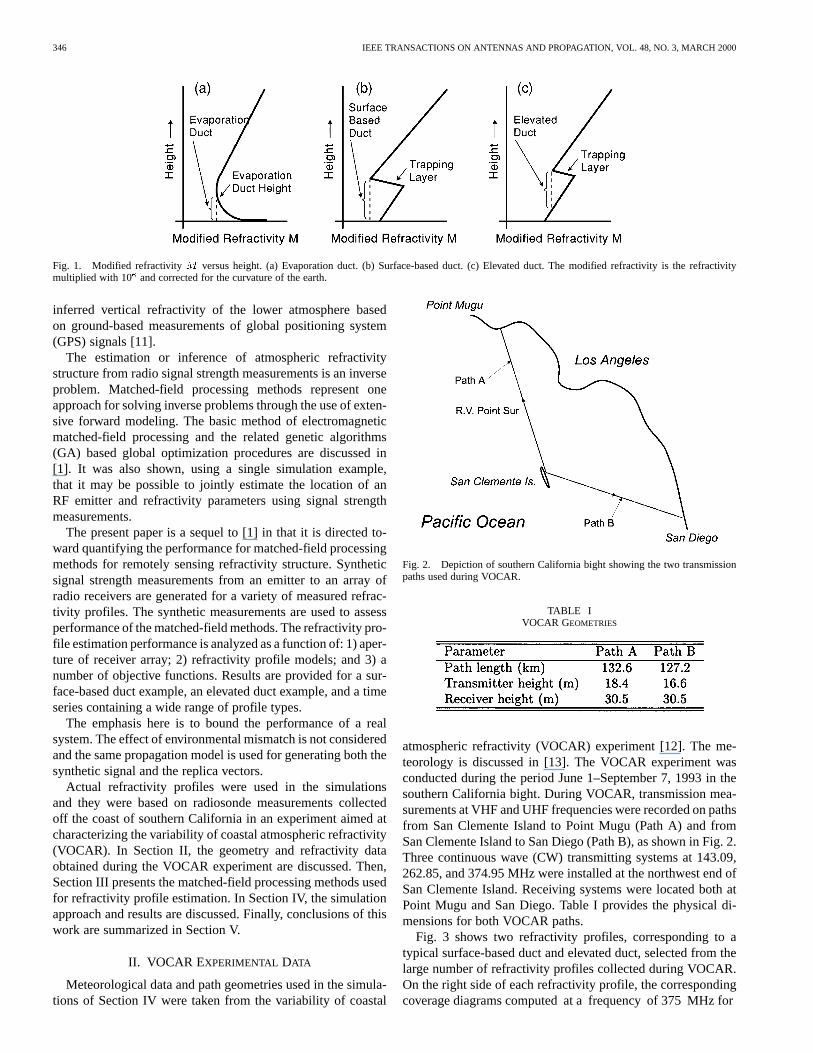
Fig. 2. Depiction of southern California bight showing the two transmissionpaths used during VOCAR.

TABLE IVOCAR GEOMETRIES

atmospheric refractivity (VOCAR) experiment [12]. The me-teorology is discussed in [13]. The VOCAR experiment wasconducted during the period June 1–September 7, 1993 in thesouthern California bight. During VOCAR, transmission mea-surements at VHF and UHF frequencies were recorded on pathsfrom San Clemente Island to Point Mugu (Path A) and fromSan Clemente Island to San Diego (Path B), as shown in Fig. 2.Three continuous wave (CW) transmitting systems at 143.09,262.85, and 374.95 MHz were installed at the northwest end ofSan Clemente Island. Receiving systems were located both atPoint Mugu and San Diego. Table I provides the physical di-mensions for both VOCAR paths.

Fig. 3 shows two refractivity profiles, corresponding to atypical surface-based duct and elevated duct, selected from thelarge number of refractivity profiles collected during VOCAR.On the right side of each refractivity profile, the correspondingcoverage diagrams computed at a frequency of 375 MHz for

GERSTOFTet al.: ESTIMATION OF RADIO REFRACTIVITY STRUCTURE USING MATCHED-FIELD ARRAY PROCESSING 347

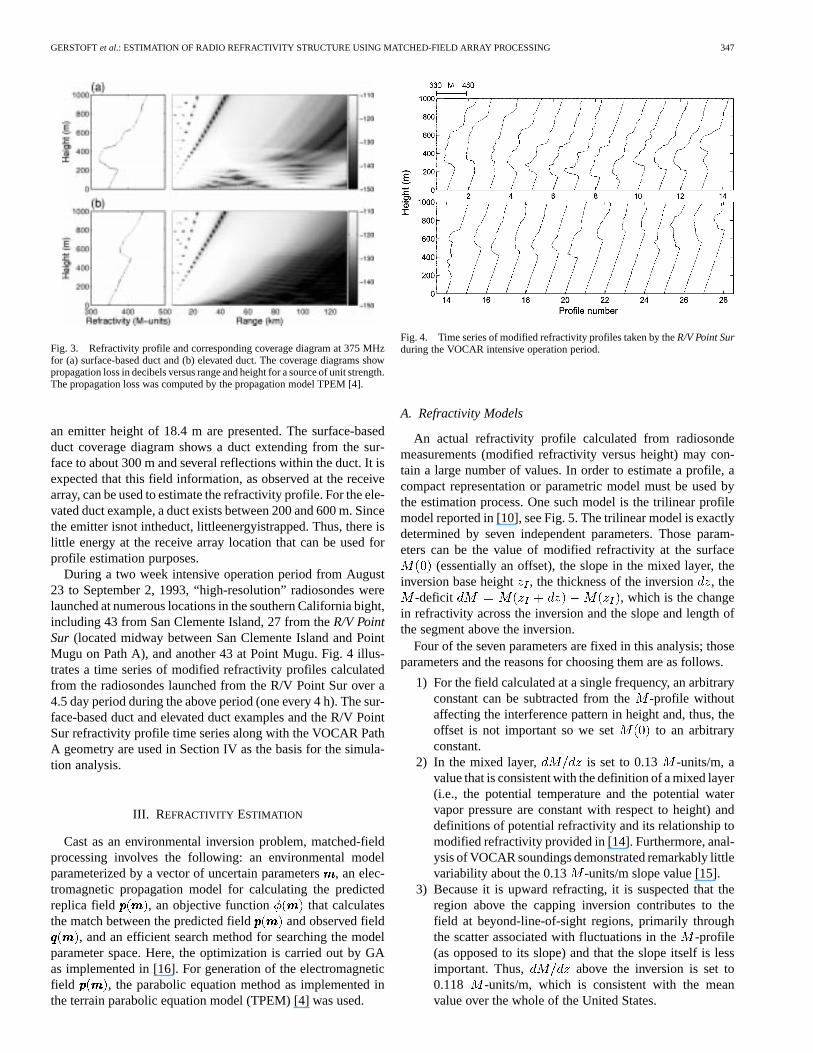
Fig. 3. Refractivity profile and corresponding coverage diagram at 375 MHzfor (a) surface-based duct and (b) elevated duct. The coverage diagrams showpropagation loss in decibels versus range and height for a source of unit strength.The propagation loss was computed by the propagation model TPEM [4].

an emitter height of 18.4 m are presented. The surface-basedduct coverage diagram shows a duct extending from the sur-face to about 300 m and several reflections within the duct. It isexpected that this field information, as observed at the receivearray, can be used to estimate the refractivity profile. For the ele-vated duct example, a duct exists between 200 and 600 m. Sincethe emitter isnot intheduct, littleenergyistrapped. Thus, there islittle energy at the receive array location that can be used forprofile estimation purposes.

During a two week intensive operation period from August23 to September 2, 1993, “high-resolution” radiosondes werelaunched at numerous locations in the southern California bight,including 43 from San Clemente Island, 27 from theR/V PointSur (located midway between San Clemente Island and PointMugu on Path A), and another 43 at Point Mugu. Fig. 4 illus-trates a time series of modified refractivity profiles calculatedfrom the radiosondes launched from the R/V Point Sur over a4.5 day period during the above period (one every 4 h). The sur-face-based duct and elevated duct examples and the R/V PointSur refractivity profile time series along with the VOCAR PathA geometry are used in Section IV as the basis for the simula-tion analysis.

III. REFRACTIVITY ESTIMATION

Cast as an environmental inversion problem, matched-fieldprocessing involves the following: an environmental modelparameterized by a vector of uncertain parameters, an elec-tromagnetic propagation model for calculating the predictedreplica field , an objective function that calculatesthe match between the predicted field and observed field

, and an efficient search method for searching the modelparameter space. Here, the optimization is carried out by GAas implemented in [16]. For generation of the electromagneticfield , the parabolic equation method as implemented inthe terrain parabolic equation model (TPEM) [4] was used.

Fig. 4. Time series of modified refractivity profiles taken by theR/V Point Surduring the VOCAR intensive operation period.

A. Refractivity Models

An actual refractivity profile calculated from radiosondemeasurements (modified refractivity versus height) may con-tain a large number of values. In order to estimate a profile, acompact representation or parametric model must be used bythe estimation process. One such model is the trilinear profilemodel reported in [10], see Fig. 5. The trilinear model is exactlydetermined by seven independent parameters. Those param-eters can be the value of modified refractivity at the surface

(essentially an offset), the slope in the mixed layer, theinversion base height , the thickness of the inversion , the

-deficit , which is the changein refractivity across the inversion and the slope and length ofthe segment above the inversion.

Four of the seven parameters are fixed in this analysis; thoseparameters and the reasons for choosing them are as follows.

1) For the field calculated at a single frequency, an arbitraryconstant can be subtracted from the-profile withoutaffecting the interference pattern in height and, thus, theoffset is not important so we set to an arbitraryconstant.

2) In the mixed layer, is set to 0.13 -units/m, avalue that is consistent with the definition of a mixed layer(i.e., the potential temperature and the potential watervapor pressure are constant with respect to height) anddefinitions of potential refractivity and its relationship tomodified refractivity provided in [14]. Furthermore, anal-ysis of VOCAR soundings demonstrated remarkably littlevariability about the 0.13 -units/m slope value [15].

3) Because it is upward refracting, it is suspected that theregion above the capping inversion contributes to thefield at beyond-line-of-sight regions, primarily throughthe scatter associated with fluctuations in the-profile(as opposed to its slope) and that the slope itself is lessimportant. Thus, above the inversion is set to0.118 -units/m, which is consistent with the meanvalue over the whole of the United States.

348 IEEE TRANSACTIONS ON ANTENNAS AND PROPAGATION, VOL. 48, NO. 3, MARCH 2000

Fig. 5. Modified vertical refractivity for a trilinear profile model.

4) The length of segment above the inversion is determinedby the maximum height used in the PE model.

That leaves , , and as the inversion variables.While simple, the trilinear profile has been used successfully

in a number of applications. An alternative to the trilinear modelwas sought on the expectation that a more complex model wouldimprove estimation performance. Another possible model is theempirical orthogonal function (EOF) model [17], [18]. Basedon observed refractivity profiles, a set of orthogonal functionsis calculated. A given profile can then be expressed as the meanof the observed profiles plus a weighted sum of the orthogonalfunctions. When used in the inverse problem, an optimizationalgorithm will vary the relative weighting of each orthogonalfunction and thus change the modeled refractivity profile.

A significant problem with the EOF approach is that it isnot efficient in expressing the “jump” in the profile above baseheight. Therefore, a variant of the EOF approach is definedwhere all observed profiles are shifted so that the jump in theprofiles occur at the same base heightand then the orthog-onal functions are calculated. This approach is elaborated fur-ther in the Appendix and is denoted as the shifted empiricalorthogonal function (SEOF) approach [15]. When used in theinverse problem, an optimization algorithm will vary the baseheight and the weighting of each orthogonal function tochange the modeled refractivity profile. Simulations have shownthat the SEOF representation requires about half the number ofcoefficients to obtain the same fit. Thus, SEOF’s are preferredover EOF’s.

B. Broad-Band Objective Functions

The relationship between the observed complex-valued datavector on an -element receive antenna array and thepredicted data at an angular frequency is describedby the model

(1)

where is the error term. The predicted data is given by, where the complex deterministic

source signal may be unknown. The transfer functionis obtained using an electromagnetic propagation

model (here the code TPEM [4] is used) and an environmentalmodel parameterized by the vector . In the following,

, etc. is abbreviated, where is theset of frequencies processed.

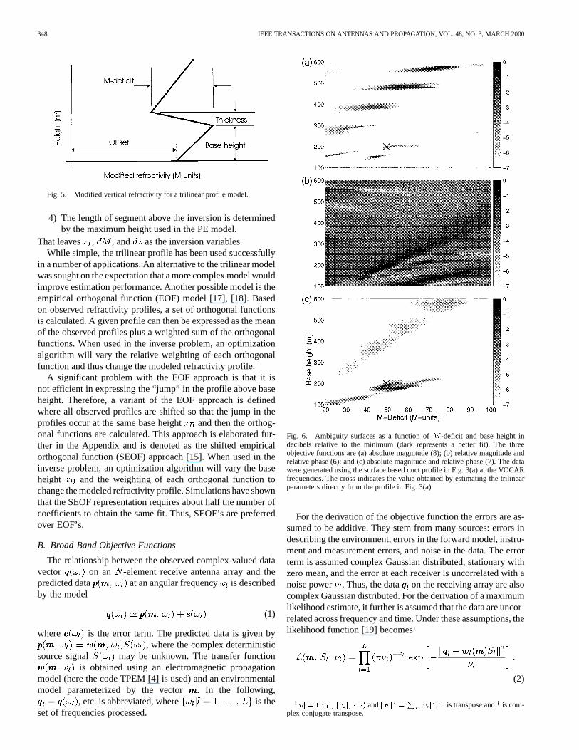
Fig. 6. Ambiguity surfaces as a function ofM -deficit and base height indecibels relative to the minimum (dark represents a better fit). The threeobjective functions are (a) absolute magnitude (8); (b) relative magnitude andrelative phase (6); and (c) absolute magnitude and relative phase (7). The datawere generated using the surface based duct profile in Fig. 3(a) at the VOCARfrequencies. The cross indicates the value obtained by estimating the trilinearparameters directly from the profile in Fig. 3(a).

For the derivation of the objective function the errors are as-sumed to be additive. They stem from many sources: errors indescribing the environment, errors in the forward model, instru-ment and measurement errors, and noise in the data. The errorterm is assumed complex Gaussian distributed, stationary withzero mean, and the error at each receiver is uncorrelated with anoise power . Thus, the data on the receiving array are alsocomplex Gaussian distributed. For the derivation of a maximumlikelihood estimate, it further is assumed that the data are uncor-related across frequency and time. Under these assumptions, thelikelihood function [19] becomes1

(2)

1jvvvj = (jv j; jv j; � � �) andkvvvk = jv j ; is transpose andis com-plex conjugate transpose.

GERSTOFTet al.: ESTIMATION OF RADIO REFRACTIVITY STRUCTURE USING MATCHED-FIELD ARRAY PROCESSING 349

Assuming that the noise powers are knownand constant across frequency, the likelihood function can befurther simplified to

(3)

The maximum likelihood estimate for is obtained byjointly maximizing (3) over the source signal and themodel parameter vector. The maximization with regard tois obtained in closed form by requiring ; this givesthe estimate . Substituting this estimate into the log-likelihoodfunction (3), the estimate can be obtained by minimizing

(4)

where the objective function for each frequency is intro-duced

(5)

Depending on thea priori assumptions for the signal, the fol-lowing maximum likelihood objective functions can be derivedfor each frequency component.

1) Relative Magnitude and Relative Phase of the Field:Thisis the so-called Bartlett objective function. When the receiversrecord the complex valued field and the complex source strength

is unknown, the source strength then is estimated as. For this objective function it is common

practice to normalize it with the norm of the data at eachfrequency. Doing this the objective function becomes

(6)

The Bartlett objective function is a weighted variation of phaseover the array. It contains no information about the propagationloss from the source to the receiver. This form is often used inocean acoustics [20], and was used in [1].

2) Absolute Magnitude and Relative Phase of theField: Here, we assume the magnitude of the sourceis known but the phase of the source signal is unknown,otherwise the same assumptions as in Section III-B.1 areused. The closed-form solution for the source strength thenis . The following objectivefunction is obtained:

(7)

This expression uses morea priori information about the sourcethan the Bartlett processor (6) and differs from the magnitudeonly objective function in that it also utilizes the phase infor-mation. Provided that the assumptions hold and that complexdata are available, this is a good alternative to the other objec-tive functions.

3) Absolute Magnitude of the Field:It is here assumed thatthe receivers record only the magnitude of the field and thesource strength is known. The complex-valued data modelin (1) is then replaced with a similar one for magnitude only. It issimilarly assumed that the errors are real Gaussian distributed.

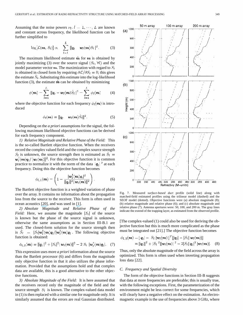
Fig. 7. Measuredsurface-based ductprofile (solid line) along withmatched-field estimated profiles using the trilinear model (dashed) and theSEOF model (dotted). Objective functions were (a) absolute magnitude (8);(b) relative magnitude and relative phase (6); and (c) absolute magnitude andrelative phase (7). Antenna apertures were: 50, 100, and 200 m. The gray linesindicate the extend of the trapping layer, as estimated from the observed profile.

[The complex-valued (1) could also be used for deriving the ob-jective function but this is much more complicated as the phasemust be integrated out [21].] The objective function becomes

(8)

Thus, only the absolute magnitude of the field across the array isoptimized. This form is often used when inverting propagationloss data [22].

C. Frequency and Spatial Diversity

The form of the objective functions in Section III-B suggeststhat data at more frequencies are preferable; this is usually true,with the following exceptions. First, the parameterization of theenvironment might be less correct for some frequencies, whichwill clearly have a negative effect on the estimation. An electro-magnetic example is the use of frequencies above 3 GHz, where

350 IEEE TRANSACTIONS ON ANTENNAS AND PROPAGATION, VOL. 48, NO. 3, MARCH 2000

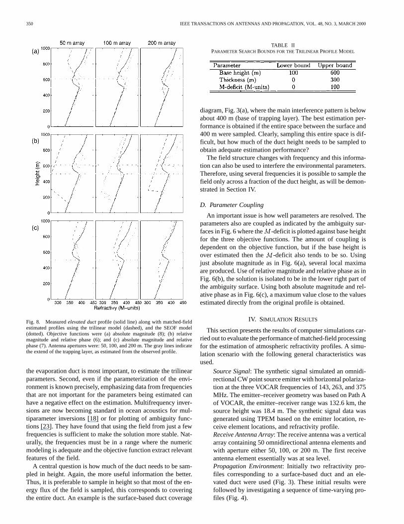
Fig. 8. Measuredelevated ductprofile (solid line) along with matched-fieldestimated profiles using the trilinear model (dashed), and the SEOF model(dotted). Objective functions were (a) absolute magnitude (8); (b) relativemagnitude and relative phase (6); and (c) absolute magnitude and relativephase (7). Antenna apertures were: 50, 100, and 200 m. The gray lines indicatethe extend of the trapping layer, as estimated from the observed profile.

the evaporation duct is most important, to estimate the trilinearparameters. Second, even if the parameterization of the envi-ronment is known precisely, emphasizing data from frequenciesthat are not important for the parameters being estimated canhave a negative effect on the estimation. Multifrequency inver-sions are now becoming standard in ocean acoustics for mul-tiparameter inversions [18] or for plotting of ambiguity func-tions [23]. They have found that using the field from just a fewfrequencies is sufficient to make the solution more stable. Nat-urally, the frequencies must be in a range where the numericmodeling is adequate and the objective function extract relevantfeatures of the field.

A central question is how much of the duct needs to be sam-pled in height. Again, the more useful information the better.Thus, it is preferable to sample in height so that most of the en-ergy flux of the field is sampled, this corresponds to coveringthe entire duct. An example is the surface-based duct coverage

TABLE IIPARAMETER SEARCH BOUNDS FOR THETRILINEAR PROFILE MODEL

diagram, Fig. 3(a), where the main interference pattern is belowabout 400 m (base of trapping layer). The best estimation per-formance is obtained if the entire space between the surface and400 m were sampled. Clearly, sampling this entire space is dif-ficult, but how much of the duct height needs to be sampled toobtain adequate estimation performance?

The field structure changes with frequency and this informa-tion can also be used to interfere the environmental parameters.Therefore, using several frequencies it is possible to sample thefield only across a fraction of the duct height, as will be demon-strated in Section IV.

D. Parameter Coupling

An important issue is how well parameters are resolved. Theparameters also are coupled as indicated by the ambiguity sur-faces in Fig. 6 where the -deficit is plotted against base heightfor the three objective functions. The amount of coupling isdependent on the objective function, but if the base height isover estimated then the -deficit also tends to be so. Usingjust absolute magnitude as in Fig. 6(a), several local maximaare produced. Use of relative magnitude and relative phase as inFig. 6(b), the solution is isolated to be in the lower right part ofthe ambiguity surface. Using both absolute magnitude and rel-ative phase as in Fig. 6(c), a maximum value close to the valuesestimated directly from the original profile is obtained.

IV. SIMULATION RESULTS

This section presents the results of computer simulations car-ried out to evaluate the performance of matched-field processingfor the estimation of atmospheric refractivity profiles. A simu-lation scenario with the following general characteristics wasused.

Source Signal: The synthetic signal simulated an omnidi-rectional CW point source emitter with horizontal polariza-tion at the three VOCAR frequencies of 143, 263, and 375MHz. The emitter–receiver geometry was based on Path Aof VOCAR, the emitter–receiver range was 132.6 km, thesource height was 18.4 m. The synthetic signal data wasgenerated using TPEM based on the emitter location, re-ceive element locations, and refractivity profile.Receive Antenna Array: The receive antenna was a verticalarray containing 50 omnidirectional antenna elements andwith aperture either 50, 100, or 200 m. The first receiveantenna element essentially was at sea level.Propagation Environment: Initially two refractivity pro-files corresponding to a surface-based duct and an ele-vated duct were used (Fig. 3). These initial results werefollowed by investigating a sequence of time-varying pro-files (Fig. 4).

GERSTOFTet al.: ESTIMATION OF RADIO REFRACTIVITY STRUCTURE USING MATCHED-FIELD ARRAY PROCESSING 351

TABLE IIIPARAMETER SEARCH BOUND FOR THESEOF PROFILE MODEL

Refractivity Profile Models: Two profile models wereused—the trilinear and SEOF. The search bounds used bythe estimation process are given in Table II for the trilinearmodel (Fig. 5) and Table III for the SEOF model.Objective Function: Three objective functions as definedby (6)–(8) were used. In all cases, the objective functionswere summed over the three VOCAR frequencies. Thematched-field replica vectors (predicted propagation data)were generated using the TPEM propagation model.Optimization Parameters: The propagation code and objec-tive function were incorporated into the SAGA code whichuses GA for optimization [24]. The GA search parameterswere: parameter quantization 128 values; population size64; reproduction size 0.5; cross-over probability 0.05;number of iterations for each population 2000; and numberofpopulations10.Thus,20 000forwardmodelingrunswereperformed for each inversion. For further information abouttheuseofGAforparameterestimationsee[16].CPU Run Time: The GA computations, 20 000 forwardmodel runs, required about 3 h of CPU time on a SUN Ultra2/2200.

A. Surface-Based Duct Example

The first simulation considered the surface-based ductexample whose refractivity profile was illustrated in Fig. 3(a)along with the corresponding coverage diagram. This profileproduces a surface-based duct up to about 300 m. Syntheticdata were generated at the three VOCAR frequencies using themeasured refractivity profile, using the VOCAR Path A geom-etry (Table I) and for each of the three receive antenna arrayapertures. Using the synthetic data, matched-field processingwas applied to estimate the modeled refractivity profile basedon the simulated measurements. Fig. 7 illustrates the inversionresults for three receive array apertures, three objective func-tions and two refractivity profile models. On each of the plots,the measured profile is indicated by the solid line, the trilinearprofile model estimate by the dashed line, and the SEOF modelestimate by the dotted line. The horizontal lines indicate thelocation of the trapping layer.

Fig. 7(a) provides the results obtained using the absolute mag-nitude objective function (8). This objective function assumesthat the emitter source strength is known and uses the magnitudeinformation across the receive array. In this case, the 100- and200-m aperture array with the trilinear refractivity model pro-vided estimated profiles that were close to the measured profile.The base height, thickness, and-deficit estimates are nearlyperfect. As seen on the three panels of Fig. 7(a), the more com-plicated SEOF profile model did not perform well.

Fig. 7(b) illustrates the result when the objective function wasBartlett objective function (6). This objective function does notassume that the emitter source strength is known and uses therelative magnitude and phase information across the array. The100-m aperture array correctly estimated a duct, but the heightwas a factor two too small. The 200-m aperture array providedgood estimates with both the trilinear and SEOF profile models.

Finally, Fig. 7(c) illustrates the results for the objective func-tion of (7). This objective function assumes that the emittersource strength is known and uses the relative phase informationacross the array as well as the magnitude information. In thiscase, fairly good estimates were obtained even with the 50-maperture array when the trilinear profile model was used. Thetrilinear profile model estimates improve as the array apertureincreases. When the SEOF model was used only the 200-m aper-ture array provided a reasonable estimate.

B. Elevated Duct Example

The second simulation considered the elevated duct examplewhose refractivity profile was illustrated in Fig. 3(b) along withthe corresponding coverage diagram. This profile has an ele-vated duct between about 200 and 600 m. Since neither the sim-ulated emitter at 18.4 m nor the receive array elements are in theduct, it is not expected that the elevated duct profile can be esti-mated as well as the surface-based duct profile. However, whatwould be desirable is the ability to distinguish between surfaceand elevated ducting conditions even if the refractivity profileestimate is not very accurate.

Fig. 8 illustrates the inversion results obtained for the elevatedduct profile example. As in the previous example, a wide varietyof results are presented for the objective function, array aperture,and refractivity profile model options. Fig. 8(a) illustrates theresults obtained using the absolute magnitude objective func-tion (8). For this case, both the trilinear and SEOF model basedestimates roughly are equivalent and clearly indicate elevatedducting conditions.

Fig. 8(b) illustrates the results obtained with the Bartlett ob-jective function (6). The Bartlett objective function does not takeinto account the emitter source strength information. By the rel-ative poor performance with this objective function, it can benoted that the elevated duct profile case requires this additionalinformation in order to obtain reasonable profile estimates.

When the absolute magnitude and relative phase objectivefunction (7) was used, the results were improved for both re-fractivity profile models, Fig. 8(c). Even the results for the 50-maperture array with the SEOF profile model were reasonable. Inthis case, the 200-m aperture array with the SEOF profile modelproduced a very good profile estimate.

C. Time Series Example

To gain a statistical indication of performance, time seriesof refractivity profiles that were calculated from radiosondeslaunched over a 4.5 day period during the VOCAR IOP fromthe R/V Point Sur are used. The 27 refractivity profiles wereillustrated in Fig. 4. Note that for the first 13 profiles there existsa relatively “strong” surface-based duct with a relativity largeaverage -deficit of about 40 -units and an average base-height of 200 m. Profile 14 is a transitional profile. Starting with

352 IEEE TRANSACTIONS ON ANTENNAS AND PROPAGATION, VOL. 48, NO. 3, MARCH 2000

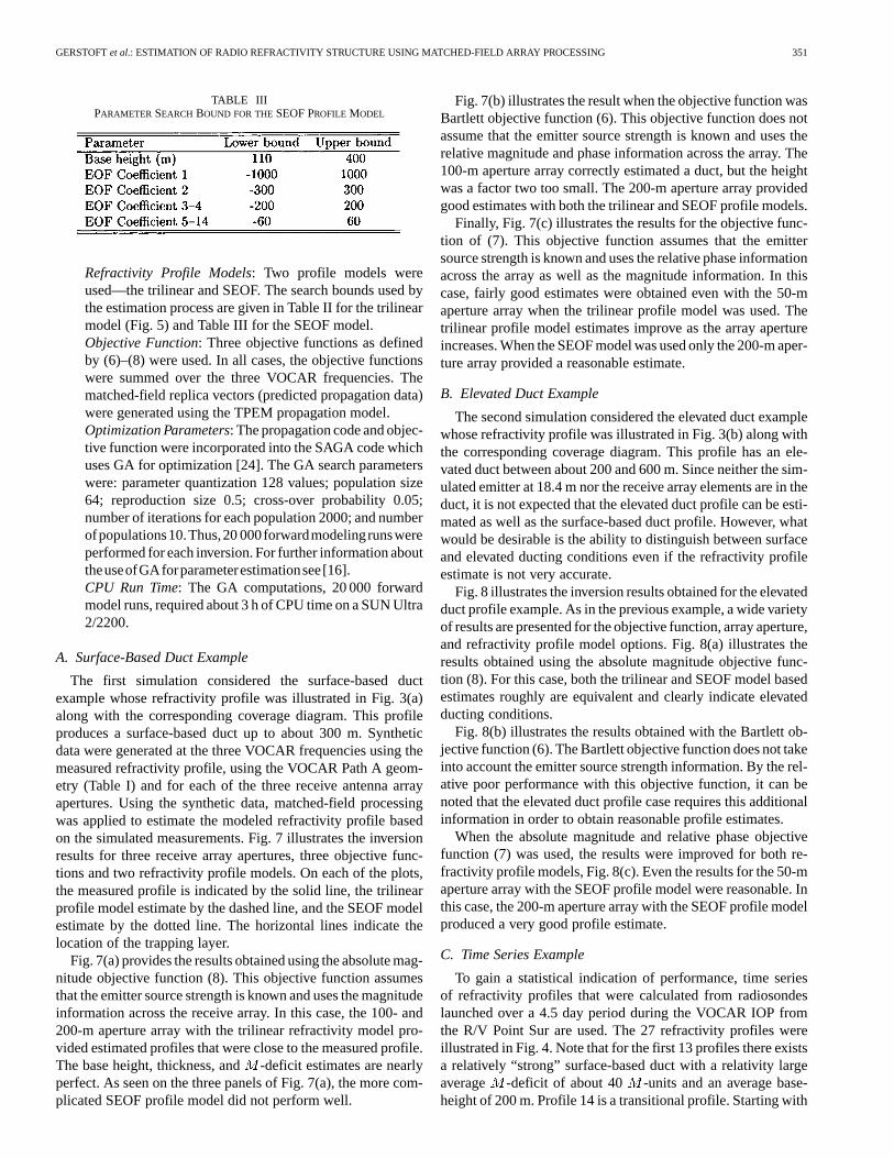
Fig. 9. Measured profiles from R/V Point Sur (solid line) along with estimatedprofiles (dashed line) for a50-m aperture array.The profiles were estimatedusing objective function (7) with the trilinear profile.

profile 15 there is a somewhat weaker elevated duct with anaverage -deficit of about 20 -units and average base heightof about 500 m.

For this example, synthetic data were generated for each ofthe 27 measured refractivity profiles. Then the matched-fieldestimation process was carried out for each profile. Based onthe results obtained for the previous two examples, it was de-cided that the absolute magnitude and relative phase objectivefunction (7), combined with the trilinear profile model wouldbe used for the analysis of the time series profiles. Both 50- and100-m aperture arrays were used.

Fig. 9 illustrates the estimation results obtained using the50-m aperture array. The estimated profiles (dashed lines) areplotted along with the measured profiles (solid lines). For a largepercentage of the profiles, about 70%, the estimated trilinearprofile model provides a relatively good fit to the measured pro-files. This is a remarkable result, as only the first 50 m of thefield was sampled by the receive array.

Fig. 10 illustrates the same situation except the 100-m aper-ture array was used. In this case, nearly all of estimated profilesare quite close to the measured profiles. In general, it looks as ifthe base height and -deficit are being estimated accurately. Inalmost all cases, both the surface-based ducts and the elevatedducts were correctly identified.

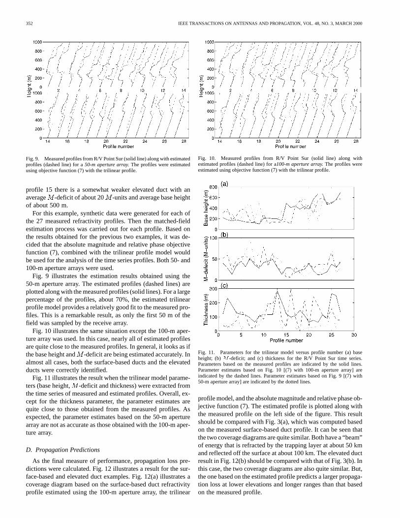
Fig. 11 illustrates the result when the trilinear model parame-ters (base height, -deficit and thickness) were extracted fromthe time series of measured and estimated profiles. Overall, ex-cept for the thickness parameter, the parameter estimates arequite close to those obtained from the measured profiles. Asexpected, the parameter estimates based on the 50-m aperturearray are not as accurate as those obtained with the 100-m aper-ture array.

D. Propagation Predictions

As the final measure of performance, propagation loss pre-dictions were calculated. Fig. 12 illustrates a result for the sur-face-based and elevated duct examples. Fig. 12(a) illustrates acoverage diagram based on the surface-based duct refractivityprofile estimated using the 100-m aperture array, the trilinear

Fig. 10. Measured profiles from R/V Point Sur (solid line) along withestimated profiles (dashed line) for a100-m aperture array.The profiles wereestimated using objective function (7) with the trilinear profile.

Fig. 11. Parameters for the trilinear model versus profile number (a) baseheight; (b)M -deficit; and (c) thickness for the R/V Point Sur time series.Parameters based on the measured profiles are indicated by the solid lines.Parameter estimates based on Fig. 10 [(7) with 100-m aperture array] areindicated by the dashed lines. Parameter estimates based on Fig. 9 [(7) with50-m aperture array] are indicated by the dotted lines.

profile model, and the absolute magnitude and relative phase ob-jective function (7). The estimated profile is plotted along withthe measured profile on the left side of the figure. This resultshould be compared with Fig. 3(a), which was computed basedon the measured surface-based duct profile. It can be seen thatthe two coverage diagrams are quite similar. Both have a “beam”of energy that is refracted by the trapping layer at about 50 kmand reflected off the surface at about 100 km. The elevated ductresult in Fig. 12(b) should be compared with that of Fig. 3(b). Inthis case, the two coverage diagrams are also quite similar. But,the one based on the estimated profile predicts a larger propaga-tion loss at lower elevations and longer ranges than that basedon the measured profile.

GERSTOFTet al.: ESTIMATION OF RADIO REFRACTIVITY STRUCTURE USING MATCHED-FIELD ARRAY PROCESSING 353

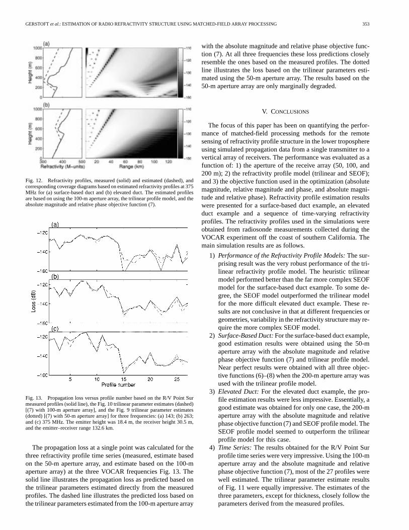
Fig. 12. Refractivity profiles, measured (solid) and estimated (dashed), andcorresponding coverage diagrams based on estimated refractivity profiles at 375MHz for (a) surface-based duct and (b) elevated duct. The estimated profilesare based on using the 100-m aperture array, the trilinear profile model, and theabsolute magnitude and relative phase objective function (7).

Fig. 13. Propagation loss versus profile number based on the R/V Point Surmeasured profiles (solid line), the Fig. 10 trilinear parameter estimates (dashed)[(7) with 100-m aperture array], and the Fig. 9 trilinear parameter estimates(dotted) [(7) with 50-m aperture array] for three frequencies: (a) 143; (b) 263;and (c) 375 MHz. The emitter height was 18.4 m, the receiver height 30.5 m,and the emitter–receiver range 132.6 km.

The propagation loss at a single point was calculated for thethree refractivity profile time series (measured, estimate basedon the 50-m aperture array, and estimate based on the 100-maperture array) at the three VOCAR frequencies Fig. 13. Thesolid line illustrates the propagation loss as predicted based onthe trilinear parameters estimated directly from the measuredprofiles. The dashed line illustrates the predicted loss based onthe trilinear parameters estimated from the 100-m aperture array

with the absolute magnitude and relative phase objective func-tion (7). At all three frequencies these loss predictions closelyresemble the ones based on the measured profiles. The dottedline illustrates the loss based on the trilinear parameters esti-mated using the 50-m aperture array. The results based on the50-m aperture array are only marginally degraded.

V. CONCLUSIONS

The focus of this paper has been on quantifying the perfor-mance of matched-field processing methods for the remotesensing of refractivity profile structure in the lower troposphereusing simulated propagation data from a single transmitter to avertical array of receivers. The performance was evaluated as afunction of: 1) the aperture of the receive array (50, 100, and200 m); 2) the refractivity profile model (trilinear and SEOF);and 3) the objective function used in the optimization (absolutemagnitude, relative magnitude and phase, and absolute magni-tude and relative phase). Refractivity profile estimation resultswere presented for a surface-based duct example, an elevatedduct example and a sequence of time-varying refractivityprofiles. The refractivity profiles used in the simulations wereobtained from radiosonde measurements collected during theVOCAR experiment off the coast of southern California. Themain simulation results are as follows.

1) Performance of the Refractivity Profile Models:The sur-prising result was the very robust performance of the tri-linear refractivity profile model. The heuristic trilinearmodel performed better than the far more complex SEOFmodel for the surface-based duct example. To some de-gree, the SEOF model outperformed the trilinear modelfor the more difficult elevated duct example. These re-sults are not conclusive in that at different frequencies orgeometries, variability in the refractivity structure may re-quire the more complex SEOF model.

2) Surface-Based Duct:For the surface-based duct example,good estimation results were obtained using the 50-maperture array with the absolute magnitude and relativephase objective function (7) and trilinear profile model.Near perfect results were obtained with all three objec-tive functions (6)–(8) when the 200-m aperture array wasused with the trilinear profile model.

3) Elevated Duct:For the elevated duct example, the pro-file estimation results were less impressive. Essentially, agood estimate was obtained for only one case, the 200-maperture array with the absolute magnitude and relativephase objective function (7) and SEOF profile model. TheSEOF profile model seemed to outperform the trilinearprofile model for this case.

4) Time Series:The results obtained for the R/V Point Surprofile time series were very impressive. Using the 100-maperture array and the absolute magnitude and relativephase objective function (7), most of the 27 profiles werewell estimated. The trilinear parameter estimate resultsof Fig. 11 were equally impressive. The estimates of thethree parameters, except for thickness, closely follow theparameters derived from the measured profiles.

354 IEEE TRANSACTIONS ON ANTENNAS AND PROPAGATION, VOL. 48, NO. 3, MARCH 2000

5) Propagation Predictions:The propagation predictions inFig. 13 at the three VOCAR frequencies based on theestimated trilinear profile parameters tracked very closelythose based on the measured profiles.

Based on the limited simulations presented here, it is demon-strated that remote sensing of time-varying refractivity profilestructure is feasible using an array with aperture 50–100 m, asimple parameterization of the refractivity profile (trilinear),and a sophisticated objective function (absolute magnitudeand relative phase across the array). The refractivity profileestimates for surface-based duct profiles were very goodwhile those for elevated ducts were less accurate. However,the inversion process clearly was able to distinguish betweensurface-based and elevated ducting conditions. Furthermore,the results showed that the estimated refractivity profiles wereof sufficient quality to provide propagation loss predictionsat all frequencies very close to those generated from trilinearversions of the original profiles.

APPENDIX

SHIFTED EMPIRICAL ORTHOGONAL FUNCTION (SEOF)REFRACTIVITY PROFILE MODEL

An observed refractivity profile , where is the height(assumed to be discrete values), may be modeled as

(9)

wheremean profile;

the empirical orthogonal functions (EOF’s) devel-oped from historical data;

the corresponding coefficients.

When used in the inverse medium problem, an optimization al-gorithm will vary the coefficients to find the esti-mated refractivity profile that provides the best match betweenthe predicted and observed propagation data.

There are three potential problems when using EOF’s forrefractivity modeling in the electromagnetic inverse mediumproblem. First, many coefficients may be required to adequatelyrepresent a profile (experience indicates that 6–10 are typicallyrequired to adequately fit the VOCAR soundings); second, non-physical profiles may result; and third EOF coefficients do noteasily transform to meteorologically meaningful parameters.

Since the thickness of the trapping layer is on the order of100–200 m and the base height can vary over 500 m, it is reason-able to expect that a more compact parameterization could beobtained by using EOF’s that are referenced to the base height.A second advantage is that in this form the base height, which isa meaningful meteorological parameter, is an explicit parameter.The shifted EOF (SEOF) parameterization is now described.

1) Each profile is shifted such that the height is refer-enced to the trapping layer base height for that pro-file

(10)

Fig. 14. Example of (a) EOF and (b) SEOF profiles (solid lines) for increasingnumbers of coefficients. The SEOF’s provide a better fit to the real profile(dashed lines) using four parameters than the EOF’s using nine parameters.

where is the modified refractivity and the superscriptdenotes that the profile was shifted.

2) Let there be shifted refractivity profiles, each profile isa column vector of length . The mean profile vector

and the covariance matrix are calculated

(11)

The notation indicates an ensemble average, the super-script indicates transpose.

3) The eigenvectors of are EOF’s spanning the setof shifted refractivity profiles used to generate. Let theeigenvalues of and corresponding eigenvectors bearranged in descending order . Alinear combination of orthogonal functions based onthe first eigenvectors yields a minimum mean-squarederror representation

(12)

where .4) An optimization algorithm will vary the base height

and the coefficients to obtain a refractivityprofile estimate.

The advantage of using the SEOF representation relative tothe EOF representation is illustrated in Fig. 14. For this profile,the SEOF representation provides a better fit using four coeffi-cients than the EOF representation when using nine coefficients.Simulations with other profiles have shown that the SEOF rep-resentation requires about half the number of EOF coefficientsto obtain the same fit.

In addition to the above general discussion, the following ad-ditional constraints were applied to the implementation usedherein. Only the region from 100 m below to 200 m above thebase height was estimated by varying the coefficients in (12) (theregions below and above were modeled using realizations basedon second-order statistics over the entire set of soundings).

GERSTOFTet al.: ESTIMATION OF RADIO REFRACTIVITY STRUCTURE USING MATCHED-FIELD ARRAY PROCESSING 355

ACKNOWLEDGMENT

The authors would like to thank R. Paulus of the SPAWARSystems Center, San Diego, CA, for carefully collecting andsupplying the VOCAR radiosonde data.

REFERENCES

[1] D. F. Gingras, P. Gerstoft, and N. L. Gerr, “Electromagnetic matchedfield processing: Basic concepts and tropospheric simulations,”IEEETrans. Antennas Propagat., vol. 42, pp. 1305–1316, Oct. 1997.

[2] G. D. Dockery, “Modeling electromagnetic wave propagation in the tro-posphere using the parabolic equation,”IEEE Trans. Antennas Prop-agat., vol. 36, pp. 1464–1470, Oct. 1988.

[3] H. V. Hitney, “Hybrid ray optics and parabolic equation methods forradar propagation modeling,” inProc. Inst. Elect. Eng. Radar ’92 Conf.,Brighton, U.K., Oct. 1992, pp. 58–61.

[4] A. E. Barrios, “A terrain parabolic equation model for propagation inthe troposphere,”IEEE Trans. Antennas Propagat., vol. 42, pp. 90–98,Jan. 1994.

[5] M. F. Levy, “Horizontal parabolic equation solution of radiowave prop-agation problems on large domain,”IEEE Trans. Antennas Propagat.,vol. 43, pp. 137–143, Feb. 1995.

[6] J. H. Richter, “Variability and sensing of the coastal environment,” inAGARD Conf. Proc. CP-567, Bremerhaven, Germany, Sept. 1994, pp.1.1–1.3.

[7] H. V. Hitney, “Remote sensing of refractivity structure by direct mea-surements at UHF,” inAGARD Conf. Proc. CP-502, Cesme, Turkey, Feb.1992, 1, pp. 1.1–1.5.

[8] D. Boyer, G. Gentry, J. Stapleton, and J. Cook, “Using remote refrac-tivity sensing to predict tropospheric refractivity from measurements ofpropagation,” inProc. AGARD SPP Symp. Remote Sensing: ValuableSource Inform., Toulouse, France, Apr. 22–25, 1996, pp. 16.1–16.13.

[9] J. Tabrikian and J. Krolik, “Theoretical performance limits on tropo-spheric refractivity estimation using point-to-point microwave measure-ments,”IEEE Trans. Antennas Propagat., vol. 47, pp. 1727–1734, Nov.1999.

[10] L. T. Rogers, “Likelihood estimation of tropospheric duct parametersfrom horizontal propagation measurements,”Radio Sci., vol. 32, pp.79–92, Jan./Feb. 1997.

[11] K. D. Anderson, “Tropospheric refractivity profiles inferred from lowelevation angle measurements of Global Positioning System (GPS) sig-nals,” in AGARD Conf. Proc. CP-567, Bremerhaven, Germany, Sept.1994, pp. 2.1–2.7.

[12] R. A. Paulus, “VOCAR: An experiment in the variability of coastal at-mospheric refractivity,” inProc. Int. Geosci. Remote Sensing Symp., vol.I. Pasadena, CA, Aug. 1994, pp. 386–388.

[13] S. D. Burk and W. T. Thompson, “Mesoscale modeling of summertimerefractive conditions in the southern California bight,”J. Appl. Meteor.,vol. 36, pp. 22–31, Jan. 1997.

[14] E. E. Gossard and R. G. Strauch,Radar Observations of Clear Air andClouds. Amsterdam, The Netherlands: Elsevier, 1983.

[15] L. T. Rogers, “Demonstration of an efficient boundary layer parameter-ization for unbiased propagation estimation,”Radio Sci., vol. 33, no. 6,pp. 1599–1608, 1998.

[16] P. Gerstoft, “Inversion of seismoacoustic data using GA and a posterioriprobability distributions,”J. Acoust. Soc. Amer., vol. 95, pp. 770–782,Feb. 1994.

[17] L. R. LeBlanc and F. H. Middleton, “An underwater acoustic sound ve-locity data model,”J. Acoust. Soc. Amer., vol. 67, pp. 2055–2062, June1980.

[18] P. Gerstoft and D. F. Gingras, “Parameter estimation using multifre-quency range-dependent acoustic data in shallow water,”J. Acoust. Soc.Amer., vol. 99, pp. 2839–2850, May 1996.

[19] D. H. Johnson and D. E. Dudgeon,Array Signal Pro-cessing. Englewood Cliffs, NJ: Prentice-Hall, 1993.

[20] D. F. Gingras and P. Gerstoft, “Inversion for geometric and geoacousticparameters in shallow water: Experimental results,”J. Acoust. Soc.Amer., vol. 97, pp. 3589–3598, June 1995.

[21] C. F. Mecklenbräuker and P. Gerstoft, “Uncertainties in geoacoustic pa-rameter estimates,” J. Computat. Acoust., to be published.

[22] L. T. Rogers, “Effects of the variability of atmospheric refractivity onpropagation estimates,”IEEE Trans. Antennas Propagat., vol. 44, pp.460–465, Apr. 1996.

[23] N. O. Booth, P. A. Baxley, J. A. Rice, P. W. Schey, W. S. Hodgkiss,G. L. D’Spain, and J. J. Murray, “Source localization with broad-bandmatched-field processing in shallow water,”IEEE J. Ocean. Eng., vol.21, pp. 402–412, Oct. 1996.

[24] P. Gerstoft, “SAGA Users guide 2.0, an inversion sofware package,”SACLANT Undersea Research Centre, SM-333, 1997.

Peter Gerstoft received the M.Sc. and the Ph.D.degrees from the Technical University of Denmark,Lyngby, Denmark, in 1983 and 1986, respectively,and the M.Sc. degree from the University of WesternOntario, London, Canada, in 1984.

From 1987 to 1992, he was employed at Ødegaardand Danneskiold-Samsøe, Copenhagen, Denmark,working on forward modeling and inversion forseismic exploration. From 1989 to 1990 he wasa Visiting Scientist at the Massachusetts Instituteof Technology, Cambridge, and at Woods Hole

Oceanographic Institute, Cape Cod, MA. From 1992 to 1997 he was SeniorScientist at SACLANT Undersea Research Centre, La Spezia, Italy, where hedeveloped the SAGA inversion code, which is used for ocean acoustic andelectromagnetic signals. From 1997 to 1999 he was with Marine PhysicalLaboratory, University of California, San Diego. Since 1999 he has been withthe Comprehensive Nuclear Test-Ban Treaty Organization, Vienna, Austria,where he is doing hydro-acoustic modeling and inversion. His research interestsinclude global optimization, modeling and inversion of acoustic, and elasticand electromagnetic signals.

Donald F. Gingras (S’68–M’68) received the B.S.degree from San Diego State University, San Diego,CA, in 1968, the M.S. degree from Northeastern Uni-versity, Boston, MA, in 1971, and the Ph.D. degreefrom the University of California, San Diego in 1986,all in electrical engineering.

From 1968 to 1971, he was a Sonar Design En-gineer with Raytheon at the Submarine Signal Divi-sion, Portsmouth RI. From 1971 to 1990 he worked inarray signal processing at the Naval Command Con-trol and Ocean Surveillance Center, San Diego, CA.

From 1990 to 1995 he led the Signal Processing Group at the SACLANT Un-dersea Research Centre, La Spezia, Italy. In 1996 he joined the Communicationsand Information Systems Department at the Space and Naval Warfare SystemsCenter, San Diego, CA. His current research interests include matched-field pro-cessing, propagation modeling, integrated services wireless networks, and mul-tiple access protocols.

L. Ted Rogerswas born in Miami, FL, on February14, 1954. He received the B.S. degree in engineeringsciences from the University of Florida, Gainesville,in 1983, and the M.S. degree in applied mathematicsfrom San Diego State University, San Diego, CA, in1990.

From 1983 until 1988, he served as a Surface War-fare Officer in the U.S. Navy. Since 1990 he has beenemployed by what is currently called the Space andNaval Warfare Systems Center, San Diego, CA. Hisprimary research interest is in improving estimation

of the refractivity structure associated with the marine atmospheric boundarylayer through combiningin situand remotely sensed observation with data fromnumerical weather prediction models.

356 IEEE TRANSACTIONS ON ANTENNAS AND PROPAGATION, VOL. 48, NO. 3, MARCH 2000

William S. Hodgkiss (S’68–M’75) was born inBellefonte, PA, on August 20, 1950. He received theB.S.E.E. degree from Bucknell University, Lewis-burg, PA, in 1972, and the M.S. and Ph.D. degreesin electrical engineering from Duke University,Durham, NC, in 1973 and 1975, respectively.

From 1975 to 1977, he worked with the NavalOcean Systems Center, San Diego, CA. From 1977to 1978 he was a Faculty Member in the ElectricalEngineering Department, Bucknell University,Lewisburg, PA. Since 1978 he has been a member of

the faculty of the Scripps Institution of Oceanography, University of California,San Diego, and on the staff of the Marine Physical Laboratory, where he iscurrently Deputy Director. He is the Applied Ocean Science Curricular GroupCoordinator, Graduate Department of the Scripps Institution of Oceanography.His present research interests are in the areas of adaptive array processing,propagation modeling, and environmental inversions with applications of theseto underwater acoustics and electromagnetic wave propagation.

Dr. Hodgkiss is a fellow of the Acoustical Society of America.