Coastal Engineering 64 (2012) 73–86

Contents lists available at SciVerse ScienceDirect

Coastal Engineering

j ourna l homepage: www.e lsev ie r .com/ locate /coasta leng

Time-dependent onshore tsunami response

Alex Apotsos ⁎, Guy Gelfenbaum, Bruce JaffePacific Coastal and Marine Science Center, USGS, 400 Natural Bridges Drive, Santa Cruz, CA, USA

⁎ Corresponding author. Tel.: +1 650 815 5915.E-mail address: aapotsos@gmail.com (A. Apotsos).

0378-3839/$ – see front matter. Published by Elsevier Bdoi:10.1016/j.coastaleng.2012.01.001

a b s t r a c t

a r t i c l e i n f o

Article history:Received 27 July 2011Received in revised form 7 January 2012Accepted 9 January 2012Available online 22 February 2012

Keywords:TsunamiInundationNumerical modelingDelft3D

While bulk measures of the onshore impact of a tsunami, including the maximum run-up elevation and in-undation distance, are important for hazard planning, the temporal evolution of the onshore flow dynamicslikely controls the extent of the onshore destruction and the erosion and deposition of sediment that occurs.However, the time-varying dynamics of actual tsunamis are even more difficult to measure in situ than thebulk parameters. Here, a numerical model based on the non-linear shallow water equations is used to exam-ine the effects variations in the wave characteristics, bed slope, and bottom roughness have on the temporalevolution of the onshore flow. Model results indicate that the onshore flow dynamics vary significantly overthe parameter space examined. For example, the flow dynamics over steep, smooth morphologies tend to betemporally symmetric, with similar magnitude velocities generated during the run-up and run-down phasesof inundation. Conversely, on shallow, rough onshore topographies the flow dynamics tend to be temporallyskewed toward the run-down phase of inundation, with the magnitude of the flow velocities during run-upand run-down being significantly different. Furthermore, for near-breaking tsunami waves inundating oversteep topography, the flow velocity tends to accelerate almost instantaneously to a maximum and then de-crease monotonically. Conversely, when very long waves inundate over shallow topography, the flow accel-erates more slowly and can remain steady for a period of time before beginning to decelerate. These resultsindicate that a single set of assumptions concerning the onshore flow dynamics cannot be applied to all tsu-namis, and site specific analyses may be required.

Published by Elsevier B.V.

1. Introduction

Tsunamis are infrequent and unpredictable events that can causecatastrophic human and economic losses. The 26 December 2004 tsu-nami in the Indian Ocean killed more than 237,000 people and leftover a million homeless (USAID, 2005). On 11 March 2011, a magni-tude 9.0 earthquake in the northern Honshu region of Japan generateda massive tsunami that devastated the country's north-eastern coast,killing more than 15,000 people, causing more than $200 billion indamage, and unleashing one of the worst nuclear crisis in decades[http://earthquake-report.com/2011/05/13/japan-tsunami-a-massive-update-for-our-catdat-situation-report-part-15/]. While these two tsu-namis are the largest in recent history, several other large tsunamishave occurred over the past decade resulting in significant destructionand loss of life in Peru (2001), the Solomon Islands (2007), Samoa andTonga (2009), Chile (2010), and Sumatra, Indonesia (2010). Theseevents underscore the need to understand better both the factorsthat control the onshore impact of tsunamis, as well as the likelihoodthat a destructive tsunami will occur (i.e., the recurrence interval)

.V.

(see González et al., 2009 on this later point). Such understandingsare necessary to improve local tsunami preparedness and to mitigatethe negative impacts of future tsunamis.

Analytical and laboratory studies of tsunami generation, propaga-tion, and inundation have been ongoing since the early 1900s (seeSynolakis and Bernard, 2006 and Synolakis and Kanoglu, 2009 for de-tailed reviews). Many early studies focused on analytical solutions tosimplified problems (e.g., Carrier and Greenspan, 1958; Kánoğlu andSynolakis, 1998; Synolakis, 1987; Tadepalli and Synolakis, 1994,1996) or laboratory experiments employing solitary waves (e.g.,Briggs et al., 1996; Synolakis, 1987; Zelt, 1991). However, these stud-ies have grown in complexity and now include closed solutionsto tsunami-like initial-value-problems (e.g., Carrier et al., 2003;Kánoğlu, 2004) and laboratory experiments using complex bathyme-tries in three-dimensional basins (e.g., Briggs et al., 1995; Swilger,2009).

Owing to the nature of tsunamis, which makes direct observationsextremely difficult, previous laboratory and analytical studies havebeen instrumental in the development of our understanding of tsu-namis. Specifically, these studies have demonstrated that the charac-teristics of the incoming tsunami waves and the local morphology canbe important to the onshore impact. For example, tsunami run-up hasbeen shown to increase with increasing wave steepness for non-breaking waves (Didenkulova et al., 2007b; Gedik et al., 2005;

74 A. Apotsos et al. / Coastal Engineering 64 (2012) 73–86

Tadepalli and Synolakis, 1994, 1996), be a function of the wave shape(e.g., Didenkulova et al., 2007a, 2008) and to be different for asym-metric and sinusoidal waves (e.g., Didenkulova and Pelinovsky,2009, 2011; Didenkulova et al., 2007b). Previous studies (e.g.,Kánoğlu and Synolakis, 1998; Kobayashi and Karajadi, 1994; Li andRaichlen, 2002; Madsen and Fuhrman, 2008) have also shown thatthe wave period and offshore morphology can affect the onshore re-sponse of a tsunami, with several studies (e.g., Apotsos et al., 2011c;Kobayashi and Karajadi, 1994; Madsen and Fuhrman, 2008) parame-terizing this effect using the Iribarren number (e.g., Battjes, 1974;Galvin, 1968). Several studies have also suggested that bottom rough-ness may only affect breaking and near-breaking tsunami waves(Lynett et al., 2002), and can be neglected for long, non-breakingwaves (Liu et al., 1995; Lynett et al., 2002).

While these laboratory and analytical studies have contributedsignificantly to the development of our understanding of how tsu-namis behave, many examined single, often highly non-linear solitarywaves inundating over fairly steep, planar morphologies. As suchstudies do not capture all the relevant dynamics associated with tsu-namis, it is unclear if the trends identified in these studies are indica-tive of the more complex interactions that occur during actualtsunamis.

Recent increases in processing power have greatly improved theutility of complex numerical models (e.g., MOST, COULWAVE,Delft3D) that can accurately simulate tsunami propagation and inun-dation using realistic wave forms and bathymetries (e.g., Arcas andTitov, 2006; Grilli et al., 2007; Ioualalen et al., 2007; Lynett and Liu,2005; Tang et al., 2009; Titov et al., 2005; Vatvani et al., 2005a,b;Wang and Liu, 2006; Wei et al., 2008). However, few comprehensivestudies using these models have been conducted to examine in detailthe local factors that dictate the onshore response of tsunamis. There-fore, a gap in knowledge exists between what we have learned fromprevious laboratory and analytical studies, and what is predicted bythe full-scale modeling of actual tsunamis. This study seeks to partial-ly fill this gap by deriving a better understanding of how various localparameters affect the time-varying onshore response of idealizedtsunamis.

Here, one horizontal dimensional (1-HD) simulations are con-ducted to explore in detail the effects of variations in the bed slope,incoming wave characteristics, and bottom roughness on theonshore response of tsunamis. Coastal features, such as reefs, man-grove forests, and large dune systems, as well as alongshore varia-tions, which can also affect the onshore impact of a tsunami (e.g.,Danielsen et al., 2005; Fernando et al., 2005; Gelfenbaum et al.,2007, 2011; Kunkel et al., 2006), are beyond the scope of this study.A previous study (Apotsos et al., 2011c) using more than 15,000 sim-ulations demonstrated that bulk measures of the onshore impact, in-cluding the maximum run-up elevation and maximumwater velocityat the still water shoreline, are a function of these local parameters.Building on the results from that study, a subset of those simulationsis used to examine how variations in these local parameters affect thetime-dependent onshore hydrodynamics, including the temporalevolution of the onshore water depth and flow velocity. While bulkparameters can be important for hazard planning, including in thedevelopment of evacuation routes and inundation maps, the time-varying flow characteristics may be more indicative of the generaldestruction and the erosion and deposition of sediment that occursonshore during a tsunami. For example, several force components, in-cluding the hydrodynamic and surge components, that are thought todominate the total force applied to onshore structures by an inunda-ting tsunami wave are a function of the instantaneous velocity andwater depth (e.g., Okada et al., 2005; Palermo et al., 2009; Yeh et al.,2005). Similarly, the deposition of suspended sediment by an inun-dating tsunami wave is controlled at least partly by the manner inwhich the onshore flow decelerates (e.g., Jaffe and Gelfenbaum,2007; Moore et al., 2007; Smith et al., 2007; Soulsby et al., 2007). As

this paper focuses specifically on the temporal evolution of the on-shore flow, readers interested in the effects on the bulk parametersare referred to Apotsos et al. (2011c), which also includes a more de-tailed discussion of the effects on non-linear morphologies.

The numerical model and modeling approach are discussed inSection 2. Specific model setups and results are presented in the sub-sections of Section 3. Some implications for other onshore impacts,including forces on structures and the erosion and deposition ofsediment, and the model simplifications are discussed in Section 4.Conclusions are presented in Section 5.

2. Numerical modeling approach

Tsunami hydrodynamics are simulated using Delft3D, a coupledhydrodynamic/sediment transport/morphological change model.The hydrodynamic component of the model solves the non-linearshallow water equations (NLSWEs) on a two- or three-dimensionalstaggered grid using a finite difference scheme (Stelling and vanKester, 1994). The numeric method used to solve the NLSWEs isbased on the conservation of mass, momentum (flow expansions),and energy head (flow contractions), and was specifically developedfor rapidly varying flows with a wide range of Froude numbers, andthe rapid wetting and drying of grid cells (Stelling and Duijmeijer,2003). The hydrodynamic model has been validated against numeri-cal and laboratory data including several of the standard tsunamibenchmarks suggested by Synolakis et al. (2008) (Apotsos et al.,2011a) as well as analytical expression of the maximum run-up ele-vation (Apotsos et al., 2011c). Delft3D has also been shown tomodel well the propagation and inundation of the 26 December2004 Indian Ocean tsunami (Apotsos et al., 2011a,b; Gelfenbaum etal., 2007; Vatvani et al., 2005a,b).

The model predicts well tsunami run-up and inundation for bothbreaking and non-breaking long waves (Apotsos et al., 2011a,c).However, it may not be as appropriate for simulating short, dispersivewaves (e.g., landslide-generated tsunamis) as the NLSWEs neglectdispersive terms, which play an important role in the propagationof shorter waves, especially in deep water (Constantin and Johnson,2008). Furthermore, the NLSWEs may not accurately represent nearbreaking waves as the omission of the dispersive terms leads to anoverprediction of wave steepening during shoaling (Jensen et al.,2003) and an increase in the tendency of waves to break before phys-ically realistic (Zelt, 1991). While higher order models based on theBoussinesq equations (e.g., Lynett et al., 2003; Madsen andFuhrman, 2008; Madsen et al., 2006), which include dispersiveterms, may be more appropriate for simulating the propagation ofdispersive waves, models based on the NLSWEs are more numericallyefficient (i.e., shorter model run times) and can capture wave break-ing without the addition of ad hoc parameters or breaking criteria(Brocchini and Dodd, 2008).

In this study, Delft3D is run as a 1-HD model (i.e., alongshore var-iations are neglected and the flow is assumed to be depth-averaged)with a cross-shore grid spacing of 5 m. The conclusions drawn hereare unchanged if a cross-shore grid spacing of 10 m or 1 m is used in-stead. All morphologies used are composed of one or two linearlysloping segments, connected to a constant depth segment (e.g.,Fig. 1) that extends only a short distance offshore [i.e., O(100 m)].While simple linear bathymetries may not be representative of actualoffshore bathymetries, they are used here for several reasons. First,they allow the simulations to be parameterized by a single variable,the Iribarren number. Using non-linear or compound slopes makesdefining an Iribarren number extremely difficult, if not impossible(see Apotsos et al., 2011c). Second, they provide a fairly simplebasis from which to draw conclusions, and thus avoid the complicat-ing factors that occur as the offshore morphology becomesmore com-plex. Third, these offshore slopes are similar to what was used inMadsen and Fuhrman (2008), who developed the analytical solutions

−4000 −2000 0 2000 4000−50

−40

−30

−20

−10

0

10E

leva

tio

n (

m)

Distance from Shoreline (m)

Fig. 1. Sample morphologies with a completely planar slope (solid curve) and a moreshallowly sloping topography (dashed curve) where β=1/100 and ho=50 m, andβon=1/800 for the dashed curve. The dotted gray line is the still water surface.

1 2 3 4 5 6 7 8 9 10−0.5

0

0.5 a

1 2 3 4 5 6 7 8 9 10−1.5

−1

−0.5

0

0.5 b

Time (min)

Wat

er L

evel

(m

)

Fig. 2. Sample wave form for (a) a leading depression sinusoidal wave (solid curve)and N waves following Tadepalli and Synolakis (1994) (dashed curve) and Carrier etal. (2003) (dotted curve), and (b) for a symmetric wave (solid curve) and a non-symmetric wave with the amplitude of the leading depression being 300% (dashedcurve) and the period being 20% (dotted curve) of the value of the trailing elevation.For the symmetric waves and the symmetric parts of the non-symmetric waves,Ho=1 m and T=6.67 min. For the waves following Tadepalli and Synolakis (1994)α=1.12, while for Carrier et al. (2003) a1=a2=0.6, k1=k2=0.8, x1=3.8125, andx2=2.44.

75A. Apotsos et al. / Coastal Engineering 64 (2012) 73–86

that were used to validate the model in Apotsos et al. (2011c). Fourth,while steeper slopes, such as 1/20, have been used in some previouslaboratory studies, the average slope from 200 m–50 m water depthto the shoreline along many coasts is often shallower than this. Forexample, Apotsos et al. (2011b) showed that the average slope from15 m water depth to the shoreline is about 1/100 offshore of KualaMeurisi, Sumatra. Therefore, while conclusions drawn from usingsimple bathymetries are not appropriate, nor intended to be used,for predicting the onshore impact of actual tsunamis, they can beused to examine if the onshore flow dynamics are sensitive to thelocal morphologic parameters (slope and roughness) as well as thecharacteristics of the incoming waves.

While actual tsunamis are often composed of a complex train ofwaves, idealized tsunami waves (i.e., sinusoidal and N waves) areused here to allow direct correlations to be drawn between thewave characteristics (i.e., height, period, and number) and the on-shore tsunami response. Two different types of N waves are simulat-ed, with the first formulated following Carrier et al. (2003),

η xð Þ ¼ a1e−k1 x−x1ð Þ2½ �−a2e

−k2 x−x2ð Þ2½ �; ð1Þ

where η is the water level deviation from the still water level, x is thecross-shore coordinate, x1 and x2 are chosen such that the wave issymmetric about the mid-point, and a1, a2, k1, and k2, are chosensuch that the period and magnitude of the waves are the desiredvalues (e.g., Fig. 2a, dotted curve). The second type of N wave is for-mulated following Tadepalli and Synolakis (1994, 1996),

η xð Þ ¼ 32

ffiffiffi3

pA sech2 γs x−x3ð Þ½ � tanh γs x−x3ð Þ½ �; ð2Þ

where γs is 32

ffiffiffiffiffiffiffiffiffiffi34A� �q

�α, A is the wave amplitude (note that Tadepalliand Synolakis, 1994 defined the wave amplitude as H to allow com-parison with similar magnitude solitary waves), and x3 is set to π.Here α is a constant that is varied such that the desired wave heightand period result (e.g., Fig. 2a, dashed curve). In this study, all thewaves created following Eqs. (1) and (2) are isosceles N waves (i.e.,the magnitude of the elevation and depression is identical). As Nwaves do not have a theoretical period, an approximate period is es-timated as the time for which the wave height is at least 1% of themaximum wave height (e.g., Fig. 2a) (Synolakis et al., 2008). Bothtypes of Nwaves contain a smaller volume of water and have a steep-er front face relative to a sinusoidal wave of the same period, with thewaves created following Tadepalli and Synolakis (1994, 1996) beingslightly steeper and containing less volume than those created fol-lowing Carrier et al. (2003).

Artificial reflections off the offshore boundary are eliminated byspecifying the incoming tsunami wave using a Riemann invariantboundary condition (Verboom and Slob, 1984), which requiresknowledge of both the incoming water level and velocity distribution

within the water column. The velocity within the water column, Vwc,of long, shallowwater waves is assumed to be approximately uniformwith depth outside the bottom boundary layer and a function of thewater level deviation. Here, water velocities derived from linear shal-

low water wave theory,Vwc ¼ ηffiffigh

q, where g is the gravitational accel-

eration and h is the water depth, and for simple waves following non-

linear shallow water wave theory, Vwc ¼ 2ffiffiffiffiffiffiffiffiffiffiffiffiffiffiffiffiffig hþ η½ �p

−ffiffiffiffiffiffigh

p� �, are

tested. For all simulations conducted here, the two formulations pre-dict almost identical values of Vwc, similar to what was found byKanoglu and Synolakis (2006). Model predictions are insensitive tothe formulation used. Comparison of simulations conducted usingthe model setup described above with simulations conducted usinga constant depth section long enough to prevent wave reflectionsoff the offshore boundary from reaching the shoreline indicates theRiemann boundary condition eliminates these artificial re-reflections.

3. Hydrodynamic results

Previous studies (e.g., Apotsos et al., 2011c; Madsen and Fuhrman,2008) have shown that the bulk parameters of a tsunami, includingthe maximum run-up elevation, Rmax, and the maximum onshore ve-locity, can vary significantly with the offshore Iribarren number, ξo,(e.g., Fig. 3) where (as originally suggested by Hughes, 2004)

ξo ¼ βffiffiffiffiffiHoL∞

q ; ð3Þ

in which Ho is the offshore wave height (taken here as Ho=2Ao, inwhich Ao is the offshore wave amplitude). The deep water wavelength, L∞, is found according to linear wave theory as

L∞ ¼ g2π

T2; ð4Þ

where T is the wave period. Here T is defined using an almost zerowater level deviation cut-off. Some previous studies (e.g.,Didenkulova et al., 2007b) have explored other definitions based on

0 5 10 15 20 25 30 35 40

2

4

6a

Rm

ax/A

o

0 5 10 15 20 25 30 35 400

1

2

Vsh

/√(g

Ao)

ξo

b

Fig. 3. Normalized maximum (a) run-up and (b) velocity from the analytical expressionsofMadsen and Fuhrman (2008) (solid gray curves), and themodel predictions using a sin-gle leading depression wave inundating over a frictionless, planar profile (dashed blackcurves) for ho=50m, β=1/100, and εo=0.03. The horizontal axis is the Iribarren num-ber. Here, Rmax is the maximum run-up elevation, Ao is the offshore wave amplitude, Vsh

is either the maximum instantaneous velocity of the shoreline (analytical expressions)or the maximum water velocity at the still water shoreline (model predictions), and g isgravitation acceleration.

0

1

2

3

4

H (

m)

a

Hmax

ti,tot

0 1 2 3 4 5 6 7

0

5

Time (min)

V (

m/s

)

b

Vmax,on

Vmax,off

Onshore directed flow Offshore directed flow

Fig. 4.Water (a) depth and (b) velocity at 100 m onshore of the still water shoreline forξo=6 where εo=0.03, ho=50 m, and β=1/100 for a symmetric sine wave with ex-amples of the time (ti,tot, and on- and offshore-directed flow) and magnitude (Hmax,Vmax,on, and Vmax,off) variables labeled. Note that in this and all following figures timeis given from the time of wave arrival at the selected location to allow easier compar-ison between different period waves.

76 A. Apotsos et al. / Coastal Engineering 64 (2012) 73–86

energy and volume. However, the inclusion of these other definitions,as well as a discussion of what is the most appropriate definition, isbeyond the scope of this paper.

These studies suggest that the run-up elevation and onshore ve-locities tend to be largest for waves close to breaking (3≤ξo≤6)and decrease both away from breaking (large ξo) and as waves shiftfurther into the breaking regime (small ξo). Here, the focus is primar-ily on the temporal evolution of the onshore flow dynamics, specifi-cally the onshore water depth, H(x,t), and flow velocity, V(x,t),where x is the cross-shore coordinate and t is time. In this study, pos-itive velocities are onshore, and x increases shoreward. Four waves ofvarying periods are simulated over morphologies covering a range ofparameter sets (ho, β, and εo), where ho is the offshore depth, β is themorphologic slope, and εo is the offshore non-linearity (εo=Ao/ho).The offshore depth and wave amplitude are taken at the toe of the off-shore slope (i.e., where the offshore bed slope intersects the constantdepth portion of the morphology). As the bulk tsunami impact pa-rameters differ with changing ξo, the periods of the four waves simu-lated for each parameter set are prescribed such that ξo is 6, 12, 22,and 40, respectively. As the model does not include dispersion orthe local physics associated with wave breaking, only non-breakingwaves are examined (i.e., ξo≥6) (Madsen and Fuhrman, 2008).

3.1. Frictionless, planar bed slopes with symmetric waves

Simulations are conducted using both single symmetric sine and Nwaves for eleven parameter sets covering εo=0.008–0.04, β=1/200–1/50, and ho=50–200 m. The waves simulated here are meantto be representative of long earthquake-generated tsunami wavesand thus only include weakly non-linear waves for the initial waterdepths prescribed. Results may be different for the much more non-linear waves that can be generated by landslides and impacts. Whilesimulations are predominately conducted using leading depressionwaves, some leading elevation sine waves are also simulated. The pa-rameter sets used here result in waves with periods between 8 and100 min, which represents well the range of periods often associatedwith tsunamis (e.g., Murty, 1977; Titov et al., 2005). While there arefew observations of the wave height, and thus the non-linearity, inwater depths between 50 and 200 m, the range of predicted maxi-mum run-up elevations of 0.5 to 16 m is in line with previous fieldstudies. In all simulations, bottom roughness is parameterized usingManning's formula, with n=0.001. A previous study (Apotsos et al.,2011c) found good agreement between frictionless analytical

expressions for and model predictions of Rmax using this value of n.Using a smaller n does not affect the conclusions drawn here.

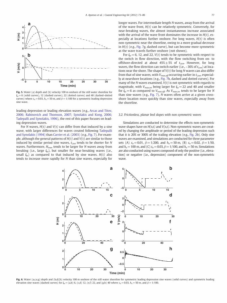
For leading depression sine waves, H(t), which represents the tem-poral water depth variation at a fixed cross-shore location, is approxi-mately symmetric at all onshore locations for all waves and parametersets examined (e.g., Figs. 4a, 5a). As the period of the wave increases(i.e., increasing ξo) the total time of inundation, ti,tot (i.e., the time overwhich H(t)>0) increases, but the maximum water depth, Hmax, de-creases (e.g., Fig. 5a, compare solid and dashed–dotted curves). For theparameter sets examined, Hmax at most onshore locations occurs at ap-proximately 50%±3% of ti,tot. For these simulations, V(t), which repre-sents the temporal water velocity variation at a fixed cross-shorelocation, onshore increases to a maximum almost instantaneously asthe wave front passes and then gradually decreases before reversing di-rections (e.g., Fig. 5b). At most onshore locations, V(t) is reasonablysymmetric with respect to the change in flow direction (i.e., when V(t)changes from positive to negative), with the flow shifting from on- tooffshore-directed at approximately 50%±3% of ti,tot (i.e., approximatelywhenHmax occurs). In general, themaximumoffshore-directed velocity,Vmax,off, occurs at the end of the run-down and is similar inmagnitude tothe maximum onshore-directed velocity, Vmax,on.

For leading elevation sine waves, the general patterns of H(t) andV(t) are similar to that for leading depression waves (e.g., Fig. 6).However, the trailing depression of these leading elevation wavescan also induce an onshore flow, especially for waves closer to break-ing and for locations close to the shoreline (note the second increasein water depth and velocity in Fig. 6a–f). This second increase isowing to the water level offshore rebounding from the drawdownthat occurs during the trailing depression. In general, Hmax, Vmax,on

and Vmax,off associated with the leading elevation are larger thanthose associated with the trailing depression. For near-breakingwaves (i.e., ξo=6), the maximum velocities are similar for leading el-evation and leading depression waves, while Hmax tends to be largerfor leading depression waves (e.g., Fig. 6a, b). For intermediate lengthwaves (i.e., ξo=12 and 22), Hmax is typically similar, but Vmax,on tendsto be larger for leading elevation waves (e.g., Fig. 6c–f). The shape ofboth H(t) and V(t) can also differ slightly for both near-breaking andintermediate length leading elevation and leading depression waves.For long waves (i.e., ξo=40), H(t) and V(t) tend to be fairly similar(e.g., Fig. 6g, h). While tsunamis can approach the shore as either

0

1

2

3

4

H (

m)

a

0 5 10 15 20 25 30 35

0

5

Time (min)

V (

m/s

)

b

Fig. 5. Water (a) depth and (b) velocity 100 m onshore of the still water shoreline forξo=6 (solid curves), 12 (dashed curves), 22 (dotted curves) and 40 (dashed–dottedcurves) where εo=0.03, ho=50 m, and β=1/100 for a symmetric leading depressionsine wave.

77A. Apotsos et al. / Coastal Engineering 64 (2012) 73–86

leading depression or leading elevation waves (e.g., Arcas and Titov,2006; Rabinovich and Thomson, 2007; Synolakis and Kong, 2006;Tadepalli and Synolakis, 1996), the rest of this paper focuses on lead-ing depression waves.

For N waves, H(t) and V(t) can differ from that induced by a sinewave, with larger differences for waves created following Tadepalliand Synolakis (1994) than Carrier et al. (2003) (e.g., Fig. 7). For exam-ple, although the general patterns of H(t) and V(t) are similar to thoseinduced by similar period sine waves, ti,tot tends to be shorter for Nwaves. Furthermore, Hmax tends to be larger for N waves away frombreaking (i.e., large ξo), but smaller for near-breaking waves (i.e.,small ξo) as compared to that induced by sine waves. H(t) alsotends to increase more rapidly for N than sine waves, especially for

0 5 10 150

2

4

H (

m)

a

0 10 20 300

2

c

0 20 400

1

2e

0 10 20 300

1

2 g

Time (

Fig. 6. Water (a,c,e,g) depth and (b,d,f,h) velocity 100 m onshore of the still water shorelinelevation sine waves (dashed curves) for ξo=(a,b) 6, (c,d) 12, (e,f) 22, and (g,h) 40 where

longer waves. For intermediate length Nwaves, away from the arrivalof the wave front, H(t) can be relatively symmetric. Conversely, fornear-breaking waves, the almost instantaneous increase associatedwith the arrival of the wave front dominates the increase in H(t), es-pecially at locations further onshore. For long waves, H(t) is oftennon-symmetric near the shoreline, owing to a more gradual decreasein H(t) (e.g., Fig. 7g, dashed curve), but can become more symmetricas the wave travels further onshore (not shown).

For ξo=6, 12, and 22, V(t) tends to be symmetric with respect tothe switch in flow direction, with the flow switching from on- tooffshore-directed at about 45%±5% of ti,tot. However, for longwaves, the flow direction can switch earlier (i.e., ~30% of ti,tot) at loca-tions near the shore. The shape of V(t) for long Nwaves can also differfrom that of sine waves, with Vmax,off occurring earlier in ti,tot, especial-ly at nearshore locations (e.g., Fig. 7h, dashed and dotted curves). Formany of the Nwaves examined, V(t) is not symmetric with regards tomagnitude, with Vmax,on being larger for ξo=22 and 40 and smallerfor ξo=6 as compared to Vmax,off. As Vmax,on tends to be larger for Nthan sine waves (e.g., Fig. 7), N waves often arrive at a given cross-shore location more quickly than sine waves, especially away fromthe shoreline.

3.2. Frictionless, planar bed slopes with non-symmetric waves

Simulations are conducted to determine the effects non-symmetricwave shapes have on H(x,t) and V(x,t). Non-symmetric waves are creat-ed by changing the amplitude or period of the leading depression suchthat it is 20% or 300% of the trailing elevation (e.g., Fig. 2b). Only sinewaves are examined, and simulations are conducted for three parametersets (A) εo=0.01, β=1/200, and ho=50m, (B) εo=0.02, β=1/50,and ho=100m, and (C) εo=0.03, β=1/100, and ho=50m. Simulationsare also conducted usingwaves composed of only the positive (i.e., eleva-tion) or negative (i.e., depression) component of the non-symmetricwave.

0 5 10 15−5

0

5

V (

m/s

)

b

0 10 20 30

−2

0

2d

0 20 40−2

0

2 f

0 10 20 30

−0.5

0

0.5

min)

h

e for symmetric leading depression sine waves (solid curves) and symmetric leadingεo=0.03, ho=50 m, and β=1/100.

0 2 4 60

5

H (

m)

a

0 5 100

5 c

0 5 10 15 200

2

4 e

0 10 20 300

1

2

3 g

0 2 4 6−10

0

10

V (

m/s

)

b

0 5 10

−5

0

5 d

0 5 10 15 20

−2

0

2f

0 10 20 30

−1

0

1

Time (min)

h

Fig. 7. Water (a,c,e,g) depth and (b,d,f,h) velocity 100 m onshore of the still water shoreline for symmetric sine waves (solid curves), N waves following Tadepalli and Synolakis(1994) (dashed curves), and N waves following Carrier et al. (2003) (dotted curves) for ξo=(a,b) 6, (c,d) 12, (e,f) 22, and (g,h) 40 where εo=0.03, ho=50 m, and β=1/100.

78 A. Apotsos et al. / Coastal Engineering 64 (2012) 73–86

When the leading depression has an amplitude of 20% or a periodof 300% of the trailing elevation, H(t) and V(t) onshore are almostcompletely a function of the trailing elevation. For these waves, H(t)

0 2 4 60

5

H (

m)

a

0 5 100

2

4 c

0 5 10 15 200

1

2e

0 10 20 300

1

2 g

Time

Fig. 8. Water (a,c,e,g) depth and (b,d,f,h) velocity 100 m onshore of the still water shorelineplitude of the leading depression is decreased to 20% (dashed curves), for non-symmetriccurves), and for simple positive elevation waves (dashed–dotted curves) for ξo=(a,b) 6, (c

is mostly symmetric and similar to that induced by a simple positiveelevation wave (e.g., Fig. 8, compare dashed, dotted and dashed–dot-ted curves). For near-breaking and intermediate length waves, H(t)

0 2 4 6−5

0

5

V (

m/s

)

b

0 5 10

−2

0

2d

0 5 10 15 20−2

0

2 f

0 10 20 30

−0.5

0

0.5

(min)

h

for symmetric sine waves (solid curves), for non-symmetric sine waves where the am-sine waves where the period of the leading depression is increased to 300% (dotted,d) 12, (e,f) 22, and (g,h) 40 where εo=0.03, ho=50 m, and β=1/100.

79A. Apotsos et al. / Coastal Engineering 64 (2012) 73–86

for the non-symmetric and positive elevation waves can differ slight-ly from that of a symmetric wave (e.g., Fig. 8a, c, e), but as the wavesbecome long, H(t) for all four waves is more similar (e.g., Fig. 8g). Thegeneral patterns of V(t) for these non-symmetric waves are similar tothat of a symmetric wave. For near-breaking waves, V(t) is reasonablysymmetric with regards to both time and magnitude, but differssomewhat from that of a symmetric wave (e.g., Fig. 8b). For longerwaves, V(t) is reasonably symmetric with time, but Vmax,on tends tobe larger relative to a symmetric wave and can be 50% larger thanVmax,off (e.g., Fig. 8h).

The patterns within H(t) and V(t) become more complex whenthe leading depression has an amplitude of 300% or a period of 20%of the trailing elevation. For these non-symmetric waves, the onshoreflow dynamics differ considerably from that induced by a symmetricwave (e.g., Fig. 9). When the amplitude of the leading depression isincreased, H(t) induced by the positive and negative components ofthe non-symmetric wave can be of a similar magnitude (notshown). For near-breaking and some intermediate length waves,the two signals positively re-enforce each other, and Hmax is oftenlarger than for a symmetric wave (e.g., Fig. 9a and c, compare solidand dashed curves). As the waves become longer, the signals fromthe two wave components separate in time. For these longer waves,Hmax is often similar to that induced by a symmetric wave, but H(t)can appear as if two separate waves have impacted the coast (e.g.,Fig. 9e and g, dashed curves, note two separate increases in H(t)).When the period of the leading depression is decreased, H(t)is mostly dominated by the positive wave component, especiallyfor near-breaking waves (e.g., Fig. 9a and c, compare dotted anddashed–dotted curves). However, for longer waves, the shortenedleading depression becomes important and H(t) can be composed oftwo distinct increases in the water depth (e.g., Fig. 9e and g, dottedcurves).

For these non-symmetric waves, V(t) is affected by both the dy-namics of the leading depression and the trailing elevation. In

0 2 4 60

5

H (

m)

a

0 5 100

2

4 c

0 5 10 15 200

1

2e

0 10 20 30 400

1

2 g

Time (

Fig. 9. Water (a,c,e,g) depth and (b,d,f,h) velocity 100 m onshore of the still water shorelineplitude of the leading depression is increased to 300% (dashed curves), for non-symmetricurves), and for simple positive elevation waves (dashed–dotted curves) for ξo=(a,b) 6, (c

general, Vmax,on is larger than that induced by a symmetric wave, es-pecially near the shoreline (e.g., Fig. 9). In general, this is becauseVmax,on near the shoreline is associated with the dynamics of the lead-ing depression and not the trailing elevation. However, the flow in-duced by the leading depression does not reach Rmax, and furtheronshore the flow dynamics are dominated by the trailing elevation.For near-breaking waves, V(t) typically decreases monotonicallyfrom Vmax,on, similar to what occurs for symmetric waves (e.g.,Fig. 9b). However, for longer waves, the arrival of the positive eleva-tion can be observed as a second, smaller increase in V(t) (e.g., Fig. 9d,f, h). Depending on the preceding dynamics, the positive elevationcan either simply decrease the magnitude of the offshore-directedflow (e.g., Fig. 9d, dashed curve), or can force a second period ofonshore-directed flow (e.g., Fig. 9h, dashed curve). For all waves sim-ulated, the later stages of run-down tend to be dominated by the dy-namics of the trailing elevation, and are similar to what occurs for asymmetric wave.

3.3. Frictionless, planar bed slopes with shallow onshore topography andsymmetric waves

Simulations are conducted to examine the effects of shallower on-shore topography on H(x,t) and V(x,t). Only sine waves are examined,and the onshore bed slope is gradually made more shallow (βon=1/300, 1/500, 1/800 and 1/1200) for three parameter sets (A) εo=0.01,β=1/200, and ho=50 m, (B) εo=0.02, β=1/50, and ho=100 m,and (C) εo=0.03, β=1/100, and ho=50 m. For all morphologies, βand βon intersect at the still water shoreline (e.g., Fig. 1, dashedcurve).

Decreasing βon causes H(t) and V(t) to become less symmetric, es-pecially for near-breaking waves (e.g., Fig. 10). For example, withξo=6, Hmax occurs at b25%, b10% and b6% of ti,tot for βon=1/300, 1/800, and 1/1200, respectively. For longer waves, a shallower βon isnecessary before the shape of H(t) becomes non-symmetric (e.g.,

0 2 4 6

−5

0

5

V (

m/s

)

b

0 5 10−5

0

5 d

0 5 10 15 20−5

0

5 f

0 10 20 30 40−4

0

4

min)

h

for symmetric sine waves (solid curves), for non-symmetric sine waves where the am-c sine waves where the period of the leading depression is decreased to 20% (dotted,d) 12, (e,f) 22, and (g,h) 40 where εo=0.03, ho=50 m, and β=1/100.

0 10 20 30 400

2

4

H (

m)

a

0 10 20 30 400

1

2

3 c

0 10 20 30 40 500

1

2

e

0 20 400

1

2g

0 10 20 30 40−10

0

10

V (

m/s

)

b

0 10 20 30 40−10

0

10 d

0 10 20 30 40 50

−5

0

5f

0 20 40

−5

0

5

Time (min)

h

Fig. 10. Water (a,c,e,g) depth and (b,d,f,h) velocity 100 m onshore of the still water shoreline for symmetric sine waves with ξo=(a,b) 6, (c,d) 12, (e,f) 22, and (g,h) 40 whereεo=0.025, ho=50 m, β=1/100, and βon=1/100 (solid curves), 1/300 (dashed curves), 1/800 (dotted curves) and 1/1200 (dashed–dotted curves).

80 A. Apotsos et al. / Coastal Engineering 64 (2012) 73–86

compare Fig. 10a and g). At a given onshore location, the total eleva-tion above the still water level reached by a wave decreases with de-creasing βon, with a smaller decrease for longer waves (not shown).However, owing to the lower bed elevations on morphologies withshallower βon, Hmax can be larger or smaller as βon becomes moreshallow. In general, Hmax is larger on steeper βon near the shoreline,but larger for more shallow βon further onshore.

The shape of V(t) changes as βon becomesmore shallow. As βon de-creases, V(t) still increases rapidly as the wave front arrives. However,the flow can continue to accelerate behind the wave front and doesnot initially begin to decelerate as quickly, resulting in a period of al-most uniform onshore flow (e.g., Fig. 10). For shallow βon the switchfrom on- to offshore-directed flow tends to occur after Hmax occurs,indicating that the water depth begins to decrease even as water con-tinues to inundate landward. There is also a clear change in the dy-namics as the flow switches from on- to offshore-directed (note thechange in the slope of V(t) near the transition). The acceleration ofthe offshore-directed flow (i.e., the slope of the offshore-directed ve-locity) appears to be dominated to a greater degree by the slope of theonshore topography than by the wave characteristics (i.e., it is similarfor all four waves). Conversely, the deceleration of the onshore-directed flow appears to be at least partly influenced by the wavecharacteristics (e.g., Fig. 10, compare onshore directed flow in b andh). In general, as βon decreases, Vmax,on and Vmax,off tend to increaseup to a point and then remain constant for further decreases in βon

(e.g., Fig. 10).

3.4. Planar bed slopes with shallow onshore topography, realistic rough-ness, and symmetric waves

Simulations are conducted to examine the effects of including amore realistic bottom roughness by first increasing the roughness ev-erywhere from 0.001 to 0.02, and then increasing just the onshoreroughness from 0.02 to 0.1 for three parameter sets (A) εo=0.01,

β=1/200, and ho=50 m, (B) εo=0.02, β=1/50, and ho=100 m,and (C) εo=0.03, β=1/100, and ho=50 m. For all simulations,βon=1/800.

As the bottom roughness increases, H(t) becomes less symmetric,with run-down dominating ti,tot (e.g., Fig. 11). For the roughest on-shore topography (i.e., n=0.1 onshore), Hmax occurs at b10% of ti,totfor even the longest wave. Although H(t) is significantly skewed to-ward decreasing water depths, the initial decrease in H(t) followingHmax is similar to increasing H(t). However, approximately when theflow switches from on- to offshore-directed, H(t) begins to decreasemore slowly, developing into what is termed here as a slowly de-creasing run-down tail. The rate of decrease in H(t) during the run-down tail appears to be a function of the onshore topographic charac-teristics (i.e., slope and roughness) as it is similar for all four waves fora given bottom roughness and bed slope. As the bottom roughness in-creases, water tends to pile up near the shoreline, especially for near-breaking waves, resulting in increased Hmax near the shoreline, butdecreased Hmax further shoreward and a significantly reduced inun-dation distance and Rmax (not shown). These results are consistentwith Apotsos et al. (2011c) and Dutykh et al. (2011), who showedthat maximum run-up decreases with increasing roughness. Howev-er, the results presented here also clearly demonstrate the cross-shore dependence of an increasing roughness on the onshore flowdynamics.

Increasing the bottom roughness generally decreases the magni-tude of V(t) and affects significantly the shape of the offshore-directed flow (e.g., Fig. 11). In all cases, Vmax,on and Vmax,off decreaseas the bottom roughness increases. However, while the magnitudeof Vmax,on decreases with increasing roughness, the general shape ofthe onshore-directed flow does not change significantly. Conversely,unlike on smooth morphologies where Vmax,off tends to occur nearthe end of the run-down (e.g., Fig. 11b, d, f, h, solid curves), forrough topographies Vmax,off often occurs soon after the flow switchesdirections (e.g., Fig. 11b, d, f, h, dashed, dashed–dotted and dotted

0 50 100 1500

2

4

H (

m)

a

0 50 100 1500

2

c

0 50 100 1500

1

2e

0 50 100 150 2000

1

2g

0 50 100 150−10

−5

0

5

V (

m/s

)

b

0 50 100 150

−5

0

5 d

0 50 100 150−8−6−4−2

02 f

0 50 100 150 200−6

−4

−2

0

2

Time (min)

h

Fig. 11. Water (a,c,e,g) depth and (b,d,f,h) velocity 100 m onshore of the still water shoreline for symmetric sine waves with ξo=(a,b) 6, (c,d) 12, (e,f) 22, and (g,h) 40 whereεo=0.025, ho=50 m, β=1/100, βon=1/800 and n=0.001 everywhere (solid curves), n=0.01 everywhere (dashed curves), n=0.02 offshore and 0.05 onshore (dotted curves)and n=0.02 offshore and 0.1 onshore (dashed–dotted curves).

81A. Apotsos et al. / Coastal Engineering 64 (2012) 73–86

curves). The offshore-directed flow velocity then slowly decreasesback toward zero. The change in shape of the offshore-directed, butnot the onshore-directed, flow, further suggests that the run-downis dictated by topographic characteristics (slope and roughness), butthat the run-up is at least partly a function of the incoming wavecharacteristics.

3.5. Planar bed slopes with shallow onshore topography, realistic rough-ness, and non-symmetric waves

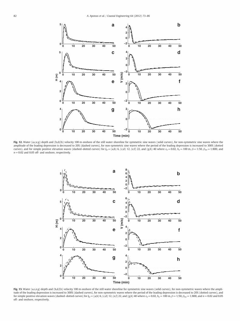
Simulations are conducted to determine the effects of non-symmetric waves inundating over rough, shallow onshore topogra-phies. For these simulations, βon=1/800 and n=0.02 and 0.05 off-and onshore, respectively. Non-symmetric waves similar to thosedescribed in Section 3.2 are simulated for three parameter sets(A) εo=0.01, β=1/200, and ho=50m, (B) εo=0.02, β=1/50, andho=100 m, and (C) εo=0.03, β=1/100, and ho=50m.

Similar to Section 3.2, when the amplitude of the leading depres-sion is decreased or the period increased, the onshore flow is domi-nated by the dynamics of the trailing elevation. In general, both H(t)and V(t) are similar to that induced by simple positive elevation andsymmetric waves, especially for longer waves (e.g., Fig. 12). Fornear-breaking waves, the general patterns are similar, but Hmax andVmax,on can be slightly smaller than for a symmetric wave.

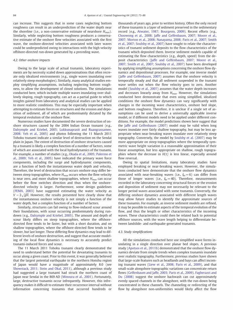
When the leading depression has an increased amplitude or de-creased period, H(t) and V(t) can differ from that induced by a sym-metric wave (e.g., Fig. 13). However, the differences are not as largeas those observed on steeper, frictionless topographies (i.e.,Section 3.2). In both cases, the general patterns of H(t) and V(t) donot appear to be affected for near-breaking waves, although the mag-nitudes of Hmax and Vmax,on can increase relative to a symmetric wavewhen the amplitude of the leading depression is increased (e.g.,Fig. 13a and b, compare solid and dashed curves). For longer waves,the signal from the leading depression becomes more noticeable

(e.g., Fig. 13e–h), but is not as pronounced as it was over steeper, fric-tionless morphologies (i.e., Section 3.2). Near the shore, Vmax,on tendsto be associated with the dynamics of the leading depression and to in-crease relative to that induced by a symmetric wave. However, furtheronshore, the dynamics of the leading depression play less of a role,and Vmax,on for the symmetric and non-symmetric waves is more simi-lar. The decreased importance of the leading depression in these simu-lations as compared to those in Section 3.2, especially away from thestill water shoreline, is likely owing to the fact that the thinner, fasterflow induced by the leading depression is affected to a greater degreeby the increased bottom roughness and decreased bed slope than theslower, deeper flow induced by the trailing elevation.

3.6. Multiple symmetric waves

Simulations are conducted to examine the effects on H(x,t) andV(x,t) owing to the inclusion of multiple waves using a subset of thesimulations discussed in Sections 3.1, 3.3, 3.4, and 3.5. In all cases,simulations are conducted with one, two, and three identical sinewaves.

For symmetric waves inundating over frictionless, planar bedslopes (i.e., Section 3.1) each wave is observed onshore as a separate,almost identical signal within H(t) and V(t) (e.g., Fig. 14, solid curves).For all waves simulated, the water advected onshore by one wavedrains completely offshore before the subsequent wave arrives.While the signals from the second and third wave are essentiallyidentical, Hmax and Vmax,on associated with these waves can be slightlylarger (b~7%) than that for the first wave for waves close to breaking(i.e., ξo=6). This slight increase in Hmax and Vmax,on from the first tothe second wave may be related to the fact that while the waves donot interact onshore, later waves arrive before the water level off-shore has returned to a stationary position. This altered initial sealevel may affect the characteristics of the incoming waves, and slight-ly alter the onshore dynamics (see alsoMadsen and Schäffer, 2010). For

0 10 20 30 40 50

0 10 20 30 40 50

0 10 20 30 40 50

0 10 20 30 40 50

0

5

H (

m)

a

0

5 c

0

2

4 e

0

2

4 g

0 10 20 30 40 50−2

0

2

4

V (

m/s

)

b

0 10 20 30 40 50−2

0

2

4 d

0 10 20 30 40 50

0

2 f

0 10 20 30 40 50−2

0

2

Time (min)

h

−2

Fig. 12. Water (a,c,e,g) depth and (b,d,f,h) velocity 100 m onshore of the still water shoreline for symmetric sine waves (solid curves), for non-symmetric sine waves where theamplitude of the leading depression is decreased to 20% (dashed curves), for non-symmetric sine waves where the period of the leading depression is increased to 300% (dottedcurves), and for simple positive elevation waves (dashed–dotted curves) for ξo=(a,b) 6, (c,d) 12, (e,f) 22, and (g,h) 40 where εo=0.02, ho=100 m, β=1/50, βon=1/800, andn=0.02 and 0.05 off- and onshore, respectively.

0 10 20 30 40 50

0 10 20 30 40 50

0 10 20 30 40 50

0 10 20 30 40 50

0

5

H (

m)

a

0

5 c

0

2

4 e

0

2

4 g

0 10 20 30 40 50

0 10 20 30 40 50

0 10 20 30 40 50

0 10 20 30 40 50

−202468

V (

m/s

)

b

−2

0

2

4

6d

−2

0

2

4f

−2

0

2

4

Time (min)

h

Fig. 13. Water (a,c,e,g) depth and (b,d,f,h) velocity 100 m onshore of the still water shoreline for symmetric sine waves (solid curves), for non-symmetric waves where the ampli-tude of the leading depression is increased to 300% (dashed curves), for non-symmetric waves where the period of the leading depression is decreased to 20% (dotted curves), andfor simple positive elevation waves (dashed–dotted curves) for ξo=(a,b) 6, (c,d) 12, (e,f) 22, and (g,h) 40 where εo=0.02, ho=100 m, β=1/50, βon=1/800, and n=0.02 and 0.05off- and onshore, respectively.

82 A. Apotsos et al. / Coastal Engineering 64 (2012) 73–86

0 10 20 300

2

4

H (

m)

a

0 20 40 600

2

c

0 50 1000

1

2e

0 50 100 150 2000

1

2g

0 10 20 30−5

0

5

V (

m/s

)

b

0 20 40 60

−5

0

5 d

0 50 100−6−4−2

02 f

0 50 100 150 200

−4

−2

0

2

Time (min)

h

Fig. 14. Water (a,c,e,g) depth and (b,d,f,h) velocity 50 m onshore of the still water shoreline for three identical symmetric sine waves for ξo=(a,b) 6, (c,d) 12, (e,f) 22, and (g,h) 40where εo=0.025, ho=50 m, β=1/100 for frictionless, planar slopes (solid curves), frictionless, shallow onshore topography with βon=1/800 (dashed curves), and for βon=1/800and n=0.02 offshore and 0.05 onshore (dotted curves).

83A. Apotsos et al. / Coastal Engineering 64 (2012) 73–86

waveswith largermagnitudes or shorter periods than examined here, itis possible that consecutive waves may interact onshore.

For symmetric waves inundating over frictionless, planar bedslopes with shallow onshore topography (i.e., Section 3.3), the longerwaves do not interact onshore and there is little effect on the onshoredynamics owing to multiple waves (e.g., Fig. 14e–h, dashed curves).However, as the waves approach breaking, they begin to interact on-shore, with subsequent waves arriving before the preceding wave hasdrained completely offshore (e.g., Fig. 14a–d, dashed curves). As theamplitude of the incoming waves increases, the period at which thewaves begin to interact onshore also increases. For waves that inter-act onshore, the effects on H(t) and V(t) can be complex. For example,under some conditions Hmax can increase with each wave even asVmax,on decreases (e.g., Fig. 14a and b, dashed curves). In other cir-cumstances, Hmax induced by the second wave can be larger thanHmax of the first wave, while Hmax associated with the third wave issmaller thanHmax for the first two waves (not shown). Under other cir-cumstances, Hmax from the first and third waves can be similar, butsmaller than that associated with the second wave (e.g., Fig. 14c). Theexact effects on H(t) depend on the complex interactions of the differ-ent waves. However, in all cases, while Hmax near the shoreline can in-crease when multiple waves are simulated, Rmax does not change (i.e.,water can pile up near the shoreline, but not further onshore). This ap-pears to contradict Apotsos et al. (2011c) who found that on shallowonshore topographies, Rmax increases with an increasing number ofwaves. This apparent contradiction is owing to the lack of a realistic bot-tom roughness in the simulations conducted here. Neglecting bottomroughness allows for larger offshore-directed flow velocities, whichcan significantly slow the inundation of later waves. As the patterns ofH(t) and V(t) are complex and depend on the unrealistic assumptionof a smooth bottom, they are not discussed further.

For symmetricwaves inundating over planar bed slopeswith shallowonshore topography and realistic roughness (i.e., Section 3.4) almost allthe waves simulated interact onshore with the preceding wave (e.g.,

Fig. 14, dotted curves). In general, the effects on H(t) and V(t) across allthe simulations examined are more consistent than over frictionlessmorphologies. At most onshore locations, H(t) and V(t) for each waveare similar in shape, although the arrival of a subsequent wave cutsshort the run-down phase of the preceding wave. The initial wavefront of laterwaves can be steeper (i.e., a sharper increase inH(t)) but ac-celerate more slowly (i.e., V(t) increases to Vmax,on more slowly) due tothe interaction with the offshore-directed run-down of the previouswave. While Hmax near the shoreline typically does not change as thenumber of waves increases, further onshore Hmax tends to increasewith an increasing number of waves (not shown). Conversely, awayfrom themaximumextent of inundation,Vmax,on tends to decrease slight-ly from the first to second wave, but then remain similar for later waves(e.g., Fig. 14b, d, f, h, dotted curves). The decrease in Vmax,on from the firstto the second wave tends to be larger for near-breaking waves. Close toRmax, both Hmax and Vmax,on increase with an increasing number ofwaves, consistent with an increasing Rmax with each new wave.

In general, the effects on the patterns in H(t) and V(t) when sim-ulating multiple non-symmetric waves inundating over rough, shal-low onshore topographies (i.e., Section 3.5) are similar to thoseobserved for more symmetric waves. However, for some waves, espe-cially those with long period leading depressions, the waves do notinteract onshore, and the signals from each individual wave are sepa-rate and almost identical. Conversely, when the amplitude of theleading depression is increased, the effects on V(t) and H(t) can beslightly larger than those induced for the symmetric waves.

4. Some implications for other onshore dynamics and futuremodeling

4.1. Bottom roughness and conservative estimates

The simulations conducted here indicate that although Rmax de-creases with increasing bottom roughness, Hmax near the shoreline

84 A. Apotsos et al. / Coastal Engineering 64 (2012) 73–86

can increase. This suggests that in some cases neglecting bottomroughness can result in an underprediction of the water depth nearthe shoreline (i.e., a non-conservative estimate of nearshore Hmax).Similarly, while neglecting bottom roughness produces a conserva-tive estimate of the onshore flow velocities associated with the firstwave, the onshore-directed velocities associated with later wavescould be underpredicted owing to interactions with the high velocityoffshore-directed run-down generated by a preceding wave.

4.2. Other onshore impacts

Owing to the large scale of actual tsunamis, laboratory experi-ments are by necessity scaled down approximations that often recre-ate only idealized environments (e.g., single waves inundating overrelatively steep morphologies). Similarly, many analytical studies em-ploy simplifying assumptions, including neglecting bottom rough-ness, to allow the development of closed solutions. The simulationsconducted here, which include multiple waves inundating over shal-lowly sloping, rough topography, can act as a partial guide to whichinsights gained from laboratory and analytical studies can be appliedto more realistic conditions. This may be especially important whenattempting to estimate forces on structures and the erosion and depo-sition of sediment, all of which are predominately dictated by thetemporal evolution of the onshore flow.

Numerous studies have documented the severe destruction of on-shore structures caused by the 2004 Indian Ocean tsunami (e.g.,Dalrymple and Kriebel, 2005; Lukkunaprasit and Ruangrassamee,2008; Yeh et al., 2005) and photos following the 11 March 2011Tohoku tsunami indicate a similar level of destruction on the Sendaiplain in Japan. The extent of destruction of onshore structures causedby a tsunami is likely a complex function of a number of factors, someof which are associated with the local hydrodynamics of the tsunami.For example, a number of studies (e.g., Okada et al., 2005; Palermo etal., 2009; Yeh et al., 2005) have indicated the primary wave forcecomponents, including the surge and hydrodynamic components,are a function of both the instantaneous water depth and velocity.Therefore, the level of destruction that occurs onshore may differ be-tween steep topographies, where Hmax occurs when the flow velocityis near zero, and more shallow topographies, where Hmax can occurbefore the flow switches direction and thus when the onshore-directed velocity is larger. Furthermore, some design guidelines(FEMA, 2003) have suggested estimating the water velocity asV ¼ 2

ffiffiffiffiffiffiffigH

p. However, the results presented here clearly show that

the instantaneous onshore velocity is not simply a function of thewater depth, but a complex function of a number of factors.

Similarly, structures can fail owing to flow-induced scour aroundtheir foundations, with scour occurring predominately during run-down (e.g., Dalrymple and Kriebel, 2005). The amount and depth ofscour likely differs on steep topographies, where the offshore-directed flow tends to be faster, but with a short duration, and onshallow topographies, where the offshore-directed flow tends to beslower, but last longer. These differing flow dynamics may lead to dif-ferent levels of onshore destruction, and suggest that accurate model-ing of the local flow dynamics is necessary to accurately predicttsunami-induced forces and scour.

The 11 March 2011 Tohoku tsunami clearly demonstrated theneed to understand better the potential for devastating tsunamis tooccur along a given coast. Prior to this event, it was generally believedthat the largest potential earthquake in the northern Honshu regionof Japan would have a magnitude of approximately 8.0 (seeShowstack, 2011; Stein and Okal, 2011), although a previous studyhad suggested a large tsunami had struck the northern coast ofJapan near Sendai in the 869 AD (Minoura et al., 2001). Fortunately,large, destructive tsunamis occur infrequently. However, this infre-quency makes it difficult to estimate their recurrence interval withoutinformation concerning tsunamis that occurred hundreds or

thousands of years ago, prior to written history. Often the only recordof these tsunamis is a layer of sediment preserved in the sedimentaryrecord (e.g., Atwater, 1987; Bourgeois, 2009). Recent efforts (e.g.,Choowong et al., 2008; Jaffe and Gelfenbaum, 2007; Moore et al.,2007; Morton et al., 2008; Nanayama, 2008; Paris et al., 2007; Smithet al., 2007; Soulsby et al., 2007) have sought to relate the character-istics of tsunami sediment deposits to the flow characteristics of thetsunami which deposited them. Inverse sediment models capable ofestimating the flow characteristics (e.g., depth, speed) from the de-posit characteristics (Jaffe and Gelfenbaum, 2007; Moore et al.,2007; Smith et al., 2007; Soulsby et al., 2007) have been developedby applying simplifying assumptions concerning the onshore flow dy-namics and depositional processes. For example, one inverse model(Jaffe and Gelfenbaum, 2007) assumes that the onshore velocity istemporally steady and that all sediment suspended in the tsunamiwave settles out when the flow velocity goes to zero. Anothermodel (Soulsby et al., 2007) assumes that the water depth increasesand decreases linearly away from Hmax. However, the simulationsconducted here demonstrate that even using simplified, idealizedconditions the onshore flow dynamics can vary significantly withchanges in the incoming wave characteristics, onshore bed slope,and bottom roughness. Therefore, it is unclear if a single set of as-sumptions can be used to derive a universally applicable inversemodel, or if different models need to be applied under different con-ditions. For example, the model predictions shown here suggest thatthe Jaffe and Gelfenbaum (2007) model may be valid when longwaves inundate over fairly shallow topography, but may be less ap-propriate when near-breaking waves inundate over relatively steeptopography. Conversely, the model by Soulsby et al. (2007) may bemore appropriate on steep topographies where the temporally sym-metric wave height variation is a reasonable approximation of theirlinear assumption, but less appropriate on shallow, rough topogra-phies where the decrease in H(t) is less linear, especially aroundflow reversal.

Owing to spatial limitations, many laboratory studies haveemployed breaking or near-breaking waves. However, the simula-tions conducted here demonstrate that the onshore flow dynamicsassociated with near-breaking waves (i.e., ξo=6) can differ fromthose of longer waves (i.e., ξo=40). Therefore, measurementsrecorded in the laboratory concerning structural forces or the erosionand deposition of sediment may not necessarily be relevant to thelonger period waves associated with some tsunamis. Conversely, thediffering onshore dynamics associated with different length wavesmay allow future studies to identify the approximate sources ofthese tsunamis. For example, as inverse sediment models are refined,it may be possible to estimate aspects of the temporal evolution of theflow, and thus the length or other characteristics of the incomingwaves. These characteristics could then be related back to potentialoffshore sources, with the wave length helping to differentiate be-tween landslide- and earthquake-generated tsunamis.

4.3. Study simplifications

All the simulations conducted here use simplified wave forms in-undating in a single direction over planar bed slopes. A previousstudy (Apotsos et al., 2011b) demonstrated that the onshore flow dy-namics deviate from simple trends when complex tsunamis inundateover realistic topography. Furthermore, previous studies have shownthat large-scale features such as headlands and bays can affect incom-ing tsunami waves (Liew et al., 2008; Paris et al., 2009), and thatsmall-scale alongshore topographic variations can concentrate returnflows (Gelfenbaum and Jaffe, 2003; Paris et al., 2009). Fagherazzi andDu (2008) suggest the onshore backwash can cut approximatelyevenly spaced channels in the alongshore, with the run-down beingconcentrated in these channels. The channeling or redirecting of theflow by alongshore non-uniformities would likely affect the flow

85A. Apotsos et al. / Coastal Engineering 64 (2012) 73–86

depths and velocities predicted here. Furthermore, the simulationsconducted here assume that no water infiltrates into the soil duringinundation. Onshore infiltration could result in both reduced waveheights and velocities, especially during run-down. Therefore, thisstudy does not seek to establish what will occur, but merely attemptsto partially bridge the gap between various sources of previously de-rived knowledge.

5. Conclusions

The simulations conducted here demonstrate that the onshoreflow dynamics of tsunamis can be affected by changes in the onshorebed slope, incoming wave characteristics, and bottom roughness.These model results build on trends identified in previous laboratoryand analytical studies, which were not meant to be universally appro-priate, and suggest that the onshore dynamics of two tsunamis (or asingle tsunami inundating over two different coastal areas) can differsignificantly. The flow dynamics over steep, smooth morphologiestend to be temporally symmetric, with similar magnitude velocitiesgenerated during the run-up and run-down phases of inundation.Conversely, on shallow, rough onshore topographies the flow dynam-ics tend to be temporally skewed toward the run-down phase of in-undation, with significantly different flow velocities generatedduring run-up and run-down. Furthermore, the flow induced bynear-breaking waves inundating over steep topography tends to ac-celerate almost instantaneously to a maximum as the wave frontpasses before decreasing monotonically. Conversely, the flow inducedby long waves inundating over shallow topography accelerates moreslowly and can remain reasonably steady for a period of time beforebeginning to decelerate. In some circumstances, a single, non-symmetric wave can generate an onshore flow signal that includestwo separate increases in the water depth and velocity, which couldlead an observer to conclude two separate waves impacted thecoast. Multiple waves within a single tsunami do not always interactonshore, but are more likely to do so when the waves are spaced closetogether, inundate over shallow, rough topography, and have largemagnitudes.

The results presented here suggest that a single set of assumptionsconcerning the onshore flow dynamics cannot be applied to all tsu-namis. However, the results could be used to identify which insightsgained from previous laboratory and analytical studies can be appliedto more realistic conditions. This is important because the temporalevolution of the onshore flow dynamics is extremely difficult to mea-sure in situ, but is important for a number of processes, including theforces applied to onshore structures and the erosion and deposition ofsediment. Finally, while these simulations confirm that the onshoreflow dynamics are complex, this complexity could be used to helpboth identify the magnitude of pre-written history tsunamis, as wellas link these tsunamis to the offshore source by which they were gen-erated. This information would give coastal managers and scientists abetter idea of how likely large, destructive tsunamis or earthquakesare to occur in a given area, and allow them to plan accordingly.

Acknowledgments

This research was funded by a USGS Mendenhall Postdoctoral Fel-lowship and the USGS Coastal and Marine Geology Program. Thismanuscript was significantly improved by comments and suggestionsoffered by Eric Geist, Steve Watt, and two anonymous reviewers.

References

Apotsos, A., Buckley, M., Gelfenbaum, G., Jaffe, B., Vatvani, D., 2011a. Nearshore tsunamiinundation model validation: toward sediment transport applications. Pure andApplied Geophysics. doi:10.1007/s00024-011-0291-5.

Apotsos, A., Gelfenbaum, G., Jaffe, B., 2011b. Process-based modeling of tsunami inun-dation and sediment transport. Journal of Geophysical Research 116, F01006.doi:10.1029/2010JF001797.

Apotsos, A., Jaffe, B.E., Gelfenbaum, G., 2011c. Wave characteristic and morphologic ef-fects on the onshore hydrodynamic response of tsunamis. Coastal Engineering.doi:10.1016/j.coastaleng.2011.06.002.

Arcas, D., Titov, V., 2006. Sumatra tsunami: lessons for modeling. Surveys in Geophysics27, 679–705.

Atwater, B.F., 1987. Evidence for great Holocene earthquakes along the outer coast ofWashington State. Science 236, 942–944.

Battjes, J.A., 1974. Surf similarity. Proc. 14th Int. Coastal Eng. Conf. ASCE, pp. 466–480.Bourgeois, J., 2009. Geologic effects and records of tsunamis. The Sea. : Tsunamis, CH 3,

15. Harvard University Press, pp. 55–91.Briggs, M.J., Synolakis, C.E., Harkins, G.S., Green, D.R., 1995. Laboratory experiments of

tsunami runup on a circular island. Pure and Applied Geophysics 144, 569–593.Briggs, M.J., Synolakis, C.E., Kanoglu, U., Green, D.R., 1996. Benchmark problem #3:

runup of solitary waves on a vertical wall, long-wave runup models. InternationalWorkshop on Long Wave Modeling of Tsunami Runup, Friday Harbor, San JuanIsland, WA, September 12–16, 1995.

Brocchini, M., Dodd, N., 2008. Nonlinear shallow water equation modeling for coastalengineering. Journal of Waterway, Port, Coastal and Ocean Engineering 134.doi:10.1061/(ASCE)0733-950X 134:2(104).

Carrier, G.F., Greenspan, H.P., 1958. Water waves of finite amplitude on a sloping beach.Journal of Fluid Mechanics 4, 97–109.

Carrier, G.F., Wu, T.T., Yeh, H., 2003. Tsunami run-up and draw-down on a plane beach.Journal of Fluid Mechanics 475, 79–99.

Choowong, M., Murakoshi, N., Hisada, K., Charusiri, P., Charoentitirat, T., Chutakositkanon,V., Jankaew, K., Kanjanapayont, P., Phantuwongraj, S., 2008. 2004 Indian Ocean tsunamiinflow and outflow at Phuket, Thailand. Marine Geology 248, 179–192.

Constantin, A., Johnson, R.S., 2008. Propagation of very long waves, with vorticity, overvariable depth, with applications to tsunamis. Fluid Dynamics Research 40,175–211.

Dalrymple, R.A., Kriebel, D.L., 2005. Lessons in engineering from the tsunami in Thailand.The Bridge, 35. National Academy of Engineering, pp. 4–16.

Danielsen, F., Sǿrensen, M.K., Olwig, M.F., Selvam, V., Parish, F., Burgess, N.D., Hiraishi,T., Karunagaran, V.M., Rasmussen, M.S., Hansen, L.B., Quarto, A., Suryadiputra, N.,2005. The Asian tsunami: a protective role for vegetation. Science 310, 643.

Didenkulova, I., Pelinovsky, E., 2009. Non-dispersive travelling waves in inclined shal-low water channels. Physics Letters A 373 (42), 3883–3887. doi:10.1016/j.physleta.2009.08.051.

Didenkulova, I., Pelinovsky, E., 2011. Nonlinear wave evolution and runup in an in-clined channel of a parabolic cross-section. Physics of Fluids 23 (8), 086602.doi:10.1063/1.3623467.

Didenkulova, I., Kurkin, A., Pelinovsky, E., 2007a. Run-up of solitary waves on slopeswith different profiles. Izvestiya Atmospheric and Oceanic Physics 43 (3),384–390. doi:10.1134/S0001433807030139.

Didenkulova, I., Pelinovsky, E., Soomere, T., Zahibo, N., 2007b. Runup of nonlinearasymmetric waves on a place beach. In: Kundu, A. (Ed.), Tsunami and Non-LinearWaves, pp. 175–190.

Didenkulova, I., Pelinovsky, E., Soomere, T., 2008. Runup characteristics of symmetricalsolitary tsunami waves of “unknown” shapes. Pure and Applied Geophysics 165(11–12), 2249–2264. doi:10.1007/s00024-008-0425-6.

Dutykh, D., Labart, C., Mitsotakis, D., 2011. Long wave run-up on random beaches.Physical Review Letters 107 (18), 184504. doi:10.1103/PhysRevLett.107.184504.

Fagherazzi, S., Du, X., 2008. Tsunamigenic incisions produced by the December 2004earthquake along the coasts of Thailand, Indonesia and Sri Lanka. Geomorphology99, 120–129.

FEMA, 2003. 3rd ed. Coastal Construction Manual, vol. 3. Federal Emergency Manage-ment Agency, Jessup, Md. (FEMA 55).

Fernando, H.J.S., Mendis, S.G., McCulley, J.L., Perera, K., 2005. Coral poaching worsenstsunami destruction in Sri Lanka. EOS. Transactions 86, 301–304.

Galvin, C.J., 1968. Breaker type classification on three laboratory beaches. Journal ofGeophysical Research 73, 3651–3659.

Gedik, N., Irtem, E., Kabdasli, S., 2005. Laboratory investigation of tsunami run-up.Ocean Engineering 32. doi:10.1016/j.oceaneng.2004.10.013.

Gelfenbaum, G., Jaffe, B., 2003. Erosion and sedimentation from the 17 July, 1998 PapuaNew Guinea tsunami. Pure and Applied Geophysics 160, 1969–1999.

Gelfenbaum, G., Vatvani, D., Jaffe, B., Dekker, F., 2007. Tsunami inundation and sedi-ment transport in the vicinity of coastal mangrove forest. Proc. of Coastal Sediment'07. doi:10.1061/40926(239)86.

Gelfenbaum, G., Apotsos, A., Stevens, A., Jaffe, B., 2011. Effect of fringing reefs on tsuna-mi inundation: American Samoa. Earth-Science Reviews. doi:10.1016/j.earscirev.2010.12.005.

González, F.I., Geist, E.L., Jaffe, B., Kanoglu, U., Mofjeld, H., Synolakis, C.E., Titov, V.V.,Arcas, D., Bellomo, D., Carlton, D., Horning, T., Johnson, J., Newman, J., Parsons, T.,Peters, R., Peterson, C., Priest, G., Venturato, A., Weber, J., Wong, F., Yalciner, A.,2009. Tsunami pilot study working group “probabilistic tsunami hazard assess-ment at seaside, Oregon for near- and far-field seismic sources”. Journal of Geo-physical Research, Oceans 114, C11023. doi:10.1029/2008JC005132.

Grilli, S.T., Ioualalen, M., Asavanant, J., Shi, F., Kirby, J.T., Watts, P., 2007. Source con-straints and model simulation of the December 26, 2004 Indian Ocean tsunami.Journal of Waterway, Port, Coastal and Ocean Engineering 414–428.

Hughes, S.A., 2004. Estimation of wave run-up on smooth, impermeable slopes usingthe wave momentum flux parameter. Coastal Engineering 51, 1085–1104.

Ioualalen, M., Asavanant, J., Kaewbanjak, N., Grilli, S.T., Kirby, J.T., Watts, P., 2007.Modeling the 26 December 2004 Indian Ocean tsunami: case study of impact in

86 A. Apotsos et al. / Coastal Engineering 64 (2012) 73–86

Thailand. Journal of Geophysical Research 112, C07024. doi:10.1029/2006JC003850.

Jaffe, B., Gelfenbaum, G., 2007. A simple model for calculating tsunami flow speed fromtsunami deposits. Sedimentary Geology 200, 347–361.

Jensen, A., Pedersen, G., Wood, D., 2003. An experimental study of wave run-up at asteep beach. Journal of Fluid Mechanics 486. doi:10.1017/S0022112003004543.

Kánoğlu, U., 2004. Nonlinear evolution and runup-rundown of long waves over a slopingbeach. Journal of Fluid Mechanics 513, 363–372.

Kanoglu, U., Synolakis, C., 2006. The initial value problem solution of nonlinearshallow-water wave equations. Physical Review Letters 97, 148501.

Kánoğlu, U., Synolakis, C.E., 1998. Long wave runup on piecewise linear topographies.Journal of Fluid Mechanics 374, 1–28.

Kobayashi, N., Karajadi, E., 1994. Surf-similarity parameter for breaking solitary-waverunup. Journal of Waterway, Port, Coastal and Ocean Engineering 120, 645–650.

Kunkel, C., Hallberg, R., Oppenheimer, M., 2006. Coral reefs reduce tsunami impact inmodel simulations. Geophysical Research Letters 33, L23612. doi:10.1029/2006GL027892.

Li, Y., Raichlen, F., 2002. Non-breaking and breaking solitary wave run-up. Journal ofFluid Mechanics 456, 295–318.

Liew, S.C., Gupta, A., Wong, P.P., Kwoh, L.K., 2008. Coastal recovery following the de-structive tsunami of 2004: Aceh, Sumatra, Indonesia. The Sedimentary Record 4–9.

Liu, P.L.-F., Cho, Y.S., Briggs, M.J., Kanoglu, U., Synolakis, C.E., 1995. Run-up of solitarywaves on a circular island. Journal of Fluid Mechanics 302, 259–285.

Lukkunaprasit, P., Ruangrassamee, A., 2008. Building damage in Thailand in the 2004Indian Ocean Tsunami and clues for tsunami-resistant design. The IES JournalPart A: Civil and Structural Engineering 1, 17–30.

Lynett, P., Liu, P., 2005. A numerical study of run-up generated by three-dimensional land-slides. Journal of Geophysical Research 110, C03006. doi:10.1029/2004JC002443.

Lynett, P., Wu, T., Liu, P., 2002. Modelling wave runup with depth-integrated equations.Coastal Engineering 46, 89–107.

Lynett, P., Borrero, J., Liu, P., Synolakis, C.E., 2003. Field survey and numerical simula-tions: a review of the 1998 Papua New Guinea tsunami. Pure and AppliedGeophysics 160, 2119–2146.

Madsen, P.A., Fuhrman, D.R., 2008. Run-up of tsunamis and long waves in terms of surf-similarity. Coastal Engineering 55, 209–223.

Madsen, P.A., Schäffer, H., 2010. Analytical solutions for tsunami runup on a planebeach: single waves, N-waves and transient waves. Journal of Fluid Mechanics645, 27–57.

Madsen, P.A., Fuhrman, D.R., Wang, B., 2006. A Boussinesq-type method for fully non-linear waves interacting with a paridly varying bathymetry. Coastal Engineering53, 487–504.

Minoura, K., Imamura, F., Sugawara, D., Kono, Y., Iwashita, T., 2001. The 869 Jogan tsu-nami deposit and recurrence interval of large-scale tsunami on the Pacific coast ofnortheast Japan. Journal of Natural Diseases and Sciences 23 (2), 83–88.

Moore, A.L., McAdoo, B.G., Ruffman, A., 2007. Landward fining from multiple sourcesin a sand sheet deposited by the 1929 Grand Banks tsunami, Newfoundland.Sedimentary Geology 200 (3–4), 336–346.

Morton, R.A., Goff, J.A., Nichol, S.L., 2008. Hydrodynamical implications of texturaltrends in sand deposits of the 2004 tsunami in Sri Lanka. Sedimentary Geology207, 56–64.

Murty, T.S., 1977. Seismic Sea Waves: Tsunamis. Bulletin, 198. Department of Fisheriesand Environment: Fisheries and Marine Service, Ottawa, Canada. 337 pp.

Nanayama, F., 2008. Sedimentary characteristics and depositional processes of onshoretsunami deposits: An example of sedimentation associated with the 12 July 1993Hokkaido-Nansei-Oki earthquake tsunami. In: Shiki, Tsuji, Minoura, Yamazaki(Eds.), Tsunamiites — Features and Implications, pp. 63–80.

Okada, T., Sugano, T., Ishikawa, T., Ohgi, T., Takai, S., Hamabe, C., 2005. Structural DesignMethods of Buildings for Tsunami Resistance (SMBTR). The Building Center ofJapan, Japan.

Palermo, D., Nistor, I., Nouri, Y., Cornett, A., 2009. Tsunami loading of near-shorelinestructures: a primer. Canadian Journal of Civil Engineering 36, 1804–1815.

Paris, R., Lavigne, F., Wassmer, P., Sartohadi, J., 2007. Coastal sedimentation associatedwith the December 26, 2004 tsunami in Lhok Nga, West Banda Aceh (Sumatra,Indonesia). Marine Geology 238, 93–106.

Paris, R., Wassmer, P., Sartohadi, J., Lavigne, F., Barthomeuf, B., Desgages, E., Grancher,D., Baumert, P., Vautier, F., Brunstein, D., Gomez, C., 2009. Tsunamis as geomorphiccrises: lessons from the December 26, 2004 tsunami in Lhok Nga, West Banda Aceh(Sumatra, Indonesia). Geomorphology 104, 59–72.

Rabinovich, A., Thomson, R., 2007. The 26 December 2004 Sumatra tsunami: analysis oftide gauge data from the world ocean part 1: Indian Ocean and South Africa. Pureand Applied Geophysics 164. doi:10.1007/s00024-006-0164-5.

Showstack, R., 2011. Concerns over modeling and warning capabilities in wake ofTohoku earthquake and tsunami. EOS. Transactions 92 (17), 143–144.

Smith, D.E., Foster, I.D.L., Long, D., Shi, S., 2007. Reconstructing the pattern and depth offlow onshore in a palaeotsunami from associated deposits. Sedimentary Geology200, 362–371.

Soulsby, R.L., Smith, D.E., Ruffman, A., 2007. Reconstructing tsunami run-up fromsedimentary characteristics — a simple mathematical model. Proc. of CoastalSediments '07, pp. 1075–1088.

Stein, S., Okal, E., 2011. The size of the 2011 Tohoku earthquake need not have been asurprise. Eos 92 (27), 227–228.

Stelling, G.S., Duijmeijer, S.P.A., 2003. A numerical method for every Froude number inshallow water flows, including large scale inundations. International Journal forNumerical Methods in Fluids 43, 1329–1354.

Stelling, G.S., van Kester, J.A.T.M., 1994. On the approximation of horizontal gradientsin sigma coordinates for bathymetry with steep bottom slopes. InternationalJournal for Numerical Methods in Fluids 18, 915–935.

Swilger, D.T., 2009. Laboratory study investigating the three dimensional turbulenceand kinematic properties associated with a breaking solitary wave, Master Thesis,Texas A&M.

Synolakis, C.E., 1987. The runup of solitary waves. Journal of Fluid Mechanics 185,523–545.

Synolakis, C.E., Bernard, E.N., 2006. Tsunami science before and beyond Boxing Day2004. Philosophical Transactions of the Royal Society of London, Series A 364,2231–2265.

Synolakis, C.E., Kanoglu, U., 2009. Chapter 8: tsunami modeling: development ofbenchmark models. The Sea. : Volume 15—Tsunamis. Harvard University Press,pp. 237–294.

Synolakis, C.E., Kong, L., 2006. Runup measurements of the December 2004 IndianOcean tsunami. Earthquake Spectra 22 (Suppl. 3), S67–S91.

Synolakis, C.E., Bernard, E.N., Titov, V.V., Kanoglu, U., Gonzalez, F., 2008. Validation andverification of tsunami numerical models. Pure and Applied Geophysics 165,2197–2228.

Tadepalli, S., Synolakis, C., 1994. The run-up of N-waves on sloping beaches. Proceedingsof the Royal Society of London 445, 99–112.

Tadepalli, S., Synolakis, C.E., 1996. Model for the leading waves of tsunamis. PhysicalReview Letters 2141–2144.

Tang, L., Titov, V., Chamberlin, C., 2009. Development, testing, and application of site-specific tsunami inundation models for real-time forecasting. Journal of Geophys-ical Research 114, C12025. doi:10.1029/2009JC005476.

Titov, V., Rabinovich, A.B., Mofjeld, H.O., Thomson, R.E., Gonzalez, F.I., 2005. The globalreach of the 26 December 2004 Sumatra tsunami. Science 309, 2045–2048.

U.S. Agency for International Development (USAID), 2005. Fact Sheet, July 7. http//www.usaid.gov/our_work/humanitarian_assistance/disaster_assistance/countries/Indian_ocean/fy2005/indianocean_et_fs39-07-07-2005.pdf.

Vatvani, D., Schrama, E., van Kester, J., 2005a. Hindcast of tsunami flooding in Aceh–Sumatra.Proc. of the 5th International Symposium on Ocean Wave Measurement and Analysis,Madrid, Spain.

Vatvani, D., Boon, J., Ramanamurty, P.V., 2005b. Flood risk due to tsunami and tropicalcyclones and the effect of tsunami excitations on tsunami propagations. Proc. ofthe IAEA Workshop on External Flooding Hazards at NNPS, Kalpakkam — TamilNadu, India.

Verboom, G.K., Slob, A., 1984.Weakly-reflective boundary conditions for two-dimensionalwaterflowproblems. 5th Int. Conf. on Finite Elements inWater Resources, Burlington,Vermont.

Wang, X., Liu, P.L., 2006. An analysis of 2004 Sumatra earthquake fault plane mecha-nisms and Indian Ocean tsunami. Journal of Hydraulic Research 44 (2), 147–154.

Wei, Y., Bernard, E., Tang, L., Weiss, R., Titov, V., Moore, C., Spillane, M., Hopkins, M.,Kánoğlu, U., 2008. Real-time experimental forecast of the Peruvian tsunami ofAugust 2007 for U.S. coastlines. Geophysical Research Letters 35, L04609.

Yeh, H., Robertson, I., Preuss, J., 2005. Development of Design Guidelines for Structuresthat Serve as Tsunami Vertical Evacuation Sites. Report No. 2005–4. WashingtonDepartment of Natural Resources, Olympia, Wash.

Zelt, J.A., 1991. The run-up of nonbreaking and breaking solitary waves. CoastalEngineering 15, 205–246.