Tightness of radially-symmetric solutions to 2D

aggregation-diffusion equations with weak interaction forces

Ruiwen Shu∗

June 4, 2020

Abstract

We prove the tightness of radially-symmetric solutions to 2D aggregation-diffusion equa-

tions, where the pairwise attraction force is possibly degenerate at large distance. We first re-

duce the problem into the finiteness of a time integral in the density on a bounded region, by

introducing a new assumption on the interaction potential called the essentially radially con-

tractive (ERC) property. Then we prove this finiteness by using the 2-Wasserstein gradient

flow structure, combining with the continuous Steiner symmetrization curves and the local

clustering curve. This is the first tightness result on the 2D aggregation-diffusion equations

for a general class of weakly confining potentials, i.e., those W (r) with limr→∞W (r) < ∞,

and serves as an important step towards the study of equilibration.

1 Introduction

In this paper we continue the study in [26] on the large time behavior of the aggregation-

diffusion equation

∂tρ+∇ · (ρu) = ∆(ρm), u(t,x) = −∫∇W (x− y)ρ(t,y) dy, m > 1, (1.1)

where ρ(t,x) is the density distribution function of a large group of particles, x ∈ Rd being

the spatial variable, t ∈ R≥0 being the temporal variable. The term ∇ · (ρu) describes the

pairwise attraction force among particles, given by a radial interaction potential W = W (r), r =

|x|, W ′(r) > 0. The term ∆(ρm) with m > 1 is a porous-medium type diffusion term, modeling

the localized pairwise repulsion forces among particles [24], making the particles less likely to

concentrate. (1.1) arises naturally in the study of the collective behavior of large groups of

swarming agents [21, 22, 6, 5, 23, 28] and the chemotaxis phenomena of bacteria [25, 17, 16,

15, 4, 3, 9]. The 2D case (d = 2) is of significant importance because of its application in

chemotaxis: in fact, (1.1) with m = 1 and W being the Newtonian attraction is exactly the

well-known Keller-Segel equation [25, 17].

∗Department of Mathematics, University of Maryland, College Park, MD 20742, USA

(rshu@cscamm.umd.edu). The author’s research was supported in part by NSF grants DMS-1613911 and

ONR grant N00014-1812465.

1

arX

iv:2

006.

0195

5v1

[m

ath.

AP]

2 J

un 2

020

(1.1) is (at least formally) the 2-Wasserstein gradient flow of the total energy, as the sum of

the internal energy and the interaction energy

E[ρ] = S[ρ] + I[ρ] :=1

m− 1

∫ρ(x)m dx +

1

2

∫ ∫W (x− y)ρ(y) dyρ(x) dx, (1.2)

in the sense that

dE

dt= −

∥∥∥δEδρ

∥∥∥2

= −∫ ∣∣∣u(t,x)− m

m− 1∇(ρ(t,x)m−1)

∣∣∣2ρ(t,x) dx, E(t) := E[ρ(t, ·)]. (1.3)

Therefore, it is natural to study the equilibration of (1.1), i.e., when t → ∞, whether it is true

that the solution ρ(t, ·) converges to a steady state ρ∞, characterized by

u∞(x)− m

m− 1∇(ρ∞(x)m−1) = 0, ∀x ∈ suppρ∞. (1.4)

We will also use the bilinear version of the interaction energy

I[ρ1, ρ2] :=

∫ ∫W (x− y)ρ1(y) dyρ2(x) dx, I[ρ] =

1

2I[ρ, ρ]. (1.5)

There has been a rich literature on the study of steady states of (1.1), including existence,

uniqueness, structures, etc., see [2, 20, 27, 10, 18, 12, 8, 13, 7, 14], and we refer to [26] for

a discussion on them. For the case m ≥ 2 and W is no more singular than the Newtonian

attraction near the origin, the results in [2, 12, 14] imply that the steady state exists, is unique,

and is radially-decreasing1.

However, there are very few existing results on the equilibration of (1.1). In fact, [18] proves

the equilibration of radially-symmetric solutions for Newtonian attraction and its variant (to

be precise, the convolution of the Newtonian potential with a radially-decreasing function with

certain regularity), with exponential convergence rate. [12] proves the equilibration of general

solutions for 2D Newtonian attraction, without an explicit convergence rate. Both results rely

on the special structure of the Newtonian attraction potential.

To prove equilibration of (1.1) with general interaction potentials, the biggest difficulty is

the issue of tightness, i.e., whether there holds

For all ε > 0, there exists R > 0, such that

∫|x|>R

ρ(t,x) dx < ε, ∀t ≥ 0. (1.6)

Tightness could avoid a positive amount of mass from escaping to infinity, and provide compact-

ness of the solution {ρ(t, ·)}t≥0. Tightness allows one to subtract a subsequence {ρ(tk, ·)}∞k=1

with limk→∞ tk = ∞, converging strongly, and then equilibration could follow from the energy

balance (1.2).

Tightness is especially hard to obtain in the case of weakly confining potentials, defined as

those W with limr→∞W (r) <∞, because there is no hope to obtain tightness directly from the

energy balance (1.2). The author’s recent work [26] gives the first result for the equilibration of

(1.1) for a general class of weakly confining potentials. In [26], the key assumptions include the

following: the spatial dimension d = 1; W ′(r) has a lower bound of the type r−α for large r; m

is large in the sense that m > max{α, 2}; the initial data is radially-symmetric and the initial

1A density distribution ρ(x) is radially-symmetric if ρ is a function of r = |x|, and radially-decreasing if ρ(r),

as a function of r, is decreasing on [0,∞).

2

energy is not too large. Under these assumptions, [26] proved the convergence to the steady

state as t→∞ with algebraic rate, in the sense that E(t)− E[ρ∞] ≤ C(1 + t)−γ , γ > 0.

The purpose of the current work is to generalize the tightness result in [26] from 1D to 2D,

which would be the key step towards the study of equilibration of (1.1) in 2D. We first recall

the 1D tightness obtained in [26], the uniform bound of the first moment: (where x is denoted

as x in 1D) ∫|x|ρ(t, x) dx < C, ∀t ≥ 0. (1.7)

Its proof includes the following major steps:

• Reduce (1.7) to the finiteness of the time integral∫ ∞0

∫ 6R1

5R1

ρ(t, x) dxdt, (1.8)

where R1 > 0 is large. This is done by considering the φ-moment mφ(t) =∫φ(x)ρ(t, x) dx,

where φ = χ5R1≤|x|≤6R1] ∗ |x|, with |x| being the fundamental solution to the Laplacian

operator. In the time evolution of the φ-moment, the contribution from the attraction

term is always negative, due to the convexity of φ, and the contribution from the diffusion

term can be controlled by (1.8), using ∆φ = χ5R1≤|x|≤6R1.

• Prove the finiteness of∫∞

0

∫ 6R1

5R1µ(t, x) dxdt, where µ is the non-radially-decreasing part of

ρ (see (2.37) through (2.40) for definition). Based on the gradient flow structure of (1.1),

this is done by the continuous Steiner symmetrization (CSS), first introduced by [12]

(denoted as CSS1), being a curve of density distributions, along which the total energy is

decreasing whenever the initial distribution ρ is not radially-decreasing. A variant of it

(denoted as CSS2) is designed to handle the degeneracy of W ′(r) at large r.

• Prove the finiteness of∫∞

0

∫ 6R1

5R1ρ∗(t, x) dxdt, where ρ∗ is the radially-decreasing part of ρ.

This is done by the local clustering curve, which is a way of transporting a given density

distribution ρ, imitating the formation of local clusters at low density regions. The latter

has been numerically observed in [1, 11], and appears to be a key difficulty in the study of

(1.1).

In the current work, we prove the tightness of 2D radially-symmetric solution2 to (1.1), see

Theorem 2.1, under certain assumptions which will be specified later. The proof follows the

same steps as [26], but two major new difficulties arise:

• In 2D, it is natural to take the test function φ = χ5R1≤|x|≤6R1∗ 1

2π ln |x|, with 12π ln |x|

being the fundamental solution to the Laplacian operator, as a generalization to 1D. φ(x) ∼C ln |x| for large |x|, and thus the uniform boundedness of the φ-moment implies tightness.

However, φ is no longer convex (see Figure 1 in Section 2.2): in this case the attraction

term may give positive contribution to the time evolution of the φ-moment, making it out

of control.

To handle this difficulty, we introduce a new concept called the essentially radially con-

tractive (ERC) property for the interaction potential W , see Theorem 2.2. The ERC

2For radially-symmetric solution, one could rewrite (1.1) into a 1D PDE in the radial variable r. However, in

this paper we still use the original PDE (1.1) because it is more convenient for most of the techniques.

3

property basically says that the attraction among annuli far away from the origin does not

increase the φ-moment, and it can be guaranteed under a clean assumption (2.1). This

assumption allows the attraction force W ′(r) to behave like r−(3−ε), thus allowing weakly

confining potentials. In fact, the Newtonian attraction is W ′(r) = r−1, and thus we allow

the attraction force to be almost two orders more degenerate than the Newtonian, for large

r.

• In 2D, the CSS curve is ineffective in decreasing the interaction energy, for (non-radially-

decreasing) level sets of the form {x : rj ≤ |x| ≤ Rj} with Rj >> rj , see Figure 2 (left) in

Section 2.4. Therefore the CSS curve cannot control the time integral of such ‘flat’ level

sets.

To handle this difficulty, we manage to show that the ‘flat’ level sets, denoted as ρ[, behave

similarly to the radially-decreasing part, in terms of its degeneracy at large radius (see

(2.44)), as well as the potential field generated by them (see Lemma 4.10). Therefore, the

‘sharp’ non-radially-decreasing part is controlled by CSS, while the ‘flat’ part, together with

the radially-decreasing part, is controlled by the local clustering curve with an improved

energy estimate.

Finally, we would like to give some intuitions about what one could expect for the tightness of

general 2D solutions to (1.1). In fact, radially-symmetric solutions are ‘unstable’, in the following

sense: when the initial data is close to but not exactly radially-symmetric, and the attraction

force is well-localized, one expects the formation of local clusters within a relatively short time

scale, which breaks the radial symmetry. In other words, if (intuitively) one uses some quantity

d(t) to measure the distance between ρ(t, ·) and the set of radially-symmetric functions, then

d(t) ∼ d(0)eλt, λ > 0 within some time interval [0, T ].

However, such ‘instability’ should be distinguished from the concept of instability of steady

states: in the former case, assuming equilibration holds, then ρ(t, ·) ≈ ρ∞ if t is large, with ρ∞being radially-symmetric, which basically implies that d(t) is uniformly small for all time if d(0)

is small; in the latter case, for unstable steady states, even if the initial data deviates from it by

an arbitrarily small amount, this deviation will eventually grow to O(1).

Therefore, we expect the general 2D solutions can be separated into two scenarios:

• d(0) is small enough. Then d(t) is small for all time, and the whole solution could be

treated as a perturbation of radially-symmetric solutions studied in the current paper.

• Otherwise, one expects the emergence of a finite number of local clusters at some time T .

Then we are more or less back to the 1D situation, in terms of tightness: for example, if

there are only two clusters, centered at (−a, 0) and (a, 0), then it is less likely to have some

mass escaping to infinity towards the x2-direction, and one could focus on the tightness

issue for the x1-direction. In other words, a test function φ(x) ≈ χ5R1≤|x1|≤6R1∗ 1

2π ln |x|,which grows like |x1| when x1 is large, might work for the tightness estimates.

Therefore, despite its ‘instability’, the study of radially-symmetric solutions still appears to

be an important step towards the study of general 2D solutions to (1.1).

The rest of this paper is organized as follows: in Section 2 we state the main result (Theorem

2.1), and give an outline of its proof, including the important intermediate results; in Section 3

4

we prove Theorem 2.2 which guarantees the ERC property under the assumptions of the main

result; in Section 4 we give some lemmas which will be used in later proofs; in Section 5 we use

the CSS curves and the local clustering curve to prove Theorem 2.4, the finiteness of the time

integral in ρ.

2 The main result

In this paper, all C (for large constants) and c (for small constants) will denote positive

constants which may depend on W , m, ρin, if not stated otherwise, and they may differ from

line to line.

2.1 Assumptions

We propose the following assumptions:

• (A1) The interaction potential W is radial: W = W (r), r = |x|. W is attractive: W ′(r) >

0, ∀r > 0, and satisfies

− α ≤ rW ′′(r)W ′(r)

≤ A, ∀r > 0, (2.1)

for some 1 < α < 3 and A > 0.

• (A2) The interaction potential W satisfies the following upper bound:

W ′(r) ≤ Cr−1, ∀r > 0. (2.2)

• (A3) m > (α+ 1)/2.

• (A4) The initial data is radially-symmetric: ρin(x) = ρin(r), non-negative, having compact

support, ‖ρin‖L∞ <∞, and the total mass is normalized to 1:∫ρin(x) dx = 1.

• (A5) The initial data satisfies the sub-critical condition

E[ρin] <1

2limr→∞

W (r). (2.3)

.

We make the following remarks on the assumptions:

• It is important to notice that (A1) implies that

(W ′(r)rα)′ = W ′′(r)rα + αW ′(r)rα−1 ≥ 0, (2.4)

and thus W ′(r)rα is an increasing function in r. In other words, there holds the lower

bound

W ′(r) ≥ cr−α =: λ(r), ∀r ≥ 1. (2.5)

One example which satisfies (A1) and (A2) is W ′(r) = r−1(1 + r)−(2−ε) for any ε > 0,

which gives rise to a weakly confining potential W (r), behaving like r−(2−ε) for large r.

5

• The strength of the assumption (A1) is between structural and non-structural: on one

hand it allows the potential W (r) to change convexity as a function of r, but on the other

hand it requires properties besides merely the size of W ′ (the reader is invited to compare

it with the assumption (A2) in [26]).

In fact, the precise form of (A1) is only used to guarantee the ERC property, as defined

in Theorem 2.2. Other parts of the proof only rely on (A1) through (2.5). Therefore, the

main theorem (Theorem 2.1) is still true if one replaces (A1) by the ERC property, in

case (2.5) holds. Clearly (A1) is not a necessary condition for the ERC property, and it

remains open to explore more families of ERC potentials.

• The assumption (A2) says that the potential W is no more singular than the Newtonian

attraction near the origin. In the proof, it implies Lemma 4.8, which is used frequently to

estimate bad terms.

• In (A3), notice that it does not require m ≥ 2, which allows situations where the steady

states may not be unique, c.f. [14], and the existence of steady states is not implied by [2].

In other words, tightness can be guaranteed without having/knowing the existence and

uniqueness of steady states. This is indeed also the case in the 1D result [26], but was not

pointed out explicitly there.

• The assumption (A5) guarantees that at least a positive amount of mass always stays near

the origin, see Lemma 4.9 (similar to the assumption (A6) in [26]). It looks different from

the latter because the ‘everything runaway’ situation is different in 2D and 1D: in 2D (or

multi-D) radially-symmetric solutions, when mass are running away to infinity, it scatters

into larger and larger annuli; while in 1D radially-symmetric solutions, it is separated into

two bulks of mass moving left and right.

2.2 The main result

Theorem 2.1. Let (A1)-(A5) be satisfied. Then the solution ρ(t,x) to (1.1) has log-moment

uniformly bounded in time: ∫ρ(t,x) ln(1 + |x|) dx ≤ C, ∀t ≥ 0. (2.6)

This theorem gives the tightness (1.6) of the solution ρ(t,x). We first give the proof of this

theorem by assuming the intermediate results (namely, Theorem 2.2 and Theorem 2.4), and later

turn to the discussion on them.

We will frequently use the variables x,y ∈ R2, and their polar coordinates are always denoted

as

x = (r cosϕ, r sinϕ)T , y = (s cos θ, s sin θ)T . (2.7)

Proof of Theorem 2.1. STEP 1: the test function φ.

Fix R1 > 0 large enough3. Define the radial test function φ(x) = φ(r) by

φ(x) = χ7R1≤|x|≤8R1(x) ∗ 1

2πln |x|, (2.8)

3The curly R1 should be distinguished from the Rj appeared later in (2.39).

6

0 10 20 30 40 50 60 70 80 90 100r

15

20

25

30

35

(r)

6 6.5 7 7.5 8 8.5 9 9.5 10r

15

15.5

16

16.5

17

17.5

(r)

�� = 1

Figure 1: The test function φ as defined in (2.8), in the radial variable. In the figure, R1 = 1

is taken. Compared to [26], here we take the interval [7R1, 8R1] instead of [5R1, 6R1] for minor

technical reasons.

which satisfies

∆φ = χ7R1≤|x|≤8R1. (2.9)

See Figure 1 for illustration.

We first show that the uniform-in-time bound of

mφ(t) :=

∫φ(x)ρ(t,x) dx, (2.10)

implies (2.6). We rewrite φ as

φ(x) =1

2π

∫7R1≤|y|≤8R1

ln |x− y|dy =1

2π

∫ 8R1

7R1

∫ π

−πln |x− y|dθ · sds, (2.11)

where we used the polar coordinates (2.7). Since φ is radially-symmetric, we may take x =

(r, 0)T , r > 0.

We claim that (viewing φ as a function of r)

φ′(r) ≥ 0, ∀r > 0; φ′(r) = 0, ∀0 < r ≤ 7R1. (2.12)

To see this, for any s ≥ 7R1,

∂r

∫ π

−πln |x− y|dθ =

1

2∂r

∫ π

−πln(r2 + s2 − 2rs cos θ) dθ =

∫ π

−π

r − s cos θ

r2 + s2 − 2rs cos θdθ. (2.13)

For r > s, the RHS is clearly positive. For r < s, using the fact that∫ π−π ln |x−y|dθ is harmonic

and radially-symmetric in {x : |x| < s}, it is clearly constant in x. Combining the two cases and

integrating in 7R1 ≤ s ≤ 8R1 gives (2.12).

Therefore we have the lower bound

φ(x) ≥ φ(0), ∀x. (2.14)

7

Also, it is clear that φ(x) behaves like C ln |x| as |x| → ∞. Therefore it follows that the uniform-

in-time bound of (2.10) implies (2.6).

Next we aim to show the uniform-in-time bound of (2.10). The time evolution of mφ is given

by

d

dtmφ =−

∫φ(x)∇ · (ρ(x)u(x)) dx +

∫φ(x)∆(ρ(x)m) dx

=

∫∇φ(x) · u(x)ρ(x) dx +

∫∆φ(x)ρ(x)m dx,

(2.15)

where the t-dependence is omitted. Then the two terms on the RHS are treated separately.

STEP 2: the contribution from the interaction term.

Take R1 large, so that Theorem 2.2 implies that (2.28) with R1 replaced by 8R1 holds for

any r > s ≥ R (where F [φ,W ](r, s) is defined in (2.27), and R is a large number given by

Theorem 2.2, depending on R1). Then∫∇φ(x) · u(x)ρ(x) dx

=−∫ ∫

∇φ(x) · ∇W (x− y)ρ(y) dyρ(x) dx

=− 1

2

∫ ∫(∇φ(x)−∇φ(y)) · ∇W (x− y)ρ(y) dyρ(x)

=− 1

2

∫∫(r,s)∈[0,7R1]×[0,7R1]

(∇φ(x)−∇φ(y)) · ∇W (x− y)ρ(y) dyρ(x) dx

− 1

2

∫∫(r,s)∈[7R1,R]×[7R1,R]

(∇φ(x)−∇φ(y)) · ∇W (x− y)ρ(y) dyρ(x) dx

−∫∫

(r,s)∈[7R1,R]×[R,∞)

(∇φ(x)−∇φ(y)) · ∇W (x− y)ρ(y) dyρ(x) dx

−∫∫

(r,s)∈[7R1,∞)×[0,7R1]

(∇φ(x)−∇φ(y)) · ∇W (x− y)ρ(y) dyρ(x) dx

− 1

2

∫∫(r,s)∈[R,∞)×[R,∞)

(∇φ(x)−∇φ(y)) · ∇W (x− y)ρ(y) dyρ(x) dx

=:I1 + I2 + I3 + I4 + I5,

(2.16)

where we used the symmetry between x and y in the second and third equalities.

We estimate I1, I2, I3, I4, I5 as follows:

• By (2.12), I1 = 0. Also,

I4 =−∫∫

(r,s)∈[7R1,∞)×[0,7R1]

∇φ(x) · ∇W (x− y)ρ(y) dyρ(x) dx ≤ 0, (2.17)

since

∇φ(x) ·∇W (x−y) =φ′(r)W ′(|x− y|)

r · |x− y| x ·(x−y) ≥ φ′(r)W ′(|x− y|)r · |x− y| (r2−rs) ≥ 0, (2.18)

for any r > s, using φ′(r) ≥ 0 from (2.12).

• To estimate I2 and I3, we consider two radially-symmetric sets A and B inside {|x| ≥ 7R1}.By Lemma 4.8 (which also gives the fact that ‖∇φ‖L∞ < ∞ when replacing W by ln r),

8

we have ∣∣∣∣∫B

∇φ(x) · ∇W (x− y)ρ(y) dy

∣∣∣∣ ≤ C ∣∣∣∣∫B

∇W (x− y)ρ(y) dy

∣∣∣∣=C

∣∣∣∣∫ ∇W (x− y)

∫B

ρ(u)δ(|y| − u) dudy

∣∣∣∣ ≤ C ∫B

ρ(u) du

=C

∫B

1

uρ(u)udu ≤ C

∫B

ρ(y) dy,

(2.19)

where we used the notation B to denote the radial range of B, and used the assumption

B ⊂ {|x| ≥ 7R1} in the last inequality. Then integrating in x ∈ A and symmetrizing gives∫∫(r,s)∈A×B

(∇φ(x)−∇φ(y)) · ∇W (x− y)ρ(y) dyρ(x) dx ≤ C∫A

ρ(y) dy

∫B

ρ(y) dy.

(2.20)

Applying this with A = B = {|x| ∈ [7R1,R]} and A = {|x| ∈ [7R1,R]}, B = {|x| ∈[R,∞)} gives

|I2|+ |I3| ≤ C∫r∈[7R1,R]

ρ(x) dx. (2.21)

• Finally, we rewrite

I5 =−∫∫

(r,s)∈[R,∞)×[R,∞), r>s

(∇φ(x)−∇φ(y)) · ∇W (x− y)ρ(y) dyρ(x) dx

=− 2π

∫∫(r,s)∈[R,∞)×[R,∞), r>s

F [φ,W ](r, s)sρ(s) dsrρ(r) dr,

(2.22)

by using the polar coordinates as in (2.7), and eliminating the ϕ variable by radial sym-

metry. Here F [φ,W ](r, s) is defined in (2.27). Then we have I5 ≤ 0 by Theorem 2.2 since

φ(x) =∫ 8R1

7R1φε(x) dε, using the notation in (2.28).

Therefore ∫∇φ(x) · u(x)ρ(x) dx ≤ C

∫r∈[7R1,R]

ρ(x) dx. (2.23)

STEP 3: the contribution from the diffusion term.

By the construction of φ as a convolution of χ7R1≤|x|≤8R1with the fundamental solution of

the Laplacian, we have∫∆φ(x)ρ(x)m dx =

∫7R1≤|x|≤8R1

ρ(x)m dx ≤ ‖ρ‖m−1L∞t,x

∫7R1≤|x|≤8R1

ρ(x) dx, (2.24)

using m ≥ 1 and the uniform L∞ bound in Lemma 4.3.

Combining STEP 1 and STEP 2 gives

d

dtmφ ≤ C

∫|x|∈[7R1,R]

ρ(x) dx. (2.25)

Integrating in t gives

mφ(t) ≤ mφ(0) + C

∫ t

0

∫|x|∈[7R1,R]

ρ(t1,x) dx dt1. (2.26)

Then the uniform bound of mφ follows from Theorem 2.4 for R1 large enough, applied to a finite

union of annuli which covers [7R1,R].

9

2.3 The essentially-radially-contractive (ERC) property

We define F [φ,W ](r, s) by

F [φ,W ](r, s) =

∫ π

−π

(∇φ((r, 0)T )−∇φ((s cos θ, s sin θ)T )

)· ∇W

((r, 0)T − (s cos θ, s sin θ)T

)dθ,

(2.27)

which is the change in the φ-moment coming from the interaction between two circles with radius

r and s. The arguments φ and W may be omitted when it is clear from the context.

Theorem 2.2. (A1) implies that W is essentially-radially-contractive (ERC), defined as the

following property: for any R1 > 0, there exists R > R1, such that

F [φε,W ](r, s) ≥ 0, φε(x) := δ(|x| − ε) ∗ 1

2πln |x|, (2.28)

for all 0 < ε ≤ R1 and r > s ≥ R.

The issue of ERC is the main difference between the situation in 1D and 2D: for 1D one has

the ERC property for any attractive potential W , in the sense that (2.28) holds with F and φε

replaced by4 F1D[φ,W ](r, s) = φ′(r − s)W ′(r − s) + φ′(r + s)W ′(r + s), φε(x) = δ(|x| − ε) ∗ |x|,where |x| is the fundamental solution of the Laplacian in 1D. In fact, this comes from the

convexity of φε. However, in 2D, the ERC property may fail for some attractive potential W

due to the non-convexity of φε(x), and one needs the extra assumption (A1) to guarantee the

ERC property. To illustrate how (A1) helps with the ERC property, we prove the following

Proposition 2.3. Let α > 1. For any r > s > 0,

F[

ln |x|, |x|−α+1

−α+ 1

](r, s) ≥ 0 ⇔ α ≤ 3. (2.29)

To prove this proposition, we introduce the following notations:

β =α+ 1

2> 1, z =

1

2

(rs

+s

r

)> 1, (2.30)

which will be used in this proof, as well as Section 3.

Proof.

∇(ln |x|) =x

r2, ∇

( |x|−α+1

−α+ 1

)= r−(α+1)x. (2.31)

Thus (with the notations (2.30))

F (r, s) =

∫ π

−π((r − s cos θ)2 + (s sin θ)2)−β

(1

r− 1

scos θ,−1

ssin θ

)T· (r − s cos θ,−s sin θ) dθ

=s−2β

∫ π

−π

((r

s− cos θ)2 + (sin θ)2

)−β(sr− cos θ,− sin θ

)T·(rs− cos θ,− sin θ

)Tdθ

=s−2β

∫ π

−π

(r2

s2+ 1− 2

r

scos θ

)−β(2− (

r

s+s

r) cos θ

)dθ

=2−β+1(rs)−βf(z),

(2.32)

4In 1D the unit sphere consists of two points, corresponding to θ = 0, π in (2.27).

10

where

f(z) :=

∫ π

−π(z − cos θ)−β(1− z cos θ) dθ, z > 1. (2.33)

To analyze the positivity of f(z), we use integration by parts to compute (for any β > 1)∫ π

−π(z − cos θ)−β sin2 θ dθ =− 1

β − 1

∫ π

−πsin θ d(z − cos θ)−β+1

=1

β − 1

∫ π

−π(z − cos θ)−β+1 cos θ dθ

=1

β − 1

∫ π

−π(z − cos θ)−β(z cos θ − 1 + sin2 θ) dθ

=1

β − 1

(− f(z) +

∫ π

−π(z − cos θ)−β sin2 θ dθ

).

(2.34)

Therefore

f(z) = (2− β)

∫ π

−π(z − cos θ)−β sin2 θ dθ, (2.35)

where the last integrand is non-negative. The conclusion follows by noticing that β ≤ 2⇔ α ≤ 3.

Despite its simplicity, this proposition enables us to prove Theorem 2.2 by using comparison

argument for W with the power-law potential r−α+1/(−α+ 1), in view of (2.4) (a consequence

of (A1)). The difference between φε and ln |x| can be handled by perturbative arguments, if α

is strictly less than 3.

2.4 Finiteness of time integral in ρ

In this subsection we prove the following result, which was used in the last step of the proof

of Theorem 2.1:

Theorem 2.4. For R1 > 0 large enough, the solution ρ(t,x) to (1.1) satisfies∫ ∞0

∫7R1≤|x|≤8R1

ρ(t,x) dx dt <∞. (2.36)

The proof of Theorem 2.4 follows a similar approach as [26]: use the gradient flow structure of

(1.1) and design curves of density distributions which decrease the total energy, c.f. Lemma 4.1.

We introduce the h-representation (similar to [26]) of a radially-symmetric density distribution

ρ(x), viewed as a function of r:

ρ(r) =

∫ ∞0

∑j

χIj(h)(r) dh, (2.37)

where the level sets of ρ is decomposed as

{r : ρ(r) ≥ h} =⋃j

Ij(h), (2.38)

as a disjoint union of closed intervals5, with I0 being the unique interval containing 0 (if there

is such an interval). We write

Ij = [rj , Rj ], Rj > rj . (2.39)

5We will always assume that the union in (2.38) is a finite union, and any Ij which is a single point is ignored.

The general case can be treated by approximation arguments, which are omitted in this paper.

11

Rj

rj I(1)j

I(2)j

I(1)j

⇢⇤(r)

µ](r)

µ](r)

µ[(r)

Figure 2: Left: the CSS1 curve for a slice Ij = {x : rj ≤ |x| ≤ Rj}. The red part is moving hor-

izontally towards the center, and its area becomes small if rj << Rj . Right: the decomposition

(2.41). The blue part µ[ contains those slices with rj << Rj .

In [26], we used the decomposition

ρ(r) = ρ∗(r) + µ(r), ρ∗(r) =

∫ ∞0

χI0(h)(r) dh, (2.40)

as its radially-decreasing and non-radially-decreasing parts, and used the continuous Steiner

symmetrization (CSS) curves and the local clustering curve to control ρ∗ and µ respectively.

However, in 2D, the CSS curves are not effective in decreasing the interaction energy if rj << Rj ,

see Figure 2 (left). Therefore, for fixed6 0 < ε < 1/4, we need to further decompose µ and write

ρ(r) = ρ∗(r) + µ](r) + µ[(r), (2.41)

where the sharp and flat parts of µ are defined as

µ](r) =

∫ ∞0

∑j≥1,sharp

χIj(h)(r) dh, µ[(r) =

∫ ∞0

∑j≥1,flat

χIj(h)(r) dh, (2.42)

where a radial interval Ij(h), j ≥ 1 is called sharp if rj ≥ εRj , and otherwise flat. See Figure 2

(right) for illustration.

For the sharp part µ], the case rj << Rj is ruled out, and we handle its time integral by

using the CSS curves and obtain

Proposition 2.5. For R1 > 0 large enough, we have∫ ∞0

∫4R1≤|x|≤R2

µ](t,x) dx dt <∞, (2.43)

for any R2 > 4R1.

6The ε dependence will be suppressed when unnecessary. Also, ε should be distinguished from any ε used in

this paper.

12

For the flat part µ[, it shares the following property with ρ∗:

ρ∗(r) + µ[(r) ≤ C1

r2, ∀r > 0, (2.44)

which is the key property in the energy analysis in the local clustering curve, providing the

degeneracy of the internal energy at large r. This enable us to handle both ρ∗ and µ[ by the

local clustering curve, and obtain

Proposition 2.6. For R1 > 0 large enough, we have∫ ∞0

∫7R1≤|x|≤8R1

(ρ∗(t,x) + µ](t,x)) dx dt <∞. (2.45)

Combining Propositions 2.5 and 2.6 gives Theorem 2.4.

3 Proof of Theorem 2.2: the ERC property

We start from some lemmas. Define

η(ε) :=1

2π

∫ π

−π

1− ε cos θ

(1− ε cos θ)2 + (ε sin θ)2dθ, (3.1)

for |ε| < 1. Then we have

Lemma 3.1. η(ε) is a smooth even function in ε, satisfying the estimate

|η′(ε)| ≤ Cε, |η(ε)− 1| ≤ Cε2, ∀|ε| ≤ 1

2. (3.2)

Furthermore

η(ε) ≤ C, ∀|ε| < 1. (3.3)

Proof. The smoothness of η(ε) follows from the fact that the denominator (1−ε cos θ)2+(ε sin θ)2

is away from 0 near any fixed |ε| < 1. The even property of η(ε) follows from

η(ε) =1

π

∫ π

0

1− ε cos θ

(1− ε cos θ)2 + (ε sin θ)2dθ, (3.4)

and the change of variable θ 7→ π − θ. Therefore η′(0) = 0 and (3.2) follows from η(0) = 1.

To see (3.3), for ε > 12 ,

η(ε) =1

π

∫ π

0

(1− ε) + ε(1− cos θ)

[(1− ε) + ε(1− cos θ)]2 + (ε sin θ)2dθ ≤ C

∫ π

0

(1− ε) + εθ2

[(1− ε) + εθ2]2 + ε2θ2dθ

≤C∫ π

0

(1− ε) + θ2

θ2 + (1− ε)2dθ ≤ C

∫ π

0

1− εθ2 + (1− ε)2

dθ + C = C tan−1 θ

1− ε∣∣∣πθ=0

+ C ≤ C.

(3.5)

The uniform bound of η(ε) on [0, 12 ] follows from its smoothness.

Then we prove an estimate on an angular integral:

13

Lemma 3.2. Fix 1 < β < 2. Then

z − 1

z

∫ π

−π(z − cos θ)−β dθ ≤ C

∫ π

−π(z − cos θ)−β(1− z cos θ) dθ, ∀z > 1, (3.6)

where C depends on β.

The main point of this lemma is the behavior near z = 1: reformulating the RHS integral as∫ π−π(z − cos θ)−β sin2 θ dθ by (2.33) and (2.35), the sin2 θ factor in the integrand is degenerate

near θ = 0, which is exactly the place where the factor (z− cos θ)−β is most singular. The z− 1

factor on the LHS quantifies this degeneracy for z near 1.

Proof. By (2.33) and (2.35), the integral on the RHS of (3.6) is∫ π

−π(z − cos θ)−β(1− z cos θ) dθ

=(2− β)

∫ π

−π(z − cos θ)−β sin2 θ dθ

≥(2− β)

∫ π/2

0

(z − cos θ)−β sin2 θ dθ + (2− β)

∫ 3π/4

π/2

(z − cos θ)−β sin2 θ dθ

≥(2− β)

∫ π/2

0

(z − cos θ)−β sin2 θ dθ + c(z + 1)−β .

(3.7)

We write the LHS of (3.6) as

z − 1

z

∫ π

−π(z − cos θ)−β dθ =

2

z

∫ π

0

(z − cos θ)−β(z − 1) dθ

=2

z

∫ π/2

0

(z − cos θ)−β(z − 1) dθ +2

z

∫ π

π/2

(z − cos θ)−β(z − 1) dθ

≤2

z

∫ π/2

0

(z − cos θ)−β(z − 1) dθ + C(z − 1)z−β−1

≤2

∫ π/2

0

(z − cos θ)−β(z − 1) dθ + C(z + 1)−β ,

(3.8)

where we used z > 1. Therefore it suffices to prove

IL :=

∫ π/2

0

(z − cos θ)−β(z − 1) dθ ≤ C∫ π/2

0

(z − cos θ)−β sin2 θ dθ =: CIR. (3.9)

We cut the above integrals into 0 ≤ θ ≤ θ1 and θ1 ≤ θ ≤ π/2, where θ1 ∈ [0, π/2] is

determined by {sin2 θ1 = z − 1, if there exists such θ1 ∈ (θ0, π/2);

π/2, otherwise.(3.10)

For any θ with θ1 < θ ≤ π/2, it is clear that

sin2 θ ≥ z − 1, (3.11)

and thus ∫ π/2

θ1

(z − cos θ)−β(z − 1) dθ ≤∫ π/2

θ1

(z − cos θ)−β sin2 θ dθ. (3.12)

14

By the definition of θ1 we have

min{√z − 1,

π

2} ≤ θ1 ≤

π

2

√z − 1. (3.13)

Therefore ∫ θ1

0

(z − cos θ)−β(z − 1) dθ ≤∫ θ1

0

(z − 1)−β(z − 1) dθ ≤ C(z − 1)1−βθ1, (3.14)

and ∫ π/2

0

(z − cos θ)−β sin2 θ dθ ≥∫ θ1

θ1/2

(z − 1 +

θ2

2

)−β( 2

π· θ)2

dθ

≥∫ θ1

θ1/2

(z − 1 +

θ21

2

)−β( 2

π· θ1

2

)2

dθ ≥ c(z − 1 + θ21)−βθ3

1.

(3.15)

Now we compare the RHS of (3.14) and (3.15). If θ1 = π/2, then (3.13) gives z − 1 ≥ 1.

Then

(z − 1 + θ21)−βθ2

1 ≥ c, (z − 1)1−β ≤ 1, (3.16)

which gives IL ≤ CIR. If θ1 < π/2, then (3.13) gives√z − 1 ≤ θ1 ≤ π

2

√z − 1. Therefore

(z − 1 + θ21)−βθ2

1 ≥ c(z − 1)1−β , (3.17)

which also gives IL ≤ CIR.

Proof of Theorem 2.2. We first notice that (2.4) (a consequence of (A1)) implies that W ′(r)rα

is an increasing function in r. Similarly

(W ′(r)r−A)′ = W ′′(r)r−A −AW ′(r)r−A−1 ≤ 0, (3.18)

and thus W ′(r)r−A is a decreasing function in r.

STEP 1: rescaling.

We will show that it suffices to prove the case when R = 1 and R1 sufficiently small.

Assume this case has been proved. In the general case, we first notice the following rescaling:

F [φε,W ](r, s)

=

∫ π

−π

(∇φε((r, 0)T )−∇φε((s cos θ, s sin θ)T )

)· ∇W

((r, 0)T − (s cos θ, s sin θ)T

)dθ

=

∫ π

−π

(∇φε(R(

r

R , 0)T )−∇φε(R(s

R cos θ,s

R sin θ)T ))

· ∇W(R(

r

R , 0)T −R(s

R cos θ,s

R sin θ)T)

dθ

=1

R2F [φ, W ](

r

R ,s

R ),

(3.19)

where

W (r) = W (Rr), ∇W (x) = R∇W (Rx), (3.20)

and

φ(r) = φε(Rr), ∇φ(x) = R∇φε(Rx). (3.21)

15

W satisfies (2.1) (with the same constants α and A) by noticing that

rW ′′(r)

W ′(r)=RrW ′′(Rr)W ′(Rr) . (3.22)

φ can be written as

φ(r) =1

2π

∫δ(|Rx− y| − ε) ln |y|dy

=1

2π

∫δ(R(|x− y

R| −ε

R ))

(ln | yR|+ lnR) dy

=1

2πR

∫δ(|x− y

R| −ε

R)

(ln | yR|+ lnR) dy

=R2π

∫δ(|x− y| − ε

R)

(ln |y|+ lnR) dy

=Rφε/R(x) +R lnR

2π

∫δ(|y| − ε

R)

dy,

(3.23)

where the last term is independent of x, and therefore ∇φ = R∇φε/R. Then

F [φ, W ](r

R ,s

R ) = RF [φε/R, W ](r

R ,s

R ) ≥ 0, ∀r > s ≥ R, (3.24)

by the assumed case, if R is large enough so that ε/R ≤ R1/R is small enough.

STEP 2: expand F (r, s).

In the rest of the proof, we assume R = 1 and ε ≤ R1 sufficiently small. We will omit the

subscript of φε and write it as φ.

Using ∇W (x) = W ′(|x|) x|x| , we write F (r, s) as

F (r, s) =

∫ π

−π

W ′(dθ)dθ

(∇φ((r, 0)T )−∇φ((s cos θ, s sin θ)T )

)·(

(r, 0)T − (s cos θ, s sin θ)T)

dθ,

(3.25)

where dθ is defined as (recall the definition of z in (2.30))

dθ =∣∣∣(r, 0)T − (s cos θ, s sin θ)T

∣∣∣ =√r2 + s2 − 2rs cos θ, d2

θ = 2rs(z − cos θ). (3.26)

The radially-symmetric function φ can be written as

φ(r) =1

2π

∫ π

−πln∣∣∣(r, 0)T − ε(cos θ, sin θ)T

∣∣∣dθ =1

4π

∫ π

−πln(

(r− ε cos θ)2 + (ε sin θ)2)

dθ. (3.27)

Then

∇φ(x) =x

r· 1

2π

∫ π

−π

r − ε cos θ

(r − ε cos θ)2 + (ε sin θ)2dθ =

x

r2η(ε

r), (3.28)

where η(ε) is defined in (3.1). Then we write(∇φ((r, 0)T )−∇φ((s cos θ, s sin θ)T )

)·(

(r, 0)T − (s cos θ, s sin θ)T)

=(η(ε

r)(

1

r, 0)T − η(

ε

s)1

s(cos θ, sin θ)T

)· (r − s cos θ,−s sin θ)T

=2−(rs

+s

r

)cos θ +

1

r

(η(ε

r)− 1

)(r − s cos θ) +

1

s

(η(ε

s)− 1

)(s− r cos θ).

(3.29)

16

Therefore F can be written as

F (r, s) =2

∫ π

−π

W ′(dθ)dθ

· (1− z cos θ) dθ

+

∫ π

−π

W ′(dθ)dθ

·[1

r

(η(ε

r)− 1

)(r − s cos θ) +

1

s

(η(ε

s)− 1

)(s− r cos θ)

]dθ

=2M + I,

(3.30)

where z is defined in (2.30).

STEP 3: the case r ≥ C1s, where C1 is large, to be determined. In this case we have

z ≥ r/(2s) ≥ C1/2.

By (3.26), we further write

W ′(dθ)dθ

= w(z − cos θ), w(u) :=W ′(√

2rsu)√2rsu

. (3.31)

Notice that (2.1) implies

w′(u) =W ′′(√

2rsu)√2rsu

·√

2rs

2√u− W ′(

√2rsu)√

2rsu· 1

2u

≥− α W ′(√

2rsu)√2rsu ·

√2rsu

·√

2rs

2√u− W ′(

√2rsu)√

2rsu· 1

2u,

=− βw(u)

u

(3.32)

where β is defined in (2.30), and similarly

w′(u) ≤A− 1

2· w(u)

u. (3.33)

Integrating these differential inequalities in u, we see that for any u > 0,

w(z) exp(−β · 1

z· u) ≤ w(z + u) ≤ w(z) exp(

A− 1

2· 1

z· u). (3.34)

Therefore we proved the case u ≥ 0 of∣∣∣w(z + u)

w(z)− 1∣∣∣ ≤ exp(

A

zu)− 1 ≤ 2A

z, ∀|u| ≤ 1, (3.35)

by assuming A > α without loss of generality, and z ≥ C1/2 large enough. The case u < 0 can

be proved similarly.

STEP 3-1: estimate M .

17

rs

Figure 3: The case r ≥ C1s. In the third equality of (3.36), the cancellation between θ and

θ + π is used, as shown in the two arrows in the picture. This originates from the term

∇φ((s cos θ, s sin θ)T ) · ((r, 0)T − (s cos θ, s sin θ)T ) in (3.29), which is the inner product between

an arrow and its corresponding dashed segment.

Using (3.32) and (3.35), the term M in (3.30) is estimated by

M =

∫ π

−πw(z − cos θ)(1− z cos θ) dθ

=

∫ π

−πw(z − cos θ) dθ − z

∫ π

−πw(z − cos θ) cos θ dθ

=

∫ π

−πw(z − cos θ) dθ − z

∫ π

0

(w(z − cos θ)− w(z + cos θ)) cos θ dθ

=

∫ π

−πw(z − cos θ) dθ − 2z

∫ π/2

0

(w(z − cos θ)− w(z + cos θ)) cos θ dθ

=

∫ π

−πw(z − cos θ) dθ + 2z

∫ π/2

0

∫ cos θ

− cos θ

w′(z + u) du cos θ dθ

≥∫ π

−πw(z − cos θ) dθ − 2βz

∫ π/2

0

∫ cos θ

− cos θ

w(z + u)

z + udu cos θ dθ

≥2π(1− 2A

z)w(z)− πβ · (1 +

1

z − 1) · (1 +

2A

z)w(z)

≥cw(z),

(3.36)

by taking z ≥ C1/2 large, since β < 2. See Figure 3 for illustration. Now C1 is chosen so that

the above estimate holds.

STEP 3-2: estimate I.

18

To estimate the term I in (3.30), we notice that

1

r

(η(ε

r)− 1

)(r − s cos θ) +

1

s

(η(ε

s)− 1

)(s− r cos θ)

=− 1

s

(η(ε

s)− 1

)r cos θ +

[1

r

(η(ε

r)− 1

)(r − s cos θ) +

(η(ε

s)− 1

)].

(3.37)

By (3.2), the coefficient in front of cos θ can be estimated by∣∣∣1s

(η(ε

s)− 1

)r∣∣∣ ≤ C(

ε

s)2 r

s≤ Cε2z, (3.38)

since s ≥ 1, and the rest can be estimated by∣∣∣1r

(η(ε

r)− 1

)(r − s cos θ) +

(η(ε

s)− 1

)∣∣∣ ≤ Cε2, (3.39)

since r > s ≥ 1.

Notice that, first, as in the estimate of M ,∣∣∣ ∫ π

−πw(z − cos θ) · cos θ dθ

∣∣∣ ≤ Cw(z)

z. (3.40)

Next, by (3.35), ∫ π

−πw(z − cos θ) dθ ≤ Cw(z). (3.41)

Therefore

|I| ≤ Cε2w(z), (3.42)

and it can be absorbed by M (see (3.36)) if ε is small enough. Therefore the proof of the case

r ≥ C1s is finished.

STEP 4: the case r < C1s. In this case z = 12 ( rs + s

r ) ≤ C1 = C (since C1 = C1(A, β) is

already chosen).

We further write the main term M into two parts, by comparing the potential W with the

potential r−α+1

−α+1 . Define

θ0 = cos−1 1

z∈ (0,

π

2), a0 = W ′(dθ0)dαθ0 . (3.43)

See Figure 4 (left) for illustration. Then we write

M =a0

∫ π

−πd−2βθ ·

(2− (

r

s+s

r) cos θ

)dθ

+

∫ π

−π

(W ′(dθ)dθ

− a0d−2βθ

)·(

2− (r

s+s

r) cos θ

)dθ

=2(2rs)−βa0

∫ π

−π(z − cos θ)−β · (1− z cos θ) dθ

+ 2

∫ π

−πd−1θ (W ′(dθ)− a0d

−αθ ) · (1− z cos θ) dθ

=:2M1 + 2M2.

(3.44)

Lemma 3.6 implies M1 ≥ 0 with a lower bound. Then we estimate the terms M2 and I

separately.

19

rs✓0

bad

good

d✓0

W 0(r)

a0r�↵

d✓0bad part smallerthan power-law good part larger than power-law

d✓1

2a0r�↵

use blue part toabsorb withI |✓| > ✓1

Figure 4: Left: the definition of θ0 separates the sign of the integrand in M , as defined in (3.30).

Right: comparison with power-law interactions. For r ≤ dθ0 , the integrand in M is negative

(bad), and W ′(r) is smaller than the power-law a0r−α. For r ≥ dθ0 , the integrand in M is

positive (good), and W ′(r) is larger than the power-law a0r−α. When r is even larger (r ≥ dθ1),

W ′(r) is at least twice as large as a0r−α, and the extra part (blue region) can be used to control

I.

STEP 4-1: positivity of M2.

By the definition of a0, we have

W ′(dθ0)dαθ0 = a0. (3.45)

By (2.4) and the increasing property of the map θ 7→ dθ for θ ∈ (0, π), we have

(W ′(dθ)− a0d−αθ ) · (cos θ0 − cos θ) ≥ 0, ∀θ ∈ (−π, π). (3.46)

Notice that cos θ0− cos θ = 1z (1− z cos θ) by (3.43), the definition of θ0. Therefore the integrand

of M2 is non-negative, which implies M2 ≥ 0. See Figure 4 (right) for illustration.

STEP 4-2: estimate I.

Noticing that s < r ≤ Cs, we give the following estimate for the integrand of I:∣∣∣∣1r(η(ε

r)− 1

)(r − s cos θ) +

1

s

(η(ε

s)− 1

)(s− r cos θ)

∣∣∣∣=

∣∣∣∣1r(η(ε

r)− 1

)(r − s) +

1

s

(η(ε

s)− 1

)(s− r)

∣∣∣∣+∣∣∣[sr

(η(ε

r)− 1

)+r

s

(η(ε

s)− 1

)](1− cos θ)

∣∣∣=|r − s| ·

∣∣∣∣(1

r− 1

s

)(η(ε

r)− 1

)− 1

s

(η(ε

s)− η(

ε

r))∣∣∣∣+

∣∣∣[sr

(η(ε

r)− 1

)+r

s

(η(ε

s)− 1

)](1− cos θ)

∣∣∣≤|r − s| ·

∣∣∣1r− 1

s

∣∣∣ · ∣∣∣η(ε

r)− 1

∣∣∣+ |r − s| ·∣∣∣1s

∣∣∣ · ∣∣∣η(ε

s)− η(

ε

r)∣∣∣+ Cε2(1− cos θ)

1

r2

≤Cε2(|r − s|2 1

r4+ (1− cos θ)

1

r2

),

(3.47)

where we used (3.2) for small ε.

20

Then notice that

z2 − 1 =(r + s)2

4r2s2(r − s)2 ≥ 1

4r2(r − s)2, (3.48)

which impliesz − 1

z≥ c 1

r2(r − s)2, (3.49)

since z ≤ C.

We cut the I integral into |θ| ≤ θ1 and θ > θ1, where θ1 > θ0 is determined by{W ′(dθ1)dαθ1 = 2a0, if there exists such θ1 ∈ (θ0, π);

π, otherwise.(3.50)

In the first case in (3.50), by (3.18), we have(dθ1dθ0

)α= 2

W ′(dθ0)

W ′(dθ1)≥ 2(dθ0dθ1

)A, (3.51)

which implies1− 1

z cos θ1

1− 1z cos θ0

=dθ1dθ0≥ 1 + c, c = 21/(A+α) − 1 > 0. (3.52)

In the second case in (3.50), we have

1− 1z cos θ1

1− 1z cos θ0

=1 + 1

z

1− 1z2

≥ 1 + c, (3.53)

since z ≤ C. Therefore

1− z cos θ1 =1− z2(

1− (1− 1

zcos θ1)

)≥ 1− z2

(1− (1 + c)(1− 1

zcos θ0)

)=1− z2

(1− (1 + c)(1− 1

z2))

= 1− z2(−c+1 + c

z2) = c(z2 − 1) ≥ c(z − 1),

(3.54)

and the same holds when θ1 is replaced by any θ ∈ [θ1, π].

Case 1: |θ| ≤ θ1. In this case W ′(dθ)dαθ ≤ 2a0.

∫ θ1

−θ1

W ′(dθ)dθ

·∣∣∣1r

(η(ε

r)− 1

)(r − s cos θ) +

1

s

(η(ε

s)− 1

)(s− r cos θ)

∣∣∣dθ≤Ca0ε

2

∫ π

−πd−2βθ ·

(|r − s|2 1

r4+ (1− cos θ)

1

r2

)dθ

=Ca0ε2(rs)−β

( 1

r2· z − 1

z

∫ π

−π(z − cos θ)−β dθ +

1

r2

∫ π

−π(z − cos θ)−β(1− cos θ) dθ

),

(3.55)

by (3.47) and (3.49). To handle the second integral above,∫ π

−π(z − cos θ)−β(1− cos θ) dθ

=2

∫ π/2

0

(z − cos θ)−β2 sin2(θ/2) dθ + 2

∫ π

π/2

(z − cos θ)−β2 sin2(θ/2) dθ

≤4

∫ π/2

0

(z − cos θ)−β sin2 θ dθ + C

≤C∫ π

−π(z − cos θ)−β(1− z cos θ) dθ,

(3.56)

21

where we used (3.7) with z ≤ C. Then combined with Lemma 3.6 to handle the first integral on

the RHS of (3.55), we obtain∫ θ1

−θ1

W ′(dθ)dθ

·∣∣∣1r

(η(ε

r)− 1

)(r − s cos θ) +

1

s

(η(ε

s)− 1

)(s− r cos θ)

∣∣∣dθ≤Ca0ε

2(rs)−β1

r2·∫ π

−π(z − cos θ)−β(1− z cos θ) dθ ≤ Cε2M1,

(3.57)

using r ≥ 1.

Case 2: |θ| > θ1. The integral I with |θ| > θ1 is empty if θ1 = π. Therefore we only need to

consider the first case in (3.50).

We notice that for |θ| > θ1, (3.50) implies that

W ′(dθ)dθ

≥ 1

2

(W ′(dθ)dθ

− a0d−2βθ

), (3.58)

and (3.54) with (3.49) implies that

|r − s|2 ≤ Cr2(1− z cos θ), z − 1 ≤ C(1− z cos θ). (3.59)

Therefore∫θ1≤|θ|≤π

W ′(dθ)dθ

·∣∣∣1r

(η(ε

r)− 1

)(r − s cos θ) +

1

s

(η(ε

s)− 1

)(s− r cos θ)

∣∣∣ dθ≤Cε2

∫θ1≤|θ|≤π

(W ′(dθ)dθ

− a0d−2βθ

)·(|r − s|2 1

r4+ (1− cos θ)

1

r2

)dθ

≤Cε2 1

r2

∫θ1≤|θ|≤π

(W ′(dθ)dθ

− a0d−2βθ

)· (1− z cos θ) dθ

≤Cε2M2,

(3.60)

using r ≥ 1 and the fact that the integrand in M2, being the same as the last integrand, is

nonnegative.

Finally, by choosing ε small enough, we can absorb the integral I with |θ| ≤ θ1 and |θ| > θ1

by M1 and M2 respectively, and therefore the proof of the case r < C1s is finished.

4 Some lemmas

In this section we give some lemmas which will be used in the proof of Theorem 2.4.

4.1 Basic lemmas

From now on, ρ(t, ·) always denotes the solution to (1.1). ρt(·) denotes a curve of density

distribution, i.e., a family of density distributions parametrized by t ≥ 0, starting from some

given ρ = ρ0. ρt may refer to different curves in different contexts.

We first state the following lemma which is a consequence of the 2-Wasserstein gradient flow

structure of (1.1).

22

Lemma 4.1. Let ρt(x), 0 ≤ t ≤ t1, t1 > 0 satisfy ρ0 = ρin and

∂tρt +∇ · (ρtvt) = 0, (4.1)

for some velocity field vt(x) with∫|vt|2ρt dx <∞. Assume

d

dt

∣∣∣t=0

E[ρt] < 0. (4.2)

Then the solution ρ(t,x) to (1.1) satisfies

d

dt

∣∣∣t=0

E[ρ(t, ·)] ≤ − ( ddtE[ρt(·)])2∫|vt|2ρt dx

∣∣∣t=0

. (4.3)

This lemma is the multi-dimensional version of Lemma 3.1 of [26], and can be proved in a

similar way. Therefore we omit its proof. This lemma says that, as long as we can find a curve

ρt which decreases the total energy, with its 2-Wasserstein cost∫|vt|2ρt dx being finite, then we

obtain a lower bound for the energy dissipation rate of the solution ρ(t, ·).The following lemma describes the cost of a CSS-type curve in the 2-Wasserstein sense, when

the curve is described by the horizontal movement of the level sets at each level h. It is the

multi-dimensional analogue of Lemma 4.6 of [26], and can be proved in a similar way, and we

omit its proof.

Lemma 4.2. Let ρt be defined by

ρt(x) =

∫ ∞0

(χS0(h)(x) +

∑j≥1

χSj,t(h)(x))

dh, (4.4)

where the sets Sj,t(h), j ≥ 1 are translations of Sj,0(h) with speed 1:

Sj,t(h) = Sj,0(h) + tωj(h), ωj(h) ∈ S1. (4.5)

Then at t = 0, ρt satisfies (4.1) with

v0(x) =1

ρ0(x)

∫ ρ0(x)

0

∑j≥1,x∈Sj,0

ωj(h) dh (4.6)

Furthermore, we have the estimate∫|v0|2ρ0 dx ≤

∫ ∞0

∑j≥1

|Sj,0(h)|dh. (4.7)

The last estimate shows that, if some slices Sj,t(h), j ≥ 1 are moving with speed 1 while

other slices S0(h) are not moving, then the cost of the curve ρt is bounded by the total mass of

all moving mass.

The following lemma is a direct consequence of Theorem 1.1 of [19]:

Lemma 4.3. The solution ρ(t, ·) to (1.1) satisfies

‖ρ‖L∞([0,∞)×R2) ≤ C. (4.8)

Finally we show that the total energy is bounded from below:

23

Lemma 4.4. There exists E− ∈ R such that

E[ρ(t, ·)] ≥ E−, ∀t ≥ 0. (4.9)

Proof. (A2) implies that

W (r) = W (1)−∫ 1

r

W ′(s) ds ≥W (1)− C∫ 1

r

1

sds = W (1) + C ln r, ∀0 < r ≤ 1. (4.10)

Therefore, for any t,x,∫|x−y|≤1

W (x− y)ρ(t,y) dy ≥∫|x−y|≤1

(W (1) + C ln |x− y|)ρ(t,y) dy

≥min{W (1), 0}+ C‖ρ‖L∞∫|x−y|≤1

ln |x− y|dy ≥ a,(4.11)

for some a ∈ R, independent of t,x. Also,∫|x−y|>1

W (x− y)ρ(t,y) dy ≥∫|x−y|>1

W (1)ρ(t,y) dy ≥ min{W (1), 0}. (4.12)

Therefore,

I[ρ(t, ·)] ≥ a+ min{W (1), 0}, (4.13)

and then the conclusion follows from the positivity of S[ρ(t, ·)].

4.2 Lemmas on the force field

In this subsection we give several lemmas, which will be used to quantify the energy change

in the CSS curves.

We define the interaction energy between two horizontal ‘slices’ as

Ix2,y2 [f, g] :=

∫ ∫W (x− y)f(x1)g(y1) dy1 dx1, (4.14)

as a refined version of the bilinear interaction energy (1.5), where x = (x1, x2)T and y = (y1, y2)T ,

and f and g are functions of one variable.

In this subsection, all λ appeared in an inequality denotes a positive lower bound of all

possibly used values of W ′. Therefore, λ depends on W and the parameters appeared in the

statement. In the applications in later sections, the proper value of λ will be made clear in the

context.

In fact, all results in this subsection works for all radial attractive potentials and do not

require the assumptions (A1)-(A5), except Lemma 4.8 which requires (A2).

Lemma 4.5. Let c > 0, z > 0. Then

d

dt

∣∣∣t=0Ix2,y2 [χ[−z,z], δ(· − (c− t))] ≤ 0, (4.15)

where Ix2,y2 is defined in (4.14). Furthermore, if |x2 − y2| ≤ c, then

d

dt

∣∣∣t=0Ix2,y2 [χ[−z,z], δ(· − (c− t))] ≤ −cλmin{c, z}. (4.16)

24

x2 = 0

z�z

(c, y2)

|x2 � y2| = c

|x2 � y2| = c

quantitativeenergy decay

energy decaymay be degenerate

x2 = 0

z�z

|x2 � y2| = c

|x2 � y2| = c

Figure 5: Left: Lemma 4.5, decay of interaction energy when moving a point mass against

an interval. This decay may become degenerate when c << |x2 − y2| (blue point), since the

movement is horizontal, but the direction of the force may be almost vertical. This is avoided

by the condition |x2 − y2| ≤ c. Right: Lemma 4.6, decay of interaction energy when moving an

interval against an interval. The dashed red segment and the colored red segment denote the

case of (4.23) and (4.24) respectively.

See Figure 5 (left) for illustration.

Proof. If c > z, then

d

dt

∣∣∣t=0Ix2,y2 [χ[−z,z], δ(· − (c− t))]

=d

dt

∣∣∣t=0

∫ ∫W (x− y)χ[−z,z](x1)δ(y1 − (c− t)) dy1 dx1

=d

dt

∣∣∣t=0

∫W(

(x1 − (c− t), x2 − y2)T)χ[−z,z](x1) dx1

=

∫∇W

((x1 − c, x2 − y2)T

)· ~e1χ[−z,z](x1) dx1,

(4.17)

where ~e1 denotes the unit vector (1, 0)T . Notice that

∇W(

(x1 − c, x2 − y2)T)· ~e1 =

W ′(√

(x1 − c)2 + (x2 − y2)2)

√(x1 − c)2 + (x2 − y2)2

(x1 − c). (4.18)

Therefore the last integrand in (4.17) is always negative, since x1 − c ≤ z − c < 0 by c > z, and

W ′(r) > 0. This proves (4.15) (for the case c > z).

Furthermore, if |x2 − y2| ≤ c, then√(x1 − c)2 + (x2 − y2)2 ≤

√(x1 − c)2 + (x1 − c)2 =

√2|x1 − c|, ∀x1 ≤ 0. (4.19)

25

Therefore ∫∇W

((x1 − c, x2 − y2)T

)· ~e1χ[−z,z](x1) dx1

≤− 1√2

∫ 0

−zW ′(√

(x1 − c)2 + (x2 − y2)2)

dx1

≤− 1√2λz,

(4.20)

which proves (4.16) (for the case c > z).

If c ≤ z, then by symmetry we have∫∇W

((x1−c, x2−y2)T

)·~e1χ[−z,z](x1) dx1 =

∫∇W

((x1−c, x2−y2)T

)·~e1χ[−z,2c−z](x1) dx1,

(4.21)

and the conclusion is obtained by using a translated version of the case c > z.

Lemma 4.6. Let c > 0, z > 0, z′ > 0. Then

d

dt

∣∣∣t=0Ix2,y2 [χ[−z,z], χ[(c−t)−z′,(c−t)+z′]] ≤ 0. (4.22)

Furthermore, if c > z′ and |x2 − y2| ≤ c, then

d

dt

∣∣∣t=0Ix2,y2 [χ[−z,z], χ[(c−t)−z′,(c−t)+z′]] ≤ −cλmin{z, c}z′. (4.23)

If |x2 − y2| ≤ c− z − z′, then

d

dt

∣∣∣t=0Ix2,y2 [χ[−z,z], χ[(c−t)−z′,(c−t)+z′]] ≤ −cλ(S, S′) · |S| · |S′|, (4.24)

for any S ⊂ [−z, z] and S′ ⊂ [c− z′, c + z′], and λ(S, S′) denotes a lower bound for all possibly

used W ′ in the interaction between (x1, x2) and (y1, y2) with x1 ∈ S and y1 ∈ S′.

Notice that the last condition |x2− y2| ≤ c− z− z′ says that the horizontal distance between

the closest pair of endpoints of the two intervals {x2} × [−z, z] and {y2} × [c − z′, c + z′] is at

least their vertical distance |x2 − y2|. See Figure 5 (right) for illustration.

Proof. We first show (4.22). If c > z′, then

d

dt

∣∣∣t=0Ix2,y2 [χ[−z,z], χ[(c−t)−z′,(c−t)+z′]] =

∫ c+z′

c−z′

d

dt

∣∣∣t=0Ix2,y2 [χ[−z,z], δ(· − (c1− t))] dc1, (4.25)

with c1 > 0 always holds. Then (4.22) follows from (4.15). If c ≤ z′, then by symmetry we have

d

dt

∣∣∣t=0Ix2,y2 [χ[−z,z], χ[(c−t)−z′,(c−t)+z′]] =

d

dt

∣∣∣t=0Ix2,y2 [χ[−z,z], χ[z′−c−t,(c−t)+z′]], (4.26)

and (4.22) follows from the previous case.

To see (4.23), notice that in the case c > z′ and |x2 − y2| ≤ c, in (4.25) there holds

c1 ≥ |x2 − y2|, ∀c ≤ c1 ≤ c + z′. (4.27)

Then applying (4.16) to these c1 gives (4.23).

26

To see (4.24), we write

d

dt

∣∣∣t=0Ix2,y2 [χ[−z,z], χ[(c−t)−z′,(c−t)+z′]]

=

∫ c+z′

c−z′

d

dt

∣∣∣t=0Ix2,y2 [χ[−z,z], δ(· − (c1 − t))] dc1

=

∫ c+z′

c−z′

∫ z

−z∇W

((x1 − c1, x2 − y2)T

)· ~e1 dx1 dc1,

(4.28)

and |x2− y2| ≤ c1−x1 always holds, due to the assumption |x2− y2| ≤ c− z− z′. Therefore the

integrand above is always negative, and those (x1, x2) and (y1, y2) with x1 ∈ S and y1 ∈ S′ can

be estimated in the same way as the proof of Lemma 4.5 to give (4.24).

Lemma 4.7. Potential generated by a disk is attractive:∫∇W (x− y) · x

|x|χ|y|≤R(y) dy ≥ cλmin{R, |x|}2, (4.29)

for any x 6= 0, R > 0.

Proof. By radial symmetry, we may assume x = (r, 0)T , r > 0 without loss of generality. Thenx|x| = ~e1.

Notice that

−∫∇W (x− y) · x

|x|χ|y|≤R(y) dy

=

∫ R

−R

d

dt

∣∣∣t=0Ix2,0

[χ[−√R2−x2

2,√R2−x2

2

], δ(· − (r − t))]

dx2

≤− cλ∫x2∈[−R,R],|x2|≤r

min{r,√R2 − x2

2

}dx2,

(4.30)

by Lemma 4.5.

For the case |x| = r > R, we have∫x2∈[−R,R],|x2|≤r

min{r,√R2 − x2

2

}dx2 =

∫x2∈[−R,R]

√R2 − x2

2 dx2 = cR2. (4.31)

For the case r ≤ R, we have∫x2∈[−R,R],|x2|≤r

min{r,√R2 − x2

2

}dx2 =

∫x2∈[−r,r]

min{r,√R2 − x2

2

}dx2

≥∫x2∈[−r/2,r/2]

min{r,√R2 − x2

2

}dx2 ≥

∫x2∈[−r/2,r/2]

1

2r dx2 = cr2.

(4.32)

Lemma 4.8. Assume (A2). Then the potential generated by a circle is Lipschitz:∣∣∣∣∫ ∇W (x− y)δ(|y| −R) dy

∣∣∣∣ ≤ C, (4.33)

for any x ∈ R2, R > 0. Furthermore, if |x| > R, then∫∇W (x− y)δ(|y| −R) dy ≥ cλR. (4.34)

27

Notice that the density distribution δ(|y| −R) has total mass 2πR.

Proof. (4.34) can be proved similarly as the case r > R of Lemma 4.7 and we omit its proof.

By radial symmetry, we may assume x = (r, 0)T , r > 0 without loss of generality. Then the

vector∫∇W (x− y)δ(|y| −R) dy is parallel to ~e1.

Then we compute∫∇W (x− y) · ~e1δ(|y| −R) dy

=R

∫ π

−π∇W

((r −R cos θ,−R sin θ)T

)· ~e1 dθ

=R

∫ π

−πW ′(√

r2 − 2rR cos θ +R2) r −R cos θ√

r2 − 2rR cos θ +R2dθ.

(4.35)

By the assumption (A2),

W ′(r) ≤ C 1

r. (4.36)

If r > R, then r −R cos θ > 0 for any θ. Therefore∣∣∣∣R ∫ π

−πW ′(√

r2 − 2rR cos θ +R2) r −R cos θ√

r2 − 2rR cos θ +R2dθ

∣∣∣∣=R

∫ π

−πW ′(√

r2 − 2rR cos θ +R2) r −R cos θ√

r2 − 2rR cos θ +R2dθ

≤CR∫ π

−π

r −R cos θ

r2 − 2rR cos θ +R2dθ

=CR

rη(R

r),

(4.37)

where η is defined in (3.1). Then the conclusion follows from the uniform bound (3.3).

If r < R, then define the reflected point r = 2R− r which satisfies r > R. We claim

|r −R cos θ| ≤ r −R cos θ,√r2 − 2rR cos θ +R2 ≥ c

√r2 − 2rR cos θ +R2. (4.38)

The first inequality is clear. To see the second inequality, we separate into the following cases:

• If |θ| < 0.1(1− rR ), then√r2 − 2rR cos θ +R2 =

√(r −R cos θ)2 + (R sin θ)2 ≥ R cos θ − r

≥R(

1− 0.12

2(1− r

R)2)− r,

(4.39)

and√r2 − 2rR cos θ +R2 ≤ r−R cos θ+R| sin θ| ≤ r−R

(1− 0.12

2(1− r

R)2)

+ 0.1R(1− r

R).

(4.40)

Taking quotient gives (with y := r/R)

√r2 − 2rR cos θ +R2

√r2 − 2rR cos θ +R2

≥ 1− 0.005(1− y)2 − y2− y − 1 + 0.005(1− y)2 + 1− y =

(1− y)(0.995 + 0.005y)

(1− y)(2.005− 0.005y)≥ 1

3.

(4.41)

for any 0 ≤ y < 1.

28

• If 0.1(1− rR ) ≤ |θ| ≤ π

2 , then√r2 − 2rR cos θ +R2 ≥ R| sin θ| ≥ 2

πR|θ|, (4.42)

and √r2 − 2rR cos θ +R2 ≤r −R cos θ +R| sin θ| ≤ r −R(1− θ2

2) +R|θ|

≤R− r + 2R|θ| ≤ 10R|θ|+ 2R|θ| = 12R|θ|.(4.43)

• If |θ| ≥ π2 , then√

r2 − 2rR cos θ +R2 ≥ R,√r2 − 2rR cos θ +R2 ≤ 3R. (4.44)

This proves (4.38), and the conclusion follows from the previous case r > R.

4.3 Consequence of the subcritical condition

We first show that, the subcritical condition (A5) is the key to guarantee that a positive

amount of mass will stay near the center:

Lemma 4.9. There exists R1 > 0 large, and cρ > 0, such that∫|x|≤R1

ρ(t,x) dx ≥ cρ, ∀t ≥ 0. (4.45)

Proof. (A4) implies that for any t ≥ 0, ρ(t, ·) is non-negative, radially-symmetric, and has mass

1. (A5) implies that there exists R0 > 0 large and ε > 0 small, such that

E[ρin] ≤ 1

2W (R0)− ε. (4.46)

Therefore,

E[ρ(t, ·)] ≤ E[ρin] ≤ 1

2W (R0)− ε, (4.47)

for all t ≥ 0.

Suppose on the contrary that for some t ≥ 0,∫|x|≤R1

ρ(t,x) dx < cρ, (4.48)

for some large R1 > 0 and small cρ > 0 to be determined. Then (omitting the dependence on t

from now on) ∫|x|≥R1

ρ(x) dx > 1− cρ. (4.49)

Therefore, at fixed x = (r, 0)T with r > R1/2, the potential generated by ρ can be written as

(with dθ as defined in (3.26))∫W (x− y)ρ(y) dy =

∫ ∞0

∫ π

−πW (dθ) dθsρ(s) ds

=

∫∫([0,∞)×[−π,π]

)\(

[r−R0,r+R0]×[−θ0,θ0]

)W (dθ) dθsρ(s) ds

+

∫∫[r−R0,r+R0]×[−θ0,θ0]

W (dθ) dθsρ(s) ds,

(4.50)

29

rr � R0 r + R0

✓0

Figure 6: The decomposition (4.50). The blue region corresponds to the last term, which contains

every point with dθ < R0.

where

θ0 = θ0(r) = 2R0/r, (4.51)

is small by taking r > R1/2 large. See Figure 6 for illustration.

STEP 1: estimate the first term on the RHS of (4.50).

We first claim that for any (s, θ) ∈(

[0,∞)× [−π, π])\(

[r−R0, r+R0]× [−θ0, θ0])

, we have

dθ ≥ R0. (4.52)

In fact, if |s− r| > R0, then either |r− s cos θ| > R0 or |s− r cos θ| > R0 (depending on whether

r > s or s > r). Thus (4.52) follows by noticing

dθ =√

(r − s cos θ)2 + (s sin θ)2 =√

(s− r cos θ)2 + (r sin θ)2. (4.53)

If |θ| > θ0, then (4.52) follows from

|r sin θ| ≥ r · 2

πθ ≥ r · 2

π· 2R0

r≥ R0. (4.54)

30

Therefore ∫∫([0,∞)×[−π,π]

)\(

[r−R0,r+R0]×[−θ0,θ0]

)W (dθ) dθsρ(s) ds

≥W (R0)

∫∫([0,∞)×[−π,π]

)\(

[r−R0,r+R0]×[−θ0,θ0]

) dθsρ(s) ds

=W (R0)

(1−

∫∫[r−R0,r+R0]×[−θ0,θ0]

dθsρ(s) ds

)

=W (R0)

(1− 2θ0

∫[r−R0,r+R0]

sρ(s) ds

)

≥W (R0)

(1− θ0

π

∫∫[0,∞)×[−π,π]

dθsρ(s) ds

)

=W (R0)(

1− θ0

π

).

(4.55)

STEP 2: estimate the second term on the RHS of (4.50).

First notice that

|s− r cos θ| ≤ |s− r|+ r(1− cos θ) ≤ R0 + r · θ20

2= R0 + r · 2R2

0

r2≤ 2R0, (4.56)

if r > R1/2 is large enough. It follows that

dθ =√

(s− r cos θ)2 + (r sin θ)2 ≤ |s− r cos θ|+ r|θ0| ≤ 4R0. (4.57)

Then, notice that (A2) implies that, for any 0 < u ≤ 4R0,

W (u) =W (4R0)−∫ 4R0

u

W ′(u1) du1 ≥W (4R0)− C∫ 4R0

u

1

u1du1

=(W (4R0)− C ln(4R0)

)+ C lnu =: A+ C lnu,

(4.58)

(where A may be positive or negative). Therefore∫∫[r−R0,r+R0]×[−θ0,θ0]

W (dθ) dθsρ(s) ds

≥A∫∫

[r−R0,r+R0]×[−θ0,θ0]

dθsρ(s) ds+ C

∫∫[r−R0,r+R0]×[−θ0,θ0]

ln dθ dθsρ(s) ds.

(4.59)

As in (4.55), we have∫∫

[r−R0,r+R0]×[−θ0,θ0]dθsρ(s) ds ≤ θ0

π . To estimate the other term,∫ θ0

−θ0ln dθ dθ =

1

2

∫ θ0

−θ0ln(

(s− r cos θ)2 + (r sin θ)2)

dθ

≥∫ θ0

−θ0ln |r sin θ|dθ ≥ 2θ0 ln

2r

π+ 2

∫ θ0

0

ln θ dθ = 2θ0 ln2r

π+ 2(θ0 ln θ0 − θ0).

(4.60)

Therefore we obtain∫∫[r−R0,r+R0]×[−θ0,θ0]

W (dθ) dθsρ(s) ds

≥− |A| · θ0

π+ C

(2θ0 ln

2r

π+ 2(θ0 ln θ0 − θ0)

)∫[r−R0,r+R0]

sρ(s) ds

≥− |A| · θ0

π+ min

{C(

2θ0 ln2r

π+ 2(θ0 ln θ0 − θ0)

), 0},

(4.61)

31

where the last inequality follows from the fact that the total mass is 1.

STEP 3: estimate the potential for small r.

For r = |x| ≤ R1/2, we have∫W (x− y)ρ(y) dy =

∫|y|>R1

W (x− y)ρ(y) dy +

∫|y|≤R1

W (x− y)ρ(y) dy. (4.62)

The first term is estimated by∫|y|>R1

W (x− y)ρ(y) dy ≥W (R1/2)

∫|y|>R1

ρ(y) dy ≥ min{W (R1/2), 0}, (4.63)

since |x− y| ≥ R1/2 always holds in this case.

To estimate the second term on the RHS of (4.62), using the L∞ bound on ρ (from Lemma

4.3) and the increasing property of W (r),∫|y|≤R1

W (x− y)ρ(y) dy ≥∫|y−x|≤δ

W (x− y)‖ρ‖L∞ dy ≥ ‖ρ‖L∞∫|y|≤δ

(A+ C ln |y|) dy,

(4.64)

using the notation (4.58), where the first inequality is obtained by minimizing among all possible

ρ with the same total mass and L∞ bound, and

δ =

√∫|y|≤R1

ρ(y) dy

π‖ρ‖L∞≤√

cρπ‖ρ‖L∞

, (4.65)

is determined by∫|y|≤R1

ρ(y) dy =∫|y−x|≤δ ‖ρ‖L∞ dy.

Then notice that ∫|y|≤δ

ln |y|dy = 2π

∫ δ

0

s ln sds = 2π(δ2

2ln δ − δ2

4), (4.66)

and we obtain∫W (x− y)ρ(y) dy ≥ min{W (R1/2), 0} − C|A| · πδ2 + C · 2π(

δ2

2ln δ − δ2

4). (4.67)

STEP 4: choose R1 and cρ to finalize.

STEPs 1 and 2 imply that for any |x| > R1/2,∫W (x−y)ρ(y) dy ≥W (R0)

(1− θ0

π

)+(−|A| · θ0

π+min

{C(

2θ0 ln2r

π+2(θ0 ln θ0−θ0)

), 0}),

(4.68)

By choosing R1 large enough so that r > R1/2 is large and θ0 = 2R0/r is small enough, we can

obtain ∫W (x− y)ρ(y) dy ≥W (R0)− ε/2, ∀|x| > R1/2. (4.69)

For |x| ≤ R1/2, from STEP 3, by taking cρ small,∫W (x− y)ρ(y) dy ≥ min{W (R1/2), 0} − ε, ∀|x| ≤ R1/2, (4.70)

from (4.67) (recall (4.65), the definition of δ, implying that δ can be made small if cρ is small).

32

Therefore we obtain

2I[ρ] =

∫ ∫W (x− y)ρ(y) dyρ(x) dx

=

∫|x|>R1/2

∫W (x− y)ρ(y) dyρ(x) dx +

∫|x|≤R1/2

∫W (x− y)ρ(y) dyρ(x) dx

≥∫|x|>R1/2

(W (R0)− ε/2)ρ(x) dx +

∫|x|≤R1/2

(min{W (R1/2), 0} − ε)ρ(x) dx

≥(1− cρ)(W (R0)− ε/2) + (min{W (R1/2), 0} − ε)cρ≥W (R0)− ε/2−

(W (R0) + (ε−min{W (R1/2), 0})

)cρ.

(4.71)

By further taking cρ small, we have∣∣∣W (R0) + (ε−min{W (R1/2), 0})∣∣∣cρ ≤ ε

4, (4.72)

which contradicts (4.47).

Next we show that the mass near the center guaranteed by Lemma 4.9 provides enough

attraction force towards the center, by the following lemma and its corollary:

Lemma 4.10. For any 0 < δ < 1, there holds∫∇W (x− y) · x

|x|(ρ∗(y) + ρ[(y)

)dy

≥ cλ(r + δ−1/2)

∫|y|≤r

(max{ρ∗(y)− δ, 0}+ max{ρ[(y)− δ, 0}

)dy − Cε2

r.

(4.73)

Proof. Using the h-representation (2.37),∫∇W (x− y) · x

|x| (ρ∗(y) + ρ[(y)) dy

=

∫ ∞0

[ ∫∇W (x− y) · x

|x|χ|y|≤R0(h)(y) dy +∑j flat

∫∇W (x− y) · x

|x|χrj(h)≤|y|≤Rj(h)(y) dy]

dh

=

∫ ∞0

[ ∫∇W (x− y) · x

|x|χ|y|≤R0(h)(y) dy +∑j flat

∫∇W (x− y) · x

|x|χ|y|≤Rj(h)(y) dy]

dh

−∫ ∞

0

∑j flat

∫∇W (x− y) · x

|x|χ|y|≤rj(h)(y) dy dh.

(4.74)

In the last expression, the first term is the positive contribution from the potential generated

by disks. Notice that by (2.44),

R0(h) ≤ Ch−1/2, Rj(h) ≤ Ch−1/2, ∀j flat. (4.75)

33

Then Lemma 4.7, applied to those h ≥ δ, implies that∫ ∞0

[ ∫∇W (x− y) · x

|x|χ|y|≤R0(h)(y) dy +∑j flat

∫∇W (x− y) · x

|x|χ|y|≤Rj(h)(y) dy]

dh

≥cλ(r + δ−1/2)

∫ ∞δ

[min{R0(h), r}2 +

∑j flat

min{Rj(h), r}2]

dh

≥cλ(r + δ−1/2)

∫|y|≤r

(max{ρ∗(y)− δ, 0}+ max{ρ[(y)− δ, 0}

)dy.

(4.76)

For the negative contributions in (4.74) from {|y| ≤ rj(h)}, by (4.33) for s > r/2, together

with a trivial estimate (which follows from (A2))∣∣∣∣∫ ∇W (x− y) · x

|x|δ(|y| − s) dy

∣∣∣∣ ≤ C sr , ∀s ≤ r

2, (4.77)

we obtain ∣∣∣∣∣∣∫ ∞

0

∑j flat

∫∇W (x− y) · x

|x|χ|y|≤rj(h)(y) dy dh

∣∣∣∣∣∣≤∫ ∞

0

∑j flat

∫ rj(h)

0

∣∣∣∣∫ ∇W (x− y) · x

|x|δ(|y| − s) dy

∣∣∣∣ dsdh

≤C∫ ∞

0

∑j flat

(∫ min{rj(h),r/2}

0

s

rds+ (rj(h)−min{rj(h), r/2})

)dh

=C

∫ ∞0

∑j flat

(min{rj(h), r/2}22r

+ (rj(h)−min{rj(h), r/2}))

dh.

(4.78)

If rj(h) ≤ r/2, then the flatness of the interval Ij gives

min{rj(h), r/2}22r

+ (rj(h)−min{rj(h), r/2}) =rj(h)2

2r≤ Cε2

r(Rj(h)2 − rj(h)2). (4.79)

If rj(h) > r/2, then we also have

min{rj(h), r/2}22r

+ (rj(h)−min{rj(h), r/2}) =r

8+ rj(h)− r

2≤ rj(h)

≤2rj(h)2

r≤ Cε2

r(Rj(h)2 − rj(h)2).

(4.80)

Therefore ∣∣∣∣∣∣∫ ∞

0

∑j flat

∫∇W (x− y) · x

|x|χ|y|≤rj(h)(y) dy dh

∣∣∣∣∣∣≤Cε

2

r

∫ ∞0

∑j flat

(Rj(h)2 − rj(h)2) dh =Cε2

r

∫µ[(y) dy ≤ Cε2

r.

(4.81)

Combining everything together, we have∫∇W (x− y) · x

|x| (ρ∗(y) + ρ[(y)) dy

≥cλ(r + δ−1/2)

∫|y|≤r

(max{ρ∗(y)− δ, 0}+ max{ρ[(y)− δ, 0}

)dy − Cε2

r.

(4.82)

34

Corollary 4.11. Let R1 be large enough such that Lemma 4.9 holds with cρ > 0, and R2 > R1.

Let ε = ε(R1,R2, cρ) be small enough. Then∫∇W (x− y) · x

|x|(ρ∗(y) + ρ[(y) + ρ](y)χ|y|≤R1

(y))

dy ≥ cλ(R2 + CR1), (4.83)

for any R1 ≤ |x| ≤ R2.

Proof. First notice that by (4.34),∫∇W (x− y) · x

|x|ρ](y)χ|y|≤R1(y)) dy =

∫ R1

0

∫∇W (x− y) · x

|x|δ(|y| − s) dyρ](s) ds

≥cλ(R1 +R2)

∫ R1

0

sρ](s) ds = cλ(R1 +R2)

∫|y|≤R1

ρ](y) dy.

(4.84)

Therefore, by Lemma 4.10, for small δ > 0,∫∇W (x− y) · x

|x|(ρ∗(y) + ρ[(y) + ρ](y)χ|y|≤R1

(y))

dy

≥cλ(R2 + δ−1/2)

[∫|y|≤R1

ρ](y) dy +

∫|y|≤r

(max{ρ∗(y)− δ, 0}+ max{ρ[(y)− δ, 0}

)dy

]− Cε2

R1

≥cλ(R2 + δ−1/2)

[∫|y|≤R1

ρ](y) dy +

∫|y|≤R1

(max{ρ∗(y)− δ, 0}+ max{ρ[(y)− δ, 0}

)dy

]− Cε2

R1

≥cλ(R2 + δ−1/2)

[∫|y|≤R1

ρ](y) dy +

∫|y|≤R1

(ρ∗(y) + ρ[(y)

)dy − 2πδR2

1

]− Cε2

R1

≥cλ(R2 + δ−1/2)(cρ − 2πδR21)− Cε2

R1.

(4.85)

We choose δ =cρ

4πR21

and then ε ≤ c√cρλ(R2 + δ−1/2)R1 and obtain the conclusion.

5 Proof of Theorem 2.4: CSS and local clustering curves

In this section we prove Theorem 2.4. We will prove Proposition 2.5 and Proposition 2.6,

using the CSS curves and the local clustering curve, respectively.

Following (2.37), ρ(x) can be written as

ρ(x) =

∫ ∞0

∑j

χIj(h)(x) dh, Ij(h) := {x : |x| ∈ Ij(h)}. (5.1)

Notice that Ij(h) can be decomposed as

Ij =I(1)j ∪ I

(2)j

:={x : |x2| < rj ,

√r2j − x2

2 ≤ |x1| ≤√R2j − x2

2

}∪{x : rj ≤ |x2| ≤ Rj , |x1| ≤

√R2j − x2

2

},

(5.2)

35

and

χIj (x) =

χ√r2j−x2

2≤x1≤√R2j−x2

2(x1) + χ−

√R2j−x2

2≤x1≤−√r2j−x2

2(x1), |x2| < rj

χ|x1|≤√R2j−x2

2(x1), rj ≤ |x2| ≤ Rj

. (5.3)

We will define curves of density distributions ρt, starting from ρ = ρ(t0, ·) as the solution to

(1.1) at some time. In particular, the starting distribution ρ is radially-symmetric, non-negative,

having total mass 1, and satisfies the L∞ bound (Lemma 4.3).

5.1 CSS1 curve

Define the CSS1 curve ρt (as in [12]) for small t > 0 by7

I(1)j,t =

{x : |x2| < rj ,

√r2j − x2

2 − t ≤ |x1| ≤√R2j − x2

2 − t}, ∀h, ∀j ≥ 1, (5.4)

and I(2)j stays unmoved. See Figure 2 (left) for illustration.

Proposition 5.1. For any R3 > 0, the CSS1 curve ρt satisfies

d

dt

∣∣∣t=0

E[ρt] ≤ −cε2λ(2R3)(∫|x|≤R3

µ](x) dx)2

. (5.5)

It is important to notice that this estimate only gives energy dissipation from the sharp part

µ], and becomes degenerate when ε gets small.

Proof. The internal energy S[ρt] is constant in t because each |Ij,t| is so, and (with the ‘r2j − x2

2

being too small’ issue ignored)

(m− 1)S[ρt] =

∫ρt(x)m dx =

∫ ∞0

∑j

|Ij,t(h)|mhm−1 dh. (5.6)

We compute the interaction energy change along ρt:

d

dt

∣∣∣t=0I[ρt] =

1

2

∫ ∞0

∫ ∞0

∑j,j′

d

dt

∣∣∣t=0I[χIj,t(h), χIj′,t(h′)] dh′ dh. (5.7)

7This definition is problematic at those x2 with r2j −x22 being too small, but this does not affect later estimates

since we only care about arbitrarily small t > 0. This issue will be ignored in the rest of this paper.

36

For fixed h, h′, j, j′,

d

dt

∣∣∣t=0I[χIj,t(h), χIj′,t(h′)]

=d

dt

∣∣∣t=0

∫ ∫W (x− y)χIj,t(h)(x)χIj′,t(h′)(y) dy dx

=d

dt

∣∣∣t=0

∫rj≤|x2|≤Rj

∫rj′≤|y2|≤Rj′

Ix2,y2 [χ|x1|≤√R2j−x2

2, χ|y1|≤

√R2j′−y

22

] dy2 dx2

+d

dt

∣∣∣t=0

∫|x2|<rj

∫rj′≤|y2|≤Rj′

Ix2,y2 [χ√r2j−x2

2−t≤x1≤√R2j−x2

2−t, χ|y1|≤

√R2j′−y

22

] dy2 dx2

+d

dt

∣∣∣t=0

∫|x2|<rj

∫|y2|<rj′

Ix2,y2 [χ√r2j−x2

2−t≤x1≤√R2j−x2

2−t, χ√

r2j′−y

22−t≤y1≤

√R2j′−y

22−t

] dy2 dx2

+d

dt

∣∣∣t=0

∫|x2|<rj

∫|y2|<rj′

Ix2,y2 [χ√r2j−x2

2−t≤x1≤√R2j−x2

2−t, χ−

√R2j′−y

22+t≤y1≤−

√r2j′−y

22+t

] dy2 dx2

+ similar terms,

(5.8)

and ’similar terms’ include those with j, j′ exchanged, or the signs of x1, y1 flipped. Notice that

in the last expression of (5.8), the first term (I(2)j with I

(2)j′ ) is zero because both intervals in x1

and y1 are not moving. The third term (I(1)j -right with I

(1)j′ -right) is zero because both intervals

are moving with the same speed 1 towards left. The second (I(1)j -right with I

(2)j′ ) and fourth

(I(1)j -right with I

(1)j′ -left) terms are negative, by Lemma 4.6.

To give quantitative estimate, we consider the fourth term in the last expression of (5.8), with

Ij(h) and Ij′(h′) being sharp. For fixed x2, y2 with |x2| ≤ rj/2 and |y2| ≤ rj′/2, the horizontal

distance between closest endpoints of the two intervals appeared in Ix2,y2 is√r2j − x2

2 −(−√r2j′ − y2

2

). ≥√

3

2(rj + rj′) (5.9)

Combined with the vertical distance bound |x2 − y2| ≤ 12 (rj + rj′), we can apply (4.24) with

S =[√

r2j − x2

2,√R2j − x2

2

]∩{x1 :

√x2

1 + x22 ≤ R3

},

S′ =[−√R2j′ − y2

2 ,−√r2j′ − y2

2

]∩{y1 :

√y2

1 + y22 ≤ R3

},

(5.10)

and obtain

d

dt

∣∣∣t=0Ix2,y2 [χ√

r2j−x22−t≤x1≤

√R2j−x2

2−t, χ−

√R2j′−y

22+t≤y1≤−

√r2j′−y

22+t

] ≤ −cλ(2R3) · |S| · |S′|.

(5.11)

Now we give a lower bound of |S|. If Rj < R3, then S =[√

r2j − x2

2,√R2j − x2

2

]. Then

|S| ≥ Rj − rj for any |x2| ≤ rj/2. Integrating in |x2| ≤ rj/2 gives∫|x2|≤rj/2

|S|dx2 ≥ rj(Rj − rj) ≥ cε|Ij |, (5.12)

where we used Rj ≤ rj/ε (from the sharpness of Ij) and |Ij | = |{x : |x| ∈ Ij}| = π(R2j − r2

j ) ≤(1 + 1

ε )π(Rj − rj)rj .

37

If Rj ≥ R3, then one can replace Rj by R3 and conduct the same estimate, and obtain∫|x2|≤rj/2

|S|dx2 ≥ rj(R3 − rj)≥0 ≥ cε|Ij ∩ {|x| ≤ R3}|, (5.13)

which works for both cases.

Therefore we integrate (5.11) in |x2| ≤ rj/2 and |y2| ≤ rj′/2, and obtain

d

dt

∣∣∣t=0

∫|x2|<rj

∫|y2|<rj′

Ix2,y2 [χ√r2j−x2

2−t≤x1≤√R2j−x2

2−t, χ−

√R2j′−y

22+t≤y1≤−

√r2j′−y

22+t

] dy2 dx2

≤− cλ(2R3) · ε2 · |Ij ∩ {|x| ≤ R3}| · |I ′j ∩ {|x| ≤ R3}|.(5.14)

Then summing in j, j′ and integrating in h, h′ gives the conclusion.

Proposition 5.2. For any R3 > 0,∫ ∞0

(∫|x|≤R3

µ](t,x) dx)4

dt ≤ C 1

ε4λ(2R3)2. (5.15)

Proof. Lemma 4.2 implies that the cost of the CSS1 curve is bound by 1. Applying Lemma 4.1

to the CSS1 curve with Proposition 5.1, we get

d

dtE[ρ(t, ·)] ≤ −cε4λ(2R3)2

(∫|x|≤R3

µ](t,x) dx)4

. (5.16)

Integrating in t ∈ [0,∞), the conclusion follows from the lower bound of E (Lemma 4.4).

5.2 CSS2 curve

Fix R1 ≥ 1 large enough, such that Lemma 4.9 applies.

Fix R2 > 4R1. If Ij(h) = [rj , Rj ], j ≥ 1 is sharp and contains R2, then we split Ij into

Ij = I(j,1) ∪ I(j,2) := [rj ,R2] ∪ [R2, Rj ]. (5.17)

Notice that I(j,1) and I(j,2) are also sharp. In this subsection, all the indices j will refer to this

‘after-split’ version: (j, 1) and (j, 2) are different indices. Under this notation, all sharp intervals

Ij does not contain R2 as an interior point.

Lemma 5.3. For fixed Ij = [rj , Rj ] ⊂ (0,R2] with 12 (rj + Rj) > R1, there exists a unique

0 < r∗j ≤ rj, such that for |x2| ≤ rj,

1

2

(√r2j − x2

2 +√R2j − x2

2

)∈ [R1,R2] ⇔ |x2| ≤ r∗j . (5.18)

For notational convenience, r∗j will be understood as −1 for those Ij with 12 (rj +Rj) < R1,

which agrees with (5.18).

Proof. It is clear that 12

(√r2j − x2

2 +√R2j − x2

2

)≤ R2 always holds. Notice that x2 7→

12

(√r2j − x2

2 +√R2j − x2

2

)is a decreasing function on [0, r2], whose value is 1

2 (rj +Rj) > R1 at

x2 = 0. Then the conclusion follows.

38

RjrjR1

r⇤j

Figure 7: The CSS2 curve, applied on a sharp Ij , with Rj ≤ R2. r∗j is determined by the

condition that the midpoint of a slice[√

r2j − x2

2,√R2j − x2

2

](the blue curve) is equal to R1.

Only the red part (and its symmetric counterparts) are moving (towards the center) in the CSS2

curve.

Define the CSS2 curve ρt by

I(1)j,t ∩(R× {x2}) =

√r2j − x2

2 − t ≤ |x1| ≤√R2j − x2

2 − t, |x2| ≤ r∗jI

(1)j ∩ (R× {x2}), otherwise

∀h, ∀j ≥ 1, sharp, Rj ≤ R2,

(5.19)

where r∗j is given as in Lemma 5.3, and everything else (j = 0, j ≥ 1 flat, or Rj > R2) stays

unmoved. This definition does not cause collision of slices at the split point |x| = R2 (i.e.,

between I(j,1) and I(j,2) in the original notation), because the condition Rj ≤ R2 guarantees

that any radial interval like I(j,2) does not move. See Figure 7 for illustration.

Proposition 5.4. Assume ε = ε(R1,R2) is small enough. The CSS2 curve ρt satisfies

d

dt

∣∣∣t=0

E[ρt]

≤−(c− C

∫R2≤|y|≤R3

µ](y) dy)·∫ ∑

j≥1, sharp,Rj≤R2

∫|x2|≤r∗j

(√R2j − x2

2 −√r2j − x2

2

)dx2 dh,

(5.20)

for some large R3 = R3(R1,R2), where c and C may depend on R1 and R2.

Notice that the last integral in h is exactly the total moving mass (up to a constant multiple).

We start by proving the following lemma concerning the area of the moving mass:

39

Lemma 5.5. Fix 0 < κ < 1. For any 0 < r∗1 ≤ r1 < R1,∫|x2|≤κr∗1

(√R2

1 − x22 −

√r21 − x2

2

)dx2 ≥ cκ

∫|x2|≤r∗1

(√R2

1 − x22 −

√r21 − x2

2

)dx2. (5.21)

Notice that the constant cκ does not depend on the sharpness r1/R1.

Proof. First notice that√R2

1 − x22 −

√r21 − x2

2 =R2

1 − r21√

R21 − x2

2 +√r21 − x2

2

, (5.22)

is an increasing function in x2, for 0 ≤ x2 ≤ r1. Thus√R2

1 − x22 −

√r21 − x2

2 ≥ R1 − r1. (5.23)

If r∗1 ≤ R1/2, then for any 0 ≤ x2 ≤ r∗1 ,√R2

1 − x22 −

√r21 − x2

2 ≤R2

1 − r21√

R21 −min{R1/2, r1}2 +

√r21 −min{R1/2, r1}2

≤CR21 − r2

1

R1≤ C(R1 − r1).

(5.24)

Then the conclusion follows since the integrand in (5.21) is comparable for all possibly used x2.

If r∗1 > R1/2, then∫|x2|≤κr∗1

(√R2

1 − x22 −

√r21 − x2

2

)dx2 ≥ 2κr∗1(R1 − r1) ≥ κR1(R1 − r1), (5.25)

and ∫|x2|≤r∗1

(√R2

1 − x22 −

√r21 − x2

2

)dx2 ≤ C|{x : r1 ≤ |x| ≤ R1}| ≤ CR1(R1 − r1). (5.26)

Then the conclusion follows.

Proof of Proposition 5.4. Similar to the CSS1 curve, the internal energy S[ρt] is constant in t.

To estimate the interaction energy change along ρt,

d

dt

∣∣∣t=0I[ρt] =

d

dt

∣∣∣t=0I[ρ, ρt]

=d

dt

∣∣∣t=0

∫ ∑j≥1, sharp,Rj≤R2

I[ρ∗(y) + ρ[(y), χIj,t(h)] dh

+1

2

d

dt

∣∣∣t=0

∫ ∫ ∑j′≥1, sharp,Rj′≤R2

∑j≥1, sharp,Rj≤R2

I[χIj′,t(h′), χIj,t(h)] dhdh′

+d

dt

∣∣∣t=0

∫ ∑j≥1, sharp,Rj≤R2

I[µ](y)χ|y|≥R2(y), χIj,t(h)] dh,

(5.27)

where the symmetry between (h, j) and (h′, j′) is used in the second term on the RHS. Now we

discuss the contribution from the three terms separately.

40

STEP 1: radially-decreasing and flat parts: the first term on the RHS of (5.27), for fixed

(h, j).

First notice that this term is possibly nonzero only when

(Rj + rj)/2 ≥ R1, (5.28)

since otherwise Ij,t is constant in t.

d

dt

∣∣∣t=0I[ρ∗(y) + ρ[(y), χIj,t ]

=d

dt

∣∣∣t=0

∫ ∫W (x− y)(ρ∗(y) + ρ[(y)) dy · χIj,t(x) dx

=2d

dt

∣∣∣t=0

∫|x2|≤r∗j

∫ ∫W (x− y)(ρ∗(y) + ρ[(y)) dy · χ√

r2j−x22−t≤x1≤

√R2j−x2

2−t(x1) dx1 dx2

=− 2

∫|x2|≤r∗j

∫ ∫∇W (x− y) · ~e1(ρ∗(y) + ρ[(y)) dy · χ√

r2j−x22≤x1≤

√R2j−x2

2(x1) dx1 dx2,

(5.29)

where the second inequality follows from left-right symmetry. Here the integral domain |x2| ≤ r∗jare exactly those moving slices, by (5.19).

Notice that the vector∫∇W (x− y)(ρ∗(y) + ρ[(y)) dy is parallel to x

|x| by radial symmetry.

Combined with Lemma 4.10, we have∫∇W (x− y) · ~e1(ρ∗(y) + ρ[(y)) dy

≥[cλ(r + δ−1/2)

(∫|y|≤r

(ρ∗(y) + ρ[(y)) dy − 2πδr2)≥0− Cε2

r

]· x1

r,

(5.30)

for any δ > 0 and x1 > 0, where we denote f≥0 := max{f, 0} for any quantity f . Therefore

d

dt

∣∣∣t=0I[ρ∗(y) + ρ[(y), χIj,t ]

≤− cλ(R2 + δ−1/2)

∫|x2|≤r∗j

∫ √R2j−x2

2

√r2j−x2

2

(∫|y|≤r

(ρ∗(y) + ρ[(y)) dy − 2πδr2)≥0· x1

rdx1 dx2

+ Cε2

∫|x2|≤r∗j

∫ √R2j−x2

2

√r2j−x2

2

x1

r2dx1 dx2.

(5.31)

Notice that for |x2| ≤ rj/2,

x1 ≥√r2j − (rj/2)2 =

√3

2rj ⇒ x1

r=

x1√x2

1 + x22

≥ c. (5.32)

41

Therefore, the first term on the RHS of (5.31) can be estimated by∫|x2|≤r∗j

∫ √R2j−x2

2

√r2j−x2

2

(∫|y|≤r

(ρ∗(y) + ρ[(y)) dy − 2πδr2)≥0· x1

rdx1 dx2

≥c∫|x2|≤r∗j /2

∫ √R2j−x2

2

(√r2j−x2

2+√R2j−x2

2)/2

(∫|y|≤r

(ρ∗(y) + ρ[(y)) dy − 2πδr2)≥0

dx1 dx2

≥c(∫|y|≤R1

(ρ∗(y) + ρ[(y)) dy − 2πδR22

)·∫|x2|≤r∗j /2

(√R2j − x2

2 −√r2j − x2

2

)dx2

≥c(∫|y|≤R1

(ρ∗(y) + ρ[(y)) dy − 2πδR22

)·∫|x2|≤r∗j

(√R2j − x2

2 −√r2j − x2

2

)dx2,

(5.33)

using r∗j ≤ rj in the first inequality, r ≥(√

r2j − x2

2 +√R2j − x2

2

)/2 ≥ R1 and r ≤ R2 in the

second inequality, and Lemma 5.5 (with κ = 1/2) in the last inequality. The second term on the

RHS of (5.31) can be estimated by

ε2

∫|x2|≤r∗j

∫ √R2j−x2

2

√r2j−x2

2

x1

r2dx1 dx2

≤ε2

∫|x2|≤r∗j

∫ √R2j−x2

2

√r2j−x2

2

1

rdx1 dx2

≤ε2 1

rj

∫|x2|≤r∗j

(√R2j − x2

2 −√r2j − x2

2

)dx2

≤εR1

∫|x2|≤r∗j

(√R2j − x2

2 −√r2j − x2

2

)dx2,

(5.34)

where the last inequality uses the flatness of Ij , and Rj ≥ R1 (from (5.28)).

STEP 2: sharp parts inside R2: the second term on the RHS of (5.27), for fixed (h, j) and

(h′, j′).

Similar to the CSS1 analysis,

d

dt

∣∣∣t=0I[χIj,t(h), χIj′,t(h′)]

=d

dt

∣∣∣t=0

∫|x2|<r∗j

∫rj′≤|y2|≤Rj′

Ix2,y2 [χ√r2j−x2

2−t≤x1≤√R2j−x2

2−t, χ|y1|≤

√R2j′−y

22

] dy2 dx2

+d

dt

∣∣∣t=0

∫|x2|<r∗j

∫r∗j′≤|y2|≤rj′

Ix2,y2 [χ√r2j−x2

2−t≤x1≤√R2j−x2

2−t, χ√

r2j′−y

22≤y1≤

√R2j′−y

22

] dy2 dx2

+d

dt

∣∣∣t=0

∫|x2|<r∗j

∫r∗j′≤|y2|≤rj′

Ix2,y2 [χ√r2j−x2

2−t≤x1≤√R2j−x2

2−t, χ−

√R2j′−y

22≤y1≤−

√r2j′−y

22

] dy2 dx2

+d

dt

∣∣∣t=0

∫|x2|<r∗j

∫|y2|<r∗j′

Ix2,y2 [χ√r2j−x2

2−t≤x1≤√R2j−x2

2−t, χ√

r2j′−y

22−t≤y1≤

√R2j′−y

22−t

] dy2 dx2

+d

dt

∣∣∣t=0

∫|x2|<r∗j

∫|y2|<r∗j′

Ix2,y2 [χ√r2j−x2

2−t≤x1≤√R2j−x2

2−t, χ−

√R2j′−y

22+t≤y1≤−

√r2j′−y

22+t

] dy2 dx2

+ similar terms.

(5.35)

See Figure 8 for illustration.

42

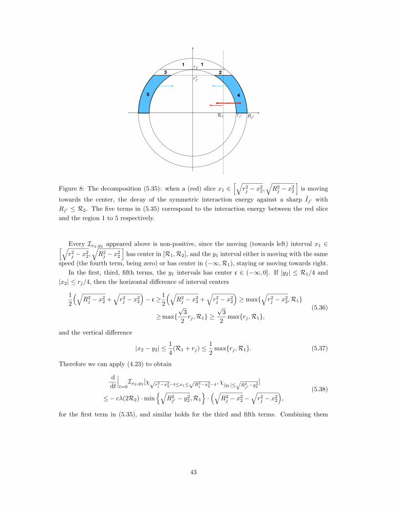
1 123

R1

45

rj0

r⇤j0

rj0 Rj0

Figure 8: The decomposition (5.35): when a (red) slice x1 ∈[√

r2j − x2

2,√R2j − x2

2

]is moving

towards the center, the decay of the symmetric interaction energy against a sharp Ij′ with

Rj′ ≤ R2. The five terms in (5.35) correspond to the interaction energy between the red slice

and the region 1 to 5 respectively.

Every Ix2,y2 appeared above is non-positive, since the moving (towards left) interval x1 ∈[√r2j − x2

2,√R2j − x2

2

]has center in [R1,R2], and the y1 interval either is moving with the same

speed (the fourth term, being zero) or has center in (−∞,R1), staying or moving towards right.

In the first, third, fifth terms, the y1 intervals has center c ∈ (−∞, 0]. If |y2| ≤ R1/4 and

|x2| ≤ rj/4, then the horizontal difference of interval centers

1

2

(√R2j − x2

2 +√r2j − x2

2

)− c ≥1

2

(√R2j − x2

2 +√r2j − x2

2

)≥ max{

√r2j − x2

2,R1}

≥max{√

3

2rj ,R1} ≥

√3

2max{rj ,R1},

(5.36)

and the vertical difference

|x2 − y2| ≤1

4(R1 + rj) ≤

1

2max{rj ,R1}. (5.37)

Therefore we can apply (4.23) to obtain

d

dt

∣∣∣t=0Ix2,y2 [χ√

r2j−x22−t≤x1≤

√R2j−x2

2−t, χ|y1|≤

√R2j′−y

22

]

≤− cλ(2R2) ·min{√

R2j′ − y2

2 ,R1

}·(√

R2j − x2

2 −√r2j − x2

2

),

(5.38)

for the first term in (5.35), and similar holds for the third and fifth terms. Combining them

43

together and integrating in x2, y2, we obtain

d

dt

∣∣∣t=0I[χIj,t(h), χIj′,t(h′)]

≤− cλ(2R2) ·∫|y2|≤R1/4

min{√

R2j′ − y2

2 −√

max{R2j′ − y2

2 , 0},R1

}dy2

·∫|x2|≤min{r∗j ,rj/4}

(√R2j − x2

2 −√r2j − x2

2

)dx2

≤− cλ(2R2) · |Ij′ ∩ {|y2| ≤ R1/4}| ·∫|x2|≤r∗j

(√R2j − x2

2 −√r2j − x2

2

)dx2,

(5.39)

by Lemma 5.5 (with κ = 1/4). Also notice the lower bound∣∣∣Ij′ ∩ {|y2| ≤ R1/4}∣∣∣ ≥ ∣∣∣Ij′ ∩ {| sin θ| ≤ R1/(4R2)}

∣∣∣ ≥ cR1

R2|Ij′ |, (5.40)

since the radial set Ij′ ⊂ {y : |y| ≤ R2}.STEP 3: sharp parts outside R2: the third term on the RHS of (5.27), for fixed (h, j).

We use Lemma 4.8 to obtain (noticing that R2 ≥ 1 by assumption)∣∣∣∣∫ ∇W (x− y)µ](y)χR2≤|y|≤R3(y) dy

∣∣∣∣ ≤ C ∫ R3

R2

µ](r) dr, (5.41)

where R3 > R2 is to be determined. Also,∣∣∣∣∫ ∇W (x− y)µ](y)χ|y|≥R3(y) dy

∣∣∣∣ ≤ C 1

R3 −R2

∫µ](y)χ|y|≥R3

(y) dy ≤ C 1

R3 −R2, (5.42)

for any |x| ≤ R2, by (A2), since |x− y| ≥ R3 −R2 for the LHS integral.

Therefore, since all the slices in Ij,t are moving at speed at most 1,∣∣∣∣ d

dt

∣∣∣t=0I[µ](y)χ|y|≥R2

(y), χIj,t ]

∣∣∣∣≤C(∫ R3

R2

µ](r) dr +1

R3 −R2

)∫|x2|≤r∗j

(√R2j − x2

2 −√r2j − x2

2

)dx2

≤C( 1

R2

∫R2≤|y|≤R3

µ](y) dy +1

R3 −R2

)∫|x2|≤r∗j

(√R2j − x2

2 −√r2j − x2

2

)dx2.

(5.43)

Combining the three steps together, summing in j and integrating in h, we obtain

d

dt

∣∣∣t=0I[ρt]

≤[− cλ(R2 + δ−1/2)

(∫|y|≤R1

(ρ∗(y) + µ[(y)) dy − 2πδR22

)+ CεR1

− cλ(2R2)R1

R2

∫|y|≤R2

µ](y) dy + C( 1

R2

∫R2≤|y|≤R3

µ](y) dy +1

R3 −R2

)]·∫ ∑

j≥1, sharp,Rj≤R2

∫|x2|≤r∗j

(√R2j − x2

2 −√r2j − x2

2

)dx2 dh.

(5.44)

Notice that the last integral is exactly the total moving mass (up to a constant multiple). Finally

we choose the parameters δ, ε,R3. We first notice that∫|y|≤R1

(ρ∗(y) + µ[(y)) dy +

∫|y|≤R2

µ](y) dy ≥∫|y|≤R1

ρ(y) dy ≥ cρ, (5.45)

44

by Lemma 4.9. Therefore, by choosing δ = cR1R−32 small enough, we may absorb the bad term

2πδR22. Then choosing ε small enough and R3 large enough, we may absorb the bad terms CεR1

and C 1R3−R2

respectively. Then the conclusion follows.

Proof of Proposition 2.5. Define R3 as in Proposition 5.4. In this proof we omit the dependence

of constants on R1,R2,R3, ε for simplicity. Proposition 5.2 implies that for any ε > 0,∣∣∣{t :

∫R2≤|y|≤R3

µ](t,y) dy ≥ ε}∣∣∣ ≤ C

ε4. (5.46)

Take ε such that Cε ≤ c/2 where c, C are the constants appeared in (5.20). Then, except a set

T ⊂ [0,∞) with |T | <∞, one has

d

dtE[ρ(t, ·)] ≤ −c ·

∫ ∑j≥1, sharp,Rj≤R2

∫|x2|≤r∗j

(√R2j − x2

2−√r2j − x2

2

)dx2 dh, ∀t /∈ T , (5.47)

by applying Lemma 4.1 with Proposition 5.4, in view of the fact that the cost of the CSS2 curve is

controlled by the total moving mass∫ ∑

j≥1, sharp,Rj≤R2

∫|x2|≤r∗j

(√R2j − x2

2−√r2j − x2

2

)dx2 dh,

by Lemma 4.2.

Notice that for fixed j ≥ 1, sharp, Rj ≤ R2, if Rj ≥ 4R1, then

1

2

(√R2j − x2

2 +√r2j − x2

2

)≥ 1

2

√R2j − x2

2 ≥1

4Rj ≥ R1, (5.48)

for any |x2| ≤ min{Rj/2, rj}. Therefore by definition r∗j ≥ min{Rj/2, rj} ≥ rj/2. Therefore∫|x2|≤r∗j

(√R2j − x2

2 −√r2j − x2

2

)dx2 dh ≥

∫|x2|≤rj/2

(√R2j − x2

2 −√r2j − x2

2

)dx2 dh ≥ c|Ij |,

(5.49)

using the sharpness of Ij (the last c depends on ε). Combined with (5.47) and the lower bound

of E (Lemma 4.4), we obtain ∫t/∈T

∫4R1≤|x|≤R2

µ](t,x) dx dt ≤ C. (5.50)

The finiteness of the integral in t ∈ T follows from the finiteness of T and the uniform L∞ bound

of ρ (Lemma 4.3).

5.3 The local clustering curve

Fix R1 > 0 large. Fix 2R1 ≤ R ≤ 4R1 to be determined. Define the local clustering curve

ρt by the velocity field

v(x) = −|x| − RR1· χR≤|x|≤8R1

(x) · x

|x| , (5.51)

i.e., ρt satisfies

∂tρt +∇ · (ρtv) = 0, (5.52)

45

with initial data ρ0 = ρ. ρt is compressing the mass in {R ≤ |x| ≤ 8R1}, and we have the lower

bound

∇ ·v =1

R1(−2 +

R|x| ) ·χR≤|x|≤8R1

(x) +8R1 − RR1

δ(|x| − 8R1) ≥ − 2

R1·χR≤|x|≤8R1

(x). (5.53)

which means the compression effect is not too strong.

We recall the lemma of local clustering8 from [26]:

Lemma 5.6 (Lemma of local clustering, Lemma 5.1 of [26]). Let R > 0, ρ(x) be a decreasing

non-negative function defined on [R, 4R], and m > 1. Then there exists r ∈ [R, 2R] such that∫ 4R

r

ρ(x)m dx ≤ a∫ 4R

r

(x− r)ρ(x) dx, a =CmRρ(R)m−1. (5.54)

Proposition 5.7. Let R1 be large enough, and ε = ε(R1, cρ) be small enough. Then there exists

R ∈ [2R1, 4R1], such that the local clustering curve ρt satisfies

d

dt

∣∣∣t=0

E[ρt] ≤ −cλ(CR1) ·∫R≤r≤8R1

(r − R)ρ(r) dr + C

∫2R1≤|y|≤8R1

µ](y) dy, (5.55)

if ∫2R1≤|y|≤R3

µ](y) dy ≤ cλ(CR1), (5.56)

for some large R3 = R3(R1).

Proof. STEP 1: estimate the decay of the interaction energy.

d

dt

∣∣∣t=0I[ρt] =I[ρ, ∂t|t=0ρt]

=−∫ ∫

W (x− y)ρ(y) dy∇ · (ρ(x)v(x)) dx

=

∫R≤|x|≤8R1

∫∇W (x− y)ρ(y) dyρ(x)v(x) dx,

(5.57)

by noticing that v(x) is zero except the range R ≤ |x| ≤ 8R1. We decompose∫∇W (x− y)ρ(y) dy =

∫∇W (x− y)

(ρ∗(y) + µ[(y) + µ](y)χ|y|≤R(y)

)dy

+

∫∇W (x− y)µ](y)χ|y|>R(y) dy.

(5.58)

Corollary 4.11 (with R2 = 8R1) shows that, for R1 large enough, for any R ≤ |x| ≤ 8R1,∫∇W (x− y) · x

|x|(ρ∗(y) + ρ[(y) + ρ](y)χ|y|≤R1

(y))

dy ≥ cλ(CR1), (5.59)

if ε is small enough. Next, (5.41) and (5.42), with R2 replaced by R ≥ 2R1, implies that, for

any R ≤ |x| ≤ 8R1,∣∣∣∣∫ ∇W (x− y)µ](y)χ[R,∞)(y) dy

∣∣∣∣ ≤ C ∫ R3

2R1

µ](r) dr + C1

R3 − 8R1. (5.60)

8The original lemma in [26] is stated with 3R in the place of 4R, but this current version can be proved in

exactly the same way.

46

⇢⇤(r) ⇢⇤(r)

µ[(r)

µ](r)

µ](r)

⇢⇤(r)µ[(r)

2R1 8R1

Figure 9: The definition of ρ∗∗. In ρ∗(r) + µ[(r), the right blue region is shifted towards left

to obtain ρ∗∗. This change may make∫R≤r≤8R1

ρ∗∗(r)m dr smaller than∫R≤r≤8R1

(ρ∗(r) +

µ[(r))m dr since some mass is shifted out of the interval [R, 8R1], and this is compensated by

the third term in (5.66).

We take R3 large enough so that C 1R3−8R1

≤ cλ(CR1)/2, and obtain∫∇W (x− y) · x

|x|ρ(y) dy ≥ cλ(CR1)− C∫ R3

2R1

µ](r) dr. (5.61)

Therefore, under the assumption (5.56), we have

d

dt

∣∣∣t=0I[ρt] ≤ −cλ(CR1)

∫R≤|x|≤8R1

|x| − RR1

ρ(x) dx ≤ −cλ(CR1)

∫R≤r≤8R1

(r − R)ρ(r) dr.

(5.62)

STEP 2: estimate the increment of the interaction energy.

d

dt

∣∣∣t=0S[ρt] =−m

∫ρ(x)m−1∇ · (ρ(x)v(x)) dx = m(m− 1)

∫ρ(x)m−1∇ρ(x) · v(x) dx

=(m− 1)

∫∇(ρ(x)m) · v(x) dx = −(m− 1)

∫ρ(x)m∇ · v(x) dx

≤2(m− 1)

R1

∫R≤|x|≤8R1

ρ(x)m dx ≤ C∫R≤r≤8R1

ρ(r)m dr

≤C∫R≤r≤8R1

(ρ∗(r) + µ[(r))m dr + C

∫2R1≤r≤8R1

µ](r) dr,

(5.63)

using (5.53) in the first inequality, and the uniform bound of ‖ρ‖L∞ (from Lemma 4.3) in the

last inequality.

To estimate the first term in the last expression above, we define ρ∗∗(r) as the non-increasing

rearrangement of ρ∗(r) + µ[(r) on [2R1, 8R1]. See Figure 9 for illustration.

47

Then the RHS integral in (5.62) can be estimated as∫R≤r≤8R1

(r − R)ρ(r) dr ≥∫R≤r≤8R1

(r − R)(ρ∗(r) + µ[(r)) dr

=

∫2R1≤r≤8R1

(r − R)χR≤r≤8R1(r)(ρ∗(r) + µ[(r)) dr

≥∫

2R1≤r≤8R1

(r − R)χR≤r≤8R1(r)ρ∗∗(r) dr

=

∫R≤r≤8R1

(r − R)ρ∗∗(r) dr,

(5.64)

since (r − R)χR≤r≤8R1(r) is increasing on [2R1, 8R1]. Also notice that

ρ∗∗(2R1) = sup2R1≤r≤8R1

(ρ∗(r) + µ[(r)) ≤C

R21

, (5.65)

by (2.44).

Now we claim∫R≤r≤8R1

(ρ∗(r) + µ[(r))m dr

≤C(∫R≤r≤8R1

ρ∗∗(r)m dr +ρ∗∗(2R1)m−1

R1

∫R≤r≤8R1

(r − R)ρ(r) dr),

(5.66)

if ε < 1/4. To see this, we write

(ρ∗(r) + µ[(r))χ2R1≤r≤8R1(r) =

∫ ∞0

(χI0∩[2R1,8R1](r) +

∑j≥1, flat

χIj∩[2R1,8R1](r))

dh. (5.67)

Clearly I0 ∩ [2R1, 8R1] stays the same under the non-increasing rearrangement ρ∗∗, see the left

blue region in Figure 9. For j ≥ 1, flat, if ε < 1/4, then Ij cannot be a subset of [2R1, 8R1]. We

separate into two cases:

• 2R1 ∈ Ij . In this case Ij ∩ [2R1, 8R1] stays the same under the non-increasing rearrange-

ment.

• 2R1 /∈ Ij . In this case 8R1 ∈ Ij , and Ij ∩ [2R1, 8R1] is shifted towards the center by the

distance τj = rj − Rj−1 > 0, under the non-increasing rearrangement, see the right blue

region in Figure 9.

Therefore

ρ∗∗(r) =

∫ ∞0

(χI0∩[2R1,8R1](r) +

∑j≥1, flat, 2R1∈Ij

χIj∩[2R1,8R1](r)

+∑

j≥1, flat, 2R1 /∈Ijχ(Ij−τj)∩[2R1,8R1](r)

)dh.

(5.68)

Notice that for any function ψ(r) =∫∞

0χS(h)(r) dh with S(h) = {r : ψ(r) ≥ h}, one has∫

ψ(r)m dr =

∫ ∞0

|S(h)| ·mhm−1 dh. (5.69)

48

Therefore, in (5.67) and (5.68), taking the intersection of every involved interval with [R, 8R1]

and integrating in r gives∫R≤r≤8R1

(ρ∗(r) + µ[(r))m dr =

∫ ∞0

(|I0 ∩ [R, 8R1]|+

∑j≥1, flat

|Ij ∩ [R, 8R1]|)·mhm−1 dh,

(5.70)

and ∫R≤r≤8R1

ρ∗∗(r)m dr =

∫ ∞0

(|I0 ∩ [R, 8R1]|+

∑j≥1, flat, 2R1∈Ij

|Ij ∩ [R, 8R1]|

+∑

j≥1, flat, 2R1 /∈Ij|(Ij − τj) ∩ [R, 8R1]|

)·mhm−1 dh.

(5.71)

Also notice that

ρ∗∗(2R1)m−1

R1

∫R≤r≤8R1

(r − R)ρ(r) dr

≥ρ∗∗(2R1)m−1

∫6R1≤r≤8R1

ρ(r) dr

≥ρ∗∗(2R1)m−1

∫6R1≤r≤8R1

(ρ∗(r) + µ[(r)) dr

≥∫

6R1≤r≤8R1

(ρ∗(r) + µ[(r))m dr

=

∫ ∞0

(|I0 ∩ [6R1, 8R1]|+

∑j≥1, flat

|Ij ∩ [6R1, 8R1]|)·mhm−1 dh,

(5.72)

using R ≤ 4R1 and the equality in (5.65).

Therefore, to show (5.66), the terms with I0 and Ij , j ≥ 1, flat, 2R1 ∈ Ij in (5.70) can be

controlled by (5.71), and it suffices to show that for any j ≥ 1, flat, 2R1 /∈ Ij , there holds

|Ij ∩ [R, 8R1]| ≤ C|Ij ∩ [6R1, 8R1]|, (5.73)

and thus controlled by (5.72). In fact, since 8R1 ∈ Ij , we may separate into two cases:

• If Ij ∩ [R, 8R1] ⊂ [6R1, 8R1], then (5.73) holds with C = 1, since |Ij ∩ [R, 8R1]| ≤ |Ij | and

|Ij ∩ [6R1, 8R1]| = |Ij ∩ [R, 8R1]|.

• Otherwise, we have [6R1, 8R1] ⊂ Ij since 8R1 ∈ Ij . Therefore |Ij ∩ [6R1, 8R1]| = 2R1 and

|Ij ∩ [R, 8R1]| ≤ 8R1 − R ≤ 6R1, and thus (5.73) holds with C = 3.

Therefore we have proved (5.66).

Now we choose R by Lemma 5.6 applied to ρ∗∗(r) on [2R1, 8R1], and then∫R≤r≤8R1

ρ∗∗(r)m dr ≤ C

R1ρ∗∗(2R1)m−1

∫R≤r≤8R1

(r − R)ρ∗∗(r) dr. (5.74)

Combining with (5.66), we have∫R≤r≤8R1

(ρ∗(r) + µ[(r))m dr ≤ C ρ

∗∗(2R1)m−1

R1

∫R≤r≤8R1

(r − R)ρ(r) dr. (5.75)

49

STEP 3: take R1 large to finalize.

Combining STEP 1 and STEP 2, we have

d

dt

∣∣∣t=0

E[ρt] ≤−(cλ(CR1)− C ρ

∗∗(2R1)m−1

R1

)∫R≤r≤8R1

(r − R)ρ(r) dr

+ C

∫2R1≤r≤8R1

µ](r) dr,

(5.76)

under the assumption (5.56). By (2.5) (a consequence of (A1)) and (5.65),

λ(CR1) = cR−α1 ,ρ∗∗(2R1)m−1

R1≤ CR−(2m−1)

1 . (5.77)

Therefore, with (A3), we can choose R1 large enough, so that C ρ∗∗(2R1)m−1

R1≤ cλ(CR1)/2, and

obtain the conclusion.

Proof of Proposition 2.6. By applying (5.55) to ρ(t, ·) (the solution to (1.1)) for any fixed t ≥ 0

and using (2.5) and Lemma 4.1, we obtain

d

dtE[ρ(t, ·)]

≤−

[−c1R−α1

∫R(t)≤r≤8R1

(r − R(t))ρ(t, r) dr + C1

∫2R1≤|y|≤8R1

µ](t,y) dy]2

R−21

∫R(t)≤r≤8R1

(r − R(t))2ρ(t, r) dr,

(5.78)

provided that the quantity inside the bracket is negative, and (5.56) holds, i.e.,∫2R1≤|y|≤R3

µ](t,y) dy ≤ c2R−α1 . (5.79)

Here R(t) is determined by ρ(t, ·), satisfying 2R1 ≤ R(t) ≤ 4R1. The denominator in (5.78) is

the cost of the local clustering curve, and c1, C1, c2 are constants.

Then we define the sets T1,2,3 ⊂ [0,∞) as follows:

• T1 contains those t with∫

2R1≤|y|≤8R1µ](t,y) dy ≥ c2R−α1 . Proposition 2.5 shows that

|T1| <∞. It follows that∫t∈T1

∫R(t)≤r≤8R1

(r − R(t))ρ(t, r) dr dt <∞. (5.80)

• T2 contains those t /∈ T1 with∫R(t)≤r≤8R1

(r − R(t))ρ(t, r) dr ≤ 2C1Rα1c1

∫2R1≤|y|≤8R1

µ](t,y) dy. (5.81)

It follows that∫t∈T2

∫R(t)≤r≤8R1

(r − R(t))ρ(t, r) dr dt ≤ 2C1Rα1c1

∫t∈T2

∫2R1≤|y|≤8R1

µ](t,y) dy dt <∞,(5.82)

where the second inequality uses Proposition 2.5.

50

• T3 = [0,∞)\(T1∪T2). It then follows that (5.56) holds, and the quantity inside the bracket

in (5.78) is less than − c1R−α1

2

∫R(t)≤r≤8R1

(r − R(t))ρ(t, r) dr, and then

d

dtE[ρ(t, ·)] ≤− cR−2α

1

[∫R(t)≤r≤8R1

(r − R(t))ρ(t, r) dr]2

R−21

∫R(t)≤r≤8R1

(r − R(t))2ρ(t, r) dr

≤− cR−2α+11

∫R(t)≤r≤8R1

(r − R(t))ρ(t, r) dr,

(5.83)

for t ∈ T3, using the fact that 0 ≤ r − R(t) ≤ CR1 for any R(t) ≤ r ≤ 8R1. Therefore∫t∈T3

∫R(t)≤r≤8R1

(r − R(t))ρ(t, r) dr dt <∞. (5.84)

Combining the three parts gives∫ ∞0

∫R(t)≤r≤8R1

(r − R(t))ρ(t, r) dr dt <∞. (5.85)

Then the final conclusion follows, by noticing that∫R(t)≤r≤8R1

(r−R(t))ρ(t, r) dr ≥ cR1

∫7R1≤r≤8R1

ρ(t, r) dr ≥ c∫

7R1≤|x|≤8R1

ρ(t,x) dx, (5.86)

since R(t) ≤ 4R1.

Acknowledgement

The author would like to thank Jose Carrillo, Franca Hoffmann, Dave Levermore and Eitan

Tadmor for helpful discussions. The author would also like to thank Jiuya Wang for giving a

first proof of Proposition 2.3.

References

[1] R. Bailo, J. A. Carrillo, and J. Hu. Fully discrete positivity-preserving and energy-

dissipating schemes for aggregation-diffusion equations with a gradient flow structure.

preprint, arXiv:1811.11502.

[2] J. Bedrossian. Global minimizers for free energies of subcritical aggregation equations with

degenerate diffusion. Appl. Math. Letters, 24(11):1927–1932, 2011.

[3] A. Blanchet, J. A. Carrillo, and P. Laurencot. Critical mass for a Patlak-Keller-Segel model

with degenerate diffusion in higher dimensions. Calc. Var. Partial Differential Equations,

35:133–168, 2009.

[4] A. Blanchet, J. Dolbeault, and B. Perthame. Two-dimensional Keller-Segel model: optimal

critical mass and qualitative properties of the solutions. Electronic J. Differ. Equat., (44):1–

32, 2006.

51

[5] S. Boi, V. Capasso, and D. Morale. Modeling the aggragative behavior of ants of the species

polyergus rufescens. Nonlinear Anal. Real World Appl., 1(163-176), 2000.

[6] M. Burger, V. Capasso, and D. Morale. On an aggregation model with long and short range

interactions. Nonlinear Anal. Real World Appl., 8:939–958, 2007.

[7] V. Calvez, J. A. Carrillo, and F. Hoffmann. Uniqueness of stationary states for singular

Keller-Segel type models. preprint, arXiv:1905.07788.

[8] V. Calvez, J. A. Carrillo, and F. Hoffmann. Equilibria of homogeneous functionals in the

fair-competition regime. Nonlinear Anal., 159:85–128, 2017.

[9] V. Calvez and L. Corrias. The parabolic-parabolic Keller-Segel model in R2. Comm. Math.

Sci., 6(2):417–447, 2008.

[10] J. A. Carrillo, D. Castorina, and B. Volzone. Ground states for diffusion dominated free

energies with logarithmic interaction. SIAM J. Math. Anal., 47(1):1–25, 2015.

[11] J. A. Carrillo, K. Craig, L. Wang, and C. Wei. Primal dual methods for Wasserstein gradient

flows. preprint, arXiv:1901.08081.

[12] J. A. Carrillo, S. Hittmeir, B. Volzone, and Y. Yao. Nonlinear aggregation-diffusion equa-

tions: radial symmetry and long time asymptotics. Invent. Math., 218(3):889–977, 2019.

[13] J. A. Carrillo, F. Hoffmann, E. Mainini, and B. Volzone. Ground states in the diffusion-

dominated regime. Calc. Var. Partial Differential Equations, 57(5):127, 2018.

[14] M. G. Delgadino, X. Yan, and Y. Yao. Uniqueness and non-uniqueness of steady states of

aggregation-diffusion equations. preprint, arXiv:1908.09782, 2019.

[15] D. Horstmann. From 1970 until present: the Keller-Segel model in chemotaxis and its

consequences. preprint, 2003.

[16] W. Jager and S. Luckhaus. On explosions of solutions to a system of partial differential

equations modelling chemotaxis. Trans. Amer. Math. Soc., 329:819–824, 1992.

[17] E. F. Keller and L. A. Segel. Initiation of slide mold aggregation viewed as an instability.

J. Theor. Biol., 26:399–415, 1970.

[18] I. Kim and Y. Yao. The Patlak–Keller–Segel model and its variations: properties of solutions

via maximum principle. SIAM J. Math. Anal., 44(2):568–602, 2012.

[19] I. Kim and Y. P. Zhang. Regularity properties of degenerate diffusion equations with drifts.

SIAM J. Math. Anal., 50(4):4371–4406, 2018.

[20] E. H. Lieb and H. T. Yau. The Chandrasekhar theory of stellar collapse as the limit of

quantum mechanics. Comm. Math. Phys., 112(1):147–174, 1987.

[21] A. Mogilner and L. Edelstein-Keshet. A non-local model for a swarm. J. Math. Biol.,

38:534–570, 1999.

52

[22] A. Mogilner, L. Edelstein-Keshet, L. Bent, and A. Spiros. Mutual interactions, potentials,

and individual distance in a social aggregation. J. Math. Biol., 47:353–389, 2003.

[23] D. Morale, V. Capasso, and K. Oelschlager. An interacting particle system modelling

aggregation behavior: from individuals to populations. J. Math. Biol., 50:49–66, 2005.

[24] K. Oelschlager. Large systems of interacting particles and the porous medium equation. J.

Diff. Equat., 88(2):294–346, 1990.

[25] C. S. Patlak. Random walk with persistence and external bias. Bull. Math. Biophys.,

15:311–338, 1953.

[26] R. Shu. Equilibration of aggregation-diffusion equations with weak interaction forces.

preprint, arXiv:2003.04230.

[27] G. Strohmer. Stationary states and moving planes. Parabolic and Navier-Stokes equations,

81(Part 2):501–513, 2008.

[28] C. M. Topaz, A. L. Bertozzi, and M. A. Lewis. A nonlocal continuum model for biological

aggregation. Bull. Math. Biol., 68:1601–1623, 2006.

53