Three Essays on Environment

and Development: A

Behavioral Perspective

Inaugural - Dissertation

zur

Erlangung der wirtschaftswissenschaftlichen Doktorwürde

des Fachbereichs Wirtschaftswissenschaften

der Philipps-Universität Marburg

eingereicht von:

Tobias Vorlaufer

M.Sc. aus Frankfurt am Main

Erstgutacher: Prof. Dr. Michael Kirk

Zweitgutachter: Prof. Dr. Björn Vollan

Einreichungstermin: 18.05.2018

Prüfungstermin: 30.07.2018

Erscheinungsort: Marburg

Hochschulkennzi�er: 1180

ii

iii

iv

Acknowledgements

Firstly, I would like to express my sincere gratitude to my supervisor MichaelKirk for the opportunity to conduct research within the SASSCAL project,his dedicated support during the last years and for creating a friendly, en-couraging and productive environment at our working group. Special thanksgo to Björn Vollan, my co-supervisor, for our extended discussions, his cre-ativity for and his feedback on the experimental designs, analyses and manu-scripts. My SASSCAL colleagues and co-authors Tom Dufhues and ThomasFalk not only contributed to my dissertation through introducing me to thefieldwork in southern Africa and the long-lasting discussions at the initialstages of my PhD studies, but also provided essential feedback later on. Iam grateful for the feedback of Evelyn Korn and of the many conference andworkshop participants, to whom I presented my research.

My time in Marburg would not have been as enjoyable without my fel-low PhD students Boban Aleksandrovic, Lawrence Brown, Christian Hönow,Lukas Kampenhuber, Matthias Mayer and Ivo Steimanis and their persist-ent commitment for extended lunch breaks. These regular meetings providednot only encouraging and inspiring discussions on my own work and researchin general, but luckily also extended to more relevant topics. Many thanksalso to Adrian Pourviseh and Martin Voß for their research assistance.

Without a doubt the research would not have been possible without theexcellent work of the many research assistants both in Zambia and Nami-bia including Sunday Kasemone, Precious Moonga, Buumba Malowo, OscarChimbangu, James Moono, Johannes Mashare and Annastasia Kaweto.Moreover, I am highly indebted to all participating communities for theirtime, effort and hospitality during the data collection.

Last, but by no means least, I am especially grateful for the unconditionalsupport of my family, especially my parents. They fostered my curiosity forother cultures and always encouraged me to pursue whatever I set my mindto. Thank you.

v

vi

Zusammenfassung

Die vorliegende kumulative Dissertation umfasst drei einzelne Essays miteiner verhaltensökonomischen Perspektive auf Umweltthemen in Entwick-lungsländern. Die ersten beiden Aufsätze basieren auf experimentellen Me-thoden und Datensätzen, die im Rahmen eines Forschungsaufenthaltes inSambia erhoben wurden. Sambia zählt zu den bewaldetsten Ländern in Sub-sahara Afrika, zeichnet sich jedoch auch durch schnelle Landnutzungsverän-derungen, insbesondere Entwaldung, aus.

Der erste Aufsatz befasst sich mit Zahlungen für Ökosystemleistungen(engl.: PES) als potentielles Anreizinstrument für eine nachhaltige Land-nutzung im globalen Süden. Landwirtschaft, insbesondere kleinbäuerlicheLandwirtschaft in Entwicklungsländern, wird als Hauptverursacher von Ent-waldung weltweit betrachtet. Parallel haben afrikanische Länder den land-wirtschaftlichen Sektor als zentralen Akteur in ihren Wachstumsstrategienidentifiziert und zielen auf eine Erhöhung der Produktivität ab. EmpirischeUntersuchungen zeigen jedoch, dass in den meisten Fällen Produktivitätsstei-gerungen in der Landwirtschaft negative Auswirkungen auf die Flächennut-zung, insbesondere Entwaldung, haben. PES, die (bereits existierende) För-derprogramme in der Landwirtschaft an den Erhalt von Waldflächen knüp-fen, sind ein potentielles Instrument, um diesen Zielkonflikt zu entschärfen.Die bisherige Forschung zu PES hat diese Verknüpfung bisher jedoch nurunzureichend behandelt. Der vorliegende Aufsatz basiert auf einem DiscreteChoice Experiment in Sambia, das Präferenzen von Kleinbauern für PES-Verträge erhoben hat. In hypothetischen Verträgen wurden Landwirtschaft-sinputs bzw. Barzahlungen, die an den Erhalt von bestehenden Waldflächengeknüpft sind, Kleinbauern angeboten. Die Ergebnisse zeigen, dass die Teil-nehmer Zahlungen in Form von Inputs stärker wertschätzen als Barzahlungenund dementsprechend bei dieser Zahlungsform geringere Beträge für einenVerzicht auf die Rodung von zusätzlichen Waldflächen verlangen. PES, dieZahlungen in Form von landwirtschaftlichen Inputs anbieten, sind daher eineffektives Politikinstrument, um den Schutz von bestehenden Wäldern beigleichzeitiger Förderung der kleinbäuerlichen Landwirtschaft zu gewährleis-ten.

Der zweite Aufsatz dieser Dissertation untersucht die Effekte von Um-weltmigration, verursacht durch nicht-nachhaltige kleinbäuerliche Landnut-

vii

zung, auf Kooperationsverhalten in ruralen Ziel-Communities. Migrationführt potentiell zur Diskriminierung von Migranten, verringert das Sozialka-pital und Vertrauen zwischen Dorfbewohnern und hat daher negative Aus-wirkungen auf das Kooperationsverhalten im Allgemeinen. Im Rahmen derDatenerhebungen in Sambia wurden neben einer Haushaltsbefragung incen-tivierte, ökonomische Feldexperimente (Public Good Experimente) einge-setzt, um Kooperationsverhalten zu messen. In den Experimenten wurde dieGruppenzusammensetzung hinsichtlich Migranten und der autochthonen Be-völkerung exogen variiert. Die Forschungsergebnisse liefern ein detailliertesBild, inwiefern Migration Kooperation in Ziel-Communities, die über einenlangen Zeitraum kontinuierlichen Migrationsströmen ausgesetzt waren, be-einflusst. Auf der einen Seite finden wir keine Evidenz in den Befragungs-und Experimentdaten für negative Auswirkungen von Migration auf Koope-rationsverhalten. Auf der anderen Seite zeigen die Ergebnisse jedoch, dassdie spezifischen Effekte stark davon abhängen, welche Eigenschaften Migran-ten relativ zu der angestammten Bevölkerung haben. Im Forschungsgebietweisen Migranten im Durchschnitt ein mehrfach höheres Einkommen als dieautochthone Bevölkerung auf. In Dörfern, in denen diese Einkommensunter-schiede besonders stark ausgeprägt sind, kooperieren Migranten mehr, wennsie als Minderheit am Experiment teilnehmen. Die Haushaltsbefragungenbestätigen diese Tendenz: Migranten tragen in diesen Dörfern auch mehr zuöffentlichen Gütern wie Schulen und Bohrlöchern bei, insbesondere, wenn sieüber ein hohes Einkommen verfügen und je kürzer sie in dem Dorf leben.Dieses Verhalten interpretieren wir als Signal von Migranten bezüglich ihrerPro-Sozialität und ihrem Willen, sich in die Dorfgemeinschaft zu integrieren.Unsere Ergebnisse zeigen, dass die Effekte von Migration auf Kooperationin ländlichen Gebieten von den Eigenschaften der Migranten relativ zu derangestammten Bevölkerung abhängen. Darüber hinaus deuten die Ergebnis-se darauf hin, dass Dorfgemeinschaften resilient gegenüber Migrationsbewe-gungen sind und ihre Kooperationsfähigkeiten trotz dieser Veränderungenaufrechterhalten können.

Der dritte und letzte Aufsatz dieser Dissertation ist ein methodischerBeitrag zu Feldexperimenten, die vermehrt in der umweltökonomischen For-schung in Entwicklungsländern eingesetzt werden. Im Rahmen von zwei Fel-dexperimenten in Namibia wurde untersucht, welche Abläufe hinsichtlichder Anonymität von Entscheidungen zwischen Experimenter und Teilnehmersogenannte Demand-Effekte minimieren können. Anhand des Dictator unddes Joy-of-Destruction-Experiments wurde pro- bzw. anti-soziales Verhaltenbei 480 Teilnehmern gemessen. Neben einem strikten Doppel-Anonymitäts-Treatment, das die individuellen Entscheidungen von Teilnehmern nicht zu-ordnen lässt, wurden zwei verschiedene Varianten von Einfach-Anonymitätimplementiert, die Rückschlüsse der Experimenter auf individuelles Verhal-ten zulassen. Die Ergebnisse zeigen, dass eine methodisch-fundierte Imple-mentierung von Experimenten im Feld einen hohen Stellenwert haben soll-

viii

te. Sowohl im Dictator als auch Joy-of-Destruction-Experiment ist Doppel-Anonymität keine Voraussetzung, um Demand-Effekte erfolgreich zu mini-mieren. Vielmehr ist es die Anonymität der Teilnehmer während des Expe-riments, die sowohl pro- als auch anti-soziales Verhalten signifikant beein-flusst. Sobald individuelle Entscheidungen direkt, jedoch privat dem Expe-rimenter mitgeteilt werden, beobachten wir signifikant stärkeres pro-sozialesund signifikant weniger anti-soziales Verhalten. Die Ergebnisse zeigen, dasseine ex-post Zuordnung der individuellen Entscheidungen nach den Expe-rimenten durch Identifikationsnummern keine zusätzlichen Demand-Effekteim Vergleich zur vollen Doppel-Anonymität induziert. Zusätzlich zeigt dieserAufsatz, dass Experiment-Protokolle die Entscheidungsumgebung der Teil-nehmer exakt erfassen sollten, um die Replizierbarkeit von Feldexperimentezu gewährleisten.

ix

Contents

1 Synopsis: Problem Statement, Structure and Contribu-tion 1

1.1 The Environment-Development Nexus . . . . . . . . . . . . 11.2 PES and Agricultural Intensification . . . . . . . . . . . . . 31.3 Migration, Environmental Change and Collective Action . . 41.4 Experimental Methods in the Field . . . . . . . . . . . . . . 51.5 Outlook . . . . . . . . . . . . . . . . . . . . . . . . . . . . . 7

2 Payments for Ecosystem Services and Agricultural Inten-sification: Evidence from a Choice Experiment on Defor-estation in Zambia 15

2.1 Introduction . . . . . . . . . . . . . . . . . . . . . . . . . . . 162.2 Method and Experimental Design . . . . . . . . . . . . . . . 20

2.2.1 Stated Preferences and Discrete Choice Experiments 202.2.2 Theory and Econometric Models . . . . . . . . . . . 212.2.3 Attributes & Hypothesis . . . . . . . . . . . . . . . . 23

2.3 Study Context and Sample . . . . . . . . . . . . . . . . . . 262.4 Results . . . . . . . . . . . . . . . . . . . . . . . . . . . . . . 30

2.4.1 Random Parameter Logit Model . . . . . . . . . . . 302.4.2 Latent Class Logit Model . . . . . . . . . . . . . . . 322.4.3 Estimated Choice Probabilities and Sensitivity to Pay-

ment Amount . . . . . . . . . . . . . . . . . . . . . . 342.5 Discussion . . . . . . . . . . . . . . . . . . . . . . . . . . . 36

2.5.1 Preferences for Cash Versus In-Kind Payments . . . 362.5.2 Environmental Effectiveness of PES . . . . . . . . . 37

2.6 Conclusion . . . . . . . . . . . . . . . . . . . . . . . . . . . . 39

3 How Migrants Benefit Poor Communities: Evidence onCollective Action in Rural Zambia 45

3.1 Introduction . . . . . . . . . . . . . . . . . . . . . . . . . . . 463.2 Responses to Migration: Identity, Inequality and Cooperation 493.3 Material and Method . . . . . . . . . . . . . . . . . . . . . . 51

3.3.1 Participant Recruitment and Survey Design . . . . . 513.3.2 Site and Sample Description . . . . . . . . . . . . . . 53

x

3.3.2.1 Migrant and Migration Characteristics . . . 533.3.2.2 Village Characteristics . . . . . . . . . . . . 54

3.3.3 Experimental Design . . . . . . . . . . . . . . . . . . 573.4 Results . . . . . . . . . . . . . . . . . . . . . . . . . . . . . . 59

3.4.1 Experimental Data: Primed Identities and Effects onCooperation . . . . . . . . . . . . . . . . . . . . . . . 59

3.4.2 Experimental Data: Income Inequalities and Cooper-ation . . . . . . . . . . . . . . . . . . . . . . . . . . . 61

3.4.3 Survey Data: Contributions to Real Public Goods . 643.5 Discussion . . . . . . . . . . . . . . . . . . . . . . . . . . . . 663.6 Conclusion . . . . . . . . . . . . . . . . . . . . . . . . . . . . 69

4 Effects of Double-Anonymity on Pro- and Anti-Social Be-havior: Experimental Evidence from a Lab in the Field 77

4.1 Introduction . . . . . . . . . . . . . . . . . . . . . . . . . . . 784.2 Literature Review . . . . . . . . . . . . . . . . . . . . . . . . 814.3 Experimental Design and Procedures . . . . . . . . . . . . . 82

4.3.1 Double-Anonymous Procedures . . . . . . . . . . . . 824.3.2 Dictator Game . . . . . . . . . . . . . . . . . . . . . 844.3.3 Joy-of-Destruction Mini-Game . . . . . . . . . . . . 854.3.4 Experimental Procedures . . . . . . . . . . . . . . . 864.3.5 Sampling . . . . . . . . . . . . . . . . . . . . . . . . 87

4.4 Results . . . . . . . . . . . . . . . . . . . . . . . . . . . . . . 884.4.1 Dictator Game . . . . . . . . . . . . . . . . . . . . . 884.4.2 Joy-of-Destruction Mini-Game . . . . . . . . . . . . 90

4.5 Discussion . . . . . . . . . . . . . . . . . . . . . . . . . . . . 924.6 Conclusion . . . . . . . . . . . . . . . . . . . . . . . . . . . . 94

Appendices 101

A Chapter 2 101A.1 Contract Choice Estimation . . . . . . . . . . . . . . . . . . 101A.2 Introduction and Choice Situation Example . . . . . . . . . 103A.3 Risk Elicitation Experiment . . . . . . . . . . . . . . . . . . 105A.4 Alternative Model Specifications . . . . . . . . . . . . . . . 106A.5 Latent Class Models for Subsets . . . . . . . . . . . . . . . . 108A.6 Latent Class Model Selection Criteria . . . . . . . . . . . . . 110

B Chapter 3 111B.1 Descriptive Statistics . . . . . . . . . . . . . . . . . . . . . . 111B.2 Rounds 2 – 4 . . . . . . . . . . . . . . . . . . . . . . . . . . 112B.3 Individual Cash Income . . . . . . . . . . . . . . . . . . . . 119B.4 Correlation - Village Characteristics . . . . . . . . . . . . . 121B.5 Regression Results - Pooled Contributions Migrants and Locals 122

xi

B.6 Regression Results Main Treatment Effects - Migrants . . . 124B.7 Regression Results Main Treatment Effects - Locals . . . . . 126B.8 Regression Results - Individual Relative Income . . . . . . . 128B.9 Regression Results - Income Ratio . . . . . . . . . . . . . . 130B.10 Regression Results - Income Ratio and Relative Individual

Income . . . . . . . . . . . . . . . . . . . . . . . . . . . . . . 132B.11 Regression Results - Real Public Good Contributions . . . . 134B.12 Experimental Protocol . . . . . . . . . . . . . . . . . . . . . 136B.13 Balancing Tests between Treatments . . . . . . . . . . . . . 148B.14 Socio-Economic Characteristics in Villages Below and Above

the Median Income Ratio . . . . . . . . . . . . . . . . . . . 153B.15 Migrant Perception Index . . . . . . . . . . . . . . . . . . . 155B.16 Socio-Economic Status Index . . . . . . . . . . . . . . . . . 156

C Chapter 4 159C.1 Protocol: General Introduction . . . . . . . . . . . . . . . . 159C.2 Protocol: Dictator Game . . . . . . . . . . . . . . . . . . . . 161

C.2.1 Senders . . . . . . . . . . . . . . . . . . . . . . . . . 161C.2.2 Receivers . . . . . . . . . . . . . . . . . . . . . . . . 162

C.3 Protocol: Joy of Destruction Mini-Game . . . . . . . . . . . 163C.4 Treatment Plan . . . . . . . . . . . . . . . . . . . . . . . . . 166C.5 Socio-Economic Characteristics of Sample . . . . . . . . . . 167C.6 Regression Analyses . . . . . . . . . . . . . . . . . . . . . . 169C.7 Stated Decisions . . . . . . . . . . . . . . . . . . . . . . . . 171C.8 Prediction of Probabilities for Receiving Help . . . . . . . . 175C.9 Socio-Economic Status Index . . . . . . . . . . . . . . . . . 179

xii

Chapter 1

Synopsis: Problem Statement,Structure and Contribution

Tobias Vorlauferaa School of Business & Economics, Philipps-Universität Marburg, Germany

1.1 The Environment-Development Nexus

A wide range of ecosystem services (ES) are essential for human well-beingsuch as food, groundwater regulation or carbon sequestration (MillenniumEcosystem Assessment, 2005). Costanza et al. (2014) estimate that ecosys-tems around the globe provide services worth between US$ 125 - 145 trillioneach year. Despite the overall importance of ES, we have witnessed anunprecedented and alarming rate of environmental degradation and changeover the last decades, accounting for an annual loss of ES between US$ 4.3- 20.2 trillion/year between 1997 and 2011 (Costanza et al., 2014). Exam-ples among many are the rapid loss of biodiversity (Butchart et al., 2010)and productive soils (Amundson et al., 2015). Meanwhile, climate change isconsidered one of the largest challenges for humankind in the 21st century(IPCC, 2014b; Stern, 2007). Climate change will not only directly impacthuman well-being, but also further accelerate environmental changes such asbiodiversity loss (Pereira et al., 2010).

These dynamics pose a significant challenge for societies in the globalsouth. On the one hand, the livelihoods of people in developing countries- especially in rural areas - fundamentally depend on ES. Forests, for ex-ample, provide more than 2.4 billion people with biomass for cooking; 1.3billion people live in houses primarily made of forest products (FAO, 2015).Especially the poor in developing countries rely on non-timber forest pro-duce for nutrition and as an income source. Rural populations in developingcountries are, furthermore, highly dependent on agriculture as their main

1

Chapter 1

livelihood activity. Of 570 millions farms worldwide, 84% cultivate less thantwo hectares. The vast majority of these farms is located in developingcountries, many of them subsistence farmers (Lowder et al., 2016). As aconsequence, populations in Africa, Asia and Latin America are most vul-nerable to environmental change in general and climate change in particular,while these regions have limited resources for adaptation measures (IPCC,2014a; Morton, 2007; Adger et al., 2003). On the other hand, governmentsin the global south aim to eradicate poverty by boosting economic growththat likely intensifies the current pressure on ecosystems. These countriestherefore have to pursue pathways that reconcile both economic and envi-ronmental trade-offs.

This dissertation includes three individual essays that contribute to theresearch on environmental issues in developing countries. The three pa-pers apply experimental methods and are based on three different datasetscollected in Zambia and Namibia. The first paper evaluates the scope ofPayments for Ecosystem Services (PES) to conserve forest ecosystems andincrease agricultural productivity in Zambia. PES are a relatively novelmarket-based policy tool that complement existing conservation policies suchas command-and-control, taxes, cap-and-trade and integrated conservationand development approaches (e.g. community-based natural resource man-agement) (Kinzig et al., 2011). They rest on the assumption that monetaryincentives conditional on conservation efforts stipulate ES providers (i.e. re-source users) to take the environmental costs of their actions into accountand consequently increase conservation efforts (Wunder, 2005, 2015). Theseschemes are typically financed by people benefiting from the specific ES.More than 550 PES schemes have been implemented so far, with an esti-mated annual transaction volume between 36 and 42 billion US$ (Salzmanet al., 2018).

The second paper of this dissertation studies the impact of environ-mentally-driven internal rural-to-rural migration on collective action in hostcommunities in Zambia. Migration has been an effective adaptation strat-egy to environmental change throughout human history (McLeman, 2014).Initial estimations suggested that up to 200 million people could be forcedto migrate due to climate change (Myers, 2002). A more recent study bythe World Bank suggests that climate change could trigger the migration of143 million people within countries (Rigaud et al., 2018). While migrationoffers an effective adaptation strategy for better-off households with suffi-cient resources for relocation (Black et al., 2011b), the wider consequencesof migration for societies are less well understood. One such aspect is theimpact of migration on social dynamics in host communities, in particular oncollective action. In developing countries collective action is not only neededto provide a wide range of public goods, but is also essential for successfulcommon pool resource management (Ostrom, 1990; Rustagi et al., 2010).

The third paper of this dissertation is a methodological contribution to

2

1.2. PES and Agricultural Intensification

lab-in-the-field experiments. This method is increasingly applied to studyenvironmental issues (in developing countries). One major concern are, how-ever, demand effects and the auxiliary question which experimental proce-dures minimize them. Based on fieldwork in rural Namibia, the third paperevaluates whether different degrees of experimenter-subject anonymity cansuccessfully reduce demand effects in a field setting. In the remainder of thischapter I will summarize each of the three papers in more detail and highlighttheir contributions to the existing literature in their respective fields.

1.2 PES and Agricultural Intensification

Land-cover changes in the tropics, in particular deforestation, significantlycontribute to the global loss of ES and greenhouse gas emissions (Houghton,2013; van der Werf et al., 2009). It is estimated that 80% of forest lossbetween 2000 and 2010 was associated with agricultural expansion, largelydriven by small-scale agriculture in developing countries (Hosonuma et al.,2012). Meanwhile, many African governments reintroduced input subsidyprograms to boost agricultural productivity (Jayne and Rashid, 2013). Yet,the empirical relationship between agricultural intensification and deforesta-tion suggests that gains in agricultural productivity increase pressure onforests due to higher relative profits from farming (Angelsen and Kaimowitz,2001; Angelsen, 2010). From a policy perspective it is therefore relevantto devise interventions to conserve forests while increasing productivity inagriculture.

The first paper - which is joint work with Michael Kirk, Thomas Falkand Thomas Dufhues - is based on a Discrete Choice Experiment (DCE)implemented in Zambia (Chapter 2, Vorlaufer et al., 2017). The countryprovides a highly suitable case for research on environmental change - inparticular land cover changes - due to several dynamics that are exemplaryfor developing countries, in particular in Sub-Saharan Africa. Zambia stillhosts significant areas of forest ecosystems. Two thirds of the land remainsto be covered by forests, but the annual forest loss is estimated at 167,000ha/year between 1990 and 2010 (a 0.3 % deforestation rate) (FAO, 2011).The predominant drivers of deforestation are the expansion of smallholderagriculture and charcoal production (Vinya et al., 2011). At the same time,the Zambian government has identified agriculture as one key sector for theirdevelopment agenda. Agricultural input subsidies for smallholders have beenreintroduced with the aim to intensify agriculture (Mason et al., 2013).

This paper investigates whether and to what extent the two policy objec-tives of reducing forest conservation and agricultural intensification can besimultaneously addressed by PES schemes that provide agricultural inputsconditional on avoided deforestation. To do this a DCE was designed andimplemented that elicits smallholders’ preferences for PES contracts. As

3

Chapter 1

one specific attribute, different payment vehicles (cash payments, agricul-tural inputs delivered to the villages, and agricultural input vouchers) wereincluded. DCE have been applied in the past to elicit preferences among PESrecipients for various contract features (e.g. Costedoat et al., 2016; Cranfordand Mourato, 2014; Balderas Torres et al., 2013). Yet, none of these pa-pers have elicited and compared preferences for agricultural inputs and cashpayments1. From a neo-classical, micro-economic perspective smallholderswould be expected to prefer cash payments over input vouchers, since thelatter benefit is less flexible. We find however evidence that on average re-spondents prefer payments in vouchers or in-kind over cash. Evidence froma randomized control trial in Kenya indicates that smallholders are aware oftheir present-bias and prefer to commit early before the growing season tobuying fertilizers (Duflo et al., 2011). A similar explanation fits to the statedpreferences in our study: respondents prefer PES that commit themselves toinvest PES benefits into agriculture. Such PES contracts could consequentlyact as commitment devices for smallholders while addressing a dual policyobjective.

1.3 Migration, Environmental Change and Collec-tive Action

The second, joint paper with Björn Vollan focuses on the effect of internalmigration on social dynamics, in particular cooperation, in host commu-nities (see Chapter 3). While climate change is projected to substantiallycontribute to the growing number of internal migrants as described above,systematic scientific knowledge concerning the wider consequences of internalmigration is lacking2. Especially, for rural communities in developing con-texts, essential public goods such as boreholes, schools or road infrastructureare often jointly provided and maintained by community members. Differentstrains of the economic and psychological literature outline potential chan-nels through which in-migration may affect collective action. Research ongroup identities indicates that cooperation rates are higher among in-groupmembers. However, these effects are less clear when drawing on naturalidentities such as nationality or ethnicity (Lane, 2016). In addition, mi-grants and locals are not distinct categories. Migrants may assimilate overtime into the host communities, hereby loosing their identity as migrants.On the other hand migration is costly. As a result migrants are often rel-atively better-off than those who stay behind. It is also not uncommon for

1Kaczan et al. (2013) included fertilizer payments as one attribute in their DCE. Dueto the one-time payment of this in-kind payment, their results do not carry the sameimplications for combining existing agricultural input subsidy programs with PES.

2In an unpublished working paper Sircar and van der Windt (2015) study the impactof internal, involuntary migration on pro-social behavior in eastern Congo.

4

1.4. Experimental Methods in the Field

migrants to be relatively better-off than the inhabitants of their destinationareas. Migrants therefore potentially aggravate economic inequalities in hostcommunities. Generally, research on economic inequality indicates detrimen-tal effects on cooperation, trust and social capital. Nevertheless, research onresettled communities indicates that better-off migrants potentially engagein community building or signaling of pro-sociality (Barr, 2003). In this casein-migration may boost collective action.

With overall high internal migration rates, Zambia constitutes an idealcountry for such research (Bell et al., 2015). From the collected dataset, mostmigrants left Southern Zambia, where smallholders lack sufficient fertile agri-cultural land. These dynamics are expected to further intensify with climatechange and its impact on agricultural yields in the southern part of the coun-try (Kanyanga et al., 2013). Due to high internal migration intensities, themost recent wave of internal migrants did not increase ethnic, religious orlingual diversity. Our paper therefore contributes a novel perspective on in-migration which is not confounded with these dynamics. Such a perspectiveis especially relevant in areas with a strong historical exposure to migration,which is common across regions in Sub-Saharan Africa (Adepoju, 1995).

Experimental methods, in particular a linear public good experimentthat exogenously varies the group composition with respect to migrants andlocals, as well as self-reported survey data on public good contributions areharnessed in this paper to measure cooperation. Overall our results indicatethat in-migration does not inhibit cooperation. To the contrary, we find ev-idence for positive effects in villages where migrants are substantially richerthan locals. In these villages migrants contribute more in the experiment, ifpaired with a majority of locals. Relatively richer migrants also contributesignificantly more to real-world public goods in these villages, as stated inthe household survey. These results suggest that in-migration does not nec-essarily erode collective action and that communities even potentially benefitfrom in-migration. A relatively strong national identity that was promotedacross ethnic boundaries after colonialism in Zambia likely mediates thisrelationship (Lindemann, 2011; Miguel, 2004).

1.4 Experimental Methods in the Field

The last, single-author paper of this dissertation is a methodological con-tribution to experimental research in economics (see Chapter 4). Lab ex-periments conducted in field settings with real-world resource users are in-creasingly employed for the research of environmental topics3. An ad-hocliterature search of published articles in peer-reviewed journals through the

3These types of experiments are usually referred to as artefactual field experiment,framed field experiment (Harrison and List, 2004) or lab-in-the-field experiment (Gneezyand Imas, 2017).

5

Chapter 1

Figure 1.4.1: Number of Annual Journal Publications withLab-in-the-Field Experiments (2000 - 2017) (Own Illustration, Data:

EconLit Database)

EconLit Database reveals that experimental methods are increasingly ap-plied in economics in general4. Out of 222 papers published between 2000 and2017, 80 (36%) publications cover environmental topics (see Figure 1.4.1).Reflecting the growing importance of this method within (environmental)economics and the recent debate about replicability of experimental findingsin psychology (Open Science Collaboration, 2015) and economics (Camereret al., 2016), it is imperative to design and implement such experimentsbased on rigorous empirical evidence.

One major concern in experimental research remain experimenter-demandeffects that pose a particular challenge if correlated with the treatment effectsstudied (Zizzo, 2010). Once mechanism to reduce demand effects is subject-experimenter anonymity. The vast majority of existing studies on demandeffects and anonymity has been carried out in controlled lab environments(see Barmettler et al., 2012 for an overview). These studies find ambiguousresults and a meta-analysis by Engel (2011) suggests that double-anonymousprotocols do not affect giving in dictator games. In a field setting demandeffects are likely more pronounced than in laboratories, since researchers can-

4Following keywords were used for identifying peer-reviewed journal articles: (framedfield experiment OR artefactual field experiment OR lab-in-the-field OR field lab) AND(environment OR conservation OR natural resources OR renewable resources OR commonpool resources OR ecosystem OR PES OR fishery OR forest OR irrigation OR water ORland). The second part of the syntax was applied to identify experimental research onenvironmental topics.

6

1.5. Outlook

not rely on a permanent infrastructure to recruit and run experiments andhence commonly have more direct face-to-face interactions with the subjects.In addition, the social distance between experimenter and subjects is com-monly larger, especially in developing countries. Previous research indicatesthat the presence of a white foreigner reduces giving in dictator experimentsin Sierra Leone (Cilliers et al., 2015). Despite these fundamental differencesbetween field and lab settings, only two studies so far have reported com-parisons between single- and double-anonymous procedures in the field. Yet,they are limited in their sample size and transparency of experimental proce-dures (Lesorogol and Ensminger, 2014; Cardenas, 2014). The third paper ofthis dissertation can be, therefore, considered the first explicitly methodolog-ical study that evaluates whether different degrees of experimenter-subjectanonymity affect social experimenter-demand effects in the field.

To do this, Dictator Games (DG) and Joy-of-Destruction Mini-Games(JoD) have been conducted with 480 subjects in rural Namibia. In additionto a strict double-anonymous treatment two single-anonymous treatmentswere implemented. One treatment was designed to resemble as closely aspossible the double-anonymous protocol, but allowed to identify individualdecisions ex-post with a unique player ID. The second single-anonymoustreatment involved disclosing the individual decision directly to the exper-imenter. Both in the DG and JoD, strict double-anonymous proceduresdo not reveal significantly different experimental decisions than the ceteris-paribus single-anonymity treatment. However, observed behavior is signif-icantly more pro-social in the DG and significantly less anti-social in theJoD, if subjects reveal their decisions personally to the experimenter in thesecond single-anonymous treatment. These findings highlight that a soundimplementation of experiments in the field requires at least privacy for indi-viduals during the experiment, but not necessarily strict double-anonymousprocedures. Lab-in-the-field experiments should, furthermore, clearly de-scribe the decision-making environment of subjects including the degree ofsubject-experimenter anonymity in order to increase the prospects of repli-cation.

1.5 Outlook

This dissertation aims to highlight that a behavioral perspective on indi-vidual decision-making is essential to a) better understand the impact ofenvironmental change on societies in developing countries and b) developmore effective policy interventions to reconcile development and environ-mental objectives. To do this experimental methods provide a promisingmethodological toolbox.

Any policy intervention is likely to induce behavioral changes. This isin particular true for policy interventions that are based on economic incen-

7

Chapter 1

tives or disincentives. Clearly, to evaluate the impact of a specific policyinstrument the gold standard are randomized control trials, that are costlyand time consuming to implement. Despite the well-known weaknesses ofstated preference methods (i.e. the hypothetical bias), they allow to deriveprojections how individuals would react to policies before they are actu-ally implemented. The first paper exemplifies that smallholders in Zambiaprefer in-kind over cash payments for PES contracts, indicating their prefer-ence to use PES contracts as a commitment device. Eliciting preferences forpotential policy interventions, by applying stated preference methods suchas DCE, allows to design policies that more effectively reach the targetedpopulation and therefore potentially induce greater behavioral change. Onemajor question with respect to PES remains whether a strict conditionalityof payments is more effective than unconditional payments due to the po-tential crowding-out of pro-environmental values. A second area of debate isthe targeting of individuals who will most likely engage in environmentallydestructive activities and possibilities to allow for self-selection into differentPES contracts. Stated preferences in conjunction with other experimen-tal methods provide a valuable methodological toolbox for answering thesequestions.

The second paper contributes a novel perspective on the (secondary) ef-fects of environmental change on societies. To better understand the trade-offs associated with particular adaptation strategies, such as migration, it isessential to also look at their impact beyond the individual level. On thesocietal level this includes for example the impact of migration on institu-tions, but also trust and cooperation (at the village level) and pro-socialpreferences of both migrants and non-migrants. Little rigorous scientific ev-idence exists regarding the impact of in- and out-migration on these societaloutcomes. In this context, experimental methods, in particular lab-in-the-field experiments, are useful to a) provide an incentivized measure for theoutcome variables of interest and b) exogenously vary the exposure to thetreatment variable. Our results indicate that the effect of in-migration oncooperation is highly context specific. Further research on internal migra-tion and its impact on host communities should therefore more explicitlyfocus on capturing different degrees of contextual variables. Moreover, welimited our research on cooperative behavior. Without a doubt investigatingother immediate outcomes such as pro-social preferences, trust and solidar-ity would provide a more nuanced understanding of the matter at hand. Afurther avenue for future research is to investigate how out-migration affectscommunities with respect to collective action and their capacity to adapt toenvironmental change.

Despite the growing application of experiments in the field and theirpromising contribution to environmental economics, we have to acknowl-edge the unique characteristics of doing experimental research in developingcountries. The third paper therefore highlights that experimental methods -

8

1.5. Outlook

that have been developed in a lab environment with subjects from WEIRD5

societies - have to be thoroughly tested in the field. Especially, demandeffects remain a major concern when data is collected in developing coun-tries by researchers from abroad and is not limited to experimental research.Lab-in-the-field experiments however allow to systematically test the impactof different experimental procedures on demand effects. The third papershould be considered a contribution to this emerging field of methodologicalstudies. A better understanding of the methodological pitfalls of lab-in-the-field experiments consequently remains a prerequisite for the contributionof behavioral economics to the study of environmental issues in developingcountries.

References

Adepoju, A. (1995). Migration in Africa. In Baker, J. and Aina, T. A., edi-tors, The migration experience in Africa. Nordiska Afrikainstitutet, Upp-sala.

Adger, W. N., Huq, S., Brown, K., Conway, D., and Hulme, M. (2003). Adap-tation to climate change in the developing world. Progress in DevelopmentStudies, 3(3):179–195.

Amundson, R., Berhe, A. A., Hopmans, J. W., Olson, C., Sztein, A. E., andSparks, D. L. (2015). Soil and human security in the 21st century. Science,348(6235):1261071–1261071.

Barmettler, F., Fehr, E., and Zehnder, C. (2012). Big experimenter is watch-ing you! Anonymity and prosocial behavior in the laboratory. Games andEconomic Behavior, 75(1):17–34.

Barr, A. (2003). Trust and Expected Trustworthiness: Experimental Evi-dence from Zimbabwean Villages. The Economic Journal, 113(489):614–630.

Bell, M., Charles-Edwards, E., Ueffing, P., Stillwell, J., Kupiszewski, M., andKupiszewska, D. (2015). Internal migration and development: comparingmigration intensities around the world. Population and Development Re-view, 41(1):33–58.

Black, R., Bennett, S. R. G., Thomas, S. M., and Beddington, J. R. (2011).Climate change: Migration as adaptation. Nature, 478(7370):447–449.

Butchart, S. H. M., Walpole, M., Collen, B., Strien, A. v., Scharlemann, J.P. W., Almond, R. E. A., Baillie, J. E. M., Bomhard, B., Brown, C., Bruno,5Western, Educated, Industrialized, Rich, and Democratic.

9

Chapter 1

J., Carpenter, K. E., Carr, G. M., Chanson, J., Chenery, A. M., Csirke,J., Davidson, N. C., Dentener, F., Foster, M., Galli, A., Galloway, J. N.,Genovesi, P., Gregory, R. D., Hockings, M., Kapos, V., Lamarque, J.-F.,Leverington, F., Loh, J., McGeoch, M. A., McRae, L., Minasyan, A., Mor-cillo, M. H., Oldfield, T. E. E., Pauly, D., Quader, S., Revenga, C., Sauer,J. R., Skolnik, B., Spear, D., Stanwell-Smith, D., Stuart, S. N., Symes,A., Tierney, M., Tyrrell, T. D., Vié, J.-C., and Watson, R. (2010). GlobalBiodiversity: Indicators of Recent Declines. Science, 328(5982):1164–1168.

Camerer, C. F., Dreber, A., Forsell, E., Ho, T.-H., Huber, J., Johannesson,M., Kirchler, M., Almenberg, J., Altmejd, A., Chan, T., Heikensten, E.,Holzmeister, F., Imai, T., Isaksson, S., Nave, G., Pfeiffer, T., Razen, M.,and Wu, H. (2016). Evaluating replicability of laboratory experiments ineconomics. Science, 351(6280):1433–1436.

Cardenas, J. C. (2014). Social Preferences Among the People of Sanquiangain Colombia. In Ensminger, J. and Henrich, J., editors, Experimenting withSocial Norms: Fairness and Punishment in Cross-Cultural Perspective.Russell Sage Foundation.

Cilliers, J., Dube, O., and Siddiqi, B. (2015). The white-man effect: Howforeigner presence affects behavior in experiments. Journal of EconomicBehavior & Organization, 118:397–414.

Costanza, R., de Groot, R., Sutton, P., van der Ploeg, S., Anderson, S. J.,Kubiszewski, I., Farber, S., and Turner, R. K. (2014). Changes in theglobal value of ecosystem services. Global Environmental Change, 26:152–158.

Engel, C. (2011). Dictator games: a meta study. Experimental Economics,14(4):583–610.

FAO (2011). State of the World’s Forests 2011. Food and Agriculture Orga-nization of the United Nations, Rome.

FAO (2015). State of the world’s forests: enhancing the socioeconomic bene-fits from forests. Food and Agriculture Organization of the United Nations,Rome.

Gneezy, U. and Imas, A. (2017). Lab in the Field. In Banerjee, A. V. andDuflo, E., editors, Handbook of Economic Field Experiments, volume 1,pages 439–464. North-Holland.

Harrison, G. W. and List, J. A. (2004). Field Experiments. Journal ofEconomic Literature, 42(4):1009–1055.

10

1.5. Outlook

Houghton, R. A. (2013). The emissions of carbon from deforestation anddegradation in the tropics: past trends and future potential. Carbon Man-agement, 4(5):539–546.

IPCC (2014a). Climate change 2014: impacts, adaptation, and vulnerability,volume 1. Cambridge University Press, Cambridge and New York.

IPCC (2014b). Climate Change 2014: Synthesis Report. Contribution ofWorking Groups I, II and III to the Fifth Assessment Report of the Inter-governmental Panel on Climate Change. IPCC, Geneva, Switzerland.

Kanyanga, J., Thomas, T. S., Hachigonta, S., and Sibanda, L. M. (2013).Zambia. In Hachigonta, S., Nelson, G. C., Thomas, T. S., and Sibanda,L. M., editors, Southern African agriculture and climate change: a com-prehensive analysis, pages 255–287. International Food Policy ResearchInstitute, Washington, D.C.

Kinzig, A. P., Perrings, C., Chapin, F. S., Polasky, S., Smith, V. K., Tilman,D., and Turner, B. L. (2011). Paying for Ecosystem Services—Promiseand Peril. Science, 334(6056):603–604.

Lane, T. (2016). Discrimination in the laboratory: A meta-analysis of eco-nomics experiments. European Economic Review, 90(Supplement C):375–402.

Lesorogol, C. K. and Ensminger, J. (2014). Double-Blind Dictator Gamesin Africa and the United States: Differential Experimenter Effects. In En-sminger, J. and Henrich, J., editors, Experimenting with Social Norms:Fairness and Punishment in Cross-Cultural Perspective. Russell SageFoundation.

Lindemann, S. (2011). Inclusive Elite Bargains and the Dilemma of Unpro-ductive Peace: a Zambian case study. Third World Quarterly, 32(10):1843–1869.

Lowder, S. K., Skoet, J., and Raney, T. (2016). The Number, Size, andDistribution of Farms, Smallholder Farms, and Family Farms Worldwide.World Development, 87:16–29.

McLeman, R. (2014). Climate and Human Migration: Past Experiences,Future Challenges. Cambridge University Press, New York, 1st edition.

Miguel, E. (2004). Tribe or Nation?: Nation Building and Public Goods inKenya versus Tanzania. World Politics, 56(3):327–362.

Millennium Ecosystem Assessment (2005). Ecosystems and human well-being: synthesis. Island Press, Washington, DC.

11

Chapter 1

Morton, J. F. (2007). The impact of climate change on smallholder andsubsistence agriculture. Proceedings of the National Academy of Sciences,104(50):19680–19685.

Myers, N. (2002). Environmental refugees: a growing phenomenon of the21st century. Philosophical Transactions of the Royal Society of LondonB: Biological Sciences, 357(1420):609–613.

Open Science Collaboration (2015). Estimating the reproducibility of psy-chological science. Science, 349(6251):aac4716.

Ostrom, E. (1990). Governing the Commons: The Evolution of Institutionsfor Collective Action. Cambridge University Press, Cambridge, New York.

Pereira, H. M., Leadley, P. W., Proenca, V., Alkemade, R., Scharlemann, J.P. W., Fernandez-Manjarres, J. F., Araujo, M. B., Balvanera, P., Biggs,R., Cheung, W. W. L., Chini, L., Cooper, H. D., Gilman, E. L., Guenette,S., Hurtt, G. C., Huntington, H. P., Mace, G. M., Oberdorff, T., Re-venga, C., Rodrigues, P., Scholes, R. J., Sumaila, U. R., and Walpole, M.(2010). Scenarios for Global Biodiversity in the 21st Century. Science,330(6010):1496–1501.

Rigaud, K. K., de Sherbinin, A., Jones, B., Bergmann, J., Clement, V.,Ober, K., Schewe, J., Adamo, S., McCusker, B., Heuser, S., and Midgley,A. (2018). Groundswell: Preparing for Internal Climate Migration. WorldBank, Washington, DC.

Rustagi, D., Engel, S., and Kosfeld, M. (2010). Conditional Cooperationand Costly Monitoring Explain Success in Forest Commons Management.Science, 330(6006):961–965.

Salzman, J., Bennett, G., Carroll, N., Goldstein, A., and Jenkins, M. (2018).The global status and trends of Payments for Ecosystem Services. NatureSustainability, 1(3):136–144.

Sircar, N. and van der Windt, P. (2015). Pro-social Behaviors in the Con-text of Rural Migration: Evidence from an Experiment in the DR Congo.Unpublished Working Paper.

Stern, N. H., editor (2007). The economics of climate change: the Sternreview. Cambridge University Press, Cambridge, UK ; New York.

van der Werf, G. R., Morton, D. C., DeFries, R. S., Olivier, J. G., Kasibhatla,P. S., Jackson, R. B., Collatz, G. J., and Randerson, J. T. (2009). CO2emissions from forest loss. Nature geoscience, 2(11):737–738.

Vorlaufer, T., Falk, T., Dufhues, T., and Kirk, M. (2017). Payments forecosystem services and agricultural intensification: Evidence from a choiceexperiment on deforestation in Zambia. Ecological Economics, 141:95–105.

12

1.5. Outlook

Wunder, S. (2005). Payments for Environmental Services: Some Nuts andBolts. CIFOR Occasional Paper 42, Center for International ForestryResearch, Bogor, Indonesia.

Wunder, S. (2015). Revisiting the concept of payments for environmentalservices. Ecological Economics, 117:234–243.

13

Chapter 1

14

Chapter 2

Payments for EcosystemServices and AgriculturalIntensification: Evidence froma Choice Experiment onDeforestation in Zambia

Tobias Vorlaufera, Thomas Falkb, Thomas Dufhuesc & MichaelKirka

a School of Business & Economics, Philipps-Universität Marburg, Germanyb International Crops Research Institute for the Semi-Arid Tropics (ICRISAT),Hyderabad, India

c Leibniz Institute of Agricultural Development in Transition Economies (IAMO),Halle, Germany

This chapter has been published as joint paper: Vorlaufer, T., Falk, T., Dufhues,T., & Kirk, M. (2017). Payments for ecosystem services and agricultural intensifi-cation: Evidence from a choice experiment on deforestation in Zambia. EcologicalEconomics, 141, 95–105.

15

Chapter 2

Abstract

Agriculture is considered to be one of the major drivers of deforestationworldwide. In developing countries in particular this process is driven bysmall-scale agriculture. At the same time, many African governments aimto increase agricultural productivity. Empirical evidence suggests, however,that win-win relationships between agricultural intensification and forestconservation are the exception. Payments for Ecosystem Services (PES)could be linked to agriculture support programs to simultaneously achieveboth goals. Due to potentially higher profits from intensified agriculturethan from pure cash transfers, potential payment recipients may prefer in-kind over conventional cash payments. Nevertheless, little scientific evidenceexists regarding the preferences of potential PES recipients for such instru-ments. We report from a discrete choice experiment in Zambia that elicitedpreferences of smallholder farmers for PES contracts. Our results suggestthat potential PES recipients in Zambia value in-kind agricultural inputsmore highly than cash payments (even when the monetary value of the in-puts is lower than the cash payment), highlighting that PES could potentiallysucceed in conserving forests and intensifying smallholder agriculture. Re-spondents who intended to clear forest within the next three years were foundto require higher payments, but could be motivated to enroll in appropriatelydesigned PES.

2.1 Introduction

Deforestation and forest degradation is recognized as major source of globalCO2 emissions, especially in developing countries (van der Werf et al., 2009).Hosonuma et al. (2012) estimate that four-fifths of forest loss between 2000and 2010 was associated with agricultural expansion, largely driven by small-scale agriculture in developing countries. Meanwhile, increasing agriculturalsmallholder productivity is for many African governments a critical pathwayto achieve the Sustainable Development Goals of ending poverty, achievingfood security, and improving nutrition. To achieve this, many African gov-ernments reintroduced input subsidy programs (Jayne and Rashid, 2013).

It remains however contested whether agricultural intensification de-creases deforestation. Benhin (2006) highlights that in the absence of im-proved technologies many small-scale farmers rely on newly-cleared and fer-tile forest land as a cheap production input. Hence, increasing agriculturalyields on existing farmland could reduce the pressure to clear new areas. Atthe same time agricultural intensification commonly increases the relativereturns from agriculture vis-a-vis forestry, creating stronger incentives to ex-pand agricultural areas (Angelsen and Kaimowitz, 2001). Especially in fron-tier regions, promoting agricultural productivity may in fact increase pres-

16

2.1. Introduction

sure on forests (Angelsen, 2010). Ewers et al. (2009) conclude that increasedyields of staple crops saved forest land in developing countries between 1979and 1999. But a potential reduction in cultivated areas was counterbalancedby increasing cultivation of non-staple crops. In a global, cross-country anal-ysis of historic data, Rudel et al. (2009) find no general evidence for agricul-tural intensification reducing cultivated areas. Consequently, a fundamentalquestion is how to increase productivity of smallholder agriculture withoutfurther aggravating pressure on forests.

Payments for Ecosystem Services1 (PES) are an increasingly discussedand implemented policy instrument to reduce deforestation (e.g. Muradian,2013). PES play a central role in REDD+ as part of global climate changemitigation strategies (Angelsen, 2009). In the context of deforestation, PESare predominantly conceptualized as incentives that compensate land ownersfor the opportunity costs of alternative land uses.

This paper evaluates the scope of PES schemes that restrict forest clear-ing by smallholder farmers by offering conditional assistance in agriculturalintensification2. The underlying idea is that participating farmers receiveagricultural inputs conditional on land use practices which maintain thecapacity of ecosystems to provide essential services. The novelty of the pro-posed combination of agricultural support and PES is that farmers poten-tially attain benefits from increased productivity that are larger than thedirect benefits received in the scheme, allowing to reduce transfer amountscompared to conventional PES. To our knowledge no literature explicitly fo-cused on the potential link between agricultural support programs and PES(cf Karsenty, 2011). Designing PES as supportive incentives through provid-ing agricultural support may also outperform conventional PES in terms ofcomplementing existing motivations for conservation behavior. Experimen-tal studies have shown that the supportive framing of incentives crowd-inintrinsic motivations for environmental-friendly behavior (Frey and Jegen,2001; Vollan, 2008; Cranford and Mourato, 2014). In contrast, PES framedas pure market transactions may reduce such intrinsic motivations (Mura-dian, 2013; Rode et al., 2015).

To the best of our knowledge, incentivizing PES with support for agricul-tural intensification is a yet rarely implemented approach. There is evidencethat beneficiaries can prefer in-kind payments over cash payments (Engel,2016). One explanation is that in-kind payments can assure productive in-vestments instead of immediate consumption (Asquith et al., 2008; Zabel

1Following Wunder (2015, p. 241) we understand PES as “voluntary transactions be-tween service users and service providers that are conditional on agreed rules of naturalresource management for generating offsite services”.

2Participating farmers would receive agricultural inputs, conditional that they havenot cleared any additional forests for agriculture. This conditionality contrasts such in-strument from conventional input subsidy programs and complies with the PES definitionprovided by Wunder (2015, p. 241).

17

Chapter 2

and Engel, 2010). PES recipients in Bolivia opted for payments in bee-hives and apiculture training instead of cash (Asquith et al., 2008). In-kindpayments may be furthermore a viable alternative to cash payments in loca-tions where access to certain goods is constrained. Zabel and Engel (2010)conducted a choice experiment among potential recipients for a carnivoreprotection scheme in India. They find that the delivery of in-kind paymentsis preferred by respondents living further away from markets where accessto products is connected to high transaction costs.

There is also evidence that in-kind payments can support the adoption ofenvironmentally friendly practices. Wunder and Albán (2008) report fromtwo PES in Ecuador that provide training in forestry in addition to cashpayments. Grillos (2017) presents PES, which provide in-kind paymentswith various goods that can be used for environmental conservation. Cran-ford and Mourato (2014) evaluated the prospective benefits of a credit-basedPES scheme through a choice experiment in Ecuador. Under the proposedinstruments borrowers would be required to adopt environmentally friendlyagricultural practices such as agro-forestry and would in return benefit fromreduced interest rates. Kaczan et al. (2013) elicit preferences for differentpayment mechanisms among potential PES participants in Tanzania. Theyinclude an up-front fertilizer payment in addition to annual cash paymentsin their choice experiment. Upfront fertilizer would significantly increase theprofitability of environmental-friendly agroforestry. They find that respon-dents would accept PES contracts of 10 years only by receiving this up-frontpayment.

Research on in-kind-based PES3 highlights however some challenges re-lated to alternative payment vehicles (cf Engel, 2016): a) In-kind paymentsare ideally divisible into small units to allow flexible compensation. In thecase of training activities this seems hardly possible. b) In-kind payments areideally required on a regular basis. For instance in the case of Asquith et al.(2008), demand for beehives and apiculture training is decreasing after someyears, requiring to adopt new payment vehicles. c) In-kind payments areoften required or implemented as up-front payment, especially if they aim topromote environmental friendly practices. It seems difficult or impossible towithdraw such once-off payments in case of non-compliance (Kaczan et al.,2013). Agricultural inputs for seasonal agriculture can circumvent many ofthese pitfalls. First, inputs such as seeds and fertilizer can be divided intosmall units that would allow compensation proportional to the individualconservation efforts. Second, such inputs are usually required every year,so that annually receiving inputs can be conditional on the conservationoutcomes in the prior year.

3Two studies have elicited preferences for PES with in-kind group payments such ashealth, education and employment projects or productive assets (Balderas Torres et al.,2013; Costedoat et al., 2016). Since these benefits would accrue at the collective level, onecannot infer which proportion is due to the in-kind payment alone.

18

2.1. Introduction

A better understanding of the preferences of small-scale farmers is cru-cial to designing and implementing such novel incentive schemes. Programsbased on the target group’s preferences have a higher enrollment and like-lihood of contract adherence (Petheram and Campbell, 2010). This relatesnot only to payment-related characteristics as indicated above, but also toattributes such as contract length or implementing organization. This papersets out to answer three research questions:

1. Do potential PES recipients prefer agricultural support through inputprovisioning over cash payments?

2. How are such PES programs best adapted to farmers’ preferences interms of payment-unrelated characteristics?

3. Can such programs motivate farmers who are most likely to carry outenvironmentally destructive activities to enroll in PES to ensure envi-ronmental effectiveness?

Zambia provides a suitable showcase for this research, as it is one of themost densely forested countries in Africa and experiences high deforestationrates. Small-scale agriculture is considered to be one of the major driversof deforestation (Vinya et al., 2011). At the same time, increasing agricul-tural productivity of small- and medium-scale farmers, particularly througha fertilizer subsidy program, is a policy objective in Zambia (Mason et al.,2013).

PES schemes require clearly defined property rights over forests, eitherat the individual, community or state level (Wunder, 2009). Most PES arediscussed and implemented under individual property rights of forests. Inthis case, recipients receive a compensation conditional on conserving theprivate forest area. In the case of common property forests, a larger group offorest users can potentially engage in deforestation. For this type of propertyrights, group-based PES where payments are conditional on the conservationperformance of the group and not the individual are appropriate (Engel,2016). Land in Zambia is vested in, administered, and controlled by thepresident and shall be used for the common benefit of the people of Zambia(RoZ, 1995, Art. 3,5). Similarly, ownership of trees and forest produce onany land is vested in the president (RoZ, 1999, Art. 3). Individualized tenureon customary land such as our project area is limited to use rights (RoZ,1995, Art. 8). Critical is in particular the stipulation of the Forest Act thattrees may be felled and land cleared by residents of customary areas for thepurpose of agriculture (RoZ, 1999, Art. 38). The majority of land in Zambiais under customary tenure (61%), where also most forests are found (63%)(ZFD and FAO, 2008). In these areas, local chiefs and headmen allocateindividual land use rights to the local population.

In this tenure situation, individual contracts for forests with individualuse rights or group payments for common forests alone would risk that de-

19

Chapter 2

forestation is simply shifted to areas that are not covered by PES. We there-fore collected individual preferences for receiving payments that compensatefarmers for remaining on their current privately-owned agricultural land andnot converting forests to new cultivation areas, irrespective of whether theforest is located on land used privately or communally. Such individual con-tracts would require however a full enrollment rate at the community level,since non-participating farmers could continue to clear both private and com-mon forests. This hints at the general challenge of PES schemes for commonproperty forests. There are different options for addressing these challengesranging from individual contracts targeting most conservation-averse resi-dents, customary and/or statutory regulatory backup and group contracts.Although we do not explicitly focus on group contracts in this study, in-dividual preferences ideally also inform the design of such PES. Discussingrespective institutional options is, however, beyond the scope of this paper.

We use a Discrete Choice Experiment (DCE) to elicit preferences for PEScontract design attributes, in particular preferences for cash vs- in-kind pay-ments. In addition, we include payment-unrelated attributes such as contractlength, implementing organization and forest co-benefits to identify whichcontract characteristics best motivate farmers to enroll in PES schemes. OurDCE allows to separately analyze preferences of farmers with and withoutintentions to clear forest in the near future. Through this we can evaluatewhich PES contracts motivate farmers who are most likely to engage in envi-ronmentally destructive activities to enroll in PES to ensure environmentaleffectiveness. Our results suggest that potential PES recipients in Zambiavalue in-kind agricultural inputs more highly than cash payments (even whenthe monetary value of the inputs is lower than the cash payment), highlight-ing that PES could potentially succeed in conserving forests and intensifyingsmallholder agriculture. Respondents who intended to clear forest withinthe next three years were found to require higher payments, but could bemotivated to enroll in appropriately designed PES.

2.2 Method and Experimental Design

2.2.1 Stated Preferences and Discrete Choice Experiments

We compare alternative PES contract designs using Discrete Choice Ex-periments (DCE). In the field of environmental economics, stated preferencemethods in general and DCE in particular have been applied for the valuationof ecosystem services or other non-market environmental goods (Carson andCzajkowski, 2014). More recently the method has also been used to revealpreferences for policy instruments such as PES (e.g. Costedoat et al., 2016;Cranford and Mourato, 2014; Balderas Torres et al., 2013). The methodol-ogy rests on the assumption that respondents’ choices between hypotheticalalternatives – in our case PES contracts - reveal the order of their prefer-

20

2.2. Method and Experimental Design

ences. The hypothetical nature of decision making in DCE however raisesquestions concerning the incentive compatibility. The so-called hypotheticalbias may result from lack of incentives for respondents to truthfully revealtheir preferences. Several techniques have been proposed to minimize thishypothetical bias. Among them cheap talk is widely used, but it’s effec-tiveness has been debated (see Ladenburg and Olsen, 2014 for a discussionon this topic). Despite these drawbacks, DCE offer the advantage of notrequiring the costly and lengthy implementation of policy programs to elicitrevealed preferences. DCE also allow to evaluate potential combinations ofprogram characteristics simultaneously, while deriving an overall ‘willingnessto accept’ for program participation (Kaczan et al., 2013).

We included in the introduction of the DCE a short reminder to carefullymake the decisions (see Appendix A.2). In addition, we adopted a sequentialdesign. First respondents were asked to choose between two contracts andafterwards asked if they would accept it over the status quo. Especially inthe choice situations between alternative contracts we are, however, littleconcerned about structural biases as the attributes do not provoke strongsocial desirability. We acknowledge that in the decision whether to acceptthe better of the two contracts respondents may feel that it is expected fromthem to choose a contract. But as in any other DCE, we cannot determineto what extent a hypothetical bias is present and our findings should beconsequently interpreted with caution.

2.2.2 Theory and Econometric Models

In our choice experiment, each alternative PES contract is described by a setof attributes (see Section 2.2.3). We assume that respondent n chooses be-tween j = 1, ..., J contracts, that each generate a utility Unj . We assume thatrespondent n maximizes her overall utility by accepting the contract with therelatively largest utility. Let Unj denote the overall utility of respondent nfor contract j that consists of a systematic, observed utility component Vnjand an unobserved utility component εnj .

Unj = Vnj + εnj (2.2.1)

The observed utility component of respondent n is assumed to be a linearadditive function of xnjk variables for k = 1, ...,K attributes that describecontract j, each weighted with a coefficient βnjk:

Vnj =

K∑k=1

xnjk βnjk (2.2.2)

To analyze our experimental data, we applied the random parameter logit

21

Chapter 2

(RPL) model4 as it allows for preference heterogeneity across the sampledpopulation to be taken into account. It assumes that the coefficients βjkvary over respondents (but not across choice situations) with density f(β).This density can be characterized by parameters θ such as mean and vari-ance of β′ in the population. RPL allows the repeated choices of the samerespondents across different choice situations to be accounted for (Revelt andTrain, 1998).

In order to identify sample segments with shared preferences and socio-economic characteristics, we also applied a latent class model (LCM). Insteadof assuming that β′ are continuously distributed with parameters θ, LCMsassume a discrete distribution of β′ with a finite set of values. As a con-sequence, LCMs do not require any a-priori distributional assumptions forf(β). LCMs assume that the sample is segmented in a given number oflatent classes q, each with shared preferences and hence specific parameterestimates β′q. Latent class membership probabilities are estimated for eachindividual conditional on socio-economic covariates.

Based on the LCM we furthermore estimated choice probabilities fora PES contract optimally adapted to the respondents and the status quowith variable transfer amounts. This allows us to derive estimations for theminimum transfer amounts needed to make respondents with forest clearingintentions accept PES. The detailed methodology can be found in AppendixA.1. Both RPL and LCM were estimated with R 3.2.3 (R Core Team, 2015)using the GMNL Package (Sarrias and Daziano, 2015).

Respondents were confronted with a series of choice situations. Eachchoice situation consisted of two separate PES contracts that differed intheir attributes. We adapted a sequential design (Veldwijk et al., 2014).Firstly, respondents were asked which of the two PES contracts they pre-ferred. Secondly, they were asked whether they would accept the preferredcontract over the status-quo without PES. See Appendix A.2 for the generalintroduction of the choice experiment and a choice situation example.

To reduce the number of choice situations presented to each respondentwe generated an efficient design. Recent empirical evidence suggests thatefficient designs gain more precise parameter estimates than the commonlyused orthogonal designs (Bliemer and Rose, 2011; Yang et al., 2014) andperform better in terms of behavioral efficiency (Yao et al., 2014). The gen-eration of efficient designs requires prior knowledge of parameter estimates,which can sometimes be obtained from existing studies. We conducted apilot study to gain prior estimates. The pilot survey covered 73 individuals(292 choice observations) in eight randomly selected villages, using an or-thogonal design. Based on the estimated parameters of a conditional logitmodel a D-Efficient Design was generated with the software package Ngene.

4A detailed theoretical derivation for the RPL model and LCM can be found in Train(2009).

22

2.2. Method and Experimental Design

To reduce the cognitive burden for respondents and reduce fatigue, the 16generated choice situations were further split into four sets with four choicesituations each. The respondents were then randomly assigned to one of thesets.

2.2.3 Attributes & Hypothesis

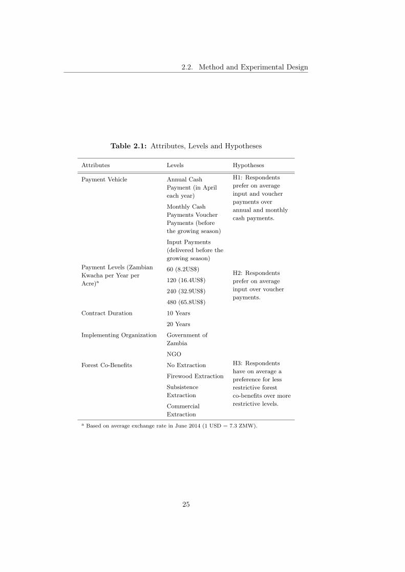
To answer the first research question, i.e. the potential scope of providingagricultural inputs instead of cash payments at reduced program costs, thedefining attribute of the choice experiment specifies how the payments aremade. Including realistic payment vehicles in the choice sets, required us tocombine several specific characteristics within the payment attribute. Cashpayments on one hand can be done monthly or annual. In this case, they aredesigned to compensate farmers for the additional income they could derivefrom newly cleared agricultural areas, around the harvest season startingfrom April. Agricultural inputs are, in contrast, required before the grow-ing season in November/ December each year. In a similar manner, in-kindpayments can be either inputs that are delivered to each village or vouchersthat can only be redeemed in shops that are based in the district capital.Including several distinct payment attributes such as timing, location andpayment type would have led to unrealistic combinations (such as monthlypayments in agricultural inputs). We therefore opted to include four crediblecombinations of timing, location and type of payment within one attribute.This has however the disadvantage that we cannot clearly identify whetherand to what extent particular aspects of a payment vehicle influenced itsfinal valuation. We included two different levels of in-kind payments withvariation in the delivery plus two kinds of cash payment: (a) Annual cashpayments in April each year; (b) Monthly cash payments; (c) In-kind pay-ment with agricultural inputs (seeds, fertilizer and pesticides) delivered tothe village5 at the beginning of each growing season (hereafter referred to asinput payments); (d) In-kind payment with agricultural inputs (see above)as a voucher that can be redeemed in the district capital at the beginning ofeach growing season (hereafter referred to as voucher payment).

Kaczan et al. (2013) conducted a choice experiment on PES in Tanzaniaand found a strong preference for a one-off upfront in-kind fertilizer paymentover individual or collective cash payments. We therefore expect input andvoucher payments to be preferred to cash payments (Hypothesis 1). Whileinput payments include the delivery of the inputs to the village and voucherpayment implies that transport must be covered by recipients, we expectinput payments to be preferred to voucher payments (Hypothesis 2).

5It was specified that the inputs are delivered to the village, but not whether to thehouseholds directly or to a central point in each village. We belief that this distinctionwould however only result in small changes in the valuation. Villages are relatively smalland due to small field sizes the actual amount of fertilizer per household would be small.

23

Chapter 2

PES commonly aim at compensating for the opportunity costs of conser-vation (Engel, 2016). The main economic benefits of forest clearing in theresearch area accrue due to the shifting of agriculture from old fields to newlycleared areas with higher soil fertility. Initial levels for the payment amountswere therefore estimated by reviewing literature on the opportunity costs ofagricultural land uses, in particular maize yields in Zambia (Xu et al., 2009).Further adaptation throughout the pre-test and pilot led to a final range of8.2 – 65.8 US$ per year per acre. With the maximum amount it is possibleto cover the entire input costs for maize cultivation (optimal quantity of fer-tilizer as suggested by Xu et al. (2009) and hybrid seeds). The correspondingvalues for monthly cash payments were included, if the payment vehicle wasmonthly cash payments6.

Regarding our second and third research questions, we included fourattributes besides payment vehicle in the design (see Table 2.1). Knowledgeabout recipients’ preferences regarding these attributes allows adapting PESdesigns to reduce transfers amounts, to assure high enrollment rates andeffectiveness in terms of environmental outcomes.

Several choice experiments included the contract duration as an attributein their experimental design. Overall empirical evidence is inconclusive.Some studies found a preference for shorter contracts (5 vs 9 vs 17 years)(Balderas Torres et al., 2013), while others found preferences for longer con-tracts (15 vs 25 vs 35 years) (Arifin et al., 2009) and (3 vs 10 years) (Zabeland Engel, 2010). In the latter cases, however, the provision of the environ-mental service required large investments that are only likely to pay-off afterlong periods. In the research area, clearing is for most households an irregu-lar activity. Roughly half of the respondents (49%) have cleared in the last5 years. The majority of these households (73%) has cleared in this periodonly once. Only 6% has cleared every year within this period. Short contractperiods would therefore risk that households simply clear forest after a PEScontract expires. We therefore specified a minimum contract duration of 10years and included a second level of 20 years.

In the context of REDD+, it has been demonstrated that PES schemescan be implemented by governments directly or through other organizationsunder a multi-level REDD+ scheme (Wertz-Kanounnikoff and Angelsen,2009). Empirical studies from Zambia suggest that trust in the govern-ment, particularly at the local level, is low. Non-Governmental Organiza-tion (NGO) leaders are, however, considered to be less corrupt (Mulengaet al., 2004). Therefore, we gave two options for implementing organization:the Government of Zambia and a generic NGO. To our knowledge, none ofthe reviewed choice experiments on PES in developing countries varied theimplementing organization in their design.

6In the payment amount description for input and voucher payments, we specified theamount with respect to fertilizer (see Appendix A.2).

24

2.2. Method and Experimental Design

Table 2.1: Attributes, Levels and Hypotheses

Attributes Levels Hypotheses

Payment Vehicle Annual CashPayment (in Aprileach year)

H1: Respondentsprefer on averageinput and voucherpayments overannual and monthlycash payments.

Monthly CashPayments VoucherPayments (beforethe growing season)

Input Payments(delivered before thegrowing season)

Payment Levels (ZambianKwacha per Year perAcre)a

60 (8.2US$) H2: Respondentsprefer on averageinput over voucherpayments.

120 (16.4US$)

240 (32.9US$)

480 (65.8US$)

Contract Duration 10 Years

20 Years

Implementing Organization Government ofZambia

NGO

Forest Co-Benefits No Extraction H3: Respondentshave on average apreference for lessrestrictive forestco-benefits over morerestrictive levels.

Firewood Extraction

SubsistenceExtraction

CommercialExtraction

a Based on average exchange rate in June 2014 (1 USD = 7.3 ZMW).

25

Chapter 2

Various timber and non-timber forest products play a significant role inthe livelihoods of rural communities in Zambia and provide common cop-ing strategies in times of idiosyncratic shocks (Kalaba et al., 2013). Weincluded four levels of forest co-benefits that each specify what kind of for-est products can be extracted and for what use: (a) no extraction of anytype of forest product; (b) only the collection of dead firewood is allowedfor home consumption; (c) collection of any timber and non-timber forestproduct is allowed for home consumption; (d) collection of any timber andnon-timber forest product is allowed for home consumption and commercialuse. The last corresponds with the current level of forest use restrictions.Evidence from Vietnam suggests that potential PES recipients want to keeptheir rights to collect forest products (Petheram and Campbell, 2010). Dueto the overall importance of forest products for rural livelihoods in Zambia,we therefore expect respondents to show a clear preference for weaker forestuse restrictions (Hypothesis 3).

An Alternative Specific Constant (ASC) is included in the econometricmodel to capture the overall utility derived from the status quo (Hensheret al., 2015, pp. 53-54). The co-benefits attribute is included in effectscoding7, since the commercial and subsistence extraction of forest productsis allowed in the status quo. The remaining attributes cannot be defined forthe status quo, as they apply only to situations with a PES contract. In thiscase a hybrid coding is preferred (Cooper et al., 2012). The payment amountvariable is treated as quasi-continuous and defined as 0 US$ for the statusquo. The final observed component of the utility models for Contracts A, Band the status quo can hence be summarized as follows:

VA/B =β0 annual.cashA/B + β1monthly.cashA/B + β2 inputA/B

+ β3 voucherA/B + β4 amountA/B + β5 durationA/B

+ β6 no.benefitsA/B + β7 firewoodA/B + β8 subsistence.benefitsA/B

+ β9 commercial.benefitsA/B + β10 organizationA/B

(2.2.3)

VSQ =βSQ + β9 commercial.benefitsSQ (2.2.4)

2.3 Study Context and Sample

The study is based on a sample of 320 smallholder farmers located in MumbwaDistrict in the Central Province of Zambia, roughly 160 km from the nation’scapital (see Figure 2.3.1). The research area is part of a dedicated bufferzone of the Kafue National Park, the Mumbwa Game Management Area.

7When an ASC is used for the status quo, dummy coding would result in confoundingthe ASC with the base category effect of the dummy coded variable. In this case, effectscoding is preferred over dummy coding as it specifies the estimates of the effect codesrelative to the average effect of the variable and not relative to a specified base category(Bech and Gyrd-Hansen, 2005).

26

2.3. Study Context and Sample

The area was selected due to its diversity in forest-agriculture landscapesand accelerating forest clearing. While the research site still hosts signifi-cant areas of forest, agriculture especially through smallholders continuallyreduces forested areas. Between 2010 and 2014, 49% of our sampled house-holds cleared forest. Of the respondents, 42% indicated that they intendedto clear additional forest in the next three years. These deforestation dy-namics cannot be considered sustainable: between 2010 and 2014 the areaof agricultural land of our sample increased by 32%.

Within Mumbwa District we selected the Chibuluma and Kabulwebulwechiefdoms in the western part of the district. They comprise 45 and 73 vil-lages respectively and accommodate roughly 1,400 households each. Listsof all villages in both chiefdoms were compiled and 22 villages were selectedrandomly8. Based on household lists obtained from traditional authorities,18 households were randomly selected per village and the respective house-hold heads were invited to participate. In cases where the household headwas ill or absent, the acting household head was interviewed. This appliedto 17% of respondents.

Qualitative, exploratory research was conducted between April 2014 andMay 2015 in Zambia. The choice experiments and a corresponding householdsurvey were conducted between May and September 2015. We tested theexperimental design with an initial pre-test with twelve respondents to reviewattribute levels, explanation of choice tasks and contracts. To assure thatrespondents have understood the experiment and managed to compare thetwo different contracts, each choice experiment was individually administeredby a research assistant. The attributes of each contract were explained in-depth and respondents could ask questions at any point of the experiment.Difficulties in choosing can result in delayed responses, fatigue and boredom.We have neither experienced those signs during the pre-test nor during theactual survey. Key socio-economic characteristics and variables used in theLCM are summarized in Table 2.2.

Maize constitutes the most important crop in the sample occupying ap-proximately 60% of the cultivation area in 2013/14 and 300 out of 320 house-holds cultivated the crop. On average households from the sample achievemaize yields of 1.5t/ha. Similar yields are found by more comprehensivestudies in the same agro-ecological region of Zambia (Xu et al., 2009). Fertil-izer is predominantly applied for maize cultivation. Overall, 192 households(60%) have applied fertilizer for maize in the season 2013/14, while only 11households (3%) applied fertilizer to other crops, mainly vegetables. Out of

8Two randomly selected villages could not be covered by the study. In one case theheadman denied permission to conduct research, while the headman position in the othervillage was vacant and recruiting of respondents proved difficult. In other villages, afew invited households could not participate due to absence or illness. Two respondentsrefused to participate in the choice experiment and were excluded from the dataset. Towhat extent this affects the representativeness of our sample cannot be determined.

27

Chapter 2

Figure 2.3.1: Geographical Location of the Research Area (Source: OwnIllustration)

the 125 households that have not applied any fertilizer, 90% state that cashconstraints were the main reason for not using any fertilizer. On average 120kg/ha of fertilizer was applied to maize, which is significantly lower than theofficial recommendation by extension services of 400kg/ha (Xu et al., 2009).

Recent studies however indicate that official recommendations for fertil-izer quantities promoted by extension services are often not economicallyviable for farmers (e.g. Duflo et al., 2008).While the economic profitabilityof fertilizer application depends on a number of moderating variables suchas maize-fertilizer price ratio, timely application and seed varieties, Xu et al.(2009) find that between one third and two third of the recommended ni-trogen quantity is economically viable for smallholder farmers in the sameagro-ecological region in Zambia, if provided on time. In our sample, 41%and 81% of fertilizer users have applied in 2013/14 below one and two thirdof the official recommendations respectively. Increasing the application offertilizer, especially if combined with the adoption of hybrid seeds, wouldconsequently allow most smallholder farmers in our sample to increase maizeyields.

28

2.3. Study Context and Sample

Table 2.2: Socio-Economic Characteristics of Sample

Statistic N (%) Mean St.Dev.

Min- Max

Age (years) 320 44.74 15.7 19 - 87

Female Respondents 103(32%)

Education (Years of Schooling)a 320 6.38 3.17 0 - 13

Respondents who Migrated in LastFive Years

54(17%)

Risk Aversion Scoreb 320 6.62 2.26 1 - 8

Total Field Size (cultivated andfallows in hectare)

320 6.88 10.26 0.40 - 80.94

Cultivation Area 2014/15 aspercent of Total Field Size

320 63.03 29.22 0 - 100

Total Cash Income (2014/15) inUS$c

319d 706.60 1,559.40 0 - 18,190

Crop Production Share AmongTotal Cash Income (2014/15)

307d 44.63 39.80 0 - 100

Years of Fertilizer Use (2010-2014) 320 2.61 2.09 0 - 5

Number of Years when Forest wasCleared (2010-2014)

320 0.75 1.10 0 - 5

Respondents with ClearingIntention (2015-2017)

134(42%)

a Education above higher secondary school is coded as 13 years; b Elicited througha risk experiment (see Appendix A.3): (1-3 Risk Loving, 4 Risk Neutral, 5-6 RiskAverse, 7-8 Highly Risk Averse); c 1 US$ = 7.3 ZMW; d The remaining respondentscould not provide this information.

29

Chapter 2

2.4 Results

2.4.1 Random Parameter Logit Model

We report models of the combined dataset with (a) the choices between twohypothetical contracts and (b) the choice to accept or reject the preferredcontract9. The dataset comprises two questions per choice set, so with 320individuals and four choice sets each a total of 2,560 choice observations wereobtained. The RPL model includes four random parameters for attributesthat are found to be heterogeneously distributed, indicated by significantstandard deviations of parameters at the 0.01 level (Table 2.3). All randomparameters were specified as normally distributed.

The results of the RPL model indicate that input payments are signifi-cantly preferred over any other payment vehicle (first column Table 2.3). Theleast preferred vehicle is monthly cash payment, followed by annual cash pay-ments. Even though voucher payment is the second most preferred level, theeffect is not statistically significant from the grand mean of all payment vehi-cle levels. We observe a significant heterogeneity regarding the valuation ofinput payments in the sample, indicated by a significant standard deviationof the random parameter. Nevertheless, small fractions of respondents favoralternative payment vehicles. Only 4.9%, 0.78% and 0.13% of respondentsprefer voucher, annual and monthly cash payments, respectively, over inputpayments. Overall, we can confirm Hypothesis 1 that respondents preferon average input and voucher payments over annual and monthly cash pay-ments. Furthermore, we can confirm Hypothesis 2 that respondents preferon average input over voucher payments.

The RPL model results allow the marginal rate of substitution betweenspecific attributes of interests to be calculated (Hensher et al., 2015, p. 378).Specifically, we are interested in how much the payment level in US$ per yearper acre should change to maintain the same level of utility, if respondentswere paid with vouchers or inputs instead of annual cash transfers. Onaverage, respondents would require 79.1 and 25 US$ per year per acre less ifthey received agricultural inputs or vouchers, respectively, instead of cash.

The status quo parameter is negative, implying that on average respon-dents prefer the contractual limitations of the PES contract to the statusquo. The random parameter distribution indicates that 18.5% have a posi-tive parameter estimate for the status quo and hence would require additionalincentives to accept the proposed contracts.

Higher payments are preferred over smaller ones. The four levels of for-est co-benefits show a significant impact on the respondents’ choices. A fullprohibition of any forest use is the least preferred attribute level, followed byfirewood benefits only. In contrast to Hypothesis 3, the level that permits ex-

9Models with the choice between the two hypothetical contracts only are presented inAppendix A.4.

30

2.4. Results

Table 2.3: Results of the Random Parameter Logit Models

Full Dataset Future Clearing No Future ClearingStatus Quo −2.45∗∗∗ −1.57∗∗∗ −3.14∗∗∗

(0.28) (0.38) (0.43)Annual Cash Paymentb −0.42 −0.51 −0.35Monthly Cash Payment −0.80∗∗∗ −0.73∗∗∗ −0.88∗∗∗

(0.11) (0.17) (0.14)Voucher Payment 0.08 0.25∗∗ −0.06

(0.08) (0.13) (0.11)In-Kind Payment 1.14∗∗∗ 0.99∗∗∗ 1.29∗∗∗

(0.16) (0.24) (0.22)No Forest Benefits −1.97∗∗∗ −1.88∗∗∗ −2.09∗∗∗

(0.18) (0.28) (0.25)Firewood Benefits −0.23∗∗∗ −0.54∗∗∗ −0.04

(0.09) (0.15) (0.11)Subsistence ForestBenefits 1.20∗∗∗ 1.42∗∗∗ 1.07∗∗∗

(0.10) (0.17) (0.13)Commercial ForestBenefitsb 1.00 1.00 1.00

Amount 0.02∗∗∗ 0.02∗∗∗ 0.02∗∗∗

(0.00) (0.00) (0.00)Contract Duration −0.04 0.03 −0.08

(0.06) (0.09) (0.08)Organization 0.12∗∗∗ −0.01 0.20∗∗∗

(0.04) (0.07) (0.06)Standard Deviationa

SD Status Quo 2.73∗∗∗ 2.72∗∗∗ 2.77∗∗∗

(0.29) (0.42) (0.42)SD In-Kind Payment 0.64∗∗∗ 0.71∗∗∗ 0.64∗∗∗

(0.15) (0.22) (0.22)SD No Forest Benfits 0.81∗∗∗ 0.96∗∗∗ 0.75∗∗∗

(0.13) (0.25) (0.17)SD Firewood Benefits 0.54∗∗∗ 0.59∗∗∗ 0.55∗∗∗

(0.12) (0.21) (0.16)AIC 2445.89 1108.48 1328.36Log Likelihood -1208.95 -540.24 -650.18Num. obs. 2560.00 1088.00 1472.00∗∗∗p<0.01, ∗∗p<0.05, ∗p<0.1; Standard Errors in Parentheses;a All random parameter esti-mates are based on 1000 Halton Draws. The random parameters are assumed to be normallydistributed. b The parameter of the effects-coded base category is calculated as the negativesum of the other level estimates (Cooper et al., 2012).

31

Chapter 2

traction of forest products for subsistence use is preferred over contracts thatallow collection of forest products for commercial purposes. This differencein effects is significant at the 0.05 level (one sample, right-tailed z-test: H1:subsistence.benefits > commercial.benefits, z=1.921, p-value=0.027). Onaverage, respondents would accept 9.8 US$ per acre per year less if commer-cial extraction of forest products was not allowed, while maintaining theirright to collect forest products for their subsistence. In addition, our sampletends to prefer an NGO to the government as the implementing organiza-tion. This effect is small in magnitude but statistically significant at the 0.01level. Contract duration is the only attribute that shows no significant effecton respondents’ contract choices.

In addition, we further split the sample between respondents with andwithout self-stated intention to convert forests to agricultural land in the nextthree years. The respective regression results are shown in the second andthird column of Table 2.3. Overall, valuations of the individual attributes aresimilar between both sub-samples. Both groups prefer input over voucherand cash payments. The only noticeable difference is in the status quovaluation. Respondents with clearing intention value the status quo lessnegatively: 28 % of respondents with intention to clear have a positive statusquo valuation compared to only 13% of the respondents without clearingintention.

2.4.2 Latent Class Logit Model

In order to further explore the heterogeneous preferences for contract at-tributes and how they are related to socio-economic covariates, we present aLCM. This also allows us to identify whether preferences for those householdsmost likely to clear forest are systematically different. We determined threeclasses as appropriate due to relatively good performance across different in-formation criteria10. Table 2.4 summarizes the parameter estimates for eachclass and respective class membership predictions based on socio-economiccovariates.

With respect to payment vehicle we find that Class 3 does not choosetheir contract depending on how payments are made. No payment vehicle co-efficient is significant. However, this class is most sensitive to payment levels.In contrast, Classes 1 and 2 show similar preferences for input over voucherpayments and monthly and annual cash payments are the least preferredpayment vehicle. Both classes seem to dominate the average preferencesfound in the RPL model. Access to fertilizer does not consistently predictpreferences for input payments. Even though Classes 2 and 3 have differentpreferences for input payment, respondents of both classes applied fertilizer

10The Akaike’s Information Criterion, the modified Akaike’s Information Criterion withpenalty factor three and the Bayesian Information Criteria (see Appendix A.6 for moreinformation).

32

2.4. Results

Table 2.4: Latent Class Model Parameter Estimates

Class 1 Class 2 Class 3Status Quo 2.45∗∗∗ −2.68∗∗∗ −0.57

(0.41) (0.23) (0.45)Annual Cash Paymenta −0.90 −0.38 0.15Monthly Cash Payment −1.10∗∗∗ −0.86∗∗∗ 0.43

(0.33) (0.13) (0.41)Voucher Payment 0.32 0.14∗ −0.46

(0.24) (0.09) (0.41)In-Kind Payment 1.68∗∗∗ 1.10∗∗∗ −0.12

(0.39) (0.18) (0.47)No Forest Benefits −0.40 −1.82∗∗∗ −3.14∗∗∗

(0.44) (0.20) (1.02)Firewood Benefits −0.48∗∗ 0.17∗ −1.84∗∗∗

(0.24) (0.09) (0.35)Subsistence ForestBenefits 0.26 1.06∗∗∗ 1.96∗∗∗

(0.24) (0.11) (0.69)Commercial ForestBenefitsa 0.62 0.59 3.02

Amount 0.01∗∗ 0.01∗∗∗ 0.06∗∗∗

(0.00) (0.00) (0.01)Contract Duration −0.02 −0.15∗∗ 0.55∗

(0.15) (0.07) (0.33)Organization −0.12 0.10∗∗ 0.09

(0.11) (0.04) (0.24)Class Membership

Intercept 1.00∗∗∗ 1.41∗∗∗

(0.32) (0.37)Age 0.02∗∗∗ −0.00

(0.00) (0.01)Gender (female) −0.33∗∗ 0.05

(0.16) (0.19)Migrated (last five years) −1.07∗∗∗ −0.86∗∗∗

(0.19) (0.22)Risk Aversion 0.13∗∗∗ −0.05∗

(0.03) (0.03)Years of Fertilizer Useb −0.23∗∗∗ −0.16∗∗∗

(0.04) (0.04)Years of Clearingb 0.68∗∗∗ 1.46∗∗∗

(0.16) (0.18)Planned Clearing −0.53∗∗∗ −0.78∗∗∗

(0.14) (0.17)Average ClassMembership Probability 11.51 64.31 24.18

AIC 2317.47Log Likelihood -1112.73Num. obs. 2504.00∗∗∗p<0.01, ∗∗p<0.05, ∗p<0.1; Standard Errors in Parentheses; a Theparameter of the effects-coded base category is calculated as the neg-ative sum of the other level estimates (Cooper et al., 2012); b In thelast five years.

33

Chapter 2

less frequently in the last five years than Class 1, as indicated by negativeand significant coefficients.

Socio-economic covariates show that past and future clearing behaviorsignificantly affects class membership probabilities. Respondents who clearedless frequently in the past five years and have plans to clear in the next threeyears are more likely to belong to Class 1. The largest Class 2 (64%) has anegative appraisal for the status quo, whereas the small Class 1 (12%) wouldrequire additional incentives to enter the contract, indicated by a positiveand significant status quo coefficient.

2.4.3 Estimated Choice Probabilities and Sensitivity to Pay-ment Amount

Next, we illustrate to what extent the different latent classes are sensitiveto changes in payment levels. The LCM model is used to estimate choicesbetween the status quo and the PES contract most preferable to the samplerespondents. Furthermore, we estimate the share of respondents with clear-ing intentions who are likely to accept PES contracts at varying paymentlevels. The RPL suggests that, on average, the most preferred contractsfeature input payments, subsistence forest benefits, a 10-year contract dura-tion and an NGO as implementing organization. Even though the optimalPES contract was designed according to the RPL results, the design doesnot strongly oppose the preferences of any class from the LCM. Individualchoice probabilities were estimated for the overall LCM, conditional on classmembership probabilities (see Appendix A.1). Respondents with a choiceprobability greater than 0.8 for the PES contract are classified as acceptingthe PES contract, whereas those with choice probabilities greater than 0.8for the status quo are classified as refusing the contract. The results areillustrated in Figure 2.4.1.

Overall, we observe a major increase in respondents accepting the PEScontract from 60% to almost 90% with payments doubling from 20 to 40US$ per year per acre. Changes in payments below and beyond this rangeshow only minor effects on choice probabilities. At the same time, we ob-serve substantial differences for the acceptance probabilities between classes.Class 2 with a negative status quo coefficient is highly likely to accept thePES contract, irrespective of payment levels. Increases in payments have,however, a substantial positive effect on choice probability for Classes 1 and3. Overall, choice probability for Class 3 is higher than for Class 1 and signif-icantly increases from below 30% to roughly 80% within the payment rangeof 0-40 US$ per year per acre. Class 1 members are less sensitive to changesin payments levels. Class 1 is, however, critical for a PES scheme to provideadditional environmental benefits. Respondents with future clearing plansare more likely to belong to this segment. Thus, we separately estimatedcontract choice probabilities based on LCMs (see Appendix A.5) for respon-

34

2.4. Results

Figure 2.4.1: Estimated Choices and Choice Probabilities by LatentClasses for Optimal PES Contracts Relative to Payment Levels

Figure 2.4.2: Estimated Choices for Optimal PES Contracts Relative toPayment Levels of Respondents With and Without Clearing Intentions in

the Next Three Years

35

Chapter 2

dents with and without the intention to clear forest within the next threeyears (see Figure 2.4.2). For respondents without clearing intention, contractacceptance is strongly increasing within the range of 0 to 10 US$ per year peracre to more than 90%. A relatively small share of less than 10% are likely todecline the PES contract irrespective of the payment amount. Respondentswith plans to clear show an overall lower contract acceptance probability,with higher shares of indecisive respondents. But with payments rising from20 to 40 US$ per year per acre, contract acceptance substantially increasesfrom below 40% to more than 80%. While no respondents with clearingplans would refuse the contract, a share of almost 20% remains indecisiveirrespective of the payment amount.

2.5 Discussion

2.5.1 Preferences for Cash Versus In-Kind Payments

Our first research question was to evaluate to what extent respondents pre-fer in-kind agricultural support to cash payments. Potentially, profits fromintensified agriculture allow respondents to achieve higher monetary bene-fits than solely from cash transfers. Similarly to Kaczan et al. (2013), whodefined in-kind payments as one-off payments at the beginning of the con-tract, we find that payments as agricultural inputs (including fertilizer) arepreferred to cash payments of the same value and with the same frequency(annual). Our results also suggest that voucher payments are preferred tocash payments. While preferences for input payments could be explainedwith significant transaction costs that occur when acquiring fertilizer withreceived cash payments, the preferences for vouchers over cash payments areless intuitive. We offer two potential explanations for these results.

Duflo et al. (2011) show both theoretically and empirically that present-biased farmers procrastinate over fertilizer purchase due to decision andtransactions costs and alternative investment opportunities prior to the nextgrowing season. Such farmers eventually fail to purchase fertilizer. If our re-spondents are however aware of such time-inconsistent behavior, they couldpreventively prefer vouchers to cash payments. A second possible expla-nation for the preferences for voucher over cash payments is based on thecapabilities to save cash payments. This is especially valid since the cashpayments were designed to be paid out in April each year, around harvesttime and months before fertilizers are commonly purchased. Lack of accessto financial services and social obligations to share cash income with largerfamily networks potentially limit capabilities for saving cash over longer peri-ods. Voucher could be hence perceived as attractive pre-commitment devicefor farmers to assure that inputs are acquired before the next growing season(cf Bryan et al., 2010).

36

2.5. Discussion

Even though both models find heterogeneity for the valuation of in-kindpayments, adoption of such payment vehicles would not compromise con-tract attractiveness among sample segments. The LCM reveals that onefourth of the respondents are ambivalent regarding the payment vehicle,while the remaining respondents clearly prefer input and voucher payments.Interestingly, the LCM indicates that past fertilizer use cannot explain pref-erence heterogeneity for input payments. Fertilizer adoption in our sampleis relatively low and many farmers applying fertilizer often do not man-age to acquire optimal quantities (see Section 2.3). Both the adoption ofimproved seeds and optimal fertilizer quantities would hence significantly in-crease agricultural productivity for the vast majority of the sampled farmers.Overall, these results underline that PES schemes paying in-kind with inputsor vouchers could achieve secondary developmental objectives of agriculturalintensification.

From a policy design perspective, the preferences for input and voucherpayments also indicate that certain payment vehicles can reduce the costs ofPES. Respondents are willing to accept smaller transfer amounts under inputor voucher payments, other attributes being equal. Considering that voucherand cash payments most likely imply transaction costs of similar magnitude,vouchers provide a viable option to reduce overall program costs. Whethervouchers or input that are delivered to the villages are preferred in terms ofcost-efficiency depends on the relative transaction costs for both vehicles. Ifinput payments imply transaction costs above 54.1 US$ per year per acrecompared to voucher payments, the latter payment vehicle is preferred.

2.5.2 Environmental Effectiveness of PES

To deliver effective positive environmental outcomes, PES schemes need toreach all segments of the population and, most importantly, those which aremost likely to carry out environmentally destructive activities. Our modelsindicate that a large share of respondents would agree to PES contractswhich contractually bind them not to clear any forest for agriculture, evenwithout any additional payments. Kaczan et al. (2013) found similar resultsfor a large segment of their sample. They explain differences in the statusquo valuation with heterogeneous attitudes towards environmental policyinterventions and different opportunity costs for agroforestry. In our case,preferences to save land for future generations or preferences for securingland-use rights for both their current agricultural land and forests are apotential explanation for the negative status quo valuation of the majority.Households with plans to clear forest within the next three years are morelikely to require additional incentives to enroll in PES schemes, potentiallydue to higher opportunity costs of avoiding forest clearing.

Our initial hypothesis concerning forest co-benefits stated that lower re-strictions of forest use are preferred to more restrictive ones. In contrast, the

37

Chapter 2

analyses found that restrictions of commercial forest use are preferred overthe status quo, which allows to collect forest products both for subsistenceand commercial purposes. Based on qualitative follow-up questions afterthe choice experiments, we explain this preference by concerns for excessivecommercial extraction (mainly charcoal production). Only few householdsderive significant cash income from commercial extraction of forest products.Many respondents stated that a regulation of commercial extraction wouldconserve forests for subsistence use. This indicates that respondents’ choices,at least partly, reflect which contract they want the overall community toaccept. These findings also suggest that restrictions of the commercial useof forests can provide additional incentives for most respondents to enroll insuch a PES scheme.

All three models highlight that respondents have positive preferences forthe amount of incentive payments, which is also in line with former studies(Balderas Torres et al., 2013; Costedoat et al., 2016; Kaczan et al., 2013).Furthermore, most respondents with clearing plans can be motivated to par-ticipate in the PES scheme, if payment levels are sufficient. The estimatedchoice probabilities for an optimal PES design suggest that around 40 US$per year per acre, contract acceptance increases substantially. Through sep-arate models for households with and without clearing plans, we found thatwithin the range of 20-40 US$ enrollment rates of households with clearingintention increase sharply up to 80%. DCE that capture preference hetero-geneity can consequently help design PES schemes and set payment levelsto ensure that critical segments of a population enroll and a positive envi-ronmental outcome is realized.

To be effective in achieving the desired forest conservation, the PESscheme we designed requires a full acceptance rate at the community level.Nevertheless, our results show that approximately 10% of the respondentsare reluctant to accept an optimal contract design with payments between40 and 100 US$ per year per acre. Moreover, we find that roughly 20% of re-spondents with clearing intentions remain indecisive regarding PES contractsthat pay 40 US$ per year per acre. An effective scheme under a commonproperty regime requires full enrollment rates. Our discrete choice exper-iment was solely designed as individual decision making. Consequently, itremains open whether reluctant respondents would alter their decision if themajority of a community joined a PES scheme. Potentially, further uniden-tified contract features could convince this small share of the population tojoin the scheme.

Despite different valuations for the status quo among respondents withand without clearing intentions, we do not find preference heterogeneityfor the remaining contract attributes. Different preferences for these at-tributes would allow to offer specifically tailored contracts. Ideally, respon-dents without clearing intentions would then self-select into contracts withpreferred characteristics and lower payment amounts. This would allow to

38

2.6. Conclusion

cost-efficiently ensure full enrollment rates at the community level. Eventhough this does not apply to our sample, stated preferences methods, inparticular DCE, allow to identify whether heterogeneous preferences allowfor such self-selection mechanism.

The long-term environmental impact of any PES schemes ultimately de-pends on the question how households react to the termination of the in-centives. Conventional PES provide additional monetary income for thetime of PES contracts, which could be either used directly for consumptionor invested in productive activities such as agriculture. In contrast, agri-cultural inputs are directly providing means to increase productivity fromagriculture. With a termination of such PES, households are likely to haverealized higher yields from agriculture and are confronted with higher in-centives to increase their production by clearing additional forests (Phelpset al., 2013). As a result, renewing contracts under the input-based PESmay require higher payments than under a conventional PES (if monetarytransfers are predominantly used for consumption and not invested in agri-culture). This could eventually compromise the relative cost advantage ofthe proposed PES schemes compared to conventional PES.

2.6 Conclusion

Our results indicate that there is a potential to harness synergetic interac-tions between PES for forest conservation and agricultural intensification.At our study site, most farmers expressed willingness to refrain from for-est clearing if compensated through PES. Respondents show preferences foragricultural inputs or vouchers over cash transfers. Such PES schemes mayalso be more cost efficient, if additional transaction costs of agricultural inputprovisioning do not exceed the reduced transfer amounts that are possiblecompared to cash payments. We used fertilizer as an example as it is atechnology which is well known in the study region. Further research couldexplore to what extent inputs related to more innovative and sustainableintensification strategies would be appreciated. This is especially importantin areas, where such PES schemes may foster excessive fertilizer application,that in turn has adverse environmental impacts such as water pollution.Moreover, we find that contract duration, implementing organization andpermitted use of forests affect the valuation of PES contracts.

To effectively reduce deforestation, PES should specifically target house-holds which are most likely to clear forest in future. Our results confirm thatthey demand higher payments than farmers who express no strong intentionto extend their fields. Nevertheless, the vast majority of such respondents canbe motivated to enroll for PES at reasonable payment levels. The method-ology presented here provides the means to identify such critical segments ofa PES target population and elicit their design preferences.

39

Chapter 2

This hints at the challenge facing any PES scheme in an area with cus-tomary tenure but individualized land-use rights in ensuring full individualenrollment in the PES scheme. Without this, the environmental outcomeof schemes is at high risk. Large forest areas could be cleared by only afew non-participating famers. In such cases, individual PES would have tobe embedded in a polycentric multi-layer forest governance framework. Po-tential options include for example group contracts or customary laws thatcomplement individual PES contracts. In the latter case, customary insti-tutions could enforce and sanction land-use restrictions, if supported by amajority of the community. It remains for future research to investigate howand which alternative governance approaches best harness the individualpreferences for PES contracts presented in this paper.

References

Angelsen, A. (2009). Policy options to reduce deforestation. In Angelsen,A. and Brockhaus, M., editors, Realising REDD+: national strategy andpolicy options, pages 125–138. Center for International Forestry Research,Bogor, Indonesia.

Angelsen, A. (2010). Policies for reduced deforestation and their impact onagricultural production. Proceedings of the National Academy of Sciences,107(46):19639–19644.

Angelsen, A. and Kaimowitz, D., editors (2001). Agricultural technologiesand tropical deforestation. CABI Publishing/ Center for InternationalForestry Research, New York.

Arifin, B., Swallow, B. M., Suyanto, S., and Coe, R. D. (2009). A conjointanalysis of farmer preferences for community forestry contracts in the Sum-ber Jaya Watershed, Indonesia. Ecological Economics, 68(7):2040–2050.

Asquith, N. M., Vargas, M. T., and Wunder, S. (2008). Selling two en-vironmental services: In-kind payments for bird habitat and watershedprotection in Los Negros, Bolivia. Ecological Economics, 65(4):675–684.

Balderas Torres, A., MacMillan, D. C., Skutsch, M., and Lovett, J. C. (2013).Payments for ecosystem services and rural development: Landowners’ pref-erences and potential participation in western Mexico. Ecosystem Services,6:72–81.

Bech, M. and Gyrd-Hansen, D. (2005). Effects coding in discrete choiceexperiments. Health Economics, 14(10):1079–1083.

Benhin, J. K. A. (2006). Agriculture and Deforestation in the Tropics: ACritical Theoretical and Empirical Review. AMBIO: A Journal of theHuman Environment, 35(1):9–16.

40

2.6. Conclusion

Bliemer, M. C. J. and Rose, J. M. (2011). Experimental design influenceson stated choice outputs: An empirical study in air travel choice. Trans-portation Research Part A: Policy and Practice, 45(1):63–79.

Bryan, G., Karlan, D., and Nelson, S. (2010). Commitment Devices. AnnualReview of Economics, 2(1):671–698.

Carson, R. T. and Czajkowski, M. (2014). The discrete choice experimentapproach to environmental contingent valuation. In Hess, S. and Daly,A., editors, Handbook of choice modelling, pages 202–235. Edward Elgar,Cheltenham, UK; Northampton, MA, USA.

Cooper, B., Rose, J., and Crase, L. (2012). Does anybody like water restric-tions? Some observations in Australian urban communities. AustralianJournal of Agricultural and Resource Economics, 56(1):61–81.

Costedoat, S., Koetse, M., Corbera, E., and Ezzine-de Blas, D. (2016). Cashonly? Unveiling preferences for a PES contract through a choice experi-ment in Chiapas, Mexico. Land Use Policy, 58:302–317.

Cranford, M. and Mourato, S. (2014). Credit-Based Payments for Ecosys-tem Services: Evidence from a Choice Experiment in Ecuador. WorldDevelopment, 64:503–520.

Duflo, E., Kremer, M., and Robinson, J. (2008). How High Are Rates of Re-turn to Fertilizer? Evidence from Field Experiments in Kenya. AmericanEconomic Review, 98(2):482–488.

Duflo, E., Kremer, M., and Robinson, J. (2011). Nudging Farmers to UseFertilizer: Theory and Experimental Evidence from Kenya. AmericanEconomic Review, 101(6):2350–2390.

Engel, S. (2016). The Devil in the Detail: A Practical Guide on DesigningPayments for Environmental Services. International Review of Environ-mental and Resource Economics, 9(1–2):131–177.

Ewers, R. M., Scharlemann, J. P. W., Balmford, A., and Green, R. E. (2009).Do increases in agricultural yield spare land for nature? Global ChangeBiology, 15(7):1716–1726.

Frey, B. S. and Jegen, R. (2001). Motivation Crowding Theory. Journal ofEconomic Surveys, 15(5):589–611.

Grillos, T. (2017). Economic vs non-material incentives for participation inan in-kind payments for ecosystem services program in Bolivia. EcologicalEconomics, 131:178–190.

Hensher, D. A., Rose, J. M., and Greene, W. H. (2015). Applied choiceanalysis. Cambridge University Press, Cambridge, 2nd edition.

41

Chapter 2

Hosonuma, N., Herold, M., De Sy, V., Fries, R. S. D., Brockhaus, M., Ver-chot, L., Angelsen, A., and Romijn, E. (2012). An assessment of deforesta-tion and forest degradation drivers in developing countries. EnvironmentalResearch Letters, 7(4):044009.

Jayne, T. and Rashid, S. (2013). Input subsidy programs in sub-SaharanAfrica: a synthesis of recent evidence. Agricultural Economics, 44(6):547–562.

Kaczan, D., Swallow, B. M., and Adamowicz, W. V. (2013). Designing apayments for ecosystem services (PES) program to reduce deforestationin Tanzania: An assessment of payment approaches. Ecological Economics,95:20–30.

Kalaba, F. K., Quinn, C. H., and Dougill, A. J. (2013). The role of for-est provisioning ecosystem services in coping with household stresses andshocks in Miombo woodlands, Zambia. Ecosystem Services, 5:143–148.

Karsenty, A. (2011). Combining conservation incentives with investment.Perspective 7, CIRAD Agricultural Research for Development, Paris.

Ladenburg, J. and Olsen, S. B. (2014). Augmenting short Cheap Talk scriptswith a repeated Opt-Out Reminder in Choice Experiment surveys. Re-source and Energy Economics, 37:39–63.

Mason, N. M., Jayne, T., and Mofya-Mukuka, R. (2013). Zambia’s inputsubsidy programs. Agricultural Economics, 44(6):613–628.

Mulenga, C. L., Chikwanha, A. B., and Msoni, M. (2004). Satisfaction withdemocracy and performance of the new deal government: attitudes andperceptions of Zambians. Afrobarometer Working Paper Series, 41.

Muradian, R. (2013). Payments for Ecosystem Services as Incentives forCollective Action. Society & Natural Resources, 26(10):1155–1169.

Petheram, L. and Campbell, B. M. (2010). Listening to locals on pay-ments for environmental services. Journal of Environmental Management,91(5):1139–1149.

Phelps, J., Carrasco, L. R., Webb, E. L., Koh, L. P., and Pascual, U. (2013).Agricultural intensification escalates future conservation costs. Proceedingsof the National Academy of Sciences, 110(19):7601–7606.

R Core Team (2015). R: A Language and Environment for Statistical Com-puting. R Foundation for Statistical Computing, Vienna, Austria.

Revelt, D. and Train, K. (1998). Mixed Logit with Repeated Choices: House-holds’ Choices of Appliance Efficiency Level. Review of Economics andStatistics, 80(4):647–657.

42

2.6. Conclusion

Rode, J., Gómez-Baggethun, E., and Krause, T. (2015). Motivation crowdingby economic incentives in conservation policy: A review of the empiricalevidence. Ecological Economics, 117:270–282.

RoZ (1995). The Lands Act. Republic of Zambia, Lusaka, Zambia.

RoZ (1999). The Forests Act. Republic of Zambia, Lusaka, Zambia.

Rudel, T. K., Schneider, L., Uriarte, M., Turner, B. L., DeFries, R.,Lawrence, D., Geoghegan, J., Hecht, S., Ickowitz, A., Lambin, E. F.,Birkenholtz, T., Baptista, S., and Grau, R. (2009). Agricultural inten-sification and changes in cultivated areas, 1970–2005. Proceedings of theNational Academy of Sciences, 106(49):20675–20680.

Sarrias, M. and Daziano, R. (2015). GMNL: Multinomial Logit Models withRandom Parameters. R package version 1.1.

Train, K. (2009). Discrete Choice Methods with Simulation. CambridgeUniversity Press, Cambridge; New York, 2nd edition.

van der Werf, G. R., Morton, D. C., DeFries, R. S., Olivier, J. G., Kasibhatla,P. S., Jackson, R. B., Collatz, G. J., and Randerson, J. T. (2009). CO2emissions from forest loss. Nature geoscience, 2(11):737–738.

Veldwijk, J., Lambooij, M. S., de Bekker-Grob, E. W., Smit, H. A., andde Wit, G. A. (2014). The Effect of Including an Opt-Out Option inDiscrete Choice Experiments. PLoS ONE, 9(11):e111805.

Vinya, R., Syampungani, S., Kasumu, E. C., Monde, C., and Kasubika, R.(2011). Preliminary study on the drivers of deforestation and potentialfor REDD+ in Zambia. FAO, Zambian Ministry of Lands and NaturalResources, Lusaka, Zambia.

Vollan, B. (2008). Socio-ecological explanations for crowding-out effectsfrom economic field experiments in southern Africa. Ecological Economics,67(4):560–573.

Wertz-Kanounnikoff, S. and Angelsen, A. (2009). Global and nationalREDD+ architecture Linking institutions and actions. In Realising REDD,pages 13–23.

Wunder, S. (2009). Can payments for environmental services reduce defor-estation and forest degradation? In Angelsen, A. and Brockhaus, M.,editors, Realising REDD+: national strategy and policy options, pages213–223. Center for International Forestry Research, Bogor, Indonesia.

Wunder, S. (2015). Revisiting the concept of payments for environmentalservices. Ecological Economics, 117:234–243.

43

Chapter 2

Wunder, S. and Albán, M. (2008). Decentralized payments for environmentalservices: The cases of Pimampiro and PROFAFOR in Ecuador. EcologicalEconomics, 65(4):685–698.

Xu, Z., Guan, Z., Jayne, T., and Black, R. (2009). Factors influencing theprofitability of fertilizer use on maize in Zambia. Agricultural Economics,40(4):437–446.

Yang, F., Chen, L., Cheng, Y., Luo, X., and Ran, B. (2014). An Empir-ical Study of Parameter Estimation for Stated Preference ExperimentalDesign. Mathematical Problems in Engineering, 2014:e292608.

Yao, R. T., Scarpa, R., Rose, J. M., and Turner, J. A. (2014). ExperimentalDesign Criteria and Their Behavioural Efficiency: An Evaluation in theField. Environmental and Resource Economics, 62(3):433–455.

Zabel, A. and Engel, S. (2010). Performance payments: A new strategy toconserve large carnivores in the tropics? Ecological Economics, 70(2):405–412.

ZFD and FAO (2008). Integrated Land Use Assessment (ILUA) 2005 - 2008.Zambia Forestry Department, Food and Agriculture Organization of theUnited Nations, Lusaka, Zambia.

44

Chapter 3

How Migrants Benefit PoorCommunities: Evidence onCollective Action in RuralZambia

Tobias Vorlaufera & Björn Vollana

a School of Business & Economics, Philipps-Universität Marburg, Germany

Abstract

This paper investigates the effects of internal migration on the cooperationin host communities in rural Zambia, where in-migration is not confoundedwith increased ethnic or religious diversity. Potentially, in-migration couldtrigger discrimination, decrease overall levels of trust and hence negativelyimpact the propensity for collective action at the village level. We mea-sure cooperative behavior through both self-stated survey information onpublic good contributions and incentivized decisions in a lab-in-the-field ex-periment. Different group compositions with respect to migrants and localswere introduced in a linear public good experiment. Our findings providea nuanced perspective on how in-migration can affect cooperation in hostcommunities that have been exposed to migration for relatively long peri-ods. First, we find no evidence in the survey and experimental data thatin-migration negatively affects cooperation across villages. Second, the par-ticular effect of in-migration depends on the characteristics of the migrantsrelative to the villagers in the host communities. In our research area, mi-grants are generally wealthier and have higher incomes. We find evidencethat in villages where these inequalities are more pronounced, migrants con-tribute more to public goods if exposed as the minority in the experiment. In

45

Chapter 3

these villages, migrants also contribute more to real public goods the morerecently they have settled in the village and the higher their household in-come. The cooperation of better-off migrants is likely considered a signal ofpro-sociality and the intention to integrate into the host community. Ourfindings indicate that the effects of migration on social dynamics in hostcommunities are highly context specific and contingent on characteristics ofthe migrants in relation to the autochthonous population. More importantly,we provide evidence that communities that have been exposed to migrationin the past can successfully accommodate migrants without negative conse-quences for the social fabric in these communities.

3.1 Introduction

The majority of migrants around the globe move within national borders:as of 2005, more than 760 million people lived outside their region of birth(Bell and Charles-Edwards, 2013). Climatic changes are expected to furtherintensify internal migration, especially in the Global South. A large shareof “climate migrants” are expected to move within countries, estimated atup to 143 million people by 2050, with 86 million people in Sub-SaharanAfrica alone (Rigaud et al., 2018). While the poorest households may beunable to migrate and remain exposed to increasing environmental risks(Black et al., 2011b), better-off households with higher asset ownership buildresilience through either temporal or permanent migration (Warner and Afifi,2014). As a consequence, internal migration is considered a viable adaptationstrategy for better-off households that are able to increase their resiliencethrough migration (Black et al., 2011a). It remains an open question how in-migration of more affluent people affects the host communities, in particularwith respect to collective action that is crucial for most rural communitiesin the Global South. Internal migration is, however, often overlooked inthe media and in scientific analyses, as it often does not pose the sameobvious problems inherent in the migration of people that speak a differentlanguage and practice different cultural norms or religions1. Our study on theeffects of internal migration on collective action does not confound migrationwith these well-known factors of potential conflict and thus broadens theperspective on the effects of migration on host communities.

Many rural communities in developing countries jointly provide basicpublic goods such as schools or water supply given the weak governmentfunding. Ethnic diversity, which is likely to increase as a result of internal

1When focusing on international migration from developing countries, the dominantview is often that migrants are most likely to occupy jobs in the low skilled labor market,which may lead to competition among workers in that sector and declining wages thatgive rise to social problems such as a loss in social cohesion due to increased heterogeneityof values and norms, even resulting in xenophobia, which erodes norms of cooperation inthe host country (Collier, 2015; Hainmueller and Hopkins, 2014).

46

3.1. Introduction

migration in multi-ethnic countries, has been shown to negatively affect trustand cooperation (Putnam, 2007). In line with this argument, ethnic hetero-geneity decreases social capital, rendering the enforcement of social sanctionsless effective and thereby reducing cooperation at the community level, asshown by Miguel and Gugerty (2005) for Kenya. To better understand theeffects of migration on collective action, we believe it is imperative to alsoconsider cases where incoming migrants are on average richer than the hostpopulation to explicitly capture the different capacities migrants may haveand the resulting roles they assume in society. This situation is not un-common, as empirical work indicates that risk-taking (Jaeger et al., 2010),more patient (Goldbach and Schlüter, 2018) and better-educated (Malamudand Wozniak, 2012) individuals are more likely to migrate within countries.Richer migrants may be especially willing to cooperate, as they might bemore altruistic due to feelings of inequality aversion (Buckley and Croson,2006). Migrants in general may be more likely to cooperate to signal theirgood intentions by building up reputation and social status in the host com-munity and contribute to “community building” (Barr, 2003).

To our best knowledge, Sircar and van der Windt (2015) provide the onlystudy on the effect of rural-to-rural migration on pro-social behavior in a de-veloping country context2. They report experimental findings from easternCongo (DRC), where migration and displacement have been predominantlydriven by years of civil conflict. In their study area, migration is mostlyinvoluntary, and migrants are significantly poorer than locals. They findthat initially, migrants exhibit levels of pro-sociality similar to locals amongthemselves. However, due to a lack of pro-social behavior of locals towardsmigrants, they eventually become less pro-social. As a result, migrationdoes reduce overall pro-sociality at the group (village) level. Another strainof literature focuses on resettled communities3 and the effect on solidarityand trust. Gobien and Vollan (2016) find that after one and a half years ofvoluntary resettlement in Cambodia, people in heterogeneous, resettled com-munities exhibit lower levels of solidarity than a similar non-resettled controlgroup. In her seminal paper, Barr (2003) shows that 20 years after volun-tary resettlement, Zimbabwean communities exhibit lower levels of trustingbehavior than non-resettled communities. At the same time, trusting behav-ior is less responsive to expected trustworthiness in resettled communities,which can be interpreted as the intent of community-building. Furthermore,

2In a recent study, Wang et al. (2016), for example, found that out-migration negativelyaffects collective action for the maintenance of irrigation systems in rural China. We lookat the complementary effect, namely, how in-migration affects cooperation in rural hostcommunities.

3While resettlement is an outcome of a planned process (in most cases overlooked bygovernment agencies and for a group of households), migration is commonly a volun-tary individual or household decision. We nevertheless believe that resettled householdsexperience a situation similar to migrated households of newly settling in a different vil-lage/community.

47

Chapter 3

resettled communities continue to invest in community building, as indi-cated by a larger number of civil society organizations. Such organizationsare likely to fulfill functions similar to those of kinship and ethnic networksin non-resettled communities (Barr, 2004). In a follow-up study, Barr et al.(2015) highlight that wealthier households played crucial roles in foundingthese organizations, particularly in relatively poorer villages, that were laterjoined by other villagers. The authors hypothesize that in poorer villages,relatively better-off inhabitants felt a greater obligation to provide support.

Our paper investigates the effect of in-migration on cooperative behav-ior in host communities that have experienced high rates of in-migration inthe past. To do this, we combine survey data covering income levels andself-stated information on cooperative behavior with lab-in-the-field experi-ments in central Zambia, covering in total 18 villages in two chiefdoms. Thesample contains both villages where migrants have on average income that islower than or similar to that of locals and villages where the average migrantincome is significantly higher. The lab-in-the-field public good experimentsprovide us with an incentivized measurement of the individual propensity tocooperate under similar circumstances across villages and individuals. Theexperiments also allowed us to exogenously vary the group compositionswith respect to migrants and locals. Zambia provides an ideal country forinvestigation due to the high internal migration intensity (Bell et al., 2015).Climate change is expected to further aggravate migration dynamics by low-ering agricultural yields in the southern part of the country (Kanyanga et al.,2013). Because of a long history of migration, our research site in centralZambia already contains ethnically diverse communities. Therefore, we canstudy the effects of the most recent wave of in-migration (over the last 10years) without the often-accompanied effects of increasing ethnic, religious,linguistic or cultural diversity. In addition, our research area is character-ized by customary land tenure systems, where traditional authorities overseeland distribution. Only under very exceptional conditions can a village head-man deny migrants land, minimizing the capabilities of host communities topre-select migrants.

Our results indicate that there are no detrimental effects of internal mi-gration on the propensity for cooperation in communities. Migrants andlocals exhibit similar levels of cooperation elicited through the experimentand in the self-stated survey information. Moreover, varying group com-positions in the experiment with respect to migrants and locals does notsignificantly affect the individual contributions of either migrants or locals.Additionally, migrants who are relatively better-off than locals do not ex-hibit significantly different experimental behavior than worse-off migrants.However, we find evidence for village effects. In particular, in villages withstrong income inequalities between migrants and locals, migrants contributemore if matched with more locals in the experiment. Survey data on contri-butions to community projects indicates that better-off migrant households

48

3.2. Responses to Migration: Identity, Inequality and Cooperation

indeed contribute more than worse-off migrant households, especially if theyrecently moved to a village with strong income inequalities between migrantsand locals. A potential explanation is that migrants exhibit higher levels ofcooperative behavior to signal their pro-sociality in villages where incomeinequalities between migrants and locals are evident.

3.2 Responses to Migration: Identity, Inequalityand Cooperation

Due to the lack of previous research on internal migration and its effects oncollective action, our paper draws on two prominent strands in the psycho-logical and experimental economics literature on cooperation: group identityand inequality. From this literature, we derive three conjectures that outlineindependent channels through which in-migration may affect cooperation.The exogenous variation in our experiment stems from manipulating thegroup composition in terms of number of locals and migrants (defined asliving less than 10 years in the chiefdom). Revealing the migration status isan informational treatment, but it is unclear how participants interpret thisinformation. In addition, the treatment may also strengthen both migrantand local identities through priming. One possibility is that migration sta-tus evokes negative reactions leading to discrimination, similarly to studiesusing different identity priming techniques. A growing body of experimentalresearch indicates that identity-based discrimination can be induced by ar-tificially creating group identities in the lab (Balliet et al., 2014). However,discriminatory behavior is less salient when dealing with real-world identitiessuch as religion, ethnicity or nationality (Lane, 2016)4. In addition, the dis-tinction between out- and in-group may be difficult in the case of migrationsince migrants assimilate over time into the communities. As such, migrant

4A large body of experimental research has studied the effects of a shared group identityon cooperation and discrimination (Balliet et al., 2014; Lane, 2016) by inducing a commonidentity through the minimal group paradigm (Chen and Li, 2009; Smith, 2011; Bicskeiet al., 2016) or through the use of natural identities. These studies suggest that homoge-neous groups with respect to characteristics such as nationality (Carpenter and Cardenas,2011; Finocchiaro Castro, 2008), Kibbutz Membership (Ruffle and Sosis, 2006) or armyplatoons (Goette et al., 2006) lead to higher cooperation owing to either taste-based (cfBecker, 2010) or statistical discrimination (cf Arrow, 1973). Some studies conclude thatlower expectations regarding out-group members’ contribution (i.e., statistical discrimina-tion) are predominantly responsible for lower cooperation levels (Smith, 2011), includinggroup identities based on political and religious affiliations (Koopmans and Rebers, 2009)and among religiously mixed groups in India (Keuschnigg and Schikora, 2014). Yet, thisfinding is challenged by the meta-analysis of Lane (2016). To the best of our knowledge,no study has used information about the migration history of individuals as an experi-mental manipulation. However, in the context of this study, we expect that making thisinformation salient reduces cooperation if migrants and locals each share strong groupidentities.

49

Chapter 3

identities are not natural categories that are constant over time. Neverthe-less, out-group discrimination or in-group favoritism potentially occurs inthe case of migration.

Conjecture 1: If migrant and local identities are sufficiently strong, weexpect higher cooperation rates in homogenous groups than in hetero-geneous groups.

Since migration is costly, migrants are often better-off than stayers. There-fore, migrants tend to be better educated, more risk taking, more patientand hence economically more successful than those who stay behind (Akgüçet al., 2016; Gibson and McKenzie, 2011; Jaeger et al., 2010; Goldbach andSchlüter, 2018). Migration therefore often induces additional economic in-equality, which has been shown to reduce cooperation, trust and social cap-ital. In general, economic inequality reduces the likelihood of cooperationas indicated by lab experiments5 (Anderson et al., 2008; Nishi et al., 2015;Rapoport and Suleiman, 1993) and a meta-analysis (Zelmer, 2003). In partic-ular, higher endowed individuals reduce their relative contributions (Cherryet al., 2005; Heap et al., 2016). A few studies have focused on real-worldwealth or income inequalities and their impact on cooperative behavior andfound that wealth inequalities at the group level reduce cooperation (Carde-nas, 2003; Hayo and Vollan, 2012)6.

Contributing money in public good games is a measure of cooperation butmay also be driven by altruism or trust, especially if groups are composed ofricher and poorer individuals. Using Canadian census data, Payne and Smith(2015) find that increases in inequality at the neighborhood and municipal-ity levels lead to higher charitable giving. Côté et al. (2015) use survey andexperimental data to investigate whether income inequality mediates the re-lationship between income and altruistic behavior. They find that relativelybetter-off participants are less generous than lower-income participants instates with high inequalities and vice versa. Regarding trust, Alesina andLa Ferrara (2002) draw on survey data from the US to find that individ-ual characteristics such as income increases trust, while income inequality atthe community level decreases general trust. Experimental studies confirmthat inequality reduces both trust and trustworthiness, especially if the rel-ative standing of each individual is publicly known (Anderson et al., 2006;Heap et al., 2013; Lei and Vesely, 2010). Lastly, empirical studies indicate

5In these laboratory experiments, inequality is induced through varying the initialendowments (e.g. Heap et al., 2016), the show-up fee (e.g. Anderson et al., 2008) or themarginal benefits from the public good (e.g. Fisher et al., 1995). Studies that find apositive effect of economic inequality on cooperation are, for example, non-linear publicgood (Chan et al., 1996, 1999) or public bad experiments (Cardenas et al., 2002).

6Visser and Burns (2015) found that real absolute and relative income as well as mea-sures for economic inequality at the community level had no significant effect on experi-mental behavior. These mixed findings may be explained by the low salience of real worldincome (inequalities) in the experimental setting.

50

3.3. Material and Method

that economic inequality undermines social capital, measured as member-ship in clubs and organizations (Alesina and La Ferrara, 2000). Findingsfrom Tanzania indicate that especially rich people in villages with high as-set inequality are less likely to be members of economic, social and politicalgroups (La Ferrara, 2002).

Conjecture 2: If economic inequality increases due to migration, relativelyricher individuals cooperate less than relatively poorer individuals.

Our study deviates from the studies on inequality since we not only lookat income per se but also consider a situation where a specific sub-groupof a population has a higher income on average. At the same time, thesub-group of migrants likely aspires to build social status, strengthen theirsocial networks and integrate into the host communities. Previous findings ofresearch on resettled communities indicate that individuals are more likely totrust others to build community networks (Barr, 2003) and especially better-off households more frequently engage in setting up community organizations(Barr et al., 2015). Relatively richer migrants may therefore cooperate morein heterogeneous groups to signal pro-sociality and engage in communitybuilding, which would counterbalance the detrimental effects of increasedinequality (see Conjecture 2).

Conjecture 3: If migrants want to signal pro-sociality and engage in com-munity building, migrants – who are relatively richer than locals –cooperate more in heterogeneous groups than in homogenous groups.

3.3 Material and Method

3.3.1 Participant Recruitment and Survey Design

The study was conducted in central Zambia, in the western part of MumbwaDistrict (see Figure 3.3.1) between May and September 2015. We selectedtwo specific chiefdoms that experienced high in-migration over the last decade.In a second step, we identified all villages with a sufficient number of mi-grant and local households. With the support from village headmen, wecompiled household lists for each village and collected prior information onthe migration status of each household. Then, a random household samplewas drawn stratified by migrant status (10 locals and six migrants that wererequired by the experimental design). The household head was invited forthe experiment, but in case the household head was unavailable, the actinghead participated.

In total, 20 experimental sessions were conducted in 18 different villages,yielding 320 observations. An individual household survey was administeredafter the experiment. In addition to standard socio-economic characteris-tics of the participants and households, we also collected information on

51

Chapter 3

Figure 3.3.1: Location of the Research Area (Source: Own Illustration)

migration background such as origin and reasons for migration. The sur-vey included a specific section on contributions to public goods within thelast 12 months. Here, we asked participants how much their household hadcontributed in cash and in-kind to community projects and activities. Self-stated information on cooperative behavior unquestionably faces inherentchallenges, caused for example by a social-desirability bias in answering thequestion and recalling behavior from the last 12 months. However, twoaspects are reflected in the survey data that are not captured by the ex-periment. First, households have in reality different financial capabilities ofcontributing to real-world public goods, whereas in the experiment, all par-ticipants receive the same endowment. Second, decisions in the experimentare anonymous to other participants. In everyday life, however, contribu-tions to real-world public goods signal pro-social preferences and build andmaintain trust and social capital. Such aspects likely inform the decisionof newly arriving migrants to engage in community projects. The surveydata hence can substantiate our experimental findings with a higher degreeof external validity while representing only correlational evidence. The twomethods thus complement each other.

The final dataset consists of 296 observations with 111 migrants and 185locals. Out of the 320 participants, nine participants provided conflictinginformation concerning their migrant status during registration and in thepost-experiment questionnaire7. Furthermore, 15 participants could not cor-

7Four and five of these participants were initially classified as locals and migrants,

52

3.3. Material and Method

rectly answer the test question for the experiment at the second attempt.These 24 participants were excluded from the dataset8.

3.3.2 Site and Sample Description

3.3.2.1 Migrant and Migration Characteristics

Based on qualitative interviews9 conducted prior to the main data collection,a migrant was defined as someone who settled within the last 10 years inthe village and migrated from outside the chiefdom. Locals, on the otherhand, were either born in the chiefdom or settled there more than 10 yearsago. The focus on chiefdoms as a geographical distinction for migration wasrequired since many households move between relatively small neighboringvillages. These households are not considered migrants, as they are usuallywell known within the communities. Within the 10-year period, in-migrationhas occurred in similar magnitudes. From nine to 12 migrants from our sam-ple settled per year over the last 10 years in the area (except in the ongoingyear of the study in 2015). Most migrants in our sample migrated fromrural areas (80%) to the research site (on average from 300 km distance).The main motivation for leaving was the lack of fertile, arable land in theold villages (56%), followed by family reunions (20%) and personal conflicts(11%). Overall, 51.4% of our participants are Tonga by tribe, who predom-inantly settle in southern Zambia. Their language is closely related to theIla language, traditionally spoken in the research area.

Table 3.1 summarizes key socio-economic characteristics of the sample bymigrant status. Overall, migrants have a significantly higher cash income of804 USD/year compared to 376 USD/year of locals. This also translates intoa higher socio-economic status, measured by asset and livestock ownership.Not surprisingly, migrants have a more positive perception of other migrantsand fewer kinship ties in each experimental session than locals have. Addi-tionally, migrants more frequently intermarry with other ethnicities and areon average better educated than locals.

Most migrants left rural areas in southern Zambia, where fertile, arableland has become scarce for those who would like to expand their farmingactivities, in search for better opportunities. On the one hand, migration iscostly, so better-off households are more likely to migrate in the first place.On the other hand, more commercially oriented farmers with a higher cash

respectively. If more than three migrants had been misclassified in the same session,it could affect the credibility of the treatments. However, the five excluded migrantsparticipated in five different sessions.

8All results are robust to the inclusion of all participants. Detailed results are availablefrom the authors upon request.

9These interviews were conducted in villages that are not included in the final sample.This was done to assure that the participants did not receive information on the purposeof the research prior to the experiment.

53

Chapter 3

income may also see greater benefits in migrating, especially if land accessremains a challenge in their home communities. Since we have only cross-sectional survey data, we cannot determine whether migrants have a higherincome prior to or due to migration. However, we find supportive evidencethat migrants already had a higher cash income than locals before relocating(see Appendix B.3).

Table 3.1: Socio-Economic Characteristics of Sample by Migrant Status

Mean

Variable Locals Migrants P-Value

Age (Years) 43.85 43.06 0.875

Education (Years) 6.23 7.24 0.035**

Cash Income (USD, Year) 376.16 803.81 0.000***

Cash Income/ Village Average 0.78 1.44 0.002***

Socio-Economic Statusb -0.12 0.13 0.020**

Risk Aversion 5.19 5.27 0.97

Real Public Good Contributions(USD, Year)

4.31 5.9 0.232

Migrant Perception Indexc -0.18 0.32 0.000***

Group Membership 0.93 1.03 0.308

Friendship Ties 1.52 1.37 0.639

Kinship Ties 1.74 1.04 0.001***

Male (Share)a 75.68 79.28 0.568

Household Head (Share)a 81.62 86.49 0.353

Multi-Ethnic Households (Share)a 47.57 35.14 0.049**

Joint F-Test 0.000***

* p<0 .1, **p <0.05, ***p<0 .01; a Chi-Square Test (otherwiseMann-Whitney-U-Test), b Index based on asset and livestock ownership (seeAppendix B.16), c Index based on statement approvals. The higher thescore is, the more positive the perception of migrants (see Appendix B.15).

3.3.2.2 Village Characteristics

In addition to the individual characteristics, village data were obtained fromhousehold lists. The data include the number of households in each villageand whether each household migrated within the last 10 years from outsidethe chiefdom. Due to the random sampling and the relatively large shareof households covered in each village (min 26%, max 76%, mean 45%), wecan furthermore extrapolate the individual survey information to the villagelevel. The 18 covered villages differ in size, ethnic composition and especially

54

3.3. Material and Method

prior exposure to in-migration and the income inequalities between migrantsand locals (see Table 3.2). The villages are relatively small, with the smallestvillage including 22 households (HHs) and the largest 68 HHs (average of39 HHs). Due to the small size of villages, we expect that it is commonknowledge whether somebody migrated less than 10 years ago and wherethey came from (which is supported by our experiences during the datacollection). On average, 33% of the HHs settled within the last 10 years fromoutside the chiefdom in the villages and are defined as migrants. However,this share varies considerably, between 15 and 64%. Similarly, the share ofhouseholds that migrated more than 10 years ago (and are classified as localsin our experiment) and the share of indigenous population vary substantiallyacross villages. Some villages have no indigenous population, while othershave up to 36% of indigenous households.

Villages with higher indigenous population experienced less in-migrationdating more than 10 years prior to the experiment (Pearson Correlation -0.92; t = -8.95, df = 14, p-value = 0.00). However, these villages have beenexposed to more in-migration over the last 10 years (Pearson Correlation0.73; t = 3.98, df = 14, p-value = 0.00). Vice versa, villages with increasedin-migration more than 10 years ago have been exposed to less migrationin the last 10 years (Pearson Correlation -0.94; t = -9.98, df = 14, p-value= 0.00). This pattern is likely driven by village characteristics such as theavailability of land and its accessibility.

Due to the strong exposure to in-migration, ethnic diversity across thevillages is relatively high. Following Alesina et al. (2003), we computed theethnic fractionalization index (0 for no fractionalization, 1 for maximum frac-tionalization) for each village and the migrant and local sub-groups individu-ally (see Table 3.2). Locals are generally more fractionalized than migrants.Nevertheless, migration does not significantly alter ethnic heterogeneity inthe sampled villages. Moreover, ethnic fractionalization is not significantlycorrelated with exposure to migration at the village level (see Appendix B.4).While the potential effects of in-migration are often confounded with the ef-fect of increasing ethnic heterogeneity, the research context of this studyallows the assessment of the impact of in-migration with constant ethnicheterogeneity.

Across villages, we also observe a high variation in income inequality.The Gini coefficient for cash income ranges from 0.34 to 0.81. As shown inthe previous section, migrants have a significantly higher cash income thanlocals. We measure cash income inequality between migrants and locals bythe average migrant income by village relative to the average local income(hereafter referred to as income ratio)10. On average, migrants have income

10Most inequality measures such as the Gini coefficient only capture inequality withinone population. One exception is the decomposable Theil Index that can separately derivewithin and between group inequality. We opted, however, for this simpler measure becauseit captures not only the between group inequality but also the direction of inequalities

55

Chapter 3

Table 3.2: Village Level Characteristics Below and Above the IncomeRatio Median

Mean

Variable Min Max Overall IncomeRatio >Median

IncomeRatio≤Median

Size (Households) 22.00 68.00 39.17 42.00 36.33

Share of MigratedHouseholds (0-10 years)

14.63 64.29 33.09 28.74 37.43

Share of MigratedHouseholds (> 10 years)a

3.97 85.37 48.68 54.85 42.52

Share of IndigenousHouseholdsa

0.00 36.36 18.23 16.41 20.05

Ethnic Fractionalizationb 0.62 0.9 0.74 0.73 0.75

Ethnic Fractionalization(Locals)b

0.42 0.86 0.7 0.71 0.7

Ethnic Fractionalization(Migrants)b

0.00 0.83 0.56 0.59 0.52

Gini Coefficient Incomeb 0.34 0.81 0.56 0.64 0.48**

Income Ratio (Migrants,Locals)b

0.38 6.96 2.35 3.71 0.98***

Joint F-Test (p-value) 0.12

* p<0 .1, **p <0.05, ***p<0 .01; Test between villages above and below the median cash incomeratio; a Shares estimated by combining village level data and sample data; b Based on sample data

that is 2.3 times higher than that of locals. In five out of 18 villages, themigrants have a lower average income than the locals. In eight villages, theincome differences are apparent, with migrants having two or more times theincome of locals. Due to the small size of the villages, we believe that thesocio-economic status of a household is generally known. As a consequence,the participants should be aware of income differences between locals andmigrants in their villages. Migrants in villages above and below the medianincome ratio share similar characteristics. Migrants are only significantlyolder (46 vs 41 years) in villages above the median income ratio. However,locals in villages above the median income ratio have significantly lower cashincome, contribute significantly less to real-world public goods and are lesslikely to be members of community groups than are locals in villages belowthe median (see Appendix B.14). The income ratio between migrants andlocals is highly correlated with general income inequality at the village levelmeasured by the Gini coefficient (Pearson correlation 0.74, t = 4.45, df = 16,p-value = 0.00). Income inequalities at the village level may be confoundedby other village characteristics. Table 3.2, Columns 5 and 6, shows the

(whether migrants or locals earn more on average).

56

3.3. Material and Method

differences in average village characteristics in villages above and below themedian income ratio. Except for the income ratio itself and overall incomeinequality, villages are not significantly different in both sub-samples. Thisis also indicated by weak correlations between village characteristics and theincome ratio (see Appendix B.4).

3.3.3 Experimental Design

In addition to self-reported contributions to community-provided public goodssuch as schools and boreholes, we experimentally elicited cooperative behav-ior in an artefactual field experiment. We took a linear public good gamewith j = 1, ..., n participants as the baseline for our experiment. Eachparticipant receives an endowment e that she can either keep for herself or(partly) invest in the group account. Each endowment token contributed tothe group account ci benefits each participant by a fixed pay-off β. FollowingIsaac and Walker (1988), player i receives the individual pay-off:

πi = ei − ci + βn∑

j=1

cj (3.3.1)

With 1n < β < 1, the experiment poses a social dilemma. The coop-

erative and socially optimal strategy is to contribute the full endowment tothe public good (ci = ei). The non-cooperative behavior predicted by theNash Equilibrium implies no contribution to the public good (ci = 0). Eachexperimental group consisted of four participants (n = 4), receiving an ini-tial endowment of 10 tokens each (ei = 10). The marginal per capita returnfrom the group account was β = 0.5. Due to a variety of collective actionthat can be found in different villages in the research area, the experimentwas framed as a neutral group project instead of a specific cooperation task.

To study the effect of heterogeneous group composition with respect tomigrants and locals, we exogenously varied the group composition in theexperiment (based on the distinction explained in Section 3.3.2). Migrantshares in different villages are most likely confounded with other contextualvariables. Through the random assignment of group compositions, we cantherefore assess the effect of group heterogeneity on cooperative behavior.In total, we include four specific treatments with unique group compositionswithin each session of 16 people consisting of 10 locals and six migrants(see Table 3.3): homogeneous local groups (MIG0) with four locals only;evenly mixed groups with two migrants and two locals each (MIG2); andtwo heterogeneous majority compositions with three migrants and one local(MIG3) and three locals and one migrant (MIG1). Due to the limited numberof migrants, we decided to include no treatment with migrants only11.

11Tests for differences in socio-economic characteristics between treatments indicate nosystematic differences for migrants (see Appendix B.13). These tests indicate significant

57

Chapter 3

Table 3.3: Treatments: Group Compositions

Treatment Locals Migrants

MIG0 4 0

MIG1 3 1

MIG2 2 2

MIG3 1 3

We are aware that the strict distinction between migrants and localsapplied in the experiment cannot capture the gradual distinctions made inreality. We would expect minor differences in the perception of two individu-als who moved to the village 10 and 11 years ago, even though one is classifiedas local and the other as migrant in our experiment. Participants, however,received only information regarding the migrant status of the fellow groupmembers without revealing their identity. Upon registration, participantsdrew a number that randomly assigned them to one of the four treatmentgroups. Throughout the session, respondents consequently knew only thatthey were in a group with three other participants, without knowing theirexact identity but the distribution of locals and migrants.

After registration, participants were briefed about the itinerary and struc-ture of the experiment12. We privately asked participants six test questionsto check their understanding of the experiment. Right after the test ques-tions, we informed participants about their group composition and the re-spective share of migrants. To minimize demand effects, migrants were notdirectly named as such. The group composition was revealed by providingthe number of group members “who have settled from outside this chiefdombetween 2005 and 2015 in this village”.

To increase familiarity with the decision making, a non-incentivized prac-tice round was implemented prior to the one-shot decision without revealingactual choices. First, participants filled in their contributions, followed bytheir beliefs regarding average contributions of their fellow group members.The belief elicitation was not incentivized to reduce the potential influenceof the belief elicitation on contributions (Gächter and Renner, 2010) andto minimize the cognitive burden for participants. At no point did partici-pants receive feedback about individual or group decisions. The experimentreported here was the first of four one-shot decisions. We concentrate on

differences between treatments for a few characteristics among locals. We assume thatthese differences do not systematically affect contributions. Nevertheless, we control forkey socio-economic characteristics in regressions provided in the appendix as a robustnesscheck.

12The protocol is provided in Appendix B.12. The protocol was translated from Englishto Tonga (the predominant local language). A back-translation was done by a third personto assure an adequate translation and to improve critical passages.

58

3.4. Results

the first round since it provides the cleanest proxy for cooperation underdifferent group compositions. The other three decisions involved the reac-tion of groups to some form of outside leadership and are not reported here(see Appendix B.2). An individual questionnaire was administered after theexperiment. Participants received their pay-off in private, which ranged be-tween 2.1 and 7.5 US$. On average, participants in the experiment earned 5.2US$ including a show-up fee, which corresponds to two days of agriculturalpiecework in the area.

3.4 Results

The presentation of the results is divided into three sub sections. First,we focus on and compare the average contributions to the experiment andwhether the group composition treatments affect experimental behavior. Asshown in the previous section, migrants have on average a higher incomethan locals. In subsection two, we therefore investigate whether the relativeindividual income and income inequalities between migrants and locals at thevillage level interact with the treatments. In the third subsection, we analyzereal world public good contributions to investigate whether the experimentalfindings are supported by the survey data.

3.4.1 Experimental Data: Primed Identities and Effects onCooperation

Contributing the full endowment is the most frequent choice (25%) of mi-grants and locals, followed by the contribution of half the endowment (5tokens, 17%). The choices by treatment and migrant status are quite het-erogeneous, reflecting the different strategies, motivations and beliefs of therespondents (see Appendix B.1). On average, locals contributed 5.79 pointsof their endowment to the public good, which is slightly more than the av-erage contribution of 5.5 by migrants. Contributions are, however, not sig-nificantly different between migrants and locals (Mann-Whitney-U Test, W= 10723, p-value = 0.5185). Regression analyses with varying specificationsincluding village fixed effects and controls find that migrant status does notsignificantly explain experimental contributions (see Appendix B.5).

Migrants were exposed to three different treatments. The average contri-butions and beliefs regarding the average group contribution are illustratedin Figure 3.4.1. Accordingly, average contributions slightly vary across treat-ments, ranging from 5.26 tokens in the MIG2 to 6.17 tokens in the MIG1treatment. Average beliefs are lowest in the MIG2 treatment, with 5.24tokens, followed by the MIG1 with 5.56, and are highest in the MIG3 treat-ment, with 5.76 tokens. Both contributions and beliefs are, however, not sig-nificantly different between the treatments (Contributions: Kruskal-Wallis

59

Chapter 3

Figure 3.4.1: Average Contributions and Beliefs by Treatment andMigrant Status (with Bootstrapped Confidence Intervals, 10,000

repetitions)

chi-squared = 0.81, df = 2, p-value = 0.67, Beliefs: Kruskal-Wallis chi-squared = 0.44, df = 2, p-value = 0.80). Regression analyses controlling forboth individual socio-economic and village characteristics confirm the find-ing that the contributions of migrants are not significantly affected by thedifferent treatments (see Appendix B.6). These results also hold for differentspecifications of the treatment variable such as categorical and continuous(number of migrants per group) as well as village fixed effects.

Finding 1: Migrants’ average contributions in the experiment are not sig-nificantly affected by the group composition.

After looking in detail at migrant behavior, we now turn the focus to theexperimental behavior of locals. In the experiment, locals were exposed –in addition to the three heterogeneous group treatments – to a homogenousgroup with four locals only. The average contributions and beliefs in thesefour treatments are illustrated in Figure 3.4.1. Average contributions rangebetween 6.15 tokens in the MIG2 and 5.58 tokens in the MIG0 treatment.

60

3.4. Results

Beliefs are also highest in the MIG2 treatment (6.44 tokens) and lowestin the MIG0 treatment (5.16 tokens). Non-parametric tests indicate thatthese differences are statistically not significant (Contributions: Kruskal-Wallis chi-squared = 0.83, df = 3, p-value = 0.84, Beliefs: Kruskal-Wallischi-squared = 4.63, df = 3, p-value = 0.20). These results are also confirmedby regression analyses (see Appendix B.7).

Findings 2: Locals’ behavior in the experiment is not significantly affectedby the group composition.

3.4.2 Experimental Data: Income Inequalities and Cooper-ation

Due to the large income differences between migrants and locals, informationon the group composition in the experiment also carries information regard-ing the cash income of the fellow group members. Migrants with a relativelyhigher income than locals might, for example, contribute more if paired with– on average – poorer locals (e.g., due to stronger altruistic preferences). Theexperimental behavior observed in the different treatments could, therefore,be driven by the income differences that are associated with the migrantstatus. Potentially, we could have introduced in the experimental design anadditional variation of the endowment (to mimic real world income inequal-ities). We think, however, that a further manipulation in the experimentwould not exclude the potential effect that the migrant status is confoundedwith real-world income inequalities. We therefore harness the real-world vari-ations in income inequalities at the village level and consequently analyzeour data for such heterogeneous treatment effects in the experiment.

Such heterogeneous effects may emerge at two different levels. First,the individual income relative to the out-group (migrants/locals) could drivehow both migrants and locals react to the group composition. Migrants, whoare aware of their relatively higher income than locals, could, for example,contribute more in groups with a majority of locals. Second, potential villageeffects are based on such individual income effects but take the argumentfurther. In villages where migrants have a significantly higher income thanlocals, migrants are on average more likely to exhibit cooperative behavior.Such behavior may become a universal norm for migrants irrespective of theirindividual income. Cooperation thus emerges as a social norm for migrantssignaling pro-sociality.

To assess whether individual income or inequalities at the village levelaffect experimental contributions, we control for both individual and villagecharacteristics (see Table 3.4). The p-values are derived for all models in thispaper with the wild cluster bootstrap-t method at the village level (Cameronet al., 2008). Model 1 introduces the individual income relative to the averageincome of locals and the interaction with the continuous treatment variable.

61

Chapter 3

Table 3.4: Regression Results of Migrants’ Experimental Contributions

Dependent variable:

Contribution

(1) (2) (3)

Treatment: No ofMigrants

-0.283 0.916** 0.880**

Relative Cash Income -0.066 -0.195

Income Ratio 0.855** 0.999***

Treatment: No ofMigrants x Relative CashIncome

0.026 0.117

Treatment: No ofMigrants x Income Ratio

-0.486*** -0.561***

Constant -0.155 -0.936 0.106

Observations 109 109 109

R2 0.347 0.39 0.398

Adjusted R2 0.242 0.292 0.285

F Statistic 3.295*** 3.965*** 3.534***

(df = 15; 93) (df = 15; 93) (df = 17; 91)

*p<0.1; **p<0.05; ***p<0.01; Individual Controls: Age, Gender, Education,Household Head, Socio-Economic Status, Cash Income (USD), Belief; VillageControls: Size, Ethnic Fractionalization, Migrant Share; OLS Estimator withWild Cluster Bootstrapped t-Statistics (p-values only) at the village level

62

3.4. Results

This variable specifies the number of migrants in the group (one to three).None of the terms is statistically significant, indicating that migrants – whohave a higher cash income than locals – do not contribute more the higherthe number of locals in the group.

The second model introduces the village income ratio as the interactionwith the treatment variable. Generally, migrants contribute significantlymore with an increasing number of migrants in the group (on average 0.92points of their endowment for each additional migrant). This treatment ef-fect is, however, neutralized with an increasing income ratio at the villagelevel, eventually leading to higher contributions of migrants if they are inthe minority. This relationship is illustrated in Figure 3.4.2. With an in-come ratio of one, for example (same average income between migrants andlocals in the village), migrants would contribute more if paired with twoother migrants and one local (MIG3) than with three locals (MIG1). Abovean income ratio of approximately two, migrants contribute more if pairedwith three locals (MIG1) than in groups with two (MIG2) or only one lo-cal (MIG3). The group composition consequently has varying effects onthe contribution behavior of migrants depending on the income ratio at thevillage level. These results remain robust when controlling for the relativeindividual income (Model 3) as well as when introducing categorical insteadof continuous treatment variables (see Appendix B.8, B.9, B.10).

Finding 3: In villages with high income inequalities between migrants andlocals, migrants contribute more if in the minority. In villages with lowincome inequalities between migrants and locals, migrants contributeless if in the minority.

Since migrants respond to the group composition differently in villageswith low and high income inequalities, we run the respective models for lo-cals (see Appendix B.8, B.9, B.10). The individual cash income (relativeto the average migrant cash income) has a significant and positive effect onexperimental contributions in some model specifications but cannot be con-sidered robust. Non-significant interactions between the continuous treat-ment variable indicate that the effect is also not different across treatments.Additionally, neither income inequalities between locals and migrants at thevillage level nor its interaction with the treatment variable significantly ex-plain contributions.

Finding 4: The group composition has no significant effect on locals’ exper-imental contributions, irrespective of the income inequalities betweenlocals and migrants at the village level.

63

Chapter 3

Figure 3.4.2: Marginal Effects at the Mean of Income Ratio and GroupComposition

3.4.3 Survey Data: Contributions to Real Public Goods

Our experimental results suggest that migrants contribute more if they arein the minority and if they live in villages with large income inequalities13.To provide further supportive evidence for the external validity of our find-ings, we collected information on contributions to real public goods (PG)within the last 12 months in the post-experimental questionnaire (see Sec-tion 3.3.1). Overall, most of these contributions are for schools (excludingschool fees, 67%) and boreholes (26%). Other purposes of contributions in-clude traditional ceremonies, health facilities, roads and bridges. Due tolarge variations in the need for collective action across the different villages,we can only estimate models on the individual level, while controlling withvillage fixed effects for this heterogeneity. The migrant status itself has nosignificant effect on self-stated PG contributions as indicated by village fixedeffects regressions (see Appendix B.5).

Table 3.5 shows the regression results for migrants only. Model 2 suggeststhat migrant households contribute significantly more the higher their cashincome and the longer they have stayed in the village. On average, anincrease in 200 USD cash income leads to one additional USD contributed toPG. Each additional year leads to a 0.62 USD increase in PG contributions.This cash income effect, however, decreases the longer migrants stay in thevillage. Figure 3.4.3 illustrates the marginal effects of income on real PG

13Analyses of real world PG contributions can be found in Appendix B.11.

64

3.4. Results

Table 3.5: Regression Results of Real Public Good Contributions ofMigrants

Dependent variable:

Real Public Good Contribution

All Income Ratio≤ Median

Income Ratio> Median

(1) (2) (3) (4) (5) (6)

Cash Income(USD, year)

0.003 0.005*** 0.002 -0.001 0.004 0.006***

Years inVillage

0.082 0.615* 0.168 -0.124 -0.039 0.689*

Cash Incomex Years inVillage

-0.001*** 0.001 -0.001***

Observations 109 109 55 55 54 54

R2 0.374 0.443 0.269 0.28 0.418 0.518

Adjusted R2 0.232 0.308 0.082 0.075 0.265 0.377

F Statistic 17.523*** 17.267*** 5.267*** 4.089*** 10.048*** 11.011***

(df = 3;88) (df = 4;87) (df = 3;43) (df = 4;42) (df = 3;42) (df = 4;41)

*p<0.1; **p<0.05; ***p<0.01; Controls: Membership in Community Groups; Wild ClusterBootstrapped t-Statistics (p-values only) at the Village Level and Village Fixed Effects

contributions by different durations in the village. Accordingly, new migrantssignificantly increase contributions with their income. While this effect issmaller for households who have lived in the village for five years, increasesin cash income lead to lower contributions after staying 10 years or more inthe village. Considering the low absolute level of PG contributions (Mean:4.9 USD, Median: 1.4 USD per year; 75th percentile: 6.85 USD per year),the effects of income and duration of stay are considerable in terms of theirsize.

Since our experimental results find effects of group heterogeneity only invillages with a high income ratio between migrants and locals, we furthersplit the sample of migrant households to run separate regressions betweenvillages with an income ratio below and above the median14. Models 3 and4 include migrated households in villages with an income ratio below 1.6.In these villages, migrants have an average cash income that is comparablewith the locals’ average income. Here, neither cash income nor the length ofstay significantly predicts PG contributions. In villages with an income ratioabove the median of 1.6 (Models 5 and 6), however, we find the same effectof both cash income and duration of stay as in Model 2. This indicates thatonly in villages with high income inequalities between migrants and locals

14Due to village fixed effects, we cannot introduce the village income ratio as indepen-dent variable. We therefore provide the results for a sample split along the median of thevillage income ratio variable.

65

Chapter 3

Figure 3.4.3: Marginal Effects at the Mean of Cash Income and Years inVillage and Frequencies of Cash Income Among Migrants

do richer newly arrived migrants contribute more. These results are robustwhen controlling for additional socio-economic characteristics (see AppendixB.11).

Finding 5: In villages with high income inequalities between migrants andlocals, migrated households with relatively higher cash income con-tribute more to real public goods. This effect, however, decreases thelonger migrants have stayed in the village.

3.5 Discussion

In the analysis, we first focused on the average treatment effect across vil-lages. The average contributions of both migrants and locals are not sig-nificantly affected by the group composition (Finding 1 and 2). However,beliefs seem to be in line with actual behavior pointing towards the overallplausibility of the results. Additionally, average donations are higher thanthose in other studies indicating no negative effects of migration or othercontextual factors on cooperation in general (Zelmer, 2003). Experimentalevidence suggests that cooperation is higher in groups with a shared iden-tity (see Section 3.2). Lane (2016) provides a comprehensive meta-analysisof experimental studies on discrimination and concludes that the strengthof out-group discrimination varies greatly between different types of groupidentities studied. In light of this finding, our results indicate that migrantand local identities in our study area are not sufficiently strong to trigger

66

3.5. Discussion

out-group discrimination or in-group favoritism. Two specific aspects poten-tially explain the low importance of migrant and indigenous identities. Thearea has experienced continuous migration flows for at least 40 years. As aresult, only a minority of households can be considered indigenous. Further-more, post-independence policies in Zambia focused on building a nationalidentity instead of promoting tribal or ethnic identities (Lindemann, 2011).Miguel (2004) explains different outcomes with respect to public good pro-visioning and ethnic heterogeneity in Kenya and Tanzania with a strongernation-building in the latter country. A strong national identity thereforecan prevail over narrower identities based on ethnicity or locality. In ourresearch area, migrants thus might not see themselves foremost as migrantsbut as members of the same nation and thus just as entitled to land as theindigenous population is. In fact, traditional authorities usually allow mi-grants to settle within communities and allocate land parcels without anypayments, if unoccupied land is available (Unruh et al., 2005)15.

However, our results should be interpreted with two aspects in mind.First, making group compositions salient could have induced social experi-menter demand effects that affected different treatments to different extents,thus reducing the effect sizes. To minimize such biases, we did not directlyuse the term “migrant” during the experiment. Second, our design can onlylook at the medium- to long-term effects of migration since our definitionof migrants and locals is based on a 10-year cut-off. It could be that in-migration within fewer years does in fact alter cooperative behavior at thevillage level, i.e., that more recent migration triggers out-group discrimina-tion.

Migrants who participated in our experiments are on average younger,better educated and better-off than locals. Therefore, migrants also alterthe socio-economic composition in small villages; more specifically, migra-tion increases overall economic inequality in some villages. These variationsat the village level significantly affect how the different treatments influ-enced decisions in the experiment. In villages with high income inequalitiesbetween migrants and locals, migrants contribute more if in the minority. Invillages with low income inequalities between migrants and locals, migrantscontribute less if in the minority (Finding 3). We find a similar tendencywith contributions to real PG. High-income migrant households contributeon average more in villages with large income inequalities. However, thiseffect decreases the longer migrants have stayed in the village, eventuallyleading to similar contributions of migrants and locals (Finding 5). How-ever, we find no evidence that income inequalities at the village level affectthe experimental decision-making of locals (Finding 4).

15In a separate survey of village headman in the area, only 12 out of 30 headmen havedenied migrants land to settle within the last 5 years. All of them stated as the reason ofrefusal that there was no unoccupied land within the village boundaries.

67

Chapter 3

We propose two potential explanations for these results. The first drawson individual income and social preferences. Migrants have on average ahigher income and therefore want to contribute more to real PG. Migrantscan be consequently considered more altruistic than locals. In the experi-ment, they then contributed more the higher the share of locals in the group(who are on average poorer than the migrants themselves), driven by other-regarding preferences. The second explanation refers not only to individualpreferences but also to norms regarding cooperative behavior at the villagelevel. In villages with high income inequalities between migrants and locals,the relatively richer migrants are expected to contribute more to PG. Con-tributing more than locals is hence becoming a social norm for newly settledhouseholds. This explanation is similar to findings that resettled commu-nities in Zimbabwe engage in community building through setting up civilsociety organizations to compensate for the loss of kinship and ethnic net-works (Barr, 2004). In this case, a higher engagement of richer households insetting up such community organizations can be explained by the obligationof relatively better-off inhabitants to provide support (Barr et al., 2015).

If the first explanation applied, richer migrants would contribute more inthe experiment if paired with relatively poorer locals. In this case, migrantswith a high individual income relative to the income of locals or with a highabsolute cash income would contribute more if in the minority. However, wefind no evidence that only richer migrants contribute more in the experimentbecause they are better-off than locals. Instead, migrants – independent oftheir wealth or income – contribute more if in the minority and in villageswith high income inequalities. Since the endowment in the experiment isfixed for all participants, we also see that poorer migrants in the experimentcontribute more in these villages. The second explanation therefore betterfits the behavioral pattern in both the experimental and survey data. Whilethe majority of the experimental and observational studies find that eco-nomic inequality decreases cooperation, trust and social capital (see Section3.2), our findings highlight that the relationship between economic inequality,migration and cooperation is multifaceted. Increasing economic inequalitytriggered by migration can eventually lead to higher levels of cooperationamong migrants.

Similar to the findings of Li et al. (2017) and Chakravarty et al. (2016),our results suggest that contextual factors influence whether identities, inour case migrant and local identities, affect individual behavior. Chakravartyet al. (2016) find that religious fragmentation at the village level triggers in-group favoritism in India. Li et al. (2017) find that priming a common iden-tity in a “struggling” neighborhood leads to lower charitable giving, whereasis has no effect in a low- to middle-income neighborhood. In our study, mi-grants tend to cooperate more in out-group dominated groups – but only invillages where they are substantially richer than locals.

68

3.6. Conclusion

3.6 Conclusion

This paper set out to investigate whether in-migration in a high-migrationcontext affects communities’ propensity for cooperation. We presented bothexperimental and survey evidence suggesting that migrants and locals ex-hibit similar levels of cooperation. Moreover, experimentally varying thegroup composition in the public good experiment with respect to locals andmigrants did not affect the contributions of the two groups. As shown inSection 3.3.2, the research area has been exposed to migration over severaldecades, resulting in ethnically heterogeneous communities. These resultshave important implications for understanding how migration flows affectsocial dynamics in Sub-Saharan Africa – a region that has been shaped bymany different forms of migration before, during and after colonialization(Adepoju, 1995). As a result, many communities in Sub-Saharan Africaare ethnically diverse and peacefully experience repeated and continuous in-and out-flows of migrants. This experience may have shaped institutionsand norms that can quickly build and maintain social capital despite in-migration. While climate change will most likely increase internal migrationin the Global South in general and in Sub-Saharan Africa in particular, ourresults suggest that communities may be able to cope with such changesand maintain their capacity for cooperation. Even though our study areahas a significant share of migrants who settled in these villages during thelast ten years (on average one third of the population), our results may notnecessarily hold in case of substantially higher rates of in-migration.

In addition, our results highlight that the characteristics of migrants arean important mediator for the effects of migration on cooperation in hostcommunities. The experimental results suggest that migrants are more likelyto cooperate if in the minority and in villages with high income inequalitiesbetween locals and migrants (compared to villages with less income inequali-ties). Moreover, survey data reveal that relatively better-off migrants in suchvillages contribute more to real-world public goods. However, the longer theyhave settled in the village, the weaker this effect becomes.

Recognizing that characteristics of migrants in relation to the host com-munities are an important mediator for the effects of migration on socialdynamics naturally limits the extent to which our findings can be general-ized to rural-to-rural migration in Sub-Saharan Africa. Since migration iscommonly associated with significant costs, the effects of migration on in-come inequalities in host communities should be considered in future researchon internal migration. Relying on cross-sectional survey and experimentaldata furthermore limits our identification of the causal effect of migrationon cooperative behavior. We partly addressed this aspect by exogenouslyvarying group composition in the public good experiment. Nevertheless, ourfindings – especially with respect to heterogeneous village effects – should beinterpreted with caution, also considering the lack of previous research on

69

Chapter 3

this topic. Our data only capture cooperation at one point in time and focuson villages with substantial in-migration over the last 10 years and thus donot support any conclusions concerning an overall decline in cooperation dueto in-migration at the village level. Future studies would considerably ben-efit from the use of panel data to address these shortcomings. Nevertheless,we hope that our paper contributes to a more nuanced perspective of theimpact of migration by showcasing that migration does not necessarily erodecommunities’ capacities for collective action.

References

Akgüç, M., Liu, X., Tani, M., and Zimmermann, K. F. (2016). Risk attitudesand migration. China Economic Review, 37:166–176.

Alesina, A., Devleeschauwer, A., Easterly, W., Kurlat, S., and Wacziarg, R.(2003). Fractionalization. Journal of Economic growth, 8(2):155–194.

Alesina, A. and La Ferrara, E. (2000). Participation in Heterogeneous Com-munities. Quarterly Journal of Economics, 115(3):847–904.

Alesina, A. and La Ferrara, E. (2002). Who trusts others? Journal of PublicEconomics, 85(2):207–234.

Anderson, L. R., Mellor, J. M., and Milyo, J. (2006). Induced heterogeneityin trust experiments. Experimental Economics, 9(3):223–235.

Anderson, L. R., Mellor, J. M., and Milyo, J. (2008). Inequality and pub-lic good provision: An experimental analysis. The Journal of Socio-Economics, 37(3):1010–1028.

Arrow, K. (1973). The theory of discrimination. In Ashenfelter, O. andRees, A., editors, Discrimination in labor markets, pages 3–33. PrincetonUniversity Press, Princeton, NJ.

Balliet, D., Wu, J., and De Dreu, C. K. W. (2014). Ingroup favoritism incooperation: a meta-analysis. Psychological Bulletin, 140(6):1556–1581.

Barr, A. (2003). Trust and Expected Trustworthiness: Experimental Evi-dence from Zimbabwean Villages. The Economic Journal, 113(489):614–630.

Barr, A. (2004). Forging Effective New Communities: The Evolution ofCivil Society in Zimbabwean Resettlement Villages. World Development,32(10):1753–1766.

Barr, A., Dekker, M., and Fafchamps, M. (2015). The Formation ofCommunity-Based Organizations: An Analysis of a Quasi-Experiment inZimbabwe. World Development, 66:131–153.

70

3.6. Conclusion

Becker, G. S. (2010). The Economics of Discrimination. The University ofChicago Press, Chicago.

Bell, M. and Charles-Edwards, E. (2013). Cross-national comparisons ofinternal migration: an update of global patterns and trends. PopulationDivision Technical Paper 2013/1, United Nations Department of Economicand Social Affairs, New York.

Bell, M., Charles-Edwards, E., Ueffing, P., Stillwell, J., Kupiszewski, M., andKupiszewska, D. (2015). Internal migration and development: comparingmigration intensities around the world. Population and Development Re-view, 41(1):33–58.

Bicskei, M., Lankau, M., and Bizer, K. (2016). Negative reciprocityand its relation to anger-like emotions in identity-homogeneous and -heterogeneous groups. Journal of Economic Psychology, 54(SupplementC):17–34.

Black, R., Adger, N., Arnell, N., Dercon, S., Geddes, A., and Thomas, D.(2011a). Migration and Global Environmental Change: Future Challengesand Opportunities. Foresight, The Government Office for Science, London.

Black, R., Bennett, S. R. G., Thomas, S. M., and Beddington, J. R. (2011b).Climate change: Migration as adaptation. Nature, 478(7370):447–449.

Buckley, E. and Croson, R. (2006). Income and wealth heterogeneity in thevoluntary provision of linear public goods. Journal of Public Economics,90(4–5):935–955.

Cameron, A. C., Gelbach, J. B., and Miller, D. L. (2008). Bootstrap-BasedImprovements for Inference with Clustered Errors. The Review of Eco-nomics and Statistics, 90(3):414–427.

Cardenas, J. C. (2003). Real wealth and experimental cooperation: experi-ments in the field lab. Journal of Development Economics, 70(2):263–289.

Cardenas, J. C., Stranlund, J., and Willis, C. (2002). Economic inequalityand burden-sharing in the provision of local environmental quality. Eco-logical Economics, 40(3):379–395.

Carpenter, J. and Cardenas, J. C. (2011). An Intercultural Examination ofCooperation in the Commons. Journal of Conflict Resolution, 55(4):632–651.

Chakravarty, S., Fonseca, M. A., Ghosh, S., and Marjit, S. (2016). Religiousfragmentation, social identity and cooperation: Evidence from an artefac-tual field experiment in India. European Economic Review, 90:265–279.

71

Chapter 3

Chan, K. S., Mestelman, S., Moir, R., and Muller, R. A. (1996). The Volun-tary Provision of Public Goods under Varying Income Distributions. TheCanadian Journal of Economics, 29(1):54–69.

Chan, K. S., Mestelman, S., Moir, R., and Muller, R. A. (1999). Heterogene-ity and the voluntary provision of public goods. Experimental Economics,2(1):5–30.

Chen, Y. and Li, S. X. (2009). Group Identity and Social Preferences. TheAmerican Economic Review, 99(1):431–457.

Cherry, T. L., Kroll, S., and Shogren, J. F. (2005). The impact of endowmentheterogeneity and origin on public good contributions: evidence from thelab. Journal of Economic Behavior & Organization, 57(3):357–365.

Collier, P. (2015). Exodus: How Migration Is Changing Our World. OxfordUniversity Press, New York.

Côté, S., House, J., and Willer, R. (2015). High economic inequality leadshigher-income individuals to be less generous. Proceedings of the NationalAcademy of Sciences, 112(52):15838–15843.

Finocchiaro Castro, M. (2008). Where are you from? Cultural differencesin public good experiments. The Journal of Socio-Economics, 37(6):2319–2329.

Fisher, J., Isaac, R. M., Schatzberg, J. W., and Walker, J. M. (1995). Het-erogenous demand for public goods: Behavior in the voluntary contribu-tions mechanism. Public Choice, 85(3-4):249–266.

Gächter, S. and Renner, E. (2010). The effects of (incentivized) belief elicita-tion in public goods experiments. Experimental Economics, 13(3):364–377.

Gibson, J. and McKenzie, D. (2011). The microeconomic determinants ofemigration and return migration of the best and brightest: Evidence fromthe Pacific. Journal of Development Economics, 95(1):18–29.

Gobien, S. and Vollan, B. (2016). Exchanging Land for Solidarity: SolidarityTransfers among Voluntarily Resettled and Non-resettled Land-ReformBeneficiaries. American Journal of Agricultural Economics, 98(3):802–818.

Goette, L., Huffman, D., and Meier, S. (2006). The Impact of Group Mem-bership on Cooperation and Norm Enforcement: Evidence Using Ran-dom Assignment to Real Social Groups. The American Economic Review,96(2):212–216.

72

3.6. Conclusion

Goldbach, C. and Schlüter, A. (2018). Risk aversion, time preferences, andout-migration. Experimental evidence from Ghana and Indonesia. Journalof Economic Behavior & Organization, 150:132–148.

Hainmueller, J. and Hopkins, D. J. (2014). Public Attitudes Toward Immi-gration. Annual Review of Political Science, 17(1):225–249.

Hayo, B. and Vollan, B. (2012). Group interaction, heterogeneity, rules,and co-operative behaviour: Evidence from a common-pool resource ex-periment in South Africa and Namibia. Journal of Economic Behavior &Organization, 81(1):9–28.

Heap, S. P. H., Ramalingam, A., and Stoddard, B. V. (2016). Endowmentinequality in public goods games: A re-examination. Economics Letters,146:4–7.

Heap, S. P. H., Tan, J. H. W., and Zizzo, D. J. (2013). Trust, inequality andthe market. Theory and Decision, 74(3):311–333.

Isaac, R. M. and Walker, J. M. (1988). Group Size Effects in Public GoodsProvision: The Voluntary Contributions Mechanism. The Quarterly Jour-nal of Economics, 103(1):179–199.

Jaeger, D. A., Dohmen, T., Falk, A., Huffman, D., Sunde, U., and Bonin,H. (2010). Direct Evidence on Risk Attitudes and Migration. The Reviewof Economics and Statistics, 92(3):684–689.

Kanyanga, J., Thomas, T. S., Hachigonta, S., and Sibanda, L. M. (2013).Zambia. In Hachigonta, S., Nelson, G. C., Thomas, T. S., and Sibanda,L. M., editors, Southern African agriculture and climate change: a com-prehensive analysis, pages 255–287. International Food Policy ResearchInstitute, Washington, D.C.

Keuschnigg, M. and Schikora, J. (2014). The dark side of leadership: An ex-periment on religious heterogeneity and cooperation in India. The Journalof Socio-Economics, 48(Supplement C):19–26.

Koopmans, R. and Rebers, S. (2009). Collective action in culturally similarand dissimilar groups: an experiment on parochialism, conditional cooper-ation, and their linkages. Evolution and Human Behavior, 30(3):201–211.

La Ferrara, E. (2002). Inequality and group participation: theory and evi-dence from rural Tanzania. Journal of Public Economics, 85(2):235–273.

Lane, T. (2016). Discrimination in the laboratory: A meta-analysis of eco-nomics experiments. European Economic Review, 90(Supplement C):375–402.

73

Chapter 3

Lei, V. and Vesely, F. (2010). In-Group versus Out-Group Trust: The Impactof Income Inequality. Southern Economic Journal, 76(4):1049–1063.

Li, S. X., de Oliveira, A. C. M., and Eckel, C. (2017). Common identity andthe voluntary provision of public goods: An experimental investigation.Journal of Economic Behavior & Organization, 142(Supplement C):32–46.

Lindemann, S. (2011). Inclusive Elite Bargains and the Dilemma of Unpro-ductive Peace: a Zambian case study. Third World Quarterly, 32(10):1843–1869.

Malamud, O. and Wozniak, A. (2012). The Impact of College on Migration:Evidence from the Vietnam Generation. Journal of Human Resources,47(4):913–950.

Miguel, E. (2004). Tribe or Nation?: Nation Building and Public Goods inKenya versus Tanzania. World Politics, 56(3):327–362.

Miguel, E. and Gugerty, M. K. (2005). Ethnic diversity, social sanctions, andpublic goods in Kenya. Journal of Public Economics, 89(11–12):2325–2368.

Nishi, A., Shirado, H., Rand, D. G., and Christakis, N. A. (2015). In-equality and visibility of wealth in experimental social networks. Nature,526(7573):426–429.

Payne, A. A. and Smith, J. (2015). Does income inequality increasecharitable giving? Canadian Journal of Economics/Revue canadienned’économique, 48(2):793–818.

Putnam, R. D. (2007). E Pluribus Unum: Diversity and Community in theTwenty-first Century The 2006 Johan Skytte Prize Lecture. ScandinavianPolitical Studies, 30(2):137–174.

Rapoport, A. and Suleiman, R. (1993). Incremental Contribution in Step-Level Public Goods Games with Asymmetric Players. Organizational Be-havior and Human Decision Processes, 55(2):171–194.

Rigaud, K. K., de Sherbinin, A., Jones, B., Bergmann, J., Clement, V.,Ober, K., Schewe, J., Adamo, S., McCusker, B., Heuser, S., and Midgley,A. (2018). Groundswell: Preparing for Internal Climate Migration. WorldBank, Washington, DC.

Ruffle, B. J. and Sosis, R. (2006). Cooperation and the in-group-out-groupbias: A field test on Israeli kibbutz members and city residents. Journalof Economic Behavior & Organization, 60(2):147–163.

74

3.6. Conclusion

Sircar, N. and van der Windt, P. (2015). Pro-social Behaviors in the Con-text of Rural Migration: Evidence from an Experiment in the DR Congo.Unpublished Working Paper.

Smith, A. (2011). Group composition and conditional cooperation. TheJournal of Socio-Economics, 40(5):616–622.

Unruh, J., Cligget, L., and Hay, R. (2005). Migrant land rights receptionand ‘clearing to claim’ in sub-Saharan Africa: A deforestation examplefrom southern Zambia. Natural Resources Forum, 29(3):190–198.

Visser, M. and Burns, J. (2015). Inequality, social sanctions and cooperationwithin South African fishing communities. Journal of Economic Behavior& Organization, 118:95–109.

Wang, Y., Chen, C., and Araral, E. (2016). The Effects of Migration onCollective Action in the Commons: Evidence from Rural China. WorldDevelopment, 88:79–93.

Warner, K. and Afifi, T. (2014). Where the rain falls: Evidence from 8countries on how vulnerable households use migration to manage the risk ofrainfall variability and food insecurity. Climate and Development, 6(1):1–17.

Zelmer, J. (2003). Linear Public Goods Experiments: A Meta-Analysis.Experimental Economics, 6(3):299–310.

75

Chapter 3

76

Chapter 4

Effects of Double-Anonymityon Pro- and Anti-SocialBehavior: ExperimentalEvidence from a Lab in theField

Tobias Vorlauferaa School of Business & Economics, Philipps-Universität Marburg, Germany

Abstract

This paper examines whether different degrees of subject-experimenter anony-mity influence pro- and anti-social behavior in lab-in-the-field experiments.To do this we conducted the Dictator Game (DG) and Joy-of-DestructionMini-Game (JoD) with 480 subjects in rural Namibia. In addition to a strictdouble-anonymous treatment we introduce two single-anonymous treatments.Our results carry relevant implication for a methodologically sound imple-mentation of lab-in-the-field experiments. Both in the DG and JoD, strictdouble-anonymous procedures are not necessarily required to minimize ex-perimenter demand effects. However, if subjects are required to reveal theirdecision personally to experimenters, observed behavior is significantly morepro-social in the DG and significantly less anti-social in the JoD. Minimiz-ing behavioral artifacts in lab-in-the-field experiments consequently requiressufficient privacy for subjects from experimenters during decision-making,however not necessarily a strict double-anonymous procedure.

77

Chapter 4

4.1 Introduction

Economic experiments are increasingly conducted in field settings, many indeveloping countries. Lab-in-the field experiments allow to harness vari-ations in contextual variables, for example ecological conditions (Predigeret al., 2014), affectedness by natural disasters (Cassar et al., 2017) or reli-gious fragmentation at the village level (Chakravarty et al., 2016) that aredifficult to mimic in the lab1. Several unique characteristics of lab-in-the-field experiments suggest that they are especially likely to be vulnerableto social Experimenter-Demand Effects (EDE) (Zizzo, 2010)2. The socialdistance between researchers and subjects is commonly larger; often accom-panied by larger perceived status differences between subjects and experi-menters. Cilliers et al. (2015) found for example that the presence of whiteforeigners significantly increases pro-social behavior in a field setting in SierraLeone. Moreover, lab-in-the-field experiments cannot rely on permanent in-frastructure to recruit and run experiments. As a result experimenters havecommonly more face-to-face interactions with subjects and often cooperatewith local institutions or NGOs to recruit subjects. One option to reducesuch social EDE are double-anonymous procedures that assure experimenter-subject anonymity throughout the experiment. This paper contributes tothe methodological foundations of lab-in-the-field experiments by evaluat-ing three different procedures with varying degrees of experimenter-subjectanonymity. To do this we conduced the Dictator Game (DG) and Joy-of-Destruction Mini-Game (JoD) in rural Namibia.

The effect that subjects adapt their behavior (consciously or uncon-sciously) due to the awareness that they are observed is generally known asthe “Hawthorne-Effect” or the observer effect (Levitt and List, 2011). Alsoknown in the experimental literature as Experimenter-demand effects (EDE),the effect describes a behavioral change of subjects “due to cues about whatconstitutes appropriate behavior (behavior ‘demanded’ from them)” (Zizzo,2010, 75)3. Subjects may feel obliged to show socially acceptable behavioror think that the likelihood of participation in future experiments dependson the appropriateness of their decision. EDE are a particular concern, ifpositively correlated with the true experimental objective (Zizzo, 2010). Forexample, a difference in experimental behavior of two samples from different

1These advantages however may come at the cost of reduced control compared tolaboratories (List, 2001, see Harrison, 2005 for a detailed discussion).

2We acknowledge that certain aspects may minimize social EDE compared to lab exper-iments. For example in developing countries, subjects usually receive considerably highermonetary incentives in relation to their income. If lab experimenters are furthermoreinvolved in teaching at universities, this may also induce strong social EDE.

3Klein et al. (2012) provide a historical overview on the discussion and practices withregard to “experimenter bias” and “demand characteristics” in experimental psychology.Rosenthal and Rosnow (2009) provide an extended account of psychological research on“experimenter effects”.

78

4.1. Introduction

locations or with different characteristics (e.g. gender) may be misleading, ifone group is more susceptible for EDE than the other. Furthermore, certaintreatments may induce stronger EDE compared to a control treatment, thusbiasing the estimation of the treatment effect itself. One example are ex-periments that vary group compositions to measure discriminative behavior(e.g. Chakravarty et al., 2016).

Assuring experimenter-subject anonymity is one among many mecha-nisms to reduce in particular social EDE4. Several characteristics of lab-in-the-field experiments render the implementation of subject-experimenteranonymity, however, more difficult than in a controlled lab environment5 andare likely to create additional costs. Lab-in-the-field experiments are com-monly conducted in venues that do not provide the same level of privacy aslabs. Researchers often have no or few alternatives for venues and sometimesall experimental procedures have to be conducted in one room. In addition,non-standard subject pools are commonly less educated and many subjectshave - especially in developing countries - low literacy skills. Therefore, ex-perimenters often directly assist, observe and/or record decisions. Due tothe greater variance of socio-economic characteristics in non-standard sub-ject pools, it is usually desirable to connect experimental data to informa-tion from post-experiment questionnaires. This requirement adds additionalcomplexity to double anonymous procedures in the field; especially if ques-tionnaires have to be administered by enumerators.

From a methodological perspective it is therefore especially important tobetter understand and systematically investigate whether and to what extentcurrent experimental procedures and practices influence behavior in lab-in-the-field experiments. One key question is which procedures successfullyminimize social EDE in a field setting. To our knowledge only two studiescompare double- and single-anonymous procedures in the field (Lesorogoland Ensminger, 2014; Cardenas, 2014). Cardenas (2014) conducted DGin rural Colombia under a single-anonymous and strictly double-anonymouscondition. While he finds a significant difference between the two treatments,this effect may be confounded by cross-talk, since the double-anonymoussessions were conducted after the single-anonymous sessions in the same

4Other methods to minimize EDE include for example sufficiently large monetarystakes, a between-subject design and non-deceptive obfuscation (Zizzo, 2010). Also,double-anonymity is unlikely reducing social EDE at the session or even higher levels(e.g. village, region). For example Cilliers et al. (2015) show that subjects in aid-receivingvillages give significantly less in the dictator game, potentially to indicate need for externalaid. Such effects cannot be mitigated by experimenter-subject anonymity, since experi-menters can attribute aggregated experimental behavior to sessions, villages, regions, etc.

5In the following we will refer to subject-subject anonymity as single-anonymous andsubject-experimenter with subject-subject anonymity as double-anonymous. Some studiesrefer to these categories as single- and double-blind. In some disciplines double blind ex-periments refer however to a situation where experimenters do not know, which treatmenta specific subject received. We therefore follow the wording of Barmettler et al. (2012).

79

Chapter 4

villages. In addition, the double-anonymous treatment only includes 15 ob-servations. Lesorogol and Ensminger (2014) conducted DG lab-in-the-fieldexperiments in one community in the US and two communities in Kenya.They find evidence for EDE in their US sample, but not in Kenya. Thelack of detailed information regarding the single-anonymous procedures donot allow to infer how decisions were made in this treatment (in privateor with the experimenter present). Furthermore, their sample sizes for theKenyan double-anonymous treatments only include 16 and 23 observationsrespectively.

This paper’s contribution to the existing research on double-anonymityis threefold and thereby tries to go beyond the two studies presented above.First, we implemented three treatments with varying degrees of anonymity.A strict Double-Anonymous (DA) treatment is compared with two differ-ent single-anonymous procedures. One single-anonymity treatment is de-signed to be as similar to the double-anonymous procedure as possible -to which we refer as Pseudo-Double-Anonymous (PDA). The experimentalprocedures here resembled exactly the DA condition, except that individ-uals received an ID number that allows to trace back individual decisionsafter the experiment. A second single-anonymous treatment involved dis-closing the individual decision directly face-to-face to the experimenter - towhich we refer as Single-Anonymous (SA). All three procedures can be ap-plied in a field setting. Second, we conducted besides the common DG as ameasure of pro-social preferences, the Joy-of-Destruction Mini-Game (JoD)where subjects can engage in spiteful behavior. Existing studies on dou-ble anonymity focused predominantly on pro-social behavior. Social normsconcerning anti-social behavior are potentially even stronger than normsconcerning pro-social or altruistic behavior. In this case, single anonymityshould induce stronger social EDE in the JoD. Third, we conducted our ex-periments with 480 participants in rural Namibia. To our knowledge this isthe first explicitly methodological study investigating whether different de-grees of subject-experimenter anonymity induce social EDE in a field settingwith a non-standard subject pool.

Our results suggest that following a strict DA procedure is not neces-sarily needed. PDA procedures create a sense of anonymity, even thoughdecisions can be linked to subjects through a unique ID. Behavior in thePDA treatment is not significantly different from a pure DA procedure inboth the DG and JoD. We find however evidence that SA procedures in-duce EDE compared to the PDA and DA conditions: subjects significantlyincrease transfers in the DG and are significantly less likely to engage in spite-ful behavior in the JoD. Experimental procedures should therefore allow forsufficient privacy of subjects during decision-making and decisions shouldnot be directly recorded by experimenters. Moreover, our findings highlightthat a clear and consistent documentation of procedures for lab-in-the-fieldexperiments is crucial to assure the replicability of findings.

80

4.2. Literature Review

The remaining paper is structured as follows. In the next section wereview in detail the existing literature on double-anonymity in lab experi-ments. Section 4.3 presents the experimental design and procedures withemphasis on the three variations in anonymity. This is followed by the re-sults in Section 4.4. The paper concludes with a final discussion of the mainfindings and a conclusion in Sections 4.5 and 4.6 respectively.

4.2 Literature Review

In addition to the two studies that implemented both single and double-anonymous DG in field settings (Lesorogol and Ensminger, 2014; Cardenas,2014), a number of lab experiments have investigated the effect of double-anonymity without clearly finding support for or against it6. Most studiesin this context have been conducted with the DG, as it allows to imple-ment double-anonymous protocols with relative ease. While some studiesfind that transfers in a single-anonymous condition are higher than underdouble-anonymity7 (Hoffman et al., 1994; Cardenas, 2014; Sass et al., 2015),other studies find no evidence for anonymity effects (Hoffman et al., 1996;Bolton et al., 1998; Barmettler et al., 2012) or mixed evidence (Lesorogol andEnsminger, 2014). Other types of experiments are less well studied in thisregard, potentially because assuring double-anonymity is logistically moredemanding if pay-offs depend on the decisions of more than one person. Coxand Deck (2005) find that second movers in the single-anonymous trust gameare more likely to act trustworthy as under double-anonymity. Contrary tothis, both Deck et al. (2013) and Barmettler et al. (2012) find no evidencefor anonymity effects both among first and second movers. Similar, contra-dicting results exist for the Ultimatum Game: Bolton and Zwick (1995) findevidence for an anonymity effect among second movers; Barmettler et al.(2012) find no behavioral difference under different anonymity conditions.To our knowledge, Laury et al. (1995) is the only study focusing on cooper-ative behavior in a public good experiment. Here, subjects behavior is notsignificantly affected by double-anonymity.

6Two other relevant studies focused on methods beyond lab experiments. Alpizaret al. (2008) conducted a natural experiment by collecting donations for a national parkin Costa Rica. They manipulated the degree of anonymity towards the collector, but findno significant difference in donations. In a referendum based contingent valuation study,List et al. (2004) examine to what extent double-anonymity affects stated preferences fordonations for an environmental NGO. Using the random response technique to assuredouble-anonymity significantly reduces the likelihood of voting for a binding donationcompared to the conventional non-anonymous elicitation, both in a hypothetical and realsetting.

7Franzen and Pointner (2012) compare behavior in a DG in a conventional double-anonymous treatment with one using the Random Response Technique. Contributions aresignificantly lower in the latter treatment. They explain it with a higher credibility of theRandom Response Technique compared to a conventional double-anonymous procedure.

81

Chapter 4

As suggested by Barmettler et al. (2012) these divergent findings mayresult from different procedures and comparisons across studies. Some stud-ies vary along double-anonymity additional variables such as how decisionsare made (cash vs. decision sheet; Bolton et al., 1998; Hoffman et al., 1994),the location of group members (same room vs. different room; Laury et al.,1995) or the framing of the decision (Hoffman et al., 1994). In addition,some single-anonymous procedures require disclosing the decision to the ex-perimenter personally (e.g. Hoffman et al., 1996; Bolton and Zwick, 1995;Cardenas, 2014; Sass et al., 2015). Other studies also explicitly mentionthat subjects’ decisions are double-anonymous (e.g. Laury et al., 1995; Coxand Deck, 2005; Deck et al., 2013)8. In the next section we summarize ourexperimental procedures. To address such shortcomings of previous studies,we include one single anonymous procedure that allows a nearly ceteris-paribus comparison with double-anonymity and a second single-anonymousprocedure that also differs in terms of how the decision is made (face-to-faceto experimenters).

4.3 Experimental Design and Procedures

4.3.1 Double-Anonymous Procedures

Depending on the type of experiment, different double-anonymous proce-dures have been implemented. In the case of DG, subjects can simply receivean envelope with the endowment and then make the decision in private asimplemented by Lesorogol and Ensminger (2014) and Cardenas (2014). Inmany cases, however, individual pay-offs also depend on the decision of othersubjects, requiring to prepare pay-offs after individual decisions have beenmade. Such experiments require more advanced procedures to assure double-anonymity. In the following we briefly discuss the most common proceduresand their practicality in a field setting.

Monitor: Monitors are recruited from the subjects and oversee the pay-offprocedure (e.g. Barmettler et al., 2012; Hoffman et al., 1994). Subjectsrandomly receive an ID that is not disclosed to the experimenter. Af-ter private decisions are made, experimenters prepare the pay-offs inprivate. A monitor is randomly chosen from the subjects to controlthat each individual is receiving the right envelope. These procedurespotentially allow to disclose the individual IDs by the monitor, compro-mising double-anonymity. The key question consequently is whethersuch procedures create a sense of double-anonymity among subjects.In labs it is unlikely that the monitor will be contacted after the exper-iment to disclose ID numbers without knowing the other subjects. In arural setting in the field, this is possible and may reduce the credibility.

8Barmettler et al. (2012) provide a detailed discussion on the different procedures.

82

4.3. Experimental Design and Procedures

In some cases the monitor is not a randomly chosen participant butanother experimenter not previously involved in preparing the pay-offs(e.g. Laury et al., 1995).

Random Response Technique: Two random devices are used to concealthe individual decisions. The first random device (e.g. coin toss) isused to decide whether a respondent takes the decisions herself or usesa second random device to determine her decision. The experimenterdoes not observe the outcome of the first random device and is, hence,not aware whether the subject made the decision herself or not. Sincethe probability distribution of both random devices is known to theresearcher, one can infer the distribution of decisions (e.g. List et al.,2004; Franzen and Pointner, 2012). While this procedure strictly as-sures double-anonymity, the procedure is complex and may be diffi-cult to explain to non-standard subjects with low formal education.Subjects without sufficient understanding of the procedures might notfollow the instructions (e.g. state the outcome of the second randomdevice as decision, even though they were not supposed to) and thusbias the estimation of the experimental outcome.

Anonymous Hand-Over: Subjects randomly receive an ID that is notdisclosed to the experimenter. After private decisions are made ex-perimenters prepare the pay-offs in private. During hand-over experi-menters and subjects are visually separated, to prevent observing whois receiving an envelope with a specific ID (e.g. Rigdon et al., 2009).While this procedure is sufficiently simple for the field, it requires asuitable venue.

Boxes: Each subject randomly receives a key to a box without disclosingit to the experimenters. After the decision are made in private, eachsubject disposes the decision sheet into the box and locks it. The ex-perimenter then privately opens the boxes with a second key, recordsthe decisions and prepares pay-offs that are placed in the boxes. After-wards subjects open their boxes in private, take the pay-off and leavethe key (e.g. Berg et al., 1995; Cox and Deck, 2005; Deck et al., 2013).Due to the shortcomings of the three above presented procedures, weopted for this method in the JoD experiment.

Except for the random response technique the presented procedures allow tocollect socio-economic data, if the subjects fill in the post-experiment ques-tionnaire independently. When enumerators have to administer the question-naire, subject-experimenter anonymity is nevertheless compromised. Ques-tionnaires could be filled by enumerators without any ID number and thenhanded over by participants with the ID number during payment (in caseof monitors or anonymous hand-overs) or locked in the boxes. The personal

83

Chapter 4

information disclosed in the questionnaire would potentially allow to identifyexperimental decisions ex-post.

4.3.2 Dictator Game

In the well-known Dictator Game (DG) one subject receives a fixed endow-ment and has to decide how much to allocate to her partner (Engel, 2011).The second subject benefits from the transfer, but can neither accept norreject it (Forsythe et al., 1994). In each session ten subjects acted as senders,who each received an envelope with 60 NAD in cash (≈ 4.5 USD). The re-ceivers participated in two later sessions. It was known to the senders thattheir identity will not be revealed to their matched partner at any point.The endowment was given to senders in four bills (2 x 10 NAD, 2 x 20 NAD)allowing to divide the transfer money to the second player in 10 NAD incre-ments.9 Depending on the particular treatment in each session, proceduresdiffered as follows10:

Double Anonymous (DA): Subjects individually drew one out of tenidentical envelopes from a box and went with it to a private booth.They then removed the money they would like to keep and sealed theenvelopes. After leaving the booth they dropped the envelopes in abox. This box was visible to everyone to assure that the experimentercould not open single envelopes (before all subjects made their de-cision) and attribute them to subjects. After all decisions were madeExperimenter 1 opened the envelopes and recorded the decisions in pri-vate. This treatment assures strict anonymity towards other subjectsand the experimenters.

Pseudo Double Anonymous (PDA): Subjects randomly drew an IDnumber from a bag. This procedure was done with the group, sothat the subjects could know the ID number of each other. Subjectswere called individually by their ID number and received an envelope.The respective ID number was stapled on a sheet to the outside of theenvelopes. Subjects went into the private booth and then removed themoney they would like to keep and sealed the envelopes. After leavingthe booth they dropped the envelopes in a box, visible to everyone.After all decisions were made Experimenter 1 opened the envelopesand recorded the decisions in private. After that the experimenterremoved the stapled ID sheets from the envelopes to assure subject-subject anonymity. When the second players received the envelopes,all envelopes consequently looked exactly the same. The difference to

9Heavy manila envelopes were used to prevent subjects and experimenters from seeingwhether or how much money was put in the envelopes.

10The protocol of the DG and JoD can be found in Appendix C.1, C.2 and C.3.

84

4.3. Experimental Design and Procedures

the DA treatment is the use of an ID number, by which subjects arecalled to the booth and which is later removed from the envelopes11.

Single Anonymous (SA): Subjects randomly drew an ID number. Sub-jects individually drew one out of ten identical envelopes from a boxand went with it to a private booth. They then removed the moneythey would like to keep, called Experimenter 2 to record the decisionand ID number and then sealed the envelope. After leaving the booththey dropped the envelope in a box, visible to everyone.

4.3.3 Joy-of-Destruction Mini-Game

We adapted the design of the Joy-of-Destruction (JoD) Mini-game, pioneeredby Abbink and Herrmann (2011). Subjects were randomly matched withsomeone of the same session (n=10), without knowing the partner’s identity.Each subject received 20 points (≈ 1.5 USD) and made one decision: whetherto destroy 10 points of the partner’s endowment at the cost of 2 points. Eachsubject makes the decision without knowing their partner’s decision. Thestrictly dominant strategy of a rational, pay-off maximizing individual wouldbe “not destroy”. The four possible outcomes are summarized in Table 4.1.Since the final pay-offs depend on both player’s decisions, the DA protocolrequired to implement a more complex procedure.

Table 4.1: Pay-Off Structure JoD

Player B

Destroy Not Destroy

Player ADestroy 8/8 18/10

Not Destroy 10/18 20/20

Double Anonymous (DA): Each player picked one out of ten identicalenvelopes. Each envelope contained the decision sheet and a num-bered key. In the decision booth 10 small locked boxes were placed.Each numbered key could be used to open a corresponding box. Aftermaking the decision in the booth, subjects opened the boxes, placedthe envelopes with the decision sheet inside the boxes, locked theirboxes and kept the keys in private. After all decisions were made,Experimenter 1 prepared the corresponding pay-offs within the boothby opening each box with a second key. Subjects went individually to

11During the pre-test we tested an alternative procedure for the PDA treatments inthe DG and JoD. Subjects randomly drew an envelope and wrote their ID number ona separate sheet that was put into the envelope. Due to problems of literacy we had toadapt the design.

85

Chapter 4

the booth, opened their box, took the envelope and left the key. Thisprocedure easily demonstrates that the experimenters cannot trace anydecision to individuals.

Pseudo Double Anonymous (PDA): This procedure resembled the DAtreatment, except for one detail. Subjects randomly drew an ID num-ber from a bag. This procedure was done with the group, so that thesubjects could know the ID number of each other. One by one sub-jects were called by their ID number and received an envelope. Therespective ID number was written on the outside of the envelopes.

Single Anonymous (SA): This procedure most fundamentally differs tothe other two treatments. Subjects randomly drew an ID number.They then picked one out of ten identical envelopes from a box andwent to the booth to make the decision in private. After the decision,they called Experimenter 2, who then recorded their ID number anddecision. After the experiment, Experimenter 1 prepared the pay-offsand in private handed over the envelopes with the individual pay-offsin return for the ID number.

In all three treatments, the actual decision making and decision sheets wereidentical. The respective procedures were explained to the subjects in detailbefore the decision-making, so the degree of anonymity was known by sub-jects. However, in none of the experiments the actual degree of experimenter-subject anonymity was explicitly named. After the experiment an individualquestionnaire was administered. Individual decisions can be related to sur-vey information in the PDA and SA treatment. In addition to the pay-off,subjects received a show-up fee of 20 NAD (≈ 1.5 USD).

4.3.4 Experimental Procedures

While the DG and JoD differ in how the three treatments were implemented,both experiments share several characteristics. In all three treatments, theactual decision-making was identical (in private inside the booth, with cashin the DG and identical decision sheets in the JoD). The respective proce-dures were explained to the subjects in detail before the decision-making,so the degree of anonymity was known by subjects. However, in none ofthe experiments the actual degree of experimenter-subject anonymity wasexplicitly named. After the experiment an individual questionnaire was ad-ministered for all three treatments. However, individual decisions can berelated to survey information only in the PDA and SA treatment. In ad-dition to the pay-offs, subjects received a show-up fee of 10 NAD (≈ 0.75USD) in the DG and 20 NAD (≈ 1.5 USD) in the JoD. Average earnings are63 NAD (≈ 4.7 USD) for the DG and 44 NAD (≈ 3.3 USD) in the JoD.

86

4.3. Experimental Design and Procedures

In each sampled village (see Section 4.3.5) two DG and two JoD ses-sions were implemented on the same day. After two experimental sessionsin the morning that included only senders of the DG, the corresponding re-ceivers of the DG participated in two afternoon sessions, who also played theJoD12. Here, subjects individually drew one of the envelopes with the trans-fers from a bag after the JoD was finalized 13. All experiments in one villagewere conducted on the same day. To minimize cross talk, the sessions of thesame experiment (but with two different treatments) were conducted consec-utively. Both experiments were implemented as a between-subject design,i.e. each subject received only one treatment, to minimize potential EDE. Inaddition, the team of research assistants (experimenters) and their respec-tive roles in the sessions was not changed throughout data collection. Eachvillage was randomly assigned a combination of two different treatments forboth the DG and JoD14.

4.3.5 Sampling

The experiments were conducted in 12 different villages in the Kavango EastRegion of Namibia (see Figure 4.3.1). The design was pre-tested in twoadditional villages during seven sessions (4 DG, 3 JoD). The experimentalprotocols were translated from English into the local language and back-translated by two different research assistants. Conflicting and ambiguousparts were then jointly changed. In order to cover a variety of contexts,villages were selected along two roads: to the east of the regional capitalalong the Kavango river in a relatively densely populated area and to thesouth of the regional capital in a sparser populated area. In each village twosessions of the DG and JoD each were conducted. The respective treatmentcombination for each village was randomly assigned.

Subjects were randomly selected at the village level. Prior to the ex-periment, a village meeting was announced by the respective headman forall adults in the village. At the day of the experiment and after a generalintroduction of the research team, each present adult (above 18 years) drewa card from a bag that determined whether and in which session she wouldparticipate. The final DG and JoD datasets contain 239 and 237 observationsrespectively. Four observations had to be excluded due to missing decisions

12The senders did not receive the information that receivers will participate in anotherexperiment.

13The receivers were not aware that they will receive transfers from the DG until theJoD was finalized to assure that potential expectations of the transfer will not influencedecisions in the JoD.

14Three treatments yield 12 unique combinations of two different treatments, consideringthe order of the treatments. These twelve combinations were randomly assigned to thevillages for the DG and JoD independently. The treatment plan can be found in AppendixC.4.

87

Chapter 4

Figure 4.3.1: Location of Research Sites (Source: Own Illustration)

15. The socio-economic characteristics of the DG and JoD Sample can befound in Appendix C.5. Statistical tests confirm that the randomization en-sured the absence of significant differences between most treatment groupsin terms of observable socio-economic characteristics16.

4.4 Results

4.4.1 Dictator Game

Table 4.2 summarizes the mean transfer to the second player in the DG andthe share of subjects who did not transfer anything by treatment. Subjectssent on average 6.5 NAD or 10.8 % of their endowment to their partners.There are however considerable differences between treatments. Transfersare on average highest in the SA treatment. Here, also more than half of the

15In one DG session 40% of participants have been San people. Anecdotal evidencesuggests that that the San people have significantly different sharing norms as they aretraditionally hunters and gatherers. Indeed, anthropological research suggests that foodsharing and reciprocity plays a significant role in the San culture (Workman and Reader,2014, p226-229). At the same time, experimental research across several small-scale so-cieties indicate that “group-level differences in economic organization and the structureof social interactions explain a substantial portion of the behavioral variation across so-cieties”(Henrich et al., 2005). Since the concerned session received the DA treatment wecannot exclude these observations individually or control for the ethnicity of participants.We therefore opted for replacing all four sessions in the concerned village with four sessionsfrom one additional village.

16A joint F-test for differences for the DG sample indicates that subjects are significantlydifferent between the SA and PDA treatment (see Appendix C.5). Our results are howeverrobust to the inclusion of a wide range of socio-economic characteristics in regressionanalyses (see Appendix C.6). We therefore think that these differences do not drive thereported treatment effects.

88

4.4. Results

Figure 4.4.1: Dictator Game Transfers by Treatment

participants sent 10 NAD or more to their partners. Figure 4.4.1 illustratesthe distribution of decisions by treatment. In the SA treatment, participantsare less likely to transfer nothing and more likely to transfer 10 or 20 NAD.

Table 4.2: Observations and Decisions by Treatment - DG

Treatment Observations Mean Transfer % > 0

Double Anonymous 79 5.70 39.24

Pseudo Double Anonymous 80 5.25 35

Single Anonymous 80 8.50 55

Non-parametric tests indicate that the SA treatment significantly affectsindividual decisions compared to the DA and PDA treatment at the 0.05level (see Table 4.3 ). At the same time, subjects in the PDA and DA treat-ment are significantly more likely to send no money to the second playercompared to the SA condition (significant at the 0.5 and 0.1 level, see Table4.3). These findings are also confirmed in regression analyses (see AppendixC.6), even though some model specifications only find a significant effect atthe 0.1 level. In the post-experiment questionnaire we furthermore directlyasked for the individual decisions (see Appendix C.7). For the DG we finda significant difference between real and stated decisions for the DA treat-ment. We interpret this as supportive evidence for smaller social EDE in

89

Chapter 4

the DA treatment, since subjects in this treatment want to conceal theirreal decisions to the experimenter. We can summarize our first findings asfollows:

Finding 1: The degree of anonymity towards the experimenter significantlyaffects decisions in the dictator game. Pro-social behavior is more likelyto be observed under a single-anonymous condition than under double-or pseudo-double-anonymous conditions.

Finding 2: There is no significant behavioral difference between double-anonymous and pseudo-double-anonymous procedures in the DictatorGame, which allows revealing individual decisions ex-post.

Table 4.3: Tests for Treatment Effects - DG

Comparison Mann-Whitney-UTest: P-Value

Chi-Squared Test:P-Valuea

DA - SA 0.043 0.067

DA - PDA 0.494 0.697

PDA - SA 0.006 0.017

a for binary decision variable (Transfer/No Transfer)

4.4.2 Joy-of-Destruction Mini-Game

The experimental procedures for the DA and PDA treatment involved open-ing and closing locked boxes (see Section 4.3). A number of older and lesseducated participants did not manage to independently do so. In this caseone experimenter had to assist them inside the booth, compromising theanonymity of their decision. Out of 157 participants 36 required assistance(circa 23 %). We therefore present the results for the full sample and areduced sample that compares only decisions of subjects in the DA andPDA treatment, who did not receive help, with a similar control group inthe SA treatment. To create a similar control group, we use data from thePDA treatment to estimate the effect of socio-economic characteristics on theprobability to require help. We then use this model to predict for subjectsin the SA treatment the individual probability to require help and excludethose with a probability larger than 0.7 from the sample (see Appendix C.8).

First, we will focus on the full sample. The average frequencies of de-structions by treatment are given in Table 4.4 (Row 1-3). Spiteful behavioris more frequent in the DA and PDA treatments (18 % and 25 % respec-tively) than in the SA treatment (13 %). Subjects in the SA treatmentare, however, only significantly less likely to engage in spiteful behavior thansubjects in the PDA treatment, while behavioral differences between the SA

90

4.4. Results

Table 4.4: Observations and Decisions by Treatment - JoD

Sample Treatment Observations % Reducing

FullDouble Anonymous 78 17.95

Pseudo Double Anonymous 79 25.32

Single Anonymous 80 12.50

ReducedDouble Anonymous 62 19.35

Pseudo Double Anonymous 59 23.73

Single Anonymous 60 5.00

Table 4.5: Tests for Treatment Effects - JoD

Sample Comparison Chi-SquaredTest P-Value

Fisher’s Ex-act Test P-Value

FullDA - SA 0.464 0.381

DA - PDA 0.354 0.333

PDA - SA 0.063 0.044

ReducedDA - SA 0.033 0.025

DA - PDA 0.716 0.659

PDA - SA 0.008 0.004

and DA treatments are not significant (see Table 4.5). A probit model thatestimates the likelihood to engage in spiteful behavior does not find anysignificant treatment effects (see Appendix C.6).

The reduced dataset excludes participants that required assistance inthe DA and PDA treatments, as well as 20 participants in the SA treatment,whose estimated probability to receive help is larger than 0.717. Averagefrequencies of destruction are given in Table 4.4 (Row 4-6). Subjects underthe SA condition are significantly less likely to reduce their partner’s income(5 %) compared to the DA and PDA treatments (19 % and 24 % respec-tively), as indicated by statistical tests (see Table 4.5). These findings arealso confirmed by a probit regression (see Appendix C.6).

Finding 3: Anti-social behavior is significantly more likely under double orpseudo-double-anonymity than in single-anonymous conditions. These

17Subjects in the DA and PDA treatment who did not receive help are significantlyyounger and better educated than all subjects in the SA treatment. After excludingSA subjects who are estimated to require help if they participated in the DA or PDAtreatment, subjects in all three treatments are similar across all socio-economic observables(see Appendix C.8).

91

Chapter 4

results only apply to respondents who do not require assistance and asimilar control group with single-anonymity.

Finding 4: There is no significant behavioral difference between double-anonymous and pseudo-double-anonymous procedures in the Joy-of-Destruction Mini-Game, which allows revealing individual decisionsex-post.

4.5 Discussion

We will discuss our findings first with respect to existing studies on double-anonymity and second with respect to the methodological implications forlab-in-the-field experiments. In the SA treatment of the DG, subjects trans-fer on average 14.2% of their endowments to the second player and 45% of therespondents do not share any of their endowments. Cardenas and Carpenter(2008) review a number of DG studies with non-standard subjects in devel-oping countries. All studies report mean transfers larger than 25% of theendowment. A meta analysis by Engel (2011) finds that on average subjectstend to give 28.3% of their endowment and only 36.1% of subjects transfernothing. Yet, the meta analysis finds considerable variation between studies;average transfers below 20% of the endowment are not uncommon. Despiterelatively low rates of pro-social behavior under SA, we still find a signifi-cantly lower frequency of pro-sociality in the other two treatments. Hence,social EDE can be successfully reduced by the DA and PDA procedures. Oursample also shows relatively low frequencies of anti-social behavior. In theJoD, only 5% of subjects in the SA treatment engaged in spiteful behavior.But under the DA and PDA treatments, rates of spiteful behavior increaseto 19% and 24% respectively. Prediger et al. (2014) conducted the same ex-periment in Southern Namibia and report that 32% of their sample reducedtheir partners’ endowments. The relatively higher frequency of anti-socialbehavior could be explained by lower monetary stakes in their experiments(roughly 50% lower).

Our brief review of existing experimental studies on experimenter-subjectanonymity has indicated that both findings and procedures considerably varybetween studies (see Section 4.2). Barmettler et al. (2012) and Deck et al.(2013) are one of the few studies who examine anonymity effects under nearlyperfect ceteris-paribus conditions. Both studies find no significant behavioraldifference between SA and DA conditions. As mentioned above, some single-anonymous procedures required to disclose the decision to the experimenterpersonally (Hoffman et al., 1996; Bolton and Zwick, 1995; Cardenas, 2014;Sass et al., 2015). Among these four studies, three studies find a signifi-cant difference between SA and DA treatments (Bolton and Zwick, 1995;Cardenas, 2014; Sass et al., 2015). This suggests that anonymity effectsare especially likely, if decisions are directly observed by the experimenter.

92

4.5. Discussion

In line with this, we find that behavior in our single-anonymous procedure(which entails disclosing the decision to the experimenter personally) is sig-nificantly different from behavior under double-anonymous procedures. Ourresults provide further evidence, that not the actual fact whether decisionsare double-anonymous is important, but indeed the actual distance betweenthe experimenter and the subject. Accordingly, procedures that provide suf-ficient distance between experimenters and subjects during decision-making(as our PDA treatment) do not invoke significantly different behavior thanstrict double-anonymity. Such procedures can therefore successfully mini-mize social EDE compared to single-anonymous procedures.

For the JoD experiment we have analyzed two different samples. Thefull sample included subjects who required help during the DA and PDAtreatment. Here we find no consistent evidence for social EDE in the single-anonymous procedure. When excluding these subjects and similar subjectsfrom the SA treatment, frequencies of anti-social behavior in the SA treat-ment decrease considerably. In the other two treatments results remain sta-ble. A fitting explanation is that older and less-educated subjects, whorequired help, are less prone to social EDE. They hence engage more oftenin spiteful behavior in the SA treatment than other subjects and to a similarextent in all three treatments.

What are the methodological implications of our findings for lab-in-the-field experiments? We believe that our results highlight the importance fora sound methodological foundation of experimental procedures18. Differentdegrees of subject-experimenter anonymity significantly affect pro- and anti-social behavior in both the DG and JoD. As discussed above, requiring sub-jects to disclose their decisions personally to the experimenter invokes socialEDE. Experimental procedures and decision-making should be consequentlydesigned to allow subjects to make decisions in private. Double-anonymity isideally revealed only without the subjects being present (as in our case insidea separate booth by one experimenter, while subjects were interviewed). Afundamental, positive implication for lab-in-the-field experiments is that IDnumbers to link individual decisions to socio-economic survey data alone donot invoke social EDE (as indicated by the results of our PDA treatment).Using ID numbers as well as boxes with keys to assure sufficient distancebetween experimenter and subjects during decision-making and pay-off dis-

18We acknowledge that in some specific cases depending on the research question,it may be advantageous to lift experimenter-subject anonymity to invoke social EDE.One could argue more generally that lifting experimenter-subject anonymity introduces ahigher degree of realism in lab-in-the-field experiments. Such conclusion should be madewith caution, since experimenter-subject interactions do most of the time not resemblesubject-subject interactions. Especially when conducting experiments in a setting whereresearchers and subjects commonly do not interact (e.g. foreign researchers), social EDEare most likely not the same as demand effects induced from other subjects. In such casesit may be preferable to lift subject-subject anonymity, while maintaining experimenter-subject anonymity.

93

Chapter 4

tribution induces no significant behavioral differences compared to a strictdouble-anonymous procedure.

One major concern is, however, that in our case almost 25 % of subjectsdid not manage to follow these procedures and required assistance. Whilethose observations can be excluded from the dataset, spill-overs to subjectswho followed the double-anonymous procedure may exist. Subjects that didnot require any help could anticipate in strategic experiments a strongersocial EDE among participants that required help and respond with theirdecisions accordingly. Especially in low income countries with high ratesof illiteracy, our procedure seems too complex, especially for older and lesseducated subjects. A simpler procedure with a separate experimenter thatprepares the pay-offs and another experimenter who monitors distributionof payments through envelopes with ID numbers may reduce social EDE tosome extent. Whether this is in fact the case remains to be investigatedby future research. This issue points to a general challenge for lab-in-the-field experiments in developing countries. The inclusion of older and less-educated subjects increases the representativeness of the sample, but is likelyto add more noise to the experimental data (since a higher share of suchsubjects will not fully understand the experiment or procedures). We donot want to recommend any strategy, since the severity of this trade-offis case-specific. However, implementing double-anonymous procedures willindisputably amplify this trade-off.

Our findings strongly encourage a clear and consistent documentation ofexperimental sessions in the field. Non-standard subjects (such as older andless educated people) regularly require assistance during decision-makingor more elaborate one-on-one explanations. Experimenters should there-fore keep records of such instances allowing experimenter-subject interac-tions to be considered in the data analysis. In addition, we strongly suggestlab-in-the-field experiments to record the role different experimenters havein each session. If there are variations between sessions, one should con-trol for them in the analysis. More generally, lab-in-the-field experimentswould increase their replicability, if information concerning subject-subjectand experimenter-subject anonymity as well as information on the decision-making environment (e.g. in private or public) is provided. This would befacilitated by developing a checklist that researchers could provide togetherwith published manuscripts in the supplementary material.

4.6 Conclusion

This paper set out to study the effect of different degrees of experimenter-subject anonymity on pro- and anti-social behavior through lab-in-the fieldexperiments in Namibia. Our results suggest that a pseudo-double-anonymous procedure - that assures subject-experimenter anonymity through-

94

4.6. Conclusion

out the experiments - represents a suitable compromise between costly double-anonymous procedures and single-anonymous protocols that are likely to biasexperimental findings by inducing social EDE. It has to be acknowledged thatour study was conducted in one specific location, applied two specific tech-niques to assure experimenter-subject anonymity and is limited to two typesof experiments (DG and JoD). Further corroborative evidence is needed fromdifferent contexts, methods (such as the random-response technique or mon-itors) and experiments to gain a broader understanding of procedures thateffectively reduce social EDE. We hope that our contribution will encour-age further research on this topic and thereby advance the methodologicalfoundation of lab-in-the-field experiments.

References

Abbink, K. and Herrmann, B. (2011). The Moral Costs of Nastiness. Eco-nomic Inquiry, 49(2):631–633.

Alpizar, F., Carlsson, F., and Johansson-Stenman, O. (2008). Anonymity,reciprocity, and conformity: Evidence from voluntary contributions to anational park in Costa Rica. Journal of Public Economics, 92(5–6):1047–1060.

Barmettler, F., Fehr, E., and Zehnder, C. (2012). Big experimenter is watch-ing you! Anonymity and prosocial behavior in the laboratory. Games andEconomic Behavior, 75(1):17–34.

Berg, J., Dickhaut, J., and McCabe, K. (1995). Trust, Reciprocity, andSocial History. Games and Economic Behavior, 10(1):122–142.

Bolton, G. E., Katok, E., and Zwick, R. (1998). Dictator game giving: Rulesof fairness versus acts of kindness. International Journal of Game Theory,27(2):269–299.

Bolton, G. E. and Zwick, R. (1995). Anonymity versus Punishment in Ulti-matum Bargaining. Games and Economic Behavior, 10(1):95–121.

Cardenas, J. C. (2014). Social Preferences Among the People of Sanquiangain Colombia. In Ensminger, J. and Henrich, J., editors, Experimenting withSocial Norms: Fairness and Punishment in Cross-Cultural Perspective.Russell Sage Foundation.

Cardenas, J. C. and Carpenter, J. (2008). Behavioural Development Eco-nomics: Lessons from Field Labs in the Developing World. The Journalof Development Studies, 44(3):311–338.

95

Chapter 4

Cassar, A., Healy, A., and von Kessler, C. (2017). Trust, Risk, and TimePreferences After a Natural Disaster: Experimental Evidence from Thai-land. World Development, 94:90–105.

Chakravarty, S., Fonseca, M. A., Ghosh, S., and Marjit, S. (2016). Religiousfragmentation, social identity and cooperation: Evidence from an artefac-tual field experiment in India. European Economic Review, 90:265–279.

Cilliers, J., Dube, O., and Siddiqi, B. (2015). The white-man effect: Howforeigner presence affects behavior in experiments. Journal of EconomicBehavior & Organization, 118:397–414.

Cox, J. C. and Deck, C. A. (2005). On the Nature of Reciprocal Motives.Economic Inquiry, 43(3):623–635.

Deck, C., Servátka, M., and Tucker, S. (2013). An examination of the ef-fect of messages on cooperation under double-blind and single-blind payoffprocedures. Experimental Economics, 16(4):597–607.

Engel, C. (2011). Dictator games: a meta study. Experimental Economics,14(4):583–610.

Forsythe, R., Horowitz, J. L., Savin, N. E., and Sefton, M. (1994). Fair-ness in Simple Bargaining Experiments. Games and Economic Behavior,6(3):347–369.

Franzen, A. and Pointner, S. (2012). Anonymity in the dictator game revis-ited. Journal of Economic Behavior & Organization, 81(1):74–81.

Harrison, G. W. (2005). Field Experiments and Control. In Harrison, G. W.,Carpenter, J. P., and List, J. A., editors, Field experiments in economics.Elsevier JAI, Amsterdam; Oxford.

Henrich, J., Boyd, R., Bowles, S., Camerer, C., Fehr, E., Gintis, H., McEl-reath, R., Alvard, M., Barr, A., and Ensminger, J. (2005). " Economicman" in cross-cultural perspective: Behavioral experiments in 15 small-scale societies. Behavioral and brain sciences, 28(6):795–814.

Hoffman, E., McCabe, K., Keith, S., and Smith, V. (1994). Preferences,Property Rights, and Anonymity in Bargaining Games. Games and Eco-nomic Behavior, 7(3):346–380.

Hoffman, E., McCabe, K., and Smith, V. L. (1996). Social Distance andOther-Regarding Behavior in Dictator Games. The American EconomicReview, 86(3):653–660.

Klein, O., Doyen, S., Leys, C., Gama, P. A. M. d. S. d., Miller, S., Questi-enne, L., and Cleeremans, A. (2012). Low Hopes, High Expectations:

96

4.6. Conclusion

Expectancy Effects and the Replicability of Behavioral Experiments. Per-spectives on Psychological Science, 7(6):572–584.

Laury, S. K., Walker, J. M., and Williams, A. W. (1995). Anonymity andthe voluntary provision of public goods. Journal of Economic Behavior &Organization, 27(3):365–380.

Lesorogol, C. K. and Ensminger, J. (2014). Double-Blind Dictator Gamesin Africa and the United States: Differential Experimenter Effects. In En-sminger, J. and Henrich, J., editors, Experimenting with Social Norms:Fairness and Punishment in Cross-Cultural Perspective. Russell SageFoundation.

Levitt, S. D. and List, J. A. (2011). Was There Really a Hawthorne Effectat the Hawthorne Plant? An Analysis of the Original Illumination Exper-iments. American Economic Journal: Applied Economics, 3(1):224–238.

List, J. A. (2001). Do Explicit Warnings Eliminate the Hypothetical Biasin Elicitation Procedures? Evidence from Field Auctions for Sportscards.The American Economic Review, 91(5):1498–1507.

List, J. A., Berrens, R. P., Bohara, A. K., and Kerkvliet, J. (2004). Exam-ining the Role of Social Isolation on Stated Preferences. The AmericanEconomic Review, 94(3):741–752.

Prediger, S., Vollan, B., and Herrmann, B. (2014). Resource scarcity andantisocial behavior. Journal of Public Economics, 119:1–9.

Rigdon, M., Ishii, K., Watabe, M., and Kitayama, S. (2009). Minimal socialcues in the dictator game. Journal of Economic Psychology, 30(3):358–367.

Rosenthal, R. and Rosnow, R. L. (2009). Artifacts in behavioral research:Robert Rosenthal and Ralph L. Rosnow’s classic books: a re-issue of Arti-fact in behavioral research, Experimenter effects in behavioral research andThe volunteer subject. Oxford University Press, New York.

Sass, M., Timme, F., and Weimann, J. (2015). The Dynamics of DictatorBehavior. CESifo Working Paper No. 5348.

Workman, L. and Reader, W. (2014). Evolutionary psychology: an introduc-tion. Cambridge University Press, Cambridge; New York, 3rd edition.

Zizzo, D. J. (2010). Experimenter demand effects in economic experiments.Experimental Economics, 13(1):75–98.

97

Chapter

98

Appendices

99

Appendix A

Chapter 2

A.1 Contract Choice Estimation

The estimated choice probabilities between the status quo and an optimalPES design are based on the Latent Class Models for the whole sample andsubsample with clearing intentions (see Appendix A.5).

Latent class models assume that each decision maker is a member of anunobserved latent class q with specific parameter estimates β′q. The choiceprobability for alternative i among J alternatives by decision maker n ishence conditional on class membership q:

Prob[yn = i|class = q] = Pn|q =exp(Vqi)∑jexp(Vqj)

(A.1.1)

The prior probability for decision maker n belonging to latent class q canbe expressed as a logit formula, where z′n are decision-maker characteristicsthat determine class membership and respective parameter estimates θq foreach class:

Hnq =exp(z

′nθq)∑Q

q=1exp(z′nθq)

q = 1, ..., Q, θQ = 0 (A.1.2)

Finally, leading to the overall choice probability as the summed prod-uct of class membership probabilities and the respective choice probabilitiesconditional on class membership:

Pi =

Q∑q=1

HnqPn|q (A.1.3)

For the estimation, individual latent class membership probabilities Hnq

are taken from the respective latent class models. Pn|q for the status quo andthe optimal PES design are calculated for each latent class separately, basedon Equation 1 with the latent class coefficients specifying the marginal utility

101

Appendix A

of each attribute level. The payment amount variable is varied between 0 and100 US$ per year per acre. The overall choice probability Pi for the PEScontract is then calculated with Equation 3 and Hnq from the respectivelatent class model. Respondents with Pi ≥ 0.8 for choosing the contract areclassified as accepting the contract, whereas respondents with Pi < 0.2 areclassified as rejecting the contract. The remaining respondents are classifiedas indecisive.

102

A.2. Introduction and Choice Situation Example

A.2 Introduction and Choice Situation Example

The choice experiment and the contracts were described to the respondentas follows:

In the following I will ask you a number of hypothetical ques-tions. As you might know forests generate a number of benefitssuch as soil protection and water regulation. Imagine that some-body is offering you a contract where you commit yourself not toclear additional forest for agriculture, neither on your current noron any other land. In exchange you would receive some money.In the following questions you can choose between two contracts,which differ according to certain details. Or you can decide toaccept none of the contracts. Then you would receive no money,but could clear forest areas as before. Please keep in mind, thatyour choices have no impact in reality. However, take your timeand try to make choices as careful as possible.

103

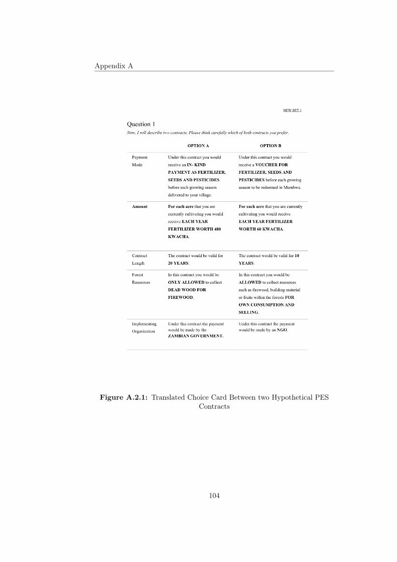
Appendix A

Figure A.2.1: Translated Choice Card Between two Hypothetical PESContracts

104

A.3. Risk Elicitation Experiment

A.3 Risk Elicitation Experiment

For eliciting risk preferences, a survey-based hypothetical experiment wasconducted without monetary pay-offs. The design is adapted from Brick,Visser and Burns (2012). Respondents were confronted with three consec-utive choices between a fixed pay-out of 25 Zambian Kwacha (ZMW) anda lottery with 50% winning probability. The winning amount of the lot-tery was varied depending on the choices in the previous questions. In caseswhere the lottery was lost the respondent would earn nothing. The overallpayout structure of the three consecutive questions are illustrated in FigureA.3.1. Based on the answers to the last question each respondent can beclassified according to her risk preferences. The resulting variable specifieseight categories of risk aversion (see Table A.1).

Figure A.3.1: Payoff and Question Structure of Risk PreferenceElicitation Experiment

Table A.1: Risk Preferences Categories and the Constant Relative RiskAversion (r)

Category r

8 > .757 0.62 < r < .756 .42 < r < .625 .24 < r < .424 0 < r < .243 -.36 < r < 02 -.94 < r < -3.61 < -.94

References

Brick, K., Visser, M., & Burns, J. (2012). Risk Aversion: ExperimentalEvidence from South African Fishing Communities. American Journal ofAgricultural Economics, 94(1), 133–152.

105

Appendix A

A.4 Alternative Model Specifications

Likelihood ratio test indicates that the full random parameter model hasno significantly better goodness-of-fit than the parsimonious random param-eter model χ2(6) = 3.295, p = 0.771. The likelihood ratio test indicatesthat the parsimonious random parameter model provides a significantly bet-ter goodness-of-fit than the conditional logit model: χ2(4) = 226.36, p =2.2 e(−16).

Table A.2: Results of Conditional and Random Parameter ModelEstimations for the Combined Dataset

Combined DatasetConditional Logit Random Parameter Logit

Full Parsimonious

Status Quo −1.32(0.11)∗∗∗ −2.41(0.30)∗∗∗ −2.45(0.28)∗∗∗

Monthly CashPayment −0.49(0.08)∗∗∗ −0.85(0.12)∗∗∗ −0.80(0.11)∗∗∗

Voucher Payment 0.02(0.06) 0.07(0.09) 0.08(0.08)

Input Payment 0.71(0.11)∗∗∗ 1.22(0.18)∗∗∗ 1.14(0.16)∗∗∗

Amount 0.01(0.00)∗∗∗ 0.02(0.00)∗∗∗ 0.02(0.00)∗∗∗

Contract Duration 0.01(0.04) −0.03(0.06) −0.04(0.06)No Forest Benefits −1.30(0.11)∗∗∗ −2.13(0.24)∗∗∗ −1.97(0.18)∗∗∗

Firewood Benefits −0.16(0.06)∗∗∗ −0.26(0.10)∗∗ −0.23(0.09)∗∗∗

Subsistence ForestBenefits 0.84(0.07)∗∗∗ 1.31(0.15)∗∗∗ 1.20(0.10)∗∗∗

Organization 0.08(0.03)∗∗ 0.13(0.05)∗∗∗ 0.12(0.04)∗∗∗

Standard Deviationa

Status Quo 2.87(0.32)∗∗∗ 2.73(0.29)∗∗∗

Monthly CashPayment 0.05(0.21)

Voucher Payment 0.34(0.25)

Input Payment 0.71(0.17)∗∗∗ 0.64(0.15)∗∗∗

Amount 0.01(0.01)

Contract Duration 0.24(0.14)∗

No Forest Benefits 0.83(0.15)∗∗∗ 0.81(0.13)∗∗∗

Firewood Benefits 0.58(0.15)∗∗∗ 0.54(0.12)∗∗∗

Subsistence ForestBenefits 0.30(0.25)

Organization 0.20(0.18)

AIC 2664.25 2454.6 2445.89

Log Likelihood −1322.13 −1207.3 −1208.95Num. obs. 2560 2560 2560∗∗∗p < 0.01, ∗∗p < 0.05, ∗p < 0.1; Standard Errors in Parentheses;a Allrandom parameter estimates are based on 1000 Halton Draws. The randomparameters are assumed to be normally distributed.

106

A.4. Alternative Model Specifications

Table A.3: Results of Conditional and Random Parameter ModelEstimations for the Reduced Dataset (First Question Only)

First Question OnlyConditional Logit Random Parameter Logit

Full Parsimonious

Monthly CashPayment −0.73(0.11)∗∗∗ −0.94(0.19)∗∗∗ −0.81(0.14)∗∗∗

Voucher Payment 0.15(0.08)∗∗ 0.18(0.11)∗ 0.17(0.09)∗

Input Payment 1.13(0.17)∗∗∗ 1.34(0.28)∗∗∗ 1.16(0.22)∗∗∗

Amount 0.01(0.00)∗∗∗ 0.02(0.00)∗∗∗ 0.02(0.00)∗∗∗

Contract Duration −0.07(0.05) −0.05(0.08) −0.03(0.07)No Forest Benefits −1.51(0.18)∗∗∗ −2.08(0.34)∗∗∗ −1.83(0.24)∗∗∗

Firewood Benefits −0.12(0.07)∗ −0.18(0.10)∗ −0.15(0.08)∗

Subsistence ForestBenefits 0.89(0.09)∗∗∗ 1.20(0.18)∗∗∗ 1.06(0.12)∗∗∗

Organization 0.06(0.03)∗ 0.16(0.06)∗∗∗ 0.14(0.05)∗∗∗

Standard Deviationa

Monthly CashPayment 0.00(0.29)

Voucher Payment 0.47(0.28)∗

Input Payment 0.91(0.23)∗∗∗ 0.81(0.16)∗∗∗

Amount 0.00(0.01)

Contract Duration 0.16(0.24)

No Forest Benefits 1.12(0.22)∗∗∗ 1.03(0.16)∗∗∗

Firewood Benefits 0.42(0.22)∗

Subsistence ForestBenefits 0.03(0.44)

Organization 0.25(0.16)

AIC 1475.23 1452.03 1440.75

Log Likelihood −728.61 −708.01 −709.37Num. obs. 1280 1280 1280∗∗∗p < 0.01, ∗∗p < 0.05, ∗p < 0.1; Standard Errors in Parentheses;a Allrandom parameter estimates are based on 1000 Halton Draws. The randomparameters are assumed to be normally distributed.

107

Appendix A

A.5 Latent Class Models for Subsets

Table A.4: Results of the Latent Class Model with Clearing Intention

Class 1 2 3

Status Quo 3.12(0.67)∗∗∗ −0.35(0.40) −2.43(0.46)∗∗∗

Annual CashPaymenta −1.88 −0.23 −0.2

Monthly CashPayment −2.03(0.63)∗∗∗ 0.41(0.44) −1.12(0.36)∗∗∗

Voucher Payment 1.14(0.45)∗∗ 0.12(0.30) 0.27(0.18)

Input Payment 2.77(0.72)∗∗∗ −0.30(0.39) 1.05(0.38)∗∗∗

No Forest Benefits −1.55(0.72)∗∗ −2.93(1.00)∗∗∗ −1.80(0.43)∗∗∗

Firewood Benefits −0.48(0.34) −1.29(0.26)∗∗∗ 0.19(0.18)

Subsistence ForestBenefits 1.06(0.40)∗∗∗ 1.88(0.68)∗∗∗ 1.53(0.33)∗∗∗

Commercial ForestBenefitsa 0.97 2.34 0.08

Amount 0.01(0.01)∗ 0.05(0.01)∗∗∗ 0.01(0.00)∗

Contract Duration −0.19(0.22) 0.27(0.29) −0.16(0.14)Organization −0.13(0.18) −0.15(0.19) 0.18(0.12)

Class MembershipIntercept −1.48(0.44)∗∗∗ −1.31(0.43)∗∗∗

Age 0.02(0.01)∗∗ 0.01(0.01)∗

Gender (female) −0.26(0.28) 0.93(0.25)∗∗∗

Migrated (last fiveyears) 0.82(0.29)∗∗∗ 0.71(0.29)∗∗

Risk Aversion 0.22(0.04)∗∗∗ 0.14(0.04)∗∗∗

Years of FertilizerUse (last fiveyears)

0.02(0.05) 0.10(0.05)∗

Years of Clearing(last five years) 0.53(0.20)∗∗∗ 0.37(0.20)∗

Average ClassMembershipProbability

16.15 46.15 37.69

AIC 1020.459Log Likelihood -466.22Num. obs. 1040∗∗∗p < 0.01, ∗∗p < 0.05, ∗p < 0.1; Standard Errors in Parentheses;a Theparameter of the effects-coded base category is calculated as the negativesum of the other level estimates (Cooper et al., 2012).

108

A.5. Latent Class Models for Subsets

Table A.5: Results of the Latent Class Model without Clearing Intention

Class 1 2 3

Status Quo 3.58(0.97)∗∗∗ −3.21(0.33)∗∗∗ −0.42(0.80)Annual CashPaymenta 0.12 −0.53 1.19

Monthly CashPayment −1.32(0.68)∗ −0.99(0.20)∗∗∗ −0.57(0.40)

Voucher Payment −0.87(0.53) 0.12(0.12) −0.79(0.52)Input Payment 2.07(0.75)∗∗∗ 1.40(0.26)∗∗∗ 0.17(0.71)

No Forest Benefits 0.87(0.81) −2.05(0.29)∗∗∗ −2.69(0.94)∗∗∗

Firewood Benefits −0.32(0.53) 0.35(0.15)∗∗ −1.50(0.35)∗∗∗

Subsistence ForestBenefits −1.36(0.72)∗ 0.82(0.16)∗∗∗ 2.16(0.53)∗∗∗

Commercial ForestBenefitsa 0.81 0.88 2.03

Amount 0.02(0.01)∗ 0.02(0.00)∗∗∗ 0.05(0.01)∗∗∗

Contract Duration −0.02(0.30) −0.24(0.10)∗∗ 0.68(0.39)∗

Organization 0.09(0.24) 0.09(0.06)∗ 0.85(0.32)∗∗∗

Class MembershipIntercept 6.54(0.83)∗∗∗ 4.55(1.01)∗∗∗

Age −0.01(0.01) −0.03(0.01)∗∗∗

Gender (female) −0.23(0.26) 0.17(0.30)

Migrated (last fiveyears) −0.79(0.30)∗∗∗ −3.71(1.91)∗

Risk Aversion −0.37(0.09)∗∗∗ −0.05(0.13)Years of FertilizerUse (last fiveyears)

−0.09(0.06) −0.16(0.07)∗∗

Years of Clearing(last five years) −1.36(0.24)∗∗∗ −1.82(0.28)∗∗∗

Average ClassMembershipProbability

7.1 66.12 26.78

AIC 1299.46Log Likelihood -605.739Num. obs. 1464∗∗∗p < 0.01, ∗∗p < 0.05, ∗p < 0.1; Standard Errors in Parentheses;a Theparameter of the effects-coded base category is calculated as the negativesum of the other level estimates (Cooper et al., 2012).

109

Appendix A

A.6 Latent Class Model Selection Criteria

We applied three information criteria for the selection of classes in the latentclass models: the Akaike’s Information Criterion: AIC = −2LL + 2P ;the modified Akaike’s Information Criterion with penalty factor 3: AIC3 =−2LL+ 3P ; the Bayesian Information Criteria: BIC = −2LL+ P ln(N),where LL is the log likelihood of the fitted model, N is the number ofobservations and P is the number of independent parameters in the model(Dias, 2006). Table A.6 provides these information criteria for the LatentClass Models with covariates between two to ten classes.

Table A.6: Information Criteria of Latent Class Models

Classes AIC AIC3 BIC Log Likelihood

2 2390.1 2418.1 2553.2 -1167.03 2317.5 2363.5 2585.4 -1112.74 2323.4 2387.4 2696.2 -1097.75 2325.2 2407.2 2802.9 -1080.66 2319.4 2419.4 2901.9 -1059.77 2544.4 2662.4 3231.8 -1154.28 2456.4 2592.4 3248.7 -1092.29 2379.0 2533.0 3276.2 -1035.510 2499.2 2671.2 3501.2 -1077.6

References

Dias, J. G. (2006). Latent Class Analysis and Model Selection. In M.Spiliopoulou, R. Kruse, C. Borgelt, A. Nürnberger, & W. Gaul (Eds.), FromData and Information Analysis to Knowledge Engineering. Studies in Classi-fication, Data Analysis, and Knowledge Organization (pp. 95–102). Berlin,Heidelberg: Springer.

110

Appendix B

Chapter 3

B.1 Descriptive Statistics

Figure B.1.1: Frequency of Contributions by Treatment and MigrantStatus

111

Appendix B

Table B.1: Contributions and Beliefs by Migrant Status and Treatment

Status Migrants LocalsTreatment MIG1 MIG2 MIG3 MIG0 MIG1 MIG2 MIG3

N 18 38 55 74 57 34 20ContributionMean 6.17 5.26 5.44 5.58 5.82 6.15 5.85

ContributionSD 3.42 3.42 3.63 3.20 3.33 3.53 3.08

Belief 5.56 5.24 5.76 5.16 6.11 6.44 5.25Belief SD 3.52 2.85 3.32 3.00 3.41 3.29 3.26

B.2 Rounds 2 – 4

Table B.2: Average Contributions by Treatment and Migrant Status(Round 2 - 4)

Status Migrants LocalsTreatment MIG0 MIG1 MIG2 MIG3 MIG1 MIG2 MIG3

Round 1 5.58 5.82 6.15 5.85 6.17 5.26 5.44Round 2 5.77 6.23 6.24 6.00 6.00 5.95 5.55Round 3 6.15 6.21 5.38 6.55 5.61 6.05 6.00Round 4 6.36 6.53 5.74 6.60 6.06 6.53 5.98

112

B.2. Rounds 2 – 4

Table B.3: Regression Results Round 2 - Migrants

Dependent variable:Contribution

(1) (2) (3) (4)

Treatment: No ofMigrants −0.125 −0.041

(0.417) (0.415)

MIG1 0.020 −0.115(0.916) (0.910)

MIG2 −0.197 −0.109(0.888) (0.886)

Belief 0.443∗∗∗ 0.445∗∗∗ 0.423∗∗∗ 0.422∗∗∗

(0.101) (0.102) (0.109) (0.110)

Age −0.026 −0.026 −0.089 −0.090(0.150) (0.151) (0.173) (0.174)

Age2 −0.0002 −0.0002 0.001 0.001

(0.002) (0.002) (0.002) (0.002)

Gender: Male 0.603 0.611 0.007 −0.0002(1.122) (1.128) (1.271) (1.281)

HH Head −0.454 −0.482 −0.362 −0.345(1.307) (1.323) (1.342) (1.362)

Education (years) 0.038 0.038 0.056 0.056

(0.115) (0.116) (0.123) (0.124)

Socio-Economic Status 0.556 0.556 0.303 0.302

(0.389) (0.391) (0.411) (0.413)

Cash Income (USD, year) −0.0004 −0.0004 −0.0003 −0.0003(0.0002) (0.0002) (0.0002) (0.0002)

Village Size 0.061∗∗ 0.061∗∗

(0.026) (0.026)

Migrant Share Village 0.006 0.006

(0.025) (0.025)

Ethnic FractionalizationVillage 0.568 0.521

(5.986) (6.022)

Constant 1.874 1.720

(5.271) (5.248)

Observations 109 109 109 109R2 0.284 0.284 0.189 0.189

Adjusted R2 0.195 0.186 −0.069 −0.082F Statistic 3.176∗∗∗ 2.904∗∗∗ 2.117∗∗ 1.883∗∗∗∗p<0.01, ∗∗p<0.05, ∗p<0.1; Wild Cluster Bootstrapped t-Statistics (p-values only); Models 3 and 4 with village fixed effects.

113

Appendix B

Table B.4: Regression Results Round 2 - Locals

Dependent variable:Contribution

(1) (2) (3) (4)

Treatment: No ofMigrants 0.122 0.116

(0.217) (0.215)

MIG1 0.220 0.199

(0.526) (0.521)

MIG2 −0.005 0.063

(0.624) (0.619)

MIG3 0.571 0.484

(0.757) (0.749)

Belief 0.377∗∗∗ 0.382∗∗∗ 0.343∗∗∗ 0.346∗∗∗

(0.072) (0.073) (0.076) (0.078)

Age 0.123∗ 0.125 0.131∗ 0.133∗

(0.081) (0.082) (0.084) (0.086)

Age2 −0.001∗ −0.001 −0.001 −0.001(0.001) (0.001) (0.001) (0.001)

Gender: Male 0.160 0.190 −0.214 −0.194(0.693) (0.699) (0.724) (0.730)

HH Head 0.033 0.020 0.199 0.190

(0.801) (0.810) (0.822) (0.832)

Education (years) 0.042 0.034 0.073 0.067

(0.076) (0.077) (0.077) (0.080)

Socio-Economic Status 0.204 0.205 0.307 0.307

(0.307) (0.309) (0.315) (0.318)

Cash Income (USD, year) −0.001∗∗∗ −0.001∗∗∗ −0.001∗∗∗ −0.001∗∗

(0.0004) (0.0004) (0.0005) (0.0005)

Village Size 0.009 0.009

(0.018) (0.019)

Migrant Share Village −0.014 −0.014(0.017) (0.017)

Ethnic FractionalizationVillage 6.893∗∗∗ 6.865∗∗∗

(3.819) (3.837)

Constant −4.215 −4.211(3.351) (3.395)

Observations 183 183 183 183R2 0.238 0.239 0.189 0.190

Adjusted R2 0.184 0.176 0.053 0.042

F Statistic 4.413∗∗∗ 3.775∗∗∗ 4.031∗∗∗ 3.278∗∗∗∗∗∗p<0.01, ∗∗p<0.05, ∗p<0.1; Wild Cluster Bootstrapped t-Statistics (p-values only); Models 3 and 4 with village fixed effects.

114

B.2. Rounds 2 – 4

Table B.5: Regression Results Round 3 - Migrants

Dependent variable:Contribution

(1) (2) (3) (4)

Treatment: No ofMigrants 0.248 0.316

(0.402) (0.412)

MIG1 0.475 0.372

(0.883) (0.903)

MIG2 0.577 0.653

(0.855) (0.879)

Belief 0.450∗∗∗ 0.452∗∗∗ 0.427∗∗∗ 0.428∗∗∗

(0.097) (0.098) (0.108) (0.109)

Age 0.116 0.116 −0.040 −0.040(0.144) (0.145) (0.171) (0.173)

Age2 −0.001 −0.001 0.0004 0.0004

(0.002) (0.002) (0.002) (0.002)

Gender: Male 0.740 0.751 0.178 0.183

(1.081) (1.087) (1.261) (1.271)

HH Head −0.722 −0.765 −0.781 −0.793(1.259) (1.274) (1.331) (1.351)

Education (years) 0.076 0.075 0.071 0.071

(0.111) (0.112) (0.122) (0.123)

Socio-Economic Status 0.158 0.159 0.197 0.198

(0.375) (0.377) (0.407) (0.410)

Cash Income (USD, year) −0.0003 −0.0003 −0.0002 −0.0002(0.0002) (0.0002) (0.0002) (0.0002)

Village Size 0.051∗ 0.051∗

(0.025) (0.025)

Migrant Share Village 0.016 0.016

(0.024) (0.024)

Ethnic FractionalizationVillage 10.318∗∗∗ 10.244∗∗

(5.767) (5.800)

Constant −9.838∗∗∗ −9.637∗∗∗

(5.078) (5.055)

Observations 109 109 109 109R2 0.326 0.327 0.185 0.185

Adjusted R2 0.242 0.234 −0.073 −0.087F Statistic 3.868∗∗∗ 3.543∗∗∗ 2.068∗∗ 1.839∗∗∗∗p<0.01, ∗∗p<0.05, ∗p<0.1; Wild Cluster Bootstrapped t-Statistics (p-values only); Models 3 and 4 with village fixed effects.

115

Appendix B

Table B.6: Regression Results Round 3 - Locals

Dependent variable:Contribution

(1) (2) (3) (4)

Treatment: No ofMigrants −0.212 −0.228

(0.210) (0.211)

MIG1 −0.478 −0.493(0.496) (0.498)

MIG2 −1.686∗∗∗ −1.647∗∗∗

(0.588) (0.592)

MIG3 0.440 0.326

(0.714) (0.716)

Belief 0.519∗∗∗ 0.555∗∗∗ 0.513∗∗∗ 0.552∗∗∗

(0.069) (0.069) (0.074) (0.074)

Age 0.074 0.069 0.079 0.071

(0.078) (0.077) (0.082) (0.082)

Age2 −0.001 −0.0005 −0.0004 −0.0004(0.001) (0.001) (0.001) (0.001)

Gender: Male 0.441 0.606 0.236 0.369

(0.670) (0.659) (0.709) (0.698)

HH Head −0.425 −0.609 −0.464 −0.653(0.774) (0.764) (0.804) (0.795)

Education (years) −0.045 −0.086 0.001 −0.042(0.073) (0.073) (0.076) (0.076)

Socio-Economic Status −0.220 −0.179 −0.242 −0.203(0.296) (0.291) (0.309) (0.304)

Cash Income (USD, year) −0.0001 −0.0003 0.00005 −0.0001(0.0004) (0.0004) (0.0004) (0.0004)

Village Size 0.016 0.016

(0.018) (0.018)

Migrant Share Village 0.005 0.003

(0.017) (0.016)

Ethnic FractionalizationVillage 10.616∗∗∗ 10.533∗∗∗

(3.691) (3.617)

Constant −7.174∗∗ −6.535∗

(3.239) (3.200)

Observations 183 183 183 183R2 0.323 0.357 0.251 0.288

Adjusted R2 0.275 0.304 0.127 0.159

F Statistic 6.746∗∗∗ 6.668∗∗∗ 5.820∗∗∗ 5.668∗∗∗∗∗∗p<0.01, ∗∗p<0.05, ∗p<0.1; Wild Cluster Bootstrapped t-Statistics (p-values only); Models 3 and 4 with village fixed effects.

116

B.2. Rounds 2 – 4

Table B.7: Regression Results Round 4 - Migrants

Dependent variable:Contribution

(1) (2) (3) (4)

Treatment: No ofMigrants 0.002 −0.064

(0.420) (0.424)

MIG1 0.602 0.349

(0.921) (0.928)

MIG2 0.220 0.022

(0.892) (0.904)

Belief 0.389∗∗∗ 0.394∗∗∗ 0.370∗∗∗ 0.374∗∗∗

(0.102) (0.102) (0.111) (0.112)

Age 0.162 0.162 0.132 0.135

(0.151) (0.151) (0.177) (0.178)

Age2 −0.002 −0.002 −0.002 −0.002(0.002) (0.002) (0.002) (0.002)

Gender: Male 1.496 1.526 1.680∗ 1.720∗

(1.130) (1.134) (1.299) (1.307)

HH Head −1.985∗∗ −2.099∗∗ −1.956∗∗∗ −2.050∗∗∗

(1.317) (1.329) (1.371) (1.390)

Education (years) 0.099 0.099 0.012 0.012

(0.116) (0.116) (0.126) (0.126)

Socio-Economic Status −0.027 −0.026 −0.180 −0.177(0.392) (0.393) (0.420) (0.421)

Cash Income (USD, year) −0.0003 −0.0003 −0.0001 −0.0001(0.0002) (0.0002) (0.0002) (0.0002)

Village Size 0.079∗∗ 0.078∗∗

(0.026) (0.026)

Migrant Share Village 0.008 0.008

(0.025) (0.025)

Ethnic FractionalizationVillage 1.307 1.113

(6.030) (6.051)

Constant −3.078 −3.197(5.310) (5.273)

Observations 109 109 109 109R2 0.271 0.275 0.165 0.168

Adjusted R2 0.180 0.176 −0.100 −0.110F Statistic 2.974∗∗∗ 2.773∗∗∗ 1.800∗ 1.630∗∗∗p<0.01, ∗∗p<0.05, ∗p<0.1; Wild Cluster Bootstrapped t-Statistics (p-values only); Models 3 and 4 with village fixed effects.

117

Appendix B

Table B.8: Regression Results Round 4 - Locals

Dependent variable:Contribution

(1) (2) (3) (4)

Treatment: No ofMigrants −0.132 −0.130

(0.235) (0.231)

MIG1 −0.103 −0.139(0.564) (0.554)

MIG2 −1.153∗ −1.110(0.670) (0.658)

MIG3 0.354 0.319

(0.812) (0.797)

Belief 0.334∗∗∗ 0.355∗∗∗ 0.291∗∗∗ 0.316∗∗∗

(0.078) (0.079) (0.081) (0.083)

Age 0.009 0.010 0.003 0.002

(0.088) (0.088) (0.090) (0.091)

Age2 −0.0001 −0.0001 0.0001 0.0002

(0.001) (0.001) (0.001) (0.001)

Gender: Male −0.290 −0.177 −0.579 −0.481(0.750) (0.750) (0.778) (0.777)

HH Head 0.269 0.173 0.086 −0.021(0.867) (0.869) (0.882) (0.885)

Education (years) 0.022 −0.007 0.043 0.013

(0.082) (0.083) (0.083) (0.085)

Socio-Economic Status −0.338 −0.318 −0.166 −0.147(0.332) (0.332) (0.339) (0.339)

Cash Income (USD, year) −0.0003 −0.0004 −0.0004 −0.001(0.0005) (0.0005) (0.0005) (0.0005)

Village Size 0.010 0.010

(0.020) (0.020)

Migrant Share Village −0.007 −0.008(0.019) (0.019)

Ethnic FractionalizationVillage 8.522∗∗∗ 8.448∗∗∗

(4.134) (4.115)

Constant −2.126 −1.852(3.627) (3.641)

Observations 183 183 183 183R2 0.159 0.177 0.102 0.121

Adjusted R2 0.100 0.108 −0.047 −0.039F Statistic 2.687∗∗∗ 2.578∗∗∗ 1.975∗∗ 1.929∗∗∗∗∗p<0.01, ∗∗p<0.05, ∗p<0.1; Wild Cluster Bootstrapped t-Statistics (p-values only); Models 3 and 4 with village fixed effects.

118

B.3. Individual Cash Income

B.3 Individual Cash Income

If migrants would only gain a higher income after migration, this effect wouldmost likely increase with time and it is unclear why migrants would be moresuccessful farmers as they all tend to grow similar crops with similar farmingtechniques. On the contrary, migrated households are for example requiredto clear forest areas for agriculture, which commonly takes several years andthey don’t possess the local knowledge of the soils and climate as localsmight do. Nevertheless, we carried out an analysis to see whether wealth ofmigrants differs with the number of years they migrated. In line with ourarguments above we find that migrants, who just recently migrated (0 to2 years ago) do not have a significant different cash income than migrantswho moved earlier (3 to 5 and 6 to 10 years ago, see Column 1, Table B.9). In addition, we can control for other individual characteristics that mightinfluence that migrants have a higher income than locals such as age andeducation. Through regression analysis we find that age has a quadraticrelationship with cash income: above an age of 57.5 years the average cashincome declines again. After controlling for such individual characteristics,we find that migrants still have a significant higher cash income than locals(see Column 2, Table B.9 below). We interpret these findings as supportive(but not conclusive) evidence that migrants were better-off before migrationthan locals in the host communities.

119

Appendix B

Table B.9: Regression Results Individual Cash Income

Dependent variable:Cash Income

Migrants Overall(1) (2)

Migrated 3-5 Years −170.407(500.668)

Migrated 6-10 Years −122.393(457.598)

Migrant 328.079∗∗

(137.429)

Age 118.981∗∗ 67.609∗∗∗

(94.088) (27.127)

Age2 −1.035∗∗ −0.614∗∗∗

(1.014) (0.278)

Gender: Male 402.465 238.943

(697.886) (224.948)

Household Head −163.265 −160.943(730.513) (247.615)

Education (Years) 95.038 64.559

(68.935) (23.051)

Observations 109 292R2 0.080 0.089

Adjusted R2 −0.182 0.011

F Statistic 1.048 4.356∗∗∗∗∗∗p<0.01, ∗∗p<0.05, ∗p<0.1; Wild Cluster Bootstrapped t-Statistics (p-values only); Village Fixed Effects.

120

B.4. Correlation - Village Characteristics

B.4 Correlation - Village Characteristics

Table B.10: Correlations Between Village Characteristics

Size(Households)

ShareofMigratedHouseholds(0-10years)

ShareofMigratedHouseholds(>10years)a

ShareofIndigenousHouseholdsa

EthnicFractionalizationb

EthnicFractionalization(Locals)b

EthnicFractionalization(Migrants)b

GiniCoefficientIncomeb

Size

(Hou

seho

lds)

Shareof

Migrated

Hou

seho

lds(0-10years)

-0.38

Shareof

Migrated

Hou

seho

lds(>

10years)

a0.46

-0.94

∗∗∗

Shareof

Indigeno

usHou

seho

ldsa

-0.49∗

0.71

∗∗-

0.91

∗∗∗

EthnicFraction

alizationb

0.22

-0.09

0.23

-0.37

EthnicFraction

alization

(Locals)

b0.20

0.30

-0.14

-0.08

0.51

∗

EthnicFraction

alization

(Migrants)

b0.29

-0.39

0.30

-0.15

0.20

-0.50∗

GiniC

oefficientIncomeb

0.22

-0.27

0.33

-0.34

-0.21

-0.04

0.02

IncomeGap

(Migrants,

Locals)b

0.44

-0.42

0.42

-0.34

-0.07

0.05

0.25

0.74

∗∗∗

∗∗∗p<

0.01,∗∗

p<

0.05,∗p<

0.1;(Som

ersRan

kCorrelation

),aEstim

ated

shares

bycombining

villa

gelevelda

taan

dsampleda

ta;

bBased

onsample.

121

Appendix B

B.5 Regression Results - Pooled Contributions Mi-grants and Locals

Table B.11: Regression Results Pooled Sample - ContributionsExperiment

Dependent variable:Contribution

OLS FE(1) (2) (3) (4)

MIG1 −0.054 −0.243 0.003 −0.388MIG2 −0.156 −0.511 −0.145 −0.625MIG3 −0.171 −0.396 −0.098 −0.494Migrant −0.135 0.776 −0.107 0.747

Belief 0.508∗∗∗ 0.576∗∗∗ 0.450∗∗∗ 0.523∗∗∗

Age 0.160∗∗∗ 0.122∗∗∗

Age2 −0.002∗∗∗ −0.001∗∗∗

Gender: Male 0.516 0.032

HH Head −0.193 −0.043Education(years) −0.143∗∗ −0.116∗

Socio-EconomicStatus −0.110 −0.153

Cash Income(USD, year) −0.0003∗∗ −0.0002

Years in Village 0.029 0.026

Village Size 0.028

Migrant ShareVillage −0.0004

Ethnic Frac-tionalizationVillage

−0.506

Constant 2.956∗∗∗ −1.313Observations 296 239 296 239R2 0.236 0.333 0.196 0.279

Adjusted R2 0.223 0.285 0.132 0.175

F Statistic 17.945∗∗∗ 6.940∗∗∗ 13.334∗∗∗ 6.191∗∗∗∗∗∗p < 0.01, ∗∗p < 0.05, ∗p < 0.1; Wild Cluster Bootstrappedt-Statistics (p-values only); Models 3 and 4 include village fixedeffects.

122

B.5. Regression Results - Pooled Contributions Migrants and Locals

Table B.12: Regression Results Pooled Sample - Real World Public GoodContributions

Dependent variable:Real PG Contribution

(1) (2)

Age −0.198 −0.190Age2 0.002 0.002

Gender: Male 3.919 3.811

HH Head −4.252 −4.170Education (years) −0.012 −0.001Socio-EconomicStatus −0.841 −0.451

Cash Income(USD, year) 0.003 0.001

GroupMemberships 1.683∗∗∗ 1.630∗∗∗

Migrant 0.364 −0.817Cash Income(USD, year) xMigrant

0.002

Observations 292 292R2 0.180 0.190

Adjusted R2 0.099 0.107

F Statistic 6.443∗∗∗ 6.201∗∗∗∗∗∗p < 0.01, ∗∗p < 0.05, ∗p < 0.1; Wild Cluster Boot-strapped t-Statistics (p-values only); Village Fixed Ef-fects.

123

Appendix B

B.6 Regression Results Main Treatment Effects -Migrants

Table B.13: Regression Results - Migrants - OLS

Dependent variable:Contribution

(1) (2) (3) (4)

No of Migrants −0.361 −0.233MIG2 −0.725 −0.728MIG3 −0.847 −0.643Belief 0.564∗∗∗ 0.610∗∗∗ 0.561∗∗∗ 0.605∗∗∗

Age 0.110 0.110

Age2 −0.001 −0.001Gender: Male 1.207∗ 1.181∗

HH Head −1.431 −1.332Education(years) −0.114 −0.114

Socio-EconomicStatus −0.075 −0.072

Cash Income(USD, year) −0.0003∗ −0.0003∗

Years in Village −0.008 −0.012Village Size 0.056 0.057

Migrant ShareVillage 0.012 0.012

Ethnic Frac-tionalizationVillage

−0.028 0.182

Constant 3.208∗∗ −0.358 3.048∗∗ −0.496Observations 111 109 111 109R2 0.264 0.347 0.265 0.349

Adjusted R2 0.250 0.257 0.245 0.252

F Statistic 19.366∗∗∗ 3.875∗∗∗ 12.889∗∗∗ 3.602∗∗∗∗∗∗p < 0.01, ∗∗p < 0.05, ∗p < 0.1; Wild Cluster Bootstrappedt-Statistics (p-values only).

124

B.6. Regression Results Main Treatment Effects - Migrants

Table B.14: Regression Results - Migrants - Village Fixed Effects

Dependent variable:Contribution

(1) (2) (3) (4)

No of Migrants −0.254 −0.107MIG2 −0.852 −0.774MIG3 −0.714 −0.454Belief 0.450∗∗∗ 0.513∗∗∗ 0.445∗∗∗ 0.505∗∗∗

Age −0.038 −0.042Age2 0.0002 0.0003

Gender: Male 0.235 0.167

HH Head −1.078 −0.922Education(years) −0.130 −0.131

Socio-EconomicStatus −0.005 −0.005

Cash Income(USD, year) −0.0002 −0.0002

Years in Village −0.048 −0.054Observations 111 109 111 109R2 0.188 0.251 0.194 0.258

Adjusted R2 0.019 0.001 0.015 −0.002F Statistic 10.560∗∗∗ 2.715∗∗∗ 7.223∗∗∗ 2.529∗∗∗∗∗∗p < 0.01, ∗∗p < 0.05, ∗p < 0.1; Wild Cluster Bootstrappedt-Statistics (p-values only); Village Fixed Effects

125

Appendix B

B.7 Regression Results Main Treatment Effects -Locals

Table B.15: Regression Results - Locals - OLS

Dependent variable:Contribution

(1) (2) (3) (4)

No of Migrants 0.041 0.008

MIG1 −0.210 −0.238MIG2 −0.049 −0.282MIG3 0.227 0.287

Belief 0.475∗∗∗ 0.507∗∗∗ 0.481∗∗∗ 0.519∗∗∗

Age 0.160∗ 0.155∗

Age2 −0.002∗∗ −0.002∗

Gender: Male 0.071 0.113

HH Head 0.313 0.241

Education(years) −0.083 −0.093

Socio-EconomicStatus 0.022 0.040

Cash Income(USD, year) −0.0004 −0.0004

Village Size 0.018 0.017

Migrant ShareVillage −0.016 −0.017

Ethnic Frac-tionalizationVillage

1.916 1.911

Constant 3.040∗∗∗ −2.104 3.100∗∗∗ −1.804Observations 185 183 185 183R2 0.221 0.298 0.223 0.300

Adjusted R2 0.213 0.248 0.205 0.242

F Statistic 25.833∗∗∗ 6.004∗∗∗ 12.881∗∗∗ 5.153∗∗∗∗∗∗p < 0.01, ∗∗p < 0.05, ∗p < 0.1; Wild Cluster Bootstrappedt-Statistics (p-values only).

126

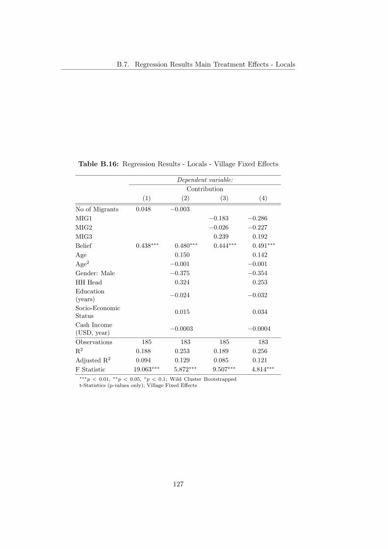
B.7. Regression Results Main Treatment Effects - Locals

Table B.16: Regression Results - Locals - Village Fixed Effects

Dependent variable:Contribution

(1) (2) (3) (4)

No of Migrants 0.048 −0.003MIG1 −0.183 −0.286MIG2 −0.026 −0.227MIG3 0.239 0.192

Belief 0.438∗∗∗ 0.480∗∗∗ 0.444∗∗∗ 0.491∗∗∗

Age 0.150 0.142

Age2 −0.001 −0.001Gender: Male −0.375 −0.354HH Head 0.324 0.253

Education(years) −0.024 −0.032

Socio-EconomicStatus 0.015 0.034

Cash Income(USD, year) −0.0003 −0.0004

Observations 185 183 185 183R2 0.188 0.253 0.189 0.256

Adjusted R2 0.094 0.129 0.085 0.121

F Statistic 19.063∗∗∗ 5.872∗∗∗ 9.507∗∗∗ 4.814∗∗∗∗∗∗p < 0.01, ∗∗p < 0.05, ∗p < 0.1; Wild Cluster Bootstrappedt-Statistics (p-values only); Village Fixed Effects

127

Appendix B

B.8 Regression Results - Individual Relative In-come

Table B.17: Regression Results - Migrants - Individual Cash Income

Dependent variable:Contribution

(1) (2) (3) (4) (5) (6)

No of Migrants −0.277 −0.328 −0.283MIG2 −0.645 −0.208 0.172

MIG3 −0.679 −0.484 −0.265No of Migrantsx Relative CashIncome (toLocals)

0.024 0.026

MIG2 xRelative CashIncome (toLocals)

−0.215∗∗ −0.457∗∗∗

MIG3 xRelative CashIncome (toLocals)

−0.123 −0.223

Relative CashIncome (toLocals)

−0.082∗ −0.142 −0.066 −0.081∗ 0.070 0.432∗∗∗

Belief 0.571∗∗∗ 0.571∗∗∗ 0.609∗∗∗ 0.568∗∗∗ 0.551∗∗∗ 0.599∗∗∗

Age 0.106 0.114

Age2 −0.001 −0.002Gender: Male 1.127 0.976

HH Head −1.380∗ −1.315Education(years) −0.108 −0.122

Socio-EconomicStatus −0.053 −0.097

Cash Income(USD, year) −0.0003 −0.001∗

Years in Village −0.005 −0.028Village Size 0.057 0.052

Migrant ShareVillage 0.013 0.012

Ethnic Frac-tionalizationVillage

−0.098 −0.895

Constant 3.230∗∗ 3.352∗∗ −0.155 3.152∗∗ 2.981∗∗ 0.264

Observations 109 109 109 109 109 109R2 0.279 0.279 0.347 0.281 0.288 0.372

Adjusted R2 0.258 0.252 0.242 0.253 0.246 0.255

F Statistic 13.545∗∗∗ 10.086∗∗∗ 3.295∗∗∗ 10.140∗∗∗ 6.871∗∗∗ 3.170∗∗∗

∗∗∗p < 0.01, ∗∗p < 0.05, ∗p < 0.1; Wild Cluster Bootstrappedt-Statistics (p-values only).

128

B.8. Regression Results - Individual Relative Income

Table B.18: Regression Results - Locals - Individual Cash Income

Dependent variable:Contribution

(1) (2) (3) (4) (5) (6)

No of Migrants 0.066 0.247 0.079

MIG1 −0.304 −0.457 −0.576MIG2 −0.023 0.656 0.263

MIG3 0.326 0.889 0.382

No of Migrantsx Relative CashIncome (toMigrants)

−0.190∗∗∗ −0.073

MIG1 xRelative CashIncome (toMigrants)

0.311 0.563

MIG2 xRelative CashIncome (toMigrants)

−0.957 −0.780

MIG3 xRelative CashIncome (toMigrants)

−0.523∗∗ −0.058

Relative CashIncome (toMigrants)

−0.046 0.219 0.550∗∗∗ −0.062 0.159 0.550∗∗∗

Belief 0.501∗∗∗ 0.486∗∗∗ 0.496∗∗∗ 0.509∗∗∗ 0.478∗∗∗ 0.488∗∗∗

Age 0.152∗ 0.143

Age2 −0.001∗ −0.001∗

Gender: Male −0.001 0.005

HH Head 0.338 0.303

Education(years) −0.088 −0.100

Socio-EconomicStatus 0.105 0.138

Cash Income(USD, year) −0.001 −0.001

Village Size 0.029 0.031

Migrant ShareVillage −0.012 −0.010

Ethnic Frac-tionalizationVillage

2.003 2.088

Constant 2.838∗∗∗ 2.705∗∗∗ −2.638 2.932∗∗∗ 2.924∗∗∗ −2.311Observations 183 183 183 183 183 183R2 0.246 0.255 0.310 0.249 0.266 0.324

Adjusted R2 0.233 0.238 0.253 0.228 0.233 0.249

F Statistic 19.473∗∗∗ 15.241∗∗∗ 5.394∗∗∗ 11.735∗∗∗ 7.893∗∗∗ 4.360∗∗∗

∗∗∗p < 0.01, ∗∗p < 0.05, ∗p < 0.1; Wild Cluster Bootstrappedt-Statistics (p-values only).

129

Appendix B

B.9 Regression Results - Income Ratio

Table B.19: Regression Results - Migrants - Village Income Ratio(Migrants/ Locals)

Dependent variable:Contribution

(1) (2) (3) (4) (5) (6)

No of Migrants −0.363 0.943∗∗ 0.916∗∗

MIG2 −0.732 1.769 1.671

MIG3 −0.852 2.146∗∗ 2.025∗∗

No of Migrantsx VillageIncome Ratio

−0.536∗∗∗ −0.486∗∗∗

MIG2 x VillageIncome Ratio −1.015∗∗∗ −1.023∗∗∗

MIG3 x VillageIncome Ratio −1.224∗∗∗ −1.139∗∗∗

Village IncomeRatio −0.151 1.092∗∗∗ 0.855∗∗ −0.152 0.791∗∗∗ 0.617∗

Belief 0.569∗∗∗ 0.599∗∗∗ 0.638∗∗∗ 0.566∗∗∗ 0.593∗∗∗ 0.634∗∗∗

Age 0.080 0.088

Age2 −0.001 −0.001Gender: Male 0.689 0.461

HH Head −0.781 −0.453Education(years) −0.127 −0.129

Socio-EconomicStatus −0.0005 −0.035

Cash Income(USD, year) −0.0002 −0.0002

Years in Village −0.022 −0.035Village Size 0.065 0.069

Migrant ShareVillage 0.001 0.002

Ethnic Frac-tionalizationVillage

−1.428 −1.352

Constant 3.554∗∗ 0.360 −0.936 3.396∗∗ 0.925 −0.680Observations 111 111 109 111 111 109R2 0.270 0.312 0.390 0.272 0.322 0.404

Adjusted R2 0.250 0.286 0.292 0.244 0.283 0.292

F Statistic 13.196∗∗∗ 12.035∗∗∗ 3.965∗∗∗ 9.881∗∗∗ 8.244∗∗∗ 3.623∗∗∗

∗∗∗p < 0.01, ∗∗p < 0.05, ∗p < 0.1; Wild Cluster Bootstrappedt-Statistics (p-values only).

130

B.9. Regression Results - Income Ratio

Table B.20: Regression Results - Locals - Village Income Ratio(Migrants/ Locals)

Dependent variable:Contribution

(1) (2) (3) (4) (5) (6)

No of Migrants 0.040 −0.340 −0.217MIG1 −0.208 −0.388 −0.351MIG2 −0.051 −1.133 −1.320MIG3 0.226 −0.617 0.174

No of Migrantsx VillageIncome Ratio

0.160 0.099

MIG1 x VillageIncome Ratio 0.081 0.030

MIG2 x VillageIncome Ratio 0.454 0.423

MIG3 x VillageIncome Ratio 0.353 0.073

Village IncomeRatio 0.035 −0.128 −0.226 0.035 −0.117 −0.248

Belief 0.475∗∗∗ 0.459∗∗∗ 0.498∗∗∗ 0.480∗∗∗ 0.464∗∗∗ 0.512∗∗∗

Age 0.141 0.134

Age2 −0.001∗ −0.001Gender: Male 0.083 0.011

HH Head 0.200 0.148

Education(years) −0.090 −0.110

Socio-EconomicStatus 0.069 0.104

Cash Income(USD, year) −0.0004 −0.001

Village Size 0.024 0.024

Migrant ShareVillage −0.021 −0.022

Ethnic Frac-tionalizationVillage

1.413 1.438

Constant 2.957∗∗∗ 3.434∗∗∗ −0.742 3.019∗∗∗ 3.466∗∗∗ −0.208Observations 185 185 183 185 185 183R2 0.221 0.229 0.303 0.223 0.232 0.310

Adjusted R2 0.209 0.212 0.244 0.201 0.197 0.235

F Statistic 17.164∗∗∗ 13.353∗∗∗ 5.206∗∗∗ 10.268∗∗∗ 6.651∗∗∗ 4.101∗∗∗

∗∗∗p < 0.01, ∗∗p < 0.05, ∗p < 0.1; Wild Cluster Bootstrappedt-Statistics (p-values only).

131

Appendix B

B.10 Regression Results - Income Ratio and Rela-tive Individual Income

Table B.21: Regression Results - Migrants - Village Income Ratio(Migrants/ Locals) and Relative Individual Income

Dependent variable:Contribution

(1) (2) (3) (4) (5) (6)

No of Migrants −0.282 0.964∗∗ 0.880∗∗

MIG2 −0.660 1.662 2.378

MIG3 −0.692 2.321∗∗∗ 2.583∗∗∗

No of Migrantsx VillageIncome Ratio

−0.583∗∗∗ −0.561∗∗∗

No of Migrantsx Relative CashIncome (toLocals)

0.080 0.117

MIG2 x VillageIncome Ratio −0.802∗∗ −0.960∗∗∗

MIG3 x VillageIncome Ratio −1.239∗∗∗ −1.313∗∗∗

MIG2 xRelative CashIncome (toLocals)

−0.154 −0.427∗∗∗

MIG3 xRelative CashIncome (toLocals)

−0.020 −0.086

Village IncomeRatio −0.086 1.251∗∗∗ 0.999∗∗∗ −0.088 0.786∗∗∗ 0.607∗∗

Relative CashIncome (toLocals)

−0.072∗∗∗ −0.261 −0.195 −0.070∗∗∗ 0.014 0.491∗∗∗

Age 0.058 0.067

Age2 −0.001 −0.001Gender: Male 0.508 0.216

HH Head −0.653 −0.434Education(years) −0.102 −0.119

Socio-EconomicStatus 0.083 −0.004

Cash Income(USD, year) −0.001 −0.001∗∗

Years in Village 0.001 −0.029Village Size 0.064 0.062∗

Migrant ShareVillage 0.005 0.004

Ethnic Frac-tionalizationVillage

−2.565 −3.986

Belief 0.572∗∗∗ 0.602∗∗∗ 0.653∗∗∗ 0.569∗∗∗ 0.582∗∗∗ 0.650∗∗∗

Constant 3.415∗∗ 0.392 0.106 3.344∗∗ 0.976 1.527

Observations 109 109 109 109 109 183R2 0.281 0.328 0.398 0.282 0.339 0.437

Adjusted R2 0.253 0.289 0.285 0.248 0.279 0.309

F Statistic 10.147∗∗∗ 8.303∗∗∗ 3.534∗∗∗ 8.105∗∗∗ 5.635∗∗∗ 3.412∗∗∗

∗∗∗p < 0.01, ∗∗p < 0.05, ∗p < 0.1; Wild Cluster Bootstrappedt-Statistics (p-values only).

132

B.10. Regression Results - Income Ratio and Relative Individual Income

Table B.22: Regression Results - Locals - Village Income Ratio(Migrants/ Locals) and Relative Individual Income

Dependent variable:Contribution

(1) (2) (3) (4) (5) (6)

No of Migrants 0.063 0.007 −0.148MIG1 −0.298 −0.983 −0.972MIG2 −0.023 −0.200 −0.661MIG3 0.312 0.689 0.310

No of Migrantsx VillageIncome Ratio

0.086 0.083

No of Migrantsx Relative CashIncome (toMigrants)

−0.158∗ −0.033

MIG1 x VillageIncome Ratio 0.178 0.137

MIG2 x VillageIncome Ratio 0.271 0.300

MIG3 x VillageIncome Ratio 0.072 0.042

MIG1 xRelative CashIncome (toMigrants)

0.473 0.630

MIG2 xRelative CashIncome (toMigrants)

−0.657 −0.506

MIG3 xRelative CashIncome (toMigrants)

−0.491 −0.045

Village IncomeRatio 0.050 −0.027 −0.139 0.044 −0.054 −0.164

Relative CashIncome (toMigrants)

−0.017 0.221 0.509∗∗∗ −0.036 0.133 0.475∗∗

Age 0.140 0.129

Age2 −0.001 −0.001Gender: Male 0.041 −0.026HH Head 0.252 0.291

Education(years) −0.093 −0.110

Socio-EconomicStatus 0.130 0.163

Cash Income(USD, year) −0.001 −0.001

Village Size 0.031 0.033

Migrant ShareVillage −0.014 −0.013

Ethnic Frac-tionalizationVillage

1.729 1.870

Belief 0.501∗∗∗ 0.479∗∗∗ 0.492∗∗∗ 0.509∗∗∗ 0.476∗∗∗ 0.490∗∗∗

Constant 2.701∗∗∗ 2.812∗∗∗ −1.763 2.810∗∗∗ 3.084∗∗∗ −1.281Observations 183 183 183 183 183 183R2 0.247 0.258 0.312 0.249 0.270 0.327

Adjusted R2 0.230 0.232 0.246 0.224 0.218 0.234

F Statistic 14.573∗∗∗ 10.188∗∗∗ 4.706∗∗∗ 9.749∗∗∗ 5.229∗∗∗ 3.531∗∗∗

∗∗∗p < 0.01, ∗∗p < 0.05, ∗p < 0.1; Wild Cluster Bootstrappedt-Statistics (p-values only).

133

Appendix B

B.11 Regression Results - Real Public Good Con-tributions

Table B.23: Regression Results - Migrants - Real Public Goods

Dependent variable:Real Public Good Contribution

All Income Ratio =< Median Income Ratio > Median(1) (2) (3) (4) (5) (6)

Age −0.305∗ −0.050 −0.872Age2 0.003 0.0002 0.008

Gender: Male 0.018 2.171 0.994

HH Head −2.382 1.154 −7.941Education(years) 0.014 −0.388 0.202

Socio-EconomicStatus 0.888 0.922 1.028

Cash Income(USD, year) 0.003 0.003 0.001 0.002 0.003 0.004

GroupMembership 2.745∗∗ 2.507∗∗∗ 3.875∗∗ 3.631∗∗∗ 2.822 1.631

Years in Village 0.096 0.082 0.118 0.168 −0.048 −0.039Observations 109 109 55 55 54 54R2 0.389 0.374 0.309 0.269 0.459 0.418

Adjusted R2 0.196 0.232 −0.008 0.082 0.204 0.265

F Statistic 5.811∗∗∗ 17.523∗∗∗ 1.840∗ 5.267∗∗∗ 3.397∗∗∗ 10.048∗∗∗

∗∗∗p < 0.01, ∗∗p < 0.05, ∗p < 0.1; Wild Cluster Bootstrappedt-Statistics (p-values only)and Village Fixed Effects.

134

B.11. Regression Results - Real Public Good Contributions

Table B.24: Regression Results - Migrants - Real Public Goods withYears in Village Interaction

Dependent variable:Real Public Good Contribution

All Income Ratio =< Median Income Ratio > Median(1) (2) (3) (4) (5) (6)

Age −0.068 −0.095 −0.248Age2 0.0004 0.001 0.003

Gender: Male 0.557 1.583 −0.400HH Head −3.708 1.797 −8.647Education(years) 0.386 −0.368 1.051

Socio-EconomicStatus 2.516 0.899 4.333

Cash Income(USD, year) 0.005∗∗∗ 0.005∗∗∗ −0.002 −0.001 0.006∗∗∗ 0.006∗∗∗

GroupMembership 1.991 2.445∗∗∗ 3.818∗ 3.653∗∗ 1.322 1.634

Years in Village 0.795∗∗ 0.615∗ −0.153 −0.124 0.739 0.689

Cash Income xYears in Village −0.001∗∗∗ −0.001∗∗∗ 0.0005 0.001 −0.001∗∗ −0.001∗∗∗

Observations 109 109 55 55 54 54R2 0.487 0.443 0.318 0.280 0.628 0.518

Adjusted R2 0.316 0.308 −0.023 0.075 0.437 0.377

F Statistic 7.692∗∗∗ 17.267∗∗∗ 1.680 4.089∗∗∗ 5.916∗∗∗ 11.011∗∗∗

∗∗∗p < 0.01, ∗∗p < 0.05, ∗p < 0.1; Wild Cluster Bootstrappedt-Statistics (p-values only) and Village Fixed Effects.

Table B.25: Regression Results - Locals - Real Public Goods

Dependent variable:Real Public Good Contribution

All Income Ratio =< Median Income Ratio > Median(1) (2) (3) (4) (5) (6)

Age −0.264 −0.369 −0.401 −0.369 −0.158 −0.324∗

Age2 0.003∗ 0.004∗ 0.004 0.004 0.002 0.004∗∗∗

Gender: Male 5.842 7.342 5.516

HH Head −5.149∗∗ −0.826 −8.209 −2.317∗ −2.211 0.977

Education(years) −0.039 −0.148 0.024

Socio-EconomicStatus −1.725 −1.433 −1.652

Cash Income(USD, year) 0.002 0.002 0.003

GroupMembership 1.211∗ 1.016∗∗ 0.902 0.783 1.412 1.330∗∗

Observations 183 185 92 93 91 92R2 0.083 0.028 0.103 0.031 0.096 0.041

Adjusted R2 −0.063 −0.097 −0.089 −0.114 −0.100 −0.105F Statistic 1.781∗ 1.194 1.072 0.638 0.977 0.845∗∗∗p < 0.01, ∗∗p < 0.05, ∗p < 0.1; Wild Cluster Bootstrappedt-Statistics (p-values only)and Village Fixed Effects.

135

Appendix B

B.12 Experimental Protocol

Instructions for experimenters in [...]

Instructions given in private to participants in grey

Registration

[PRIVATE BRIEFING]

Good morning, we are glad that you have followed our invitation and cameto this workshop. This morning we will do several group activities. You willshortly learn more about these activities. We have invited in total 16 people,for which we have to wait now.

The workshop this morning will take about 4 hours, including waiting time.Afterwards we have organized some snacks and drinks.

In addition, we have some further questions for you. These questions will beasked in an individual interview, which takes roughly 1 hour. The interviewwill take place after the workshop. You have to wait until you will be calledto the interview. As mentioned in the invitation you will receive some moneyfor compensation. Consider that you only receive the money if we have alsointerviewed you.

If you find that this workshop is something that you do not wish to partici-pate in for any reason, or you already know that you will not be able to stayfor the whole day, please let us know immediately so that you can leave.

[REGISTER PARTICIPANTS IN THE REGISTRATION FORM.EVERY PLAYER SELECTS AN ID CARD FROM TWO BAGS DEPEND-ING ON HIS/HER MIGRATION STATUS. MIGRANT ID: 3,4,7,9,12,14]

[ONCE 16 PARTICIPANTS HAVE BEEN REGISTERED, SAVE THE FILEAND GO TO NEXT PAGE.]

[PREPARE 4 PARTICIPANT LISTS FOR INTERVIEWS]

General Introduction

[ASSIGN EVERYONE A SEAT ACCORDING TO THE ID FROM HIGHTO LOW NUMBERS.]

[PREPARE THE DECISION CARDS AND CONDITIONAL DECISIONCARDS BY FILLING IN PLAYER ID.]

Thank you all for coming to this workshop today. This workshop is orga-nized by the SASSCAL research project from the University of Marburg,Germany. My name is [NAME OF EXPERIMENTER] and this is [NAMEOF EXPERIMENTER], who work for this project and conduct this work-

136

B.12. Experimental Protocol

shop. The information we will gather today will be used for research purposesonly. We have conducted and will conduct similar workshops in other villagesof this chiefdom.

Today we would like to play several group activities with you. You can earnsome money that you are permitted to keep and take home. You must un-derstand that this is not our private money but given to us by the universityfor research. If you listen to the following instructions carefully, you can, de-pending on your decisions and the decisions of the other participants, earnbetween 15 and 55 Kwacha. It is therefore very important that you listen tothese instructions with care. We are interested in your decision during theactivities. However, there are no “right” or “wrong” answers.

After the activities, you have to answer a few questions. This will takeapproximately 1 hour. You have to wait until it is your turn for the interview.You will receive your payments only after the interview.

Before we start, I have to make some important remarks:

1. The workshop consists of several rounds. In each round, you will playin groups of four people, but you will never know with whom in thisroom you play together. In the workshop, you will play in the samegroup, meaning that you will play with the same three other players.

2. In each round, you will make one or more decisions. Your fellow groupmembers will not come to know your decisions at any point. This isthe reason that we will not ask your name in any of the activities. Wewill identify your decision in the game with an identity card like this[SHOW PLAYER ID CARD]. Please do not lose this card. You haveto return the card to us when you are paid.

3. All the decisions you make today will be kept private. Therefore, wewill call you one-by-one to make your decisions.

4. You will be paid 5 Kwacha for coming to this workshop. In addition,you will receive the money earned in the rounds. [NAME OF EX-PERIMENTER] will be responsible for payments and keep record ofall decisions you take, to make sure that you receive the right amount.

5. During these activities, we will not speak in terms of Kwacha, but inpoints. At the end of the workshop the total amount of points you haveearned will be converted to Kwacha. For two points you will receive 1Kwacha.

6. It is very important that you understand the activities and the decisionyou can take. Therefore, we will check your understanding by askingeach of you test questions about the activities. If you do not under-

137

Appendix B

stand something you may always ask [NAME OF EXPERIMENTER]to explain it again.

7. We would like to keep the game anonymous, therefore, please do notdiscuss the activities with each other. In case we find that you aretalking during the workshop, we will exclude you immediately fromthe workshop. In this case, you will not receive any money.

8. We want to conduct the same workshop in other villages of this chief-dom. For the success of the project it is very important that partici-pants do not know too many details about the content of the workshopbefore participating. Therefore, please do not discuss what we havedone in this workshop with anybody afterwards.

9. If you have questions, always raise your hand and wait until one ofthe assistants comes to you. Then you can ask your question andthe assistant will answer it. You are not allowed to talk to otherparticipants during the activities. In case you have to leave the roomduring the workshop, please notify [NAME OF EXPERIMENTER]in advance. It is only allowed that one person at a time leaves theworkshop. Please switch off your mobile phones. If you violate theserule, you will be dismissed from the workshop and not receive anymoney.

Thank you in advance for your effort and time.

[ASK THE GROUP]

Do you have any questions?

Basic Instructions

Each decision in this workshop today will be similar. We will now giveyou instructions how this activity is played. After the instructions, we willask you privately few questions to check whether you have understood theactivity.

At the beginning of each round, each player will receive 10 points from us.Now you have to decide how many of the 10 points to keep for yourself (andput it in your private account) and how many to contribute for a groupproject. Both you and your three other group members will benefit from theamount contributed to the project. We will explain later how this works indetail. You may put any amount between 0 and 10 points into the project.

[USE BEANS AND BOWLS FOR ILLUSTRATION]

Now let us assume that out of 10 points, you put 1 point into the project.

[ASK THE GROUP]

138

B.12. Experimental Protocol

How many points does the player have in his private account?

Have you understood this part?

Now, let us assume that out of 10, you put 2 points into the project.

[ASK THE GROUP]

How many points does the player have in his private account?

[CARRY ON WITH EXAMPLES FOR 5, 10 POINTS]

[ASK THE GROUP]

Have you understood this part?

Do you need additional examples?

As mentioned before you are playing in groups of four participants. However,you do not know who in this room is in your group. Let us see what happensif everyone in the group has decided how much to contribute to the project.Remember that everyone in the group has to decide for him/herself how muchto contribute to the project without talking to the other group members.

The following will happen with points you and your fellow group memberscontributed to the project. [NAME OF EXPERIMENTER] will add 1 pointto each point you and the other three group members contributed to theproject.

For example, each of the four players have contributed 1 point to the project.We have hence 1 + 1 + 1 + 1 = 4 points in the project account. For eachpoint in the project account one additional point will be added. We havehence in the end 4 + 4 = 8 points in the project.

[ASK THE GROUP]

Have you understood this part?

Let’s have a look at a second example. If each member of your group puts2 points into the project, we have in total 2 + 2 + 2 + 2 = 8 points in theproject. The project amount will be increased by 8 points. Now, the finalamount of money in the project is 16 points.

[CARRY ON WITH EXAMPLES FOR 5 POINTS]

I repeat, the project amount will be increased by the same number of pointsthat you and your fellow group members put in the project.

[ASK THE GROUP]

Have you understood this part?

If you and the three other group members however decide to put 0 points intothe project, no additional points will be put to the project and the projectremains with 0 points.

[ASK THE GROUP]

139

Appendix B

Have you understood this?

Do you need additional examples?

[IF YES, SELECT ANOTHER PERSON AND REPEAT THE EXAMPLESIN THE SAME ORDER.]

After the project money has increased, it will be divided equally betweenyou and the other three players in your group, irrespective of how much youhave put into the project.

For example, if the project contains 4 points, it will be increased by 4 points.Now the total value of the project is 8 points, and both you and the threeother player get 2 points each from the project.

[CARRY ON WITH EXAMPLES FOR 6, 8, 10 POINTS]

[ASK THE GROUP]

Have you understood this part?

Let us see what happens if the project contains 0 points. However, since0 does not increase, both you and the other three players will get 0 pointsfrom the project.

[ASK THE GROUP]

Have you understood this part?

Do you need additional examples?

Please remember that any points that you and the three other group mem-bers put into the project is first increased by the same number of points andthen divided equally among the four players in your group.

Any amount that you put in your pocket remains the same. If you put 1point in your pocket, it remains 1 point. It neither increases nor it is divided.Your final earning from the game is the amount you have in your pocket plusthe additional amount you receive from the project.

[ASK THE GROUP]

Have you understood this part?

Examples

Let us make a few examples: Please note that since this is an example, wewill tell how many points to put into the project. But when we play theactual game, you will have to decide this on your own, without any helpfrom us. However, there is no right and wrong answers as long as you putbetween 0 and 10 points to the project. Remember you have to decide howmany points you want to contribute to the project and how many points youwant to keep for yourself.

[SHOW EXAMPLES ON POSTERS]

140

B.12. Experimental Protocol

1. Let us say you and the three fellow players contribute each 5 points tothe project. In total, we have thus 20 points in the project. For eachpoint contributed [NAME OF EXPERIMENTER] adds 1 point. Thus,the sum is 20+20= 40 points. Because everybody of you receives thesame income from the project, irrespective of your contribution, wedivide the 40 points by 4, which is 10 points. Thus, everybody of youwill earn 10 points from the project.

[ASK THE GROUP]

Have you understood this part?

But remember, this is only the first part of your earning. To get yourtotal earning, you have to add the points you kept for yourself. Let’stake a look at yours and the other group members’ earnings:

You contributed 5 points. Thus, your earning from the private accountis 5 points. You get 10 points from the project. In total, you receive 5+ 10 = 15 points.

[ASK THE GROUP]

Have you understood this part?

The other three players contributed the same amount like you. Every-one thus earns 5 points from his private account. In addition, everyonereceives 10 points from the group project. Thus, everyone receives 15points each.

[ASK THE GROUP]

Have you understood this part?

2. Let us look at another example. Assume that you contribute 10 pointsto the project, the second member 4 points, the third member 2 pointsand fourth member 0 points then the total group contribution is 16points. For each point contributed [NAME OF EXPERIMENTER]adds 1 point. Thus, the sum is 16 + 16= 32 points. Because everybodyof you receives the same income from the project, irrespective of yourcontribution, we divide the 32 points by 4, which is 8 points. Thus,everybody of you will earn 8 points from the project.

[ASK THE GROUP]

Have you understood this part?

But remember, this is only the first part of your earning. To get yourtotal earning, you have to add the points you kept for yourself. Let’stake a look at yours and the other group members’ earnings:

You contributed 10 points. Thus your earning from the private accountis 0. You get 8 points from the project. In total you receive 0 + 8 =8 points.

141

Appendix B

[ASK THE GROUP]

Have you understood this part?

The second player contributed 4 points. His/her earning from theprivate account is therefore (10-4) = 6 points. 6 points plus the 8points from the project means a total earning of 14 points.

[ASK THE GROUP]

Have you understood this part?

The third player contributed 2 points. His/her earning from the privateaccount is therefore (10-2) = 8 points. 8 points plus the 8 points fromthe project means a total earning of 16 points.

[ASK THE GROUP]

Have you understood this part?

The fourth member of the group, who contributed nothing to theproject, also gets 8 points from the project. Additionally, he/she getsthe 10 points he/she kept in his/her private account. His/her totalincome is therefore 18 points.

[ASK THE GROUP]

Have you understood this part?

3. The other three players decide to contribute 10 points to the project,you decide to contribute nothing. In this case the group contribu-tion is (10+10+10+0=) 30 points. For each point contributed [NAMEOF EXPERIMENTER] adds 1 point. The sum is 30+30= 60 points.Because everybody of you receives the same income from the project,irrespective of your contribution, we divide the 60 points by 4, which is15 points. Thus, everybody of you will earn 15 points from the project.

[ASK THE GROUP]

Have you understood this part?

You will receive 15 points from the project plus the 10 points you keptfor yourself = 25 points.

[ASK THE GROUP]

Have you understood this part?

The second, third and fourth member each contributed 10 points to theproject, thus they did not keep any points in their private accounts.Their total earnings each are 0 points from the private account plus 15points from the project is equal to 15 points.

[ASK THE GROUP]

Have you understood this part?

142

B.12. Experimental Protocol

4. Each Player contributes 10 points to the project. Thus, the total con-tribution is 4 x 10 = 40 points. For each point contributed, [NAME OFEXPERIMENTER] will add 1 point. The sum is 40+40= 80 points.80 points divided by 4 is 20 points. Thus, everybody’s earning fromthe project is 20 points.

Since nobody kept any points for himself, 20 points is also the totalearning for everybody.

[ASK THE GROUP]

Have you understood this part?

5. Each player decides to keep his points for himself. Thus, nobody con-tributes to the project. In that case everybody will earn 10 points fromthe private account and nothing from the project, because none of youcontributed to the project. Thus, the total income of each member is10 points.

[ASK THE GROUP]

Have you understood this part?

Let us summarize the key results from these examples:

1. If all players put 0 points into the project, everyone earns 10 points.

2. If all players put 10 points into the project, everyone earns 20 points.At this point the group as a whole has earned the maximum points.

3. If you and the other players put the same amount into the project,everyone earns the same amount.

4. If you put less than the other players in the project, you earn morethan the other players.

5. If you put more into the project than the other players, you earn lessthan the other players.

Remember that for each decision you do not know what the three othergroup members contribute. You will also not come to know this at any laterpoint.

If you have any questions, you may ask them now. Otherwise, we will callyou one by one and ask seven questions to check if you have understood thegame or not. Therefore, please tell us if we need to repeat the examples ornot.

[IF YES, REPEAT THE EXAMPLES IN THE SAME ORDER.]

143

Appendix B

Control Questions

[ASK EVERY PLAYER TO GO TO THE SECOND EXPERIMENTER.ASK FOLLOWING QUESTIONS AND FILL ANSWERS INTO QUES-TION FORM.]

1. How many points do you get at the start of each round? Answer: 10points

2. What can you do with the 10 points you receive in the beginning?Answer: I can contribute between 0 and 10 points to the project, andkeep the remaining amount for myself.

3. If you put 3 points into the project, how much is left in your privateaccount? Answer: 7 points

4. If the group puts in total 20 points in the project, by how much will itincrease? Answer: 20 points

5. If you put 8 points into the project and the other players also put 8points into the project, who earns more? Answer: All players earn thesame.

6. If you put 4 points into the project and the other players put 8 pointseach into the project, who earns more? Answer: I earn more.

[RECORDANSWERS. FOR THOSEWHODID NOTANSWER CORREC-TLY, REPEAT EXPLANATIONS AND REPEAT QUESTIONS. RECORDANSWERS FOR SECOND AND THIRD TIME.]

[CONTINUE WITH NEXT SECTION PRIVATELY]

Group Composition

[USE GROUP INFO SHEET AND RESPECTIVE PLAYER ID]

Before the activities start, I would like to give you some information on yourgroup. You do not know with whom you are playing but I can give you somedetails about your fellow players.

IF HOM:

Your group consists of persons like you who have settled in this village formore than 10 years.

IF MIX:

Your group consists of 2 persons who have settled in this village for morethan 10 years and 2 persons who have settled from outside this chiefdombetween 2005 and 2015 in this village.

144

B.12. Experimental Protocol

IF MAJ-NAT:

Your group consists of 3 persons who have settled in this village for more than10 years and 1 person who has settled from outside this chiefdom between2005 and 2015 in this village.

IF MAJ-MIG:

Your group consists of 3 persons who have settled from outside this chiefdombetween 2005 and 2015 in this village and 1 person who has settled in thisvillage for more than 10 years.

Practice Round

[ENTER QUESTIONS FORMS IN LAPTOP]

Now we start with the practice round. This round does not affect yourearnings today. In this round, you will get familiar with the decisions youwill take later.

Each player writes his decision on a decision sheet like this. [SHOW DE-CISION POSTER] Please remember that you will not come to know theidentity of your fellow group members or the amount they put in the project.

You have to decide how many of your 10 points you want to contribute tothe project. You can contribute any amount from 0 to 10. Your contributionwill be put into the project account and the remaining amount will be storedin your private account.

[ASK THE GROUP]

Do you have any questions?

Even though you do not know the contributions of the other three groupmembers, you might have an expectation what they are contributing. Inthis field of your decision card [SHOW FIELD FOR EXPECTATION ONPOSTER] you can fill in what you think the others contribute. It is impor-tant that you do not write down what you want the others to contribute,but what you think they contribute. Since they can also contribute between0 and 10 points, you can fill in a number between 0 and 10.

[ASK THE GROUP]

Do you have any questions?

We will now call you one-by-one to one of the experimenters. There youmake your decisions and then put your decision card into a bag. Rememberthat this decision does not yet affect your earnings. Please remain seatedand do not talk in the meantime.

[CALL PARTICIPANTS ONE BY ONE TO THE EXPERIMENTERS.]

Please fill in your contribution to the group project in the upper box on the

145

Appendix B

card. Since you have 10 points in the beginning, you can put in any amountbetween 0 and 10 points. Remember, that nobody will ever come to knowyour decision.

Have you filled in your contribution?

Please fill in what you expect your fellow three group members to contributeeach to the project. Use the lower box for this. Since they can each putbetween 0 and 10 points in the project, you can fill in a number between 0and 10. Remember that nobody will get to know your decisions.

Have you filled in your expectation?

Please put the card into the bag.

[CALL NEXT PARTICIPANT]

Round 1

[ENTER QUESTIONS FORMS IN LAPTOP]

Now we start with the first round. From now on your decisions will affectthe amount of money you will earn today. Please remember that you willnot come to know the identity of your fellow group members or the amountthey put in the project. You have to decide how many of your 10 points youwant to contribute to the project. You can contribute any amount from 0to 10.

We will now call you one-by-one to the experimenters, where you make yourdecision. Please remember that from now on your decision will affect yourearnings. Remember that you play with the people, as we indicated ear-lier after the test questions. Please remain seated and do not talk in themeantime.

[CALL PARTICIPANTS ONE BY ONE TO THE EXPERIMENTERS.]

Please fill in your contribution to the group project in the upper box on thecard. Since you have 10 points in the beginning, you can put in any amountbetween 0 and 10 points. Remember, that nobody will ever come to knowyour decision.

Have you filled in your contribution?

Please fill in what you expect your fellow three group members to contributeeach to the project. Use the lower box for this. Since they can each putbetween 0 and 10 points in the project, you can fill in a number between 0and 10. Remember that nobody will get to know your decisions.

Have you filled in your expectation?

Please put the card into the bag.

[CALL NEXT PARTICIPANT]

146

B.12. Experimental Protocol

Figure B.12.1: Decision Sheet (translated to English)

147

Appendix B

B.13 Balancing Tests between Treatments

Table B.26: Pairwise F-Tests for Differences in Socio-EconomicCharacteristics between Treatments

Pairwise ComparisonP-Valuea

Locals Migrants

MIG1 – MIG2 0.6257 0.8437MIG1 – MIG3 0.0770* 0.3964MIG2 – MIG3 0.4122 0.9941MIG0 – MIG1 0.378 –MIG0 – MIG2 0.5994 –MIG0 – MIG3 0.8841 –* p<0 .1, **p <0.05, ***p<0 .01; a Derived from F-Tests for LinealProbability Models with Age, Education, Cash Income, Relative CashIncome to Village, Socio-Economic Status, Risk Aversion, Real Public GoodContributions, Migrant Perception Index, Group Membership, FriendshipTies, Kinship Ties, Gender, Household Head and Multi-Ethnic Household asindependent variables and treatment as dependent variable.

Table B.27: Differences in Socio-Economic Characteristics betweenTreatments MIG1 and MIG2 - Migrants

Variable MIG1 MIG2 P-Value

Age (Years) 45.11 42.08 0.352

Education (Years) 7.44 7.58 0.529

Cash Income (USD, Year) 632.80 719.68 0.55

Cash Income/ Village Average 1.18 1.50 0.586

Socio-Economic Statusb 0.35 0.15 0.557

Risk Aversion 4.67 5.37 0.398

Real Public Good Contributions(USD, Year) 4.20 5.58 0.79

Migrant Perception Indexc 0.38 0.36 0.689

Group Membership 1.28 1.00 0.444

Friendship Ties 1.00 1.26 0.358

Kinship Ties 0.78 0.89 0.864

Male (Share)a 72.22 81.58 0.654

Household Head (Share)a 72.22 89.47 0.211

Multi-Ethnic Households (Share)a 50.00 31.58 0.301∗∗∗ p < .01, ∗∗ p < .05, ∗ p < .1;a Chi-Square Test (otherwiseMann-Whitney-U-Test),b Index based on asset and livestock ownership (seeAppendix B.16),c Index based on statement approvals. The higher the scorethe more positive the perception of migrants (see Appendix B.15).

148

B.13. Balancing Tests between Treatments

Table B.28: Differences in Socio-Economic Characteristics betweenTreatments MIG1 and MIG3 - Migrants

Variable MIG1 MIG3 P-Value

Age (Years) 45.11 43.07 0.405

Education (Years) 7.44 6.95 0.969

Cash Income (USD, Year) 632.8 922.2 0.435

Cash Income/ Village Average 1.18 1.48 0.517

Socio-Economic Statusb 0.35 0.04 0.255

Risk Aversion 4.67 5.40 0.418

Real Public Good Contributions(USD, Year) 4.20 6.68 0.767

Migrant Perception Indexc 0.38 0.27 0.498

Group Membership 1.28 0.96 0.467

Friendship Ties 1.00 1.56 0.166

Kinship Ties 0.78 1.22 0.588

Male (Share)a 72.22 80.00 0.716

Household Head (Share)a 72.22 89.09 0.175

Multi-Ethnic Households (Share)a 50.00 32.73 0.3∗∗∗ p < .01, ∗∗ p < .05, ∗ p < .1;a Chi-Square Test (otherwiseMann-Whitney-U-Test),b Index based on asset and livestock ownership (seeAppendix B.16),c Index based on statement approvals. The higher the scorethe more positive the perception of migrants (see Appendix B.15).

Table B.29: Differences in Socio-Economic Characteristics betweenTreatments MIG2 and MIG3 - Migrants

Variable MIG2 MIG3 P-Value

Age (Years) 42.08 43.07 0.935

Education (Years) 7.58 6.95 0.578

Cash Income (USD, Year) 719.68 922.20 0.994

Cash Income/ Village Average 1.50 1.48 0.949

Socio-Economic Statusb 0.15 0.04 0.737

Risk Aversion 5.37 5.40 0.941

Real Public Good Contributions(USD, Year) 5.58 6.68 0.462

Migrant Perception Indexc 0.36 0.27 0.594

Group Membership 1.00 0.96 0.712

Friendship Ties 1.26 1.56 0.544

Kinship Ties 0.89 1.22 0.575

Male (Share)a 81.58 80.00 1

Household Head (Share)a 89.47 89.09 1

Multi-Ethnic Households (Share)a 31.58 32.73 1∗∗∗ p < .01, ∗∗ p < .05, ∗ p < .1;a Chi-Square Test (otherwiseMann-Whitney-U-Test),b Index based on asset and livestock ownership (seeAppendix B.16),c Index based on statement approvals. The higher the scorethe more positive the perception of migrants (see Appendix B.15).

149

Appendix B

Table B.30: Differences in Socio-Economic Characteristics betweenTreatments MIG0 and MIG1 - Locals

Variable MIG0 MIG1 P-Value

Age (Years) 43.28 42.42 0.462

Education (Years) 6.58 6.35 0.699

Cash Income (USD, Year) 361.37 329.97 0.302

Cash Income/ Village Average 0.78 0.69 0.429

Socio-Economic Statusb −0.11 −0.07 0.9

Risk Aversion 4.93 5.12 0.746

Real Public Good Contributions(USD, Year) 5.30 4.07 0.638

Migrant Perception Indexc −0.22 −0.22 0.913

Group Membership 0.80 1.23 0.015∗∗

Friendship Ties 1.43 1.56 0.168

Kinship Ties 1.43 2.16 0.041∗∗

Male (Share)a 78.38 71.93 0.518

Household Head (Share)a 81.08 73.68 0.424

Multi-Ethnic Households (Share)a 51.35 43.86 0.5∗∗∗ p < .01, ∗∗ p < .05, ∗ p < .1;a Chi-Square Test (otherwiseMann-Whitney-U-Test),b Index based on asset and livestock ownership (seeAppendix B.16),c Index based on statement approvals. The higher the scorethe more positive the perception of migrants (see Appendix B.15).

Table B.31: Differences in Socio-Economic Characteristics betweenTreatments MIG0 and MIG2 - Locals

Variable MIG0 MIG2 P-Value

Age (Years) 43.28 45.91 0.321

Education (Years) 6.58 4.97 0.017∗∗

Cash Income (USD, Year) 361.37 295.53 0.529

Cash Income/ Village Average 0.78 0.67 0.642

Socio-Economic Statusb −0.11 −0.25 0.418

Risk Aversion 4.93 5.88 0.166

Real Public Good Contributions(USD, Year) 5.30 2.35 0.182

Migrant Perception Indexc −0.22 0.07 0.051∗

Group Membership 0.80 0.88 0.468

Friendship Ties 1.43 1.62 0.817

Kinship Ties 1.43 1.74 0.629

Male (Share)a 78.38 76.47 1

Household Head (Share)a 81.08 88.24 0.517

Multi-Ethnic Households (Share)a 51.35 44.12 0.623∗∗∗ p < .01, ∗∗ p < .05, ∗ p < .1;a Chi-Square Test (otherwiseMann-Whitney-U-Test),b Index based on asset and livestock ownership (seeAppendix B.16),c Index based on statement approvals. The higher the scorethe more positive the perception of migrants (see Appendix B.15).

150

B.13. Balancing Tests between Treatments

Table B.32: Differences in Socio-Economic Characteristics betweenTreatments MIG0 and MIG3 - Locals

Variable MIG0 MIG3 P-Value

Age (Years) 43.28 46.50 0.296

Education (Years) 6.58 6.75 0.8

Cash Income (USD, Year) 361.37 696.58 0.509

Cash Income/ Village Average 0.78 1.20 0.4

Socio-Economic Statusb −0.11 −0.03 0.592

Risk Aversion 4.93 5.20 0.775

Real Public Good Contributions(USD, Year) 5.30 4.69 0.365

Migrant Perception Indexc −0.22 −0.36 0.485

Group Membership 0.80 0.65 0.856

Friendship Ties 1.43 1.55 0.938

Kinship Ties 1.43 1.65 1

Male (Share)a 78.38 75.00 0.985

Household Head (Share)a 81.08 95.00 0.244

Multi-Ethnic Households (Share)a 51.35 50.00 1∗∗∗ p < .01, ∗∗ p < .05, ∗ p < .1;a Chi-Square Test (otherwiseMann-Whitney-U-Test),b Index based on asset and livestock ownership (seeAppendix B.16),c Index based on statement approvals. The higher the scorethe more positive the perception of migrants (see Appendix B.15).

Table B.33: Differences in Socio-Economic Characteristics betweenTreatments MIG1 and MIG2 - Locals

Variable MIG1 MIG2 P-Value

Age (Years) 42.42 45.91 0.15

Education (Years) 6.35 4.97 0.049∗∗

Cash Income (USD, Year) 329.97 295.53 0.727

Cash Income/ Village Average 0.69 0.67 0.784

Socio-Economic Statusb −0.07 −0.25 0.465

Risk Aversion 5.12 5.88 0.244

Real Public Good Contributions(USD, Year) 4.07 2.35 0.097∗

Migrant Perception Indexc −0.22 0.07 0.184

Group Membership 1.23 0.88 0.173

Friendship Ties 1.56 1.62 0.26

Kinship Ties 2.16 1.74 0.27

Male (Share)a 71.93 76.47 0.818

Household Head (Share)a 73.68 88.24 0.166

Multi-Ethnic Households (Share)a 43.86 44.12 1∗∗∗ p < .01, ∗∗ p < .05, ∗ p < .1;a Chi-Square Test (otherwiseMann-Whitney-U-Test),b Index based on asset and livestock ownership (seeAppendix B.16),c Index based on statement approvals. The higher the scorethe more positive the perception of migrants (see Appendix B.15).

151

Appendix B

Table B.34: Differences in Socio-Economic Characteristics betweenTreatments MIG1 and MIG3 - Locals

Variable MIG1 MIG3 P-Value

Age (Years) 42.42 46.50 0.122

Education (Years) 6.35 6.75 0.615

Cash Income (USD, Year) 329.97 696.58 0.18

Cash Income/ Village Average 0.69 1.20 0.209

Socio-Economic Statusb −0.07 −0.03 0.646

Risk Aversion 5.12 5.20 0.912

Real Public Good Contributions(USD, Year) 4.07 4.69 0.594

Migrant Perception Indexc −0.22 −0.36 0.497

Group Membership 1.23 0.65 0.053∗

Friendship Ties 1.56 1.55 0.443

Kinship Ties 2.16 1.65 0.177

Male (Share)a 71.93 75.00 1

Household Head (Share)a 73.68 95.00 0.089∗

Multi-Ethnic Households (Share)a 43.86 50.00 0.831∗∗∗ p < .01, ∗∗ p < .05, ∗ p < .1;a Chi-Square Test (otherwiseMann-Whitney-U-Test),b Index based on asset and livestock ownership (seeAppendix B.16),c Index based on statement approvals. The higher the scorethe more positive the perception of migrants (see Appendix B.15).

Table B.35: Differences in Socio-Economic Characteristics betweenTreatments MIG2 and MIG3 - Locals

Variable MIG2 MIG3 P-Value

Age (Years) 45.91 46.50 0.844

Education (Years) 4.97 6.75 0.057∗

Cash Income (USD, Year) 295.53 696.58 0.419

Cash Income/ Village Average 0.67 1.20 0.333

Socio-Economic Statusb −0.25 −0.03 0.858

Risk Aversion 5.88 5.20 0.48

Real Public Good Contributions(USD, Year) 2.35 4.69 0.06∗

Migrant Perception Indexc 0.07 −0.36 0.101

Group Membership 0.88 0.65 0.465

Friendship Ties 1.62 1.55 0.81

Kinship Ties 1.74 1.65 0.809

Male (Share)a 76.47 75.00 1

Household Head (Share)a 88.24 95.00 0.732

Multi-Ethnic Households (Share)a 44.12 50.00 0.892∗∗∗ p < .01, ∗∗ p < .05, ∗ p < .1;a Chi-Square Test (otherwiseMann-Whitney-U-Test),b Index based on asset and livestock ownership (seeAppendix B.16),c Index based on statement approvals. The higher the scorethe more positive the perception of migrants (see Appendix B.15).

152

B.14. Socio-Economic Characteristics in Villages Below and Above theMedian Income Ratio

B.14 Socio-Economic Characteristics in Villages Be-low and Above the Median Income Ratio

Table B.36: Socio-Economic Characteristics of Migrants by VillagesBelow and Above the Median Income Ratio

Variable Above Below P-Value

Age (Years) 45.62 40.55 0.083∗

Education (Years) 7.55 6.95 0.276

Cash Income (USD, Year) 1135.95 477.71 0.147

Cash Income/ Village Average 1.93 0.95 0.325

Socio-Economic Statusb 0.16 0.10 0.986

Risk Aversion 5.44 5.11 0.674

Real Public Good Contributions(USD, Year) 7.14 4.68 0.759

Migrant Perception Indexc 0.29 0.35 0.483

Group Membership 1.05 1.00 0.973

Friendship Ties 1.38 1.36 0.828

Kinship Ties 0.85 1.21 0.33

Male (Share)a 76.36 82.14 0.605

Household Head (Share)a 87.27 85.71 1.000

Multi-Ethnic Households (Share)a 41.82 28.57 0.207

Joint F-Test 0.450∗∗∗ p < .01, ∗∗ p < .05, ∗ p < .1;a Chi-Square Test (otherwiseMann-Whitney-U-Test),b Index based on asset and livestock ownership (seeAppendix B.16),c Index based on statement approvals. The higher the scorethe more positive the perception of migrants (see Appendix B.15).

153

Appendix B

Table B.37: Socio-Economic Characteristics of Locals by Villages Belowand Above the Median Income Ratio

Variable Above Below P-Value

Age (Years) 44.84 42.87 0.871

Education (Years) 6.16 6.30 0.934

Cash Income (USD, Year) 238.82 512.01 0.00∗∗∗

Cash Income/ Village Average 0.49 1.07 0.00∗∗∗

Socio-Economic Statusb −0.16 −0.08 0.383

Risk Aversion 5.15 5.24 0.716

Real Public Good Contributions(USD, Year) 3.92 4.70 0.049∗∗

Migrant Perception Indexc −0.06 −0.29 0.111

Group Membership 0.79 1.06 0.09∗

Friendship Ties 1.54 1.49 0.301

Kinship Ties 1.55 1.91 0.158

Male (Share)a 73.91 77.42 0.863

Household Head (Share)a 83.70 79.57 0.122

Multi-Ethnic Households (Share)a 40.22 54.84 0.814

Joint F-Test 0.001∗∗∗

∗∗∗ p < .01, ∗∗ p < .05, ∗ p < .1;a Chi-Square Test (otherwiseMann-Whitney-U-Test),b Index based on asset and livestock ownership (seeAppendix B.16),c Index based on statement approvals. The higher the scorethe more positive the perception of migrants (see Appendix B.15).

154

B.15. Migrant Perception Index

B.15 Migrant Perception Index

The migrant perception index (MPI) is based on the first component of aPrincipal Component Analysis (PCA). The PCA includes five statementswhere respondents indicated their degree of agreement on a scale from 0(disagree) to 10 (agree). The respective statements and loadings are reportedin Table B.38. Table B.39 reports the average replies to each statement byMPI quartiles.

Table B.38: Summary Statistics and Loadings for Migrant PerceptionVariables

Variable Statement LoadingComponent

1

MeanAnswer

ST1 I know most of my goodfriends since childhood.

0.56 3.691

ST2 Migrants look more attheir own benefits,

compared to old settlers.

0.80 2.653

ST3 Overall it is good for thecommunity, if new

migrants settle in thisvillage.

-0.34 8.269

ST4 People who recentlymigrated here contributeless time or money tocommunity activities.

0.77 2.144

ST5 Long-standing residentsof this village can be

trusted more than peoplethat migrated here.

0.56 5.775

Proportion of Variance 0.40

Table B.39: Average Reply to Statements by MPI Quartiles

MPI Quartile ST1 ST2 ST3 ST4 ST5

1 (-2.58, -0.886] 6.910 5.603 6.333 5.154 7.4622 (-0.886 ,0.183] 3.654 3.936 8.449 2.808 6.2563 (0.183, 0.881] 3.282 1.013 8.782 0.500 5.5384 (0.881, 1.72] 1.051 0.101 9.494 0.051 3.810

155

Appendix B

B.16 Socio-Economic Status Index

The socio-economic status (SES) index was derived as the first component ofa Principal Component Analysis, comprising variables that cover householdassets, housing quality and livestock ownership. The respective loadings ofthe first principal component capture 30% of the overall variance in the data.Table B.40 shows summary statistics for all variables and their respectiveloadings. Table B.41 summarizes the average SES scores and the respectivevariable means for the quartiles of the SES index.

Table B.40: Summary Statistics and Loadings for Socio-Economic StatusVariables

Type Average/Share

StandardDeviation

Loading

Household AssetsBicycle Dummy 0.7600 0.292

Generator or SolarSystem

Dummy 0.5475 0.572

Mobile Phone Dummy 0.5825 0.420Motorized Vehicle Dummy 0.0475 0.373

Ox Cart Dummy 0.1500 0.644Radio Dummy 0.5175 0.504TV Dummy 0.1575 0.454

Housing MaterialConcrete Floor Dummy 0.1350 0.371Corrugated Iron

RoofDummy 0.4775 0.545

Brick Wall Dummy 0.2475 0.534Livestock Ownership

Cattle Number 3.2650 5.9832 0.794Goats Number 3.1125 6.4707 0.562

Trained Oxen Number 1.0375 1.8247 0.719Untrained Oxen Number 0.5000 1.4885 0.610

156

B.16. Socio-Economic Status Index

Table B.41: Socio-Economic Variable Means by SES Quartiles

Quartile Poorest Second Third Richest

Average SES Score -1.00 -0.48 0.13 1.36Share of Household with Assets

Bicycle 0.54 0.76 0.84 0.92Generator or Solar System 0.05 0.44 0.81 0.91

Mobile Phone 0.22 0.6 0.7 0.85Motorized Vehicle 0.00 0.02 0.04 0.13

Ox Cart 0.00 0.01 0.06 0.52Radio 0.07 0.41 0.74 0.84TV 0.00 0.02 0.13 0.47

Share of Households with Improved Housing MaterialConcrete Floor 0.02 0.04 0.14 0.33

Corrugated Iron Roof 0.06 0.26 0.74 0.84Brick Wall 0.00 0.08 0.33 0.58

Average Number of Owned LivestockCattle 0.06 1.29 2.11 9.66Goats 0.69 1.74 3.49 6.76

Trained Oxen 0.01 0.48 0.66 3.01Untrained Oxen 0.02 0.10 0.34 1.56

157

Appendix B

158

Appendix C

Chapter 4

C.1 Protocol: General Introduction

[COLLECT COLORED REGISTRATION CARDS]To begin with, we would like to thank you all for coming here today.We will conduct a workshop where you will earn real money. Different par-ticipants may receive different amounts of money. What you earn dependspartly on your decisions and partly on the decisions of others. The moneythat you can earn is not our private money, but it is provided by the Germangovernment.All information collected today will be used for research only. The informa-tion will not be given to the Government of Namibia, Germany or any otherorganization.The schedule for today looks as follows:

1. We will explain the procedure of the workshop.

2. We will play a small game. This is when you can earn money.

3. After the game each of you answers a short questionnaire.

Part of the money you will receive during the game. In addition, you willreceive 10$ for participating at the end of the workshop.Before starting, I would like to give you some general information:

1. If at any time, you think that this is something that you do not wishto participate in for any reason, you are free to leave. You will howeveronly get all money you earned if you stay until the end of the workshop.

2. If you already know that you will not be able to stay for 1 hour, thenyou should leave right away.

3. We require your complete and undistracted attention. Please, followthe instructions carefully and do not use your phone or engage in anyother distracting activity.

159

Appendix C

4. It is not allowed to talk to each other during the workshop. You canask questions after raising your hand. Any violation of this rule willlead to the exclusion from the workshop and the payments.

5. ONLY PDA AND SA TREATMENT | Every one of you will soondraw a unique player ID from this bag. Do not show your player IDto any other participant. Please keep this ID until the end. You mustreturn the ID before receiving 10 N$ for participation at end of theworkshop. |

6. We will conduct further workshops after this one. For this reason, itis important that you do not talk about this workshop with someonewho has not participated today.

AFTER KNOWING THESE RULES, IS THERE ANYBODY WHO DOESNOT WANT TO PARTICIPATE?DO YOU HAVE ANY QUESTIONS?ONLY PDA AND SA TREATMENT | You will now draw your uniqueplayer ID. [LET RESPONDENTS DRAW PLAYER NUMBERS] |

160

C.2. Protocol: Dictator Game

C.2 Protocol: Dictator Game

C.2.1 Senders

Double Anonymity Pseudo DoubleAnonymity

Single Anonymity

This game is played by two individuals: Player 1 and Player 2. Noone knows with whom they are playing, and they never will know.Each person will take only one decision. Persons who are a Player 2

will therefore never be also Player 1.Each of you in this workshop is a Player 1. The corresponding

Players 2 will participate in a later workshop today. All players aretherefore from this village.

Each Player 1 will receive 60 N$. As a Player 1, you will decide howto divide the money with Player 2. You can send between 0 N$ and60 N$ to Player 2. You will take home whatever you do not send toPlayer 2. Player 2 will take home whatever you have send him or

her from the 60 N$.In this box are 10 identical envelopes like this one [SHOW

ENVELOPE]. Each envelope contains 60 N$.[EXPERIMENTER]will call you one byone and you will pickone envelope from this

box

[EXPERIMENTER]will call you one by

one and hand over oneenvelope.

[EXPERIMENTER]will call you one byone and you will pickone envelope from this

boxAttached to theenvelope is also asheet like this one.

[SHOW ENVELOPE].Your player ID is

written on this sheet.You will then go to this booth in private [SHOW AT BOOTH]. Youwill decide how much of the 60 N$ you wish to keep for yourself andput that away in a pocket or private place. Put the amount you

wish to send to Player 2 inside the envelope.After you made your decision, seal the

envelope.After you made yourdecision, you call

[EXPERIMENTER].He will go to the

booth and record yourdecision. After that,seal your envelope.

[SHOW HOW TO SEAL THE ENVELOPE]When you return, place the envelope in this large box and sit down

again.

161

Appendix C

Double Anonymity Pseudo DoubleAnonymity

Single Anonymity

After all of you in this location have madetheir decision, [EXPERIMENTER] will go tothe booth. Here he will open the envelopes

one by one and record the decisions.[EXPERIMENTER]will then remove theattached ID SHEETS.

After that allenvelopes will look

identical.When we will conduct the workshop with the Players 2 later today,everyone will receive one envelope and keep the money that is inside.DO YOU HAVE ANY QUESTIONS? Remember that there are noright or wrong decisions and no one from this village will ever know

your decision.We will now start withthe decisions and calleveryone one by oneto the booth. [CALLPARTICIPANTS TO

THE BOOTH]

We will now start withthe decisions and calleveryone one by oneby their player ID tothe booth. [CALL

PARTICIPANTS BYTHEIR PLAYER IDTO THE BOOTH]

We will now start withthe decisions and calleveryone one by oneto the booth. [CALLPARTICIPANTS TO

THE BOOTH]

C.2.2 Receivers

[AFTER EVERYONE HAS MADE FIRST DECISION]This morning we played a different game in the workshop.Each participant received 60 N$. He or she then decided how much to sendto another person in this workshop. They did not know whom they weresending money.The amount sent to the other person, will be handed to him/her. And theparticipants remain with the money they did not send.I have 10 envelopes here, that can contain between 0 and 60 N$. We willdistribute the envelopes now. Each person will draw one envelope from thisbag.DO YOU HAVE ANY QUESTIONS?[LET RESPONDENT DRAW AN ENVELOPE FROM THE BAG]

162

C.3. Protocol: Joy of Destruction Mini-Game

C.3 Protocol: Joy of Destruction Mini-Game

Double Anonymity Pseudo DoubleAnonymity

Single Anonymity

During this game you will have the chance to earn points, whichwill be converted into cash at the end of today’s workshop. For each

point you will receive 1 N$. In this game, you are randomlymatched with another participant in this workshop. This person

will be your partner in this game. You will not learn the identity ofthe participant you are matched with. Your partner will also never

learn about your identity.You and your partner both receive 20 POINTS in the beginning.

You then have to decide whether to reduce your partner’s points orto leave it as it is. Reducing your partner’s income will cost you 2POINTS. By paying 2 POINTS, you can reduce the other partner’s

income by 10 POINTS. Your partner takes the same decision.He/she can also choose between leaving your income unchanged orreducing it by 10 POINTS. Your partner will have the same cost – 2POINTS – if he or she chooses to reduce your income. You will only

learn about your partner’s decision at the end of the workshop,when you will receive the payment. [EXPLAIN THE EXAMPLESLOUDLY, SLOWLY AND CLEARLY BY USING POSTERS]

Let’s have a look at examples.

1. If both of you choose to leave the other person’s income un-changed, both of you will earn the 20 POINTS that you got atthe beginning.

2. If both of you choose to reduce the other person’s income,both of you will earn 8 POINTS. Your initial 20 POINTS willbe reduced by your partner by 10 POINTS. Reducing yourpartner’s income will costs you in addition 2 POINTS.

3. If you choose to reduce your partner’s income, but he/shedecides to leave your income unchanged, you will earn 18POINTS (20 – 2) and your partner will earn 10 POINTS (20– 10).

4. If you choose to leave your partner’s income unchanged, buthe/she decides to reduce yours, you will earn 10 POINTS (20– 10) and your partner will earn 18 POINTS (20 – 2).

DO YOU HAVE ANY QUESTIONS?

163

Appendix C

Double Anonymity Pseudo DoubleAnonymity

Single Anonymity

I will now explain how you will make the decision and receive thepayments. You will make the decision in private inside the booth

[SHOW AT BOOTH]. Each one of you will receive an envelope withthe decision sheet like this one [SHOW DECISION SHEET]. Thenyou have to decide whether you want to pay 2 Points to reduce theincome of your partner by 10 Points or not. Please remember, thatyou get 20 Points and that each point is N$ 1 worth. On the sheetyou are asked whether you want to reduce your partner’s income. Ifyou want to reduce his/her income you have to cross “YES”. If youwant to leave your partner’s income you have to cross “NO”. DO

YOU HAVE ANY QUESTIONS?All decision sheets andenvelopes look exactly

the same.[EXPERIMENTER]will call you one byone and you will pickone envelope from this

box.

Each of you willreceive an envelopewith the decisionsheet. On the

envelope, you will findyour ID number.

All decision sheets andenvelopes look exactly

the same.[EXPERIMENTER]will call you one byone and you will pickone envelope from this

box.Inside the envelope is also a key like this onewith a letter on it. Do not show the letter toanyone. Put it in a private place or your

pockets.Once you have made your decision you will

open with this key the box with thecorresponding letter on it.

Place your decision sheet inside the envelope.[SHOW DECISION SHEET]

Put the envelope inside the box and lock it.After everyone has made his/her decision

[EXPERIMENTER] will go to the booth andopen each box and record the decisions of

everyone.[EXPERIMENTER] will then prepare for

each of you an envelope with the money youhave earned including the 20 N$

participation fee.At the end of the workshop you will be ableto go to the booth in private and open thebox. You can take the envelope, leave the

key and leave the workshop directly.

You will then go tothis booth in private[SHOW AT BOOTH].After you made yourdecision, you call

[EXPERIMENTER].He will go to the

booth and record yourdecision.

After everyone hasmade his/her decision[EXPERIMENTER]will then prepare for

each of you anenvelope with themoney you have

earned including the20 N$ participation

fee.At the end of theworkshop you will

receive this envelopefrom

[EXPERIMENTER]in exchange for your

player ID.

164

C.3. Protocol: Joy of Destruction Mini-Game

Double Anonymity Pseudo DoubleAnonymity

Single Anonymity

DO YOU HAVE ANY QUESTIONS? [DEMONSTRATEPROCEDURE IF NECESSARY]

DOES ANYONE NEED ASSISTANCEWITH WRITING OR LOCKING OR

OPENING THE BOX?

DOES ANYONENEED ASSISTANCEWITH WRITING?

Remember that there are no right or wrong decisions and no onefrom this village will ever know your decision.

We will now start with the decisions and call everyone one by one tothe booth. [CALL PARTICIPANTS TO THE BOOTH]

[PUT BOTHPAPERS INSIDETHE ENVELOPE

AND THEENVELOPE IN THE

BOX]

All three treatments included the same decision sheet as shown in FigureC.3.1.

Figure C.3.1: Decision Sheet Joy-of-Destruction Experiment (translatedto English)

165

Appendix C

C.4 Treatment Plan

Village NoDictator Game Joy-of-Destruction Mini-Game

Session 1 Session 2 Session 1 Session 2

Pre-Test PDB DB DB –Pre-Test SB DB DB SB

1 PDB DB DB PDB2 SB DB PDB DB3 PDB SB SB PDB4 DB SB SB DB5 DB PDB SB PDB6 DB PDB DB SB7 SB PDB DB SB8 SB PDB DB PDB9 DB SB PDB DB10 SB DB PDB SB11 PDB SB PDB SB12 PDB DB SB DB

166

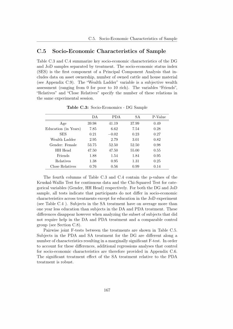
C.5. Socio-Economic Characteristics of Sample

C.5 Socio-Economic Characteristics of Sample

Table C.3 and C.4 summarize key socio-economic characteristics of the DGand JoD samples separated by treatment. The socio-economic status index(SES) is the first component of a Principal Component Analysis that in-cludes data on asset ownership, number of owned cattle and house material(see Appendix C.9). The “Wealth Ladder” variable is a subjective wealthassessment (ranging from 0 for poor to 10 rich). The variables “Friends”,“Relatives” and “Close Relatives” specify the number of these relations inthe same experimental session.

Table C.3: Socio-Economics - DG Sample

DA PDA SA P-Value

Age 39.98 41.19 37.99 0.49

Education (in Years) 7.85 6.62 7.54 0.28

SES 0.21 −0.02 0.23 0.27

Wealth Ladder 2.95 2.79 3.01 0.82

Gender: Female 53.75 52.50 52.50 0.98

HH Head 47.50 47.50 55.00 0.55

Friends 1.88 1.54 1.84 0.95

Relatives 1.38 0.95 1.31 0.25

Close Relatives 0.76 0.56 0.99 0.14

The fourth columns of Table C.3 and C.4 contain the p-values of theKruskal-Wallis Test for continuous data and the Chi-Squared Test for cate-gorical variables (Gender, HH Head) respectively. For both the DG and JoDsample, all tests indicate that participants do not differ in socio-economiccharacteristics across treatments except for education in the JoD experiment(see Table C.4 ). Subjects in the SA treatment have on average more thanone year less education than subjects in the DA and PDA treatment. Thesedifferences disappear however when analyzing the subset of subjects that didnot require help in the DA and PDA treatment and a comparable controlgroup (see Section C.8).

Pairwise joint F-tests between the treatments are shown in Table C.5.Subjects in the PDA and SA treatment for the DG are different along anumber of characteristics resulting in a marginally significant F-test. In orderto account for these differences, additional regressions analyses that controlfor socio-economic characteristics are therefore provided in Appendix C.6.The significant treatment effect of the SA treatment relative to the PDAtreatment is robust.

167

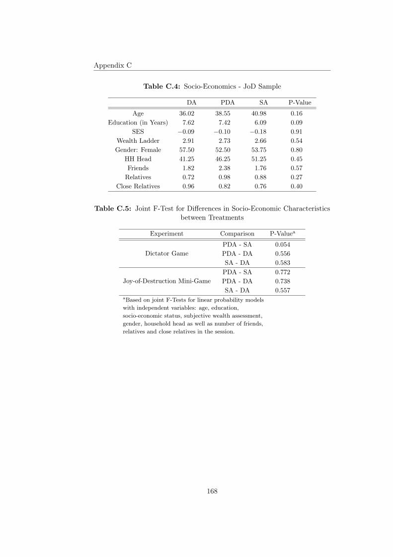
Appendix C

Table C.4: Socio-Economics - JoD Sample

DA PDA SA P-Value

Age 36.02 38.55 40.98 0.16

Education (in Years) 7.62 7.42 6.09 0.09

SES −0.09 −0.10 −0.18 0.91

Wealth Ladder 2.91 2.73 2.66 0.54

Gender: Female 57.50 52.50 53.75 0.80

HH Head 41.25 46.25 51.25 0.45

Friends 1.82 2.38 1.76 0.57

Relatives 0.72 0.98 0.88 0.27

Close Relatives 0.96 0.82 0.76 0.40

Table C.5: Joint F-Test for Differences in Socio-Economic Characteristicsbetween Treatments

Experiment Comparison P-Valuea

Dictator GamePDA - SA 0.054PDA - DA 0.556SA - DA 0.583

Joy-of-Destruction Mini-GamePDA - SA 0.772PDA - DA 0.738SA - DA 0.557

aBased on joint F-Tests for linear probability modelswith independent variables: age, education,socio-economic status, subjective wealth assessment,gender, household head as well as number of friends,relatives and close relatives in the session.

168

C.6. Regression Analyses

C.6 Regression Analyses

Table C.6: Regression Results - Dictator Game

Dependent variable:Transfer Amount Transfer (Yes/No)OLS Tobit Probita

(1) (2) (3)

PDA −0.446 −1.725 −0.044(1.567) (3.907) (0.079)

SA 2.804∗ 7.030∗ 0.157∗∗

(1.647) (3.666) (0.079)

Intercept 5.696∗∗∗ −5.511∗

(1.061) (3.095)

Observations 239 239 239R2 0.019

Adjusted R2 0.011∗∗∗p < 0.01, ∗∗p < 0.05, ∗p < 0.1; Robust standard errorsin parantheses; a Binary Dependent Variable (No Transfer/Transfer), Marginal effects

Table C.7: Robustness Check - Dictator Game

Dependent variable:Transfer

Robust Regression Quantile (Median) Regression(1) (2)

PDA −0.086 0.000

(−0.08) (0.00)

SA 2.044∗ 10.000∗∗∗

(1.84) (3.95)

Observations 239 239∗∗∗p < 0.01, ∗∗p < 0.05, ∗p < 0.1; Marginal effects; t statis-tics in parentheses; Robust Regression based on "rreg" Statafunction and Quantile Regression based on "qreg" Stata func-tion

169

Appendix C

Table C.8: Regression Results Dictator Game - SA and PDA Treatmentwith Socio-Economic Controls

Dependent variable:Transfer Amount Transfer (Yes/No)

OLS Probita

(1) (2)

SA 3.567∗∗ 0.225∗∗∗

(1.629) (0.083)

Age 0.122 0.004

(0.080) (0.004)

Education (years) 0.435 0.010

(0.264) (0.012)

Socio-Economic Status −0.618 −0.047(1.245) (0.055)

Subjective Wealth 0.289 0.044

(0.488) (0.029)

Gender: Male −1.414 0.060

(1.882) (0.087)

Household Head −0.441 0.064

(2.140) (0.109)

Friends in Session 0.406 0.007

(0.476) (0.021)

Relatives in Session −0.292 0.010

(0.480) (0.029)

Close Relatives in Session −0.332 −0.007(0.628) (0.040)

Intercept −2.846(4.325)

Observations 155 155R2 0.058

Adjusted R2 −0.007∗∗∗p < 0.01, ∗∗p < 0.05, ∗p < 0.1; Robust standard errorsin parantheses; a Binary Dependent Variable (No Transfer/Transfer), Marginal effects

170

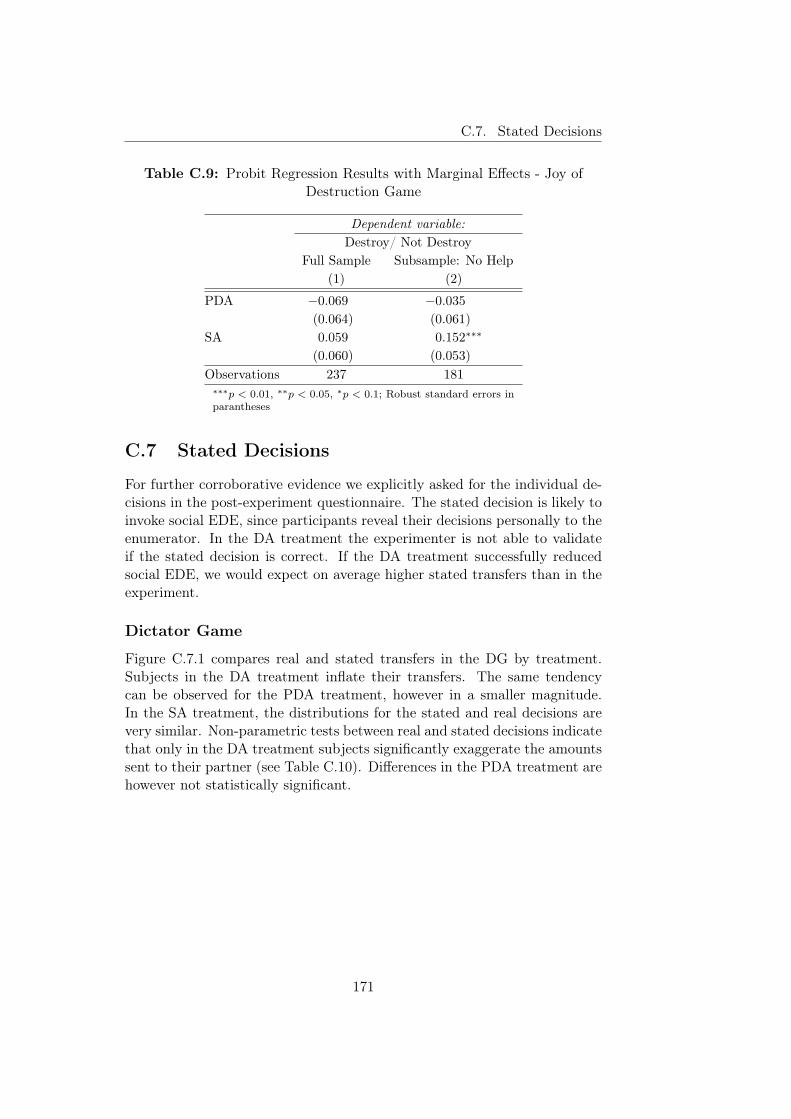
C.7. Stated Decisions

Table C.9: Probit Regression Results with Marginal Effects - Joy ofDestruction Game

Dependent variable:Destroy/ Not Destroy

Full Sample Subsample: No Help(1) (2)

PDA −0.069 −0.035(0.064) (0.061)

SA 0.059 0.152∗∗∗

(0.060) (0.053)

Observations 237 181∗∗∗p < 0.01, ∗∗p < 0.05, ∗p < 0.1; Robust standard errors inparantheses

C.7 Stated Decisions

For further corroborative evidence we explicitly asked for the individual de-cisions in the post-experiment questionnaire. The stated decision is likely toinvoke social EDE, since participants reveal their decisions personally to theenumerator. In the DA treatment the experimenter is not able to validateif the stated decision is correct. If the DA treatment successfully reducedsocial EDE, we would expect on average higher stated transfers than in theexperiment.

Dictator Game

Figure C.7.1 compares real and stated transfers in the DG by treatment.Subjects in the DA treatment inflate their transfers. The same tendencycan be observed for the PDA treatment, however in a smaller magnitude.In the SA treatment, the distributions for the stated and real decisions arevery similar. Non-parametric tests between real and stated decisions indicatethat only in the DA treatment subjects significantly exaggerate the amountssent to their partner (see Table C.10). Differences in the PDA treatment arehowever not statistically significant.

171

Appendix C

Figure C.7.1: Dictator Game: Real and Stated Transfers by Treatment

Table C.10: Mann-Whitney-U-Tests Between Stated and Real Transfersby Treatment - DG Game

TreatmentAverageTransfersStated

AverageTransfers

RealP-Value

Double Anonymous 8.451 5.696 0.021

Pseudo DoubleAnonymous 6.329 5.250 0.313

Single Anonymous 8.875 8.500 0.789

Joy-of-Destruction Mini-Game

Similar to the DG, we asked subjects in the JoD during the post-experimentquestionnaire for their decision in the experiment. The distribution of realand stated decisions by treatment for the full sample is shown in Figure C.7.2.In contrast to the DG, we find however no significant differences betweenstated and real decisions for the three different treatments (see Table C.10).These results also hold for the reduced dataset (see Figure C.7.3, Table C.12)

172

C.7. Stated Decisions

Figure C.7.2: JoD Game: Real and Stated Decisions by Treatment (FullSample)

Table C.11: Fisher’s Exact Test Between Stated and Real Decisions byTreatment - JoD Game - Full Sample

TreatmentShare

ReducedStated

ShareReducedReal

P-Value

Double Anonymous 19.481 17.949 0.839

Pseudo DoubleAnonymous 21.622 25.316 0.703

Single Anonymous 13.333 12.500 1.000

Table C.12: Fisher’s Exact Test Between Stated and Real Decisions byTreatment - JoD Game - Reduced Sample

TreatmentShare

ReducedStated

ShareReducedReal

P-Value

Double Anonymous 17.910 19.355 1.000

Pseudo DoubleAnonymous 21.053 23.729 0.825

Single Anonymous 10.169 5.000 0.322

173

Appendix C

Figure C.7.3: JoD Game: Real and Stated Decisions by Treatment(Reduced Sample)

174

C.8. Prediction of Probabilities for Receiving Help

C.8 Prediction of Probabilities for Receiving Help

The PDA and DA procedure in the JoD included keys and boxes to concealthe individual decisions to the experimenter. In both treatments roughly23% of subjects required help. In order to create a similar control group forthe SA treatment, which did not involve any boxes and keys, we estimateda probit model for the probability to require help (see Table C.13). Overall,80 respondents in the PDA procedure used boxes and their identity can belinked with the socio-economic survey data. These observations are includedin the model. We find that education has a strong and significant impacton the likelihood to require help. Older participants are also more likely torequire help. In addition, subjects who appeared drunk to the experimentwere more likely to require help. The sessions were implemented in theafternoon. The randomized invitation to the experiment was however donein the morning, so that 5 out of 240 subjects showed up drunk. Due to therelatively low share, we do not think that it substantially affects our findings.

Table C.13: Probit Regression Results for Receiving Help (with MarginalEffects)

Dependent variable:Received Help (Yes/No)

Education (in Years) −0.046∗∗∗

(0.018)

Age 0.012∗

(0.007)

Male −0.063(0.099)

HH Head −0.048(0.153)

Socio-Economic Status 0.110

(0.086)

Drunk 0.887∗∗∗

(0.045)

Observations 80Log Likelihood −24.409Akaike Inf. Crit. 62.819∗∗∗p < 0.01, ∗∗p < 0.05, ∗p < 0.1; Robust standarderrors in parantheses

175

Appendix C

Figure C.8.1: Frequency of Predicted Probabilities for Receiving Help

The final probit model was then used to predict the probability for sub-jects in the SA treatment to require help. The frequency of predicted prob-abilities is shown in Figure C.8.1. We opted to exclude subjects with aprobability of p > 0.7 from the SA treatment. While this threshold is tosome extent chosen arbitrarily, it results in 20 out of 80 subjects to be ex-cluded. This corresponds to a similar share of exclusions as in the other twotreatments. Table C.14 shows socio-economic characteristics of subjects inthe PDA and DA treatment who did not receive help and of all subjects inthe SA treatment. Kruskal-Wallis Tests indicate that SA subjects are signif-icantly older and less educated than subjects in the PDA and DA treatment,because older and less educated subjects have required more likely help.After constructing a similar control group for the SA treatment, Kruskal-Wallis Tests find however no significant differences between treatments withrespect to socio-economic observables (see Table C.15). This indicates thatour method of constructing a similar control group with the SA treatmentwas relatively successful. Pairwise joint F-tests between the treatments in-dicate however that subjects are not significantly different from each otherboth in the reduced sample and when excluding only subjects who receivedhelp in the PDA and DA treatment (see Table C.16). Nevertheless, we can-not rule out that subjects in these treatments differ concerning unobservablecharacteristics.

176

C.8. Prediction of Probabilities for Receiving Help

Table C.14: Socio-Economics - JoD Sample (DA, PDA: No Help; SA: FullSample)

DA PDA SA P-Value

Age 33.90 34.29 40.98 0.03

Education (in Years) 8.06 8.92 6.09 0.00

SES −0.05 −0.08 −0.18 0.80

Wealth Ladder 2.96 2.88 2.66 0.49

Gender: Female 59.42 49.15 53.75 0.50

HH Head 36.23 38.98 51.25 0.14

Friends 1.90 1.95 1.76 0.83

Relatives 0.71 0.97 0.88 0.36

Close Relatives 0.99 0.66 0.76 0.19

Table C.15: Socio-Economics - JoD Sample (No Help)

DA PDA SA P-Value

Age 33.90 34.29 34.50 0.84

Education (in Years) 8.06 8.92 7.88 0.51

SES −0.05 −0.08 −0.20 0.52

Wealth Ladder 2.96 2.88 2.75 0.66

Gender: Female 59.42 49.15 56.67 0.49

HH Head 36.23 38.98 40.00 0.90

Friends 1.90 1.95 1.57 0.59

Relatives 0.71 0.97 0.83 0.39

Close Relatives 0.99 0.66 0.67 0.16

177

Appendix C

Table C.16: Joint F-Tests for Differences in Socio-EconomicCharacteristics between Treatments for Reduced Sample

Sample Comparison P-Valuea

Reduced: DA, PDA, SAPDA - SA 0.963PDA - DA 0.454SA - DA 0.883

Reduced: DA, PDA; Full: SAPDA - SA 0.141PDA - DA 0.454SA - DA 0.174

aBased on joint F-Tests for linear probability modelswith independent variables: age, education,socio-economic status, subjective wealth assessment,gender, household head as well as number of friends,relatives and close relatives in the session.

178

C.9. Socio-Economic Status Index

C.9 Socio-Economic Status Index

The socio-economic status (SES) index was derived as the first component ofa Principal Component Analysis, comprising variables that cover householdassets, housing quality and cattle ownership. The first principal componentcaptures 23% of the overall variance in the data. Table C.17 shows sum-mary statistics for all variables and their respective loadings. Table C.18summarizes the average SES scores and the respective variable means forthe quantiles of the SES index.

Table C.17: Summary Statistics and Loadings for Socio-Economic StatusVariables

Type Average/Share

StandardDeviation

Loading

Household AssetsMobile Phone Dummy 0.860 0.286

Radio Dummy 0.519 0.491TV Dummy 0.212 0.750

Refrigerator Dummy 0.198 0.771Vehicle Dummy 0.113 0.648

Housing MaterialBricks Dummy 0.013 0.102

Cement/Plaster Dummy 0.027 0.403Corrugated Iron Dummy 0.217 0.402

Soil Dummy 0.615 -0.388Livestock Ownership

Cattle Number 5.398 15.500 0.397

179

Chapter C

Table C.18: Socio-Economic Variable Means by SES Quantiles

Quantile Poorest Second Third Fourth Richest

Average SES Score -0.90 -0.54 -0.28 0.24 1.70Share of Households with Assets

Mobile Phone 0.68 0.82 0.97 0.96 0.97Radio 0.00 0.60 0.57 0.73 0.87TV 0.00 0.00 0.00 0.26 0.80

Refrigerator 0.00 0.00 0.00 0.19 0.80Vehicle 0.00 0.00 0.00 0.08 0.49

Share of Households with Housing MaterialBricks 0.00 0.01 0.00 0.03 0.03

Cement/Plaster 0.00 0.00 0.00 0.02 0.12Corrugated Iron 0.00 0.05 0.38 0.37 0.45

Soil 0.87 0.72 0.53 0.42 0.39Average Number of Owned Livestock

Cattle 0.00 1.94 5.88 6.17 15.37

180