Three Essays on Bank Credit and Resource Allocation

École des Hautes Études en Sciences Sociales

École doctorale d’Économie de Paris

Paris-Jourdan Sciences Économiques – École d’Économie de Paris

Analyse et Politique Économiques

Discipline : Sciences Économiques

THIBAULT LIBERT

T h r e e E s s a y s o n B a n k C r e d i t a n d

R e s o u r c e A l l o c a t i o n

Thèse dirigée par: Xavier Ragot

Date de soutenance : le 27 novembre 2019

Rapporteurs 1 Johan Hombert, HEC Paris

2 Isabelle Méjean, École Polytechnique

Jury 1 Flora Bellone, Université Côte d’Azur

2 Christophe Cahn, Banque de France

3 Laurent Clerc, ACPR

4 Xavier Ragot, Sciences Po Paris

Remerciements

Une these est un chemin long et eprouvant. Au moment de clore ce chapitre, et apres

presque cinq annees qui auront vu s’alterner les phases d’exaltation et de decouragement, j’ai

la l’occasion d’exprimer ma reconnaissance envers les personnes qui m’ont accompagne, guide

et soutenu.

Mes premiers remerciements sont naturellement adresses a Xavier Ragot, mon directeur de

these. J’ai rencontre Xavier au cours de mes etudes a l’Ecole d’Economie de Paris. Il a supervise

mes travaux lorsque j’ai redige mon memoire en deuxieme annee de master, et a ensuite accepte

de diriger ma these de doctorat. Il a joue un role primordial tout au long de mon parcours, en

m’orientant vers un poste de doctorant en contrat Cifre a la Banque de France, puis en suivant

avec bienveillance l’evolution de mes recherches et en me remettant dans le droit chemin lorsque

j’en avais besoin. Je remercie egalement Flora Bellone, qui a fait partie de mon comite de these

et m’a fait profiter de ses conseils, ainsi qu’Isabelle Mejean et Johan Hombert, qui ont accepte

d’etre les rapporteurs de cette these et ont contribue a ameliorer mes travaux par la pertinence

de leurs remarques.

La premiere partie de ce doctorat a ete realisee a l’observatoire des entreprises de la Banque

de France, sous la supervision de Christophe Cahn. Christophe a guide mes premiers pas

dans les arcanes de cette venerable institution, m’a laisse deambuler en chaussettes dans les

couloirs, et m’a pousse a publier le second chapitre de cette these en document de travail,

malgre ma passivite legendaire. J’adresse egalement mes plus chaleureux remerciements a mes

collegues de l’observatoire, en premier lieu a Benjamin Bureau, qui a partage mon bureau

pendant plus de deux ans, mais aussi a Frederic Vinas, Adrien Boileau, Matthias Burker, Louis-

Marie Harpedanne de Belleville, et plus generalement a l’ensemble des membres du service, qui

ont rendu mon passage parmi eux agreable et fructueux.

J’ai ensuite poursuivi mes travaux au sein du service d’analyse des risques bancaires de

l’ACPR. J’y ai notamment ecrit le troisieme chapitre de cette these, en collaboration avec Paul

Beaumont, qui m’aura grandement aide a conclure ce doctorat et a qui je dois indeniablement

une fiere chandelle. Je profite de ces quelques lignes pour lui exprimer toute ma reconnaissance.

Je remercie egalement mon deuxieme co-auteur, Christophe Hurlin, ainsi que l’ensemble de

mes collegues et amis de l’ACPR, notamment les membres emerites de ce pole d’elite qu’est le

2

PST/PJaC: Boubacar Camara, Lucas Vernet, Sylvain Peyron, Tamaki Descombes et notre raıs

a nous, Jean-Luc Thevenon. Camille Lambert-Girault, Oana Toader, Sebastien Diot, Clement

Torres, Justine Pedrono, George Overton, Sandrine Lecarpentier, Mathias Le et Eric Vansteen-

berghe ont chacun contribue a egayer mon quotidien. Cette liste est probablement incomplete,

et nombreux sont ceux qui meriteraient d’y figurer. Je remercie egalement Laurent Clerc, qui a

accepte de faire partie du jury de cette these et a suivi avec attention l’evolution de nos travaux.

Au dela des personnes rencontrees au sein de mes differents services, j’ai noue de belles

amities tout au long de ce doctorat. Je remercie naturellement les doctorants Cifre de la

Banque de France, en particulier Simon Ray, Charlotte Sandoz, Giulia Aliprandi et Timothee

Gigout-Magiorani. Merci egalement a la taverne du croissant, au cafe blanc et aux deux ecus

pour avoir fourni les innombrables litres de bieres engloutis en compagnie de mes amis Theo

Nicolas, Brendan Vannier, David Gauthier, Francois Robin, Kevin Parra-Ramirez et Mikael

Beatriz. Refaire le monde en leur compagnie aura sans doute ete le plus bel accomplissement

de ce doctorat.

J’exprime enfin toute ma gratitude a ma famille, Nathalie, Olivier, Martin, Tiana et Mar-

guerite, qui m’ont toujours encourage malgre le caractere hautement obscur et esoterique de

mes elucubrations economiques. Mes derniers remerciements vont a ma compagne, Barbara,

soutien tendre et indefectible, dont je m’efforce d’illuminer la vie autant qu’elle illumine la

mienne. Cette these lui est dediee.

3

Resume

De maniere generale, cette these vise a evaluer dans quelle mesure l’heterogeneite mi-

croeconomique influence les tendances et fluctuations des agregats macroeconomiques, en par-

ticulier le credit bancaire, la productivite, et l’interaction entre ces deux variables.

La premiere partie de la these est motivee par la faiblesse de la croissance de la productivite

globale des facteurs (PGF) observee post crise dans la plupart des pays developpes. Cette partie

etudie l’evolution et les caracteristiques de l’allocation des ressources dans le secteur manufac-

turier francais avant, pendant, et apres la Grande Recession. L’inefficacite de l’allocation des

facteurs a freine la croissance de la productivite au cours de la decennie qui a precede la crise.

Elle explique egalement une part significative des fluctuations observees pendant la Grande

Recession, l’interaction entre les inefficiences de l’allocation du facteur capital et du facteur

travail jouant un role majeur. Par ailleurs, le ralentissement post crise semble etre principale-

ment du a l’atonie de la croissance de la productivite individuelle des firmes, plutot qu’a une

deterioration de l’efficacite de l’allocation des ressources.

La deuxieme partie de la these etudie comment la structure granulaire de la distribution

des prets aux entreprises en France faconne le caractere cyclique du credit bancaire agrege.

Les chocs de credit microeconomiques affectant les plus gros emprunteurs sont pour une large

part a l’origine de cette correlation, alors que les chocs individuels specifiques aux banques

n’y contribuent pas de maniere significative. Cela suggere qu’au niveau macroeconomique les

mecanismes propres aux emprunteurs granulaires dominent l’effet des frictions financieres qui

pourraient contraindre les entreprises plus petites, ainsi que le canal du bilan des banques. La

forte concentration observee dans la distribution des emprunteurs affecte egalement les flux de

liquidite des banques: elle restreint la diversification et conduit a une synchronisation accrue

des lignes de credit.

La troisieme partie de la these relie la repartition des facteurs a l’allocation du credit.

Cette partie suggere que la propension des banques a preter a des entreprises saines a ete

significativement reduite tant pendant la crise de 2007-2009 que pendant la crise de la zone

Euro. Les chocs bancaires impactent l’activite reelle des entreprises; cette reduction a ainsi

contribue a diminuer l’ecart d’investissement entre les entreprises de bonne qualite et celles de

qualite inferieure, ce qui a eu tendance a orienter le facteur capital vers des firmes qui etaient plus

4

risquees et moins productives. L’augmentation soudaine des inefficiences liees a une mauvaise

allocation du capital observee en temps de crise peut donc refleter des perturbations affectant

l’allocation du credit.

Mots cles: Productivite; Allocation des facteurs de production; Granularite; Credit bancaire;

Heterogeneite microeconomique.

5

Abstract

From a broad perspective, this thesis aims at exploring the extent to which microeconomic

heterogenity shapes the trends and fluctuations of aggregate outcomes, by focusing on bank

credit, productivity, and the interaction between these two variables.

The first part of the thesis is motivated by the weakness of the total factor productivity

(TFP) growth observed post-crisis in most developed countries. It examines the evolution

and characteristics of resource misallocation in the French manufacturing sector before, during,

and after the Great Recession. The inefficiency of the input allocation dampened productivity

growth in the lead-up to the crisis. It also accounts for a sizeable part of the disruptions observed

during the Great Recession, with the interplay between labor and capital misallocation playing

a major role. On the other hand, the post-crisis slowdown appears to be mostly driven by the

sluggishness of the firm-level TFP growth, rather than by a worsening of resource misallocation.

The second part of the thesis examines how the granular structure of the loan distribution

in France shapes the cyclicality of aggregate bank credit lent to non-financial corporations.

Microeconomic credit shocks affecting the largest borrowers largely drive this comovement,

while bank individual shocks do not contribute significantly. It suggests that at the macro level

mechanisms specific to the granular borrowers dominate both the effect of the financial frictions

constraining smaller firms and the bank lending channel. The high level of concentration on

the borrower side also affects bank liquidity flows: it leads credit line takedowns to be less

diversifiable and more synchronized.

The third part of the thesis relates input allocation to credit allocation. It suggests that the

propensity of banks to lend to healthy firms was significantly reduced during both the 2007-2009

crisis and the Eurozone crisis. As bank lending shocks affect firm-level real outcomes, this re-

duction contributed to decrease the investment gap between high-quality and low-quality firms,

thereby directing capital input towards companies that were more risky and less productive.

The surge in capital misallocation observed in time of crisis may therefore reflect disruptions

affecting credit allocation.

Key words: Productivity; Input allocation; Granularity; Bank credit; Microeconomic hetero-

geneity.

6

Contents

Remerciements 2

Resume 4

Abstract 6

Contents 7

List of Figures 10

List of Tables 12

1 General Introduction 14

1.1 The great productivity slowdown . . . . . . . . . . . . . . . . . . . . . . . . . . . 14

1.2 Misallocation before, during, and after the Great Recession . . . . . . . . . . . . 18

1.3 Granular borrowers . . . . . . . . . . . . . . . . . . . . . . . . . . . . . . . . . . . 21

1.4 Bank lending shocks, credit allocation, and capital allocation . . . . . . . . . . . 25

2 Misallocation before, during, and after the Great Recession 28

2.1 Introduction . . . . . . . . . . . . . . . . . . . . . . . . . . . . . . . . . . . . . . . 29

2.2 Theoretical framework . . . . . . . . . . . . . . . . . . . . . . . . . . . . . . . . . 33

2.2.1 The efficient allocation . . . . . . . . . . . . . . . . . . . . . . . . . . . . . 33

2.2.2 Production functions and output aggregators . . . . . . . . . . . . . . . . 35

2.2.3 Capital, labor and the log-normality assumption . . . . . . . . . . . . . . 37

2.2.4 Misallocation and aggregate TFP . . . . . . . . . . . . . . . . . . . . . . . 39

2.3 Data . . . . . . . . . . . . . . . . . . . . . . . . . . . . . . . . . . . . . . . . . . . 40

2.3.1 Data description . . . . . . . . . . . . . . . . . . . . . . . . . . . . . . . . 40

2.3.2 Estimation of the parameters . . . . . . . . . . . . . . . . . . . . . . . . . 43

7

2.4 Empirical results . . . . . . . . . . . . . . . . . . . . . . . . . . . . . . . . . . . . 44

2.4.1 Distortions and firm characteristics . . . . . . . . . . . . . . . . . . . . . . 44

2.4.2 Misallocation and contribution to the variations in TFP . . . . . . . . . . 47

2.5 Robustness checks . . . . . . . . . . . . . . . . . . . . . . . . . . . . . . . . . . . 52

2.6 Conclusion . . . . . . . . . . . . . . . . . . . . . . . . . . . . . . . . . . . . . . . 53

2.7 Tables and figures . . . . . . . . . . . . . . . . . . . . . . . . . . . . . . . . . . . 55

2.8 The log-normality assumption . . . . . . . . . . . . . . . . . . . . . . . . . . . . . 63

2.9 Sector-specific elasticities of substitution . . . . . . . . . . . . . . . . . . . . . . . 65

3 Granular Borrowers 67

3.1 Introduction . . . . . . . . . . . . . . . . . . . . . . . . . . . . . . . . . . . . . . . 68

3.2 Granular borrowers . . . . . . . . . . . . . . . . . . . . . . . . . . . . . . . . . . . 72

3.2.1 Presentation of the data set . . . . . . . . . . . . . . . . . . . . . . . . . . 72

3.2.2 Credit concentration: evidence at the bank and aggregate level . . . . . . 75

3.3 Estimating firm and bank shocks . . . . . . . . . . . . . . . . . . . . . . . . . . . 76

3.3.1 Presentation of the methodology . . . . . . . . . . . . . . . . . . . . . . . 76

3.3.2 Single- and multiple-bank borrowers . . . . . . . . . . . . . . . . . . . . . 79

3.3.3 Aggregation and normalization of the shocks . . . . . . . . . . . . . . . . 80

3.3.4 External validation of the firm components . . . . . . . . . . . . . . . . . 81

3.4 Granular borrowers and the cyclicality of aggregate credit . . . . . . . . . . . . . 83

3.4.1 Granularity and cyclicality . . . . . . . . . . . . . . . . . . . . . . . . . . 83

3.4.2 Dissecting the cyclicality of aggregate credit . . . . . . . . . . . . . . . . . 84

3.4.3 Granular shocks and granular trends . . . . . . . . . . . . . . . . . . . . . 87

3.4.4 Robustness checks . . . . . . . . . . . . . . . . . . . . . . . . . . . . . . . 88

3.5 Bank liquidity risk and borrower concentration . . . . . . . . . . . . . . . . . . . 93

3.5.1 Can banks pool borrower idiosyncratic risk? . . . . . . . . . . . . . . . . . 93

3.5.2 Borrower concentration as a source of synchronization . . . . . . . . . . . 95

3.6 Conclusion . . . . . . . . . . . . . . . . . . . . . . . . . . . . . . . . . . . . . . . 96

3.7 Tables and figures . . . . . . . . . . . . . . . . . . . . . . . . . . . . . . . . . . . 98

4 Bank lending shocks, credit allocation, and capital allocation 118

4.1 Introduction . . . . . . . . . . . . . . . . . . . . . . . . . . . . . . . . . . . . . . . 119

4.2 Data . . . . . . . . . . . . . . . . . . . . . . . . . . . . . . . . . . . . . . . . . . . 123

8

4.3 Estimation of bank credit shocks . . . . . . . . . . . . . . . . . . . . . . . . . . . 124

4.4 Main variables and descriptive statistics . . . . . . . . . . . . . . . . . . . . . . . 128

4.5 Results . . . . . . . . . . . . . . . . . . . . . . . . . . . . . . . . . . . . . . . . . . 131

4.5.1 Aggregate bank shocks and credit allocation . . . . . . . . . . . . . . . . . 131

4.5.2 Average real effects of bank shocks on firm-level outcomes . . . . . . . . . 132

4.5.3 From credit allocation to resource allocation . . . . . . . . . . . . . . . . . 134

4.6 Conclusion . . . . . . . . . . . . . . . . . . . . . . . . . . . . . . . . . . . . . . . 137

4.7 Figures . . . . . . . . . . . . . . . . . . . . . . . . . . . . . . . . . . . . . . . . . 138

4.8 Tables . . . . . . . . . . . . . . . . . . . . . . . . . . . . . . . . . . . . . . . . . . 143

Bibliography 147

9

List of Figures

1.1 Total Factor Productivity over time. . . . . . . . . . . . . . . . . . . . . . . . . . 15

2.1 Variation of misallocation over time . . . . . . . . . . . . . . . . . . . . . . . . . 49

2.2 Variation of misallocation over time, shutting down the entry-exit channel . . . . 55

2.3 Variation of misallocation over time, using wage bills to measure labor input . . 56

2.4 Variation of misallocation over time, defining sectors at the 2-digits level . . . . . 56

2.5 Variation of misallocation over time, keeping sectoral weights constant . . . . . . 57

2.6 Variation of misallocation over time, using sector-specific elasticities . . . . . . . 57

3.1 Coverage of the credit registry. . . . . . . . . . . . . . . . . . . . . . . . . . . . . 98

3.2 Sectoral repartition of credit (2007). . . . . . . . . . . . . . . . . . . . . . . . . . 101

(a) Long-term credit . . . . . . . . . . . . . . . . . . . . . . . . . . . . . . . . . 101

(b) Credit lines . . . . . . . . . . . . . . . . . . . . . . . . . . . . . . . . . . . . 101

3.3 Distribution of credit (banks). . . . . . . . . . . . . . . . . . . . . . . . . . . . . . 102

3.4 Distribution of credit (firms). . . . . . . . . . . . . . . . . . . . . . . . . . . . . . 103


(b) Credit lines . . . . . . . . . . . . . . . . . . . . . . . . . . . . . . . . . . . . 103

3.5 Concentration and volatility. . . . . . . . . . . . . . . . . . . . . . . . . . . . . . 104


(b) Credit lines . . . . . . . . . . . . . . . . . . . . . . . . . . . . . . . . . . . . 104

3.6 Single- and multiple-bank firms: aggregate variations. . . . . . . . . . . . . . . . 105


(b) Credit lines . . . . . . . . . . . . . . . . . . . . . . . . . . . . . . . . . . . . 105

(c) Long-term credit . . . . . . . . . . . . . . . . . . . . . . . . . . . . . . . . . 105

(d) Credit lines . . . . . . . . . . . . . . . . . . . . . . . . . . . . . . . . . . . . 105

3.7 Single- and multiple-bank firms: bank-level variations. . . . . . . . . . . . . . . . 106

10


(b) Credit lines . . . . . . . . . . . . . . . . . . . . . . . . . . . . . . . . . . . . 106

3.8 Time series of Macroq, Firmq and Bankq. . . . . . . . . . . . . . . . . . . . . . . 107

(a) Macroq . . . . . . . . . . . . . . . . . . . . . . . . . . . . . . . . . . . . . . 107

(b) Firmq . . . . . . . . . . . . . . . . . . . . . . . . . . . . . . . . . . . . . . . 107

(c) Bankq . . . . . . . . . . . . . . . . . . . . . . . . . . . . . . . . . . . . . . . 107

(d) ∆Creditq . . . . . . . . . . . . . . . . . . . . . . . . . . . . . . . . . . . . . 107

3.9 External validation of the firm components - graph. . . . . . . . . . . . . . . . . 108

3.10 Illustration of the role of granularity. . . . . . . . . . . . . . . . . . . . . . . . . . 111

4.1 Number of borrowing relationships . . . . . . . . . . . . . . . . . . . . . . . . . . 138

4.2 Share of firms by credit rating and by quarter . . . . . . . . . . . . . . . . . . . . 139

4.3 Average productivity by credit rating and by quarter . . . . . . . . . . . . . . . . 139

4.4 Bank shocks aggregated by firms credit rating, variation over time . . . . . . . . 140

4.5 Aggregate bank shock of firms rated A relative to firms rated C . . . . . . . . . . 141

4.6 Average investment rate by credit rating and by quarter . . . . . . . . . . . . . . 142

4.7 Average change in employment by credit rating and by quarter . . . . . . . . . . 142

11

List of Tables

2.1 Descriptive statistics, French manufacturing sector . . . . . . . . . . . . . . . . . 41

2.2 Coverage in FIBEN relative to INSEE, French manufacturing sector . . . . . . . 42

2.3 Firm characteristics by labor distortion quartiles . . . . . . . . . . . . . . . . . . 46

2.4 Firm characteristics by capital distortion quartiles . . . . . . . . . . . . . . . . . 46

2.5 Capital misallocation, labor misallocation and total misallocation by year . . . . 48

2.6 Changes in total misallocation and in its three components . . . . . . . . . . . . 50

2.7 Changes in total misallocation and in its three components, shutting down the

entry-exit channel . . . . . . . . . . . . . . . . . . . . . . . . . . . . . . . . . . . 58

2.8 Changes in total misallocation and in its three components, using wage bills to

measure labor input . . . . . . . . . . . . . . . . . . . . . . . . . . . . . . . . . . 59

2.9 Changes in total misallocation and in its three components, defining sectors at

the 2-digits level . . . . . . . . . . . . . . . . . . . . . . . . . . . . . . . . . . . . 60

2.10 Changes in total misallocation and in its three components, keeping sectoral

weights constant . . . . . . . . . . . . . . . . . . . . . . . . . . . . . . . . . . . . 61

2.11 Changes in total misallocation and in its three components, using sector-specific

elasticities . . . . . . . . . . . . . . . . . . . . . . . . . . . . . . . . . . . . . . . . 62

3.1 Descriptive statistics: firm-bank level. . . . . . . . . . . . . . . . . . . . . . . . . 99

3.2 Descriptive statistics: bank-level. . . . . . . . . . . . . . . . . . . . . . . . . . . . 99

3.3 Descriptive statistics: aggregate-level. . . . . . . . . . . . . . . . . . . . . . . . . 100

3.4 External validation of the firm components - regression results. . . . . . . . . . . 109

3.5 Decomposition of the cyclicality of aggregate credit. . . . . . . . . . . . . . . . . 109

3.6 Contribution of top borrowers. . . . . . . . . . . . . . . . . . . . . . . . . . . . . 110

3.7 Robustness checks I - Normalization, firm-bank relationships. . . . . . . . . . . . 112

3.8 Robustness checks II - Coverage, unit of observation. . . . . . . . . . . . . . . . . 113

12

3.9 Robustness checks III - Definition of firm individual shocks. . . . . . . . . . . . . 114

3.10 Robustness checks IV - OLS regression. . . . . . . . . . . . . . . . . . . . . . . . 115

3.11 Including single-bank firms : out-of-sample test. . . . . . . . . . . . . . . . . . . . 116

3.12 Bank exposure to borrower liquidity shocks. . . . . . . . . . . . . . . . . . . . . . 117

3.13 Synchronization and borrower shocks. . . . . . . . . . . . . . . . . . . . . . . . . 117

4.1 Descriptive statistics . . . . . . . . . . . . . . . . . . . . . . . . . . . . . . . . . . 143

4.2 Aggregate bank shocks and credit allocation . . . . . . . . . . . . . . . . . . . . . 144

4.3 Average real effects of bank credit shocks . . . . . . . . . . . . . . . . . . . . . . 145

4.4 Average real effects of bank credit shocks, alternative investment rates . . . . . . 146

4.5 Real effects of bank credit shocks, by category and by period . . . . . . . . . . . 147

13

Chapter 1

General Introduction

1.1 The great productivity slowdown

Paul Krugman started Chapter 1 of his 1990 book, “The Age of Diminished Expectations”,

by stating: “Productivity isn’t everything, but in the long run it is almost everything”. This

opinion is widely shared, as productivity has proven to be one of the main drivers improving

living standards over long spans of time. It explains why aggregate total factor productivity

(TFP), i.e the efficiency with which hours of labor and services provided by the stock of capital

are converted into aggregate real output, has long been a topic of intense interest for the

economics profession. It also explains why the sluggish productivity growth that has been

characterizing most developed economies since the global financial crisis is a subject of major

concern.

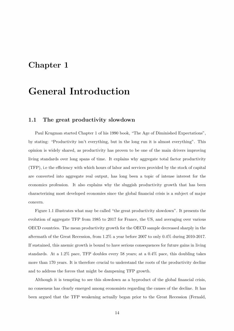
Figure 1.1 illustrates what may be called “the great productivity slowdown”. It presents the

evolution of aggregate TFP from 1985 to 2017 for France, the US, and averaging over various

OECD countries. The mean productivity growth for the OECD sample decreased sharply in the

aftermath of the Great Recession, from 1.2% a year before 2007 to only 0.4% during 2010-2017.

If sustained, this anemic growth is bound to have serious consequences for future gains in living

standards. At a 1.2% pace, TFP doubles every 58 years; at a 0.4% pace, this doubling takes

more than 170 years. It is therefore crucial to understand the roots of the productivity decline

and to address the forces that might be dampening TFP growth.

Although it is tempting to see this slowdown as a byproduct of the global financial crisis,

no consensus has clearly emerged among economists regarding the causes of the decline. It has

been argued that the TFP weakening actually began prior to the Great Recession (Fernald,

14

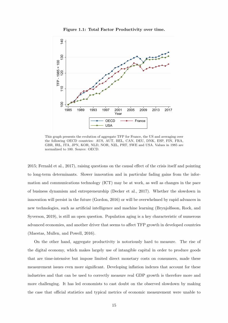
Figure 1.1: Total Factor Productivity over time.

100

110

120

130

140

TFP

- 19

85 =

100

1985 1989 1993 1997 2001 2005 2009 2013 2017Year

OECD FranceUSA

This graph presents the evolution of aggregate TFP for France, the US and averaging overthe following OECD countries: AUS, AUT, BEL, CAN, DEU, DNK, ESP, FIN, FRA,GBR, IRL, ITA, JPN, KOR, NLD, NOR, NZL, PRT, SWE and USA. Values in 1985 arenormalized to 100. Source: OECD.

2015; Fernald et al., 2017), raising questions on the causal effect of the crisis itself and pointing

to long-term determinants. Slower innovation and in particular fading gains from the infor-

mation and communications technology (ICT) may be at work, as well as changes in the pace

of business dynamism and entrepreneurship (Decker et al., 2017). Whether the slowdown in

innovation will persist in the future (Gordon, 2016) or will be overwhelmed by rapid advances in

new technologies, such as artificial intelligence and machine learning (Brynjolfsson, Rock, and

Syverson, 2019), is still an open question. Population aging is a key characteristic of numerous

advanced economies, and another driver that seems to affect TFP growth in developed countries

(Maestas, Mullen, and Powell, 2016).

On the other hand, aggregate productivity is notoriously hard to measure. The rise of

the digital economy, which makes largely use of intangible capital in order to produce goods

that are time-intensive but impose limited direct monetary costs on consumers, made these

measurement issues even more significant. Developing inflation indexes that account for these

industries and that can be used to correctly measure real GDP growth is therefore more and

more challenging. It has led economists to cast doubt on the observed slowdown by making

the case that official statistics and typical metrics of economic measurement were unable to

15

capture the gains in productivity linked to the digital revolution. In other words, the decrease

in the growth rate of aggregate TFP could merely reflect an increase in measurement errors

due to the rapid transformation of the economy. Although the presence of effects causing an

underestimation or overestimation of macroeconomic growth is hardly deniable, recent papers

suggest that mismeasurement does not provide an explanation of the productivity puzzle. Byrne,

Fernald, and Reinsdorf (2016) argue that correcting for potential biases to US productivity

actually leaves the recent downshift in TFP growth little changed. Syverson (2017) finds that

the mismeasurement hypothesis would imply disproportionately large missing growth rates of

digital technology industries. Aghion et al. (2019a) show that missing growth due to the use

of price imputation by statistical offices in case of creative destruction is substantial. On the

other hand, they find that it is an order of magnitude smaller than needed to account for the

slowdown in measured growth.

TFP growth has been undeniably dragged down by structural forces that were at work

before the global financial crisis. However, the abruptness and persistence of the slowdown that

appears in figure 1.1 makes it hard to blame exclusively long-term forces. As most recent papers

tend to suggest that measurement issues can hardly account for the bulk of the productivity

decline, one may legitimely wonder to which extent crisis-related factors play a role in the

post-crisis productivity trend (Adler et al., 2017).

The severe downturns that are typically associated to financial crisis episodes are usually

followed by large and persistent output losses (Cerra and Saxena, 2008). Adler et al. (2017)

show that these output losses reflect not only a persistent decline in employment growth and

accumulation of capital input, but also significant losses in TFP. The Great Recession makes no

exception in this regard, but the factors that may explain such sluggishness are still not entirely

understood. In order to get a glimpse of the determinants weakening macro productivity, it

is useful to see aggregate TFP growth as the result of three distinct channels. Assuming that

inputs are optimally allocated in a frictionless economy, it is quite intuitive to consider aggregate

productivity as the reflect of the firm-level TFP distribution. The evolution of this distribution

in the wake of the Great Recession is likely to provide some insights on the causes of the

disappointing economic recovery. The individual productivity distribution may be decomposed

into two components: (i) an extensive margin, corresponding to entries and exits of firms that

might be relatively more or less productive than incumbent companies, and (ii) an intensive

margin, representing the fact that the individual productivity of these incumbent firms might

16

itself be changing over time.

In other words, it could be the case that low TFP growth post-crisis is driven by highly

productive firms being forced to shut down their businesses, or conversely by low productivity

firms, which would have to stop their activities in normal times, being able to continue their

operations. It could also be driven by a wide firm-level decline in productivity, which would

then appear in macro-statistics.

Both margins have recently been explored by the economics literature. Decker et al. (2016)

present evidence that the US economy has seen a decline in high growth firms, and especially

high growth young firms. Although this trend decline started in the 2000s, it appears that

it continued after the crisis. Other studies focusing on Southern Europe countries show that

the weakening of the banking system during the crisis led banks to lend to risky and low-

productivity firms, therefore enabling these corporations, which would have been insolvent

otherwise, to continue their operations (Acharya et al., 2019).

Regarding the intensive margin, it has been argued that the severe tightening of credit

conditions during the crisis had a particularly strong impact on firms that already exhibited

financial fragilities (Duval, Hong, and Timmer, 2019). As a consequence these firms experienced

a highly persistent decline in post-crisis individual TFP. The underlying force that connect

financial frictions to weak productivity growth at the firm level has also be explored. One

channel through which these frictions affect total factor productivity is lower productivity-

enhancing investment, such as Research and Development expenditures. Because this type of

investment is often intangible, the corresponding assets may be harder to pledge as collateral

than other types of assets, as they are bound to be difficult to recover for the firm creditors

in case of default. Financing investment in intangible capital is therefore more costly than

financing tangible assets acquisition, and this difference widens in time of financial crisis (Garcia-

Macia, 2017). Hence, the lack of resources devoted to innovation activities could play a role in

dampening firm-level productivity and aggregate TFP.

An extensive and rapidly growing strand of research in the economics literature has focused

on the third channel affecting macro productivity, the efficiency of the allocation of factors

of production across firms and across sectors. As a matter of fact, for an unchanged firm-

level TFP distribution, allocating labor and capital to firms that are characterized by a weak

level of productivity creates output losses. These losses are then reflected by aggregate TFP,

because reallocating factors of production from low productivity firm to firms at the top of

17

the TFP distribution would improve aggregate output without necessarily increasing the total

stock of inputs used in the economy. Changes in macroeconomic efficiency does not simply

mirror changes in microeconomic efficiency: the great productivity slowdown could very well

reflect a growing deterioration of allocational efficiency triggered by the violent disruption that

affected the structures of the economy during the global financial crisis. Measuring what is

widely called “Misallocation” and assessing its evolution before, during and after the Great

Recession may shed some light on the post-crisis stagnation that has been characterizing most

developed countries. The second chapter of this thesis adresses this task.

1.2 Misallocation before, during, and after the Great Recession

Lionel Robbins famously wrote that “Economics is the science which studies human be-

haviour as a relationship between ends and scarce means which have alternative uses”. This

definition emphasizes the key insight of the misallocation literature: inputs are scarce resources

that are distributed across firms in order to produce, this distribution being itself the result

of various economic mechanisms interacting with each other. Because factors of production

may have alternative uses, i.e may be used by alternative production units, this allocation is

not necessarily the most efficient one: resources allocated to a given firm might be used in a

more effective manner by another company. The empirical branch of the misallocation liter-

ature therefore aims at answering the following questions: how efficient is the current input

distribution? By how much could we boost output by improving this allocation? How does

allocational efficiency evolve over time, and to which extent does this evolution contribute to

changes in aggregate productivity?

One way to measure the efficiency of the input allocation consists in elaborating a theoret-

ical framework which basically describes (i) the technology under which a given firm converts

its resources into output and (ii) the aggregation structure of the economy. This framework is

then used in order to characterize the optimal allocation, i.e the allocation which maximizes

aggregate production for a given stock of inputs. Misallocation can therefore be seen as a

thought experiment. By bringing the framework to the data one is able to compare the ob-

served aggregate output to the counterfactual level of production that would be obtained by

implementing the optimal allocation; in other words, allocational inefficiency is measured as

the macroeconomic loss in output (or equivalently TFP) that stems from the observed input

18

allocation (Hsieh and Klenow, 2009).

Let’s immediately clear up any misunderstanding: this thought experiment voluntarily takes

a normative point of view, because one needs a metric in order to be able to define what

“efficient” means and map input allocations into aggregate outcomes. On the other hand, the

framework which is specified is typically largely agnostic about the various forces that may

widen the gap between optimal and observed TFP. One may be tempted to see this gap as

reflecting frictions that drive the economy away from an idealistic free market economy. Such

interpretation would lead to incorrect conclusions. First, maximizing aggregate output is not

necessarily the only way to measure welfare. Second, recent papers show that forces such as

physical adjustment costs, which can hardly be controlled by public authorities, can very well

account for a large part of misallocation (Asker, Collard-Wexler, and De Loecker, 2014). From

an empirical point of view, misallocation should be seen as a decomposition that sheds light on

the fluctuations of aggregate TFP by identifying the part that is related to changes in input

allocation.

Although sensitive to measurement errors (Bils, Klenow, and Ruane, 2018), this method-

ology has proven to be a powerful tool, as it provides an analytical framework to think about

various economic issues. The recent misallocation literature started as a way to answer a long-

standing question in economics: why does income per capita differ so much across countries?

Even after adjusting for changes in the quantity of resources such as capital stock and labor

input, poor countries still produce much less than developed countries. It implies that differ-

ences in productivity are a key factor. The misallocation literature suggested that differences

in inputs allocation matter a lot, and explain to some degree why living standards largely differ

across countries. This strand of research then explored to which extent variations of misalloca-

tion over time, within a given country or a given sector, account for the sustained TFP gains in

time of growth, the sharp decline that is often observed during severe recessions, and the recent

TFP slowdown.

In the second chapter of this thesis I develop a framework in line with the seminal Hsieh

and Klenow (2009) methodology. I then apply this framework to a firm-level dataset covering

the bulk of the French manufacturing sector from 1990 to 2015. I focus on within-industry

misallocation: as a matter of fact, reallocating inputs across firms makes sense only if one is

willing to assume that these companies use factors of production that are relatively similar and

homogeneous. Claiming that one may increase global productivity by transfering specialized

19

workers from the car industry to the agrifood sector would be highly questionable. I therefore

consider the French manufacturing sector as an aggregation of narrowly-defined industries, and

use standard assumptions in order to express total misallocation as a weighted sum of measures

of sectoral allocational inefficiency.

I then provide an exact decomposition of misallocation as the sum of three distinct compo-

nents, respectively reflecting three sources of inefficiency. The first component represents the

effect of capital misallocation, i.e the inefficiency that would be observed at the aggregate level

if the labor input were optimally allocated. The second part represents labor misallocation, i.e

the loss in manufacturing TFP that can be related to distortions affecting the labor allocation,

under the assumption that the capital allocation is efficient. The third component reflects the

interaction between both types of input: because to some degree firms are able to substitute

between labor and capital, the loss in aggregate TFP is amplified when firms that suffer from

a lack of capital also suffer from a lack of labor.

Armed with this decomposition, I assess the contribution of misallocation and its three

components to the evolution of aggregate TFP in the manufacturing sector before, during,

and after the Great Recession. The main findings are the following: first, it appears that

misallocation increased steadily during the decade preceding the Great Recession. I estimate

that this gradual deterioration generated a loss in annual productivity growth of approximately

0.8 percentage points. In other words, if allocational efficiency had remained to its 1997 level,

2007’s manufacturing TFP would have been 8% higher. These losses are mainly related to an

increase in labor misallocation, except at the beginning of the 2000s, a period during which

capital misallocation played the main role. These results echo recent empirical studies which

show that countries in southern Europe experienced a significant increase in productivity losses

during the lead-up to the crisis (Gopinath et al., 2017).

Second, I find that misallocation substantially contributed to the sharp fall in aggregate

TFP that occurred during the Great Recession and to the improvement observed during its

immediate aftermath. I estimate that changes in allocational efficiency accounts for roughly

25% of the 2007-2009 decline and 20% of the 2010 recovery. Furthermore, I highlight a peculiar

characteristic of misallocation during the crisis. It turns out that the interplay between labor

and capital misallocation had a proncounced impact, while it is relatively stable the rest of the

time. As more and more papers build models that are designed to capture the fall in macro

TFP due to input misallocation in time of crisis, I argue that these models should incorporate

20

economic mechanisms that are able to replicate this characteristic. In particular, I sketch an

illustrative example which shows that when labor and capital are both dynamic inputs, models

that relate the crisis to an increase in microeconomic uncertainty (Bloom et al., 2018) lead to

productivity losses that are consistent with this empirical result.

Finally, I find that misallocation is rather stable post-crisis. In my theoretical framework the

part of macro TFP that is unrelated to input allocation is denoted “efficient” TFP and reflects

the aggregation of firm-level productivities. Because aggregate TFP growth was dampened by

an increase in misallocation before the crisis, one can deduce that efficient TFP was actually

growing faster than observed TFP. On the other hand, the fact that allocational inefficiency

does not contribute either positively or negatively after the crisis means that the sluggishness of

observed TFP growth mirrors the weakness of efficient TFP growth. It implies that compared

to the pre-crisis trend the decline was even more pronounced for efficient TFP, and therefore

suggests that focusing on mechanisms that affect within-firm productivity is key to understand

the great productivity slowdown.

From a broader point of view, this chapter falls within a recent and growing trend in macroe-

conomics, which states that much can be learned on aggregate outcomes by studying the per-

vasive heterogeneity which often characterizes microeconomic outcomes (Ghironi, 2018). The

increasing availability of large micro datasets goes hand in hand with an emerging consensus,

which argues that modern macroeconomics should not abstract from crucial features of micro

distributions. The third chapter of the thesis follows this path, and examines how the granular

structure of the loan distribution impacts the fluctuations of bank credit over the business cy-

cle, the correlation between financial flows and the real economy being the subject of a revived

interest since the global financial crisis.

1.3 Granular borrowers

Until recently the traditional macroeconomics literature used to appeal to aggregate shocks

in order to account for fluctuations and comovements between macroeconomic variables. Be-

cause large economies are composed of millions of individual agents on both the household and

the firm sides, idiosyncratic shocks independently affecting these entities or a very small frac-

tion of them were thought unable to drive aggregate volatility. The various “good” and “bad”

shocks that may randomly impact microeconomic agents were in this view bound to cancel out

21

when summing over a large number of actors.

This point of view has been challenged by papers which show that when the economy is

poorly diversified, i.e when only a few individuals account for a large fraction of the macroe-

conomic activity, idiosyncratic shocks do not necessarily average out. In a sense the presence

of very large entities offers a microfoundation for aggregate shocks, which may to some extent

be the reflect at the macro level of random shocks hitting microeconomic actors. For example,

Gabaix (2011) show that idiosyncratic movements of the largest 100 firms in the US explain

about one-third of variations in output growth. In the first part of this introduction I argued

that much can be learnt about aggregate productivity trends by looking at input distributions;

similarly, much can be learnt about the credit cycle that was so violently disrupted during the

global financial crisis by looking at loan distributions.

The third chapter of this thesis is a joint work with Paul Beaumont from Universite Paris-

Dauphine and Christophe Hurlin from Universite d’Orleans. We use a data set covering the

bulk of firm-bank relationships in France between 1999-Q1 and 2016-Q4 in order to examine the

granular structure of the loan distribution, and its implications for the cyclicality of bank credit.

The fact that the French credit market is dominated on the lender side by only a few very large

banks is well known and documented. We show that it is also characterized by a high level of

concentration on the borrower side, an empirical observation which has been to our knowledge

largely overlooked. More precisely, we find in our data set that the top 100 borrowers make

up on average for 18% of the total volume of long-term credit and 64% of the total amount

of undrawned credit lines. In technical terms, it suggests that the loan distribution on both

the bank and firm sides is “fat-tailed”. It also suggests that there is room for Gabaix (2011)’s

granular hypothesis: fluctuations of bank credit over the cycle may be driven by macroeconomic

shocks affecting every firms or every banks, but may also be attributable to shocks hitting only

a few very large banks or very large firms. We therefore aim at decomposing credit growth at

the aggregate level into macro trends and individual bank and firm components.

Distinguishing between these different drivers provides insights on the mechanisms that

could account for the correlation between aggregate credit and the business cycle. For example

it has been argued that this comovement reflects the financial accelerator, that is to say the view

that financial frictions can amplify the response of the economy to aggregate shocks (Bernanke,

Gertler, and Gilchrist, 1996). A recession may worsen financial conditions and impair firm’s

access to credit at a time when the need for external funds is rising, which in turn exacerbates the

22

downturn. A key implication is that small firms, which are likely to be financially constrained,

should experience reduced access to credit relative to large borrowers. In other words, small

borrowers’ credit shocks should be more cyclical and account for a sizeable part of the aggregate

comovement. Another source of aggregate credit fluctuations over the cycle is the bank lending

channel, which holds that monetary policy shocks work in part by affecting the supply of loans

granted by banks. This view examines to which extent higher interest rates or lower GDP

growth reduce loan granting, with a stronger effect for banks with low capital or liquidity

(Jimenez et al., 2012). Should this channel play an important role in shaping aggregate credit

cyclicality, one would fairly expect bank-level lending variations to capture a large part of the

comovement between aggregate credit and GDP.

We first focus on long-term credit, which accounts for the bulk of total credit in our data

set. We document a positive, strong relationship at the bank level between the concentration

of the portfolio of borrowers and the variance of the credit growth rate. It implies that banks

that are more likely to be sensitive to firms’ credit shocks also tend to be more volatile. Al-

though it suggests that the aggregation of borrowers’ individual shocks may contribute to credit

fluctuations, at least at the bank level, it could also be the case that bank specific variables

simultaneously drive the variance of its credit growth rate and the degree of diversification of

its borrower base. The main empirical challenge that we face therefore consists in separately

identifying credit variations originating from individual borrowers from changes in lending that

are bank related. We perform to that end a weighted linear regression of the credit growth at

the firm-bank level on a full set of bank-time and firm-time fixed effects, in line with Amiti and

Weinstein (2018). The two sets of fixed effects respectively identify (up to a constant term)

factors that simultaneously shift the evolution of credit in all the firm relationships of a bank

and in all the bank relationships of a firm. We define individual components as the deviation

of the estimated fixed effects from a common trend. In the end, aggregate credit variations can

be expressed as the sum of two terms, respectively reflecting the aggregation of firm and bank

components, and of a third term common to all lending relationships.

Our methodology allows to assess the respective contributions to the cyclicality of aggregate

credit of individual variations originating from the borrower and the lender side. Should the loan

size distribution of firms and banks not be fat-tailed, these contributions would be negligible and

the large majority of the correlation between credit and GDP would be explained by the macro

component. On the contrary, we find that firm shocks explain a sizeable part of the comovement

23

of aggregate credit with the business cycle. Individual bank variations, by contrast, do not seem

to significantly contribute to the correlation with GDP fluctuations. The skewness of the credit

distribution confers moreover a disproportionate importance to large borrowers compared to

the loan volume they represent, with more than two thirds of the contribution of firm shocks

originating from the top 100 borrowers. Our findings therefore question the macro significance

of the theories that relate fluctuations of credit over the cycle to financial frictions constraining

small firms or to the bank lending channel.

This empirical result does not solely reflect random, independent shocks individually af-

fecting the granular borrowers and driving the cyclicality of aggregate credit. For the top 100

firms we find that the individual components we estimate are significantly correlated to each

other. Although this correlation is low and close to zero, it is still sufficient to have a sizeable

effect on aggregate comovement. Our granular component therefore captures to some extent

trends that are common to this small set of granular borrowers, and which may represent for

example an easier access to other sources of external finance or lower financial constraints. It

is then the granular structure of the loan distribution, i.e the high share of the top 100 firms

in aggregate credit, which allows mechanisms specific to only a small number of firms to affect

macroeconomic fluctuations.

In the second part of this chapter we study the implications of the under-diversification of

the borrower bases on bank liquidity flows. When borrowers face idiosyncratic and diversifiable

credit line takedowns, banks can reallocate liquidity between liquidity-poor firms and firms

with excess liquidity. When credit line portfolios are concentrated, however, banks may have

to hold liquid assets to hedge against negative idiosyncratic shocks affecting very large firms.

Relying on our decomposition of credit variations, we estimate that in the absence of individual

borrower components the variance of credit lines at the bank level would fall on average by 18%

to 31%. The role of borrower shocks on credit line variations is therefore sizeable and similar

in magnitude to the contribution of the macro component, for instance. Since large firms have

credit commitments in multiple banks, borrower shocks may also increase aggregate variance

by making banks more correlated with each other. Consistently with this idea, we find that

the variance of the aggregate firm component is driven by the linkages that result from banks

granting credit lines to common borrowers and therefore being exposed to common shocks. This

result suggests that granular borrowers lead credit lines variations to be less diversifiable and

more synchronized between banks.

24

Our findings do not imply that bank lending shocks have no effects on the real economy; in

fact, numerous recent papers in the literature show that bank shocks affect real outcomes, both

at the aggregate and at the firm level. On the other hand, the second chapter of this thesis

shows that in time of crisis the deterioration of the efficiency of input allocation contributes to

a drop in aggregate productivity. The fourth chapter thus examines how bank-related shocks

impact credit allocation, and then how changes in credit allocation affect capital allocation

across firms.

1.4 Bank lending shocks, credit allocation, and capital alloca-

tion

Disruptions hitting the banking sector can dampen economic growth by inducing a contrac-

tion in credit supply (Chodorow-Reich, 2014). Firms that borrow from banks in worse financial

conditions may have difficulties in receiving new loans, expanding pre-existing ones, or may

have to borrow at higher interest rates. Furthermore, stickiness in borrower-lender relation-

ships implies that clients of weaker banks cannot easily turn to healthier institutions during

a crisis. Adverse conditions on the credit market are converted into a worsening of financial

constraints, which then translates into effects on real outcomes at the borrower level: affected

firms are typically found to decrease their investment rate, employment growth and output

growth. Banking shocks may also affect economic activity at higher levels of aggregation, for

example when a small number of financial institutions accounts for a large share of aggregate

lending (Amiti and Weinstein, 2018), or through indirect effects such as a decline in aggregate

demand (Huber, 2018): the reduction in employment by directly affected firms leads to a fall in

households’ consumption, which then may impact firms that were not constrained in the first

place.

Rather than looking at the direct firm-level or aggregate real effect, a related branch of

the literature has examined the role of misdirected bank lending in aggravating recessions and

prolonging stagnations. In this view, banks might have an incentive to provide subsidized

lending at advantageous interest rates to firms that would be otherwise insolvent, for instance

in order to mitigate their ratio of non-performing loans and avoid regulatory scrutiny. This

phenomenon has been called “zombie lending”, and has been shown to have negative spillover

effects on non-zombie firms. As a matter of fact, granting loans to distressed borrowers results in

25

crowding-out credit to productive firms; it also keeps zombie firms artificially alive and thereby

distorts market competition, which in turn negatively affects the other firms operating in the

same industries and generates barriers to entry.

Such credit misallocation has been found to play an important role in weakening growth

during the Japanese lost decade. Caballero, Hoshi, and Kashyap (2008) show that Japanese

banks kept lending to otherwise insolvent firms during the 1990s, and that the congestion created

by zombie firms then reduced profit, investment and employment growth for healthy companies.

Concerns about the great productivity slowdown, and in particular about the sluggish economic

recovery in Europe, have led economists to argue that European countries might be experiencing

a zombie lending episode (Hoshi and Kashyap, 2015). Hence, examining the evolution of credit

(mis)allocation is particularly important in order to understand whether the financial crisis and

the subsequent Eurozone crisis gave rise to significant distorsions in bank lending. Furthermore,

the zombie lending literature emphasizes negative spillovers but surprisingly few papers directly

connect credit misallocation to resource misallocation (Blattner, Farinha, and Rebelo, 2019);

the fourth chapter of this thesis therefore aims at providing empirical evidence linking bank

lending shocks to the efficiency of input allocation.

To perform this analysis I use data coming from two different sources, the French credit

registry containing bank-firm loan data, and the FIBEN database which gathers information

from firms’ balance sheets and profit and loss statements. This database also provides the

Banque de France credit rating, which classifies companies according to their capacity to meet

their financial commitments over a three-year horizon. It is based on accounting and financial

data, but also on qualitative insights gathered during on-site visits and interviews. I use this

credit rating to group firms in three categories, in order to distinguish between borrowers. It

provides a synthetic measure of the healthiness of the firm: I show that companies in the

category containing the lowest ratings are more indebted, less productive and more likely to

default.

I then estimate bank lending shocks by regressing growth in credit at the firm-bank level

on a set of fixed effects. To control for borrower credit shocks I assume that firms with similar

characteristics have the same credit demand. Recent papers have shown that such methodology

provides valid alternative demand controls for the widely used firm-time fixed effects, and that

it allows to encompass not only multiple-relationships companies, but also single-bank firms.

Moreover, rather than assuming that banks have homogeneous credit shocks for all their bor-

26

rowers, I estimate lending shocks that differ depending on the quality of the firm. To do so I

replace traditional bank-time fixed effects by bank-rating-time fixed effects. Because the shocks

aggregate to match growth in lending for total credit and for each firm category, I am able to

assess to which extent the bank lending channel drives changes in aggregate credit granted to

high quality firms relatively to unhealthy borrowers. In other words, I examine the evolution of

credit allocation which is bank-related. I find that it is strongly disrupted in time of crisis: the

gap in credit growth between healthy borrowers and low-quality firms which is attributable to

bank shocks is sharply reduced during both the Great Recession and the 2011-2012 Eurozone

crisis.

I then examine how bank lending impacts real outcomes. I first perform the standard

firm-level regression, which consists in estimating the effect of bank shocks on variables such as

investment, employment and output, controlling for typical firm characteristics such as size, age

and productivity. In line with the literature, I find that this effect is sizeable and significant: a

one standard deviation in the bank credit shock increases investment, employment growth and

change in sales by respectively 8.5%, 10.5%, and 5% for the average firm.

This result by itself does not allow to map bank-related variations in credit allocation into

changes in input allocation. I therefore allow firms in different categories to have different sen-

sitivities by including interactions between the bank shock variable, rating dummies and two

dummies corresponding to the financial crisis and the Eurozone crisis. The OLS regression

matches the average investment rate and employment growth for each firm category and each

time period. Hence, by neutralizing the bank lending channel one is able to deduce how fluctua-

tions in credit allocation contribute to reduce or enlarge the gap in investment and employment

between high-quality and low-quality companies. I find that the fall in the propensity of banks

to lend to healthy firms led during both recessions to a sizeable reduction of the investment

gap between the two types of firms. For example, I find that the difference in the average

investment rate decreased by 5 percentage points during the Great Recession, while it would

have decreased by 3.5 percentage points in the absence of bank credit shocks. I conclude that

surges in capital misallocation that are often observed in time of crisis may to some extent be

explained by shifts affecting credit allocation.

Eventually, the second, third, and fourth chapters of this thesis humbly try to contribute to

a strand of research which, in the wake of the 2007-2009 crisis, re-examines aggregate outcomes

through the lens of microeconomic heterogeneity and financial disruptions.

27

Chapter 2

Misallocation before, during, and

after the Great Recession

Abstract

This paper assesses resource misallocation dynamics and its impact on aggregate TFP inthe French manufacturing sector between 1990 and 2015. I provide an exact decompositionof allocational inefficiency into three components: labor misallocation, capital misalloca-tion, and a third term representing the interplay between both. Misallocation increasedsubstantially between 1997 and 2007, generating a loss in annual TFP growth of roughly0.8 percentage points. This increase is mainly related to labor misallocation, except at thebeginning of the 2000s, when capital misallocation played the leading role. The impact ofallocational efficiency during the Great Recession is sizeable: it accounts for roughly 25%of the 2007-09 decline in TFP and 20% of the improvement observed in the immediate af-termath of the crisis. The main feature behind the rise in misallocation during the crisisis the predominance of the interplay component, which is stable the rest of the time. Itsuggests that one should pay special attention to mechanisms disrupting both labor andcapital markets in the wake of financial crises. Finally, allocational efficiency remains ratherconstant after 2010: the post-crisis slowdown in productivity growth is therefore even morepronounced for efficient TFP than for observed TFP.

28

2.1 Introduction

The efficiency of inputs allocation among heterogeneous production units has recently been

the subject of a vigorous interest from the economics profession. Taking advantage of the in-

creasing availability of large micro datasets, this lively branch of the economic literature has

emphasized the role of resource misallocation in accounting for differences in aggregate produc-

tivity, both across countries (Banerjee and Duflo, 2005; Restuccia and Rogerson, 2008; Hsieh

and Klenow, 2009) and over time (Gopinath et al., 2017). Exploring the micro determinants

of total factor productivity (TFP) is all the more relevant at a time when its evolution during

and after the Great Recession is the subject of a particular concern.1

In this paper, I assess misallocation and its impact on the evolution of aggregate productivity

before, during, and after the Great Recession. To do so I make use of a large dataset covering

a wide sample of French firms and focus on the manufacturing sector.2 I decompose TFP

into two components, one reflecting the optimal level of aggregate productivity and the other

the loss in TFP due to micro distortions affecting firms inputs demands. To go further I

provide an exact decomposition of the misallocation component between three distinct parts,

measuring respectively the effect of labor misallocation (i.e. the gain in TFP from removing

labor distortions when capital is efficiently allocated), the effect of capital misallocation (i.e.

the gain in TFP from removing capital distortions when labor is efficiently allocated), and the

interplay between these two sorts of distortions.

As long as consumers spend optimally, aggregate output is maximized when inputs are allo-

cated such that firms’ marginal revenue products (MRP) are equalized. As a result distortions

driving these marginal revenue products away from the optimal level and creating dispersion in

producers MRP also generates a loss in total production.

The ratio between the optimal level of output and the actual one is therefore an intuitive

and comprehensive measure of the level of efficiency associated to the observed input allocation

(Hsieh and Klenow, 2009). As aggregate inputs stocks are kept constant when comparing

various allocations this measure also represents the ratio between the aggregate TFP which

would be observed under an efficient allocation of resources, and the one which is observed

under the actual allocation. Differences in aggregate TFP therefore derive from changes in

1See for example Fernald (2015); Reifschneider, Wascher, and Wilcox (2015); Anzoategui et al. (2019).2After data cleaning the data set consists in an unbalanced panel containing on average 38,000 firm-year

observations (for a total of 100,669 distinct firms) from 1990 to 2015.

29

efficient productivity and changes in the measure of misallocation.3

Seminal articles in the misallocation literature have focused on resource allocation as a

source of measured TFP differences across countries, which itself accounts for large portion of

differences in output per capita.4 Banerjee and Duflo (2005) provide evidence from the micro-

development literature of enormous dispersion of rates of return to the same factor within a

single economy. In light of these empirical facts they argue that misallocation is an important

source of productivity differences across countries. Restuccia and Rogerson (2008) use a mod-

ified version of the standard growth model to make similar conclusions, showing in particular

that policies creating prices heterogeneity in the supply-side of the economy can lead to sizeable

decreases in output and TFP. Hsieh and Klenow (2009) (HK hereafter) use micro-data on man-

ufacturing plants to show that hypothetically reallocating inputs to equalize marginal products

to the extent observed in the US would increase TFP by 30 to 50% in China and by 40 to

60% in India. In this paper I perform a quantitative exercise inspired by the HK methodology;

while they find that equalizing marginal revenue products within industries would increase US

manufacturing TFP by 30.7 % in 1987 and by 42.9 % in 1997, I find from 1990 to 2015 an

average TFP loss of 28.6 % for the French manufacturing sector (22.2 in 1990, 22.9 in 1997).

It suggests that while allocational efficiency could largely explain differences in TFP between

developed and developing countries, there is no evidence that France may suffer from such an

efficiency gap compared to the US.5

A growing strand of the literature has also explored the evolution of misallocation over

time and its impact on TFP growth. In particular, recent articles have focused on the role

of allocational efficiency in accounting for the relatively poor economic performance in various

Southern European countries since the late 1990’s (see Reis (2013) and Dias, Marques, and

Richmond (2016) for Portugal; Calligaris (2015) for Italy; Garcia-Santana et al. (2019) for

Spain). These articles find a significant increase in misallocation over time, implying a sizeable

loss in annual output and productivity growth.6 Consistently with these empirical findings, I

3Importantly one has to be cautious when interpreting changes in misallocation as a decreasing or increasingscope for welfare-improving policies. As emphasized by Asker, Collard-Wexler, and De Loecker (2014) allocationalefficiency may reflect factors that can hardly be affected by public authorities, like physical adjustment costs.

4Restuccia and Rogerson (2013), Hopenhayn (2014) and Restuccia and Rogerson (2017) provide surveys andperspectives on this issue and more broadly on the misallocation literature.

5See Bellone and Mallen-Pisano (2013) for a comparison of French and US allocational efficiency. On theother hand, Bils, Klenow, and Ruane (2018) suggest that measured differences in revenue per inputs could alsoreflect poor measurement of revenues or costs. The existence of such measurement errors would in turn biascross-country comparisons.

6Impaired growth in allocative efficiency also had a sizeable impact on aggregate labor productivity in theUS (Decker et al., 2017).

30

show that the French manufacturing sector experienced during the decade preceding the Great

Recession a deterioration of allocational efficiency, generating a loss in annual TFP growth

of approximately 0.8 percentage points. One leading explanation for the productivity loss

empirically observed in Southern Europe is capital misallocation induced by the fall in interest

rates that followed the introduction of the euro, as emphasized by Gopinath et al. (2017). They

document a significant increase in the dispersion of capital MRP, a flat dispersion of labor

MRP, and a deterioration of allocational efficiency in Spain, Italy, and Portugal.7 They then

show theoretically that this is the outcome of an economy where financial constraints direct

capital inflows to firms that have higher net worth but are not necessarily more productive.8

Interestingly I find that misallocation in the French manufacturing sector is mainly related to

a rise in capital misallocation during the few years following the creation of the euro.9 Outside

this period I find that the deterioration of allocational efficiency is mainly related to an increase

in labor misallocation.

This paper also contributes to the literature linking the huge drops observed in TFP during

depressions with resource allocation. Decline in aggregate productivity is a notable feature of

crisis episodes (Kehoe and Prescott, 2002; Calvo, Izquierdo, and Talvi, 2006), and the Great

Recession makes no exception (Christiano, Eichenbaum, and Trabandt, 2015). Various articles

find that inputs misallocation contributes significantly to the decrease in measured TFP during

financial crises (see Oberfield (2013) for the Chilean crisis of 1982, Ziebarth (2014) for the Great

Depression in the US, Sandleris and Wright (2014) for the 2001 Argentine crisis). In line with

those findings, I show that between 2007 and 2009 a rise in misallocation accounts roughly for

25% of the drop in observed manufacturing TFP comparing with its pre-crisis trend.

From a theoretical perspective, several recent papers have endogenized TFP as depending on

financial frictions in models with heterogeneous production units (see Midrigan and Xu (2014);

Moll (2014); Buera and Moll (2015) among others). In particular, credit market imperfections

and their impact on capital misallocation are often seen as the main channel explaining the drop

7On the other hand Gopinath et al. (2017) find no deterioration of allocational efficiency for France duringthe 2000’s, including during the Great Recession.

8Challe, Lopez, and Mengus (2019) provide another explanation by linking the large capital inflows in South-ern Europe following the creation of the euro currency with a significant decline in the quality of institutions. Thisdegradation then increases the share of inefficient projects, thereby lowering average firms’ TFP and increasingthe dispersion of idiosyncratic productivities.

9Providing evidence on whether the mechanism described by Gopinath et al. (2017) is at work for the Frenchmanufacturing sector is beyond the scope of this paper. Cette, Fernald, and Mojon (2016) provide VAR andpanel-data evidence suggesting that changes in real interest rates have influenced productivity dynamics in thesecond half of the 1990’s and the early 2000s, in particular in Italy and Spain. They find that the decline ininterest rates also had an impact on French labor productivity, although smaller.

31

in TFP during the Great Recession (Khan and Thomas, 2013; Di Nola, 2015). To assess the

relative role of capital and labor misallocation I provide in this paper an exact decomposition

of HK’s measure of allocational efficiency between three components, respectively reflecting the

pure effect of labor misallocation, the pure effect of capital misallocation and the interplay

between both kinds of misallocation. Under rather strong assumptions, namely idiosyncratic

distortions and productivities are jointly log-normally distributed and the number of firms per

sector is large, misallocation can be written as a weighted sum of the variances of labour and

capital MRP and of the covariance between both. These moments are therefore widely used

by the literature as alternative measures of allocational efficiency or as reflecting the relative

strengths of labor and capital misallocation.10 The decomposition I propose, which still relies

on the HK famework, has three advantages compared with the previous one. First, it does not

rely on the above-mentioned assumptions. Importantly, even if one is ready to accept these

assumptions, the decomposition I propose is shown to be in this case strictly equivalent to the

log-normal approximation. Second, it has a more immediate economic interpretation in terms

of output loss. Third, it does not ignore other important factors affecting misallocation, such

as the correlation between idiosyncratic TFP and distortions on inputs MRP.11

I use this decomposition to show that the main factor behind the deterioration of allocational

efficiency in the French manufacturing sector during the Great Recession is the increase of the

interplay component, whereas pure capital or labor misallocation by itself can only account for

a small part of the rise in misallocation. Therefore I argue that theoretical and quantitative

models intending to reproduce the impact of misallocation on aggregate productivity during

the crisis should be able to replicate such feature. More precisely, models where misallocation

derives exclusively from distortions on capital MRP (or equivalently solely from distortions on

labor MRP) may miss an important driving force. On the other hand, I use a simple example to

show that this empirical result is consistent with models that incorporate dynamic adjustments

for both labor and capital inputs and which focus on micro productivity dispersion during

recessions (Kehrig, 2015; Bloom et al., 2018).

Finally I examine the role of misallocation in shaping the post-crisis slowdown in aggregate

productivity. The reduced TFP growth in the US and in Europe in the wake of the Great-

10See for example Larrain and Stumpner (2017).11Restuccia and Rogerson (2008) stress that distortions that are correlated with idiosyncratic productivity

considerably worsen misallocation. Decker et al. (2017) provide evidence suggesting interactions between within-firm productivity and measures of allocative efficiency. Finally, the fact that such correlation does not appear inthe log approximation is also emphasized by Gilchrist, Sim, and Zakrajsek (2013).

32

Recession is a hotly debated issue. While some argue that the huge drop in economic activity

experienced during the crisis damaged the productive capacity of the economy and lead to the

post-crisis slowdown in TFP (Reifschneider, Wascher, and Wilcox, 2015; Anzoategui et al.,

2019), others claim that productivity growth slowed prior to the Great Recession, ruling out

causal effect of the crisis itself (Fernald, 2015). Given the various empirical evidence document-

ing the sizeable impact of misallocation on measured productivity, one may wonder to what

extent this anemic growth can be a byproduct of changes in the efficiency of resource alloca-

tion.12 I show that a drop in misallocation in the immediate aftermath of the crisis can accout

for roughly 20% of the 2010 recovery in observed manufacturing TFP.13 On the other hand I

find that after this sharp recovery allocational efficiency remains essentially flat. As misalloca-

tion increased during the decade preceding the Great Recession, the efficient TFP growth rate

was higher than the observed TFP growth rate during this period. The post-crisis slowdown

in productivity growth is therefore even more pronounced for efficient TFP than for observed

TFP: misallocation does not appear as a driver of TFP stagnation.

The road map for the remainder of the paper is as follows. Section 2.2 develops a simple

theoretical framework inspired by Hsieh and Klenow (2009)’s seminal contribution. Section 2.3

describes the data. Section 2.4 presents the main empirical results regarding distortions, mis-

allocation and its contribution to changes in observed TFP. Section 2.5 provides robustness

checks. Section 2.6 concludes.

2.2 Theoretical framework

2.2.1 The efficient allocation

I consider an economy composed of S distinct sectors. There are ns firms operating in sector

s, each firm producing a differentiated good. Individual production functions14 and aggregators

at the sectoral level and at the economy level are given by :

yis = fis(kis, lis)

12See for example Barnett et al. (2014) and Gerth and Otsu (2018).13Chen and Irarrazabal (2015) also study the link between misallocation and post-crisis recovery, analysing

the few years following the 1982 Chilean depression.14I follow standard models of macroeconomics and economic growth by specifying the framework directly in

terms of value-added. I therefore use 2-factor production functions. For an example of how intermediate inputsand input-output tables may impact misallocation, see Jones (2013). Sandoz (2018) uses French data to introduceintermediate inputs in the standard misallocation frameworks, with a focus on international trade.

33

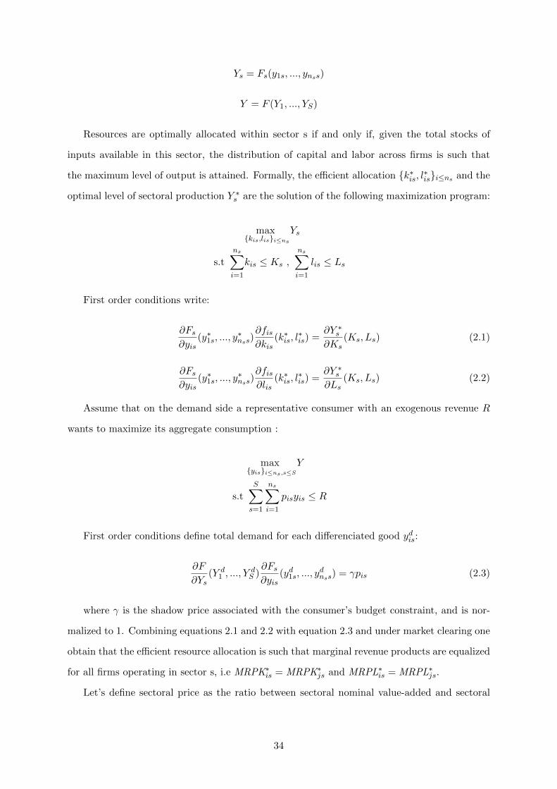
Ys = Fs(y1s, ..., ynss)

Y = F (Y1, ..., YS)

Resources are optimally allocated within sector s if and only if, given the total stocks of

inputs available in this sector, the distribution of capital and labor across firms is such that

the maximum level of output is attained. Formally, the efficient allocation {k∗is, l∗is}i≤ns and the

optimal level of sectoral production Y ∗s are the solution of the following maximization program:

max{kis,lis}i≤ns

Ys

s.t

ns∑i=1

kis ≤ Ks ,

ns∑i=1

lis ≤ Ls

First order conditions write:

∂Fs∂yis

(y∗1s, ..., y∗nss)

∂fis∂kis

(k∗is, l∗is) =

∂Y ∗s∂Ks

(Ks, Ls) (2.1)

∂Fs∂yis

(y∗1s, ..., y∗nss)

∂fis∂lis

(k∗is, l∗is) =

∂Y ∗s∂Ls

(Ks, Ls) (2.2)

Assume that on the demand side a representative consumer with an exogenous revenue R

wants to maximize its aggregate consumption :

max{yis}i≤ns,s≤S

Y

s.tS∑s=1

ns∑i=1

pisyis ≤ R

First order conditions define total demand for each differenciated good ydis:

∂F

∂Ys(Y d

1 , ..., YdS )∂Fs∂yis

(yd1s, ..., ydnss) = γpis (2.3)

where γ is the shadow price associated with the consumer’s budget constraint, and is nor-

malized to 1. Combining equations 2.1 and 2.2 with equation 2.3 and under market clearing one

obtain that the efficient resource allocation is such that marginal revenue products are equalized

for all firms operating in sector s, i.e MRPK∗is = MRPK∗js and MRPL∗is = MRPL∗js.

Let’s define sectoral price as the ratio between sectoral nominal value-added and sectoral

34

physical output, Ps =

(ns∑i=1

pisyis

)/Ys. Now assume that Fs is homogeneous of degree one.

By Euler’s homogeneous function theorem one gets from equation 2.3 the following demand

equations:

∂F

∂Ys(Y d

1 , ..., YdS ) = Ps (2.4)

∂Fs∂yis

(yd1s, ..., ydnss) =

pisPs

(2.5)

Denoting p∗is and P ∗s the equilibrium prices when the input allocation is efficient, equa-

tions 2.1, 2.2 and 2.5 imply that under allocational efficiency individual marginal revenue prod-

ucts are equal to sectoral MRP:

MRPK∗is = P ∗s∂Y ∗s∂Ks

(Ks, Ls) (2.6)

MRPL∗is = P ∗s∂Y ∗s∂Ls

(Ks, Ls) (2.7)

It is quite standard in the literature on misallocation to map observed marginal revenue

products onto exogenous distortions. Under the previous framework it is intuitive to define

these distortions as wedges driving marginal revenue products away from their within-sector

optimal levels.15 Formally:

MRPKis = (1 + τkis)MRPK∗is

MRPLis = (1 + τ lis)MRPL∗is

Using equations 2.4, 2.6 and 2.7 one can easily show that these two distortions write :

1 + τkis =

kisyis

∂fis(kis,lis)∂kis

KsY ∗s

∂Y ∗s (Ks,Ls)∂Ks

YsY∂F (Y1,...,YS)

∂YsY ∗sY ∗

∂F (Y ∗1 ,...,Y∗S )

∂Y ∗s

pisyiskis

Ks

PsYs

Y

Y ∗(2.8)

1 + τ lis =

lisyis

∂fis(kis,lis)∂lis

LsY ∗s

∂Y ∗s (Ks,Ls)∂Ls

YsY∂F (Y1,...,YS)

∂YsY ∗sY ∗

∂F (Y ∗1 ,...,Y∗S )

∂Y ∗s

pisyislis

LsPsYs

Y

Y ∗(2.9)

2.2.2 Production functions and output aggregators

To bring this framework to the data one requires functional-form assumptions on production

functions and on output aggregation. I follow Hsieh and Klenow (2009) and use a constant

15It is important to keep in mind that these exogenous distortions can reflect a large set of frictions, like forexample financial constraints, physical adjustment costs, firing costs, heterogeneous mark-ups among others.

35

return to scale production function. The output of each sector is the outcome of aggregating

the differentiated goods in a CES manner. Finally, sectoral aggregates are combined into a

single aggregate good using a Cobb-Douglas production technology.

yis = ziskαsis l

1−αsis (2.10)

Ys =

(ns∑i=1

yρs−1ρs

is

) ρsρs−1

(2.11)

Y =S∏s=1

Y θss where

S∑s=1

θs = 1 (2.12)

zis is the idiosyncratic productivity of firm i in sector s.16 ρs is the elasticity of substitution

between goods within sector s. Notice that output elasticities are allowed to differ across

industries but not across firms within a given industry.

Under the previous functional-form assumptions demand equations 2.4 and 2.5 write:

PsYsY

= θs (2.13)

yisYs

=

(pisPs

)−ρs(2.14)

I follow Foster, Haltiwanger, and Syverson (2008) by distinguishing between revenue pro-

ductivity (TFPR) and physical productivity (TFPQ) :

TFPRis := piszis =pisyis

kαsis l1−αsis

TFPQis := zis =yis

kαsis l1−αsis

In most firm-level datasets variables are expressed in nominal terms and firm-specific prices are

not available, which makes revenue productivity easier to measure than physical productivity.17

Using demand equations one can derive physical productivity from nominal value-added and

inputs quantities:

TFPQis = (YsPρss )− 1ρs−1

(pisyis)ρsρs−1

kαsis l1−αsis

(2.15)

16Here idiosyncratic productivity is considered as exogenous. See Syverson (2011) for a survey on the deter-minants of micro-productivity.

17Furthermore, under constant return to scale the equalization of inputs MRP implies the equalization offirms’ TFPR.

36

Interestingly, the previous equation implies that in a given sector and at a given time period one

can obtain relative idiosyncratic productivities without using sectoral deflators (and therefore

avoiding a potential source of measurement error, since the use of sectoral deflators would mean

that differences in firm-specific prices would show up in the measure of physical productivities).

2.2.3 Capital, labor and the log-normality assumption

The previous assumptions on production functions and sectoral aggregators imply that the

capital (labor) elasticity of individual output in sector s is equal to the capital (labor) elasticity

of the sectoral production function one obtain under optimal allocation. The Cobb-Douglas

aggregator implies that the sectoral output elasticity of aggregate production is a constant.

Therefore from equations 2.8 and 2.9 labor distortions and capital distortions write:

1 + τkis =pisyiskis

Ks

PsYs

Y

Y ∗

1 + τ lis =pisyislis

LsPsYs

Y

Y ∗

One can express observed aggregate TFP at the sectoral level, TFPs = Ys/(Kαss L1−αs

s ), as

a function of idiosyncratic productivities and capital and labor distortions. In log this equation

writes

ln(TFPs) =ρs

ρs − 1· ln

(ns∑i=1

zρs−1is (1 + τkis)

(1−ρs)αs(1 + τ lis)(1−ρs)(1−αs)

)

− αs · ln

(ns∑i=1


(1−ρs)αs−1(1 + τ lis)(1−ρs)(1−αs)

)

− (1− αs) · ln

(ns∑i=1


(1−ρs)αs(1 + τ lis)(1−ρs)(1−αs)−1

)(2.16)

From equation 2.16 one can easily get the efficient sectoral productivity TFP∗s by equalizing

inputs MRP (that is to say, by setting distortions equal to 1). Interestingly one can also get the

TFP that would have been observed if, for an unchanged distribution of MRPK (MRPL), labor

(capital) had been efficiently allocated, i.e. MRPL (MRPK) had been equalized. This variable

is denoted TFP∗,ls (TFP∗,ks ). Following Hsieh and Klenow (2009), an intuitive measure of the

extent of misallocation in sector s is given by the ratio between efficient TFP and observed

TFP, assessing the loss in sectoral productivity (or equivalently in output) associated with

the current inputs allocation. I use the same intuition and define capital misallocation (labor

37

misallocation) as the ratio between TFP∗s and TFP∗,ls (TFP∗,ks ), assessing the loss in TFP

induced by distortions affecting the MRPK (MRPL) distribution. In other words, this measure

of capital (labor) misallocation provides an answer to the following question: if there were no

labor (capital) distortions in sector s, by how much could we still boost sectoral TFP eliminating

capital (labor) distortions? Formally these three measures write :

Ms =TFP∗sTFPs

(2.17)

Ms,k =TFP∗sTFP∗,ls

(2.18)

Ms,l =TFP∗s

TFP∗,ks(2.19)

Ms,k and Ms,l respectively measure the magnitudes of capital and labor misallocation in

sector s, making use of the theoretical framework previously defined. To disentangle these

two types of misallocation the literature has widely used reduced-form estimates, in particular

looking at measures of MRP dispersion.18 Indeed, under the assumption that idiosyncratic

productivity, capital distortion and labor distortion are jointly log-normal within each sector

one can show that:19

ln (Ms)a.s.−−−−→

ns→∞

1

2αs (1 + αs(ρs − 1)) ·Var

[ln(1 + τks )

]+

1

2(1− αs) (1 + (1− αs)(ρs − 1)) ·Var

[ln(1 + τ ls)

]+ αs(1− αs)(ρs − 1) · Cov

[ln(1 + τks ), ln(1 + τ ls)

](2.20)

Under this approximation misallocation can come from either dispersion in log-MRPK,

dispersion in log-MRPL, or correlation between the two distortions. If labor distortions are

equalized the variance of log-MRPK is the only source of misallocation, and therefore consti-

tutes a sufficient statistic to measure “pure” capital misallocation. Although very useful, this

approximation may seem unsatisfying for several reasons. First, it necessitates additional as-

18Gopinath et al. (2017) compare the evolution of MRPK dispersion and MRPL dispersion over time in varioussouthern-european countries. They find that MRPL dispersion is stable while MRPK dispersion increases, whichmotivates the use of a model linking capital misallocation with the decline of the real interest rate followingthe introduction of the euro. Larrain and Stumpner (2017) show that capital account liberalization reducesthe dispersion in the return to capital, particularly in sectors more reliant on external finance. They mapthis reduction into aggregate TFP gains, and argue that capital account liberalization increases aggregate TFPthrough more efficient firm capital allocation by 10% to 16%.

19See appendix 2.8.

38

sumptions with respect to the HK framework (the log-normality assumption, and the fact that

the number of firms per sector need to be large). More importantly, the correlation between

idiosyncratic productivities and distortions does not appear in this decomposition, whereas mis-

allocation is worse when firms that suffer from a lack of resources (i.e., firms with high MRP)

are also the most productive ones.20 The measures of capital and labor misallocation I propose

stick to the structural framework without any further assumptions, and do not a priori ignore

the above-mentioned correlation.

I define a third term, representing the impact of the interaction between labor and capital

distortions, such that the log of sectoral misallocation is equal to the sum of the log of each

component:

ln (Ms) = ln (Ms,k) + ln (Ms,l) + ln (Ms,int) (2.21)

It can be shown21 that under the log-normality assumption each part of equation 2.21 is

directly related to its counterpart in equation 2.20:

ln (Ms,k)a.s.−−−−→

ns→∞

1

2αs (1 + αs(ρs − 1)) ·Var

[ln(1 + τks )

]

ln (Ms,l)a.s.−−−−→

ns→∞

1

2(1− αs) (1 + (1− αs)(ρs − 1)) ·Var

[ln(1 + τ ls)

]ln (Ms,int)

a.s.−−−−→ns→∞

αs(1− αs)(ρs − 1) · Cov[ln(1 + τks ), ln(1 + τ ls)

]Therefore, and importantly, even if one is willing to consider as plausible the assumptions

needed to get equation 2.20, and to overlook the fact that it ignores important factors affecting

misallocation, the decomposition I propose would be in this case strictly equivalent to the log-

normal approximation.

2.2.4 Misallocation and aggregate TFP

Aggregate TFP is given by:

TFP =S∏s=1

(TFPs

(Ks

K

)αs (LsL

)1−αs)θs

20See Restuccia and Rogerson (2008) and Gilchrist, Sim, and Zakrajsek (2013).21See appendix 2.8.

39

and aggregate misallocation is a simple function of sectoral misallocations :

M =TFP∗

TFP=

S∏s=1

M θss

Therefore variation in observed aggregate TFP over time can be decomposed into variations

in efficient TFP and variations in misallocation:

∆ ln(TFP) = ∆ ln(TFP∗)−∆ ln(M)

Variation in aggregate misallocation can itself be further decomposed into three components

using equation 2.21: capital misallocation, labor misallocation, and the interaction term, where

each element is the aggregation of the sectoral counterparts:

∆ ln(M) = ∆ ln(Mk) + ∆ ln(Ml) + ∆ ln(Mint)

ln(Mk) =

S∑s=1

θs ln(Ms,k)

ln(Ml) =

S∑s=1

θs ln(Ms,l)

ln(Mint) =

S∑s=1

θs ln(Ms,int)

2.3 Data

2.3.1 Data description

In this section I describe the firm-level dataset I use to perform my analysis, the FIBEN

database. This unique database was initially set up by the Banque de France to facilitate the

implementation of monetary policy. All the companies recorded in the database are awarded

a rating that provides information on their ability to meet their financial commitments. Only

claims on the most highly-rated companies are eligible for bank refinancing.

The database gathers information on all companies with sales at least equal to 750,000

euros, covering the years 1989 to the present day. A broad range of information is gathered,

including accounting and financial data from balance sheets and profit and loss statements,

but also descriptive details, such as the firm’s name, legal status and business code. The

40

information is gathered from a variety of sources, including journals of legal notices, registrars

of commercial courts, France’s national statistics office (INSEE) and credit institutions, as well

as the companies themselves.

I drop from the dataset observations for which the basic accounting equality does not hold.

When the average number of employees declared by the firm is equal to zero I set this variable

as missing. Restricting the database to the manufacturing sector the dataset is an unbalanced

panel of approximately 1,100,000 observations covering a total of about 110,000 firms. Table

2.1 provides descriptive statistics for some variables of interest, including nominal value added

(given by the difference between gross output and intermediate consumptions), payments to

labor, tangible and intangible fixed assets, and average number of employees.

Table 2.1: Descriptive statistics, French manufacturing sector

Variable Obs. Firms Mean SD Q1 Median Q3

No employees 1,043,427 107,124 76.27 564.42 11 21 46Sales 1,076,460 110,124 19,403.92 347,409.6 1,268 2,472 6,478Nominal VA 1,076,460 110,124 4,885.22 62,966.17 490 901 2,065Fixed assets 1,075,161 110,108 3,074.36 44,828.07 92 253 777Total assets 1,074,939 110,104 15,304.6 224,845.3 738 1,532 4,247Wage bill 1,075,155 110,108 2,145.21 19,190.58 275 500 1,089Age 1,061,644 106,294 293.1 262.5 120 220 379.5

Note : Nominal value added is given by the difference between gross nominal output and intermediate consump-tions. Age is expressed in months. All other variables except the number of employees are expressed in thousandsof euros.

The first challenge in the dataset is to harmonize accounting periods; as a matter of fact,

even if most of the firms follow the regular calendar year, a non-negligible share of the data

collected corresponds to other accounting periods. In order to deal with this issue I assume

that the gross output, the intermediate consumption, the payments to labor and the number

of employees of a given firm over a given accounting period are the same each month. Then

for each firm I reconstruct yearly data by summing monthly data (or averaging, in the case of

the number of employees). In the dataset the stock of fixed assets is recorded at the end of

the accounting period; I proceed with linear interpolation to estimate the quantity of assets at

the end of the calendar year, and I assume that fixed assets used by a firm in order to produce

during year t correspond to the mean of the fixed assets stocks at the end of year t-1 and year

t.22

I use INSEE’s aggregate data (publicly available online) to check for the representativeness

22Because I use the lag value of fixed assets in order to define the capital stock variable I drop the first yearof observations in my dataset, which therefore goes from 1990 to 2015.

41

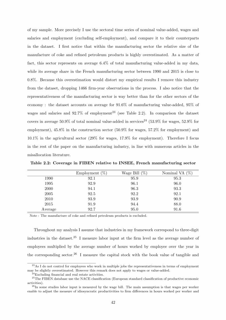
of my sample. More precisely I use the sectoral time series of nominal value-added, wages and

salaries and employment (excluding self-employment), and compare it to their counterparts

in the dataset. I first notice that within the manufacturing sector the relative size of the

manufacture of coke and refined petroleum products is highly overestimated. As a matter of

fact, this sector represents on average 6.4% of total manufacturing value-added in my data,

while its average share in the French manufacturing sector between 1990 and 2015 is close to

0.8%. Because this overestimation would distort my empirical results I remove this industry

from the dataset, dropping 1466 firm-year observations in the process. I also notice that the

representativeness of the manufacturing sector is way better than for the other sectors of the

economy : the dataset accounts on average for 91.6% of manufacturing value-added, 95% of

wages and salaries and 92.7% of employment23 (see Table 2.2). In comparison the dataset

covers in average 50.9% of total nominal value-added in services24 (53.9% for wages, 52.9% for

employment), 45.8% in the construction sector (50.9% for wages, 57.2% for employment) and

10.1% in the agricultural sector (29% for wages, 17.9% for employment). Therefore I focus

in the rest of the paper on the manufacturing industry, in line with numerous articles in the

misallocation literature.

Table 2.2: Coverage in FIBEN relative to INSEE, French manufacturing sector

Employment (%) Wage Bill (%) Nominal VA (%)

1990 92.1 95.9 95.31995 92.9 96.1 96.02000 94.1 96.3 93.32005 92.5 92.2 92.12010 93.9 93.9 90.92015 91.9 94.4 88.0

Average 92.7 95.0 91.6

Note : The manufacture of coke and refined petroleum products is excluded.

Throughout my analysis I assume that industries in my framework correspond to three-digit

industries in the dataset.25 I measure labor input at the firm level as the average number of

employees multiplied by the average number of hours worked by employee over the year in

the corresponding sector.26 I measure the capital stock with the book value of tangible and

23As I do not control for employees who work in multiple jobs the representativeness in terms of employmentmay be slightly overestimated. However this remark does not apply to wages or value-added.

24Excluding financial and real estate activities.25The FIBEN database use the NACE classification (European standard classification of productive economic

activities).26In some studies labor input is measured by the wage bill. The main assumption is that wages per worker

enable to adjust the measure of idiosyncratic productivities to firm differences in hours worked per worker and

42

intangible fixed assets deflated by the industry price deflator for investment goods. Finally, I

measure production with nominal value added (gross output minus intermediate consumption)

deflated by the corresponding value-added deflator.27 Firm-level observations are dropped if

the capital stock, the labor input or the value-added variable are either non-positive or missing.

At this point the dataset is composed of 976,451 firm-year observations.

Importantly, entry and exit from the dataset do not correspond to actual entry and exit;

firms may disappear from the dataset when their sales fall below the 750,000 euros threshold,

and exit may also reflect restructurations and takeovers rather than firms shutting down their

businesses. Finally, I emphasize that I work only with unconsolidated accounts.

2.3.2 Estimation of the parameters

I now describe how I infer the parameters used in the theoretical framework from the dataset.

In a perfect economy with no frictions one would naturally approximate the elasticity of output

with respect to labor by the share of nominal value-added devoted to nominal expenditure on

labor. But as the whole analysis relies on the existence of distortions driving the economy

away from an efficient optimum one cannot separately identify differences in technology and

differences in distortions from differences in factor expenditure shares. I assume that on average

firms within a given industry are undistorted (even if a particular firm still may face a distortion

in a particular year). More precisely, I compute for each year and for each firm operating in

industry s its labor expenditure share28 and I assume that the median of this variable over

the years and over the firms reflects the true value of the elasticity of output with respect to

labor. Then under the assumption of constant return to scale it is straightforward to deduce

for each industry the elasticity of output with respect to capital.29 As stressed by Hsieh and

Klenow (2009) another issue that arises when deducing production elasticities from factor shares

is that we have to take into account the markups associated with the market power of the firms

in workers skills. However differences in wages may also be explained by rent sharing and by wage bargainingbetween the firms and the workers. I will use this alternative specification as a robustness check.

27The average number of hours worked by employee for a given year, the investment deflators and the value-added deflators are taken from the INSEE database (available online), although the data are given for a broaderlevel of aggregation than the three-digit level.

28Payments to labor used to compute labor expenditure shares include the wage bills, fringe benefits andemployer social security contributions.

29I do not use standard semi-parametric methods such as Olley and Pakes (1996) and Levinsohn and Petrin(2003) for two reasons. First these methods require assumptions on firms capital and labor demands, whereas oneadvantage of the structural framework I develop is that it does not require any hypothesis on how firms behave.Second, these methods frequently provide very low elasticities for capital, because this input is notoriously moreprone to measurement errors than labor.

43

in these differentiated good industries. I assume that rents coming from these markups are

divided between workers and capital owners proportionally to the factor expenditure shares,

and directly appear in the payments to labor used to deduce output elasticities.

In order to measure sectors’ shares θs I compute for each year and for each sector the

ratio of the sectoral nominal value added to total nominal value added in the economy. These

parameters are time-varying.

Most empirical studies in the misallocation literature set the elasticity of substitution be-

tween goods ρs equal to an arbitrary value, considered as the same for all sectors in the economy.

In line with these studies I set ρs equal to 3 in my baseline computations. However this assump-

tion may seem unsatisfying, as the value of the elasticity of substitution is bound to vary across

sectors and probably impacts the magnitude of the results. As a matter of fact, it determines

the sectoral aggregates (equation 2.11), the elasticity of the individual demand equations (equa-

tion 2.14) and the measures of idiosyncratic productivity (equation 2.15). Allowing elasticities

to vary across sectors constitutes therefore an important step forward. As a robustness check I

estimate sector specific elasticities, using an econometric strategy inspired by De Loecker (2011)

(see appendix 2.9).30

2.4 Empirical results

I now apply the theoretical framework developed in section 2.2 to the FIBEN dataset in

order to quantify the evolution of misallocation over time and its contribution to the variation

in observed TFP.

To guard against the effect of mismeasurement I follow Hsieh and Klenow (2009) and trim

the top and bottom 1% outliers of both physical and revenue productivity for each year and

within each sector. After trimming the dataset includes 945,014 firm-year observations.

2.4.1 Distortions and firm characteristics

Tables 2.3 and 2.4 respectively present univariate comparisons of key descriptive variables

by labor distortion and capital distortion quartiles. The quartiles are constructed each year and

for each sector. All variables except log distortions are normalized by their sector-year means.

30I do not claim that this econometric strategy enables me to control for all sources of endogeneity bias.Moreover it relies on arguably strong (although standard) assumptions. The main point here is to get reasonableestimates and to examine whether my main empirical results still hold when allowing for sector specific elasticities.

44

I am interested in whether the characteristics of firms which suffer from a lack of resources

(i.e., firms with high labor or capital distortions) differ from those which should be granted less

inputs (i.e., firms with low labor or capital distortions).

Firms’ value added and capital stock increase monotonically with labor distortions. It

suggests that for a given distribution of capital labor should optimally be reallocated from firms

with relatively low nominal VA and capital stock to firms with relatively high nominal VA and

capital stock: the mean firm in the fourth quartile produces 41% more and owns a capital stock

52% higher than its sector-year average, while the mean firm in the first quartile produces 43%

less and owns 44% less capital. As for labor input itself the pattern is not so clear: the mean

increases until Q3 but then decreases for the fourth quartile, while the labor input of the median

firm is decreasing with labor distortions. The same observation applies to the age variable, both

the mean and the median increasing until Q3 and then decreasing for the fourth quartile.

Regarding capital distortions, the mean of value-added, labor and capital decreases mono-

tonically (although the median for value-added and labor in Q1 is lower than in Q2). It suggests

that for a given distribution of labor one can increase output by reallocating capital from firms

with high nominal VA, high labor input and high capital stock to firms producing less with less

inputs. The results for the capital variable are particularly striking: the capital stock of the

mean firm in Q1 is 2.5 times larger than the sector-year average, while the mean firm in Q4

owns a capital stock more than 7 times smaller. Considering the age variable, it is again hard

to draw any firm conclusion, both mean and median increasing then decreasing with capital

distortions.

Tables 2.3 and 2.4 also provide useful information on the dispersion of both MRP distribu-

tions, and on the correlation with firms’ productivity. On one hand substracting the median

log-distortion in Q1 from the median log-distortion in Q4 indicates that the MRPK dispersion

is higher than the MRPL dispersion (2.094 versus 0.809 for the difference between median log-

distortions, 2.354 versus 0.946 for the difference between mean log-distortions). It suggests that

there is relatively more room for capital reallocation than for labor reallocation if one wants

to improve allocational efficiency. On the other hand TFPQ increases monotonically with both

distortions, meaning that firms suffering from a lack of resources are also the most produc-

tive ones. However, the productivity gap between low MRPL and high MRPL firms is more

pronounced: the mean firm in the fourth (first) labor distortion quartile is 59.8% more (46%

less) productive than its sector-year average, while the mean firm in the fourth (first) capital

45

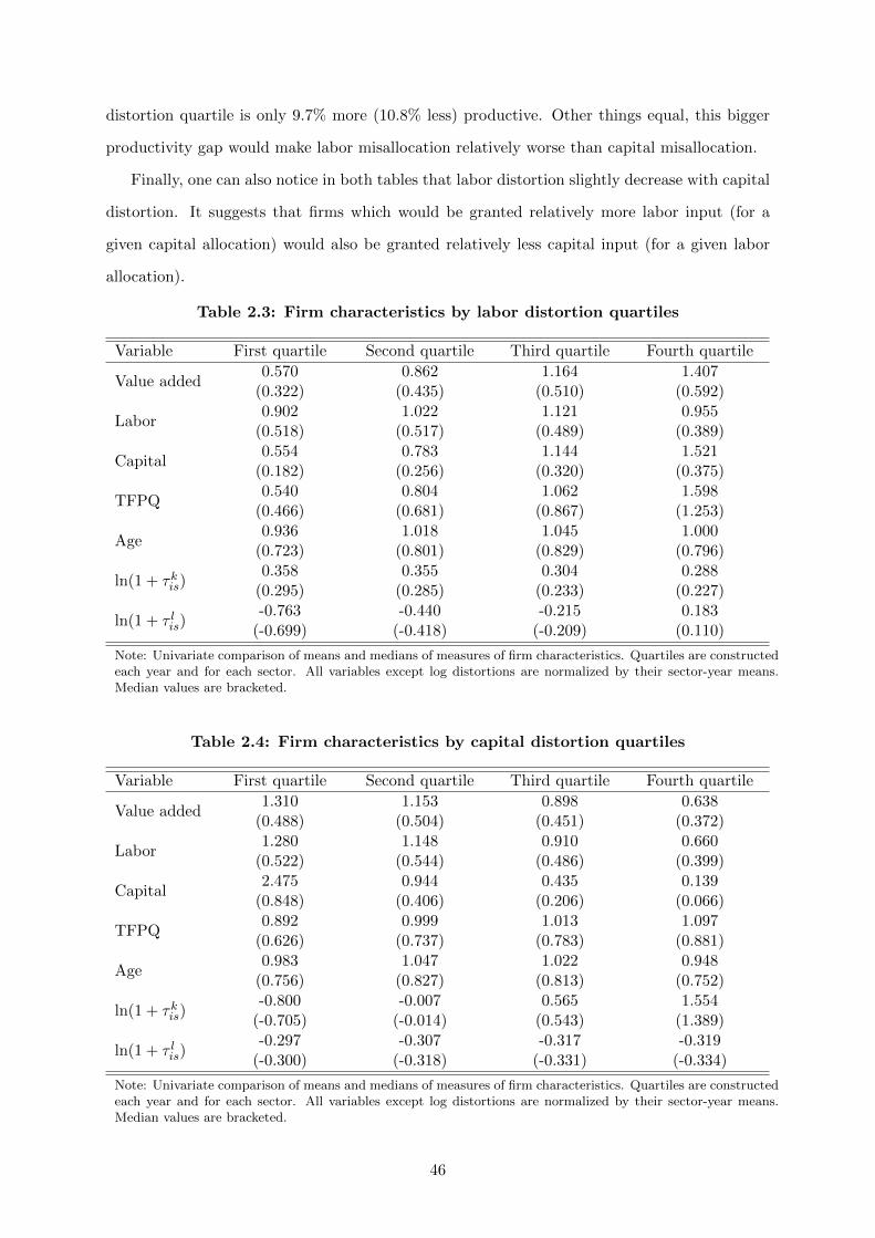
distortion quartile is only 9.7% more (10.8% less) productive. Other things equal, this bigger

productivity gap would make labor misallocation relatively worse than capital misallocation.

Finally, one can also notice in both tables that labor distortion slightly decrease with capital

distortion. It suggests that firms which would be granted relatively more labor input (for a

given capital allocation) would also be granted relatively less capital input (for a given labor

allocation).

Table 2.3: Firm characteristics by labor distortion quartiles

Variable First quartile Second quartile Third quartile Fourth quartile

Value added0.570 0.862 1.164 1.407

(0.322) (0.435) (0.510) (0.592)

Labor0.902 1.022 1.121 0.955

(0.518) (0.517) (0.489) (0.389)

Capital0.554 0.783 1.144 1.521

(0.182) (0.256) (0.320) (0.375)

TFPQ0.540 0.804 1.062 1.598

(0.466) (0.681) (0.867) (1.253)

Age0.936 1.018 1.045 1.000

(0.723) (0.801) (0.829) (0.796)

ln(1 + τkis)0.358 0.355 0.304 0.288

(0.295) (0.285) (0.233) (0.227)

ln(1 + τ lis)-0.763 -0.440 -0.215 0.183

(-0.699) (-0.418) (-0.209) (0.110)

Note: Univariate comparison of means and medians of measures of firm characteristics. Quartiles are constructedeach year and for each sector. All variables except log distortions are normalized by their sector-year means.Median values are bracketed.

Table 2.4: Firm characteristics by capital distortion quartiles

Variable First quartile Second quartile Third quartile Fourth quartile

Value added1.310 1.153 0.898 0.638

(0.488) (0.504) (0.451) (0.372)

Labor1.280 1.148 0.910 0.660

(0.522) (0.544) (0.486) (0.399)

Capital2.475 0.944 0.435 0.139

(0.848) (0.406) (0.206) (0.066)

TFPQ0.892 0.999 1.013 1.097

(0.626) (0.737) (0.783) (0.881)

Age0.983 1.047 1.022 0.948

(0.756) (0.827) (0.813) (0.752)

ln(1 + τkis)-0.800 -0.007 0.565 1.554

(-0.705) (-0.014) (0.543) (1.389)

ln(1 + τ lis)-0.297 -0.307 -0.317 -0.319

(-0.300) (-0.318) (-0.331) (-0.334)

Note: Univariate comparison of means and medians of measures of firm characteristics. Quartiles are constructedeach year and for each sector. All variables except log distortions are normalized by their sector-year means.Median values are bracketed.

46

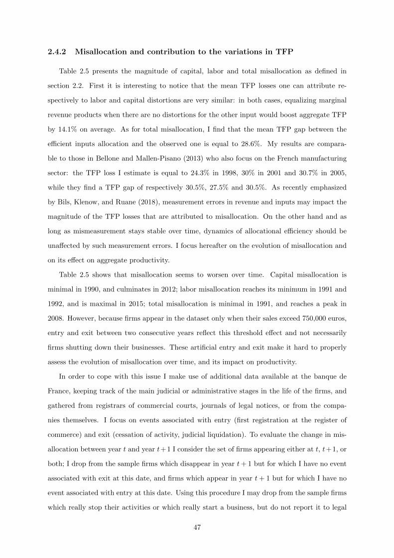
2.4.2 Misallocation and contribution to the variations in TFP

Table 2.5 presents the magnitude of capital, labor and total misallocation as defined in

section 2.2. First it is interesting to notice that the mean TFP losses one can attribute re-

spectively to labor and capital distortions are very similar: in both cases, equalizing marginal

revenue products when there are no distortions for the other input would boost aggregate TFP

by 14.1% on average. As for total misallocation, I find that the mean TFP gap between the

efficient inputs allocation and the observed one is equal to 28.6%. My results are compara-

ble to those in Bellone and Mallen-Pisano (2013) who also focus on the French manufacturing

sector: the TFP loss I estimate is equal to 24.3% in 1998, 30% in 2001 and 30.7% in 2005,

while they find a TFP gap of respectively 30.5%, 27.5% and 30.5%. As recently emphasized

by Bils, Klenow, and Ruane (2018), measurement errors in revenue and inputs may impact the

magnitude of the TFP losses that are attributed to misallocation. On the other hand and as

long as mismeasurement stays stable over time, dynamics of allocational efficiency should be

unaffected by such measurement errors. I focus hereafter on the evolution of misallocation and

on its effect on aggregate productivity.

Table 2.5 shows that misallocation seems to worsen over time. Capital misallocation is

minimal in 1990, and culminates in 2012; labor misallocation reaches its minimum in 1991 and

1992, and is maximal in 2015; total misallocation is minimal in 1991, and reaches a peak in

2008. However, because firms appear in the dataset only when their sales exceed 750,000 euros,

entry and exit between two consecutive years reflect this threshold effect and not necessarily

firms shutting down their businesses. These artificial entry and exit make it hard to properly

assess the evolution of misallocation over time, and its impact on productivity.

In order to cope with this issue I make use of additional data available at the banque de

France, keeping track of the main judicial or administrative stages in the life of the firms, and

gathered from registrars of commercial courts, journals of legal notices, or from the compa-

nies themselves. I focus on events associated with entry (first registration at the register of

commerce) and exit (cessation of activity, judicial liquidation). To evaluate the change in mis-

allocation between year t and year t+1 I consider the set of firms appearing either at t, t+1, or

both; I drop from the sample firms which disappear in year t+ 1 but for which I have no event

associated with exit at this date, and firms which appear in year t+ 1 but for which I have no

event associated with entry at this date. Using this procedure I may drop from the sample firms

which really stop their activities or which really start a business, but do not report it to legal

47

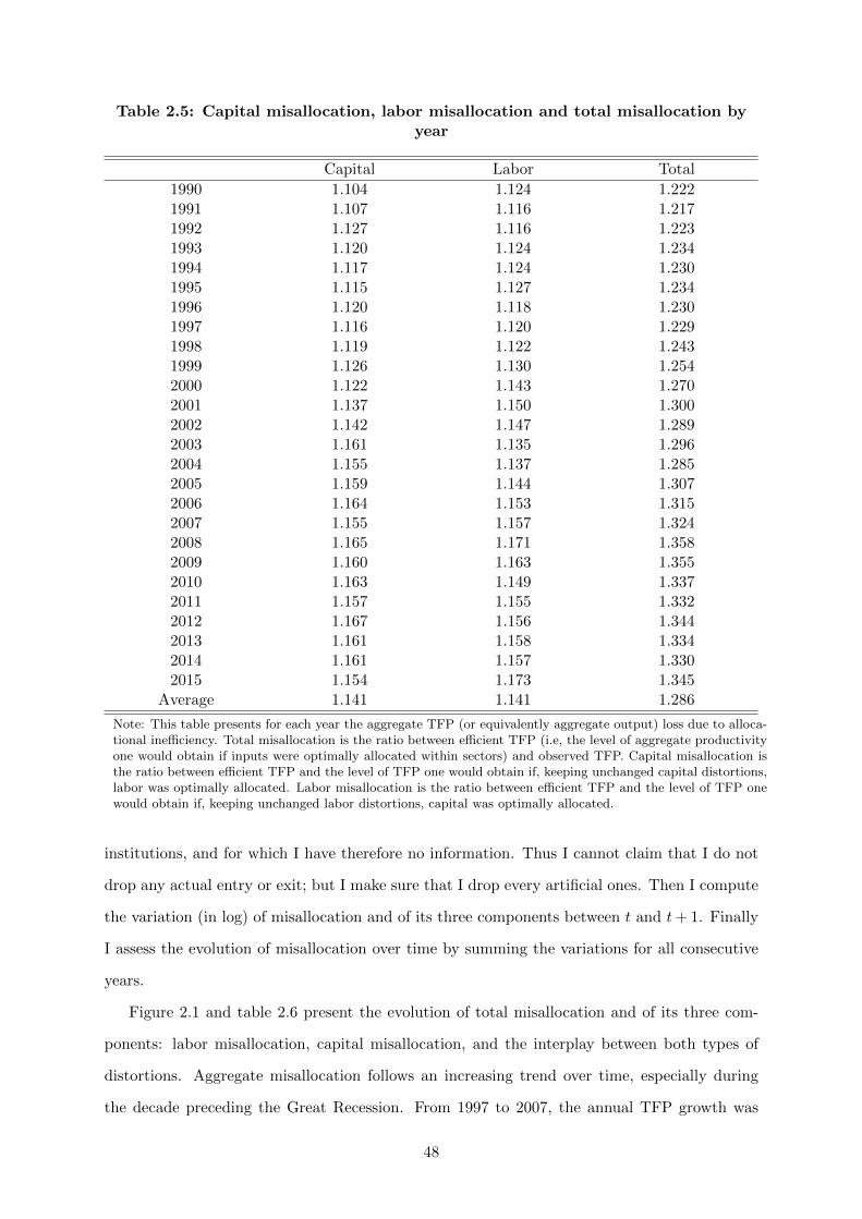
Table 2.5: Capital misallocation, labor misallocation and total misallocation byyear

Capital Labor Total

1990 1.104 1.124 1.2221991 1.107 1.116 1.2171992 1.127 1.116 1.2231993 1.120 1.124 1.2341994 1.117 1.124 1.2301995 1.115 1.127 1.2341996 1.120 1.118 1.2301997 1.116 1.120 1.2291998 1.119 1.122 1.2431999 1.126 1.130 1.2542000 1.122 1.143 1.2702001 1.137 1.150 1.3002002 1.142 1.147 1.2892003 1.161 1.135 1.2962004 1.155 1.137 1.2852005 1.159 1.144 1.3072006 1.164 1.153 1.3152007 1.155 1.157 1.3242008 1.165 1.171 1.3582009 1.160 1.163 1.3552010 1.163 1.149 1.3372011 1.157 1.155 1.3322012 1.167 1.156 1.3442013 1.161 1.158 1.3342014 1.161 1.157 1.3302015 1.154 1.173 1.345

Average 1.141 1.141 1.286

Note: This table presents for each year the aggregate TFP (or equivalently aggregate output) loss due to alloca-tional inefficiency. Total misallocation is the ratio between efficient TFP (i.e, the level of aggregate productivityone would obtain if inputs were optimally allocated within sectors) and observed TFP. Capital misallocation isthe ratio between efficient TFP and the level of TFP one would obtain if, keeping unchanged capital distortions,labor was optimally allocated. Labor misallocation is the ratio between efficient TFP and the level of TFP onewould obtain if, keeping unchanged labor distortions, capital was optimally allocated.

institutions, and for which I have therefore no information. Thus I cannot claim that I do not

drop any actual entry or exit; but I make sure that I drop every artificial ones. Then I compute

the variation (in log) of misallocation and of its three components between t and t+ 1. Finally

I assess the evolution of misallocation over time by summing the variations for all consecutive

years.

Figure 2.1 and table 2.6 present the evolution of total misallocation and of its three com-

ponents: labor misallocation, capital misallocation, and the interplay between both types of

distortions. Aggregate misallocation follows an increasing trend over time, especially during

the decade preceding the Great Recession. From 1997 to 2007, the annual TFP growth was

48

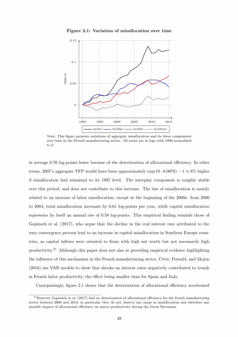
Figure 2.1: Variation of misallocation over time

1990 1995 2000 2005 2010 2015

0

0.05

0.1

0.15

1990=0

ln(M) ln(Mk) ln(Ml) ln(Mint)

Note: This figure presents variations of aggregate misallocation and its three componentsover time in the French manufacturing sector. All series are in logs with 1990 normalizedto 0.

in average 0.76 log-points lower because of the deterioration of allocational efficiency. In other

terms, 2007’s aggregate TFP would have been approximately exp(10 · 0.0076)− 1 ≈ 8% higher

if misallocation had remained to its 1997 level. The interplay component is roughly stable

over this period, and does not contribute to this increase. The rise of misallocation is mainly

related to an increase of labor misallocation, except at the beginning of the 2000s: from 2000

to 2004, total misallocation increases by 0.61 log-points per year, while capital misallocation

represents by itself an annual rise of 0.58 log-points. This empirical finding reminds those of

Gopinath et al. (2017), who argue that the decline in the real interest rate attributed to the

euro convergence process lead to an increase in capital misallocation in Southern Europe coun-

tries, as capital inflows were oriented to firms with high net worth but not necessarily high

productivity.31 Although this paper does not aim at providing empirical evidence highlighting

the influence of this mechanism in the French manufacturing sector, Cette, Fernald, and Mojon

(2016) use VAR models to show that shocks on interest rates negatively contributed to trends

in French labor productivity, the effect being smaller than for Spain and Italy.

Unsurprisingly, figure 2.1 shows that the deterioration of allocational efficiency accelerated

31However Gopinath et al. (2017) find no deterioration of allocational efficiency for the french manufacturingsector between 2000 and 2012; in particular they do not observe any surge in misallocation and therefore anysizeable impact of allocational efficiency on macro productivity during the Great Recession.

49

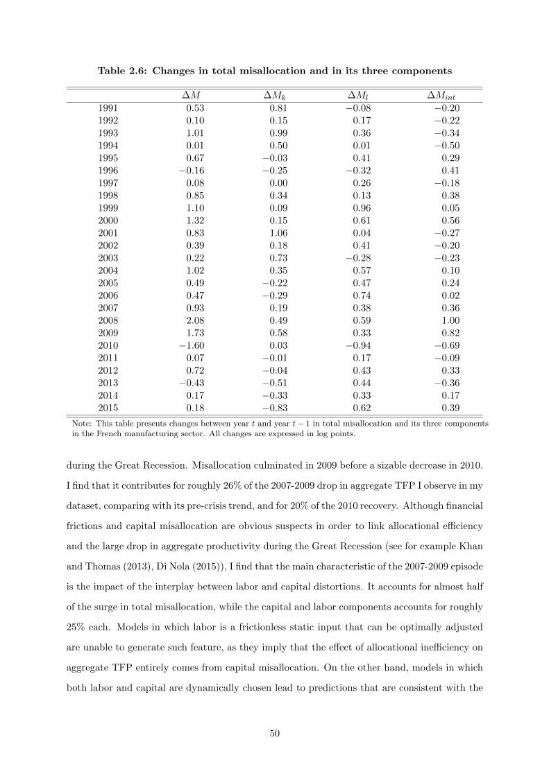
Table 2.6: Changes in total misallocation and in its three components

∆M ∆Mk ∆Ml ∆Mint

1991 0.53 0.81 −0.08 −0.201992 0.10 0.15 0.17 −0.221993 1.01 0.99 0.36 −0.341994 0.01 0.50 0.01 −0.501995 0.67 −0.03 0.41 0.291996 −0.16 −0.25 −0.32 0.411997 0.08 0.00 0.26 −0.181998 0.85 0.34 0.13 0.381999 1.10 0.09 0.96 0.052000 1.32 0.15 0.61 0.562001 0.83 1.06 0.04 −0.272002 0.39 0.18 0.41 −0.202003 0.22 0.73 −0.28 −0.232004 1.02 0.35 0.57 0.102005 0.49 −0.22 0.47 0.242006 0.47 −0.29 0.74 0.022007 0.93 0.19 0.38 0.362008 2.08 0.49 0.59 1.002009 1.73 0.58 0.33 0.822010 −1.60 0.03 −0.94 −0.692011 0.07 −0.01 0.17 −0.092012 0.72 −0.04 0.43 0.332013 −0.43 −0.51 0.44 −0.362014 0.17 −0.33 0.33 0.172015 0.18 −0.83 0.62 0.39

Note: This table presents changes between year t and year t− 1 in total misallocation and its three componentsin the French manufacturing sector. All changes are expressed in log points.

during the Great Recession. Misallocation culminated in 2009 before a sizable decrease in 2010.

I find that it contributes for roughly 26% of the 2007-2009 drop in aggregate TFP I observe in my

dataset, comparing with its pre-crisis trend, and for 20% of the 2010 recovery. Although financial

frictions and capital misallocation are obvious suspects in order to link allocational efficiency

and the large drop in aggregate productivity during the Great Recession (see for example Khan

and Thomas (2013), Di Nola (2015)), I find that the main characteristic of the 2007-2009 episode

is the impact of the interplay between labor and capital distortions. It accounts for almost half

of the surge in total misallocation, while the capital and labor components accounts for roughly

25% each. Models in which labor is a frictionless static input that can be optimally adjusted

are unable to generate such feature, as they imply that the effect of allocational inefficiency on

aggregate TFP entirely comes from capital misallocation. On the other hand, models in which

both labor and capital are dynamically chosen lead to predictions that are consistent with the

50

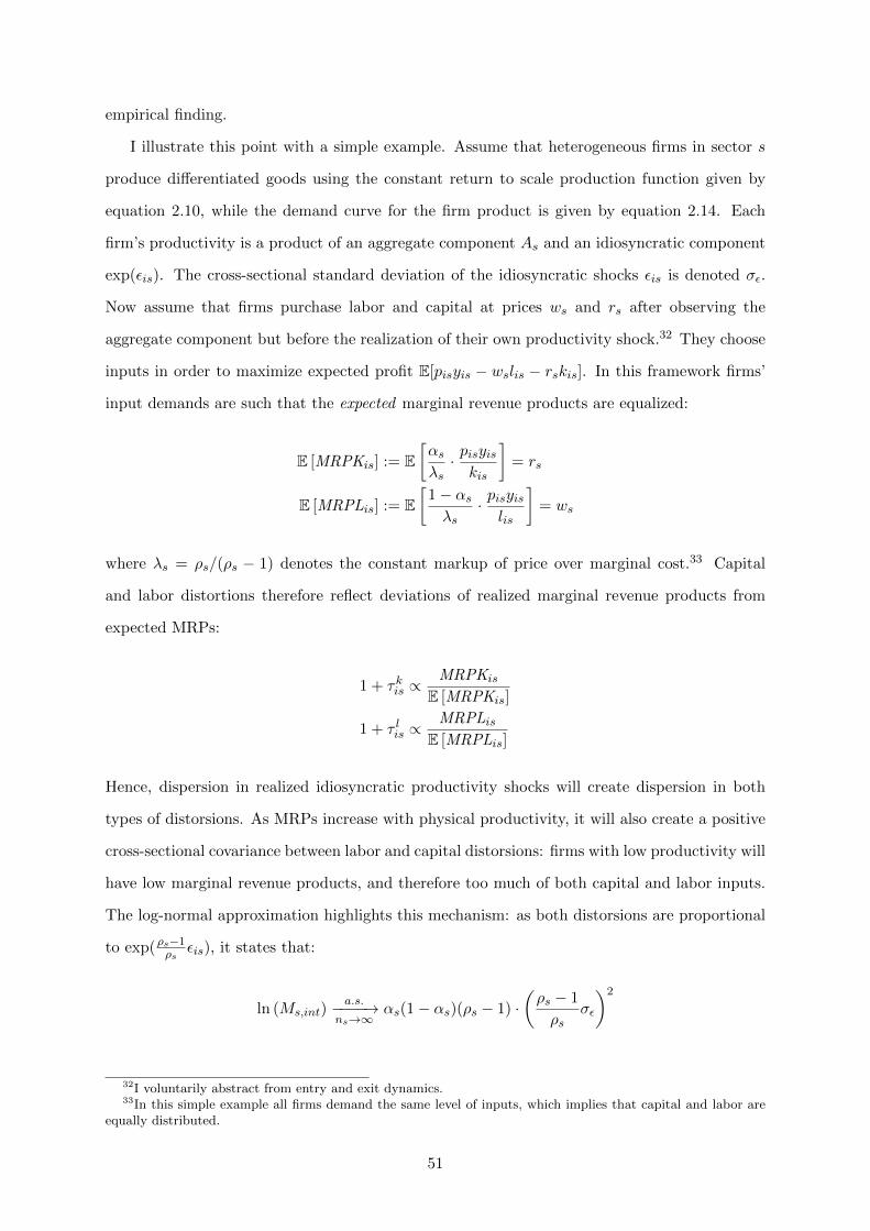
empirical finding.

I illustrate this point with a simple example. Assume that heterogeneous firms in sector s

produce differentiated goods using the constant return to scale production function given by

equation 2.10, while the demand curve for the firm product is given by equation 2.14. Each

firm’s productivity is a product of an aggregate component As and an idiosyncratic component

exp(εis). The cross-sectional standard deviation of the idiosyncratic shocks εis is denoted σε.

Now assume that firms purchase labor and capital at prices ws and rs after observing the

aggregate component but before the realization of their own productivity shock.32 They choose

inputs in order to maximize expected profit E[pisyis − wslis − rskis]. In this framework firms’

input demands are such that the expected marginal revenue products are equalized:

E [MRPKis] := E[αsλs· pisyiskis

]= rs

E [MRPLis] := E[

1− αsλs

· pisyislis

]= ws

where λs = ρs/(ρs − 1) denotes the constant markup of price over marginal cost.33 Capital

and labor distortions therefore reflect deviations of realized marginal revenue products from

expected MRPs:

1 + τkis ∝MRPKis

E [MRPKis]

1 + τ lis ∝MRPLis

E [MRPLis]

Hence, dispersion in realized idiosyncratic productivity shocks will create dispersion in both

types of distorsions. As MRPs increase with physical productivity, it will also create a positive

cross-sectional covariance between labor and capital distorsions: firms with low productivity will

have low marginal revenue products, and therefore too much of both capital and labor inputs.

The log-normal approximation highlights this mechanism: as both distorsions are proportional

to exp(ρs−1ρs

εis), it states that:

ln (Ms,int)a.s.−−−−→

ns→∞αs(1− αs)(ρs − 1) ·

(ρs − 1

ρsσε

)2

32I voluntarily abstract from entry and exit dynamics.33In this simple example all firms demand the same level of inputs, which implies that capital and labor are

equally distributed.

51

The fact that the interplay component accounts for a sizeable part of the surge in misallocation

during the crisis is therefore consistent with recent papers that show that microeconomic un-

certainty (represented by the cross sectional dispersion σε) sharply increased during the Great

Recession. In particular, Bloom et al. (2018) build a model with time-varying uncertainty and

nonconvex adjustment costs in both capital and labor. They find that increased uncertainty

affects aggregate productivity by reducing input reallocation in the economy. Although other

types of model may also be able to reproduce the findings I emphasize in this paper, my empirical

results are qualitatively consistent with this strand of research.34

Finally, misallocation is rather stable from 2010 to 2015. I find no deterioration or improve-

ment, although it appears that capital misallocation decreases and compensates an increase in

labor misallocation. As a consequence one can hardly consider allocational efficiency as a driver

of the low TFP growth in the wake of the Great Recession, at least in the French manufactur-

ing sector. Actually the difference between the pre-2007 and the post-2010 growth rate is even

higher for efficient TFP than for actual TFP: focusing on productivity at the firm-level may

therefore shed more light on aggregate TFP slowdown than exploring changes in the efficiency

of factors allocation.35

2.5 Robustness checks

In this section I assess the sensitivity of my findings by performing various robustness checks.

First, I estimate the change in log-misallocation between year t and year t+ 1 that is obtained

shutting down the entry exit channel and focusing on incumbent firms, i.e keeping in the sample

only firms that appear at both t and t + 1. Second, I measure physical productivity using as

labor input the wage bill declared by the firm, in order to control for the quality of the workforce

and for the quantity of hours worked per employee. I also assess the robustness of the results

to alternative industry definitions, by defining sectors at the two-digit level rather than at the

three-digit level. Because changes in allocational efficiency may be driven by changes in the

relative weights of high and low misallocation industries over time, I measure the parameters of

34Other papers focusing on countercyclical dispersion of micro outcomes include for example Bachmann andBayer (2014) and Kehrig (2015).

35Recent papers have explored the within-firm channel: in particular, Duval, Hong, and Timmer (2019) showthat the interplay between preexisting financial fragilities and tightening credit conditions weakened individualproductivity after the crisis. They provide evidence that credit supply restrictions led vulnerable firms to decreaseintangible capital investment. Manaresi and Pierri (2019) make a similar point by studying the impact of bankcredit supply on firm productivity in Italy.

52

the Cobb-Douglas aggregator by sectors’ average weights. Finally, most empirical papers in the

misallocation literature assume that the elasticity of substitution between goods is constant for

all sectors. I estimate sector-specific elasticities by assuming that the gross output production

function is Leontieff in materials and then reproduce the analysis. Appendix 2.9 contains details

on the econometric methodology which is used. All figures and tables describing the evolution

of misallocation and its components for the various robustness checks I perform can be found

in appendix 2.7.

In all cases misallocation clearly follows an increasing trend during the decade preceding

the Great Recession: the annual loss in TFP growth due to the deterioration of allocational

efficiency goes from 0.67 (focusing on incumbent firms) to 0.88 log-points (defining sectors at

the two-digit level). At the beginning of the 2000’s capital misallocation is the main driver

of total misallocation, while labor misallocation is the main contributor the rest of the 1997-

2007 decade. The interplay component remains stable until 2007, but increases sharply from

2007 to 2009: it is the first contributor to the rise in misallocation during the Great Recession,

whatever the specification. Total misallocation culminates in 2009 and decreases sharply in

2010. Its contribution to the 2007-2009 drop in aggregate TFP (comparing with the pre-

crisis trend) is comprised between 23% (sectors defined at the 2-digit level) and 31% (sector-

specific elasticities), while it accounts for 17% (sector-specific elasticities) to 26% (constant

sectoral weights) of the 2010 recovery. Finally, in all cases post-crisis misallocation is quite flat,

changes in labor misallocation and changes in capital misallocation compensating each other.

These observations therefore corroborate the empirical results I obtained with the baseline

specification.

2.6 Conclusion

In this paper I measure the contribution of resource misallocation to the variations in ag-

gregate productivity from 1990 to 2015 in the French manufacturing sector. I provide an exact

decomposition of allocational efficiency between three components: labor misallocation, capi-

tal misallocation, and the interplay between both types of misallocation. During the decade

preceding the Great Recession misallocation worsen over time, creating an annual loss in TFP

growth comprised between 0.67 and 0.88 log-points. Labor misallocation is the main driver of

this rise, except at the beginning of the 2000s, capital misallocation being in this case the main

53

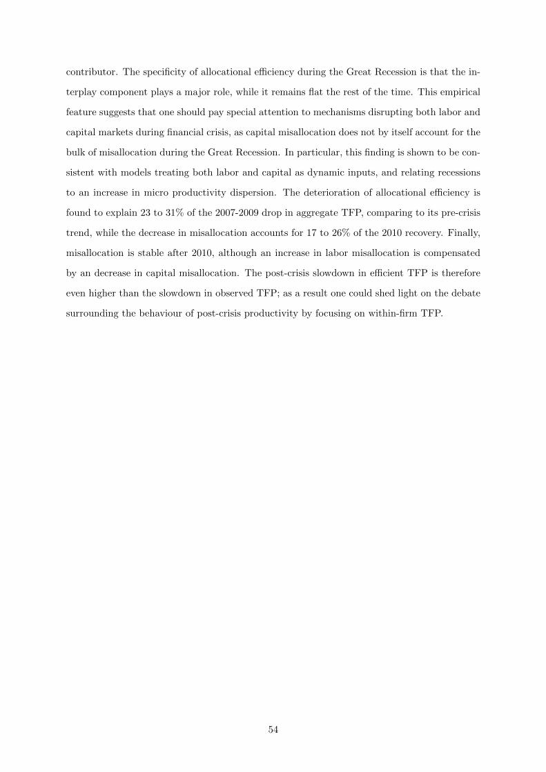
contributor. The specificity of allocational efficiency during the Great Recession is that the in-

terplay component plays a major role, while it remains flat the rest of the time. This empirical

feature suggests that one should pay special attention to mechanisms disrupting both labor and

capital markets during financial crisis, as capital misallocation does not by itself account for the

bulk of misallocation during the Great Recession. In particular, this finding is shown to be con-

sistent with models treating both labor and capital as dynamic inputs, and relating recessions

to an increase in micro productivity dispersion. The deterioration of allocational efficiency is

found to explain 23 to 31% of the 2007-2009 drop in aggregate TFP, comparing to its pre-crisis

trend, while the decrease in misallocation accounts for 17 to 26% of the 2010 recovery. Finally,

misallocation is stable after 2010, although an increase in labor misallocation is compensated

by an decrease in capital misallocation. The post-crisis slowdown in efficient TFP is therefore

even higher than the slowdown in observed TFP; as a result one could shed light on the debate

surrounding the behaviour of post-crisis productivity by focusing on within-firm TFP.

54

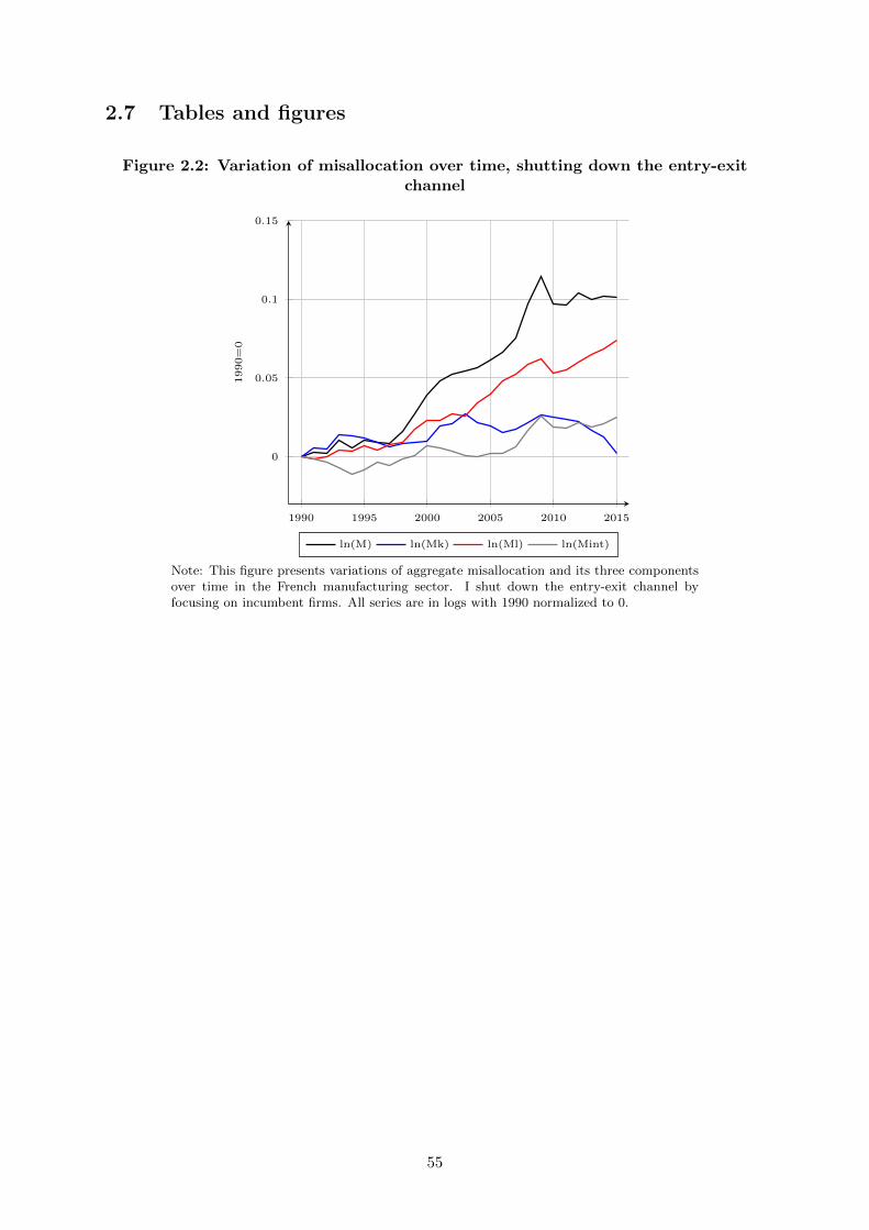
2.7 Tables and figures

Figure 2.2: Variation of misallocation over time, shutting down the entry-exitchannel

1990 1995 2000 2005 2010 2015

0

0.05

0.1

0.15

1990=0


Note: This figure presents variations of aggregate misallocation and its three componentsover time in the French manufacturing sector. I shut down the entry-exit channel byfocusing on incumbent firms. All series are in logs with 1990 normalized to 0.

55

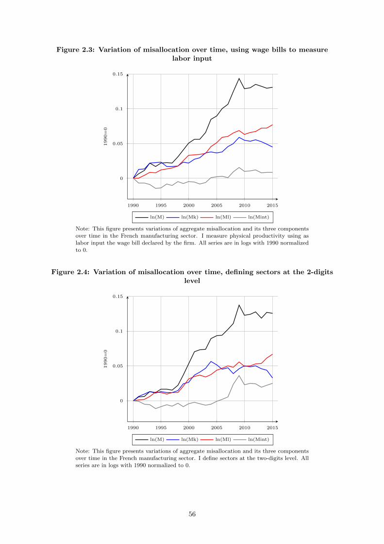
Figure 2.3: Variation of misallocation over time, using wage bills to measurelabor input

1990 1995 2000 2005 2010 2015

0

0.05

0.1

0.15

1990=0


Note: This figure presents variations of aggregate misallocation and its three componentsover time in the French manufacturing sector. I measure physical productivity using aslabor input the wage bill declared by the firm. All series are in logs with 1990 normalizedto 0.

Figure 2.4: Variation of misallocation over time, defining sectors at the 2-digitslevel

1990 1995 2000 2005 2010 2015

0

0.05

0.1

0.15

1990=0


Note: This figure presents variations of aggregate misallocation and its three componentsover time in the French manufacturing sector. I define sectors at the two-digits level. Allseries are in logs with 1990 normalized to 0.

56

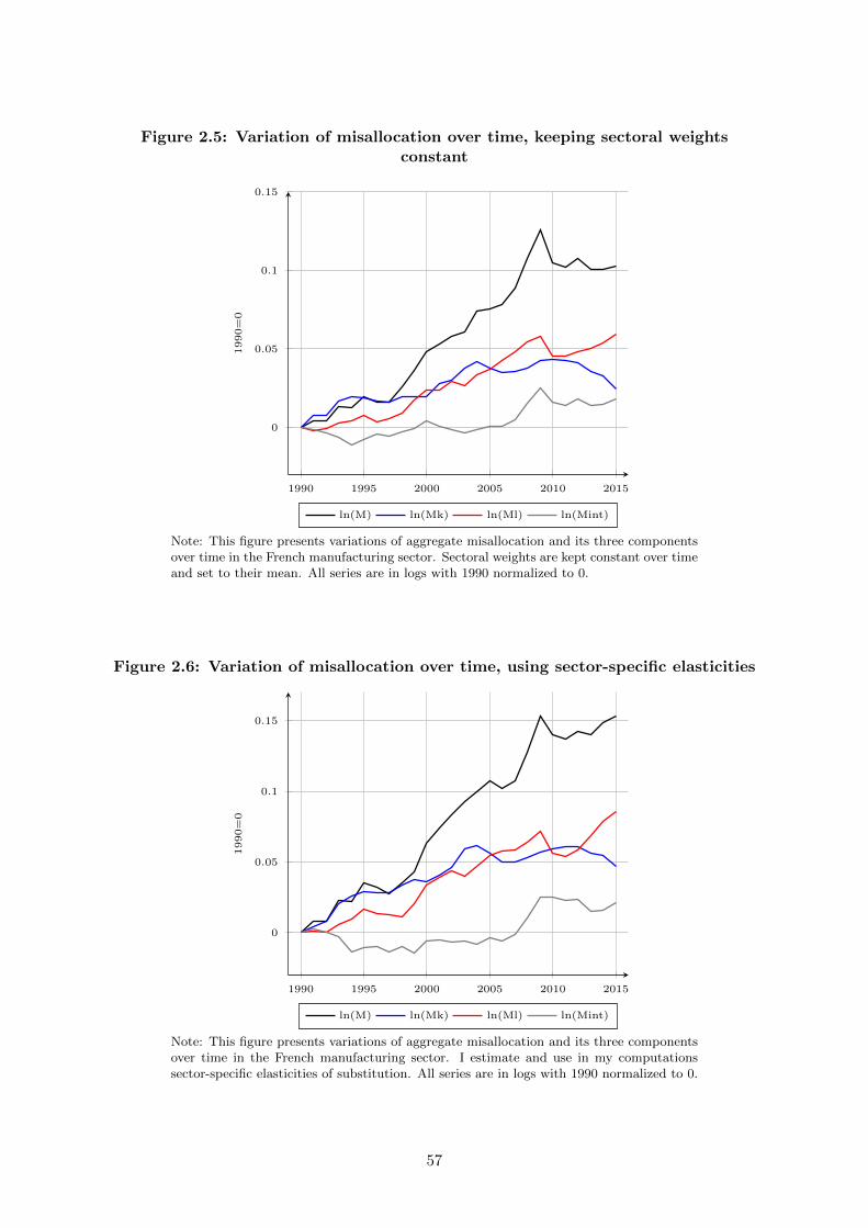
Figure 2.5: Variation of misallocation over time, keeping sectoral weightsconstant

1990 1995 2000 2005 2010 2015

0

0.05

0.1

0.15

1990=0


Note: This figure presents variations of aggregate misallocation and its three componentsover time in the French manufacturing sector. Sectoral weights are kept constant over timeand set to their mean. All series are in logs with 1990 normalized to 0.

Figure 2.6: Variation of misallocation over time, using sector-specific elasticities

1990 1995 2000 2005 2010 2015

0

0.05

0.1

0.15

1990=0


Note: This figure presents variations of aggregate misallocation and its three componentsover time in the French manufacturing sector. I estimate and use in my computationssector-specific elasticities of substitution. All series are in logs with 1990 normalized to 0.

57

Table 2.7: Changes in total misallocation and in its three components, shuttingdown the entry-exit channel


1991 0.28 0.54 −0.14 −0.121992 −0.10 −0.04 0.15 −0.211993 0.89 0.88 0.38 −0.371994 −0.52 −0.04 −0.04 −0.441995 0.49 −0.18 0.35 0.321996 −0.12 −0.28 −0.29 0.451997 −0.10 −0.25 0.35 −0.201998 0.74 0.19 0.12 0.431999 1.14 0.09 0.85 0.202000 1.21 0.04 0.57 0.602001 0.87 1.02 −0.03 −0.122002 0.41 0.15 0.45 −0.192003 0.21 0.62 −0.16 −0.252004 0.21 −0.55 0.87 −0.112005 0.51 −0.26 0.53 0.242006 0.46 −0.36 0.83 −0.012007 0.96 0.17 0.40 0.392008 2.13 0.41 0.64 1.082009 1.76 0.53 0.34 0.892010 −1.71 −0.18 −0.86 −0.672011 −0.07 −0.16 0.16 −0.072012 0.71 −0.12 0.47 0.362013 −0.36 −0.56 0.50 −0.302014 0.16 −0.39 0.36 0.192015 −0.09 −1.03 0.53 0.41

Note: This table presents changes between year t and year t-1 in total misallocation and its three componentsin the French manufacturing sector. I shut down the entry-exit channel by focusing on incumbent firms. Allchanges are expressed in log points.

58

Table 2.8: Changes in total misallocation and in its three components, usingwage bills to measure labor input


1991 0.63 1.30 −0.01 −0.661992 0.51 0.07 0.44 0.001993 1.03 0.84 0.42 −0.231994 −0.47 0.09 −0.03 −0.531995 0.48 0.04 0.39 0.051996 0.05 −0.66 0.16 0.551997 −0.06 0.00 0.13 −0.191998 0.90 0.10 0.25 0.551999 1.02 0.55 0.79 −0.322000 0.98 −0.11 0.79 0.302001 0.54 0.55 0.05 −0.062002 −0.01 0.19 0.06 −0.262003 1.01 0.68 0.14 0.192004 1.84 0.15 0.97 0.722005 0.52 −0.15 0.54 0.132006 1.03 0.14 0.83 0.062007 0.62 0.79 0.08 −0.252008 1.83 0.44 0.54 0.852009 1.88 0.87 0.35 0.662010 −1.47 −0.36 −0.57 −0.542011 0.18 −0.13 0.29 0.022012 0.49 0.16 0.15 0.182013 −0.27 −0.26 0.44 −0.452014 −0.29 −0.38 0.04 0.052015 0.12 −0.41 0.49 0.04

Note: This table presents changes between year t and year t-1 in total misallocation and its three componentsin the French manufacturing sector. I measure physical productivity using as labor input the wage bill declaredby the firm. All changes are expressed in log points.

59

Table 2.9: Changes in total misallocation and in its three components, definingsectors at the 2-digits level


1991 0.57 0.58 0.10 −0.111992 0.05 0.37 0.06 −0.381993 0.70 0.33 0.43 −0.061994 −0.15 −0.19 0.62 −0.581995 0.47 0.22 0.00 0.251996 −0.01 −0.11 −0.21 0.311997 −0.13 −0.07 0.15 −0.211998 0.73 0.30 0.02 0.411999 1.43 0.96 0.93 −0.462000 1.66 0.24 1.02 0.402001 1.69 1.07 0.38 0.242002 0.31 0.37 0.16 −0.222003 0.05 0.60 −0.29 −0.262004 1.54 0.97 0.42 0.152005 0.47 −0.52 0.57 0.422006 0.03 −0.62 0.33 0.322007 0.86 0.20 0.32 0.342008 0.80 −0.78 −0.20 1.782009 2.69 0.70 0.75 1.242010 −1.50 0.40 −0.64 −1.262011 0.14 −0.12 0.11 0.152012 0.39 0.13 0.29 −0.032013 −0.91 −0.43 0.05 −0.532014 0.80 −0.21 0.74 0.272015 −0.16 −1.13 0.62 0.35

Note: This table presents changes between year t and year t-1 in total misallocation and its three components inthe French manufacturing sector. I define sectors at the two-digits level. All changes are expressed in log points.

60

Table 2.10: Changes in total misallocation and in its three components, keepingsectoral weights constant


1991 0.40 0.74 −0.21 −0.131992 0.00 0.03 0.16 −0.191993 0.93 0.90 0.31 −0.281994 −0.09 0.26 0.15 −0.501995 0.69 −0.02 0.36 0.351996 −0.31 −0.27 −0.40 0.361997 −0.01 −0.01 0.17 −0.171998 0.98 0.32 0.36 0.301999 1.04 0.04 0.85 0.152000 1.16 −0.05 0.65 0.562001 0.50 0.88 −0.03 −0.352002 0.49 0.19 0.52 −0.222003 0.33 0.78 −0.25 −0.202004 1.31 0.42 0.70 0.192005 0.13 −0.40 0.32 0.212006 0.29 −0.33 0.62 0.002007 1.01 0.11 0.53 0.372008 1.90 0.15 0.65 1.102009 1.80 0.54 0.30 0.962010 −2.04 0.03 −1.19 −0.882011 −0.29 −0.02 −0.06 −0.212012 0.55 −0.15 0.33 0.372013 −0.70 −0.55 0.22 −0.372014 0.02 −0.32 0.33 0.012015 0.14 −0.84 0.57 0.41

Note: This table presents changes between year t and year t-1 in total misallocation and its three componentsin the French manufacturing sector. Sectoral weights are kept constant over time and set to their mean. Allchanges are expressed in log points.

61

Table 2.11: Changes in total misallocation and in its three components, usingsector-specific elasticities


1991 0.78 0.39 0.12 0.271992 0.05 0.43 −0.11 −0.271993 1.47 1.21 0.54 −0.281994 −0.11 0.56 0.41 −1.081995 1.36 0.32 0.73 0.311996 −0.37 −0.07 −0.32 0.021997 −0.47 −0.02 −0.11 −0.341998 0.84 0.55 −0.10 0.391999 0.78 0.40 0.88 −0.502000 2.02 −0.16 1.34 0.842001 1.07 0.48 0.51 0.082002 0.93 0.55 0.49 −0.112003 0.96 1.31 −0.39 0.042004 0.65 0.19 0.69 −0.232005 0.82 −0.53 0.84 0.512006 −0.59 −0.60 0.28 −0.272007 0.53 0.00 0.06 0.472008 2.05 0.31 0.56 1.182009 2.57 0.39 0.74 1.442010 −1.32 0.21 −1.56 0.032011 −0.30 0.13 −0.19 −0.242012 0.56 0.01 0.46 0.092013 −0.25 −0.44 1.00 −0.812014 0.87 −0.16 0.98 0.052015 0.49 −0.77 0.72 0.54

Note: This table presents changes between year t and year t-1 in total misallocation and its three components inthe French manufacturing sector. I estimate and use in my computations sector-specific elasticities of substitution.All changes are expressed in log points.

62

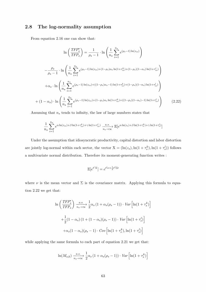
2.8 The log-normality assumption

From equation 2.16 one can show that:

ln

(TFP∗sTFPs

)=

1

ρs − 1· ln

(1

ns

ns∑i=1

e(ρs−1) ln(zis)

)

− ρsρs − 1

· ln

(1

ns

ns∑i=1

e(ρs−1) ln(zis)+(1−ρs)αs ln(1+τkis)+(1−ρs)(1−αs) ln(1+τ lis)

)

+αs · ln

(1

ns

ns∑i=1

e(ρs−1) ln(zis)+((1−ρs)αs−1) ln(1+τkis)+(1−ρs)(1−αs) ln(1+τ lis)

)

+ (1− αs) · ln

(1

ns

ns∑i=1

e(ρs−1) ln(zis)+(1−ρs)αs ln(1+τkis)+((1−ρs)(1−αs)−1) ln(1+τ lis)

)(2.22)

Assuming that ns tends to infinity, the law of large numbers states that

1

ns

ns∑i=1

eα ln(zis)+β ln(1+τkis)+γ ln(1+τ lis)a.s.−−−−→

ns→∞E[eα ln(zs)+β ln(1+τks )+γ ln(1+τ ls)]

Under the assumption that idiosyncratic productivity, capital distortion and labor distortion

are jointly log-normal within each sector, the vector X = (ln(zs), ln(1 + τks ), ln(1 + τ ls)) follows

a multivariate normal distribution. Therefore its moment-generating function writes :

E[et′X ] = et

′ν+ 12t′Σt

where ν is the mean vector and Σ is the covariance matrix. Applying this formula to equa-

tion 2.22 we get that:

ln

(TFP∗sTFPs

)a.s.−−−−→

ns→∞

1

2αs (1 + αs(ρs − 1)) ·Var

[ln(1 + τks )

]

+1

2(1− αs) (1 + (1− αs)(ρs − 1)) ·Var

[ln(1 + τ ls)

]+αs(1− αs)(ρs − 1) · Cov

[ln(1 + τks ), ln(1 + τ ls)

]while applying the same formula to each part of equation 2.21 we get that:

ln(Ms,k)a.s.−−−−→

ns→∞

1

2αs (1 + αs(ρs − 1)) ·Var

[ln(1 + τks )

]

63

ln(Ms,l)a.s.−−−−→

ns→∞

1

2(1− αs) (1 + (1− αs)(ρs − 1)) ·Var

[ln(1 + τ ls)

]ln(Ms,int) := ln(Ms)− ln(Ms,k)− ln(Ms,l)

a.s.−−−−→ns→∞

αs(1−αs)(ρs−1) ·Cov[ln(1 + τks ), ln(1 + τ ls)

]

64

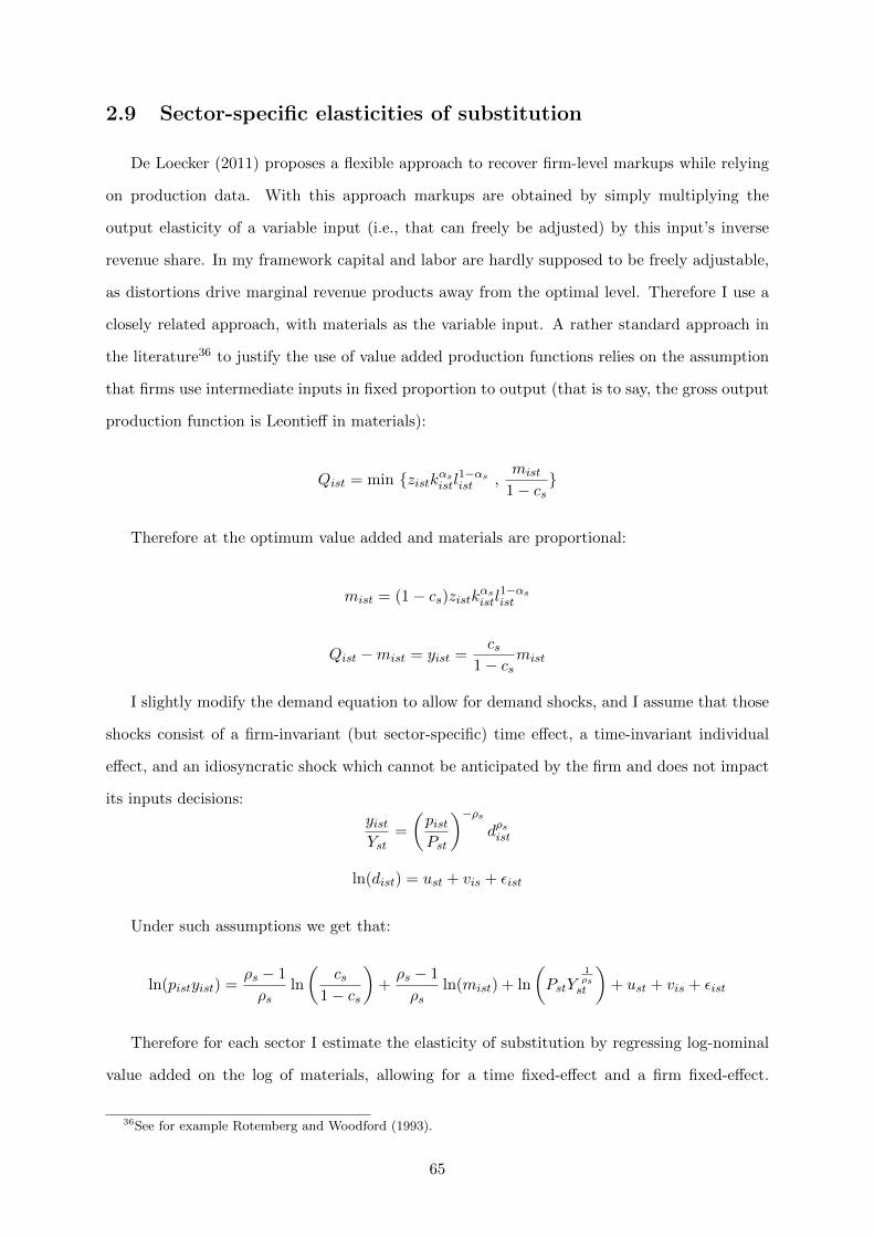
2.9 Sector-specific elasticities of substitution

De Loecker (2011) proposes a flexible approach to recover firm-level markups while relying

on production data. With this approach markups are obtained by simply multiplying the

output elasticity of a variable input (i.e., that can freely be adjusted) by this input’s inverse

revenue share. In my framework capital and labor are hardly supposed to be freely adjustable,

as distortions drive marginal revenue products away from the optimal level. Therefore I use a

closely related approach, with materials as the variable input. A rather standard approach in

the literature36 to justify the use of value added production functions relies on the assumption

that firms use intermediate inputs in fixed proportion to output (that is to say, the gross output

production function is Leontieff in materials):

Qist = min {zistkαsistl1−αsist ,

mist

1− cs}

Therefore at the optimum value added and materials are proportional:

mist = (1− cs)zistkαsistl1−αsist

Qist −mist = yist =cs

1− csmist

I slightly modify the demand equation to allow for demand shocks, and I assume that those

shocks consist of a firm-invariant (but sector-specific) time effect, a time-invariant individual

effect, and an idiosyncratic shock which cannot be anticipated by the firm and does not impact

its inputs decisions:

yistYst

=

(pistPst

)−ρsdρsist

ln(dist) = ust + vis + εist

Under such assumptions we get that:

ln(pistyist) =ρs − 1

ρsln

(cs

1− cs

)+ρs − 1

ρsln(mist) + ln

(PstY

1ρsst

)+ ust + vis + εist

Therefore for each sector I estimate the elasticity of substitution by regressing log-nominal

value added on the log of materials, allowing for a time fixed-effect and a firm fixed-effect.

36See for example Rotemberg and Woodford (1993).

65

Defining sectors at the three-digit level I estimate 85 elasticities of substitution; the average

elasticity and the median elasticity are respectively equal to 3.2 and 3.1, therefore very close

to the initial specification. The min elasticity is 1.8, the max 7.6, Q1 and Q3 are respectively

equal to 2.7 and 3.5.

66

Chapter 3

Granular Borrowers

with Paul Beaumont & Christophe Hurlin

Abstract

This paper uses a credit registry covering the quasi universe of firm-bank relationships inFrance for the period 1999-2016 to provide a detailed account of the role of very largeborrowers (“granular borrowers”) in shaping bank-level and aggregate credit variations. Wedocument that the distribution of borrowers is fat-tailed, the top 100 borrowers making up onaverage for 18% of the aggregate amount of long-term credit and 64% of total undrawn creditlines. We adapt the methodology of Amiti and Weinstein (2018) to identify the contributionsof firm, bank, and aggregate shocks to credit variations at any level of aggregation. At themacroeconomic level, we show that the aggregate properties of credit largely reflect thegranular borrowers’ shocks. This finding highlights the limitations of using time seriesof aggregate credit to assess the magnitude of financial frictions in the economy. At thebank-level, we find that the concentration of the portfolio of credit lines exposes lenders toconsiderable borrower idiosyncratic risk and leads liquidity flows to be more synchronizedacross banks. It suggests that the presence of granular borrowers may represent a limit todiversification.

67

3.1 Introduction

The “granular view” conceptualized by Gabaix (2011) has put the size distribution of firms

(and in particular the recurrent presence of fat tails) at the forefront of empirical research in

macroeconomics. As the law of large numbers does not apply in the presence of very large

actors, idiosyncratic shocks do not average out and, instead, can be important drivers of aggre-

gate fluctuations. According to this approach, the analysis of the microeconomic behavior of

such actors can yield new answers to long-standing macroeconomic questions.1 In finance, the

prevalence of big banks throughout the world has therefore prompted researchers to explore the

role of the distribution of bank size for the propagation of credit shocks to the real economy.2

By contrast, however, the presence of heavy tails in the distribution of borrowers has been so

far largely overlooked. Using a data set covering the quasi universe of firm-bank relationships in

France including both private and public companies between 1999-Q1 and 2016-Q4, we provide

novel evidence of an extreme degree of concentration of credit on the borrower side. Our analysis

reveals that the top 100 borrowing firms make up for 18% of the aggregate amount of long-term

credit and 64% of total undrawn credit lines.

The presence in the economy of firms borrowing non-trivial fractions of aggregate credit

(“granular borrowers”) has two broad sets of implications. First, aggregate properties of credit

are likely to be driven to a large extent by the characteristics and behaviour of granular bor-

rowers. A “representative” agent model calibrated using moments of the aggregate credit time

series, it follows, would effectively reproduce the economic behavior of a restricted sample of

firms with extensive access to credit. Second, the ability of banks to diversify risk is limited

as the set of borrowers is itself very concentrated. This statement challenges in particular the

idea that banks are able to provide liquidity under the form of credit lines by smoothing fund

withdrawals on a diversified portfolio of borrowers (Holmstrom and Tirole, 1998; Kashyap, Ra-

jan, and Stein, 2002). In a granular economy, granting credit lines could expose banks to a

non-diversifiable and potentially non-negligible amount of liquidity risk. This paper provides a

careful assessment of the empirical validity of these two assertions.

1These include the origins of business cycles (Di Giovanni, Levchenko, and Mejean, 2014; Carvalho andGrassi, 2019), of country comparative advantage (Gaubert and Itskhoki, 2018), or the presence of internationalbusiness cycles comovements (Di Giovanni, Levchenko, and Mejean, 2017; Di Giovanni, Levchenko, and Mejean,2018).

2See Buch and Neugebauer (2011); Bremus and Buch (2017); Bremus et al. (2018) for cross-country analysisof granular banks and Amiti and Weinstein (2018); Alfaro, Garcıa-Santana, and Moral-Benito (2019) for studiesof the transmission of bank shocks through lending and input-output relationships.

68

The main empirical challenge that we face is to separately identify credit variations orig-

inating from individual borrowers (“firm components”) from bank-level shocks affecting the

different pools of borrowers (“bank components”). Building on Amiti and Weinstein (2018),

we perform to that end a weighted linear regression of the credit growth rate at the firm-bank

level on a full set of bank-time and firm-time fixed effects. The two sets of fixed effects respec-

tively identify (up to a constant term) factors that simultaneously shift the evolution of credit

in all the firm relationships of a bank and in all the bank relationships of a firm. We define

individual components as the deviation of the estimated fixed effects from a common trend. In

the end, credit variations can be expressed as the sum of two terms, respectively reflecting the

aggregation of firm-specific and bank-specific shocks, and of a third term common to all lending

relationships (“macro component”).

We propose a simple modification of the procedure proposed by Amiti and Weinstein (2018).

We show that using the mid-point growth rate defined by Davis, Haltiwanger, and Schuh (1996)

not only considerably simplifies the estimation but also allows to account for the entry and exit

of firms and banks, a necessary feature when dealing with the universe of borrower-lender

relationships. With this procedure, the loan-weighted averages of the estimated firm and bank

components at time t exactly match the bank, firm, and aggregate credit growth for all the

lending relationships active either at t− 1 or t.

Armed with this decomposition, we first inspect the implications of the presence of granular

borrowers for the properties of aggregate credit. We devote our attention to a moment of key

interest in the macro-finance literature, namely the comovement of credit borrowed by non-

financial corporations with the business cycle. The presence of a robust, positive relationship

between the two is largely considered as reflecting to some extent the manifestation of financial

frictions affecting firms.3 Based on this insight, numerous studies have relied on the analysis

of the evolution of aggregate credit over the business cycle to infer the importance of financial

frictions in determining macroeconomic outcomes.4

Our methodology allows to assess the respective contribution to the cyclicality of aggregate

credit of individual variations originating from the borrower and the lender side. Should the loan

3The interpretation is that the ability of firms to borrow is linked to their net worth because of the presence offinancial constraints, and net worth mechanically fluctuates with the business cycle. The cyclicality of aggregatecredit is therefore largely considered as a manifestation of the “financial accelerator” (Bernanke, Gertler, andGilchrist, 1996; Kiyotaki and Moore, 1997), i.e. the magnifiying role of the financial sector in the propagation ofnegative shocks.

4For instance, see Chari, Kehoe, and McGrattan (2007), Smets and Wouters (2007), Justiniano, Primiceri,and Tambalotti (2010) or Jermann and Quadrini (2012).

69

size distribution of firms and banks not be fat-tailed, these contributions would be negligible

and the large majority of the correlation between credit and GDP would be explained by the

macro component.

On the contrary, we find that firm-specific shocks explain between 60% and 80% of the

comovement of aggregate credit with the business cycle. Bank idiosyncratic variations, by

contrast, do not seem to significantly contribute to the correlation with GDP fluctuations.

The skewness of the credit distribution confers moreover a disproportionate importance to

large borrowers compared to the loan volume they represent, with more than two thirds of the

contribution of firm shocks originating from the top 100 borrowers. It follows that the properties

of aggregate credit are to a large extent determined by the behavior of granular borrowers. All

in all, we contribute to the granularity literature by quantitatively showing that shocks affecting

individual agents or a very small fraction of them shape not only real macro variables, but also

aggregate financial flows; and by showing that granularity on the borrower side is the essential

driver of aggregate credit fluctuations, in sharp contrast with common wisdom.

Our findings imply that the analysis of the cyclicality of aggregate credit is unlikely to give

useful insights on the intensity or the nature of financing frictions applying to the bulk of non-

financial firms. Instead of tightening credit constraints, the decrease in aggregate bank lending

during downturns could actually reflect the differential cyclicality of investment opportunities

of granular borrowers or the presence of substitution patterns between credit and other types

of financing.5 In that respect, our paper strongly advocates for removing the largest borrowers

when studying the determinants of firm financing over the business cycle.6

We then turn to the bank-level implications of the presence of granular borrowers. When

borrowers face idiosyncratic and diversifiable funding shocks, Holmstrom and Tirole (1998)

shows that granting credit lines allows banks to optimally reallocate liquidity between liquidity-

poor firms and firms with excess liquidity. In the presence of aggregate shocks, however, the

reallocation process breaks down and there is a need for an external supply of liquidity.7 Our

paper documents a different yet complementary limit to the capacity of banks to act as “liquidity

5See Covas and Den Haan (2011) and Begenau and Salomao (2019) for evidence for large firms of substitutionpatterns between debt and equity over the business cycle.

6The fact that the disproportionate influence of large borrowers on aggregate financing flows occult thebehaviour of smaller firms has been recognized by Covas and Den Haan (2011) and acknowledged in particularby Eisfeldt and Muir (2016) or Begenau and Salomao (2019). This paper, however, is the first to provide aquantitative assessment of the influence of large borrowers in shaping aggregate credit fluctuations.

7See Ivashina and Scharfstein (2010); Cornett et al. (2011); Bord and Santos (2014); Ippolito et al. (2016)for evidence of bank runs on credit lines during the 2008 financial crisis.

70

pools”. When the distribution of borrowers is fat-tailed, banks may not be able to diversify

idiosyncratic liquidity risk, even when the number of borrowers gets infinitely large. Holding

liquid assets becomes therefore necessary not only to hedge against the possibility of runs on

credit lines but also against negative idiosyncratic shocks affecting granular borrowers.

In line with the presence of under-diversification, we document a positive, strong relationship

between the bank-level concentration of the portfolio of borrowers and the variance of total

undrawn credit lines. Relying on our decomposition of credit variations, we estimate further

that in the absence of borrower idiosyncratic shocks, the variance of credit lines would fall on

average by 18% to 31%. The role of borrower shocks on bank-level credit line variations is

therefore sizeable and comparable in magnitude to the effect of macro shocks, for instance.

In the aggregate, firm-specific shocks contribute substantially to credit lines fluctuations.

The variance of the aggregate firm component amounts to 84% of the variance of aggregate

credit line variations. There are two main channels that explain the importance of borrower

shocks in aggregate fluctuation. As explained above, high borrower portfolio concentration first

leads to high bank-level variance of credit lines. Since large borrowers have credit commitments

in multiple banks, however, borrower idiosyncratic shocks may also increase aggregate variance

by making banks more correlated with each other. We find that the variance of the aggregate

firm component is driven by the linkages between banks which result from the presence of

common borrowers. This result suggests that granular borrowers lead liquidity flows to be less

diversifiable and more coordinated between banks.

The remainder of the paper is organized as follows. We present our data set and provide de-

scriptive statistics on the credit distribution in section 3.2. Section 3.3 describes our estimation

methodology. The results on the cyclicality of aggregate credit are presented and discussed in

section 3.4. We analyze the role of granular borrowers for bank-level liquidity risk in section 3.5.

Section 3.6 concludes.

Related literature

This paper draws on and contributes to three separate strands of research. The first body

of research has been initiated by Covas and Den Haan (2011) and explores the cross-sectional

heterogeneity of firms’ financing over the business cycle to infer the distribution of financial

frictions in the economy (Begenau and Salomao, 2019; Crouzet and Mehrotra, 2019).8 While

8The use of firm size as a proxy for financial constraints to analyse the differential sensitivity of firms tomacroeconomic shocks dates back at least to Gertler and Gilchrist (1994). Recently, Chodorow-Reich (2014) and

71

this literature zooms in on the differences in cyclicality of debt between firms, our focus is on

assessing the contributions of large borrowers to the fluctuations of aggregate credit over the

cycle. Overall, the heterogeneity in firm financing policies combined with the large influence

of granular borrowers highlights the limitations of using aggregate credit data to assess the

magnitude of financial frictions in the economy.

Our paper then adds to the literature on the role of banks as “liquidity providers” (Kashyap,

Rajan, and Stein, 2002). Acharya, Almeida, and Campello (2013) show in particular that bank

lines of credit to firms with greater aggregate risk (high beta) are more expensive as the liquidity

risk they pose cannot be diversified away. We document another limit to diversification, namely

the high degree of concentration of the credit lines portfolios. More broadly, this paper indicates

that the composition of the portfolio of loan commitments is in itself a useful object of study

to assess the liquidity risk faced by banks.9

The last stream of research aims at exploring the implications in macroeconomics and in

finance of the existence of granular economic agents. Previous work has focused on the role

of banks in the transmission of financial shocks to the real economy (Buch and Neugebauer,

2011; Amiti and Weinstein, 2018; Alfaro, Garcıa-Santana, and Moral-Benito, 2019) and in the

formation of sovereign bond yields (Gabaix and Koijen, 2019), on the effects of the presence

of large institutional investors on stock and CDS prices (Greenwood and Thesmar, 2011; Ben-

David et al., 2019; Siriwardane, 2019), and on the asset pricing consequences of a granular

production network (Herskovic, 2018). This paper is to our knowledge the first to provide a

detailed account of the importance of granular borrowers in shaping bank-level and aggregate

credit variations.

3.2 Granular borrowers

3.2.1 Presentation of the data set

We use a comprehensive dataset on quarterly bank-firm level credit issued from the French

credit registry covering the period 1999-Q1 to 2016-Q4. The credit registry contains information

on loans granted by every national or foreign bank (credit institution or investment company)

Mian and Sufi (2014) relied on the size of firms to analyze the real effects of financial constraints during theGreat Recession.

9Following Kashyap, Rajan, and Stein (2002), the literature has mostly focused on the correlation betweendeposit outflows and credit line takedowns to assess banks’ ability to provide liquidity on demand. See Gatevand Strahan (2006); Ivashina and Scharfstein (2010); Acharya and Mora (2015); Ippolito et al. (2016).

72

to every firm located in France. At the end of each month, all financial institutions which are

subject to the 1984 Banking Act have to report the total loan amount extended to any borrowing

firm located in France as soon as this amount exceeds a given reporting threshold.10 The data

set records for each bank-firm relationship the breakdown of credit by type of exposure.11 We

focus in the analysis on two main types of exposure. Long-term credit is defined as credit with

a maturity of more than year at issuance. Credit lines are computed as the sum of all undrawn

commitments (including documentary credits). The exposure of a bank to a firm is the sum of

its individual loans as well as of the bank’s share in syndicated loans.

[Insert figure 3.1 here]

On top of credit exposures, the data set gives basic information on the firm (location,

size indicator, 5-digits sector). The registry also includes the credit score attributed by the

Bank of France, which assesses the medium-term probability of default of the firm.12 It is

assigned by analysts based on hard information (tax returns, trade bills) as well as interviews

conducted with managers. While all firms could in principle receive a credit score, only firms

with sales exceeding e750,000 are in fact assessed by the Bank of France13. The credit score is

communicated on demand to credit institutions.

To construct our sample, we consider only French non-financial firms and we exclude self-

employed entrepreneurs. We also choose to remove public credit institutions from the analysis.

Public supply of credit is large in France (about 30% of total long-term credit), but primarily

directed towards specific entities and sectors (motorway companies, public housing sector, ...).

It is therefore likely to be determined by different objectives from the private supply of credit

which constitutes our main object of focus.

Whenever a bank disappears because of an absorption, all credit exposures are reallocated

to the absorbing bank, leading to unwanted interruptions of banking relationships. The French

10The threshold was set to e75,000 at the firm-bank level until January 2006. It has then been lowered toe25,000 at the firm-agency level and has stayed that way ever since. In order to ensure a constant coverageover the full period, we only consider loan-level data associated to borrowers for which banks have an aggregateexposure exceeding the pre-2006 reporting threshold.

11The different types of exposure are: current accounts, commercial debts, factoring, other short-term debt,property leasing, equipment leasing, credit with maturity of more than one year at issuance, export credit andsecuritized loans, undrawn commitments and available documentary credits. Undrawn commitments can havevarious maturities, ranging from less than a year (operating credit lines) to several years (investment credit lines).We do not include in the analysis the different types of short-term loans as their definitions in the data set havesignificantly evolved over time.

12The categories of the credit score are (in descending order): 3++, 3+, 3, 4+, 4, 5+, 5, 6, 7, 8, 9, P. Creditratings below 7 indicate that at least one payment incident has been recently recorded for the firm. See Cahn,Girotti, and Salvade (2018) for more information on the credit score.

13Only 23.5% of firms on average do have a credit score each quarter in our data set.

73

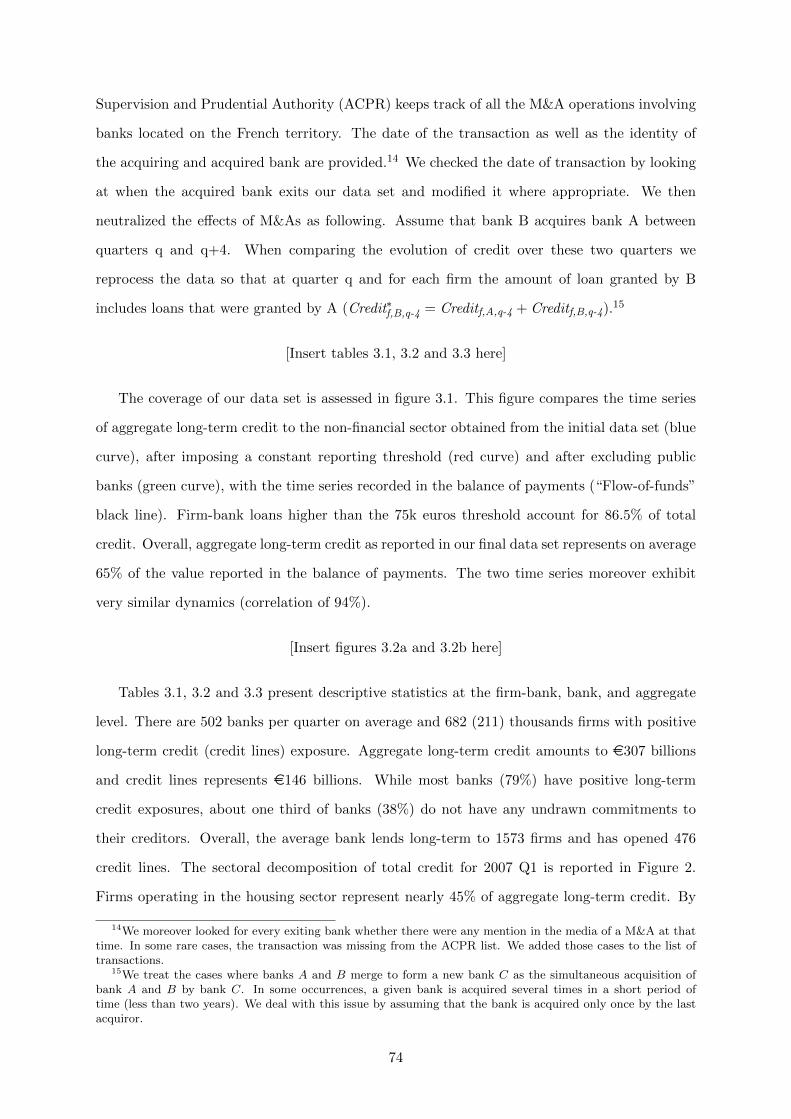
Supervision and Prudential Authority (ACPR) keeps track of all the M&A operations involving

banks located on the French territory. The date of the transaction as well as the identity of

the acquiring and acquired bank are provided.14 We checked the date of transaction by looking

at when the acquired bank exits our data set and modified it where appropriate. We then

neutralized the effects of M&As as following. Assume that bank B acquires bank A between

quarters q and q+4. When comparing the evolution of credit over these two quarters we

reprocess the data so that at quarter q and for each firm the amount of loan granted by B

includes loans that were granted by A (Credit∗f,B,q-4 = Creditf,A,q-4 + Creditf,B,q-4).15

[Insert tables 3.1, 3.2 and 3.3 here]

The coverage of our data set is assessed in figure 3.1. This figure compares the time series

of aggregate long-term credit to the non-financial sector obtained from the initial data set (blue

curve), after imposing a constant reporting threshold (red curve) and after excluding public

banks (green curve), with the time series recorded in the balance of payments (“Flow-of-funds”

black line). Firm-bank loans higher than the 75k euros threshold account for 86.5% of total

credit. Overall, aggregate long-term credit as reported in our final data set represents on average

65% of the value reported in the balance of payments. The two time series moreover exhibit

very similar dynamics (correlation of 94%).

[Insert figures 3.2a and 3.2b here]

Tables 3.1, 3.2 and 3.3 present descriptive statistics at the firm-bank, bank, and aggregate

level. There are 502 banks per quarter on average and 682 (211) thousands firms with positive

long-term credit (credit lines) exposure. Aggregate long-term credit amounts to e307 billions

and credit lines represents e146 billions. While most banks (79%) have positive long-term

credit exposures, about one third of banks (38%) do not have any undrawn commitments to

their creditors. Overall, the average bank lends long-term to 1573 firms and has opened 476

credit lines. The sectoral decomposition of total credit for 2007 Q1 is reported in Figure 2.

Firms operating in the housing sector represent nearly 45% of aggregate long-term credit. By

14We moreover looked for every exiting bank whether there were any mention in the media of a M&A at thattime. In some rare cases, the transaction was missing from the ACPR list. We added those cases to the list oftransactions.

15We treat the cases where banks A and B merge to form a new bank C as the simultaneous acquisition ofbank A and B by bank C. In some occurrences, a given bank is acquired several times in a short period oftime (less than two years). We deal with this issue by assuming that the bank is acquired only once by the lastacquiror.

74

contrast, head offices and firms in other service activities concentrate most of the credit lines

(respectively 32% and 23%). At a later stage our analysis will focus on multiple-bank firms. We

find 77 thousands firms with positive long-term credit in at least two banks and 19 thousands

with several opened credit lines.

3.2.2 Credit concentration: evidence at the bank and aggregate level

We use our data set to explore the empirical distribution of credit. Figure 3.3 shows that

the distribution of banks is heavy-tailed as well: the top 10% of banks account in our sample

for 63% of long-term credit in 2007Q1. Concentration appears to be higher for credit lines, with

78% of total undrawn commitments issued by the top decile of banks. These figures are line

with the high degree of concentration observed in most large banking systems.


We then turn to the properties of the empirical distribution of borrowers which, by compar-

ison, have not been subject to the same intense scrutiny. Figures 3.4a and 3.4b give a graphical

representation of the distribution of long-term credit and credit lines. Firms are ordered by

percentile according to the size of their credit exposure: a firm in the top 1% of borrowers will

therefore belong to the [99,100] interval. Long-term credit exhibits a high degree of concentra-

tion: while firms in the bottom half of the distribution represent on average less than 10% of

total credit, 47% of credit is attributed to firms in the top 1% of borrowers. This pattern is very

stable over time though slightly more pronounced at the height of the financial crisis (2009-Q1).

Strikingly, credit lines appear to be even more concentrated: firms in the bottom 99% represent

a mere 17% of total exposure. By contrast, almost two thirds (64%) of the aggregate amount

of credit lines can be traced down to a group of 100 top borrowers.


What does the presence of very large borrowers imply for banks? Faced with a concentrated

distribution of borrowers, the ability of banks to diversify borrower risk is mechanically limited.

Some banks will necessarily have, to a certain extent, to bear the risk associated with an under-

diversification of their credit portfolio.

We formalize this idea by calculating for each bank b and each quarter q the Herfindahl-

Hirschmann index of the loan portfolio. For each bank present in at least three consecutive years

75

(12 quarters) in the data set, we then compare the average of its HHI index to the standard

deviation of its total credit growth rate. Following Di Giovanni, Levchenko, and Mejean (2014),

we take the standard deviation and the square root of the HHI index in logs.


The corresponding scatter plots are displayed in figures 3.5a and 3.5b. There is a strong,

positive relationship between the average degree of concentration of the bank and the volatility

of its credit growth rate.16 In the case of long-term credit, it shows that banks which display

large lending volatility (and therefore potentially large comovements with the business cycle)

are also those that are plausibly affected by borrowers idiosyncratic shocks. Indeed, firms credit

shocks are less likely to cancel out when the HHI index of the loan portfolio is high. In the

case of credit lines, this pattern suggests that banks with under-diversified borrower portfolios

are subject to larger variations of undrawn commitments. This makes banks more vulnerable

to off-balance sheet liquidity risk, which when materialized can have adverse consequences on

their financial health and their ability to originate new loans (Ivashina and Scharfstein, 2010;

Cornett et al., 2011; Acharya and Mora, 2015).

The graphical representation of the link between volatility and concentration is however not

sufficient in itself to conclude that the individual shocks hitting granular borrowers drive credit

fluctuations. Other bank-level variables (such as the business model of the bank or its reliance

on certain types of funding) might simultaneously determine the variance of its credit exposure

and the degree of diversification of the portfolio of borrowers. In order to explore further the

role of granular borrowers, we need to be able to disentangle the contribution of firms and banks

in the magnitude of credit fluctuations, a task we now turn to.

3.3 Estimating firm and bank shocks

3.3.1 Presentation of the methodology

Our ultimate goal is to assess the role of granular borrowers on credit fluctuations. We focus

in the following on credit at the aggregate level, but the analysis is easily adaptable to other

degrees of aggregation. Total credit Creditq is by definition given by Creditq =∑

f,b∈Rq Creditfbq

where Rq is the set of banking relationships between firms f and bank b at time q. We then

16The correlation between both variables is equal to 0.8 for long-term credit and 0.6 for undrawn credit lines.

76

compute the evolution of aggregate credit between q − 4 and q as

∆Creditq = 2 ∗ (Creditq − Creditq−4)

Creditq + Creditq−4

This alternative specification of the growth rate has been put forward by Davis, Haltiwanger,

and Schuh (1996) and is referred to as the “mid-point growth rate” (or MPGR). Defining weights

wfbq as wfbq = (Creditfbq-4 + Creditfbq)/(Creditq-4 + Creditq), we get that

∆Creditq =∑

f,b∈Rq∪Rq−4

wfbq∆Creditfbq (3.1)

where ∆Creditfbq is the MPGR of credit at the firm-bank level. This decomposition simply states

that aggregate credit fluctuations can be expressed as a weighted sum of individual variations.

Credit variations as such are not informative to assess the role of the loan distribution of

borrowers as they reflect the outcome of a joint process between the lender and the borrower.

Following Khwaja and Mian (2008), the introduction of firm-time fixed effects (and then bank-

time fixed effects) has become a standard tool in the empirical banking literature to separate

the role of firms and banks in the evolution of credit.17 We decompose accordingly the growth

rate of credit ∆Creditfbq in a firm-specific, bank-specific, and match-specific component

∆Creditfbq = αfq + βbq + εfbq (3.2)

The firm-time αfq and bank-time βfq components capture factors that simultaneously shift the

evolution of credit in all the banking relationships of a firm and all the borrower relationships

of a bank.18 It follows that equation 3.2 can only be estimated for firms with multiple banking

relationships (“multiple-bank firms”).19 We explore the implications of this restriction in the

next subsection.

By construction, the match-specific component measures the deviation of the actual vari-

ation of credit at the firm-bank level from the sum of the two trends. Whether most of the

17See Paravisini (2008); Chodorow-Reich (2014); Jimenez et al. (2014); Behn, Haselmann, and Wachtel (2016);Jimenez et al. (2017); Carletti et al. (2019); Fraisse, Le, and Thesmar (forthcoming) for examples of causal analysisrelying on firm-time fixed effects. See Paravisini, Rappoport, and Schnabl (2017); Amiti and Weinstein (2018);Alfaro, Garcıa-Santana, and Moral-Benito (2019) for examples of settings including both bank-time and firm-timefixed effects.

18Note that this specification encompasses any empirical model that would regress growth in lending on a setof variables measuring bank-level and firm-level characteristics.

19All the banks in our data set have more than two clients.

77

cross-sectional variance is captured by the bank and firm components or the match-specific

residual will then depend on the degree of heterogeneity in firms’ borrowing across banks and

banks’ lending between firms.20

Our methodology aims at identifying firm and bank shocks so as to assess their role in the

fluctuations of aggregate credit. Our research question, however, does not require us to take a

strong stance on the structural interpretation of the different types of components. We therefore

remain largely agnostic throughout the analysis about the economic origins of the shocks. The

firm-time component may as well relate to demand (variations in input costs, productivity

shocks) as to supply. In the event of a default on a trade bill, for instance, all banks might want

to cut lending to the defaulting firm at the same time, leading to a low value of αfq. Similarly, a

low bank-specific component βbq may either indicate that the bank is cutting back lending due

to funding constraints or that borrowers are all reducing their credit exposure to this particular

bank. This latter case is particularly relevant in the case of credit lines where the existence of

“runs” (simultaneous drawdowns in periods of reduced access to liquidity) is well-known by the

finance literature (e.g., Ivashina and Scharfstein (2010); Ippolito et al. (2016)).

We need a method to estimate firm and bank components at the individual level that can be

consistently used to decompose the evolution of credit at higher degrees of aggregation. Amiti

and Weinstein (2018) recommends to that end to estimate equation 3.2 with weighted least

squares (WLS). With this procedure, the loan-weighted average of the estimated firm and bank

components will exactly match the bank, firm, and aggregate credit growth rates. Formally, αfq

and βbq verify the equations:

∆Creditfq = αfq +∑b∈Rfq

w(f)bqβbq (3.3)

∆Creditbq = βbq +∑f∈Rbq

w(b)fqαfq (3.4)

∆Creditq =∑b∈Bq

wbqβbq +∑f∈Fq

wfqαfq (3.5)

where Rfq is the set of banks lending to firm f at time q or q−4, Rbq is the set of firms borrowing

from bank b at time q or q − 4, Fq and Bq are the set of banks with positive credit exposure at

20If in particular banks are specialized in certain sectors of markets (Paravisini, Rappoport, and Schnabl,2017), firms will be unable to substitute between banks and the firm-specific component will explain a smallshare of the firm’s credit variation. For that reason, we perform the analysis in a robustness check at the level ofthe banking group as groups are less likely to be specialized than bank units. We also try to focus on preciselydefined categories of credit so as to maximize the degree of substitutability between bank relationships.

78

time q or q − 4, w(f)bq is the weight of bank b in total borrowing of firm f and w(b)fq is the

weight of firm f in total lending of bank b. Credit variations are expressed in mid-point growth

rates; accordingly, the size of a credit exposure is computed as the average exposure between

time q − 4 and q.

We depart from the methodology of Amiti and Weinstein (2018) by replacing the standard

growth rate (i.e., (Creditfbq − Creditfbq-4)/Creditfbq-4) with the mid-point growth rate. This

simple modification has important implications for the estimation process. First, the mid-point

growth rate is by definition bounded between -2 and 2. As a result, the estimates of the bank

and firm components are naturally less sensitive to large credit increases and therefore more

robust to outliers.

Second, the MPGR is defined both for new loans (Creditfbq-4 = 0) and for terminated loans

(Creditfbq = 0) while the standard growth rate is only defined in the latter case. Amiti and

Weinstein (2018) address this issue by modifying the WLS moment equations to account for the

formation of new lending relationships. The resulting estimation procedure becomes however

computationally demanding in the presence of a large number of firms.21 By contrast, our

approach can be readily estimated using the high-dimensional fixed-effects estimation routines

that are now implemented on most econometric softwares. Third, while the Amiti-Weinstein

procedure can account for new loans, it can not deal with the entry of firms or banks. Using the

mid-point growth rate enables us to cover the whole distribution of multiple-bank borrowers,

including new ones.22

3.3.2 Single- and multiple-bank borrowers

Our methodology relies on the presence of multiple-bank firms. This restriction may limit

the validity of our analysis if aggregate credit fluctuations vary a lot whether single-bank firms

are included or not. We show in this section that to a large extent, restricting the sample to

multiple-bank firms preserves credit dynamics at various levels of aggregation.

[Insert figures 3.6a, 3.6b, 3.6c and 3.6d here]

21Amiti and Weinstein focus on listed Japanese firms. Their data set includes as a consequence less than 2,000firms a year. By contrast, we estimate on average 75,000 firm shocks per quarter. This type of computationalissues to estimate bank-time and firm-time fixed effects on large data sets has also been raised by Alfaro, Garcıa-Santana, and Moral-Benito (2019) and Degryse et al. (2019).

22A last advantage of using the midpoint growth rate is that it increases the set of multiple-bank firms. Whenvariation in lending is measured by the standard growth rate, being a multiple-bank firms is equivalent to havingmultiple preexisting relationships. When it is measured using the midpoint growth rate, it is equivalent to havingmultiple preexisting or new relationships. This increases the number of firm-bank-time observations by 31%.

79

Firms with multiple bank relationships constitute a small subset of the universe of borrowers.

Only 11% of firms borrow long-term in more than two banks, and 9% of firms have multiple

credit lines (table 3.3). Yet, multiple-bank firms represent 50% of the aggregate long-term credit

and 83% of the credit lines. Figure 3.6 compares the times series of aggregate credit including

or excluding single-bank firms over the period 1999-Q1 to 2016-Q4. The level of the aggregate

credit to multiple-bank firms mimics total credit quite well (Panel A). In growth rates, long-term

credit borrowed by such firms appears to be a bit more volatile than total long-term credit.23

Still, the two series co-moves closely together with a correlation of 94%. For credit lines, the

correlation is almost perfect (97%).


Does the restriction to multiple-bank borrowers also preserve credit dynamics at the bank

level? Figure 3.7 gives a graphical representation of the banks’ mean credit growth rate including

(x -axis) and excluding single-bank firms (y-axis). Each point represents a bank and the average

growth rates are computed over the entire period of existence of the bank. Restricting the

sample does not appear to alter the dynamics of the banks’ credit portfolio, either for long-term

credit (correlation of 92%) or credit lines (89%). The banks for which there are some apparent

divergences are small banks which have few firms at each period. In this case, withdrawing the

loans granted to multiple-bank clients results in zero total credit and in a mid-point growth

rate equal to −200% or 200%. In the following, we further restrict the data set to banks having

more than 100 multiple-bank borrowers in order to avoid this kind of issue. By simplicity, we

refer to the resulting data set as the “connected set”.

3.3.3 Aggregation and normalization of the shocks

At each time period the estimates αfq and βbq are identified up to two normalizations. We

choose to remove the cross-sectional medians of the firm and the bank components so as to make

them directly interpretable as deviations from a common trend. The deviation to the median

will serve as our baseline definition for an idiosyncratic shock.24 We use alternative definitions

such as the deviation to the (simple) mean as well as others specifications in section 3.4.4.

Denoting αq and βq the medians of αfq and βbq, equation 3.5 can be rewritten as

23Unless specified otherwise, credit variations are always computed in midpoint growth rates.24Empirically, the normalization using the median proved to yield the most consistent results across specifi-

cations.

80

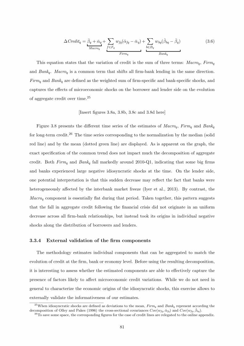
∆Creditq = βq + αq

Macroq

+∑f∈Fq

wfq(αfq − αq)

Firmq

+∑b∈Bq

wbq(βbq − βq)

Bankq

(3.6)

This equation states that the variation of credit is the sum of three terms: Macroq, Firmq

and Bankq. Macroq is a common term that shifts all firm-bank lending in the same direction.

Firmq and Bankq are defined as the weighted sum of firm-specific and bank-specific shocks, and

captures the effects of microeconomic shocks on the borrower and lender side on the evolution

of aggregate credit over time.25

[Insert figures 3.8a, 3.8b, 3.8c and 3.8d here]

Figure 3.8 presents the different time series of the estimates of Macroq, Firmq and Bankq

for long-term credit.26 The time series corresponding to the normalization by the median (solid

red line) and by the mean (dotted green line) are displayed. As is apparent on the graph, the

exact specification of the common trend does not impact much the decomposition of aggregate

credit. Both Firmq and Bankq fall markedly around 2010-Q1, indicating that some big firms

and banks experienced large negative idiosyncratic shocks at the time. On the lender side,

one potential interpretation is that this sudden decrease may reflect the fact that banks were

heterogeneously affected by the interbank market freeze (Iyer et al., 2013). By contrast, the

Macroq component is essentially flat during that period. Taken together, this pattern suggests

that the fall in aggregate credit following the financial crisis did not originate in an uniform

decrease across all firm-bank relationships, but instead took its origins in individual negative

shocks along the distribution of borrowers and lenders.

3.3.4 External validation of the firm components

The methodology estimates individual components that can be aggregated to match the

evolution of credit at the firm, bank or economy level. Before using the resulting decomposition,

it is interesting to assess whether the estimated components are able to effectively capture the

presence of factors likely to affect microeconomic credit variations. While we do not need in

general to characterize the economic origins of the idiosyncratic shocks, this exercise allows to

externally validate the informativeness of our estimates.

25When idiosyncratic shocks are defined as deviations to the mean, Firmq and Bankq represent according thedecomposition of Olley and Pakes (1996) the cross-sectional covariances Cov(wfq, αfq) and Cov(wfq, βbq).

26To save some space, the corresponding figures for the case of credit lines are relegated to the online appendix.

81


A natural source of information on firm-level credit shocks is provided by the default status

of firms made available in the credit registry. This status indicates whether the firm has recently

defaulted on a trade bill or entered a procedure to safeguard or to liquidate the firm (“distressed

firm”). Using an event study setting, a firm is said to be treated at q = 0 if its default status

switches from “non-distressed” to “distressed” at that time.27 The control group is defined as

the set of firms in the same department, in the same risk category, in the same industry and

of similar size as treated firms at q = −1 but that never become distressed.28 When multiple

control firms are found for a single treated firms, we select the one that minimize the absolute

distance in terms of total long-term credit exposures at q = −1. At the end of the process,

each treated firm is matched with zero (in which case it is dropped) or exactly one control firm.

We impose that all treated and control firms are present in the database between q = −4 and

q = 0.

This procedure leads us to retain 3516 control and treated firms. Figure 3.9 presents the

evolution of the mean firm-specific shock αfq = αfq−αq four quarters before and after the default

event for treated firms and control firms. Before the treatment, firm components evolve similarly

for control firms and treated firms. At q = 0, the idiosyncratic components of treated firms fall

sharply on average. By comparison, the curve follows its pre-existing trend for control firms.

Table 3.9 validates this graphical illustration. The table displays the results of the regression

αfq = µf + γPostq + δPostq × Treatedf + εfq

Postq is a dummy variable equal to one (zero) when q is greater or equal (strictly inferior) to

zero. Treatedf is equal to one when f belongs to the treated group, zero otherwise. In line with

the figure, we find that firm-level shocks fell relatively more after q = 0 for treated than for

control firms (δ < 0).

[Insert table 3.4 here]

After being declared in financial distress, treated firms may exit the credit registry as they

go bankrupt or because their total credit exposure falls below the reporting threshold. This is

27For the sake of readability, we make use in this subsection of the vocabulary of randomized controlledtrials (“treated firms”, “control firms”). This is admittedly not completely appropriate in our context as the“treatment” is probably not random. This is however not a problem for our econometric analysis as we do notattempt to obtain causal links.

28Firms are sorted in 16 industries, 4 size and risk categories as well as 101 departments.

82

reflected in the data by a credit growth rate equal to -200%, which leads by construction to

a very low idiosyncratic component. The drop in individual shocks may therefore be entirely

driven by credit adjustments at the extensive margin. Column 2 shows that we find a negative

and significant coefficient even when imposing that firms stay in the credit registry during the

two year period around q = 0 (“surviving firms”). This implies that firm components also

capture idiosyncratic variations of the quantity of credit (intensive margin).

3.4 Granular borrowers and the cyclicality of aggregate credit

3.4.1 Granularity and cyclicality

This section explores the implications of the presence of granular borrowers for the cycli-

cality of aggregate long-term credit. The empirical importance of large firms for the properties

of aggregate credit is a priori unclear. Indeed, a peculiar and interesting feature of credit is

that both the distribution of borrowers and lenders feature heavy tails (see subsection 3.2.2).

While the granularity literature suggests that the cyclicality of aggregate credit will be dispro-

portionately determined by idiosyncratic shocks affecting large actors, it offers little guidance

to determine whether firm or bank microeconomic variations will matter more in the aggregate.

Equation 3.6 provides a simple way to assess the respective contributions to the credit cycle

of idiosyncratic shocks on the borrower and the lender side. In line with Covas and Den Haan

(2011), we measure the cyclicality of aggregate credit as the comovement between the growth

rate of aggregate credit and the growth rate of the non-financial sector real GDP.29 Let ∆GDPq-k

be the growth rate of real GDP between q − k − 4 and q − k (k is an integer between 0 and 5).

∆GDPq-k is normalized so that its standard deviation is equal to one. Using equation 3.6, we

get that

Corr(∆Creditq,∆GDPq−k) =πMacro · Corr(Macroq,∆GDPq−k) (3.7)

+ πBank · Corr(Bankq,∆GDPq−k)

+ πFirm · Corr(Firmq,∆GDPq−k)

where, for instance, πFirm is the ratio of the standard deviation of Firmq (σFirm) to the

standard deviation of ∆Creditq (σCredit). For clarity, we refer to πX · Corr(Xq,∆GDPq−k) as

29Data on GDP comes from the French National Statistics Institute (Insee).

83

Share(Xq,∆GDPq−k).

Before presenting the results of the decomposition implied by equation 3.7, it is useful as a

benchmark to estimate an upper bar of the contribution of firm idiosyncratic shocks in a non-

granular setting. Assume that firm shocks αfq are independent random variables with identical

variance σ. Following Gabaix (2011) we can show that the standard deviation of Firmq is

proportional to the square root of the Herfindahl-Hirschmann index of the repartition of credit

across borrowers:

σFirm = σ

√∑f∈Ft

w2ft

As long as the variance of the loan distribution of borrowers is finite (a condition that is

generally not satisfied in the presence of fat tails), the law of large numbers ensures that when

the number of firms N becomes infinitely large, the square root of the Herfindahl will at the limit

be proportional to 1/√N . Since the covariance between two random variables is bounded by

the product of the standard deviations, the maximal contribution of firms idiosyncratic shocks

to aggregate credit cyclicality will also decay at rate 1/√N . To simplify the analysis, consider

the extreme example of an equal repartition of credit between firms (i.e. wft = 1/N). In this

case, we would have

| Share(Firmq,∆GDPq−k) |≤σ

σCredit· 1√

N

To get an estimate of σ, we calculate for each time period the cross-sectional standard deviation

of the firm shocks and take the average over time. We find σ equal to 76%, set k equal to 4

quarters and take N equal to the average number of firms per quarter (approximately 75,000

firms). We obtain that if credit were equally distributed between borrowers, the contribution of

idiosyncratic shocks on the firm side would not exceed 8% of the observed comovement between

the evolution of credit and GDP growth.

3.4.2 Dissecting the cyclicality of aggregate credit

Figure 3.8d displays the time series of the growth rate of long-term credit (aggregated over

all the bank-firm relationships in the connected set) and of the real GDP of the non-financial

sector. We choose the value of k, the lag of the GDP growth rate, to be equal to one year (4

quarters) so as to maximize the observed correlation (49.4%) with the growth rate of credit.30

30Correlation with leads of GDP are either non-significantly different from zero or negative in some cases. Wechose therefore to focus on lags of GDP for the sake of clarity.

84

The statistical relationship between the two series is clearly visible on the graph: one year after

a decrease in real GDP, credit appears to fall in sizeable proportions.


Table 3.5 gives the results of the decomposition of the cyclicality of aggregate credit given

by equation 3.7. Following Di Giovanni, Levchenko, and Mejean (2014), we compute standard

errors using a block bootstrap procedure to account for the small sample size (68 observations)

and the presence of serial correlation in the residuals.31 The correlation between GDP and

credit is only significant at 5% for k between 3 and 5 quarters and decreases in magnitude after

k = 4. Strikingly, only firm individual shocks appear to be significantly related to the business

cycle. About 80% of the total correlation with lag 4 of GDP is attributable to Firmq, meaning

that the importance of firm-specific variations is about 10 times higher than it would have been

in the absence of borrower granularity.

By contrast, bank idiosyncratic shocks Bankq appear to play a limited role in the cyclicality

of aggregate credit. This in itself should not be taken a sign that bank granular shocks do not

affect real activity.32 Our results suggest, however, that the credit cycle does not find its origins

in shocks affecting homogeneously the lending relationships of large banks. The heterogeneity

in loan size within the pool of borrowers is actually so large that most of the correlation between

credit and GDP can be traced to shocks affecting individual borrowers.

We explore further the role of granular borrowers by breaking down the weighted sum of firm

components Firmq by borrower loan size. Consider a partition of Fq, the set of firms present at

time q, in S subsets F1q, ..., FSq. For example, one simple partition would consist in dividing

Fq in firms in the bottom 99% of the credit distribution and firms in the top 1%. The firm

component can be in this line decomposed as

Firmq =

S∑s=1

µsq

∑f∈Fsq

νfsq(αfq − αq)

=

S∑s=1

µsqFirmsq

where µsq denotes the share of subset s in aggregate credit at time q and νfsq the weight of

firm f in subset s. This decomposition, however, is impractical for the decomposition of the

correlation of credit with GDP as weights µsq also vary with time. We define to that end an

31Our moving block bootstrap procedure (Kunsch, 1989) is based on 1000 replications and a block length of4 observations.

32Amiti and Weinstein (2018) and Alfaro, Garcıa-Santana, and Moral-Benito (2019) show that bank shockshave a sizeable impact on firm-level and aggregate real variables such as investment or employment.

85

alternative firm component, Firm∗q by replacing weights µsq with their average over time. As

a result, we are able to further decompose the aggregate impact of firm-level shocks into the

weighted sum of each subset’s own contribution:

Corr(Firm∗q ,∆GDPq−k) =

S∑s=1

µsρsCorr(Firmsq,∆GDPq−k) (3.8)

where ρs is the ratio of the standard deviation of Firmsq to the standard deviation of Firm∗q .


Table 3.6 presents the results of the decomposition obtained with equation 3.8. Column 1

first shows that replacing Firmq with Firm∗q does not alter much the correlations with the dif-

ferent lags of GDP. The weighted sum of idiosyncratic shocks to firms below the 95th percentile

of the credit distribution Firm0−95q appears to be significantly correlated to GDP for all values

of k, although the coefficient is only significant at the 10% level for contemporaneous GDP.

On the other hand, its contribution to the cyclicality of aggregate credit does not exceed 11%

for the lag 4 of GDP, which is somewhat consistent with the benchmark given in section 3.4.1.

By comparison, individual shocks to firms in the top 100 of borrowers represent 55% of the

correlation.

Perhaps more importantly, we can see that the top 100 borrowers actually impose its struc-

ture of cyclicality to the aggregate time series. While Firm0−95q comoves with contemporaneous

GDP, the correlation becomes not significant once the rest of the distribution is included. The

cyclicality of the firm component increases sharply when considering lagged values of GDP, this

surge being largely driven by the top 100 borrowers. To a large extent, therefore, relying on

aggregate data to analyze the evolution of credit over the business cycle amounts to focusing

on the microeconomic behavior of a restricted set of large borrowers. As the latter are presum-

ably financially unconstrained, inferring the intensity of financial frictions in the economy by

matching aggregate credit fluctuations is likely to lead to biased conclusions.


Figure 3.10 gives a graphical illustration of the role of the loan distribution. We compare

the contribution of each size bucket to total credit in volume (dark grey) and to the correlation

of firm idiosyncratic shocks to GDP, Corr(Firm∗q ,∆GDPq−4) (light grey). Firms below the 95th

86

percentile of the credit distribution, for instance, represent on average 31% of total credit and

14% of the correlation. Strikingly, the weight in total credit increases much faster than the

contribution to cyclicality as we progressively add firms from the right tail of the distribution.

This graph shows that granularity is not a pure size effect: the influence of shocks affecting the

top 100 borrowers is disproportionate compared to their weight in total credit.

The weights µsρs present in equation 3.8 allows to rationalize the over-representation of

granular borrowers. Imagine that we progressively zoom in on the right tail of distribution, by

defining s as the top 10,000, then 1,000, and eventually 100 borrowers for instance. As we focus

on a smaller sample, the variance of the weighted sum of idiosyncratic shocks will increase,

hence a higher variance share ρs. In normal-tailed distributions, µs should however become

very small, leading in total to a negligible contribution of top borrowers. The slow convergence

of µs towards zero as s moves to the top of the credit distribution makes shocks to granular

borrowers exert a disproportionate influence on aggregate credit.

3.4.3 Granular shocks and granular trends

Because the individual components we estimate are expressed as deviations from a common

cross-sectional median or alternatively mean, we sometimes refer to these components as id-

iosyncratic shocks. On the other hand, these shocks are not necessarily independent from each

other: the fact that to a large extent the cyclicality of aggregate credit can be traced back to the

top 100 borrowers may reflect mechanisms that are specific to this type of firms. For example,

large borrowers may be able to react relatively more to investment opportunities because they

have easier access to alternative sources of external financing, or because they tend to be less

financially constrained. Such mechanisms would induce positive pairwise correlation between

the individual shocks of the granular borrowers, which in turn would contribute to increase the

variance of the aggregate granular component Firmtop100q and the magnitude of its comovement

with the business cycle.

To measure this pairwise correlation we first define for each granular borrower i the granular

component that one would observe in the absence of this firm:

Firmtop100−iq =

∑f∈Ftop100−i,q

νfq1− νiq

αfq

Then we regress Firmtop100−iq on αiq and a set of firm fixed effects. The estimated coefficient

87

is equal to 0.056 and significant at the 1% level.33 Hence, the correlation between shocks is

positive but small: one may be tempted to conclude that “at the firm level, most variation is

idiosyncratic” (Gabaix, 2011).

However, it may be the case that even a small level of correlation between firms is enough to

have a sizeable impact on aggregate fluctuations. To understand why, assume that individual

standard deviations σg and pairwise correlations corrg are constant across granular borrowers.

The variance of Firmtop100q writes

Var(Firmtop100

q

)= σ2

g (hg + corrg − hg · corrg)

≈ σ2g (hg + corrg)

where hg denotes the Herfindhal of the repartition of credit within the set of granular borrowers.

The first order approximation holds as long as both the pairwise correlation and the Herfind-

hal index are close to zero.34 It implies that the relative contributions of concentration and

correlation to the standard deviation of the aggregate component are directly related to their

relative magnitudes. As a counterfactual exercise, we estimate the comovement of Firm∗q with

the business cycle that one would obtain by setting corrg to zero.35 We find that the contribu-

tion of Firmtop100q would decrease from 0.270 to 0.128, which in turn would lower by almost 40%

the covariance between Firm∗q and one-year lag GDP, everything else equal. It suggests that

mechanisms specific to granular borrowers and inducing a positive correlation between their

individual shocks contribute to amplifying the cyclicality of the granular component. It is then

the granular structure of the loan distribution, i.e the large share of the top 100 firms in total

credit, which enables these mechanisms to impact aggregate cyclicality.

3.4.4 Robustness checks

We assess in this subsection the sensitivity of our findings to the specification of the method-

ology. In table 3.7, we report for each specification the decomposition of the correlation between

33The fixed-effect regression implies that the estimated coefficient is a weighted sum ofCov(Firmtop100−i

q , αiq)/Var(αiq). Under the assumption that standard deviations and pairwise correla-tions are constant across firms the coefficient we obtain is therefore an estimation of Corr(αiq, αjq). The standarderrors are clustered at the firm level. We do not report the results of the regression in order to save some space.

34Gabaix (2011) reports that the median of the herfindhals generated by Monte Carlo simulations for a highlygranular economy (Zipf distribution) with 106 firms is equal to (0.12)2 = 0.0144, while he finds for the largestUS firms that the correlation between the growth rates of sales is close to 0.07.

35To measure σg we calculate the cross sectional variance among the top 100 firms and take the square rootof the time average. We measure hg as the average over time of the Herfindhal index for the set of granularborrowers. The counterfactual standard deviation is then equal to σg

√hg.

88

the credit growth rate and the four-quarter lag of the GDP growth rate. The top panel displays

the decomposition obtained with the baseline specification. Remember that the baseline de-

composition is obtained by (i) setting the median of the shocks at zero, (ii) keeping only firms

with two banking relationships in a given quarter and (iii) keeping only banks with at least 100

relationships in a given quarter.


Defining both bank-specific and firm-specific components as deviations to the mean (instead

of the median) leads to slightly different results (see second panel of table 3.7). The contribution

of Firmq to the cyclicality of aggregate credit (44%), in particular, is significantly reduced by

comparison to the baseline case (80%). The correlations are however imprecisely estimated.

Since the behavior of the different components does not appear moreover to be very affected

by the choice of the normalization (see figure 3.8), we favor the results obtained with the

deviation to the median in the analysis. Eventually we notice that in the mean normalization

case the impact of borrowers individual shocks (although attenuated) remains large, close to

the effect of the macro component, and way higher than both the non-granular benchmark and

the contribution of bank shocks.

The third panel shows that imposing a minimum number of borrowers by bank of 10 firms do

not change much our conclusions. The largest part of the correlation between the credit growth

rate and the lagged GDP growth rate (0.553) is still explained by the correlation of the firm

component with the GDP growth rate (0.381). Symmetrically, increasing the minimum required

number of banking relationships for firms to 4 banks decreases the number of multiple-bank

firms but may improve the precision of estimates of the firm components. As a matter of fact,

our matched bank-firm loan dataset can be seen as a bipartite graph, in which interactions occur

between two type of individuals but not within each type. Jochmans and Weidner (2019) suggest

that the sparsity of the underlying network affects the accuracy with which the fixed effects

can be estimated. They show that the second smallest eigenvalue of the network’s normalized

Laplacian matrix is a measure of global connectivity of the graph, and that the upper bounds on

the variances of the estimated fixed effects are smaller when this measure is large. Restricting the

dataset to firms borrowing from at least 4 banks strongly increases the corresponding eigenvalue,

from 0.08 in our main specification to 0.15.36 Still, the correlation of aggregate credit to the

36We compute these eigenvalues for the data corresponding to 2009-Q2. Because we perform a WLS estimation,the underlying network is a weighted graph, in which the weight of the edge connecting bank b to firm f is equal

89

business cycle remains primarily explained by firm individual components, which suggests that

the precision of the estimated fixed effects is unlikely to drive our results.


Foreign banks might be less sensitive to the French business cycle, which may lower the

cyclicality of aggregate credit. Panel 2 of table 3.8 shows that it is not the case: if anything,

the correlation of aggregate credit to the business cycle is slightly lower when excluding for-

eign banks. Panel 3 then displays the results of the estimations obtained when excluding the

housing sector. The housing sector represents a disproportionate part of long-term credit (see

subsection 3.2.1). Since real estate firms financing decisions are determined by very specific

mechanisms, it is interesting to assess how our results change after excluding them from the

data set.37 We find that the decomposition of the cyclicality of aggregate credit remains very

similar to the baseline results. This suggests that the presence of the housing sector does not

drive in itself our findings.

In an other robustness exercise, we consolidate banks at the group-level. An immediate

drawback of this approach is that it mechanically reduces the number of multiple-bank firms.

However, as banking groups are less likely to be specialized in some sector of activities or

geographical markets (the French banking sector is dominated by so-called “universal” banks),

firms might be more able to substitute credit between lenders. This may lead to a better

identification of both bank and firm fixed effects in equation 3.2, which, in turn, could affect

the decomposition of the cyclicality of aggregate credit. Panel 4 shows however that our results

are not modified when banks are consolidated at a higher degree of aggregation.

A potential explanation of the fact that bank idiosyncratic components do not contribute

much to the cyclicality of aggregate credit is that we do not allow for enough heterogeneity in

the behavior of banks. Bank lending behavior might indeed vary between different groups of

borrowers. Our specification may in that sense impose too much constraints in that it assumes

an homogeneous bank component. In particular, if banking lending behavior depends on the

loan size of the borrower, the firm aggregate component Firmq might erroneously capture some

part of the variation of aggregate credit that should in theory be attributed to Bankq. We use

to the average exposure between q − 4 and q. The global connectivity is even more improved when consideringthe (unweighted) graph associated to the OLS estimation, from 0.06 to 0.23.

37In particular, real estate firms are not scored by the Bank of France. A significant fraction of real estatefirms are created to isolate and regroup the real estate assets of business groups and as such do not generate anycash-flows. Traditional financial analysis does not apply for this type of firms, hence the absence of credit score.

90

therefore a statistical rule to break down banks in sub-units. A borrower is classified as being

small (large) if it borrows less (more) than the bank average. We then break each bank in a

“retail” bank (which lends to small borrowers) and a “wholesale” bank (which lends to large

ones) and rerun the estimations with twice as much bank components as in the baseline spec-

ification. We find that allowing heterogeneous bank idiosyncratic shocks does not significantly

alter our results.

Measuring the change in lending by mid-point growth rates enables us to account for both the

formation and the termination of firm-bank relationships. On the other hand, it implies that the

distribution of our dependent variable displays mass points at 2 and −2, which might affect the

econometric estimation. Therefore we restrict our initial dataset to ongoing relationships and

discard both terminating and new loans. Under such specification our decomposition focuses on

the intensive margin of credit growth. One may wonder to which extent the entries and exits of

loan relationships impact the observed comovement between total credit and GDP. Panel 6 of

table 3.8 shows that removing the extensive margin tends to lower the correlation of aggregate

credit to the business cycle. Although the macro component now contributes negatively to our

measure of cyclicality, we still find that bank shocks play a very limited role while the firm

component drives to a large extent the correlation.


In order to rule out sectoral or geographical variations from Firmq, we use as alternative def-

inition of idiosyncratic shocks the deviation to the conditional median. We successively take the

median by industry, credit score category, size category, administrative division (“departement”)

and by the category defined by the intersection of all the precedent variables (“cell”). Table 3.9

reports the contemporaneous and lagged correlations between the GDP growth rate and the

different time series of Firmq obtained with these definitions. The correlations of the firm

component with the one-year lag of the GDP growth rate are all positive and significant and

represent 62% to 80% of the aggregate correlation.


The estimation of equation 3.2 with weighted least squares gives by construction more im-

portance to firms and banks with larger outstanding volumes of credit. One may therefore

suspect that the importance of firm shocks in the aggregate fluctuations of credit mechanically

91

derives from the estimation method. In table 3.10, we present the results obtained by estimating

equation with ordinary least squares instead of WLS. A drawback of this specification is that

the weighted sum of residuals does not cancel out in the aggregate: we add therefore a fourth

term to the decomposition (match-specific component) that we name Matchq. The resulting de-

composition is close to the one obtained with the baseline specification. The correlation between

aggregate credit and GDP, when high and significant, is mainly driven by the firm component.

The contribution of the match-specific component is large when focusing on contemporaneous

GDP, but then slowly fades out as we consider lagged time series.

By construction, the decomposition of the cyclicality of aggregate credit excludes single-

bank firms. In a last robustness exercise, we attempt to assess the relative contributions of the

different components when including the entire population of borrowers. To that end, we first

compute the mid-point growth rate ∆Creditaggq of aggregate long-term credit using the data

set we obtained before restricting it to the connected set. This time series therefore includes

credit borrowed by single-bank firms. We then regress ∆Creditaggq on the time series Macroq,

Bankq and Firmq obtained from equation 3.6. Table 3.11 displays the results obtained with the

baseline specification and by defining idiosyncratic shocks as the deviation to the mean.38


We use the estimated coefficients to compute the contribution of each of the three terms to

the correlation of ∆Creditaggq with ∆GDPq−4. The total correlation is given in the bottom of

the table and is equal to 0.601. The respective contributions of each component are displayed

below the standard errors of the coefficients. The decomposition now includes a fourth element,

corresponding to the comovement of the estimated error term with the business cycle and

displayed in the “Residual” line. We find that in our baseline specification firm-specific shocks

would remain a first order determinant of the cyclicality of aggregate credit (58% of the total

correlation). In the specification with the mean, Firmq becomes the second contributing factor

behind Macroq but still explains 29% of the link between credit and the business cycle.

38Note that if ∆Creditaggq was exactly equal to ∆Creditq, all the coefficients would be equal to one. Interestingly,we find for both specifications that the coefficients for Macroq and Bankq are not statistically different from one.The Firmq coefficient appears by contrast to be lower than one. Also notice that for both normalizations the R2is high, respectively equal to 91.3 and 93.4%. Our aggregate time series estimated on the set of multi-bank firmsare therefore able to capture the bulk of aggregate credit fluctuations, even when including single-bank firms.

92

3.5 Bank liquidity risk and borrower concentration

3.5.1 Can banks pool borrower idiosyncratic risk?

We turn in this section to the implications of the presence of granular borrowers on bank-

level variations of undrawn credit lines. Banks’ ability to provide liquidity on demand through

credit lines or deposits will depend on the distribution of liquidity outflows (Holmstrom and

Tirole, 1998; Kashyap, Rajan, and Stein, 2002). In particular, if banks are unable to pool the

idiosyncratic risk of their borrowers, they may have to hoard more liquid assets to hedge against

negative shocks affecting individual borrowers.

We obtain with our decomposition the following equality for the evolution of undrawn credit

lines at the bank-level:

∆Creditbq = Macroq + βbq +∑

w(b)fqαfq

= Macroq + Bankbq + Firmbq (3.9)

It is easy to see following the logic of section 3.4.1 that a bank’s exposure to borrower idiosyn-

cratic risk will depend on whether the distribution of its borrower base w(b) is fat-tailed or not.

Given the extreme degree of concentration of credit lines (see section 3.2.2), there are reasons

to believe that the ability of banks to pool idiosyncratic risk is actually limited.


We have to slightly adjust our methodology to quantify the importance of idiosyncratic risk

in banks’ credit line portfolios. First, since the portfolio of borrowers is likely to be managed at

the level of the group, we consolidate banks by banking group in the remainder of the analysis.

Second, we focus our study on the six largest banking groups.39 This choice allows first to keep

only banks with very large borrower bases for which the law of large numbers should apply in

the absence of granular borrowers. Moreover, the selected banks are present during the whole

time period, which greatly simplifies the analysis in the following. Third, because of a change

in the treatment of short-term loans in the credit registry, the analysis of credit lines at the

firm-level is not reliable around 2006. We choose therefore to focus on the period starting from

2008-Q1 and ending in 2016-Q4.

39The six largest banking groups account in our sample for 84% of lending to firms.

93

We incorporate these changes into our estimation procedure to get the firm, bank and macro

components of bank-level variations of credit lines. In order to quantify the role of borrower

individual shocks, we compute for each bank the variance of the counterfactual time series of

credit lines variations if Firmbq were constantly equal to zero. In a second step, we compute the

average across banks of the resulting variances that we compare to the average variance of the

original ∆Creditbq time series.40 We do the same counterfactual exercise by setting successively

Macroq, Bankbq and the weighted sum of firm components for the top 10 borrowers FirmTop 10bq

to zero in equation 3.9.41 The estimated counterfactual variances are displayed in table 3.12.

From equation 3.9, it is apparent that muting borrower idiosyncratic shocks will have a

large effect on bank-level credit lines variance if (i) firm-specific shocks are very volatile, (ii)

borrower portfolios are not diversified, (iii) the weighted sum of borrower idiosyncratic shocks

is positively correlated with the other components of the decomposition.

Our findings suggest that banks are substantially exposed to borrower idiosyncratic risk.

Without borrower idiosyncratic shocks, bank-level variance of credit lines is reduced by 31%.

The effect is larger than for the bank and macro components (respectively 29% and 9%). Muting

the individual shocks of the ten largest borrowers reduces the variance even more (44%). This

is expected as FirmTop 10bq is likely to be more volatile than Firmbq.

One may fear that the large role of borrower risk in our findings could be an artifact of

our definition of idiosyncratic shocks. Since we look at deviations from a common macro

trend, our shocks could actually incorporate sectoral or geographical factors. We therefore

proceed to the same exercise using the deviation to the median by cell as a more demanding

definition of idiosyncratic shocks (a cell being the intersection of a sector, a credit risk category,

a size category and a geographical zone; see section 3.4.4). As expected, muting borrower

idiosyncratic shocks reduces less the variance of credit lines (19%). By contrast, the importance

of macro shocks becomes larger (31%). Still, the role of borrower idiosyncratic risk on credit

line variations appears to be far from negligible. Overall, our results strongly supports the idea

that on average, banks are not fully able to diversify away the idiosyncratic risk of borrowers

in their credit lines portfolio.

40We build here on the methodology used by Kramarz, Martin, and Mejean (2019) to estimate the level ofunder-diversification of French exporters.

41Note that this counterfactual exercises take the weights of firms in the bank credit lines portfolio as given.In practice, however, the weights are themselves a function of the past values of the different components. Wechose to abstract from these indirect effects to keep the intuition simple.

94

3.5.2 Borrower concentration as a source of synchronization

The previous subsection established that banks are exposed to borrower idiosyncratic risk.

We turn now to the implications of this additional source of risk for aggregate liquidity flows.

There are indeed several reasons to believe that borrower risk may be correlated across banks.

Remember first that by construction, firms in our sample borrow from multiple banks. The

presence of granular borrowers in several credit lines portfolios could therefore lead credit lines

variations to be synchronized across banks. Second, input-output linkages can make idiosyn-

cratic shocks propagate across the production network. A supplier hit by a natural disaster,

for instance, is likely to draw on its credit line to make up for the decrease in production. In

turn, the customers of the firm may themselves need to rely on their credit lines to handle the

disruption of their supply chain.42


We test this hypothesis by decomposing the variance of aggregate borrower risk. To simplify

the analysis, we set bank weights wb equal to their time average in the computation of the time

series Firm∗q. This allows us to write

Var(Firm∗q) =∑b

w2bVar(Firm∗bq) +

∑b

∑c 6=b

wbwcCov(Firm∗bq,Firm∗cq)

= Directq + Linkq (3.10)

Equation 3.10 states that the aggregate variance of borrower idiosyncratic shocks is the sum

of (i) Directq, the weighted sum of bank-level variances and (ii) Linkq, the weighted sum of the

covariances of borrower idiosyncratic shocks between banks. The Linkq component reflects the

fact that different banks have common borrowers and are therefore subject to common shocks,

but it may also be driven by pairwise correlations between the firms that constitute banks’

borrower bases. To disentangle both mechanisms we measure the share of Linkq which is driven

by common shocks :

Commonq =∑b

∑c 6=b

wbwc

∑Rbcq

w(b)fqw(c)fqVar(αfq)

42For evidence of propagation of idiosyncratic shocks along the production network, see Barrot and Sauvagnat

(2016).

95

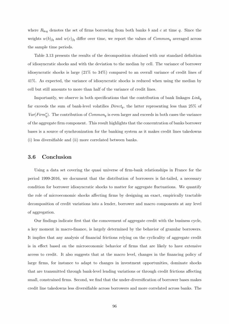
where Rbcq denotes the set of firms borrowing from both banks b and c at time q. Since the

weights w(b)fq and w(c)fq differ over time, we report the values of Commonq averaged across

the sample time periods.

Table 3.13 presents the results of the decomposition obtained with our standard definition

of idiosyncratic shocks and with the deviation to the median by cell. The variance of borrower

idiosyncratic shocks is large (21% to 34%) compared to an overall variance of credit lines of

41%. As expected, the variance of idiosyncratic shocks is reduced when using the median by

cell but still amounts to more than half of the variance of credit lines.

Importantly, we observe in both specifications that the contribution of bank linkages Linkq

far exceeds the sum of bank-level volatilies Directq, the latter representing less than 25% of

Var(Firm∗q). The contribution of Commonq is even larger and exceeds in both cases the variance

of the aggregate firm component. This result highlights that the concentration of banks borrower

bases is a source of synchronization for the banking system as it makes credit lines takedowns

(i) less diversifiable and (ii) more correlated between banks.

3.6 Conclusion

Using a data set covering the quasi universe of firm-bank relationships in France for the

period 1999-2016, we document that the distribution of borrowers is fat-tailed, a necessary

condition for borrower idiosyncratic shocks to matter for aggregate fluctuations. We quantify

the role of microeconomic shocks affecting firms by designing an exact, empirically tractable

decomposition of credit variations into a lender, borrower and macro components at any level

of aggregation.

Our findings indicate first that the comovement of aggregate credit with the business cycle,

a key moment in macro-finance, is largely determined by the behavior of granular borrowers.

It implies that any analysis of financial frictions relying on the cyclicality of aggregate credit

is in effect based on the microeconomic behavior of firms that are likely to have extensive

access to credit. It also suggests that at the macro level, changes in the financing policy of

large firms, for instance to adapt to changes in investment opportunities, dominate shocks

that are transmitted through bank-level lending variations or through credit frictions affecting

small, constrained firms. Second, we find that the under-diversification of borrower bases makes

credit line takedowns less diversifiable across borrowers and more correlated across banks. The

96

resulting synchronization largely drives the volatility of aggregate liquidity flows.

While our paper documents the implications of the presence of granular borrowers, it is

silent on the reasons leading to such high degrees of credit concentration. What are the costs of

diversifying the base of borrowers? Does the funding structure of banks, and in particular their

access to a stable base of deposits, play a role in determining the concentration of their loan

portfolio? To which extent these granular borrowers rely on alternative sources of financing over

the cycle? Answering those questions would help understanding the sources of the exposure of

banks and ultimately of the aggregate credit market to borrower idiosyncratic risk.

97

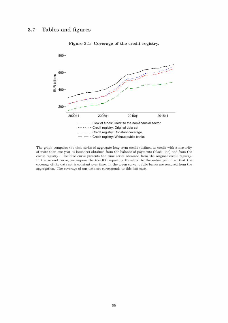
3.7 Tables and figures

Figure 3.1: Coverage of the credit registry.

200

400

600

800E

UR

bill

ions

2000q1 2005q1 2010q1 2015q1

Flow of funds: Credit to the non-financial sectorCredit registry: Original data setCredit registry: Constant coverageCredit registry: Without public banks

The graph compares the time series of aggregate long-term credit (defined as credit with a maturityof more than one year at issuance) obtained from the balance of payments (black line) and from thecredit registry. The blue curve presents the time series obtained from the original credit registry.In the second curve, we impose the e75,000 reporting threshold to the entire period so that thecoverage of the data set is constant over time. In the green curve, public banks are removed from theaggregation. The coverage of our data set corresponds to this last case.

98

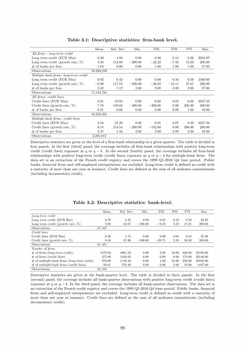
Table 3.1: Descriptive statistics: firm-bank level.

Mean Std. Dev. Min P25 P50 P75 Max

All firms : long-term creditLong term credit (EUR Mns) 0.39 4.00 0.00 0.08 0.14 0.26 3924.97Long term credit (growth rate, %) 4.50 112.89 −200.00 −22.22 −7.33 15.63 200.00# of banks per firm 1.04 0.66 0.00 1.00 1.00 1.00 57.00

Observations 59,286,238

Multiple-bank firms: long-term creditLong term credit (EUR Mns) 0.82 6.43 0.00 0.08 0.16 0.39 2560.00Long term credit (growth rate, %) −0.99 117.73 −200.00 −36.02 −10.11 27.61 200.00# of banks per firm 2.42 1.12 2.00 2.00 2.00 2.00 57.00


All firms: credit linesCredit lines (EUR Mns) 0.61 10.95 0.00 0.00 0.02 0.08 4657.50Credit lines (growth rate, %) 7.78 159.02 −200.00 −200.00 0.00 200.00 200.00# of banks per firm 0.31 0.60 0.00 0.00 0.00 1.00 43.00


Multiple-bank firms: credit linesCredit lines (EUR Mns) 2.58 24.20 0.00 0.01 0.07 0.29 4657.50Credit lines (growth rate, %) 6.15 154.54 −200.00 −182.80 0.00 200.00 200.00# of banks per firm 2.47 1.44 2.00 2.00 2.00 2.00 43.00


Descriptive statistics are given at the level of a firm-bank relationship in a given quarter. The table is divided infour panels. In the first (third) panel, the coverage includes all firm-bank relationships with positive long-termcredit (credit lines) exposure at q or q − 4. In the second (fourth) panel, the coverage includes all firm-bankrelationships with positive long-term credit (credit lines) exposure at q or q − 4 for multiple-bank firms. Thedata set is an extraction of the French credit registry and covers the 1999 Q1-2016 Q4 time period. Publicbanks, financial firms and self-employed entrepreneurs are excluded. Long-term credit is defined as credit witha maturity of more than one year at issuance. Credit lines are defined as the sum of all undrawn commitments(including documentary credit).

Table 3.2: Descriptive statistics: bank-level.


Long-term creditLong term credit (EUR Bns) 0.76 2.45 0.00 0.01 0.10 0.58 42.95Long term credit (growth rate, %) 3.80 62.07 −200.00 −9.23 5.52 17.21 200.00

Observations 27, 447

Credit linesCredit lines (EUR Bns) 0.46 1.74 0.00 0.00 0.04 0.24 25.36Credit lines (growth rate, %) 9.48 87.90 −200.00 −20.71 5.28 38.62 200.00


Number of firms# of firms (long-term credit) 1573.92 4961.58 0.00 2.00 58.00 886.00 82195.00# of firms (credit lines) 475.89 1448.02 0.00 0.00 8.00 173.00 26140.00# of multiple-bank firms (long-term credit) 370.00 1149.49 0.00 1.00 24.00 250.00 20102.00# of multiple-bank firms (credit lines) 93.81 278.49 0.00 0.00 2.00 45.00 4447.00


Descriptive statistics are given at the bank-quarter level. The table is divided in three panels. In the first(second) panel, the coverage includes all bank-quarter observations with positive long-term credit (credit lines)exposure at q or q − 4. In the third panel, the coverage includes all bank-quarter observations. The data set isan extraction of the French credit registry and covers the 1999 Q1-2016 Q4 time period. Public banks, financialfirms and self-employed entrepreneurs are excluded. Long-term credit is defined as credit with a maturity ofmore than one year at issuance. Credit lines are defined as the sum of all undrawn commitments (includingdocumentary credit).

99

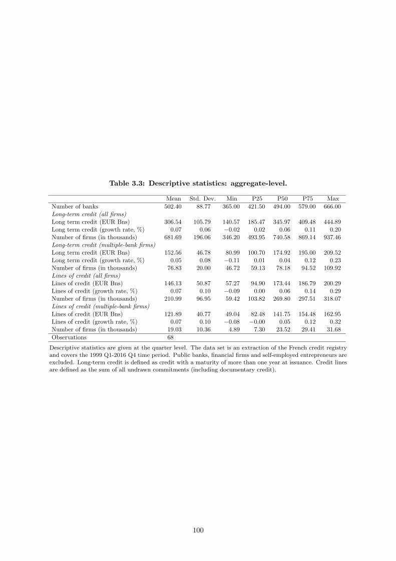
Table 3.3: Descriptive statistics: aggregate-level.


Number of banks 502.40 88.77 365.00 421.50 494.00 579.00 666.00Long-term credit (all firms)Long term credit (EUR Bns) 306.54 105.79 140.57 185.47 345.97 409.48 444.89Long term credit (growth rate, %) 0.07 0.06 −0.02 0.02 0.06 0.11 0.20Number of firms (in thousands) 681.69 196.06 346.20 493.95 740.58 869.14 937.46Long-term credit (multiple-bank firms)Long term credit (EUR Bns) 152.56 46.78 80.99 100.70 174.92 195.00 209.52Long term credit (growth rate, %) 0.05 0.08 −0.11 0.01 0.04 0.12 0.23Number of firms (in thousands) 76.83 20.00 46.72 59.13 78.18 94.52 109.92Lines of credit (all firms)Lines of credit (EUR Bns) 146.13 50.87 57.27 94.90 173.44 186.79 200.29Lines of credit (growth rate, %) 0.07 0.10 −0.09 0.00 0.06 0.14 0.29Number of firms (in thousands) 210.99 96.95 59.42 103.82 269.80 297.51 318.07Lines of credit (multiple-bank firms)Lines of credit (EUR Bns) 121.89 40.77 49.04 82.48 141.75 154.48 162.95Lines of credit (growth rate, %) 0.07 0.10 −0.08 −0.00 0.05 0.12 0.32Number of firms (in thousands) 19.03 10.36 4.89 7.30 23.52 29.41 31.68

Observations 68

Descriptive statistics are given at the quarter level. The data set is an extraction of the French credit registryand covers the 1999 Q1-2016 Q4 time period. Public banks, financial firms and self-employed entrepreneurs areexcluded. Long-term credit is defined as credit with a maturity of more than one year at issuance. Credit linesare defined as the sum of all undrawn commitments (including documentary credit).

100

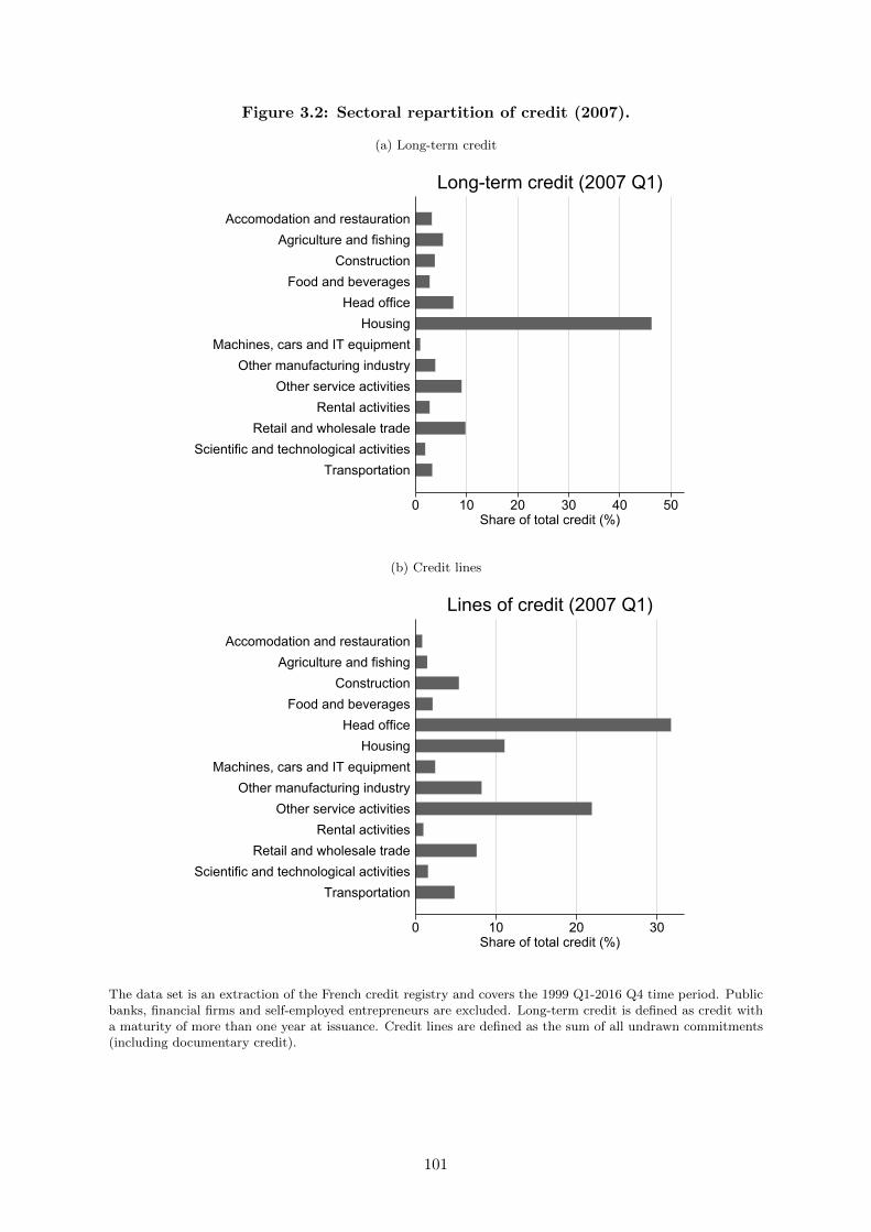
Figure 3.2: Sectoral repartition of credit (2007).

(a) Long-term credit

0 10 20 30 40 50Share of total credit (%)

TransportationScientific and technological activities

Retail and wholesale tradeRental activities

Other service activitiesOther manufacturing industry

Machines, cars and IT equipmentHousing

Head officeFood and beverages

ConstructionAgriculture and fishing

Accomodation and restauration

Long-term credit (2007 Q1)

(b) Credit lines

0 10 20 30Share of total credit (%)

TransportationScientific and technological activities

Retail and wholesale tradeRental activities

Other service activitiesOther manufacturing industry

Machines, cars and IT equipmentHousing

Head officeFood and beverages

ConstructionAgriculture and fishing

Accomodation and restauration

Lines of credit (2007 Q1)

The data set is an extraction of the French credit registry and covers the 1999 Q1-2016 Q4 time period. Publicbanks, financial firms and self-employed entrepreneurs are excluded. Long-term credit is defined as credit witha maturity of more than one year at issuance. Credit lines are defined as the sum of all undrawn commitments(including documentary credit).

101

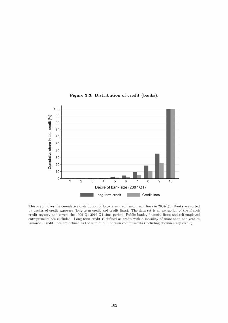
Figure 3.3: Distribution of credit (banks).

0

10

20

30

40

50

60

70

80

90

100

Cum

ulat

ive

shar

e in

tota

l cre

dit (

%)

1 2 3 4 5 6 7 8 9 10

Decile of bank size (2007 Q1)

Long-term credit Credit lines

This graph gives the cumulative distribution of long-term credit and credit lines in 2007-Q1. Banks are sortedby deciles of credit exposure (long-term credit and credit lines). The data set is an extraction of the Frenchcredit registry and covers the 1999 Q1-2016 Q4 time period. Public banks, financial firms and self-employedentrepreneurs are excluded. Long-term credit is defined as credit with a maturity of more than one year atissuance. Credit lines are defined as the sum of all undrawn commitments (including documentary credit).

102

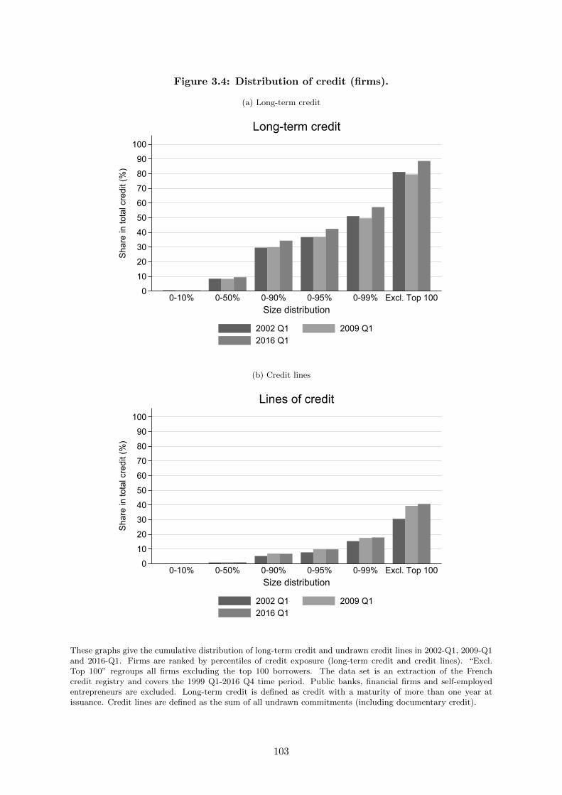
Figure 3.4: Distribution of credit (firms).


0

10

20

30

40

50

60

70

80

90

100

Sha

re in

tota

l cre

dit (

%)

0-10% 0-50% 0-90% 0-95% 0-99% Excl. Top 100Size distribution

Long-term credit

2002 Q1 2009 Q12016 Q1

(b) Credit lines

0

10

20

30

40

50

60

70

80

90

100

Sha

re in

tota

l cre

dit (

%)

0-10% 0-50% 0-90% 0-95% 0-99% Excl. Top 100Size distribution

Lines of credit

2002 Q1 2009 Q12016 Q1

These graphs give the cumulative distribution of long-term credit and undrawn credit lines in 2002-Q1, 2009-Q1and 2016-Q1. Firms are ranked by percentiles of credit exposure (long-term credit and credit lines). “Excl.Top 100” regroups all firms excluding the top 100 borrowers. The data set is an extraction of the Frenchcredit registry and covers the 1999 Q1-2016 Q4 time period. Public banks, financial firms and self-employedentrepreneurs are excluded. Long-term credit is defined as credit with a maturity of more than one year atissuance. Credit lines are defined as the sum of all undrawn commitments (including documentary credit).

103

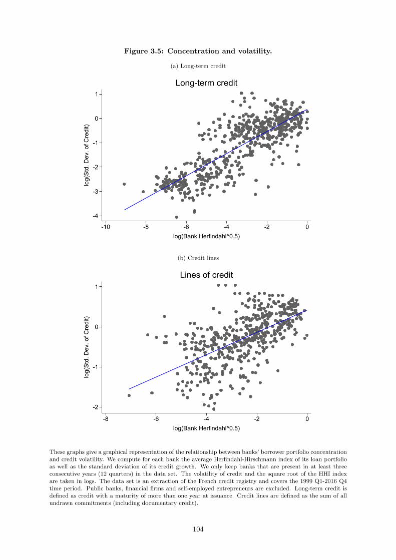
Figure 3.5: Concentration and volatility.


-4

-3

-2

-1

0

1lo

g(S

td. D

ev. o

f Cre

dit)

-10 -8 -6 -4 -2 0log(Bank Herfindahl^0.5)

Long-term credit

(b) Credit lines

-2

-1

0

1

log(

Std

. Dev

. of C

redi

t)

-8 -6 -4 -2 0log(Bank Herfindahl^0.5)

Lines of credit

These graphs give a graphical representation of the relationship between banks’ borrower portfolio concentrationand credit volatility. We compute for each bank the average Herfindahl-Hirschmann index of its loan portfolioas well as the standard deviation of its credit growth. We only keep banks that are present in at least threeconsecutive years (12 quarters) in the data set. The volatility of credit and the square root of the HHI indexare taken in logs. The data set is an extraction of the French credit registry and covers the 1999 Q1-2016 Q4time period. Public banks, financial firms and self-employed entrepreneurs are excluded. Long-term credit isdefined as credit with a maturity of more than one year at issuance. Credit lines are defined as the sum of allundrawn commitments (including documentary credit).

104

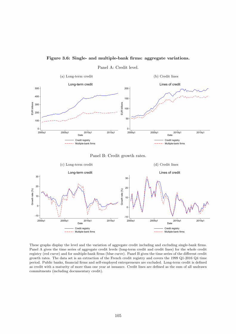
Figure 3.6: Single- and multiple-bank firms: aggregate variations.

Panel A: Credit level.


0

100

200

300

400

500

EU

R b

illio

ns

2000q1 2005q1 2010q1 2015q1Date

Credit registryMultiple-bank firms

Long-term credit

(b) Credit lines

0

50

100

150

200

EU

R b

illio

ns

2000q1 2005q1 2010q1 2015q1Date


Lines of credit

Panel B: Credit growth rates.

(c) Long-term credit

-10

0

10

20

30

Gro

wth

rate

(%)

2000q1 2005q1 2010q1 2015q1Date


Long-term credit

(d) Credit lines

-10

0

10

20

30

Gro

wth

rate

(%)

2000q1 2005q1 2010q1 2015q1Date


Lines of credit

These graphs display the level and the variation of aggregate credit including and excluding single-bank firms.Panel A gives the time series of aggregate credit levels (long-term credit and credit lines) for the whole creditregistry (red curve) and for multiple-bank firms (blue curve). Panel B gives the time series of the different creditgrowth rates. The data set is an extraction of the French credit registry and covers the 1999 Q1-2016 Q4 timeperiod. Public banks, financial firms and self-employed entrepreneurs are excluded. Long-term credit is definedas credit with a maturity of more than one year at issuance. Credit lines are defined as the sum of all undrawncommitments (including documentary credit).

105

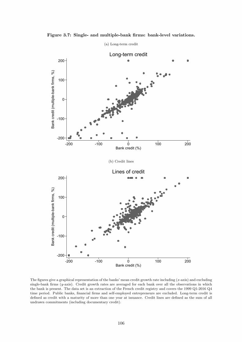
Figure 3.7: Single- and multiple-bank firms: bank-level variations.


-200

-100

0

100

200

Ban

k cr

edit

(mul

tiple

-ban

k fir

ms,

%)

-200 -100 0 100 200Bank credit (%)

Long-term credit

(b) Credit lines

-200

-100

0

100

200

Ban

k cr

edit

(mul

tiple

-ban

k fir

ms,

%)

-200 -100 0 100 200Bank credit (%)

Lines of credit

The figures give a graphical representation of the banks’ mean credit growth rate including (x -axis) and excludingsingle-bank firms (y-axis). Credit growth rates are averaged for each bank over all the observations in whichthe bank is present. The data set is an extraction of the French credit registry and covers the 1999 Q1-2016 Q4time period. Public banks, financial firms and self-employed entrepreneurs are excluded. Long-term credit isdefined as credit with a maturity of more than one year at issuance. Credit lines are defined as the sum of allundrawn commitments (including documentary credit).

106

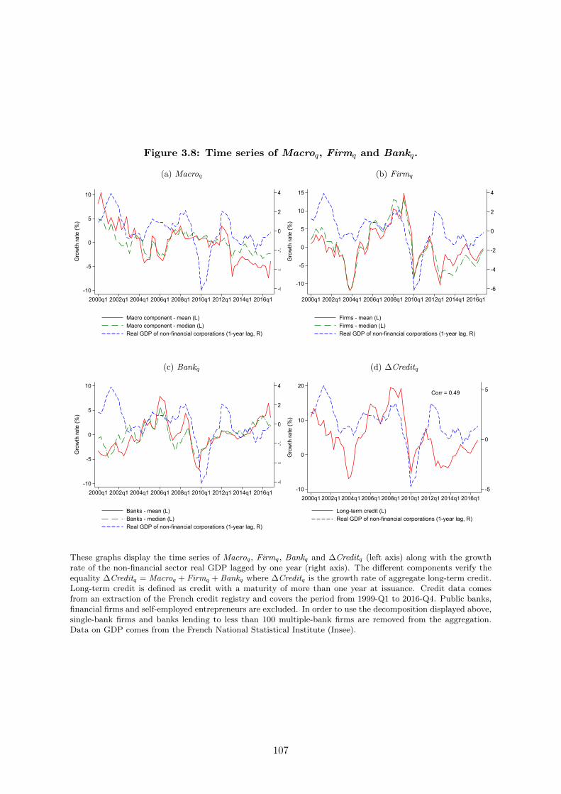
Figure 3.8: Time series of Macroq, Firmq and Bankq.

(a) Macroq

-6

-4

-2

0

2

4

-10

-5

0

5

10

Gro

wth

rate

(%)

2000q1 2002q1 2004q1 2006q1 2008q1 2010q1 2012q1 2014q1 2016q1

Macro component - mean (L)Macro component - median (L)Real GDP of non-financial corporations (1-year lag, R)

(b) Firmq

-6

-4

-2

0

2

4

-10

-5

0

5

10

15

Gro

wth

rate

(%)

2000q1 2002q1 2004q1 2006q1 2008q1 2010q1 2012q1 2014q1 2016q1

Firms - mean (L)Firms - median (L)Real GDP of non-financial corporations (1-year lag, R)

(c) Bankq

-6

-4

-2

0

2

4

-10

-5

0

5

10

Gro

wth

rate

(%)

2000q1 2002q1 2004q1 2006q1 2008q1 2010q1 2012q1 2014q1 2016q1

Banks - mean (L)Banks - median (L)Real GDP of non-financial corporations (1-year lag, R)

(d) ∆Creditq

Corr = 0.49

-5

0

5

-10

0

10

20

Gro

wth

rate

(%)

2000q1 2002q1 2004q1 2006q1 2008q1 2010q1 2012q1 2014q1 2016q1

Long-term credit (L)Real GDP of non-financial corporations (1-year lag, R)

These graphs display the time series of Macroq, Firmq, Bankq and ∆Creditq (left axis) along with the growthrate of the non-financial sector real GDP lagged by one year (right axis). The different components verify theequality ∆Creditq = Macroq + Firmq + Bankq where ∆Creditq is the growth rate of aggregate long-term credit.Long-term credit is defined as credit with a maturity of more than one year at issuance. Credit data comesfrom an extraction of the French credit registry and covers the period from 1999-Q1 to 2016-Q4. Public banks,financial firms and self-employed entrepreneurs are excluded. In order to use the decomposition displayed above,single-bank firms and banks lending to less than 100 multiple-bank firms are removed from the aggregation.Data on GDP comes from the French National Statistical Institute (Insee).

107

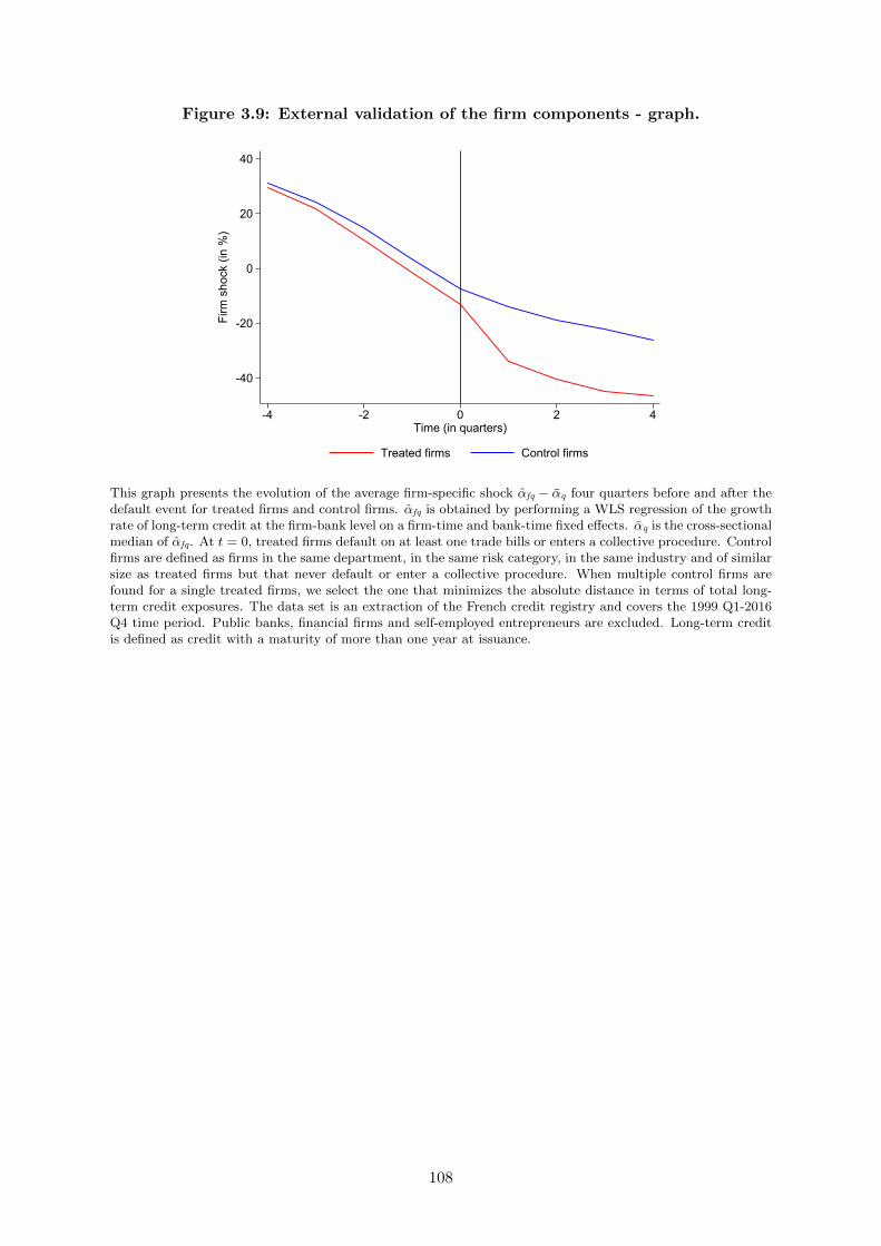
Figure 3.9: External validation of the firm components - graph.

-40

-20

0

20

40

Firm

sho

ck (i

n %

)

-4 -2 0 2 4Time (in quarters)

Treated firms Control firms

This graph presents the evolution of the average firm-specific shock αfq − αq four quarters before and after thedefault event for treated firms and control firms. αfq is obtained by performing a WLS regression of the growthrate of long-term credit at the firm-bank level on a firm-time and bank-time fixed effects. αq is the cross-sectionalmedian of αfq. At t = 0, treated firms default on at least one trade bills or enters a collective procedure. Controlfirms are defined as firms in the same department, in the same risk category, in the same industry and of similarsize as treated firms but that never default or enter a collective procedure. When multiple control firms arefound for a single treated firms, we select the one that minimizes the absolute distance in terms of total long-term credit exposures. The data set is an extraction of the French credit registry and covers the 1999 Q1-2016Q4 time period. Public banks, financial firms and self-employed entrepreneurs are excluded. Long-term creditis defined as credit with a maturity of more than one year at issuance.

108

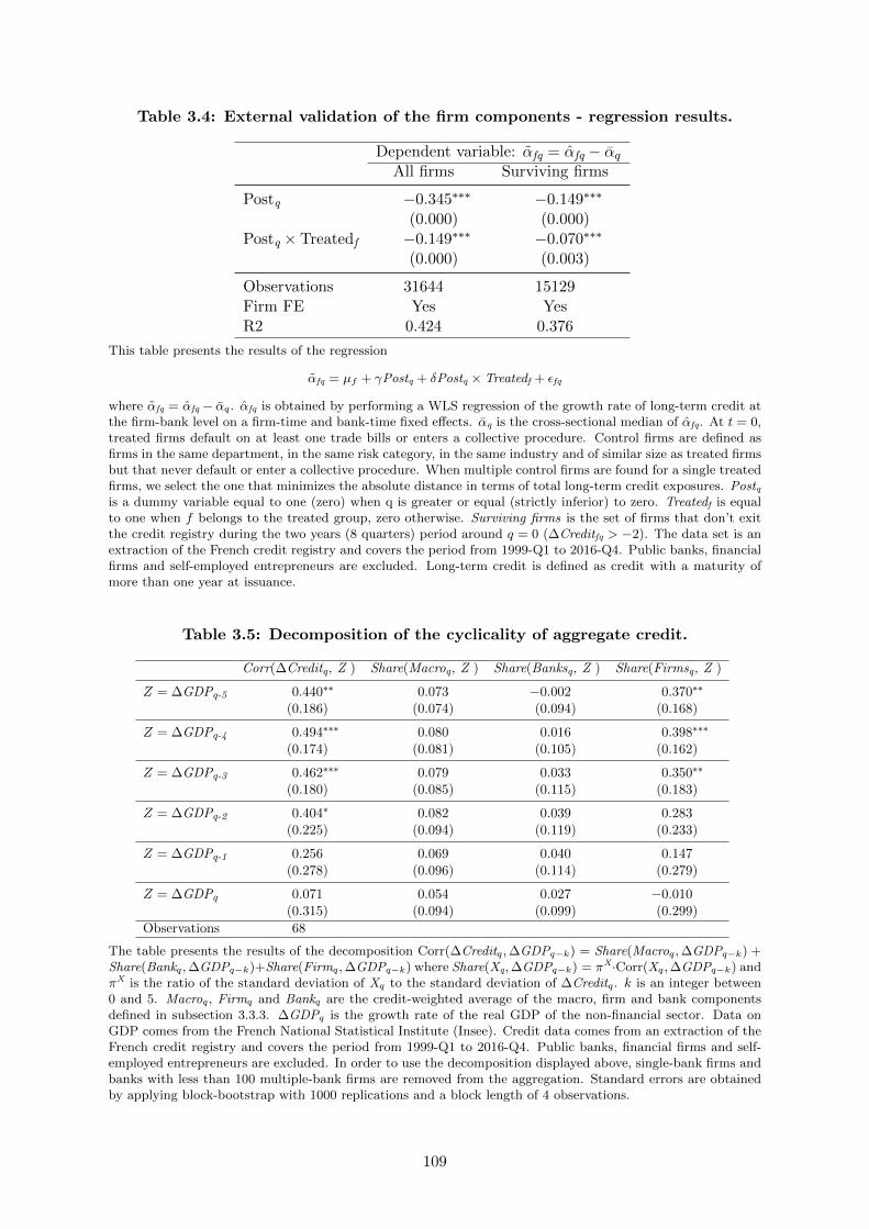
Table 3.4: External validation of the firm components - regression results.

Dependent variable: αfq = αfq − αqAll firms Surviving firms

Postq −0.345∗∗∗ −0.149∗∗∗

(0.000) (0.000)Postq × Treatedf −0.149∗∗∗ −0.070∗∗∗

(0.000) (0.003)

Observations 31644 15129Firm FE Yes YesR2 0.424 0.376

This table presents the results of the regression

αfq = µf + γPostq + δPostq × Treatedf + εfq

where αfq = αfq − αq. αfq is obtained by performing a WLS regression of the growth rate of long-term credit atthe firm-bank level on a firm-time and bank-time fixed effects. αq is the cross-sectional median of αfq. At t = 0,treated firms default on at least one trade bills or enters a collective procedure. Control firms are defined asfirms in the same department, in the same risk category, in the same industry and of similar size as treated firmsbut that never default or enter a collective procedure. When multiple control firms are found for a single treatedfirms, we select the one that minimizes the absolute distance in terms of total long-term credit exposures. Postqis a dummy variable equal to one (zero) when q is greater or equal (strictly inferior) to zero. Treatedf is equalto one when f belongs to the treated group, zero otherwise. Surviving firms is the set of firms that don’t exitthe credit registry during the two years (8 quarters) period around q = 0 (∆Creditfq > −2). The data set is anextraction of the French credit registry and covers the period from 1999-Q1 to 2016-Q4. Public banks, financialfirms and self-employed entrepreneurs are excluded. Long-term credit is defined as credit with a maturity ofmore than one year at issuance.

Table 3.5: Decomposition of the cyclicality of aggregate credit.

Corr(∆Creditq, Z ) Share(Macroq, Z ) Share(Banksq, Z ) Share(Firmsq, Z )

Z = ∆GDPq-5 0.440∗∗ 0.073 −0.002 0.370∗∗

(0.186) (0.074) (0.094) (0.168)

Z = ∆GDPq-4 0.494∗∗∗ 0.080 0.016 0.398∗∗∗

(0.174) (0.081) (0.105) (0.162)

Z = ∆GDPq-3 0.462∗∗∗ 0.079 0.033 0.350∗∗

(0.180) (0.085) (0.115) (0.183)

Z = ∆GDPq-2 0.404∗ 0.082 0.039 0.283(0.225) (0.094) (0.119) (0.233)

Z = ∆GDPq-1 0.256 0.069 0.040 0.147(0.278) (0.096) (0.114) (0.279)

Z = ∆GDPq 0.071 0.054 0.027 −0.010(0.315) (0.094) (0.099) (0.299)

Observations 68

The table presents the results of the decomposition Corr(∆Creditq,∆GDPq−k) = Share(Macroq,∆GDPq−k) +Share(Bankq,∆GDPq−k)+Share(Firmq,∆GDPq−k) where Share(Xq,∆GDPq−k) = πX·Corr(Xq,∆GDPq−k) andπX is the ratio of the standard deviation of Xq to the standard deviation of ∆Creditq. k is an integer between0 and 5. Macroq, Firmq and Bankq are the credit-weighted average of the macro, firm and bank componentsdefined in subsection 3.3.3. ∆GDPq is the growth rate of the real GDP of the non-financial sector. Data onGDP comes from the French National Statistical Institute (Insee). Credit data comes from an extraction of theFrench credit registry and covers the period from 1999-Q1 to 2016-Q4. Public banks, financial firms and self-employed entrepreneurs are excluded. In order to use the decomposition displayed above, single-bank firms andbanks with less than 100 multiple-bank firms are removed from the aggregation. Standard errors are obtainedby applying block-bootstrap with 1000 replications and a block length of 4 observations.

109

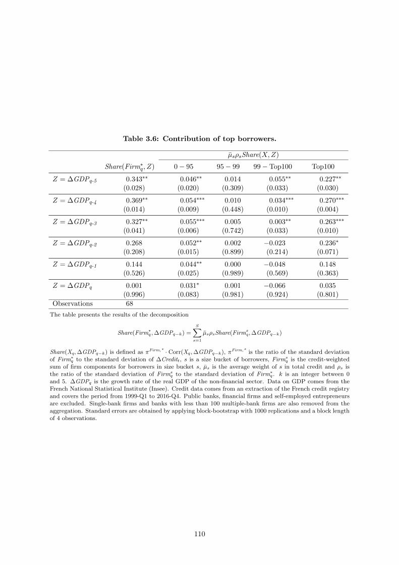
Table 3.6: Contribution of top borrowers.

µsρsShare(X,Z)

Share(Firm∗q , Z) 0− 95 95− 99 99− Top100 Top100

Z = ∆GDPq-5 0.343∗∗ 0.046∗∗ 0.014 0.055∗∗ 0.227∗∗

(0.028) (0.020) (0.309) (0.033) (0.030)

Z = ∆GDPq-4 0.369∗∗ 0.054∗∗∗ 0.010 0.034∗∗∗ 0.270∗∗∗

(0.014) (0.009) (0.448) (0.010) (0.004)

Z = ∆GDPq-3 0.327∗∗ 0.055∗∗∗ 0.005 0.003∗∗ 0.263∗∗∗

(0.041) (0.006) (0.742) (0.033) (0.010)

Z = ∆GDPq-2 0.268 0.052∗∗ 0.002 −0.023 0.236∗

(0.208) (0.015) (0.899) (0.214) (0.071)

Z = ∆GDPq-1 0.144 0.044∗∗ 0.000 −0.048 0.148(0.526) (0.025) (0.989) (0.569) (0.363)

Z = ∆GDPq 0.001 0.031∗ 0.001 −0.066 0.035(0.996) (0.083) (0.981) (0.924) (0.801)

Observations 68

The table presents the results of the decomposition

Share(Firm∗q ,∆GDPq−k) =

S∑s=1

µsρsShare(Firmsq,∆GDPq−k)

Share(Xq,∆GDPq−k) is defined as πFirm,* · Corr(Xq,∆GDPq−k), πFirm,* is the ratio of the standard deviationof Firm∗q to the standard deviation of ∆Creditt, s is a size bucket of borrowers, Firms

q is the credit-weightedsum of firm components for borrowers in size bucket s, µs is the average weight of s in total credit and ρs isthe ratio of the standard deviation of Firms

q to the standard deviation of Firm∗q . k is an integer between 0and 5. ∆GDPq is the growth rate of the real GDP of the non-financial sector. Data on GDP comes from theFrench National Statistical Institute (Insee). Credit data comes from an extraction of the French credit registryand covers the period from 1999-Q1 to 2016-Q4. Public banks, financial firms and self-employed entrepreneursare excluded. Single-bank firms and banks with less than 100 multiple-bank firms are also removed from theaggregation. Standard errors are obtained by applying block-bootstrap with 1000 replications and a block lengthof 4 observations.

110

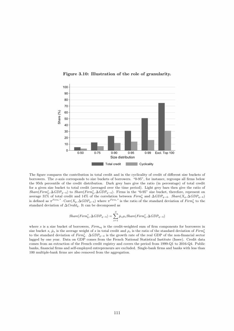
Figure 3.10: Illustration of the role of granularity.

0

10

20

30

40

50

60

70

80

90

100

Sha

re (%

)

0-50 0-75 0-90 0-95 0-99 Excl. Top 100Size distribution

Total credit Cyclicality

The figure compares the contribution in total credit and in the cyclicality of credit of different size buckets ofborrowers. The x-axis corresponds to size buckets of borrowers. “0-95”, for instance, regroups all firms belowthe 95th percentile of the credit distribution. Dark grey bars give the ratio (in percentage) of total creditfor a given size bucket to total credit (averaged over the time period). Light grey bars then give the ratio ofShare(Firms

q,∆GDPq−4) to Share(Firm∗q ,∆GDPq−4). Firms in the “0-95” size bucket, therefore, represent onaverage 31% of total credit and 14% of the correlation between Firm∗q and ∆GDPq−4. Share(Xq,∆GDPq−4)

is defined as πFirm,* · Corr(Xq,∆GDPq−4) where πFirm,* is the ratio of the standard deviation of Firm∗q to thestandard deviation of ∆Creditq. It can be decomposed as

Share(Firm∗q ,∆GDPq−4) =

S∑s=1

µsρsShare(Firmsq,∆GDPq−4)

where s is a size bucket of borrowers, Firmsq is the credit-weighted sum of firm components for borrowers insize bucket s, µs is the average weight of s in total credit and ρs is the ratio of the standard deviation of Firms

q

to the standard deviation of Firm∗q . ∆GDPq−4 is the growth rate of the real GDP of the non-financial sectorlagged by one year. Data on GDP comes from the French National Statistical Institute (Insee). Credit datacomes from an extraction of the French credit registry and covers the period from 1999-Q1 to 2016-Q4. Publicbanks, financial firms and self-employed entrepreneurs are excluded. Single-bank firms and banks with less than100 multiple-bank firms are also removed from the aggregation.

111

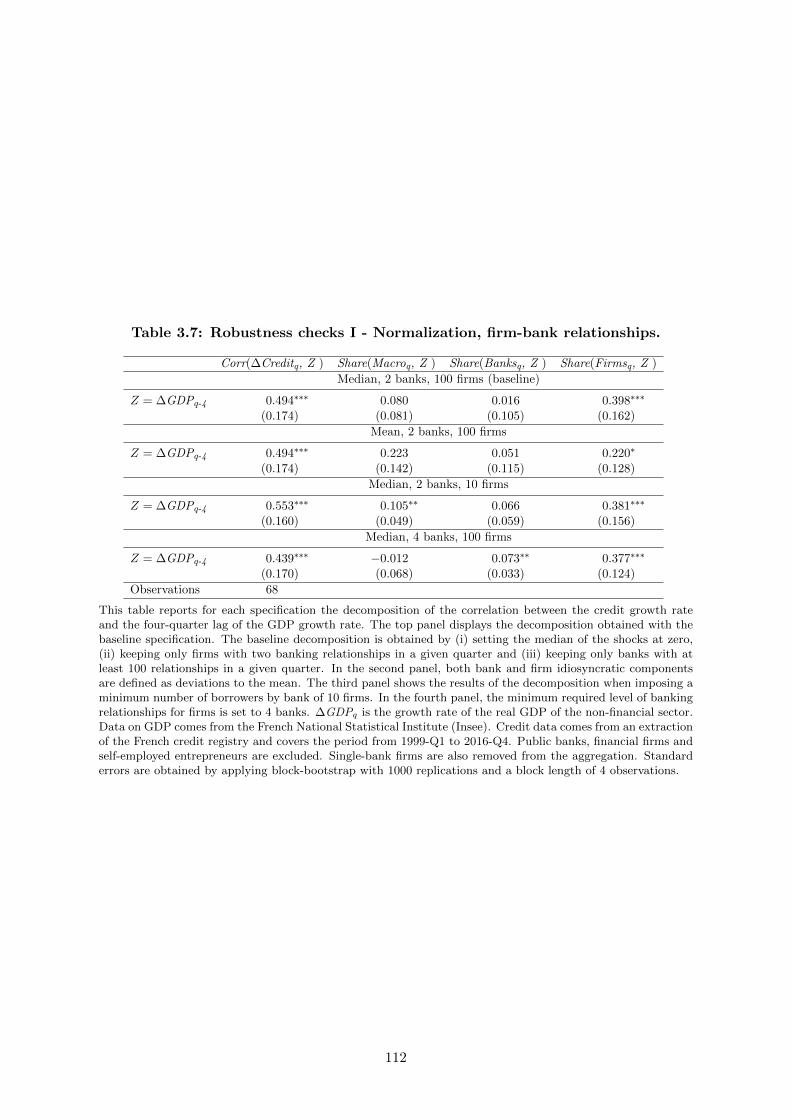
Table 3.7: Robustness checks I - Normalization, firm-bank relationships.


Median, 2 banks, 100 firms (baseline)

Z = ∆GDPq-4 0.494∗∗∗ 0.080 0.016 0.398∗∗∗

(0.174) (0.081) (0.105) (0.162)

Mean, 2 banks, 100 firms

Z = ∆GDPq-4 0.494∗∗∗ 0.223 0.051 0.220∗

(0.174) (0.142) (0.115) (0.128)

Median, 2 banks, 10 firms

Z = ∆GDPq-4 0.553∗∗∗ 0.105∗∗ 0.066 0.381∗∗∗

(0.160) (0.049) (0.059) (0.156)

Median, 4 banks, 100 firms

Z = ∆GDPq-4 0.439∗∗∗ −0.012 0.073∗∗ 0.377∗∗∗

(0.170) (0.068) (0.033) (0.124)

Observations 68

This table reports for each specification the decomposition of the correlation between the credit growth rateand the four-quarter lag of the GDP growth rate. The top panel displays the decomposition obtained with thebaseline specification. The baseline decomposition is obtained by (i) setting the median of the shocks at zero,(ii) keeping only firms with two banking relationships in a given quarter and (iii) keeping only banks with atleast 100 relationships in a given quarter. In the second panel, both bank and firm idiosyncratic componentsare defined as deviations to the mean. The third panel shows the results of the decomposition when imposing aminimum number of borrowers by bank of 10 firms. In the fourth panel, the minimum required level of bankingrelationships for firms is set to 4 banks. ∆GDPq is the growth rate of the real GDP of the non-financial sector.Data on GDP comes from the French National Statistical Institute (Insee). Credit data comes from an extractionof the French credit registry and covers the period from 1999-Q1 to 2016-Q4. Public banks, financial firms andself-employed entrepreneurs are excluded. Single-bank firms are also removed from the aggregation. Standarderrors are obtained by applying block-bootstrap with 1000 replications and a block length of 4 observations.

112

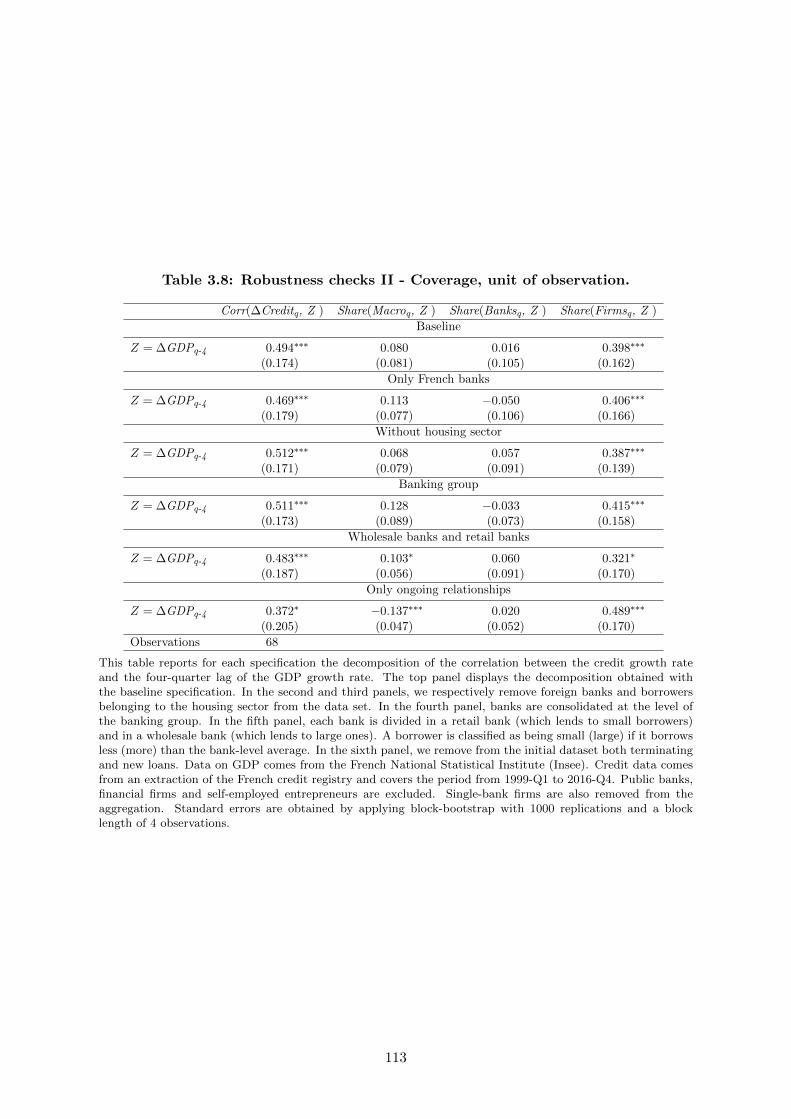
Table 3.8: Robustness checks II - Coverage, unit of observation.


Baseline

Z = ∆GDPq-4 0.494∗∗∗ 0.080 0.016 0.398∗∗∗

(0.174) (0.081) (0.105) (0.162)

Only French banks

Z = ∆GDPq-4 0.469∗∗∗ 0.113 −0.050 0.406∗∗∗

(0.179) (0.077) (0.106) (0.166)

Without housing sector

Z = ∆GDPq-4 0.512∗∗∗ 0.068 0.057 0.387∗∗∗

(0.171) (0.079) (0.091) (0.139)

Banking group

Z = ∆GDPq-4 0.511∗∗∗ 0.128 −0.033 0.415∗∗∗

(0.173) (0.089) (0.073) (0.158)

Wholesale banks and retail banks

Z = ∆GDPq-4 0.483∗∗∗ 0.103∗ 0.060 0.321∗

(0.187) (0.056) (0.091) (0.170)

Only ongoing relationships

Z = ∆GDPq-4 0.372∗ −0.137∗∗∗ 0.020 0.489∗∗∗

(0.205) (0.047) (0.052) (0.170)

Observations 68

This table reports for each specification the decomposition of the correlation between the credit growth rateand the four-quarter lag of the GDP growth rate. The top panel displays the decomposition obtained withthe baseline specification. In the second and third panels, we respectively remove foreign banks and borrowersbelonging to the housing sector from the data set. In the fourth panel, banks are consolidated at the level ofthe banking group. In the fifth panel, each bank is divided in a retail bank (which lends to small borrowers)and in a wholesale bank (which lends to large ones). A borrower is classified as being small (large) if it borrowsless (more) than the bank-level average. In the sixth panel, we remove from the initial dataset both terminatingand new loans. Data on GDP comes from the French National Statistical Institute (Insee). Credit data comesfrom an extraction of the French credit registry and covers the period from 1999-Q1 to 2016-Q4. Public banks,financial firms and self-employed entrepreneurs are excluded. Single-bank firms are also removed from theaggregation. Standard errors are obtained by applying block-bootstrap with 1000 replications and a blocklength of 4 observations.

113

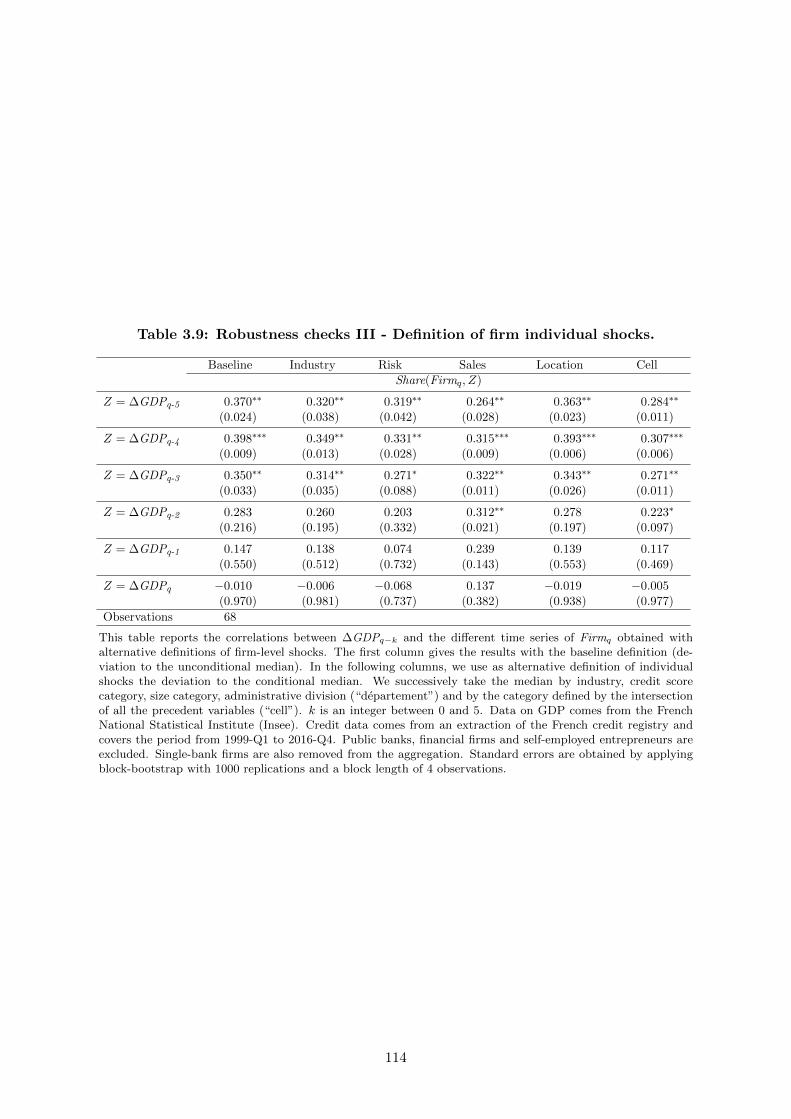
Table 3.9: Robustness checks III - Definition of firm individual shocks.

Baseline Industry Risk Sales Location CellShare(Firmq, Z)

Z = ∆GDPq-5 0.370∗∗ 0.320∗∗ 0.319∗∗ 0.264∗∗ 0.363∗∗ 0.284∗∗

(0.024) (0.038) (0.042) (0.028) (0.023) (0.011)

Z = ∆GDPq-4 0.398∗∗∗ 0.349∗∗ 0.331∗∗ 0.315∗∗∗ 0.393∗∗∗ 0.307∗∗∗

(0.009) (0.013) (0.028) (0.009) (0.006) (0.006)

Z = ∆GDPq-3 0.350∗∗ 0.314∗∗ 0.271∗ 0.322∗∗ 0.343∗∗ 0.271∗∗

(0.033) (0.035) (0.088) (0.011) (0.026) (0.011)

Z = ∆GDPq-2 0.283 0.260 0.203 0.312∗∗ 0.278 0.223∗

(0.216) (0.195) (0.332) (0.021) (0.197) (0.097)

Z = ∆GDPq-1 0.147 0.138 0.074 0.239 0.139 0.117(0.550) (0.512) (0.732) (0.143) (0.553) (0.469)

Z = ∆GDPq −0.010 −0.006 −0.068 0.137 −0.019 −0.005(0.970) (0.981) (0.737) (0.382) (0.938) (0.977)

Observations 68

This table reports the correlations between ∆GDPq−k and the different time series of Firmq obtained withalternative definitions of firm-level shocks. The first column gives the results with the baseline definition (de-viation to the unconditional median). In the following columns, we use as alternative definition of individualshocks the deviation to the conditional median. We successively take the median by industry, credit scorecategory, size category, administrative division (“departement”) and by the category defined by the intersectionof all the precedent variables (“cell”). k is an integer between 0 and 5. Data on GDP comes from the FrenchNational Statistical Institute (Insee). Credit data comes from an extraction of the French credit registry andcovers the period from 1999-Q1 to 2016-Q4. Public banks, financial firms and self-employed entrepreneurs areexcluded. Single-bank firms are also removed from the aggregation. Standard errors are obtained by applyingblock-bootstrap with 1000 replications and a block length of 4 observations.

114

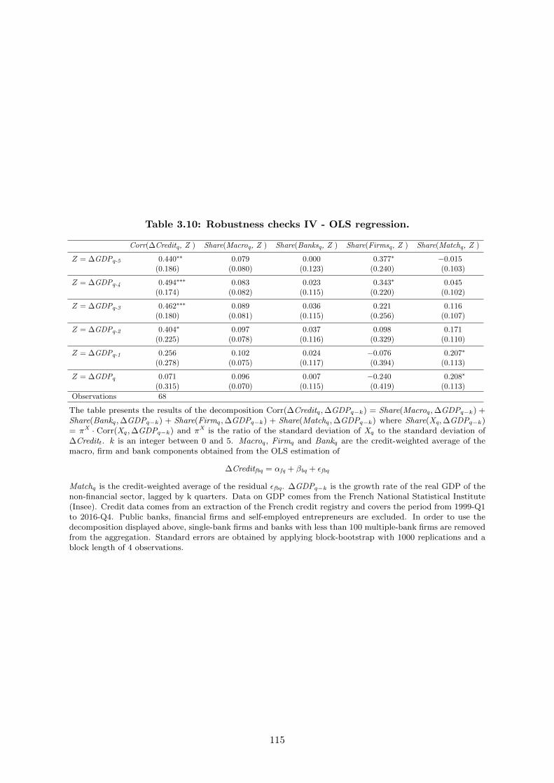
Table 3.10: Robustness checks IV - OLS regression.

Corr(∆Creditq, Z ) Share(Macroq, Z ) Share(Banksq, Z ) Share(Firmsq, Z ) Share(Matchq, Z )

Z = ∆GDPq-5 0.440∗∗ 0.079 0.000 0.377∗ −0.015(0.186) (0.080) (0.123) (0.240) (0.103)

Z = ∆GDPq-4 0.494∗∗∗ 0.083 0.023 0.343∗ 0.045(0.174) (0.082) (0.115) (0.220) (0.102)

Z = ∆GDPq-3 0.462∗∗∗ 0.089 0.036 0.221 0.116(0.180) (0.081) (0.115) (0.256) (0.107)

Z = ∆GDPq-2 0.404∗ 0.097 0.037 0.098 0.171(0.225) (0.078) (0.116) (0.329) (0.110)

Z = ∆GDPq-1 0.256 0.102 0.024 −0.076 0.207∗

(0.278) (0.075) (0.117) (0.394) (0.113)

Z = ∆GDPq 0.071 0.096 0.007 −0.240 0.208∗

(0.315) (0.070) (0.115) (0.419) (0.113)

Observations 68

The table presents the results of the decomposition Corr(∆Creditq,∆GDPq−k) = Share(Macroq,∆GDPq−k) +Share(Bankq,∆GDPq−k) + Share(Firmq,∆GDPq−k) + Share(Matchq,∆GDPq−k) where Share(Xq,∆GDPq−k)= πX · Corr(Xq,∆GDPq−k) and πX is the ratio of the standard deviation of Xq to the standard deviation of∆Creditt. k is an integer between 0 and 5. Macroq, Firmq and Bankq are the credit-weighted average of themacro, firm and bank components obtained from the OLS estimation of

∆Creditfbq = αfq + βbq + εfbq

Matchq is the credit-weighted average of the residual εfbq. ∆GDPq−k is the growth rate of the real GDP of thenon-financial sector, lagged by k quarters. Data on GDP comes from the French National Statistical Institute(Insee). Credit data comes from an extraction of the French credit registry and covers the period from 1999-Q1to 2016-Q4. Public banks, financial firms and self-employed entrepreneurs are excluded. In order to use thedecomposition displayed above, single-bank firms and banks with less than 100 multiple-bank firms are removedfrom the aggregation. Standard errors are obtained by applying block-bootstrap with 1000 replications and ablock length of 4 observations.

115

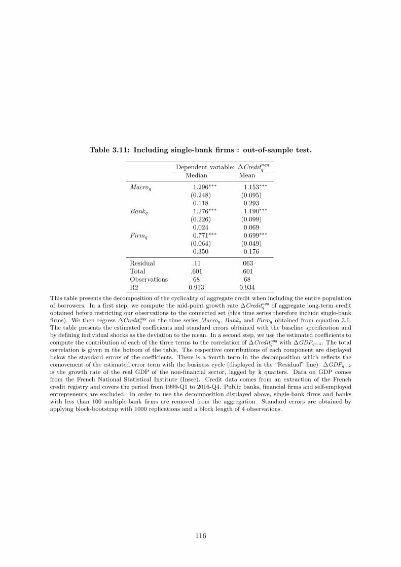
Table 3.11: Including single-bank firms : out-of-sample test.

Dependent variable: ∆Creditaggq

Median Mean

Macroq 1.296∗∗∗ 1.153∗∗∗

(0.248) (0.095)0.118 0.293

Bankq 1.276∗∗∗ 1.190∗∗∗

(0.226) (0.099)0.024 0.069

Firmq 0.771∗∗∗ 0.699∗∗∗

(0.064) (0.049)0.350 0.176

Residual .11 .063Total .601 .601Observations 68 68R2 0.913 0.934

This table presents the decomposition of the cyclicality of aggregate credit when including the entire populationof borrowers. In a first step, we compute the mid-point growth rate ∆Creditaggq of aggregate long-term creditobtained before restricting our observations to the connected set (this time series therefore include single-bankfirms). We then regress ∆Creditaggq on the time series Macroq, Bankq and Firmq obtained from equation 3.6.The table presents the estimated coefficients and standard errors obtained with the baseline specification andby defining individual shocks as the deviation to the mean. In a second step, we use the estimated coefficients tocompute the contribution of each of the three terms to the correlation of ∆Creditaggq with ∆GDPq−4. The totalcorrelation is given in the bottom of the table. The respective contributions of each component are displayedbelow the standard errors of the coefficients. There is a fourth term in the decomposition which reflects thecomovement of the estimated error term with the business cycle (displayed in the “Residual” line). ∆GDPq−kis the growth rate of the real GDP of the non-financial sector, lagged by k quarters. Data on GDP comesfrom the French National Statistical Institute (Insee). Credit data comes from an extraction of the Frenchcredit registry and covers the period from 1999-Q1 to 2016-Q4. Public banks, financial firms and self-employedentrepreneurs are excluded. In order to use the decomposition displayed above, single-bank firms and bankswith less than 100 multiple-bank firms are removed from the aggregation. Standard errors are obtained byapplying block-bootstrap with 1000 replications and a block length of 4 observations.

116

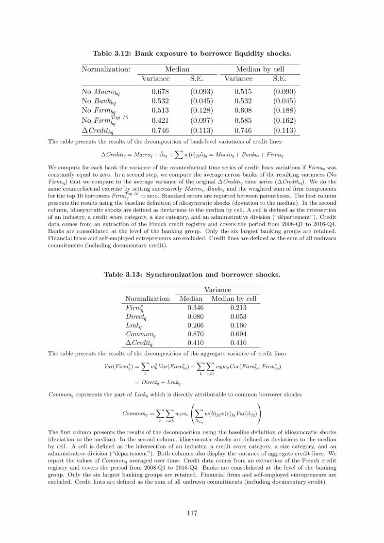
Table 3.12: Bank exposure to borrower liquidity shocks.

Normalization: Median Median by cellVariance S.E. Variance S.E.

No Macrobq 0.678 (0.093) 0.515 (0.090)No Bankbq 0.532 (0.045) 0.532 (0.045)No Firmbq 0.513 (0.128) 0.608 (0.188)

No FirmTop 10bq 0.421 (0.097) 0.585 (0.162)

∆Creditbq 0.746 (0.113) 0.746 (0.113)

The table presents the results of the decomposition of bank-level variations of credit lines:

∆Creditbq = Macroq + βbq +∑

w(b)fqαfq = Macroq + Bankbq + Firmbq

We compute for each bank the variance of the counterfactual time series of credit lines variations if Firmbq wasconstantly equal to zero. In a second step, we compute the average across banks of the resulting variances (NoFirmbq) that we compare to the average variance of the original ∆Creditbq time series (∆Creditbq). We do thesame counterfactual exercise by setting successively Macroq, Bankbq and the weighted sum of firm componentsfor the top 10 borrowers FirmTop 10

bq to zero. Standard errors are reported between parentheses. The first columnpresents the results using the baseline definition of idiosyncratic shocks (deviation to the median). In the secondcolumn, idiosyncratic shocks are defined as deviations to the median by cell. A cell is defined as the intersectionof an industry, a credit score category, a size category, and an administrative division (“departement”). Creditdata comes from an extraction of the French credit registry and covers the period from 2008-Q1 to 2016-Q4.Banks are consolidated at the level of the banking group. Only the six largest banking groups are retained.Financial firms and self-employed entrepreneurs are excluded. Credit lines are defined as the sum of all undrawncommitments (including documentary credit).

Table 3.13: Synchronization and borrower shocks.

VarianceNormalization: Median Median by cell

Firm∗q 0.346 0.213

Directq 0.080 0.053Linkq 0.266 0.160Commonq 0.870 0.694∆Creditq 0.410 0.410

The table presents the results of the decomposition of the aggregate variance of credit lines:

Var(Firm∗q) =∑b

w2bVar(Firm∗bq) +

∑b

∑c6=b

wbwcCov(Firm∗bq,Firm∗cq)

= Directq + Linkq

Commonq represents the part of Linkq which is directly attributable to common borrower shocks:

Commonq =∑b

∑c6=b

wbwc

∑Rbcq

w(b)fqw(c)fqVar(αfq)

The first column presents the results of the decomposition using the baseline definition of idiosyncratic shocks(deviation to the median). In the second column, idiosyncratic shocks are defined as deviations to the medianby cell. A cell is defined as the intersection of an industry, a credit score category, a size category, and anadministrative division (“departement”). Both columns also display the variance of aggregate credit lines. Wereport the values of Commonq averaged over time. Credit data comes from an extraction of the French creditregistry and covers the period from 2008-Q1 to 2016-Q4. Banks are consolidated at the level of the bankinggroup. Only the six largest banking groups are retained. Financial firms and self-employed entrepreneurs areexcluded. Credit lines are defined as the sum of all undrawn commitments (including documentary credit).

117

Chapter 4

Bank lending shocks, credit

allocation, and capital allocation

Abstract

This paper makes use of bank-firm lending data in France for the period 2005-2016 in orderto examine how bank lending shocks shape credit allocation and resource allocation overtime. To do so I distinguish between high quality and low quality firms using the Banquede France credit rating. Firms at the bottom of the rating scale are smaller, younger, lessproductive and more indebted. I find that bank credit shocks have sizeable real effects onfirm-level investment rate, employment growth and output growth. These shocks tend todirect aggregate credit towards high quality borrowers, which in turn fosters investment forthis type of firms. On the other hand, the relative propensity of banks to lend to healthycompanies is found to be significantly reduced in time of crisis. During the 2008-09 crisisand the 2012-13 recession this change in credit allocation decreased the gap in investmentbetween both types of firms; in particular it accounts for 30% of the reduction observedduring the Great Recession, and thereby contributed to capital misallocation.

118

4.1 Introduction

In this paper I examine the effect of the bank lending channel on credit allocation for a large

sample of French firms and a time period covering both recessions consecutive to the subprime

mortgage crisis and the Eurozone crisis. I estimate bank credit shocks using matched bank-firm

level data and find significant alteration of credit allocation during both crisis episodes. I then

analyse how these variations affect the allocation of capital and labour.

The extent to which banks tend to lend to firms that are relatively more healthy or less

risky has long been a subject of interest, in particular since the Japanese economic stagnation

of the 90s. Peek and Rosengreen (2005) and Caballero, Hoshi, and Kashyap (2008) show

that during the Japanese Lost Decade banks directed credit towards firms that would have

been otherwise insolvent, and that this “zombie lending” behaviour had a significant effect on

economic performance. The recent debates on the causes and consequences of the sluggish

recovery observed after the Great Recession brought into focus the role of credit misallocation

as a potential driver of this slowdown. McGowan, Andrews, and Millot (2017) argue that

the prevalence of zombie firms have risen in OECD countries since the mid-2000s, and that the

larger share of such companies constrain the growth of more productive firms. From a European

perspective, recent papers argue that a weakening of the banking sector led under-capitalized

banks to restrain credit to healthy borrowers. Acharya et al. (2019) analyse how bank lending

reacted to the 2012 ECB’s Outright Monetary Transactions (OMT) program. They find that

banks that remained weakly capitalized post-OMT engaged in zombie lending, which in turn

dampened the economic recovery, particularly in Southern Europe. Using data on bank-firm

relationships in Italy Schivardi, Sette, and Tabellini (2018) also show that under-capitalized

banks are more likely to cut credit to healthy but not to zombie firms; on the other hand they

find little effect of such lending behaviour on the performance of healthy companies during the

financial crisis.

Although the main goal of this paper also consists in examining the impact of bank lending

behaviour on credit allocation, I differ from this litterature by distinguishing firms according

to their credit ratings rather than attempting to identify zombies.1 To do so I classify firm-

time observations in three distinct categories using their Banque de France credit rating. I

use this variable to distinguish between borrowers for two main reasons. First, it is a credible

1Zombie firms are often defined as distressed firms receiving subsidized credit, i.e. loans at below-marketinterest rates (see Caballero, Hoshi, and Kashyap (2008), Giannetti and Simonov (2013), Acharya et al. (2019)).

119

determinant of credit supply decisions: Cahn, Girotti, and Salvade (2018) show that firms

receiving an exogeneous upgrade in their Banque de France rating experience greater access

to bank credit and start new bank relationships more easily. Second, it provides a synthetic

measure of the healthiness of the firm: companies with low ratings are found to be more risky2,

more indebted, and less productive. As mentioned above, numerous papers in the zombie

lending literature show that weakened banks engage relatively more in zombie lending than

healthy banks. I also differ on this point by focusing on how bank shocks affect credit allocation

in absolute terms, i.e. examining whether in the aggregate the bank lending channel tends to

direct credit more to high-quality or to low-quality borrowers, and how this effect evolves over

time. I find that on average from 2005Q2 to 2016Q4 banks tend to lend more to high-quality

borrowers (category denoted A) than to low-quality companies (category denoted C): in the

absence of firm shocks the difference between the (mid-point) credit growth rates of firms rated

A and firms rated C would be on average equal to 10.4 percentage points. I also find that this

difference is sharply reduced during both the Great Recession and the recession consecutive to

the Euro Crisis, respectively down to 2.7 and 1 percentage points. It therefore indicates that

during both recessions the propensity of banks to lend to healthy firms was largely attenuated.

Beyond credit availability and credit allocation, the recent literature on the bank lending

channel examines how bank credit shocks impact real activity. Such research agenda has been

motivated by the substantial disruptions affecting the credit market and firms’ real outcomes

in various advanced economies since the financial crisis. Chodorow-Reich (2014), Berton et al.

(2018), Bentolila, Jansen, and Jimenez (2018) and Greenstone, Mas, and Nguyen (2019) study

the effect of credit supply shocks on firm-level employment. Amiti and Weinstein (2018) show

that idiosyncratic bank shocks are an important determinant of both firm-level and aggregate

investment rates. Paravisini et al. (2015) study the effect of credit supply shocks on export ac-

tivities. Cingano, Manaresi, and Sette (2016), Acharya et al. (2018) and Alfaro, Garcıa-Santana,

and Moral-Benito (2019) find sizeable effects at the firm level for employment, investment and

output. All in all, most papers in this literature show that the bank lending channel significantly

affects real outcomes.3

Starting with Khwaja and Mian (2008), numerous papers in this literature have made use of

matched bank-firm loan data to identify credit supply shocks. The typical empirical framework

2Aghion et al. (2019b) show that such firms have about 8% chance of being liquidated in the near future.3A noticeable exception is Greenstone, Mas, and Nguyen (2019), who finds that lending shocks had small

effect on both small firm and overall employment during the Great Recession in the US.

120

consists in regressing a measure of the growth in lending on bank-time and firm-time fixed

effects. The use of firm-time dummies in order to control for credit demand implies that bank

shocks are estimated on the sample of multi-bank firms. As emphasized by Degryse et al. (2019),

performing such estimation on databases in which single-bank firms are predominant leads to a

drastic reduction of the sample used.4 Furthermore, as these firms may significantly differ from

multi-bank firms, excluding them is likely to bias the magnitude of bank credit shocks and of

their impact. I therefore replace firm-time fixed effects with cell-time fixed effects, where cells

are groups of firms with similar characteristics. Degryse et al. (2019) show that such methods

provide valid alternative demand controls for traditional firm-time fixed effects. I then allow

banks to have different lending shocks depending on the quality of their borrowers, replacing

bank-time fixed effects by bank-rating-time fixed effects. Finally I follow Amiti and Weinstein

(2018) by estimating shocks that match the aggregate growth in lending, for total credit and for

each category of firms. I then measure the estimated bank credit shocks at the firm level and

quantify the average effect of these shocks on firms’ real outcomes, namely corporate investment,

employment growth and sales growth. Controlling for various firm characteristics and including

firm fixed effects I find a significant and sizeable impact of bank credit shocks: a one standard

deviation change increases the average firm’s investment rate, employment growth and output

growth by roughly 9%, 10% and 5%.5

I then assess how variations in credit allocation over time affects the allocation of capital

and labor. Following Hsieh and Klenow (2009), a lively branch of the economic literature has

emphasized the role of resource allocation in accounting for differences in aggregate produc-

tivity, both across countries and over time.6 In particular, several articles focus on the effects

of financial frictions (Moll (2014), Midrigan and Xu (2014), Larrain and Stumpner (2017)).

However, and somehow suprisingly, little empirical evidence on the impact of bank lending

on resource allocation is available.7 Schivardi, Sette, and Tabellini (2018) ask whether bank

under-capitalization (associated with zombie lending) is correlated with revenue productivity

4The prevalence of mono-bank firms is a characteristic of the French credit market. See for example Beatriz,Coffinet, and Nicolas (2018).

5I find slightly higher impacts when including sector-location dummies rather than firm fixed effects.6For example Gopinath et al. (2017) relate the low productivity growth observed in Southern Europe during

the 2000s to an increase of misallocated capital inflows following the adoption of the euro. Libert (2017) showthat misallocation generated a loss in annual manufacturing TFP growth of almost one percentage point in Franceduring the decade preceding the Great Recession, and significantly contributed to the large variations in observedproductivity during the financial crisis.

7Notice that bank credit shocks may impact aggregate productivity not only through input allocation, but alsoby directly affecting firm-level TFP. Manaresi and Pierri (2019) introduce bank shocks in a model of productionwith financial constraints and find that a contraction in credit supply reduces firm productivity growth.

121

dispersion and ultimately with misallocation in the input markets. They find that low cap-

italization of banks in Italy accounts for only a modest part of resource misallocation. Bai,

Carvalho, and Phillips (2018) show that bank deregulation episodes in the US led to a shift in

the allocation of bank credit supply toward more productive firms, which in turn led to a reallo-

cation of labor towards such companies. In the context of emerging markets, Cong et al. (2019)

study the real effects of credit allocation during China’s economic stimulus of 2009-10. They

show that new credit was allocated relatively more toward state-owned firms and firms with

lower marginal productivity of capital. As a result firms with higher initial capital productivity

experienced lower investment during the stimulus years.

I make use of the empirical framework relating firm-specific bank credit shocks to investment

rate and employment growth in order to examine how inputs allocation would have evolved in

the absence of such shocks. More precisely, I normalize the estimated shocks so that setting

them to zero only impacts loans allocation and leaves unchanged the aggregate credit growth. I

find that over the whole time period under scrutiny and in the absence of bank lending shocks

the investment rate of the average high quality borrower would have been 11.2 percentage points

higher than the mean investment rate of low quality borrowers. As the observed investment

gap is on average equal to 13.3 percentage points I conclude that the bank lending channel

accounts for 1− 11.2/13.3 ≈ 16% of the investment gap between these two categories of firms,

therefore contributing to directing capital input towards firms that are relatively less risky and

more productive. On the other hand, the propensity of banks to lend to such firms is strongly

attenuated in time of crisis. I observe that the investment gap between high and low quality

borrowers was reduced during the financial crisis (from 13.7 p.p outside of recession periods to 8.7

p.p during 2008Q4-2010Q2), I therefore ask to which extent bank credit shocks contributed to

this reduction. I show that neutralizing the effect of bank shocks the decrease of the investment

gap would have been 30% less pronounced. Reproducing the same counterfactual exercise for

the recession consecutive to the Eurozone crisis I also find that bank credit shocks tended to

attenuate the difference in investment rates. On the other hand I find little effect regarding

employment growth. Eventually it indicates that bank-related variations in credit allocation

contributed to a relative increase in capital misallocation in time of crisis.

The remainder of the paper is structured as follows. Section 4.2 describes the data used

in the empirical analysis. Section 4.3 presents the methodology used to estimate bank credit

shocks. Section 4.4 provides summary statistics for the overall sample and for each firm category.

122

In section 4.5 I report the main results regarding the effect of bank credit shocks on credit

allocation, firm-level real outcomes and resource allocation. Section 4.6 concludes.

4.2 Data

In order to disentangle bank-related change in lending from firm-related change in borrowing

I make use of the French national credit registry. This database gathers on a quarterly basis

and at the firm-bank level8 data on credit exposures. Information is collected as long as the

outstanding amount of loans granted by bank b to firm f exceeds 75k euros (before 2006Q1)

or 25k euros (since 2006Q1). As I want to cover as much as possible the pre-crisis period I

impose the 75k threshold on the whole dataset. Credit exposures are categorized as short-term

(loans with maturity up to one year) or long-term (more than one year). In the remainder

of this paper I will focus on long-term credit exposures. I drop loans lent by state-owned

and government institutions such as the Caisse des Depots et Consignations (Deposits and

Consignments Fund) in order to focus on bank lending shocks arising from private institutions.

I keep track of mergers and restructurings in the banking sector by investigating entry and exit

at the bank level. Whenever I find reports in the media or within the information system of

the Banque de France indicating that bank b had absorbed bank b′ between t− 1 and t, I first

check that aggregate credit lent by b′ indeed declines sharply, as b starts reporting loans that

were previously reported by b′; then I recode loans in both time t − 1 and t as coming from

the absorbing institution. At this point the dataset covers the quarters 1999Q1 to 2016Q4 and

consists in 53,771,267 firm-bank-time observations; 46,355,078 distinct firm-time observations;

and 27,447 distinct bank-time observations.

In order to recover firm level variables and characteristics I use the FIBEN database. This

unique database was initially set up by the Banque de France in order to facilitate the im-

plementation of monetary policy. It gathers information on all companies which sales exceed

750,000 euros, and covers the years 1989 to the present day. A wide range of information

is gathered, including accounting and financial data from balance sheets and profit and loss

statements, as well as descriptive details such as the firm’s name or legal status. Firm-level

variables are reported at the non-consolidated level. As will become clear in the next sections,

a key variable throughout my analysis is the Banque de France credit rating. The rating scale

8Both firms and banks are identified at the non-consolidated level.

123

changed in April 2004, the reform consisting in a refinement of the original rating categories

and in the introduction of three new rating levels. It is unfortunately not possible to map the

previous rating categories to the new rating scale. Hence I drop from the dataset firms that

are not rated according to the current index. I also drop from the dataset companies that

report accounting periods shorter or longer than twelve months; state-owned companies and

self-employed entrepreneurs; and all observations corresponding to firms that operate in the

petroleum industry, in the real-estate, financial and agricultural sectors, as well as the holding

companies.

Finally I merge this database with the dataset coming from the credit registry. The fi-

nal dataset covers the quarters 2004Q2 to 2016Q4 and consists in 6,031,929 firm-bank-time

observations; 3,865,294 firm-time observations; and 14,348 bank-time observations.

4.3 Estimation of bank credit shocks

Since the seminal work of Khwaja and Mian (2008), numerous articles in the economic and

financial literature have used matched bank-firm data in order to disentangle the bank lending

channel from the firm borrowing channel. As argued by Amiti and Weinstein (2018), many

empirical models in this literature can be written as

δfbt = αft + βbt + εfbt (4.1)

where δfbt denotes a measure of the growth in lending from bank b to firm f between t− 1 and

t. αft and βbt denote coefficients associated to a full set of firm and bank fixed effects, and

are respectively interpreted as firm and bank credit shocks. Specific firm-bank interactions are

captured by the error term εfbt. Such model encompasses any specification that would regress

growth in lending on a set of vectors corresponding to firm-level and bank-level characteristics.

Empirical models that consists in an OLS or WLS estimation of equation 4.1 rely upon firms

borrowing from multiple banks, because firm-time fixed effects are used in order to control for

credit demand. By assuming that demand originating from a given firm is homogeneous for

the various banks it borrows from, variation in lending to the same firm by different banks

can be attributed to bank credit supply. When applied to countries where the vast majority of

firms borrow from only one bank, such models may lead to a drastic reduction of the number

124

of firms and firm-bank relationships used to estimate bank credit shocks.9 Furthermore, single

relationship firms may differ significantly from firms borrowing from multiple lenders: excluding

them is likely to bias the estimated bank supply component. To overcome this limitation

recent papers have introduced a slight modification of the initial Khwaja and Mian (2008)

framework. This modification consists in clustering firms according to characteristics that are

seen as typical determinants of credit demand.10 By assuming that credit demand within a

cluster is homogeneous, it is now change in lending to the same cluster by different banks

that is used to estimate bank shocks. Degryse et al. (2019) show that clustering firms by

industry, location and size provides valid alternative demand controls: focusing on the dataset

with multiple-relationship borrowers, this estimation leads to a set of bank shocks that are

qualitatively similar to shocks obtained using firm-time fixed effects.11 Furthermore, the use of

industry-location-size-time fixed effects allow to encompass a large fraction of single-relationship

firms. They show that bank shocks estimated on this larger sample have real effects on firm-

level outcomes that are significantly more pronounced than what would be obtained with shocks

estimated by traditional firm-time fixed effects.

Statistics performed on the French credit registry show that the vast majority of French

firms borrow from only one bank.12 Restricting the dataset to firms for which I have detailed

balance sheet information does not reverse the finding: figure 4.1 shows that on average only

31% of the firms I observe are multiple-relationship borrowers. Therefore I follow Degryse et al.

(2019) and place firms into cells based on firm characteristics. More precisely, a cell c is defined

at time t as the set of firms operating in the same sector, same location, with comparable size,

age and productivity.13 Equation 4.1 now writes:

δfbt = αct + βbt + εfbt (4.2)

It is important to notice that both equations 4.1 and 4.2 assume that bank credit shocks

are themselve homogeneous, i.e. the bank component βbt is common for all firms in relationship

9For example Degryse et al. (2019) document that over 80% of Belgian firms are single-relationship firms.10Although motivated by other constraints than the the prevalence of single-relationship firms, Acharya et al.

(2018) and Acharya et al. (2019) also aggregate firms into clusters in order to control for borrower characteristics.11They also perform this analysis on clusters defined with additional firm characteristics: age, current asset

ratio and risk measures.12See Beaumont, Hurlin, and Libert (2019).13The industry bins are based on two-digit NACE classification codes; location bins correspond to the French

administrative regions; age bins are defined as firms that are 0-5, 5-10, 10-20 and 20+ years old; size bins arebased on quintiles of total assets ; productivity bins are based on quintiles of productivity.

125

with bank b. Therefore the impact of bank shocks on the firm’s total growth in lending will be

strictly identical for all firms borrowing in the same proportion from the same set of banks. As a

result such specification is bound to occult a large part of bank-related factors that drive credit

allocation over time. As ultimately the goal of this paper consists in assessing to which extent

bank lending affects investment and employment through credit allocation it is crucial to allow

banks to have lending policies that depend on the different types of borrowers they lend to. I

use the Banque de France credit rating in order to distinguish between borrowers. Replacing

bank-time fixed effect by bank-rating-time fixed effect provides a simple way to estimate bank

supply shocks that differ depending on the credit rating of the firm. Therefore equation 4.2

becomes

δfbt = αct + βbrt + εfbt (4.3)

For each time periods {t − 1, t} the propensity of bank b to lend to firms rated r at t − 1 is

estimated by comparing within a given cell c the change in credit for firms with different credit

ratings.

Finally, some recent papers have shed light on how different measures of growth in lending

and different methods of estimation may impact the estimated shocks. Amiti and Weinstein

(2018) show that measuring the left hand side of equation 4.1 by percentage changes and ad-

equately modifying the moment equations imposed by a WLS estimation provide bank shocks

that account for new loans and match the bank, firm and aggregate credit growth rates. Beau-

mont, Hurlin, and Libert (2019) show that measuring the growth in lending by mid-point growth

rates and estimating equation 4.1 with WLS provide bank shocks that take into account en-

try/exit of firms, banks and loans and that match the bank, firm and aggregate credit mid-point

growth rate. I therefore define the left hand side of equation 4.3 as

δfbt = 2 ·Lfbt − Lfb,t−1

Lfbt + Lfb,t−1

where Lfbt denotes lending by bank b to firm f at time t. In my main specification I estimate

equation 4.3 by WLS with weights (Lfbt + Lfb,t−1)/2. The sample on which the estimation

is performed includes approximately 94% of the total number of observations and 91% of the

number of distinct firms appearing in the initial sample. The WLS estimation provides shocks

126

that match the total growth in lending I observe in my dataset:

δt =∑c

Lct + Lc,t−1

Lt + Lt−1αct +

∑b,r

Lbrt + Lbr,t−1

Lt + Lt−1βbrt

I normalize for each time period the estimated shocks by setting to zero the weighted mean:

αct = αct −∑c

Lct + Lc,t−1

Lt + Lt−1αct

βbrt = βbrt −∑b,r

Lbrt + Lbr,t−1

Lt + Lt−1βbrt

Importantly it implies that setting to zero each bank shock βbrt leaves unchanged the aggregate

growth of credit, and therefore only modifies credit allocation.

The estimated shocks also match the total growth in lending from t− 1 to t of firms rated

r at time t− 1. Denoting Fr,t−1 the set of such firms we have the following equality:

δrt =∑b

wbrtβbrt +∑

f∈Fr,t−1

wfrtαct

where weights wbrt and wfrt are defined as:

wbrt =Lbrt + Lbr,t−1

Lrt + Lr,t−1

wfrt =Lft + Lf,t−1

Lrt + Lr,t−1

Using the normalized shocks and defining the aggregate bank shock for the set of firms rated r

as βrt =∑b

wbrtβbrt one obtains that

δrt − δt = βrt +∑

f∈Fr,t−1

wfrtαct (4.4)

Time series of aggregate bank shocks βrt therefore indicates how the bank lending channel

drives changes in total lending granted to firms rated r relatively to aggregate credit growth. In

particular equation 4.4 also implies that the difference in lending growth between two categories

127

r and r′ reflects the relative effects of both types of shocks:

δrt − δr′t = βrt − βr′t +∑

f∈Fr,t−1

wfrtαct −∑

f∈Fr′,t−1

wfr′tαct (4.5)

Therefore by comparing the aggregate bank shock βrt for two different credit ratings r and r′

one can assess how the bank lending channel affects credit allocation, and how this effect evolves

over time.

Eventually, this methodology aims at identifying bank shocks so as to assess their role in

shaping credit allocation. For sake of simplicity, these estimates are sometimes refered to in the

literature as credit supply shocks. On the other hand, the econometric methodology remains

largely agnostic about the economic origins of these shocks. As a result, they are not necessarily

interpretable directly in terms of credit supply. In this paper, the bank components merely

reflect bank-specific changes in the distribution of lending across different types of borrowers.

4.4 Main variables and descriptive statistics

Through my analysis I make use of firm characteristics measured using the balance sheets

and profit and loss statements gathered in the FIBEN database. I measure employment by

the average number of employees. The size variable corresponds to the book value of total

assets. The loan-to-asset ratio is measured by the ratio between the total amount of borrowings

from credit institutions and total assets. In order to measure productivity I approximate the

labor elasticity at the sectoral level by the median of the share of nominal value-added devoted

to nominal expenditure on labor. Under a standard Cobb-Douglas production function with

constant return to scale the capital elasticity is simply one minus labor elasticity. I measure

revenue productivity as the ratio between nominal value added and the product of capital and

labor quantities, weighted by their respective elasticities.14 Revenue productivity at the firm

level is then normalized by the median for all firms operating at the same time period in the same

two-digit sector, and is denoted TFPR. Finally I take the log of this variable and winsorize at

the top and bottom 0.5% level.15 The age variable is measured as the number of years between

the end of the accounting period and the date of the first registration of the firm at the register

14I measure capital input by the book value of fixed assets, and labor input by the wage bill of the firm.15This measure of productivity therefore corresponds to the TFPR measure defined in Foster, Haltiwanger,

and Syverson (2008) and Hsieh and Klenow (2009). In particular Hsieh and Klenow (2009) show that reallocatinginputs from firms with low TFPR to firms with high revenue productivity increases aggregate productivity.

128

of commerce.

I follow Amiti and Weinstein (2018) and measure the bank shock at the firm level as a

weighted sum of the bank shocks I estimated in section 4.3. Therefore for a given firm f rated

r at the beginning of the accounting period the bank shock writes

Bank Shockf,t =∑B

Lfbt + Lfb,t−1

Lft + Lf,t−1βbrt (4.6)

The firm-level bank shock is then winsorized at the 0.5 and 99.5% level. For each firm and at

each time period I also keep track of the number of bank relationships appearing in the credit

registry.

In order to examine the real effect of bank shocks I consider three different measures of firm

outcomes: investment, growth in employment and growth in output. Growth in employment

and growth in output are respectively measured by the log difference of the average number

of employees and the log difference of sales. Investment is measured by the change in the

gross value of tangible fixed assets, as a fraction of the initial capital stock.16 Finally these

three measures are also winsorized at 0.5 and 99.5% level. Summary statistics for the various

variables described are reported in Panel A of Table 4.1.

In my analysis I examine the heterogeneity of bank lending through the lense of firms credit

rating. To do so I make use of the Banque de France credit rating, that classifies companies

according to their capacity to meet their financial commitments over a three-year horizon.17

All firms with total sales greater than 750,000 euros are rated by the Banque de France, apart

from public institutions, credit institutions and entities without commercial or industrial activ-

ities. The assessment is based on both hard and soft information: hard information consists

in accounting and financial data, while soft information derives from qualitative insights gath-

ered during on-site visits and interviews. The main users of Banque de France’s credit ratings

are credit institutions, that access the ratings on demand and in return of the payment of a

fee. Along with the credit rating credit institutions get access to a wide range of firm level

information.

Firms are rated from 3++ to 9 (or P in case of corporate insolvency). For simplicity I

group firms in three different categories: category A includes firms which credit rating goes

16I exclude from tangible fixed assets the assets related to real estate properties.17Cahn, Girotti, and Salvade (2018) provide a detailed description of the Banque de France credit rating, and

use the 2004 reform of the rating scale to show that this rating is a determinant of bank lending decisions.

129

from 3++ (outstanding capacity to fulfil its financial commitments) to 3 (strong capacity to

meet its financial commitments). Category B includes firms which credit rating goes from 4+

(good capacity) to 5+ (rather weak capacity). Category C includes firms which credit rating

goes from 5 (weak capacity) to P (firms that are legally identified as bankrupt). The propensity

of banks to lend to these different categories of firms therefore reflects their inclination to lend

to borrowers that are more or less risky and unhealthy.

Firms rated C account for 13% of the observations in my sample, while firms rated A and

firms rated B respectively represents 25% and 62% of the dataset. Figure 4.2 describes the

evolution of the shares of each category. The share of firms rated C is rather stable over time.

The share of firms rated A is slightly decreasing (from 30% in 2005Q2 to 22% in 2016Q4)

and corresponds to an increase in the share of firms rated B (from 58% in 2005Q2 to 65% in

2016Q4). Panel B of Table 4.1 reports the mean of the main firm variables for each rating

category. Firms rated C are smaller than firms rated A or B in terms of employment, total

assets and total sales. They are also younger and have a higher loan-to-asset ratio. Their bank

lending shock is significantly lower, which indicates that on average over the whole time period

banks tend to lend more to firms that are less risky and more healthy. They engage in fewer

bank relationships and are significantly less productive. Finally they invest less and grow less,

both in terms of employment and output.

One may wonder to which extent each category remains homogeneous other time. As a

matter of fact, it could be the case that the evolution of bank lending to firms in a given category

mirrors a relative deterioration or improvement of the healthiness and riskiness of such firms.

In such case it would reflect a composition effect rather than changes in the relative propensity

to lend to these companies. Figure 4.3 alleviates this concern by describing the evolution of

the average (log) revenue productivity for each category over time. Panel B of Table 4.1 shows

that the average firm in category C is 21% less productive (exp(−0.193− 0.047)− 1) than the

average firm in category A and 11% less productive (exp(−0.193 + 0.074)− 1) than the average

firm in category B. It appears from figure 4.3 that these productivity gaps are stable over time,

therefore suggesting that the relative efficiency of each type of firms remains unchanged.

130

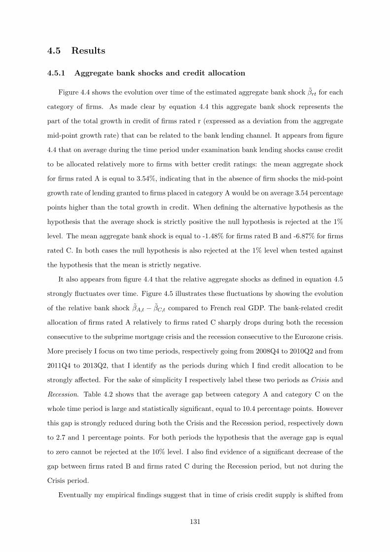
4.5 Results

4.5.1 Aggregate bank shocks and credit allocation

Figure 4.4 shows the evolution over time of the estimated aggregate bank shock βrt for each

category of firms. As made clear by equation 4.4 this aggregate bank shock represents the

part of the total growth in credit of firms rated r (expressed as a deviation from the aggregate

mid-point growth rate) that can be related to the bank lending channel. It appears from figure

4.4 that on average during the time period under examination bank lending shocks cause credit

to be allocated relatively more to firms with better credit ratings: the mean aggregate shock

for firms rated A is equal to 3.54%, indicating that in the absence of firm shocks the mid-point

growth rate of lending granted to firms placed in category A would be on average 3.54 percentage

points higher than the total growth in credit. When defining the alternative hypothesis as the

hypothesis that the average shock is strictly positive the null hypothesis is rejected at the 1%

level. The mean aggregate bank shock is equal to -1.48% for firms rated B and -6.87% for firms

rated C. In both cases the null hypothesis is also rejected at the 1% level when tested against

the hypothesis that the mean is strictly negative.

It also appears from figure 4.4 that the relative aggregate shocks as defined in equation 4.5

strongly fluctuates over time. Figure 4.5 illustrates these fluctuations by showing the evolution

of the relative bank shock βA,t − βC,t compared to French real GDP. The bank-related credit

allocation of firms rated A relatively to firms rated C sharply drops during both the recession

consecutive to the subprime mortgage crisis and the recession consecutive to the Eurozone crisis.

More precisely I focus on two time periods, respectively going from 2008Q4 to 2010Q2 and from

2011Q4 to 2013Q2, that I identify as the periods during which I find credit allocation to be

strongly affected. For the sake of simplicity I respectively label these two periods as Crisis and

Recession. Table 4.2 shows that the average gap between category A and category C on the

whole time period is large and statistically significant, equal to 10.4 percentage points. However

this gap is strongly reduced during both the Crisis and the Recession period, respectively down

to 2.7 and 1 percentage points. For both periods the hypothesis that the average gap is equal

to zero cannot be rejected at the 10% level. I also find evidence of a significant decrease of the

gap between firms rated B and firms rated C during the Recession period, but not during the

Crisis period.

Eventually my empirical findings suggest that in time of crisis credit supply is shifted from

131

healthy firms to companies relatively more risky and less efficient. Although my paper remains

silent on the underlying factors driving such fluctuations, some articles in the literature have

examined how credit allocation is altered during recessions and stagnations. Peek and Rosen-

green (2005) and Caballero, Hoshi, and Kashyap (2008) explore the role that bank lending

played during the Japanese lost decade by directing credit to zombie firms that would be other-

wise insolvent. Such behaviour is often related to a weakening of the banking sector: Schivardi,

Sette, and Tabellini (2018) show in the context of the European financial crisis in Italy that

under-capitalized banks are more likely to cut credit to healthy firms and to lend instead to

zombie firms. Acharya et al. (2019) show that the indirect recapitalization of European banks

through the ECB’s Outright Monetary Transactions program launched in 2012 partly translated

into zombie lending by banks that still remained weakly-capitalized post-OMT.

4.5.2 Average real effects of bank shocks on firm-level outcomes

I now examine how the estimated bank shocks impact real outcomes at the firm level, looking

at the effect on investment, employment and output as defined in section 4.4. To do so I run

the following regression:

Yft = δ Bank Shockft + µXft + εft (4.7)

where Yft is either investment, change in (log) employment or change in (log) sales between t−1

and t. Firm controls include rating dummies corresponding to the three categories A, B and

C; a dummy equal to one when the firm borrow from multiple banks at time t; age dummies

corresponding to firms with age between 0 and 5, 5 and 10, 10 and 20 and higher than 20 years;

size measured at t−1 as the log of total assets; loan-to-asset ratio and (log) revenue productivity

as defined in section 4.4 and measured at t − 1. To further control for credit demand at the

firm level, and consistently with the measure of firm-specific bank shocks, I include firm shocks

measured as the shocks obtained with the Amiti and Weinstein (2018) estimator:

Firm Shockf,t = 2 ·Lft − Lf,t−1

Lft + Lf,t−1− Bank Shockf,t

I also include sector-time fixed effects, location-time fixed effects and alternatively sector-

location or firm fixed effects.18 Standard errors are clustered at the main bank level.

18Sectors are based on two-digit NACE classification codes; locations correspond to the French administrativeregions. When including firm fixed effects I keep firms with at least three observations.

132

Table 4.3 reports the impact of the bank lending shocks on firm outcomes for the 2005Q2-

2016Q4 period. I first discuss the sign and statistical significance of the coefficients associated to

firm characteristics. Unsurprisingly it appears in most specifications that firms rated B and C

tend to invest less and to grow relatively less in terms of employment and sales when compared

to firms rated A. The gap in investment rate between firms rated A and firms rated B is not

statistically significant when including sector-location fixed effects; in all other specifications

and for the three outcomes I consider coefficients are negative and significantly different from

zero at the 1% level. Small firms, young firms and firms in relationship with multiple banks

tend to have higher investment, employment growth and output growth. When including sector-

location fixed effects and for the employment and sales outcomes the sign of the relation with

the size variable is reversed, but the coefficient is either close to zero or not significant. Finally

I find that firms that are less productive and with a higher loan-to-asset ratio invest less and

grow less in terms of employment. Focusing on output growth I find that the sign tends to

be reversed for these two variables, although the coefficient for the loan-to-asset ratio is not

significant at the 10% level when including sector-location dummies.

The coefficient associated to the bank shock variable provides an estimate of the average full-

sample real effect of the bank lending channel. The effect is positive and statistically significant

at the 1% level for the three dependent variables and for each specification. The estimated

coefficients are also economically sizeable. Estimates from columns (1), (3) and (5) imply that

a one standard deviation increase in the bank credit shock measured at the firm level respectively

increases investment, change in employment and change in sales by 9.6%, 17.3% and 8.2% of the

observed full-sample averages.19 When including firm fixed effects rather than sector-location

fixed effects the magnitudes are somehow attenuated but remain sizeable: columns (2), (4) and

(6) imply that a one standard deviation increase in the credit supply shock increases investment,

employment growth and output growth respectively by 8.5%, 10.5% and 5% of the observed

means. Finally table 4.4 shows that the magnitude of the impact does not depend on how

investment is measured. I run the same regressions but define the investment rate as a share

of total assets (columns (1) and (2)); or consider total fixed assets rather than tangible fixed

assets (columns (3) and (4)). The estimates are still positive and significant at the 1% level.

A one standard deviation increase in the bank shock increases these two alternative measures

19Means and standard deviations are based on the observations for which the regressions are estimated, andtherefore slightly differ from the values reported in table 4.1.

133

of investment respectively by 8.8% and 10.9% for the average firm with sector-location fixed

effects; and by 7.8% and 9.1% with firm fixed effects.

The average effects I estimate are in lines with related papers. For a sample of Spanish firms

from 2003 to 2013 Alfaro, Garcıa-Santana, and Moral-Benito (2019) find that the direct effect

of a one standard deviation change in the credit supply shock they estimate leads to an increase

in firm investment of 10% of the average observed investment rate. Using Belgian data Degryse

et al. (2019) finds an effect corresponding to a 3.6% change in investment for the average firm in

their sample. More broadly my empirical findings are consistent with the literature analyzing

the real effects of the bank lending channel: see in particular Chodorow-Reich (2014); Cingano,

Manaresi, and Sette (2016); Bentolila, Jansen, and Jimenez (2018); Berton et al. (2018).

4.5.3 From credit allocation to resource allocation

I now examine how credit allocation impacts input allocation, focusing on investment and

employment growth. To do so I first allow firms with different ratings to have heterogeneous

sensitivities to their bank credit shock:

Yft =∑

r∈A,B,C

δr Bank Shockft + µXft + εft

Columns (1) and (3) in table 4.5 report the results. Regarding investment firms with better

ratings react slightly more to bank credit shocks,20 but the effect is still positive and significant

at the 1% level for each category. Regarding employment I find that the impact of bank shocks

is mostly driven by firms rated B: the coefficient associated to firms rated A is significant at the

5% level but is almost divided by two, while the coefficient associated to firms rated C is close

to zero and not significant at the 10% level.

Because rating dummies are included in the set of firm-level characteristics, this framework

provides a way to evaluate the effect of heterogeneity in bank shocks on resource allocation.

As a matter of fact the OLS estimation imposes that the average of the error term for each

category is equal to zero. Therefore one can assess the gap in investment and in employment

growth between the average firm rated r and the average firm rated r′ that would be observed

in the absence of credit supply shocks. Comparing this counterfactual gap with the observed

gap enables to deduce the relative contribution of the bank-related credit allocation. More

20In each case the coefficients are found to be different from each other at the 1% level.

134

precisely, I denote Yr the empirical mean of the dependent variable for firms rated r over the

full time period and Y ′r the mean one would observe by setting to zero bank supply shocks.21

The relative contribution of bank lending to resource allocation between firms rated r and r′ is

therefore computed as 1− (Y ′r − Y ′r′)/(Yr − Yr′).

The average investment rate over the whole time period for firms rated A is 13.3 percentage

points higher than the mean investment rate of firms rated C.22 As the average bank shocks

are respectively equal to 3.97% and -6.53% the counterfactual gap between the two types of

firms is equal to 13.3− 0.224 · 3.97− 0.180 · 6.53 ≈ 11.2 percentage points. In other words I find

that bank lending shocks account for 1 − 11.2/13.3 ≈ 16% of the investment gap between the

average firm rated A and the average firm rated C, therefore contributing to directing capital

input towards firms that are relatively less risky and more productive. Regarding the investment

gap between firms rated B and firms rated C I estimate the contribution at roughly 9%.23 I

reproduce this exercise for the employment growth variable: unsurprisingly the effect of credit

allocation on the gap between category A and category C is almost negligible, as for both types

of firms change in labor input is found to be little sensitive to bank credit shocks. Bank shocks

account for only 1% of the difference in the average employment growth. I find similar results

when comparing categories B and C; all in all it indicates that the effect of credit allocation on

resource allocation is mostly concentrated on the capital input.

As argued previously, I find credit allocation to be significantly altered in time of crisis.

Although on average over time investment tends to be fostered for healthy and riskless firms,

the fact that the propensity of banks to lend to these firms rather than to low quality borrowers is

highly reduced may lead to a relative increase in capital misallocation during crises or recessions.

Figures 4.6 and 4.7 respectively display the evolution over time of the average investment rate

and the average employment growth by firm rating category. Outside of the Crisis and Recession

periods defined in section 4.5.1, the investment rate of the average firm rated A is 13.7 percentage

points higher than the investment rate of the average firm rated C. Figure 4.6 shows that this

gap is significantly reduced during the Crisis period, down to 8.7 percentage points. On the

other hand I do not find evidence of such decrease during the Recession period: in fact the gap

21Recall that I normalize the bank shocks in section 4.3 so that setting to zero these shocks leaves unchangedthe aggregate credit growth; this counterfactual exercise therefore only reflects changes in credit allocation.

22As in the previous section my computations are based on the observations for which the regressions areestimated.

23I also find that bank lending shocks increase by 35% the investment gap between firms rated A and firmsrated B. However notice that in absolute terms the gap between these two types of firms is quite modest: 3.2percentage points (100*(0.344-0.312)), and 2.1 percentage points in the absence of bank credit shocks.

135

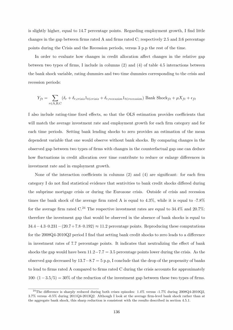
is slightly higher, equal to 14.7 percentage points. Regarding employment growth, I find little

changes in the gap between firms rated A and firms rated C; respectively 2.5 and 3.6 percentage

points during the Crisis and the Recession periods, versus 3 p.p the rest of the time.

In order to evaluate how changes in credit allocation affect changes in the relative gap

between two types of firms, I include in columns (2) and (4) of table 4.5 interactions between

the bank shock variable, rating dummies and two time dummies corresponding to the crisis and

recession periods:

Yft =∑

r∈A,B,C

(δr + δr,crisis1t∈crisis + δr,recession1t∈recession) Bank Shockft + µXft + εft

I also include rating-time fixed effects, so that the OLS estimation provides coefficients that

will match the average investment rate and employment growth for each firm category and for

each time periods. Setting bank lending shocks to zero provides an estimation of the mean

dependent variable that one would observe without bank shocks. By comparing changes in the

observed gap between two types of firms with changes in the counterfactual gap one can deduce

how fluctuations in credit allocation over time contribute to reduce or enlarge differences in

investment rate and in employment growth.

None of the interaction coefficients in columns (2) and (4) are significant: for each firm

category I do not find statistical evidence that sentivities to bank credit shocks differed during

the subprime mortgage crisis or during the Eurozone crisis. Outside of crisis and recession

times the bank shock of the average firm rated A is equal to 4.3%, while it is equal to -7.8%

for the average firm rated C.24 The respective investment rates are equal to 34.4% and 20.7%:

therefore the investment gap that would be observed in the absence of bank shocks is equal to

34.4−4.3 ·0.231−(20.7+7.8 ·0.192) ≈ 11.2 percentage points. Reproducing these computations

for the 2008Q4-2010Q2 period I find that setting bank credit shocks to zero leads to a difference

in investment rates of 7.7 percentage points. It indicates that neutralizing the effect of bank

shocks the gap would have been 11.2−7.7 = 3.5 percentage points lower during the crisis. As the

observed gap decreased by 13.7−8.7 = 5 p.p, I conclude that the drop of the propensity of banks

to lend to firms rated A compared to firms rated C during the crisis accounts for approximately

100 · (1−3.5/5) = 30% of the reduction of the investment gap between these two types of firms.

24The difference is sharply reduced during both crises episodes: 1.4% versus -1.7% during 2008Q4-2010Q2,3.7% versus -0.5% during 2011Q4-2013Q2. Although I look at the average firm-level bank shock rather than atthe aggregate bank shock, this sharp reduction is consistent with the results described in section 4.5.1.

136

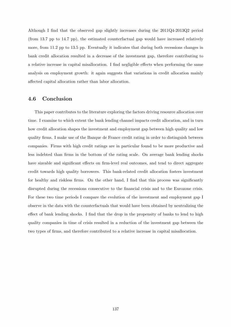
Although I find that the observed gap slightly increases during the 2011Q4-2013Q2 period

(from 13.7 pp to 14.7 pp), the estimated counterfactual gap would have increased relatively

more, from 11.2 pp to 13.5 pp. Eventually it indicates that during both recessions changes in

bank credit allocation resulted in a decrease of the investment gap, therefore contributing to

a relative increase in capital misallocation. I find negligible effects when performing the same

analysis on employment growth: it again suggests that variations in credit allocation mainly

affected capital allocation rather than labor allocation.

4.6 Conclusion

This paper contributes to the literature exploring the factors driving resource allocation over

time. I examine to which extent the bank lending channel impacts credit allocation, and in turn

how credit allocation shapes the investment and employment gap between high quality and low

quality firms. I make use of the Banque de France credit rating in order to distinguish between

companies. Firms with high credit ratings are in particular found to be more productive and

less indebted than firms in the bottom of the rating scale. On average bank lending shocks

have sizeable and significant effects on firm-level real outcomes, and tend to direct aggregate

credit towards high quality borrowers. This bank-related credit allocation fosters investment

for healthy and riskless firms. On the other hand, I find that this process was significantly

disrupted during the recessions consecutive to the financial crisis and to the Eurozone crisis.

For these two time periods I compare the evolution of the investment and employment gap I

observe in the data with the counterfactuals that would have been obtained by neutralizing the

effect of bank lending shocks. I find that the drop in the propensity of banks to lend to high

quality companies in time of crisis resulted in a reduction of the investment gap between the

two types of firms, and therefore contributed to a relative increase in capital misallocation.

137

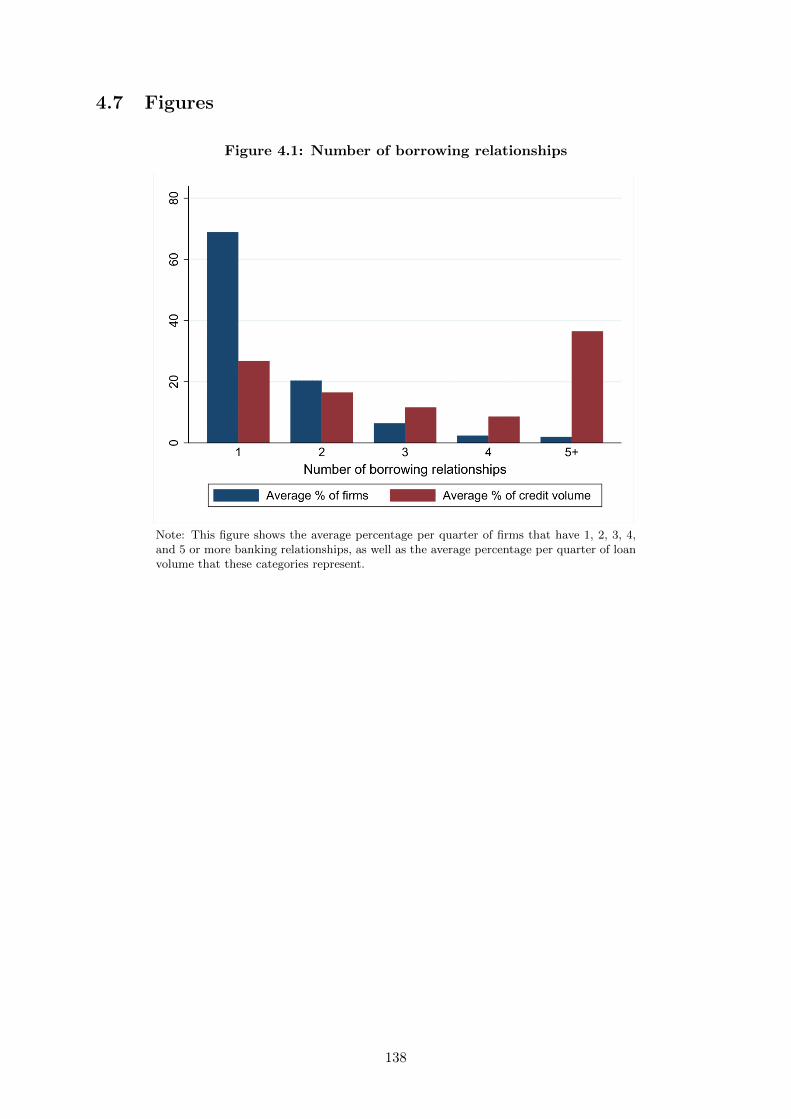
4.7 Figures

Figure 4.1: Number of borrowing relationships

Note: This figure shows the average percentage per quarter of firms that have 1, 2, 3, 4,and 5 or more banking relationships, as well as the average percentage per quarter of loanvolume that these categories represent.

138

Figure 4.2: Share of firms by credit rating and by quarter

Note: This figure shows the evolution over time of the percentage of firms that are ratedA, B or C at the beginning of the accounting period. A firm-time observation is labeledas quarter Q1 (resp. Q2; Q3; Q4) when the company reports its balance sheets and profitand loss statements between March and May (resp. June and August; September andNovember; December and February).

Figure 4.3: Average productivity by credit rating and by quarter

Note: This figure shows the evolution over time of the average productivity by creditrating. Productivity is defined as the revenue productivity normalized by the sector-timemedian, in log.

139

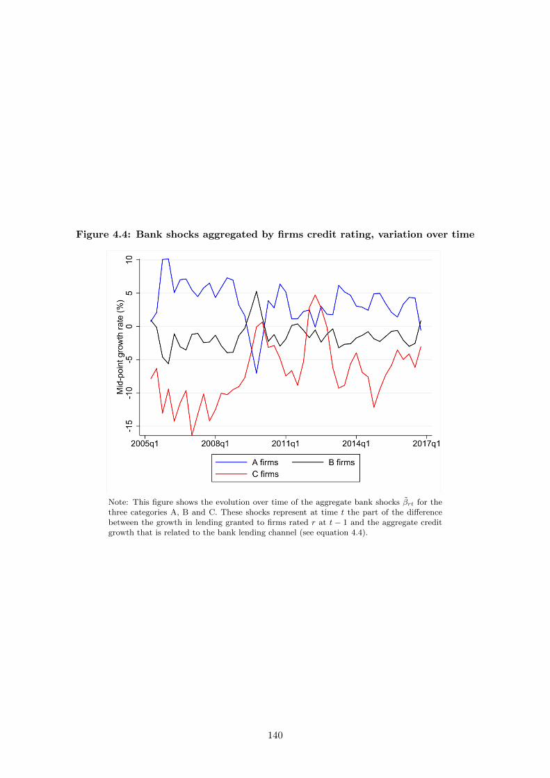
Figure 4.4: Bank shocks aggregated by firms credit rating, variation over time

Note: This figure shows the evolution over time of the aggregate bank shocks βrt for thethree categories A, B and C. These shocks represent at time t the part of the differencebetween the growth in lending granted to firms rated r at t − 1 and the aggregate creditgrowth that is related to the bank lending channel (see equation 4.4).

140

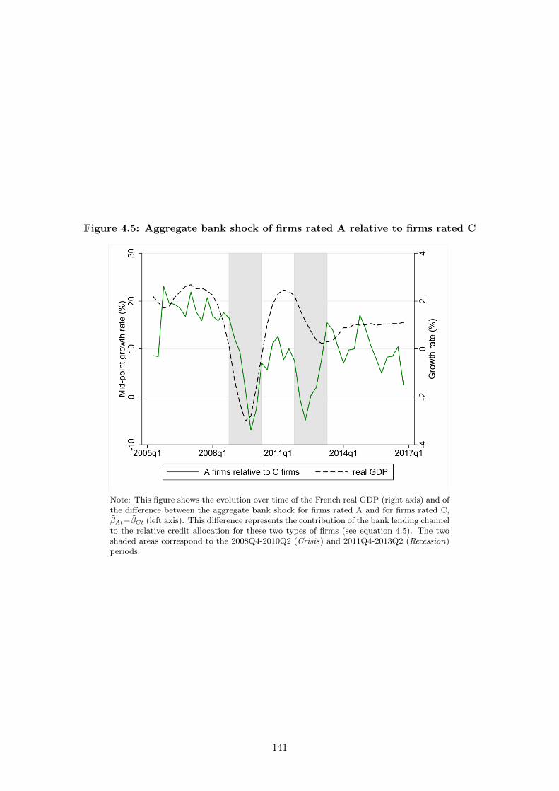
Figure 4.5: Aggregate bank shock of firms rated A relative to firms rated C

Note: This figure shows the evolution over time of the French real GDP (right axis) and ofthe difference between the aggregate bank shock for firms rated A and for firms rated C,βAt−βCt (left axis). This difference represents the contribution of the bank lending channelto the relative credit allocation for these two types of firms (see equation 4.5). The twoshaded areas correspond to the 2008Q4-2010Q2 (Crisis) and 2011Q4-2013Q2 (Recession)periods.

141

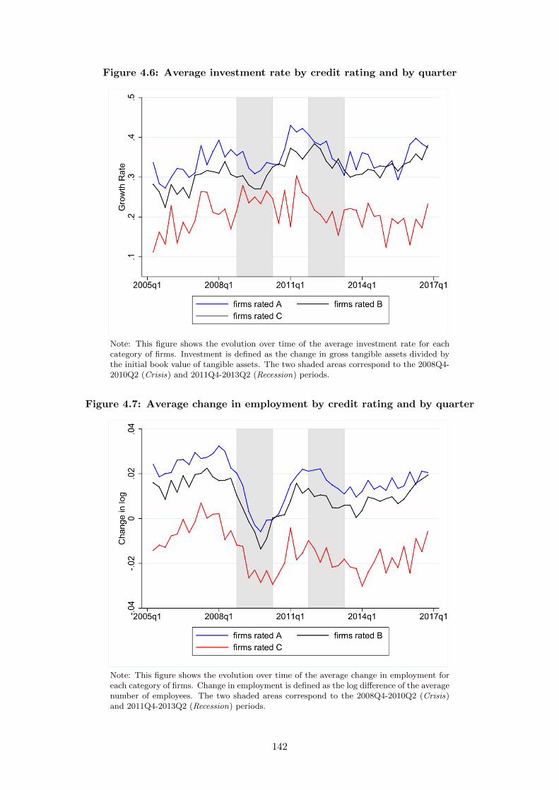
Figure 4.6: Average investment rate by credit rating and by quarter

Note: This figure shows the evolution over time of the average investment rate for eachcategory of firms. Investment is defined as the change in gross tangible assets divided bythe initial book value of tangible assets. The two shaded areas correspond to the 2008Q4-2010Q2 (Crisis) and 2011Q4-2013Q2 (Recession) periods.

Figure 4.7: Average change in employment by credit rating and by quarter

Note: This figure shows the evolution over time of the average change in employment foreach category of firms. Change in employment is defined as the log difference of the averagenumber of employees. The two shaded areas correspond to the 2008Q4-2010Q2 (Crisis)and 2011Q4-2013Q2 (Recession) periods.

142

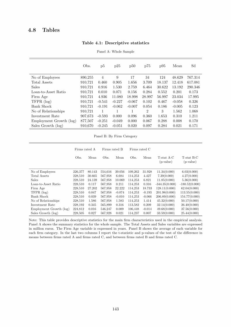
4.8 Tables

Table 4.1: Descriptive statistics

Panel A: Whole Sample

Obs. p5 p25 p50 p75 p95 Mean Sd

No of Employees 890,255 4 9 17 34 124 48.629 767.314Total Assets 910,721 0.460 0.905 1.656 3.709 18.137 12.418 617.081Sales 910,721 0.916 1.530 2.759 6.464 30.622 13.192 290.346Loan-to-Asset Ratio 910,721 0.010 0.071 0.156 0.284 0.552 0.201 0.173Firm Age 910,721 4.936 11.080 18.998 28.997 56.997 23.034 17.995TFPR (log) 910,721 -0.541 -0.227 -0.067 0.102 0.467 -0.058 0.326Bank Shock 910,721 -0.191 -0.062 -0.007 0.054 0.186 -0.005 0.123No of Relationships 910,721 1 1 1 2 3 1.562 1.068Investment Rate 907,673 -0.593 0.000 0.096 0.360 1.653 0.310 1.211Employment Growth (log) 877,507 -0.251 -0.049 0.000 0.067 0.288 0.008 0.170Sales Growth (log) 910,670 -0.245 -0.051 0.020 0.097 0.284 0.021 0.171

Panel B: By Firm Category

Firms rated A Firms rated B Firms rated C

Obs. Mean Obs. Mean Obs. Mean T-stat A-C T-stat B-C(p-value) (p-value)

No of Employees 226,377 80.143 554,616 39.056 109,262 31.928 11.34(0.000) 6.03(0.000)Total Assets 228,510 30.665 567,958 6.684 114,253 4.427 7.39(0.000) 4.27(0.000)Sales 228,510 24.139 567,958 10.069 114,253 6.821 11.85(0.000) 5.36(0.000)Loan-to-Asset Ratio 228,510 0.117 567,958 0.211 114,253 0.316 -344.35(0.000) -180.52(0.000)Firm Age 228,510 27.202 567,958 22.222 114,253 18.733 128.11(0.000) 62.04(0.000)TFPR (log) 228,510 0.047 567,958 -0.074 114,253 -0.193 201.98(0.000) 113.55(0.000)Bank Shock 228,510 0.039 567,958 -0.010 114,253 -0.066 206.89(0.000) 154.77(0.000)No of Relationships 228,510 1.586 567,958 1.583 114,253 1.414 45.32(0.000) 50.17(0.000)Investment Rate 228,192 0.345 565,899 0.316 113,582 0.209 32.14(0.000) 26.40(0.000)Employment Growth (log) 224,812 0.016 546,247 0.009 106,448 -0.014 49.68(0.000) 37.56(0.000)Sales Growth (log) 228,505 0.027 567,928 0.021 114,237 0.007 33.59(0.000) 25.44(0.000)

Note: This table provides descriptive statistics for the main firm characteristics used in the empirical analysis.Panel A shows the summary statistics for the whole sample. The Total Assets and Sales variables are expressedin million euros. The Firm Age variable is expressed in years. Panel B shows the average of each variable foreach firm category. In the last two columns I report the t-statistic and p-values of the test of the difference inmeans between firms rated A and firms rated C, and between firms rated B and firms rated C.

143

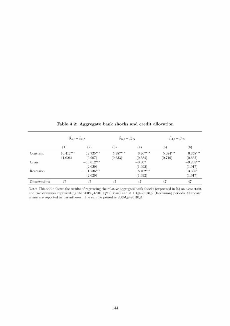
Table 4.2: Aggregate bank shocks and credit allocation

βA,t − βC,t βB,t − βC,t βA,t − βB,t

(1) (2) (3) (4) (5) (6)

Constant 10.412∗∗∗ 12.725∗∗∗ 5.387∗∗∗ 6.367∗∗∗ 5.024∗∗∗ 6.358∗∗∗

(1.026) (0.907) (0.633) (0.584) (0.716) (0.662)Crisis −10.012∗∗∗ −0.807 −9.205∗∗∗

(2.629) (1.692) (1.917)Recession −11.736∗∗∗ −8.402∗∗∗ −3.335∗

(2.629) (1.692) (1.917)

Observations 47 47 47 47 47 47

Note: This table shows the results of regressing the relative aggregate bank shocks (expressed in %) on a constantand two dummies representing the 2008Q4-2010Q2 (Crisis) and 2011Q4-2013Q2 (Recession) periods. Standarderrors are reported in parentheses. The sample period is 2005Q2-2016Q4.

144

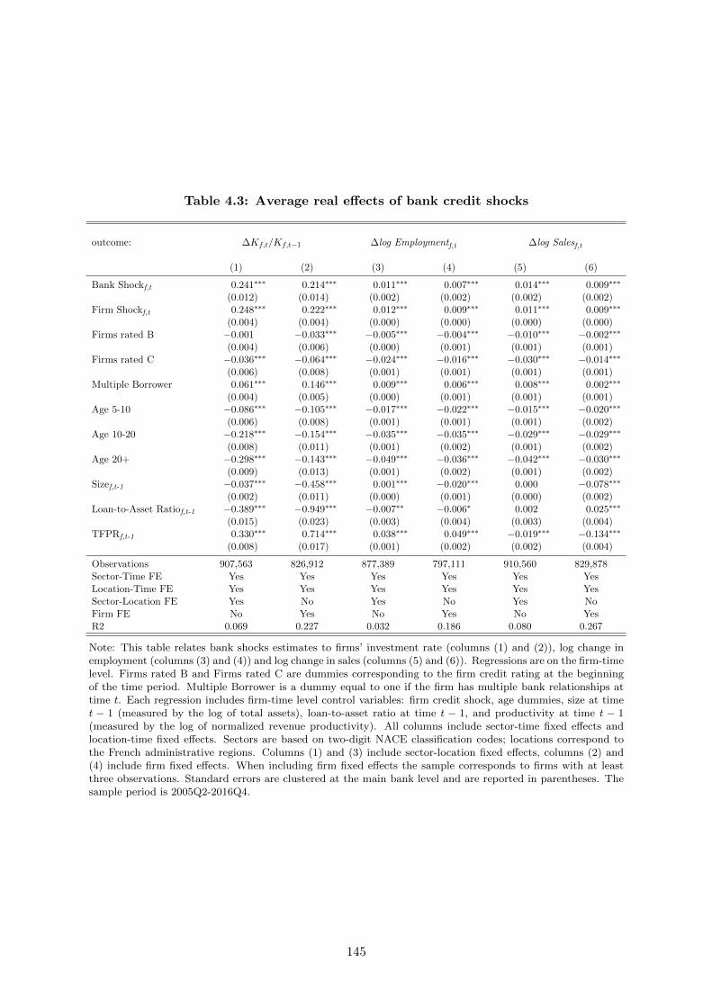
Table 4.3: Average real effects of bank credit shocks

outcome: ∆Kf,t/Kf,t−1 ∆log Employmentf,t ∆log Salesf,t

(1) (2) (3) (4) (5) (6)

Bank Shockf,t 0.241∗∗∗ 0.214∗∗∗ 0.011∗∗∗ 0.007∗∗∗ 0.014∗∗∗ 0.009∗∗∗

(0.012) (0.014) (0.002) (0.002) (0.002) (0.002)Firm Shockf,t 0.248∗∗∗ 0.222∗∗∗ 0.012∗∗∗ 0.009∗∗∗ 0.011∗∗∗ 0.009∗∗∗

(0.004) (0.004) (0.000) (0.000) (0.000) (0.000)Firms rated B −0.001 −0.033∗∗∗ −0.005∗∗∗ −0.004∗∗∗ −0.010∗∗∗ −0.002∗∗∗

(0.004) (0.006) (0.000) (0.001) (0.001) (0.001)Firms rated C −0.036∗∗∗ −0.064∗∗∗ −0.024∗∗∗ −0.016∗∗∗ −0.030∗∗∗ −0.014∗∗∗

(0.006) (0.008) (0.001) (0.001) (0.001) (0.001)Multiple Borrower 0.061∗∗∗ 0.146∗∗∗ 0.009∗∗∗ 0.006∗∗∗ 0.008∗∗∗ 0.002∗∗∗

(0.004) (0.005) (0.000) (0.001) (0.001) (0.001)Age 5-10 −0.086∗∗∗ −0.105∗∗∗ −0.017∗∗∗ −0.022∗∗∗ −0.015∗∗∗ −0.020∗∗∗

(0.006) (0.008) (0.001) (0.001) (0.001) (0.002)Age 10-20 −0.218∗∗∗ −0.154∗∗∗ −0.035∗∗∗ −0.035∗∗∗ −0.029∗∗∗ −0.029∗∗∗

(0.008) (0.011) (0.001) (0.002) (0.001) (0.002)Age 20+ −0.298∗∗∗ −0.143∗∗∗ −0.049∗∗∗ −0.036∗∗∗ −0.042∗∗∗ −0.030∗∗∗

(0.009) (0.013) (0.001) (0.002) (0.001) (0.002)Sizef,t-1 −0.037∗∗∗ −0.458∗∗∗ 0.001∗∗∗ −0.020∗∗∗ 0.000 −0.078∗∗∗

(0.002) (0.011) (0.000) (0.001) (0.000) (0.002)Loan-to-Asset Ratiof,t-1 −0.389∗∗∗ −0.949∗∗∗ −0.007∗∗ −0.006∗ 0.002 0.025∗∗∗

(0.015) (0.023) (0.003) (0.004) (0.003) (0.004)TFPRf,t-1 0.330∗∗∗ 0.714∗∗∗ 0.038∗∗∗ 0.049∗∗∗ −0.019∗∗∗ −0.134∗∗∗

(0.008) (0.017) (0.001) (0.002) (0.002) (0.004)

Observations 907,563 826,912 877,389 797,111 910,560 829,878Sector-Time FE Yes Yes Yes Yes Yes YesLocation-Time FE Yes Yes Yes Yes Yes YesSector-Location FE Yes No Yes No Yes NoFirm FE No Yes No Yes No YesR2 0.069 0.227 0.032 0.186 0.080 0.267

Note: This table relates bank shocks estimates to firms’ investment rate (columns (1) and (2)), log change inemployment (columns (3) and (4)) and log change in sales (columns (5) and (6)). Regressions are on the firm-timelevel. Firms rated B and Firms rated C are dummies corresponding to the firm credit rating at the beginningof the time period. Multiple Borrower is a dummy equal to one if the firm has multiple bank relationships attime t. Each regression includes firm-time level control variables: firm credit shock, age dummies, size at timet − 1 (measured by the log of total assets), loan-to-asset ratio at time t − 1, and productivity at time t − 1(measured by the log of normalized revenue productivity). All columns include sector-time fixed effects andlocation-time fixed effects. Sectors are based on two-digit NACE classification codes; locations correspond tothe French administrative regions. Columns (1) and (3) include sector-location fixed effects, columns (2) and(4) include firm fixed effects. When including firm fixed effects the sample corresponds to firms with at leastthree observations. Standard errors are clustered at the main bank level and are reported in parentheses. Thesample period is 2005Q2-2016Q4.

145

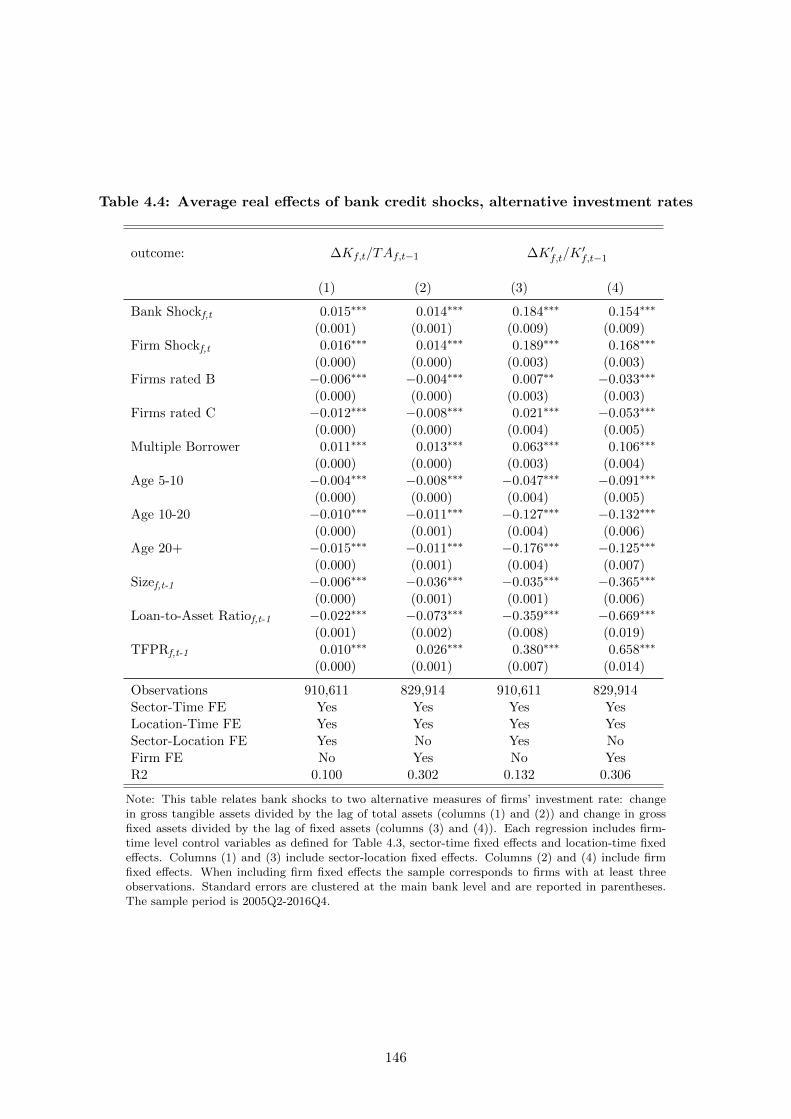
Table 4.4: Average real effects of bank credit shocks, alternative investment rates

outcome: ∆Kf,t/TAf,t−1 ∆K ′f,t/K′f,t−1

(1) (2) (3) (4)

Bank Shockf,t 0.015∗∗∗ 0.014∗∗∗ 0.184∗∗∗ 0.154∗∗∗

(0.001) (0.001) (0.009) (0.009)Firm Shockf,t 0.016∗∗∗ 0.014∗∗∗ 0.189∗∗∗ 0.168∗∗∗

(0.000) (0.000) (0.003) (0.003)Firms rated B −0.006∗∗∗ −0.004∗∗∗ 0.007∗∗ −0.033∗∗∗

(0.000) (0.000) (0.003) (0.003)Firms rated C −0.012∗∗∗ −0.008∗∗∗ 0.021∗∗∗ −0.053∗∗∗

(0.000) (0.000) (0.004) (0.005)Multiple Borrower 0.011∗∗∗ 0.013∗∗∗ 0.063∗∗∗ 0.106∗∗∗

(0.000) (0.000) (0.003) (0.004)Age 5-10 −0.004∗∗∗ −0.008∗∗∗ −0.047∗∗∗ −0.091∗∗∗

(0.000) (0.000) (0.004) (0.005)Age 10-20 −0.010∗∗∗ −0.011∗∗∗ −0.127∗∗∗ −0.132∗∗∗

(0.000) (0.001) (0.004) (0.006)Age 20+ −0.015∗∗∗ −0.011∗∗∗ −0.176∗∗∗ −0.125∗∗∗

(0.000) (0.001) (0.004) (0.007)Sizef,t-1 −0.006∗∗∗ −0.036∗∗∗ −0.035∗∗∗ −0.365∗∗∗

(0.000) (0.001) (0.001) (0.006)Loan-to-Asset Ratiof,t-1 −0.022∗∗∗ −0.073∗∗∗ −0.359∗∗∗ −0.669∗∗∗

(0.001) (0.002) (0.008) (0.019)TFPRf,t-1 0.010∗∗∗ 0.026∗∗∗ 0.380∗∗∗ 0.658∗∗∗

(0.000) (0.001) (0.007) (0.014)

Observations 910,611 829,914 910,611 829,914Sector-Time FE Yes Yes Yes YesLocation-Time FE Yes Yes Yes YesSector-Location FE Yes No Yes NoFirm FE No Yes No YesR2 0.100 0.302 0.132 0.306

Note: This table relates bank shocks to two alternative measures of firms’ investment rate: changein gross tangible assets divided by the lag of total assets (columns (1) and (2)) and change in grossfixed assets divided by the lag of fixed assets (columns (3) and (4)). Each regression includes firm-time level control variables as defined for Table 4.3, sector-time fixed effects and location-time fixedeffects. Columns (1) and (3) include sector-location fixed effects. Columns (2) and (4) include firmfixed effects. When including firm fixed effects the sample corresponds to firms with at least threeobservations. Standard errors are clustered at the main bank level and are reported in parentheses.The sample period is 2005Q2-2016Q4.

146

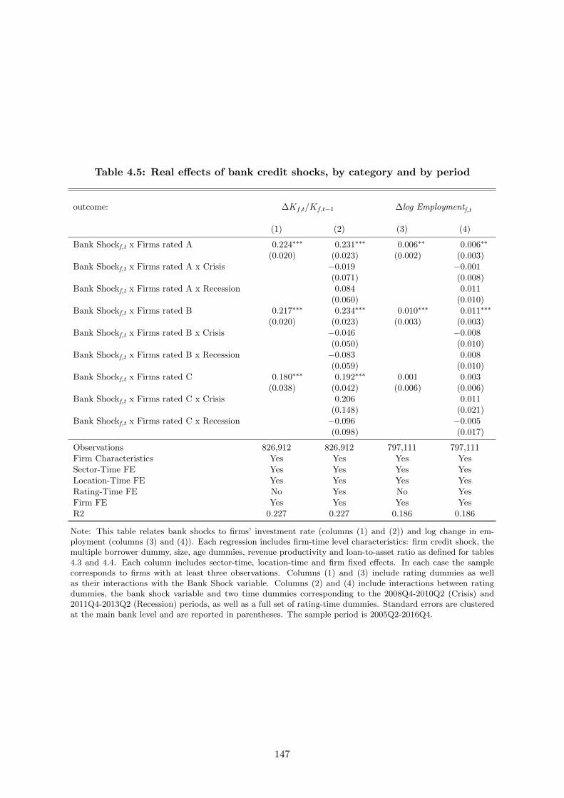
Table 4.5: Real effects of bank credit shocks, by category and by period

outcome: ∆Kf,t/Kf,t−1 ∆log Employmentf,t

(1) (2) (3) (4)

Bank Shockf,t x Firms rated A 0.224∗∗∗ 0.231∗∗∗ 0.006∗∗ 0.006∗∗

(0.020) (0.023) (0.002) (0.003)Bank Shockf,t x Firms rated A x Crisis −0.019 −0.001

(0.071) (0.008)Bank Shockf,t x Firms rated A x Recession 0.084 0.011

(0.060) (0.010)Bank Shockf,t x Firms rated B 0.217∗∗∗ 0.234∗∗∗ 0.010∗∗∗ 0.011∗∗∗

(0.020) (0.023) (0.003) (0.003)Bank Shockf,t x Firms rated B x Crisis −0.046 −0.008

(0.050) (0.010)Bank Shockf,t x Firms rated B x Recession −0.083 0.008

(0.059) (0.010)Bank Shockf,t x Firms rated C 0.180∗∗∗ 0.192∗∗∗ 0.001 0.003

(0.038) (0.042) (0.006) (0.006)Bank Shockf,t x Firms rated C x Crisis 0.206 0.011

(0.148) (0.021)Bank Shockf,t x Firms rated C x Recession −0.096 −0.005

(0.098) (0.017)

Observations 826,912 826,912 797,111 797,111Firm Characteristics Yes Yes Yes YesSector-Time FE Yes Yes Yes YesLocation-Time FE Yes Yes Yes YesRating-Time FE No Yes No YesFirm FE Yes Yes Yes YesR2 0.227 0.227 0.186 0.186

Note: This table relates bank shocks to firms’ investment rate (columns (1) and (2)) and log change in em-ployment (columns (3) and (4)). Each regression includes firm-time level characteristics: firm credit shock, themultiple borrower dummy, size, age dummies, revenue productivity and loan-to-asset ratio as defined for tables4.3 and 4.4. Each column includes sector-time, location-time and firm fixed effects. In each case the samplecorresponds to firms with at least three observations. Columns (1) and (3) include rating dummies as wellas their interactions with the Bank Shock variable. Columns (2) and (4) include interactions between ratingdummies, the bank shock variable and two time dummies corresponding to the 2008Q4-2010Q2 (Crisis) and2011Q4-2013Q2 (Recession) periods, as well as a full set of rating-time dummies. Standard errors are clusteredat the main bank level and are reported in parentheses. The sample period is 2005Q2-2016Q4.

147

Bibliography

Acharya, V., H. Almeida, F. Ippolito, and A. Perez (2014). “Credit lines as monitored liquidity

insurance: Theory and evidence”. Journal of Financial Economics 112.3, pp. 287–319.

Acharya, V. V., H. Almeida, and M. Campello (2013). “Aggregate risk and the choice between

cash and lines of credit”. Journal of Finance 68.5, pp. 2059–2116.

Acharya, V. V. and N. Mora (2015). “A crisis of banks as liquidity providers”. Journal of

Finance 70.1, pp. 1–43.

Acharya, V. V., T. Eisert, C. Eufinger, and C. Hirsch (2018). “Real effects of the sovereign

debt crisis in Europe: evidence from syndicated loans”. Review of Financial Studies 31.8,

pp. 2855–2896.

— (2019). “Whatever it takes: the real effects of unconventional monetary policy”. Review of

Financial Studies, forthcoming.

Adler, G., R. A. Duval, D. Furceri, S. Kilic-Celik, K. Koloskova, and M. Poplawski-Ribeiro

(2017). “Gone with the headwinds: Global productivity”. IMF Staff Discussion Note.

Aghion, P., A. Bergeaud, T. Boppart, P. J. Klenow, and H. Li (2019a). “Missing growth from

creative destruction”. American Economic Review 109.8, pp. 2795–2822.

Aghion, P., A. Bergeaud, G. Cette, R. Lecat, and H. Maghin (2019b). “The inverted-U rela-

tionship between credit access and productivity growth”. Economica 86.341, pp. 1–31.

Alfaro, L., M. Garcıa-Santana, and E. Moral-Benito (2019). “On the direct and indirect real

effects of credit supply shocks”. NBER Working Paper.

Amiti, M. and D. E. Weinstein (2018). “How much do idiosyncratic bank shocks affect invest-

ment? Evidence from matched bank-firm loan data”. Journal of Political Economy 126.2,

pp. 525–587.

Anzoategui, D., D. Comin, M. Gertler, and J. Martinez (2019). “Endogenous technology adop-

tion and R&D as sources of business cycle persistence”. American Economic Journal: Macroe-

conomics 11.3, pp. 67–110.

Asker, J., A. Collard-Wexler, and J. De Loecker (2014). “Dynamic inputs and resource misal-

location”. Journal of Political Economy 122.5, pp. 1013–1063.

148

Bachmann, R. and C. Bayer (2014). “Investment dispersion and the business cycle”. American

Economic Review 104.4, pp. 1392–1416.

Bai, J., D. Carvalho, and G. M. Phillips (2018). “The impact of bank credit on labor reallocation

and aggregate industry productivity”. Journal of Finance 73.6, pp. 2787–2836.

Banerjee, A. V. and E. Duflo (2005). “Growth theory through the lens of development eco-

nomics”. In: Handbook of Economic Growth. Ed. by P.Aghion and S.Durlauf. Amsterdam:

Elsevier, pp. 473–552.

Banque de France (2016). Assessment of Risks to the French Financial Systems. Tech. rep.

Barnett, A., B. Broadbent, A. Chiu, J. Franklin, and H. Miller (2014). “Impaired capital real-

location and productivity”. National Institute Economic Review 228.1, pp. 35–48.

Barrot, J.-N. and J. Sauvagnat (2016). “Input specificity and the propagation of idiosyncratic

shocks in production networks”. Quarterly Journal of Economics 131.3, pp. 1543–1592.

Beatriz, M., J. Coffinet, and T. Nicolas (2018). “Relationship lending and SMEs funding costs

over the cycle: why diversification of borrowing matters”. Journal of Banking & Finance.

Beaumont, P., C. Hurlin, and T. Libert (2019). “Granular borrowers”. mimeo.

Begenau, J. and J. Salomao (2019). “Firm Financing over the Business Cycle”. Review of Fi-

nancial Studies 32.4, pp. 1235–1274.

Behn, M., R. Haselmann, and P. Wachtel (2016). “Procyclical capital regulation and lending”.

Journal of Finance 71.2, pp. 919–956.

Bellone, F. and J. Mallen-Pisano (2013). “Is misallocation higher in France than in the United

States?” GREDEG Working Paper 38.

Ben-David, I., F. Franzoni, R. Moussawi, and J. Sedunov (2019). “The Granular Nature of

Large Institutional Investors”. CEPR Discussion Papers.

Bentolila, S., M. Jansen, and G. Jimenez (2018). “When credit dries up: job losses in the Great

Recession”. Journal of the European Economic Association 16.3, pp. 650–695.

Bernanke, B. S. and A. S. Blinder (1992). “The Federal Funds Rate and the Channels of Mon-

etary Transmission”. American Economic Review, pp. 901–921.

Bernanke, B. S., M. Gertler, and S. Gilchrist (1996). “The financial accelerator and the flight

to quality”. Review of Economics and Statistics 78.1, pp. 1–15.

Berton, F., S. Mocetti, A. F. Presbitero, and M. Richiardi (2018). “Banks, firms, and jobs”.

Review of Financial Studies 31.6, pp. 2113–2156.

Bils, M., P. J. Klenow, and C. Ruane (2018). “Misallocation or Mismeasurement?” mimeo.

149

Blank, S., C. M. Buch, and K. Neugebauer (2009). “Shocks at large banks and banking sector

distress: The Banking Granular Residual”. Journal of Financial Stability 5.4, pp. 353–373.

Blattner, L., L. Farinha, and F. Rebelo (2019). “When losses turn into loans: The cost of

undercapitalized banks”. mimeo.

Bloom, N., M. Floetotto, N. Jaimovich, I. Saporta-Eksten, and S. J. Terry (2018). “Really

uncertain business cycles”. Econometrica 86.3, pp. 1031–1065.

Bord, V. M. and J. A. Santos (2014). “Banks’ liquidity and the cost of liquidity to corporations”.

Journal of Money, Credit and Banking 46.s1, pp. 13–45.

Bremus, F. and C. M. Buch (2017). “Granularity in banking and growth: Does financial openness

matter?” Journal of Banking & Finance 77, pp. 300–316.

Bremus, F., C. M. Buch, K. N. Russ, and M. Schnitzer (2018). “Big Banks and Macroeconomic

Outcomes: Theory and Cross-Country Evidence of Granularity”. Journal of Money, Credit

and Banking 50.8, pp. 1785–1825.

Brynjolfsson, E., D. Rock, and C. Syverson (2019). “Artificial intelligence and the modern

productivity paradox: A clash of expectations and statistics”. In: The economics of artificial

intelligence: An agenda. Ed. by J. G. A. Agrawal and A. Goldfarb.

Buch, C. M. and K. Neugebauer (2011). “Bank-specific shocks and the real economy”. Journal

of Banking & Finance 35.8, pp. 2179–2187.

Buera, F. J. and B. Moll (2015). “Aggregate implications of a credit crunch: The importance

of heterogeneity”. American Economic Journal: Macroeconomics 7.3, pp. 1–42.

Byrne, D. M., J. G. Fernald, and M. B. Reinsdorf (2016). “Does the United States have a

productivity slowdown or a measurement problem?” Brookings Papers on Economic Activity

47.1, pp. 109–182.

Caballero, R. J., T. Hoshi, and A. K. Kashyap (2008). “Zombie lending and depressed restruc-

turing in Japan”. American Economic Review 98.5, pp. 1943–1977.

Cahn, C., M. Girotti, and F. Salvade (2018). “External credit ratings and bank lending”. Banque

de France Working Papers 691.

Calligaris, S. (2015). “Misallocation and total factor productivity in Italy : evidence from firm-

level data”. Labour 29.4, pp. 367–393.

Calvo, G. A., A. Izquierdo, and E. Talvi (2006). “Sudden stops and phoenix miracles in emerging

markets”. American Economic Review 96.2, pp. 405–410.

Carletti, E., F. De Marco, V. Ioannidou, and E. Sette (2019). “Banks as Patient Lenders:

Evidence from a Tax Reform”. CEPR Discussion Papers.

150

Carvalho, V. M. and B. Grassi (2019). “Large Firm Dynamics and the Business Cycle”. Amer-

ican Economic Review 109.4, pp. 1375–1425.

Cerra, V. and S. C. Saxena (2008). “Growth dynamics: The myth of economic recovery”. Amer-


Cette, G., J. G. Fernald, and B. Mojon (2016). “The Pre-Great Recession slowdown in produc-

tivity”. European Economic Review 88.C, pp. 3–20.

Challe, E., J. I. Lopez, and E. Mengus (2019). “Institutional quality and capital inflows: Theory

and evidence”. Journal of International Money and Finance 96, pp. 168–191.

Chari, V. V., P. J. Kehoe, and E. R. McGrattan (2007). “Business cycle accounting”. Econo-

metrica 75.3, pp. 781–836.

Chen, K. and A. Irarrazabal (2015). “The role of allocative efficiency in a decade of recovery”.

Review of Economic Dynamics 18.3, pp. 523–550.

Chodorow-Reich, G. (2014). “The employment effects of credit market disruptions: Firm-level

evidence from the 2008–9 financial crisis”. Quarterly Journal of Economics 129.1, pp. 1–59.

Christiano, L. J., M. S. Eichenbaum, and M. Trabandt (2015). “Understanding the Great Re-

cession”. American Economic Journal : Macroeconomics 7.1, pp. 110–167.

Cingano, F., F. Manaresi, and E. Sette (2016). “Does credit crunch investment down? New

evidence on the real effects of the bank-lending channel”. Review of Financial Studies 29.10,

pp. 2737–2773.

Cong, L. W., H. Gao, J. Ponticelli, and X. Yang (2019). “Credit allocation under economic

stimulus: evidence from China”. Review of Financial Studies, forthcoming.

Cornett, M. M., J. J. McNutt, P. E. Strahan, and H. Tehranian (2011). “Liquidity risk man-

agement and credit supply in the financial crisis”. Journal of Financial Economics 101.2,

pp. 297–312.

Covas, F. and W. J. Den Haan (2011). “The cyclical behavior of debt and equity finance”.

American Economic Review 101.2, pp. 877–99.

Crouzet, N. and N. R. Mehrotra (2019). “Small and Large Firms over the Business Cycle”.

NBER Working Paper.

Davis, S. J., J. Haltiwanger, and S. Schuh (1996). “Small business and job creation: Dissecting

the myth and reassessing the facts”. Small Business Economics 8.4, pp. 297–315.

De Loecker, J. (2011). “Recovering markups from production data”. International Journal of

Industrial Organization 29.Special issue 37th EARIE, pp. 350–355.

151

Decker, R. A., J. Haltiwanger, R. S. Jarmin, and J. Miranda (2016). “Where has all the skewness

gone? The decline in high-growth (young) firms in the U.S”. European Economic Review

86.C, pp. 4–23.

— (2017). “Declining dynamism, allocative efficiency, and the productivity slowdown”. Amer-


Degryse, H. and S. Ongena (2001). “Bank relationships and firm profitability”. Financial man-

agement, pp. 9–34.

Degryse, H., O. De Jonghe, S. Jakovljevic, K. Mulier, and G. Schepens (2019). “Identifying

credit supply shocks with bank-firm data: Methods and applications”. Journal of Financial

Intermediation, forthcoming.

Di Giovanni, J., A. A. Levchenko, and I. Mejean (2014). “Firms, destinations, and aggregate

fluctuations”. Econometrica 82.4, pp. 1303–1340.

— (2017). “Large firms and international business cycle comovement”. American Economic

Review 107.5, pp. 598–602.

— (2018). “The micro origins of international business-cycle comovement”. American Economic

Review 108.1, pp. 82–108.

Di Nola, A. (2015). “Capital misallocation during the Great Recession”. MPRA Paper 68289.

Diamond, D. W. and P. H. Dybvig (1983). “Bank runs, deposit insurance, and liquidity”. Journal

of Political Economy 91.3, pp. 401–419.

Dias, D. A., C. R. Marques, and C. Richmond (2016). “Misallocation and productivity in the

lead up to the Eurozone crisis”. Journal of Macroeconomics 49.C, pp. 46–70.

Duval, R. A., G. H. Hong, and Y. Timmer (2019). “Financial frictions and the great productivity

slowdown”. Review of Financial Studies, forthcoming.

Eisfeldt, A. L. and T. Muir (2016). “Aggregate external financing and savings waves”. Journal

of Monetary Economics 84, pp. 116–133.

Fernald, J. G. (2015). “Productivity and potential output before, during and after the Great

Recession”. NBER Macroeconomics annual 29.1, pp. 1–51.

Fernald, J. G., R. E. Hall, J. H. Stock, and M. W. Watson (2017). “The Disappointing Recovery

of Output after 2009”. Brookings Papers on Economic Activity 47.1, pp. 1–81.

Fernholz, R. T. and C. Koch (2017). “Big Banks, Idiosyncratic Volatility, and Systemic Risk”.


Foster, L., J. Haltiwanger, and C. Syverson (2008). “Reallocation, firm turnover, and efficiency:

selection on productivity or profitability?” American Economic Review 98.1, pp. 394–425.

152

Fraisse, H., J. Hombert, and M. Le (2018). “The competitive effect of a bank megamerger on

credit supply”. Journal of Banking & Finance 93, pp. 151–161.

Fraisse, H., M. Le, and D. Thesmar (forthcoming). “The real effects of bank capital require-

ments”. Management Science.

Gabaix, X. (2011). “The granular origins of aggregate fluctuations”. Econometrica 79.3, pp. 733–

772.

Gabaix, X. and R. S. Koijen (2019). “Granular Instrumental Variables”. NBER Working Paper.

Garcia-Macia, D. (2017). “The financing of ideas and the great deviation”. IMF Working Paper

No 17/176.

Garcia-Santana, M., E. Moral-Benito, J. Pijoan-Mas, and R. Ramos (2019). “Growing like Spain:

1995-2007”. International Economic Review, forthcoming.

Gatev, E. and P. E. Strahan (2006). “Banks’ advantage in hedging liquidity risk: Theory and

evidence from the commercial paper market”. Journal of Finance 61.2, pp. 867–892.

Gaubert, C. and O. Itskhoki (2018). “Granular comparative advantage”. NBER Working Paper.

Gerth, F. and K. Otsu (2018). “The post-crisis slump in Europe: a business cycle accounting

analysis”. The B.E. Journal of Macroeconomics 18.1, pp. 1–25.

Gertler, M. and S. Gilchrist (1994). “Monetary policy, business cycles, and the behavior of small

manufacturing firms”. Quarterly Journal of Economics 109.2, pp. 309–340.

Ghironi, F. (2018). “Macro needs micro”. Oxford Review of Economic Policy 34.1–2, pp. 195–

218.

Giannetti, M. and A. Simonov (2013). “On the real effects of bank bailouts: micro evidence

from Japan”. American Economic Journal: Macroeconomics 5.1, pp. 135–167.

Gilchrist, S., J. W. Sim, and E. Zakrajsek (2013). “Misallocation and financial market frictions :

some direct evidence from the dispersion in borrowing costs”. Review of Economic Dynamics

16.1, pp. 159–176.

Gopinath, G., S. Kalemli-Ozcan, L. Karabarbounis, and C. Villegas-Sanchez (2017). “Capi-

tal Allocation and Productivity in South Europe”. Quarterly Journal of Economics 132.4,

pp. 1915–1967.

Gordon, R. (2016). The rise and fall of American growth: The United States standard of living

since the Civil war. Princeton University Press.

Greenstone, M., A. Mas, and H.-L. Nguyen (2019). “Do credit market shocks affect the real econ-

omy? Quasi-experimental evidence from the Great Recession and normal economic times”.

American Economic Journal: Economic Policy, forthcoming.

153

Greenwood, R. and D. Thesmar (2011). “Stock price fragility”. Journal of Financial Economics

102.3, pp. 471–490.

Herskovic, B. (2018). “Networks in production: Asset pricing implications”. Journal of Finance

73.4, pp. 1785–1818.

Holmstrom, B. and J. Tirole (1998). “Private and public supply of liquidity”. Journal of Political

Economy 106.1, pp. 1–40.

Hopenhayn, H. A. (2014). “Firms, misallocation, and aggregate productivity: a review”. In:

Annual Review of Economics Vol 6. Ed. by K. Arrow and T. Bresnahan, pp. 735–770.

Hoshi, T. and A. K. Kashyap (2015). “Will the US and Europe avoid a Lost Decade? Lessons

from Japan’s postcrisis experience”. IMF Economic Review 63.1, pp. 110–163.

Hsieh, C.-T. and P. J. Klenow (2009). “Misallocation and manufacturing TFP in China and

India”. Quaterly Journal of Economics 124.4, pp. 1403–1448.

Huber, K. (2018). “Disentangling the effects of a banking crisis: Evidence from German firms

and counties”. American Economic Review 108.3, pp. 868–898.

Ippolito, F., J.-L. Peydro, A. Polo, and E. Sette (2016). “Double bank runs and liquidity risk

management”. Journal of Financial Economics 122.1, pp. 135–154.

Ivashina, V. and D. Scharfstein (2010). “Bank lending during the financial crisis of 2008”.

Journal of Financial Economics 97.3, pp. 319–338.

Iyer, R., J.-L. Peydro, S. da Rocha-Lopes, and A. Schoar (2013). “Interbank liquidity crunch

and the firm credit crunch: Evidence from the 2007–2009 crisis”. Review of Financial Studies

27.1, pp. 347–372.

Jermann, U. and V. Quadrini (2012). “Macroeconomic effects of financial shocks”. American


Jimenez, G., S. Ongena, J.-L. Peydro, and J. Saurina (2012). “Credit supply and monetary pol-

icy: identifying the bank balance-sheet channel with loan applications”. American Economic

Review 102.5, pp. 2301–2326.

— (2014). “Hazardous times for monetary policy: What do twenty-three million bank loans say

about the effects of monetary policy on credit risk-taking?” Econometrica 82.2, pp. 463–505.

— (2017). “Macroprudential policy, countercyclical bank capital buffers, and credit supply:

evidence from the Spanish dynamic provisioning experiments”. Journal of Political Economy

125.6, pp. 2126–2177.

Jochmans, K. and M. Weidner (2019). “Fixed-Effect Regressions on Network Data”. Economet-

rica 87.5, pp. 1543–1560.

154

Jones, C. I. (2013). “Misallocation, economic growth and input-output economics”. In: Ad-

vances in economics and econometrics, Tenth world congress, applied economics. Ed. by M.

D.Acemoglu and E.Dekel. Cambridge University Press, pp. 419–456.

Justiniano, A., G. E. Primiceri, and A. Tambalotti (2010). “Investment shocks and business

cycles”. Journal of Monetary Economics 57.2, pp. 132–145.

Kashyap, A. K., O. A. Lamont, and J. C. Stein (1994). “Credit conditions and the cyclical

behavior of inventories”. Quarterly Journal of Economics 109.3, pp. 565–592.

Kashyap, A. K., R. Rajan, and J. C. Stein (2002). “Banks as liquidity providers: An explanation

for the coexistence of lending and deposit-taking”. Journal of Finance 57.1, pp. 33–73.

Kehoe, T. J. and E. C. Prescott (2002). “Great depressions of the 20th century”. Review of

Economic Dynamics 5.1, pp. 1–18.

Kehrig, M. (2015). “The cyclical nature of the productivity distribution”. mimeo.

Khan, A. and J. K. Thomas (2013). “Credit shocks and aggregate fluctuations in an economy

with production heterogeneity”. Journal of Political Economy 121.6, pp. 1055–1107.

Khwaja, A. I. and A. Mian (2008). “Tracing the impact of bank liquidity shocks: Evidence from

an emerging market”. American Economic Review 98.4, pp. 1413–1442.

Kiyotaki, N. and J. Moore (1997). “Credit cycles”. Journal of Political Economy 105.2, pp. 211–

248.

Kramarz, F., J. Martin, and I. Mejean (2019). “Volatility in the Small and in the Large: The

Lack of Diversification in International Trade”. CREST Working Paper.

Krugman, P. (1990). The age of diminished expectations. MIT Press.

Kunsch, H. R. (1989). “The jackknife and the bootstrap for general stationary observations”.

The Annals of Statistics, pp. 1217–1241.

Larrain, M. and S. Stumpner (2017). “Capital account liberalization and aggregate productivity:

the role of firm capital allocation”. Journal of Finance 72.4, pp. 1825–1858.

Levinsohn, J. and A. Petrin (2003). “Estimating production functions using inputs to control

for unobservables”. Review of Economic Studies 70.2, pp. 317–341.

Libert, T. (2017). “Misallocation before, during and after the Great Recession”. Banque de

France Working Papers 658.

Maestas, N., K. J. Mullen, and D. Powell (2016). “The effect of population aging on economic

growth, the labor force and productivity”. NBER Working Paper No. 22452.

Manaresi, F. and N. Pierri (2019). “Credit supply and productivity growth”. IMF Working

Paper No. 19/107.

155

McGowan, M. A., D. Andrews, and V. Millot (2017). “The walking dead? Zombie firms and pro-

ductivity performance in OECD countries”. OECD Economics Department Working Papers

1372.

Mian, A. and A. Sufi (2014). “What explains the 2007–2009 drop in employment?” Econometrica

82.6, pp. 2197–2223.

Midrigan, V. and D. Y. Xu (2014). “Finance and misallocation: evidence from plant-level data”.


Moll, B. (2014). “Productivity losses from financial frictions: can self-financing undo capital

misallocation?” American Economic Review 104.10, pp. 3186–3221.

Oberfield, E. (2013). “Productivity and misallocation during a crisis: evidence from the Chilean

crisis of 1982”. Review of Economic Dynamics 16.1, pp. 100–119.

Olley, S. and A. Pakes (1996). “The Dynamics of Productivity in the Telecommunications

Equipment Industry”. Econometrica 64.6, pp. 1263–1297.

Ottonello, P. and T. Winberry (2018). “Financial heterogeneity and the investment channel of

monetary policy”. NBER Working Paper.

Paravisini, D. (2008). “Local bank financial constraints and firm access to external finance”.

Journal of Finance 63.5, pp. 2161–2193.

Paravisini, D., V. Rappoport, and P. Schnabl (2017). “Specialization in bank lending: Evidence

from exporting firms”. NBER Working Paper.

Paravisini, D., V. Rappoport, P. Schnabl, and D. Wolfenzon (2015). “Dissecting the effect of

credit supply on trade: evidence from matched credit-export data”. Review of Economic

Studies 82.1, pp. 333–359.

Peek, J. and E. S. Rosengreen (2005). “Unnatural selection: perverse incentives and the misal-

location of credit in Japan”. American Economic Review 95.4, pp. 1144–1166.

Reifschneider, D., W. Wascher, and D. W. Wilcox (2015). “Aggregate supply in the United

States: Recent developments and implications for the conduct of monetary policy”. IMF


Reis, R. (2013). “The Portuguese slump and crash and the Euro crisis”. Brookings Papers on

Economic Activity 46.1, pp. 143–210.

Restuccia, D. and R. Rogerson (2008). “Policy distorsions and aggregate productivity with

heterogeneous establishments”. Review of Economic Dynamics 11.4, pp. 707–720.

— (2013). “Misallocation and productivity”. Review of Economic Dynamics 16.1, pp. 1–10.

— (2017). “The causes and costs of Misallocation”. Journal of Economic Perspectives 31.3,

pp. 151–174.

156

Rotemberg, J. J. and M. Woodford (1993). “Dynamic general equilibrium models with imper-

fectly competitive product markets”. NBER Working Paper 4502.

Sandleris, G. and M. Wright (2014). “The costs of financial crises: ressource misallocation,

productivity and welfare in the 2001 Argentine Crisis”. Scandinavian Journal of Economics

116.1, pp. 87–127.

Sandoz, C. (2018). “Input prices, allocation of resources and TFP growth: Evidence from Chi-

nese imports in France”. mimeo.

Schivardi, F., E. Sette, and G. Tabellini (2018). “Credit misallocation during the European

financial crisis”. CEPR Discussion Papers.

Siriwardane, E. N. (2019). “Limited investment capital and credit spreads”. Journal of Finance

74.5, pp. 2303–2347.

Smets, F. and R. Wouters (2007). “Shocks and frictions in US business cycles: A Bayesian DSGE

approach”. American Economic Review 97.3, pp. 586–606.

Syverson, C. (2011). “What determines productivity?” Journal of Economic Literature 49.2,

pp. 326–365.

— (2017). “Challenges to mismeasurement explanations for the US productivity slowdown”.

Journal of Economic Perspectives 31.2, pp. 165–186.

Ziebarth, N. L. (2014). “Misallocation and productivity during the Great Depression”. North-

western university mimeo.

157

Three Essays on Bank Credit and Resource Allocation

Documents

Transcript of Three Essays on Bank Credit and Resource Allocation