GUNS, PARASITES, AND STATES: THREEESSAYS ON COMPARATIVE DEVELOPMENT

AND POLITICAL ECONOMY

BY

EMILIO DEPETRIS CHAUVIN

B.A., UNIVERSIDAD DE BUENOS AIRES, 2003

M.A., BROWN UNIVERSITY, 2009

A DISSERTATION SUBMITTED IN PARTIAL FULFILLMENT OF THE

REQUIREMENTS FOR THE DEGREE OF DOCTOR OF PHILOSOPHY

IN THE DEPARTMENT OF ECONOMICS AT BROWN UNIVERSITY

PROVIDENCE, RHODE ISLAND

MAY 2014

c� Copyright 2014 by Emilio Depetris Chauvin

To Jennifer with all my love and deepest gratitude

This dissertation by Emilio Depetris Chauvin is accepted in its present form

by the Department of Economics as satisfying the

dissertation requirement for the degree of Doctor of Philosophy.

Date

David Weil, Adviser

Recommended to the Graduate Council

Date

Pedro Dal Bo, Reader

Date

Stylianos Michalopoulos, Reader

Date

Brian Knight, Reader

Approved by the Graduate Council

Date

Peter Weber, Dean of the Graduate School

iii

Vita

Emilio Depetris Chauvin was born on September 3th, 1979 in Buenos Aires, Ar-

gentina. He earned his Bachelor’s degree from Universidad de Buenos Aires in 2003.

He started his graduated studies in Argentina and completed all the course work for

the M.A. in Economics at Universidad de San Andres. Before joining Brown Univer-

sity, he worked as an economist in several think tanks and as country economist for

the World Bank in Argentina. He enrolled in Brown University’s Economics Ph.D.

program in 2008 and obtained his M.A. in Economics in 2009. While at Brown, he

was a fellow of the Initiative in Spatial Structures in the Social Sciences (S4). In

the course of his graduate school career, he was awarded a Brown Graduate School

Fellowship, the Abramson Prize for Best Third-year Research Paper, a Merit Disser-

tation Fellowship, and the Professor Borts Prize for Oustanding Ph.D. Dissertation in

Economics. He received a Ph.D. in 2014 and will continue his research and teaching

in Economics as an Assistant Professor at Universidad de los Andes in Colombia.

iv

Acknowledgements

This dissertation could not have been finished without the help and support from

many professors, colleagues, friends, and my family. I wish to o↵er my most heartfelt

thanks to all of them here.

I owe an immense debt of gratitude to my main advisor, David Weil, and my thesis

committee members, Pedro Dal Bo, Stelios Michalopoulos, and Brian Knight. I am

particularly grateful to David. His advice, guidance, support, and mentorship during

my years at Brown were crucial for my professional development. David is not only

one of the smartest scholars I have ever met but also a great human being. I would

certainly be remiss in failing to acknowledge the key role played by Pedro in making

my journey at Brown possible. He was not only instrumental in bringing me to Brown

University but also in making me feel that my lovely Argentina was actually not that

far. With his scientific meticulousness, Pedro also taught me how to think outside

the box. Brian and Stelios had nurtured my intellectual development by generously

providing their time, invaluable comments, and unwavering guidance. I would also

like to take this opportunity to thank Oded Galor who was always willing to help. I

appreciate the fact that his o�ce door was always open whenever I needed advice.

Many thanks also go to Peter Howitt, Vernon Henderson, Ken Chay, Louis Put-

terman and Blaise Melly for comments, help, and advice in di↵erent stages of my

graduate studies. I thank Juan Carlos Hallak, Daniel Heymann, and Walter Sosa Es-

cudero for their invaluable support, help, and mentoring in the transition to my Phd

studies at Brown University. I wish to thank Boris Gershman, Alejandro Molnar, Ri-

v

cardo Perez Truglia, Leandro Gorno, Quamrul Ashraf, Raphael Franck, participants

of Macroeconomics Lunch and Macroeconomics Seminar at Brown University, semi-

nar participants at Universidad de San Andres, NEUDC 2013, Boston-Area Working

Group in African Political Economy at the Institute for Quantitative Social Science

(Harvard University), UNC at Chapel Hill, Notre Dame University, FGV-EPGV (Rio

de Janeiro), FGV-EESP (Sao Paulo), ITAM, and Universidad de los Andes for com-

ments and helpful discussions on the main chapter of this dissertation.

I would also like to thank my friend and fairy godmother, Angelica Vargas, who has

been supportive not only in practical matters but also emotionally since the first

day I arrived to Providence. Her kindness and hilarious sense of humor is something

that I will certainly miss. Several friends made my grad school experience a terrific

ride and I thank them for their companionship and fun: Omer Ozak, Judith Gallego,

Fede Droller, Flor Borreschio, Ruben Durante, Maya Judd, Sarah Overmyer, Angelica

Duran, Jack Sweeney, Diego Diaz, Carla Alberti, Paco Jurado, Chaparro-Martinez

family, Martin Fiszbein, Seba Di Tella, Meche Politi, and Perez-Truglia family.

I wish to thanks my parents, Juan Manuel and Silvia, not only for their love but

also for breeding my passion for learning. I am thankful and grateful to my siblings

Nicolas, Irene, Julian, Ana, and Pablo for being always there and for make me laugh.

I am happy guy and you are all indeed responsible for that! This six-years journey

would not have been such a wonderful experience without the arrival of my daughter

Violeta. This little person brought immense joy and fulfillment to my life. Violeta,

your smile is the most powerful force helping me to push forward!

I dedicate this dissertation to my wife Jennifer. All the sacrifices she made along

the way to enable the pursuit of my dream are nothing else but the proof of her

unconditional love. Jennifer, I will be always deeply indebted to you. Te amo!

vi

Contents

List of Figures x

List of Tables xii

1 State History and Contemporary Conflict: Evidence from Sub-SaharanAfrica 1

1.1 Introduction . . . . . . . . . . . . . . . . . . . . . . . . . . . . . . . . 1

1.2 Relationship with the Existing Literature . . . . . . . . . . . . . . . . 7

1.3 A New Index of State History at the Sub-national Level . . . . . . . . 9

1.3.1 Overview of the Construction Procedure . . . . . . . . . . . . 9

1.4 Empirical Relationship between State History and Contemporary Con-flict . . . . . . . . . . . . . . . . . . . . . . . . . . . . . . . . . . . . . 17

1.4.1 Sources and Description of Conflict Data . . . . . . . . . . . . 17

1.4.2 Cross Sectional Evidence . . . . . . . . . . . . . . . . . . . . . 19

1.4.3 Panel Data Evidence: Weather Induced-Agricultural Produc-tivity Shock, State History, and Conflict . . . . . . . . . . . . 43

1.5 Identifying Potential Mechanisms at Work: State History and Atti-tudes Towards State Institutions . . . . . . . . . . . . . . . . . . . . . 46

1.6 Conclusion . . . . . . . . . . . . . . . . . . . . . . . . . . . . . . . . 56

Appendix 1.A: Variable Definitions 75

vii

Appendix 1.B: Construction of the Instrument 79

Appendix 1.C: Construction of Weather-Induced Productivity Shock 82

2 Malaria and Early African Development: Evidence from the SickleCell Trait 92

2.1 Introduction . . . . . . . . . . . . . . . . . . . . . . . . . . . . . . . . 92

2.2 Malaria and Sickle Cell Disease . . . . . . . . . . . . . . . . . . . . . 97

2.3 Measuring the Historical Burden of Malaria Using Data on the SickleCell Trait . . . . . . . . . . . . . . . . . . . . . . . . . . . . . . . . . 101

2.3.1 Measuring the Overall Burden of Malaria . . . . . . . . . . . . 108

2.3.2 Comparison of Malaria Burden to Malaria Ecology . . . . . . 111

2.3.3 Comparison of Malaria Burden to Modern Malaria MortalityRates . . . . . . . . . . . . . . . . . . . . . . . . . . . . . . . 116

2.4 Assessing the Importance of Malaria to Early African Development . 118

2.4.1 Ethnic Group Analysis . . . . . . . . . . . . . . . . . . . . . . 118

2.5 Model-Based Estimates of the Economic Burden of Malaria . . . . . . 127

2.5.1 Direct E↵ect of Malaria Mortality . . . . . . . . . . . . . . . 127

2.5.2 Economic E↵ects of Malaria Morbidity . . . . . . . . . . . . . 140

2.6 Conclusion . . . . . . . . . . . . . . . . . . . . . . . . . . . . . . . . . 142

3 Fear of Obama: An Empirical Study of the Demand for Guns andthe U.S. 2008 Presidential Election 150

3.1 Introduction . . . . . . . . . . . . . . . . . . . . . . . . . . . . . . . . 150

3.2 Data and Aggregated Empirical Evidence on Gun Sales . . . . . . . . 157

3.2.1 A Proxy of the Demand for Guns . . . . . . . . . . . . . . . . 157

3.2.2 A Descriptive Analysis of the Aggregated Evolution of Gun Sales159

3.3 Empirical Strategy and Results . . . . . . . . . . . . . . . . . . . . . 163

viii

3.3.1 Quantifying the Obama e↵ect . . . . . . . . . . . . . . . . . . 163

3.3.2 Potential Mechanisms . . . . . . . . . . . . . . . . . . . . . . 170

3.3.3 Robustness Check . . . . . . . . . . . . . . . . . . . . . . . . . 181

3.4 Conclusions . . . . . . . . . . . . . . . . . . . . . . . . . . . . . . . . 186

Appendix 3.A: Additional Tables 198

Bibliography 202

ix

List of Figures

1.1 Evolution of Historical Map Boundaries (1000 - 1850 CE) . . . . . . . 10

1.2 Example of Score Calculation. East Africa (1800 - 1850 CE) . . . . . 12

1.3 Spatial Distribution of State History Index . . . . . . . . . . . . . . . 14

1.4 Conflict and State History . . . . . . . . . . . . . . . . . . . . . . . . 25

1.5 Sensitivity of Estimates to Exclusion of Countries . . . . . . . . . . . 31

1.6 Time Elapsed Since Neolithic Revolution . . . . . . . . . . . . . . . . 36

1.7 Alternative Measure Using Historical Cities . . . . . . . . . . . . . . 42

2.1 Sickle Cell Gene Frequency from Piel et al (2010) . . . . . . . . . . . 101

2.2 E↵ect of a Hypothetical Malaria Eradication on Evolution of Carriers 106

2.3 Implications of Varying Sickle Cell Prevalence for Malaria Burden . . 110

2.4 Worldwide Distribution of Malaria Ecology . . . . . . . . . . . . . . . 112

2.5 Malaria Ecology in Africa . . . . . . . . . . . . . . . . . . . . . . . . 113

2.6 Population Density by Ethnic Groups from EA (1967) . . . . . . . . 120

2.7 Consumption and Income Profiles . . . . . . . . . . . . . . . . . . . . 132

2.8 Change in Survival Probabilities due to Malaria . . . . . . . . . . . . 136

3.1 Presidential Elections and Firearm Background Check Reports . . . . 161

3.2 Growth in Background Checks by State (July08-June09 vs July07-June08) . . . . . . . . . . . . . . . . . . . . . . . . . . . . . . . . . . 162

x

3.3 Geographic Distribution Obama Victory E↵ect . . . . . . . . . . . . . 170

3.4 Change in Attitudes Toward Gun Control. More important to ProtectGun Rights or Control Gun Ownership? . . . . . . . . . . . . . . . . 172

xi

List of Tables

1.1 Summary Statistics. Grid Cell Sample . . . . . . . . . . . . . . . . . 58

1.2 OLS Estimates - Baseline Specification . . . . . . . . . . . . . . . . . 59

1.3 OLS Estimates - Accounting for Genetic and Ecological Diversity . . 60

1.4 OLS Estimates - Additional Controls . . . . . . . . . . . . . . . . . . 61

1.5 OLS Estimates. Di↵erent Conflict Measures . . . . . . . . . . . . . . 62

1.6 OLS Estimates. Heterogeneity Across Regions . . . . . . . . . . . . . 63

1.7 OLS Estimates. Discount Factors and Importance of Medieval Period 64

1.8 OLS Estimates - Intensive vs Extensive Margin of Political Centralization 65

1.9 First-Stage. Neolithic Instrument . . . . . . . . . . . . . . . . . . . . 66

1.10 IV Estimates . . . . . . . . . . . . . . . . . . . . . . . . . . . . . . . 67

1.11 Alternative Measure. Historical Proximity to Cities . . . . . . . . . . 68

1.12 Conflict, State History, and Weather Shocks -Panel Data Evidence(1989-2010)- . . . . . . . . . . . . . . . . . . . . . . . . . . . . . . . . 69

1.13 Conflict, State History, and Weather Shocks -Panel Data Evidence(1989-2010)- . . . . . . . . . . . . . . . . . . . . . . . . . . . . . . . . 70

1.14 State Legitimacy and State History . . . . . . . . . . . . . . . . . . . 71

1.15 State Legitimacy and State History. Internal vs External Norms . . . 72

1.16 Trust and State History . . . . . . . . . . . . . . . . . . . . . . . . . 73

1.17 Trust in Local Policy Makers, Traditional Leaders, and State History 74

xii

2.1 Components of the Cost of Malaria . . . . . . . . . . . . . . . . . . . 144

2.2 Malaria Burden vs. Malaria Ecology: Grid Cell Analysis . . . . . . . 145

2.3 Malaria Burden vs. Malaria Ecology: Ethnic Group Analysis . . . . . 146

2.4 Malaria and Population Density . . . . . . . . . . . . . . . . . . . . . 147

2.5 Malaria and Ethnic Prosperity . . . . . . . . . . . . . . . . . . . . . . 148

2.6 Years Lost to Disability per capita, WHO AFRO Region . . . . . . . 149

3.1 Obama Victory E↵ect . . . . . . . . . . . . . . . . . . . . . . . . . . 189

3.2 Obama E↵ect . . . . . . . . . . . . . . . . . . . . . . . . . . . . . . . 190

3.3 Obama E↵ect and Gun-Control Fear . . . . . . . . . . . . . . . . . . 191

3.4 Obama E↵ect and Race Bias . . . . . . . . . . . . . . . . . . . . . . . 192

3.5 Both Hypotheses Together . . . . . . . . . . . . . . . . . . . . . . . . 193

3.6 Omitting Election Aftermath . . . . . . . . . . . . . . . . . . . . . . 194

3.7 Using Polls Data . . . . . . . . . . . . . . . . . . . . . . . . . . . . . 195

3.8 Using Alternative Measures for Prejudice . . . . . . . . . . . . . . . . 196

3.9 Further Robustness Check . . . . . . . . . . . . . . . . . . . . . . . . 197

3.10 Summary Statistics . . . . . . . . . . . . . . . . . . . . . . . . . . . . 199

3.11 State Characteristics . . . . . . . . . . . . . . . . . . . . . . . . . . . 200

3.12 State Characteristics (Continuation) . . . . . . . . . . . . . . . . . . 201

xiii

Preface

This dissertation is composed of three chapters on comparative development and

political economy. Chapter I examines empirically the role of historical political cen-

tralization on the likelihood of contemporary civil conflict in Sub-Saharan Africa. It

combines a wide variety of historical sources to construct an original measure of long-

run exposure to statehood at the sub-national level. It then exploits variation in this

new measure along with geo-referenced conflict data to document a robust negative

relationship between long-run exposure to statehood and contemporary conflict.

Chapter 1 argues that regions with long histories of statehood are better equipped

with mechanisms to establish and preserve order. Two pieces of evidence consis-

tent with this hypothesis are provided. First, regions with relatively long historical

exposure to statehood are less prone to experience conflict when hit by a negative

economic shock. Second, exploiting contemporary individual-level survey data for 18

Sub-Saharan countries, Chapter 1 also provides evidence that within-country long

historical statehood experience is linked to people’s positive attitudes toward state

institutions and traditional leaders

Chapter 2 examines the e↵ect of malaria on economic development in Africa over

the very long run. Using data on the prevalence of the mutation that causes sickle

cell disease it measures the impact of malaria on mortality in Africa prior to the

period in which formal data were collected. The presented estimate suggests that in

the more a✏icted regions, malaria lowered the probability of surviving to adulthood

by about ten percentage points, which is roughly twice the current burden of the

xiv

disease. The reduction in malaria mortality has been roughly equal to the reduction

in other causes of mortality. Chapter 2 then asks whether the estimated burden

of malaria had an e↵ect on economic development in the period before European

contact. Examining both mortality and morbidity, it does not find evidence that

the impact of malaria would have been very significant. These model-based findings

are corroborated by a more statistically-based approach, which shows little evidence

of a negative relationship between malaria ecology and population density or other

measures of development, using data measured at the level ethnic groups.

Chapter 3 provides a valuable input for the analysis of future gun policies in the US

and their social, economic, and political ramifications. It focuses on the understanding

of the economic and non-economic determinants of the decision of acquiring firearms.

Particularly, Chapter 3 exploits monthly data constructed from futures markets on

presidential election outcomes and a novel proxy for firearm purchases, to analyzes

how the demand for guns responded to the likelihood of Barack Obama being elected

in 2008. The existence of a large Obama e↵ect on the demand for guns is documented,

being this political e↵ect larger than the e↵ect associated to the worsening economic

conditions. Furthermore, Chapter 3 presents empirical evidence consistent with the

hypotheses that the unprecedented increase in the demand for guns was partially

driven by both a fear of a future Obama gun-control policy and racial prejudice.

xv

Chapter 1

State History and Contemporary Conflict:Evidence from Sub-Saharan Africa

1.1 Introduction

1 Civil conflict imposes enormous costs on a society. In addition to lives lost as a

direct result of violent confrontations, there may be persistent negative consequences

to health and social fragmentation. Economic costs extend beyond short-term disrup-

tion of markets, as conflict may also shape long-run growth via its e↵ect on human

capital accumulation, income inequality, institutions, and culture. Not surprisingly,

understanding the determinants of civil conflict has been the aim of a growing body

of economic and political science literature.2

The case of Sub-Saharan Africa has received considerable attention for the simple

1I am grateful to Gordon McCord, Stelios Michalopoulos, and Omer Ozak for sharing data,Nickolai Riabov and Lynn Carlson for computational assistance with ArcGIS and R, and SantiagoBegueria for helpful discussions and suggestions regarding the Standardized Precipitation Evapo-transpiration Index.

2Blattman and Miguel (2010) provide an extensive review and discussion on the literature ofcivil conflict, including the theoretical arguments and salient empirical findings on the causes andconsequences of civil conflict.

1

2reason that civil conflict has been particularly prevalent in this part of the world;

over two thirds of Sub-Saharan african countries experienced at least one episode of

conflict since 1980. Many scholars have pointed to civil conflict as a key factor holding

back African economic development (see, for example, Easterly and Levine 1997).

In this paper I explore the relationship between the prevalence of modern civil conflict

and historical political centralization. Specifically, I uncover a within-country robust

negative relationship between long-run exposure to statehood and the prevalence of

contemporary conflict. My approach of studying a historical determinant of modern

civil conflict is motivated by the empirical literature showing evidence on the impor-

tance of historical persistence for understanding current economic development (see

Galor 2011; Nunn 2013; and Spoloare and Wacziarg 2013 for extensive reviews). My

paper draws on a strand of this literature which documents that traditional African

institutions not only survived the colonial period but that they still play an important

role in modern African development (Gennaioli and Rainer, 2007; and Michalopoulos

and Papaioannou, 2013, among others).

Why would the long history of statehood matter for contemporary conflict? Similarly

to Persson and Tabellini (2009)’s idea of “democratic capital”, I argue that the ac-

cumulation of experience with state-like institutions may result in an improved state

capacity over time.3 Therefore, regions with long histories of statehood should be bet-

ter equipped with mechanisms to establish and preserve order. These institutional

capabilities can be manifested, for example, in the ability to negotiate compromises

and allocate scarce resources, the existence of traditional collective organizations and

legal courts to peacefully settle di↵erences over local disputes, or even a stronger

presence of police force. As a result, regions with long history of statehood should

experience less conflict.

3State capacity can be broadly defined as the abilities acquired by the state to implement a widerange of di↵erent policies (Besley and Persson 2010).

3

A key aspect of my approach is to exploit within-country di↵erences in the preva-

lence of modern conflict and its correlates. I take my empirical analysis to a fine sub-

national scale for several reasons. First, conflict in Africa is often local and does not

extend to a country’s whole territory.4 Second, there is arguably large within-country

heterogeneity in historical determinants of conflict, including historical exposure to

state institutions. Given that modern borders in Sub-Saharan Africa were artificially

drawn during colonial times without consideration of previous historical boundaries

(Green, 2012), substantial heterogeneity in location histories and people characteris-

tics persists today within those borders. Therefore, the aggregation of these charac-

teristics at the country level averages out a rich source of heterogeneity. Third, other

determinants of conflict that have previously been highlighted in the literature, such

as weather anomalies or topography, are in fact geographical and location-specific.

Fourth, exploiting within-country variation in deeply-rooted institutions allows me to

abstract from country-level covariates, such as national institutions or the identity of

the colonial power that ruled the country.

Pre-colonial Sub-Saharan Africa comprised a large number of polities of di↵erent

territorial size and varying degrees of history of political centralization (Murdock,

1967). At one extreme of the spectrum of political centralization were large states,

such as Songhai in modern day Mali, which had a king, a professional army, public

servants and formal institutions such as courts of law and diplomats. On the other

extreme, there were groups of nomadic hunter-gatherers with no formal political head

such as the Bushmen of South Africa. Some centralized polities were short-lived

(e.g., Kingdom of Butua in Modern day Zimbabwe), some mutated over time (e.g.,

Songhai), and some still persist today (e.g., Kingdom of Buganda). Historical political

centralization varies even within countries. Consider, for example, the case of Nigeria,

4Raleigh et al (2009) argue that civil conflict does not usually expand across more than a quarterof a country’s territory.

4

where the Hausa, the Yoruba, and the Igbo represent almost 70 percent of the national

population and have quite di↵erent histories of centralization. Unlike the Hausa and

Yoruba, the Igbo had a very short history of state centralization in pre-colonial time

despite having settled in southern Nigeria for centuries.

In order to account for this heterogeneity in historical state prevalence, I develope an

original measure which I refer to as the State History Index at the sub-national level.

For this purpose, I combine a wide variety of historical sources to identify a compre-

hensive list of historical states, along with their boundaries and chronologies. In its

simplest version, my index measures for a given territory the fraction of years that

the territory was under indigenous state-like institutions over the time period 1000 -

1850 CE. I then document a within-country strong negative correlation between my

state history index and geo-referenced conflict data. My OLS results are robust to a

battery of within-modern countries controls ranging from contemporaneous conflict

correlates and geographic factors to historical and deeply-rooted plausible determi-

nants of modern conflict.5 Moreover, I show that these results are not driven by

historically stateless locations, influential observations, heterogeneity across regions,

or the way conflict is coded.

Nonetheless, this uncovered robust statistical association does not neccesarily imply

causality. Indeed, history is not a random process in which long-run exposure to

statehood has been randomly assigned across regions. The historical formation and

evolution of states is a complex phenomenom. Factors underlying the emergence

and persistence of states may still operate today. To the extent that some of those

factors are unobserved, isolating the causal e↵ect of historical statehood on conflict

is a di�cult task. I argue, however, that it is unlikely that my OLS results are fully

5For instance, the results are not particularly driven by, inter alia, the confounding e↵ects ofgenetic diversity (proxied by migratory distance from the cradle of humankind in Ethiopia) andecological diversity.

5

driven by omitted factors. Following Altonji, Elder, and Taber (2005)’s approach I

show that the influence of unobservables would have to be considerable larger than

the influence of observables to explain away the uncovered correlation.

To support the case that state history has left its marks on the patterns of contem-

poraneous conflict, I present two additional pieces of evidence consistent with my

main hypothesis. First, I show that regions with relatively long historical exposure

to statehood are remarkably less prone to experience conflict when hit by a negative

agricultural productivity shock. Second, I present empirical evidence on potential un-

derlying mechanisms by exploiting contemporary individual-level survey data for 18

Sub-Saharan countries and showing that long history of statehood is associated with

people’s positive attitudes towards state institutions. In this sense, I show that key

state institutions are regarded as more legitimate and trustworthy by people living

in districts with long history of statehood. Moreover, I also show that support for

local traditional leaders is also significantly larger in those districts. None of these

individual-level results is driven by unobservable ethnic characteristics (i.e., estimates

are conditional on ethnic indentity fixed e↵ects), which constitutes a striking result

and suggests that the institutional history of the location where people currently live

matters for people’s opinion about state institutions independently of the history of

their ancestors.

Given the obvious limitations in documenting historical boundaries in Sub-Saharan

Africa, a significant degree of measurement error is likely to be present in my index

which will introduce a bias in my OLS estimates. To tackle this limitation, I follow

two instrumental variable approaches. First, I draw on the proposed link between the

neolithic revolution and the rise of complex political organizations (Diamond 1997).

Using archaeological data containing the date and location of the earliest evidence of

crop domestication within Africa I construct a measure of the time elapsed since the

6

neolithic revolution at a fine local level. IV estimates suggest a stronger statistical

association between long-run exposure to statehood and my outcome variables; this

finding is consistent with the idea that measurement error in my state history index

introduces a sizeable downward bias. To address concerns regarding the validity of the

exclusion restriction, I examine whether my IV estimates are a↵ected by the inclusion

of several biogeographical controls. The addition of a rich set of covariates does not

qualitatively a↵ect my results.

My second IV approach to mitigate the bias from measurement error exploits time

and cross-sectional variation from a panel of historical African cities. To the extent

that kingdoms and empires tended to have a large city as political center, I use time-

varying proximity to the closest large city during the time period 1000-1800 CE to

construct an alternative measure of the degree of influence from centralized polities.

Using this new measure as an instrument for my original state history index, I obtain

similar results which provides additional support to my main hypothesis.

The paper is organized as follows. Section 2 discusses the relationship and contribu-

tion of this paper to the existing literature. Section 3 introduces an original index

of state history at the local level. Section 4 presents the OLS and IV results on

the empirical relationship between state history and contemporary conflict both in a

cross-section and in a panel data setting in which I exploit additional time variation

from weather-induced agricultural shocks. Section 5 reports the empirical results on

mechanisms by exploiting individual-level survey data. Section 6 o↵ers concluding

remarks.

7

1.2 Relationship with the Existing Literature

This paper belongs to a vibrant body of work within economics tracing the historical

roots of contemporary development. Specifically, my work is related to economic re-

search on the relationship between institutional history and contemporary outcomes;

a line of research which originates in Engerman and Sokolo↵ (1997), La Porta e al.

(1999), and Acemoglu, Johnson, and Robinson (2001). In particular, this paper is re-

lated to the literature examining the developmental role of state history (Bockstette,

Chanda, and Putterman 2002, Hariri 2012, and Bates 2013). It is methodologically

related to Bockstette, Chanda, and Putterman (2002) which introduces a State Antiq-

uity Index at the country level.6 I contribute to the related literature by constructing

an original measure at the local level.

Particularly in the context of Africa, my work is also related to works on the impact of

pre-colonial political centralization on contemporary outcomes (Gennaioli and Rainer,

2007; Huillery, 2009, Michalopoulos and Papaioannou, 2013). More importantly, my

work contributes to the line of research on how historical factors have shaped the

observed pattern of conflict during the African post-colonial era (Michalopoulos and

Papaioannou 2011, and Besley and Reynal-Querol 2012).7 Of most relevance to my

work is Wig (2013) who finds that ethnic groups with high pre-colonial political cen-

tralization and that are not part of the national government are less likely to be

involved in ethnic conflicts. While attempting to address a similar question on how

historical political centralization may prevent conflict, there are two main di↵erences

6Bockstette, Chanda, and Putterman (2002) introduces the State Antiquity Index and showsthat it is correlated with indicators of institutional quality and political stability at the country level.Borcan, Olsson, and Putterman (2013) extends the original index back to 4th millenium BCE.

7Michalopoulos and Papaioannou (2011) exploits a quasi-natural experiment to show that civilconflict is more prevalent in the historical homeland of ethnicities that were partitioned during thescramble for Africa. Besley and Reynal-Querol (2012) provides suggestive evidence of a legacy ofhistorical conflict by documenting a positive empirical relationship between pattern of contemporaryconflict and proximity to the location of recorded battles during the time period 1400 - 1700 CE.

8

between Wig (2013) and my work. First, unlike Wig (2013) who only focuses on eth-

nic political centralization recorded by ethnographers around the colonization period,

I trace the history of statehood further back in time to account for di↵erences on

long-run exposure to statehood. Doing so, I find that not only the extensive but also

the intensive margin of prevalence of historical institutions matters crucially to un-

derstand contemporary conflict. Second, I provide evidence of potential mechanisms

underlying my reduced form findings by documenting a strong relationship between

state history and positive attitudes toward state institutions and traditional leaders.8

My work contributes to the literature on the interaction between state capacity (or

contemporary institutions in general) and conflict (Fearon and Laitin 2003, Besley

and Persson 2008, among others).9 In particular, my paper provides empirical evi-

dence that long history of pre-colonial state capacity at the sub-national level may

reduce the likelihood of civil conflict in a region of the world where national gov-

ernments have limited penetration (Michalopoulos and Papaioannou 2013c). It is

worthwhile to note that most of the empirical work on the link between contemporary

institutions (in particular state capacity) and conflict is conducted across countries.

Methodologically, I depart from this approach. Rather than focusing on contemporary

institutional di↵erences at the national level, I investigate the role of deeply-rooted

institutional characteristics at the sub-national level in shaping state legitimacy and

the propensity to engage in conflict. Finally, my work is also methodologically related

to recent literature in economics that takes a local approach to conflict (Besley and

Reynal-Querol, 2012; Harari and La Ferrara, 2012).10

8In addition, I do not restrict my analysis to ethnic conflict; rather, I study a more generaldefinition of civil conflict.

9In addition to state capacity, the role of cohesive political institutions (Besley and Persson 2011,Collier, Hoe✏er, and Soderbom 2008) has been also emprically studied.

10In revealing how a deeply-rooted factor relates to contemporary conflict, this paper also connectsto recent work by Arbatli, Ashraf, and Galor (2013), which shows that genetic diversity stronglypredicts social conflict.

9

1.3 A New Index of State History at the Sub-

national Level

1.3.1 Overview of the Construction Procedure

In this section I present an overview of the construction procedure of my new index of

state history at the sub-national level. Two dimensions are relevant for my purpose;

the time period to consider for the computation of the index and the definition of a

geographical location for which the index is calculated. That is, I have to define the

units of analysis that will determine the scope of both the extensive and the intensive

margin of state history.

Time period under analysis. I focus on the period 1000-1850 CE for two reasons. First,

the aim of my research is to examine the legacy of indigenous state history, thus I

consider only pre-colonial times. I am not neglecting, however, the importance of the

colonial and post-colonial periods to understand contemporary pattern of conflict.

In fact, the persistence of most of the indigenous institutions during and after the

colonial indirect rule experience represents an important part of the main argument

in this paper. Second, I ignored years before 1000 CE due to the low quality of

historical information and to the fact that no much known variation on historical

states would have taken place in Sub-Saharan Africa before that period.11 I then

follow Bockstette, Chanda, and Putterman (2002), and divide the period 1000-1850

CE in 17 half-centuries. For each 50 years period I identify all the polities relevant

for that period. I consider a polity to be relevant for a given half-century period if

it existed for at least twenty six years during that fifty-years interval. Therefore, I

11There would have been few cases of state formation before 1000 CE in Sub-Saharan Africa: theAksum and Nubian Kingdoms (Nobadia and Alodia) in the Ethiopian Highland and along the Nileriver, the Siwahalli City-States in East Africa, Kanem in Western Chad, and Ghana and Gao in theWest African Sahel (Ehret 2002).

10

construct seventeen cross sections of the historical boundaries previously identified in

the pre-colonial Sub-Saharan Africa. Figure 1.1 displays the evolution of historical

map boundaries over the period 1000-1850 CE.12

Figure 1.1: Evolution of Historical Map Boundaries (1000 - 1850 CE)

Definition of geographic unit. My empirical analysis focuses on two di↵erent defi-

nitions for sub-national level (i.e: geographical unit of observation). First, I focus

on grid cells; an artificial constructions of 2 by 2 degrees. Second, I also focus on

African districts and thus construct a 1-degree radius bu↵er around the centroid of

each district.13 Given these di↵erent levels of aggregation to compute my index of

12NOTE on Figure 1.1: The boundaries of the large territory on North Africa appearing duringthe time period 1000-1200 CE belong to the Fatimid Caliphate which was wrongly included in aprevious version of my index. Although this historical map intersects a minor part of North EastSudan it is not considered for the computation of the index used in this paper because the Fatimidsare not indigenous to Sudan.

13A district is a second order administrative division with an intermediate level of disagregationbetween a region or province and a village.

11

state history, I start by constructing the index at a su�cient fine level. Therefore,

I divide Sub-Saharan Africa in 0.1 by 0.1 degree pixels (0.1 degree is approximately

11 kilometers at the equator). I then dissolve the compiled historical maps into 0.1

by 0.1 degree pixels taking the value 1 when an historical state intersects the pixel,

and 0 otherwise.14 For a given level of aggregation i, its state history value would be

determined by:

State Historyi =P1850

1000 �t ⇥ Si,t with t = 1000, 1050, 1100, ..., 1850

where, Si,t =P

✓p,tP

is the score of i in period t, with ✓p,t taking the value 1 if the

pixel p is intersected by the map of an historical state in period t, 0 otherwise; and

P being the number of pixels in i.15 The variable � is the discount factor. Since I do

not have any theoretical reason to pick a particular discount factor, I base most of

my analysis in a discount factor of 1. Figure 1.2 shows an example of the calculation

of the score in East Africa circa 1800 when the level of aggregation is a grid cell of 2

degree by 2 degree.

There are three crucial and challenging pieces in the construction of the index. First,

my procedure requires the compilation of a comprehensive list of historical states.

Second, the boundaries of those historical states have to be identified, digitized and

georeferenced. Third, an even more di�cult task is to account for potential expansions

and contractions of those boundaries over time.

Identifying historical states. I use a wide variety of sources to identify historical maps

of states in pre-colonial Sub-Saharan Africa for the time period 1000-1850 CE.16

14Therefore, the pixel will take a value 1 even when an overlap of two historical states exists.That is, a pixel intersected multiple times is considered only once.

15Therefore, the score Si,t denotes what fraction of the territory of i is under an historical statein the period t.

16I define Sub-Saharan Africa to all the geography contained within the borders of the fol-lowing countries: Angola, Benin, Botswana, Burkina Faso, Burundi, Cameroon, Central AfricanRepublic, Chad, Congo DRC, Congo, Cote d’Ivoire, Ethiopia, Eritrea, Gabon, Gambia, Ghana,

12

Figure 1.2: Example of Score Calculation. East Africa (1800 - 1850 CE)

Identifying what constituted a state in the remote past of Africa is not a easy task.

Of course, historical records are incomplete and some time the demarcation between

tribes and kingdoms was not that clear. Further, heterogeneity in political structures

was indeed very large in pre-colonial Africa. Nonetheless, my operative definition of

states includes city-states, kingdoms, and empires and it is built upon the conception

of a centralized power exercising influence over some periphery. That is, a historical

state is the result of the amalgamation of smaller settlement units in a relatively

large unit of territory ruled by centralized political head. I consider the existence of

an army as a necessary but not su�cient condition to constitute a state. For instance,

the Galla people (also known as Oromo) in modern Ethiopia developed states only

two hundred years after conquering ethiopian soil (Lewis, 1966). Before founding

the five Gibe kingdoms, Galla people were governed at the village level. Although

Guinea, Guinea-Bissau, Kenya, Lesotho, Liberia, Madagascar, Malawi, Mali, Mauritania, Mozam-bique, Namibia, Niger, Nigeria, Rwanda, Senegal, Sierra Leone, Somalia, South Africa, Sudan,Swaziland, Tanzania, Togo, Uganda, Zambia, and Zimbabwe.

13

coordinated in the competition against neighboring kingdoms, each local independent

group was under its own leader. Thus, I only considered the Galla’s polities once the

Gibe kingdoms were established in late eighteenth century. Note that my notion

of state is not necessary a proxy for societal complexity.17 Non-political centralized

complex societies such as the Igbo in modern Nigeria, which had a complex system

of calendars (Oguafo) and banking (Isusu), are not considered as historical states. In

fact, only after conforming the trade confederacy in the year 1690, I consider the Aro,

a subgroup of the Igbo, to be taken into account for the computation of my index.

The starting point then was to identify the historical states referenced in the version

3.1 of the State Antiquity Index introduced in Bockstette, Chanda, and Putterman

(2002). I complement this initial list with a variety of additional sources (Ajayi and

Crowler 1985, Barraclough 1979, Vansina 1969, McEvedy 1995, Murdock 1967, and

Ehret 2002). Once I complete the list of all the polities to be taken into account in the

computation of my state history index, I document approximate dates of foundation

and declination of each polity. Table A.1 in the appendix includes the complete list

of polities (with their relevant dates) used in the computation of my index. Note that

I only consider indigenous states in my analysis. Therefore, I do not consider foreign

states such as the Portuguese colony in the coastal strip of Angola (present for more

than four hundred years) or occupations such as Morocco’s in Songhai’s territory at

the beginning of the seventeenth century.

Compilation of historical maps. The following task was to identify, digitize and geo-

reference the maps of the historical states on the list. Some of the maps were already

digitized and some of them were also georeferenced.18 When a map of a given polity

17Note also that stateless does not imply either absence of laws or existence of a small societies.The Nuer of the Souther Sudan and the Tiv of Nigeria serve as good examples.

18For instance, some maps from McEvedy’s (1995) Atlas of African History were already digitizedand georeferenced by AfricaMap, a project developed by the Center for Geographic Analysis atHarvard. After checking for inconsistencies with original sources and correcting irregularities inborder drawings, I also considered some maps digitized by the ThinkQuest Project of The Oracle

14

was available for more than one period of time, I took into account all of them for

my analysis. This helps me to partially account for expansions and contractions of

states’ geographic influence over time.19 Some judgment was needed when two sources

disagreed in the way the boundaries of a historical state were recorded for a similar

historical period. I kept the map I found more reliable.20 I abstract for now from the

di�culties (and consequences) of defining historical map boundaries; I discuss this

issue below in more detail.

Cross-Sectional Variation. Figure 1.3 displays the cross-sectional variation of my

State History Index based on grid-cell aggregation (with a discount factor of 1).

Sub-Saharan Africa is divided in 558 grid cells of 2 degree by 2 degree. Following

Bockstette, Chanda, and Putterman (2002), I rescale the index by dividing all the

values by the maximum possible value; therefore State Historyi 2 [0, 1].

Figure 1.3: Spatial Distribution of State History Index

Education Foundation.19For instance, I was able to document how political influence of Songhai’s people evolved over

my period of analysis. Figure 1 includes the first Songhai polity (pre-imperial) during the timeperiod c.1000-c.1350CE around the city of Gao, its expansion consistent with the establishment ofthe Songhai Empire from c.1350 CE to c.1600CE and the late formation of Dendi Kingdom as aresult of the Morrocan invasion and declination of the empire in c.1600 CE.

20In some cases I made the decision based on the consistency with natural borders like majorsrivers or elevations.

15

Roughly one third of Sub-Saharan Africa has no state history before 1850 CE. State

history is more prevalent in the north, particularly in western part of Sahel, the

highlands of Ethiopia, and the region along the Nile river. In this sense, proximity to

water is a relevant factor to explain the historical presence of states. In particular,

proximity to major rivers such as Niger, Benue, Senegal, Volta, Congo, and Zambezi;

and great lakes such as Victoria, Tanganyika, Malawi, and Chad correlates with high

values of the index. Almost no state history is documented in the African rainforest

and South-West Africa.

Major sources of measurement error. Any attempt to rigorously define state bound-

aries in pre-colonial Africa is doomed to imperfection for several reasons. Indigenous

historical records are scarce in Sub-Saharan Africa; and most of the modern recon-

struction of African history relies upon account by travelers, traders and missionaries

(particularly during the nineteenth century), the transmission from oral history, or

analysis of archaeological sites. Further, this scarcity of historical records exacer-

bates the farther south or away from the coast one looks. Most importantly perhaps,

almost no indigenous map making existed in pre-colonial Africa (Herbst, 2000). Re-

gardless of the problems due to lack of historical records, the extension of authority

to the periphery in pre-colonial Africa was itself irregular, contested, and weak. As

argued by Herbst (2000), boundaries were, in consequence, a reflection of this di�-

culty of broadcasting power from the center. Therefore, the lines of demarcation for

boundaries of any historical state are, by construction, inevitably imperfect. As a

matter of fact, I find di↵erent historical atlases displaying quite dissimilar maps for

the same polity under similar period of time. Nevertheless, while bearing in mind the

aforementioned caveat, documenting imperfect boundaries provides at least a useful

starting point for my empirical analysis.

The aforementioned imperfection in the demarcation of boundaries represents a source

16

of measurement error a↵ecting my econometric analysis. There is little reason to

believe that this particular measurement error is correlated with the true measure of

state antiquity. Therefore, this would represent a case of classical errors-in-variables

that would introduce an attenuation bias in the OLS estimates of the relationship

between historical state prevalence and conflict.

An additional source of measurement errors in my state history variable will result

from the introduction of an upper bound when computing the index. When consider-

ing only historical states starting 1000 CE, I am excluding many years of state history

in region with long history of statehood. For instance, I am omitting more than 250

years of the Ghana empire in West Africa. Further, the Kingdom of Aksum, existing

during the period 100-950 CE and located in modern day Eritrea and Ethiopia, was

not considered in the computation of the state history index. Since locations with

some history of state before 1000 CE tend to present high values of my index, the

introduction of the bound in the period of analysis for its computation would tend

to underestimate the long run exposure to statehood for some regions. Therefore,

an additional upward bias in the OLS estimates is introduced. It is precisely for the

sake of alleviating the resulting biases due to measurement error in my data what will

provide a key motivation for the implementation of an instrumental approach later

on.

17

1.4 Empirical Relationship between State History

and Contemporary Conflict

1.4.1 Sources and Description of Conflict Data

In this paper I exploit georeferenced conflict event data to construct di↵erent measures

of conflict prevalence at the sub-national level. There are two leading georeferenced

conflict datasets for Sub-Saharan Africa, the Uppsala Conflict Data Program Georef-

erenced Events Dataset (UCDP GED, from now on) and the Armed Conflict Location

Events Dataset (ACLED, from now on). For reasons I detail below, the core of my

analysis is based on UCDP GED. However, I show that the main results are not

dependent on the choice of the conflict dataset.

The UCDP GED, version 1.5 (November 2012) provides geographically and tempo-

rally disaggregated data for conflict events in Africa (for a full description of the

dataset, see Sundberg and Melander, 2013). Specifically, UCDP GED provides the

date and location (in latitude and longitude) of all conflict events for the period 1989-

2010. A conflict event is defined as “the incidence of the use of armed force by an

organized actor against another organized actor, or against civilians, resulting in at

least one direct death in either the best, low or high estimate categories at a specific

location and for a specific temporal duration” (Sundberg et al, 2010). The dataset

comprises of all the actors and conflicts found in the aggregated, annual UCDP data

for the same period. UCDP GED traces all the conflict events of “all dyads and

actors that have crossed the 25-deaths threshold in any year of the UCDP annual

data” (Sundberg et al, 2010). Note that the 25-deaths threshold is the standard

coding to define civil conflict and that the definition for dyad does not exclusively

need to include the government of a state as a warring actor. Finally, also note

18

that once a dyad crossed the 25-deaths threshold, all the events with at least one

death are included in the dataset. That is, these events are included even when they

occurred in a year where the 25-deaths threshold was not crossed and regardless of

whether they occurred before the year in which the threshold was in fact crossed. The

UCDP GED contains 21,858 events related to approximately 400 conflict dyads for

the whole African continent. More than 50 percent of those events include the state as

one of the warring actors (although only about 10 percent of conflict dyads included

the state). For the best estimate category, the total fatality count is approximately

750,000 deaths (Sundberg and Melander, 2013).

I prefer UCDP GED over ACLED for several reasons. First, the definition of conflict

event in UCDP GED is restricted to fatal events and it adheres to the general and

well established definitions in UCDP–PRIO Armed Conflict Dataset, which has been

extensively used in the conflict literature (see for example, Miguel et al, 2004, and

Esteban et al, 2012). On the contrary, the definition of event in ACLED includes non-

violent events such as troop movements, the establishment of rebel bases, arrests, and

political protests. Moreover, the definitions of armed conflict and what constitutes

an event in ACLED is not fully specified. This is indeed worrisome because it makes

harder to understand the potential scopes of measurement errors in the conflict data.

Nonetheless, ACLED data does allow the user to identify battle and other violent

events. Second, UCDP GED provides an estimate of number of casualties per event

that allows me to calculate an alternative measure of conflict intensity. Third, Eck

(2012) argues that ACLED presents higher rates of miscoding. Fourth, the UCDP

GED provides a larger temporal coverage (22 years vs 14 years in ACLED).

Despite of my aforementioned reasons to choose UCDP GED over ACLED, the lat-

ter has been recently used by economists (see, for instance, Harari and La Ferrara

2013, Besley and Reynal-Querol 2012, and Michalopoulos and Papaioannou 2012).

19

Therefore, I show as a robustness check exercise that using ACLED data does not

qualitatively a↵ect the main results of my empirical exercise.

1.4.2 Cross Sectional Evidence

I start my empirical analysis by looking at the statistical relationship between preva-

lence of conflict and state history at the 2 by 2 degree grid cell level. The key

motivation to have an arbitrary construction (i.e., grid cell) as unit of observation,

as opposed to subnational administrative units, is to mitigate concerns related to the

potential endogeneity of the borders of those political units. In particular, politi-

cal borders within modern countries may be a direct outcome of either patterns of

contemporary conflict or any of its correlates (such as ethnic divisions).21

Table 1 presents summary statistics of the 558 grid cells in my sample. The average

area of a grid cell in my sample is 42,400 square kilometer which represents approx-

imately one tenth of the average size of a Sub-Saharan African country. A mean

conflict prevalence of .189 implies that, during the period 1989-2010, an average grid

cell experienced 4 years with at least one conflict event. Approximately one fourth

21The determination of the spatial resolution (i.e., size and position of the unit of observation)may be subject to the modifiable areal unit problem (MAUP), which may a↵ect the results due to thepotential existence of an statistical bias resulting from the scaling and zoning methods (see Wrigleyet al, 1996). Zoning does not appear to quite relevant in the study of conflict at the grid cell level(Hariri and La Ferrara, 2013). I pragmatically centered the northwesternmost grid cell so it perfectlycorresponds with the raster of gridded population data (originally in a resolution of 2.5 arc-minutes-aproximately 5km at the equator-). The election of the size of the unit of observation is a moredelicate issue. Choosing a higher resolution facilitates the identification of local factors a↵ectingthe prevalence of conflict. However, a higher resolution may not only exacerbate measurementerror but also make spatial dependence more relevant for the identification of local e↵ects. On theone hand, higher resolution would make nearby observations more dependent of each other, thusintroducing potential underestimation of standard errors of point estimates. This is an issue thatcan be addressed by implementing spatially robust or clustered robust estimation methods. Onthe other hand, spatial dependance in the dependent variable is more problematic since neglectionof this dependence would bias the point estimates. Therefore, when choosing the size of my unitof observation, I attempt to balance the trade-o↵ between masking subnational heterogeneity andintroducing a potential bias due to spatial dependence. I acknowledge that implementing a 2 by2 degrees approach does not completely overcome spatial dependence issues. In ongoing work, Iexplore some of these issues.

20

of the grid cells had at least one conflict onset.22 I now turn to the analysis of the

empirical relationship between state history and contemporary conflict at the grid

cell level. I begin by estimating the following baseline equation:

Conflicti,c = ↵ + �StateHistoryi +G0

i�+X0

i�+ C0

iZ + �c + ✏i,c (1.4.1)

where i and c denote grid cells and countries respectively. The variable Conflicti,c is

a measure of conflict prevalence and represents the fraction of years with at least one

conflict event during the period 1989-2010 for the grid cell i in country c. The variable

StateHistoryi is my new index for state history at the sub-national level i. Therefore,

� is the main coe�cient of interest in this exercise. The vector G0i denotes a set of

geographic and location specific controls. The vector X0i includes a set of controls for

ecological diversity and a proxy for genetic diversity. C0i is also a vector and includes

potential confounding variables which may be also arguably outcomes of historical

state formation. Thus, including these variables may result in a potential bad control

problem (see Angrist and Pischke 2009, for discussion). Finally, �c is country c fixed

e↵ect included to account for time-invariant and country-specific factors, such as

national institutions, that may a↵ect the prevalence of conflict.23

OLS Estimates

Table 2 provides a first statistical test to document a strong negative correlation

between state history and contemporary conflict at the sub-national level. Below

22Conflict onset is defined as the first event within a dyad.23 Each grid cell is assigned to exclusively one country when defining country dummies. When

one grid cell crosses country borders it is assigned to the country with the largest share on the gridcell. Given the relevance of proximity to international borders as a correlate of conflict, for theremainder of the paper I will control for a variable indicating the number of countries intersectedby each grid cell.

21

each estimation of my coe�cient of interest I report four di↵erent standard errors.

To start with and just for sake of comparison I report robust standard errors which

are consistent with arbitrary forms of heterokedasticity. I also report standard errors

adjusted for two-dimensional spatial autocorrelation for the cases of 5 degrees and

10 degrees cut-o↵ distances.24 I finally report standard errors adjusted for clustering

at the country level. For all the specifications in Table 2 standard errors clustered

at the country level are much larger than under the other alternative methods. This

pattern holds for all the specifications presented in this paper. Therefore, clustering

at the country level appears to be the most conservative approach to avoid over-

rejection of the null hypothesis regarding the statistical significance of the coe�cient

of interest. For the remainder of this paper, I report standard errors and statistics of

the hypothesis test that are robust to within-country correlation in the error term.

I now turn to the analysis of the estimates in Table 2. For the first column I only focus

on the statistical relationship between state history and conflict after controlling for

country dummies. The point estimate for � suggests a negative (albeit statistically

insignificant at standard levels of confidence when clustering standard errors at the

cuntry level - p-value = .14) correlation between state history and conflict prevalence.

In column 2 I add a vector of geo-strategic controls that may also correlate with

historical prevalence of states.25 Distances to the ocean and the capital of the country

are intended to proxy the peripheral location of the grid cell. To further account for

the possibility of within-country variation in national state penetration, I also control

for terrain’s characteristics (i.e: elevation and ruggedness) that were highlighted in

24I follow Conley (1999)’s methodology in which the asymptotic covariance matrix is estimated asa weighted average of spatial autocovariances where the weights are a product of kernel functions inNorth-South and East-West dimensions. These weights are zero beyond an specified cuto↵ distance.I consider 3 cuto↵s distances, namely 3, 5, and 10 degrees.

25By geo-strategic dimension I refer to geographical or geo-political characteristic of the gridcell that may a↵ect the likelihood of conflict through its e↵ect on either the capabilities of centralgovernment to fight insurgency or the benefits for any of the warring actors (such as seizing thecapital or controlling major roads). See appendix to detailed description of all the variables.

22

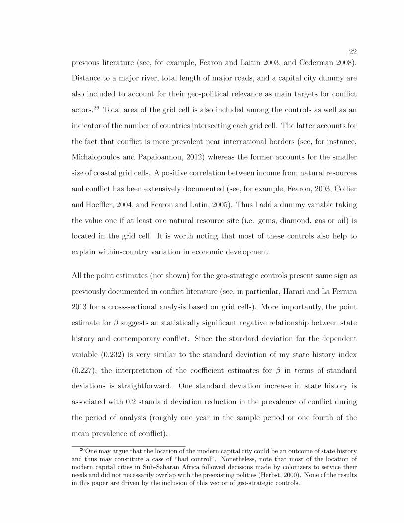
previous literature (see, for example, Fearon and Laitin 2003, and Cederman 2008).

Distance to a major river, total length of major roads, and a capital city dummy are

also included to account for their geo-political relevance as main targets for conflict

actors.26 Total area of the grid cell is also included among the controls as well as an

indicator of the number of countries intersecting each grid cell. The latter accounts for

the fact that conflict is more prevalent near international borders (see, for instance,

Michalopoulos and Papaioannou, 2012) whereas the former accounts for the smaller

size of coastal grid cells. A positive correlation between income from natural resources

and conflict has been extensively documented (see, for example, Fearon, 2003, Collier

and Hoe✏er, 2004, and Fearon and Latin, 2005). Thus I add a dummy variable taking

the value one if at least one natural resource site (i.e: gems, diamond, gas or oil) is

located in the grid cell. It is worth noting that most of these controls also help to

explain within-country variation in economic development.

All the point estimates (not shown) for the geo-strategic controls present same sign as

previously documented in conflict literature (see, in particular, Harari and La Ferrara

2013 for a cross-sectional analysis based on grid cells). More importantly, the point

estimate for � suggests an statistically significant negative relationship between state

history and contemporary conflict. Since the standard deviation for the dependent

variable (0.232) is very similar to the standard deviation of my state history index

(0.227), the interpretation of the coe�cient estimates for � in terms of standard

deviations is straightforward. One standard deviation increase in state history is

associated with 0.2 standard deviation reduction in the prevalence of conflict during

the period of analysis (roughly one year in the sample period or one fourth of the

mean prevalence of conflict).

26One may argue that the location of the modern capital city could be an outcome of state historyand thus may constitute a case of “bad control”. Nonetheless, note that most of the location ofmodern capital cities in Sub-Saharan Africa followed decisions made by colonizers to service theirneeds and did not necessarily overlap with the preexisting polities (Herbst, 2000). None of the resultsin this paper are driven by the inclusion of this vector of geo-strategic controls.

23

I now consider the potential e↵ects of land endowment and the disease environment.

Early state development has been influenced by the geographic, climatic, demographic

and disease environment (Diamond 1997, Reid 2012, and Alsan 2013). I first include,

in column 3, a measure of soil suitability to grow cereal crops which not only posi-

tively correlates with early statehood but also it correlates with modern population

density, an important driver of conflict.27 Then, in column 4, I introduce two mea-

sures accounting for the ecology of malaria (from Conley, McCord, and Sachs 2010)

and the suitability for the tsetse fly. The former weakly correlate with my index of

state history whereas the latter is strongly negatively correlated with it. In addition,

Cervellati, Sunde, and Valmori (2012) find that persistent exposure to diseases a↵ects

the likelihood of conflict by a↵ecting the opportunity cost of engaging in violence. In

column 5 I include together the two set of controls. The point estimate for � remains

unaltered.

Potential confounding e↵ects of genetic and ecological diversity. In Table 3 I explore

whether the main correlation of interest documented so far may partially account

for the e↵ect of genetic diversity on conflict. Ashraf and Galor (2013a, 2013b) argue

that genetic diversity had a long-lasting e↵ect on the pattern of economic development

and ethnolinguistic heterogeneity (including fractionalization among other measures).

Even more importantly, Arbatli, Ashraf, and Galor (2013) show that genetic diversity

strongly correlates with several measures of social conflict. Unfortunately, no data

on genetic diversity at the grid cell level exists. To tackle this problem, I use the

fact that migratory distance from the location of human origin (i.e: Addis Adaba

in Ethiopia) is a strong linear predictor of the degree of genetic diversity in the

populations (Ramachandran et al. 2005, Liu et al. 2006, and Ashraf and Galor

27Data on soil suitability for growing cereal comes from the Food and Agriculture Organization(FAO)’s Global Agro-Ecological Zones (GAEZ) database. The suitability of the soil is calculatedbased on the physical environment (soil moisture conditions, radiation, and temperature) relevant foreach crop under rain-fed conditions and low use of inputs. The suitability measure ranges between0 (not suitable) to 1 (very suitable).

24

2013a).28 Results in column 1 shows that migratory distance to Addis Adaba enters

with the expected sign suggesting that genetic diversity has a positive impact on

conflict.29 Nevertheless, the point estimate for � is a↵ected remarkably little (albeit

it slightly decreases in size).

Fenske (2012) shows that ecological diversity is strongly related to the presence of

pre-colonial states in Sub-Saharan Africa. Diversity in ecology correlates with poten-

tial drivers of conflict such as linguistic or cultural diversity (Michalopoulos 2012, and

Moore et al, 2002) and population density (Fenske 2012, Osafo-Kwaako and Robin-

son 2013). In addition, herders cope with climate limitations by moving between

ecological zones which potentially leads to land-related conflicts with farmers (a well-

documented phenomenon in conflict literature, in particular for the Sahel region -see

Benjaminsen et al 2012). To account for this potential bias, I follow Fenske (2012)

and measure ecological diversity as a Herfindahl index constructed from the shares of

each grid’s area that is occupied by each ecological type on White’s (1983) vegetation

map of Africa.30 Point estimates in column 2 of Table 3 show that ecological diversity

presents indeed a statistically significant and positive correlation with contemporary

conflict. The negative association between state history and conflict remains statis-

tically strong. Further, I obtain a similar point estimate when controlling for both

ecological and genetic diversity in column 3. Figure 1.4 depicts the scatter plot and

partial regression line for the statistical relationship between contemporary conflict

and state history from the last specification in Table 3 (labels corresponds to the

28Migratory distance from each grid cell’s centroid to Addis Adaba is constructed based on Ozak(2012a, 2012b), who calculated the walking time cost (in weeks) of crossing every square kilometer onland. The algorithm implemented takes into account topographic, climatic, and terrain conditions,as well as human biological abilities (Ozak 2012a).

29Controlling for distance and its square (to account for the fact that genetic diversity has beenshown to have a hump-shaped relationship with economics development) does not a↵ect the results.

30They are 18 major ecological types in White’s (1983) map: altimontaine, anthropic, azonal,bushland and thicket, bushland and thicket mosaic, cape shrubland, desert, edaphic grassland mo-saic, forest, forest transition and mosaic, grassland, grassy shrubland, secondary wooded grassland,semi-desert, transitional scrubland, water, woodland, woodland mosaics, and transitions. See ap-pendix.

25

country ISO codes).

Figure 1.4: Conflict and State History

Robustness Checks

Considering potential “bad controls” and potential mediating channels. There are

certainly others contemporaneous and historical confounding factors for my analy-

sis. I next show how the point estimate for my variable of interest is a↵ected by

the inclusion of additional controls which can be arguably considered outcomes of a

long-run exposure to centralized polities. While not conclusive, changes in my main

point estimate when including these controls may be suggestive of the existence of

mediating channels through which state history impacts modern conflict. I focus on

pre-colonial economic prosperity, population density, ethnic fractionalization, slave

trade prevalence, proximity to historical trade routes and historical conflict sites, and

26

contemporary development (proxied by light density at nights obtained from satellite

images). I start with pre-colonial ethnic controls accounting for historical levels of

prosperity and economic sophistication.31 I focus on two sets of ethnicity level vari-

ables. First, I consider the subsistence income shares derived from hunting, fishing,

animal husbandry, and agriculture (variables v2 to v5 from Ethnographic Atlas).32

Second, I consider a variable describing the pattern of settlement. This variable (v30

from Ethnographic Atlas) is coded in order of increasing settlement sophistication

taking values from 1 (nomadic) to 8 (complex settlement). Overall, my point esti-

mate for � does not change (albeit its precision is improved) with the addition of

these controls in column 1.

Next I analyze the confounding e↵ect of population density.33 Unfortunately no de-

tailed historical data on population density exists at my level of analysis to the best

of knowledge. I only observe population density in 1960 instead and, to the extend

that population density may have a persistent e↵ect over time, I use it to proxy for

within-country variation of population density in pre-colonial times.34 Further, using

population figures from 1960 alleviates concerns of reverse causality from contempo-

31I construct pre-colonial ethnographic measures at the grid cell level based on information fromthe Ethnographic Atlas (Murdock, 1967) and the spatial distribution of ethnic groups from Mur-dock’s (1959) map. All these measures are 1960 population-weighted averages of traits of ethnicgroups whose historical homelands intersect a given grid cell. I basically follow the procedure de-scribed in Alesina, Giuliano, and Nunn (2013). See appendix for details.

32 I omit the category share of income from gathering activities to avoid multicollinearity.33Population density is positively correlated with the prevalence of conflict (see, among others,

Buhaug and Rød, 2006; Raleigh and Hegre, 2009, and Sundberg and Melander, 2013). It has beenargued that low population density was one of the main obstacles for state formation in the pre-colonial Sub-Saharan Africa (see, among others, Bates 1983, Diamond 1997, and Herbst 2000). Thishypothesis is, however, contested in a recent work by Philip Osafo-Kwaako and James Robinson(2013). On the other hand, high population density in the past may have also negatively a↵ectedethnic diversity by reducing isolation (Ahlerup and Olsson, 2012).

34The use of this proxy can help to illustrate the importance of the bias when including a badcontrol. Consider for simplicity that conflict (C) is only related to state history (S) and historicalpopulation density (P ), then the true model I would like to estimate is: Ci = �0 + �1Si + �2Pi + ui

. However, I only have data on population density in 1960 (P 1960 ) which is a function of bothS and P : P 1960 = �0 + �1Si + �2Pi + ✏i . When regressing C on S and P1960, I am estimating

Ci =h�0 � �2

�0

�1

i+h�1 � �2

�2

�1

iSi+

�2

�1P 1960i +

⇣ui � �2

✏i�1

⌘. Since it is apparent that �2 > 0, �2 > 0,

and �1 > 0, the inclusion of population density in 1960 would overestimate the negative impact ofstate history on conflict.

27

rary conflict to population distributions. The point estimates for � increases almost

10% and remains strongly statistically significance. I next construct an ethnic frac-

tionalization variable based on the index introduced in Alesina et al (2003).35 For

similar aforementioned reasons I compute a fractionalization index based on grid pop-

ulation in 1960.36 The point estimates for � remains unaltered when including ethnic

fractionalization as control.37 I next consider slave trade.38 I construct population-

weighted averages of slave trade prevalence at the grid cell level using Nathan Nunn’s

data. The expected correlation between slave trade prevalence and state history is

ex ante ambiguous.39 Results in column 4 show that the introduction of slave trade

prevalence as a determinant of contemporary conflict does not a↵ect the estimation

of �. The inclusion of shortest distance to historical trade routes in column 5 does

not a↵ect the results. I next add the distance to the closest historical battle during

the period 1400-1700 CE. This variable is constructed upon information recorded

and georeferenced by Besley and Reynal-Querol (2012) who find a robust correlation

35Ethnic fractionalization denotes the probability that two individuals randomly selected froma grid cell will be from di↵erent ethnic groups. In order to be consistent throughout this papermy definition of ethnic group is based on Murdock (1959). Therefore, I construct shares of ethnicpopulation using gridded population and the spatial distribution of ethnic groups in Murdock’s map.See appendix for details.

36Ethnic heterogeneity is a commonly stressed determinant of conflict (see, among others, Easterlyand Levine 1997 and Collier, 1998) and it is likely to be correlated with state history ( see Bockstetteet al, 2002; and Ahlerup and Olsson, 2012).

37I obtain almost identical results (not shown) if I use ethnolinguistic fractionalization (i.e: usingethnologue to compute linguistic distances between pair of ehtnic groups within a grid) instead ofehtnic fractionalization.

38Why would slave trade be important for contemporary conflict? First, Nunn (2008) finds thatslave trade resulted in long-run underdevelopment within Africa. More importantly, historical slavetrade has been shown to have an e↵ect on ethnic fragmentation (Whatley and Gillezeau, 2011b) andindividual’s mistrust (Nunn and Wantchekon, 2011), which are both arguably potential drivers ofsocial conflict.

39On the one hand, Nunn (2008) suggests that slave trade could have been an impediment forpre-colonial state development in Africa. In the same direction, Whatley and Gillezeau (2011a)argues that increasing international demand for slaves might have reduced the incentive to statecreation (relative to slave raiding) by driving the marginal value of people as slaves above theirmarginal value as tax payers. On the other hand, there exist several historical accounts linking therise of some African kingdoms to the slave trade (see, for example, Law 1977 for the case of the OyoEmpire, and Reid 2012). For instance, while analyzing the role of warfare, slavery and slave-taking inYoruba state-building, Ejiogu (2011) documents slave-taking campaigns of Oyo against neighboringNupe (note that Oyo -part of Yoruba - and Nupe share territories within grid cells).

28

between proximity to the location of historical battles and contemporary conflict.40

Results in column 6 are in line with Besley and Reynal-Querol’s (2012) main find-

ing. As expected, the point estimate of my variable of interest slightly increases and

remains statistically significant. One-standard deviation increase in state history is

statistically related to a reduction of the prevalence of conflict of 1/4 of its standard

deviation. Neither the inclusion of (ln of) light density, as measured in Michalopoulos

and Papaioannou (2013), or the inclusion of the previous variables all together a↵ect

the statistical significance of my main finding. Therefore, if anything, the inclusion of

these potential confounders makes the negative statistical association between state

history and contemporary conflict stronger.

Robustness to the choice of conflict measure (dataset, incidence, onset, and intensity).

I next show that the main results are robust to the election of the georeferenced

conflict dataset and the way conflict is coded. For column 1 of Table 5, I construct

the conflict measure using ACLED. Therefore, the dependent variable accounts for

the fraction of years with at least one broadly defined conflict event in ACLED. In

column 2 I only consider battle events recorded in ACLED. For column 3 I consider

any violent event (i.e: battles and violence against civilians). In column 4 I focus

on riots. For all the conflict indicators but riots I find the same pattern: a strong

negative statistical relationship between conflict and state history (for the case of

conflict the p-value for � is slighty above 0.1).

In column 5 I focus on a measure of conflict intensity. The dependent variable is the

(log of) number of casualties due to conflict (best estimate in UCDP-GED). The point

estimate for � rea�rms the hypothesized negative e↵ect of state history on conflict.

40They also show that proximity to historical conflict site correlates with mistrust, stronger ethnicidentity, and weaker sense of national identity. Provided this documented long-lasting e↵ect andconsidering that violent conflict between and within historical African states was part of the state-building processes in the past (see, among others, Lewis, 1966; Ben-Amos Girshick and Thornton,2001; Ejiogu 2011; Reid 2012 and Bates 2013), the omission of this control would underestimate thee↵ect of state history on contemporary conflict.

29

My conflict measure under the baseline specification represents the prevalence of

conflict violence. It does not make distinction between onset and incidence of violence.

That is, this measure does not distinguish a violent event that represents the onset

of a new conflict within a dyad from an event that is the continuation of previous

confrontations. In column 6 I consider a measure of prevalence of conflict onset (i.e:

first confrontation within a dyad). I identify all conflict onsets in the period of analysis

and code 1 a grid cell - year observation if at least one onset occurs. As a result, my

conflict measure in column 6 represents the fraction of years with at least one conflict

onset in the grid cell. Only 149 grid cells experienced at least one conflict onset (out

of 417 di↵erent conflicts in the period 1989-2010). The point estimate suggests that

the onset of conflict is strongly and negatively related to long history of statehood.

Heterogeneity across regions. I next explore whether the uncovered relationship be-

tween state history and contemporary conflict holds within Sub-Saharan Africa re-

gions. I estimate the specification in column 3 of Table 3 for two regions, namely

West-Central Africa and East-South Africa.41 Results in column 1 and 2 of Table 6

are in line with previous results. In column 3 I exclude Western Africa to show that

this particular region is not driving the main results.

Excluding countries and influential observations. I sequentially estimate the specifi-

cation in column 3 of Table 3 by excluding one country at a time. Figure 1.5 depicts

thirty seven di↵erent point estimates with their associated t-statistics; the excluded

country is labeled in the x-axis. All the coe�cients fall in the interval [-0.15, -0.22].

All coe�cients but the one for the specification excluding Sudan are statistically sig-

nificant at the 1 percent level (for the case of Sudan, the p-value is 0.013). There are

two reasons for the somehow relative weaker result when excluding Sudan: (1) sample

41I follow UN to classify each country in one of the 5 UN regions (North, South, East, West, andCentral). Only one country belongs to North (Sudan) and it is assigned to East. I group the originalregions in only 2 regions to balance the number of observations in each sample.

30

size drops by 10 percent increasing the standard errors (The statistical significances

and standard errors of other covariates are also a↵ected -results not shown-), and (2)

Sudan presents some locations with very high values of the state history index; loca-

tions for which my state history may be underestimating their true long-run exposure

to statehood.42 Excluding those locations reduce the upward bias in the OLS esti-

mate due to the measurement error from bounding the period of analysis above the

year 1000 CE.43 The same pattern arises when excluding another country with long

history of states before 1000 CE (i.e: Ethiopia). Finally, the strong negative statisti-

cal association between state history and conflict persists when excluding influential

observations. In this vein, I follow the standard practice of estimating � when ex-

cluding all the observations for which | DFBETAi |> 2/pN where N is the number

of observations and DFBETAi is the di↵erence between the estimate of � when the

observation i is excluded and included (scaled by standard error calculated when this

observation is excluded). The point estimate is -0.16 (statistically significant at the

1 percent level -results not shown-).

On the discount factor and long-run exposure. I next explore how my OLS estimates

are a↵ected by the election of di↵erent discount factors to compute the state history

index. I report in columns 1 to 4 of Table 7 results for four di↵erent specifications

with discount rates of 5, 10, 25, and 50 percent. For the sake of comparison, I report

both the point estimates and the beta standardized coe�cients. All the specifica-

tions include the full set of controls as in Table 3. Only when a discount rate of

50 percent is applied, my coe�cient of interest is slightly statistically insignificant

under the conventional levels of confidence. Two facts are worths to note. First, the

42The Nubian Kingdoms (northern Sudan) were founded several centuries before 1000 CE.43I estimated additional specifications in which I excluded all the observations with some exposure

to states during the period 1000-1100 CE. Consistently with the existence of measurement error frombounding the analysis above 1000 CE introducing an upward bias, the beta standardized coe�cientslightly decreased about 10 percent (albeit they remained strongly statistically significant -resultsnot shown-) when I excluded those observations.

31

Figure 1.5: Sensitivity of Estimates to Exclusion of Countries

higher the discount rate, the lower the statistical significance of the coe�cient for

the corresponding state history measure. Second, the beta standardized coe�cient is

also decreasing on the discount rate suggesting indeed that history has an influence

on conflict. For instance, the beta standardized coe�cient when the discount rate is

0 (i.e., -0.20, not show in Table 7) is more than 50 percent larger that for the case

in which the discount rate is 25 percent. For columns 5, 6, and 7 I break my period

of analysis in two sub-periods, namely before and after 1500 CE when external influ-

ence became more relevant for Africa due to the prevalence of slave trade and early

european colonialism. In columns 5 I only consider the accumulation of state expo-

sure from 1500 CE to 1850 CE. Albeit statistically and economically weaker, there is

still a negative statistical association between state history and modern conflict. In

columns 6 I only consider the period 1000 -1500 CE and the coe�cient of interest is

strongly significant and of the similar magnitude when compared with the estimation

from the specification using my original measure of state history. When including

32

both measures only the one considering the accumulation from 1000 CE to 1500 CE

is strongly statistically and economically significant. This result suggests that the

state history that matters the most is the one accumulated before 1500 CE.

Intensive versus extensive margin. To argue that what matter the most is the inten-

sive margin of exposure to state institutions (long history) rather than the extensive

margin (any state vs. no state at all right before the Scramble for Africa), I estimate

a new specification in column 1 of Table 8 for which the state history variable is the

state history score the last period considered in the computation of my index (i.e.,

1800 - 1850 CE). The coe�cient estimate, albeit negative, is statistically insignifi-

cant. Further, I construct a 1960 population-weighted average of the degree of ethnic

centralization in the grid cell using the Ethnographic Atlas’s variable “Juridisctional

Hierarchy beyond the Local Community” which ranges from 1 (no juridisction above

village level) to 4 (large state). This variable has been used to document the impor-

tance of political centralization for current pattern of development (Gennaioli and

Rainer 2007a, and Michalopoulos and Papaioannou 2013). Result in column 2 shows

that the correlation between late pre-colonial ethnic centralization and the prevalence

of modern conflict is not statistically significant. This result is quantitatively very

similar to the point estimates in column 1. One can still argue that it is not the

long history of state but its complete absence what explains the uncovered statistical

association. In this sense, it may be the case that locations with no history of state

whatsoever are located in remote and unpopulated regions with little national state

penetration where rebel groups can easily operate. In the specification of column 3 I

exclude all the observations with no history of state whatsoever (223 grid cells) and

show that my main results are not driven by those locations. The point estimate is

very similar and strongly statistically significant. If I restrict the sample even more

and consider only locations with at least 100 years of state history (Thus, I exclude

329 grid cells) I obtain even stronger results (column 4).

33

Assessing the extent of bias from unobservables. The point estimates reported so far

may still be biased due to unobservable factors correlated with both contemporaneous

conflict and long-run exposure to states. How large would this selection on unobserv-

ables need to be (relative to selection on observables) to attribute the entire OLS

estimates previously reported to a unobservable selection e↵ect? I follow the intuitive

heuristic in Nunn and Wantchekon (2011) based on Altonji, Elder, and Taber (2005)

to assess the degree of omitted variables bias by studying stability of the estimates for

�. The underlying idea is that, under the assumption that selection on observables

is proportional to selection on unobservables, a coe�cient not changing much as one

adds controls would be suggesting that there is little remaining bias. I thus compare

the point estimate in the last specification in Table 3 which includes a full set of

controls (�1 = �.198) with the point estimate when only a basic set of controls (i.e.,

country fixed e↵ect and geographical controls) is included (�2 = �.191). The ratio

between �1 and �1� �2 (the selection on observables) suggests that selection on unob-

servables would have to be more than 20 times the selection on observables to explain

away the entire statistically relationship between state history and contemporaneous

conflict.

Instrumental Variable Approach

I have already documented a strong negative statistical relationship between history

of statehood and contemporary conflict at the sub-national level. This historical

link is robust to a battery of within modern countries controls ranging from con-

temporaneous conflict correlates, geographic factors, to historical and deeply rooted

determinants of social conflict. Unfortunately, history is not a random process. Even

in a close to ideal and hypothetical quasi-random historical event determining the

geographic assignment of long-run exposure to state capacities within Sub-Saharan

34

Africa, the challenge of isolating the causal e↵ect of state history on contemporary

conflict is particularly di�cult. Although one could argue that reverse causality from

conflict to historical exposure to state-like institutions is not a source of concern for

the identification of my parameter of interest, there may still be omitted variables

correlated with both state history and contemporary conflict which may be driving

the uncovered statistical association. I aim, however, to convince the reader here that

hard-to-account-for factors manifested in di↵erences in long-run exposure to central-

ized institutions matter crucially to understand contemporary patterns of conflict

within Sub-Saharan Africa. In addition to a potential omitted variable bias, mea-

surement error may also a↵ect my point estimates in an ex-ante ambiguous direction

depending on the true structure of the relevant measurement error. It is precisely for

the sake of alleviating the potential bias from measurement error in my state history

index what primarily motivates the introduction of an instrumental variable strategy.

I follow two strategies. First, I exploit variation across locations on the timing elapsed

since the neolithic revolution. Second, I construct an alternative measure to account

for the degree of influence from politically centralized states by exploiting variation

in the proximity to historical cities for the time period 1000 - 1800 CE.

Time Elapsed since Neolithic Revolution

Several studies have established a link between the neolithic revolution and the rise

of complex political organization. For instance, Diamond (1997) argues that the

transition from hunter-gathered societies to settled agricultural communities is an

essential factor to explain the rise of proto-states, and subsequently the formation

of states. Agriculture allowed nomadic societies to settle, generate food surpluses,

and shorten birth intervals (Ashraf and Michalopoulos 2010; Diamond 1997), which

in turn resulted in denser populations. Further, the storage of those food surpluses

35

allowed the emergence of non-food-producing sectors, hence economic specialization

and also social stratification manifested not only in the existence of a labor force

involved in the production process (both, foods and non-foods production) but also a

labor force designated to provide public services (including armies). By implication,

the possibility of taxation and the emergence of political organization, facilitates the

rise of states.

A strong positive correlation between the timing elapsed since the neolithic revolution

and Bockstette, Chanda, and Putterman (2002)’s state antiquity index has been em-

pirically documented at the country level (see, for instance, Hariri 2012, and Petersen

and Skaaning, 2010). Further, substantial variation in the timing of the transition to

agriculture exists within the Sub-Saharan Africa. I therefore exploit Neolithic arche-

ological sites information to construct the time elapsed since neolithic revolution at

a finer geographical level and use this to instrument for my state antiquity index at

the sub-national level. I discuss the construction of the instrument in the appendix.

Figure 1.6 depicts the geographical distribution of the time elapsed since the neolithic

revolution.

Table 9 presents point estimates for di↵erent specifications of the first-stage. All the

specifications include the set of controls from my prefered specification in Table 3

(column 3). I report 3 di↵erent standard errors (i.e: clustered at the country level

and adjusted for spatial autocorrelation for cut-o↵ distances of 5 and 10 degrees).

Again, clustering at the country level appears to be the most conservative approach.

Point estimate in column 1 suggests a statistically significant association between the

time elapased since the neolithic revolution and my state history index. However,

this association is only statistically significant at the 3 percent level due to a weaker

association within the Central Africa region. Indeed, my constructed measure of

the timing since the first adoption of agriculture is statistically insignificant within

36

Figure 1.6: Time Elapsed Since Neolithic Revolution

that region (column 2). In particular, observations from four countries explain this

weaker statistical performance: Gabon, Congo, Congo DR, and Angola. It is well

stablished that a group of Bantu people migrated south from modern-day Cameroon

to modern-day Namibia across the rainforest. Although this Bantu migration route

crossed the territory of modern-day Gabon, Congo, Congo DR, and Angola, no ar-

chaelogical information has been recorded on agricutural adoption (Putterman, 2006).

Therefore the interpolated values for most of the observation from these four coun-

tries mostly depend on archaelogical evidence from two sites in Cameroon and the

Namibia-Botswana border. When I exclude these countries from my sample, the first-

stage is much stronger (column 3). An alternative way to statistically improve the

performance of the first-stage is to consider the square of the instrument rather than

its level. Indeed, the statistical association between the square of my instrument and

my index of state history is stronger (column 4). To avoid reducing my sample size

by 20 percent due to the exclusion of these countries for which the linear relationship

is weaker, I use the square of the time elapsed since the neolithic revolution as an

37

instrument for state history. I provide below evidence that the results are not driven

by this particular specification.

In Table 10 I report IV results. The specification in column 1 includes the set of con-

trols from specification in column 3 of Table 3. The point estimate is roughly 3 times

larger that the previously reported OLS estimates; finding that is consistent with the

idea that measurement error in my state history variable was indeed introducing a

sizeable bias toward zero (albeit it is also consistent with my instrument picking up

the e↵ect of other confounding factors, issue I discuss below). The point estimate for

� in column 1 suggests that one-standard deviation increase in state history implies

a .71-standard deviation reduction in the prevalence of contemporary conflict. This

magnitude is equivalent to roughly 4 years of conflict in my period of analysis. My

IV estimate may be still biased due to the omission of variables that could plausibly

correlate with both contemporary conflict and the timing of the transition to agri-

culture. Therefore, I now focus on biogeographical variables which had been shown

to correlate with my instrument. In column 2 I add absolute latitude. As Diamond

(1997) argues, technologies and institutions have historically spread more easily at

similar latitudes where climate and day duration were not drastically di↵erent. This

is particularly true for the spread of agriculture within Africa. Regardless of the dis-

cussion of the ultimate underlying mechanisms, the high correlation between absolute

latitude and development has been widely documented in the economic growth and

development literature (see, for example, Spoloare and Wacziarg, 2013). Absolute

latitude enters negatively and statistically significant in this specification; reducing

15 percent the size of � which remains strongly statistically significant.

Haber (2012) argue that variation in biological (and technological) characteristics of

crops had a long-run e↵ect on institution and development. In addition, Sub-Saharan

centralized military states were historically more prevalent in areas with soils suitable

38

for the generation of agriculture surpluses to maintain armies (Reid 2012). Given their

ease of storage and transport, cereals had a natural advantage over other crops, such

as tubers and tree crops, to produce those necessary surpluses.44 For the particular

case of Sub-Saharan Africa, the most important indigenous crop for this matter are

sorghum and millet. Further, it was precisely the domestication of sorghum and millet

what played a crucial role in the transition to the Neolithic in this region. Hence, in

column 3 I hold constant biogeographical factors a↵ecting these crops by adding the

principal component of the soil suitability to grow millet and sorghum.45 The point

estimate for � remain statistically significant and economically sizeable (the size of

coe�cient varies little with respect to the baseline specification in column 1).

I next consider the potential confounding e↵ect of climate variability. Ashraf and

Michalopoulos (2013) show that historical climatic volatility has a non-monotonic ef-

fect on the timing of the adoption of agriculture. On the other hand, Durante (2009)

show that, within Europe, variation in social trust is driven by historical variation

in climate. When I include intertemporal temperature volatility, its square, and his-

torical mean temperature, the size of my point estimates decreases by 30 percent

(albeit it remains statistically significant).46 This fact is consistent with the possi-

bility that my hypothesized mitigation e↵ect of a location history on contemporary

conflict may partially confound with higher levels of social trust induced by historical

climate variability. The addition of the set of pre-colonial ethnic characteristics in

column 5 reduces the point estimates by almost 20 percent (albeit it remains strongly

statistically significant). This result represents suggestive evidence that pre-colonial

44The tubers and tree crops have relative low levels of storability (compared with cereals) sincethey typically perish within days or weeks of harvesting.

45Data on soil suitability for growing millet and sorghum comes from the Food and AgricultureOrganization (FAO)’s Global Agro-Ecological Zones (GAEZ) database.

46I use variation in modern data to proxy historical climatic variation. Ashraf and Michalopoulos(2013) show that spatial variation in temperature volatility remains largely stable over long periodsof time; thus contemporary climate data can be meaningfully employed as informative proxies forprehistoric ones.

39

di↵erences in economic prosperity (proxied by the degree of the sophistication of

settlement patterns and the type of economic activities) may represent a mediating

channel through which long history of statehood of a given location may result in

lower levels of modern conflict. In column 6 I include all the aforementioned controls

together. Even under this challenging horse race the point estimates for � remains

negative and statistically significant at the 5 percent level. The IV point estimates

doubles my prefered specification in the OLS case. The Kleibergen-Paap rk Wald F

statistic is above the rule of thumb thus weak instruments would not be a concern. In

the last column of Table 10 I exclude the four Central African countries for which the

linear relationship between the neolithinc instrument and my state history index was

statistically weak and show that instrumenting state history with the time elapsed

since the neolithic revolution in levels lead to very similar point estimates compared

to the case with the squared instrument in the full sample.

A note about hypothesized e↵ects of the neolithic revolution on contemporary out-

comes. The onset of the neolithic revolution was certainly one of the most important

historical events for humankind. The economic literature has provided mixing evi-

dence regarding the existence of a direct association between this historical event and

contemporaneous outcomes. Some works have emphasized the long-lasting e↵ect of

the neolithic revolution on pre-industrial era’s outcomes (see, among others, Ashraf

and Galor 2011). Other works have shown that countries which experienced early

transition to agriculture tend to have higher level of per capita income today (par-

ticularly after “ancestry adjustment”, see Spoloare and Wacziarg, 2013). This line

of argument emphasizes that the neolithic revolution may be responsable for cross-

sectional di↵erences in human capital and technologies in the pre-industrial era and,

to the extent that those di↵erences may be persistent, may still have an e↵ect on

current outcomes. In fact, the reduction on the size of my IV point estimates when

including pre-colonial prosperity measures is consistent with this view although it

40

does not explain away the statistical association of interest. In addition, the inclu-

sion of light density at nights to proxy for contemporary levels of development does

not a↵ect my point estimates (results not shown). Using individual-level data and

exploiting variation in my instrument for about 1,600 districts, I do not find evidence

that my instrument significantly correlates with education levels (results not shown).

On the other hand, a line of research argues that neolithic still exert a negative e↵ect

on contemporary outcomes. In particular, Olsson and Paik (2013) argue that an early

transition to agriculture might have directly shaped institutional trajectories by pro-

moting autocracy (similar argument is presented in Hariri, 2012) and thus facilitating

extractive institutions which turn in lower levels of development. In addition, Paik

(2011) shows that, within Europe, early adoption of agriculture positively correlates

with strong preference for obedience. This line of argument is based on the idea

that precisely the experience with early political organization is the mediating chan-

nel through which the neolithic revolution a↵ects contemporary outcomes. Bearing

in mind that measuring culture traits is a di�cult task, I later show that the time

elapsed since the neolithic revolution can be linked to trust in state institutions.

In sum, although I cannot rule out the possibility that other hard-to-account factors

may be driven the uncovered statisticaly association, IV estimates exploiting informa-

tion on the timing elapsed since the neolithic revolution provides additional evidence

consistent with my hypothesized negative e↵ect of long-run exposure to statehood

on modern pattern of conflict. This negative statistical association estimated from

variation in the timing since the earliest date of domestication of plants is not driven

by biogeographical factors such as land quality to grow cereals (cereals in general

or sorghum and millet in particular), proximity to water (rivers and oceans), ele-

vation, intertemporal climate variability, di↵erences in disease environment (malaria

and tse-tse), ecological and genetic diversity or absolute distance to the equator. I

41

find evidence that pre-colonial di↵erences in prosperity may constitute a mediating

channel underlying my reduced-form relationship.

Proximity to Historical Cities

I construct an independent imperfect measure of state history by exploiting informa-

tion on the location and evolution of above sixty large African cities (of which thirty

five were located in Sub-Saharan Africa) during the period 1000 - 1800 CE.47 To the

extent that kingdoms and empires tended to have a large city as political center, I

consider proximity to a large city as an indicator of the degree of influence from a

centralized power. I introduce this new measure for several reasons. First, to show

that the negative statistical association uncovered in the OLS case still hold when

using an alternative measure. Second, this new measure will overcome a potential

caveat in my original measure of state history which assumes an homegeneous e↵ect

of centralization within the boundaries of a historical polity. This assumption had

two implications: (1) the introduction of a sharp discontinuity at the border of the

boundary, and (2) inconsistency with the idea that broadcasting power strenght may

depend on the distance from the political center. Third, this new measure can be

used to instrument the original state history measure and mitigates the attenuation

bias from measurement error.

Construction. This measure exploits time-varying proximity to large cities. There-

fore, some cities exert influence to their periphery only for particular time intervals.

For instance, Djenne, in modern Mali, only enters in my panel of cities for the period

1300 - 1600 CE (See Table A.3 in appendix for the list of georeferenced cities). For

each hundred years period I calculate the shortest distance to closest city from the

47I define a city to be large if it has more than ten thousand inhabitants. The list of cities comesfrom Chandler (1987) and Eggiman (2000).

42

centroid of each grid cell. I then calculate within-grid average of the distances for

the whole period of analysis and map them into a 0 to 1 interval so the grid cell

with the minimum average distance takes the value 1. Figure 1.7 displays the cross-

sectional variation of this alternative measure.48 As in the case of my original State

History Index, this new measure presents higher values in western part of the Sahel,

the highlands of Ethiopia, and the region along the Nile river.

Figure 1.7: Alternative Measure Using Historical Cities

In column 1 of Table 11 I present the OLS estimate for the reduced-form conflict

and historical proximity to cities. I find the same the pattern as before. Historical

proximity to cities for the time period 1000 - 1800 CE is negatively and strongly

statistically associated to prevalence of modern conflict. In column 2 I present the

IV estimate for my state history index when using historical proximity to cities as

a instrument. I find results which are similar to the IV case using the time elapsed

48By construction, due to its dependance on distances, this measure presents a more continuoussupport.

43

since the neolithic as an instrument. The point estimate is slighlty larger; fact that

is consistent with the possibility that historical proximity to cities is picking up the

e↵ect of other omitted variables on conflict. Finally, in column 3 I include both

instruments and find similar results. With this overidentified model at hands I test

the exogeneity of the instruments. The Hansen J statistics suggests no rejection of

the null hypothesis that my set of instruments are exogenous. Note that all the

specifications where including not only the set of controls from Table 3 but also

account for the joint e↵ects of absolute latitude, suitability to grow sorghum and

millet, intertemporal climate variability

1.4.3 Panel Data Evidence: Weather Induced-Agricultural

Productivity Shock, State History, and Conflict

In a comprehensive synthesis of the climate-conflict literature, Burke, Hsiang, and

Miguel (2013) argue that there is strong causal evidence linking climatic events to

conflict. The existence of an income mechanism underlying this causal link has been

proposed repeatedly times in the conflict literature but it has not been definitively

identified yet. Harari and La Ferrara (2013) present convincing evidence that what

drives the observed empirical relationship between weather shocks and conflict in

Africa is weather anomalies occurring within the growing season of the main local

crops. In addition, Schenkler and Lobell (2010) shows that crop yields are indeed

a↵ected by growing season precipitation and temperature. Moreover, Brown et al

(2011) argue that persistent drought conditions is the most significant climate influ-

ence on GDP per capita growth in Africa. Given the high dependance of Sub-Saharan

Africa economies on rainfed agriculture, these results provide strong evidence consis-

tent with the existence of an income mechanism. Therefore, I draw upon Harari

and La Ferrara (2013) to construct weather-induced agricultural shock by exploiting

44

information on spatial distribution of crops, planting and harvesting calendars, and

variability on water balance anomalies across space and time.49 I hypothesize that

locations with long history of statehood should be better equipped of mechanisms to

mitigate the negative e↵ects of weather shocks. To support my hypothesis, I exploit

panel data variation (over the time period 1989-2010) in the prevalence of conflict,

weather-induced productivity shocks, and the interaction of my state history index

with those shocks to estimate the following equation:

Conflicti,c,t = ↵ + �StateHistoryi + �Shocki,t + �StateHistoryi ⇥ Shocki,t

+G0

i�+X0

i�+ C0

iZ +W0

i,t⇧+ �c + µi + ⌫t + ✏i,c,t (1.4.2)

Where t indexes year. The variable Conflicti,c,t takes the value 1 if at least one

conflict event occurs in the grid cell i in year t, and 0 otherwise. The variables

StateHistoryi, G0i, X

0i , and C

0i are the same defined for equation (1). The vector

W0i,t includes year averages of monthly precipitation and temperature deviation from

historical monthly means to account for any independent e↵ect that these variables

may have on conflict outside of the growing season. The variable ⌫t denotes a year

fixed e↵ect whereas µi is a collection of grid cell fixed e↵ect which is included only in

some specifications (when included I cannot identify �, �,�, Z, and �c). The main

coe�cient of interest in this exercise is �. Standard errors are clustered at the grid

cell level.

In column 1 of Table 12 I present OLS estimates an specification of equation (2)

for which yearly weather variables and grid fixed e↵ect are not included. The point

estimates suggest: a) an statistically significant negative correlation between conflict

and state history, b) an statistically significant positive impact of negative weather

49I discuss the construction of the weather-induced agricultural shock in the appendix.

45

shocks on conflict, and c) a negative correlation between the interaction term of the

two aforementioned variables and conflict, which is consistent with my hypothesized

mitigating e↵ect of state history when a location is hit by a shock. In the following

columns I present IV estimates. Column 2 shows the results for the same specification

as in column 1. One-standard deviation increase in the shock measure statistically

relates with 5 percent increase in the likelihood of experiencing at least one conflict

event in a grid without history of state (The unconditional probability of having

conflict is 0.18). The estimated coe�cient for � suggests that for the grid with the

mean value of state history (i.e: 0.16), the negative impact of a weather shock on

conflict is quite smaller than for the case of no previous state history. That is, one-

standard deviation increase in the weather shock implies only 1.2 percent increase

in the likelihood of conflict. In column 3 I add grid cell fixed e↵ect, thus I can-

not identify �, E, �, �, and ⇤. The point estimate for the direct e↵ect of weather

shock on conflict remains almost unaltered whereas for the case of the interaction

term it is slightly smaller, albeit statistically significant and representing economi-

cally meaningful mitigation e↵ect of state history. The addition of yearly measures

of precipitation and temperature deviation in column 4 does not substantially a↵ect

the previous result. In the last specification in column 5, I include conflict prevalence

lagged one period to account for conflict dynamics. Indeed, results in column 5 show

that conflict in t� 1 strongly predicts conflict in t. Albeit slightly smaller in size, the

point estimates for the weather shock variable and its interaction with state history

remain both statistically significant.

Other interaction e↵ects. I next consider a set of di↵erent cross-sectional character-

istics that when interacted with weather shocks may partially account for the result

previously documented, namely that locations with relatively long history of state

are less prone to experience conflict when hit by a shock. This set of characteristics

includes light density at nights (proxy of regional development), soil suitability for

46

cultivating cereals, pre-colonial agricultural dependence, and historical temperature

volatility. All the specifications in Table 13 include both year and grid fixed e↵ects.

The first column serves as a comparison. The point estimates from columns 2 to 5

suggest that locations with higher light density at night, better cereal suitability, and

higher pre-colonial dependence on agriculture are more prone to experience conflict

when hit by a shock. On the contrary, locations with higher temperature volatility

are less prone to have conflict. The inclusion of these interaction terms separately or

jointly (in column 6) does not wash away the statistical significance of the negative

coe�cient for the interaction term state history and weather shock.

1.5 Identifying Potential Mechanisms at Work: State

History and Attitudes Towards State Institu-

tions

It has been stressed that the lack of state legitimacy represents an underlying cause

of the prevalence of civil conflict in Sub-Saharan Africa. It is argued that the lack

of legitimacy undermines the institutional capacity and authority of a state to rule

by consent rather than by coercion. Not surprisingly, Rotberg (2004) argues that

the lack of legitimacy causes, in fact, state fragility; a concept that it is partially

defined in terms of a society’s probability to face major conflicts.50 States with low

levels of legitimacy tend to devote more resources towards retaining power rather

than towards e↵ective governance, which undermines even more its popular support

and increases the likelihood of political turnover (Gilley, 2006). On the contrary,

citizens that consider a government to be legitimate are less likely to rebel. Does state

50For instance, a legitimacy score accounts for almost 50% of the State Fragility Index computedby the Center for Systemic Peace. Moreover, the operational definition of fragility in the index isassociated with state capacity to manage conflict.

47

history at the sub-national level shape individual’s perception of state legitimacy? I

argue that attitudes towards state institutions such as tax department, police force,

and court of laws provide an informative way to measure views of legitimacy of the

state. I thus show a strongly positive and robust correlation between individual’s

belief regarding the legitimacy of these key state institutions and state history. I

also present additional results suggesting the presence of a legacy of state history

on individuals’ trust in state institutions. Moreover, I present suggestive empirical

evidence that state history can be linked to modern support for traditional leaders.

Sources and Description of Individual-Level Data

In this section I exploit individual-level survey data to document the aforementioned

potential mechanisms at work. My analysis is based on the Round 4 of Afrobarom-

eter in 2008 and 2009 (Afrobarometer 4, from now on). The Afrobarometer 4 is a

collection of comparative series of nationally representative surveys for twenty coun-

tries in Sub-Saharan Africa: Benin, Botswana, Burkina Faso, Cape Verde, Ghana,

Kenya, Lesotho, Liberia, Madagascar, Malawi, Mali, Mozambique, Namibia, Nigeria,

Senegal, South Africa, Tanzania, Uganda, Zambia, and Zimbabwe. These countries

have undergone some degree of political and economic liberalization during the last

20 years (Logan, 2013). In addition, the Afrobarometer 4 sample does not include

countries under authoritarian regimes or civil wars (Afrobarometer, 2007). Nonethe-

less, all the countries in the Afrobarometer 4 sample but Benin, Burkina Faso, Cape

Verde, and Malawi experienced violent conflict events during the period 1989-2010.51

They also present high heterogeneity in key variables such as state history, historical

51The list of countries in Afrobarometer 4 with at least one conflict with more than 25 deathsduring the period 1989-2010 is (event counts in parenthesis): Botswana (1), Ghana (34), Kenya(307), Lesotho (5), Liberia (510), Madagascar (39), Mali (98), Mozambique (261), Namibia (21),Nigeria (319), Senegal (187), South Africa (2624), Tanzania (9), Uganda (1549), Zambia (10), andZimbabwe (45).

48

conflict, and other correlates of civil conflict.

The Afrobarometer 4 relies on personal interviews conducted in local languages where

the questions are standardized so responses can be compared across countries (Afro-

barometer, 2007). These questions asses, among other topics, individuals attitudes

toward democracy, markets, and civil society. In particular, I exploit information re-

garding individuals attitude toward state institutions and trust in politicians, public

servants, and other individuals in general. I also benefit from a module of ques-

tions on local traditional authority. As described in detail below, the information

in Afrobarometer 4 also allows me to construct controls at the level of village (i.e:

enumeration area) and district.

The original sample size in Afrobarometer 4 is over 26,000 respondents. Cape Verde

and Lesotho are not included in my analysis.52 In addition, districts that I was not

able to georeference, as well as individuals who could not be matched with ethnic

names in Murdock’s (1959) map were removed from the sample.53 The final sample

consists of 22,527 respondents from 1,625 districts and 221 di↵erent ethnic groups

under Murdock’s (1959) classification.54

State History and State Legitimacy

I construct a measure of individual’s attitude toward the legitimacy of state insti-

tutions based on the individual’s level of agreement with the following statements:

(1) the courts have the right to make decisions that people always have to abide by;

52I exclude Lesotho and Cape Verde from my analysis for several reasons. I exclude Cape Verdebecause it was not taken into account in the original computation of my state antiquity index, noquestion on traditional leaders were asked during the round 4 of Afrobarometer, and di�culties tomatch the ethnicities of the respondents with Murdock’s data. I exclude Lesotho due to di�cultiesto match ethnicities.

53My georeferencing work was built upon a previous work by Stelios Michalopoulos.54320 ethnicities are originally self-reported in my sample. Appendix includes the list of ethnicities

and their match with names in Murdock’s (1959) map

49

(2) the police always have the right to make people obey the law; and (3) the tax

department always has the right to make people pay taxes. The possible responses,

coded from 1 to 5, are: “strongly disagree”, “disagree”, “neither agree nor disagree

or don’t know”, “agree” and “strongly agree”. Thus, my measure of state legitimacy

is the first principal component of the responses to these questions about the legiti-

macy of the court decisions, police enforcement, and the tax department. I examine

the statistical relationship between state legitimacy and state history by estimating

di↵erent specifications of the following equation:

State Legitimacyi,e,a,d,c = ↵ + �StateHistoryd,c + I0i,e,a,d,c�+ A

0a,d,c�+D

0d,cE

+X0

d,cH + ⌘c + ✓e + ✏i,e,a,d,c (1.5.1)

where i, e, a , d, and c index individuals, ethnicity, enumeration area (village), dis-

trict, and country, respectively. The variable StateHistoryd,c represents the state

antiquity index for a bu↵er with a 1-degree radius (approximately 100 kilometers)

and centroid located at the coordinates of the district. The vector I0i,e,a,d,c denotes a

set of the respondent’s characteristics such as age, age squared, education level, living

conditions, unemployment status, and gender.55

The vector A0a,d,c denotes a set of enumeration area-level covariates including a rural

dummy and a subset of variables designed to capture the prevalence of public good

provision and proxy for the quality of local government.56 In a study for South Africa,

55 The education variable takes value from 0 (no formal schooling) to 10 (post-graduate). Theliving condition variable is a self assessment of the respondent and takes values from 1 (very bad) to5 (very good). Unemployment and gender are dummies variables taking value 1 if the respondent isunemployed and male, respectively. The Afrobarometer 4 does not include information on occupationof the respondent.

56I introduce 6 dummies indicating the presence of police, school, electricity, piped water, sewagesystem, and health clinic. Note that an enumeration area or village is the lowest order administrativeunit available in Afrobarometer 4.

50

Carter (2011) shows that individual who are more satisfied with the quality of public

good provision tend to see the state as legitimate. In addition, Gennaioli and Rainer

(2007b) argue that history of state centralization had an impact on the quality of

local government public provision.57 This hypothesis is contested by Bandyopadhyay

and Green (2012) who find no correlation between pre-colonial centralization and

local public good provision in Uganda.58 Nonetheless, it worths to note that the

introduction of the public good provision dummies has little impact on the estimation

of the main coe�cient of interest.

The vector D0d,c is a set of district-level variables accounting for di↵erences in develop-

ment, which includes distance to the capital city, infant mortality, and per capita light

density (in logs).59 The X0d,c denotes a vectors of district-level covariates, respectively;

which are included in di↵erent specifications of equation (3) and are discussed below.

Finally, ⌘c and ✓e are country and ethnicity fixed e↵ect. Since the main variable of

interest, i.e: StateHistoryd,c, varies at the district level, I adjust the standard errors

for potential clustering at the district level.60

Basic OLS and IV results. The set of controls I0i,e,a,d,c, A

0a,d,c, and D

0d,c is included in

all the specifications.To capture those ethnic-specific factors that may both a↵ect the

state legitimacy and also correlate with my state antiquity index at the district level, I

include ethnic fixed e↵ects. It is worths to mention that I am able to identify �, even

after the introduction of ethnic fixed e↵ect, because almost half of the individuals

in my sample are not currently living in the historical homeland of their ancestors.

57Although robust to di↵erent specifications, the evidence in Gennaioli and Rainer (2007b) isarguably far from being conclusive due to pitfalls of aggregation of ethnographic data at the countrylevel (and the number of countries being small).

58Although testing Gennaioli and Rainer’s (2007b) main hypothesis at the local level representsan improvement from the original work, it is unclear that results in Bandyopadhyay and Green(2012) can be regarded as representatives of the whole Sub-Saharan Africa.

59Bandyopadhyay and Green (2012) also show that ethnic pre-colonial centralization positivelycorrelates with level of development at the subnational and individual levels in Uganda.

60See appendix for all the details regarding definitions of the variables included in my analysis.

51

Thus, it is also important to emphasize that the estimated coe�cient for � would be

be representing the average statistical relationship between state history of the district

and attitude toward legitimacy of state institutions for those individuals living outside

the historical homeland of their ethnic groups. The OLS result suggests that there is

no statistical relationship between state history at the district level and individual’s

opinion about the legitimacy of the state. On the contrary, the IV estimate suggests

an statistically strong and positive correlation between these two variables. Therefore,

the history of the place where people live, outside of the tradition of the people living

in that place, is relevant to shape people’s beliefs regarding the legitimacy of the

state institutions. The positive coe�cient of interest is not only strongly statistically

significant, but it is also economically meaningful: one-standard deviation increase in

state history (i.e.; 0.26) is associated with more than one-standard deviation increase

(i.e; 1.2) in the state legitimacy index. Note that neither Gabon, Congo, Congo

DR, nor Angola are included in the Afrobarometer 4. As a result, the first-stage

specification using the years elapsed since the neolithic revolution in levels (instead of

its square) produces a similar fit. I thus present next the results using the instrument

in levels.

I next consider additional district-level controls in a validity exercise which is similar

to the one implemented above for the study of the relationship state history and

conflict. The introduction of migratory distance, ecological diversity, soil suitability

for millet and sorghum, absolute latitude and the set of variables accounting for

intertemporal temperature volatility (intertemporal temperature volatility, its square,

and historical mean temperature) in column 3 of Table 14 reduces the size of � by 15

percent (albeit it remains statistically significant at the 5 percent level).61

Further district-level controls. I next consider a subset of district-level controls in-

61Adding these controls separateley lead to similar results.

52

cluded in X0d,c. I consider the potential confounding e↵ect of prevalence of historical

conflict,62 ethnic fractionzalition,63 and slave trade.64 I measure prevalence of his-

torical conflict with an indicator variable taking the value 1 if at least one historical

battle in the period 1400-1700 took place less than 100 kilometers away from the cen-

troid of the district. I construct a fractionalization measure at the district level using

information of the ethnicities of the respondents. I construct two measures of slave

trade prevalence at the district level. First, I follow Nunn and Wantchekon (2011)

and calculate the historical slave trade exposure for the ethnic group that historically

inhabited the location (district) where the respondent currently lives. Second, I con-

struct the weighted average slave trade prevalence of the district based on the slave

trade exposure of all the ethnic groups reported in the survey for that district. The

addition of these controls slightly increase the size of point estimate for �.65

Note that the Kleibergen-Paap rk Wald F statistics are slightly below the “rule of

thumb” generally applied to identify a weak instruments problem.66 Nonetheless,

under a weak instrument problem my IV estimate would be biased toward OLS which

62Using Afrobarometer data, Besley and Reynal-Querol (2012) show that the prevalence of his-torical conflict at the country level is correlated with less trust, stronger sense of ethnic identity anda weaker sense of national identity.

63For the particular case of rural western Kenya, Miguel and Gugerty (2005) show that ethnicdiversity is associated with lower provision of public good at the local level. They argue thatthis collective action failure follows from the inability to impose social sanctions in highly diversecommunities. Although I already control for the degree of public provisions, this inability could alsobe related to low levels of trust and trustworthiness. In fact, Barr (2003) argues that low levels oftrust is related to ethnic heterogeneity (in Zimbabwe).

64Nunn and Wantchekon (2011) show that individuals from ethnic groups that were stronglya↵ected by the slave trade in the past are less trusting today. In particular, those individualstrust less on the local councils. I argued above that the relationship between the history of stateformation and slave trade prevalence is ambiguous. Nonetheless, if any relationship exists (regardlessof its direction), omitting the impact of slave trade would introduce a bias in the estimation of mycoe�cient of interest. In line with Nunn and Watchekon’s (2011) hypothesis, the prevalence of slavetrade at the ethnicity level has indeed a negative impact (and strongly statistically significant) onthe legitimacy of the state.

65Adding these controls separately lead to similar results.66Note that I do not use the Stock and Yogo’s critical values to evaluate the strength of the

instrument. Baum, Scha↵er, and Stillman (2007) suggest to apply caution on using Stock andYogo’s critical values (which were compiled for an i.i.d. case) in cluster robust specifications. Forthat reason, I still use the Staiger and Stock (1997)’s rule that the F-statistic should be at least 10for weak identification not to be considered a problem.

53

is close to zero. Further, I also report point estimates based on Fuller 1 estimator;

a biased corrected limited information maximum likelihood estimator. It has been

argued that this type of k-class estimator have a better finite-sample performance

than 2SLS when instruments are potentially weak (Baum, Scha↵er, and Stillman

2007, and Stock, Wright, and Yogo 2002). Point estimates from Fuller 1 estimator

are remarkably similar and statistically significant.

Internal vs External Cultural Norms. I attempt to distinguish whether it is the state

history of the place where people live versus the state history of the ancestors of the

people living in that place what matters for people’s opinion about state legitimacy.

For that purpose I also construct the average state history of each respondent’s ethnic

groups based on the historical distribution of ethnic homelands (from Murdock 1959).

The first specification in column 1 of Table 15 includes ethnic fixed e↵ect and suggests

that people living in districts with long history of statehood remarkably regard state

institutions as more legitimate. In column 2 I do not include ethnic fixed e↵ect

and focus on the average state history of the ethnic group of the respondent. I

do not find a statistically significant association between long history of statehood

at the ethnic level and views of legitimacy of state institutions. When I introduce

district-fixed e↵ect the point estimate for state history of the respondent’s ethnic

group increases in size but remains statistically insignificant. These are indeed striking

results since ethnicity is arguably one of the most relevant vehicles for cultural norms

at the individual level. Therefore, the strong positive impact of state history at the

district level on legitimacy (even when holding ethnic characteristic fixed) and the

apparent nonexistent statistically association between the ethnic-based state history

measure (when holding district characteristics fixed) strongly suggests that it is the

long run exposure to statehood of the location, rather of the history of the ancestors

of the people living in that location, what determines individual’s belief about state

legitimacy.

54

State History, Trust in Institutions and Traditional Leaders

Does history impose a legacy of confidence in state institutions? Lipset (1959) argued

that state legitimacy is related to the capacity of a political system to convince its

citizens that the prevailing institutions are not only appropriate but also the proper

ones for them. Trust in state institutions is therefore a key element on which legit-

imacy is built. I next examine the statistical relationship between state history and

trust in state institutions by estimating an analogue equation to (3) where the depen-

dent variable is Trusti,e,a,d,c instead of State Legitimacy. Trust is each individual’s

answer to di↵erent questions on several levels of trust. The question asked “How

much do you trust in each of the following” and then it listed specific individuals or

institutions. I recoded each original answer to a 5-point scale where 1 is “not at all”

and 5 is “a lot”. Following the methodology in Logan (2013), I coded the answers

“don’t know” at the mid-point. All the variables on the right-hand side of equation

(3) are the same defined above for equation (2).

Trust in State Institutions. Table 16 presents IV estimates of the relationship between

state history at the district level and measure of respondent’s trust (OLS results along

with Fuller (1) estimates are also reported in Table 16). All the specifications include

the set of controls I0i,e,a,d,c, A

0a,d,c, D

0d,c, and the set of predetermined district-level

controls using the IV validity exercise (migratory distance to Addis Adaba, ecological

diversity, absolute latitude, suitability for millet and sorghum, and climate volatility

measures ). In column 1 I focus on trust in institutions. This measure is based on

the first principal components of each individual’s answer regarding the level of trust

in police and courts of law.67I find a strong positive statistical association between

trust in institutions and state history at the district level.

67There is no question regarding trust on tax department in Afrobarometer 4.

55

Do individuals living in districts with relative high historical exposure to statehood

trust more in general? Results in column 2 and 3 of Table 16 suggest that my

previous results was not just picking up a higher level of trust. Respondents living in

districts with long history of statehood do not trust more in relatives (column 2) or

compatriots (column 3). All the coe�cients are not statistically di↵erent from zero

under usual levels of confidence. In fact, all the point estimates are negative and of

the relative small size.

State History and Trust in Politicians. The point estimate in column 4 of Table 16

suggests that individual’s trust in politicians is not strongly statistically related to

state history at the district level (a first principal components of each individual’s

trust level in the president -or Prime Minister for some countries-, the parliament -or

national assembly-, and the opposition political parties). Adding separately each of

these components of this measure lead to similar results (not shown).

The role of the Traditional Leaders. Colonization did not eliminate several impor-

tant pre-colonial obligations of the African traditional leaders. In fact, local tradi-

tional leaders still play an important role on the allocation of land and the resolution

of local disputes. The way they still exercise public authority vary between and

within countries (Logan, 2013). Michalopoulos and Papaioannou (2013b) document

the strong influence of traditional leaders in governing the local community. It is

precisely the interaction between local leaders and pre-colonial centralization what

provides the foundation for Gennaioli and Rainer (2007b)’s main argument. I next

analyze whether state history can explain popular support for local traditional lead-

ers. The coe�cient estimate for � in column 1 of Table 17 shows that state history is

not statistically associated to a measure of trust in local councilors. On the contraty,

results in column 2 suggests that individuals living in district with relative higher his-

torical exposure to statehood tend to trust more in local traditional leaders. There

56

is also a strong positive statistical association between state history and individuals’

perception on the influence of traditional leaders governing the local community (col-

umn 3).68 Moreover, the relationship between state history and preferred (instead

of actual) influence of the traditional leaders is even statistically and economically

stronger (column 4).69

1.6 Conclusion

This paper adds to a growing literature in economics that seeks to better understand

the role that historical factors play in shaping contemporary development outcomes.

In particular, it contributes to the understanding of the developmental role of history

of statehood by rigorously looking at the statistical relationship between state history

and the prevalence conflict at the sub-national level. For this purpose, I introduce of

a novel index of state history at the sub-national level. I uncover a strong negative

statistical relationship between my state histroy index and the prevalence of modern

conflict. This relationship is robust to several confounding factors. Although I cannot

rule out the possibility that unobservables are partially accounting for this uncovered

statitical association, I argue that the influence of those factors would have to be

substantially larger than the documented influence of observed factors to explain

away my main result.

Motivated by the possibility that the construction of my index may result in sub-

stantial measurement error and thus introduces a bias in OLS estimates, I follow two

68The individuals answered the following question “How much influence do traditional leaderscurrently have in governing your local community?”. The variable is coded in a 5-point scale from1 (none) to 5 (great deal of influence). Again, I coded the answer “don’t know” at the mid-point.

69The preferred influence variable is based on the following question “Do you think that theamount of influence traditional leaders have in governing your local community should increase,stay the same, or decrease?”. The variable is coded in a 6-point scale from 1 (decrease a lot) to 5(increase a lot). Again, I coded the answer “don’t know” at the mid-point whereas and as missingvalue when people refused to answer.

57

instrumental variable approaches. First, I use the timing elapsed since the neolithic

revolution as a source of exogenous variation to document a similar pattern as in the

OLS case. Second I use an alternative measure to account for the degreee of historical

influence from political centralization based on the proximity to historical cities over

the time period 1000 - 1800 CE. The results are again consistent with my hipothesis

that locations with long history of statehood should have better abilities to establish

and preserve order.

I also exploit panel data variation in the prevalence of conflict, weather-induced pro-

ductivity shocks, and the interaction of my state history index with those shocks

to document that location with relatively high historical exposure to state capacity

are remarkably less prone to experience conflict when hit by a negative agricultural

productivity shock.

I then turn to specific potential mechanisms and examine an explanation for the un-

covered relationship. By exploiting individual-level survey data, I show that state

history can be linked to people’s positive attitudes towards state institutions. In par-

ticular, I show that key state institutions, along with traditional leaders, are regarded

as more legitimate and trustworthy by people living in district with long history of

statehood.

Bearing in mind that identifying a causal e↵ect of historical presence of statehood

on contemporary conflict is a di�cult task, I present empirical evidence that hard-

to-account-for factors manifested in di↵erences in long-run exposure to centralized

institutions crucially matters to understand contemporary conflict.

58

Table 1.1: Summary Statistics. Grid Cell SampleVariable Mean Std. Dev. Min Max

Conflict Prevalence 0.19 0.23 0.00 1.00

Conflict Onset 0.27 0.44 0.00 1.00

State History 1000 - 1850 CE 0.16 0.23 0.00 1.00

Area (square km) 42367 12239 122 49231

Distance Ocean (’00 km) 6.18 4.75 0.00 16.84

Distance Major River (’00 km) 4.17 3.25 0.00 15.58

Capital Dummy 0.07 0.26 0.00 1.00

Distance Capital (km) 641.7 435.9 24.7 1912.5

Total Road Length (’00 km) 4.36 4.74 0.00 38.58

Mean Elevation (m) 616.5 425.4 -4.6 2221.9

Ruggedness 66583 78892 960 540434

Natural Resources Dummy 0.41 0.49 0.00 1.00

Number of Countries in Grid 1.62 0.72 1.00 4.00

Cereal Suitability 0.28 0.17 0.00 0.71

TseTse Fly Suitability 0.34 0.40 0.00 1.00

Malaria Ecology early 20th Century 5.71 4.90 0.00 18.52

Ethnic Fractionalization in 1960 0.45 0.27 0.00 1.00

ln of Population Density in 1960 0.10 0.14 0.00 0.91

Pre-Colonial Hunting Dependence 0.96 0.91 0.00 4.00

Pre-Colonial Fishing Dependence 0.72 0.72 0.00 5.21

Pre-Colonial Pastoralism Dependence 3.15 2.39 0.00 9.00

Pre-Colonial Agricultural Dependence 4.46 2.12 0.00 8.41

Pre-Colonial Settlement Pattern 4.77 2.23 1.00 8.00

Slave Trade (log of Slave Exports/Area) 4.31 4.19 0.00 14.36

Distance to Historical Conflict (’00 km) 5.74 3.50 0.09 16.79

Ecological Diversity (Herfindhal Index) 0.32 0.23 0.00 0.75

Migratory Distance to Addis Adaba (weeks) 4.70 2.24 0.03 9.45

Note: Sample Size is 558 grid cells. See full details of the variable definitions in Appendix

59

Table 1.2: OLS Estimates - Baseline Specification

Dependent Variable: Conflict Prevalence 1989-2010 (fraction of years with at least one conflict event)

(1) (2) (3) (4) (5)

State History 1000 - 1850 CE -0.109** -0.191*** -0.193*** -0.197*** -0.196***

robust std err (0.045) (0.041) (0.041) (0.042) (0.042)

spat. adj. std err (5 degrees) (0.054) (0.047) (0.047) (0.048) (0.048)

spat. adj. std err (10 degrees) (0.064) (0.054) (0.053) (0.053) (0.056)

std err clust country (0.075) (0.061) (0.057) (0.061) (0.060)

Country Dummies Y Y Y Y Y

Geo-strategic Controls N Y Y Y Y

Cereal Suitability N N Y N Y

Disease Environment N N N Y Y

Observations 558 558 558 558 558

R-squared 0.349 0.510 0.517 0.516 0.519

*** p<0.01, ** p<0.05, * p<0.1 (robust case). The unit of observation is a grid cell. The geo-strategic

controls are distance to ocean, distance to major river, distance to capital, capital dummy, total road

length, mean elevation, ruggedness terrain, total area, dummy for natural resources sites, and number

of countries intersected by the grid. Cereal suitability represents the soil suitability for cultivating

cereals (FAO’s GAEZ database). Disease environment control include malaria ecology in early

20th century and TseTse fly suitability (predicted distribution from FAO).

60

Table 1.3: OLS Estimates - Accounting for Genetic and Ecological Diversity

Dependent Variable: Conflict Prevalence 1989-2010 (fraction of years with at least one conflict event)

(1) (2) (3)

State History 1000 - 1850 CE-0.185*** -0.209*** -0.198***

(0.064) (0.060) (0.063)

Mig. Distance to Addis Adaba -0.059*** -0.056***

(0.019) (0.018)

Ecological Diversity 0.117** 0.111**

(0.052) (0.049)

Country Dummies Y Y Y

Geo-strategic Controls Y Y Y

Cereal Suitability Y Y Y

Disease Environment Y Y Y

Observations 558 558 558

R-squared 0.534 0.529 0.543

Robust standard errors clustered at the country level in parentheses. *** p<0.01, ** p<0.05, * p<0.1.

The unit of observation is a grid cell. The basic set of controls is described in Table 2. Migratory

Distance to Addis Adaba proxies for genetic diversity. The longer the distance to Addis Adaba,

the lower the genetic diversity. Ecological diversity is a Herfindhal index based on Vegetation types

from White (1983).

61

Tab

le1.4:

OLSEstim

ates

-Additional

Con

trols

Dep

endentVariable:Con

flictPrevalence

1989-2010(fractionof

yearswithat

leaston

econflictevent)

(1)

(2)

(3)

(4)

(5)

(6)

(7)

(8)

State

History

1000

-1850

CE

-0.199***

-0.223***

-0.200***

-0.199***

-0.194***

-0.212***

-0.213***

-0.233***

(0.055)

(0.060)

(0.062)

(0.064)

(0.064

)(0.062)

(0.064)

(0.064)

Additional

Con

trol

Precolonial

Lnof

Pop

Ethnic

Slave

HistTrade

Distance

Light

All

Prosperity

Density

Fraction

Trade

Rou

tes

HistCon

flict

Density

Coe�cientAdd.Con

trol

P-valueJo

intSig.

0.367**

0.051

0.001

-0.015

-0.006

0.026*

P-valueJo

intSig.

[0.11]

(0.146)

(0.037)

(0.005)

(0.033)

(0.007)

(0.014)

[0.0296]

Cou

ntry

Dummies

YY

YY

YY

YY

Geo-strategic

Con

trols

YY

YY

YY

YY

CerealSuitab

ility

YY

YY

YY

YY

Disease

Env

iron

ment

YY

YY

YY

YY

Migratory

Distance

toAddis

Adab

aY

YY

YY

YY

Y

EcologicalDiversity

YY

YY

YY

YY

Observations

558

558

558

558

558

558

558

558

R-squ

ared

0.549

0.558

0.545

0.543

0.543

0.545

0.550

0.565

Rob

ust

stan

darderrors

clustered

atthecountry

levelin

parentheses.***

p<0.01,**

p<0.05,*p<0.1.

Theunitof

observationis

agrid

cell.

Thebasic

setof

controls

isdescribed

inTab

les2an

d3.

See

appendix

fordefinitionof

thead

ditional

controls.

62

Tab

le1.5:

OLSEstim

ates.Di↵erentCon

flictMeasures

Dep

endentVariable

All

Battles

Violence

Riots

Log

ofCon

flict

Con

flicts

Casualties

Onset

(1)

(2)

(3)

(4)

(5)

(6)

State

History

1000

-1850

CE

-0.093

-0.157**

-0.124*

0.011

-1.408***

-0.277***

(0.061)

(0.060)

(0.063)

(0.030)

(0.469)

(0.089)

Dataset

ACLED

ACLED

ACLED

ACLED

UCDP-G

ED

UCDP-G

ED

Cou

ntry

Dummies

YY

YY

YY

Geo-strategic

Con

trols

YY

YY

YY

CerealSuitab

ility

YY

YY

YY

Disease

Env

iron

ment

YY

YY

YY

Migratory

Distance

toAddis

Adab

aY

YY

YY

Y

EcologicalDiversity

YY

YY

YY

Rob

ust

stan

darderrrorsclustered

atthecountry

levelin

parentheses.***

p<0.01,**

p<0.05,*p<0.1.

Theunit

ofob

servationis

agrid

cell.Con

flictmeasuresin

columns1,2,3,4,

and6represent

thefraction

of

yearswithat

leat

oneconflicteventin

grid.ACLED

datacomprisestheperiod1997-2010.

Con

flicton

setis

defined

asthefirsteventwithin

adyad.Thesetof

controls

isdescribed

inTab

les2an

d3.

63

Table 1.6: OLS Estimates. Heterogeneity Across Regions

Dependent Variable: Conflict Prevalence 1989-2010 (fraction of years with at least one conflict event)

(1) (2) (3)

State History 1000 - 1850 CE -0.133* -0.223* -0.171*

(0.068) (0.105) (0.088)

Regions Included in Sample West-Central East-South All but West

Country Dummies Y Y Y

Geo-strategic Controls Y Y Y

Cereal Suitability Y Y Y

Disease Environment Y Y Y

Migratory Distance to Addis Adaba Y Y Y

Ecological Diversity Y Y Y

Observations 274 284 425

R-squared 0.539 0.632 0.547

Robust standard errors clustered at the country level in parentheses.*** p<0.01, ** p<0.05, * p<0.1.

The unit of observation is a grid cell. The basic set of controls is described in Tables 2 and 3.

64

Tab

le1.7:

OLSEstim

ates.Discount

Factors

andIm

portance

ofMedievalPeriod

Dep

endentVariable:Con

flictPrevalence

1989-2010(fractionof

yearswithat

leaston

econflictevent)

5%10%

25%

50%

0%0%

0%

Discount

Discount

Discount

Discount

Discount

Discount

Discount

(1)

(2)

(3)

(4)

(5)

(6)

(7)

Discounted

State

History

1000

-1850

CE

-0.176***

-0.157**

-0.114*

-0.107

(0.061)

(0.060)

(0.057)

(0.067)

State

History

1500-1850CE

-0.099*

-0.039

(0.051)

(0.042)

State

History

1000-1500CE

-0.195***

-0.175***

(0.063)

(0.063)

Betacoe�

cient

-0.185

-0.170

-0.130

-0.099

-0.120

-0.201

na

Cou

ntry

Dummies

YY

YY

YY

Y

Geo-strategic

Con

trols

YY

YY

YY

Y

CerealSuitab

ility

YY

YY

YY

Y

Disease

Env

iron

ment

YY

YY

YY

Y

Migratory

Distance

toAddis

Adab

aY

YY

YY

YY

EcologicalDiversity

YY

YY

YY

Y

Observations

558

558

558

558

558

558

558

R-squ

ared

0.540

0.537

0.531

0.527

0.530

0.544

0.545

Rob

ust

stan

darderrors

clustered

atthecountry

levelin

parentheses.***

p<0.01,**

p<0.05,*p<0.1.

Theunit

ofob

servationis

agrid

cell.Thebasic

setof

controls

isdescribed

inTab

les2an

d3.

65

Tab

le1.8:

OLSEstim

ates

-Intensive

vsExtensive

Marginof

Political

Centralization

Dep

endentVariable:Con

flictPrevalence

1989-2010(fractionof

yearswithat

leaston

econflictevent)

(1)

(2)

(3)

(4)

State

History

Score

1800

CE

-0.048

(0.038)

Ethnic

Centralization(v33

Eth.Atlas)

-0.019

(0.015)

State

History

1000

-1850

CE

-0.207***

-0.217**

(0.057)

(0.101)

Cou

ntry

Dummies

YY

YY

Geo-strategic

Con

trols

YY

YY

CerealSuitab

ility

YY

YY

Disease

Env

iron

ment

YY

YY

Migratory

Distance

toAddis

Adab

aY

YY

Y

EcologicalDiversity

YY

YY

Sam

ple

Full

Full

State

>100yearsof

History

>0

State

History

Observations

558

558

335

229

R-squ

ared

0.524

0.524

0.559

0.600

Rob

ust

stan

darderrors

clustered

atthecountry

levelin

parentheses.***

p<0.01,**

p<0.05,*p<0.1.

Theunitof

observation

isagrid

cell.State

History

Score

1800

CE

representsthefraction

ofgrid

whichwas

under

acentralizedstateduringthe

period1800

-1850

CE.Ethnic

Centralizationis

1960-pop

ulation

weigh

tedaverageof

Ethnographic

Atlas’s

variab

lev3

3

(Jurisdiction

alHierarchy

Beyon

dLocal

Com

munity)

rangingfrom

1to

5(L

arge

States).Thebasic

setof

controls

is

described

inTab

les2an

d3.

66

Table 1.9: First-Stage. Neolithic Instrument

Dependent Variable: State History 1000 - 1850 CE

(1) (2) (3) (4)

Time Elapsed Since Neolithic 0.185** 0.054 0.250***

spat. adj. std err (5 degrees) (0.049) (0.078) (0.051)

spat. adj. std err (10 degrees) (0.055) (0.087) (0.060)

std err clust country (0.085) (0.147) (0.079)

Square of Time Elapsed Since Neolithic 0.034***

spat. adj. std err (5 degrees) (0.007)

spat. adj. std err (10 degrees) (0.008)

std err clust country (0.012)

Country Dummies Y Y Y Y

Geo-strategic Controls Y Y Y Y

Cereal Suitability Y Y Y Y

Disease Environment Y Y Y Y

Migratory Distance to Addis Adaba Y Y Y Y

Ecological Diversity Y Y Y Y

Sample Full Central Africa Restricted Full

Observations 558 141 465 558

R-squared 0.456 0.533 0.471 0.467

*** p<0.01, ** p<0.05, * p<0.1 (clustered at country level case). The unit of observation is a grid cell.

Specification in Column 3 excludes observations from Gabon, Congo, Congo DR, and Angola.

The basic set of controls is described in Tables 2 and 3.

67Tab

le1.10:IV

Estim

ates

Dep

endentVariable:Con

flictPrevalence

1989-2010(fractionof

yearswithat

leaston

econflictevent)

(1)

(2)

(3)

(4)

(5)

(6)

(7)

State

History

1000

-1850

CE

-0.712***

-0.618***

-0.718***

-0.527**

-0.599***

-0.410**

-0.386**

(0.209)

(0.202)

(0.204)

(0.221)

(0.225)

(0.186)

(0.186)

Absolute

Latitude

-0.010**

-0.003

0.002

(0.004)

(0.006)

(0.006)

Suitab

ilityforSorgh

um

andMilletCultivation

-0.008

0.014

-0.026

(0.030)

(0.027)

(0.029)

HistoricalMeanTem

perature

0.001

0.002

0.009

(0.008)

(0.009)

(0.005)

Tem

perature

Volatility

-0.072

-0.094*

-0.112*

(0.050)

(0.051)

(0.066)

Squ

areof

Tem

perature

Volatility

0.005

0.007

0.009

(0.005)

(0.005)

(0.006)

Pre-C

olon

ialEthnic

Con

trols(p-valuejointsign

.)[0.1863]

[0.3612]

[0.0123]

Cou

ntry

Dummies

YY

YY

YY

Y

Geo-strategic

Con

trols

YY

YY

YY

Y

CerealSuitab

ility

YY

YY

YY

Y

Disease

Env

iron

ment

YY

YY

YY

Y

Migratory

Distance

toAddis

Adab

aY

YY

YY

YY

EcologicalDiversity

YY

YY

YY

Y

Specification

forNeolithic

Instrument

Squ

are

Squ

are

Squ

are

Squ

are

Squ

are

Squ

are

Linear

F(cluster-rob

ust

statistics,country

level)

7.964

7.022

9.018

9.828

13.234

16.798

22.534

Observations

558

558

558

558

558

558

465

R-squ

ared

0.084

0.170

0.079

0.233

0.196

0.306

0.369

Rob

ust

stan

darderrrorsclustered

atthecountry

levelin

parentheses.***

p<0.01,**

p<0.05,*p<0.1.

Theunitof

observationis

agrid

cell.

Thebasic

setof

controls

isdescribed

inTab

les2an

d3.

Absolute

latitudecorrespon

dsto

thegrid’s

centroid.Suitab

ilityforsorghu

man

d

milletis

theprincipal

compon

entof

soilsuitab

ilityforgrow

ingthesetw

ocrop

s(FAO’s

GAEZdataset).

Tem

perature

datais

from

theperiod

1978-2010an

dproxy

forhistoricalfigu

res(See

Ashrafan

dMichalop

oulos,

2013).

Tem

perature

volatility

representstheintertem

poral

stan

dard

deviation

ofmon

thly

data.

Pre-colon

ialethnic

controlsare5ethnograhic

variab

lesrepresentingwithin-grid

1960-pop

ulation

weigh

tedaverages

ofsettelem

entpatternscomplexity

andsubistenceincomeshares

from

hunting,

fishing,

anim

alhu

sban

dry,an

dagriculture.

Specification

inColumn7excludes

observationsfrom

Gab

on,Con

go,Con

goDR,an

dAngola.

68

Table 1.11: Alternative Measure. Historical Proximity to Cities

Dependent Variable: Conflict Prevalence 1989-2010 (fraction of years with at least one conflict event)

(1) OLS (2) IV (3) IV

Historical Proximity Cities -0.542**

(0.257)

State History 1000 - 1850 CE -0.601*** -0.488***

(0.156) (0.163)

Instrument Proximity Proximity Cities

Cities and Neolithic Sq.

F (cluster-robust statistics, country level) 8.674 12.825

Hansen J Statistic Over. Test 0.2075

Country Dummies Y Y Y

Geo-strategic Controls Y Y Y

Cereal Suitability Y Y Y

Disease Environment Y Y Y

Migratory Distance to Addis Adaba Y Y Y

Ecological Diversity Y Y Y

Absolute Latitude Y Y Y

Suitability for Sorghum and Millet Y Y Y

Intertemporal Temperature Volatility Y Y Y

Observations 558 558 558

R-squared 0.573 0.211 0.274

Robust standard errors clustered at the country level in parentheses. *** p<0.01, ** p<0.05, * p<0.1.

The unit of observation is a grid cell. All the controls are described in Tables 2, 3, and 10.

69

Tab

le1.12:Con

flict,State

History,an

dWeather

Shocks

-Pan

elDataEvidence

(1989-2010)-

Dep

endentVariable:Con

flictPrevalence

(1ifat

leaston

econflicteventin

grid-year)

(1)OLS

(2)IV

(3)IV

-FE

(4)IV

-FE

(5)IV

-FE

Shock*

State

History

1000

-1850

CE

-0.035*

-0.245***

-0.229***

-0.223***

-0.170***

(0.020)

(0.071)

(0.070)

(0.069)

(0.056)

NegativeWeather

Shock

0.017***

0.051***

0.052***

0.050***

0.038***

(0.005)

(0.011)

(0.011)

(0.011)

(0.009)

State

History

1000

-1850

CE

-0.197***

-0.574***

(0.041)

(0.160)

LaggedCon

flict

0.275***

(0.017)

Cou

ntry

Dummies

YY

NN

N

GridFE

NN

YY

Y

YearFE

YY

YY

Y

Geo-strategic

Con

trols

YY

NN

N

CerealSuitab

ility

YY

NN

N

Disease

Env

iron

ment

YY

NN

N

Migratory

Distance

toAddis

Adab

aY

YN

NN

EcologicalDiversity

YY

NN

N

YearlyPrecipitationan

dTem

perature

Variation

NN

NY

Y

F(cluster-rob

ust

statistics,country

level)

24.9

40.1

40.1

39.9

Observations(grids)

[years]

12,276

(558)[22]

12,276

(558)[22]

12,276

(558)[22]

12,276

(558)[22]

11,718

(558)[21]

Rob

ust

stan

darderrors

clustered

atthegrid

levelin

parentheses.***

p<0.01,**

p<0.05,*p<0.1.

Theunitof

observationis

agrid-year.

See

appendix

fordetails

regardingtheweather

shock.

Yearlyprecipationvariationis

thestan

darddeviation

ofmon

thly

precipationwhithin

ayear.

Yearlytemperature

variationis

theaverageof

mon

thly

deviation

from

historicalmeanmon

thly

temperature.Thesetof

controls

isdescribed

inTab

les

2,3,

and10.

70

Tab

le1.13:Con

flict,State

History,an

dWeather

Shocks

-Pan

elDataEvidence

(1989-2010)-

Dep

endentVariable:Con

flictPrevalence

(1ifat

leaston

econflicteventin

year)

(1)

(2)

(3)

(4)

(5)

(6)

Shock*

State

History

1000

-1850

CE

-0.177***

-0.128***

-0.116**

-0.162***

-0.151***

-0.145***

(0.056)

(0.044)

(0.047)

(0.051)

(0.057)

(0.052)

NegativeWeather

Shock

0.039***

0.061***

0.011

-0.006

0.045***

0.019

(0.009)

(0.015)

(0.008)

(0.007)

(0.010)

(0.017)

Additional

Interacted

Con

trol

Light

Density

Cereal

Agric.Pre-

Tem

p.

ALL

Suitab

ility

Colon

ialDep.

Volatility

(p-valuejointsig.)

Shock*

Additional

Interacted

Con

trol

0.010***

0.065***

0.010***

-0.003*

[0.0000]

(0.003)

(0.018)

(0.002)

(0.002)

LaggedCon

flict

0.276***

0.275***

0.274***

0.276***

0.274***

0.276***

(0.017)

(0.017)

(0.017)

(0.017)

(0.017)

(0.017)

GridFE

YY

YY

YY

YearFE

YY

YY

YY

F(cluster-rob

ust

statistics,country

level)

24.897

40.099

40.133

39.93

38.568

Observations(grids)

[years]

11,718(558)[21]

11,718(558)[21]

11,718(558)[21]

11,718(558)[21]

11,718(558)[21]

11,718(558)[21]

Rob

ust

stan

darderrors

clustered

atthegrid

levelin

parentheses.***

p<0.01,**

p<0.05,*p<0.1.

Theunitof

observationis

agrid-year.

See

appendix

fordetails

regardingtheweather

shockan

dad

ditional

interacted

controls.Yearlyprecipationvariationis

thestan

darddeviation

ofmon

thly

precipationwhithin

ayear.

71

Table 1.14: State Legitimacy and State History

Dependent Variable: Views on State Institutions Legitimacy

(1) OLS (2) IV (3) IV (4) IV

State History 1000 - 1850 CE (District) 0.0224 4.614** 4.051** 4.538**

(0.100) (1.964) (1.755) (1.955)

Migratory Distance to Addis Adaba -0.0296* -0.0284*

(0.015) (0.015)

Absolute Latitude District -0.0266** -0.0266**

(0.012) (0.013)

Ecological Diversity 0.0780 0.0653

(0.138) (0.143)

Suitability for Sorghum and Millet Cultivation 0.126** 0.136**

(0.053) (0.057)

Historical Mean Temperature 0.0117 0.0107

(0.008) (0.009)

Temperature Volatility -0.0978 -0.0999

(0.082) (0.087)

Square of Temperature Volatility 0.0202 0.0198

(0.015) (0.016)

F (cluster-robust statistics, district level) 8.477 9.547 8.985

Fuller 1 Point Estimate for State History 4.581** 4.025** 4.506**

(1.942) (1.738) (1.934)

Old Conflict within 100km radius N N N Y

Fractionalization District N N N Y

Slave Trade Prevalence District N N N Y

Mean Slave Trade People in District N N N Y

Observations 22,527 22,527 22,527 22,527

Robust standard errors clustered at the district level in parentheses. *** p<0.01, **p<0.05, * p<0.1.

The dependent variable is the first principal component of the responses to 3 questions about the

legitimacy of the court decisions, police enforcement, and the tax department (see main text for details).

The state history variable is calculated for a bu↵er of 100km radius from district’s centroid. All specifications

include controls at the individual, village, and district level as well as country and ethnic fixed e↵ects

The individual controls are for age, age squared, male indicator, unemployment indicator, education ordered

measure (from 0 -no formal education- to 9 -graduate education-), and living condition ordered measure (from 1

- very bad- to 5 -very good-). Village controls are 6 indicators for public good provisions: police station, school,

electricity, piped water, sewage, and health clinic. District controls are distance to the capital of the country,

infant mortality, per capita light density at nights, and urban indicator. See main text for definition of the

additional district controls.

72

Table 1.15: State Legitimacy and State History. Internal vs External Norms

Dependent Variable: Views on State Institutions Legitimacy

(1) (2) (3)

State History 1000 - 1850 CE (District) 4.614**

(1.964)

State History 1000 - 1850 CE (Ethnicity) 0.414 1.561

(1.110) (1.340)

F (cluster-robust statistics, district level) 8.477 8.719 8.859

District Controls Y Y N

Country FE Y Y N

Ethnic FE Y N N

District FE N N Y

Observations 22,527 22,527 22,527

Main results are IV estimates. Robust standard errors clustered at the district level in parentheses.

*** p<0.01, **p<0.05, * p<0.1 The dependent variable is the first principal component of the

responses to 3 questions about the legitimacy of the court decisions, police enforcement, and

the tax department (see main text for details). The state history variable is calculated for a

bu↵er of 100km radius from district’s centroid. All specifications include individual and village

level controls. The set of controls is described in Table 14.

73

Tab

le1.16:Trust

andState

History

Dep

endentVariable:Trust

in

(1)Institution

s(2)Relatives

(3)Com

patriots

(4)Politicians

State

History

1000

-1850

CE

(District)

2.606**

-1.355

-0.930

1.550

(1.263)

(0.859)

(1.011)

(1.169)

F(cluster-rob

ust

statistics,districtlevel)

9.597

9.668

9.63

12.205

Fuller

1Point

Estim

ateforState

History

2.590**

-1.348

-0.924

1.542

(1.251)

(0.853)

(1.004)

(1.161)

OLSPoint

Estim

ateforState

History

0.202**

-0.255***

-0.113

-0.0107

(0.087)

(0.064)

(0.079)

(0.107)

Observations

22,525

22,453

22,155

22,383

Mainresu

ltsareIV

estimates.Rob

ust

stan

darderrors

clustered

atth

edistrictlevel

inparen

theses.**

*p<0.01,**p<0.05,*p<0.1

Allsp

ecifica

tion

sincludeth

efullsetof

controlsin

column4of

Tab

le14

.OLSan

dFuller

1pointestimates

arealso

reported.

Thedep

enden

tva

riable

isth

eresp

onse

toth

equestionHow

much

doyo

utrust

in(subject)?

Ireco

ded

each

originalansw

er

toa5pointscale

where1is

“notatall”and5is

“alot”.See

main

textfordetails.Forth

eca

seoftrust

ininstitutionsth

e

dep

enden

tva

riable

isth

efirstprincipalco

mponen

tofth

eresp

onsesto

thetrust

questionsrelatedto

policeandco

urt

oflaws.

Thestate

history

variable

isca

lculatedforabu↵er

of100km

radiusfrom

district’scentroid.Thesetofco

ntrols

isdescribed

inTable

14

74

Tab

le1.17:Trust

inLocal

PolicyMakers,Traditional

Leaders,an

dState

History

Trust

Traditional

Leader

Influence

Local

Cou

ncilors

Traditional

Leader

Perceived

Prefered

(1)

(2)

(3)

(4)

State

History

1000

-1850

CE

(District)

-0.480

2.500*

5.335**

5.359***

(1.165)

(1.386)

(2.267)

(2.066)

F(cluster-rob

ust

statistics,districtlevel)

9.62

9.601

8.619

8.657

Fuller

1Point

Estim

ateforState

History

-0.476

2.484*

5.300**

5.321***

(1.158)

(1.374)

(2.242)

(2.039)

OLSPoint

Estim

ateforState

History

0.172

0.162

0.589***

0.168*

(0.109)

(0.100)

(0.111)

(0.089)

Observations

22,523

22,528

22,115

22,137

Mainresu

ltsareIV

estimates.Rob

ust

stan

darderrors

clustered

atth

edistrictlevel

inparen

theses.**

*p<0.01,**p<0.05,*p<0.1

OLSandFuller

1pointestimatesare

also

reported

.Forth

efirst2co

lumnsth

edep

enden

tva

riable

isth

eresp

onse

toth

equestions

How

much

doyo

utrust

inloca

lco

uncilors

/trad

itional

lead

ers?

Theperceived

influen

ceva

riab

leis

based

onth

equestion

How

much

influen

cedotraditionallead

erscu

rren

tlyhav

ein

gov

erningyourloca

lco

mmunity?Theva

riable

isco

ded

ina5-pointscale

from

1(n

one)

to5(greatdea

lofinfluen

ce).

Thepreferedinfluen

ceva

riable

isbasedonth

equestion

“Doyo

uth

inkth

atth

eamountofinfluen

ce

thetraditionalleadershav

ein

gov

erningyourloca

lco

mmunitysh

ould

increa

se,stay

thesame,

ordecrease?THeva

riable

isco

ded

ina5

pointscale

from

1(d

ecrease

alot)

to5(increa

sealot).Thestate

history

variable

isca

lculatedforabu↵er

of100km

radiusfrom

district.

Allsp

ecifica

tion

sincludeth

efullsetof

controlsin

column4of

Tab

le14

.

Appendix A: Variable Definitions

(Cross-section of Grid Cells)

Conflict Prevalence: fraction of years with at least one conflict event in the grid cell

during the period 1989-2010. Own calculation based on UCDP GED, version 1.5

(November 2012).

Conflict Onset: fraction of years with at least one conflict onset in the grid cell. An

onset is the first confrontation event within a dyad. Own calculations based on UCDP

GED, version 1.5 (November 2012).

State History: see main text for definition.

Area: Total land area of the grid cell (in square kilometers).

Distance Ocean: distance from the centroid of the grid cell to the nearest ocean (in

hundred of kilometers).

Distance Major River: distance from the centroid of the grid cell to the nearest ma-

jor river (in hundred of kilometers). Own calculation based on EMEA rivers dataset

from ArcGis Online.

Capital Dummy: variable taking value 1 if the capital city of the country to which

the grid cell was assigned is in the grid cell.

Distance Capital: distance from the centroid of the grid cell to the capital city of the

country to which the grid cell was assigned (in kilometers).

75

76

Total Road Length: total length of major roads intersecting the grid cell (in hundred

of kilometers). Own calculations based on Global GIS Database compiled by the

United States Geological Survey.

Mean elevation: within-grid average elevation of the terrain (in meters above the

sea level). Own calculation by taking within-grid average across original pixels in

source dataset. Data comes from National Oceanic and Atmospheric Administration

(NOAA) and U.S. National Geophysical Data Center, TerrainBase, release 1.0, Boul-

der, Colorado.

Available at http://www.sage.wisc.edu/atlas/data.php?incdataset=Topography

Ruggedness: within-grid average ruggedness of the terrain across 30-by-30 arc-second

cells. Ruggedness measure comes from Nunn and Puga (2012).

Natural Resources Dummy: variable taking value 1 if at least one natural resource

site (either gems, diamond, gas or oil) is located in the grid cell. Location of the nat-

ural resource sites comes from PRIO’s Diamond Resources and Petroleoum Datasets.

Available at www.prio.no/Data/Geographical-and-Resources-Datasets

Number of Countries in Grid: total number of countries that are intersected by the

grid cell. South Sudan is included in Sudan.

Cereal Suitability : within-grid average cereal suitability of the soil from Food and

Agriculture Organization (FAO)’s Global Agro-Ecological Zones (GAEZ) database.

Tse-tse Fly Suitability : within-grid average predicted suitability for tse-tse flies from

FAO/IAEA.

Malaria Ecology in early 20th century : within-grid average of average malaria ecology

for the time period 1901-1905. Original data from Conley, McCord, and Sachs (2010).

Migratory Distance to Addis Adaba: Temporal lenght (in weeks) of the optimal mi-

gratory path to Addis Adaba from the centroid of the grid. Constructed based on

Ozak (2012a, 2012b).

Ecological Diversity : Herfindahl index constructed from the shares of each grid’s area

77

that is occupied by each ecological type on White’s (1983) vegetation map of Africa.

Ethnic Fractionalization in 1960: this variable is computed at the grid level i with

the following formula: Fi = 1�nP

g=1↵2i,g. Where ↵i,g is the fraction of total population

in grid cell i that live in the portion of the historical homeland of group g that is

intersected by the grid i. Population counts are from 1960 and comes from UNEP

GRID Sioux Falls (Nelson 2004). The spatial distribution of ethnic groups is based

on Murdock’s (1959) map.

Ln of Population Density: log of 1 + population density in 1960 (people per squared

kilometer). Population data comes from UNEP GRID Sioux Falls (Nelson 2004).

Pre-Colonial Variables: the following variables are 1960 population-weighted averages

of traits of ethnic groups whose historical homelands intersect a given grid cell. The

weights are the aforementioned ↵i,g (see definition of Ethnic Fractionalization). Pre-

colonial dependence variables denote subsistence income shares derived from hunting,

fishing, pastoralism, and agricultural (variables v2, v3, v4, and v5 in the Ethno-

graphic Atlas (1967) respectively). Pre-Colonial Settlement Pattern denotes the level

of settlement complexity (variable v30 from Ethnograhic Atlas). A previous match-

ing between ethnic territories (as displayed in Murdock (1959)’s map) and ethnic

traits was needed for the computation of the population-weighted averages. Most

of the ehtnic traits come from the Ethnographic Atlas and were complemented with

information in Atlas Vorkolonialer Gesellschaften (i.e: german for Atlas of Precolo-

nial Societies). Matching was based on previous work by Fenske (2012), Nunn and

Wantchekon (2011), and the Atlas Vorkolonialer Gesellschaften.

Slave Trade Prevalence: Original slave prevalence data comes at the ethnic level

(Nunn and Wantchekon, 2011). The total number of slaves taken from a grid cell i,

Si, is imputed by doing: Si =Pe

✓i,eSe where e indexes ethnic group, ✓i,e = POPi,e

POPe,

and POP are 1960 population counts.

Historical Trade Routes : shortest distance (in 100km) from centroid of grid to his-

78

torical trade routes recorded by Brince (1981)’s “An Historical Atlas of Islam”.

Distance to Historical Conflict : shortest distance (in 100km) from centroid of grid to

historical battle georeferenced in Besley and Reynal-Querol (2012).

Light Density : log of 0.01 + within-grid average luminosity. Following Michalopou-

los and Papaioannou (2013), average luminosity is calculated for the time period

2007-2008.

Appendix B: Construction of the

Instrument

Recent works in economics (Olson and Paik, 2012, and Ashraf and Michalopoulos,

2012) have used Pinhasi et al (2005)’s data on location and calibrated C14-dates

estimated for archaeological sites to construct the timing of the initial adoption of

agriculture at fine geographical level (such as region within countries). Unfortunately,

Pinhasi et al (2005)’s data only cover neolithic settlements in Europe and the Middle

East. In addition, African archaeology is relative new and has not yet accumulated

the density of data as in Europe and America (Shaw et al, 1993). However, we do

know that, unlike other regions, plant domestication did not spread from a single

point within the African continent: adoptions of indigenous crops independently oc-

curred at least in five di↵erent regions of Africa.70 I use a variety of archaeological

sources to compile geographic location and date of earliest plant domestication for

24 representative archaeological sites in Sub-Saharan Africa.71 I then follow Olson

and Paik (2012) and construct a continuous raster map of the time elapsed since the

neolithic by interpolating the earliest date of crop adoption from my compiled data

of archaeological sites. The interpolation is based on an inverse distance weighting

70Evidence places those regions of first domestication in the Western Sahel (pearl millet), MiddleNiger delta (african wild rice), West Africa (yam), Sudan-Chad (sorghum), and Ethiopia (te↵).

71Table A.2 in appendix lists the archaeological sites.79

80

method which relies on a underlying assumption that the closest archeological site

provides the best information on the approximate earliest date of crops adoption.

Formally, the date of earliest domestication of crops for the location i (i.e: a pixel in

the raster map) will be given by:

bT (Li) =P24

s �iT (Ls)

Where T (Ls) is the date of earliest domestication of crops in the location L of archeo-

logical site s and �i = d�pi,s /

P24s d�p

i,s is a weight factor with di,s being distance between

location i and location of site s. Finally, p is a power parameter determined by min-

imizing the root-mean-square prediction error.

Figure 5 (in main text) depicts the geographical distribution of the predicted time

elapsed since the neolithic revolution based on archaeological data. The diamond

figures represent the location of the archaeological sites (see appendix for list of sites

with their source of references), the numbers next to each figure represent the date

of earliest domestication of crops.72 Note that the earliest date of domestication

(7200 years before present times -BP-) is located in Faiyum region of Egypt and

does not represent a case of domestication of an indigenous crop rather a di↵usion

of agriculture from the Fertile Crescent, which in fact spread even southward over

central Sudan around 5000 BP. Sorghum remains dating to 4000 BP in the Adrar

Bous site in the Tnr desert (Niger) represents the earliest evidence of indigenous crop

domestication. Archaeological sites in Mali, Ghana, and Mauritania are the earliest

evidence of domestication of pearl millet around 3500 BP. By 2600 BP agriculture

already spread into northern Senegal, and by 2300 BP in southern Cameroon. The

archaeological site with the earliest date of domestication, around 3200 BP, in East

72To avoid an edge e↵ect and fully cover the Sub-Saharan surface in the interpolation process Iinclude 4 edges denoted with the letter X (See Table A.2 in appendix). The edge e↵ect results fromthe fact that the inverse distance interpolation method cannot estimated a value located beyond themost extreme known value.

81

Africa is located in Kenya. Agriculture adoption happened much later in Malawi

(1900 BP), northern South Africa (1700 BP), Zambia (1400 BP), and northwestern

Botswana (1100 BP).

Appendix C: Construction of

Weather-Induced Productivity

Shock

I construct a weather-induced productivity shock to the agricultural sector in two

main steps which I explain in detail below. In the first step I construct five crop-

specific weather shocks. In the second step I aggregate these shocks into one indicator.

As in Harari and La Ferrara (2013), I construct my weather shocks using the Standard-

ized Precipitation-Evapotranspiration Index (SPEI) developed by Vicente-Serrano et

al (2010).

Drought index. The SPEI is a multiscalar drought index, which considers the joint

e↵ects of temperature and precipitation on droughts (Vicente-Serrano et al 2010).

The SPEI is based on the climatic water balance equation which depends on total

precipitation and the capacity of the soil to retain water (i.e: evapotranspiration).

Formally; the water balance equation for a given month t:

Dt = Prect � PETt,

where Prect and PETt are precipitation and potential evapotranspiration (both in

82

83

mm), respectively. The PET need to be estimated using di↵erent climate inputs

(such as temperature, cloud cover, and wind speeds) of which temperature is the most

relevant. This water balance (deficit or superavit) can be aggregated at di↵erent scales

k (i.e: number of months). Then, a given Dkt is fitted to a Log-logistic distribution to

obtain the SPEIkt for a given month t and scale k over which water deficits/superavits

accumulate. Since the SPEI is a standardized variable (with mean value of zero and

standard deviation of 1), it can be compared over time and space (Vicente-Serrano et

al, 2010) regardless of the election of k and t.73 Low and negative values of the SPEI

denote relative high water balance deficits (Droughts).

As discussed in Harari and La Ferrara (2013), the original SPEI series are based

on CRU TS3.0 data which relies on gauge data. This poses a problem in the con-

text of Sub-Saharan Africa where gauge data (in particular historical data) is scarce,

then highly interpolated, and potentially endogenous to the existence of conflict. I

therefore recalculate all the necessary SPEI series using more reliable climate data

from ECMWF ERA-Interim dataset (Dee et al., 2011) and the NOAA 20th century

reanalysis (Earth System Research Laboratory, NOAA, U.S. Department of Com-

merce, 2009), and the R package provided by the authors of the original index.

Crop-specific weather shocks. I focus on five staple crops: sorghum, millet, cassava,

groundnuts, and maize. According to Schlenker and Lobell (2010), these crops are

among the most relevant nutritional sources of calories, protein, and fat in Sub-

Saharan Africa. They are also among the most relevant staple crops in terms of

production (Depetris-Chauvin et al, 2012). In addition, these crops are highly de-

pendent on rain. Although rice and wheat are also very relevant for this region, I

excluded them from my analysis because they are highly irrigated (Schenkler and

73In other words, the SPEI is measured in units of standard deviation from the historical averageof the water balance (i.e: average over the period for which input climatic variables are available).

84

Lobell, 2010).74 I then follow the main approach in Harari and La Ferrara (2013).

For each grid cell and each of the five aforementioned crops I identify the planting

and harvesting months.75 Therefore, I identify the length of the growing season (k)

and the harvest month (t) for each crop in each grid-cell.76 Hence, for a given year,

SPEIkc,itc,i represents a weather shock specific to the crop c in grid i.

Weather-Induced Agricultural Productivity Shock. I create an aggregate weather-

induced agricultural productivity shock for each grid i and year T by doing:

NegativeWeather Shocki,T = �Pc

✓c,i ⇥ SPEIkc,itc,i,T

where kc,i and tc,i are growing season length and harvest month for crop c in grid

i, respectively. ✓c,i are the normalized harvest shares for each crop c in grid i.77

There are two main departures from Harari and La Ferrara (2013) regarding the

methodology implemented to create the shock. First, instead of focusing in the main

crop (in term of harvested area) within a set of twenty six possible crops, I focus

on the five most popular rainfed crops for Sub-Saharan Africa and use their relative

importance (in terms of harvested area) to weight them in the aggregation within a

grid cell. Second, Harari and La Ferrara (2013) define weather shock as the fraction of

consecutive growing season months presenting an SPEI of 4 months of accumulation

(scale 4) that is one standard deviation below the historical mean. They do state

that their results are robust to di↵erent time scales. I am less agnostic regarding

the relevant scale (i.e: the number of months over which water deficits/superavits

accumulate) and force it to be determined by the length of each growing season,

74Since spatial variation in irrigation technologies is expected to be highly correlated with weathervariation, including highly irrigated-crops would underestimate the statistical relationship betweencrop-specific weather shocks and conflict.

75All the information on crop calendars comes from Mirca 2000.76In some regions a crop may have two growing seasons within a year; I focus only in the primary

season.77The shares of areas harvested for each crop are calculated based on M3-Crops.

85

instead.78 My approach allows for a more parsimonious definition of shocks and

makes possible the distinction between moderate and extreme drought events.79

78I thank Santiago Bergueria -one of the authors of the SPEI- for this suggestion.79For instance, between an SPEI value of -1 and -3.

86

Table A.1. List of Historical States

Date of

Establishment (1) Unestablishment (2)

Dongola (Makuria) b 1000 1314

Alwa b 1000 1500

Kanem Empire b 1000 1387

Kingdom of Ghana b 1000 1235

Pre-imperial Mali b 1000 1230

Pre-imperial Songhai (Gao) b 1000 1340

Siwahili city-states3 b 1000 1500

Mossi States 1100 a 1850

Ethiopia (Abyssinia) 1137 a 1850

Akan (Bonoman) 1200 1700

Imperial Mali 1200 1600

Buganda 1300 a 1850

Songhai Empire 1340 1590

Wollof Empire 1350 1549

Bornu-Kanem 1387 a 1850

Kingdom of Congo 1390 a 1850

Kingdom of Bamum 1398 a 1850

Yoruba (Oyo) 1400 a 1850

Nupe Kingdom 1400 a 1850

Darfur (Daju-Tunjur until c1600) 1400 a 1850

Hausa States 1400 1800

Adal Sultanate 1415 1577

Mwenemutapa (Kingdom of Mutapa) 1430 1760

Benin Empire 1440 a 1850

Kingdom of Butua (Butwa) 1450 1683

87

(continuation) Table A.1. List of Historical States

Date of

Establishment (1) Unestablishment (2)

Kingdom of Rwanda 1500 a 1850

Bunyoro-Kitara 1500 a 1850

Kingdom of Merina 1500 a 1850

Maravi Kingdom 1500 1700

Kingdom of Idah (Igala) 1500 a 1850

Kwararafa 1500 1700

Nkore Kingdom (Ankole) 1500 a 1850

Kotoko Kingdom 1500 a 1850

Mandara Kingdom (Wandala) 1500 a 1850

Funj Sultanate 1504 1821

Kingdom of Bagirmi (Baguirmi Sultanate) 1522 a 1850

Kingdom of Ndongo (Angola) 1530 1670

Kingdom of Jolof (Senegal) 1550 a 1850

Kingdom of Menabe 1550 a 1850

Awsa (Aussa Sultanate since c1730) 1577 a 1850

Luba Empire 1585 a 1850

Air Sultanate 1591 a 1850

Dendi Kingdom 1591 a 1850

Teke (Anziku Kigdom) 1600 a 1850

Kingdom of Dahomey 1600 a 1850

Kuba Kingdom (Bushongo) 1625 a 1850

Wadai (Ouaddai Empire) 1635 a 1850

Lunda Empire 1665 a 1850

Kingdom of Burundi 1680 a 1850

Rozwi Empire 1684 1834

Aro trading confederacy 1690 a 1850

88

(continuation) Table A.1. List of Historical States

Date of

Establishment(1) Unestablishment(2)

Kindom of Boina 1690 1808

Ashanti Empire 1700 a 1850

Kingdom of Orungu (Gabon) 1700 a 1850

Kong Empire 1710 a 1850

Bamana Empire (Segu) 1712 a 1850

Imamate of Futa Jallon 1725 a 1850

Lozi Kingdom 1750 a 1850

Mbailundu 1750 a 1850

Calabar (Akwa Akpa) 1750 a 1850

Kaarta (Baambara in Nioro) 1753 a 1850

Imamate of Futa Toro 1776 a 1850

Gibe States 1780 a 1850

Xhosa 1780 a 1850

Azande Kingdom 1800 a 1850

Swaziland (House of Dlamini) 1800 a 1850

Ovimbundu (4) 1800 a 1850

Yaka (4) 1800 a 1850

Borgu States 1800 a 1850

Sokoto Caliphate 1804 a1850

Zulu Kingdom 1816 a1850

Note: (1) b stands for before. (2 ) a stands for after. (3) Mogadishu, Mombasa, Gedi, Pate,

Lamu, Malindi, Zanzibar, Kilwa, and Sofala. (4) approximate date

89

Table A.2. Archaelogical Data Used to Construct Neolithic Instrument

Site Date Lat Lon Reference

Nqoma Site, Botswana 1100 -18.8 21.8 Manning et al (2011) -1-

Shongweni Site, South Africa 1100 -29.9 30.7 Manning et al (2011) -2-

Chundu Site, Zambia 1400 -17.6 25.7 Harlan (1976)

Silver Leaves , South Africa 1700 -24.0 31.0 Manning et al (2011) -3-

Knope Site, Malawi 1900 -15.8 35.0 Harlan (1976)

Bwamb-Sommet Site, Cameroon 2300 2.9 9.9 Manning et al (2011)

Abang Minko’o Site, Cameroon 2300 2.4 11.3 Manning et al (2011)

Walald, Senegal 2600 16.5 -14.2 Manning et al (2011)

Gajiganna, Nigeria -Chad Basin- 2930 11.8 13.2 Harlan (1976)

Jenn Jenno, Mali 3000 13.9 -4.6 Harlan (1976) -4-

Ti-n-Akof, Burkina Fasso 3000 14.5 -0.2 Manning et al (2011)

Deloraine Farm, Kenya 3200 -0.4 36.1 Marshall and Hildebrand (2002)

Ntereso, Ghana 3250 7.5 -2.9 Cowan and Watson (1992)

Tichitt site, Mauritania 3500 18.4 -9.5 Harlan (1976)

Oualata site, Mauritania 3500 17.3 -7.0 Harlan (1976)

Birimi, Ghana 3500 10.5 -0.4 Manning et al (2011)

Lower Tilemsi Site, Mali 3500 16.9 0.2 Manning et al (2011) -5-

Adrar Bous in the Tnr Desert 4000 20.4 9.0 Smith (1995)

El Zakiab, Sudan 5000 15.8 32.6 Marshall and Hildebrand (2002)

Faiyum, Egypt 7200 29.5 30.6 Shaw (1993)

90

(continuation) Table A.2. Archaelogical Data Used to Construct Neolithic Instrument

Auxiliary and Highly Speculative Data

Site Date Lat Lon Reference

South Extreme Edge 1100 -34.8 20.8 Based on Shongweni Site

Lakaton’I Anja Site, Madagascar 1600 -12.3 49.4 Burney et al (2004) -6-

Taolambiby Site, Madagascar 2300 -23.7 44.6 Burney et al (2004) -7-

West Extreme Edge 3000 15.1 -18.1 Somalia (Putterman 2006)

East Extreme Edge 3500 11.4 51.5 Senegal (Putterman 2006)

Notes: 1. Coordinates are for Tsodilo Hills. 2. Coordinates are approximate. 3. Northern Province,

South Africa. Coordinates are approximate. 4. Harlan (1976) mentioned a late domestication

(circa 2000BP) but Putterman (2006) put first date for agriculture at 3000BP based on Harlan’s

argument. 5. Coordinates are for Karkarinchinkat Site. 6. Evidence of settlement but probably

not long-term occupation. Very speculative. 7. This is the earliest evidence of human presence.

Very speculative.

91Tab

leA.3.HistoricalCitiesUsedin

AlternativeMeasure

City

Source

Date

City

Source

Date

Saint-D

enis

Eggim

ann

1800

Agades

Chan

dler

1600-1700

Zim

bab

we

Chan

dler

1300-1400

Zagha

Chan

dler

1200

PortLou

isChan

dler

1800

Don

gola

Chan

dler

1000-1500

Kilwa

Eggim

ann

1200-1700

Loanda

Chan

dler,

Eggim

ann

1600-1800

Non-Sub-Saharan

Cities

Sao

Salvador

Chan

dler,

Eggim

ann

1500

Qus

Chan

dler

1000-1400

Loango

Chan

dler,

Eggim

ann

1700-1800

Asyut

Chan

dler,

Eggim

ann

1200-1800

Calab

arEggim

ann

1800

Giza

Eggim

ann

1800

Gbara

Chan

dler

1600-1800

Bulaq

Chan

dler

1000-1800

Benin

Chan

dler,

Eggim

ann

1600-1800

Tan

taChan

dler

1800

Why

dah

Chan

dler,

Eggim

ann

1800

Mah

alla

elKubra

Eggim

ann

1800

Lagos

Eggim

ann

1800

Dam

anhou

rEggim

ann

1800

Allad

aChan

dler

1600

Alexa

ndria

Chan

dler,

Eggim

ann

1000-1800

Kumasi

Chan

dler,

Eggim

ann

1700-1800

Dam

ietta

Chan

dler,

Eggim

ann

1200-1800

Abom

eyChan

dler,

Eggim

ann

1700-1800

Marrakech

Chan

dler,

Eggim

ann

1200-1800

Bon

gaChan

dler

1700-1800

Tripoli

Chan

dler

1500-1800

Ife

Eggim

ann

1800

Azammur

Chan

dler

1500

Oyo

Chan

dler,

Eggim

ann

1400-1800

Meknes

Chan

dler,

Eggim

ann

1300-1800

Freetow

nEggim

ann

1800

Rab

at-Sale

Chan

dler

1000-1800

Zaria

Chan

dler,

Eggim

ann

1600-1800

Taza

Chan

dler

1500

Masseny

aEggim

ann

1600-1800

Tlemcen

Eggim

ann

1300-1800

Kebbi

Chan

dler,

Eggim

ann

1800

Kairw

anChan

dler

1000-1800

Kan

oChan

dler,

Eggim

ann

1200-1800

Oran

Chan

dler

1500-1800

Gon

dar

Chan

dler,

Eggim

ann

1700-1800

Tan

ger

Eggim

ann

1800

Katsina

Chan

dler

1600-1800

Ceuta

Chan

dler

1200-1400

Segou

Eggim

ann

1700-1800

Tagaste

Chan

dler

1500-1600

Sennar

Chan

dler,

Eggim

ann

1600-1800

Con

stan

tine

Eggim

ann

1400-1800

Jenne

Chan

dler

1300-1600

Algiers

Eggim

ann

1500-1800

Axu

mChan

dler,

Eggim

ann

1000-1800

Bejaia

Eggim

ann

1200-1800

Sob

aChan

dler

1000-1300

Tunis

Chan

dler,

Eggim

ann

1300-1800

Gao

Chan

dler

1000-1500

Annab

aEggim

ann

1800

Tim

buktu

Chan

dler,

Eggim

ann

1000-1800

Chapter 2

Malaria and Early African Development: Evidence

from the Sickle Cell Trait

2.1 Introduction

1 It is impossible to understand the pattern of comparative economic development in

the world today without understanding comparative development in the past. Con-

sider, for example, a horizon of 500 years. Countries and regions that were highly

developed as of the year 1500 are, for the most part, among the most developed today.

Exceptions to this regularity, such as China, tend to be growing quickly. Taking into

account flows of population over the last half millennium makes this correlation even

stronger: Countries populated by people whose ancestors lived in the most developed

countries are most likely to rich today. Looking within countries, people who are

descended from parts of the world that were highly developed in the year 1500 are

1This chapter is the product of a joint collaboration with David Weil. We are grateful to RonaldD. Lee, Andrew Mason, Gordon McCord, Nathan Nunn, and Fred Piel for sharing data, to FatimaAqeel, Federico Droller, Daniel Prinz, and Scott Weiner for research assistance, and to QuamrulAshraf, Adriana Lleras-Muney, Stelios Michalopoulos and seminar participants at Boston University,Harvard University, Harvard Center for Population and Development Studies, Indiana University,New York University, Pennsylvania State University, Princeton University, UCLA, University ofConnecticut, and University of Pennsylvania for helpful comments

92

93

on average higher up in the income distribution than people descended from regions

that were not developed.2

Going back further back in time, there is still strong predictive power of past develop-

ment for present outcomes. Comin, Easterly, and Gong (2010) show that not only is

a countrys level of technology from 500 years ago predictive of income today, but so is

the level of technology 2,000 or 3,000 years ago. Hibbs and Olsson (2004) show that

the date at which the transition from hunting and gathering to settled agriculture

took place is predictive of a countrys income today.

The fact that development in the past is so predictive of development today suggests

two possible theories. First, it may be that the same factors that influenced develop-

ment in previous historical eras are still operative in the present. Examples of such

factors are genetic attributes of populations, slowly changing aspects of culture or

institutions, and characteristics of geography or climate. 3 Alternatively, it may be

that the specific factors that caused past underdevelopment are no longer relevant

today, but that the fact of past underdevelopment itself is causal of current under-

development. For example, it could be that the early development advantage of the

Eurasian land mass arose from the historical presence of plentiful species of large

seeded grasses and domesticable animals, as argued by Diamond (1997), but that the

continuation of the development gap between Eurasia and other regions results from

the e↵ect of colonial institutions that Europeans were able to impose on much of the

rest of the world as a result of this initial advantage.4

2Chanda and Putterman (2007), Putterman and Weil (2010).3See, for example, Ashraf and Galor (2012) and Sachs, Malaney, and Spielman (2004). Spolaore

and Wacziarg (2013) discuss the di↵erent possible channels by which characteristics that impacteconomic outcomes might be transmitted intergenerationally.

4See, for example, Acemoglu, Johnson, and Robinson (2001) and Nunn (2008). A related argu-ment, stressed by Spolaore and Wacziarg (2013) is that past di↵erences in development are causal forcurrent outcomes because of barriers to transmission of productivity enhancing innovations amongpopulations with di↵erent historical roots.

94

Whichever of these theories is correct (and obviously it is possible for both of them

to have some validity), there is clearly much to be learned by looking at the roots

of development di↵erences in the past. In this paper, we examine the historical

impact on development of malaria. Malaria is one of the most significant diseases

in the world today in terms of its humanitarian burden. Malarias control is widely

studied by biologists and social scientists. Economists actively debate its role in

a↵ecting growth in the modern world.5 However, as the above discussion makes clear,

it would be possible that even if malaria were not important in a↵ecting economic

development today directly, it could nonetheless have been an important determinant

of development historically and via that channel indirectly a↵ect development today.

In studying the role of malaria in long run development, we are also inevitably study-

ing the long run development of Africa. Both historically and today, Africa has been

the major focus of the disease. Indeed, malaria was not present in the tropical re-

gions of the new world until it was accidentally brought there by Europeans (McNeill,

1977). Historians of Africa attribute a large role to diseases in general, and malaria in

particular, in shaping development (Akyeampong, 2006). For example, Webb (2006)

describes malaria, along with trypanosomiasis (transmitted by the tsetse fly) as hav-

ing profoundly influenced African patterns of settlement as well as culture. Alsan

(2013) also finds a large role for trypanosomiasis in shaping population density in

Africa. The data we analyze below gives us a unique opportunity to assess the role

of malaria in shaping geographic heterogeneity in Africa.6

5The widely quoted estimate of Gallup and Sachs (2001) is that malaria reduces growth of GDPper capita by 1.3 percent per year in the African countries most a✏icted. See Weil (2010) for anextensive critique of this literature.

6Weil (2011) paints a picture of African development in 1500, both relative to the rest of the worldand heterogeneity within the continent itself, using as his indicators population density, urbanization,technological advancement, and political development. Ignoring North Africa, which was generallypart of the Mediterranean world, the highest levels of development by many indicators are found inEthiopia and in the broad swathe of West African countries running from Cameroon and Nigeriaeastward along the coast and the Niger river. In this latter region, the available measures show alevel of development just below or sometimes equal to that in the belt of Eurasia running from Japanand China, through South Asia and the Middle East, into Europe. Depending on the index used,

95

Analysis of the role played by malaria in shaping historical development is severely

hampered by a lack of data. Biologists only came to understand the nature of the

disease in the late nineteenth century. Accounts from travelers and other historical

records provide some evidence of the impact of the disease going back millennia, but

these are hardly su�cient to draw firm conclusions.7 Even today, trained medical per-

sonnel have trouble distinguishing between malaria and other diseases without the use

of microscopy or diagnostic tests. As discussed below, there do exist data (malaria

ecology) which measure the extent to which the environment in di↵erent geographical

regions is supportive of malaria. One can look at the empirical relationship between

this malaria ecology measure and economic development, either currently or histori-

cally. We discuss such a statistical approach below. However, such an approach faces

severe limitations. One problem is that the malaria ecology variable is not scaled

in way that allows for easy economic interpretation. Further, it is di�cult to know

whether one has controlled for correlates of malaria ecology that might independently

influence the process of development. These correlates could be other factors that

directly influence output today (either other diseases, or the tropical climate, which

a↵ects agriculture) or they could be the result of historical processes, for example

institutional quality, which Acemoglu, Johnson, and Robinson (2001) argue was in-

fluenced by the disease environment. In this paper we address the lack of information

on malarias impact historically by using genetic data. In the worst a✏icted areas,

malaria left an imprint on the human genome that can be read today. Specifically, we

look at the prevalence of the gene that causes sickle cell disease. Carrying one copy of

this gene provided individuals with a significant level of protection against malaria,

but people who carried two copies of the gene died before reaching reproductive age.

Thus the degree of selective pressure exerted by malaria determined the equilibrium

West Africa was above or below the level of development in the Northern Andes and Mexico. Muchof the rest of Africa was at a significantly lower level of development, although still more advancedthan the bulk of the Americas or Australia.

7Akyeampong (2006), Mabogunje and Richards (1985).

96

prevalence of the gene in the population. By measuring the prevalence of the gene

in modern populations, we can thus back out an estimate of the severity of malaria

historically. We compare these estimates to the burden of malaria today and discuss

how the change in malaria mortality has compared to the change in mortality from

other sources.

With estimates of the extent of malaria mortality in hand, we then turn to look at

the impact of the disease on economic development. We take two approaches. The

first is statistical: we present regressions of a number of measures of development

within Africa on a malaria burden measure we create based on sickle cell prevalence.

Of particular note, we apply our analysis to a data set measured at the level of

ethnic groups as an alternative to more common country-level analyses. The sec-

ond approach eschews regressions, instead using the machinery of standard economic

modeling, along the lines of Ashraf, Lester, and Weil (2007). In the current paper,

we focus in particular on quantifying the economic e↵ects of malaria mortality of the

magnitude estimated from our genetic data.

The rest of this paper is organized as follows. In Section 1, we discuss the biology of

the link between malaria and sickle cell disease. Section 2 presents and applies our

model for using the current level of sickle cell prevalence to estimate the historical

burden of malaria, including comparisons of malarias historical burden to its current

level and to the historical burden of other diseases. We then turn to the question

of how malaria a↵ected development. Section 3 presents a statistical analysis of

the relationship between the malaria burden measure we create and a number of

measures of development within Africa. In Section 4 we take a model-based approach

to evaluating cost of the malaria mortality, and also discuss the e↵ect of malarial

morbidity. Section 5 concludes.

97

2.2 Malaria and Sickle Cell Disease

Background

Malaria is caused by the plasmodium parasite, which is transmitted to humans

through the bite of a female anopheles mosquito. Early symptoms of malaria in-

clude fever, chills, severe headache, and vomiting. In severe cases these are followed

by respiratory distress, severe anemia, or neurological symptoms (cerebral malaria).

Infants are protected from the disease in the first few months of life by a combination

of maternal antibodies and characteristics of the structure of fetal hemoglobin. In

malaria endemic areas, most children have developed substantial immunity by the

age of five.

Africa currently accounts for 85 percent of world malaria cases and 90 percent of world

malaria deaths. The geographical pattern of malaria’s severity is largely determined

by the climactic conditions that support mosquito breeding as well as by the mix of

mosquito species present. There are significant di↵erences in the vectorial capacity

among the approximately 20 species of anopheles that transmit malaria, based on

factors such as the mosquito’s preferred targets, biting frequency, and lifespan. The

most e↵ective vector, Anopheles Gambiae, is the principal vector in Africa.

Several mutations have arisen in human populations that provide resistance to malaria.

These include the mutation causing thalassemia, which is present in Mediterranean,

Arab, and Asian populations; the absence of the Du↵y blood group in west Africa;

hemoglobin E in Southeast Asia; and hemoglobin C in West Africa (Allison, 2002;

Nelson and Williams, 2006). The most important such mutation is the one that

causes sickle cell disease.

The sickle cell trait is a mutation in the gene the produces hemoglobin, the oxygen-

98

carrying component in red blood cells. Individuals carry two copies of this gene,

one received from each parent. Individuals who carry one normal copy of the gene

(referred to as A type) and one copy with the sickle cell mutation (S type) are carriers

of the disease. In individuals of the AS genotype, a fraction of the hemoglobin in their

red blood cells have an abnormal structure. In individuals who have two copies of the

sickle cell gene (SS genotype), almost all hemoglobin molecules are of the abnormal

type.

In conditions of inadequate oxygen supply (hypoxia), hemoglobin produced by the S

gene becomes rigid, leading to a characteristic sickle shape of red blood cells. Carriers

of sickle cell trait generally do not su↵er many adverse e↵ects.8 However, there can be

negative consequences from sickling in conditions of low oxygen such as unpressurized

airplane flights and extremely rigorous exercise (Motulsky, 1964). In individuals of

the SS genotype, such sickling of red blood cells is far more common, leading to acute

episodes of disease in which abnormally shaped cells restrict blood flow to organs.

Such individuals also su↵er from anemia and reduced resistance to infection. In 1994,

life expectancy for SS children in the United States was 42 years for males and 48 years

for females. In the absence of modern medical care, individuals of the SS genotype

are not able to survive to adulthood.

The sickle cell mutation is relevant to malaria because infection of a red blood cell

with the malaria parasite leads to hypoxia. In individuals of the AS genotype such

blood cells sickle and are then eliminated by the body’s immune system, lessening the

burden of infection. Carriers of the sickle cell trait are particularly resistant to severe

malarial episodes; they are less resistant to mild cases. The mechanism by which AS

carriers are protected from malaria is di↵erent than the acquired immunity that both

AA and AS individuals achieve following repeated exposure to the disease.

8Williams et al. (2005) show the absence of any significant e↵ect of carrier status on a widerange of childhood diseases.

99

The benefit that possessing a single copy of the sickle cell gene conveys counterbal-

ances the biological cost incurred when homozygous SS children are stricken with

sickle cell disease. An individual of the AS genotype is more likely to reach adult-

hood than is an individual of the AA genotype, but the former is also more likely to

see his/her child die of sickle cell disease. This is known as a heterozygote advan-

tage or balanced polymorphism. As shown more formally below, the stronger is the

pressure of malaria on survival, the more advantaged are individuals who carry the

S gene, and in equilibrium, the higher the percentage of the population who will be

carriers. Indeed, it was the correlation of high prevalence of the sickle cell gene and

the presence of malaria that first led scientists to understand the protective role of

the sickle cell mutation. As will be seen in the next section, the underlying genetic

mechanism by which the sickle cell trait is transmitted provides a means of mapping

sickle cell prevalence into an estimate of the mortality burden of malaria.

Piel et al. (2010) present a global geo-database of S gene frequency based on compre-

hensive electronic search of academic publications presenting S gene frequency figures.

Each reference included in the dataset meets the criterion that the surveyed popu-

lation was representative of the indigenous population of a particular location. Piel

et al. assign a geographic coordinate to all samples with the distribution of AS and

AA genotypes that meet their strict inclusion criteria. Using a Bayesian model-based

geostatistical framework they then create a continuous map of the sickle cell gene

frequency resulting in 10 km by 10 km resolution global raster grid. It is important

to note that throughout our paper we use the terminology sickle cell trait prevalence

(the fraction of people who are carriers of the allele S) instead of sickle cell gene (or

S allele) frequency as in Piel et al (2010). Since very few S homozygotes survive to

adulthood, the sickle cell trait prevalence is very close to 1/2 of the sickle cell gene

frequency.

100

Figure 2.1 presents the geographic distribution of S gene frequency from Piel et al.

The maximum levels of the mutation are located in West-Central Africa (Gabon and

Congo). The west part of Africa, from Cameroon to Senegal, shows a large hetero-

geneity in the prevalence of the mutation, ranging from almost complete absence in

some places and very high values (above 20 percent) in others. Medium level fre-

quencies are also located in the proximity of Lake Victoria. Finally, no mutation is

documented in the southern part of the continent.9

9Several theories have been proposed regarding the origin of the sickle cell mutation. Most ofthem deal with its location while some attempts have been made to estimate its age. A singlemutation theory was initially postulated. Two di↵erent places of origin were proposed, Singer(1958) proposed the Rwenzori Mountains in Central Africa whereas Lehmann (1964) postulated theArabian Peninsula (which was a fertile plain during Neolithic times). However, substantial geneticevidence supports the multicentric origin hypothesis today. According to this hypothesis the sicklecell mutation was the result of independent events happening in at least five di↵erent places (four inAfrica and one in Asia). Studies in molecular genetics found that the HbS gene is associated with atleast four di↵erent beta-globin haplotypes in Africa, which di↵er in at least three di↵erent geneticmarkers (in other words, the mutation presents four or more chromosomes from separate locations)providing evidence of the multicentric origin of the mutation. The four di↵erent haplotypes arereferred to as Benin, Senegal, Cameroon, and Bantu (Central Africa). Regarding the estimationof the date of the origin for the mutation some scholars have argued that the mutations probablyarose less than 6000 years ago in response to the spread of agriculture. In particular, they arguedthat the time of origin coincided with the time malaria became endemic due to the developmentof slash-and-burn agriculture (see, for example Wiesenfeld, 1967 and Livingstone, 1958). On thecontrary, in the first attempts applying statistical calculations it was suggested that the mutationdeveloped between 3,000 and 6,000 generations or approximately between 70,000 and 150,000 yearsago (see, for example, Kurnit, 1979 and Soloman, 1979). A more recent genetic study based on anethnically well-dened population (lacking of recent admixture and amalgamation) suggests a muchyounger age for at least one the original mutations. According to Currat et al (2002), mutationrelated to the Senegal haplotype arose less than 3,000 years ago

101

Figure 2.1: Sickle Cell Gene Frequency from Piel et al (2010)

2.3 Measuring the Historical Burden of Malaria

Using Data on the Sickle Cell Trait

Model

Our goal is to examine what the prevalence of the sickle cell trait among African pop-

ulations tells us about the impact of malaria historically. As described above, every

adult carries two alleles. These can be either sickle cell (S) or normal (A). A person

with the SS genotype will develop sickle cell disease and not survive to adulthood.

A person who carries the sickle cell trait (AS) will have a survival advantage against

102

malaria in comparison to someone who doesnt (AA).10

We consider a simple model in which deaths occur due to either malaria or to other

causes. Let M be the probability of dying of malaria, conditional on not dying

of something else. Similarly, let P be the probability of dying of something else,

conditional on not dying from malaria.11 The deaths that we are concerned with are

those between birth and adulthood, which is taken to be the age at which children

are produced. The number of adults from a cohort of newborns will be given by:

Surviving Adults = (1�M)(1� P )Newborns (2.3.1)

Throughout the analysis, we will assume that the probability of dying from non-

malaria causes, P, is the same for individuals with the AS and AA genotypes. The

probabilities of dying from malaria, di↵er between AA and AS genotypes. We des-

ignate these probabilities MAA and MAS. It is also useful to designate the relative

survival rates of these two genotypes, which we call �:

� =(1�MAA)(1� P )

(1�MAS)(1� P )=

(1�MAA)

(1�MAS)(2.3.2)

� is the probability of a non-carrier living into adulthood relative to the probability

of a carrier living into adulthood. The smaller is �, the larger is the advantage of the

AS genotype. A value of � = 1 would indicate that there is no advantage to carrying

the sickle cell gene. The values for MAA and MAS, and thus for �, will depend on

both the disease environment and the state of medical technology. For example, in

10We ignore other mutations. In the presence of other mutations that also control malaria, thegenetic benefit of carrying the S trait is reduced, but its cost remains the same. Thus our analysis,based only on the S trait, will understate the full burden of malaria.

11For the purposes of this part of the analysis, it does not matter whether deaths due to sickle celldisease are counted as being due to malaria or due to a non-malaria cause. In our analysis below,we include deaths due to sickle cell disease as part of our measure of malaria burden, because in theabsence of the disease, such deaths would not occur.

103

a place where there are no malaria mosquitoes, MAA and MAS will both be equal

to zero, and � will be equal to one. Clearly, the availability of modern medical care

should mean that both MAA and MAS are lower today than they were in the past.

However, it is not clear a priori which mortality rate would be reduced by more.

Relative Survival in Modern Populations. Although our main objective is asking what

role malaria played historically, it is of interest to see what information is available

about relative survival today. One way to measure relative survival is to compare

prevalence among adults to that among newborns. The relevant equation is:

AAAdults

AS Adults=

(1�MAA)(1� P )AAnewborns

(1�MAS)(1� P )AS newborns(2.3.3)

Morrow and Moss (2006) report on data from the Garki study, conducted in a region

of high malaria transmission in Nigeria in the 1970s. Among adults, 28.96 percent of

the population was AS, while 70.2 percent were AA. Among newborns, 23.6 percent

were AS and 73.78 percent AA. Entering these figures in the equation above gives

a value of � = 77.5 percent. More generally, Morrow and Moss report that the

prevalence of the sickle cell trait in West Africa trait rises from 20-24 percent among

newborns to 26-29 percent among adults.12

Another approach is to look at survival directly. Motulsky (1964, table 2) examined

the relative survival of over 15,000 children in the Congo in the 1950s, a time and

place where modern treatments for malaria would have been relatively scarce. The

study compared families where one parent was AS and one AA, on the one hand, to

12Examining the Baamba of Uganda, who live in extremely high malaria environment, Lehmannand Raper (1956) report that the fraction of sicklers (AS or SS) rises from 30 percent of those underfive years age to 37 percent among adults. Using these figures in equation (2.3.3), this would imply avalue of � = 73 percent. This calculation understates the size of the mortality di↵erential, however,both because those in the under five age group will have already experienced di↵erential mortalityfrom malaria and because the group of young sicklers presumably includes a larger fraction of SSindividuals than does the adult group.

104

families in which both parents were AA, on the other. Since half of the children in

the former group were carriers, compared to none in the latter, one can back out the

relative survival of AS vs. AA children. The study found mortality from all causes

of 24 percent among AS children vs. 27.4 percent among AA. The implied value

of � is .955. Part of the explanation for the di↵erent estimates � in the Congo vs.

West Africa may be a di↵erence in the severity of malaria. In the Congo, the malaria

ecology index is 12.1; in West Africa it is generally in the neighborhood of 20.

Measuring Relative Survival in Historical Populations

We now turn to our main line of inquiry, which is using observed frequency of the

sickle cell trait to back out the severity of malaria. Let be the fraction of adults in

generation t who are carriers (AS). We assume that no one born with SS lives into

adulthood. Thus the fraction of the adult population who are not carriers is . The

fraction of alleles in the adult generation that are S is simply . Assuming that mating

between carriers and non-carriers is random, the fractions of children born who are

of each type are:

AA :�1� ⇡t

2

�2

AS : ⇡t

�1� ⇡t

2

�

SS :�⇡t2

�2

The di↵erence equation for ⇡, which relates prevalence among adults in successive

generations, is:

⇡t+1 =⇡t

�1� ⇡t

2

�

⇡t

�1� ⇡t

2

�+ �

�1� ⇡t

2

�2 =⇡t

� + ⇡t

�1� �

2

� (2.3.4)

105

We solve for the steady state by setting ⇡t = ⇡t+1:

⇡ss =1� �

1� �2

(2.3.5)

This has the properties we would expect: the smaller is the �, that is the greater is

the survival advantage of being a carrier, the larger is the equilibrium fraction of the

adult population that will be carriers.

We can turn this equation around to infer the burden of malaria on survival based

on the prevalence of the sickle cell trait among adults:

� =1� ⇡ss

1� ⇡ss2

(2.3.6)

This equation says that if 20 percent of the adult population are carriers in a steady

state, then � = .89 , in other words that people with the AA were only 89 percent as

likely to live to adulthood as those with AS.

Current vs. Historical Prevalence. The analysis above considers a population that is

in equilibrium in terms of the selective impact of malaria and the prevalence of the

sickle cell trait. Such a steady state presumably existed in Africa in the period before

European contact. However, the only data on sickle cell prevalence available comes

from observations over the last 60 years.13 One might worry that modern prevalence

rates are not the same as those that held historically, because the health environment

has been changing over time. To address this question, it is straightforward to use

equation (2.3.4) to look at how prevalence ⇡ changes in response to a change in

relative survival (�).

13Testing predates modern technology for genetic analysis. Carriers of the sickle cell gene canbe reliably diagnosed by taking a drop of blood and mixing in a reducing agent to induce hypoxia,then examining with a microscope whether blood cells have sickled.

106

As an example, we consider the case where there is initially a steady state of ⇡ = .20

, and correspondingly � = 0.89. In generation 1, the value of � is set to one, corre-

sponding to the complete eradication of malaria, or the removal of the population to

a place where the disease is not present. Figure 2 shows the fraction of the population

that will be carriers of the sickle cell trait after a set number of generations. The

figure shows that the initial decline is very rapid, but that there is long tailing o↵

once the prevalence gets su�ciently low.

Figure 2.2: E↵ect of a Hypothetical Malaria Eradication on Evolution of Carriers

In principle, one could test this model by looking at how the prevalence of the sickle

cell trait changes in a population that was removed from exposure to malaria at a

known time. Although the data are in practice not su�cient for a formal test, the case

of African Americans provides a rough consistency check. We start by calculating the

fraction of adults who are carriers in the countries that were the source of slaves that

came to the United States. Specifically, we combined two data sources. We used

data from Piel et al. (2010) on the prevalence of the sickle cell trait among adults in

modern African countries. We combined these with estimates from Putterman and

Weil (2010, main appendix, part II.3) on the fractions of the slaves who came to the

United States originating in each African country. Multiplying and summing these

107

two series, we estimate that 16.2 percent of slaves who came to the United States

were carriers of the sickle cell trait (calculation available on request).

The other piece of information needed is the date on which the ancestors of todays

African Americans left Africa. Obviously, this took place over several centuries, and

we do not know of an estimate of the average date of departure. As a rough estimate

that the average ancestor of todays African Americans left Africa around 1750 – a

span of roughly 10 generations.

Starting with 16.2 percent prevalence and applying equation (2.3.4) for ten genera-

tions would lead to a prevalence of 9.0 percent today. However, one has to deal with

the issue of admixture with other populations. Putterman and Weil (2010, Appendix

B) summarize literature on the fraction of African American heritage that is due

to non-Africans, reporting 20 percent as a rough consensus figure. That admixture

took place at unknown points in time over the last three centuries. The earlier that

admixture took place, the higher would be the prevalence of the trait among African

Americans today. If the entire admixture took place in the last generation, the preva-

lence today would be 7.2 percent. By contrast, if the entire admixture took place ten

generations ago, our calculation would yield a prevalence of 7.9 percent today

In fact, the prevalence of the trait among African Americans today is 8 percent.14

Thus the model slightly under-predicts the prevalence of the sickle cell trait among

African Americans. One possible source of this error could be that that African

slaves brought to the Americas did not find themselves in a completely malaria-free

environment. For example, McGuire and Coelho (2011) stress slaves immunity to

malaria as one of the reasons that southern planters favored them over indentured

servants.

14National Heart, Lung, and Blood Institute (1996).

108

In terms of our use of current prevalence of the sickle cell trait to measure the historical

burden of malaria, it is not clear that this analysis of the dynamics of prevalence

matters much, since there is little reason to believe that contact with Europeans

did anything to reduce the impact of malaria in Africa until the second half of the

twentieth century, which is when most of the measures of sickle cell come from.

2.3.1 Measuring the Overall Burden of Malaria

Knowing the relative survival of carriers and non-carriers does not tell us the overall

e↵ect of malaria, for two reasons. First, in addition to deaths from malaria, we must

take into account the cost of sickle-cell disease itself. This issue is easily addressed

by looking at the fraction of adults who are carriers, from which we can derive the

fraction of children who will su↵er from sickle cell disease. The underlying data on

the number of carriers is the same data used to estimate �.

The second reason that knowing � (relative survival) does not tell us the overall

burden of malaria is because a given value of could be consistent with di↵erent levels

of absolute survival. For example, � = .80 could be consistent with MAA = 0.20

and MAS = 0, but it could also be consistent with MAA = 0.60 and MAS = 0.50.

Dealing with this issue requires bringing to bear additional data. Specifically, we

need an additional piece of information on MAA, MAS, or their ratio. One can

look at modern populations for some information, with the caveat that modern data

on survival is not necessarily informative about survival in Africa prior to European

contact, where both the disease environment and the level of medical care di↵ered

from today.

Allison (2002, Table 2) reports results from an examination of 104 child malaria deaths

from di↵erent countries in Africa, in which the weighted average prevalence of the

109

sickle cell trait was 21 percent. Only one child examined had the sickle cell trait, which

would suggest that the trait is almost completely protective against malaria death.

However, a di↵erent set of investigations (Allison 2002, Table 1) that looked at severe

P. falciparum infections rather than deaths found a relative incidence of infections

in AS that was 46 percent as high that for AA. Both sets of studies just described

were conducted in the 1950s or very early 1960s. A larger and more recent study

(Hill et al., 1991) examined children in The Gambia. Children who were severely ill

with malaria were compared to a control group. The severely ill children had cerebral

malaria or severe malarial anemia. Without treatment, most of the children in this

group would have died.

Among the severe malaria group, the frequency of the AS genotype was 1.2 percent,

while among the control group it was 12.9 percent. This implies that the relative risk

of developing severe symptoms (and presumably dying without medical care) in AS

as compared to AA is 0.08. 15 A third study (Williams et al, 2005) concluded that

HbAS was 90 percent protective against severe or complicated malaria. These studies

suggest that reasonable bounds on MAS are zero on the low end, and to assume that

MAS

MAA = 0.08 on the upper end.16

With estimates of MAS and MAA, we are in a position to look at the overall costs

of malaria. There are three components to this cost: deaths from malaria among

children who are carriers of the sickle cell trait, death from malaria among children

who are not carriers, and deaths from sickle cell disease. Table 1 shows the fractions of

15Another study (Greenwood, Marsh, and Snow, 1991) examined children in Kenya, finding thatthe sickle cell trait was present in only 1.8 percent of children with severe malaria anemia but3.9 percent of children with uncomplicated malaria. This finding confirms that the trait is moreprotective against severe malaria than against mild cases. However, because no data are given onthe prevalence of the trait in the overall population, one cannot back out the relative risk of AA vs.AS.

16Given a ratio of malaria mortality in the two groups, along with the equation for �, we cansolve the for the group rates of malaria mortality. These are MAA = 1��

1��X and MAS = X(1��)1��X ,

where X is the ratio of MAS to MAA

110

births that fall into each category, the death rate for each group, and the total fraction

of child deaths (from malaria or sickle cell disease) that are due to each category. The

overall fraction of children who die due to malaria and sickle cell disease is simply the

sum of the three terms in the right hand column.

Figure 2.3 does a more extensive analysis, considering di↵erent values of ⇡, the preva-

lence of the sickle cell trait among the adult population. We consider values ranging

from zero to 40 percent, which is the highest level observed among specific popula-

tions. For each value of ⇡, we calculate the implied value of �, assuming that the

prevalence represents a steady state (equation 2.3.6). We also show the fraction of

newborn children who will die of sickle cell disease and the malaria death rates for

non-carriers under the two di↵erent assumptions about the death rate for carriers dis-

cussed above, specifically that MAS = 0 and that MAS

MAA = 0.08. Finally, we show the

overall burden of malaria and sickle cell disease, once again for the two assumptions

about the death rate for carriers discussed above.

Figure 2.3: Implications of Varying Sickle Cell Prevalence for Malaria Burden

111

The figure shows that, at least within the range of the two estimates we have available,

the assumption regarding the degree of protection a↵orded to carriers of the sickle

cell mutation is not very important.

The fraction of the overall burden that takes the form of sickle cell disease rises with

prevalence. For example, when ⇡ = 0.20, roughly one-tenth of the overall burden is in

the form of deaths from sickle cell disease, with the other nine tenths due to malaria

cases. When ⇡ = 0.20, sickle cell deaths account for roughly 20 percent of the burden.

It is also of interest to calculate the net benefit of the sickle cell mutation, that is,

the level of mortality in the presence of the mutation relative to the case where it

is absent. The level of mortality absent the mutation can simply be read from the

line representing MAA, since in this case everyone would have the mortality rate of

non-carriers. For example, in the case of 20 percent prevalence of the sickle cell trait,

overall mortality due to malaria and sickle cell disease is 10

2.3.2 Comparison of Malaria Burden to Malaria Ecology

As mentioned above, our malaria burden index is not the first attempt to construct a

systematic measure of the impact of malaria. The malaria ecology index of Kisezewski

et al. (2004) has been extensively used in the literature. The index takes into ac-

count both climactic factors and the dominant vector species to give an overall mea-

sure of how congenial the environment is to the spread of malaria. It does not take

into account public health interventions such as swampdraining or di↵erences among

countries in economic development or health care infrastructure. In other words, it

represents the component of malaria variation that is exogenous to human interven-

tion. The index is calculated for grid squares of 0.5 degree longitude by 0.5 degree

latitude. Figure 2.4 shows data for the whole world, and Figure 2.5 shows a close-up of

112

Africa. With the exception of New Guinea and some areas of southeast Asian, Africa

is the only part of the world in which the index reaches its highest levels. Regions in

which malaria played a significant role historically but has now been eradicated, such

as Greece, Southern Italy, and the American South, are all seen to have relatively low

values for the malaria ecology index. Within Africa, there is substantial variation in

the index.

Figure 2.4: Worldwide Distribution of Malaria Ecology

We can similarly construct our measure of malaria burden, starting with data on the

prevalence of the sickle cell mutation among indigenous populations. Specifically, we

use the 10 km. by 10 km. resolution global raster grid of S gene prevalence constructed

by Piel et al (2010). We assume that the malaria mortality of AS genotype relative to

the AA type is 0.08. None of the results that follow are qualitatively a↵ected by this

assumption.17 The malaria burden index is a transformation of the data in Figure

2.1 and looks very similar to that figure.

In this section we compare the performance of these two indices in explaining malaria

prevalence both in the past and in the present. We focus our analysis in two di↵erent

17Results are available upon request.

113

Figure 2.5: Malaria Ecology in Africa

levels of aggregation: first, grid squares of 0.5 degree longitude by 0.5 degree latitude,

and second, ethnic groups mapped by Murdock (1959). We show that regardless of

the level of aggregation our measure explains a larger fraction of the variation of two

di↵erent measures of malaria prevalence.

We use two di↵erent dependent variables: (1) a dummy variable for having a highly

malarious environment c.1900, and (2) malaria endemicity in the year 2007. The

first measure is constructed based on Lysenkos (1968) map categorizing the world

at the beginning of the twentieth century into six classes of malaria transmission

intensity in order of severity: no malaria, epidemic, hypoendemic, mesoendemic,

hyperendemic, and holoendemic. We focus in the two worst malaria environments

as highly malarious, and construct a measure which is the fraction of the territory

of our unit of analysis (grid cell or ethnic group) in which malaria fell in this range.

114

The second measure accounts for the average plasmodium falciparum transmission

intensity (parasite rate) in 2007 and comes from Hay et al. (2009).

Table 2 presents the main statistical results at the grid cell level. We adjust standard

errors for two-way spatial autocorrelation with cut-o↵ distance of 5 degrees (approx-

imately 550 km at the equator). In addition to the point estimates and standard

errors we report standardized coe�cients in brackets (i.e, the fraction of standard de-

viation changes in the dependent variable due to a one-standard deviation change in

the relevant malaria measure). For columns 1 to 3 the dependent variable is the share

of grid cell under highly malarious environment. For columns 4 to 6, the dependent

variable is malaria endemicity in 2007. For the two sets of regressions our measure

of malaria burden explains a larger variation of the dependent variable. According

to the results in columns 1 and 2, our measure explains 15 percent more variation

of circa 1900 malaria severity. When running a horserace both independent variables

remain highly statistically significant, although the t-statistic for our measure de-

creases far less. The same pattern holds when we look at modern malaria endemicity

as dependent variable (columns 4 to 6). Across all the specifications in Table 2 the

standardized coe�cients for our measure are consistently larger than for the case of

malaria ecology.

We repeat the exercise focusing our analysis on ethnic groups mapped by Murdock

(1959) at the time of colonization in Africa. We restrict our analysis to the 525 ethnic

groups that we include later on in our study of the relationship between malaria

burden and early development. Table 3 presents the main statistical results. We

cluster the standard errors at the ethnolinguistic family level.18 We find the same

pattern documented in Table 2: our measure explain more variation of both highly

18The statistical significance of these results is not a↵ected if we adjust the standard error forspatial autocorrelation in the error term. Moreover, the standard errors when clustering at theethnolinguistic family level tend to be larger than when adjusting by spatial autocorrelation.

115

malarious environment c.1900 and malaria endemicity in the year 2007. In fact,

the di↵erence in the R-squared is much larger than in the grid cell case, with our

measure explaining 80 percent more of the variation of malaria severity in early 20th

century and almost 50 percent more of current levels of malaria endemicity.19 Again,

the standardized coe�cients for our measure are consistently larger across all the

specifications.

We also experimented other robustness checks.20 Motivated by the possibility that

climate change occurred during late 20th century may be responsible of the relatively

weaker performance of the malaria ecology index in explaining highly malarious envi-

ronment circa 1900, we repeat the same exercise using a malaria ecology index based

on early 20th climate data.21 We find the same pattern in the data. We also cre-

ate 1960 population-weighted measures of both the dependent and the independent

variables.22 Again, the same pattern documented in Table 2 and 3 holds. We obtain

similar results when we create an additional measure of malaria endemicity c.1900

by averaging the six classes of malaria transmission intensity documented in Lysenko

map (recall that each of the six classes listed in order of severity and assigned to an

integer value in a 0 to 5 scale).

Overall, our finding is that the new malaria burden measure is superior to malaria

19We additionally investigated ethnic groups in which the malaria ecology and malaria burdenmeasure give very di↵erent values. The bulk of these have low levels of malaria burden relativeto their level of malaria ecology. They are all highly clustered in three particular places: BurkinaFaso and Southern Mali; Southern Chad; and Eastern Sudan. In addition, these ethnic groups tendto rely more on cereals as their main crop (as opposed to roots and tree fruits, or no agricultureactivity whatsoever). Modern genetic work has documented the low frequency of sickle cell gene (andother known protective genes) for ethnic groups living in Burkina Faso, where malaria transmissionis very high. These groups have an unexpectedly low susceptibility to falciparum malaria, whichwould point out to the possibility that other unknown genetic factors of resistance to malaria mightbe involved

20Results are available upon request.21We thank Gordon McCord for providing this data. This version of the malaria ecology is the

average ecology index for the period 1900 -1905 CE.22We create population-weighted averages using estimates of population in 1960 at approximately

0.1 decimal degree resolutions (approximately 1km at the equator) from the African PopulationDatabase Documentation, UNEP GRID Sioux Falls.

116

ecology for predicting the severity of malaria in Africa, although clearly there is more

information in the two indices taken together than in either one separately.23 An

additional advantage of the malaria burden measure that is worth mentioning is that

its quantitative interpretation is very simple: it represents the fraction of children

expected to die from malaria or sickle cell disease, conditional on not dying of some-

thing else. By contrast, malaria ecology is an index of the stability of transmission of

the malaria parasite and does not have a simple interpretation in terms of the human

e↵ect of the disease. Using it to assess the importance of malaria for health or eco-

nomic outcomes requires scaling the malaria ecology index in a regression framework,

as in Sachs (2003).

2.3.3 Comparison of Malaria Burden to Modern Malaria Mor-

tality Rates

For the WHO AFRO region, the under-five death rate from malaria is 0.59 percent

per year. Multiplying this number by five gives an approximation to the probability of

dying from malaria in the first five years of life, which is very close to the probability

of dying from malaria before reproductive age.

The fraction of children who die of malaria is not exactly comparable to what we

estimate in the historical data, because our measure M is the probability of dying of

malaria conditional on not dying of something else. Such a measure is not usually

examined in modern data, but it can be constructed relatively easily. Consider the

case of Nigeria, which is a very heavily a✏icted country. The life table for Nigeria for

2006 shows that the probability of woman surviving to age 25 is approximately 0.75.

23Outside of Africa we do not view our measure as a viable alternative to the malaria ecologyindex because the sickle cell mutation is not present among many indigenous populations.

117

Taking this age to be the equivalent of adulthood in our historical data, we have:

0.75 = (1�M)(1� P ) (2.3.7)

Annual malaria deaths for children under five are estimated to be 8.8 per thousand,

or 0.88 percent. This implies that roughly 4.4 percent of children will die of malaria

before their fifth birthday. We assume that there are no further malaria deaths

beyond this age. To incorporate this data into an estimate, we need to deal with

the ambiguity of timing in the simple demographic model with which we started.

Specifically, the model implies that a fraction (1�M)(1�P ) of children will survive

both malaria and other conditions, but it is less clear about what those who don’t

survive die of.24 If malaria mortality comes before that from other conditions, then

a fraction M will die of malaria and a fraction (1 �M)P will die of other causes; if

other conditions come first, then a fraction P will die of other causes and (1� P )M

will die of malaria. The truth is obviously somewhere in the middle both malaria

and non-malaria mortality is highly concentrated among the very young. For lack of

any firm data, we simply assume that deaths due to malaria and ”other” had equal

time profiles, which implies:

0.044 = M(1� P ) +PM2

M + P(2.3.8)

Solving for equations (2.3.7) and (2.3.8) yieldsM = 0.054 and P = 0.207. To compare

the malaria burden, we can look at the fraction of the Nigerian population who are

carriers of the sickle cell trait today. In the data of Piel et al., 9.8 percent of adult

24The fraction who die is M + P �MP . This can be rewritten as M(1� P ) + P (1�M) +MP ,where the first term is children who died of malaria but would not have died otherwise, the secondterm is children who died of something else but would not have died of malaria, and the third termis children who died of one but would have died of the other.

118

alleles are of the S type (this is the average over the area Nigeria, weighted by current

population density), implying that roughly 19.6 percent of adults are carriers. This in

turn implies that slightly less than 10 percent of children would have died of malaria

before reproductive age, conditional on not dying of something else. Thus the burden

of malaria has fallen by a little less than half. Below we discuss the comparison of

the level of decline in malaria mortality to the decline in mortality from other causes.

2.4 Assessing the Importance of Malaria to Early

African Development

We turn now to an statistical analysis on the importance of malaria to early African

development. We view this analysis as exploratory. In the absence of a source of

exogenous variation on historical malaria burden, it is di�cult to identify the precise

impact of malaria on development in the past with any reasonable degree of certainty.

Although we attempt to account for several confounding factors in our analysis, bias

due to measurement error in our malaria burden variable and some degree of reverse

causality is likely to be present in the point estimates we report next. Therefore,

our strategy is to simply investigate whether the conditional correlations between

our historical malaria burden variable and several measures of early development are

consistent with a sizeable and statistically significant negative impact of malaria on

early African development.

2.4.1 Ethnic Group Analysis

We start our analysis by looking at the statistical association between population den-

sity and our measure of historical burden of malaria. We focus on population density,

119

rather than income, for the usual Malthusian reasons. Using population figures from

Murdock (1967)s Ethnographic Atlas (EA) we construct population density figures

at the ethnic group level for the colonial period. The EA is a database on 1,167 eth-

nic groups of six di↵erent regions of the world, including Sub-Saharan Africa. This

database includes a variety of information from the level of subsistence economy to

the degree of political integration of each group. For some of the African ethnicities,

the EA also includes information on population size and year of its estimation. We

identified figures and date for over 250 African ethnic groups. In order to compute

the population density we use total land area for each ethnic group as implied from

shape-file from the digitalized version of the ethnicities map in Murdock (1959). Since

there is no perfect match between ethnicity names in Murdock (1967) and Murdock

(1959)s map we were initially able to locate only 219 ethnicities with population fig-

ures. We then follow Fenske (2012) and match 23 additional ethnicities ending with

a total of 242 population density observations in our sample. The date of estimation

of population figures varies in the range period 1880-1960. More than 60 percent of

the sample belongs to the first half of the 20th century.

Figure 2.6 displays the population density for the ethnicities in our sample. We

divide the sample in quintiles of the number of people per square kilometer at the

ethnicity level. Ethnic groups from Central, East and West Africa are more prevalent

in our sample whereas only 5 groups belong to North Africa Except for the cluster

of very densely populated groups near Lake Victoria, the quintiles seem to be evenly

distributed across in the Sub-Saharan Africa. A closer look to West Africa suggests

that there is variation in population density even within that region.

120

Figure 2.6: Population Density by Ethnic Groups from EA (1967)

The e↵ect of Malaria on Population Density during Colonial

Time

In order to assess the e↵ect of malaria environment in our measure of ethnicity pros-

perity during the colonial time we estimate several di↵erent specifications of the

following equation 25:

ln(P )i = ↵ + �Mi + �Li + �Mi ⇥ Li + ✓0Ti + ⇢0Gi + ⇡0Ii + µR + ✏i (2.4.1)

Where the subscript i denotes ethnic group, P is population density, M is our measure

of historical malaria burden, L is a land quality measure, T is a vector of 8 decade

25We use our malaria burden measure for the case in which AS relative malaria mortality of0.08 in all the empirical analysis in this paper. Using a di↵erent assumptions regarding the relativeprotection of AS genotypes does not a↵ect our statistical results.

121

dummies for the period 1880 -1950, G and I are vectors of geography/climate and ex-

ternal influence controls, respectively, and µR is a collection of 13 ethnographic region

dummies from EA (1967). We describe these controls in detail below. Finally, ✏ is

the error term that is allowed to be heteroskedastic. Since several ethnic groups share

common ancestors and belong to the same ethnolinguistic family, the error term is

likely to be correlated within an ethnolinguistic family.26 We thus follow Michalopou-

los and Papaioannou (2011) and cluster the standard errors at the ethnolininguistic

family level.27

Table 4 presents the first statistical results. In column 1 we only control for the decade

dummies and the set of geographic controls. The statistical relationship between geo-

graphic factors and development, either through their direct or indirect causal mech-

anisms, is well documented in the empirical literature. Those factors may correlate

also with the disease environment. To account for other diseases environment, we

include the share of each ethnic groups territory with tropical climate following the

Koeppen-Geiger classification.28 To account to the fact that the presence of water

bodies may positively correlate with both population density and malaria prevalence

(such as around Lake Victoria), we also control for the log total area of water bodies

accessible for the ethnic group (note also that humidity tends to be high near rivers

facilitating the availability of breeding sites) and geodesic distance of the centroid of

the historical homeland of each ethnic group from the nearest coastline (the greater

the distance to the coast, the lower the population density). To account to the fact

that malaria is more prevalent in less ecologically diverse areas which also tend to

26There is an alternative approach of adjusting the standard errors for spatial autocorrelation.Although this method will account for some of the autocorrelation in the error term, it will notaccount for situations in which migratory phenomena (such as the bantu expansion) placed aparttwo ethnic groups belonging to the same linguistic family.

27There are 94 ethnolinguistic families in the EA for African societies (the number of clusters inour sample is 80).

28For instance, malaria environment considerably overlap with the distribution of the Tse-Tse flywhich transmits the parasite causing sleeping sickness. Dengue and yellow fever are also commondiseases in tropical Africa.

122

be less densely populated, we include a measure of ecological diversity from Fenske

(2013).29 Finally, we also include mean elevation of terrain to account for the fact

that elevation has a strong negative e↵ect on malaria prevalence and may also have

an independent e↵ect on development.30 Interestingly, the coe�cient estimate for �

suggests a positive (albeit statistically insignificant) correlation between our measure

of malaria burden and population density. This striking positive association is also

documented in other works based on modern data at the country level (such as in

Gallup, Sachs, and Mellinger 1999). Note, however, that this correlation turns slightly

negative (albeit statistically insignificant) when we add ethnographic region dummies

in column 2.31

Several empirical and theoretical studies have identified soil suitability for agriculture

as one of the main drivers of population density. We then pay special attention to

di↵erence in land quality (L) and introduce the mean value of the index of land

suitability for agriculture as a control in column 3. This index was constructed by

Ramankutty et al. (2002) and represents the probability that a particular grid cell (of

the size of about 50 x 50 km) may be cultivated.32 The introduction of this control

does not a↵ect the previous results. Another potential bias in the estimation of �

results from the omission of ethnic-group agricultural practices. Using data for 60

communities in East and West Africa, Wiesenfeld (1967) shows a positive correlation

between the prevalence of the sickle cell trait and the cultivation of crops associated

29This measure of ecological diversity consists in a Herfindhal index based on the territorial sharesof di↵erent ecological types within the boundaries of each ethnic group’s homeland

30For instance, Gallup, Sachs, and Mellinger (1999) shows that population density is greater(lower) at high altitudes in the tropics (temperate zones).

31The ethnographic region dummies are African Hunters, South African Bantu, Central Bantu,Northeast Bantu, Equatorial Bantu, Guinea Coast, Western Sudan, Nigeria Plateau, Eastern Sudan,Upper Nile, Ethiopia/Horn, Moslem Sudan, Sahara, and North Africa.

32The authors assume that suitability for cultivation is solely a function of climate (temperature,precipitation, and potential sunshine hours) and soil properties (total organic components measuredby carbon density and nutrient availability based on soil pH). It is important to note that theindex does not account for the productivity of a particular piece of land, but simply whether thecharacteristics of the land are favorable for crop cultivation.

123

with swidden agriculture. Swidden agriculture is an extensive method consisting

on clearing small areas of forest with slash and burn practices which multiplies the

number of breeding places for the Anopheles Gambiae. Roots and tree fruits are the

main crops associated with this agricultural method and the most important ones

for the African case are yams and bananas. To account for this potential omitted

variable, we add the mean suitability for cultivation of yams and bananas in column

4.33 There is little e↵ect on our estimate of �.

Our population data belongs to the African colonial time. If some ethnic groups

located in places where the disease environment and other geographic factors handi-

capped development were also the most a↵ected by the colonial rule, then not taking

into account cross-ethnicity variation in colonial power might lead to an important

bias in the estimates of the e↵ect of malaria on population density. In column 5 we

add dummy variables indicating the colonial power ruling the land of each ethnic

group and three additional variables accounting for external influence in the devel-

opment of the ethnic group.34 In particular, we account for the importance of slave

trades for the period 1400-1900 (i.e: log of 1+ total slaves exports normalized by area

of homeland), and two dummy variables indicating if European explorers traveled

(between 1768 and 1894), or a historical trade route passed through, the homeland

of the ethnic group.35 The addition of this new set of controls does not a↵ect the

significance of the statistical association between our malaria burden measure and

population density, although the size of the point estimate increases and remains

negative.

33We use suitability for cultivation of yams and bananas rather than data on actual cultiva-tion of these crops (which is available in the Ethnographic Atlas) because the latter is likely tobe endogenous. Specifically, Wiesenfeld (1967) argues that the sickle-cell trait could reduced theenvironmental limitation of malaria, allowing populations to embrace slash-and-burn practices thathave high yields per unit labor.

34We classify colonial rule into British, French, Other Colonial Power, and Never Colonized.35We acknowledge a potential endogeneity of slave trades. The use of an alternative measure to

proxy slave trade, such as ruggedness of ethnic territory, may help to alleviate these concerns.

124

Finally, we explore the possibility of the existence of heterogeneity in the relationship

between malaria burden and population density. In the last column of Table 4 we add

the interaction of land quality and malaria burden. Although the signs of the relevant

coe�cients are consistent with the idea of an heterogeneous e↵ect of malaria burden

through land quality, their statistical significance is null.36 As a further robustness

check, we omit ethnic group observations from North Africa (results not shown). The

inclusion of these ethnic groups was not driving the previous findings.

In sum, we find little evidence of a statistical negative relationship between our mea-

sure of malaria burden and population density.37 In the next section, we exploit

additional cross-ethnic variation in a rich set of variables to asses if malaria did hold

back economic development in other dimensions.

Other Measures of Development

We turn now to the relationship between malaria burden on other measures of ethnic

development. Following Nunn and Wantchekon (2011), we exploit a rich source of

ethnic information provided by the EA (1967) and estimate a new version of equation

(2.4.1) where our dependent variable is now a given measure of ethnic development.

Table 5 presents the main results. All the specifications include the full set of con-

trols as in column 5 of Table 4.38 Since we do not longer rely on the availability

of population figures, the sample size for each specification will depend only on the

availability of the ethnographic variable for ethnic groups that can be located in the

36Note that land quality and malaria burden are not demeaned, thus their point estimates fromcolumn 6 are not directly comparable with the ones from column 5.

37We also experimented with other specifications including region dummies (i.e: West, East,Central, North, and South) and country dummies. The results are not substantially a↵ected.

38We use the same controls as in the analysis of population density with the addition of totalland area of the homeland of the ethnic group as a geographic control (the results does not dependon the inclusion of this control though).

125

Murdocks map (our largest sample consists of 523 ethnic groups).39 The assignment

of the decade dummy is based on the year to which the ethnographic data pertain

(Murdock, 1967). Note, however, that adding a time control in our regressions is

probably not crucial for most of these measures of ethnic traits since the political

and economic structure of a given ethnic group was likely to be determined in earlier

periods (i.e: pre-colonial times) and transmitted inter-generationally.

All the dependent variables in Table 5 are binary variables for which 1 indicates a

higher prosperity level (see note in table) and come from EA (except for the variable

in column 2 which is constructed using Bairoch, 1988).40 We first study the statistical

relationship between malaria burden and the mean size of local communities for each

ethnic group. The coe�cient estimate in column 1 suggests that the probability for

the mean size of the local community having 1,000 people or more is positively and

statistically associated to our historical measure of the burden of malaria. Similar

results are obtained in column 2 when considering the probability of at least one city

with population above 20 thousand people located in the homeland of the ethnic group

by 1850. Further, the point estimate in column 3 suggests an statistically significant

and positive association between our measure of malaria burden and the complexity

of settlement pattern of the ethnic group (i.e: whether the ethnic group settlement

pattern is either compact and relatively permanent or complex, as opposed of being

fully nomadic or semi sedentary). These results suggest that malaria did not impose

important impediments for the presence of complex settlement and urbanization.

We next look at the statistical association between our malaria burden and precolo-

nial political institutions. Following Gennaioli and Rainer (2007), we construct a

39We follow Fenske (2012) to match ethnicity names in EA (from Murdock 1967) and Murdock(1959)s map

40All the results in Table 4 are OLS coe�cients. We also estimated probit and ordered probit(for the original categorical variables) and reached qualitatively similar results. Thats, we do notfind evidence of historical malaria holding back development.

126

measure of centralization of political power that indicates 1 if the ethnic group has

any jurisdictional level transcending the local community (i.e; 0 indicates either no

political authority beyond the community or just the existence of petty chiefdoms).

In line with previous statistical associations, point estimates from column 4 suggest

that ethnic groups located in areas with worst malaria burden tend to have more

sophisticated political institutions beyond the local communities (i.e; large states in

the highest possible category in the spectrum of sophistication).

We next investigate if malaria burden negatively impact the ability of an ethnic

groups to generate agricultural surpluses. From column 5 in Table 5, malaria burden

is not statistically associated to intensive agriculture being the main contributor of

the subsistence economy (as opposed to gathering, fishing, hunting, pastoralism or

casual and extensive agriculture). As expected, land quality is positively impact the

probability of intensive agriculture being the main economic activity of the ethnic

group.

To summarize, we do not find evidence that the impact of malaria would have been

very significant on early African development. We do not find any negative statisti-

cally significant correlation between our measure of malaria burden and population

density when we focus on ethnic groups. We do not find consistent evidence of any

negative e↵ect on other measures of ethnic development and prosperity such as mean

size of local communities, settlement patterns, the degree of subsistence economy, and

one measure of sophistication of the political institutions. On the contrary, we find

that high historical malaria burden positively correlates with most of the aforemen-

tioned indicators.

127

2.5 Model-Based Estimates of the Economic Bur-

den of Malaria

2.5.1 Direct E↵ect of Malaria Mortality

Current analyses of the burden of disease focus on measures such as years of life lost

or disability free life years lost. From this perspective, the death of a young child is

particularly costly because he or she had so many potential life years. The ethical

considerations regarding the allocation of scarce lifesaving resources, and implicitly

the cost of death and disease experienced at di↵erent ages, are quite complex (see

Persad, Werthheimer, and Emanuael, 2009). In assessing the role that disease played

in a↵ecting development historically, however, it seems reasonable to take a purely

instrumental view of life and health, in which the primary considerations are how

much society has invested in an individual and that individual’s potential to produce

services for society in the future.

To formalize this idea, consider a simple model of production and consumption with

individuals of di↵erent ages. Let ci be the consumption of an individual of age i. We

assume that there is no storage of output between periods. Let Ni by the number of

people in age group i. The social budget constraint is

Y =TX

0

Nici (2.5.1)

Where Y is total output and T is the maximum lifespan. We assume that consumption

at each age is determined by two things: a consumption level of individuals at some

benchmark age (for example, prime age adults), which we call c , and some age-varying

relative consumption coe�cient c.

128

ci = cic

The values of c presumably reflect changing biological needs for consumption over the

course of the life cycle as well as the arrangements by which consumption is divided

up among di↵erent groups in society. One would not necessarily expect the pattern

of consumption to the same in all societies at all times. However, as discussed below,

available data do not vary all that much.

We assume that output is produced by a fixed quantity of land, X, and labor. Let

◆i be the quantity of labor supplied by an individual of age i, again, relative to

some benchmark level. As with consumption, the pattern of relative labor input

across age groups reflects both biological di↵erences and di↵erences among societies

in the economic value of di↵erent characterisics (for example, strength vs. wisdom

vs. manual dexterity). Taking the production function to be Cobb-Douglas, we have

Y = AX↵

TX

i=0

Ni◆i

!1�↵

(2.5.2)

Letting N be the total population and Ni the fraction of the population in age group

i, we can solve for the level of benchmark consumption as a function of population

size and demographic structure:

c = AX↵

0

BB@X

NTPi=0

Ni◆i

1

CCA

↵0

BB@

TPi=0

Ni◆i

TPi=0

Nici

1

CCA (2.5.3)

The first term in parenthesis is the ratio of land to e�ciency-adjusted labor. It a↵ects

the level of benchmark consumption for the usual Malthusian reasons. The second

term in parentheses can be thought of as the demographic e�ciency of the economy.

129

Consumption will be higher in a society where the population is distributed relatively

more toward ages in which people supply labor relative to ages in which they consume.

We now turn to the determination of population density. Our assumption is that in

the historical period we are examining, Africa was in Malthusian population equi-

librium. In such an equilibrium, as long as the quantity of land is constant and the

production technology is fixed, the growth rate of population is zero and the popula-

tion size is constant (or, more realistically, the population size and standard of living

are mean reverting in response to stochastic shocks). The near constancy of human

populations over long historical eras suggests that such a mechanism must have been

operating in most places for most of human history (Galor and Weil,2000). Although

there are clearly times when Malthusian constraints were lifted (such as the peopling

of the Americas in pre-historic times), a simple analysis of the e↵ect of compounding

shows that most of the time, average population growth rates must have been quite

close to zero. Without a homeostatic model of the Malthusian sort, it is vanishingly

unlikely that such near constancy of population would obtain.

Herbst (2000) argues that the abundant land was a persistent characteristic of African

economies, as a result of which it was the control of people, rather than territory,

that was of primary interest to rulers. In our view, however, historians are too quick

to dismiss the Malthusian model without having another explanation for the near

constancy of population over time. It is conceivable that, rather than land being

the binding resource, the role of equilibrating population size was played by density-

dependent disease. This is the view taken by McGuire and Coelho (2011). One can

work through a model with density dependent disease producing results very similar

to those we show here.41

41Several recent studies have argued that higher disease, through its e↵ect on the ratio of popu-lation to land, could raise income in some circumstances and conversely that health improvementscould lower income. Voigtlander and Voth (2013) argue that in Europe before the industrial revo-lution, income rose as a result of increased mortality due to plague, urbanization, and warfare, and

130

Following Kremer (1993) and many subsequent papers, we model the Malthusian

equilibrium by assuming that population size adjusts such that the level of consump-

tion (for the benchmark age) is held constant. In the empirical sections above, the

measure of development on which we focus is population density. Here, rather than

looking at the simple population density (that is N/X) we do a demographic adjust-

ment. The idea is that, just as a society populated by a high number of working age

adults relative to children can produce more output per capita, a society populated

by a high number of working age adults relative to children is also more dense for

a given level of population size. We thus scale the number of people by their labor

input weights in defining e↵ective density. That is

density =

NTPi=0

Ni◆i

X=

✓A

c

◆↵

0

BB@

TPi=0

Ni◆i

TPi=0

Nici

1

CCA

1/↵

(2.5.4)

For our primary exercise, we consider changes in age structure and density that hold

the benchmark level of consumption c constant

To use this equation to assess the e↵ect of disease mortality on the consumption

benchmark, we need estimates of the consumption and labor input profiles and the

exponent on land in the production function, as well as an estimate of the e↵ect of

that this rise in income was instrumental in knocking the continent onto the path of industrializa-tion. Acemoglu and Johnson (2009), in their analysis of the worldwide epidemiological transitionof the mid 20th century, find that countries that experienced greater increases in life expectancysaw slower growth in income per capita. And Young (2005) claims that higher mortality and lowerfertility due to HIV in South Africa will more than compensate for declines in worker productivitydue to the disease, so that income per capita will actually rise as a result of the epidemic. Ashraf,Lester, and Weil (2008) examine the Malthusian channel as part of a broader analysis of how healthimprovements a↵ect growth. They find that higher survival indeed pushes income lower through theMalthusian channel (as well as through capital dilution), although this e↵ect is more than compen-sated for in the long run by higher labor productivity due to better health. Such an e↵ect could beinduced in our model as well, if increases in the benchmark level of fertility, c, are required to increasefertility in order to make up for higher mortality. This would be an additional channel (beyond thedemographic e�ciency that we examine) by which higher mortality would lower population density.

131

disease on the age structure of the population.

Consumption and Income Profiles

A number of sources provide data on the life cycle profiles of consumption and labor

input. Mueller (1976) synthesizes data from nine societies practicing what she calls

peasant agriculture, by which she means agricultural systems which use primarily

traditional methods of cultivation, small landholdings, and low capital inputs. South

and Southeast Asia are primarily what she has in mind. The profiles are shown in

Figure 2.7. Note that Muellers data on labor input apply to production of output

as it would appear in measured GDP but exclude home production. Much of the

latter is done by women, so in her data, productivity by prime age women is only

30of output, we focus on the male profiles. For consumption, Mueller provides two

profiles in which consumption of people at each age (and of each gender) is compared

to males aged 20-54. For the medium consumption profile, children age 0-4 have a

value of 0.32; for the low consumption profile, the value is 0.12 (prime aged women

get a value of 0.80). We use the medium profile.42

Figure 2.7, along with the life table examined below, can be used to think about the

cost to society of deaths at di↵erent ages. The most costly deaths are those that

take place in young adulthood, at the age where the consumption and income curves

cross. These are individuals in whom society has invested appreciable resources (food,

childcare, education), and who have ahead of them many expected years producing

42We also examined data from two other sources, which paint a similar picture. First, Lee andMason (2009) look at data from four contemporary hunter-gatherer societies originally studied byKaplan (1994) and Howell (in press). The underlying data are in terms of calories collected andconsumed. Their data are quite similar to the profiles in Mueller. Second, Lee and Mason alsolook at data for the four poorest countries that are part of the National Transfer Account project:Kenya, Philippines, Indonesia, and India. Income in this case is labor income, including unpaidfamily labor, and pertains to both men and women. These data di↵er from the other two sourcesprimarily in showing a decline in income of the elderly that is not present in the peasant agricultureor hunter-gatherer data.

132

Figure 2.7: Consumption and Income Profiles

a surplus. Deaths of people at older ages are not as costly, since such individuals

have fewer expected years of surplus production; and similarly deaths of very young

children are less costly because society would still have to invest in them for many

years before they started producing a surplus. Under this interpretation, malaria

deaths are relatively low cost, with the exception of deaths of women in their first

pregnancies, who are near the peak of their value as assets to society in terms of the

balance between resources invested in them and services they can deliver.

Land in the Production Function

A number of studies have modeled pre-modern Malthusian economies and/or the agri-

cultural sectors of more modern economies, in which the only inputs into production

are land and labor Kremer (1993) uses 1/3 as an upper-end estimate of lands share,

based on evidence from sharecropping contracts. In the model of Hansen and Prescott

(2002), the Malthus sector, which is the only part of the economy producing output

prior to the industrial revolution, has a land share of 0.3. Stokey (2001) applies a

133

Cobb-Douglas production function to the agricultural sector for Britain in 1850, with

an exponent on land of 0.45. In the calculation reported below we use a value of

one-third as the land share in agriculture.43

Population Age Structure

The other piece of data used in the equation (2.5.4) is Ni, the relative number of

people in each age group. In general, this will be a function of both the probability of

survival to each age and the history of births or population growth. However, for the

long historical periods that we are considering, population growth must have been

very close to zero, which implies a constant number of births per year. We can thus

approximate the age structure of the population Ni with the fraction of survivors

at each age from the life table. Thus our approach to assessing the role of disease

in a↵ecting consumption possibilities is to start with a baseline life table and then

consider alternations that would result from eliminating or adding particular sources

of mortality, using information on the age of death from di↵erent diseases.

This exercise requires choosing a baseline life table that represents Africa in the

pre-colonial period. Systematic data on life expectancy in Africa is widely available

only starting in the 1950s. For the period 1950-55, the United Nations estimate of

life expectancy at birth in sub-Saharan Africa is 37.8 years (United Nations, 2009).

Acemoglu and Johnson (2007) date the beginning of the international epidemiological

transition, driven by more e↵ective public health measures, the discovery of new

chemicals and drugs, and international interventions to 1940. Although the transition

43The other issue relevant here is the elasticity of substitution between land and other inputs.The studies discussed here all use a Cobb Douglas production function, in which the elasticity ofsubstitution is one. Weil and Wilde (2009) use modern data on the share of natural resources paidto fixed factors of production to estimate this elasticity of substitution. Their estimate is close to 2,although very imprecise. The higher is the elasticity of substitution, the larger will be the e↵ect ofchange in demographic structure on population density.

134

came late to Africa, it is very likely that the 1950-55 figure represents an improvement

relative to previous decades. Clearly after 1955 the pace of change was rapid. The UN

estimates that life expectancy in sub-Saharan Africa rose by two years in each of the

subsequent five year periods. Further evidence that health improvements were already

underway by 1950 comes from data on total population size. Africa’s population grew

at a rate of 1.0 percent per year between 1900 and 1950, compared to a growth rate

of 0.2 percent per year over the previous century (United Nations, 1999).

Data for the period prior to 1950 are very sparse. Acemoglu and Johnson (2007,

Appendix C) pull together disparate sources to present a few estimates for the period

before 1950. These are, Angola in 1940: 35 (both sexes); Mozambique in 1940: 45

(both sexes); Ghana in 1948: 38 (both sexes); and Mauritius, 1942-46: 32.3 (male)

and 33.8 (female). Riley (2005) estimates that prior to the health transition (he uses

a di↵erent definition than Acemoglu and Johnson) that began in Africa in the 1920s,

life expectancy at birth averaged 26.4 years (this is the mean of 12 estimates, which

range from 22.5 to 31.0.).44 In Asia, life expectancy prior to the health transition,

which started there between 1870 and 1890, was 27.4. In Europe the transition started

in the 1770s, and prior to it life expectancy was 34.3.

Riley comments that available estimates of African mortality prior to the health

transition all come from European colonies in Africa. There is a reasonable basis

for thinking that life expectancy may have been higher prior to colonization, the

arrival of Arabic speaking merchants, and the dislocations produced by the slave

trade. Unfortunately, almost no information for this period is available. Steyn (2003)

examines mortality in the pre-colonial period in northern South Africa thorugh an

examination of skeletal remains. She estimates life expectancy in the period 1000-1300

44Some represntative values are Angola: 27 years in 1940; Egypt: 30-33 years in the 1930s; Ghana:28 years in 1921;Kenya: 23.9 years in the 1930s; South African black population: 38.1-40 years in1935-40; Tunisia: 28.8 in the 1920s; Uganda: 23.9 in the 1930s; Zimbabwe: 26.4 in mid 1930s.

135

AD at 23.2, with the probability of surviving to age 20 being 48 percent. Remains

for the post-1830 period show a slight decline in life expectancy after the expansion

of European influence.

Based on the above discussion, we use as our baseline the United Nations (1982)

model life table for a population with life expectancy at birth of 35 years (male and

female combined).45 This is the lowest life expectancy for which the model life table

is available. 46

To apply this framework to di↵erent diseases, one needs a profile of the mortality

e↵ect of the disease at di↵erent ages. For malaria, we use age-group death rates from

Murray and Lopez (1996).47 To model the e↵ect of malaria on the historical life

table we proceed as follows. We start with the UN life table (life expectancy of 35)

discussed above. We take this as a benchmark. To this we add additional mortality

at each age proportional to the current age profile of malaria deaths. Specifically, we

take the current death rates from malaria and multiply them by a scaling factor, and

add these death rates to the death rates in the UN life table. The scaling factor is

chosen to match the magnitude of malaria deaths we want to model. Above, for the

case where sickle cell prevalence is moderately high (⇡ = 0.20), we showed that M ,

the implied probability of dying from malaria conditional on not dying of something

45Unfortunately, the model life tables that are available, to the extent that they reflect Africandata at all, certainly do not reflect the pattern of age-dependent mortality that existed in the periodbefore the modern health environment of both disease and treatment was in place. It is likely thatthe pattern of mortality, and in particular the ratio of deaths at di↵erent ages, di↵ered from whatis observed today, but a priori there is no basis for guess the nature of this di↵erence.

46Once we have a life table, we can also address the issue of how the decline in the non-malariadeath probability P compares to the decline in the malaria death probability M . The UN Model lifetable with life expectancy of 35 (general model, for females) implies 57.2 percent of girls will surviveto age 25, which we can take as an average for childbearing. Thus, 0.572 = (1�M)(1� P ). Usinga value of M = 0.10 (consistent with the prevalence of the S allele in Nigeria, as discussed above)implies a value of P = 0.364. As discussed above, our analysis of modern data in Nigeria implyP = 0.207 and M = 0.054. Thus the proportional decline in malaria mortality has been almostexactly the same as the decline in mortality from other causes. However, this calculation is verysensitive to the choice of life expectancy in the historical period.

47These are 0.00559 for ages 0-4; 0.00042 for ages 5-14; 0.00033 for ages 15-44; and 0.00036 forages 45-59.

136

else prior to childbearing was 0.10. We set the scaling factor to match this probability,

taking 25 to be the age of childbearing.48 The implied scaling factor is 2.95. Figure

2.8 shows the survival curves for the baseline case and the case with high malaria.49

Life expectancy falls by 5.1 years from this additional malaria mortality.

Figure 2.8: Change in Survival Probabilities due to Malaria

E↵ects of Malaria on Density

Applying equation (2.5.4), we can calculate consumption per capita using both the

original life table and the life table modified to reflect malaria mortality. Our finding

is that adding malaria mortality reduces density by only 2.8 percent. This is obviously

an extremely small e↵ect for such a large change in mortality. We can put further

this number in context two di↵erent ways. First, Alsan (2013) also examining African

data, finds that a one standard deviation change in an index of tsetse fly impact

48Specifically, we choose the scaling factor x such that: 0.90 = (1�0.00559x)5(1�0.00042x)10(1�0.00033x)10

49Of course the UN table already includes deaths due to malaria. Another approach would beto take as the baseline a current life table stripped of malaria mortality, and then to add malariamortality back in. This procedure would yield very similar results.

137

leads to a 45 percent change in population density in the period prior to European

settlement. This e↵ect is much larger than ours. Second, we can compare the e↵ect

of malaria to variation in land quality. Ashraf and Galor (2011), using data for 1500,

estimate the coe�cient in a regression of log population density on the log of a land

quality index as 0.587.50 A reduction in density of the same magnitude as the one we

attribute to malaria could thus be induced by a reduction of 0.048 in the log of land

quality, which is less than one twenty-fifth of the standard deviation of that measure,

once again showing that the e↵ect of malaria on density that we estimate is small.

The reason that our estimate of the e↵ect of malaria is so small is two-fold. First,

malaria deaths are concentrated at young ages, and second, consumption of young

children is low relative to consumption of adults. Putting these together, most deaths

from malaria do not, in this model, represent a significant loss of resources to society.

In our calculation, deaths beyond age five account for only 1/3 of the reduction in

life expectancy due to malaria, but for 2/3 of the economic cost of the disease.

We can easily compare the implied e↵ect of malaria on density in this calculation

with the regression coe�cients estimated in the previous section. The calculation

here says that going from a malaria burden of zero to a malaria burden of 0.1 (which

is consistent with equilibrium prevalence of the sickle cell trait ⇡ = 0.2) would reduce

density by 2.8 percent. In a regression of log population density on the level of malaria

burden, this variation would produce a regression coe�cient of -0.28. In comparison

to the regression coe�cients in Table 4, this number is quite close to zero, and in

specifications where the null of zero is not rejected, this value is not rejected either.

We assess the robustness of this result with respect to three variations on the calcula-

tion. First, we consider the cost of gestation. In the model presented above, the cost

of death of a newborn is zero, which is clearly unrealistic. Having said this, we do not

50Table 2, column 2; the t-statistic is 8.3.

138

have a good estimate for the consumption price of producing a newborn child. For

lack of better data, we assume that the price is equivalent to one years consumption

for a child aged 0-4, which in Muellers data is 0.32 of the consumption of a prime age

adult. Implementing this change increases the reduction in density from 2.8 percent

to 3.4 percent.

The second variation that we consider is to allow for costs from maternal mortality.

The death of a child necessitates, in equilibrium, an additional birth, which in turn

exposes a prime age woman to mortality risk. Maternal mortality is far more costly

to society than the death of a child, because a prime aged woman has already passed

through the years in which her consumption was higher than her labor input: using

our model, the cost to society of a 1 percent chance of death of a one-year-old is

only 0.011 percent of average consumption, while the cost of a 1 percent chance of

death of a 25 year old is 0.14 percent of average consumption. To see how this e↵ect

raises the economic burden of malaria, we would ideally want an estimate of the

maternal mortality rate (MMR) in Africa during the pre-colonial period, which is

not available. As an alternative approach, we ask how large the MMR would have

to be so that the burden of malaria we calculate was doubled. The answer is that

this would require an MMR of 7 percent. To benchmark this number, MMRs in the

worst-a✏icted developing countries today are roughly 1 percent, while in historical

data from Sweden, the MMR in 1750 was 0.9 percent (Hgberg and Wall, 1986). It

thus seems to us unlikely that this channel would have a major quantitative impact

on our estimate of the economic burden of malaria.

The third variation that we consider is lowering the baseline life expectancy in our

calculation. Intuitively, the death of a child is costly to society because of the resources

that have to be used to replace him or her. The higher is baseline mortality, the more

expensive it is to produce a child of given age, because there is a lower chance of a

139

newborn reaching that age. As mentioned above, the lowest life expectancy in the

UN model life tables is 35 years. However, using the Brass life table methodology, we

can generate a family of life tables with the same general shape as the UN table, but

with lower life expectancies.51 We do this to create life tables with life expectancies

at birth of 30, 25, and 20 years. We then adjusted these life tables with the addition

of age-specific malaria mortality, as described in our baseline analysis. The result is

that in the presence of malaria, population density is reduced by 3.5, 4.6, and 6.4

percent, respectively. Thus it is true that in the presence of lower life expectancy,

the impact of malaria on population density is amplified, but for reasonable values

of life expectancy the e↵ect remains small. (Note that when life expectancy in the

absence of malaria is 20 years, life expectancy inclusive of malaria is 16.0 years, which

is significantly lower than any historical estimate that we know of.)

The above analysis shows that, at least in terms of the extra costs associated with

raising children who were subsequently going to die of malaria, the e↵ect of the

disease on population density in Africa should have been relatively low. However, it

is possible that there are other channels through which high malaria mortality may

have mattered. Death from disease may impose an obstacle to economic development

beyond the instrumental cost discussed here. Stone (1977) argues that in the face of

high child mortality, pre-modern Europeans avoided forming emotional bonds with

their young children, even to the point of giving the same name to two living children,

expecting only one to survive. In such an environment, one might also expect to see

less investment of tangible resources in the human capital (both health and education)

of their children. Thus even if high child mortality from malaria were not important

in the strict sense of draining resources from the economy, it might have contributed

51The Brass transformation is a follows. Let l(x) be the probability of living to age x in a givenlife table (we use the UN life table with life expectancy of 35). We can generate an alternative table

via the transformation l⇤ = (1 + exp(2↵ + 2��(l(x))))�1, where �(l(x)) = lnh1�l(x)l(x)

i/2. Holding

the value of � constant at one, we vary the value of ↵ in order to change life expectancy whilemaintaining the general shape of the survival curve. See United Nations (1983), chapter 1.

140

to reduced investment in children. Several recent theories of economic growth have

stressed the importance of such investments to long-term development.

2.5.2 Economic E↵ects of Malaria Morbidity

To pursue the question of how much malaria a↵ects labor input of adults, we use

data from the World Health Organization on Years Lost to Disability (Y LDs) from

particular diseases. A countrys Y LD for a given disease is constructed as:

Y LD = IxDWxL (2.5.5)

where I is the number of incident (newly-arising) cases in a period, DW is the dis-

ability weight attached to the disease, and L is the average duration of the disease

until remission or death. The crucial parameter here is the disability weight, which is

intended to be a cardinal measure of the severity of di↵erent diseases or impairments,

on a scale from 0, indicating perfect health, to 1, indicating death. Disability weights

are constructed by panels of healthcare providers and medical experts using a “person

trade-o↵” protocol which establishes utility equivalences between years of life lived in

di↵erent states of health. One year lived with a disability provides the same utility as

(1�DW ) years lived disability-free (Murray, 1996)). Disability weights are therefore

not primarily intended as a measure of labor supply. Nevertheless, these estimates

provide at least some basis for comparing the e↵ects of di↵erent diseases.52

To give an example of the interpretation of Y LD: in the data below, the average

Y LD from all causes for Africa is 0.12. This means that in the average year, the

52Some examples of disability weights are blindness (0.600), deafness (0.216), HIV (0.136), AIDS(0.505), tuberculosis sero-negative for HIV (0.264), severe iron-deficiency anemia (0.093), malariaepisodes (0.172) and neurological sequelae of malaria (0.473).

141

average man su↵ers disease episodes that deprive him of the equivalent of 12 percent

of a year’s disability free life. This could mean being fully disabled for 12 percent of

the year, 50 percent disabled for 24 percent of the year, and so on. It could also mean

su↵ering an incident that leaves him, say, 1 percent disabled for the next 12 years.

Table 6 shows the Y LDs by disease type and age (for males) for the WHO’s AFRO

region. Y LDs are counted at the age in which a disease incident occurs. Thus, for

example, the neurological sequelae of malaria are counted as years lost to disability

in the age 0-4 age group, even thought the actual years lost are spread through the

individual’s whole life. (Note that the ”total” column is based on the distribution of

the current population among age groups. Thus disabilities a↵ecting the elderly, who

are a very small percentage of the current African population, play a very minor role

in determining the total figure.)

The table shows that overall, malaria accounts for only 5 percent of total years lost to

disability. Further, almost all of these lost years were due to incidents in the first five

years of life. Some of the years lost to disability in this case a↵ected adults, through

the neurological sequelae of the disease, but much of the disability burden fell directly

on children. Although disability (which in this case really just measures su↵ering)

among children does not directly a↵ect production, one could argue that it might

have a↵ected their accumulation of skills or human capital.53 In any case, however,

the malaria burden is relatively small in comparison to that of other diseases.

As mentioned above, another potential channel through which malaria might have

a↵ected economic economic development is through shifting population away from

53Bleakley (2010), Cutler et al. (2010), and Lucas (2010) all use national anti-malaria campaignsin the middle of the 20th century as quasi-experiments in order to study the e↵ect of childhoodexposure to the disease on human capital accumulation and adult economic outcomes. Their findingsare highly variable, with Cutler et al. estimating a small e↵ect and Bleakley a very large one. Lucas,whose findings fall between the other two, estimates that a 10 percent reduction in malaria incidenceraises completed schooling by 0.1 years.

142

potentially productive areas. Gallup and Sachs give examples of this occurring in

Europe. In the context of Africa, we do not know of evidence that particular regions

were not settled because of malaria, and there is certainly evidence of people settling

in areas of tremendously high malaria transmission. Given that malaria deaths were

concentrated among the very young, and that mortality in this group was very high

from other causes in any case, it is hard to see how malaria would have had a great

influence on settlement patterns.

2.6 Conclusion

Malaney, Spielman, and Sachs (2004) write, how better to evince the power of the

parasite than with a potentially lethal modification of the genetic code as a desperate

Darwinian defense against the even more deadly ravages of malaria? Accordingly, it

may be expected that a force strong enough to rewrite our DNA will rewrite many

of the lives and economies that it touches. In this paper we have tried to address this

issue directly. That is, we have used the extent which malaria left its mark on the

human genome to back out the severity of the diseases impact, and then in turn we

have tried to assess how large the economic impact of that disease would have been.

In areas of high malaria transmission, 20 percent of the population carry the sickle cell

trait. Our estimate is that this implies that historically between 10 and 11 percent

of children died from malaria or sickle cell disease before reaching adulthood. Such a

death rate is roughly twice the current burden of malaria in such regions. Comparing

the most a↵ected to least a↵ected areas, malaria may have been responsible for a ten

percentage point di↵erence in the proability of surviving to adulthood. In areas of

high malaria transmission, our estimate is that life expectancy at birth was reduced by

approximately five years. In terms of its burden relative to other causes of mortality,

143

malaria appears to have been perhaps slightly less important historically than it is

today, although we certainly can’t rule out the decline in malaria mortality has been

proportional to the decline in mortality from other diseases.

Thus, malaria imposed a heavy mortality burden. Did it hold back economic develop-

ment? We find little reason to believe that it did. Examining the economic burden of

malaria mortality in a simple life cycle model suggests that the disease was not very

important, primarily because the vast majority of deaths that it caused were among

the very young, in whom society had invested few resources. Our analysis of malaria

morbidity, which is necessarily more speculative, also suggests a relatively minor ef-

fect of the disease on labor input, and thus on economic activity. These model-based

findings corroborate the findings of our statistical examination. Within Africa, areas

with higher malaria burden, as evidenced by the prevalence of the sickle-cell trait, do

not show lower levels of economic development or population density in the colonial

era data that we examine.

144

Table 2.1: Components of the Cost of MalariaGroup Fraction of

BirthsDeath Rate fromMalaria or SickleCell Disease

Fraction of allChildren whoDie in Category

Non-Carriers (AA)�1� ⇡

2

�2MAA

�1� ⇡

2

�2MAA

Carriers (AS) ⇡�1� ⇡

2

�MAS ⇡

�1� ⇡

2

�MAS

Sickle Cell Disease (SS)�⇡2

�21

�⇡2

�2

145

Tab

le2.2:

Malaria

Burden

vs.Malaria

Ecology

:GridCellAnalysis

Highly

Malariousc.1900

Average

Endem

icity2007

(1)

(2)

(3)

(4)

(5)

(6)

Malaria

Burden

7.571***

5.546***

3.693***

2.730***

(0.458)

(0.492)

(0.228)

(0.200)

[0.6282]

[0.4601]

[0.7102]

[0.5249]

Malaria

Ecology

0.0286***

0.0190***

0.0138***

0.00902***

(0.003)

(0.003)

(0.001)

(0.001)

[0.5880]

[0.3894]

[0.6558]

[0.4292]

Observations

10,220

10,220

10,220

10,220

10,220

10,220

R-squ

ared

0.395

0.346

0.518

0.504

0.430

0.654

Standarderrors

adjusted

for2-dim

ension

alspatialau

tocorrelationin

parentheses

(5-degrees

cut-o↵

distance).

***p<0.01,**

p<0.05,*p<0.1.

Standardized

coe�

cients

arereportedin

Brackets.

Highly

Malariousrepresentsthe

shareof

ethnic

grou

p’s

territoryunder

either

ahy

per

orholoendem

icmalaria

eviron

ment.

Average

Endem

icityin

2007

representsplasm

odium

falciparum

tran

smission

intensity

(basic

reproductivenu

mber).

Observationsrepresent

grid

cell’s

averages.

Gridcellsize

is0.5degreeby

0.5degree.

Tab

le2.3:

Malaria

Burden

vs.Malaria

Ecology

:Ethnic

GroupAnalysis

Highly

Malariousc.1900

Average

Endem

icity2007

(1)

(2)

(3)

(4)

(5)

(6)

Malaria

Burden

5.544***

4.673***

3.149***

2.546***

(0.663)

(0.653)

(0.315)

(0.322)

[0.5621]

[0.4738]

[0.6618]

[0.5350]

Malaria

Ecology

0.0177***

0.0107***

0.0112***

0.00739***

(0.004)

(0.004)

(0.002)

(0.002)

[0.4176]

[0.2509]

[0.5488]

[0.3605]

Observations

525

525

525

525

525

525

R-squ

ared

0.316

0.174

0.371

0.438

0.301

0.552

Standarderrors

clustered

atethnolingu

isticfamilylevelin

parentheses.***p<0.01,**

p<0.05,*p<0.1.

Standardized

coe�

cients

arereportedin

Brackets.

Highly

Malariousrepresentstheshareof

ethnic

grou

p’s

territory

under

either

ahy

per

orholoendem

icmalaria

eviron

ment.

Average

Endem

icityin

2007

representsplasm

odium

falciparum

tran

smission

intensity

(basic

reproductivenu

mber).

Observationsrepresent

ethnic

grou

ps’saverages.

146

147

Tab

le2.4:

Malaria

andPop

ulation

Density

Dep

endentVariable:Log

ofPop

ulation

Density

inColon

ialTim

es(E

thnographic

Atlas,1967)

(1)

(2)

(3)

(4)

(5)

(6)

Malaria

Burden

4.612

-0.148

-0.0113

-0.143

-2.489

4.001

(3.427)

(4.569)

(4.667)

(4.618)

(4.469)

(6.675)

Lan

dQuality

0.0773

0.107

0.215

0.696

(0.437)

(0.443)

(0.462)

(0.651)

Lan

dQuality*Malaria

Burden

-12.73

(11.36)

Decad

eDummies

YY

YY

YY

Geograp

hyan

dClimateCon

trols

YY

YY

YY

Ethno-RegionDummies

NY

YY

YY

Suitab

ilityforSlash-and-B

urn

Crops

NN

NY

YY

External

Infuence

Con

trols

NN

NN

YY

Observations

242

242

242

242

242

242

R-squ

ared

0.249

0.490

0.490

0.490

0.510

0.513

Standarderrors

clustered

atethnolingu

isticfamilylevelin

parentheses.***p<0.01,**

p<0.05,*p<0.1.

Thedecad

edummiescovertheperiod1840-1950(omitteddecad

e1960).Climatean

dGeograp

hycontrols

include

ecological

diversity

(Fenske,

2012),

shareof

trop

ical

clim

ateunder

Kppen

clim

ateclassification

,geod

esic

distance

of

thecentroid

ofthehistoricalhom

elan

dof

each

ethnic

grou

pfrom

thenearest

coastline,

meanelevationof

terrain,an

d

logtotalsquared

kilometersof

water

bod

iesto

whichethnic

grou

phas

access.Theethnographic

region

sareAfrican

Hunters,

Sou

thAfrican

Ban

tu,Central

Ban

tu,Northeast

Ban

tu,Equ

atorialBan

tu,Guinea

Coast,Western

Sudan

,

Nigeria

Plateau

,Eastern

Sudan

,Upper

Nile,

Ethiopia/H

orn,Moslem

Sudan

,Sah

ara,

andNorth

Africa.

Suitab

ilityfor

Slash-and-B

urn

Cropsrefers

tomeansoilsuitab

ilityforYam

andBan

ana/Plantaincultivation.External

influence

controls

includedummiesforcolonialpow

errulingthelargestshareof

ethnic

grou

pterritory,

twodummyvariab

lesifexplorer

routesor

historicaltrad

eroutesintercepthom

elan

dof

grou

p,an

dlogof

1+totalslaves

exports

normalized

byarea

ofhom

elan

d(N

unn,2008)

148

Tab

le2.5:

Malaria

andEthnic

Prosperity

Urban

ization

20K

City

Settlem

ent

Centralizationof

Intensive

in1850

Com

plexity

Political

Pow

erAgriculture

(1)

(2)

(3)

(4)

(5)

Malaria

Burden

2.899**

0.529*

2.735***

1.394*

-0.731

(1.352)

(0.309)

(0.999)

(0.723)

(0.852)

Lan

dQuality

0.0212

0.0690

0.108

-0.0731

0.283**

(0.202)

(0.0492)

(0.119)

(0.0931)

(0.121)

Decad

eDummies

YN

YY

YGeograp

hyan

dClimateCon

trols

YY

YY

YEthno-RegionDummies

YY

YY

YSuitab

ilityforSlash-and-B

urn

Crops

YY

YY

YExternal

Infuence

Con

trols

YY

YY

Y

Observations

167

524

486

523

523

R-squ

ared

0.458

0.151

0.304

0.153

0.255

Standarderrors

clustered

atethnolingu

isticfamilylevelin

parentheses.***p<0.01,**

p<0.05,*p<0.1.

Thedecad

edummiescovertheperiod1840-1950(omitteddecad

e1960).Climatean

dGeograp

hycontrols

include

ecological

diversity

(Fenske,

2012),

shareof

trop

ical

clim

ateunder

Kppen

clim

ateclassification

,geod

esic

distance

of

thecentroid

ofthehistoricalhom

elan

dof

each

ethnic

grou

pfrom

thenearest

coastline,

meanelevationof

terrain,an

d

logtotalsquared

kilometersof

water

bod

iesto

whichethnic

grou

phas

access.Theethnographic

region

sareAfrican

Hunters,

Sou

thAfrican

Ban

tu,Central

Ban

tu,Northeast

Ban

tu,Equ

atorialBan

tu,Guinea

Coast,Western

Sudan

,

Nigeria

Plateau

,Eastern

Sudan

,Upper

Nile,

Ethiopia/H

orn,Moslem

Sudan

,Sah

ara,

andNorth

Africa.

Suitab

ilityfor

Slash-and-B

urn

Cropsrefers

tomeansoilsuitab

ilityforYam

andBan

ana/Plantaincultivation.External

influence

controls

includedummiesforcolonialpow

errulingthelargestshareof

ethnic

grou

pterritory,

twodummyvariab

lesifexplorer

routesor

historicaltrad

eroutesintercepthom

elan

dof

grou

p,an

dlogof

1+totalslaves

exports

normalized

byarea

ofhom

elan

d(N

unn,2008).

Dep

endentVariable

Definitionsin

maintext

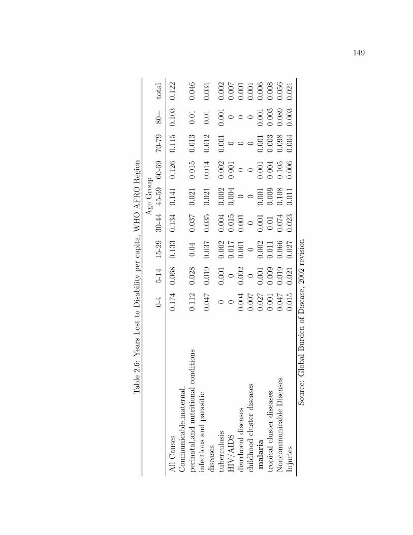
149

Tab

le2.6:

Years

Lostto

Disab

ilityper

capita,

WHO

AFRO

Region

Age

Group

0-4

5-14

15-29

30-44

45-59

60-69

70-79

80+

total

AllCau

ses

0.174

0.068

0.133

0.134

0.141

0.126

0.115

0.103

0.122

Com

municab

le,m

aternal,

0.112

0.028

0.04

0.037

0.021

0.015

0.013

0.01

0.046

perinatal,andnu

tritional

conditions

infectiousan

dparasitic

0.047

0.019

0.037

0.035

0.021

0.014

0.012

0.01

0.031

diseases

tuberculosis

00.001

0.002

0.004

0.002

0.002

0.001

0.001

0.002

HIV

/AID

S0

00.017

0.015

0.004

0.001

00

0.007

diarrhoeal

diseases

0.004

0.002

0.001

0.001

00

00

0.001

childhoo

dcluster

diseases

0.007

00

00

00

00.001

malaria

0.027

0.001

0.002

0.001

0.001

0.001

0.001

0.001

0.006

trop

ical

cluster

diseases

0.001

0.009

0.011

0.01

0.009

0.004

0.003

0.003

0.008

Non

communicab

leDiseases

0.047

0.019

0.066

0.074

0.108

0.105

0.098

0.089

0.056

Injuries

0.015

0.021

0.027

0.023

0.011

0.006

0.004

0.003

0.021

Sou

rce:

Global

Burden

ofDisease,2002

revision

Chapter 3

Fear of Obama: An Empirical Study of the Demand

for Guns and the U.S. 2008 Presidential Election

3.1 Introduction

During 2008 and early 2009, the United States media reported on skyrocketing sales

of firearms as well as shortages in common types of handgun ammunition (see, for

example, Johnson (2008); Bohn (2008); and NPR (2009)). The increase in gun sales

was measurably large: federal tax receipts from sales of pistols and revolvers increased

by almost 90 percent during the fourth quarter of 2008 compared to the same quarter

a year earlier.1 Some states experienced substantial increases in the number of appli-

cations for permits to carry concealed weapons.2 Even though this nationwide gun

1 This figure doubles the highest growth rates during 1993-1994 when both the Brady HandgunViolence Prevention Act and the Federal Assault Weapons Ban were introduced (arguably two ofthe most important gun control laws since the Gun Control Act of 1968 signed by President LyndonJohnson), and more than doubles the panic buying in the aftermath of the 9/11 terrorist attacks.

2 For instance, Florida distributed 42,895 concealed weapon / firearm applications in November2008 (an increase of 172 percent vs November 2007). Minnesota received 21,646 permit to carryapplications in 2008, up 132 percent from 9,327 a year earlier. For some states this abrupt changewas not only sizeable in terms of the flow of permits and licensees but also in their stock: the 2009-2008 flow in Arkansas’s new carry concealed weapon licensees (i.e: 38,442 new licensees) represented80 percent of the total stock of licensees as of December 2007.

150

151

phenomenon was particularly evident in the weeks following the presidential election

of Barack Obama, gun sales began to spike before Election Day. In some parts of

the United States gun purchases reached unprecedented peaks in July and September

2008, the months following Hillary Clinton’s concession speech and the Democratic

Convention, respectively. As firearm sales soared, President-elect Obama urged gun

owners “do not rush out and stock up on guns” in December 2008 (Pallasch (2008)).

Although the concurrent timing of growing gun sales and permit applications with

the 2008 US presidential election is suggestive of an e↵ect of Obama’s election on

the demand for guns, these correlations could also arise from other confounding fac-

tors, such as worsening economic conditions or a more general election e↵ect. In this

paper I quantify how the anticipation and realization of Obama’s success in the pres-

idential election a↵ected the demand for guns. Using data constructed from futures

markets on presidential election outcomes and a novel proxy for firearm purchases

(i.e: the FBI’s firearm background check reports), I show how the demand for guns

responded to monthly information regarding the likelihood of Obama being elected.

After controlling for state fixed e↵ects, di↵erent time fixed e↵ect specifications, and

state level-time varying covariates accounting for the economic climate, my point

estimate provides strong evidence for the existence of a large “Obama e↵ect:” ac-

cording to my most conservative specification, a 10-point increase in the probability

of Obama being elected is associated with a 4.5 percent increase in the demand for

guns nationwide. Moreover, this political e↵ect is larger than the e↵ect associated to

worsening economic conditions.

Why would the election of Barack Obama have a↵ected the demand for guns? I

study two potential underlying mechanisms by exploiting monthly variation in the

odds of an Obama victory interacted with cross-sectional variation in a set of relevant

state characteristics. First, a common explanation for this gun sales surge was the

152

perception and fear that the election of Obama would lead to stronger legal restric-

tions on gun ownership and use in the near future (see, for example, Johnson (2008),

and Neary (2009)). I refer to this potential mechanism as the “fear of gun control”

hypothesis and exploit heterogeneity in gun laws to evaluate its validity. While there

is an important federal component to gun regulations, most gun control policy in

the United States is decentralized. As a result, there exist substantial cross-state

di↵erences in the degree of gun law strictness regulating the sale, possession, and use

of firearms. My identification strategy assumes forward looking agents and presumes

that the potential enactment of a more restrictive federal gun control legislation was

expected to be binding in states with weak gun control and could trigger the surge

in gun sales.3 Consistent with the “fear of gun control” hypothesis, I find that the

e↵ect of the Obama election on the demand for guns was much larger in states with

weaker gun laws.

I also evaluate racial prejudice as another potential mechanism, which I refer to as the

“race bias” hypothesis. Although some social scientists have argued that the election

of Obama is the prima facie evidence that race does not matter anymore in American

politics, empirical work analysing Obama’s performance during the 2008 election

has shown mixed results (e.g., Mas and Moretti (2009); Lewis-Beck, Nadeau, and

Tien (2009); Hutchings (2009); Enos (2010); Piston (2010); and Stephens-Davidowitz

(2011)). Moreover, Sears and Tesler (2010) argue that the 2008 presidential campaign

was “the most sharply racialized campaign” in the last two decades since public

opinion was “largely polarized by racial attitudes.” Thus, it is conceivable that for

some individuals the election of the United States’ first African-American president

was seen as a personal threat (see, for example, Huppke (2009), and U.S. Department

of Homeland Security (2009)). In fact, previous research has suggested that the

3 There is empirical and anecdotal evidence supporting the hypothesis that consumers of durablegoods are forward-looking (e.g., Chevalier and Goolsbee (2009), and Mullin (2001) for the particularcase of guns).

153

perceived threat of racial violence and white antipathy toward blacks fostered the

decision of acquiring firearms during the 1970s (Northwood, Westgard, and Barb

1978). Consistent with the “race bias” hypothesis, I find that the Obama e↵ect was

also larger in states with higher levels of prejudice against blacks.

Why study the demand for guns? Gun prevalence, particularly of handguns, is very

high in the United States when compared to other developed countries.4 Moreover,

gun violence has enormous implications for mortality and morbidity.5 Firearm-related

homicide, suicide, and fatal accident rates are far higher than those in other high-

income countries.6 Futhermore, guns represent “one of the most intensely divisive

cultural issues” in United States (Rostron 2009). The gun debate has taken over not

only the political arena but also academia.7 Irrespective of their stance, participants

from both sides of the debate agree that guns matter. In fact, the private decision

to acquire a firearm may represent an important externality for the rest of society. It

is still under scrutiny whether the net externality is positive (by deterring criminals

and increasing society’s overall safety levels) or a negative (by increasing crime, gun

accidents and suicide rates). Nonetheless, Cook and Ludwig (2000) estimated the

annual social cost of gun violence at $ 100 billion. Therefore, understanding the

economic and non-economic determinants of this private decision provides a valuable

input for the analysis of future gun policies and their social, economic, and political

ramifications. I exploit a unique historical event to shed light on the determinants of

4 Di↵erent studies suggest that gun ownership is as high as 35 to 40 percent and as many as 300million firearms are privately owned in the United States (see, for example, Duggan, Hjalmarsson,and Jacob 2010 for a background on gun ownership).

5 According to the Center for Disease Control and Prevention, in 2009 about 30,000 people diedfrom gun-related homicides, suicides, and accidents, and about 70,000 su↵ered non-fatal injuries fromfirearm shots. By comparison, car accidents were the leading cause of injury deaths in 2009 with35,000 fatalities. Statistics available here: http://www.cdc.gov/injury/wisqars/LeadingCauses.html

6 When compared to 23 high-income countries, firearm-related homicide, suicide, and uninten-tional fatality rates in the United States are 19.5, 5.8, and 6.9 times higher, respectively (Hemenwayand Richardson, 2011).

7 Researchers in economics, political sciences, criminology, and public health have mainly focusedon the study of the relationships between gun prevalence and (a) crime rates, and (b) gun-relatedsuicide and accident rates.

154

the demand for guns.

My work contributes to the empirical literature on the e↵ects of both the realization

and anticipation of political events, such as the passage of a new law or the election of a

candidate, on di↵erent economic outcomes.8 In particular, it advances the empirical

and theoretical work on consumers’ behavior in anticipation of future gun policies

in two respects.9 Firstly, it provides empirical evidence consistent with stockpiling

behavior as a reaction to expected future increases in the cost of acquiring firearms.

Secondly, it sidesteps previous empirical impediments due to limitations of the data.

Specifically, my panel data setting has a considerably improved statistical power

compared to previous work and allows me to incorporate di↵erent fixed e↵ects in both

a time and a cross sectional dimension to address potential omitted variable problems.

Moreover, my analysis of (relative) high-frequency data for my gun purchases proxy

mitigates the concern regarding the reverse-causality from the gun market to the

likelihood of a political event.10 Finally, by interacting the time variation in the

prospect of an Obama presidency and cross-state di↵erences in the stringency of the

gun control laws, my setting also helps to identify heterogeneous reaction across states

that may be otherwise masked in the aggregation of the data at the national level.11

8 Economic outcomes such as the stock market performance of private firms (Gyourko and Sinai(2004) and Knight (2006)), the spread between taxable and municipal securities (Greimel and Slem-rod 1999); investment decisions (Durnev 2011), nominal interest rates (Fowler, 2006), and a varietyof financial indices (Snowberg, Wolfers, and Zitzewitz 2007).

9 Bice and Hemley (2002) estimate a supply and demand model using aggregate U.S. annual datafor the period 1961-1994 and show that the demand for new handguns increased during the years ofthe discussion and passage of the 1968 Gun Control Act (GCA). Mullin (2001) presents a conceptualmodel of consumer demand for guns, in which the e↵ect of a buyback program on gun ownershipdepends on whether the program is permanent or unanticipated and never-to-be-repeated.

10 For instance, the assassinations of Robert Kennedy and Martin Luther King occurred afterthe GCA was introduced as a bill, but before it had been passed by the congress and enacted byPresident Johnson in October 1968. Are the discussion and passage of GCA independent of theevolution of the demand for guns? By using annual data is not possible to accurately test the timingand direction of the causality between the GCA and the demand for guns.

11 My paper is also related to the empirical literature studying the demand for guns and itsrelationship with the existing gun regulation environment. In particular, Glaeser and Glendon(1998), and Kleck and Kovandzic (2009) argue that gun-control laws in general do not appear toa↵ect gun ownership. By studying how gun tra�cking (a key element for the secondary market)across states responds to cross-state di↵erences in gun policies, Knight (2011) finds that the necessary

155

My paper also contributes to the empirical literature on how racial attitudes relate

to firearms prevalence (Northwood, Westgard, and Barb (1978); Lizzote, Bordua,

and White (1981); Young (1985); Ellison (1991); and Kleck and Kovandzic (2009)).12

To the best of my knowledge, my work is the first empirical study linking high-

frequency gun purchases data (a flow) to racial attitudes at the state-level. Whether

this partially racially-motivated change in the flow of guns a↵ected their stocks (or

gun ownership rates) by race or led to any change in racially motivated incidents

involving firearms is an interesting topic for future research.13

In addition, my paper contributes to the literature in economics and political science

on the e↵ect of black candidates on behavior (see, for example, Citrin, Green, and

Sears (1990); and Washington (2006)). In particular, it is related to the growing lit-

erature on the relationship between race attitudes and the candidacy and subsequent

election of Obama (e.g., Brader and Valentino (2011), DellaVigna (2010), Mas and

Moretti (2009), and Stephens-Davidowitz (2011)).14 Most of previous empirical work

shows little evidence of the existence of a link between negative racial attitudes and

condition for the existence of cross-state externalities is empirically satisfied.12 In which is perhaps the most convincing empirical work in this area, Kleck and Kovandzic (2009)

show that handgun ownership among non-blacks (in particular Whites) is associated with raciallyprejudiced views toward Blacks.This strong positive correlation persists even after controlling for anextensive set of individual-level characteristics (and city-level covariates as well), including politicaland religious views, and subjective traits such as attitudes, opinions, and perceptions regardingprior victimization, fear of crime, proviolent attitudes, and punitiveness. Nonetheless, it is worthto mention that the main focus of Kleck and Kovandzic (2009)’s analysis is not the link prejudice-handgun ownership but the relationship between handgun ownership and city-level characteristics(i.e: crime and security).

13 More generally, my paper also contributes to a broader literature considering the relationshipbetween negative racial attitudes and a variety of di↵erent outcomes such as racial preferences indating (as in Fisman et al (2008)) and attitudes towards immigration (Dustmann and Prestion2007) to racial wage gaps (Charles and Guryan 2008) and residential segregation (Card, Mas, andRothstein 2008).

14 For instance, Brader and Valentino (2011) documents a decline in perceptions of racial dis-crimination after the election of Obama. DellaVigna (2010) finds no evidence that key events inObama’s election a↵ected either discriminatory behavior in whites or di↵erent economic outcomesfor blacks. Mas and Moretti (2009) argue that the available evidence does not suggest that racialattitudes negatively a↵ected Obama’s vote share in the 2008 presidential election whereas Stephens-Davidowitz (2011) finds opposite conclusions -as some political science research (see for instance,Lewis-Beck, Nadeau, and Tien (2009); Hutchings (2009); and Piston (2010))-.

156

the election of Obama and appears to contradict my findings. My analysis, however,

is based on a di↵erent margin. My paper focuses on a specific sub-population who

owns or is willing to acquire a firearm and may substantially di↵er, for instance, from

the median American voter.

Finally, the evidence presented in my paper tangentially relates to the literature on the

relationship between the characteristics of policy makers and policy outcomes (e.g.,

Pande (2003); Butler, Lee, and Moretti (2004); Chattopadhyay and Duflo (2004);

and Washington (2008)).15 My findings suggest that di↵erent dimensions of Obama

personality, besides his Democratic a�liation, might had helped to trigger the surge

in gun sales. Perhaps, as Washington (2006) suggests, a black Democrat may be

perceived “as far more liberal than their non-black counterparts” and, thus, more

willing to push a gun-control agenda.

My work provides empirical evidence on the existence of an Obama e↵ect on the

demand for guns and the simultaneous feasibility of the two aforementioned hypothe-

ses regarding the mechanisms underlying this Obama e↵ect. Moreover, the main

results of my work are robust to a variety of checks and extensions. Neither current

or expected worsening economic conditions at the state level nor heterogeneous re-

actions to Obama’s election due to cross-state di↵erences in previous levels of gun

ownership and Republican prevalence (as a proxy for Conservatism) explain away the

two hypothesized underlying mechanisms. Controlling for the probability of another

Democrat candidate winning the election and its interaction with the relevant state

characteristics does not substantially a↵ect the results. The results are not driven

by southern states or the inclusion of the aftermath of November 2008. Further,

the results are also robust to the use of poll data, instead of futures market data,

15 According to these empirical works, not only party a�liation would matter for policy decisions(as in Butler, Lee, and Moretti (2004)) but also characteristics such as gender (Chattopadhyay andDuflo 2004), family composition (Washington 2008) and ethnic group membership (Pande 2003).

157

and alternative measures of prejudice. Heterogeneity due to cross-state di↵erences in

consumer confidence, income, previous levels of crime and other demographic charac-

teristics such as share of rural population and relative share of black population does

not qualitatively a↵ect the main results.

The remainder of the paper is structured as follows. In section 2 I describe my measure

of the demand for guns and provide a background on the evolution of the market for

legal guns, with a focus on the 2008 presidential election. In section 3 I describe the

empirical framework and how it identifies and quantifies the Obama e↵ect, as well as

discuss potential underlying mechanisms. I also conduct the empirical analysis and

robustness checks. Section 4 concludes.

3.2 Data and Aggregated Empirical Evidence on

Gun Sales

3.2.1 A Proxy of the Demand for Guns

Measuring the demand for guns is not straightforward.16 Neither national nor state

level data on gun purchases is available. Moreover, most states do not require registra-

tion of firearms and only a few states require permits to buy them (Azrael, Cook, and

Miller 2004). Even among the states where some requirements exist, the information

is incomplete, outdated and di�cult to obtain (Jacob 2002). Quarterly data on tax

16 The gun-related empirical works have mainly relied on the use of proxies for gun prevalenceacross geographic regions. Di↵erent alternatives has been proposed such as gun magazine subscrip-tions, suicides with guns, percentage of di↵erent type of crimes with guns, fatal gun accident rates,NRA members per 100,000 resident population, hunting license rate, carry permits rate, Federalfirearms license rate, stock of guns manufactured in United States, and weapon arrests as percent-age of total arrests. None of these proxies is pertinent for my work because they are not availableon monthly basis to the best of knowledge. Therefore, I cannot exploit variation within a year tostudy the moments before and after 2008 presidential election.

158

receipts from gun sales is available only at the national level what prevents me from

examining time variation across states. However, there is a federal data source that

provides some indication of the level of the demand for guns by state and month: the

National Instant Criminal Background Check System (NICS henceforth), launched

by the FBI in 1998 and mandated by the Brady Handgun Violence Prevention Act

of 1993 (BHVPA). Before selling any firearms, federal licensee dealers must call the

FBI or other designated agencies to ensure that a potential buyer does not have a

criminal record or is not ineligible to acquire a firearm (Adams et al 2010).

Nevertheless, it is pertinent to note that the number of background check reports does

not necessarily indicate an exact number of firearms sold in a given state for a given

month (FBI 2011). First, after a report is emitted a customer might buy several guns,

or decide not to buy any after all. Second, if the prospective buyer fails the criminal

background check no sale is consummated. Third, some states do not exclusively use

the NICS to conduct background checks on a potential gun sale at federal licensee

dealers (Mayors Against Illegal Guns 2008).17 Finally, private-party gun sales are

exempt of background check unless required by state law (see Wintermute (2009)).

Specifically, gun shows represent an emblematic case in the gun control debate since

federal statutes do not regulate them. Unlicensed vendors or “occasional” sellers,

who are not required to initiate a background check make up to 50 percent of all gun

sales at gun shows (Bureau of Alcohol, Tobacco and Firearms 1999).

Despite the aforementioned drawbacks, the number of background check reports pro-

vides a good proxy for the overall demand for guns for several reasons. NICS’s figures

are the most common firearm sales indicator used in the firearm industry’s reports.

17 Some states use the NICS system for the application and renewal of gun permits or for purchasesin secondary markets such as gun shows. Meanwhile, NICS figures for Kentucky are exaggeratedlyinflated since they appear to have been performing monthly NICS checks on concealed carry per-mit holders (Mayors Against Illegal Guns 2008). For that reason Kentucky is not included in myempirical analysis.

159

The number of background checks is highly correlated with tax receipts from firearm

sales at the national level.18 Moreover, the number of background check reports in

per capita terms is also highly correlated with measures of gun ownership at state

level.19 It can be argued then that the higher the gun prevalence (stock) in a given

state, the higher the level of desired transactions (flow) per number of inhabitants

in that state. Furthermore, according to business publications in the firearm indus-

try, about 98 percent of all inquiries to the NICS turn into a firearm sale.20 Finally,

although there are thousands of gun shows annually in the United States (Duggan,

Hjalmarsson, and Jacob 2010) they represent a minor percentage of all gun sales in

the country accounting for between 4 and 9 percent of total sales, according to the

best estimates available (Wintemute 2009).21 Therefore, gun sales at gun shows that

are not captured by NICS’s statistics would represent no more than 4.5 percent of

total gun sales in the United States.

3.2.2 A Descriptive Analysis of the Aggregated Evolution of

Gun Sales

In this section I present preliminary evidence on the existence of an unusual change

in the demand for guns in the proximity of the 2008 presidential election. Its primary

purpose is solely to provide a descriptive account of the evolution of gun sales by

the inspection of aggregated figures. The discussion on the application of stricter

18 I find a correlation of 0.70 when comparing quarterly data on tax receipts from firearm salesand number of background check reports at the national level for the period 1999-2010.

19 The correlation with the state-level gun ownership estimated from the Behavioral Risk FactorSurveillance System from North Carolina (BRFSS) in 2001 is 0.78. This correlation is high not onlyin a cross section but also in a time-series analysis. The correlation of the proxy with the 9-censusregion level (there is no panel data of gun ownership at the state level) gun ownership from GSS for5 di↵erent waves is 0.84.

20 See, for instance, the American Firearms Industry Magazine (June 2010).21 According to the U.S. Department of Justice [2007], estimates on the number of gun shows per

year range between 2000 and 5200.

160

firearm regulations has been a hot topic in almost every presidential election. Thus, I

provide a first piece of evidence by comparing the evolution of my proxy of gun sales

in the proximity of the 2008 presidential election with its evolution in the proximity

of the 2000 and 2004 presidential elections in Figure 3.1. For a two-year symmetric

window covering the period before and after the election week in each of the last three

presidential elections, I plot the aggregate evolution of the weekly number of firearms

background check reports relative to the same week a year earlier. The vertical black

line denotes the week of the election (week 0). The solid black line, representing the

relative weekly numbers for the weeks surrounding the 2000 presidential election, does

not suggest any increasing demand for guns in that period, with the exception of the

aftermath of the 9-11 terrorist attacks (weeks 45 to 48).22 It is important to remark

that the gun control debate was arguably a very important issue during that election

race, in part a↵ected by the Columbine High School massacre, which occurred one

year prior. In fact, many believe that Al Gore lost his home state Tennessee, and

also Arkansas, New Hampshire and West Virginia, due to his vocal pro-gun control

stance during the Democratic primaries (Cowan and Kessler (2001)).

No abnormal evolution in the demand for guns for the two-year period surrounding

the 2004 presidential election can be inferred from the inspection of the solid gray

line.23 The implied year-on-year weekly growth rate of the number of background

check reports for that period ranges between -10 percent and 10 percent. The solid

black line with diamond markers shows a sharp increase in the demand for guns in

the week of the 2008 presidential election and in the weeks after. The average implied

year-on-year weekly growth rate of the number of background check reports for the

22 There was almost 470,000 more firearm background checks during the six months following theterrorist attacks. The same figures ascend to 1.6 million during the six months following the 2008presidential election day.

23 Due to an internal software problem, the NICS temporarily stopped for three days on May 11,2000; halting all gun sales nationwide. For that reason, the relative numbers of background checkswere artificially underestimated and overestimated for the weeks 26/27 and -26/-27, respectively. Iomitted those four weeks, which explains the two discontinuities in the solid gray line.

161

Figure 3.1: Presidential Elections and Firearm Background Check Reports

24-week period following that election is above 30 percent with the highest figure of

60 percent occurring immediately after the election. In addition, a 30 percent increase

in the firearm background check reports takes place in mid-July after Obama wins

the Democrat primaries.

Figure 3.2 presents a geographical distribution of the annual increase in the demand

for guns for the period July 2008 - June 2009. I aggregate the data to annual cumu-

lative values to facilitate the exposition. I will later exploit monthly variation in the

number of firearm background check reports. I divide the map into quintiles in terms

of the growth rate of my proxy for the demand for guns. It is worthwhile to note

that although southern states have on average higher growth rates, there seems to be

some variation even within that region.24 The states with the highest growth rates,

from 31 percent in Texas to 78 percent in Utah, are roughly evenly distributed across

24 In the robustness checks of the econometric analysis I show that none of the main results aredriven by southern states. There is no evidence of spatial autocorrelation in the growth rate ofbackground check reports (Moran’s I statistic of 0.0362).

162

the U.S. from the East Coast (Connecticut, Rhode Island, and New Jersey) and the

South (Georgia and Tennessee), to the central part of the Mountain Region (Nevada,

Utah, and Colorado) and Hawaii. Although the group with the second highest figures

is mostly represented by southern states (South Carolina, Delaware, Florida, North

Carolina, Oklahoma, and Maryland) it also includes central states such as Illinois

and Kansas. The group of states with the lowest growth rate (growth rates from -21

percent in Massachusetts to 12 percent in Vermont) is very heterogeneous not only

in terms of geographic location but also in terms of both the level of ruralism and

average income. New York, California, and Massachusetts as well as Idaho, Montana,

Mississippi, and North Dakota belong to this group.

Figure 3.2: Growth in Background Checks by State (July08-June09 vs July07-June08)

163

3.3 Empirical Strategy and Results

3.3.1 Quantifying the Obama e↵ect

Obama Victory E↵ect

Table 1 provides a first statistical test for the existence of an Obama e↵ect in the

demand for guns. Using monthly data at the state level for the number of background

check reports in per capita terms for the period March 2007-December 2009, I estimate

the following equation:25

log (yi,t) = ↵+ � ⇤Obamat + � ⇤ Zi,t + � ⇤ ⌧t + �i + t + "i,t (3.3.1)

where the subscripts i and t denote state and month respectively.26 The variable yi,t

is the number of firearm background check reports per 1,000 inhabitants. Obamat

is a dummy variable that takes the value 1 starting in November 2008. Zi,t is a

monthly indicator of the economic situation at the state level. ⌧t is a simple time

trend, and �i is the state i fixed-e↵ect. The term t denotes a collection of time

related fixed-e↵ects consisting of season, year, month of year, and month of year ⇥

state fixed-e↵ects. Table I presents the main results for the di↵erent specifications of

equation (1). Below each coe�cient two standard errors are reported. In parenthesis,

I present standard errors adjusted for clustering within state. In brackets, I present

standard errors adjusted for clustering within month. Since I am especially interested

on the e↵ect of information regarding Obama election on the demand for guns at the

25 I start the analysis in March 2007 in order to be consistent with the rest of the paper. Inaddition, I use state monthly data instead of weekly data because the latter is not publicly availablethrough the FBI’s NICS section.

26 Due to the lack of data for one of the main explanatory variables I focus my analysis on 43states. The omitted states are Hawaii, Idaho, Kentucky, Maine, Nebraska, Nevada, and NorthDakota.

164

state level, whereas that information is the same for all the states in a given month,

clustering at the month level appears to be the most conservative approach. In fact,

standard errors clustered at the month level are much larger than at the state level.

Therefore, for the rest of the paper I report only the standard errors clustered at the

month level.27 All the regressions are weighted by state population in 2008 and include

state and year fixed e↵ects to capture time-invariant state characteristics and year

specific conditions that may be related to the demand for guns. In order to capture

within year specific time variation I also include season fixed-e↵ects in columns 1

and 2 whereas in columns 3 I include month of year fixed-e↵ects.28 In specifications

from column 4 to 6 I include month of year ⇥ state fixed-e↵ects to capture monthly

seasonal pattern in the demand for guns that may be state specific.

Column 1, where I consider � = � = 0, suggests that demand for guns is significantly

positively related to the election of Obama. The point estimate from my semi-log

specification indicates that the election victory of Obama would have been related to

a 39.1 percent increase in the demand for guns (i.e., 100 ⇥ (e0.33 � 1) = 39.1). The

next specification in column 2 includes a time trend which does not a↵ect previous

finding. The introduction of month of year, and month of year⇥state fixed-e↵ects in

columns 3 and 4 slightly reduces the size of the main Obama e↵ect although does not

a↵ect its statistical significance. In column 5 I control for the state of the economy.

There is no substantial empirical evidence on the strong causal link from economic

conditions to crime rates (see Cook and Wilson (1985); and Freeman (2001) among

others). However, if people perceive that this causal mechanism does exist then it is

possible that the demand for guns presents a counter-cyclical behavior. That is, fear

of future crime due to a deteriorated economic condition would make people more

27 None of the main results is a↵ected when clustering at the state level.28 Gun sales peak during the Fall, when hunting season begins, and the holidays; whereas they

reach their lower levels during the Summer.

165

willing to buy a gun during a recession.29 Since the election of Obama coincided with

the worsening economic condition in 2008, omitting variables related to the business

cycle that potentially a↵ect also the demand for guns would introduce a bias on the

estimation of the Obama e↵ect. In order to account for the business cycle shocks

in each individual state, I add the growth rate of the state coincident index.30 As

expected, the introduction of this economic indicator reduces the size of the main

Obama e↵ect. However, this e↵ect associated with the election of Obama remains

statistically large. The point estimates in this specification suggest that the election

of Obama is associated with almost 25 percent increase in the demand for guns and

that the current worsening economic conditions played a role as a determinant of

the increasing demand for guns in my period of analysis: a one point decrease in the

monthly growth rate of activity (more than 10-point decrease in annual terms) implies

an increase in the demand for guns of 13.4 percent.31 Nonetheless, an indicator of

the future, rather than current, condition of the economy is arguably a better proxy

to account for a fear of future crime. In fact, adding a monthly leading indicator

accounting for the six-month forecast of the growth rate of the coincident index kills

the statistical significance of the contemparaneous growth rate (result not shown).

Thus, in the last specification (column 6) I substitute the growth rate of the coinci-

dent index by its six-month forecast (i.e: leading indicator).32 A one-point expected

decrease in the six-month growth rate is statistically associated to 3 percent increase

in the demand for guns whereas the election of Obama is associated with a 22 percent

increase. Thus, according to the point estimates, the suggested Obama e↵ect on the

29 Glaeser and Glendon (1998) suggests that fear of crime is associated with ownership of pistolsonly and no other form of firearms. On the other hand, Kleck and Kovandzic (2009) argue thathandgun ownership is a response to homicide, but not necessarily to fear of crime.

30 The coincident index combines four state-level indicators (i.e: nonfarm payroll employment,average hours worked in manufacturing, unemployment rate, and real wage and salary disbursement)to summarize current economic conditions in a single statistic (Clayton-Matthews and Crone 2005).

31 I also estimate additional specifications taking into account state-level growth of unemploymentand state-level growth of quarterly income per capita. The results (not shown) are consistent withthe specification using the coincident index.

32This leading indicator is also produced by the Federal Reserve Bank of Philadelphia.

166

demand for guns would be equivalent to the induced e↵ect of a enormous decrease of

approximately 15 points in the expected growth rate of activity in one year.

Incorporating Information from Future Market on Election Outcomes

Now I focus on the 2008 presidential election race and the month following Novem-

ber 2008 by studying how the change in the perception of Barack Obama being the

most likely winner of the election a↵ects the demand for guns. I continue basing my

empirical analysis on the period March 2007-December 2009.33 As mentioned before

with the analysis of Figure 1, the aggregated evolution of the number of background

check reports shows a significant increase not only in November 2008 and afterward

but also in July 2008; coinciding with Obama winning the Democrat primaries. Using

data from the Iowa Electronic Market (IEM) I construct a proxy for the probability

of Obama winning the presidential election. The IEM is an on-line futures market

where participants trade future contracts with payo↵s based on election outcomes

(Each participant can invest between $ 5 and $ 500).34 That is, the liquidation value

of the contract that represents the actual outcome of an election, will be $ 1 whereas

all other contracts will have no value.35The IEM provides information on two future

markets that are relevant for my purposes: one where payo↵s were determined by the

outcomes of the 2008 U.S. National Convention of the Democratic Party and another

33 March 2007 is the first month in my analysis because Barack Obama announced his candidacyfor president on February 10th, 2007.

34 Intrade is an alternative and similar futures market for the 2008 election. I chose IEM dataover Intrade’s just because the former is available online at no cost. Nonetheless, one should notexpect sizable and permanent price di↵erences across markets over time since this would imply theexistence risk-free profit opportunities from cross-market arbitrage.

35 I use market data instead of polls data for several reasons. First, market data eases thecalculation of the probability of Obama winning the election for the whole period of analysis becauseall the information needed is available in a higher frequency basis and in a homogenous way. Second,under non-arbitrage opportunities the market prices should reflect a consensus regarding the forecastof votes share for each candidate (Berg, Forrest, and Rietzet 2008). Third, recent research providesevidence not only on the relative accuracy of prediction markets (Berg, Forrest, and Rietzet 2008)but also on the impediments to accurate prediction for polls data due to the existence of di↵erentbias (Malter 2010). Nonetheless, using polls data does not alter the main results of my empiricalwork (see robustness check).

167

one where the outcome depended on the results of the 2008 U.S. Presidential elec-

tion. The price of the asset in the first market accounts for the probability of Obama

winning the primaries while the price of the asset in the second market accounts for

the probability of a Democrat candidate winning the presidential election.36 By mul-

tiplying these two probabilities I obtain a proxy for the probability of Barack Obama

being elected president. Given that in my new specification I attempt to disentangle

the Obama e↵ect from an overall Democrat e↵ect, I also construct another control

variable denoted probability of other Democrat candidate winning the presidential

election using the same aforementioned approach.37 38 My new identification strat-

egy is summarized in the following equation:

log (yi,t) = ↵+�⇤P (Obama)t+�⇤P (Democ�Obama)t +⇢⇤Zi,t+�⇤⌧t+�i+ t+"i,t (3.3.2)

where P (Obama)t and P (Democ�Obama)t are the 2008 election victory probabilities

for Barack Obama and any other Democrat candidate receptively, as implied from

future contracts from the IEM.39 The remaining right-hand-side variables are the

same defined above for equation (1). Table 2 presents the main results for the di↵erent

specifications of equation (2). In column 1, where I consider � = ⇢ = � = 0, the point

estimate suggests that 10 points increase in the probability of Obama winning the

election is statistically associated to 5.6 percent increase in the demand for guns. The

36 In order to build a monthly probability value I use all the daily available information on pricesand transactions for a given month. The final monthly value is the result of a weighted average ofthe daily available prices, where the daily price is the average price of the day and the weights arethe shares of total daily transactions on total amount of monthly transactions.

37 Basically, the probability of other Democrat candidate winning the presidential election is theresult of the probability of Obama losing the primary multiplied by the probability of a Democratcandidate winning the presidential election.

38 Note that these probabilities do not vary across states. Therefore, no cross-state di↵erence inperceptions regarding the likelihood of Obama’s victory, as implied from IEM data, is an implicitidentification assumption in my econometric strategy. Again, without arbitrage opportunities, theimplied probability of Obama winning the election (i.e: a market price) should reflect the consensusof market’s participants, independently of their locations.

39 Note that the variable P (Obama) takes the value 1 from November 2008 onwards while thevariable P (Democ�Obama) takes the value 0 from September 2008 on. See robustness check forresults omitting November 2008 aftermaths.

168

Democrat Party is long identified with gun control. Therefore, if a fear to future gun

control policies is operating during the election race then it could be expected that no

matter the identity of the candidate, as long as that candidate would be Democrat,

advocates of gun rights would buy more guns when a Democrat is more likely to

be elected president. In order to di↵erentiate an Obama e↵ect from a Democrat

e↵ect, I control for the probability of any other Democrat candidate being elected

in column 2. As expected, due to the fact that the two probabilities are (strongly)

negatively correlated, the Obama e↵ect is much larger than in the first specification

while the precision of the estimate is not a↵ected. Note also that the probability of

other Democrat being elected is significantly and positively related to the demand

for guns but the size of the coe�cient estimate is less than half of the estimate for

Obama. Specifically, the election of Obama would imply a 63.4 percentage increase

in the demand for guns while the election of another Democrat would imply a 25.4

percentage increase.

The estimated Obama e↵ect decreases to 51.8 percent when I control for the leading

indicator of the economic activity at the state level in column 3. Under this spec-

ification the coe�cient estimate for the e↵ect of the election of another Democrat

increases considerably to 0.42. Additionally, 1 point increase in the expected six-

month growth rate of economic activity, as measured by the leading indicator, would

imply a 2.6 percent reduction in the demand for guns. The addition of a time trend in

column 4 again decreases the size of the Obama e↵ect and increases coe�cient for the

e↵ect of another Democrat. However, the introduction of month of year fixed e↵ect

in column 5 substantially reduces the size of the latter e↵ect to the point of making it

statistically insignificant when clustering standard errors at the month level. Finally,

the introduction of month of year⇥state fixed-e↵ects in columns 6 -arguably the most

conservative specification possible- reduces the size of the main Obama e↵ect to 0.42

although does not a↵ect its statistical significance whereas it eliminates the statisti-

169

cal significance of the coe�cient for the probability of other Democrat winning the

election when I cluster the standard errors at the month level. The point estimate

for the leading indicator variable remains fairly constant across specifications.40

Geographical Pattern

In this section, I explore the geographic distribution of the main Obama e↵ect. In

Figure 3 I represent a map of United States with the implied Obama victory e↵ect

on the demand for guns by state. That is, I map the � coe�cient estimates from the

following regression.41

log (yi,t) = ↵+X

�i ⇤Obamat ⇥ State ii + � ⇤ Zi,t + �i + ⌧t + �t + "i,t (3.3.3)

State ii is a dummy variable that takes the value 1 for the state i, and 0 otherwise.

The variables �i, ⌧t, �t are the state, season, and year fixed e↵ects. The darker the

color of the state in Figure 3.3, the larger the Obama victory e↵ect (white colored

states with lines have no estimated coe�cients). A close inspection of the map reveals

some noteworthy patterns. The states in the highest quintile of the distribution of

the estimated Obama e↵ect are not clustered in any specific region of US.42 Mid-

western and western states are more prevalent in the lowest quintiles while southern

states are more common in the two highest quintiles of the distribution of the esti-

mated Obama e↵ect.43 Interestingly, states with high levels of gun ownership such

40Adding a time-varying control for the evolution of consumer expectations at the national level(using either the Reuters/University of Michigan Index of Consumer Sentiment or the ConferenceBoard’s Consumer Confidence Index) does not explain away the estimated Obama e↵ect (resultsnot shown).

41 Using these coe�cients one can calculate state-specific semi-elasticities that can be interpretedas the percentage increase in the demand for guns in a given state due to the election of Obama (bydoing 100⇥ (e�i � 1)).

42 The highest quintile consists of Tennessee, Utah, Connecticut, New Jersey, South Carolina,Indiana, Rhode Island, and Delaware.

43 The lowest quintile consists of Massachusetts, California, Wisconsin, Minnesota, Montana, New

170

as Wyoming, Montana, South Dakota, West Virginia, Mississippi and Alaska present

point estimates for the Obama e↵ect below the median.44

Figure 3.3: Geographic Distribution Obama Victory E↵ect

3.3.2 Potential Mechanisms

In this section I examine two potential mechanisms that may have accounted for the

Obama e↵ect on the demand for guns: fears of future federal gun-control policies

(i.e., “fear of gun control” hypothesis) and negative racial attitudes toward blacks

(i.e., “race bias” hypothesis). The empirical strategy in equations (1) and (2) does

Mexico, Vermont, and Arizona44 In addition, I also run a similar regression to equation 3 but instead of specifying interaction

terms with state dummies, I introduce nine census division dummies (result available upon request).The positive statistical relationship between the demand for guns and the election of Obama is largerin southern states, especially in the East South Central division (Kentucky, Tennessee, Mississippi,and Alabama) and lower in New England and the Pacific. Overall, it appears that the distributionof the largest reactions of the demand for guns to the election of Obama is mostly concentrated inthe Appalachians and the Bible Belt. Notably, the increase in the Democrat vote share in the 2008presidential election (relative to the 2004 election) was significantly smaller in that part of U.S. (Masand Moretti 2009) what would point to the possibility that negative attitude towards Obama werepresented.

171

not allow me to identify heterogeneous reactions to the election of Obama. In fact,

it may be possible that the aggregate e↵ect documented in Table 1 and 2 is the net

result of o↵setting e↵ects from heterogeneous groups. Thus, a more detailed analysis

of the monthly evolution of the demand for guns seems to be pertinent to identify the

potential existence of di↵erent marginal reactions that may vary not only over time

but also across states. The heterogeneity in State characteristics, such as strength

of gun laws and average prejudice, interacted with time variation in the likelihood of

Obama being elected would help me to shed some light on the potential mechanisms

underlying the Obama e↵ect.

Fear of Gun Control

The stockpiling of firearms as a reaction to potential restrictions on gun purchases

seems a reasonable and plausible explanation for the surge in sales in a context with

forward looking agents who recognize Democrats as more prone to support gun control

laws, Obama leading the polls, and a constant negative advertising about his position

on gun issues.45

Consistently with this line of argument, trend in attitudes toward gun control started

to show a substantial change in the proximity of the presidential election of 2008.

According to Smith (2007), support to stricter regulation on sales and possession of

firearms was widespread in 2006.46 However, there has been an increasing support

45 The National Rifle Association (NRA) spent 7 million dollars on a campaign advocating theposition that Obama posed a serious threat to the “Second Amendment rights” (Brady Campaignto Prevent Gun Violence, 2008). This figure represents more than thirty times the amount devotedagainst Al Gore in 2000 (Brady Campaign to Prevent Gun Violence 2008).

46 According to the National Opinion Research Center, around 90 percent of surveyed supportedmaking it illegal to use guns while under the influence of alcohol, more than 80 percent wantedlimitations to the sale of 50 caliber rifles, semiautomatic, and assault weapons. Above 80 percentfavored criminal background checks for all sales of guns, including private sales between individuals,and requiring a police permit to buy guns.

172

to gun right since 2008 (Pew Research Center 2010).47 As documented in Figure 4,

the fraction of people saying it was more important to control gun ownership almost

doubled the fraction of people saying it was more important to protect gun rights

in April 2007. Note, however, that theses figures are likely to be influenced by the

tragic event occurred at Virginia Tech. Nonetheless, the gap starts to shrink before

the 2008 election and it is completely closed in March 2010. Interestingly, the Tucson

Shooting of January, 2011 did not appear to a↵ect gun control preferences.48

Figure 3.4: Change in Attitudes Toward Gun Control. More important to ProtectGun Rights or Control Gun Ownership?

The existence of statistically significant coe�cients for either the dummy Obama or

the Probability of Obama winning the election, as documented in previous section, is

no evidence of the existence of a stockpiling decision originated from fears of future

anti-gun laws. It is possible that some people could have been making the decision

47 Taking into account the period 1993-2008, the vast majorities surveyed by the Pew ResearchCenter had consistently said it was more important to control gun ownership than to protect theright to own guns. According to Smith (2007), not even the fear after 9/11 terrorist attacks couldundermine the support to gun regulations.

48 All Regions experience an increasing support to gun rights during this period although thissupport is significantly lower in the East.

173

of buying guns based on impressions related not only to his stance on gun control

but also to other di↵erent perceived characteristics of Obama’s identity (even inde-

pendently of his race). For instance, people could perceive his Muslim sounded like

name as an indication of a potential threat to their security. Other people could

perceive Obama as a potential socialist and being against American values. In order

to attempt to identify a gun-control fear mechanism underlying the Obama e↵ect I

estimate di↵erent specifications of the following equation:

log (yi,t) = ↵ + � ⇤Obamat + � ⇤Obamat ⇥ SGCi +P

�s ⇤Obamat ⇥Xs,i + ⇢ ⇤ Zi,t

+ �i + t + "i,t (3.3.4)

Equation (4) focuses only on the event of the election victory of Obama. However,

the fears of stricter gun controls were already widely spread before the election week,

in part fueled by the NRA’s negative advertising showing Barack Obama as a real

threat to the “second amendment” (See Martin (2008), and Lapierre (2008)). Then, I

also estimate below an analogous specification to equation (4), in which I also exploit

information regarding the market consensus on the likelihood of Obama being elected

president.

log (yi,t) = ↵ + � ⇤ P (Obama)t + �d ⇤ P (Democ�Obama)t + � ⇤ P (Obama)t ⇥ SGCi

+X

�sP (Obama)t ⇥Xs,i + ⇢ ⇤ Zi,t + �i + t + "i,t (3.3.5)

Where SGCi is a measure of stringency of gun laws based on the 2008 Brady Score

Card for state i. The Brady Center to Prevent Gun Violence computes a state

scorecard that grades, from 0 to 100, each state according to the strength of its

174

gun laws (the higher the score, the stronger the state gun laws).49 Xs,i is a vector of

characteristics s for state i that might correlate with both the demand for guns and the

strength of state gun laws. I pay special attention to the characteristics Republican

prevalence and gun ownership levels. I include a Republican prevalence interaction

term for two reasons. First, I would like to account for a proxy of conservative concern

that also correlates with lower levels of gun control since the values associated with

the gun culture are mostly politically related to the Republican party, which has

historically been against gun control measures (Spitzer (1988); and Gimpel (1998)).

Note, however, that the empirical research linking ideology and attitudes toward gun

control has shown mixed results (Curry and Jiobu 2001). Second, given the two party

system of the United States, a person who is “afraid of Obama” is more likely to be

Republican. The inclusion of the last interaction terms try to control for the fact

that gun ownership is more common among Republicans and Conservatives (Curry

and Jiobu (2001); and Azrael et al (2007)) and also higher in states with weaker state

gun control. Republican prevalence is measured as the average margin of votes for

the Republican candidates in 1992, 1996, 2000, 2004, and 2008 presidential elections

whereas gun ownership levels are 2001 household estimates from the Behavioral Risk

Factor Surveillance System in North Carolina (BRFSS).50 51

Panels A and B in Table 3 present regression outcomes for equations (4) and (5),

respectively. For both Panels SGCi = 100� 2008Brady ScoreCardi thus the higher

the value of SGCi, the weaker the state gun law. The remainder variables Zi,t, �i,

and t are the same as defined for equations (1) and (2). All the regressions are

49 See Table A.2 for each state score card.50 In 2001 the BRFSS in North Carolina surveyed 201,881 respondents nationwide, asking them,

”Are any firearms now kept in or around your home? Include those kept in a garage, outdoor storagearea, car, truck, or other motor vehicle.”

51I also allow flexibility in the functional form for the interaction terms.Table S2 in supplementaryappendix includes the specifications for which the interaction terms are discrete variables. In thoseadditional regressions SGC (Xs,i ) is a dummy variable for whether the state i presents a value ofSGC (Xs,i ) below (above) the median.

175

weighted by state population in 2008. The error term is allowed to be heteroskedastic

and correlated at the month-level.

Since the interaction terms are not demeaned, an statistically insignificant coe�cient

for the main Obama term (i.e: �) should not to be interpreted as evidence of the

absence of the Obama e↵ect. That is, the coe�cient estimates for � in equations (4)

and (5) are not directly comparable with the ones in Tables 1 and 2. Nonetheless,

for each specification I report the implied Obama victory e↵ect (i.e., P (Obama) =

Obama = 1) at the mean value of interacted variables along with the F-statistics for

the null hypothesis � = � = �s = 0 (i.e., no existence of the Obama e↵ect). Finally,

the coe�cient � captures the di↵erential Obama e↵ect in the demand for guns for

state with weaker gun laws. Therefore, � > 0 would be consistent with the hypothesis

of the existence of a firearm stockpiling reaction induced by fears of stronger legal

restrictions on guns.52

Results in column 1 in Panel A of Table 3 are consistent with the existence of a large

e↵ect of the election of Obama in the demand for guns (F-Statistics 36.8 for the null

� = � = 0). More importantly, the point estimates for � suggests that there was an

di↵erential increase in sales in states with lower levels of state gun control (significant

at the 1 percent level). The magnitude of the e↵ect is large. The point estimates

suggest, for instance, that given the election of Obama, states with no compulsory

universal background checks and gun purchase permit requirements (25 points in

Brady Score) hypothetically experienced a demand for guns 9 percent larger than

states where those requirements existed in 2008. The addition of the other interaction

52 Although there is no accurate statistics about the exact number and location of gun shows,Lott (2003) collected state level figures for the period 1989-2001 from the Gun Show Calendar. Usingthat data I find that the prevalence of gun shows is negatively associated to some di↵erent measuresof state gun control laws. Then, if the “gun control fear” hypothesis is correct one may expect to seean increase of the demand for guns in the secondary market (which includes gun shows) as well. Ifthat is the case, the negative correlation between the weakness of state gun laws and the prevalenceof gun shows would suggest that my point estimates for � should be interpreted as lower bounds.

176

terms in column 2 does not substantially a↵ect the size of � but improves its statistical

precision (t-statistic increases more than 10 percent). Interestingly, after the election

of Obama the demand for guns was also higher in states with higher Republican

prevalence but smaller in states with high levels of gun ownership. The addition of

month of year⇥ state fixed-e↵ects in column 3 or month fixed-e↵ect in column 4 does

not substantially a↵ect the results for �. In sum, the election of Obama implied a

di↵erential increase the demand for guns with low levels of gun control and a mean

e↵ect between 24 and 32 percent (mean Obama e↵ect= exp(�+�⇥SGC+�s⇥Xs)�1).

Finally, the coe�cient estimates capturing the e↵ect of future shocks to the economic

activity on the demand for guns are consistent with the results for the specifications

presented in Table 1. Nonetheless, the statistically significance of this economic e↵ect

vanishes when I include month fixed-e↵ect.53

In Panel B in Table 3 I present the regression outcomes for di↵erent specifications

of equation (5) where I exploit variation in the probability of Barack Obama being

elected president as implied from future market prices. After controlling for state,

season, and year fixed-e↵ects, the probability of other Democrat being elected and

the growth rate of economic activity, the point estimate for � in column 1 in Panel

B suggests that 1-point increase in SGC is statistically associated with an additional

0.6 percent increase in the demand for guns. Accounting for Republican prevalence

and gun ownership interacted both with the probability of Obama victory in column

2 does not a↵ect the size of the di↵erential e↵ect (significant at 1 percent level).

The addition of month of year⇥ state fixed-e↵ects or month fixed-e↵ect in columns 3

and 4, respectively, does not substantially a↵ect the results, namely: (i) the implied

53 Most of the variation (95 percent) of this economic variable is within variation (i.e: over time).

Therefore, the month fixed-e↵ect is absorbing most of the variation needed to identify the economic

shock e↵ect. See Table A.1 in appendix.

177

partial e↵ect of an Obama Victory at the mean value of the interacted controls is con-

sistent with 44 to 57 percent increments in the demand for guns; and (ii) in line with

a pattern consistent with a fear of future gun control measures, the Obama e↵ect was

statistically larger in states with weaker gun control laws. The point estimate in the

most conservative case (column 4, in which I include state and month fixed-e↵ects),

suggests that the fear of the hypothetical implementation of the same gun measures

currently existing in California (the state with the strongest gun control measures ac-

cording to the Brady Campaign) would make the Obama e↵ect more than 30 percent

larger in Arizona. The estimate coe�cient for the Republican prevalence interaction

term is also statistically significant and represents a meaningful magnitude: increasing

the average Republican margin by 10 points would make the Obama e↵ect 7 percent

higher (a 10-point increase in the average Republican margin in Georgia, for instance,

would lead to the level of Republican prevalence in Kansas). In addition, for all the

specifications I obtain large F-statistics for the null hypothesis � = � = �s = 0.

Race Bias

It could be argued that, despite of the NRA’s negative advertising; there was no clear

rationale for believing ex-ante that Obama’s gun policies would be extraordinarily

more restrictive than those of Hillary Clinton or John McCain. Although Obama had

consistently supported gun control measures in the past (Brady Campaign to Prevent

Gun Violence 2008), he also made repeated claims to advocate the upholding and

respect of the “Second Amendment”.54 On the other hand, John McCain sponsored

the McCain-Lieberman gun-show bill which would have given the federal government

the legal tools to close the gun show “loophole” on a national basis. Prior to the 2008

54 For example Obama said at a campaign rally in Lebanon, Va., on September 9, 2008: “Ibelieve in the second amendment. I believe in people’s lawful right to bear arms. I will not takeyour shotguns away. I will not take your rifle away. I won’t take your handgun away...there are somecommon-sense gun safety laws that I believe in. But I am not going to take your guns away”.

178

election, the NRA had referred to McCain as “one of the premier flag-carriers for

the enemies of the Second Amendment,” rating him with a “C” when he was seeking

reelection as senator from Arizona in 2004 (Rostron 2009). Regarding the other

Democratic Party presidential frontrunner, NRA executive Vice President Wayne

LaPierre stated that there would be “nightmare years ahead for gun owners if Hillary

Clinton is elected president of the United States” (See Lapierre (2008) ). The fact

that Barack Obama did not have a particularly relative stronger anti-gun record or

campaign positions begs the question as to why the likelihood of his election would

induce a surge in gun sales.

Focusing on local biracial elections, Rich (1989) argues that Black candidates may

result in ”intense apprehensions and fear” among Whites. Northwood, Westgard,

and Barb (1978) suggest that white working class amtiphaty towards blacks partially

explained the rise of gun ownership in the urban non-South during the ’70s. In this

vein, the election of the first Black president might have represented a unique driver for

racial tension, specially among prejudiced people. There is some anecdotal evidence

pointing toward this possibility. The major white nationalist web site temporarily

shut down in the days following the presidential election due to the large amount

of internet tra�c (see Wright (2011) and Huppke (2009)). The Southern Poverty

Poverty Law Center (2009) reported an increasing activities of racialized right-wing

groups.55 Homeland Security (2009) stated that “the high volume of purchases and

stockpiling of weapons and ammunition by right-wind extremist (...) [is a] primary

concern to law enforcement”. Can prejudice partially account for the unusual surge

in gun sales documented in the previous section? In order to study this question I

consider regressions of a similar form to equations (4) and (5). Nonetheless, instead

of focusing on the interaction term including SGCi I examine how a measure of

55 Although Bill Clinton’s administration also faced virulent right-wing group, which were weak-ened by the end of the 1990s; they were not primarily motivated by race hate (Southern PovertyLaw Center 2009).

179

racial attitude towards blacks at the state level interacted with the time variation

of information regarding Obama’s likelihood of becoming president is statistically

associated with the demand for guns. I thus include a variable Prejudicei proxying

for racial prejudice against black at the state level i. The prejudice index comes from

Charles and Guryan (2008) and represents an average over a 30 years period for an

aggregate measure of racially prejudiced sentiments at the the state level.56

A measure of prejudice is not required to be perfect for the purpose of my estimations;

rather it solely needs to provide some indication on racial prejudice di↵erences across

states. Nevertheless, the geographic distribution of prejudice might have changed over

time introducing measurement error in my analysis. Under classical errors-in-variables

my OLS estimation of prejudice interacted term would tend to be underestimated and

biased the results against finding statistically significant results. Notwithstanding,

it is not clear what is the magnitude and nature of the measurement error in my

prejudice variable, I show that the main results are robust to the use of di↵erent

prejudice measures that capture most current trends on racial sentiments (see Table

8 in robustness check section).

The two panels in Table 4 emulate Table 3. I continue controlling for the interaction

terms including Republican prevalence and gun ownership in order to partially ac-

count for di↵erences in Conservatism. My measure of prejudice against blacks may

have a component of symbolic racism which has been argued to confound with con-

servative ideology (Feldman and Huddy 2005). Note that the coe�cient estimates

capturing the di↵erential Obama e↵ect for higher levels of prejudice are statistically

significant at the 1 percent level in all the specifications. Results from column 1

56 Using multiple waves (1972-2004) of the GSS and responses from white people aged 18 andolder to more than 20 di↵erent racial prejudice questions, Charles and Guryan (2008) build a proxyfor prejudice at the state level. They focus only on questions that are exclusively related to racialprejudice, omitting in their analysis the ones touching on government policies and race. Afternormalizing responses, they construct a individual-level prejudice index for each respondent andthen aggregate these figures at the state level (see Table A.2 for each state value of the index).

180

in Panel A suggest that the election of Obama is statistically associated with a 26-

percent increase in the demand for guns for a state with mean values of prejudice. The

point estimate (� = 0.252) from column 4 in Panel A suggests that a two standard

deviation increase in the level of average prejudice (for instance, Alabama’s prejudice

level is 2 standard deviation above Tennessee’s) would imply an additional 10 percent

increase in the demand for guns when Obama was elected. Note that the coe�cient

estimates for all the other covariates are consistent with the ones obtained in Table 3.

In addition, the F-statistics for the hypothesis testing of the existence of the Obama

e↵ect are very large. The implied Obama e↵ects evaluated at the mean are slightly

smaller for all the specifications but remains very similar to the ones obtained in

Table 3.

I find a larger e↵ect of prejudice when I use market prices from IEM in Panel B. All

the coe�cient estimates for the prejudice interaction terms are positive and strongly

significant, indicating a pattern consistent with racial sentiments playing a role in the

unusual increase of the demand for guns during my period of analysis. The magni-

tude of this race related e↵ect is very large. For instance, for the most conservative

estimation it implies that a hypothetical 2 standard deviation increase in the level

of average prejudice is statistically associated with a 13-percent increment in the de-

mand for guns when Obama is elected. The estimate coe�cient for the Republican

prevalence interaction term is also statistically significant and represents a meaning-

ful magnitude: increasing the average Republican margin by 10 points would make

the Obama e↵ect 11 percent larger. Nonetheless, this coe�cient estimate is upward-

biased due to the omission of the interaction term capturing the weakness of State

Gun Laws which are positive correlated with Republican prevalence over the last 20

years (see point estimates in Table 5).

181

3.3.3 Robustness Check

In this section, I consider a variety of robustness checks. I first provide evidence

that the two aforementioned mechanisms are not competing or mutually excludable.

Results in Table 5 show that the joint inclusion of both interaction terms in all

my specifications does not substantially a↵ect the main results obtained in Tables

3 and 4.57 That is, coe�cient estimates for both interaction terms are statistically

significant, with the expected signs, and in similar magnitudes.58

All the specifications estimated so far are based on the period March 2007-December

2009. In my second robustness check, I exclusively focus on the election race, omitting

all state-month observations after November 2008. Column 1 in Table 6 shows that

the Obama e↵ects remain strongly statistically significant suggesting that a 10-point

increase in the probability of Obama victory is associated with an increase in the de-

mand of guns of 5.8 percent. Remarkably, the coe�cient estimate for the probability

of other Democrat winning the election is now significant at the 10 percent level sug-

gesting that a 10-point increase in P (Democ�Obama)t would increase the demand for

guns in 4.6 percent. The coe�cients for the main Obama term and its interactions in

column 2 are jointly statistically significantly di↵erent from zero (F-Statistic is 23.32)

whereas the implied Obama e↵ect evaluated at the mean values of interacted variables

is 0.64. Note that the point estimates for the interaction between the probability of

Obama winning the election and the weakness of state gun control measure substan-

tially increases in size and gains more precision. The results for both the average

57 To save space Table 5 only reproduces specifications with Probability of Obama Victory andContinuous interaction terms (to be compared with Panels B in Tables 3 and 4). The same qualitativeresults remain for Panels A (results available upon request).

58 Although estimates weighted by state population seem to be the most appropriate and pre-ferred estimates for general inference and discussion of policy implications, I also estimated the 4specifications in Table V without using population weights (results not shown). The point estimatesare larger for the main Obama e↵ect and smaller for both weak state gun and prejudice interactionterms. The former interaction term is always statistically significant at 1 percent level whereas thelatter presents p-values slightly above 0.1 for 2 specifications.

182

prejudice and average Republican margin interaction terms are statistically weaker.

The introduction of month fixed e↵ects in column 3 does not alter the key findings.

Note, however, that the sharp drop in sample size in these specifications is likely to

partially account for this reduction in the precision of the estimation of some of the

coe�cients. In sum, these results would suggest that the fear of gun control was the

most important underlying mechanism driving the Obama e↵ect during the election

race.

My identification strategy somehow assumes that individuals are informed about

the evolution of the each probability implied from IEM data. Ordinary individuals

may have di�culties understanding the concepts involved in the calculation of those

probabilities and their implications.59 In addition, general knowledge of the existence

of IEM data may not be widely spread. Therefore, it is conceivable that individuals

end up using poll data as their primary source of information (or proxy) to update

the likelihoods of each of the election outcomes. In Table 7 I use normalized poll

data for both the 2008 presidential and Democrat primary elections instead of the

IEM data to account for the likelihood of Obama and other Democrat winning the

election.60 The results are similar to and consistent with the ones obtained in my

preferred specifications in Tables 3 and 4. However, the results in columns 4 through

59 Another potential objection is, in line with Tversky and Kahneman (1974), that individualsmay make decisions based of subjective assessments of probabilities which, in some cases, may bequite di↵erent from the true (objective) probabilities.

60 The source of the poll data is pollster.com. In order to have some measure of comparabilitybetween my proxy and the probability data from IEM I proceed as follows. I construct the normalized(i.e: I transform the shares of all candidates so they add to one) poll data for Obama winning theprimary by using the monthly average of the polls asking for the favorite Democrat candidate. ThenI follow the same procedure using the polls on Obama vs McCain (assuming that McCain wasthe Republican candidate with probability equal to 1) and obtaining a proxy for the unconditionalprobability of Obama winning the election. By taking the product of the two normalized poll figures(i.e: Obama winning the primary and Obama vs McCain) I obtain the poll data on the likelihoodof Obama winning the election. In order to construct the poll proxy for other Democrat candidatewinning election I use the same procedure using the probability of Obama losing the primary andthe data on polls “Clinton vs McCain” (assuming that Clinton was the only Democrat alternativeto Obama). Note that, as in previous specifications, P (Obama) takes the value 1 in November 2008and afterward while P (Democ�Obama) takes the value 0 from September 2008 on.

183

6 are statistically stronger when compared to Table 6 (when I reduce the period of

analysis to March 2007-November 2008). In particular, the prejudice interaction term

is now statistically significant at the 5 percent level.

In my fourth robustness check exercise I focus on alternative measures for prejudice.

All the specifications include state and month fixed-e↵ects. In column 1 of Table 8 I

account for the number of racially motivated hate crimes reported to the FBI in 2008

(per million of people covered by the agencies reporting to the FBI). The coe�cient

estimate for its interaction term with the probability of Obama winning the election

is positive and statistically di↵erent from zero (at the 10 percent level) suggesting

that 2 standard deviations increase in the number of racially motivated hate crimes

per million of inhabitants would be statistically related to a 2 percent increase in

the demand for guns when Obama is elected. This magnitude is relative small when

comparing with my previous findings. The accuracy of FBI’s hate crime data is

subject of debate among experts (see, for example, Perry (2001); and Rubenstein

(2004)) since measurement error is likely to be present.61 For the second specification

in column 2 I use a racial attitude measure from Fisman et al (2008).62 The coe�cient

for this interaction term is also positive and strongly statistically significant. A two

standard deviation increase in the level of prejudice is statistically associated with

almost 16 percent increase in the demand for guns when Obama is elected. In column

61 Even the FBI cautions of making cross-sectional comparison based on hate crime data. Further-more, according to the Bureau of Justice Assistance (1997) “...many police jurisdictions, especiallythose in rural areas, simply do not have the manpower, inclination, or technical expertise to recordhate crimes, and other jurisdictions fear that admitting the existence of hate crimes will cause theircommunities cultural, political, and economic repercussions”. Law enforcement and citizen attitudetoward reporting hate crimes might be correlated with the true level of prejudice of a given location.Since hate crime under-reporting would be more likely in states where race prejudice is in somedegree more institutionalized, this measurement error might be introducing a downward bias in theestimation of the relevant coe�cient.

62This measure accounts for the fraction of respondents that answered yes to the GSS’s question“Do you think there should be laws against marriages between (Negroes/Blacks/African-Americans)and whites?”They compute this variable at the state level using all the responses for the period 1988-1991. Note that this variable take into consideration all the respondents no matter their race so itwill not be picking up the e↵ect of the specific negative attitude towards black from white people(as in Charles and Guryan (2008)) but an overall prejudice e↵ect.

184

3 I use Mas and Moretti (2009)’s measure of prejudice.63 I find similar results.64 In the

last specification in column 4 I use a proxy for racial animus developed in Stephens-

Davidowitz (2011) which is based in the volume of (normalized) Google search for

racially charged language by State.65 Again, I find similar results: a two standard

deviation increase in state’s racially charged search index is statistically associated

with more than 14 percent increase in the demand for guns when Obama is been

elected.

Table 9 includes further robustness checks. All specifications include state and month

fixed e↵ects. Therefore, they are intended to be compared with column 4 in Table 5.

In column 1 I add the four interactions between the probability of other Democrat

winning the election and the relevant state characteristics (i.e: gun control weakness,

prejudice, Republican prevalence, and gun ownsership rates) to assure that previous

results were not just picking up a more general Democrat e↵ect. None of the four co-

e�cients for the P (Democ�Obama)t interaction terms are statistically significant at the

standard levels of confidence (results not reported in table). The point estimates for

the interaction terms are broadly consistent with my previous findings. Nonetheless,

the coe�cient estimates for the interaction term for average prejudice become larger

and more statistically significant whereas the weak state gun control interaction term

is somewhat weaker although still significant at the 10 percent level. I acknowledge

that applying my regression analysis to election of 1992 may be arguably a better

robustness check. In fact, federal tax receipt from firearms sales rose by an average

63 Mas and Moretti (2009) use a similar measure as in Fisman et al (2008) since it is based on theresponse to same GSS’s question. The most important di↵erence is that Mas and Moretti (2009)take into consideration only the fraction of whites who support anti-interracial-marriage laws.Theyalso expand the sample size including all GSS’s waves between 1990 and 2006.

64 Both prejudice measures from Fisman et al (2008) and Mas and Moretti (2009) are not availablefor New Mexico thus regressions in columns 2 and 3 are based in 42 states.

65 Stephens-Davidowits (2011)’s measure is based on the percentage of an state’s searches thatincluded the word “nigger” or its plural for the period 2004-2007. Each percentage is divided byWest Virginia percentage (i.e: state with the larger percentage) and multiplied by 100. Therefore,West Virginia’s racial animus measure is 100.

185

25 percent during the 4 quarters following the election of Bill Clinton and concur-

ring with the discussion in Congress of the Brady Handgun Violence Prevention Act

and the Federal Assault Weapons Ban. Unfortunately, there is no monthly data on

cross-state variation in gun purchases -or any proxy- for that period (NIC’s data is

available since 1999).

In my next robustness check I explore whether any of my main results is driven by

the South. According to the average prejudice index computed from GSS data by

Charles and Guryan (2008), southern states tend to have levels of prejudice above

the national average. In addition, southern states also had larger increases in the

demand for guns after the election of Obama. Thus, in column 2, I omit from the

sample all the southern states. Results remain unaltered.66

From column 3 to 5 I consider state heterogeneity in other confounding variables.

First, in column 3 I add an interaction term exploiting cross-state variation in public

perception about US economy for 2008.67 Although states in which consumers had

lower confidence in both the current and future state of the economy experienced

higher increases in the demand for guns when the odds of the election of Obama

increased, results obtained in Table 5 are not a↵ected. In column 4 I use informa-

tion from Google Trends about the relative intensity of searches including the terms

“stimulus” and “economic stimulus” for the period January-September 2008 as an-

other proxy for public concern’s about the state of the economy.68 Consistently with

66The results are unaltered when I omit each southern census region at a time. None of the threesouthern sub-regions appear to be driving the main results. Results available upon request

67I use Gallup’s economic confidence index which is based in 2 questions regarding public per-ception of the current and future economic conditions. Residents of states mostly a↵ected by unem-ployment in 2008 (such as Michigan and Rhode Island) had the most negative perceptions in 2008.Oil-producing states (such as Texas, Utah and North Dakota) that were somehow benefited fromthe surge in oil prices were the least negative in 2008 (Saad, 2009).

68Each state’s score (i.e: Search Volume Index) is relative to the state with the highest score(wich is always 100) of relative searches for a particular term. In my specification I use the averageof the states’ score for the terms “stimulus” and “economic stimulus”. Using exclusively either theformer or the latter does not a↵ect the results (results available upon request)

186

the previous finding, states with relative more search volume for the two terms also

experienced a higher demand for guns when Obama election probability was higher.

The inclusion of this new interaction term does not a↵fect the statistical significance

of the prejudice and weak gun control interaction terms although it reduces the size

of the estimated coe�cient for the latter.

In the last column of Table 9 I add four additional interaction terms to account

for state characteristics that may confound with my prejudice and weak gun control

meassures. I include black population (relative to white population) which is strongly

and positively correlated with my measure of prejudice, average crime rate in the

period 2006-2007 (positively correlated with weak gun control), income per capita

in 2007 (negatively correlated with the two measures), and rural population share

(positively correlated weak gun control). The coe�cients for weak gun control and

prejudice interactions are statiscally significant at 1 the percent level after controlling

for this new set of interactions (adding one control at a time does not a↵ect the

conclusions. Results available upon request).

3.4 Conclusions

My reading of the overall body of evidence is that the election of Barack Obama had

a significant e↵ect on the demand for guns. Using monthly data constructed from

futures markets on presidential election outcomes and monthly-state information on

a novel proxy for demand for guns, I showed how the demand for guns responded to

information regarding the final outcome of the election. After controlling for state

fixed e↵ects, di↵erent time fixed e↵ect specifications, and state level-time varying

covariates accounting for the economic climate, my point estimates suggest a large

Obama e↵ect on the demand for guns.

187

However, the reaction to Obama was not homogeneous across the U.S. I presented

empirical evidence consistent with the hypothesis that the unusual increase in the

demand for guns was partially driven by fears of Obama’s future gun-control policy.

The response of the demand for guns to increases in the likelihood of the election

of Obama was significantly larger in states with weaker state gun control. I also

presented evidence consistent with the idea that racial attitudes also played a dif-

ferentiating role since the Obama e↵ect was larger in states with higher levels of

prejudice against blacks (result robust to alternative measures of prejudice). I also

showed that these two hypotheses are complementary rather that competing. The

evidence presented would also suggest that not only the party a�liation but also the

identity of the candidate would matter to explain the demand for guns in the months

surrounding the 2008 presidential election.

My conclusions must be understood in terms of a macro level e↵ect since my analysis

attempts to infer individuals’ behavior by analyzing patterns from aggregate data.

Thus, the evidence I present does not prove that individuals reacted in such a way

but rather provides evidence for the validity of these hypotheses. On the other hand,

my empirical setting cannot shed light on the race of the people buying the firearms.

It is equally possible that the existence of racial tension in a given state -measured by

the prejudice among whites-, led both blacks and whites to buy firearms. Yet further

macro and micro-empirical analysis would be necessary to address the question of

whether the racial composition of gun ownership (a stock) was a↵ected by the unusual

change in flow.69 Moreover, I do not have evidence that the firearms sold during the

period of analysis actually implied an increase in overall gun ownership. The available

data from NICS allows no distinction between people buying guns for the first time

69 The GSS provides micro level data on gun ownership, race, political ideology and race attitudeamong others. The gun ownership figures from the GSS are the most accepted at the macro level.However, they are only representative at the national and nine census regional levels (Davis andSmith 1998).

188

and previous gun owners increasing their stocks. The lack of clear consensus on the

best way to measure both racial attitudes and their e↵ect on political and social

attitudes (Feldman and Huddy 2009) represents another drawback to identifying the

racial attitudes di↵erentiate shift in the demand for guns.

Unfortunately, I cannot fully control for unobserved heterogeneity across states. There-

fore, there are other plausible explanations consistent with the heterogeneous reac-

tions to Obama, aside from the fear of future gun control and race bias motivation.

Nonetheless, these explanations are more likely to be complementary rather than

competing. For instance, since gun prevalence appears to be a social norm when

there is mistrust of public justice or where there is a tradition of private retribution

(Glaeser and Glendon 1998), it could be argued that the reaction to Obama is a

mere consequence of general mistrust of the Federal government, or opposition to

governmental intrusion into the private lives of citizens that may correlate with fear

of losing gun rights or animosity against blacks. Although I include two interaction

terms (i.e: Republican prevalence, as a proxy for conservatism, and gun ownership)

trying to mitigate these problems and partially rule out other explanations, careful

micro-analysis could further support my findings. Nevertheless, there is anecdotal

evidence that provides some additional support to the gun control fear explanation

and its scope. First, some states have been pushing to expand new pro-gun laws, even

regulations that have been previously rejected, in apparent anticipation of expected

tighter future federal gun legislation (Urbina 2010). Second, according to a Gallup’s

survey of October 2009, 41 percent of those surveyed believed that Obama would try

to ban gun sales while this figures rose to 55 percent when taking into account only

gun owner respondents.70

70 http://www.gallup.com/poll/123602/Many-Gun-Owners-Think-Obama-Will-Try-Ban-Gun-Sales.aspx

189

Tab

le3.1:

Obam

aVictory

E↵ect

Dep

endentvariab

le:Log

ofCriminal

Firearm

Backg

roundChecks

per

1,000inhab

itan

ts

(1)

(2)

(3)

(4)

(5)

(6)

Obam

a0.333

0.323

0.309

0.309

0.221

0.2

(0.0264)***

(0.0243)***

(0.0167)***

(0.0203)***

(0.0238)***

(0.0259)***

[0.0375]***

[0.0431]***

[0.0475]***

[0.0575]***

[0.0578]***

[0.0536]***

%Growth

State

CoincidentIndex

-0.134

(0.0310)***

[0.0253]***

LeadingIndicator

-0.0297

(0.00687)***

[0.00564]***

State

FE

YY

YY

YY

SeasonFE

YY

NN

NN

YearFE

YY

YY

YY

Trend

NY

YY

YY

Mon

thof

YearFE

NN

YN

NN

Mon

thof

Year-State

FE

NN

NY

YY

R-squ

ared

0.507

0.508

0.563

0.780

0.798

0.801

***sign

ificant

atthe1percent.**sign

ificant

atthe5percent.*

sign

ificant

at10

percent.Standarderrors

clustered

atstatelevel(m

onth

level)

inparentheses

(inbrackets).Allmod

elsareweigh

tedby

statepop

ulation

in2008.Allspecification

sincluded

constan

t(not

reported).

Sam

ple

size

is1,462state-mon

thob

servations(43states).

Thelead

ingindicator

foreach

statepredicts

thesix-mon

thgrow

thrate

ofthecoincidentindex.

190

Tab

le3.2:

Obam

aE↵ect

Dep

endentvariab

le:Log

ofCriminal

Firearm

Backg

roundChecks

per

1,000inhab

itan

ts

(1)

(2)

(3)

(4)

(5)

(6)

P(O

bam

a)0.563

0.639

0.518

0.485

0.416

0.416

(0.0442)***

(0.0507)***

(0.0537)***

(0.0525)***

(0.0425)***

(0.0514)***

[0.0597]***

[0.0851]***

[0.0724]***

[0.0766]***

[0.0946]***

[0.113]***

P(D

emoc-O

bam

a)0.254

0.42

0.494

0.275

0.274

(0.0579)***

(0.0740)***

(0.0897)***

(0.0789)***

(0.0912)***

[0.267]

[0.246]*

[0.221]**

[0.212]

[0.257]

LeadingIndicator

-0.0264

-0.0298

-0.0271

-0.027

(0.00572)***

(0.00637)***

(0.00636)***

(0.00816)***

[0.00776]***

[0.00691]***

[0.00497]***

[0.00635]***

State

FE

YY

YY

YY

SeasonFE

YY

YY

NN

YearFE

YY

YY

YY

Trend

NN

NY

YY

Mon

thof

YearFE

NN

NN

YN

Mon

thof

Year-State

FE

NN

NN

NY

R-squ

ared

0.511

0.513

0.527

0.531

0.585

0.801

***sign

ificant

atthe1percent.**sign

ificant

atthe5percent.*

sign

ificant

at10

percent.Standarderrors

clustered

atstatelevel(m

onth

level)

inparentheses

(inbrackets).Allmod

elsareweigh

tedby

statepop

ulation

in2008.Allspecification

sincluded

constan

t(not

reported).

Sam

ple

size

is1,462state-mon

thob

servations(43states).

Thelead

ingindicator

foreach

statepredicts

thesix-mon

thgrow

thrate

ofthecoincidentindex.

191

Tab

le3.3:

Obam

aE↵ectan

dGun-C

ontrol

Fear

Dep

endentvariab

le:Log

ofCriminal

Firearm

Backg

roundChecks

per

1,000inhab

itan

ts

Pan

elA:F(O

bam

a)=

Obam

aPan

elB:F(O

bam

a)=

P(O

bam

a)(1)

(2)

(3)

(4)

(1)

(2)

(3)

(4)

F(O

bam

a)-0.0144

0.182**

0.196***

0.146

0.414***

0.366***

(0.0626)

(0.0823)

(0.0613)

(0.0996)

(0.126)

(0.117)

F(O

bam

a)*Weakn

essState

GunCon

trol

0.00360***

0.00353***

0.00292***

0.00324***

0.00519***

0.00502***

0.00443***

0.00470***

(0.000882)

(0.000764)

(0.000556)

(0.000788)

(0.00130)

(0.00112)

(0.000740)

(0.00112)

F(O

bam

a)*Average

RepublicanMargin

0.00508***

0.00447***

0.00568***

0.00693***

0.00620***

0.00

778***

(0.00171)

(0.000643)

(0.00170)

(0.00228)

(0.000951)

(0.00220)

F(O

bam

a)*GunOwnership

-0.00543***

-0.00600***

-0.00506***

-0.00717***

-0.00757***

-0.00690***

(0.00129)

(0.000423)

(0.00130)

(0.00181)

(0.000583)

(0.00179)

LeadingIndicator

-0.0276***

-0.0271***

-0.0292***

-0.00184

-0.0253***

-0.0243***

-0.0252***

-0.000395

(0.00638)

(0.00661)

(0.00538)

(0.00367)

(0.00757)

(0.00787)

(0.00617)

(0.00363)

P(D

emoc-O

bam

a)0.413

0.407

0.258

(0.247)

(0.249)

(0.264)

R-squ

ared

0.565

0.573

0.827

0.657

0.571

0.579

0.837

0.664

MeanObam

aE↵ect

0.322

0.304

0.232

0.569

0.553

0.443

F-Statistic

Obam

aE↵ect

36.80

41.86

55.72

28.42

31.17

68.76

***sign

ificant

atthe1percent.**sign

ificant

atthe5percent.*

sign

ificant

at10

percent.Standarderrors

clustered

atmon

thlevelin

parentheses.

Allmod

elsareweigh

tedby

statepop

ulation

in2008.Sam

ple

size

is1,462state-mon

thob

servations(w

ith43

states).

Allspecification

sincludeState

FEs.

Columns(1)an

d(2)also

includeSeasonan

dYearFEs.

Columns(3)includeMon

thof

YearX

State

andYearFEs.

Columns(4)includeMon

thFE.

Thelead

ingindicator

foreach

statepredicts

thesix-mon

thagrowth

rate

ofthecoincidentindex

192

Tab

le3.4:

Obam

aE↵ectan

dRaceBias

Dep

endentvariab

le:Log

ofCriminal

Firearm

Backg

roundChecks

per

1,000inhab

itan

ts

Pan

elA:F(O

bam

a)=

Obam

aPan

elB:F(O

bam

a)=

P(O

bam

a)(1)

(2)

(3)

(4)

(1)

(2)

(3)

(4)

F(O

bam

a)0.216***

0.361***

0.342***

0.475***

0.666***

0.586***

(0.0291)

(0.0534)

(0.0552)

(0.0706)

(0.0924)

(0.114)

F(O

bam

a)*Prejudice

0.328***

0.282***

0.197***

0.252***

0.441***

0.367***

0.283***

0.33

1***

(0.0874)

(0.0673)

(0.0288)

(0.0715)

(0.132)

(0.102)

(0.0401)

(0.105)

F(O

bam

a)*Average

RepublicanMargin

0.00817***

0.00702***

0.00851***

0.0113***

0.0101***

0.0119***

(0.00156)

(0.000734)

(0.00155)

(0.00209)

(0.000833)

(0.00204)

F(O

bam

a)*GunOwnership

-0.00333**

-0.00409***

-0.00311*

-0.00403*

-0.00460***

-0.00389*

(0.00158)

(0.000487)

(0.00158)

(0.00226)

(0.000753)

(0.00223)

LeadingIndicator

-0.0301***

-0.0275***

-0.0292***

-0.00251

-0.0287***

-0.0247***

-0.0253***

-0.000948

(0.00651)

(0.00666)

(0.00563)

(0.00393)

(0.00782)

(0.00795)

(0.00654)

(0.00394)

P(D

emoc-O

bam

a)0.435*

0.410

0.258

(0.245)

(0.249)

(0.263)

R-squ

ared

0.546

0.571

0.824

0.655

0.546

0.575

0.831

0.660

MeanObam

aE↵ect

0.264

0.284

0.219

0.499

0.533

0.427

F-Statistic

Obam

aE↵ect

33.94

31.35

73.92

25.75

21.50

82.46

***sign

ificant

atthe1percent.**sign

ificant

atthe5percent.*

sign

ificant

at10

percent.Standarderrors

clustered

atmon

thlevelin

parentheses.

Allmod

elsareweigh

tedby

statepop

ulation

in2008.Sam

ple

size

is1,462state-mon

thob

servations(w

ith43

states).

Allspecification

sincludeState

FEs.

Columns(1)an

d(2)also

includeSeasonan

dYearFEs.

Columns(3)includeMon

thof

YearX

State

andYearFEs.

Columns(4)includeMon

thFE.

Thelead

ingindicator

foreach

statepredicts

thesix-mon

thagrowth

rate

ofthecoincidentindex

193

Tab

le3.5:

BothHyp

otheses

Together

Dep

endentvariab

le:Log

ofCriminal

Firearm

Backg

roundChecks

per

1,000inhab

itan

ts

(1)

(2)

(3)

(4)

P(O

bam

a)0.166*

0.465***

0.401***

(0.0962)

(0.120)

(0.117)

P(O

bam

a)*Weakn

essState

GunCon

trol

0.00457***

0.00424***

0.00385***

0.00402***

(0.00112)

(0.000988)

(0.000702)

(0.000991)

P(O

bam

a)*Average

Prejudice

0.248**

0.284***

0.208***

0.254**

(0.0919)

(0.0921)

(0.0329)

(0.0961)

P(O

bam

a)*Average

RepublicanMargin

0.00767***

0.00674***

0.00839***

(0.00232)

(0.000925)

(0.00224)

P(O

bam

a)*GunOwnership

-0.00776***

-0.00800***

-0.00745***

(0.00172)

(0.000576)

(0.00170)

LeadingIndicator

-0.0267***

-0.0259***

-0.0265***

-0.00341

(0.00762)

(0.00790)

(0.00630)

(0.00384)

P(D

emoc-O

bam

a)0.422*

0.417

0.270

(0.247)

(0.248)

(0.262)

R-squ

ared

0.576

0.586

0.840

0.670

MeanObam

aE↵ect

0.552

0.534

0.426

F-Statistic

Obam

aE↵ect

20.02

25.16

71.27

***sign

ificant

atthe1percent.**sign

ificant

atthe5percent.*

sign

ificant

at10

percent.Standarderrors

clustered

atmon

th

levelin

parentheses.Allmod

elsareweigh

tedby

statepop

ulation

in2008.Sam

ple

size

is1,462state-mon

thob

servations

(with43

states).

Allspecification

sincludeState

FEs.

Columns(1)an

d(2)also

includeSeasonan

dYearFEs.

Columns(3)includeMon

thof

YearX

State

andYearFEs.

Columns(4)includes

Mon

thFE.Thelead

ingindicator

foreach

statepredicts

thesix-mon

thagrowth

rate

ofthecoincidentindex.

194

Tab

le3.6:

OmittingElectionAftermath

Dep

endentvariab

le:Log

ofCriminal

Firearm

Backg

roundChecks

per

1,000inhab

itan

ts

(1)

(2)

(3)

P(O

bam

a)0.586***

0.292

(0.0634)

(0.224)

P(O

bam

a)*Weakn

essState

GunCon

trol

0.00619***

0.00618***

(0.00157)

(0.00157)

P(O

bam

a)*Average

Prejudice

0.246

0.243

(0.180)

(0.181)

P(O

bam

a)*Average

RepublicanMargin

0.00652*

0.00667*

(0.00352)

(0.00364)

P(O

bam

a)*GunOwnership

-0.00442

-0.00447

(0.00288)

(0.00292)

LeadingIndicator

-0.00517

-0.00182

0.00238

(0.0113)

(0.0110)

(0.00749)

P(D

emoc-O

bam

a)0.462*

0.452*

(0.253)

(0.253)

***sign

ificant

atthe1percent.**sign

ificant

atthe5percent.*

sign

ificant

at10

percent.Standarderrors

clustered

atmon

thlevelin

parentheses.Allmod

elsareweigh

tedby

statepop

ulation

in2008.Sam

ple

size

is903state-mon

th

observations(w

ith43

states).

Allspecification

sincludeState

FEs.

Columns(1)an

d(2)also

includes

Seasonan

dYearFE.

Columns(3)includes

Mon

thFE.F-Statistic

fortheObam

aE↵ectfrom

resultsin

column2is

23.32.

Theim

plied

Obam

a

e↵ectevaluated

atthemeanvalues

ofinteracted

variab

lesis

0.64.Thelead

ingindicator

foreach

statepredicts

the

six-mon

thgrow

thrate

ofthecoincidenttheindex.

195

Tab

le3.7:

UsingPollsData

Dep

endentvariab

le:Log

ofCriminal

Firearm

Backg

roundChecks

per

1,000inhab

itan

ts

(1)

(2)

(3)

(4)

(5)

(6)

P(O

bam

a)0.468***

0.416***

0.520***

0.149

(0.0727)

(0.114)

(0.0773)

(0.170)

P(O

bam

a)*Weakn

essState

GunCon

trol

0.00383***

0.00366***

0.00606***

0.00608***

(0.000898)

(0.000915)

(0.00134)

(0.00136)

P(O

bam

a)*Average

Prejudice

0.277***

0.256***

0.346**

0.347**

(0.0821)

(0.0872)

(0.129)

(0.132)

P(O

bam

a)*Average

RepublicanMargin

0.00727***

0.00778***

0.00625*

0.00616*

(0.00219)

(0.00214)

(0.00326)

(0.00332)

P(O

bam

a)*GunOwnership

-0.00689***

-0.00665***

-0.00212

-0.00211

(0.00159)

(0.00158)

(0.00224)

(0.00230)

LeadingIndicator

-0.0213***

-0.0210***

-0.00411

0.000896

0.00242

0.000258

(0.00768)

(0.00765)

(0.00392)

(0.00839)

(0.00820)

(0.00764)

P(D

emoc-O

bam

a)0.244

0.243

0.266

0.263

(0.157)

(0.157)

(0.182)

(0.182)

MeanObam

aE↵ect

0.484

0.581

F-Statistic

Obam

aE↵ect

21.29

12.98

Period

Mar-2007/Dec-2009

Mar-2007/Nov-2008

***sign

ificant

atthe1percent.**sign

ificant

atthe5percent.*

sign

ificant

at10

percent.Standarderrors

clustered

atmon

thlevelin

parentheses.

Allmod

elsareweigh

tedby

statepop

ulation

in2008.Sam

ple

size

infirst(last)

3columnsis

1462

(903)state-mon

thob

servations(w

ith43

states).

Allspecification

sincludeState

FEs.

Columns(1),(2),(4),

and(5)also

includeSeasonan

dYearFEs.

Columns(3)an

d(6)includeMon

thFE.

Thelead

ingindicator

foreach

statepredicts

thesix-mon

thgrow

thrate

ofthecoincidentindex.

196

Tab

le3.8:

UsingAlternativeMeasuresforPrejudice

Dep

endentvariab

le:Log

ofCriminal

Firearm

Backg

roundChecks

per

1,000inhab

itan

ts

(1)

(2)

(3)

(4)

P(O

bam

a)*AlternativePrejudiceMeasure

0.000982*

2.625***

0.788***

0.00518***

(0.000531)

(0.449)

(0.210)

(0.00169)

P(O

bam

a)*Average

RepublicanMargin

0.0122***

0.0121***

0.0113***

0.0126***

(0.00201)

(0.00205)

(0.00198)

(0.00213)

P(O

bam

a)*GunOwnership

-0.00251

-2.54e-05

-0.00579**

-0.00356

(0.00259)

(0.00275)

(0.00234)

(0.00232)

LeadingIndicator

0.00334

0.00495

0.00163

-0.000943

(0.00389)

(0.00408)

(0.00397)

(0.00382)

PrejudiceMeasure

HateCrimes

Fisman

etal

Mas

andMoretti

Stephens-Dav

idow

itz

in2008

(FBI)

(2008)

(2008)

(2011)

***sign

ificant

atthe1percent.**sign

ificant

atthe5percent.*

sign

ificant

at10

percent.Standarderrors

clustered

atmon

th

levelin

parentheses.Allmod

elsareweigh

tedby

statepop

ulation

in2008.Sam

ple

size

is1462

(1438)

state-mon

thob

servations

and(3)).incolum

(1)an

d(4)(columns(2).

Allspecification

sincludeState

andMon

thFEs.

Prejudicemeasure

incolumn(1)

representsthenu

mber

ofracially

motivated

hatecrim

esper

million

ofpeople

coveredby

agencies

reportingto

theFBI.

Prejudicemeasure

incolum

(4)is

normalized

Goo

glesearch

volumeforracially

chargedlangu

agefrom

Stephens-Dav

idow

itz

(2011).Thelead

ingindicator

foreach

statepredicts

thesix-mon

thgrow

thrate

ofthecoincidentindex.

197Tab

le3.9:

Further

Rob

ustnessCheck

Dep

endentvariab

le:Log

ofCriminal

Firearm

Backg

roundChecks

per

1,000inhab

itan

ts

(1)

(2)

(3)

(4)

(5)

P(O

bam

a)*Weakn

essState

GunCon

trol

0.00329*

0.00492***

0.00397***

0.00239***

0.00427***

(0.00163)

(0.00118)

(0.000988)

(0.000802)

(0.00116)

P(O

bam

a)*Average

Prejudice

0.426***

0.334**

0.255**

0.251**

0.186***

(0.145)

(0.126)

(0.0962)

(0.0965)

(0.0634)

P(O

bam

a)*Average

RepublicanMargin

0.00986*

0.0145***

0.0112***

0.0109***

0.00981***

(0.00525)

(0.00219)

(0.00231)

(0.00203)

(0.00167)

P(O

bam

a)*GunOwnership

-0.00884**

-0.0133***

-0.00777***

-0.0130***

-0.00892***

(0.00337)

(0.00246)

(0.00173)

(0.00180)

(0.00270)

P(O

bam

a)*Econom

icCon

fidence

Index

2008

-0.00345***

(0.00120)

P(O

bam

a)*Goo

gle’sVolumeSearchfor

0.00628***

”Stimulus”

and”E

conom

icStimulus”

(0.00140)

P(O

bam

a)*RelativeBlack-W

hitePop

ulation

0.0752

(0.128)

P(O

bam

a)*IncomePer

Cap

ita

0.00970***

(0.00220)

P(O

bam

a)*CrimeRate

0.000784

(0.00252)

P(O

bam

a)*Shareof

RuralPop

ulation

0.00405**

(0.00195)

LeadingIndicator

-0.00379

-0.00480

-0.00645

-0.00441

-0.00239

(0.00381)

(0.00734)

(0.00428)

(0.00384)

(0.00423)

R-squ

ared

0.670

0.598

0.671

0.675

0.674

State-M

onth

Observations

1,462

952

1,462

1,462

1,462

Number

ofStates

4328

4343

43

***sign

ificant

atthe1percent.**sign

ificant

atthe5percent.*

sign

ificant

at10

percent.Standarderrors

clustered

atmon

th

inparentheses.Allmod

elsareweigh

tedby

statepop

ulation

in2008.Allspecification

sincludeState

andMon

thFes.Thelead

ing

indicator

foreach

statepredicts

thesix-mon

thgrow

thrate

ofthecoincidentindex.IncomePer

Cap

itais

averagequ

arterly

personal

incomein

2007.Crimerate

istheaveragecrim

erate

in20

06-2007.

Appendix A: Additional Tables

198

199

Tab

le3.10:SummaryStatistics

Variable

Level

ofVariation

Mean

Std.Dev.

Min

Max

Observations

Lnof

#BCR/1kinhab

.overall

1.17

0.63

-1.23

2.52

N=

1462

between

0.59

-0.87

2.13

n=

43within

0.25

0.29

1.99

T=

34Prob(O

bam

a),from

IEM

overall(w

ithin)

0.58

0.37

0.09

1.00

T=

34Prob(O

bam

a),from

pollsdata

overall(w

ithin)

0.55

0.39

0.13

1.00

T=

34Prob(D

emocrat-O

bam

a),from

IEM

overall(w

ithin)

0.14

0.17

0.00

0.44

T=

34Prob(D

emocrat-O

bam

a),from

pollsdata

overall(w

ithin)

0.16

0.17

0.00

0.40

T=

34LeadingIndicator

(Prediction

ofSix-M

onth

Growth

Rate)

overall

-0.87

1.79

-8.03

3.64

N=

1462

between

0.68

-2.57

0.20

n=

43within

1.66

-6.86

3.49

T=

34BradyState

Score

Card2008

(SGC)

overall(between)

18.49

18.64

2.00

79.00

n=

43Average

Prejudice

overall(between)

0.05

0.20

-0.22

0.66

n=

43Average

RepublicanMargin

overall(between)

-0.26

13.68

-26.03

30.77

n=

43GunOwnership

overall(between)

37.38

12.93

12.30

59.70

n=

43

BCR:Backg

roundcheckreports.N,n,an

dT

denotestate-mon

th,state,

andmon

thob

servationsrespectively.

200

Tab

le3.11:State

Characteristics

Lnof

#BCR

BradyScore

Average

Average

Rep.

Gun

/1kinhab

.08

Prejudice

Margin

Ownership

State

Mean

Std.Dev

Value

Group

Value

Group

Value

Group

Value

Group

Alabam

a1.61

0.31

15Low

0.66

High

15.16

High

51.7

High

Alaska

1.94

0.21

4High

-0.11

Low

20.95

High

57.8

High

Arizona

0.96

0.17

6High

-0.07

Low

4.99

High

31.1

Low

Arkan

sas

1.69

0.27

6High

0.52

High

0.08

High

55.3

High

California

0.61

0.12

79Low

-0.13

Low

-14.41

Low

21.3

Low

Colorad

o1.53

0.23

16Low

-0.15

Low

-0.24

Low

34.7

Low

Con

necticut

1.31

0.26

54Low

-0.13

Low

-14.95

Low

16.7

Low

Delaw

are

0.53

0.27

22Low

0.11

High

-13.81

Low

25.5

Low

Florida

0.80

0.21

6High

0.17

High

-0.32

Low

24.5

Low

Georgia

1.04

0.30

7High

0.37

High

6.81

High

40.3

High

Illinois

1.40

0.21

28Low

0.05

High

-15.84

Low

20.2

Low

Indiana

1.05

0.31

8High

0.15

High

9.40

High

39.1

Low

Iowa

1.06

0.34

16Low

-0.06

Low

5.11

High

42.8

High

Kan

sas

1.30

0.29

7High

0.00

High

16.89

High

42.1

High

Lou

isiana

1.44

0.34

2High

0.24

High

4.82

High

44.1

High

Marylan

d0.24

0.24

53Low

-0.03

Low

-17.00

Low

21.3

Low

Massachusetts

0.45

0.25

54Low

-0.15

Low

-26.03

Low

12.6

Low

Michigan

1.03

0.19

22Low

0.00

Low

-9.12

Low

38.4

Low

Minnesota

1.45

0.21

11Low

-0.06

Low

-8.86

Low

41.7

High

Mississippi

1.54

0.36

5High

0.37

High

12.77

High

55.3

High

Missouri

1.49

0.25

4High

0.16

High

-1.16

Low

41.7

High

Mon

tana

2.13

0.16

8High

-0.06

Low

9.67

High

57.7

High

New

Ham

pshire

1.47

0.15

11Low

-0.17

Low

-4.18

Low

30.0

Low

201

Tab

le3.12:State

Characteristics(C

ontinu

ation)

Lnof

#BCR

BradyScore

Average

Average

Rep.

Gun

/1kinhab

.08

Prejudice

Margin

Ownership

State

Mean

Std.Dev

Value

Group

Value

Group

Value

Group

Value

Group

New

Jersey

-0.87

0.23

63Low

-0.06

Low

-11.66

Low

12.3

Low

New

Mexico

1.45

0.18

6High

-0.03

Low

-6.06

Low

34.8

Low

New

York

-0.04

0.20

51Low

0.46

High

-22.97

Low

18.0

Low

North

Carolina

1.08

0.27

20Low

0.02

High

6.09

High

41.3

High

Ohio

0.93

0.26

13Low

0.10

High

-1.43

Low

32.4

Low

Oklah

oma

1.58

0.25

2High

0.07

High

20.15

High

42.9

High

Oregon

1.35

0.20

18Low

-0.19

Low

-7.80

Low

39.8

Low

Pennsylvan

ia1.38

0.18

26Low

0.07

High

-7.04

Low

34.7

Low

Rhod

eIsland

-0.04

0.23

47Low

-0.15

Low

-25.71

Low

12.8

Low

Sou

thCarolina

1.21

0.29

9High

0.25

High

11.92

High

42.3

High

Sou

thDakota

1.81

0.31

6High

0.01

High

11.23

High

56.6

High

Tennessee

1.38

0.36

7High

0.28

High

5.23

High

43.9

High

Texas

1.13

0.25

9High

0.07

High

12.87

High

35.9

Low

Utah

1.71

0.43

4High

-0.16

Low

30.77

High

43.9

High

Vermon

t1.05

0.21

9High

-0.06

Low

-21.01

Low

42.0

High

Virginia

1.05

0.26

18Low

0.06

High

3.25

High

35.1

Low

Washington

1.37

0.18

18Low

-0.22

Low

-10.77

Low

33.1

Low

WestVirginia

1.87

0.26

4High

0.31

High

0.90

High

55.4

High

Wisconsin

0.99

0.29

12Low

-0.07

Low

-5.84

Low

44.4

High

Wyoming

2.02

0.20

9High

-0.08

Low

26.13

High

59.7

High

Bibliography

Chapter 1

[1] Afrobarometer. 2007. “Round 4 Survey Manual.”

[2] Ahlerup, P. and O. Olson. 2012. “The Roots of Ethnic Diversity.” Journal ofEconomic Growth 17(2), 71-102

[3] Ajayi, J. F. and M. Crowder. 1985. “Historical Atlas of Africa.” CambridgeUniversity Press,

[4] Alesina, A., A. Devleeschauwer, W. Easterly, S. Kurlat, and R. Wacziarg. 2003.“Fractionalization.” Journal of Economic Growth, 8:155-94.

[5] Alesina, A., P. Giuliano, and N. Nunn. 2013. “On the Origin of Gender Roles:Women and the Plough.” Quarterly Journal of Economics 128, no. 2: 469-530.

[6] Alsan, M., 2013. “The E↵ects of the Tse-Tse Fly on African Development.”mimeo.

[7] Altonji, J. G., T. E. Elder, and C. R. Taber. 2005. “Selection on Observed andUnobserved Variables: Assessing the E↵ectiveness of Catholic Schools,” Jounalof Political Economy, 113(1), 151— 184.

[8] Angrist, J. D. and J.-S. Pischke. 2009. “Mostly Harmless Econometrics : AnEmpiricist’s Companion.” Princeton: Princeton University Press.

[9] Arbatli, E., Q. Ashraf, and O. Galor. 2013. “The Nature of Civil Conflict.”mimeo.

[10] Ashraf, Q. and S. Michalopoulos. 2013. “Climatic Fluctuations and the Di↵usionof Agriculture.” NBER Working Paper 18765.

202

203

[11] Ashraf, Q. and O. Galor. 2013. “The “Out of Africa” Hypothesis, Human Ge-netic Diversity, and Comparative Economic Development.” American EconomicReview, 103(1):1-46.

[12] Ashraf, Q. and O. Galor. 2013. “Genetic Diversity and the Origins of CulturalFragmentation.” American Economic Review Papers and Proceedings, 103(3):528-533.

[13] Ashraf, Q. and O. Galor. 2013. “The “Out of Africa” Hypothesis, Human Ge-netic Diversity, and Comparative Economic Development.” American EconomicReview, 103(1):1-46.

[14] Bandyopadhyay, S. and E. Green. 2012. “Pre-Colonial Political Centralizationand Contemporary Development in Africa.” Afrobarometer Working Paper No.141.

[15] Bates, R. H. 1983. “Essays on the Political Economy of Rural Africa.” CambridgeUniversity Press, New York.

[16] Bates, R. H. 2013. “The Imperial Peace in Colonial Africa and Africa’s Un-derdevelopmet”. in Emmanuel Akyeampong, Robert H. Bates, Nathan Nunn,and James A. Robinson, eds., Africa’s Development in Historical Perspective,Cambridge: Cambridge University Press, forthcoming.

[17] Barr, A. 2003. “Trust and expected trustworthiness: experimental evidence fromZimbabwean villages.” Economic Journal, 113(489), 614-630.

[18] Barraclough. G. 1979. “The Times Atlas of World History. “ Maplewood, N.J.

[19] Baum,C. F., M. E. Scha↵er, and S. Stillman. 2007).“Enhanced Routines for In-strumental Variables/Generalized Method of Moments Estimation and Testing,”The Stata Journal, 7(4), 465–506.

[20] Ben-Amos Girshick, P., and J. Thornton. 2001. “Civil War in the Kingdom ofBenin, 1689-1721: Continuity or Political Change?,” Journal of African History,42(3), 353-376.

[21] Benjaminsen, T.A., K. Alinon,, H. Buhaug, and J.T Buseth. 2012. “Does ClimateChange Drive Land-use Conflicts in the Sahel,” Journal of Peace Research 49(1):97–111.

[22] Besley, T. and T. Persson. 2010. “State capacity, conflict and development”,Econometrica 78, 1-34.

[23] Besley, T. and M. Reynal-Querol. 2012. “The Legacy of Historical Conflict. Ev-idence from Africa.” Working paper.

[24] Blattman, C. and E. Miguel. 2010. “Civil War.” Journal of Economic Literature,48(1): 3-57.

204

[25] Bockstette, V., A. Chanda, and L. Putterman. 2002. “States and markets: Theadvantage of and early start.” Journal of Economic Growth, 7, 347–369.

[26] Borcan, O., O. Olsson, and L. Putterman. 2013. “State History over Six Millenia:New Data and Results”. mimeo.

[27] Brown, C., R. Meeks, K. Hunu, and W. Yu. 2011. “Hydroclimate risk to economicgrowth in sub-Saharan Africa.” Climatic Change, 106 (4), 621-647.

[28] Buhaug, H. and J. K. Rd. 2006. “Local determinants of African civil wars, 1970-2001.” Political Geography 25(3): 315 -335

[29] Burke, M., S.M. Hsiang, and E. Miguel. 2013. “Quantifying the Climatic Influ-ence on Human Conflict, Violence and Political Instability.” mimeo.

[30] Carter, D. 2011. “Sources of State Legitimacy in Contemporary South Africa: ATheory of Political Goods.” Afrobarometer Working Paper No134.

[31] Chandler, T. 1987. “Four Thousand Years of Urban Growth: An Historical Cen-sus.” Edwin Mellon Press, Lewiston, NY.

[32] Cederman, L. E. 2008. ‘‘Articulating the Geo-Cultural Logic of Nationalist In-surgency.’’ In Order, Conflict, and Violence, edited by Stathis N. Kalyvas, IanShapiro, and Tarek Masoud. Cambridge: Cambridge University Press.

[33] Cervellati, M., U. Sunde., and S. Valmori, “Disease Environment and Civil Con-flicts,” 2011. IZA Discussion Paper No. 5614.

[34] Conley, T.G. 1999. “GMM Estimation with Cross Sectional Dependence.” Jour-nal of Econometrics, 92(1): 1-45

[35] Conley, D., G. McCord, and J. Sachs. 2010. “Improving Empirical Estimationof Demographic Drivers: Fertility, Child Mortality & Malaria Ecology,” SocialScience Research Network Working Paper.

[36] Collier, P. 1998. “The Political Economy of Ethnicity.” Annual World BankConference on Development Economics, ed. B. Preskovic and J. E. Stigletz, 387-399. Washington, D.C.: The World Bank.

[37] Collier, P. and A. Hoe✏er. 2004. “Greed and grievance in civil wars,” OxfordEconomic Papers, 56, 663-695.

[38] Collier, P. , A. Hoe✏er, and M. Sonderbom. 2008. “Post-conflict risk,” Journalof Peace Research, 45 (4): 461-478.

[39] Dee, D.P., Uppala, S. M., Simmons, A. J., Berrisford, P., Poli, P., Kobayashi, S.,Andrae, U., Balmaseda, M. A., Balsamo, G., Bauer, P., Bechtold, P., Beljaars, A.C. M., van de Berg, L., Bidlot, J., Bormann, N., Delsol, C., Dragani, R., Fuentes,M., Geer, A. J., Haimberger, L., Healy, S. B., Hersbach, H., Holm, E. V., Isaksen,

205

L., Kollberg, P., Kohler, M., Matricardi, M., McNally, A. P., Monge-Sanz, B.M., Morcrette, J.-J., Park, B.-K., Peubey, C., de Rosnay, P., Tavolato, C. ,Thopaut, J.-N. , Vitart, F.. 2011. “The ERA-Interim reanalysis: configurationand performance of the data assimilation system,” Quarterly Journal of the RoyalMeteorological Society, 137 (656), 553-597.

[40] Depetris-Chauvin, N., Mulangu, F., and Porto, G. 2012 “Food Production andConsumption Trends in Sub-Saharan Africa: Prospects for the Transformationof the Agricultural Sector”. Background paper for the First African Human De-velopment Report, UNDP.

[41] Diamond, J. 1997. “Guns, Germs and Steel.” W.W. Norton & Co., New York.

[42] Durante, R. 2009. “Risk, Cooperation and the Economic Origins of Social Trust:an Empirical Investigation,” MPRA Paper 25887, University Library of Munich,Germany.

[43] Earth System Research Laboratory, NOAA, U.S. Department of Commerce.2009. “NOAA-CIRES Twentieth Century Global Reanalysis Version II.” Re-search Data Archive at the National Center for Atmospheric Research, Compu-tational and Information.

[44] Easterly, W. and R. Levine. 1997. “Africa’s Growth Tragedy: Policies and EthnicDivisions.” The Quarterly Journal of Economics, 112(4): 1203-1250.

[45] Eggimann, G. 2000. “La Population des villes des tiers mondes de 1500 la 1950,”Universite de Geneve, Centre d’histoire economique comparee.

[46] Eck, K. 2012. “In Data We Trust? A Comparison of UCDP GED and ACLEDConflict Events Datasets,” Cooperation and Conflict, 47(1) 124-141.

[47] Ehret, C. 2002. “The civilizations of Africa: a history to 1800.” University Pressof Virginia.

[48] Ejiogu. E. C. 2011. “State Building in the Niger Basin in the Common Eraand Beyond, 1000-Mid 1800s: The Case of Yorubaland.” Journal of Asian andAfrican Studies 2011 46: 593.

[49] Englebert, P. 2000a. “State Legitimacy and Development in Africa.” Lynne Ri-enner Publishers.

[50] Englebert, P. 2000b. “Pre-Colonial Institutions and Post-Colonial States andEconomic Development in Tropical Africa.” Political Reseach Qarterly 53(7) :7-36.

[51] Esteban, J., L. Mayoral, and D. Ray. 2012. “Ethnicity and Conflict: An EmpiricalStudy.” American Economic Review, 102(4): 1310-1342

206

[52] Fearon, J. D., and D. D. Laitin. 2003. ‘‘Ethnicity, Insurgency, and Civil War.’’American Political Science Review 97 (1): 75-90.

[53] Fearon, J. D. 2005. “Primary commodities exports and civil war,” Journal ofConflict Resolution, 49, 4, 483-507.

[54] Fenske, J. 2012. “Ecology, trade and states in pre-colonial Africa.” Forthcoming,Journal of the European Economic Association.

[55] Galor, O. 2011. “Unified Growth Theory”. Princeton University Press.

[56] Gennaioli, N. and I. Rainer. 2007a. “Precolonial Centralization and InstitutionalQuality in Africa.” In M. Gradstein and K. Konrad, ed., Institutions and Normsin Economic Development, MIT Press.

[57] Gennaioli, N. and I. Rainer. 2007b. “The Modern Impact of Precolonial Central-ization in Africa,” Journal of Economic Growth. 12:185-234

[58] Gilley, B. 2006. “The meaning and measure of state legitimacy: Results for 72countries”. European Journal of Political Research 45: 499-525.

[59] Green, E. 2012. “On the Size and Shape of African States.” International StudiesQuarterly 56(2): 229–244.

[60] Harari, M. and E. La Ferrara. 2013. “Conflict, Climate and Cells: A Disaggre-gated Analysis.” CEPR Discussion Paper no. 9277. London, Centre for EconomicPolicy Research. http://www.cepr.org/pubs/dps/DP9277.asp.

[61] Hariri, J.G. 2012. “The Autocratic Legacy of Early Statehood” American Polit-ical Science Review, 106 ( 3) 471-494.

[62] Haber, S. 2012. “Rainfall and Democracy: Climate, Technology, and the Evolu-tion of Economic and Political Institutions.” mimeo.

[63] Herbert, L. S. 1966. “The Origins of African Kingdoms.” Cahiers d’etudesafricaines. Vol.6 N23., 402-407.

[64] Herbst, J. 2000 “States and Power in Africa: Comparative Lessons in Authorityand Control.” Princeton University Press.

[65] Huillery, E. 2009. “History Matters: The Long Term Impact of Colonial Pub-lic Investments in French West Africa,” American Economic Journal - AppliedEconomics, 1(2): 176-215.

[66] Hyslop, D., and G. Imbens. 2001. “Bias from Classical and Other Forms ofMeasurement Error,” Journal of Business and Economic Statistics.

[67] La Porta, R., F. Lopez-De Silanes, A. Schleifer, and R. Vishny. 1999. “The qualityof government”, Journal of Law, Economic, and Organisation, 15: 222-279.

207

[68] Law, R. 1977. “The Oyo empire: c. 1600-c. 1836: a west African imperialism inthe era of the Atlantic slave trade.” Clarendon press.

[69] Lewis, H. S. 1966. “The Origins of African Kingdoms” In: Cahiers d’etudesafricaines. 6 (23), 402-407.

[70] Liu, H., F. Prugnolle, A. Manica, and F. Balloux. 2006. “A geographically ex-plicit genetic model of worldwide human-settlement history.” American Journalof Human Genetics, 79, 230–237.

[71] Logan , C. 2013. “The Roots of Resilience: Exploring Popular Support forAfrican Traditional Authorities.” African A↵airs, 112 (448): 353-376.

[72] McEvedy, C. 1995. “Penguin Atlas of African history.” New ed., rev. ed. London;New York: Penguin Books.

[73] Michalopoulos, S. 2012. “The Origins of Ethnnolinguistic Diversity.” AmericanEconomic Review, 102(4): 1508-39.

[74] Michalopoulos, S. and E. Papaioannou. 2012. “The Long Run E↵ects of theScramble for Africa,” NBER w17620.

[75] Michalopoulos, S. and E. Papaioannou. 2013.“Pre-colonial Ethnic Institutionsand Contemporary African Development.” Econometrica, 81(1): 113–152.

[76] Michalopoulos, S. and E. Papaioannou. 2013b. “On the Ethnic Origins of AfricanDevelopment: Traditional Chiefs and Pre-colonial Political Centralization.”mimeo.

[77] Michalopoulos, S. and E. Papaioannou. 2013c. “National Institutions and Sub-national Development in Africa”, Quarterly Journal of Economics, forthcoming.

[78] Miguel, E., and M. K. Gugerty. 2005. “Ethnic Diversity, Social Sanctions andPublic Goods in Kenya,” Journal of Public Economics, 89, 2325–2368.

[79] Miguel, E., S. Satyanath, and E. Sergenti. 2004. “Economic Shocks and CivilConflict: An Instrumental Variables Approach.” Journal of Political Economy112 (4): 725-53.

[80] Moore, J. L., L. Manne, T. Brooks, N. D. Burgess, R. Davies, C. Rahbek, P.Williams and A. Balmford. 2002. “The Distribution of Cultural and BiologicalDiversity in Africa.” Proceedings: Biological Sciences 269 (1501): 1645-1653

[81] Murdock, G. P. 1959. “Africa: Its People and their Culture History,” McGraw-Hill Book Company, New York.

[82] Murdock, G. P. 1967. “Ethnographic Atlas.” University of Pittsburgh Press.

[83] Muller, H.-P., C. Kock Marti, E. Seiler Schiedt, and B. Arpagaus. 2000. “Atlasvorklonialer Gesellschaften” . Reimer.

208

[84] Nelson, A. 2004. “African Population Database Documentation, UNEP GRIDSioux Falls.” Available at: http://na.unep.net/siouxfalls/datasets/datalist.php

[85] Nunn, N. 2008. “The Long Term E↵ects of Africa’s Slave Trades.” QuarterlyJournal of Economics. 123(1):139-176.

[86] Nunn, N. 2013. “Historical Development.” Harvard University. mimeo

[87] Nunn N, and D. Puga . 2012. “Ruggedness: The Blessing of Bad Geography inAfrica.” Review of Economics and Statistics;94(1):20-36.

[88] Nunn N, and L. Wantchekon. 2011. “The Slave Trade and the Origins of Mistrustin Africa.” American Economic Review. 101(7):3221-3252.

[89] Olson, O, and C. Paik. 2012. “A Western Reversal Since the Neolithic? TheLong-Run Impact of Early Agriculture.” mimeo.

[90] Osafo-Kwaako, P. and J. Robinson. 2013. “Political centralization in pre-colonialAfrica,” Journal of Comparative Economics, 41 (1): 6-21.

[91] Ozak, O. 2012. “The Voyage of Homo-Economicus: some economic measures ofdistance.” mimeo.

[92] Ozak, O. 2012. “Distance to the Technological Frontier and Economic Devel-opment,” Departmental Working Papers 1201, Southern Methodist University,Department of Economics.

[93] Persson, T. and G. Tabellini. 2009. “Democractic capital: The nexus of politicaland economic change”, American Economic Journal: Macroeconomics 1, 88-126.

[94] Petersen, M.B. and S.E. Skaaning. 2010. “Ultimate Causes of State Formation:The Signi�cance of Biogeography, Di↵usion, and Neolithic Revolutions,” His-torical Social Research 35(3), 200-226.

[95] Pinhasi, R., J. Fort, and A. J. Ammerman. 2005. “Tracing the Origin and Spreadof Agriculture in Europe.” PLoS Biology, 3(12): 2220-2228.

[96] Putterman, L. 2006. “Agricultural Transition Year: Country Data Set,” BrownUniversity. mimeo.

[97] Raleigh, C. and H. Hegre. 2009. “Population size, concentration, and civil war.A geographically disaggregated analysis,” Political Geography, 8 (4): 224-238.

[98] Ramachandran, S., O. Deshpande, C. C. Roseman, N.A. Rosenberg, M.W. Feld-man, and L. Cavalli-Sforza. 2005. “Support for the relationship of genetic andgeographic distance in human populations for a serial founder e↵ect origininat-ing in Africa.” Proceedings of the National Academy of Science USA, 102(44),15942–15947.

[99] Reid, R. 2012. “Warfare in African History.” Cambridge University Press.

209

[100] Schlenker, W., and D. B. Lobell. 2010. “Robust negative impacts of climatechange on African agriculture.” Environ. Res. Lett. 5 (1).

[101] Selway, J. and K. Templeman. 2012.”The Myth of Consociationalism? ConflictReduction in Divided Societies.” Comparative Political Studies 45 (12): 1-30.

[102] Shaw, T. editor. 1993. “The Archaeology of Africa: Foods, Metals, and Towns.”London: Routledge.

[103] Spoloare, E. and R. Wacziarg. 2013. “How Deep Are the Roots of EconomicDevelopment?” Journal of Economic Literature, 51(2), 1-45.

[104] Staiger, D., and J. H. Stock. 1997. “Instrumental variables regression with weakinstruments.” Econometrica 65(3): 557–86.

[105] Stock, J. H., J. H. Wright, and M. Yogo. 2002. “A Survey of Weak InstrumentsandWeak Identification in Generalized Method of Moments.” Journal of Businessand Economic Statistics, 20(4): 518-529.

[106] Sundberg, R, M. Lindgren and A. Padskocimaite. 2010. “UCDP GED Code-book version 1.0-2011,” Department of Peace and Conflict Research, UppsalaUniversity.

[107] Sundberg, R, and E. Melander. 2013. “Introducing the UCDP GeoreferencedEvent Dataset,” Journal of Peace Research, 50(4), 523-532.

[108] Thyne, C. L. 2012. “Information, Commitment, and Intra-War Bargaining: Thee↵ect of Governmental Constriants on Civil War Duration.” International StudiesQuarterly. 56 (2) 307-321.

[109] Vansina, J. 1962. “A Comparison of African Kingdoms.” Journal of the Inter-national African Institute, 32 (4) 324-335.

[110] Vicente-Serrano S.M., Begueria S., Lopez-Moreno J.I., Angulo M., El KenawyA. 2010. “A global 0.5 gridded dataset (1901-2006) of a multiscalar droughtindex considering the joint e↵ects of precipitation and temperature.” Journal ofHydrometeorology 11(4), 1033-1043.

[111] Whatley, W., and R. Gillezeau. 2011a. “The Fundamental Impact of the SlaveTrade on African Economies.” In Economic Evolution and Revolution in His-torical Time, ed. P. Rhode, J. Rosenbloom and D. Weiman. Stanford: StanfordUniversity Press.

[112] Whatley, W., and R. Gillezeau. 2011b. “The Impact of the Transatlantic SlaveTrade on Ethnic Stratification in Africa.” American Economic Review, 101(3):571-76.

[113] White, F. 1983. “The vegetation of Africa: a descriptive memoir to accompanythe UNESCO/AETFAT/UNSO vegetation map of Africa.” Natural resourcesresearch, 20:1–356.

210

[114] Wig, T. 2013. “Peace from the Past: Pre-colonial Political Institutions andContemporary Ethnic Civil Wars in Africa.” mimeo.

[115] Wrigley, N., Holt, T., Steel, D., and Tranmer, M. 1996. “Analysing, modellingand resolving the ecological fallacy.” In P. Longley, & M. Batty (Eds.), Spatialanalysis: Modelling in a GIS environment (pp. 23-40). Cambridge, UK: Geo-information International.

Chapter 2

[116] Acemoglu, D., S. Johnson, and J. Robinson. 2001. “The Colonial Origins ofComparative Development: An Empirical Investigation,” American EconomicReview, 91, 13691401.

[117] Acemoglu, D. and S. Johnson. 2007. “Disease and Development: The E↵ect ofLife Expectancy on Economic Growth,” Journal of Political Economy 115, pp.925-985,

[118] Akyeampong, E.l Kwaku. 2006. “Disease in West African History” in EmmanuelKwaku Akyeampong, ed., Themes in West Africa’s History, Athens, OH: OhioUniversity Press.

[119] Alsan, M. 2013. “The E↵ect of the TseTse Fly on African Development,”mimeo.

[120] Ashraf, Q. and O. Galor. 2011. “Dynamics and Stagnation in the MalthusianEpoch,” American Economic Review, 101(5), pp. 2003-2041.

[121] Ashraf, Q., A. Lester, and D. N. Weil. 2008. “When Does Improving HealthRaise GDP?” NBER Macroeconomics Annual 2008.

[122] Bairoch, P. 1988.“Cities and Economic Development : From the Dawn of His-tory to the Present.” Chicago: University of Chicago Press, 1988.

[123] Bleakley, H. 2010. “Malaria eradication in the Americas: A retrospective anal-ysis of childhood exposure.” American Economic Journal: Applied Economics:1-45.

[124] Chanda, A. and L. Putterman. 2007. “Early Starts, Reversals and Catch-upin the Process of Economic Development,” Scandinavian Journal of Economics109, 387-413.

[125] Comin, D., W. Easterly, and E. Gong. 2010. “Was the Wealth of Nations Deter-mined in 1000 BC?.” American economic journal. Macroeconomics 2.3: 65-97.

211

[126] Cutler, D, W. Fung, M. Kremer, M. Singhal, and T. Vogl. 2010. “Early-lifemalaria exposure and adult outcomes: Evidence from malaria eradication inIndia.” American Economic Journal: Applied Economics: 72-94.

[127] Currat M, Trabucher G, Rees D, Perrin P, Harding RM, et al. 2002. “Molecularanalysis of the -globin gene cluster in the Niokholo Mandenka population revealsa recent origin of the s Senegal mutation”.Am J Hum Genet. 70:207223

[128] Diamond, J. 1997 “Guns, Germs, and Steel: The Fates of Human Societies,”New York: W. W. Norton and Co.

[129] Fenske, J. 2013. “Does Land Abundance Explain African Institutions?” Forth-coming, Economic Journal.

[130] Fenske, J. 2013. “Ecology, trade, and states in pre-colonial Africa,” Forthcom-ing, Journal of the European Economic Association.

[131] Gallup, J. L. and J. D. Sachs.2001. “The Economic Burden of Malaria,” Amer-cian Journal of Tropical Medicine and Hygeine, 64 (1, supplement), pp. 85-96.

[132] Gallup, J. L., J. D. Sachs, and A. Mellinger. 1999. “Geography and EconomicDevelopment,” International Regional Science Review 22 (2), 179-232.

[133] Galor, O., and D. N. Weil. 2000. “Population, Technology, and Growth: FromMalthusian Stagnation to the Demographic Transition and Beyond,” AmericanEconomic Review 90, 806-828.

[134] Gennaioli, N. and I. Rainer, 2007. “The Modern Impact of Precolonial Central-ization in Africa” Journal of Economic Growth 12, 185.234.

[135] Greenwood, B., K. Marsh, and R. Snow. 1991. “Why do some African childrendevelop severe malaria?” Parasitology Today; 7(10):277-81.

[136] Hansen, G. D., and E. C. Prescott. 2002. “Malthus to Solow.” American Eco-nomic Review, 92(4): 1205-1217.

[137] Hay, S.I., C.A. Guerra, P.W. Gething, A.P. Patil, A.J. Tatem et al. 2009. “Aworld malaria map: Plasmodium falciparum endemicity in 2007.” PLoS Med6(3).

[138] Hill, Adrian V.S. et al. 1991. “Common West Africa HLA antigens are associ-ated with protection from severe malaria,” Nature volume 352, pp. 595-600.

[139] Hibbs, D. A., and O. Olsson. 2004. “Geography, biogeography, and why somecountries are rich and others are poor,” Proceedings of the National Academy ofSciences 101, 3715-3720.

[140] Hgberg, U., and S. Wall. 1986. “Secular Trends in Maternal Mortality in Swedenfrom 1750 to 1980,” Bulletin of the World Health Organization 64(1), pp. 79-84.

212

[141] Hopkins, A. G. 1973. “An Economic History of West Africa New York:Columbia University Press.

[142] Hopkins, D. R. 2002. “The Greatest Killer: Smallpox in History, second edition,Chicago: University of Chicago Press.

[143] Kiszewski, A., A. Mellinger, A. Spielman, P. Malaney, J. Sachs, and S. E.Sachs. 2004. “A Global Index of the Stability of Malaria Transmission,” AmericanJournal of Tropical Medicine and Hygiene, Vol. 70, No. 5, pp. 486-498.

[144] Kremer, M. 1993. “Population Growth and Technological Change: One MillionB.C. to 1990,” Quarterly Journal of Economics 106:3, 681-716.

[145] Kurnit D. M. 1979. “Evolution of sickle variant gene.” Lancet. 1:104.

[146] Lee, R. D. and A. Mason. 2010. “Generational Economics in a ChangingWorld,”mimeo.

[147] Lehmann H. 1964. “Origin of the sickle cell.” Agr J Sci; 50: 140.

[148] Lehmann, H., and A. B. Raper. 1956. “Maintenance of High Sickling in anAfrican Community,” British Medical Journal, 333-336.

[149] Livingtone, Frank B. 1958. “Anthropological Implications of Sickle Cell GeneDistribution in West Africa.” Am Anth. 60: 533-562.

[150] Lucas, A. M. 2010. “Malaria eradication and educational attainment: evidencefrom Paraguay and Sri Lanka.” American Economic Journal: Applied Economics2.2: 46-71.

[151] Mabogunje, A. L. and P.l Richards. 1985. “The land and peoples of West Africa”in Ajayi, J.F.A. and Michael Crowder, eds. History of West Africa, volume 1,3rd edition.

[152] Maddison, A. 2003. “The World Economy: Historical Statistics.” Paris, France:OECD.

[153] Maleney, P. , A. Spielman, and J. D. Sachs. 2004, “The Malaria Gap,” Am J.trop hygiene and medicine;71(2 Suppl):141-6.

[154] McGuire, R. A., and P. R. P. Coelho. 2011. “Parasites, Pathogens, and Progress:Diseases and Economic Development,” Cambridge, MA: MIT Press.

[155] McNeill, W. 1977. “Plagues and Peoples, New York: Anchor Books.

[156] Michalopoulos, S. and E. Papaioannou. 2011. “The Long-Run E↵ects of theScramble for Africa” Mimeo.

213

[157] Modiano D, G. Luoni, B.S. Sirima et al. 2001. “The lower susceptibility to Plas-modium falciparum malaria of Fulani of Burkina Faso (West Africa) is associatedwith low frequencies of classic malaria-resistance genes.” Trans R Soc Trop MedHyg; 95:14952.

[158] Morrow, R. H., and W. J. Moss. 2006. “The Epidemiology and Control ofMalaria” in Nelson, Kennard, and Carolyn M. Williams, eds., Infectious DiseaseEpidemiology: Theory and Practice second edition, Jones and Bartlett Publish-ers, 1087-1138.

[159] Motulsky, A. 1964. “Hereditary Red Cell Traits and Malaria,” Am. J. Trop.Med. Hyg., 13 (Part 1), pp. 147-158

[160] Murray, C. J. D., and A. D. Lopez. 1996. “The Global Burden of Disease: AComprehensive Assessment of Mortality and Disability from Diseases, Injuriesand Risk Factors in 1990 and Projected to 2020, ” Cambridge, MA: HarvardUniversity Press.

[161] National Heart, Lung, and Blood Institute. 1996. “Facts About Sickle CellAnemia.” NIH Publication No. 96-4057.

[162] Persad, G., A. Wertheimer, and E.l J. Emanuel. 2009. “Principles for allocationof scarce medical intervetions,” The Lancet; 373: 423-31.

[163] Piel, F.B. et al. 2010. “Global distribution of the sickle cell gene and geo-graphical confirmation of the malaria hypothesis.” Nat. Commun. 1:104 doi:10.1038/ncomms1104.

[164] Putterman, L., and D. N. Weil. 2010. “Post-1500 population flows and the long-run determinants of economic growth and inequality.” The Quarterly Journal ofEconomics 125.4: 1627-1682.

[165] Ramankutty, N., J. A. Foley, and J. Norman and K. McSweeney. 2002. “TheGlobal Distribution of Cultivable Lands: Current Patterns and Sensitivity toPossible Climate Change,” Global Ecology and Biogeography, 11, 377392.

[166] Riley, J. C. 2005. “Estimates of Regional and Global Life Expectancy, 1800-2001,” Population and Development Review 31(3), 537-543.

[167] Sachs, J. D. 2003. “Institutions Don’t Rule: Direct E↵ects of Geography on PerCapita Income,” NBER Working Paper 9490.

[168] Soloman E., and W.F. Bodmer.1979. “Evolution of sickle variant gene.” Lancet.1:923.

[169] Steyn, M. 2003.“A Comparison between Pre- and Post-Colonial Health in theNorthern Parts of South Africa, a Preliminary Study,” World Archaeology, Vol.35:2, Archaeology of Epidemic and Infectious Disease, pp. 276-288

214

[170] Stokey, Nancy L. 2001. “A Quantitative Model of the British Industrial Revo-lution, 1780-1850.” Carnegie-Rochester Conference Series on Public Policy, 55:55-109.

[171] Stone, L. 1977. “The Family, Sex and Marriage in England, 1500-1800,”.

[172] Spolaore, E., and R. Wacziarg. 2013. “How Deep Are the Roots of Economic De-velopment?” Journal of Economic Literature, American Economic Association,vol. 51(2), pages 325-69, June.

[173] United Nations, Department of Economic and Social A↵airs, Population Divi-sion. 2009.“World Population Prospects: The 2008 Revision”, New York.

[174] United Nations, Department of Economic and Social A↵airs, Population Divi-sion.1999. “The World at Six Billion” New York.

[175] United Nations, Department of Economic and Social A↵airs, Population Divi-sion. 1982. “Model Life Tables for Developing Countries.”

[176] United Nations Department of Economic and Social A↵airs, Population Divi-sion. 1983 “Manual X: Indirect Techniques for Demographic Estimation” (UnitedNations publication, Sales No. E.83.XIII.2).

[177] Voigtlnder, N., and H-J. Voth. 2013. “The three horsemen of riches: Plague,war, and urbanization in early modern Europe.” The Review of Economic Studies80.2: 774-811.

[178] Webb, J. L. A. 2006. “Ecology and Culture in West Africa” in EmmanuelKwaku Akyeampong, ed., Themes in West Africa’s History, Athens, OH: OhioUniversity Press.

[179] Webb, James L. A. 2008. “Humanity’s Burden: A Global History of Malaria”,Cambridge, UK: Cambridge University Press.

[180] Weil, D. N. 2010. “Endemic Diseases and African Economic Growth: Challengesand Policy Responses,” Journal of African Economies.

[181] Weil, D. N. forthcoming. “The Impact of Malaria on African Development overthe Longue Dure” in Emmanuel Akyeampong, Robert Bates, Nathan Nunn, andJames A. Robinson eds., Africas Development in Historical Perspective.

[182] Weil, D. N. and J. Wilde. 2009. “How Relevant is Malthus for Economic Devel-opment Today?” American Economic Review.

[183] Weisenfeld, S. L. 1967. “Sickle Cell Trait in Human Biological and CulturalEvolution,” Science, CLVII, 1135-1140.

215

[184] Williams T.N., T.W. Mwangi, S. Wambua, N.D. Alexander, M. Kortok, R.W.Snow, and K. Marsh. 2005. “Sickle cell trait and the risk of Plasmodium fal-ciparum malaria and other childhood diseases,” Journal of Infectious Diseases,192(1):178-86.

[185] World Health Organization. 2005. “Global Burden of Disease.”

Chapter 3

[186] Adams, D. B., A. D. Boutilier, M. Bowling, R. J. Frandsen, and G. A. Lauver.2010. “Background Checks For Firearm Transfers, 2009 - Statistical Tables. NCJ231679. http://bjs.ojp.usdoj.gov/index.cfm?ty=pbdetail&iid=2214

[187] American Firearms Industry Magazine. June 2010.http://www.amfire.com/book-Archive/AMFIRE-JUNE10-MAG.pdf

[188] Azrael, D., D. Hemenway, L. Hepburn, and M. Miller. 2007. “The U.S. gun stock: results fromthe 2004 National Firearms Survey,” Inj Prev;13:15-9.

[189] Azrael, D., P. J. Cook, and M. Miller. 2004.“State and Local Prevalence of Firearms Own-ership: Measurement, Structure, and Trends,” Journal of Quantitative Criminology 20, 1:43-62.

[190] Berg, J., N. Forrest, and T. Rietz. 2008. “Prediction Market Accuracy in the Long Run,”International Journal of Forecasting 24:285-300.

[191] Bice, D. C. and D. D. Hemley. 2002. “The Market for New Handguns: An Empirical Investi-gation,” Journal of Law and Economics, Vol. 45, No. 1: 251-265.

[192] Bohn, K. 2008. “Gun sales surge after Obama’s election,” CNN on line Article, Novem-ber 11, 2008. http://articles.cnn.com/2008-11-11/justice/obama.gun.sales 1 gun-shop-brady-campaign-gun-owner? s=PM:CRIME

[193] Brader, T. and N. A. Valentino. 2011. “The Sword’s Other Edge: Perceptions of Discriminationand Racial Policy Opinion after Obama,” Public Opin Q 75: 201-226.

[194] Brady Campaign to Prevent Gun Violence. 2008. “Guns and the 2008 Presidential Election:Common Sense Gun Laws won, the NRA Lost, and What It Means,”http://www.bradycenter.org/xshare/pdf/reports/guns-2008election.pdf

[195] Bureau of Alcohol, Tobacco and Firearms. 1999. Gun shows: Brady checks and crime guntraces. Washington, DC: Bureau of Alcohol, Tobacco and Firearms.

[196] Bureau of Justice Assistance, O�ce of Justice Programs, U.S. Department of Justice. 1997. APolicymaker’s Guide to Hate Crimes. NCJ 162304.

[197] Butler, M. J, D. S. Lee, and E. Moretti. 2004. “Do Voters A↵ect or Elect Policies? Evidencefrom the U.S. House,” Quarterly Journal of Economics, 119 (3): 807–859.

[198] Card, D., A. Mas, and J. Rothstein. 2008. “Tipping and the Dynamics of Segregation,” Quar-terly Journal of Economics, 123, no. 1: 177–218.

216

[199] Charles, K. K., and J. Guryan. 2008. “Prejudice and Wages: An Empirical Assessment ofBecker’s The Economics of Discrimination,” Journal of Political Economy, vol. 116, no. 5.

[200] Chattopadhyay, R. and E. Duflo. 2004. “Women as Policy Makers: Evidence from a India-WideRandomized Policy Experiment,” Econometrica, 72(5): 1409-1443.

[201] Chevalier, J. and A. Goolsbee. 2009. “Are Durable Goods Consumers Forward-Looking? Ev-idence from College Textbooks,” Quarterly Journal of Economics, 124(4): 1853-84

[202] Citrin, J., D. P. Green, and D. O. Sears. 1990. “White Reactions to Black Candidates: WhenDoes Race Matter?” Public Opinion Quarterly 54(1):74-96.

[203] Clayton-Matthews, A. and T. M. Crone. 2005. “Consistent Economic Indexes for the 50States,” The Review of Economics and Statistics Vol. 87, No. 4: 593-603.

[204] Cook, P. J. and J. Q. Wilson. 1985. “Unemployment and Crime: What is the Connection?”The Public Interest 79: 3-8.

[205] Cook, P. and J. Ludwig. 2000. “Gun Violence: The Real Costs.” 242 pp. New York, OxfordUniversity Press

[206]

[207] Cowan, J. and J. Kessler. 2001. “Changing the Gun Debate.” In Blueprint/The New Democrat,July 2001, pp. 30-33

[208] Curry, T. J. and R. M. Jiobu. 2001. “Lack of Confidence in the Federal Government and theOwnership of Firearms,” Social Science Quarterly,Volume 82, Number 1.

[209] Davis, J. and T. W. Smith. 1998. “General social surveys, 1972–1998,”. Chicago: NationalOpinion Research Center.

[210] DellaVigna, S. 2010. “The Obama E↵ect on Economic Outcome: Evidence from Event Stud-ies,” Mimeo. http://elsa.berkeley.edu/˜sdellavi/wp/obama10-07-08.pdf

[211] Duggan, M., R. Hjalmarsson, and B. A. Jacob. 2010. “The Short-Term and Localized E↵ectof Gun Shows: Evidence from California and Texas,” Review of Economics and Statistics. Vol.93, No. 3: 786-799

[212] Duggan, M. 2001. “More guns, more crime,” Journal of Political Economy, 109: 1086–1114.

[213] Durnev, A. 2011. “The Real E↵ects of Political Uncertainty: Elections and Investment Sensi-tivity to Stock Prices”, mimeo. http://papers.ssrn.com/sol3/papers.cfm?abstract id=1549714

[214] Ellison, C. G. 1991. “Southern culture and firearms ownership,” Social Science Quarterly, Vol72(2), 267-283

[215] Enos, R. D. 2010. “The persistence of Racial Threat: evidence from the 2008 election,” Amer-ican Political Science Association, Annual Meeting Washington, DC.

[216] Federal Bureau of Investigation. Total NICS Firearm Background Checks by State, Nov. 30,1998 – November 30, 2011.http://www.fbi.gov/about-us/cjis/nics/reports/120711state-totals 1998-2011-2.pdf

[217] Feldman, S. and L. Huddy. 2005. “Racial resentment and White Opposition to Race-ConsciousPrograms: Principles or Prejudice?” American Journal of Political Science 49(1): 168-183.

217

[218] Feldman, S. and L. Huddy. 2009. “On Assessing the Political e↵ects of Racial Prejudice,”Annual Review of Political Science, Vol. 12: 423-447.

[219] Fisman, R., S. S. Iyengar, E. Kamenica, and I. Simonson. 2008. “Racial Preferences in Dating,”Review of Economic Studies Vol. 75:117–132

[220] Fowler, J. H. 2006. “Elections and Markets: The E↵ect of Partisanship, Policy Risk, andElectoral Margins on the Economy,” The Journal of Politics, Vol. 68, No. 1, pp. 89–103.

[221] Freeman, R. B. 2001. “Does the Booming Economy Help Explain the Fall in Crime?” Per-spectives on Crime and Justice: 1999-2000 Lecture Series: Volume IV.

[222] Gimpel, J. G. 1998. “Packing heat at the polls: gun ownership, interest group endorsementsand voting behavior in gubernatorial elections,” Social Science Quarterly.

[223] Glaeser, E. L. and S. Glendon. 1998. “Who Owns Guns? Criminals, Victims, and the Cultureof Violence,” The American Economic Review, Vol. 88, No. 2, Papers and Proceedings of theHundred and Tenth Annual Meeting of the American Economic Association: 458-462.

[224] Greimel, T. and J. Slemrod. 1999. “Did Steve Forbes scare the US municipal bond market,”Journal of Public Economics 74: 81– 96.

[225] Gyourko, J. and T. Sinai. 2004. “The asset price incidence of capital gains taxes: Evidencefrom the taxpayer relief act of 1997 and publicly-traded real estate firms,” Journal of PublicEconomics 88 (7–8): 1543–1565.

[226] Hemenway, D. and Erin G. Richardson. 2011. “Homicide, suicide and unintentional firearmfatality: comparing the United States with other high-income countries, 2003”, Journal ofTrauma; 70:238-43.

[227] Huppke, R. W. 2009. “Obama inauguration a recruiting tool for hate groups,” The ChicagoTribune, January 22, 2009.

[228] Hutchings, V. L. 2009. “Change or more of the same? Evaluating racial attitudes in theObama Era,” Public Opinion Quarterly, Vol. 73, No. 5: 917–942.

[229] Jacobs, J. B. 2002. Can Gun Control Work? Oxford University Press, New York.

[230] Johnson, K. 2008. “On Concerns Over Gun Control, Gun Sales Are Up,” The New York Times,November 7, 2008

[231] Kahneman, D. and A. Tversky. 1974. “Judgment under Uncertainty: Heuristics and Biases,”Science, New Series, Vol. 185, No. 4157: 1124-1131

[232] Knight, B. 2006. “Are policy platforms capitalized into equity prices? Evidence from theBush/Gore 2000 Presidential Election,” Journal of Public Economics 90: 751–773.

[233] Knight, B. 2011. “State Gun Policy and Cross-State Externalities: Evidence from Crime GunTracing.” NBER Working Papers 17469, National Bureau of Economic Research, Inc.

[234] Kleck, G. and T. Kovandzic. 2009. “City-Level Characteristics and Individual Handgun Owner-ship: E↵ects of Collective Security and Homicide,” Journal of Contemporary Criminal Justice,Vol. 25, No:1: 45- 66

[235] Lapierre, W. 2008. “The Election Promise Gun Owners Can‘t Ignore,”.http://www.nraila.org/Issues/Articles/Read.aspx?id=272&issue

218

[236] Lewis-Beck, M. S., R. Nadeau, and C. Tien. 2010. “Obama’s missed landslide: a racial cost?”PS: Political Science & Politics 43:69-76.

[237] Lizotte, A. J., D. J. Bordua, and C. S. White. 1981. “Firearm ownership for sport and pro-tection: Two not so divergent models”. American Sociological Review. 46:499–503.

[238] Lott, J. R. 2003.The Bias Against Guns: Why almost everything you’ve heard about guncontrol is wrong. Regnery Publishing, Inc.

[239] Malter, D. 2010. “Analyzing Obama’s Out- and Under Performance in the 2008 PresidentialElections: Social Desirability Bias, Sample Selection, and Momentum Neglect in the Polls”,mimeo.

[240] Martin, J. 2008. “NRA plans $40M fall blitz targeting Obama,” Politico, June, 30, 2008

[241] Mas, A. and E. Moretti. 2009. “Racial Bias in the 2008 Presidential Election,” AmericanEconomic Review: Papers & Proceedings 99: 323-329.

[242] Mayors Against Illegal Guns. 2008. The movement of Illegal Guns in America.http://www.mayorsagainstillegalguns.org/downloads/pdf/trace report final.pdf

[243] Mullin, W. P. 2001. “Will gun buyback programs increase the quantity of guns?” InternationalReview of Law and Economics 21. 87–102.

[244] Neary, B. 2009. “Fear of regulation drives gun, ammo shortage” Associated Press. March 29,2009.

[245] Northwood, L. K., R. Westgard, and C. E. Barb. 1978. “Law abiding one-man armies”. Society,16(1), 69-74.

[246] NPR. 2009. “Gun Shop Owner Links Ammo Shortage To Obama” NPR on line article, April7, 2009. http://www.npr.org/templates/story/story.php?storyId=102851807

[247] Pallasch, A. M. 2008. “Obama: Don’t stock up on guns,” Chicago Sun-Times, December 8,2008.

[248] Pande, R. 2003. “Can Mandated Political Representation Increase Policy Influence for Disad-vantaged Minorities? Theory and Evidence From India,” American Economic Review, 93 (4):1132–1151.

[249] Perry, B. 2001. In The Name of Hate: Understanding Hate Crimes. New York: Routledge.

[250] Piston, S. 2010. “How Explicit Racial Prejudice Hurt Obama in the 2008 Election,” PoliticalBehavior.

[251] Rich, W. 1989. “C. Coleman young and Detroit politics: 1973-1986. Detroit, MI: Wayne StateUniversity Press.

[252] Rostron, A. 2009. “Cease Fire: A ‘Win-Win’ Strategy on Gun Policy for the Obama Admin-istration,” Harvard Law & Policy Review.

[253] Rubenstein, W. B. 2004. “The Real Story of U.S. Hate Crime Statistics: An Empirical Anal-ysis,” Tulane Law Review, Vol. 78: 1213-1246.

[254] Saad, L. 2009. “State of the States: Consumer Confidence. No economic oasis, little relief tobe found across the country”. Gallup on line article. January 29, 2009.

219

[255] Sears, D. O. and M. Tesler. 2010 ’Obama’s Race: The 2008 Election and the Dream of aPost-Racial America.” Chicago: University of Chicago Press.

[256] Smith, T. W. 2007. Public Attitudes towards the Regulation of Firearms. National OpinionResearch Center, University of Chicago.

[257] Snowberg, E., J. Wolfers, and E. Zitzewitz. 2007. “Partisan Impacts on the Economy: Evidencefrom Prediction Markets and Close Elections,” The Quarterly Journal of Economics, 122 (2):807-829.

[258] Southern Poverty Law Center. 2009. The second Wave: Return of the Militias. Special Report,August 2009.

[259] Spitzer, R. J. 1988. “Gun control: Constitutional mandate or myth?” In Raymond Tatalovichand Byron Daynes (eds.), Social Regulatory Policy. Boulder, CO: West-view: 213-227.

[260] Stephens-Davidowitz, S. 2011. “The E↵ects of Racial Animus on Voting: Evidence UsingGoogle Search Data,” Job Market Paper. Harvard University. Department of Economics.

[261] U.S. Department of Homeland Security. 2009. Rightwing extremism: current economic andpolitical climate fueling resurgence in radicalization and recruitment. Washington (DC): U.S.Department of Homeland Security. Report No.: IA-0257-09.

[262] U.S. Department of Justice. The Bureau of Alcohol, Tobacco, Firearms and Explosives. 2007.’Investigative Operations at Gun Shows. U.S. Department of Justice. O�ce of the InspectorGeneral. Evaluation and Inspection Division.

[263] Urbina, I. 2010. “Fearing Obama Agenda, States Push to Loosen Gun Laws,” The New YorkTimes, February 24, 2010.

[264] Washington, E. 2006. “How Black Candidates A↵ect Voter Turnout,” The Quarterly Journalof Economics 121 (3): 973-998

[265] Washington, E. 2008. “Female Socialization: How Daughters A↵ect Their Legislator Fathers’Voting on Women’s Issues,” American Economic Review, 98 (1): 311–322.

[266] Wintemute, G. 2009. “Inside gun shows: what goes on when everybody thinks nobody iswatching.’ Sacramento, CA: Violence Prevention Research Program.

[267] Wolf Harlow, C. 2005. Hate Crime Reported by Victims and Police. National Criminal Vic-timization Survey and Uniform Crime Reporting. Bureau of Justice Statistics.

[268] Wright, J. 2010.“The Obama Haters: Behind the Right-Wing Campaign of Lies, Innuendo,and Racism,” 1th ed. Potomac Books Inc.

[269] Young, R. L. 1985.“Perceptions of crime, racial attitudes, and firearms ownership”. SocialForces. 64, 473-486.