Three essays on the relationship between the economy and the living standards

Three essays on the relationship

between the economy and the living

standards

Inaugural-Dissertation

zur Erlangung des Grades

Doctor oeconomiae publicae (Dr. oec. publ.)

an der Ludwig-Maximilians-Universitat Munchen

2007

vorgelegt von

Michela Coppola

Referent: Prof. John Komlos, Ph. D.

Korreferent: Prof. Dr. Joachim Winter

Promotionabschlussberatung 18. Juli 2007

to my mother

for making me eager to learn more

to my father

for teaching me with his example to work hard

to Hanjo and Sarah

for having given a meaning to this effort

Acknowledgements

The completion of this thesis would have been much more difficult, if not

impossible, without the support, suggestions, and encouragements of many

people.

First and foremost, I would like to thank my supervisor, Professor John

Komlos whose excellent academic guidance, very helpful advice and contin-

uous support helped me in all the stages of my work. I also thank him for

providing me the data on the British German Legion that were used to write

the second chapter of this thesis. I would also like to thank Professor Joachim

Winter and Dr. Sascha Becker for having patiently answered my (often too)

long emails, giving me useful comments and suggestions. I am also grateful

to Professor Winter and to Professor Hillinger for agreeing to serve as second

and third examiners of my thesis.

Comments on my work by Professors Jorg Baten, Brian A’Hearn, Stephen

Jenkins, Michael Haines,Scott Eddie were greatly appreciated. Participants

at the doctoral Seminar at the Chair Economic History and at the research

workshop “Empirical Economics” at the University of Munich have been

important source of feedback and encouragement.

Furthermore, I would like to thank my colleagues at the Munich Graduate

2

School of Economics not only for the many stimulating discussions, but also

for the good time I had with them. Without them, writing this dissertation

would have been much more difficult and much less fun. In particular, I thank

Francesco Cinnirella and my officemates Romain Baeriswyl, Ludek Kolecek

and my personal LATEX assistant Christian Mugele.

Financial support from the Deutsche Forschungsgemeinschaft (DFG), and

a research grant from the Economic History Association are also gratefully

acknowledged.

I would also like to thank Professors Gianni Toniolo and Giovanni Vecchi,

the supervisors of my master thesis at the University of Rome “Tor Vergata”,

whose brilliant lectures and intellectual sharpness turned on my interest for

economic research.

Finally, I would like to thank my family for their support during all these

years. My special, final thank belongs to Hanjo Kohler and his family, whose

love, support and cheerfulness enabled me to go through the good and the

bad moments, and to complete this work.

Munich, February 2006

3

Contents

Introduction i

1 Biological living standards and mortality in Central Italy at

the beginning of the 19th century 1

1.1 Introduction . . . . . . . . . . . . . . . . . . . . . . . . . . . . 1

1.2 The data . . . . . . . . . . . . . . . . . . . . . . . . . . . . . . 4

1.3 Regression results . . . . . . . . . . . . . . . . . . . . . . . . . 13

1.3.1 Cross-sectional effects . . . . . . . . . . . . . . . . . . . 13

1.3.2 Time trends . . . . . . . . . . . . . . . . . . . . . . . . 25

1.3.3 Sensitivity analysis . . . . . . . . . . . . . . . . . . . . 30

1.4 Mortality analysis . . . . . . . . . . . . . . . . . . . . . . . . . 31

1.4.1 Theoretical framework . . . . . . . . . . . . . . . . . . 32

1.4.2 Estimation results . . . . . . . . . . . . . . . . . . . . . 37

1.5 Summary and conclusions . . . . . . . . . . . . . . . . . . . . 42

2 The biological standard of living in Germany before unifica-

4

tion 1815 - 1840 45

2.1 Introduction . . . . . . . . . . . . . . . . . . . . . . . . . . . . 45

2.2 Living standards in Germany in the first half of the 19th cen-

tury: a quick overview . . . . . . . . . . . . . . . . . . . . . . 48

2.3 Materials and methods . . . . . . . . . . . . . . . . . . . . . . 52

2.4 Results . . . . . . . . . . . . . . . . . . . . . . . . . . . . . . . 62

2.4.1 Cross sectional results and height trends . . . . . . . . 62

2.4.2 Agrarian reforms and living standards in Prussia . . . 72

2.5 Summary and conclusions . . . . . . . . . . . . . . . . . . . . 78

3 Obesity and the labour market in Italy, 2001− 2003 81

3.1 Introduction . . . . . . . . . . . . . . . . . . . . . . . . . . . . 81

3.2 Statistical issues . . . . . . . . . . . . . . . . . . . . . . . . . . 85

3.3 Data, variables and estimation strategy . . . . . . . . . . . . . 90

3.4 Probit results . . . . . . . . . . . . . . . . . . . . . . . . . . . 98

3.5 Instrumental variable approach . . . . . . . . . . . . . . . . . 104

3.5.1 The instruments . . . . . . . . . . . . . . . . . . . . . 104

3.5.2 Instrumental variables with binary dependent variables 106

3.6 Robustness check . . . . . . . . . . . . . . . . . . . . . . . . . 119

3.7 Concluding remarks . . . . . . . . . . . . . . . . . . . . . . . . 126

3.A Appendix . . . . . . . . . . . . . . . . . . . . . . . . . . . . . 130

5

3.A.1 Correction for misreporting in height and weight . . . . 130

Bibliography 132

6

Introduction

The concept of living standards is at the base of economics: as Pigou argues

in his The Economics of Welfare, ‘The social enthusiasm which revolts form

the sordidness of mean streets and joylessness of withered lives ’ is, in fact,

‘the beginning of economic science’ (Pigou, 1952, p.5). Since Adam Smith’s

“The Wealth of Nations”, several economists tackled questions such as what

determines and how to improve the welfare of a society. 1 The long-lasting

debate on the effect of industrialization on the living standards has involved,

and continues to involve, generations of economic historians.2

No agreement exists, however, on how to define welfare and therefore

on how to appropriately quantify and compare it across countries and/or

across time. Economists traditionally identify welfare with material prosper-

ity and monetary measures (such as real wage at the micro level and per

capita GDP at the macro level) are used to assess the level of living stan-

dard.3 In the 1960’s there was interest among sociologists in so-called social

1See for example Kaldor (1939) Hicks (1940) Little (1957) Pigou (1952) de V. Graaf(1957) Sen (1984).

2Among the works on the living standard during the industrial revolution see for ex-ample Hartwell and Engerman (1975), Lindert and Williamson (1983), Crafts (1997),Feinstein (1998), Komlos (1998)

3See for example Pigou (1952) where the terms “economic welfare”, “standard of living”or “material prosperity” are used almost as synonyms. On the emphasis put on themonetary measures of welfare such as the GDP see also Lucas (1988).

i

indicators (quantitative measures of education, health, pollution - to asses

the features of the social system)4 and some scholars stressed the shortcom-

ings of the traditional economic indicators in reflecting the broader concept

of quality of life.5 Amartya Sen’s work represents an important departure

among economists.6 He provided a more rigorous conceptualization of the

standard of living that stimulated research on new measures of welfare to in-

clude aspects as mortality, education, inequality, poverty rates, child health,

index of freedom, and even gender discrimination.

Nowadays, the analysis of welfare is multidimensional and a broader set

of instruments is used to assess socio-economic well-being. Recent research

includes works on happiness (Frey and Stutzer, 2002a,b), the United Nations

Human Development Index (UNDP (2004)), poverty or green accounting.7

This thesis analyses the relationship between the economy and the stan-

dard of living, meant in this modern, broader sense. It focuses on two coun-

tries (i.e. Italy and Germany) and on time periods (such as the first half of

the 19th century) that, despite their intrinsic interest, remained up to now

at the margin of the economic debate.

The first two chapters are devoted to the analysis of the effect of socio-

economic processes, such as industrialization, market globalization, urbaniza-

tion, agricultural policies on biological welfare measured using human height.

Physical stature has been used by development economists and cliome-

trician as an indicator of well-being, inasmuch as it is sensitive to features of

4For a review on the origins and the developments in the field of the social indicatorsLand (1983).

5See for example Gross (1966), Carley (1981).6See for example Sen (1976, 1979, 1984)7For a review on the evolution of the measures of ‘progress’ see Komlos and Snowdon

(2005)

ii

the economic environment some of which are not fully captured by monetary

measures (such as, work effort and the incidence of diseases). Height reflects

the biological standard of living as distinct from conventional concepts, in-

dicating how well the human organism thrives in its socio-economic environ-

ment. Individuals who are poorly fed and have recurrent infections rarely

grow well in either childhood or adolescence and are unable to achieve a final

adult height that is commensurate with their genetic potential. For children

and adolescents, height depends essentially on past food consumption and

the incidence of diseases. Changes in socio-economic factors that influence

the availability of nutrients or of the claims on them (such as changes in the

price of food or in public health policies) are then reflected in adult stature.

Anthropometric research has made important contributions to the un-

derstanding of the impact of economic processes and institutional changes

(such as industrialization and globalization) on the standard of living of so-

cial groups usually excluded by traditional statistics (such as self-sufficient

peasants, slaves, children, or women). Another important contribution of

the research agenda has been demonstrating how rapid economic expansion

did not always bring with it an overall improvement in physical welfare (as

in the case of the US in the mid of 19th century). Finally, on account of the

scarcity or utter absence of conventional economic data, stature proves to be

extremely useful in the field of economic history.

Life expectancy was suggested by Hicks and Streeten (1979) as welfare in-

dicator, inasmuch as it measures how basic needs (such as nutrition, housing,

access to drinkable water or health care) are met by the society.

The first chapter analyses the development of the living standards in

Central and Northern Italy at the beginning of the 19th century. While the

iii

debate on the welfare effects of the Industrial Revolution has been up to now

focused mainly on Great Britain and the United States, other areas, such

as central Italy, deserve attention. As many other European countries, also

the Papal states had to face at the end of the 18th century the challenge

of modernization. Unprecedented rates of population growth, the increased

demand of Mediterranean staples from abroad, the French Revolution and

the Napoleonic rule, brought in Italy several elements of novelty in the socio-

economic structure.8 Using newly collected data on soldiers who enrolled

in the papal army, the chapter offers a breakdown of the biological living

standard and sketches its evolution between the end of the 18th and the

beginning of the 19th century using both height and mortality as indicators.

Some results are worth of emphasis. Despite the great economic variety

within the Papal states, no significant birth-province effects are found neither

in height, nor in the mortality experience. Not only the levels are similar,

but also the time trends are almost parallel, highlighting a generalized failure

of the agricultural system in keeping the pace with an increasing demand:

in contrast with the usual believes, also the Po-plain area, regarded as the

most economically advanced part of the Papal states, experienced a decline

in the biological standard of living comparable with that of more backward

areas within the Papal dominions.

A certain degree of inequality in the distribution of the resources emerges

from the analysis, with the agricultural laborers being at the bottom and

the educated group being at the top of the height distribution. A significant

penalty existed both in terms of height and mortality for inhabitants of big

cities: the presumably better access to hospitals and the early diffusions of

public health measures in cities, did not compensate for the worse disease

8Grab (2000), Davis (2000).

iv

environment (due to the high population density) and the higher food prices.

The second chapter analyses the case of Germany at the beginning of

the 19th century. Despite progress in some areas of the German confeder-

ation (such as Saxony or the district of Nurnberg), at the beginning of the

19th century the major economic indicators were not far advanced, whereas

one century later, the unified German Empire had one of the world’s lead-

ing economies. The impressive catch-up took place mainly after 1870, but

it is during the first decades of the 19th century that important economic

and social reforms that set the basis for the subsequent fast growth were

implemented. This chapter analyses for the first time the trend and regional

variation in height in the German confederation. Furthermore, a separate

analysis for the Prussian kingdom contributes to the debate among German

economic historians on the welfare effects of the agrarian reforms.

The results show a downturn in height, as in many other parts of Europe

and America, particularly substantial for those born at the end of the 1830s.

Both an increase in food prices and a deterioration of the disease environment

can be at the base of the height decline. The separate analysis of different

regions highlights a major North-South differential in height. Interestingly,

the height advantage for the northern states is comparable to that observ-

able in contemporary Germany. The different regional height trends reveal

how common shocks had different effects on the living standards despite the

economic unification achieved with the Zollverein. In the Prussian kingdom

no significant height differences emerge between districts where the agrarian

reforms were implemented - according to the amount of land that peasant

lost, in a mild and in a harsh fashion. This outcome, together with an es-

timated declining height trend in the Western part of Prussia and a stable

height trend in the Eastern part, suggests that the agrarian reforms were not

v

so detrimental to the standard of living of the industrial working class. The

increase in small and middle size plots in the West, in fact, could have led

to a lost of economies of scale so that the agricultural sector may have been

not able to satisfy an increasing demand for its products coming from the

industrial sector.

Finally, the third chapter explores the relationship between the economy

and the standard of living in contemporary Italy, using body size (defined

with several measures) as an indicator of welfare. Rather than analysing the

effect of economic changes on the biological living standards (as in the first

two chapters), the last chapter focuses on the reverse link that goes from

biological outcomes (weight) to economic performance: more specifically,

the analysis aims at determine if body size affects negatively labour market

outcomes, defined as the probability of being employed and the probability

of being in managerial position. This part of the thesis adds to the growing

body of literature on this issue a twofold contribution. From a geographical

point of view, Italy, a country up to now almost neglected, is analysed. From

a methodological point of view, the chapter proposes a new set of instruments

to deal with the endogeneity problem that may arises in such investigation.

After correcting for endogeneity, the relationship between body size and

the probability of being employed appears to be significantly negative for

both men and women. In contrast with most of the existing literature, the

results highlight the presence of discrimination against heavy workers ir-

respectively of their sex. Using a Rivers and Vuong two step procedure,

endogeneity with respect to body size measures is identified when the occu-

pational status is analyzed: considering body size as an exogenous regressor,

therefore, leads to inconsistent estimates that may conduct to underestimate

the degree of discrimination that workers encounter on the labour market

vi

because of their body size. The relationship between body size and profes-

sional position appears to be generally not statistically significant both with

and without correction for the endogeneity.

A possible explanation for the results is proposed. It is argued that phys-

ical appearance works for employers as an imperfect signal of productivity.

Lacking the full set of information concerning the employee’s productivity,

an employer may chose to hire a normal size individual rather than a bigger

one, as a big body size may convey the signal of a lower productivity. How-

ever, when decisions concerning career advancements of employees have to

be taken, the employer has the opportunity to observe workers’ productivity.

She has not to rely any more upon imperfect signals such as physical appear-

ance and body size plays no role in determining the probability of reaching

top professional positions.

vii

Chapter 1

Biological living standards and

mortality in Central Italy at

the beginning of the 19th

century

1.1 Introduction

At the end of the eighteen century, Italian states, as many other western

countries, had to face the challenge of modernization. The heartlands of

the industrial revolution were geographically distant from the Italian penin-

sula. Nonetheless, Italy felt from an early date the effect of the economic

changes that were undergoing in Europe at that time. Increased demand for

Mediterranean staples placed new incentives on commercial farming, bring-

ing instability and precariousness to the rural world. Furthermore, unprece-

1

dented rates of population growth put additional pressure on the agricultural

resources, giving rise to an acute land-hunger that became cause of rural dis-

content. Not all the changes were driven just by market forces: also the

most conservative rulers, in fact, realized that in order to sustain their dy-

nastic independence, they needed economic growth, so they tried to drive

the change. Their answers to this challenge were dissimilar and had differ-

ent outcomes.1The French revolution and the Napoleonic rule, finally, repre-

sented another element of novelty in the Italian panorama at the beginning

of the 19th century. During the two decades of the French administration

old dynasties were deposed, fiscal and financial administration was rational-

ized, aristocratic and ecclesiastical privileges were abolished, boundaries were

changed and regions aggregated. Italy experienced for the first time in its

history a united code of law, one administrative organization, a uniform tax

system and, in the end, an integrated market. These innovations accelerated

the pace of modernization of the Italian states but brought also social costs.2

The goal of this study is to better understand the effects of the socioeco-

nomic transformation on the welfare of the population. In order to address

the topic data on height are used. This indicator of well being, widely used

in economics because of its sensitiveness to features of the economic environ-

ment that are not fully captured by monetary measures, is particularly useful

in this context, where the reliability or the representativeness of other mea-

sures is under question.3Physical stature, in fact, correlates positively with

income, allowing us to expand the analysis beyond the limits of GDP or real

1Davis (2000)2Grab (2000)3P. Malanima has reconstructed series of per capita GDP and of real wages for Centre-

North Italy for the period 1300-1861. However, he uses data just from Tuscany andLombardy. Given the big regional difference in Italy at that time, the representativenessof the series for the whole Centre North is at least questionable. See Malanima (2003).For the use of height in economics see the review in Steckel (1995).

2

wages availability.4Anthropometric data were already used in the analysis of

Italian economic history. The existing literature offers a pretty good picture

of the height evolution from the second half of the 19th century to the end

of the 20th.5Heights were also used in the study of Northern Italy during

the Austrian rule (1730-1860).6 My intent is to extend this analysis also to

the central part of Italy, the Papal States, in order to have a wider picture

of Italian Development before the unification. The analysis of the mortality

experience adds to this picture, a further piece of information.

The papal dominions formed one of the largest Italian states in 19th

century, stretching from the frontiers of the kingdom of Naples to the Po

valley and from the Tyrrhenian to the Adriatic Sea (see figure 1.1 in the

next section). The territories included under the authority of the Popes

were various: flat lands in the north (corresponding to the current region

Romagna), mountains in the landlocked central region (now called Umbria),

hills and access to the see in the coastal regions (todays Lazio on the west and

Marches on the east), and a big city, Rome, that was one of the most populous

in Europe. The agrarian regimes and the tenure system varied from area

to area.7Internal tariffs and a substantial lack of infrastructure limited trade

among provinces that, in the end, can be considered as separated territories.8

These features make the Papal State an interesting case of study, giving us the

opportunity to analyze how different economic substrata reacted to common,

external shocks, as the unification of the market, the increase in agricultural

4The correlation is always observed in cross sectional data. In time series there is animportant exception: the so called Antebellum puzzle (for more details see Komlos (1998)

5 For the analysis of the secular trend in heights in later periods see Arcaleni (2006)and Federico (2003)

6A’Hearn (2003) used data from the Hapsburg army, covering the regions Lombardyand Veneto.

7see Zamagni (1993), Zamagni (2005)8Woolf (1973), Caracciolo (1973), Pescosolido (1994).

3

prices and in the demand for land and food.

1.2 The data

A sample of soldiers recruited in the Papal state’s army in the Restoration

years is here analysed. Since 1793, soldiers were enrolled in the army mainly

on a voluntary base. The soldier was signing a contract with the State, re-

ceiving a certain amount of money for serving the army for at least three

years. In 1822, an edit passed the principle of compulsory conscription.

However, given the numerous exceptions and the possibility to pay for sub-

stitutes, the enrolment was practically still voluntary. After the revolution

in 1831, the authorities imposed to local municipalities to provide the army

two recruits every 1,000 inhabitants. The net of privileges and exemptions,

however, made impossible this forced enrolment, that was in the end limited

only to vagrants and unemployed.9

Each regiment collected information on the personnel in special registers.

When a recruit was joining the regiment, a new file was created on the

register where all the relevant information on the military life of the recruit

(such as promotions or transfers to other regiments) were recorded. Height

was recorded in Piedi (feet), Pollici (inches: one inch was the twelfth part of

a foot) and Linee (lines: a line was the twelfth part of a inch). In addition to

height, the files report the year and the place (town and region) of birth, the

last place where the recruit resided, former profession, the date in which the

recruit joined the army and the date when he joined the regiment and his

admission status (if as a volunteer, as a convict forced to join the army or as

9Ilari (1989)

4

a readmitted deserter). Grade advancements and the date of the death were

also recorded if these events happened during the time spent in the army.10

From a sample of these registers (Matricola sottoufficiali di fanteria, reg-

istri n 1433, 1437, 1449, 1459 and 1483 ), stored in the Rome state archive,11

information for 9,855 soldiers was collected. The range of birth year goes

from 1752 to 1824, with the best coverage in the years of the French domin-

ion (1790 - 1815) (Table 1.1)

Table 1.1: Composition of the sample by birth cohort

Birth cohort Frequency Percentagebefore 1785 580 6.511786 - 1790 738 8.281791 - 1795 1,363 15.201796 - 1800 2,010 22.561801 - 1805 1,558 17.491806 - 1810 1,516 17.021801 - 1815 915 10.271816 and later 229 2.57Total 8,909 100.00

The papal dominions formed one of the largest Italian states in the nine-

teenth century, stretching north from Rome to the lower Po valley, east to

the Adriatic and south to the frontiers of the Kingdom of Naples (Figure

1.1, left panel), corresponding to the modern regions of Romagna, Marche,

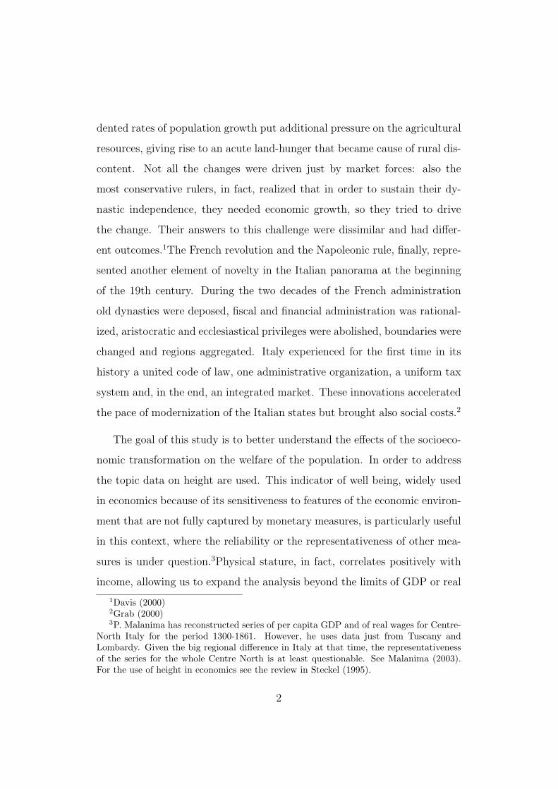
Umbria and Lazio (Figure 1.1, right panel).12All these areas are well repre-

sented in the sample, although the majority of the soldiers (40%) were born

in Romagna, and in particular in the legation of Bologna (Table 1.2).

10Unfortunately, information about the death was collected only for 60% of the presentsample.

11Archivio di Stato di Roma, sede succursale. Via Galla Placidia 93, 00159 Roma.12Before 1815, the papal dominions included also the small enclaves of Benevento and

Pontecorvo in southern Italy. Those enclaves were lost after the Vienna settlement.

5

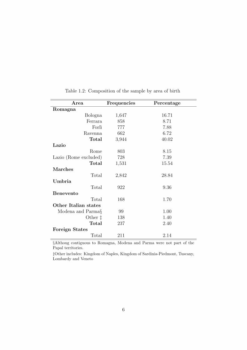
Table 1.2: Composition of the sample by area of birth

Area Frequencies PercentageRomagna

Bologna 1,647 16.71Ferrara 858 8.71

Forlı 777 7.88Ravenna 662 6.72

Total 3,944 40.02Lazio

Rome 803 8.15Lazio (Rome excluded) 728 7.39

Total 1,531 15.54Marches

Total 2,842 28.84Umbria

Total 922 9.36Benevento

Total 168 1.70Other Italian states

Modena and Parma§ 99 1.00Other ‡ 138 1.40Total 237 2.40

Foreign StatesTotal 211 2.14

§Althoug contiguous to Romagna, Modena and Parma were not part of thePapal territories.‡Other includes: Kingdom of Naples, Kingdom of Sardinia-Piedmont, Tuscany,Lombardy and Veneto

6

Figure 1.1: Location of the papal States and of their different regions

More than 400 different jobs were listed in the original registers. They

were aggregated in 15 categories according to the degree of skills required,

and the economic sector of activity (Table 1.3).13The sample is not totally

representative of the professional composition of the underlying population.

Indeed, although agricultural labourers represent the relative majority of

the recruits, their percentage is definitely too low if we consider that in

1911, when the structure of the population was much more industrial than

in the period here analysed, in the regions formerly belonging to the papal

dominions, individuals employed in agriculture represented on average more

13The professional groups are as follows:“Agricultural labourers” (peasants, fishers,shepherd); “Barbers”; “Elite”(practitioners, writers, students, land owners); “Food”(cooks, butchers, bakers, millers, pastry cooks); “Masons”; “Metal Workers” (blacksmiths,armourers, grinders); “Miscellaneous crafts” (hut makers, rope makers, tanners, painters,printers); “Retail” (innkeeper, fruiterer, shopkeeper); “Shoemakers”; “Skilled woodwork-ers” (carpenters, cabinet makers, turners, ebony carvers);“Soldiers”; “Tailors”; “Textile”(weavers, combers, spinners); “Unemployed”; “Unskilled” (domestic servants, coachmen,rag-and-bone men, launderers)

7

than 60% of the labour force.14

Nearly half of the sample is represented by skilled or partially skilled

craftsmen (the professions under the groups “Mason”, “Metal workers”, “Skilled

woodworkers”, “Shoemakers”, “Tailors”, “Textiles” and “Miscellaneous crafts”,

that include skilled artisans such as blacksmiths, carpenters, tanners or

weavers). A not negligible percentage (more than 7% of the total) is made

of recruits from the wealthy and/or educated classes (such as land owners,

practitioners, writers). Although the sample is not a random selection of

the underlying population, it still represents a wide range of social classes.

The following analysis, therefore, pertains a portion of the early 19th century

society in central Italy that goes beyond the poorest among the poor ones.

Table 1.3: Composition of the sample by profession

Profession Frequency PercentageAgricultural laborers 2,104 23.18Barbers 178 1.96Elite 686 7.56Food 374 4.12Masons 461 5.08Metal Workers 438 4.83Miscellaneous crafts 719 7.92Retail 229 2.52Shoemakers 1,204 13.27Skilled Woodworkers 431 4.75Soldiers 454 5.00Tailors 448 4.94Textiles 603 6.64Unemployed, note listed 169 1.86Unskilled 578 6.37Total 9,076 100.00

14According to the indstrial census of 1911, in Umbria and Marche agricultural workersrepresented respectively 74.3% and 71.6% of the labour force; in Emilia-Romagna theywere the 63.8% and in Lazio the 56.3%. See V. Zamagni (1987, 2006)

8

The professional composition of the sample does not change a lot over

the enrolment years covered, except for a constant decline in the percentage

of soldiers over time and an increase in the percentage of shoemakers and

textile workers (Table 1.4). The percentage of agricultural laborers enrolled

in the sample shows big fluctuations form period to period. As the labor

demand in the agricultural sector was subject to wider fluctuations from one

year to the other, according to the A look at the composition of the sample

by birth cohorts, does not reveal big changes either.

Table 1.4: Professional composition by triennium of enrolment

1814-1816

1817-1819

1820-1822

1823-1825

1826-1828

1829-1831

1832-1836

Agricultural laborers 17.80 25.05 24.69 18.25 26.72 29.19 16.65Barbers 2.60 1.76 1.43 1.43 2.08 1.96 2.12Elite 8.52 10.37 7.11 8.23 5.40 5.95 7.42Food 3.72 3.52 3.83 5.19 4.89 4.53 4.24Masons 5.56 6.37 4.72 7.51 5.17 4.05 3.18Metal Workers 4.84 3.88 3.77 3.04 5.23 6.62 6.36Miscellaneous crafts 7.75 7.58 7.95 6.98 7.87 7.84 8.87Retail 2.50 2.18 2.93 2.33 2.87 2.36 1.99Shoemakers 13.26 10.19 13.15 13.06 12.77 13.24 18.28Skilled Woodworkers 5.20 3.70 5.56 3.76 3.94 5.27 6.49Soldiers 7.70 7.70 5.20 5.37 2.70 2.91 1.99Tailors 5.81 6.25 3.11 5.55 3.49 4.73 5.70Textiles 7.85 5.76 5.68 7.33 6.41 5.88 8.87Unemployed 0.66 0.67 3.77 3.22 3.43 0.81 0.93Unskilled 6.22 5.03 7.11 8.77 7.03 4.66 7.02N 1,961 1,649 1,673 559 1,778 1,480 755

As many other military samples, also this one has to deal with the problem

of truncation from below. Height was in fact used to define physical ability

to serve the army. Although information on the official minimum height

requirement (MHR) applied is missing, a graphical examination of the data

reveals a clear truncation point (TP) for the infantry at 60 inches (5 feet,

9

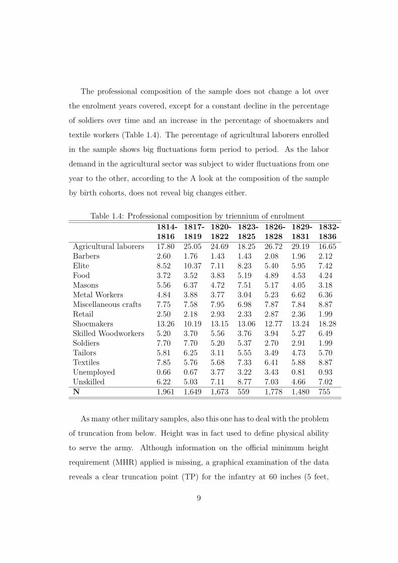
0 inches and 0 lines): figure 1.2 plots the height distribution for the whole

sample; height distributions for each enrolment year do not differ from this

one.15About 11% of the recruits aged 18 years or more, however, have a height

that is below 60 inches suggesting that the enforcement of the MHR was

variable. As a consequence, rather than having a clearly-truncated normal

distribution, with the left tail missing below the TP, we rather observe a

left tail increasingly deficient. Imposing a normal distribution on the height

histogram makes clearer this point: while the right tail fits well the normal

curve, on the left frequencies drop off too sharply.

Figure 1.2: Height distribution. Soldiers aged 18 or more. Row data

050

010

0015

00F

requ

ency

48495051525354555657585960616263646566676869707172737475Height in inches

Observation number: 8454

Figure 1.2 and figure 1.3 reveal also that data suffer from rounding to

the nearest whole-inch and from heaping. The latter problem is particularly

evident inasmuch as the observations at 60 inches are abnormally frequent.

15For the enrolment year 1814, the graphical examination does not show a clear TP:height distribution in this case appear to be pretty normal or with a TP set at 62 inches.The resulting distribution, however, can be the outcome of the small number of soldiersenrolled in that year (only 158) rather than in an application of a higher MHR, especiallyin a war year as 1814.

10

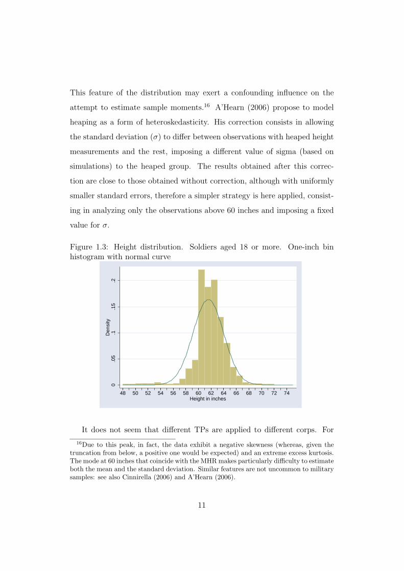
This feature of the distribution may exert a confounding influence on the

attempt to estimate sample moments.16 A’Hearn (2006) propose to model

heaping as a form of heteroskedasticity. His correction consists in allowing

the standard deviation (σ) to differ between observations with heaped height

measurements and the rest, imposing a different value of sigma (based on

simulations) to the heaped group. The results obtained after this correc-

tion are close to those obtained without correction, although with uniformly

smaller standard errors, therefore a simpler strategy is here applied, consist-

ing in analyzing only the observations above 60 inches and imposing a fixed

value for σ.

Figure 1.3: Height distribution. Soldiers aged 18 or more. One-inch binhistogram with normal curve

0.0

5.1

.15

.2D

ensi

ty

48 50 52 54 56 58 60 62 64 66 68 70 72 74Height in inches

It does not seem that different TPs are applied to different corps. For

16Due to this peak, in fact, the data exhibit a negative skewness (whereas, given thetruncation from below, a positive one would be expected) and an extreme excess kurtosis.The mode at 60 inches that coincide with the MHR makes particularly difficulty to estimateboth the mean and the standard deviation. Similar features are not uncommon to militarysamples: see also Cinnirella (2006) and A’Hearn (2006).

11

example grenadiers are, as expected, generally taller than infantrymen, that

is, their height distribution is shifted to the right. However the truncation

appear to be always at 60 inches, indicating that this corp was made with

the tallest among the recruits that were accepted into the army (Figure 1.4).

The same applies for the hunters the other special corp of the papal army.

Figure 1.4: Height distribution. Grenadiers aged 18 or more. Row data

020

4060

80F

requ

ency

51 52 53 54 55 56 57 58 59 60 61 62 63 64 65 66 67 68 69 70 71Height in inches

Observation number: 976

Due to sample truncation, a standard OLS approach fails to give con-

sistent and unbiased estimates. Among the several methods that have been

proposed to correct for this problem, truncated maximum likelihood (TML)

regression has proven to be the most effective, and it will be used to in the

following analysis.17

Given that the reported heights appear to be rounded to the nearest

whole-inch, the TML estimator requires adjustment, as long as the effective

TP does not coincide with the apparent TP. If, as it seems to be the case, the

17A review of the principal methods used to correct for truncation in height samples ispresented in Komlos (2004). See also A’Hearn (2004)

12

height of 59.5 inches tall recruits was rounded up and reported as 60 inches,

the former and not the latter represents the effective truncation point. A

simple modification rule consists in applying a TP equal to the apparent one

(60 inches in this sample) minus one-half the rounding interval (a quarter-

inch here). Subject to this rule, the TML estimator has been shown to be

unbiased with rounded data.18 In the following analysis, therefore, a TP of

59.75 inches has been applied.

Another regression is also performed using a TP of 60 inches (so that

all the observation below or equal to this threshold are discarded from the

analysis) and constraining the standard deviation σ to be equal to 6.86 cm,

a value suggested as a plausible figure for male, based on data for modern

populations. Alongside the attenuation of the heaping problem mentioned

before, this approach offers greater sampling precision when compared with

unconstrained estimations, regardless of any bias introduced by incorrect

restrictions σ.19

1.3 Regression results

1.3.1 Cross-sectional effects

Table 1.5 presents the estimated results. As already mentioned, height was

recorded in feet, inches and lines. In Europe in the 19th century, several

different ”feet” were used, each one with a different relation with the linear

meter. The Austrian foot, for example, was equal to 31.6 cm, while the

French foot (also known as Parisian foot) used to be equal to 32.5 cm until

18See Komlos (2004) and A’Hearn (2004)19A’Hearn (2004)

13

1812, when it was set to 33.3 cm. The foot was a common unit of measure-

ment also in the Italian states. Its length varied enormously not only form

state to state, but very often also from town to town.20As the original sources

do not specify which foot was used to measure the soldiers, the conversion

in centimetres has to be inferred. A possible strategy consists in convert the

MHR applying different standards to see if the derived measure is plausible

or not.

The papal army could have adopted as unit of measurement the “Roman

foot”, equal to 29,8 centimetres.21 The MHR would have then been in this

case equal to 149 centimetres. Such a small lower bound is in line with the

one adopted few decades later in the new kingdom of Italy.22 However, the

height of soldiers aged 18 years or more would range between 120 and 180

centimetres, with 2% of the recruits shorter than 138 cm a too lower bound

to be credible. Transforming the regression results with this coefficient would

lead to an estimated mean of less than 150cm, a value that does not compare

well with the 165 cm of contemporaneous Northern Italians or with the 162

cm of Italians born only few decades later.23 Furthermore, the Roman foot

was divided in 16 once (ounces) and not in 12 feet and 12 lines as in these

registers.

An alternative can be represented by the “Austrian foot”. After Napoleon’s

defeat, in fact, the Congress of Vienna made Austria the new protector of

the papal states. The Austrian army remained throughout the territories

20For example in Bologna 1 foot = 38 centimetres while in the other areas of Romagna1 foot = 29,8 centimetres. See C. (1880)

21Martini (1883)22The newly created Italian army in 1863, in fact, adopted a MHR of 150 cm (Arcaleni

1998, 2006)23For Northern Italians see A’Hearn (2003); for the Italians born in 1854 see Ar-

caleni(2006)

14

and the Vienna settlement allowed Hapsburg troops to occupy key papal

fortresses.24 Traditionally, the papal army used to adopt the military or-

ganization, weapons and uniform of the army of the allied foreign power.

It could be the case, than, that among the other features, the papal army

adopted also the Austrian MHR, and in particular Austrian instrument to

measure the height of the recruits. In this case, one foot equals 31.6 cm

(and 1 inch = 2.63 cm); the MHR would then be equal to 158 centimetres.

The same lower threshold was applied for the recruits in the Austrian army

in the Italian regions of Lombardy and Veneto.25 Until 1840, however, in

the Austrian measurement system, one line represented a quarter inch and

only after 1840 it represented one-twelfth inch. Despite the big percentage

of observations with a recorded line equal to zero (41% of the sample), no

concentration around specific numbers can be appreciated.26 In other words,

the lines appear to represent always one-twelfth inch. Given that the recruits

collected in this sample entered the army before 1840, the Austrian foot does

not seem a plausible candidate.

A last opportunity could be represented by the “French foot”. The papal

army, in fact, could have kept some of the military practices adopted by the

French army, which ruled over those territories until 1814. This choice could

have been driven by practical reasons: the military staff of the papal army

could have served and thus have being trained in the Napoleonic army, or they

could have used measurement instruments left by the French. The French

foot, as it was used before the decimalized system of units of 1799, was equal

to 32.5 cm (1 inch = 2.71); its use was abolished during the French revolution,

but, given the difficulties of using the newly introduced metric system, in

24Laven (2000).25A’Hearn (2003)26The distribution does not change considering different enrolment years

15

1812 a system of measurement (mesures usuelles) was introduced that acted

as a compromise between traditional and new measures. According to the

mesures usuelles, a foot was equal to a third of a meter (33.3 cm, and therefore

1 inch = 2.77 cm). If the papal army in 1814 adopted the new French foot,

then, the latter coefficient is the one that it has to be applied, leading to a

MHR equal to 166.6 centimeters; it is also likely, however, that the papal

army could have used the old French foot if this was the standard adopted

during the French rule and even before.27 In this case the MHR would be

equal to 162.5cm. MHRs pretty high in comparison to the average height of

the population were not infrequent in Europe at that time.28 In the case of

Italy, 166 centimetres appear to be higher than the average height of Italian

men born in 1854, and higher than the estimated height for Northern Italians

born in the 1830s, while 162.5 cm are quite close to the average height of

Italians born in 1854 and slightly below that of Northern Italians.29 If the

French foot was then the standard applied, the TP should be on the right

of the height distribution or, at best, it could coincide with the mean of

the population. The graphical analysis of the height distribution (figure 1.2)

would support this hypothesis. Furthermore, the relative high number of

observations below the TP is coherent with a MHR fixed at a very high

level, making the French foot a very plausible choice. Finally, the estimated

mean would be close to 163 cm, a value that is comparable to Arcaleni’ and

A’Hearn’s estimates.

27Actually, this could be the case. The analysis of a small sample of papal soldiersin 1802, reveal an identical height distribution and an identical MHR. One may suspect,then, that the papal army continued to adopt its own foot (based maybe on the Frenchfoot), irrespectively of what happened in France.

28The Saxonian army, for example, applied during the 18th century a MHR of 72 Saxo-nian inches (circa 170 cm) (Cinnirella (2006)); the British army in the first decades of the19th century a MHR of 65 British inches (circa 165 cm) Cinnirella (2007); the Austrianarmy applied before 1795 a MHR of 63 Austrian inches (165.9 cm) (A’Hearn (2003))

29See Arcaleni (2006) and A’Hearn (2003)

16

The “French foot” as it was before the mesures usuelles, is then applied

to convert the estimated coefficients in centimeters. The first model applies

a TP of 59.75 inches (161.8 cm) and considers younger and older soldiers

together. The second model applies the same TP, but restrict the analysis

only to soldiers aged 20 years or more. The reason for this restriction is

that the higher percentage of teen-agers (whose growing process was not

completed) in the later birth cohorts may lead to a spurious downward trend

in height. The third model, finally, accounts for the heaping problem fixing

a higher TP (60 inches, 162.5 cm) and constraining the standard deviation

to be equal to 6.86 cm (2.53 inches if using the French foot).

Table 1.5: Truncated Maximum Likelihood Estimate

Variable Model 1 Model 2 Model 3

Birth cohort

- 1785 1.243∗ 1.619∗∗ 0.953†

1786 - 1790 0.141 0.525 -0.119

1791 - 1795 0.287 0.761† 0.230

1796 - 1800 Reference Reference Reference

1801 - 1805 -1.048∗∗ -0.498 -0.135

1806 - 1810 -3.068∗∗ -1.947∗∗ -0.690

1811 - 1815 -3.055∗∗ -1.725∗∗ 0.003

1816 - -5.210∗∗ -5.105∗ -5.430∗

Region of birth

Bologna Reference Reference Reference

Ferrara -0.138 -0.252 -0.414

Forli 0.393 0.290 0.363

Continued on next page...

17

... table 1.5 continued


Ravenna 0.130 0.046 0.160

Lazio 0.073 -0.041 0.818

Roma 0.295 0.566 1.105

Marche -0.179 -0.236 -0.219

Umbria -0.701 -0.341 0.122

Benevento -1.942† -2.944∗ 0.295

Urban birth

If born in a mountain area 0.141 0.298 0.011

if born in a city with more

than 50,000 inh.

-1.408∗∗ -1.533∗∗ -1.099†

if born in a city with a port -0.823 -0.209 0.631

if born in an administrative

center

-0.802∗ -0.737† -0.330

if born in a town (more than

15,000 inh. in 1861)

-0.236 -0.016 0.306

if born in a rural place and

emigrated to a town

-1.159∗∗ -1.062∗ -0.636

Age dummies

age 15 -3.631† - -

age 16 -3.231∗∗ - -

age 17 -3.859∗∗ - -

age 18 -2.792∗∗ - -

age 19 -1.124† - -

age 20 0.041 0.531 -0.008


18



age 21 Reference 0.485 -0.214

age 22 -0.864 -0.439 -0.991†

age 23 -0.282 0.246 -0.414

age 24 - 49 -0.720 Reference Reference

age 50 0.401 1.064 0.937

Military Grade

simple soldier Reference Reference Reference

officer 1.541∗∗ 1.511∗∗ 1.397∗∗

musician -1.665 -0.317 0.379

head quarter 4.636∗∗ 3.653∗∗ 3.821∗∗

grenadier 8.029∗∗ 7.750∗∗ 6.299∗∗

Provenance

volunteer Reference Reference Reference

deserter 0.311 0.539 0.959

prisoner -0.043 -0.217 -0.165

Professional categories

Agricultural laborer Reference Reference Reference

Barber 2.077∗ 1.389 0.972

Elite 3.564∗∗ 3.461∗∗ 2.898

Food 0.482 0.154 -0.097

Mason 0.290 0.287 0.292

Metal Workers 1.698∗∗ 1.094† 0.444

Miscellaneous crafts 1.281∗ 0.934† 0.463

Retail 1.259 0.785 0.598


19



Shoemaker 1.148∗ 0.829† 0.376

Skilled Woodworkers 1.070 0.921 0.263

Soldier 2.860∗∗ 2.635∗∗ 2.166∗∗

Tailor 0.737 0.458 0.450

Textiles 1.332∗ 1.416∗ 1.257†

Unemployed, not listed 1.099 0.528 0.826

Unskilled 0.658 0.734 0.720

Intercept 163.441∗∗ 162.802∗∗ 164.010∗∗

Standard Deviation 6.775∗∗ 6.597∗∗ 6.859

N 7,821 6,035 5,109

Significance levels : † : 10% ∗ : 5% ∗∗ : 1%

Data in original measures (inches)

A number of cross-sectional patterns may be highlighted. No signifi-

cant differences between birth regions are evident in any of the three model

specifed, with the only exception of Benevento. Soldiers born in the enclave

of Benevento were 0.71 inch (1.9 cm) shorter than soldiers born in the area

of Bologna. When the analysis is restricted to adults, the difference increases

to 1.075 inches (2.9 cm). Both genetics and economics may help in explain-

ing this result. Southern Italians, in fact, are also nowadays shorter than

northern Italians and that could be due to a different pool of genes. From

an economical point of view, the status of small enclave in southern Italy en-

joyed by Benevento, may have been detrimental for the biological standard

20

of living. In particular, the small extension of the territory and therefore of

the land available for agriculture, may have force Benevento’s inhabitant to

import foodstuff from the surrounding Kingdom of the two Sicilies. Given

the custom tariffs in place between the two states, food may have been more

expensive in Benevento than in other parts of the Papal states, reducing the

biological welfare of the population. The small number of observations (only

193 recruits from Benevento), however, calls for caution in the interpretation

of this result.

Although not significant at usual levels, the signs on the coefficients on

the other birth regions are as expected, with the only exception of Lazio and

Rome that enjoy a positive premium. Soldiers from area that includes the

mouth of the Po river (the Legation of Ferrara) were 0.038(0.10) inches(cm)

shorter, difference that increases to 0.073(0.19) inches(cm) when only the

adults are considered. This result may be the consequence of the poor disease

environment of those regions, characterized by a geographical conformation

(low-lying areas with stagnant water) particularly favourable for the breeding

of the malaria mosquito.30 The negative sign on the height coefficients for the

conscripts born in Umbria and Marche is also consistent with the economic

backwardness of these regions, with an agricultural system based mainly

on sharecropping. An height penalty for those regions in comparison with

the Emilia-Romagna, is highlighted also in Arcaleni (2006) for the cohort of

Italians born in 1927.31

The lack of significant differences in height (that persists even using al-

ternative territorial definitions) between areas with very few interaction and

with marked differences in both the economic and the natural environment,

30See Braglia (1962), Zamagni (1993), pp. 48-49.31See Arcaleni (2006), fig.3 p.30 and tab.1 p.31

21

is somehow surprising. Most probably, the similarities among these areas

were much bigger than it is usually described. In particular, they could have

shared a common structure of the society with welfare nets (such as guilds or

parishes) that may have helped to working class to achieve the same degree

of access to the resources (particularly food), irrespectively of the different

agrarian systems.

Being born in a metropolis (namely in the city of Rome or Bologna) im-

plies a significant height penalty of half inch (circa 1.57 cm). The difference

for those born in other urban areas (such as, portal cities, administrative

centres or in medium size towns32), is still negative but generally not signif-

icant. Height penalties for a urban-birth is not a new result for historical

populations.33 Different factors can explain this result. Cities, for example

may have enjoyed a worse disease environment. Despite public health mea-

sures (such as sewers) and the availability of hospitals, the high population

density in urban environments eases the transmission of diseases.34 A second

reason why the urban environment could lead to shorter heights is related

with the higher cost of food. Being specialized in manufacturing and service

sector activities, urban inhabitants had to “import” food from the country-

side. If this connection was not working properly, foodstuff in cities may

have been more expensive or, for the same price paid in the countryside, its

quality may have been lower. Given that a height penalty is observable only

for big cities and administrative centers, we could argue that is the density

of population (and therefore the worse disease environment) the main factor

32In this study a medium size town is defined as a municipality that in 1861 had 15,000or more inhabitants. The urban share in this municipalities at the time of unification was19%.(Santis (2002)) This implies that those towns had at least 3,000 inhabitants. All theadministrative centres are also medium size towns.

33Such penalty is found in Northern Italy (A’Hearn (2003)), Bavaria (Baten and Murray(2000)), Cinnirella (2006).

34See for example Anderson and May (1991), Arita et al. (1986).

22

affecting negatively height in cities and not the higher food price. If that was

the case, in fact, we would have expected a significant height penalty also in

the other urban environments (portal cities and medium size towns) that had

to import food as well from the countryside.This result and its interpretation

would be also coherent with the fact that in Italy the degree of urbanization

was much higher than the European average since the 16th century.35 This

long tradition of urbanization may have strengthen the ties between towns

and countrysides and improved the commercial channels between the two, so

that no significant differences in food availability may have been noted.

Emigration from the countryside to cities appears to be detrimental for

the biological living standards, leading to a height penalty of circa 0.4 inches

(1.08 cm). The ignorance of the timing of the movement (if done during

the childhood, following the family, or later searching fortune), however, is a

confounding factor. In particular, it does not possible to know if this result

is genuine or if it is the outcome of a self-selection of the short countrymen

into the migration stream to the cities.

Recruits born in mountainous areas appear to be taller that the others,

although the coefficient is not significant. As expected, the lower density of

population in these areas, the colder climate, less favourable for the breeding

of viruses and bacteria, and the relative isolation they enjoyed, preventing

their food prices to fluctuate due to external market changes, affected posi-

tively the biological standard of living of those recruits.

In line with similar samples, the estimated age effects show an annual

increase in height from age 15 through the mid 20’s, with a global increase of

35In Italy the share of individuals living in cities never went below 12% since the 16thcentury, whereas in the rest of Europe this percentage was equal to 5% 1500 and 10% atthe beginning of the 19th century. See Santis (2002)

23

about 4 centimetres.36 The magnitude of the coefficients is credible, although

the height gains are pretty small making the central Italians more similar to

the Bavarians or the Saxonian rather than to Northern Italians.37 Further-

more, while growth for the latter group appear to be prolonged well beyond

the age of 20, in this sample, the height of recruits older than 20 years is not

statistically different from the height of 24 years old soldiers. The pubertal

growth of these individuals, then, does not appear to be delayed in time, a

results that may suggest an adequate nutritional status during childhood.

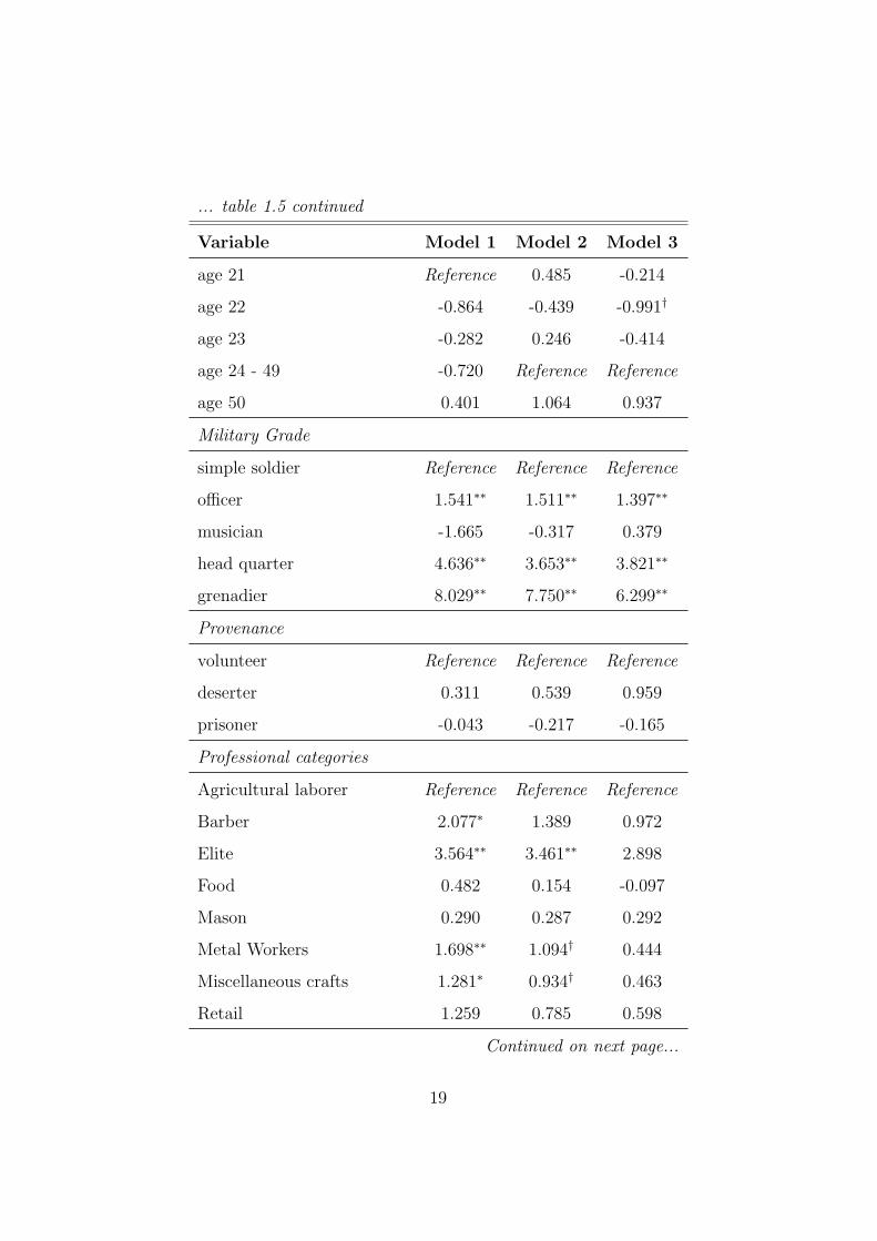
The estimated occupational effects on height reveal a certain degree of

inequality in the distribution of wealth in the papal states. Recruits’ occu-

pation, in fact, can be considered a proxy for the social status of the parents

and thus of the nutritional status in the earliest years (the most crucial in

determining final height). If access to food and to health care is very different

between social classes and if the degree of social mobility is low (so that is

unlikely that the offspring of a poor family ends up in a better status and

vice versa), significant height differences between various professional groups

are expected. The obtained results are coherent with this picture. Agricul-

tural labourers are at the bottom of the scale, with all the other professional

groups enjoying an height premium. At the other extreme of the scale there

are the middle and upper class (the group “Elite” that includes property

owners, merchants and professions requiring some degree of education) and

the soldiers, with an height advantage of 1.3 inches (4.2 cm) and 1.4 inches

(3.6 cm) respectively. Skilled workers - such as shoemakers, metal workers

36See for example A’Hearn (2003), A’Hearn (2006), Baten and Murray (2000), Cinnirella(2006)

37For Lombardy and Veneto, A’Hearn (2003) estimates an increase from age 16 to age24 of more than 8 centimetres. Using a different sample, A’Hearn (2006) obtains similarincrease of about 7 cm. For Bavaria, Baten and Murray (2000) estimate a differencebetween 18 years old and 24 years old of 3.5 cm while for Saxony, Cinnirella (2006) findsan increase form age 16 to age 22 of 3 centimetres.

24

or craftsmen, enjoy as well a statistically significant height premium. In con-

trast with what expected, but in line with the results for northern Italians,38

recruits with a preferential access to food (such as butchers, cooks, bakers)

are not significantly taller than agricultural labourers.

The unequal distribution of wealth is somehow confirmed by the signifi-

cant height premium enjoyed by officiers and members of the head quarter.

Education, in fact, was a rewarded merit in order to make advancements in

the military ranks. As a results, officers came mainly from the middle and

upper classes that had access to education.39

1.3.2 Time trends

The estimated time trend, show a clear downturn in height in the first fifteen

years of the 19th century, with a decline of 1.9 inches (5.1 cm) from 1796 to

1815. The downward trend is confirmed also when the analysis is restricted

only to soldiers aged 20 years or more (model 2).40 It seems, then, that the

trend is genuine and not spuriously imparted by the higher percentage of

teenagers in the last two birth-cohorts. A declining height trend in the last

quarter of the 18th century is a feature common to many other European

countries such as Bavaria, France, Britain, the Habsburg empire, Saxony,41

which experienced a strong demographic growth the put under pressure agri-

38A’Hearn (2003).39Not surprisingly, more than 17% of the officers and almost 22% of the members of the

head quarter belong the “Elite” group, whereas this professional category represents onlya bit more than 7% of the whole sample.

40Similar results are obtained also when other age restrictions are used (excluding thesoldiers up to 21 years, up to 22 years, up to 23 years).

41For Bavaria see Baten (1999); for France see Weir (1997), Komlos (1994); for Britainsee Komlos (1993); for the Habsburg empire see Komlos (1985), Komlos (1989); for Saxonysee Cinnirella (2006). For an overview of height trend in Europe in 18th century see alsoKomlos and Cinnirella (2005).

25

cultural resources, boosting up the prices for food.

However, while in the rest of Europe much of the decline was accomplished

by the early 1800s, in the papal states average height continued to fall well

into the 1820s, as depicted in figure 1.5. As in Saxony, also in the papal states

the years of the Napoleonic rule coincide with a sharp decline in height. The

turmoil following the French victories in Italy, the increased tax burden and

the administrative reforms that characterized these years may have had a

negative effect on the biological standard of living of the local population.

Figure 1.5: Height trend in the papal states and in other European countries.Soldiers aged 20 years or more

Sources: Papal states: weighted average of the regional and professional coefficientsfrom Tab. 1.5, model 2; England: Komlos (1993), Tab. 6, height of soldiers in the Britisharmy, average index for all age groups multiplied by base (167.6 cm); Northern Italy:A’Hearn (2003), tab.2; Saxony: Cinnirella (2006), Tab. 2, model 1 (Adults); Hungary:personal communication from Komlos

Other quantitative evidence points out a worsening of the living standards

in these decades. Malanima’s recent estimates, in fact, highlight a growth in

aggregate terms of the GDP in Central and Northern Italy, financed primarily

26

by a decline in the standard of living of the population.42 Per capita GDP

reached the minimum over the last six centuries in the first two decades of

the 19th century. In the same period, both agricultural and urban wages

decreased while prices increased, reducing drastically the real wages of the

working class. The estimated height trend in the papal states is coherent

with the story that emerges from Malanima’s estimates (Figure 1.6 and 1.7:

height trend on the right axis).

Figure 1.6: Height trend for soldiers aged 20 years or more and per capitaGDP index in Central-Northern Italy (1860 = 100)

158

160

162

164

Hei

ght i

n ce

ntim

eter

s

9698

100

102

104

106

Per

cap

ita G

DP

inde

x

1 2 3 4 5 6 7 8years

before 1785

1786 − 1790

1791 − 1795

1796 − 1800

1801 − 1805

1806 − 1810

1811 − 1815

1816 and later

years

Per capita GDP index Height in centimeters

Source: Height trend: present estimates; per capita GDP index: Malanima (2003),Ap-pendix 1

Given the differences not only in the kind of political rule the Frenchmen

exerted in the papal states but also in the economic system that characterised

the different areas, a separate height trend for each region is then estimated

and plotted in figure 1.8; for comparison, the height trend for the Northern

regions (Lombardy and Veneto) is also plotted. The height trend of the last

42See Malanima (2003)

27

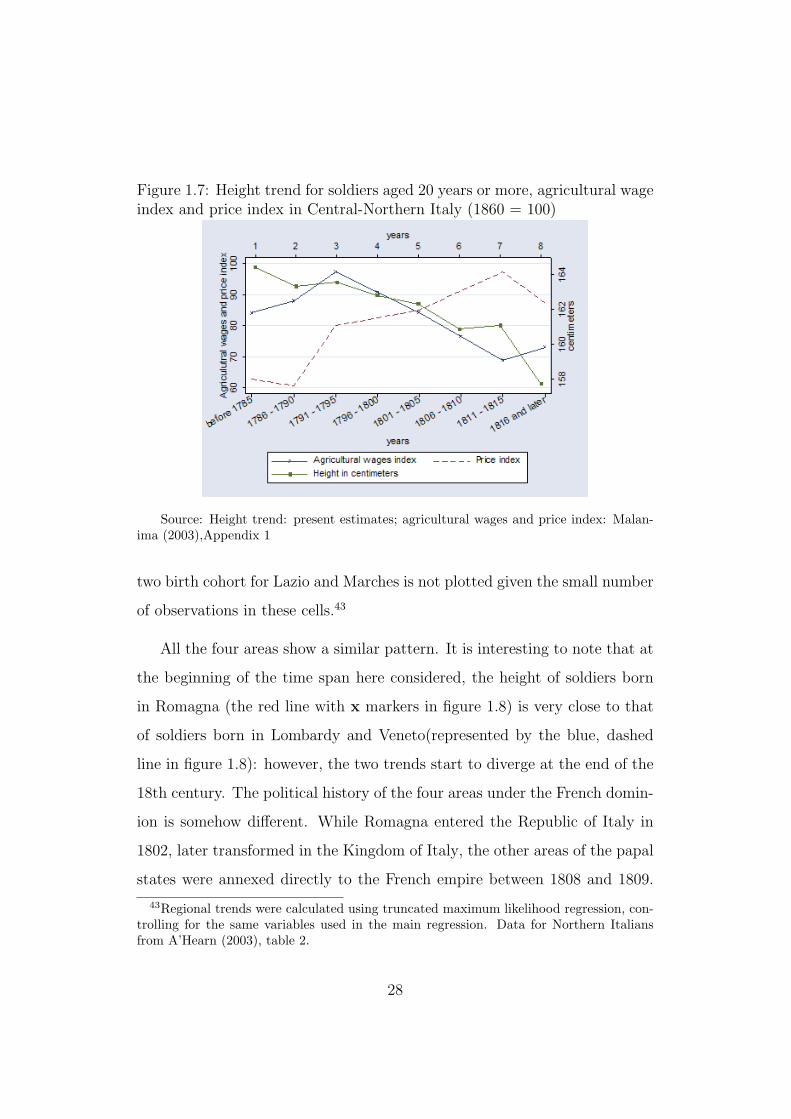
Figure 1.7: Height trend for soldiers aged 20 years or more, agricultural wageindex and price index in Central-Northern Italy (1860 = 100)

Source: Height trend: present estimates; agricultural wages and price index: Malan-ima (2003),Appendix 1

two birth cohort for Lazio and Marches is not plotted given the small number

of observations in these cells.43

All the four areas show a similar pattern. It is interesting to note that at

the beginning of the time span here considered, the height of soldiers born

in Romagna (the red line with x markers in figure 1.8) is very close to that

of soldiers born in Lombardy and Veneto(represented by the blue, dashed

line in figure 1.8): however, the two trends start to diverge at the end of the

18th century. The political history of the four areas under the French domin-

ion is somehow different. While Romagna entered the Republic of Italy in

1802, later transformed in the Kingdom of Italy, the other areas of the papal

states were annexed directly to the French empire between 1808 and 1809.

43Regional trends were calculated using truncated maximum likelihood regression, con-trolling for the same variables used in the main regression. Data for Northern Italiansfrom A’Hearn (2003), table 2.

28

Figure 1.8: Regional height trends

155

160

165

170

Hei

ght i

n ce

ntim

eter

s

before 1785

1786−1790

1791−1795

1796−1800

1801−1805

1806−1810

1811−1815

1816 and later

Birth cohort

Northern Italy RomagnaMarche LazioUmbria

Source: Romagna, Marche, Lazio and Umbria: present estimates; Northern Italy:A’Hearn (2003), Tab.2

Napoleon’s transformation of the Republic and Kingdom of Italy surpassed

that of any other part of Italy, inasmuch as French domination here lasted

longer than in any other part of the peninsula.44Old ecclesiastic privileges

were dismantled and most of the Church lands were sold. A central au-

thority, fairly efficient and reliable, was created. Eliminating all the internal

tariffs and making use of a uniform commercial code, a single currency and

common measures, the French administration succeeded in the creation of a

unified market between areas formerly belonging to several different states.

Furthermore, the extensive construction of roads and waterways improved

the communications in the area. Landowners mainly benefited from these

reforms, as they purchased most of the confiscated Church land, they enjoyed

a bigger market and a rise in the prices for grain, rice and wine. The paralysis

of commerce and the decline of the textile industry due to the Continental

44Grab (2000)

29

blockade, shifted resources into an already rich and capitalistic agriculture,

encouraging further its growth.

The other three areas that were annexed directly to imperial France.

The French legal code (the Code Napoleon) and taxation were introduced;

convents were dispersed, many Church lands sold and some public works

were initiated. However, the reforms were less incisive than in Romagna,

partially because of the shorter time these regions were under the French

administration, partially because, being directly ruled by French prefects,

there was no opportunity (as on the contrary happened in Romagna) to create

a new class of local administrators introduced to the modern administrative

practices and institutions.

The situation for the lower classes, however, appears to have been heavy

in all the four areas, irrespectively of the different political rule and of the

deepness of the reform process. The estimated regional height trend reveal

that higher taxes on consumption goods and the consequences of the agricul-

tural commercialization affected negatively the biological standard of living

in similar ways.

1.3.3 Sensitivity analysis

In section 1.2 we already discuss about the problem of heaping. The abnor-

mally high frequency of observations at 60 inches may exert a counfounding

influence on the attempt to estimate sample moments. To account for that,

another model has been estimated using only the observations above the ap-

parent TP of 60 inches. One disadvantage of this strategy consists in the

reduction of the sample size. However, even after discarding all the obser-

vation below or equal to 60 inches, sample size does not appear to be a

30

major problem. A second problem introduced by applying a higher TP is

the increased variability of the TML. In particular, as the truncation point

approaches the mean and only the right tail of the distribution is observable,

it could be difficult to distinguish between distributions with different means

and standard deviations.45 For this reason we constrained the standard de-

viation of the distribution to be equal to 6.86 cm, a value suggested as a

plausible figure for male, based on data for modern populations.46

Model 3 in table 1.5 reports the estimated results. With only few excep-

tions, the height coefficients loose their significance. The only results that

remain significant at standard levels are the height penalty for the recruits

born in big cities, and the height premium for officers and members of the

head quarter and, among the professional groups, for soldiers. The sign of

the coefficients is unchanged in the vast majority of the cases; the magnitude,

however, is sensibly reduced.

1.4 Mortality analysis

As already mentioned in section 1.2, the registers here collected reported also

the date of death of the recruit, in case he died while being in the army. The

availability of this information allows us to perform a mortality analysis.

For all the recruits but one (who sunk), the registers report the sentence

“died in the hospital”. In other words, it seems that none of the recruits died

on the battlefield, but rather because of diseases although the information on

the exact cause of death is missing. An estimation of the survival probability,

45A’Hearn (2004)46A’Hearn and Komlos (2003)

31

then, can offers further information on the diseases environment in central

Italy in the first half of the 19th century, and on how it changed according

to different socio-economic characteristics.

1.4.1 Theoretical framework

Some aspects of survival analysis data, such as censoring and non-normality,

generate great difficulties when trying to analyse the data using traditional

linear regression. For this reason, special methods, able to deal with such

problems, have been developed and will be used in this section. An essential

tool in this kind of analysis is the hazard rate. This quantity summarizes

the concentration of exit times at each instant, conditional on survival up

to each point,47 allowing to model explicitly the instantaneous probability of

experiencing a certain event (death, in our case) as depending on the time

already spent in the initial state (being alive in our case). Other indicators

of interest, such as the density function fi or the survivor function Si , can be

derived from the hazard rate.

What is of major interest, here, is to investigate how some socio-economic

conditions modify the mortality experience of the individuals. For this reason

we want the hazard rate to depend not only on the survival time, but also

on a set of individual characteristics Xi . In a discrete time setting (that is,

considering intervals of time rather than a continuum of instants) as the one

in this paper, the hazard rate hi,t = Pr(t − 1 ≤ t | T ≥ t − 1, Xi) is the

probability of dying in the time interval [t − 1, t) (where t measures age in

years), conditional on survival up to time t − 1 and on a set of individual

covariates Xi . The best way to estimate the effect of on mortality is to use

47For this definition, see Jenkins (2004)

32

maximum likelihood (ML) methods.

The likelihood function used, has to be appropriate for the type of process

that generated the data, that is the type of sampling from the underlying

population of soldiers. To understand that, the nature of the registers and

of the selection of soldiers from registers has to be clarified. As already men-

tioned in section 1.2, each register pertain to a specific regiment of the papal

army; it “born” with the regiment, was kept updated until the regiment was

in place, and it was closed when the regiment was disbanded. Each soldiers

that joined the regiment, as a volunteer or as a soldier transferred to the

current regiment from another one, was recorded, irrespectively on the time

he effectively served up in the army. Given that the registers were randomly

chosen, we have then a random sample of individuals from the stock of those

who survived up to the age at which they entered the regiments sampled.48

This kind of sampling (called in the literature stock sampling) causes a clear

sample selection problem: by construction, in fact, all the individuals that

were born in the same years as the sampled ones, but that died before the

regiment was created are excluded form the sample. These observations are

not missing at random, as only individuals with higher survival times have a

greater chance of selection. The implemented likelihood function, therefore,

has to correct for this bias.

Another aspect that is relevant for the analysis is the censoring time ci,

that is the time after which we stop following the observation. A fundamental

assumption in this kind of analysis, in fact, is that, conditional on the set of

covariates X, the duration (that is the total number of years spent alive) is

48It is worth to remark here that this is not a random sample of the whole populationthat survived up to a certain age, but is a random sample of the population of soldiers,that is of all those individuals that entered or were interested in entering the army.

33

independent of ci. To check if this assumption holds, we have to consider the

structure of the data we have. While for those who died we know exactly the

entire length of their spell (that is, how many years they lived), for all the

others the exact age of their death is unknown and therefore they are right-

censored. There are several reasons why these observations may be censored:

i) the soldier deserted at a certain point of time; ii) the soldier served for

five years (the time stated in the contract they signed) and then left the

army; iii) after five year the soldier decided to remain in the army and he

survived the disbandment of the regiment.49If we consider the observations

for which we do not know the year of death as censored at the interview

date (that is the last time they were observed alive) and we use all the

other observation with the completed spell, it is likely that the conditional

independence assumption is violated. It could be the case, in fact, that the

decision of remaining in the army was driven by some unobservable factors

that affected also longevity. For example, if those with better (worse) health

conditions were also more likely to stay longer in the army (so that their death

is more likely to be observed because the time they were under observation

was longer), then survival time is not anymore independent on the censoring

point and we would overestimate (underestimate) the survival probability.

The conditional independence assumption clearly holds when ci is constant

for all the individuals. If the percentage of soldiers that successfully deserted

(that is, that managed to desert and that was not captured after that) is

negligible, then all the soldiers in the sample were in the army for at least

five years. We can therefore consider all the observations for which we do not

know the date of death as well as the spells that ended after more than five

49Another possibility would be that the soldier was transferred to another regimentbefore the disbandment of the observed one. No such cases were reported in the collectedregisters.

34

years from the entrance into the regiment as right-censored at the age they

had when they entered the regiment plus five years. All that given, we can

now specify the likelihood contribution of a censored spell at time j. This is

is given by the discrete time survivor function :

c£i = Si(j) =j∏

k=1

(1− hi,k) (1.1)

while the contribution of an uncensored spell is given by the discrete time

density function:

u£i = fi(j) = hi,j · Si(j − 1) =hi,j

1− hi,j

j∏

k=1

(1− hi,k) (1.2)

If diis a censoring indicator equal to 1 if duration i is uncensored and 0

otherwise, the likelihood for the whole sample is:

£ =N∏

i=1

(c£i)di(u£i)

1−di =N∏

i=1

hi,j

1− hi,j

j∏

k=1

(1− hi,k)

j∏

k=1

(1− hi,k)

(1.3)

Simplifying the above expression and taking the logarithm, we obtain the

log-likelihood function:

L =N∑

i=1

di log

(hi,j

1− hi,j

)+

N∑

i=1

j∑

k=1

log(1− hi,k) (1.4)

Introducing a binary indicator variable yi,k such that :

if di = 1 ⇒ yi,k = 1 in the last year of individual i ’s life, and yi,k = 0

otherwise;

35

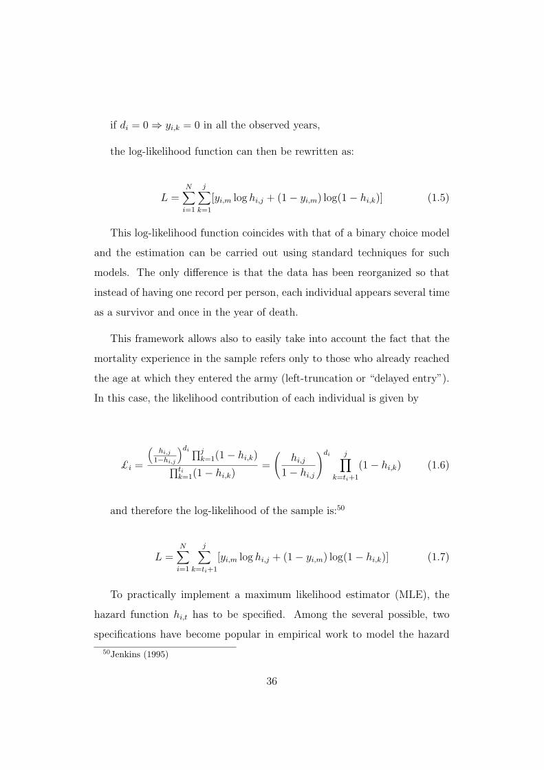
if di = 0 ⇒ yi,k = 0 in all the observed years,

the log-likelihood function can then be rewritten as:

L =N∑

i=1

j∑

k=1

[yi,m log hi,j + (1− yi,m) log(1− hi,k)] (1.5)

This log-likelihood function coincides with that of a binary choice model

and the estimation can be carried out using standard techniques for such

models. The only difference is that the data has been reorganized so that

instead of having one record per person, each individual appears several time

as a survivor and once in the year of death.

This framework allows also to easily take into account the fact that the

mortality experience in the sample refers only to those who already reached

the age at which they entered the army (left-truncation or “delayed entry”).

In this case, the likelihood contribution of each individual is given by

£i =

(hi,j

1−hi,j

)di ∏jk=1(1− hi,k)

∏tik=1(1− hi,k)

=

(hi,j

1− hi,j

)di j∏

k=ti+1

(1− hi,k) (1.6)

and therefore the log-likelihood of the sample is:50

L =N∑

i=1

j∑

k=ti+1

[yi,m log hi,j + (1− yi,m) log(1− hi,k)] (1.7)

To practically implement a maximum likelihood estimator (MLE), the

hazard function hi,t has to be specified. Among the several possible, two

specifications have become popular in empirical work to model the hazard

50Jenkins (1995)

36

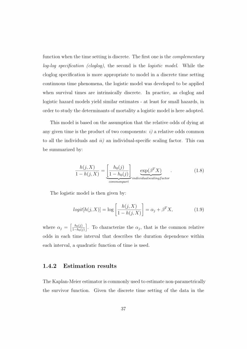
function when the time setting is discrete. The first one is the complementary

log-log specification (cloglog), the second is the logistic model. While the

cloglog specification is more appropriate to model in a discrete time setting

continuous time phenomena, the logistic model was developed to be applied

when survival times are intrinsically discrete. In practice, as cloglog and

logistic hazard models yield similar estimates - at least for small hazards, in

order to study the determinants of mortality a logistic model is here adopted.

This model is based on the assumption that the relative odds of dying at

any given time is the product of two components: i) a relative odds common

to all the individuals and ii) an individual-specific scaling factor. This can

be summarized by:

h(j,X)

1− h(j, X)=

[h0(j)

1− h0(j)

]

︸︷︷︸commonpart

exp(βT X)︸︷︷︸individualscalingfactor

. (1.8)

The logistic model is then given by:

logit[h(j, X)] = log

[h(j, X)

1− h(j, X)

]= αj + βT X, (1.9)

where αj =[

h0(j)1−h0(j)

]. To characterize the αj, that is the common relative

odds in each time interval that describes the duration dependence within

each interval, a quadratic function of time is used.

1.4.2 Estimation results

The Kaplan-Meier estimator is commonly used to estimate non-parametrically

the survivor function. Given the discrete time setting of the data in the

37

present study, an adjusted version of the Kaplan-Meier estimator, the lifetable

estimator, is here used. Figure 1.9 plots the survivor function (and the 95%

confidence interval, the vertical blue lines around each point estimate) for the

Papal states’ sample. The comparison with the life tables for the Swedish

cohort born in 1795, the English cohort born in 1841 and the Italian cohort

born in 187251 does not highlight major differences in the survival probabil-

ities at younger ages. These estimates suggest that the mortality experience

in Central-Northern Italy at the beginning of the 19th century was not dis-

similar from that of other European nations until about age 40; thereafter

it diverged substantially, and the life table curve for the Papal states lies

constantly below that of the other countries.

Figure 1.9: Life table plot for male survival after age 20

.2.4

.6.8

1P

ropo

rtio

n su

rviv

ed

20 25 30 35 40 45 50 55 60 65 70Age

Italy, born 1872 England and Wales, born 1841Sweden, born 1795 Papal states95% confidence interval

Source: Papal states: present estimates; Italy, Sweden, England and Wales: Humanmortality database (data downloaded on January 20, 2007), available at www.mortality.org

Results of the logit regression model with the indicator variable yi,kas

51Life table for Sweden, England and Italy from the Database (2007) (data downloadedon January, 20, 2007), available at www.mortality.org.

38

a dependent variable are shown in table 1.6. In addition to controlling for

individual age (and its square), the model include also the calendar year in

order to account for long-run trends, although, due to collinearity, it is not

possible to disentangle effects that accrue for either the birth year or the

year when at risk of dying. A dummy variable for particularly warm and

cold years is also used to account for unusual weather conditions that may

have implied environmental stress.52 Model 2 additionally uses a index of

urban real wages in the year at risk of death to control for changing in the

purchasing power of the working class.53 The individual characteristics here

considered as relevant in determining the mortality rate are the area of birth

(grouped in four macro-regions), the birth in an urban area (that is in a city

that, in 1861, had at least 15,000 thousand inhabitants54) and the profession

(grouped in six big categories);55 Model 3 adds to this set of variables also

height measured in inches56 to capture the long-lasting effects on mortality

of nutritional insults at younger ages and a dummy variable equal to 1 if the

individual moved to a rural area.

52Temperature values refers to annual average temperature in Rome(source:www.wetterzentrale.de/klima/troma.html) A year is define as warm (cold)if the temperature was 1 standard deviation higher (lower) that the average annualtemperature in the time span 1811 1906.

53The urban real wages index is constructed linearly interpolating the series in Malanima(2003). As the linear interpolation smooths the yearly variations in the real wages and asthe series do not take into account regional differences, this index has to be considered avery rough proxy for the trend in the real purchasing power of the working class.

54The category “urban”, then, include here all together the same categories used inthe height regression (metropolis (Rome and Bologna), the portal towns (Ancona andCivitavecchia) the administrative centers and the municipalities with at least 15,000 in-habitants in 1861).

55The categories are so defined: agricultural laborers, upper class (practitioners, writers,students, land owners, soldiers); skilled craftsmen (blacksmiths, armourers, grinders, car-penters, cabinet makers, turners, carvers); unskilled workers (unemployed, domestic ser-vants, coachmen, launderers); textile workers (tailors, weavers, combers, spinners); other(barbers, bakers, butchers, millers, hut makers, rope makers, tanners, painters, innkeeper,shopkeeper, shoemakers).

56Several different measures of height have been used (such as predicted height, dummyvariable for being tall), but the results are virtually unchanged.

39

Table 1.6: Survival analysis estimates (odds ratios)

Variable Model 1 Model 2 Model 3Region of birth

Romagna Reference Reference ReferenceMarche 1.118 0.867 0.863

Lazio 1.033 1.040 1.045Umbria 1.124 1.090 1.099

Urban birthBirth in an urban environment 1.105 1.116 1.160

Emigration form city to country - - 0.448Professional groups

Agricultural laborers 0.941 0.974 0.992Skilled craftsmen 0.637∗ 0.643∗ 0.647∗

Upper class 0.913 0.892 0.891Unskilled 1.290 1.200 1.225

Textiles 0.743 0.742 0.745Other Reference Reference Reference

Environmental variablesWarm year 0.412∗∗ 0.260∗∗ 0.259∗∗

Cold year 1.111 0.812 0.808Urban real wages index - 0.323∗∗ 0.321∗∗

Height in inches - - 1.002Pseudo R-squared 0.018 0.041 0.043

All models include also age, age squared and year at risk as additional regressors.Significance levels : † : 10% ∗ : 5% ∗∗ : 1%

40

No significant differences in the estimated mortality rates emerge, with

the only exception of the skilled craftsmen (such as carpenters, blacksmiths,

armourers, grinders), whose odds of dying was almost 35% lower than that

of the other workers. This results holds also trying different professional

groupings or different specifications of the model.

In particular, the expected negative effect of the urban environment on

the mortality experience is not significant: being born in an urban environ-

ment increases the odds of dying by almost 10%, but the coefficient is not

significant at the usual levels. Individuals born in cities, that moved in a

rural environment, reduced by almost 50% their probability to die (model

3), confirming, indirectly, the negative effect of cities on survival.

As in other studies (Lee (1997), Costa (1993), Costa (2003), Murray

(1997)), height does not appear to affects the probability of dying: one inch

more not only does not significantly reduces the odd ratios, but it seems to

even increase the risk of dying. Some caution has to be used in interpreting

this results, because, as noted in Costa (2004), the relationship between

height and mortality is very sensitive to sample size.

The mortality experience does not differ in a relevant fashion across ge-

ographical areas, and the result does not change using different definitions

of “region” or controlling for being born in special environments such as

lowlands or mountains.

Environmental variables appear to be significant and their coefficient is in

line with what expected. A year warmer than average reduces by more than

half the probability of dying, while an increase by one point of the urban real

wages index decreases this probability by circa 70%.

One could argue that the lack of significance is due to the non-randomness

41

of the sample here analysed. The selection of soldiers, in fact, is a random

sample of the population of soldiers, but it is not a random sample of the

whole population, as only the ones who decided to enrol and that were ac-

cepted into the army are observed. If the enrollment decision was driven

by some unobservable factors that affected also the odds of dying, then we

observe a relatively homogeneous population in terms of survival probability,

so that no differences arise due to place of birth or profession.

Imagine that individuals born in a rural and in an urban environment en-

joy a very different survival probability, with the latter having significantly

shorter survival rates. Furthermore, only individuals with (unobserved) bet-

ter health (and therefore with survival probabilities above a certain thresh-

old) applied and were accepted into the army. The estimated survival prob-

abilities overestimate of course the “true” survival probability in both the

populations. However, given that a bigger portion of individuals with “bad”

survival curves is not observed in the urban group, the upward bias is bigger

for this group pushing the estimated survival curve closer to that of the rural

group, making the differences not significant. The sign of the coefficients,

however, could still highlight the right direction of the change. In other

words, if we observe an increased probability of dying for individuals born in

cities, and this result is stable across specifications, we can then believe that

a negative effect on survival really existed in cities, even if the coefficients

are not significant at the usual levels.

42

1.5 Summary and conclusions

Using a sample of soldiers enrolled in the papal army between the 1814 and

the 1836, the evolution of the standard of living of the population in Central

and Northern Italy at the beginning of the 19th century is investigated in

this work. The analysis has been conducted looking at two dimension of

the broader concept of “living standards”: the evolution of height and the

mortality experience.

Several patterns can be highlighted: despite the great economic variety

within the papal States, no significant birth-province effects in height are

found. The same lack of differences emerges also when the mortality expe-

rience is analysed. Occupational differences however emerge from the height

analysis and to a lesser extent also from the survival analysis, highlighting a

certain degree of inequality in the wealth distribution in the society, with the

agricultural laborers being the most disadvantaged in terms of height and

the educated class being at the top of the height distribution. The urban-

rural differential in height reveals a disadvantage for individuals born in big

metropolis and administrative centers; difficulties in sanitation in these cen-

ters, as well as the high density of population, may have led to a worse disease

environment. This explanation finds a confirmation in the higher (although

not significant) probability of dying for individuals born in cities, and in the

increased probability of surviving for individuals who emigrated from towns

to rural areas.

The estimated time trend highlights a decline in height for the cohorts

born under the French rule. The dismantling of the corporative organizations

with the consequent exposure to the market forces and competition coupled

with the lost of the charitable functions provided by the guilds and with the

43

reorganization of the charitable system that excluded from their services all

but the extremely poor ones.57 These abrupt changes together with economic

conditions that were negative in all Europe (high food prices, years with bad

harvests and the disruption of the international trade)58 led to a downward

trend more accentuated than in other countries. This result holds even after

correcting for the spurious downward trend imparted by the presence of many

young (and not completely grown) soldiers in the last birth cohorts.

The results appear to be sensitive to the truncation point applied in

the truncated maximum likelihood regression: estimating the model using a

higher truncation point and constraining the standard deviation to be equal

to 6.86 centimeters, in fact, lead to not significant results.

Regional height trends reveal a similar pattern in all the four areas: high

taxes on consumption and an increasingly commercialized agriculture re-

duced the biological welfare of the lower classes, irrespectively of the politi-

cal regime. Also the most advance and dynamic area within the papal states

(Romagna), failed to keep a level of living standard comparable to that of

its neighbor northern regions.

57Davis (2000)58On bad climatic conditions see for example: Post (1974). O’Rourke (2006) shows how

the continental blockade and the disruption of trade led to a sensitive welfare reduction(although with several differences) in the countries involved in the wars.

44

Chapter 2

The biological standard of

living in Germany before

unification 1815 - 1840

2.1 Introduction

At the beginning of the twentieth century, the unified German Empire had

one of the world’s leading economies, with the largest and most modern fac-

tories in many strategic sectors.1 However, the situation was rather different

within the German confederation a century earlier. Despite progress in some

regions (such as Saxony or the district of Nurnberg), the major economic

indicators were not far advanced. The conventional wisdom dates the be-

ginning of the process of Modern Economic Growth2 after 1870 and most

1Cameron (1997)2The term Modern Economic Growth was used by Simon Kuznets to identify a partic-

ular period characterized by high rates of growth of per capita product and population,increase in productivity, structural transformation of the economy and of the society and

45

research on German economic history has focused on this period.

Nonetheless, the first half of the nineteenth is especially interesting be-

cause of the important economic and social reforms that set the basis for

the subsequent impressive catch-up growth. Despite the relevance of this

period, few quantitative studies have been devoted to it and the important

issue of living standards have been all but neglected. This is in stark con-

trast for British scholarship, where the standard of living debate has been a

long-standing topic of intense controversy. Estimates of per capita gross do-

mestic product (GDP) in Germany do not exist for the period before 1850,3

and data on real wages have a limited scope.4 Furthermore, the destruc-

tion of many archival sources during World War II complicates all aspects of

historical investigation, including that of height.

In such a context, anthropometric research can be of use in the analysis

of the effects of changes in the economic structure on welfare. The relation

between human height and the socio-economic environment is well known.

Although genes play a relevant role in determining adult anthropometric

characteristics, environmental factors are the main determinants in trends in

height as well as of the differences in mean height among genetically similar

populations.5 Individuals who are poorly fed and have recurrent infections

rarely grow well in either childhood or adolescence and are unable to achieve a

final adult height that is commensurate with their genetic potential. For chil-

dren and adolescents, height depends essentially on past food consumption

increasing market integration. See Kuznets (1973).3See, for example, Fremdling (1995). Angus Maddison has estimated German per

capita GDP for 3 benchmark years: 1820, 1830 and 1850. The data are available at hisweb sitehttp://www.ggdc.net/maddison/

4Mitchells series from 1820, for example, covers only industrial workers starting from1820.

5See for example the study of Cavelaars et al. (2000). A guide to other recent studiescan be found in Rona (2000)

46

and the incidence of diseases. Changes in socio-economic factors that influ-

ence the availability of nutrients or of the claims on them (such as changes

in the price of food or in public health policies) are then reflected in adult

stature. Given the multiple external influences on net nutritional intake,

inferences about the biological standard of living are not straightforward

and require careful consideration of all the possible factors. Nonetheless,

the analysis of stature has proved to be a useful tool and during the past

20 years, anthropometric research has made important contributions toward

understanding the effect of economic processes and institutional changes on

the biological standard of living.6

Time trends of height during the early nineteenth century have been es-

timated for many countries such as the United States, England and France

as well as for the Habsburg Empire.7 In Germany, height trends are known

for three states (Bavaria, Wurttemberg and Saxony),8 but data for the en-

tire country have not yet been analyzed and data for Wurttemberg pertain

only to the second half of the century. In this article, a unique dataset is

used to reconstruct the height trend for Germany during the first half of the

nineteenth century.9 Time trends are also derived for the main regions, allow-

ing comparison of the effects of different economic policies on the biological

standard of living.

6See Steckel (1995), Fogel (1994), Komlos (1985).7This is a short anthology of articles on height trends. For the US, see Komlos (1998);

for England, see Nicholas and Steckel (1991) and Komlos (1993); for France, see Komlos(1994) and Weir (1997); for the Habsburg Empire, see Komlos (1989)

8For Bavaria see Baten (1999), Baten (2001) and for Wrttemberg, see Twarog (1997);for Saxony, see Cinnirella (2006)

9The appropriateness of the term “Germany” is questionable, given that it did notexist as such before 1871. The Vienna settlement in 1815 created a conglomeration of 39separate states.( Tipton (2003b)) Here, “Germany” is defined as the set of states (withthe exception of Alsace-Lorraine) that became part of the German empire in 1871.

47

2.2 Living standards in Germany in the first

half of the 19th century: a quick overview

At the beginning of the nineteenth century, the German economy was pri-

marily agrarian. A review of the most recent estimates from Angus Maddison

shows that German per capita GDP in 1820 was one of the lowest in Western

Europe. Nearly a century later, on the eve of World War I, per capita GDP

had more than doubled, and Germany was among the wealthier European

nations. In 1860, the German GDP was still behind that of France and Aus-

tria and was less than 60% of the British GDP. By 1913 it was ahead of

Austria, France, Sweden and it was 75% of the British GDP (Table 2.1).

Table 2.1: German per capita GDP in international comparison 1820 - 1913(1990 International Geary - Khamis dollars)

1820 1830 1840 1850 1860 1870 1913Austria 1,218 1,399 1,515 1,650 1,778 1,863 3,465Belgium 1,319 1,354 1,847 2,293 2,692 4,220Denmark 1,274 1,330 1,428 1,767 1,741 2,003 3,912France 1,135 1,191 1,428 1,597 1,892 1,876 3,485Germany 1,077 1,328 1,428 1,639 1,860 3,648Italy 1,117 1,350 1,447* 1,486 2,564Netherlands 1,838 2,013 2,283 2,371 2,377 2,672 4,049Sweden 1,198 1,175 1,231 1,289 1,488 2,557 3,096United Kingdom 1,706 1,749 1,990 2,330 2,830 3,031 4,921Source: Maddison’s web site http://www.eco.rug.nl/ Maddison/∗ Data for 1861

This super performance had deep roots that extended back to the begin-

ning of the nineteenth century. The French Revolution and the Napoleonic

Wars, with the defeat of the Prussian Army at Jena and Auerstadt, stimu-

lated an important series of reforms. A new group of younger government

officials dedicated to reform came into power and introduced many socio-

48

economics edicts. Already in the 18th century Prussia was in the forefront

by creating a universal primary education system. In 1807 and 1808, it eman-

cipated the peasantry from bondage to the aristocratic landlords (Bauernbe-

freiung), and created occupational freedom in the cities in order to reduce the

power of the artisan guilds to determine eligibility for employment with man-

ufacturers (Gewerbefreiheit). The Prussian example was followed in many

other states, with the divesting of state-owned manufacturing enterprises

across Germany.10

Napoleon’s defeat and the Vienna settlement that returned the traditional

elites to power did not stop the modernization process. During the first half

of the nineteenth century, Germany continued to invest heavily in human cap-

ital. German administrators became increasingly conscious of the economic

changes in other countries, which showed that industrialization is necessary

for the creation of a strong economy. The adjustments that were necessary

to transform Germany into an industrialized country were, however, difficult

for private entrepreneurs to accomplish by themselves. The new technologies

were complex and expensive, and the limited markets in the small German

states generated concern about whether sufficient revenue would be gener-

ated to recover the initial investments. The implications of these argument

were actively debated at the time, and much was accomplished by local gov-

ernments.11 One of the major achievements was the establishment in 1834 of

the Zollverein, which, through the abolition of internal custom duties, unified

most of the German states (with the significant exclusion of Austria) into a

single market.

10Tipton (2003a)11 Beck (1992). For a review of the successes of the government in fostering industrial-

ization see Henderson (1958)

49

The socio-economic transformations connected with this process were

substantial. The balance of power shifted toward middle-class groups, as

old forms of dependence were abolished and new forms were created. What

were the effects of these rapid and fundamental changes on living standards?

Data pertaining to living standards in Germany at the beginning of the

nineteenth century are limited. Figure 2.1 shows an index of real industrial

wages during 1820-1855. After a small increase during the 1820s, the in-

dex changed little during the 1830s and began to decrease in the mid-1840s.

Apart from questions concerning their reliability, these data are limited to

industrial workers and thereby exclude data for peasants and prevent infer-

ences about the living standards of people who were not in the labour force,

such as women or children.

Figure 2.1: Industrial real wages index in Germany 1820 - 1855

8010

012

014

016

018

0R

eal w

age

inde

x 19

13 =

100

1820 1825 1830 1835 1840 1845 1850 1855Year

Real wages index 1913=100 Lowess smoother

Source: Mitchell (1992)

In recent decades, several investigators have argued for moving beyond

measuring living standards in terms of monetary units to measurements in-

50

volving broader concepts.12 The pattern obtained for Germany using such

concepts does not indicate a major improvement in the standard of living

during the first half of the nineteenth century. Mortality rates were high and

even increased during much of the period (figure 2.2). Life expectancy at

birth was relatively low at the beginning of the century and did not begin to

increase until after 1850. For example, during the 1820s, a 20-year-old person

could expect to live until about age 60, with a slight increase beginning only

in the 1860s.13

Figure 2.2: Mortality in Germany 1817 - 1850

2224

2628

30D

eath

s pr

o 1,

000

inha

bita

nts

1820 1825 1830 1835 1840 1845 1850Year

Deaths pro 1,000 inhabitants Lowess smoother

Source: Hoffmann (1965), Table 1 pag. 172

Data on caloric availability, a measure of another dimension of the living

standards, reveals that Germans consumed enough calories to fully satisfy

their nutritional needs only beginning with 1885-9 (figure 2.3).

The economic reforms implemented in Germany seem not to have pro-

12On the living standard debate, see, for example, Sen (1984).13 For an overview of the main studies on mortality in Germany in the nineteenth century

see Guinnane (2003); data on remaining life expectancy at age 20 from Imhof (1990)).

51

Figure 2.3: Actual vs. Ideal caloric consumption in Germany 1850 - 1900

Source: Hoffmann (1965), Table 170 pag. 659

duced major changes in living standards during the period under considera-

tion. Important improvements in the standard of living are not evident, but

neither are the substantial increase in the prevalence of poverty and the de-

terioration of living standards hypothesized by historians and contemporary

observers.14

2.3 Materials and methods

Data on the height of Germans born during 1815-1840,15 who served as sol-

diers under the British flag at the time of the Crimean War (1854-1856) are

analysed. In accordance with firmly established military tradition, in 1854,

the British government allowed the military to recruit foreign soldiers to sup-

14Knapp (1887), Harnisch (1974).15As shown in table 2.2, more than 80% of the observations belong to the cohorts born

during 1820- 1835, so our analysis is particularly significant for that period.

52

plement the regular army, given the substantial loss of soldiers at the end of

that year and the difficulty in attracting new domestic recruits.16

The original data set includes records for approximately 13,500 soldiers.

In addition to height, the recruitment lists specify age, state and city of

provenance, former profession, date of physical examination and regiment.

The database was compiled using British German legion: Nominal Rolls (6-

16) and the Inspection certificates of the recruits (32 - 35) (Public Record

Office London, England, WO15). Because two sources were used, records for

some recruits appeared more than once. Thus, almost 5,000 duplicates were

excluded from the analysis.17

The duplicate records facilitated testing of the accuracy of the measure-

ments. For one-half of the soldiers whose records appeared more than once,

the measured height was exactly the same. When there were discrepancies,

the reported heights differed by less than 0.5 inches (i.e., slightly more than

1 centimetre). This imparts some confidence in the accuracy of the data.

Additionally, we have records for nearly 2,000 soldiers who were not born

in German states. Data were grouped into seven regions: Prussia, Baden-

Wurttenberg, Bayern, Sachsen -Thuringia, Hessen, Mecklemburg and Han-

nover. Figure 2.4 shows their location and table 2.2 shows the composition

according to birth cohort and region.

The representative nature of the data must be considered. Because of

enlistment into the British army was voluntary, self-selection could be a con-

founding factor.18 Thus, the conditions under which recruitment occurred,

16For a detailed history of the foreign legion during the Crimean War see Bayley (1977).17 Several tests were performed on the data to exclude from records that were not

initially recognized as duplicates because of slight variations in the spelling of recruit’sname (e.g., Mathias vs. Matthias).

18This problem appears in all studies that use data from volunteer army. See, for

53

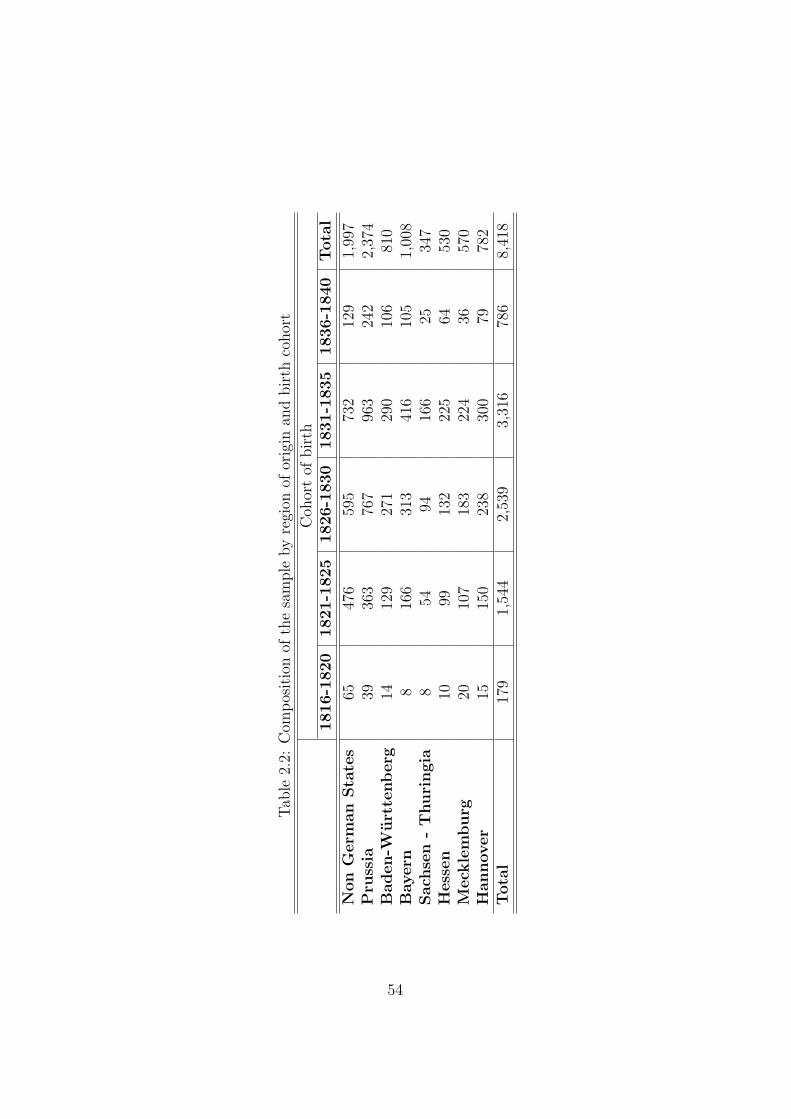
Tab

le2.

2:C

ompos

itio

nof

the

sam

ple

by

regi

onof

orig

inan

dbir

thco

hor

t

Coh

ort

ofbir

th1816-1

820

1821-1

825

1826-1

830

1831-1

835

1836-1

840

Tota

l

Non

Germ

an

Sta

tes

6547

659

573

212

91,

997

Pru

ssia

3936

376

796

324

22,

374

Baden-W

urt

tenberg

1412

927

129

010

681

0B

ayern

816

631

341

610

51,

008

Sach

sen

-T

huri

ngia

854

9416

625

347

Hess

en

1099

132

225

6453

0M

eck

lem

burg

2010

718

322

436

570

Hannover

1515

023

830

079

782

Tota

l17

91,

544

2,53

93,

316

786

8,41

8

54

and the possible reasons why an individual chose to enlist should be consid-

ered. British recruitment operations in the Germans states were delegated to

Baron von Stutterheim, a charismatic figure who served in the British army

in the late 1830s and also participated in the Schleswig-Holstein uprising

against Denmark in 1848. The involvement of this influential personage is

crucial: his emphatic liberal views reflected the political convictions of many

of the soldiers who served with him during the 1848 rebellion. At the end

of the revolutionary storm, being too destitute perhaps to afford the cost

of the trip back home, many soldiers gravitated to the coastal cities (Kiel,

Altona, Hamburg and Lubeck) where they led a poverty-stricken existence.

The arrival of Stutterheim in Hamburg on April 1855 was welcomed by the

Schleswig-Holstein veterans, who were apparently destined, in absence of

other alternatives, to be absorbed into the ranks of the urban proletariat

and casual labourers of the counting houses and docks of the great German

northern ports. Within a few weeks, Stutterheim raised a force of several

thousands men, despite the fact that recruitment for the foreign legion had

been declared illegal in January of 1855 by the Senate of Hamburg and by

the city of Lubeck and despite the efforts of the local police to stop the

recruitment activities.

The collection point was set in Helgoland, a small island 70 km from the

German coastline that, after the Napoleonic Wars, belonged to Britain.19 No

aid was given to the potential soldiers to help them reach Helgoland. Travel

to Helgoland was not an easy task, given the lack of a regular service by

steamship (which was closed during the winter season), and the substantial

police surveillance of the embarkation procedures in the main ports. In many

example, Mokyr and Grada (1996)19See figure 2.4 for the approximate location of Helgoland.

55

Figure 2.4: German states after 1815, regional groups and location of Hel-goland island

cases, the men had then to travel to the small and distant cities of Stade or

Gluckstadt and find a local sailor willing to adjust his normal route to take

them to Helgoland.20

To better understand the possible factors involved in self selection, one

might consider the decision to enlist in the army as tantamount to the deci-

sion to participate in the labour force. The rational individual would choose

to enlist if the wage he would obtain from the army, w, was higher than his

20An idea of the difficulties faced by the recruits in their travel to the recruitment pointappears in the letters to home written by the recruits. [Steinhart (1859)]

56

reservation wage, wr, defined as the wage at which he was indifferent with

respect to enrolling in the army or being unemployed or working at home.

y∗ = w − wR

≤ 0 not in the sample

> 0 in the sample

The reservation wage for an individual was a function of his human capi-

tal (i.e., educational attainment and physical capability) and the conditions

of the labour market (e.g., the unemployment rate) where he lived. Distance

from the recruitment point also played a role, with an effect that, at first

glance, is unclear. A first line of reasoning leads to expect a positive associa-

tion between distance and the reservation wage. If the soldier came directly

from home, the farther away the country of origin, the greater was the cost

to reach Helgoland, and, therefore, the greater is the wage that had to be

offered by the army to compensate for the cost of travel. Given that the

army offered a fixed wage (w), we may expect a lower number of recruits

coming from regions very faraway from the recruitment point. However, if

the financial situation of the majority of the recruits is taken into account,

we suppose that, as the distance from the recruitment point increases, the

reservation wage decreases. This is the case insofar as people coming from

distant regions (such as Bavaria or Baden) were part of the crowd of veter-

ans of the Schleswig-Holstein uprising who could not afford the cost of the

trip back home and, therefore, who searched the harbour looking for any

jobs, including low-paying ones. In contrast, veterans from northern regions

were more likely to be able to afford returning to their home towns after

the conflict. Thus, the cost of searching for a job was lower for the latter

group, because they could rely on the support of their family and on a better

knowledge of the local economic conditions.

57

In light of these considerations, the sample cohort likely comprises pri-

marily poor and unskilled workers who were mainly from southern German

states. The characteristics of the sample substantiate these considerations.

Almost 100 different professions were listed in the original documents, and

they were grouped into 11 categories. Although the majority of the recruits

were unskilled workers, recruits from other professions were also represented:

skilled industrial workers (e.g., molders and carpenters) and white collar

workers (e.g., secretaries, physicians, merchants and renters) represent 16%

of the sample (Table 2.3). The variety of professions reported suggests that

the sample is composed of a broad spectrum of workers.

Table 2.3: Composition of the sample by profession

Profession Frequency PercentageElite 552 6.69Services 501 6.07Food 712 8.63Skilled industrial workers 742 8.99Tailors 412 4.99Shoemakers 598 7.25Textiles 366 4.44Miscellaneous crafts 878 10.64Soldiers 500 6.06Unskilled workers 1,156 14.01No profession listed, unreadable, unemployed 1,833 22.22

The occupation can be organised into 3 major sectors (Agriculture, In-

dustry and Services) to compare the composition of the sample with that of

the population of the German states at large. As shown in figure 2.5, the

recruits were employed predominantly in non-agricultural occupations, and

the agricultural sector is highly underrepresented (despite the inclusion of the

workers with no profession listed). The analysis, therefore, mainly pertain to

what we might call the “industrial proletariat”. The heights of the recruits

58

should, in turn, be compared with those of persons from other lower classes.

Figure 2.5: Composition of the sample by sector of activity

Note:Population data for year 1852Source: Hoffmann (1965), Table 20 pag. 204

Although recruitment was in a remote location that was difficult to reach,

the sample provides good regional coverage for all the birth cohorts (figure

2.6).21 The percentage of recruits from Prussia is slightly less than that for

the general population, whereas the percentages of recruits from Bavaria,

Baden and Hessen is moderately greater than those for the general popu-

lation. The discrepancies, however, all appear to be less than 10%. Our

sample, therefore, is not biased toward specific regions. On the contrary,

the regional composition of the sample is very similar to that of the general

population.

21The census data are from Mitchell (1992) and are available for 1816, 1828 and 1834.The sample data were aggregated into regions that cohere with the definition used in thecensus.

59

Figure 2.6: Sample and population composition by regions

Source: Population data: Mitchell (1992); Sample: own calculationsNote: Population composition by region is calculated as average from the censuses for

the years 1816, 1828 and 1834

60

As with the vast majority of military cohorts, this sample is affected by

the problem of truncation, because of the minimum height requirement im-

posed on the recruits. Figure 2.7 clearly shows a truncation point at 62 inches

(157.48 cm).22 If truncation is not adequately taken into account, estimates

will be biased. Truncated maximum likelihood regression has proven to be

an efficient way to explicitly model this phenomenon, giving unbiased and

consistent estimates.23

Figure 2.7: Height distribution of German born soldiers

0.1

.2.3

.4D

ensi

ty

60 61 62 63 64 65 66 67 68 69 70 71 72 73 74 75 76 77Height in British inches

22Changes in the truncation point across regiments, time and regions were analysed. Inall cases, the military height requirement was fixed at 62 inches.

23 A review of the principal methods used to correct for truncation in height samples ispresented in Komlos (2004). See also A’Hearn (2004)

61

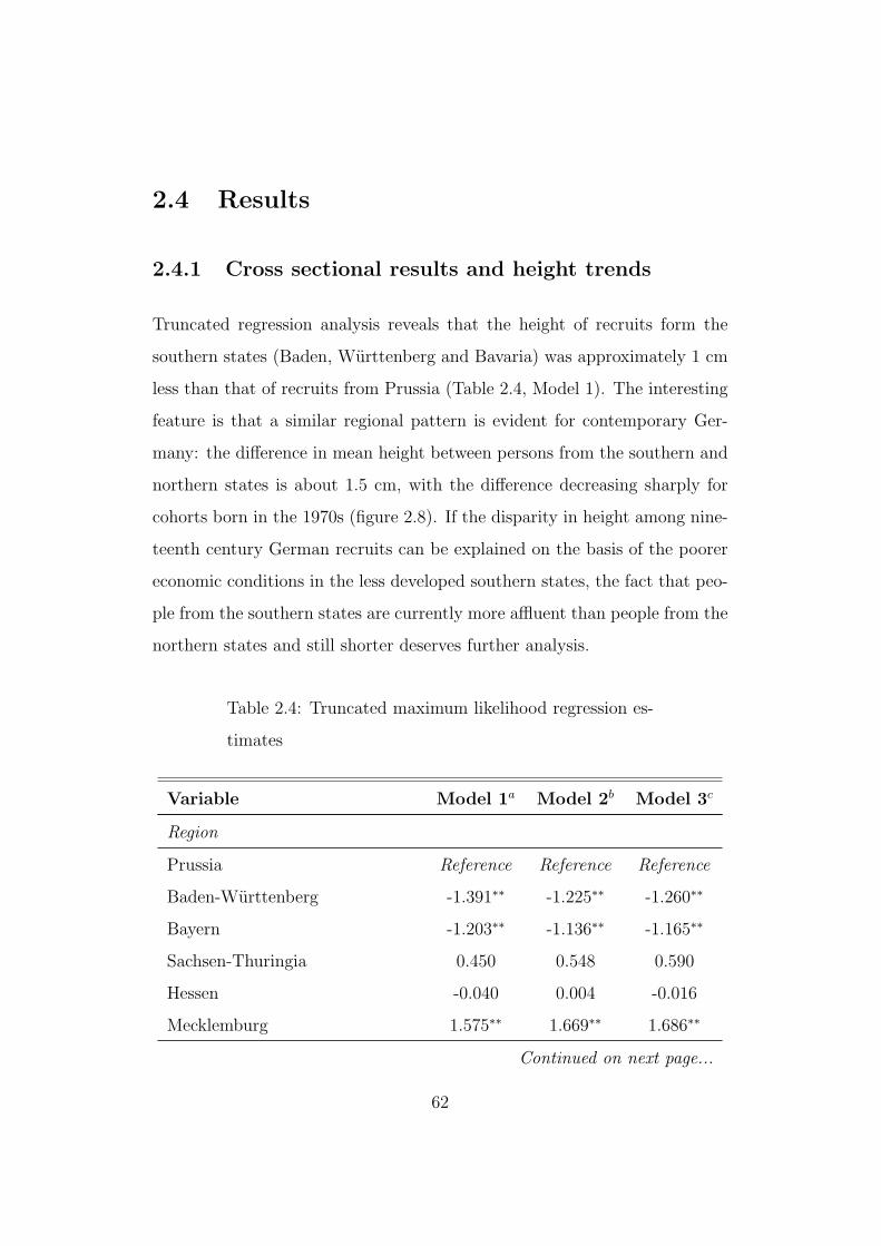
2.4 Results

2.4.1 Cross sectional results and height trends

Truncated regression analysis reveals that the height of recruits form the

southern states (Baden, Wurttenberg and Bavaria) was approximately 1 cm

less than that of recruits from Prussia (Table 2.4, Model 1). The interesting

feature is that a similar regional pattern is evident for contemporary Ger-

many: the difference in mean height between persons from the southern and

northern states is about 1.5 cm, with the difference decreasing sharply for

cohorts born in the 1970s (figure 2.8). If the disparity in height among nine-

teenth century German recruits can be explained on the basis of the poorer

economic conditions in the less developed southern states, the fact that peo-

ple from the southern states are currently more affluent than people from the

northern states and still shorter deserves further analysis.

Table 2.4: Truncated maximum likelihood regression es-

timates

Variable Model 1a Model 2b Model 3c

Region

Prussia Reference Reference Reference

Baden-Wurttenberg -1.391∗∗ -1.225∗∗ -1.260∗∗

Bayern -1.203∗∗ -1.136∗∗ -1.165∗∗

Sachsen-Thuringia 0.450 0.548 0.590

Hessen -0.040 0.004 -0.016

Mecklemburg 1.575∗∗ 1.669∗∗ 1.686∗∗


62


Variable Model 1a Model 2 b Model 3c

Hannover 1.627∗∗ 1.774∗∗ 1.788∗∗

Profession

Elite 4.067∗∗ 4.153∗∗ 4.213∗∗

Services 2.338∗∗ 2.349∗∗ 2.381∗∗

Food 1.079∗ 1.089∗ 1.122∗

Agricultural labor, hunters and

fishers

3.363∗∗ 3.233∗∗ 3.309∗∗

Skilled metal workers 1.225∗∗ 1.175∗∗ 1.221∗∗

Textiles workers and tailors 0.316 0.504 0.520

Miscellaneous crafts 1.406∗∗ 1.452∗∗ 1.481∗∗

Soldiers 5.067∗∗ 5.074∗∗ 5.145∗∗

Unskilled workers Reference Reference Reference

No profession listed, unreadable,

unemployed

2.276∗∗ 2.352∗∗ 2.410∗∗

Birth cohort

1816-1820 1.729∗ 1.717∗ 1.715∗

1821-1825 0.688∗ 0.680∗ 0.682∗

1826-1830 Reference Reference Reference

1831-1835 0.145 -0.399 -0.643∗

1836-1840 - -1.213∗∗ -1.925∗∗

Age dummies

age 20 -2.379∗∗ - -

age 21 -1.631∗∗ -1.085∗∗ -0.846∗

age 22 -0.732 -0.190 0.054


63


Variable Model 1a Model 2 b Model 3c

age 23 -0.147 0.403 0.649

age 24 or more Reference Reference Reference

Intercept 164.489∗∗ 164.387∗∗ 164.329∗∗

Standard deviation 6.495∗∗ 6.470∗∗ 6.509∗∗

N 5,575 6,200


a : latest birth cohort excluded

b : latest birth cohort (1836-1840)included. Height at age 21 for recruits aged 18

to 20 calculated using the annual height increments of Hungarian soldiers born in

1780/1790 from Komlos (1989), bottom of tab. 2.10 page 80.

c : latest birth cohort (1836-1840)included. Height at age 21 for recruits aged 18

to 20 calculated using the annual height increments of Hungarian soldiers born in

1750/1760 from Komlos (1989), bottom of tab. 2.10 pag. 80.

The available evidence on income distribution in German states in the

19th century highlights some degrees of inequality: in Prussia in 1875 the

share of the top quintile was about 48%, while in Saxony the top quin-

tile owned the 56% of the resources.24 Since height is sensitive to income

distribution and since previous occupation is a proxy for the social status,

differences across different occupational groups are expected. The results are

coherent with the expectation (Figure 2.9). Soldiers were the tallest group,

more than 5 cm taller than unskilled workers. Recruits belonging to the elite

group (e.g. merchants, students, physicians) enjoyed a height premium of 4

24See Kuznets (1955) and Procopovitch (1926).

64

Figure 2.8: Average difference in height between Northern and Southernstates in contemporary Germany

1.3

1.4

1.5

1.6

1.7

1.8

cent

imet

ers

1940 1945 1950 1955 1960 1965 1970Year of birth

North/south average difference Lowess smoother

Source: Bundesministerium (1997)

65

cm, while those with privileged access to food (as butchers or cooks) were

slightly more than 1 cm taller than recruits from other professions. Finally,

low skilled workers from the manufacturing sector (e.g. tailors, weavers,

spinners) were not significantly taller than unskilled workers.

Figure 2.9: Height premiums by professional categories

Source: coefficients from tab.2.4, model 1

A decreasing trend in height is evident for the first 15 years after the

Vienna settlement. Heights reached a trough for the cohorts born at the

end of the 1820s and remained stable thereafter: recruits born during 1826

- 1830 are 1.7 cm shorter than recruits born during 1816-1820, whereas the

height of recruits born during 1830 - 1835 is not significantly different from

the height of the cohort born during 1826-1830 (model 1, table 2.4). This

trend generally accords with the data for most European countries which

66

showed a decrease in height among birth cohorts from the 1830s.25 While in

comparison with the rest of Europe the estimated decline starts a bit earlier,

the timing and the magnitude are coherent with the results obtained for both

Saxony and Bavaria.26

In estimating the height trend the presence of soldiers less than 20 years

of age in the last birth cohorts is a possible confounding factor. In well fed

populations, normal pubertal growth ends at the age of 20. In case of poor

net nutrition during childhood, however, the growth process past the usual

age of cessation and extends into the early 20s. As the dummy variables that

control for the age show, in fact, that recruits younger than 21 years of age

were significantly shorter than 24 or more years old. These young men likely

had not reached their final adult height. Given that the last birth cohort

includes only individuals younger than 20 years, the contemporaneous pres-

ence of dummy variables for birth cohort and for age would cause a problem

of multicollinearity, so in model 1 the last cohort was excluded from the re-

gression. Model 2 and 3 offer a correction for the problem of young recruits,

giving an indication of the possible direction of the height trend in the late

1830s. Using the annual height increments estimated for the Hungarian sol-

diers born at the end of 18th century, a forecast of the height the youngest

recruits would have had at the age of 21 was constructed. Two different

scenarios are considered. Model 2 represent a lower bound scenario: the co-

efficients used for the forecast are those estimated for soldiers born in 1780s

and 1790s, a period of decline in the nutritional status of the population in

25For further discussion and bibliography on the height decrease in Europe and theunited States in the 1830s, see Komlos (1998). Recent evidence outlined a downturn inUS heights between 1820 and 1840 for the working class but not for the upper-middleclass. See Sunder.

26Saxon recruits born in 1815 1819 are 1.71 cm taller than recruits born in 1825 1829(Cinnirella (2006), tab. 5); Bavarian convicts born in 1810 1819 are 1.52 cm taller thanconvicts born in 1825 1829 (Baten and Murray (2000)- tab. 5 pag 360).

67

Hungary in comparison with the 1750s and 1760s. The estimated growth

increments between ages 18 and 21 for the Hungarian recruits born in the

latter period are used to forecasts the heights used in model 3, representing,

then, a more favourable scenario.27 In both cases, the declining trend ex-

tends beyond the 1820s well into the 1830s. Different robustness checks were

applied. In particular, the height of the youngest recruits was forecasted us-

ing the cumulative height increments of modern, well fed adolescents: even

using the most favourable assumptions, the coefficient for the birth at the

end of the 1830s stays negative.28

The sample numerosity allows also to estimate the time trend in heights

at a regional level (figure 2.10) .29 Some regional differences appear. While

Baden Wurttemberg shows a sharply declining height trend, heights in the

neighboring Kingdom of Bavaria appear to be increasing at the beginning of

the 1830s. The northern areas of Hannover, Mecklenburg and Hessen show

a similar path, although Hanover has, among the three, wider fluctuations.

The estimated trends and levels of height reveal that the negative differential

for the southern states, highlighted already in the cross sectional analysis,

persisted during the first half of the century. It is also interesting to note

that, despite their contiguity, the southern states (Baden Wurttemberg and

Bavaria) show a divergent trend.

27For further details on the estimated annual growth coefficients and for a discussion ofthe nutritional status in Hungary at the end of the 18th century see Komlos (1989).

28Even when the counterfactual height was constructed using the height increases ofcontemporary American boys aged 13.5 years (coefficient taken from Tanner and Davies(1985)), the latest birth cohort would still be 0.4 cm shorter than the cohort born at theend of the 1820’s.

29 We exclude from the analysis Saxony and the Thuringian states, given the small num-ber of observations. Results are obtained using truncated maximum likelihood regressor,using the same controls as in the tab.2.4.

68

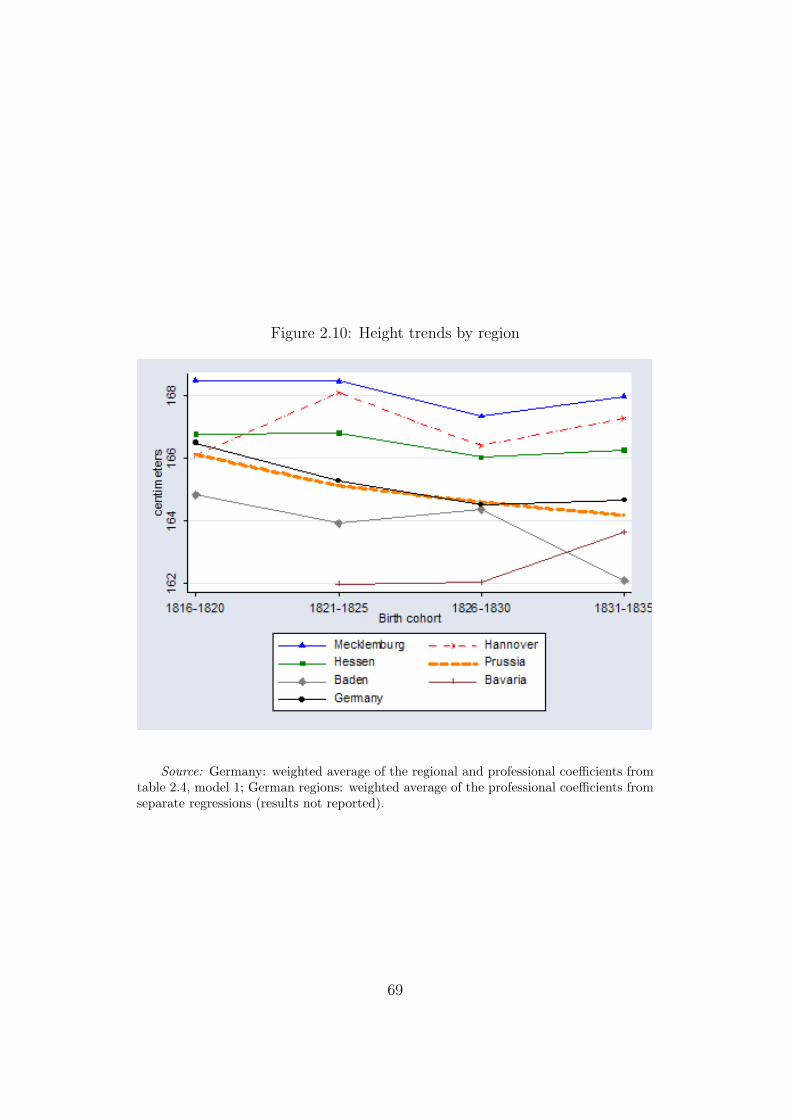
Figure 2.10: Height trends by region

Source: Germany: weighted average of the regional and professional coefficients fromtable 2.4, model 1; German regions: weighted average of the professional coefficients fromseparate regressions (results not reported).

69

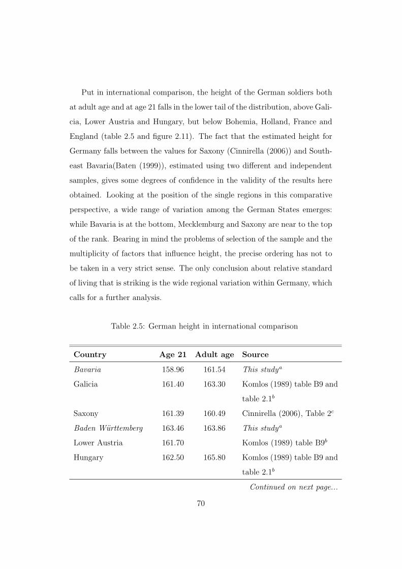
Put in international comparison, the height of the German soldiers both

at adult age and at age 21 falls in the lower tail of the distribution, above Gali-

cia, Lower Austria and Hungary, but below Bohemia, Holland, France and

England (table 2.5 and figure 2.11). The fact that the estimated height for

Germany falls between the values for Saxony (Cinnirella (2006)) and South-

east Bavaria(Baten (1999)), estimated using two different and independent

samples, gives some degrees of confidence in the validity of the results here

obtained. Looking at the position of the single regions in this comparative

perspective, a wide range of variation among the German States emerges:

while Bavaria is at the bottom, Mecklemburg and Saxony are near to the top

of the rank. Bearing in mind the problems of selection of the sample and the

multiplicity of factors that influence height, the precise ordering has not to

be taken in a very strict sense. The only conclusion about relative standard

of living that is striking is the wide regional variation within Germany, which

calls for a further analysis.

Table 2.5: German height in international comparison

Country Age 21 Adult age Source

Bavaria 158.96 161.54 This studya

Galicia 161.40 163.30 Komlos (1989) table B9 and

table 2.1b

Saxony 161.39 160.49 Cinnirella (2006), Table 2c

Baden Wurttemberg 163.46 163.86 This studya

Lower Austria 161.70 Komlos (1989) table B9b

Hungary 162.50 165.80 Komlos (1989) table B9 and

table 2.1b


70



Germany (whole) 162.68 164.44 This studya

Prussia 163.10 164.13 This studya

Southeast Bavaria 163.41 Baten(1999) tab.6.4 col.1d

Bohemia 163.80 166.30 Komlos (1989) table B9 and

table 2.1b

Hessen 163.99 166.12 This studya

Netherland 164.40 Drukker and Tassenaar

(1997), Table 9A.1e

France 164.50 Weir (1997), Table 5B.1f

Hannover 164.59 166.91 This studya

Northern Italy 165.38 166.63 A’Hearn (2003), Table 2 g

England 166.10 Komlos (1998), Fig.2h

Saxony and Thuringia 167.26 167.83 This studya

Mecklemburg 166.85 167.79 This studya

Switzerland 166.76 167.56 Kues (2006), Table 2i

a : Truncated Maximum Likelihood estimates. Unskilled worker, born during 1815

1840. Adult = older than 23. Separate estimates for each region.

b : Height at age 21: Quantile-bend estimates for ages 19-20 plus 1 cm. Soldiers born

in the late 1830’s. Adult height: truncated sample means converted to estimates of

population mean assuming a standard deviation of 6.86 cm, a normal distribution,

and an effective truncation point 0.5” below the official MHR of 63”.

c : Truncated Maximum Likelihood estimates. Craftsman born in an industrial region

between 1829-1829.

d : 21 years old conscript from the working class, born between 1825-1829 in a rural

area


71



e : Median height at age 20 plus 6.4mm

f : Median height, ages 20-21, soldiers born in the late 1830’s

g : Truncated Maximum Likelihood estimates. Soldiers born 1825 - 1830, rural

residence, no occupation given.

h : Index for age 20 - 23, times 167.7 cm base.

i : Truncated Maximum likelihood estimates. Soldiers born between 1825-1829

Figure 2.11: German height in international comparison

Source: table 2.5

72

2.4.2 Agrarian reforms and living standards in Prussia

One of the more debated questions in the economic history of Germany per-

tains to the effect of the agrarian reforms (Bauernbefreiung) on the living

standard of the population. German states differed in the timing of the

reforms and in their strength. Prussia at the beginning of the nineteenth

century implemented several reforms in a fundamental fashion to renew the

agricultural sector; Saxony and Hanover followed its example and imple-

mented similar reforms during the 1830s but in a weaker fashion, providing

financial support to peasants who wanted to buy their land. Other states

(such as Bavaria) waited until the second half of the nineteenth century to

start any reform. The effect of these processes on the living standard of peas-

ants has been controversial. Scholars have argued whether the reforms led to

the pauperization of the peasantry.30 Although appealing, the comparison

between the different German states has to be interpreted cautiously, because

many external factors changed between the early reforms of some states and

the late reforms of other states. In this respect, Prussia, having implemented

the agrarian reforms at the same time but with different nuances within its

large boundaries, offers a good set to test the effect of these changes.

Given the considerable extension and the economic differences of Prus-

sian territories, the height trend is estimated separately for its east and west

provinces. The indication of the city of provenance was available for approx-

imately half of the Prussian recruits and for 88% of them it was possible to

locate the city in the east or in the west part of the Prussian kingdom. 62%

of the recruits came from the West, while the remaining 38% were from the

30Harnisch (1974) agree with the pessimistic view expressed by Knapp (1887). Henning(1996) criticizes this view. For further discussion on the effect of the agrarian reforms seeBaten (2003).

73

East. Recalling the discussion on the selection of the recruits in section 2.3,

given that the majority of the Prussian participants in the 1848 revolution

were coming from Rhineland and Westphalia (two districts of West Prus-

sia31), these percentages are not surprising. The first birth cohort was left

out from the analysis given the small number of observations while the last

birth cohort was left out to prevent a spurious downward trend due to the

presence in this cohort of soldiers who had not reach yet their adult height.

Although the cohort coefficients are not significant, the signs characterize a

divergent height trend for the two areas, decreasing for the West and slightly

increasing for the East (figure 2.12).

The traditional reconstruction of the effects of the Prussian reforms points

to the concentration of the land in the hands of the Junkers estate owners

and of the large scale peasant cultivators in the East: small farmers either

became daily labourers for the big landowners or emigrated to the cities.

The comparative advantage enjoyed by these big estates in the grain produc-

tion, strengthened the tendency toward grain monoculture. As a function

of the land redistribution and of the emphasis on grain, a marked decline in

livestock holding among the peasantry was observable. The increased grain

exports induced the substitution in the peasant diet of wheat and rye with

the nutritionally inferior potatoes. On the contrary, in the West, where the

peasants traditionally enjoyed stronger tenurial rights, the reforms produced

a more balanced land distribution. Furthermore the process of enclosure of

common lands as implemented in the West, encouraged the retention of live-

stock by small sized peasants, a trend encouraged also by the adoption of

31What is here defined as West Prussia are the territories that were situated on theleft of the Kingdom of Hanover and it has not to be confused with the region “WestPrussia”, one of the region of the Eastern part of the Prussian kingdom, corresponding tothe modern area of Danzig (Poland)

74

Figure 2.12: Height trends in the Eastern and Western Prussian territories

162.

516

316

3.5

164

164.

516

5ce

ntim

eter

s

1821−1825 1826−1830 1831−1835Birth cohort

East Prussia West Prussia

75

new fodder crops that improved the milk yields.32 If that was the case, given

that Eastern recruits in the sample were coming mainly from areas where the

agrarian reforms were implemented in a harsh fashion,33 a decline in their

height and an increase in Western soldier’s height would have been expected.

Given the small sample size, great caution has to be used in interpreting

the results. Furthermore, it is worth to remind us that there are data only

for a few soldiers who previously worked in the agricultural sector. If, as

highlighted in section 2.3, this sample is representative of the industrial lower

classes, the positive height trend in the East may reveal that the agrarian

reforms and the stronger commercialization of the agricultural products that

followed, improved the food supplies of that part of the population that was

not working in the primary sector. On the contrary, in the West the increase

in the number of medium size holdings, if beneficial for the peasants, may

have not been able to support, at least at the beginning, the food demand of

the industrial sector. As a consequence, the poorest in this group may have

suffered a decline in their biological living standards. The Western recruits,

however, were enjoying an higher level of living standards, as suggested by

the cross sectional analysis of the Prussian recruits (Table 2.6). Although the

differences between recruits coming from different areas are not statistically

significant, the sign of the coefficient for the recruits coming from the Western

is positive, signalling a height premium for those recruits. Baten (2003), using

a different set of indicators, draws similar conclusions.34Further analysis is,

of course, necessary. However, if confirmed, the results support the idea that

32 See Lee (1984, 1981)33For a classification of the Prussian districts according to the type of agrarian reforms

see Baten (2003), table 12.1, p. 392. 60% of the east Prussian recruits were classifiedinto districts. The districts that are classified as “harsh” type (Posen, Pomerania, Berlin,Silesia) represent 54% of the sample, while the eastern districts classified as “mild” type(East Prussia, Brandenburg, Danzig, Saxony) represent the 46% of the sample.

34See Baten (2003), pag.391 394.

76

the agrarian reforms were at least not detrimental to the living standards of

the industrial lower classes in the East.

Table 2.6: Height determinants in Prussia

Variable Coefficient (Std. Err.)

Region

Unknown Reference

Harsh -0.563 (1.004)

Mild 0.091 (1.024)

West 0.149 (0.837)

Profession

Elite 3.683∗∗ (1.306)

Services 2.850∗ (1.212)

Food -0.183 (1.520)

Agricultural laborers, hunters

and fishers

2.832 (1.850)

Skilled metal workers 0.261 (1.093)

Textiles workers and tailors 0.687 (1.089)

Miscellaneous crafts 1.632 (1.029)

Soldiers 6.004∗∗ (1.210)

Unskilled Reference

No profession listed, unreadable,

unemployed

3.165∗∗ (0.912)

Age

Age 20 -2.464∗ (1.099)

Age 21 -1.114 (0.845)


77


Variable Coefficient (Std. Err.)

Age 22 -0.336 (0.991)

Age 23 0.818 (0.879)

Age 24 and more Reference

Intercept 163.477∗∗ (1.141)

Standard deviation 6.815∗∗ (0.272)

N 1110

Log-likelihood -3427.236

χ2(16) 58.053


2.5 Summary and conclusions

Using a sample of German soldiers enrolled as mercenaries in the British

army during the Crimean War, the trend and the regional variation in height

of recruits born during the first half of the 19th century has been investigated.

This analysis contributed to shed some light on the evolution of the living

standard in Germany during a period of economic transformation. Three

main results can be highlighted.

The estimated height trend for the whole country shows a decline par-

ticularly substantial for those born at the end of the 1830s. Despite the

limitations of the data, the negative trend appear to be robust to several

78

corrections for confounding factors. Given the multiplicity of components

that influence final height, is hard to say, without further data, what is driv-

ing this trend. A possible explanation is the increase in food prices, a pattern

common to many other European states at that time, that led to a general-

ized height decline in Europe and America. According to the industrial wage

index, however, the working class was generally able to keep its purchasing

power, as the index appears to be stable from 1820 to 1840 (figure 2.1).

Another factor that may have had contributed to the deterioration of the

living standards, is the worsening of the disease environment: the increased

urbanization related with the outset of the industrial society, the scarce pro-

vision of public sanitation and the difficult access to medical cares for the

poor ones, may have favored the transmission of diseases. In this respect, it

is interesting to note that the declining trend goes along with an increase in

the mortality rates in Germany (figure 2.13).

Sample size allowed for the analysis at a finer geographical level. Height

trend at regional level reveals a major North-South differential not only in

level (the height advantage for the northern states is comparable to that ob-

servable in contemporary Germany), but also in trends. While, in fact, Prus-

sia and Baden - Wurttemberg experienced a remarkable decline, height in

Central and Northern states (Hessen, Hanover and Mecklemburg) was much

less affected, and in Bavaria the estimated trend is even increasing. Despite

the economic unification of the German states achieved with the Zollverein

in 1834, common shocks had different effect on the biological standard of

living, probably due to different institutions at a local level. The limits of

the present data, however, do not allow for further investigation.

Finally, this paper contributed to the debate on the effect of the agrarian

reforms in Prussia on the living standards . The increasing height trend in

79

Figure 2.13: Height trends and mortality rate in Germany

Sources and notes: Height on the left axis; weighted average of the birth cohortcoefficients from table 2.4. Mortality on the right axis; Hoffmann (1965) table 1 pag. 172

80

the eastern districts of the Kingdom in comparison with a declining trend in

the Western part, together with the absence of significative height differences

between districts where reforms were implemented in a stronger fashion and

districts where the reforms were milder, suggests that the agrarian reforms

were not so detrimental to the standard of living of the industrial working

class. The increase in small and middle size plots in the West, in fact, could

have led to a lost of economies of scale so that the agricultural sector may

have been not able to satisfy an increasing demand for its product coming

from the industrial sector. On the contrary, the stronger commercialization

of agricultural products fostered by the harsher reforms implemented in the

East, improved the food supplies of that part of the population not employed

in the agricultural sector.

81

Chapter 3

Obesity and the labour market

in Italy, 2001− 2003

3.1 Introduction

The percentage of severely overweight and obese individuals rose dramati-

cally in the last decades in western nations. In most European countries,

obesity prevalence increased by 10 40% in the last ten years.1 Apart for

being recognised as a disease by the World Health Organization,2 obesity

may be considered as an economic phenomenon because of the important

costs that it entails.3 Obesity, in fact, is a substantial risk factor for a range

of diseases (such as hypertension, cardiovascular diseases, osteoarthritis, di-

abetes and certain types of cancer) which lead to higher direct health care

costs and increases the indirect costs related to morbidity and mortality of

1WHO (2003)2WHO (2000)3Finkelstein et al. (2005)

82

obese individuals.4 Additionally, there are other social effects, inasmuch as

obese individuals may suffer from stigmatization and discrimination.

Since the seminal paper of Hamermesh and Biddle (1994), the relationship

between physical appearance and labour market outcomes has been widely

documented, and many of these studies pointed out the negative effect of

body weight on wages or earnings among both men and women.5 Part of the

relationship may be determined by culture. For example, in a society with

stronger cultural norms for thin body types, employers may be more likely

to discriminate against obese employees. It is then likely that labour market

outcomes of obese workers differ across countries.

While this relation has been intensively studied in the US,6 the empirical

evidence available for Europe is more limited. Some studies focus on Eu-

rope as a whole, using the European Community Household Panel. Brunello

and D’Hombres (2007), pooling all the countries together and using an in-

strumental variable approach, find a negative association between wages and

body size measured with the Body Mass Index (BMI)7 - for both men and

women. When they divide the countries in two groups (the “beer-belt” - Aus-

tria, Belgium, Denmark, Finland and Ireland and the “olive-belt” -Greece,

Italy, Portugal and Spain) they find that the negative effect is much stronger

4For a review of the medical literature on the relation between obesity and diseases:Sturm (2002) For a review of the literature on the medical costs of obesity see Bhattacharyaand Bundorf (2005).

5See among the others Averett and Korenmann (1996), pagan and Davila (1997) andCawley (2004).

6There are several articles that focused on the effect of obesity on earnings in theUS. Among them Register and Williams (1990) Gortmaker et al. (1993) Averett andKorenmann (1996) Behrman and Rosenzweig (2001) Cawley (2004). On the secular trendin obesity and height in the U.S. see also Komlos and Baur (2004)

7The Body Mass Index is measured as weight in Kilos divided by height in squaredmeters. Although BMI does not directly measure the percentage of fat, it is found to behighly correlated with other commonly used measures of obesity. Kannel (1983)

83

in Southern Europe. Similarly, Sousa (2005), using a propensity score ap-

proach, finds that overweight and obesity decrease labour force participation

for women and increase that for men. The results are similar also when she

estimates the effect separately in Northern and Southern countries. The main

flaw of pooling all the countries together, is that the coefficient structure (in-

cluding that on the body size measure) is restricted to be the same for Europe

as a whole, or, at best, for the same sub-sample of countries. Moreover, the

fact that Brunello and D’Hombres (2007) find a different BMI wage relation-

ship for each of these groups strongly support the idea of a relationship that

differs across countries. For these reasons, Garcia and Quintana-Domeque

(2007) estimate the association between body size and labour market out-

comes without restricting all associations to be equal across countries. They

find weak evidence that obese worker are more likely to be unemployed or

tend to be more segregated in self-employment jobs. They also find the as-

sociation regarding unemployment and wages to be different for men and

women and to be heterogeneous across different European countries. The

statistical significance of the association between labour market outcomes

and obesity, though, appear to be low. Using the same dataset but focus-

ing on deviations from the median BMI, Fahr (2006)) finds that the negative

relation between body mass and wages is neither confined to severe obese em-

ployees nor to women only. The findings differ substantially across countries,

but it is interesting to note that the negative association is rather confined

to men: deviating from the reference BMI reduces wages for men in 4 out of

9 countries, while in only 2 countries for women.

Other studies focus on specific countries. There are works on United

Kingdom (Sargent and Blanchflower (1994), Harper (2000), Morris (2006)),

Finland (Sarlio-Latheenkorva and Lahelma (1999)), Germany (Cawley et al.

84

(2005); Heineck (2005) studies the relation using height as a measure of body

size), Denmark (Greve (2006)) and France (Paraponaris et al. (2005)). The

evidence is mixed. In UK Sargent and Blanchflower (1994) and Harper (2000)

find that, conditioned on being obese (at the age of 16 and at the age of 23

respectively), hourly earnings (respectively at the age of 23 and at the age of

33) for women were lower, while no such relation was found for men. Morris

(2006) finds in an OLS regression a significant and negative effect of BMI

on occupational attainments for women and positive one for men, although

the latter is not robust across different specifications. However, after using

instrumental variables for BMI, no significant effect either for men or women

is found. Similar trends are highlighted also in Finland, where obese women

have lower income levels, but not obese men, and in Denmark, where for men

overweight and obesity seem to have even a positive effect on employment.

On the contrary, empirical evidence for Germany shows that obesity is neg-

atively associated with wages both for women and for men, although after

using instrumental variables to address the endogeneity of weight, there is no

evidence that body size causally affects earnings. Finally, Paraponaris et al.

(2005) analyse the relation between obesity and employability, finding that

in France upward deviations from the mean BMI significantly increase the

percentage of time spent unemployed during working years, and decrease the

probability of regaining employment after a period of unemployment.

This study aims at giving a further evidence to complete the picture of

which are the effects of obesity on labour market outcomes, measured in terms

of probability of being employed nad probability of reaching top professional

positions. Italy differs under two relevant aspects from the ones that have

been analysed up to now in the literature. First, in contrast with the Anglo-

Saxon countries, the centralized bargaining system to determine wages and

85

the high trade union coverage make more difficult for employers to calibrate

wages according to worker’s productivity. Standard results obtained for the

US or the UK, then, cannot be applied in this different institutional setting.

Second, Italy is a country with one of the lowest obesity rates in Europe,

but that experienced since the end of the 1990s a substantial growth in the

incidence of obesity.de Galdeano (2005) These features affect the perception

of body size among people and, in turn, the degree of stigmatization and

discrimination against heavier individuals. The relative rarity of obesity in

Italy (especially if compared with the incidence of this condition in the US),

may affect labour market outcomes in a different fashion. Despite these

peculiar features, Italy has been not analysed thoroughly. The present study

will then bridge this gap.

3.2 Statistical issues

Identify a causal effect of body size on labour market outcomes without

experimental data is a challenging task because of the endogeneity problem.

As pointed out by Cawley (2004), in fact, the observed correlation may reflect

three possible relations: the effect of obesity on labour market outcomes, the

effect of labour outcomes on obesity and the effect of a third, unobserved

factor on both obesity and outcomes.

The effect of obesity on labour market is what we would like to observe

and it may arise in several ways. First, obesity may directly affect worker

productivity tout - court. Obese workers, in fact, may be slower than other

workers or they may be sick more often. If that is the case, after controlling

for a set of productivity related variables, obesity should not significantly

86

affect labour market success any more. Second, obesity may affect produc-

tivity in a specific occupation or sector. This may arise because customers

may prefer to deal with attractive people (customer discrimination), so, all

other thing equal, good looking workers are more productive because they

are able to attract more customers.8 In this respect, then, obese workers are

less productive than other workers, but only in those sectors or occupations

where there is customer discrimination. In this case, no difference in labour

market outcomes between obese and non-obese workers should be observed

in those sectors or occupations where there is no specific return to physical

appearance. Finally, obesity may affect labour achievements because of pure

employer discrimination. In other words, employers may prefer individual

with certain physical characteristics which are unrelated with productivity,

leaving the less preferred group with fewer job opportunities and lower pay.

Pure discrimination may arise not only because employers may simply dislike

obese workers, but also because they may erroneously ascribe productivity

related qualities to physical appearance.9 If that is the case, after controlling

for productivity, obese worker should have lower wages irrespective of the

sector of the labour market.

As mentioned before, however, the observed relation may also reflect the

effect of labour market on body size, inasmuch as poor labour attainments

may cause obesity (reverse causality). This would be true if poorer people

consume cheaper, more fattening food. Studies for the U.S. show that cost

is the most significant predictor of dietary choices and that for people with a

low socio-economic status, food costs more because it is purchased in smaller

8For the theory of customer discrimination see Becker (1957)9Psychological studies, for example, suggest that greater height among men is positively

related to perceived social status which may result in tall men being treated preferentially(see Martel and Biller (1987)). Economical studies find discrimination against short men,Herpin (2005), or the existence of a pay premium for tall men, Harper (2000).

87

quantities and there is more reliance on processed food.10 Furthermore, poor

neighbourhoods in the U.S. have a limited access to supermarkets which offer

a wider variety of food at lower prices, so that poor communities may not

have an equal access to the variety of healthy food choices, making dietary

changes difficult to achieve.11 If that may be the case for the U.S., it is less

realistic for Italy, where fresh and healthy food is easily available at a low

price.12 However, poor neighbourhoods often lack green areas where people

can exercise for free. In this respect, then, poor individuals may get fatter

because they do not have the opportunity to do enough physical activity.13

Finally, the relationship between labour market outcomes and obesity

may be the effect of a third factor that affects both, as for example individual

time preferences (unobserved heterogeneity). Individuals who have higher

marginal rates of time preferences may be less concerned about the possible

long term health effects of obesity and, consequently, be more likely to be

obese.14 Furthermore, such myopic individuals may also be less likely to

invest in education or to engage in training programs, resulting in a flatter

career profile.15

Several empirical strategies have been suggested to disentangle causality

10Foley and Pollard (1998); Mackerras (1997). Although processed food costs more thannon-processed food (that is, a frozen pizza costs more than flour, water, tomato sauce andcheese separately bought), it is cheaper in terms of time needed to prepare it. As forlow-income households time is a very scarce resource (both parents need probably to workfull time), processed food is more may be in this respect cheaper and therefore preferred.

11Morland et al. (2002)12For Italy in the year 1999, for example, the comparative price level index for fruit and

vegetables was 92.5 and 92.1 respectively (EU15 = 100), in comparison with the 107.3 ofUnited Kingdom, 107.9 of Germany, 109.8 of France or 121 of Finland. (Source: Eurostatwebsite)

13Physical activity is here meant in a broader sense, including also a simple activity likewalking.

14Komlos et al. (2004)15Baum and Ford (2004)

88

from correlation in the relationship between labour market outcomes and

obesity. As pointed out by Garca and Quintana Domeque, all the approaches

come along with severe shortcomings. A first strategy consists in replacing

current values with lagged measures of body size,16 and is based on the

assumption that lagged weight is uncorrelated with the current residual in

the regression of labour market outcome on body size. While this strategy

perfectly remove any contemporaneous effect of labour success on weight,

it does not deal satisfactorily with the problem of omitted factors (such as

genetic factors or self esteem) that may affect both past measures of body

size and present labour market outcomes.

A second strategy to deal with the endogeneity problem is to use differ-

ences either with another individual with highly correlated genes (such as

a same-sex sibling or a twin)17 or with previous measures of the same indi-

vidual (fixed effect model).18 The main assumption behind this strategy is

that all the unobserved heterogeneity is constant within pairs. If that is the

case, differencing eliminates the variance in body size that is attributable to

shared genes and shared environment. Recent research however, calls this

assumption into question as it is shown that epigenetic differences might be

present between adult twins. In other words, as the individuals go through

life, environmental differences affect differently which genes are turned on or

switched off, so that individuals with similar (or identical as with monozy-

gotic twins) genes, might have different outcomes in their adulthood.19 That

would imply a non constancy of unobserved heterogeneity. The assumption

16Gortmaker et al. (1993), Sargent and Blanchflower (1994),Averett and Korenmann(1996), Harper (2000), Conley and Glauber (2005)

17Averett and Korenmann (1996), Behrman and Rosenzweig (2001), Baum and Ford(2004), Cawley (2004), Cawley et al. (2005), Conley and Glauber (2005)

18Baum and Ford (2004), Cawley (2004) and Brunello and D’Hombres (2007).19Fraga et al. (2005)

89

would still be valid when using individual fixed effect model in a relatively

short time span. As highlighted by Garca and Quintana Domeque, the

problem here is that the shorter the time period, the higher the imprecision

of the estimates (in the limit, if there is no change at all, the estimation is

not possible). On the contrary, the longer the time period considered, the

higher the precision of the estimates, but the lower is the likelihood that the

unobserved heterogeneity stays constant over time, leading to inconsistent

estimates. In any case a differencing strategy is not able to deal with the

problem of reverse causality.

Recently, Sousa (2005) applied a propensity score approach. This method

consists in creating, on the base of observable characteristics, similar groups

of individuals and in comparing within each group the mean outcomes for the

obese and the non obese. The average difference in the outcomes across all

the groups is a consistent estimate of the average effect of obesity on labour

achievements under the assumption that individuals, that are similar in their

observable characteristics, are similar also in their unobservable ones. A

central role, then, is given to the variables chosen to determine the similarity:

the better and more informative the data are, the easier is to credibly justify

the assumption and the matching procedure. As shown by Heckman et al.

(1997), omitting important variables can seriously increase bias in resulting

estimates. Furthermore, the selected variables have to be such that they

affect the probability of being obese but they are not influenced by obesity.

Therefore a very long panel dataset is required, that ideally gives information

on individual characteristics before the onset of obesity, a phenomenon that

develops in most cases at very young ages. Given the small set of variable

used in Sousa (2005) and the relatively short length of her panel dataset, it

is difficult to avoid the suspicion of serious bias in her results.

90

A strategy widely used in the literature is the instrumental variables ap-

proach (IV), that is the use of a set of variables (instruments) that are highly

correlated with the endogenous regressor conditional on the other variables

that affect the dependent variable (relevance condition), but that are uncor-

related with the error term of the regression (exogeneity condition). Several

instruments have been proposed: the weight of the child as instrument for

the weight of the mother Cawley (2000), the weight (adjusted for sex and

age) of a sibling (Cawley (2004),Cawley et al. (2005)), mean BMI and preva-

lence of obesity across individuals living in the health authority where the

respondent lives (Morris (2006)), assumption of obesity related medicaments

and mortality status of the individual’s parents (Greve (2006)). In all the

cases, the exogeneity condition is likely to be violated.20

In this study an instrumental variable approach is used to estimate the

effect of body size on labour market outcomes. Using the richness of infor-

mation on food and spare time habits included in the survey, a new set of

instruments is proposed. Although significantly correlated with the endoge-

nous variable, the proposed set is less likely than other instruments used in

the literature to violate the exogeneity condition.

3.3 Data, variables and estimation strategy

Individual level data used in this paper come from three round (years 2001 to

2003) of a survey on several aspects of the Italian households’ habits (AVQ

Aspetti della vita quotidiana) conducted by the Italian Institute of Statistics

20For a discussion of the shortcomings of the instruments see Garcia and Quintana-Domeque (2007).

91

(ISTAT).21 The aim of the AVQ is to analyse how the households are living

and their degree of satisfaction with public services and is articulated in sev-

eral thematic areas such as health conditions, life styles, drugs consumption

and usage of health services, spare time and so on.

The survey is run on a yearly basis. For every round a new sample is

drawn and using a mixture of face-to-face interviews and self-administered

questionnaires, data are collected both at the individual and the household

level. Each year around 20,000 households (circa 53,000 individuals) were

interviewed .

The survey includes self-reported data on height and weight, with whom

the BMI index (kg/m2) was constructed to measure obesity. Self-reported

anthropometric variables contain usually measurement errors. It has been

shown, in fact, that height and weight are misreported by individuals, whose

deviations from the true data usually tend toward a “preferred” body size.22

The extent of the error change according to several characteristics such as age,

sex or actual weight: men tend to over report their height and women under

report their weight, old people misreport both height and weight while heav-

ier subjects under report their real weight.23 Those errors are compounded

in the derived BMI variable and this is important when individuals are classi-

fied into standard categories of BMI (underweight, normal weight, overweight

and obese, all based on some fixed BMI thresholds). Misclassification of over-

weight and obese subjects as belonging to a lower BMI category would bias

the relative probabilities of labour market success associated with increasing

21ISTAT, “Indagine multiscopo sulle famiglie. Aspetti della vita quotidiana.” Anno2001, 2002, 2003. The survey can be purchased at www.istat.it/servizi/infodati/

22Ziebland et al. (1996)23Roberts (1995), Paeratakul et al. (2002), Kuczmarski et al. (2001), Ezzati et al. (2006).

Danubio et al. (2006) conducted a study on Italian youths, finding as well misreporting ofheight and weight.

92

BMI. Unlike other datasets (such as the Third National Health and Nutrition

Examination Survey), this survey does not allow to properly correct for the

measurement error, given that there is not a sub sample of individuals that

were measured and with whom correct the other measures. The introduced

bias, however, is not expected to contaminate too much the estimations for

several reasons. First, the presence of the interviewer reduced the scope for

big misreporting.24 Second, studies that correct for bias, find little variation

in the misreporting with age from 25 to 54 (individual in those ages represent

65% of sample used in this study).25 Furthermore Lakdawalla and Philippson

(2002), after correcting for the misreporting in weight, find that the extent

of the error in their sample is not sufficiently large so as to appreciably affect

the estimates of their models. Third, given that men and women models

are always estimated separately, the sex bias variation is not a concern here.

Finally, the IV approach deals with the endogeneity problem and corrects

also for systematic measurement errors in the reported height and weight.

Appendix 3.A offers a possible correction for the problem of misreporting and

presents the results obtained with and without correction. No major differ-

ences emerge after the systematic errors in the anthropometric measures is

corrected.

Although most of the questions are referred to all the individual present

in the household (from age 0 on) given the interest of the present study

in the effect of body size on labour market outcomes, only individuals in

their working age (18 to 65 years) are considered. Furthermore, individuals

that are out of the labour force, either because of their own decision (such

as housewives, students and retired people) or because of external reasons

24Ezzati et al. (2006) find that the presence of the interviewer significantly reduce theerrors.

25See Thomas and Frankenberg (2000).

93

(such as disability and individuals on military duty), are excluded from the

analysis. The results are then based on a final sample of 68,231 individuals.26

There is no generally accepted definition of the measure for the labour

market outcomes.27 Wages or actual earnings are among the most often used

measures in the literature.28 Unfortunately, the AVQ does not provide this

kind of information. Individuals are rather asked their labour market sta-

tus, if they were occupied in the past, the economic sector of activity and

the professional position within the occupation. This paper focuses then on

two measures: the labour market status (employee, self-employed and unem-

ployed) and, for the sub sample of the employees, the professional position

(blue collar workers and apprentices, intermediate employees, executive em-

ployees and managers). These two measures may be particularly appropriate

to analyse the effect of body size in the Italian labour market. According to

the OECD (1994) Employment Outlook, in fact, Italy has both one of the

highest collective bargaining coverage rate and trade union density.29 Exist-

ing evidence shows that in those countries where bargaining is centralized and

union membership is high, the reduction in wage inequality due to the unions

is strong. As already suggested by Garca and Quintana Domeque then, if

employers are limited in their possibility to calibrate wages to different type

26The sample is made of circa 40,000 men and 27,000 women. Almost 8,000 individualsare classified as unemployed; almost 16,000 individuals are self−employed and 48,000 areemployees; 4,000 employees are in the top professional positions (executive employees ormanagers).

27Harper and Haq (1997); Morris (2006)28See, among the others, Cawley (2004), Cawley et al. (2005), Conley and Glauber

(2005).29The collective bargaining coverage rate is defined as the number of employees covered

by a collective agreement over the total number of employees. In the year 2000 in Italymore than 80% of the employees were covered by collective agreements, whereas the OECDweighted average is 35%. The trade union density is measured as the percentage of wageand salary earners covered by unions: in the year 2000, that was equal to 35%, a percentageabove the OECD weighted average of 21%. See OECD (1994), table 3.3, p. 145.

94

of workers, the only way they have to discriminate across individuals is dur-

ing the hiring process. In other words, if there is any discrimination against

obese workers, given that the employer cannot pay them a lower wage, he

will prefer not to hire them at all.30 The same should be true for the obese

employees: if there is any discrimination, they will be less likely to advance

in the profession.

We first estimate the relationship between body size and the probability

of being employed using a probit regression without correcting for endogene-

ity (section 3.4). The same model is also used to estimate in the sub-sample

of the employees, the effect of body size on the probability of being a man-

ager or a executive employee. We deal subsequently with the endogeneity

problems highlighted in section 3.2, estimating the models using a set of suit-

able instruments described in section 3.5.1. Finally, as a robustness check,

we estimate the relationship using a multinomial logit with three outcomes

(section 3.6): employee, self-employed and unemployed. This approach is jus-

tified by the fact that if there is discrimination in the hiring process, obese

individuals not only will be more likely to be unemployed, but they will also

be more likely to be in self-employment jobs. Also the association between

body size and professional position in the sub sample of the employees, is

re-estimated considering more than one outcome: manager and executive em-

ployee, intermediate employee and blue-collar worker. An ordered probit is

more appropriate in this case, given that the different outcomes are naturally

ordered (being a manager is a better outcome than being an intermediate

employee, although it is not possible to say that is twice better than being a

blue-collar worker). Again, if obese employees are hampered in their careers,

30As a partial confirmation, studies that analyse the relationship between wages andbody size using the ECHP, found no significant relation for Italy (Fahr (2006), Garcia andQuintana-Domeque (2007))

95

they will be less likely to be in higher professional positions.

To characterize body size, four alternative measures are used: 1) weight

in kilos controlling for height in centimetres; 2) logarithm of the BMI; 3)

three indicator variables for clinical weight classification;31 4) an indicator

of the relative position in the sex and age distribution of the BMI.32 The

first measure is meant to capture the differences in outcomes for individuals

with different heights. Several studies, in fact, point out the positive effects

of height on labour achievements for both men and women,33 so it could be

that heavy but tall individuals have different outcomes. The logarithm of

BMI is used to capture eventual non linearities in the relation between body

size and labour market status. The same aim is pursed using the dummy

variables; this approach, however, has the advantage of not imposing any

functional form on the relationship. The latter indicator, finally, is meant

to capture the effect of social norms.34 As pointed out by Harper (2000),

in fact, relative rather than absolute measures of obesity provide a better

explanation of different labour market achievements. Furthermore, relative

measures are less sensitive to misreported anthropometric data, and that

reduce the bias due to measurement errors.

Besides the body size variable, both the labour market status and the

professional position equations include other regressors: age and age squared,

number of years of completed education, a dummy variable if the individual

is living in the south of the country, an indicator of the economic sector of

31ccording to the WHO, the indicators are so defined: BMI below 18.5 is underweight,between 18.5 and 24.99 is normal weight, between 25 and 29.99 is overweight and over 30is obese.

32Three indicators are used: being in the top quintile, in the second top quintile and inthe bottom quintile. Five age groups are considered: 18 29; 30 39; 40 49; 50 59; 60 andolder.

33See Heineck (2005), Judge and Cable (2004),Persico et al. (2004)), Schultz (2002)34On the effect of social norms on wages, see Fahr (2006).

96

activity (in 9 categories), a dummy variable if the individual is in a good

health status, the number of chronic diseases that affects the interviewee,

number of nights spent in the hospital in the three months preceding the

interview, dummy variables that account for the year in which the interview

took place, number of members of the household, a dummy variable for

being married or living together with the partner, the number of children

aged 0 to 5 years and the number of children aged 6 to 13 years. The last

two variables are particularly important for females, as the presence and the

number of children affects both their weight gain and their labour supply.

Although the relevance of those regressors in the male equation is much

lower, they have been kept for comparability. Finally, to control for potential

big misreporting, an indicator whether the answer was given directly to the

interviewer is included. Table 3.1 presents basic descriptive statistics for the

samples of men and women.

Table 3.1: Descriptive statistics of the main covariates

by sex

Variable Average Min Max

Women Subsample

BMI 22.71 15.05 42.97

Age 38.09 18 65

Education 11.43 0 21

Living in the southa 0.33 0 1

Health statusb 0.36 0 1

Number of chronic diseases 0.40 0 15


97



Number of nights spent in the

hospital in the last 3 months

0.17 0 82

Households members 3.28 1 11

Marriedc 0.55 0 1

Children 0 - 15 0.18 0 3

Children 6 - 13 0.26 0 5

Presence of the interviewerd 0.40 0 1

Economic sector of activity

Agriculture 0.06

Industry, extraction 0.14

Construction 0.01

Trade, hotels, restaurants 0.19

Transports, communications 0.02

Intermediation, rentals 0.04

Public administration 0.10

Education, health care, social services 0.19

Other services 0.14

Men Subsample

BMI 25.30 14.51 42.24

Age 39.89 18 65

Education 10.45 0 21

Living in the southa 0.40 0 1

Health statusb 0.87 0 1

Number of chronic diseases 0.39 0 15


98



Number of nights spent in the

hospital in the last 3 months

0.15 0 90

Households members 3.40 1 12

Marriedc 0.60 0 1

Children 0 - 15 0.19 0 4

Children 6 - 13 0.28 0 5

Presence of the interviewerd 0.37 0 1

Economic sector of activity

Agriculture 0.06

Industry, extraction 0.24

Construction 0.11

Trade, hotels, restaurants 0.15

Transports, communications 0.06

Intermediation, rentals 0.04

Public administration 0.10

Education, health care, social services 0.07

Other services 0.12

a : Dummy variable = 1 if the respondent lives in the south

b : Dummy variable = 1 if the respondent states that his health condition is “good”

or “very good”

c : Dummy variable = 1 if the respondent is married or is living together with the

partner

d : Dummy variable = 1 if the questionnaire was compiled while the interviewer was

present

99

3.4 Probit results

Table 3.2 reports the results for women and men (in the upper and lower panel

respectively) of a probit estimation of the probability of being employed. The

table reports marginal effects. They indicate how a marginal change (or a

discrete change in the case of dichotomous variables) in the body size measure

affects the probability of being employed. All the regressions are unweighed.

The probability of an individual being sampled in the survey (and thus the

AVQ sampling weights), in fact, is not a function of the dependent variable

of our model. In this case then, an unweighed regression is more efficient

than a weighed one, yielding smaller standard errors.35

The estimated association reveals a negative correlation between the log

BMI and the probability of being employed for women: a 10% increase in

BMI (that means an increase of 6 kilos for women with an average height)

decreases by 0.34% the probability of being employed (Upper panel, column

1, first row).36 The penalization seems to affect heavier women more than

the others: women in the second top quintile do not significantly differ form

women in the median range, while the probability of being employed de-

creases by 1% for women in the top quintile of the BMI distribution. The

relationship has an opposite sign for men, where a bigger body size increases

the probability of employment. In particular, a 10% increase in the individ-

35see Winship and Radbill (1994).36It is worth to remind that when the independent variable X enters the regression in

log-form, the interpretation of the results goes like this: a 1% change in X, changes thedependent variable Y by β%. In our case, if β = 0.034, a 1% increase in BMI changes theprobability of being employed by 0.034% and therefore a 10% increase in BMI changes theprobability of being employed by (10 ∗ 0.034)%

100

ual BMI (that means an increase of 8 kilos for men with an average height)

increases the probability of being occupied by 0.25%. Big deviations from

the median range of BMI, however, seem not to pay off. Only men in the

second top quintile have a significantly bigger probability of being occupied,

while for men in the top quintile the coefficient is not significant. Given

that muscles weigh more than fat, it is be possible that men classified as

overweight have a high total mass of muscles. Their advantage in the labour

market may be then stem from the positive health signal that the big size

lead to the potential employer. Finally, being in the bottom quintile of the

BMI distribution represents a penalty for men, whose probability of being

employed is reduced.

Height is a positive determinant of the probability of being occupied:

coeteris paribus, each centimetre above the average size increase this prob-

ability by 0.1%. To put it differently: having a height that is a standard

deviation above the mean height, increase the probability of being occupied

by 0.6% and 0.7% for women and men respectively.

Body size and obesity may have a different effect on the labour market

status of young and old individuals. Therefore, separate regressions have

been performed for individuals aged 18 to 39 years and for individuals aged

40 to 65 (Table 3.2, second and third row of each panel). None of the body

size measures in the regression for women over 40 years has a significant co-

efficient, while the negative effect of body size on the probability of being

employed is particularly strong in the youngest group. In particular, for clin-

ically obese women under 40 the probability of being occupied is reduced by

4.4%, and for women in the top quintile of the distribution, this probability is

reduced by 2.2%. Note that being in the top quintile of the BMI distribution

does not necessarily mean an unhealthy BMI: in the youngest age group for

101

Tab

le3.

2:Lab

our

Mar

ket

Sta

tus

Equat

ions.

Mar

ginal

effec

ts,pro

bit

esti

mat

ion

Pro

bab

ility

ofbei

ng

emplo

yed:

wom

enlo

gB

MI

Heig

ht

Weig

ht

Top

quin

tile

Seco

nd

top

quin

tile

Bott

om

quin

tile

Obese

Over

weig

ht

Under

weig

ht

(1)

(2)

(3)

(4)

(5)

(6)

(7)

(8)

(9)

Full

sam

ple

-0.0

34∗

0.00

1∗-0

.001∗

-0.0

10∗

-0.0

030.

001

-0.0

13-0

.011∗

0.00

418

-39

year

s-0

.072∗

0.00

2∗-0

.001∗

-0.0

22∗

-0.0

09-0

.000

-0.0

44∗

-0.0

34∗

0.00

340

-65

year

s-0

.003

0.00

0-

0.00

00.

000

0.00

30.

003

0.00

10.

001

0.00

7P

robab

ility

ofbei

ng

emplo

yed:

men

log

BM

IH

eig

ht

Weig

ht

Top

quin

tile

Seco

nd

top

quin

tile

Bott

om

quin

tile

Obese

Over

weig

ht

Under

weig

ht

(1)

(2)

(3)

(4)

(5)

(6)

(7)

(8)

(9)

Full

sam

ple

0.02

5∗0.

001∗

0.00

00.

001

0.00

5∗-0

.007∗

0.00

40.

006∗

-0.0

0618

-39

year

s0.

032∗

0.00

1∗0.

000

0.00

20.

010∗

-0.0

08†

0.00

60.

006

0.00

240

-65

year

s0.

015

0.00

0-0

.000

-0.

001

0.00

1-0

.007∗

0.00

30.

004∗

-0.0

47∗

Sign

ifica

nce

leve

ls:

†:10

%∗:

5%

102

example (18 to 30 years) women with a BMI of 23.5 (that is, a BMI within

the range of values considered healthy) belong already to the top quintile of

the distribution.

Also young and old men are affected differently by body size in their

labour status. In particular, the positive effect of a bigger body size is much

smaller in the over 40s group: a 10% increase in the BMI increases the

probability of being employed by 0.15% while for the youngest the increase

is 0.32%. Also being in the top quintiles of the BMI distribution represents

an advantage only for men in the 18-39 group. On the contrary, being thin

is more penalized in the older group: for clinically underweight men over

40 years, the probability of being occupied is almost 5% lower. This result,

however, may just be the outcome of the small number of observations in the

cell: only 1.29% (329 observations) of men older than 40 years, in fact, are

classified as clinically underweight.

When the analysis is restricted at the subgroup of the employees (Ta-

ble 3.3), body size appears to be correlated with the professional position

achieved in the profession only for men who are clinically overweight. The

effect appears to be stronger for men in the older age group: the coefficient

on log(BMI), in fact, is 0.038 while it is only 0.012 for men in the 18-39 age

group. A bigger body size does not seem to affect women’s probability to

become an executive employee or a manager in a significant fashion. The

sign of the coefficient is however negative, pointing out at a penalization in

the career suffered by broader women.

The results obtained in this section reveal a positive correlation of body

size and labour market outcomes for men and a negative one for women. For

men the advantages deriving from body size are only limited to small, upper

103

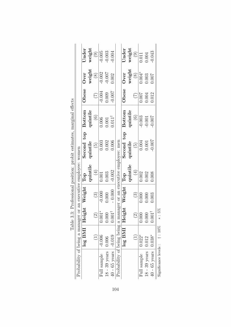
Tab

le3.

3:P

rofe

ssio

nal

pos

itio

n:

pro

bit

esti

mat

es,m

argi

nal

effec

ts

Pro

bab

ility

ofbei

ng

am

anag

eror

anex

ecuti

veem

plo

yee:

wom

enlo

gB

MI

Heig

ht

Weig

ht

Top

quin

tile

Seco

nd

top

quin

tile

Bott

om

quin

tile

Obese

Over

weig

ht

Under

weig

ht

(1)

(2)

(3)

(4)

(5)

(6)

(7)

(8)

(9)

Full

sam

ple

-0.0

060.

001∗

-0.0

000.

001

0.00

30.

006

-0.0

04-0

.002

-0.0

0518

-39

year

s0.

006

0.00

00.

000

0.00

30.

002

0.00

10.

009

-0.0

07-0

.003

40-

65ye

ars

-0.0

190.

001†

-0.

000

-0.0

020.

006

0.01

1†-0

.007

0.00

2-0

.004

Pro

bab

ility

ofbei

ng

bei

ng

am

anag

eror

anex

ecuti

veem

plo

yee:

men

log

BM

IH

eig

ht

Weig

ht

Top

quin

tile

Seco

nd

top

quin

tile

Bott

om

quin

tile

Obese

Over

weig

ht

Under

weig

ht

(1)

(2)

(3)

(4)

(5)

(6)

(7)

(8)

(9)

Full

sam

ple

0.02

2∗0.

000

0.00

00.

002

0.00

4-0

.003

0.00

70.

004∗

0.01

118

-39

year

s0.

012

0.00

00.

000

0.00

20.

001

-0.0

010.

004

0.00

30.

004

40-

65ye

ars

0.03

8∗0.

001†

0.00

30.

008

-0.0

07-0

.007

0.01

20.

007

-0.0

43

Sign

ifica

nce

leve

ls:

†:10

%∗:

5%

104

deviations from the average. While being heavier represents a penalty for

women who are searching for a job, being particularly thin is not an advan-

tage either. For both sexes, the effects of the body size on the probability of

being occupied are stronger in the youngest group rather than in the older.

Once employed, however, body size does not appear to be a matter of concern

any more, playing no role in the probability of reaching managerial positions.

As already pointed above, however, the results are likely to be biased

because of endogeneity and cannot be interpreted causally. The next section

offers a possible correction for the mentioned problem based on the instru-

mental variable technique.

3.5 Instrumental variable approach

3.5.1 The instruments

There are several reasons to believe that body size is an endogenous regressor:

labour market outcomes can itself affect body size, or unobserved factors

such as individual time preferences may affect both body size and labour

market outcomes. Furthermore, measurement errors in the BMI variable due

to systematic misreporting of height or weight represent an additional source

of bias.

To cope with this problem, an instrumental variable regression approach

is applied. The set of instruments used in this paper includes variables that

capture attitudes towards food, smoke and physical activity of the peers of

the respondent, that is of people with whom the respondent may relate and

compare himself. More specifically, the instruments are the percentages by

105

sex, age class and region of residence of the respondent, of non-smokers, of

alcohol drinkers (individuals that drink more than half liter of beer or wine

per day and individuals who are used to drink alcohol outside of meals), of

people that consume no fruit or vegetables, of people that use to do some

physical activity and the average number of hours daily spent watching TV.

The first requirement that an instrument has to fulfil to be valid, is that

it is correlated with the endogenous measure of body size, conditional on the

other variables that may affect occupational attainments. It is well known

that the main risk factors for obesity are an incorrect nutrition (with an ex-

cessive intake of high- fat, high-calorie foods and a limited consumption of

high-fiber, low-calorie foods) and physical inactivity (NHLBI (1998) ). Smok-

ing is another factor that affects individual’s weight. Although the direction

of the relationship is still a matter of debate,37 the fact that smoke and eat-

ing habits are correlated (with smokers generally consuming less fruit and

vegetables or less high fiber grains) it is widely accepted.38 While individual

preferences are ultimately driving these behaviours, environmental influences

affect also individual attitudes to smoke, food intake and exercise becoming,

in the end, another determinant of obesity (James (1995)). The selected

instruments, therefore, are expected to be non-weak predictor of individual

body size conditional on the other covariates, inasmuch as they provide a

measure of obesity-affecting environmental influences. A simple way to test

the strength of the instrument is to regress the endogenous variable on all

the other covariates plus the instruments and to run than a F-test for the

significance of the instruments coefficients. Staiger and Stock (1997) sug-

37While an extensive medical literature supports the idea that smoking facilitates weightcontrol (see U.S. Department for Health (1990) for a review of the medical studies), recentstudies question the negative relationship between BMI and smoking (see Gruber andFrakes (2006)).

38See for example Subar et al. (1990))

106

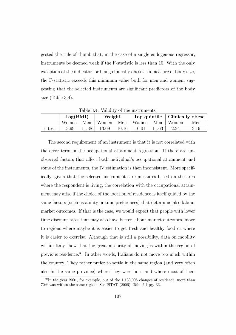
gested the rule of thumb that, in the case of a single endogenous regressor,

instruments be deemed weak if the F-statistic is less than 10. With the only

exception of the indicator for being clinically obese as a measure of body size,

the F-statistic exceeds this minimum value both for men and women, sug-

gesting that the selected instruments are significant predictors of the body

size (Table 3.4).

Table 3.4: Validity of the instruments

Log(BMI) Weight Top quintile Clinically obeseWomen Men Women Men Women Men Women Men

F-test 13.99 11.38 13.09 10.16 10.01 11.63 2.34 3.19

The second requirement of an instrument is that it is not correlated with

the error term in the occupational attainment regression. If there are un-

observed factors that affect both individual’s occupational attainment and

some of the instruments, the IV estimation is then inconsistent. More specif-

ically, given that the selected instruments are measures based on the area

where the respondent is living, the correlation with the occupational attain-

ment may arise if the choice of the location of residence is itself guided by the

same factors (such as ability or time preferences) that determine also labour

market outcomes. If that is the case, we would expect that people with lower

time discount rates that may also have better labour market outcomes, move

to regions where maybe it is easier to get fresh and healthy food or where

it is easier to exercise. Although that is still a possibility, data on mobility

within Italy show that the great majority of moving is within the region of

previous residence.39 In other words, Italians do not move too much within

the country. They rather prefer to settle in the same region (and very often

also in the same province) where they were born and where most of their

39In the year 2001, for example, out of the 1,133,006 changes of residence, more than70% was within the same region. See ISTAT (2006), Tab. 2.4 pg. 36.

107

relatives are still living. Moving to other regions is mostly driven by job

opportunities rather than by the desire of living healthier, so it is really un-

likely that the choice of the location of residence is endogenous in the labour

outcomes equation.

3.5.2 Instrumental variables with binary dependent vari-

ables

In linear models, the standard solution to the endogeneity bias is an estimator

such as two-stage least squares (2SLS). Two great advantages of linear 2SLS

estimation are its numerical simplicity and the fact that it does not require

explicit modelling of the endogenous regressor. All that is needed are valid

(in the sense explained in the previous section) instruments, no matter if the

endogenous regressor is discrete, limited or truncated. Unfortunately, unless

we are willing to use a liner probability model (LPM), 2SLS is inconsistent

for most limited dependent models.

The LPM cannot be a good description of the population response prob-

ability, because the predicted probability can be outside the unit interval.

However, LPM offers very often a convenient approximation to the underly-

ing response probability for common values of the covariates. For this reason,

we start estimating a LPM using 2SLS; given that the selected instruments

appear to be weak when the indicators for being clinically obese are used,

the LPM has been estimated without these measures.

Generally speaking, the IV results reveal a stronger effect of BMI on

occupation. In particular, three interesting outcomes emerge: i) the increase

in the estimated effect in both groups, ii) the change in the direction of the

108

effect of body size for men (from positive in the regression without taking

into account endogeneity to negative), and iii) the fact that in the full sample

BMI has a stronger negative effect for men than for women.

Table 3.5: Labour market status equation: linear proba-

bility model with instrumental variables

Log

(BMI)

Height Weight Top

quintile

Second top

quintile

Bottom

quintile

(1) (2) (3) (4) (5) (6)

Probability of being employed: women

Full

sample

-0.192 0.008† -0.001 2.155† -1.835∗ 0.739

18−39

years

-1.274∗ 0.021∗ -0.020∗ 0.750† -1.494∗ -0.171

40−65

years

-0.403† 0.019∗ -0.006 0.435∗ -0.151 0.375†

Probability of being employed: men

Log

(BMI)

Height Weight Top

quintile

Second top

quintile

Bottom

quintile

(1) (2) (3) (4) (5) (6)

Full

sample

-2.383∗ 0.053∗ -0.019∗ 2.834∗ .1911 2.944∗

18−39

years

-1.898∗ 0.068∗ -0.019∗ 0.863 -1.193 0.427

40−65

years

-0.844∗ 0.021∗ 0.002 1.275 -0.203 0.681


109


Significance levels : † : 10% ∗ : 5%

Exogenous Regressors:age, age squared, number of household members, years of com-

pleted studies, number of children aged 0 to 5 years, number of children aged 6 to

13 years, marital status, residence in Southern Italy, interview year, presence of the

interviewer, health satisfaction, number of chronic illness, number of nights spent in

the hospital in the last three months.

Instruments:(all the percentages have to be considered by age class, sex and region

of residence): percentage of individuals who eat fruit only some time per week or

less, percentage of individuals who eat vegetables only some time per week or less,

percentage of individuals who eat leaf vegetables only some time per week or less,

percentage of non-smokers, percentage of individuals who drink more than half litre

of beer or wine per day, percentage of individuals that use to drink alcohol outside

the main meals, percentage of individuals practising regularly some physical activity,

average number of hours spent daily watching TV.

According to the IV estimates, a 10% increase in the BMI reduce by 2%

the probability of being occupied for women (although the coefficient is not

significant), while for men this probability is reduced by almost 24%. In

accordance with other studies that find a positive correlation between height

and labour success especially for men,40 height appears to affect positively

the probability to be occupied: one centimetre more, increase the probability

of being employed by almost 1% for women and 5% for men. The effect

is stronger in the youngest group: each centimetre more than the average

height, leads to an increase in the probability of being employed by 2.1% for

women and 7% for men. The results obtained using indicators for the relative

40Hubler (2006), Heineck (2005), Judge and Cable (2004).

110

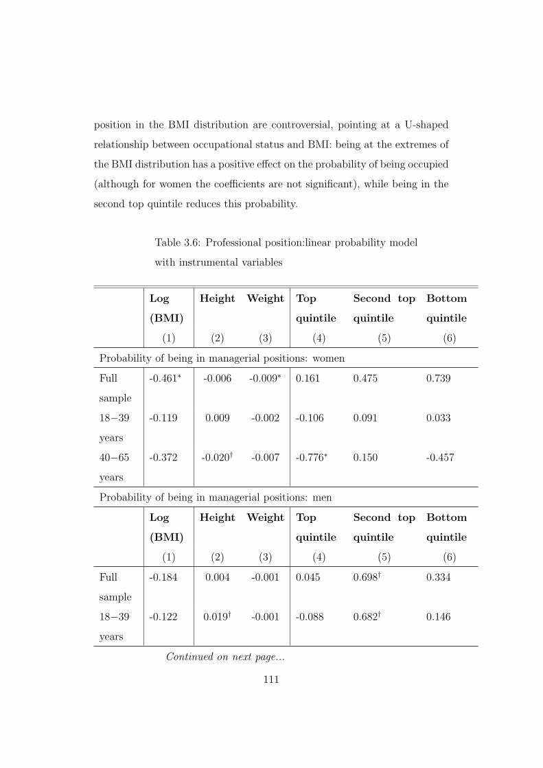
position in the BMI distribution are controversial, pointing at a U-shaped

relationship between occupational status and BMI: being at the extremes of

the BMI distribution has a positive effect on the probability of being occupied

(although for women the coefficients are not significant), while being in the

second top quintile reduces this probability.

Table 3.6: Professional position:linear probability model

with instrumental variables

Log

(BMI)

Height Weight Top

quintile

Second top

quintile

Bottom

quintile

(1) (2) (3) (4) (5) (6)

Probability of being in managerial positions: women

Full

sample

-0.461∗ -0.006 -0.009∗ 0.161 0.475 0.739

18−39

years

-0.119 0.009 -0.002 -0.106 0.091 0.033

40−65

years

-0.372 -0.020† -0.007 -0.776∗ 0.150 -0.457

Probability of being in managerial positions: men

Log

(BMI)

Height Weight Top

quintile

Second top

quintile

Bottom

quintile

(1) (2) (3) (4) (5) (6)

Full

sample

-0.184 0.004 -0.001 0.045 0.698† 0.334

18−39

years

-0.122 0.019† -0.001 -0.088 0.682† 0.146


111


40−65

years

-0.465 0.003 -0.008 0.329 -0.121 0.159















The relation between body size and professional position appear to be

only slightly significant also after correcting for endogeneity. For both men

and women the magnitude of the estimated effects is bigger using a LPM

with instrumental variables. However, only the coefficients on log(BMI) and

weight for the whole sample of women, and the coefficient on being in the

top quintile of the BMI distribution for women over 40’s are significant at

conventional levels. In comparison with the simple probit estimates, the sign

of the coefficients on log(BMI) reverts for men, from positive to negative;

none of the coefficients, however, is significant at the standard 5% level.

112

Aside from the issue of predicted probabilities being negative or greater

than one, the LPM implies that a coeteris paribus unit increase in the co-

variate xj always change the probability by the same amount, regardless of

the initial value of xj . For this reason a probit model is more accurate and,

therefore, preferable.

In order to estimate a probit correcting for endogeneity,however, we need

to make some fairly strong assumption.

We can write the model as:41

ys1 = z1δ1 + α1y2 + u1 (3.1)

y2 = z1δ21 + z2δ22 + v2 = zδ2 + v2 (3.2)

y1 = I[ys1 > 0] (3.3)

What is observable is variable y1 that assumes value 1 when the under-

lying latent variable ys1, that depends on a set of regressors z1 and on the

endogenous variable y2, is greater than 0. Equation 3.3 represent a reduced

form for y2 regressor, which is supposed to be a linear function of the ex-

ogenous regressors in equation 3.2 and of some other regressors z2. The

endogeneity problem arises if the error terms u1 and v2 are correlated.

Assuming that the vector of disturbances of equations 3.2 and 3.3 is

independent of z, has zero mean and has a bivariate normal distribution,

efficient estimators of the parameters of the structural equation 3.2 can be

derived. The normality assumption limits the types of endogenous regressors

that can be considered. In particular, because v2 is supposed to be normally

41The notation used is the same as in Wooldridge (2003), pag. 472

113

distributed, we are assuming that y2 given z is normal; thus y2 should have

features of a normal random variable and cannot be, for example, a discrete

one. For this reason, we focus on log BMI as a measure of body-size. As

shown in illustration 3.1, in fact, the estimated distribution of this variable

is fairly normal.

Figure 3.1: Sample distribution of log(BMI)

01

23

4D

ensi

ty

2.5 3 3.5 4Log(BMI)

Kernel density estimate

Normal density

men

01

23

Den

sity

2.5 3 3.5 4Log(BMI)

Kernel density estimate

Normal density

women

Given these assumption, we apply Newey’s two-step procedure (N2SP) to

obtain the coefficient estimates. The procedure consists in: i) estimating the

reduced form parameters using a least squares estimator and then ii) solving

for the structural parameters by applying the Amemiya’s generalized least

squares estimator.42

42Amemiya (1978) presents the AGLS estimator. For a summary of how AGLS workssee Maddala (1983). The two-step estimator used here is presented in Newey (1987). All

114

Table 3.7: Probability of being occupied: IV estimates.

Marginal effects of log(BMI)

Women Men

Full sample -0.553∗(0.181) -1.218∗(0.225)

N 26,382 39,658

Pseudo R2 0.33 0.26

18−39 years -1.233∗(0.386) -1.124∗(0.277)

N 15,608 20,980

Pseudo R2 0.34 0.28

40−65 years -0.284†(0.158) -0.673∗(0.279)

N 10,774 18,678

Pseudo R2 0.17 0.16















the estimates are obtained using the command ivprob written by J. Harkness in Stata 8.0.

115

In comparison with the results obtained using a LPM, the estimated

marginal effects are smaller for men and for the two subsample of young and

old women. The bigger penalty deriving from body size suffered by men

in comparison with women is confirmed also using the N2SP, although the

difference is not so big as in the LPM estimate. The separate analysis of the

effect in the two subsamples of young and old individuals reveals that while

the negative effect of BMI on occupation is stronger for men than for women

in the over 40’s group, in the youngest subsample women are slightly more

penalized than men. The estimated effect in the older group is much smaller:

a 10% increase in individual BMI leads to a reduction in the probability of

being occupied by 3% and 7% for women and men respectively. However,

while in the simple probit regression (table 3.2) the coefficients on body-size

for this group were not significant, in the IV regression the negative effect of

BMI appears to be significant.

Table 3.8: Probability of being occupied: IV estimates.

Marginal effects of log(BMI)

Women Men

Full sample -0.318∗(0.157) -0.114 (0.178)

N 19,592 27,220

Pseudo R2 0.24 0.34

18−39 years -0.012 (0.194) 0.013 (0.142)

N 11,286 14,669

Pseudo R2 0.20 0.27


116


40−65 years -0.290 (0.243) -0.549 (0.457)

N 8,216 12,551

Pseudo R2 0.28 0.35















Concerning the relationship between BMI and professional position, N2SP

leads generally to smaller effects than the LPM. Only the coefficient for

women is however significant: when the relation is investigated in the two

subgroups of young and old individual, none of the estimated effects is sig-

nificantly different from zero. This result confirms the hypothesis that the

significant reduction in the probability of being occupied suffered by heavier

workers can be the outcome of pure employer discrimination. In the first

stage of the selection of the candidate, employers may erroneously attach

117

to body size productivity related characteristic, preferring a normal size in-

dividual. However, once the heavier worker is employed, the employer can

observe worker’s productivity and in decisions concerning career advance-

ments, physical characteristics play a smaller role.

Table 3.9: Test for endogeneity: Rivers and Vuong procedure

Dependent variable: probability of being employedLog(BMI) Weight Top quintile Clinically obese

Women Men Women Men Women Men Women MenResidual 4.16∗ 12.67∗ 0.06∗ 0.16∗ -1.51∗ -0.75 -5.12∗ 2.99†

(st. er.) (1.35) (1.81) (0.02) (0.02) (0.52) (0.49) (2.07) (1.53)R2 0.33 0.26 0.33 0.26 0.33 0.26 0.33 0.26Dependent variable: probability of being a manager

Log(BMI) Weight Top quintile Clinically obeseWomen Men Women Men Women Men Women Men

Residual 2.08 3.09 0.04 0.04 1.22† -0.67 7.07∗ 3.50†

(st. er.) (1.58) (2.16) (0.03) (0.03) (0.66) (0.66) (2.51) (1.80)R2 0.22 0.29 0.22 0.29 0.22 0.29 0.22 0.29Significance levels : † : 10% ∗ : 5%

To test for the endogeneity of the body size measures, the two-step ap-

proach suggested by Rivers and Vuong (1998) is used. The procedure consists

in first estimating equation 3.3 running an OLS regression of the endogenous

regressor y2 on all the covariates plus the instruments. The second step

consists in adding the residuals v2 from the OLS regression in the probit re-

gression of the dependent variable on all the covariates plus the endogenous

regressor. A significant coefficient θv2 on the residuals in the probit regression

indicates that endogeneity exists.

118

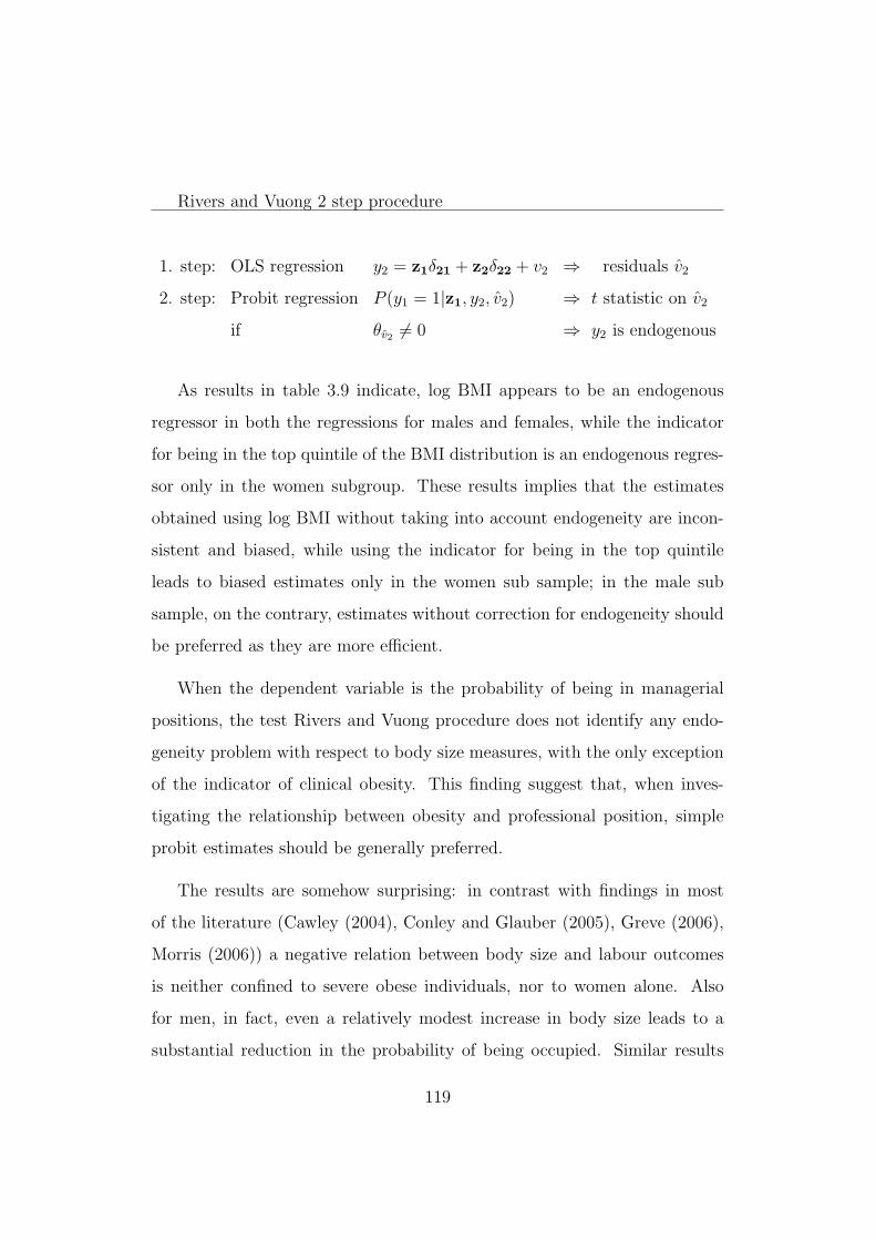
Rivers and Vuong 2 step procedure

1. step: OLS regression y2 = z1δ21 + z2δ22 + v2 ⇒ residuals v2

2. step: Probit regression P (y1 = 1|z1, y2, v2) ⇒ t statistic on v2

if θv2 6= 0 ⇒ y2 is endogenous

As results in table 3.9 indicate, log BMI appears to be an endogenous

regressor in both the regressions for males and females, while the indicator

for being in the top quintile of the BMI distribution is an endogenous regres-

sor only in the women subgroup. These results implies that the estimates

obtained using log BMI without taking into account endogeneity are incon-

sistent and biased, while using the indicator for being in the top quintile

leads to biased estimates only in the women sub sample; in the male sub

sample, on the contrary, estimates without correction for endogeneity should

be preferred as they are more efficient.

When the dependent variable is the probability of being in managerial

positions, the test Rivers and Vuong procedure does not identify any endo-

geneity problem with respect to body size measures, with the only exception

of the indicator of clinical obesity. This finding suggest that, when inves-

tigating the relationship between obesity and professional position, simple

probit estimates should be generally preferred.

The results are somehow surprising: in contrast with findings in most

of the literature (Cawley (2004), Conley and Glauber (2005), Greve (2006),

Morris (2006)) a negative relation between body size and labour outcomes

is neither confined to severe obese individuals, nor to women alone. Also

for men, in fact, even a relatively modest increase in body size leads to a

substantial reduction in the probability of being occupied. Similar results

119

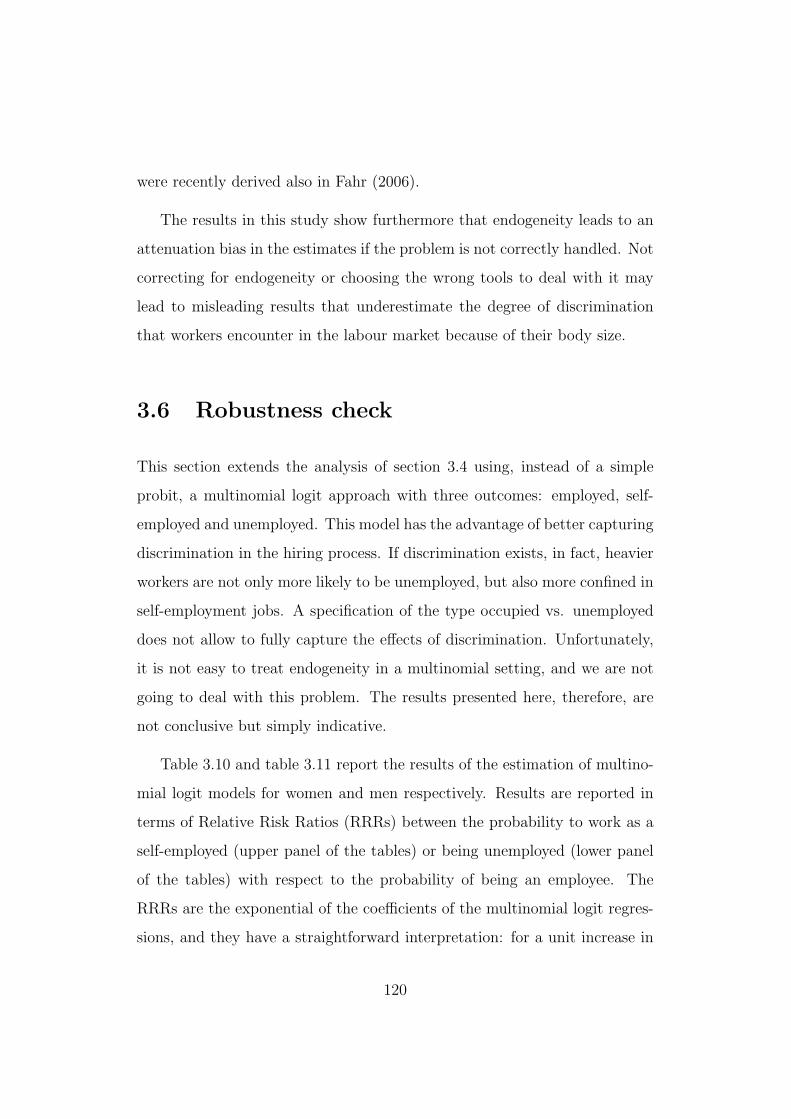
were recently derived also in Fahr (2006).

The results in this study show furthermore that endogeneity leads to an

attenuation bias in the estimates if the problem is not correctly handled. Not

correcting for endogeneity or choosing the wrong tools to deal with it may

lead to misleading results that underestimate the degree of discrimination

that workers encounter in the labour market because of their body size.

3.6 Robustness check

This section extends the analysis of section 3.4 using, instead of a simple

probit, a multinomial logit approach with three outcomes: employed, self-

employed and unemployed. This model has the advantage of better capturing

discrimination in the hiring process. If discrimination exists, in fact, heavier

workers are not only more likely to be unemployed, but also more confined in

self-employment jobs. A specification of the type occupied vs. unemployed

does not allow to fully capture the effects of discrimination. Unfortunately,

it is not easy to treat endogeneity in a multinomial setting, and we are not

going to deal with this problem. The results presented here, therefore, are

not conclusive but simply indicative.

Table 3.10 and table 3.11 report the results of the estimation of multino-

mial logit models for women and men respectively. Results are reported in

terms of Relative Risk Ratios (RRRs) between the probability to work as a

self-employed (upper panel of the tables) or being unemployed (lower panel

of the tables) with respect to the probability of being an employee. The

RRRs are the exponential of the coefficients of the multinomial logit regres-

sions, and they have a straightforward interpretation: for a unit increase in

120

the variable keeping all the other covariates constant, they show the change

in the relative risk for the outcome of interest (being self-employed or be-

ing unemployed) in comparison with the base category (being an employee).

So, for example, the weight coefficient 1.009 for women on table 3.10, lower

panel, first row, third column, tells that for a unit increase in the weight, the

probability of being unemployed rather than an employee increases by 0.9%.

Roughly speaking, a coefficient greater than (smaller than) one indicates that

the variable in question increases (decreases) the probability of being in the

considered outcome rather then in the base value.

For women, body size seems to have no significant effect on the probabil-

ity of being self-employed, while it strongly affects the probability of being

unemployed: women in the top quintile of the BMI distribution have a 17%

higher probability of being unemployed, while for clinically obese women this

probability is 25% higher. The risk of unemployment estimated using the log-

arithm of BMI as body size measure is particularly high in comparison with

all the previous estimates (probit without correcting for endogeneity, LPM

with IV and N2SP): a 10% increase in the BMI for women aged less than 40

years, for example, more than doubles the risk of being unemployed rather

than an employee.

Men’s labour market outcomes are affected by body size in a different

manner. In contrast with the results for women, body size is not particu-

larly significant in determining the relative risk of being unemployed. The

few coefficients that are significant at a standard level reveal that thinness

is a characteristic not rewarded in the male labour market, while a little

upward deviation in the body size slightly decrease the relative risk of be-

ing unemployed. Considering the attenuation bias of the estimates without

correcting for endogeneity, the weak (and positive) correlation between obe-

121

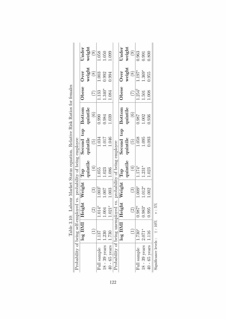
Tab

le3.

10:

Lab

our

Mar

ket

Sta

tus

equat

ion.

Rel

ativ

eR

isk

Rat

ios

for

fem

ales

Pro

bab

ility

ofbei

ng

self-e

mplo

yed

vs.

pro

bab

ility

ofbei

ng

emplo

yee

log

BM

IH

eig

ht

Weig

ht

Top

quin

tile

Seco

nd

top

quin

tile

Bott

om

quin

tile

Obese

Over

weig

ht

Under

weig

ht

(1)

(2)

(3)

(4)

(5)

(6)

(7)

(8)

(9)

Full

sam

ple

1.13

71.

014∗

1.00

3†1.

055

1.03

40.

990

1.13

31.

003

1.05

818

-39

year

s1.

230

1.00

41.

007

1.02

31.

017

0.98

41.

340∗

0.99

21.

050

40-

65ye

ars

1.73

01.

021∗

1.00

31.

086

1.04

61.

039

1.08

40.

994

1.09

9P

robab

ility

ofbei

ng

unem

plo

yed

vs.

pro

bab

ility

ofbei

ng

emplo

yee

log

BM

IH

eig

ht

Weig

ht

Top

quin

tile

Seco

nd

top

quin

tile

Bott

om

quin

tile

Obese

Over

weig

ht

Under

weig

ht

(1)

(2)

(3)

(4)

(5)

(6)

(7)

(8)

(9)

Full

sam

ple

1.73

0∗0.

987∗

1.00

9∗1.

174∗

1.05

80.

987

1.25

4†1.

197∗

0.96

318

-39

year

s2.

071∗

0.98

3∗1.

012∗

1.23

1∗1.

095

1.00

21.

501

1.36

9∗0.

991

40-

65ye

ars

1.11

60.

995

1.00

21.

023

0.09

30.

936

1.00

80.

955

0.80

0

Sign

ifica

nce

leve

ls:

†:10

%∗:

5%

122

Tab

le3.

11:

Lab

our

Mar

ket

Sta

tus

equat

ion.

Rel

ativ

eR

isk

Rat

ios

for

mal

es

Pro

bab

ility

ofbei

ng

self-e

mplo

yed

vs.

pro

bab

ility

ofbei

ng

emplo

yee

log

BM

IH

eig

ht

Weig

ht

Top

quin

tile

Seco

nd

top

quin

tile

Bott

om

quin

tile

Obese

Over

weig

ht

Under

weig

ht

(1)

(2)

(3)

(4)

(5)

(6)

(7)

(8)

(9)

Full

sam

ple

2.22

7∗1.

002c

1.01

0†1.

221∗

1.06

1†0.

920∗

1.34

6∗1.

138∗

0.78

018

-39

year

s2.

631∗

0.99

81.

013

1.12

3∗1.

107∗

0.90

8†1.

440∗

1.18

9∗0.

894

40-

65ye

ars

1.95

7∗1.

006†

1.00

9∗1.

205∗

1.01

60.

939

1.31

2∗1.

094∗

0.80

0P

robab

ility

ofbei

ng

unem

plo

yed

vs.

pro

bab

ility

ofbei

ng

emplo

yee

log

BM

IH

eig

ht

Weig

ht

Top

quin

tile

Seco

nd

top

quin

tile

Bott

om

quin

tile

Obese

Over

weig

ht

Under

weig

ht

(1)

(2)

(3)

(4)

(5)

(6)

(7)

(8)

(9)

Full

sam

ple

0.71

9†0.

993∗

0.99

61.

029

0.90

8†1.

124∗

0.99

70.

917∗

1.08

718

-39

year

s0.

766

0.99

0∗0.

997

1.02

20.

896

1.10

10.

991

0.95

81.

002

40-

65ye

ars

0.71

80.

996

0.99

71.

094

0.09

831.

197†

0.97

90.

884

2.46

8∗

Sign

ifica

nce

leve

ls:

†:10

%∗:

5%

123

sity and unemployment for men is not surprising. Apart from econometric

reasons however, the relation can be also explained with the role that men

traditionally have in the household. Given that men are usually the bread-

winners, their incentive to exit the unemployment status is higher than for

women, who can usually rely upon their male partner’s income to live. In

this respect, the fact that for men being in the top quintile of the distribution

increases the risk of being self-employed by 20%(while for women in the top

quintile the relationship is not significant) can be seen as a sign of discrim-

ination: employers prefer normal size men, so bigger individuals to support

their families turns to self-employment jobs.

Coherently with the results obtained in the previous sections, also the

multinomial logit approach reveal a different effect of body size on labour

market status in the two subgroups of young and old individuals. The effect

of BMI and obesity, in fact, is generally for both men and women much

stronger in the former group rather than in the latter: all in all, physical

appearance is more relevant in determining labour market status in earlier

stages of one’s own career, while for individuals at the end of their working

lives, other factors contribute more in explaining labour outcomes.

Overall and keeping in mind that the results may be biased due to endo-

geneity of the body size measure, we could interpret the estimated associa-

tions as a sign of discrimination against obese workers of both sexes, although

the effect differs according to age and gender. Men below the age of 40 and

women aged 40 years and more are the groups whose labour outcomes are

more affected by a deviation from the median BMI.

For the subgroup of the employees, the association between obesity and

professional position has been estimated. The AVQ questionnaire classifies

124

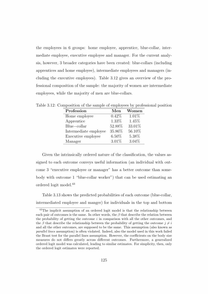
the employees in 6 groups: home employee, apprentice, blue-collar, inter-

mediate employee, executive employee and manager. For the current analy-

sis, however, 3 broader categories have been created: blue-collars (including

apprentices and home employee), intermediate employees and managers (in-

cluding the executive employees). Table 3.12 gives an overview of the pro-

fessional composition of the sample: the majority of women are intermediate

employees, while the majority of men are blue-collars.

Table 3.12: Composition of the sample of employees by professional position

Profession Men WomenHome employee 0.42% 1.01%Apprentice 1.33% 1.45%Blue−collar 52.88% 33.01%Intermediate employee 35.86% 56.10%Executive employee 6.50% 5.38%Manager 3.01% 3.04%

Given the intrinsically ordered nature of the classification, the values as-

signed to each outcome conveys useful information (an individual with out-

come 3 “executive employee or manager” has a better outcome than some-

body with outcome 1 “blue-collar worker”) that can be used estimating an

ordered logit model.43

Table 3.13 shows the predicted probabilities of each outcome (blue-collar,

intermediated employee and manger) for individuals in the top and bottom

43The implicit assumption of an ordered logit model is that the relationship betweeneach pair of outcomes is the same. In other words, the β that describe the relation betweenthe probability of getting the outcome i in comparison with all the other outcomes, andthe β that describe the relationship between the probability of getting the outcome j 6= iand all the other outcomes, are supposed to be the same. This assumption (also known asparallel lines assumption) is often violated. Indeed, also the model used in this work failedthe Brant test for the parallel lines assumption. However, the coefficients on the body sizemeasures do not differs greatly across different outcomes. Furthermore, a generalizedordered logit model was calculated, leading to similar estimates. For simplicity, then, onlythe ordered logit estimates were reported.

125

Table 3.13: Ordered logit predicted probabilities

Men WomenTop quintile Not top

quintileTop quintile Not top

quintileApprentice,Blue−collar

0.56 0.55 0.32 0.26

Intermediateemployee

0.42 0.42 0.66 0.71

Executiveemp./manager

0.02 0.02 0.02 0.03

Bottom quintile Not bottomquintile

Top quintile Not bottomquintile

Apprentice,Blue−collar

0.56 0.55 0.25 0.28

Intermediateemployee

0.42 0.42 0.72 0.69

Executiveemp./manager

0.02 0.02 0.03 0.02

Relative position on BMI distribution as measure of body size

quintile of the BMI distribution in comparison with all the others. Body size

hampers women more than men in their career. On the one hand side, set-

ting all the other variables at their sample mean, the probability of being in

the blue-collar category in comparison with the other categories is for women

in the top quintile of the BMI distribution 8 percent point higher than for

all the other women, while their probability of being intermediate employees

is 5 percent point lower.44 On the other side, women in the bottom quintile

of the distribution have a relatively higher probability of being managers or

intermediate employees and a lower probability of being blue-collar workers.

44The probability of being a blue-collar worker is 26% for women not in the top quintileof the BMI distribution while is 32% for women in the top quintile (table 3.13 right-upperpanel, first row): the probability of being blue-collar workers is therefore 26 − 32 = 8%higher. At the same time, the probability of being an intermediate employee is 66% forwomen in the top quintile and 71% for all the other women: for bigger women, therefore,the probability of being intermediate employees is 71− 66 = 5% lower.

126

On the contrary, the predicted probabilities for men do not show any signifi-

cant difference, neither when men in the top quintile are compared with the

others, nor when the comparison is between men in the bottom quintile and

all the others. The results are quite similar when the logarithm of BMI is

used as measure of body size.

Illustration 3.2 plots the predicted probabilities for women (top panel)

and men (lower panel) of being in each of the 3 outcomes for discrete incre-

ments of log(BMI).45 While for women the probability of being in the better

outcomes (intermediate employee and manager) decreases and the probabil-

ity of being a blue collar increases as the logarithm of BMI increases, for men

no change in the predicted probabilities can be appreciated.

3.7 Concluding remarks

In this study, using a survey that investigates several aspects of households’

habits, the relationship between body size and labour market status in Italy

has been investigated.

The contribution to the growing body of literature on this issue is twofold:

from a geographical point of view, this work investigates Italy, a country

up to now almost neglected. The analysis of this country, characterized

by labour market rigidities, a low average BMI and a fast increase in the

incidence of obesity, helps in better understanding the effect of social norms

45The predicted probabilities have been estimated using a ordered logit model, control-ling also for age, age squared, number of children aged 0 to 5 years, number of childrenaged 6 to 13 years, number of household members, marital status, number of years ofstudying, self-reported health status, number of nights spent in the hospital in the last 3months, number of chronic diseases suffered, residence in the South of Italy, presence ofthe interviewer, year dummies, economic sector of activity. All the covariates are set attheir sample means.

127

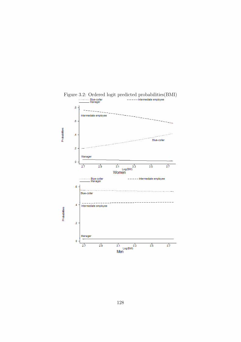
Figure 3.2: Ordered logit predicted probabilities(BMI)

128

and discrimination in an institutional setting very different from the Anglo-

Saxon one, widely covered by the existing literature. From a methodological

point of view, this paper proposes a new set of instruments to deal with

the endogeneity problem. The set include variables that capture attitudes

towards food, smoking and physical activity of the peers of the respondent,

that is of people with whom the respondent may relate and compare himself.

The instruments are found to be non-weak predictor of body size measures

and are plausibly not themselves endogenous with labour market outcomes.

Controlling for a broad set of individual covariates, probit regressions,

without controlling for endogeneity of the body size measure, highlight a

negative relation between body size and probability of being employed for

women and a positive one for men. After correcting for endogeneity, how-

ever, the relationship appears to be significantly negative for both men and

women. In contrast with most of the existing literature, the results high-

light the presence of discrimination against heavy workers irrespectively of

their sex. We estimate also the model using a multinomial logit with three

outcomes: employee, self-employed and unemployed. The multinomial logit

results partially confirm the presence of discrimination also against men. The

fact that heavier male workers tend to be more segregated in self-employment

jobs, in fact, may be interpreted as the outcome of employers discrimination

in the hiring process. Using a Rivers and Vuong two step procedure, we iden-

tify endogeneity with respect to body size measures when the occupational

status is analyzed: considering body size as an exogenous regressor, then,

leads to inconsistent estimates and IV estimates should be preferred. This

study shows then that endogeneity leads to an attenuation bias in the esti-

mates if the problem is not correctly handled. Not correcting for endogeneity

or choosing the wrong tools to deal with it may conduct to misleading results

129

that underestimate the degree of discrimination that workers encounter on

the labour market because of their body size.

The relationship between body size and professional position in the sub-

group of the employees appears to be not statistically significant for females,

while for men it is significant only when the logarithm of the BMI is chosen

as a measure of body size. Also IV coefficients are generally not significant.

However, the Rivers and Vuong two steps procedure does not identify any

endogeneity. In this case, the probit estimates should be preferred as they

are more efficient.

A possible explanation for these results is that physical appearance works

for employers as an imperfect signal of productivity. Obesity is usually re-

lated with lower health status and thus with lower productivity, although

not all the obese individuals are unhealthy. The employer do not have full

information concerning the productivity of the individual and, as a body size

bigger than average convey the signal that the worker is less productive, she

may choose to hire a normal-size individual rather than a bigger one. How-

ever, when decisions concerning career advancements of employees have to

be taken, the employer has the opportunity to observe workers’ productivity

and she has not to rely any more upon imperfect signals (such as physical ap-

pearance). That is why body size plays no role in determining the probability

of reaching top professional positions.

130

3.A Appendix

3.A.1 Correction for misreporting in height and weight

This section proposes a possible correction for the misreporting of the an-

thropometric variables (height and weight) used to measure body size.

A correction suggested in the literature consists in predicting the “true”

values for height and weight using information on the relationship between

true and reported values in a subsample of individuals that were actually

measured. Separately by sex and gender, the true measures are regressed on

the reported ones and the obtained coefficients are used to correct height and

weight of the individuals for whom only the reported measured are known.46

As already highlighted in section 1.2, the survey used does not allow to

correct for the measurement error, as there is not a sub sample of individuals

that were measured and with whom correct the other measures. A different

strategy, therefore, is applied in this work. A study by Danubio et al. (2006)

conducted on a sample Italian adults aged 18 to 36 years old, finds that

on average men overreport height by 1.2% and underreport weight by 1.9%,

while women overreport their height by 1.8% and underreport their weight by

3%. Height and weight of the individuals in this sample have been corrected

using this information on the average bias.47 Table 3.14 reports the probit

estimated with and without correction. Given that the sample analised by

Danubio et al. (2006) consists of young individuals and that the extent of

misreporting increases with age, the analysis has been restricted only to the

subgroup of young individuals (aged 18 to 39).48

46see Cawley (2004), Bound et al. (2002) Lee and Sepanski (1995)47Greve (2006) applies a similar strategy for Denmark.48The results are similar if the correction is applied to the whole sample of individuals.

131

Table 3.14: Probit estimates with and without correction for misreportingthe anthropometric measures

Probability of being employedWithout correction With correction

Body size measure Men Women Men WomenLog(BMI) 0.032 - 0.072 0.032 -0.072Height 0.001 0.002 0.001 0.002Weight 0.000 -0.001 0.000 -0.001Top quintile 0.002 -0.022 0.002 -0.022Second top quintile 0.020 -0.009 0.010 -0.009Bottom quintile -0.008 0.000 -0.008 0.000Obese 0.006 -0.044 0.011 -0.036Overweight 0.006 -0.034 0.008 -0.019Underweight 0.002 0.003 0.010 -0.002Probability of being a managerLog(BMI) 0.012 0.006 0.012 0.006Height 0.000 0.001 0.000 0.001Weight 0.000 0.000 0.000 0.000Top quintile 0.002 0.003 0.002 0.003Second top quintile 0.001 0.002 0.001 0.002Bottom quintile - 0.001 0.001 -0.000 0.001Obese 0.004 0.009 0.004 0.014Overweight 0.003 -0.007 0.001 -0.000Underweight 0.004 -0.003 0.009 -0.008

132

No major differences emerge after correcting for misreporting. The biggest

discrepancies emerge when the clinical definition of obesity, overweight and

underweight are used as measures of body size. Once correcting for misre-

porting, the positive effect of overweight and obesity on the probability of

being employed is even bigger for men, while the estimated negative effect for

women is reduced.As already highlighted in other studies, systematic errors

in reporting anthropometric measures do not affect in a sensible fashion the

results and can be, therefore, disregarded.49

49See for example Lakdawalla and Philippson (2002), Greve (2006)

133

Bibliography

B. A’Hearn. Anthropometric evidence on living standards in northern italy,

1730 1860. Journal of Economic History, 63(2):351–381, 2003.

B. A’Hearn. A restricted maximum likelihood estimator for historical height

samples. Economics and Human Biology, 2(1):5–19, 2004.

B. A’Hearn. Remapping italys path to the 19th century: Anthropometric

signposts. Journal of European Economic History, 35(2), 2006.

B. A’Hearn and J. Komlos. Improvements in maximum likelihood estimators

of truncated normal samples with prior knowledge of σ: A simulation

based study with application to historical height samples. Technical report,

Munchener Wirtschaftswissenschaftliche Beitrage (VWL), 8 2003.

T. Amemiya. The estimation of a simultaneous equation generalized probit

model. Econometrica, 46(5):1193 – 1205, 1978.

R.R. Anderson and R.M. May. Infectious Diseases of Humans: Dynamics

and Control. Oxford University press, Oxford, 1991.

E. Arcaleni. Secular trend and regional differences in the stature of italians,

18541980. Economics and Human Biology, 4:24–38, 2006.

134

I. Arita, J. Wickett, and F. Fenner. Impact of population density on immu-

nization programmes. Journal of Hygiene, 96:459 – 466, 1986.

S. Averett and S. Korenmann. The economic reality of the beauty myth.

Journal of Human Resources, 31(2):304 – 330, 1996.

J. Baten. Ernahrung und wirtschaftliche Entwicklujng in Bayern, 1730 1880.

Steiner Verlag, Stuttgart, 1999.

J. Baten. Climate, grain production and nutritional status in southern ger-

many during the xviiith century. The Journal of European Economic His-

tory, 30:9–47, 2001.

J. Baten. Consumption, and leisure: The standard of living. In S. Ogilvie

and R. Overy, editors, Germany: A New social and Economic History,

volume III: 1800-1989, pages 383–422. Oxford university Press, Inc., 2003.

J. Baten and J. E. Murray. Heights of men and women in 19th-century

bavaria: Economic, nutritional, and disease influences. Explorations in

Economic History, 37:351–369, 2000.

C. L. Baum and W.F. Ford. The wage effects of obesity: a longitudinal study.

Health Economics, 13:885 – 899, 2004.

C.C. Bayley. Mercenaries for the Crimea. McGill-Queen’s university press,

1977.

H. Beck. The social policies of prussian officials: The bureaucracy in a new

light. Journal of Modern History, 64:263–298, 1992.

G. Becker. The Economics of Discrimination. Chicago University Press,

Chicago, 1957.

135

J. R. Behrman and M.R. Rosenzweig. The returns to increasing body weight.

In PIER working paper, number 01-052, 2001.

J. Bhattacharya and M. K. Bundorf. The incidence of the health care costs

of obesity. NBER Working paper series, (11303), 2005.

J. Bound, C.Brown, and N. Mathiowetz. Measurement error in survey data.

In J. Heckman and E. Leamer, editors, Handbook of Econometrics, vol-

ume 5, pages 3705–3843. Springer-Verlag, New - York, 2002.

A. Braglia. La grande bonificazione ferrarese. Secolo XV - secolo XX. SATE,

Ferrara, 1962.

G. Brunello and B. D’Hombres. Does obesity body weight affects wages? ev-

idence from europe. Economics and Human Biology, (forthcoming), 2007.

A. C. Trattato elementare di aritmentica ad uso dei corsi tecnici, ginnasiali,

liceali e delle scuole militari. G.B. Paravia, 1880.

R. Cameron. A Concise Economic history of the World from Paleolithic

Times to the present. Oxford university Press, Inc., 1997.

A. Caracciolo. La storia economica. In R. Romano and C. Vivanti, editors,

Storia d’Italia, volume 3, pages 511 – 693. Giulio Einaudi editore, Torino,

1973.

M. Carley. Social Measurement And Social Indicators : Issues Of Policy And

Theory. Allen & Unwin, London, 1981.

A. E. J. M Cavelaars, A. E. Kunst, J. J. M. Geurts, et al. Persistent variations

in average height between countries and between socio-economic groups:

An overview of 10 european countries. Annals of Human Biology, 27(4):

407–421, 2000.

136

J. Cawley. Body weight and womens labor market outcomes. NBER Working

Paper, (7841), 2000.

J. Cawley. The impact of obesity on wages. Journal of Human Resources,

39(2):451 – 474, 2004.

J. Cawley, M. Grabka, and D. Lillard. A comparison of the relationship

between obesity and earnings in the u.s. and germany. Journal of Applied

Social Science Studies (Schmollers Jahrbuch), 125:119 – 129, 2005.

F. Cinnirella. On the road to industrialization: Biological standard of liv-

ing in saxony, 18th and 19th century. In Second Conference on German

Cliometrics, Tubingen, June, 7-10 2006.

F. Cinnirella. Optimists or pessimists? a revision of the standard of living

in england, 18th and 19th century. University of Munich, 2007.

D. Conley and R. Glauber. Gender, body mass and economic status. NBER

working paper series, (11343), 2005.

D. L. Costa. Height, weight, wartime stress, and older age mortality: Evi-

dence from the union army records. Explorations in Economic History, 30:

424–449, 1993.

D. L. Costa. Understanding mid-life and older age mortality declines: evi-

dence from union army veterans. Journal of Econometrics, 112:175 – 192,

2003.

D.L. Costa. The measure of man and older age mortality: evidence from the

gould sample. Journal of Economic History, 64(1):1–23, 2004.

N. F. R. Crafts. Some dimensions of the ‘quality of life’ during the british

industrial revolution. The Economic History Review, 50(4):617 – 639, 1997.

137

M.E. Danubio, G. Miranda, M. G. Vinciguerra, E. Vecchi, and F. Rufo.

Comparison of self-reported and measured height and weight: implications

for obesity research among youth. University of L’Aquila and University

of Rome La Sapienza, 2006.

Human Mortality Database, 2007. University of California,Berkley (USA)

and Max Planck Institute for Demographic Research (Germany). Available

at http://www.mortality.org.

J. A. Davis. Economy, society and the state. In J. A. Davis, editor, Italy in

the Nineteenth Century, pages 235 – 295. Oxford University Press, 2000.

A. Sanz de Galdeano. The obesity epidemic in europe. IZA Discussion Paper,

(1814), 2005.

J. de V. Graaf. Theoretical Welfare Economics. Cambridge University Press,

1957.

Bundesministerium der Verteidigung. Korpermasse bei musterungsunter-

suchungen wehrpflichtiger sowie bei einstellungs- und entlassungsunter-

suchungen von soldaten der bundeswehr 1991 bis 1995. Beitrage zur

Wehrmedizinalstatistik, 93, 1997.

J.W. Drukker and V. Tassenaar. Paradoxes of modernization and material

well-being in the netherlands during the nineteenth century. In R. Steckel

and R. Floud, editors, Health and Welfare during Industrialization, pages

331–378. University of Chicago Press,, 1997.

M. Ezzati, H. Martin, S. Skjold, S. Vander Hoorn, and C.J.L. Murray. Trends

in national and state-level obesity in the usa after correcting for self-

reported bias: analysis of health surveys. Journal of the Royal Society

of Medicine, 99:250 – 257, 2006.

138

R. Fahr. The wage effects of social norms: evidence of deviations from peers’

body mass in europe. IZA Discussion Paper, (2323), 2006.

G. Federico. Heights, calories and welfare: a new perspective on italian

industrialization, 1854-1913. Economics and Human Biology, 1:289 – 308,

2003.

C. Feinstein. Pessimism perpetuated: Real wages and the standard of living

inbritain during and after the industrial revolution. Journal of Economic

History, 58(3):625–658, 1998.

E. A. Finkelstein, C.J. Ruhm, and K.M. Kosa. Economic causes and conse-

quences of obesity. Annual Review of Public Health, 26:239 – 257, 2005.

R. W. Fogel. The relevance of malthus for the study of mortality today:

Long-run influences on health, mortality, labor force participation, and

population growth. NBER Historical Working Paper, (54), 1994.

R. M. Foley and C. M. Pollard. Food cent$ - implementing and evaluating

a nutrition education project focusing on value for money. Australian and

New Zeeland Journal of Public Health, 22(4):494–501, 1998.

M.F. Fraga, E. Ballestar, M.F. Paz, S. Ropero, F. Setien, M.L. Ballestar,

D. Heine-Suner, J.C. Cigudosa, M. Urioste, J. Benitez, M. Boix-

Chornet, A. Sanchez-Aguilera, C. Ling, E. Carlsson, P. Poulsen, A. Vaag,

Z. Stephan, T.D.Spector, Y. Z. Wu, C. Plass, and M. Esteller. Epigenetic

differences arise during the lifetime of monozygotic twins. In Proceedings of

the National academy of Science of the United States of America, volume

102, 2005.

R. Fremdling. German national account for the 19th and early 20th century.

Scandinavian Economic History Review, 43:77–100, 1995.

139

B. S. Frey and A. Stutzer. Happiness and Economics: How the Economy

and Institutions Affect Human Well-Being. Princeton University Press,

Princeton, 2002a.

B. S. Frey and A. Stutzer. What can economists learn from happiness re-

search. Journal of Economic Literature, 40:402–435, 2002b.

J. Garcia and C. Quintana-Domeque. Obesity, employment and wages in

europe. In J. Cawley K. Bolin, editor, Advances in Health Economics and

Health Services Research, volume 17: The economics of obesity. 2007.

S.L. Gortmaker, A. Must, J.M. Perrin, A.M. Sobol, and W. H. Dietz. So-

cial and economic consequences of overweight in adolescence and young

adulthood. New England Journal of Medicine, 392(14):1008 – 1012, 1993.

A. Grab. From the french revolution to napoleon. In J.A. Davis, editor, Italy

in the Nineteenth Century, pages 25 – 50. Oxford University Press, 2000.

J. Greve. Obesity and labour market outcomes: new danish evidence. Cornell

University and Aarhus school of Business, Denmark, 2006.

B. M. Gross. The state of the nation: social systems accounting. In R. Bauer,

editor, Social Indicators. M.I.T. Press, Cambridge, MA, 1966.

J. Gruber and M. Frakes. Does falling smoking lead to rising obesity? Journal

of health Economics, 25:183 – 197, 2006.

T. W. Guinnane. Population and the economy in germany, 1800-160. In

S. Ogilvie and R. Overy, editors, Germany: A New social and Economic

History, volume III: since 1800, pages 35–70. Oxford university Press, Inc.,

2003.

140

D. S. Hamermesh and J.E. Biddle. Beauty and the labour market. American

Economic Review, 84(5):1174 – 1195, 1994.

H. Harnisch. Statistische untersuchungen zum verlauf der kapitalistischen

agrarreformen in den preußischen ostprovinzen (1811 bis 1865). Jahrbuch

fur Wirtschaftsgeschichte, 74:149 –183, 1974.

B. Harper. Beauty, stature and the labour market: a british cohort study.

Oxford Bulletin of Economics and Statistics, 62:771 – 800, 2000.

B. Harper and M. Haq. Occupational attainment of men in britain. Oxford

Economics Papers, 49(4):638 – 650, 1997.

R. M. Hartwell and S. L. Engerman. Models of immiserisation: the theoretical

basis of pessimism. In A. J. Taylor, editor, The standard of living in Britain

in the industrial revolution, pages 183 –213. Methuen, London, 1975.

J. J. Heckman, H. Ichimura, and P.E. Todd. Matching as an econometric

evaluation estimator: Evidence from evaluating a job training programme.

The Review of Economic Studies, 64(4):605 – 654, 1997.

G. Heineck. Up in the skies? the relationship between height and earnings in

germany. LABOUR: Review of Labour Economics and Industrial Relations,

19(3):469 – 484, 2005.

W. O. Henderson. The state and the industrial revolution in Prussia : 1740-

1870. Liverpool University Press, 1958.

F.W. Henning. Handbuch der Wirtschafts- und Sozialgeschichte Deutsch-

lands, volume 2: Deutsche Wirtschafts- und Sozialgeschichte im

19.Jahrhundert. 1996.

141

N. Herpin. Love, careers and height in france, 2001. Economics and Human

Biology, 3(3):420 – 449, 2005.

J.R. Hicks. Valuation of social income. Economica, 7, 1940.

N. Hicks and P. Streeten. Indicators of development: The search for a basic

needs yardstick. World Development, 7(6):567 – 580, 1979.

W. G. Hoffmann. Das Wachstum der Deutschen Wirtschaft seit der Mitte

des 19. Jahrhunderts. Springler Verlag, 1965.

O. Hubler. The nonlinear link between height and wages: an empirical in-

vestigation. IZA Discussion Paper, (2394), 2006.

V. Ilari. Storia del servizio militare in Italia, volume 1: 1506 - 1870. Centro

militare di studi strategici / Rivista Militare, 1989.

A. E. Imhof. Life Expectancies in Germany from the 17th to the 19th Century.

VCH, Acta Humaniora, 1990.

ISTAT. Movimento migratorio della popolazione residente. Number 14 in

Annuario. Istituto Nazionale di Statistica, Roma, 2006.

W.P. James. A public health approach to the problem of obesity. Interna-

tional Journal of Obesity and Related Metabolic Disorders, 19(Suppl. 3):

37 – 45, 1995.

S. P. Jenkins. Easy ways to estimate discrete time duration models. Oxford

Bulletin of Economics and Statistics, 57:129 – 138, 1995.

S. P. Jenkins. Survival analysis. Institute for Social and Economic

Research, University of Essex, Colchester, UK. Downloadable from

142

http://www.iser.essex.ac.uk/teaching/degree/stephenj/ec968/pdfs/ec968lnotesv6.pdf,

2004.

T. A. Judge and D.M. Cable. The effect of physical height on workplace

success and income: preliminary test of a theoretical model. Journal of

Applied Psychology, 89(3):428 – 441, 2004.

N. Kaldor. Welfare proposition and interpersonal comparisons of utility.

Economic Journal, 49, 1939.

W. Kannel. Health and obesity: an overview. In P.R. Kuo H.L. Conn, E.A.

De Felice, editor, Health and Obesity. Raven, New - York, 1983.

G. F. Knapp. Die Bauernbefreiung und der Ursprung der Landarbeiter in

den alteren Teilen Preußens. Verlag Duncker & Humblot, Leipzig, 1887.

J. Komlos. Stature and nutrition in the habsburg monarchy: The standard of

living and economic development. American Historical Review, 90(1149-

1161), 1985.

J. Komlos. Nutrition and Economic Development in the Eighteenth-Century

Habsburg Monarchy. An Anthropometric History. Princeton University

Press, 1989.

J. Komlos. The secular trend in the biological standard of living in the united

kingdom. Economic History Review, 46:115–144, 1993.

J. Komlos. The nutritional status of french students. Journal of Interdisci-

plinary History, 24:493–508, 1994.

J. Komlos. Shrinking in a growing economy? the mystery of physical stature

during the industrial revolution. Journal of Economic History, 58:779–802,

1998.

143

J. Komlos. How to (and how not to) analyze deficient height samples: an

introduction. Historical Methods, 37(4):160–173, 2004.

J. Komlos and M. Baur. From the tallest to (one of) the fattest: the enigmatic

fate of the american population in the 20th century. Economics and Human

Biology, 2:57 – 74, 2004.

J. Komlos and F. Cinnirella. European heights in the early 18th century.

In Discussion papers in Economics. University of Munich, department of

economics, 2005.

J. Komlos, P.K. Smith, and B. Bogin. Obesity and the rate of time preference:

is there a connection? Journal of Biosocial Science, 36:209 – 219, 2004.

J. Komlos and B. Snowdon. Measures of progress and other tall stories.

World Economics, 6(2):87 – 135, 2005.

M.F. Kuczmarski, R.J. Kuzcmarski, and M. Najjar. Effects of age on validity

of self-reported height, weight and body mass index. findings from the third

national health and nutrition examination survey, 1988 1994. Journal of

the American Dietetic Association, 100(1):28 – 34, 2001.

A. B. Kues. On the biological standard of living in switzerland, circa 1830.

University of Munich, 2006.

S. Kuznets. Economic growth and income inequality. The American Eco-

nomic Review, 45(1):1–28, 1955.

S. Kuznets. Modern economic growth: Findings and reflections. The Amer-

ican Economic Review, 63(3):247–258, Jun. 1973.

D. Lakdawalla and T. Philippson. The growth of obesity and technological

change. NBER Working Paper, (8946), 2002.

144

K. C. Land. Social indicators. Annual Review of Sociology, 9:1–26, 1983.

D. Laven. The age of restoration. In J.A. Davis, editor, Italy in the Nineteenth

Century, pages 51 – 73. Oxford University Press, 2000.

C. Lee. Socioeconomic background, disease, and mortality among union army

recruits: implications for economic and demographic history. Explorations

in Economic History, 34(1):27–55, 1997.

L. Lee and J.H. Sepanski. Estimation of linear and nonlinear errors-in-

variables models using validation data. Journal of the American Statistical

Association, 90(429):130 – 140, 1995.

W.R. Lee. Mortality level and agrarian reform in early 19th century prus-

sia: some regional evidence. In G. Fridlizius T. Bengtsson and R. Ohls-

son, editors, Pre-Industrial Population Change: The Mortality Decline and

Short-Term Population Movements, pages 161–190. 1981.

W.R. Lee. The impact of agrarian change on women’ work and child care in

early-nineteenth-century prussia. In J.C. Fout, editor, German Women in

the Nineteenth Century: A Social History. 1984.

P.H. Lindert and J. G. Williamson. English workers’ living standards during

the industrial revolution: a new look. The Economic History Review, 36

(1):1–25, 1983.

I.M.D. Little. A Critique of Welfare Economics. Clarendon Press, Oxford,

second edition, 1957.

R. Lucas. On the mechanics of economic development. Journal of Monetary

Economics, 22(1):3 –42, 1988.

145

D. Mackerras. Disadvantaged and the cost of food. Australian and New

Zeeland Journal of Public Health, 21:218, 1997.

G.S. Maddala. Limited-Dependent and Qualitative Variables in Economet-

rics. Cambridge University Press, 1983.

P. Malanima. Measuring the italian economy. 1300 1861. Rivista di Storia

Economica, 19(3):265 – 296, 2003.

L.F. Martel and H.B. Biller. Stature and Stigma. D.C. Heath and Company,

Lexington, 1987.

A. Martini. Manuale di metrologia. Misure, pesi e monete in uso attualmente

e anticamente presso tutti i popoli. Editrice E.R.A., Roma, 1883.

B. R. Mitchell. International Historical Statistics: Europe , 1750-2000. Pal-

grave MacMillan, 1992.

J. Mokyr and C. O Grada. Height and health in the united kingdom 1815 -

1860: Evidence from the east india company army. Explorations in Eco-

nomic History, 33:141 – 168, 1996.

K. Morland, S. Wing, A. Diez Roux, and C. Poole. Neighborhood character-

istics associated with the location of food stores and food service places.

American Journal of Preventive Medicine, 22(1):23 – 29, 2002.

S. Morris. Body mass index and occupational attainment. Journal of Health

Economics, 25:347 – 364, 2006.

J. Murray. Standards of the present for people of the past: height, weight, and

mortality among men of amherst college, 1834-1949. Journal of Economic

History, 57(3):585–606, 1997.

146

NHLBI (1998). Clinical Guidelines on the Identification, Evaluation and

Treatment of Overweight and Obesity in Adults, 1998. National Heart,

Lung, and Blood Institute, NHI publication No. 98-4083. National Health

Institutes, New York.

W. Newey. Simultaneous estimation of limited dependent variable models

with endogenous explanatory variables. Journal of Econometrics, 36(3):

231 – 250, 1987.

S. Nicholas and R. Steckel. Heights and living standards of english workers

during the early years of industrialisation, 1770-1815. Journal of Economic

History, 51:937–957, 1991.

OECD. OECD Employment Outlook. OECD, Paris, 1994.

K. H. O’Rourke. War and welfare: Britain, france and the united states

1807-14. Trinity College Dublin economic papers, (tep2008), 2006.

S. Paeratakul, M.A. White, D.A. Williamson, D.H. Ryan, and G.A. Bray.

Sex, race/ethnicity, socioeconomic status, and bmi in relation to self-

perception of overweight. Obesity Research, 10(5):345 – 350, 2002.

J.A. pagan and A. Davila. Obesity, occupational attainment and earnings.

Social Science Quarterly, 78:756 – 770, 1997.

A. Paraponaris, S. Berengere, and B. Venetlou. Obesity, weight status and

employability: empirical evidence from a french national survey. Eco-

nomics and Human Biology, 3(2):241 – 258, 2005.

N. Persico, A. Postelwaite, and D. Silverman. The effect of adolescent expe-

rience on labor market outcomes: The case of height. Journal of Political

Economy, 112:1019 – 1053, 2004.

147

G. Pescosolido. L’economia e la vita materiale. In G. Sabbatucci and V. Vi-

dotto, editors, Storia d’Italia, volume 1: le premesse dell’unita, pages 3 –

118. Gius. Laterza & Figli Spa, Roma − Bari, 1994.

A. C. Pigou. The Economics of Welfare. Macmillian, London, fourth edition,

1952.

J.D. Post. A study in meteorological and trade cycle history: the economic

crises following the napoleonic wars. Journal of Economic History, 34(2):

315 – 349, 1974.

S. N. Procopovitch. The distribution of national income. The Economic

Journal, 36(141):69–82, 1926.

C. A. Register and D. R. Williams. The wage effects of obesity. Social Science

Quarterly, 71:130 – 140, 1990.

D. Rivers and Q.H. Vuong. Limited information estimators and exogeneity

tests for simultaneous probit models. Journal of Economitrics, 39:347 –

366, 1998.

R.J. Roberts. Can self-reported data accurately describe the prevalence of

overweight? Public health, 109(4):275 – 284, 1995.

R. Rona. The impact of the environment on height in europe: Conceptual

and theoretical considerations. Annals of Human Biology, 27(2):111–126,

2000.

G. De Santis. Due secoli di storia della popolazione. In P. Ciocca and G. To-

niolo, editors, Storia economica d’Italia, volume 3: Iundustrie, mercati,

istituzioni, pages 39 – 71. Gius. Laterza & Figli Spa, Roma − Bari, 2002.

148

J. Sargent and D. Blanchflower. Obesity and stature in adolescence and

earnings in young adulthood. analysis of a british cohort. Archives of

Pediatrics and Adolescent Medicine, 148:681 – 687, 1994.

S. Sarlio-Latheenkorva and E. Lahelma. The association of body mass index

with social and economic disadvantage in women and men. International

Journal of Epidemiology, 28:445 – 449, 1999.

P.T. Schultz. Wage gains associated with height as a form of health human

capital. AEA Papers and Proceedings, 92(2):349 – 353, 2002.

A. Sen. Real national income. Review of Economic Studies, 43(1):19–39,

1976.

A. Sen. The welfare basis of real income comparisons. Journal of Economic

Literature, 17(1):1–45, 1979.

A. Sen. The living standard. Oxford Economic Papers, 36:74–90, 1984.

S. Sousa. Does size matter? a propensity score approach to the effect of bmi

on labour market outcomes. In Nineteenth ESPE Conference and General

Assembly in Paris, 16 - 18 June 2005.

D. Staiger and J.H. Stock. Instrumental variables regression with weak in-

struments. Econometrica, 65:557– 586, 1997.

R. Steckel. Stature and the standard of living. Journal of Economic literature,

33(4):1903–1940, Dec. 1995.

G. Steinhart. Briefe aus Helgoland. Zwickau, 1859.

R. Sturm. The effect of obesity, smoking and drinking on medical problems

and costs. Health Affairs, 21(2):245–253, 2002.

149

A.F. Subar, L.C. Harlan, and M.E. Mattson. Food and nutrient intake dif-

ferences between smokers and non-smokers in the us. American Journal

of Public Health, 80(11):1323 – 1329, 1990.

M. Sunder. On the biological standard of living of the middle class in 19th

century america. University of Munich.

A.M. Tanner and P.S.W. Davies. Clinical longitudinal standards for height

and height velocity for north american children. Journal of Pediatrics, 107:

317 329, 1985.

D. Thomas and E. Frankenberg. The measurement and interpretation of

health in social surveys. RAND, Working Paper, (DRU-2550-NIA), 2000.

F.B. Tipton. Government and the economy in the xix century. In S. Ogilvie

and R. Overy, editors, Germany: A New social and Economic History,

volume III: since 1800, pages 106–151. Oxford university Press, Inc., 2003a.

F.B. Tipton. The regional dimension: economic geography, economic devel-

opment, and national integration in the nineteenth and twentieth centuries.

In S. Ogilvie and R. Overy, editors, Germany: A New social and Economic

History, volume III: since 1800, pages 1–34. Oxford university Press, Inc.,

2003b.

S. Twarog. Heights and living standards in germany, 1850 1939: The case of

wurttemberg,. In R.H. Steckel and R. Floud, editors, Health and Welfare

During Industrialization, pages 161–200. The University of Chicago Press,

1997.

UNDP (2004). Human Development Report 2004. Oxford University Press,

New York, 2004.

150

U.S. Department for Health (1990). Out of the ashes: Choosing a method to

quit smoking, 1990. U.S. Department for Health and Human Services, US

Government Printing Office, Washington DC.

D. Weir. Economic welfare and physical well-being in france, 17501990. In

R.H. Steckel and R. Floud, editors, Health and Welfare During Industri-

alization, pages 161–200. The University of Chicago Press, 1997.

WHO (2000). Obesity: preventing and managing the global epidemic. WHO

technical report series 894, WHO, 2000.

WHO (2003). Diet nutrition and the prevention of chronic diseases. WHO

technical report series 916, WHO, 2003.

C. Winship and L. Radbill. Sampling weight and regression analysis. Socio-

logical Methods & Research, 23(2):230 – 257, 1994.

J.M. Wooldridge. Econometric Analysis of Cross Section and Panel Data.

The MIT Press, Cambridge, MA, 2003.

S. J. Woolf. La storia politica e sociale. In R. Romano and C. Vivanti,

editors, Storia d’Italia, volume 3, pages 5 – 510. Giulio Einaudi editore,

Torino, 1973.

V. Zamagni. The Economic history of italy. 1860 - 1990. Clarendon Press,

Oxford, 1993.

V. Zamagni. Introduzione alla storia economic d’Italia. Il Mulino, Bologna,

2005.

S. Ziebland, M. Thorogood, A. Fuller, and J. Muire. Desire for the body

normal body image and discrepancies between self reported and measured

151

height and weight in a british population. Journal of Epidemiological Com-

munity Health, 50(1):105 – 106, 1996.

152

Eidesstatliche Versicherung

Ich versichere hiermit eidesstatlich, dass ich die vorliegende Arbeit selbstandig

und ohne fremde Hilfe verfasst habe. Die aus fremden quellen direkt oder

indirekt ubernommenen Gedanken sowie mir gegebene Anregungen sind als

solche kenntlich gemacht. Die Arbeit wurde bisher keiner anderen Prufungsbehorde

vorgelegt und auch noch nicht veroffentlicht.

Munchen, 28. Februar 2007

Michela Coppola

153

Curriculum Vitae

October 2003 - March 2007 Ph.D. program in economics

Munich Graduate School of Economics

Ludwig-Maximilians-Universitat, Munich

September 2002 - July 2003 Master in International Economics (Graduate program)

Universita di Roma “Tor Vergata”

November 1995 - April 2002 Laurea degree in Economics (Master Equivalent)

Universita di Roma “Tor Vergata”

September 1990 - July 1995 High school degree

Liceo Classico “M.T. Cicerone”, Frascati (Roma)

27 January 1977 Born in Fermo (Ap), Italy

154

Three essays on the relationship between the economy and the living standards

Documents

Transcript of Three essays on the relationship between the economy and the living standards