Three Essays on Tariff and Non-Tariff Barriers to Trade and U.S. Market Access to China

Mina Hejazi

Dissertation submitted to the faculty of the Virginia Polytechnic Institute and State University in partial fulfillment of the requirements for the degree of

Doctor of Philosophy

In Economics, Agricultural and Life Sciences

Jason H. Grant, Chair Mary A. Marchant, Co-Chair

David R. Orden Wen You

July 14, 2017 Blacksburg, Virginia

Keywords: Intensive and Extensive Margins of trade, Non-Tariff Measures to Trade , and

Market Access to China

Copyright 2017, Mina Hejazi

Three Essays on Tariff and Non-Tariff Barriers to Trade and U.S. Market Access to China

Mina Hejazi

ABSTRACT

International trade encourages innovation, boosts development, reduces poverty, creates new markets, enhances competitiveness, improves product quality, and expands the consumer choice set. This dissertation is composed of three papers examining barriers to agricultural trade. The first two papers examine the impact of tariff and non-tariff barriers to agricultural trade while the third paper investigates China’s domestic agricultural and international trade policies in order to promote U.S. market access in China.

The first paper investigates how trade liberalization expands the range of products available for import and consumption. A multinomial logit framework of unordered export categories is developed: no trade margin, disappearing margin, intensive margin, and extensive margin. The findings of this paper suggest exporters gain from tariff reductions because they can establish new product relationships with the U.S. and enhance their U.S., and potentially global, supply chains. In addition, if consumers value variety in consumption, the extensive product margin results can be viewed as a positive welfare gain for U.S. agri-food consumers.

The second paper focuses on non-tariff measures (NTM), which have significant implications for agricultural trade and food marketing. This paper focuses on maximum residue limits (MRLs) for pesticides and their trade restricting nature on U.S. fresh fruit and vegetable trade under the Trans-Atlantic Trade and Investment Partnership (T-TIP) and the Trans-Pacific Partnership (TPP). Specifically, this research develops a bilateral index to measure the stringency of destination market tolerances for pesticide residues relative to those faced in the United States. Using a Heckman two-step model, the results shed considerable light on existing regulatory heterogeneity, which has important implications for policy to focus on increasing compatibility of NTMs across trading nations.

The third paper examines China’s evolving agricultural and trade policies and discusses the potential impact on U.S. exports to China. China's agricultural imports, and policies affecting those agricultural products, have important implications for the U.S. as the leading export supplier to the Chinese market. China’s price support programs, aimed at improving food security and Chinese farmers’ incomes, increased domestic prices. This created a gap between domestic and international prices that led to excessive Chinese stockpiles. In response, China implemented respective target prices for cotton and soybeans, eliminated the price support for corn, and continues to introduce new policies.

Three Essays on Tariff and Non-Tariff Barriers to Trade and U.S. Market Access to China

Mina Hejazi

General Audience Abstract

International trade encourages innovation, boosts development, reduces poverty, creates new markets, enhances competitiveness, improves product quality, and expands the consumer choice set. This dissertation is composed of three papers examining barriers to agricultural trade. The first two papers examine the impact of tariff and non-tariff barriers to agricultural trade while the third paper investigates China’s domestic agricultural and international trade policies in order to promote U.S. market access in China.

The first paper investigates how trade liberalization expands the range of products available for import and consumption. The findings of this paper suggest exporters gain from tariff reductions because they can establish new product relationships with the U.S. and enhance their U.S., and potentially global, supply chains. In addition, if consumers value variety in consumption, the extensive product margin results can be viewed as a positive welfare gain for U.S. agri-food consumers.

The second paper focuses on non-tariff measures (NTM), which have significant implications for agricultural trade and food marketing. This paper focuses on maximum residue limits (MRLs) for pesticides and their trade restricting nature on U.S. fresh fruit and vegetable trade under the Trans-Atlantic Trade and Investment Partnership (T-TIP) and the Trans-Pacific Partnership (TPP). Specifically, this research develops a bilateral index to measure the stringency of destination market tolerances for pesticide residues relative to those faced in the United States. The results show that there are considerable differences in existing MRL regulations across trading nations.

The third paper examines China’s evolving agricultural and trade policies and discusses the potential impact on U.S. exports to China. China's agricultural imports, and policies affecting those agricultural products, have important implications for the U.S. as the leading export supplier to the Chinese market. China’s price support programs, aimed at improving food security and Chinese farmers’ incomes, increased domestic prices. This created a gap between domestic and international prices that led to excessive Chinese stockpiles. In response, China implemented respective target prices for cotton and soybeans, eliminated the price support for corn, and continues to introduce new policies.

iv

Acknowledgements

I would like to express my deepest gratitude to my co-advisors, Dr. Jason Grant and Dr. Mary

Marchant, for all of their guidance, patience and support throughout my study. Additionally, I

thank othmembers of my dissertation committee members: Dr. Wen You and Dr. David Orden,

for all of their valuable comments and suggestions on my research. I thank Dr. Everett Peterson

for his advice, discussion and feedback on the first two papers. Finally, I would like to thank my

family for their countless love and support to achieve this goal.

v

Contents 1. Introduction ................................................................................................................................. 1 2. Tariff Changes and the Margins of Trade: A Case Study of U.S. Agri-Food Imports ............... 4

2.1. Introduction .......................................................................................................................... 4 2.2. U.S. Agri-Food Imports ....................................................................................................... 7 2.3. Theoretical and Empirical Model ...................................................................................... 12 2.4. Data .................................................................................................................................... 21 2.5. Results ................................................................................................................................ 24

2.5.1. Logit Model of Exporting Status ................................................................................ 25 2.5.2. Results of Multinomial Logit Model (MNL) .............................................................. 27 2.5.3. Removing the No-Trade Category .............................................................................. 30

2.6. Conclusions ........................................................................................................................ 32 References ................................................................................................................................. 35 Figures....................................................................................................................................... 38 Tables ........................................................................................................................................ 39

3. Hidden Trade Costs? Maximum Residue Limits and US Exports to Trans-Atlantic and Trans-

Pacific Trading Partners ................................................................................................................ 44 3.1. Introduction ........................................................................................................................ 44 3.2. MRL Policy Setting ........................................................................................................... 48 3.3. Previous NTM and MRL Work ......................................................................................... 51 3.4. Indices of Regulatory Heterogeneity ................................................................................. 55 3.5. Empirical Approach ........................................................................................................... 57 3.6. Data Description ................................................................................................................ 64 3.7. Results ................................................................................................................................ 68

3.7.1. Bilateral Stringency Index .......................................................................................... 69 3.7.2. Econometrics Results .................................................................................................. 73

3.7.2.1. OLS, Poisson and Negative binomial Model ....................................................... 73 3.7.2.2. Intensive and Extensive Margins of Trade .......................................................... 75

3.8. Conclusions ........................................................................................................................ 78 References ................................................................................................................................. 81

vi

Figures....................................................................................................................................... 85 Tables ........................................................................................................................................ 90 Appendix ................................................................................................................................. 102

4. China’s Agricultural Domestic and Trade Policies since WTO Accession--Impact on U.S.

Agricultural Commodity Exports ............................................................................................... 103 4.1. Introduction ...................................................................................................................... 103 4.2. Overview of U.S. Agricultural Exports to China ............................................................. 105 4.3. China’s Agricultural and Development Goals ................................................................. 107 4.4. China’s Agricultural Domestic and Trade Policies Post-WTO Accession ...................... 108

4.4.2. Domestic Price Support, Temporary Reserve Programs and Consequences ............ 111 4.4.2.1. Domestic Price Support Program...................................................................... 111 4.4.2.2. Temporary Reserve Program ............................................................................. 112 4.4.2.3. Consequences of Current Policies ..................................................................... 114

4.4.2.3.1. Price Gap ..................................................................................................... 114 4.4.2.3.2. Stock Accumulation .................................................................................... 115 4.4.2.3.3. Environmental Concern .............................................................................. 115

4.4.3. China’s trade policies -- Tariffs ................................................................................ 116 4.4.4. China’s trade policies -- Tariff Rate Quotas ............................................................. 118 4.4.5. China’s trade policies -- Free Trade Agreements (FTAs) ........................................ 119

4.5. Evolving Policies to Resolve China’s Challenges ........................................................... 120 4.5.1. Elimination of price supports for all commodities except rice and wheat ............... 121 4.5.2. Target Price for Cotton and Soybeans - Pilot Program............................................. 121

4.5.2.1. Cotton ................................................................................................................. 121 4.5.2.2. Soybeans ............................................................................................................ 123

4.5.3. Stockpiles and Ending the Support Price for Corn - Pilot Program ......................... 124 4.6. China’s Policies: Impacts on U.S. Agricultural Commodity Exports ............................. 124

4.6.1. Changes in China’s corn support price since WTO accession and impacts on feed

substitute markets................................................................................................................ 125 4.7. Summary and Conclusions .............................................................................................. 126 References ............................................................................................................................... 129 Figures..................................................................................................................................... 134

vii

Tables ...................................................................................................................................... 140 5. Conclusions ............................................................................................................................. 141

1

1. Introduction

International trade encourages innovation, boosts development, reduces poverty, creates new

markets, enhances competitiveness, improves product quality, and expands the consumer choice

set. This dissertation is composed of three papers examining barriers to agricultural trade. The

first two papers examine the impact of tariff and non-tariff barriers to agricultural trade while the

third paper investigates China’s domestic agricultural and international trade policies in order to

promote U.S. market access in China.

The first paper, entitled “Tariff Changes and the Margins of Trade: A Case Study of U.S.

Agri-Food Imports,” investigates how trade liberalization expands the range of products

available for import and consumption. Recent contributions to the theoretical and empirical trade

literature underscore the channels by which exporting occurs, either through increasing the

intensity of existing trade flows or by establishing new trade relationships. However, less is

known about the extent to which trade liberalization influences the likelihood of trade along

these channels. This paper develops a multinomial logit model to assess how tariff changes on

agri-food imports affect the probability that country-commodity pairs will enter, exit, or maintain

a presence in the U.S. agri-food import market. Using detailed bilateral tariff and trade data

between 1996 and 2006, the results suggest that while U.S. tariff reductions provide a small but

statistically significant increase on the probability of maintaining existing trade relationships, the

magnitude of the impact on new exports is twice as large as both the impact on continuously

traded goods and disappearing products. The results have important policy implications

regarding the channels by which imports change in conjunction with changes in U.S. agri-food

import tariffs.

2

The second paper, entitled “Hidden Trade Costs? Maximum Residue Limits and US

Exports to Trans-Atlantic and Trans-Pacific Trading Partners,” focuses on non-tariff measures

(NTM), such as sanitary and phytosanitary measures (SPS), which have significant implications

for agricultural trade and food marketing. SPS measures are not new, but their significance in

international agri-food trade continues to grow. Despite recent data collection efforts, the current

literature has not led to a consensus regarding the impact of SPS measures on trade nor has it led

to a prescribed framework for how to address SPS policy reforms in multilateral and bilateral

trade negotiations. This paper focuses on a specific type of SPS measure that features

prominently in the current mega-regional trade negotiations (TPP and T-TIP), namely food

safety standards in the form of maximum residue limits. First, the paper constructs a

comprehensive database of country-and-product specific MRLs for global fresh fruit and

vegetable trade and develops a novel bilateral stringency index to quantify the degree of MRL

regulatory heterogeneity between trading nations for the years 2013 and 2014. Second, a formal

econometric model is developed to investigate the trade restricting nature of these measures. The

results suggest that for any given fresh fruit or vegetable product, importer MRL standards that

are marginally stricter than exporter MRLs can impart significant reductions in bilateral trade.

However, when MRL policies are roughly equivalent, as is the case between the US and some of

its TPP trading partners, the actual restrictiveness of this SPS policy diminishes dramatically.

The results have important implications for the current mega-regional negotiations (TPP and T-

TIP).

The third paper, entitled “China’s Agricultural Domestic and Trade Policies since WTO

Accession--Impact on U.S. Agricultural Commodity Exports,” reviews China’s agricultural

policies, and discusses the potential impact on U.S. exports to China. From the U.S. perspective,

3

China is one of the top markets for U.S. agricultural exports. From China’s perspective, the U.S.

is China’s top supplier of its agricultural imports. From China’s policy perspective, its long-term

goals are to enhance food security and increase farmers’ incomes. To accomplish these goals, the

Chinese government implemented agricultural and trade policies that steadily increased domestic

support. China’s policymakers intervened in the market by not only providing support prices, but

also steadily increasing support prices. This intervention led to price disparities between

domestic and international prices in agricultural commodity markets. Both this and China’s

openness to the world market demonstrated after joining the WTO in 2001 resulted in a dramatic

increase in imports of certain agricultural commodities and an accumulation of excessive

stockpiles of domestically produced agricultural commodities. Most recently, the Chinese

government strived to reduce its large stockpiles, especially for cotton and corn, and narrow the

price gap between China’s domestic and international markets by changing its agricultural

policies, particularly price support policies for cotton, soybeans, and corn. A new target price

policy replaced the price support and temporary reserve programs for cotton to decrease

production and reduce stockpiles. A new target price policy was also implemented for soybeans

to increase soybean production. The Chinese government recently announced a pilot program to

eliminate the corn price support policy to reduce production and stockpiles. This new pilot corn

price policy resulted in lower domistic corn prices which impacted the global agricultural

market, including the United States, by temporarily reducing China’s imports of corn substitutes.

4

2. Tariff Changes and the Margins of Trade: A Case Study of U.S. Agri-Food Imports

2.1. Introduction

Recent advances in the empirical and theoretical trade literature emphasize the role of firm-level

productivity differences to explain bilateral trade patterns along the intensive and extensive

margins (Melitz, 2003; Helpman, Melitz, and Rubinstein, 2008; Chaney, 2008; Bernard et al.,

2009). Melitz’s (2003) framework shows that only the most productive firms are able to enter

export markets. Reductions in trade costs, either from lower tariffs or transportation costs, will

therefore encourage firms that are currently exporting to expand their export sales (i.e., the

intensive margin) and induce new firms to select into export markets (i.e., the extensive margin).

Chaney (2008) shows succinctly that the degree of competition among products influences the

intensive margin through its effect on variable trade costs, while the extensive margin depends

more on the fixed costs of exporting and firm heterogeneity. Absent firm-level data, Helpman,

Melitz, and Rubinstein (2008) consider how the decision to export is affected by trade costs at

the country level using zero trade flow records. Bernard et al. (2009) find that short-term (long-

term) variations in imports and exports (e.g., one-year intervals) are explained by changes in the

intensive (extensive) margin.

In addition to new firms entering export markets (extensive partner margin), firms that

are currently exporting may expand the number of products/varieties (extensive product margin)

exported. Bernard, Redding, and Schott (2011) extends the Melitz model to multi-product and

multi-destination firms and find that trade liberalization can induce firms to expand into export

markets by adding new products using U.S. manufacturing data and incorporating evidence from

the Canada-U.S. Free Trade Agreement (CUSTA). Hummels and Klenow (2005) examined

5

cross-country differences in exported varieties defined at the six-digit level of the harmonized

system (HS) and find that the extensive product margin accounts for 60% of the trade of larger

economies. For U.S. trade, Broda and Weinstein (2006) estimate that 30% of the growth of

imports over 1972–2001 occurred in product varieties that previously did not exist.

Other studies have reviewed the effects of Free Trade Agreements (FTAs) on the

extensive margin of firm- and product-level trade (Molina, Bussolo, and Iacovone, 2010; Kehoe

and Ruhl, 2013). Molina, Bussolo, and Iacovone (2010) find that FTAs exert a positive effect on

the number of new exporters and new products at the firm level within the Dominican Republic-

Central American Free Trade Agreement (CAFTA-DR). Kehoe and Ruhl (2013) introduce a

“least-traded goods” effect after implementation of the North American Free Trade Agreement

(NAFTA), whereby goods that were not exported in the past or experienced trade below a certain

threshold are still potential exports along the extensive margin. Their results point to the fact

that—with no significant changes in NAFTA’s trade policy—trade flows along the extensive

margin are negligible. However, Iacovone and Javorcik Iacovone and Javorcik (2008) provide

evidence that Mexican firms increased the number of goods exported after the implementation of

NAFTA in 1994, and Debaere and Mostashari (2010) find that U.S. tariff changes on industrial

product imports have a small but statistically significant effect on the extensive product margin

of U.S. imports.

This article assesses the extent to which trade liberalization vis-à-vis tariff changes

affects the probability of entering, exiting, or maintaining a presence in the U.S. agri-food import

market. Unlike previous studies, this study develops a multinomial framework to study three

mutually exclusive margins of agri-food imports—existing, new, and disappearing margins of

bilateral trade. More specifically, the purpose of this article is threefold. First, following

6

Helpman, Melitz, and Rubinstein (2008) we develop a theoretical logit model at the country-

product level to explain the margins of U.S. agri-food imports. Second, we develop a detailed

database that matches U.S. agri-food tariff changes to corresponding bilateral imports between

1996 and 2006 along with several robustness checks on these two years. Finally, we extend the

probit model developed in Helpman, Melitz, and Rubinstein (2008) to a multinomial logit setting

of unordered categories of agri-food exporting status.

It should be noted that while the model in Helpman, Melitz, and Rubinstein (2008) is a

two-stage heterogeneous firms model predicting entry into exporting and then the intensity of

export flows at the country level using zeros in the trade flow matrix, in this paper we do not

attempt to explain how tariff changes may influence the second-stage intensity of exports via a

gravity-like equation. Rather, our purpose is to derive and extend the first-stage selection

equation to a multinomial framework of four categories of export status: (i) goods that have the

potential to be traded but remain non-traded; (ii) disappearing goods trade; (iii) new goods trade

(extensive margin); and (iv) continuously traded goods (intensive margin).

Our work contributes to the new-new trade literature understanding welfare applications

from aggregate productivity changes, variety changes, and heterogeneous firms. In traditional

theory, trade and welfare gains come from specialization through comparative advantage or

factor endowments, whereas in new trade theory the trade and welfare gains arise from a

combination of economies of scale and the expansion of more varieties available to consumers.

The new-new trade theory with heterogeneous firms (Melitz, 2003) identifies aggregate

productivity growth as an additional source of welfare gain. This productivity growth is due to

the reallocation of resources from exiting low-productivity firms to expanding or entering high-

productivity firms into export markets. Thus, the selection and market share shifting to more

7

productive firms are important features of new-new trade theory that were not predicted in the

old and even the new trade theory based on monopolistic competition (Krugman, 1979).

Additional welfare gains in a heterogeneous firms setup are possible if trade liberalization

increases product market competition, which leads to lower mark-ups of price over marginal

cost. Consequently, both falling mark-ups and rising average productivity play a role in declining

prices and rising real incomes (Bernard et al., 2007; Redding, 2010; Melitz and Redding, 2014,

2013; Baldwin and Ravetti, 2014). Although we do not exploit firm-level transaction data in this

article, the results reflect the underlying dynamics of firms based on Melitz (2003) and the

selection equation in Helpman, Melitz, and Rubinstein (2008), where we observe new products

along the extensive margin of trade and disappearing products resulting from tariff changes.

We find consistent evidence that agri-food tariff liberalization enhances the entry of

country-product export pairs into the U.S. market. Extending the analysis to a multinomial

setting, we find that more restrictive trade policies increase the probability of disappearing

goods, decrease the probability of shipping new goods (extensive margin), and have a negligible

effect on the intensive margin or continuously traded goods. The results have important policy

implications regarding the channels by which imports change in conjunction with changes in

tariffs.

2.2. U.S. Agri-Food Imports

The value of U.S. imports of agricultural and food products doubled from $39.5 billion in 1996

to almost $80 billion in 2006. Figure 2.1 decomposes the growth of imports into existing

(intensive margin, henceforth IM), newly traded extensive-margin goods (henceforth EM), and

disappearing goods between the two time periods. 1 Existing goods, or the IM, are defined as the

1 We choose 1996–2006 because this period coincides with the implementation of market access commitments agreed to during the Uruguay Round Agreement on Agriculture (URAA) negotiations and the formal establishment

8

set of country-product observations that had non-zero trade with the United States in 1996 and

2006, whereas newly traded goods, or the EM, are defined as those country-product pairs that did

not trade with the United States in 1996 but did trade in 2006. Finally, disappearing goods are

defined as the set of country-product observations that had positive trade with the United States

in 1996 but not in 2006.2

Perhaps not surprising, figure 2.1 illustrates that the majority of U.S. agri-food import

growth is the result of increased trade with existing partner-product relationships that were active

in 1996. Relative to the total U.S. agri-food import growth of $40.5 billion ($79.9 - $39.5)

between 1996 and 2006, increased trade along the IM of $36.7 billion ($73.8 - $37.4) represents

almost 91% ($36.7/$40.5) of this growth. Smaller, new country-product relationships (EM)

increased by roughly $6.1 billion, contributing nearly 10% to U.S. agri-food import growth.

Approximately 6%, or $2.4 billion, of existing trade in 1996 was absent from the market in 2006

(disappearing trade). This interesting result is consistent with Besedeš and Prusa (2006), who

find a considerable amount of churning in trade relationships as exporters test the U.S. market

but later fail. Thus, while the expansion of existing trade relationships continues to dominate the

growth of U.S. agri-food imports, the formation of new partner-product relationships represents

an increasingly important trend.

While instructive, decomposing agri-food trade along each margin at the aggregate level

masks a number of important trends at the country-product level. For example, Canada and

Mexico, which are part of NAFTA (1994), have historically supplied nearly 50% of U.S. agri-

of the World Trade Organization (WTO) in 1995. Since 1996, the United States has also negotiated a number of Free Trade Agreements (FTAs), which often contain some upfront tariff eliminations and some phase-in periods for sensitive products. We consider other time periods in the empirical analysis as robustness checks. 2 Extensive margin and disappearing goods trade can also be found by subtracting existing goods trade from the total value of trade in 2006 and the value of existing goods trade from the total in 1996, respectively.

9

food imports. More recently, however, new country-product export growth has emerged from

China, Brazil, Chile, Australia, Indonesia, New Zealand, Colombia, and the EU-15 countries

(treated as a single country). Whereas figure 2.1 decomposed the IM and EM across all partners

and products, table 2.1 breaks down the intensive and extensive product margins for a given

country as well as the share of products that have been subject to a change in the ad valorem

equivalent duty and the median duty change between 1996 and 2006.3

On an absolute basis, the EU-15, Canada, and Mexico experienced the highest export

growth to the U.S. market of $7.8, $7.7, and $6.1 billion worth of agri-food product exports,

respectively. However, these three countries differ in terms of the channels by which this import

growth has occurred. Canada’s profile consists of over $1.3 billion in new goods, which

accounted for over 17% of its export growth to the U.S. market. Mexican and EU-15 export

growth, on the other hand, was more concentrated in existing goods, which grew by $5.7 and

$7.5 billion, respectively, comprising over 90% of both countries’ total export growth.

Conversely, while Brazil’s export growth along the extensive margin of $1.1 billion is second

only to Canada on an absolute scale, the contribution of the extensive margin for Brazil is 57.2%

as a share of its total export growth—one of the highest EM growth rates among all countries in

our sample. Similarly, China also experienced a significant contribution of newly traded goods at

$387 million, or 11.4% of its total agri-food export growth. For Chile, Australia, the EU-15, and

low- and high-income countries as a group, U.S. import growth is more concentrated along the

existing goods’ channels.

In the remaining columns of table 2.1, we report the number of Harmonized System (HS)

products traded, the share of overall and newly traded products that experienced tariff reductions,

and the median average tariff change. Tariff changes between 1996 and 2006 occurred for 3 Details on the calculation of tariff changes between 1996 and 2006 are discussed in the data section.

10

several reasons. First, since the United States is a member of the World Trade Organization

(WTO), any exporting partner that is also a WTO member will benefit from a reduction in tariffs

resulting from U.S. market access commitments implemented under the Uruguay Round

Agreement on Agriculture (URAA) that was phased in over a six-year period for developed

economies.4

Second, tariff reductions can occur because of the implementation of FTAs. The United

States has established FTAs with twenty countries, notably with Canada and Mexico (NAFTA)

in 1994, the Dominican Republic (CAFTA-DR) in 2006, Chile and Morocco in 2004, and

Australia in 2005. These agreements have resulted in most agricultural products facing duty-free

access in the United States. Remaining, sensitive agricultural tariffs on sugar, dairy, rice,

peanuts, and tobacco products are scheduled to be liberalized over a transitional period extending

up to twenty years in some cases (Johnson, 2009; Adcock and Rosson, 2004; U.S. Chamber of

Commerce, International Affairs, 2015).

Third, for some products and countries, tariff changes resulting from the formation of

FTAs may not force a reduction in applied tariffs because some agricultural products already

entered the U.S. duty free under preferential arrangements such as the Generalized System of

Preferences (GSP) for developing countries, initiated in 2001; the African Growth and

Opportunity Act (AGOA), initiated in 2000; the Caribbean Basin Initiative (CBI), initiated in

1984; and the Andean Trade Preference Act (ATPA), initiated in 1991 (Paggi et al., 137;

Hornbeck, 2012).

4 However, it is important to note that URAA tariff reduction commitments were from bound rates, which can be much higher than applied rates on some products creating large gaps between the two tariff rates. Thus, the agreed overall average tariff cut of 36% for agricultural products would only change applied tariffs if the gap between bound and applied rates was less than the required percentage tariff cut.

11

Columns 7–11 of table 2.1 illustrate the total number of agri-food products exported at

the six-digit level of the Harmonized System (HS) for each individual country and the total

number of country-commodity pair exports to the U.S. market in the case of the EU-15 and low-

and high-income groups.5 Also reported is the share of all products and newly traded goods that

experienced tariff reductions between 1996 and 2006 as well as the median reduction in the ad

valorem equivalent (AVE) tariff rate. Perhaps due to the signing of an FTA with the United

States, Australia stands out as the country with the largest shares of all and newly traded

products experiencing a tariff reduction between 1996 and 2006, at 40% and nearly 10% ,

respectively. Canada exported the largest number of HS-6 digit agri-food lines to the United

States, at 650 products and, like Australia, enjoyed tariff reductions on a relatively large share of

products (38.9%). However, tariff reductions on newly traded goods originating in Canada were

the lowest of all countries at around 2% and with a median tariff reduction on new goods of

1.5%. Brazil experienced the smallest share of products with tariff reductions at 15.5% but

realized the largest median tariff reduction for all goods (along with Australia) at 2.8%, the

second largest share of new goods facing a tariff reduction (6.9%) behind Australia, and tied for

the largest median tariff reduction on new goods (along with Chile) at 5.3%. The U.S. tariff data

also indicate that while the median reductions in AVE tariffs are relatively modest in magnitude

(ranging from a low of 1% on Canadian goods to a high of 7.9% for new goods from low-income

countries), the overall tariff distribution is skewed left, implying that the U.S. agri-food market

has become more open, on average, and exporting countries have enjoyed a decrease in AVEs

more often than an increase.

5 As described in more detail in the data section, each unit of observation in the empirical analysis is a country-

commodity pair.

12

Thus, the data seem to suggest that the new goods margin of trade is influenced not only

by tariff liberalization but also by the magnitude by which tariffs are reduced. China, Brazil, and

Chile all enjoyed relatively larger median tariff reductions on the new goods margin of trade

compared to traditional export sources such as Canada and Mexico. However, the preceding

analysis did not control for other factors affecting the probability of exporting along each

margin. The next section develops a formal model of selection into exporting.

2.3. Theoretical and Empirical Model

To identify the impact of trade liberalization on the probability of exporting, a framework similar

to HMR (2008) is developed. While the model is based on firm-level heterogeneity, as HMR

(2008) note: “the features of marginal exporters can be identified from the variation in the

characteristics of the destination countries” (p. 4). Further, unlike HMR who use aggregate

export flows, we employ product level trade data.

On the demand side, the world economy consists of R countries producing and

consuming a continuum of agri-food commodities. A constant elasticity of substitution (CES)

sub-utility function represents consumer preferences in each country r for agri-food commodity

k. A representative consumer in country r maximizes:

(1)

subject to:

(2)

where Brk is the set of consumable varieties available in country r, and xrk( ) is the quantity of

variety in commodity k consumed in country r, k is the elasticity of substitution across

varieties of commodity k, prk( ) is the price of variety in commodity k in country r, and Yrk is

13

the optimal expenditure allocated for consumption in country r. To ease notation we suppress

time period subscripts.

Solving this utility maximization problem and substituting the budget constraint equation

(2) in the first order condition gives country r’s demand for each variety:

(3) .

The denominator in equation (3) is the ideal CES price index defined as follows:

(4) .

Thus, country r’s demand for each variety in commodity k is,

(5)

On the supply side, firms are assumed to have a country- and firm-specific component of

unit costs, crk and ark, respectively. ark represents the number of the country’s inputs used by the

firms per unit of output and crk measures the cost of this combination of inputs. Unit costs are

country specific representing differences in factor inputs across countries, whereas 1/ark

represents productivity differences across firms within a country with less productive firms

holding higher values of ark. Following Melitz (2003) and HMR (2008), we assume the

distribution of ark across firms can be described by a product-specific cumulative distribution

function Gk (ark), which is symmetric across all countries with support [ ,

.

Home production and distribution incur only production costs (Melitz 2003). However,

when firms in origin country (o)6 engage in export sales in the destination country (d), two

6 Note that hereafter o denotes for an origin country, and d denotes for a destination country.

14

additional costs must be incurred. First, sector level fixed costs (fodk), define the costs associated

with establishing a trade relationship such as information, institutions, paper work, product

compliance, etc., and are destination specific but independent of firm productivity. Second,

variable costs ( odk), which are also commodity- and destination-specific, define the costs

associated with shipment quantities such as transportation costs, tariffs, and other surcharges,

which are assumed to be of the “iceberg” form such that in order to have one unit from country o

shipped to country d, odk will be greater than one.

The supply side is characterized by monopolistic competition whereby firms have

symmetric cost functions but are asymmetric with respect to productivity. Firms in country o

maximize profits by charging the standard markup pricing rule , where

, > 1. Thus, if firms in country o export to destination country d,

consumers in country d (foreign country) pay the delivered price,

(6) ,

while producers in country o realize sector k profits of:

(7) .

Simplifying the profit function in (7) using equations (5) and (6) we have:

(8)

The profit function in equation (8) has a few of important properties. First, since domestic

market sales do not require payment of fixed costs (fook = 0), countries’ internal trade (where

= 1) earn positive profits. Second, country-pair (od) export sales by firms in the origin

country depend on their own productivity (aok) in relation to a destination specific cutoff value

Therefore if then exporting from o to d is profitable because a firm in

the origin country o can cover both fixed and variable costs and will have positive sales from

15

exporting commodity k to destination country d. This leads to an important conclusion raised by

HMR (2008) whereby only a fraction G( of country o’s firms will find it profitable to export

to destination market d. When firms produce differentiated products, only a subset of products

(Bd) will be available to destination market consumers compared to the set of products in sector k

that are produced and traded globally. Third, equation (8) allows for the explicit possibility of

zero trade, disappearing trade, and extensive and intensive margin trade because of fixed and

variable trade cvost components. For example, if the least productive firms have a coefficient

that is below the lower support of G(aok) (aok < aL) then no firms will find it profitable to

export. Conversely, if all firms have technical coefficients above the upper support of G(aok) (aok

> ) then all firms in country o will find it profitable to export.

With this in mind, we can define a latent variable (Zodk) for the most productive firms

using the lower “cutoff” value of in country o and product k (see also Debaere and

Mostahsari 2010):

(9) .

Thus, equation (9) is defined as the ratio of variable export profits to the fixed costs

(common across all exporters) of exporting such that positive profits exist if Zodk(aok,L) > 1.

Because of the interplay of variable and fixed costs along with our interest in how tariff changes

impact the four margins of trade in a multinomial setting, equation (9) forms the basis for our

empirical model.

Following HMR (2008) and firms’ selection into export markets, the fixed costs of trade

are assumed to be stochastic:

(10) ,

16

where, the measure of country-pair specific fixed costs is defined as and is the random

component. With one importer in our sample (i.e., the US) and because we assume fixed costs of

exporting are constant across countries for a given destination market but not necessarily across

products, we capture these by specifying a comprehensive set of goods-specific fixed effects.

The variable component of trade costs in equation (9) is specified as:

(11) ,

where dod is the natural logarithm of the distance between country o and country d, todk is the

AVE tariff rate applied by destination country d on the origin country o for commodity k,

denotes other variable costs between o and d, and uokd denotes the random component of variable

trade costs.7

Substituting equations (10) and (11) into the latent variable equation (9) yields:

(12)

where, is an origin-commodity fixed effect absorbing and

, is a destination-commodity fixed effect capturing and

, and is a commodity-specific fixed effect absorbing not only the remaining terms in

equation (9) ( but also the sector specific fixed costs of trading with

a single importing country (US), and is a random error term of .

Equation (12) is estimated for the year 2006 conditional on observed policy changes that

may (or may not) have taken place relative to the base year 1996. Thus, the estimation

framework is based on a comparison of two points in time (Debaere and Mostashari 2010), with

7 Note that in equation (11) since the elasticity of substitution is greater than one, σk > 1, we specify the variables with negative signs.

17

1996 serving as our reference year and 2006 the counterfactual year. Within this framework, four

(unordered) export outcomes are possible:

1) No trade margin: country o did not export product k to the US in either time period

2) Disappearing margin: country o exported product k in 1996 but not in 2006

3) Intensive margin: country o exported product k in both 1996 and 2006

4) Extensive margin: country o exported product k in 2006 but not in 1996

Outcome 1 is straightforward and is our benchmark category defined as the “no trade”

margin. Category 2 is defined as “disappearing goods” since exporters had positive shipments in

the initial year but zero trade in the end year. Category 3 is referred to as “continuous” or the

intensive margin trade. Finally, outcome 4 is defined as the “new goods” or trade along the

extensive margin. Our analysis is focused in particular on outcomes two through four conditional

on tariff rate changes in the US agri-food import market. That is, we wish to evaluate the extent

to which variable trade costs vis à vis tariff changes influence the probability of disappearing

exports, maintaining a presence in the market, or establishing a new trade relationship with the

United States.

Letting Tok be an indicator variable equalling 1 when country o exports product k to the

US, and 0 otherwise, and noting the unordered categorical nature of these four trading outcomes,

a multinomial logistic model (MNL) is an appropriate empirical tool. Thus, the probability of

observing any one of the four possible exporting categories (c) conditional on tariff rate changes

and other explanatory variables collapsed into is specified as follows:

(13)

where and c = 1, …, 4 categorical outcomes, ,

and the main explanatory variables in are defined as follows:

18

Tariff Changes (Δtok) defined as the 2006 AVE tariff minus the 1996 AVE tariff

Log Distance (Dod) defined as the natural logarithm of the distance between

origin country (o) and the United States.

GDP Growth defined as the change in natural logarithm of origin country GDP

in 2006 minus the natural logarithm of the origin country’s GDP in 1996.

Exports Status (statusok,1996) defined as a binary variable equal to one if

exporting country o had positive exports of product k to the US in the base year

(1996), and zero otherwise

Several other specification and estimation issues need to be addressed in a multinomial

logit framework. First, we assume each exporting status is unique and has a singular value,

allowing us to assign an ordinal number to each outcome with the independent variables held

constant across each exporting category. Thus, for each independent variable the MNL estimates

a set of c-1 coefficients where c denotes the number of exporting categories. The MNL model

assumes independence across choices, also known as the Independence of Irrelevant Alternatives

(IIA). Therefore, the relative probability of observing a categorical outcome is unaffected if we

add another outcome or drop one of the existing outcomes (Kennedy, 1998). In our sample of US

import data, we do not expect the IIA assumption to be an issue because we attempt to include

all possible categories of exporting. However, testing the IIA hypothesis as suggested by

MacFadden et al. (1976) and Small and Hsiao (1985) (Long and Freese, 2006) indicates the IIA

assumption has not been violated. Further, in the empirical analysis we conduct a specification

that drops one of the categorical outcomes and the estimation results are consistent, which is

supportive of the IIA assumption.

19

Second, we also conducted two additional tests that are suggested for a Multinomial

Logit Model (Long and Freese, 2006). First to examine the validity of the independent variables

we used the Likelihood Ratio test, which showed that all explanatory variables are significant in

the model. Second, we conducted a Wald test to check whether we can combine outcome

categories. Both tests confirm the independent variables are significantly different between each

pair of categorical outcomes.

Third, a recent article by Santos-Silva and Tenreyro (2015) provides an important

critique of the HMR (2008) selection into exporting equation. Their critique rests on the

assumption about the distribution of the error term in the first-stage probit equation where

normality is always a maintained assumption. However, in this paper we focus on the first stage

selection equation in a logit-based framework where normality is not a maintained assumption.

We note however, that both models yield similar results. We report the results along with robust

standard errors in estimation to partially mitigate heteroscedasticity issues raised in Santos-Silva

and Tenreyro (2015).

Fourth, there may be some concern about the endogeneity of tariffs. It is widely

established in the econometrics literature that the endogeneity of explanatory variables in non-

linear categorical dependent variables is difficult to handle. As Wooldridge (2014) notes,

methods where fitted values obtained in first-stage regressions are plugged in for endogenous

explanatory variables in a second stage equation are generally inconsistent for both the

parameters and marginal effects. Thus, to the best of our knowledge in a multinomial logit

setting there are few methodological advances to handle instrumental variables (IV). As a

(partial) solution to this problem, however, most of the tariff variation in US agri-food imports is

cross-sectional in nature (i.e., tariffs vary considerably more across countries and products than

20

over time for a given country-product pair) and thus sector specific fixed effects can capture

unobserved factors that may otherwise be in the error term but potentially correlated with tariffs

(Debaere and Mostashari 2010).

Fifth, we estimate the multinomial logit model in equation (13) with commodity-specific

intercept shifters. Because the US is the only importing country in our sample, sector-specific

dummy variables are common to all exporting countries and thus can absorb the influence of US

domestic production and supply availability as well as changes in demand or tastes and

preferences for specific products.8 However, as a robustness check we discuss briefly the results

from adding an additional variable to the model measuring changes in import expenditure shares

for each HS6-digit product in an HS2-digit industry. We also present a more demanding

specification that includes grouped exporter-by-commodity fixed effects to control for changes

in preferences for goods that are differentiated by country of origin.

Finally, while the focus of this article is to determine the degree to which tariff changes

explain existing, disappearing, and newly trade goods, non-tariff measures (NTMs) such as

sanitary and phyto-sanitary (SPS) measures or technical barriers to trade (TBT) could also

impact the various margins of US agri-food imports. Because of recognized NTM data

limitations precluding a comprehensive assessment of NTMs (see Grant, Peterson and

Ramniceanu 2015), to address this issue we adopt two approaches. First, to the extent that SPS

and TBT measures are time-invariant, we can control for their influence through the use of

commodity-specific fixed effects which will help control for those agri-food sectors which tend

to be plagued by animal disease, plant health and food safety related non-tariff issues.

8 While changes in US domestic production levels can impact import quantity demanded, retrieving production data that matches the detailed HS6-digit trade data was not feasible as discussed in the data section.

21

Second, with the exception of a some well-known pest-specific SPS issues between the

US and its trading partners related to plant health (Japanese apple dispute; Argentine lemons) a

relatively large share of SPS trade disruptions since 1995 are because of animal disease related

issues (i.e., foot and mouth disease (FMD), Bovine Spongiform Encephalopathy, Blue Tongue,

Avian Influenza (AI), Porcine Epidemic Diarrhea (PED) virus, Schmallenberg virus, etc.) (see

Grant and Arita Forthcoming 2016). Thus, to determine whether our tariff change coefficients

are sensitive to animal disease-related SPS measures, we discuss in the results section an

additional multinomial logit scenario where all six-digit product lines in the Harmonized System

(HS6) representing beef, pork, poultry, and dairy product codes are dropped from estimation.

2.4. Data

Bilateral U.S. agri-food import data over the period of 1996–2008 are collected from the U.S.

International Trade Commission (USITC) at the 6-digit level of the Harmonized System (HS).

Agri-food products are classified according to the World Trade Organization’s (WTO)

Multilateral Trade Negotiating (MTN) categories and include products from two-digit chapters

01–24 (excluding Chapter 03 – Fish and seafood products) as well as select codes in higher

chapters, such as cotton (Chapters 51–53).9

As described in the previous section, we use GDP data from the World Bank

Development Indicators (in U.S. dollars) and the United Nations National Accounts as a measure

of origin country economic size and level of development.10 While GDP data are available for a

9 WTO’s MTN categories can be found here (p. 24):

https://www.wto.org/english/tratop_e/tariffs_e/tariff_profiles_2006_ e/tariff_profiles_2006_e.pdf

10 Production data were initially retrieved from the Food and Agricultural Organization Productions Statistics database (PROD-STAT). However, FAO production codes do not map well to HS6-digit products. Further, FAO production values are incomplete for many countries and time periods due to incomplete data on producer prices. In some cases (i.e., Taiwan), we use GDP data from the Penn World Tables (6.3) to supplement WB and UN data when it is incomplete or missing. WB Development Indicators Data can be accessed (with subscription) at: http://ddp-ext.worldbank.org/ext/DDPQQ/ member.do?method=getMembers&userid=1&queryId=135, and UN

22

much wider set of countries and time periods, an important shortcoming is that this series does

not have a commodity dimension. Thus, in an alternative specification we also control for origin

production using country-commodity specific fixed effects where commodities are grouped

according to their 4-digit chapter of the harmonized system (bok) (equations 12 and 13). Bilateral

distance between the United States and its partner countries is retrieved from the Centre d’Etudes

Prospectives et d’Informations Internationales (CEPII) geo-distance dataset (Mayer and Zignago,

2006).11

Bilateral tariffs at the HS6-digit level are computed using the comprehensive customs

import values contained in the USITC’s Tariff and Trade Data web.12 The customs data available

are the Free on Board (FOB) customs value of shipments; the Cost, Insurance and Freight (CIF)

value; the dutiable value of imports; the values of the duties collected; and the CIF charges to

export a particular product from a given country to the U.S. market. One of the key advantages

of using customs values is that they report the value of duties collected for the year (independent

of transport, insurance, and freight costs), making it possible to calculate a true measure of the

AVE. This is important given the paucity of reliable tariff data over our timeframe (2006 relative

to 1996) and the pervasive use of specific, seasonal, and compound tariffs in U.S. agri-food

imports.

To provide some context, cucumber imports (fresh or chilled) face a tariff of $0.0042/kg

if imported during between December 1 and the last day of February in the following year,

GDP data can be retrieved at: http://unstats.un.org/ unsd/snaama/dnllist.asp. Penn World Tables can be accessed at the Center for International Comparisons at the University of Pennsylvania’s website: http://pwt.econ.upenn.edu/

11 CEPII is a Paris-based independent European research institute on the international economy. CEPII’s research program and datasets can be accessed at www.cepii.com. CEPII uses the great circle formula to calculate the geographic distance between countries, referenced by latitudes and longitudes of the largest urban agglomerations in terms of population.

12 Available at: https://dataweb.usitc.gov/

23

compared to a $0.0056/kg tariff if imported in any other month.13 Tariffs on fresh or chilled

grapes (HS 080610) are (i) tariff-free between April 1 and June 30, (ii) levied as a specific tariff

of $1.13/m3 between February 15 and March 31, and (iii) levied at $1.80/m3 at any other time of

the year. U.S. tariffs on mushrooms (HS 070951) are applied as a compound policy with

combinations of specific and ad valorem rates consisting of 0.08/kg plus 20% for non-

preferential countries and duty free for most free trade agreement partners with the exception of

Korea ($0.017/kg + 4%), Oman ($0.026/kg + 6%), and Australia ($0.033/kg + 7.6%).

Conversely, tariffs on non-preferential asparagus imports are purely ad valorem, with the United

States applying a 5% duty on imports entering between September 15 and November 15 and a

21.3% duty on imports entering in any other month.

A limitation of the USITC customs values is that the calculation of the AVE tariff is

limited to products with non-zero import values. If Argentine grapes were exported in 1996 but

disappeared in 2006 (category 2), then calculation of the AVE tariff change absent data on duties

collected in 2006 is not feasible. Similarly, missing tariff data also occur for extensive margin

trade (category 4) in the initial year (1996) and the no trade margin (category 1) in both years

(1996 and 2006).

To overcome this issue we develop a two-step approach. First, we search for any two data

points with observable tariff information between the beginning and ending years in our sample

(1996 and 2006). When trade occurs in at least two or more years between 1996 and 2006 for a

given country-HS6 commodity pair, tariff changes are computed as the difference between the

last and first year that trade occurs. Second, we replace the missing observations of tariff changes

13 Other provisions include zero duties on most (but not all) products for countries with preferential trading programs with the United States, including Bahrain, Canada, Mexico, Australia, Peru, Columbia, Morocco, Korea, and Oman.

24

with zero when there is potential for trade.14 That is, if an exporting country has the potential to

export commodity k but there are no observations to calculate an AVE tariff change, we assume

there is no change in tariff for that country-product pair. However, because of the sensitivity of

this assumption, we also report estimation results that do not include observations when missing

tariff changes are replaced with zeros.

Table 2.2 reports summary statistics for U.S. tariff changes defined as the ending year

(2006) tariff minus the beginning year (1996) tariff and other variables used in the model. There

were 5,039 AVE tariff reductions that occurred at the 6-digit HS country-commodity level over

1996– 2006, 2,573 tariff increases, and 11,571 observations where the AVE tariff remained

unchanged. Thus, nearly 40% of country-commodity pairs experienced a different ad valorem

tariff equivalent in 2006 compared to 1996, and 66% of this share (5,039) were in the form of

tariff reductions. Important examples of tariff liberalization in our sample include raspberries

from Turkey, cherries from China, grape wines from Belgium, sunflower seeds/oil from Turkey,

cocoa powder from the United Kingdom, olives and fresh cheese from Brazil, and grape juice

and margarine from Argentina. These products experienced the highest absolute reduction in the

AVE between 1996 and 2006, and some of these products experienced relatively high growth

rates along the extensive margin. For example, Argentinian grape juice comprises 3.6% of the

share of all newly traded goods on a value basis.

2.5. Results

The econometric results are organized in two sections. Section one presents the results from

estimating a logit model conditional on tariff changes to understand better the intensive and

extensive margins of U.S. agri-food imports.

14 In our sample, if an origin country o exports a commodity k at least once over ten years, we consider country o

to have the potential to trade commodity k.

25

Section two estimates the extended multinomial logit model (equation 13) with all four

unordered potential categories of exporting as well as the aforementioned scenario that drops the

no-trade category because of data limitations and replaces the benchmark category with the more

stable continuously traded product category. Finally, it is problematic to refer to the continuously

traded category as the intensive margin because initially we do not distinguish whether

continuous trade was higher or lower in 2006 compared to 1996. In the final scenario we attempt

to shed light on this point by splitting the continuously traded category into two outcomes: (i)

continuously traded goods where the level of trade was higher in 2006 compared to 1996 (higher

trade intensity) and (ii) continuously traded goods where the level of trade was lower in 2006

compared to 1996.

In both sections we examine the robustness of our findings to alternative beginning and

ending year periods and our assumption regarding missing AVE tariff values. All regressions

include grouped country and/or commodity dummy variables.15

2.5.1. Logit Model of Exporting Status

We begin by investigating the effect of tariff changes on the probability of exporting. Columns

(1)–(3) of table 2.3 report the marginal effects along with robust standard errors in parentheses.

The marginal effects of the difference in the log of exporters’ GDP are statistically significant

with the correct sign, as expected. A higher percentage growth in GDP of exporting countries

leads to the higher probability of exporting by 0.08 using our preferred specifications in columns

2 and 3 (table 2.3). The marginal effect of the logarithm of distance has the correct negative sign

and is statistically significant. As expected, distance—as a proxy for shipping costs—decreases

the probability of exporting. The indicator variable Status has the largest positive and statistically

15 Grouped commodity and country dummies are based on the frequencies with which they are exported to the United States at the HS4-digit level.

26

significant impact on the probability of exporting agri-food products to the U.S. market. This

demonstrates that if good k was exported by country o in 1996, the probability of exporting the

same product in 2006 increases by approximately 0.40 (columns 1–3).

For each scenario in table 2.3, the marginal effects of U.S. agri-food tariff changes are

reported separately for the intensive and extensive margins by interacting the AVE tariff change

variable with the status variable. Two interesting results emerge. First, tariff reductions increase

the probability of exporting along both the intensive (Status= 1) and extensive (Status= 0)

margins.16 Put another way, a one-unit increase in AVE tariffs reduces the likelihood of

exporting by 0.163 to 0.187 for newly traded products (i.e., varieties that were traded in 2006 but

not in 1996) and by 0.086 to 0.099 for continuously traded products (i.e., varieties that were

traded in both 1996 and 2006). Second, while the marginal effects conditional on each exporting

status are statistically significant, their magnitudes are quite different. For newly traded goods,

the magnitude of the marginal effect on the probability of exporting is twice as large as

continuously traded products. Thus, tariff reforms appear to have a significant positive effect on

the probability of exporting, but the effects are more pronounced for newly traded products.

Even though the initial results are encouraging, it could be argued that the estimates may

be sensitive to the selection of the beginning (1996) and ending year (2006) from which to define

continuously and newly traded goods (columns 4 and 5). Further, it is also of interest to see

whether the results vary systematically with exporters’ development status (columns 6 and 7).

The results for the extensive margin of exports are robust and statistically significant for each

begin-and-end year combination and level of exporter development. Moreover, for the alternate

begin and/or end year combinations, the extensive margin marginal effects are nearly 1.5 times

16 Because the tariff change variable is defined as the 2006 tariff minus the 1996 tariff a reduction in tariffs over this time period yields a negative tariff change. If more negative tariff changes (a smaller number) are associated with a higher likelihood of exporting, we therefore expect the coefficient on tariff changes to be negative.

27

larger than the 1996/2006 sample. While the marginal effects of tariff changes have the correct

sign for continuously traded goods (Status= 1), they are statistically significant only in the case

of exports from high-income economies, which matches our earlier description based on table

2.2. In summary, it appears that U.S. agri-food trade liberalization in the form of tariff changes

has more of an effect on whether a country trades at all than on whether a country continues to

trade.

2.5.2. Results of Multinomial Logit Model (MNL)

While the logit framework was useful in determining how tariff changes affect the intensive and

extensive margins of U.S. agri-food imports, it did not consider two other margins of trade: the

disappearing and no-trade margins. Conceptually, an increase in tariffs or tariffs that witnessed

no change but remain at high levels could lead to products disappearing from or never entering

the U.S. agri-food market. In this subsection we discuss the results from estimation of a

multinomial logit model with four unordered export categories: Category 1 – no trade margin;

Category 2 – disappearing margin; Category 3 – new goods margin; and Category 4 –

continuously traded margin. For identification purposes, category 1 defines the base outcome.

Columns (1)–(3) of table 2.4 present the marginal effects of the three categories of

exporting. Similar to the previous results, distance and GDP growth are generally of the correct

sign and statistically significant. For example, higher GDP growth of exporting countries

between 1996 and 2006 is associated with a significantly lower probability of disappearing

goods (category 2) and higher probability of new (category 3) and continuously traded (category

4) goods (although the results are more fragile with respect to income growth in the latter

category). While distance is statistically significant, it has the expected sign only for continuous

trade along the intensive margin (category 4) (columns 1–3). For the disappearing (new goods)

28

margin, a one-unit increase in distance between the United States and its trading partners results

in a lower (higher) probability of disappearing (new) products. While somewhat counterintuitive,

this result likely reflects the fact that U.S. trade with its North American neighbors, Canada and

Mexico, occurs predominantly along the intensive margin and has been stable for many years.

The positive and statistically significant marginal effect of distance on the extensive margin is

likely because new goods trade is coming from more distant trading partners.17

The results for tariff changes are more illuminating. First, the marginal effects for the

disappearing margin are positive and significant suggesting that more restrictive tariffs (i.e.,

tariff changes that are less negative or more positive) increase the probability of export failures.

More specifically, a one-unit increase in the tariff change between 1996 and 2006 decreases the

probability of disappearing goods by roughly 0.04 percentage points (columns 1–3). Second,

tariff changes continue to exert a relatively large and statistically significant positive impact on

the extensive margin. Here, a one-unit increase in the AVE tariff change between 1996 and 2006

decreases the probability of exporting new goods by 0.10 (columns 1–3) to 0.12 (columns 4–5)

depending on the specification (table 2.4). Third, tariff reductions also seem to influence the

likelihood of maintaining a presence in the market (intensive margin), although the magnitudes

of the marginal effects for this category are about half those of category 3 (the extensive margin).

In columns 4 and 5 of table 2.4, we examine the robustness of our results to the chosen

beginning and end year of our sample period. In column 4 we change both the beginning year

and ending year (1998–2008) and column 5 changes only the end year (1996–2008). These

17A few studies have focused on the distance effect on the extensive and intensive margin of trade. For instance, Lin and Sim (2012) provide some evidence of increasing (decreasing) extensive (intensive) margins at longer (shorter) distances. Further evidence of this is also provided in Cheong, Kwak, and Tang (2016). The negative marginal effect for the disappearing margin is more challenging to explain but could reflect the fact that more distant trading partners export fewer products because of higher shipping costs and thus have fewer product turnovers (see also Besedeš and Prusa, 2006).

29

changes produce consistent results although the marginal effect of tariff changes are not

statistically significant for disappearing goods and marginally significant for continuously traded

goods (1996–2008). For extensive margin trade, on the other hand, the results are robust and

consistently point to the fact that tariff changes appear to be an important explanation for the

growth of new agri-food import varieties.

An important point is that our intensive margin category of continuously traded products

does not establish whether tariff changes lead to higher or lower levels of continuous trade in

2006 compared to 1996. In column 6 of table 2.4, we shed light on the way in which tariff

changes impact the level of continuously traded products by splitting the intensive margin

category into two outcomes—one in which continuous trade was lower in 2006 compared to

1996 (outcome 4, Trade 96 > Trade 06) and one in which continuous trade was higher (outcome

5, Trade 96 < Trade 06). The results are robust. Not only do tariff reductions increase the

probability of higher intensive margin agri-food exports in 2006 by 0.089 percentage points

(outcome 5), the tariff change coefficient has the opposite sign for lower intensive margin

exports (outcome 4), suggesting that higher tariffs in 2006 compared to 1996 increase the

probability of lower export values by 0.064 percentage points.

Further, the absolute values of the magnitude of the coefficients for higher and lower

intensive margin categories are not equal. The tariff change coefficient (-0.89) on the probability

of higher intensive margin exports is nearly 1.5 times larger in absolute value than the lower

intensive margin category (0.64). Thus, tariff reductions appear to have a bigger impact in

absolute terms on the probability of having higher exports of continuously traded products than

tariff increases do on the probability of having lower exports. Finally, the magnitude of the tariff

change coefficient for lower intensive margin exports is consistent in magnitude and significance

30

with disappearing products (0.064 versus 0.040, respectively). That is, higher tariffs in 2006

compared to 1996 increase the likelihood of lower levels of intensive margin exports by roughly

the same extent as products disappearing from the market altogether.

2.5.3. Removing the No-Trade Category

As a final check on the sensitivity of our results, we revisit our assumption of inserting zero tariff

changes when data on AVE tariffs were missing in the USITC database. In this scenario we

eliminate category 1, the “no trade” margin since this category accounts for nearly all missing

AVE tariff data and replace it with category 4, continuously traded goods, which now serves as

the benchmark outcome. Because the intensive margin category is the most stable and has the

most complete and reliable tariff data, this modification should increase estimation efficiency.

The results are contained in table 2.5.

Perhaps the most interesting feature of this scenario is that the marginal effects for

disappearing and extensive margin trade are all of the correct sign and statistically significant.

Further, on an absolute basis the magnitudes of the probability of disappearing and new goods

trade are nearly identical and complement each other (0.090 and 0.119, respectively). Thus,

while U.S. tariff liberalization increases the probability of exporting along the extensive margin,

it simultaneously decreases the probability of disappearing goods by roughly an equal magnitude

(0.068 to 0.096) (table 2.5).

Finally, we also estimated two additional specifications while not reported. First, the

marginal effects of new, disappearing, and continuously traded products could be picking up SPS

and/or TBT regulatory barriers as opposed to tariff changes because of the prevalence of non-

tariff SPS measures affecting agri-food trade. The extent to which our results are biased,

however, depends on the degree to which SPS and TBT measures are correlated with tariff

31

changes, for which the evidence is tenuous (see Kee, Nicita, and Olarreaga, 2009; Beverelli,

Neumüller, and Teh, 2014). Moreover, the lack of high-quality NTM data with consistent time

and country coverage (1996–2006) precludes explicit controls in the model.

However, in an attempt to determine whether our tariff change coefficients are impacted

by SPS- and TBT-related measures, we re-estimated the multinomial logit model by dropping all

HS6-digit beef, pork, poultry, and dairy live and processed animal product codes (HS2-digit

chapters 01, 02, and 04). As discussed in the model section, dropping these product codes was

driven by the overwhelming prevalence of animal disease related SPS concerns over our sample

period (Grant and Arita, 2016).18 The estimation results with grouped commodity and country

fixed effects on this sub-sample of the data produced robust and consistent results. Tariff

reductions increase the likelihood of new goods (coeff. = 0.09 ) and continuously traded goods

(coeff. = 0.07 ) and reduced the likelihood of disappearing trade (coeff. = 0.15). The latter result

for disappearing products was only marginally significant, suggesting that the full sample—

including animal products—for this category may be driven to some extent by NTMs.

Second, the model includes controls for changing U.S. tastes and preferences between

1996 and 2006. For example, U.S. olive oil imports have grown more than threefold since 1996:

from $200 million to over $700 million in 2006. However, with one importer (the United States),

changes in the representative consumers’ tastes and preferences are partially controlled for by

commodity-specific fixed effects. In addition, if products are differentiated by country of origin,

then specifications that include grouped commodity-by-country fixed effects will mitigate some

of this concern. However, to address this comment more directly, we estimated a multinomial

18 There are other prominent SPS-related concerns about plant-based and other products such as apples (Japan),

lemons (Argentina), and avocados (Mexico) and TBT-related concerns about labelling and certification of Genetically Modified Organisms (GMOs). However, some of these—particularly GMOs—affect U.S. agri-food exports, whereas this study focuses on U.S. agri-food imports.

32

logit model inclusive of import expenditure shares. First, we calculated the import share of each

exporter-by-HS6-digit product in each HS2-digit industry chapter for both 1996 and 2006.

Second, we took the difference of the import shares over the two points in time and added this

variable to the model to control for products that witnessed significant import growth (or

decline).

Adding this variable changed the results very little. The probability of new goods

extensive margin trade increases and the probability of disappearing goods decreases for each

one-unit increase in the difference of the import expenditure share. Further, the sign and

significance of our tariff change policy variable changed very little, with the addition of import

expenditure shares with a coefficient of 0.09 (p-value = 0.01) and 0.03 (p-value = 0.33) for new

and disappearing goods, respectively.

2.6. Conclusions

This article investigated an important question concerning international agri-food trade: how do

trade policies in the form of tariff changes affect the probability of continuous, disappearing, and

newly traded U.S. agri-food imports? Recent contributions to the theoretical and empirical trade

literature emphasize firm-level productivity differences and the intensive and extensive margins

of trade—the so called new-new trade theory (Melitz, 2003; Chaney, 2008; Helpman, Melitz,

and Rubinstein, 2008). While these studies have pushed the frontier of international economics

research, relatively few studies have examined how explicit trade policies impact the likelihood

of trade along each margin (see Beverelli, Neumüller, and Teh, 2014, for an application of trade

facilitation on the margins of trade). We extended the empirical literature by developing a

multinomial logit framework to assess how detailed product-line tariff changes on U.S. agri-food

33

imports affect the probability that country-commodity pairs will enter, exit, or maintain a

presence in the U.S. import market.

The empirical results provide robust evidence that agri-food tariff liberalization enhances

the entry of country-product export pairs into the U.S. agri-food market. Extending the analysis

to a multinomial setting, our most important findings are as follows. First, the marginal impact of

tariff reductions on new exports is two times greater than the impact on continuously traded

goods, suggesting that the extensive or new goods trade margin is more sensitive to changes in

trade policy than that of established products already in the market. The larger impact of tariff

changes on new exports compared to existing exports indicates product variety (and availability)

gains, which are an important source of consumer welfare (Broda and Weinstein, 2006; Feenstra

and Kee, 2007; Bernard, Redding, and Schott, 2011). Second, by directly linking detailed

country-product variation in tariff changes, we found that trade liberalization increases the

product variety set vis-à-vis a higher likelihood of extensive margin trade while simultaneously

reducing the probability of disappearing varieties. Thus, our findings likely reflect the underlying

dynamics of heterogeneous firms, where we observe new products traded along the extensive

margin, and simultaneously a lower probability of disappearing products in the wake of U.S.

tariff reductions. While the Melitz (2003) model is based on firm-level data, our disaggregated

country-level data, with explicit records denoting zero trade flows for specific agri-food

products, suggests selection effects into (and out of) agri-food exporting along the lines of

Helpman, Melitz, and Rubinstein (2008).

The policy implications of this article are threefold. First, exporters gain from tariff

reductions in that they can establish new product relationships with the United States and

enhance their U.S. and potentially their global supply chains. For developing countries with

34

interests in exporting agricultural products, tariff reductions lead to enhanced market access

opportunities and a reduced likelihood of disappearing products, leading to a more reliable and

sustainable source of export revenues. Second, in terms of product variety and availability,

consumers gain access to consistent food supplies year-round, lower prices of new and existing

imported products when tariffs are reduced, and reduced probabilities of disappearing product

varieties. Third, if consumers value variety in consumption as Broda and Weinstein (2006) have

found, then on net we view our results as a positive welfare gain for U.S. agri-food consumers.

Finally, while we restricted our attention to the impact of tariff changes on the margins of

U.S. agri-food imports, other policy instruments, such as NTMs, are likely to have a significant

impact on the way in which export growth occurs. Although difficult in terms of data needs, we

view the impact of NTMs on the margins of trade as a fruitful area of future research.

35

References

Adcock, F., and P. Rosson. “The U.S.-Chile Free Trade Agreement: Issues for U.S. Agriculture.” Center for North American Studies CNAS 2004-1, Department of Agricultural Economics, Texas Agricultural Experiment Station Texas Cooperative Extension, Texas A&M, College Station, TX, 2004. Available online at http://cnas.tamu.edu/uschilefta3.pdf. Baldwin, R. E., and C. Ravetti. “Emissions, Exporters and Heterogeneity: Asymmetric Trade Policy and Firms’ Selection.” CTEI Working Papers CTEI-2014-2, The Graduate Institute Geneva Center for Trade and Economic Integration, Geneva, Switzerland, 2014. Available online at https://www.wto.org/english/res_e/reser_e/gtdw_e/wkshop14_e/chiara_ravetti_e.pdf. Bernard, A. B., J. B. Jensen, S. J. Redding, and P. K. Schott. “Firms in International Trade.” Journal of Economic Perspectives 21(2007):105–130. doi: 10.1257/jep.21.3.105. ———. “The Margins of US Trade.” American Economic Review 99(2009):487–493. doi: 10.1257/aer.99.2.487. Bernard, A. B., S. J. Redding, and P. K. Schott. “Multiproduct Firms and Trade Liberalization.” Quarterly Journal of Economics 126(2011):1271–1318. doi: 10.1093/qje/qjr021. Besedeš, T., and T. J. Prusa. “Product Differentiation and Duration of US Import Trade.” Journal of International Economics 70(2006):339–358. doi: 10.1016/j.jinteco.2005.12.005. Beverelli, C., S. Neumüller, and R. Teh. “A New Look at the Extensive Trade Margin Effects of Trade Facilitation.” Staff Working Paper ERSD-2014-16, World Trade Organization, Geneva, Switzerland, 2014. Available online at http://hdl.handle.net/10419/104759. Broda, C., and D. E. Weinstein. “Globalization and the Gains From Variety.” The Quarterly Journal of Economics 121(2006):541–585. doi: 10.1162/qjec.2006.121.2.541. Chaney, T. “Distorted Gravity: The Intensive and Extensive Margins of International Trade.” American Economic Review 98(2008):1707–1721. doi: 10.1257/aer.98.4.1707. Cheong, J., D. W. Kwak, and K. K. Tang. “The Distance Effects on the Intensive and Extensive Margins of Trade over Time.” Empirical Economics 50(2016):253–278. doi: 10.1007/s00181-015-0927-x. Debaere, P., and S. Mostashari. “Do Tariffs Matter for the Extensive Margin of International Trade? An Empirical Analysis.” Journal of International Economics 81(2010):163–169. doi: 10.1016/j.jinteco.2010.03.005. Feenstra, R. C., and H. L. Kee. “Trade Liberalisation and Export Variety: A Comparison of Mexico and China.” World Economy 30(2007):5–21. doi: 10.1111/j.1467-9701.2007.00869.x.

36

Grant, J., E. Peterson, and R. Ramniceanu. “Assessing the Impact of SPS Regulations on U.S. Fresh Fruit and Vegetable Exports.” Journal of Agricultural and Resource Economics 40(2015):144– 163. Grant, J. H., and S. Arita. “Revealed Concerns: A New Look at the Impact of Non-Tariff Measures on Agri-Food Trade.” Commissioned Paper Forthcoming, International Agricultural Trade Research Consortium, St. Paul, MN, 2016. Helpman, E., M. Melitz, and Y. Rubinstein. “Estimating Trade Flows: Trading Partners and Trading Volumes.” Quarterly Journal of Economics 123(2008):441–487. doi: 10.1162/qjec.2008.123.2.441. Hornbeck, J. F. “The Dominican Republic-Central America-United States Free Trade Agreement (CAFTADR): Developments in Trade and Investment.” CRS Report for Congress R42468, Congressional Research Service, Washington, DC, 2012. Hummels, D., and P. J. Klenow. “The Variety and Quality of a Nation’s Exports.” American Economic Review 95(2005):704–723. doi: 10.1257/0002828054201396. Iacovone, L., and B. S. Javorcik. Multi-Product Exporters: Diversification And Micro-Level Dynamics. Policy Research Working Papers. World Bank, 2008. Johnson, R. “Food Security: The Role of Agricultural Trade.” IPC Discussion Paper, International Food & Agricultural Trade Policy Council, Washington, DC, 2009. Available online at http://agritrade.org/Publications/documents/FoodSecurity.pdf. Kee, H. L., A. Nicita, and M. Olarreaga. “Estimating Trade Restrictiveness Indices.” The Economic Journal 119(2009):172–199. doi: 10.1111/j.1468-0297.2008.02209.x. Kehoe, T. J., and K. J. Ruhl. “How Important Is the New Goods Margin in International Trade?” Journal of Political Economy 121(2013):358–392. doi: 10.1086/670272. Kennedy, P. A Guide to Econometrics. Cambridge, MA: MIT Press, 1998. Krugman, P. “Increasing Returns, Monopolistic Competition, and International Trade.” Journal of International Economics 9(1979):469–479. doi: 10.1016/0022-1996(79)90017-5. Lin, F., and N. C. Sim. “Death of Distance and the Distance Puzzle.” Economics Letters 116(2012):225–228. doi: 10.1016/j.econlet.2012.03.004. Long, J. S., and J. Freese. Regression Models for Categorical Dependent Variables Using Stata. College Station, TX: StataCorp, 2006, 2nd ed. Mayer, T., and S. Zignago. Notes on CEPII’s Distance Measures. Paris: CEPII, 2006. Available online at http://www.cepii.fr/distance/noticedist_en.pdf.

37

McFadden, D., K. Train, and W. B. Tye. “An Application of Diagnostic Tests for the Independence from Irrelevant Alternatives Property of the Multinomial Logit Model.” Transportation Research Record 637(1977):39–45. Melitz, M. J. “The Impact of Trade on Intra-Industry Reallocations and Aggregate Industry Productivity.” Econometrica 71(2003):1695–1725. doi: 10.1111/1468-0262.00467. Melitz, M. J., and S. J. Redding. “New Trade Models, New Welfare Implications.” NBER Working Paper 18919, National Bureau of Economic Research, 2013. Available online at http://scholar.harvard.edu/files/melitz/files/hhgft_012514_figs.pdf. ———. “Heterogeneous Firms and Trade.” In G. Gopinath, E. Helpman, and K. Rogoff, eds., Handbook of International Economics, vol. 4. Elsevier, 2014. Molina, A. C., M. Bussolo, and L. Iacovone. The DR-CAFTA And The Extensive Margin : A Firm-Level Analysis. Policy Research Working Papers. The World Bank, 2010. Available online at http://elibrary.worldbank.org/doi/book/10.1596/1813-9450-5340. Paggi, M. S., P. L. Kennedy, F. Yamazaki, and T. Josling. “Regional Trade Agreements and Implications for US Agriculture: The Case of CAFTA-DR.” Choices 20(137):2005. Redding, S. J. “Theories of Heterogeneous Firms and Trade.” CEP Discussion Paper 994, London School of Economics and Political Science Centre for Economic Performance, London, 2010. Available online at http://cep.lse.ac.uk/pubs/download/dp0994.pdf. Santos Silva, J. M. C., and S. Tenreyro. “Trading Partners and Trading Volumes: Implementing the Helpman-Melitz-Rubinstein Model Empirically.” Oxford Bulletin of Economics and Statistics 77(2015):93–105. doi: 10.1111/obes.12055. Small, K. A., and C. Hsiao. “Multinomial Logit Specification Tests.” International Economic Review 26(1985):619–627. doi: 10.2307/2526707. U.S. Chamber of Commerce, International Affairs. The Open Door of Trade: The Impressive Benefits of America’s Free Trade Agreements. Washington, DC, 2015. Available online at https://www.uschamber.com/sites/default/files/open_door_trade_report.pdf. Wooldridge, J. M. “Quasi-Maximum Likelihood Estimation and Testing for Nonlinear Models with Endogenous Explanatory Variables.” Journal of Econometrics 182(2014):226–234. doi: 10.1016/j.jeconom.2014.04.020.

38

Figures

Figure 2.1. Decomposition of U.S. Agricultural and Food Imports ($bil.), 1996 vs. 2006 Source: U.S. International Trade Commission (USITC) at the six-digit level of the Harmonized System (HS), available at https://dataweb.usitc.gov/.

39

Tab

les

Tabl

e 2.

1. G

row

th o

f Int

ensi

ve a

nd E

xten

sive

Mar

gins

acr

oss A

gri-F

ood

Expo

rters

to U

nite

d St

ates

in 2

006

Com

pare

d to

199

6

Tota

l

Sh

are

of

No

. of

Shar

e of

M

edia

n Sh

are

of

Med

ian

AVE

Im

port

Con

tinuo

us

New

ly

New

ly

Dis

appe

arin

g H

S6

Exis

ting

AVE

New

Goo

ds

Tarif

f

Gro

wth

Tr

aded

Tr

aded

Tr

aded

G

oods

Pr

oduc

ts

Prod

ucts

with

Ta

riff

with

Tar

iff

Red

uctio

n fo

r E

xpor

ter

($ M

il.)

($ M

il.)

($ M

il.)

Goo

ds

($ M

il.)

Expo

rted

Tarif

f Red

uctio

n R

educ

tion

Red

uctio

n Ne

w G

oods

Can

ada

7,69

5 7,

068

1,32

5 17

.2%

69

8 65

0 38

.9%

1.

0%

2.2%

1.

5%

Mex

ico

6,11

5 5,

714

510

8.3%

10

9 49

4 25

.5%

3.

2%

2.8%

1.

4%

Chi

na

3,38

1 3,

016

387

11.4

%

22

467

34.0

%

1.9%

6.

6%

2.3%

B

razi

l 1,

965

902

1,12

3 57

.2%

59

29

1 15

.5%

2.

8%

6.9%

5.

3%

Chi

le

1,68

9 1,

651

114

6.7%

76

26

4 29

.9%

2.

6%

6.4%

5.

3%

Aus

tralia

1,

751

1,70

7 56

3.

2%

11

293

40.3

%

2.8%

9.

6%

4.9%

E

U-1

5 7,

838

7,54

4 72

6 9.

3%

432

3,33

4 35

.2%

1.

9%

5.7%

3.

5%

Low

-Inco

me

3,59

9 3,

201

569

15.8

%

171

3,12

2 12

.8%

4.

1%

3.8%

7.

9%

Hig

h-In

com

e 36

,760

33

,466

5,

517

15.0

%

2,22

3 12

,813

25

.4%

2.

0%

5.0%

4.

9%

Not

es: L

ow- a

nd h

igh-

inco

me

coun

tries

are

cla

ssifi

ed a

ccor

ding

to th

e W

orld

Ban

k’s l

ist o

f hig

h- a

nd lo

w-in

com

e ec

onom

ies.

AV

E de

note

s the

ad

valo

rem

eq

uiva

lent

tarif

f dut

y in

clus

ive

of sp

ecifi

c ta

riffs

and

oth

er ta

xes/

fees

col

lect

ed a

t the

bor

der b

ut e

xclu

sive

of t

rans

port

mar

gins

. AV

E ta

riff d

ata

are

colle

cted

fr

om th

e U

.S. i

nter

natio

nal T

rade

Com

mis

sion

’s d

utia

ble

valu

es (s

ee h

ttp://

data

web

.usi

tc.g

ov/)

72 January 2017

40

Tab

le 2

.2. S

umm

ary

Stat

istic

s by

Exp

ortin

g C

ateg

ory

--

----

----

----

----

----

----

----

----

----

----

----

Trad

e C

ateg

ory-

----

----

----

----

----

----

----

----

----

----

----

-

Vari

able

C

ateg

ory

1:

No-

Trad

e M

argi

n C

ateg

ory

2:

Dis

appe

arin

g M

argi

n C

ateg

ory

3:

Inte

nsiv

e M

argi

n C

ateg

ory

4:

Ext

ensi

ve M

argi

n Lo

g D

ista

nce

Mea

n 8.

89

8.81

8.

88

8.73

St

dev

0.51

0.

64

0.54

0.

78

Min

6.

31

6.31

6.

31

6.31

M

ax

9.69

9.

69

9.69

9.

69

TAR

IFF

CH

AN

GE

(t20

06 –

t1996

)

M

ean

-0.0

03

-0.0

01

-0.0

12

-0.0

05

Stde

v 0.

073

0.11

9 0.

110

0.09

4 M

in

-2.5

56

-1.0

00

-1.8

57

-1.0

09

Max

2.

320

2.62

3 0.

674

1.25

0 G

DP

GR

OW

TH

(t2006

– t19

96)

Mea

n ($

Bil.

) $1

38

$197

$1

98

$299

St

dev

($ B

il.)

$278

$3

33

$357

$4

27

Min

($ B

il.)

-$34

9 -$

349

-$34

9 -$

349

Max

($ B

il.)

$1,8

57

$1,8

57

$1,8

57

$1,8

57

N

(per

trad

e ca

tego

ry)

9,14

4 1,

990

3,40

1 4,

648

Not

es: C

ateg

ory

1 is

def

ined

as U

.S a

gri-f

ood

impo

rts w

ith z

ero

trade

in b

oth

1996

and

200

6. C

ateg

ory

2 is

def

ined

as U

S ag

ri-fo

od im

ports

with

pos

itive

trad

e in

19

96 b

ut z

ero

trade

in 2

006.

Cat

egor

y 3

is th

e se

t of U

S ag

ri-fo

od im

ports

with

pos

itive

trad

e in

199

6 an

d 20

06. C

ateg

ory

4 is

the

set o

f US

agri-

food

impo

rts

with

zer

o tra

de in

199

6 an

d po

sitiv

e tra

de in

200

6.

Sour

ce: A

utho

rs c

alcu

latio

ns fr

om U

SITC

trad

e da

ta

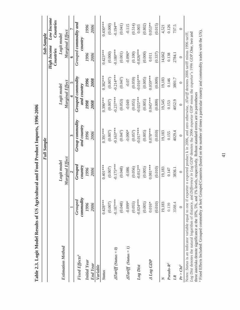
41

Tab

le 2

.3. L

ogit

Mod

el R

esul

ts o

f US

Agr

icul

tura

l and

Foo

d Pr

oduc

t Im

port

s, 19

96-2

006

F

ull S

ampl

e Su

b-Sa

mpl

e

H

igh

Inco

me

Cou

ntri

es

Low

Inco

me

Cou

ntri

es

Est

imat

ion

Met

hod

Logi

t mod

el

Logi

t mod

el

Logi

t mod

el

Mar

gina

l Eff

ect

Mar

gina

l Eff

ect

Mar

gina

l Eff

ect

1

2 3

4 5

6 7

Fix

ed E

ffect

sa G

roup

ed

com

mod

ity

Gro

uped

co

untr

y G

roup

com

mod

ity

and

coun

try

Gro

uped

com

mod

ity

and

coun

try

Gro

uped

com

mod

ity a

nd

coun

try

Initi

al Y

ear

1996

19

96

1996

19

98

1996

19

96

1996

E

nd Y

ear

2006

20

06

2006

20

08

2008

20

06

2006

Va

riab

le

St

atus

0.

428*

**

0.40

1***

0.

391*

**

0.39

6***

0.

382*

**

0.42

3***

0.

430*

**

(0.0

07)

(0.0

07)

(0.0

07)

(0.0

07)

(0.0

07)

(0.0

00)

(0.0

00)

Tari

ff (S

tatu

s = 0

) -0

.187

***

-0.1

75**

* -0

.163

***

-0.2

37**

* -0

.214

***

-0.1

80**

* -0

.194

**

(0.0

48)

(0.0

48)

(0.0

47)

(0.0

53)

(0.0

47)

(0.0

01)

(0.0

41)

Tari

ff (

Stat

us =

1)

-0.0

99*

-0.0

86

-0.0

90*

-0.0

49

-0.0

7 -0

.096

* -0

.115

(0

.055

) (0

.056

) (0

.057

) (0

.055

) (0

.059

) (0

.100

) (0

.514

) Lo

g D

ist

-0.0

24**

* -0

.012

**

-0.0

17**

* -0

.025

***

-0.0

16**

* -0

.026

***

0.00

3 (0

.005

) (0

.005

) (0

.005

) (0

.005

) (0

.005

) (0

.000

) (0

.802

) L

og G

DP

0.01

6*

0.08

1***

0.

078*

**

0.04

5***

0.

059*

**

0.01

1 0.

053*

* (0

.010

) (0

.010

) (0

.010

) (0

.009

) (0

.009

) (0

.337

) (0

.015

)

N

19,1

83

19,1

83

19,1

83

19,5

45

19,1

83

14,6

62

4,52

1 Ps

eudo

-R2

0.13

9 0.

147

0.15

5 0.

153

0.14

6 0.

138

0.12

6 LR

35

88.4

38

36.1

40

29.4

40

52.9

38

01.7

27

84.1

73

7.5

Pr >

Chi

2 0

0 0

0 0

0 0

Not

es: S

tatu

s is

an

indi

cato

r var

iabl

e eq

ual t

o on

e if

expo

rter o

exp

orte

d pr

oduc

t k in

200

6, a

nd z

ero

othe

rwis

e,

Tari

ff de

note

s 20

06 ta

riff m

inus

199

6 ta

riff,

Log

Dis

t den

otes

the

natu

ral l

ogar

ithm

of d

ista

nce,

and

Diff

eren

ce in

Log

GD

P de

note

s th

e 20

06 e

xpor

ter G

DP

min

us th

e ex

porte

r’s

1996

GD

P.O

ne, t

wo

and

thre

e as

teris

ks d

enot

e si

gnifi

canc

e at

the

10%

, 5%

, and

1%

leve

ls, r

espe

ctiv

ely.

Rob

ust s

tand

ard

erro

rs a

re in

par

enth

eses

a F

ixed

Eff

ects

Incl

uded

: Gro

uped

com

mod

ity a

t hs4

/ Gro

uped

Cou

ntrie

s (b

ased

on

the

num

ber o

f tim

es a

par

ticul

ar c

ount

ry a

nd c

omm

odity

trad

es w

ith th

e U

S).

42

Table 2.4. Multinomial Logit Results of US Agricultural and Food Products, 1996-2006 Alter fixed effects Change begin/end year Modified intensive

margins Estimation Method Multinomial Logit model: Base outcome = category 1 (No trade margin) (1) (2) (3) (4) (5) (6)

Grouped commodity

Grouped countries

Group commodity

/group countries

Grouped commodity /grouped countries

Group commodity /group countries

Initial Year 1996 1996 1996 1998 1996 1996 End Year 2006 2006 2006 2008 2008 2006 Variable 2. Disappearing Goods

Tariff 0.040* 0.038* 0.040* 0.015 0.014 0.040* (0.025) (0.024) (0.025) (0.027) (0.026) (0.025) Log Dist -0.015*** -0.016*** -0.016*** -0.004 -0.015*** -0.015*** (0.003) (0.004) (0.004) (0.004) (0.004) (0.003)

Log GDP -0.046*** -0.040*** -0.040*** -0.024*** -0.039*** -0.046*** (0.007) (0.007) (0.007) (0.007) (0.007) (0.007)

3. Extensive Margins Tariff -0.107*** -0.104*** -0.103*** -0.121*** -0.126*** -0.110***

(0.030) (0.030) (0.029) (0.031) (0.029) (0.030) Log Dist 0.016*** 0.018*** 0.016*** 0.009* 0.020*** 0.016*** (0.005) (0.005) (0.005) (0.005) (0.005) (0.005)

Log GDP 0.051*** 0.059*** 0.058*** 0.043*** 0.056*** 0.058*** (0.008) (0.009) (0.009) (0.008) (0.007) (0.008)

4. Intensive Margins Trade 96 > Trade 06a Tariff -0.051* -0.030 -0.025 -0.027 -0.043 0.064***

(0.034) (0.032) (0.031) (0.033) (0.031) (0.018) Log Dist -0.078*** -0.059*** -0.063*** -0.056*** -0.063*** -0.017*** (0.005) (0.005) (0.005) (0.004) (0.004) (0.003)

Log GDP -0.098*** 0.009*** 0.007 -0.015* -0.023*** -0.026*** (0.010) (0.010) (0.010) (0.009) (0.009) (0.006)

5. Intensive Margins Trade 96 < Trade 06a

Tariff - - - - - -0.089*** (0.027) Log Dist - - - - - -0.054*** (0.004)

Log GDP - - - - - 0.033 (0.009) N 19,183 19,183 19,183 19,545 19,183 19,183 Pseudo-R2 0.014 0.040 0.049 0.044 0.049 0.045 LR 676 1900 2300 2132 2317 2366 Pr > Chi2 0.000 0.000 0.000 0.000 0.000 0

Notes: Tariff denotes 2006 tariff minus 1996 tariff, Log Dist denotes the natural logarithm of distance, and Log GDP denotes the 2006 exporter GDP minus the exporter’s 1996 GDP. One, two and three asterisks denote significance at the 10%, 5%, and 1% levels, respectively. Robust standard errors are in parentheses Fixed Effects Included: Grouped commodity at hs4 and Grouped Countries (based on the number of times a particular country and commodity trades with the US). a Trade 96 > Trade 06 (Trade 96 < Trade 06) refers to intensive margin outcome when exports by region o of commodity k are less (more) in 2006 compared to 1996.

43

Table 2.5. Modified Multinomial Logit Results of US Agricultural and Food Products,

1996-2006

Alter fixed effects Change begin and/or end year

Estimation Method Multinomial Logit model Marginal Effect

Multinomial Logit model Marginal Effect

(1) (2) (3) (4) (5)

Grouped commodity

Grouped countries

Group commodity

/group countries

Grouped commodity /grouped countries

Initial Year 1996 1996 1996 1998 1996 End Year 2006 2006 2006 2008 2008 Variable Marginal Effect

2 Disappearing Goods Tariff Change 0.096** 0.089** 0.095** 0.068* 0.090** (0.040) (0.039) (0.041) (0.041) (0.043) Log Distance 0.001 -0.008 -0.005 0.011* -0.004 (0.006) (0.006) (0.006) (0.006) (0.006) Difference in Log GDP -0.054*** -0.083*** -0.081*** -0.046*** -0.070*** (0.013) (0.013) (0.013) (0.012) (0.012)

3 Extensive Margins Tariff Change -0.090** -0.101** -0.108*** -0.113*** -0.119*** (0.046) (0.046) (0.046) (0.047) (0.047) Log Distance 0.073*** 0.066*** 0.067*** 0.044*** 0.070*** (0.007) (0.008) (0.008) (0.007) (0.008) Difference in Log GDP 0.161*** 0.094*** 0.095*** 0.083*** 0.113*** (0.014) (0.015) (0.015) (0.014) (0.013)

4 Base Outcome: Intensive Margins N 9,957 9,957 9,957 10,119 9,923 Pseudo-R2 0.014 0.032 0.037 0.035 0.040 LR 295.5 661.9 764.5 747.9 833.8 Pr > Chi2 0.000 0.000 0.000 0.000 0.000 Notes: Category 4 – continuous or intensive margin trade - serves as the base outcome and the no trade category is omitted from estimation. Tariff denotes 2006 tariff minus 1996 tariff, Log Dist denotes the natural logarithm of distance, and Log GDP denotes the 2006 exporter GDP minus the exporter’s 1996 GDP. One, two and three asterisks denote significance at the 10%, 5%, and 1% levels, respectively. Robust standard errors are in parentheses a Fixed Effects Included: Grouped commodity at hs4/ Grouped Countries (based on the number of times a particular country and commodity trades with the US).

44

3. Hidden Trade Costs? Maximum Residue Limits and US Exports to Trans-Atlantic and Trans-Pacific Trading Partners

3.1. Introduction

We have witnessed a significant shift in the focus of agricultural trade policy concerns

from border related costs such as tariffs, quotas, and exports subsidies that dominated much

of the research and policy agenda in the lead up to the historic Uruguay Round Agreement on

Agriculture (URAA), to non-tariff measures (NTMs) and a plethora of “behind the border”

policies in the form of regulatory measures and product standards. While tariffs remain high

on a handful of agricultural sectors and tariff-rate quotas guarantee at least some access in

certain markets, most agricultural economists agree that new 21st century obstacles to trade

are more obscure in nature and have the potential to be more trade distorting (Beghin,

Maertens and Swinnen 2015; Josling, Roberts, and Orden 2004; OECD 2005; WTO 2012).

As Baldwin (1999) noted more than a decade ago: “…the lowering of tariffs has, in effect,

been like draining a swamp. The lower water level has revealed all the snags and stumps of

non-tariff barriers that still have to be cleared away” (p. 237).19

Broadly defined, NTMs are policy measures, other than ordinary customs tariffs, that

can potentially have an economic effect on international trade in goods, changing quantities

traded, or prices or both (UNCTAD 2010). Among the potential list of NTMs affecting

agricultural and food trade, Sanitary and Phytosanitary (SPS) measures feature prominently.

First, SPS measures are pervasive in agri-food trade because of the sensitive nature of issues

such as food safety and the protection of plant and animal health from pest and disease risks.

Second, the World Trade Organization (WTO) Agreement on the Application of SPS

19 Baldwin was not the only prominent Economist to highlight the increasing prevalence of NTMs. Lawrence (1996) noted that “… once tariffs are removed, complex problems remain because of differing regulatory policies among nations” (pg. 7) and Preeg (1998) concludes that: “…as border restrictions [tariffs] are reduced or eliminated, other policies become relatively more important in influencing trade flows and thus need to be assimilated in the trade relationship” (p. 50).

45

measures permits countries to adopt their own set of standards provided these measures are

based on a risk assessment, not discriminatory between countries with similar conditions, and

are minimally trade distorting to prevent the disingenuous use of these measures as

instruments of disguised protectionism (Josling, Roberts and Orden, 2004). Third, SPS and

TBT measures are the most frequently encountered NTMs according to data collected from

official sources such as the United Nations Conference on Trade and Development’s

(UNCTAD) Trade Analysis and Information System (TRAINS) and the WTO’s new

Integrated Intelligence Portal (I-TIP). They are also considered among the most relevant

impediments to exports, according to a small sample of NTM business surveys conducted by

the World Bank.

A major impediment to research progress on NTMs in agri-food trade is the difficulty

in constructing NTM datasets suitable for empirical analyses because of the many different

forms NTMs can be applied, when and how each measure is imposed, and on which

country/commodity pairs. Although there is no complete global inventory of public and

private NTM measures, multi-country and multi-institutional efforts to define, classify and

categorize NTMs and their role in international trade have been undertaken the most recent

being the UNCATD (2015) report culminating several years of effort by an expert committee

termed the Multi-Agency Support Team (MAST). Despite these efforts, quantification of

NTMs and in particular, those that represent significant obstacles to trade including case-

studies and full-scale inventory approaches, has not lead to a consensus about the impact of

NTMs on trade nor has it led to a prescribed framework of how to address NTM policy

reforms in multilateral and bilateral negotiations. Difficulties arise because of the enormous

amount of data collection that is required to obtain accurate empirical results that reflect

economic outcomes and because of the wide range of channels by which NTMs can impact

46

agricultural trade, commercial transactions, and even the ability of firms to establish new

trading relationships.

The evidence to date has been mixed (see Li and Beghin 2013; Beghin, Maertens and

Swinnen 2015; WTO 2012) and oftentimes the proverbial water has become muddied as

more obscure measures are identified. While new information and improved NTM

classification systems has increased our understanding of the nature of these measures it has

simultaneously revealed a large and diverse universe of applicable measures whether justified

or not. In principle, the United Nations Conference on Trade and Development (UNCTAD)

maintains and periodically updates its Trade Analysis and Information System (TRAINS)

database that covers well over 100 types of NTMs affecting agricultural and non-agricultural

trade. However, the applicability of the TRAINS database has been subject to criticism for

several reasons (Disdier, Fontagne and Mimouni 2008; Peterson et al. 2013; Grant et al.,

2015). First, even if an NTM is notified in the TRAINs database very little information exists

describing the type of measure affecting trade. Second, TRAINS does not contain a bilateral

country-pair dimension which means researchers must assume that if an import measure is

notified it applies to all exporters. Third, unlike agricultural tariffs for which WTO Members

are required to notify rates and any changes in applicable duties, NTMs are not subject to

such comprehensive reporting requirements. Further, the use of NTMs changes over time as

new types of measures appear when new ingredients or supplements are registered for use or

cost saving input technologies such as new pesticides becomes available.

While many SPS regulations are in place to protect animal and plant health from

imported pests and disease, a particular type of SPS regulations known as Maximum Residue

Limits (MRLs) or tolerances, are designed to safeguard human health. MRLs describe the

maximum legal level of concentration of pesticides or feed additives that a country is willing

to accept in or on the surfaces of food products. Although MRLs have become a key

47

regulatory measure to limit human exposure to chemicals and veterinary drug residue, overly

restrictive tolerances or limits set by importing countries that deviate significantly from

international standards or those maintained by exporting countries may provide incremental

reductions in human health and environmental hazards but will almost certainly increase

compliance costs for foreign and domestic producers, consumer prices of food products in

importing countries, and in some cases may shut off trade as products get rejected at the

border (Xiong and Beghin, 2012a).

In the March 2014 Report on SPS Measures (USTR 2014), the Office of the US Trade

Representative highlighted a number of discriminatory SPS measures affecting US fruit and

vegetable (FV) and animal product trade. A common theme in this report was the concern of

overly burdensome maximum residue limits (MRLs), particularly regarding pesticides and

aflatoxins in tree nuts and restrictions or bans concerning biotechnology, ractopamine,

trichinosis, bovine spongiform encephalopathy (BSE), avian influenza (AI) and certain

veterinary drugs imposed on US exports of animal products. Perhaps not surprisingly, many

of the country-product examples of SPS restrictions listed in the report lie in Asia and Europe

– two continents that are part of the large mega-regional trade deals with the US.

While broad-based approaches to quantify the effect of NTMs on trade are useful for

developing a “big picture”, simply put, NTMs include a very diverse array of policies that

can have heterogeneous impacts on trade (Beghin, Maertens and Swinnen 2015). Given

persistent difficulties in constructing suitable NTM datasets, this article adopts a targeted

approach investigating a specific type of SPS regulation in a particular product class of US

trade, namely maximum residue limits affecting fresh fruits and vegetable (FV) exports.

More specifically, the purpose of this article is first to construct a novel dataset of MRLs.

Second, we develop a bilateral stringency index of MRL heterogeneity between trading

partners. Following Li and Beghin’s (2013) index work, we modify their index, which is

48

designed to evaluate the stringency of members’ MRLs with respect to the international

standard, to incorporate an explicit bilateral dimension. The decision to export and the

intensity of exports with a given bilateral partner likely depend more on the stringency of

MRL standards in the importing nation as opposed to the international standard. Third, we

disaggregate the stringency index into three common classes of chemicals – herbicide,

fungicide and insecticide. Therefore, our indices vary not only by product and/or country but

potentially by type of chemical. Fourth, we empirically develop a formal econometric model

to access the trade restricting nature of these measures. Further, a Heckman approach is

applied to explore whether exporting nations facing stringent MRL policies in destination

markets actually export at all. We develop a bilateral trade flow equation to test the degree to

which MRLs reduce both the probability and intensity of trade.20 Finally, we use the bilateral

stringency indices and the empirical model to shed light on key regulatory differences

between the US and its main trading partners in the Trans-Pacific and Trans-Atlantic trade

negotiations.

3.2. MRL Policy Setting

While the SPS Agreement allows WTO Members to adopt their own set of

regulations, it encourages countries to apply internationally accepted science-based standards

established by the Codex Alimentarius Commission (henceforth CAC or Codex).21 The

Codex Committee on Pesticide Residues (CCPR) is the primary body responsible for

establishing MRLs for pesticide residues. While the CCPR’s responsibility is to establish

MRLs for pesticides in specific food items or in groups of food, the Joint Food and

Agricultural Organization (FAO)/World Health Organization (WHO) Meeting on Pesticide

20 The extensive margin describes as the emergence of new trade flows (i.e. the probability of having strictly positive trade flows), and the intensive margin introduces as the value of these positive flows (Besedeš and Prusa, 2011). 21 The Codex Alimentarius Commission (CAC) “develops harmonized international food standards to protect health of consumers and ensure fair practices in food trade” (http://www.fao.org/fao-who-codexalimentarius/en/).

49

Residues (JMPR) is responsible for reviewing the appropriate toxicology and residue field

data, conducting dietary risk assessments, and recommending specific MRLs to the CCPR.

Thus, human health risk assessments must be conducted to ensure food safety before a Codex

MRL can be established (Epstein, 2013; Madden, 2014; WHO 2009).

The CCPR follows a three-step process to establish a Codex MRL. First, a member

country nominates a chemical/commodity to the CCPR. Second, the JMPR reviews the data

provided for this chemical/commodity. Finally, according to the WHO (2009), the

establishment of the MRL will be considered by the CCPR, if the JMPR’s review confirms

that there are no issues or concerns. Although the CAC sets the MRLs for most agricultural

and livestock products, WTO members are not legally bound to adopt such standards and

there is no means to enforce equivalency with the international standard. As such, MRLs vary

widely across countries as discussed shortly because of differences in residue definitions,

usage patterns, formulations used in the residue field experiments that may differ from

pesticide use in actual production settings, and in the procedures used to determine MRL

levels (Madden, 2014). In such circumstances, countries can adopt standards that differ from

Codex as long as they are science-based, non-discriminatory, and minimally trade-distorting

(Beghin, 2014).

Thus, no official harmonized level of MRL exists globally (Achterbosch et al., 2009;

Drogue and DeMaria, 2010; Van der Meulen and van der Velde, 2004). For example, the

European Union (EU) and the United States (US) have established different MRLs for the

chemical Methidathion - a widely used organophosphate insecticide used in the production of

oranges and other citrus fruits. Because the insecticide can be toxic to humans, avian species,

and honeybees, the EU’s harmonized SPS policy sets a more stringent residue limit of 0.02

parts per million (ppm), compared to the US which establishes a less stringent standard of

four ppm. For comparison, the CAC international standard for Methidalthion in oranges is

50

two ppm.22

In the US, the Environmental Protection Agency (EPA) is responsible for establishing

residue limits on pesticides that have been registered and approved for use (e.g., have been

determined with “reasonable certainty” not to pose a harmful threat to human or environment

health). In setting the tolerance, the EPA considers: the toxicity of the pesticide and its break-

down products, how much of the pesticide is applied and the frequency of application; and

how much of the pesticide (i.e., the residue) remains in or on the surfaces of food by the time

it is prepared for retail markets. Pesticide manufacturers, or registrants, are required to

submit a variety of scientific trials that identify possible harmful effects the chemical could

have on humans (its toxicity), and the amount of the chemical (or breakdown products) likely

to remain in or on the surface of food. This information is then used in the EPA’s risk

assessment and determination of the tolerance. Once an EPA tolerance is established, the

limit applies both to domestically produced and imported products. In addition, established

MRLs can be updated if new information regarding toxicity or residue data warrants a

revision to the existing tolerance (EPA website, 2014).

In the EU, MRLs apply to 315 fresh and processed agricultural products. In cases

where pesticides have not been registered, the EU maintains a default MRL of 0.01 mg/kg.

The EU’s standard setting MRL process first involves estimating residue levels in or on a

crop when the pesticides are applied under the Good Agricultural Practice (GAP). Second,

the total daily intake of the specific pesticide is estimated using consumer intake models and

the established residue level. Third, an acceptable daily intake (ADI) is established using

information based on toxicological tests. Sensitive groups of consumers such as children are

considered in order to determine a safe ADI limit as well as a second limit referred to as the

22 It should be noted that international and country-specific MRL standards for a given chemical differ depending on the product. For example, the CAC international MRL standard for pears and table grapes is 1 ppm compared to 0.1 ppm for onions and tomatoes and 0.01 ppm for Macadamia nuts. In the empirical exercise, we develop an index to measure dissimilarities in two trading partners MRL standards for a given product.

51

Acute Reference Dose23 (ARFD). Once these intake limits are computed, the European

Commission (EC) establishes a new MRL or revises the existing MRL based on the condition

that the daily consumer intake of residues is less than the ADI. For crops and chemicals

produced and used outside of the EU, MRLs are established upon request of the exporting

country (EC website, 2014; Smolka, 2006).

3.3. Previous NTM and MRL Work

A growing body of empirical literature has emerged exploring the relationship

between NTMs and international trade. Because of data limitations, most empirical

investigations of NTMs employ either broad-based inventory approaches which attempt to

cover the widest possible scope of notified NTMs, or focus on a single case-study where

better information is available for a specific type of measure. Swann et al. (1996) found that

non-tariff standards generally promoted trade in the United Kingdom (UK). Their results

initially challenged the predominant view that standards restrict trade. Subsequent studies

have often found negative effects of NTMs on trade. Examining the trade impacts of country

specific and bilaterally shared standards in 12 OECD countries and 471 industries over the

period 1985-1995, Moenius (2004) finds a negative effect of national standards on trade in

non-manufacturing sectors. Using frequency and converge ratios for 61 product groups,

including some agri-food commodities, Fontagné, Mimouni and Pasteels (2005) find that SPS

and TBT measures have a negative impact on agri-food trade but not necessarily on trade in

industrial products. Disdier, Fontagne, and Mimouni (2008) use notification frequencies on

NTMs and the ad valorem tariff-equivalents estimated by Kee, Nicita and Olarreaga (2008)

to estimate broad-based impacts of NTM regulations on agri-food trade. They find that

NTMs have a negative influence on trade in cut flowers, processed food products (e.g.

23 ARFD is the pesticide dose that can be consumed during one day (short time), without considerable health hazard (Smolka, 2006).

52

beverages) and meat, but a strong positive influence on trade in cereals, wool and

albuminoids/starch.

Jayasinghe, Beghin and Moschini (2009) depart from broad-based inventory

approaches and focus on a particular product – US corn seed exports. Making use of the

EXCERPT database, the authors use a count variable to determine the number of SPS

measures affecting corn seed exports and find that trade is decreasing in the number of

foreign SPS/TBT standards required. Similarly, Peterson et al. (2013) and Grant et al. (2015)

focus on phyto-sanitary treatments (i.e., Methyl Bromide, Cold and refrigeration treatments,

etc.) impacting US fresh fruit and vegetable trade. Both studies find that SPS measures tend

to reduce US trade initially. However, an innovation in their study is that exporters can

overcome the fixed costs of establishing treatment facilities once exporters accumulate

product treatment experience in the global market place such that the negative phyto-sanitary

trade effect vanishes.

Equally important broad-based and case-study approaches have been conducted in the

context of standards and residue limits related to food safety. In terms of broad-based

approaches, an important empirical assessment of the trade effects of NTM regulatory

heterogeneity was accomplished in the NTM-IMPACT project (see Orden, Beghin and Henry

2012 for a summary). An aggregate data set of regulations and standards measured on a

comparable basis for the EU and nine of its trade partners were assembled by collaborators at

twelve institutions. The vast array of NTMs covered by the project are technically complex

and difficult to evaluate, aggregate, and quantify. Winchester et al. (2012) articulated these

challenges and described the procedures followed to develop a comprehensive snapshot of

EU regulatory heterogeneity in 2008-09 including measures for import requirements

concerning food safety, animal and plant health, labeling, traceability, conformity assessment

and certification requirements. Indices of the heterogeneity of trade regulation (HIT) were

53

computed in each of these areas. Concluding evidence from this project indicates that

regulatory differences in NTMs negatively impact EU trade.

Case-study approaches have offered a number of additional insights. Otsuki et al.

(2001) finds a negative effect of the EU’s aflatoxin standard on African groundnut exports.

Moving from the CAC standard established by the FAO and the WHO to the more stringent

European Commission standard decreases African exports of cereals, dried fruits, and nuts to

Europe by $670 million. Xiong and Beghin (2012a) recently overturned the estimated effect

in Otsuki et al. (2001), by considering possible demand enhancing effects of SPS regulations.

However, other case-studies addressing many of the econometric criticisms raised in Xiong

and Beghin (2012a) tend to corroborate the significant negative effects of MRL stringency.

Examples include Wilson and Otsuki (2004) for MRLs on chlorpyrifos in banana exports;

Wilson, et al. (2003) on the effect of residue limit standards on tetracycline in beef exports;

Chen, et al. (2008) on food safety standards impacting China’s exports of vegetables, fish and

aquatic products; Drogué and DeMaria (2012) on MRLs affecting apples and pears; and

Disdier and Marette (2010) on antibiotics impacting crustaceans exports.

While the focus of these studies tends to be narrower in terms of commodity

coverage, the results tend to show more stringent maximum residue limits and food safety

standards negatively impact trade, particularly for developing nations. Comparing the

stringency of MRLs between trade partners is complicated because there are often numerous

residue limits that apply to any given product.24 First, some of the aforementioned studies

tend to compare an importers MRL policy with the Codex established international standard

without paying much attention to regulatory differences between origin and destination

countries. Even if an importer’s MRL policy is more stringent than the international standard

24 For example, the US has established tolerances for 131 chemicals for apples. However, the same number of registered tolerances is not identical across countries. For apples, the number of established tolerances for chemicals varies from 45 in China, 79 in Canada, to 112 in Japan. This compares to 68 MRLs registered by Codex.

54

there are cases where an exporter’s MRL policy may be the most restrictive. If exporting

firms face a more stringent domestic MRL policy than either the international or importer’s

standard, it is not likely that the importer’s MRL policy could be considered overly trade

distorting even if the importer’s MRL policy is more stringent than the international standard.

Second, a drawback with case-study approaches that focus on one chemical class such as

Aflatoxins is that if other MRLs are operating, the empirical analysis may overstate the

impacts of the targeted Aflatoxin MRL.

An alternative approach is to consider a targeted stringency index that captures and

summarizes the full spectrum of a country’s MRL standard for a given product. Such an

approach has several advantages. First, the index is bilateral in the sense that we can pay

attention to hidden trade obstacles facing exporters in the proposed mega-regional

agricultural negotiations. Second, the index can be computed on a product-by-product basis

(i.e., apples, pears, grapes, lettuce, etc.) for each exporting partner thereby capturing only

those chemicals registered for use for a given product. Finally, the index is targeted at a

specific type of SPS policy – namely MRLs. An important drawback in the construction of

indices in studies such as Winchester et al. (2012) and the NTM-Impact project for the EU is

that the index assigns equal weight to all types of NTMs covered regardless of the importance

and/or intensity of their use in the underlying production process excluding MRLs

(Winchester et al., 2012; Li and Beghin, 2013; Achterbosch et al., 2009; Burnquist et al.,

2011; Drogue and DeMaria, 2012; Ferro et al., 2013; Foletti and Shingal, 2014a and b).

Indeed, Winchester et al. (2012) argue that the general nature of the index makes it difficult

to determine the importance of individual (or groups of) NTMs for a given product and

country pair. The authors state further that it is difficult to know without expert evaluation

which standards matter and which do not for a given product and country pair.

55

3.4. Indices of Regulatory Heterogeneity

Constructing a measure encapsulating the degree of regulatory MRL heterogeneity

remains an open empirical issue. Achterbosch et al. (2009) constructed stringency levels of

MRLs affecting Chile’s exports of fruits to the EU over the period of 1996-2007 using

averages of the actual difference in MRLs for each pesticide divided by the sum of the limits

for the two trading partners. Foletti and Shingal (2014a) build on Achterbosch et al.’s (2009)

framework by separate the stringency index into two measures – one when the exporter

maintains a stricter limit and the second when the importer maintains a stricter limit – with

the goal of testing the claim that regulatory heterogeneity always creates compliance costs for

countries no matter where this heterogeneity comes from. Drogue and DeMaria (2012)

compute the respective distance between each country’s MRL standards by subtracting the

Pearson’s coefficient correlation from one, which gives an index with domain [0, 2]. When

the index value is close to zero (two), the two trading partners have the same (dissimilar)

MRL standards. However, a major shortcoming of the Pearson index is that it does not

provide information about which trading partner (importer or exporter) has the stricter MRL.

For reasons discussed previously, we believe such information is crucial to the question of

whether differences in MRLs represent barriers or catalysts to trade.

Winchester et al. (2012) develop directional 25 and non-directional heterogeneity

indices of trade regulation (DHIT and HIT respectively), as defined by Rau et al. (2010),

based on the Gower index of (dis)similarity (Gower 1971). The standards investigated,

however, include import requirements concerning food safety, animal and plant health,

labeling, traceability, conformity assessment, process requirements and certification

requirements. Thus, the number of measures involved in the computation of the HIT is very

large, and they weight all NTMs equally in their index, arguing that using all of the

25 Only for MRL index, but for other standards there is a lack of additional knowledge to determine the direction of stringency.

56

information is a better alternative than focusing on just a few NTMs, which is equivalent to

putting a weight of zero on all but those few. Indices over a large number of NTMs; however,

makes it difficult to determine which measures are responsible for trade disruptions and the

direction of stringency (can not determine which one of the importer or exporter has more

stringent standard).

With this in mind, the starting point in our analysis is a modification of Li and

Beghin’s (2013) non-linear exponential index 26 that takes into account the dissimilarity of

MRL policies between country-pairs rather than between a destination’s standard relative to

the international Codex limit. Formally, the bilateral stringency index (BSI) between origin

region o and destination region d for the c classes of chemicals used in the production of

product k is defined as follows:

(1) BSIcodk 1Nck

expp Nck

MRLopk MRLdpkMRLopk

where Nck is the number of chemicals in chemical class c used in the production of

commodity k, MRLopk is the maximum residue limit for the pth chemical in class c for

commodity k in region o and MRLdpk is the maximum residue limit for the pth chemical in

class c for commodity k in region d. As we mentioned above, one of the limitation of

previous studies in this line of work is they often employ an aggregate measure of stringency

or dissimilarity over all chemicals. However, this index makes it difficult to determine which

measures are responsible for trade disruptions. To address this concern, we disaggregate the

BSI index of MRL stringency into separate indices for different chemicals. Thus, we consider

three broad classes of pesticides - herbicides, insecticides, and fungicides – to identify

whether MRL policy dissimilarities between the destination and origin regions vary

systematically across different classes of chemicals (c).

26 In their study, Li and Beghin (2013) explicitly provide the properties of the non-linear exponential stringency index (p. 59 and 60).

57

The advantages of the exponential function are that it maps heterogeneous BSI

differences onto the range zero (exp(- )) and 2.72 (exp(1)) and penalizes larger MRL

differences between o and d relatively more. For example, if the destination region has a

much stricter MRL for chemical p in class c (i.e., 0.1 ppm) compared with the origin region

(i.e., 5 ppm), reflecting a heterogeneous regulatory situation, then the ratio of MRLs will

approach a value of unity and the BSI function will approach its upper limit of exp(1) = 2.72.

Conversely, if the origin region has a much stricter MRL for chemical p in class c compared

to the destination region, then the ratio of MRLs will be negative and in the limit the

exponential function will approach zero, reflecting the fact that the destination region MRL is

not likely to represent a “barrier” to trade because exporting firms are already required to

meet a more stringent domestic tolerance. Finally, if the origin and destination regions have

the same MRL for chemical p in class c, then the ratio equals zero and the BSI is exp(0) = 1,

reflecting an equivalent or harmonized SPS situation.

As described shortly, the BSI is calculated for all countries with established MRL

standards and the requirement that the chemical is used in production based on data provided

by the USDA/NASS surveys of pesticide use for 26 fruits and 25 vegetable crops across

producers in the United States. All else constant, stricter MRLs in the destination country

relative to the origin country are expected to have a negative impact on trade. The extent to

which trade falls for incremental increases in the BSI, however, is clearly an open empirical

question.

3.5. Empirical Approach

In order to quantify the extent to which MRL policy dissimilarities reduce fruit and

vegetable trade between trading partners, a product-level model of bilateral trade is

developed based on the work of Anderson and van Wincoop (2003), Baldwin and Taglioni

(2006), Peterson et al. (2013) and Grant et al. (2015) and augmented to focus not only on the

58

overall impact of all trading partners, but in particular on U.S. exports to the EU and TPP

markets. The model assumes all varieties of commodity k are differentiated by origin region

o and consumer preferences in destination region d for commodity k are weakly separable,

which can be described by a CES utility function of the following form:

(2) udk odk

1 k qodk

k1 k

o1

R

k k1

where δodk denotes a preference parameter for commodity k exported by region o to

region d. R represents the total number of regions. qodk is the quantity of commodity k

exported by origin region o and consumed in destination region d. The elasticity of

substitution between all varieties of commodity k is described by σk. Time period subscripts

are suppressed as discussed further below due to the limited time-series nature of the MRL

data.

A representative consumer in region d maximizes its utility (2) conditional on her

budget constraint. The following describes the consumers’ expenditure function allocated to

consumption of commodity k in region d from region o:

(3) Vodk podkqodk , Solving this utility maximization problem and substituting the budget constraint

equation (3) in the first order condition gives consumer demand for quantity of commodity k

in region d from region o. In equation (3) podk is consumer price for commodity k in region d

from region o, which is linked to producer price for commodity k in region o through the

price linkage equation:

(4) podk todk ppok ,

where todk defines the trade costs of exporting commodity k from region o into region

d and pp_ok denotes producer prices in region o. Substituting the optimal quantity along with

equation (4) in equation (3) yields the following expenditure function for commodity k in

region d from region o:

59

(5) Vodk odk todk ppook 1 k Edk

PIdk1 k

,

where Edk is commodity k specific in region d’s expenditure and the denominator in

equation (5) is the CES price index (PIdk) defined as follows:

(6) PIdk rdk prdk1 k

r1

R1

1 k.

Equation (5) shows region o’s sales to each destination market that is a function of

economic size (Edk), origin prices relative to the overall price index (pp_ok and PIok), bilateral

trade costs and preferences (δodk). This expenditure function (equation 5) defines the elements

of gravity model developed in Anderson and van Wincoop (2003) and Baldwin and Taglioni

(2006). Therefore, summation of consumer expenditures across destination markets,

including o’s market evaluated at the producer price in region o, will give the total sales of

commodity k that is produced in region o. Assuming market clearing condition for

commodity k, the total quantity of commodity k produced in region o (Yok) will equal to the

quantity demanded in domestic market (oo), as well as the quantity demanded across

destination markets (od).

(7) Yok Vodkd1

R

odk todk ppook 1 k Edk

PIdk1 k

d1

R

Using equation (7), we can solve for ppok1 k

and substitute the result into equation (5)

as suggested by Anderson and van Wincoop (2003). The expenditure function in equation (8)

incorporates an explicit commodity dimension developed by Peterson et al. (2013) and Grant

et al. (2015), which was a modification of Baldwin and Taglioni’s (2006) expenditure

function.

(8) Vodk odktodk

1 kYokEdkodktodk

1 k EdkPIdk

1 kd1

R

PIdk1 k

odktodk

1 kYokEdkokPIdk

1 k.

60

Similar to Grant et al. (2015), trade costs in equation (8) are a multiplicative function

of transportation margins, and consist of several factors to transport k from producers in

region o to consumers in region d. To capture the extent to which bilateral MRL stringency

impacts trade costs, we employ this index as a proxy for trade costs, along with geographical

distance and an indicator of free trade agreements. In equation (9), we initially assume trade

costs are variable; however, later in this section we examine the extent to which BSI impacts

the probability of exporting. Thus, we will consider bilateral MRL stringency, not only as

variable cost of trade, but also as the fixed cost of trade, where firms require to cover fixed

cost in order to start a new relationship.

(9) todk1 k distod

1 exp RTAod BSIodkc

c zodk

0

where, distod is the geographical distance between regions o and d, RTAod is an

indicator of free trade agreements, BSIodk is the bilateral stringency index defined in previous

section (equation 1) and recalling that we define c = 3 classes of pesticide MRL categories

(herbicides, insecticides, and fungicides), and zodk are other potentially unobserved

determinants of trade costs.

Finally, to re-write equation (8) in the format of the product line gravity model, some

further modifications are necessary. First, the CES utility function is homothetic, so an

increase in Edk yields a proportional increase in Vodk, holding all other variables constant.

Second, in equation (8) Edk is not directly observable and there is a long history of

encountering difficulties estimating trade models because most of the variables involved are

not directly observable. However, the expenditure for commodity k in region d is a function

of income and the price indices for each commodity. Third, the price indices, Ωodk and PIdk,

are also not directly observable. Previous empirical studies such as Peterson et al. (2013),

Grant et al. (2015) and many other studies assume expenditure (Edk) is a function of total

income per capita (GDP) and employ GDP in their models, and also use production quantities

61

as a proxy for production value (Yok). Furthermore, these studies use time varying country-

specific fixed effects for unobservable price indices as suggested by Baldwin and Taglioni

(2006), Anderson and van Wincoop (2003), Feenstra (2004) and many others. In this study,

since MRL data availability limits our analysis to two years of data, we adopt an alternative

approach, which captures expenditure, production value and price indices using time-

invariant country and commodity-specific fixed effects (o, d and k) as consistent alternatives.

These dummy variables control for production levels in the exporting country, expenditure in

importing countries and the unobserved price indices.

The final alteration is the issue of zero trade flows. Santos-Silva and Tenreyro (2006),

Pham and Martin (2008), Helpman, et al. (2008) and Jayasinghe, et al. (2009) show that

omitting zero trade flows leads to biased estimates due to sample selection issues, particularly

if the reason for the existence of zero trade is correlated with right-hand side variables such

as MRL policies. One approach to incorporate zero trade flows is the Poisson pseudo-

maximum likelihood (PPML) estimation framework as discussed in Santos-Silva and

Tenreyro (2006). Substituting equation (1) into (9), and then equation (9) into equation (7),

along with Edk and Yok yields our baseline model of product line trade flows:

(10) Xodk exp o d k cBSIcodk 1 lnDistod

c

2RTAod

cUSEUc

BSIcodkIUSEU cUSTPPc

BSIcodkIUSTPP odk

where Xodk is the export value of bilateral fresh fruit and vegetable trade between o

and d, and IUS-EU and IUS-TPP are indicator variables equal to one if o is the US and d belongs

to the EU or TPP countries, respectively. By including these terms, we allow the EU and TPP

MRL policies with respect to US exports to have potentially different trade impacts. πo, πd

and πk are exporter, importer and commodity fixed effects, and εodkt is the multiplicative error

term.

62

While the Poisson model controls for zero trade flows and sample selection bias,

based on the nature of our data, a zero trade observation may indicate a more restrictive MRL

policy imposed by a destination country. In particular, an important consideration of MRL

policies is whether exporting nations facing stringent MRL policies in destination markets

actually export at all. While estimating the Poisson model on two sets of data, first on

positive export data and then on positive and zero export data, provides some information,

whether omitting zeros lead to significantly different BSI results, Helpman, et al. (2008) offer

an intuitive approach. Helpman, et al. (2008) develop a model of selection into exporting,

which considers the fixed costs firms need to cover in order to export commodity k from

region o to region d. Based on Melitz’s (2003) firm heterogeneity framework, only the most

productive firms are able to enter export markets. Furthermore, Crivelli and Groeschl (2016)

explain different SPS measures can have heterogeneous effects on trade, particularly the costs

of trade, including fixed and variable costs. The Helpman, et al. (2008) model developed

from Heckman (1979) enables us to distinguish the effect of MRL policy on the extensive

(i.e., probability of exporting) and intensive (intensity of exports) margins of trade. Other

studies in this line, Crivelli and Groeschl (2016), Disdier and Marette (2010), Jayasinghe,

Beghin and Moschini (2010), and Xiong and Beghin (2012) examine the impact of different

SPS measures on the extensive and intensive margins of trade.27

Thus, the final objective of the empirical modeling is whether exporting nations

facing stringent MRL policies in destination markets actually export at all. To do so, we

investigate the impact of regulatory stringency of MRL standards on both the probability and

level of trade, while controlling for sample selection issues. To that end, a two-stage

Heckman model is developed to distinguish the impact of MRL policy on the probability of

27 While Crivelli and Groeschl (2016) in their study use a broader measure (concern over SPS measures reported to the WTO by exporter at HS4 product line), the three other studies focus on a specific measure. Disdier and Marette (2010) use country specific MRLs; Jayasinghe, Beghin and Moschini (2010) apply SPS regulations using export certification; and Xiong and Beghin (2012) use aflatoxin contaminants.

63

exporting and the intensity of exports. Heckman’s (1979) model retain the log-linear

transformation of the model and treats zero trade flows as censored observations. The model

includes both a selection and outcome equation as follows:

(11) Yodk* o d k cBSIcodk 1 lnDistod

c

2RTAod 3Langod odk

(12) lnXodk* o d k cBSIcodk 1 lnDistod

c

2RTAod odk

where Yodk* is a latent variable predicting whether or not bilateral trade between o and

d is observed and ln (X*odk) is the natural logarithm of the intensity of bilateral trade. Y*odk

and lnX*odk are not observable in the selection and outcome equations, respectively, but we

do observe Yodk = 1 if Y*odk > 0 and Yodk = 0 if Y*odk < 0 and lnXodk = lnX*odk if Y*odk > 0 and

lnXodk is not observed if Y*odk < 0. The model can be estimated by a two-step procedure

suggested by Heckman (1979) or the one-step maximum likelihood estimation where the

selection and outcome equation are estimated simultaneously. The two-step procedure first

estimates the bivariate selection equation using a Probit model and generates the standard

inverse of the Mills ratio,28 which is subsequently included as an additional regressor in the

outcome equation.

The advantage of the Heckman model is that it can effectively estimate both the

extensive and intensive margins of trade by explicitly modeling zero trade flows. That is, it

allows us to determine if stringent MRL policies impact the probability of exporting, the

intensity of exports, or both. In this model an appropriate exclusion restriction is often

required29, Helpman, et al. (2008) use regulation costs and common religion as exclusion

restriction variables. Crivelli and Groeschl (2016) also include common religion as an

excluded variable, while other studies in this line employ an excluded variable based on the

28 The inverse Mills ratio is the ratio of the probability density function (PDF) over the cumulative distribution function (CDF) (Cameron and Trivedi, 2010). 29 While Cameron and Trivedi (2010) note that the system is theoretically just-identified through the non-linearity of the inverse mills ratio, for practical purposes, they suggest the model requires an exclusion restriction in the selection equation.

64

availability of data, such as common language, colonial ties, and time.30 Disdier and Marette

(2010) include common language in their selection equation. In this article, we include

common language, Langod, as an exclusion restriction because common language may help to

facilitate understanding of destination market information on rules and regulations of MRL

standards and may help expedite product compliance issues.

3.6. Data Description

Information on MRLs during 2013 and 2014 are obtained from the global MRL

database maintained by the Foreign Agricultural Service (FAS) (see mrldatabase.com). Since

the global MRL database is frequently updated and without archives, we extracted the MRL

data first in December 2013 and then again in December 2014. The established MRL data for

each fruit and vegetable by each individual country including CODEX standards were

retrieved. The total number of pesticides with established MRLs reported in the global MRL

database is 256 chemicals. However, not all pesticides with established MRLs are approved

for use. Therefore, we have retrieved data from the National Agricultural Statistics Service

(NASS) producer surveys that report 162 chemicals used in fruit and vegetable production.

NASS develops surveys to determine on-farm chemical use and pest management

information for agricultural commodities. Each chemical’s biological name is then matched

with the chemical identifier reported in the global MRL database.

Once the list of active chemicals is created, it is then merged with the global MRL

data, leaving us with a three-dimensional database of MRLs that varies by country,

commodity, and the pesticide chemical name. Our product sample includes 51 fruit and

vegetable products (FVs) (see appendix table A) at the 6-digit level of harmonized system for

85 countries with reported MRL tolerances for 162 pesticides used in production over the

sample period 2013 and 2014. The raw unbalanced dataset has 678,252 observations

30 Xiong and Beghin (2012) include a colonial tie dummy variable as exclusion restriction in their model, while Jayasinghe and Beghin (2010) employ a set of time dummy variable in their selection equation.

65

31consisting of a year, country, commodity and pesticide dimension. However, around 42%

of observations are missing because an MRL is not registered for use in a given country or an

established MRL has not been registered. While some countries maintain default values (e.g.

the EU introduces a default value of 0.01 ppm) if no MRL is reported, replacing these

missing values with default values does not add much information to our sample (35% of the

observations are still missing).

Reported MRLs can be divided into six categories – Codex standards, European

Union standards, United States standards, Gulf Cooperation Council (GCC) standards, other

countries with their own standards, and countries deferring to exporting countries’ standards.

Among the 88 countries listed in Table 3.1 for which we collected MRL information, 27

countries adopt the Codex standard for all products and 31 countries set their own standards.

Sixteen countries defer to the EU’s standard, seven countries use their trading partners’

(exporting countries) standards, four countries adopt the GCC standards, and Mexico defers

to the US standards. With the exception of Peru (Codex deferral) and Mexico (US deferral),

all of the Trans-Pacific Partnership (TPP) and T-TIP members (Australia, Brunei, Canada,

Chile, Japan, Malaysia, Mexico, New Zealand, Peru, Singapore, United States and Vietnam

and the EU) set their own MRL standards. Importantly as discussed previously and shown in

Table 3.2, some countries establish a default MRL, which can be used if a specific MRL is

not reported, a pesticide has not been registered for use, or is in the process of being

registered for use. The default values demonstrate the most stringent residue concentration

that is permitted.32

Table 3.3 provides a comparison of the MRL data for countries that set their own

standards relative to the international standard (Codex) and the United States. It also presents

for each country the Codex-based stringency index scores defined in Li and Beghin (2013).

31 There are 336,510 and 341,742 observations in 2013 and 2014, respectively. 32 Further information available at www.MRLdatabase.com.

66

Column (1) (Table 3.3) illustrates the share of each country’s MRLs that are stricter (i.e., a

tighter limit) than Codex. Relative to the international standard, Brazil’s MRL standards

appear to be the most stringent among all countries in Table 3.3 with 61 percent of its

standards being set at stricter limits than those advocated by Codex. Column (2) presents

similar results but instead of the Codex we compare MRL stringencies to the United States.

Here, Russia appears to set the most restrictive tolerances with 68 percent of established

MRLs being more stringent than the corresponding values set by the United States.33

Following Russia, Brazil, Turkey, Iceland and Norway with 64 percent and the EU with 63

set their MRLs more stringent than the United States.

Columns (3) and (4) summarizes the degree of MRL policy dissimilarity as measured

by the bilateral stringency index (BSI) relative to Codex. Interestingly, our Codex-based BSI

calculation reveals that Thailand, Malaysia, Saudi Arabia, Canada, India, Singapore, South

Africa, China, the US, New Zealand, Japan 34 and the GCC all have BSI values less than one

indicating a less stringent MRL policy compared to Codex. Conversely, the remaining

countries from Brazil to Brunei have Codex-based BSI levels above unity indicating a more

stringent level of MRL policy. Also of interest are the Codex-based BSI’s for EU and TPP

countries. Among TPP countries, Chile and Australia have the highest MRL stringency index

levels at 1.07 and 1.05, respectively which indicates only a slightly more restrictive MRL

policy compared to Codex, whereas many other TPP members including Japan and New

Zealand have indices that are much less stringent than Codex and the United States. On the

other hand, with an MRL index of 1.25 the EU ranks eighth in terms of its MRL stringency

compared to Codex. It should be noted that, the result of MRL index for EU are the same as

the results of MRL index in the Li and Beghin’s paper. The final two columns in Table 3.3 33 While Russia reports a limited number of established MRLs, those established MRLs have the most stringent values compared to the US standards. 34 Our Codex-based BSI for Japan in this paper is less stringent than the one Li and Beghin’s reported, while the index without including default are similar. It should be noted that, the range of products and the year in our paper are different compared to the Li and Beghin’s study.

67

report the number of established and non-established MRLs in our database. As shown, the

US has the highest number of established MRLs (14,311), while Indonesia has the lowest

number of established MRLs (384).

Also of interest is the fact that MRL tolerances differ widely across products for the

same chemical. For instance, Acetamiprid is an odorless neonicotinoid insecticide, which

controls for sucking insects on some fruits such as citrus, pome, and grapes and leafy

vegetables. Codex has established 12 different tolerances for this chemical depending on the

fruit or vegetable product being traded. However, the EU, Japan and the US set 19, 15 and 14

unique values for this chemical, respectively, and their values are consistent with Codex

ranging from 0.01 to around 5 ppm (with the exception of 15 ppm for the United States).

While it is conceivable that biological and production factors necessitate 19 different

tolerance levels for a given pesticide (as in the EU), it could also be the case that countries

are creating MRL policy flexibility similar to the way in which countries set different tariff

rates for the same product depending on the country of origin. At the other extreme, more

generic pesticides such as 2,4-D have a much lower range of Codex tolerances across

products ranging from a low of two ppm to a high of ten ppm (and the only other unique

tolerances are two and five ppm). Similar ranges exist for 2,4-D MRLs in the EU, Japan and

the US.

One of the objectives of this study is to disaggregate the stringency index into

separate indices over the class of commonly used pesticides in agriculture, which may

provide more accurate stringency measures. As we mentioned previously, to determine which

measures are responsible for trade disruptions, we disaggregate the BSI index of MRL

stringency into separate indices for different chemicals. Pesticides applicable for fruits and

vegetables can be divided into several classes of chemicals - herbicide, insecticide and

fungicide. Each of them has different characteristics in type and different amounts of

68

resistance in fruits and vegetables. Therefore, we add another dimension to our dataset, which

is the type of chemical. Each chemical is mapped to each class of chemical. Our dataset

consists of 63 insecticides, 45 herbicides, 42 fungicides, and 12 “other.” If a type of chemical

does not belong to one of the three classes of chemicals we call it “other.”35 It should be

noted that, the “other” category is ignored because the number of active chemical in this

category were negligible.

Finally, annual bilateral trade of fresh fruits and vegetable products are merged with

the constructed MRL database. The bilateral annual export flows of FVs between trading

partners are obtained from the United Nations Commodity Trade Statistics Database at 6-

digit level of harmonized system. Geographical distance is taken from the Centre d’Etudes

Prospectives et d’Informations Internationales (CEPII) geo-distance dataset (Mayer and

Zignago 2006).36 Information on Regional Trade Agreements (RTAs) data is obtained from

Grant (2013) and De Sousa (2012). Table 3.4 presents the summary statistics for the variables

in our econometric model. Our sample contains 95 exporters and importers37, 51 fruit and

vegetable products over a two year sample period. The final sample includes 257,647

observations, of which 65% observations are zero trade flows.38

3.7. Results

The results are organized as follows. In section one we present qualitative illustrations

of the MRL bilateral stringency index across countries, products and classes of chemicals

35 Rodenticides, molluscicides, nematicides, plant growth regulators and acaricides 36 CEPII is an independent European research institute on the international economy stationed in Paris, France. CEPII’s research program and datasets can be accessed at www.cepii.com. CEPII uses the great circle formula to calculate the geographic distance between countries, referenced by latitudes and longitudes of the largest urban agglomerations in terms of population. 37 The number of countries is extended to 95 from the original numbers, which were 85. In particular, we kept those EU members who have fruits and vegetables trade flow but did not report MRLs in the global MRL database. The missing MRL values are replaced with the MRLs reported by EU. EU harmonized its MRL system since 2008. 38 In order to explore if a country has the potential to export a given commodity, we assume if an exporter did not export a given commodity at least 3 times over a period of 10 years (2004-2014), we consider that the exporter does not have the potential to export a given commodity. We make this assumption because retrieving data at 6-digit level of FVs from Food and Agricultural Organization (FAO) is not feasible.

69

focusing our attention on the EU and TPP markets. While these results illustrate basic trends

and bilateral stringency levels across countries and products, they do not establish a more

casual link between MRL policy dissimilarities and trade. Section two presents the formal

econometric results to test and quantify the extent to which regulatory heterogeneity in MRL

policies disrupt bilateral trade in fresh fruits and vegetables.

3.7.1. Bilateral Stringency Index

Table 3.5 presents the simple and trade-weighted averages of the BSI overall and

across four different classes of pesticides. Columns (1) and (2) illustrate the simple and trade-

weighted averages across partner countries assuming the US is the exporting nation.39

Among the countries listed in Table 3.5, Iceland, Norway, Switzerland, the EU,

Russia, Turkey, Brazil and the United Arab Emirates have the highest stringency index based

on simple averages of the BSI. These countries have a stringency index above 1.5, which

shows a potentially high level hidden trade costs in the form of strict food safety tolerances.

Iceland has the highest trade weighted BSI against the United States. Commodities with high

stringency indices between the US and Norway include brussels sprouts, cauliflower,

broccoli, spinach, avocado and leeks with stringency levels between 1.91 and 2.01. The top

imported commodities such as apples and grapes have more moderate stringency levels of

1.45 and 1.29, respectively, but still above one indicating the US firms faces greater MRL

stringency for exports compared to serving the domestic market. Russian’s imports of melons

and cherries from the US, for example, have BSIs of 2.17 and 1.92, respectively. The BSIs

for the rest of the countries listed in Table 3.5 show moderate stringency levels between one

and 1.5. It is also worth mentioning that major importers of US FVs such as Canada, Mexico

and Japan have the least stringent MRLs on average.

39 Recall the BSI is not symmetric and thus the direction of trade flow matters.

70

Table 3.5 also displays BSIs for many of the Trans Pacific Partnership (TPP)

countries. Among TPP countries, Chile and Australia have higher equally weighted

stringency level of BSIs of approximately 1.29. However, Chile’s trade weighted BSI is

much higher than its unweighted BSI, suggesting that commodities sourced from the US with

greater values of imports tend to have stricter MRL tolerances. Conversely, for the EU, the

trade-weighted BSI is lower than the equally weighted BSI, indicating that US export

intensity is higher in less stringent MRL product categories.

Columns (3) through (8) of Table 3.5 also report the stringency level of tolerances for

different classes of chemicals. Turkey’s BSI for herbicides and fungicides has the highest

stringency indices above two, while it has a moderate level of stringency for insecticides on

average. In order to simplify these results, Figure 3.1 plots the average trade-weighted

bilateral stringency indices for different classes of chemicals, where the vertical axis shows

the average stringency level when the US is the exporting country. Again, Brazil, the EU,

Iceland, Norway and Russia rank the highest (> 1.5) in stringency among all US trading

partners for the insecticides index. Switzerland has an insecticide index around 1.5 and the

remaining countries have moderate levels below 1.5 for insecticides. A broader range of

countries/regions, including some in the TPP and T-TIP, have herbicide BSIs above 1.5,

including Chile, the EU, Indonesia, Norway, Peru, Saudi Arabia, Switzerland, Turkey and

Vietnam. BSI-insecticides and BSI-herbicides for China and Japan, and the BSI-fungicides

for New Zealand are the only countries with indices below one. It is also apparent that BSI-

fungicides generally have a stricter stringency index compared to other classes of chemicals.

While the highest level of stringency belongs to BSI-herbicide for Turkey, the BSI-fungicides

are consistently close to or above 1.5.

Figure 3.2 displays a distribution plot (boxplot) of the range of the BSIs across

commodities within a given country and is useful to decipher the variability of MRL policies

71

for select destination countries. The figure shows that although China has a relatively less

stringent MRL policy overall, it has the highest variation among the three pesticide indices

compared to other countries (the exception being fungicides for Indonesia). On the other

hand, Canada, Japan, Australia and Korea have a much narrower MRL policy span.

Table 3.6 and Figure 3.3 both illustrate average and the variability, respectively, of

BSI levels across commodities. Table 3.6 illustrates that vegetables have stricter BSI levels

using both equally and trade weighted averages across US trading partners. Specifically,

brussels sprouts, broccoli, cauliflower, avocados and celery are five commodities facing the

most restrictive MRL tolerances globally. Among fresh fruits and vegetables, apples, leaf

lettuce, strawberries and grapes rank the highest among US exports in 2013 and 2014, but on

average face moderate stringency levels ranging between 1.14 (grapes) to 1.32 (strawberries).

In figure 3.3 fresh tomato exports face the smallest range and lowest level of MRL tolerances

for each pesticide class and commodity. For cherries, broccoli, leaf lettuce and onions,

however, not only the level but also the variability of MRLs is relatively high.

Given the sensitive nature of NTMs and food safety issues in the T-TIP and TPP

negotiations, we next analyze the BSI indices with respect to these markets to assess current

regulatory heterogeneity faced by US exporters (Figures 3.4 and 3.5). For TPP markets

(Figure 3.4), our results indicate that eight commodities (grapefruits, lemons and limes,

oranges, leaf lettuce, tomatoes, pears and quinces, apples, peaches and nectarines) out of 48

commodities with significant exports rank in the top 20 least stringent indices to TPP

countries in 2013 and 2014. Apples, which ranked 17 out of the 20 of the least stringent MRL

tolerances, is the top export of US fruits and vegetables to TPP countries. Here the BSIs are

close to one which illustrates that TPP MRLs are closer to equivalent with the US compared

to those faced in the EU (figure 3.5). The top fruit and vegetable exports to the EU are

grapefruit, apples, grapes, onions, raspberries and blackberries, strawberries, and cherries.

72

According to our results, three commodities (apples, grapes, and mushrooms and truffles)

rank in the top 10 least stringent indices to the EU in 2013 and 2014. On the other hand,

avocados and cauliflower rank among the most stringent MRL commodities exported to the

EU. Comparing the EU and TPP markets indicates that the stringency levels for the EU are

much stricter than those in TPP markets, with values frequently exceeding 1.5 for certain

commodities and pesticide classes in the former, compared to values much closer to unity in

the latter.

Figure 3.6 also plots the variations of BSI indices for each chemical class for the EU

and TPP markets. The boxplot of the EU indices shows stricter indices and wider dispersion

compared to TPP markets, particularly among fungicides indicating room for negotiations

that would be subject for committee for scenario investigation over MRLs in this class of

pesticides. In addition, we conducted a non-parametric two-sample Wilcoxon rank-sum test

to test whether differences between the indices across the EU and TPP markets are

significantly different. The equality of the BSI indices was easily rejected.

Finally, Table 3.7 simplifies the analysis further by categorizing commodities into bin

ranges: less than one, between one and 1.5, and greater than 1.5.40 Interestingly, the majority

of BSIs for TPP markets fall into the middle category, with a smaller but still significant

number of commodities – 15, 11 and 5 for insecticides, herbicides and fungicides,

respectively – exhibiting BSIs less than one. This underscores the important point that for

most fruit and vegetable products, TPP countries have roughly similar BSIs to those of the

US. In the EU, the majority of BSIs fall into the last category - greater than 1.5 – indicating a

more stringent MRL policy environment and the potential for MRL harmonization in the

trade negotiations.

40 Note that, some fruits and/or vegetables do not have BSI indices across all the classes of chemicals. Therefore, the total numbers of commodities across different classes of chemicals for the EU and/or TPP markets are not equal.

73

3.7.2. Econometrics Results

The econometric estimates reported here shed light on the degree to which differences

in MRL regulatory stringencies affect bilateral exports of fruits and vegetables between

trading partners. In the results part we discuss the following. First, we discuss aggregate BSI

impacts on trade flows. Second, we discuss the results by augmenting the model with

indicators for US exports to TPP and T-TIP markets and the interaction of these with the BSI.

In the third section, we distinguish between the different classes of chemicals to determine if

the negative and significant trade flow effects of the aggregate BSI results are systematically

driven by a particular class of chemicals. Finally, we examine the effects of MRL policy

dissimilarities on the probability of exporting and the intensity of exports using a Heckman

model. In all regressions, importer, exporter and commodity fixed effects are included and

standard errors are clustered by country-pairs.

3.7.2.1. OLS, Poisson and Negative binomial Model

Table 3.8 considers the aggregate BSI effects across all countries and between the

US-EU and US-TPP. The results for geographical distance and belonging to a mutual

regional trade agreement are of the correct sign and statistically significant across all

specifications. In terms of MRL policy, the BSI showcases a negative and statistically

significant sign across all model specifications in columns (1)-(6) suggesting that higher BSIs

– indicative of a more stringent tolerance in the destination compared to the origin market –

significantly reduces bilateral fresh fruit and vegetable exports. Thus, overall, the impact of

MRL tolerances is trade impeding because it likely requires more careful production, testing

and compliance costs to serve international markets with stricter food safety guidelines. The

economic interpretation is similar to a semi-elasticity since the dependent variable is in logs

while the BSI is a levels index. A stricter BSI equivalent to an increase in the BSI by 0.1 at

the mean (the BSI mean equals to 1.039, which is about 10.39% increase) reduces fruit and

74

vegetable exports by 7% in the OLS model (column 1) and 8.8% in the Poisson model

(Column 2).

However, these results are across all countries and products in the database. As well

will see, when we introduce individual controls for US exports to the EU and TPP markets in

the OLS model (column 4), the results paint an asymmetric picture of MRL trade impacts.

Here, the BSI coefficient is more negative and statistically significant for US exports to the

EU, but has a positive and statistically significant interaction coefficient for US trade with

TPP partners.41 The result of F-test for the difference between the estimated coefficients also

confirms that the US-EU and US-TPP coefficients are statistically different (p-value = 0.00).

Quantitatively, the estimates imply that stricter bilateral stringencies of MRLs (by 0.1 at

mean) declines US export of fruits and vegetables to the EU members by a striking 23.6% in

OLS model (column 4). Thus, the effect of stricter MRLs is quite elastic with respect to its

effect on US-EU trade. To examine which countries, among TPP countries are driving the

fact that the TPP BSI coefficient is much less strict than EU BSI for US exports, we estimate

the model with two different data samples (Table 3.12). First, we exclude Canada and

Mexico from the TPP sample, interestingly the TPP BSI for US export coefficient (0.88)

magnitude increases (nothing else change) and indicates more lax effect of MRL policies on

exports of fruits and vegetables from the US to TPP market, excluding Canada and Mexico.

Furthermore, if we only exclude Canada from the TPP market data, the parameter estimated

increases even more (1.19). These estimation results for these two new sets of data show,

most TPP countries, excluding Canada are driving the fact that the TPP BSI coefficient is

much less strict than EU BSI for US exports.

In addition to the baseline estimations, we also allow the BSI effect to vary over

41 The mean BSI index for EU and TPP markets are 1.59 and 1.12, respectively.

75

fungicides, herbicides and insecticides (table 3.9).42 In a similar format to table 3.4 columns

(1)-(3) report the results of chemical class-specific BSIs across all trading partners, while

columns (4)-(6) distinguish between US-EU and US-TPP markets. The results are robust.

With the exception of fungicides in the Poisson model, more restrictive MRL policies tend to

impose negative and statistically significant trade distortions (Columns 1-3). In columns (4)-

(6), the impact of BSIs for different classes of chemicals on the US-EU and the US-TPP

markets are more sensitive and fragile given the lower number of observations in these

categories making identification more challenging. However, some interesting findings

emerge. First, the mostly negative BSI effects reported in columns (4)-(6) turns out to be

driven almost entirely by fungicides and insecticides for the US-EU and insecticides in

particular for the US-TPP markets. The results have important policy implications because

they suggest specific chemical classes on which trade negotiators can focus attention.

Second, herbicide indices of MRL stringency appear to enhance US exports. Because the

BSIs measure the stringency of MRL heterogeneity for the US-TPP markets, the results for

herbicides suggest that tighter restriction boost trade, and the potential demand enhancing

impact of MRL policy with respect to herbicide MRLs.

3.7.2.2. Intensive and Extensive Margins of Trade

We now turn to the results of the Heckman model, which is presented in 3.10. Similar

to the previous section, we first discuss aggregate BSI impact on the probability of exporting

and the intensity of exports. Second, we discuss the results of aggregate BSI impact on the

US exports to EU and TPP markets based on the augmented model. Third, the results of

chemical class-specific BSIs across all trading partners are presented. Finally, we report and

discuss the results of the dis-aggregate BSIs based on the different classes of chemicals for

US exports to EU and TPP markets. In all regressions, importer, exporter and commodity

42 The last category of chemical class “Other” are dropped from regression estimations because a small number of observations belonging to this category.

76

fixed effects are included and standard errors are clustered by country-pairs. Furthermore,

through all specifications, we include common language as the exclusion restriction in the

selection model. We also use common religion as exclusion restriction43 and the results are

robust (Table 3.12).

The results in Table 3.10, columns (1) and (2) suggest that MRL stringency reduces

the probability of market entry by -0.03 (selection equation, where the marginal effect 44 of

MRL stringency is -0.03) as well as decreases the intensity of exports by -0.51. Thus, MRL

policies likely impart significant fixed and variable trade costs of exporting, judging by the

negative and significant extensive and intensive margin results. Columns (3) and (5)

distinguish the impact of MRL stringency on the probability of exporting and the intensity of

export between US-EU and US-TPP markets. While MRL policy indicates a negative impact

on the decision to export between US-EU and US-TPP (the marginal effect for the estimated

parameter of MRL policy for US export to EU is negative and statistically significant (-0.12),

but not statistically significant for US export to TPP markets), the impact of MRL tolerances

between US-EU and US-TPP markets is opposite. MRL policy plays an impeding role on the

intensity of US exports to EU (-1.15), while this impact is trade enhancing with respect to the

US exports to TPP markets (1.06 and statistically significant). Previous studies in this line

also find interesting results. Similar to the former result for US-EU, Jayasinghe, Beghin and

Moschini (2010) also find a negative and statistically significant impact of MRLs on the

probability and volume of US export demand for corn seeds. However, similar to the latter

result for US-TPP markets, Disdier and Marette (2010) find while the impact of MRLs on

extensive margin is negative but insignificant, it negatively and significantly affects the

43 Common religion may also strongly affect the export decision; however, once the new trade relation has been created, it may not impact the amount of trade. Data on common religion across country pairs are collected from Elhanan Helpman’s homepage. In their study, Helpman et al. (2008) calculate the index of common religion between trading partners as (% Protestants in region o × % Protestants in region d) + (% Catholics in region o × % Catholics in region d) + (% Muslims in region o × % Muslims in region d). 44 Since the selection equation is a probit model, we also estimate the marginal effects of the parameter estimated in the selection equation.

77

intensive margin of imported crustaceans. Furthermore, Crivelli and Groeschl’s (2016) find

interesting and similar results for their study of the impact of SPS measures on the extensive

and intensive margin of trade. Their results (similar to us with respect to the US export to

TPP markets) show SPS measures have a negative and significant impact on the market

entry, which increase fixed costs of trade. However, SPS standards have positive and

significant impact on the intensity of trade. In particular, those exporters who overcome the

fixed costs of trade indicate the safety of their products to consumers, and consequently their

standards have a positive impact on the intensive of trade.

Additionally, columns (5) and (6) report the results of chemical class-specific BSIs

across all trading partners. The results show MRL policy has a negative impact across all

chemical classification at both margins of trade. Lastly, columns (7) and (8) report the results

of chemical class-specific BSIs while distinguishing MRL policy effects between US-EU and

US-TPP markets. While the results are more sensitive and fragile because of the low number

of observations in these categories, overall our findings are mostly consistent to our previous

specifications. Where for those parameter estimated that are statistically significant, MRL

policy has a negative effect on the extensive and intensive margins of trade for US-EU, while

negative effect on the extensive margin of trade but positive effect on the intensive margin of

trade for US-TPP markets. The coefficients on the gravity control variables are consistent

with existing gravity estimates through all specifications. The geographical distance between

two trade partners has negative impact on bilateral trades on both the probability of exporting

and the volume of trade, while having RTAs fosters exports of fruits and vegetables between

trade partners at both margins of trade. Common language reduces the fixed costs of trade

and positively affects the probability of exporting.45

45 The results are consistent when we include common religion as the exclusion restriction in the model.

78

3.8. Conclusions

In this article we focus on a specific type of SPS measures that are prominently

featured in the current mega-regional trade negotiations, namely food safety standards in the

form of maximum residue limits. This paper introduce the bilateral stringency index to assess

how regulatory heterogeneity (and convergence) for pesticide tolerances used in the

production process of fresh fruits and vegetables impacts trade between the US and its

partner countries in the aggregate and in the proposed mega-regional trade deals. We develop

the aggregated bilateral stringency index based on different classes of chemicals, which

provides further insight as to the types of pesticides that influence trade flows. In particular,

previous studies in this line of work often employ an aggregate measure of stringency or

dissimilarity over all chemicals with established MRLs relative to the international standard,

whereas we develop a bilateral stringency measure based the fact that it likely matters more

to exporters what the MRL policy is in the destination market as opposed to what tolerance

level is advocated by Codex.

Second, we construct a new database on international fruit and vegetable exports

matched to maximum residue limits for each country in 2013 and 2014. The results of the

country-level index indicate that Brazil, Iceland, Norway, Switzerland, Turkey, and the EU

rank among the most stringent among all US trading partners, Canada and China, two of the

top markets for US exports of fruits and vegetables show moderate stringency levels, while

Japan is consistently among the least restrictive MRL partners in our database. At product

level, brussels sprouts, avocadoes and celery rank among the highest MRL stringent

commodities whereas the top US fruit exports consisting of apples, grapes, oranges, cherries

and strawberries, have a moderate stringency index. Further, the results clearly indicate that

there is a significant gap in regulations regarding maximum residue limits among several

major US foreign markets for fruits and vegetables, particularly EU and TPP. For instance,

79

the BSI-insecticide for apples is stricter than BSI-herbicide and BSI-fungicide between the

US and the EU, while there is virtually no difference among the three classes of chemical

indices for apple trade between the US and TPP markets. The stringency index results also

provide a snapshot of regulatory heterogeneity between the US and its important export

markets in the EU and TPP countries. Overall, the bilateral stringency indices suggest much

stricter regulations for the EU compared to TPP markets for both fruits and vegetables and

across different classes of chemicals, suggesting that trade negotiators will likely want to

emphasize the dissimilarity of MRL tolerances in the T-TIP negotiations. Thus, the results of

this study provide important policy implications as the negotiations between the US and TPP

and T-TIP countries progress. It should be noted that while recently the US has formally

withdrawn from TPP, the results of this research is useful for any bilateral trade agreement

between the US and TPP countries individually (i.e., Japan).

Using the bilateral stringency indices, we also empirically develop a formal

econometric model to understand the trade restricting nature of these measures for fruits and

vegetables. More importantly, our augmented trade model has the characteristic to distinguish

the impact of MRL policy on exports across all potential exporters and between the US as an

exporter and its main trading partners in the Trans-Pacific and Trans-Atlantic trade

negotiations. We contribute to the analysis of SPS measures by estimating the impact of

bilateral MRL stringency using several specification models. Our findings shed light on the

impact of MRL stringency on exports for fruits and vegetables across all trading partners,

which impedes trade; it likely requires more careful production, testing and compliance costs

to serve international markets with stricter food safety guidelines. However, when we

introduce individual controls for US exports to the EU and TPP markets, the results paint a

contrasting picture of MRL effects on US exports. The results suggest MRL policy impedes

US exports to EU, while it enhances trade with respect to the US exports to TPP markets. The

80

latter result is suggestive of the potentially demand enhancing of MRL policy. Therefore, it is

important to take into account the preference of consumer in term of food safety.

Additionally, we also allow the BSI effect to vary over different classes of chemicals,

fungicides, herbicides and insecticides. Our findings show the most negative BSI effect turns

out to be caused almost entirely by fungicides and insecticides for the US-EU and

insecticides for the US-TPP markets. This result is particularly interesting for trade

negotiators – it may enable them to focus attention on specific chemical classes. Furthermore,

herbicide indices of MRL stringency appear to enhance US exports to TPP markets. This

suggests stricter MRL policy of the US may serve as a demand enhancing effect on the US

exports to TPP markets, and tighter restriction boost trade.

Lastly, an important consideration of MRL policies is whether exporting nations

facing stringent MRL policies in destination markets actually export at all. Therefore, we

point out the impact of MRL policy on a market entry barrier to all potential exporters, while

decomposing exports into extensive and intensive margins of trade. Our results suggest that

MRL stringency decreases both the probability of exports as well as the intensity of exports

across all trading partners. Thus, MRL policies likely impart significant fixed and variable

trade costs of exporting judging by the negative and significant extensive and intensive

margin results. Hence, MRL policy constitutes a market entry barrier to all exporters.

81

References

Achterbosch, T., A. Engler, and M.L. Rau, M. 2009. Measure the measure : the impact of differences in pesticide MRLs on Chilean fruit exports to the EU. Paper presented at the International Association of Agricultural Economists Conference, Beijing, China, 08.

Anderson, J.E., and E. van Wincoop. 2003. Gravity and Gravitas: A Solution to the Border Puzzle. American Economic Review 93(1): 170–192.

Baldwin, R. 2000. Regulatory Protectionism, Developing Nations and a Two-Tiered World Trading System. Brookings Trade Forum. Washington, DC: Brookings Institute Press.

Baldwin, R., and D. Taglioni. 2006. Gravity for Dummies and Dummies for Gravity Equations. National Bureau of Economic Research Working Paper 12516.

Beghin, J. C., and J. C. Bureau. 2001. Quantification of sanitary, phytosanitary, and technical barriers to trade for trade policy analysis. Working Paper 01-WP291. Center for Agricultural and Rural Development, Iowa State University.

Beghin, J. 2014. The Protectionism of Food Safety Standards in International Agricultural Trade. Agricultural Policy Review, Center for Agricultural and Rural Developmnet (CARD), Iowa State University.

Beghin, J., M. Maertens, and J. Swinnen, 2015. Nontariff Measures and Standards in Trade and Global Value Chains, Annual Review of Resource Economics, Annual Reviews 7(1): 425-450.

Burnquist, H. L., K. Shutes, M.L. Rau, M.J. Pinto de Souza, and R. Nunes de Faria. 2011. Heterogeneity Index of Trade and Actual Heterogeneity Index – the case of maximum residue levels (MRLs) for pesticides. Poster prepared for presentation at the Agricultural & Applied Economics Association’s 2011 AAEA & NAREA Joint Annual Meeting, Pittsburgh, Pennsylvania, 06.

Cameron, A.C. and P.K. Trivedi. 2010. Microeconometrics: Method and Applications. Cambridge University Press, New York.

Center for International Development at Harvard University. 2004. Sanitary and Phytosantary Measures and Technical Barriers to Trade Summary. Global Trade Negotitations Home Page. http://www.cid.harvard.edu/cidtrade/issues/spstbt.html

CEPII (2005), GeoDist: Distances and Geographical Database (Paris: CEPII). Available at:http://www.cepii.fr.

Chen, C, J. Yang, and C. Findlay. 2008. Measuring the Effect of Food Safety Standards on China’sAgricultural Exports. Review of World Economics 144(1): 83–106.

Crivelli, P. and J. Groeschl. 2016. The impact of Sanitary and Phytosanitary Measures on Market Entry and Trade Flows. The World Economy. 39(3): 444-473 doi: 10.1111/twec.12283

De Sousa, J. 2012. The currency union effect on trade is decreasing over time, Economics Letters 117(3): 917-920.

Disdier, A., L. Fontaigné, and M. Mimouni. 2008. The Impact of Regulations on Agricultural Trade: Evidence from the SPS and TBT Agreements. American Journal of Agricultural Economics 90(2): 336–350.

82

Disdier, A.C. and S. Marette (2010), ‘The Combination of Gravity and Welfare Approaches for Evaluating Nontariff Measures’, American Journal of Agricultural Economics, 92, 3, 713–26.

Drogué, S., and F. DeMaria. 2010. Do different regulations in Maximum Residue Levels of pesticides affect trade competitiveness? The case of apples and pears. Presented at 12. Annual conference ETSG 2010, Lausanne, CHE (2010-09-09 - 2010-09-11). http://prodinra.inra.fr/record/40781

Drogué, S., and F. DeMaria. 2012. Pesticide residues and trade, the apple of discord? Food Policy 37(6): 641–649.

Epstein, R. 2013. Codex Alimentarius Committee on Pesticide Residues, Science and technology Program, USDA. ftp://ftp.fao.org/codex/alimentarius/a131_24e.pdf

European Commission website, http://ec.europa.eu/ (accessed May 2014).

Feenstra, R. 2004. Advanced International Trade:Theory and Evidence. Princeton, NJ: Princeton University Press.

Ferro, E., J.S. Wilson, and T. Otsuki. 2013. The effect of product standards on agricultural exports from developing countries. The World Bank, Policy Research Working Paper Series: 6518, 2013. Development Research Group, Trade and International Integration Team, 06.

Foletti, L., and A. Shingal. 2014a. Stricter Regulation Boosts Exports: the case of Maximum Residue Levels in Pesticides. MPRA Paper 59895, University Library of Munich, Germany.

Foletti, L., and A. Shingal. 2014b. Trade Effects of MRL Harmonization in the EU. Working Paper 2014/5, nccr trade regulation, swiss national centre of competence in research.

Fontagne, L., M. Mimouni, and J.-M. Pasteels. 2005. Estimating the Impact of Environmental SPS and TBT on International Trade. Integration and Trade 22: 7–37.

Grant, J. H., E. Peterson, and R. Ramniceanu. 2015. Assessing the Impact of SPS Regulations on U.S. Fresh Fruit and Vegetable Exports. Journal of Agricultural and Resource Economics. 40(1): 144-163. Copyright 2015 Western Agricultural Economics Association. ISSN 1068-5502

Grant, J.H. and S. Arita. 2016 Forthcoming. Revealed Concerns: A New Look at the Impact of Non-Tariff Measures on Agri-Food Trade, Commissioned Paper, International Agricultural Trade Research Consortium (IATRC), June 2016.

Grant, J.H. 2013. Is the Growth of Regionalism as Significant as the Headlines Suggest? Lessons for Agricultural Trade, Agricultural Economics 44(1): 93-109

Gower, J.C. 1971. A General Coefficient of Similarity and Some of Its Properties. Biometrics 27(4): 857-871.

Heckman,J. J. 1979. Sample Selection Bias and a Specification Error. Econometrica 47(1): 153–161.

Helpman, E., Melitz, M., and Y. Rubinstein. 2008. Estimating trade flows:Trading partners and trading volumes. Quarterly Journal of Economics 123: 441–487.

Jayasinghe, S., J. Beghin, and G. Moschini. 2009. Determinants of World Demand for U.S. corn Seeds: The Role of Trade Costs. American Journal of Agricultural Economics 92 (4): 999–1010.

Josling, T., D. Roberts, and D. Orden. 2004. Food Regulation and Trade:Toward a Safe and Open Global System .Washington,DC: Institute for International Economics.

83

Kee, H. L., A. Nicita, M. Olarreaga. 2008. Import Demand Elasticities and Trade Distortions. The Review of Economics and Statistics 90(4): 666–682, by the President and Fellows of Harvard College and the Massachusetts Institute of Technologyta

Lawrence, R.Z. 1996. Regionalism, Multilateralism, and Deeper Integration. Washington, D.C.: The bookings Institution, Integrating National Economics Series.

Li, Y., and J.C. Beghin. 2013. Protectionism indices for non-tariff measures: An application to maximum residue levels. Food Policy 45(01): 57–68. http://doi.org/10.1016/j.foodpol.2013.12.005

Madden, B. 2014. MRL Meeting. Office of Pesticide Programs, Registration Division, U.S. Environmental Protection Agency.

Mayer, T., and S. Zignago. 2006. Notes on CEPII’s Distance Measures. Unpublished manuscript. Paris, France, May. Available at: http://www.cepii.fr/ anglaisgraph/workpap/summaries/wp_resume.asp?annee=2011&ref=25& NoDoc=3877

Melitz, J. 2003. The Impact of Trade on Intra-Industry Reallocations and Aggregate Industry Productivity. Econometrica 71(6): 1695-1725.

Moenius, J. 2004. Information versus Product Adaptation: The Role of Standards in Trade. Working Paper, Kellogg School of Management, Northwestern University.

Orden, D., J.C. Beghin, and G. Henry. 2012. Key Findings of the NTM-IMPACT Project. The World Economy 35(8): 967-972.

Organization for Economic Co-operation and Development. 2005. Agricultural Policies in OECD Countries: Monitoring and Evaluation in 2005. Paris, September.

Otsuki, T., J.S. Wilson, and M. Sewadeh. 2001. What Price Precaution ? European Harmonisation of Aflatoxin Regulations and African Groundnut Exports. European Review of Agricultural Economics 28(2): 263–284.

Peterson, E., J. Grant, D. Roberts, and V. Karov. 2013. Evaluating the Trade Restrictiveness of Phytosanitary Measures on U.S. Fresh Fruit and Vegetable Imports. American Journal of Agricultural Economics 95: 842–858. doi: 10.1093/ajae/aat015.

Pham, C., and W. Martin. 2008. Estimating the Gravity Model When Zero Trade Flows are Important (Economic Series 2008-03). Burwood, VIC, Australia: Deakin University, Faculty of Business and Law.

Preeg, E. H. 1998. From Here to Free Trade, University of Chicago Press, Chicago, IL.

Rau, M., K. Shutes, and S. Schlueter. 2010. Index of Heterogeneity of Requirements in International Agri-food Trade. Assesment of the Impacts of Non-Tariff Measures NTM on the Competitiveness of the EU and Selested Trade Partners. NTM Impact Working Paper 10/01.

Rau, M.L., K. Shutes, S. Schlueter, M. Poto, and B. van der. Meulen. 2010. Requirements in International Agri-Food Trade: Constructing an Index of Regulatory Heterogeneity. Assesment of the Impacts of Non-Tariff Measures NTM on the Competitiveness of the EU and Selested Trade Partners. NTM Impact Working Paper 10/03.

Santos Silva, J.M.C., and S.Tenreyro. 2006.The Log of Gravity. Review of Economics and

Statistics 88 (4): 641–658. Santos Silva, J.M.C.,and S.Tenreyro. 2011. Further Simulation Evidence on the Performance of the Poisson Pseudo-Maximum Likelihood Estimator. Economic Letters 112 (2): 220–222.

84

Smolka, S. 2006. The new EU-Regulation on Maximum Residue Levels of Pesticides in Food - An Overview. Paper presented at the Seminar of Pesticide Residues in Food – Regulation, Monitoring, Policy, Modra, Slovakia, 06. www.pan-germany.org, www.pesticide-residues.org

Swann,G.P., P. Temple, and M. Shurmer. 1996. Standards and Trade Performance: The UK Experience. Economic Journal 106: 1297–1313.

USDA FAS MRL Global database, https://www.globalmrl.com/home (accessed December 2013 and December 2014).

United States Trade Representative. 2014. Report on Sanitary and Phytosanitary Measures

Van Der Meulen, B.M.J., and M. Van Der. Velde. 2004. Food Safety Law in the European Union. European Food Law Institute serires. Published by Wageningen Academic Publishers, 09.

Wheat, D. 2013. Tighter EU Standards Threaten Exports of U.S. Apples, Pears. Capital Press, 09.

World Health Organization (WHO). 2009. Principles and methods for the risk assessment of chemicals in food. Published under the joint sponsorship of the United Nations Environment Programme, the International Labour Organization and the World Health Organization, ISBN 978 92 4 157240 8 (NLM classification: WA 712), ISSN 0250-863X.

Wilson, J.S., and T. Otsuki. 2004. To Spray or Not to Spray: Pesticides, Banana Exports, and Food Safety. Food Policy 29(2): 131–146.

Wilson, J.S., T. Otsuki, and B. Majumdsar. 2003. Balancing food safety and risk: do drug residue limits affect international trade in beef? The Journal of International Trade & Economic Development. Taylor and Francis Journals 12(4): 377-402.

Winchester, N., M.L. Rau, C. Goetz, B. Larue, T. Otsuki, K. Shutes, C. Wieck, H.L. Burnquist, H. M.J. Pinto de Souza, and R. Nunes de Faria. 2012. The Impact of Regulatory Heterogeneity on Agri-food Trade. World Economy 35(8): 973–993.

Wolff, C. 2014. SPS Issues at the WTO. Thematic SPS Workshop on Risk Analysis, WTO, Centre William Rappard, Geneva, 10.

World Trade Organization. 2012. World Trade Report. Trade and public policies: A closer look at non-tariff measures in the 21st century.

WTO Committee on SPS Measures. 2013. Specific Trade Concerns, G/SPS/GEN/204/Rev.13, 02.

Xiong, B., and J.C. Beghin. 2012a. Does European Aflatoxin Regulation Hurt Groundnut Exporters from Africa? European Review of Agricultural Economics 39 (4): 589–609

Xiong, B., and J.C. Beghin. 2012b. Stringent Maximum Residue Limits, Protectionism, and Competitiveness. International Trade Research Consortium, Working Paper 142384, Department of Economicss, Iowa State University.

Xiong, B., and J.C. Beghin. 2013. Disentangling Demand-Enhancing and Trade-Cost Effects of Maximum Residue Regulations. Staff General Research Papers 34393, Department of Economicss, Iowa State University.

85

Figu

res

Figu

re 3

.1. T

he B

SI in

dice

s at c

ount

ry le

vel f

or d

iffer

ent c

lass

of c

hem

ical

- tra

de w

eigh

ted

(ass

umin

g th

e U

S as

ori

gin

coun

try)

86

Figu

re 3

.2. T

he b

ox p

lot B

SI in

dice

s at c

ount

ry le

vel f

or in

sect

icid

es, h

erbi

cide

s and

fung

icid

es

87

Figu

re 3

.3. T

he b

ox p

lot B

SI in

dice

s at c

omm

odity

leve

l for

diff

eren

t cla

ss o

f che

mic

al in

sect

icid

es, h

erbi

cide

s and

fung

icid

es

88

Figure 3.4. TPP Stringency Indices for Top US Exports – Trade Weighted

Figure 3.5. EU Stringency Indices for Top US Exports – Trade Weighted

89

Figure 3.6. The box plot BSI indices for different classes of chemicals across the EU and TPP markets – Trade Weighted

90

Tables

Table 3.1. List of Countries that report pesticides MRL standards

List of countries Notes

Codex

Algeria Costa Rica Kenya Philippines

Some countries may defer to the US or the EU if there is no Codex MRL

Angola Dominican Republic Lebanon Trinidad and Tobago

Bahamas Ecuador Morocco Tunisia

Bangladesh El Salvador Netherlands Antilles

United Arab Emirates

Barbados Guatemala Nicaragua Venezuela Bermuda Hong Kong Pakistan Honduras Cambodia Jamaica Panama Colombia Jordan Peru

European Union

Belgium French Pacific Islands Ireland Portugal

Denmark French West Indies Italy Spain Finland Germany Netherlands Sweden

France Greece Poland United Kingdom

Exporting countries

Albania Antigua and Barbuda Cayman Islands Haiti

Nevis Sri Lanka St. Lucia Gulf

Cooperation Council

Bahrain Kuwait Oman Qatar Saudi Arabia

Own standards

Argentina China Israel South Africa

Some countries may defer to

Codex if there is no own standard

Australia Cuba Japan South Korea Brazil Egypt Malaysia Switzerland Brunei Iceland New Zealand Taiwan Canada India Norway Thailand Chile Indonesia Russia Turkey Customs Union of Belarus, Kazakhstan, and Russia Singapore Vietnam

United States Mexico Source: MRLdatabase.com, December 2013 and 2014

91

Table 3.2. Default MRL in parts per million (ppm)

Default MRL in parts per million (ppm) Country

0.01 ppm Japan

0.01 ppm Norway

0.01 ppm EU

0.01 ppm Iceland

0.1 ppm Canada A default MRL of 0.01 ppm applies when no GCC, Codex, US or EU MRL is established. Saudi Arabia

Codex MRL Brazil

Codex MRL Chile Codex MRL India Codex MRL Israel Codex MRL Thailand Codex MRLs Cuba Codex MRLs Singapore Codex MRLs Vietnam Codex MRL + 0.01 ppm Argentina Codex MRLs + 0.01 ppm Malaysia EU MRL regulations + 0.01 ppm Turkey

EU MRLs United Arab Emirates (UAE)

Least restrictive value between MRLs established in their national regulation (0.1 ppm default included) and MRLs established by Codex. New Zealand

Less restrictive value established in the EU and Codex regulations + 0.01 ppm South Africa

US MRLs + EU MRLs Dominican Republic

When there is a conflict between the two regulations, MRLs established by the Customs Union take precedence. Russia

Source: MRLdatabase.com, December 2013, 2014

92

Table 3.3. Comparing MRL patterns across countries with Codex and US MRLs, and their level of protectionism (International science-based Codex)

Region

More stringent

than Codex %

More stringent than US

%

Level of protectionism (international science base

codex)

Level of protectionism (international science base codex) with

default value

Number of established

MRLs

Number of non-

established MRLs

Brazil 61 64 1.52 1.12 2,065 12,246 Turkey 51 64 1.43 1.39 1,454 12,857 Russia 53 68 1.39 1.57 904 13,407 Switzerland 42 62 1.35 1.35 9,167 5,144 Iceland 35 64 1.29 1.44 10,361 3,950 Norway 35 64 1.29 1.44 10,361 3,950 Taiwan 45 55 1.28 1.28 6,271 8,040 European Union 32 63 1.25 1.40 10,513 3,798 Israel 20 54 1.19 1.19 5,247 9,064 United Arab Emirates 0 60 1.13 1.13 10,871 3,440 South Korea 34 45 1.10 1.10 7,852 6,459 Argentina 10 51 1.09 1.31 4,530 9,781 Chile 8 46 1.07 1.07 5,511 8,800 Australia 38 51 1.05 1.05 5,191 9,120 Indonesia 5 47 1.02 1.02 384 13,927 Vietnam 5 46 1.02 1.02 4,242 10,069 Brunei 8 43 1.01 1.01 4,856 9,455 Thailand 1 45 1.00 1.00 3,927 10,384 Malaysia 3 44 0.99 1.21 4,168 10,143 Saudi Arabia 1 43 0.98 0.98 4,033 10,278 Canada 37 19 0.97 1.28 5,242 9,069 India 2 40 0.96 0.96 4,425 9,886 Singapore 5 40 0.94 0.94 4,514 9,797 South Africa 0 57 0.91 1.00 10,956 3,355 China 21 43 0.89 0.89 827 13,484 United States 30 0 0.88 0.88 14,311 0 New Zealand 0 35 0.87 0.94 4,704 9,607 Japan 17 32 0.73 0.93 9,146 5,165 Gulf Cooperation Council1 12 26 0.64 0.64 398 13,913

Note: Codex numbers of established MRLs are 3,839 and non-established MRLs are 10,472. 1 Gulf Cooperation Council consists of Bahrain, Kuwait, Oman, Qatar, and Saudi Arabia

93

Table 3.4. Summary Statistics

Variable Mean Std. Dev. Min Max Trade flow $796,281 $11.6 mil. $0.000 $1660.0 mil. Log Distance 8.587 1.000 4.394 9.894 RTA 0.372 0.483 0.000 1.000

BSI 1.039 0.317 0.000 2.715 BSI-Fungicides 1.040 0.340 0.000 2.717 BSI-Herbicides 1.051 0.402 0.000 2.711 BSI-Insecticides 1.045 0.367 0.000 2.715

Note: Number of observation equal to 257,647.

94

Tab

le 3

.5. T

he B

SI in

dice

s at C

ount

ry L

evel

for

diff

eren

t cla

ss o

f che

mic

al (a

ssum

ing

the

US

as o

rigi

n co

untr

y)

B

SI

B

SI-in

sect

icid

es

B

SI-h

erbi

cide

s

BSI

-fun

gici

des

Reg

ion

E

qual

ly

wei

ghte

d T

rade

w

eigh

ted

E

qual

ly

wei

ghte

d T

rade

w

eigh

ted

E

qual

ly

wei

ghte

d T

rade

w

eigh

ted

E

qual

ly

wei

ghte

d T

rade

w

eigh

ted

Icel

and

1.67

9 1.

587

1.69

6 1.

660

1.65

2 1.

473

1.70

2 1.

573

Nor

way

1.

673

1.68

0 1.

691

1.71

0 1.

648

1.55

1 1.

711

1.79

3 Sw

itzer

land

1.

620

1.51

8 1.

627

1.51

9 1.

484

1.62

0 1.

727

1.52

8 Eu

rope

an U

nion

1.

620

1.56

7 1.

630

1.59

1 1.

635

1.54

7 1.

616

1.52

1 R

ussi

a 1.

596

1.55

9 1.

677

1.69

0 1.

388

1.19

6 1.

795

1.92

0 Tu

rkey

1.

570

1.40

3 1.

486

1.39

9 2.

207

2.19

0 2.

018

2.12

5 B

razi

l 1.

551

1.65

7 1.

557

2.00

6 1.

302

1.14

1 1.

867

1.62

0 U

nite

d A

rab

Emira

tes

1.50

7 1.

377

1.46

8 1.

428

1.62

4 1.

460

1.49

0 1.

206

Sout

h A

fric

a 1.

459

1.46

6 1.

403

1.45

3 1.

578

1.53

3 1.

512

1.43

4 Ta

iwan

1.

426

1.45

6 1.

329

1.39

7 1.

522

1.52

1 1.

635

1.52

3 Is

rael

1.

360

1.28

8 1.

330

1.25

1 1.

279

1.26

8 1.

652

1.18

8 C

hile

1.

288

1.46

0 1.

252

1.36

6 1.

379

1.59

2 1.

344

1.78

4 A

ustra

lia

1.27

7 1.

181

1.25

1 1.

174

1.25

8 1.

080

1.40

5 1.

393

Arg

entin

a 1.

263

1.29

0 1.

166

1.22

7 1.

204

1.33

8 1.

293

1.34

6 In

done

sia

1.25

2 1.

087

1.23

8 1.

037

1.64

6 1.

592

0.93

9 1.

189

Sout

h K

orea

1.

251

1.20

4 1.

200

1.12

6 1.

029

1.00

4 1.

576

1.67

9 Th

aila

nd

1.24

3 1.

201

1.14

7 1.

137

1.59

4 1.

491

1.29

6 1.

153

Saud

i Ara

bia

1.23

2 1.

207

1.14

2 1.

147

1.41

3 1.

558

1.30

9 1.

218

Bru

nei

1.19

2 1.

206

1.13

9 1.

129

1.13

0 1.

162

1.32

9 1.

312

Vie

tnam

1.

168

1.17

4 1.

037

1.11

9 1.

760

1.62

6 1.

144

1.11

4 Pe

ru

1.16

5 1.

191

1.04

8 1.

163

1.68

8 1.

776

1.18

2 1.

085

Indi

a 1.

151

1.15

7 1.

106

1.20

2 1.

060

0.83

4 1.

247

1.13

0 Si

ngap

ore

1.14

4 1.

112

1.07

8 1.

033

1.16

6 1.

250

1.23

9 1.

186

Mal

aysi

a 1.

142

1.13

1 1.

044

1.07

4 1.

401

1.44

4 1.

308

1.12

5 G

CC

1 1.

117

1.13

1 1.

122

1.12

7 1.

057

1.22

5 1.

309

1.22

8 C

anad

a 1.

115

1.12

1 1.

080

1.10

7 1.

080

1.16

5 1.

155

1.12

9 N

ew Z

eala

nd

1.08

4 1.

063

0.96

4 0.

989

1.46

7 1.

454

1.09

0 0.

962

Chi

na

1.06

6 1.

054

0.89

2 0.

726

1.42

8 1.

437

1.41

5 1.

443

Mex

ico

1.00

0 1.

000

1.00

0 1.

000

1.00

0 1.

000

1.00

0 1.

000

Japa

n

0.95

2 0.

922

0.

872

0.81

7

1.00

8 0.

999

1.

120

1.12

0 1 G

CC

: Gul

f Coo

pera

tion

Cou

ncil

95

Tab

le 3

.6. T

he B

SI in

dice

s at c

omm

odity

leve

l for

diff

eren

t cla

ss o

f che

mic

al (a

ssum

ing

the

US

as o

rigi

n co

untr

y)

BSI

BSI

-inse

ctic

ides

BSI

-her

bici

des

B

SI-f

ungi

cide

s

Com

mod

ity

E

qual

ly

wei

ghte

d T

rade

w

eigh

ted

E

qual

ly

wei

ghte

d T

rade

w

eigh

ted

E

qual

ly

wei

ghte

d T

rade

w

eigh

ted

E

qual

ly

wei

ghte

d T

rade

w

eigh

ted

BR

USS

ELS

SPR

OU

TS

1.

618

1.20

4

1.62

9 1.

215

1.

254

1.28

6

1.68

2 1.

136

BR

OC

CO

LI

1.60

7 1.

273

1.65

5 1.

295

1.21

6 1.

330

1.70

2 1.

191

CA

ULI

FLO

WER

1.

566

1.18

1 1.

642

1.23

1 1.

209

1.25

7 1.

479

1.02

9 A

VO

CA

DO

S 1.

557

1.30

0 1.

221

1.11

6 1.

723

1.44

3 2.

224

1.70

6 C

ELER

Y

1.55

7 1.

308

1.66

1 1.

333

1.13

4 1.

440

1.40

0 1.

253

MA

NG

OES

1.

533

1.75

0 1.

251

1.56

6 1.

769

1.81

8 2.

013

2.25

3 C

AR

RO

TS

1.48

2 1.

187

1.59

0 1.

165

1.10

1 1.

221

1.36

8 1.

147

PIN

EAPP

LES

1.47

8 1.

353

1.45

8 1.

341

1.43

8 0.

814

1.99

4 1.

619

ON

ION

S 1.

477

1.30

6 1.

498

1.36

0 1.

323

1.30

0 1.

571

1.30

1 LE

EKS

1.41

7 1.

225

1.51

2 1.

073

1.41

9 1.

098

1.40

1 1.

321

PAPA

YA

S 1.

405

1.08

8 1.

122

0.77

6 1.

762

1.48

5 1.

631

1.59

7 A

SPA

RA

GU

S 1.

404

1.20

5 1.

338

1.11

4 1.

392

1.31

8 1.

407

1.16

2 H

EAD

LET

TUC

E 1.

381

1.19

6 1.

377

1.24

3 1.

177

1.40

9 1.

502

1.12

2 SP

INA

CH

1.

371

1.02

6 1.

363

1.02

0 1.

198

1.01

0 1.

566

1.09

9 PO

TATO

ES

1.34

4 1.

202

1.33

3 1.

231

1.43

1 1.

133

1.32

4 1.

204

EGG

PLA

NTS

1.

337

1.02

3 1.

261

1.04

0 1.

196

1.10

5 1.

510

0.96

1 ST

RA

WB

ERR

IES

1.32

0 1.

187

1.21

6 1.

083

1.55

8 1.

192

1.30

2 1.

300

PEPP

ERS

1.31

7 1.

225

1.27

9 1.

183

1.22

8 1.

499

1.35

5 1.

108

LEA

F LE

TTU

CE

1.29

6 1.

042

1.26

9 1.

060

1.28

0 1.

540

1.41

5 0.

962

FRES

H B

EAN

S 1.

286

1.16

9 1.

243

1.15

4 1.

595

1.21

0 1.

233

1.16

4 SQ

UA

SH, P

UM

PKIN

S A

RTI

CH

OK

E &

1.

279

1.21

0 1.

310

1.17

8 1.

208

1.49

4 1.

286

1.19

0 B

AN

AN

AS

1.27

5 1.

309

1.06

0 0.

993

1.55

1 1.

829

1.34

9 1.

332

CU

CU

MB

ERS

1.27

2 1.

158

1.33

5 1.

212

1.17

0 1.

140

1.14

4 1.

095

PEA

S 1.

262

1.18

2 1.

209

1.24

3 1.

677

1.14

1 1.

062

1.11

1 R

ASP

BER

RIE

S &

BLA

CK

BER

RIE

S 1.

262

1.20

5 1.

068

1.04

7 1.

624

1.12

1 1.

467

1.40

6 K

IWIF

RU

IT

1.25

6 1.

223

1.08

9 1.

187

1.74

8 1.

239

1.21

4 1.

416

CH

ERR

IES

1.25

1 1.

161

1.13

1 1.

020

1.35

4 1.

141

1.51

0 1.

461

APP

LES

1.24

8 1.

139

1.28

8 1.

161

1.37

3 1.

217

1.19

1 1.

110

MEL

ON

1.

231

1.10

0 1.

325

1.12

6 1.

162

1.12

5 1.

027

1.01

6 PE

AR

S &

QU

INC

ES

1.22

8 1.

130

1.20

9 1.

136

1.65

2 1.

201

1.22

8 1.

136

PEA

CH

ES &

NEC

TAR

INES

1.

228

1.18

3 1.

192

1.13

7 1.

425

1.17

4 1.

328

1.25

8 G

RA

PEFR

UIT

1.

223

1.10

3 1.

181

1.04

3 1.

593

1.15

9 1.

106

1.23

8 C

RA

NB

ERR

IES

& B

LUEB

ERR

IES

1.22

0 1.

140

1.14

4 1.

099

1.52

0 1.

094

1.28

8 1.

240

GA

RLI

C

1.21

2 1.

249

1.05

8 1.

220

1.00

4 0.

995

1.38

7 1.

346

LEM

ON

S &

LIM

ES

1.20

4 0.

953

1.13

8 0.

871

1.66

1 1.

137

1.15

2 1.

126

PLU

MS

& S

LOES

1.

199

1.10

7 1.

046

0.93

5 1.

434

1.33

0 1.

566

1.40

4 O

RA

NG

ES

1.19

3 1.

052

1.15

1 0.

985

1.56

1 1.

149

1.11

5 1.

292

APR

ICO

TS

1.19

0 1.

137

1.10

5 0.

933

1.34

0 1.

044

1.38

8 1.

389

MA

ND

AR

INS

& C

LEM

ENTI

NES

1.

168

0.95

9 1.

105

0.92

5 1.

497

1.01

8 1.

152

1.02

3 TO

MA

TOES

1.

168

1.04

9 1.

157

1.07

8 1.

123

0.98

4 1.

184

1.03

7 G

RA

PES

1.14

4 1.

105

1.12

1 1.

025

1.10

2 1.

116

1.15

9 1.

142

DA

TES

1.14

0 1.

039

1.14

0 1.

039

- -

- -

96

FIG

S 1.

079

1.00

4 1.

043

1.00

3 1.

459

0.90

8 -

- LE

GU

MES

EX

C P

EAS

BEA

NS

1.06

8 1.

009

1.08

0 1.

051

1.22

2 1.

086

0.97

1 0.

955

MU

SHR

OO

MS

& T

RU

FFLE

S

0.87

5 0.

868

0.

878

0.81

8

1.

002

1.00

1

97

Table 3.7. The stringency level across products for TPP markets and the European Union

BSI<1 1<BSI<1.5 1.5<BSI

TPP BSI-insecticides 15 33 0 BSI-herbicides 11 31 4 BSI-fungicides 5 38 3

EU BSI-insecticides - 12 36 BSI-herbicides - 13 33 BSI-fungicides - 18 28

Table 3.8. Bilateral Stringency Indices Impacts on Exports of Fruits and Vegetables

(1) (2) (3) (4) (5) (6)

Estimation Method OLS Poisson Negative Binomial OLS Poisson

Negative Binomial

Fixed Effects Included BSI -0.70*** -0.88*** -0.44*** -0.68*** -0.86*** -0.41***

(0.03) (0.15) (0.08) (0.03) (0.15) (0.08) BSI US-EU -2.36*** -1.38*** -1.58***

(0.08) (0.14) (0.09) BSI US-TPP 0.70*** -0.15 0.39***

(0.11) (0.2) (0.11) Log Distance -1.69*** -0.99*** -1.34*** -1.70*** -1.00*** -1.36***

(0.01) (0.03) (0.02) (0.01) (0.03) (0.02) RTA 0.99*** 1.07*** 0.80*** 0.93*** 0.98*** 0.73***

(0.02) (0.1) (0.05) (0.02) (0.1) (0.05)

Observations 257,647 257,647 257,647 257,647 257,647 257,647 (pseudo) R2 0.527 0.572 0.308 0.529 0.598 0.309

Note: The dependent variable is the log of one plus the value of exports in column (1) and (3) and the level of exports in column (2) and (5). The dependent variable in column (3) and (6) are scaled by million. Robust standard errors are in parentheses. One, two and three asterisks denote significance at the 10%, 5% and 1% levels, respectively. Fixed effects included importer, exporter & commodity.

98

Table 3.9. Bilateral Stringency Indices Impacts on Exports of Fruits and Vegetables (1) (2) (3) (4) (5) (6)

Estimation Method OLS Poisson Negative Binomial OLS Poisson

Negative Binomial

Fixed Effects Included BSI-Fungicides -0.27*** 0.002 -0.34*** -0.25*** -0.04 -0.32***

(0.04) (0.14) (0.08) (0.04) (0.14) (0.08) BSI-Herbicides -0.39*** -0.47*** -0.34*** -0.38*** -0.51*** -0.31***

(0.03) (0.09) (0.06) (0.03) (0.1) (0.06) BSI-Insecticides -0.51*** -1.05*** -0.68*** -0.49*** -0.95*** -0.65***

(0.04) (0.18) (0.08) (0.04) (0.18) (0.08) BSI-Fungicides US-EU -0.54 -0.33 -0.87**

(0.44) (0.91) (0.38) BSI-Herbicides US-EU -0.26 0.55 0.84*

(0.48) (0.73) (0.5) BSI-Insecticides US-EU -1.70*** -1.51 -1.46***

(0.62) (0.93) (0.53) BSI-Fungicides US-TPP -0.07 0.54 0.5

(0.39) (0.33) (0.33) BSI-Herbicides US-TPP 0.75*** 1.14*** -0.32

(0.28) (0.3) (0.26) BSI-Insecticides US-TPP -0.11 -1.61*** 0.29

(0.43) (0.38) (0.4) Log Distance -1.71*** -1.00*** -1.37*** -1.71*** -1.02*** -1.39***

(0.01) (0.04) (0.02) (0.01) (0.04) (0.03) RTA 0.93*** 1.08*** 0.84*** 0.86*** 0.97*** 0.75***

(0.03) (0.1) (0.05) (0.03) (0.11) (0.05) Observations 207,258 207,258 207,258 207,258 207,258 207,258 (pseudo) R2 0.542 0.614 0.312 0.544 0.592 0.313

Note: The dependent variable is the log of one plus the value of exports in column (1) and (3) and the level of exports in column (2) and (5). The dependent variable in column (3) and (6) are scaled by million. Robust standard errors are in parentheses. One, two and three asterisks denote significance at the 10%, 5% and 1% levels, respectively. Fixed effects included importer, exporter & commodity.

99

Table 3.10. Bilateral Stringency Indices Impacts on Exports of Fruits and Vegetables Estimation Method Heckman Selection Model (1) (2) (3) (4) (5) (6) (7) (8) Selection

Pr(expodk>0

Outcome Equation

Selection Equation

Outcome Equation

Selection Equation

Outcome Equation

Selection Equation

Outcome Equation

BSI -0.17*** -0.51*** -0.17*** -0.49*** (0.02) (0.05) (0.02) (0.05)

BSI US-EU -0.78*** -1.15*** (0.04) (0.07)

BSI US-TPP -0.02 1.06*** (0.06) (0.11)

BSI-Fungicides -0.09*** -0.32*** -0.09*** -0.28*** (0.02) (0.06) (0.02) (0.06)

BSI-Herbicides -0.11*** -0.23*** -0.11*** -0.21*** (0.01) (0.04) (0.01) (0.04)

BSI-Insecticides -0.09*** -0.50*** -0.09*** -0.46*** (0.02) (0.07) (0.02) (0.07)

BSI-Fungicides US-EU -0.26 -0.05 (0.23) (0.37)

BSI-Herbicides US-EU -0.03 0.16 (0.19) (0.39)

BSI-Insecticides US-EU -0.46** -1.30*** (0.22) (0.5)

BSI-Fungicides US-TPP -0.34*** -0.21 (0.09) (0.34)

BSI-Herbicides US-TPP 0.21** 0.58** (0.07) (0.25)

BSI-Insecticides US-TPP 0.08 0.68* (0.11) (0.37)

Log Distance -0.71*** -1.23*** -0.71*** -1.26*** -0.73*** -1.26*** -0.73*** -1.30*** (0.01) (0.02) (0.01) (0.02) (0.01) (0.02) (0.01) (0.02)

RTA 0.29*** 0.62*** 0.29*** 0.52*** 0.25*** 0.69*** 0.25*** 0.57*** (0.01) (0.04) (0.01) (0.04) (0.01) (0.04) (0.01) (0.04)

Common Language 0.31*** 0.31*** 0.29*** 0.29*** (0.01) (0.01) (0.02) (0.02)

Observations 257,647 257,647 207,258 207,258 Estimated rho 0.093*** 0.109*** 0.096*** 0.129*** (0.009) (0.009) (0.010) (0.009) Estimated lambda 0.275*** 0.325*** 0.284*** 0.383*** (0.028) (0.027) (0.030) (0.028)

Note: Robust standard errors are in parentheses. One, two and three asterisks denote significance at the 10%, 5% and 1% levels, respectively. Fixed effects included importer, exporter & commodity. Common Language is the exclusion restriction variable in the model.

100

Table 3.11. Bilateral Stringency Indices Impacts on Exports of Fruits and Vegetables

Estimation Method Heckman Selection Model (1) (2) (3) (4) (5) (6) (7) (8) Selection

Equation Outcome Equation

Selection Equation

Outcome Equation

Selection Equation

Outcome Equation

Selection Equation

Outcome Equation

BSI -0.15*** -0.49*** -0.15*** -0.47*** (0.01) (0.05) (0.02) (0.05)

BSI US-EU -0.78*** -1.14*** (0.04) (0.08)

BSI US-TPP -0.14** 1.09*** (0.05) (0.11)

BSI-Fungicides -0.08*** -0.32*** -0.08*** -0.28*** (0.02) (0.06) (0.02) (0.06)

BSI-Herbicides -0.11*** -0.23*** -0.11*** -0.20*** (0.01) (0.04) (0.01) (0.04)

BSI-Insecticides -0.08*** -0.47*** -0.08*** -0.44*** (0.02) (0.07) (0.02) (0.07)

BSI-Fungicides US-EU -0.33 -0.07 (0.23) (0.40)

BSI-Herbicides US-EU -0.08 0.40 (0.02) (0.42)

BSI-Insecticides US-EU -0.39* -1.57*** (0.23) (0.56)

BSI-Fungicides US-TPP -0.37*** -0.27 (0.09) (0.34)

BSI-Herbicides US-TPP 0.15** 0.59** (0.06) (0.25)

BSI-Insecticides US-TPP 0.03 0.67* (0.09) (0.37)

Log Distance -0.72*** -1.27*** -0.72*** -1.31*** -0.75*** -1.31*** -0.75*** -1.29*** (0.01) (0.02) (0.01) (0.02) (0.01) (0.02) (0.01) (0.02)

RTA 0.29*** 0.62*** 0.28*** 0.53*** 0.25*** 0.69*** 0.25*** 0.59*** (0.01) (0.04) (0.01) (0.04) (0.01) (0.04) (0.01) (0.04)

Common Religion 0.34*** 0.33*** 0.31*** 0.31*** (0.02) (0.02) (0.02) (0.02)

Observations 238,670 238,670 190,279 190,279 Estimated rho 0.121*** 0.135*** 0.127*** 0.144*** (0.010) (0.010) (0.010) (0.010) Estimated lambda 0.362*** 0.404*** 0.381*** 0.431*** (0.032) (0.031) (0.034) (0.032)

Note: Robust standard errors are in parentheses. One, two and three asterisks denote significance at the 10%, 5% and 1% levels, respectively. Fixed effects included importer, exporter & commodity. Common Language is the exclusion restriction variable in the model.

101

Table 3.12. Bilateral Stringency Indices—Subsample TPP markets

(1) (2) (3) (4) (5) (6) Estimation Method OLS Poisson OLS Poisson OLS Poisson Fixed Effects Included BSI -0.68*** -0.86*** -0.68*** -0.87*** -0.68*** -0.87***

(0.03) (0.15) (0.03) (0.15) (0.032) (0.15) BSI US-EU -2.36*** -1.38*** -2.36*** -1.16*** -2.29*** -1.04***

(0.08) (0.14) (0.08) (0.15) (0.08) (0.15) BSI US-TPP 0.70*** -0.15

(0.11) (0.2) BSI US-TPP (excluding Canada and Mexico) 0.88*** 0.97***

(0.12) (0.19) BSI US-TPP (excluding Canada) 1.19*** 1.35*** (0.11) (0.17) Observations 257,647 257,647 257,647 257,647 257,647 257,647 (pseudo) R2 0.529 0.598 0.529 0.599 0.528 0.601

Note: The dependent variable is the log of one plus the value of exports in column (1) and (3) and the level of exports in column (2) and (5). The dependent variable in column (3) and (6) are scaled by million. Robust standard errors are in parentheses. One, two and three asterisks denote significance at the 10%, 5% and 1% levels, respectively. Fixed effects included importer, exporter & commodity.

102

Appendix

Table A. List of commodities

Fruits Vegetables APPLES ASPARAGUS APRICOTS BROCCOLI AVOCADOS BRUSSELS SPROUTS BANANAS CARROTS CHERRIES CAULIFLOWER CITRUS NES CELERY CRANBERRIES & BLUEBERRIES CUCUMBERS CURRANTS EGGPLANTS DATES FRESH BEANS FIGS GARLIC GRAPEFRUIT GLOBE ARTICHOKES GRAPES HEAD LETTUCE KIWIFRUIT LEAF LETTUCE LEMONS & LIMES LEEKS MANDARINS & CLEMENTINES LEGUMES EXC PEAS BEANS MANGOES MUSHROOMS & TRUFFLES MELON ONIONS ORANGES PEAS PAPAYAS PEPPERS PEACHES & NECTARINES POTATOES PEARS & QUINCES RADISHES ETC PINEAPPLES SPINACH PLUMS & SLOES SQUASH, PUMPKINS, ARTICHOKES & OKRA RASPBERRIES & BLACKBERRIES TOMATOES STRAWBERRIES WITLOOF CHICORY WATERMELONS

103

4. China’s Agricultural Domestic and Trade Policies since WTO Accession--Impact on U.S. Agricultural Commodity Exports

I would also like to acknowledge financial support for my third essay from the Agriculture and Food Research Initiative (AFRI) of the U.S. Department of Agriculture National Institute of Food and Agriculture, USDA-NIFA-AFRI Grant Number 2014-67023-21946. 4.1. Introduction

In November 2015, Cheng Guoqiang, a Bureau Secretary General of the Development

Research Center, the State Council of China in Beijing said

“We don’t have to produce major grains all by ourselves for two reasons. First, the

environmental carrying capacity is limited in China. Second, it is not necessary to

produce all grains from the perspective of food security” (China Agricultural News,

2015).

In recent years, the Chinese government implemented agricultural policies that steadily

increased domestic support to raise farmers’ income and promote the country’s long-term

food security goals (Zhong and Zhu, 2017). China’s policymakers intervened in its

agricultural commodity markets by increasing support prices and allocating numerous

subsidies to farmers. This intervention led to a price wedge between China’s domestic and

international markets, increased production, and resulted in an excessive accumulation of

stocks for supported commodities as well as high feed prices for China’s livestock industry

(Zhong, 2015; Anderson-Sprecher and Bugang, 2015; Hejazi and Marchant, 2017). At the

same time, the production cost of major agricultural commodities, particularly input costs,

rose rapidly in China (Zhong, 2015). Thus, China’s policymakers have been at a crossroads

regarding commodity policies as the Chinese government has come to realization that the

continuation of its support prices for agricultural commodities are more likely to cause

greater price distortions and send distorted signals to both the domestic and international

markets.

104

These issues matter for both Chinese policymakers and foreign markets because China is one

of the major importers of agricultural commodities in the world (Marchant, 2017). While

China accounts for almost 19% of the world’s population, it has only 11% of its arable land

(World Bank, 2016).46 Additionally “moderate to severe soil degradation affects more than

40% of China’s arable land, exacerbated by overuse of fertilizer, intensive grazing and the

reliance on biomass for rural energy” (Campbell, 2016). Therefore, China has great potential

to be a destination market for agricultural exports with land abundant regions in the world

(Coleman, Fry and Boughner, 2002). In 2001, China became a member of the World Trade

Organization (WTO) and significantly opened up its markets,47 resulting in a dramatic

increase of agricultural imports (Gale, 2013). China’s influence on global agricultural

markets has grown over the years and is now more likely to grow rapidly (Hansen et al.,

2017). Thus, China’s policy changes are more likely to significantly impact world

agricultural commodity markets, especially the U.S., as China’s number one supplier of

agricultural commodities (Gale, Hansen and Jewison, 2015).

While China’s agricultural trade policies play an important role in its imports, policies vary

depending on the commodity and self-sufficiency targets (Gale, Hansen and Jewison, 2015).

However, these trade policies may be non-transparent to China’s trading partners. For

example, the tariff rates quota system is set to create a transparent trade channel compared to

pre-WTO internal quota and licensing systems. However, the Chinese government uses this

system to regulate and control the level of imports into China (Hansen, 2015; Gale, Hansen

and Jewison, 2015). These issues particularly create uncertainty and greater risks for

exporting agricultural commodities to China.

Given this uncertainty and risk, the main objective of this research is to document and review

China’s agricultural domestic and trade policies post-WTO accession. In this research we

46 World Bank population data is updated for the year 2015, but last updated data for arable land is 2013. 47 Because of reducing its tariffs and eliminating absolute import quotas (Colby, Diao and Tuan, 2001).

105

sought to answer the question on why China and its agricultural policies are important for

U.S. agricultural exports. This research contributes to recent literature by collecting,

reviewing, and analyzing policies from many sources with a focus on China’s evolving

agricultural policies and discussing the potential impact on U.S. exports to China.

Additionally, it provides U.S. agribusiness exporters with updated and better knowledge to

evaluate potential risks and opportunities associated with diverse agricultural and trade

policies in China.

The rest of this paper is organized as follows: first, China’s growing demand for major

agricultural commodities from the U.S. is explored. Second, China’s agricultural and

development goals are reviewed, and following that, China’s agricultural and trade policies to

achieve its goals are discussed. Fourth, China’s recent or new challenges as a result of current

policies are examined, followed by introducing China’s evolving agricultural policies.

Finally, potential impacts of China’s policies on U.S. agricultural commodity exports to

China are identified.

4.2. Overview of U.S. Agricultural Exports to China

Before accession into the WTO, the value of China’s agricultural imports were relatively low.

However, in recent decades, China’s place in the world market has vastly grown and is

currently the leading agricultural importing country worldwide (Hansen et al., 2017; Gale,

Hansen and Jewison, 2015). China’s total agricultural imports rapidly increased from below

$15 billion in 2001 to above $115 billion in 2015 (UN Comtrade).48 China’s top suppliers of

agricultural imports, including the U.S., Brazil, Australia, Canada, New Zealand and

Argentina, are countries with abundant land resources (Gale, Hansen and Jewison, 2015).

China’s limited arable land and large population (or available per capita arable land) create

potential export opportunities for countries with abundant land and water resources.

48 In this paper the value of imports and exports are nominal values.

106

U.S. exports of agricultural products to China rose rapidly from below $2.5 billion in 2001 to

above $23 billion in 2015. Even though in 2015 China’s import of agricultural products from

the U.S. decreased by 16% compared to 2014, the U.S. remains China’s leading supplier

(Figure 4.1). In 2008, China was the fourth top destination for U.S. agricultural exports.

Between 2012-14 and again in 2016, China surpassed Canada to become the leading market

for U.S. agricultural exports, figure 4.2 (Hansen et al., 2017; Gale, Hansen and Jewison,

2015). China’s dramatic upward trend of import flows should be treated with caution in the

future, given China’s recent economic downturn (Economist’s View, May 2016).

[Insert Figures 4.1 and 4.2 Here]

Figure 4.3 shows U.S. agricultural exports to China by commodity between 2001 and 2015

(excluding cattle hides). The U.S. share of China’s imports for oilseeds, cereal grains, cotton

and meat were 33%, 30%, 11% and 8%, respectively (UN Comtrade, 2016). Soybeans, the

top U.S. agricultural commodity exported to China, accounts for nearly all of U.S. oilseed

exports and captures the largest share of China’s imports from the United States. U.S. cereal

grain exports, which include wheat, rice, corn and sorghum, increased, particularly since

2011, because of dramatic increases in exports of sorghum as feed substitutes in response to

China’s high domestic corn price. It should be noted that while China has import restrictions

on corn, it does not have any import restrictions for sorghum. The U.S. exports of cotton

surged in 2012 in response to the high domestic cotton price. Thus, China’s high domestic

price for cotton created an export opportunity for U.S. cotton exports in the short run. The

U.S. export share of meat declined drastically, from 40% in 2011 to 17% in 2014 and finally

to 8% in 2015. This decline occurred for a variety of reasons such as food safety and

antidumping issues (Xie and Marchant, 2015).49

49 U.S. poultry exports fell in 2010 following an antidumping action against U.S. poultry by China. Furthermore, China banned all poultry imports from the U.S. in January 2015 because of avian influenza outbreaks, even though the illness was discovered only in specific regions of the U.S. (Xie and Marchant, 2015). U.S. beef imports have been banned since 2003 due to bovine spongiform encephalopathy (USTR-SPS report, 2012).

107

[Insert Figure 4.3 Here]

In recent years, U.S. exports of distillers’ dried grains (DDGs) and sorghum as feed

substitutes increased dramatically (Figure 4.4) in response to China’s high domestic corn

price.

Furthermore, China’s corn imports are limited due to import restriction, e.g. Tariff Rate

Qoutas (TRQs). In contrast, there are no import restrictions on feed substitutes. The U.S.

DDG exports to China increased by six million metric tons (mmt) between 2009-2015.

Similarly, U.S. sorghum exports increased by 8.8 mmt between 2013-2015. Prior to China’s

high corn prices, there were virtually no imports of feed substitutes (Anderson-Sprecher and

Ji, 2016). In December 2010, China started and imposed a 5% anti-dumping (AD) duty

against the DDGs exported from the United States (Legos and Junyang, 2012). Thus, this has

dropped U.S. exports of DDGs to China in 2011 and has been extended until June 2012.

However, the U.S. recovered from this anti-dumping case since its DDG exports significantly

increased in 2012 and afterwards. Recently, China again imposed a 33% anti-dumping (AD)

duty against the DDGs exported from the United States to limit their imports (Anderson-

Sprecher and Ji, 2016).

[Insert Figure 4.4 Here]

While the above section provided a historical view of U.S-China agricultural exports from a

U.S. export perspective, the next section discusses the Chinese government’s agricultural and

development goals.

4.3. China’s Agricultural and Development Goals

The major policy objective of China has always centered on increasing grain capacity to

sustain 95% self-sufficiency, which is emphasized in China’s Five Year Plans and its No. 1

documents (OECD, 2011 and 2013). The definition of self-sufficiency changed toward the

end of 2013 and Chinese policymakers relaxed their food security goal to maintain absolute

108

food security in staple grains -- rice and wheat -- and allow moderate grain imports for

animal feed -- corn (OECD, 2015; Anderson-Sprecher and Junyang, 2014).

Increasing China’s rural income growth is another top priority of the Chinese government to

ensure an improvement of farmers’ incomes (Tuan, Zhong and Ke, 2004). These goals are

considered as major factors that contribute to China’s political stability and are critical or

pivotal when formulating and implementing the country’s agricultural and trade policies

(Zhong, 2015). To fulfill these goals, the Chinese government implemented various

agricultural and trade policies since its WTO accession in 2001. These policies are discussed

below.

4.4. China’s Agricultural Domestic and Trade Policies Post-WTO Accession

Focusing on agricultural domestic policies to maintain grain self-sufficiency and rural income

growth, the Chinese government has encouraged farmers to increase production using

agricultural commodity subsidies50 and price support programs. With regard to China’s trade

policy for agricultural products a hybrid market approach was adopted post-WTO accession

in 2001. China’s trade reforms after joining the WTO include shifting from a planned trade

regime to one based on tariffs, limiting the role of state trading enterprises, and moving

toward a more market-driven economy (OECD, 2005). Combined with its WTO

commitment, China has adopted a more open trade regime, which significantly reduced

import tariffs (Hansen, Tuan and Somwaru, 2011). However, like other countries Chinese

policymakers have also kept in place key policy instruments, such as tariff variations and

tariff rate quotas (TRQs), to protect its agricultural domestic market (Lohmar et al., 2009).

These key policy instruments are discussed below.

4.4.1. Major Agricultural Commodity Subsidies

Since 2004, China’s agricultural policy embarked on a new course to increase production and

50 For example, direct payments, improved seeds and agricultural machinery purchases.

109

promote food security. The Chinese government began to allocate subsidies to rice farmers.

Over time, the amount of subsides increased and expanded to other types of subsidies and

additional commodities (Gale, 2013; Meng, 2012). At the starting point in 2004, subsidies

were allocated nationwide (Gale, Lohmar and Tuan, 2005) in terms of direct payments,

improved seeds and agricultural machinery purchases for rice, wheat, corn and soybeans and

eventually expanded to cotton and rapeseed.

Focusing on agricultural domestic policies to maintain grain self-sufficiency and rural income

growth, the Chinese government encouraged farmers to increase production by allocating

direct payments to farmers (Huang, Wang, and Rozelle, 2013). Allocating improved seeds

subsidies to farmers encouraged adoption of new crop varieties with increased yields.

Agricultural machinery purchase subsidies were distributed to farmers to indirectly reduce

production costs (Zhong, Chen and Zhu, 2016). Gradually in 2006, comprehensive or

general-input subsidies and transfer payments were also introduced. Comprehensive input

subsidies include fertilizers, pesticides, plastic films and diesel and were introduced to

compensate the increase in input prices (Zhong, Chen and Zhu, 2016). Transfer payments

were first distributed to grain counties and in 2008 expanded to oilseed and pork counties. In

2008, an insurance subsidy was introduced and the Chinese government distributed

insurance subsidies to support farmers to cover some of farmers’ losses from the

consequences of a natural disaster (Zhong, Chen and Zhu, 2016). In 2009, the Chinese

Ministry of Agriculture and the Chinese Ministry of Finance expanded the improved seed

subsidies for rice, wheat, corn and cotton to cover the entire available arable land and include

soybean acreage in the regions of Liaoning, Jilin, Heilongjiang and Inner Mongolia

(Bermouna and Li, 2014).

[Insert Figure 4.5 Here]

Figure 4.5 depicts China’s expenditures on major agricultural subsidy programs between

110

2004 and 2014. Overall, the total support by the Central Government increased from less than

$2 billion in 2004 to $20 billion in 2009 and to greater than $30 billion in 2013 (county

transfer payments are excluded). However, the total support stopped growing and slightly

decreased in 2014 (Gale, 2015). Since implementation in 2004, the overall growth in

subsidy payments to Chinese farmers reflects a strategy of continuously increasing

annual subsidies.

Beginning in 2015, the Chinese government introduced a new agricultural support policy that

combined three former subsidies (1) high quality seeds or varieties, (2) direct payments and

(3) comprehensive input subsidies. This new combined policy was named “agricultural

support and protection subsidies” and also referred to as “3 in 1” policy (seed, input and

production subsidy). Pilot programs for this new policy have been implemented for selected

provinces including Anhui, Shandong, Hunan, Sichuan, and Zhejiang (major grain-producing

provinces). 51 The goal for introducing this new policy was to protect land productivity,52

increase farm size, use subsidies in a more efficient way, and support production of

moderate-scale operations (Tuan, 2015; WTO, 2016).

As developed countries53 reduced farm subsidies for agriculture, China, as a developing

country, spends more on subsidies (The Economist, May 2015). According to the 2017

OECD database, the amount of China’s domestic support doubled between 2009 and 2015.54

China’s domestic support continues to increase, while the allocated domestic support to

51 Source: Gale et al., 2005. 52 Scarce land and abundant labor encourage the Chinese farmers to maximize land productivity by intensively using labor and variable inputs particularly fertilizers (OECD, 2007). While the rapid increase of fertilizer in China may have helped to increase land production capacity the overwhelmingly usage of fertilizer and pesticide input use has caused a steady decline in total factor productivity (Wong, 1987). 53 In OECD countries, average spending on farm subsidies dropped from 1.6% to 0.9% of GDP between 1995-97 and 2010-12 (The Economist, May 2015). 54 OECD reports the producer subsidy equivalents (PSEs), which measure the value of agricultural subsidies as a percentage of the value of production at the farm level, including output and input price policies as well as direct payments (OECD, 2017).

111

farmers have already reached its WTO limits on the Amber Box 55 (according to the Clever

and Xinping report in 2015). The Amber Box subsidies are limited because the WTO under

the agricultural commitments restricts this type of subsides to 8.5 percent of the value of

production. Therefore, China has recently explored other methods like decoupled payments

or other allowable agricultural support under the WTO regulations (under Green Box

measures) to support farmers’ incomes (Clever and Xinping, 2015; OECD, 2013). Most

recently, the U.S. has raised its concern to the WTO regarding China’s domestic support

because China’s support already used up its Amber Box payment levels. In particular, the

U.S. has brought a trade enforcement action to the WTO, claiming China’s government

provided excessive support in the form of domestic support for the production of rice, wheat

and corn (USDA, 2016). In the press release related to the complaint, the U.S. makes the

argument that the Chinese government’s excessive support levels have distorted Chinese

domestic prices, undercut American farmers (negative economic effect on the U.S. exports of

rice, wheat, and corn), and China failed to meet its commitment to the WTO (USDA, 2016).

A dispute panel was established by the WTO for this complaint on January 2017, and

recently, the WTO dispute panel has been composed (Orden et al., 2017).

4.4.2. Domestic Price Support, Temporary Reserve Programs and Consequences

4.4.2.1. Domestic Price Support Program

Starting in 2004, China shifted from taxing agriculture to exploring ways to directly assist

farmers by providing production subsidies as part of China’s price support program56 (Gale

2013). The primary tool used to encourage production of targeted crops was a minimum

purchase price for commodities produced in major producing regions in China. This policy

has been applied to rice and wheat since 2004 and expanded to include soybeans, rapeseed 55 Domestic subsidy measures impact production directly and fall into the Amber Box. Based on WTO commitments these types of support must be reduced to a certain pre-determined level for the WTO (WTO website). 56 China’s government gradually eliminated the agriculture tax paid to the government by farmers, and finally the centuries-old agricultural tax was completely eliminated in all provinces in 2006.

112

and corn in 2008 (Gale 2013). Policies for rice and wheat staple grains are explicitly

introduced as a minimum procurement price policy through which the government guarantees

to purchase rice and wheat if the market price is lower than the support price (OECD, 2011).

The Chinese National Development and Reform Commission along with the Ministry of

Agriculture determine minimum prices for rice and wheat each year to support farmers in

major producing areas (FAO, 2012). The prices vary based on different types of grain and are

set for a varying time period after harvest (Zhong, Chen and Zhu, 2016). Beginning in 2004,

the minimum prices were set below the world market prices. However, domestic prices have

increased annually through 2015 above the world price levels (Figure 4.6).

When the grain market price falls below the minimum, farmers sell their commodities to state

enterprises at the minimum purchase price. The three main state enterprises are SINOGRAIN

(China Grain Reserves Corporation), COFCO (China National Cereals, Oils, and Foodstuffs

Corporation), and CGLC (China Grain and Logistics Corporation).57 These corporations

intervene in the purchase of grains and support Chinese farmers’ incomes (FAO, 2012). In

order to maintain a sufficient amount of supply in the market when the price is high, weekly

auctions are held by the Chinese government to release grain procured under the minimum

price program. The Chinese government has increased minimum prices to protect Chinese

producers from rising input costs and the appreciation of the yuan (OECD 2013). From 2008

to 2015, percentage increases in the price support were 96% to 111% for different types (long

grain, medium and short grains) of rice, 71% for wheat, 68% for corn, 30% for rapeseed,

49% for soybeans, and 8% for cotton 58 (Figure 6; Gale, 2013).

[Insert Figure 4.6 Here]

4.4.2.2. Temporary Reserve Program

The temporary reserve program was introduced by the Chinese government under a system of

57 Since March 2013, CGLC merged and operates as a subsidiary of COFCO limited (Bloomberg, June 2016). 58 Cumulative increases in price support for cotton was between 2011-2015.

113

ad hoc temporary buying and storaging programs for corn, rapeseed, soybeans, pork and

sugar cane in 2008 (Tuan, 2015), and in 2011 for cotton (OECD, 2011). For example,

Chinese authorities purchased large volumes of these commodities to support farmers when

international prices fell sharply, especially in early 2009 during the global economic crisis

(FAO, 2012; Gale, 2013). The intent of the reserve program was to allow the Chinese

government to use stockpiles and consequently reduce imports (Gale, 2013; OECD, 2013).

However, both increases in the production levels and imports have left the government with

excessive stockpiles of many agricultural commodities, which increased costs of

stockholding. Thus, in 2013, the public stockholding cost for various commodities

reached $8.8 billion (OECD, 2015).

The temporary reserve program for frozen pork aims to not only support producers but to

stabilize the market for consumers’ welfare and to control inflation (Zhong, Chen and Zhu,

2016). In 2009, the government set a price monitoring system for pork based on the ratio of

the pork to corn price to ensure a stable pork supply to the market and to protect Chinese

farmers’ income. Under this policy, when the price ratio is low, the Chinese Government

subsidizes pork meat processors in order to stockpile frozen pork meat, and later when the

price ratio is high they can sell frozen pork meat onto the market (Rabobank, 2012).

Figure 4.7 shows the trend of China’s stocks of major agricultural commodities since joining

the WTO in 2001. Stocks of corn, cotton and wheat have dramatically increased since 2010.

China is currently evolving its price support policies (e.g., target price for cotton and

soybeans) to mitigate its excessive stock levels and to reduce stock additions.

[Insert Figure 4.7 Here]

Based on Anderson-Sprecher et al. reports in 2015, by the end of the 2014/15 marketing year,

China held 59% of global cotton stocks. China attempted to manage its reserve cotton while

selling stocks and limiting extra import quotas (Anderson-Sprecher et al., 2015). Even though

114

China applied policy instruments to reduce production and limit imports, large cotton stocks

continue, which amounts to 61% of the world’s total stocks by the end of 2015/16

(Anderson-Sprecher et al., 2015). Due to China’s record corn production, corn stocks have

reached a record high. The data from supply and utilization tables (figure 7) reports ending

stocks for corn of 100 million metric tons (PS&D USDA-FAS FAS, 2016). However, the

actual levels of corn stockpiles are even greater (China Daily, 2016).

Ren Zhengxiao, head of the State Administration of Grain, in the China Daily (2016)

reported that “the corn stockpile is expected to reach 200 million metric tons by April,”

which is equal to the total amount of corn that China consumes in a year (Wei, January

2016). Through auction, the Chinese government has not been successful in selling the

excessive corn stockpiles because of the high domestic prices and inconsistency in the quality

of corn stocks (Anderson-Sprecher et al., 2015).

Chinese agricultural stockpiles reached a record high in 2015. The annual growth rate of

domestic grain production was lower than 3%, while the annual growth rate of grain stocks

exceeded 8% (China Agricultural News, 2015). The State Grain Administration published a

notice on its official site about the acquisition and safe-storage of autumn grains in 2015,

since grain stocks reached a new record high. The amount of stockpiled grain in storage

facilities was unprecedented with very limited remaining storage capacity (China

Agricultural News, 2015).

4.4.2.3. Consequences of Current Policies

4.4.2.3.1. Price Gap

China continuously increased the support price for key agricultural commodities to achieve

its long-term food security goal and raise farmers’ incomes. However, the price support and

reserve programs have distorted China’s agricultural markets. Most Chinese agricultural

commodity market prices exceeded the world commodity price, which created a strong

115

incentive to import (Clever and Xinping, 2015). Figure 4.8 compares the wheat price in

China to the U.S. price, as well as corn, rice, soybeans and cotton prices between 2001 and

2015. It illustrates that while U.S. and international prices fell sharply in 2009, China’s

wheat, corn, rice, soybeans and cotton prices followed an upward trend (Gale, 2015).

[Insert Figure 4.8 Here]

4.4.2.3.2. Stock Accumulation

The “price support and reserve programs have distorted China’s agricultural markets and

created inefficiencies in the distribution of the country’s production resources” (Zhong, Chen

and Zhu 2016, p 10). Since the time of implementation, the price support level for most

Chinese agricultural commodities increased despite falling international prices between 2012

and 2015 (Clever and Xinping, 2015). Chinese authorities have purchased large volumes of

domestic commodities at support prices. This left the government with excessive stockpiles

(Clever and Xinping, 2015). Furthermore, low international prices have created a strong

incentive for China to import (Clever and Xinping, 2015). Thus, imports increased for the

same commodities that the Chinese government purchased under the temporary reserve

program. In other words, China’s imports increased (imports added to the domestic market)

simultaneously with an increase in stock accumulation (production stored and taken out of

the domestic market). Consequently, the oversupply of agricultural commodities has caused a

growing financial burden on the Chinese government.

4.4.2.3.3. Environmental Concern

While China’s grain production doubled between 1978 and 2013, the usage of fertilizer input

(based on nitrogen equivalent) increased by more than seven-fold (Zhong, Chen and Zhu,

2016). In 2013, the usage of fertilizer in China’s crop production was three times the

average usage of fertilizer in the world (Figure 4.9). This application of fertilizer has raised

great environmental concerns.

116

[Insert Figure 4.9 Here]

Chinese policymakers are aware of these negative environmental impacts. In response,

Chinese officials emphasized sustainable food production in their recent Five Year Plan and

their No. 1 Document (Anderson-Sprecher and Bugang, 2015). As previously mentioned,

Chinese policymakers modified the definition of food security to sustain self-sufficiency in

only wheat and rice and allow the increase imports of feed grains, particularly corn.

Furthermore, they are considering strategies to enhance food productivity by reducing the use

of inputs instead of increasing the levels of outputs (Zhong, Chen and Zhu, 2016).

In sum, China’s new policies have built large stocks (especially for cotton and corn, figure

4.7), created a financial burden, resulted in excessive usage of fertilizer, and finally domestic

prices have become much higher than import prices. These have become new challenges for

Chinese policymakers.

Since 2015, the minimum prices have remained at the same level as in 2014 for rice and

wheat (OCED, 2015), and China is now debating how to reform its price support program to

reduce price interventions and balance its stockpiles of agricultural commodities (Gale,

2016). Thus, the Chinese support price policy is evolving and will be discussed in the section

titled evolving policies to resolve the challenges. The rest of this section focuses on China’s

trade policy instruments.

4.4.3. China’s trade policies -- Tariffs

As a result of WTO accession, China’s averaged applied tariffs for agricultural products

dropped from 23.1% in 2001 to 18.2% in 2002. This rate fell even more to 15.3% in 2005,

which was in line with its WTO commitments. The tariff ranges varied from 0% to 121.6% in

2001 and this upper bound (121.6%) declined to 65% in 2005 (OECD, 2005) and has

remained at this level through 2016 (WTO, 2016). China’s grain and oilseeds tariffs dropped

from 51.9% during 2001 to 11% in 2005.

117

For balancing domestic supply and demand, tariff rates are occasionally adjusted. The

average applied tariff remained the same during 2005-2010 and in 2011 declined slightly by

0.2% (OECD, 2011). In 2011-2013, the government reduced import tariffs for certain

agricultural imports to contain inflation: agricultural machinery, fertilizers, animal feed,

infant formula, and frozen seafood (OECD, 2013).

In 2014, the average applied tariff dropped from 15.1% to 14.8% and maintained this rate in

2015 (WTO, 2016). Even though the average applied agricultural tariff fell since WTO

accession (table 4.1), tariffs for rice, wheat, cotton, sugar and tobacco did not. The Chinese

government considers rice, wheat, cotton and sugar as its most important agricultural

commodities and tobacco as a significantly sensitive commodity (OECD, 2015).

[Insert Table 4.1 Here]

China presumably applied higher tariffs to agricultural commodities that are of national

importance to safeguard production. For example, the highest tariffs are applied to cereals

and preparations (23.3%), sugar (30.9%), cotton (22.0%) and tobacco (21.8%), while other

products, such as fruits, vegetables, and animal products, have applied tariffs below average

because of their comparative advantage in production (these commodities are labour-

intensive farm products59) (WTO, 2016; Huang and Rozelle, 2002). Soybeans, with a high

level of imports, have tariff rates equal to 10.5%, which is one of China’s lowest tariff

protections (WTO, 2016).

Reviewing China’s agricultural tariffs reveals that China applies low tariffs for commodities

in which it has a high comparative advantage (with the exception of soybeans), while China

applies high tariffs for commodities of national importance (WTO, 2016). Based on the 2006

WTO report, these varied levels of tariffs may display a potential source of price distortion,

59 With the largest population in the world, China has limited arable land, but an abundance of labor to produce labor-intensive agricultural commodities.

118

which seems to stem from China’s food security goal through sufficient domestic supply

(WTO, 2006).

4.4.4. China’s trade policies -- Tariff Rate Quotas

China retained the tariff rate quota (TRQ) system for a set of agricultural products and

fertilizers (55 tariff lines at the 8-digit level of the harmonized system in 2005) (WTO,

2006).60 TRQs restrict the quantity of imports in order to support Chinese farmers’ incomes.

Wheat, rice, corn, soybean oil, rapeseed oil, palm oil, sugar, cotton and wool are subject to

TRQs. In 2006, TRQs were eliminated for soybean oil, palm oil and rapeseed oil, and only

tariffs (see above; not TRQs) are applicable for these commodities. Therefore 47 tariff lines

at the 8-digit level of the harmonized system were subject to TRQs in 2006 and afterward

(WTO, 2009).

The ad valorem rates are considered for both in-quota and out-of-quota tariff rates (WTO,

2016). 61 The in-quota tariffs are around 1% and the out-of-quota tariffs are significantly

higher and are mostly equal to bound rates (Table 4.2 depicts the TRQs for grains and

cotton). Cotton imports have always exceeded the specified in-quota level (quota fill rate)

since the time of implementation (in-quota imports for cotton is 0.894 million tonnes per

year) (OECD, 2015; WTO, 2016). Based on the 2015 OECD report, a sliding duty is applied

for above quota imports (OECD, 2015). Sugar imports have also exceeded its quota fill rate

(in-quota imports for sugar is 1.945 million tonnes per year) (WTO, 2016). The quota fill

rates for the rest of the commodities are low (OECD, 2016). While these fill rates for wheat,

60 “The 55 tariff lines are included in HS Chapters 10 (wheat and meslin, corn, rice), 11 (cereal flour other than wheat and meslin, cereal groats), 15 (soybean oil, palm oil, rape colza, mustard oil), 17 (cane or beet sugar), 3 (mineral chemical fertilizers) and 51 (wool and waste of wool). Although fertilizer is not an agricultural product under the WTO definition, it is included in this section because of its importance as an input. Upon accession, China replaced quantitative import restrictions on sugar, cotton, and three types of fertilizers (DAP, NPK, and urea) by TRQs” (WTO document WT/ACC/CHN/49, 1 October 2001). 61 Except the out-of-quota rate for a type of cotton, which is subject to a sliding duty, which depends on the price of cotton; however, it cannot exceed 40% (more detail refers to WTO reports 2016).

119

corn and rice increased recently, they did not exceed the boundary for the in-quota rate

(OECD, 2015).

[Insert Table 4.2 Here]

China’s National Development and Reform Commission (NDRC) manage the quota system

for grains and cotton, and the Ministry of Commerce (MOFCOM) are responsible for the

remaining commodities. The NDRC and MOFCOM administrate and publish the

announcement for TRQ levels and also determine how much of import quotas are allocated to

state trading enterprises.

While limiting the influence of state trading enterprises (STEs), which was one of the gradual

liberalization goals of China’s foreign trade regime, the Chinese government allows STEs to

control imports of key agricultural commodities. The state trading enterprises influence key

agricultural imports to ensure a stable supply of these commodities. STEs control the import

of grains (including corn, rice, and wheat), sugar, tobacco, cotton and chemical fertilizers

and they are responsible to set import prices, which are based on the c.i.f. (cost, insurance and

freight) prices, plus tariffs and other charges. The share of imports under TRQs allocated to

STEs is relatively high. STEs have the authorization to import 90% of the wheat quota, 70%,

60%, 50% and 33% of the sugar, corn, rice, and cotton quotas, respectively (Anderson-

Sprecher et al., 2015; WTO, 2012). The remaining imports under TRQs are allocated to

private enterprises (Hansen, Tuan and Somwaru, 2011; Anderson-Sprecher et al., 2015).

4.4.5. China’s trade policies -- Free Trade Agreements (FTAs)

As of December 2015, 15 preferential trade agreements were signed by the Chinese

government (WTO, 2016). Concurrently, 12 Trans-Pacific Partnership (TPP) countries62 –

including the U.S. – signed a trade agreement; however, China was not involved. It should be

62 The 12 countries include US, Japan, Malaysia, Vietnam, Singapore, Brunei, Australia, New Zealand, Canada, Mexico, Chile and Peru.

120

noted that seven out of twelve TPP countries have already signed FTAs with China. As of

January 2017, the U.S. formally withdrew from TPP.

China continues to expand free trade agreements (FTA) to diversify its agricultural suppliers

beyond the U.S. and South America. The Asia-Pacific Trade Agreement (APTA) is a FTA

among developing countries in the Asia-Pacific region as a preferential trading agreement in

2009. China is further extending its FTA with other countries and as a result has signed a

number of bilateral FTAs with Chile (in force since 2006), Pakistan (2007), New Zealand

(2008), Singapore (2008), Peru (2009) and Costa Rica (2011) (OECD, 2011).

In January 2010, the China-ASEAN Free Trade Area (CAFTA) was implemented, which is

among China and Brunei, Indonesia, Malaysia, the Philippines, Singapore and Thailand.

China also offered unilateral preferential tariffs on certain products to the least developed

countries in 2013 (WTO, 2012; OECD, 2015). In mid-2014, the bilateral trade agreements

between China and Switzerland and Iceland, respectively, were implemented (Ministry of

Commerce, 2015; OECD, 2015). The China-Australia FTA, ChAFTA, was concluded and

announced in November 2014 (OECD, 2015). China also signed a FTA with South Korea in

June 2015 and agreed to implement it on December 2015 (Qing, 2015).

4.5. Evolving Policies to Resolve China’s Challenges

To recap, the key challenges identified from the above sections include (1) high Chinese

domestic prices relative to international prices, (2) growing Chinese stockpiles along with (3)

the sustainability of agricultural development. China continuously increased its support price

for key agricultural commodities in an effort to achieve its long-term food security goal and

raise farmers’ incomes. But the support price and reserve programs distorted China’s

agricultural markets and, as previously mentioned, created inefficiencies in the allocation of

the country’s natural resources (Zhong, Chen and Zhu, 2016).

121

4.5.1. Elimination of price supports for all commodities except rice and wheat

The major challenges confronting Chinese policymakers currently are how to increase

farmers’ income and improve food security without distorting domestic market prices and

accumulating massive stockpiles. To do so, in the 13th Five Year Plan, the Chinese

government announced a market oriented price formation system (Zhong, Chen and Zhu,

2016), and began abandoning its price support program for major agricultural commodities,

except rice and wheat. Rice and wheat are the two food grains that the Chinese government

continues to purchase at its minimum support price. However, this price policy will no

longer be based on continuously increasing minimum prices each year. Thus, the

minimum support price will not be used as a tool for increasing farmers’ income (Clever and

Xinping, 2016b). It should be noted that, the price support may decline relative to the

declining world prices but the rate of farmers’ income protection may increase. The Chinese

government introduced pilot programs in selected provinces that have changed the support

price policy into a target price for cotton and soybeans and terminated the support price for

corn, discussed below.

4.5.2. Target Price for Cotton and Soybeans - Pilot Program

In the 2014/15 marketing year, Chinese policymakers introduced a target price policy pilot

program for cotton and soybeans, which replaced the support price and temporary reserve

programs. Under this policy if the target prices are above market prices, the Chinese

government allocates a direct subsidy to farmers, based on the difference between the target

and market prices. Unlike the prior price support/temporary reserve programs, stocks will not

be accumulated since the governement no longer purchases the supported commodities.

4.5.2.1. Cotton

The Chinese government introduced the target price policy for cotton to reduce large

stockpiles, which accumulated because of the support price embodied in the temporary

122

reserve programs. Specifically, high domestic cotton prices encouraged farmers to produce

more, while the surplus was purchased by the Chinese governemnt and went to stocks.

Simultaneously, low international prices increased cotton imports even though the Chinese

government had imposed limits on the amount of imports using TRQs.

The target price began in the marking year 2014/15 and covers cotton in only Xinjiang

Autonomous Region, the key cotton production area in China (Clever and W. Xinping,

2015). If the market price for cotton falls below the target price the Chinese government will

distribute direct subsidies to farmers (OECD, 2015; Zhong, Chen and Zhu, 2016). The

payment mechanism is based on the 90% of funds allocated to producers on the basis of

certified production sold and 10% allocated to the southern part of Xinjiang to be paid on the

basis of certified planted area (OECD, 2017).

In 2014/15, the target price for cotton was $3,220.00 (19,800 Yuan) per ton and this price

was reduced in the 2015/16 to $3,081.00 (19,100 Yuan) per ton (Figure 4.10). Therefore

cotton profits and production were effectively reduced in 2015/16 as a result of the lower

target price in the previous marketing year. The target price for cotton continued to decline in

the following marketing year 2016/17 to $2,906.00 (18,600 Yuan) per ton (Clever and

Xinping, 2016a). While the target price for cotton declined since the time of implementation,

it is still higher than the international price for cotton (17,147.47 and 13,238.50 Yuan per ton

in 2014 and 2015, respectively).

According to Clever and Xinping report (2016a), this new pilot policy was successful for

cotton in the first two years of its implementation “in terms of contribution to a market

oriented cotton price formulation mechanism, a stable cotton acreage and a reasonable

income for farmers” as well as “in facilitating the restructuring of the cotton industry and

increasing the efficiency of the government” direct subsidy allocated to the target price policy

for cotton (Clever and Xinping, 2016a p.17). Based on the 2017 OECD report, the target

123

price will maintain until 2020 (OECD, 2017).

[Insert Figure 4.10 Here]

4.5.2.2. Soybeans

Unlike cotton, where the motivation behind the target price was to reduce stockpiles, for

soybeans, the pilot target price program was to encourage production. It began in the

marketing year 2014/15 and covers soybeans in four Northeast provinces of Heilongiang,63

Jilin, Liaoning and Inner Mongolia (Clever and Xinping, 2015). Similar to cotton under this

policy, if market price for soybeans falls below the target price, a direct subsidy is allocated

to farmers based on the difference between the target and market prices and the area of

production (Clever and Xinping, 2014; OECD, 2015; Zhong, Chen and Zhu, 2016).

However, soybean farmers are still struggling to boost yields and production levels. Based on

the Clever and Xinping report (2016b), soybean yield remains constant due to the lack of

accessing enhanced seed technology (Clever and Xinping, 2016b).

In the marketing year 2015/16, this new pilot policy encouraged farmers to increase soybean

production; however, this impact was negligible. Similarly, it seems there was no change in

soybean production in the marketing year 2016-17, but the Chinese government continues

this new pilot price policy for the marketing year 2016-17 (Anderson-Sprecher and Ji, 2016).

In 2014-15, the target price for soybeans was $770.50 (4,800 Yuan) per ton (Figure 4.11 and

Anderson-Sprecher et al., 2015). This target price has not changed since the time of

implementation (Anderson-Sprecher and Ji, 2016). In comparison with the international price

for soybeans, the Chinese target price for soybeans is higher than the international price for

soybeans (3,864 and 3,097 Yuan per ton in 2014 and 2015, respectively).

[Insert Figure 4.11 Here]

Since the implementation of the target price policy, the target price for cotton has been

63 Heilongiang is the largest soybean-producing province in China.

124

reduced, while the target price for soybeans has been constant.

4.5.3. Stockpiles and Ending the Support Price for Corn - Pilot Program

Toward the end of March 2016, Liu Xiannan, Director of the Economy and Trade Office of

China’s NDRC, publicized an end to the price support policy for corn. The Chinese

government introduced a new mechanism of market purchase for corn and ended the

temporary reserve program in the Northeastern provinces and Inner Mongolia (Clever and

Xinping, 2016b). The main reasons for ending the floor price for corn include China’s

excessive stocks of corn, environmental concerns and unsustainable farming practice with

excessive use of fertilizer (Clever and Xinping, 2016b). China experienced corn surpluses for

consecutive years with growing stockpiles (refer to figure 4.7). Some corn stocks have

deteriorated and cannot be sold (Clever and Xinping, 2016b).

As a result of announcing the elimination of the corn support price policy, China’s corn price

fell, which affected the value of corn stocks. The price of corn fell sharply from RMB1,586

in January, 2016 to RMB 1,497 at the end of March, 2016 (Clever and Xinping, 2016b). For

China’s corn stockpiles, this decline led to a paper loss of over $10 billion and even larger

total costs when considering the cost of storing corn and the corn stocks that were already

molded (Clever and Xinping, 2016b). The Chinese government on the other hand encouraged

increased corn consumption in industrial uses, such as processing and ethanol production

(Gale et al., 2009).

4.6. China’s Policies: Impacts on U.S. Agricultural Commodity Exports

China continuously reformed its agricultural policies (described above) to achieve its

development and agricultural goals. However, its agricultural “policies have played a

significant role in promoting U.S. agricultural exports with varying degrees for different

commodities” since WTO accession (Gale 2013, p. 33). These policy changes have important

implications for U.S. agribusiness exporters because China is one of the top destinations for

125

U.S. agricultural exports (figure 4.2). The following section exemplifies the impact of

China’s agricultural policies on U.S. agricultural exports with an example of China’s policies

for corn over time.

4.6.1. Changes in China’s corn support price since WTO accession and impacts on feed

substitute markets

As described above, beginning in 2008 China’s continuously increased the support price for

corn creating a price gap, where China’s domestic corn price far exceeded the world corn

price (figure 4.8). Due to import restrictions (imposing TRQs), China’s corn imports were

limited. In contrast, there were no import restrictions on animal feed substitutes for corn. This

resulted in a significant increase in world and U.S. exports of feed substitutes to China, e.g.,

sorghum, DDGs and barley.

However, with the recent pilot program to eliminate China’s Northeastern corn support price,

both China’s domestic and the global market are impacted. Many farmers in China have

profited from producing corn because of its high domestic price. With this new policy

China’s domestic corn price falls and producing corn will not be as profitable for Chinese

farmers (Clever and Xinping, 2016b). The export level of feed substitutes such as sorghum,

barley and DDGs, rapidly increased since 2012 because of China’s high domestic corn price.

More recently (2016), the declining domestic corn price is expected to decrease feed

substitute imports. Sorghum and barley imports fell by 33% and 29% in the marketing year

2015/16, respectively (Clever and Xinping, 2016b). Further, based on the Clever and Xinping

report (2016b), sorghum and barley imports are predicted to fall by 26% and 14% in the

marketing year 2016/17, respectively (Figure 4.12).

[Insert Figure 4.12 Here]

This policy change will impact U.S. sorghum exports (Wang and Malaga, 2016). The U.S.

exported 90% of its sorghum to China in 2014/15 (Clever and Xinping, 2016b; Wang and

126

Malaga, 2016). Similarly, this new policy to eliminate China’s corn support price (a free

market corn price) may impact U.S. DDG exports to China, which rapidly increased during

recent years (figure 4.4).64 In the short-term, this new policy reduces the export of U.S. and

world feed substitutes to China due to the release of existing corn stock reserves. In the long-

run, when corn stockpiles reach a certain level, it is expected that domestic demand and

supply for corn will determine China’s domestic corn price and imports of feed substitutes

(Zhong, Chen and Zhu, 2016).

The review of these policy changes points out how China’s agricultural policies play a role in

U.S. agricultural exports to China (Marchant, 2017). China’s evolving agricultural policies

should be closely and timely monitored by the U.S. government and U.S. agribusiness

exporters (Gale, 2015). In sum, China’s agricultural imports are increasing; however, as

Zhong (2016) described several factors might influence U.S. exports to China, including (1)

“the periodically political difficulties” and (2) “disputes on non-farm trade” between the two

countries as well as (3) “China’s changing priority in overall development.”

4.7. Summary and Conclusions

In this research we sought to answer the question on why China and its agricultural policies

are important for U.S. agricultural exports. From the U.S. perspective, China is one of the top

markets for U.S. agricultural exports, and in fact between 2012-14 and again in 2016, China

surpassed Canada to become our top market. U.S. agricultural exports to China rose rapidly

from below $2.5 billion in 2001 to above $25 billion in 2016. From China’s perspective, the

U.S. is China’s top supplier of its agricultural imports. Even though in 2015 China’s import

of agricultural products from the U.S. decreased compared to the previous year, the U.S.

remains the leading supplier among China’s major importing countries.

64 It should be noted that figure 4 reports data based on the calendar year; however, figure 14 reports data based on the marketing year.

127

From China’s policy perspective, the Chinese government implemented agricultural and trade

policies that steadily increased domestic support to raise farmers’ income and promote its

long-term food security goals. To accomplish these goals, China’s policymakers intervened

in the market by not only providing support prices but also steadily increasing support prices.

This intervention led to price disparities between domestic and international prices in

agricultural commodity markets. Both this and China’s openness to the world market

demonstrated after joining the WTO in 2001 resulted in a dramatic increase in imports of

certain agricultural commodities and an accumulation of large stockpiles of domestically

produced agricultural commodities.

Most recently, Chinese policymakers have strived to reduce China’s large stockpiles,

especially for cotton and corn, and to narrow the price gap between China’s domestic and

international markets. In order to achieve these goals, Chinese policymakers changed its

agricultural policies, particularly support price policies for cotton, soybeans and corn. A new

target price policy replaced the support price and temporary reserve programs for cotton in

the Xinjiang Autonomous Region to decrease production and cotton stockpiles. This new

pilot policy for soybeans is implemented in the four Northeast provinces to increase soybean

production. Furthermore, the Chinese government recently announced a pilot program to

eliminate the support price policy for corn in the Northeastern provinces and Inner Mongolia

to reduce corn production and corn stockpiles. Implementing this new pilot corn price policy

impacted the global agricultural market along with the United States. The recently lower

domestic corn price reduced China’s imports of corn substitutes, sorghum and DDGs, which

were dramatically increased especially from the U.S. in the last few years due to high

domestic corn prices in China (figures 4.4 and 4.12).

Despite China’s evolving agricultural policies, which are temporarily reducing import of

agricultural commodities and the recent economic downturn, China’s increase and expansion

128

of imports may be inevitable in the long-run (Hejazi and Marchant, 2017). In summary,

China has one-fifth of the world’s population along with one-tenth of the world’s arable land.

Therefore China is not likely to avoid its dependence on the global market (World Bank,

2016), including the U.S., either through trade or foreign direct investment.

129

References Anderson-Sprecher, A., and W. Bugang. 2015. Chinese Government Tackles High Production Costs and Uncompetitive Prices in New Agriculture Strategy. Washington, DC: U.S. Department of Agriculture, Foreign Agricultural Service, GAIN Report CH15010. Available online at http://gain.fas.usda.gov/Recent%20GAIN%20Publications/Chinese%20Government%20Tackles%20High%20Production%20Costs%20and%20Uncompetitive%20_Beijing_China%20-%20Peoples%20Republic%20of_3-19-2015.pdf

Anderson-Sprecher, A., and J. Ji. 2016. China’s Decision to End Corn Floor Price Shakes Grain and Feed Market. Washington, DC: U.S. Department of Agriculture, Foreign Agricultural Service, GAIN Report CH16027. Available online at http://gain.fas.usda.gov/Recent%20GAIN%20Publications/Grain%20and%20Feed%20Annual_Beijing_China%20-%20Peoples%20Republic%20of_4-8-2016.pdf

Anderson-Sprecher, A., and J. Junyang. 2014. Grain and Feed Annual, GAIN Report 14016. Available online at http://gain.fas.usda.gov/Recent%20GAIN%20Publications/Grain%20and%20Feed%20Annual_Beijing_China%20-%20Peoples%20Republic%20of_4-2-2014.pdf

Anderson-Sprecher, A., J. Wei, and C. Liwen. 2015. Grain and Feed Annual, GAIN Report 15014. Available online at http://gain.fas.usda.gov/Recent%20GAIN%20Publications/Grain%20and%20Feed%20Annual_Beijing_China%20-%20Peoples%20Republic%20of_5-11-2015.pdf

Bermouna, S., and J. Li. 2014. China’s Agricultural Project Finance and Support Policies. European Food and Feed Law Review, 9(3): 171-178.

Campbell, C. 2016. China May Not Have Enough Arable Land to Feed Its People. But Big Changes Are Coming. Time, August 17. Available online at http://time.com/4455462/china-agriculture-food-security

China Agricultural News, November 2015. The Grain Stock Reached Historic High with Limited Storage Capacity in China. In Chinese. Available online at http://www.caas.cn/nykjxx/fxyc/262974.shtml.

Clever, J., and W. Xinping. 2014. Cotton and Products Update November Lockup Report, GAIN Report 14055. Available online at http://gain.fas.usda.gov/Recent%20GAIN%20Publications/Cotton%20and%20Products%20Update_Beijing_China%20-%20Peoples%20Republic%20of_11-28-2014.pdf

Clever, J., and W. Xinping. 2015. Cotton and Products Annual . Washington, DC: U.S. Department of Agriculture, Foreign Agricultural Service, GAIN Report CH15011. Available online at http://gain.fas.usda.gov/Recent%20GAIN%20Publications/Cotton%20and%20Products%20Annual_Beijing_China%20-%20Peoples%20Republic%20of_4-2-2015.pdf

Clever, J., and W. Xinping. 2016a. Cotton and Products Annual, Chinese Production and Imports to Drop to Lowest Level in Over a Decade, GAIN Report 16024. Available online at http://gain.fas.usda.gov/Recent%20GAIN%20Publications/Cotton%20and%20Products%20Annual_Beijing_China%20-%20Peoples%20Republic%20of_4-5-2016.pdf

Clever, J., and W. Xinping. 2016b. Oilseeds and Products Annual Prospects for China’s Oilseed Market Remain Strong, GAIN Report 16022. Available online at

130

http://gain.fas.usda.gov/Recent%20GAIN%20Publications/Oilseeds%20and%20Products%20Annual_Beijing_China%20-%20Peoples%20Republic%20of_3-29-2016.pdf

Colby, H., X. Diao and F. Tuan. 2001. China’s WTO Accession: Conflicts with Domestic Agricultural Policies and Institutions. TMD Discussion Paper No. 68, Trade and Macroeconomics Division International Food Policy Research Institute, Washington, D.C. Available online at http://ageconsearch.umn.edu/bitstream/16269/1/tm010068.pdf

Coleman, J.R., J.T. Fry and D.S. Boughner. 2002. The Impact of China’s Accession to the WTO on U.S. Agricultural Exports. OFFICE OF INDUSTRIES WORKING PAPER U.S. International Trade Commission, No. ID- 03. September. Available online at http://agris.fao.org/agris-search/search.do?recordID=US2016210154

Economist’s View. 2016. Impact of Chinese Slowdown on U.S. No Longer Negligible, May 12. Available online at http://economistsview.typepad.com/economistsview/2016/05/impact-of-chinese-slowdown-on-us-no-longer-negligible.html

Food and Agricultural Organization (FAO) of the United Nations. 2012. Agriculture and Trade Policy Background Note: People’s Republic of China, Rome, Italy.

Gale, F. 2013. Growth and Evolution in China’s Agricultural Support Policies, ERR-153, U.S. Department of Agriculture, Economic Research Service. Available online at http://www.ers.usda.gov/media/1156829/err153.pdf.

Gale, F., 2015. China’s Evolving Agricultural Policy. Economic Research Service. Available online at http://www.iica.int/sites/default/files/events/presentations/2015-10/chinaocos_evolving_agricultural_policy_fred-gale-english.pdf

Gale, F., J. Hansen and M. Jewison. 2015. China’s Growing Demand for Agricultural Imports, EIB-136, U.S. Department of Agriculture, Economics Research Services.

Gale, F., B. Lohmar and F. Tuan. 2005. China’s New Farm Subsidies Fred Gale, WRS-05-01, U.S. Department of Agriculture, Economic Research Service. Available online at http://www.ers.usda.gov/media/872040/wrs0501_002.pdf.

Gale, F., F. Tuan, X. Wang and Z. Cao. 2009. China is Using More Corn for Industrial Products, FDS-09K-01, U.S. Department of Agriculture, Economic Research Service. Available online at http://www.ers.usda.gov/mediaImport/153522/fds09k01.pdf.

Hanson, J., M.A. Marchant, F. Tuan, and A. Somwaru. 2017. "U.S. Agricultural Exports to China Increased Rapidly Making China the Number One Market." Choices. Quarter 2. Available online: http://www.choicesmagazine.org/choices-magazine/theme-articles/us-commodity-markets-respond-to-changes-in-chinas-ag-policies/us-agricultural-exports-to-china-increased-rapidly-making-china-the-number-one-market

Hansen, J., M. Marchant, F. Tuan, F. Zhong, Z. Jing, A. Somwaru and M. Hejazi. 2015. China’s Evolving Agricultural Policies in Determining the Future of China’s Commodity Trade: Policies, Paper presented at the China’s Evolving Agricultural Policies - Food Security versus Market Access Symposium for the 29th International Association of Agricultural Economist (IAAE), Triennial Conference, Milan, Italy, August 8–15.

Hansen, J., F. Tuan and A. Somwaru. 2011. Do China’s Agricultural Policies Matter for World Commodity Markets? China Agricultural Economic Review, 3 (1): 6-25, Emerald Group Publishing Limited 1756-137X, doi 10.1108/17561371111103516.

Hejazi, M. and M.A. Marchant. 2017. "China’s Evolving Agricultural Support Policies." Choices. Quarter 2. Available online: http://www.choicesmagazine.org/choices-

131

magazine/theme-articles/us-commodity-markets-respond-to-changes-in-chinas-ag-policies/chinas-evolving-agricultural-support-policies

Huang, J., and S. Rozelle. 2002. Changes in China’s agricultural sector: Trade, market and policy reform. Proceeding of the WCC-101, Washington, DC, April 14-16.

International Food Policy Research Institute (IFPRI). 2015. China’s Food and Nutrition Security under Rapid Transformation: Enhanced Strategic Partnership with WFP. A Final Report Submitted to World Food Programme (WFP), Rome, Italy.

Lagos, J.E and J. Junyang. 2012. Grain and Feed Annual. GAIN Report 12022. Available online at http://gain.fas.usda.gov/Recent%20GAIN%20Publications/Grain%20and%20Feed%20Annual_Beijing_China%20-%20Peoples%20Republic%20of_3-2-2012.pdf

Lohmar, B., F. Gale, F. Tuan and J. Hansen. 2009. China’s Ongoing Agricultural Modernization: Challenges Remain after 30 years of Reform. Economic Information Bulletin No. 51, U.S. Department of Agriculture, Economic Research Service. Washington DC.

Marchant, M.A. 2017. "Theme Overview: U.S. Commodity Markets Respond to Changes in China's Ag Policies." Choices. Quarter 2. Available online: http://www.choicesmagazine.org/choices-magazine/theme-articles/us-commodity-markets-respond-to-changes-in-chinas-ag-policies/theme-overview-us-commodity-markets-respond-to-changes-in-chinas-ag-policies

Meng, L. 2012. Can grain subsidies impede rural–urban migration in hinterland China? Evidence from field surveys, China Economic Review, 23: 729-741.

Ministry of Agriculture (MOA). 2014. The Policy Measures of 2014 to Deepen National Rural Reform, Support Grain Production and Promote Farmers Income, Available online at http://www.moa.gov.cn/zwllm/zwdt/201404/t20140425_3884555.htm (in Chinese translated by OECD)

Ministry of Commerce, 2013. Available online at http://fta.mofcom.gov.cn/list/chinadmen/endmnews/1/encateinfo.html

—2015. Ministry of Commerce

Orden, D., L. Brink, and M. Hejazi. 2017. "The WTO Dispute on China’s Agricultural Support." Choices. Quarter 2. Available online: http://www.choicesmagazine.org/choices-magazine/theme-articles/us-commodity-markets-respond-to-changes-in-chinas-ag-policies/the-wto-dispute-on-chinas-agricultural-supports

Organization for Economic Co-operation and Development (OECD). 2017. Agricultural support (indicator). doi: 10.1787/6ea85c58-en (Accessed July 2017)

Organization for Economic Co-operation and Development (OECD). 2005. Agriculture Policy Monitoring and Evaluation: OECD Countries and Emerging Economies, Paris.

—2007. Agriculture Policy Monitoring and Evaluation —2009. Agriculture Policy Monitoring and Evaluation —2011. Agriculture Policy Monitoring and Evaluation —2013. Agriculture Policy Monitoring and Evaluation —2015. Agriculture Policy Monitoring and Evaluation —2017. Agriculture Policy Monitoring and Evaluation

Rabobank. 2012. Industrialization of China’s pork supply chain. Rabobank. Netherlands, September. (pdf 503kb).

132

Terazono, E. 2014. China Could Face Paper Losses of Over $10bn on Its Corn Reserves, Financial Times April, https://www.ft.com/content/5fdc5bfa-0260-11e6-af1d-c47326021344

The Economist. 2015. China's inefficient agricultural system. May 21. Available online at http://www.economist.com/blogs/economist-explains/2015/05/economist-explains-27

Tuan, F. 2015. China’s Evolving Agricultural Support Policies-Since WTO Accession, Paper presented at the China’s Evolving Agricultural Policies - Food Security versus Market Access symposium for the 29th International Association of Agricultural Economist (IAAE) triennial conference, Milan, Italy, August 8–15.

Tuan, F., Z. Funing and B. Ke. 2004. China’s Agricultural Policy: Past, Recent Development and Future Alternatives, in Tso, T.C. and Kang, H. (Eds), Dare to Dream: Vision of 2050 Agriculture in China, China Agricultural University Press, Beijing.

United Nations Comtrade, 2016. Data obtained from http://comtrade.un.org/db/dqQuickQuery.aspx (accessed June 2016).

U.S. Department of Agriculture (USDA). 2016. United States Challenges Excessive Chinese Support for Rice, Wheat, and Corn, Office of Communications, Release No. 0195.16, September 9. Available online at https://ustr.gov/about-us/policy-offices/press-office/press-releases/2016/september/united-states-challenges

USDA. 2017. Global Agricultural Trade System. Washington, DC: U.S. Department of Agriculture, Foreign Agricultural Service. Available online: https://apps.fas.usda.gov/gats/default.aspx

U.S. Department of Agriculture, Foreign Agricultural Service (USDA-FAS), Market and Trade Data, PSD. https://apps.fas.usda.gov/psdonline/ (accessed June 2016).

United States Trade Representative (USTR). 2012. Sanitary and Phytosanitay (SPS) reports. March.

Wang, H., and J. Malaga. 2016. “What Would be the Corn and Sorghum Price Gap Allowing China to Continue Importing Sorghum?” Paper presentation at the Southern Agricultural Economics Association annual meeting, San Antonio, Texas, Feb. Available online at https://ageconsearch.umn.edu/record/229887?ln=en

Wei, X. 2016. China Must Lower Corn Prices to Clear Stockpile: Official. China Daily, January 2016.

Wilde, P. 2013. Food Policy in the United States: An Introduction, 1st Edition, Routledge, Social Science - 236 pages.

Wong, L. F. 1987. Agricultural Productivity in China and India: A Comparative Analysis. Economic Development Center, Department of Economics and Department of Agricultural and Applied Economics, University of Minnesota, Bulletin Number 87-3.

World Bank. 2016. Data obtained from http://www.worldbank.org/ (accessed October 2016).

World Trade Organization (WTO). 2016. Agriculture Negotiations: Background Fact Sheet Domestic Support in Agriculture. Available online at https://www.wto.org/english/tratop_e/agric_e/agboxes_e.htm (accessed June 2016).

World Trade Organization (WTO). 2006. Trade Policy Review: China, Geneva. Available online at www.wto.org

—2008. Trade Policy Review —2012. Trade Policy Review

133

—2016. Trade Policy Review

Xie, C, and M.A. Marchant. 2015. Supplying China’s Growing Appetite for Poultry, International Food and Agribusiness Management Review, 18 (A): 115-136. Available online at https://www.ifama.org/resources/Documents/v18ia/Xie-Marchant.pdf

Qing, S. 2015. S. Korea, China agrees to implement FTA on Dec. 20. December 9. Available online at http://news.xinhuanet.com/english/2015-12/09/c_134899915.htm

Zhong, F. 2015. China’s Trade Policy and Imports Restrictions, Paper presented at the China’s Evolving Agricultural Policies - Food Security versus Market Access symposium for the 29th International Association of Agricultural Economist (IAAE) triennial conference, Milan, Italy, August 8–15.

Zhong, F. 2016. Discussant comments on the “Identifying Challenges and Success Stories for U.S. Exporters to China” track session presented at the 2016 Agricultural and Applied Economics Association (AAEA) annual meeting, Boston, MA, August 2.

Zhong, F., K. Chen, and J. Zhu. In press. China’s Evolving Agricultural and Trade Policies – Impact on U.S. Exports. In W. H. Meyers and T. H. Johnson, eds. Handbook of International Food and Agricultural Policies, Volume I: Policies for Agricultural Markets and Rural Economic Activity. Singapore: World Scientific.

Zhong, F. and J. Zhu. 2017. "Food Security in China from a Global Perspective." Choices. Quarter 2. Available online: http://www.choicesmagazine.org/choices-magazine/theme-articles/us-commodity-markets-respond-to-changes-in-chinas-ag-policies/food-security-in-china-from-a-global-perspective

134

Figures Figure 4.1: China’s agricultural imports by source countries, 2001-2015 ($ Billion)

Source: Figure generated from UN Comtrade data. Note: China’s import data include products from two-digit chapters 01 through 24 as well as select codes in higher chapters such as cotton. Figure 4.2: U.S. agricultural exports by destination countries, 2001-2016 ($ Billion)

Source: Figure generated from USDA, Forign Agricultural Service data, 2017.

0.0

5.0

10.0

15.0

20.0

25.0

30.0

United States Brazil

Australia Canada

New Zealand Argentina

0.0

5.0

10.0

15.0

20.0

25.0

30.0

35.0 China Canada

Mexico Japan

South Korea

135

Figure 4.3: U.S. agricultural exports to China by commodity (excluding cattle hides), 2001-2015 ($ Million)

Source: Figure generated from UN Comtrade data. Figure 4.4: U.S. animal feed exports to China, corn, sorghum and distillers’ dried grains (DDGs), 2001-2015 (1000 MT)

Source: Figure generated from UN Comtrade data.

0

2000

4000

6000

8000

10000

12000

14000

16000

18000Oilseeds Cereal grains

Cotton Meat

DDGs

0

1000

2000

3000

4000

5000

6000

7000

8000

9000

10000

Corn

Sorghum

DDGs

136

Figure 4.5. China’s major agricultural subsidies: expenditures 2004-14 ($ Billion)

Source: Figure generated from Tuan 2015 Note: County transfer payments are not reported in figure 5. Figure 4.6. China’s support prices, 2004-2015 ($ per metric ton; support price for cotton is shown on the right axis due to different scale)

Source: Figure generated from USDA calculations, ERS using announcements by China National Development and Reform Commission (Gale, 2013); 2011-2015 data were collected from various USDA-GAIN reports.

0.00

5.00

10.00

15.00

20.00

25.00

30.00

35.00

Insurance subsidies

General imput subsidy

Agricutural machinery

Improved seeds/breeds

Direct payments to grainproducers

2900

2950

3000

3050

3100

3150

3200

3250

3300

3350

0

100

200

300

400

500

600

700

800

900

Rice

Wheat

Corn

Rapeseed

Soybean

- - - Cotton

137

Figure 4.7. China’s stockpiles of major agricultural commodities, marketing year from October 2004 to September 2016

Source: Figure generated from USDA-FAS, Market and Trade Data, Production, Supply and Distribution (PSD), Year 2014 refers to 2014/2015, 10/2014-09/2015. Note: left axis: 1000 MT and cotton is shown on the right axis 1000 bales (480 lb.).

138

Figure 4.8. China’s domestic and international prices of wheat, corn, rice and soybeans ($ per metric ton) and cotton (U.S. cents per lb.).

Source: ERS analysis of data from China National Grain and Oils Information Center and USDA, 2015 Figure 4.9. Fertilizer use in China, the United States and the world (Kilograms per hectare of arable land)

Source: World Bank Development Indicators; Anderson-Sprecher and Bugang, 2015.

0

100

200

300

400

0

500

1,000

1,500

2,000

2,500

3,000$/mtRMB/mt Wheat Prices

China

U.S. wheat 0

100

200

300

400

0

500

1,000

1,500

2,000

2,500

3,000

$/mtRMB/mt Corn Prices

China import region

U.S.

0

200

400

600

800

0

1,000

2,000

3,000

4,000

5,000

$/mtRMB/mt Medium grain-Rice Prices

China medium grainThailandVietnam

0

200

400

600

800

0

1,000

2,000

3,000

4,000

5,000

$/mtRMB/mt Long grain-Rice Prices

China long grainThailandVietnam

0

100

200

300

400

500

600

0

1,000

2,000

3,000

4,000

5,000$/mtRMB/mt Soybean Prices

China production region

U.S.0

50

100

150

200

0

5,000

10,000

15,000

20,000

25,000

30,000

$/100lb.RMB/mt Cotton Prices

China

International

139

Figure 4.10. China’s cotton support policy evolution and cotton production

Source: Figure generated from FAS/Beijing Estimates/Forecast (Clever and Xinping 2016a). Note: MY11/12 to MY13/14 is government support price; MY14/15 to MY16/17 is “target price” for Xinjiang only. Left axis: Price (RMB/ton) and right axis: Production (1000 tons). Figure 4.11. China’s soybean support/target price and production average wholesale soybean price (RMB/ton)

Source: Figure generated from State Grain Administration (Clever and Xinping, 2016b) and OECD 2017.

0

1,000

2,000

3,000

4,000

5,000

6,000

7,000

8,000

9,000

17,500

18,000

18,500

19,000

19,500

20,000

20,500

21,000

Production Support/Target Price

Price (RMB/ton)

Production1000 tonneChina began target price

0

2,000

4,000

6,000

8,000

10,000

12,000

14,000

16,000

0

1,000

2,000

3,000

4,000

5,000

6,000

2010 2011 2012 2013 2014 2015Production Support/Target Price

China began target price

Price: RMB/ton Production: 1000 tonne

140

Figure 4.12: China’s total sorghum, barley and corn imports from the world, marketing year from October to September 2001/2016 (1000 MT)

Source: Figure generated from USDA-FAS, Market and Trade Data, PSD, Year 2014 refers to 2014/2015, 10/2014-09/2015.

Tables Table 4.1. Average applied tariffs for agricultural products Year 2001 2005 2015 Average applied tariffs 23.1% 15.3% 14.8%

Source: OECD, 2005; WTO, 2016 Table 4.2. Tariff Rate Quotas for selected commodities (2013-14) Commodities TRQ

(Metric Tons)

Private Share

State Enterprise

Share

Tariff rate within TRQ

Tariff rate out of TRO

Wheat 9,636,000 10% 90% 1% 65% Corn 7,200,000 40% 60% 1% 65% Rice (short and long grain)

5,320,000 50% 50% 1% 65%

Cotton 894,000,000 67% 33% 1% 40% Source: WTO, 2016; Anderson-Sprecher et al., 2015

020004000600080001000012000 CornSorghumBarley

141

5. Conclusions

This dissertation focused on examining barriers to agricultural trade. The first paper

investigated an important question concerning international agri-food trade: how do trade

policies in the form of tariff changes affect the probability of continuous, disappearing, and

newly traded U.S. agri-food imports? The second paper focused on a specific type of SPS

measures that are prominently featured in the current mega-regional trade negotiations (TPP

and T-TIP), namely food safety standards in the form of maximum residue limits. The third

paper sought to answer the question on why China and its agricultural policies are important

for U.S. agricultural exports.

The first paper extends the empirical literature related to the firm-level productivity

differences and the intensive and extensive margins of trade by developing a multinomial

logit framework to assess how detailed product-line tariff changes on U.S. agri-food imports

affect the probability that country-commodity pairs will enter, exit, or maintain a presence in

the U.S. import market. The empirical results suggest that exporters gain from tariff

reductions in that they can establish new product relationships with the U.S. and enhance

their U.S., and potentially their global, supply chains. For developing countries with interests

in exporting agricultural products, tariff reductions lead to enhanced market access

opportunities and a reduced likelihood of disappearing products, leading to a more reliable

and sustainable source of export revenues. Moreover, in terms of product variety and

availability, consumers gain access to consistent food supplies year-round, lower prices of

new and existing imported products when tariffs are reduced, and reduced probabilities of

disappearing product varieties. Furthermore, if consumers value variety in consumption, then

net results are a positive welfare gain for U.S. agri-food consumers.

142

The second paper introduces the bilateral stringency index to assess how regulatory

heterogeneity (and convergence) for pesticide tolerances used in the production process of

fresh fruits and vegetables impacts trade between the US and its partner countries in the

aggregate and in the proposed mega-regional trade deals (TPP and T-TIP). This paper

developed the aggregated bilateral stringency index based on different classes of chemicals,

which provides further insight as to the types of pesticides that influence trade flows. The

stringency index results also provide a snapshot of regulatory heterogeneity between the US

and its important export markets in the EU and TPP countries. Overall, the bilateral

stringency indices suggest much stricter regulations for the EU compared to TPP markets for

both fruit and vegetables and across different classes of chemicals, suggesting that trade

negotiators will likely want to emphasize the dissimilarity of MRL tolerances in the T-TIP

negotiations. Thus, the results of this study provide important policy implications as the

negotiations between the US and TPP and T-TIP countries progress. It should be noted that

while recently the US has formally withdrawn from TPP, the results of this research are

useful for any bilateral trade agreement between the US and TPP countries individually (i.e.,

Japan). Using the bilateral stringency indices, this paper contributes to the analysis of SPS

measures by estimating the impact of bilateral MRL stringency using several specification

models. The findings shed light on the impact of MRL stringency on exports for fruit and

vegetables across all trading partners, which impedes trade; it likely requires more careful

production, testing and compliance costs to serve international markets with stricter food

safety guidelines. The results painted a contrasting picture of MRL effects on US exports.

The results suggest MRL policy impedes US exports to the EU, while it enhances trade with

respect to US exports to TPP markets.

The third paper reviewed China’s evolving agricultural and trade policies, and

discussed the potential impact on U.S. exports to China. From the U.S. perspective, China is

143

one of the top markets for U.S. agricultural exports. From China’s perspective, the U.S. is

China’s top supplier of its agricultural imports. From China’s policy perspective, its long-

term goals are to enhance food security and increase farmers’ incomes. To accomplish these

goals, the Chinese government implemented agricultural and trade policies that steadily

increased domestic support. China’s policymakers intervened in the market by not only

providing support prices, but also steadily increasing support prices. This intervention led to

price disparities between domestic and international prices in agricultural commodity

markets. Both this and China’s openness to the world market demonstrated after joining the

WTO in 2001 resulted in a dramatic increase in imports of certain agricultural commodities

and an accumulation of large stockpiles of domestically produced agricultural commodities.

Most recently, the Chinese government strived to reduce its large stockpiles, especially for

cotton and corn, and narrow the price gap between China’s domestic and international

markets by changing its agricultural policies, particularly price support policies for cotton,

soybeans, and corn. A new target price policy replaced the price support and temporary

reserve programs for cotton to decrease production and reduce stockpiles. A new target price

policy was also implemented for soybeans to increase soybean production. The Chinese

government recently announced a pilot program to eliminate the corn price support policy to

reduce production and stockpiles. This new pilot corn price policy impacted the global

agricultural market, including the United States, by reducing China’s imports of corn

substitutes. Despite China’s evolving agricultural policies, which are reducing imports of

some agricultural commodities, and the recent economic downturn, China’s increase and

expansion of imports may be inevitable in the long-run. In closing, China has one-fifth of the

world’s population along with one-tenth of the world’s arable land. Therefore China is not

likely to avoid its dependence on the global market, including the U.S., either through trade

or foreign direct investment.