three-dimensional finite element modelling in piled raft
164
THREE-DIMENSIONAL FINITE ELEMENT MODELLING IN PILED RAFT FOUNDATION DESIGN A THESIS SUBMITTED TO THE GRADUATE SCHOOL OF NATURAL AND APPLIED SCIENCES OF MIDDLE EAST TECHNICAL UNIVERSITY BY SINEM SONGÜR IN PARTIAL FULFILLMENT OF THE REQUIREMENTS FOR THE DEGREE OF MASTER OF SCIENCE IN CIVIL ENGINEERING JUNE 2019
-
Upload
khangminh22 -
Category
Documents
-
view
1 -
download
0
Transcript of three-dimensional finite element modelling in piled raft
THREE-DIMENSIONAL FINITE ELEMENT MODELLING IN PILED RAFT
FOUNDATION DESIGN
A THESIS SUBMITTED TO
THE GRADUATE SCHOOL OF NATURAL AND APPLIED SCIENCES
OF
MIDDLE EAST TECHNICAL UNIVERSITY
BY
SINEM SONGÜR
IN PARTIAL FULFILLMENT OF THE REQUIREMENTS
FOR
THE DEGREE OF MASTER OF SCIENCE
IN
CIVIL ENGINEERING
JUNE 2019

Approval of the thesis:
THREE-DIMENSIONAL FINITE ELEMENT MODELLING IN PILED
RAFT FOUNDATION DESIGN
submitted by SINEM SONGÜR in partial fulfillment of the requirements for the
degree of Master of Science in Civil Engineering Department, Middle East
Technical University by,
Prof. Dr. Halil Kalıpçılar
Dean, Graduate School of Natural and Applied Sciences
Prof. Dr. Ahmet Türer
Head of Department, Civil Engineering
Assist. Prof. Dr. Nejan Huvaj Sarıhan
Supervisor, Civil Engineering, METU
Examining Committee Members:
Prof. Dr. Erdal Çokça
Civil Engineering Department, METU
Assist. Prof. Dr. Nejan Huvaj Sarıhan
Civil Engineering, METU
Assist. Prof. Dr. Onur Pekcan
Civil Engineering Department, METU
Prof. Dr. Sami Oğuzhan Akbaş
Civil Engineering Department, Gazi University
Assoc. Prof. Dr. Berna Unutmaz
Civil Engineering Department, Hacettepe University
Date: 26.06.2019

iv
I hereby declare that all information in this document has been obtained and
presented in accordance with academic rules and ethical conduct. I also declare
that, as required by these rules and conduct, I have fully cited and referenced all
material and results that are not original to this work.
Name, Surname:
Signature:
Sinem Songür
v
ABSTRACT
THREE-DIMENSIONAL FINITE ELEMENT MODELLING IN PILED
RAFT FOUNDATION DESIGN
Songür, Sinem
Master of Science, Civil Engineering
Supervisor: Assist. Prof. Dr. Nejan Huvaj Sarıhan
June 2019, 146 pages
This thesis is about optimization of load sharing between piles and raft. Starting with
comparison of two pile models named volume pile and embedded pile in a finite
element software, verification with an existing building was made. In the next part of
the thesis, optimization on pile configuration, pile length, soil type and soil models are
presented. Based on the results, it can be concluded that as spacing over diameter ratio
increases, settlement reduction ratio also increases and piled raft coefficient, which is
ratio of the axial load on piles over total load, decreases. Moreover, increase in single
and total pile lengths also increases the piled raft coefficient, whereas it decreases
settlement reduction ratio. Lastly, it is implied that a value of “80” for “total length of
piles / length of single pile” leads to optimum conditions for all cases analyzed in this
study.
Keywords: Piled Raft Foundations, Volume Piles, Embedded Piles, Optimization,
Finite Element Modelling
vi
ÖZ
KAZIKLI RADYE TEMEL TASARIMINDA ÜÇ BOYUTLU SONLU
ELEMANLAR MODELLEMESİ
Songür, Sinem
Yüksek Lisans, İnşaat Mühendisliği
Tez Danışmanı: Dr. Öğr. Üyesi Nejan Huvaj Sarıhan
Haziran 2019, 146 sayfa
Bu çalışma, kazıklar ve radye arasındaki yük paylaşımının optimizasyonu üzerinedir.
Sonlu elemanlar yazılımında hacimsel kazık ve gömülü kazık isimli iki kazık
modelinin karşılaştırılması ile başlanarak, var olan bir bina üzerinde doğrulama
çalışması yapılmıştır. Sonraki aşamada ise, kazık yerleşimi, kazık boyu, zemin tipi ve
zemin modellerinin optimizasyonu sunulmaktadır. Sonuçlara dayanarak, kazık aralığı
ve çap oranı arttıkça, oturma azaltma oranının da arttığı ve kazıklara gelen yükün
toplam yüke oranı olan kazıklı radye katsayısının azaldığı görülmektedir. Ayrıca, tek
kazık uzunluğu ve toplam kazık uzunluğundaki artış, kazıklı radye katsayısını
artırırken, oturma azaltma oranını düşürmektedir. Son olarak, “toplam kazık uzunluğu
/ tek kazık uzunluğu” oranı için “80” değerinin bu çalışmadaki tüm durumlar için
optimum koşulları sağladığı sonucu çıkarılmıştır.
Anahtar Kelimeler: Kazıklı Radye Temeller, Hacimsel Kazıklar, Gömülü Kazıklar,
Optimizasyon, Sonlu Eleman Modellemeleri

vii
Dedicated to my family
viii
ACKNOWLEDGMENTS
I would like to thank gratefully to my supervisor Assist. Prof. Dr. Nejan Huvaj Sarıhan
for her guiding light, sage advices, patience and understanding. Whenever I have
abandoned myself to despair or lost my enthusiasm, she has always encouraged me to
recover and go on my study in a friendly way.
I would like to express my gratitude towards my superiors Demet Yakışır, Hasan
Selim Çaşka, Zeynep Aslı Polat and Adile Sıla Papila for their support and
understanding. They have always helped me maintain the balance between academy
and work so that having a trustworthy relationship with my superiors has provided me
to focus on my study easily.
I would also like to thank my workmates Hayati Arslan, Göker Toklucu and Ece Toruk
for their helpfulness in work and Andaç Anakök for his technical support in my
computer problems. Having such friends in business life is my luck since they make
the workplace environment enjoyable and improve my motivation.
I am thankful to Anıl Ekici for his contribution and guidance in my study by the help
of his valuable experience and intelligence.
I am grateful to Necla, İsmail, Furkan and Serkan Altın for their endless love,
unconditional help and self-sacrifice. They and their moral and material support have
always been with me since the day I was born.
My greatest appreciation is to my mother Süheyla, my father Mehmet and my sister
İrem Bilge Songür. They always believe in me and stand by me in each decision that
I take. They make me who I am. I owe my family for everything I have in my life.
Finally, I would like to express my deepest gratitude to my husband Yılmaz Emre
Sarıçiçek. He is not only a beloved husband, but also a close friend, a colleague, a
teacher and a mentor in my research and in my whole life. Thanks to his great mind,
he always enlightens me with patience and tolerance.
ix
TABLE OF CONTENTS
ABSTRACT ................................................................................................................. v
ÖZ ............................................................................................................................ vi
ACKNOWLEDGMENTS ....................................................................................... viii
TABLE OF CONTENTS ........................................................................................... ix
LIST OF TABLES .................................................................................................... xii
LIST OF FIGURES ................................................................................................. xiv
CHAPTERS
1. INTRODUCTION ................................................................................................ 1
1.1. General Information .......................................................................................... 1
1.2. Problem Statement ............................................................................................ 3
1.3. Research Objectives .......................................................................................... 3
1.4. Scope ................................................................................................................. 4
2. LITERATURE REVIEW ..................................................................................... 5
2.1. Design Methodology of Piled Raft Foundation ................................................ 5
2.2. Volume Pile and Embedded Pile Properties .................................................... 12
2.3. Various Numerical Studies .............................................................................. 16
2.4. Experimental Studies ....................................................................................... 25
3. METHODOLOGY AND VERIFICATION ....................................................... 31
3.1. Introduction ..................................................................................................... 31
3.2. Volume Pile and Embedded Pile Properties of Plaxis 3D ............................... 31
x
3.2.1. Volume Pile .............................................................................................. 31
3.2.2. Embedded Pile .......................................................................................... 32
3.3. A Case Study on Pile Modelling Type............................................................ 33
3.3.1. Volume Pile Modelling of Torhaus .......................................................... 35
3.3.2. Embedded Pile Modelling of Torhaus ...................................................... 37
3.4. Evaluation of Conclusions and Verification of the Embedded Pile Property . 40
4. PARAMETRIC STUDY .................................................................................... 47
4.1. Model Size, Boundary Conditions and Initial Conditions .............................. 47
4.2. Material Model and Input Parameters ............................................................. 51
4.3. Structural Model and Input Parameters .......................................................... 57
4.4. Mesh and Fineness Effect ............................................................................... 63
4.5. Staged Construction ........................................................................................ 66
4.6. Solution of an Example Analysis .................................................................... 68
5. DISCUSSION OF RESULTS ............................................................................ 83
5.1. Implications of the Results ............................................................................ 103
5.1.1. Implications of Mohr Coulomb and Hardening Soil Model Results for Sand
.......................................................................................................................... 103
5.1.2. Implications of Mohr Coulomb and Hardening Soil Model Results for Clay
.......................................................................................................................... 104
5.1.3. Implications of Soft Soil Creep Model Results for Clay ........................ 104
5.1.4. Implications of 3D Axial Load Profile Results for Sand ....................... 105
5.1.5. Implications of 3D Axial Load Profile Results for Clay ........................ 105
5.1.6. Implications of Change of Single Pile Loads in Long Term Results for Clay
.......................................................................................................................... 106
6. CONCLUSIONS .............................................................................................. 107

xi
REFERENCES ......................................................................................................... 109
A. THREE DIMENSIONAL PILE LOAD PROFILES ........................................ 115
B. TABULATION OF ANALYSES RESULTS OF PARAMETRIC STUDY ... 139
xii
LIST OF TABLES
TABLES
Table 2.1. Explanations of parameters (Clancy & Randolph, 1996) ........................... 9
Table 2.2. Recommendations for parameters (Clancy & Randolph, 1996) ................. 9
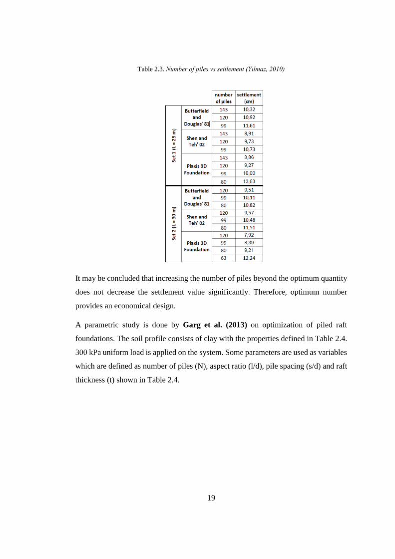
Table 2.3. Number of piles vs settlement (Yılmaz, 2010) ......................................... 19
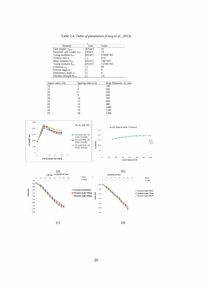
Table 2.4. Table of parameters (Garg et al., 2013) .................................................... 20
Table 2.5. Settlement results for different number of piles (Alver & Özden, 2015) . 23
Table 2.6. The results of change in pile length and number of piles (Alver & Özden,
2015) .......................................................................................................................... 23
Table 2.7. Test summary (Patil et al., 2014) .............................................................. 26
Table 3.1. Plaxis 3D Reference Manual “cylinder” command definitions ................ 31
Table 3.2. Soil parameters (Sönmez, 2013) ............................................................... 35
Table 3.3. Raft parameters (Sönmez, 2013) .............................................................. 35
Table 3.4. Volume pile parameters ............................................................................ 36
Table 3.5. Beam element parameters ......................................................................... 36
Table 3.6. Embedded pile parameters (Engin & Brinkgreve, 2009) ......................... 38
Table 3.7. Axial loads of piles ................................................................................... 41
Table 3.8. Summary of results ................................................................................... 45
Table 4.1. Plaxis 3D Material Models Manual (2013) - Appendix B ....................... 52
Table 4.2. Soil parameters ......................................................................................... 55
Table 4.3. Model case table ....................................................................................... 60
Table 4.4. Raft parameters ......................................................................................... 62
Table 4.5. Pile parameters ......................................................................................... 62
Table 4.6. Mesh size effect ........................................................................................ 65
Table 4.7. Geometric, structural and material input parameters ................................ 69
Table 4.8. Axial force on each pile ............................................................................ 79
Table B.1. L=20, Mohr Coulomb Model results for sand ....................................... 139
xiii
Table B.2. L=30, Mohr Coulomb Model results for sand ........................................ 139
Table B.3. L=40, Mohr Coulomb Model results for sand ........................................ 140
Table B.4. L=20, Hardening Soil Model results for sand ........................................ 140
Table B.5. L=30, Hardening Soil Model results for sand ........................................ 141
Table B.6. L=40, Hardening Soil Model results for sand ........................................ 141
Table B.7. L=20, Mohr Coulomb Model results for clay ........................................ 142
Table B.8. L=30, Mohr Coulomb Model results for clay ........................................ 142
Table B.9. L=40, Mohr Coulomb Model results for clay ........................................ 143
Table B.10. L=20, Hardening Soil Model results for clay ....................................... 143
Table B.11. L=30, Hardening Soil Model results for clay ....................................... 144
Table B.12. L=40, Hardening Soil Model results for clay ....................................... 144
Table B.13. L=20, Soft Soil Creep Model results for clay ...................................... 145
Table B.14. L=30, Soft Soil Creep Model results for clay ...................................... 145
Table B.15. L=40, Soft Soil Creep Model results for clay ...................................... 146
xiv
LIST OF FIGURES
FIGURES
Figure 1.1. Representation of total vertical load ‘VPR’ carried by different foundation
systems (Mandolini et al., 2013) .................................................................................. 1
Figure 1.2. Mechanism and interactions of combined pile-raft foundation (CPRF)
(ISSMGE, 2013) .......................................................................................................... 2
Figure 2.1. Selection chart for design approach (Mandolini et al., 2013) ................... 6
Figure 2.2. Load and settlement curves of diverse design approaches (Poulos, 2001) 7
Figure 2.3. Load settlement curve for preliminary design (Poulos, 2002) .................. 9
Figure 2.4. αrp values for Lp/dp = 25, Kps = 1000 and Krs =10 (Clancy & Randolph,
1996) .......................................................................................................................... 10
Figure 2.5. Design method flowchart for piled raft foundations (Prakoso & Kulhawy,
2001) .......................................................................................................................... 11
Figure 2.6. αs and αL values for piled raft foundation design .................................... 12
Figure 2.7. (a) Alzey Bridge pile test and embedded pile model load results (b) South
Surra pile test and embedded pile model load results (Engin et al., 2008) ................ 13
Figure 2.8. (a) Embedded pile model view (b) Volume pile model view (Dao, 2011)
................................................................................................................................... 14
Figure 2.9. Load and displacement curves of embedded pile and volume pile models
(Dao, 2011) ................................................................................................................ 15
Figure 2.10. (a) Impact of s/d ratio on load carrying capacity (b) Impact of s/d raft
thickness on load carrying capacity (c), (d), (e) Impact of l/d ratio on load carrying
capacity (f) Impact of l/d ratio on α (g) Impact of l/d ratio on total settlement (h) Impact
of raft thickness on differential settlement (Garg et al., 2013) .................................. 21
Figure 2.11. Contact pressure distribution of the raft elements (Kuwabara, ............. 24
Figure 2.12. Load sharing in piled raft (Horikoshi & Randolph, 1998) .................... 27
Figure 2.13. Test setup (Elwakil & Azzam, 2016) .................................................... 28
xv
Figure 3.1. Volume pile view with beam element inside it ....................................... 32
Figure 3.2. (a) Embedded pile view (b) Embedded pile (Brinkgreve, 2014)............. 33
Figure 3.3. (a) Side view of Torhaus building (b) Top view of the foundation (Reul &
Randolph, 2003) ......................................................................................................... 34
Figure 3.4. Mesh model ............................................................................................. 37
Figure 3.5. General view of Torhaus model .............................................................. 38
Figure 3.6. (a) Initial phase (b) Excavation phase (c) Piles phase (d) Raft phase (e)
Loading phase ............................................................................................................ 40
Figure 3.7. Torhaus building pile pattern (Reul & Randolph, 2003) ......................... 41
Figure 3.8. Comparison of axial load results ............................................................. 42
Figure 3.9. Comparison of Pile 1d to Pile 6d axial load results ................................. 43
Figure 3.10. Comparison of Pile 1g to Pile 6g axial load results ............................... 44
Figure 4.1. (a) Displacement of 0.5B distanced boundaries (b) Displacement of B
distanced boundaries (c) Displacement of 2B distanced boundaries (d) Displacement
of 4B distanced boundaries ........................................................................................ 50
Figure 4.2. General view of the model ....................................................................... 51
Figure 4.3. Stress – strain behaviour of Mohr Coulomb model (Plaxis 3D Manual,
2013) .......................................................................................................................... 53
Figure 4.4. Stress – strain behaviour of Hardening Soil model (Plaxis 3D Manual,
2013) .......................................................................................................................... 54
Figure 4.5. Stress – strain behaviour of Soft Soil Creep model (Plaxis 3D Manual,
2013) .......................................................................................................................... 54
Figure 4.6. Top view and 3 dimensional view of each foundation ............................ 59
Figure 4.7. 10 - node tetrahedral element (Plaxis 3D Scientific Manual, 2013)........ 64
Figure 4.8. 6 – node triangular element (Plaxis 3D Scientific Manual, 2013) .......... 64
Figure 4.9. 10 - node tetrahedral element (Plaxis 3D Scientific Manual, 2013)........ 64
Figure 4.10. (a) Whole model mesh view (b) Structural model mesh view ........... 66
Figure 4.11. (a) General view of the initial phase (b) General view of the excavation
phase (c) General view of the pile phase (d) General view of the raft phase (e) General
view of the loading phase ........................................................................................... 67
xvi
Figure 4.12. Project properties window ..................................................................... 71
Figure 4.13. Modify soil layers window .................................................................... 71
Figure 4.14. Soil material set – General tab .............................................................. 72
Figure 4.15. Soil material set – Parameters tab ......................................................... 72
Figure 4.16. Final view of the model ......................................................................... 73
Figure 4.17. Raft material set .................................................................................... 74
Figure 4.18. Pile material set ..................................................................................... 74
Figure 4.19. (a) Perspective view of the structural model (b) Top view of the structural
model ......................................................................................................................... 75
Figure 4.20. Mesh view ............................................................................................. 75
Figure 4.21. Displacement in vertical direction (uz) .................................................. 76
Figure 4.22. Top view of the displacement in vertical direction (uz) ........................ 77
Figure 4.23. Axial forces of piles .............................................................................. 78
Figure 4.24. 3 - dimensional illustration of axial loads on piles ................................ 79
Figure 5.1. SRR vs s/d chart for sand ........................................................................ 84
Figure 5.2. SRR vs Total Length chart for sand ........................................................ 85
Figure 5.3. SRR vs L chart for sand .......................................................................... 86
Figure 5.4. α vs L chart for sand ................................................................................ 87
Figure 5.5. α vs s/d chart for sand .............................................................................. 88
Figure 5.6. α vs Total Length chart for sand ............................................................. 89
Figure 5.7. SRR vs s/d chart for clay ......................................................................... 90
Figure 5.8. SRR vs Total Length chart for clay ......................................................... 91
Figure 5.9. SRR vs L chart for clay ........................................................................... 92
Figure 5.10. α vs L chart for clay .............................................................................. 92
Figure 5.11. α vs s/d chart for clay ............................................................................ 93
Figure 5.12. α vs Total Length chart for clay ............................................................ 94
Figure 5.13. SRR vs s/d chart for clay ....................................................................... 95
Figure 5.14. SRR vs Total Length chart for clay ....................................................... 95
Figure 5.15. SRR vs L chart for clay ......................................................................... 96
Figure 5.16. α vs L chart for clay .............................................................................. 96
xvii
Figure 5.17. α vs s/d chart for clay ............................................................................. 97
Figure 5.18. α vs Total Length chart for clay............................................................. 97
Figure 5.19. SRR vs α chart for sand ......................................................................... 98
Figure 5.20. SRR vs α chart for clay .......................................................................... 99
Figure 5.21. 3D axial load profile of piled raft foundation with L=20 m and s/d=2.5
.................................................................................................................................. 100
Figure 5.22. 3D axial load profile of piled raft foundation with L=20 m and s/d=2.25
.................................................................................................................................. 100
Figure 5.23. 3D axial load profile of piled raft foundation with L=40 m and s/d=2.5
.................................................................................................................................. 101
Figure 5.24. 3D axial load profile of piled raft foundation with L=40 m and s/d=2.25
.................................................................................................................................. 101
Figure 5.25. Pile numbers of the model with L=30 and s/d=7................................. 102
Figure 5.26. Change of pile loads in 300 days, 600 days and 1000 days ................ 102
Figure A.1. L=20 m s/d=9 ........................................................................................ 115
Figure A.2. L=20 m s/d=4.5 ..................................................................................... 115
Figure A.3. L=20 m s/d=2.5 ..................................................................................... 116
Figure A.4. L=20 m s/d=9 ........................................................................................ 116
Figure A.5. L=20 m s/d=4.5 ..................................................................................... 117
Figure A.6. L=20 m s/d=2.5 ..................................................................................... 117
Figure A.7. L=30 m s/d=9 ........................................................................................ 118
Figure A.8. L=30 m s/d=4.5 ..................................................................................... 118
Figure A.9. L=30 m s/d=2.5 ..................................................................................... 119
Figure A.10. L=30 m s/d=9 ...................................................................................... 119
Figure A.11. L=30 m s/d=4.5 ................................................................................... 120
Figure A.12. L=30 m s/d=2.5 ................................................................................... 120
Figure A.13. L=40 m s/d=9 ...................................................................................... 121
Figure A.14. L=40 m s/d=4.5 ................................................................................... 121
Figure A.15. L=40 m s/d=2.5 ................................................................................... 122
Figure A.16. L=40 m s/d=9 ...................................................................................... 122
xviii
Figure A.17. L=40 m s/d=4.5 .................................................................................. 123
Figure A.18. L=40 m s/d=2.5 .................................................................................. 123
Figure A.19. L=20 m s/d=9 ..................................................................................... 124
Figure A.20. L=20 m s/d=4.5 .................................................................................. 124
Figure A.21. L=20 m s/d=2.5 .................................................................................. 125
Figure A.22. L=20 m s/d=9 ..................................................................................... 125
Figure A.23. L=20 m s/d=4.5 .................................................................................. 126
Figure A.24. L=20 m s/d=2.5 .................................................................................. 126
Figure A.25. L=30 m s/d=9 ..................................................................................... 127
Figure A.26. L=30 m s/d=4.5 .................................................................................. 127
Figure A.27. L=30 m s/d=2.5 .................................................................................. 128
Figure A.28. L=30 m s/d=9 ..................................................................................... 128
Figure A.29. L=30 m s/d=4.5 .................................................................................. 129
Figure A.30. L=30 m s/d=2.5 .................................................................................. 129
Figure A.31. L=40 m s/d=9 ..................................................................................... 130
Figure A.32. L=40 m s/d=4.5 .................................................................................. 130
Figure A.33. L=40 m s/d=2.5 .................................................................................. 131
Figure A.34. L=40 m s/d=9 ..................................................................................... 131
Figure A.35. L=40 m s/d=4.5 .................................................................................. 132
Figure A.36. L=40 m s/d=2.5 .................................................................................. 132
Figure A.37. L=20 m s/d=9 ..................................................................................... 133
Figure A.38. L=20 m s/d=4.5 .................................................................................. 133
Figure A.39. L=20 m s/d=2.5 .................................................................................. 134
Figure A.40. L=30 m s/d=9 ..................................................................................... 134
Figure A.41. L=30 m s/d=4.5 .................................................................................. 135
Figure A.42. L=30 m s/d=2.5 .................................................................................. 135
Figure A.43. L=40 m s/d=9 ..................................................................................... 136
Figure A.44. L=40 m s/d=4.5 .................................................................................. 136
Figure A.45. L=40 m s/d=2.5 .................................................................................. 137
1
CHAPTER 1
1. INTRODUCTION
1.1. General Information
A pile foundation consists of three elements namely pile cap, certain number of piles
and the soil. Conventional pile foundation design assumes that piles carry all structural
loads and the pile cap does not contribute to the load carrying capacity.
In the last few decades, piled raft design concept has been increasingly used for the
foundation design of many buildings especially high rise buildings and towers. Unlike
the conventional pile foundation design, this design approach considers the
contribution of the raft to the load carrying capacity. In other words, structural load is
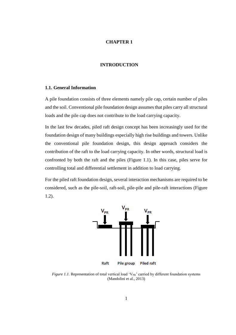
confronted by both the raft and the piles (Figure 1.1). In this case, piles serve for
controlling total and differential settlement in addition to load carrying.
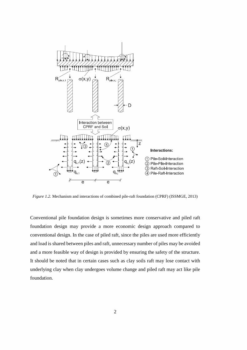
For the piled raft foundation design, several interaction mechanisms are required to be
considered, such as the pile-soil, raft-soil, pile-pile and pile-raft interactions (Figure
1.2).
Figure 1.1. Representation of total vertical load ‘VPR’ carried by different foundation systems
(Mandolini et al., 2013)
2
Figure 1.2. Mechanism and interactions of combined pile-raft foundation (CPRF) (ISSMGE, 2013)
Conventional pile foundation design is sometimes more conservative and piled raft
foundation design may provide a more economic design approach compared to
conventional design. In the case of piled raft, since the piles are used more efficiently
and load is shared between piles and raft, unnecessary number of piles may be avoided
and a more feasible way of design is provided by ensuring the safety of the structure.
It should be noted that in certain cases such as clay soils raft may lose contact with
underlying clay when clay undergoes volume change and piled raft may act like pile
foundation.
3
1.2. Problem Statement
Finite element method (FEM) is generally used in the design of piled raft foundations.
Analytical solutions, laboratory studies-experiments and real case measurements are
compared with the results of finite element solutions in various studies in order to
provide verification of them. There are many examples of designs conducted via FEM
analyses in the literature such as Reul & Randolph (2003), Prakoso & Kulhawy (2001)
and Sönmez (2013).
In this study, piled raft foundation is modelled by three-dimensional finite element
method, using Plaxis 3D software. In order to provide a guideline for designers, it is
essential to combine variables such as soil type, soil model, pile length, pile
configuration and pile modelling approach. Therefore, this thesis focuses on
examining the effects of these variables.
1.3. Research Objectives
This study aims at investigating the load-sharing and settlement characteristics of
piled raft foundations. More specific objectives are as follows:
(1) To study the load sharing mechanism between the piles and the cap by the help
of three-dimensional finite element analyses
(2) To calculate settlements via finite element analyses and to compare them with
the results of real cases
(3) To provide an optimum design by changing the length, configuration or
geometrical positioning of piles in sands and clays under various material models
(4) To design the piles by both ‘Volume pile’ and ‘Embedded pile’ features of
Plaxis 3D finite element program and to compare the results of different approaches
in order to check whether embedded pile can replace volume pile or not due to time
concerns
4
1.4. Scope
This study investigates the design of piled raft foundations by Plaxis 3D finite element
software. In Chapter 2, literature review is presented. Design methodology, volume
pile and embedded pile properties of software, some numerical and experimental
studies are summarized by researching bearing capacity and settlement results. In
Chapter 3, methodology and comparison of volume pile and embedded pile properties
of Plaxis 3D are provided by verification of a real case. In Chapter 4, two hypothetical
cases consisting of either sand or clay are studied by using embedded pile property.
Moreover, building and analyzing a model in Plaxis 3D are also presented. In Chapter
5, results of the analyses and conclusions are discussed.
5
CHAPTER 2
2. LITERATURE REVIEW
2.1. Design Methodology of Piled Raft Foundation
Mandolini et al. (2013) consider the fact that piles and the raft both carry the total
structural load in collaboration in the piled raft foundation design concept. In other
words, the total structural load (VPR) is shared among piles and the raft unlike the
conventional pile foundation design concept that ignores the load capacity of the raft.
Mandolini et al. (2013), represents the aforementioned load sharing behavior with a
load sharing ratio (αpr) among piles and the raft and describes the load sharing ratio as
the portion of the load carried by the piles. (Eqn 2.1)
αpr =∑ 𝑉𝑝𝑖𝑙𝑒,𝑖
𝑛𝑖=1
𝑉𝑃𝑅 (Eqn 2.1)
where “n” represents the number of piles and “Vpile” represents the load carried by a
single pile.
As illustrated in Figure 1.1, αpr = 0 implies a raft foundation whereas αpr = 1 implies a
pile foundation without support of the raft. For a piled raft foundation 0< αpr <1
condition is valid.
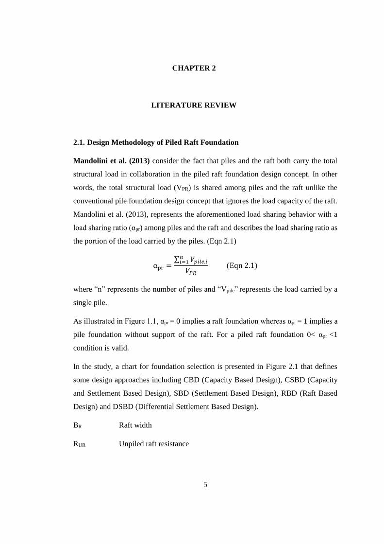
In the study, a chart for foundation selection is presented in Figure 2.1 that defines
some design approaches including CBD (Capacity Based Design), CSBD (Capacity
and Settlement Based Design), SBD (Settlement Based Design), RBD (Raft Based
Design) and DSBD (Differential Settlement Based Design).
BR Raft width
RUR Unpiled raft resistance
6
wUR, wadm Average settlement of the unpiled raft and admissible average
settlement
FS Factor of safety
Figure 2.1. Selection chart for design approach (Mandolini et al., 2013)
For a convenient FS=3, “A” point might be considered as optimum where wur/wadm
equals to 1.
Point 1 represents RBD in which wur and FSur are acceptable.
For Point 2 and Point 3, both the wur and FSur are not acceptable since wur is greater
than wadm and FSur is under the convenient limit. In order to overcome the FS issue
and settlement problem, piles must be added to the system.
For Point 4 and Point 5, FSur is acceptable. However, wur is not acceptable since it is
greater than wadm. In order to decrease the settlement, piles must be added to the
system.
Poulos (2001) explains the design concept and issues of piled raft foundations by
defining the stages of the design process with favourable and unfavourable conditions.
7
Just like the any other foundation systems, the issues of ultimate load capacity under
the lateral, vertical and moment loads, total maximum and differential settlements,
structural design properties of raft and piles such as moment, shear for raft and axial
load for piles must be considered in the design of piled raft foundations.
Poulos (2001) reported that favourable soil conditions in which the piled raft
foundations can be successfully applied are stiff clays and dense sands. On the other
hand, unfavourable soil conditions include soft clays or loose sands close to the
surface, soft compressible layers at the bottom layers and the layers prone to swelling
or consolidation. In such cases, raft-soil contact should always exist.
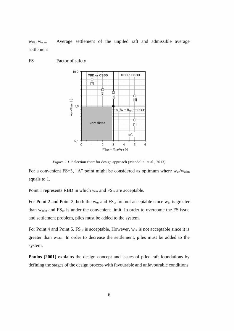
Various design approaches are available related to piled rafts. To be more precise, load
and settlement behaviour of piled raft foundation depending on different design
approaches can be seen at the Figure 2.2. Curve 0 represents the raft only design with
excessive settlements. Curve 1 is the traditional design approach that the piles are
assumed to carry the total load. Curve 2 shows the “creep piling” case in which the
piles are designed to carry the working load corresponding to 70 - 80% of the ultimate
load with a lower factor of safety compared to Curve 1. Curve 3, which belongs to the
case in which the piles are placed effectively to control differential settlement,
represents the optimum solution by meeting the minimum requirements of design load
and allowable solution while the others seem to be over or under-designed.
Figure 2.2. Load and settlement curves of diverse design approaches (Poulos, 2001)
8
Finally, the crucial points and stages of the design process are summarized as below:
In the first stage, necessary number of piles is determined in order to provide
to fulfill the requirements of design load and allowable settlements.
In the second stage, pile location and general properties are determined
according to the loading.
In the last stage, details of the design are presented such as location,
configuration and number of the piles and the load, moment and settlement
results of raft and piles are computed.
Poulos (2002), discusses the design issues of piled raft foundations by explaining the
essential points to be considered by the designers.
Piled raft foundations can effectively be used in cases in which the raft alone can
almost meet the load carrying capacity but cannot adequately meet the requirements
of allowable total and differential settlements. Therefore, first, the performance of
unpiled raft should be analyzed when starting the design. Then, the main points
including raft thickness, pile type, pile configuration, pile length and pile diameter
must be decided. For this decision, overall vertical load capacity, overall load
settlement behaviour and overall differential settlement must be considered.
In overall load settlement part, Poulos (2002) proposes the following equations to
determine the stiffness of piled raft and the load taken by raft (Poulos & Davis, 1980;
Randolph & Clancy, 1993).
𝑘𝑝𝑟 =(𝑘𝑝 + 𝑘𝑟(1 − 2𝛼𝑝𝑟))
(1 − 𝛼𝑝𝑟2 𝑘𝑟
𝑘𝑝))
(𝐸𝑞𝑛 2.2)
𝑃𝑟
𝑃𝑡=
𝑘𝑟(1 − 𝛼𝑐𝑝)
𝑘𝑝 + 𝑘𝑟(1 − 2𝛼𝑐𝑝) (𝐸𝑞𝑛 2.3)

9
where kpr is piled raft stiffness, kp is pile group stiffness, kr is raft stiffness αpr is raft –
pile interaction factor, Pr is the load carried by raft and Pt is the total load. Finally, in
the result of above equations, following chart is obtained (Figure 2.3.). kpr is calculated
from Eqn 2.2 and it is operated until Point A. Beyond Point A, kr is operated until
Point B. After this point, ultimate load capacity of piled raft foundation is reached.
Figure 2.3. Load settlement curve for preliminary design (Poulos, 2002)
The studies of Clancy & Randolph (1996), provide a basis for Poulos (2002) and
recommend the following parameter range in Table 2.2.
Table 2.1. Explanations of parameters (Clancy & Randolph, 1996)
Table 2.2. Recommendations for parameters (Clancy & Randolph, 1996)
10
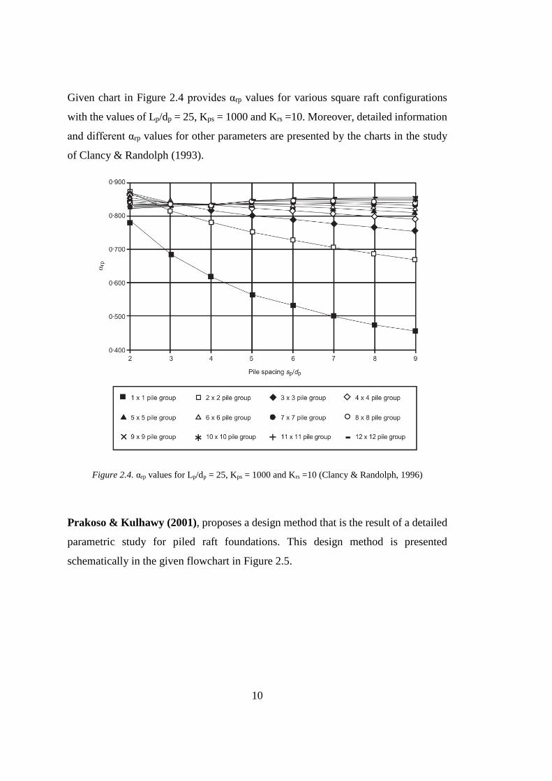
Given chart in Figure 2.4 provides αrp values for various square raft configurations
with the values of Lp/dp = 25, Kps = 1000 and Krs =10. Moreover, detailed information
and different αrp values for other parameters are presented by the charts in the study
of Clancy & Randolph (1993).
Figure 2.4. αrp values for Lp/dp = 25, Kps = 1000 and Krs =10 (Clancy & Randolph, 1996)
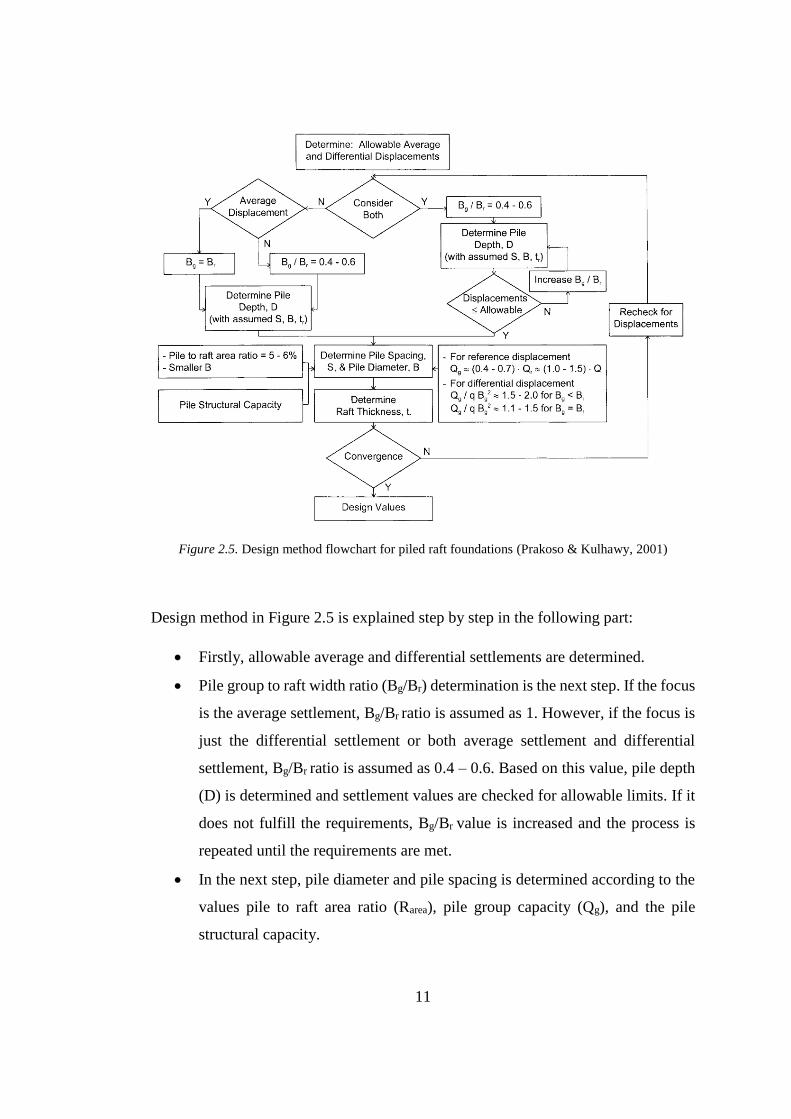
Prakoso & Kulhawy (2001), proposes a design method that is the result of a detailed
parametric study for piled raft foundations. This design method is presented
schematically in the given flowchart in Figure 2.5.
11
Figure 2.5. Design method flowchart for piled raft foundations (Prakoso & Kulhawy, 2001)
Design method in Figure 2.5 is explained step by step in the following part:
Firstly, allowable average and differential settlements are determined.
Pile group to raft width ratio (Bg/Br) determination is the next step. If the focus
is the average settlement, Bg/Br ratio is assumed as 1. However, if the focus is
just the differential settlement or both average settlement and differential
settlement, Bg/Br ratio is assumed as 0.4 – 0.6. Based on this value, pile depth
(D) is determined and settlement values are checked for allowable limits. If it
does not fulfill the requirements, Bg/Br value is increased and the process is
repeated until the requirements are met.
In the next step, pile diameter and pile spacing is determined according to the
values pile to raft area ratio (Rarea), pile group capacity (Qg), and the pile
structural capacity.
12
In the final step, raft thickness (tr) is determined based on structural design.
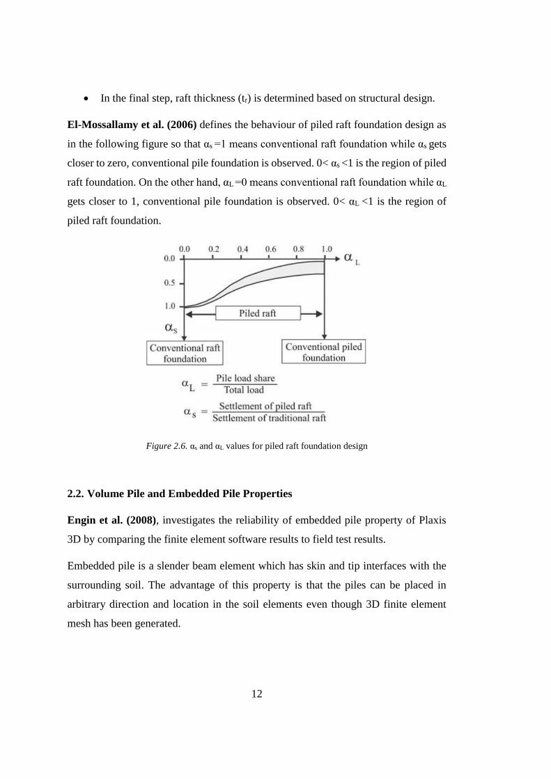
El-Mossallamy et al. (2006) defines the behaviour of piled raft foundation design as
in the following figure so that αs =1 means conventional raft foundation while αs gets
closer to zero, conventional pile foundation is observed. 0< αs <1 is the region of piled
raft foundation. On the other hand, αL =0 means conventional raft foundation while αL
gets closer to 1, conventional pile foundation is observed. 0< αL <1 is the region of
piled raft foundation.
Figure 2.6. αs and αL values for piled raft foundation design
2.2. Volume Pile and Embedded Pile Properties
Engin et al. (2008), investigates the reliability of embedded pile property of Plaxis
3D by comparing the finite element software results to field test results.
Embedded pile is a slender beam element which has skin and tip interfaces with the
surrounding soil. The advantage of this property is that the piles can be placed in
arbitrary direction and location in the soil elements even though 3D finite element
mesh has been generated.
13
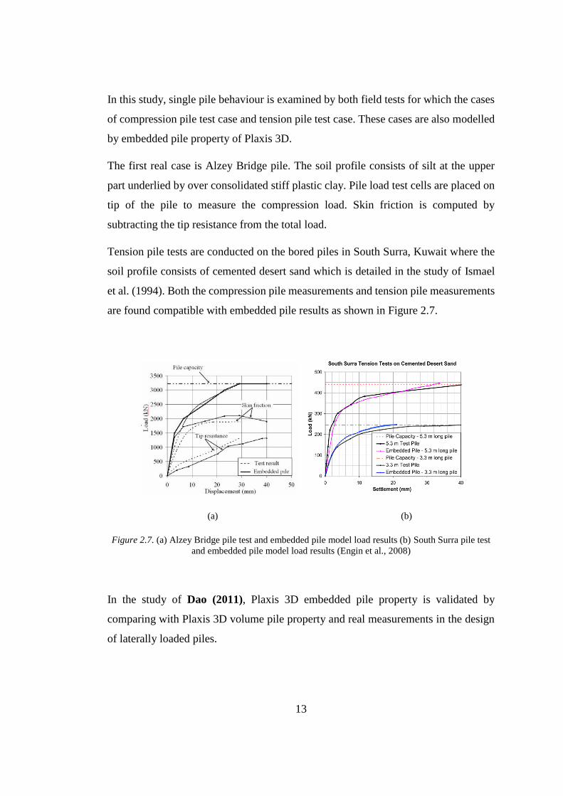
In this study, single pile behaviour is examined by both field tests for which the cases
of compression pile test case and tension pile test case. These cases are also modelled
by embedded pile property of Plaxis 3D.
The first real case is Alzey Bridge pile. The soil profile consists of silt at the upper
part underlied by over consolidated stiff plastic clay. Pile load test cells are placed on
tip of the pile to measure the compression load. Skin friction is computed by
subtracting the tip resistance from the total load.
Tension pile tests are conducted on the bored piles in South Surra, Kuwait where the
soil profile consists of cemented desert sand which is detailed in the study of Ismael
et al. (1994). Both the compression pile measurements and tension pile measurements
are found compatible with embedded pile results as shown in Figure 2.7.
(a) (b)
Figure 2.7. (a) Alzey Bridge pile test and embedded pile model load results (b) South Surra pile test
and embedded pile model load results (Engin et al., 2008)
In the study of Dao (2011), Plaxis 3D embedded pile property is validated by
comparing with Plaxis 3D volume pile property and real measurements in the design
of laterally loaded piles.
14
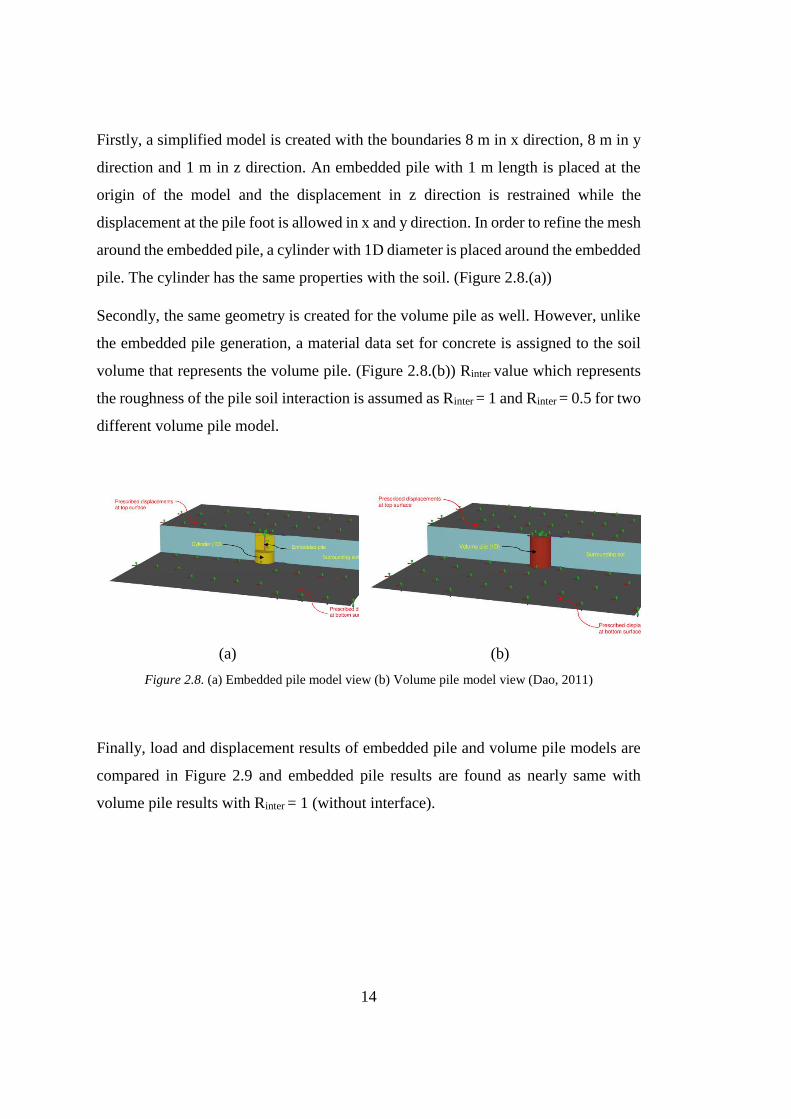
Firstly, a simplified model is created with the boundaries 8 m in x direction, 8 m in y
direction and 1 m in z direction. An embedded pile with 1 m length is placed at the
origin of the model and the displacement in z direction is restrained while the
displacement at the pile foot is allowed in x and y direction. In order to refine the mesh
around the embedded pile, a cylinder with 1D diameter is placed around the embedded
pile. The cylinder has the same properties with the soil. (Figure 2.8.(a))
Secondly, the same geometry is created for the volume pile as well. However, unlike
the embedded pile generation, a material data set for concrete is assigned to the soil
volume that represents the volume pile. (Figure 2.8.(b)) Rinter value which represents
the roughness of the pile soil interaction is assumed as Rinter = 1 and Rinter = 0.5 for two
different volume pile model.
(a) (b)
Figure 2.8. (a) Embedded pile model view (b) Volume pile model view (Dao, 2011)
Finally, load and displacement results of embedded pile and volume pile models are
compared in Figure 2.9 and embedded pile results are found as nearly same with
volume pile results with Rinter = 1 (without interface).

15
Figure 2.9. Load and displacement curves of embedded pile and volume pile models (Dao, 2011)
Sluis et al. (2014), investigates the use of embedded pile feature in and compare the
displacement and bending moment results with the ones of Plaxis 3D analysis for a
pile row under lateral load.
They state that piles are used to be modelled as plate or node to node anchor in Plaxis
2D before embedded pile feature of Plaxis. However, these two methods both have
disadvantages.
In plate method, plates are created by taking the pile properties for unit width in out
of plane. Nevertheless, this causes to decrease the effect of pile soil interaction by
interfering the soil mesh and limits the out of plane spacing to lower values.
Node to node anchor method totally ignores the interaction between soil and pile since
soil covers all the model including the node to node anchor elements and mesh is
continuous that is independent from the pile. In addition, node to node anchor method
can only be used for axially loaded piles since it ignores lateral interaction.
Embedded pile feature reflects the benefits of both plate and node to node anchor.
Embedded pile behaves like a beam element but in a continuous mesh in the existence
of both pile and soil. So, the pile soil interaction is modelled Plaxis 2D well.
16
Finally, embedded pile feature of Plaxis 2D is validated by comparing to Plaxis 3D
results in terms of axial load including both compression and tension load; lateral
loading resulting from external forces and soil movements. The results are 2D and 3D
analyses are found as compatible.
Sheil & McCabe (2012), investigate the single pile and pile group behaviour in soft
clay which are modelled by Plaxis 3D embedded pile feature. Pile group finite element
results are compared to the field test data in order to see the convenience of embedded
pile feature. The comparison presents that this feature provides compatible results with
field test data and considered as reasonable due to time saving and less computational
effort.
In this study, bearing capacity of embedded pile that is related to the embedded pile
properties of maximum skin resistance Tmax and maximum base resistance Fmax are
also explained. In embedded pile feature, bearing capacity of the pile is not a result of
finite element analyses. It must be an input parameter in the material set properties of
pile. Tmax and Fmax values are generally determined by pile load tests. The skin
resistance is considered in three ways including:
Linear skin friction is defined at pile head and bottom of the pile as Ttop,max and
Tbot,max
Multi linear skin friction is used for multi-layered soil profiles with a certain
Ttop,max and varying Tbot,max along the pile at different locations.
Layer dependent skin friction considers the soil strength parameters such as
friction angle (φ), cohesion (c) and pile interface factor Rinter.
2.3. Various Numerical Studies
In the dissertation of Ryltenius (2011), piled raft foundations are modelled in four
ways by Plaxis 3D and Plaxis 2D FEM programs to compare the results of two and
17
three dimensioned analysis. One model is established in three dimensional and three
models are established in two dimensional in soft clay to discuss pile raft interaction.
In piled raft foundations, contrary to the conventional pile foundation design, load
distribution between raft and piles is the matter. While raft contributes to the load
carrying capacity, piles are used for total and differential settlement reduction.
According to the results of the analysis:
In two dimensional model, raft carries 51 % of the total load. Maximum settlement is
121 mm and the differential settlement is 16 mm.
In three dimensional model, raft carries 36 % of the total load. Maximum settlement
is 56 mm and the differential settlement is 11 mm.
A series of analysis are done for different spacing of piles and different raft dimensions
for both two and three dimensions. Two dimension analysis results of settlement and
load carrying capacity of raft are overestimated compared to three dimensional model.
In the stıudy of Reul & Randolph (2003), foundations of three buildings in Frankfurt,
Germany, named Westend 1, Messeturm and Torhaus der Messe, are investigated and
back analysis results of piled raft foundations obtained from three dimensional FEM
analyses by ABAQUS program, in a subsoil condition of overconsolidated Frankfurt
clay underlied by rocky Frankfurt limestone are presented. Measured values are
compared to results of analytical solutions and finite element analyses.
First building Westend 1 consists of a 208 m high tower and a 60 m low rise section.
Piled raft belongs to the tower part with the raft dimensions of 47 x 62 x 3-4.65 m and
40 bored piles with 1.3 m diameter, 30 m length. Measured center settlement value is
120 mm 2.5 years after the completion of construction whereas the finite element
result is 110 mm. according to the measured records, raft carries 50 % of the total load
while the finite element result is 44 %.
Second building Messeturm is a 256 m high tower. Foundation is a piled raft with the
raft dimensions of 58.8 x 58.8 x 3-6 m and 64 bored piles with 1.3 m diameter,
18
different lengths of 26.9, 30.9 and 34.9 m. Measured center settlement value is 144
mm whereas the finite element result is 174 mm. according to the measured records,
raft carries 57 % of the total load while the finite element result is 40 %.
Third building Torhaus der Messe is a 130 m high tower. Foundation is two piled rafts
10 m apart from each other with the raft dimensions of 17.5 x 24.5 x 2.5 m and 84
bored piles with 0.9 m diameter, 20 m length. Average measured center settlement
value of two rafts is 124 mm whereas the finite element result is 96 mm. According to
the measured records, raft carries 33 % of the total load while the finite element result
is 24 %.
As a result, settlement calculations are compatible with the measured ones but the raft
load is underestimated compared to measured values.
In the thesis of Yılmaz (2010), two sets of piled raft foundations with raft dimensions
24x28x2 m and 2.25 m spacing are analyzed by Plaxis 3D program. Number of piles
is 143, 120 and 99 alternately and pile length is 25 m for the first set. Number of piles
is 120, 99 and 80 alternately and pile length is 30 m for the second set. Effects of
number of piles and pile length on settlement values are investigated. Results of the
analyses are compared with analytical methods of Butterfield and Douglas (1981) and
Shen and Teh (2002) (Table 2.3).
19
Table 2.3. Number of piles vs settlement (Yılmaz, 2010)
It may be concluded that increasing the number of piles beyond the optimum quantity
does not decrease the settlement value significantly. Therefore, optimum number
provides an economical design.
A parametric study is done by Garg et al. (2013) on optimization of piled raft
foundations. The soil profile consists of clay with the properties defined in Table 2.4.
300 kPa uniform load is applied on the system. Some parameters are used as variables
which are defined as number of piles (N), aspect ratio (l/d), pile spacing (s/d) and raft
thickness (t) shown in Table 2.4.
20
Table 2.4. Table of parameters (Garg et al., 2013)
(a) (b)
(c) (d)
21
(e) (f)
(g) (h)
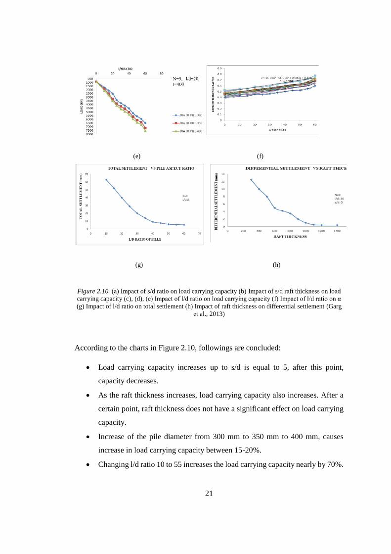
Figure 2.10. (a) Impact of s/d ratio on load carrying capacity (b) Impact of s/d raft thickness on load
carrying capacity (c), (d), (e) Impact of l/d ratio on load carrying capacity (f) Impact of l/d ratio on α
(g) Impact of l/d ratio on total settlement (h) Impact of raft thickness on differential settlement (Garg
et al., 2013)
According to the charts in Figure 2.10, followings are concluded:
Load carrying capacity increases up to s/d is equal to 5, after this point,
capacity decreases.
As the raft thickness increases, load carrying capacity also increases. After a
certain point, raft thickness does not have a significant effect on load carrying
capacity.
Increase of the pile diameter from 300 mm to 350 mm to 400 mm, causes
increase in load carrying capacity between 15-20%.
Changing l/d ratio 10 to 55 increases the load carrying capacity nearly by 70%.
22
Other than the finite element software solution, load on components are
calculated by the help of Capacity reduction factor (α). The capacity of the
components of the piled raft foundation system is calculated by conventional
methods and multiplied by the capacity reduction factor. Capacity reduction
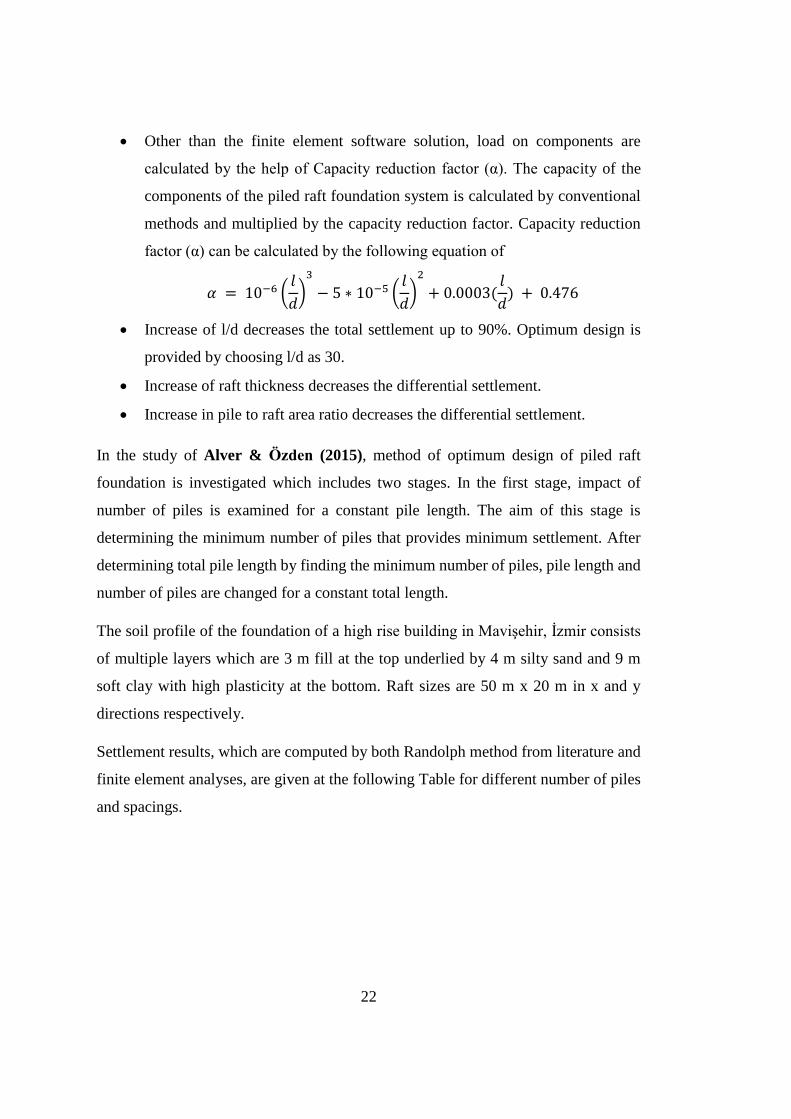
factor (α) can be calculated by the following equation of
𝛼 = 10−6 (𝑙
𝑑)
3
− 5 ∗ 10−5 (𝑙
𝑑)
2
+ 0.0003(𝑙
𝑑) + 0.476
Increase of l/d decreases the total settlement up to 90%. Optimum design is
provided by choosing l/d as 30.
Increase of raft thickness decreases the differential settlement.
Increase in pile to raft area ratio decreases the differential settlement.
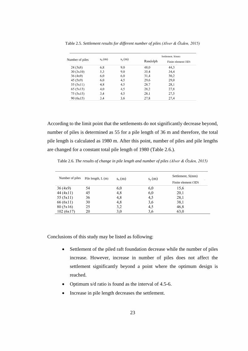
In the study of Alver & Özden (2015), method of optimum design of piled raft
foundation is investigated which includes two stages. In the first stage, impact of
number of piles is examined for a constant pile length. The aim of this stage is
determining the minimum number of piles that provides minimum settlement. After
determining total pile length by finding the minimum number of piles, pile length and
number of piles are changed for a constant total length.
The soil profile of the foundation of a high rise building in Mavişehir, İzmir consists
of multiple layers which are 3 m fill at the top underlied by 4 m silty sand and 9 m
soft clay with high plasticity at the bottom. Raft sizes are 50 m x 20 m in x and y
directions respectively.
Settlement results, which are computed by both Randolph method from literature and
finite element analyses, are given at the following Table for different number of piles
and spacings.
23
Table 2.5. Settlement results for different number of piles (Alver & Özden, 2015)
According to the limit point that the settlements do not significantly decrease beyond,
number of piles is determined as 55 for a pile length of 36 m and therefore, the total
pile length is calculated as 1980 m. After this point, number of piles and pile lengths
are changed for a constant total pile length of 1980 (Table 2.6.).
Table 2.6. The results of change in pile length and number of piles (Alver & Özden, 2015)
Conclusions of this study may be listed as following:
Settlement of the piled raft foundation decrease while the number of piles
increase. However, increase in number of piles does not affect the
settlement significantly beyond a point where the optimum design is
reached.
Optimum s/d ratio is found as the interval of 4.5-6.
Increase in pile length decreases the settlement.
Number of piles Finite element (3D)
Settlement, S(mm)
Finite element (3D)
Settlement, S(mm) Number of piles Pile length, L (m)
24
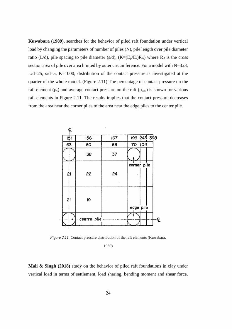
Kuwabara (1989), searches for the behavior of piled raft foundation under vertical
load by changing the parameters of number of piles (N), pile length over pile diameter
ratio (L/d), pile spacing to pile diameter (s/d), (K=(Ep/Es)RA) where RA is the cross
section area of pile over area limited by outer circumference. For a model with N=3x3,
L/d=25, s/d=5, K=1000; distribution of the contact pressure is investigated at the
quarter of the whole model. (Figure 2.11) The percentage of contact pressure on the
raft element (pc) and average contact pressure on the raft (pcav) is shown for various
raft elements in Figure 2.11. The results implies that the contact pressure decreases
from the area near the corner piles to the area near the edge piles to the center pile.
Figure 2.11. Contact pressure distribution of the raft elements (Kuwabara,
1989)
Mali & Singh (2018) study on the behavior of piled raft foundations in clay under
vertical load in terms of settlement, load sharing, bending moment and shear force.
25
The analyses are conducted by Plaxis 3D software. 15 different pile configurations are
arranged with different pile spacing, length, diameter and raft – soil stiffness ratio. A
square raft with 45 m x 45 m is loaded 200 kPa.
Conclusions of the study can be summarized as follows;
The optimum s/d ratio is determined as 5-6 where the settlement and bending
moment reach to minimum values.
The optimum piled group to raft width ratio is found as 0.6 where the bending
moment is minimum.
Increase in pile diameter causes decrease in average and differential settlement
and increase in load sharing ratio of pile group.
Increase in raft - soil stiffness ratio causes increase in shear force. However, bending
moment is slightly affected by raft - soil stiffness ratio beyond the value of 0.09.
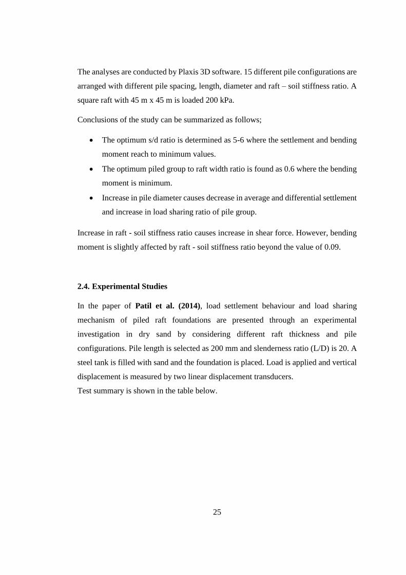
2.4. Experimental Studies
In the paper of Patil et al. (2014), load settlement behaviour and load sharing
mechanism of piled raft foundations are presented through an experimental
investigation in dry sand by considering different raft thickness and pile
configurations. Pile length is selected as 200 mm and slenderness ratio (L/D) is 20. A
steel tank is filled with sand and the foundation is placed. Load is applied and vertical
displacement is measured by two linear displacement transducers.
Test summary is shown in the table below.
26
Table 2.7. Test summary (Patil et al., 2014)
Results of the experiments imply that at the beginning of the loading, piles carry the
major part of the load. However, as the settlement increases, load is transferred to the
raft. Load shared by piles and settlement reduction ratio increase with the increasing
number of piles. But, beyond a certain number of piles settlement reduction ratio does
not affected much. Increase of raft thickness does not affect the load shared by piles
and settlement.
Horikoshi & Randolph (1998) considers the effective placement of the piles under
the raft in order to provide an optimum design. Pile group is located at the center of
the raft in such a way that total and differential settlements remain in an acceptable
range (Figure 2.12).
27
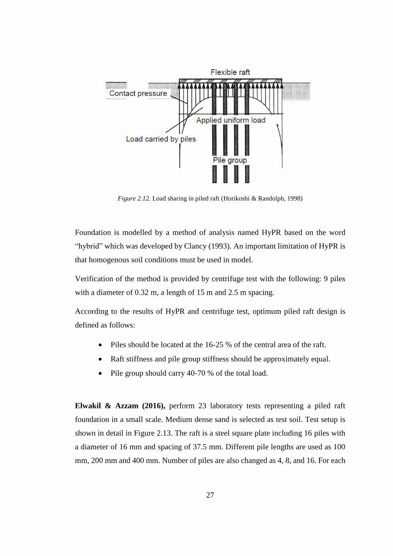
Figure 2.12. Load sharing in piled raft (Horikoshi & Randolph, 1998)
Foundation is modelled by a method of analysis named HyPR based on the word
“hybrid” which was developed by Clancy (1993). An important limitation of HyPR is
that homogenous soil conditions must be used in model.
Verification of the method is provided by centrifuge test with the following: 9 piles
with a diameter of 0.32 m, a length of 15 m and 2.5 m spacing.
According to the results of HyPR and centrifuge test, optimum piled raft design is
defined as follows:
Piles should be located at the 16-25 % of the central area of the raft.
Raft stiffness and pile group stiffness should be approximately equal.
Pile group should carry 40-70 % of the total load.
Elwakil & Azzam (2016), perform 23 laboratory tests representing a piled raft
foundation in a small scale. Medium dense sand is selected as test soil. Test setup is
shown in detail in Figure 2.13. The raft is a steel square plate including 16 piles with
a diameter of 16 mm and spacing of 37.5 mm. Different pile lengths are used as 100
mm, 200 mm and 400 mm. Number of piles are also changed as 4, 8, and 16. For each
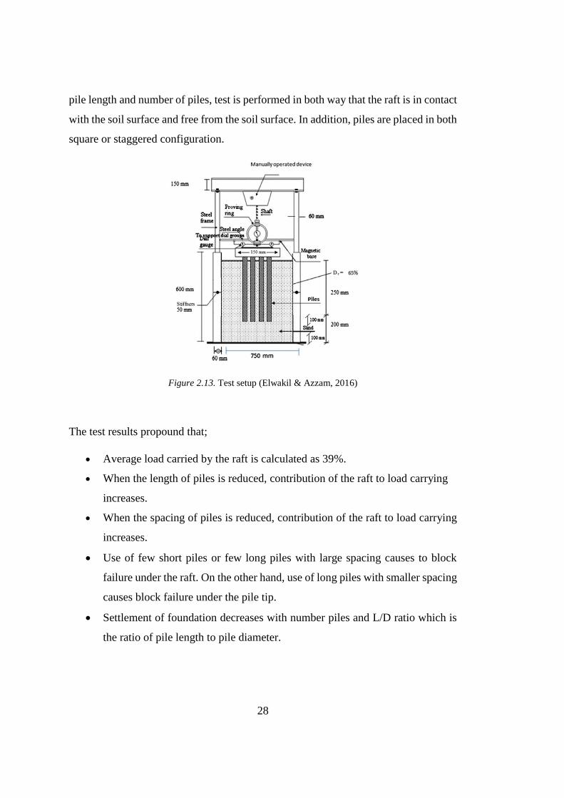
28
pile length and number of piles, test is performed in both way that the raft is in contact
with the soil surface and free from the soil surface. In addition, piles are placed in both
square or staggered configuration.
Figure 2.13. Test setup (Elwakil & Azzam, 2016)
The test results propound that;
Average load carried by the raft is calculated as 39%.
When the length of piles is reduced, contribution of the raft to load carrying
increases.
When the spacing of piles is reduced, contribution of the raft to load carrying
increases.
Use of few short piles or few long piles with large spacing causes to block
failure under the raft. On the other hand, use of long piles with smaller spacing
causes block failure under the pile tip.
Settlement of foundation decreases with number piles and L/D ratio which is
the ratio of pile length to pile diameter.
29
Mosawi et al. (2011), conduct some laboratory tests in order to investigate the
behavior of piled raft foundation. The experiment is performed with a soil tank with
the length of 0.6 m, width of 0.6 m, height 0.6 m and filled with medium dense sand.
The dimensions of the tank is selected in a way so that the boundaries do not limit the
failure zone of foundation. The material of piles and the raft is aluminum alloy.
Piled raft geometry is formed by changing some parameters in each test. Pile spacing
is selected as 5 cm and kept constant for all the tests. Thickness of raft is determined
as 5 mm and 2.5 mm. l/d ratio is changed as 20, 25 and 30. Pile diameters are 9 mm,
12 mm, 15 mm and pile lengths are 200 mm, 250 mm, 300 mm. Pile configurations
are formed as 2x1, 3x1, 2x2 and 3x2. The vertical load applied on foundation is either
5 kN or 10 kN. Unpiled raft is also examined for comparison.
The experiment results are as follows;
The percentage of the load carried by pile group is found as 28%, 38%, 56%,
79% for pile configurations 2x1, 3x1, 2x2, 3x2, respectively with a diameter
of 9 mm and a raft thickness of 5 mm. This implies that increase in number of
piles also increases the percentage of the load carried by pile group.
For the unpiled raft, thickness of raft slightly influence the load carrying
capacity. On the other hand, raft size increase also raises the load carrying
capacity.
Increase in pile diameter, pile length and number of piles also increases the load
carrying capacity.

31
CHAPTER 3
3. METHODOLOGY AND VERIFICATION
3.1. Introduction
In this chapter, different types of pile modelling in Plaxis 3D that are volume pile and
embedded pile are investigated in order to provide the verification of the results of
both pile modelling types and determine which one will be used in Chapter 4 for the
hypothetical cases.
3.2. Volume Pile and Embedded Pile Properties of Plaxis 3D
3.2.1. Volume Pile
Volume pile comprises three dimensional volume elements, which interact with the
surrounding soil.
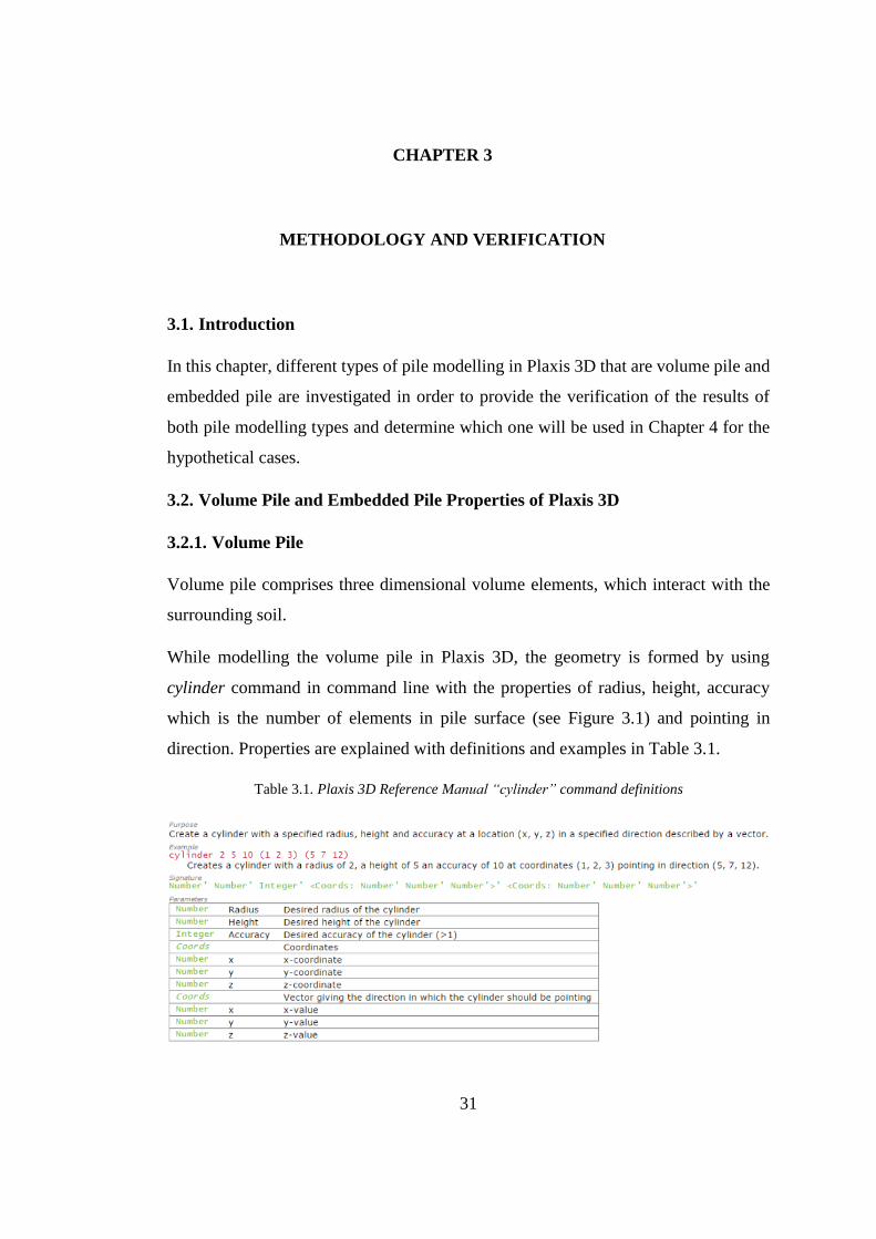
While modelling the volume pile in Plaxis 3D, the geometry is formed by using
cylinder command in command line with the properties of radius, height, accuracy
which is the number of elements in pile surface (see Figure 3.1) and pointing in
direction. Properties are explained with definitions and examples in Table 3.1.
Table 3.1. Plaxis 3D Reference Manual “cylinder” command definitions
32
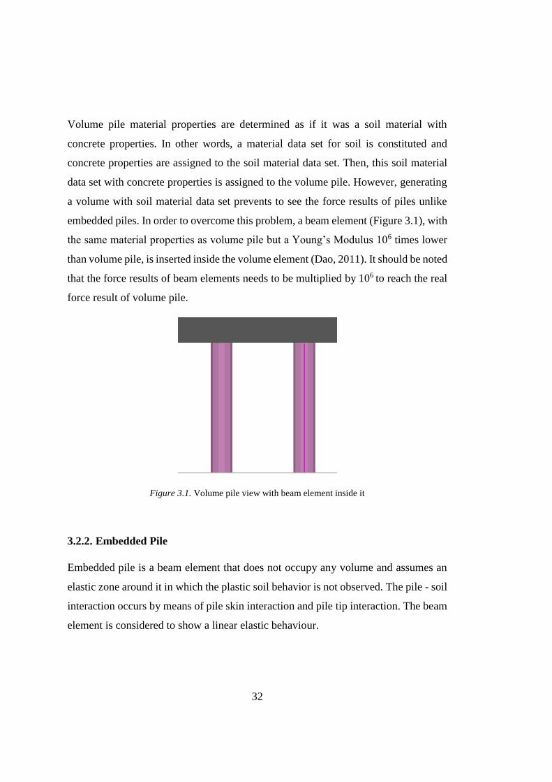
Volume pile material properties are determined as if it was a soil material with
concrete properties. In other words, a material data set for soil is constituted and
concrete properties are assigned to the soil material data set. Then, this soil material
data set with concrete properties is assigned to the volume pile. However, generating
a volume with soil material data set prevents to see the force results of piles unlike
embedded piles. In order to overcome this problem, a beam element (Figure 3.1), with
the same material properties as volume pile but a Young’s Modulus 106 times lower
than volume pile, is inserted inside the volume element (Dao, 2011). It should be noted
that the force results of beam elements needs to be multiplied by 106 to reach the real
force result of volume pile.
Figure 3.1. Volume pile view with beam element inside it
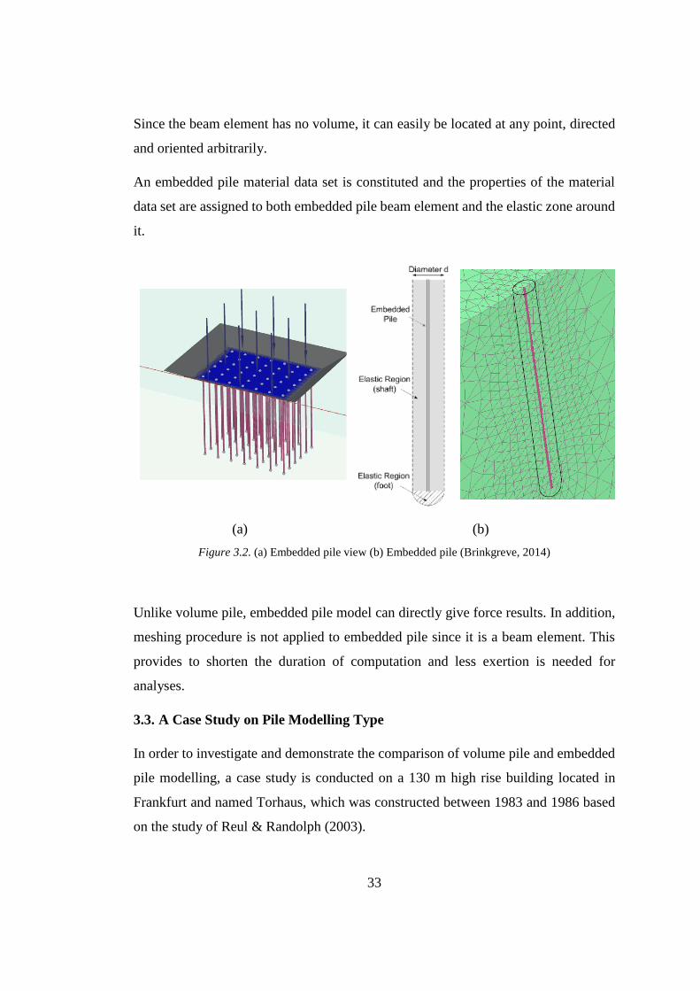
3.2.2. Embedded Pile
Embedded pile is a beam element that does not occupy any volume and assumes an
elastic zone around it in which the plastic soil behavior is not observed. The pile - soil
interaction occurs by means of pile skin interaction and pile tip interaction. The beam
element is considered to show a linear elastic behaviour.
33
Since the beam element has no volume, it can easily be located at any point, directed
and oriented arbitrarily.
An embedded pile material data set is constituted and the properties of the material
data set are assigned to both embedded pile beam element and the elastic zone around
it.
(a) (b)
Figure 3.2. (a) Embedded pile view (b) Embedded pile (Brinkgreve, 2014)
Unlike volume pile, embedded pile model can directly give force results. In addition,
meshing procedure is not applied to embedded pile since it is a beam element. This
provides to shorten the duration of computation and less exertion is needed for
analyses.
3.3. A Case Study on Pile Modelling Type
In order to investigate and demonstrate the comparison of volume pile and embedded
pile modelling, a case study is conducted on a 130 m high rise building located in
Frankfurt and named Torhaus, which was constructed between 1983 and 1986 based
on the study of Reul & Randolph (2003).
34
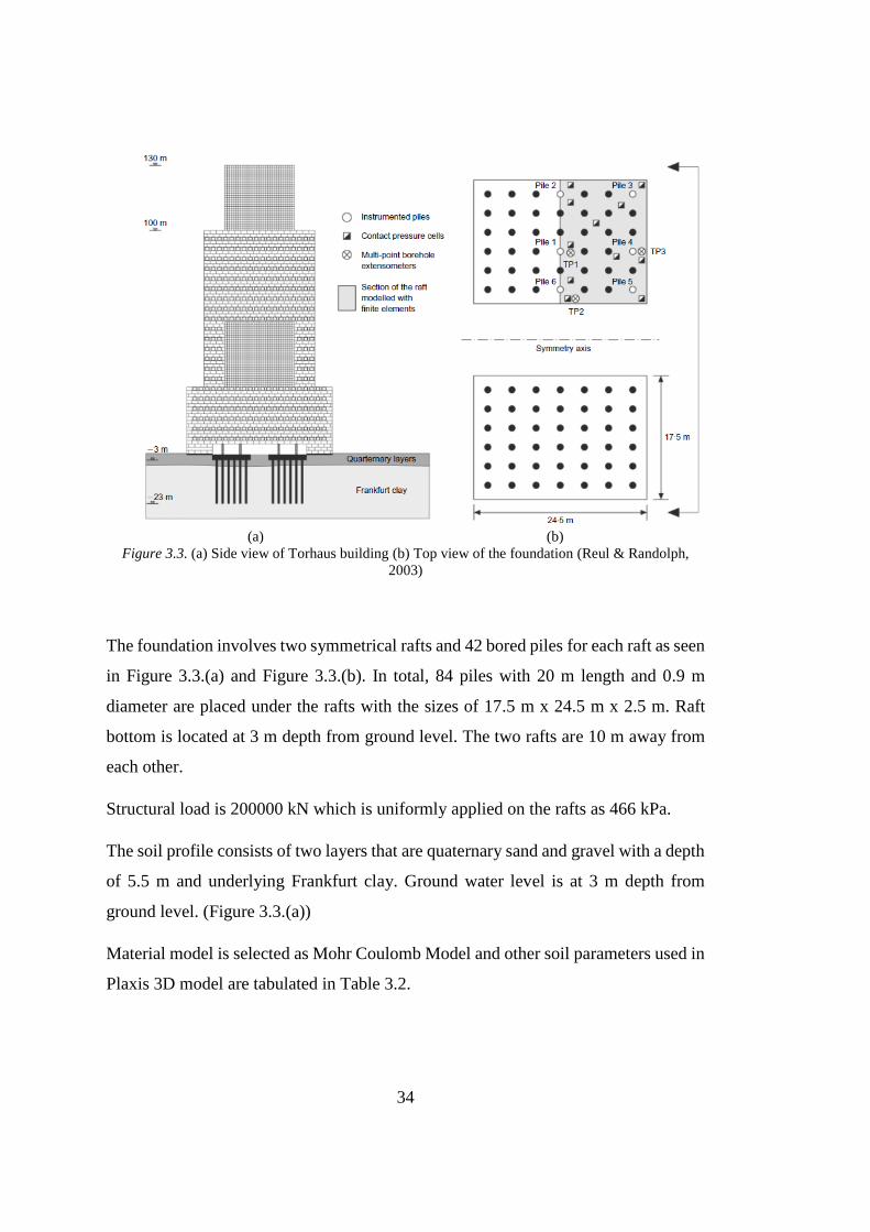
(a) (b)
Figure 3.3. (a) Side view of Torhaus building (b) Top view of the foundation (Reul & Randolph,
2003)
The foundation involves two symmetrical rafts and 42 bored piles for each raft as seen
in Figure 3.3.(a) and Figure 3.3.(b). In total, 84 piles with 20 m length and 0.9 m
diameter are placed under the rafts with the sizes of 17.5 m x 24.5 m x 2.5 m. Raft
bottom is located at 3 m depth from ground level. The two rafts are 10 m away from
each other.
Structural load is 200000 kN which is uniformly applied on the rafts as 466 kPa.
The soil profile consists of two layers that are quaternary sand and gravel with a depth
of 5.5 m and underlying Frankfurt clay. Ground water level is at 3 m depth from
ground level. (Figure 3.3.(a))
Material model is selected as Mohr Coulomb Model and other soil parameters used in
Plaxis 3D model are tabulated in Table 3.2.
35
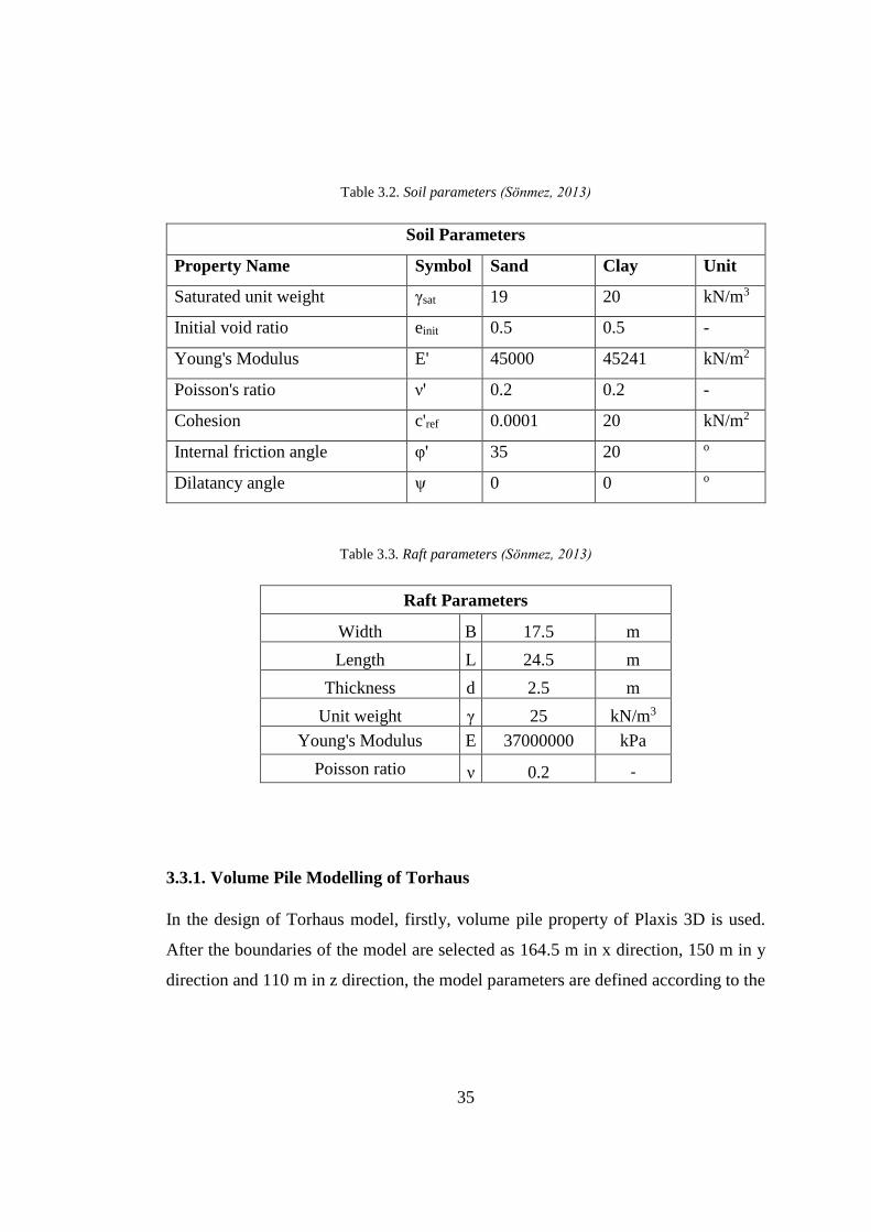
Table 3.2. Soil parameters (Sönmez, 2013)
Soil Parameters
Property Name Symbol Sand Clay Unit
Saturated unit weight γsat 19 20 kN/m3
Initial void ratio einit 0.5 0.5 -
Young's Modulus E' 45000 45241 kN/m2
Poisson's ratio ν' 0.2 0.2 -
Cohesion c'ref 0.0001 20 kN/m2
Internal friction angle φ' 35 20 o
Dilatancy angle ψ 0 0 o
Table 3.3. Raft parameters (Sönmez, 2013)
Raft Parameters
Width B 17.5 m
Length L 24.5 m
Thickness d 2.5 m
Unit weight γ 25 kN/m3
Young's Modulus E 37000000 kPa
Poisson ratio ν 0.2 -
3.3.1. Volume Pile Modelling of Torhaus
In the design of Torhaus model, firstly, volume pile property of Plaxis 3D is used.
After the boundaries of the model are selected as 164.5 m in x direction, 150 m in y
direction and 110 m in z direction, the model parameters are defined according to the
36
input parameters in Chapter 3.3 and volume piles are created by using following
sample cylinder command in Plaxis 3D:
“cylinder 0.45 20 10 (72.05 6.875 -3) (0 0 -1)”
In order to define the input parameters for the volume pile, a soil material data set is
created with the concrete properties and the following parameters are assigned:
Table 3.4. Volume pile parameters
Volume Pile Parameters
Diameter d 0.9 m
Unit weight γ 25 kN/m3
Young's Modulus E 23500000 kPa
Material model Linear Elastic
Drainage type Non - porous
Poisson ratio ν 0.2 -
The parameters for beam element inside the volume pile are defined in following
Table:
Table 3.5. Beam element parameters
Beam Element Parameters
Area A 0.6362 m2
Unit weight γ 25 kN/m3
Young's Modulus E 23.5 kPa
Because of the “Soil body collapses” error which is explained in “Excavation” stage
of Chapter 4.5, the edges of the excavation area are inclined to 2V:5H (Sönmez, 2013).
In the “Mesh” step, “Medium” mesh is preferred in the mesh selection menu due to
the numerical problems in “Very fine” or “Fine” mesh resulting from the excessive
37
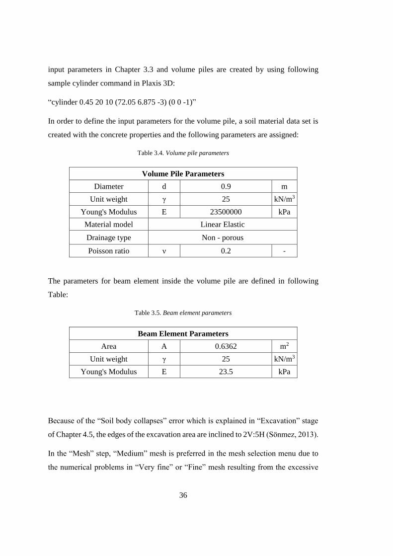
element number in model. However, the foundation part of the model is refined to
increase accuracy. Therefore, it takes 61 minutes to complete mesh process. Mesh
model can be seen in Figure 3.4.
Figure 3.4. Mesh model
Finally, the phases of Excavation, Piles, Raft and Loading are defined respectively.
(Figure 3.4) Total computation time for all stages is measured as 193 minutes.
3.3.2. Embedded Pile Modelling of Torhaus
Plaxis 3D model of Torhaus is generated based on the soil profile, geometry, soil and
raft parameters of Chapter 3.3. The half of the foundation is modelled according to the
symmetry axis in Figure 3.3.(b) due to the decrease of analysis time and computational
effort. The boundaries of the model are selected as 164.5 m in x direction, 75 m in y
38
direction and 110 m in z direction. Apart from that, the embedded pile parameters are
tabulated as below:
Table 3.6. Embedded pile parameters (Engin & Brinkgreve, 2009)
Embedded Pile Parameters
Diameter d 0.9 m
Unit weight γ 15 kN/m3
Young's Modulus E 23500000 kPa
Pile type Massive circular pile
Skin friction per unit
length
Ttop, max
Tbot, max 453 kN/m
Tip resistance force Fmax 1200 kN
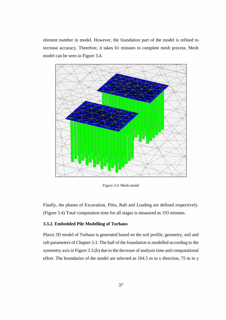
The soil profile, excavated area, the foundation and the surface load are illustrated in
Figure 3.5 below:
Figure 3.5. General view of Torhaus model
Due to the “Soil body collapses” error that is explained in “Excavation” stage of
Chapter 4.5, the edges of the excavation area is inclined to 2V:3H.
39
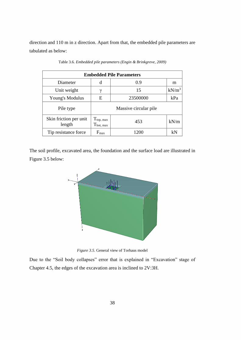
After the geometry is generated, mesh size is selected as “Very fine” and the
foundation is refined to provide more accurate results; then, “Mesh” step is completed.
In final step, staged construction stages are defined as Initial phase, Excavation, Piles,
Raft and Loading respectively. (Figure 3.6)
(a) (b)
(c) (d)
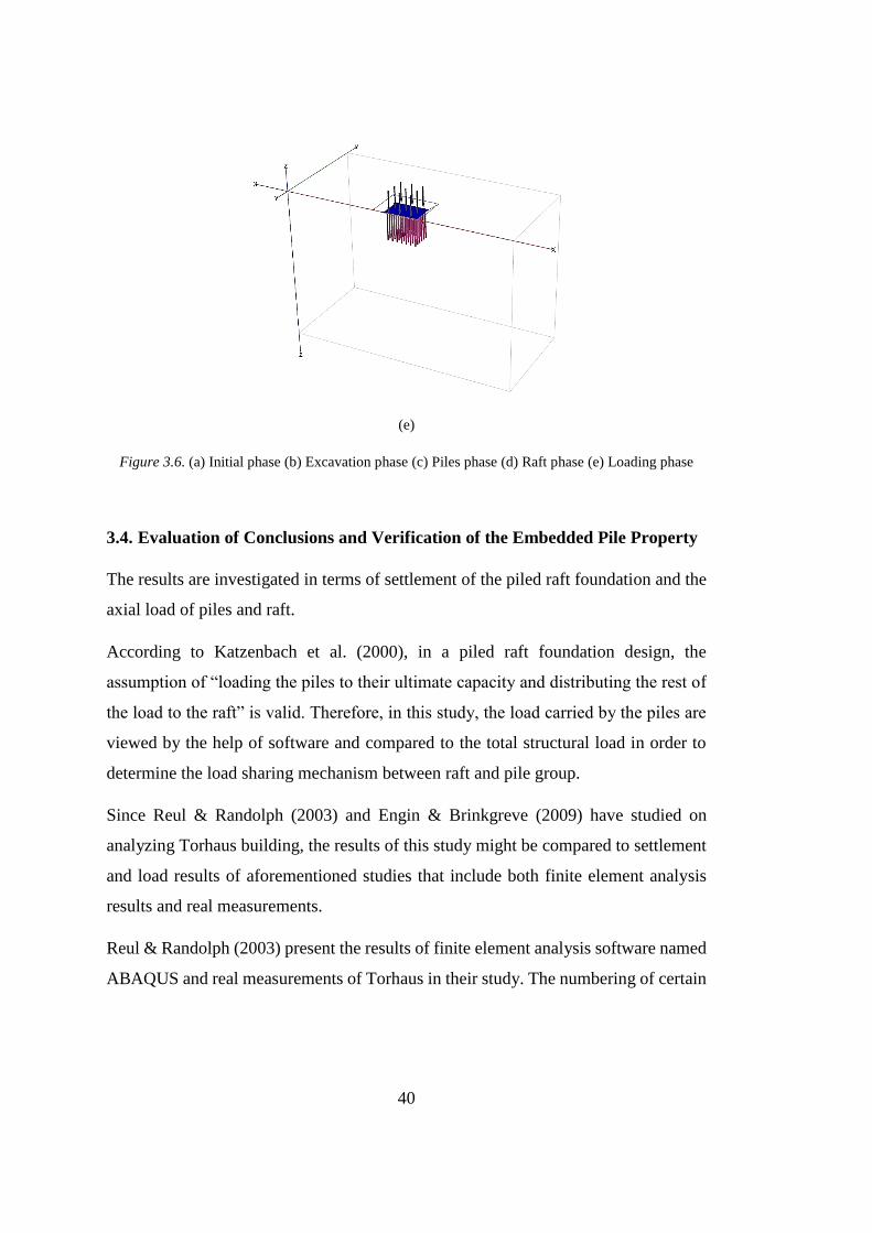
40
(e)
Figure 3.6. (a) Initial phase (b) Excavation phase (c) Piles phase (d) Raft phase (e) Loading phase
3.4. Evaluation of Conclusions and Verification of the Embedded Pile Property
The results are investigated in terms of settlement of the piled raft foundation and the
axial load of piles and raft.
According to Katzenbach et al. (2000), in a piled raft foundation design, the
assumption of “loading the piles to their ultimate capacity and distributing the rest of
the load to the raft” is valid. Therefore, in this study, the load carried by the piles are
viewed by the help of software and compared to the total structural load in order to
determine the load sharing mechanism between raft and pile group.
Since Reul & Randolph (2003) and Engin & Brinkgreve (2009) have studied on
analyzing Torhaus building, the results of this study might be compared to settlement
and load results of aforementioned studies that include both finite element analysis
results and real measurements.
Reul & Randolph (2003) present the results of finite element analysis software named
ABAQUS and real measurements of Torhaus in their study. The numbering of certain
41
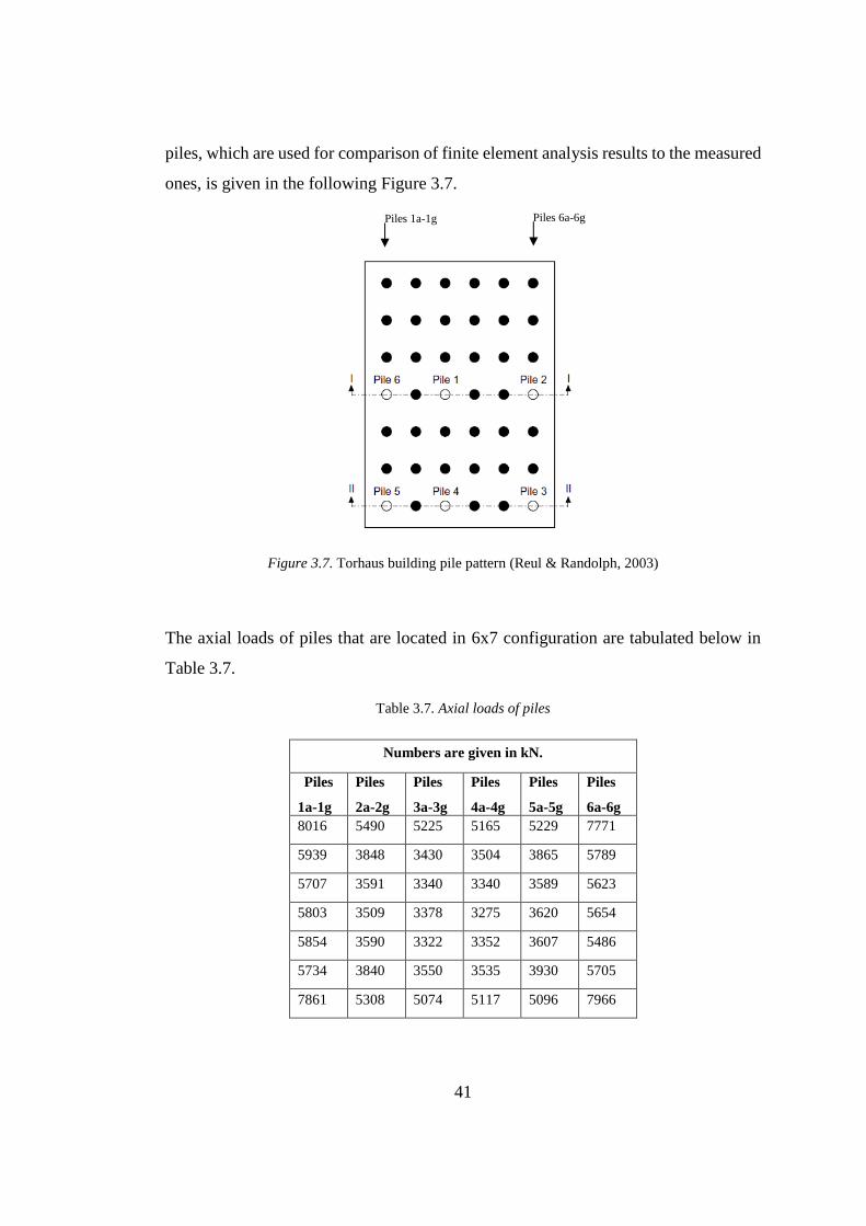
piles, which are used for comparison of finite element analysis results to the measured
ones, is given in the following Figure 3.7.
Figure 3.7. Torhaus building pile pattern (Reul & Randolph, 2003)
The axial loads of piles that are located in 6x7 configuration are tabulated below in
Table 3.7.
Table 3.7. Axial loads of piles
Numbers are given in kN.
Piles
1a-1g
Piles
2a-2g
Piles
3a-3g
Piles
4a-4g
Piles
5a-5g
Piles
6a-6g
8016 5490 5225 5165 5229 7771
5939 3848 3430 3504 3865 5789
5707 3591 3340 3340 3589 5623
5803 3509 3378 3275 3620 5654
5854 3590 3322 3352 3607 5486
5734 3840 3550 3535 3930 5705
7861 5308 5074 5117 5096 7966
Piles 1a-1g Piles 6a-6g
42
Comparison of all load results of certain piles are given in the Figure 3.8 below. Finite
element results of this study, consisting of Plaxis 3D embedded pile model and Plaxis
3D volume pile model, in addition to literature findings, namely, Plaxis 3D embedded
pile model (Engin & Brinkgreve, 2009), ABAQUS model (Reul & Randolph, 2003)
and the real measurements of February 1986 are presented in the Figure 3.8.
Figure 3.8. Comparison of axial load results
It can be concluded from Figure 3.8 that all the finite element analysis axial load
results for Pile 1, Pile 4 and Pile 6 overestimate the pile loads compared to the
measured values. On the other hand, Pile 2, Pile 3 and Pile 5 loads give approximate
results to the measured values.
Reul & Randolph (2003) also give the finite element analysis results for Cross-section
I and Cross-section II that is shown in Figure 3.7. In this study, piles are named as 1d,
2d, 3d, 4d, 5d and 6d for Cross-section I; 1g, 2g, 3g, 4g, 5g and 6g for Cross-section
0
1000
2000
3000
4000
5000
6000
7000
8000
9000
1 2 3 4 5 6
Axi
al L
oad
(kN
)
Pile Number
Plaxis3D Embedded Pile
Plaxis3D Volume Pile
Measured Values
Engin (2009)
Reul&Randolph (2003)
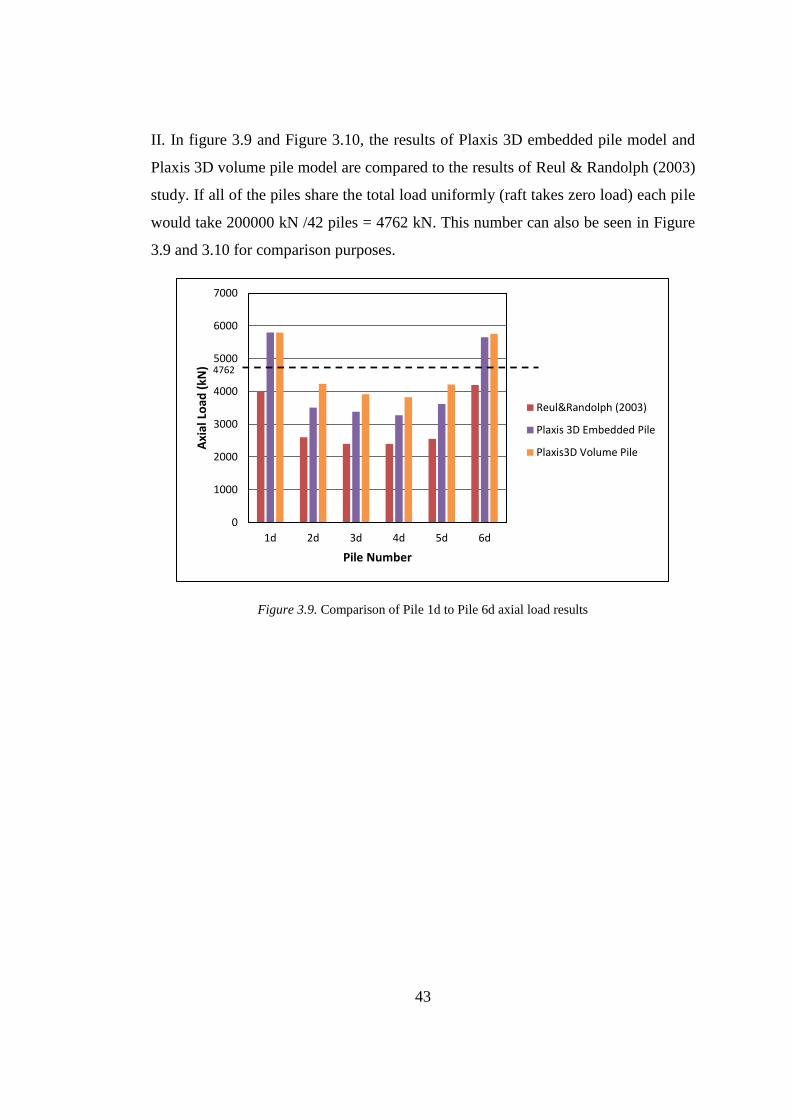
43
II. In figure 3.9 and Figure 3.10, the results of Plaxis 3D embedded pile model and
Plaxis 3D volume pile model are compared to the results of Reul & Randolph (2003)
study. If all of the piles share the total load uniformly (raft takes zero load) each pile
would take 200000 kN /42 piles = 4762 kN. This number can also be seen in Figure
3.9 and 3.10 for comparison purposes.
Figure 3.9. Comparison of Pile 1d to Pile 6d axial load results
0
1000
2000
3000
4000
5000
6000
7000
1d 2d 3d 4d 5d 6d
Axi
al L
oad
(kN
)
Pile Number
Reul&Randolph (2003)
Plaxis 3D Embedded Pile
Plaxis3D Volume Pile
4762
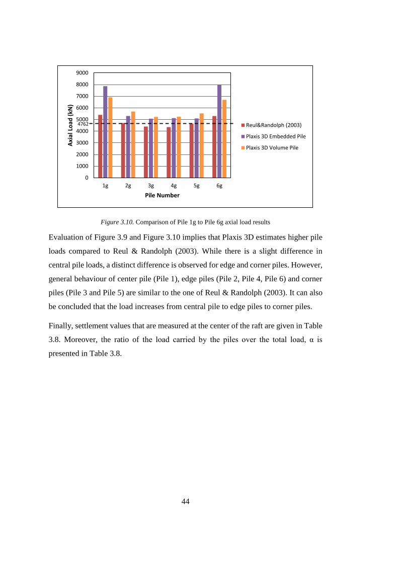
44
Figure 3.10. Comparison of Pile 1g to Pile 6g axial load results
Evaluation of Figure 3.9 and Figure 3.10 implies that Plaxis 3D estimates higher pile
loads compared to Reul & Randolph (2003). While there is a slight difference in
central pile loads, a distinct difference is observed for edge and corner piles. However,
general behaviour of center pile (Pile 1), edge piles (Pile 2, Pile 4, Pile 6) and corner
piles (Pile 3 and Pile 5) are similar to the one of Reul & Randolph (2003). It can also
be concluded that the load increases from central pile to edge piles to corner piles.
Finally, settlement values that are measured at the center of the raft are given in Table
3.8. Moreover, the ratio of the load carried by the piles over the total load, α is
presented in Table 3.8.
0
1000
2000
3000
4000
5000
6000
7000
8000
9000
1g 2g 3g 4g 5g 6g
Axi
al L
oad
(kN
)
Pile Number
Reul&Randolph (2003)
Plaxis 3D Embedded Pile
Plaxis 3D Volume Pile
4762
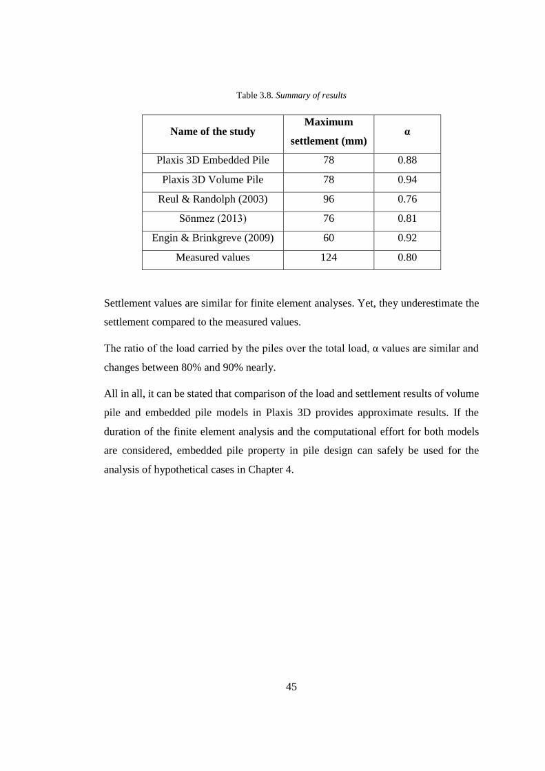
45
Table 3.8. Summary of results
Name of the study Maximum
settlement (mm) α
Plaxis 3D Embedded Pile 78 0.88
Plaxis 3D Volume Pile 78 0.94
Reul & Randolph (2003) 96 0.76
Sönmez (2013) 76 0.81
Engin & Brinkgreve (2009) 60 0.92
Measured values 124 0.80
Settlement values are similar for finite element analyses. Yet, they underestimate the
settlement compared to the measured values.
The ratio of the load carried by the piles over the total load, α values are similar and
changes between 80% and 90% nearly.
All in all, it can be stated that comparison of the load and settlement results of volume
pile and embedded pile models in Plaxis 3D provides approximate results. If the
duration of the finite element analysis and the computational effort for both models
are considered, embedded pile property in pile design can safely be used for the
analysis of hypothetical cases in Chapter 4.

47
CHAPTER 4
4. PARAMETRIC STUDY
4.1. Model Size, Boundary Conditions and Initial Conditions
It is vital that a proper model size and boundary conditions are chosen for the design
of foundations in order to provide reasonable results. On one hand, highly close
boundaries to the foundation prevent observing the deformation and stress for a
sufficient region around the foundation. To illustrate, in Figure 4.1.(a), the boundaries
are positioned 0.5B distance from the raft which results in misleading deductions. On
the other hand, extending the boundaries beyond the necessary requirements causes
ineffectual use of finite element software since it is time consuming to solve a large
model. Figure 4.1.(c), in which the boundaries are positioned 2B from the raft and
Figure 4.1.(d), in which the boundaries are positioned 4B distance from the raft, can
be considered as an unnecessarily huge model.
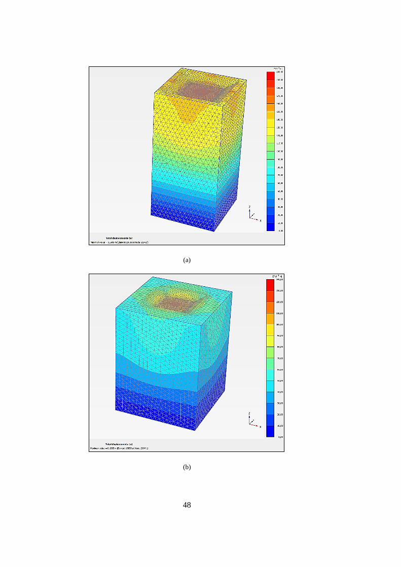
48
(a)
(b)
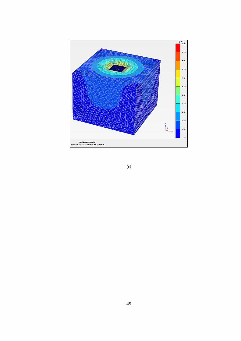
49
(c)
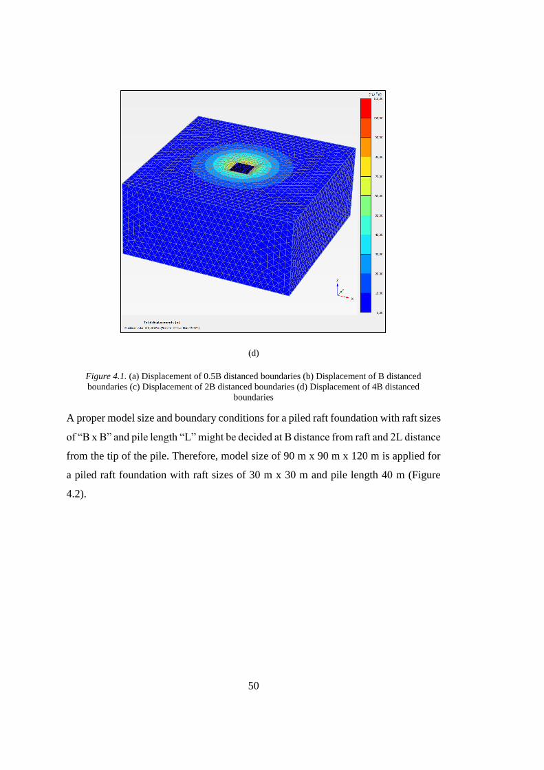
50
(d)
Figure 4.1. (a) Displacement of 0.5B distanced boundaries (b) Displacement of B distanced
boundaries (c) Displacement of 2B distanced boundaries (d) Displacement of 4B distanced
boundaries
A proper model size and boundary conditions for a piled raft foundation with raft sizes
of “B x B” and pile length “L” might be decided at B distance from raft and 2L distance
from the tip of the pile. Therefore, model size of 90 m x 90 m x 120 m is applied for
a piled raft foundation with raft sizes of 30 m x 30 m and pile length 40 m (Figure
4.2).
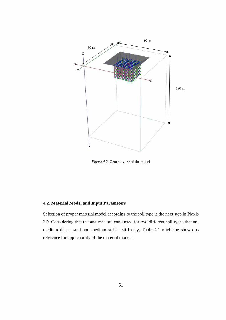
51
Figure 4.2. General view of the model
4.2. Material Model and Input Parameters
Selection of proper material model according to the soil type is the next step in Plaxis
3D. Considering that the analyses are conducted for two different soil types that are
medium dense sand and medium stiff – stiff clay, Table 4.1 might be shown as
reference for applicability of the material models.
90 m
90 m
120 m
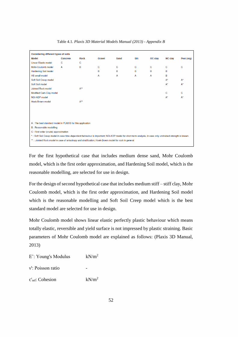
52
Table 4.1. Plaxis 3D Material Models Manual (2013) - Appendix B
For the first hypothetical case that includes medium dense sand, Mohr Coulomb
model, which is the first order approximation, and Hardening Soil model, which is the
reasonable modelling, are selected for use in design.
For the design of second hypothetical case that includes medium stiff – stiff clay, Mohr
Coulomb model, which is the first order approximation, and Hardening Soil model
which is the reasonable modelling and Soft Soil Creep model which is the best
standard model are selected for use in design.
Mohr Coulomb model shows linear elastic perfectly plastic behaviour which means
totally elastic, reversible and yield surface is not impressed by plastic straining. Basic
parameters of Mohr Coulomb model are explained as follows: (Plaxis 3D Manual,
2013)
E’: Young's Modulus kN/m2
ν': Poisson ratio -
c'ref: Cohesion kN/m2
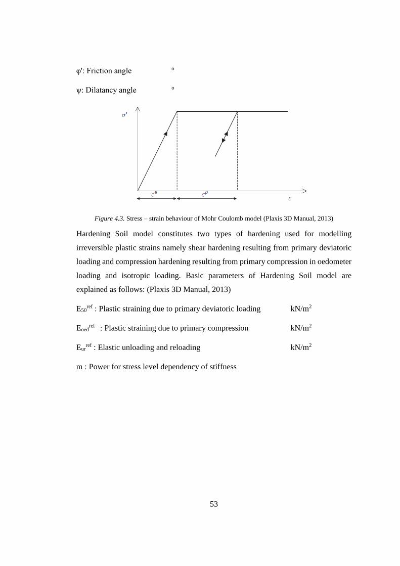
53
φ': Friction angle o
ψ: Dilatancy angle o
Figure 4.3. Stress – strain behaviour of Mohr Coulomb model (Plaxis 3D Manual, 2013)
Hardening Soil model constitutes two types of hardening used for modelling
irreversible plastic strains namely shear hardening resulting from primary deviatoric
loading and compression hardening resulting from primary compression in oedometer
loading and isotropic loading. Basic parameters of Hardening Soil model are
explained as follows: (Plaxis 3D Manual, 2013)
E50ref : Plastic straining due to primary deviatoric loading kN/m2
Eoedref : Plastic straining due to primary compression kN/m2
Eurref : Elastic unloading and reloading kN/m2
m : Power for stress level dependency of stiffness
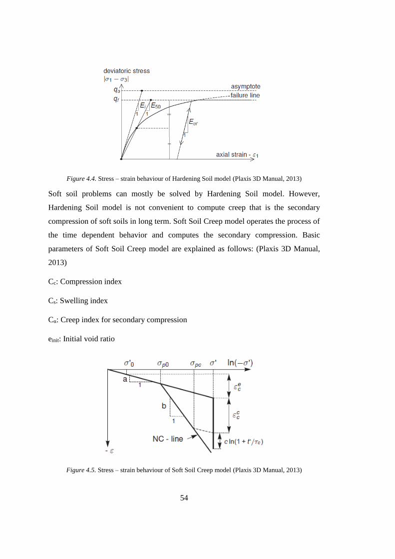
54
Figure 4.4. Stress – strain behaviour of Hardening Soil model (Plaxis 3D Manual, 2013)
Soft soil problems can mostly be solved by Hardening Soil model. However,
Hardening Soil model is not convenient to compute creep that is the secondary
compression of soft soils in long term. Soft Soil Creep model operates the process of
the time dependent behavior and computes the secondary compression. Basic
parameters of Soft Soil Creep model are explained as follows: (Plaxis 3D Manual,
2013)
Cc: Compression index
Cs: Swelling index
Cα: Creep index for secondary compression
einit: Initial void ratio
Figure 4.5. Stress – strain behaviour of Soft Soil Creep model (Plaxis 3D Manual, 2013)
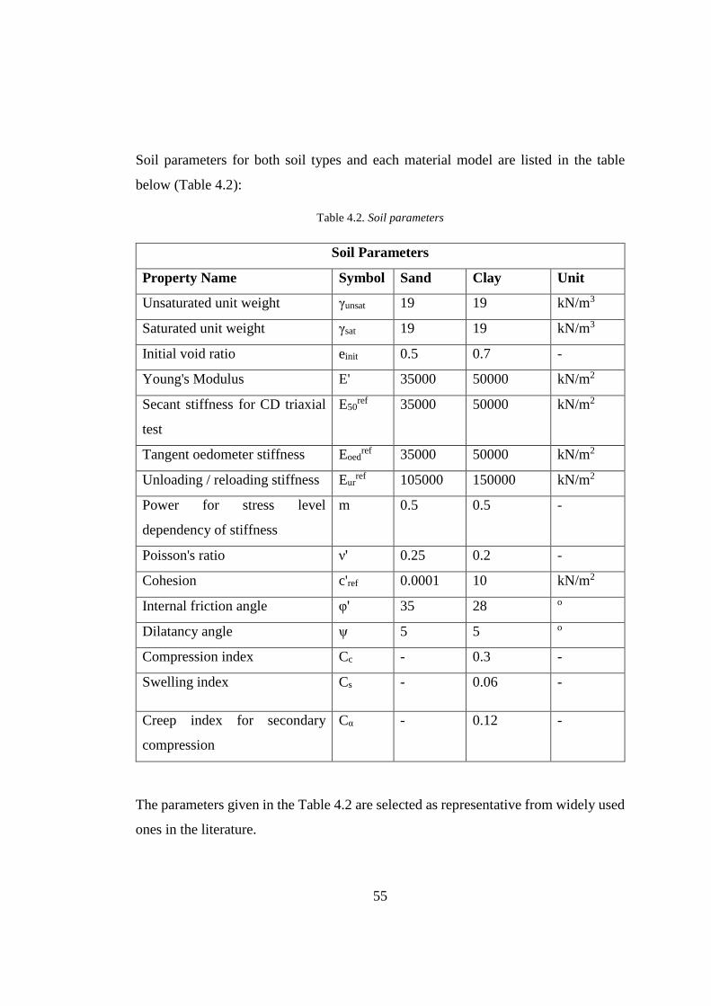
55
Soil parameters for both soil types and each material model are listed in the table
below (Table 4.2):
Table 4.2. Soil parameters
Soil Parameters
Property Name Symbol Sand Clay Unit
Unsaturated unit weight γunsat 19 19 kN/m3
Saturated unit weight γsat 19 19 kN/m3
Initial void ratio einit 0.5 0.7 -
Young's Modulus E' 35000 50000 kN/m2
Secant stiffness for CD triaxial
test
E50ref 35000 50000 kN/m2
Tangent oedometer stiffness Eoedref 35000 50000 kN/m2
Unloading / reloading stiffness Eurref 105000 150000 kN/m2
Power for stress level
dependency of stiffness
m 0.5 0.5 -
Poisson's ratio ν' 0.25 0.2 -
Cohesion c'ref 0.0001 10 kN/m2
Internal friction angle φ' 35 28 o
Dilatancy angle ψ 5 5 o
Compression index Cc - 0.3 -
Swelling index Cs - 0.06 -
Creep index for secondary
compression
Cα - 0.12 -
The parameters given in the Table 4.2 are selected as representative from widely used
ones in the literature.
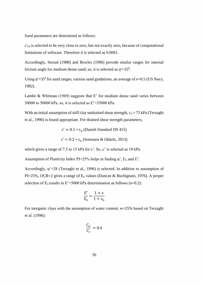
56
Sand parameters are determined as follows:
c'ref is selected to be very close to zero, but not exactly zero, because of computational
limitations of software. Therefore it is selected as 0.0001.
Accordingly, Stroud (1988) and Bowles (1996) provide similar ranges for internal
friction angle for medium dense sand; so, it is selected as φ'=350.
Using φ'=350 for sand ranges, various sand gradations, an average of e=0.5 (US Navy,
1982).
Lambe & Whitman (1969) suggests that E’ for medium dense sand varies between
30000 to 50000 kPa. so, it is selected as E’=35000 kPa.
With an initial assumption of stiff clay undrained shear strength, cu = 75 kPa (Terzaghi
et al., 1996) is found appropriate. For drained shear strength parameters,
c’ = 0.1 ∗ cu (Danish Standard DS 415)
c’ = 0.2 ∗ cu (Sorensen & Okkels, 2013)
which gives a range of 7.5 to 15 kPa for c’. So, c’ is selected as 10 kPa.
Assumption of Plasticity Index PI=25% helps in finding φ’, Eu and E’.
Accordingly, φ’=28 (Terzaghi et al., 1996) is selected. In addition to assumption of
PI=25%, OCR=2 gives a range of Eu values (Duncan & Buchignani, 1976). A proper
selection of Eu results in E’=5000 kPa determination as follows (ν=0.2):
𝐸′
𝐸𝑢=
1 + 𝜈
1 + 𝜈𝑢
For inorganic clays with the assumption of water content, w=25% based on Terzaghi
et al. (1996):
𝐶𝛼
𝐶𝑐 = 0.4
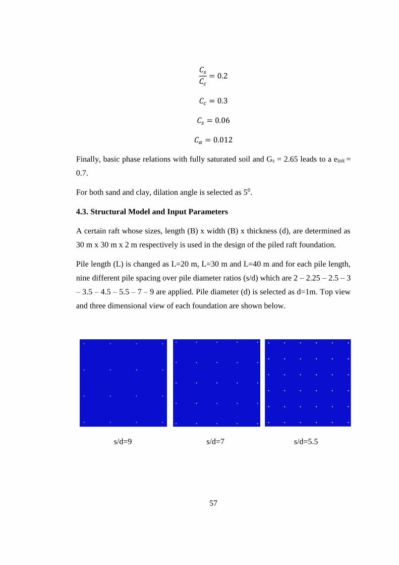
57
𝐶𝑠
𝐶𝑐= 0.2
𝐶𝑐 = 0.3
𝐶𝑠 = 0.06
𝐶𝛼 = 0.012
Finally, basic phase relations with fully saturated soil and Gs = 2.65 leads to a einit =
0.7.
For both sand and clay, dilation angle is selected as 50.
4.3. Structural Model and Input Parameters
A certain raft whose sizes, length (B) x width (B) x thickness (d), are determined as
30 m x 30 m x 2 m respectively is used in the design of the piled raft foundation.
Pile length (L) is changed as L=20 m, L=30 m and L=40 m and for each pile length,
nine different pile spacing over pile diameter ratios (s/d) which are 2 – 2.25 – 2.5 – 3
– 3.5 – 4.5 – 5.5 – 7 – 9 are applied. Pile diameter (d) is selected as d=1m. Top view
and three dimensional view of each foundation are shown below.
s/d=9 s/d=7 s/d=5.5

58
s/d=4.5 s/d=3.5 s/d=3
s/d=2.5 s/d=2.25 s/d=2
s/d=9 s/d=7 s/d=5.5
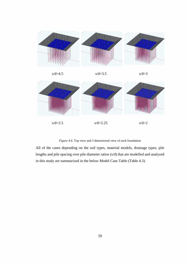
59
s/d=4.5 s/d=3.5 s/d=3
s/d=2.5 s/d=2.25 s/d=2
Figure 4.6. Top view and 3 dimensional view of each foundation
All of the cases depending on the soil types, material models, drainage types, pile
lengths and pile spacing over pile diameter ratios (s/d) that are modelled and analyzed
in this study are summarized in the below Model Case Table (Table 4.3).
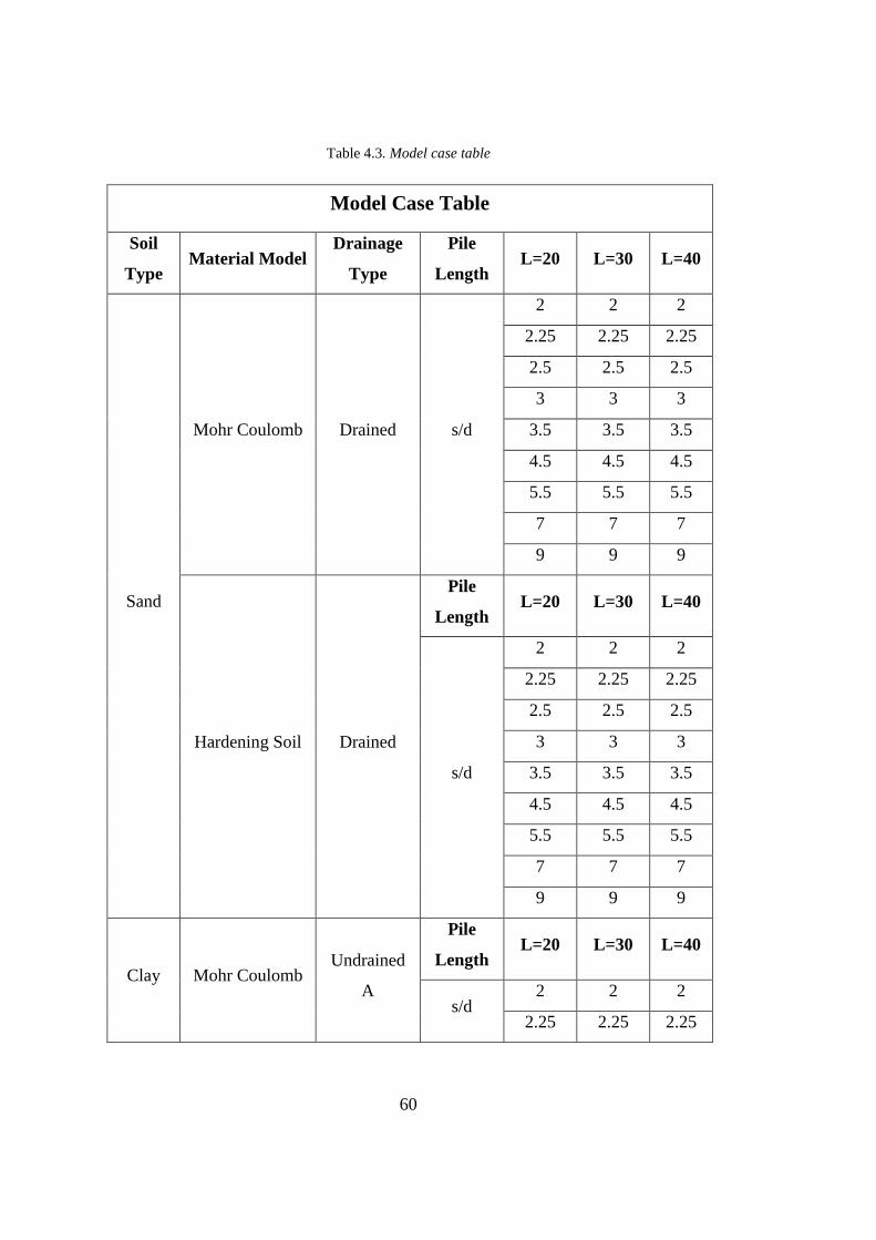
60
Table 4.3. Model case table
Model Case Table
Soil
Type Material Model
Drainage
Type
Pile
Length L=20 L=30 L=40
Sand
Mohr Coulomb Drained s/d
2 2 2
2.25 2.25 2.25
2.5 2.5 2.5
3 3 3
3.5 3.5 3.5
4.5 4.5 4.5
5.5 5.5 5.5
7 7 7
9 9 9
Hardening Soil Drained
Pile
Length L=20 L=30 L=40
s/d
2 2 2
2.25 2.25 2.25
2.5 2.5 2.5
3 3 3
3.5 3.5 3.5
4.5 4.5 4.5
5.5 5.5 5.5
7 7 7
9 9 9
Clay Mohr Coulomb Undrained
A
Pile
Length L=20 L=30 L=40
s/d 2 2 2
2.25 2.25 2.25
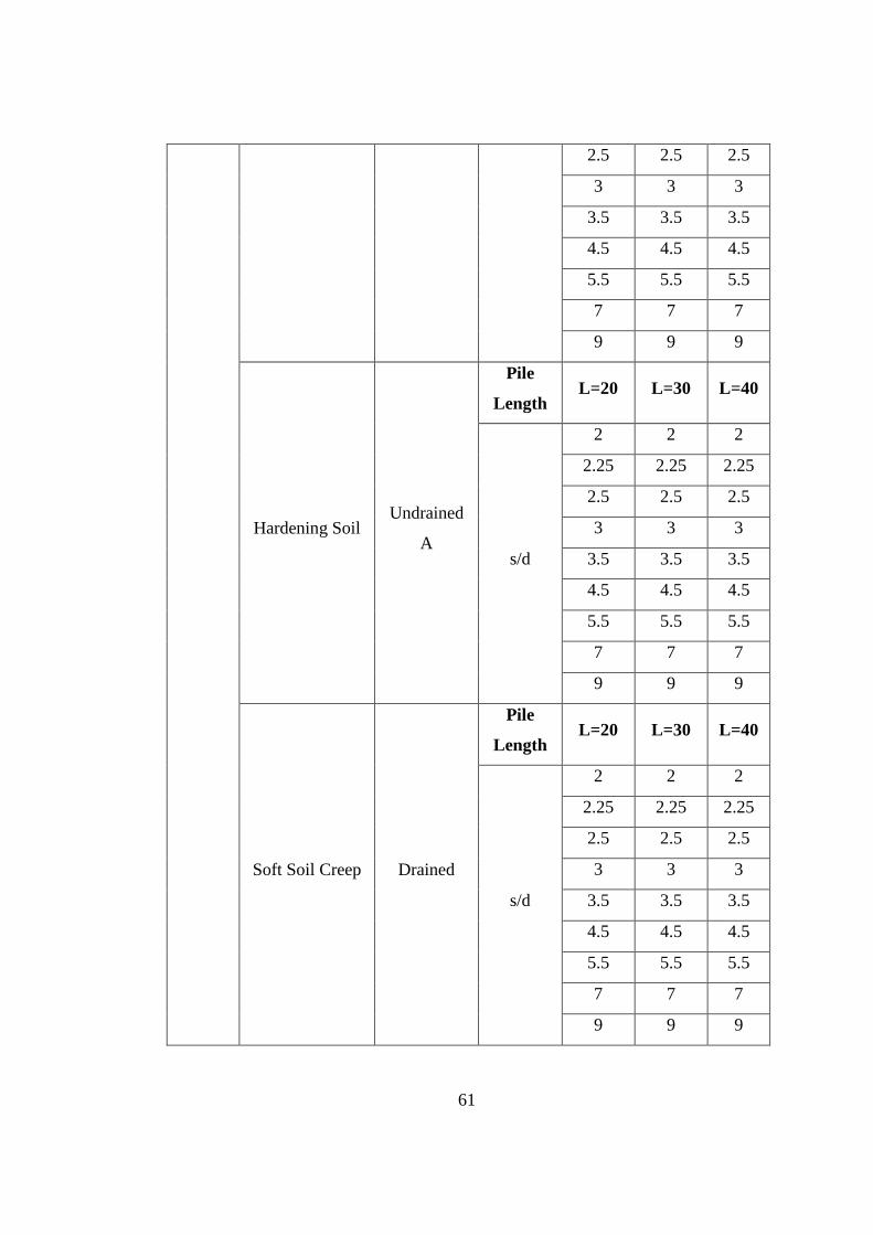
61
2.5 2.5 2.5
3 3 3
3.5 3.5 3.5
4.5 4.5 4.5
5.5 5.5 5.5
7 7 7
9 9 9
Hardening Soil Undrained
A
Pile
Length L=20 L=30 L=40
s/d
2 2 2
2.25 2.25 2.25
2.5 2.5 2.5
3 3 3
3.5 3.5 3.5
4.5 4.5 4.5
5.5 5.5 5.5
7 7 7
9 9 9
Soft Soil Creep Drained
Pile
Length L=20 L=30 L=40
s/d
2 2 2
2.25 2.25 2.25
2.5 2.5 2.5
3 3 3
3.5 3.5 3.5
4.5 4.5 4.5
5.5 5.5 5.5
7 7 7
9 9 9
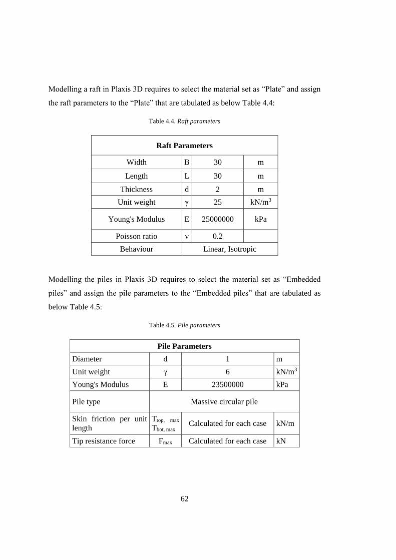
62
Modelling a raft in Plaxis 3D requires to select the material set as “Plate” and assign
the raft parameters to the “Plate” that are tabulated as below Table 4.4:
Table 4.4. Raft parameters
Raft Parameters
Width B 30 m
Length L 30 m
Thickness d 2 m
Unit weight γ 25 kN/m3
Young's Modulus E 25000000 kPa
Poisson ratio ν 0.2
Behaviour Linear, Isotropic
Modelling the piles in Plaxis 3D requires to select the material set as “Embedded
piles” and assign the pile parameters to the “Embedded piles” that are tabulated as
below Table 4.5:
Table 4.5. Pile parameters
Pile Parameters
Diameter d 1 m
Unit weight γ 6 kN/m3
Young's Modulus E 23500000 kPa
Pile type Massive circular pile
Skin friction per unit
length
Ttop, max
Tbot, max Calculated for each case kN/m
Tip resistance force Fmax Calculated for each case kN
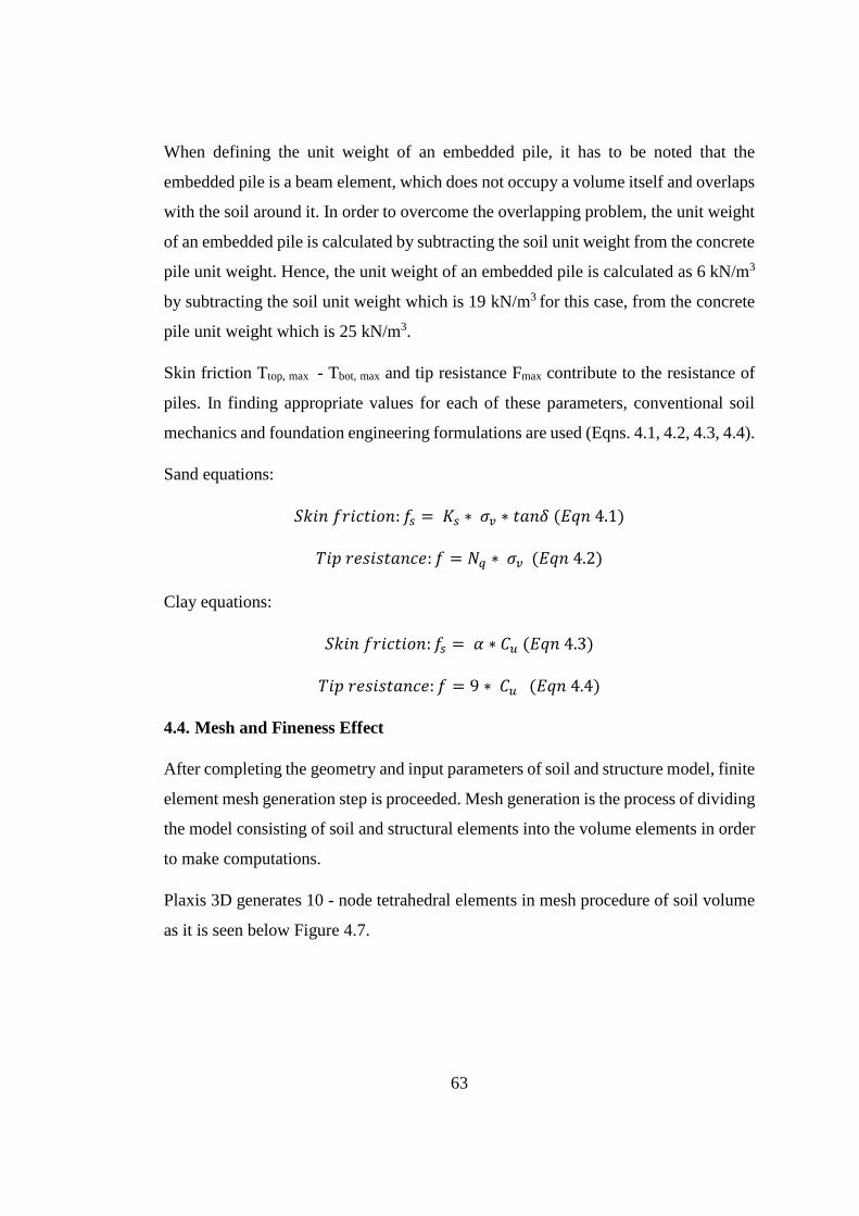
63
When defining the unit weight of an embedded pile, it has to be noted that the
embedded pile is a beam element, which does not occupy a volume itself and overlaps
with the soil around it. In order to overcome the overlapping problem, the unit weight
of an embedded pile is calculated by subtracting the soil unit weight from the concrete
pile unit weight. Hence, the unit weight of an embedded pile is calculated as 6 kN/m3
by subtracting the soil unit weight which is 19 kN/m3 for this case, from the concrete
pile unit weight which is 25 kN/m3.
Skin friction Ttop, max - Tbot, max and tip resistance Fmax contribute to the resistance of
piles. In finding appropriate values for each of these parameters, conventional soil
mechanics and foundation engineering formulations are used (Eqns. 4.1, 4.2, 4.3, 4.4).
Sand equations:
𝑆𝑘𝑖𝑛 𝑓𝑟𝑖𝑐𝑡𝑖𝑜𝑛: 𝑓𝑠 = 𝐾𝑠 ∗ 𝜎𝑣 ∗ 𝑡𝑎𝑛𝛿 (𝐸𝑞𝑛 4.1)
𝑇𝑖𝑝 𝑟𝑒𝑠𝑖𝑠𝑡𝑎𝑛𝑐𝑒: 𝑓 = 𝑁𝑞 ∗ 𝜎𝑣 (𝐸𝑞𝑛 4.2)
Clay equations:
𝑆𝑘𝑖𝑛 𝑓𝑟𝑖𝑐𝑡𝑖𝑜𝑛: 𝑓𝑠 = 𝛼 ∗ 𝐶𝑢 (𝐸𝑞𝑛 4.3)
𝑇𝑖𝑝 𝑟𝑒𝑠𝑖𝑠𝑡𝑎𝑛𝑐𝑒: 𝑓 = 9 ∗ 𝐶𝑢 (𝐸𝑞𝑛 4.4)
4.4. Mesh and Fineness Effect
After completing the geometry and input parameters of soil and structure model, finite
element mesh generation step is proceeded. Mesh generation is the process of dividing
the model consisting of soil and structural elements into the volume elements in order
to make computations.
Plaxis 3D generates 10 - node tetrahedral elements in mesh procedure of soil volume
as it is seen below Figure 4.7.
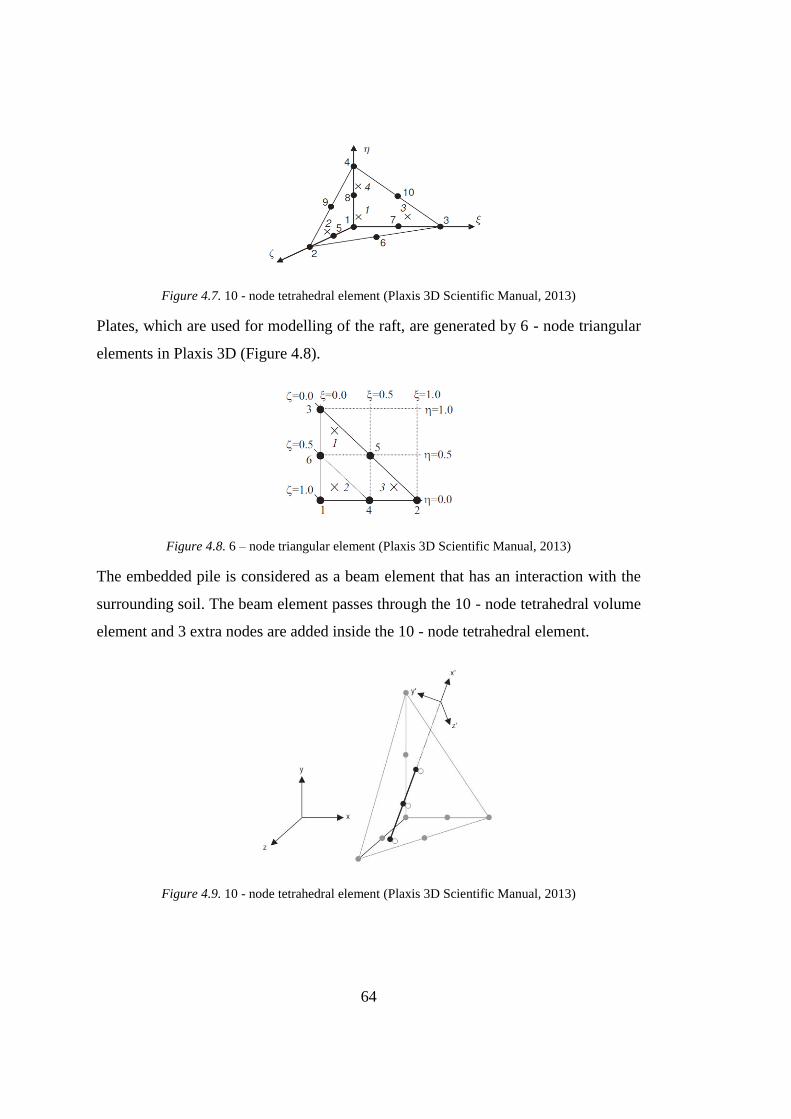
64
Figure 4.7. 10 - node tetrahedral element (Plaxis 3D Scientific Manual, 2013)
Plates, which are used for modelling of the raft, are generated by 6 - node triangular
elements in Plaxis 3D (Figure 4.8).
Figure 4.8. 6 – node triangular element (Plaxis 3D Scientific Manual, 2013)
The embedded pile is considered as a beam element that has an interaction with the
surrounding soil. The beam element passes through the 10 - node tetrahedral volume
element and 3 extra nodes are added inside the 10 - node tetrahedral element.
Figure 4.9. 10 - node tetrahedral element (Plaxis 3D Scientific Manual, 2013)
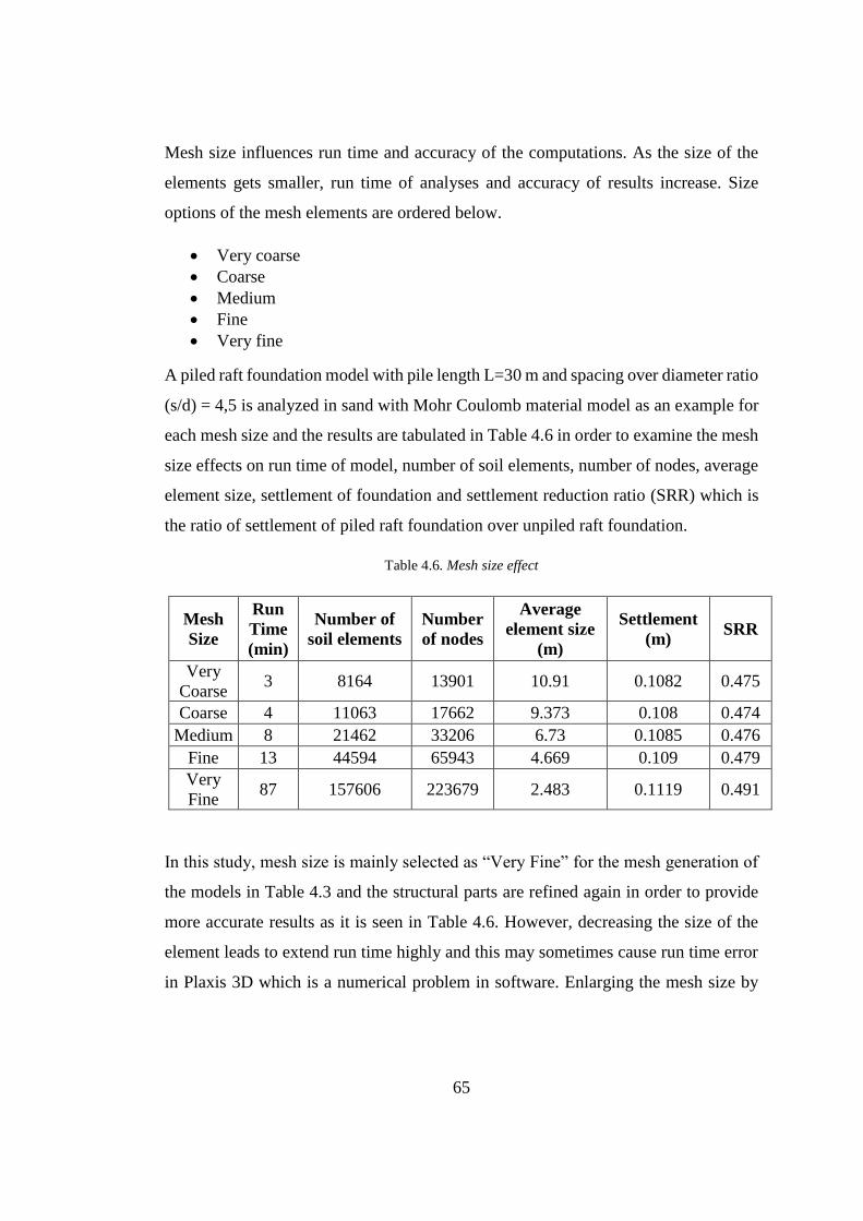
65
Mesh size influences run time and accuracy of the computations. As the size of the
elements gets smaller, run time of analyses and accuracy of results increase. Size
options of the mesh elements are ordered below.
Very coarse
Coarse
Medium
Fine
Very fine
A piled raft foundation model with pile length L=30 m and spacing over diameter ratio
(s/d) = 4,5 is analyzed in sand with Mohr Coulomb material model as an example for
each mesh size and the results are tabulated in Table 4.6 in order to examine the mesh
size effects on run time of model, number of soil elements, number of nodes, average
element size, settlement of foundation and settlement reduction ratio (SRR) which is
the ratio of settlement of piled raft foundation over unpiled raft foundation.
Table 4.6. Mesh size effect
Mesh
Size
Run
Time
(min)
Number of
soil elements
Number
of nodes
Average
element size
(m)
Settlement
(m) SRR
Very
Coarse 3 8164 13901 10.91 0.1082 0.475
Coarse 4 11063 17662 9.373 0.108 0.474
Medium 8 21462 33206 6.73 0.1085 0.476
Fine 13 44594 65943 4.669 0.109 0.479
Very
Fine 87 157606 223679 2.483 0.1119 0.491
In this study, mesh size is mainly selected as “Very Fine” for the mesh generation of
the models in Table 4.3 and the structural parts are refined again in order to provide
more accurate results as it is seen in Table 4.6. However, decreasing the size of the
element leads to extend run time highly and this may sometimes cause run time error
in Plaxis 3D which is a numerical problem in software. Enlarging the mesh size by
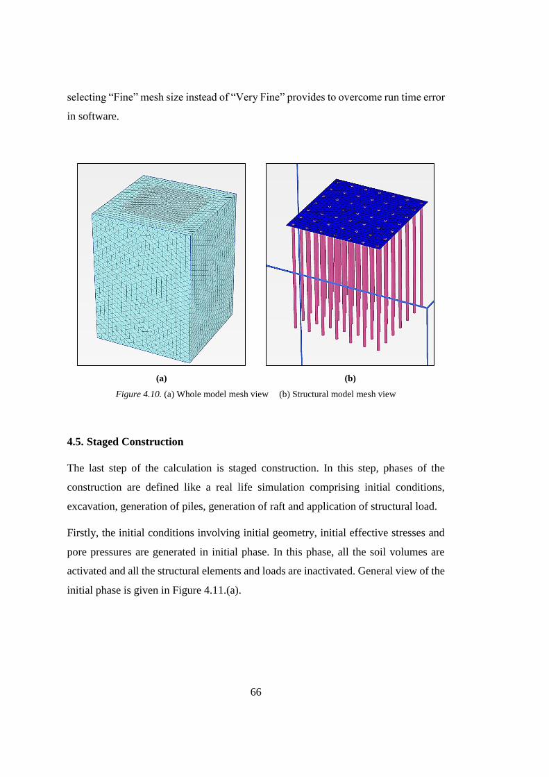
66
selecting “Fine” mesh size instead of “Very Fine” provides to overcome run time error
in software.
(a) (b)
Figure 4.10. (a) Whole model mesh view (b) Structural model mesh view
4.5. Staged Construction
The last step of the calculation is staged construction. In this step, phases of the
construction are defined like a real life simulation comprising initial conditions,
excavation, generation of piles, generation of raft and application of structural load.
Firstly, the initial conditions involving initial geometry, initial effective stresses and
pore pressures are generated in initial phase. In this phase, all the soil volumes are
activated and all the structural elements and loads are inactivated. General view of the
initial phase is given in Figure 4.11.(a).
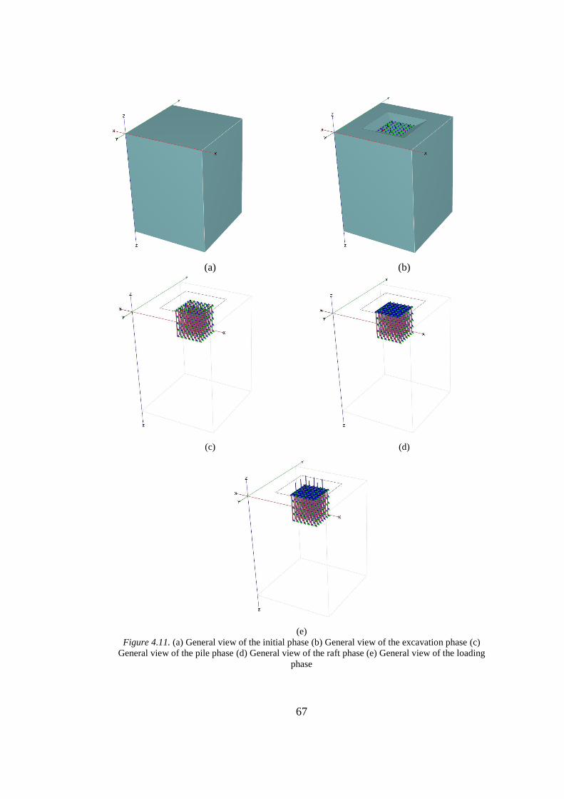
67
(a) (b)
(c) (d)
(e)
Figure 4.11. (a) General view of the initial phase (b) General view of the excavation phase (c)
General view of the pile phase (d) General view of the raft phase (e) General view of the loading
phase
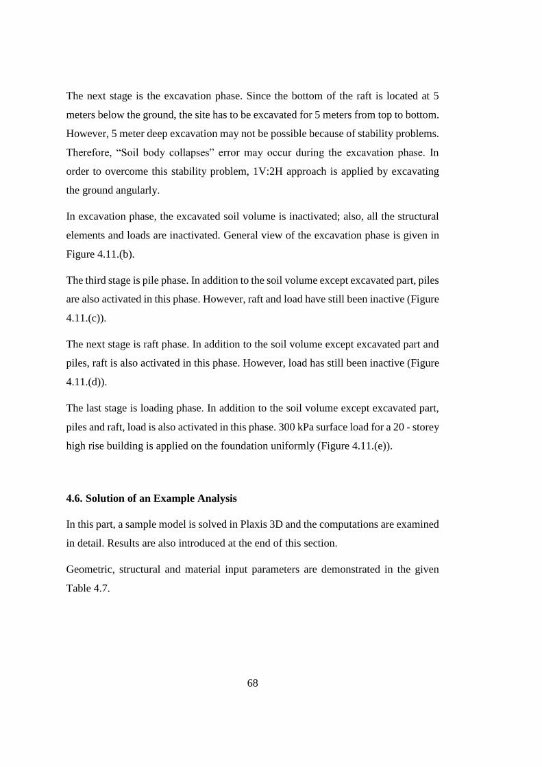
68
The next stage is the excavation phase. Since the bottom of the raft is located at 5
meters below the ground, the site has to be excavated for 5 meters from top to bottom.
However, 5 meter deep excavation may not be possible because of stability problems.
Therefore, “Soil body collapses” error may occur during the excavation phase. In
order to overcome this stability problem, 1V:2H approach is applied by excavating
the ground angularly.
In excavation phase, the excavated soil volume is inactivated; also, all the structural
elements and loads are inactivated. General view of the excavation phase is given in
Figure 4.11.(b).
The third stage is pile phase. In addition to the soil volume except excavated part, piles
are also activated in this phase. However, raft and load have still been inactive (Figure
4.11.(c)).
The next stage is raft phase. In addition to the soil volume except excavated part and
piles, raft is also activated in this phase. However, load has still been inactive (Figure
4.11.(d)).
The last stage is loading phase. In addition to the soil volume except excavated part,
piles and raft, load is also activated in this phase. 300 kPa surface load for a 20 - storey
high rise building is applied on the foundation uniformly (Figure 4.11.(e)).
4.6. Solution of an Example Analysis
In this part, a sample model is solved in Plaxis 3D and the computations are examined
in detail. Results are also introduced at the end of this section.
Geometric, structural and material input parameters are demonstrated in the given
Table 4.7.

69
Table 4.7. Geometric, structural and material input parameters
Input Parameters
Property Name Symbol Type/
Value
Unit
Soil
Soil - Sand -
Material model - Mohr
Coulomb
-
Unsaturated unit
weight
γunsat 19 kN/m3
Saturated unit
weight
γsat 19 kN/m3
Initial void ratio einit 0.5 -
Young's Modulus E' 35000 kN/m2
Power for stress
level dependency
of stiffness
m 0.5 -
Poisson's ratio ν' 0.25 -
Cohesion c'ref 0.0001 kN/m2
Internal friction
angle
φ' 35 o
Dilatancy angle ψ 5 o
Pile
Length L 30 m
Spacing s 3.5 m
Diameter d 1 m
Spacing over
diameter ratio
s/d 3.5 -
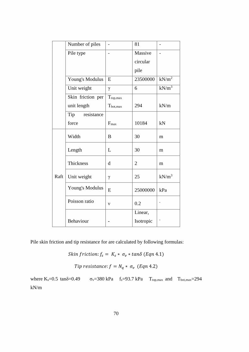
70
Number of piles - 81 -
Pile type - Massive
circular
pile
-
Young's Modulus E 23500000 kN/m2
Unit weight γ 6 kN/m3
Skin friction per
unit length
Ttop,max
Tbot,max 294 kN/m
Tip resistance
force Fmax 10184 kN
Raft
Width B 30 m
Length L 30 m
Thickness d 2 m
Unit weight γ 25 kN/m3
Young's Modulus E 25000000 kPa
Poisson ratio ν 0.2 -
Behaviour -
Linear,
Isotropic -
Pile skin friction and tip resistance for are calculated by following formulas:
𝑆𝑘𝑖𝑛 𝑓𝑟𝑖𝑐𝑡𝑖𝑜𝑛: 𝑓𝑠 = 𝐾𝑠 ∗ 𝜎𝑣 ∗ 𝑡𝑎𝑛𝛿 (𝐸𝑞𝑛 4.1)
𝑇𝑖𝑝 𝑟𝑒𝑠𝑖𝑠𝑡𝑎𝑛𝑐𝑒: 𝑓 = 𝑁𝑞 ∗ 𝜎𝑣 (𝐸𝑞𝑛 4.2)
where Ks=0.5 tanδ=0.49 σv=380 kPa fs=93.7 kPa Ttop,max and Tbot,max=294
kN/m
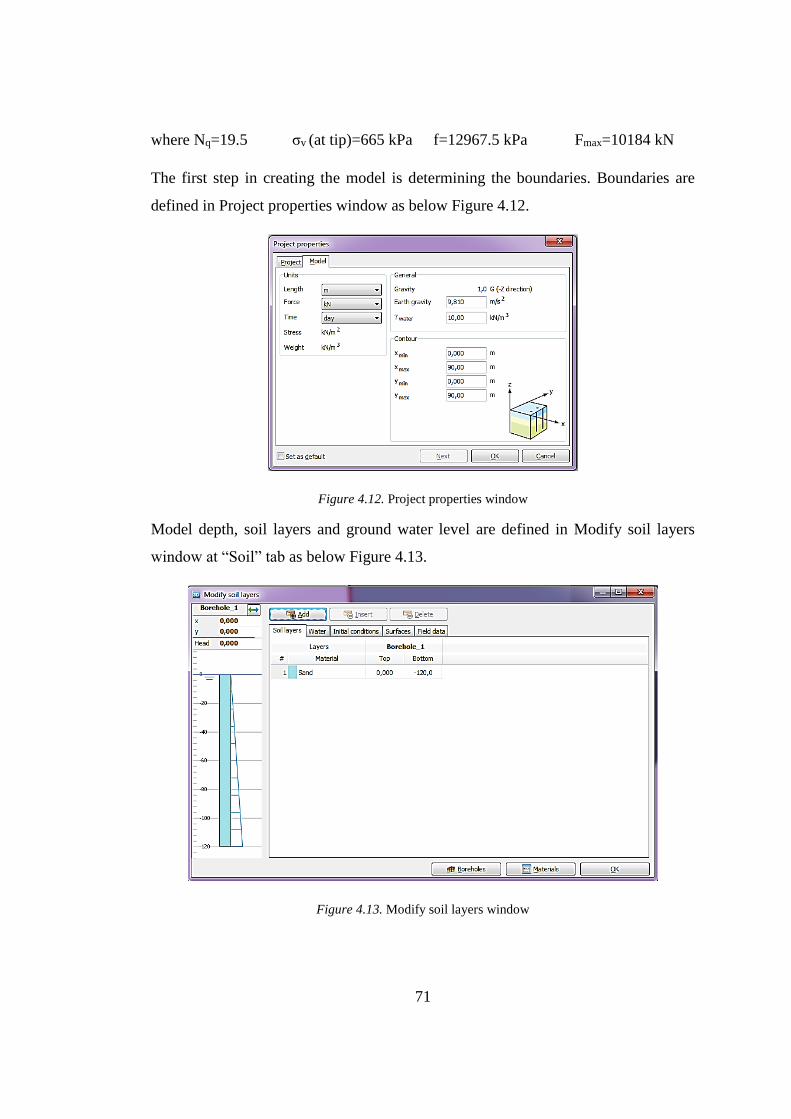
71
where Nq=19.5 σv (at tip)=665 kPa f=12967.5 kPa Fmax=10184 kN
The first step in creating the model is determining the boundaries. Boundaries are
defined in Project properties window as below Figure 4.12.
Figure 4.12. Project properties window
Model depth, soil layers and ground water level are defined in Modify soil layers
window at “Soil” tab as below Figure 4.13.
Figure 4.13. Modify soil layers window
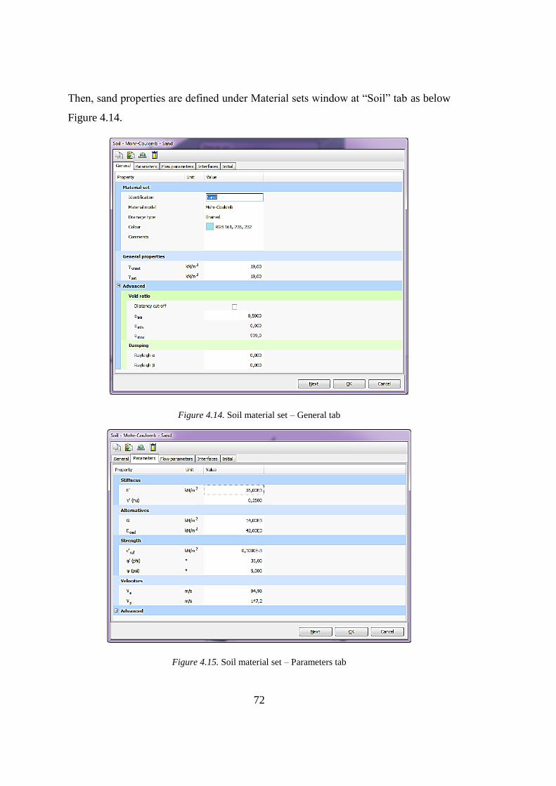
72
Then, sand properties are defined under Material sets window at “Soil” tab as below
Figure 4.14.
Figure 4.14. Soil material set – General tab
Figure 4.15. Soil material set – Parameters tab
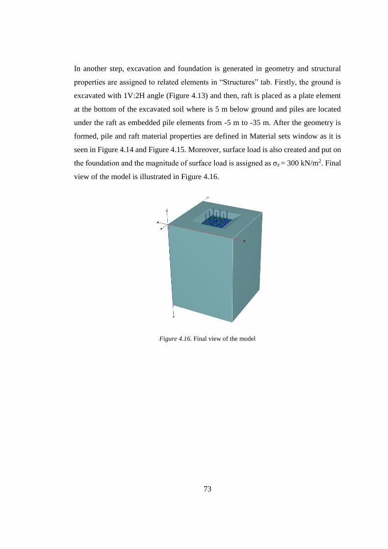
73
In another step, excavation and foundation is generated in geometry and structural
properties are assigned to related elements in “Structures” tab. Firstly, the ground is
excavated with 1V:2H angle (Figure 4.13) and then, raft is placed as a plate element
at the bottom of the excavated soil where is 5 m below ground and piles are located
under the raft as embedded pile elements from -5 m to -35 m. After the geometry is
formed, pile and raft material properties are defined in Material sets window as it is
seen in Figure 4.14 and Figure 4.15. Moreover, surface load is also created and put on
the foundation and the magnitude of surface load is assigned as σz = 300 kN/m2. Final
view of the model is illustrated in Figure 4.16.
Figure 4.16. Final view of the model
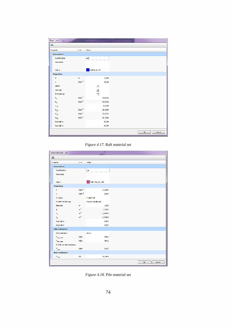
74
Figure 4.17. Raft material set
Figure 4.18. Pile material set
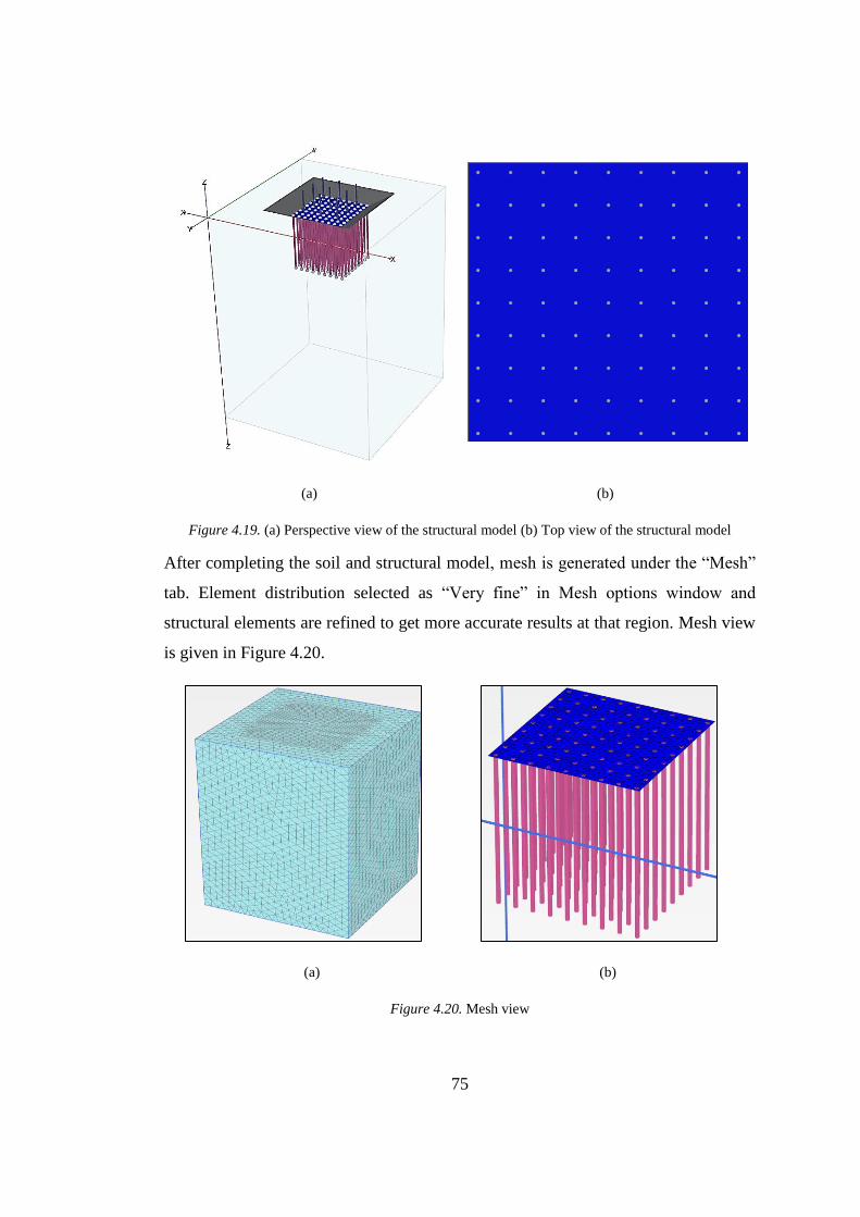
75
(a) (b)
Figure 4.19. (a) Perspective view of the structural model (b) Top view of the structural model
After completing the soil and structural model, mesh is generated under the “Mesh”
tab. Element distribution selected as “Very fine” in Mesh options window and
structural elements are refined to get more accurate results at that region. Mesh view
is given in Figure 4.20.
(a) (b)
Figure 4.20. Mesh view
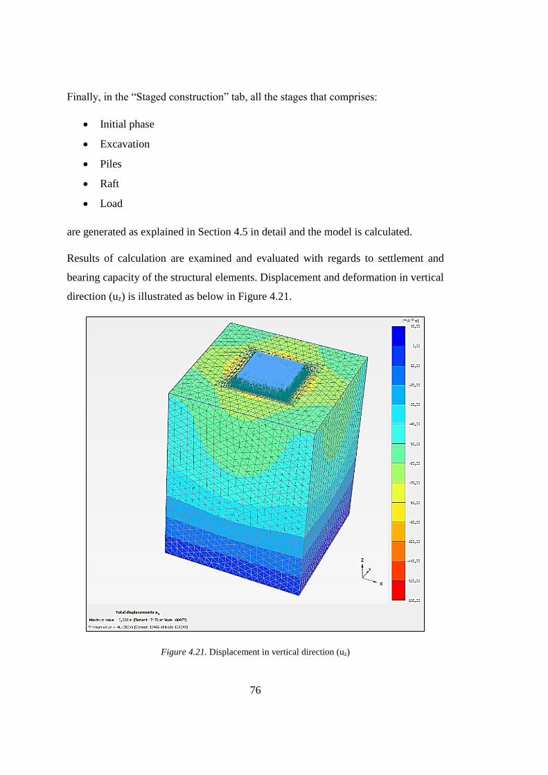
76
Finally, in the “Staged construction” tab, all the stages that comprises:
Initial phase
Excavation
Piles
Raft
Load
are generated as explained in Section 4.5 in detail and the model is calculated.
Results of calculation are examined and evaluated with regards to settlement and
bearing capacity of the structural elements. Displacement and deformation in vertical
direction (uz) is illustrated as below in Figure 4.21.
Figure 4.21. Displacement in vertical direction (uz)
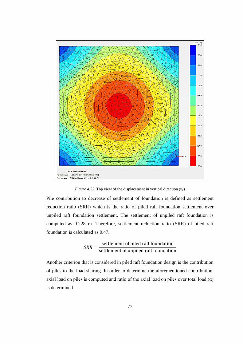
77
Figure 4.22. Top view of the displacement in vertical direction (uz)
Pile contribution to decrease of settlement of foundation is defined as settlement
reduction ratio (SRR) which is the ratio of piled raft foundation settlement over
unpiled raft foundation settlement. The settlement of unpiled raft foundation is
computed as 0.228 m. Therefore, settlement reduction ratio (SRR) of piled raft
foundation is calculated as 0.47.
𝑆𝑅𝑅 =settlement of piled raft foundation
settlement of unpiled raft foundation
Another criterion that is considered in piled raft foundation design is the contribution
of piles to the load sharing. In order to determine the aforementioned contribution,
axial load on piles is computed and ratio of the axial load on piles over total load (α)
is determined.
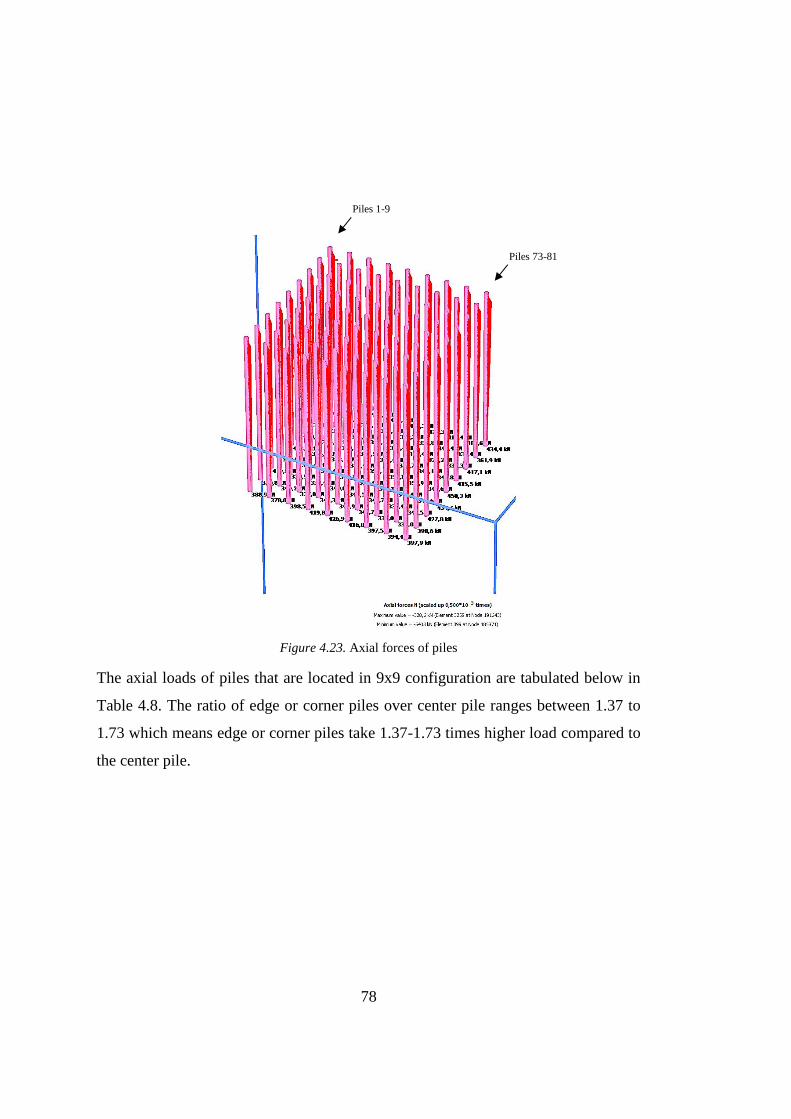
78
Figure 4.23. Axial forces of piles
The axial loads of piles that are located in 9x9 configuration are tabulated below in
Table 4.8. The ratio of edge or corner piles over center pile ranges between 1.37 to
1.73 which means edge or corner piles take 1.37-1.73 times higher load compared to
the center pile.
Piles 1-9
Piles 73-81
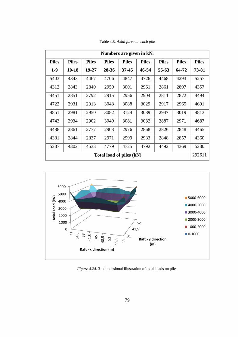
79
Table 4.8. Axial force on each pile
Numbers are given in kN.
Piles
1-9
Piles
10-18
Piles
19-27
Piles
28-36
Piles
37-45
Piles
46-54
Piles
55-63
Piles
64-72
Piles
73-81
5403 4343 4467 4706 4847 4726 4468 4293 5257
4312 2843 2840 2950 3001 2961 2861 2897 4357
4451 2851 2792 2915 2956 2904 2811 2872 4494
4722 2931 2913 3043 3088 3029 2917 2965 4691
4851 2981 2950 3082 3124 3089 2947 3019 4813
4743 2934 2902 3040 3081 3032 2887 2971 4687
4488 2861 2777 2903 2976 2868 2826 2848 4465
4381 2844 2837 2971 2999 2933 2848 2857 4360
5287 4302 4533 4779 4725 4792 4492 4369 5280
Total load of piles (kN) 292611
Figure 4.24. 3 - dimensional illustration of axial loads on piles
31
41,5
52
0
1000
2000
3000
4000
5000
6000
31
34
,5 38
41
,5 45
48
,5 52
55
,5 59 Raft - y direction
(m)
Axi
al L
oad
(kN
)
Raft - x direction (m)
5000-6000
4000-5000
3000-4000
2000-3000
1000-2000
0-1000
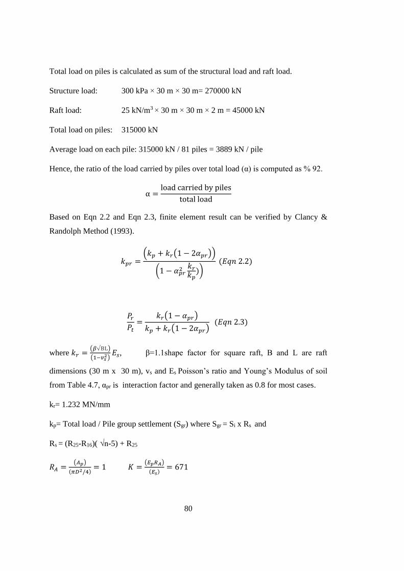
80
Total load on piles is calculated as sum of the structural load and raft load.
Structure load: 300 kPa × 30 m × 30 m= 270000 kN
Raft load: 25 kN/m3 × 30 m × 30 m × 2 m = 45000 kN
Total load on piles: 315000 kN
Average load on each pile: 315000 kN / 81 piles = 3889 kN / pile
Hence, the ratio of the load carried by piles over total load (α) is computed as % 92.
α =load carried by piles
total load
Based on Eqn 2.2 and Eqn 2.3, finite element result can be verified by Clancy &
Randolph Method (1993).
𝑘𝑝𝑟 =(𝑘𝑝 + 𝑘𝑟(1 − 2𝛼𝑝𝑟))
(1 − 𝛼𝑝𝑟2 𝑘𝑟
𝑘𝑝))
(𝐸𝑞𝑛 2.2)
𝑃𝑟
𝑃𝑡=
𝑘𝑟(1 − 𝛼𝑝𝑟)
𝑘𝑝 + 𝑘𝑟(1 − 2𝛼𝑝𝑟) (𝐸𝑞𝑛 2.3)
where 𝑘𝑟 =(𝛽√BL)
(1−𝑣𝑠2)
𝐸𝑠, β=1.1shape factor for square raft, B and L are raft
dimensions (30 m x 30 m), vs and Es Poisson’s ratio and Young’s Modulus of soil
from Table 4.7, αpr is interaction factor and generally taken as 0.8 for most cases.
kr= 1.232 MN/mm
kp= Total load / Pile group settlement (Sgr) where Sgr = Si x Rs and
Rs = (R25-R16)( √n-5) + R25
𝑅𝐴 =(𝐴𝑝)
(𝜋𝐷2/4)= 1 𝐾 =
(𝐸𝑝𝑅𝐴)
(𝐸𝑠)= 671
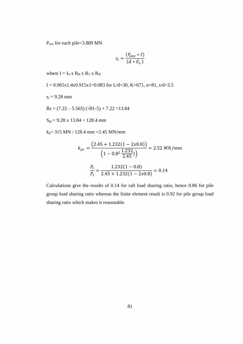
81
Pave for each pile=3.889 MN
𝑠𝑖 =(𝑃𝑎𝑣𝑒 ∗ 𝐼)
(𝑑 ∗ 𝐸𝑠 )
where I = IO x RK x RV x RH
I = 0.065x1.4x0.915x1=0.083 for L/d=30, K=671, n=81, s/d=3.5
si = 9.28 mm
Rs = (7.22 – 5.565) (√81-5) + 7.22 =13.84
Sgr = 9.28 x 13.84 = 128.4 mm
kp= 315 MN / 128.4 mm =2.45 MN/mm
𝑘𝑝𝑟 =(2.45 + 1.232(1 − 2𝑥0.8))
(1 − 0.82 1.2322.45
))= 2.52 𝑀𝑁/𝑚𝑚
𝑃𝑟
𝑃𝑡=
1.232(1 − 0.8)
2.45 + 1.232(1 − 2𝑥0.8)= 0.14
Calculations give the results of 0.14 for raft load sharing ratio, hence 0.86 for pile
group load sharing ratio whereas the finite element result is 0.92 for pile group load
sharing ratio which makes it reasonable.

83
CHAPTER 5
5. DISCUSSION OF RESULTS
In Chapter 4, a parametric study is conducted on two hypothetical cases that comprise
different pile lengths with various pile configurations. Indeed, in Chapter 4.3,
summary of all cases that are handled in this study is presented. In addition, generating
a model geometry, defining material sets and all calculation steps are explained in
detail from Chapter 4.1 to Chapter 4.6.
In Chapter 5, calculation results of Chapter 4 and evaluation of the conclusions are
presented and discussed in order to obtain the optimum design.
The results are evaluated with regards to maximum settlement of the piled raft
foundation and axial load capacity of piles and the raft. Furthermore, some other
parameters that are derived from aforementioned settlement and axial load capacity
are defined as following and used in given charts in this Chapter.
Settlement reduction ratio (SRR) and piled raft coefficient (α) are also evaluated.
Total length is the product of “number of piles at the piled raft foundation” and “the
single pile length”, which has a unit of meter (m).
Individual values of settlement and loads from which SRR and α calculated can be
seen in Appendix B.
For sand condition, drainage type is selected as “Drained” and maximum settlement
of unpiled raft foundation is calculated as 0.228 m. Following charts are given in
Figure 5.1, Figure 5.2, Figure 5.3, Figure 5.4 Figure 5.5 and Figure 5.6 for both
material models that are Mohr Coulomb and Hardening Soil and pile lengths of L=20
m, L=30 m and L=40 m.
For clay condition, drainage type is selected as “Undrained A” and maximum
settlement of unpiled raft foundation is calculated as 0.1103 m. Following charts are
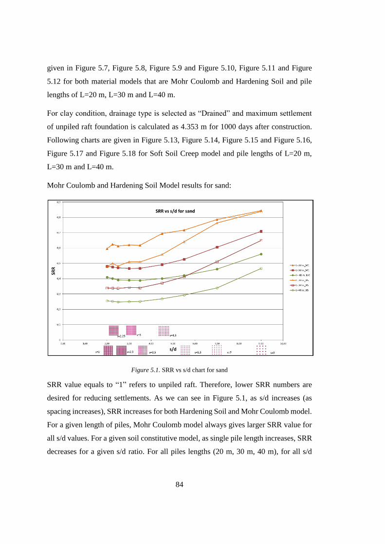
84
given in Figure 5.7, Figure 5.8, Figure 5.9 and Figure 5.10, Figure 5.11 and Figure
5.12 for both material models that are Mohr Coulomb and Hardening Soil and pile
lengths of L=20 m, L=30 m and L=40 m.
For clay condition, drainage type is selected as “Drained” and maximum settlement
of unpiled raft foundation is calculated as 4.353 m for 1000 days after construction.
Following charts are given in Figure 5.13, Figure 5.14, Figure 5.15 and Figure 5.16,
Figure 5.17 and Figure 5.18 for Soft Soil Creep model and pile lengths of L=20 m,
L=30 m and L=40 m.
Mohr Coulomb and Hardening Soil Model results for sand:
Figure 5.1. SRR vs s/d chart for sand
SRR value equals to “1” refers to unpiled raft. Therefore, lower SRR numbers are
desired for reducing settlements. As we can see in Figure 5.1, as s/d increases (as
spacing increases), SRR increases for both Hardening Soil and Mohr Coulomb model.
For a given length of piles, Mohr Coulomb model always gives larger SRR value for
all s/d values. For a given soil constitutive model, as single pile length increases, SRR
decreases for a given s/d ratio. For all piles lengths (20 m, 30 m, 40 m), for all s/d
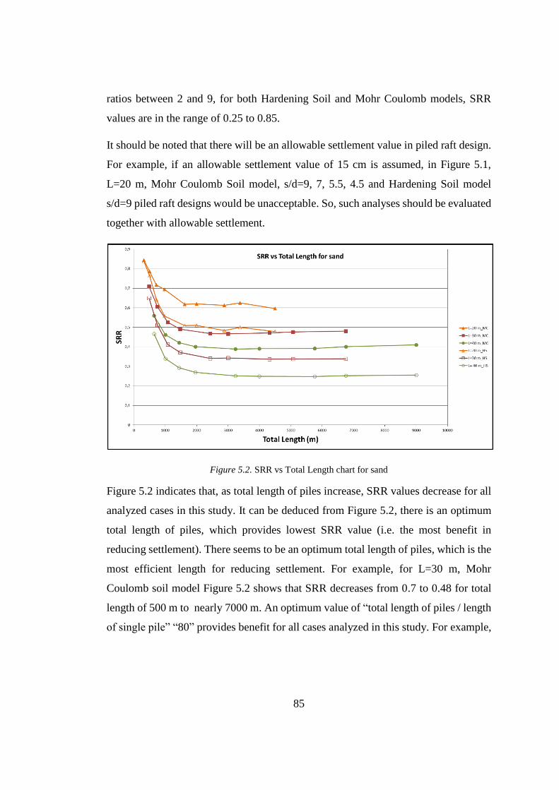
85
ratios between 2 and 9, for both Hardening Soil and Mohr Coulomb models, SRR
values are in the range of 0.25 to 0.85.
It should be noted that there will be an allowable settlement value in piled raft design.
For example, if an allowable settlement value of 15 cm is assumed, in Figure 5.1,
L=20 m, Mohr Coulomb Soil model, s/d=9, 7, 5.5, 4.5 and Hardening Soil model
s/d=9 piled raft designs would be unacceptable. So, such analyses should be evaluated
together with allowable settlement.
Figure 5.2. SRR vs Total Length chart for sand
Figure 5.2 indicates that, as total length of piles increase, SRR values decrease for all
analyzed cases in this study. It can be deduced from Figure 5.2, there is an optimum
total length of piles, which provides lowest SRR value (i.e. the most benefit in
reducing settlement). There seems to be an optimum total length of piles, which is the
most efficient length for reducing settlement. For example, for L=30 m, Mohr
Coulomb soil model Figure 5.2 shows that SRR decreases from 0.7 to 0.48 for total
length of 500 m to nearly 7000 m. An optimum value of “total length of piles / length
of single pile” “80” provides benefit for all cases analyzed in this study. For example,
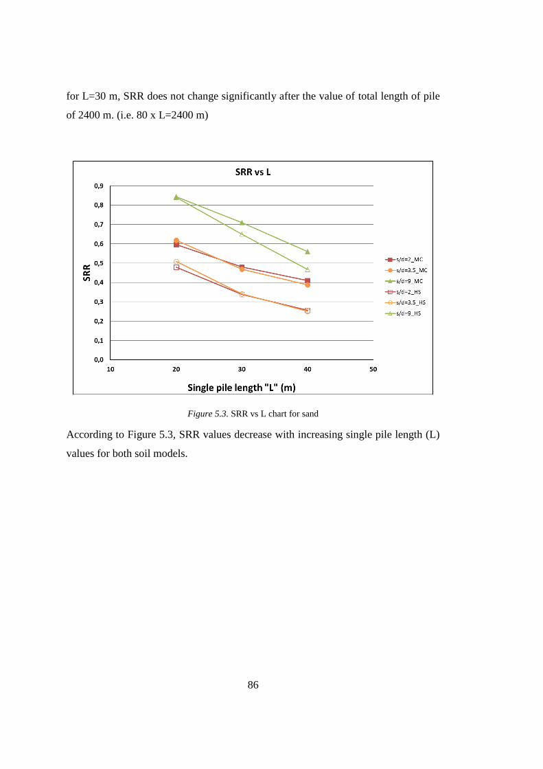
86
for L=30 m, SRR does not change significantly after the value of total length of pile
of 2400 m. (i.e. 80 x L=2400 m)
Figure 5.3. SRR vs L chart for sand
According to Figure 5.3, SRR values decrease with increasing single pile length (L)
values for both soil models.
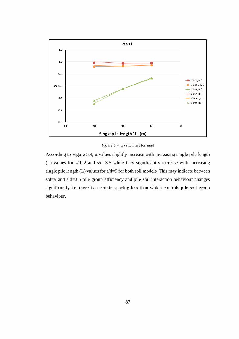
87
Figure 5.4. α vs L chart for sand
According to Figure 5.4, α values slightly increase with increasing single pile length
(L) values for s/d=2 and s/d=3.5 while they significantly increase with increasing
single pile length (L) values for s/d=9 for both soil models. This may indicate between
s/d=9 and s/d=3.5 pile group efficiency and pile soil interaction behaviour changes
significantly i.e. there is a certain spacing less than which controls pile soil group
behaviour.
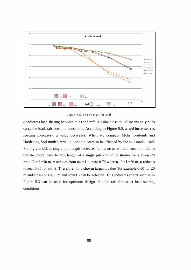
88
Figure 5.5. α vs s/d chart for sand
α indicates load sharing between piles and raft. Α value close to “1” means only piles
carry the load, raft does not contribute. According to Figure 5.5, as s/d increases (as
spacing increases), α value decreases. When we compare Mohr Coulomb and
Hardening Soil model, α value does not seem to be affected by the soil model used.
For a given s/d, as single pile length increases, α increases, which means in order to
transfer more loads to raft, length of a single pile should be shorter for a given s/d
ratio. For L=40 m, α reduces from near 1 to near 0.75 whereas for L=20 m, α reduces
to near 0.35 for s/d=9. Therefore, for a chosen target α value (for example 0.60) L=20
m and s/d=6 or L=30 m and s/d=8.5 can be selected. This indicates charts such as in
Figure 5.3 can be used for optimum design of piled raft for target load sharing
conditions.
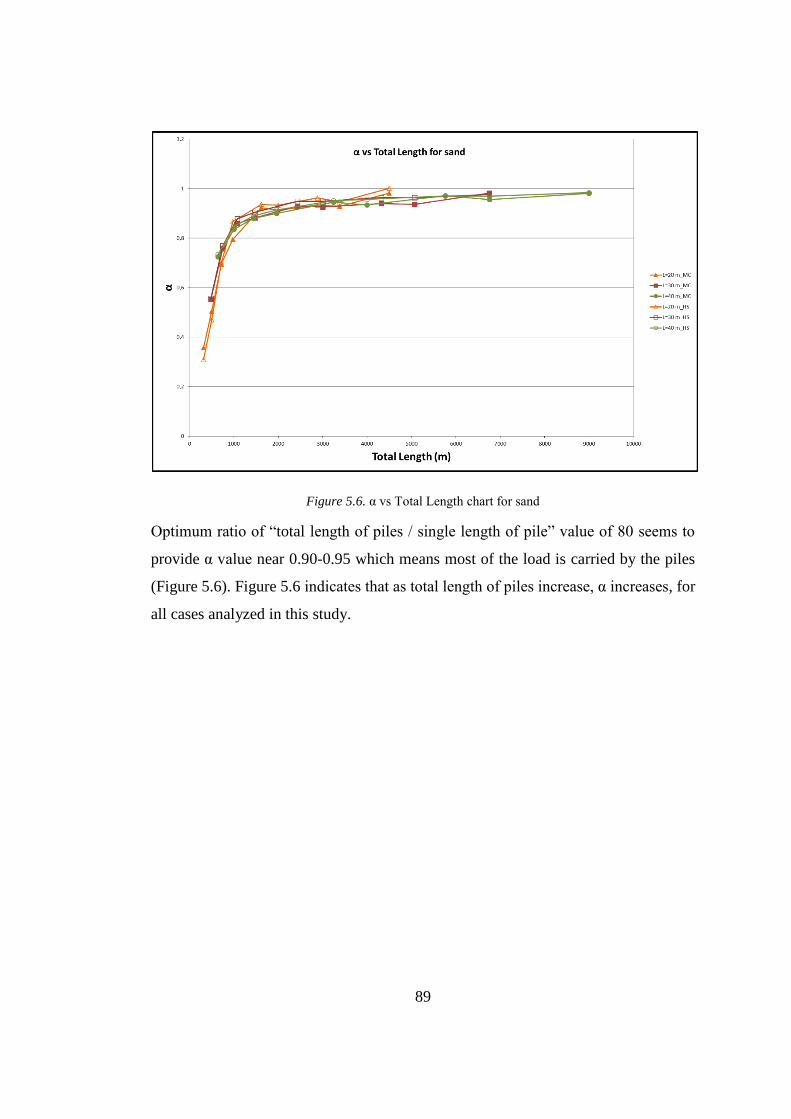
89
Figure 5.6. α vs Total Length chart for sand
Optimum ratio of “total length of piles / single length of pile” value of 80 seems to
provide α value near 0.90-0.95 which means most of the load is carried by the piles
(Figure 5.6). Figure 5.6 indicates that as total length of piles increase, α increases, for
all cases analyzed in this study.
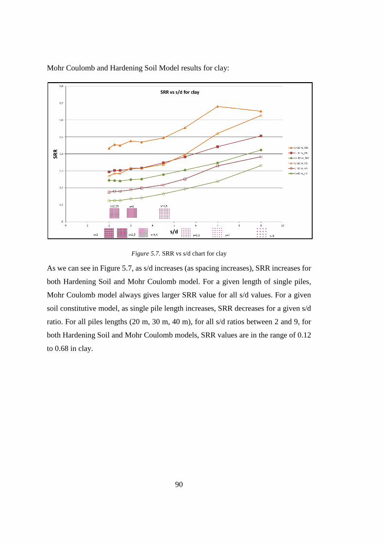
90
Mohr Coulomb and Hardening Soil Model results for clay:
Figure 5.7. SRR vs s/d chart for clay
As we can see in Figure 5.7, as s/d increases (as spacing increases), SRR increases for
both Hardening Soil and Mohr Coulomb model. For a given length of single piles,
Mohr Coulomb model always gives larger SRR value for all s/d values. For a given
soil constitutive model, as single pile length increases, SRR decreases for a given s/d
ratio. For all piles lengths (20 m, 30 m, 40 m), for all s/d ratios between 2 and 9, for
both Hardening Soil and Mohr Coulomb models, SRR values are in the range of 0.12
to 0.68 in clay.
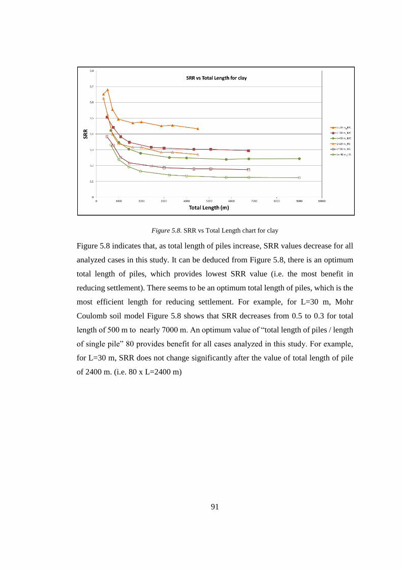
91
Figure 5.8. SRR vs Total Length chart for clay
Figure 5.8 indicates that, as total length of piles increase, SRR values decrease for all
analyzed cases in this study. It can be deduced from Figure 5.8, there is an optimum
total length of piles, which provides lowest SRR value (i.e. the most benefit in
reducing settlement). There seems to be an optimum total length of piles, which is the
most efficient length for reducing settlement. For example, for L=30 m, Mohr
Coulomb soil model Figure 5.8 shows that SRR decreases from 0.5 to 0.3 for total
length of 500 m to nearly 7000 m. An optimum value of “total length of piles / length
of single pile” 80 provides benefit for all cases analyzed in this study. For example,
for L=30 m, SRR does not change significantly after the value of total length of pile
of 2400 m. (i.e. 80 x L=2400 m)
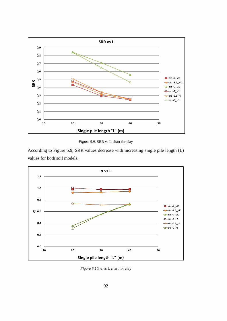
92
Figure 5.9. SRR vs L chart for clay
According to Figure 5.9, SRR values decrease with increasing single pile length (L)
values for both soil models.
Figure 5.10. α vs L chart for clay
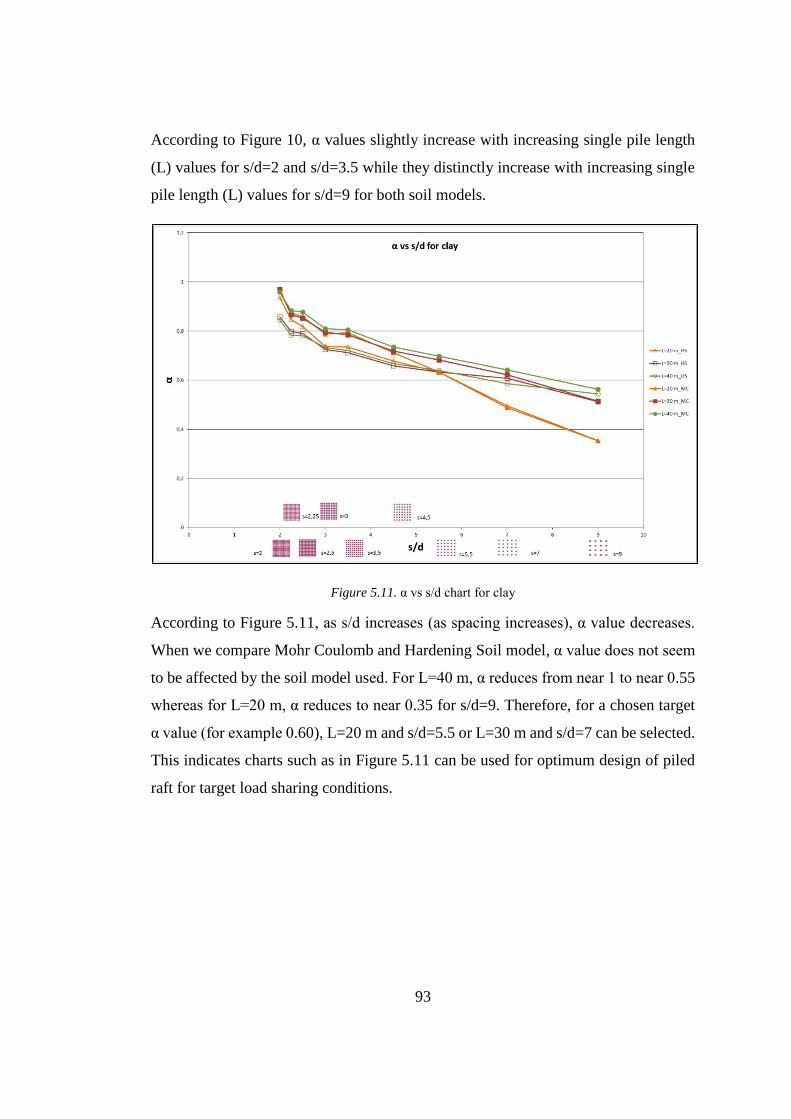
93
According to Figure 10, α values slightly increase with increasing single pile length
(L) values for s/d=2 and s/d=3.5 while they distinctly increase with increasing single
pile length (L) values for s/d=9 for both soil models.
Figure 5.11. α vs s/d chart for clay
According to Figure 5.11, as s/d increases (as spacing increases), α value decreases.
When we compare Mohr Coulomb and Hardening Soil model, α value does not seem
to be affected by the soil model used. For L=40 m, α reduces from near 1 to near 0.55
whereas for L=20 m, α reduces to near 0.35 for s/d=9. Therefore, for a chosen target
α value (for example 0.60), L=20 m and s/d=5.5 or L=30 m and s/d=7 can be selected.
This indicates charts such as in Figure 5.11 can be used for optimum design of piled
raft for target load sharing conditions.
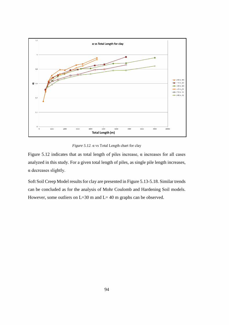
94
Figure 5.12. α vs Total Length chart for clay
Figure 5.12 indicates that as total length of piles increase, α increases for all cases
analyzed in this study. For a given total length of piles, as single pile length increases,
α decreases slightly.
Soft Soil Creep Model results for clay are presented in Figure 5.13-5.18. Similar trends
can be concluded as for the analysis of Mohr Coulomb and Hardening Soil models.
However, some outliers on L=30 m and L= 40 m graphs can be observed.
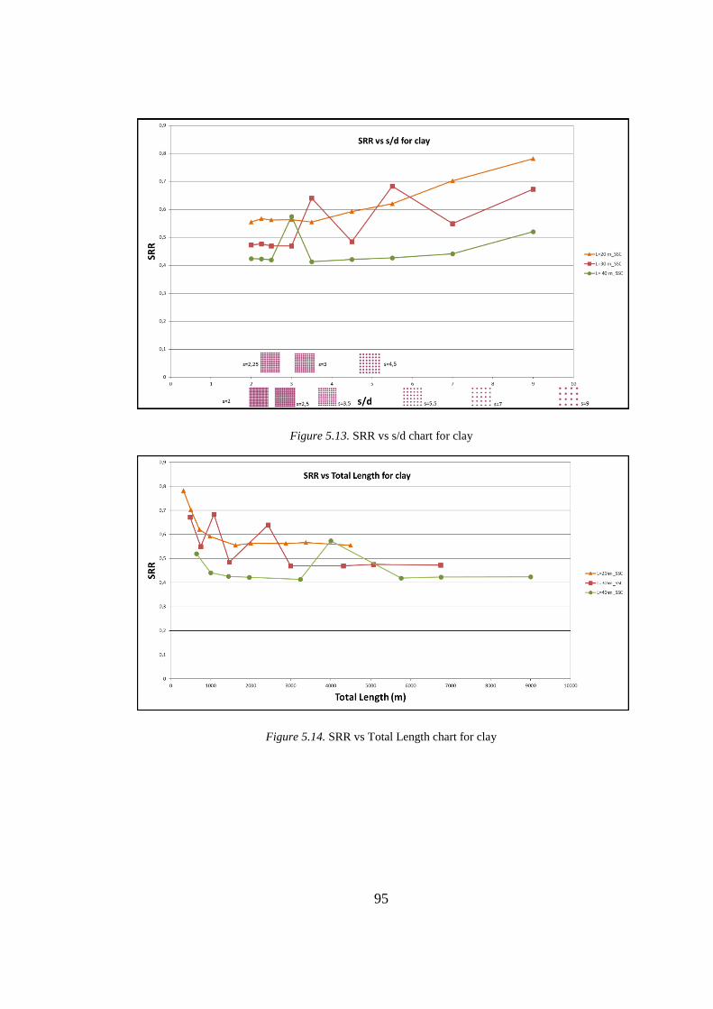
95
Figure 5.13. SRR vs s/d chart for clay
Figure 5.14. SRR vs Total Length chart for clay
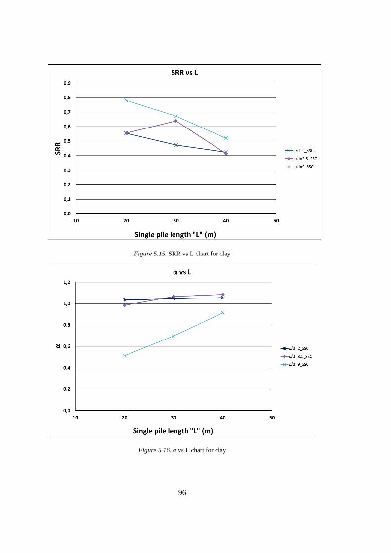
96
Figure 5.15. SRR vs L chart for clay
Figure 5.16. α vs L chart for clay
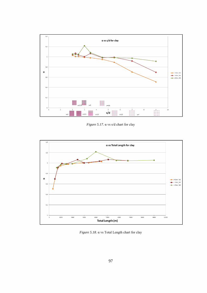
97
Figure 5.17. α vs s/d chart for clay
Figure 5.18. α vs Total Length chart for clay
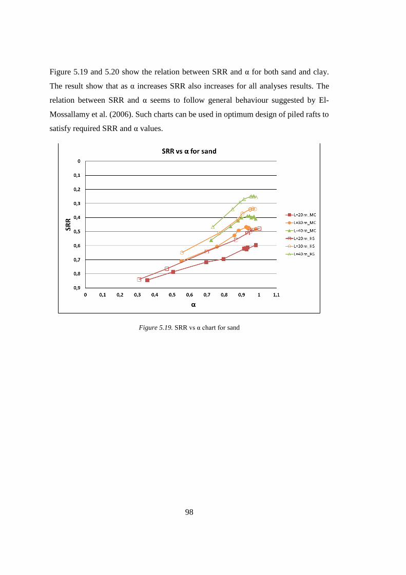
98
Figure 5.19 and 5.20 show the relation between SRR and α for both sand and clay.
The result show that as α increases SRR also increases for all analyses results. The
relation between SRR and α seems to follow general behaviour suggested by El-
Mossallamy et al. (2006). Such charts can be used in optimum design of piled rafts to
satisfy required SRR and α values.
Figure 5.19. SRR vs α chart for sand
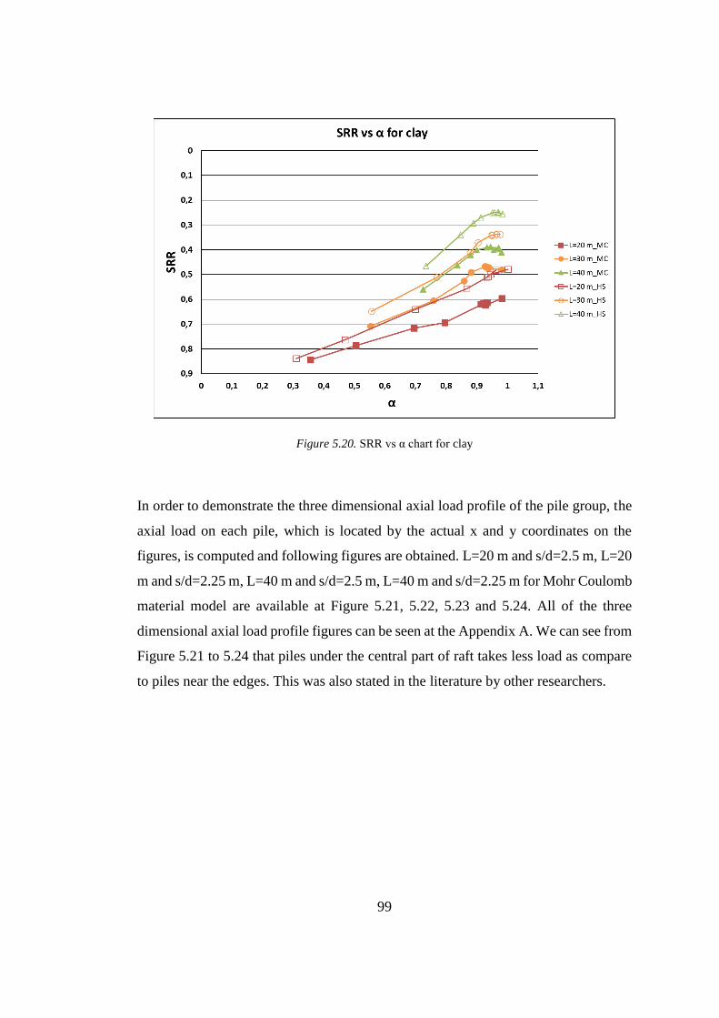
99
Figure 5.20. SRR vs α chart for clay
In order to demonstrate the three dimensional axial load profile of the pile group, the
axial load on each pile, which is located by the actual x and y coordinates on the
figures, is computed and following figures are obtained. L=20 m and s/d=2.5 m, L=20
m and s/d=2.25 m, L=40 m and s/d=2.5 m, L=40 m and s/d=2.25 m for Mohr Coulomb
material model are available at Figure 5.21, 5.22, 5.23 and 5.24. All of the three
dimensional axial load profile figures can be seen at the Appendix A. We can see from
Figure 5.21 to 5.24 that piles under the central part of raft takes less load as compare
to piles near the edges. This was also stated in the literature by other researchers.
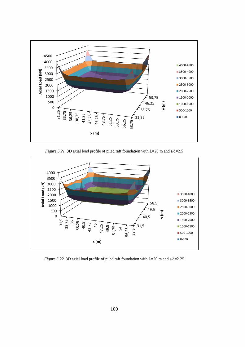
100
Figure 5.21. 3D axial load profile of piled raft foundation with L=20 m and s/d=2.5
Figure 5.22. 3D axial load profile of piled raft foundation with L=20 m and s/d=2.25
31,25
38,75
46,25
53,75
0
500
1000
1500
2000
2500
3000
3500
4000
45003
1,2
5
33
,75
36
,25
38
,75
41
,25
43
,75
46
,25
48
,75
51
,25
53
,75
56
,25
58
,75
y (m
)
Axi
al L
oad
(kN
)
x (m)
4000-4500
3500-4000
3000-3500
2500-3000
2000-2500
1500-2000
1000-1500
500-1000
0-500
31,5
40,5
49,5
58,5
0
500
1000
1500
2000
2500
3000
3500
4000
31
,5
33
,75
36
38
,25
40
,5
42
,75
45
47
,25
49
,5
51
,75
54
56
,25
58
,5
y (m
)
Axi
al L
oad
(kN
)
x (m)
3500-4000
3000-3500
2500-3000
2000-2500
1500-2000
1000-1500
500-1000
0-500
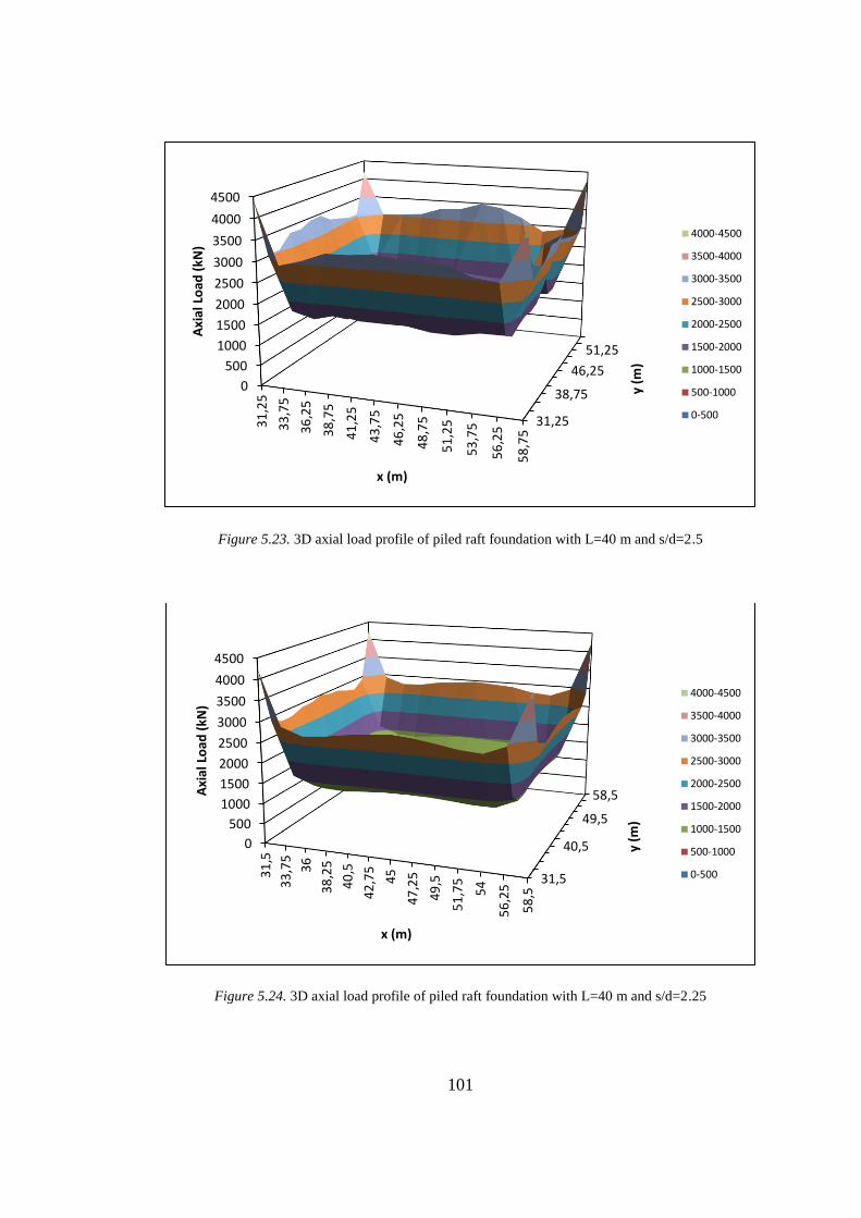
101
Figure 5.23. 3D axial load profile of piled raft foundation with L=40 m and s/d=2.5
Figure 5.24. 3D axial load profile of piled raft foundation with L=40 m and s/d=2.25
31,25
38,75
46,25
51,25
0
500
1000
1500
2000
2500
3000
3500
4000
4500
31
,25
33
,75
36
,25
38
,75
41
,25
43
,75
46
,25
48
,75
51
,25
53
,75
56
,25
58
,75
y (m
)
Axi
al L
oad
(kN
)
x (m)
4000-4500
3500-4000
3000-3500
2500-3000
2000-2500
1500-2000
1000-1500
500-1000
0-500
31,5
40,5
49,5
58,5
0
500
1000
1500
2000
2500
3000
3500
4000
4500
31
,5
33
,75
36
38
,25
40
,5
42
,75
45
47
,25
49
,5
51
,75
54
56
,25
58
,5
y (m
)
Axi
al L
oad
(kN
)
x (m)
4000-4500
3500-4000
3000-3500
2500-3000
2000-2500
1500-2000
1000-1500
500-1000
0-500
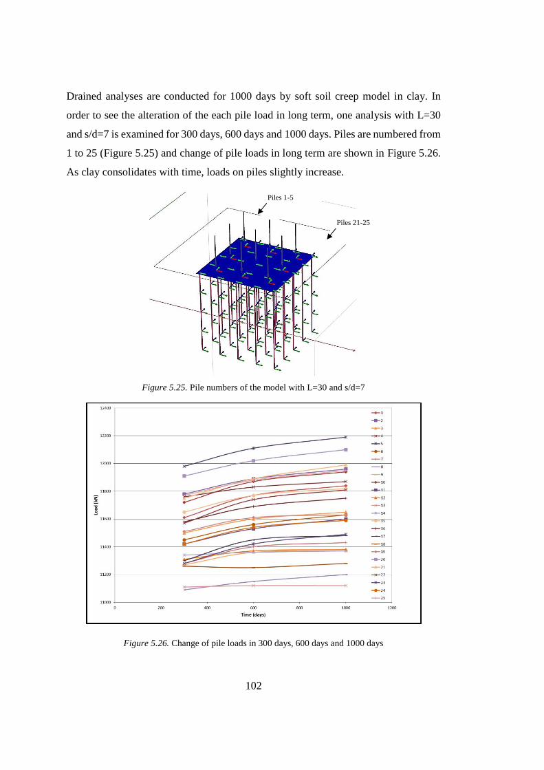
102
Drained analyses are conducted for 1000 days by soft soil creep model in clay. In
order to see the alteration of the each pile load in long term, one analysis with L=30
and s/d=7 is examined for 300 days, 600 days and 1000 days. Piles are numbered from
1 to 25 (Figure 5.25) and change of pile loads in long term are shown in Figure 5.26.
As clay consolidates with time, loads on piles slightly increase.
Figure 5.25. Pile numbers of the model with L=30 and s/d=7
Figure 5.26. Change of pile loads in 300 days, 600 days and 1000 days
Piles 1-5
Piles 21-25
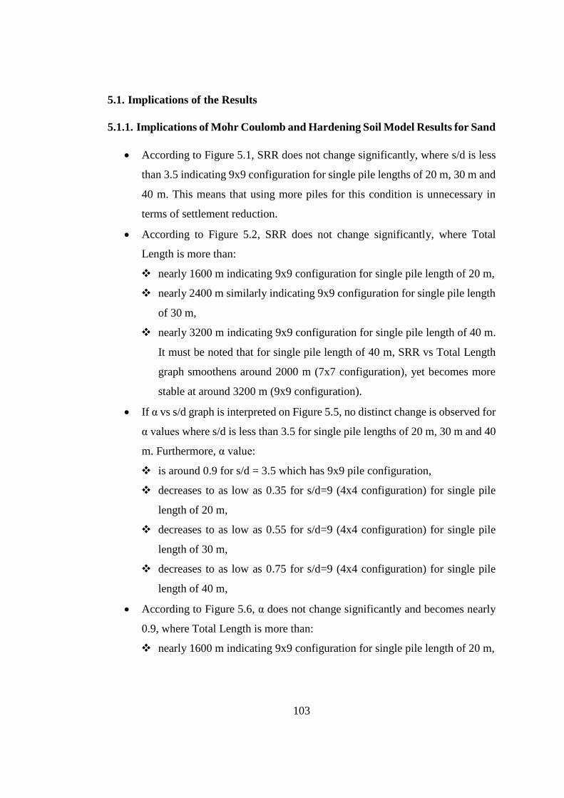
103
5.1. Implications of the Results
5.1.1. Implications of Mohr Coulomb and Hardening Soil Model Results for Sand
According to Figure 5.1, SRR does not change significantly, where s/d is less
than 3.5 indicating 9x9 configuration for single pile lengths of 20 m, 30 m and
40 m. This means that using more piles for this condition is unnecessary in
terms of settlement reduction.
According to Figure 5.2, SRR does not change significantly, where Total
Length is more than:
nearly 1600 m indicating 9x9 configuration for single pile length of 20 m,
nearly 2400 m similarly indicating 9x9 configuration for single pile length
of 30 m,
nearly 3200 m indicating 9x9 configuration for single pile length of 40 m.
It must be noted that for single pile length of 40 m, SRR vs Total Length
graph smoothens around 2000 m (7x7 configuration), yet becomes more
stable at around 3200 m (9x9 configuration).
If α vs s/d graph is interpreted on Figure 5.5, no distinct change is observed for
α values where s/d is less than 3.5 for single pile lengths of 20 m, 30 m and 40
m. Furthermore, α value:
is around 0.9 for s/d = 3.5 which has 9x9 pile configuration,
decreases to as low as 0.35 for s/d=9 (4x4 configuration) for single pile
length of 20 m,
decreases to as low as 0.55 for s/d=9 (4x4 configuration) for single pile
length of 30 m,
decreases to as low as 0.75 for s/d=9 (4x4 configuration) for single pile
length of 40 m,
According to Figure 5.6, α does not change significantly and becomes nearly
0.9, where Total Length is more than:
nearly 1600 m indicating 9x9 configuration for single pile length of 20 m,
104
nearly 2400 m similarly indicating 9x9 configuration for single pile length
of 30 m,
nearly 3200 m also indicating 9x9 configuration for single pile length of
40 m.
5.1.2. Implications of Mohr Coulomb and Hardening Soil Model Results for Clay
According to Figure 5.7, SRR seems to have a stable trend, where s/d is less
than 3,5 indicating 9x9 configuration for single pile lengths of 20 m, 30 m and
40 m. This means that using more piles beyond 9x9 for this condition is
unnecessary in terms of settlement reduction.
According to Figure 5.8, SRR does not change explicitly, where Total Length
is more than:
nearly 1600 m indicating 9x9 configuration for single pile length of 20 m,
nearly 2400 m similarly indicating 9x9 configuration for single pile length
of 30 m,
nearly 3200 m also indicating 9x9 configuration for single pile length of
40 m.
Figure 5.11 implies that the lower s/d, the higher α values are obtained.
Therefore, an optimum point cannot be observed for α vs s/d graph.
According to Figure 5.12, the lower Total Length, the higher α values are
obtained. Therefore, an optimum point cannot be observed for α vs Total
Length graph.
5.1.3. Implications of Soft Soil Creep Model Results for Clay
There is an overall trend of increasing SRR with increasing s/d together with
outliers in Figure 5.13. Moreover, SRR values are almost stable for three cases
where s/d is less than 2.5.
There is an overall trend of decreasing SRR with increasing Total Length
together with outliers in Figure 5.14.
105
From Figure 5.17, α values have tendency to decrease with increasing s/d
which is more obvious in L=20 m cases.
From Figure 5.18, α values have tendency to increase with increasing Total
Length which is more obvious in L=20 m cases.
In overall, it is important to state that abovementioned outliers are usually valid
for L=30 m and L=40 m conditions. However, L=20 m cases do not show
significant deviations.
5.1.4. Implications of 3D Axial Load Profile Results for Sand
Deductions from Appendix A for both Mohr Coulomb and Hardening Soil Model:
As s/d decreases, the corner piles get more percentage of the total load for
all pile lengths.
For s/d=9, there are usually irregularities or concave down shapes in load
sharing of the piles in different positions.
Generally, for s/d=2.5 and s/d=4.5, load percentages increase from center
piles to edge piles to corner piles. The difference between loads on corner
and central piles could be also due to rigidity of the raft.
5.1.5. Implications of 3D Axial Load Profile Results for Clay
Deductions from Appendix A for both Mohr Coulomb and Hardening Soil Model:
Similar to sand cases, as s/d decreases, the corner piles get more percentage
of the total load for all pile lengths.
Similar to sand cases, for s/d=9, there are usually irregularities or concave
down shapes in load sharing of the piles in different positions.
Different from sand cases, there happens to be a change in load percentage
among edge and corner piles. Accordingly, the load percentage is higher
in center compared to the edge in many cases. The difference between
loads on corner and central piles could be also due to rigidity of the raft.
106
Deductions from Appendix A for Soft Soil Creep Model:
Similar to sand cases, as s/d decreases, the corner piles get more percentage
of the total load for all pile lengths.
For s/d=9, there are usually irregularities in load sharing of the piles in
different positions.
Similar to sand cases, generally, for s/d=2.5 and s/d=4.5, load percentages
increase from center piles to edge piles to corner piles. The difference
between loads on corner and central piles could be also due to rigidity of
the raft.
5.1.6. Implications of Change of Single Pile Loads in Long Term Results for Clay
The representative analysis shows that, as can be expected, considering the
consolidation in long term, the soil settles and exerts a down drag force on
pile and this causes increase in axial loads on all piles in the Figure 5.26.
107
CHAPTER 6
6. CONCLUSIONS
It is known that piles serve for controlling total and differential settlement in addition
to load carrying. In piled raft design, main criteria that governs the design are relative
proportion of load carried by raft and by piles (represented by α factor) and reduction
in settlements (represented by SRR). In this study, optimization of load sharing
between piles and raft and settlement reduction ratio provided by piled raft is
investigated via 3D finite element method. For different s/d ratios, for different total
and single pile lengths, for different soil constitutive models in sand and in clay, the
results indicate that:
as s/d increases (as spacing increases), SRR increases for both Hardening
Soil and Mohr Coulomb model, for both sand and clay.
for a given length of piles, Mohr Coulomb model always gives larger SRR
values than Hardening Soil model values for all s/d values.
for a given soil constitutive model, as single pile length increases, SRR
decreases for a given s/d ratio for both Hardening Soil and Mohr Coulomb
model, for both sand and clay.
for all single pile lengths (20 m, 30 m, 40 m), for all s/d ratios between 2
and 9, for both Hardening Soil and Mohr Coulomb models, SRR values
are the range of 0.12 to 0.85.
for all single pile lengths (20 m, 30 m, 40 m), for all s/d ratios between 2
and 9, for both Hardening Soil and Mohr Coulomb models, α values are
the range of 0.3 to 1.
as s/d increases (as spacing increases), α value decreases for all analyzed
cases in this study.
108
for a given s/d, as single pile length increases, α increases, which means in
order to transfer more loads to raft, length of a single pile should be shorter
for a given s/d ratio for all analyzed cases in this study.
as total length of piles increase, α increases, for all cases analyzed in this
study.
as total length of piles increase, SRR values decrease for all analyzed cases
in this study.
an optimum value of “total length of piles / length of single pile” “80”
provides benefit for all cases analyzed in this study.
RECOMMENDATIONS FOR FUTURE RESEARCHERS
All of the conclusions in this study are based on three dimensional finite
element analyses. Field measurements on settlement and loads on piles and/or
centrifuge model test of piled raft with detailed instrumentation would verify
the results.
This study involves only vertical uniform load creating uniform pressure on
the raft. Eccentric loading due to lateral forces such as in an earthquake or
offshore wind and wave loading could be studied.
Designs with variable pile lengths in the center and in the corners could be
studied.
109
REFERENCES
Al-Mosawi, M. J., Fattah, M. Y., & Al-Zayadi, A. A. O. (2011). Experimental
Observations on the Behavior of a Piled Raft Foundation, 17(4), 1–11.
Alver, O., & Özden, G. (2015). Tabakalı Zeminlerde Kazıklı Radye Temellerin
Optimum Tasarımı. Dokuz Eylül Üniversitesi Mühendislik Fakültesi Fen ve
Mühendislik Dergisi, 17(January), 13–26.
Bowles, L. E. (1996). Foundation analysis and design. McGraw-hill.
Brinkgreve, R. B. J. (2014). Efficient modelling of pile foundations in the Finite
Element Method.
Butterfield, R. & Douglas, R.A. (1981). Flexibility coefficients for the design of piles
and pile groups, CIRIA Technical Notes, 108
Clancy, P. & Randolph, M. F. (1993). An approximate analysis procedure for piled
raft foundations. Int. J. Numer. Anal. Methods Geomech. 17, 849-869.
Clancy, P. and Randolph, M. F. (1996). Simple design tools for piled raft foundations.
Géotechnique, 46(2), 313–328. https://doi.org/10.1680/geot.1996.46.2.313
Danish Standards Association. (1998). Norm for fundering (code of practice for
foundation engineering). Danish standard DS415. 4th ed. Danish Standards
Association, Copenhagen.
Dao, T. P. T. (2011). Validation of PLAXIS Embedded Piles For Lateral Loading.
Delft University of Technology. Delft University of Technology.
Duncan, J. M. and Buchignani, A. L. (1976). An engineering manual for settlement
studies, University of California at Berkeley, Berkeley, California.
110
El - Mossallamy, Y. M., El - Nahhas, F. M., & Essawy, A. S. (2006). Innovative use
of piled raft foundation to optimize the design of high-rise buildings. In The 10th
Arab Structural Engineering Conference, 13 -15 November 2006, Kuwait (pp.
347–358). Kuwait.
Elwakil, A. Z., & Azzam, W. R. (2016). Experimental and numerical study of piled
raft system. Alexandria Engineering Journal, 55(1), 547–560.
https://doi.org/10.1016/j.aej.2015.10.001
Engin, H. K., & Brinkgreve, R. B. J. (2009). Investigation of Pile Behaviour Using
Embedded Piles. In Proceedings of the 17th International Conference on Soil
Mechanics and Geotechnical Engineering: The Academia and Practice of
Geotechnical Engineering (Vol. 2, pp. 1189–1192). https://doi.org/10.3233/978-1-
60750-031-5-1189
Engin, H. K., Septanika, E. G., & Brinkgreve, R. B. J. (2008). Estimation of Pile
Group Behavior using Embedded Piles. In 12th International Conference of
International Association for Computer Methods and Advances in Geomechanics
(IACMAG). Goa, India.
Garg, P., Singh, H., & Jha, J. (2013). Optimisation of Piled-Raft Foundation. In
UKIERI Concrete Congress - Innovations in Concrete Construction (pp. 1724–1735).
Horikoshi, K., & Randolph, M. F. (1998). A contribution to optimum design of piled
rafts. Géotechnique, 48(3), 301–317. https://doi.org/10.1680/geot.1998.48.3.301
Ismael N.F., Al-Sanad H.A. and Al-Otaibi F. (1994). Tension tests on bored piles in
cemented desert sands. Canadian Geotechnical Journal, 31(4), 597-603.
Katzenbach, R., Arslan, U. & Moorman, C. (2000). Piled Raft Projects in Germany.
In Hemsley (ed), Design Application of Piled Raft Foundations, 323-391. London:
Thomas Telford.
111
Katzenbach, Rolf, P. D.-I., & Deepankar Choudhury, P. D. (2013). ISSMGE
Combined Pile-Raft Foundation Guideline.
Kuwabara, F. (1989). An Elastic Analysis for Piled Raft Foundations in a
Homogeneous Soil. Soils and Foundations, 29(1), 82–92.
Lambe, T. W., & Whitman, R. V. (1969), Soil Mechanics, 553 pp., John Wiley, New
York.
Mali, S., & Singh, B. (2018). Behavior of large piled-raft foundation on clay soil.
Ocean Engineering, 149, 205–216. https://doi.org/10.1016/j.oceaneng.2017.12.029
Mandolini, A., Di Laora, R., & Mascarucci, Y. (2013). Rational design of piled raft.
Procedia Engineering, 57, 45–52. https://doi.org/10.1016/j.proeng.2013.04.008
Patil, J. D., Vasanwala, S. A., & Solanki, C. H. (2014). An experimental investigation
on behavior of piled raft foundation. International Journal of Geomatics and
Geosciences, 5(2), 300–311.
Plaxis 3D Tutorial, Reference, Material Models and Scientific Manuals (2013)
Poulos, H.G. & Davis, E.H. (1980). Pile foundation analysis and design. Wiley, New
York.
Poulos, H. G. (2001). Piled raft foundations: design and applications. Géotechnique,
51(2), 95–113. https://doi.org/10.1680/geot.2001.51.2.95
Poulos, H. G. (2002). Simplified Design Procedure for Piled Raft Foundations. In
Deep Foundations (pp. 441–458). Orlando, Florida, USA.
https://doi.org/10.1061/40601(256)32
Prakoso, W. A., & Kulhawy, F. H. (2001). Contribution to Piled Raft Foundation
Design. Journal Of Geotechnical and Geoenvironmental Engineering, 127(January),
17–24.
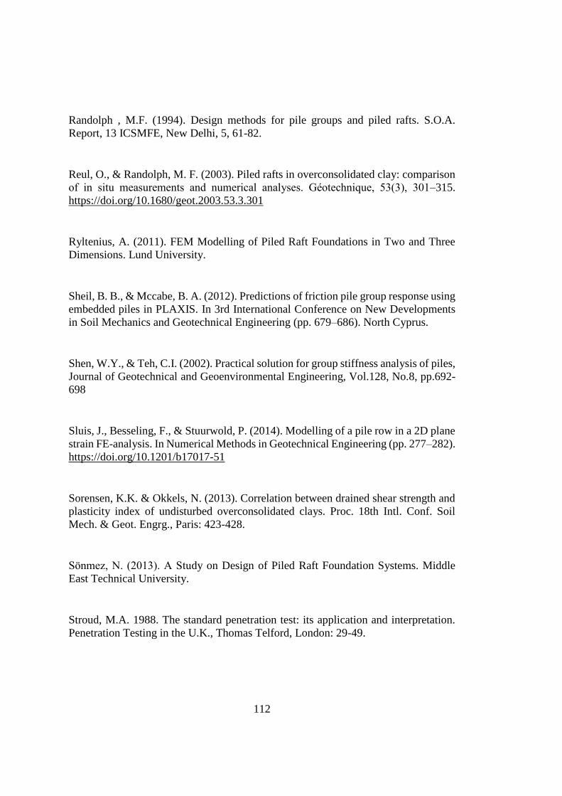
112
Randolph , M.F. (1994). Design methods for pile groups and piled rafts. S.O.A.
Report, 13 ICSMFE, New Delhi, 5, 61-82.
Reul, O., & Randolph, M. F. (2003). Piled rafts in overconsolidated clay: comparison
of in situ measurements and numerical analyses. Géotechnique, 53(3), 301–315.
https://doi.org/10.1680/geot.2003.53.3.301
Ryltenius, A. (2011). FEM Modelling of Piled Raft Foundations in Two and Three
Dimensions. Lund University.
Sheil, B. B., & Mccabe, B. A. (2012). Predictions of friction pile group response using
embedded piles in PLAXIS. In 3rd International Conference on New Developments
in Soil Mechanics and Geotechnical Engineering (pp. 679–686). North Cyprus.
Shen, W.Y., & Teh, C.I. (2002). Practical solution for group stiffness analysis of piles,
Journal of Geotechnical and Geoenvironmental Engineering, Vol.128, No.8, pp.692-
698
Sluis, J., Besseling, F., & Stuurwold, P. (2014). Modelling of a pile row in a 2D plane
strain FE-analysis. In Numerical Methods in Geotechnical Engineering (pp. 277–282).
https://doi.org/10.1201/b17017-51
Sorensen, K.K. & Okkels, N. (2013). Correlation between drained shear strength and
plasticity index of undisturbed overconsolidated clays. Proc. 18th Intl. Conf. Soil
Mech. & Geot. Engrg., Paris: 423-428.
Sönmez, N. (2013). A Study on Design of Piled Raft Foundation Systems. Middle
East Technical University.
Stroud, M.A. 1988. The standard penetration test: its application and interpretation.
Penetration Testing in the U.K., Thomas Telford, London: 29-49.
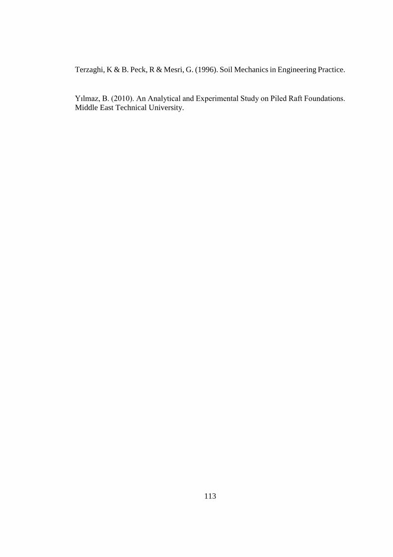
113
Terzaghi, K & B. Peck, R & Mesri, G. (1996). Soil Mechanics in Engineering Practice.
Yılmaz, B. (2010). An Analytical and Experimental Study on Piled Raft Foundations.
Middle East Technical University.

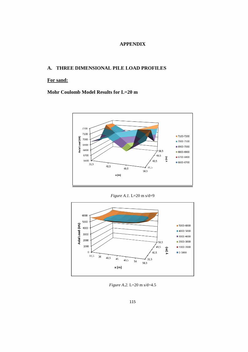
115
APPENDIX
A. THREE DIMENSIONAL PILE LOAD PROFILES
For sand:
Mohr Coulomb Model Results for L=20 m
Figure A.1. L=20 m s/d=9
Figure A.2. L=20 m s/d=4.5

116
Figure A.3. L=20 m s/d=2.5
Hardening Soil Model Results for L=20 m
Figure A.4. L=20 m s/d=9
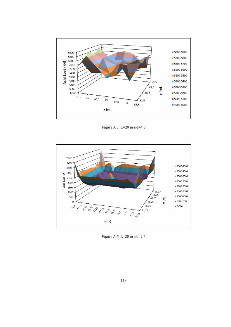
117
Figure A.5. L=20 m s/d=4.5
Figure A.6. L=20 m s/d=2.5
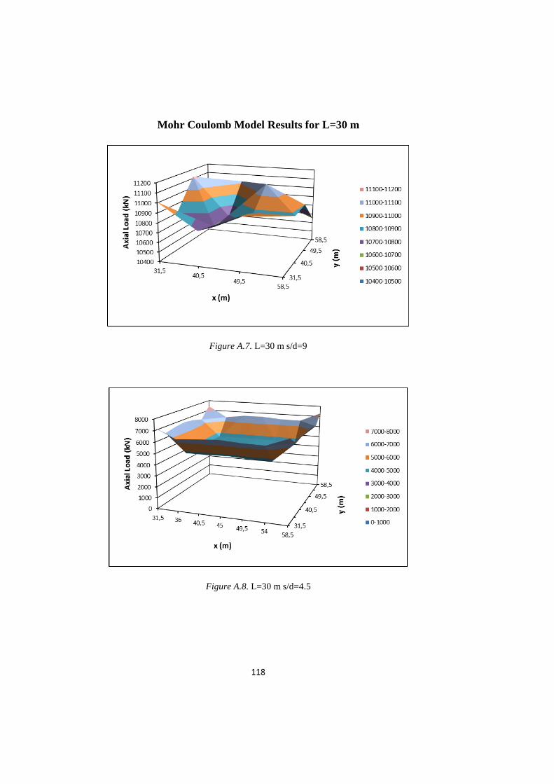
118
Mohr Coulomb Model Results for L=30 m
Figure A.7. L=30 m s/d=9
Figure A.8. L=30 m s/d=4.5
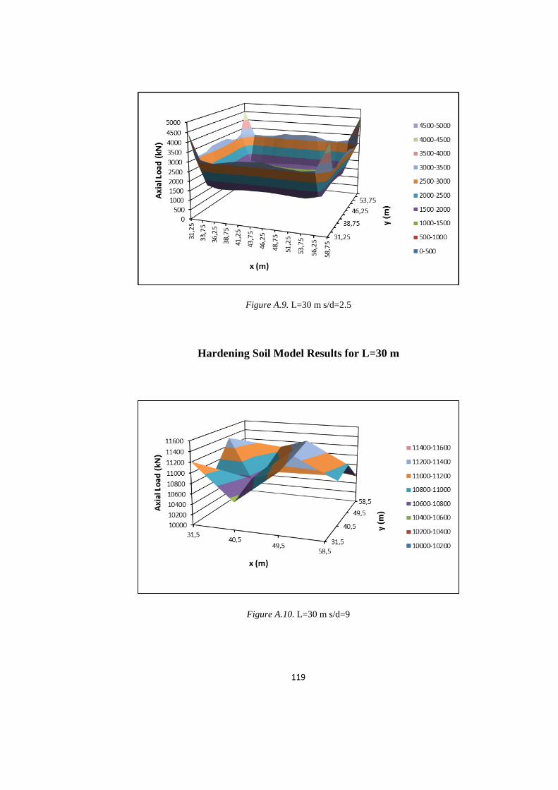
119
Figure A.9. L=30 m s/d=2.5
Hardening Soil Model Results for L=30 m
Figure A.10. L=30 m s/d=9
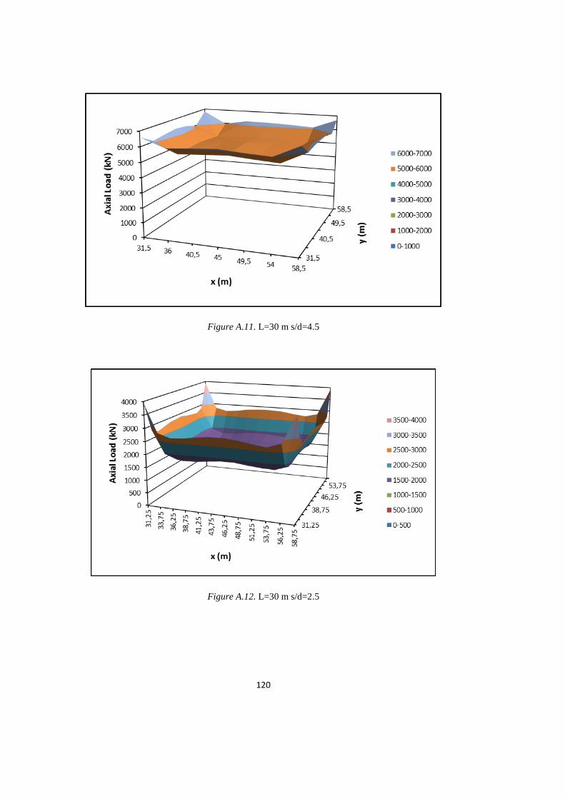
120
Figure A.11. L=30 m s/d=4.5
Figure A.12. L=30 m s/d=2.5
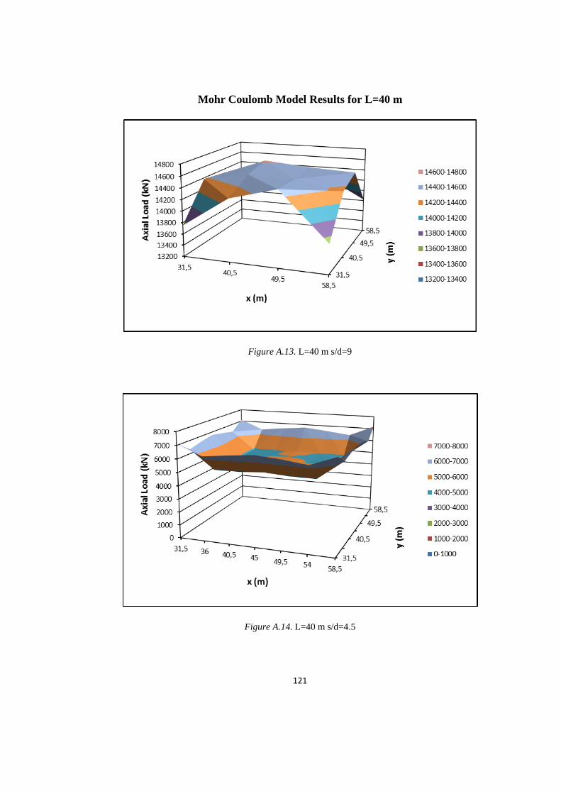
121
Mohr Coulomb Model Results for L=40 m
Figure A.13. L=40 m s/d=9
Figure A.14. L=40 m s/d=4.5
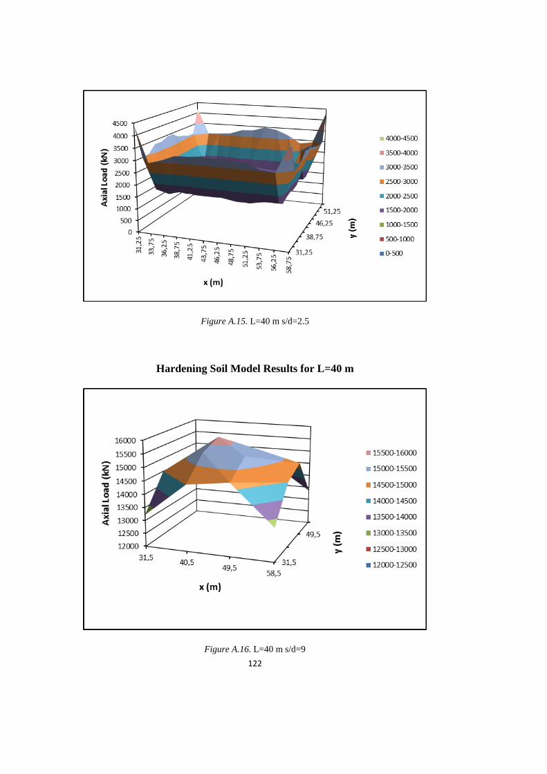
122
Figure A.15. L=40 m s/d=2.5
Hardening Soil Model Results for L=40 m
Figure A.16. L=40 m s/d=9
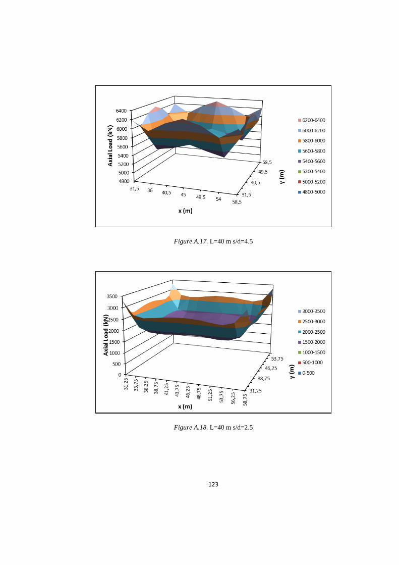
123
Figure A.17. L=40 m s/d=4.5
Figure A.18. L=40 m s/d=2.5
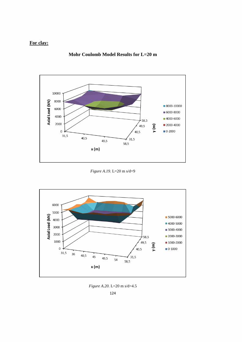
124
For clay:
Mohr Coulomb Model Results for L=20 m
Figure A.19. L=20 m s/d=9
Figure A.20. L=20 m s/d=4.5
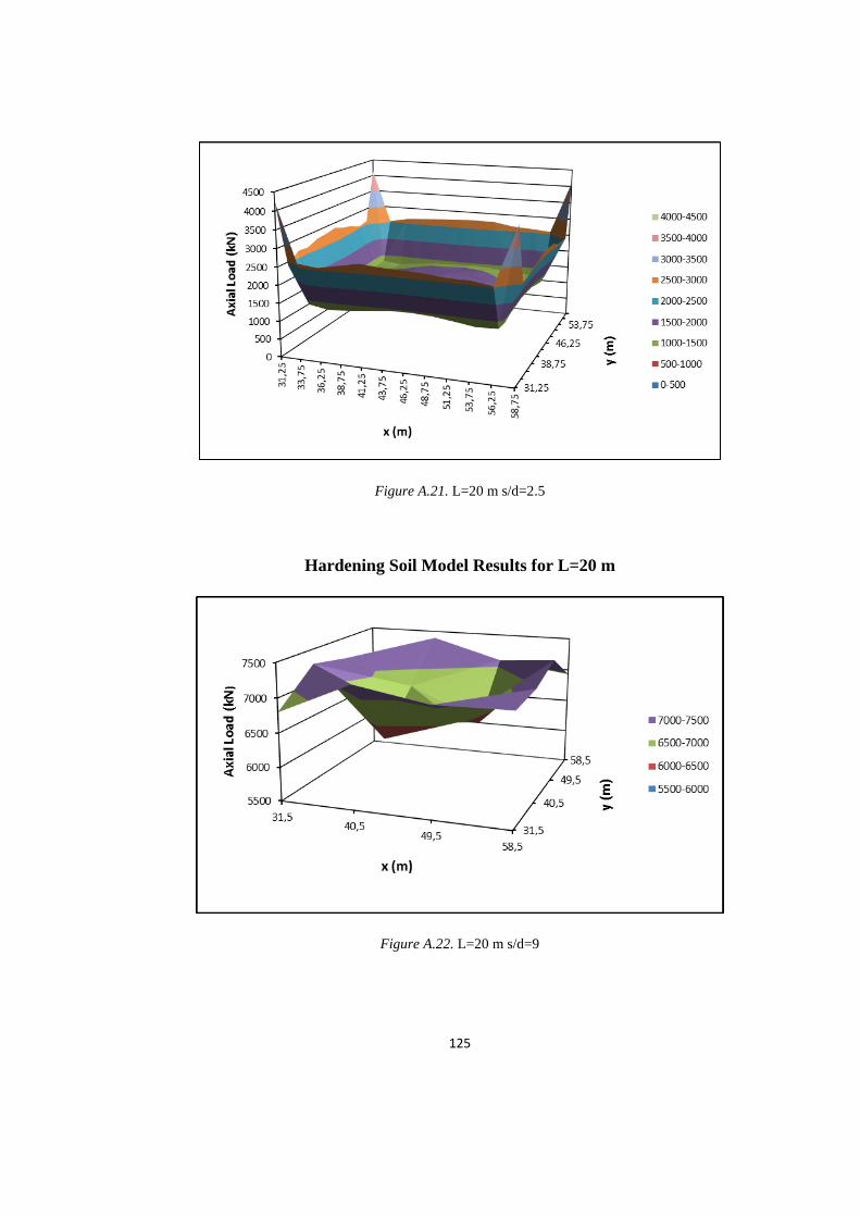
125
Figure A.21. L=20 m s/d=2.5
Hardening Soil Model Results for L=20 m
Figure A.22. L=20 m s/d=9
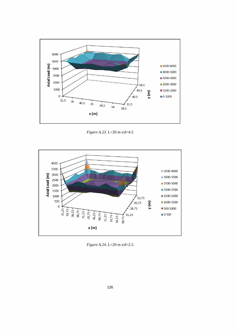
126
Figure A.23. L=20 m s/d=4.5
Figure A.24. L=20 m s/d=2.5
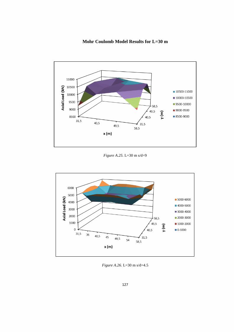
127
Mohr Coulomb Model Results for L=30 m
Figure A.25. L=30 m s/d=9
Figure A.26. L=30 m s/d=4.5
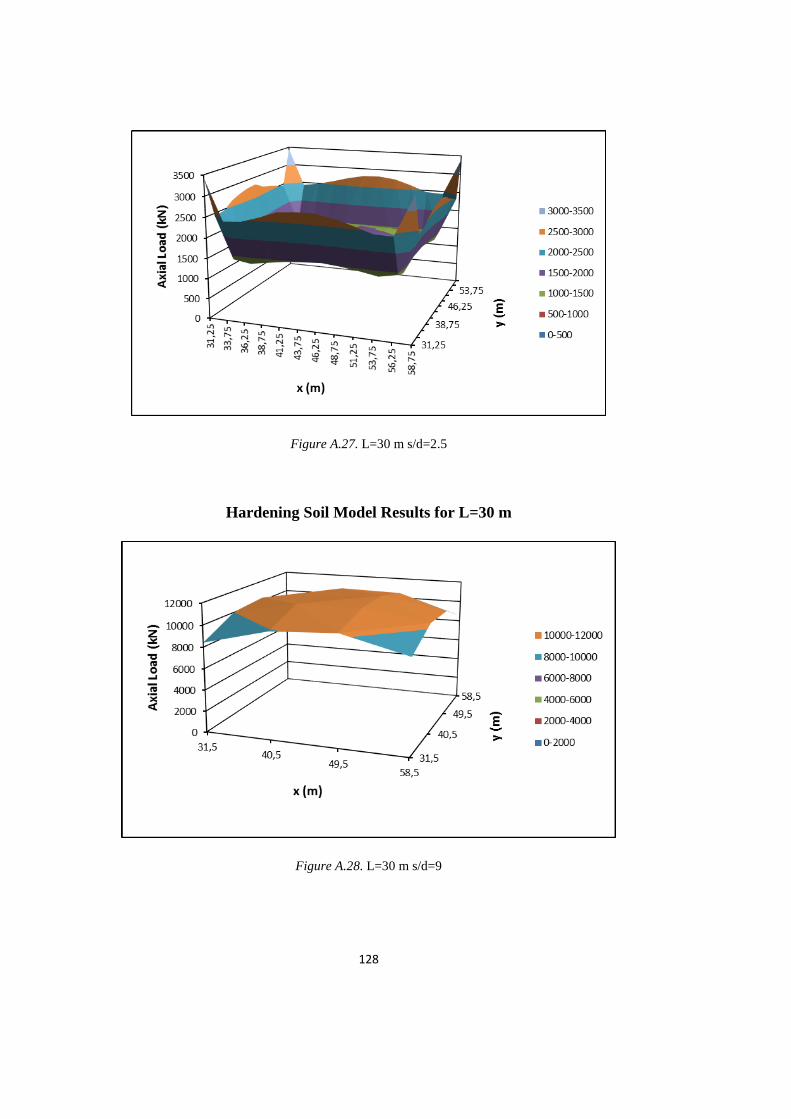
128
Figure A.27. L=30 m s/d=2.5
Hardening Soil Model Results for L=30 m
Figure A.28. L=30 m s/d=9
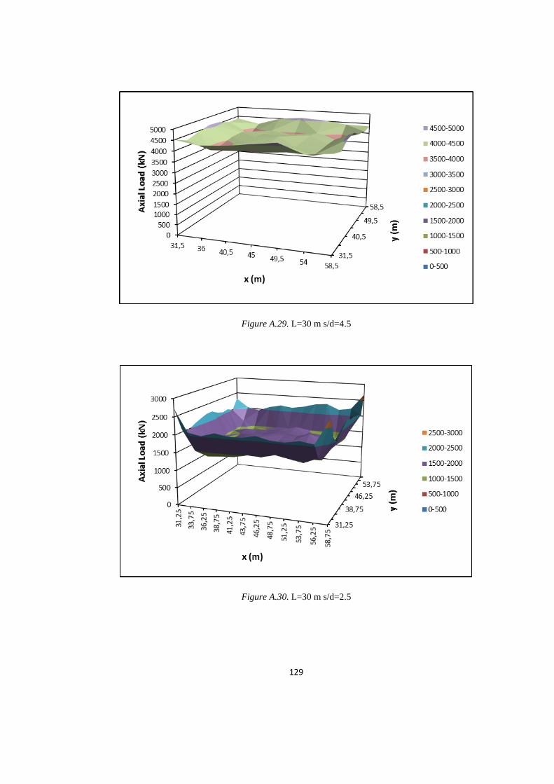
129
Figure A.29. L=30 m s/d=4.5
Figure A.30. L=30 m s/d=2.5
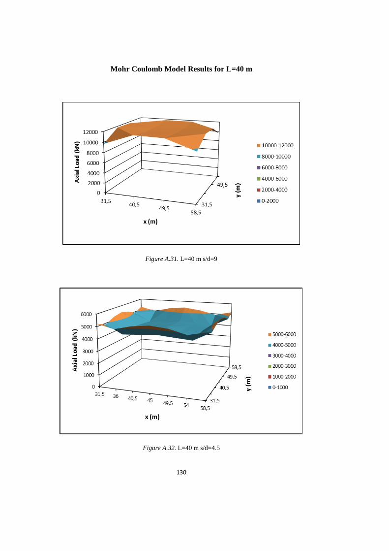
130
Mohr Coulomb Model Results for L=40 m
Figure A.31. L=40 m s/d=9
Figure A.32. L=40 m s/d=4.5
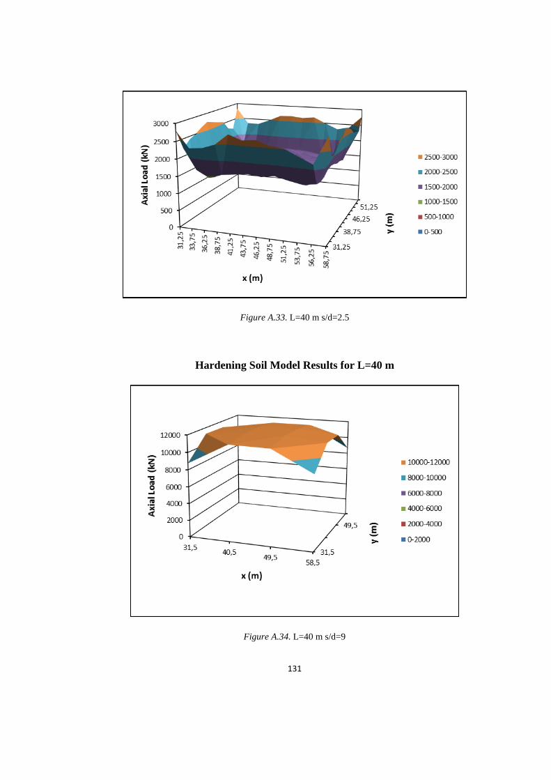
131
Figure A.33. L=40 m s/d=2.5
Hardening Soil Model Results for L=40 m
Figure A.34. L=40 m s/d=9
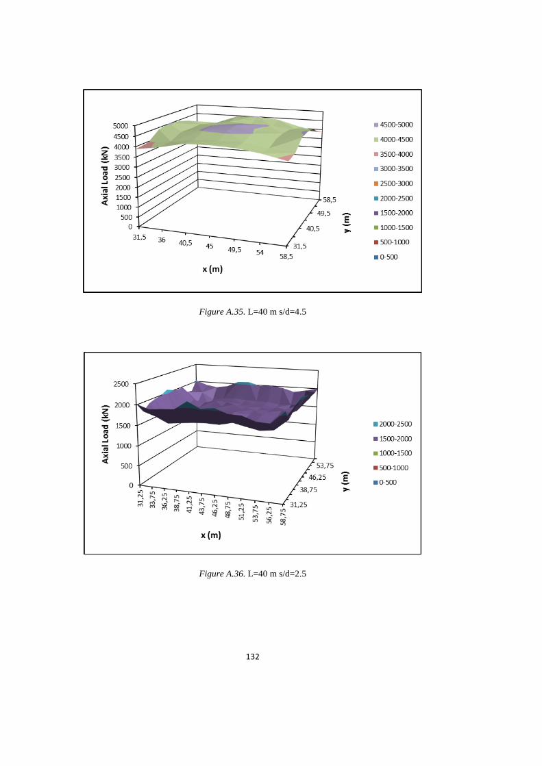
132
Figure A.35. L=40 m s/d=4.5
Figure A.36. L=40 m s/d=2.5
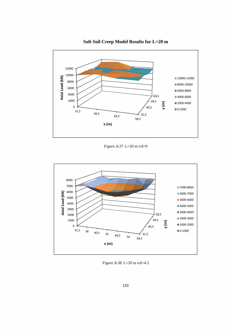
133
Soft Soil Creep Model Results for L=20 m
Figure A.37. L=20 m s/d=9
Figure A.38. L=20 m s/d=4.5
31,5
40,5
49,5
58,5
0
2000
4000
6000
8000
10000
12000
31,540,5
49,558,5
y (m
)
Axi
al L
oad
(kN
)
x (m)
10000-12000
8000-10000
6000-8000
4000-6000
2000-4000
0-2000
31,5
40,5
49,5
58,5
0
1000
2000
3000
4000
5000
6000
7000
8000
31,5 36 40,5 45 49,5 5458,5
y (m
)
Axi
al L
oad
(kN
)
x (m)
7000-8000
6000-7000
5000-6000
4000-5000
3000-4000
2000-3000
1000-2000
0-1000
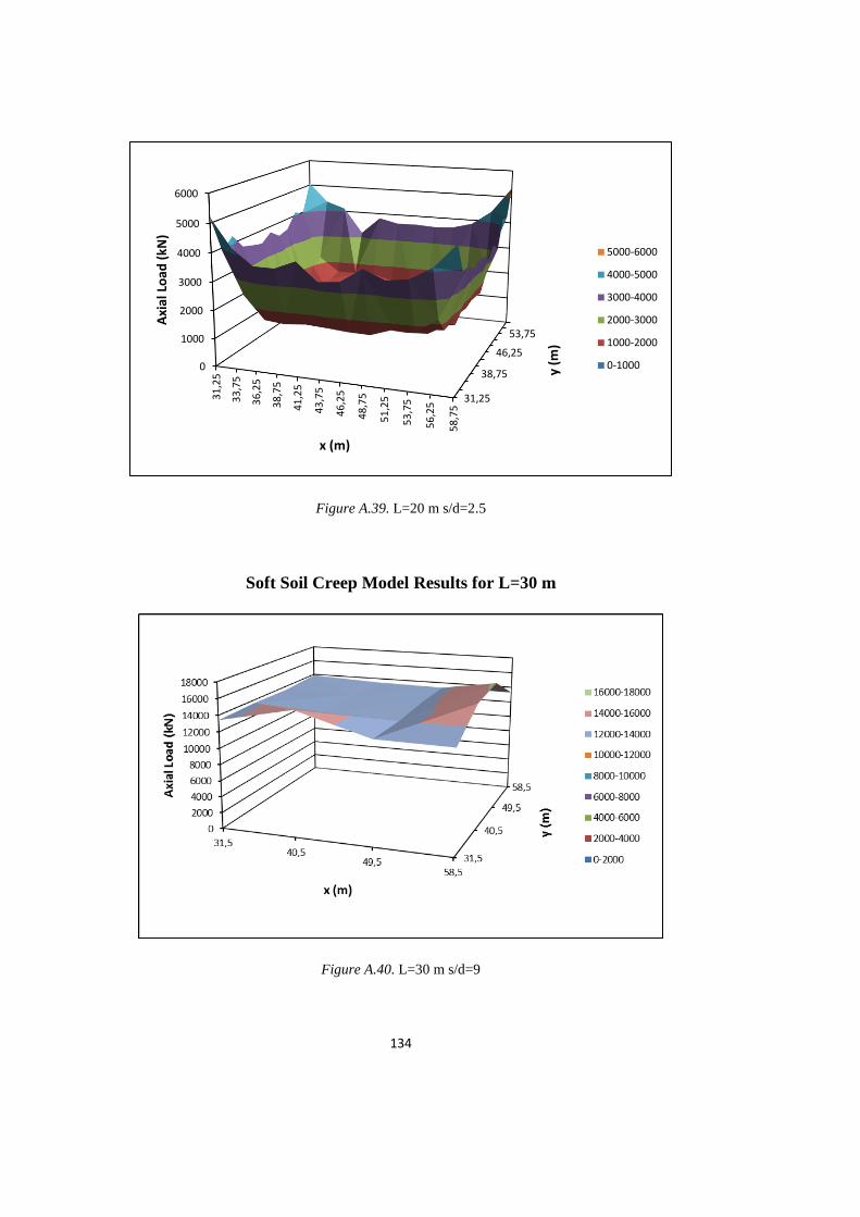
134
Figure A.39. L=20 m s/d=2.5
Soft Soil Creep Model Results for L=30 m
Figure A.40. L=30 m s/d=9
31,25
38,75
46,25
53,75
0
1000
2000
3000
4000
5000
6000
31
,25
33
,75
36
,25
38
,75
41
,25
43
,75
46
,25
48
,75
51
,25
53
,75
56
,25
58
,75
y (m
)
Axi
al L
oad
(kN
)
x (m)
5000-6000
4000-5000
3000-4000
2000-3000
1000-2000
0-1000
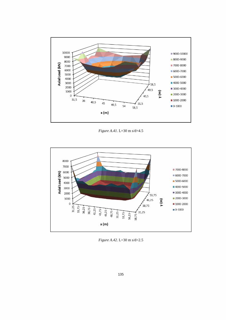
135
Figure A.41. L=30 m s/d=4.5
Figure A.42. L=30 m s/d=2.5
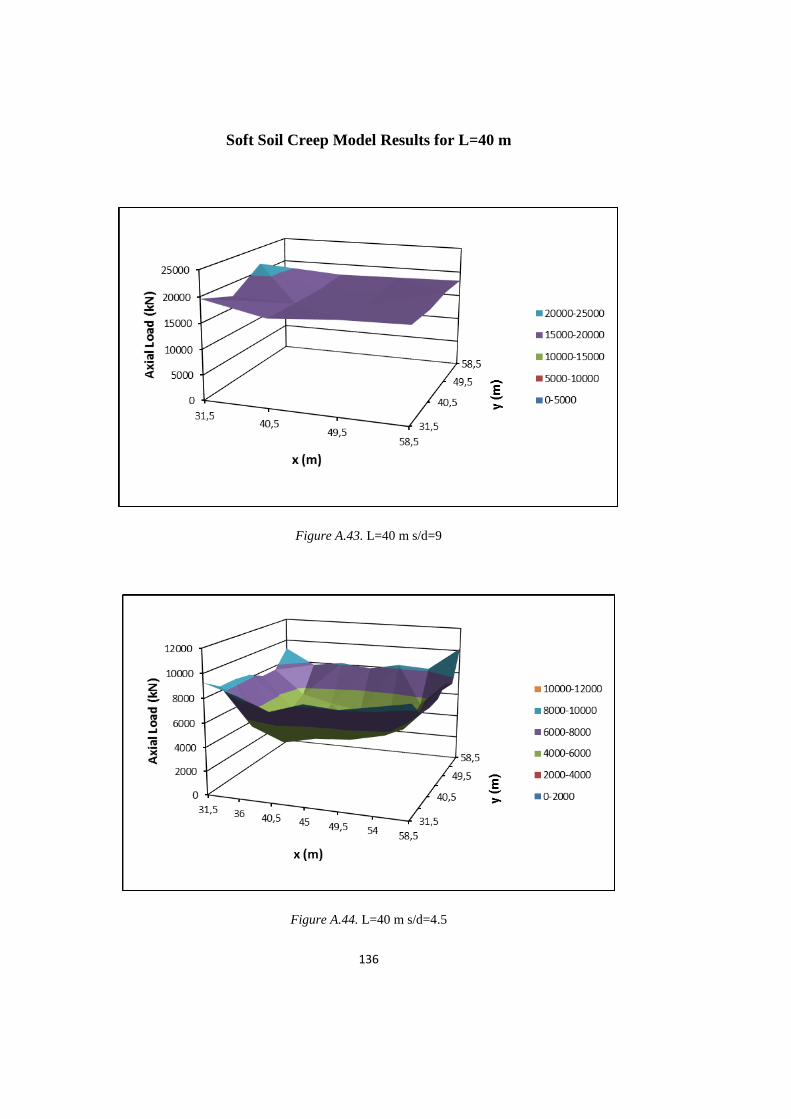
136
Soft Soil Creep Model Results for L=40 m
Figure A.43. L=40 m s/d=9
Figure A.44. L=40 m s/d=4.5
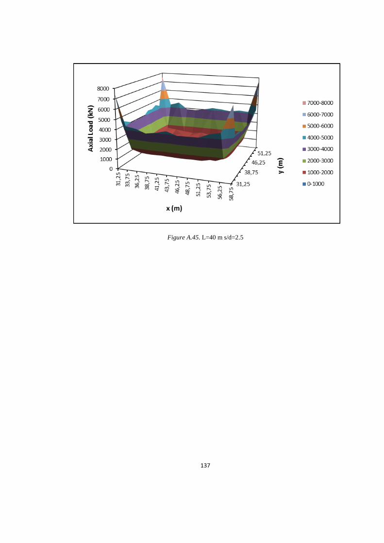
137
Figure A.45. L=40 m s/d=2.5

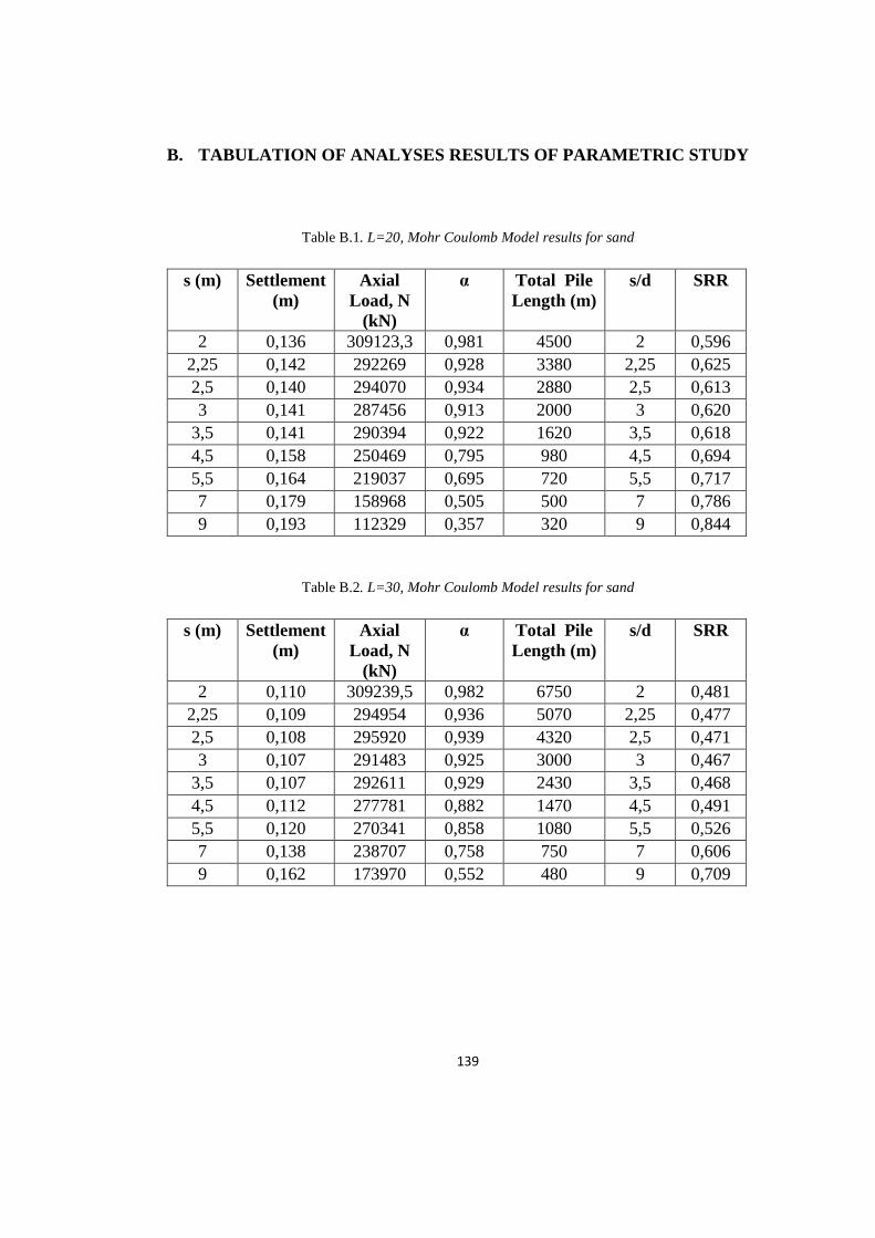
139
B. TABULATION OF ANALYSES RESULTS OF PARAMETRIC STUDY
Table B.1. L=20, Mohr Coulomb Model results for sand
s (m) Settlement
(m)
Axial
Load, N
(kN)
α Total Pile
Length (m)
s/d SRR
2 0,136 309123,3 0,981 4500 2 0,596
2,25 0,142 292269 0,928 3380 2,25 0,625
2,5 0,140 294070 0,934 2880 2,5 0,613
3 0,141 287456 0,913 2000 3 0,620
3,5 0,141 290394 0,922 1620 3,5 0,618
4,5 0,158 250469 0,795 980 4,5 0,694
5,5 0,164 219037 0,695 720 5,5 0,717
7 0,179 158968 0,505 500 7 0,786
9 0,193 112329 0,357 320 9 0,844
Table B.2. L=30, Mohr Coulomb Model results for sand
s (m) Settlement
(m)
Axial
Load, N
(kN)
α Total Pile
Length (m)
s/d SRR
2 0,110 309239,5 0,982 6750 2 0,481
2,25 0,109 294954 0,936 5070 2,25 0,477
2,5 0,108 295920 0,939 4320 2,5 0,471
3 0,107 291483 0,925 3000 3 0,467
3,5 0,107 292611 0,929 2430 3,5 0,468
4,5 0,112 277781 0,882 1470 4,5 0,491
5,5 0,120 270341 0,858 1080 5,5 0,526
7 0,138 238707 0,758 750 7 0,606
9 0,162 173970 0,552 480 9 0,709
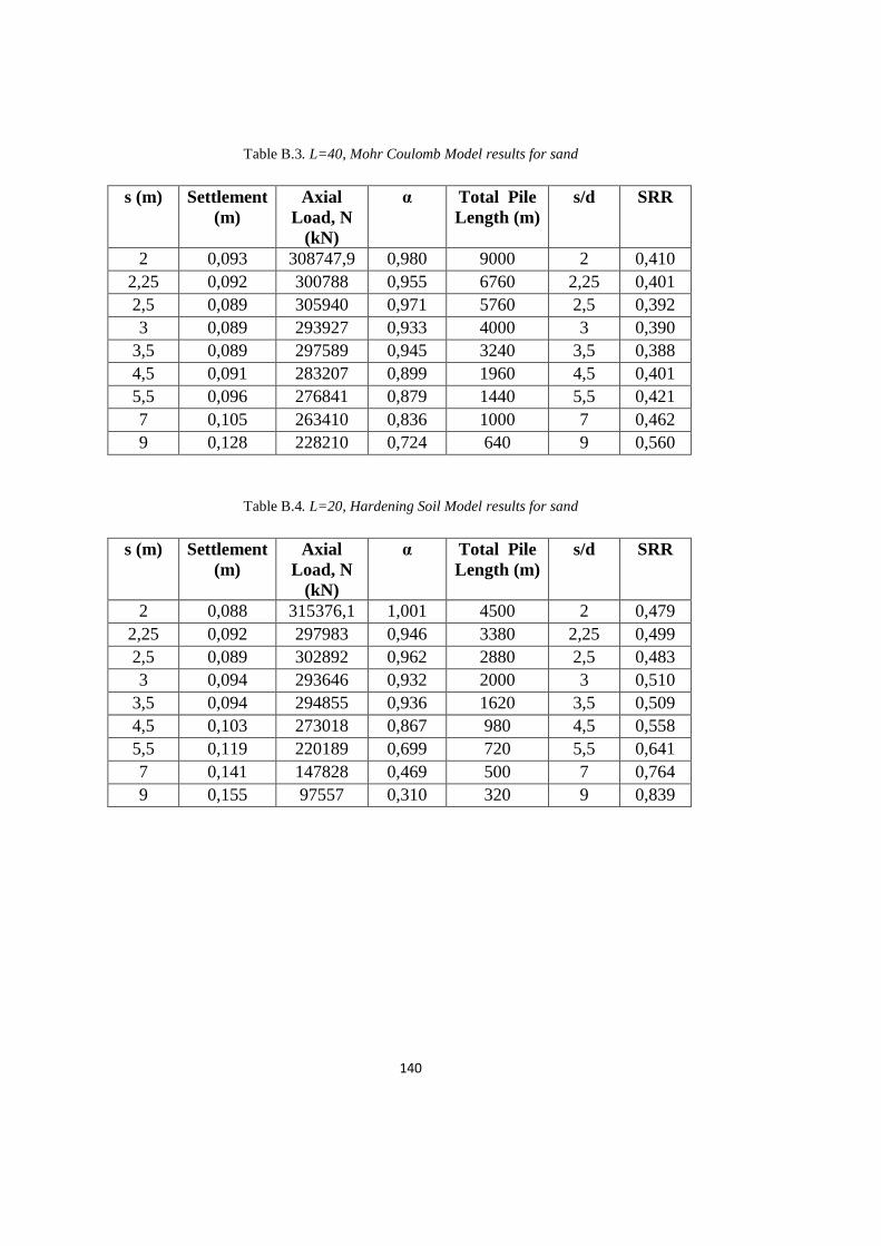
140
Table B.3. L=40, Mohr Coulomb Model results for sand
s (m) Settlement
(m)
Axial
Load, N
(kN)
α Total Pile
Length (m)
s/d SRR
2 0,093 308747,9 0,980 9000 2 0,410
2,25 0,092 300788 0,955 6760 2,25 0,401
2,5 0,089 305940 0,971 5760 2,5 0,392
3 0,089 293927 0,933 4000 3 0,390
3,5 0,089 297589 0,945 3240 3,5 0,388
4,5 0,091 283207 0,899 1960 4,5 0,401
5,5 0,096 276841 0,879 1440 5,5 0,421
7 0,105 263410 0,836 1000 7 0,462
9 0,128 228210 0,724 640 9 0,560
Table B.4. L=20, Hardening Soil Model results for sand
s (m) Settlement
(m)
Axial
Load, N
(kN)
α Total Pile
Length (m)
s/d SRR
2 0,088 315376,1 1,001 4500 2 0,479
2,25 0,092 297983 0,946 3380 2,25 0,499
2,5 0,089 302892 0,962 2880 2,5 0,483
3 0,094 293646 0,932 2000 3 0,510
3,5 0,094 294855 0,936 1620 3,5 0,509
4,5 0,103 273018 0,867 980 4,5 0,558
5,5 0,119 220189 0,699 720 5,5 0,641
7 0,141 147828 0,469 500 7 0,764
9 0,155 97557 0,310 320 9 0,839
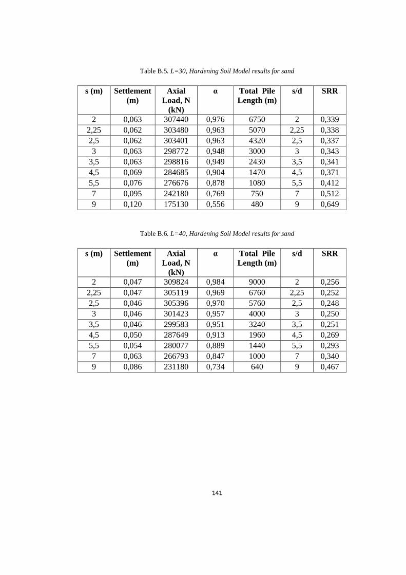
141
Table B.5. L=30, Hardening Soil Model results for sand
s (m) Settlement
(m)
Axial
Load, N
(kN)
α Total Pile
Length (m)
s/d SRR
2 0,063 307440 0,976 6750 2 0,339
2,25 0,062 303480 0,963 5070 2,25 0,338
2,5 0,062 303401 0,963 4320 2,5 0,337
3 0,063 298772 0,948 3000 3 0,343
3,5 0,063 298816 0,949 2430 3,5 0,341
4,5 0,069 284685 0,904 1470 4,5 0,371
5,5 0,076 276676 0,878 1080 5,5 0,412
7 0,095 242180 0,769 750 7 0,512
9 0,120 175130 0,556 480 9 0,649
Table B.6. L=40, Hardening Soil Model results for sand
s (m) Settlement
(m)
Axial
Load, N
(kN)
α Total Pile
Length (m)
s/d SRR
2 0,047 309824 0,984 9000 2 0,256
2,25 0,047 305119 0,969 6760 2,25 0,252
2,5 0,046 305396 0,970 5760 2,5 0,248
3 0,046 301423 0,957 4000 3 0,250
3,5 0,046 299583 0,951 3240 3,5 0,251
4,5 0,050 287649 0,913 1960 4,5 0,269
5,5 0,054 280077 0,889 1440 5,5 0,293
7 0,063 266793 0,847 1000 7 0,340
9 0,086 231180 0,734 640 9 0,467
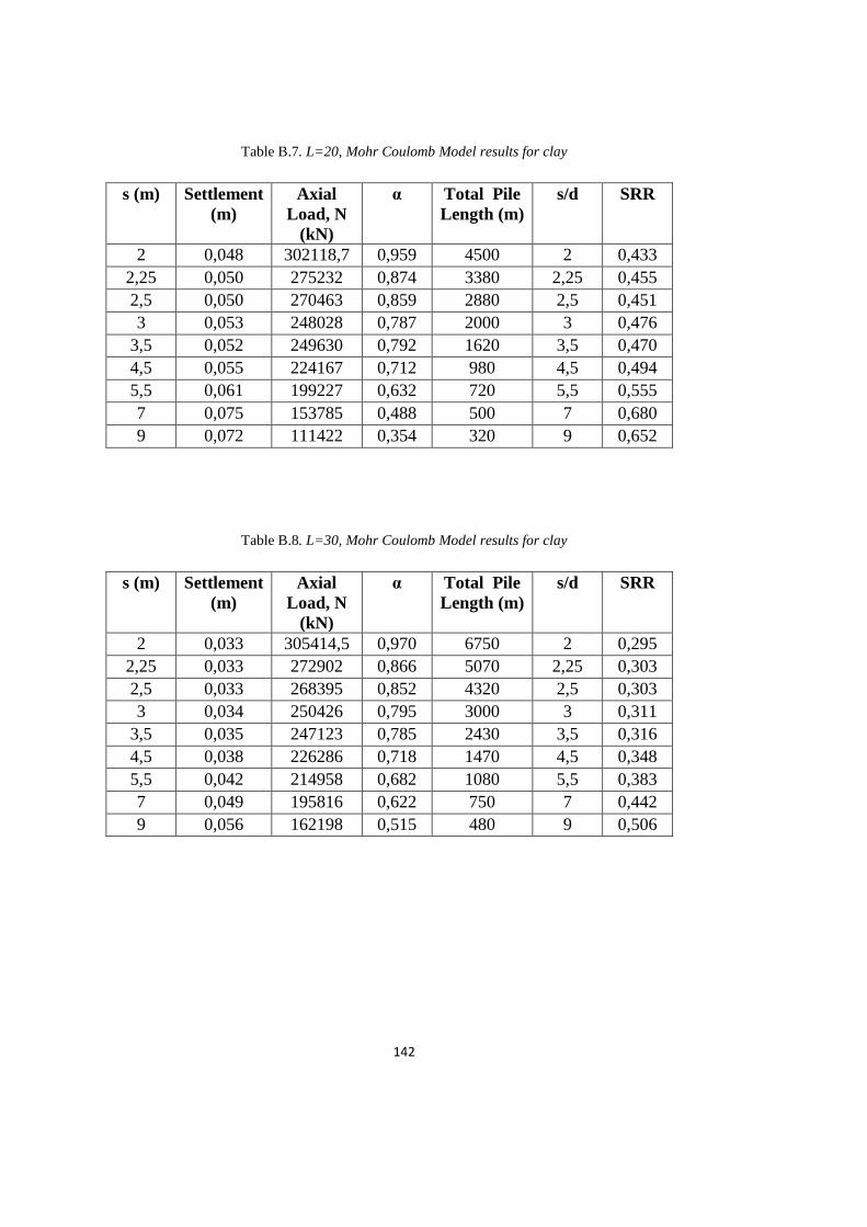
142
Table B.7. L=20, Mohr Coulomb Model results for clay
s (m) Settlement
(m)
Axial
Load, N
(kN)
α Total Pile
Length (m)
s/d SRR
2 0,048 302118,7 0,959 4500 2 0,433
2,25 0,050 275232 0,874 3380 2,25 0,455
2,5 0,050 270463 0,859 2880 2,5 0,451
3 0,053 248028 0,787 2000 3 0,476
3,5 0,052 249630 0,792 1620 3,5 0,470
4,5 0,055 224167 0,712 980 4,5 0,494
5,5 0,061 199227 0,632 720 5,5 0,555
7 0,075 153785 0,488 500 7 0,680
9 0,072 111422 0,354 320 9 0,652
Table B.8. L=30, Mohr Coulomb Model results for clay
s (m) Settlement
(m)
Axial
Load, N
(kN)
α Total Pile
Length (m)
s/d SRR
2 0,033 305414,5 0,970 6750 2 0,295
2,25 0,033 272902 0,866 5070 2,25 0,303
2,5 0,033 268395 0,852 4320 2,5 0,303
3 0,034 250426 0,795 3000 3 0,311
3,5 0,035 247123 0,785 2430 3,5 0,316
4,5 0,038 226286 0,718 1470 4,5 0,348
5,5 0,042 214958 0,682 1080 5,5 0,383
7 0,049 195816 0,622 750 7 0,442
9 0,056 162198 0,515 480 9 0,506
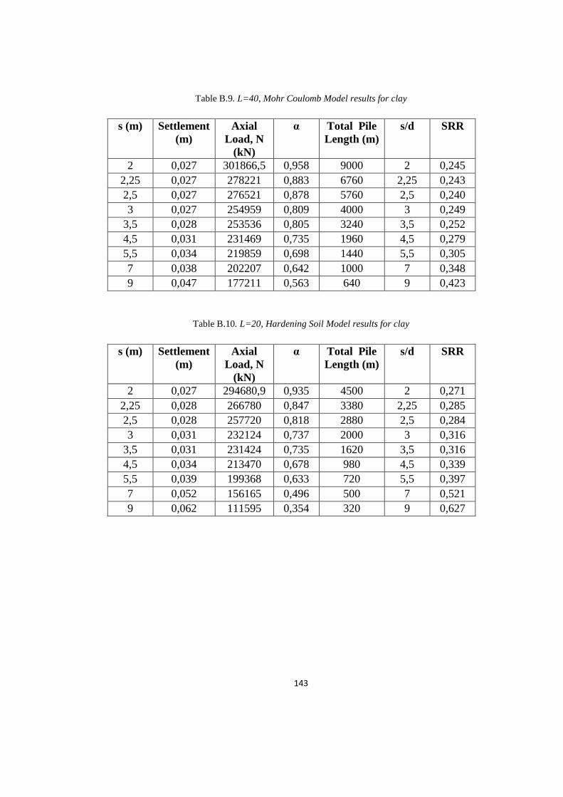
143
Table B.9. L=40, Mohr Coulomb Model results for clay
s (m) Settlement
(m)
Axial
Load, N
(kN)
α Total Pile
Length (m)
s/d SRR
2 0,027 301866,5 0,958 9000 2 0,245
2,25 0,027 278221 0,883 6760 2,25 0,243
2,5 0,027 276521 0,878 5760 2,5 0,240
3 0,027 254959 0,809 4000 3 0,249
3,5 0,028 253536 0,805 3240 3,5 0,252
4,5 0,031 231469 0,735 1960 4,5 0,279
5,5 0,034 219859 0,698 1440 5,5 0,305
7 0,038 202207 0,642 1000 7 0,348
9 0,047 177211 0,563 640 9 0,423
Table B.10. L=20, Hardening Soil Model results for clay
s (m) Settlement
(m)
Axial
Load, N
(kN)
α Total Pile
Length (m)
s/d SRR
2 0,027 294680,9 0,935 4500 2 0,271
2,25 0,028 266780 0,847 3380 2,25 0,285
2,5 0,028 257720 0,818 2880 2,5 0,284
3 0,031 232124 0,737 2000 3 0,316
3,5 0,031 231424 0,735 1620 3,5 0,316
4,5 0,034 213470 0,678 980 4,5 0,339
5,5 0,039 199368 0,633 720 5,5 0,397
7 0,052 156165 0,496 500 7 0,521
9 0,062 111595 0,354 320 9 0,627
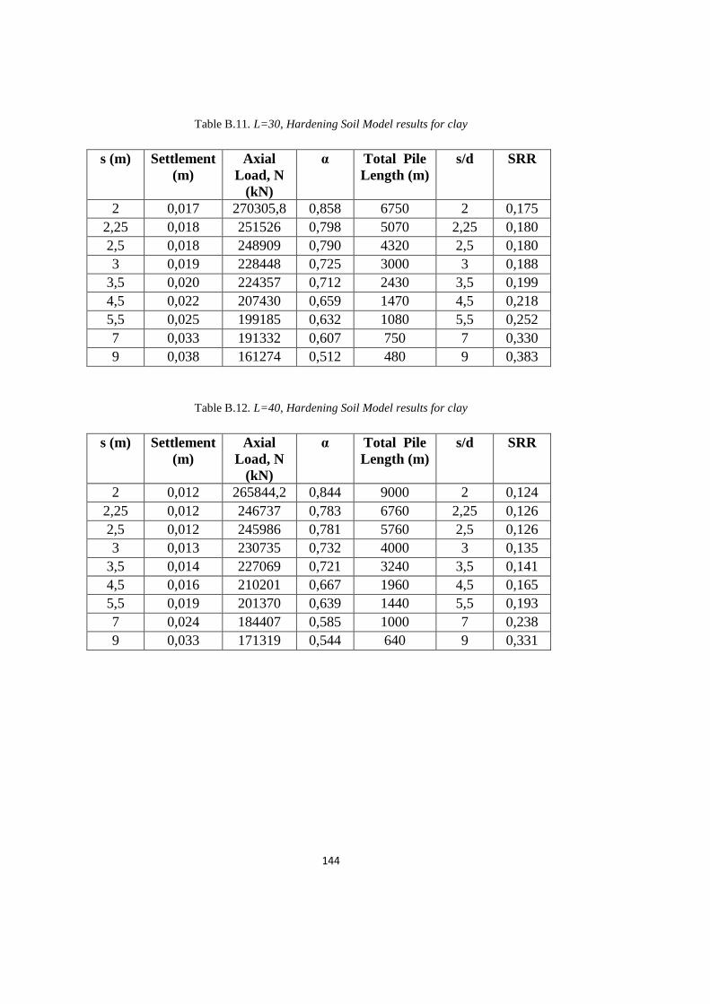
144
Table B.11. L=30, Hardening Soil Model results for clay
s (m) Settlement
(m)
Axial
Load, N
(kN)
α Total Pile
Length (m)
s/d SRR
2 0,017 270305,8 0,858 6750 2 0,175
2,25 0,018 251526 0,798 5070 2,25 0,180
2,5 0,018 248909 0,790 4320 2,5 0,180
3 0,019 228448 0,725 3000 3 0,188
3,5 0,020 224357 0,712 2430 3,5 0,199
4,5 0,022 207430 0,659 1470 4,5 0,218
5,5 0,025 199185 0,632 1080 5,5 0,252
7 0,033 191332 0,607 750 7 0,330
9 0,038 161274 0,512 480 9 0,383
Table B.12. L=40, Hardening Soil Model results for clay
s (m) Settlement
(m)
Axial
Load, N
(kN)
α Total Pile
Length (m)
s/d SRR
2 0,012 265844,2 0,844 9000 2 0,124
2,25 0,012 246737 0,783 6760 2,25 0,126
2,5 0,012 245986 0,781 5760 2,5 0,126
3 0,013 230735 0,732 4000 3 0,135
3,5 0,014 227069 0,721 3240 3,5 0,141
4,5 0,016 210201 0,667 1960 4,5 0,165
5,5 0,019 201370 0,639 1440 5,5 0,193
7 0,024 184407 0,585 1000 7 0,238
9 0,033 171319 0,544 640 9 0,331
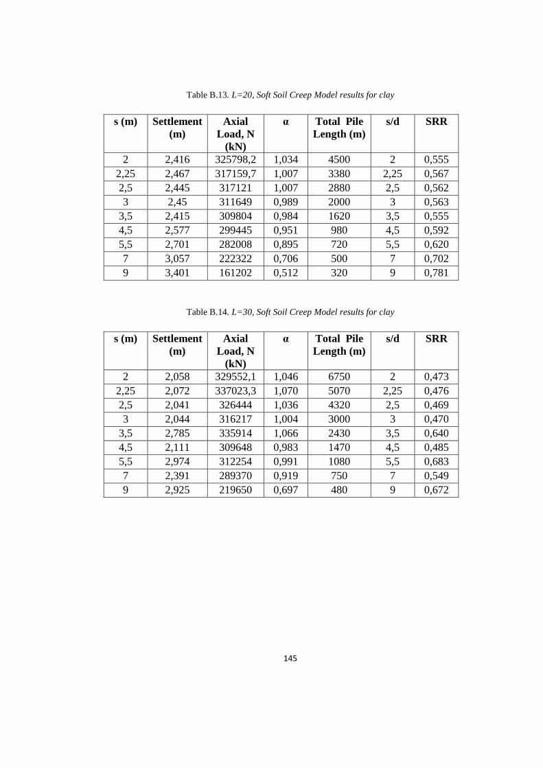
145
Table B.13. L=20, Soft Soil Creep Model results for clay
s (m) Settlement
(m)
Axial
Load, N
(kN)
α Total Pile
Length (m)
s/d SRR
2 2,416 325798,2 1,034 4500 2 0,555
2,25 2,467 317159,7 1,007 3380 2,25 0,567
2,5 2,445 317121 1,007 2880 2,5 0,562
3 2,45 311649 0,989 2000 3 0,563
3,5 2,415 309804 0,984 1620 3,5 0,555
4,5 2,577 299445 0,951 980 4,5 0,592
5,5 2,701 282008 0,895 720 5,5 0,620
7 3,057 222322 0,706 500 7 0,702
9 3,401 161202 0,512 320 9 0,781
Table B.14. L=30, Soft Soil Creep Model results for clay
s (m) Settlement
(m)
Axial
Load, N
(kN)
α Total Pile
Length (m)
s/d SRR
2 2,058 329552,1 1,046 6750 2 0,473
2,25 2,072 337023,3 1,070 5070 2,25 0,476
2,5 2,041 326444 1,036 4320 2,5 0,469
3 2,044 316217 1,004 3000 3 0,470
3,5 2,785 335914 1,066 2430 3,5 0,640
4,5 2,111 309648 0,983 1470 4,5 0,485
5,5 2,974 312254 0,991 1080 5,5 0,683
7 2,391 289370 0,919 750 7 0,549
9 2,925 219650 0,697 480 9 0,672
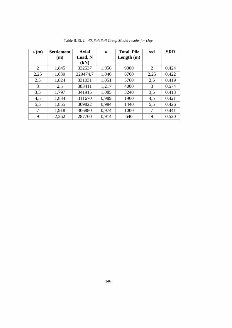
146
Table B.15. L=40, Soft Soil Creep Model results for clay
s (m) Settlement
(m)
Axial
Load, N
(kN)
α Total Pile
Length (m)
s/d SRR
2 1,845 332537 1,056 9000 2 0,424
2,25 1,839 329474,7 1,046 6760 2,25 0,422
2,5 1,824 331031 1,051 5760 2,5 0,419
3 2,5 383411 1,217 4000 3 0,574
3,5 1,797 341915 1,085 3240 3,5 0,413
4,5 1,834 311670 0,989 1960 4,5 0,421
5,5 1,855 309822 0,984 1440 5,5 0,426
7 1,918 306880 0,974 1000 7 0,441
9 2,262 287760 0,914 640 9 0,520