Dimension spatiale supplémentaire

compactifiée et champ de Higgs

branaire

Thèse de doctorat de l'université Paris-Saclay

École doctorale n° 576, Particules, Hadrons, Energie, Noyau,

Instrumentation, Imagerie, Cosmos et Simulation (PHENIICS)

Spécialité de doctorat: Constituants élémentaires

Unité de recherche : Université Paris-Saclay, CNRS, IJCLab, 91405, Orsay, France

Référent : Faculté des sciences

Thèse présentée et soutenue à Orsay, le 07/04/2020, par

Florian NORTIER

Composition du Jury

Geneviève BELANGER

Directrice de recherche, CNRS, LAPTh

Rapporteure & Examinatrice

Aldo DEANDREA

Professeur des universités,

Université Claude Bernard Lyon 1, IP2I

Rapporteur & Examinateur

Adam FALKOWSKI

Directeur de recherche, CNRS, IJCLab Examinateur

Grégory MOREAU

Maître de conférences,

Université Paris-Saclay, IJCLab

Directeur de thèse

Ulrich ELLWANGER

Professeur émérite, Université Paris-Saclay, IJCLab Co-Directeur de thèse

Th

èse

de d

oct

ora

t

NN

T : 2

020U

PA

SA

001

List of Publications

During the preparation of this PhD thesis, two preprints were published on ArXiv:— Ref. [1]: A. Angelescu, L. Ruifeng, G. Moreau and F. Nortier, Beyond brane-Higgs

regularisation: clarifying the method and model.— Ref. [2]: F. Nortier, Large Star/Rose Extra Dimension with Small Leaves/Petals.

2

Contents

List of Publications 2

Contents 6

List of Figures 8

List of Tables 9

Introduction 10

I State of the Art 14

1 Du champ de Higgs électrofaible à la hiérarchie de jauge 151.1 Modèle standard de la physique des particules . . . . . . . . . . . . . . . . . 15

1.1.1 Zoologie des fermions . . . . . . . . . . . . . . . . . . . . . . . . . . 161.1.2 Zoologie des bosons de jauge . . . . . . . . . . . . . . . . . . . . . . 171.1.3 Champ de Higgs . . . . . . . . . . . . . . . . . . . . . . . . . . . . . 19

1.2 Au-delà du modèle standard de la physique des particules . . . . . . . . . . 221.2.1 Lacunes du modèle standard . . . . . . . . . . . . . . . . . . . . . . 231.2.2 Naturalité de l’échelle électrofaible . . . . . . . . . . . . . . . . . . . 28

2 La voie des Univers branaires 312.1 Préambule historique . . . . . . . . . . . . . . . . . . . . . . . . . . . . . . . 31

2.1.1 Modèles à la Kaluza-Klein . . . . . . . . . . . . . . . . . . . . . . . . 312.1.2 Théories des supercordes . . . . . . . . . . . . . . . . . . . . . . . . 332.1.3 Branes . . . . . . . . . . . . . . . . . . . . . . . . . . . . . . . . . . . 342.1.4 Modèles phénoménologiques . . . . . . . . . . . . . . . . . . . . . . . 372.1.5 Problèmes liés à une échelle de gravité au TeV . . . . . . . . . . . . 38

2.2 Mode d’emploi pour construire un modèle extra-dimensionnel . . . . . . . . 422.2.1 Compactification de dimensions spatiales supplémentaires . . . . . . 422.2.2 Réduction dimensionnelle et décomposition de Kaluza-Klein . . . . . 46

2.3 Univers branaires et hiérarchie de jauge . . . . . . . . . . . . . . . . . . . . 482.3.1 Théorie effective pour une 3-brane . . . . . . . . . . . . . . . . . . . 482.3.2 Modèles d’ADD . . . . . . . . . . . . . . . . . . . . . . . . . . . . . 502.3.3 Modèle de RS1 . . . . . . . . . . . . . . . . . . . . . . . . . . . . . . 55

3 Bosons de jauge et fermions dans une tranche AdS5 613.1 Bosons de jauge et fermions dans le bulk . . . . . . . . . . . . . . . . . . . . 62

3.1.1 Champs de jauge . . . . . . . . . . . . . . . . . . . . . . . . . . . . . 62

3

3.1.2 Fermions de Dirac . . . . . . . . . . . . . . . . . . . . . . . . . . . . 633.2 Le Modèle Standard dans le bulk . . . . . . . . . . . . . . . . . . . . . . . . 66

3.2.1 Hiérarchie des couplages de Yukawa . . . . . . . . . . . . . . . . . . 673.2.2 Suppression des opérateurs de contact induisant des FCNCs . . . . . 683.2.3 Couplages de jauge . . . . . . . . . . . . . . . . . . . . . . . . . . . . 693.2.4 Échelle de coupure du modèle . . . . . . . . . . . . . . . . . . . . . . 69

3.3 Principales contraintes sur l’échelle de Kaluza-Klein . . . . . . . . . . . . . 703.3.1 FCNCs . . . . . . . . . . . . . . . . . . . . . . . . . . . . . . . . . . 703.3.2 Contraintes électrofaibles . . . . . . . . . . . . . . . . . . . . . . . . 713.3.3 Couplages à une boucle du boson de Higgs . . . . . . . . . . . . . . 73

3.4 Vers un achèvement ultraviolet . . . . . . . . . . . . . . . . . . . . . . . . . 743.4.1 Interprétation holographique . . . . . . . . . . . . . . . . . . . . . . 743.4.2 Gorges déformées en théorie des supercordes de type IIB . . . . . . . 78

II Original Research Work 81

4 Beyond Brane-Higgs Regularization 824.1 Introduction . . . . . . . . . . . . . . . . . . . . . . . . . . . . . . . . . . . . 824.2 Minimal Consistent Model . . . . . . . . . . . . . . . . . . . . . . . . . . . . 84

4.2.1 Spacetime Structure . . . . . . . . . . . . . . . . . . . . . . . . . . . 844.2.2 Bulk Fermions . . . . . . . . . . . . . . . . . . . . . . . . . . . . . . 854.2.3 Brane Localized Scalar Field . . . . . . . . . . . . . . . . . . . . . . 854.2.4 Yukawa Interactions . . . . . . . . . . . . . . . . . . . . . . . . . . . 864.2.5 Bilinear Boundary Terms . . . . . . . . . . . . . . . . . . . . . . . . 864.2.6 Model Extension . . . . . . . . . . . . . . . . . . . . . . . . . . . . . 87

4.3 5D Free Fermions on an Interval . . . . . . . . . . . . . . . . . . . . . . . . 884.3.1 Natural Boundary Conditions Only . . . . . . . . . . . . . . . . . . . 884.3.2 Essential Boundary Conditions from Conserved Currents . . . . . . 904.3.3 Natural Boundary Conditions with Bilinear Boundary Terms . . . . 934.3.4 Summary . . . . . . . . . . . . . . . . . . . . . . . . . . . . . . . . . 95

4.4 4D Fermion Mass Matrix including Yukawa couplings . . . . . . . . . . . . 964.5 Usual 5D Treatment: the Regularization Doom . . . . . . . . . . . . . . . . 98

4.5.1 Mixed Kaluza-Klein Decomposition . . . . . . . . . . . . . . . . . . 984.5.2 Shift of the Bounday Localized Higgs Field . . . . . . . . . . . . . . 994.5.3 Softening of the Boundary Localized Higgs Field . . . . . . . . . . . 1024.5.4 Two non-commutativities of calculation limits . . . . . . . . . . . . . 103

4.6 New 5D Treatment . . . . . . . . . . . . . . . . . . . . . . . . . . . . . . . . 1034.6.1 Fermionic Currents & Essential Boundary Conditions . . . . . . . . 1034.6.2 Failed Treatment without Bilinear Boundary Terms . . . . . . . . . 1044.6.3 Treatment with Bilinear Boundary Terms . . . . . . . . . . . . . . . 1064.6.4 Brane Localized Terms & the Dirac Distribution . . . . . . . . . . . 110

4.7 Implications . . . . . . . . . . . . . . . . . . . . . . . . . . . . . . . . . . . . 1124.7.1 Interpretation of the Analytical Results . . . . . . . . . . . . . . . . 1124.7.2 Phenomenological impacts . . . . . . . . . . . . . . . . . . . . . . . . 113

4.8 Summary & Conclusion . . . . . . . . . . . . . . . . . . . . . . . . . . . . . 114

4

5 Generalizations 1165.1 Boundary Localized Higgs Field: Generalization to a Slice of AdS5 . . . . . 116

5.1.1 Randall-Sundrum 1 Setup . . . . . . . . . . . . . . . . . . . . . . . . 1165.1.2 Field Content . . . . . . . . . . . . . . . . . . . . . . . . . . . . . . . 1175.1.3 5D Method . . . . . . . . . . . . . . . . . . . . . . . . . . . . . . . . 1195.1.4 4D Method . . . . . . . . . . . . . . . . . . . . . . . . . . . . . . . . 1235.1.5 Conclusion . . . . . . . . . . . . . . . . . . . . . . . . . . . . . . . . 123

5.2 Various Boundary Localized Terms . . . . . . . . . . . . . . . . . . . . . . . 1235.2.1 Toy Model: One Fermion in the Bulk . . . . . . . . . . . . . . . . . 1235.2.2 Boundary Localized Kinetic Terms . . . . . . . . . . . . . . . . . . . 1245.2.3 Boundary Localized Majorana Mass Terms . . . . . . . . . . . . . . 1275.2.4 Mixing Terms involving a Boundary Localized Fermion . . . . . . . 1295.2.5 Conclusion & Summary . . . . . . . . . . . . . . . . . . . . . . . . . 131

5.3 Brane-Higgs Field within the Orbifold S1/Z2 . . . . . . . . . . . . . . . . . 1315.3.1 1D Compactification Classification . . . . . . . . . . . . . . . . . . . 1315.3.2 The Model on the Orbifold S1/Z2 . . . . . . . . . . . . . . . . . . . 1325.3.3 From Fields as Distributions to Fields as Functions: an Additional

Motivation for Bilinear Brane Terms . . . . . . . . . . . . . . . . . . 1325.3.4 Method with 5D Fields as Functions . . . . . . . . . . . . . . . . . . 1345.3.5 Method with 5D Fields as Distributions . . . . . . . . . . . . . . . . 1395.3.6 An alternative Way to Recover the Interval . . . . . . . . . . . . . . 140

5.4 Higgs Field Localized at a Fixed Point of the Orbifold S1/ (Z2 × Z′2) . . . . 1425.4.1 Summary and Conclusion . . . . . . . . . . . . . . . . . . . . . . . . 146

5.5 Higgs Field Localized on a Brane Away from a Boundary of an Interval . . 1465.5.1 5D Method with Fields as Distributions . . . . . . . . . . . . . . . . 1465.5.2 Conclusion . . . . . . . . . . . . . . . . . . . . . . . . . . . . . . . . 149

6 Large Star/Rose Extra Dimension with Small Leaves/Petals 1506.1 Introduction . . . . . . . . . . . . . . . . . . . . . . . . . . . . . . . . . . . . 1506.2 Definition of a Star/Rose Extra Dimension . . . . . . . . . . . . . . . . . . 1556.3 5D Klein-Gordon Field on a Star/Rose Graph . . . . . . . . . . . . . . . . . 156

6.3.1 Klein-Gordon Equation & Junction/Boundary Conditions . . . . . . 1566.3.2 Kaluza-Klein Dimensional Reduction . . . . . . . . . . . . . . . . . . 158

6.4 5D Massless Dirac Field on a Star/Rose Graph . . . . . . . . . . . . . . . . 1636.4.1 Dirac-Weyl Equations & Junction/Boundary Conditions . . . . . . . 1636.4.2 Kaluza-Klein Dimensional Reduction . . . . . . . . . . . . . . . . . . 166

6.5 A Low 5D Planck Scale with a Star/Rose Extra Dimension . . . . . . . . . 1716.5.1 Lowering the Gravity Scale . . . . . . . . . . . . . . . . . . . . . . . 1716.5.2 Embedding the Standard Model Fields . . . . . . . . . . . . . . . . . 1726.5.3 Phenomenology . . . . . . . . . . . . . . . . . . . . . . . . . . . . . . 174

6.6 Toy Model of Small Dirac Neutrino Masses . . . . . . . . . . . . . . . . . . 1786.6.1 Zero Mode Approximation . . . . . . . . . . . . . . . . . . . . . . . . 1786.6.2 Exact Treatment . . . . . . . . . . . . . . . . . . . . . . . . . . . . . 179

6.7 Conclusion & Perspectives . . . . . . . . . . . . . . . . . . . . . . . . . . . . 183

Conclusion 186

5

Appendices 189

A Conventions 189

B Supplement Material for 5D Models with Branes 191B.1 Holography for Fermions . . . . . . . . . . . . . . . . . . . . . . . . . . . . . 191B.2 Note on the Continuity of the Fields on a Brane . . . . . . . . . . . . . . . 192B.3 Hamilton’s Principle & Noether Theorem with Distributions . . . . . . . . . 193B.4 Hamilton’s Principle for 5D Fields on an Interval . . . . . . . . . . . . . . . 194B.5 Ultraviolet Brane Thickness . . . . . . . . . . . . . . . . . . . . . . . . . . . 195

C 4D Method with a Warped Extra Dimension 196

D Résumé en français des chapitres en anglais 205D.1 Introduction . . . . . . . . . . . . . . . . . . . . . . . . . . . . . . . . . . . . 205D.2 Au-delà de la régularisation du champ de Higgs branaire . . . . . . . . . . . 206D.3 Généralisations . . . . . . . . . . . . . . . . . . . . . . . . . . . . . . . . . . 206D.4 Grande dimension supplémentaire en étoile/rose avec de petit(e)s bran-

ches/pétales . . . . . . . . . . . . . . . . . . . . . . . . . . . . . . . . . . . . 207D.5 Perspectives . . . . . . . . . . . . . . . . . . . . . . . . . . . . . . . . . . . . 208

Glossary 209

Bibliography 211

6

List of Figures

1.1 Modèle standard de la physique des particules . . . . . . . . . . . . . . . . . 151.2 Mécanisme de Higgs . . . . . . . . . . . . . . . . . . . . . . . . . . . . . . . 191.3 Règles de Feynman pour le boson de Higgs . . . . . . . . . . . . . . . . . . 221.4 Espace-temps quantique . . . . . . . . . . . . . . . . . . . . . . . . . . . . . 251.5 Paradigme standard . . . . . . . . . . . . . . . . . . . . . . . . . . . . . . . 261.6 Contenu en énergie de l’Univers . . . . . . . . . . . . . . . . . . . . . . . . . 271.7 Propriétés de la matière noire . . . . . . . . . . . . . . . . . . . . . . . . . . 271.8 Corrections à une boucle à la masse du boson de Higgs . . . . . . . . . . . . 281.9 Corrections à deux boucles d’un fermion lourd à la masse du boson de Higgs 29

2.1 Dimension spatiale supplémentaire compactifiée . . . . . . . . . . . . . . . . 322.2 Les cinq théories des supercordes et la théorie M . . . . . . . . . . . . . . . 332.3 D-branes en théorie des cordes . . . . . . . . . . . . . . . . . . . . . . . . . 342.4 Mur de domaine . . . . . . . . . . . . . . . . . . . . . . . . . . . . . . . . . 352.5 Charge électrique reliée à une brane par un tube de champ . . . . . . . . . 362.6 Désintégration d’un proton par un trou noir . . . . . . . . . . . . . . . . . . 402.7 Trous de ver . . . . . . . . . . . . . . . . . . . . . . . . . . . . . . . . . . . . 402.8 Trous de ver et bébés Univers . . . . . . . . . . . . . . . . . . . . . . . . . . 412.9 Nucléation d’une bébé brane . . . . . . . . . . . . . . . . . . . . . . . . . . 412.10 Tube de champ reliant une charge locale, emportée par une bébé brane, à

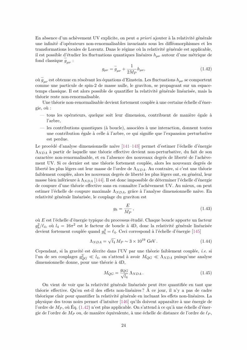
la brane mère . . . . . . . . . . . . . . . . . . . . . . . . . . . . . . . . . . . 412.11 Quasi-localisation des fermions dans une brane épaisse . . . . . . . . . . . . 422.12 Un monde unidimensionnel qui se répète tous les 2πR . . . . . . . . . . . . 432.13 Domaine fondamental . . . . . . . . . . . . . . . . . . . . . . . . . . . . . . 432.14 Orbifold R/Z2 . . . . . . . . . . . . . . . . . . . . . . . . . . . . . . . . . . . 452.15 Orbifold S1/Z2 . . . . . . . . . . . . . . . . . . . . . . . . . . . . . . . . . . 462.16 Univers branaire . . . . . . . . . . . . . . . . . . . . . . . . . . . . . . . . . 472.17 Paramétrisation de la position de la brane dans le bulk . . . . . . . . . . . . 492.18 Lignes du champ gravitationnel dans les modèles d’ADD . . . . . . . . . . . 502.19 Émission d’un graviton dans le bulk . . . . . . . . . . . . . . . . . . . . . . 542.20 Modèle de RS1 . . . . . . . . . . . . . . . . . . . . . . . . . . . . . . . . . . 56

3.1 Bosons de jauge et fermions dans une tranche AdS5 . . . . . . . . . . . . . . 613.2 Quasi-localisation d’un mode zéro fermionique . . . . . . . . . . . . . . . . . 653.3 Identification des spineurs de Weyl du SM avec les modes zéro des spineurs

de Dirac 5D . . . . . . . . . . . . . . . . . . . . . . . . . . . . . . . . . . . . 663.4 Graphique du rapport des couplages g(n)/g en fonction de c . . . . . . . . . 713.5 Contraintes sur mKK provenant de la mesure de ggh . . . . . . . . . . . . . 743.6 Correspondance AdS/CFT . . . . . . . . . . . . . . . . . . . . . . . . . . . . 75

7

3.7 Tranche AdS5 . . . . . . . . . . . . . . . . . . . . . . . . . . . . . . . . . . . 763.8 Dictionnaire AdS/CFT . . . . . . . . . . . . . . . . . . . . . . . . . . . . . . 773.9 Gorge de Klebanov-Strassler collée à un espace de Calabi-Yau . . . . . . . . 793.10 Gorges multiples . . . . . . . . . . . . . . . . . . . . . . . . . . . . . . . . . 80

4.1 Free KK wave functions of the 5D fields Q and D. . . . . . . . . . . . . . . 954.2 Inverse pyramidal picture of the method . . . . . . . . . . . . . . . . . . . . 964.3 KK wave functions of the 5D fields Q and D with Yukawa couplings. . . . 109

5.1 KK wave functions of the 5D fields Q and D with Yukawa couplings alongthe orbifold S1/Z2. . . . . . . . . . . . . . . . . . . . . . . . . . . . . . . . 139

5.2 Orbifold S1/ (Z2 × Z′2) . . . . . . . . . . . . . . . . . . . . . . . . . . . . . . 1435.3 KK wave functions of the 5D fields Q and D with Yukawa couplings along

the orbifold S1/(Z2 × Z′2). . . . . . . . . . . . . . . . . . . . . . . . . . . . 146

6.1 Plot of R/`(4+q)P as a function of q for Λ(4+q)

P = 1 TeV . . . . . . . . . . . . 1526.2 5-star and 5-rose . . . . . . . . . . . . . . . . . . . . . . . . . . . . . . . . . 156

8

List of Tables

4.1 Summary of the results of the 4D and 5D approaches . . . . . . . . . . . . . 114

5.1 Table of different identifications of the Lagrangian at points related by anisometry of the compact space. . . . . . . . . . . . . . . . . . . . . . . . . . 131

5.2 Fermionic fields Q and D on the orbifold S1/Z2. . . . . . . . . . . . . . . . 142

6.1 R, R/`(4+q)P and MKK as a function of q for Λ(4+q)

P = 1 TeV . . . . . . . . . 151

9

Introduction

The Standard Model (SM) of particle physics [3], based on Quantum Field Theory(QFT) [4–6], is well established nowadays, thanks to an undeniable experimental suc-cess. All its elementary particle content is discovered, and their properties are in goodaccordance with the theoretical predictions [7].

In particular, the ElectroWeak (EW) sector is described by the Glashow-Salam-Weinberg(GSW) model [8–10], based on the spontaneous symmetry breaking of a gauge theory. Forthat propose, one uses the Brout-Englert-Guralnik-Hagen-Higgs-Kibble mechanism [11–16] where a weakly coupled scalar field acquires a Vacuum Expectation Value (VEV). Thefluctuations of the field around its VEV describe a spin 0 particle, the Higgs boson. Itis an elementary scalar field which is not protected by a symmetry: its mass squared isquadratically sensitive to every new mass scale above ΛEW ∼ 100 GeV [17–19], so such alight scalar is not technically natural. In the modern Effective Field Theory (EFT) pointof view, when an UltraViolet (UV) theory contains an unprotected elementary scalar ofmass m in addition to particles at a mass scale M > m, once one integrates out theparticles of mass M , one needs to fine tune the parameters m and M of the UV theory tohave a light scalar in the spectrum of the EFT (see Ref. [20] for more details). In the caseof the Higgs boson of mass mh ' 125 GeV, if a new mass scale exists above O(1) TeV,then there is a fine tuning in the UV theory. There are several motivations to believe thatnew scales exist well above ΛEW :

First of all, the SM does not gives a description of gravity which includes a backreac-tion of matter and energy on the spacetime geometry in general relativity [21]. However,Einstein’s theory is classical and is not able to describe the quantum fluctuations of space-time. When one considers small fluctuations around a background metric, one gets a fieldof spin 2 particles, the gravitons, propagating on a 4D classical background. One canquantize the gravitons coupled to the SM as a non-perturbatively renormalizable QFT.Nevertheless, near the 4D Planck scale Λ(4)

P ' 2.4× 1018 GeV, one cannot consider smallquantum fluctuations around a classical metric any more: one needs a new theory of quan-tum spacetime geometry. It is expected that new degrees of freedom appear in the UVcompletion near ΛP which contribute via loop corrections to mh and induce an incrediblefine tuning to have this Higgs boson light.

Besides, in particle physics, one observes oscillations of neutrinos which implies thatat least two of them are massive. In the SM, neutrinos are massless so one needs to addnew physics to give them a mass. In the fermion sector of the SM, one observes a largemass hierarchy between the neutrino mass scale and the top mass (see Fig. 1.1). Manyhigh energy theoreticians suspect that this hierarchy could be the result of an unknownmechanism at high scale, which could also explain the particular texture of the mixingmatrices in the quark and neutrino sectors and the origin of the three fermion genera-tions. Besides, the absence of CP violation in strong interactions described by QuantumChromoDynamics (QCD) [22–26], is also a natural question since a CP violating topo-

10

logical term is authorized by the symmetries of the SM. Moreover, the SM of cosmology(ΛCDM) needs additional ingredients which are not present in the SM of particle physics:a Cold Dark Matter (CDM) sector 1, an inflaton sector, and a new CP violating sectorfor the baryogenesis. Beyond ΛCDM, if the role of dark energy is not entirely played bythe cosmological constant Λ, one needs to introduce a new exotic ingredient to explainthe observed accelerated expansion of the Universe. In the abundant literature concerningBeyond Standard Model (BSM) physics, many models whose goal is to solve one of thesequestions require a new mass scale above ΛEW . The naturalness of the EW scale, alsocalled gauge hierarchy problem, is thus a serious problem which needs to be explained bysome BSM scenario.

In QFT, spacetime is a classical background where fields propagate. In general relativ-ity, spacetime is dynamic and the theory describes how classical sources backreact on thegeometry. In both theories, the number of spacetime dimensions is not determined by firstprinciples. Possibly, in a complete theory of gravity which describes Planckian physics, thedimensionality of spacetime can be determined by the dynamics or the consistency of thetheory as in string theory [27]. In absence of a particular UV completion of gravity, oneis free to build models adding an arbitrary number of spacetime dimensions compactifiedon some geometries with a given topology. The criteria are that one should be consistentwith all the observations indicating that our Universe appears four-dimensional in currentexperiments. A higher-dimensional field theory with compactified extra dimensions can berewritten as a 4D theory by a procedure which is called Kaluza-Klein (KK) dimensionalreduction. A higher-dimensional field gives a tower of 4D fields: the KK modes. On theone hand, compactified timelike extra dimensions seem to lead to physically inconsistenttheories because the KK excitations of the fields propagating in the extra dimensionsare tachyons, which imply violation of physically reasonable conditions like causality andunitarity [28, 29]. On the other hand, spacelike extra dimensions have a long history infundamental physics, since the pioneer works by G. Nordström [30], T. Kaluza [31] andO. Klein [32, 33], because they allow to build consistent EFTs. They are the subject ofthe present PhD thesis where we will consider only one timelike dimension. The beginningof the new millenium was marked by an explosion of the number of scientific publicationson the subject of spacelike extra dimension after the appearance of some key articles withthe goal of solving the gauge hierarchy problem for some of them.

The scenario proposed by Arkani-Hamed, Dimopoulos and Dvali (ADD) [34–36], withcompactified Large Extra Dimensions (LEDs) and the SM fields localized on a 3D wall (3-brane), allows to have a higher-dimensional Planck scale at a few TeV. The 4D Planck scaleΛ(4)P is just an effective scale which is not related to masses of new degrees of freedom. This

model allows also to generate small Dirac masses for the neutrinos where the right-handedneutrinos are KK modes of a gauge singlet field propagating into the whole spactime(the bulk) [37–39]. In the simplest version with toroidal compactification, and with lessthan seven LEDs motivated by superstring/M theory, the compactification radii are largecompared to the higher-dimensional Planck length: the gauge hierarchy disappears at theprice of introducing a geometrical hierarchy to stabilize. The ADD proposition is thusjust a reformulation of the gauge hierarchy problem instead of a solution of it.

The most popular way to overcome the ADD geometrical hierarchy problem is to use asingle warped extra dimension as proposed by Randall and Sundrum [40]: the RS1 model.The SM fields are localized at the boundary of a slice of an AdS5 spacetime where the warpfactor redshifts the scale at which gravity becomes strongly coupled from 1018 GeV to theTeV scale. Quickly, it was realized that only the Higgs field needs to be localized at the

1. Notice that warm dark matter is also possible.

11

boundary and that gauge bosons and fermions can propagate into the bulk [41–46]. Thezero modes of the fields are identified with the SM particles. The fermion zero modes canbe localized near one of the two boundaries thanks to 5D Dirac masses. The wave functionof a heavy (light) SM fermion has then a big (small) overlap with the boundary localizedHiggs field. Without hierarchies in the 5D masses and Yukawa couplings, one can generatethe flavor hierarchy observed in Nature [45, 47]. In order to study the phenomenology ofthis model, it is then crucial to have a field theoretical treatment of 5D fermions in anextra dimension with spacetime boundaries which can accommodate couplings to a branelocalized Higgs field.

Most of the authors use a perturbative approach [48, 49], which we call 4D approach,where the KK spectrum and wave functions of the 5D fermion fields are worked out withoutthe brane localized interactions. They use ad hoc Dirichlet boundary conditions on thewave functions of one of the two chiralities of the KK modes in order to have a chiraltheory at the zero mode level. After that, they treat the Yukawa interactions with thebrane localized Higgs field VEV as a perturbation by truncating the KK tower and bi-diagonalize the mass matrix. An alternative method is to treat directly the brane localizedmass terms when one solves the equations for the wave functions: the 5D method. Manyauthors were puzzled by an apparent discontinuity in the KK wave functions at the Higgsfield position, and they introduce a regularization method by smoothing or shifting awayfrom the boundary the brane localized Higgs boson [49–61]. It seems puzzling that onecannot treat the Higgs boson at the boundary without this regularization procedure.

In this thesis, we begin by developping a consistent field theoretical method to treat5D fermions coupled to a brane localized Higgs field without regularization [1]. For thatpurpose, we have to introduce Henningson-Sfetsos boundary terms [1, 62–68] at both sidesof a brane. One can then solve the problem treating fields as functions or distributions.After that, we apply different methods (function/distribution fields, 4D/5D calculations,etc) to various brane localized terms (kinetic terms, Majorana masses, etc), as well asgeneralizing to several classified models (flat/warped dimensions, intervalle/orbifold, etc).

The end of the PhD is dedicated to revisit the LED possibility by compactifying anextra dimension on a star/rose graph with N � 1 identical leaves/petals of length/circum-ference ` [69]. The SM fields are localized on a 3-brane at the central vertex of the graph.One can then have a 5D Planck scale at a few TeV and choose for example ` ∼ 1/ΛEW .The large hierarchy between the 4D Planck scale Λ(4)

P and ΛEW is then reformulated as alarge N . As N is a radiatively stable quantity fixed by the spacetime geometry, which isjust a classical brackground for the EFT, this solves the technical naturalness problem ofthe Higgs boson massmh. The question of why N is very large is postponed until a Planck-ian theory of gravity. Subsequently, we use our previous results on 5D fermions to builda model of small neutrino masses, where the right-handed neutrinos are the KK modesof a gauge singlet fermion propagating into the LED and coupled to the 4D left-handedneutrino through the 4D Higgs field, both localized at the central vertex.

The manuscript of this PhD thesis entitled “Compactified Spacelike Extra Dimension& Brane Localized Higgs Field” is organized as follows:— Part I is written in French and gives the state of the art of the most popular models

with spacelike extra dimensions whose purpose is to tackle the gauge and/or flavorhierarchies problems:— Chapter 1 is a short review of the SM of particle physics and of the motivations

for BSM model buildings, insisting on the gauge hierarchy problem.— Chapter 2 is a review of the historical models with spacelike extra dimensions

12

and in particular the ones which solve or reformulate the gauge hierarchy prob-lem.

— Chapter 3 is an introduction to the models with the SM Higgs field localizedat the boundary of a slice of an AdS5 spacetime with bulk fermion and gaugefields.

— Part II contains the main research work made during this PhD thesis:— Chapter 4 describes the method to treat 5D fermions coupled to a boundary

localized Higgs field with a compactification on an interval.— Chapter 5 contains a generalization of the method of Chapter 4 towards a

compactification on 5D orbifolds, to a Higgs field localized on a brane awayfrom a boundary, and to other brane localized terms.

— Chapter 6 describes our model of LED compactified on a star/rose graph witha large number of weak scale leaves.

— Our conventions are given in Appendix A.— A summary in French of the chapters in English is given in Appendix D.— The acronyms used in this manuscript are listed in a Glossary p. 209.

13

Part I

State of the Art

14

Chapitre 1

Du champ de Higgs électrofaible àla hiérarchie de jauge

1.1 Modèle standard de la physique des particules

Figure 1.1 – (Adaptée de la Réf. [70].) Vue schématique du modèle standard de la physiquedes particules après brisure de symétrie EW.

Le SM de la physique des particules décrit les particules élémentaires de la matièreet leurs interactions. Il est construit dans le cadre de la QFT 1 sur une théorie de jaugerenormalisable [86–88] et unitaire [89–92] décrivant les interactions EW et fortes.

La théorie GSW des interactions EWs [8–10] décrit les interactions électromagnétiques[93–97] et faibles [98–100] entre les quarks et les leptons. C’est une théorie de Yang-Mills

1. Pour une revue sur le SM de la physique des particules et la QFT, voir par exemple les Réfs. [4–6, 71–85].

15

[101] basée sur les groupes de symétrie d’isospin SU(2)W et d’hypercharge U(1)Y faibles.Ajoutée à la chromodynamique quantique (QCD – Quantum ChromoDynamics) [22–26],la théorie de l’interaction forte entre les quarks colorés fondée sur le groupe de jaugeSU(3)C , on obtient une description unifiée des interactions subatomiques. Le SM contienttrois types de champs : les fermions, les bosons de jauge et le boson de Higgs (c.f. laFig. 1.1).

1.1.1 Zoologie des fermions

Les champs de matière sont des fermions de spin 1/2 dans la représentation fondamen-tale du groupe de jauge SU(3)C ×SU(2)W ×U(1)Y . Il y a trois générations séquentielles,i.e. trois répliques ayant les mêmes nombres quantiques mais de masses différentes. Lesfermions de chiralité gauche sont des isodoublets faibles 2 : T 3(f) = ±1/2 (la troisièmecomposante d’isospin faible). On distingue les leptons :

L1 =(νee−

)L

, L2 =(νµµ−

)L

, L3 =(νττ−

)L

,

et les quarks :

Q1 =(ud

)L

, L2 =(cs

)L

, L3 =(tb

)L

,

où on a utilisé les notations de la Fig. 1.1. Les fermions de chiralité droite sont des isosin-gulets faibles : T 3(f) = 0. Il y en a un pour chaque élément des isodoublets, sauf pour lesneutrinos 3 :

e1R = e−R, e2R = µ−R, e3R = τ−R ,

u1R = uR, u2R = cR, u3R = tR,

d1R = dR, d2R = sR, d3R = bR.

L’hypercharge faible est définie à partir de T 3(f) et de la charge électrique Q(f) (en unitéde charge électrique élémentaire +e) :

Y (f) = 2[Q(f)− T 3(f)

], (1.1)

Y (Li) = −1, Y (eiR) = −2, Y (Qi) = 13 , Y (uiR) = 4

3 , Y (diR) = −23 . (1.2)

La théorie GSW assigne donc les fermions de chiralité gauche et droite à des représentationsdifférentes de SU(2)W × U(1)Y : on parle de théorie chirale, par opposition à une théorievectorielle comme la QCD. En effet, les deux chiralités de quarks (leptons) sont des triplets(singulets) de couleur sous SU(3)C . On notera la relation :∑

ψ

Y (ψ) =∑ψ

Q(ψ) = 0, (1.3)

où on somme sur tous les champs d’une génération de fermions (chaque couleur étantcomptée comme un champ différent). Ceci assure l’annulation des anomalies chirales [104,105] pour chaque génération, préservant ainsi les symétries de jauge au niveau quantique(dans les diagrammes à boucle).

2. On note d’ailleurs plus communément le groupe de jauge d’isospin faible SU(2)L plutôt que SU(2)W .Cependant, dans le cadre de modèles avec des fermions se propageant dans des dimensions spatiales sup-plémentaires, des quarks vectoriels apparaissent, dont la chiralité droite est un isodoublet de SU(2)L, cequi peut prêter à confusion.

3. On sait aujourd’hui que les neutrinos sont des particules massives via le phénomène d’oscillation.Pour générer cette masse, il est souvent nécessaire d’ajouter des neutrinos de chiralité droite (c.f. lesRéfs. [102, 103], par exemple, pour une revue). Dans le SM, les neutrinos sont considérés sans masse.

16

1.1.2 Zoologie des bosons de jauge

Les champs de jauge décrivent des bosons de spin-1, médiateurs des interactions. Lenombre de bosons par interaction est égal au nombre de générateurs des groupes de sy-métrie associés.

Dans le secteur EW, on a les champs Bµ et W 1,2,3µ , correspondants respectivement aux

générateurs Y et T a (a = 1, 2, 3) des groupes U(1)Y et SU(2)W . Les générateurs T a sontreliés aux matrices de Pauli tels que

T a = σa

2 , (1.4)

vérifiantTr(σaσb) = 2δab. (1.5)

Les relations de commutation entre générateurs sont :

[T a, T b] = εabcTc et [Y, Y ] = 0, (1.6)

où εabc est le tenseur de Levi-Civita totalement antisymétrique.Dans le secteur de l’interaction nucléaire forte, on a un octet de gluons G1,...,8 associés

aux huit générateurs du groupe SU(3)C , dont les relations de commutation sont :[λA

2 ,λB

2

]= ifABC

λC

2 , (1.7)

avec les matrices de Gell-Mann (A = 1, . . . , 8) :

λ1 =

0 1 01 0 00 0 0

, λ2 =

0 −i 0i 0 00 0 0

, λ3 =

1 0 00 −1 00 0 0

,

λ4 =

0 0 10 0 01 0 0

, λ5 =

0 0 −i0 0 0i 0 0

, λ6 =

0 0 00 0 10 1 0

,

λ7 =

0 0 00 0 −i0 i 0

, λ8 = 1√3

1 0 00 1 00 0 −2

, (1.8)

vérifiantTr(λAλB) = 2δAB. (1.9)

Les constantes de structure non-nulles de SU(3)C sont :

f123 = 1,

f147 = −f156 = f246 = f257 = f345 = −f367 = 12 , (1.10)

f458 = f678 =√

32 .

17

Les tenseurs des champs pour chaque interaction s’écrivent :

Bµν = ∂µBν − ∂νBµ,

W aµν = ∂µW

aν − ∂νW a

µ + gw εabcWbµW

cν , (1.11)

GAµν = ∂µGAν − ∂νGAµ + gc fABCG

BµG

Cν ,

où gc, gw et gy sont respectivement les constantes de couplage des groupes SU(3)C ,SU(2)W et U(1)Y . On remarquera la présence des constantes de structures dans l’expres-sion des tenseurs de champs associés aux groupes de jauge non-abéliens. Cela se traduitphysiquement par une auto-interaction des gluons et bosons W , i.e. des couplages tripleset quartiques dans les lagrangiens.

Un champ fermionique ψ est couplé de manière minimale aux champs de jauge par ladérivée covariante :

Dµψ =(∂µ − igc

λA

2 GAµ − igwσa

2 Waµ − igyY (ψ)

2 Bµ

)ψ. (1.12)

Dans une théorie de Yang-Mills, imposer l’invariance d’un lagrangien de Dirac sous unesymétrie de jauge entraine de manière automatique le couplage du fermion au(x) boson(s)de jauge.

Le lagrangien du SM, invariant sous SU(3)C × SU(2)W × U(1)Y , que l’on peut écrireà ce stade, est :

LSM = −14G

AµνG

µνA −

14W

aµνW

µνa −

14BµνB

µν

(1.13)

+ iL†iDµσµLi + ie†iRDµσ

µeiR + iQ†iDµσµQi + iu†iRDµσ

µuiR + id†iRDµσµdiR,

où toutes les particules sont de masses nulles, ce qui est correct pour les gluons. Enrevanche, on mesure une masse non-nulle pour les fermions et les bosons de l’interactionfaible. De tels termes de masse correspondent à :

12m

2WW

aµW

µa et 1

2m2BBµB

µ (1.14)

pour les bosons de jauge EWs, et

−mψψψ = −mψ

(ψ†RψL + ψ†LψR

)(1.15)

pour un fermion ψ. Or, si on écrit les transformations des champs sont le groupe SU(2)L×U(1)Y , on obtient

ψL(x) 7→ exp(iαa(x)σ

a

2 + iβ(x)Y (ψ))ψL(x)

ψR(x) 7→ exp (iβ(x)Y (ψ))ψR(x)(1.16)

−→Wµ(x) 7→

−→Wµ(x)− 1

gw∂µ−→α (x)−

−→α (x)×

−→Wµ(x)

Bµ(x) 7→ Bµ(x)− 1gy∂µβ(x).

18

On en conclut que les termes de masses dans les Éqs. (1.14) et (1.15) sont manifestementnon-invariants sous ces transformations : de tels termes sont interdits dans une théorie dejauge. Il faut donc rajouter un ingrédient au modèle.

1.1.3 Champ de Higgs

Afin de donner une masse aux fermions et bosons de l’interaction faible, le SM a recourtau mécanisme de Brout-Englert-Guralnik-Hagen-Higgs-Kibble (plus communément appelémécanisme de Higgs) de brisure spontanée de symétrie [11–16]. Le but est de générer unemasse pour les bosons W± et Z, tout en préservant une masse nulle pour le photon. Pourcela, on introduit un isodoublet faible de champs scalaires complexes

H =(H+

H0

), Y (H) = 1, (1.17)

tel que sa composante électriquement neutre H0 développe une VEV non-nulle. Le poten-tiel scalaire V (H) dans le lagrangien

LH = (DµH)†(DµH)− V (H), V (H) = µ2H†H + λ(H†H)2, (1.18)

doit alors avoir une instabilité tachyonique µ2 < 0 et être stabilisé par un terme quartiqueλ(H†H)2 avec λ > 0. Ainsi, le minimum du potentiel est obtenu pour (c.f. la Fig. 1.2)

〈 0 |H| 0 〉 = 1√2

(0v

)avec v =

√−µ

2

λ. (1.19)

Si on prend à la place µ2 > 0, λ > 0 alors 〈 0 |H| 0 〉 = 0 (c.f. la Fig. 1.2) et on asimplement le lagrangien de Klein-Gordon ordinaire d’une particule de spin-0 avec unterme d’interaction quartique. Notons au passage que le cas µ2 < 0, λ < 0 correspond àun potentiel tachyonique, et donc non-physique, et que si µ2 > 0, λ < 0 alors 〈 0 |H| 0 〉 = 0est un minimum métastable qui peut se désintégrer en un vide tachyonique.

Figure 1.2 – (Adaptée de la Réf. [106].) Schéma du potentiel V (φ) d’un champ scalairecomplexe φ brisant (à droite) ou non (à gauche) une symétrie de jauge U(1), selon le signedu terme de masse µ2. Dans le cas de la brisure de symétrie, les fluctuations le long ducercle de minima correspondent au boson de Nambu-Goldstone absorbé par le boson dejauge, qui obtient ainsi sa masse. Les fluctuations, dans la direction radiale du potentiel,décrivent une particule de spin-0 massive : le boson de Higgs.

19

En revenant au premier cas qui nous intéresse, la composante chargée H+ ne doit pasacquérir de VEV afin de préserver la symétrie de jauge U(1)EM à l’origine de l’interactionélectromagnétique. Le champ H(x) peut alors s’écrire, au premier ordre, en fonction dequatre champs θ1,2,3(x) et h(x) :

H(x) =

θ2(x) + iθ1(x)1√2

(v + h(x))− iθ3(x)

= 1√2

exp(iθa(x)v

σa

2

)( 0v + h(x)

). (1.20)

On peut alors effectuer une transformation de jauge sous SU(2)W , afin de se placer dansla jauge dite unitaire, telle que

H(x) 7→ exp(−iθa(x)

v

σa

2

)H(x) = 1√

2

(0

v + h(x)

). (1.21)

En écrivant cette expression de H(x) dans le lagrangien (1.18), on obtient :

|(DµH)|2 = 12(∂µh)2 + g2

w

8 (v + h)2|W 1µ + iW 2

µ |2 + 18(v + h)2|gwW 3

µ − gyBµ|2. (1.22)

Définissons les champs W±µ , Zµ, Aµ des bosons W±, Z et du photon :

W± = 1√2

(W 1µ ∓ iW 2

µ),

Zµ = 1√g2w + g2

y

(gwW 3µ − gyBµ), (1.23)

Aµ = 1√g2w + g2

y

(gwW 3µ + gyBµ),

que l’on peut écrire sous forme matricielle :(ZµAµ

)=(

cos θw − sin θwsin θw cos θw

)(W 3µ

Bµ

), (1.24)

en introduisant l’angle de mélange faible θw, tel que

cos θw = gw√g2w + g2

y

, sin θw = gy√g2w + g2

y

. (1.25)

Les termes de masse dans Éq. (1.22) deviennent

m2WW

+µ W

−µ + 12m

2ZZµZ

µ + 12m

2AAµA

µ (1.26)

avecmW = v

2gw, mZ = v

2

√g2w + g2

y , mA = 0. (1.27)

À la fin, on obtient bien que les trois bosons de l’interaction faible sont massifs et quele photon reste sans masse : c’est la brisure spontanée de symétrie SU(2)W × U(1)Y →U(1)EM . En fait, trois des quatre degrés de liberté de l’isodoubletH (les bosons de Nambu-Goldstone [107–111]) sont absorbés par les bosons W± et Z qui acquièrent, de ce fait, une

20

polarisation longitudinale, et donc une masse. Le degré de liberté restant, h(x), décritune particule massive de spin-0 : le boson de Higgs, qui constitue ainsi la signature dumécanisme éponyme. En faisant la correspondance entre la théorie GSW et celle de Fermi,on peut relier la masse des bosons W± à la constante de Fermi GF , ce qui permet dedériver la valeur de la VEV dans le SM :

MW = v

2gw =

√√2g2w

8GF⇒ v =

√1√

2GF' 246 GeV, (1.28)

qui définit l’échelle EW.Après brisure de symétrie EW (EWSB – ElectroWeak Symmetry Breaking), on peut

écrire la dérivée covariante en fonction des états propres de masse. Introduisons les ma-trices :

σ± = 12(σ1 ± iσ2). (1.29)

Pour un fermion ψ, on a :

Dµψ =(∂µ − i

gw√2

[W+µ σ

+ +W−µ σ−]− i gw

cos θwZµ[T 3(ψ)− sin2 θw Q(ψ)

]−ieAµ Q(ψ))ψ, (1.30)

où on a défini la charge électrique :

e = gwgy√g2w + g2

y

= gw sin θw. (1.31)

Le mécanisme de Higgs permet aussi de générer les masses des fermions du SM. Pourune génération, on introduit le lagrangien

LHψ = −yeL†HeR − ydQ†HdR − yuQ†HuR + c.h., (1.32)

invariant sous SU(2)W×U(1)Y , où H = iσ2H∗ avec Y (H) = −1. Dans le cas de l’électron,on a par exemple :

LHe = − ye√2

(v + h)e†LeR + . . . . (1.33)

Le couplage à la VEV constitue un terme de masse, on obtient :

me = v√2ye, mu = v√

2yu, md = v√

2yd. (1.34)

Dans le cas de trois générations, on peut écrire des couplages de Yukawa impliquant deuxfermions de générations différentes. Ceci induit des mélanges de saveur dans le secteur desquarks. La matrice, permettant de passer des états propres de l’interaction faible (avec« ’ ») aux états propres de masse (sans « ’ »), est celle de Cabibbo-Kobayashi-Maskawa(CKM) [112, 113] : d′s′

b′

=

Vud Vus VubVcd Vcs VcbVtd Vts Vtb

dsb

, (1.35)

dont les éléments sont en général complexes. On peut absorber certaines phases en redé-finissant les champs de quarks. Au final, il en reste une : la phase de violation de CP , quivient s’ajouter aux trois angles de mélange.

21

Venons en maintenant au boson de Higgs lui-même. En développant H autour de saVEV dans l’Éq. (1.18), et en ne gardant que les termes impliquant h seul, on a :

Lh = 12(∂µh)2 − λv2h2 − λvh3 − λ

4h4, (1.36)

d’où on lit la masse du boson de Higgs :

mh =√

2λv =√

2iµ, (1.37)

en rappelant que µ est imaginaire pur dans nos conventions. On notera la présence descouplages triple et quartique de h. Quant aux termes couplant ce dernier aux bosons dejauge de l’interaction faible (V = W±, Z) et aux fermions, ils donnent

m2V

(1 + h

v

)2, −mψ

(1 + h

v

). (1.38)

Les règles de Feynman, pour le boson de Higgs, sont répertoriées sur la Fig. 1.3.

Figure 1.3 – (Adaptée de la Réf. [114].) Règles de Feynman impliquant le boson de Higgsdans le SM de la physique des particules.

1.2 Au-delà du modèle standard de la physique des parti-cules

Dans cette section, nous allons rapidement passer en revue les principales motivationspour élargir le SM et construire une théorie plus fondamentale des interactions entre lesparticules élémentaires.

22

1.2.1 Lacunes du modèle standard

Masses des neutrinos

L’observation des oscillations des trois saveurs de neutrinos connues implique qu’aumoins deux d’entre eux aient une masse [115]. Or, de tels termes de masse n’existent pasdans le SM. De nombreux mécanismes ont été proposés, impliquant souvent de nouvelleséchelles physiques à haute énergie. La solution la plus naturelle, du point de vue du SM,serait d’ajouter deux ou trois champs de neutrinos de chiralité droite, singulets sous legroupe de jauge du SM, pour pouvoir écrire des termes de Yukawa (impliquant les neutri-nos de chiralité droite, le champ de Higgs et les isodoublets faibles contenant les neutrinosde chiralité gauche) qui seraient à l’origine des termes de masse pour les neutrinos aprèsEWSB. Il est alors possible d’ajouter des termes de masse de Majorana pour les neutrinosdroits, puisqu’ils sont invariants sous le groupe de jauge du SM et renormalisables. Dansce cas, les neutrinos seraient des particules de Majorana. Le fait que les neutrinos soientdes fermions de Majorana ou de Dirac reste aujourd’hui une question ouverte en physiquedes particules.

Interaction gravitationnelle

La relativité générale 4 d’Einstein [122–130] est la théorie de l’espace, du temps et de lagravitation. C’est l’outil central pour comprendre les phénomènes astrophysiques extrêmescomme les trous noirs, les pulsars, les quasars, la fin de vie d’une étoile, la naissance etl’évolution de l’Univers. La relativité générale est une théorie classique, qui n’est pasmiscible avec le SM : la gravité est la seule interaction fondamentale connue qui n’a pasencore de formulation quantique achevée, principalement parce qu’une quantification naïveaboutit à une théorie qui n’est pas perturbativement renormalisable. La relativité généraleest donc une théorie effective des champs 5 (EFT – Effective Field Theory) qui cesse d’êtrevalide à une certaine échelle d’énergie de coupure 6 MQG, correspondant à l’échelle demasse des degrés de liberté UVs les plus légers de la gravité.

La relativité générale a une formulation lagrangienne : l’action d’Einstein-Hilbert, in-variante sous les difféomorphismes et les transformations locales de Lorentz, s’écrit :

SEH =∫d4x

√|g|(−M

2P

2 R− Λc + LSM

), (1.39)

où g est le déterminant de la métrique gµν , R est la courbure scalaire de Ricci, Λc est laconstante cosmologique, LSM est le lagrangien du SM, et MP est la masse de Planck 7,

MP =√

18πGN

' 2, 4× 1018 GeV, (1.40)

où GN est la constante de Newton. On définit aussi la longueur de Planck,

`P = 1MP

' 8, 0× 10−35 m . (1.41)

4. Voir les Réfs. [21, 116–121], par exemple, pour une revue.5. Pour une revue introduisant le concept d’EFT, c.f. les Réfs. [131–137]6. Les revues [138–140] donnent une introduction à l’étude de la gravité basée sur les EFTs.7. La définition de MP adoptée ici est généralement celle de la masse de Planck réduite. Il y a de

nombreuses définitions de la masse de Planck dans la littérature, la plus commune diffère de la notre parun facteur

√8π.

23

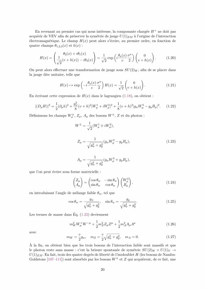
En absence d’un achèvement UV explicite, on peut a priori ajouter à la relativité généraleune infinité d’opérateurs non-renormalisables invariants sous les difféomorphismes et lestransformations locales de Lorentz. Dans le régime où la relativité générale est applicable,il est possible d’étudier les fluctuations quantiques linéaires hµν autour d’une métrique defond classique gµν :

gµν = gµν + 12MP

hµν , (1.42)

où gµν est obtenue en résolvant les équations d’Einstein. Les fluctuations hµν se comportentcomme une particule de spin-2 de masse nulle, le graviton, se propageant sur un espace-temps classique. Il est alors possible de quantifier la relativité générale linéarisée, mais lathéorie reste non-renormalisable.

Une théorie non-renormalisable devient fortement couplée à une certaine échelle d’éner-gie, où :— tous les opérateurs, quelque soit leur dimension, contribuent de manière égale à

l’arbre,— les contributions quantiques (à boucle), associées à une interaction, donnent toutes

une contribution égale à celle à l’arbre, ce qui signifie que l’expansion perturbativeest perdue.

Le procédé d’analyse dimensionnelle naïve [141–143] permet d’estimer l’échelle d’énergieΛNDA à partir de laquelle une théorie effective devient non-perturbative, du fait de soncaractère non-renormalisable, et en l’absence des nouveaux degrés de liberté de l’achève-ment UV. Si ce dernier est une théorie fortement couplée, alors les nouveaux degrés deliberté les plus légers ont leur masse de l’ordre de ΛNDA. Au contraire, si c’est une théoriefaiblement couplée, alors les nouveaux degrés de liberté les plus légers ont, en général, leurmasse bien inférieure à ΛNDA [144]. Il est donc impossible de déterminer l’échelle d’énergiede coupure d’une théorie effective sans en connaître l’achèvement UV. Au mieux, on peutestimer l’échelle de coupure maximale ΛNDA, grâce à l’analyse dimensionnelle naïve. Enrelativité générale linéarisée, le couplage du graviton est

gh = E

MP, (1.43)

où E est l’échelle d’énergie typique du processus étudié. Chaque boucle apporte un facteurg2h/`4, où l4 = 16π2 est le facteur de boucle à 4D, donc la relativité générale linéariséedevient fortement couplée quand g2

h = `4. Ceci correspond à l’échelle d’énergie [145]

ΛNDA =√l4MP ∼ 3× 1019 GeV . (1.44)

Cependant, si la gravité est décrite dans l’UV par une théorie faiblement couplée, i.e. sil’un de ses couplages g2

QG � l4, on s’attend à avoir MQG � ΛNDA puisqu’une analysedimensionnelle donne, pour une théorie à 4D,

MQG = gQG√l4

ΛNDA . (1.45)

On vient de voir que la relativité générale linéarisée peut être quantifiée en tant quethéorie effective. Qu’en est-il des effets non-linéaires ? À ce jour, il n’y a pas de cadrethéorique clair pour quantifier la relativité générale en incluant les effets non-linéaires. Laphysique des trous noirs permet d’intuiter [146] qu’ils doivent apparaître à une énergie del’ordre deMP , où Éq. (1.42) n’est plus applicable. On s’attend à ce qu’à une échelle d’éner-gie de l’ordre deMP ou, de manière équivalente, à une échelle de distance de l’ordre de `P ,

24

les effets de gravité non-linéaires et non-perturbatifs deviennent dominants. En s’inspirantde l’étude de la théorie de la gravité quantique euclidienne [147], on peut imaginer, de ma-nière très spéculative, que l’espace-temps quantique est une « mousse » [148, 149] de trousnoirs, trous de ver, bébés univers, instantons gravitationnels, et autres objets exotiques(c.f. la Fig. 1.4), dont le cadre théorique cohérent, notamment l’achèvement UV, restelargement à construire (c.f. la Réf. [150] pour une revue récente). Comme MP < ΛNDA,MQG . MP . Si MQG � MP , les degrés de liberté UV de la gravité, même faiblementcouplés, peuvent altérer significativement le comportement UV de la gravité, notammentl’échelle à laquelle les effets non-linéaires deviennent importants, qui peut être très diffé-rente de celle spéculée à partir de la relativité générale.

Figure 1.4 – (Adaptée de la Réf. [151].) Vue d’artiste de l’espace-temps à l’échelle dePlanck, dominé par des effets gravitationnels non-perturbatifs. On peut imaginer quel’espace-temps est alors une « mousse » de trous noirs, trous de ver, bébés univers etinstantons gravitationnels.

Encore aujourd’hui, beaucoup de physiciens admettent le « paradigme standard », quirepose sur deux hypothèses fortes [152] :— MQG ∼ MP , la théorie UV de la gravité est alors fortement couplée. Dans ce cas,

rien ne se passe concernant la gravité entre l’échelle du TeV, actuellement scrutéeau LHC, et MP (c.f. la Fig. 1.5).

— MQG est supposée être aussi l’énergie de coupure des modèles de physique des par-ticules décrivant les interactions fondamentales dans le cadre de la QFT (le SM etses extensions).

Le « désert » physique entre l’échelle EW et MP , qui en résulte, est appelé la hiérarchiede jauge. Souvent, on inclut dans le paradigme standard la solution la plus populaire à ceque l’on appelle le problème de hiérarchie de jauge (c.f. Section 1.2.2) : la SUperSymétrie(SUSY) [153]. Celle-ci est une éventuelle symétrie de l’espace-temps reliant bosons etfermions. Elle permet aux couplages de jauge du SM de s’unifier à une énergie autour deMGUT ∼ 1016 GeV. On parle de théories de grande unification (GUTs – Grand UnifiedTheories). La hiérarchie de jauge désigne alors l’écart en énergie entre l’échelle de brisurede la SUSY,MSUSY ∼ 1 TeV, etMGUT ∼ 1016 GeV. Dans ce manuscrit, on s’intéressera àdes modèles où la SUSY n’est pas forcément nécessaire, et on n’inclura donc pas la SUSYet les GUTs dans notre définition du paradigme standard.

Les hypothèses du paradigme standard sont très discutables. La première a été remiseen cause par les Réfs. [34–36]. Les auteurs supposent la présence de dimensions spatialessupplémentaires compactes, dont le rayon de compactification R est supérieure à `P . Ceciimplique que MP n’est qu’une échelle effective, différente de l’échelle de Planck réelle M∗ :

M2P = (2πR)nMn+2

∗ . (1.46)

25

Le même résultat peut être obtenu si on rajoute, au SM, un secteur caché (champs neutressous les interactions du SM) avec un grand nombre de degrés de liberté [154, 155] :

MP =√N M∗ , (1.47)

où N est le nombre d’espèce de particules du modèle. Les Réfs. [152, 156–158] aban-donnèrent la deuxième hypothèse pour justifier la petitesse de la constante cosmologiquemesurée par rapport aux échelles de la physique des particules testées aux collisionneurs.MQG peut alors être très inférieure à l’échelle d’énergie où le SM cesse d’être une des-cription correcte de la Nature. Les effets de la théorie UV de la gravité doivent alors être« doux », i.e. qu’ils n’augmentent pas le couplage effectif du SM à la gravité, celle-ci peutalors continuer à être négligée dans l’étude des processus en collisionneur.

Figure 1.5 – (Adaptée de la Réf. [159].) Vue schématique du paradigme standard.

Modèle standard de la cosmologie

Le SM de la cosmologie, le ΛCDM, suppose l’existence d’autres champs de particulespour reproduire les observations. Ainsi, environ 70% du contenu en énergie de l’Univers estconstitué d’énergie noire pour expliquer l’accélération de son expansion. Dans le ΛCDM,ce rôle est tenu par la constante cosmologique Λc. Environ 25% est constitué de matièrenoire froide (CDM – Cold Dark Matter), et seulement environ 5% est constitué de matièredu SM de la physique des particules. Le contenu en énergie de l’Univers est résumé par laFig. 1.6

L’hypothèse de nouvelles particules constituant la CDM est aujourd’hui la meilleurepour expliquer toutes les évidences observationnelles de masse manquante dans l’Univers :les courbes de rotation des galaxies [160–164], la collision d’amas [165], la formation des

26

structures [166], le fond diffus cosmologique (CMB – Cosmic Microwave Background) [167],et la nucléosynthèse primordiale (BBN – Big Bang Nucleosynthesis) [168]. Les propriétésde la matière noire et les évidences observationnelles pour celles-ci sont résumées par laFig. 1.7.

Le ΛCDM fait également l’hypothèse d’une époque de l’Univers primordial où celui-ciest en expansion rapide : l’inflation [169]. Cette phase est provoquée par la rétroaction surla métrique d’au moins un champ scalaire : l’inflaton.

Figure 1.6 – (Adaptée de la Réf. [170].) Contenu en énergie de l’Univers.

Figure 1.7 – (Adaptée de la Réf. [171].) Résumé des propriétés de la matière noire et deleurs évidences observationnelles.

27

1.2.2 Naturalité de l’échelle électrofaible

On vient de voir que le SM n’est pas la théorie ultime de la physique. C’est doncune EFT, certes renormalisable et unitaire, mais qui cesse d’être valide à une échelle decoupure ΛUV . Intéressons nous aux corrections radiatives à une boucle à la masse du bosonde Higgs, générées principalement par le quark top, le boson de Higgs lui-même, les bosonsW± et Z (c.f. la Fig. 1.8). En coupant les moments dans l’intégrale de boucle à l’échellede coupure ΛUV , on obtient :

δm2h = m2

h − (m0h)2 = Λ2

UV

32π2

[6λ+

9g2w + 3g2

y

4 − y2t

], (1.48)

où on a gardé que les contributions dominantes. mh est la masse physique du boson deHiggs, m0

h est sa masse « nue » et δmh est la contribution radiative. Si ΛUV > 10 TeV,alors les corrections radiatives sont plus grandes que la masse elle-même : la masse duboson de Higgs est quadratiquement sensible à toute échelle de nouvelle physique au-dessus de l’échelle EW. S’il n’y a pas de physique au-delà du modèle standard (BSM– Beyond Standard Model) à une échelle d’énergie inférieure à MP , alors ΛUV ∼ MP et(m0

h)2 doit être finement ajustée pour compenser la contribution radiative sur une trentained’ordre de grandeur ! C’est le problème de hiérarchie de jauge, inhérent au caractère d’EFTdu SM, et caractéristique des champs scalaires élémentaires, comme le boson de Higgs.En effet, les corrections radiatives aux masses des fermions et bosons de jauge croissentlogarithmiquement avec ΛUV , et sont proportionnelles aux masses des particules elles-mêmes :

δmψ ∼ mψ ln(

ΛUVmψ

),

(1.49)

δmV ∼ m2V ln

(ΛUVmV

).

Les corrections de boucles sont donc supprimées par le petit paramètre à l’arbre. Cephénomène est relié au critère de naturalité technique de t’Hooft [19, 172] : un paramètreest naturellement petit si, lorsqu’il est mis à zéro, la théorie a une symétrie supplémentaire.Pour les fermions et les bosons de jauge, ce sont respectivement les symétries chirale et dejauge.

Figure 1.8 – (Adaptée de la Réf. [173].) Diagrammes de Feynman des corrections à uneboucle à la masse du boson de Higgs.

Il est important de rappeler que le problème de hiérarchie est indépendant du schémade renormalisation. On trouve parfois dans la littérature que la régularisation dimension-nelle fait disparaître la divergence quadratique en ΛUV , remplacée par un pôle en 1/εcorrespondant à une divergence logarithmique. Ce n’est pas le bon argument : le problème

28

de hiérarchie n’est pas relié à la divergence quadratique mais à le sensibilité quadratiqueaux nouvelles échelles d’énergie. Par exemple, supposons l’existence d’un nouveau sca-laire lourd S de masse mS couplant au boson de Higgs par un terme −λS |H|2|S|2. Lacontribution à une boucle de la particule S est

δm2h = λS

16π2

[Λ2UV − 2m2

S ln(ΛUVmS

)+ . . .

]. (1.50)

Si ΛUV n’est pas, cette fois, une échelle BSM mais juste un régulateur (que l’on peut fairedisparaître par une régularisation dimensionnelle), la seule échelle de nouvelle physiqueest mS . On voit que la masse du boson de Higgs est quadratiquement sensible à mS , et cepeu importe le schéma de régularisation choisi pour le calcul de la boucle. Ceci reste vraimême si les états BSM ne couplent pas directement au boson de Higgs mais interagissentseulement avec les autres champs du SM. Prenons par exemple une paire de fermionslourds Ψ, chargés sous le groupe de jauge du SM mais ne couplant pas directement à H.Ils contribuent aux corrections radiatives à mh via des diagrammes à deux boucles (c.f. laFig. 1.9) :

δm2h ∼

(g2w

16π2

)2 [aΛ2

UV + 48m2Ψ ln

(ΛUVmΨ

)+ . . .

], (1.51)

où l’on retrouve une dépendance en m2Ψ.

Figure 1.9 – (Adaptée de la Réf. [173].) Diagrammes de Feynman des corrections àdeux boucles à la masse du boson de Higgs impliquant un fermion lourd Ψ, couplantindirectement au boson de Higgs via les interactions de jauge.

La valeur de mh est donc naturellement à l’échelle de la théorie fondamentale. Dupoint de vue du groupe de renormalisation Wilsonien, mh est le seul paramètre relevantdu SM, donc son importance augmente au cours du flot vers l’infrarouge (IR – InfraRed). Ilest donc difficile (ajustement fin) de trouver une trajectoire du groupe de renormalisationqui donne la valeur de mh mesurée dans l’IR. Si le boson de Higgs est réellement uneparticule élémentaire qui n’est pas protégée par une symétrie, comme c’est le cas dansle SM, alors toute échelle de nouvelle physique doit être inférieure à 10 TeV, afin que lavaleur mesurée de mh soit techniquement naturelle. Le boson de Higgs, comme toute autreparticule, couple à la gravité. Si les effets de la théorie UV de la gravité ne sont pas doux,on s’attend à ce que δm2

h soit dominée par M2QG. mh est alors techniquement naturelle si

MQG < 10 TeV et donc, d’après Éq. (1.45), si gQG < 10−15 pour une théorie à 4D et enl’absence d’un secteur caché comprenant un grand nombre de degrés de liberté. On peutainsi se demander pourquoi la théorie UV de la gravité serait si faiblement couplée mais,sans théorie explicite, il n’est pas possible de dire si c’est une reformulation du problèmede hiérarchie de jauge ou non.

Si l’échelle de gravité est très grande devant l’échelle EW, la manière conservative (dupoint de vue de la structure du SM) la plus simple de résoudre le problème de hiérarchie

29

de jauge est de supposer l’existence de la SUSY. Dans les modèles les plus simples, toutesles particules du SM ont un partenaire de même masse et couplages dont le spin diffèred’une demie unité. Comme les boucles de fermions et de bosons ont un signe opposé, lescorrections radiatives s’annulent. Ces particules n’ayant pas été découvertes, la SUSY doitêtre spontanément brisée à une échelleMSUSY . Les particules supersymétriques sont alorsplus lourdes que leurs partenaires du SM. L’échelle MSUSY doit être autour du TeV pourstabiliser la masse du boson de Higgs contre les corrections radiatives.

30

Chapitre 2

La voie des Univers branaires

2.1 Préambule historique

2.1.1 Modèles à la Kaluza-Klein

La première apparition d’une dimension spatiale supplémentaire, dans la littératurescientifique, est due à Nordström [30]. En 1914 (un an avant la publication de la relativitégénérale par Einstein), il étend la théorie de l’électromagnétisme à 5D, en utilisant un5-vecteur,

AM =(Aµφ

), (2.1)

le 4-vecteur Aµ et le scalaire φ décrivant respectivement les interactions électromagné-tiques et gravitationnelles. Ainsi, il proposa une théorie unifiée de ces deux interactionsfondamentales.

En 1921, s’appuyant sur la relativité générale, Kaluza [31] repris cette idée avec cettefois une théorie tensorielle de la gravité. La métrique à 5D se décompose comme

gMN =

gµν Aµ

ATµ φ

, (2.2)

où le scalaire φ, quelque peu embarrassant alors pour Kaluza, ajouté à la métrique gµνest compris aujourd’hui comme constituant une théorie tenseur-scalaire de la gravité àla Brans-Dicke. Ainsi, dans le modèle de Nordström, la gravité n’est qu’un effet élec-tromagnétique dans une dimension spatiale supplémentaire alors que, chez Kaluza, c’estl’interaction électromagnétique qui est un effet gravitationnel dans celle-ci. Nordström,comme Kaluza, firent l’hypothèse drastique que les champs ne dépendent pas de la coor-donnée de la dimension spatiale supplémentaire, afin d’expliquer la non-observabilité decette dernière.

Pour remédier à ce problème, Klein [32] proposa en 1926, après l’avènement de lamécanique quantique, de compactifier la dimension spatiale supplémentaire sur un cercleS1 dont le rayon R serait très petit (c.f. la Fig. 2.1). Les champs sur le cercle admettentalors une décomposition en modes de Fourier, étiquetés par l’entier n, dont le moment est

31

quantifié en n/R ; on parle aujourd’hui de décomposition de KK. Par exemple, pour unchamp scalaire φ(xµ, y), dépendant des coordonnées xµ de l’espace-temps de Minkowski à4D et de la coordonnée y d’une dimension spatiale supplémentaire, on a

φ(xµ, y) =∑n

φn(xµ)fn(y), (2.3)

où φn(xµ) et fn(y) sont respectivement les champs et les fonctions d’onde des modes deKK dans la dimension spatiale supplémentaire, étiquetés par l’entier n. En prenant unrayon suffisamment petit, les modes n > 0 sont hors de portée des expériences. U(1) étantle groupe d’isométries de S1, on comprend bien le lien intime entre la géométrie de ladimension spatiale supplémentaire et la nature de l’interaction induite. Dans les années30, Pauli [174] et Klein [33] généralisèrent l’idée au cas de deux dimensions spatialessupplémentaires compactifiées sur une sphère S2, dont le groupe d’isométries est SU(2)(c.f. la Fig. 2.1). Cette fois-ci, le modèle unifie la gravité avec une interaction basée surun groupe de jauge non-abélien : ils découvrirent alors la première théorie de Yang-Mills.

Figure 2.1 – (Adaptée de la Réf. [175].) À gauche, schéma de l’espace-temps de Kaluza-Klein, oùM4 est l’espace-temps de Minkowski à 4D et S1 est la dimension spatiale supplé-mentaire compactifiée sur un cercle. À droite, généralisation à deux dimensions spatialessupplémentaires spatiales compactifiées sur une sphère.

Le principe des théories de KK est simple et attrayant : compactifier des dimensionsspatiales supplémentaires sur une variété dont le groupe d’isométries générées par lesvecteurs de Killing se manifeste comme une théorie de jauge à 4D. En 1975, Cho etFreund [176] présentèrent la dérivation complète des théories gravitationnelles et de Yang-Mills à partir d’une théorie de dimension supérieure. Néanmoins, cette voie a un problèmede taille : l’espace-temps à 4D usuel est nécessairement courbe, rejetant la solution de typeMinkowski. Pour y remédier, les tentatives qui suivirent se focalisèrent sur la réalisationd’une compactification spontanée des dimensions spatiales supplémentaires, proposée parCremmer et Scherk [177], en incluant des scalaires et champs de jauge additionnels, maisabandonnant ainsi l’idée fondatrice de KK d’une « théorie du tout » purement gravita-tionnelle.

Motivé par le développement de la SUSY et de son application à la gravité, la su-pergravité 1 (SUGRA – SUperGRAvity), Witten [179] démontra en 1981 que le nombreminimal de dimensions spatiales supplémentaires pour réaliser une théorie de KK, incluant

1. Pour une revue sur la SUGRA, c.f. la Réf. [178].

32

le SM, est sept, ce qui correspond également au nombre maximal de dimensions spatialessupplémentaires qu’une théorie SUGRA cohérente peut avoir, laissant entrevoir le rêve quela théorie du tout pourrait être la SUGRA à 11D. Cependant, une telle théorie n’est pasrenormalisable, et Witten [179] montra qu’aucune compactification de la variété à 7D nepeut aboutir à une théorie chirale comme le secteur EW du SM. Ceci enterra définitivementla voie des scenarii de KK pour construire une théorie ultime de la physique.

2.1.2 Théories des supercordes

Figure 2.2 – (Adaptée de la Réf. [180].) Vue schématique des cinq théories des supercordesreliées entre elles via des relations de dualité. On pense que toutes ces théories ne sont quedes cas limites d’une théorie plus fondamentale à 11D : la théorie M.

En 1974, Scherk et Schwarz [181] proposèrent que les particules élémentaires de lamatière ne seraient pas des objets ponctuels, mais de petites cordes vibrantes de taille1/Ms, où l’échelle de masse Ms des premières excitations des cordes est souvent priseproche de MP (paradigme standard). Le spectre de la théorie des cordes prévoyant uneparticule sans masse de spin-2, la gravité est donc naturellement incluse dans le modèle.En outre, il a été démontré que la gravité à grande distance se comporte comme le prévoitla relativité générale, et que c’est à petites distances que les effets cordistes apparaissent.Dans une théorie des cordes 2, les grands moments euclidiens pE dans les intégrales deboucle sont coupés par des facteurs e−(pE/MP )2 , impliquant l’absence de divergences UVdans la théorie : cette dernière n’a donc pas besoin d’être renormalisée. Une telle théorie estdonc une bonne prétendante au titre de théorie quantique de la gravitation dans l’UV. Pourintroduire des fermions en théorie des cordes, et s’assurer de l’absence de tachyons dans lespectre, il faut avoir recours à la SUSY. De plus, la quantification de la supercorde requiertun espace temps à 10D. On connaît aujourd’hui cinq théories des supercordes consistantes,reliées par des relations de dualité, dont on pense qu’elles ne sont que des cas limites d’unethéorie plus fondamentale à 11D : la théorie M (c.f. la Fig. 2.2). C’est aujourd’hui, dans ce

2. Pour une revue sur les théories des cordes, voir par exemple les Réfs. [27, 182–188].

33

cadre théorique, qu’est reformulé le fantasme d’unification des interactions fondamentaleset de la matière : un unique objet fondamental, la supercorde, est à l’origine de toutes lesparticules élémentaires connues.

2.1.3 Branes

Les p-branes sont des membranes de dimension p apparaissant souvent dans les mo-dèles extra-dimensionnels. Elles sont capables de piéger certains champs à leur surface,les empêchant ainsi de se propager dans tout l’espace compactifié. Cela ouvre la porte àune myriade de nouvelles possibilités de construction de modèles. Par essence, ce sont desobjets effectifs dont la formation et la description microscopique peut avoir deux originesconnues à ce jour : les Dp-branes en théorie des supercordes ou les défauts topologiquesen théorie des champs.

D-branes

En 1995, Polchinski [189] découvrit que dans les théories des supercordes de type I etII apparaissent des membranes solitoniques de dimension p appelées p-branes de Dirichlet,ou Dp-branes. Les cordes ouvertes sont attachées par leurs extrémités à des piles de Dp-branes, et y développent des charges de Chan-Paton [190] : elles y sont chargées sous ungroupe de jauge dont le rang est déterminé par le nombres de Dp-branes de la pile. Onse retrouve alors avec une membrane sur laquelle sont piégés des champs de jauge et desfermions (c.f. la Fig. 2.3). Quant aux cordes fermées, comme le graviton, elles n’ont pasd’extrémités où s’attacher aux Dp-branes et sont donc libres de se propager dans toutl’espace-temps, appelé le bulk. Dans la vision de la relativité générale, la gravité est unepropriété géométrique de l’espace-temps, qui se propage donc dans toutes les dimensions,ce qui rejoint la description cordiste.

Figure 2.3 – (Adaptée de la Réf. [175].) Dans certains modèles de supercordes, les bosonsde jauge sont des cordes ouvertes attachées à la D-brane, alors que les gravitons sont descordes fermées se propageant dans le bulk.

34

Défauts topologiques

Dans les années 80, Akama [191], Rubakov et Shaposhnikov [192], ainsi que Visser [193],proposèrent l’idée selon laquelle les champs du SM seraient piégés au sein d’un défaut to-pologique dans le bulk, avec une ou plusieurs dimensions spatiales supplémentaires nonnécessairement compactifiées. Supposons, par exemple, l’existence d’une dimension spa-tiale supplémentaire de coordonnée z, et que la théorie a plusieurs vides discrets dégénérés,correspondant à des valeurs différentes d’un paramètre d’ordre. Appelons deux de ces videsI et II. Il existe une configuration statique des champs, un mur de domaine, qui divise lebulk en deux compartiments : dans l’un, le système est dans le vide I, alors que, dansl’autre, il est dans le vide II (c.f. la Fig. 2.4). Le mur de domaine représente une régiontransitoire topologiquement stable. Son épaisseur ε dépend des détails microscopiques dela théorie. À des distances très grandes devant ε, il peut être vu comme une membrane3D.

Figure 2.4 – (Adaptée de la Réf. [175].) À gauche, un mur de domaine séparant deuxvides distincts dégénérés. À droite, la fonction d’onde du champ φ(z) modélisant le murde domaine. Sa dérivée détermine la localisation du mode zéro.

Les excitations de la configuration en champs du mur de domaine peuvent être classéesen deux catégories. Certaines sont localisées sur le mur, leur extension spatiale le longde la direction perpendiculaire au mur étant du même ordre que ε. Elles sont souventassociées aux modes zéro de la décomposition de KK : ce sont des particules sans massese propageant uniquement le long de la surface du mur. Les autres excitations, dont lesmasses les plus légères sont de l’ordre de 1/ε, sont délocalisées et peuvent s’échapper dansle bulk. En supposant que toute la matière de notre Univers est composée de modes zéro,ces derniers sont donc confinés à la surface du mur et sont perçus comme constituant unmonde à 4D. Afin de découvrir la dimension spatiale supplémentaire, un observateur devraavoir accès à des énergies supérieures à 1/ε.

La principale distinction, entre les scénarii de KK et la localisation sur un défauttopologique, est l’échelle de masse des modes excités mE . Dans les théories de KK, cettedernière est reliée au rayon de compactification mE ∼ 1/R alors que, dans le cas desmurs de domaine, elle est reliée à l’épaisseur du mur mE ∼ 1/ε, et la dimension spatialesupplémentaire est possiblement infinie.

L’existence d’au moins un mode zéro peut être démontrée. La théorie avec une dimen-sion spatiale supplémentaire infinie est invariante sous les translations 4D. La présencedu mur de domaine brise spontanément l’invariance par translation selon la direction z :

35

la physique devient dépendante de la distance au mur le long de la dimension spatialesupplémentaire. On a donc l’existence d’un boson de Nambu-Goldstone de spin-0 confinéà la surface du mur. La fonction d’onde du mode zéro dans la dimension spatiale supplé-mentaire est donnée par la dérivée par rapport à z de celui du paramètre d’ordre φ(z)(c.f. la Fig. 2.4). Ainsi, la localisation d’un boson de spin-0 est possible. Supposons que lathéorie ait une symétrie globale sous le groupe G, qui reste non-brisée dans les vides I etII. Supposons ensuite que G soit brisé spontanément en H sur le mur. Alors les bosons deNambu-Goldstone, correspondant aux générateurs brisés, sont localisés sur celui-ci.

Qu’en est-il de la localisation des fermions de spin-1/2 ? Ces derniers peuvent êtrecouplés au champ scalaire φ modélisant le mur. Le nombre de modes zéro est donné parle théorème de l’index de Jackiw-Rebbi [194]. L’épaisseur de la fonction d’onde du modezéro est de l’ordre de l’inverse de la masse du fermion dans le bulk. Si le bulk est à 6Det le défaut topologique une hypercorde cosmique abélienne, Frère, Libanov et Troitskyproposèrent en 2000 [195, 196] de générer les trois générations de fermions du SM à partird’une seule génération à 6D grace au nombre quantique de vorticité de l’hypercorde.

Figure 2.5 – (Adaptée de la Réf. [197].) Une charge q, que l’on éloigne de la brane, estconnectée à celle-ci par un tube de champ.

Quant aux champs de jauge, il est notoirement difficile de les localiser sur un murde domaine tout en préservant l’universalité des couplages aux fermions. En effet, dansle SM par exemple, les différentes saveurs de quarks couplent de la même manière auxgluons. En 1996, Dvali et Shifman [198] proposèrent un mécanisme réalisant cette tâche.L’idée est d’avoir une théorie de jauge dans une phase de confinement dans le bulk, etune phase déconfinée sur le mur. De cette manière, le champ chromo-électrique d’unecharge résidant sur le mur ne peut pas pénétrer dans le bulk. Un modèle dual est lesuivant : un supraconducteur inhomogène avec une phase non-supraconductrice sur unplan. Des monopoles magnétiques placés loin du plan vont ressentir le confinement, alorsque ceux sur le plan interagissent via la loi de Coulomb 2D. L’universalité de la chargeest préservée dans ce modèle. Si celle-ci est déplacée du mur vers le bulk, un vortexla connectant au mur va se former (c.f. la Fig. 2.5). Le champ de jauge induit par cette

36

charge sur le mur à grande distance est alors indépendant de sa position dans la dimensionspatiale supplémentaire, et est identique à l’interaction générée par une charge placée surle mur. Une reformulation plus économe de ce mécanisme a été proposée en 2010 parOhta et Sakai [199], en introduisant une perméabilité diélectrique dépendante de z pourles champs de jauge, i.e. un couplage de jauge dépendant de la position dans la dimensionspatiale supplémentaire. Cette difficulté de localisation des bosons de jauge disparaît avecdeux dimensions spatiales supplémentaires : Oda [200, 201] montra en 2000 que les modeszéro sont localisés grâce à la gravité près d’une hypercorde (3D), dans un bulk à 6D, enpréservant un couplage universel aux fermions.

2.1.4 Modèles phénoménologiques

À la fin des années 90 et au début du nouveau millénaire, de nouveaux paradigmesprovoquèrent un gigantesque engouement pour les dimensions spatiales supplémentairesen physique des particules et en cosmologie, ouvrant la voie à une approche « du bas versle haut » pour construire des modèles extra-dimensionnels.

La première est due à Arkani-Hamed, Dimopoulos et Dvali [34–36] (ADD) en 1998. Ilsproposèrent de confiner le SM à une 3-brane, avec des dimensions spatiales supplémentairescompactifiées. L’idée phare de leur modèle est de supposer le rayon de compactificationR � `P , i.e. entre le millimètre et le femtomètre, en fonction du nombre de dimensionsspatiales supplémentaires. Ainsi, l’échelle de gravité peut être abaissée à l’échelle du TeV 3,faisant disparaître la hiérarchie de jauge et le problème qui y est inhérent. Cependant, cettedernière y est remplacée par une hiérarchie géométrique : la taille des dimensions spatialessupplémentaires considérées est très grande devant la distance caractéristique de la gravité.

Pour remédier à ce problème, Randall et Sundrum [40] (RS) publièrent, en 1999, unmodèle avec une dimension spatiale supplémentaire courbe, de taille naturelle, compactifiéesur un intervalle. Le SM est toujours sur une 3-brane à une extrémité, mais l’échelle degravité dépend de la position dans la dimension spatiale supplémentaire, évoluant d’unbout à l’autre de l’intervalle de MP jusqu’à l’échelle du TeV (là où est positionnée la 3-brane du SM). Cette fois, la hiérarchie de jauge, apparente à 3+1D, est expliquée par uneffet de courbure dans la dimension spatiale supplémentaire, et l’échelle EW est stabiliséepar une échelle de coupure au TeV sur la 3-brane : c’est le modèle de RS1.

Dans la foulée, la même année, Randall et Sundrum [208] montrèrent qu’une 3-brane,où est localisé le SM, avec une dimension spatiale supplémentaire infinie, courbe l’espacedans celle-ci de manière à localiser le mode zéro du graviton près de la 3-brane. Il n’y adonc pas toujours besoin de compactifier les dimensions spatiales supplémentaires pourretrouver la gravité newtonienne à 3+1D dans le régime accessible actuellement par l’ex-périence : c’est le modèle de RS2.

En 2000, Dvali, Gabadadze et Porrati (DGP) [157] proposèrent un modèle où le SMest localisé sur une 3-brane plongée dans un espace de Minkowski infini à 5D. Un termede courbure scalaire à 4D localisé sur la 3-brane implique que la gravité apparaît 4Dà courte distance. À grandes distances, par contre, elle devient 5D, donnant lieu à denouvelles solutions pour la cosmologie, notamment une réinterprétation de l’origine del’accélération de l’expansion de l’Univers.

Toujours la même année, Appelquist, Cheng et Dobrescu [209] étudièrent un modèleavec une dimension spatiale supplémentaire plate, compactifiée sur un intervalle dont lalongueur est de l’ordre d’un dixième d’attomètre, dans laquelle tous les champs du SM se

3. L’idée d’abaisser l’échelle de la gravité était apparue quelques années auparavant en théorie dessupercordes [202–207].

37

propagent : on parle de dimension spatiale supplémentaire universelle (UED – UniversalExtra Dimension). Si les 3-branes situées à chaque bord de l’UED sont identiques (mêmescouplages localisés) alors le modèle possède une symétrie sous la réflexion par rapport aumilieu de l’intervalle. Ceci implique que la parité de KK (−1)n, où n étiquette les niveauxde KK, est conservée. La KK-particule n = 1 la plus légère est stable, on parle de LKP(Lightest Kaluza-Klein Particle). Celle-ci est alors une bonne candidate pour la matièrenoire.

En 2004, Cremades, Ibánez et Marchesano [210] étudièrent des modèles avec 2, 4 ou 6dimensions spatiales supplémentaires plates, compactifiées sur des tores magnétisés. Si desfermions se propagent dans les dimensions supplémentaires, le champ magnétique génèreN modes zéro chiraux dégénérés pour les tours de KK. On peut ainsi générer à la foisla chiralité et la structure en trois générations du SM. Ces modèles effectifs sont censéscapturer l’essentiel de la physique à basse énergie de modèles UV semi-réalistes en théoriedes supercordes.

On a pris ici le parti de citer les modèles historiques dont l’impact est si important qu’ilsont chacun ouvert leur axe de recherche en physique des particules et/ou en cosmologie.La plupart des modèles qui suivirent en sont des variantes et des raffinements. L’explosiondu nombre d’articles dans la littérature sur les dimensions spatiales supplémentaires nepermet pas d’en faire une liste exhaustive, et de nombreux mécanismes très intéressantsne sont pas cités ici.

2.1.5 Problèmes liés à une échelle de gravité au TeV

Les modèles qui résolvent le problème de hiérarchie de jauge, avec des dimensions spa-tiales supplémentaires et les champs du SM sur une 3-brane, ramènent l’échelle de coupure,et donc de gravité, à l’échelle du TeV. Or, des phénomènes gravitationnels non-perturbatifs,comme les trous noirs, les instantons gravitationnels, les trous de ver, et la nucléation debébés univers ou de bébés branes sont connus pour ne pas conserver les charges associéesà des symétries globales. Il est donc couramment admis qu’une théorie UV de la gravité,reproduisant la relativité générale à basse énergie, ne peut pas avoir de symétrie globale :c’est l’un des critères des «Marécages 4 » [211]. Par contre, la gravité conserve les symétriesde jauge. Prenons l’exemple de la conservation du nombre baryonique B (charge globaleassociée à la symétrie accidentelle U(1)B) et de la charge électrique Q (charge locale) dansle SM.— Un trou noir n’a pas de charge globale, c’est le théorème de calvitie [212–219]. À

l’inverse, il peut avoir une charge de jauge [220, 221]. Comme l’illustre la Fig. 2.6,un trou noir virtuel peut absorber un proton et s’évaporer par radiation de Hawking[222–224]. Cependant, les modèles microscopiques de trous noirs, où ces derniers sontdécrits comme des condensats de Bose-Einstein de gravitons [225, 226], prédisent queles trous noirs peuvent avoir des charges globales [227, 228]. Dans ces modèles, lesarguments impliquant le théorème de calvitie, basés sur la relativité générale, sontalors valables dans la limite semi-classique idéale, que ne vérifie jamais un trou noirdans la Nature.

— Un trou de ver est constitué d’une gorge terminée par une bouche à chaque extrémité.Il forme ainsi un pont entre deux régions du même Univers ou entre deux Universdifférents (c.f. la Fig. 2.7). Un trou de ver virtuel peut transporter une charge globale

4. On appelle « Marécages » l’ensemble des EFTs qui ne sont pas consistantes avec un achèvement UVdécrivant la gravité.

38

d’une région de l’espace à une autre beaucoup plus éloignée, ou dans un autre Univers[150, 229–232], comme le montre la Fig. 2.7.

— Un bébé Univers correspond à un trou de ver coupé au niveau de la gorge (c.f.Fig. 2.8). Autrement dit, il n’y a pas encore d’Univers où ressortir. La gorge enformation correspond à la nucléation du bébé Univers. Une charge globale peut êtreemmenée par le bébé Univers en formation [150, 229].

— Comme on l’a vu à la Section 2.3.1, si la 3-brane, sur laquelle est localisé le SM,n’est pas un point singulier de l’espace compactifié, elle peut fluctuer. On a appelébranons les degrés de liberté de fluctuation. La Réf. [233] a mis en évidence, qu’àune énergie comparable à la tension de la 3-brane, appelée brane mère, celle-ci peutse contorsionner jusqu’à créer une bébé brane indépendante (c.f. Fig. 2.9). Lors desa formation, la bébé brane peut capturer des particules de la brane mère, et lesemmener avec elle lorsqu’elle s’éloigne dans le bulk. Si ces particules ont des chargesglobales, comme B, un observateur sur la brane mère verra une disparition de cescharges, donc une non-conservation de B. On pourrait craindre qu’il en soit de mêmepour les charges locales, comme Q. Cependant, une particule de charge Q, emportéepar la bébé brane, va créer un tube de champ qui la relie à sa position initiale surla brane mère (c.f. Fig. 2.10). Si l’énergie est suffisante, ce tube va se briser, engénérant une paire particule-antiparticule, telle que l’antiparticule ait une charge−Q. La bébé brane va alors emporter la paire électriquement neutre, formée de laparticule initiale et de l’antiparticule créée. Quant à la particule créée de charge Q,elle va rester sur la brane mère, assurant la conservation de la charge électrique. Onpeut généraliser ce raisonnement au cas de charges locales associées à des symétriesnon-abéliennes.

Tous ces phénomènes seraient interprétés dans une expérience comme une désintégrationdu proton. On doit alors inclure, dans l’EFT extra-dimensionnelle, des opérateurs decontact à quatre fermions sur la 3-brane du SM de type C

Λ2ψψψψ, où C est le coefficientadimensionné de l’opérateur, et Λ est l’échelle de coupure sur la 3-brane ramenée au TeV(échelle fondamentale dans les modèles à la ADD, ou échelle de la gravité sur la brane IRdue à l’effet du facteur de déformation dans le modèle de RS1). Le même constat peut êtrefait avec les opérateurs violant le nombre leptonique L, ou induisant des courants neutresde changement de saveur (FCNCs – Flavor Changing Neutral Currents). Par ailleurs, onsait expérimentalement que :

Λ�B & 1015 GeV,Λ�L& 1014 GeV,

ΛFCNC,��CP & 103 − 105 GeV. (2.4)

Pour un modèle où l’échelle de gravité est au TeV, on a alors deux cas possibles :— Ces processus sont rares dans la théorie UV de la gravité, et donc le coefficient,

devant les opérateurs effectifs, est supprimé : C � 1, il n’y a alors pas de problème.— Dans le cas contraire, C ∼ 1 et il faut donc trouver des mécanismes supplémentaires

pour supprimer ces opérateurs dangereux.Pour les symétries U(1)B et U(1)L, on peut, par exemple, les jauger (la gravité conserve

les charges de jauge). On obtient une théorie avec des anomalies de jauge qui peuvent êtreannulées par le mécanisme de Green-Schwarz [234–238], motivé par les constructions dela théorie de jauge du SM avec des D-branes [239–241] : les bosons de jauge acquièrent

39

une masse à l’échelle des supercordes tout en préservant les symétries globales U(1)B etU(1)L. Dans d’autres modèles, on jauge les symétries de saveur approximatives du SM,SU(3)5 ≡ SU(3)QL × SU(3)uR × SU(3)dR × SU(3)LL × SU(3)eR , pour supprimer lesopérateurs de FCNCs [242–247]. Ces nouvelles symétries de jauge sont alors brisées surdes branes distantes de celle du SM, et la brisure est communiquée à cette dernière pardes champs scalaires dans le bulk : les flavons. Alternativement, si la 3-brane du SM estépaisse (un mur de domaine, par exemple), on peut construire un modèle où les fonctionsd’onde de KK des fermions sont des gaussiennes localisées en des points différents de ladimension spatiale supplémentaire pour les leptons et les quarks (c.f. la Fig. 2.11). Lefaible recouvrement, entre les gaussiennes des quarks et des leptons, supprime ainsi lesopérateurs de contact de désintégration du proton [248].

Figure 2.6 – (Adaptée de la Réf. [175].) Désintégration d’un proton par un trou noir. Lenombre baryonique est violé alors que la charge électrique est conservée.

Figure 2.7 – À gauche (adaptée de la Réf. [150]), un trou de ver, en gravité quantiqueeuclidienne, relie deux régions d’un même Univers ou constitue un pont entre deux Univers.À droite (adaptée de la Réf. [175]), un proton s’échappe de notre Univers par un trou dever virtuel.

40

Figure 2.8 – (Adaptée de la Réf. [150].) À droite, trou de ver connectant deux Univers.À gauche, nucléation d’un bébé Univers (ou semi-trou de ver).

Figure 2.9 – (Adaptée de la Réf. [233].) Nucléation d’une bébé brane.

Figure 2.10 – (Adaptée de la Réf. [233].) Tube de champ reliant une charge locale,emportée par une bébé brane, à la brane mère.

41

Figure 2.11 – (Adaptée de la Réf. [175].) 3-brane épaisse où les champs de quarks et deleptons sont localisés en des points différents de l’épaisseur de la brane.

2.2 Mode d’emploi pour construire un modèle extra-dimensionnel

2.2.1 Compactification de dimensions spatiales supplémentaires

Comme nous l’avons vu dans la section précédente, il est possible que des dimensionsspatiales supplémentaires soient indétectables pour des expériences de basse énergie, sielles sont enroulées en un espace compact de petit volume. Nous allons revenir ici plus endétail sur cette idée.

Compactification sur une variété lisse

Considérons un monde unidimensionnel, la droite réelle R, paramétrisé par la coor-donnée x. Pour chaque point P le long de cette droite, il y a un unique nombre réel x(P )appelé la coordonnée x du point P . Un bon système de coordonnée, pour cette droiteinfinie, satisfait deux conditions :— Deux points distincts P1 6= P2 ont des coordonnées différentes x(P1) 6= x(P2).— L’affectation des coordonnées aux points est continue : deux points voisins ont des

coordonnées presque égales.Choisissons une origine à cette droite, et utilisons la distance depuis cette origine commebonne coordonnée. Imaginons maintenant un observateur se déplaçant dans cette ligne-monde et remarquant l’étrange caractéristique suivante : la même scène se répète à chaquefois qu’il se déplace d’une distance 2πR. S’il rencontre une autre personne en x = 0, ilvoit des clones de celle-ci en x = 2πRn, avec n ∈ Z (c.f. la Fig. 2.12). Il n’y a pas moyende distinguer une droite avec cette étrange propriété d’un cercle S1 de rayon R. Dans cedernier cas, il n’y a pas de clones mais seulement la même personne que l’observateurrencontre à chaque tour du cercle. Pour exprimer cela mathématiquement, il suffit depenser le cercle comme une droite où tous les points, dont les coordonnées diffèrent de2πR, correspondent au même point physique. Cela revient à définir la classe d’équivalencesuivante :

P1 ∼ P2 ⇐⇒ x(P1) = x(P2) + 2πRn, n ∈ Z. (2.5)

L’intervalle [0, 2πR) est appelé le domaine fondamental de l’identification (2.5). C’est unsous-espace qui doit satisfaire deux conditions :

— Deux points dans le domaine fondamental ne sont pas identifiés.— Tout point de l’espace entier est dans le domaine fondamental ou est relié par une

identification à un point de ce dernier.

42

Figure 2.12 – (Adaptée de la Réf. [187].) Un monde unidimensionnel qui se répète tousles 2πR.

Pour construire l’espace généré par cette identification, on prend l’adhérence du do-maine fondamental, ici [0, 2πR], et on effectue l’identification de ses bords, ici x = 0 etx = 2πR, ce qui donne le cercle S1 de rayon R (c.f. la Fig. 2.13). On dit que l’identification(2.5) a compactifié la dimension. Cela peut sembler un moyen bien compliqué de décrire uncercle. Cependant, pour S1, une coordonnée est soit discontinue, soit multivaluée. Définirla théorie des champs sur R, avec la classe d’équivalence (2.5), permet d’utiliser un bonsystème de coordonnée, lequel est multivalué sur S1. De plus, en théorie des champs, unetelle identification revient à imposer une symétrie pour l’action, ce qui rend le problèmeplus simple en pratique.

Figure 2.13 – (Adaptée de la Réf. [187].) L’intervalle [0, 2πR) est le domaine fondamentalpour la droite avec l’identification (2.5). L’espace généré est le cercle de rayon R.

Voyons maintenant comment construire de manière générale une théorie des champsavec des dimensions spatiales supplémentaires compactifiées sur une variété lisse. Consi-dérons une théorie à (d+ 1)D, avec k = d− 3 dimensions spatiales supplémentaires et uneaction définie comme

Sd+1 =∫dd+1Ld+1[φ(z)], (2.6)

où on a le lagrangien Ld+1 du champ φ(z). On dit que la théorie est compactifiée surM4 ×C, où M4 est l’espace-temps de Minkowski à 4D, et C est un espace compact à kD,si les coordonnées de l’espace à (d + 1)D peuvent être séparées comme zM = (xµ, ym)(M ∈ J0, dK, µ ∈ J0, 3K, m ∈ J1, kK). Le lagrangien à 4D est obtenu après intégration surles coordonnées ym de C :

L4 =∫dky Ld+1[φ(xµ, ym)]. (2.7)

En général, on peut écrire C = M/G, où M est une variété non-compacte, et G est ungroupe discret agissant librement sur M par les opérateurs τg : M → M , pour g ∈ G. Mest appelé l’espace de recouvrement de C. On dit que G agit librement surM si seulementτι a des points fixes dans M , où ι est l’identité dans G. Les opérateurs τg constituentune représentation de G. C est donc construit par identification des points y et τg(y) qui

43

appartiennent à la même orbite ; on définit alors la relation d’équivalence :

y ∼ τg(y). (2.8)

Après identification, la physique ne dépend pas des points individuels deM mais seulementdes orbites (chaque point de C correspond à une unique orbite), ainsi

Ld+1[φ(x, y)] = Ld+1[φ(x, τg(y))], (2.9)

dont une condition nécessaire et suffisante pour le champ est

φ(x, τg(y)) = Tg φ(x, y) , (2.10)

puisqueLd+1[Tg φ] = Ld+1[φ] , (2.11)

où Tg est un élément de la représentation du groupe G agissant dans l’espace des champs.Si Tg = I, où I est l’identité, on parle de compactification ordinaire. Si Tg 6= I, on parle decompactification de Scherk-Schwarz [249–251], et Tg est appelé un twist de Scherk-Schwarz.Pour les compactifications ordinaires et de Scherk-Schwarz, les champs sont mono-valuéssur l’espace de recouvrementM . Pour la compactification ordinaire, les champs sont mono-valués sur l’espace compact C. Par contre, pour la compactification de Scherk-Schwarz,les champs sont multi-valués sur C.

Dans l’exemple de la compactification de R sur S1 : d = 4 (k = 1), M = R, G = 2πRZet C = S1. Le n-ième élément du groupe 2πRZ est représenté par τn, tel que

∀y ∈ R, τn(y) = y + 2πRn. (2.12)

L’identification (2.5) revient donc à faire l’identification y ∼ τn(y). Le groupe 2πRZ a uneinfinité d’éléments mais ils peuvent tous être obtenus à partir d’un seul générateur : latranslation de 2πR représentée par τ1. Le twist T correspondant est défini par :

φ(x, y + 2πR) = T φ(x, y), (2.13)

et les twists des autres éléments de 2πRZ sont donnés par Tn = Tn.

Compactification sur un orbifold

On peut également construire des identifications qui ont des points fixes [252–255],i.e. des points reliés à eux-mêmes par celles-ci. Prenons l’exemple de la droite réelle,paramétrisée par la coordonnée x, sur laquelle on effectue l’identification x ∼ −x. Undomaine fondamental est la demi-droite x > 0. Notons que le point au bord x = 0doit être inclus dans le domaine fondamental, lequel est identifié avec lui-même : c’estl’exemple le plus simple d’un orbifold, un espace obtenu par des identifications qui ontdes points fixes. Ces derniers sont des points singuliers : la demi-droite x > 0 est unevariété unidimensionnelle conventionnelle pour x > 0, alors que le point x = 0 est unpoint d’arrêt. Cet orbifold est noté R/Z2, où Z2 est la transformation : x 7→ −x (c.f. laFig. 2.14).

44

Figure 2.14 – (Adaptée de la Réf. [187].) L’identification x ∼ −x sur la droite donne unedemi-droite : c’est l’orbifold R/Z2.

On peut définir la compactification sur un orbifold de la manière suivante. Soit C unevariété compacte et H un groupe discret représenté par les opérateurs ζh : C → C, pourh ∈ H, agissant non-librement sur C. On définit alors la classe d’équivalence suivante :

y ∼ ζh(y). (2.14)

La condition nécessaire et suffisante est que les champs définis en deux points identifiésdiffèrent par une transformation Zh, élément de la représentation de H dans l’espace deschamps :

φ(x, ζh(y)) = Zh φ(x, y). (2.15)

Le fait que H agisse non-librement sur C signifie que certaines transformations ζh(y) ontdes points fixes dans C. L’espace quotient O = C/H n’est pas une variété lisse mais a dessingularités aux points fixes : c’est un orbifold.

L’exemple le plus simple d’orbifold compact est l’intervalle. Dans ce cas, k = 1, C =S1 de rayon R et H = Z2. L’action du seul élément non-trivial de Z2 (l’inversion) estreprésentée par ζ0, telle que

ζ0(y) = −y, (2.16)

ce qui satisfait ζ20 = 1. La condition sur les champs est

φ(x,−y) = Z0 φ(x, y), (2.17)

où Z20 = I2, et I2 est la matrice identité 2 × 2. Dans l’espace des champs, Z0 est une

matrice diagonalisable, de valeurs propres ±1. L’orbifold S1/Z2 est une variété avec desbords en y = 0 et y = πR, les points fixes (c.f. la Fig. 2.15). La compactification sur S1

permet aussi de définir un twist de Scherk-Schwarz T avec l’Éq. (2.13). Z0 et T doiventsatisfaire une condition de consistance. Considérons un point de coordonnée y dans ledomaine fondamental de S1. Appliquons d’abord une réflexion par rapport à y = 0 etensuite une translation de 2πR, ce qui correspond à y 7→ 2πR − y. C’est équivalent àconsidérer d’abord une translation de −2πR et une réflexion par rapport à y = 0. Ceciimplique la condition :

τ1ζ0 = ζ0τ−11 , (2.18)

ce qui équivaut dans l’espace des champs à :

TZ0 = Z0T−1 ⇔ Z0TZ0 = T−1. (2.19)

Pour un twist non-trivial T 6= I, on peut toujours trouver une combinaison de T et Z0 quiagit comme une autre réflexion :

ζL = τ1ζ0 : y 7→ 2πR− y. (2.20)

45

C’est en fait une réflexion par rapport à y = πR : si y = πR−x, ζL effectue la transforma-tion y 7→ πR+x, donc x 7→ −x. La condition de consistance (2.19) appliquée à ZL = TZ0donne

Z2L = (TZ0)2 = (TZ0)(Z0T

−1) = I2. (2.21)

La description de l’orbifold S1/Z2, avec des twists de Scherk-Schwarz non-triviaux, estdonnée par deux parités Z2 et Z′2 par rapport aux points fixes respectifs y = 0 et y = L,qui ne commutent pas nécessairement. On parle d’orbifold S1/ (Z2 × Z′2).

Figure 2.15 – (Adaptée de la Réf. [159].) Le cercle S1 de rayon R est soumis à uneidentification sous Z2, devenant l’orbifold S1/Z2 avec deux points fixes en y = 0 et y =2πR.

Il n’est cependant pas obligatoire de décrire l’intervalle avec un orbifold. On peut trèsbien construire une théorie des champs consistante directement sur l’intervalle I = [0, L] oùL = πR [50, 256, 257]. Les Réfs. [51, 258] comparent les descriptions orbifold et intervalle.

2.2.2 Réduction dimensionnelle et décomposition de Kaluza-Klein

Pour construire une théorie avec des dimensions spatiales supplémentaires, on com-mence par choisir : la géométrie de l’espace compactifié, la position des éventuelles p-branes, le contenu en champs (localisés sur une p-brane ou libres de se propager dans lebulk), c.f. la Fig. 2.16.

On écrit l’action du bulk à (d + 1)D en termes des champs dans les différentes repré-sentations du groupe de Lorentz à (d+ 1)D SO(d, 1). On effectue la même démarche avecl’action des p-branes. On compactifie ensuite les dimensions spatiales supplémentaires surla géométrie choisie, et on résout les équations d’Einstein (si on désire tenir compte de larétroaction de la tension des p-branes sur la métrique) avec un ansatz assurant un espace-temps de Minkowski pour les quatre dimensions usuelles (ou de de Sitter si on fait de lacosmologie).

L’étape suivante est la réduction dimensionnelle à 4D. SO(d, 1) est plus grand queSO(3, 1), pour d > 3, chaque représentation de SO(d, 1) étant plus grande que cellecorrespondante de SO(3, 1). Ceci implique qu’une seule représentation de SO(d, 1) sedécompose en plusieurs représentations différentes de SO(3, 1). Cependant, différentesreprésentations de SO(3, 1) correspondent à des particules de spins différents. Ainsi, onvoit que certaines particules de spins différents en 4D peuvent être vues comme différentescomposantes d’une seule particule dans un espace-temps de plus haute dimensionalité, avecun seul spin associé à SO(d, 1). C’est l’idée à la base de la théorie de KK : l’Éq. (2.2) montreque le graviton à 5D se décompose en graviton, graviphoton et graviscalaire à 4D. Lorsde la construction du modèle, on décompose donc les champs à d+ 1D en représentationsirréductibles de SO(3, 1). Ensuite, on effectue une décomposition de KK des champs,qui dépendent toujours des coordonnées des dimensions spatiales supplémentaires, en une

46

somme infinie de produits de champs à 4D et de leurs fonctions d’onde de KK, fonctionspropres de l’opérateur de Laplace dans l’espace compactifié. L’action effective à 4D estalors obtenue en intégrant sur les coordonnées de l’espace compactifié, l’orthonormalisationdes fonctions d’onde de KK étant imposée afin d’avoir des termes cinétiques canoniques à4D.

Figure 2.16 – (Adaptée de la Réf. [259].) Vue schématique d’un modèle d’Univers branaireissu d’un modèle de théorie des supercordes à haute énergie. Au-delà des trois dimensionsspatiales connues (en bleu), il peut y avoir des dimensions spatiales supplémentaires le longde notre p-brane (en vert) où les extrémités de cordes ouvertes sont attachées (en noir), etaussi des dimensions spatiales supplémentaires transverses (en jaune) où la gravité décritepar des cordes fermées (en rouge) se propage.

Il y a ainsi deux signatures expérimentales de l’existence de dimensions spatiales sup-plémentaires :— L’apparition d’une multitudes d’états de KK, appelée tour de KK, pour le graviton

et certaines ou toutes les particules connues du SM.— L’apparition de nouveaux champs de spins différents se combinant avec les champs

connus pour former des représentations irréductibles de SO(d, 1).La première implication signifie qu’il y aurait une tour de KK de gravitons (qui ont toujoursaccès à toutes les dimensions spatiales supplémentaires), et possiblement des tours pourles leptons, les quarks et les bosons de jauge (à part s’ils sont piégés sur une 3-brane), dontle mode zéro correspond à la particule du SM. Tous les modes d’une tour de KK ont lesmêmes nombres quantiques (spins, charges de jauge, ...). Pour la deuxième implication,les champs de spins différents issus d’une même représentation de SO(d, 1) ont les mêmescharges de jauge, et ont possiblement une tour de KK associée (parfois, les degrés de

47

liberté d’une tour de KK peuvent être absorbés par une autre tour : les modes de celle-ciacquièrent ainsi leur masse, d’une manière analogue au mécanisme de Higgs).

2.3 Univers branaires et hiérarchie de jaugeDans cette section, nous allons passer en revue les différents modèles extra-dimensionnels

historiques, résolvant le problème de hiérarchie de jauge, où le SM est localisé sur une 3-brane. Pour des revues sur le sujet, voir les Réfs. [159, 175, 197, 260–268].

2.3.1 Théorie effective pour une 3-brane

Commençons par poser les bases de la description effective d’un Univers confiné àune 3-brane [269, 270]. Considérons une 3-brane dans un espace temps à (d + 1)D. Lescoordonnées dans le bulk, XM , sont étiquetées par M = 0, 1, · · · , d et celles sur la p-brane, xµ, par µ = 0, 1, 2, 3. Les coordonnées du point x sur la 3-brane sont YM (x), dontla dépendance en x rappelle que les YM (x) sont des champs (c.f. la Fig. 2.17). La métriquedans le bulk est GMN (X), associée au vielbein à (d+ 1)D EAM (X), où A/α est l’indice deLorentz de l’espace tangent au point X/x. L’EFT que l’on veut construire doit décrire depetites fluctuations des champs autour d’un état du vide. On peut supposer que la 3-braneest plate, plongée dans un bulk lui-aussi plat. Le vide est alors :

EAM (X) = δAM , GMN (X) = ηMN , YM (x) = δMµ xµ. (2.22)

Si on considère la distance entre deux points de la 3-brane, séparés par une distanceinfinitésimale, un observateur sur celle-ci ou dans le bulk mesure la même distance, i.e.

ds2 = GMN (X(x))dYMdY N

= GMN (Y (x))∂µYM∂νYNdxµdxν , (2.23)

ce qui donne la métrique induite sur la 3-brane :

gµν(x) = GMN (Y (x))∂µYM∂νYN . (2.24)

On peut alors écrire l’action générale pour des champs localisés sur la 3-brane. Les sy-métries qui nous guident sont celles des transformations générales de coordonnées dansl’espace des X et des x. Pour décrire des fermions, on doit définir le vielbein induit sur la3-brane :

eαµ = RαAEAM (X)∂µYM , (2.25)

où RαA est une représentation de SO(d, 1).Sur la 3-brane, sont localisés des champs typiques du contenu du SM : un scalaire φ,

deux spineurs de Weyl ψL/R qui se couplent à φ via un couplage de Yukawa y, un bosonde jauge Aµ qui se couple à ψ et φ avec la constante de couplage g. L’action effective,décrivant ces champs sur la 3-brane et leurs interactions, est donnée par

Sbrane =∫d4x

√|g|(−f4 + gµνDµφ

†Dνψ −14g

µρgνσFµνFρσ

+[iψ†Le

µασ

αDµψL + iψ†Re

µασ

αDµψR − y ψ†RφψL + h.c.]

+ . . .), (2.26)

où Fµν = ∂µAν − ∂νAµ, Dµ = ∂µ − igAµ, et l’ellipse désigne des termes de dimensionssupérieures. Le terme −f4 est la tension de la 3-brane, i.e. sa densité d’énergie, qui estdéterminée par la théorie UV donnant une description microscopique de la 3-brane. Elle

48

doit être exactement compensée par un ajustement fin, et ainsi pouvoir travailler avecle vide minkowskien de l’Éq. (2.22). L’action (2.26) s’ajoute à celle d’Einstein-Hilbertdécrivant la gravité dans le bulk :

−∫dd+1X

√|G|

(Md−1∗2 R+ ΛB

), (2.27)

où M∗ et ΛB sont respectivement la masse de Planck et la constante cosmologique dansle bulk.

Figure 2.17 – (Adaptée de la Réf. [263].) Paramétrisation de la position de la brane dansle bulk.

À cause de l’invariance sous la reparamétrisation à 4D de la 3-brane, on doit choisir desconditions de fixation de jauge, afin d’éliminer les composantes non-physiques de YM (x).Il y a quatre coordonnées sur la brane, donc on a besoin des quatre conditions :

Y µ(x) = xµ, (2.28)

qui fixent complètement la jauge. Seules les composantes le long de la dimension spatialesupplémentaire, Y m(x), demeurent, correspondant aux degrés de liberté des fluctuationsde la 3-brane autour de son état du vide. Après réduction dimensionnelle, ils se manifestentcomme des particules de spin-0 : les branons. Pour obtenir les champs Y m(x), avec unenormalisation canonique des termes cinétiques, on effectue l’expansion du terme dominantdans l’action de la 3-brane, ce qui se réduit à simplement la tension de cette dernière :∫

d4x√|g|(−f4 + · · ·

), (2.29)

où la dépendance à l’ordre dominant en Y de la métrique induite est

gµν = ηµν + ∂µYm∂νYm + · · · (2.30)

et √|g| = 1 + 1

2∂µYm∂µYm + · · · (2.31)

49

Ainsi, le terme dominant de l’action est∫d4x

(−f4 + f4

2 ∂µYm∂µYm

). (2.32)

On peut alors définir le champ avec une normalisation canonique :

Zm = f2Y m. (2.33)

Dans le cas d’une brane de tension f4 < 0, le terme cinétique est négatif et les branonssont des fantômes d’Ostrogradsky. La brane est donc instable et se désagrège. La solutionest d’éliminer les degrés de liberté des branons, i.e. empêcher la brane de bouger en lapositionnant, par exemple, à un point fixe d’un orbifold.

2.3.2 Modèles d’ADD

Compactification sur une variété toroïdale

La nouvelle classe de modèles BSM, proposée par Arkani-Hamed, Dimopoulos et Dvali(ADD) [34–36], constitue la renaissance des dimensions spatiales supplémentaires en phy-sique fondamentale. L’idée de base est de ramener l’échelle de la gravité au TeV, afin defaire disparaître la hiérarchie de jauge et le désert du paradigme standard. Les champs duSM sont confinés à une 3-brane, et l’espace compactifié doit avoir un volume suffisammentgrand pour diluer la gravité, qui apparaît de faible intensité pour un observateur sur la3-brane (c.f. la Fig. 2.18).

Figure 2.18 – (Adaptée de la Réf. [159].) S’il existe des dimensions spatiales supplémen-taires transverses à notre 3-brane, les lignes du champ gravitationnel, entre deux massessur cette dernière, s’échappent dans l’espace compactifié, expliquant ainsi la faiblesse de lagravité comparée aux autres interactions fondamentales qui n’ont pas accès aux dimensionsspatiales supplémentaires.

Dans sa version la plus simple, le modèle d’ADD repose sur les hypothèses suivantes :— Il existe k dimensions spatiales supplémentaires de rayon de compactification com-

mun R, l’espace compactifié étant un tore à kD de volume Vk = Lk, où L = 2πR.— Les champs fermioniques, de jauge et de Higgs, sont piégés sur une 3-brane dans le

bulk.

50

— La constante cosmologique est nulle dans le bulk, et la tension la 3-brane compenseexactement l’énergie du vide créée par les champs qui y sont localisés : l’espace-tempsest minkowskien dans le bulk et sur la 3-brane.

— La 3-brane est rigide, i.e. la brane brise explicitement l’invariance par translationdans le bulk et les branons sont massifs et découplent de l’EFT : on peut doncnégliger les fluctuations de la position de la brane dans le bulk : Y m = 0.

L’action S de ce modèle est constituée de deux parties :

S = Sbulk + Sbrane, (2.34)

où Sbrane est l’action du SM localisé sur la 3-brane (les indices de Lorentz étant contractésavec la métrique induite sur la 3-brane) et l’action dans le bulk Sbulk est l’action d’Einstein-Hilbert à (4 + k)D :

Sbulk = −Mk+2∗2

∫d4+kx

√|g(4+k)|R(4+k), (2.35)

où M∗ est l’échelle la masse de Planck à (4 + k)D, et g(4+k), R(4+k) sont respectivementle déterminant de la métrique et le scalaire de courbure de Ricci à (4 + k)D, avec

ds2 = g(4+k)MN dxMdxN . (2.36)

Sous nos hypothèses, en développant la métrique autour de son état du vide, on a :

ds2 =(ηµν + hµν

)dxµdxν −R2∑

k

dθ2(k), (2.37)

où on a utilisé un système de coordonnées cylindriques. On a écrit seulement les fluctua-tions hµν de la partie à 4D car on veut déterminer comment l’action à 4D est incluse danscelle à (4 + k)D. On peut alors calculer les quantités :√

|g(4+k)| = Rk√|g(4)|, R(4+k) = R(4), (2.38)

et ainsi, l’action de l’Éq. (2.35) donne :

Sbulk = −Mk+2∗2 Vk

∫d4x

√|g(4)|R(4). (2.39)

Si on définit l’échelle de Planck du paradigme standard comme

M2P = Mk+2

∗ Vk = Mk+2∗ Lk, (2.40)

on retrouve l’action d’Einstein-Hilbert habituelle à 4D (1.39) avec une constante cosmo-logique nulle. Si L ∼ 1/M∗, alors M∗ ∼MP . Dans ce cas, la masse de Planck de la théorieextra-dimensionnelle est la même que celle de la relativité générale à 4D, ce qui a étélongtemps supposé en théorie des supercordes. En revanche, si L > 1/M∗, M∗ < MP . MP

n’est alors plus une échelle fondamentale, mais une échelle effective dérivée de la géométriedu système.

On peut linéariser la relativité générale :

g(4+k)MN = η

(4+k)MN + 1

2M (k/2)+1∗

hMN . (2.41)

51

Dans les scénarii d’ADD, l’échelle d’énergie, à partir de laquelle la relativité généralelinéarisée devient fortement couplée, est alors

ΛNDA = `1/(2+k)4+k M∗ , (2.42)

où `4+k est le facteur de boucle à (4 + k)D,

`4+k = (4π)(4+k)/2 Γ(4 + k

2

). (2.43)

Les effets gravitationnels non-linéaires apparaissent à l’échelle M∗ < ΛNDA. Il est impor-tant de rappeler que l’échelle, à laquelle apparaissent les nouveaux degrés de liberté de lathéorie UV de la gravité, peut tout de même être très inférieure à M∗, si l’achèvement UVest une théorie faiblement couplée :

g2QG = `4+k

(MQG

ΛNDA

)2+k, (2.44)

comme discuté dans le troisième article d’ADD [36]. Cependant, on suppose généralementdans la littérature que MQG ∼ M∗ est l’échelle de coupure du SM (ou de l’une de sesextensions). On choisit alors le volume de l’espace compactifié suffisamment grand pourramener la masse de Planck près de l’échelle EW (Éq. (2.40)). La théorie UV de la gravitén’a donc plus forcément besoin d’être très faiblement couplée pour résoudre le problèmede hiérarchie avec un secteur de Higgs non-protégé par une symétrie.

La réduction dimensionnelle du graviton à (d+1)D et la décomposition de KK donnent,pour les modes zéro, le graviton à 4D, des graviphotons et graviscalaires, dont le radion :un scalaire décrivant les fluctuations de la taille de l’espace compact. Dans le modèled’ADD, l’espace-temps est plat, donc la décomposition de KK pour le graviton est unesimple décomposition de Fourier, et la masse du n-ième niveau de KK est mn = n/R. Laprésence d’une tour de KK-gravitons modifie la loi Newton de la gravité à 4D. Le potentielgravitationnel, entre deux corps de masse m1 et m2 distants de r, est alors

V (r) = −G(4)N

m1m2r

(1 +

∑n

gne−mnr), (2.45)

où G(4)N est la constante gravitationnelle de Newton usuelle à 4D. Pour r > R, on peut ne

retenir que le premier mode, pour lequel g1 = 83k [271]. La déviation à la loi de Newton

dépend donc de R, qui se calcule à partir de l’échelle de Planck dans le bulk M∗ avecl’Éq. (2.40) :

R = 12π

(M2P

Mk+2∗

)1/k

. (2.46)

On peut prendre, par exemple, M∗ = 10 TeV, pour résoudre le problème de hiérarchiede jauge. La longueur de Planck associée est `∗ = 1/M∗ = 1, 9 × 10−20 m. On obtient letableau suivant :

k L L/`∗ m11 1, 2 Gm 5, 9× 1028 1, 1 feV2 4, 7 µm 2, 4× 1014 0, 26 eV3 76 pm 3, 9× 109 16 keV4 0, 30 pm 1, 6× 107 4, 0 MeV5 11 fm 5, 7× 105 0, 11 GeV6 1, 2 fm 6, 2× 104 1, 0 GeV7 0, 25 fm 1, 2× 104 4, 9 GeV

52

La plupart des études du modèle d’ADD considèrent k ∈ J1 − 7K, motivé par un achève-ment UV en théorie des supercordes [35] ou en théorie M. On remarque que l’on a L� `∗.On a donc fait disparaître la hiérarchie de jauge au prix d’en faire apparaître une autre,cette fois géométrique. Il faut alors chercher un mécanisme de stabilisation de la tailledes dimensions spatiales supplémentaires, ce qui est très difficile dans le modèle d’ADD 5

[275–281]. Le cas k = 1 est clairement exclu par le succès de la gravité newtonienne dansl’étude du système solaire. Pour k > 1, il faut tester la gravité à des échelles submillimé-triques avec des expériences de Cavendish. La limite actuelle pour k = 2 est R < 37 µm[282] et donc M∗ > 1, 4 TeV.

On peut définir le tenseur énergie-impulsion à partir de l’action du SM localisé sur la3-brane :

Tµν = 2√|g|δSSMδgµν

, (2.47)

où on a utilisé la métrique induite sur la 3-brane gµν . Le champ de graviton est alors définicomme une fluctuation linéaire de la métrique de fond minkowskienne :

gµν = ηµν + 12M (k/2)+1∗

hµν . (2.48)

L’interaction entre le graviton et le SM s’écrit alors

Sint =∫d4x

12M (k/2)+1∗

Tµνhµν , (2.49)

où hµν est la superposition des états propres de KK 4D. En effet, la décomposition de KKdu graviton s’écrit

hµν(xµ, ym) =∞∑

K1=−∞· · ·

∞∑Kk=−∞

1√Vkh−→Kµν(xµ) exp

i−→K · −→yR

, (2.50)

où les coordonnées des dimensions spatiales supplémentaires sont notées ym. Après inser-tion dans l’action d’interaction graviton/SM, on obtient

Sint =∑−→K

∫d4x

12MP

Tµνh−→Kµν , (2.51)

où on a utilisé la relation (2.40) entre l’échelle de Planck à 4D et celle à (4 + k)D. ChaqueKK-graviton couple individuellement aux champs du SM avec un couplage en 1/MP .Néanmoins, la taille des dimensions spatiales supplémentaires étant grande, ils formentun quasi-continuum, et les processus inclusifs, où l’on somme sur tous les états, ont leurssections efficaces supprimées seulement par une puissance de M∗.

Dans les collisionneurs de particules, on peut produire des gravitons qui s’échappentdans le bulk (c.f. la Fig. 2.19). Après réduction de KK, l’émission de gravitons dans lebulk correspond à la production de KK-gravitons. Leur largeur de désintégration est de

l’ordre de Γ ∼ m3n

M2P

. Ils ont donc un temps de vie extrêmement long et, une fois produits,

ils ne se désintègreront pas dans le détecteur. Ce sont donc des particules quasi-stables

5. Néanmoins, certaines compactifications en théorie des supercordes peuvent autoriser de grands vo-lumes [272–274]. Cependant, pour une échelle de corde au TeV, certains modules sont si légers qu’ilsmédient de nouvelles forces à très longue portée, exclues par les limites expérimentales actuelles.

53

interagissant très faiblement. Leur signature est donc de l’énergie transverse manquante(��ET ). On peut citer les processus typiques :

e+ + e− → γ +��ET (2.52)

ou encoreq + q → j +��ET (2.53)

où j désigne un jet. On définit souvent l’échelle M∗, telle que Mk+2∗ = (2π)kMk+2

∗ , consi-dérée comme l’échelle de coupure du modèle dans la littérature expérimentale. Dans uncollisionneur hadronique comme le LHC, les canaux les plus prometteurs sont ceux dontles états finaux sont j+��ET ou γ+��ET . Les bornes les plus sévères proviennent de l’analysedu canal j +��ET [283] : M∗ > 9, 9 (5, 3) TeV pour k = 2 (6). D’autres contraintes prove-nant d’échanges de gravitons virtuels existent, mais dépendent de la manière de traiter lacoupure UV de l’EFT, et sont donc plus discutables.

Figure 2.19 – (Adaptée de la Réf. [284].) Une collision électron-positron sur la 3-brane,où sont localisés les champs du SM, peut produire un photon qui se propage sur la 3-braneet un graviton qui est libre de s’échapper dans le bulk.

Les KK-gravitons légers peuvent être produits en grande quantité dans les étoiles,emportant ainsi de l’énergie. Il faut alors que la luminosité des gravitons émis soit suffi-samment faible pour assurer un bon accord entre les modèles stellaires et les observations,donnant une borne inférieure sur M∗. La plus sévère provient de la supernova SN 1987a[285] : M∗ > 11 (0.8) TeV pour k = 2 (3). Après une explosion de supernova, la plupartdes gravitons restent piégés par la gravité dans l’étoile à neutron résultante. Il faut quecelle-ci ne soit pas excessivement chauffée par les désintégrations des KK-gravitons enphotons, on obtient ainsi [286] M∗ > 701 (25.5) TeV pour k = 2 (3). On a aussi des bornesvenant de la cosmologie [287]. Pour éviter l’effondrement gravitationnel de l’Univers parles KK-gravitons reliques, M∗ > 7 TeV pour k = 2. La désintégration des KK-gravitonsreliques en photons donne également une contribution au fond diffus cosmologique, on aalors la borne M∗ > 100 TeV pour k = 2.

Les bornes, provenant des processus de désintégration des KK-gravitons en photons,peuvent être réduites si ceux-ci se désintègrent principalement en particules d’un secteurcaché, par exemple des champs localisés sur une autre brane [36].

Notons que l’on a supposé les dimensions spatiales supplémentaires compactifiées surun tore carré. De manière générale, une variété compactifiée est décrite par des modules devolume et des modules de forme. Par exemple, pour k = 2, le module de forme est l’angleθ entre les deux directions de compactification. Dans la discussion précédente, le tore carrécorrespond à θ = π/2. La Réf. [288] a mis en évidence que le spectre des KK-gravitonsdépend fortement de θ. Dans certains cas, il est possible de maintenir le rapport entre

54

M∗ et MP tout en augmentant l’écart entre les masses de deux KK-gravitons. En faisantvarier θ, on peut aussi induire des croisements entre niveaux de KK ou interpoler entredes modèles avec différents k.

Compactification sur une variété hyperbolique

Une variété hyperbolique à k dimension Hk est une variété avec une courbure constantenégative. On définit la variété compacte hyperboliqueHk/Γ où Γ est un sous-groupe discretdes isométries de Hk. On obtient ainsi un espace de genre (nombre de « trou ») g > 1,caractérisé par deux longueurs Rc et LΓ. Rc est le rayon de courbure, c’est une propriétélocale, alors que LΓ ∼ Rc ln(g) est reliée au volume et est une propriété globale. Onpeut alors considérer un modèle d’ADD en remplaçant le tore T k par Hk/Γ [289]. Lesvariétés compactes hyperboliques ont une propriété importante donnée par le théorèmede rigidité de Mostow-Prasad : pour k > 2, une fois que l’on a fixé Rc et le volume, iln’y a pas d’autre module. De plus, le volume de la variété, en unité de Rc, ne peut pasêtre changé tout en maintenant l’homogénéité de la géométrie. Ainsi, la stabilisation d’untel espace compactifié se réduit au problème de stabilisation du seul module Rc, i.e. leradion. La topologie des variétés compactes hyperboliques est en général compliquée, onpeut néanmoins estimer leur volume pour LΓ � Rc/2 :

V CHMk ∼ Rkc exp

[(k − 1)LΓ

Rc

], (2.54)

avec toujours M2P = Mk+2

∗ V CHMk . Pour k = 3, M∗ = 1 TeV et Rc ∼ `∗, on a LΓ ∼ 35`∗

et donc g ∼ e35, on parle alors d’ « Univers gruyère » [290]. En conséquence, l’une descaractéristiques intéressantes de la compactification sur une variété compacte hyperboliqueest de générer une hiérarchie exponentielle entre M∗ et MP , mais sans réintroduire unenouvelle hiérarchie géométrique trop grande entre LΓ et `∗.

Après réduction dimensionnelle, on peut montrer que le spectre gravitationnel contientun mode zéro pour le graviton, le radion (pas d’autres graviscalaires sans masse pourd > 2), mais pas de graviphoton (pas d’isométries pour Hk/Γ). Concernant les KK-gravitons, KK-graviphotons et KK-graviscalaires, l’échelle de KKmKK et l’écart d’énergieentre les modes dépendent de la topologie précise de la variété compacte hyperbolique.On peut cependant estimer que mKK > R−1

c , ce qui relâche la plupart des contraintesexpérimentales existantes pour le modèle d’ADD compactifié sur un tore [289].

2.3.3 Modèle de RS1

Principe

Randall et Sundrum proposèrent une autre classe de modèles résolvant le problème dehiérarchie de jauge avec des dimensions spatiales supplémentaires de petite taille. Cettefois, le mécanisme utilise une propriété étonnante des espaces courbes : l’échelle de cou-pure d’une EFT dépend de la position de l’observateur dans l’espace compactifié. Dansles modèles d’ADD, on néglige la rétroaction gravitationnelle de la tension des branes surla métrique, contrairement aux modèles de RS1. Dans le modèle originel [40], on a unedimension spatiale supplémentaire compactifiée sur l’orbifold S1/Z2 de rayon R, topologi-quement équivalent à un intervalle de longueur L = πR. Deux 3-branes sont localisés auxpoints fixes de l’orbifold, i.e. aux bords de l’intervalle en y = 0, L, de tensions respectivesVUV et VIR. On peut contre-balancer l’effet des tensions branaires par une constante cos-mologique ΛB dans le bulk. Après intégration sur la dimension spatiale supplémentaire,

55

la théorie effective à 4D a alors une constante cosmologique nulle. En chaque point de ladimension spatiale supplémentaire, on impose que la métrique induite à 4D soit minkows-kienne, et que les composantes de la métrique à 5D dépendent seulement de la coordonnéey de la dimension spatiale supplémentaire. L’ansatz général pour cette métrique est alors

ds2 = e−A(y)ηµνdxµdxν − dy2, (2.55)

où e−A(y) est appelé le facteur de déformation.

Figure 2.20 – (Adaptée de la Réf. [291].) Schéma de la géométrie du modèle de RS1.À gauche, tranche AdS5 bornée par deux 3-branes. À droite, construction de l’orbifoldS1/Z2.

Dans la description dite de « l’intervalle » [258, 292, 293], l’action du système s’écrit

S = SEH + SUV + SIR + SGH , (2.56)

avec l’action d’Einstein-Hilbert du bulk à 5D,

SEH = −∫d4x

∫ L

0dy√|g|(M3∗

2 R+ ΛB

), (2.57)

l’action de la brane UV,

SUV = −∫UV−brane

d4x√|gUV |VUV , (2.58)

l’action de la brane IR,

SIR = −∫IR−brane

d4x√|gIR|VIR , (2.59)

et le terme de Gibbons-Hawking [258, 292–294] sur les bords de l’intervalle,

SGH = −∫UV−brane

d4x√|gUV |M3

∗ K −∫IR−brane

d4x√|gIR|M3

∗ K , (2.60)

où K est la courbure extrinsèque, et gUV/IR est le déterminant de la métrique induite surla brane UV/IR. En résolvant les équations d’Einstein, on trouve alors que

A(y) = 2ky avec ΛB = −6M3∗k

2 < 0 et VUV = −VIR = −ΛBk

> 0, (2.61)

56

où k est la courbure de l’espace. L’espace à 5D est donc une tranche Anti-de Sitter à5D (AdS5) reposant sur deux conditions d’ajustement fin : l’une pour la valeur de laconstante cosmologique à 4D et l’autre imposant que les tensions des 3-branes doiventêtre exactement opposées. On remarquera que VIR < 0, mais cela ne pose pas de problèmed’instabilité ici, car la 3-brane est positionnée à un point fixe d’un orbifold (c.f. la Fig. 2.20),donc il n’y a pas de branons-fantômes associés.

Dans la littérature, on suppose aussi généralement, de manière implicite, que l’achève-ment UV de la gravité est une théorie fortement couplée. La relativité générale linéariséedevient non-perturbative à l’échelle

ΛNDA = `1/35 M∗ , (2.62)

où M∗ et `5 = 24π3 sont respectivement l’échelle de Planck réduite et le facteur de boucleà 5D. Quant aux effets gravitationnels non-linéaires, on estime qu’ils devraient apparaîtreà l’échelle M∗ < ΛNDA, donc M∗ est supposée être l’échelle fondamentale du modèle.

Dans le modèle de RS1 originel, les champs du SM sont localisés sur la brane IR, sonaction est :

SSM =∫d4x

∫ L

0dy δ(y − L)

√|g|[gµν(DµH)†DνH − λ(H†H − v2)2 + · · ·

], (2.63)

où on a écrit les termes impliquant seulement le champ de Higgs H dont v est la VEV,naturellement à l’échelle de gravité fondamentaleM∗, mais suffisamment inférieure à celle-ci pour être encore dans le régime de validité de la théorie des champs : v ∼ 0.1 M∗. Eninsérant l’expression de la métrique (Éqs. (2.55) et (2.61)), l’action du SM devient

SSM =∫d4x

[ηµν(DµH)†DνH − λ(H†H − (e−kLv)2)2 + · · ·

], (2.64)

où les champs ont été canoniquement renormalisés :

H = e−kLH pour un scalaire, (2.65)

Aµ = Aµ pour un boson de jauge, (2.66)

ψ = e−(3/2)kLψ pour un fermion. (2.67)

Après avoir intégré sur la dimension spatiale supplémentaire, la VEV du Higgs dans lathéorie effective à 4D v est alors naturellement à une échelle d’énergie plus basse que leparamètre de la théorie extra-dimensionnelle v :

v = e−kLv. (2.68)

Comme on ne veut pas réintroduire de hiérarchie géométrique, on s’attend à ce que M∗ ∼MP et donc pour kL ∼ 35, on a

v ∼ 0.1 e−kLM∗ ∼ 0.1 TeV. (2.69)

On retrouve ainsi l’échelle d’énergie de la VEV du Higgs dans le SM ! Cependant, pourrésoudre le problème de hiérarchie de jauge, la valeur de la VEV doit être stabilisée parrapport aux corrections radiatives. Le moyen le plus simple de le vérifier est de régulariserla théorie à la Pauli-Villars en introduisant des particules fantômes de masse ΛUV , l’échellede coupure de la théorie sur la brane UV. Lors de la renormalisation des champs, la massede ces particules, i.e. l’échelle de coupure, est naturellement abaissée comme la VEV du

57

Higgs, assurant ainsi la stabilité de cette dernière, d’après l’Éq. (1.48). Ainsi, l’échellede coupure Λ dans une tranche AdS5 dépend de la position dans la dimension spatialesupplémentaire [295] :

Λ(y) = e−kyΛUV , (2.70)où on suppose ΛUV ∼M∗.

Pour relier la masse de Planck réduite à 4DMP à celle dans le bulkM∗, on va procédercomme pour le modèle d’ADD. Considérons la fluctuation hµν de la métrique associée augraviton à 4D :

ds2 = e−2ky(ηµν + hµν

)dxµdxν − dy2. (2.71)

Le terme donnant l’action d’Einstein-Hilbert à 4D est alors

− M3∗

2

∫d4x

∫ L

0dy√|g(4)|e−2kyR(4), (2.72)

où on identifie la masse de Planck réduite

M2P = M3

∗

∫d4x

∫ L

0dy e−2ky = M3

∗2k

(1− e−2kL

). (2.73)

Pour kL ∼ 35 et k ∼M∗, on a bienM∗ ∼MP . Plus précisément, la métrique du modèle deRS1 est obtenue par résolution des équations d’Einstein, on a donc la contrainte k < M∗.On peut alors estimer une borne supérieure sur k/MP . 0.1.

Secteur gravitationnel

Le graviton à 5D donne, en principe, après réduction dimensionnelle à 4D, une tour degravitons, de graviphotons et de graviscalaires. La fluctuation de la métrique du modèlede RS1 s’écrit

ds2 = e−2kygµνdxµdxν +Aµdx

µdy − b2dy2, (2.74)où gµν paramétrise les fluctuations du graviton, Aµ celles du graviphoton et b celles dugraviscalaire. La compactification intervalle/orbifold 6 implique que la tour de graviphotonsn’a pas de mode zéro. Les états excités des tours de graviphotons et de graviscalaires sontabsorbés par ceux de la tour de gravitons, donnant ainsi leur masse aux KK-gravitons, demanière similaire au mécanisme de Higgs. Finalement, dans une jauge physique, il reste legraviton sans masse, sa tour de KK-gravitons massifs et un graviscalaire sans masse.

La décomposition de KK, pour le champ hµν(xµ, y) du graviton dans le modèle deRS1, est donnée par

hµν(xµ, y) =∞∑n=0

hnµν(xµ)fnh (y), (2.75)

où les champs hnµν(xµ) décrivent les KK-gravitons, et les fnh (y) sont leurs fonctions d’ondede KK normalisées telles que

1L

∫ L

0dy fnh (y)fmh (y) = δnm. (2.76)

La résolution des équations d’Euler-Lagrange, obtenues à partir de la variation de l’action,permet d’obtenir une forme analytique pour ces fonctions d’onde de KK. Le mode zéroest ainsi quasi-localisé près de la 3-brane en y = 0 avec une fonction d’onde de KK

f0h(y) = e−ky. (2.77)

6. À cause de la symétrie Z2 inhérente à l’orbifold, ds2 doit être invariant sous celle-ci : Aµ est doncimpair sous Z2 et ne peut avoir de mode zéro.

58

On a alors un modèle où la gravité est quasi-localisée dans la dimension spatiale supplé-mentaire, ce qui permet de reformuler la résolution du problème de hiérarchie de jaugedans le modèle de RS1 : le graviton est quasi-localisé sur la 3-brane, dite UV, où la gravitéest forte, et un observateur positionné sur l’autre 3-brane, dite IR, ressent seulement laqueue de la fonction d’onde de KK du graviton ; l’intensité de la gravité y est exponen-tiellement supprimée. Pour les modes de KK, leurs fonctions d’onde sont des fonctions deBessel quasi-localisées près de la brane IR, et leurs masses sont données par

mj = xj mKK , (2.78)

avec l’échelle de KK mKK = ke−kL, et

xj '

3, 8 j = 1 ,7, 0 j = 2 ,10, 2 j = 3 ,16, 5 j = 4 ,

...

(2.79)

Une prédiction importante du modèle de RS1 est donc l’apparition d’une tour de KK-gravitons à une échelle mKK ∼ 1 TeV, accessible au LHC, et non à l’échelle de l’inverse dela longueur propre de la dimension spatiale supplémentaire (proche de l’échelle de Planckavec une dimension spatiale supplémentaire de petite taille). De plus, la quasi-localisationdes KK-gravitons près de la brane IR, où est confinée la matière, induit un couplage aveccelle-ci exponentiellement augmenté par rapport à celui du mode zéro, localisé près de labrane UV ; le lagrangien d’interaction est de la forme :

− 1MP

Tµνh0µν −

1MP e−kL

Tµν∞∑n=1

hnµν . (2.80)

On peut alors rechercher ces KK-gravitons sous la forme de résonances individuelles auLHC. En supposant un rapport k/MP = 0.1, les bornes inférieures les plus sévères, sur lamasse du premier mode de KK, proviennent des canaux en dilepton [296] (m1 > 3, 1 TeV)et diphoton [297] (m1 > 3, 85 TeV). Dans le scénario du chapitre suivant, où les bosons dejauge et les fermions se propagent dans la dimension spatiale supplémentaire, les limitesprécédentes ne s’appliquent plus : les couplages des KK-gravitons au ee/µµ/γγ sont sup-primés. Le premier mode de KK du champ de graviton est alors plus lourd que les premiersmodes de KK des autres champs se propageant dans la dimension spatiale supplémentaire.

Intéressons nous maintenant au graviscalaire. C’est en fait le champ qui décrit les fluc-tuations de la longueur L = πR de la dimension spatiale supplémentaire, d’où son nomde radion. Dans le modèle de RS1 que l’on a présenté jusqu’alors, L n’est pas fixée dy-namiquement : on a juste choisi la valeur qui nous arrangeait pour résoudre le problèmede hiérarchie de jauge. L’absence d’un potentiel jouant ce rôle entraîne que le radion estsans masse. Il génère ainsi une nouvelle interaction gravitationnelle scalaire de portée in-finie qui modifie la loi de Newton, ce qui est expérimentalement exclu. Le mécanisme deGoldberger-Wise [298] permet de stabiliser dynamiquement la dimension spatiale supplé-mentaire, et ainsi de donner une masse au radion. Il faut alors ajouter un champ scalairedans le bulk avec un terme de masse, cela engendre un potentiel non-trivial pour L : lamasse dans le bulk tend à réduire L. En ajoutant des potentiels scalaires, chacun localisésur une des deux 3-branes, et ayant des minima différents, le scalaire acquiert un profilnon-trivial le long de la dimension spatiale supplémentaire. Le terme cinétique tend alorsà avoir ses dérivées petites et donc à augmenter L, pour minimiser l’énergie cinétique dans

59

la direction de la dimension spatiale supplémentaire. Il y a ainsi apparition d’un minimumqui stabilise L avec des valeurs naturelles pour les paramètres du lagrangien : le radionacquiert une masse inférieure à celle des KK-gravitons [299, 300]. On peut approximer lefacteur de déformation de la métrique (2.55) par sa valeur sans la rétroaction du scalaire :A(y) = 2ky. Des deux conditions d’ajustement fin (2.61), il ne reste que celle associée àla constante cosmologique : le modèle de RS1 fait disparaître l’ajustement fin de la massedu boson de Higgs, sans en introduire un autre que celui de la constante cosmologique,déjà présent dans le SM couplé à la gravité. Du fait de l’ajout d’un champ scalaire dans lebulk, le radion acquiert une tour de KK dont les masses des modes sont du même ordre degrandeur que celles des KK-gravitons. Le radion peut se mélanger avec le boson de Higgs[301], altérant potentiellement la phénoménologie standarde de ce dernier [299, 302, 303].Des recherches expérimentales du radion au LHC ont été effectuées [304, 305], via sa pro-duction en fusion de gluons et sa désintégration en dihiggs, excluant sa masse entre 300et 1100 GeV, et entre 1150 et 1550 GeV, pour une constante de désintégration de 1 TeV.

60

Chapitre 3

Bosons de jauge et fermions dansune tranche AdS5

Figure 3.1 – (Adaptée de la Réf. [173].) Vue schématique du modèle de RS1 avec les bosonsde jauge et les fermions dans le bulk. Le champ de Higgs est localisé sur la brane IR. Lesmodes zéro des bosons de jauge sans masse ont des fonctions d’onde de KK constantes lelong de la dimension spatiale supplémentaire, assurant ainsi l’universalité des couplagesavec les modes zéro des fermions. Ces derniers sont quasi-localisés différemment dans lebulk selon s’ils sont légers (près de la brane UV : faible recouvrement avec le champ deHiggs), ou lourds (près de la brane IR : fort recouvrement avec le champ de Higgs).

Afin de résoudre les éventuels problèmes liés à une échelle de gravité au TeV sur labrane IR du modèle de RS1, on a vu au chapitre précédent que l’on peut construire desmodèles en jaugeant U(1)B × U(1)L et les symétries de saveur approximatives du SM,SU(3)5. Cependant, jauger toutes les symétries de saveur peut paraître très artificiel. Il atrès vite été réalisé que, pour résoudre le problème de hiérarchie de jauge, seul le champ deHiggs nécessite d’être localisé sur la brane IR, alors que les bosons de jauge et les fermionspeuvent se propager dans le bulk [41–46] (c.f. la Fig. 3.1). La brane UV assure alors uneéchelle de coupure suffisamment élevée pour supprimer les opérateurs de contact générantdes FCNCs. On peut aussi utiliser la liberté sur la quasi-localisation des modes zéro desfermions pour générer la hiérarchie de masse du SM [45, 47]. Pour une introduction à cette

61

thématique, voir les Réfs. [51, 306–308].

3.1 Bosons de jauge et fermions dans le bulkNous allons ici décrire, en théorie des champs, des bosons de jauge et des fermions se

propageant dans le bulk du modèle de RS1. On utilisera la description de la dimensionspatiale supplémentaire sur un intervalle I = [0, L] [50, 257], équivalente à celle sur l’or-bifold S1/Z2. On suppose que ces champs ont une rétroaction gravitationnelle négligeablesur la géométrie. La métrique est alors :

ds2 = e−2kyηµνdxµdxν − dy2. (3.1)

3.1.1 Champs de jauge

Considérons un champ de jauge AM dans le bulk du modèle de RS1 [41, 42, 257].Il a une dimension de masse [AM ] = 1. On va chercher à décrire le champ libre, et lesinteractions sont traitées en théorie des perturbations comme usuellement en QFT. Onpeut alors se concentrer sur une théorie de jauge abélienne, puisque le caractère non-abéliense traduit par une auto-interaction des bosons de jauge. L’action s’écrit

SA = − 14g2

5

∫d4x

∫ L

0dy gMP gNSFMNFPS , (3.2)

où g5 est le couplage de jauge à 5D et FMN = ∂MAN − ∂NAM . On travaille dans lajauge où A4 = 0 et ∂µAµ = 0. L’application du principe de Hamilton requiert l’annulationséparée des variations de l’action dans le bulk et sur chaque 3-brane. On obtient ainsi leséquations d’Euler-Lagrange dans le bulk :

∂µFµν − ∂y

(e−2ky∂yA

ν)

= 0, (3.3)

et les conditions aux bords :δAµ ∂yAµ|y=0,L = 0. (3.4)

Ces dernières sont satisfaites si l’on suppose les champs arbitraires sur les 3-branes et sion les y laisse varier : δAµ|y=0,L 6= 0. On parle de conditions aux bords naturelles, quiimposent ainsi des conditions aux bords de Neumann (N) pour le champ : ∂yAµ|y=0,L = 0.

Pour construire l’EFT à 4D, on effectue une décomposition de KK :

Aµ(xµ, y) = 1√L

∑n

Anµ(xµ)fnA(y), (3.5)

où les Anµ(xµ) sont les modes de KK de masse mnA satisfaisant l’équation de Proca :

∂µFµν + (mnA)2Anν = 0. (3.6)

Les fonctions d’onde fnA(y) des modes de KK sont orthonormalisées de manière à avoirdes termes cinétiques canoniques dans le lagrangien à 4D :

1L

∫ L

0dy fnA(y)fmA (y) = δnm. (3.7)

En insérant la décomposition (3.5) et l’Éq. (3.6) dans l’Éq. (3.3), on obtient des équationsde Sturm-Liouville pour les fonctions d’onde de KK :

∂y(e−2ky∂yf

nA

)+ (mn

A)2 fnA = 0. (3.8)

62

Pour le mode zéro, m0A = 0, la solution générale est donnée par

f0A(y) = A+Be2ky (3.9)

où A et B sont des constantes à déterminer. Pour des conditions aux bords de Neumannsur chaque 3-branes (NN), A = 1 et B = 0, la solution est donc

f0A(y) = 1. (3.10)

Le mode zéro d’un boson de jauge sans masse a une fonction d’onde de KK constante lelong de la dimension spatiale supplémentaire, il n’est donc pas localisé dans le bulk. Eninsérant la décomposition de KK (3.5) et la fonction d’onde de KK du mode zéro (3.10)dans l’action (3.2), on peut identifier le couplage de jauge à 4D :

g4 = g5√L. (3.11)

Pour les modes de KK avec mnA 6= 0, la solution générale pour les fonctions d’onde de

KK est donnée par

fnA(y) = NnA eky

[J1

(mnA

ke−ky)

+ bnA Y1

(mnA

ke−ky)]

, (3.12)

où bnA, NnA et mn

A sont des constantes que l’on peut déterminer en imposant les conditionsaux bords (NN) et en utilisant les conditions d’orthonormalisation (3.7). On peut alorsaussi dériver le spectre de masse :

∀n ∈ N∗, mnA = xn mKK , (3.13)

avec l’échelle de KK, mKK = ke−kL, et

xj '

2, 45 n = 1 ,5, 56 n = 2 ,8, 70 n = 3 ,11, 83 n = 4 ,

...

(3.14)

On peut approximer le spectre de masse avec (kL� 1)

xj '(n− 1

4

)π. (3.15)

L’étude des fonctions d’onde des modes de KK montre que ces derniers sont quasi-localisésprès de la brane IR.

3.1.2 Fermions de Dirac

Intéressons nous maintenant au cas d’un fermion libre de spin 1/2, Ψ, dans le bulk dumodèle de RS1 [43, 45]. Il a une dimension de masse [Ψ] = 2. L’action s’écrit :

SΨ =∫d4x

∫ L

0dy

[i

2(ΨeMA ΓA∇MΨ−∇MΨeMA ΓAΨ

)− ck ΨΨ

](3.16)

63

où Ψ = Ψ†Γ0 et ∇MΨ = (∇MΨ)†Γ0. ΓM = (γµ, iγ5) sont les matrices de Dirac à 5D.c paramétrise la masse du champ fermionique dans le bulk, il est naturellement d’ordreO(1). Pour l’espace AdS5, on a le fünfbein eMA = (ekyδµα, 1), et la connexion de spin :

ωM =(i

2ke−kyγµγ

5, 0). (3.17)

La dérivée covariante est définie par ∇M = ∂M + ωM . On notera que la contributionde la connexion de spin s’annule dans l’action (3.16), on peut alors faire la substitution∇M → ∂M . En prévision de la réduction dimensionnelle à 4D, on décompose le champ Ψen spineurs de Weyl :

Ψ =(ψLψR

). (3.18)

On peut appliquer le principe de Hamilton, où on annule toujours séparément les variationsde l’action dans le bulk et sur les bords. On obtient ainsi les équations d’Euler-Lagrangepour les champs ψL et ψR :

ekyiσµ∂µψL − ∂yψR + (2− c)k ψR = 0,ekyiσµ∂µψR + ∂yψL − (2 + c)k ψL = 0, (3.19)

et les conditions aux bords :

δψ†LψR∣∣∣y=0,L

= 0 et δψ†RψL∣∣∣y=0,L

= 0. (3.20)

La méthode habituelle, pour satisfaire ces conditions aux bords sur l’une des 3-branes, estd’y imposer une condition de Dirichlet (D) pour l’un des champs ψC , avec C ≡ L ou R,ce qui implique δψC = 0.

L’étape suivante de la réduction dimensionnelle est d’effectuer la décomposition deKK :

ψC(xµ, y) = e(3/2)ky√L

∑n

ψnC(xµ)fnC(y), (3.21)

où les ψnC(xµ) sont les modes de KK de massemnΨ satisfaisant les équations de Dirac-Weyl :

iσµ∂µψ

nL(xµ) = mn

Ψ ψnR(xµ),iσµ∂µψ

nR(xµ) = mn

Ψ ψnL(xµ). (3.22)

Les fonctions d’onde fnC(y) des modes de KK sont orthonormalisées, tel que :

1L

∫ L

0dy fnC(y)fmC (y) = δnm. (3.23)

Le facteur e(3/2)ky dans la décomposition de KK (3.21) permet d’avoir une normalisa-tion canonique des termes cinétiques pour les modes de KK, ainsi qu’une interprétationphysique des fonctions d’onde fnC(y) en terme de localisation des KK-fermions dans ladimension spatiale supplémentaire. En utilisant les Éqs. (3.22) et (3.21) dans l’Éq. (3.20),on trouve les équations pour les fonctions d’onde de KK :

∂yfnL +mn

ΨekyfnR − k(1

2 + c

)fnL = 0,

∂yfnR −mn

ΨekyfnL − k(1

2 − c)fnR = 0. (3.24)

64

Pour le mode zéro, m0 = 0, les équations pour les fonctions d’onde de KK fnL et fnRsont découplées. La solution générale est donnée par

f0L(y) = AL exp

([12 + c

]ky

),

f0R(y) = AR exp

([12 − c

]ky

), (3.25)

où AL et AR sont des constantes à déterminer. Imposer une condition de Dirichlet sur ψLou ψR, à l’une des deux extrémités de l’intervalle, se transpose sur les fonctions d’ondeaprès décomposition de KK (3.21). Avec la forme des fonctions d’onde de KK (3.25), unecondition (D) pour ψL (ψR) revient à avoir f0

L(y) = 0 (f0R(y) = 0) et donc à éliminer le

mode zéro correspondant. Un champ 5D Ψ auquel on impose des conditions aux bordsde Dirichlet à chaque bord (DD) sur ψL (ψR) aura donc un seul mode zéro ψ0

R (ψ0L) : la

théorie est chirale au niveau des modes zéro. Le coefficient de normalisation de sa fonctiond’onde de KK est donné par les Éqs. (3.23) et (3.25) :

AL =

√kL(1 + 2c)ekL(1+2c) − 1

, AR =

√kL(1− 2c)ekL(1−2c) − 1

. (3.26)

D’après les Éqs. (3.25), un mode zéro de chiralité gauche (droite) est quasi-localisé près dela brane UV si c < −1/2 (c > 1/2) ou près de la brane IR si c > −1/2 (c < 1/2). Il n’est paslocalisé dans le bulk dans le cas particulier où c = −1/2 (c = 1/2). La quasi-localisationdu mode zéro est illustrée sur la Fig. 3.2.

Figure 3.2 – (Adaptée de la Réf. [308].) Schéma de la quasi-localisation d’un mode zérode chiralité droite, en fonction du paramètre c.

Pour les modes de KK avec mnΨ 6= 0, les équations des fonctions d’onde (3.24) peuvent

être découplées en les dérivant. On obtient alors des équations de Sturm-Liouville dont lessolutions ont la forme :

fnL(y) = NnL eky

[Jc−(1/2)

(mn

Ψke−ky

)+ bnL Yc−(1/2)

(mn

Ψke−ky

)],

fnR(y) = NnR eky

[Jc+(1/2)

(mn

Ψke−ky

)+ bnR Yc+(1/2)

(mn

Ψke−ky

)], (3.27)

65

où bnC , NnC et mn

Ψ sont des constantes à déterminer en faisant un choix de conditions auxbords et en utilisant les conditions d’orthonormalisation (3.23). En se focalisant sur lesconditions aux bords induisant l’existence d’un mode zéro identifiable avec l’une des deuxchiralités d’un fermion du SM, le spectre de masse peut être approximé par (kL� 1) :

∀n ∈ N∗, mnΨ '

(n− 1

4 + |α|2

)π mKK , (3.28)

où α = c − 12

(α = c+ 1

2

)pour ψL (ψR) ayant des conditions aux bords (DD). Comme

pour les bosons de jauge, les modes de KK sont quasi-localisés près de la brane IR.

3.2 Le Modèle Standard dans le bulkDans la suite de ce chapitre, on va considérer une tranche AdS5, où le champ de Higgs

est localisé sur la brane IR, et où les champs fermioniques et de jauge du SM sont promusà des champs 5D. Les bosons de jauge observés sont alors identifiés avec les modes zéro dechamps de jauge 5D avec des conditions aux bords (NN). Le secteur EW du SM est unethéorie chirale : les fermions de chiralité gauche et droite se transforment différemmentsous le groupe de jauge. Or, on a vu que le mode zéro d’un spineur de Dirac 5D est dechiralité gauche ou droite. Ainsi, pour chaque spineur de Weyl ψi du SM, on introduit unspineur de Dirac 5D Ψi dans la même représentation du groupe de jauge (où i est l’indexde saveur). Les conditions aux bords sont alors choisies pour que le spineur de Weyl dechiralité gauche ψi,L (droite ψi,R) soit identifié avec le mode zéro du spineur dans le bulkΨ(L)i (Ψ(R)

i ), c.f. la Fig. 3.3.

Figure 3.3 – (Adaptée de la Réf. [307].) Identification des spineurs de Weyl du SM avecles modes zéro des spineurs de Dirac 5D. Les lignes en pointillés indiquent l’absence d’unmode zéro.

66

3.2.1 Hiérarchie des couplages de Yukawa

L’action des couplages de Yukawa, entre les fermions dans le bulk et le champ de Higgslocalisé sur la brane IR, s’écrit :∫

d4x

∫ L

0dy√|g| δ(y − L) Yij

kΨ(L)i (xµ, y)H(xµ)Ψ(R)

j (xµ, y) + h.c.

=∫d4x yij ψ

(0)i,L(xµ)H(xµ)ψ(0)

j,R(xµ) + h.c. + couplages des KK-particules, (3.29)

où Yij est le couplage de Yukawa à 5D adimensionné car on a introduit l’échelle naturelledu modèle 1/k, et yij est le couplage de Yukawa effectif 4D. Pour passer de la premièreà la deuxième ligne, on a effectué une décomposition de KK (3.21) dans l’action et on arenormalisé le Higgs (c.f. l’Éq. (2.65)), yij est alors défini par :

yij =∫ L

0dy δ(y − L)

√|g| e

k(3y+L)

Lf0L(y)f0

R(y). (3.30)

Avec des couplages à 5D et des paramètres de masse dans le bulk naturels, Yij ' 1 etci ∼ O(1), on va voir que l’on peut générer une hiérarchie dans les couplages à 4D [45, 47]sans invoquer de symétries de saveur. Prenons un modèle simplifié où ci,R = −ci,L ≡ ci,sans mélange de saveur. Les Éqs. (3.25), (3.26) et (3.30) donnent :

yii = Yii1− 2ci

ekL(1−2ci) − 1ekL(1−2ci). (3.31)

Quand ci > 1/2, le couplage de Yukawa à 3+1D dépend exponentiellement du paramètrede masse dans le bulk ci, on a approximativement (kL� 1) :

yii ' Yii (2ci − 1) ekL(1−2ci), (3.32)

consistant avec des fermions quasi-localisés près de la brane UV, dont les fonctions d’ondede KK ont un faible recouvrement avec la brane IR où est localisé le champ de Higgs.On peut alors reproduire, par exemple, le couplage de Yukawa de l’électron dans le SM,ye ∼ 10−6, avec ce ' 0, 68. À l’inverse, quand ci < 1/2, les fermions sont quasi-localisésprès de la brane IR sans suppression exponentielle :

yii ' Yii (1− 2ci) . (3.33)

Dans ce cas, le couplage de Yukawa du quark top dans le SM, yt ∼ 1, est obtenu pourct ' 0. Les couplages des autres fermions sont générés pour ct . ci . ce. On donne uneillustration de la quasi-localisation des modes zéro des champs fermioniques à la Fig. 3.1.

Il est important de noter que les couplages de Yukawa, entre les fermions dans le bulket le champ de Higgs, induisent un mélange des modes zéro avec les modes excités : labase de KK dans la décomposition (3.5) n’est pas celle des états propres de masse aprèsEWSB. N’utiliser que les modes zéro, pour obtenir les masses des fermions du SM, restenéanmoins une bonne approximation à l’ordre v2/m2

KK . Les Réfs. [53, 309] donnent uneanalyse détaillée des paramètres ci où la hiérarchie de masse des fermions et la matriceCKM peuvent être naturellement expliquées par le recouvrement des fonctions d’onde deKK.

67

3.2.2 Suppression des opérateurs de contact induisant des FCNCs

Dans le modèle de RS1 originel, que l’on a décrit à la Section 2.3.3, les fermions sontlocalisés, comme le champ de Higgs, sur la brane IR. Comme expliqué à la Section 2.1.5, desopérateurs de contact, potentiellement générés par des effets gravitationnels, sont affectéspar le facteur de courbure sur la brane IR lors de la renormalisation des champs desÉqs. (2.65), (2.66) et (2.67). Ainsi, les opérateurs, induisant la désintégration du protonet des FCNCs, ne sont supprimés que par l’échelle de coupure sur la brane :∫

d4x

∫ L

0dy δ(y − L)

√|g| 1

Λ25ψi(x

µ)ψj(xµ)ψk(xµ)ψl(xµ)

=∫d4x

1(Λ5e−kL)2 ψi(x

µ)ψj(xµ)ψk(xµ)ψl(xµ), (3.34)

où Λ5 est l’échelle à laquelle la gravité devient fortement couplée sur la brane UV. De lamême manière, pour l’opérateur générant des masses pour les neutrinos, on a∫

d4x

∫ L

0dy δ(y − L)

√|g| 1

Λ5ψTL,i(xµ)C5ψL,i(xµ)H(xµ)H(xµ)

=∫d4x

1Λ5e−kL

ψTL,i(xµ)C5ψL,i(xµ)H(xµ)H(xµ). (3.35)

Les contraintes expérimentales de l’Éq. (2.4) sur les échelles de suppression de ces opéra-teurs excluent le modèle de RS1 comme solution au problème de hiérarchie de jauge, siles coefficients de ces opérateurs ne sont pas naturellement très supprimés dans la théorieUV de la gravité.

Pour éviter de jauger les symétries de saveur dans le bulk, comme évoqué à la Sec-tion 2.1.5, on autorise les fermions et les bosons de jauge à se propager dans la dimensionspatiale supplémentaire [45, 47]. Cette fois, les opérateurs de contact, générant les FCNCset la désintégration du proton, sont de la forme :∫

d4x

∫ L

0dy√|g| 1

Λ35Ψi(x

µ, y)Ψj(xµ, y)Ψk(xµ, y)Ψl(xµ, y)

=∫d4x

1Λ2

4ψ

0i (x

µ)ψ0j (xµ)ψ0

k(xµ)ψ0

l (xµ) + · · · , (3.36)

où on a utilisé la décomposition de KK (3.21). En utilisant les Eqs. (3.25) et (3.26), l’échelleeffective de suppression à 4D est donnée par :

1Λ2

4= k

Λ35NiNjNkNl

e(4−ci−cj−ck−cl)kL − 14− ci − cj − ck − cl

avec Ni =√

1− 2ciekL(1−2ci) − 1

. (3.37)

Pour des valeurs 1/2 . ci . 1, 1 TeV . Λ4 . MP . On peut vérifier que les opérateursgénérant des FCNCs sont suffisamment supprimés pour être en accord avec les contraintesexpérimentales de l’Éq. (2.4), tout en générant la hiérarchie de masse des fermions. Pourla troisième génération de quarks, on s’attend, par contre, à observer des déviations parrapport aux prédictions du SM, car les processus de FCNCs sont moins supprimés. Quantà l’opérateur générant la désintégration du proton, il nécessite ci & 1. Les masses desfermions sont alors trop faibles pour être compatibles avec le SM. Pour finir, intéressonsnous à l’opérateur de contact générant des masses de Majorana pour les neutrinos :∫

d4x

∫ L

0dy δ(y − L)

√|g| 1

Λ25ψTL,i(xµ, y)C5ψL,i(xµ, y)H(xµ)H(xµ)

=∫d4x

1Λ4ψ0TL,i(xµ)C5ψ

0L,i(xµ)H(xµ)H(xµ) + · · · , (3.38)

68

où1

Λ4= k

Λ25N2i e2(1−ci)kL (3.39)

Ceci, combiné à l’Éq. (3.32) donnant les couplages de Yukawa pour les doublets d’isospingauche des leptons, donne une masse trop grande aux neutrinos (Éq. (2.4)). La symétrieU(1)B×U(1)L doit donc quand même être jaugée afin d’interdire ces opérateurs de contact.

3.2.3 Couplages de jauge

Les modes zéro des fermions étant quasi-localisés différemment le long de la dimensionspatiale supplémentaire, on pourrait penser que l’universalité des couplages des fermionsaux bosons de jauge est perdue, excluant ainsi le modèle extra-dimensionnel. Considéronsl’action du couplage entre un boson de jauge (associé à une symétrie U(1) pour simplifier)et un champ fermionique se propageant dans le bulk :∫

d4x

∫ L

0dy√|g| g5 Ψi(x

ν , y)eµαΓαAµ(xν , y)Ψi(xν , y)

=∑C,n,m

∫d4x g0nm

4 ψn

C,i(xν)γµA0

µ(xν)ψmC,i(xν) + · · · , (3.40)

où on a inséré les décompositions de KK (3.5) et (3.21). Le couplage de jauge à 4D estalors défini par :

g0nm4 = g5

L√L

∫ L

0dy f0

A(y)fnC,i(y)fmC,i(y) (3.41)

La fonction d’onde de KK du boson de jauge étant constante le long de la dimensionspatiale supplémentaire, on peut utiliser la relation d’orthonormalisation des fonctionsd’onde de KK fermioniques (3.23) pour trouver que :

g0nm4 = g5√

Lδnm, (3.42)

en accord avec l’Éq. (3.11). En conclusion, le couplage des KK-fermions aux bosons dejauge est universel, et le modèle est sauf.

Cependant, il est important de remarquer que ce résultat n’est valable que pour lescouplages aux bosons de jauge non affectés par la VEV du Higgs sur la brane IR. Pour lesbosons W± et Z, les conditions aux bords ne sont pas de simples conditions de Neumann,mais impliquent la VEV du Higgs. Les fonctions d’onde de KK des modes zéro sontdéformées (par rapport au cas sans VEV) près de la brane IR, affectant les couplagesaux fermions lourds (localisés près de la brane du Higgs) comme les quarks t et b. Ons’attend donc à avoir des déviations par rapport aux couplages du SM, induisant ainsi descontraintes sur le modèle (voir, par exemple, la Réf. [53] pour une discussion détaillée).

3.2.4 Échelle de coupure du modèle

Il est important d’insister sur le fait qu’un modèle extra-dimensionnel doit être traitédans le cadre d’une EFT car, comme on l’a vu dans les paragraphes précédents, la plupartdes couplages renormalisables du SM ont, lorsque les champs sont promus à se propagerdans le bulk, une dimension de masse négative et sont donc non-renormalisables. On peutestimer l’échelle d’énergie à partir de laquelle un couplage non-renormalisable devient non-perturbatif par analyse dimensionnelle naïve [308, 310]. À 5D, un couplage de jauge g5 et

69

un couplage de Yukawa Y5 (entre un scalaire localisé sur une 3-brane et un fermion dansle bulk) ont une dimension de masse −1. Ils deviennent non-perturbatifs quand [308]

g25 = l5

NΛ , Y5 =√N

l4

l5NΛ , (3.43)

où l4 = 16π2 et l5 = 24π3 sont respectivement les facteurs de boucle à 4D et 5D, et N estle facteur de multiplicité d’états du vertex considéré.

3.3 Principales contraintes sur l’échelle de Kaluza-KleinComme nous venons de le voir, autoriser les fermions et les bosons de jauge à avoir

accès à la dimension spatiale supplémentaire permet de construire un modèle de saveurrobuste. Néanmoins, la présence d’une tour de KK, pour chaque fermion et boson de jauge,implique de nouvelles contraintes expérimentales sur l’échelle de Kaluza-Klein mKK , etdonc sur l’échelle de coupure sur la brane-IR puisque Λ(L) & 10 mKK .

3.3.1 FCNCs

Étant donné que les modes zéro des fermions sont localisés à différents endroits dansla dimension spatiale supplémentaire, leurs couplages aux KK-bosons de jauge dépend dela saveur. Ces couplages sont de la forme :

gn004 = g5

L√L

∫ L

0dy fnA(y)

∣∣∣f0C,i(y)

∣∣∣2 . (3.44)

Bien qu’ils soient diagonaux dans la base fermionique des états propres de jauge, le faitqu’ils dépendent du paramètre c implique que des éléments non-diagonaux sont induitsdans la base des états propres de masse. Des FCNCs, possiblement associés à une violationde CP , pourront alors être générés à l’arbre. Par exemple, un KK-gluon G′µ peut participeraux oscillations K0 −K0 via le diagramme de Feynman [308] :

Sur la Fig. 3.4, on a le graphique du rapport g(n)/g, où g(n) est le couplage d’un fermionau n-ième KK-boson de jauge, et g est le couplage du même fermion au mode zéro duboson de jauge. Quand c est grand et négatif, les fermions sont quasi-localisés près de labrane IR et le rapport g(n)/g approche une valeur asymptotique

√kL correspondant à un

fermion localisé sur la brane IR. Pour c > 1/2, les fermions sont quasi-localisés près de labrane UV, et le couplage devient rapidement universel pour toutes les saveurs de fermions.Ceci est dû au fait que la fonction d’onde des KK-bosons de jauge est presque plate, saufprès de la brane IR. Ainsi dans l’Éq. (3.44), on a :∫ L

0dy fnA(y)

∣∣∣f0C,i(y)

∣∣∣2 ' fnA(0)∫ L

0dy∣∣∣f0C,i(y)

∣∣∣2 = fnA(0), (3.45)

en utilisant la condition de normalisation (3.23). Pour un fermion quasi-localisé près dela brane UV, la dépendance en c est donc très faible : les vertex de changement de sa-veur, impliquant un KK-boson de jauge, sont donc supprimés. Ce résultat est typique des

70

modèles dont la métrique est proche de AdS5 [45, 311, 312]. Pour une métrique AdS5,les Réfs. [313, 314] donnent une borne inférieure autour de mKK & 4 − 8 TeV. On peutabaisser ces contraintes en ajoutant de nouvelles symétries de saveur [315, 316].

Figure 3.4 – (Adaptée de la Réf. [307].) Graphique du rapport des couplages g(n)/g enfonction de c pour n = 1 (trait plein), n = 2 (tirés) et n = 3 (pointillés).

3.3.2 Contraintes électrofaibles

Principe

La présence d’une tour de KK, pour chaque fermion et boson de jauge, impacte aussile calcul des observables dans le secteur EW, impliquant de nouvelles contraintes sur lemodèle. Notamment, la relation m2

W ' m2Z cos2 θw, en très bon accord avec les mesures

expérimentales, suggère l’existence d’une symétrie carcérale.Dans le SM, si l’on met les couplages d’hypercharge gy et de Yukawa à zéro, on peut

montrer l’existence d’une symétrie globale :

SU(2)jaugeL × SU(2)globaleR −→EWSB

SU(2)globalediag ≡ SU(2)carcérale. (3.46)

En pratique, on peut réécrire le lagrangien du SM avec un champ de Higgs sous la formed’un bidoublet de SU(2)L × SU(2)R :

H =(H0∗ H+

−H− H0

). (3.47)

Sa VEV, 〈 0 |H| 0 〉 = v×I2, préserve le sous-groupe diagonal de SU(2)jaugeL ×SU(2)globaleR .Comme les trois bosons W se transforment comme un triplet (singulet) sous SU(2)jaugeL

(SU(2)globaleR ), donc comme un triplet sous SU(2)carcérale, les composantes chargées etneutres ont la même masse après EWSB. L’ajout de gy 6= 0 induit un mélange entre W 3

µ

et Bµ, et ainsi une séparation en masse des bosons Z et W± : m2W = m2

Z cos2 θw. Leseffets de brisure de la symétrie carcérale par les couplages de Yukawa (dominés par celuidu quark top) sont plus petits, puisqu’ils interviennent à l’ordre des boucles.

Dans notre modèle extra-dimensionnel, le lagrangien a la même forme que celui duSM, il y a donc aussi une symétrie carcérale pour gy et les couplages de Yukawa nuls.

71

Elle est toujours brisée à l’arbre par gy, et par les couplages de Yukawa à l’ordre desboucles. Cependant, les couplages des KK-bosons du champ de jauge BM au champ deHiggs sont augmentés d’un facteur approximatif

√kL � 1 par rapport aux modes zéro.

Même constat pour les couplages des KK-quarks top au champ de Higgs. La violation dela symétrie carcérale par les KK-particules va donc être plus importante que par les modeszéro, via les diagrammes de Feynman suivants, où les lignes internes correspondent auxpropagateurs des KK-particules [308] :

La borne inférieure actuelle sur l’échelle de KK, provenant des mesures de précisionEW, est [317] : mKK > 6 TeV. Pour adoucir ces contraintes, une solution populaire estde jauger la symétrie carcérale dans le bulk et sur la brane IR, et de la briser sur labrane UV [318]. Cependant, cela nécessite d’ajouter plusieurs champs au modèle, et defortes contraintes ont été mises en évidence, provenant des mesures expérimentales descouplages du boson de Higgs [59, 61]. Nous allons présenter ci-dessous une autre solutionplus économique.

Termes cinétiques branaires

On peut, en toute généralité, ajouter au modèle des termes cinétiques localisés surles 3-branes (BLKTs – Brane Localised Kinetic Terms), pour les champs de jauge et lesfermions dans le bulk, qui n’ont pas de conditions aux bords de Dirichlet sur la braneconsidérée :

LBLKT = δ(y)k

[−1

4rUV FµνFµν + iαUV ΨCe

µαΓα∂µΨC

]+δ(y − L)

k

[−1

4rIRFµνFµν + iαIRΨCe

µαΓα∂µΨC

]. (3.48)

où αUV,IR et rUV,IR sont les coefficients des BLKTs. Ces termes, autorisés par les symé-tries du modèle, sont générés par les corrections radiatives [319] mais peuvent être aussiprésents à l’arbre dans l’EFT. En utilisant les décompositions de KK (3.5) et (3.21), ilsvont modifier les conditions aux bords pour les fonctions d’onde de KK et les conditionsd’orthonormalisations (3.7) et (3.23) :

1L

[∫ L

0dy fnA(y)fmA (y) + rUV

kfnA(0)fmA (0) + rIR

kfnA(L)fmA (L)

]= δnm, (3.49)

1L

[∫ L

0dy fnC(y)fmC (y) + αUV

kfnC(0)fmC (0) + αIR

kfnC(L)fmC (L)

]= δnm. (3.50)

La relation (3.11), reliant le couplage de jauge effectif à 4D au couplage de jauge à 5D, estégalement modifiée :

1g2

4= 1g2

5

[L+ rUV

k+ rIR

k

]. (3.51)

Le principal effet des BLKTs est de repousser les fonctions d’onde des KK-particules de la3-brane où ils sont quasi-localisés. Si on ajoute des BLKTs sur la brane IR où est localisé

72

le champ de Higgs, on va alors diminuer le recouvrement des fonctions d’onde de KKavec le champ de Higgs, et donc diminuer les couplages correspondants. Les contraintes,provenant des mesures de précision EW, sont alors adoucies [317, 320–323]. La Réf. [317]montre qu’une valeur de mKK ∼ 3 TeV reste autorisée pour des coefficients de BLKTsnaturels, i.e. d’ordre O(1).

3.3.3 Couplages à une boucle du boson de Higgs

Les couplages du boson de Higgs aux gluons et aux photons se font par l’intermédiaired’une boucle où contribuent les KK-particules [55, 58–61, 324–329]. Ainsi, on a le dia-gramme de Feynman du couplage hgg, avec la boucle dans laquelle circulent les quarks duSM et les KK-quarks :

et les diagrammes du couplages hγγ, avec les boucles de fermions, KK-fermions, bosonsde jauge et KK-bosons de jauge :

Les contraintes les plus sévères proviennent de la mesure du couplage ggh [59], et la borneinférieure sur mKK augmente avec le couplage de Yukawa Yij à 5D, puisque les KK-quarksvont alors coupler plus fortement au champ de Higgs. La Fig. 3.5 présente un graphiquedes régions d’exclusion du modèle en fonction de l’amplitude des Yij et de l’échelle de KK.

73

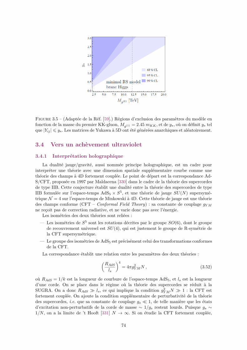
Figure 3.5 – (Adaptée de la Réf. [59].) Régions d’exclusion des paramètres du modèle enfonction de la masse du premier KK-gluon,Mg(1) = 2.45 mKK , et de y∗, où on définit y∗ telque |Yij | 6 y∗. Les matrices de Yukawa à 5D ont été générées anarchiques et aléatoirement.

3.4 Vers un achèvement ultraviolet

3.4.1 Interprétation holographique

La dualité jauge/gravité, aussi nommée principe holographique, est un cadre pourinterpréter une théorie avec une dimension spatiale supplémentaire courbe comme unethéorie des champs à 4D fortement couplée. Le point de départ est la correspondance Ad-S/CFT, proposée en 1997 par Maldacena [330] dans le cadre de la théorie des supercordesde type IIB. Cette conjecture établit une dualité entre la théorie des supercordes de typeIIB formulée sur l’espace-temps AdS5 × S5, et une théorie de jauge SU(N) supersymé-trique N = 4 sur l’espace-temps de Minkowski à 4D. Cette théorie de jauge est une théoriedes champs conforme (CFT – Conformal Field Theory) : sa constante de couplage gYMne reçoit pas de correction radiative, et ne varie donc pas avec l’énergie.

Les isométries des deux théories sont reliées :— Les isométries de S5 sont les rotations décrites par le groupe SO(6), dont le groupe

de recouvrement universel est SU(4), qui est justement le groupe de R-symétrie dela CFT supersymétrique.

— Le groupe des isométries de AdS5 est précisément celui des transformations conformesde la CFT.

La correspondance établit une relation entre les paramètres des deux théories :(RAdSls

)4= 4πg2

YMN , (3.52)

où RAdS = 1/k est la longueur de courbure de l’espace-temps AdS5, et ls est la longueurd’une corde. On se place dans le régime où la théorie des supercordes se réduit à laSUGRA. On a donc RAdS � ls, ce qui implique la condition g2

YMN � 1 : la CFT estfortement couplée. On ajoute la condition supplémentaire de perturbativité de la théoriedes supercordes, i.e. que sa constante de couplage gs � 1, de telle manière que les étatsd’excitation non-perturbatifs de la corde de masse ∼ 1/gs restent lourds. Puisque gs ∼1/N , on a la limite de ’t Hooft [331] N → ∞. Si on étudie la CFT fortement couplée,

74

on peut alors utiliser la correspondance AdS/CFT et calculer les observables physiques àpartir de la théorie gravitationnelle classique faiblement couplée.

Figure 3.6 – (Adaptée de la Réf. [173].) Schéma de la correspondance AdS/CFT. Lesisométries de l’espace-temps AdS5 correspondent à la symétrie conforme de la CFT à 4D.Se déplacer dans la direction z revient à une transformation du groupe de renormalisationde la théorie à 4D.

Dans les modèles à 5D qui nous intéressent, on a simplement une théorie des champsdéfinie sur l’espace-temps AdS5. On conjecture la dualité jauge/gravité qui nous per-met d’établir une correspondance entre une théorie gravitationnelle classique définie surl’espace-temps AdS5 et une CFT fortement couplée. On peut utiliser l’explication heuris-tique suivante. Considérons la métrique de l’espace-temps AdS5 (Éq. (3.1)) et effectuonsle changement de variable suivant :

RAdSz

= e−y/RAdS . (3.53)

On obtient la métrique :

ds2 =(RAdSz

)2 (ηµνdx

µdxν − dz2). (3.54)

La transformationz → eαz , α ∈ R , (3.55)

d’une tranche à 4D de AdS5 :

ds2 =(RAdSz

)2ηµνdx

µdxν , (3.56)

se traduit par un changement d’échelle de la métrique effective à 4D :

x→ eαx . (3.57)

75

Se déplacer vers les z croissants équivaut donc à augmenter les échelles de longueur à 4D, etdonc à diminuer les échelles d’énergie, µ ∼ 1/z (c.f. la Fig. 3.6). Ces considérations mènentà l’interprétation holographique de la dimension spatiale supplémentaire, où la coordonnéez correspond au flot du groupe de renormalisation dans la CFT à 4D. L’évolution d’unefonction d’onde de KK quand z croît correspond à l’évolution du coefficient d’un opérateurde la CFT quand µ décroît. Pour une description détaillée de la correspondance AdS/CFTdans le cadre de la théorie des champs, voir les Réfs. [245, 306, 307, 332–335]. Dans lasuite, on va donner les éléments principaux du dictionnaire AdS/CFT.

Les modèles type RS1 ne sont pas formulés sur un espace-temps AdS5 entier mais surune tranche de celui-ci (c.f. la Fig. 3.7). Quelle est l’interprétation des deux 3-branes ?— La brane UV correspond à une échelle de coupure de la CFT à haute énergie, ΛUV ∼

1/RAdS . Elle introduit une échelle de masse dans les CFT, et est donc une sourcede brisure de la symétrie conforme. En s’éloignant de la brane UV, on diminuel’énergie dans la CFT, et le bulk devient immédiatement AdS : la CFT devient alorsrapidement conforme sous l’échelle de coupure UV. Toute source de brisure de lasymétrie conforme, introduite par la coupure UV, doit donc être une déformationirrelevante de la CFT.

— La brane IR est une coupure brusque de l’espace-temps AdS5 en z = R′, et corres-pond à une déformation relevante de la CFT, impliquant une brisure spontanée de lasymétrie conforme, et un phénomène de confinement à l’échelle ΛIR ∼ 1/R′. On peutmontrer que la présence de la brane IR est responsable de la quantification du spectrede KK des différents champs dans le bulk, dont les états les plus légers apparaissentprès de l’échelle ΛIR. Pour chaque état de KK de la théorie extra-dimensionnelle, ilexiste un opérateur composite dans la CFT. La brane IR doit être interprétée commeun modèle simplifié du confinement.

Figure 3.7 – (Adaptée de la Réf. [336].) Schéma de la tranche AdS5. Les 3-branes coupentl’espace brusquement, introduisant une brisure de la symétrie conforme dans l’UV et l’IR.

Les états liés existent lorsque l’on considère la CFT à des énergies proches de l’échellede confinement ΛIR, ce qui implique que les KK-particules, qui ont leur fonction d’ondelocalisée près de la brane IR dans la tranche AdS5, sont duaux des états composites. Àl’inverse, un état localisé près de la brane UV interagit faiblement avec les états de KK(états composites de la CFT). On en conclut que (c.f. la Fig. 3.8) :— Pour chaque état localisé sur la brane IR, il existe un état composite dans la CFT.

76

— Pour chaque état localisé sur la brane UV, il existe un état élémentaire dans la CFT.— Pour chaque mode qui se propage dans le bulk, il existe une particule partiellement

composite dans la CFT. C’est un mélange d’états élémentaires et composites, à l’ins-tar du mélange entre le méson ρ et le photon en QCD. Pour une particule, dont lafonction d’onde de KK est piquée près de la brane UV (IR), il existe une particuleprincipalement élémentaire (composite) dans la CFT. Pour une particule, dont lafonction d’onde de KK est plate, il existe une particule dans la CFT qui est unmélange équilibré entre états élémentaires et composites.

Figure 3.8 – (Adaptée de la Réf. [336].) Schéma du dictionnaire AdS/CFT. Les étatsélémentaires (composites) sont localisés près de la brane UV (IR).

Dans le modèle de RS1 originel, tous les champs du SM sont localisés sur la brane IR, ilexiste donc pour chacun d’entre eux des états composites dans la CFT. Dans les modèlesde ce chapitre :— Le champ de Higgs est localisé sur la brane IR. Le boson de Higgs est donc composite

dans la CFT. Le problème de hiérarchie de jauge est résolu parce qu’au dessus del’échelle de confinement, le boson de Higgs disparaît et les préons 1 (non-scalaires),qui le constituent, apparaissent.

— Les modes zéro du graviton et des fermions légers du SM ont leur fonction d’ondede KK piquée près de la brane UV : ils sont donc partiellement composites dans laCFT, et principalement élémentaires.

— L’isodoublet et l’isosingulet faibles du quark top, ainsi que les KK-particules, ontleur fonction d’onde de KK piquée près de la brane IR : ils sont donc partiellementcomposites dans la CFT, et principalement composites.

— Les modes zéro des bosons de jauge du SM ont leur fonction d’onde de KK plate :ils sont donc partiellement composites dans la CFT, mélanges équilibrés entre étatsélémentaires et composites. On notera que les bosons de jauge massifs du SM ontune fonction d’onde de KK qui n’est pas tout à fait plate près de la brane IR, ilssont donc légèrement plus composites qu’élémentaires dans la CFT.

1. Si les particules du SM ont une substructure, on appelle parfois préons les particules les constituant.

77

En conclusion, les modèles de théorie des champs dans une tranche AdS5 peuvent êtreconsidérés comme un outil de calcul pour étudier des modèles composites. Dans cette vi-sion, la dimension spatiale supplémentaire n’est pas physique, on peut parler de dimensionspatiale supplémentaire auxiliaire : la Nature est décrite par une CFT fortement couplée,et on utilise la dualité jauge/gravité pour calculer les observables dans un modèle extra-dimensionnel. Comme la CFT est une théorie de jauge à 4D, elle est renormalisable. Ilest néanmoins très important d’avoir à l’esprit que la correspondance AdS/CFT, dansun modèle phénoménologique à 5D, permet de faire davantage des discussions qualita-tives que quantitatives sur la CFT. Contrairement à la conjecture initiale en théorie dessupercordes, le modèle à 5D ne permet pas d’avoir accès à la dynamique préoniques dela CFT. Il n’est d’ailleurs pas garanti qu’il existe une théorie avec confinement dont ladynamique reproduit exactement les valeurs des observables calculés à 5D [66]. Autrementdit, de la même manière qu’un achèvement dans l’UV n’est pas garanti pour le modèlephénoménologique à 5D, il en va de même pour la CFT. Le principe holographique doitdonc être utilisé avec prudence. Les contraintes sur les modèles à 5D ne peuvent pas être,en général, directement appliquées aux modèles composites. Par contre, qualitativement,la découverte des premiers états excités des particules du SM ne permettrait pas de tran-cher entre un scenario extra-dimensionnel et un scenario composite. Seule la découverte deplusieurs niveaux d’excitation différents, dont on pourrait extraire l’expression du spectrede masse, permettrait de déterminer qui d’une dimension supplémentaire ou d’une théoriede jauge avec confinement décrit correctement ces résonances.

3.4.2 Gorges déformées en théorie des supercordes de type IIB

Construction

Si la dimension spatiale supplémentaire est physique, il est nécessaire de trouver unachèvement UV qui soit une théorie extra-dimensionnelle. Celle-ci doit résoudre le pro-blème de non-renormalisabilité des interactions de jauge et de Yukawa dans un espace-temps à plus de 4D. Une candidate naturelle est l’une des théories des supercordes (c.f.la Réf. [337] pour une revue). Il y a notamment des tentatives intéressantes dans le typeIIB. Typiquement, les six dimensions spatiales supplémentaires sont compactifiées, dontla taille est de l’ordre de `P . Cependant, en ajoutant des configurations non-triviales dechamps de p-formes dans l’espace compactifié, on obtient des quanta de flux, lesquelspeuvent générer une dimension spatiale supplémentaire plus grande que les autres où lacourbure est importante. On obtient une géométrie dite de gorge déformée, jouant un rôlesimilaire au bulk entre les 3-branes UV et IR du modèle de RS1. La taille de la gorgeest stabilisée par les flux, ce que l’on peut modéliser dans l’EFT par le mécanisme deGoldberger-Wise [338].

Dans ces constructions, l’espace est de la forme AdS5 × X5, où X5 est une variétécompacte à 5D. AdS5 est la géométrie proche de l’horizon d’une pile de N D3-branes. Ily a alors N unités de flux dans X5. Le point de départ est la construction de Klebanov-Witten [339], où X5 = T 1,1 ' (SU(2)× SU(2)) /U(1). La théorie n’est pas régulée dansl’IR, i.e. que la géométrie présente une singularité nue. Pour la résoudre, on utilise laconstruction de Klebanov-Strassler [334, 340], où X5 = S2 × S3, avec S2 se réduisantà un point au bout de la pointe de la gorge. La géométrie, près de la pointe IR, n’estalors plus AdS5. Les constructions de Klebanov-Witten et de Klebanov-Strassler ont desgéométries non-compactes, s’étendant à l’infini dans la direction associée au rayon AdS5.Il faut alors compléter la géométrie dans l’UV par une variété compacte de Calabi-Yau.Dans la construction de Klebanov-Strassler, le spectre est alors normalisable et discret

78

[341]. Dans le modèle effectif de RS1, la pointe de la gorge et l’espace de Calabi-Yau sontrespectivement modélisés par les branes IR et UV. La Fig. 3.9 présente une illustration dela géométrie d’une gorge déformée.

Pour introduire les champs du SM dans le bulk [342, 343], on ajoute une pile de D7-branes s’enroulant autour d’un 3-cycle de X5. Les bosons de jauge et les fermions ne sepropagent pas alors dans une, mais quatre dimensions spatiales supplémentaires. De plus,la déformation de la géométrie AdS5, près de la pointe IR dans la solution de Klebanov-Strassler, a des conséquences importantes pour la phénoménologie des KK-particules. Eneffet, les fonctions d’onde de KK de celles-ci sont quasi-localisées près de la brane IR, etleurs couplages sont donc très sensibles à la géométrie de la pointe de Klebanov-Strassler,qui n’est pas AdS5. Dans la littérature, il y a peu d’études des contraintes sur mKK dansces modèles. Des constructions simplifiées [344–346] montrent que les KK-particules sontfortement couplées près de la pointe IR. On s’attend donc à avoir une borne inférieure surmKK dramatiquement plus élevée que dans une tranche AdS5, ce qui remet sérieusementen question le potentiel du modèle pour résoudre le problème de hiérarchie de jauge avecles bosons de jauge et les fermions dans le bulk. Construire un achèvement UV préservant,ou même améliorant, les contraintes expérimentales sur mKK dans un modèle aussi simpleque celui de RS1 reste donc un défi important.

Figure 3.9 – (Adaptée de la Réf. [343].) Schéma d’une gorge de Klebanov-Strassler colléeà un espace de Calabi-Yau. Loin de la pointe IR, la gorge peut être décrite par la solutionplus simple de Klebanov-Witten.

Gorges multiples

En théorie des supercordes de type IIB, les compactifications avec flux peuvent donnernaissance, non pas à une, mais à une multitude de gorges déformées, collées au même espacede Calabi-Yau. On obtient ainsi un Univers « pieuvre » où la « tête » serait l’espace deCalabi-Yau et les « tentacules » les gorges (c.f. la Fig. 3.10). On peut alors considérer uneEFT où les dimensions transverses des gorges sont négligeables, et où l’espace de Calabi-Yau est réduit à une 3-brane UV. Chaque gorge est alors modélisée par un intervalle,

79

et toutes partagent la même brane UV, comme illustré sur la Fig. 3.10. Autrement dit,on colle plusieurs tranches AdS5 ensemble, et la physique UV de l’espace de Calabi-Yauest décrite par des opérateurs localisés sur la brane UV. Les champs peuvent alors sepropager dans une ou plusieurs gorges, ouvrant la porte vers une large variété de modèles,possibilités pourtant peu exploitées dans la littérature. Les Réfs. [69, 347] donnent les basesde construction d’une théorie des champs dans cette géométrie, et la Réf. [348] montreque l’on peut stabiliser la longueur de chaque gorge avec une généralisation du mécanismede Goldberger-Wise. En ayant des gorges de différentes longueurs, chaque brane IR reçoitun facteur de déformation différent ; on génère ainsi naturellement différentes échellesd’énergie dans le modèle. Quelques applications phénoménologiques ont été proposées[349–351] pour construire notamment des modèles de saveur [352], de neutrinos [353], deleptogénèse [354], de secteurs cachés [355, 356], de matière noire [357] et d’axions [358, 359].

Figure 3.10 – (Adaptée de la Réf. [347].) En haut : Illustration d’une variété de Calabi-Yau de laquelle naissent les bases de gorges déformées. En bas : Dans l’approche d’EFTde la Réf. [347], les dimensions transverses des gorges sont négligées, et ces dernières sontmodélisées par une seule dimension spatiale supplémentaire. Les gorges se rejoignent enun point : la brane UV.

80

Part II

Original Research Work

81

Chapter 4

Beyond Brane-HiggsRegularization

This chapter is a personal adaptation of Ref. [1] written in collaboration with AndreiAngelescu, Ruifeng Leng and Grégory Moreau.

4.1 Introduction

The paradigm of scenarii with spacelike extra dimensions (and the composite Higgsmodels dual via the AdS/CFT correspondance) represents an alternative to SUSY foraddressing the gauge hierarchy problem of the SM. Moreover, the warped extra dimensionscenarii with SM fields in the bulk allow to generate the SM fermion mass hierarchy froma simple geometrical picture of fermion KK wave functions along the extra dimension. Torealize those two hierarchical features, the Higgs field, providing masses to fermions andweak gauge bosons of the SM via EWSB, is often stuck exactly on the IR-brane.

In supersymmetric models with a warped geometry (see Ref. [360] for a review), thetwo Higgs doublets are localized at the boundary of the extra dimension and SUSY isbroken on the opposite side. On the one hand, if the Higgs doublets are on the IR-brane [361, 362], then the big gauge hierarchy problem is still solved by the warp factor,and SUSY protects the masses of the Higgs bosons from radiative corrections betweenthe EW scale and the quantum gravity scale on the IR-brane (indeed the current LHCconstraints push the quantum gravity scale on the IR-brane up to O(10) TeV, implyinga little hierarchy problem for the mass of the Higgs boson). On the other hand, if theHiggs doublets are on the UV-brane [363–366], SUSY solves the entire gauge hierarchyproblem. In both cases, the fermion mass hierarchy is generated by allowing the gauge andmatter fields to propagate in the bulk. The same mechanism gives a sfermion spectrumcompatible with the experimental bounds in the flavor sector.

In the present chapter, we discuss a rigorous 5D treatment of a brane localized Higgsscalar field, interacting with bulk quarks/leptons, which presents subtleties that deserveto be looked at more deeply. Let us recall these subtle aspects. The brane localizedinteractions between the 5D fields and the Higgs boson on the IR-brane involves a Diracdistribution, which may induce an unusual discontinuity in the KK wave function alongthe extra dimension for some of the bulk fermions: the so-called “jump problem” [50,367]. This motivated the introduction [49–55] of a regularization of the Dirac distribution(smoothing the Dirac distribution or shifting it from the boundary) in the calculation of theKK fermion mass spectra and effective four-dimensional (4D) Yukawa couplings. Althoughthere is no profound theoretical reason to apply such a regularization procedure (implying

82

interaction-free boundary conditions for fermions), nowadays most of the theoretical andphenomenological studies of the warped models with a brane localized SM Higgs field (seee.g. Refs. [49, 54–61]) are relying on this Dirac distribution regularization.

We first present the mathematical inconsistencies of this regularization procedure usedin the literature. Then, instead of regularizing, we develop the rigorous determination ofthe KK wave functions – taking into account the nature of the Dirac distribution in theHiggs couplings – which leads to bulk fermion KK wave functions without discontinuitieson the considered internal space. Alternatively, we suggest to introduce the appropriateformalism of distributions in order to treat properly the Dirac distribution as well as allthe Lagrangian terms. We conclude from this whole approach that neither a jump of KKwave functions nor a particular problem arises when a proper mathematical frameworkis used, so that there is in fact no motivation to introduce a brane-Higgs regularization.These methods without regularization are illustrated here in the derivation of the KKfermion mass spectrum – the same ideas apply to the calculation of effective 4D Yukawacouplings. This calculation of the mass spectrum is performed in a simplified model with aflat extra dimension, the minimal field content and without gauge symmetry. Neverthelessthis toy model already possesses all the key ingredients to study the delicate brane-Higgsaspects. Hence our conclusions can be directly extended to the realistic warped modelswith bulk SM matter addressing the fermion flavor and gauge hierarchy.

Several new methods for the calculation of the spectrum are proposed which furtherallow for confirmations of the analytical results. Those methods apply to alternative usesof the 5D or the 4D approaches, employing distributions or functions. Note that from ahistorical point of view, the method established here arises naturally in the theory of vari-ational calculus, as the Lagrangian boundary terms (brane-Higgs couplings to fermions)are included in a new boundary condition [368]. Furthermore, the present method fol-lows the prescription of considering the Dirac function to be a distribution. By the way,the distributions were defined with mathematical rigor during the 1940’s by L. Schwartz[369, 370] precisely for the purpose of consistently solving physical problems.

Besides, the performed exhaustive exploration of the solutions for the KK wave func-tion, in the context of two fermion fields propagating along a flat extra dimension withneither bulk mass nor BLKTs, allows to show that while in the free case either Neumannor Dirichlet conditions are possible at both interval boundaries (with possibly differentconditions at the two boundaries), once their brane-Higgs couplings are introduced, onlythe new type of boundary conditions involving the Yukawa coupling constants exists atthe boundary where the Higgs field is localized.

The rigorous result obtained here for the KK mass spectrum is different from the onederived through the regularization of Dirac distributions, as it is detailed in the presentwork. This difference is physical and analytical which is also important because determin-ing the fermion mass formula is part of the precise theoretical understanding of the higher-dimensional setup with a brane localized Higgs boson, since the Higgs properties are testedat the LHC with an increasing accuracy. Phenomenological studies of the brane localizedHiggs interaction within warped models can be found in Refs. [55–61, 324–329, 371].

At the level of calculating Higgs production/decay rates, a theoretical debate appearedin the literature [58] on models with brane-Higgs coupling to bulk matter. Indeed, a para-doxal non-commutativity arose in the calculation: different physical results were obtainedfor Higgs processes when taking ε→ 0 and then NKK →∞ [55, 57] or the opposite order[56] 1. A consequence of our present work is that the ambiguity is solved since our conclu-

1. Here NKK is the number of exchanged KK states at the level of the loop amplitude and ε is theinfinitesimal parameter introduced to regularize the Dirac distribution.

83

sion is that the regularization must not be applied (in turn no ε has to be introduced).Furthermore, the mass spectrum obtained here allows to point out the necessity for

bulk fermions (with or without coupling to a brane localized scalar field) to have certainBilinear Boundary Terms (BBTs) (studied in a different context in Refs. [62–66]) whichare mass terms from the point of view of the spinorial structure but do not introduce newcontributions to physical masses. Indeed, such terms guarantee the existence of physicalsolutions (with correct profile normalizations, Hermitian conjugate boundary conditionsand satisfying the decoupling limit argument) and the (non-trivial) exact matching be-tween the 5D and 4D analytical calculations. These boundary terms are part of thedefinition of the self-consistent 5D model with bulk fermions coupled to a brane localizedscalar field, although they are newly introduced in this context.

At a brane without Yukawa coupling, instead of including the BBTs, we find that onecan alternatively impose an essential boundary condition (in contrast to natural boundaryconditions coming from the Lagrangian variations), consistent with the condition thata fermion current along the extra dimension must vanish at the boundaries (exclusivelywithin the 4D approach in case of brane localized Yukawa interactions). Indeed, the genericreason for the presence of the BBTs is the consistent and complete geometrical definitionof models with an extra dimension compactified on an interval to which fermionic matteris confined. With the BBTs, the chiral nature of the SM at the level of the zero modes(left-handed for the weak isodoublets and right-handed for the weak isosinglets) is entirelyinduced by the signs in front of BBTs. This new relation shows how the particular chiralproperties of the SM could be explained by an underlying theory, through the signs of theBBTs.

The plan of the chapter is the following. We begin by defining our toy model in Section4.2 and explain how to generalize it to a realistic warped model reproducing the SM atlow energy. In Section 4.3, we discuss in detail the natural versus essential boundaryconditions for bulk fermions – at the boundaries of the extra dimension – and also toderive the free fermion mass spectrum (in the absence of Yukawa interactions), which isuseful in particular for the 4D approach or more generically for a solid comprehension ofthe mass spectrum. In particular the boundary conditions arising from considerations onthe probability currents are discussed. We expose the so-called 4D method, where thecoupling of the bulk fermions to the Higgs field VEV is introduced with an infinite matrixto bi-diagonalize. In Section 4.5, we discuss the main drawbacks of the 5D method withregularization of the Dirac distribution which one can find in the literature. In Section 4.6,we present our 5D method. In Section 4.7, we apply our results, together with a discussionof the phenomenological impacts. We summarize and conclude in Section 4.8.

4.2 Minimal Consistent Model

4.2.1 Spacetime Structure

We consider a 5D toy model with a space-time E5 =M4 × I.— M4 is the usual 4D Minkowski spacetime. An event in M4 is characterized by its

4-vector coordinates xµ where µ = 0, 1, 2, 3 is the Lorentz index.— I is the interval [0, L], guaranteeing chiral fermions at low energies (below the first

KK mass scale). I is parametrized by the extra coordinate y and bounded by twoflat 3-branes at y = 0 and y = L.

— A point of the whole 5D spacetime E5 is labeled by its coordinates zM with an indexM ∈ J0, 4K. zM can be split into (xµ, y).

84

4.2.2 Bulk Fermions

We consider the minimal spin-1/2 fermion field content allowing to write down a 4Drenormalizable SM Yukawa-like coupling between zero mode fermions (of different chiral-ities) and a scalar field (see Subsection 4.2.4): a pair of fermions Q and D. Both are alsopropagating along the extra dimension, as we have in mind an extension of the model to arealistic scenario with bulk matter (c.f. Subsection 4.2.6) where Q,D will be left and righthanded down type quark fields. According to the discussion in Appendix B.2, there arebranes only at the boundaries so we take the 5D fields continuous up to the boundaries.Using the notation,

←→∂M =

−→∂M−

←−∂M , the 5D fields Q(xµ, y) and D(xµ, y) of mass dimension

2 have thus the following kinetic terms:

SΨ =∫d4x

∫ L

0dy LΨ ,

with LΨ = i

2(QΓM

←→∂MQ+DΓM

←→∂MD

), (4.1)

where ΓM denote the 5D Dirac matrices. In our notations a 5D Dirac spinor, being in theirreducible representation of the Lorentz group, reads

Q =(QLQR

)and D =

(DL

DR

), (4.2)

in terms of the two two-component Weyl spinors. L/R stands for the left/right-handedchirality. Let us rewrite the bulk action of Eq. (4.1) in a convenient form:

SΨ =∫d4x

∫ L

0dy LΨ ,

with LΨ =∑

F=Q,D

12(iF †Rσ

µ←→∂µFR + iF †Lσµ←→∂µFL + F †R

←→∂yFL − F †L

←→∂yFR

). (4.3)

4.2.3 Brane Localized Scalar Field

The subtle aspects arise when the fermions couple to a single 4D real scalar field H(mass dimension 1), confined on a boundary taken here to be at y = L (as inspired bywarped scenarii addressing the gauge hierarchy problem). The action of this scalar fieldhas the generic form

SH =∫d4x

∫ L

0dy δ(y − L) LH ,

with LH = 12 ∂µH∂

µH − V (H) , (4.4)

where the action of a Dirac distribution centered at y = a on a testfunction ϕ(y) is definedas ∫ L

0dy δ(y − a)ϕ(y) = ϕ(a) . (4.5)

The potential V possesses a minimum which generates a non-vanishing VEV for the fieldH, which can be expanded as

H = v + h(xµ)√2

, (4.6)

in analogy to the SM Higgs field.

85

4.2.4 Yukawa Interactions

We focus on the following basic interactions in order to study the subtleties inducedby the coupling of the brane scalar field to bulk fermions,

SY =∫d4x

∫ L

0dy δ(y − L) LY ,

with LY = −Y5 Q†LHDR − Y ′5 Q

†RHDL + H.c. . (4.7)

Considering operators involving H, Q and D up to dimension 5 allows to include thisYukawa coupling of interest 2. The complex coupling constants Y5 = eiαY |Y5| and Y ′5 =eiα′Y |Y ′5 | of Yukawa type (with a mass dimension -1), entering these two distinct terms,are independent (i.e. parameters with possibly different values) as the fermion fields onthe 3-brane at y = L are strictly chiral (see for instance Ref. [54]).

When calculating the KK fermion mass spectrum, we restrict our considerations to theVEV of H. Indeed, we have in mind that the interactions of the fluctuation of the Higgsboson with the fermions are treated in perturbation theory, as usual in QFT. Hence, wecan decompose the action (4.7) into SY = SX + ShQD such that

SX =∫d4x

∫ L

0dy δ(y − L) LX ,

with LX = −X Q†LDR −X ′ Q†RDL + H.c. , (4.8)

and the compact notations X = v√2Y5 and X ′ = v√

2Y ′5 , and

ShQD =∫d4x

∫ L

0dy δ(y − L) LhQD ,

with LhQD = − Y5√2hQ†LDR −

Y ′5√2hQ†RDL + H.c. . (4.9)

4.2.5 Bilinear Boundary Terms

Interestingly, the presence of certain BBTs for the bulk fermions coupled to the braneHiggs field will turn out to be required to recover the SM in the decoupling limit as willbe demonstrated in detail in Subsection 4.6.3. The necessity and exact form (includingnumerical coefficients) of these terms will be confirmed in Subsection 4.6.3 by the exactanalytical matching between the 4D and 5D calculations of the KK mass spectrum. Theseboundary terms read 3

SB =∫d4x

∫ L

0dy [δ(y)− δ(y − L)] LB ,

with LB = 12(DD −QQ

), (4.10)

They do not involve new parameters (multiplying the operators).

2. Notice that for instance a dimension-6 operator of type 1M2 δ(y − L)Q†

L/RH2DR/L, M being a mass

scale, would be treated in a similar way as the couplings in Eq. (4.7) (and can contribute to the Yukawacouplings (4.7) through the scalar field VEV).

3. Similar terms, leading in particular to LB = 12(DD −Q

DQD), would be present in a model version

extended to the EW symmetry of the SM, with the Q field promoted to an SU(2)L doublet QD. Incontrast, terms of the kind Q

UD (or QD) or Q

UQD would obviously not belong to a gauge invariant form.

86

Note that this kind of boundary terms (4.10) is a specific case of boundary mass termsthat one can add to the model:

SBBT =∫d4x

∫ L

0dy [δ(y) + δ(y − L)] LBBT ,

with LBBT = −∑

F=Q,D

µF (y)2 FF, (4.11)

when µQ(0) = µD(L) = 1 and µQ(L) = µD(0) = −1. In Ref. [62], Henningson and Sfetsosintroduced by hand such kind of terms only at the UV-brane (y = 0) of a warped 5Dmodel with an arbitrary coefficient µF (0), in order to derive the AdS/CFT correspon-dance in the calculation of correlation functions for spinors (see also Ref. [63]). Then,Arutyunov and Frolov justified them in Ref. [64] with a fixed coefficient µF (0) = ±1 inthe Lagrangian formulation, to obtain a consistent Hamiltonian formulation when oneperforms the Legendre transformation in the case of a full AdS spacetime. Refs. [65, 66]showed that they are necessary to apply Hamilton’s principle – see Annexe B.1. Notethat one is free to add also such kind of terms at the IR-brane (y = L). The AdS/CFTduality can be used to give a holographic interpretation of warped models (from which thepresent simplified scenario is inspired) in terms of composite Higgs models. Refs. [67, 68]make use of boundary terms to select boundary conditions with Hamilton’s principle for5D symplectic-Majorana fermions.

The necessity of boundary localized terms, in a field theory defined on a manifoldwith boundaries, is not a surprise as it is known for a long time in the context of gravity.Indeed, Gibbons-Hawking boundary terms [258, 292–294] are needed in order to cancelthe variation of the Ricci tensor at the boundary of the manifold.

4.2.6 Model Extension

The toy model considered is thus characterized by the action

S5D = SΨ + SH + SY + SB . (4.12)

Nevertheless, the conclusions of the present work can be directly generalized to realisticwarped models with bulk SM matter solving the fermion mass and gauge hierarchies.Indeed, working with a warped extra dimension instead of a flat one would not affect theconceptual subtleties concerning the coupling of bulk fermions to a brane scalar field. Theboundaries at y = 0 and y = L would then become the UV and IR-branes, respectively.Similarly, the scalar potential V (H) can be extended to any potential (like the SM Higgspotential breaking the EW symmetry) as long as it still generates a VEV for the scalarfield as here. In this context the H singlet can be promoted to the Higgs doublet under theSM SU(2)W gauge group, simply by inserting doublets in the kinetic term of Eq. (4.4).The whole structure of the coupling of Eq. (4.8) between bulk fermions and the branelocalized VEV would remain the same in case of fermions promoted to SM SU(2)W weakisodoublets: after index contraction of the doublet (QU , QD)t with down/up-quark singletsD,U , one would obtain two replicas of the structure (4.8) with the forms QDCDC′ andQU

CUC′ where C(′) denotes the chirality. Hence the procedure described in this workshould be applied to both terms separately 4. The same comment holds for the SM colortriplet contraction and the extension of the field content to three generations of quarksand leptons of the SM. Notice that the flavor mixings would be combined with the mixings

4. The action in Eq. (4.12) would be trivially generalized as well to a scenario with a gauge symmetry.

87

among fermion modes of the KK towers, without any impact on the present considerationsconcerning brane localized couplings.

4.3 5D Free Fermions on an IntervalIn this part, we calculate the fermionic mass spectrum in the basic case where Y5 =

Y ′5 = 0 in Eq. (4.7) (Refs [50, 307]), pointing out the correct treatment. We considerthe system with a compactification on an interval with only the free bulk action SΨ inEq. (4.3). The main interest of this section is to develop a rigorous procedure for applyingthe boundary conditions.

4.3.1 Natural Boundary Conditions Only

In order to extract the Euler-Lagrange equations and the boundary conditions forthe bulk fermions, we apply Hamilton’s principle with the action (4.3) for each fermionF = Q,D 5. According to the discussion in Appendix B.2, we take the variations of thefields continuous in the bulk and at the boundaries since there are no branes away fromthe boundaries. Assuming the values of the fields at the boundaries FL/R(xµ, y = 0, L)= FL/R

∣∣∣0,L

to be initially unknown (unfixed by ad hoc boundary conditions), their valuesshould be deduced from the minimization of the action with respect to them, consideringthus generic field variations δFL/R

∣∣∣0,L

. In other words, FL/R∣∣∣0,L

should be obtained fromthe so-called natural boundary conditions 6 [368]. The stationary action condition can besplit into conditions associated to each field without loss of generality. After an integrationby part of each term, we get

0 = δF †LSΨ =

∫d4x

∫ L

0dy δF †L

[iσµ∂µFL − ∂yFR

]+∫d4x

12[(δF †L FR

)∣∣∣L−(δF †L FR

)∣∣∣0

], (4.13)

0 = δF †RSΨ =

∫d4x

∫ L

0dy δF †R [iσµ∂µFR + ∂yFL]

+∫d4x

12[−(δF †R FL

)∣∣∣L

+(δF †R FL

)∣∣∣0

], (4.14)

where we drop the boundary term at infinity of the four usual dimensions. The bulk andbrane variations of Eqs. (4.13)-(4.14) must vanish separately (respectively the volume andthe surface terms) to ensure δ

F †L/R

SΨ = 0 for generic field variations 7. We get the bulkEuler-Lagrange equations iσµ∂µFR + ∂yFL = 0 ,

iσµ∂µFL − ∂yFR = 0 ,

(4.15)

and the boundary conditionsFL|0,L = FR|0,L = 0. (4.16)

5. The Euler-Lagrange equations for the conjugate fields are trivially related.6. The notion of natural boundary conditions has already been introduced in the treatment of scalars

and gauge fields with brane localized mass terms [257].7. A functional variation reads δFL/R(zM ) = κ ηL/R(zM ) with a generic function ηL/R(zM ) and an

infinitesimal parameter κ→ 0.

88

Let us now deduce from these equations involving the 5D fields the relations among theKK wave functions along the extra dimension.

To develop a 4D effective picture, let us replace the 5D fields in the relations obtainedjust above by their standard KK decomposition,

FL/R (xµ, y) = 1√L

∑n

fnL/R(y)FnL/R (xµ) , (4.17)

where fnL/R = qnL/R or dnL/R are the dimensionless KK wave functions along the extradimension, associated respectively to the 4D fields FnL/R = QnL/R or Dn

L/R (n is the KKlevel integer index). If they are not vanishing for all y, the KK wave functions are or-thonormalized such that

∀n , ∀m ,1L

∫ L

0dy fn∗L/R(y) fmL/R(y) = δnm, (4.18)

from the requirement of canonically normalized and diagonal kinetic terms for the 4Dfields after inserting the KK decomposition (4.17) into the 5D field kinetic terms (4.3).Each KK-fermion is described by 4D Dirac-Weyl equations,

∀n,

iσµ∂µF

nL (xµ)−mn F

nR (xµ) = 0 ,

iσµ∂µFnR (xµ)−mn F

nL (xµ) = 0 ,

(4.19)

where mn are the mass eigenvalues of the KK excitation tower for the fermions such that,for each KK mode, one has the action

SnF = αnL iFn†L σ

µ∂µF

nL + αnR iF

n†R σµ∂µF

nR − αnLαnRmn

(Fn†R FnL + Fn†L FnR

), (4.20)

where αnL/R = 1 if fnL/R(y) 6= 0, and αnL/R = 0 if fnL/R(y) = 0. Inserting the KK decompo-sition (4.17) and the Dirac equations (4.19) into the 5D Euler-Lagrange equations (4.15),one can directly extract the differential equations for the KK wave functions,

∀n ,

∂yfnR(y)−mn f

nL(y) = 0,

∂yfnL(y) +mn f

nR(y) = 0,

(4.21)

whose solutions for the zero modes (m0 = 0) are

f0L/R(y) = Af,0L/R , (4.22)

where the Af,0L/R’s are complex coefficients. For the massive modes (mn 6= 0), the firstorder differential equations (4.21) can be combined into second order equations,

∀n,(∂2y +m2

n

)fnL/R(y) = 0, (4.23)

which are the equations for independent harmonic oscillators whose solutions have thegeneral form

∀n, fnL/R(y) = Af,nL/R cos(mn y) +Bf,nL/R sin(mn y) , (4.24)

where Af,nL/R, Bf,nL/R are complex coefficients. Eq. (4.21) is a system of first order coupled

equations which imposes the relations Af,nL = Bf,nR and Af,nR = −Bf,n

L for mn 6= 0.

89

Now, inserting Eq. (4.17) into the boundary conditions (4.16), we obtain the followingDirichlet boundary conditions for any KK wave function

∀n, fnL/R(0) = fnL/R(L) = 0. (4.25)

For massive modes, a Dirichlet boundary condition for a KK wave function associatedto one chirality, fnL/R(0, L) = 0, combined with Eq. (4.21), gives a Neumann boundarycondition for the KK wave function of the other chirality, ∂yfnR/L(0, L) = 0. Hence,the KK wave functions have both Dirichlet and Neumann boundary conditions at eachboundary. When applied to the expression of the KK wave functions in Eqs. (4.24)-(4.24),the boundary conditions lead to ∀n, Af,nL = Af,nR = Bf,n

L = Bf,nR = 0, hence

∀n, fnL/R(y) = 0, (4.26)

which means that there are no KK modes. This problem comes from the fact that thesystem is overconstrained at the boundaries. Indeed, the KK wave function equations(4.21) relate fnL(y) and fnR(y) on-shell for the massive modes: a boundary condition onfnL(y) is also a constraint on fnR(y) and vice versa. Therefore, the KK wave functions fnL(y)and fnR(y) for mn 6= 0 depend on the same three parameters: the mass mn and the twocomplex coefficients Bf,n

L/R. For the zero modes, f0L(y) and f0

R(y) depend each on one com-plex coefficient Af,0L/R. The variation of the action at the boundaries in Eqs. (4.13)-(4.14)involves the variations of both FL and FR so there are two natural boundary conditions foreach boundary. The system is thus overconstrained, that is why the KK wave functionsvanish everywhere for all modes.

In order to have a non-trivial 5D fermion model interesting for physics, we have tochoose another kind of boundary conditions (see the next Subsection 4.3.2). In Subsec-tion 4.3.3, we show that if we modify our model by introducing the BBTs (4.10), we avoidthe above problems.

4.3.2 Essential Boundary Conditions from Conserved Currents

Regarding the geometrical field configuration within the present model, each fermionis defined only along the interval [0, L]. This model building hypothesis, that fermions donot propagate outside the interval, translates into the condition of a vanishing conservedcurrent transversal to the branes at both boundaries for each fermion species separately(without possible compensations) – as was discussed in Ref. [268] for a scalar field case.

Formally speaking, there are two conserved currents defined independently for the twobulk fermions, involving the 5D fields F = Q,D:

jMQ = QΓMQ, jMD = D ΓMD, with the local conservation law ∂MjMF = 0 , (4.27)

as predicted by Noether’s theorem applied to the global fermionic symmetry U(1)Q×U(1)Dof the free action in Eq. (4.1). The symmetries are based on the distinct transformations,

Q 7→ e−iαqQ , D 7→ e−iαdD, (4.28)

where αf = αq, αd (∈ R) are the continuous parameters of the transformations. Infinites-imal field variations give δF = −iαfF , δF = iαfF . The condition that the component ofthe conserved currents transverse to the branes vanishes at the boundaries is thus,

j4F

∣∣∣0,L

= F Γ4F∣∣∣0,L

= i(F †LFR − F

†RFL

)∣∣∣0,L

= 0 , (4.29)

90

It implies the following possible Dirichlet boundary conditions,

FL|0 = 0 or FR|0 = 0 and FL|L = 0 or FR|L = 0, (4.30)

which translate into boundary conditions for the KK wave functions after the KK decom-position (4.17),

∀n, fnL(0) = 0 or fnR(0) = 0, and fnL(L) = 0 or fnR(L) = 0. (4.31)

One can impose ad hoc conditions on the fields at the boundaries from the begin-ning, instead of using natural boundary conditions derived from the variational calculus[368]. Such boundary conditions will be called essential boundary conditions. Having fixedfields at boundaries is equivalent to have vanishing functional variations, δFL|0,L = 0 orδFR|0,L = 0. The conditions (4.30) of vanishing fields at the boundaries can be imposedas essential boundary conditions: they correspond to some fields initially fixed at theboundaries [geometrical field configuration]. This is in contrast to our first treatment[above], where all the boundary fields FL/R

∣∣∣0,L

were assumed to be initially arbitrary, andthen we obtained the natural boundary conditions through Hamilton’s principle. In theliterature, Dirichlet boundary conditions are imposed by hand as essential boundary con-ditions [50, 307]. Here, we justify these essential boundary conditions by the requirementof vanishing probability currents at the boundaries.

Keeping these new essential boundary conditions (4.30)-(4.31) in mind, let us applyHamilton’s principle to the action (4.3) as in Eqs. (4.13)-(4.14). The vanishing of the bulkvariations is identical to the previous treatment and leads to the same equations (4.15).However, the boundary variations – in the two-component notations –(

δF †LFR)∣∣∣

0,L=(δF †RFL

)∣∣∣0,L

= 0, (4.32)

are vanishing this time by the choice of one of the four possible essential boundary condi-tions (4.30) which read

1) FL|0 = 0 and FL|L = 0, 2) FL|0 = 0 and FR|L = 0,3) FR|0 = 0 and FL|L = 0, 4) FR|0 = 0 and FR|L = 0, (4.33)

recalling that FL/R∣∣∣0,L

= 0 implies δFL/R∣∣∣0,L

= 0. In other words, for instance, if F (†)L

∣∣∣0

=0 then there is no need to minimize the action with respect to this known field at theboundary so that the corresponding variation term [involving δF †L

∣∣∣0] in Eq. (4.32) should

be absent. Hence to obtain complete boundary conditions, we have to combine only theessential boundary conditions (4.33) with the KK wave functions equations (4.21) [andtheir solutions (4.24)]. For the fields which are not fixed at the boundaries by essentialboundary conditions, their variation must be generic. We obtain the following four possiblesets of wave functions and KK mass spectrum equations (∀n),

1) (−−) : fnL(y) = −Af,nR sin(mn y), (++) : fnR(y) = Af,nR cos(mn y) ; sin(mn L) = 0,2) (−+) : fnL(y) = −Af,nR sin(mn y), (+−) : fnR(y) = Af,nR cos(mn y) ; cos(mn L) = 0,3) (+−) : fnL(y) = Af,nL cos(mn y), (−+) : fnR(y) = Af,nL sin(mn y) ; cos(mn L) = 0,4) (++) : fnL(y) = Af,nL cos(mn y), (−−) : fnR(y) = Af,nL sin(mn y) ; sin(mn L) = 0,

(4.34)

91

In Eq. (4.34), we have used the standard boundary condition notations, i.e. − or + forexample at y = 0 stands respectively for the Dirichlet or Neumann KK wave functionboundary condition: fnL/R(0) = 0 or ∂yfnL/R(0) = 0. For instance (−+) denotes Dirichlet(Neumann) boundary condition at y = 0 (y = L). For the boundary conditions 1) and 2),we would like to know if the phase of Af,nL is physical. For that purpose, we perform thetransformations:

Af,nL 7→ eiθnAf,nL =⇒ (fnL , fnR) 7→ (eiθnfnL , eiθnfnR) , (4.35)

which let the KK wave functions equations (4.21) and the orthonormalization conditions(4.18) invariant, thus the phase of Af,nL is not physical and one can take Af,nL = |Af,nL |.For the boundary conditions 3) and 4), the same method is applied to conclude that thephase of Af,nR is not physical. We take Af,nR = |Af,nR |. The boundary conditions 1) and 4)have the following solutions for the KK mass spectrum:

sin(mn L) = 0 ⇒ mn = nπ

L, n ∈ N . (4.36)

As mn = −nπ/L is also solution of the mass spectrum equation (4.36), we will show thatthe sign of mn is not physical. One can perform the transformations{

mn 7→ −mn

FnR 7→ −FnR or FnL 7→ −FnL(4.37)

Then, the 4D actions of each KK modes (4.20) (and thus the Dirac equations (4.19)), theKK wave functions equations (4.21) and the orthonormalization conditions (4.18) (usingthe parity of the solutions (4.34)) are invariant. One can conlude that the sign of mn isnot physical and take mn ≥ 0. The boundary conditions 2) and 3) have the solutions:

cos(mn L) = 0 ⇒ mn = (2n+ 1) π

2L , n ∈ N. (4.38)

mn = −(2n + 1)π/(2L) is also solution of the mass spectrum equation (4.38). By usingthe same method as above, one can show that the sign of mn is not physical and takemn ≥ 0. Therefore, in the case of the first complete boundary conditions above, the 5Dfield F possesses a zero mode (m0 = 0) with a KK wave function f0

R(y) associated to aright-handed chirality 4D field F 0

R [c.f. Eq. (4.17)], since f0L(y) = 0 – in contrast to the

second complete boundary conditions without zero mode (m0 6= 0). The constants |Af,nL |and |Af,nR | are fixed by the orthonormalization conditions (4.18).

Now let us impose on the 5D fields Q,D the realistic complete boundary conditions inEq. (4.34) to fix the model. D,Q are associated respectively to the first and fourth com-plete boundary conditions of Eq. (4.34), implying the existence of zero mode 4D fields,which is realistic as, in standard warped scenarios including Yukawa interactions, the var-ious measured quark masses are expected to originate mainly from the EWSB mechanism.Furthermore, within an extended realistic warped model (as described in Subsection 4.2.6)the Q field is promoted to a SM SU(2)W gauge doublet, which is consistent with the left-handed chirality of the zero mode 4D field Q0

L imposed by the fourth complete boundaryconditions, while D is the SU(2)L singlet down-quark, compatible with the right-handedchirality of D0

R driven by the first complete boundary conditions. The KK wave functionsassociated to these realistic boundary conditions are{

q0L(y) = 1 , q0

R(y) = 0 ,d0L(y) = 0 , d0

R(y) = 1 , (4.39)

92

for the massless zero modes, and{qnL(y) =

√2 cos(mn y) , qnR(y) =

√2 sin(mn y) ,

dnL(y) = −√

2 sin(mn y) , dnR(y) =√

2 cos(mn y) , (4.40)

for the excited modes with mn = n (π/L), n ∈ N∗. The second and third completeboundary conditions of Eq. (4.34) are not realistic for a describtion of SM fermions, sincethey predict neither zero mode 4D fields nor chiral states (only vector-like modes). Achiral model can thus be recovered at low-energy for a specific choice of complete boundaryconditions on the boundaries of the interval.

One can notice that the action SΨ (4.1) has an accidental global SU(2) symmetrywhose fundamental representation acts on the doublet (Q,D). However, we do not wantthis symmetry in our model: our choice of boundary conditions 1) and 4) in Eq. (4.34)break this SU(2) symmetry explicitely. Indeed, one can check that the component of theassociated Noether’s current transverse to the 3-branes is not vanishing for these boundaryconditions. This is not a problem since the SU(2) symmetry is not in our list of symmetrieswhich define our model.

4.3.3 Natural Boundary Conditions with Bilinear Boundary Terms

We propose an alternative solution to the problem of 5D free fermions with the extradimension compactified on an interval. Instead of imposing essential boundary conditionswhen performing Hamilton’s principle with the action SΨ in Eq. (4.3), we add the boundaryterms (4.11) allowing for natural boundary conditions. This is the point of view adoptedin Ref. [258] for a 5D scalar field and 5D gravity, and in Refs. [67, 68] for a 5D symplectic-Majorana fermion. We will see that the two methods give the same physical mass spectrumas in the previous subsection if the boundary terms have fixed coefficients. Essentialboundary conditions and natural boundary conditions with BBTs correspond to two waysto describe the same model.

Let us apply Hamilton’s principle by considering the sum of the actions (4.3) and (4.11)involving the two-component spinor fields:

0 = δF †L

(SΨ + SBBT ) =∫d4x

∫ L

0dy δF †L

[iσµ∂µFL − ∂yFR

]−1

2

∫d4x [1 + µF (0)]

(δF †LFR

)∣∣∣0

+12

∫d4x [1− µF (L)]

(δF †LFR

)∣∣∣L, (4.41)

0 = δF †R

(SΨ + SBBT ) =∫d4x

∫ L

0dy δF †R [iσµ∂µFR + ∂yFL]

+12

∫d4x [1− µF (0)]

(δF †RFL

)∣∣∣0

−12

∫d4x [1 + µF (L)]

(δF †RFL

)∣∣∣L. (4.42)

For generic field variations δF †L/R∣∣∣0,L

, the bulk and brane variations in Eqs. (4.41) and(4.42) have to vanish separately, leading to the same equations as in Eq. (4.15) and in turn,via Eqs. (4.19) and (4.17), to the Euler-Lagrange equations (4.21) with solutions (4.22)-(4.24). We are thus left with the natural boundary conditions (generic field variations at

93

the boundaries):

[1 + µF (0)] FR|0 = [1− µF (L)] FR|L = [1− µF (0)] FL|0 = [1 + µF (L)] FL|L = 0. (4.43)

For µF (0) 6= ±1 and µF (L) 6= ±1, we get the same boundary conditions as in Eq. (4.16)which, after a KK decomposition (4.17) and solving the KK wave functions equations(4.21), leads to vanishing KK wave functions everywhere (4.25) in the bulk as in Subsec-tion 4.3.1. Indeed, the system is still overconstrained by the natural boundary conditions(see discussion below Eq. (4.26)). In order to obtain interesting natural boundary con-ditions for physics, one should take µF (0) = ±1 and µF (L) = ±1. In these cases, thevariation of the action at the boundaries (Eq. (4.42)) involves only one of the two chiral-ities: FL or FR. This implies that there is only one natural boundary condition for eachboundary instead of two:

µF (0) = 1 ⇒ FR|0 = 0, µF (0) = −1 ⇒ FL|0 = 0,µF (L) = 1 ⇒ FL|L = 0, µF (L) = −1 ⇒ FR|L = 0. (4.44)

Performing a KK decomposition (4.17) and using Eq. (4.21), one obtains the followingboundary conditions for the KK wave functions:

1) µF (0) = −µF (L) = −1 ⇒ (−−) : fnL(y), (++) : fnR(y),2) µF (0) = µF (L) = −1 ⇒ (−+) : fnL(y), (+−) : fnR(y),3) µF (0) = µF (L) = 1 ⇒ (+−) : fnL(y), (−+) : fnR(y),4) µF (0) = −µF (L) = 1 ⇒ (++) : fnL(y), (−−) : fnR(y),

(4.45)

where we used the same numbering as in Eq. (4.34). The associated KK wave functionsolutions and mass spectrum are the same (the system is not overconstraines anymore).As in Subsection 4.3.2, we take the boundary conditions 1) and 4) respectively for thefields D and Q, so the boundary terms are the ones of Eq. (4.10).

The kinetic terms (4.1) and the BBTs (4.11) are invariant under the global symmetriesU(1)Q and U(1)D so there are conserved currents JMQ and JMD (see Appendix B.3 for adiscussion on Noether’s theorem with boundary terms). From Eq. (B.15), the conservedcurrents are

JMF = jMF ΘI , ΘI(y) = θ(y)− θ(y − L) (4.46)with jMF defined as in Eq. (4.27) and where θ(y) is the Heaviside distribution. j4

F is givenby Eq. (4.29). The 5-divergence of this conserved current vanishes:

∂MJMF = ∂Mj

MF ΘI + j4

F [δ(y)− δ(y − L)] = 0 . (4.47)

From the conservation of jMF in the bulk, we have

∂MjMQ = 0. (4.48)

The fields are differentiable with continuous derivatives on [0, L], thus Eq. (4.48) can beextended to the 3-branes. Using this last result in (4.47), we have

∂MJMF = j4

F [δ(y)− δ(y − L)] = 0 . (4.49)

We get Eq. (4.29), which is guaranteed by the boundary conditions (4.45). Therefore, usingthis method, the boundary conditions on the currents are a consequence of Hamilton’sprinciple instead of a requirement imposed by essential boundary conditions.

The global SU(2) symmetry of the action (4.1) is not a symmetry of the boundaryterms (4.10) and thus of the natural boundary conditions through Hamilton’s principle.Here, the symmetry is broken explicitely in the action. In Subsection 4.3.2, the action wasinvariant under the SU(2) symmetry but it was broken by the choice of essential boundaryconditions.

94

4.3.4 Summary

In Fig. 4.1, we give a plot of the free profiles along the extra dimension.

Figure 4.1 – Free KK wave functions of the 5D fields Q and D.

We summarize and provide an overview of the method followed in this section to obtainthe fermion mass spectrum and KK wave functions along the spacelike extra dimension(s)– allowing to calculate the 4D effective Yukawa couplings which had not been consideredhere. For this purpose, we present in Fig. 4.2 a general schematic description of this methodfor a well-defined extra-dimensional model. The figure must be understood as follows. Agiven extra-dimensional model is defined by its geometrical set-up (spacetime structureand geometrical field configuration), its field content and its internal (gauge groups,. . . ) aswell as other kinds of symmetries (restricted to the Poincaré group here) of symmetries.These ingredients determine entirely the action from which Noether’s theorem predictsthe conserved currents. The basic assumptions on the boundaries of the internal spacewhere the fields propagate translate into conditions on these currents 8. In turn thosegeometrical field configurations fix some fields at the boundaries. One can use essentialboundary conditions (and hence impose vanishing field variations) or natural boundaryconditions with well chosen boundary terms in the action. The KK decomposition allowsto separate the Euler-Lagrange equations into the ones for the 4D fields and for the KKwave functions along the extra dimension(s). The last step is to solve the KK wave functionequation, together with the previously obtained complete boundary conditions, to find themass spectrum.

8. The geometrical condition imposed along the three usual spatial dimensions being that the fieldsand their derivatives must decrease quickly at large distance and vanish at infinity.

95

Figure 4.2 – Inverse pyramidal picture illustrating the general principle for determiningKK wave functions and masses within a given model based on extra dimension(s) (BCmeans “Boundary Condition”).

4.4 4D Fermion Mass Matrix including Yukawa couplings

In this subsection, we describe the two steps of a first method [48, 49] to include theeffects of the Yukawa terms (4.8) on the final fermion mass spectrum. First, the free KKwave functions and free spectrum are calculated within a 5D approach whose treatmentwas exposed in detail in Section 4.3. Secondly, one can write a mass matrix for the 4Dfermion fields involving the pure KK masses (the free spectrum of the first step) as wellas the masses induced by the Higgs VEV in the Yukawa terms (4.8) (with free KK wavefunctions of first step) which mix the KK modes. The bi-diagonalization of this matrixgives rise to an infinite set of eigenvalues constituting the physical masses, as will bepresented here.

We focus on the interval compactification with the fermion terms of the 5D action (4.12),with or without SB, in order to work out the mass spectrum. This action leads – afterinsertion of the free KK decomposition (4.17), the use of the orthonormalization condi-tion (4.18) when one integrates over the fifth dimension – to the canonical kinetic termsfor the 4D fermion fields as well as to the following fermionic 4D effective mass termsin the Lagrangian density (and to independent 4D effective Higgs-fermion couplings notdiscussed here),

− χ†LMχR + H.c. (4.50)

where χL and χR are the free KK bases (Eq. (4.17)) for the left and right-handed 4Dfields 9

χL =(Q0L, D

0L, Q

1L, D

1L, Q

2L, D

2L, · · ·

),

χR =(Q0R, D

0R, Q

1R, D

1R, Q

2R, D

2R, · · ·

),

(4.51)

9. Notice that there exists only one chirality for the zero modes as explained above with the freesolutions (4.34).

96

and where the infinite mass matrixM reads (see Ref. [49])

M =

m0 α00 0 α01 0 α02 · · ·β00 m0 β01 0 β02 0 · · ·0 α10 m1 α11 0 α12 · · ·β10 0 β11 m1 β12 0 · · ·0 α20 0 α21 m2 α22 · · ·β20 0 β21 0 β22 m2 · · ·...

......

...... . . .

. (4.52)

mn is the free spectrum of the first and fourth solutions of Eq. (4.34), and the off-diagonalterms αij and βij describe the mixings between the KK modes (obtained in Section 4.3)induced by the Yukawa couplings. They are given by the overlap of the free KK wavefunction with the Higgs-brane:

∀(i, j) ∈ N2, αij = X

L

∫dy δ(y − L) qiL(y) djR(y) = X

LqiL(L) djR(L),

∀(i, j) ∈ N?2, βij = X ′

L

∫ L

0dy δ(y − L) diL(y) qjR(y) = X ′

LdiL(L) qjR(L).

(4.53)

From the first and fourth solutions of Eq. (4.34) respectively for dnL/R(y) and qnL/R(y) inthe studied model, βij = 0.

The physical fermion mass spectrum is obtained by bi-diagonalizing the mass ma-trix (4.52). The eigenstate basis is then

ψL =(ψ0L, ψ

1L, ψ

2L, · · ·

),

ψR =(ψ0R, ψ

1R, ψ

2R, · · ·

).

(4.54)

This method is called the perturbative method in the sense that truncating the massmatrix at a given KK level corresponds to keeping only the dominant contributions to thelightest mass eigenvalue being the measured fermion mass (higher KK modes tend to mixless with the zero mode due to larger mass differences).

Extracting the mass spectrum equation from the characteristic equation for the Hermi-tian-squared mass matrix (4.52), in the case of infinite KK towers, is not trivial. Thisuseful calculation was addressed analytically in Ref. [49] for the present toy model withreal Yukawa couplings Y5 and Y ′5 in Eq. (4.7). The resulting exact equation, without anyapproximation is

∀n ∈ N, tan2(|Mn|L) = X2, (4.55)

so the mass spectrum {|Mn|} = {|Mk|, |Ml|} is given by the two equations:

tan(|Mk|L) = X ⇒ |Mk| =1L

[kπ + arctan(X)] , k ∈ N

tan(|Ml|L) = −X ⇒ |Ml| =1L

[lπ − arctan(X)] , l ∈ N∗. (4.56)

One can verify that in the limit of vanishing Yukawa couplings (X → 0), the two KKspectra |Mk| and |Ml| converge to the two free spectra (4.36) (one for each 5D field Q,D). Truncating the spectra at a given KK level N , one can see that there is a one-to-onecorrespondance between the KK modes. Rewriting the spectra with the unique label n,one gets:

|Mn| =1L|nπ + arctan(X)| , n ∈ Z. (4.57)

97

Let us notice that if one includes SB in Eq. (4.12), the boundary terms are includedin the mass matrix (4.52). Then the would-be induced 4D mass matrix elements vanishsince SB involves (−−) KK wave functions at y = L, like the βij coefficients in Eq. (4.53).Hence the mass eigenvalues are unchanged.

4.5 Usual 5D Treatment: the Regularization DoomIn the previous Section 4.3, the fermion wave functions did not satisfy equations of

motion including interactions with the Higgs field localized on the boundaries. In this part,we work out the fermion mass spectrum in the model defined by the 5D action (4.12), usingthe alternative 5D approach based on the brane-Higgs regularizations [49, 53, 54, 58, 59]and we point out non-rigorous features of these methods.

4.5.1 Mixed Kaluza-Klein Decomposition

As we have seen in Eqs. (4.51) and (4.52), after EWSB, the infinite towers of QnL andDnL fields of the free KK basis (4.51) mix (as well as the QnR and Dn

R) to form 4D fieldsψnL (and ψnR) of the mass eigenstate basis (4.54). In order to take into account this mixingwithin the 5D approach, we expand the 5D fields in the mass eigenstate basis (4.54) insteadof the free KK basis (4.51). It is called a mixed KK decomposition [instead of the free onein Eq. (4.17)] [53, 54], defined as follows,

QL (xµ, y) = 1√L

∑n

qnL(y)ψnL (xµ),

QR (xµ, y) = 1√L

∑n

qnR(y)ψnR (xµ),

DL (xµ, y) = 1√L

∑n

dnL(y)ψnL (xµ),

DR (xµ, y) = 1√L

∑n

dnR(y)ψnR (xµ).

(4.58)

The 4D fields ψnL/R (∀n) must satisfy the Dirac-Weyl equations iσµ∂µψ

nL (xµ) = Mn ψ

nR (xµ) ,

iσµ∂µψnR (xµ) = Mn ψ

nL (xµ) ,

(4.59)

where the spectrumMn includes contributions to masses from the Yukawa couplings (4.8).Note that in contrast to the free case, there is a unique mass spectrum Mn for a unique4D field tower ψnL/R(xµ). Fo each KK mode, one has the action:

Snψ = iψn†L σµ∂µψ

nL + iψn†R σ

µ∂µψnR −Mn

(ψn†R ψ

nL + ψn†L ψ

nR

). (4.60)

In order to guarantee the existence of diagonal and canonical kinetic terms for the 4Dfields ψnL/R, the associated new KK wave functions must now obey the two followingorthonormalization conditions,

∀n , ∀m ,1L

∫ L

0dy [qn∗C (y) qmC (y) + dn∗C (y) dmC (y)] = δnm, (4.61)

for a chirality index C ≡ L or R. These two conditions are different from the four ones ofEq. (4.18) due to the new mixed KK decomposition.

98

4.5.2 Shift of the Bounday Localized Higgs Field

Here we highlight the formal problems of the 5D process by shifting the brane-Higgsfield away from the boundary [49–52] to get the fermion mass tower. The consideredfermion terms of the 5D action (4.12) are SΨ and SX (without SB which was missed in therelevant literature and which will be taken into account in Subsection 4.6). The variationsof the studied action lead to the same free boundary conditions, QR|0,L = DL|0,L = 0, andto the following bulk Euler-Lagrange equations including the Yukawa coupling constantspresent in the mass terms with X and X ′ [instead of the free ones in Eq. (4.15)],

iσµ∂µQL − ∂yQR − δ(y − L)XDR = 0 ,

iσµ∂µQR + ∂yQL − δ(y − L)X ′DL = 0 ,

iσµ∂µDL − ∂yDR − δ(y − L)X ′QR = 0 ,

iσµ∂µDR + ∂yDL − δ(y − L)X QL = 0 ,

(4.62)

where X and X ′ are taken real. Indeed, in view of regularizing the brane-Higgs field, theYukawa interactions must be included in the bulk Euler-Lagrange equations [49] as donein the literature. Inserting the mixed KK decomposition (4.58) into the 5D field Euler-Lagrange equations (4.62) allows to factorize out the 4D fields, obeying the 4D Diracequations (4.59), and to obtain the KK wave function equations for each mode (insteadof the free ones in Eq. (4.21)):

∀n ,

∂yqnR(y)−Mn q

nL(y) = − δ(y − L)X dnR(y) ,

∂yqnL(y) +Mn q

nR(y) = δ(y − L)X ′ dnL(y) ,

∂ydnR(y)−Mn d

nL(y) = − δ(y − L)X ′ qnR(y) ,

∂ydnL(y) +Mn d

nR(y) = δ(y − L)X qnL(y) .

(4.63)

Here we underline a first mathematical issue of this usual approach: introducing δ(y−L)Dirac distributions 10 in these KK wave function equations requires to treat the KK wavefunctions as distributions 11. The right-hand sides of the equations (4.63) involve productsof the four KK wave functions and δ(y−L) which are well defined if the KK wave functionsare continuous at y = L. As we will see, some of the KK wave functions are insteaddiscontinuous at y = L.

The apparent “ambiguity” noticed in the literature (in the context of a warped extradimension) was that the Yukawa terms in Eq. (4.63) are present only at the y = Lboundary and might thus affect the fermion boundary conditions. In order to avoid thisquestion, a regularization of the brane-Higgs coupling was suggested allowing to maintainthe free fermion boundary conditions in the presence of Yukawa interactions. Here is themain drawback of all the regularization methods: when applying Hamilton’s principle, theboundary term from the integration by parts of the variation of the bulk action (4.3) has tovanish without the variation of the localized Lagrangian including the Yukawa couplings(4.8), leading to free boundary conditions. One should instead impose the variation of thecomplete boundary term at y = L to vanish, as we did in Subsection 4.6.

10. Strictly speaking, a Dirac distribution is a distribution although its historical name is “Dirac deltafunction” [372].11. Also called “generalized functions” in mathematical analysis.

99

Regularization I Drawbacks

For the type of regularization first applied in the literature [50–52], called Regular-ization I [49], one begins by using the free boundary conditions dnL(L) = qnR(L) = 0 (seerespectively the first and fourth solutions in Eq. (4.34)) in the system of equations (4.63)which becomes

∀n ,

∂yqnR(y)−Mn q

nL(y) = − δ(y − L)X dnR(y) ,

∂yqnL(y) +Mn q

nR(y) = 0 ,

∂ydnR(y)−Mn d

nL(y) = 0 ,

∂ydnL(y) +Mn d

nR(y) = δ(y − L)X qnL(y) .

(4.64)

In the next step of this method, the usual trick is to shift the brane-Higgs coupling fromthe brane at y = L (TeV-brane in a warped framework) by an amount ε:

∀n ,

∂yqnR(y)−Mn q

nL(y) = − δ(y − [L− ε])X dnR(y) ,

∂yqnL(y) +Mn q

nR(y) = 0 ,

∂ydnR(y)−Mn d

nL(y) = 0 ,

∂ydnL(y) +Mn d

nR(y) = δ(y − [L− ε])X qnL(y) .

(4.65)

Then the integration of the four equations (4.65) over an infinitesimal range, tending tozero and centered at y = L− ε, leads to 12

∀n ,

qnR([L− ε]+)− qnR([L− ε]−) = −X dnR(L− ε) ,

qnL([L− ε]+)− qnL([L− ε]−) = 0 ,

dnR([L− ε]+)− dnR([L− ε]−) = 0 ,

dnL([L− ε]+)− dnL([L− ε]−) = X qnL(L− ε) .

(4.66)

We see an inconsistency arising here in the regularization process: the first and fourthrelations in Eq. (4.66) show that the KK wave functions qnR(y) and dnL(y) possess a dis-continuity at y = L − ε, and thus at y = L in the limit ε → 0, using the free boundaryconditions 13. Hence their product with the Dirac distribution centered at y = L is notdefined in the original equations (4.63). As a consequence, the action (4.8) is ill-definedsince the Dirac distribution δ(y − L) multiplies the KK wave functions qnR(y) and dnL(y)not being continuous at y = L.

In the following steps of this regularization I, one solves Eq. (4.65) first in the interval[0, L− ε) (bulk Euler-Lagrange equations without Yukawa couplings) and applies the freeboundary conditions dnL(0) = qnR(0) = 0. Then one solves Eq. (4.65) on (L − ε, L] beforeapplying the jump and continuity conditions (4.66) at y = L− ε on the resulting KK wavefunctions. The last step is to apply the free boundary conditions at y = L on these KKwave functions and take the limit ε→ 0 (to recover the studied brane-Higgs model) of the

12. The integration of Eq. (4.65) could also be performed over the interval [L− ε, L]; this variant of thecalculation, suggested in Refs. [50–52], represents in fact an equivalent regularization process leading tothe same physical results but with identical mathematical inconsistencies.13. The KK wave functions qnL(y), dnR(y) are usually assumed to be continuous at y = L− ε while qnR(y),

dnL(y) remain unknown exactly at this point.

100

boundary conditions. The obtained boundary conditions give rise to the equation whosesolutions constitute the fermion mass spectrum with real Yukawa couplings [49],

∀n ∈ N, tan2(Mn L) = X2 (4.67)

exactly as the 4D approach result of Eq. (4.57).

Regularization II Drawbacks

Within the regularization II [49], the Higgs coupling is first shifted along y in the bulkequations (4.63), which become

∀n ,

∂yqnR(y)−Mn q

nL(y) = − δ(y − [L− ε])X dnR(y) ,

∂yqnL(y) +Mn q

nR(y) = δ(y − [L− ε])X ′ dnL(y) ,

∂ydnR(y)−Mn d

nL(y) = − δ(y − [L− ε])X ′ qnR(y) ,

∂ydnL(y) +Mn d

nR(y) = δ(y − [L− ε])X qnL(y) .

(4.68)

Integrating these four relations over an infinitesimal range centered at y = L− ε gives

∀n ,

qnR([L− ε]+)− qnR([L− ε]−) = −X dnR(L− ε) ,

qnL([L− ε]+)− qnL([L− ε]−) = X ′ dnL(L− ε) ,

dnR([L− ε]+)− dnR([L− ε]−) = −X ′ qnR(L− ε) ,

dnL([L− ε]+)− dnL([L− ε]−) = X qnL(L− ε) .

(4.69)

This set of conditions shows that the four KK wave functions undergo a jump at y = L−ε,in conflict with the continuity required by the products of the shifted Dirac distributionsand the KK wave functions on the right-hand side of the equations (4.68). In other terms,the continuity conditions (4.69) depend on the right-hand sides of the equations so thatone must choose a value for each KK wave function exactly at y = L− ε. Taking a meanvalue weighted by a real number c 14, Eq. (4.69) takes the form

∀n ,

qnR([L− ε]+)− qnR([L− ε]−) = −X dnR([L−ε]−) + c dnR([L−ε]+)1+c ,

qnL([L− ε]+)− qnL([L− ε]−) = X ′dnL([L−ε]−) + c dnL([L−ε]+)

1+c ,

dnR([L− ε]+)− dnR([L− ε]−) = −X ′ qnR([L−ε]−) + c qnR([L−ε]+)

1+c ,

dnL([L− ε]+)− dnL([L− ε]−) = XqnL([L−ε]−) + c qnL([L−ε]+)

1+c .

(4.70)

Looking at the left-hand sides of those four equations, one observes that jumps may ariseat y = L (in the limit ε → 0) for the four KK wave functions [for each nth mode].Determining which KK wave functions are discontinuous requires to consider the freeboundary conditions at y = L (before applying the limit ε → 0), the various c values(including infinity) and the four KK wave functions simultaneously [as they are relatedthrough Eq. (4.70)]. The hypothesis that all of the four KK wave functions are continuousat y = L − ε (in the limit ε → 0) corresponds to the same field configuration as in the

14. Different values of c correspond to physically equivalent regularizations based on different inputvalues of the Yukawa coupling constants (different coupling definitions).

101

absence of Yukawa interactions and leads thus to a free fermion mass spectrum. This kindof solution was not considered in the literature since it does not reproduce the SM at low-energies and is thus not realistic. Therefore, there exists at least one KK wave functiondiscontinuous at y = L which in turn involves ill-defined products with δ(y − L) in theoriginal KK wave function equations (4.63). Furthermore, the obtained discontinuous KKwave function [at y = L] multiplies δ(y−L) in Eq. (4.8), spoiling the mathematical validityof this action.

In the next steps of regularization II, Eq. (4.68) is first solved over the domain [0, L−ε)(free bulk Euler-Lagrange equations) and the free boundary conditions at y = 0 are appliedto the resulting KK wave functions. Eq. (4.68) is then solved over (L − ε, L] before thejump/continuity conditions (4.70) at y = L − ε are applied to the obtained KK wavefunctions. Finally the free boundary conditions at y = L are implemented on thoseKK wave functions and one applies the limit ε → 0 to the boundary conditions. Theseboundary conditions lead to the equation giving the fermion mass spectrum with realYukawa couplings [49],

∀n ∈ N, tan2(Mn L) =( 4X

4 +XX ′

)2, (4.71)

which can still be shown [49] to be physically equivalent to the result of regulariza-tion I (4.67) as the definition of the Yukawa couplings are also different in the two regu-larizations.

4.5.3 Softening of the Boundary Localized Higgs Field

Another type of regularization used in the literature (for warped models) [49, 54–56]consists in replacing the Dirac distribution δ(y − L) of Eq. (4.8) by a normalized squarefunction:

δε(y − L) =

1ε, y ∈ [L− ε, L] ,

0 otherwise,(4.72)

with ε > 0. The limit when ε→ 0 is formaly the Dirac “function”:

δ(y − L) =

∞ when y = L ,

0 otherwise(4.73)

as in Dirac’s original article [372]. Of course, this is not a true function in the mathematicalsense. This object has a meaning only in the framework of distribution theory built byL. Schwartz [369, 370]. The Dirac distribution δ(y − L) is defined from its action on afunction ϕ(y) continuous at y = L such that∫ L

0dy δ(y − L)ϕ(y) = ϕ(L) . (4.74)

What is allowed is to say that δε(y−L) converges weakly on δ(y−L) when ε→ 0, whichmeans that

limε→0

∫ L

0dy δε(y − L)ϕ(y) =

∫ L

0dy δ(y − L)ϕ(y) = ϕ(L) . (4.75)

We insist on the fact that this is allowed because ϕ(y) is continuous at y = L.

102

In Refs. [54–56], they found that by naively integrating the equations in the system(4.63) around y = L, the KK wave functions are discontinuous and they propose toregularize δ(y − L) with δε(y − L) precisely in a case where it is not allowed. Then, theysolve the system of equations (4.63) in the two regions [0, L − ε) and (L − ε, L]. TheKK wave functions solutions are connected at y = L − ε by continuity. They get a massspectrum which depends both of X and X ′. For giving a meaning to this regularizationprocedure, δ(y − L) in Eq. (4.63) should multiply only continuous wave functions. Thishappens when X and/or X ′ vanish. We need X 6= 0 to give their masses to the zero modesof QL and DR as in the SM. In order to be allowed to soften the brane-Higgs, we have totake X ′ = 0 in a regularization procedure which is well defined in distribution theory.

4.5.4 Two non-commutativities of calculation limits

The analytical differences of the mass spectra found in the Regularizations I and II,as well as via the softened and shifted brane-Higgs, could be compensated by differentinput values for the Yukawa coupling constants (Y5 and Y ′5) to get identical physical massvalues [49]. Nevertheless, the Regularizations I and II are in fact physically different withrespect to the existence of measurable flavor violating effective 4D Yukawa couplings atleading order in v2/M2

KK (with MKK the KK scale) which are generated by the Y ′5 cou-plings [54] being present exclusively within Regularization II (as appears clearly in the4D approach). This physical difference between the two schemes of regularization raisesthe paradoxal question of which one is the correct analytical scheme to use, and repre-sents thus a confirmation of the inconsistency of regularizing the Higgs peak. These twoschemes of regularization are obtained [49] by commuting in the 4D calculation (of massesand couplings) the order of implementation of the two limits ε → 0 [the regularizationparameter ε defined in Eq. (4.65)] and N → ∞ [the upper value N of the KK level n inEq. (4.17)]. Therefore, this physical non-commutativity of calculation limits reflects theinconsistency of the Higgs peak regularization. Another paradoxal non-commutativity ofcalculation limits arising in the context of regularization of a brane-Higgs coupled to bulkfermions was discussed in Ref. [58, 59]: different results for Higgs production/decay rateswhen taking ε→ 0 and then NKK →∞ 15 [55] or the inverse order [56] in their calculation.We can thus interpret now this second non-commutativity of calculation limits as anotherhint for the problematic brane-Higgs regularization (also expected with a warped extradimension). The origin of the two non-commutativities is the mathematically ill-defined(see above) and unnecessary (see below) Higgs regularization (introducing ε).

4.6 New 5D TreatmentIn this part, we present a method to calculate the fermionic mass spectrum which

does not require any kind of regularization. We follow the main lines of the methodologydeveloped for the free case in Section 4.3 and summarized in Fig. 4.2.

4.6.1 Fermionic Currents & Essential Boundary Conditions

We begin with considerations of the fermion currents, as justified in Section 4.3, todefine the geometrical field configuration of the considered scenario (see the schematicillustration of Fig. 4.2). In this scenario, the two 5D fields Q,D propagate only in theinterval [0, L]. This set-up translates into a condition of a vanishing current perpendicular

15. Here NKK stands for the number of excited fermion eigenstates exchanged at the loop-level.

103

to both boundaries (see Appendix B.3 for a discussion on Noether’s theorem with boundaryterms); this current is now the sum of the individual currents of type (4.29) for the twofermion species Q,D since those fermions are mixed at y = L through the terms (4.8).More precisely, there exists a current involving the two 5D fields:

jM = QΓMQ+D ΓMD with the local conservation relation ∂MjM = 0 , (4.76)

as obtained by Noether’s theorem applied to the global fermionic U(1) symmetry of theaction made of Eqs. (4.3), (4.10) and Eq. (4.8). The associated transformations,

QL/R 7→ e−iαQL/R , DL/R 7→ e−iαDL/R, (4.77)

with α (∈ R) a continuous parameter [now forced by the invariant terms (4.8) to be com-mon to the two fields Q,D]. Finally, the conditions for a vanishing current perpendicularto the two boundaries are,

j4∣∣∣0,L

=(QΓ4Q+D Γ4D

)∣∣∣0,L

= i(Q†LQR −Q

†RQL +D†LDR −D†RDL

)∣∣∣0,L

= 0 .(4.78)

Those relations constitute boundary conditions for the currents.However, the brane localized Yukawa terms (4.8) are not invariant under the individual

U(1)Q and U(1)D symmetries so the individual currents jMQ and jMD defined in Eq. (4.27)are separately conserved locally only outside the boundary at y = L, which leads to theconditions of vanishing currents at y = 0 in Eq. (4.30). These are satisfied if one imposesthe same essential boundary conditions at y = 0 on the fermion wave functions, as in thefree case, and the 4D mass matrix method in Subsection 4,

QR|0 = DL|0 = 0. (4.79)

4.6.2 Failed Treatment without Bilinear Boundary Terms

We study the mass spectrum considering the action SΨ (4.3) for the kinetic terms andthe Yukawa couplings action SX (4.8), but without the BBTs SB (4.10) for the moment.The boundary fields at y = 0 are fixed by the essential boundary conditions (4.79), whereasthey are initially free at y = L so that their functional variations will be taken generic andcontinuous including the boundaries (see Appendix B.2). Without loss of generality, thestationary action condition can be split into the following conditions for each field,

0 = δQ†L

(SΨ + SX) =∫d4x

∫ L

0dy δQ†L

[iσµ∂µQL − ∂yQR

]+∫d4x

[δQ†L

(12QR −XDR

)]∣∣∣∣L, (4.80)

0 = δQ†R

(SΨ + SX) =∫d4x

∫ L

0dy δQ†R [iσµ∂µQR + ∂yFL]

+∫d4x

[−δQ†R

(12QL +X ′DL

)]∣∣∣∣L, (4.81)

0 = δD†L

(SΨ + SX) =∫d4x

∫ L

0dy δD†L

[iσµ∂µDL − ∂yDR

]+∫d4x

[δD†L

(12DR −X ′∗QR

)]∣∣∣∣L, (4.82)

104

0 = δD†R

(SΨ + SX) =∫d4x

∫ L

0dy δD†R [iσµ∂µDR + ∂yDL]

+∫d4x

[−δD†R

(12DL +X∗QL

)]∣∣∣∣L, (4.83)

where the field variations at y = 0 are zero because of the essential boundary conditions.For generic field variations, the bulk and brane variations of Eqs. (4.80), (4.81), (4.82)and (4.83), must vanish separately. The bulk part of Eqs. (4.80), (4.81), (4.82) and (4.83)leads to identical bulk Euler-Lagrange equations as in Eq. (4.15). The brane parts givethe natural boundary conditions:

(QR − 2X DR)|L = 0, (DL + 2X∗ QL)|L = 0,(QL + 2X ′ DL)|L = 0, (DR − 2X ′∗ QR)|L = 0,QR|0 = 0, DL|0 = 0,

(4.84)

satisfying the boundary current conditions (4.30) and (4.78), and leading to consistencyrelations,

4XX ′∗ = 4X∗X ′ = 1 , (4.85)which imply 4|XX ′| = 1 and α′Y = αY [π]. Eq. (4.85) gives conditions which relate differ-ent parameters of the model. They appear because our model is overconstrained at theboundaries (similar to the discussion below Eq. (4.26)). The variation of the action at theboundaries (Eq. (4.80)-(4.83)) involves the variations of both FL and FR. There is thus onenatural boundary condition for each field at each boundary, while FL and FR are relatedon-shell by the Euler-Lagrange equations (4.15): the system is thus overconstrained.

The Euler-Lagrange equations (4.15) lead, via the relevant mixed KK decomposi-tion (4.58) and 4D Dirac-Weyl equations (4.59), to the equations for the KK wave functionsalong the whole interval [0, L],

∀n ,

∂yqnR(y)−Mn q

nL(y) = 0,

∂yqnL(y) +Mn q

nR(y) = 0,

∂ydnR(y)−Mn d

nL(y) = 0,

∂ydnL(y) +Mn d

nR(y) = 0.

(4.86)

The KK decomposition (4.58) in Eq. (4.84), together with Eq. (4.86), gives the completeboundary conditions,

∀n ,

qnR(L)− 2X dnR(L) = 0, ∂yqnL(L) + 2XMn d

nR(L) = 0,

dnL(L) + 2X∗ qnL(L) = 0, ∂ydnR(L) + 2X∗Mn q

nL(L) = 0,

qnL(L) + 2X ′ dnL(L) = 0, ∂yqnR(L) + 2X ′Mn d

nL(L) = 0,

dnR(L)− 2X ′∗ qnR(L) = 0, ∂ydnL(L) + 2X ′∗Mn q

nR(L) = 0,

qnR(0) = 0, ∂yqnL(0) = 0,

dnL(0) = 0, ∂ydnR(0) = 0.

(4.87)

The boundary conditions are not of type (++) or (−−) anymore. One can call them (+×)and (−×), where a boundary condition (×) refers to the dependence on X, X ′ at y = L.

We can now solve the bulk equations (4.86) with the boundary conditions (4.87). Thissystem of coupled first order equations can be decoupled into second order ones so that

∀n,(∂2y +M2

n

)fnL/R(y) = 0, (4.88)

105

whose solutions are given by

∀n, fnL/R(y) = Af,nL/R cos(Mn y) +Bf,nL/R sin(Mn y), (4.89)

with real constant parameters Af,nL/R, Bf,nL/R. The coupled equations (4.86) impose the

relations Af,nL = Bf,nR and Af,nR = −Bf,n

L . The solutions (4.89) of Eq. (4.86) inserted intothe complete boundary conditions at y = 0 (4.87) give rise to the following profiles,

∀n ,{qnL(y) = Anq cos(Mn y), qnR(y) = Anq sin(Mn y),dnL(y) = −And sin(Mn y), dnR(y) = And cos(Mn y), (4.90)

with Anq ≡ Aq,nL = Bq,n

R and And ≡ Ad,nR = −Bd,n

L . The normalization conditions (4.61) give|Anq | = |And | = 1. When these four solutions are injected into the boundary conditions aty = L (4.84), one obtains the equations for the mass spectrum,

∀n, tan(Mn L) = 2X AndAnq

= 2X∗AnqAnd

⇒ tan2(Mn L) = 4|X|2, (4.91)

and∀n, cot(Mn L) = 2X ′ A

nd

Anq= 2X ′∗

AnqAnd

⇒ cot2(Mn L) = 4|X ′|2. (4.92)

These two mass spectra are equivalent thanks to the relation (4.85) but they do not matchthe mass spectrum (4.57) of the 4D method.

Moreover, the Yukawa coupling y00 between two zero modes is obtained by injectingthe KK decomposition (4.58) in Eq. (4.9) and then by using the BCs at y = L (4.87) andthe relation (4.85):

ShQD =∫d4x

(−y00√

2hψ0†

L ψ0R + H.c. + other terms involving the excited KK modes

)(4.93)

thusy00 = Y5

Lq0L(L) d0

R(L) + Y ′5Ld0L(L) q0

R(L) = 0. (4.94)

A vanishing Yukawa coupling for the zero modes is not compatible with the SM at lowenergy. All these problems show that this approach is not consistent.

Another failure of the present treatment can be seen when one takes the limit ofvanishing Yukawa couplings (X = X ′ = 0). One expects that the 5D and 4D mass matrixmethods match, i.e. the complete boundary conditions (4.87) should be the same as thefree ones in Subsection 4.4: QL : (++), QR : (−−), DL : (−−), DR : (++). Instead,we have QL : (+±), QR : (−±), DL : (−±), DR : (+±), where (±) means that thereis a Neumann and a Dirichlet boundary conditions on the same KK wave function at thesame boundary. This implies vanishing KK wave function everywhere along the extradimension.

4.6.3 Treatment with Bilinear Boundary Terms

In order to overcome the drawbacks discussed in Subsection 4.6.2, we add to the modelthe BBTs (4.10). The boundary fields are free to vary on the branes. Hamilton’s principle

106

applied to SΨ +SX +SB (Eqs. (4.3), (4.8), (4.10)), insisting on continuous field variations(see Appendix B.2) field variations, gives

0 = δQ†L

(SΨ + SB + SX) =∫d4x

∫ L

0dy δQ†L

[iσµ∂µQL − ∂yQR

]+∫d4x

{[δQ†L (QR −XDR)

]∣∣∣L−[δQ†LQR

]∣∣∣0

}, (4.95)

0 = δQ†R

(SΨ + SB + SX) =∫d4x

∫ L

0dy δQ†R [iσµ∂µQR + ∂yFL]

+∫d4x

[δQ†R

(−X ′DL

)]∣∣∣L, (4.96)

0 = δD†L

(SΨ + SB + SX) =∫d4x

∫ L

0dy δD†L

[iσµ∂µDL − ∂yDR

]+∫d4x

[δD†L

(−X ′∗QR

)]∣∣∣L, (4.97)

0 = δD†R

(SΨ + SB + SX) =∫d4x

∫ L

0dy δD†R [iσµ∂µDR + ∂yDL]

+∫d4x

{[−δD†R (DL +X∗QL)

]∣∣∣L

+[δD†RDL

]∣∣∣0

}. (4.98)

Variations of the action in the bulk and on the branes must vanish separately. TheEuler-Lagrange equations (4.15) are still valid and give, after the KK decomposition, theequations for the KK wave functions (4.86). This time, the natural boundary conditionsfrom the vanishing variations of the action on the branes are{

(QR −X DR)|L = 0, (DL +X∗ QL)|L = 0,X ′ DL|L = 0, X ′∗ QR|L = 0. (4.99)

It is straightforward to check that the boundary current conditions (4.30) and (4.78) aresatisfied by the natural boundary conditions (4.99) which can be further rewritten withoutloss of generality as

(QR −XDR)|L = 0, (DL +X∗QL)|L = 0, X ′ = 0 or (QR|L = 0 and DL|L = 0),QR|0 = 0, DL|0 = 0, (4.100)

which leads to

BCs 1 : XDR|L = 0, X∗QL|L = 0, QR|L = 0, DL|L = 0,QR|0 = 0, DL|0 = 0,

or, BCs 2 : (QR −XDR)|L = 0, (DL +X∗QL)|L = 0, X ′ = 0,QR|0 = 0, DL|0 = 0. (4.101)

As shown in Subsection 4.6.2 in Eq. (4.94), the Yukawa coupling Y5 must be present toallow this scenario to reproduce the SM at EW energies. Hence one has X 6= 0 so thatthe BCs 1 reads

BC 1 : DR|L = 0, QL|L = 0, QR|L = 0, DL|L = 0,QR|0 = 0, DL|0 = 0. (4.102)

107

Then, combining these BCs 1 with the bulk Euler-Lagrange equations (4.15) would leadto vanishing 5D fields: the presence of the mass term with Y ′5 6= 0 leads to an additionalnatural boundary condition which overconstrains the system. Let us move to the BCs 2by taking Y ′5 = 0 (thus X ′ = 0 and we recover the condition guessed in Subsection 4.5.3,which can be expressed in terms of the KK wave functions thanks to the relevant mixed KKdecomposition (4.58), and then combined with the equations for the KK wave functions(4.86). We get the complete boundary conditions,

∀n ,

qnR(L)−X dnR(L) = 0, ∂yqnL(L) +XMn d

nR(L) = 0,

dnL(L) +X∗ qnL(L) = 0, ∂ydnR(L) +X∗Mn q

nL(L) = 0,

qnR(0) = 0, ∂yqnL(0) = 0,

dnL(0) = 0, ∂ydnR(0) = 0.

(4.103)

One can check that in the limit X = X ′ = 0, one recovers the free boundary conditionsof the 4D mass matrix approach in Subsection 4: QL : (++), QR : (−−), DL : (−−),DR : (++).

Eq. (4.86) and the boundary conditions at y = 0 in Eq. (4.103) lead to the same KKwave functions (4.90) as in Subsection 4.6.2. When these four solutions are injected intothe boundary conditions (4.103) at y = L, one obtains

∀n, tan(Mn L) = XAndAnq

= X∗AnqAnd

⇒ tan2(Mn L) = |X|2. (4.104)

The mass spectrum is thus

tan(Mn L) = ±|X| ⇒ Mn = ± 1L

[nπ + arctan(|X|)] , n ∈ Z (4.105)

The normalization conditions of Eq. (4.61) (n = m) give, with the KK wave functions ofEq. (4.90), Anq = eiβnq and And = eiβnd with βnq , βnd ∈ R. Moreover, Eq. (4.104), togetherwith the mass spectrum equation in Eq. (4.105), leads to

tan(Mn L) = |X| ⇒ Anq = ei(βnd+αY ) , And = eiβnd , (4.106)

tan(Mn L) = −|X| ⇒ Anq = −ei(βnd+αY ) , And = eiβnd . (4.107)

When one changes the sign of Mn, one goes from the spectrum (4.106) to the spectrum(4.107). When one performs the transformation{

Mn 7→ −Mn ,ψnR 7→ −ψnR or ψnL 7→ −ψnL ,

(4.108)

the 4D actions of each KK modes (4.60) (and thus the Dirac equations (4.59)), the KKwave functions equations (4.86) and the orthonormalization conditions (4.61) (using theparity of the solutions (4.90)) are invariant. One can conlude that the sign of Mn is notphysical and consider only the spectrum (4.106) which is physically equivalent to (4.107).The phase βnd is not fixed yet. To see if it is physical, we perform the shift βnd 7→ βnd+θn, andcheck that the KK wave function equations (4.86) and the orthonormalization conditions(4.61) are invariant, so one can take βnd = 0 since it is not physical. What about αY ? Byperforming the shift αY 7→ αY + θ, we check also that (4.86) and (4.61) are invariant so

108

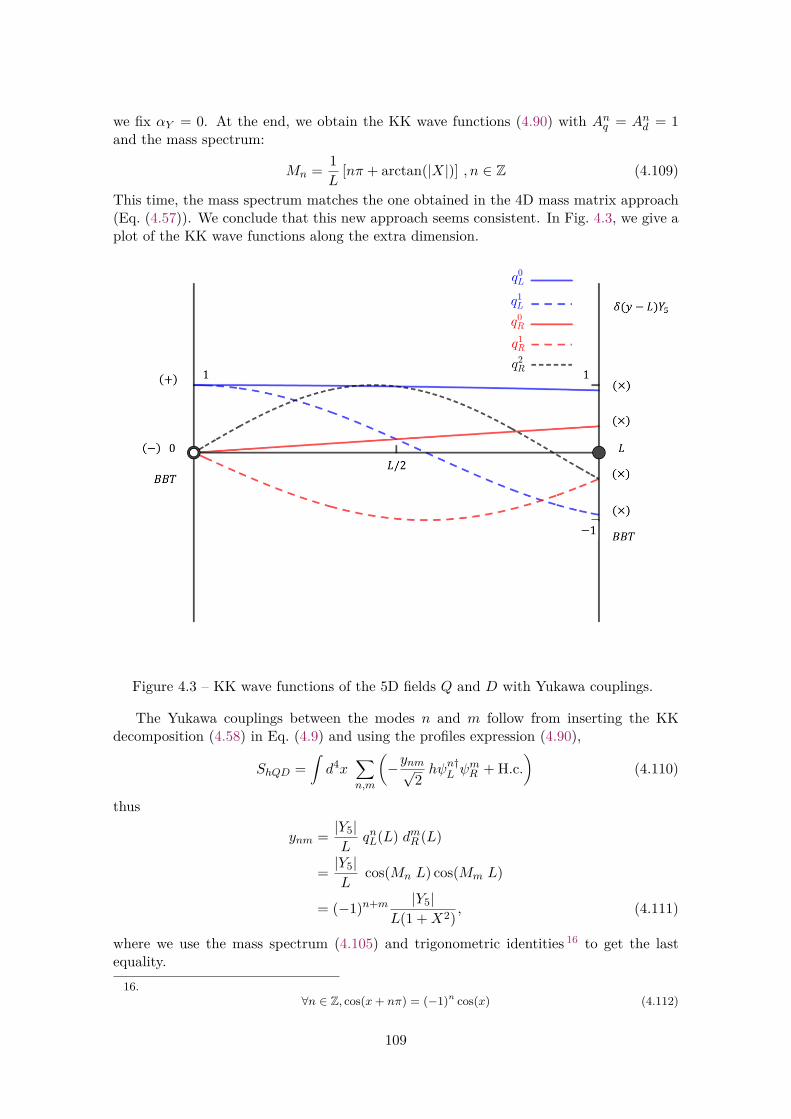
we fix αY = 0. At the end, we obtain the KK wave functions (4.90) with Anq = And = 1and the mass spectrum:

Mn = 1L

[nπ + arctan(|X|)] , n ∈ Z (4.109)

This time, the mass spectrum matches the one obtained in the 4D mass matrix approach(Eq. (4.57)). We conclude that this new approach seems consistent. In Fig. 4.3, we give aplot of the KK wave functions along the extra dimension.

Figure 4.3 – KK wave functions of the 5D fields Q and D with Yukawa couplings.

The Yukawa couplings between the modes n and m follow from inserting the KKdecomposition (4.58) in Eq. (4.9) and using the profiles expression (4.90),

ShQD =∫d4x

∑n,m

(−ynm√

2hψn†L ψ

mR + H.c.

)(4.110)

thus

ynm = |Y5|L

qnL(L) dmR (L)

= |Y5|L

cos(Mn L) cos(Mm L)

= (−1)n+m |Y5|L(1 +X2) , (4.111)

where we use the mass spectrum (4.105) and trigonometric identities 16 to get the lastequality.16.

∀n ∈ Z, cos(x+ nπ) = (−1)n cos(x) (4.112)

109

4.6.4 Brane Localized Terms & the Dirac Distribution

In this part, we reformulate the method in Subsection 4.6.3 with the formalism ofdistributions [369, 370]. As it corresponds just to reexpress the procedure in the languageof distributions, the physical results are the same.

The 5D Action as a Distribution

One can treat the 5D fields as distributions in order to handle boundary localizedinteractions. In this subsection, we choose a different approach where the fields are stillfunctions but the action is built with rectangular and Dirac distributions.

To formulate our model using Dirac distributions for the brane localized terms, wedefine the 5D fields on y ∈ R and use a rectangular distribution ΘI(y) = θ(y)− θ(y − L)to restrict the action to the physical compact space. The 5D action is thus rewritten as

SΨ + SB + SX =∫d4x

∫ +∞

−∞dy {LΨ ΘI(y) + LB [δ(y)− δ(y − L)] + LX δ(y − L)} .

(4.114)An important remark is that the fields in the Lagrangians LΨ (4.3), LX (4.8) and LB(4.10)must be continuous at the positions of the 3-branes in order to define the product betweenthe Dirac distributions and the Lagrangians LB, LX in Eq. (4.114).

Hamilton’s principle applied to the action (4.114), varying each field, with genericvariations at the boundaries, leads to

0 = δQ†L

(SΨ + SB + SX) =∫d4x

∫ +∞

−∞dyΘI(y) δQ†L

[iσµ∂µQL − ∂yQR

]+∫d4x

∫ +∞

−∞dy[δ(y − L) δQ†L (QR −XDR)− δ(y) δQ†LQR

],

(4.115)

0 = δQ†R

(SΨ + SB + SX) =∫d4x

∫ +∞

−∞dyΘI(y) δQ†R [iσµ∂µQR + ∂yFL]

+∫d4x

∫ +∞

−∞dy δ(y − L) δQ†R

(−X ′DL

), (4.116)

0 = δD†L

(SΨ + SB + SX) =∫d4x

∫ +∞

−∞dyΘI(y) δD†L

[iσµ∂µDL − ∂yDR

]+∫d4x

∫ +∞

−∞dy δ(y − L) δD†L

(−X ′∗QR

), (4.117)

0 = δD†R

(SΨ + SB + SX) =∫d4x

∫ +∞

−∞dyΘI(y) δD†R [iσµ∂µDR + ∂yDL]∫

d4x

∫ +∞

−∞dy[−δ(y − L) δD†R (DL +X∗QL) + δ(y) δD†RDL

],

(4.118)

cos(arctan(x)) = 1√1 + x2

(4.113)

110

where we used the fact that ∂yΘI(y) = δ(y) − δ(y − L) since ∂yθ(y) = δ(y). The genericfield variations should be understood as playing the role of testfunctions. One gets theequations including distributions,

(iσµ∂µQL − ∂yQR

)ΘI(y) + (QR −XDR) δ(y − L)−QR δ(y) = 0,

(iσµ∂µQR + ∂yQL) ΘI(y)−X ′DL δ(y − L) = 0,(iσµ∂µDL − ∂yDR

)ΘI(y)−X ′∗QR δ(y − L) = 0,

(iσµ∂µDR + ∂yDL) ΘI(y)− (DL +X∗QL) δ(y − L) +DL δ(y) = 0.

. (4.119)

One can notice that, in the formalism of distribution theory, the 5D Euler-Lagrange equa-tions contain the information leading to the natural boundary conditions via the productswith δ(y − L). If one applies the distribution equations (4.119) on a testfunction η(y),whose support supp(η) is such that supp(η) ⊂]0, L[, one gets simply

∫ +∞

−∞dy[(iσµ∂µFL − ∂yFR

)ΘI(y) η(y)

]= 0,∫ +∞

−∞dy [(iσµ∂µFR + ∂yFL) ΘI(y) η(y)] = 0.

(4.120)

For a generic testfunction η(y), this leads to the bulk Euler-Lagrange equations (4.15)for the 5D fields restricted to (0, L). Assuming that the 5D fields are differentiable withrespect to y with continuous derivatives, one can extend the viability of this Euler-Lagrangeequations system (4.120) to [0, L]. Then, using them in the system (4.119), we obtain

(QR −XDR) δ(y − L) = 0,X ′DL δ(y − L) = 0,X ′∗QR δ(y − L) = 0,

(DL +X∗QL) δ(y − L) = 0.

(4.121)

Again, one obtains the same boundary conditions as in Eq. (4.100). At the end, werecover the system of 5D Euler-Lagrange equations (4.15) and boundary conditions ofSubsection 4.6.3. The solution of the equations is thus the same (see the discussion inSubsection 4.6.3 below Eq. (4.100)). Therefore, treating the Yukawa terms as distributionsis just another mathematical way to treat brane localized couplings of bulk fields.

Currents and Distributions

The formalism of distributions is particulary convenient to study the currents asso-ciated to the 5D fields. We come back to the two transformations U(1)Q,D in Subsec-tion 4.3.2. It is straightforward to generalize Noether’s theorem to the case of a Lagrangiandistribution as in Eq. (4.114). The current associated to the field F = Q,D is

JMF = jMF ΘI , (4.122)

with jMF defined as in Eq. (4.27), and in particular j4F is given by the same expression

as in Eq. (4.29). Moreover, Noether’s theorem gives the expression for the divergence ofthese currents (|αf | � 1) [71],

∂MJMF = ∂

∂αf(L∗Ψ ΘI(y) + (L∗B + L∗X) δ(y − L)) , (4.123)

111

where the ∗ means the transformed Lagrangian under U(1)F . Therefore, even if thecurrents JMF are not conserved on the 3-brane at y = L, Eq. (4.123) can still provideinformation, linking the bulk currents to the Yukawa couplings on the 3-brane. For theleft-hand side of (4.123), using (4.122), one gets

∂MJMF = ∂Mj

MF ΘI + j4

F [δ(y)− δ(y − L)] . (4.124)

Restricting our study to the bulk, it is clear from Eq. (4.1) that U(1)F is a symmetry ofLΨ so the associated current is conserved outside of the branes,

∂MjMQ = 0. (4.125)

Again, we know that the fields are differentiable with continuous derivatives on [0, L], thusEq. (4.125) can be extended to the 3-branes. Using this last result in (4.124), we have

∂MJMF = j4

F [δ(y)− δ(y − L)] ,= −j4

F δ(y − L), (4.126)

where we used the fact that j4F vanishes at y = 0 since there is no mixing term between

Q and D here 17. Subsequently, one can express the right-hand side of Eq. (4.123) with(4.8) for the transformation U(1)Q,

∂L∗∂αQ

= i[X∗D†RQL −X Q†LDR +X ′∗D†LQR −X

′Q†RDL

]δ(y − L), (4.127)

hence (4.126) with (4.29) leads to[(Q†RQL −Q

†LQR

)−X∗D†RQL +X Q†LDR +X ′Q†RDL −X ′∗D†LQR

]∣∣∣y=L

= 0. (4.128)

which is trivially satisfied by the BCs 2 in Eq. (4.101) that we choose. One can repeat thesame exercise for the transformation U(1)D. Our choice of boundary conditions is thusconsistent with the conservation laws of the currents.

4.7 Implications

4.7.1 Interpretation of the Analytical Results

The matching of the fermion mass spectra obtained in the distinct 4D (Subsection 4.4)and 5D (Subsection 4.6.3) approaches constitutes a confirmation of both the spectra andthe feature that regularizing (performed in none of the 4D and 5D approaches) is notrequired for the calculation. The 5D method is obviously different from the 5D regular-izations (of type I and II) discussed in the literature and whose inconsistencies have beenpointed out in Section 4.5.

As a corollary, note that there is no other theoretical reason other than a would-beregularization to introduce a temporary shift along y of the Dirac distribution in thespectrum calculation. This shows the uniqueness of the fermion mass spectrum since sucha shift could modify the spectrum (as in the regularization II). Indeed, in particular inthe 4D approach, the coefficients βij of Eqs. (4.52)-(4.53) would tend to zero as shift ofthe brane on which the Higgs is localized would go to zero, implying a change of the mass

17. but the constraint that j4 (4.78) has to vanish at y = L remains.

112

spectrum if this limit is taken after (like in the 4D regularization II) the infinite KK towerlimit of the mass matrix characteristic equation [49].

Besides, the independence of the final fermion mass spectrum (4.105) on the parameterX ′ is an important result since most approaches including brane-Higgs regularization leadto a X ′ dependeence. The condition X ′ = 0 is required in order to have a system ofEuler-Lagrange equations with boundary conditions which is not overconstrained.

Let us now interpret physically the absence of the role of the Y ′5 coupling (involved inX ′) in the final spectrum (4.105) which depends only on X. In the 4D approach, startingwith the free action SΨ + SB, the KK wave functions dnL(y) and qnR(y) (∀n), defined inEq. (4.17) and given respectively by the first and fourth solutions of Eq. (4.34) (see thediscussion below this equation), vanish at the boundary y = L. Hence the term with acoefficient X ′ in the action SX of Eq. (4.8), added to the above free action SΨ + SB, getsmultiplied by a vanishing factor from the integration over the interval due to the Diracdistribution δ(y−L). More intuitively, the Y ′5 term localized at the boundary y = L, andcoupling the brane localized Higgs boson to the bulk fermions DL, QR, should not haveany effect since the associated free fermionic KK wave functions vanish at this boundary.Moreover, if this term is absent at tree level, it will not be perturbatively generated[319, 323], and thus this situation is technically natural. This feature is confirmed bythe rigorous procedure of solving the Euler-Lagrange equations and complete boundaryconditions leading to the mass spectrum (4.105).

4.7.2 Phenomenological impacts

In the appropriate treatment developed in the present chapter without regularization,the obtained mass spectrum and the effective 4D Yukawa coupling depend on Y5 but noton Y ′5 coupling constant.

The results for fermion masses and profiles are also correct when one invokes the brane-Higgs Regularization I for which the Y ′5 dependence cancels. Hence, the phenomenologicalanalyses in the literature based on such results are still valid: see for instance Ref. [47,48, 53, 328, 373–375]. Those arguments apply also to the geometrical background withwarped extra dimensions where the spectrum is expected to be independent of Y ′5 as well.

However, if the Regularization II or the softering of the brane-Higgs are used, theobtained fermion masses and 4D Yukawa couplings depend on both Y5 and Y ′5 so that theresults differ effectively from the correct ones. Hence, the phenomenological studies basedon these analytical results (for example Ref. [54, 55, 58–60]) should be reconsidered.

In addition, the effective 4D Yukawa couplings to fermions and their KK excitationsaffect the main Higgs production mechanism at the Large Hadron Collider (LHC): thegluon-gluon fusion via triangular loops of (KK) fermions. Hence the effect of the realisticlimit [49] of vanishing Y ′5 on the constraints on KKmasses derived in the studies [55, 58–60],within the warped background and based on the Regularization II, should be consideredas well.

Besides, the rotation matrices diagonalizing the 4D fermion mass matrix (4.52) do notdiagonalize simultaneously the effective 4D Yukawa coupling matrix since the latter onedoes not contain matrix elements due to the pure KK masses. The induced flavor violating4D Yukawa couplings are generated at leading order by Y ′5 contributions as can be showndiagrammatically [54]. Hence there exist FCNC effects in measured ∆F = 2 processessuch as K−K, B−B and D−D mixings, mainly produced by tree-level exchanges of theHiggs boson via Y ′5 couplings. These lead to considerable lower bounds on the KK bosonmass scale found to be around 6− 9 TeV in the analysis [54] on warped extra dimensionsusing indeed the Regularization II. Hence these bounds should be significantly alleviated

113

in the realistic situation where Y ′5 → 0; this limit should be applied since the independencefound in the present paper on Y ′5 (extended via flavor indices) remains true for the case ofthree flavors, as well as for fermion bulk masses, as it is clear in the 4D approach wherethe βij-elements (4.53) of the mass matrix still vanish. The predictions of Ref [54], basedon Regularization II, that FCNC reactions involving Yukawa couplings, like the rare topquark decay t → ch and exotic Higgs boson decay to charged leptons h → µτ , can beobservable at the LHC deserve reconsiderations as well when Y ′5 = 0.

4.8 Summary & ConclusionFor bulk fermions coupled to a brane-Higgs boson we have shown that the proper

calculation of the fermion masses and effective 4D Yukawa couplings does not rely onbrane-Higgs regularizations. The justifications are the following ones: (i) There are nojumps of the fermion wave functions at the boundary where the Higgs field is localized sothere is no motivation to introduce an arbitrary regularization, (ii) the regularizations suf-fer from several mathematical discrepancies confirmed by two known non-commutativitiesof calculation limits, (iii) our method without any regularization is validated in particularby the matching between the 4D versus 5D treatments.

In the rigorous method developed for both free and brane-coupled bulk fermions, wehave also pointed out the necessity to either include BBTs in the Lagrangian, or alterna-tively impose conditions on vanishing conserved currents at the boundaries of the interval.The arguments go as follows: (i) the presence of BBTs guarantees the conditions on cur-rents which define the field geometrical configuration of the model, (ii) the BBTs andthe conditions on currents allow to define a model which is not overconstrained and tofind physically consistent fermion masses, bulk profiles and effective 4D Yukawa couplings(solutions fulfilling the normalization constraints and the decoupling limit condition), (iii)the BBTs lead to the expected matching between the 4D and 5D calculation results. Wesummarize the results in Tab. 4.1. The BBTs indicate a possible origin of the chiral natureof the SM as well as of its chirality distribution among quark/lepton SU(2)W doubletsand singlets.

NBCs only EBCs BBTs & NBCs

4D approach Not physical BCs (±) BCs (±)

5D approach Not physical Impossible BCs (×)

Table 4.1 – Summary of the results of the 4D and 5D approaches. We use the followingacronyms: BC for Boundary Condition, EBC for Essential Boundary Condition, NBC forNatural Boundary Condition.

The general methodology worked out reveals that the information regarding the defi-nition of a higher-dimensional model are not necessarily fully contained in the action itself– through the deduced Euler-Lagrange equations and the natural boundary conditions –but might be partly included as well through essential boundary conditions.

114

We finished the analysis by the phenomenological impacts of the new calculationmethod which predicts the independence of the fermion masses and effective 4D Yukawacouplings on the Y ′5 parameter of the Lagrangian. This feature, with respect to the Regu-larization II or to the softening of the brane-Higgs usually applied in the literature, shouldin particular alleviate significantly the previously obtained severe bounds on KK massesinduced by FCNC processes generated via flavor violating couplings of the Higgs boson.

115

Chapter 5

Generalizations

This chapter is a personal adaptation of a collection of unpublished works in collabo-ration with Andrei Angelescu, Ruifeng Leng and Grégory Moreau.

In this chapter, we continue our exploration of the treatment of brane localized termsfor 5D fermions. In Section 5.1, we treat the model of Chapter 4 on an AdS5 spacetime.In Section 5.2, we apply our methods to the case of other boundary terms usually studiedin brane world literature. In Section 5.5, we generalize the study of Chapter 4 to the caseof a Higgs field localized on a brane away from a boundary. Finally, in Section 5.3, westudy the model of Chapter 4 on an orbifold background.

5.1 Boundary Localized Higgs Field: Generalization to aSlice of AdS5

5.1.1 Randall-Sundrum 1 Setup

In this section, we want to generalize the model of Chapter 4 to the case of a warpedextra dimension. We consider the 5D spacetime of the RS1 model. The extra dimension isstill compactified on an interval I = [0, L] but now the two 3-branes have opposite tensions.The gravitationnal backreaction of the brane tensions is balanced by the introduction ofa negative bulk cosmological constant. At the price of a fine tunning between thesequantities, the fifth dimension is warped in order to get a 5D bulk as a slice of an AdSspacetime. Once integration is performed over the compact coordinate, the effective 4Dcosmological constant vanishes. The 5D metric, solution of the Einstein equations, is givenby

ds2 = e−2kyηµνdxµdxν − dy2 ≡ gMNdx

MdxN , (5.1)

where 1/k is the AdS curvature. The fünfbein eAM is defined by

gMN = eAMeBNηAB (5.2)

and its inverse by eMA eBM = δBA , with A ∈ {a, 4} and a ∈ {0, 1, 2, 3}. We define also

e =∣∣∣det eAM

∣∣∣. It is often more convenient to work in the conformally flat frame by makingthe coordinate transformation

z = eky

k, (5.3)

116

such that the conformally flat fünfbein is

eMA = kz δMA and e = (kz)−5 , (5.4)

sogMN =

( 1kz

)2ηMN . (5.5)

In this frame, the UV-brane at y = 0 and the IR-brane at y = L, where the electroweaksymmetry breaking occurs, are respectively at z = 1/k and z = 1/T , where T = ke−kL.If M∗ is the 5D gravity scale, one should have M∗/k & O(10) such that we are in theclassical regime where one can use the Einstein equations: the AdS5 background metricis well defined. The cut-off 1 on the UV-brane is usually taken ΛUV ∼ M∗ and the oneon the IR-brane is ΛIR = e−kLΛUV , because of the gravitational redshift induced by thewarp factor. If one takes ΛIR ∼ O(1) TeV and a IR-brane localized Higgs field, one cansolve the naturalness problem of the Higgs sector in the SM.

In the following, we focus on a toy model containing only bulk fermions and a branelocalized Higgs field, and study their resulting Yukawa interactions.

5.1.2 Field Content

Brane Localized Higgs field

The Higgs field is still confined to the IR-brane. For simplicity, we take just a realscalar without gauge quantum numbers. Its Lagrangian has the generic form

LH = 12 ∂µH ∂µH − V (H). (5.6)

As for the SM, the minimum of the Higgs potential V (H) determines a non-vanishingVEV v for H

H(x) = k

T· v + h(x)√

2. (5.7)

The factor k/T comes from the induced metric (Eq. (5.5)) on the IR-brane and the usualrescaling of the brane localized Higgs field, in order to define v as the electroweak VEV.

Fermion Content and Yukawa Interactions

Our goal is to study a chiral 4D effective field theory with renormalizable Yukawacouplings to the Higgs field, in order to generate Dirac masses for the fermions as, forexample, in the quark sector of the SM. For that purpose, the minimal spin-1/2 fermionfield content is a couple of fermions, Q and D. In the spirit of RS1 models with bulkmatter, the fields Q(x, y) and D(x, y) propagate in the extra dimension. We split thefermion Lagrangian into a free part LFΨ, the BBTs LB, and a Yukawa interaction with theHiggs field LY , such that the 5D action is

S5D =∫d4x

∫ L

0dy e

{LQΨ + LDΨ + [δ(y)− δ(y − L)]LB + δ(y − L) (LH + LY )

}. (5.8)

The passage to the conformally flat frame requires the following substitution: δ(y) →δ(z − k−1) and δ(y − L)→ k

Tδ(z − T−1).

1. i.e. the scale at which gravity becomes strong.

117

The free Lagrangian for a fermion F = Q,D is

LFΨ = i

2(FeMA ΓA∇MF −∇MFeMA ΓAF

)−MF FF , (5.9)

with F = F†Γ0 and ∇MF = (∇MF)† Γ0. The covariant derivative ∇M = ∂M + ωMcontains the spin connection ωM . It is known that in the case of the RS metric, Eq. (5.1),the contribution of ωM cancels in the action and one can safely replace ∇M → ∂M inEq. (5.9). We define the bulk mass MF in units of the fundamental scale k such thatMF = cF k. The 5D spin-1/2 fermions are decomposed as

F =(Fα

F†α

), (5.10)

in terms of two Weyl spinors 2 Fα and F α with α, α ∈ {1, 2}. We point out that the baron F

α is part of the name of the field, and does not denote the operation of Hermitianconjugation. After some algebra, Eq. (5.9) becomes

LFΨ = kz

[i(F †σ

µ∂µF + Fσµ∂µF

†)+ 12(F←→∂z F − F †

←→∂z F

†)]− k cF (FF + F †F†),

(5.11)where we have dropped a 4-divergence term from an integration by parts. Below the KKscale (in the decoupling limit), we would like to recover the SM so we would like zeromodes for Q and D only. For that purpose, one needs the BBTs,

LB = 12(DD −QQ

). (5.12)

The Yukawa interactions with the Higgs field are

LY = −Y5DHQ− Y ′5 D†HQ† + H.c. . (5.13)

One can check whether the phases of the 5D Yukawa couplings Y5 and Y ′5 have a physicalimpact. Performing one of the two substitutions Y5 → eiα1 Y5 or Y ′5 → eiα2 Y ′5 , one cannotfind a transformation of the fermion fields which leave the Lagrangians (5.13), (5.13) and(5.13) invariant. However, if one performs the following simultaneous transformations:Y5 → eiα Y5, Y ′5 → e−iα Y ′5 , Q → e−iαQ and Q → e−iαQ, the Lagrangians (5.13), (5.13)and (5.13) are invariant. This means that the phase of only one Yukawa coupling isphysical. We focus on the VEV of the Higgs field and include the H boson fluctuationonly in a later subsection, which deals with the Yukawa couplings. LFY therefore becomes

LFX = −XDQ−X ′D†Q† + H.c. , (5.14)

with the compact notation X = Y5k

T· v√

2and X ′ = Y ′5

k

T· v√

2.

2. From now on, we use calligraphic letters to denote 5D (Dirac) spinors and typed letters to denoteWeyl spinors.

118

5.1.3 5D Method

Euler-Lagrange Equations and Boundary Conditions

One can generalize Hamilton’s principle in Appendix B.4 to the case of a metric witha warp factor. With the Lagrangian e(LQΨ +LDΨ) (5.11), the 5D Euler-Lagrange equations(B.19) give

iσµ∂µF − ∂zF

† + 2− cFz

F† = 0,

iσµ∂µF† + ∂zF −

2 + cFz

F = 0.(5.15)

At z = 1/k, we obtain the natural boundary conditions (B.22) Q|y=0,L = 0 and D|y=0,L =0. At z = 1/T , the Hamilton’s principle with the Lagrangians e (LQΨ + LDΨ) (5.11),

e

( 1T

)k

TLB (5.12) and e

( 1T

)k

TLY (5.13) give the natural boundary condition (B.23)

Q†∣∣∣z=1/T

= D|z=1/T = 0 or else X ′ = 0 , (5.16)

and (Q† −XD

†)∣∣∣z=1/T

= (D +X∗Q)|z=1/T = 0 . (5.17)

In order to obtain a mass spectrum which depends on X (we want to recover the SMin the decoupling limit), we choose X ′ = 0 so Y ′5 = 0. As the phase of only Y5 or Y ′5is physical, we can take Y5 = |Y5| and thus X = |X|. In the limit X → ∞, one needslimz→1/T D = limz→1/T Q = 0 in order to keep limz→1/T Q and limz→1/T D finite, so aninfinite Higgs field VEV is equivalent to a Dirichlet boundary conditions on Q and D.

Kaluza-Klein Decomposition & Equations for the KK Wave Functions

Because of the mass term LFX localized on the IR-brane, the two KK towers from Qand Q will mix respectively with the ones from D and D. We follow the same method asin Section 4.6, and introduce the mixed KK decomposition:

Q(x, z) = (kz)3/2∑n

qn(z)ψn(x),

Q†(x, z) = (kz)3/2∑

n

qn(z)ψ†n(x),

D(x, z) = (kz)3/2∑n

dn(z)ψn(x),

D†(x, z) = (kz)3/2∑

n

dn(z)ψ†n(x),

(5.18)

where the Weyl spinors ψn(x) and ψ†n(x) obey the usual Dirac-Weyl equations,

∀n , iσµ∂µψn (x) = mn ψ†n (x) ,

iσµ∂µψ†n (x) = mn ψn (x) , (5.19)

119

with mn the mass of the nth KK mode, and where fn(z) and fn(z) (f = q, d) are the KKwave functions, orthonormalized so that∫ 1/T

1/k

dz

kz[q∗n(z) qm(z) + d∗n(z) dm(z)] = δnm,

∫ 1/T

1/k

dz

kz

[q∗n(z) qm(z) + d

∗n(z) dm(z)

]= δnm ,

(5.20)

in order to recover canonical kinetic terms for the KK modes when plugging the mixedKK decomposition into the 5D action from Eq. (5.8). This, together with the Dirac-Weylequations, Eq. (5.19), and the 5D Euler-Lagrange equations (5.15), gives the equations forthe KK wave functions

∂zfn(z)−mn fn(z)− 1z

(12 − cF

)fn(z) = 0,

∂zfn(z) +mn fn(z)− 1z

(12 + cF

)fn(z) = 0.

(5.21)

One can easily decouple these first order differential equations into second order equations:(z2∂2

z + z∂z +m2nz

2 −[cF −

12

]2)(

fn(z)kz

)= 0,

(z2∂2

z + z∂z +m2nz

2 −[cF + 1

2

]2)(

f(z)kz

)= 0.

(5.22)

These are Bessel equations, whose solutions are combinations of Bessel functions of thefirst and the second kind:

qn(z) = kz

N qnf qn(z) with f qn(z) = Jα(mnz) + bqn Yα(mnz),

qn(z) = kz

Nq

n

fqn(z) with f

qn(z) = Jα+1(mnz) + b

q

n Yα+1(mnz),

dn(z) = kz

Ndn

fdn(z) with fdn(z) = Jβ+1(mnz) + bdn Yβ+1(mnz),

dn(z) = kz

Nd

n

fdn(z) with f

dn(z) = Jβ(mnz) + b

d

n Yβ(mnz),

(5.23)

where α = ±(cQ −

12

)and β = ±

(cD + 1

2

). We choose the prescription + for α and −

for β and will come back later on the reason for this choice.

Boundary Conditions & Mass Spectrum

The boundary conditions at z = k−1, Q|z=1/k = 0 and D|z=1/k = 0, translate intoDirichlet boundary conditions for the KK wave functions of Q and D,

qn

(k−1

)= 0 and dn

(k−1

)= 0. (5.24)

120

One can combine them with the first order equations for the KK wave function fromEq. (5.21) to get the boundary conditions:

[∂zqn(z)− k(α+ 1)qn(z)]|z=1/k = 0,

[∂zdn(z)− k(β + 1)dn(z)

]∣∣∣z=1/k

= 0.(5.25)

These boundary conditions are consistent with Eq. (5.21) and the KK wave functions inEq. (5.23) if

N qn = N

q

n , Ndn = −Nd

n , bqn = bq

n = −Jα+1

(mn

k

)Yα+1

(mn

k

) , bdn = bd

n = −Jβ+1

(mn

k

)Yβ+1

(mn

k

) . (5.26)Using the mixed KK decomposition (Eq. (5.18)) in the boundary conditions at z = T−1

from Eq. (5.17), one gets

fqn(T−1)N qn

+Xfdn(T−1)Ndn

= 0,

Xf qn(T−1)N qn

+ fdn(T−1)Ndn

= 0.

(5.27)

This represents a system of two linear equations for the inverse of the normalization coef-ficients Nf

n . This system has non-trivial solutions (i.e. non-zero) only when the associateddeterminant vanishes. This gives us the relation from which we can extract the massspectrum mn:

fqn(z) fdn(z)

f qn(z) fdn(z)

∣∣∣∣∣∣z=1/T

= X2, (5.28)

which is independent of the normalization coefficients Nfn .

In the case of equal bulk masses, the left-handed zero mode of Q and the right-handedzero mode of D have the same KK wave functions. In our sign convention for α and β,this is simply the condition α = β, from which it follows that the common localizationparameter is c .= cQ = −cD. This also implies that bn

.= bqn = bdn and Nn.= N q

n = Ndn.

Using the KK wave functions from Eq. (5.23), the mass spectrum from Eq. (5.28) isdetermined by (

Jα+1(mnz) + bn Yα+1(mnz)Jα(mnz) + bn Yα(mnz)

)2∣∣∣∣∣z=T−1

= X2. (5.29)

Normalization Conditions

In the same way as in Section 4.6, it is easy to show that one can take the normalizationconstants N q

n and Ndn real. The KK wave functions are thus real. Let us have a closer

look at the normalization conditions in Eq. (5.20) for the exact KK wave functions. Theseconditions read for n = m. ∫ T−1

k−1

dzz

[q2n(z) + d2

n(z)]

= k, (5.30)∫ T−1

k−1

dzz

[q

2n(z) + d

2n(z)

]= k, (5.31)

121

and in the following we focus on showing that these two conditions are equivalent.We start by simplifying Eqs. (5.30) and (5.31). To achieve this, we first consider the

coupled equations for the KK wave functions d and d:

∂zdn +mndn + βdnz

= 0, (5.32)

∂zdn −mndn − (β + 1) ∂zdnz

= 0. (5.33)

We now perform two operations on the coupled equations: we multiply (i) Eq. (5.32) bydn and Eq. (5.33) by dn and (ii) Eq. (5.32) by dn and Eq. (5.33) by dn, and in both caseswe take the sum of the resulting equations. After a few lines of algebra, it is possible toexpress the two KK wave functions, dn and dn, in terms of their derivatives

d2n

z= ∂z

d2n + d

2n

2 + β

mn

dndnz

, (5.34)

d2n

z= ∂z

d2n + d

2n

2 + β + 1mn

dndnz

. (5.35)

If one repeats the exercise for the q KK wave functions, the following relations are derived:

q2n

z= ∂z

q2n + q

2n

2 − α+ 1mn

qnqnz

, (5.36)

q2n

z= ∂z

q2n + q

2n

2 − α

mn

qnqnz

. (5.37)

Inserting Eqs. (5.34)-(5.37) into the normalization conditions from Eqs. (5.30) and (5.31),we find that∫ T−1

k−1dz ∂z

d2n + d

2n + q2

n + q2n

2 + β dndn − α qnqnmnz

+ dndnmnz

= k, (5.38)

∫ T−1

k−1dz ∂z

d2n + d

2n + q2

n + q2n

2 + β dndn − α qnqnmnz

− qnqnmnz

= k. (5.39)

Note that the only difference between the two previous equations is the third terms inEqs. (5.38) and (5.39). Since the KK wave functions are continuous and differentiable onthe closed interval [k−1, T−1], we can write the difference between Eqs. (5.38) and (5.39)as ∫ T−1

k−1dz ∂z

[dndn + qnqn

mnz

]= dn(z)dn(z) + qn(z)qn(z)

mnz

∣∣∣∣T−1

k−1. (5.40)

We now use the boundary conditions for the KK wave functions to show that the aboveexpression vanishes. Indeed, as qn(k−1) = dn(k−1) = 0 and

dn(T−1) = qn(T−1)X

, dn(T−1) = −Xqn(T−1), (5.41)

one immediately realizes that the expression in Eq. (5.40) vanishes. As a consequence,Eqs. (5.38) and (5.39) are identical, which means that the two normalization conditions inEqs. (5.30) and (5.31) are equivalent. In other words, Eqs. (5.30) and (5.31) cannot deter-mine both normalization constants Nd

n and N qn, but only provide a relationship between

the two.

122

4D Yukawa Couplings

The 4D Yukawa couplings between the KK modes and the Higgs boson can be obtainedby developping the Higgs field around its VEV in Eq. (5.13) and performing the KKdecompositions of the 5D fields. One simply obtains

ynm = Y5 dn

(T−1

)qm(T−1

). (5.42)

5.1.4 4D Method

The 4D method to compute the mass spectrum and Yukawa couplings was done in anunpublished work by our collaborator Andrei Angelescu. We give it in Appendix C forcompleteness. As expected, the results of the 5D and 4D methods match.

5.1.5 Conclusion

In this section, we have generalized the treatment of 5D fermions coupled to a bound-ary localized Higgs field of Chapter 4 to a warped extra dimension. The lightest mode canbe identified with a fermion of the SM which obtain his mass from the boundary localizedHiggs field. The method to treat the boundary localized mass terms and Yukawa inter-actions is still the same: one has to add BBTs in order to have a well defined 5D methodand also to get the matching between the 4D and 5D methods.

5.2 Various Boundary Localized TermsWe are going to study various boundary localized terms without the regularization

procedure. We will see the necessity of introducing BBTs for each case.

5.2.1 Toy Model: One Fermion in the Bulk

We consider a 5D flat spacetime. The extra dimension is compactified on an intervalI of length L, with two 3-branes set at the boundaries. Our goal is to study various branelocalized kinetic and mass terms for a bulk fermion field F , using a rigorous mathemat-ical treatment. The corresponding fermionic Lagrangian splits into a free part (withoutinteraction) LFK containing the kinetic term, and a brane localized part LFL at y = L, suchthat the 5D action is

S5D =∫d4x

∫ L

0dy[LFK + δ(y − L)LFL

]. (5.43)

The bulk part of the Lagrangian reads

LFK = i

2F ΓM←→∂ MF , (5.44)

where the 5D spin-1/2 fermions are decomposed as

F =(Fα

F†α

), (5.45)

in terms of two Weyl spinors Fα and F †α with α, α ∈ {1, 2} (see Appendix A). After somealgebra and an integration by parts (we drop the 4-divergence), Eq. (5.44) becomes

LFK = i(F †σ

µ∂µF + Fσµ∂µF

†)+ 12(F←→∂yF − F †

←→∂yF

†). (5.46)

123

In Appendix B.4, we explain how to apply Hamilton’s principle for a field theory withan extra dimension compactified on I. The 5D Euler-Lagrange equations for F and F(Eq. (B.19)) originate only from the bulk Lagrangian LFΨ (5.46) (Eq. (B.19)), and we get

iσµ∂µF − ∂yF

† = 0 ,

iσµ∂µF† + ∂yF = 0 . (5.47)

In absence of a brane localized Lagrangian and a Higgs field, we would like that the 5Dfermion field reduces to a massless 4D chiral fermion (SM-like before EWSB) in the limitL→ 0 (decoupling limit). For that purpose, it is convenient to decompose the 5D theoryinto a 4D theory by performing a KK decomposition: each 5D field becomes an infinitetower of 4D KK modes, each of them has a KK wave function along the extra dimension.In order to conserve only the left-handed or the right-handed zero mode, we impose theso-called chiral boundary conditions. Here, we choose to have a left-handed zero modeso the chiral boundary conditions consist of Dirichlet boundary conditions at y = 0, Lfor F . In Chapter 4, it is shown that the chiral boundary conditions can be essentialboundary conditions induced by conditions on the conserved current at the boundaries.Then, one can include the brane localized Lagrangians as an infinite matrix in the KK basisto diagonalize. Here we use the alternative method, where the brane localized operatorsgenerate boundary conditions for the 5D fields.

5.2.2 Boundary Localized Kinetic Terms

We begin by studying Brane Localized Kinetic Terms (BLKTs) at y = L such that

LFL = κ iF †σµ∂µF + κ′ iFσµ∂µF

†, (5.48)

where κ and κ′ are real parameters with mass dimension −1: the magnitude of the BLKTs.They only involve the partial dervatives ∂µ since terms involving ∂y involve subtleties thatwe will not consider here [376–378]. In an extra-dimensional model with branes, theBLKTs are allowed by the symmetries in the EFT. The UV completion can imply largeBLKTs at tree level leading to important phenomenological consequences [317, 320–323].Even if absent at tree level, the BLKTs are still generated radiatively [319]. In this case,their magnitude is not large, as they originate from loop corrections.

In order to rewrite the 5D theory as a 4D one, we perform a KK decomposition of thefields,

F (x, y) = 1√L

∑n

fn(y)ψn(x) ,

F† (x, y) = 1√

L

∑n

fn(y)ψ†n(x) . (5.49)

With this KK decomposition, the 5D Euler-Lagrange equations (5.47) reduce to the firstorder differential equations for the KK wave functions fn(y) and fn(y):

∀n , ∂yfn(y) +mn fn(y) = 0 ,∂yfn(y)−mn fn(y) = 0 , (5.50)

and the two 4D Weyl spinors ψn(x) and ψ†n(x) combine into a Dirac spinor of mass mn,which represents the n-th fermionic KK level, described by the Dirac-Weyl equations

124

(5.19). In order to get canonical kinetic terms for the 4D KK modes, the wave functionsfn(y) and fn(y) are orthonormalized as

∀n , 1L

∫ L

0dy [1 + κ δ(y − L)] f∗n(y)fm(y) = δnm ,

1L

∫ L

0dy[1 + κ′ δ(y − L)

]f∗n(y)fm(y) = δnm . (5.51)

The first order equations can be decoupled into second order ones as

∀n ,(∂2y +m2

n

)fn(y) = 0(

∂2y +m2

n

)fn(y) = 0 . (5.52)

The general solutions are

∀n , fn(y) = An cos(mn y) +Bn sin(mn y) ,fn(y) = An cos(mn y) +Bn sin(mn y) . (5.53)

where An, Bn, An and Bn are complex coefficients. The first order equations (5.50) imposethe relations An = Bn and Bn = −An. We keep the same boundary conditions at y = 0as in the absence of BLKTs, F |y=0 = 0, so after the KK decomposition (5.49) and withEq. (5.50),

∀n , fn(0) = ∂yfn(0) = 0 . (5.54)

When imposed on the KK wave functions (5.53), the boundary conditions (5.54) give

∀n , fn(y) = An cos(mn y) ,fn(y) = An sin(mn y) . (5.55)

Failed treatment without bilinear boundary terms

Using Appendix B.4, Hamilton’s principle applied to the action (5.43) with the La-grangians (5.46) and (5.48) gives the natural boundary conditions at y = L (Eq. (B.23)),(

F† + 2κ iσµ∂µF

)∣∣∣y=L

= 0 ,(F − 2κ′ iσµ∂µF

†)∣∣∣y=L

= 0 . (5.56)

With the KK decomposition (5.49) and the 4D Dirac-Weyl equations (5.19), the nat-ural boundary conditions at y = L (5.56) become boundary conditions for the KK wavefunctions,

∀n , fn(L) + 2κmn fn(L) = 0 ,fn(L)− 2κ′mn fn(L) = 0 , (5.57)

which lead tofn(L) = fn(L) = 0 (5.58)

or else to the relation:∀n , −4κκ′m2

n = 1 . (5.59)

125

With the KK wave functions of Eq. (5.55), the boundary conditions (5.58) lead to wavefunctions (and a 5D field) which vanish everywhere in the extra dimension (not physical),c.f. Chapter 4. Eqs. (5.55) and (5.59) give the mass spectrum

tan(mn L) = −2κmn , f (5.60)

combined to Eq. (5.59). There is thus only one massive KK mode (no KK tower) whosemass fix the parameter κ′ which is not a free parameter. In fact, Eq. (5.59) results fromthe fact that the system is overconstrained (see discussion below Eq. (4.85) where wehave a similar problem). Moreover, in the 4D method, κ′ should not play a role sincethe matrix element involving κ′ are proportional to the overlap of wave functions withDirichlet boundary conditions so they vanish (no 4D/5D matching).

Treatment with bilinear boundary terms

To overcome the previous difficulty, we add to the action (5.43) BBTs:

SB =∫d4x

∫ +∞

−∞dy [δ(y)− δ(y − L)] LFB , (5.61)

withLFB = −1

2FF = −12(FF + F †F

†), (5.62)

and we will take also κ′ = 0. The choice κ′ 6= 0 corresponds to a non-vanishing BLKTleading to a variation of the action at y = L involving δF while we have also the variation ofthe BLKT depending on κ whose variation implies also δF : there are two natural boundaryconditions at the boundary. As the 5D Euler-Lagrange equations (5.47) relate F and Fon-shell, a non-vanishing κ overconstrains the system. The absence of BLKT for a 5D fieldwith a Dirichlet boundary condition 3 was already noted in the literature. In Ref [323],it was noticed that the BLKT for a field with a Dirichlet boundary condition vanishesat tree level. In the context of holography, Ref. [66] showed that the absence of branelocalized terms for fields with Dirichlet boundary conditions is required by Hamilton’sprinciple. Moreover, if a brane localized operator is absent at tree level for fields withDirichlet boundary conditions, it is not radiatively generated [319].

Hamilton’s principle applied to the action (5.43), with the Lagrangians (5.46), (5.48)and (5.62), gives the natural boundary conditions at y = L (Eq. (B.23)),(

F† + κ i σ

µ∂µF

)∣∣∣y=L

= 0 , (5.63)

andκ′ = 0 or iσµ∂µF

†∣∣∣y=L

= 0 , (5.64)

and the natural boundary conditions at y = 0, F |y=0 = 0.As above, we use a KK decomposition (5.49). The KK modes satisfy Eq. (5.19) and

their wave functions are normalized with (5.51). The boundary conditions (5.63) and(5.64) give

∀n , fn(L) + κmn fn(L) = 0 , (5.65)

andκ′ = 0 or else ∀n , mn fn(L) = 0 . (5.66)

3. It is a perturbative argument based on the fact that one solves the Euler-Lagrange equations firstwithout the BLKTs and then includes them perturbatively through a 4D matrix to diagonalize.

126

The effect of the BLKTs is due to the boundary conditions. For mn 6= 0 in the bound-ary condition (5.65) with BBTs, the limit κ → ∞ implies limy→L fn(y) = 0 to keeplimy→L fn(y) finite, since the KK wave functions are bounded as they must be normal-ized. One can thus impose Dirichlet boundary condition by a BLKT of infinite magnitude.

The KK wave functions satisfy Eq. (5.50). This is in contrast to what appeared inthe literature. In [50], the BLKT is present in the equations for the KK wave functionsmultiplied by a Dirac distribution. The mass spectrum is obtained by integrating theseequations over a small interval around the boundary. In Chapter 4, it was shown that sucha treatment leads to mathematical inconsistencies and that a Dirac distribution must betreated more carefully within the theory of distributions. The simplest way is to put theboundary terms in the boundary conditions, as we do here.

The KK wave functions are still given by Eq. (5.55). With the boundary conditionat y = L (5.65) and the KK wave functions expressions (5.55), we get the transcendentalequation

tan(mn L) = −κmn , (5.67)

whose solutions give the mass spectrum depending on κ. We see that the BLKT affectthe mass spectrum and the shape of the KK wave functions only for n 6= 0. On the otherhand, when n = 0, the mode is massless and κ will only play a role via the normalizationcondition. Indeed, combining Eqs. (5.51), (5.55) and (5.67), we obtain

|An| =(1

2 + κ

2L(1 + κ2m2n)

)−1/2. (5.68)

5.2.3 Boundary Localized Majorana Mass Terms

In this subsection, we study the case of a Majorana mass term localized on the 3-brane[50] at y = L, which is described by the following Lagrangian:

LFL = −µ2(FF + F †F †

)− µ′

2(FF + F

†F†), (5.69)

with µ, µ′, dimensionless real parameters. Such terms are possible because physics on the3-brane is 4D and therefore Majorana spinors exist, contrary to the 5D bulk where onlyDirac spinors can be defined. These terms could play an important role in brane worldmodel building with neutrinos or with 5D SUSY.

We define a KK decomposition,

F (x, y) = 1√L

∑n

fn(y) νn (x) ,

F† (x, y) = 1√

L

∑n

fn(y) ν†n (x) , (5.70)

where the KK states are Majorana fermions νn of mass mn, obeying the homonymousequations,

iσµ∂µνn (x) = mn ν

†n (x) ,

iσµ∂µν†n (x) = mn νn (x) . (5.71)

The KK wave functions are orthonormlized to recover canonical 4D kinetic terms for theKK modes, so

2L

∫ L

0

(f∗n(y)fm(y) + f

∗n(y)fm(y)

)= δnm . (5.72)

127

The 5D Euler-Lagrange equations (B.19) lead, after the KK decomposition (5.70) andusing the Majorana equations (5.71), to the coupled first order differential equations (5.50)for the KK wave functions. Their solution is similar to the one below Eq. (5.50) with thesame boundary condition at y = 0 (5.54), and we get the KK wave functions in Eq. (5.55).

Failed treatment without bilinear boundary terms

We apply Hamilton’s principle to the action (5.43) with the Lagrangians (5.46) and(5.69) and get the natural boundary conditions (Appendix B.4, Eq. (B.23)),(

F† − 2µF †

)∣∣∣y=L

= 0 ,(F + 2µ′ F

)∣∣∣y=L

= 0 , (5.73)

soF |y=L = F |y=L = 0 , (5.74)

or else− 4µµ′ = 1 . (5.75)

The case of Eq. (5.74) with the KK wave functions (5.55) gives vanishing wave functions(and 5D field) everywhere in the extra dimension, which is not physical. Now we examinethe case of the relation (5.75). The KK decomposition (5.70) in Eq. (5.73) gives theboundary conditions at y = L:

f(L)− 2µ f(L) = 0 ,f(L) + 2µ′ f(L) = 0 , (5.76)

which are applied to the wave functions (5.55) to get the equation for the mass spectrum:

tan(mn L) = 2µ . (5.77)

µ′ is not an independent parameter, which means that the system is overconstrained.Moreover, in the 4D method, µ′ should not play a role since the matrix element involvethe overlap with wave functions which have Dirichlet boundary conditions so they vanish:we do not have the 5D/4D matching. Besides, in the limit µ, µ′ → 0, F |y=L = F = 0. Onewould expect to recover the free case in this limit, where only F has a Dirichlet boundarycondition at y = L. Indeed, when the brane localized Majorana mass terms (5.69) areincluded with an infinite matrix in the free KK basis 4 to diagonalize, the limit µ, µ′ → 0reduces to the boundary condition of the free case. Instead, we have Dirichlet boundaryconditions for both F and F at y = L, and this is known to imply vanishing 5D fields ateach point in the bulk.

Treatment with bilinear boundary terms

In the same way as in the case of the BLKTs, we modify the model by adding theboundary term SB (Eqs. (5.61) and (5.62)). The effect of the brane localized Majoranaterm enters via the boundary conditions at y = L. In order to give a mass to the zeromode, we would like non-vanishing µ. The presence of the term with µ′ overconstrained

4. Here, we are a bit premature when speaking about a KK basis because we have not yet defined theKK decomposition of the 5D fields. However, we do not need the details at this level and the general ideashould be clear.

128

the system in the same way as in the discussion with the BLKT involving κ′ so we willtake also µ′ = 0. Again, the brane-localized term, involving fields with Dirichlet boundaryconditions in the free case, is vanishing and is not radiatively generated (Ref. [319]).

Hamilton’s principle with the Lagrangians (5.46), (5.69) and (5.62) gives the naturalboundary conditions at y = L (Appendix B.4, Eq. (B.23)),(

F† − µF †

)∣∣∣y=L

= 0 , (5.78)

andµ′ = 0 or else F

∣∣∣y=L

= 0 , (5.79)

and the natural boundary condition at y = 0, F |y=0 = 0.The natural boundary conditions (5.78) and (5.79) translate into boundary conditions

for the KK wave functions as

∀n , fn(L)− µ fn(L) = 0 , (5.80)

andµ′ = 0 or ∀n , fn(L) = 0 . (5.81)

We chose µ′ = 0. One can notice that, in the case µ→∞, one needs limy→L fn(y) = 0 inorder to maintain limy→L fn(L) finite, since the KK wave functions are bounded. One canthus impose Dirichlet boundary conditions by an infinite brane localized Majorana mass.

The boundary condition at y = L (5.80) gives, with the KK wave functions (5.55), theequation for the mass spectrum,

tan(mn L) = µ , (5.82)

whose solutions aremn = 1

L[arctan(µ) + nπ] , n ∈ Z . (5.83)

The normalization conditions (5.72) applied to the profiles (5.55) give the normalizationcoefficients |An| = 1/

√2.

5.2.4 Mixing Terms involving a Boundary Localized Fermion

We now turn towards the case of a bulk fermion F and a brane localized Weyl fermionW . The two fermions can mix on the IR brane via a Dirac mass term, with the relevantpiece of Lagrangian being

LFL = iWσµ∂µW† −M

(WF + F †W

†), (5.84)

with M is a real parameter of mass dimension 1/2.We use the KK decomposition (5.49), the wave functions are orthonormalized such

that we recover canonical 4D kinetic terms for the KK fields:1L

∫ L

0dy f∗n(y)fm(y) = δnm ,

aW∗n aWm + 1L

∫ L

0dy f

∗n(y)fm(y) = δnm . (5.85)

The boundary field can be decomposed in the basis spanned by ψn,

W† (x) =

∑n

aWn ψ†n (x) , (5.86)

129

where aWn are mixing coefficients. The KK decomposition (5.49) and the Dirac equations(5.19) are used to obtain the system in Eq. (5.50) from (B.19). The boundary conditionsat y = 0 are still those in Eq. (5.54). We obtain the KK wave functions of Eq. (5.55).

Failed treatment without bilinear boundary terms

The presence of the brane localized term (5.84) requires to use natural boundary con-dition. Hamilton’s principle with the Lagrangians (5.46) and (5.84) gives (Appendix B.4,Eq. (B.23))

F†∣∣∣y=L− 2MW

† = 0 ,

F |y=L = 0 ,

iσµ∂µW† −M F |y=L = 0 . (5.87)

By using the decompositions (5.49) and (5.86), we get

f(L)− 2M aWn = 0 ,f(L) = 0 ,

mn aWn = 0 . (5.88)

With the KK wave functions of Eq. (5.55), we have wave functions which vanish everywherein the extra dimension. Indeed, the system (5.88) is overconstrained. Since F and F arerelated on-shell by the Euler-Lagrange equations (5.47), there is one natural boundarycondition too much which overconstrains the system.

Treatment with bilinear boundary terms

In order to treat correctly the brane localized fermion, we add to the action the BBTs(Eqs. (5.61) and (5.62)). When we apply Hamilton’s principle to the Lagrangians (5.46),(5.62) and (5.84), we obtain the natural boundary conditions,

F†∣∣∣y=L−MW

† = 0 ,

iσµ∂µW† −M F |y=L = 0 , (5.89)

and the natural boundary condition at y = 0, F |y=0 = 0.The two boundary conditions at y = L (5.89) give, with Eqs. (5.49) and (5.86),

aWn = 1M√Lfn(L) ,

aWn = M

mn

√Lfn(L) ,

(5.90)

from which we get the transcendental equation for mn,

mnfn(L)fn(L) = M2 =⇒ mn tan(mn L) = M2 . (5.91)

The normalization coefficients are given by Eq. (5.85), using Eqs. (5.55) and (5.91):

|An| =(

12 + M2

2L(m2n +M4)

)−1/2

. (5.92)

130

5.2.5 Conclusion & Summary

We have studied different scenarii of 5D fermions with a boundary localized term:BLKT, Majorana mass, Dirac mass with a boundary localized 4D fermion. In every case,the absence of BBTs implies pathologies, which indicates that the model is overconstrained.By adding a BBT and allowing a boundary localized term only for the left or right-handed5D field, we get models wich are not overconstrained.

5.3 Brane-Higgs Field within the Orbifold S1/Z2

5.3.1 1D Compactification Classification

When one builds a field theory with a compactified extra dimension, the existence, thedegenerescence and the mass spectrum of the KK modes depend on the compact geometry.

Once we have chosen our 1D compact space (the circle S1 or the interval I), one canstill impose that the action is symmetric under some field transformations with respect toisometries of this compactified space: physics has to be the same at points related by theisometry. In Fig. 5.1, we give several examples:— The circle S1 of radius R is invariant under a translation of generator πR or under a

reflection Z2 with respect to an axis passing through its center. One can thus imposeto the Lagrangian: L(y + πR) = L(y) or L(−y) = L(y) for the orbifold S1/Z2. Onecan also wind the infinite real line R around S1 and define a winding number. TheLagrangian on R has thus to verify L(y + n 2πR) = L(y) with the winding numbern ∈ Z.

— The interval I = [0, L], is invariant under the reflection Z2 : y 7→ −y with respectto the midpoint of the interval. One can thus impose the Lagrangian to be invariantunder this transformation. Like for S1, one can define a winding number on theinterval which is the number of return trips.

GeometryLagrangian Winding Translation Parity

Table 5.1 – Table of different identifications of the Lagrangian at points related by anisometry of the compact space.

One can then combine these different cases to define more complicated orbifolds likeS1/(Z2 × Z′2) (see Section 5.4). Moreover, the interval and the circle are the smallest

131

building blocks for more complicated 1D geometries: one can glue different circles and/orintervals to obtain metric graphs (see Chapter 6).

5.3.2 The Model on the Orbifold S1/Z2

The traditional way to obtain a 4D chiral theory, at the level of the zero modes, froma 5D theory is by compactifying the extra dimension on an orbifold. In this part, wereformulate our 5D treatment of Section 4.6 with an orbifold background. We use thedefinition of an orbifold given in Subsection 2.2.1. Let S1 be the circle of radius R. Weassign a coordinate y ∈ (−πR, πR] to the points of S1. The orbifold S1/Z2 is obtainedby defining an equivalence relation between the points of S1 belonging to the same orbitunder Z2:

y ∼ −y . (5.93)

We want to study the model of Chapter 4 on the geometry M4 × S1/Z2. The standardprocedure is to define the field theory on the covering space S1. Physics has to be thesame at points belonging to the same equivalence class: the values of the fields at thesepoints have to match up to a symmetry transformation of the fields:

Φ(−y) = Z Φ(y) , Z2 = I , (5.94)

and the Lagrangian is the same at these points:

L(−y) = L(y) . (5.95)

The orbifold S1/Z2 has two fixed points at y = 0, πR, which have the properties of 3-branes. Its fundamental domain is the interval [0, πR].

The model has the same field content as in Subsection 4.2. The bulk action of Eq. (4.1)becomes

SΨ =∫d4x

∮ +πR

−πRdy LΨ , (5.96)

with LΨ defined as in Eq. (4.3). The transformation laws for the fermionic fields Q andD under Z2 are chosen as, Q (xµ,−y) = −γ5Q (xµ, y) =⇒ QL even, QR odd,

D (xµ,−y) = γ5D (xµ, y) =⇒ DL odd, DR even,(5.97)

under which the action SΨ (5.96) is invariant. The choice of the sign in front of γ5 inEq. (5.97) is free and determines the chirality of the zero mode for the 5D Dirac field.Here, we require that the zero modes for the field Q/D are left/right-handed respectivelyto recover the SM at low energies.

.

5.3.3 From Fields as Distributions to Fields as Functions: an AdditionalMotivation for Bilinear Brane Terms

The branes at the fixed points are not boundaries of the covering space S1, we have thusto discuss if the fields are continuous or discontinuous across the branes (see Appendix B.2).The even (odd) fields are even (odd) with respect to each fixed point. Even fields arecontinuous across the branes since a point-like discontinuity has no effect in distribution

132

theory. If the odd fields are continuous at y = 0, L, they have to vanish at the fixedpoints: when one applies Hamilton’s principle, their variations have thus to vanish as wellat y = 0, L. If fields are discontinuous at y = 0, L, their values at the fixed points are notprescribed by the parity of the fields since the jumps are at the fixed points.

We use the distribution theory to define the partial derivatives ∂y in LΨ (5.100) as weakderivatives for (discontinuous) odd fields. We treat the fields as distributions 5, which acton test functions whose supports are included in the compactified geometry. We definethe regular distributions QL/R, DL/R. The weak partial derivatives give

∂yQL = {∂yQL} ,

∂yQR = {∂yQR}+ (QR|0+ − QR|0−) δ(y) +(QR|−πR+ − QR|πR−

)δ(y − πR) ,

∂yDL = {∂yDL}+ (DL|0+ − DL|0−) δ(y) +(DL|−πR+ − DL|πR−

)δ(y − πR) ,

∂yDR = {∂yDR} , (5.98)

where{∂yQL/R

},{∂yDL/R

}are the regular distributions associated to the partial deriva-

tives ∂yQL/R, ∂yDL/R.The action for the kinetic terms in distribution theory is

SΨ =∫d4x

∮ +πR

−πRdy LΨ ,

with LΨ =∑

F=Q,D

12

(iFR

†σµ←→∂µ FR + iFL

†σµ←→∂µ FL + FR

†←→∂y FL − FL

†←→∂y FR

). (5.99)

FL or FR have to be continuous at y = 0, L, such that the products FR†←→∂y FL and FL

†←→∂y FR

in the kinetic terms are well defined. By using (5.98), we can thus rewrite the action SΨ(5.96) in terms of fields treated as functions:

SΨ =∫d4x

{[(∫ 0−

−πR+dy +

∫ πR

0dy

)LΨ

]− LB|0− + LB|0+ − LB|πR− + LB|−πR+

},

with LΨ =∑

F=Q,D

12(iF †Rσ

µ←→∂µFR + iF †Lσµ←→∂µFL + F †R

←→∂yFL − F †L

←→∂yFR

),

and LB = 12(D†LDR −Q†LQR

)+ H.c. , (5.100)

where the BBTs LB (identical to the ones from the compactification on an interval atEq. (4.10)) come from the weak partial derivative of the odd discontinuous fields at thefixed points. We notice that this action is also valid for continuous odd fields at y = 0, L,where the boundary terms vanish. It is important to see here that the BBTs are not addedby hand to the orbifold S1/Z2 description (as in the interval case) but originate from theweak partial derivative of the odd field discontinuous at the fixed points. In the secondintegral of Eq. (5.100), we have included the points y = 0, πR to recover the starting pointof the method with the fields as functions. Indeed, we require that all the fields have awell defined partial right-hand (left-hand) derivative ∂y at y = 0 (y = πR) in order to beable to include these points in the action.

5. See Refs. [369, 370] for an introduction to the theory of distributions by L. Schwartz. For anapplication to quantum mechanics.

133

The boundary mass terms for the fermions of Eq. (4.8), using a Dirac distribution,become

SX =∫d4x

∮ +πR

−πRdy δ(y − πR) LX ,

with LX = −X QL†DR −X ′ QR

†DL + H.c. , (5.101)

where the action of a Dirac distribution centered at y = a on a test function ϕ(y) is definedas ∮ +πR

−πRdy δ(y − a)ϕ(y) = ϕ(a) . (5.102)

As they involve δ(y−πR), the terms involving X and X ′ require that the products Q†LDR

and Q†RDL are continuous at y = L respectively. The X-terms give mass to the zero modeof QL and DR, which are identified with the 4D fields of the SM, so we need X 6= 0 torecover the SM in the decoupling limit: Q†LDR has thus to be continuous. As QL andDR are even fields, we choose them continuous across the branes. The X ′-terms are notmandatory to recover the SM in the decoupling limit so QR and DL can be discontinous.The fields QR and DL are odd. If they are continuous at the fixed points, they haveto vanish at y = πR and the terms involving the coupling X ′ in the Lagrangian LX(Eq. (5.101)) vanish. If they are non-vanishing and discontinuous at y = L the productQ†RDL can still be continuous because QR and DL are odd. We have thus to keep theX ′-terms in general.

5.3.4 Method with 5D Fields as Functions

If we want to treat the problem of a brane away from the boundary by keeping the 5Dfields as functions, we have to cut the integral of the action in two pieces on both sides ofthe brane. If a 5D field is discontinuous across a brane, the 5D kinetic term is in generalnot defined at the brane position. We require that it is defined at least on the left or onthe right of the brane which is equivalent to have a 5D field with a well defined derivative(and thus continuous) on the left or on the right side of the brane. For a brane at y = `in the extra dimension, we have the action:

S =∫d4x

∫ +πR

−πR+dy Lbulk +

∫d4x Lbrane|y=πR , (5.103)

where Lbulk and Lbrane are the Lagrangians in the bulk and on the brane respectively.Then, one uses Hamilton’s principle and treats the brane as a boundary in order to get5D Euler-Lagrange equations in the bulk and junction conditions on the brane.

5D Free Fermions

In this part, we revisit our treatment of free fermions of Section 4.3 but with theorbifold S1/Z2 compactification.

No Bilinear Brane Terms

If one does not define the fields as distributions from the start but begins with functions,one does not have the argument to include the BBTs. If one tries to treat the freecase without BBTs, one finds vanishing 5D fields everywhere as in the interval case inSubsection 4.3.1, which is a motivation to include the BBTs.

134

Including the Bilinear Brane Terms

We consider SΨ (5.100) with the possibility that odd fields (and their variations) canbe discontinuous at the positions of the 3-branes. We apply Hamilton’s principle, treatingthe fixed points as boundaries:

0 = δQ†L

(SΨ + SX) =∫d4x

(∫ 0−

−πR+dy +

∫ πR

0dy

)δQ†L

[iσµ∂µQL − ∂yQR

]+∫d4x

[(δQ†LQR

)∣∣∣0−−(δQ†LQR

)∣∣∣−πR+

]+∫d4x

[(δQ†LQR

)∣∣∣πR−−(δQ†LQR

)∣∣∣0+

], (5.104)

0 = δQ†R

(SΨ + SX) =∫d4x

(∫ 0−

−πR+dy +

∫ πR

0dy

)δQ†R [iσµ∂µQR + ∂yQL] , (5.105)

0 = δD†L

(SΨ + SX) =∫d4x

(∫ 0−

−πR+dy +

∫ πR

0dy

)δD†L

[iσµ∂µDL − ∂yDR

], (5.106)

0 = δD†R

(SΨ + SX) =∫d4x

(∫ 0−

−πR+dy +

∫ πR

0dy

)δD†R [iσµ∂µDR + ∂yDL]

+∫d4x

[−(δD†RDL

)∣∣∣0−

+(δD†RDL

)∣∣∣−πR+

]+∫d4x

[−(δD†RDL

)∣∣∣πR−

+(δD†RDL

)∣∣∣0+

], (5.107)

We vary the action with respect to fields which are eigenstate of the Z2 symmetry sothe variation of a field has the same parity as the field. We can thus use the parity(Eq. (5.97)) and the right-hand (left-hand) continuity of the fields and their variations aty = 0 (y = πR) to rewrite the variations of the action at y = 0−,−πR+ as variations aty = 0, πR:

0 = δQ†L

(SΨ + SX) =∫d4x

(∫ 0−

−πR+dy +

∫ πR

0dy

)δQ†L

[iσµ∂µQL − ∂yQR

]+2∫d4x

[(δQ†LQR

)∣∣∣πR−(δQ†LQR

)∣∣∣0

], (5.108)

0 = δD†R

(SΨ + SX) =∫d4x

(∫ 0−

−πR+dy +

∫ πR

0dy

)δD†R [iσµ∂µDR + ∂yDL]

+2∫d4x

[−(δD†RDL

)∣∣∣πR

+(δD†RDL

)∣∣∣0

]. (5.109)

The Euler-Lagrange equations are (4.15) (with y ∈ S1) and the natural boundary condi-tions are

QR|0,πR = DL|0,πR = 0 , (5.110)so we find that the odd fields are continuous at the fixed points on-shell. On the orbifoldS1/Z2 the KK decomposition and the orthonormalization of the KK wave functions aredefined such that

FL/R (xµ, y) = 1√2πR

∑n

fnL/R(y)FnL/R (xµ) , (5.111)

135

∀n , ∀m ,1

2πR

∫ +πR

−πRdy fn∗L/R(y) fmL/R(y) = δnm , (5.112)

where we normalize on the entire covering space S1. The KK modes satisfy the Dirac-Weyl equations (4.19) and the system of equations for the KK wave function is the oneof Eq. (4.21) (with y ∈ S1). One can solve the equations as in Subsection 4.3.2, with thecomplete boundary conditions

∀n , qnR(0, πR) = dnL(0, πR) = ∂yqnL(0, πR) = ∂yd

nR(0, πR) = 0 . (5.113)

The solutions on [0, πR] and mass spectrum are still the ones in Eqs. (4.39)-(4.40) (withL = πR). The solutions on (−πR, 0) are obtained from the ones on [0, πR] with the Z2symmetry.

Essential Boundary Conditions

We apply Hamilton’s principle imposing the continuity of the fields (and their varia-tions) at the fixed points. The odd fieds are thus vanishing at y = 0, πR. This can beused as essential boundary conditions for the Hamilton’s principle, so

QR|0,πR = DL|0,πR = 0 ⇒ δQR|0,πR = δDL|0,πR = 0 . (5.114)

The variations at the fixed points of Eqs. (5.104)-(5.107) are thus vanishing. The Euler-Lagrange equations are still (4.15). Then we introduce the KK decomposition (5.111)and the orthonormalization conditions (5.112). The system of equations for the KK wavefunction is the one of Eq. (4.21). One can solve them as in Subsection 4.3.2, with theessential boundary conditions (5.114) leading to the complete boundary conditions (5.113).The solutions and mass spectrum are still the ones in Eqs. (4.39)-(4.40) (with y ∈ S1 andL = πR).

Brane Localized Yukawa Interactions with the 4D Method

As in Section (4.4), one can add the brane localized mass term as a matrix in the freeKK basis and bi-diagonalize it. In the following, we focus on the 5D method.

Brane Localized Yukawa Interactions with the 5D Method

In this subsection, we use the 5D method to compute the mass spectrum of the fermionscoupled to the Higgs VEV with the orbifold S1/Z2 description, parallel to the treatmentin Section 4.6 in the interval picture.

The regularization procedure in the context of the orbifold S1/Z2 was not consideredin detail in the relevant literature for the shift of the Higgs peak [53]. We find similarinconsistencies for the regularizations of the brane-Higgs coupling as on the interval stud-ied in Section 4.5.2 due to products of Dirac distributions with discontinuous functions.The problems of the regularizations relying on the softening of the brane-Higgs couplingdiscussed in Subsection 4.5.3 remain present as well within the orbifold framework.

Neither Bilinear Brane Terms nor Essential Boundary Conditions

If we do not include the BBTs, we find the same problems than in Subsection 4.6.2 forthe interval.

136

Bilinear Brane Terms

We consider the action SΨ +SX (Eqs. (5.100) and (5.101)). When we perform Hamil-ton’s principle, we do not impose the continuity of the odd fields through the fixed points:

0 = δQ†LSΨ =

∫d4x

(∫ 0−

−πR+dy +

∫ πR

0dy

)δQ†L

[iσµ∂µQL − ∂yQR

]+∫d4x

[(δQ†LQR

)∣∣∣0−−(δQ†LQR

)∣∣∣−πR+

]+∫d4x

[(δQ†LQR

)∣∣∣πR−−(δQ†LQR

)∣∣∣0+

]−∫d4x X δQ†LDR

∣∣∣∣πR

, (5.115)

0 = δQ†RSΨ =

∫d4x

(∫ 0−

−πR+dy +

∫ πR

0dy

)δQ†R [iσµ∂µQR + ∂yQL]

−∫d4x X ′ δQ†RDL , (5.116)

0 = δD†LSΨ =

∫d4x

(∫ 0−

−πR+dy +

∫ πR

0dy

)δD†L

[iσµ∂µDL − ∂yDR

]−∫d4x X ′∗ δD†LQR , (5.117)

0 = δD†RSΨ =

∫d4x

(∫ 0−

−πR+dy +

∫ πR

0dy

)δD†R [iσµ∂µDR + ∂yDL]

+∫d4x

[−(δD†RDL

)∣∣∣0−

+(δD†RDL

)∣∣∣−πR+

]+∫d4x

[−(δD†RDL

)∣∣∣πR−

+(δD†RDL

)∣∣∣0+

]−∫d4x X∗ δD†RQL

∣∣∣∣πR. (5.118)

With the parity of the fields in Eq. (5.97) and the right-hand (left-hand) continuity aty = 0 (y = πR), we rewrite the variations of the action at y = −πR+, 0− as variations aty = 0, πR:

0 = δQ†LSΨ =

∫d4x

(∫ 0−

−πR+dy +

∫ πR−

0+dy

)δQ†L

[iσµ∂µQL − ∂yQR

]+2∫d4x

[(δQ†LQR

)∣∣∣πR−−(δQ†LQR

)∣∣∣0+

]−∫d4x X δQ†LDR

∣∣∣∣πR

, (5.119)

0 = δD†RSΨ =

∫d4x

(∫ 0−

−πR+dy +

∫ πR−

0+dy

)δD†R [iσµ∂µDR + ∂yDL]

+2∫d4x

[−(δD†RDL

)∣∣∣πR−

+(δD†RDL

)∣∣∣0+

]−∫d4x X∗ δD†RQL

∣∣∣∣πR. (5.120)

137

We get the Euler-Lagrange equations (4.15) extended on S1 \ {0, πR} and the boundaryconditions:

QR −X

2 DR

∣∣∣∣πR

= 0 , DL + X∗

2 QL

∣∣∣∣πR

= 0 ,

X ′ DL|πR = 0 , X ′∗ QR|πR = 0 ,QR|0 = 0 , DL|0 = 0 . (5.121)

It is clear that if the odd fields are continuous or X ′ 6= 0 (QR|πR = DL|πR = 0) then, forX 6= 0, DR|πR = QL|πR = 0, we get Dirichlet boundary conditions for all fields (and thusvanishing 5D fields everywhere in the bulk). Therefore, in order to have a physical model,one has to take a discontinuity for the odd fields and X ′ = 0.

We perform a mixed KK decomposition,

QL (xµ, y) = 1√2πR

∑n

qnL(y)ψnL (xµ),

QR (xµ, y) = 1√2πR

∑n

qnR(y)ψnR (xµ),

DL (xµ, y) = 1√2πR

∑n

dnL(y)ψnL (xµ),

DR (xµ, y) = 1√2πR

∑n

dnR(y)ψnR (xµ),

(5.122)

where the KK modes satisfy the Dirac-Weyl equations (4.59) and the KK wave functionsare orthonormalized so that

∀n , ∀m ,1

2πR

∫ +πR

−πRdy[qn∗L/R(y) qmL/R(y) + dn∗L/R(y) dmL/R(y)

]= δnm. (5.123)

The discussion is the same as in Section 4.6, below Eq. (4.100), with the replacementsEq. (4.58) 7→ Eq. (5.122), Eq. (4.61) 7→ Eq. (5.123) and Y5 7→ Y5/2: we obtain the KKwave function solutions (4.90) on [0, πR] and the mass spectrum (4.109) (with and L = πRand X 7→ X/2). The solutions on (−πR, 0) are obtained from the ones on [0, πR] ith theZ2 symmetry. The mass spectra of the compactification on the orbifold S1/Z2 and theinterval [0, πR] are equivalent if the 5D Yukawa couplings Y5 between the two modelsdiffer by a factor 2. Y5 is an input, not an observable, and the two spectra span the samerange of observables so one can say that the models are dual (i.e. same observables) forvalues of Y5 which differ by a factor 2.

Essential Boundary Conditions

If we do not include the BBTs, and impose a jump to the odd fields as essentialboundary conditions, we will find the same problems than without BBTs nor essentialboundary conditions.

138

Summary

In Fig. 5.1, we give a plot of the KK wave functions along the extra dimension.

Figure 5.1 – KK wave functions of the 5D fields Q and D with Yukawa couplings alongthe orbifold S1/Z2.

The summary table is the same as for the interval: Tab. 4.1, which illustrates theduality between the interval and the orbifold S1/Z2 up to a factor two in the mass spectrumand the normalization of the wave functions.

In the orbifold description, the essential boundary conditions are related to the conti-nuity of the odd fields across the fixed points. In the interval description, they come fromthe requirement of vanishing transverse conserved currents at the boundaries.

The BBTs are justify by four different ways: (i) there is no physical solutions withoutthem; (ii) They have a geometrical role in the sense that either they take into account theboundary of the interval (vanishing currents) or they specify the field junction in the caseof a periodic extra dimension; (iii) they allow the 4D/5D matching; (iv) they appear fromthe weak derivative of the fields treated as distributions.

As in the case of the interval, in the 4D approach, the X ′-terms do not affect the massmatrix. In the 5D approach, X ′ = 0 is implied by the vanishing of the variation of theaction at the fixed points. So there is a 4D/5D matching regarding the independance ofthe X ′ parameter. This result hold in both the approaches with functions/distributionsand interval/orbifold.

5.3.5 Method with 5D Fields as Distributions

When a brane is away from a boundary as the fixed point of S1/Z2 on S1, 5D fields canbe discontinuous across the brane. It is then practical to associate regular distributionsto the 5D fields in order to have 5D Euler-Lagrange equations with the Yukawa couplingsin factor of a Dirac distribution. This method is interesting only for the 5D treatment ofbrane localized Yukawa couplings which involves Dirac distribution (the free case and the4D method are trivial with distributions since the KK wave functions are continuous).

Once the action is defined with a Lagrangian involving distributions, one can useHamilton’s principle within distribution theory. The variations of the fields are test func-tions whose supports are included in the compact space. A brane away from the boundaries

139

does not give a boundary term in the action but generates a term proportional to a Diracdistribution in the 5D Euler-Lagrange equations. On the covering space S1, there is noboundary terms since, after the integration by parts,∮ +πR

−πRdy ∂yA = 0 , (5.124)

where A is the regular distribution associated to the function A(xµ, y) discontinuous aty = 0,±πR. To solve the 5D Euler-Lagrange equations, it is convenient to solve themfirst in the regions outside the brane and then to integrate the equations over the extradimension in a small neighborhood of the brane to get the junction conditions on thebrane. We recover the same boundary conditions as with the method with functions.

5.3.6 An alternative Way to Recover the Interval

In this subsection, we present an alternative treatment of the model of Subsection 5.3with an extra dimension compactified on the orbifold S1/Z2, with the 5D fields as functions(but one can do it also with distributions). We start with the action defined on the coveringspace S1 and reduce it to an action on the interval [0, πR] with the Z2 at the level of theaction. Of course, this is equivalent to the previous methods where we recover the intervalsolutions by applying the Z2 symmetry at the level of the KK wave functions.

The action is

SFermion = SΨ + SY + SB , (5.125)

with SΨ, SY and SB defined as the actions of the kinetic terms, the brane localized Yukawainteractions and the BBTs respectively (L = πR):

SΨ =∫d4x

∫ L

−L+dy LΨ , (5.126)

with LΨ defined in Eq. (4.3) where the partial derivatives ∂y are defined on the left sideat y = L,

SY =∫d4x LY |L , (5.127)

with LY defined in Eq. (5.127), and

SB =∫d4x

12

[(DD −QQ

)∣∣∣0−−L+

+(DD −QQ

)∣∣∣L−0+

]. (5.128)

When calculating the mass spectrum of the KK fermions, we restrict our attention tothe VEV v ofH (4.6). Hence, we decompose the Yukawa interactions into SY = SX+ShQDand the action involving only the fermions becomes:

SXFermion = SΨ + SX + SB . (5.129)

SX =∫d4x LX |L,

with LX = −X Q†LDR −X ′ Q†RDL + H.c. , (5.130)

140

with the compact notations X = v√2Y5, X ′ =

v√2Y ′5 , and

ShQD =∫d4x LhQD|L ,

with LhQD = − Y5√2hQ†LDR −

Y ′5√2hQ†RDL + H.c. . (5.131)

We begin by cutting the integral over y of the kinetic terms (5.129) at the brane-Higgsposition:

SΨ =∫d4x

∫ L

−L+dy LΨ

=∫d4x

{∫ 0−

−L+dy LΨ +

∫ L−

0+dy LΨ

}, (5.132)

where the right-hand (left-hand) partial derivatives ∂y of the 5D fields are defined at y = 0(y = L). We have thus the right-hand (left-hand) continuity of the 5D fields at y = 0(y = L).

We choose the transformation laws for the fermionic fields Q and D under Z2 as: Q (xµ,−y) = −γ5Q (xµ, y) =⇒ QL even, QR odd,

D (xµ,−y) = γ5D (xµ, y) =⇒ DL odd, DR even.(5.133)

Considering the Lagrangian symmetry Z2, and performing a change of variable in thekinetic terms (5.132):

SΨ 3∫d4x

∫ 0−

−L+dy LΨ

=∫d4x

∫ L−

0+dy′ LΨ

=∫d4x

∫ L−

0+dy LΨ ,

with y′ = −y. (5.134)

Then we separate the brane localized mass terms into two identical parts by the con-tinuity of the 5D fields on the left side of y = L and we use the symmetry under Z2:

SX =∫d4x LX |L =

∫d4x LX |L−

=∫d4x

12 [LX |L− + LX |−L+ ] ,

where LX |L− = LX |−L+ . (5.135)

We can also use the transformation laws (5.133) in the BBTs (5.128):

SB 3∫d4x

12(DD −QQ

)∣∣∣0−−L+

=∫d4x

12

{(D†γ5γ0γ5D −Q†γ5γ0γ5Q

)∣∣∣0+

L−

}=∫d4x

12(DD −QQ

)∣∣∣L−0+

. (5.136)

141

We rewrite SXFermion as

SXFermion = SΨ + SX + SB

=∫d4x

{∫ 0−

−L+dy LΨ +

∫ L−

0+dy LΨ

}+∫d4x

12 [LX |L− + LX |−L+ ]

+∫d4x

12

[(DD −QQ

)∣∣∣0−−L+

+(DD −QQ

)∣∣∣L−0+

]= SXFermion1 + SXFermion2 ,

with SXFermion1 =∫d4x

[∫ 0−

−L+dy LΨ + 1

2LX∣∣∣∣−L+

+ 12(DD −QQ

)∣∣∣∣0−−L+

],

SXFermion2 =∫d4x

[∫ L−

0+dy LΨ + 1

2LX∣∣∣∣L−

+ 12(DD −QQ

)∣∣∣∣L−0+

]. (5.137)

Using (5.134), (5.135), (5.136) into (5.137), we find the identity:

SXFermion1 = SXFermion2 . (5.138)

Finally, we separate the action SXFermion (5.129) into 2 identical parts:

SXFermion = 2 SXFermion2 . (5.139)

We can thus treat SXFermion2 as the basic building block and go back to the interval scenario[0, L] in Subsection 4.6.3. If we search for the profiles in (−L, 0), we just need to use thetransformation laws (5.133) for fermionic fields Q and D.

DomainsFields QL/R DL/R

qnL(y) qnR(y) dnL(y) dnR(y)(−L, 0) Anq cos(Mn y) Anq sin(Mn y) −And sin(Mn y) And cos(Mn y)[0, L] Anq cos(Mn y) Anq sin(Mn y) −And sin(Mn y) And cos(Mn y)

Mass spectrum Mn = 1L

[nπ + arctan

( |X|2

)], n ∈ Z

Table 5.2 – Fermionic fields Q and D on the orbifold S1/Z2.

5.4 Higgs Field Localized at a Fixed Point of the OrbifoldS1/ (Z2 × Z′2)

As we explained in Subsection 2.2.1 (we keep the same definitions and notations), acompactification on S1 allows the possibility of a Scherk-Schwarz twist. If one mods outS1 by a Z2 symmetry with respect to y = 0, the Scherk-Schwarz twist is constrained. Onecan combine it with the Z2 symmetry in order to define a new reflection symmetry Z′2with respect to y = πR:

y ∼ 2πR− y . (5.140)

The two fixed points of the orbifold S1/ (Z2 × Z′2) are still y = 0 and y = πR, and thefundamental domain is the interval [0, πR]. It is convenient to define the field theory on anextended circle of circumference 4πR with the coordinate y ∈ (−2πR, 2πR] (see Fig. 5.2).

142

Figure 5.2 – (Adapted from Ref. [51].) The action of the reflections Z2 and Z′2 in theextended circle picture. We use the notations of Subsection 2.2.1.

The model has the same field content as in Subsection 4.2. Again, we treat the fields asdistributions, which act on test functions whose supports are included into the compactifiedgeometry, and we use the method 1 of Appendix 5.3.5. We will give only the method withfunctions including the brane localized interaction, and we will motivate the BBTs bydefining the fields as distributions in the Lagrangians.

Fields as Distributions

The bulk action at the level of distributions is

SΨ =∫d4x

∮ +2πR

−2πRdy LΨ ,

with LΨ =∑

F=Q,D

12

(iFR

†σµ←→∂µ FR + iFL

†σµ←→∂µ FL + FR

†←→∂y FL − FL

†←→∂y FR

). (5.141)

We choose the transformation laws for the fermionic fields Q and D under Z2 as inEq. (5.97) and under Z′2 as Q (xµ, 2πR− y) = −γ5Q (xµ, y) =⇒ QL even, QR odd,

D (xµ, 2πR− y) = γ5D (xµ, y) =⇒ DL odd, DR even,(5.142)

under which the action SΨ (5.96) is invariant (the parities even and odd are consideredwith respect to the point y = πR). The choice of the signs in front of γ5 in Eqs. (5.97)and (5.142) is free. They determine if the 5D field has a zero mode and its chirality. Here,we require that Q/D has a left/right-handed zero mode respectively in order to recoverthe SM at low energy.

143

On each brane at y = −πR, πR, there is one copy of the same Higgs field. The actionfor the brane localized Higgs fields H (real scalar fields in this toy model) is thus

SH =∫d4x

∮ 2πR

−2πRdy [δ(y − πR) + δ(y + πR)]LH ,

with LH = 12 ∂µH∂

µH − V (H) , (5.143)

where the action of a Dirac distribution centered at y = a on a test function ϕ(y) is definedas ∮ +2πR

−2πRdy δ(y − a)ϕ(y) = ϕ(a) . (5.144)

The brane localized Yukawa interactions are

SY =∫d4x

∫ L

0dy [δ(y − πR) + δ(y + πR)]LY ,

with LY = −Y5 Q†LHDR − Y ′5 Q

†RHDL + H.c. . (5.145)

By keeping only the Higgs VEV (Eq. (4.6)), we have the brane localized mass terms:

SX =∫d4x

∮ +2πR

−2πRdy [δ(y − πR) + δ(y + πR)] LX ,

with LX = −X QL†DR −X ′ QR

†DL + H.c. , (5.146)

Again, we need X 6= 0 in order to give a mass to the zero modes of QL and DR so these5D fields have to be continuous at y = −πR, πR. However, the X ′-terms are not requiredby the decoupling argument. If the odd fields QR and DL are continuous, they have tovanish on the branes so the X ′-terms vanish. If the odd fields are discontinuous at thefixed points, their product is continuous so we keep the X ′-terms.

The weak partial derivatives give

∂yQL = {∂yQL} ,∂yDR = {∂yDR} , (5.147)

for the even fields,

∂yQR = {∂yQR}+ (QR|0+ − QR|0−) δ(y) + (QR|πR+ − QR|πR−) δ(y − πR)

+(QR|−2πR+ − QR|2πR−

)δ(y − 2πR) +

(QR|−πR+ − QR|−πR−

)δ(y + πR) ,(5.148)

for the odd field QR, and

∂yDL = {∂yDL}+ (DL|0+ − DL|0−) δ(y) + (DL|πR+ − DL|πR−) δ(y − πR)

+(DL|−2πR+ − DL|2πR−

)δ(y − 2πR) +

(DL|−πR+ − DL|−πR−

)δ(y + πR) ,(5.149)

for the odd field DL. After that, we can rewrite the action SΨ (5.141) as

SΨ =∫d4x

{[(∫ −πR−2πR

dy +∫ 0−

−πR+dy +

∫ πR−

0+dy +

∫ 2πR−

πR+dy

)LΨ

]− LB|0− + LB|0+ − LB|πR− + LB|πR+ − LB|2πR− + LB|−2πR+ − LB|−πR− + LB|−πR+

},

(5.150)

As in the case of the orbifold S1/Z2 in Section 5.3, BBTs appears on both sides of thebranes.

144

Mass Spectrum

In order to obtain the KK mass spectrum and the wave functions, we use the samemethod as in Subsection 5.3.4. We apply Hamilton’s principle to the action SΨ + SXEqs. (5.150) and (5.146). From the vanishing of the variation of the action in the bulk,we get the Euler-Lagrange equations (4.15) extended on y ∈ S1 \ {−πR, 0, πR, 2πR}. Thevariation of the action on the branes gives the natural boundary conditions (5.121). Wegive the different steps for the variations of the actions at the two equivalent branes aty = −πR, πR[

δQ†LQR]−πR−−πR+

+[δQ†LQR

]πR−πR+−X δQ†LDR

∣∣∣−πR−X δQ†LDR

∣∣∣πR

= 0 ,

−2 δQ†LQR∣∣∣−πR+

+ 2 δQ†LQR∣∣∣πR−−X δQ†LDR

∣∣∣−πR−X δQ†LDR

∣∣∣πR

= 0 ,

4 δQ†LQR∣∣∣πR−− 2X δQ†LDR

∣∣∣πR

= 0 ,

δQ†L

(QR −

X

2 DR

)∣∣∣∣πR

= 0 , (5.151)

where we used the Z′2 symmetry (Eq. (5.142)) to go from the first line to the second oneand the Z2 symmetry (Eq. (5.97)) to go from the second line to the second one. By usingthe same method for each field variation, we get the same boundary conditions as forthe orbifold S1/Z2: Eq. (5.121). As for the orbifold S1/Z2, the fields QR and DL arediscontinuous across the branes where the Higgs field is localized and X ′ = 0. The freecase is obtained by taking X = X ′ = 0 and we get that every field is continuous at thefixed points.

We perform a mixed KK decomposition,

QL (xµ, y) = 1√4πR

∑n

qnL(y)ψnL (xµ),

QR (xµ, y) = 1√4πR

∑n

qnR(y)ψnR (xµ),

DL (xµ, y) = 1√4πR

∑n

dnL(y)ψnL (xµ),

DR (xµ, y) = 1√4πR

∑n

dnR(y)ψnR (xµ),

(5.152)

where the KK modes satisfy the Dirac-Weyl equations (4.59) and the KK wave functionsare orthonormalized so that

∀n , ∀m ,1

4πR

∫ +2πR

−2πRdy[qn∗L/R(y) qmL/R(y) + dn∗L/R(y) dmL/R(y)

]= δnm , (5.153)

where we normalize on the whole extended circle. The discussion is the same as in Sec-tion 4.6, below Eq. (4.100), with the replacements Eq. (4.58) 7→ Eq. (5.152), Eq. (4.61) 7→Eq. (5.153) and Y5 7→ Y5/2: we obtain the KK wave function solutions (4.90) on [0, πR]and the mass spectrum (4.109) (with L = πR and X 7→ X/2). We obtain the solutionson the whole extended circle by using the symmetries Z2 and Z′2. The mass spectrum isthe same as in the case of the compactification on the orbifold S1/Z2. There is again thisdifference of a factor 2 with the mass spectrum of the compactification on the interval[0, πR] (see below Eq. (5.123)y for a discussion). We conclude that all these models aredual.

145

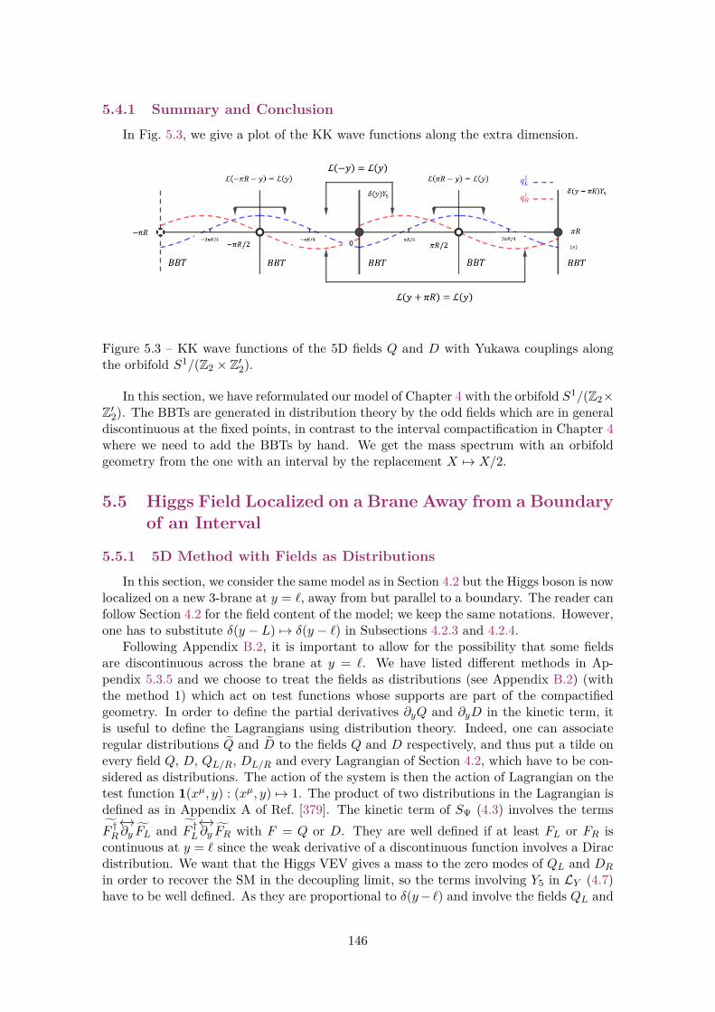
5.4.1 Summary and Conclusion

In Fig. 5.3, we give a plot of the KK wave functions along the extra dimension.

Figure 5.3 – KK wave functions of the 5D fields Q and D with Yukawa couplings alongthe orbifold S1/(Z2 × Z′2).

In this section, we have reformulated our model of Chapter 4 with the orbifold S1/(Z2×Z′2). The BBTs are generated in distribution theory by the odd fields which are in generaldiscontinuous at the fixed points, in contrast to the interval compactification in Chapter 4where we need to add the BBTs by hand. We get the mass spectrum with an orbifoldgeometry from the one with an interval by the replacement X 7→ X/2.

5.5 Higgs Field Localized on a Brane Away from a Boundaryof an Interval

5.5.1 5D Method with Fields as Distributions

In this section, we consider the same model as in Section 4.2 but the Higgs boson is nowlocalized on a new 3-brane at y = `, away from but parallel to a boundary. The reader canfollow Section 4.2 for the field content of the model; we keep the same notations. However,one has to substitute δ(y − L) 7→ δ(y − `) in Subsections 4.2.3 and 4.2.4.

Following Appendix B.2, it is important to allow for the possibility that some fieldsare discontinuous across the brane at y = `. We have listed different methods in Ap-pendix 5.3.5 and we choose to treat the fields as distributions (see Appendix B.2) (withthe method 1) which act on test functions whose supports are part of the compactifiedgeometry. In order to define the partial derivatives ∂yQ and ∂yD in the kinetic term, itis useful to define the Lagrangians using distribution theory. Indeed, one can associateregular distributions Q and D to the fields Q and D respectively, and thus put a tilde onevery field Q, D, QL/R, DL/R and every Lagrangian of Section 4.2, which have to be con-sidered as distributions. The action of the system is then the action of Lagrangian on thetest function 1(xµ, y) : (xµ, y) 7→ 1. The product of two distributions in the Lagrangian isdefined as in Appendix A of Ref. [379]. The kinetic term of SΨ (4.3) involves the termsF †R←→∂y FL and F †L

←→∂y FR with F = Q or D. They are well defined if at least FL or FR is

continuous at y = ` since the weak derivative of a discontinuous function involves a Diracdistribution. We want that the Higgs VEV gives a mass to the zero modes of QL and DR

in order to recover the SM in the decoupling limit, so the terms involving Y5 in LY (4.7)have to be well defined. As they are proportional to δ(y− `) and involve the fields QL and

146

DR, these two fields have to be continuous at y = `. As for the terms involving Y ′5 , whichare also proportional to δ(y − `), they involve the fields QR and DL, and their presenceis not necessary for recovering the SM in the decoupling limit. QR and/or DL can bediscontinuous at y = `. The product of two discontinuous function can be continuous butif it is not, the terms proportional to Y ′5 are not defined, thus one has to take Y ′5 = 0.With these constraints, we have the weak partial derivatives:

∂yQL = {∂yQL} ,∂yQR = {∂yQR}+ (QR|`+ − QR|`−) δ(y − `) ,∂yDL = {∂yDL}+ (DL|`+ − DL|`−) δ(y − `) ,∂yDR = {∂yDR} , (5.154)

where the{∂yFL/R

}’s are the regular distributions associated to the functions ∂yFL/R.

One can use Eq. (5.154) to go from a distributional to a functional treatment of theLagrangians and fields where BBTs appear from the weak partial derivative of the discon-tinuous fields. We can thus continue to use the Lagrangians of Section 4.2 with fields asfunctions if one adds to S5D (4.12) the action

S′B =∫d4x LB|`+ − LB|`− . (5.155)

We apply Hamilton’s principle to the action SΨ + SB + S′B + SX with arbitrary fieldvariations in the bulk and at the boundaries. For the fields continuous (discontinuous)across the brane at y = `, the variations are continuous (discontinuous) and arbitrary aty = `. We get

0 = δQ†L

(SΨ + SB + S′B + SX) =∫d4x

(∫ `−

0dy +

∫ L

`+dy

)δQ†L

[iσµ∂µQL − ∂yQR

]+∫d4x

[δQ†LQR

]L0

−∫d4x δQ†L

∣∣∣`

([QR]`

+

`− +X DR|`), (5.156)

0 = δQ†R

(SΨ + SB + S′B + SX) =∫d4x

(∫ `−

0dy +

∫ L

`+dy

)δQ†R [iσµ∂µQR + ∂yFL]

−∫d4x X ′

(δQ†RDL

)∣∣∣`, (5.157)

0 = δD†L

(SΨ + SB + S′B + SX) =∫d4x

(∫ `−

0dy +

∫ L

`+dy

)δD†L

[iσµ∂µDL − ∂yDR

]−∫d4x X ′∗

(δD†LQR

)∣∣∣`, (5.158)

0 = δD†R

(SΨ + SB + S′B + SX) =∫d4x

(∫ `−

0dy +

∫ L

`+dy

)δD†R [iσµ∂µDR + ∂yDL]

−∫d4x

[δD†RDL

]L0

+∫d4x δD†R

∣∣∣`

([DL]`

+

`− −X∗ QL|`

), (5.159)

147

with the notation [g(y)]ba = g(b) − g(a). We obtain the Euler-Lagrange equations (4.15)in the bulk, and the following conditions at the branes at y = 0, L, ` respectively:

QR|0,L = DL|0,L = 0 , (5.160)

and

[QR]`+

`− = −X DR|` ,

[DL]`+

`− = X∗ QL|` ,

X ′ DL|` = X ′∗ QR|` = 0 .

(5.161)

If QR and DL are continuous at y = `, with non-vanishing Y5 and Y ′5 in general (and thusX and X ′ are non-vanishing too), we have

QL|` = QR|` = DL|` = DR|` = 0 . (5.162)

A Dirichlet condition at y = ` for both chirality implies in general vanishing KK wavefunctions and 5D fields everywhere in the extra dimension. In order to have a physicallyinteresting scenario, we need to relax the continuity condition for QR and DL across thebrane at y = `: Y ′5 = 0 so X ′ = 0 and the third line of Eq. (5.161) is satisfied whateverare the values of DL|` and QR|`.

As the fields Q and D mix due to the brane localized mass term involving X, weexpand the 5D fields into a mixed KK decomposition:

QL (xµ, y) =∑n

qnL(y)ψnL (xµ),

QR (xµ, y) =∑n

qnR(y)ψnR (xµ),

DL (xµ, y) =∑n

dnL(y)ψnL (xµ),

DR (xµ, y) =∑n

dnR(y)ψnR (xµ).

(5.163)

The 4D fields ψnL/R (∀n) satisfy the Dirac-Weyl equations (4.59). The mass spectrum Mn

includes the contributions whose origin is the Yukawa couplings (4.8). The wave functionsfnL/R (f = q or d) are orthonormalized with the conditions:

∀n , ∀m ,

∫ L

0dy[qn∗L/R(y) qmL/R(y) + dn∗L/R(y) dmL/R(y)

]= δnm . (5.164)

The mixed KK decompositions (5.163) are inserted into the Euler-Lagrange equations(4.15), and into the conditions at the branes (5.160) and (5.161). We get the equationsfor the KK wave functions (4.86), the boundary conditions:

qnR(0, L) = dnL(0, L) = 0 , (5.165)

and the junction conditions: [qnR(y)]`

+

`− = −X dnR(`) ,

[dnL(y)]`+

`− = X∗ qnL(`) .(5.166)

148

We solve the equations for the KK wave functions (4.86) in the two different regions:y < ` and y > ` with the boundary conditions (5.165). We obtain:

∀y < ` ,

qnL(y) = Aq cos(Mn y) , dnL(y) = −Ad sin(Mn y) ,

qnR(y) = Aq sin(Mn y) , dnL(y) = Ad cos(Mn y) ,(5.167)

and:

∀y > ` ,

qnL(y) = Bq cos [Mn(y − L)] , dnL(y) = −Bd sin [Mn(y − L)] ,

qnR(y) = Bq sin [Mn(y − L)] , dnL(y) = Bd cos [Mn(y − L)] ,(5.168)

with Af , Bf ∈ C∗. The fields QL and DR are continuous at y = ` so the wave functionsqnL(y) and dnR(y) are also continuous across this brane, and we get

Bf = Afcos(Mn y)

cos [Mn(y − L)] . (5.169)

The junction conditions (5.166) with the wave functions (5.167) and (5.168) give

[tan(Mn y)]``−L = XAdAq

= X∗AqAd

, (5.170)

thus we have the equation for the mass spectrum([tan(Mn y)]``−L

)2= |X|2 , (5.171)

equivalent to[tan(Mn y)]``−L = ±|X| , (5.172)

and we have |Aq| = |Ad|. The KK wave functions are orthonormalized by Eq. (5.164),such that

|Aq| = |Ad| =[`+

(cos2(Mn `)

cos2 [Mn(`− L)]

)(L− `)

]−1/2

. (5.173)

In a similar way as below Eq. (4.107), one can show that the phases of Af and Y5, andthe sign of Mn are not physical, so one can take Af = |Af |, Y5 = |Y5| and Mn = |Mn|.Therefore, the two mass spectra of Eq. (5.172) are equivalent and correspond to thesame KK modes since one can go frome the first to the second by the transformationMn 7→ −Mn.

The Yukawa couplings between the modes n and m follow from inserting the KKdecompositions (5.163) in Eq. (4.9):

ynm = |Y5| qnL(`) dmR (`) . (5.174)

5.5.2 Conclusion

In this section, we have illustrated the differences between a Higgs field localized on abrane away from a boundary and on a brane at a boundary. If the brane is at a boundary,the BBTs are explicitely introduced in the action from the beginning and all fermion fieldsare continuous along the extra dimension. If the brane is away from a boundary, the branelocalized terms imply a jump at the brane position for one of the two chiralities of the 5Dfermion field. The distribution theory is very convenient in this case and the BBTs areimplicitely generated on both sides of the brane by the weak partial derivative along theextra dimension of the discontinuous fields.

149

Chapter 6

Large Star/Rose Extra Dimensionwith Small Leaves/Petals

This chapter is an adaptation of Ref. [2] written under the supervision of Ulrich Ell-wanger.

6.1 IntroductionThe huge gauge hierarchy between the 4D Planck scale,

Λ(4)P =

√√√√ 18πG(4)

N

' 2.4× 1018 GeV, (6.1)

where G(4)N is the 4D gravitational Newton constant, and the measured Higgs boson mass

mh ' 125 GeV, is one of the internal puzzles of the Standard Model (SM) of particlephysics [3] when one couples it to gravity. If the Higgs boson is described by an elementaryscalar field which is not protected by a symmetry, the radiative corrections to m2

h arequadratically sensitive to mass scales of new degrees of freedom. Such degrees of freedomare expected at least at scales where gravitational self interactions become strong, which isthe 4D Planck scale Λ(4)

P in the usual setup. Then the measured mh implies an incrediblefine tuning between the Higgs boson bare mass and the radiative corrections: this is thenaturalness problem of the Higgs boson mass due to the large hierarchy between the 4DPlanck scale Λ(4)

P and the ElectroWeak (EW) scale (usually called the gauge hierarchyproblem) [17–19]. A possibility to solve this issue is to embed the SM into a theory wherethe true Planck scale, i.e. the scale where gravitational self interactions become strongand new degrees of freedom are expected, is in the 1− 10 TeV range. However, this doesnot solve the question how a UltraViolet (UV) completion of quantum gravity is achieved.

In 1998, N. Arkani-Hamed, S. Dimopoulos and G.R. Dvali (ADD) proposed in Ref. [34]to compactify q ∈ N∗ flat spacelike extra dimensions on a q-dimensional compact space Cqof volume Vq with a factorizable spacetime geometry

M4 × Cq , (6.2)

where M4 is the 4D Minkowski spacetime. The 4D Planck scale Λ(4)P is then just an

effective scale given by the relation[Λ(4)P

]2=[Λ(4+q)P

]q+2Vq , (6.3)

150

involving the (4 + q)D Planck scale

Λ(4+q)P =

[1

8πG(4+q)N

]1/(q+2)

, (6.4)

whereG(4+q)N is the (4+q)D gravitational Newton constant. Λ(4+q)

P is the real scale at whichgravity becomes strongly coupled, so it is the true cut-off of the QFT, and this model solvesthe gauge hierarchy problem if Λ(4+q)

P ∼ O(1) TeV with a large compactified volume Vq. Inthe ADD models, the SM fields must be localized on a 3-brane, in contrast to gravity whichis a property of (4+q)D spacetime in general relativity. At large distances between two testmasses on the 3-brane, gravity appears as a feebly coupled theory, because gravitationalfluxes spread into the large volume Vq of the bulk. Quickly [36], it was realized that theKaluza-Klein (KK) modes of fields propagating into this large volume Vq have couplings tothe SM fields suppressed by

√Vq. One can thus build natural models of feebly interacting

particles, i.e. particles which have a tiny coupling constant with the SM, like right-handedneutrinos [37–39], axions [380, 381], dark photons [36], etc. In Ref. [36], ADD proposeda simple toroidal compactification Cq = (R1)q, where R1 is the circle of radius R, andVq = (2πR)q. The bulk fields, like the graviton, generate a tower of KK modes with auniform mass gap of 1/R. For a benchmark value Λ(4+q)

P = 1 TeV, the (4 + q)D Plancklength is `(4+q)

P = 1/Λ(4+q)P ' 2 × 10−19 m, and one gets Tab. 6.1 and Fig. 6.1 from

Eq. (6.3).

q R (m) R/`(4+q)P MKK (eV)

1 2× 1011 9× 1029 1× 10−18

2 8× 10−5 4× 1014 3× 10−3

4 2× 10−12 8× 106 1× 105

6 4× 10−15 2× 104 5× 107

22 8× 10−19 4 3× 1011

Table 6.1 – R, R/`(4+q)P and MKK as a function of q for Λ(4+q)

P = 1 TeV.

Motivated by UV completions in superstring/M-theory [35, 188] requiring 10/11 space-time dimensions, most of the efforts concentrated on q ≤ 7. The compactification radius Rmust then be stabilized at a large value compared to `(4+q)

P , which reintroduces a geomet-rical hierarchy [36] with a low KK mass gap: too light KK-gravitons are constrained byastrophysics, cosmology and collider physics 1. When one probes gravitational Newton’slaw at large [small] distances with respect to R, gravity appears 4D [(4 + q)D]. The caseq = 1 is excluded because it leads to a modification of 4D gravitational Newton’s law atthe scale of the solar system. ADD’s proposal is thus often associated with the LargeExtra Dimensions (LEDs) paradigm, and is just a reformulation of the gauge hierarchyproblem.

In the literature, there are interesting propositions to stabilize such large compactifi-cation radii [275–281]. To circumvent this geometric hierarchy problem, a solution can beto abandon the framework of UV completions by superstring/M-theory, and to increasethe number of extra dimensions. To our knowledge, this possibility was mentioned only inRef. [36]. Fig. 6.1 shows that, for sufficiently large q, the remaining hierarchy disappears:

1. For a review of the constraints on the simplest ADD model with toroidal compactification, see thechapter Extra Dimensions Searches by Y. Gershtein and A. Pomarol in Ref. [7].

151

R ∼ `(4+q)P . A possible trail to UV complete this kind of model could be via Loop Quantum

Gravity (LQG) [382] since, a priori, LQG does not fix the number of spatial dimensions.First attempts to add spacelike extra dimensions to LQG were made in Refs. [383–392].

10 15 20 25 30 350

10

20

30

40

50

60

Figure 6.1 – Plot of R/`(4+q)P as a function of q for Λ(4+q)

P = 1 TeV.

The most popular way to overcome the geometrical hierarchy problem is the warpedextra dimension scenario proposed in 1999 by L. Randall and R. Sundrum (RS) in Ref. [40],known as the RS1 model. A less known resolution is the compactification of q ≥ 2 spacelikeextra dimension on a compact hyperbolic manifold with a large genus (number of holes)proposed in 2000 by N. Kaloper, J. March-Russell, G.D. Starkman and M. Trodden inRef. [289] (see also Ref. [290]).

The goal of the present work is to discuss another compactification geometry to solvethe geometrical hierarchy problem in the ADD models. In 2005, H.D. Kim proposed inRef. [69] to realize ADD’s idea by compactifying a LED on a 1D singular variety: a metricgraph 2, like a star or a rose with respectively N leaves/petals of equal length/circumfer-ence `. It was shown that, for large N , one can build a phenomenologically viable modelwith only a single LED which gives sizable submillimeter deviations to the Newtonian lawof gravity in tabletop experiments. The KK mass scale is MKK = 1/` ∼ O(10 − 100)meV. Here, we want to push the concept further and we take ` close to `(5)

P for large N ,so MKK = 1/` ∼ O(0.1− 1) TeV which does not reintroduce a scale hierarchy and evadeall constrains on traditional ADD models (with a compactification on a low dimensionaltorus) coming from submillimeter tests of Newtonian gravity, astrophysics and cosmol-ogy. The integer N is radiatively stable so the scenario solves completely the naturalnessproblem of the Higgs mass. Moreover, Ref. [69] gives no information on the way to embedthe SM fields in the proposed geometry. Are they bulk or brane localized fields? In thiswork, we will see that the SM fields must be localized on a 3-brane and we find particulary

2. Metric graphs have interesting applications in physics, chemistry and mathematics (see Ref. [393] fora short review). For that purposes, a 2D QFT on a star graph background was developped in Refs. [394–397]. The reader can find a mathematical introduction to the spectral analysis of differential operatorsdefined on metric graphs, the so-called quantum graphs, in Ref. [398].

152

interesting to localize them on the junction (central vertex) of the star/rose graph.In the context of the compactification of an extra dimension on a metric graph, the star

graph is the most popular [69, 347, 348, 352, 354], mainly because, with AdS5 leaves, theseeffective 5D brane worlds capture the low energy behavior of models with warped throats,arising in flux compactification in type IIB superstring theory [340, 341, 349, 350, 399, 400],when one integrates out the modes associated to the transverse dimensions of the throats.In this work, we study a spacelike extra dimension compactified on a flat star/rose graphwith identical leaves/petals by adopting a bottom-up approach: we are completely agnosticabout the origin of this curious geometry in a UV theory like string theories, LQG, etc.The definition of the 5D spacetime background is given in Section 6.2.

The authors of Ref. [347] analyzed a Klein-Gordon field, a Dirac field, a Maxwell fieldand Einsteinian gravity propagating in an extra dimension compactified on a star with Nleaves of different lengths. For that purpose, they define a copy of the same 5D field oneach leaf. The copies are connected at the junction of the star through brane localizedinteractions and the continuity of the metric. Of course, a different 5D field on each leafis not equivalent to only one 5D field defined on the whole star graph. In order to recoveronly one zero mode propagating on the whole star, they add brane localized mass termsand take the limit of infinite masses such that N − 1 zero modes decouple from the EFT.We find this procedure a bit cumbersome. Moreover, the meaning of an infinite branelocalized mass term is not clear when the cut-off of the EFT is not so far above the KKscale MKK = 1/`. That is why we choose in this work the more straigtforward approachof Refs. [69, 401] where a 5D field is defined on the whole metric graph from the start.

The KK mass spectrum and wave functions of a 5D massless real scalar field on astar/rose graph were studied in Ref. [69]. In Section 6.3, we generalize it by adding a5D mass to the scalar field and correct a mistake in the treatment of Ref. [69]. Besides,we clarify the method and hypothesises of this previous study, especially the hypothesisof continuity of the scalar field across the cental vertex of the star/rose graph. For thatpurpose, we require that the Lagrangian, and more specifically the kinetic term, is welldefined in the context of the distribution theory 3 formulated by L. Schwartz.

Recently, a 5D Dirac field with a compactification on a flat rose graph was consideredin Ref. [401]. They took petals of possibly different circumferences and included a 5DDirac mass for the fermion. In their approach, they allowed to choose arbitrary boundaryconditions on each side of the vertex of the rose which are consistent with Hamilton’sprinciple, i.e for which the variation of the action at the vertex is vanishing. In particular,both left and right-handed fields can be discontinuous at the vertex: the kinetic term isthus not defined here, even in distribution theory. In this framework, they consideredthe rose graph as a master quantum graph since one can reduce it to a star graph by asuitable choice of boundary conditions. They studied the general mathematical propertiesof the boundary conditions for the rose graph and gave a way to classify them. Theirwork is restricted to the analysis of the zero modes only: the KK mass spectrum andwavefunctions of the excited modes were not considered. They determined the numberof zero mode solutions for each type of boundary conditions in their classification. Theirwork was motivated by the future goals of generating three fermion generations and thefeatures of the flavor sector of the SM fermions from the zero modes of only one generationof 5D fermions. However, they did not give the details of a concrete realistic model inthis article. In Section 6.4, we study the particular case of a 5D massless Dirac field ona star/rose graph with identical leaves/petals. We use a different approach compared to

3. See Refs. [369, 370] for an introduction to distribution theory by L. Schwartz. For an application toquantum mechanics, see Appendix A of Ref. [379].

153

the one of Ref. [401]. In the same way as for the scalar field, we constrain the possibleboundary conditions at the junction in order to have a well defined kinetic term in theLagrangian in distribution theory. This implies that at least one of the left or right-handed fields is continuous across the junction, in contrast to Ref. [401] where both fieldscan be discontinuous at this vertex and for which the kinetic term is not defined there.Moreover, we keep only the natural boundary conditions at the vertices, i.e. the boundaryconditions for which the action variation at the vertices vanish for arbitrary field variations[1, 257, 268, 368]. Indeed, we prefer boundary conditions originating from the variationof the action (and thus of the fields) at the vertices. We also make use of the boundaryterms for 5D fermions whose importance was stressed in Chapters 4 and 5. Within ourtreatment of the rose graph, these restrictions are equivalent to choose one set of boundaryconditions at the vertex of the rose graph in Ref. [401]. In our approach, one cannot recoverthe boundary conditions at the vertices of the star graph from the ones of the rose graph:one has to treat the star graph separately. Besides, we do not restrict ourselves to thestudy of the zero modes only; we determine the KK mass spectrum and wavefunctions ofall KK modes.

In Section 6.5, we propose a model to reduce the gravity scale to the TeV scale witha large compactified volume, but with the EW and KK scales which coincide. The SMfields are localized on the 3-brane at the central vertex of the star/rose, and we computetheir couplings to spinless KK-gravitons. We find that the results are very different fromstandard ADD models in the literature, due to the very specific features of the rose/stargraph with identical leaves/petals. We also discuss briefly what kind of physics is expectedin the Planckian and trans-Planckian regime of the model, and the possibility of a hiddensector made of KK-gravitons, and of a dark matter candidate: a stable black hole remnant[402–405], the Planckion [406, 407].

In Section 6.6, we revisit the models of Refs. [37–39], which generate small Dirac neu-trino masses with right-handed neutrinos identified with the zero modes of gauge singletfermions propagating in a large compactified volume, by adapting this idea to our space-time geometries. We consider a toy model with only one generation of neutrinos. Weuse alternatively the zero mode approximation and the exact treatment concerning thebrane localized Yukawa coupling between the SM Higgs field with the 5D neutrino and the4D left-handed neutrino of the SM particle content. For this exact treatment of a branelocalized Yukawa interaction, we use the 5D method that we developped in Chapters 4and 5. We find that a large number of KK-neutrinos are sterile and are part of the hiddensector of the proposed models.

We conclude and propose some perspectives in Section 6.7. In Appendix A, we giveour conventions for the 5D Minkowski metric, the Dirac matrices and spinors.

154

6.2 Definition of a Star/Rose Extra DimensionIn this section, we define the geometries on which we compactify. The reader is refered

to Chapter 1 of Ref. [398] for basic definitions, vocabulary and properties of metric andquantum graphs which we will use in what follows.

The N -star SN (see Fig. 6.2) is defined as the flat equilateral star graph with N bondsfrom 1 vertex of degree N to N vertices of degree 1. It is a flat 1D space of volumeL = N` obtained by gluing N intervals (the leaves) of length ` at a common boundaryJ (the junction). The ith leaf ends at the opposite side of the junction J : the boundaryBi. SN is symmetric under the group ΣN , which is the set of all permutations of the Nleaves. For example, S1 is the interval of length `, S2 the interval of length 2` symmetricunder a reflection (Σ2 ' Z2) with respect to the midpoint J , and S3 is a claw. The coupleof coordinates (y, i) ∈ [0, `] × J1, NK are assigned to every point of the ith leaf with theidentification:

∀(i, j), i 6= j, (0, i) ∼ (0, j) ≡ (0) . (6.5)

The N -rose RN (see Fig. 6.2) is defined as the flat equilateral rose graph (also calledrhodonea or bouquet of circles), with N loops (1 vertex of degree 2N). It is a flat 1D spaceof volume L = N` obtained by gluing N circles (the petals), of radius R and circumference` = 2πR, at a single point V (the vertex). RN is symmetric under the group ΣN , whichis the set of all permutations of the N petals. For example, R1 is a circle, R2 a lemniscat,R3 a trifolium, and R4 a quadrifolium. The couple of coordinates (y, i) ∈ [0, `]× J1, NK isassigned to every point of the ith petal, with the identifications:

(y, i) ∼ (y + `, i) , (6.6)

and∀(i, j), i 6= j, (0, i) ∼ (0, j) ≡ (0) . (6.7)

We want to study a field theory on the flat factorizable geometry

M4 ×KN , (6.8)

with KN = SN or RN . The coordinates can be split as (zM , i) = (xµ, y, i), where xµ arethe coordinates of M4. One has M ∈ J0, 4K, and µ ∈ J0, 3K. The junction J/V and theboundaries Bi break explicitely the 5D Lorentz-Poincaré symmetries to the 4D ones, butthe 5D symmetries are still preserved locally in the bulk. The junction and boundariesare thus 3-branes, which do not fluctuate into the bulk, where one can localize 4D fieldsand brane localized kinetic and/or interaction terms for the bulk fields. The 3-branes atthe boundaries are called Bi-branes, and the 3-brane at the junction is called J/V -branefor KN = SN/RN .

155

Figure 6.2 – Embeddings of a 5-star S5 (one the left) and of a 5-rose R5 (on the right) inR2.

6.3 5D Klein-Gordon Field on a Star/Rose Graph

6.3.1 Klein-Gordon Equation & Junction/Boundary Conditions

We study a 5D real scalar field Φ (xµ, y, i) of mass dimension 3/2 and of mass MΦdefined on M4 × KN . The Lagrangian describing the dynamics of this field must bedefined at least at the level of distributions. We can associate a regular distributionΦ (xµ, y, i) 4 to the function Φ (xµ, y, i). The action for Φ (xµ, y, i) is defined as the actionof the Klein-Gordon Lagrangian distribution

LΦ = 12 ∂

M Φ ∂M Φ− M2Φ

2 Φ2 , (6.9)

with M2Φ ≥ 0, on the testfunction 1 : (xµ, y, i) 7→ 1. We use the definition of the product

of two distributions given in Appendix A of Ref. [379]. We stress that the product of twodistributions is not defined in general but we can define it in some particular cases. Wehave thus

SΦ =⟨LΦ,1

⟩, (6.10)

in the bracket notation, and

SΦ =

∫d4x

N∑i=1

∫ `

0dy LΦ for KN = SN ,

∫d4x

N∑i=1

∮ `

0dy LΦ for KN = RN ,

(6.11)

with the symbolic integral notation. Is it possible to have a discontinuous field Φ (xµ, y, i)across the J/V -brane? This is relevant except for KN = S1 (the interval) where the J-

4. It is important to remind that a distribution is not a function of spacetime: it is a functional whichacts on testfunctions which are functions of spacetime. Our notation Φ (xµ, y, i) just means that thisdistribution acts on testfunctions whose supports are included intoM4 × SN .

156

brane is not a junction but a boundary 5. In the case of a discontinuity at the junction,we have the weak partial derivative

∂yΦ =

{∂yΦ} for KN = S1 ,

{∂yΦ}+(

N∑i=1

Φ|y=0+

)δ(y) for KN = SN , N 6= 1 ,

{∂yΦ}+[N∑i=1

(Φ|y=0+ − Φ|y=`−

)]δ(y) for KN = RN ,

(6.12)

where {∂yΦ} is the regular distribution associated to the partial derivative ∂yΦ not definedat y = 0. The Dirac distribution centered at y = 0 is defined by its action on a functiong(y, i) defined on KN and continuous at y = 0 as

〈δ(y), g(y, i)〉 ≡N∑i=1

∫ `

0dy δ(y) g(y, i) ≡ g(0) for KN = SN ,

〈δ(y), g(y, i)〉 ≡N∑i=1

∮ `

0dy δ(y) g(y, i) ≡ g(0) for KN = RN .

(6.13)

Then, (∂yΦ)2 in the kinetic term is not defined because it generates a brane localizedmass term proportional to δ2(y) which has no sense in the theory of distributions (seeAppendix A of Ref. [379]). This remark is valid for any bosonic field. Some authors (seefor example Ref. [258]) try to give a meaning to a model with discontinuous scalar fieldby adding a counterterm, localized on the brane and proportional to δ2(y), which cancelsexactly the problematic δ2(y) coming from the kinetic term. We insist on the fact that thisis a purely symbolic computation, since the object δ2(y) has no definition in distributiontheory. From a physicist point of view, the presence of a mass term proportional to δ2(y)“integrated” over the coordinate y in the action means that a mass term proportional toδ(0) is localized at y = 0. Of course, δ(0) is also not defined in distribution theory, buta physicist would interpret it as a formal infinite mass term localized on the brane, asin original Dirac’s article [372] where he introduced his famous Dirac “function”. As arealistic brane world model is always in the framework of an EFT, there is an intrinsiccut-off Λ in the model. If an infinitely thin brane is problematic, one can imagine thatit has a thickness in the UV completion of order 1/Λ. The mass proportional to δ(0)can thus be replaced by Λ. This problem is somewhat similar to the one of divergentloops in QFT. One can then ask ourselves if it is possible to regularize the brane bygiving it a thickness of 1/Λ, and then renormalize the brane localized mass term in orderto eliminate its cut-off dependency. In the context of a 1D singular variety like metricgraphs, one can imagine to regularize the vertices of degree larger than two by adding atransverse spacelike extra dimension compactified on a circle of radius 1/Λ. Then, thescalar field is not discontinuous at the junction but varies quickly within a distance lessthan 1/Λ. One can then study this regularized model, integrate out the modes associatedto the transverse dimension, and then see if one can consistently add a brane localizedcounterterm to renormalize the problematic brane localized mass term. Investigating if

5. A field which is discontinuous at a boundary is equivalent to a field continuous at this boundary.Indeed, two functions equal almost everywhere are associated to the same regular distribution.

157

this procedure is possible is beyond the scope of this work. Here, we will circumvent theproblem by considering a field Φ (xµ, y, i) continuous across the J/V -brane:

∀(i, j) , Φ(xµ, 0+, i

)= Φ

(xµ, 0+, j

)≡ Φ (xµ, 0) , (6.14)

which has to satisfy periodicity conditions on the V -brane:

Φ(xµ, 0+, i

)= Φ

(xµ, `−, i

)for KN = RN . (6.15)

One can thus associate a function to the Lagrangian LΦ which is defined at each pointofM4 ×KN 6. We apply Hamilton’s principle to the action SΦ, with arbitrary variationsof the field δΦ(xµ, y, i) in the bulk and on the branes. Since the field Φ(xµ, y, i) must becontinuous at the junction, this is also the case for its variations. We get the Klein-Gordonequation for the 5D field Φ (xµ, y, i):

∀y 6= 0 ,(∂M∂M +M2

Φ

)Φ (xµ, y, i) = 0 , (6.16)

a Kirchhoff junction condition on the J/V -brane from the integrals over total derivatives:

N∑i=1

∂yΦ(xµ, 0+, i

)= 0 for KN = SN ,

N∑i=1

[∂yΦ (xµ, y, i)]`−

y=0+ = 0 for KN = RN ,

(6.17)

with [g(y)]by=a = g(b)− g(a), and Neumann boundary conditions on the Bi-branes:

∂yΦ (xµ, `, i) = 0 . (6.18)

6.3.2 Kaluza-Klein Dimensional Reduction

Separation of Variables

We want to perform the KK dimensional reduction of the 5D field theory to an effective4D one in terms of KK degrees of freedom. For that purpose, we look for solutions of theKlein-Gordon equation (6.16) by separation of variables. We write the 5D field Φ (xµ, y, i)as

Φ (xµ, y, i) = φ (xµ) fφ(y, i) , (6.19)

where φ (xµ) is a 4D field and fφ(y, i) is a function defined on KN . The general solutionof the 5D Klein-Gordon equation (6.16) is then a superposition of all lineary independentsolutions (6.19). We label each KK mode solution by a triplet (b, nb, db), where:

— b labels the different KK towers for the same 5D field which are defined by differentmass spectra (see below);

— nb labels the levels in the KK tower b;— db labels the degenerate modes for each KK level (b, nb). We choose the notation db,

instead of the more appropriate one d(b, nb), for simplifying the notations since wewill see that each KK level for a KK tower b has the same degeneracy: there is thusno ambiguity.

6. One can thus “forget about the tildes” in Eqs. (6.9) and (6.11).

158

Therefore, the general 5D field Φ (xµ, y, i) can be expanded as

Φ (xµ, y, i) =∑b

∑nb

∑db

φ(b, nb, db) (xµ) f (b, nb, db)φ (y, i) . (6.20)

The 5D equation (6.16) splits into the Klein-Gordon equations for the 4D fields φ(b, nb, db)(xµ):(∂µ∂µ +

[m

(b, nb)φ

]2)φ(b, nb, db)(xµ) = 0 , (6.21)

with [m

(b, nb)φ

]2= M2

Φ +[k

(b, nb)φ

]2, (6.22)

and the differential equations for the functions f (b, nb, db)φ (y, i):

∀y 6= 0 ,(∂2y +

[k

(b, nb)φ

]2)f

(b, nb, db)φ (y, i) = 0 , (6.23)

where[m

(b, nb)φ

]2≥ 0 is the mass squared of the KK modes φ(b, nb, db)(xµ), and

[k

(b, nb)φ

]2∈

[−M2Φ, +∞) is an eigenvalue of the operator ∂2

y on KN associated to the eigenfunctionsf

(b, nb, db)φ (y, i). The functions f (b, nb, db)

φ (y, i) are orthonormalized such that, if we insertthe expression of the 5D field Φ (xµ, y, i) of Eq. (6.20) in the Lagrangian LΦ (6.9), andthen perform the sum over i and the integration over y in the action SΦ (6.11), we get theaction:

SΦ =∫d4x

∑b

∑nb

∑db

L(b, nb, db)φ , (6.24)

with the Klein-Gordon Lagrangians for the 4D fields φ(b, nb, db)(xµ):

L(b, nb, db)φ = 1

2 ∂µφ(b, nb, db) ∂µφ

(b, nb, db) −

[m

(b, nb)φ

]22

[φ(b, nb, db)

]2. (6.25)

The orthonormalization conditions for the functions f (b, nb, db)φ (y, i) are then

N∑i=1

∫ `

0dy f

(b, nb, db)φ (y, i) f

(b′, n′b′ , d′b′ )

φ (y, i) = δbb′δnbn

′b′ δdbd

′b′ . (6.26)

The functions f (b, nb, db)φ (y, i) can thus be interpretated as the wave functions of the

KK modes φ(b, nb, db) (xµ) along the extra dimension. The conditions on the 5D fieldΦ (xµ, y, i) on the 3-branes are naturally transposed to conditions on the KK wave functionsf

(b, nb, db)φ (y, i). We have thus continuity conditions on the J/V -brane from Eq. (6.14):

∀(i, j) , f (b, nb, db)φ

(0+, i

)= f

(b, nb, db)φ

(0+, j

)≡ f (b, nb, db)

φ (0) , (6.27)

periodicity conditions on the V -brane from Eq. (6.15):

f(b, nb, db)φ

(0+, i

)= f

(b, nb, db)φ

(`−, i

)for KN = RN , (6.28)

Kirchhoff junction conditions on the J/V -brane from Eq. (6.17):

N∑i=1

∂yf(b, nb, db)φ

(0+, i

)= 0 for KN = SN ,

N∑i=1

[∂yf

(b, nb, db)φ (y, i)

]`−y=0+

= 0 for KN = RN ,

(6.29)

159

and Neumann boundary conditions on the Bi-branes from Eq. (6.18):

∂yf(b, nb, db)φ (`, i) = 0 . (6.30)

One can check that the KK wave functions f (b, nb, db)φ (y, i) and the masses m(b, nb)

φ aredefined up to unphysical global signs.

Zero Modes

We are looking for zero mode solutions (b = 0, n0 = 0, k(0, 0)φ = 0) of Eq. (6.23). For

both compactifications on SN and RN , there is only one zero mode (d0 ∈ {1}) whose wavefunction is flat, such that:

f(0, 0, 1)φ (y, i) =

√1N`

. (6.31)

Excited Modes

One can show that the case[k

(b, nb)φ

]2< 0 has no solution: the zero mode is thus the

lightest mode. We then focus on the case[k

(b, nb)φ

]2> 0.

a) N-Star

The general solutions of Eq. (6.23), satisfying the Neumann boundary conditions(6.30), are of the form:

f(b, nb, db)φ (y, i) = A

(b, nb, db)i cos

[k

(b, nb)φ (y − `)

], (6.32)

with A(b, nb, db)i ∈ R. The continuity conditions (6.27) give

∀(i, j) , A(b, nb, db)i cos

[k

(b, nb)φ `

]= A

(b, nb, db)j cos

[k

(b, nb)φ `

], (6.33)

which leads to two kinds of excited KK modes: the KK wave functions f (b, nb, db)φ (y, i) can

vanish or not on the J-brane.

First case: f (b, nb, db)φ (0) = 0

Eq. (6.33) gives the KK mass spectrum 7

cos[k

(b, nb)φ `

]= 0 =⇒

b=1k

(1, n1)φ =

(n1 + 1

2

)π

`, n1 ∈ N , (6.34)

7. In Ref. [69], the author introduced an i-dependance of the KK mass spectrum k(i, 2, n2)φ for the

condition f (i, 2, n2, d2)φ (0) = 0 without justification. According to our Eqs. (6.20), (6.21) and (6.23), a KK

wave function f (b, nb, db)φ (y, i) is defined on the whole metric graph and is associated to only one KK mode

φ(b, nb, db)(xµ) characterized by its mass m(b, nb)φ and thus, with Eq. (6.22), by only one eigenvalue k(b, nb)

φ .This comes from the fact that the factorizable geometry M4 × SN means that the same 4D MinkowskispacetimeM4 is a factor of each leaf of the star graph SN : the Lorentz-Poincaré symmetries force a KKmode to have the same mass in all leaves. In spite of this remark, the KK mass spectrum and wavefunctions of Ref. [69] are correct if one suppresses the i-dependance of the eigenvalues k(i, 2, n2)

φ . The sameremark applies to the treatment of the rose graph RN .

160

which defines the KK tower b = 1. The Kirchhoff junction conditions (6.29) implyN∑i=1

A(1, n1, d1)i = 0 . (6.35)

Each KK level (1, n1) is thus N − 1 times degenerate (d1 ∈ J1, N − 1K) and the KK wavefunctions are

f(1, n1, d1)φ (y, i) = ε

(d1)i

√2`

cos[k

(1, n1)φ (y − `)

], (6.36)

with the (N − 1)-vector basis:−→ε(1) = 1√

2(1,−1, 0, · · · , 0) ,

−→ε(2) = 1√

6(1, 1,−2, 0, · · · , 0) ,

...−−−−→ε(N−1) = 1√

N(N − 1)(1, 1, · · · , 1,−(N − 1)) . (6.37)

Second case: f (b, nb, db)φ (0) 6= 0

We have cos[k

(b, nb)φ `

]6= 0 so Eq. (6.33) gives

∀(i, j) , A(b, nb, db)i = A

(b, nb, db)j ≡ A(b, nb, db) . (6.38)

The Kirchhoff junction conditions (6.29) lead to the KK mass spectrum

sin[k

(b, nb)φ `

]= 0 =⇒

b=2k

(2, n2)φ = n2

π

`, n2 ∈ N∗ , (6.39)

which defines the KK tower with b = 2 whose KK levels are not degenerate (d2 ∈ {1}).The KK wave functions are

f(2, n2, 1)φ (y, i) =

√2N`

cos[k

(2, n2)φ (y − `)

]. (6.40)

b) N-Rose

To satisfy the continuity conditions (6.27), the KK wave functions f (b, nb, db)φ (y, i) can

vanish or not at the vertex.

First case: f (b, nb, db)φ (0) = 0

The general solutions of Eq. (6.23) with f (b, nb, db)φ (0) = 0 are of the form:

f(b, nb, db)φ (y, i) = A

(b, nb, db)i sin

[k

(b, nb)φ y

], (6.41)

with A(b, nb, db)i ∈ R. The periodicity conditions at the vertex (6.28) give sin

[k

(b, nb, db)φ `

]=

0. Moreover, the Kirchhoff junction conditions (6.29) imply

(cos

[k

(b, nb)φ `

]− 1

) N∑i=1

A(b, nb, db)i = 0 . (6.42)

161

There are thus two possibilities:— First possibility:

The KK mass spectrum is cos[k

(b, nb)φ `

]6= 1

sin[k

(b, nb)φ `

]= 0

=⇒b=1

k(1, n1)φ = (2n1 + 1) π

`, n1 ∈ N , (6.43)

and defines the KK tower b = 1. From the conditions (6.42), we get Eq. (6.35) sod1 ∈ J1, N − 1K and the KK wave functions are

f(1, n1, d1)φ (y, i) = ε

(d1)i

√2`

sin[k

(1, n1)φ y

], (6.44)

with the (N − 1)-vector basis (6.37).— Second possibility:

The KK mass spectrum is cos[k

(b, nb)φ `

]= 1

sin[k

(b, nb)φ `

]= 0

=⇒b=2

k(2, n2)φ = 2n2

π

`, n2 ∈ N∗ , (6.45)

which satisfies Eq. (6.42) and defines the KK tower b = 2. We get d2 ∈ J1, NK andthe KK wave functions are

f(2, n2, d2)φ (y, i) = η

(d2)i

√2`

sin[k

(2, n2)φ y

], (6.46)

with the N -vector basis:−−→η(1) = (1, 0, · · · , 0) ,−−→η(2) = (0, 1, 0, · · · , 0) ,

...−−→η(N) = (0, · · · , 0, 1) . (6.47)

Second case: f (b, nb, db)φ (0) 6= 0

The general solutions of Eq. (6.23) are of the form:

f(b, nb, db)φ (y, i) = A

(b, nb, db)i cos

[k

(b, nb)φ y + ϕ

(b, nb, db)i

], (6.48)

with A(b, nb, db)i , ϕ

(b, nb, db)i ∈ R. The periodicity conditions (6.28) give

A(b, nb, db)i cos

[ϕ

(b, nb, db)i

]= A

(b, nb, db)i cos

[k

(b, nb)φ `+ ϕ

(b, nb, db)i

]. (6.49)

The KK wave functions f (b, nb, db)φ (y, i) do not vanish at the vertex so A(b, nb, db)

i 6= 0, andone gets two possibilities:

— First possibility:The KK mass spectrum is

k(b, nb)φ = 2nb

π

`, nb ∈ N∗ . (6.50)

162

Each KK level (b, nb) with f(b, nb, db)φ (0) 6= 0 is thus degenerate with the N KK modes

of the level (2, n2): d2 ∈ J1, N + 1K and we label the modes with non-vanishingwave functions at the junction by the triplet (2, n2, N + 1). By imposing the or-thogonality conditions (6.73) between the KK wave functions (6.46) and (6.48),one has ϕ(2, n2, N+1)

i = 0 (mod π). The continuity conditions (6.27) imply that∀i , A(2, n2, N+1)

i ≡ A(2, n2, N+1) 6= 0. The Kirchhoff junction conditions (6.29) lead tosin(k

(2, n2)φ `

)= 0 which is satisfied by the spectrum (6.50). The KK wave functions

are thusf

(2, n2, N+1)φ (y, i) =

√2N`

cos(m

(2, n2)φ y

). (6.51)

— Second possibility:ϕ

(b, nb, db)i = −k(b, nb)

φ

`

2 (mod π) . (6.52)

Then, the Kirchhoff junction conditions (6.29) imply the same KK mass spectrumas in Eq. (6.50), and we find that the KK wave function is the same as in Eq. (6.51).This second possibily is thus redundant and does not define additional KK modes.

Finally, we insist on the fact that all KK towers labeled by b are present in the spectrum:they do not correspond to different models. The 5D field Φ(xµ, y, i) has one zero modeof mass MΦ in both geometries (KN = SN or RN ) and excited modes. For a massless5D field (MΦ = 0), the mass gap between the KK modes is of the order of 1/`. Some ofthe KK modes have wave functions which vanish at the junction. We will see a physicalapplication of these results in Subsection 6.5.3, where we will study a toy model of a 5Dspinless graviton which is just a real scalar field with MΦ = 0. The zero mode is thusidentified with the 4D massless graviton (where we do not take into account the spin).

6.4 5D Massless Dirac Field on a Star/Rose Graph

6.4.1 Dirac-Weyl Equations & Junction/Boundary Conditions

We study a 5D massless Dirac field

Ψ(xµ, y, i) =(

ΨL(xµ, y, i)ΨR(xµ, y, i)

)(6.53)

of mass dimension 2 defined on M4 × KN , where the fields ΨL(xµ, y, i) and ΨR(xµ, y, i)describe respectively fermion fields of left and right-handed 4D chirality. To the functionΨ(xµ, y, i), we associate the regular distribution

Ψ(xµ, y, i) =(

ΨL(xµ, y, i)ΨR(xµ, y, i)

). (6.54)

163

The action for Ψ(xµ, y, i) is

SΨ =

∫d4x

∫ `

0dy{LΨ + [δ(y) s(0) + δ(y − `) s(`, i)] LBBT

}for KN = S1 ,

∫d4x

N∑i=1

∫ `

0dy[LΨ + δ(y − `) s(`, i) LBBT

]for KN = SN , N 6= 1 ,

∫d4x

N∑i=1

∮ `

0dy LΨ for KN = RN ,

(6.55)where the action of the Dirac distribution centered at y = ` on a function g(y, i) definedon SN and continuous at y = ` is

N∑i=1

∫ `

0dy δ(y − `) g(y, i) =

N∑i=1

g(`, i) , (6.56)

s(0) = ±1 and s(`, i) = ±1. The massless Dirac Lagrangian for the 5D field Ψ (xµ, y, i) is

LΨ = i

2 ΨΓM←→∂M Ψ ,

= 12

(iΨR

†σµ←→∂µ ΨR + iΨL

†σµ←→∂µ ΨL + ΨR

†←→∂y ΨL − ΨL

†←→∂y ΨR

), (6.57)

where Ψ = Γ0Ψ,←→∂M =

−→∂M −

←−∂M and ΓM =

(γµ, iγ5) are the 5D Dirac matrices 8. We

define also the Bilinear Boundary Terms (BBTs) [1, 62–68] on the Bi-branes:

LBBT = 12 ΨΨ ,

= 12

(ΨL†ΨR + ΨR

†ΨL

), (6.58)

which are necessary to define a suitable action for a 5D Dirac field in presence of spacetimeboundaries, with the pre-factors in Eq. (6.55): s(0) = ±1 and s(`, i) = ±1. In what follows,we choose s(0) = −s(`, i) = 1 for all i.

Let us discuss whether the fields ΨL/R(xµ, y, i) are discontinuous across the J/V -brane,except for KN = S1 (the interval) where the J-brane is not a junction but a boundary. Ifthis is the case the weak partial derivative gives

∂yΨL/R =

{∂yΨL/R

}for KN = S1 ,

{∂yΨL/R

}+(

N∑i=1

ΨL/R

∣∣∣y=0+

)δ(y) for KN = SN , N 6= 1 ,

{∂yΨL/R

}+[N∑i=1

(ΨL/R

∣∣∣y=0+

− ΨL/R

∣∣∣y=`−

)]δ(y) for KN = RN ,

(6.59)where

{∂yΨL/R

}is the regular distribution associated to the partial derivative ∂yΨL/R

not defined at y = 0. In order to have ΨR†←→∂y ΨL and ΨL

†←→∂y ΨR well defined in the kinetic

8. Our convention for the Dirac algebra is given in Appendix A.

164

term, ΨR(xµ, y, i) must be continuous at y = 0 if ΨL(xµ, y, i) is discontinuous at y = 0,and vice versa. Indeed, the product of a regular distribution g(y) with δ(y) is well definedonly if g(y) is associated to a function g(y) continuous at y = 0 9 (see Appendix A ofRef. [379]). In what follows, we choose ΨR(xµ, y, i) continuous on the J/V -brane:

∀(i, j) , ΨR

(xµ, 0+, i

)= ΨR

(xµ, 0+, j

)≡ ΨR (xµ, 0) , (6.60)

with the periodicity condition on the V -brane:

ΨR

(xµ, 0+, i

)= ΨR

(xµ, `−, i

)for KN = RN . (6.61)

However, ΨL(xµ, y, i) is free to be discontinuous across the J/V -brane without introducinga pathology into the model. Therefore, if one wants to add a brane localized term on theJ/V -brane for KN 6= S1, it can only involve ΨR(xµ, y, i), otherwise ΨL(xµ, y, i) has also tobe continuous. If this is not the case, the coupling in front of the brane localized term hasto vanish such that this term does not exist. This result can be extended to any fermionicfield. The action (6.55) is then

SΨ =

∫d4x

{(∫ `

0dy LΨ

)−[1

2 ΨΨ]`y=0

}for KN = S1 ,

∫d4x

N∑i=1

{(∫ `

0+dy LΨ

)−[1

2 ΨΨ]`y=0+

}for KN = SN , N 6= 1 ,

∫d4x

N∑i=1

{(∫ `−

0+dy LΨ

)−[1

2 ΨΨ]`−y=0+

}for KN = RN ,

(6.62)

withLΨ = i

2 ΨΓM←→∂MΨ , (6.63)

where we see how the BBTs at the junction (J/V -brane) appear in the action SΨ whengoing from the description in terms of distributions to a description in terms of functions.This is in complete analogy with the Gibbons-Hawking boundary terms [294] which appearon both sides of a brane away from a spacetime boundary when one studies gravity inbrane world models and with the metric considered as a function instead of a distribution[258, 292, 293, 409, 410].

We apply Hamilton’s principle to the action SΨ, with arbitrary variations of the fieldsδΨL/R(xµ, y, i) in the bulk and on the branes. As ΨR(xµ, y, i) has to be continuous, it isclear that δΨR(xµ, y, i) is also continuous. In the case of ΨL(xµ, y, i), which can be discon-tinuous across the J/V -brane, one has to allow for variations δΨL(xµ, y, i) discontinuousat the junction in general. We get the massless Dirac-Weyl equations for the 5D fieldsΨL/R (xµ, y, i):

∀y 6= 0 ,

iσµ∂µΨR(xµ, y, i) + ∂yΨL(xµ, y, i) = 0 ,

iσµ∂µΨL(xµ, y, i)− ∂yΨR(xµ, y, i) = 0 ,

(6.64)

9. Intuitively, δ(y) applied to a function g(y, i) measures the value g(0) by averaging the value of g(y, i)in a 1D volume contracting to the point at y = 0 (see Chapter 1 of Ref. [408]), i.e. with a resolution lessthan the inverse of the cut-off of the EFT (zero thickness brane limit). This procedure is well defined if thefunction g(y, i) does not vary too quikly in the neighborhood of y = 0. If g(y, i) is discontinuous at y = 0,i.e. the value of g(y, i) changes rapidly near y = 0 in a distance less than the inverse of the cut-off of theEFT, one cannot use δ(y) to mesure its value at y = 0. Moreover, the value of a field at a point whereit is discontinuous has no physical meaning since we are dealing with an EFT, where we probe distanceslarger than the inverse of the cut-off.

165

a Kirchhoff junction condition for the left-handed field on the J/V -brane from the integralsover total derivatives:

N∑i=1

ΨL

(xµ, 0+, i

)= 0 for KN = SN ,

N∑i=1

[ΨL (xµ, y, i)]`−

y=0+ = 0 for KN = RN ,

(6.65)

and Dirichlet boundary conditions for the left-handed field on the Bi-branes:

ΨL (xµ, `, i) = 0 . (6.66)

The conserved Noether current associated to the symmetry U(1) : Ψ 7→ e−iαΨ, withα ∈ R, is

jMΨ = ΨΓMΨ with ∂MjMΨ = 0 . (6.67)

This requires a Kirchhoff condition for the current at the junction:

N∑i=1

jMΨ

(xµ, 0+, i

) != 0 for KN = SN ,

N∑i=1

[jMΨ (xµ, y, i)

]`−y=0+

!= 0 for KN = RN .

(6.68)

For the component M = 4 one gets

N∑i=1

(Ψ†LΨR −Ψ†RΨL

)∣∣∣y=0+

!= 0 for KN = SN ,

N∑i=1

[Ψ†LΨR −Ψ†RΨL

]`−y=0+

!= 0 for KN = RN ,

(6.69)

which is satisfied by the Kirchhoff junction condition (6.65) with the continuity (6.60) andperiodicity (6.61) conditions on the J/V -brane.

6.4.2 Kaluza-Klein Dimensional Reduction

Separation of Variables

In order to perform the KK dimensional reduction of the 5D field theory, we use thesame method as in Subsection 6.3.2 for the scalar field, with the same system of labels forthe KK modes. We expand the 5D fields ΨL/R (xµ, y, i) as

ΨL (xµ, y, i) =∑b

∑nb

∑db

ψ(b, nb, db)L (xµ) f (b, nb, db)

L (y, i) ,

ΨR (xµ, y, i) =∑b

∑nb

∑db

ψ(b, nb, db)R (xµ) f (b, nb, db)

R (y, i) ,(6.70)

where ψ(b, nb, db)L/R (xµ) are 4D Weyl fields and f

(b, nb, db)L/R (y, i) are functions defined on KN .

The 5D equations (6.64) split into Dirac-Weyl equations for the 4D fields ψL/R (xµ):iσµ∂µψ

(b, nb, db)R (xµ)−m(b, nb)

ψ ψ(b, nb, db)L (xµ) = 0 ,

iσµ∂µψ

(b, nb, db)L (xµ)−m(b, nb)

ψ ψ(b, nb, db)R (xµ) = 0 ,

(6.71)

166

and the differential equation for the functions f (b, nb, db)L/R (y, i):

∀y 6= 0 ,

∂yf

(b, nb, db)R (y, i)−m(b, nb)

ψ f(b, nb, db)L (y, i) = 0 ,

∂yf(b, nb, db)L (y, i) +m

(b, nb)ψ f

(b, nb, db)R (y, i) = 0 ,

(6.72)

where m(b, nb)ψ is the mass of the KK modes (b, nb, db). The functions f (b, nb, db)

L/R (y, i) areorthonormalized with the conditions

N∑i=1

∫ `

0dy

[f

(b, nb, db)L/R (y, i)

]∗f

(b′, n′b′ , d′b′ )

L/R (y, i) = δbb′δnbn

′b′ δdbd

′b′ , (6.73)

and can thus be interpretated as the wave functions of the KK modes ψ(b, nb, db)L/R (xµ) along

the extra dimension. The conditions on the 5D field ΨL/R (xµ, y, i) at the vertices arenaturally transposed to conditions on the KK wave functions f (b, nb, db)

L/R (y, i) and can becombined with Eq. (6.72). We have thus continuity conditions on the J/V -brane fromEq. (6.60):

∀(i, j), f (b, nb, db)R

(0+, i

)= f

(b, nb, db)R

(0+, j

)≡ f (b, nb, db)

R (0) , (6.74)

and periodicity conditions on the V -brane from (6.61):

f(b, nb, db)R

(0+, i

)= f

(b, nb, db)R

(`−, i

)for KN = RN . (6.75)

Eq. (6.65) corresponds to Kirchhoff junction conditions for the wave functions of the left-handed KK modes on the J/V -brane:

N∑i=1

f(b, nb, db)L

(0+, i

)= 0 for KN = SN ,

N∑i=1

[f

(b, nb, db)L (y, i)

]`−y=0+

= 0 for KN = RN ,

(6.76)

which, combined to Eq. (6.72), give junction conditions for the wave functions of theright-handed KK modes with m(b, nb)

ψ 6= 0:

N∑i=1

∂yf(b, nb, db)R

(0+, i

)= 0 for KN = SN ,

N∑i=1

[∂yf

(b, nb, db)R (y, i)

]`−y=0+

= 0 for KN = RN .

(6.77)

Eq. (6.66) leads to Dirichlet boundary conditions for the left-handed KK modes on theBi-branes:

f(b, nb, db)L (`, i) = 0 , (6.78)

which, combined to Eq. (6.72), give Neumann boundary conditions for the right-handedKK modes with m(b, nb)

ψ 6= 0:∂yf

(b, nb, db)R (`, i) = 0 . (6.79)

One can check that the couples of KK wave functions f (b, nb, db)L/R (y, i) are defined up to

unphysical global phases, and that the sign of the masses m(b, nb)ψ is also unphysical.

167

Zero Modes

We are looking for zero mode solutions (b = 0, n0 = 0, m(0, 0)ψ = 0) of Eq. (6.72) for

which the first order differential equations are decoupled. For both compactifications onSN and RN , there is only one right-handed zero mode (d0 ∈ {1}). Its wave function iscontinuous across the J/V -brane and flat:

f(0, 0, 1)R (y, i) =

√1N`

. (6.80)

For the left-handed zero modes, it is necessary to distinguish between the compactificationon SN and RN .

a) N-Star

There is no left-handed zero mode for KN = SN . The theory is thus chiral at thelevel of the zero mode 10, which generalizes the well known result of the particular caseof a compactification on the interval S1. The compactification on a star graph is thusvery interesting since it allows to build models where the SM fields propagate in theextra dimension: the SM particles are identified with the zero modes of the 5D fields. InSection 6.6, we will identify the right-handed neutrinos with the zero modes of 5D Diracfields coupled to brane localized 4D left-handed neutrinos. The goal is to propose a toymodel to obtain small Dirac neutrino masses.

b) N-Rose

For KN = RN , we have N degenerate left-handed zero modes (d0 ∈ J1, NK). Thisconfirms the claim in Ref. [401] that one can generate several zero modes from only one5D fermion on a rose graph. The theory is vector-like at the level of the zero modes, whichgeneralizes the result of the compactification on a circle R1 in the literature. Therefore,with the compactification on a rose graph, one cannot build models with the SM fieldspropagating in the extra dimension except if one is able to propose a mechanism whichgenerates chirality by giving a mass to the mirror partners of the SM fermions. If thisis possible, one recovers the three SM generations by taking N = 3. The KK wavefunctions f (0, 0, d0)

L (y, i) are flat in each petal and discontinuous across the V -brane (exceptfor KN = R1, the circle, where they can be taken continuous):

∀y 6= 0 , f (0, 0, d0)L (y, i) = η

(d0)i

√1`, (6.81)

with theN -vector basis (6.47). Notice that the values of the KK wave functions f (0, 0, d0)L (y, i)

at y = 0 are unknown since these KK wave functions are discontinuous here. However,this is not a problem since our field theory is defined in the framework of distributiontheory. Indeed, the value of a field at one point is meaningless: two functions equal almosteverywhere are associated to the same regular distribution.

10. If one takes ∀i , s(0) = −s(`, i) = −1 and ΨL(xµ, y, i) continuous at the junction instead ofΨR(xµ, y, i), it exchanges the KK mass spectra and wave functions of the left-handed and right-handedmodes, and one gets a left-handed zero mode.

168

Excited Modes

We are looking for massive KK modes (m(b, nb)ψ 6= 0). The coupled first order differential

equations (6.72) can be decoupled into second order ones:

∀y 6= 0 ,(∂2y +

[m

(b, nb)ψ

]2)f

(b, nb, db)L/R (y, i) = 0 . (6.82)

The KK wave functions f (b, nb, db)R (y, i) are continuous across the junction. In the same

way as in the case of the scalar field, it is necessary to distinguish between the cases wherethe f (b, nb, db)

R (y, i)’s vanish or not at the junction. One can follow the same method asin Subsection 6.3.2. We will not give again all the details here since there is no majortechnical difference. We summarize the results in what follows.

a) N-Star

First case: f (b, nb, db)R (0) = 0

The KK mass spectrum is

m(1, n1)ψ =

(n1 + 1

2

)π

`, n1 ∈ N , (6.83)

and defines the KK tower b = 1. Each KK level is N−1 times degenerate (d1 ∈ J1, N−1K)and the KK wave functions are

∀y 6= 0 , f (1, n1, d1)L (y, i) = −ε(d1)

i

√2`

sin[m

(1, n1)ψ (y − `)

],

∀y , f (1, n1, d1)R (y, i) = ε

(d1)i

√2`

cos[m

(1, n1)ψ (y − `)

],

(6.84)

with the (N − 1)-vector basis (6.37). The f (1, n1, d1)L (y, i)’s are discontinuous across the

J-brane (except for KN = S1, the interval, where they are taken continuous).

Second case: f (b, nb, db)R (0) 6= 0

The KK mass spectrum is

m(2, n2)ψ = n2

π

`, n2 ∈ N∗ , (6.85)

which is not degenerate (d2 ∈ {1}) and defines the KK tower b = 2. The KK wavefunctions are

f(2, n2, d2)L (y, i) = −

√2N`

sin[m

(2, n2)ψ (y − `)

],

f(2, n2, d2)R (y, i) =

√2N`

cos[m

(2, n2)ψ (y − `)

],

(6.86)

where the f (2, n2, d2)L (y, i)’s can be taken continuous across the J-brane.

169

b) N-Rose

First case: f (b, nb, db)R (0) = 0

There are two cases:— First case:

The KK mass spectrum is

m(1, n1)ψ = (2n1 + 1) π

`, n1 ∈ N , (6.87)

and defines the KK tower b = 1 with d1 ∈ J1, N − 1K. The KK wave functions are∀y 6= 0 , f (1, n1, d1)

L (y, i) = ε(d1)i

√2`

cos[m

(1, n1)ψ y

],

∀y , f (1, n1, d1)R (y, i) = ε

(d1)i

√2`

sin[m

(1, n1)ψ y

],

(6.88)

with the (N − 1)-vector basis (6.37). The f (1, n1, d1)L (y, i)’s are discontinuous across

the V -brane.— Second possibility:

The KK mass spectrum is

m(2, n2)ψ = 2n2

π

`, n2 ∈ N∗ , (6.89)

and defines the KK tower b = 2 with d2 ∈ J1, NK. The KK wave functions are∀y 6= 0 , f (2, n2, d2)

L (y, i) = η(d2)i

√2`

cos[m

(2, n2)ψ y

],

∀y , f (2, n2, d2)R (y, i) = η

(d2)i

√2`

sin[m

(2, n2)ψ y

],

(6.90)

with the N -vector basis (6.47). The f (2, n2, d2)L (y, i)’s are discontinuous across the

V -brane (except for KN = R1, the circle, where they can be taken continuous).

Second case: f (b, nb, db)R (0) 6= 0

The KK mass spectrum is the same as in Eq. (6.89). Each KK level (b, nb) is thusdegenerate with the N KK modes of the level (2, n2) so d2 ∈ J1, N + 1K: we label the KKmodes with non-vanishing wave functions at the junction by the triplet (2, n2, N+1). TheKK wave functions are

f(2, n2, N+1)L (y, i) = −

√2N`

sin[m

(2,n2)ψ y

],

f(2, n2, N+1)R (y, i) =

√2N`

cos[m

(2,n2)ψ y

],

(6.91)

where the f (2, n2, N+1)L (y, i)’s can be taken continuous across the V -brane.

Like for the scalar field, all KK towers labeled by b are present in the spectrum. Eachexcited KK level is vector-like for both compactification, and the mass gap between theKK modes is of the order of 1/`.

170

6.5 A Low 5D Planck Scale with a Star/Rose Extra Dimen-sion

In this section, we propose an ADD model with brane localized 4D SM fields wheregravity propagates in a large star/rose extra dimension with large N and a natural valuefor `.

6.5.1 Lowering the Gravity Scale

With a LED compactified on a metric graph KN = SN or RN , one can obtain a low5D Planck scale. In this case, Eq. (6.3) gives[

Λ(4)P

]2= L

[Λ(5)P

]3, L = N` . (6.92)

To solve the gauge hierarchy problem, we have to choose Λ(5)P ' 1 TeV, obtained with

L ' 1 × 1012 m. In order to be in the Effective Field Theory (EFT) regime, i.e. belowthe 5D Planck scale, we need ` > `

(5)P , with `

(5)P = 1/Λ(5)

P ' 2 × 10−19 m. In practice,`/`

(5)P ' 10 with a large N ' 6 × 1029 should be enough, and thus a KK mass scale near

the EW scale: MKK = 1/` ' 100 GeV. Such heavy KK-gravitons evade completely theconstrains from submillimeter tests of 4D gravitational Newtons’s law, stellar physics andcosmology (see footnote 1 p. 151). If one allows for 1% of fine tuning for mh by pushingΛ(5)P up to 10 TeV with N ' 6 × 1027, one can even allow for MKK ' 1 TeV. Moreover,

if the concepts of space and volume still make sense at the Planck scale Λ(5)P , by taking

` ' `(5)P and N ' 6 × 1030 to get Λ(5)

P ' 1 TeV, there is no tower of KK-gravitons in theEFT, instead the first experimental hints for a low 5D Planck scale are strongly coupledquantum gravity phenomena near Λ(5)

P . Such a large N seems puzzling at first glance: thereader would wonder whether our proposition is just a reformulation of the gauge hierarchyproblem into why N is so large. However, in the EFT, N is a conserved integer so it isstable under radiative corrections, it does not need to be dynamically stabilized, and has nopreferred value. When `� `

(5)P , the models proposed in this article are formulated in the

context of EFTs defined on a classical background spacetimeM4×KN , where the numberof leaves/petals N is fixed by the definition of the model, even in presence of gravity.Possibly, N becomes a dynamical quantity in a theory of Planckian gravity involving aquantum spacetime. The situation is somewhat similar to other Beyond Standard Model(BSM) scenarii in the literature to solve the hierarchy problem:— The model of Ref. [289] where q ≥ 2 spacelike dimension are compactified on a

compact hyperbolic manifold of genus g (the number of holes) and of volume Vq.A compact hyperbolic manifold has two length scales: a curvature radius Rc and alinear size L ∼ Rc log(g). For L� Rc/2, we have

Vq ∼ Rqc exp[(q − 1) L

Rc

]. (6.93)

For q = 3, Λ(7)P ' 1 TeV, and Rc ∼ 1/Λ(7)

P , the formula gives L ∼ 35Rc so the numberof holes is very large: g ∼ e35 ∼ 1015.

— The model of Refs. [275, 411], where q spacelike extra dimensions are stabilized bya large number N of branes with inter-brane forces, forming a brane crystal.

N ∼ 1αq

[Λ(4)P

Λ(4+q)P

]2

' 1030

αq, (6.94)

171

for Λ(4+q)P ' 1 TeV, where α is a parameter which controls the inter-brane distance.

One should have α ' 10 in order to be in the regime where general relativity is validand also to avoid a new fine tuning.

— The model proposed by G.R. Dvali et al. in Refs. [154, 155, 412–415] involving alarge number Np of particle species. This is a 4D model where the scale at whichgravity becomes strongly coupled ΛG is given by

ΛG = Λ(4)P√Np

. (6.95)

This effect can be understood perturbatively as being the result of the radiativecorrections of Np particle species to the graviton propagator. Then, ΛG ' 1 TeVfor Np ' 6 × 1030. From Eqs. (6.92) and (6.95) it is a curious coincidence thatNp = N =

(Λ(4)P /Λ(5)

P

)2' 6× 1030 when ` = `

(5)P . One can make the same remarks

for the number of branes in the brane crystal model when αq = 1 in Eq. (6.94),which means that the inter-brane distance is the fundamental Planck length.

— The model of N -naturalness proposed by N. Arkani-Hamed et al. in Ref. [416].There are N SM-like sectors which are mutually non-interacting. The Higgs massparameter squared µ2

H takes values between −Λ2H and Λ2

H , where Λ2H is the scale

common to the N sectors that cuts the quadratic divergences to µ2H . Then, for a

wide range of µ2H distributions, one expects that some sectors are accidentally tuned

at the 1/N level, such that |µ2H | ∼ Λ2

H/N . The sector with the smallest non-zeroVacuum Expectation Value (VEV) is identified with our sector. When ΛH � ΛEW ,N has thus to be large in order to have |µH | ∼ 100 GeV. There is then no need fornew physics at the TeV scale!

In our effective model, the only quantity which needs to be dynamically stabilized isthe leaf/petal length/circumference `, otherwise the radion, i.e. the scalar field whichrepresents the fluctuations of `, remains massless and conflicts with the null result fromthe search for a new force of infinite range. On the one hand, if ` & O(10) × `(5)

P , thecorrections of Planckian gravity can safely be neglected, and it is important to add afield theoretical mechanism to the model to stabilize `. On the other hand, if ` ∼ `

(5)P ,

one expects O(1) corrections from Planckian gravity, and one needs a complete theory ofgravity to formulate the model and address its stabilization.

6.5.2 Embedding the Standard Model Fields

Up to this subsection we did not mention how we embed the SM fields into the proposedspacetime geometries. On the one hand, in the ADD-like models in the literature, theSM fields must be localized on a 3-brane, while gravity and possibly other exotic fieldspropagate in the bulk [34–36, 38, 242, 243, 275]. On the other hand, in the RS1-like models,one can allow some or all SM fields to propagate in the extra dimension [41–46, 417–419].One reason is that the KK scale in the ADD and RS1 models are respectively below andabove the TeV scale. The absence of discovery of low mass KK excitations for the SMparticles rules out an ADD model with bulk SM fields. In the case of an ADD model witha star extra dimension, where it is possible to embed a chiral model at the zero mode level,one can naively think that it allows the SM fields to propagate in the bulk with a KKmass scale MKK = 1/` ∼ O(1) TeV. However, one should also consider the magnitude ofthe couplings of the zero mode gauge bosons. In the RS1 model with a 5D gauge field,

172

the 5D gauge coupling g(5)RS (of mass dimension −1/2) is related to the zero mode gauge

coupling g(4)RS by the relation [42]:

g(4)RS = g

(5)RS√LRS

, (6.96)

where LRS is the proper length of the warped extra dimension. LRS is not large comparedto the 5D Planck length `

(5)P , so for a natural gauge coupling g(5)

RS ∼ 1/√

Λ(5)P , one has

g(4)RS ∼ O(1), which is the good magnitude for a SM gauge coupling. However, in the ADDmodel with a (4 + q)D gauge field, the higher dimensional gauge coupling g(4+q)

ADD (of massdimension −q/2) is related to the zero mode gauge coupling g(4)

ADD by the relation [263]:

g(4)ADD = g

(4+q)ADD√Vq

. (6.97)

With a natural value for the gauge coupling

g(4+q)ADD ∼

[Λ(4+q)P

]−q/2, (6.98)

one obtains with Eq. (6.3):

g(4)ADD ∼

1√Vq[Λ(4+q)P

]q = Λ(4+q)P

Λ(4)P

∼ 10−16 , (6.99)

so g(4)ADD is a very tiny coupling and cannot be identified with a SM gauge coupling. This

result depends only on the volume of the compactified space, i.e. on the hierarchy betweenthe 4D and (4 + q)D Planck scales. It is still valid for the geometries considered in thisarticle, where V1 = L. Therefore, the gauge coupling argument is much stronger thanthe one of the KK mass scale to rule out bulk SM fields: it applies to every compactifiedgeometry one can imagine to realize an ADD model.

After this discussion, it is clear that the SM fields must be localized on a 3-brane, likein the other ADD models in the literature. The J/V -brane and the Bi-branes are naturalcandidates to strictly localize the 4D SM fields 11. It is interesting to notice that if onelocalizes the SM fields on the Bi-branes of a star extra dimension, one has N copies of theSM fields, if one does not want to break explicitly the ΣN symmetry of SN . Then, if onesoftly breaks this symmetry only by the mass term of the Higgs field, one can hope to beable to realize the N -naturalness idea proposed in Ref. [416], with the reheaton (the fieldwhich populates the Universe after inflation by decaying into SM particles and possiblyother fields) as a bulk field. The Higgs mass parameter is then

|µH | ∼Λ(5)P

N, (6.100)

where a first 1/√N factor comes from the effect of theN SM fields copies coupled to gravity

(c.f. (6.95)), and a second one comes from the uniform distribution of the parameters µ2H

discussed in Ref. [416]. Although there are N copies of the SM fields, Ref. [416] gives two

11. See Ref. [420] for a recent discussion on the consistency of a 5D EFT coupled to gravity with 4Dfields strictly localized on a 3-brane. Only the argument in Subsection 5.1 in Ref. [420] applies to ourmodel (see discussion in Appendix B.5).

173

explicit models where the reheaton decays preferencially into our SM sector, which bringsback together a large number of SM sectors with the constraints from cosmology. Appliedto our setup, it is thus possible to have a higher Λ(5)

P with no new physics at the TeVscale, which could explain the null result from the search for beyond SM particles at theLarge Hadron Collider (LHC). This idea needs to be investigated deeper in a future work.Here, we will consider only one copy of the SM fields, and localize them on the J/V -brane.The gauge hierarchy problem is then fully solved by the volume of the compactified extradimension, with strongly coupled quantum gravity effects accessible to the LHC or a futurehadronic collider.

6.5.3 Phenomenology

Kaluza-Klein Gravitons

In an ADD model, gravity and possibly other exotic fields propagate into the extradimensions. It is then crucial for our proposition to have an idea of the implication ofgravitons propagating into the bulk. The KK dimensional reduction of a 5D graviton[263] leads to a tower of KK-gravitons with a zero mode, and one massless graviscalar(the radion). A massless graviphoton is also present if there is no boundary for the extradimension (present for the N -rose RN and absent for the N -star SN ). As the existence ofKK-gravitons can have important phenomenological effects, one has to extract their KKmass spectrum and their couplings to the SM fields. By a suitable gauge choice, the Euler-Lagrange equations for a 5D massless graviton reduce to Klein-Gordon equations. Onecan thus study a 5D massless real scalar field coupled minimaly to the energy momentumtensor of the SM to obtain the KK mass spectrum and the couplings of spinless KK-gravitons. This 5D spinless graviton Φ couples to the energy momentum sources throughthe effective metric:

gµν =

1 + Φ

2[Λ(5)P

]3/2 ηµν , (6.101)

so the coupling of the 5D spinless graviton to the energy momentum tensor Tµν of the 4DSM fields on the J/V -brane is

∫d4x

N∑i=1

∫ `

0dy δ(y) Φ

2[Λ(5)P

]3/2 Tµµ for KN = SN ,

∫d4x

N∑i=1

∮ `

0dy δ(y) Φ

2[Λ(5)P

]3/2 Tµµ for KN = RN .

(6.102)

withTµν = 2√

|g|δSSMδgµν

∣∣∣∣∣gµν=ηµν

, (6.103)

where SSM is the action of the SM. One can then use the KK decomposition of Sub-section 6.3.2 with MΦ = 0 and treat the brane localized interactions with the SM fieldsas a perturbation. The zero mode is identified with the 4D massless graviton. Only theKK-gravitons with a wave function which does not vanish on the J/V -brane couple to the

174

SM fields. The interaction term (6.102) gives

∫d4x

12Λ(4)

P

φ(0, 0, 1)(xµ)Tµµ +√

22Λ(4)

P

nmax2∑n2=1

(−1)n2 φ(2, n2, 1)(xµ)Tµµ

for KN = SN ,

∫d4x

12Λ(4)

P

φ(0, 0, 1)(xµ)Tµµ +√

22Λ(4)

P

nmax2∑n2=1

φ(2, n2, N+1)(xµ)Tµµ

for KN = RN .

(6.104)The KK modes whose wave functions do not vanish at y = 0 couple individually to theenergy momentum tensor of the SM with a coupling suppressed by Λ(4)

P : they are thus veryfeebly coupled. However, the brane localized SM fields couple to the linear superpositionof KK modes:

Φ′ (xµ) = 1√1 + 2nmax2

φ(0, 0, 1)(xµ) +√

2nmax2∑n2=1

(−1)n2 φ(2, n2, 1)(xµ)

for KN = SN ,

Φ′ (xµ) = 1√1 + 2nmax2

φ(0, 0, 1)(xµ) +√

2nmax2∑n2=1

φ(2, n2, N+1)(xµ)

for KN = RN ,

(6.105)where nmax2 is the KK level of the heaviest KK mode indexed by n2 below the cut-off Λ(5)

P .The interaction term (6.104) is thus∫

d4x

√1 + 2nmax2

2Λ(4)P

Φ′ Tµµ . (6.106)

By definition, nmax2 = Λ(5)

P `

πfor KN = SN ,

nmax2 = Λ(5)P `

2π for KN = RN .

(6.107)

We compare two benchmark scenarii:— Benchmark scenario #1 : Λ(5)

P ' 1 TeV and N = 1. This case is the traditionalsituation of ADD models in the literature with only one extra dimension. MKK ∼O(10−18) eV, which is excluded by the success of 4D gravitational Newton’s law atthe scale of the solar system. Then, with Eq. (6.92),

nmax2 = 1π

[Λ(4)P

Λ(5)P

]2

for K1 = S1 ,

nmax2 = 12π

[Λ(4)P

Λ(5)P

]2

for K1 = R1 ,

(6.108)

and we have thus a very large multiplicity of KK-gravitons: nmax2 ∼ O(1030). The

175

interaction term (6.106) is approximatively

∫d4x

1√

2πΛ(5)P

Φ′ Tµµ for K1 = S1 ,

∫d4x

12√πΛ(5)

P

Φ′ Tµµ for K1 = R1 .

(6.109)

The couplings of the SM fields to the linear superposition of KK modes (6.105) are ofthe order of O(1/Λ(5)

P ). This is also the case in the more realistic models with morethan one extra dimension which can pass with success the submillimeter tests of 4Dgravitational Newton’s law. The KK tower can thus be probed and constrained atthe LHC, which pushes Λ(4+q)

P up to 5-10 TeV 12.

— Benchmark scenario #2 : Λ(5)P ' 1 TeV and N ' 6 × 1029. In this case, the

large volume is generated by a large N and MKK ' 100 GeV. There is thus a lowmultiplicity of KK modes which couple to the SM fields: nmax1 ∼ O(10). Moreover,the couplings of the SM fields to the linear superposition of KK modes (6.105) is ofO(1/Λ(4)

P ) from Eq. (6.106). The KK tower is thus completely invisible in currentexperiments! The compactification on a N -star/N -rose can thus circumvent thecurrent LHC constrains on the KK-gravitons of traditionnal ADD models! It is alsoimportant to notice that this amazing feature of the N -star SN compactificationis valid only if the SM fields are localized on the J-brane. If one localizes themon one of the Bi-branes instead, they couple also to the KK-gravitons whose wavefunctions vanish at the J-brane. One can easily show that this crucial differenceimplies that the coupling of the energy momentum tensor of the SM fields to thelinerar superposition of KK-gravitons is of the same form as in Eq. (6.109). Thecouplings to the KK-graviton tower are then of O(1/Λ(5)

P ) as in the case of standardADD models, and one will be able to constrain this scenario at the LHC.

As argued in Ref. [420], a UV completion including gravity should require a branethickness. In the EFT, this brane thickness should imply higher-dimensional operatorsinvolving the brane localized SM fields and the partial derivatives of the 5D gravitonfield (see discussion in Appendix B.5). The large number of KK-gravitons which do notcouple to the SM fields in our model will then have non-vanishing coupling to the SM viathese higher-dimensional operators. It would be interesting to see the impact of the branethickness on our results. However, as the higher-dimensional operators are suppressed byhigher powers of Λ(5)

P , the constraints from the LHC on the KK-graviton towers shouldstill be weaker than the ones in traditional ADD models. Moreover, the Wilson coefficientsin front of these higher-dimensional operators are unknown in the EFT, and one can stillimagine that they are naturally suppressed in the UV completion.

Ultraviolet Gravitational Objects

It has been speculated for a long time [421] that the collision of two particles with atrans-Planckian center of mass energy and a sub-Planckian impact parameter producesa semi-classical black hole 13, according to Thorne’s hoop conjecture [422]. This leadG. R. Dvali et al. to argue in Refs. [423, 424], that the trans-Planckian spectrum of gravityis made of semi-classical black holes instead of new perturbative degrees of freedom: this

12. See the footnote 1 p. 151.13. By semi-classical, we mean a classical black hole coupled to quantum fields.

176

is called the asymptotic darkness of gravity. Black holes are classical Non-PerturbativeGravitational Objects (NPGOs). The Planck scale Λ(5)

P is then the frontier between theparticle world and the black hole world, where the transition in the spectrum should beassured smoothly between Perturbative Gravitational Objects (PGOs) and NPGOs.

To describe Planckian gravity, one needs a complete theory of quantum gravity. Ifthey exist, new PGO degrees of freedom should pop up at energies below Λ(5)

P . If theyare enough coupled to the SM, one can expect to see them at the LHC. NPGOs areexpected to appear near the cut-off scale Λ(5)

P , when the coupling to 5D gravitons becomesnon-perturbative. However, in the case of the benchmark scenario #2, we saw that thecoupling of the energy-momentum tensor of the SM to the linear superposition of KK-gravitons is suppressed by Λ(4)

P instead of Λ(5)P , so one expects that the couplings of the

brane localized SM fields to the tower of KK-gravitons remains perturbative well aboveΛ(5)P , questioning the possibility of producing NPGOs in trans-Planckian collisions of SM

particles. However, once the linear superposition of KK-gravitons with a trans-Planckianenergy leaves the J/V -brane, where it was perturbatively produced through SM fields in atrans-Planckian collision, it will interact with all the KK-gravitons, including those whosewave functions vanish on the J/V -brane. This last process is non-perturbative above Λ(5)

P

and will produce a NPGO. Thus, production of NPGOs near and above Λ(5)P is possible

in our model.The phenomenology of semi-classical micro black holes is well described by QFT in

curved spacetime for which one can study their decay via Hawking radiation 14. However,these objects are produced in very trans-Planckian collisions. With Λ(5)

P ∼ O(1) TeV,it is now currently admitted that only states dominated by quantum corrections can beproduced at LHC energies, like Quantum Black Holes (QBHs) [220, 221, 403, 429–439].For observing the production and decay of true semi-classical black holes, the FutureCircular Collider proton-proton (FCC pp) with a center of mass energy of 100 TeV shouldbe more appropriate.

Arguments coming from the idea that the Planck length is the shortest length scalethat one can probe in Nature [423, 424] suggest that QBHs and semi-classical balck holesform a discrete tower of states instead of a continuum [403, 440]. Nevertheless, the formfactors of PGOs and NPGOs near Λ(5)

P can be computed only within a complete theory ofgravity. It is then very speculative to put constrains on this kind of objects. The messageis that our model predicts new exotic physics near Λ(5)

P ∼ O(1) TeV, but it is very difficultto translate the current bounds on new physics signals at the LHC into bounds on thecut-off scale Λ(5)

P without concrete UV completions of our brane world models. It wouldbe fascinating that NPGOs near the TeV scale are at the origin of the multiple recentanomalies measured in flavor physics by the LHCb collaboration 15.

Besides, the lightest QBH, the Planckion [406, 407], is the last stage of the evaporationof a semi-classical black hole by Hawking radiation. In some models, this black holeremnant [402–405] is stable and one can speculate that it can constitute a part of darkmatter [403, 444, 445]. There are also a large number of KK-gravitons below the TeVscale whose wave functions vanish on the J/V -brane, where the SM fields are localized(see Subsection 6.3.2): these KK-gravitons interact only with gravity in the bulk, andconstitute a natural hidden sector which could be populated by NPGOs during the earlyUniverse at the TeV scale.14. See Refs. [425–428] for reviews and a more complete list of references.15. See for example Refs. [441–443] for a current status of the flavor anomalies and a complete list of

references.

177

6.6 Toy Model of Small Dirac Neutrino Masses

6.6.1 Zero Mode Approximation

It is known from Refs. [37–39] that if the left-handed neutrinos, localized on the SMbrane, interact with gauge singlet neutrinos, propagating in the bulk in the form of aninternal torus (R1)q of radius R and large volume Vq, one can get small Dirac masses forthe neutrinos. With one left-handed neutrino and one gauge singlet neutrino (withoutBLKTs), the Dirac mass is [38]:

mν '

∣∣∣y(4+q)ν

∣∣∣ v√2Vq

, Vq = (2πR)q , (6.110)

where v is the SM Higgs field VEV, and y(4+q)ν is the (4 + q)D Yukawa coupling of mass

dimension −q/2. Eq. (6.110) is valid if one can use the zero mode approximation, i.e.neglect the mixing between the zero mode and the KK-excitations of the bulk gaugesinglet neutrino: ∣∣∣y(4+q)

ν

∣∣∣ v√2Vq

�MKK ≡1R. (6.111)

For a natural value ∣∣∣y(4+q)ν

∣∣∣ ∼ [Λ(4+q)P

]−q/2, (6.112)

with Λ(4+q)P ∼ O(1) TeV, one has, with Eq. (6.3),

mν ∼v√

2Vq[Λ(4+q)P

]q = vΛ(4+q)P√

2Λ(4)P

∼ O(0.1) meV , (6.113)

which is a good order of magnitude for the neutrino masses.We want to see if it is possible to build such a model for a LED compactified on the

metric graph KN . For the compactification on a star/rose graph, one takes a 4D left-handed neutrino νL(xµ) of mass dimension 3/2 localized on the J/V -brane, and a 5Dgauge singlet neutrino Ψ(xµ, y, i) of mass dimension 2 propagating into the bulk. Theaction of the model is

Sν =

SΨ +

∫d4x

N∑i=1

∫ `

0dy δ(y)

(Lν + LΨν

)for KN = SN ,

SΨ +∫d4x

N∑i=1

∮ `

0dy δ(y)

(Lν + LΨν

)for KN = RN .

(6.114)

The free action SΨ is given by Eq. (6.55), and

Lν = 1(y, i)× i

2 ν†Lσ

µ←→∂µνL , (6.115)

where 1(y, i) is the regular distribution associated to the function 1(y, i) : (y, i) 7→ 1. Thebrane localized mass term is

Lψν = −y(5)ν v√

2ν†LΨR + H.c. , (6.116)

178

where y(5)ν can be taken real since a phase shift of the Yukawa coupling can be compensated

by a phase shift of the field νL(xµ). We have imposed that the leptonic number L isconserved, so U(1)L is a symmetry of the model: there is thus no bulk and brane localizedMajorana mass terms for the neutrino fields. We have also assumed the absence of a bulkDirac mass term to simplify the discussion. The product of δ(y) with the interaction termLψν on the J/V -brane is well defined in Sν (6.114) since the field ΨR(xµ, y, i) is continuousat y = 0. By adopting a perturbative approach, where Lψν is treated as a perturbation,one can perform the KK dimensional reduction of Section 6.4. In the regime where wecan use the zero mode approximation, i.e. when

y(5)ν v√2L�MKK ≡

1`, (6.117)

we get a mass term for the zero mode neutrino:

−mν ν†Lψ

(0, 0, 1)R + H.c. , (6.118)

with

mν = y(5)ν v√

2f

(0, 0, 1)R (0) = y

(5)ν v√2L

. (6.119)

For a natural valuey(5)ν

√Λ(5)P ∼ 1 , (6.120)

with Λ(5)P ' 1 TeV, one has, from Eqs. (6.92), (6.110) and (6.119),

mν ∼v√

2LΛ(5)P

= vΛ(5)P√

2Λ(4)P

∼ O(0.1) meV . (6.121)

As mν � MKK ≡ 1/` for the benchmark scenario #2, the zero mode approximation isthus justified.

However, within the perturbative approach, we find that the N left-handed zero modesin Section 6.4 for KN = RN do not get masses from the brane localized mass term(6.116). They remain massless and do not mix with the left-handed neutrino localized onthe V -brane: they are sterile neutrinos which do not participate in neutrino oscillations.However, they are coupled to gravity and may have an impact on the cosmological history.As our model requires very large N , it appears to be ruled out by cosmological constraintswhich are sensible to the number of light fermionic degrees of freedom. Even with a branelocalized reheaton, which does not couple to the modes with discontinuous wave functionslike the N left-handed zero modes, NPGOs should produce them in the early Universe.A solution could be to add a new ingredient to the model to give a mass to these N zeromodes. A priori, our toy model is thus interesting only for the compactification on a stargraph.

6.6.2 Exact Treatment

Euler-Lagrange Equations & Junction/Boundary Conditions

In this subsection, we will take the effect of the brane localized mass term LΨν on theKK mass spectrum exactly into account with the 5D method of Ref. [1]. From Hamilton’sprinciple applied to the action Sν (6.114), we get the Euler-Lagrange equations: Eq. (6.64)and

iσµ∂µνL(xµ)−M ΨR(xµ, 0) = 0 , (6.122)

179

with

M = y(5)ν v√

2. (6.123)

We get also a Kirchhoff junction condition for the left-handed field on the J/V -brane:

N∑i=1

ΨL(xµ, 0+, i) = M νL(xµ) for KN = SN ,

N∑i=1

[ΨL(xµ, y, i)]`−

y=0+ = M νL(xµ) for KN = RN ,(6.124)

and Dirichlet boundary conditions (6.66) for the left-handed field on the Bi-branes.

Separation of Variables

We want to solve the field equations by separation of variables and sum over all linearlyindependant solutions. We thus write the KK decomposition (6.70) and expand νL(xµ)as a linear superposition of the left-handed KK modes which are the mass eigenstates:

νL(xµ) =∑b

∑nb

∑db

a(b, nb, db) ψ(b, nb, db)L (xµ) , (6.125)

with a(b, nb, db) ∈ C. Indeed, the brane localized mass term induces a mixing between thefield νL(xµ) and the KK modes of ΨL(xµ, y, i) obtained in Section 6.4. Here, we expandthe fields νL(xµ) and ΨL(xµ, y, i) in the same KK basis spanned by the ψ(b, nb, db)

L ’s (thebasis of the mass eigenstates). The reader can follow the discussion between Eqs. (6.70)and (6.73), we will use the same notations but we stress that, in Section 6.4, ψ(b, nb, db)

L

is an element of the KK basis without brane localized mass term and, here, it is anelement of the KK basis including the effect of the brane localized mass term. Besides,the orthonormalization conditions (6.73) for the functions f (b, nb, db)

L/R (y, i) 6= 0 are replacedby[a(b, nb, db)

]∗a(b′, n′

b′ , d′b′ ) +

N∑i=1

∫ `

0dy

[f

(b, nb, db)L (y, i)

]∗f

(b′, n′b′ , d′b′ )

L (y, i) = δbb′δnbn

′b′ δdbd

′b′ ,

N∑i=1

∫ `

0dy

[f

(b, nb, db)R (y, i)

]∗f

(b′, n′b′ , d′b′ )

R (y, i) = δbb′δnbn

′b′ δdbd

′b′ .

(6.126)The conditions on the 5D fields ΨL/R(xµ, y, i) are transposed to conditions on the KKwave functions f (b, nb, db)

L/R (y, i) by using Eq. (6.70). We have still the continuity conditions(6.74) on the J/V -brane, and the periodicity conditions (6.75) on the V -brane. There isa new Kirchhoff junction condition on the J/V -brane from Eq. (6.124):

N∑i=1

f(b, nb, db)L (0+, i) = a(b, nb, db)M for KN = SN ,

N∑i=1

[f

(b, nb, db)L (y, i)

]`−y=0+

= a(b, nb, db)M for KN = RN ,(6.127)

and the Dirichlet (6.78) and Neumann (for m(b, nb)ψ 6= 0) (6.79) boundary conditions on

the Bi-branes from Eqs. (6.66) and (6.72). Moreover, Eq. (6.122), with Eqs. (6.71), (6.70)and (6.125), gives:

a(b, nb, db)m(b, nb)ψ = M f

(b, nb, db)R (0) . (6.128)

180

For m(b, nb)ψ 6= 0, Eqs. (6.127) and (6.128) together lead to:

N∑i=1

f(b, nb, db)L (0+, i) = M2

m(b, nb)ψ

f(b, nb, db)R (0) for KN = SN ,

N∑i=1

[f

(b, nb, db)L (y, i)

]`−y=0+

= M2

m(b, nb)ψ

f(b, nb, db)R (0) for KN = RN .

(6.129)

One can check that the couples of KK wave functions f (b, nb, db)L/R (y, i) are defined up to

unphysical global phases, and that the sign of the masses m(b, nb)ψ is also unphysical.

Zero Modes

We are looking for zero modes (b = 0, n0 = 0, m(0, 0)ψ = 0) with M 6= 0 for which

the first order differential equations (6.72) are decoupled. There is no zero mode solutionfor KN = SN . For KN = RN , there is no right-handed zero mode. However, we haveN degenerate left-handed zero modes described by the wave functions of Eq. (6.81): thetheory is chiral at the level of the zero modes. Therefore, the brane localized mass termgenerates chirality in the rose graph compactification by lifting the degeneracy betweenthe right and left-handed zero modes which exists in absence of brane localized Yukawacouplings (see Subsection 6.4.2). Moreover, we have a(0, 0, d0) = 0, which means that theleft-handed zero modes do not mix with the left-handed neutrino localized on the V -brane:they are sterile neutrinos which do not participate in neutrino oscillations and they interactonly through gravity. As discussed previously, this scenario with large N should be ruledout by cosmological constraints on the number of light fermion species.

Massive Modes

Let us look at massive KK modes (m(b, nb)ψ 6= 0). The coupled first order differential

equations (6.72) can be decoupled into second order ones: Eq. (6.82). The KK wavefunctions f (b, nb, db)

R (y, i) are still continuous across the junction. We will use the samemethod as in Subsections 6.3.2 and 6.4.2. We give the results in what follows.

a) N-Star

First case: f (b, nb, db)R (0) = 0

The results are identical to the ones in Subsection 6.4.2, Paragraph “First case: f (b, nb, db)R (0) =

0” of a) p. 169. This condition gives the mass spectrum (6.83) which defines the KK towerb = 1. We have a(1, n1, d1) = 0 from Eq. (6.128) so the left-handed modes do not mix withνL(xµ): they are completely sterile, interact only with gravity, and are thus part of thehidden sector of the model.

Second case: f (b, nb, db)R (0) 6= 0

The KK mass spectrum is given by the transcendental equation:

m(2, n2, d2)ψ tan

[m

(2, n2)ψ `

]= M2

N, n2 ∈ N , (6.130)

181

whose solutions m(2, n2)ψ define the KK tower b = 2 and are not degenerate (d2 ∈ {1}). We

have a(2, n2, 1) 6= 0 from Eq. (6.128) so the left-handed modes mix with νL(xµ). The lightestmode (2, 0, 1) is identified with the neutrino we observe in Nature 16. In the decouplinglimit `→ 0, the mass of this mode is given by Eq. (6.119) in the zero mode approximation.Indeed, in this limit the excited KK modes decouple and their mixing with the lightestmassive mode (2, 0, 1) goes to zero. The KK wave functions are

∀y 6= 0 , f (2, n2, 1)L (y, i) = −

N`

2 + M2(2N − 1)

2

[m(2, n2)ψ

]2+[M2

N

]2

−1/2

sin[m

(2, n2)ψ (y − `)

],

∀y , f (2, n2, 1)R (y, i) =

N`

2 + M2(2N − 1)

2

[m(2, n2)ψ

]2+[M2

N

]2

−1/2

cos[m

(2, n2)ψ (y − `)

],

(6.131)where the f

(2, n2, 1)L (y, i)’s are discontinuous across the J-brane. This discontinuity is

sourced by the brane localized interaction.

b) N-Rose

We give the massive KK modes with the N -rose compactification for completeness butwithout additional assumptions this model should be incompatible with cosmology.

First case: f (b, nb, db)R (0) = 0

The results are identical to the ones in Subsection 6.4.2, Paragraph “First case: f (b, nb, db)R (0) =

0” of b) p. 170. By following this discussion, we get two different mass spectra (6.87) and(6.89) which defines the KK towers b = 1, 2 respectively. We have a(b, nb, db) = 0 fromEq. (6.128) with b = 1, 2 so the left-handed modes do not mix with νL(xµ): they arecompletely sterile (hidden sector).

Second case: f (b, nb, db)R (0) 6= 0

The KK mass spectrum is given by the transcendental equation:

m(3, n3)ψ tan

[m

(3, n3)ψ

`

2

]= M2

2N , n3 ∈ N , (6.132)

whose solutions m(3, n3)ψ define the KK tower b = 3 and are not degenerate (d3 ∈ {1}).

We have a(3, n3, 1) 6= 0 from Eq. (6.128) so the left-handed modes mix with νL(xµ). Thelightest massive mode (3, 0, 1) is identified with the observed neutrino. In the decoupling

16. Of course, we observe three generations of neutrinos in Nature and here we consider a toy modelwith only one generation.

182

limit ` → 0, we recover that the mass of this mode is given by Eq. (6.119) of the zeromode approximation. The KK wave functions are

∀y 6= 0 , f (3, n3, 1)L (y, i) = −

N`

2 + M2(2N − 1)

2

[m(3, n3)ψ

]2+[M2

2N

]2

−1/2

sin[m

(3, n3)ψ

(y − `

2

)],

∀y , f (3, n3, 1)R (y, i) =

N`

2 + M2(2N − 1)

2

[m(3, n3)ψ

]2+[M2

2N

]2

−1/2

cos[m

(3, n3)ψ

(y − `

2

)],

(6.133)where the f (3, n3, 1)

L (y, i)’s have a discontinuity across the V -brane sourced by the branelocalized interaction.

In a nutshell, the massive KK modes have still a mass gap of order 1/`. Only theKK modes, whose right-handed Weyl spinors have non-vanishing wave functions at thejunction without brane localized Yukawa couplings (see Subsection 6.4.2), are affected bythe addition of the brane localized SM left-handed neutrino νL(xµ) and Higgs field. TheKK masses are shifted and the wave functions of the left-handed Weyl spinors becomediscontinuous at the junction 17. This result is easy to understand when the Yukawainteraction with the VEV of the Higgs field is treated as a perturbation: only non-vanishingwave functions at the junction in Subsection 6.4.2 will have non-vanishing matrix elements.These modes mix with the SM left-handed neutrino. The other ones are completely sterileand interact only through gravity.

6.7 Conclusion & PerspectivesIn this work, we studied the possibily of compactifying a large spacelike extra dimension

on a star/rose graph with identical leaves/petals. In Sections 6.3 and 6.4, we worked outthe KK decomposition of a Klein-Gordon and Dirac field respectively. In order to havea well defined kinetic term for the field in distribution theory, we showed that a bosonicfield and one of the left or right-handed 5D fermionic field have to be continuous acrossthe junction of the star/rose graph. We found that, for a 5D Dirac field, the theory ischiral (vector-like) at the level of zero modes for a star (rose) extra dimension. For bothbosonic and fermionic massless fields, the KK scale is given by the inverse of the leaf/petallength/circumference. One can thus realize a large compactified volume with a high KKscale if one has a large number of small leaves/petals. This possibility was investigatedin Section 6.5 in order to lower the gravity scale to the TeV scale and to solve the gaugehierarchy problem between the 4D Planck and EW scales. We also showed that if the SM

17. In the literature, it is known that an interaction localized on a brane away from a boundary orat a fixed point of the orbifolds R1/Z2 and R1/(Z2 × Z′2) implies a discontinuity for a 5D fermion field[49, 50, 53, 55, 58, 59, 367]. See also Refs. [446–451] for flavor models with point interactions to generateseveral zero modes from a unique discontinuous 5D fermion field.

183

fields are localized on the 3-brane at the junction of the star/rose graph, they couple onlyto few modes of the whole tower of KK-gravitons. The couplings to this KK tower arethen suppressed by the huge 4D Planck scale instead of the 5D one at the TeV scale: theKK-gravitons are thus completely invisible at the LHC! This result is in sharp contrast tostandard ADD models in the literature with compactification on a torus or its orbifolds,where the SM fields couple to the whole tower of KK-gravitons, which implies couplingssuppressed only by the 5D Planck scale (near a TeV) which one can constrain at the LHC.Nevertheless, our proposition can still be probed at hadronic colliders through the searchof strongly coupled phenomena induced by gravity like QBHs at the LHC or semi-classicalblack holes at the FCC pp. The absence of a theory of Planckian gravity renders difficultto make precise predictions concerning the production and decay of QBHs or other exoticstates near the Planck scale. It is thus delicate to translate the LHC data into constraintson the 5D Planck scale of our model and thus to estimate the degree of fine tuning whichremains to accomodate an EW scale at 100 GeV. Finally, we proposed in Section 6.6 torealize in our scenario a toy model of small Dirac neutrino masses. For that purpose, weconsidered only one generation of neutrinos coupled to one gauge singlet fermion in thebulk. The huge compactified volume suppresses the 5D Yukawa coupling of order unity,and we were able to reproduce the good order of magnitude for the mass of the neutrinos,with a model which accomodates also a 5D Planck scale at the TeV scale. The model isrealistic only for the compactification on a star graph since the rose graph predicts a largenumber of massless left-handed sterile neutrinos incompatible with cosmology. Moreover,our models have a hidden sector constituted of secluded KK-gravitons and sterile KK-neutrinos possibly populated during the early Universe by the decays of NPGOs in thebulk. The Planckion could also be a candidate to dark matter.

We also want to discuss some perspectives for future investigations. As a follow-up ofthe present work, it would be important to study the unitarity constrains on our models,since a low gravity scale is known to need a UV completion at a scale lower than thehigher-dimensional Planck scale in standard ADD models with a toroidal compactifica-tion [452, 453]. It is also important to see how the mechanism to produce small neutrinomasses is influenced by adding bulk and brane localized Majorana mass terms, in the wayof Ref. [37]. Moreover, strongly coupled gravity at the TeV scale may generate dangerousbrane localized higher-dimensional operators inducing proton decay, large Majorana neu-trino masses and Flavor Changing Neutral Currents (FCNCs) [35]. Without knowledgeof the UV completion, we cannot know if these operators are naturally suppressed. Ifthis is not the case, the natural value of their Wilson coefficients are suppressed only bythe TeV scale and one has to add new ingredients to the scenarii to forbid them, likegauging some global symmetries of the SM as the baryon and lepton numbers [454] andother flavor symmetries [242–244], or splitting the brane localized SM fermion fields witha non-vanishing brane thickness [248]. Besides, beyond the motivations for the presentwork, we stress that the 5D background geometries that we studied here can be used ingeneral to generate feebly coupled interactions. Indeed, the couplings of the whole KKtower of a 5D field, coupled to SM fields localized at the junction of the star/rose graph,are in general suppressed by the square root of the compactified volume. One can easilyimagine how it can be used to build consistent models of axions and dark matter withorder one 5D couplings. Moreover, a 5D field has KK modes whose wave functions vanishat the junction where the SM is localized: they are thus good candidates for a hiddensector. The star graph compactification with a small number of leaves can also be usedto build models of 5D SM fields as the theory is chiral at the level of zero modes for 5Dfermions. Generating N fermion zero modes from only one 5D fermion propagating into

184

a rose graph with N petals is interesting from the point of view of flavor physics. Weproposed a mechanism to get a chiral model at the level of the zero modes by addingbrane localized terms which give a mass to the mode of opposite chirality. Moreover, itwould be interesting to see if one can implement a 5D supersymmetric field theory or 5Dsupergravity on the star/rose background. In every scenario, it is important to add a fieldtheoretical mechanism to stabilize the leaf/petal length scale.

185

Conclusion

In modern particle physics, the gauge and flavor hierarchies are one of the main moti-vations for believing that new mass scales, at which new degrees of freedom pop up, existwell above the TeV scale. This belief motivates model building to stabilize the EW scaleΛEW ∼ 100 GeV against radiative corrections. The paradigm of spacelike extra dimensionoffers the possibility that all these new scales, including the gravity scale, are in reality inthe 1− 10 TeV range.

In the RS1 model, spacetime is a slice of AdS5 and the warp factor redshifts the scale atwhich gravity becomes strongly coupled from the 4D Planck scale to the TeV scale on theIR-brane where the SM Higgs boson is localized. If gauge bosons and fermions propagateinto the bulk, one can address the flavor hierarchy by quasilocalizing the fermion zeromodes along the warped extra dimension. In this picture, it is important to understand thefield theoretical treatment of 5D fermions coupled to a Higgs field localized on a 3-brane,which is treated in the literature with an unnecessary and incorrect brane regularizationprocedure. This last point is at the heart of the first part of this PhD thesis. We haveshown that it is required to add BBTs to the action for the 5D fermions in order to beable to employ natural boundary conditions without overconstraining the system. Theseterms are used for both free and interacting 5D fields. When the brane is a boundaryof the extra dimension, all 5D fields are continuous on this brane and the BBTs must beadded by hand from the start. Moreover, only one of the two chiralities can have boundarylocalized kinetic and/or interaction terms. However, when the Higgs field is localized on abrane away from a boundary, the left or the right-handed field is discontinuous across thebrane. This jump generates BBTs at both sides of the brane through the 5D kinetic termdefined in distribution theory. In this framework, only the field which is continuous acrossthe brane is allowed to have brane localized interactions with the Higgs field. These resultscan be extended to any kind of brane localized kinetic or interaction terms involving 5Dfermions. They require to reexamine the phenomenology of warped models with a branelocalized Higgs field coupled to 5D fermion and gauge fields when they were treated bythe brane-Higgs regularization as in previous studies.

In the ADD models, one adds q LEDs compactified on a qD torus with a factorizablegeometry. The large compactified volume dilutes gravity which appears feebly coupledto an observer localized on a 3-brane. Nevertheless, gravity becomes strongly coupledat the TeV scale. Within a UV completion in superstring/M-theory, one has q ≤ 7,and the gauge hierarchy problem is reformulated as a geometrical hierarchy problem: thecompactification radii need to be stabilized at large values compared to the (4+q)D Plancklength, which is difficult to achieve in practice. In the second part of this PhD thesis, we

186

have proposed to compactify a single LED on a star/rose graph with a large number ofidentical leaves/petals of length/circumference of O(1/ΛEW ), where the 5D Planck scaleis of O(1) TeV (without a large geometrical hierarchy to stabilize). The 4D SM fieldsare localized at the central vertex of the star/rose graph. We predict a feebly coupledtower of KK-gravitons invisible in current experiments with a KK scale of O(ΛEW ). Ourscenarii lead also to TeV scale strongly coupled gravitational phenomena and to an infinitetower of trans-TeV semi-classical black holes. If there is a stable black hole remnant afterevaporation, the Planckion, it could constitute a part of dark matter. Moreover, wepropose a toy model to generate light Dirac neutrinos, where the right-handed neutrinosare KK modes of gauge singlet fermions propagating in the extra dimension. In ourmodels, a large number of KK-gravitons and of sterile KK-neutrinos interact only withgravity and consititute a dark sector. This part was also the opportunity to clarify thefield theory and KK decomposition of bosons and fermions propagating into an extradimension compactified on a metric graph. A well defined field theory at the level of thedistributions requires that the bosonic fields are continuous across the vertices. For thefermions, the left and/or right-handed chirality must be continuous across the vertices.Only a continuous field can have brane localized kinetic and/or interaction terms at thevertices, which generalizes the result of the first part.

Compactification of an extra dimension on metric graphs is an interesting new area tobuild new 5D models. The traditional compactifications on a circle, an interval and theirorbifolds are the smallest building blocks since one can glue them as we want in orderto get any metric graph. It would be interesting to explorate the various possibilitiesthat such new geometries allow in future works. Having KK wave functions which vanishat the vertex where SM fields are localized is a new portal for dark matter. Moreover,the compactification on a rose graph with N petals allows to have N zero modes for onechirality of the 5D field, and we have seen that a brane localized mass term at the vertexgives a mass to the zero mode of opposite chirality. It is thus tempting to imagine that onecan generate the three generations of SM fermions from only one 5D generation. In thismanuscript, we have sketched a model for small Dirac neutrino masses. It is importantto investigate the possibility of adding Majorana mass terms and to take into account themixings among the three generations of neutrinos.

187

Appendices

188

Appendix A

Conventions

We use the natural units where we have the reduced Planck constant } = 1 and thespeed of light c = 1.

The flat metric isηµν = diag(+1,−1,−1,−1,−1). (A.1)

The 4D Dirac matrices (in the local Lorentz frame of each point of the manifold) are takenin the Weyl representation

γa =(

0 σa

σa 0

)with

{σa =

(I, σi

),

σa =

(I,−σi

).

(A.2)

where(σi)i∈J1,3K are the 3 Pauli matrices. We define γµ = δµaγ

a in order to symplify thenotations.

σ1 =(

0 11 0

), σ2 =

(0 −ii 0

), σ3 =

(1 00 −1

), (A.3)

and thus a 4D Dirac spinor Ψ can be decompose in its chiral components

Ψ = ΨL + ΨR with ΨL.=(ψL0

)=(ψα0

)and ΨR

.=(

0ψR

)=(

0ψ†α

). (A.4)

The spinor indices are raised and lowered with the antisymmetric symbol

ε12 = −ε21 = ε21 = −ε12 = 1 and ε11 = ε22 = ε11 = ε22 = 0, (A.5)

with εαβεβγ = εγβεβα = δγα and εαβεβγ = εγβεβα = δγα. Repeated indices contracted like

αα or α

α (A.6)

can be omitted for clarity.

We have also the 4D chirality operator

γ5 = i3∏

a=0γa =

(−I 00 I

), (A.7)

which defines the projectors on 4D chirality

PL,R = I ∓ γ5

2 , (A.8)

189

such that for the 4D Dirac spinor Ψ{ΨL,R = ∓γ5 ΨL,R,

ΨL,R = ±ΨL,R γ5.

(A.9)

With our conventions, the 5D Dirac matrices are

ΓA =(γa, iγ5

). (A.10)

190

Appendix B

Supplement Material for 5DModels with Branes

B.1 Holography for FermionsIn this appendix, we recall the way of performing Hamilton’s principle in a holographic

context following Ref [66], to show the effect of the Henningson-Sfetsos terms. We wantto describe a free fermion field F in a 5D bulk with the extra dimension compactified onan interval [0, L]. Usually, because of the AdS/CFT correspondence, the bulk is a slice ofAdS5, but this is not essential for our discussion, so we consider a flat extra dimension.The bulk part of the action is similar to the one in Eq. (4.3),

SΨ =∫d4x

∫ L

0dy

12(iF †Rσ

µ←→∂µFR + iF †Lσµ←→∂µFL + F †R

←→∂yFL − F †L

←→∂yFR

). (B.1)

In the holographic context, one has to choose a source field which has to be fixed atone boundary, and allows the remaining degrees of freedom to vary. One cannot fixsimultaneously FL and FR on the brane at y = 0 because a 5D Lagrangian for a fermioncontains only first order derivatives. Here we choose FL as our source field,

FL(xµ, y = 0) = F 0L (δFL = 0 at y = 0), (B.2)

and FR is free to vary. Hamilton’s principle for each field leads to

0 = δF †LSΨ =

∫d4x

∫ L

0dy δF †L

[iσµ∂µFL − ∂yFR

]+∫d4x

12[(δF †L FR

)∣∣∣L−(δF †L FR

)∣∣∣0

], (B.3)

0 = δF †RSΨ =

∫d4x

∫ L

0dy δF †R [iσµ∂µFR + ∂yFL]

+∫d4x

12[−(δF †R FL

)∣∣∣L

+(δF †R FL

)∣∣∣0

]. (B.4)

δFL|0 = 0, but δFR|0 is generic so the boundary variations at y = 0 vanish only if oneadds a Henningson-Sfetsos term at y = 0,

SB = −∫d4x dy δ(y) 1

2(F †LFR + F †RFL

). (B.5)

191

This boundary term at y = 0 is thus essential to cancel the brane variations in theholographic context. It is important to notice that other brane terms (as brane kineticterms for example) can be localized at y = 0 if they are functions of FL only (δFL|0 = 0 sothe brane variations vanish). In the holographic approach, the value of the field at y = 0is determined by the equations of motion for F 0

L 6= 0 after the bulk has been integratedout. The choice of FL as a source field is equivalent to a Neumann boundary condition forit (and thus a Dirichlet boundary condition for FR). Brane localized terms for a field arehence only consistent with a (+) boundary condition. In the same way, if FR is chosen asthe source field (FR is (+) and FL is (−)), the boundary variations vanish with a braneterm as in Eq. (B.5) but with the opposite sign.

Since in the holographic approach the source fields are chosen at one boundary sothere is no similar motivation to introduce a Henningson-Sfetsos boundary term at y = L.In the literature, the brane variations at y = L vanish by imposing by hand a Dirichletboundary condition for FL or FR at y = L.

B.2 Note on the Continuity of the Fields on a BraneA priori, a 5D field can be discontinuous across a brane. It is thus important to

investigate whether continuity is required by the definition of the Lagrangian in orderto know if one has to take continuous or discontinuous variations of the field across thebrane when applying Hamilton’s principle. In order to deal with a discontinuous field,it is convenient to use distribution theory. One can associate a regular distributionsΦ(xµ, y) = φ(xµ) f(y) to a 5D field 1 Φ(xµ, y) = φ(xµ) f(y). There are two cases todistinguish for the brane position:

1) If the brane is at y = ` away from a boundary of the extra dimension, the weakpartial derivative with respect to y is

∂yΦ = {∂yΦ}+(

Φ|y=`+ − Φ|y=`−)δ(y − `) , (B.6)

where {∂yΦ} (xµ, y) = φ(xµ) ∂yf(y) is the regular distribution associated to the partialderivative ∂yΦ(xµ, y) = φ(xµ) ∂yf(y). We distinguish two cases:— f(y = `−) 6= f(y = `+) so the discontinuity implies non-vanishing brane localized

terms proportional to δ(y−`) from Eq. (B.6). When one applies Hamilton’s principle,one has to take discontinuous field variations allowing for δΦ|y=`− 6= δΦ|y=`+ .

— f(y = `±) 6= f(y = `) but f(y = `−) = f(y = `+) so the term proportional to δ(y−`)vanishes in Eq. (B.6). One can define a continuous field Φ′(xµ, y) = φ(xµ) f ′(y) suchthat f ′(y 6= `) = f(y 6= `) and f ′(`) = f(`±). According to distribution theory[369, 370], Φ′(xµ, y) and Φ(xµ, y) are associated to the same distribution Φ(xµ, y)since they are equal everywhere except on the hypersurface at y = `. From the pointof view of distribution theory, Φ(xµ, y) and Φ′(xµ, y) belong to the same equivalenceclass so one can take a field Φ(xµ, y) continuous at y = ` from the beginning. In thiscase, when one applies Hamilton’s principle, the variations of the field δΦ(xµ, y) aretaken continous at y = ` too.

2) If the brane is the boundary at y = L of the extra dimension, the field Φ(xµ, y) =φ(xµ) f(y) can be discontinuous on this hypersurface: f(L−) 6= f(L). However, if wedefine the continuous field Φ′(xµ, y) = φ(xµ) f ′(y) such that f ′(y 6= L) = f(y 6= L) andf ′(L) = f(L−), it belongs to the same equivalence class as Φ(xµ, y) from the point of vue

1. In general, a 5D field is a sum of products of 4D fields with wave functions along the extra dimension.

192

of distribution theory, since the two fields are equal everywhere except on the boundaryy = L. As in the second case of 1), the weak partial derivative with respect to y does nothave a singular term at y = L:

∂yΦ = {∂yΦ} . (B.7)One can take a field Φ(xµ, y) continuous at y = L as starting point. In this case, whenone applies Hamilton’s principle, the variations of the field δΦ(xµ, y) are taken continuousat y = L too.

B.3 Hamilton’s Principle & Noether Theorem with Distri-butions

In this Appendix, we want to generalize Hamilton’s principle and Noether’s theoremwith the Lagrangian as a distribution. We have a 5D field φ(xµ, y) propagating into anextra dimension compactified on an interval I = [0, L]. We call Lbulk(φ, ∂Mφ), L0(φ, ∂µφ)and LL(φ, ∂µφ) the Lagrangians in the bulk, on the boundary at y = 0 and on the boundaryat y = L respectively. The action is

S =∫d4x

∫ +∞

−∞dy L , (B.8)

with the Lagrangian distribution

L = ΘI(y)Lbulk + δ(y)L0 + δ(y − L)LL , (B.9)

where ΘI(y) = θ(y)− θ(y − L), with the Heaviside distribution θ(y).Hamilton’s principle gives:

0 = δS =∫d4x

∫ +∞

−∞dy

{δφ

∂L∂φ

+ δ(∂Mφ) ∂L∂(∂Mφ)

},

=∫d4x

∫ +∞

−∞dy

{δφ

[∂L∂φ− ∂M

∂L∂(∂Mφ)

]}+∫d4x

[δφ

∂L∂(∂Mφ)

]+∞

y=−∞,

(B.10)

where we have used the fact that the integral of the 4-divergence give a surface term atthe infinity which vanishes. The field variations δφ are testfunctions whose supports areincluded into R so δφ(xµ,±∞) = 0, and we get the 5D Euler-Lagrange equations withdistributions:

∂L∂φ− ∂M

∂L∂(∂Mφ) = 0 . (B.11)

Let the field transform under an infinitesimal global continuous symmetry:

φ(xµ, y) 7→ φ(xµ, y) + α∆φ(xµ, y) . (B.12)

If the symmetry is internal, the Lagrangian is invariant:

L(xµ, y) 7→ L(xµ, y) (B.13)

so

0 = α∆L = (α∆φ) ∂L∂φ

+ ∂M (α∆φ) ∂L∂(∂Mφ)

= α∆φ[∂L∂φ− ∂M

∂L∂(∂Mφ)

]+ α∂M

(∆φ ∂L

∂(∂Mφ)

). (B.14)

193

When the Euler-Lagrange equations (B.11) are satisfied, the current

JM = ∆φ ∂L∂(∂Mφ)

= ΘI(y) ∆φ ∂Lbulk∂(∂Mφ) + δ(y) ∆φ ∂L0

∂(∂µφ) + δ(y − L) ∆φ ∂LL∂(∂µφ) (B.15)

is conserved:∂MJ

M = 0 , (B.16)

and we recover Noether’s theorem.

B.4 Hamilton’s Principle for 5D Fields on an IntervalIn this appendix, we formulate the Hamilton’s principle for a field theory with an

extra dimension compactified an interval I = [0, L]. We consider a set of complex fieldsφi(xµ, y). The bulk Lagrangian is LB(φi, ∂Mφi). In general, there are boundary localizedterms so we add a brane Lagrangian at y = 0, L0(φi, ∂µφi), and at y = `, LL(φi, ∂µφi).The 5D action is

S =∫d4x

∫ +∞

−∞dy [ΘI(y)LB + δ(y)L0 + δ(y − L)LL] . (B.17)

The Hamilton’s principle applied to S, varying the fields φi, reads

0 = δS

=∫d4x

∫ L

0dy∑i

{δφi

∂LB∂φi

+ δ(∂Mφi)∂LB

∂ (∂Mφi)

}

+∫d4x

∑i

{δφi

∂L0∂φi

+ δ(∂µφi)∂L0

∂ (∂µφi)

}∣∣∣∣∣y=0

+∫d4x

∑i

{δφi

∂LL∂φi

+ δ(∂µφi)∂LL

∂ (∂µφi)

}∣∣∣∣∣y=L

=∫d4x

∫ L

0dy∑i

{δφi

∂LB∂φi

− δφi ∂M(

∂LB∂ (∂Mφi)

)+ ∂y

(δφi

∂L0∂ (∂yφi)

)}

+∫d4x

∑i

{δφi

∂L0∂φi− δφi ∂µ

(∂L0

∂ (∂µφi)

)}∣∣∣∣∣y=0

+∫d4x

∑i

{δφi

∂LL∂φi

− δφi ∂µ

(∂LL

∂ (∂µφi)

)}∣∣∣∣∣y=L

=∫d4x

∫ L

0dy∑i

{δφi

[∂LB∂φi

− ∂M(

∂LB∂ (∂Mφi)

)]}

+∫d4x

∑i

{δφi

[∂L0∂φi− ∂µ

(∂L0

∂ (∂µφi)

)− ∂LB∂ (∂yφi)

]}∣∣∣∣∣y=0

+∫d4x

∑i

{δφi

[∂LL∂φi

− ∂µ

(∂LL

∂ (∂µφi)

)+ ∂LB∂ (∂yφi)

]}∣∣∣∣∣y=L

. (B.18)

194

In the third equality we use an integration by parts, dropping as usual the 4-divergencewhich gives boundary terms at infinity. For generic field variations, the action varia-tions in the bulk and at the boundaries vanish separately, giving the bulk Euler-Lagrangeequations,

∀i , ∂LB∂φi

− ∂M(

∂LB∂ (∂Mφi)

)= 0 , (B.19)

and the brane variations,

∀i ,∫d4x

{δφi

[∂L0∂φi− ∂µ

(∂L0

∂ (∂µφi)

)− ∂LB∂ (∂yφi)

]}∣∣∣∣∣y=0

= 0 , (B.20)

∀i ,∫d4x

{δφi

[∂LL∂φi

− ∂µ

(∂LL

∂ (∂µφi)

)+ ∂LB∂ (∂yφi)

]}∣∣∣∣∣y=L

= 0 . (B.21)

On the one hand, if the field values at the boundaries are prescribed by a constraint,then the brane variations are zero so Eqs. (B.22) and (B.23) are satisfied. On the otherhand, for unconstrained fields at the boundaries, the field variations have to be genericand Eqs. (B.22) and (B.23) imply the so-called natural boundary conditions,

∀i , ∂L0∂φi− ∂µ

(∂L0

∂ (∂µφi)

)− ∂LB∂ (∂yφi)

∣∣∣∣∣y=0

= 0 , (B.22)

and∀i , ∂LL

∂φi− ∂µ

(∂LL

∂ (∂µφi)

)+ ∂LB∂ (∂yφi)

∣∣∣∣∣y=L

= 0 . (B.23)

B.5 Ultraviolet Brane Thickness

In Ref. [420], it is argued that a brane treated as an infinitely thin hypersurface in anEFT coupled to gravity should have a thickness in the UV completion. Indeed, if thereis a minimal length scale in Nature as argued in several approaches to quantize gravity,a brane should have a thickness at least of the order of this minimal length. In the EFTwhere the brane is treated as a hypersurface, the brane thickness in the UV completioncan manifest itself by the presence of higher-dimensional operators such that the braneaction is [420]

Sbrane =∫d4x

∫dy

+∞∑n=0

β(n) L(n) ∂ny δ(y − `) , (B.24)

where the coefficients β(n>0) vanish in the limit of an infinite Planck scale. Ref. [420] claimsthat the fields localized on the brane must be quasi-localized 5D fields (so must havea y-dependence) in order to have non-vanishing higher-dimensional operators involvingderivatives of δ(y− `) required by the UV completion. We find that this argument can beeasily circumvented if the Lagrangians L(n>0) involve the 5D graviton field which dependson y. Indeed, this is enough to guarantee that the action of the products L(n) ∂ny δ(y − `)(n > 0) on the test function 1(xµ, y) are non-vanishing. In this case, the other brane-localized fields can be 4D fields coupled to the 5D graviton without any problem to UVcomplete the EFT with a theory involving a brane thickness.

195

Appendix C

4D Method with a Warped ExtraDimension

Unpublished work by Andrei Angelescu.

In this appendix, we calculate the fermionic mass spectrum and the Yukawa couplingsof the model in Section 5.1 by using the so-called 4D method. The idea of this methodis to treat the brane-localized Yukawa interactions as perturbations. Thus, one solves thefree Euler-Lagrange equations to obtain the free fermionic KK wave functions, and thenuses these KK wave functions to calculate their overlaps with the brane localized Higgsfield, which in turn gives the fermionic mass and Yukawa matrices in the interaction basis.To pass to the mass or physical basis, the infinite mass matrix has to be diagonalized, andthe Yukawa matrix rotated to the mass basis. In the following, we describe this calculationin detail.

The relevant part of the Lagrangian is the effective 4D mass Lagrangian, given by

Lmass = −Ψ · [M ] ·Ψ + h.c. . (C.1)

By choosing to work in the basis spanned by the 4D spinors Qi and Di,

Ψ = (Q0, Q1, Q2, · · · , D0, D1, D2, · · · ), (C.2)Ψ = (Q0, Q1, Q2, · · · , D0, D1, D2, · · · ), (C.3)

the mass matrix reads, in block matrix notation, as

[M ] =(Mq A0 Md

). (C.4)

The elements of the block matrices can be written as

(Mq)ij = Mqiδij , (Md)ij = Mdiδij , (A)ij = aqiadj , (C.5)

where i, j 1 go from 0 to N , N being the number of KK levels taken into account (whichshall be sent to infinity at the end). Mqi (Mdi) represent the free KK masses of the Q (D)5D fermion KK tower. Similarly, aqi (adi) are the (++) free fermion KK wave functions

1. Throughout this section, we will not use the Einstein summation convention. Sums over indices willalways be explicit.

196

evaluated on the IR brane and multiplied by a Yukawa coupling. For the moment, we donot need the explicit expressions of the masses and KK wave functions. We will specifythem later on, when needed.

In order to obtain the 0-mode and KK fermion eigenmasses, one has to diagonalizeeither one of the two "squared" mass matrices,

[M ]†[M ] =(M2q MqA

A†Mq M2d +A†A

), [M ][M ]† =

(M2q +AA† AMd

MdA† M2

d

). (C.6)

Given the high (or infinite, when N → ∞) dimensionality, the usual methods of findingthe eigenvalues of [M ]†[M ] or [M ][M ]†, such as calculating the characteristic polynomial,would be cumbersome, if not impossible. However, as we show in the following, there isa way of circumventing this technical difficulty by closely inspecting the unitary matricesthat diagonalize [M ]†[M ] and [M ][M ]†.

We thus consider the two unitary matrices UL and UR, which diagonalize [M ][M ]† and[M ]†[M ] respectively:

UL([M ][M ]†

)U †L = UR

([M ]†[M ]

)U †R = D2, (D)mn = mnδmn. (C.7)

At the same time, the two unitary matrices bi-diagonalize the mass-matrix,

UL [M ]U †R = D. (C.8)

Using the unitarity of UL and UR, U †L,R = U−1L,R, one derives the following matrix equations:(

[M ]†[M ])U †R = U †RD

2,([M ][M ]†

)U †L = U †LD

2, [M ]U †R = U †LD, (C.9)

which represent the starting point for our calculation of UL,R.We start by inspecting UR. Borrowing the bra-ket notation from Quantum Mechanics

(and slightly abusing it), we write UR as

U †R =(|V0 〉 |V1 〉 |V2 〉 · · ·

), (C.10)

with |Vn 〉 denoting column vectors. By construction, |Vn 〉 are the eigenvectors of[M ]†[M ], with the physical squared masses m2

n as eigenvalues:

[M ]†[M ] |Vn 〉 = m2n |Vn 〉. (C.11)

Similarly to the block decomposition used in Eq. (C.6), we write the eigenvector |Vn 〉 as

|Vn 〉 =(|ϕn 〉|χn 〉

), (C.12)

where

|ϕn 〉 =∑i

〈 i |ϕn 〉| i 〉 →

ϕn0

ϕn1...

, |χn 〉 →

χn0χn1...

. (C.13)

Therefore, in block matrix notation, the eigenvector and eigenvalue equation, Eq. (C.11),becomes: (

M2q MqA

A†Mq M2d +A†A

)(|ϕn 〉|χn 〉

)= m2

n

(|ϕn 〉|χn 〉

). (C.14)

197

The matrix equation above is equivalent to the system of equations

(M2di −m

2n

)χni + adi

a2q

N∑j=0

adjχnj +

N∑j=0

Mqjaqjϕnj

= 0, (C.15)

(M2qi −m

2n

)ϕni +Mqiaqi

N∑j=0

adjχnj = 0, (C.16)

where ϕni and χni are the unknowns, and a2q ≡

∑Nj=0 a

2qj . Solving for the unknowns, one

findsϕni = cn

Mqiaqim2n −M2

qi

, χni = dnadi

m2n −M2

di

, (C.17)

where we used the notation

cn ≡N∑j=0

adjχnj , dn ≡ a2

q

N∑j=0

adjχnj +

N∑j=0

Mqjaqjϕnj . (C.18)

Although the two terms in dn diverge when N → ∞, it turns out that their sum, andhence dn, are finite, as we shall see below. Before continuing, we define the following sums:

Sq(x) ≡N∑i=0

a2qi

x2 −M2qi

, Sq(mn) ≡ Sqn , (C.19)

Sd(x) ≡N∑i=0

a2di

x2 −M2di

, Sd(mn) ≡ Sdn . (C.20)

With the help of the two definitions above, and inserting Eq. (C.17) in Eq. (C.18), we findthe following system of equations:

cn = dnSdn , dn = a2q (dnSdn − cn) + cnm

2nSqn . (C.21)

Clearly, this system admits a solution only if

m2nSqnSdn = 1, (C.22)

which represents the equation that determines the physical mass spectrum, i.e. the eigen-values mn. Thus, the matrix elements of UR become:

ϕni = cnMqiaqi

m2n −M2

qi

, χni = cnSdn

adim2n −M2

di

. (C.23)

Computing the elements of UL proceeds in a similar fashion as for the case of URdescribed above. Writing UL as

U †L =(| V0 〉 | V1 〉 | V2 〉 · · ·

), (C.24)

and decomposing its columns as

| Vn 〉 =(| ϕn 〉| χn 〉

), (C.25)

198

we repeat the steps taken earlier for U †R and find the same equation for the mass spectrum,m2nSqnSdn = 1. We also find that the elements of UL are given by

ϕni = cnSqn

aqim2n −M2

qi

, χni = cnMdiadi

m2n −M2

di

. (C.26)

Moreover, the relation between cn and cn can be determined by using the matrix equation[M ]U †R = U †LD, and reads

cn = mnSqncn =√SqnSdn

cn. (C.27)

The expression of cn can be found through a multitude of ways, such as enforcing unitarityfor UL/R or inserting Eqs. (C.26) and (C.23) into Eqs. (C.7) or (C.8). Either way, cn isgiven by the equation

c2n Sqn F (mn) = 1, (C.28)

with

− F (mn) = 1 + m2n

Sqn

dSq(x)dx2

∣∣∣∣x=mn

+ m2n

Sdn

dSd(x)dx2

∣∣∣∣x=mn

= 12

d log[x2Sq(x)Sd(x)

]d log x

∣∣∣∣x=mn

.

(C.29)The expression of cn is important for calculating the mass basis Yukawa couplings ymn,which are given by

v ymn =(〈 ϕm | 〈 χm |

)(0 A0 0

)(|ϕn 〉|χn 〉

)= 〈 ϕm |A|χn 〉 = mmSqmcmcn. (C.30)

It is now clear that, in order to explicitly calculate the eigenmasses, given by Eq. (C.22),and the Yukawa couplings, given by Eq. (C.30), we need to evaluate the infinite sumsSq(x) and Sd(x) and their first derivatives, both for x = m2

n. We detail this procedure inthe following.

To start with, we list the expressions of the free fermionic KK wave functions, evaluatedat z = 1/T , i.e. on the IR brane:

qi(T−1) = λ

Ni(q)[Yα+1(γqi)Jα(λγqi)− Jα+1(γqi)Yα(λγqi)] , (C.31)

qi(T−1) = λ

Ni(q)[Yα+1(γqi)Jα+1(λγqi)− Jα+1(γqi)Yα+1(λγqi)] , (C.32)

di(T−1) = −λNi(d) [Yβ(γdi)Jβ(λγdi)− Jβ(γdi)Yβ(λγdi)] , (C.33)

di(T−1) = λ

Ni(d) [Yβ(γdi)Jβ−1(λγdi)− Jβ(γdi)Yβ−1(λγdi)] , (C.34)

where i > 0. For i = 0 (zero-mode KK wave functions), which correspond to γ0 = 0,only the (++) fields have non-vanishing KK wave functions, whose values on the IR braneread:

q0(T−1) =

√2(α+ 1)k

1− λ−2(α+1) , d0(T−1) =

√2βk

1− λ−2β . (C.35)

These KK wave functions listed above are necessary for writing down the expressions ofaqi and adi , which are given by

a2qi = X

λq2i (T−1), a2

di = X

λd

2i (T−1), (C.36)

199

for all i ≥ 0. In the previous equations, we used several simplifying notations:

λ ≡ k

T= exp(kL), γqi,di ≡

Mqi,di

k. (C.37)

Because of their similarity, the derivation of both Sdn and Sqn proceeds along the samelines. Thus, we concentrate on the evaluation of Sdn , defined in Eq. (C.20), for which werely on several mathematical formulas presented in Ref. [455], which provide closed-formexpressions for infinite sums involving Bessel functions. Also, to avoid notation clutter,we write in the following γi ≡ γdi and ai ≡ adi . Thus, Sdn is given by

Sdn = 1k2

(a2

0x2n

+∞∑i=1

a2i

x2n − γ2

i

), (C.38)

where xn ≡ mn/k. While a20 is straightforward to compute and reads

a20 = 2βXk

λ(1− λ−2β) , (C.39)

ai are more challenging, as they involve the calculation of the normalization constantNi(d). This constant can be obtained by imposing the normalization condition for di(z),namely ∫ T−1

k−1dz d

2i (z)kz

= 1. (C.40)

The integral above can be computed with the help of Eq. (4.5) of Ref. [455], and gives thefollowing value for the normalization constant:

N2i (d) = 2

π2γ2i k

[J2β(γi)

J2β(λγi)

− 1], i > 0, (C.41)

which in turn allows us to express a2i in closed form for i > 0:

a2i = λπ2Xk γ2

i

2 × [Yβ(γi)Jβ−1(λγi)− Jβ(γi)Yβ−1(λγi)]2

J2β(γi)/J2

β(λγi)− 1. (C.42)

Inserting Eqs. (C.39) and (C.42) into Eq. (C.38), one can write Sdn as

Sdn = X

λk

[2β

1− λ−2β1x2n

+ π2λ2

2

∞∑i=1

γ2i

x2n − γ2

i

[Yβ(γi)Jβ−1(λγi)− Jβ(γi)Yβ−1(λγi)]2

J2β(γi)/J2

β(λγi)− 1

].

(C.43)Clearly, the challenge is to evaluate the infinite sum in the equation above. Fortunately,the infinite sum we are interested in can be evaluated with the help of Eq. (4.19) fromRef. [455]. We take a short break from our computation to briefly explain this equation.

Let γi be defined by

Yβ(γi)Jβ(λγi)− Jβ(γi)Yβ(λγi) = 0, (C.44)

and let F (z) 2 be a complex function satisfying certain properties listed in Ref. [455] (allthe cases of F (z) we are considering satisfy these properties). Denoting as zn the poles

2. Here and in the following z denotes a complex variable and not the conformal coordinate along theextra dimension.

200

of F (z) lying complex right half-plane (including the imaginary axis and thus the origin),Eq. (4.19) from Ref. [455] states that:

∞∑i=1

γi [Jβ(γi)Yβ−1(λγi)− Yβ(γi)Jβ−1(λγi)]J2β(γi)/J2

β(λγi)− 1F (γi) =

= 1π

∑η=0,zn

(2− δ0η) Resz=η

[Yβ(λz)Jβ−1(λz)− Jβ(λz)Yβ−1(λz)

Jβ(z)Yβ(λz)− Yβ(z)Jβ(λz) F (z)], (C.45)

with Res standing for residue. In our case, γi are given by the equation di(T−1) = 0,which coincides with the condition in Eq. (C.44). This means that indeed we can useEq. (C.45) to evaluate the infinite sum arising in Eq. (C.43). The function F (z) neededfor our purpose is given by

F (z) = z [Jβ(z)Yβ−1(λz)− Yβ(z)Jβ−1(λz)]x2n − z2 , (C.46)

whose only pole in the complex right half-plane is at z = xn (for a given n), which is asimple pole. Using the expression of F (z) and the Bessel function identity

Yβ(λz)Jβ−1(λz)− Jβ(λz)Yβ−1(λz) = − 2πλz

, (C.47)

the sum in Eq. (C.45) becomes

− 2π2λ

∑η=0,zn

(2− δ0η) Resz=η1

x2n − z2

Jβ(z)Yβ−1(λz)− Yβ(z)Jβ−1(λz)Jβ(z)Yβ(λz)− Yβ(z)Jβ(λz) . (C.48)

Let us denote the function in above equation, whose residues have to be evaluated, asG(z). In the right half of the complex plane, G(z) has a simple pole at z = xn (inheritedfrom F (z)) and another simple pole at z = 0. The residue at the origin is given by

Resz=0G(z) = 2βλ(1− λ−2β)

1x2n

, (C.49)

with the residue at z = xn being

Resz=xnG(z) = − 12xn

Jβ(xn)Yβ−1(λxn)− Yβ(xn)Jβ−1(λxn)Jβ(xn)Yβ(λxn)− Yβ(xn)Jβ(λxn) = 1

2xndn(T−1)dn(T−1) , (C.50)

with dn and dn being the exact KK wave functions obtained in the so-called 5D approach.Gluing all the pieces together, we find that the infinite sum from Eq. (C.43) evaluates to

π2λ2

2

∞∑i=1

γ2i

x2n − γ2

i

[Yβ(γi)Jβ−1(λγi)− Jβ(γi)Yβ−1(λγi)]2

J2β(γi)/J2

β(λγi)− 1= − 2β

1− λ−2β1x2n

− λ

xn

dn(T−1)dn(T−1) .

(C.51)Inserting the above equality into the expression of Sdn from Eq. (C.43), we note that thecontribution from the residue in z = 0 exactly cancels the contribution from the termcorresponding to a2

0, leaving a simple final expression for Sdn :

Sdn = − X

mn

dn(T−1)dn(T−1) . (C.52)

201

Using the same techniques as above, one can compute Sqn as well, whose expression is

Sqn = X

mn

qn(T−1)qn(T−1)

. (C.53)

The sign difference between the two sums comes from the negative sign in front of di,cf Eq. (C.33). With the expressions of the two sums, Eq. (C.22), which determines thephysical mass spectrum, translates to

− qn(T−1)dn(T−1)qn(T−1)dn(T−1)

= X2, (C.54)

which indeed coincides with the mass spectrum (5.28) obtained in the 5D approach.Having derived the mass spectrum, we now focus on the calculation of the 4D Yukawa

couplings in the so-called "4D approach". In the following, we work only with the exactKK wave functions, which we write below in a way that will be convenient later on:

qn(z) ≡ kz

Nqn

fq(xn, z) = kz

Nqn

[Yα+1(xn)Jα(xnkz)− Jα+1(xn)Yα(xnkz)] , (C.55)

qn(z) ≡ kz

Nqn

fq(xn, z) = kz

Nqn

[Yα+1(xn)Jα+1(xnkz)− Jα+1(xn)Yα+1(xnkz)] , (C.56)

−dn(z) ≡ kz

Ndn

fd(xn, z) = kz

Ndn

[Yβ(xn)Jβ(xnkz)− Jβ(xn)Yβ(xnkz)] , (C.57)

dn(z) ≡ kz

Ndn

fd(xn, z) = kz

Ndn

[Yβ(xn)Jβ−1(xnkz)− Jβ(xn)Yβ−1(xnkz)] . (C.58)

Combining Eqs. (C.18) and (C.30), the expression for the effective Yukawa couplingsbecomes

v ymn =√SqmSqn

mm√F (mm)F (mn)

= 1√SdmF (mm)SqnF (mn)

, (C.59)

where we have use the mass spectrum equation (C.22) for the second step. In order toobtain the expressions for the Yukawa couplings, one needs to calculate F (mn), definedin Eq. (C.29):

F (mn) = 12

dd log x

logfq(x, T−1)f

d(x, T−1)

fq(x, T−1)fd(x, T−1)

x=xn

= xn2

ddx

log fq(x, T−1)

fq(x, T−1) + log

fd(x, T−1)

fd(x, T−1)

x=xn

. (C.60)

Note that in the above equation we took advantage of the logarithmic derivative fromEq. (C.29) to substitute mn by xn = mn/k.

In tackling Eq. (C.60), we first evaluate the part containing the d-KK wave functions:

ddx

logfd(x, T−1)

fd(x, T−1)

x=xn

=fd(xn, T−1)∂xfd(x, T

−1)− fd(xn, T−1)∂xfd(x, T−1)

fd(xn, T−1)fd(xn, T−1)

∣∣∣∣x=xn

.

(C.61)

202

Using the following two relations between Bessel functions,

Z ′a(x) = Za−1(x)− a

xZa(x) = a

xZa(x)− Za+1(x), (C.62)

Ya(x)Ja−1(x)− Ja(x)Ya−1(x) = − 2πx, (C.63)

where Z denotes either first (J) or second order (Y ) Bessel functions, we find that

∂x[fd(x, T−1)

]x=xn

= λfd(xn, T−1)− fd(xn, T−1)Jβ+1(xn)

Jβ(xn) + fd(xn, k−1)Jβ(λxn)

Jβ(xn) ,

(C.64)

∂x[fd(x, T−1)

]x=xn

= −λfd(xn, T−1) + fd(xn, T−1)Jβ−1(xn)

Jβ(xn)

+ fd(xn, k−1)Jβ−1(λxn)

Jβ(xn) −fd(xn, T−1)xn

. (C.65)

Using the two equations above, the Bessel function recurrence relation

Jβ−1(x) + Jβ+1 = 2βxJβ(x), (C.66)

and the relation

Jβ(λxn)fd(x, T−1)− Jβ−1(λxn)fd(x, T−1)

Jβ(xn) = −fd(xn, k−1)λ

, (C.67)

we obtain from Eq. (C.61)

ddx

logfd(x, T−1)

fd(x, T−1)

x=xn

= − 1xn

+ λ

dn(T−1)dn(T−1)

[ 2βλxn

dn(z)dn(z) + d2n(z) + d2

n(z)] ∣∣∣∣∣T−1

k−1

.

(C.68)Note that, at an intermediate step, we replaced fq,d and f

q,dby the exact KK wave

functions, using Eqs. (C.55) - (C.58). We have also used the simplifying notation

f(z)∣∣ba≡ f(b)− f(a). (C.69)

In a similar way, one can obtain the piece containing the q-KK wave functions fromEq. (C.60):

ddx

[log fq(x, T

−1)fq(x, T−1)

]x=xn

= 1xn− λ

qn(T−1)qn(T−1)

[− 2αλxn

qn(z)qn(z) + q2n(z) + q2

n(z)] ∣∣∣∣∣T−1

k−1

.

(C.70)Taking another step towards the final expression for F (mn), we make use of the bound-ary conditions in z = T−1 of the exact KK wave functions, qn(T−1) = Xdn(T−1) anddn(T−1) = −Xqn(T−1), and insert Eqs. (C.68) and (C.70) in Eq. (C.60) to get

F (mn) = λxn2

1dn(T−1)dn(T−1)

×

×{q

2n(z) + q2

n(z) + d2n(z) + d2

n(z) + 2λxn

[βdn(z)dn(z)− αqn(z)qn(z)

]} ∣∣∣∣T−1

k−1.

(C.71)

203

Note that, in the equation above, the quantity which is to be evaluated between T−1 andk−1 is exactly the same quantity appearing in the normalization condition for the KKwave functions, as described in the section dealing with the 5D approach:

{q

2n(z) + q2

n(z) + d2n(z) + d2

n(z) + 2λxn

[βdn(z)dn(z)− αqn(z)qn(z)

]} ∣∣∣∣T−1

k−1= 2k. (C.72)

With this observation, we arrive at the final expression for F (mn):

F (mn) = λmn

dn(T−1)dn(T−1), (C.73)

where we have used the definition of xn, mn = kxn. Inserting Eq. (C.73) into Eq. (C.59),and using the expression of Sdn and Sqn form Eqs. (C.20) and (C.19), together with theboundary conditions in z = T−1, we find that the effective 4D Yukawa couplings are givenby (5.42) which indeed matches the relation derived using the 5D approach.

204

Annexe D

Résumé en français des chapitresen anglais

D.1 IntroductionLe modèle standard de la physique des particules connait un succès expérimental indé-

niable. Son secteur électrofaible est basé sur le mécanisme de brisure spontanée de symétriede jauge dont la pierre angulaire est le champ de Higgs. Cependant, le boson de Higgsest traité dans le modèle standard comme une particule élémentaire de spin 0 qui n’estpas protégée par une symétrie, donc sa masse est quadratiquement sensible à toute échellede nouvelle physique (critère de naturalité technique de ’t Hooft) et les paramètres de lathéorie UltraViolette (UV) doivent être finement ajustés : c’est le problème de hiérarchiede jauge. Si une telle nouvelle physique existe au-dessus du TeV, un mécanisme devraitprotéger la masse du Higgs des corrections radiatives non loin de l’échelle électrofaible.L’existence d’au moins l’échelle de Planck à 1018 GeV, où la plupart des théoriciens s’at-tendent à ce que de nouveaux degrés de liberté apparaissent pour réguler le comportementde la gravité dans l’UV, rend le problème de hiérarchie de jauge bien réel.

L’hypothèse, que des dimensions spatiales supplémentaires compactifiées et des branesexistent, permet de construire des modèles où l’échelle de gravité est ramenée au TeV surla brane où se trouve le champ de Higgs : elle agit comme une échelle de coupure surles corrections radiatives, et un boson de Higgs léger est naturel. Il existe deux classes detels modèles : ADD (Arkani-Hamed - Dimopoulos - Dvali) et RS (Randall - Sundrum).Les modèles ADD utilisent des dimensions spatiales supplémentaires compactifiées sur desespaces avec un grand volume, où les champs du modèle standard sont localisés sur une3-brane, et où la gravité est diluée par le grand volume et apparaît faiblement couplée surla brane. En revanche, elle devient fortement couplée au TeV. Pour un petit nombre dedimensions supplémentaires compactifiées sur un tore, les rayons de compactification sontgrands devant la longueur de Planck dans le bulk. Cette nouvelle hiérarchie géométriqueest en général difficile à stabiliser dans un modèle réaliste. Quant au modèle RS, il nécessiteune seule dimension supplémentaire courbe compactifiée sur un intervalle (ou de manièreéquivalente l’orbifold S1/Z2). La courbure entraine que les échelles de gravité aux deuxbords de l’intervalle soient exponentiellement séparées : l’une est à 1018 GeV, et correspondà l’échelle de Planck 4D de la relativité générale, et l’autre est au TeV. Si le boson deHiggs est localisé sur une 3-brane au bord où l’échelle de gravité est au TeV, il n’y aplus de problème de hiérarchie de jauge. Les bosons de jauge et les fermions du modèlestandard sont libres de se propager dans le bulk. Si les fermions ont des masses de Dirac 5Ddifférentes, il est possible de localiser différemment les modes zéro le long de la dimension

205

supplémentaire, et on peut reproduire la hiérarchie de masse des fermions du modèlestandard : la fonction d’onde d’un fermion léger (lourd) aura un petit (grand) recouvrementavec la brane où est localisé le champ de Higgs. Il est alors crucial de comprendre commenttraiter en théorie des champs l’interaction de fermions 5D avec un champ de Higgs branaire.

D.2 Au-delà de la régularisation du champ de Higgs bra-naire

Au Chapitre 4, on étudie un modèle jouet avec une dimension spatiale supplémentairecompactifiée sur un intervalle. Deux champs de Dirac 5D sont couplés à un scalaire localisésur une 3-brane à un bord de l’intervalle. Le champ scalaire acquiert une valeur moyennedans le vide, ce qui donne une masse localisée aux fermions. Ce modèle jouet reproduitainsi, de manière simplifiée, le modèle de génération des masses des fermions dans le modèleRS avec les bosons de jauge et les fermions du modèle standard dans le bulk.

On réexamine tout d’abord le cas d’un fermion 5D libre. Si on applique naïvementle principe d’Hamilton sur l’action du bulk, et que l’on prend des conditions aux bordsnaturelles, on obtient des solutions pour les champs nulles partout : le système est sur-contraint aux bords. Pour avoir des solutions physiques, il faut imposer des conditions auxbords essentielles de Dirichlet, compatibles avec l’annulation sur les bords de la composantetransverse du courant de Dirac conservé. Une autre possibilité est d’ajouter des termes debord qui sont des termes de masse avec un coefficient fixé à ±1/2, analogues aux termes deGibbons-Hawking en gravité. Ces termes de bord vont compenser la variation sur le bordde l’une des deux chiralités du champ 5D, évitant ainsi au système d’être sur-contraint.

Ensuite, on critique la procédure de régularisation du champ de Higgs branaire de lalittérature qui est en fait inutile et qui manque de rigueur mathématique. Deux typesde régularisations sont proposés dans la littérature : déplacer la brane sur laquelle estlocalisé le champ de Higgs dans le bulk ou lui donner une épaisseur. Dans les deux cas, lesauteurs incluent des termes de masse localisés qui impliquent le produit d’une distributionde Dirac avec des champs discontinus en ce point, ce qui n’est pas défini en théorie desdistributions.

On propose alors une méthode 5D où les termes de masse localisés sont pris en comptedans les conditions aux bords en résolvant les équations différentielles donnant les fonctionsd’onde dans le bulk de chaque mode de Kaluza-Klein. Les termes de bord optionnels dansle cas libre sont alors essentiels pour obtenir des solutions physiques viables. Le principed’Hamilton entraîne que certains termes de masse localisés sur les bords doivent être nulspour ne pas que le système soit sur-contraint : les termes de masse localisés ne peuventfaire intervenir que l’une des deux chiralités des champs 5D. Le spectre de masse estalors identique à celui de la méthode dite 4D, où on résout d’abord le spectre de Kaluza-Klein libre, et où on inclut les termes de masse localisés comme une matrice infinie àbi-diagonaliser. Dans cette méthode, les opérateurs localisés, qui doivent être nuls dans laméthode 5D, ne contribuent pas car ils impliquent les champs libres qui s’annulent sur lesbords.

D.3 GénéralisationsAu Chapitre 5, on présente diverses applications et extensions de notre méthode 5D

pour des fermions avec des termes branaires.Tout d’abord, on reprend le modèle du Chapitre 4 mais avec une dimension spatiale

206

supplémentaire courbe. On prend l’exemple d’une tranche AdS5. Ceci ne change pas letraitement des conditions aux bords de l’intervalle et les conclusions sont similaires àcelles dans le cas d’une dimension plate.

On s’intéresse ensuite à différents termes localisés sur un bord que l’on peut rencontrerdans la littérature sur les fermions 5D : termes cinétiques branaires, masse de Majoranabranaire, mélange avec un fermion branaire. On se limite à une dimension spatiale sup-plémentaire plate et on calcule le spectre de masse. À chaque fois, on montre qu’il estnécessaire d’inclure les termes de bord, discutés plus haut, pour avoir des solutions consis-tantes où le système n’est pas sur-contraint (relations entre les paramètres indépendantsdu modèle).

On étudie également le modèle du Chapitre 4 avec les orbifolds S1/Z2 et S1/ (Z2 × Z′2).Les champs de chiralités opposées, provenant d’un même champ 5D, ont une parité dif-férente sous les symétries Z2 et Z′2. On définit la théorie des champs sur les espaces derecouvrement : les branes ne sont alors plus sur les bords de l’espace. Les termes de masseinduisent des discontinuités à travers les branes pour les champs impairs. Comme pourl’intervalle, le principe d’Hamilton implique que les termes de masse branaires pour leschamps impairs doivent être nuls. Quand les champs sont définis au sens des distributions,on peut passer au formalisme des fonctions, et les champs discontinus génèrent ainsi destermes de bord identiques à ceux que l’on doit ajouter ab initio dans le cas de l’intervalle.Le spectre de masse est identique à celui du modèle avec un intervalle (à un facteur 2 prèsqui peut être éliminé par une redéfinition du couplage de Yukawa 5D). Ces modèles sontdonc duaux.

Pour terminer, on reprend le modèle du Chapitre 4 où on a déplacé la brane sur laquelleest localisé le champ de Higgs dans le bulk. Les termes de masse impliquent que certainschamps sont discontinus à travers la brane. La forme des termes cinétiques impose quel’une des deux chiralités d’un champ 5D doit être continue. De la même manière que pourles orbifolds, des termes de bord sur la brane sont générés par la dérivée au sens desdistributions des champs discontinus.

D.4 Grande dimension supplémentaire en étoile/rose avecde petit(e)s branches/pétales

Au Chapitre 6, on propose un type de modèle ADD qui ne souffre pas d’une grande hié-rarchie géométrique à stabiliser. L’idée est de compactifier une dimension spatiale supplé-mentaire sur un graphe étoile/rose avec un grand nombre N de petit(e)s branches/pétalesidentiques. Avec une échelle de Planck 5D Λ(5)

P ' 1 TeV et une longueur/circonférence desbranches/pétales ` ' 100 GeV, on obtient N ' 6× 1029. N est fixé par la géométrie, il estdonc conservé et stable sous les corrections radiatives dans la théorie effective. L’originede la grande valeur de N se trouve dans la théorie UV de la gravité où on s’attend à ceque N soit déterminé dynamiquement.

On étudie la décomposition de Kaluza-Klein d’un champ 5D scalaire réel massif et d’unchamp 5D de Dirac sans masse. Pour que l’action soit bien définie au sens des distributions,le champ scalaire doit être continu à travers la jonction alors que seulement l’une des deuxchiralités du champ de Dirac doit y être continue. Certains modes de Kaluza-Klein ont leursfonctions d’onde (celles qui sont continues) qui s’annulent à la jonction de l’étoile/rose.On trouve que l’échelle de Kaluza-Klein est donnée par 1/`. Pour un champ scalaire, il n’ya qu’un seul mode zéro. Pour un champ de Dirac sur l’étoile, il n’y a un mode zéro quepour le champ chiral continu à travers la jonction. Sur la rose, le champ chiral continu n’aqu’un seul mode zéro alors que le champ de chiralité opposée, qui peut être discontinu, en

207

a N . On peut ainsi générer N générations au niveau des modes zéro à partir d’une seulegénération de champ 5D.

En supposant les champs du modèle standard localisés sur une 3-brane à la jonction del’étoile/rose, on montre avec un modèle jouet de graviton 5D sans spin que les couplagesde la tour de KK-gravitons au modèle standard sont très supprimés comparés aux modèlesADD avec une compactification toroïdale, car seul le petit nombre de KK-gravitons, dontla fonction d’onde ne s’annule pas à la jonction, couple au modèle standard. Les KK-gravitons, qui ne couplent pas au modèle standard, constituent un secteur caché. Ons’attend donc seulement à observer des phénomènes de gravité quantique fortement couplésaux LHC à 14 TeV. Un FCC-pp à 100 TeV permettrait d’observer la base de la tour detrous noirs semi-classiques trans-planckiens. Un trou noir quantique au TeV, le Planckion,est peut-être stable et ainsi constitue une partie de la matière noire.

Pour terminer, on étudie également un modèle jouet où une génération de neutrinogauche est localisée à la jonction d’une étoile/rose, et est couplée via le champ de Higgs àun neutrino 5D singulet de jauge. La masse de Dirac du mode le plus léger est suppriméepar la racine carrée du volume du graphe, ce qui permet de générer le bon ordre degrandeur pour la masse des neutrinos observés tout en ayant l’échelle de gravité au TeV.Seul le graphe étoile est phénoménologiquement viable car, sur la rose, on a N neutrinosgauches stériles sans masse couplés seulement à la gravité qui posent un problème pour lacosmologie du modèle. Une partie des KK-neutrinos sont stériles et constituent un secteurcaché.

D.5 PerspectivesOn a vu que certains opérateurs localisés doivent être nuls pour obtenir des solutions

physiquement intéressantes. On sait néanmoins que les corrections radiatives génèrent desopérateurs localisés sur les branes. En traitant les termes localisés comme des perturbationsdes solutions libres, on voit que les opérateurs qui doivent être nuls à l’arbre ne sont pasgénérés radiativement. Il paraît intéressant de vérifier cela avec les solutions exactes.

Dans la littérature sur les modèles à 5D, la dimension spatiale supplémentaire estgénéralement compactifiée sur un cercle ou un intervalle (ainsi que sur les orbifolds équi-valents). Quelques auteurs ont généralisé la compactification à des graphes métriques. Lecercle et l’intervalle sont alors vus comme les briques élémentaires que l’on assemble pourobtenir n’importe quel graphe.

Il serait intéressant d’utiliser les propriétés géométriques des graphes pour construiredes modèles de matière noire où une KK-particule est stable. Les exemples de l’étoile/rose,avec un grand nombre de branches/pétales, permettent d’avoir des KK-particules trèsfaiblement couplées, ce qui est intéressant pour les modèles de matière noire, d’axions, deneutrinos, etc.

On a vu également comment générer N modes zéro pour un champ de Dirac 5D sur unerose, et comment donner une masse au mode zéro miroir en localisant une interaction sur levertex. Il serait alors intéressant de construire un modèle de saveur où les trois générationsde fermions du modèle standard sont les modes zéro d’une seule génération de fermions 5Dse propageant sur une rose à trois pétales. On pourrait aussi rechercher d’autres graphesmétriques qui ont la propriété de générer plusieurs modes zéro fermioniques.

Pour terminer, il serait intéressant d’étudier aussi la construction de théorie des champs5D supersymétriques sur des graphes métriques.

208

Glossary

ADD : Arkani-Hamed, Dimopoulos and Dvali

AdS : Anti-de Sitter

BBN : Big Bang Nucleosynthesis

BBT : Bilinear Boundary Term

BLKT : Brane Localized Kinetic Term

BSM : Beyond the Standard Model

CDM : Cold Dark Matter

CFT : Conformal Field Theory

CMB : Cosmic Microwave Background

DGP : Dvali, Gabadadze and Porrati

EFT : Effective Field Theory

EWSB : ElectoWeak Symmetry Breaking

FCC pp : Future Circular Collider proton-proton

FCNC : Flavor Changing Neutral Current

GUT : Grand Unified Theory

GSW : Glashow-Salam-Weinberg

IR : InfraRed

KK : Kaluza-Klein

LED : Large Extra Dimension

209

LHC : Large Hadron Collider

LKP : Lightest Kaluza-Klein Particle

LQG : Loop Quantum Gravity

NPGO : Non-Perturbative Gravitationnal Object

PGO : Perturbative Gravitational Object

QBH : Quantum Black Hole

QCD : Quantum ChromoDynamics

QFT : Quantum Field Theory

RS : Randall and Sundrum

SM : Standard Model

SUGRA : SUperGRAvity

SUSY : SUperSYmmetry

UED : Universal Extra Dimension

UV : UltraViolet

VEV : Vacuum Expectation Value

210

Bibliography

[1] A. Angelescu, R. Leng, G. Moreau and F. Nortier, Beyond brane-Higgsregularisation: clarifying the method and model, 1912.12954.

[2] F. Nortier, Large Star/Rose Extra Dimension with Small Leaves/Petals,2001.07102.

[3] J. F. Donoghue, E. Golowich and B. R. Holstein, Dynamics of the Standard Model.2nd Edition. Cambridge Monographs on Particle Physics, Nuclear Physics andCosmology. Cambridge University Press, 2014.

[4] M. E. Peskin and D. V. Schroeder, An Introduction to Quantum Field Theory.Addison-Wesley, 1995.

[5] S. Weinberg, The Quantum Theory of Fields I: Foundations. Cambridge UniversityPress, 2005.

[6] S. Weinberg, The Quantum Theory of Fields II: Modern Applications. CambridgeUniversity Press, 2013.

[7] Particle Data Group collaboration, M. Tanabashi et al., Review of ParticlePhysics, Phys. Rev. D98 (2018) 030001.

[8] S. L. Glashow, Partial-symmetries of weak interactions, Nucl. Phys. 22 (1961)579–588.

[9] S. Weinberg, A Model of Leptons, Phys. Rev. Lett. 19 (1967) 1264–1266.

[10] A. Salam, Weak and Electromagnetic Interactions, Conf. Proc. C680519 (1968)367–377.

[11] P. W. Higgs, Broken Symmetries and the Masses of Gauge Bosons, Phys. Rev.Lett. 13 (1964) 508–509.

[12] P. W. Higgs, Broken symmetries, massless particles and gauge fields, Phys. Lett.12 (1964) 132–133.

[13] F. Englert and R. Brout, Broken Symmetry and the Mass of Gauge Vector Mesons,Phys. Rev. Lett. 13 (1964) 321–323.

[14] G. S. Guralnik, C. R. Hagen and T. W. B. Kibble, Global Conservation Laws andMassless Particles, Phys. Rev. Lett. 13 (1964) 585–587.

[15] P. W. Higgs, Spontaneous Symmetry Breakdown without Massless Bosons, Phys.Rev. 145 (1966) 1156–1163.

211

[16] T. W. B. Kibble, Symmetry Breaking in Non-Abelian Gauge Theories, Phys. Rev.155 (1967) 1554–1561.

[17] K. G. Wilson, Renormalization Group and Strong Interactions, Phys. Rev. D3(1971) 1818.

[18] L. Susskind, Dynamics of spontaneous symmetry breaking in the Weinberg-Salamtheory, Phys. Rev. D20 (1979) 2619–2625.

[19] G. ’t Hooft, Naturalness, Chiral Symmetry, and Spontaneous Chiral SymmetryBreaking, NATO Sci. Ser. B 59 (1980) 135–157.

[20] T. Cohen, As Scales Become Separated: Lectures on Effective Field Theory, PoSTASI2018 (2019) 011, [1903.03622].

[21] S. M. Carroll, Spacetime and Geometry: An Introduction to General Relativity.Addison-Wesley, 2004.

[22] M. Gell-Mann, A schematic model of baryons and mesons, Phys. Lett. 8 (1964)214–215.

[23] G. Zweig, An SU(3) model for strong interaction symmetry and its breaking.Version 1, .

[24] G. Zweig, An SU(3) model for strong interaction symmetry and its breaking.Version 2, in Developments in the Quark Theory of Hadrons. Vol. 1. 1964 - 1978(D. Lichtenberg and S. P. Rosen, eds.), pp. 22–101. 1964.

[25] H. Fritzsch, M. Gell-Mann and H. Leutwyler, Advantages of the color octet gluonpicture, Phys. Lett. 47B (1973) 365–368.

[26] D. J. Gross and F. Wilczek, Ultraviolet Behavior of Non-Abelian Gauge Theories,Phys. Rev. Lett. 30 (1973) 1343–1346.

[27] K. Becker, M. Becker and J. H. Schwarz, String Theory and M-theory: A ModernIntroduction. Cambridge University Press, 2006.

[28] F. J. Yndurain, Disappearance of matter due to causality and probability violationsin theories with extra timelike dimensions, Phys. Lett. B256 (1991) 15–16.

[29] G. R. Dvali, G. Gabadadze and G. Senjanovic, Constraints on Extra TimeDimensions, hep-ph/9910207.

[30] G. Nordström, On the possibility of unifying the electromagnetic and thegravitational fields, Phys. Z. 15 (1914) 504–506, [physics/0702221].

[31] T. Kaluza, On The Unification Problem In Physics, Sitzungsber. Preuss. Akad.Wiss. Berlin (Math. Phys.) 1921 (1921) 966–972, [1803.08616].

[32] O. Klein, Quantum Theory and Five-Dimensional Theory of Relativity, Z. Phys.37 (1926) 895–906.

[33] O. Klein, On the theory of charged fields, Surveys High Energ. Phys. 5 (1986)269–285.

212

[34] N. Arkani-Hamed, S. Dimopoulos and G. R. Dvali, The hierarchy problem and newdimensions at a millimeter, Phys. Lett. B429 (1998) 263–272, [hep-ph/9803315].

[35] I. Antoniadis, N. Arkani-Hamed, S. Dimopoulos and G. R. Dvali, New dimensionsat a millimeter to a fermi and superstrings at a TeV, Phys. Lett. B436 (1998)257–263, [hep-ph/9804398].

[36] N. Arkani-Hamed, S. Dimopoulos and G. R. Dvali, Phenomenology, astrophysics,and cosmology of theories with submillimeter dimensions and TeV scale quantumgravity, Phys. Rev. D59 (1999) 086004, [hep-ph/9807344].

[37] K. R. Dienes, E. Dudas and T. Gherghetta, Light neutrinos without heavy massscales: a higher-dimensional seesaw mechanism, Nucl. Phys. B557 (1999) 25,[hep-ph/9811428].

[38] N. Arkani-Hamed, S. Dimopoulos, G. R. Dvali and J. March-Russell, Neutrinomasses from large extra dimensions, Phys. Rev. D65 (2001) 024032,[hep-ph/9811448].

[39] G. R. Dvali and A. Yu. Smirnov, Probing large extra dimensions with neutrinos,Nucl. Phys. B563 (1999) 63–81, [hep-ph/9904211].

[40] L. Randall and R. Sundrum, Large Mass Hierarchy from a Small Extra Dimension,Phys. Rev. Lett. 83 (1999) 3370–3373, [hep-ph/9905221].

[41] H. Davoudiasl, J. L. Hewett and T. G. Rizzo, Bulk gauge fields in theRandall-Sundrum model, Phys. Lett. B473 (2000) 43–49, [hep-ph/9911262].

[42] A. Pomarol, Gauge bosons in a five-dimensional theory with localized gravity, Phys.Lett. B486 (2000) 153–157, [hep-ph/9911294].

[43] Y. Grossman and M. Neubert, Neutrino masses and mixings in non-factorizablegeometry, Phys. Lett. B474 (2000) 361–371, [hep-ph/9912408].

[44] S. Chang, J. Hisano, H. Nakano, N. Okada and M. Yamaguchi, Bulk standardmodel in the Randall-Sundrum background, Phys. Rev. D62 (2000) 084025,[hep-ph/9912498].

[45] T. Gherghetta and A. Pomarol, Bulk fields and supersymmetry in a slice of AdS,Nucl. Phys. B586 (2000) 141–162, [hep-ph/0003129].

[46] H. Davoudiasl, J. L. Hewett and T. G. Rizzo, Experimental probes of localizedgravity: On and off the wall, Phys. Rev. D63 (2001) 075004, [hep-ph/0006041].

[47] S. J. Huber and Q. Shafi, Fermion masses, mixings and proton decay in aRandall–Sundrum model, Phys. Lett. B498 (2001) 256–262, [hep-ph/0010195].

[48] F. Goertz and T. Pfoh, On the perturbative approach in the Randall-Sundrummodel, JHEP 10 (2008) 035, [0809.1378].

[49] R. Barceló, S. Mitra and G. Moreau, On a boundary-localized Higgs boson in 5Dtheories, Eur. Phys. J. C75 (2015) 527, [1408.1852].

[50] C. Csáki, C. Grojean, J. Hubisz, Y. Shirman and J. Terning, Fermions on aninterval: Quark and lepton masses without a Higgs, Phys. Rev. D70 (2004) 015012,[hep-ph/0310355].

213

[51] C. Csáki, J. Hubisz and P. Meade, TASI Llectures on Electroweak SymmetryBreaking from Extra Dimensions, in Physics in D ≥ 4. Proceedings, TheoreticalAdvanced Study Institute in elementary particle physics, TASI 2004, Boulder,USA, June 6-July 2, 2004, pp. 703–776, 2005, hep-ph/0510275.

[52] C. Grojean, New approaches to electroweak symmetry breaking, Phys. Usp. 50(2007) 1–35.

[53] S. Casagrande, F. Goertz, U. Haisch, M. Neubert and T. Pfoh, Flavor physics inthe Randall-Sundrum model I. Theoretical setup and electroweak precision tests,JHEP 10 (2008) 094, [0807.4937].

[54] A. Azatov, M. Toharia and L. Zhu, Higgs mediated flavor changing neutralcurrents in warped extra dimensions, Phys. Rev. D80 (2009) 035016, [0906.1990].

[55] S. Casagrande, F. Goertz, U. Haisch, M. Neubert and T. Pfoh, The custodialRandall-Sundrum model: from precision tests to Higgs physics, JHEP 09 (2010)014, [1005.4315].

[56] A. Azatov, M. Toharia and L. Zhu, Higgs boson production from gluon fusion inwarped extra dimensions, Phys. Rev. D82 (2010) 056004, [1006.5939].

[57] F. Goertz, U. Haisch and M. Neubert, Bounds on warped extra dimensions from aStandard Model-like Higgs boson, Phys. Lett. B713 (2012) 23–28, [1112.5099].

[58] M. Carena, S. Casagrande, F. Goertz, U. Haisch and M. Neubert, Higgs productionin a warped extra dimension, JHEP 08 (2012) 156, [1204.0008].

[59] R. Malm, M. Neubert, K. Novotny and C. Schmell, 5D perspective on Higgsproduction at the boundary of a warped extra dimension, JHEP 01 (2014) 173,[1303.5702].

[60] J. Hahn, C. Hörner, R. Malm, M. Neubert, K. Novotny and C. Schmell, Higgsdecay into two photons in a warped extra dimension, Eur. Phys. J. C74 (2014)2857, [1312.5731].

[61] R. Malm, M. Neubert and C. Schmell, Higgs couplings and phenomenology in awarped extra dimension, JHEP 02 (2015) 008, [1408.4456].

[62] M. Henningson and K. Sfetsos, Spinors and the AdS / CFT correspondence, Phys.Lett. B431 (1998) 63–68, [hep-th/9803251].

[63] W. Mueck and K. S. Viswanathan, Conformal field theory correlators fromclassical field theory on anti–de Sitter space: Vector and spinor fields, Phys. Rev.D58 (1998) 106006, [hep-th/9805145].

[64] G. E. Arutyunov and S. A. Frolov, On the origin of supergravity boundary terms inthe AdS / CFT correspondence, Nucl. Phys. B544 (1999) 576–589,[hep-th/9806216].

[65] M. Henneaux, Boundary terms in the AdS / CFT correspondence for spinor fields,in Mathematical methods in modern theoretical physics. Proceedings, InternationalMeeting, School and Workshop, ISPM’98, Tbilisi, Georgia, September 5-18, 1998,pp. 161–170, 1998, hep-th/9902137.

214

[66] R. Contino and A. Pomarol, Holography for fermions, JHEP 11 (2004) 058,[hep-th/0406257].

[67] G. von Gersdorff, L. Pilo, M. Quiros, A. Riotto and V. Sanz, Fermions andsupersymmetry breaking in the interval, Phys. Lett. B598 (2004) 106–112,[hep-th/0404091].

[68] G. von Gersdorff, L. Pilo, M. Quiros, A. Riotto and V. Sanz, Supersymmetry fromboundary conditions, Nucl. Phys. B712 (2005) 3–19, [hep-th/0411133].

[69] H. D. Kim, Hiding an extra dimension, JHEP 01 (2006) 090, [hep-th/0510229].

[70] Site web du CERN, https://cds.cern.ch/record/1473657?ln=fr.

[71] C. Itzykson and J. B. Zuber, Quantum Field Theory. International Series In Pureand Applied Physics. McGraw-Hill, 1980.

[72] F. Halzen and A. D. Martin, Quarks And Leptons: An Introductory Course InModern Particle Physics. John Wiley & Sons, 1984.

[73] T. P. Cheng and L. F. Li, Gauge theory of elementary particle physics. OxfordScience Publications, 1984.

[74] L. H. Ryder, Quantum Field Theory. Cambridge University Press, 1996.

[75] D. Bailin and A. Love, Introduction to Gauge Field Theory. CRC Press, 1986.

[76] D. J. Griffiths, Introduction to Elementary Particles. WILEY-VCH Verlag GmbH& Co. KGaA, 1987.

[77] S. Pokorski, Gauge Field Theories. Cambridge University Press, 2005.

[78] G. F. Sterman, An Introduction to Quantum Field Theory. Cambridge UniversityPress, 1993.

[79] I. J. R. Aitchison and A. J. G. Hey, Gauge Theories in Particle Physics: APractical Introduction. Vol. 1: From Relativistic Quantum Mechanics to QED.CRC Press, 2012.

[80] I. J. R. Aitchison and A. J. G. Hey, Gauge Theories in Particle Physics: APractical Introduction. Vol. 2: Non-Abelian Gauge Theories: QCD and theElectroweak Theory. CRC Press, 2012.

[81] A. Zee, Quantum field theory in a nutshell. Princeton University Press, 2003.

[82] T. Banks, Modern Quantum Field Theory. Cambridge University Press, 2014.

[83] C. Quigg, Gauge Theories of the Strong, Weak, and Electromagnetic Interactions.Princeton University Press, 2013.

[84] M. D. Schwartz, Quantum field theory and the Standard Model. CambridgeUniversity Press, 2014.

[85] M. Thomson, Modern particle physics. Cambridge University Press, 2013.

[86] G. ’t Hooft, Renormalization of massless Yang-Mills fields, Nucl. Phys. B33 (1971)173–199.

215

[87] G. ’t Hooft, Renormalizable Lagrangians for massive Yang-Mills fields, Nucl. Phys.B35 (1971) 167–188.

[88] G. ’t Hooft and M. J. G. Veltman, Regularization and renormalization of gaugefields, Nucl. Phys. B44 (1972) 189–213.

[89] C. H. Llewellyn Smith, High energy behaviour and gauge symmetry, Phys. Lett.46B (1973) 233–236.

[90] J. S. Bell, High energy behaviour of tree diagrams in gauge theories, Nucl. Phys.B60 (1973) 427–436.

[91] J. M. Cornwall, D. N. Levin and G. Tiktopoulos, Uniqueness of SpontaneouslyBroken Gauge Theories, Phys. Rev. Lett. 30 (1973) 1268–1270.

[92] J. M. Cornwall, D. N. Levin and G. Tiktopoulos, Derivation of gauge invariancefrom high-energy unitarity bounds on the S matrix, Phys. Rev. D10 (1974) 1145.

[93] P. A. M. Dirac, Quantum theory of emission and absorption of radiation, Proc.Roy. Soc. Lond. A114 (1927) 243.

[94] W. Heisenberg and W. Pauli, On Quantum Field Theory. (In German), Z. Phys.56 (1929) 1–61.

[95] S. Tomonaga, On a Relativistically Invariant Formulation of the Quantum Theoryof Wave Fields, Prog. Theor. Phys. 1 (1946) 27–42.

[96] J. S. Schwinger, On Quantum-Electrodynamics and the Magnetic Moment of theElectron, Phys. Rev. 73 (1948) 416–417.

[97] R. P. Feynman, The Theory of Positrons, Phys. Rev. 76 (1949) 749–759.

[98] E. Fermi, Trends to a Theory of β Radiation, Nuovo Cim. 11 (1934) 1–19.

[99] E. Fermi, An Attempt of a Theory of β-Radiation. I, Z. Phys. 88 (1934) 161–177.

[100] R. P. Feynman and M. Gell-Mann, Theory of the Fermi Interaction, Phys. Rev.109 (1958) 193–198.

[101] C.-N. Yang and R. L. Mills, Conservation of Isotopic Spin and Isotopic GaugeInvariance, Phys. Rev. 96 (1954) 191–195.

[102] K. Zuber, Neutrino physics. Taylor & Francis Group, 2004.

[103] C. Giunti and C. W. Kim, Fundamentals of Neutrino Physics and Astrophysics.Oxford University Press, 2007.

[104] S. L. Adler and W. A. Bardeen, Absence of Higher-Order Corrections in theAnomalous Axial-Vector Divergence Equation, Phys. Rev. 182 (1969) 1517–1536.

[105] R. Jackiw, Lectures on Current Algebra and its Applications. 1972.

[106] Site Web: Quantum Diaries, https://www.quantumdiaries.org/2012/02/14/why-do-we-expect-a-higgs-boson-part-ii-unitarization-of-vector-boson-scattering/.

[107] Y. Nambu, Axial Vector Current Conservation in Weak Interactions, Phys. Rev.Lett. 4 (1960) 380–382.

216

[108] Y. Nambu and G. Jona-Lasinio, Dynamical Model of Elementary Particles Basedon an Analogy with Superconductivity. I, Phys. Rev. 122 (1961) 345–358.

[109] Y. Nambu and G. Jona-Lasinio, Dynamical Model of Elementary Particles Basedon an Analogy with Superconductivity. II, Phys. Rev. 124 (1961) 246–254.

[110] J. Goldstone, Field theories with « Superconductor » solutions, Nuovo Cim. 19(1961) 154–164.

[111] J. Goldstone, A. Salam and S. Weinberg, Broken Symmetries, Phys. Rev. 127(1962) 965–970.

[112] N. Cabibbo, Unitary Symmetry and Leptonic Decays, Phys. Rev. Lett. 10 (1963)531–533.

[113] M. Kobayashi and T. Maskawa, CP-Violation in the Renormalizable Theory ofWeak Interaction, Prog. Theor. Phys. 49 (1973) 652–657.

[114] H. E. Logan, TASI 2013 lectures on Higgs physics within and beyond the StandardModel, 1406.1786.

[115] Y. Wang and Z.-z. Xing, Neutrino Masses and Flavor Oscillations, Adv. Ser.Direct. High Energy Phys. 26 (2016) 371–395, [1504.06155].

[116] S. Weinberg, Gravitation and Cosmology : Principles and Applications of theGeneral Theory of Relativity. John Wiley and Sons, 1972.

[117] S. W. Hawking and G. F. R. Ellis, The large scale structure of space-time.Cambridge Monographs on Mathematical Physics. Cambridge University Press,2011.

[118] C. W. Misner, K. S. Thorne and J. A. Wheeler, Gravitation. W. H. Freeman andCompany, 1973.

[119] R. M. Wald, General Relativity. Chicago University Press, 1984.

[120] B. F. Schutz, A First Course in General Relativity. Cambridge University Press,1985.

[121] J. B. Hartle, Gravity: An Introduction to Einstein’s General Relativity.Addison-Wesley, 2003.

[122] A. Einstein, On the Foundations of the Generalized Theory of Relativity and theTheory of Gravitation, Phys. Z. 15 (1914) 176–180.

[123] A. Einstein, Covariance Properties of the Field Equations of the Theory ofGravitation Based on the Generalized Theory of Relativity, Z. Math. Phys. 63(1914) 215–225.

[124] A. Einstein, The Formal Foundation of the General Theory of Relativity,Sitzungsber. Preuss. Akad. Wiss. Berlin (Math. Phys.) 1914 (1914) 1030–1085.

[125] A. Einstein, On the General Theory of Relativity, Sitzungsber. Preuss. Akad. Wiss.Berlin (Math. Phys.) 1915 (1915) 778–786.

217

[126] A. Einstein, The Field Equations of Gravitation, Sitzungsber. Preuss. Akad. Wiss.Berlin (Math. Phys.) 1915 (1915) 844–847.

[127] D. Hilbert, Die Grundlagen der Physik. 1., Gott. Nachr. 27 (1915) 395–407.

[128] A. Einstein, The Foundation of the General Theory of Relativity, Annalen Phys. 49(1916) 769–822.

[129] A. Einstein, Approximative Integration of the Field Equations of Gravitation,Sitzungsber. Preuss. Akad. Wiss. Berlin (Math. Phys.) 1916 (1916) 688–696.

[130] A. Einstein, Hamilton’s Principle and the General Theory of Relativity,Sitzungsber. Preuss. Akad. Wiss. Berlin (Math. Phys.) 1916 (1916) 1111–1116.

[131] H. Georgi, Effective Field Theory, Ann. Rev. Nucl. Part. Sci. 43 (1993) 209–252.

[132] A. V. Manohar, Effective Field Theories, Lect. Notes Phys. 479 (1997) 311–362,[hep-ph/9606222].

[133] I. Z. Rothstein, TASI Lectures on Effective Field Theories, 2003, hep-ph/0308266.

[134] C. P. Burgess, An Introduction to Effective Field Theory, Ann. Rev. Nucl. Part.Sci. 57 (2007) 329–362, [hep-th/0701053].

[135] J. Bain, Effective Field Theories, in The Oxford Handbook of Philosophy of Physics(R. Batterman, ed.), p. 224, 2013, http://ls.poly.edu/ jbain/papers/EFTs.pdf.

[136] B. Gripaios, Lectures on Effective Field Theory, 1506.05039.

[137] A. V. Manohar, Introduction to Effective Field Theories, in Les Houches summerschool: EFT in Particle Physics and Cosmology Les Houches, Chamonix Valley,France, July 3-28, 2017, 2018, 1804.05863.

[138] J. F. Donoghue, Introduction to the Effective Field Theory Description of Gravity,in Advanced School on Effective Theories Almunecar, Spain, June 25-July 1, 1995,1995, gr-qc/9512024.

[139] C. P. Burgess, Quantum Gravity in Everyday Life: General Relativity as anEffective Field Theory, Living Rev. Rel. 7 (2004) 5–56, [gr-qc/0311082].

[140] J. F. Donoghue, M. M. Ivanov and A. Shkerin, EPFL Lectures on GeneralRelativity as a Quantum Field Theory, 1702.00319.

[141] S. Weinberg, Phenomenological Lagrangians, Physica A96 (1979) 327–340.

[142] A. Manohar and H. Georgi, Chiral quarks and the non-relativistic quark model,Nucl. Phys. B234 (1984) 189–212.

[143] A. G. Cohen, D. B. Kaplan and A. E. Nelson, Counting 4π’s in strongly coupledsupersymmetry, Phys. Lett. B412 (1997) 301–308, [hep-ph/9706275].

[144] G. F. Giudice and M. McCullough, A clockwork theory, JHEP 02 (2017) 036,[1610.07962].

[145] G. F. Giudice and A. Strumia, Constraints on extra-dimensional theories fromvirtual-graviton exchange, Nucl. Phys. B663 (2003) 377–393, [hep-ph/0301232].

218

[146] T. Han, G. D. Kribs and B. McElrath, Black Hole Evaporation with SeparatedFermions, Phys. Rev. Lett. 90 (2003) 031601, [hep-ph/0207003].

[147] G. W. Gibbons and S. W. Hawking, Euclidian Quantum Gravity. World ScientificPublishing Company, 1993.

[148] S. W. Hawking, Wormholes in spacetime, Phys. Rev. D37 (1988) 904–910.

[149] S. W. Hawking, Virtual black holes, Phys. Rev. D53 (1996) 3099–3107,[hep-th/9510029].

[150] A. Hebecker, T. Mikhail and P. Soler, Euclidean Wormholes, Baby Universes, andTheir Impact on Particle Physics and Cosmology, Front. Astron. Space Sci. 5(2018) 35, [1807.00824].

[151] Site Web,https://gravityphysics.com/2017/06/04/re-how-the-huge-energy-of-quantum-vacuum-gravitates-to-drive-the-slow-accelerating-expansion-of-the-universe/.

[152] G. R. Dvali, G. Gabadadze, M. Kolanovic and F. Nitti, Scales of gravity, Phys.Rev. D65 (2002) 024031, [hep-th/0106058].

[153] S. Weinberg, The Quantum Theory of Fields III: Supersymmetry. CambridgeUniversity Press, 2013.

[154] G. Dvali, Black holes and large N species solution to the hierarchy problem,Fortsch. Phys. 58 (2010) 528–536, [0706.2050].

[155] G. Dvali and M. Redi, Black hole bound on the number of species and quantumgravity at CERN LHC, Phys. Rev. D77 (2008) 045027, [0710.4344].

[156] R. Sundrum, Towards an effective particle string resolution of the cosmologicalconstant problem, JHEP 07 (1999) 001, [hep-ph/9708329].

[157] G. R. Dvali, G. Gabadadze and M. Porrati, 4D gravity on a brane in 5DMinkowski space, Phys. Lett. B485 (2000) 208–214, [hep-th/0005016].

[158] R. Sundrum, Fat gravitons, the cosmological constant and submillimeter tests,Phys. Rev. D69 (2004) 044014, [hep-th/0306106].

[159] K. R. Dienes, New directions for new dimensions: An introduction to Kaluza-Kleintheory, large extra dimensions, and the brane world, in Particle physics andcosmology: The quest for physics beyond the standard model(s). Proceedings,Theoretical Advanced Study Institute, TASI 2002, Boulder, USA, June 3-28, 2002,pp. 447–545, 2002.

[160] V. C. Rubin and W. K. Ford, Jr., Rotation of the Andromeda Nebula from aSpectroscopic Survey of Emission Regions, Astrophys. J. 159 (1970) 379–403.

[161] S. M. Faber and J. S. Gallagher, Masses and Mass-To-Light Ratios of Galaxies,Ann. Rev. Astron. Astrophys. 17 (1979) 135–183.

[162] S. M. Kent, Dark matter in spiral galaxies. II - Galaxies with H I rotation curves,Astron. J. 93 (1987) 816–832.

219

[163] Y. Sofue and V. Rubin, Rotation curves of spiral galaxies, Ann. Rev. Astron.Astrophys. 39 (2001) 137–174, [astro-ph/0010594].

[164] G. Bertone, D. Hooper and J. Silk, Particle dark matter: Evidence, candidates andconstraints, Phys. Rept. 405 (2005) 279–390, [hep-ph/0404175].

[165] D. Clowe, M. Bradac, A. H. Gonzalez, M. Markevitch, S. W. Randall, C. Joneset al., A direct empirical proof of the existence of dark matter, Astrophys. J. 648(2006) L109–L113, [astro-ph/0608407].

[166] V. Springel, C. S. Frenk and S. D. M. White, The large-scale structure of theUniverse, Nature 440 (2006) 1137, [astro-ph/0604561].

[167] Planck collaboration, Y. Akrami et al., Planck 2018 results. X. Constraints oninflation, 1807.06211.

[168] A. Coc and E. Vangioni, Primordial nucleosynthesis, Int. J. Mod. Phys. E26(2017) 1741002, [1707.01004].

[169] A. H. Guth, Inflationary universe: A possible solution to the horizon and flatnessproblems, Phys. Rev. D23 (1981) 347–356.

[170] Site Web, https://blog.byjus.com/composition-of-space-or-universe/.

[171] M. Dutra, Origins for dark matter particles : from the ”WIMP miracle” to the”FIMP wonder”. PhD Thesis. Université Paris-Saclay, 2019.

[172] G. ’t Hooft, C. Itzykson, A. Jaffe, H. Lehmann, P. K. Mitter, I. M. Singer et al.,Recent Developments in Gauge Theories. Proceedings, Nato Advanced StudyInstitute, Cargese, France, August 26 - September 8, 1979, NATO Sci. Ser. B 59(1980) pp.1–438.

[173] C. Csáki and P. Tanedo, Beyond the Standard Model, in Proceedings, 2013European School of High-Energy Physics (ESHEP 2013): Paradfurdo, Hungary,June 5-18, 2013, pp. 169–268, 2015, 1602.04228, DOI.

[174] W. Pauli, On the formulation of the laws of nature with five homogeneouscoordinates. 2. Dirac’s equations for matter waves, Annalen Phys. 18S5 (1933)337–372.

[175] M. Shifman, Large Extra Dimensions: Becoming Acquainted with an AlternativeParadigm, Int. J. Mod. Phys. A25 (2010) 199–225, [0907.3074].

[176] Y. M. Cho and P. G. O. Freund, Non-Abelian gauge fields as Nambu-Goldstonefields, Phys. Rev. D12 (1975) 1711.

[177] E. Cremmer and J. Scherk, Spontaneous compactification of extra spacedimensions, Nucl. Phys. B118 (1977) 61–75.

[178] D. Z. Freedman and A. Van Proeyen, Supergravity. Cambridge University Press,2012.

[179] E. Witten, Search for a realistic Kaluza-Klein theory, Nucl. Phys. B186 (1981) 412.

[180] Site web, https://tex.stackexchange.com/questions/304219/color-area-inside-curved-lines-in-tikz/304221.

220

[181] J. Scherk and J. H. Schwarz, Dual models for non-hadrons, Nucl. Phys. B81(1974) 118–144.

[182] M. B. Green, J. H. Schwarz and E. Witten, Superstring Theory. Vol. 1:Introduction. Cambridge Monographs on Mathematical Physics. CambridgeUniversity Press, 1988.

[183] M. B. Green, J. H. Schwarz and E. Witten, Superstring Theory. Vol. 2: LoopAmplitudes, Anomalies and Phenomenology. Cambridge University Press, 1988.

[184] J. Polchinski, String Theory. Vol. 1: An Introduction to the Bosonic String.Cambridge Monographs on Mathematical Physics. Cambridge University Press,2007.

[185] J. Polchinski, String Theory. Vol. 2: Superstring Theory and Beyond. CambridgeMonographs on Mathematical Physics. Cambridge University Press, 2007.

[186] C. V. Johnson, D-branes. Cambridge Monographs on Mathematical Physics.Cambridge University Press, 2005.

[187] B. Zwiebach, A First Course in String Theory. Cambridge University Press, 2006.

[188] L. E. Ibanez and A. M. Uranga, String Theory and Particle Physics: AnIntroduction to String Phenomenology. Cambridge University Press, 2012.

[189] J. Polchinski, Dirichlet Branes and Ramond-Ramond charges, Phys. Rev. Lett. 75(1995) 4724–4727, [hep-th/9510017].

[190] J. E. Paton and H.-M. Chan, Generalized Veneziano model with isospin, Nucl.Phys. B10 (1969) 516–520.

[191] K. Akama, An Early Proposal of ’Brane World’, Lect. Notes Phys. 176 (1982)267–271, [hep-th/0001113].

[192] V. A. Rubakov and M. E. Shaposhnikov, Do we live inside a domain wall?, Phys.Lett. 125B (1983) 136–138.

[193] M. Visser, An exotic class of Kaluza-Klein models, Phys. Lett. 159B (1985) 22–25,[hep-th/9910093].

[194] R. Jackiw and C. Rebbi, Solitons with fermion number 1/2, Phys. Rev. D13 (1976)3398–3409.

[195] M. V. Libanov and S. V. Troitsky, Three fermionic generations on a topologicaldefect in extra dimensions, Nucl. Phys. B599 (2001) 319–333, [hep-ph/0011095].

[196] J. M. Frere, M. V. Libanov and S. V. Troitsky, Three generations on a local vortexin extra dimensions, Phys. Lett. B512 (2001) 169–173, [hep-ph/0012306].

[197] V. A. Rubakov, Large and infinite extra dimensions, Phys. Usp. 44 (2001) 871–893,[hep-ph/0104152].

[198] G. R. Dvali and M. A. Shifman, Dynamical compactification as a mechanism ofspontaneous supersymmetry breaking, Nucl. Phys. B504 (1997) 127–146,[hep-th/9611213].

221

[199] K. Ohta and N. Sakai, Non-Abelian Gauge Field Localized on Walls withFour-Dimensional World Volume, Prog. Theor. Phys. 124 (2010) 71–93,[1004.4078].

[200] I. Oda, Bosonic fields in the stringlike defect model, Phys. Rev. D62 (2000)126009, [hep-th/0008012].

[201] I. Oda, Localization of matters on a string-like defect, Phys. Lett. B496 (2000)113–121, [hep-th/0006203].

[202] I. Antoniadis, A possible new dimension at a few TeV, Phys. Lett. B246 (1990)377–384.

[203] I. Antoniadis and K. Benakli, Limits on extra dimensions in orbifoldcompactifications of superstrings, Phys. Lett. B326 (1994) 69–78,[hep-th/9310151].

[204] E. Witten, String theory dynamics in various dimensions, Nucl. Phys. B443(1995) 85–126, [hep-th/9503124].

[205] P. Horava and E. Witten, Heterotic and Type I string dynamics fromeleven-dimensions, Nucl. Phys. B460 (1996) 506–524, [hep-th/9510209].

[206] J. D. Lykken, Weak scale superstrings, Phys. Rev. D54 (1996) R3693–R3697,[hep-th/9603133].

[207] T. Banks and M. Dine, Couplings and scales in strongly coupled heterotic stringtheory, Nucl. Phys. B479 (1996) 173–196, [hep-th/9605136].

[208] L. Randall and R. Sundrum, An Alternative to Compactification, Phys. Rev. Lett.83 (1999) 4690–4693, [hep-th/9906064].

[209] T. Appelquist, H.-C. Cheng and B. A. Dobrescu, Bounds on universal extradimensions, Phys. Rev. D64 (2001) 035002, [hep-ph/0012100].

[210] D. Cremades, L. E. Ibánez and F. Marchesano, Computing Yukawa couplings frommagnetized extra dimensions, JHEP 05 (2004) 079, [hep-th/0404229].

[211] E. Palti, The Swampland: Introduction and Review, 2019, 1903.06239.

[212] R. Ruffini and J. A. Wheeler, Introducing the black hole, Phys. Today 24 (1971) 30.

[213] J. B. Hartle, Long-Range Neutrino Forces Exerted by Kerr Black Holes, Phys. Rev.D3 (1971) 2938–2940.

[214] J. D. Bekenstein, Nonexistence of Baryon Number for Static Black Holes, Phys.Rev. D5 (1972) 1239–1246.

[215] J. D. Bekenstein, Nonexistence of Baryon Number for Black Holes. II, Phys. Rev.D5 (1972) 2403–2412.

[216] J. D. Bekenstein, Transcendence of the Law of Baryon-Number Conservation inBlack-Hole Physics, Phys. Rev. Lett. 28 (1972) 452–455.

[217] C. Teitelboim, Nonmeasurability of the baryon number of a black-hole, Lett. NuovoCim. 3S2 (1972) 326–328.

222

[218] C. Teitelboim, Nonmeasurability of the lepton number of a black hole, Lett. NuovoCim. 3S2 (1972) 397–400.

[219] C. Teitelboim, Nonmeasurability of the Quantum Numbers of a Black Hole, Phys.Rev. D5 (1972) 2941–2954.

[220] X. Calmet, W. Gong and S. D. H. Hsu, Colorful quantum black holes at the LHC,Phys. Lett. B668 (2008) 20–23, [0806.4605].

[221] D. M. Gingrich, Quantum black holes with charge, colour, and spin at the LHC, J.Phys. G37 (2010) 105008, [0912.0826].

[222] Ya. B. Zeldovich, Charge Asymmetry of the Universe Due to Black HoleEvaporation and Weak Interaction Asymmetry, Pisma Zh. Eksp. Teor. Fiz. 24(1976) 29–32.

[223] Ya. B. Zeldovich, A new type of radioactive decay: gravitational annihilation ofbaryons, Phys. Lett. A59 (1976) 254.

[224] F. C. Adams, G. L. Kane, M. Mbonye and M. J. Perry, Proton Decay, Black Holes,and Large Extra Dimensions, Int. J. Mod. Phys. A16 (2001) 2399–2410,[hep-ph/0009154].

[225] G. Dvali and C. Gomez, Black hole’s quantum N -portrait, Fortsch. Phys. 61 (2013)742–767, [1112.3359].

[226] G. Dvali and C. Gomez, Black holes as critical point of quantum phase transition,Eur. Phys. J. C74 (2014) 2752, [1207.4059].

[227] G. Dvali and C. Gomez, Black Hole’s 1/N Hair, Phys. Lett. B719 (2013) 419–423,[1203.6575].

[228] F. Kühnel and M. Sandstad, Baryon-number conservation in Bose-Einsteincondensate black holes, Phys. Rev. D92 (2015) 124028, [1506.08823].

[229] S. B. Giddings and A. Strominger, Baby universe, third quantization and thecosmological constant, Nucl. Phys. B321 (1989) 481–508.

[230] L. F. Abbott and M. B. Wise, Wormholes and global symmetries, Nucl. Phys.B325 (1989) 687–704.

[231] S. B. Giddings and A. Strominger, String wormholes, Phys. Lett. B230 (1989)46–51.

[232] S. R. Coleman and K.-M. Lee, Wormholes made without massless matter fields,Nucl. Phys. B329 (1990) 387–409.

[233] G. R. Dvali and G. Gabadadze, Non-conservation of global charges in the BraneUniverse and baryogenesis, Phys. Lett. B460 (1999) 47–57, [hep-ph/9904221].

[234] M. B. Green and J. H. Schwarz, Anomaly cancellations in supersymmetric D = 10gauge theory and superstring theory, Phys. Lett. 149B (1984) 117–122.

[235] A. Sagnotti, A note on the Green-Schwarz mechanism in open-string theories,Phys. Lett. B294 (1992) 196–203, [hep-th/9210127].

223

[236] L. E. Ibanez, R. Rabadan and A. M. Uranga, Anomalous U(1)’s in type I and typeIIB D = 4, N = 1 string vacua, Nucl. Phys. B542 (1999) 112–138,[hep-th/9808139].

[237] E. Poppitz, On the one-loop Fayet-Iliopoulos term in chiral four-dimensional type Iorbifolds, Nucl. Phys. B542 (1999) 31–44, [hep-th/9810010].

[238] P. Anastasopoulos, M. Bianchi, E. Dudas and E. Kiritsis, Anomalies, anomalousU(1)’s and generalized Chern-Simons terms, JHEP 11 (2006) 057,[hep-th/0605225].

[239] I. Antoniadis, E. Kiritsis and T. N. Tomaras, A D-brane alternative to unification,Phys. Lett. B486 (2000) 186–193, [hep-ph/0004214].

[240] L. E. Ibanez, F. Marchesano and R. Rabadan, Getting just the standard model atintersecting branes, JHEP 11 (2001) 002, [hep-th/0105155].

[241] I. Antoniadis, E. Kiritsis, J. Rizos and T. N. Tomaras, D-branes and the standardmodel, Nucl. Phys. B660 (2003) 81–115, [hep-th/0210263].

[242] Z. Berezhiani and G. R. Dvali, Flavor violation in theories with TeV scale quantumgravity, Phys. Lett. B450 (1999) 24–33, [hep-ph/9811378].

[243] N. Arkani-Hamed and S. Dimopoulos, New origin for approximate symmetriesfrom distant breaking in extra dimensions, Phys. Rev. D65 (2002) 052003,[hep-ph/9811353].

[244] N. Arkani-Hamed, L. J. Hall, D. Tucker-Smith and N. Weiner, Flavor at the TeVscale with extra dimensions, Phys. Rev. D61 (2000) 116003, [hep-ph/9909326].

[245] R. Rattazzi and A. Zaffaroni, Comments on the holographic picture of theRandall-Sundrum model, JHEP 04 (2001) 021, [hep-th/0012248].

[246] C. Delaunay, O. Gedalia, S. J. Lee, G. Perez and E. Ponton, Ultravisible warpedmodel from flavor triviality and improved naturalness, Phys. Rev. D83 (2011)115003, [1007.0243].

[247] Y. Eshel, S. J. Lee, G. Perez and Y. Soreq, Shining flavor and radionphenomenology in warped extra dimension, JHEP 10 (2011) 015, [1106.6218].

[248] N. Arkani-Hamed and M. Schmaltz, Hierarchies without symmetries from extradimensions, Phys. Rev. D61 (2000) 033005, [hep-ph/9903417].

[249] J. Scherk and J. H. Schwarz, Spontaneous breaking of supersymmetry throughdimensional reduction, Phys. Lett. 82B (1979) 60–64.

[250] J. Scherk and J. H. Schwarz, How to get masses from extra dimensions, Nucl.Phys. B153 (1979) 61–88.

[251] E. Cremmer, J. Scherk and J. H. Schwarz, Spontaneously broken N = 8supergravity, Phys. Lett. 84B (1979) 83–86.

[252] P. Candelas, G. T. Horowitz, A. Strominger and E. Witten, Vacuum configurationsfor superstrings, Nucl. Phys. B258 (1985) 46–74.

224

[253] E. Witten, Symmetry breaking patterns in superstring models, Nucl. Phys. B258(1985) 75.

[254] L. J. Dixon, J. A. Harvey, C. Vafa and E. Witten, Strings on orbifolds, Nucl. Phys.B261 (1985) 678–686.

[255] L. J. Dixon, J. A. Harvey, C. Vafa and E. Witten, Strings on orbifolds (II), Nucl.Phys. B274 (1986) 285–314.

[256] A. Hebecker and J. March-Russell, The structure of GUT breaking by orbifolding,Nucl. Phys. B625 (2002) 128–150, [hep-ph/0107039].

[257] C. Csáki, C. Grojean, H. Murayama, L. Pilo and J. Terning, Gauge theories on aninterval: Unitarity without a Higgs boson, Phys. Rev. D69 (2004) 055006,[hep-ph/0305237].

[258] Z. Lalak and R. Matyszkiewicz, Boundary terms in brane worlds, JHEP 11 (2001)027, [hep-th/0110141].

[259] I. Antoniadis, From Extra-Dimensions: Multiple Brane Scenarios and theirContenders, Int. J. Mod. Phys. A25 (2010) 5817–5845.

[260] J. L. Hewett and M. Spiropulu, Particle Physics Probes of Extra SpacetimeDimensions, Ann. Rev. Nucl. Part. Sci. 52 (2002) 397–424, [hep-ph/0205106].

[261] G. Gabadadze, ICTP Lectures on Large Extra Dimensions, ICTP Lect. Notes Ser.14 (2003) 77–120, [hep-ph/0308112].

[262] R. Rattazzi, Cargese Lectures on Extra Dimensions, in Particle physics andcosmology: The interface. Proceedings, NATO Advanced Study Institute, School,Cargese, France, August 4-16, 2003, pp. 461–517, 2003, hep-ph/0607055.

[263] C. Csáki, TASI Lectures on Extra Dimensions and Branes, in From fields tostrings: Circumnavigating theoretical physics. Ian Kogan memorial collection (3volume set), pp. 605–698, 2004, hep-ph/0404096.

[264] A. Perez-Lorenzana, An Introduction to Extra Dimensions, J. Phys. Conf. Ser. 18(2005) 224–269, [hep-ph/0503177].

[265] J. L. Hewett, Phenomenology of Extra Dimensions, in Particle physics beyond thestandard model. Proceedings, Summer School on Theoretical Physics, 84th Session,Les Houches, France, August 1-26, 2005, pp. 229–262, 2005.

[266] G. D. Kribs, TASI 2004 lectures on the phenomenology of extra dimensions, inPhysics in D ≥ 4. Proceedings, Theoretical Advanced Study Institute in elementaryparticle physics, TASI 2004, Boulder, USA, June 6-July 2, 2004, pp. 633–699,2006, hep-ph/0605325.

[267] T. G. Rizzo, Introduction to Extra Dimensions, AIP Conf. Proc. 1256 (2010)27–50, [1003.1698].

[268] H.-C. Cheng, 2009 TASI Lecture – Introduction to Extra Dimensions, in Physics ofthe large and the small, TASI 09, proceedings of the Theoretical Advanced StudyInstitute in Elementary Particle Physics, Boulder, Colorado, USA, 1-26 June2009, pp. 125–162, 2011, 1003.1162.

225

[269] R. Sundrum, Effective field theory for a three-brane universe, Phys. Rev. D59(1999) 085009, [hep-ph/9805471].

[270] R. Sundrum, Compactification for a three-brane universe, Phys. Rev. D59 (1999)085010, [hep-ph/9807348].

[271] E. G. Adelberger, B. R. Heckel and A. E. Nelson, Tests of the GravitationalInverse-Square law, Ann. Rev. Nucl. Part. Sci. 53 (2003) 77–121,[hep-ph/0307284].

[272] V. Balasubramanian, P. Berglund, J. P. Conlon and F. Quevedo, Systematics ofmoduli stabilisation in Calabi-Yau flux compactifications, JHEP 03 (2005) 007,[hep-th/0502058].

[273] J. P. Conlon, F. Quevedo and K. Suruliz, Large-volume flux compactifications:Moduli spectrum and D3/D7 soft supersymmetry breaking, JHEP 08 (2005) 007,[hep-th/0505076].

[274] M. Cicoli, C. P. Burgess and F. Quevedo, Anisotropic modulus stabilisation: stringsat LHC scales with micron-sized extra dimensions, JHEP 10 (2011) 119,[1105.2107].

[275] N. Arkani-Hamed, S. Dimopoulos and J. March-Russell, Stabilization ofsubmillimeter dimensions: The new guise of the hierarchy problem, Phys. Rev.D63 (2001) 064020, [hep-th/9809124].

[276] N. Arkani-Hamed, L. J. Hall, D. Tucker-Smith and N. Weiner, Solving thehierarchy problem with exponentially large dimensions, Phys. Rev. D62 (2000)105002, [hep-ph/9912453].

[277] A. Mazumdar and A. Perez-Lorenzana, A dynamical stabilization of the radionpotential, Phys. Lett. B508 (2001) 340–346, [hep-ph/0102174].

[278] S. M. Carroll, J. Geddes, M. B. Hoffman and R. M. Wald, Classical stabilization ofhomogeneous extra dimensions, Phys. Rev. D66 (2002) 024036, [hep-th/0110149].

[279] A. Albrecht, C. P. Burgess, F. Ravndal and C. Skordis, Exponentially large extradimensions, Phys. Rev. D65 (2002) 123506, [hep-th/0105261].

[280] I. Antoniadis, K. Benakli, A. Laugier and T. Maillard, Brane to bulksupersymmetry breaking and radion force at micron distances, Nucl. Phys. B662(2003) 40–62, [hep-ph/0211409].

[281] M. Peloso and E. Poppitz, Quintessence from shape moduli, Phys. Rev. D68 (2003)125009, [hep-ph/0307379].

[282] D. J. Kapner, T. S. Cook, E. G. Adelberger, J. H. Gundlach, B. R. Heckel, C. D.Hoyle et al., Tests of the Gravitational Inverse-Square Law below the Dark-EnergyLength Scale, Phys. Rev. Lett. 98 (2007) 021101, [hep-ph/0611184].

[283] CMS collaboration, A. M. Sirunyan et al., Search for new physics in final stateswith an energetic jet or a hadronically decaying W or Z boson and transversemomentum imbalance at

√s = 13 TeV, Phys. Rev. D97 (2018) 092005,

[1712.02345].

226

[284] Site Web: Quantum Diaries,https://www.quantumdiaries.org/2012/03/15/not-higgs/.

[285] C. Hanhart, J. A. Pons, D. R. Phillips and S. Reddy, The likelihood of GODs’existence: improving the SN 1987a constraint on the size of large compactdimensions, Phys. Lett. B509 (2001) 1–9, [astro-ph/0102063].

[286] S. Hannestad and G. G. Raffelt, Supernova and neutron-star limits on large extradimensions reexamined, Phys. Rev. D67 (2003) 125008, [hep-ph/0304029].

[287] L. J. Hall and D. Tucker-Smith, Cosmological constraints on theories with largeextra dimensions, Phys. Rev. D60 (1999) 085008, [hep-ph/9904267].

[288] K. R. Dienes, Shape versus Volume: Making Large Flat Extra DimensionsInvisible, Phys. Rev. Lett. 88 (2002) 011601, [hep-ph/0108115].

[289] N. Kaloper, J. March-Russell, G. D. Starkman and M. Trodden, CompactHyperbolic Extra Dimensions: Branes, Kaluza-Klein Modes, and Cosmology, Phys.Rev. Lett. 85 (2000) 928–931, [hep-ph/0002001].

[290] D. Orlando and S. C. Park, Compact hyperbolic extra dimensions: a M -theorysolution and its implications for the LHC, JHEP 08 (2010) 006, [1006.1901].

[291] A. Ahmed, Scalar fields within warped extra dimension, Ph.D. thesis, Warsaw U.,2015.

[292] H. A. Chamblin and H. S. Reall, Dynamic dilatonic domain walls, Nucl. Phys.B562 (1999) 133–157, [hep-th/9903225].

[293] M. Carena, J. D. Lykken and M. Park, Interval approach to braneworld gravity,Phys. Rev. D72 (2005) 084017, [hep-ph/0506305].

[294] G. W. Gibbons and S. W. Hawking, Action integrals and partition functions inquantum gravity, Phys. Rev. D15 (1977) 2752–2756.

[295] W. D. Goldberger and I. Z. Rothstein, High Energy Field Theory in TruncatedAnti–de Sitter Space, Phys. Rev. Lett. 89 (2002) 131601, [hep-th/0204160].

[296] CMS collaboration, V. Khachatryan et al., Search for narrow resonances indilepton mass spectra in proton-proton collisions at

√s = 13 TeV and combination

with 8 TeV data, Phys. Lett. B768 (2017) 57–80, [1609.05391].

[297] CMS collaboration, V. Khachatryan et al., Search for high-mass diphotonresonances in proton–proton collisions at 13 TeV and combination with 8 TeVsearch, Phys. Lett. B767 (2017) 147–170, [1609.02507].

[298] W. D. Goldberger and M. B. Wise, Modulus Stabilization with Bulk Fields, Phys.Rev. Lett. 83 (1999) 4922–4925, [hep-ph/9907447].

[299] C. Csáki, M. L. Graesser and G. D. Kribs, Radion dynamics and electroweakphysics, Phys. Rev. D63 (2001) 065002, [hep-th/0008151].

[300] T. Tanaka and X. Montes, Gravity in the brane-world for two-branes model withstabilized modulus, Nucl. Phys. B582 (2000) 259–276, [hep-th/0001092].

227

[301] G. F. Giudice, R. Rattazzi and J. D. Wells, Graviscalars from higher-dimensionalmetrics and curvature-Higgs mixing, Nucl. Phys. B595 (2001) 250–276,[hep-ph/0002178].

[302] D. Dominici, B. Grzadkowski, J. F. Gunion and M. Toharia, The scalar sector ofthe Randall–Sundrum model, Nucl. Phys. B671 (2003) 243–292, [hep-ph/0206192].

[303] J. F. Gunion, M. Toharia and J. D. Wells, Precision electroweak data and themixed radion-Higgs sector of warped extra dimensions, Phys. Lett. B585 (2004)295–306, [hep-ph/0311219].

[304] CMS collaboration, V. Khachatryan et al., Search for resonant pair production ofHiggs bosons decaying to two bottom quark–antiquark pairs in proton–protoncollisions at 8 TeV, Phys. Lett. B749 (2015) 560–582, [1503.04114].

[305] CMS collaboration, V. Khachatryan et al., Search for heavy resonances decaying totwo Higgs bosons in final states containing four b quarks, Eur. Phys. J. C76 (2016)371, [1602.08762].

[306] T. Gherghetta, Les Houches Lectures on Warped Models and Holography, inParticle physics beyond the standard model. Proceedings, Summer School onTheoretical Physics, 84th Session, Les Houches, France, August 1-26, 2005,pp. 263–311, 2006, hep-ph/0601213.

[307] T. Gherghetta, TASI Lectures on a Holographic View of Beyond the StandardModel Physics, in Physics of the large and the small, TASI 09, proceedings of theTheoretical Advanced Study Institute in Elementary Particle Physics, Boulder,Colorado, USA, 1-26 June 2009, pp. 165–232, 2011, 1008.2570.

[308] E. Ponton, TASI 2011: Four Lectures on TeV Scale Extra Dimensions, in TheDark Secrets of the Terascale: Proceedings, TASI 2011, Boulder, Colorado, USA,Jun 6 - Jul 11, 2011, pp. 283–374, 2013, 1207.3827, DOI.

[309] S. J. Huber, Flavor violation and warped geometry, Nucl. Phys. B666 (2003)269–288, [hep-ph/0303183].

[310] Z. Chacko, M. A. Luty and E. Ponton, Massive higher dimensional gauge fields asmessengers of supersymmetry breaking, JHEP 07 (2000) 036, [hep-ph/9909248].

[311] K. Agashe, G. Perez and A. Soni, B-Factory Signals for a Warped ExtraDimension, Phys. Rev. Lett. 93 (2004) 201804, [hep-ph/0406101].

[312] K. Agashe, G. Perez and A. Soni, Flavor structure of warped extra dimensionmodels, Phys. Rev. D71 (2005) 016002, [hep-ph/0408134].

[313] M. Bauer, S. Casagrande, U. Haisch and M. Neubert, Flavor physics in theRandall-Sundrum model: II. Tree-level weak-interaction processes, JHEP 09 (2010)017, [0912.1625].

[314] J. A. Cabrer, G. von Gersdorff and M. Quiros, Flavor phenomenology in general5D warped spaces, JHEP 01 (2012) 033, [1110.3324].

[315] J. Santiago, Minimal flavor protection: a new flavor paradigm in warped models,JHEP 12 (2008) 046, [0806.1230].

228

[316] M. Bauer, R. Malm and M. Neubert, Solution to the Flavor Problem of WarpedExtra-Dimension Models, Phys. Rev. Lett. 108 (2012) 081603, [1110.0471].

[317] S. Fichet and G. von Gersdorff, Anomalous gauge couplings from composite Higgsand warped extra dimensions, JHEP 03 (2014) 102, [1311.6815].

[318] K. Agashe, A. Delgado, M. J. May and R. Sundrum, RS1, custodial isospin andprecision tests, JHEP 08 (2003) 050, [hep-ph/0308036].

[319] H. Georgi, A. K. Grant and G. Hailu, Brane couplings from bulk loops, Phys. Lett.B506 (2001) 207–214, [hep-ph/0012379].

[320] H. Davoudiasl, J. L. Hewett and T. G. Rizzo, Brane-localized kinetic terms in theRandall-Sundrum model, Phys. Rev. D68 (2003) 045002, [hep-ph/0212279].

[321] M. Carena, E. Ponton, T. M. P. Tait and C. E. M. Wagner, Opaque branes inwarped backgrounds, Phys. Rev. D67 (2003) 096006, [hep-ph/0212307].

[322] M. Carena, A. Delgado, E. Ponton, T. M. P. Tait and C. E. M. Wagner, Precisionelectroweak data and unification of couplings in warped extra dimensions, Phys.Rev. D68 (2003) 035010, [hep-ph/0305188].

[323] M. Carena, A. Delgado, E. Ponton, T. M. P. Tait and C. E. M. Wagner, Warpedfermions and precision tests, Phys. Rev. D71 (2005) 015010, [hep-ph/0410344].

[324] B. Lillie, Collider phenomenology of Higgs bosons in left-right symmetricRandall-Sundrum models, JHEP 02 (2006) 019, [hep-ph/0505074].

[325] A. Djouadi and G. Moreau, Higgs production at the LHC in warpedextra-dimensional models, Phys. Lett. B660 (2008) 67–71, [0707.3800].

[326] G. Bhattacharyya and T. S. Ray, Probing warped extra dimension via gg → h andh→ γγ at LHC, Phys. Lett. B675 (2009) 222–225, [0902.1893].

[327] G. Cacciapaglia, A. Deandrea and J. Llodra-Perez, H → γγ beyond the StandardModel, JHEP 06 (2009) 054, [0901.0927].

[328] C. Bouchart and G. Moreau, Higgs boson phenomenology and vacuum expectationvalue shift in the Randall-Sundrum scenario, Phys. Rev. D80 (2009) 095022,[0909.4812].

[329] U. K. Dey and T. S. Ray, Higgs-gluon coupling in warped extra dimensional modelswith brane kinetic terms, Phys. Rev. D93 (2016) 011901, [1507.04357].

[330] J. M. Maldacena, The Large-N Limit of Superconformal Field Theories andSupergravity, Int. J. Theor. Phys. 38 (1999) 1113–1133, [hep-th/9711200].

[331] G. ’t Hooft, A planar diagram theory for strong interactions, Nucl. Phys. B72(1974) 461.

[332] N. Arkani-Hamed, M. Porrati and L. Randall, Holography and phenomenology,JHEP 08 (2001) 017, [hep-th/0012148].

[333] K. Skenderis, Lecture notes on holographic renormalization, Class. Quant. Grav.19 (2002) 5849–5876, [hep-th/0209067].

229

[334] M. J. Strassler, The Duality Cascade, in Progress in string theory. Proceedings,Summer School, TASI 2003, Boulder, USA, June 2-27, 2003, pp. 419–510, 2005,hep-th/0505153, DOI.

[335] R. Sundrum, From fixed points to the fifth dimension, Phys. Rev. D86 (2012)085025, [1106.4501].

[336] C. Csáki, S. Lombardo and O. Telem, TASI Lectures on Non-supersymmetric BSMModels, in Proceedings, Theoretical Advanced Study Institute in ElementaryParticle Physics : Anticipating the Next Discoveries in Particle Physics (TASI2016): Boulder, CO, USA, June 6-July 1, 2016, pp. 501–570, WSP, WSP, 2018,1811.04279, DOI.

[337] M. Reece and L.-T. Wang, Randall-Sundrum and strings, JHEP 07 (2010) 040,[1003.5669].

[338] F. Brummer, A. Hebecker and E. Trincherini, The throat as a Randall–Sundrummodel with Goldberger–Wise stabilization, Nucl. Phys. B738 (2006) 283–305,[hep-th/0510113].

[339] I. R. Klebanov and E. Witten, Superconformal field theory on threebranes at aCalabi-Yau singularity, Nucl. Phys. B536 (1998) 199–218, [hep-th/9807080].

[340] I. R. Klebanov and M. J. Strassler, Supergravity and a confining gauge theory:duality cascades and χSB-resolution of naked singularities, JHEP 08 (2000) 052,[hep-th/0007191].

[341] S. B. Giddings, S. Kachru and J. Polchinski, Hierarchies from fluxes in stringcompactifications, Phys. Rev. D66 (2002) 106006, [hep-th/0105097].

[342] A. Karch and E. Katz, Adding flavor to AdS/CFT, JHEP 06 (2002) 043,[hep-th/0205236].

[343] T. Gherghetta and J. Giedt, Bulk fields in AdS5 from probe D7 branes, Phys. Rev.D74 (2006) 066007, [hep-th/0605212].

[344] G. Shiu, B. Underwood, K. M. Zurek and D. G. E. Walker, Probing the Geometryof Warped String Compactifications at the Large Hadron Collider, Phys. Rev. Lett.100 (2008) 031601, [0705.4097].

[345] P. McGuirk, G. Shiu and K. M. Zurek, Phenomenology of infrared smooth warpedextra dimensions, JHEP 03 (2008) 012, [0712.2264].

[346] P. R. Archer and S. J. Huber, Electroweak constraints on warped geometry in fivedimensions and beyond, JHEP 10 (2010) 032, [1004.1159].

[347] G. Cacciapaglia, C. Csaki, C. Grojean and J. Terning, Field theory on multithroatbackgrounds, Phys. Rev. D74 (2006) 045019, [hep-ph/0604218].

[348] S. S. C. Law and K. L. McDonald, Broken symmetry as a stabilizing remnant,Phys. Rev. D82 (2010) 104032, [1008.4336].

[349] S. Dimopoulos, S. Kachru, N. Kaloper, A. E. Lawrence and E. Silverstein, Smallnumbers from tunneling between brane throats, Phys. Rev. D64 (2001) 121702,[hep-th/0104239].

230

[350] S. Dimopoulos, S. Kachru, N. Kaloper, A. E. Lawrence and E. Silverstein,Generating small numbers by tunneling in multithroat compactifications, Int. J.Mod. Phys. A19 (2004) 2657–2704, [hep-th/0106128].

[351] G. Cacciapaglia, C. Csaki, C. Grojean, M. Reece and J. Terning, Top and bottom:A brane of their own, Phys. Rev. D72 (2005) 095018, [hep-ph/0505001].

[352] S. Abel and J. Barnard, Strong coupling, discrete symmetry and flavour, JHEP 08(2010) 039, [1005.1668].

[353] B. Gripaios, Neutrinos in a Sterile Throat, Nucl. Phys. B768 (2007) 157–176,[hep-ph/0611218].

[354] A. Bechinger and G. Seidl, Resonant Dirac leptogenesis on throats, Phys. Rev. D81(2010) 065015, [0907.4341].

[355] K. L. McDonald and D. E. Morrissey, Low-energy probes of a warped extradimension, JHEP 05 (2010) 056, [1002.3361].

[356] K. L. McDonald and D. E. Morrissey, Low-energy signals from kinetic mixing witha warped abelian hidden sector, JHEP 02 (2011) 087, [1010.5999].

[357] A. Ahmed, B. Grzadkowski, J. F. Gunion and Y. Jiang, Higgs dark matter from awarped extra dimension — the truncated-inert-doublet model, JHEP 10 (2015) 033,[1504.03706].

[358] T. Flacke, B. Gripaios, J. March-Russell and D. Maybury, Warped axions, JHEP01 (2007) 061, [hep-ph/0611278].

[359] T. Flacke and D. Maybury, Aspects of Axion Phenomenology in a slice of AdS5,JHEP 03 (2007) 007, [hep-ph/0612126].

[360] T. Gherghetta, Supersymmetry breaking in a warped geometry after the first run ofthe LHC, Mod. Phys. Lett. A30 (2015) 1540014.

[361] T. Gherghetta and A. Pomarol, The standard model partly supersymmetric, Phys.Rev. D67 (2003) 085018, [hep-ph/0302001].

[362] T. Gherghetta, B. von Harling and N. Setzer, A natural little hierarchy for RSfrom accidental SUSY, JHEP 07 (2011) 011, [1104.3171].

[363] T. Gherghetta and A. Pomarol, A warped supersymmetric standard model, Nucl.Phys. B602 (2001) 3–22, [hep-ph/0012378].

[364] M. Gabella, T. Gherghetta and J. Giedt, Gravity dual and CERN LHC study ofsingle-sector supersymmetry breaking, Phys. Rev. D76 (2007) 055001, [0704.3571].

[365] Y. Buyukdag, T. Gherghetta and A. S. Miller, Predicting the superpartnerspectrum from partially composite supersymmetry, Phys. Rev. D99 (2019) 055018,[1811.08034].

[366] Y. Buyukdag, T. Gherghetta and A. S. Miller, Partially composite supersymmetry,Phys. Rev. D99 (2019) 035046, [1811.12388].

[367] J. A. Bagger, F. Feruglio and F. Zwirner, Generalized Symmetry Breaking onOrbifolds, Phys. Rev. Lett. 88 (2002) 101601, [hep-th/0107128].

231

[368] R. Courant and D. Hilbert, Methods of Mathematical Physics, Vol. 1. IntersciencePublishers, 1953.

[369] L. Schwartz, Théorie des distributions. Hermann, 1966.

[370] L. Schwartz, Mathematics for the physical sciences. Hermann, 1966.

[371] M. Frank, N. Pourtolami and M. Toharia, Higgs bosons in warped space, from thebulk to the brane, Phys. Rev. D87 (2013) 096003, [1301.7692].

[372] P. A. M. Dirac, The physical interpretation of the quantum dynamics, Proc. Roy.Soc. Lond. A113 (1927) 621–641.

[373] S. J. Huber and Q. Shafi, Seesaw mechanism in warped geometry, Phys. Lett.B583 (2004) 293–303, [hep-ph/0309252].

[374] G. Moreau and J. I. Silva-Marcos, Neutrinos in a warped extra dimension, JHEP01 (2006) 048, [hep-ph/0507145].

[375] G. Moreau and J. I. Silva-Marcos, Flavour physics of the RS model with KKmasses reachable at LHC, JHEP 03 (2006) 090, [hep-ph/0602155].

[376] M. Carena, T. M. P. Tait and C. E. M. Wagner, Branes and Orbifolds are Opaque,Acta Phys. Polon. B33 (2002) 2355, [hep-ph/0207056].

[377] F. del Aguila, M. Perez-Victoria and J. Santiago, Bulk fields with general branekinetic terms, JHEP 02 (2003) 051, [hep-th/0302023].

[378] F. del Aguila, M. Perez-Victoria and J. Santiago, Effective description of braneterms in extra dimensions, JHEP 10 (2006) 056, [hep-ph/0601222].

[379] A. Messiah, Quantum Mechanics, Vol. 1. Series in physics. North-Holland, 1961.

[380] S. Chang, S. Tazawa and M. Yamaguchi, Axion model in extra dimensions withTeV scale gravity, Phys. Rev. D61 (2000) 084005, [hep-ph/9908515].

[381] K. R. Dienes, E. Dudas and T. Gherghetta, Invisible axions and large-radiuscompactifications, Phys. Rev. D62 (2000) 105023, [hep-ph/9912455].

[382] C. Rovelli and F. Vidotto, Covariant Loop Quantum Gravity. CambridgeMonographs on Mathematical Physics. Cambridge University Press, 2014.

[383] N. Bodendorfer, T. Thiemann and A. Thurn, New variables for classical andquantum gravity in all dimensions: I. Hamiltonian analysis, Class. Quant. Grav.30 (2013) 045001, [1105.3703].

[384] N. Bodendorfer, T. Thiemann and A. Thurn, New variables for classical andquantum gravity in all dimensions: II. Lagrangian analysis, Class. Quant. Grav.30 (2013) 045002, [1105.3704].

[385] N. Bodendorfer, T. Thiemann and A. Thurn, New variables for classical andquantum gravity in all dimensions: III. Quantum theory, Class. Quant. Grav. 30(2013) 045003, [1105.3705].

[386] N. Bodendorfer, T. Thiemann and A. Thurn, New variables for classical andquantum gravity in all dimensions: IV. Matter coupling, Class. Quant. Grav. 30(2013) 045004, [1105.3706].

232

[387] N. Bodendorfer, T. Thiemann and A. Thurn, New variables for classical andquantum gravity in all dimensions: V. Isolated horizon boundary degrees offreedom, Class. Quant. Grav. 31 (2014) 055002, [1304.2679].

[388] N. Bodendorfer, T. Thiemann and A. Thurn, Towards loop quantum supergravity(LQSG): I. Rarita–Schwinger sector, Class. Quant. Grav. 30 (2013) 045006,[1105.3709].

[389] N. Bodendorfer, T. Thiemann and A. Thurn, Towards loop quantum supergravity(LQSG): II. p-form sector, Class. Quant. Grav. 30 (2013) 045007, [1105.3710].

[390] N. Bodendorfer, T. Thiemann and A. Thurn, Towards Loop Quantum Supergravity(LQSG), Phys. Lett. B711 (2012) 205–211, [1106.1103].

[391] N. Bodendorfer, T. Thiemann and A. Thurn, New variables for classical andquantum (super)-gravity in all dimensions, PoS QGQGS2011 (2011) 022.

[392] A. Thurn, Higher dimensional and supersymmetric extensions of loop quantumgravity, Ph.D. thesis, Erlangen - Nuremberg U., 2013.

[393] P. Kuchment, Graph models for waves in thin structures, Waves Random Media 12(2002) R1–R24.

[394] B. Bellazzini and M. Mintchev, Quantum fields on star graphs, J. Phys. A39(2006) 11101–11118, [hep-th/0605036].

[395] B. Bellazzini, M. Mintchev and P. Sorba, Bosonization and scale invariance onquantum wires, J. Phys. A40 (2007) 2485–2508, [hep-th/0611090].

[396] B. Bellazzini, M. Burrello, M. Mintchev and P. Sorba, Quantum Field Theory onStar Graphs, Proc. Symp. Pure Math. 77 (2008) 639, [0801.2852].

[397] B. Bellazzini, M. Mintchev and P. Sorba, Quantum fields on star graphs with boundstates at the vertex, J. Math. Phys. 51 (2010) 032302, [0810.3101].

[398] G. Berkolaido and P. Kuchment, Introduction to Quantum Graphs. MathematicalSurveys and Monographs. American Mathematical Society, 2013.

[399] H. L. Verlinde, Holography and compactification, Nucl. Phys. B580 (2000)264–274, [hep-th/9906182].

[400] S. Kachru, R. Kallosh, A. D. Linde and S. P. Trivedi, De Sitter vacua in stringtheory, Phys. Rev. D68 (2003) 046005, [hep-th/0301240].

[401] Y. Fujimoto, T. Inoue, M. Sakamoto, K. Takenaga and I. Ueba, 5d Dirac fermionon quantum graph, J. Phys. A52 (2019) 455401, [1904.12458].

[402] B. Koch, M. Bleicher and S. Hossenfelder, Black hole remnants at the LHC, JHEP10 (2005) 053, [hep-ph/0507138].

[403] G. Dvali, C. Gomez and S. Mukhanov, Probing quantum geometry at LHC, JHEP02 (2011) 012, [1006.2466].

[404] L. Bellagamba, R. Casadio, R. Di Sipio and V. Viventi, Black Hole Remnants atthe LHC, Eur. Phys. J. C72 (2012) 1957, [1201.3208].

233

[405] G. L. Alberghi, L. Bellagamba, X. Calmet, R. Casadio and O. Micu, Charged BlackHole Remnants at the LHC, Eur. Phys. J. C73 (2013) 2448, [1303.3150].

[406] H. J. Treder, The Planckions as Largest Elementary Particles and as Smallest TestBodies, Found. Phys. 15 (1985) 161–166.

[407] G. Dvali, Strong Coupling and Classicalization, Subnucl. Ser. 53 (2017) 189–200,[1607.07422].

[408] A. Demidov, Generalized functions in mathematical physics: main ideas andconcepts. Nova Science Publishers, 2001.

[409] A. Lue, The phenomenology of dvali-gabadadze-porrati cosmologies, Phys. Rept.423 (2006) 1–48, [astro-ph/0510068].

[410] C. Charmousis, R. Gregory, N. Kaloper and A. Padilla, DGP specteroscopy, JHEP10 (2006) 066, [hep-th/0604086].

[411] S. Corley and D. A. Lowe, Solving the hierarchy problem with brane crystals, Phys.Lett. B505 (2001) 197–205, [hep-ph/0101021].

[412] G. Dvali, Nature of Microscopic Black Holes and Gravity in Theories with ParticleSpecies, Int. J. Mod. Phys. A25 (2010) 602–615, [0806.3801].

[413] G. Dvali and S. N. Solodukhin, Black Hole Entropy and Gravity Cutoff, 0806.3976.

[414] G. Dvali, I. Sawicki and A. Vikman, Dark Matter via many copies of the StandardModel, JCAP 0908 (2009) 009, [0903.0660].

[415] G. Dvali and M. Redi, Phenomenology of 1032 dark sectors, Phys. Rev. D80 (2009)055001, [0905.1709].

[416] N. Arkani-Hamed, T. Cohen, R. T. D’Agnolo, A. Hook, H. D. Kim and D. Pinner,Solving the Hierarchy Problem at Reheating with a Large Number of Degrees ofFreedom, Phys. Rev. Lett. 117 (2016) 251801, [1607.06821].

[417] M. A. Luty and T. Okui, Conformal technicolor, JHEP 09 (2006) 070,[hep-ph/0409274].

[418] H. Davoudiasl, B. Lillie and T. G. Rizzo, Off-the-Wall Higgs in the universalRandall-Sundrum model, JHEP 08 (2006) 042, [hep-ph/0508279].

[419] G. Cacciapaglia, C. Csaki, G. Marandella and J. Terning, The gaugephobic Higgs,JHEP 02 (2007) 036, [hep-ph/0611358].

[420] S. Fichet, Braneworld Effective Field Theories–Holography, Consistency andConformal Effects, 1912.12316.

[421] G. ’t Hooft, Graviton dominance in ultra-high-energy scattering, Phys. Lett. B198(1987) 61–63.

[422] K. S. Thorne, Nonspherical Gravitational Collapse: A Short Review , in MagicWithout Magic: John Archibald Wheeler (J. Klauder, ed.), pp. 231–258, 1972.

[423] G. Dvali and C. Gomez, Self-Completeness of Einstein Gravity, 1005.3497.

234

[424] G. Dvali, S. Folkerts and C. Germani, Physics of trans-Planckian gravity, Phys.Rev. D84 (2011) 024039, [1006.0984].

[425] M. Cavaglia, Black Hole and Brane Production in TeV Gravity: A Review, Int. J.Mod. Phys. A18 (2003) 1843–1882, [hep-ph/0210296].

[426] G. L. Landsberg, Black holes at future colliders and beyond, J. Phys. G32 (2006)R337–R365, [hep-ph/0607297].

[427] P. Kanti, Black Holes at the LHC, Lect. Notes Phys. 769 (2009) 387–423,[0802.2218].

[428] S. C. Park, Black holes and the LHC: A review, Prog. Part. Nucl. Phys. 67 (2012)617–650, [1203.4683].

[429] T. G. Rizzo, Noncommutative inspired black holes in extra dimensions, JHEP 09(2006) 021, [hep-ph/0606051].

[430] G. L. Alberghi, R. Casadio and A. Tronconi, Quantum gravity effects in black holesat the LHC, J. Phys. G34 (2007) 767–778, [hep-ph/0611009].

[431] P. Meade and L. Randall, Black holes and quantum gravity at the LHC, JHEP 05(2008) 003, [0708.3017].

[432] R. Casadio and P. Nicolini, The Decay-time of non-commutative micro-black holes,JHEP 11 (2008) 072, [0809.2471].

[433] D. M. Gingrich, Noncommutative geometry inspired black holes in higherdimensions at the LHC, JHEP 05 (2010) 022, [1003.1798].

[434] P. Nicolini and E. Winstanley, Hawking emission from quantum gravity black holes,JHEP 11 (2011) 075, [1108.4419].

[435] J. Mureika, P. Nicolini and E. Spallucci, Could any black holes be produced at theLHC?, Phys. Rev. D85 (2012) 106007, [1111.5830].

[436] X. Calmet and N. Gausmann, Nonthermal Quantum Black Holes with QuantizedMasses, Int. J. Mod. Phys. A28 (2013) 1350045, [1209.4618].

[437] C. Kilic, A. Lath, K. Rose, S. Thomas, A. Lath, K. Rose et al., Jet extinction fromnonperturbative quantum gravity effects, Phys. Rev. D89 (2014) 016003,[1207.3525].

[438] A. Belyaev and X. Calmet, Quantum black holes and their lepton signatures at theLHC with CalCHEP, JHEP 08 (2015) 139, [1412.2661].

[439] N. Arsene, R. Casadio and O. Micu, Quantum production of black holes atcolliders, Eur. Phys. J. C76 (2016) 384, [1606.07323].

[440] G. Dvali, C. Gomez and S. Mukhanov, Black Hole Masses are Quantized,1106.5894.

[441] A. K. Alok, A. Dighe, S. Gangal and D. Kumar, Continuing search for new physicsin b→ sµµ decays: two operators at a time, JHEP 06 (2019) 089, [1903.09617].

235

[442] M. Algueró, B. Capdevila, A. Crivellin, S. Descotes-Genon, P. Masjuan, J. Matiaset al., Emerging patterns of New Physics with and without Lepton FlavourUniversal contributions, Eur. Phys. J. C79 (2019) 714, [1903.09578].

[443] M. Ciuchini, A. M. Coutinho, M. Fedele, E. Franco, A. Paul, L. Silvestrini et al.,New Physics in b→ s`+`− confronts new data on lepton universality, Eur. Phys. J.C79 (2019) 719, [1903.09632].

[444] J. A. Conley and T. Wizansky, Microscopic primordial black holes and extradimensions, Phys. Rev. D75 (2007) 044006, [hep-ph/0611091].

[445] T. Nakama and J. Yokoyama, Micro black holes formed in the early Universe andtheir cosmological implications, Phys. Rev. D99 (2019) 061303, [1811.05049].

[446] Y. Fujimoto, T. Nagasawa, K. Nishiwaki and M. Sakamoto, Quark mass hierarchyand mixing via geometry of extra dimension with point interactions, PTEP 2013(2013) 023B07, [1209.5150].

[447] Y. Fujimoto, K. Nishiwaki and M. Sakamoto, CP phase from twisted Higgs vacuumexpectation value in extra dimension, Phys. Rev. D88 (2013) 115007, [1301.7253].

[448] Y. Fujimoto, K. Nishiwaki, M. Sakamoto and R. Takahashi, Realization of leptonmasses and mixing angles from point interactions in an extra dimension, JHEP 10(2014) 191, [1405.5872].

[449] Y. Fujimoto, Higgs mechanism and flavor structure from an extra dimension,Ph.D. thesis, Kobe U., 2013.

[450] Y. Fujimoto, T. Miura, K. Nishiwaki and M. Sakamoto, Dynamical generation offermion mass hierarchy in an extra dimension, Phys. Rev. D97 (2018) 115039,[1709.05693].

[451] Y. Fujimoto, K. Hasegawa, K. Nishiwaki, M. Sakamoto, K. Takenaga, P. H.Tanaka et al., Dynamical generation of quark/lepton mass hierarchy in an extradimension, PTEP 2019 (2019) 123B02, [1905.11597].

[452] M. Atkins and X. Calmet, Unitarity bounds on low scale quantum gravity, Eur.Phys. J. C70 (2010) 381–388, [1005.1075].

[453] I. Antoniadis, M. Atkins and X. Calmet, Brane world models need low string scale,JHEP 11 (2011) 039, [1109.1160].

[454] P. Fileviez Perez, New paradigm for baryon and lepton number violation, Phys.Rept. 597 (2015) 1–30, [1501.01886].

[455] A. A. Saharian, The Generalized Abel-Plana formula: Applications to Besselfunctions and Casimir effect, hep-th/0002239.

236

Titre : Dimension spatiale supplementaire compactifiee et champ de Higgs branaire

Mots cles : Au-dela du modele standard, Dimensions spatiales supplementaires, Compactification, Universbranaires, Champ de Higgs, Fermions 5D

Resume : Parmi les motivations pour une theorieau-dela du Modele Standard (MS) de la physiquedes particules, l’existence de nouvelles echelles au-dessus du TeV pose la question de la stabilite del’echelle electrofaible ΛEF au travers des correctionsradiatives a la masse du boson de Higgs. Une voie at-trayante pour proteger ΛEF est de construire des sce-narii avec q Dimensions Spatiales Supplementaires(DSS) compactifiees sur un tore ou l’echelle de gra-vite a (4 + q)D est ramenee au TeV, grace a ungrand volume compactifie, et agit comme une echellede coupure pour le MS. Ces modeles souffrent d’unprobleme de stabilisation des grands rayons de com-pactification. Dans l’autre paradigme avec une pe-tite DSS courbe, le champ de Higgs est en generala un bord de la DSS (TeV-brane) ou l’echelle degravite y est ramenee au TeV par un facteur decourbure. Si les bosons de jauge et les fermionsdu MS se propagent dans la DSS courbe, on peutgenerer la hierarchie de masse des fermions. Il estdonc crucial de traiter soigneusement les masseslocalisees sur la TeV-brane pour de tels fermions,ce qui est fait dans la litterature par une procedure

de regularisation manquant de rigueur et surtouts’averant inutile, comme nous le demontrons endetails dans cette these. La premiere phase de lathese est dediee au traitement de termes de masselocalises pour les fermions a 5D, ce qui impliqued’introduire de nouveaux termes dans le Lagrangienaux bords de la DSS courbe, analogues aux termesde Gibbons-Hawking en gravite. La deuxieme phaseconsiste en une application de differentes methodes(champs fonctions/distributions, calculs 4D/5D, etc) adivers termes branaires (termes cinetiques, massesde Majorana, etc), ainsi qu’en une generalisationa plusieurs modeles (dimensions plates/courbes, in-tervalle/orbifold, etc) classifies. Dans une troisiemephase, nous proposons de compactifier une DSSplate sur un graphe etoile/rose avec un grand nombrede petites branches/petales identiques. On obtient unespace compactifie avec un grand volume sans unegrande longueur de compactification a stabiliser. Onutilise l’approche des fermions a 5D pour construireun modele jouet de petites masses de Dirac pour lesneutrinos (neutrinos gauches branaires et droits dansle bulk).

Title : Compactified Spacelike Extra Dimension & Brane-Higgs Field

Keywords : Beyond Standard Model, Spacelike Extra Dimensions, Compactification, Brane Worlds, HiggsField, 5D Fermions

Abstract : Among the motivations for a theory beyondthe Standard Model (SM) of particle physics, the exis-tence of new scales above the TeV implies the ques-tion of the stability of the electroweak scale ΛEW withrespect to radiative corrections to the Higgs bosonmass. An attractive way to protect ΛEW is to build sce-narii with q Spacelike Extra Dimensions (SED) com-pactified on a torus where the (4 + q)D gravity scaleis reduced to the TeV, through a large compactifiedvolume, and acts as a cut-off for the SM. These mo-dels suffer from a problem of stabilization of the largecompactification radii. Within the other paradigm witha small warped SED, the Higgs field is in general loca-lized at a boundary of the SED (TeV-brane) where thegravity scale is redshifted to the TeV by a warp fac-tor. If the SM gauge bosons and fermions propagateinto the warped SED, one can generate the mass hie-rarchy for fermions. It is thus crucial to treat carefullythe TeV-brane localized masses for such fermions,which is done in the literature by applying a regula-

rization process suffering from a lack of consistencyand more importantly being useless, as we demons-trate in detail in the present thesis. The first part of thethesis is devoted to the treatment of brane localizedmass terms for 5D fermions, which requires the intro-duction of new Lagrangian terms at the SED boun-daries, similar to the Gibbons-Hawking terms in gra-vity. The second part consists in applying different me-thods (function/distribution fields, 4D/5D calculations,etc) to various brane localized terms (kinetic terms,Majorana masses, etc), as well as a generalizationto several classified models (flat/warped dimensions,intervalle/orbifold, etc). In the third part, we proposeto compactify a flat SED on a star/rose graph witha large number of identical small leaves/petals. Weobtain a compactified space with a large volume wi-thout a large compactification length to stabilize. Weuse the approach of 5D fermions to build a toy modelof small Dirac neutrino masses (brane localized left-handed neutrinos and bulk right-handed ones).

Universite Paris-SaclayEspace Technologique / Immeuble DiscoveryRoute de l’Orme aux Merisiers RD 128 / 91190 Saint-Aubin, France