
THÈSE Fabien BOUX Méthodes statistiques pour l'imagerie ...
212
THÈSE Pour obtenir le grade de DOCTEUR DE L’UNIVERSITE GRENOBLE ALPES Spécialité : Mathématiques Appliquées Arrêté ministériel : 25 mai 2016 Présentée par Fabien BOUX Thèse dirigée par Florence FORBES, DR, Inria, codirigée par Emmanuel BARBIER, DR, Inserm, et coencadrée par Julyan ARBEL, CR, Inria. préparée au sein du Laboratoire Jean Kuntzmann, et du Grenoble Institut des Neurosciences (GIN), dans l'École Doctorale Mathématiques, Sciences et Technologies de l’Information, Informatique. Méthodes statistiques pour l’imagerie vasculaire par résonance magnétique : application au cerveau épileptique Thèse soutenue publiquement le 11 décembre 2020, devant le jury composé de : Monsieur Ludovic DE ROCHEFORT Chargé de recherche HDR, CNRS délégation Provence et Corse, Rapporteur Monsieur WARFIELD Keith Simon Professeur, Université Harvard Boston – États-Unis, Rapporteur Monsieur Olivier FRANCOIS Professeur des universités, Université Grenoble Alpes, Président Monsieur Benoît MARTIN Chargé de recherche HDR, CNRS délégation Bretagne Pays de Loire, Examinateur Monsieur Benjamin MARTY Docteur en sciences, Institut de Myologie - Paris, Examinateur Monsieur Julyan ARBEL Chargé de recherche HDR, Inria Centre de Grenoble Rhône-Alpes, Invité Madame Lorella MINOTTI Praticienne hospitalier, Centre Hospitalier Universitaire Grenoble Alpes, Invitée Monsieur Emmanuel BARBIER Directeur de recherche, Inserm délégation Alpes, Directeur de thèse Madame Florence FORBES Directrice de recherche, Inria Centre de Grenoble Rhône-Alpes, Directrice de thèse
-
Upload
khangminh22 -
Category
Documents
-
view
3 -
download
0
Transcript of THÈSE Fabien BOUX Méthodes statistiques pour l'imagerie ...

THÈSE
Pour obtenir le grade de
DOCTEUR DE L’UNIVERSITE GRENOBLE ALPES
Spécialité : Mathématiques Appliquées
Arrêté ministériel : 25 mai 2016
Présentée par
Fabien BOUX Thèse dirigée par Florence FORBES, DR, Inria, codirigée par Emmanuel BARBIER, DR, Inserm, et coencadrée par Julyan ARBEL, CR, Inria. préparée au sein du Laboratoire Jean Kuntzmann, et du Grenoble Institut des Neurosciences (GIN), dans l'École Doctorale Mathématiques, Sciences et Technologies de l’Information, Informatique.
Méthodes statistiques pour l’imagerie vasculaire par résonance magnétique : application au cerveau épileptique
Thèse soutenue publiquement le 11 décembre 2020, devant le jury composé de :
Monsieur Ludovic DE ROCHEFORT Chargé de recherche HDR, CNRS délégation Provence et Corse, Rapporteur
Monsieur WARFIELDKeith Simon Professeur, Université Harvard Boston – États-Unis, Rapporteur
Monsieur Olivier FRANCOIS Professeur des universités, Université Grenoble Alpes, Président
Monsieur Benoît MARTIN Chargé de recherche HDR, CNRS délégation Bretagne Pays de Loire, Examinateur
Monsieur Benjamin MARTY Docteur en sciences, Institut de Myologie - Paris, Examinateur
Monsieur Julyan ARBEL Chargé de recherche HDR, Inria Centre de Grenoble Rhône-Alpes, Invité
Madame Lorella MINOTTI Praticienne hospitalier, Centre Hospitalier Universitaire Grenoble Alpes, Invitée
Monsieur Emmanuel BARBIER Directeur de recherche, Inserm délégation Alpes, Directeur de thèse
Madame Florence FORBES Directrice de recherche, Inria Centre de Grenoble Rhône-Alpes, Directrice de thèse

Remerciements
Ce travail de thèse n’aurait pas été possible sans un grand nombre de personnes aussibien dans ma vie personnelle que dans l’environnement professionnel dans lequel j’aiévolué durant ces années de thèse. Je souhaite en particulier remercier, avec une profondegratitude, mes directeurs de thèse, Emmanuel et Florence, ainsi que Julyan qui m’ontaccompagné, soutenu et encouragé.
Je souhaite ensuite remercier mes rapporteurs, Messieurs Ludovic De Rochefort etSimon Keith Warfield, ainsi que les autres membres de mon jury de thèse, MadameLorella Minotti et Messieurs Olivier François, Benoit Martin et Benjamin Marty pouravoir accepté d’évaluer mes travaux de thèse et pour leurs précieux retours.
Je désire remercier tous les collègues du GIN avec qui j’ai pu évidemment collaborermais surtout partager de très agréables moments en salle de pause avec les croissants duvendredi matin, autour d’un verre le soir, ou durant les retraites d’équipe. Pour sa bonnehumeur et sa générosité quand il s’agit de partager les délicieuses spécialités de sa région,la mention spéciale « bonne ambiance » est attribuée à tonton Hervé. Je remercie tousles doctorants, Aurélien, Chloé, Clément B., Diego, Stenzel, ainsi que nos aînées, Emmaet Ivy, et bien évidemment Veronica avec qui j’ai partagé ces trois années, un grandmerci à elle tout particulièrement. Je n’oublie pas non plus la piscine ou les footings lemidi avec les plus sportifs, Jean-Come et Clément A., et les longues conversations avecles plus bavards, Angélique et Marie-Claude.
Je désire aussi remercier toute l’équipe d’IRMaGe pour leur aide précieuse sur laplateforme d’expérimentation. Merci particulièrement à Hervé, Olivier, Paul et Vasile, quim’ont toujours secouru lors des « anecdotiques » défaillances du matériel. Merci Clairepour ton appuie sur la partie biologie, j’arrive même à comprendre certaines conversationsdes biologistes maintenant, qui l’eût cru ? Ma reconnaissance éternelle envers Nora, quim’a soutenu durant les expériences et je pense que nombreux sont ceux qui peuventtémoigner des difficultés que l’on a surmonté ensemble. Enfin, je remercie Emma Zub,Nicola Marchi et Antoine Depaulis pour leur précieuse collaboration au sein du projet.
A tous mes amis d’enfance de ma Charente bien aimée, en particulier, Benoit, Doudouet Poil, que j’ai toujours autant de plaisir à revoir et qui restent présents dans ma viemalgré la distance. Les amis de prépa ou d’école, Agathe, Bodin, Matthieu, Olivier, Simon,Théo, Victor, et Manu le meilleur coloc’ bien évidemment. Ces trois dernières annéesm’ont également permis de faire de belles rencontres avec l’équipe du hasard, Laetitia,Lola, Marie, Nina, Pardo, et les bras cassés du vélo, Dpk, Loïc et Thibault. Je n’oublie

pas dans ces remerciements Antoine et Thibaud pour leur disponibilité et ponctualitélégendaires, mais surtout pour tous les moments partagés ensemble sur les pédales, lesskis, dans la montée de la Bastille, et bien souvent sur une chaise au bar au temps où ily en avait encore. Une pensée à ce stade pour le bar du Hasard et notre serveur préféréMika, c’est lorsque l’on perd les choses que l’on se rend compte à quel point elles noussont essentielles. Également, Florent, un grand merci à toi pour ta présence depuis silongtemps, pour tous tes conseils, ton aide et surtout pour tout le reste.
Finalement, je remercie profondément ma famille, mes parents Marcelle et Michel,et ma grand-mère Suzanne. Je remercie également ma grande sœur Anne-Claire et jela félicite pour tout ce qu’elle a également accompli cette année. Bien que les mots memanquent pour exprimer toute ma gratitude, je termine en remerciant profondémentChloé, mon plus grand soutient durant ces trois années.
Résumé
Méthodes statistiques pour l’imagerie vasculaire par résonancemagnétique : application au cerveau épileptique
L’objectif de ce travail de thèse est l’exploration de l’imagerie par résonance magné-tique (IRM) pour l’identification et la localisation des régions du cerveau impliquées dansl’épilepsie mésio-temporale. Précisément, les travaux visent 1) à optimiser un protocoled’IRM vasculaire sur un modèle animal d’épilepsie et 2) à concevoir une méthode dequantification de cartes IRM vasculaires basée sur la modélisation de la relation entresignaux IRM et paramètres biophysiques.
Les acquisitions IRM sur un modèle expérimental murin d’épilepsie mésio-temporaleavec sclérose de l’hippocampe ont été effectuées sur un scanner 9.4 T. Les donnéescollectées ont permis de quantifier sept cartes IRM cellulaires et vasculaires quelquesjours après l’état de mal épileptique puis plus tard, lorsque les crises spontanées sontapparues. Ces paramètres ont été employés pour l’identification automatique des régionsépileptogènes et des régions de propagation des crises. Afin d’augmenter la détection depetites variations des paramètres IRM chez les individus épileptiques, une méthode dequantification basée sur la résonance magnétique fingerprinting est développée. Cetteméthode consiste à identifier, parmi un ensemble de signaux simulés, le plus prochedu signal IRM acquis et peut être vue comme un problème inverse qui présente lesdifficultés suivantes : le modèle direct est non-linéaire et provient d’une série d’équationssans expression analytique simple ; les signaux en entrée sont de grandes dimensions ;les vecteurs des paramètres en sortie sont multidimensionnels. Pour ces raisons, nousavons utilisé une méthode de régression inverse afin d’apprendre à partir de simulation larelation entre l’espace des paramètres et celui des signaux. Dans un domaine largementdominé par les approches d’apprentissage profond, la méthode proposée se révèle trèscompétitive fournissant des résultats plus précis. De plus, la méthode permet pourla première fois de produire un indice de confiance associé à chacune des estimations.En particulier, cet indice permet de réduire l’erreur de quantification en rejetant lesestimations associées à une faible confiance.
Actuellement, aucun protocole clinique permettant de localiser avec précision le foyerépileptique ne fait consensus. La possibilité d’une identification non-invasive de ces régionsest donc un premier pas vers un potentiel transfert clinique.

Abstract
Statistical methods for vascular magnetic resonancefingerprinting: application to the epileptic brain
The objective of this thesis is the investigation of magnetic resonance imaging (MRI)for the identification and localization of brain regions involved in mesio-temporal lobeepilepsy (MTLE). Precisely, the work aims 1) at optimizing a vascular MRI protocolon an animal model of epilepsy and 2) at designing a method to quantify vascular MRImaps based on the modeling of the relationship between MRI signals and biophysicalparameters.
MRI acquisitions on an experimental mouse model of MTLE with hippocampalsclerosis were performed on a 9.4 T scanner. The data collected allowed the quantificationof seven cellular and vascular MRI maps a few days after the epileptic condition and laterwhen the spontaneous seizures emerged. These parameters were used for the automaticidentification of epileptogenic regions and regions of seizure propagation. To enhance thedetection of small variations in MRI parameters in epileptic subjects, a quantificationmethod based on magnetic resonance fingerprinting has been developed. This methodconsists in identifying, among a set of simulated signals, the closest one to the acquiredsignal. It can be seen as an inverse problem that presents the following difficulties: thedirect model is non-linear, as a complex series of equations or simulation tools; the inputsare high-dimensional signals; and the output is multidimensional. For these reasons, weused an appropriate inverse regression approach to learn a mapping between signal andbiophysical parameter spaces. In a field widely dominated by deep learning approaches,the proposed method is very competitive and provides more accurate results. Moreover,the method allows for the first time to produce a confidence index associated with eachestimate. In particular, this index allows to reduce the quantification error by discardingestimates associated with low confidence.
So far no clinical protocol emerges as a consensus to accurately localize epileptic foci.The possibility of a non-invasive identification of these regions is therefore a first steptowards a potential clinical transfer.

Contents
Nomenclature 7
1 Introduction 111.1 Context and objectives . . . . . . . . . . . . . . . . . . . . . . . . . . . . 111.2 Manuscript organization . . . . . . . . . . . . . . . . . . . . . . . . . . . 15
2 State of the art 172.1 Brain and epilepsy . . . . . . . . . . . . . . . . . . . . . . . . . . . . . . 17
2.1.1 Brain structure and function . . . . . . . . . . . . . . . . . . . . . 182.1.1.1 Anatomy of the brain . . . . . . . . . . . . . . . . . . . 182.1.1.2 Brain cells . . . . . . . . . . . . . . . . . . . . . . . . . . 192.1.1.3 Vascular system . . . . . . . . . . . . . . . . . . . . . . 212.1.1.4 Blood-brain barrier and capillaries . . . . . . . . . . . . 222.1.1.5 Neurogliovascular unit . . . . . . . . . . . . . . . . . . . 23
2.1.2 Epilepsy . . . . . . . . . . . . . . . . . . . . . . . . . . . . . . . . 242.1.2.1 General overview . . . . . . . . . . . . . . . . . . . . . . 242.1.2.2 Neuronal activity . . . . . . . . . . . . . . . . . . . . . . 252.1.2.3 Glial and microvascular modifications . . . . . . . . . . . 27
2.1.3 Experimental murine model . . . . . . . . . . . . . . . . . . . . . 292.1.3.1 Kindling and status epilepticus models of epilepsy . . . . 292.1.3.2 Status epilepticus models: general presentation and be-
havioral manifestations . . . . . . . . . . . . . . . . . . . 312.1.3.3 Status epilepticus models: electroencephalographic fea-
tures and neuropathological changes . . . . . . . . . . . 322.1.3.4 Status epilepticus models: imaging . . . . . . . . . . . . 34
2.2 Magnetic resonance imaging (MRI) . . . . . . . . . . . . . . . . . . . . . 382.2.1 Nuclear magnetic resonance . . . . . . . . . . . . . . . . . . . . . 38
2 Contents
2.2.1.1 Magnetization . . . . . . . . . . . . . . . . . . . . . . . 382.2.1.2 Bloch equations . . . . . . . . . . . . . . . . . . . . . . . 402.2.1.3 Basic types of MR signals . . . . . . . . . . . . . . . . . 41
2.2.2 Images and contrast . . . . . . . . . . . . . . . . . . . . . . . . . 422.2.2.1 T1 and T2 contrasts . . . . . . . . . . . . . . . . . . . . 422.2.2.2 Spatial encoding . . . . . . . . . . . . . . . . . . . . . . 432.2.2.3 k-space data . . . . . . . . . . . . . . . . . . . . . . . . 452.2.2.4 Noise in MRI . . . . . . . . . . . . . . . . . . . . . . . . 472.2.2.5 Clinical application . . . . . . . . . . . . . . . . . . . . . 48
2.3 Quantitative MRI . . . . . . . . . . . . . . . . . . . . . . . . . . . . . . . 492.3.1 Relaxation times . . . . . . . . . . . . . . . . . . . . . . . . . . . 502.3.2 Water diffusion . . . . . . . . . . . . . . . . . . . . . . . . . . . . 512.3.3 Perfusion using arterial spin labeling . . . . . . . . . . . . . . . . 542.3.4 Mapping vascular parameters using contrast agents . . . . . . . . 56
2.3.4.1 Ultrasmall superparamagnetic iron oxide . . . . . . . . . 572.3.4.2 Gadolinium . . . . . . . . . . . . . . . . . . . . . . . . . 59
2.3.5 Conclusion . . . . . . . . . . . . . . . . . . . . . . . . . . . . . . . 612.4 Magnetic resonance fingerprinting (MRF) . . . . . . . . . . . . . . . . . . 62
2.4.1 Basic principle . . . . . . . . . . . . . . . . . . . . . . . . . . . . 622.4.1.1 Acquisition sequences . . . . . . . . . . . . . . . . . . . 632.4.1.2 Simulations . . . . . . . . . . . . . . . . . . . . . . . . . 652.4.1.3 Quantification . . . . . . . . . . . . . . . . . . . . . . . 65
2.4.2 Vascular MRF . . . . . . . . . . . . . . . . . . . . . . . . . . . . . 662.4.2.1 Acquisition sequence . . . . . . . . . . . . . . . . . . . . 662.4.2.2 Simulations . . . . . . . . . . . . . . . . . . . . . . . . . 662.4.2.3 Quantification . . . . . . . . . . . . . . . . . . . . . . . 69
2.4.3 Evolution of MRF quantification methods . . . . . . . . . . . . . 702.5 Challenges and requirements . . . . . . . . . . . . . . . . . . . . . . . . . 76
3 Bayesian inverse regression for vascular MRF quantification 793.1 Introduction . . . . . . . . . . . . . . . . . . . . . . . . . . . . . . . . . . 793.2 MRF as an inverse problem . . . . . . . . . . . . . . . . . . . . . . . . . 81
3.2.1 Dictionary-based matching (DBM) method . . . . . . . . . . . . . 823.2.2 Proposed dictionary-based learning (DBL) method . . . . . . . . 823.2.3 Dictionary sampling strategy . . . . . . . . . . . . . . . . . . . . 85
Contents 3
3.3 Analysis framework . . . . . . . . . . . . . . . . . . . . . . . . . . . . . . 863.3.1 Signals . . . . . . . . . . . . . . . . . . . . . . . . . . . . . . . . . 86
3.3.1.1 Synthetic scalable signals . . . . . . . . . . . . . . . . . 863.3.1.2 Synthetic vascular MRF signals . . . . . . . . . . . . . . 863.3.1.3 Acquired vascular MRF signals . . . . . . . . . . . . . . 88
3.3.2 Analysis pipeline . . . . . . . . . . . . . . . . . . . . . . . . . . . 883.3.2.1 Dictionary design . . . . . . . . . . . . . . . . . . . . . . 883.3.2.2 Dictionary-based analysis . . . . . . . . . . . . . . . . . 883.3.2.3 Closed-form expression fitting (CEF) analysis . . . . . . 893.3.2.4 Performance evaluation . . . . . . . . . . . . . . . . . . 89
3.4 Results . . . . . . . . . . . . . . . . . . . . . . . . . . . . . . . . . . . . . 903.4.1 Synthetic scalable signals . . . . . . . . . . . . . . . . . . . . . . . 90
3.4.1.1 Effect of sampling strategy on parameter accuracy . . . 903.4.1.2 Effect of noise addition on dictionary signals . . . . . . . 913.4.1.3 Impact of the dictionary size and SNR on parameter
accuracy . . . . . . . . . . . . . . . . . . . . . . . . . . . 933.4.1.4 Boundary behavior . . . . . . . . . . . . . . . . . . . . . 963.4.1.5 Confidence index . . . . . . . . . . . . . . . . . . . . . . 97
3.4.2 Vascular MRF signals . . . . . . . . . . . . . . . . . . . . . . . . 983.4.2.1 Synthetic vascular MRF signals . . . . . . . . . . . . . . 983.4.2.2 Acquired vascular MRF signals . . . . . . . . . . . . . . 99
3.5 Discussion, conclusion and perspectives . . . . . . . . . . . . . . . . . . . 102
4 Statistical learning vs deep learning in generalized MRF applications 1054.1 Introduction . . . . . . . . . . . . . . . . . . . . . . . . . . . . . . . . . . 1054.2 Analysis framework . . . . . . . . . . . . . . . . . . . . . . . . . . . . . . 106
4.2.1 Model design . . . . . . . . . . . . . . . . . . . . . . . . . . . . . 1064.2.1.1 Neural network architecture and training . . . . . . . . . 1064.2.1.2 Calibration model parameter set and model sizes . . . . 108
4.2.2 Signals and performance evaluation . . . . . . . . . . . . . . . . . 1084.2.2.1 Standard MRF signal . . . . . . . . . . . . . . . . . . . 1084.2.2.2 Aliasing noise as modulated Gaussian noise . . . . . . . 1094.2.2.3 Analysis workflow . . . . . . . . . . . . . . . . . . . . . 1104.2.2.4 Bias-variance analysis . . . . . . . . . . . . . . . . . . . 110
4.3 Results . . . . . . . . . . . . . . . . . . . . . . . . . . . . . . . . . . . . . 111
4 Contents
4.3.1 Synthetic scalable signals . . . . . . . . . . . . . . . . . . . . . . . 1114.3.1.1 Model size: memory and simulation requirement . . . . 1114.3.1.2 Computational times . . . . . . . . . . . . . . . . . . . . 1124.3.1.3 Impact of the dictionary size and noise on parameter
estimation accuracy . . . . . . . . . . . . . . . . . . . . 1134.3.1.4 Boundary behavior . . . . . . . . . . . . . . . . . . . . . 114
4.3.2 Standard MRF signals . . . . . . . . . . . . . . . . . . . . . . . . 1164.3.2.1 Estimate accuracy and noise . . . . . . . . . . . . . . . . 1164.3.2.2 Highly undersampled data . . . . . . . . . . . . . . . . . 1174.3.2.3 Model variance . . . . . . . . . . . . . . . . . . . . . . . 117
4.3.3 Summary of results . . . . . . . . . . . . . . . . . . . . . . . . . . 1184.3.4 Ensemble learning . . . . . . . . . . . . . . . . . . . . . . . . . . 121
4.4 Discussion, conclusion and perspectives . . . . . . . . . . . . . . . . . . . 123
5 Murine model study of MTLE 1255.1 Introduction . . . . . . . . . . . . . . . . . . . . . . . . . . . . . . . . . . 1255.2 Materials and methods . . . . . . . . . . . . . . . . . . . . . . . . . . . . 126
5.2.1 Animals . . . . . . . . . . . . . . . . . . . . . . . . . . . . . . . . 1265.2.2 MTLE model . . . . . . . . . . . . . . . . . . . . . . . . . . . . . 1265.2.3 MRI . . . . . . . . . . . . . . . . . . . . . . . . . . . . . . . . . . 128
5.2.3.1 Animal preparation . . . . . . . . . . . . . . . . . . . . . 1285.2.3.2 MRI acquisition . . . . . . . . . . . . . . . . . . . . . . 1295.2.3.3 MRI quantification . . . . . . . . . . . . . . . . . . . . . 130
5.2.4 Brain immunohistochemistry and quantifications . . . . . . . . . . 1315.2.5 Statistical analyses and classification . . . . . . . . . . . . . . . . 132
5.2.5.1 Statistical analyses . . . . . . . . . . . . . . . . . . . . . 1325.2.5.2 Classification . . . . . . . . . . . . . . . . . . . . . . . . 132
5.3 Results . . . . . . . . . . . . . . . . . . . . . . . . . . . . . . . . . . . . . 1325.3.1 Tracking hippocampal MRI changes post-KA and during sponta-
neous seizures . . . . . . . . . . . . . . . . . . . . . . . . . . . . . 1325.3.2 Multiparametric analysis for the identification of epileptogenic and
seizure-spreading hippocampi . . . . . . . . . . . . . . . . . . . . 1385.3.3 Dictionary-based learning vs. steady-state methods . . . . . . . . 140
5.4 Discussion, conclusion and perspectives . . . . . . . . . . . . . . . . . . . 141
Contents 5
5.4.1 Multiparametric MRI to map the epileptic networks: clinical andexperimental evidence . . . . . . . . . . . . . . . . . . . . . . . . 141
5.4.2 Integrating imaging and histological evidence of neurovasculardamage in MTLE . . . . . . . . . . . . . . . . . . . . . . . . . . . 142
5.4.3 Study limitations and conclusions . . . . . . . . . . . . . . . . . . 143
6 Conclusion and perspectives 145
Bibliography 151
A Curriculum vitae 177
B Co-supervision of a master’s student internship 181B.1 Context . . . . . . . . . . . . . . . . . . . . . . . . . . . . . . . . . . . . 181B.2 Abstract: validation of MRI simulations . . . . . . . . . . . . . . . . . . 181
C Supplementary material - chapter 3 185C.1 Bias-variance analysis . . . . . . . . . . . . . . . . . . . . . . . . . . . . . 185
C.1.1 Frequentist analysis . . . . . . . . . . . . . . . . . . . . . . . . . . 185C.1.2 Bayesian analysis . . . . . . . . . . . . . . . . . . . . . . . . . . . 187
C.2 Data augmentation and noise modeling . . . . . . . . . . . . . . . . . . . 188
D Supplementary material - chapter 5 195
E Software 199E.1 Magnetic resonance fingerprinting package . . . . . . . . . . . . . . . . . 200E.2 MP3: Medical software for Processing multi-Parametric images Pipelines 201E.3 Vascular MRF module in MP3 software . . . . . . . . . . . . . . . . . . . 202

Nomenclature
AcronymsADC Apparent diffusion coefficientASL Arterial spin labelingAUC Area-under-curveBBB Blood-brain barrierBVf Blood volume fractionCA Contrast agentCASL Continuous arterial spin labelingCBF Cerebral blood flowCEF Closed-form expression fittingCSF Cerebrospinal fluidCT Computerized tomographyDB-DL Dictionary-based deep learningDB-SL Dictionary-based statistical learningDBL Dictionary-based learningDBM Dictionary-based matchingDCE Dynamic contrast enhancedDL Deep learningDT Decision treeDTI Diffusion tensor imagingEEG ElectroencephalographyEPG Extended phase graphEZ Epileptogenic zoneFA Flip angleFID Free induction decayFISP Fast image with steady precessionFOV Field of view
8 Nomenclature
FT Fourier transformGABA Gamma-aminobutyric acidGE Gradient echoGFAP Glial fibrillary acidic proteinGLLiM Gaussian locally linear mappingGM Grey matterIE Inversion efficiencyIR Inversion recoveryKA Kainic acid or kainatekNN k-nearest neighborsLDA Linear discriminant analysisMGE Multi gradient echoMGEFIDSE Multiple gradient echo sampling of the free induction decay and spin echoMRF Magnetic resonance fingerprintingMRI Magnetic resonance imagingMSME Multi-spin multi-echoMTLE Mesial temporal lobe epilepsyNB Naive BayesNMR Nuclear magnetic resonanceNN Neural networkPASL Pulsed arterial spin labelingpCASL Pseudo-continuous arterial spin labelingPGSE Pulsed gradient spin echoQDA Quadratic discriminant analysisRF Radio frequencyRMSE Root mean square errorROI Region of interestSE Spin echoSNR Signal-to-noise ratioSRS Spontaneous and recurrent seizuresSSFP Steady-state free precessionStO2 Tissue oxygen saturationSVD Singular value decompositionSVM Support vector machineTE Echo time
Nomenclature 9
TLE Temporal lobe epilepsyTR Repetition timeTTP Time-to-peakUSPIO Ultrasmall superparamagnetic iron oxideVSI Vessel size indexWM White matter
Mathematical notationsx or X Variablex Vector variableX Tensor variablexi, . . . , xk Sequence of k successive elements(x, y) Ordered pair
+ Addition− Subtraction× Cartesian product/ Division∝ ‘proportional to’ symbol∑ Sum
∈ ‘in’ a set symbol · SetR Set of real numbers∅ Empty set
f−1 Inverse functionexp Exponential functionln Logarithm base 2 functionlog Logarithm base 10 functioncos Cosine functionsin Sine functionarg min Argument of the minimum
p Probability distribution

10 Nomenclature
N Gaussian distributionE ExpectationVar Variance
Chapter 1
Introduction
1.1 Context and objectives
There is not one but several epilepsies. Together, they are the third most commonneurological disease, after migraine and dementia. In the public mind, epilepsy isassociated with convulsive seizures, absences, muscular rigidity, etc. But each epilepticsyndrome can manifest itself through a wide variety of symptoms and be accompaniedby mood, cognitive and sleep disorders [1]. Each one is also associated with its ownspecific evolution. It is estimated that about 500 000 persons suffer from epilepsy inFrance. Nearly half of them are under 20 years old. Internationally, the disease affectsover 50 million people with an estimate of 10 to 200 cases per 100 000 people dependingon income level and the country’s healthcare system [1]. Treatments for epilepsy aremostly drug-based. Their goal is to compensate alterations in the excitatory or inhibitorysynaptic transmission and to limit the spread of seizures. Thanks to these treatments, thedisease can be controlled, i.e. with absence of seizures in 60 to 70 % of cases [2]. Whenthe patient develops resistance to the treatment and when there is clear identification ofthe area responsible for the seizures, surgery can be considered as long as the area is focal,unique and sufficiently distant from highly functional regions (e.g. involved in language,motor skills, etc). In this case, in-depth examinations are carried out to assess the benefit-risk ratio of such a surgery. When it is curative, the operation consists in removing ordisconnecting the epileptogenic area. In practice, this is only possible in a minority ofpatients suffering from drug-resistant partial epilepsy but surgery is widely accepted asan effective therapy for refractory epilepsy [2]. For the others, palliative approaches usingneurostimulation or vagus nerve stimulation methods are good options [3]. The objectiveis then to reduce the frequency of seizures. These approaches consist in acting directly
12 Introduction
on the neuronal network responsible for the seizures, or in modulating its excitability [4].In all these cases, the localization of the epileptic area is necessary to perform medicalintervention, and the question of which method should be used to identify this area stillis an important part of epilepsy research. Indeed, current means to locate the epilepticfoci are invasive and not accurate. Another fundamental issue in epilepsy research isunderstanding how recurrent seizures (or chronic epilepsy) emerge. It is suggested thatat least 10 % of the population experience at least one seizure during their life [5]. Wealready know that factors such as a metabolic abnormality (alterations of metabolichomeostasis, cerebral hypoxia, etc.), the use of drugs and toxic substances (alcohol,neuroleptics, medications used to treat mental disorders, some antidepressants, someanalgesics, etc.), exposure to a toxic epileptogen (carbon monoxide, neurotoxic gases,etc.) or brain injury (trauma, stroke, tumor, etc.) may explain the occurrence of a singleand unique epileptic seizure [6]. But when no such accidental cause is involved, it is notalways possible to identify the origin of epilepsy. The onset of an isolated seizure doesnot necessarily lead to chronic epilepsy, which is the consequence of mechanisms leadingto the formation of a neuronal network favorable to the emergence of epileptic seizures.From a research standpoint, the question is: what tool can be used to characterize theevolution of biological changes resulting or not in a condition of recurrent seizures? Froma clinical standpoint, can these techniques be used as diagnostic tools to predict theemergence of new seizures in patients who recently had a seizure?
Nowadays, among diagnostic techniques, the electroencephalogram (EEG) is the mostspecific method for both diagnosis and monitoring of the disease in several epilepticsymptoms [7]. It consists in recording the electrical activity of the brain using electrodesplaced on the scalp. The behavior, frequency and topography of abnormalities recordedduring seizures (spikes or spike-waves) or interictally helps to characterize the epilepticsyndrome and/or to locate the brain area involved. However, a low-voltage dischargemay not appear on the scalp EEG recording during seizure, especially if it is located deepin the brain. In such a case, particular attention is paid to a well-localized flattening ofthe EEG trace, or to the disappearance of well-localized interictal EEG abnormalities,which are both good indicators of the region of seizure origin [8]. Since the EEG is nota modality with a high spatial resolution, it cannot account for the whole brain areawhich is involved in the discharge but it can help for identifying the core region of thefuture implantation of deep invasive electrodes. Invasive EEG studies are associated withadditional risks that are only justifiable if there is a good chance of obtaining essentiallocalizing information on a potentially resectable area [7]. One problem with the use
1.1 Context and objectives 13
of intracerebral EEG recordings is that the number of electrodes is limited (10-20) andmost of the brain volume is not covered by the recording. Among other diagnostictechniques, magnetic resonance imaging (MRI) has an excellent spatial resolution andis already used to eliminate the lesional cause (traumatic, vascular, tumoral, dysplasia,inflammatory or infectious) in epilepsy. Patients can also exhibit sclerosis that results inan abnormal structural MRI, and the seizure types are classified as MRI-positive partialepilepsy. However, it is still unclear whether this method can be used to identify anddelineate epileptogenic zones in cases when large modifications did not occur, such as inthe presence of sclerosis.
This work, initiated in September 2017, therefore aims at answering some of theseprevious questions. In particular, can a vascular MRI protocol and associated quantifica-tion methods be designed to detect and characterize the evolution of a chronic epilepsycondition in an experimental animal model? Because MRI is already a routine procedurein epilepsy and because the number of MRI scanners is about a thousand in France, itcould be an entry point to develop a robust method of localization and characterization ofepileptic regions. In this context, the Grenoble Institute of Neurosciences (GIN) offers anadequate environment in terms of infrastructure, since it has a clinical and a preclinicalMRI imaging platform, located close to the hospital, and in terms of expertise with thefunctional neuroimaging and brain perfusion team led by Emmanuel Barbier and thesynchronization and modulation of neural networks in epilepsy team led by Antoine De-paulis. These expertises are particularly suitable for a collaboration with Nicola Marchi’scerebrovascular and glia research team at the Institute of Functional Genomics (IGF)in Montpellier. These collaborators designed the Epicyte (cerebrovascular dynamics inepilepsy, endothelial-pericyte interface) project funded by the French national researchagency (ANR). The project targeted a clinical impact with the potential to deliver:1) pericyte damage as a novel mechanism of disease; 2) pericyte signaling as a novelpharmacological target; and 3) specific vascular MRI read-outs matching cellular changesand of pre-operative diagnostic value.
During this work, I collected MRI data using an experimental murine model on thepreclinical IRMaGe platform with the support of the staff, in particular Nora Collombfor animal preparation. This part was particularly challenging, requiring a trainingin MRI physics and animal handling. I took the animal experimentation course andobtained the related certification, which are skills somewhat distant from my initialengineering training in signal processing and computing (see my resume in appendix A).Histological imaging to assess cellular and vascular modifications and thereby validate
14 Introduction
changes observed with MRI were performed by Emma Zub (IGF, Montpellier). Dataprocessing and software development have also been an important part of the work, seeappendix E.2. They were integrated into the development of a collaborative tool withinthe GIN team. The main line of research of this work is a methodological part on thereconstruction of quantitative MRI images. It has been identified that this developmentcould be necessary for the MRI data analysis in order to be more sensitive to the smallcellular and cerebrovascular changes observed in epilepsy. Inspired by the promisingmagnetic resonance fingerprinting (MRF) method, a quantitative MRI approach, JulyanArbel and Florence Forbes from the Statify team at Inria provided and helped to developinnovative statistical approaches. It was thus possible to formalize the methodology andto develop high-performance statistical analysis methods for MRI reconstruction. Mycontributions were to overcome some of the limitations of this method and to contributeto the improvement of this new approach.
The work, initiated in September 2017, mainly focuses on these two aspects: on onehand, the collection of MRI data on the preclinical platform, and on the other hand,the development of statistical methods for data processing. The data collection wasachieved at a frequency of about one week per month during the first two years, requiringregular implementations of data processing tools and improvements of experimentationprotocols. However, the main part of data processing was completed during the third yeartogether with the interpretation of the results. The methodological development was moreextensive during the first two years but has continued uninterrupted since the beginningof the work. I also had the opportunity to co-supervise a master’s student for a 6-monthinternship, which aimed at improving the performance of the simulation tool used in mywork and to investigate the deployment of the tool on the university’s computing gridsto speed up simulations. This work is not presented in the manuscript but a summaryof the master student’s results is given in appendix B. Finally, I participated in severalnational and international congresses and conferences [9–13].
1.2 Manuscript organization 15
1.2 Manuscript organization
This manuscript is organized in 6 chapters including this introduction.
• Chapter 2: As the work has been conducted along two lines of research, theobjective of this chapter is to provide sufficient information so that scientists ineach field can appreciate the entire work. An effort has been made for clarity andconciseness. When necessary, illustrations are provided. In particular, this chaptercovers the structures and functions of the brain through a neuropathological angle,epilepsy and experimental murine models of epilepsy. It also covers the principlesof the MRI, quantitative MRI methods, in particular, cellular and vascular, and theMRF. In the section dedicated to MRF, we present the basic principles of MRF,the vascular MRF and the evolution of quantification methods. Finally, the chapterends with the objectives of the thesis.
• Chapter 3: The first contribution is a quantitative MRI method based on MRFframework. We propose a dictionary-based learning approach for estimation splitinto three steps: 1) a quasi-random sampling strategy to efficiently produce aninformative dictionary; 2) an inverse statistical regression model to learn from thedictionary a correspondence between magnetic resonance signals and physiologicalparameters; and 3) the use of this mapping to provide both parameter estimatesand their confidence indices. This study is realized for the vascular application.
• Chapter 4: The previous analysis is completed by a comparison between theproposed method and a reference dictionary-based learning method using a neuralnetwork. This study is extended to standard applications and not restricted tovascular MRF. It involves addressing new specific issues including aliasing artifactsresulting from highly undersampled data and complex-valued signal samples. Wediscuss the differences between the two models and the strengths and weaknesses ofeach. Finally, we conclude on a possible combination of the two models to providemore accurate and robust methods.
• Chapter 5: The second contribution is an MRI analysis using data acquired witha 9.4 T scanner, to quantify a suite of cellular (relaxation times and diffusion) andcerebrovascular (blood volume, microvessel diameter, tissue oxygen saturation andblood-brain barrier permeability) parameters. Acquisitions were performed both

16 Introduction
1) after status epilepticus and 2) at spontaneous seizure stage, in a mouse modelof mesial temporal lobe epilepsy induced by a unilateral injection of kainate. Weapplied basic classification methods providing multi-parametric MRI scores to inte-grate all MRI information for automatic identification of regions involved in seizures.
• Chapter 6: The manuscript closes with a general conclusion and a discussion ofpossible perspectives.
Chapter 2
State of the art
2.1 Brain and epilepsy
This section is a compilation of epilepsy and MRI background information on both ofwhich we relied during the acquisition and processing of data and during the interpretationof the results. This part is of particular interest for the understanding of chapter 5.
We first introduce the anatomical basis of the human and the mouse brains. This com-parison is intended to highlight the important similarities between the two species, whichjustify the choice of the mouse as a standard animal model for many neuropathologiesand epilepsy in particular. The objective is the presentation of the cellular environmentthat is altered and damaged in epileptic patients. Several in vivo observations werevalidated on the resected tissue using histology. However, this validation approach doesnot allow an extrapolation beyond the resected tissue. Animal models are thus essentialfor more extensive and detailed studies. There are indeed several animal models sincethere is not an animal model that replicates all characteristics of mesial temporal lobeepilepsy. We focus on the major murine models of mesio-temporal lobe epilepsy. In afinal section, we summarize the main observations made with MRI in these experimentalanimal models.
18 State of the art
2.1.1 Brain structure and function
2.1.1.1 Anatomy of the brain
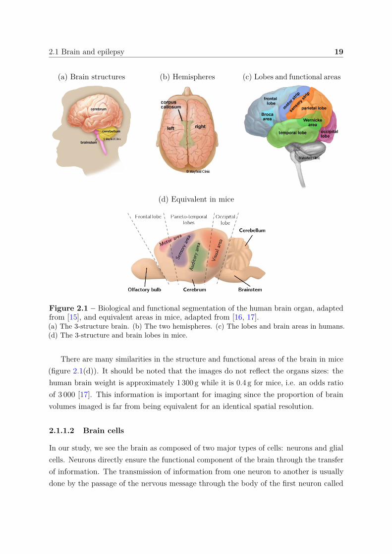
The brain is composed of three main structures: the cerebrum, cerebellum and brainstem,see figure 2.1(a). The brainstem supports vital functions of the autonomic nervous systemsuch as breathing, heartbeat and salivation. The cerebellum is involved in fundamentalfunctions, sometimes referred to as reptilian, such as movement coordination, balance,learning motor functions, and controlling circadian and heart rhythms. Discoveries havealso shown the involvement of this structure in higher level functions such as speechproduction and speech perception [14]. The cerebrum is separated into two parts: theright and left hemispheres that are connected by the corpus callosum, see figure 2.1(b).Each hemisphere is divided into four areas called lobes, themselves divided into sub-areasthat serve specific functions, see figure 2.1(c).
Here some functions associated to each lobe in humans:• Frontal lobe: control of voluntary movement (motor strip), attention, short term
memory tasks, motivation, planning, problem solving, speech: speaking and writing(Broca’s area)
• Parietal lobe: proprioceptive and mechanoceptive stimuli (sensory strip), languageprocessing
• Occipital lobe: visual processing• Temporal lobe: decoding sensory input into derived meanings for retention of visual
memory and language comprehension (Wernicke’s area).Most of the functions involve different areas of the brain that can be located in differentlobes, and there are very complex relationships between all of these areas. Some ofthem are better known than others e.g. Broca’s and Wernicke’s areas, represented infigure 2.1(c). A damaged Broca’s area may result in a disability to speak and write but apreserved ability to read and understand spoken language, a phenotype known as Broca’saphasia [18]. A damaged Wernicke’s area in the left temporal lobe can cause the personto speak in long sentences that have no meaning; add unnecessary words or even createnew words. The person can speak but has difficulty in understanding speech and istherefore unaware of their own mistakes, a phenotype known as Wernicke’s aphasia [19].This is the typical areas avoided during surgery, especially in case of resection.
The brain, is crossed by four fluid-filled cavities called ventricles. Inside the ventriclescirculates the cerebrospinal fluid that also circulates around the brain. The skull andcerebrospinal fluid help cushion the brain from injury, like a sponge in a jar full of water.
2.1 Brain and epilepsy 19
(a) Brain structures (b) Hemispheres (c) Lobes and functional areas
(d) Equivalent in mice
Figure 2.1 – Biological and functional segmentation of the human brain organ, adaptedfrom [15], and equivalent areas in mice, adapted from [16, 17].(a) The 3-structure brain. (b) The two hemispheres. (c) The lobes and brain areas in humans.(d) The 3-structure and brain lobes in mice.
There are many similarities in the structure and functional areas of the brain in mice(figure 2.1(d)). It should be noted that the images do not reflect the organs sizes: thehuman brain weight is approximately 1 300 g while it is 0.4 g for mice, i.e. an odds ratioof 3 000 [17]. This information is important for imaging since the proportion of brainvolumes imaged is far from being equivalent for an identical spatial resolution.
2.1.1.2 Brain cells
In our study, we see the brain as composed of two major types of cells: neurons and glialcells. Neurons directly ensure the functional component of the brain through the transferof information. The transmission of information from one neuron to another is usuallydone by the passage of the nervous message through the body of the first neuron called
20 State of the art
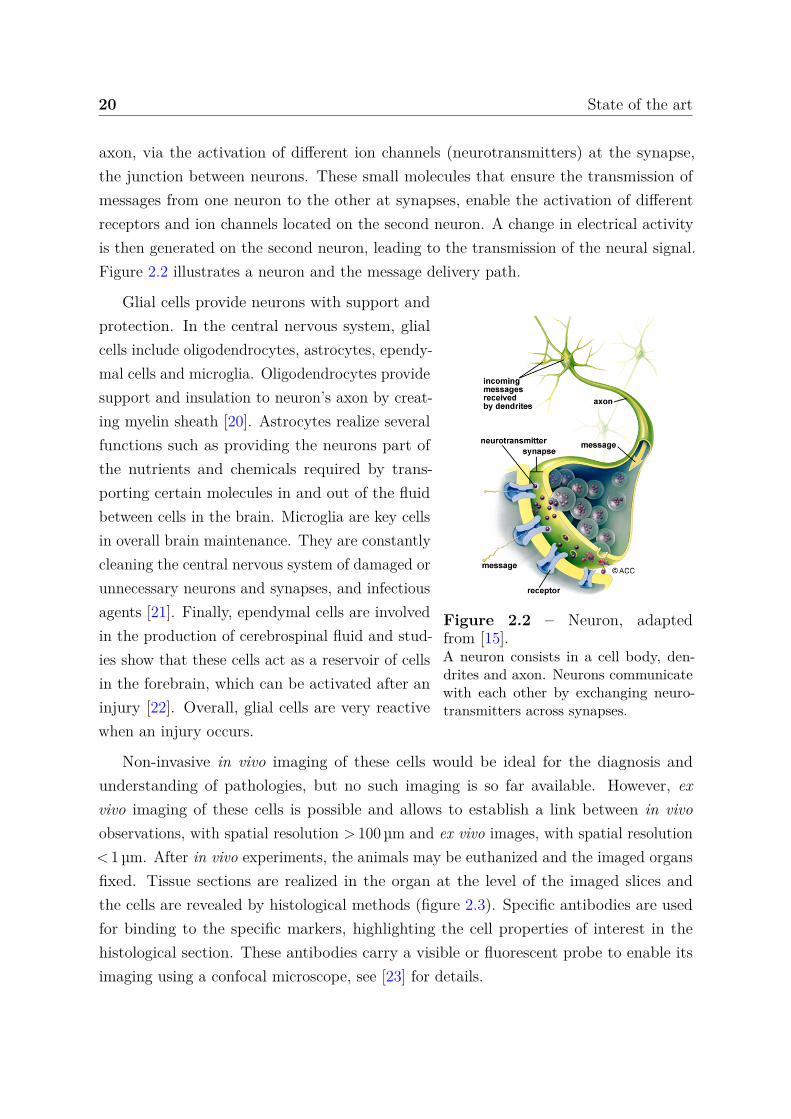
axon, via the activation of different ion channels (neurotransmitters) at the synapse,the junction between neurons. These small molecules that ensure the transmission ofmessages from one neuron to the other at synapses, enable the activation of differentreceptors and ion channels located on the second neuron. A change in electrical activityis then generated on the second neuron, leading to the transmission of the neural signal.Figure 2.2 illustrates a neuron and the message delivery path.
Figure 2.2 – Neuron, adaptedfrom [15].A neuron consists in a cell body, den-drites and axon. Neurons communicatewith each other by exchanging neuro-transmitters across synapses.
Glial cells provide neurons with support andprotection. In the central nervous system, glialcells include oligodendrocytes, astrocytes, ependy-mal cells and microglia. Oligodendrocytes providesupport and insulation to neuron’s axon by creat-ing myelin sheath [20]. Astrocytes realize severalfunctions such as providing the neurons part ofthe nutrients and chemicals required by trans-porting certain molecules in and out of the fluidbetween cells in the brain. Microglia are key cellsin overall brain maintenance. They are constantlycleaning the central nervous system of damaged orunnecessary neurons and synapses, and infectiousagents [21]. Finally, ependymal cells are involvedin the production of cerebrospinal fluid and stud-ies show that these cells act as a reservoir of cellsin the forebrain, which can be activated after aninjury [22]. Overall, glial cells are very reactivewhen an injury occurs.
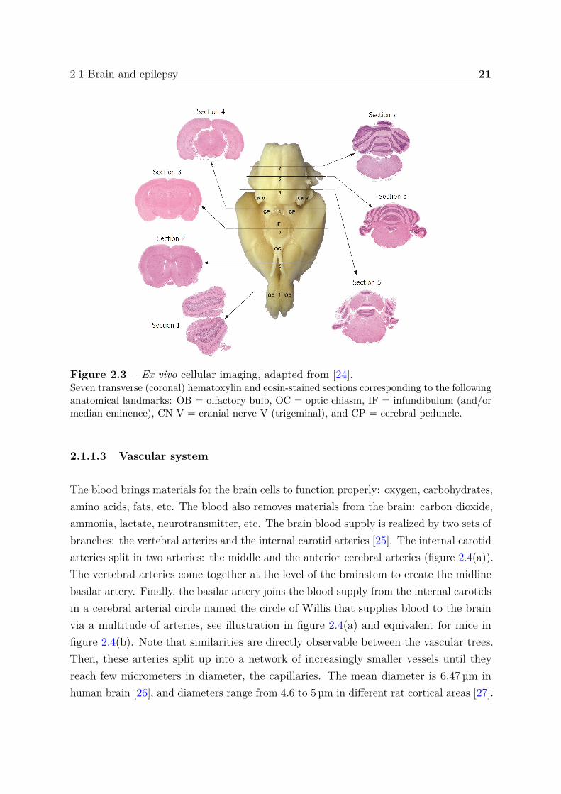
Non-invasive in vivo imaging of these cells would be ideal for the diagnosis andunderstanding of pathologies, but no such imaging is so far available. However, exvivo imaging of these cells is possible and allows to establish a link between in vivoobservations, with spatial resolution > 100 µm and ex vivo images, with spatial resolution< 1 µm. After in vivo experiments, the animals may be euthanized and the imaged organsfixed. Tissue sections are realized in the organ at the level of the imaged slices andthe cells are revealed by histological methods (figure 2.3). Specific antibodies are usedfor binding to the specific markers, highlighting the cell properties of interest in thehistological section. These antibodies carry a visible or fluorescent probe to enable itsimaging using a confocal microscope, see [23] for details.
2.1 Brain and epilepsy 21
Figure 2.3 – Ex vivo cellular imaging, adapted from [24].Seven transverse (coronal) hematoxylin and eosin-stained sections corresponding to the followinganatomical landmarks: OB = olfactory bulb, OC = optic chiasm, IF = infundibulum (and/ormedian eminence), CN V = cranial nerve V (trigeminal), and CP = cerebral peduncle.
2.1.1.3 Vascular system
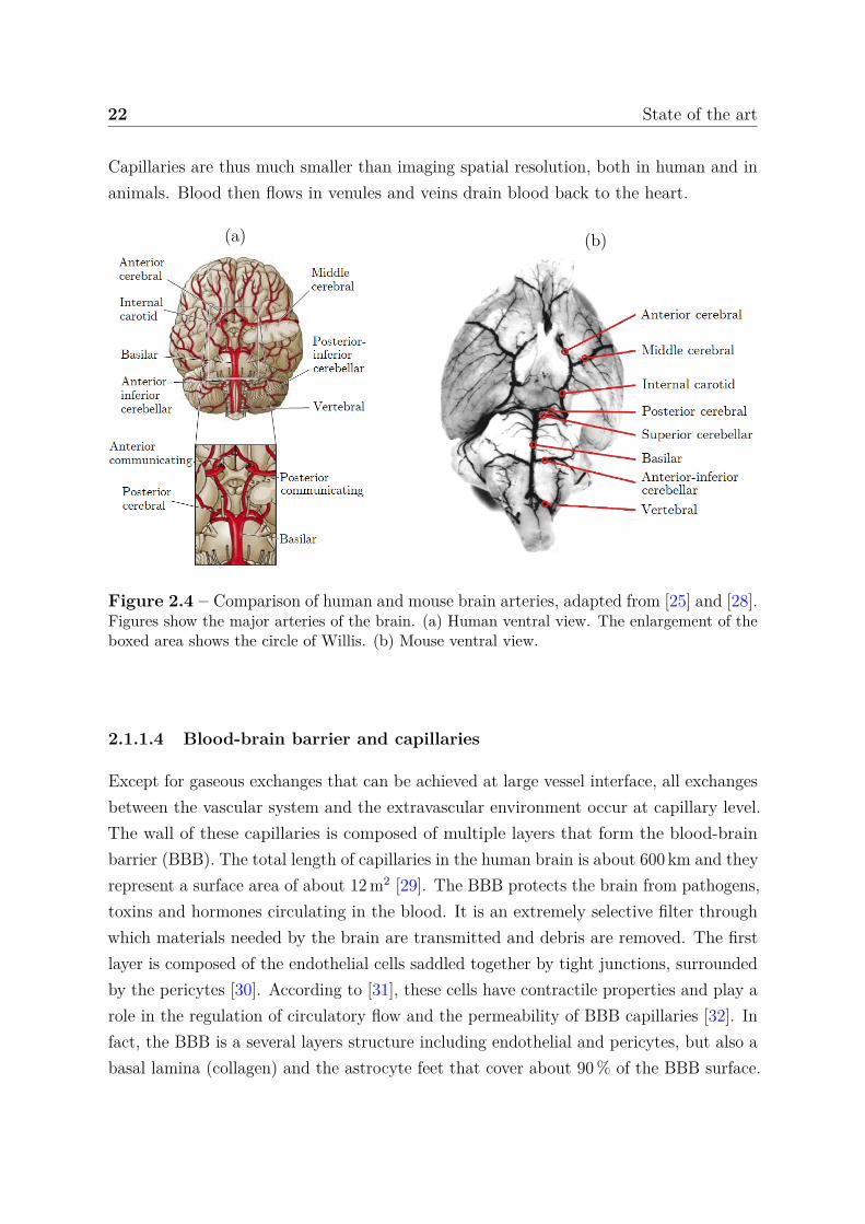
The blood brings materials for the brain cells to function properly: oxygen, carbohydrates,amino acids, fats, etc. The blood also removes materials from the brain: carbon dioxide,ammonia, lactate, neurotransmitter, etc. The brain blood supply is realized by two sets ofbranches: the vertebral arteries and the internal carotid arteries [25]. The internal carotidarteries split in two arteries: the middle and the anterior cerebral arteries (figure 2.4(a)).The vertebral arteries come together at the level of the brainstem to create the midlinebasilar artery. Finally, the basilar artery joins the blood supply from the internal carotidsin a cerebral arterial circle named the circle of Willis that supplies blood to the brainvia a multitude of arteries, see illustration in figure 2.4(a) and equivalent for mice infigure 2.4(b). Note that similarities are directly observable between the vascular trees.Then, these arteries split up into a network of increasingly smaller vessels until theyreach few micrometers in diameter, the capillaries. The mean diameter is 6.47 µm inhuman brain [26], and diameters range from 4.6 to 5 µm in different rat cortical areas [27].
22 State of the art
Capillaries are thus much smaller than imaging spatial resolution, both in human and inanimals. Blood then flows in venules and veins drain blood back to the heart.
(a) (b)
Figure 2.4 – Comparison of human and mouse brain arteries, adapted from [25] and [28].Figures show the major arteries of the brain. (a) Human ventral view. The enlargement of theboxed area shows the circle of Willis. (b) Mouse ventral view.
2.1.1.4 Blood-brain barrier and capillaries
Except for gaseous exchanges that can be achieved at large vessel interface, all exchangesbetween the vascular system and the extravascular environment occur at capillary level.The wall of these capillaries is composed of multiple layers that form the blood-brainbarrier (BBB). The total length of capillaries in the human brain is about 600 km and theyrepresent a surface area of about 12 m2 [29]. The BBB protects the brain from pathogens,toxins and hormones circulating in the blood. It is an extremely selective filter throughwhich materials needed by the brain are transmitted and debris are removed. The firstlayer is composed of the endothelial cells saddled together by tight junctions, surroundedby the pericytes [30]. According to [31], these cells have contractile properties and play arole in the regulation of circulatory flow and the permeability of BBB capillaries [32]. Infact, the BBB is a several layers structure including endothelial and pericytes, but also abasal lamina (collagen) and the astrocyte feet that cover about 90 % of the BBB surface.
2.1 Brain and epilepsy 23
2.1.1.5 Neurogliovascular unit
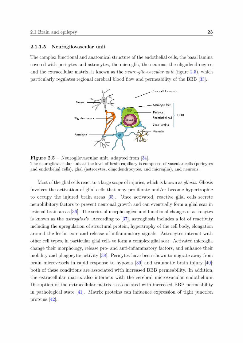
The complex functional and anatomical structure of the endothelial cells, the basal laminacovered with pericytes and astrocytes, the microglia, the neurons, the oligodendrocytes,and the extracellular matrix, is known as the neuro-glio-vascular unit (figure 2.5), whichparticularly regulates regional cerebral blood flow and permeability of the BBB [33].
Figure 2.5 – Neurogliovascular unit, adapted from [34].The neurogliovascular unit at the level of brain capillary is composed of vascular cells (pericytesand endothelial cells), glial (astrocytes, oligodendrocytes, and microglia), and neurons.
Most of the glial cells react to a large scope of injuries, which is known as gliosis. Gliosisinvolves the activation of glial cells that may proliferate and/or become hypertrophicto occupy the injured brain areas [35]. Once activated, reactive glial cells secreteneurohibitory factors to prevent neuronal growth and can eventually form a glial scar inlesional brain areas [36]. The series of morphological and functional changes of astrocytesis known as the astrogliosis. According to [37], astrogliosis includes a lot of reactivityincluding the upregulation of structural protein, hypertrophy of the cell body, elongationaround the lesion core and release of inflammatory signals. Astrocytes interact withother cell types, in particular glial cells to form a complex glial scar. Activated microgliachange their morphology, release pro- and anti-inflammatory factors, and enhance theirmobility and phagocytic activity [38]. Pericytes have been shown to migrate away frombrain microvessels in rapid response to hypoxia [39] and traumatic brain injury [40];both of these conditions are associated with increased BBB permeability. In addition,the extracellular matrix also interacts with the cerebral microsvacular endothelium.Disruption of the extracellular matrix is associated with increased BBB permeabilityin pathological state [41]. Matrix proteins can influence expression of tight junctionproteins [42].
24 State of the art
2.1.2 Epilepsy
2.1.2.1 General overview
Epilepsy is the third most common neurological disease and despite the many findings inthe field, the understanding of epilepsy remains a very important subject of study (6 524PubMed entries for epilepsy in 2019). If in the popular mind it is often limited to episodicseizures, in reality it is a disease that includes various symptoms, the most spectacularof which are indeed these well-known seizures. Epilepsy has a high risk of disability,psychiatric comorbidity, social isolation and premature death [1]. Diseases associatedwith a primary pathology are now an integral part of epilepsy. In this context, the seizurewould only be the visible part, with parallel neurobiological, cognitive, psychologicaland social consequences. In [43], the authors enumerate about 50 epilepsy syndromes.A few have a clear genetic background, but most are multifactorial in origin, linked tohereditary, lesional and/or environmental components. However, they share a commonfeature: a synchronized and abnormal excitation of a large neurons group in a particularbrain area, which can secondarily spread to other areas of the brain. It results in a suddenand intense electrical activity which causes the symptoms during seizures (involuntarymovements, auditory or visual hallucinations, absences, etc). The expression of thesesymptoms depends on the cerebral zones in which the neurons involved are located orthe role of these neural cells in the systems that manage our motor skills, cognition,emotions or behaviors.
The most typical manifestation of epilepsy is thus the epileptic seizure. We candistinguish two seizure types: generalized and (multi-)focal seizures [44]. Generalizedseizures are related to the excitation and synchronization of neurons originating fromseveral spread regions over both cerebral hemispheres. They generally associate atransitory consciousness loss (absence of a few seconds to a few minutes) with tonic(muscle contractions), myoclonic (muscle shakes) or atonic (without muscle contraction)motor signs. Focal seizures originate from a specific area of the brain, referred to as theepileptogenic zone (EZ). Depending on the area, multiple manifestations result. Thesymptoms of a focal epileptic seizure are numerous: language disorders, emotional signs(fear, laughter, ecstasy, etc.), pain, vegetative signs (salivation, apnea, tachycardia, etc.),automatic gestures and often explosive motor behavior. A loss of consciousness (orcontact with the outside world) is also often observed. The hyperexcitation of the focalseizure can spread and thus leads to a generalized seizure.
2.1 Brain and epilepsy 25
2.1.2.2 Neuronal activity
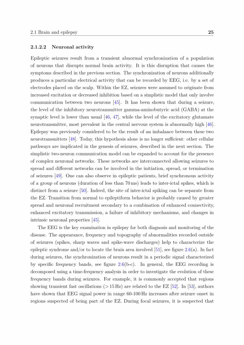
Epileptic seizures result from a transient abnormal synchronization of a populationof neurons that disrupts normal brain activity. It is this disruption that causes thesymptoms described in the previous section. The synchronization of neurons additionallyproduces a particular electrical activity that can be recorded by EEG, i.e. by a set ofelectrodes placed on the scalp. Within the EZ, seizures were assumed to originate fromincreased excitation or decreased inhibition based on a simplistic model that only involvecommunication between two neurons [45]. It has been shown that during a seizure,the level of the inhibitory neurotransmitter gamma-aminobutyric acid (GABA) at thesynaptic level is lower than usual [46, 47], while the level of the excitatory glutamateneurotransmitter, most prevalent in the central nervous system is abnormally high [46].Epilepsy was previously considered to be the result of an imbalance between these twoneurotransmitters [48]. Today, this hypothesis alone is no longer sufficient: other cellularpathways are implicated in the genesis of seizures, described in the next section. Thesimplistic two-neuron communication model can be expanded to account for the presenceof complex neuronal networks. These networks are interconnected allowing seizures tospread and different networks can be involved in the initiation, spread, or terminationof seizures [49]. One can also observe in epileptic patients, brief synchronous activityof a group of neurons (duration of less than 70 ms) leads to inter-ictal spikes, which isdistinct from a seizure [50]. Indeed, the site of inter-ictal spiking can be separate fromthe EZ. Transition from normal to epileptiform behavior is probably caused by greaterspread and neuronal recruitment secondary to a combination of enhanced connectivity,enhanced excitatory transmission, a failure of inhibitory mechanisms, and changes inintrinsic neuronal properties [45].
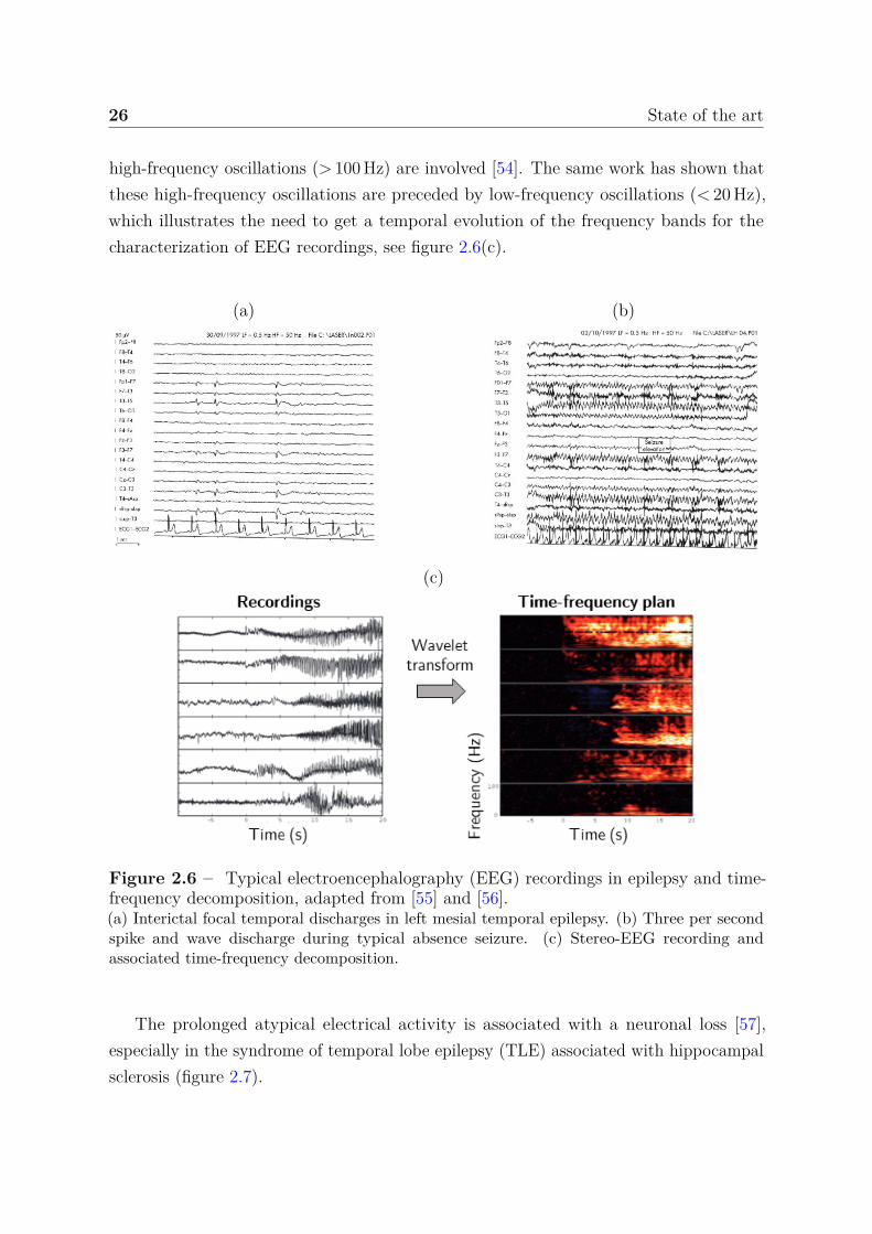
The EEG is the key examination in epilepsy for both diagnosis and monitoring of thedisease. The appearance, frequency and topography of abnormalities recorded outsideof seizures (spikes, sharp waves and spike-wave discharges) help to characterize theepileptic syndrome and/or to locate the brain area involved [51], see figure 2.6(a). In factduring seizures, the synchronization of neurons result in a periodic signal characterizedby specific frequency bands, see figure 2.6(b-c). In general, the EEG recording isdecomposed using a time-frequency analysis in order to investigate the evolution of thesefrequency bands during seizures. For example, it is commonly accepted that regionsshowing transient fast oscillations (> 15 Hz) are related to the EZ [52]. In [53], authorshave shown that EEG signal power in range 60-100 Hz increases after seizure onset inregions suspected of being part of the EZ. During focal seizures, it is suspected that
26 State of the art
high-frequency oscillations (> 100 Hz) are involved [54]. The same work has shown thatthese high-frequency oscillations are preceded by low-frequency oscillations (< 20 Hz),which illustrates the need to get a temporal evolution of the frequency bands for thecharacterization of EEG recordings, see figure 2.6(c).
(a) (b)
(c)
Figure 2.6 – Typical electroencephalography (EEG) recordings in epilepsy and time-frequency decomposition, adapted from [55] and [56].(a) Interictal focal temporal discharges in left mesial temporal epilepsy. (b) Three per secondspike and wave discharge during typical absence seizure. (c) Stereo-EEG recording andassociated time-frequency decomposition.
The prolonged atypical electrical activity is associated with a neuronal loss [57],especially in the syndrome of temporal lobe epilepsy (TLE) associated with hippocampalsclerosis (figure 2.7).

2.1 Brain and epilepsy 27
(a) (b)
(c) (d)
Figure 2.7 – Histopathologic subtypes of hippocampal sclerosis in patients with temporallobe epilepsy (TLE), adapted from [58].(a) ILAE hippocampal sclerosis (HS) type 1: pronounced pyramidal cell loss in both CA4and CA1, variable but frequently visible damage to CA3 and CA2, and variable cell loss inthe dentate gyrus. (b) ILAE HS type 2: CA1 predominant neuronal cell loss and gliosis. (c)ILAE HS type 3: CA4 predominant neuronal cell loss and gliosis. (d) No HS, gliosis only.All stainings represent NeuN immunohistochemistry with hematoxylin counterstaining using4-µm–thin paraffin embedded sections. Scale bar in (a) = 1 000 µm (applies also to (b-d)).
2.1.2.3 Glial and microvascular modifications
A prominent feature of epileptic foci in patients is an abnormal glial environment includingchronically activated astrocytes and microglia, and glial scars [59], see figure 2.8(a). Thisdysregulation of glial functions may cause seizures or promote epileptogenesis [60].Indeed, perturbation in regulation of ions, water, and neurotransmitters can promotehyperexcitability and hypersynchrony [59]. Activated astrocytes and microglia lead to therelease of pro-inflammatory mediators and could cause sustained inflammatory changesthat facilitate epileptogenesis [61]. Therefore, the main mechanisms by which glial cellscould facilitate the development of epilepsy and seizures include an increased excitabilityand inflammation.
As introduced in section 2.1.1.5, glial cells are also related to the microvascularizationand contribute to BBB function. In TLE, a significant increase of vascular density in
28 State of the art
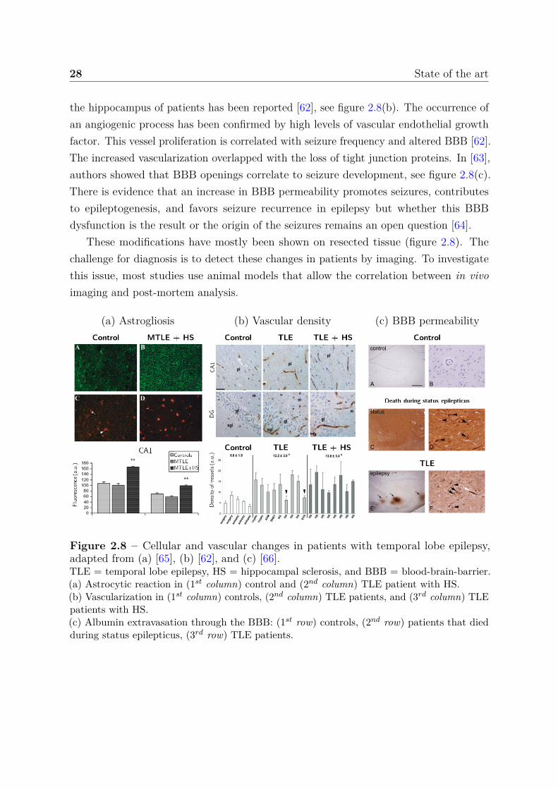
the hippocampus of patients has been reported [62], see figure 2.8(b). The occurrence ofan angiogenic process has been confirmed by high levels of vascular endothelial growthfactor. This vessel proliferation is correlated with seizure frequency and altered BBB [62].The increased vascularization overlapped with the loss of tight junction proteins. In [63],authors showed that BBB openings correlate to seizure development, see figure 2.8(c).There is evidence that an increase in BBB permeability promotes seizures, contributesto epileptogenesis, and favors seizure recurrence in epilepsy but whether this BBBdysfunction is the result or the origin of the seizures remains an open question [64].
These modifications have mostly been shown on resected tissue (figure 2.8). Thechallenge for diagnosis is to detect these changes in patients by imaging. To investigatethis issue, most studies use animal models that allow the correlation between in vivoimaging and post-mortem analysis.
(a) Astrogliosis (b) Vascular density (c) BBB permeability
Figure 2.8 – Cellular and vascular changes in patients with temporal lobe epilepsy,adapted from (a) [65], (b) [62], and (c) [66].TLE = temporal lobe epilepsy, HS = hippocampal sclerosis, and BBB = blood-brain-barrier.(a) Astrocytic reaction in (1st column) control and (2nd column) TLE patient with HS.(b) Vascularization in (1st column) controls, (2nd column) TLE patients, and (3rd column) TLEpatients with HS.(c) Albumin extravasation through the BBB: (1st row) controls, (2nd row) patients that diedduring status epilepticus, (3rd row) TLE patients.
2.1 Brain and epilepsy 29
2.1.3 Experimental murine model
In the following section, it should be understood that several models for seizures, epilep-togenesis and chronic epilepsy have been developed in several animal species. Most ofthe time, each model allows a number of specific questions to be answered. Becauseour work is intended to detect epileptogenic regions for mesial temporal lobe epilepsy inan experimental murine model, a certain amount of works are omitted in the following.Among the introduced works, it was decided to consider both mouse and rat modelsbecause the rat was considerably more extensively used in MRI studies. However, we donot claim that these models are equivalent and despite the similarities, features of thesetwo species are somewhat different (see [67]).
2.1.3.1 Kindling and status epilepticus models of epilepsy
Taken together, the clinical findings presented in the previous section have to be replicatedin order to answer many unresolved questions. The identification of the seizure onsetis especially important for surgical treatment of MTLE. Another point is the under-standing of the epileptogenesis for establishing the evolution of the epileptic disorder.Models must therefore reproduce both the epileptogenesis period and the chronic periodhistopathological, electroencephalographic and behavioral features encountered in focalepilepsy.
Several experimental animal models provide high levels of similarity with humanepilepsy, but there is no experimental model that reproduces all features of MTLE. Thetwo most commonly used animal models of MTLE are kindling and status epilepticusmodels. With the first one introduced in 1967 by Goddard [68], spontaneous seizures areinduced by repeated electrical simulations accompanied by stronger seizure responses untilthe animal reached standard seizure response. At this point, the stimulation must continueuntil the development of spontaneous crises (overkindling period in figure 2.9(a)). In thestatus epilepticus model, a status epilepticus condition (continual seizures) is inducted bychemical agents administration (among others, pilocarpine, kainate, pilocarpine-lithium,flurothyl) that terminates within several hours. Then, spontaneous seizures emerge aftera latent period that lasts for weeks or months (figure 2.9(b)).
The advantages of the kindling model are the precise focal activation of brain sites, thedevelopment of chronic epiletogenesis and the fact that the pattern of seizure propagationand generalization is readily monitored [69]. In return, kindling experiments can berelatively labor intensive because the electrodes are implanted into the brain and a large
30 State of the art
(a) Kindling model
(b) Status epilepticus models
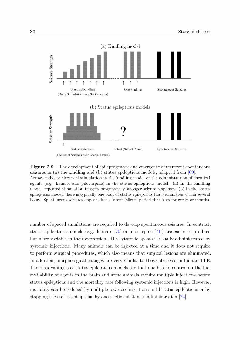
Figure 2.9 – The development of epileptogenesis and emergence of recurrent spontaneousseizures in (a) the kindling and (b) status epilepticus models, adapted from [69].Arrows indicate electrical stimulation in the kindling model or the administration of chemicalagents (e.g. kainate and pilocarpine) in the status epilepticus model. (a) In the kindlingmodel, repeated stimulation triggers progressively stronger seizure responses. (b) In the statusepilepticus model, there is typically one bout of status epilepticus that terminates within severalhours. Spontaneous seizures appear after a latent (silent) period that lasts for weeks or months.
number of spaced simulations are required to develop spontaneous seizures. In contrast,status epilepticus models (e.g. kainate [70] or pilocarpine [71]) are easier to producebut more variable in their expression. The cytotoxic agents is usually administrated bysystemic injections. Many animals can be injected at a time and it does not requireto perform surgical procedures, which also means that surgical lesions are eliminated.In addition, morphological changes are very similar to those observed in human TLE.The disadvantages of status epilepticus models are that one has no control on the bio-availability of agents in the brain and some animals require multiple injections beforestatus epilepticus and the mortality rate following systemic injections is high. However,mortality can be reduced by multiple low dose injections until status epilepticus or bystopping the status epilepticus by anesthetic substances administration [72].
2.1 Brain and epilepsy 31
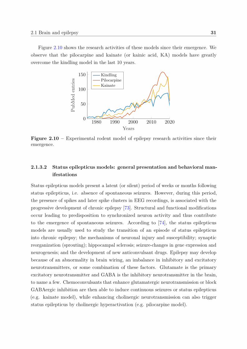
Figure 2.10 shows the research activities of these models since their emergence. Weobserve that the pilocarpine and kainate (or kainic acid, KA) models have greatlyovercome the kindling model in the last 10 years.
1980 1990 2000 2010 20200
50
100
150
Years
PubM
eden
trie
sKindlingPilocarpineKainate
Figure 2.10 – Experimental rodent model of epilepsy research activities since theiremergence.
2.1.3.2 Status epilepticus models: general presentation and behavioral man-ifestations
Status epilepticus models present a latent (or silent) period of weeks or months followingstatus epilepticus, i.e. absence of spontaneous seizures. However, during this period,the presence of spikes and later spike clusters in EEG recordings, is associated with theprogressive development of chronic epilepsy [73]. Structural and functional modificationsoccur leading to predisposition to synchronized neuron activity and thus contributeto the emergence of spontaneous seizures. According to [74], the status epilepticusmodels are usually used to study the transition of an episode of status epilepticusinto chronic epilepsy; the mechanisms of neuronal injury and susceptibility; synapticreorganization (sprouting); hippocampal sclerosis; seizure-changes in gene expression andneurogenesis; and the development of new anticonvulsant drugs. Epilepsy may developbecause of an abnormality in brain wiring, an imbalance in inhibitory and excitatoryneurotransmitters, or some combination of these factors. Glutamate is the primaryexcitatory neurotransmitter and GABA is the inhibitory neurotransmitter in the brain,to name a few. Chemoconvulsants that enhance glutamatergic neurotransmission or blockGABAergic inhibition are then able to induce continuous seizures or status epilepticus(e.g. kainate model), while enhancing cholinergic neurotransmission can also triggerstatus epilepticus by cholinergic hyperactivation (e.g. pilocarpine model).
32 State of the art
The status epilepticus induced by pilocarpine and the one induced by kainic acid aresimilar, leading to the development of spontaneous limbic motor seizures and mossy fibersprouting in the dentate gyrus [75]. The pattern of neuronal damage is similar to KAmodel but pilocarpine induces greater neocortical damage, i.e. cell loss [76, 77]. One ofthe drawback of the pilocarpine-systemic administrated model compared to kainate modelis the more extensive lesions observed [78], but systemic injections of KA also inducelarge damage out of the hippocampal regions. The mortality rate following systemicadministration of KA in rats is between 5 and 30% [72], while the pilocarpine modelis known to be more reliable because almost all treated rats will develop spontaneousseizures, independently of the duration of the status epilepticus. After the administrationof KA, animals show automatisms and a catatonic posture that often progresses tomyoclonic twitching of the head, forelimbs and rearlimbs. Typically, before and after theadministration, KA-treated rats also develop wet-dog shakes.
For both of these models, the cytotoxic agent can be delivered via systemic orintracerebral administration (generally in the hippocampus [79, 80] and amygdala forKA [81]). In fact, the behavioral, electrographic and neuropathological alterations thatfollow intracerebral injection, are similar to those observed following systematic injectionand the mortality following injection is drastically reduced [72, 79]. More generally, thevariability of models is reduced. Using unilateral intrahippocampal KA administration,we observe cell loss and complete degeneration of the hippocampus with enlargementof the granule cell layer of the dentate gyrus weeks after injections. The intraamygdalaadministration of KA could induce bilateral hippocampal lesions [82]. These lesions,distant from the injection site, result from the propagation of the seizure activity. However,these models require a surgery, which increases the labor required to produce animals.
2.1.3.3 Status epilepticus models: electroencephalographic features and neu-ropathological changes
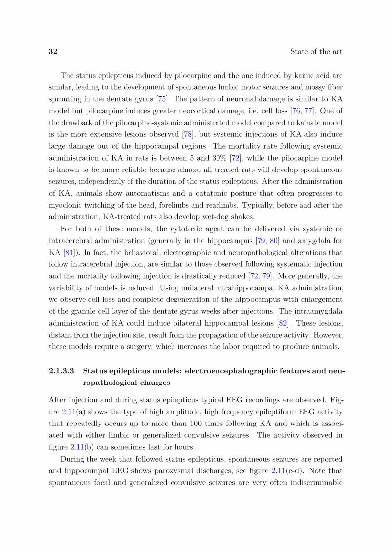
After injection and during status epilepticus typical EEG recordings are observed. Fig-ure 2.11(a) shows the type of high amplitude, high frequency epileptiform EEG activitythat repeatedly occurs up to more than 100 times following KA and which is associ-ated with either limbic or generalized convulsive seizures. The activity observed infigure 2.11(b) can sometimes last for hours.
During the week that followed status epilepticus, spontaneous seizures are reportedand hippocampal EEG shows paroxysmal discharges, see figure 2.11(c-d). Note thatspontaneous focal and generalized convulsive seizures are very often indiscriminable
2.1 Brain and epilepsy 33
Figure 2.11 – Electroencephalograms (EEG) of rats kainate model, adapted from [83].(A) First typical EEG seizure determined 12 minutes after kainate injection. (B) Typicalepileptiform activity observed several hours after kainate. (C) Paroxysmal EEG activityduring a spontaneous focal seizure. (D) Paroxysmal EEG activity during a spontaneousgeneralized convulsive seizure in an epileptic rat; (E) Atypical paroxysmal EEG activity duringa spontaneous nonconvulsive seizure in an epileptic rat. (F) Baseline EEG between seizures inthe chronic period of an epileptic rat.
in the EEG. Once spontaneous and recurrent seizures emerge, we observe around 6-7generalizations per week [83]. Typically, the baseline EEG recordings of an epileptic ratshow interictal spikes (figure 2.11(f)).
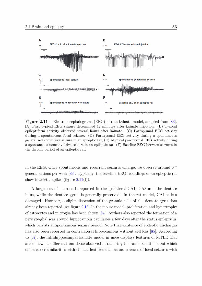
A large loss of neurons is reported in the ipsilateral CA1, CA3 and the dentatehilus, while the dentate gyrus is generally preserved. In the rat model, CA1 is lessdamaged. However, a slight dispersion of the granule cells of the dentate gyrus hasalready been reported, see figure 2.12. In the mouse model, proliferation and hypertrophyof astrocytes and microglia has been shown [84]. Authors also reported the formation of apericyte-glial scar around hippocampus capillaries a few days after the status epilepticus,which persists at spontaneous seizure period. Note that existence of epileptic dischargeshas also been reported in contralateral hippocampus without cell loss [85]. Accordingto [67], the intrahippocampal kainate model in mice displays features of MTLE thatare somewhat different from those observed in rat using the same conditions but whichoffers closer similarities with clinical features such as occurrences of focal seizures with
34 State of the art
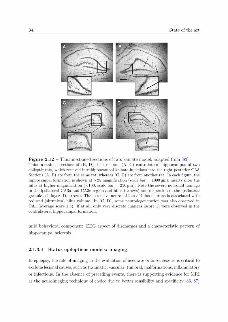
Figure 2.12 – Thionin-stained sections of rats kainate model, adapted from [83].Thionin-stained sections of (B, D) the ipsi- and (A, C) contralateral hippocampus of twoepileptic rats, which received intrahippocampal kainate injections into the right posterior CA3.Sections (A, B) are from the same rat, whereas (C, D) are from another rat. In each figure, thehippocampal formation is shown at ×25 magnification (scale bar = 1000 µm); inserts show thehilus at higher magnification (×100; scale bar = 250 µm). Note the severe neuronal damagein the ipsilateral CA3a and CA3c region and hilus (arrows) and dispersion of the ipsilateralgranule cell layer (D, arrow). The extensive neuronal loss of hilus neurons is associated withreduced (shrunken) hilus volume. In (C, D), some neurodegeneration was also observed inCA1 (average score 1.5). If at all, only very discrete changes (score 1) were observed in thecontralateral hippocampal formation.
mild behavioral component, EEG aspect of discharges and a characteristic pattern ofhippocampal sclerosis.
2.1.3.4 Status epilepticus models: imaging
In epilepsy, the role of imaging in the evaluation of accurate or onset seizure is critical toexclude lesional causes, such as traumatic, vascular, tumoral, malformations, inflammatoryor infectious. In the absence of preceding events, there is supporting evidence for MRIas the neuroimaging technique of choice due to better sensibility and specificity [86, 87].
2.1 Brain and epilepsy 35
However, computerized tomography scan (CT) can be preferred due to more widespreadavailability, rapidity of acquisition, and limited contraindications. In [86], authorsindicated, however, that 8-12 % of patients with initial negative CT scans, present positivefindings in MRI. Still, it is also possible for patients to have negative MRI. Classically,MRI is used to qualitatively assess for an atrophic hippocampus with hyperintense T2
signals (described in the subsequent section 2.2.2.1), which is a defining trait of advancedhippocampal sclerosis [88, 89]. Although qualitative imaging remains the gold standardfor diagnosis, there is a constant need to develop quantitative and automated methodsto identify hippocampal and extra-hippocampal damages. MRI can provide a precisecharacterization of the internal architecture of the hippocampus, which allows betterdetection of more subtle changes. One of the main targeted development is the detectionof the epileptogenic foci but one can also study the epileptic condition following thestatus epilepticus in experimental model to identify biomarkers of the development of achronic condition. Of course, a robust method to reduce the number of negative MRIscans is also very valuable.
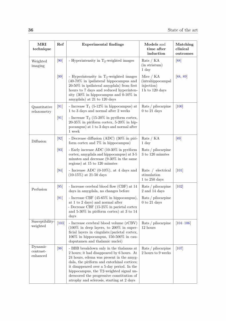
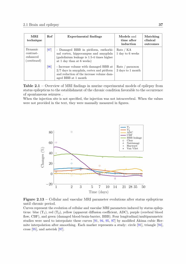
A step forward is the use of more complex MRI acquisitions such as functional,diffusion, perfusion with or without contrast agent administration among others. TheseMRI techniques are described in section 2.3 but we propose to summarize here theimportant findings associated with epilepsy. In fact, some parameters are very welldocumented while others are sometimes completely absent from the picture. We propose toreport most of the last quantitative MRI findings in experimental status epilepticus modelssummarized in table 2.1. We also propose to interpolate from few longitudinal studies,the variations of the most documented MRI parameter values during the month followingthe status epilepticus in figure 2.13. This duration includes the entire epileptogenesisthat ends with the establishment of a favorable environment for epileptic seizures. Notethat the graph was produced from several models/scanners.
Regarding cellular related MRI parameters, several works reported hyperintensityin T2-weighted images after status epilepticus [90], which matches increased T2 valuesreported in quantitative studies [91]. In this work, authors also reported increased T1
values. Usually, these parameters return to their initial values after 1-2 weeks [91].Diffusion parameters are the most documented MRI parameters in epilepsy. Earlydiffusion decreased first days after status epilepticus is followed by an increase in diffusionat the chronic period [92–94]. Regarding vascular related MRI parameters, the bloodflow first increases and then, decreases at one week [91, 95]. Finally, several works haveshown a significant increase in BBB permeability [96–98].
36 State of the art
MRItechnique
Ref Experimental findings Models andtime afterinduction
Matchingclinicaloutcomes
Weightedimaging
[90] - Hyperintensity in T2-weighted images Rats / KA(in striatum)1 day
[88]
[99] - Hyperintensity in T2-weighted images(40-70% in ipsilateral hippocampus and20-50% in ipsilateral amygdala) from firsthours to 7 days and reduced hyperinten-sity (30% in hippocampus and 0-10% inamygdala) at 21 to 120 days
Mice / KA(intrahippocampalinjection)1 h to 120 days
[88, 89]
Quantitativerelaxometry
[91] - Increase T1 (5-12% in hippocampus) at1 to 3 days and normal after 2 weeks
Rats / pilocarpine0 to 21 days
[100]
[91] - Increase T2 (15-20% in pyriform cortex,20-35% in piriform cortex, 5-20% in hip-pocampus) at 1 to 3 days and normal after1 week
Diffusion[92] - Decrease diffusion (ADC) (30% in piri-
form cortex and 7% in hippocampus)Rats / KA1 day
[89]
[93] - Early increase ADC (10-30% in pyriformcortex, amygdala and hippocampus) at 3-5minutes and decrease (9-30% in the sameregions) at 15 to 120 minutes
Rats / pilocarpine3 to 120 minutes
[94] - Increase ADC (0-10%), at 4 days and(10-15%) at 21-50 days
Rats / electricalstimulation1 to 250 days
[101]
Perfusion[95] - Increase cerebral blood flow (CBF) at 14
days in amygdala, no changes beforeRats / pilocarpine2 and 14 days
[102]
[91] - Increase CBF (45-65% in hippocampus),at 1 to 2 days) and normal after- Decrease CBF (15-25% in parietal cortexand 5-30% in piriform cortex) at 3 to 14days
Rats / pilocarpine0 to 21 days
Susceptibility-weighted
[103] - Increase cerebral blood volume (rCBV)(100% in deep layers, to 200% in super-ficial layers in cingulate/parietal cortex,106% in hippocampus, 150-500% in cau-doputamen and thalamic nuclei)
Rats / pilocarpine12 hours
[104–106]
Dynamiccontrast-enhanced
[98] - BBB breakdown only in the thalamus at2 hours; it had disappeared by 6 hours. At24 hours, edema was present in the amyg-dala, the piriform and entorhinal cortices;it disappeared over a 5-day period. In thehippocampus, the T2-weighted signal un-derscored the progressive constitution ofatrophy and sclerosis, starting at 2 days
Rats / pilocarpine2 hours to 9 weeks
[107]
2.1 Brain and epilepsy 37
MRItechnique
Ref Experimental findings Models andtime afterinduction
Matchingclinicaloutcomes
Dynamiccontrast-enhanced(continued)
[97] - Damaged BBB in piriform, enthorhi-nal cortex, hippocampus and amygdala(gadolinium leakage is 1.5-4 times higherat 1 day than at 6 weeks)
Rats / KA1 day to 6 weeks
[96] - Increase volume with damaged BBB at2/7 days in amygdala, cortex and piriformand reduction of the increase volume dam-aged BBB at 1 month
Rats / paraoxon2 days to 1 month
Table 2.1 – Overview of MRI findings in murine experimental models of epilepsy fromstatus epilepticus to the establishment of the chronic condition favorable to the occurrenceof spontaneous seizures .When the injection site is not specified, the injection was not intracerebral. When the valueswere not provided in the text, they were manually measured in figures.
1 2 3 5 7 10 14 21 28 35 50−20
0
20
40
60
80
Time (days)
Cha
nges
(%)
T1T2ADCCBFBBB leakageChoyNairismagiHaywardVan Vliet
Figure 2.13 – Cellular and vascular MRI parameter evolutions after status epilepticusuntil chronic period.Curves represent the evolution of cellular and vascular MRI parameters induced by status epilep-ticus: blue (T1), red (T2), yellow (apparent diffusion coefficient, ADC), purple (cerebral bloodflow, CBF), and green (damaged blood-brain-barrier, BBB). Four longitudinal/multiparametricstudies were used to interpolate these curves [91, 94, 95, 97] by modified Akima cubic Her-mite interpolation after smoothing. Each marker represents a study: circle [91], triangle [94],cross [95], and asterisk [97].

38 State of the art
2.2 Magnetic resonance imaging (MRI)
In this section, we briefly introduce how nuclear magnetic resonance (NMR) may beused to form images with different contrasts between tissues placed into a magneticfield. Different sources have been used to produce this section, in particular the twowebsites [108, 109] and other works referenced throughout the text.
The introduced notions will help understand the stakes of quantitative MRI andparticularly magnetic resonance fingerprinting. First, the production of an MRI signalrelies on a multitude of phenomena, most of them interfering with others. Models used instandard quantitative MRI are often based on many simplifying assumptions but complexsimulations can be performed for more accurate quantification. Second, quantitative MRIis a time-consuming technique and is subject to many sources of image deterioration.The robustness of quantification methods to these deteriorations is therefore requiredand may eventually lead to accelerated acquisitions, detailed in a dedicated section.
2.2.1 Nuclear magnetic resonance
2.2.1.1 Magnetization
Placed into a magnetic field B0, some nuclei become comparable to magnets, with anelementary magnetization. Under the action of a suitable radio-frequency (RF) pulse,these nuclei can absorb a certain amount of energy: this occurs when the RF pulse andelementary magnetization, are on resonance. In this work, the spin is assimilated toa macroscopic magnetization that can be analyzed according to the laws of classicalelectromagnetism rather than by those of quantum mechanics. For these nuclei, theinteraction of B0 with the spin generates a magnetic moment causing the spin to precess.
Exposed to a magnetic field B0, the magnetization adopts a precession movementaround the axis of the magnetic field characterized by a precession frequency ω0, knownas Larmor’s frequency, proportional to the value of the field:
ω0 = γB0, (2.1)
with γ the gyromagnetic ratio that is unique to each nucleus. In the following, we onlyfocus on hydrogen since water molecules is the main component of human tissues (65-70 %in the body and 70-75 % in the brain [110]) and the target of standard clinical MRI. Notethat the gyromagnetic ratio for the hydrogen nucleus is γ = 2.67513 × 10⁸ rad.s−1.T−1.
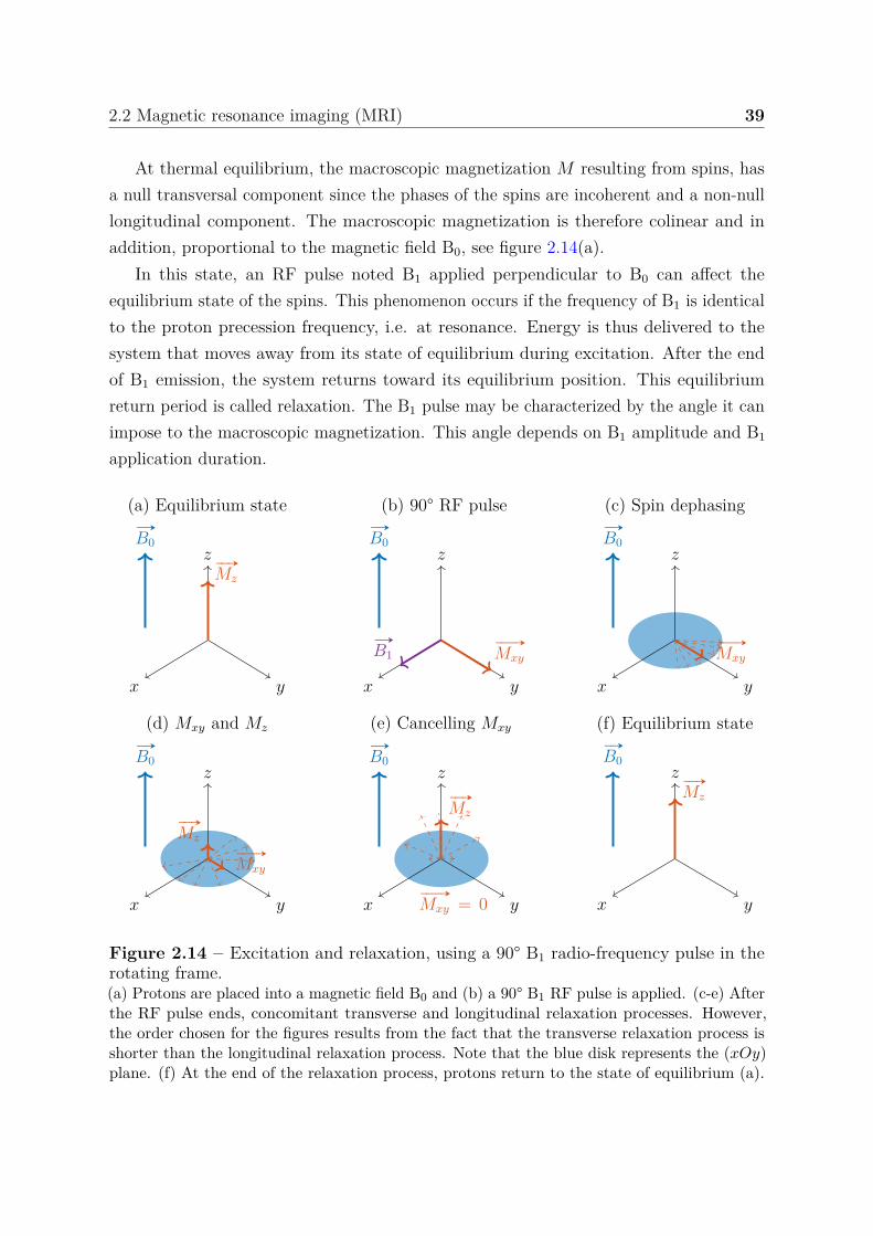
2.2 Magnetic resonance imaging (MRI) 39
At thermal equilibrium, the macroscopic magnetization M resulting from spins, hasa null transversal component since the phases of the spins are incoherent and a non-nulllongitudinal component. The macroscopic magnetization is therefore colinear and inaddition, proportional to the magnetic field B0, see figure 2.14(a).
In this state, an RF pulse noted B1 applied perpendicular to B0 can affect theequilibrium state of the spins. This phenomenon occurs if the frequency of B1 is identicalto the proton precession frequency, i.e. at resonance. Energy is thus delivered to thesystem that moves away from its state of equilibrium during excitation. After the endof B1 emission, the system returns toward its equilibrium position. This equilibriumreturn period is called relaxation. The B1 pulse may be characterized by the angle it canimpose to the macroscopic magnetization. This angle depends on B1 amplitude and B1
application duration.
(a) Equilibrium state
x y
z
# »
B0
# »
Mz
(b) 90° RF pulse
x y
z
# »
B0
# »
Mxy
# »
B1
(c) Spin dephasing
x y
z
# »
B0
# »
Mxy
(d) Mxy and Mz
x y
z
# »
B0
# »
Mz
# »
Mxy
(e) Cancelling Mxy
x y
z
# »
B0
# »
Mz
# »
Mxy = 0
(f) Equilibrium state
x y
z
# »
B0
# »
Mz
Figure 2.14 – Excitation and relaxation, using a 90° B1 radio-frequency pulse in therotating frame.(a) Protons are placed into a magnetic field B0 and (b) a 90° B1 RF pulse is applied. (c-e) Afterthe RF pulse ends, concomitant transverse and longitudinal relaxation processes. However,the order chosen for the figures results from the fact that the transverse relaxation process isshorter than the longitudinal relaxation process. Note that the blue disk represents the (xOy)plane. (f) At the end of the relaxation process, protons return to the state of equilibrium (a).
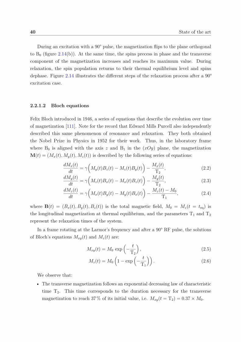
40 State of the art
During an excitation with a 90° pulse, the magnetization flips to the plane orthogonalto B0 (figure 2.14(b)). At the same time, the spins precess in phase and the transversecomponent of the magnetization increases and reaches its maximum value. Duringrelaxation, the spin population returns to their thermal equilibrium level and spinsdephase. Figure 2.14 illustrates the different steps of the relaxation process after a 90°excitation case.
2.2.1.2 Bloch equations
Felix Bloch introduced in 1946, a series of equations that describe the evolution over timeof magnetization [111]. Note for the record that Edward Mills Purcell also independentlydescribed this same phenomenon of resonance and relaxation. They both obtainedthe Nobel Prize in Physics in 1952 for their work. Thus, in the laboratory framewhere B0 is aligned with the axis z and B1 in the (xOy) plane, the magnetizationM(t) = (Mx(t), My(t), Mz(t)) is described by the following series of equations:
dMx(t)dt
= γ(
My(t)Bz(t) − Mz(t)By(t))
− Mx(t)T2
, (2.2)
dMy(t)dt
= γ(
Mz(t)Bx(t) − Mx(t)Bz(t))
− My(t)T2
, (2.3)
dMz(t)dt
= γ(
Mx(t)By(t) − My(t)Bx(t))
− Mz(t) − M0
T1, (2.4)
where B(t) = (Bx(t), By(t), Bz(t)) is the total magnetic field, M0 = Mz(t = teq) isthe longitudinal magnetization at thermal equilibrium, and the parameters T1 and T2
represent the relaxation times of the system.
In a frame rotating at the Larmor’s frequency and after a 90° RF pulse, the solutionsof Bloch’s equations Mxy(t) and Mz(t) are:
Mxy(t) = M0 exp(
− t
T2
), (2.5)
Mz(t) = M0
(1 − exp
(− t
T1
)). (2.6)
We observe that:
• The transverse magnetization follows an exponential decreasing law of characteristictime T2. This time corresponds to the duration necessary for the transversemagnetization to reach 37 % of its initial value, i.e. Mxy(t = T2) = 0.37 × M0.

2.2 Magnetic resonance imaging (MRI) 41
• The longitudinal magnetization follows an exponential law characterized by relax-ation time T1. T1 represents the time necessary for Mz(t) to reach 63 % of itsoriginal value, i.e. Mz(t = T1) = 0.63 × M0.
Note that the T1 and T2 time values depend on the intensity of the magnetic fieldB0, and that transverse relaxation occurs faster than longitudinal relaxation. Therefore,T2 is less than T1 (can be equal e.g. in pure water).
2.2.1.3 Basic types of MR signals
The recorded MR signal S(t) corresponds to an electromotive force produced by theprecession of the magnetization M(t) during resonance. This is a manifestation ofFaraday’s law of induction, wherein a changing magnetic field induces a voltage in anearby conductor. In fact, only the transverse magnetization Mxy(t) generates the currentin the receiver coil.
After a 90° RF excitation, the resulting signal is called the free induction decay (FID),a damped sine wave, see figure 2.15(a). In practice, we observe that the decay is fasterthan expected by theory due to the inhomogeneities of the magnetic field. Therefore, theexponential decays with time constant T∗
2 that reflects the combined effects of the T2
relaxation and of phase dispersion due to magnetic field inhomogeneities (T∗2 ≤ T2). A
clever manipulation of the FID signal begins by applying an external dephasing gradientfield across the tissue. This gradient causes a calibrated change in local magnetic fieldsand hence alters the resonance frequencies slightly across the tissue. This results inaccelerated dephasing of the FID. Then, the process is reversed by applying a rephasinggradient with the same magnitude but with the opposite polarity to the dephasinggradient. The resulting signal is called the gradient echo signal (GE), see figure 2.15(b).This process affects neither T2 nor T∗
2. One can recover the level of the T2 relaxation.For this, one adds a second excitation: a rephasing 180° pulse, after the 90°. This processcan refocus dephased components of the original FID into a spin echo (SE) at twice thedelay that separates RF pulses (figure 2.15(c)). We do not go into details on the spinecho, additional information can be found in [112].
These basic sequences are at the origin of the two major MRI contrasts, depending onthe type of echo recorded: the SE sequences, characterized by the presence of a 180° RFrephasing pulse and the GE sequences, more sensitive to magnetic field inhomogeneities.Any other sequence is a sophisticated combination of RF pulses and gradients. Theobjectives for any sequence are to enhance the signal of a particular tissue (contrast), as
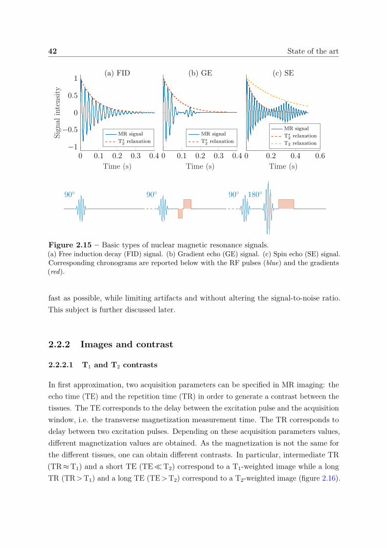
42 State of the art
0 0.1 0.2 0.3 0.4−1
−0.5
0
0.5
1
Time (s)
Sign
alin
tens
ity
(a) FID
MR signalT∗
2 relaxation
0 0.1 0.2 0.3 0.4
Time (s)
(b) GE
MR signalT∗
2 relaxation
0 0.2 0.4 0.6
Time (s)
(c) SE
MR signalT∗
2 relaxationT2 relaxation
90 90 90 180
Figure 2.15 – Basic types of nuclear magnetic resonance signals.(a) Free induction decay (FID) signal. (b) Gradient echo (GE) signal. (c) Spin echo (SE) signal.Corresponding chronograms are reported below with the RF pulses (blue) and the gradients(red).
fast as possible, while limiting artifacts and without altering the signal-to-noise ratio.This subject is further discussed later.
2.2.2 Images and contrast
2.2.2.1 T1 and T2 contrasts
In first approximation, two acquisition parameters can be specified in MR imaging: theecho time (TE) and the repetition time (TR) in order to generate a contrast between thetissues. The TE corresponds to the delay between the excitation pulse and the acquisitionwindow, i.e. the transverse magnetization measurement time. The TR corresponds todelay between two excitation pulses. Depending on these acquisition parameters values,different magnetization values are obtained. As the magnetization is not the same forthe different tissues, one can obtain different contrasts. In particular, intermediate TR(TR ≈ T1) and a short TE (TE ≪ T2) correspond to a T1-weighted image while a longTR (TR > T1) and a long TE (TE > T2) correspond to a T2-weighted image (figure 2.16).

2.2 Magnetic resonance imaging (MRI) 43
0 200 400 600 800 1 0000
0.5
1Mz(t) Mxy(t)
TR
Time (ms)
Sign
alin
tens
ity
(a) T1-weightedIntermediate TR and short TE
480 500 5200.2
0.4
0.6TE
0 2 000 4 000 6 0000
0.5
1Mz(t) Mxy(t)
Time (ms)
(b) T2-weightedLong TR and long TE
WMGM
3 000 3 100
0.2
0.4
0.6
0.8
1 TE
Figure 2.16 – Magnetization evolutions, using spin-echo sequence.White matter (WM) and grey matter (GM) transversal Mxy and longitudinal Mz magneti-zations for (a) T1-weighted image, and (b) T2-weighted image acquired at echo time (TE).T1/T2 = 600/80 ms for WM and 950/100 ms for GM. The smaller axes correspond to a zoomin on the delay TE between excitation (solid line) and acquisition time (dashed line).
At this point, we only obtain contrasts between tissues. These contrasts are relatedto the acquisition parameters and the quantification of T1 and T2 values (which areindependent of the acquisition parameters) is not available at this point. We see insection 2.3.1 how to use the theory introduced in this section to quantify T1 and T2.
2.2.2.2 Spatial encoding
We have seen how to generate a signal/contrast using an RF excitation applied on protonsin a volume but the spatial coding has so far been omitted. A typical magnetic resonance(MR) scan may contain million of voxels (generalization of the pixel in 3 dimensions),each generating its own MR signal. The location of all MR signals is encoded following acombination of different methods:
• Frequency encoding: magnetic field gradients are applied to locally modify the mainmagnetic field, causing the resonance frequency to vary as a function of position.
• Phase encoding: a gradient is applied to provide a gain or loss in phase that persistseven after the gradient has been turned off.
We only describe 2D-multislice imaging, which consists in acquiring multiple Nx × Ny
resolution images of Nz slices of tissue. This acquisition results in Nx × Ny × Nz voxels.The size of these voxels depends on the size of the volume imaged and the matrix, i.e.the size of the organ imaged and the number of voxels. Typical fields of view (FOV) are
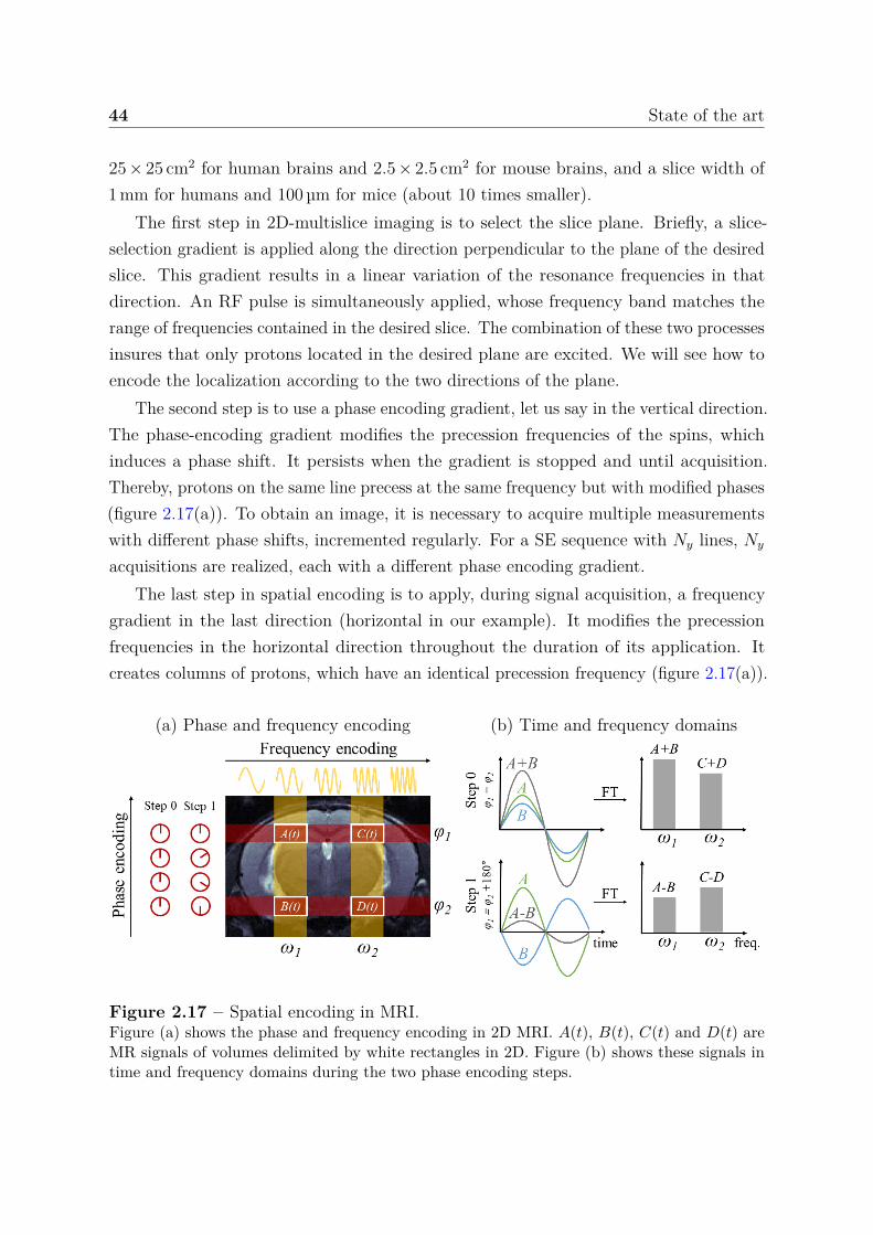
44 State of the art
25 × 25 cm2 for human brains and 2.5 × 2.5 cm2 for mouse brains, and a slice width of1 mm for humans and 100 µm for mice (about 10 times smaller).
The first step in 2D-multislice imaging is to select the slice plane. Briefly, a slice-selection gradient is applied along the direction perpendicular to the plane of the desiredslice. This gradient results in a linear variation of the resonance frequencies in thatdirection. An RF pulse is simultaneously applied, whose frequency band matches therange of frequencies contained in the desired slice. The combination of these two processesinsures that only protons located in the desired plane are excited. We will see how toencode the localization according to the two directions of the plane.
The second step is to use a phase encoding gradient, let us say in the vertical direction.The phase-encoding gradient modifies the precession frequencies of the spins, whichinduces a phase shift. It persists when the gradient is stopped and until acquisition.Thereby, protons on the same line precess at the same frequency but with modified phases(figure 2.17(a)). To obtain an image, it is necessary to acquire multiple measurementswith different phase shifts, incremented regularly. For a SE sequence with Ny lines, Ny
acquisitions are realized, each with a different phase encoding gradient.The last step in spatial encoding is to apply, during signal acquisition, a frequency
gradient in the last direction (horizontal in our example). It modifies the precessionfrequencies in the horizontal direction throughout the duration of its application. Itcreates columns of protons, which have an identical precession frequency (figure 2.17(a)).
(a) Phase and frequency encoding (b) Time and frequency domains
Figure 2.17 – Spatial encoding in MRI.Figure (a) shows the phase and frequency encoding in 2D MRI. A(t), B(t), C(t) and D(t) areMR signals of volumes delimited by white rectangles in 2D. Figure (b) shows these signals intime and frequency domains during the two phase encoding steps.
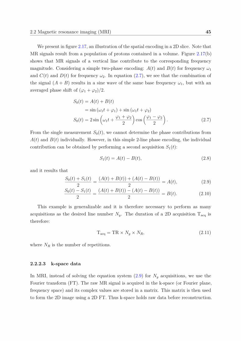
2.2 Magnetic resonance imaging (MRI) 45
We present in figure 2.17, an illustration of the spatial encoding in a 2D slice. Note thatMR signals result from a population of protons contained in a volume. Figure 2.17(b)shows that MR signals of a vertical line contribute to the corresponding frequencymagnitude. Considering a simple two-phase encoding: A(t) and B(t) for frequency ω1
and C(t) and D(t) for frequency ω2. In equation (2.7), we see that the combination ofthe signal (A + B) results in a sine wave of the same base frequency ω1, but with anaveraged phase shift of (φ1 + φ2)/2.
S0(t) = A(t) + B(t)= sin (ω1t + φ1) + sin (ω1t + φ2)
S0(t) = 2 sin(
ω1t + φ1 + φ2
2
)cos
(φ1 − φ2
2
). (2.7)
From the single measurement S0(t), we cannot determine the phase contributions fromA(t) and B(t) individually. However, in this simple 2-line phase encoding, the individualcontribution can be obtained by performing a second acquisition S1(t):
S1(t) = A(t) − B(t), (2.8)
and it results thatS0(t) + S1(t)
2 = (A(t) + B(t)) + (A(t) − B(t))2 = A(t), (2.9)
S0(t) − S1(t)2 = (A(t) + B(t)) − (A(t) − B(t))
2 = B(t). (2.10)
This example is generalizable and it is therefore necessary to perform as manyacquisitions as the desired line number Ny. The duration of a 2D acquisition Tacq istherefore:
Tacq = TR × Ny × NR, (2.11)
where NR is the number of repetitions.
2.2.2.3 k-space data
In MRI, instead of solving the equation system (2.9) for Ny acquisitions, we use theFourier transform (FT). The raw MR signal is acquired in the k-space (or Fourier plane,frequency space) and its complex values are stored in a matrix. This matrix is then usedto form the 2D image using a 2D FT. Thus k-space holds raw data before reconstruction.

46 State of the art
The filling of the entire k-space cannot be achieved at once but it can be achieved in anyorders: popular methods include Cartesian (row-by-row), radial and spiral trajectories,see figure 2.18(a, d, e). The Cartesian method was used nearly exclusively at the beginningof MRI, but today all patterns are encountered. The major benefit of radial samplingis a lower sensitivity to motion artifacts [113]. In radial acquisitions, the center ofk-space is oversampled and continuously updated due to the overlapping spokes thatrepeatedly pass through this region. This redundancy can be exploited to detect andcorrect for movement if the signal from the k-space center changes between views. Inreturn, the principal advantage of Cartesian sampling is that data elements are regularlyspaced and can be placed directly into standard array processors designed for efficient FTcomputations. Radial methods generate data points that do not fall into a rectangularmatrix. To efficiently process such non-uniformly acquired data, these points must bemorphed into a Cartesian format.
Figure 2.18 – Examples of different k-space trajectories and their associated aliasingartifacts, adapted from [114].Acquired k-space data are indicated by solid lines, while missing data are depicted with dashedlines. (a) Fully-sampled Cartesian data produces a full FOV image. (b) Uniformly undersampledCartesian k-space with an acceleration factor of R = 3 leads to coherent aliasing artifacts. (c)With variable density sampling, a higher concentration of lines is acquired near the k-spacecenter, and the imaging artifacts are more diffuse. (d) Radial data can be undersampled byskipping radial spokes at regular intervals, which leads to diffuse streaking artifacts. (e) Spiralk-space can be undersampled by skipping spiral arms, which produces incoherent swirlingartifacts.
To shorten scan time, some works have proposed to sample a smaller number of phaseencoding lines in k-space; however, without further processing, the resulting images willbe degraded by aliasing artifacts, see figure 2.18(b-e). It is also demonstrated that scan
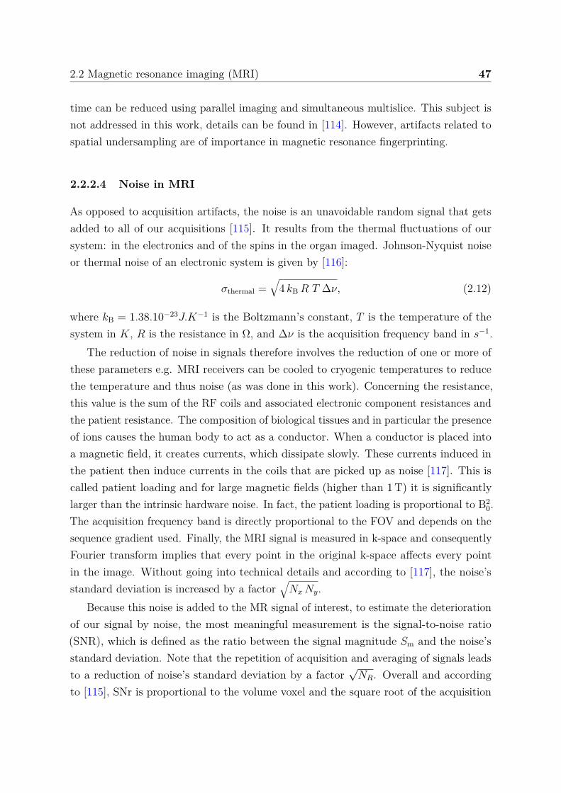
2.2 Magnetic resonance imaging (MRI) 47
time can be reduced using parallel imaging and simultaneous multislice. This subject isnot addressed in this work, details can be found in [114]. However, artifacts related tospatial undersampling are of importance in magnetic resonance fingerprinting.
2.2.2.4 Noise in MRI
As opposed to acquisition artifacts, the noise is an unavoidable random signal that getsadded to all of our acquisitions [115]. It results from the thermal fluctuations of oursystem: in the electronics and of the spins in the organ imaged. Johnson-Nyquist noiseor thermal noise of an electronic system is given by [116]:
σthermal =√
4 kB R T ∆ν, (2.12)
where kB = 1.38.10−23J.K−1 is the Boltzmann’s constant, T is the temperature of thesystem in K, R is the resistance in Ω, and ∆ν is the acquisition frequency band in s−1.
The reduction of noise in signals therefore involves the reduction of one or more ofthese parameters e.g. MRI receivers can be cooled to cryogenic temperatures to reducethe temperature and thus noise (as was done in this work). Concerning the resistance,this value is the sum of the RF coils and associated electronic component resistances andthe patient resistance. The composition of biological tissues and in particular the presenceof ions causes the human body to act as a conductor. When a conductor is placed intoa magnetic field, it creates currents, which dissipate slowly. These currents induced inthe patient then induce currents in the coils that are picked up as noise [117]. This iscalled patient loading and for large magnetic fields (higher than 1 T) it is significantlylarger than the intrinsic hardware noise. In fact, the patient loading is proportional to B2
0.The acquisition frequency band is directly proportional to the FOV and depends on thesequence gradient used. Finally, the MRI signal is measured in k-space and consequentlyFourier transform implies that every point in the original k-space affects every pointin the image. Without going into technical details and according to [117], the noise’sstandard deviation is increased by a factor
√Nx Ny.
Because this noise is added to the MR signal of interest, to estimate the deteriorationof our signal by noise, the most meaningful measurement is the signal-to-noise ratio(SNR), which is defined as the ratio between the signal magnitude Sm and the noise’sstandard deviation. Note that the repetition of acquisition and averaging of signals leadsto a reduction of noise’s standard deviation by a factor
√NR. Overall and according
to [115], SNr is proportional to the volume voxel and the square root of the acquisition
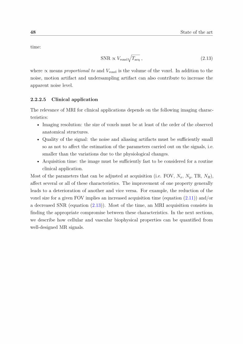
48 State of the art
time:
SNR ∝ Vvoxel√
Tacq , (2.13)
where ∝ means proportional to and Vvoxel is the volume of the voxel. In addition to thenoise, motion artifact and undersampling artifact can also contribute to increase theapparent noise level.
2.2.2.5 Clinical application
The relevance of MRI for clinical applications depends on the following imaging charac-teristics:
• Imaging resolution: the size of voxels must be at least of the order of the observedanatomical structures.
• Quality of the signal: the noise and aliasing artifacts must be sufficiently smallso as not to affect the estimation of the parameters carried out on the signals, i.e.smaller than the variations due to the physiological changes.
• Acquisition time: the image must be sufficiently fast to be considered for a routineclinical application.
Most of the parameters that can be adjusted at acquisition (i.e. FOV, Nx, Ny, TR, NR),affect several or all of these characteristics. The improvement of one property generallyleads to a deterioration of another and vice versa. For example, the reduction of thevoxel size for a given FOV implies an increased acquisition time (equation (2.11)) and/ora decreased SNR (equation (2.13)). Most of the time, an MRI acquisition consists infinding the appropriate compromise between these characteristics. In the next sections,we describe how cellular and vascular biophysical properties can be quantified fromwell-designed MR signals.
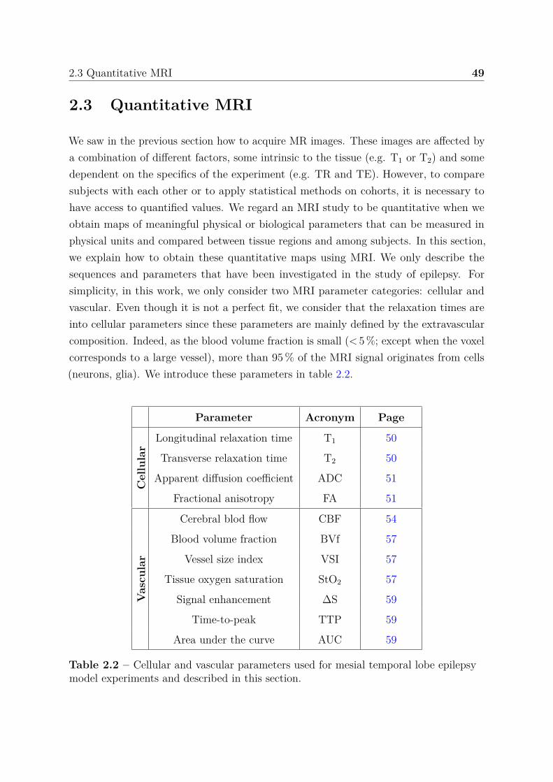
2.3 Quantitative MRI 49
2.3 Quantitative MRI
We saw in the previous section how to acquire MR images. These images are affected bya combination of different factors, some intrinsic to the tissue (e.g. T1 or T2) and somedependent on the specifics of the experiment (e.g. TR and TE). However, to comparesubjects with each other or to apply statistical methods on cohorts, it is necessary tohave access to quantified values. We regard an MRI study to be quantitative when weobtain maps of meaningful physical or biological parameters that can be measured inphysical units and compared between tissue regions and among subjects. In this section,we explain how to obtain these quantitative maps using MRI. We only describe thesequences and parameters that have been investigated in the study of epilepsy. Forsimplicity, in this work, we only consider two MRI parameter categories: cellular andvascular. Even though it is not a perfect fit, we consider that the relaxation times areinto cellular parameters since these parameters are mainly defined by the extravascularcomposition. Indeed, as the blood volume fraction is small (< 5 %; except when the voxelcorresponds to a large vessel), more than 95 % of the MRI signal originates from cells(neurons, glia). We introduce these parameters in table 2.2.
Parameter Acronym Page
Cel
lula
r
Longitudinal relaxation time T1 50
Transverse relaxation time T2 50
Apparent diffusion coefficient ADC 51
Fractional anisotropy FA 51
Vas
cula
r
Cerebral blod flow CBF 54
Blood volume fraction BVf 57
Vessel size index VSI 57
Tissue oxygen saturation StO2 57
Signal enhancement ∆S 59
Time-to-peak TTP 59
Area under the curve AUC 59
Table 2.2 – Cellular and vascular parameters used for mesial temporal lobe epilepsymodel experiments and described in this section.
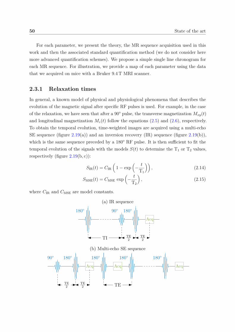
50 State of the art
For each parameter, we present the theory, the MR sequence acquisition used in thiswork and then the associated standard quantification method (we do not consider heremore advanced quantification schemes). We propose a simple single line chronogram foreach MR sequence. For illustration, we provide a map of each parameter using the datathat we acquired on mice with a Bruker 9.4 T MRI scanner.
2.3.1 Relaxation times
In general, a known model of physical and physiological phenomena that describes theevolution of the magnetic signal after specific RF pulses is used. For example, in the caseof the relaxation, we have seen that after a 90° pulse, the transverse magnetization Mxy(t)and longitudinal magnetization Mz(t) follow the equations (2.5) and (2.6), respectively.To obtain the temporal evolution, time-weighted images are acquired using a multi-echoSE sequence (figure 2.19(a)) and an inversion recovery (IR) sequence (figure 2.19(b)),which is the same sequence preceded by a 180° RF pulse. It is then sufficient to fit thetemporal evolution of the signals with the models S(t) to determine the T1 or T2 values,respectively (figure 2.19(b, c)):
SIR(t) = CIR
(1 − exp
(− t
T1
)), (2.14)
SMSE(t) = CMSE exp(
− t
T2
), (2.15)
where CIR and CMSE are model constants.
(a) IR sequence
180 90 180
Acq
TI TE2
TE2
(b) Multi-echo SE sequence
90 180
Acq
180
Acq
180 180
Acq
TE2
TE2 TE
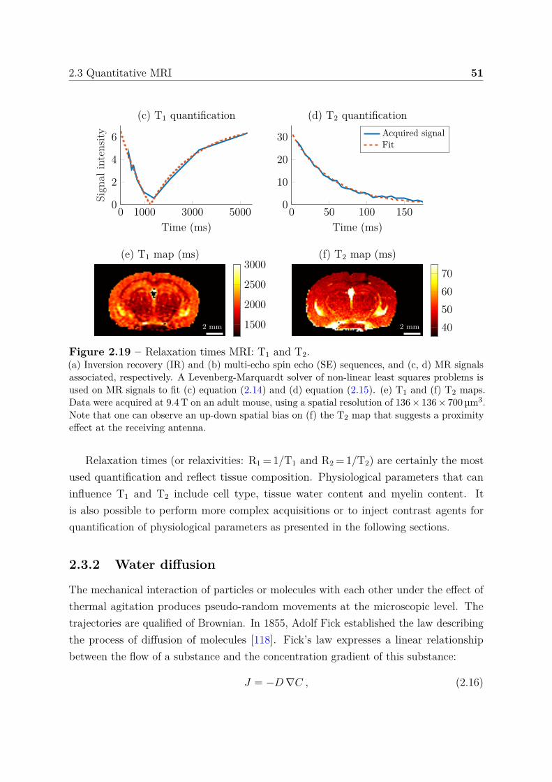
2.3 Quantitative MRI 51
0 1000 3000 50000
2
4
6
Time (ms)
Sign
alin
tens
ity(c) T1 quantification
0 50 100 1500
10
20
30
Time (ms)
(d) T2 quantificationAcquired signalFit
2 mm
(e) T1 map (ms)
1500
2000
2500
3000
2 mm
(f) T2 map (ms)
40506070
Figure 2.19 – Relaxation times MRI: T1 and T2.(a) Inversion recovery (IR) and (b) multi-echo spin echo (SE) sequences, and (c, d) MR signalsassociated, respectively. A Levenberg-Marquardt solver of non-linear least squares problems isused on MR signals to fit (c) equation (2.14) and (d) equation (2.15). (e) T1 and (f) T2 maps.Data were acquired at 9.4 T on an adult mouse, using a spatial resolution of 136 × 136 × 700 µm3.Note that one can observe an up-down spatial bias on (f) the T2 map that suggests a proximityeffect at the receiving antenna.
Relaxation times (or relaxivities: R1 = 1/T1 and R2 = 1/T2) are certainly the mostused quantification and reflect tissue composition. Physiological parameters that caninfluence T1 and T2 include cell type, tissue water content and myelin content. Itis also possible to perform more complex acquisitions or to inject contrast agents forquantification of physiological parameters as presented in the following sections.
2.3.2 Water diffusion
The mechanical interaction of particles or molecules with each other under the effect ofthermal agitation produces pseudo-random movements at the microscopic level. Thetrajectories are qualified of Brownian. In 1855, Adolf Fick established the law describingthe process of diffusion of molecules [118]. Fick’s law expresses a linear relationshipbetween the flow of a substance and the concentration gradient of this substance:
J = −D ∇C , (2.16)

52 State of the art
with J the flux of substance in mol.m−2.s−1, D the diffusion coefficient in m2.s−1 and ∇C
the gradient of the local concentration in mol.m−4. J measures the amount of substancethat will flow through a unit area during a unit time interval. The diffusion of themolecules therefore occurs in the opposite direction of the concentration gradient, i.e. thediffusion tends to homogenize the concentrations of the molecules in the environment.
The conservation law, also called Fick’s second law (in this case the equation (2.16)is called Fick’s first law), describes the variation of concentration over time as a functionof the second space derivative:
∂C
∂t= D ∇2C , (2.17)
with ∇2C the Laplacian of the local concentration in mol.m−5. To obtain an MRI signalthat is sensitive to the diffusion of water occurring in one direction of space, the pulsedgradient spin-echo (PGSE) sequence, an MRI sequence of the classical SE type but withdiffusion gradients, was proposed in [119] and is still widely used today. Two magneticfield gradients of equal intensity G and equal duration δ are applied on both sides of the180° refocusing RF pulse (figure 2.20(a)). If there is a diffusion process in the directionof these gradients during the period ∆ that separates the two gradients, then the secondphase shift does not fully compensate for the first and the attenuation of the signal maybe related to the diffusion D. Torrey modified the Bloch equations (2.2) to take intoaccount the diffusion process and solved these new Bloch-Torrey equations [120]:
SPGSE(b) = S0 exp (−bD) , (2.18)
with b = (γGδ)2(
∆ − δ
3
), (2.19)
where S0 is the signal in the absence of diffusion gradients, G the gradient intensity inT.m−1, δ the gradient duration and ∆ the time between gradients in second. The b-valuewas introduced in [121] and represents the diffusion weighting. The equation (2.18)assumes that the compartment is isotropic and therefore requires the same diffusioncoefficient in all directions.
The first and one of the most commonly used diffusion model is the diffusion tensorimaging (DTI). The model substitutes the diffusion coefficient D by a symmetricalpositive-definite tensor D of order two. Thus to determine the tensor only 6 acquisitionsare necessary. The previous equation (2.18) becomes:
S(g, b) = S0 exp(−bgT Dg
), (2.20)
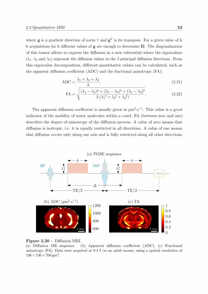
2.3 Quantitative MRI 53
where g is a gradient direction of norm 1 and gT is its transpose. For a given value of b,6 acquisitions for 6 different values of g are enough to determine D. The diagonalizationof this tensor allows to express the diffusion in a new referential where the eigenvalues(λ1, λ2 and λ3) represent the diffusion values in the 3 principal diffusion directions. Fromthis eigenvalue decomposition, different quantitative values can be calculated, such asthe apparent diffusion coefficient (ADC) and the fractional anisotropy (FA):
ADC = λ1 + λ2 + λ3
3 , (2.21)
FA =
√√√√(λ1 − λ2)2 + (λ2 − λ3)2 + (λ1 − λ3)2
2 (λ 21 + λ 2
2 + λ 23 ) . (2.22)
The apparent diffusion coefficient is usually given in µm2.s−1. This value is a goodindicator of the mobility of water molecules within a voxel. FA (between zero and one)describes the degree of anisotropy of the diffusion process. A value of zero means thatdiffusion is isotropic, i.e. it is equally restricted in all directions. A value of one meansthat diffusion occurs only along one axis and is fully restricted along all other directions.
(a) PGSE sequence
90 180
Acq
TE/2 TE/2
δ
G
δ
G
∆
2 mm
(b) ADC (µm2.s−1)
600
800
1000
1200
2 mm
(c) FA
00.20.40.60.81
Figure 2.20 – Diffusion MRI.(a) Diffusion MR sequence. (b) Apparent diffusion coefficient (ADC). (c) Fractionalanisotropy (FA). Data were acquired at 9.4 T on an adult mouse, using a spatial resolution of136 × 136 × 700 µm3.
54 State of the art
Complex diffusion images that reflect various diffusion properties of a tissue can beproduced using the eigenvalues and eigenvectors. However, most of the time, we onlyuse the regular diffusion-weighted imaging to produce ADC images (figure 2.20(b)) butFA images can also be computed (figure 2.20(c)). A more complex modeling of waterdiffusion process exist but is beyond the scope of this thesis.
2.3.3 Perfusion using arterial spin labeling
Perfusion is the tissue irrigation by blood, at capillary levels. To measure the perfusion,it is necessary to use tracers of blood circulation. These tracers can be of two natures:endogenous or exogenous. In this part, we present the tracking of endogenous tracers inthe blood, i.e. hydrogen protons. This method, known as arterial spin labeling (ASL), isparticularly valuable for its non-invasive aspect compared to the contrast agent injectionperfusion methods described in the following sections.
In an ASL sequence, an RF pulse and a magnetic field gradient are used upstream ofthe imaged volume. The idea is to « mark » the spins contained in the blood, which thenmodify the magnetic signal when perfusing the imaged brain volume. The subtraction ofthe images in the absence (called control images) and in the presence (called label images)of labeled spin allows to remove the signal originating from the static tissues and toreveal the changes caused by blood circulation. These changes depend on blood volumeand flow rate, which are the parameters known as cerebral blood volume or blood volumefraction (BVf) and cerebral blood flow (CBF). In practice, ASL imaging produces a verylow signal close to the noise level and only the repetition of the acquisitions provides, byaveraging label-control image pairs, a correct signal-to-noise level.
Numerous ASL sequences have been proposed in recent years [122]. Among thesesequences, two main types of methods appear: pulsed ASL (PASL) and continuous ASL(CASL). PASL sequences use very short RF pulses over large labeling areas, while CASLsequences, initially proposed by [123], jointly implement continuous labeling using longRF pulses located at the carotids (a few seconds) and a gradient in the direction offlow. CASL sequences allow a higher perfusion contrast but have two major drawbacks:magnetization transfer effects and high energy deposition in the tissues. The pseudo-continuous ASL (pCASL) method, presented below, combines the advantages of bothCASL and PASL sequences.
Indeed, the works [124, 125] introduce the pCASL method using very short (≈ 400 µm)repeated RF pulses as pseudo-continuous labeling. During the labeling period, positivegradients are applied during the pulses and negative gradients between pulses such that
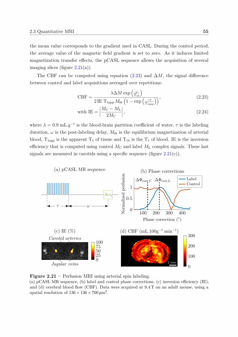
2.3 Quantitative MRI 55
the mean value corresponds to the gradient used in CASL. During the control period,the average value of the magnetic field gradient is set to zero. As it induces limitedmagnetization transfer effects, the pCASL sequence allows the acquisition of severalimaging slices (figure 2.21(a)).
The CBF can be computed using equation (2.23) and ∆M , the signal differencebetween control and label acquisitions averaged over repetitions:
CBF =λ∆M exp
(ω
T1b
)2 IE T1app M0t
(1 − exp
(−τ
T1app
)) , (2.23)
with IE =∣∣∣∣MC − ML
2MC
∣∣∣∣ , (2.24)
where λ = 0.9 mL.g−1 is the blood-brain partition coefficient of water, τ is the labelingduration, ω is the post-labeling delay, M0t is the equilibrium magnetization of arterialblood, T1app is the apparent T1 of tissue and T1b is the T1 of blood. IE is the inversionefficiency that is computed using control MC and label ML complex signals. These lastsignals are measured in carotids using a specific sequence (figure 2.21(c)).
Acq
τ ω
(a) pCASL MR sequence
100 200 300 4000
0.5
1∆Φcorr,C ∆Φcorr,L
Phase correction ()
Nor
mal
ized
perf
usio
n
(b) Phase correctionsLabelControl
(c) IE (%)
0255075100
Carotid arteries
Jugular veins 2 mm
(d) CBF (mL.100g−1.min−1)
0
100
200
300
Figure 2.21 – Perfusion MRI using arterial spin labeling.(a) pCASL MR sequence, (b) label and control phase corrections, (c) inversion efficiency (IE),and (d) cerebral blood flow (CBF). Data were acquired at 9.4 T on an adult mouse, using aspatial resolution of 136 × 136 × 700 µm3.
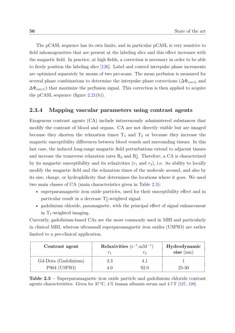
56 State of the art
The pCASL sequence has its own limits, and in particular pCASL is very sensitive tofield inhomogeneities that are present at the labeling slice and this effect increases withthe magnetic field. In practice, at high fields, a correction is necessary in order to be ableto freely position the labeling slice [126]. Label and control interpulse phase incrementsare optimized separately by means of two pre-scans. The mean perfusion is measured forseveral phase combinations to determine the interpulse phase corrections (∆Φcorr,L and∆Φcorr,C) that maximize the perfusion signal. This correction is then applied to acquirethe pCASL sequence (figure 2.21(b)).
2.3.4 Mapping vascular parameters using contrast agents
Exogenous contrast agents (CA) include intravenously administered substances thatmodify the contrast of blood and organs. CA are not directly visible but are imagedbecause they shorten the relaxation times T1 and T2 or because they increase themagnetic susceptibility differences between blood vessels and surrounding tissues. In thislast case, the induced long-range magnetic field perturbations extend to adjacent tissuesand increase the transverse relaxation rates R2 and R∗
2. Therefore, a CA is characterizedby its magnetic susceptibility and its relaxivities (r1 and r2), i.e. its ability to locallymodify the magnetic field and the relaxation times of the molecule around, and also byits size, charge, or hydrophilicity that determines the locations where it goes. We usedtwo main classes of CA (main characteristics given in Table 2.3):
• superparamagnetic iron oxide particles, used for their susceptibility effect and inparticular result in a decrease T∗
2-weighted signal.• gadolinium chloride, paramagnetic, with the principal effect of signal enhancement
in T1-weighted imaging.Currently, gadolinium-based CAs are the most commonly used in MRI and particularlyin clinical MRI, whereas ultrasmall superparamagnetic iron oxides (USPIO) are ratherlimited to a pre-clinical application.
Contrast agent Relaxivities (s−1.mM−1) Hydrodynamicr1 r2 size (nm)
Gd-Dota (Gadolinium) 3.3 4.1 1P904 (USPIO) 4.0 92.0 25-30
Table 2.3 – Superparamagnetic iron oxide particle and gadolinium chloride contrastagents characteristics. Given for 37 °C, 4 % human albumin serum and 4.7 T [127, 128].
2.3 Quantitative MRI 57
2.3.4.1 Ultrasmall superparamagnetic iron oxide
The first contrast agent presented induces magnetic susceptibility and relaxivity effects.When such a CA is compartmentalized within a voxel, these effects result in a decrease ofthe MR signal in an inhomogeneous magnetic field. This is what happens at vessel-tissueinterfaces, since CA is distributed only in the vascular compartment. This paramagneticsubstance acquires, in the magnetic field, a magnetization different from that of thesurrounding environment: on each vessel surface, and over few microns, a magnetic fieldgradient appears [129]. This increase in the heterogeneity in the magnetic field of thevoxel yield a decrease in signal intensity due to an increased spin-spin dephasing (T2
relaxation). In a first approximation and when the blood volume fraction is small, thedecrease of the signal observed in a voxel depends on the concentration of the tracerin vessels (i.e. the blood volume fraction), and on the fraction of blood in the volume.Going a little further, we can also show that this signal decrease depends on the numberof vessels and their diameter [130]. Figures 2.22(b, c) show an example of T∗
2-weightedimages before and after the injection of USPIO. On these images, it is easy to distinguish(in black because of signal decrease) the important vascular structures.
Using a multiple gradient echo sampling of the free induction decay and spin echo(MGEFIDSE) sequence (cf. below), it is possible to directly evaluate two parameters: theblood volume fraction (BVf) and the vessel size index (VSI), which are the proportion ofblood in the volume imaged in % and a weighted mean vessel radius [131], respectively.VSI is computed as:
VSI =∑R
i=1 r43i∑R
i=1 r2i
− 32
, (2.25)
where ri is the radius of the ith vessel, and R the total number of vessels in the voxel.
MGEFIDSE sequence is composed of a first 90° RF pulse and then a 180° RF pulse.Gradient echos collected after the first pulse capture information about the relaxationrate R∗
2 (inverse of T∗2) while the information acquired around twice the time between the
two pulses capture information about the relaxation rate R2 (inverse of T2). The theoryfor determining BVf and VSI is presented in [132]. The changes in relaxation rates ∆R∗
2
and ∆R2 induced by the injection of USPIO are computed using gradient echo (GE) andspin echo (SE) signal intensities, respectively. The pre- and post-injection relaxationtimes T∗
2,pre and T∗2,post are obtained by fitting the GE signal intensities to an exponential
function, see section 2.3.1. It allows to compute ∆R∗2, while ∆R2 is directly calculated
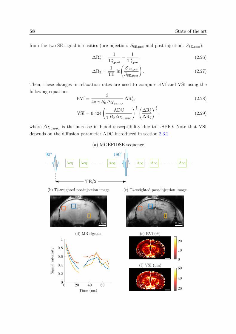
58 State of the art
from the two SE signal intensities (pre-injection: SSE,pre; and post-injection: SSE,post):
∆R∗2 = 1
T∗2,post
− 1T∗
2,pre, (2.26)
∆R2 = 1TE ln
(SSE,pre
SSE,post
). (2.27)
Then, these changes in relaxation rates are used to compute BVf and VSI using thefollowing equations:
BVf = 34π γ B0 ∆χUSPIO
∆R∗2, (2.28)
VSI = 0.424(
ADCγ B0 ∆χUSPIO
) 12(
∆R∗2
∆R2
) 32
, (2.29)
where ∆χUSPIO is the increase in blood susceptibility due to USPIO. Note that VSIdepends on the diffusion parameter ADC introduced in section 2.3.2.
(a) MGEFIDSE sequence
90
Acq Acq Acq
180
Acq Acq Acq
TE/2
2 mm
(b) T∗2-weighted pre-injection image
2 mm
(c) T∗2-weighted post-injection image
0 20 40 600
0.2
0.4
0.6
0.8
1
Time (ms)
Sign
alin
tens
ity
(d) MR signals (e) BVf (%)
0
10
20
(f) VSI (µm)
20
40
60
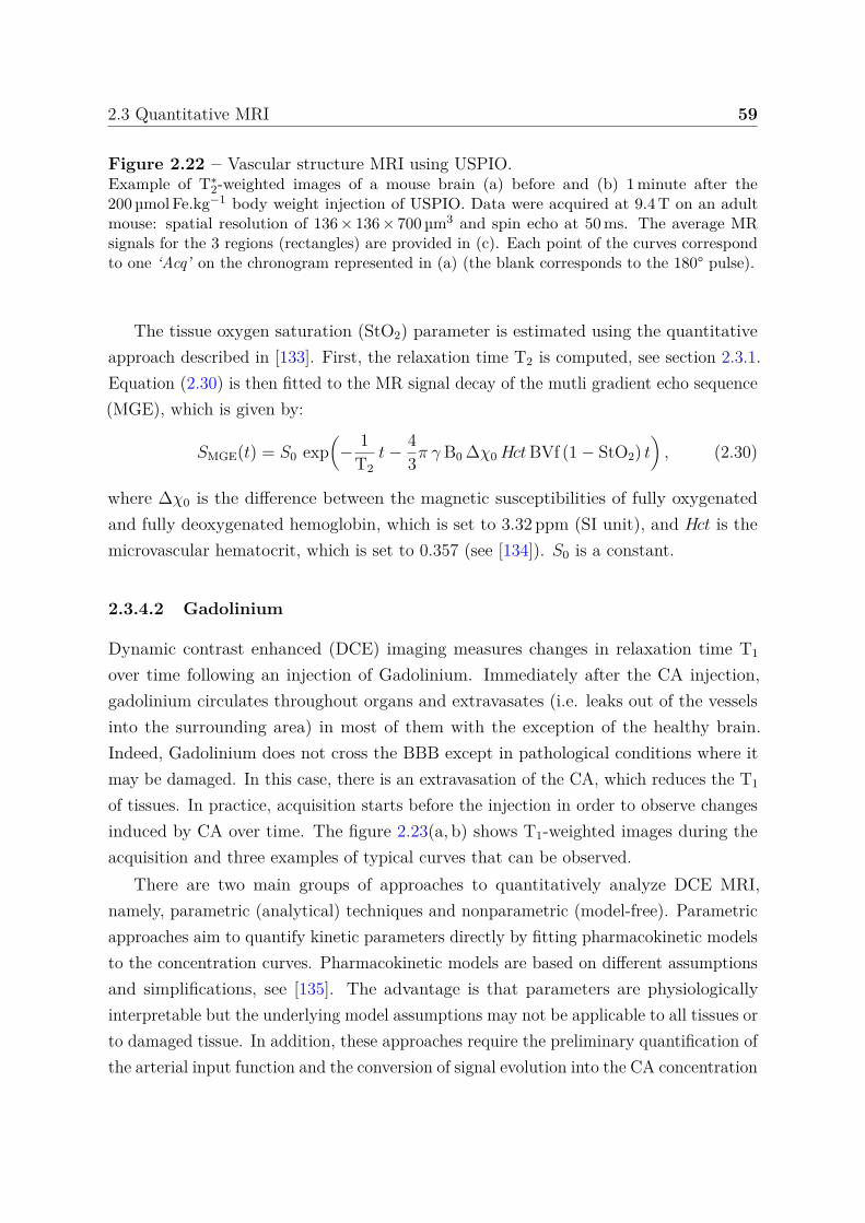
2.3 Quantitative MRI 59
Figure 2.22 – Vascular structure MRI using USPIO.Example of T∗
2-weighted images of a mouse brain (a) before and (b) 1 minute after the200 µmol Fe.kg−1 body weight injection of USPIO. Data were acquired at 9.4 T on an adultmouse: spatial resolution of 136 × 136 × 700 µm3 and spin echo at 50 ms. The average MRsignals for the 3 regions (rectangles) are provided in (c). Each point of the curves correspondto one ‘Acq’ on the chronogram represented in (a) (the blank corresponds to the 180° pulse).
The tissue oxygen saturation (StO2) parameter is estimated using the quantitativeapproach described in [133]. First, the relaxation time T2 is computed, see section 2.3.1.Equation (2.30) is then fitted to the MR signal decay of the mutli gradient echo sequence(MGE), which is given by:
SMGE(t) = S0 exp(
− 1T2
t − 43π γ B0 ∆χ0 Hct BVf (1 − StO2) t
), (2.30)
where ∆χ0 is the difference between the magnetic susceptibilities of fully oxygenatedand fully deoxygenated hemoglobin, which is set to 3.32 ppm (SI unit), and Hct is themicrovascular hematocrit, which is set to 0.357 (see [134]). S0 is a constant.
2.3.4.2 Gadolinium
Dynamic contrast enhanced (DCE) imaging measures changes in relaxation time T1
over time following an injection of Gadolinium. Immediately after the CA injection,gadolinium circulates throughout organs and extravasates (i.e. leaks out of the vesselsinto the surrounding area) in most of them with the exception of the healthy brain.Indeed, Gadolinium does not cross the BBB except in pathological conditions where itmay be damaged. In this case, there is an extravasation of the CA, which reduces the T1
of tissues. In practice, acquisition starts before the injection in order to observe changesinduced by CA over time. The figure 2.23(a, b) shows T1-weighted images during theacquisition and three examples of typical curves that can be observed.
There are two main groups of approaches to quantitatively analyze DCE MRI,namely, parametric (analytical) techniques and nonparametric (model-free). Parametricapproaches aim to quantify kinetic parameters directly by fitting pharmacokinetic modelsto the concentration curves. Pharmacokinetic models are based on different assumptionsand simplifications, see [135]. The advantage is that parameters are physiologicallyinterpretable but the underlying model assumptions may not be applicable to all tissues orto damaged tissue. In addition, these approaches require the preliminary quantification ofthe arterial input function and the conversion of signal evolution into the CA concentration
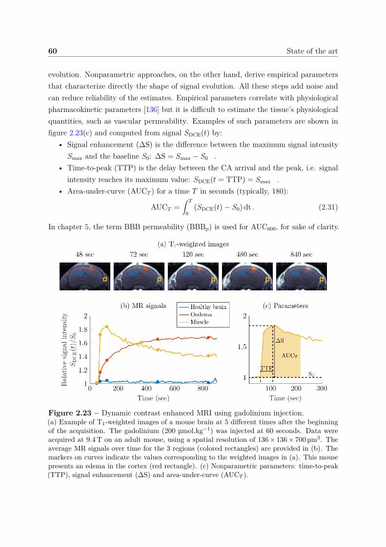
60 State of the art
evolution. Nonparametric approaches, on the other hand, derive empirical parametersthat characterize directly the shape of signal evolution. All these steps add noise andcan reduce reliability of the estimates. Empirical parameters correlate with physiologicalpharmacokinetic parameters [136] but it is difficult to estimate the tissue’s physiologicalquantities, such as vascular permeability. Examples of such parameters are shown infigure 2.23(c) and computed from signal SDCE(t) by:
• Signal enhancement (∆S) is the difference between the maximum signal intensitySmax and the baseline S0: ∆S = Smax − S0 .
• Time-to-peak (TTP) is the delay between the CA arrival and the peak, i.e. signalintensity reaches its maximum value: SDCE(t = TTP) = Smax .
• Area-under-curve (AUCT ) for a time T in seconds (typically, 180):
AUCT =∫ T
0(SDCE(t) − S0) dt . (2.31)
In chapter 5, the term BBB permeability (BBBp) is used for AUC600, for sake of clarity.
Figure 2.23 – Dynamic contrast enhanced MRI using gadolinium injection.(a) Example of T1-weighted images of a mouse brain at 5 different times after the beginningof the acquisition. The gadolinium (200 µmol.kg−1) was injected at 60 seconds. Data wereacquired at 9.4 T on an adult mouse, using a spatial resolution of 136 × 136 × 700 µm3. Theaverage MR signals over time for the 3 regions (colored rectangles) are provided in (b). Themarkers on curves indicate the values corresponding to the weighted images in (a). This mousepresents an edema in the cortex (red rectangle). (c) Nonparametric parameters: time-to-peak(TTP), signal enhancement (∆S) and area-under-curve (AUCT ).
2.3 Quantitative MRI 61
2.3.5 Conclusion
Conventional MRI, i.e. weighted imaging, is limited to reveal large morphologicalabnormalities resulting in regional differences in signal intensities within an acquiredimage. It means that MRI is intrinsically insensitive to subtle global changes that mayaffect the entire brain. In this case, quantitative MRI that allows the comparison ofmeasurements in a single subject with normal values acquired in a healthy populationis required. Conventional MRI also depends on the clinician’s expertise in imagesinterpretation and the absence of quantities is not optimal for using mathematicalmethods, e.g. classification.
However, most of quantitative MRI methods employed typically provide informationon a single parameter at a time. The acquisition of several quantitative parametersthus require significant scan time. Moreover, these quantitative maps are often highlysensitive to system imperfections [137]. Because of these scan time limits and a highsensitivity to the measurement setup and experimental conditions, robust quantitativemultiparametric MRI remains an important research focus in MRI.
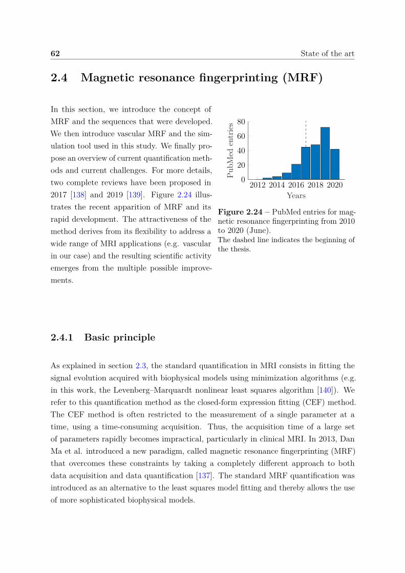
62 State of the art
2.4 Magnetic resonance fingerprinting (MRF)
2012 2014 2016 2018 20200
20
40
60
80
Years
PubM
eden
trie
s
Figure 2.24 – PubMed entries for mag-netic resonance fingerprinting from 2010to 2020 (June).The dashed line indicates the beginning ofthe thesis.
In this section, we introduce the concept ofMRF and the sequences that were developed.We then introduce vascular MRF and the sim-ulation tool used in this study. We finally pro-pose an overview of current quantification meth-ods and current challenges. For more details,two complete reviews have been proposed in2017 [138] and 2019 [139]. Figure 2.24 illus-trates the recent apparition of MRF and itsrapid development. The attractiveness of themethod derives from its flexibility to address awide range of MRI applications (e.g. vascularin our case) and the resulting scientific activityemerges from the multiple possible improve-ments.
2.4.1 Basic principle
As explained in section 2.3, the standard quantification in MRI consists in fitting thesignal evolution acquired with biophysical models using minimization algorithms (e.g.in this work, the Levenberg–Marquardt nonlinear least squares algorithm [140]). Werefer to this quantification method as the closed-form expression fitting (CEF) method.The CEF method is often restricted to the measurement of a single parameter at atime, using a time-consuming acquisition. Thus, the acquisition time of a large setof parameters rapidly becomes impractical, particularly in clinical MRI. In 2013, DanMa et al. introduced a new paradigm, called magnetic resonance fingerprinting (MRF)that overcomes these constraints by taking a completely different approach to bothdata acquisition and data quantification [137]. The standard MRF quantification wasintroduced as an alternative to the least squares model fitting and thereby allows the useof more sophisticated biophysical models.
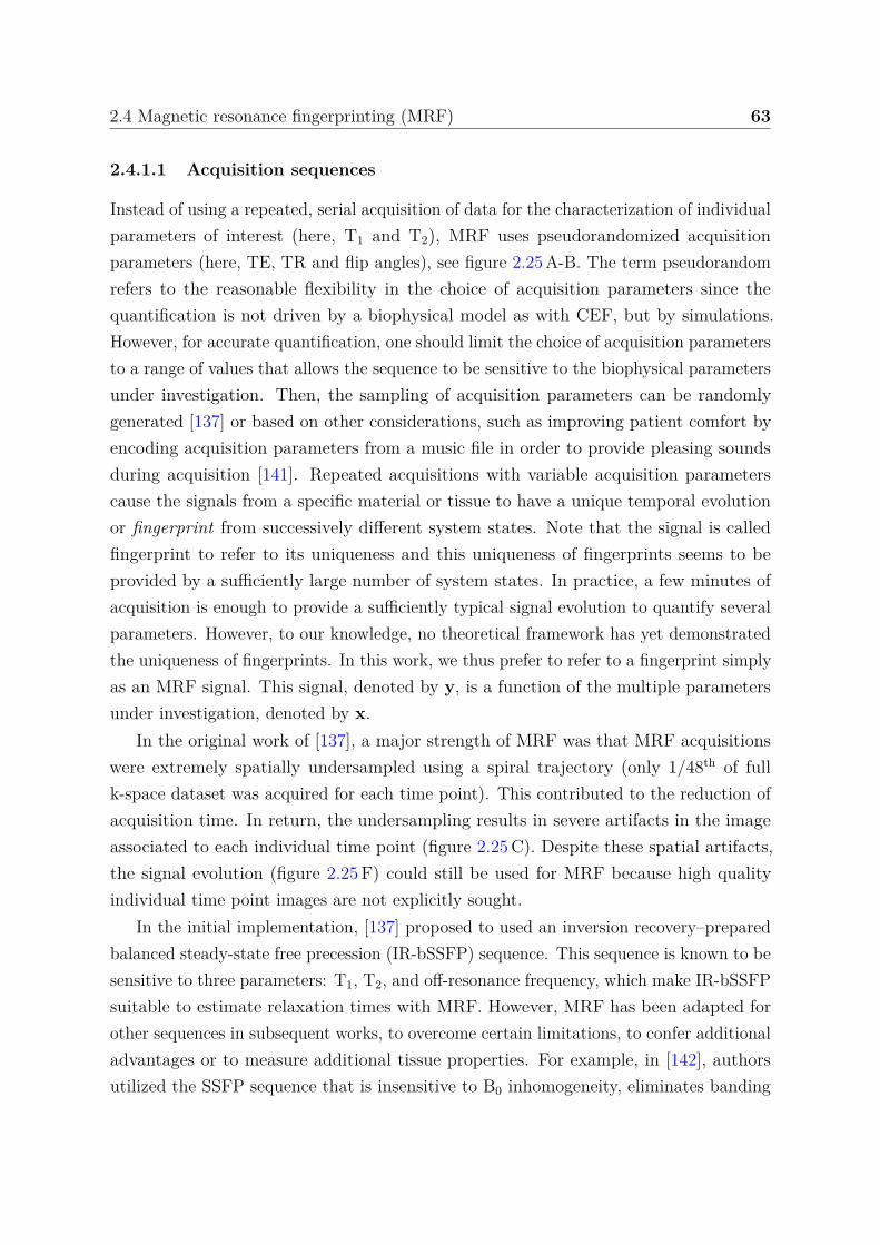
2.4 Magnetic resonance fingerprinting (MRF) 63
2.4.1.1 Acquisition sequences
Instead of using a repeated, serial acquisition of data for the characterization of individualparameters of interest (here, T1 and T2), MRF uses pseudorandomized acquisitionparameters (here, TE, TR and flip angles), see figure 2.25 A-B. The term pseudorandomrefers to the reasonable flexibility in the choice of acquisition parameters since thequantification is not driven by a biophysical model as with CEF, but by simulations.However, for accurate quantification, one should limit the choice of acquisition parametersto a range of values that allows the sequence to be sensitive to the biophysical parametersunder investigation. Then, the sampling of acquisition parameters can be randomlygenerated [137] or based on other considerations, such as improving patient comfort byencoding acquisition parameters from a music file in order to provide pleasing soundsduring acquisition [141]. Repeated acquisitions with variable acquisition parameterscause the signals from a specific material or tissue to have a unique temporal evolutionor fingerprint from successively different system states. Note that the signal is calledfingerprint to refer to its uniqueness and this uniqueness of fingerprints seems to beprovided by a sufficiently large number of system states. In practice, a few minutes ofacquisition is enough to provide a sufficiently typical signal evolution to quantify severalparameters. However, to our knowledge, no theoretical framework has yet demonstratedthe uniqueness of fingerprints. In this work, we thus prefer to refer to a fingerprint simplyas an MRF signal. This signal, denoted by y, is a function of the multiple parametersunder investigation, denoted by x.
In the original work of [137], a major strength of MRF was that MRF acquisitionswere extremely spatially undersampled using a spiral trajectory (only 1/48th of fullk-space dataset was acquired for each time point). This contributed to the reduction ofacquisition time. In return, the undersampling results in severe artifacts in the imageassociated to each individual time point (figure 2.25 C). Despite these spatial artifacts,the signal evolution (figure 2.25 F) could still be used for MRF because high qualityindividual time point images are not explicitly sought.
In the initial implementation, [137] proposed to used an inversion recovery–preparedbalanced steady-state free precession (IR-bSSFP) sequence. This sequence is known to besensitive to three parameters: T1, T2, and off-resonance frequency, which make IR-bSSFPsuitable to estimate relaxation times with MRF. However, MRF has been adapted forother sequences in subsequent works, to overcome certain limitations, to confer additionaladvantages or to measure additional tissue properties. For example, in [142], authorsutilized the SSFP sequence that is insensitive to B0 inhomogeneity, eliminates banding
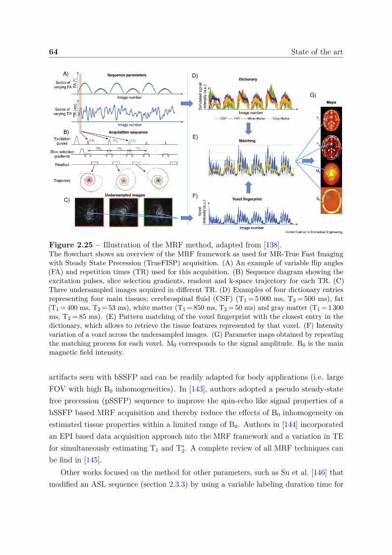
64 State of the art
Figure 2.25 – Illustration of the MRF method, adapted from [138].The flowchart shows an overview of the MRF framework as used for MR-True Fast Imagingwith Steady State Precession (TrueFISP) acquisition. (A) An example of variable flip angles(FA) and repetition times (TR) used for this acquisition. (B) Sequence diagram showing theexcitation pulses, slice selection gradients, readout and k-space trajectory for each TR. (C)Three undersampled images acquired in different TR. (D) Examples of four dictionary entriesrepresenting four main tissues; cerebrospinal fluid (CSF) (T1 = 5 000 ms, T2 = 500 ms), fat(T1 = 400 ms, T2 = 53 ms), white matter (T1 = 850 ms, T2 = 50 ms) and gray matter (T1 = 1 300ms, T2 = 85 ms). (E) Pattern matching of the voxel fingerprint with the closest entry in thedictionary, which allows to retrieve the tissue features represented by that voxel. (F) Intensityvariation of a voxel across the undersampled images. (G) Parameter maps obtained by repeatingthe matching process for each voxel. M0 corresponds to the signal amplitude. B0 is the mainmagnetic field intensity.
artifacts seen with bSSFP and can be readily adapted for body applications (i.e. largeFOV with high B0 inhomogeneities). In [143], authors adopted a pseudo steady-statefree precession (pSSFP) sequence to improve the spin-echo like signal properties of abSSFP based MRF acquisition and thereby reduce the effects of B0 inhomogeneity onestimated tissue properties within a limited range of B0. Authors in [144] incorporatedan EPI based data acquisition approach into the MRF framework and a variation in TEfor simultaneously estimating T1 and T∗
2. A complete review of all MRF techniques canbe find in [145].
Other works focused on the method for other parameters, such as Su et al. [146] thatmodified an ASL sequence (section 2.3.3) by using a variable labeling duration time for
2.4 Magnetic resonance fingerprinting (MRF) 65
each TR, removing the post-labeling delay and ordering the labeling-control pairing in apseudorandom fashion. The MRF framework has also been extended to characterize theproperties associated with the microvascular network. In [147], the authors adapted theMRF to measure BVf, mean vessel radius and StO2. We will return to this in a nextsection.
2.4.1.2 Simulations
The original implementation of MRF used a simple Bloch simulation of a single isochromat(i.e. spin) [137]. This approximation is very fast, but becomes inaccurate in the presenceof inhomogeneities of B0 inside the voxel that cause dephasing. To take this gradientdephasing into consideration, the Bloch model can be extended by averaging over anensemble of spins, but this is computationally expensive and still an approximation. Theextended phase graph (EPG) model [148] is an alternative approach that has been usedpreviously in fast image with steady precession (FISP) signal simulations [142]. TheEPG method describes the spin system as several discrete configuration states using theFT. This provides more accurate signal evolution compared to Bloch simulation whenthe spin system is affected by inhomogeneous magnetic fields.
The challenge for simulation tools is generally the balance between complexity andtime, since in MRF, we observed that the number of simulations is of the order of 105-106
(10-100 values per parameters). For GPU implementation, the snapMRF tool (fullyparallel EPG) allows the simulation of 105 signals in less than 10 seconds [149]. In CPUimplementations, EPG-X [150] and PnP-MRF [151] tools allow the simulation of thesame 105 signals in 104 and 102 seconds [149].
2.4.1.3 Quantification
To estimate the parameters of interest, a large database, referred to as a dictionary, andcontaining a large number of possible signal evolutions, is simulated using the introducedbiophysical model for a pseudorandomized acquisition (figure 2.25 D). The simulateddictionary is noted Df , where f is the model. A search is performed by comparing oneacquired signal yobs and all the simulated signals y = f(x) in the dictionary to findthe best match according to an objective function d(·, ·), usually a standard distanceor dissimilarity measure (e.g. in MRF, the dot product). The tissue parameters arethen estimated as the combination of parameter values x that generated the best signal
66 State of the art
evolution match (figure 2.25 E), i.e. that minimizes the objective function:
x = arg minx ∈ Df
d(yobs, f(x)). (2.32)
Because, this data processing is particularly robust to high noise levels, its combinationwith the highly spatially undersampled data acquisition enables the fast acquisitionof multiple parameters (figure 2.25 G) [137]. Additionally, the simulation can includethe contribution of system imperfections (e.g. B0 inhomogeneities) and thus overcomethis bias during quantification. Together, these aspects of MRF contributed to theattractiveness of the framework for quantitative MRI and we will see how this frameworkhas evolved.
2.4.2 Vascular MRF
Christen et al. have shown the possibility of applying MRF to directly quantify BVf,mean vessel radius and StO2 [147]. The authors called this framework vascular magneticresonance fingerprinting. We propose to reproduce the previous figure 2.25 for vascularMRF in figure 2.26 in order to illustrate similarities and differences.
2.4.2.1 Acquisition sequence
In this work, the full MGEFIDSE signal samples were exploited compared to the classicCEF approach introduced in section 2.3.4, which only used the samples before the 180°RF pulse and the spin echo sample. Authors proposed to use the ratio of the pre- andpost-USPIO injection MGEFIDSE signal evolutions (section 2.3.4) as the fingerprint,which reduced the effect of B0 inhomogeneities and T2’s effect on signals (figure 2.26 A).For the moment, no other sequences have been used in vascular MRF.
The MRF implementation to vascular signals required more sophisticated simulationtools than Bloch’s equations that are used for relaxation times related works.
2.4.2.2 Simulations
Using Bloch’s equations as a simulation model, the magnetization is homogeneous withinthe voxel since the voxel itself is characterized by a single T1 and a single T2 values, andplaced into a constant magnetic field (figure 2.27(a)). For vascular MRF applications,the voxel needs to be segmented into a vascular compartment and an extravascularcompartment, which results in an inhomogeneous magnetization through the voxel
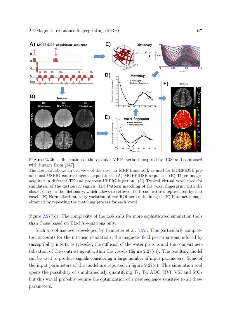
2.4 Magnetic resonance fingerprinting (MRF) 67
Figure 2.26 – Illustration of the vascular MRF method, inspired by [138] and composedwith images from [147].The flowchart shows an overview of the vascular MRF framework as used for MGEFIDSE pre-and post-USPIO contrast agent acquisitions. (A) MGEFIDSE sequence. (B) Three imagesacquired in different TE and pre/post-USPIO injection. (C) Typical virtual voxel used forsimulation of the dictionary signals. (D) Pattern matching of the voxel fingerprint with theclosest entry in the dictionary, which allows to retrieve the tissue features represented by thatvoxel. (E) Normalized intensity variation of two ROI across the images. (F) Parameter mapsobtained by repeating the matching process for each voxel.
(figure 2.27(b)). The complexity of the task calls for more sophisticated simulation toolsthan those based on Bloch’s equations only.
Such a tool has been developed by Pannetier et al. [152]. This particularly completetool accounts for the intrinsic relaxations, the magnetic field perturbations induced bysusceptibility interfaces (vessels), the diffusion of the water protons and the compartmen-talization of the contrast agent within the vessels (figure 2.27(c)). The resulting modelcan be used to produce signals considering a large number of input parameters. Some ofthe input parameters of the model are reported in figure 2.27(c). This simulation toolopens the possibility of simultaneously quantifying T1, T2, ADC, BVf, VSI and StO2
but this would probably require the optimization of a new sequence sensitive to all theseparameters.
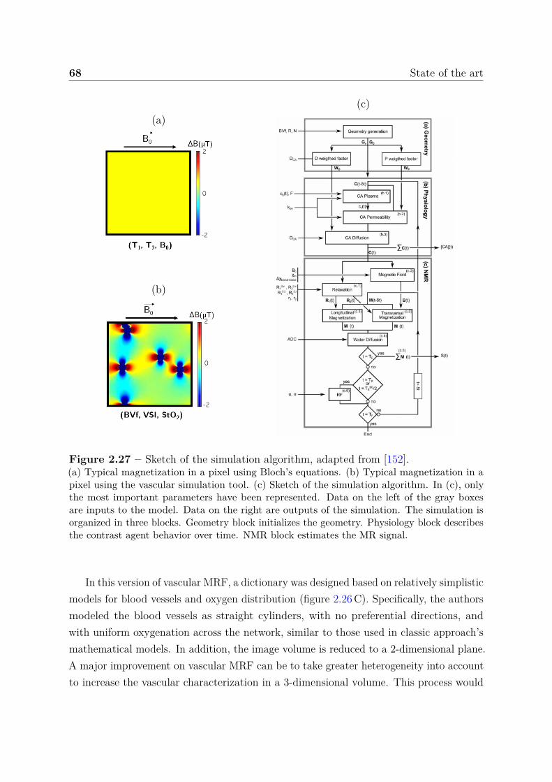
68 State of the art
(a)
(b)
(c)
Figure 2.27 – Sketch of the simulation algorithm, adapted from [152].(a) Typical magnetization in a pixel using Bloch’s equations. (b) Typical magnetization in apixel using the vascular simulation tool. (c) Sketch of the simulation algorithm. In (c), onlythe most important parameters have been represented. Data on the left of the gray boxesare inputs to the model. Data on the right are outputs of the simulation. The simulation isorganized in three blocks. Geometry block initializes the geometry. Physiology block describesthe contrast agent behavior over time. NMR block estimates the MR signal.
In this version of vascular MRF, a dictionary was designed based on relatively simplisticmodels for blood vessels and oxygen distribution (figure 2.26 C). Specifically, the authorsmodeled the blood vessels as straight cylinders, with no preferential directions, andwith uniform oxygenation across the network, similar to those used in classic approach’smathematical models. In addition, the image volume is reduced to a 2-dimensional plane.A major improvement on vascular MRF can be to take greater heterogeneity into accountto increase the vascular characterization in a 3-dimensional volume. This process would

2.4 Magnetic resonance fingerprinting (MRF) 69
certainly even overcome the proposed vascular MRF implementation as it has been shownby [153]. In this work, authors used real mouse angiograms and physiological values asthe substrate for the MR simulations. However, the generation of a dictionary for eachmouse angiogram took 70 hours on a computer cluster [153].
The consequence of using this simulation tool is that the simulation times areconsiderably increased compared to Bloch simulation. For vascular MRF, authors reportthat a single signal simulation took about 2.5 seconds on a desktop computer and thelargest dictionary of the study, composed of about 1 150 000 entries, was generated ona 30-node cluster in about 24 hours [154] (about 8-9 days with a 4-core computer).Compared to the CPU implementation of the PnP-MRF tool on a desktop computer, ittook about 75 times longer on a cluster. The processing of this amount of data is alreadyalmost impossible on a desktop computer and the addition of a single parameter wouldmake the study impossible even on high-performance hardware.
At this point, we understand that the simulation constraints are very different betweenthe two MRF applications. For simple simulations, the stakes of standard MRF onlyconsist in managing the large volume of data simulated during quantification (i.e. timeand memory), whereas in vascular MRF, the simulation time is already a concern.
2.4.2.3 Quantification
Concerning quantification, the procedure remains the same as the one of standard MRF.The parameter values that generate the vascular signal that minimizes the equation (2.32)is used as estimate (figure 2.26 D).
While it has not been clearly shown that the vascular MRF method can improveestimates on BVf and mean radius, this is mainly due to the lack of a validation solution.It is most likely that the use of all signal samples should provide this improvement. Whatis certain is that the method allows, in addition to BVf and mean radius, the quantificationof StO2, which is achieved by acquiring other sequences using CEF method. This resultsin a reduction of the scan time. The main limit to be addressed to extend the vascularMRF and quantify more parameters and/or acquire longer sequences, is the extensivesimulation times. An acceleration of the simulation tool can be considered (out of thescope of this work) but one could also investigate the optimization of the reconstructionmethods in order to reduce the need for dictionary entries, i.e. for simulations.
70 State of the art
2.4.3 Evolution of MRF quantification methods
In this section, we first summarize introduced quantitative MRI workflows. Then, webriefly review the progress achieved in MRF quantification.
Prior to the voxel-by-voxel CEF quantification, data are derived from fully (or atleast sufficiently sampled) acquired k-space data. Then signal evolutions are fitted witha biophysical model, see figure 2.28(a). The MRF quantification, was introduced asan alternative to least squares fitting approach and thereby allows the use of moresophisticated models via matching procedure. As CEF, the MRF quantification is avoxel-by-voxel quantification performed after FT and considering complex-valued signals.The MRF requires a dictionary to perform quantification, which is why we named theMRF quantification methods dictionary-based methods. The dictionary Df is composedof N entries of coupled S-sample fingerprint and P -dimensional parameters (x, y). They1, . . . , yN are generated by running a simulation model f for N different values ofthe magnetic and physiological parameters x1, . . . , xN.
In the original dictionary-based matching (DBM) method, a grid is generated withsampled values in a pre-set interval for each parameter. The dimension of the gridcorresponds to the number of parameters. Then, to invert an observed yobs, it iscompared with the signals in Df to find the best match according to the objectivefunction d(·, ·). With Df = (xn, yn = f(xn)), n = 1:N, x is thus estimated as theargument of the minimization introduced in equation (2.32). Solutions are sought withinthe discrete Df only, while in non-constrained optimization, the minimization is performedby considering the whole continuous space of parameter values. This DBM method isin particular suitable for highly noisy and artifacted data, which means that one canundersample the k-space during the acquisition, see figure 2.28(b). The performanceof the DBM method directly depends on the space discretization, i.e. the choice of thenumber of dictionary entries and the number of parameters. The larger the number N
of entry (xn, yn), the more accurate the estimates but the larger the simulation time toproduce the dictionary and the memory requirement to store the dictionary. Even fora moderate number of parameters, the required number of elements in the dictionaryrenders grid search intractable on a desktop computer.
Additionally, each new yobs requires the computation and comparison of N matchingscores d(yobs, yn). This can be costly if N is very large and if many inversions are desired(e.g. many voxels). When the dictionary is large, this might be problematic for storageand memory. Another issue is that the exhaustive matching process, when coupled with alarge dictionary, can take too much time to compute. However, as spatial undersampling
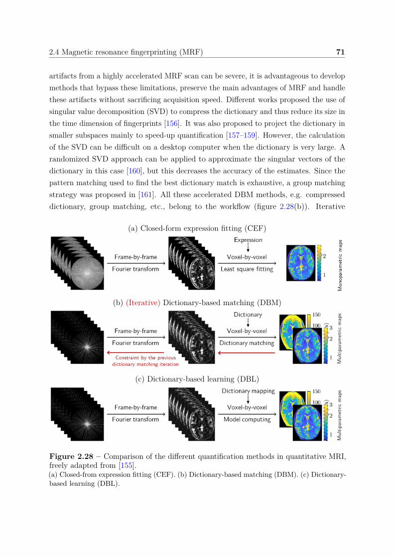
2.4 Magnetic resonance fingerprinting (MRF) 71
artifacts from a highly accelerated MRF scan can be severe, it is advantageous to developmethods that bypass these limitations, preserve the main advantages of MRF and handlethese artifacts without sacrificing acquisition speed. Different works proposed the use ofsingular value decomposition (SVD) to compress the dictionary and thus reduce its size inthe time dimension of fingerprints [156]. It was also proposed to project the dictionary insmaller subspaces mainly to speed-up quantification [157–159]. However, the calculationof the SVD can be difficult on a desktop computer when the dictionary is very large. Arandomized SVD approach can be applied to approximate the singular vectors of thedictionary in this case [160], but this decreases the accuracy of the estimates. Since thepattern matching used to find the best dictionary match is exhaustive, a group matchingstrategy was proposed in [161]. All these accelerated DBM methods, e.g. compresseddictionary, group matching, etc., belong to the workflow (figure 2.28(b)). Iterative
(a) Closed-form expression fitting (CEF)
(b) (Iterative) Dictionary-based matching (DBM)
(c) Dictionary-based learning (DBL)
Figure 2.28 – Comparison of the different quantification methods in quantitative MRI,freely adapted from [155].(a) Closed-from expression fitting (CEF). (b) Dictionary-based matching (DBM). (c) Dictionary-based learning (DBL).
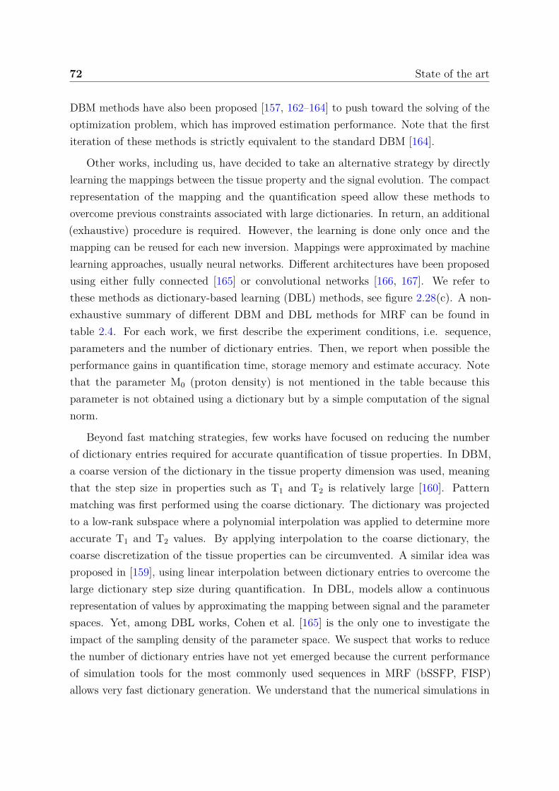
72 State of the art
DBM methods have also been proposed [157, 162–164] to push toward the solving of theoptimization problem, which has improved estimation performance. Note that the firstiteration of these methods is strictly equivalent to the standard DBM [164].
Other works, including us, have decided to take an alternative strategy by directlylearning the mappings between the tissue property and the signal evolution. The compactrepresentation of the mapping and the quantification speed allow these methods toovercome previous constraints associated with large dictionaries. In return, an additional(exhaustive) procedure is required. However, the learning is done only once and themapping can be reused for each new inversion. Mappings were approximated by machinelearning approaches, usually neural networks. Different architectures have been proposedusing either fully connected [165] or convolutional networks [166, 167]. We refer tothese methods as dictionary-based learning (DBL) methods, see figure 2.28(c). A non-exhaustive summary of different DBM and DBL methods for MRF can be found intable 2.4. For each work, we first describe the experiment conditions, i.e. sequence,parameters and the number of dictionary entries. Then, we report when possible theperformance gains in quantification time, storage memory and estimate accuracy. Notethat the parameter M0 (proton density) is not mentioned in the table because thisparameter is not obtained using a dictionary but by a simple computation of the signalnorm.
Beyond fast matching strategies, few works have focused on reducing the numberof dictionary entries required for accurate quantification of tissue properties. In DBM,a coarse version of the dictionary in the tissue property dimension was used, meaningthat the step size in properties such as T1 and T2 is relatively large [160]. Patternmatching was first performed using the coarse dictionary. The dictionary was projectedto a low-rank subspace where a polynomial interpolation was applied to determine moreaccurate T1 and T2 values. By applying interpolation to the coarse dictionary, thecoarse discretization of the tissue properties can be circumvented. A similar idea wasproposed in [159], using linear interpolation between dictionary entries to overcome thelarge dictionary step size during quantification. In DBL, models allow a continuousrepresentation of values by approximating the mapping between signal and the parameterspaces. Yet, among DBL works, Cohen et al. [165] is the only one to investigate theimpact of the sampling density of the parameter space. We suspect that works to reducethe number of dictionary entries have not yet emerged because the current performanceof simulation tools for the most commonly used sequences in MRF (bSSFP, FISP)allows very fast dictionary generation. We understand that the numerical simulations in
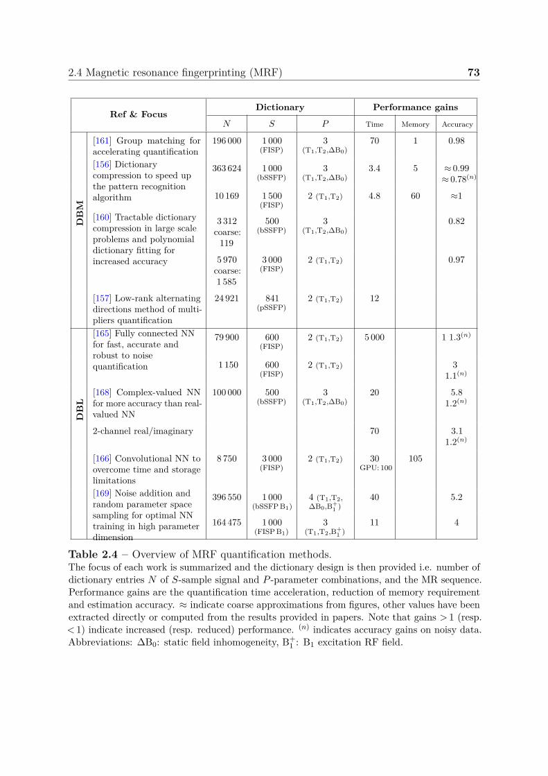
2.4 Magnetic resonance fingerprinting (MRF) 73
Ref & FocusDictionary Performance gains
N S P Time Memory Accuracy
DB
M
[161] Group matching foraccelerating quantification
196 000 1 000(FISP)
3(T1,T2,∆B0)
70 1 0.98
[156] Dictionarycompression to speed upthe pattern recognitionalgorithm
363 624 1 000(bSSFP)
3(T1,T2,∆B0)
3.4 5 ≈ 0.99≈ 0.78(n)
10 169 1 500(FISP)
2 (T1,T2) 4.8 60 ≈1
[160] Tractable dictionarycompression in large scaleproblems and polynomialdictionary fitting forincreased accuracy
3 312coarse:
119
500(bSSFP)
3(T1,T2,∆B0)
0.82
5 970coarse:1 585
3 000(FISP)
2 (T1,T2) 0.97
[157] Low-rank alternatingdirections method of multi-pliers quantification
24 921 841(pSSFP)
2 (T1,T2) 12
DB
L
[165] Fully connected NNfor fast, accurate androbust to noisequantification
79 900 600(FISP)
2 (T1,T2) 5 000 1 1.3(n)
1 150 600(FISP)
2 (T1,T2) 31.1(n)
[168] Complex-valued NNfor more accuracy than real-valued NN
100 000 500(bSSFP)
3(T1,T2,∆B0)
20 5.81.2(n)
2-channel real/imaginary 70 3.11.2(n)
[166] Convolutional NN toovercome time and storagelimitations
8 750 3 000(FISP)
2 (T1,T2) 30GPU: 100
105
[169] Noise addition andrandom parameter spacesampling for optimal NNtraining in high parameterdimension
396 550 1 000(bSSFP B1)
4 (T1,T2,∆B0,B+
1 )40 5.2
164 475 1 000(FISP B1)
3(T1,T2,B+
1 )11 4
Table 2.4 – Overview of MRF quantification methods.The focus of each work is summarized and the dictionary design is then provided i.e. number ofdictionary entries N of S-sample signal and P -parameter combinations, and the MR sequence.Performance gains are the quantification time acceleration, reduction of memory requirementand estimation accuracy. ≈ indicate coarse approximations from figures, other values have beenextracted directly or computed from the results provided in papers. Note that gains > 1 (resp.< 1) indicate increased (resp. reduced) performance. (n) indicates accuracy gains on noisy data.Abbreviations: ∆B0: static field inhomogeneity, B+
1 : B1 excitation RF field.
74 State of the art
vascular MRF are specifically computationally expensive, but a compact and accuratefingerprint representation is of key importance in MRF. In [165], authors reduced theinitial dictionary density (69 000 entries and 2 parameters) from 2 to 60 fold, see theimpact on estimate errors in figure 2.29. Using noiseless signals, the NN is more robustto the decreased dictionary density than DBM, the ratio of root mean square errors(RMSE) obtained using 1/2th and 1/60th of the dictionary entries, are 6 for T1 and 4.5for T2, while for DBM the ratio are 14.6 for T1 and 11.3. Using 1 % noise level corruptedsignals, the NN ratio are 1.6 for T1 and 1.1 for T2 and the DBM ratio are 1.2 for T1 and1.1 for T2. These results therefore suggest that DBL methods are more promising thanthe standard DBM approach for reducing the size of the dictionary.
Figure 2.29 – Impact of dictionary reduction on T1 and T2 MRF estimation accuracy,adapted from [165].RMSE of the MRF dictionary matching (open circles) and NN quantification (closed circles) forthe different undersampling factors and noise levels tested. For the noiseless acquisition (bluecurves) the error in the NN quantification was 2 fold smaller for T1 and 4 fold smaller for T2 atthe largest undersampling factor tested. For the noisy acquisition (red curves) only tissues withT2 > 11 ms were included in the error calculation for the MRF dictionary matching whereasall tissues were included in the NN quantification error. Nevertheless, the NN quantificationerror was still smaller or equal to the MRF error for all undersampling factors tested.
By considering the latest developments in MRF quantification, one can improve theestimation relying on MRF quantification methods that require less dictionary entriesto perform accurate and fast estimation. Accuracy appears to be achievable throughcontinuous data representation, spatial considerations and complex-valued data processing.Compression or learning of the dictionary seems to be the most effective approach tolimit extensive quantification time and excessive memory requirements. To optimizeand implement MRF in large scale or in time-consuming simulation (e.g. vascular), it is

2.4 Magnetic resonance fingerprinting (MRF) 75
therefore required to design a method that maintains a good parameter quantificationaccuracy but reduces significantly the number of dictionary entries. However, very fewworks address this issue.
76 State of the art
2.5 Challenges and requirements
The main stake of this thesis is to develop an MRI acquisition and data processingprotocol for the identification and characterization of MRI changes induced by anepileptic condition in an experimental animal model.
We decided to work with two kainate-induced status epilepticus models. The firstmodel, induced by intraperitoneal kainate injection, is easier to produce and allows theimaging of animals early after status epilepticus. To investigate the early modifications,the animals may be imaged over time (typically, from 24 hours to 1 week). The secondmodel, induced by intrahippocampal kainate injection, is less variable in its expressionand causes an hippocampal sclerosis, which allows the investigation of chronic condition,after the emergence of spontaneous seizures. Again, animals may be imaged over time tocharacterize the epileptogenesis period and, at least 4 weeks after injection, to characterizethe period when chronic seizure occurs. The validation of the epileptic condition can bedone early by identifying the symptoms (automatisms and a catatonic posture, myoclonictwitching of the head, forelimbs and rearlimbs) a few hours after injection, i.e. duringstatus epilepticus. One can also identify specific EEG patterns or hippocampal sclerosison anatomical MRI images for the intrahippocampal injection model.
Both cellular and vascular MRI parameter changes have been reported, among theseparameters, relaxation times T1 and T2, diffusion, perfusion, vascular density, and BBBleakage. However, most of the MRI vascular findings are related to large vessel whilechanges at the capillary levels have only been reported using ex vivo imaging or resectiontissues in patients. One can add to the well-documented cellular protocols, acquisitionswith iron oxide based contrast agents to determine the fraction of blood volume as well asthe size of the capillaries, as observed using histology. Concerning the BBB integrity, MRIfindings were obtained after long gadolinium infusion. One can also investigate imagingchanges in BBB permeability by injecting a bolus of gadolinium to reduce acquisitiontime and perform the acquisitions necessary for the quantification of all the parametersin a time compatible with the duration of animal anesthesia, i.e. less than two hours.
As small variations of these parameters are expected, methodological developments forthe processing are conducted in parallel. The MRF approach promises to provide betteraccuracy in estimating parameters and thus facilitate the detection of small changes andthis point has to be confirmed. The objective is to develop a method that allows theaccuracy of very fine grids to be achieved with no more than a few hours of simulations forthe dictionary, i.e. in vascular MRF, about 104 signals. To be viable, the method should

2.5 Challenges and requirements 77
provide a reconstruction of a multi-slice acquisition (about 106 voxels) in a few minuteson a desktop computer. The method must preserve as much as possible the advantagesof MRF, i.e. robustness to thermal noise and undersampling artifacts, flexibility andease of use, etc.
With these objectives in mind, we therefore performed MRI experiments on epilepticmouse models and develop MRF methods in parallel. MRI Data were analyzed using theexisting and the proposed methods, as developed in the next chapters.

Chapter 3
Bayesian inverse regression forvascular MRF quantification
To reach a good accuracy, the matching MRF quantification requires an informativedictionary whose cost, in terms of design, storage and exploration, is rapidly prohibitivefor even moderate numbers of parameters. In this study, we develop a robust and scalablemulti-parametric dictionary-based reconstruction to measure vascular parameters. Ourproposed method is compared to MRF matching on two types of synthetic signals:scalable and vascular MRF signals. A manuscript has been submitted to the journalIEEE Transactions on Medical Imaging [170]. Here the manuscript has been adapted.
3.1 Introduction
Magnetic resonance fingerprinting (MRF) is a novel approach to quantitative magneticresonance imaging that allows the estimation of multiple tissue properties in a singleacquisition [137, 171]. The acquisition, which consists in repeating measurements withvarying experimental conditions, generates a signal evolution (or fingerprint) that dependson the parameters of the studied tissue. To estimate these parameters, a large database,referred to as a dictionary and containing a large number of possible signal evolutions,is simulated from biophysical models. A comparison is performed between an acquiredsignal and the signals in the dictionary to find the best match according to an objectivefunction. The tissue parameters are then estimated to the values that generated thebest signal evolution match. In MRF, parameter estimation accuracy therefore dependson the number of dictionary entries, which increases exponentially with the number ofparameters. For applications with many parameters such as vascular MRF [147], the
80 Bayesian inverse regression for vascular MRF quantification
required memory size and simulation time as well as the parameter estimation time (orquantification time) quickly become a limit.
To compress the dictionary while limiting the loss of information, several authors haveused singular value decomposition to project the dictionary in a well-chosen subspace [156–161]. However, this compression procedure generally decreases parameter accuracy. Ithas also been proposed to directly find a mapping from the fingerprints to the parameterspace using kernel regression [172] or neural network approaches [165–169, 173–175]. Theresulting compact representation offers the advantage over the discrete MRF grid ofa continuous exploration of parameter values. These approaches significantly reducethe quantification time, but not the simulation time due to the need to span a highdimensional fingerprint space. To limit the simulation time, Cohen et al. [165] studieda mapping obtained from a sparse set of dictionary entries. The study, carried outwith only two parameters, led to a modest reduction of dictionary entries (up to 60).Consider a dictionary of 10 × 10 entries simulated in 1 hour. If the number of parametersincreases from 2 to 7 parameters, and always considering 10 values per parameter, thenthe dictionary computation time increases from 1 hour to more than 11 years. In thiscase, an approach that greatly reduces the need for simulation, continuously representsthe parameters without loss of precision, relies on an explainable model and reduces thequantification time becomes highly desirable [9].
To reach this goal, we adopt in this work a mapping approach that circumvents thedifficulty of learning a high-to-low mapping from a high dimensional fingerprint space to alow dimensional parameter space, learning instead the much less problematic low-to-highreverse mapping from parameters to fingerprints. More specifically, we use the Gaussianlocally linear mapping (GLLiM) model [176], which allows both a tractable learningof the low-to-high mapping and a subsequent analytical expression of the high-to-lowor signal-to-parameter mapping. Furthermore, unlike most other regression methodsthat focus on pointwise predictions, GLLiM provides a full posterior distribution perfingerprint. This distribution can then be used to compute an estimated value and aconfidence index for each parameter, using respectively the posterior expectation andstandard deviation.
In this vascular MRF study, the proposed dictionary-based learning (DBL) methodand the standard dictionary-based matching (DBM) method are compared. Syntheticscalable signals are first used to assess quantitatively the methods’ performance whileincreasing the number of parameters. Vascular MRF signals are then considered boththrough simulations and real data acquired in tumor bearing rats.

3.2 MRF as an inverse problem 81
3.2 MRF as an inverse problem
In inverse problems, the overall issue is to provide information on some parameters ofinterest x given an observed signal y, using a known direct or forward model that describeshow the parameters x translate into a signal y (figure 3.1). Among inverse problems,MRF exhibits the following difficulties: 1) the direct model is (highly) non-linear, as a(complex) series of equations or simulation tools; 2) the y’s are high-dimensional signalsand 3) many y’s need to be inverted (one for each voxel in an image); 4) the vector ofparameters x is multidimensional and predicting each component of x independently islikely to be sub-optimal.
Parameters x Signal (or fingerprint) y
Forward: y = f(x)Simulation
Inverse: x = f−1(y)Quantification
Figure 3.1 – Magnetic resonance fingerprinting as an inverse problem.
To account for possible sources of uncertainty, we focus on a statistical modelingassuming that the forward model is described by a likelihood and a prior distribution.The likelihood function is linking parameter values x to a probability of observing signaly, Lx(y) = p(y|x). A natural assumption is that Lx(y) is a Gaussian distributionN (y; f(x), Σ) centered at f(x) where f is the known simulation function that links thephysical and physiological parameters to the fingerprint and Σ is a covariance matrixaccounting for measuring or modeling imperfections. The parameter prior distribution,denoted by p(x), encodes in turns information on the possible parameter values. StandardMRF uses a finite grid of values, which corresponds to a very particular discrete prior.This probabilistic point of view allows, with the Bayesian framework, to derive a posteriordistribution p(x|y) = p(y|x)p(x)/p(y), which provides for any given y, a characterizationof x by a probability density function more informative than a single point prediction ofx. It corresponds to a richer inverse model but is not usually available in closed-formand requires approximations to be usable in practice.
More generally, most methods to solve inverse problems can be classified into twomain categories, optimization-based and learning-based methods. In the next section,we refer to standard MRF as a matching method. We show that it can be seen as apenalized optimization, which does not require statistical modeling, while the method wepropose next belongs to statistical learning approaches.

82 Bayesian inverse regression for vascular MRF quantification
3.2.1 Dictionary-based matching (DBM) method
MRF requires a large database Df , referred to as a dictionary [137]. It is made of N
entries of coupled fingerprint and parameters (x, y). The S-dimensional fingerprintsy1, . . . , yN are generated by running the simulation model f for N different values ofthe P -dimensional magnetic and physiological parameters x1, . . . , xN. In the DBMmethod, a P -dimensional grid is generated with sampled values in a pre-set interval foreach parameter. Then, to invert an observed yobs, it is compared with the signals inDf to find the best match according to an objective function d(·, ·), usually a standarddistance or dissimilarity measure (e.g. in MRF, the dot product). With Df = (xn, yn =f(xn)), n = 1:N, x is thus estimated as the argument of the following minimization:
x = arg minx ∈ Df
d(yobs, f(x)) . (3.1)
Solutions are sought in Df only, while in a non-constrained optimization the minimizationis over the whole continuous space of parameter values. The performance of the methoddepends directly on the space discretization, i.e. the choice of the number of dictionaryentries and the number of parameters. The larger the number N of entry (xn, yn), themore accurate the estimates but the larger the simulation time and memory requirement.Even for moderate number of parameters, the required number of elements in thedictionary renders grid search intractable on a desktop computer. In addition, each newyobs, requires the computation and comparison of N matching scores d(yobs, yn), whichcan be costly if N is very large and if many inversions are desired. The regression orlearning method that we propose in the next section is more efficient with respect tothese aspects.
3.2.2 Proposed dictionary-based learning (DBL) method
In contrast to the DBM method, regression and learning methods can adapt to handlemassive inversions of high dimensional data. The main principle is to transfer thecomputational cost, from 2-signal matchings to the learning of an inverse operator F−1.Equivalently, the goal is to learn a mapping from the fingerprint space to the parameterspace, for any y, with cost-less evaluation of F−1(y). The dictionary Df can be usedto estimate F−1. Learning or regression methods adapted to high dimensions includeinverse regression methods, i.e. sliced inverse regression [177], partial least squares [178],approaches based on mixtures of regressions with different variants, e.g. Gaussian locallylinear mapping (GLLiM) [176], mixtures of experts [179], cluster weighted models [180],
3.2 MRF as an inverse problem 83
and kernel methods [172]. Inverse regression methods are flexible in that they reduce thedimension in a way optimal to the subsequent mapping estimation task that can itself becarried out by any kind of standard regression tool. In that sense, the inverse regressionmethods are said to be non-parametric or semi-parametric. Similarly, in [172], the authorspropose a regression with an appropriate kernel function to learn the non-linear mapping.The procedure has the advantage to be semi-parametric but a serious limit is that thecomponents of f are optimized in each dimension separately. As regards application toMRF, the learning strategy has also been proposed by several groups using deep learningtools [165–169, 173–175]. A major limitation of these methods is that they require alarge number of training points to learn many model parameters without overfitting.
In the same vein as [172], and in contrast to deep learning approaches, we proposeto use the GLLiM method that exploits Gaussian mixture models [176]. Compared toother regression methods that focus on providing point-wise estimates, GLLiM providesa full probability distribution selected in a family of parametric models, e.g. mixture ofGaussian distributions, where the parameters are denoted by θ. The inversion operator isdefined as F−1(y) = p(x|y; θ), where θ is estimated from the dictionary. More specifically,GLLiM handles the modeling of non-linear relationships with a piecewise linear model.Each y is seen as the noisy image of x obtained from a K-component mixture of affinetransformations. This is modeled by introducing a latent variable z ∈ 1, . . . , K suchthat
y =K∑
k=1δk(z) (Akx + bk + ϵk) , (3.2)
where δk(z) indicates membership in the region k of x, having the value 1 if it belongsto the region and the value 0 otherwise. Ak is a P × S matrix and bk a vector in RP
that characterize an affine transformation. Variable ϵk corresponds to an error term inRP which is assumed to be zero-mean and not correlated with x, capturing both themodeling noise and the quantification error due to the affine approximations. In GLLiM,ϵk follows a Gaussian distribution N (0, Σk) and x follows a mixture of K Gaussiandistributions defined by p(x|z = k) = N (x; ck, Γk), and p(z = k) = πk. It follows that
p(y|x; θ) =K∑
k=1wk(x) N (y;Akx + bk, Σk), (3.3)
with wk(x) = πk N (x; ck, Γk)∑Kj=1 πj N (x; cj, Γj)
,
and θ = πk, ck, Γk,Ak, bk, Σkk=1:K is the set of parameters defining the model. Theconditional probability distribution of interest can be derived as
84 Bayesian inverse regression for vascular MRF quantification
p(x|y; θ) =K∑
k=1w∗
k(y) N (x;A∗ky + b∗
k, Σ∗k) , (3.4)
with w∗k(y) = πk N (y; c∗
k, Γ∗k)∑K
j=1 π∗j N (y; c∗
j , Γ∗j)
,
and a new parameterization θ∗ = c∗k, Γ∗
k,A∗k, b∗
k, Σ∗kk=1:K easily expressed as an analyt-
ical function of θ. The mixture setting provides some guaranties that when choosing K
large enough it is possible to approximate any reasonable relationship [179]. Automaticmodel selection criteria can also be used to select K (see [176]).
The p(x|y; θ) distribution provides both estimates of the parameters x and informationabout the confidence to be placed in these estimates. In this work, estimates are definedthrough the expectation and the confidence indices as the square root of the covariancematrix diagonal element vector:
x = E [x|y; θ] , (3.5)
CI =√
diag (Var [x|y; θ]) , (3.6)
with E [x|y; θ] = ∑Kk=1 w∗
k(y)(A∗ky + b∗
k), and
Var [x|y; θ] =K∑
k=1w∗
k(y)[Σ∗
k + (A∗ky + b∗
k)(A∗ky + b∗
k)T]
−(
K∑k=1
w∗k(y)(A∗
ky + b∗k))(
K∑k=1
w∗k(y)(A∗
ky + b∗k))T
,
where diag(·) denotes the function returning the diagonal elements of a matrix. Forthe CI, computed from the estimated posterior p(x|y; θ), to be a good indicator of theparameter estimation error, it is required that the inverted y follows the same modelused to computed θ. The use of a unique θ parameter for all inversions provides a greatgain when massive inversions are required but it also assumes that the same model isvalid for all fingerprints and that the dictionary Df is a good representation of them.In practice, acquired fingerprints may come with different noise levels. An interestingfeature of GLLiM is to adapt to this case at a very low cost. When the observed y comeswith some covariance matrix Ση corresponding to a centered Gaussian noise variable η,the initial dictionary Df may not be fully adapted if it has not been generated with thissame additional measurement error. Another training set should be simulated and usedinstead, with a corrected likelihood corresponding to N (y; f(x), Σ + Ση). Fortunately,it is straightforward to check that the structure of the Gaussian mixture approximationavoid the re-learning of the GLLiM model. Indeed, it suffices to change the estimatedΣk’s into Σk + Ση and to report this change when computing θ∗.
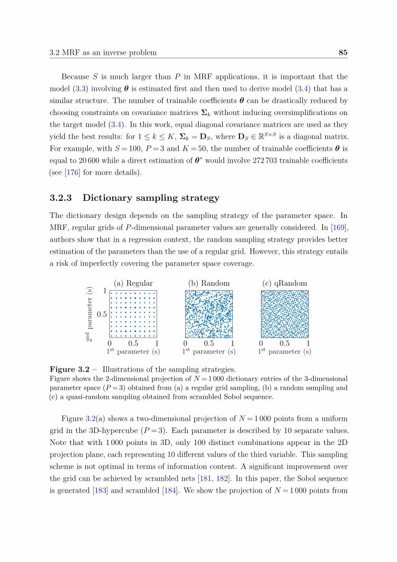
3.2 MRF as an inverse problem 85
Because S is much larger than P in MRF applications, it is important that themodel (3.3) involving θ is estimated first and then used to derive model (3.4) that has asimilar structure. The number of trainable coefficients θ can be drastically reduced bychoosing constraints on covariance matrices Σk without inducing oversimplifications onthe target model (3.4). In this work, equal diagonal covariance matrices are used as theyyield the best results: for 1 ≤ k ≤ K, Σk = DS, where DS ∈ RS×S is a diagonal matrix.For example, with S = 100, P = 3 and K = 50, the number of trainable coefficients θ isequal to 20 600 while a direct estimation of θ∗ would involve 272 703 trainable coefficients(see [176] for more details).
3.2.3 Dictionary sampling strategy
The dictionary design depends on the sampling strategy of the parameter space. InMRF, regular grids of P -dimensional parameter values are generally considered. In [169],authors show that in a regression context, the random sampling strategy provides betterestimation of the parameters than the use of a regular grid. However, this strategy entailsa risk of imperfectly covering the parameter space coverage.
0 0.5 1
0.5
1
1st parameter (s)
2nd
para
met
er(s
) (a) Regular
0 0.5 11st parameter (s)
(b) Random
0 0.5 11st parameter (s)
(c) qRandom
Figure 3.2 – Illustrations of the sampling strategies.Figure shows the 2-dimensional projection of N = 1 000 dictionary entries of the 3-dimensionalparameter space (P = 3) obtained from (a) a regular grid sampling, (b) a random sampling and(c) a quasi-random sampling obtained from scrambled Sobol sequence.
Figure 3.2(a) shows a two-dimensional projection of N = 1 000 points from a uniformgrid in the 3D-hypercube (P = 3). Each parameter is described by 10 separate values.Note that with 1 000 points in 3D, only 100 distinct combinations appear in the 2Dprojection plane, each representing 10 different values of the third variable. This samplingscheme is not optimal in terms of information content. A significant improvement overthe grid can be achieved by scrambled nets [181, 182]. In this paper, the Sobol sequenceis generated [183] and scrambled [184]. We show the projection of N = 1 000 points from
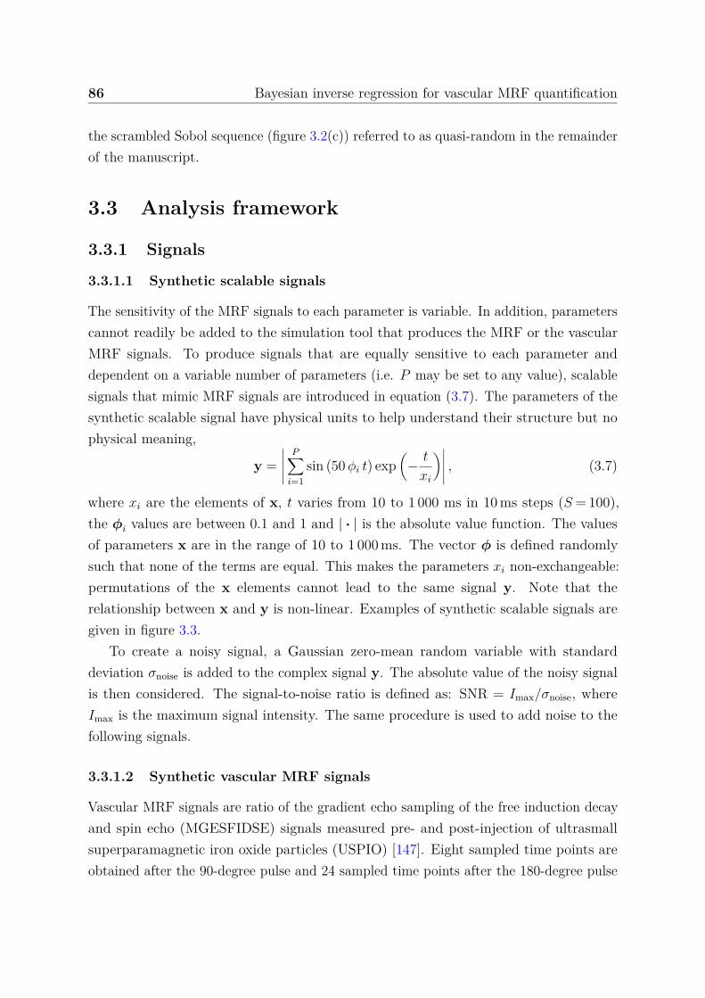
86 Bayesian inverse regression for vascular MRF quantification
the scrambled Sobol sequence (figure 3.2(c)) referred to as quasi-random in the remainderof the manuscript.
3.3 Analysis framework
3.3.1 Signals
3.3.1.1 Synthetic scalable signals
The sensitivity of the MRF signals to each parameter is variable. In addition, parameterscannot readily be added to the simulation tool that produces the MRF or the vascularMRF signals. To produce signals that are equally sensitive to each parameter anddependent on a variable number of parameters (i.e. P may be set to any value), scalablesignals that mimic MRF signals are introduced in equation (3.7). The parameters of thesynthetic scalable signal have physical units to help understand their structure but nophysical meaning,
y =∣∣∣∣∣
P∑i=1
sin (50 ϕi t) exp(
− t
xi
)∣∣∣∣∣ , (3.7)
where xi are the elements of x, t varies from 10 to 1 000 ms in 10 ms steps (S = 100),the ϕi values are between 0.1 and 1 and | · | is the absolute value function. The valuesof parameters x are in the range of 10 to 1 000 ms. The vector ϕ is defined randomlysuch that none of the terms are equal. This makes the parameters xi non-exchangeable:permutations of the x elements cannot lead to the same signal y. Note that therelationship between x and y is non-linear. Examples of synthetic scalable signals aregiven in figure 3.3.
To create a noisy signal, a Gaussian zero-mean random variable with standarddeviation σnoise is added to the complex signal y. The absolute value of the noisy signalis then considered. The signal-to-noise ratio is defined as: SNR = Imax/σnoise, whereImax is the maximum signal intensity. The same procedure is used to add noise to thefollowing signals.
3.3.1.2 Synthetic vascular MRF signals
Vascular MRF signals are ratio of the gradient echo sampling of the free induction decayand spin echo (MGESFIDSE) signals measured pre- and post-injection of ultrasmallsuperparamagnetic iron oxide particles (USPIO) [147]. Eight sampled time points areobtained after the 90-degree pulse and 24 sampled time points after the 180-degree pulse
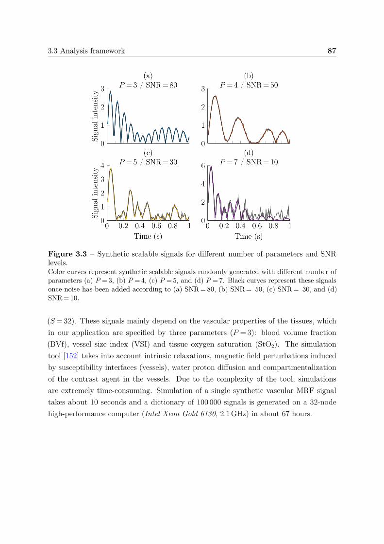
3.3 Analysis framework 87
Figure 3.3 – Synthetic scalable signals for different number of parameters and SNRlevels.Color curves represent synthetic scalable signals randomly generated with different number ofparameters (a) P = 3, (b) P = 4, (c) P = 5, and (d) P = 7. Black curves represent these signalsonce noise has been added according to (a) SNR = 80, (b) SNR = 50, (c) SNR = 30, and (d)SNR = 10.
(S = 32). These signals mainly depend on the vascular properties of the tissues, whichin our application are specified by three parameters (P = 3): blood volume fraction(BVf), vessel size index (VSI) and tissue oxygen saturation (StO2). The simulationtool [152] takes into account intrinsic relaxations, magnetic field perturbations inducedby susceptibility interfaces (vessels), water proton diffusion and compartmentalizationof the contrast agent in the vessels. Due to the complexity of the tool, simulationsare extremely time-consuming. Simulation of a single synthetic vascular MRF signaltakes about 10 seconds and a dictionary of 100 000 signals is generated on a 32-nodehigh-performance computer (Intel Xeon Gold 6130, 2.1 GHz) in about 67 hours.

88 Bayesian inverse regression for vascular MRF quantification
3.3.1.3 Acquired vascular MRF signals
Experimental data were acquired at 4.7 T (Bruker Biospin, Ettlingen, Germany) andhave been introduced in [154]. The field of view was 30 × 30 mm2 and the voxel size was234 × 234 × 800 µm3. A turbo spin-echo sequence was acquired to identify anatomicalstructures and tumor tissues. Then, two GESFIDSE sequences (S = 32) were acquired,before and after injection of UPSIO. For details on the conditions of animal preparationand data acquisition, see original data work [154].
3.3.2 Analysis pipeline
The simulated and acquired data are processed using custom code developed in the Matlabenvironment (The MathWorks Inc., Natick, Ma, USA). This code and the numericalexperiment scripts are available1, see appendix E.1 for details. Data from tumor bearingrats are processed using the Medical software for Processing multi-Parametric imagesPipelines2 [185], see appendices E.2 and E.3 for details.
3.3.2.1 Dictionary design
The dictionary is generated in two steps. First, combinations of parameter values in theparameter space are sampled using one of the sampling strategies in section 3.2.3. Then,for each combination of parameter values, the associated fingerprint is simulated usingeither equation (3.7) for synthetic scalable signals or the simulation tool described insection 3.3.1.2 for vascular MRF signals. For the DBL method, a low level, zero-meanGaussian noise (typically, SNR = 60) is added to the dictionary signals as this improvedour results (see section 3.4.1.2).
3.3.2.2 Dictionary-based analysis
The dictionary is fully stored for the DBM method or summarized by a parametric modelθ for the DBL method. To obtain this model, we use the GLLiM regression described insection 3.2.2. The model learning, a potentially time-consuming step, is performed onlyonce, just after the production of the dictionary. The model requires only the setting ofthe K calibration value. In practice, the precise K value is not critical and different K
values give similar results as long as they are sufficiently large compared to number ofdictionary entries (K ≥ 50 in our study).
1https://github.com/nifm-gin/DBL-qMRI2https://github.com/nifm-gin/MP3
3.3 Analysis framework 89
In DBM, given an observed signal yobs, an estimate x of the true xobs is calculated asthe minimization argument of equation (3.1) among the couples (x, y) in the dictionary.The observed signal and the signals in the dictionary are previously normalized to haveunit Euclidean norm. The parameters are normalized to have a mean of zero and unitvariance using scaling and translating factors that are then used to rescale the estimates.
In DBL, an estimate x of xobs is computed using equation (3.5) and a confidenceindex (CI) using equation (3.6). To obtain an accurate CI, an estimation of the signalnoise variance is required. This estimate can be derived from the data SNR and thenused as explained in section 3.2.2 to update θ adequately. We present in details, therelation between the CI and the root mean square error in appendix C.1.
3.3.2.3 Closed-form expression fitting (CEF) analysis
Vascular MRF signals can also be analyzed by fitting of a non linear biophysical model [132,147]. The closed-form expression fitting (CEF) analysis method refers to this multiple-operation procedure. First, relaxation rates are extracted by fitting the intensities ofMRI signals (synthetic or acquired). Then, these relaxation rates are used to computethe BVf and VSI parameters using equations (2.28) and (2.29).
3.3.2.4 Performance evaluation
To compare the method performance in parameter estimation, a set of M test signals isgenerated in the same way as for the dictionaries. The parameters values are randomlysampled in the parameter space and then the associated signals are computed. For eachparameter, we compute the root mean square error (RMSE) as the square root of thequadratic mean of the differences between the estimated and the true parameter values.
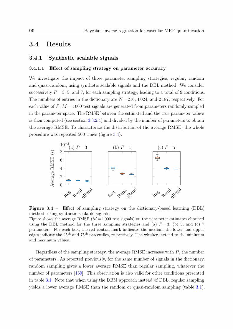
90 Bayesian inverse regression for vascular MRF quantification
3.4 Results
3.4.1 Synthetic scalable signals
3.4.1.1 Effect of sampling strategy on parameter accuracy
We investigate the impact of three parameter sampling strategies, regular, randomand quasi-random, using synthetic scalable signals and the DBL method. We considersuccessively P = 3, 5, and 7, for each sampling strategy, leading to a total of 9 conditions.The numbers of entries in the dictionary are N = 216, 1 024, and 2 187, respectively. Foreach value of P , M = 1 000 test signals are generated from parameters randomly sampledin the parameter space. The RMSE between the estimated and the true parameter valuesis then computed (see section 3.3.2.4) and divided by the number of parameters to obtainthe average RMSE. To characterize the distribution of the average RMSE, the wholeprocedure was repeated 500 times (figure 3.4).
Reg RandqR
and
0
2
4
6
8
·10−2
Aver
age
RM
SE(s
) (a) P = 3
Reg RandqR
and
(b) P = 5
Reg RandqR
and
(c) P = 7
Figure 3.4 – Effect of sampling strategy on the dictionary-based learning (DBL)method, using synthetic scalable signals.Figure shows the average RMSE (M = 1 000 test signals) on the parameter estimates obtainedusing the DBL method for the three sampling strategies and (a) P = 3, (b) 5, and (c) 7parameters. For each box, the red central mark indicates the median; the lower and upperedges indicate the 25th and 75th percentiles, respectively. The whiskers extend to the minimumand maximum values.
Regardless of the sampling strategy, the average RMSE increases with P , the numberof parameters. As reported previously, for the same number of signals in the dictionary,random sampling gives a lower average RMSE than regular sampling, whatever thenumber of parameters [169]. This observation is also valid for other conditions presentedin table 3.1. Note that when using the DBM approach instead of DBL, regular samplingyields a lower average RMSE than the random or quasi-random sampling (table 3.1).

3.4 Results 91
Dictionaries DBM DBL
P N Regular Random qRandom Regular Random qRandom
3 512 36.9 ± 0.5 48.1 ± 1.0 43.0 ± 0.8 11.0 ± 0.8 11.0 ± 0.8 9.6 ± 0.6
3 1 728 24.9 ± 0.3 31.9 ± 0.6 28.8 ± 0.5 8.1 ± 0.4 8.7 ± 0.4 8.1 ± 0.4
3 4 096 18.7 ± 0.3 23.9 ± 0.4 21.5 ± 0.4 7.6 ± 0.3 8.1 ± 0.4 7.8 ± 0.3
5 1 024 74.8 ± 0.8 88.3 ± 1.2 84.3 ± 1.0 39.8 ± 2.3 27.1 ± 0.2 25.3 ± 0.7
5 3 125 60.6 ± 0.7 70.3 ± 0.9 68.0 ± 0.8 30.3 ± 1.2 22.5 ± 0.6 21.8 ± 0.6
5 7 776 51.0 ± 0.6 58.5 ± 0.7 56.6 ± 0.8 25.2 ± 0.7 21.0 ± 0.5 20.6 ± 0.5
7 2 187 98.6 ± 0.9 112.3 ± 1.2 111.3 ± 1.2 65.6 ± 2.9 39.0 ± 1.2 38.3 ± 1.0
7 16 384 75.1 ± 0.7 83.5 ± 0.8 82.1 ± 0.8 45.3 ± 1.8 31.1 ± 0.7 30.57 ± 0.7
Table 3.1 – Effect of parameter sampling strategies on the dictionary-based methods(DBL and DBM), using synthetic scalable signals.Average RMSE (M = 1 000 test signals) on the parameter estimates obtained using the DBMand DBL methods for the three sampling strategies: grid (regular), random and quasi-random(qRandom) obtained from scrambled Sobol sequence, and 8 combinations of P and N values.
The quasi-random sampling further reduces the average RMSE up to 12.4 %. Altogether,there is a reduction of 12.3 %, 36.4 % and 41.7 % in average RMSE between regularand quasi-random sampling for 3, 5, and 7 parameters, respectively. Therefore, in thefollowing, a regular sampling is used for the DBM method and a quasi-random samplingis used for the DBL method.
3.4.1.2 Effect of noise addition on dictionary signals
To investigate the impact of noise addition on the DBL method robustness, we generatefour scalable signals dictionaries: N = 500 and 2 000 (for P = 3), and N = 2 000 and 10 000(for P = 5). We consider three data augmentation approaches (or data improvement sincethe amount of data is not necessarily increased), using various noise levels. We usedthe initial matrix Ydico of dictionary signals to build the matrix Yaugmented used to trainmapping according to one of the three following data augmentation procedures [186]:
• The dictionary fingerprints Ydico is substituted by its noisy version Ynoisy,1 accordingto SNRdico,1, see equation (3.8).
• Ydico is doubled in size with the noisy signals Ynoisy,1, see equation (3.9).• Ydico is augmented twice in size by noisy signals Ynoisy,1 and Ynoisy,2 according to
SNRdico,1 and SNRdico,2, see equation (3.10).
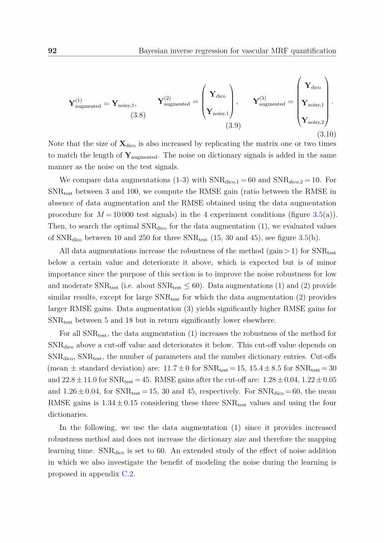
92 Bayesian inverse regression for vascular MRF quantification
Y(1)augmented = Ynoisy,1,
(3.8)
Y(2)augmented =
Ydico
Ynoisy,1
,
(3.9)
Y(3)augmented =
Ydico
Ynoisy,1
Ynoisy,2
.
(3.10)Note that the size of Xdico is also increased by replicating the matrix one or two timesto match the length of Yaugmented. The noise on dictionary signals is added in the samemanner as the noise on the test signals.
We compare data augmentations (1-3) with SNRdico,1 = 60 and SNRdico,2 = 10. ForSNRtest between 3 and 100, we compute the RMSE gain (ratio between the RMSE inabsence of data augmentation and the RMSE obtained using the data augmentationprocedure for M = 10 000 test signals) in the 4 experiment conditions (figure 3.5(a)).Then, to search the optimal SNRdico for the data augmentation (1), we evaluated valuesof SNRdico between 10 and 250 for three SNRtest (15, 30 and 45), see figure 3.5(b).
All data augmentations increase the robustness of the method (gain > 1) for SNRtest
below a certain value and deteriorate it above, which is expected but is of minorimportance since the purpose of this section is to improve the noise robustness for lowand moderate SNRtest (i.e. about SNRtest ≤ 60). Data augmentations (1) and (2) providesimilar results, except for large SNRtest for which the data augmentation (2) provideslarger RMSE gains. Data augmentation (3) yields significantly higher RMSE gains forSNRtest between 5 and 18 but in return significantly lower elsewhere.
For all SNRtest, the data augmentation (1) increases the robustness of the method forSNRdico above a cut-off value and deteriorates it below. This cut-off value depends onSNRdico, SNRtest, the number of parameters and the number dictionary entries. Cut-offs(mean ± standard deviation) are: 11.7 ± 0 for SNRtest = 15, 15.4 ± 8.5 for SNRtest = 30and 22.8 ± 11.0 for SNRtest = 45. RMSE gains after the cut-off are: 1.28 ± 0.04, 1.22 ± 0.05and 1.26 ± 0.04, for SNRtest = 15, 30 and 45, respectively. For SNRdico = 60, the meanRMSE gains is 1.34 ± 0.15 considering these three SNRtest values and using the fourdictionaries.
In the following, we use the data augmentation (1) since it provides increasedrobustness method and does not increase the dictionary size and therefore the mappinglearning time. SNRdico is set to 60. An extended study of the effect of noise additionin which we also investigate the benefit of modeling the noise during the learning isproposed in appendix C.2.
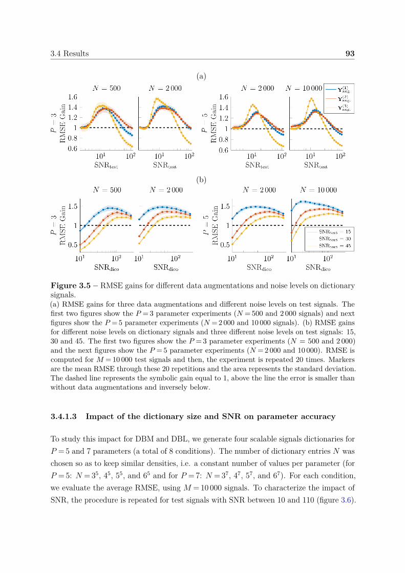
3.4 Results 93
(a)
(b)
Figure 3.5 – RMSE gains for different data augmentations and noise levels on dictionarysignals.(a) RMSE gains for three data augmentations and different noise levels on test signals. Thefirst two figures show the P = 3 parameter experiments (N = 500 and 2 000 signals) and nextfigures show the P = 5 parameter experiments (N = 2 000 and 10 000 signals). (b) RMSE gainsfor different noise levels on dictionary signals and three different noise levels on test signals: 15,30 and 45. The first two figures show the P = 3 parameter experiments (N = 500 and 2 000)and the next figures show the P = 5 parameter experiments (N = 2 000 and 10 000). RMSE iscomputed for M = 10 000 test signals and then, the experiment is repeated 20 times. Markersare the mean RMSE through these 20 repetitions and the area represents the standard deviation.The dashed line represents the symbolic gain equal to 1, above the line the error is smaller thanwithout data augmentations and inversely below.
3.4.1.3 Impact of the dictionary size and SNR on parameter accuracy
To study this impact for DBM and DBL, we generate four scalable signals dictionaries forP = 5 and 7 parameters (a total of 8 conditions). The number of dictionary entries N waschosen so as to keep similar densities, i.e. a constant number of values per parameter (forP = 5: N = 35, 45, 55, and 65 and for P = 7: N = 37, 47, 57, and 67). For each condition,we evaluate the average RMSE, using M = 10 000 signals. To characterize the impact ofSNR, the procedure is repeated for test signals with SNR between 10 and 110 (figure 3.6).
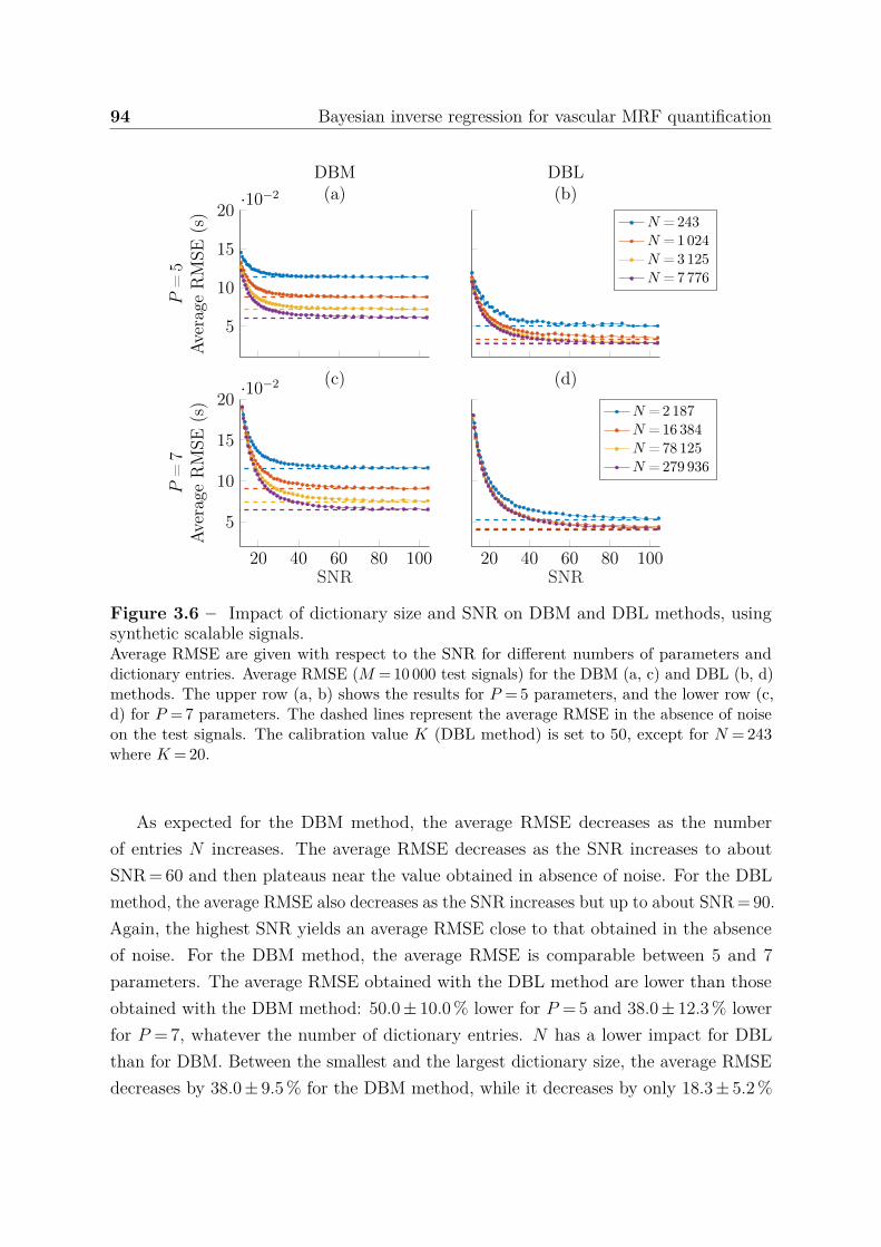
94 Bayesian inverse regression for vascular MRF quantification
5
10
15
20·10−2
P=
5Av
erag
eR
MSE
(s)
DBM(a)
DBL(b)
N = 243N = 1024N = 3125N = 7776
20 40 60 80 100
5
10
15
20·10−2
SNR
P=
7Av
erag
eR
MSE
(s)
(c)
20 40 60 80 100SNR
(d)
N = 2187N = 16 384N = 78 125N = 279 936
Figure 3.6 – Impact of dictionary size and SNR on DBM and DBL methods, usingsynthetic scalable signals.Average RMSE are given with respect to the SNR for different numbers of parameters anddictionary entries. Average RMSE (M = 10 000 test signals) for the DBM (a, c) and DBL (b, d)methods. The upper row (a, b) shows the results for P = 5 parameters, and the lower row (c,d) for P = 7 parameters. The dashed lines represent the average RMSE in the absence of noiseon the test signals. The calibration value K (DBL method) is set to 50, except for N = 243where K = 20.
As expected for the DBM method, the average RMSE decreases as the numberof entries N increases. The average RMSE decreases as the SNR increases to aboutSNR = 60 and then plateaus near the value obtained in absence of noise. For the DBLmethod, the average RMSE also decreases as the SNR increases but up to about SNR = 90.Again, the highest SNR yields an average RMSE close to that obtained in the absenceof noise. For the DBM method, the average RMSE is comparable between 5 and 7parameters. The average RMSE obtained with the DBL method are lower than thoseobtained with the DBM method: 50.0 ± 10.0 % lower for P = 5 and 38.0 ± 12.3 % lowerfor P = 7, whatever the number of dictionary entries. N has a lower impact for DBLthan for DBM. Between the smallest and the largest dictionary size, the average RMSEdecreases by 38.0 ± 9.5 % for the DBM method, while it decreases by only 18.3 ± 5.2 %
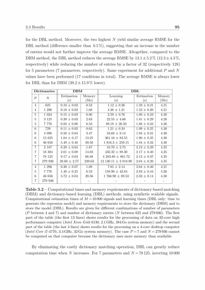
3.4 Results 95
for the DBL method. Moreover, the two highest N yield similar average RMSE for theDBL method (difference smaller than 0.5 %), suggesting that an increase in the numberof entries would not further improve the average RMSE. Altogether, compared to theDBM method, the DBL method reduces the average RMSE by 13.1 ± 5.2 % (12.3 ± 4.3 %,respectively) while reducing the number of entries by a factor of 32 (respectively 128)for 5 parameters (7 parameters, respectively). Same experiment for additional P and N
values have been performed (17 conditions in total). The average RMSE is always lowerfor DBL than for DBM (39.2 ± 15.9 % lower).
Dictionaries DBM DBL
P NEstimation
(s)Memory
(Mo)Learning
(s)Estimation
(s)Memory
(Mo)4 625 0.10 ± 0.02 0.52 1.12 ± 0.26 1.59 ± 0.21 4.214 1 296 0.18 ± 0.02 1.08 4.26 ± 1.21 1.52 ± 0.20 4.215 1 024 0.15 ± 0.02 0.86 2.59 ± 0.76 1.80 ± 0.23 4.265 3 125 0.39 ± 0.03 2.63 22.55 ± 4.66 1.81 ± 0.29 4.265 7 776 0.92 ± 0.06 6.53 89.18 ± 26.50 1.86 ± 0.32 4.266 729 0.11 ± 0.02 0.62 1.21 ± 0.34 1.99 ± 0.25 4.306 4 096 0.50 ± 0.04 3.47 34.68 ± 8.14 1.94 ± 0.31 4.306 15 625 1.84 ± 0.17 13.25 361.16 ± 83.55 1.90 ± 0.35 4.306 46 656 5.49 ± 0.48 39.56 1 816.3 ± 259.15 1.84 ± 0.32 4.307 2 187 0.29 ± 0.04 1.87 10.70 ± 2.75 2.13 ± 0.29 4.357 16 384 2.01 ± 0.08 14.03 432.32 ± 88.30 2.17 ± 0.40 4.357 78 125 9.17 ± 0.63 66.88 4 283.80 ± 861.72 2.12 ± 0.37 4.357 279 936 28.60 ± 2.57 239.63 12 130.11 ± 2 018.90 2.04 ± 0.20 4.354 1 296 0.30 ± 0.07 1.08 7.85 ± 2.14 2.64 ± 0.46 4.215 7 776 1.40 ± 0.25 6.53 158.90 ± 42.84 2.83 ± 0.44 4.266 46 656 5.72 ± 0.04 39.56 1 766.90 ± 89.53 2.33 ± 0.14 4.307 279 936 - - - - -
Table 3.2 – Computational times and memory requirements of dictionary-based matching(DBM) and dictionary-based learning (DBL) methods, using synthetic scalable signals.Computational estimation times of M = 10 000 signals and learning times (DBL only: time togenerate the regression model) and memory requirements to store the dictionary (DBM) and tostore the model (DBL). Results are given for different combinations of number of parameters(P between 4 and 7) and number of dictionary entries (N between 625 and 279 936). The firstpart of the table (the first 13 lines) shows results for the processing of data on 32-core highperformance computer (Intel Xeon Gold 6130, 2.1 GHz, 384 Go system memory) and the secondpart of the table (the last 4 lines) shows results for the processing on a 4-core desktop computer(Intel Core i7-4770, 3.4 GHz, 32 Go system memory). The case P = 7 and N = 279 936 cannotbe computed on that computer because the dictionary uses more memory than available.
By eliminating the costly dictionary matching operation, DBL can greatly reducecomputation time when N increases. For 7 parameters and N = 78 125, inverting 10 000
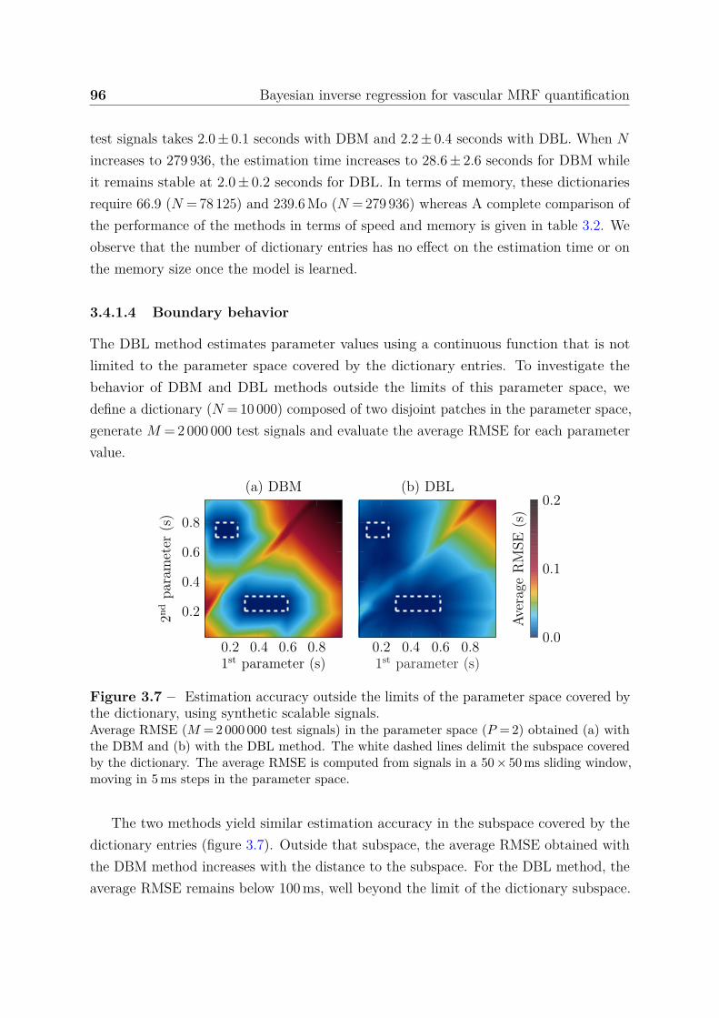
96 Bayesian inverse regression for vascular MRF quantification
test signals takes 2.0 ± 0.1 seconds with DBM and 2.2 ± 0.4 seconds with DBL. When N
increases to 279 936, the estimation time increases to 28.6 ± 2.6 seconds for DBM whileit remains stable at 2.0 ± 0.2 seconds for DBL. In terms of memory, these dictionariesrequire 66.9 (N = 78 125) and 239.6 Mo (N = 279 936) whereas A complete comparison ofthe performance of the methods in terms of speed and memory is given in table 3.2. Weobserve that the number of dictionary entries has no effect on the estimation time or onthe memory size once the model is learned.
3.4.1.4 Boundary behavior
The DBL method estimates parameter values using a continuous function that is notlimited to the parameter space covered by the dictionary entries. To investigate thebehavior of DBM and DBL methods outside the limits of this parameter space, wedefine a dictionary (N = 10 000) composed of two disjoint patches in the parameter space,generate M = 2 000 000 test signals and evaluate the average RMSE for each parametervalue.
0.2 0.4 0.6 0.8
0.2
0.4
0.6
0.8
1st parameter (s)
2nd
para
met
er(s
)
(a) DBM
0.2 0.4 0.6 0.81st parameter (s)
(b) DBL
0.0
0.1
0.2Av
erag
eR
MSE
(s)
Figure 3.7 – Estimation accuracy outside the limits of the parameter space covered bythe dictionary, using synthetic scalable signals.Average RMSE (M = 2 000 000 test signals) in the parameter space (P = 2) obtained (a) withthe DBM and (b) with the DBL method. The white dashed lines delimit the subspace coveredby the dictionary. The average RMSE is computed from signals in a 50 × 50 ms sliding window,moving in 5 ms steps in the parameter space.
The two methods yield similar estimation accuracy in the subspace covered by thedictionary entries (figure 3.7). Outside that subspace, the average RMSE obtained withthe DBM method increases with the distance to the subspace. For the DBL method, theaverage RMSE remains below 100 ms, well beyond the limit of the dictionary subspace.
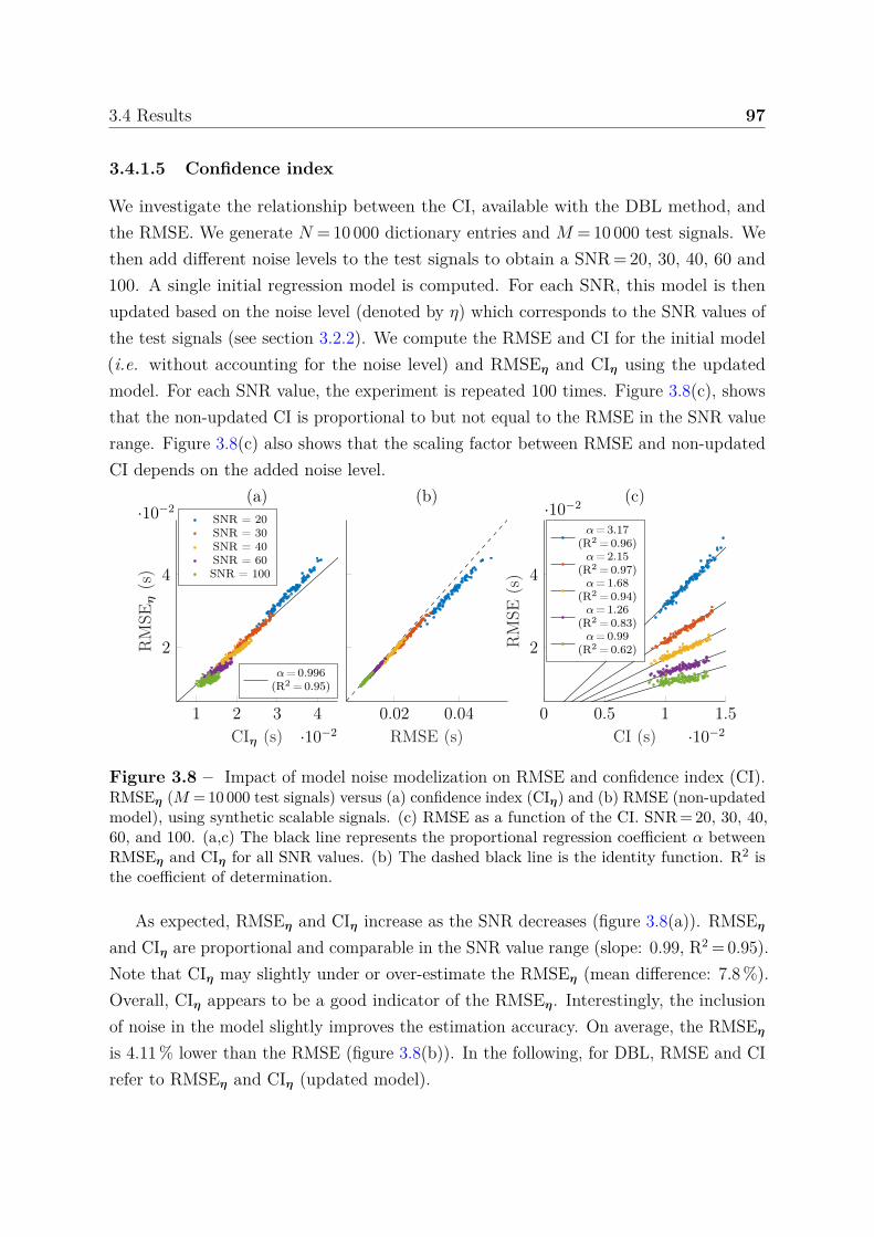
3.4 Results 97
3.4.1.5 Confidence index
We investigate the relationship between the CI, available with the DBL method, andthe RMSE. We generate N = 10 000 dictionary entries and M = 10 000 test signals. Wethen add different noise levels to the test signals to obtain a SNR = 20, 30, 40, 60 and100. A single initial regression model is computed. For each SNR, this model is thenupdated based on the noise level (denoted by η) which corresponds to the SNR values ofthe test signals (see section 3.2.2). We compute the RMSE and CI for the initial model(i.e. without accounting for the noise level) and RMSEη and CIη using the updatedmodel. For each SNR value, the experiment is repeated 100 times. Figure 3.8(c), showsthat the non-updated CI is proportional to but not equal to the RMSE in the SNR valuerange. Figure 3.8(c) also shows that the scaling factor between RMSE and non-updatedCI depends on the added noise level.
1 2 3 4
·10−2
2
4
·10−2
CIη (s)
RM
SEη
(s)
(a)
α= 0.996(R2 = 0.95)
0.02 0.04
RMSE (s)
(b)SNR = 20SNR = 30SNR = 40SNR = 60SNR = 100
0 0.5 1 1.5
·10−2
2
4
·10−2
CI (s)
RM
SE(s
)(c)
α= 3.17(R2 = 0.96)α= 2.15
(R2 = 0.97)α= 1.68
(R2 = 0.94)α= 1.26
(R2 = 0.83)α= 0.99
(R2 = 0.62)
Figure 3.8 – Impact of model noise modelization on RMSE and confidence index (CI).RMSEη (M = 10 000 test signals) versus (a) confidence index (CIη) and (b) RMSE (non-updatedmodel), using synthetic scalable signals. (c) RMSE as a function of the CI. SNR = 20, 30, 40,60, and 100. (a,c) The black line represents the proportional regression coefficient α betweenRMSEη and CIη for all SNR values. (b) The dashed black line is the identity function. R2 isthe coefficient of determination.
As expected, RMSEη and CIη increase as the SNR decreases (figure 3.8(a)). RMSEη
and CIη are proportional and comparable in the SNR value range (slope: 0.99, R2 = 0.95).Note that CIη may slightly under or over-estimate the RMSEη (mean difference: 7.8 %).Overall, CIη appears to be a good indicator of the RMSEη. Interestingly, the inclusionof noise in the model slightly improves the estimation accuracy. On average, the RMSEη
is 4.11 % lower than the RMSE (figure 3.8(b)). In the following, for DBL, RMSE and CIrefer to RMSEη and CIη (updated model).
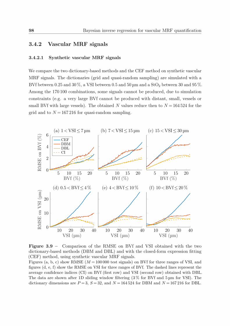
98 Bayesian inverse regression for vascular MRF quantification
3.4.2 Vascular MRF signals
3.4.2.1 Synthetic vascular MRF signals
We compare the two dictionary-based methods and the CEF method on synthetic vascularMRF signals. The dictionaries (grid and quasi-random sampling) are simulated with aBVf between 0.25 and 30 %, a VSI between 0.5 and 50 µm and a StO2 between 30 and 95 %.Among the 170 100 combinations, some signals cannot be produced, due to simulationconstraints (e.g. a very large BVf cannot be produced with distant, small, vessels orsmall BVf with large vessels). The obtained N values reduce then to N = 164 524 for thegrid and to N = 167 216 for quasi-random sampling.
5 10 15 200
2
4
6
BVf (%)
RM
SEon
BV
f(%
)
(a) 1<VSI≤ 7 µm
CEFDBMDBLCI
5 10 15 20BVf (%)
(b) 7<VSI≤ 15 µm
5 10 15 20BVf (%)
(c) 15<VSI≤ 30 µm
10 20 30 400
10
20
VSI (µm)
RM
SEon
VSI
(µm
) (d) 0.5<BVf≤ 4%
10 20 30 40VSI (µm)
(e) 4<BVf≤ 10%
10 20 30 40VSI (µm)
(f) 10<BVf≤ 20%
Figure 3.9 – Comparison of the RMSE on BVf and VSI obtained with the twodictionary-based methods (DBM and DBL) and with the closed-form expression fitting(CEF) method, using synthetic vascular MRF signals.Figures (a, b, c) show RMSE (M = 100 000 test signals) on BVf for three ranges of VSI, andfigures (d, e, f) show the RMSE on VSI for three ranges of BVf. The dashed lines represent theaverage confidence indices (CI) on BVf (first row) and VSI (second row) obtained with DBL.The data are shown after 1D sliding window filtering (3 % for BVf and 5 µm for VSI). Thedictionary dimensions are P = 3, S = 32, and N = 164 524 for DBM and N = 167 216 for DBL.

3.4 Results 99
For each method, M = 100 000 test signals (SNR = 100) are generated. To analyzethe BVf RMSE, test signals are divided into three parts: small, medium and large vesselsizes. To analyze the VSI RMSE, test signals are divided into three parts: low, mediumand large blood volumes.
For all vessel diameters, the RMSE on BVf tends to increase with BVf (figure 3.9).The DBM and CEF methods yield similar RMSE for BVf values below 10 %. For mediumand large vessels and large BVf values, the CEF method yields the highest errors. TheDBL method always yields the lowest error with an RMSE of 2.38 % for CEF, 2.68 % forDBM and 1.30 % for DBL.
For VSI values smaller than 15 µm, the behavior of the RMSE is similar in all threemethods for the three BVf ranges. Above 15 µm, the CEF method yields larger errorsthan the two dictionary-based approaches and the RMSE obtained with CEF is linearlycorrelated with the VSI value (R2 ≥ 0.99). This linear behavior has already been reportedin [187]. DBL yields a 25 % smaller RMSE than DBM, on average with an RMSE of12.46 µm for CEF, 6.11 µm for DBM, and 4.50 µm for DBL. The CI appears again tobe a good indicator of the RMSE, with maximum differences between CI and RMSE of1.07 % for BVf and 2.36 µm for VSI and average differences of 0.25 % and 0.75 µm.
3.4.2.2 Acquired vascular MRF signals
The DBL method is then applied to acquired vascular MRF signals collected from ratsbearing 9L and C6 tumors. We quantify BVf, VSI and StO2 with both dictionary-based methods (DBM and DBL) and using two numbers of dictionary entries. Thelarge dictionary (N = 170 100) is the one used previously in section 3.4.2.1. The smalldictionary (N = 4 320) is simulated with BVf between 0.33 and 12 %, VSI between 1 and20 µm and StO2 between 40 and 90 %.
All methods yield consistent estimates (figure 3.10), in which the tumor and the largevessels can be easily depicted on BVf and VSI maps. StO2 appears constant in healthytissues. However, for DBM, there are many isolated high values, suggesting noisy maps.In [154], the authors proposed to remove the last 8 signal samples and apply a spatialGaussian filtering to increase the SNR. Using the DBM method, these additional stepsallowed them to produce less noisy maps. Interestingly, with the DBL method, thesesteps are no longer required. Our approach is therefore more likely to preserve smallstructure information, which may be otherwise removed by an additional spatial filtering.
For the large dictionary, the mean BVf and VSI obtained in tumor with the DBMand DBL methods are similar but with the DBL method, we can differentiate different
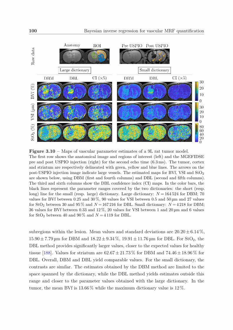
100 Bayesian inverse regression for vascular MRF quantification
Figure 3.10 – Maps of vascular parameter estimates of a 9L rat tumor model.The first row shows the anatomical image and regions of interest (left) and the MGEFIDSEpre and post USPIO injection (right) for the second echo time (6.3 ms). The tumor, cortexand striatum are respectively delineated with green, yellow and blue lines. The arrows on thepost-USPIO injection image indicate large vessels. The estimated maps for BVf, VSI and StO2are shown below, using DBM (first and fourth columns) and DBL (second and fifth columns).The third and sixth columns show the DBL confidence index (CI) maps. In the color bars, theblack lines represent the parameter ranges covered by the two dictionaries: the short (resp.long) line for the small (resp. large) dictionary. Large dictionary: N = 164 524 for DBM; 70values for BVf between 0.25 and 30 %, 90 values for VSI between 0.5 and 50 µm and 27 valuesfor StO2 between 30 and 95 % and N = 167 216 for DBL. Small dictionary: N = 4 218 for DBM;36 values for BVf between 0.33 and 12 %, 20 values for VSI between 1 and 20 µm and 6 valuesfor StO2 between 40 and 90 % and N = 4 119 for DBL.
subregions within the lesion. Mean values and standard deviations are 20.20 ± 6.14 %,15.90 ± 7.79 µm for DBM and 18.22 ± 9.34 %, 19.91 ± 11.76 µm for DBL. For StO2, theDBL method provides significantly larger values, closer to the expected values for healthytissue [188]. Values for striatum are 62.67 ± 21.73 % for DBM and 74.46 ± 18.96 % forDBL. Overall, DBM and DBL yield comparable values. For the small dictionary, thecontrasts are similar. The estimates obtained by the DBM method are limited to thespace spanned by the dictionary, while the DBL method yields estimates outside thisrange and closer to the parameter values obtained with the large dictionary. In thetumor, the mean BVf is 13.66 % while the maximum dictionary value is 12 %.
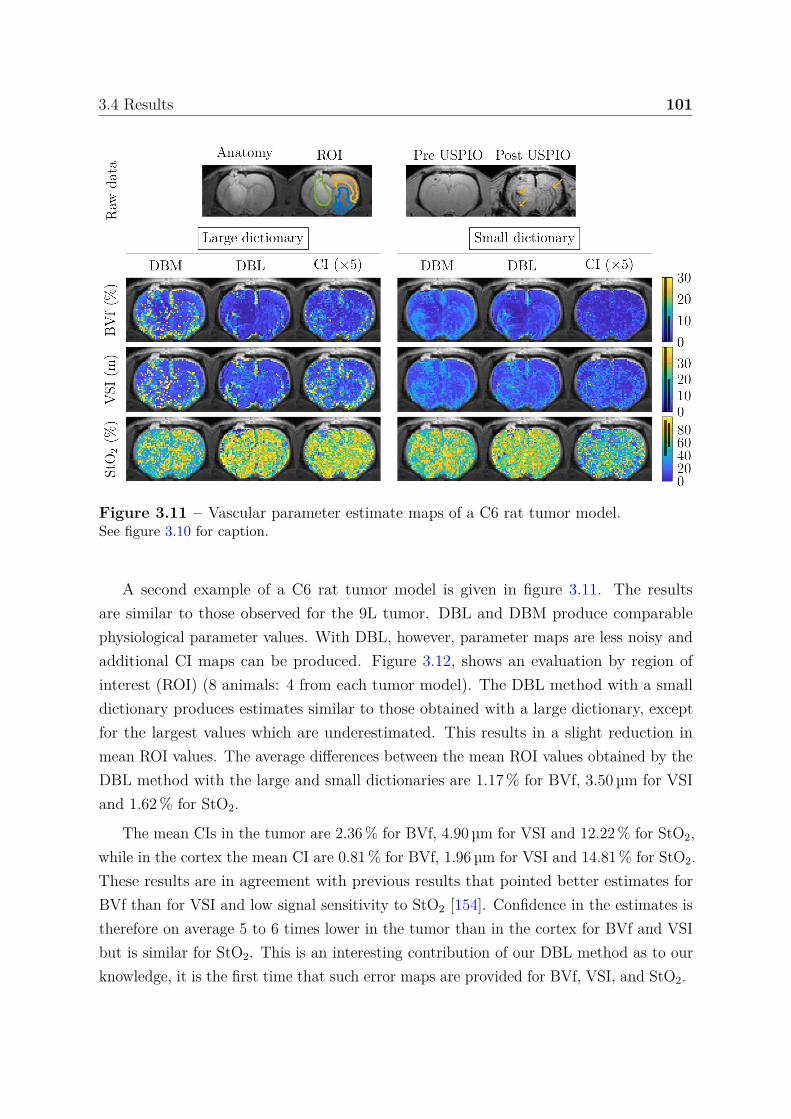
3.4 Results 101
Figure 3.11 – Vascular parameter estimate maps of a C6 rat tumor model.See figure 3.10 for caption.
A second example of a C6 rat tumor model is given in figure 3.11. The resultsare similar to those observed for the 9L tumor. DBL and DBM produce comparablephysiological parameter values. With DBL, however, parameter maps are less noisy andadditional CI maps can be produced. Figure 3.12, shows an evaluation by region ofinterest (ROI) (8 animals: 4 from each tumor model). The DBL method with a smalldictionary produces estimates similar to those obtained with a large dictionary, exceptfor the largest values which are underestimated. This results in a slight reduction inmean ROI values. The average differences between the mean ROI values obtained by theDBL method with the large and small dictionaries are 1.17 % for BVf, 3.50 µm for VSIand 1.62 % for StO2.
The mean CIs in the tumor are 2.36 % for BVf, 4.90 µm for VSI and 12.22 % for StO2,while in the cortex the mean CI are 0.81 % for BVf, 1.96 µm for VSI and 14.81 % for StO2.These results are in agreement with previous results that pointed better estimates forBVf than for VSI and low signal sensitivity to StO2 [154]. Confidence in the estimates istherefore on average 5 to 6 times lower in the tumor than in the cortex for BVf and VSIbut is similar for StO2. This is an interesting contribution of our DBL method as to ourknowledge, it is the first time that such error maps are provided for BVf, VSI, and StO2.

102 Bayesian inverse regression for vascular MRF quantification
9L C6 Cort Striat0
10
20
(a) BVf (%)CEFDBM (large dict)DBL (large dict)DBL (small dict)
9L C6 Cort Striat0
10
20
(b) VSI (µm)
9L C6 Cort Striat
40
60
80
100(c) StO2 (%)
Figure 3.12 – Mean estimates by regions of interest of the vascular parameters.(a) BVf, (b) VSI and (c) StO2 computed performing 3 methods: the closed-form expressionfitting (CEF), the dictionary-based matching (DBM) and the dictionary-based learning (DBL)using 2 different numbers of dictionary entries. The colored bars are the average values of themean vascular parameters by regions of interest (9L and C6 lesions: 4 rats, cortex (Cort) andstriatum (Striat): 8 rats) and error bars are the standard deviations centered on the averagevalues.
3.5 Discussion, conclusion and perspectives
This work presents a method for estimating vascular MRF parameters based on dictionarylearning. It preserves the main advantages of the MRF method, i.e. robustness, speedand flexibility, and meets the challenge of producing accurate estimates from a smalldictionary, even when the dimension of the parameters is large.
Regarding the design of the dictionary, we observe as [169] that random samplingof the parameter space gives more accurate estimates than grid sampling, when aninverse regression model is used. We further show that quasi-random sampling gives evenbetter estimates. However, when the DBM method is used, the grid remains the mostefficient sampling strategy. The appropriate dictionary design depends thus on the choseninversion approach (grid matching vs statistical learning). The results obtained with theDBL method suggest that the simulation of a few patches (with quasi-random sampling)in the parameter space could save even more time in the construction of the dictionary(section 3.4.1.4). This result seems specific to the regression method. Indeed, a studyusing neural networks [165] rather reported increased deviations from the true values atthe boundaries of the training dictionary. This is likely due to the vanishing gradientof the activation function in these regions. This patch approach could be implementedby combining a set of parameter values corresponding to healthy tissues and one or
3.5 Discussion, conclusion and perspectives 103
more sets corresponding to damaged tissues (e.g. tumorous tissues). If needed, a fewadditional dictionary entries can be generated to fill gaps between patches (investigatedin the next chapter, section 4.3.1.4).
Regarding the quality of the inversion, the regression approach usually involvescalibration. In GLLiM, the number of Gaussian distributions K is the only calibrationvalue that needs to be adjusted. This can be done automatically using a standardinformation criterion such as AIC or BIC [189, 190], as illustrated in [176], but this mayresult in additional learning time. We have observed that our results have little dependenceon K. In contrast, neural networks [165–169, 173–175] used to solve similar inverseproblems are very sensitive to their many complex calibration settings: architecture,batch sizes, learning rates, among others. The adjustment of all these calibration settingsis usually performed by learning the model for a large number of calibration valuecombinations, which represents a higher computational cost than determining a singlecalibration value as in GLLIM. This difference in calibration cost makes the DBL methodmore flexible in case of change in dictionary design (extension of the parameter range,additional parameters, etc.). In addition, GLLiM has the advantage of providing a richerinformation. Here, we make use of the full posterior parameter distribution provided byGLLiM to derive a CI for each estimate. We observe that this CI matches the RMSE incases where a ground truth is available (synthetic scalable; section 3.4.1.5 and syntheticvascular MRF signals; section 3.4.2.1). Interestingly, this CI reports both signal andmodel errors (derived from the dictionary) and thus reflects the whole DBL procedure.
Regarding the acquired vascular MRF signals, we observe that the number of dictionaryentries can be divided by about 40 using the DBL method and still lead to accuratemaps. The maps produced with the DBL method are significantly less noisy than thoseobtained with the DBM method and some structures, not observed with DBM, appear inthe lesions. The additional tissue contrast provided by DBL could therefore contributeto improved tumor characterization [191].
In conclusion, this first evaluation of the DBL method appears promising. It reducesthe simulation time and the memory required for dictionary storage, improves parameteraccuracy, reduces the estimation time, and provides a first confidence index on parameterestimates. The DBL method could become even more efficient as the number of pa-rameters to be estimated increases, which can happen when considering all the possiblecontributions of the tissues and the scanner to the signal. In addition, the flexibility ofthe proposed approach opens the door to further improvements. In particular, futurework should include the adaptation and optimization of the dictionary sampling strategy

104 Bayesian inverse regression for vascular MRF quantification
with respect to the targeted range of parameters to estimate. In addition, MRI producescomplex-valued data but machine learning methodologies are generally designed forreal-valued data. Dealing with complex-valued data could boost the performance ofDBL [168]. This requires an adjustment of the inverse regression method also left tofuture work.
Chapter 4
Statistical learning vs deep learningin generalized MRF applications
This study is in line with the previous one. The objective is to compare the performanceof the proposed dictionary-based learning method (chapter 3) with a DBL method usinga neural network. Part of this study was presented during the 2020 congress of theInternational Society for Magnetic Resonance in Medicine (ISMRM) [13]. This sectionalso extends the previous study to further investigations using standard MRF signalsto estimate relaxation times T1 and T2, and off-resonance. This results in investigatinghighly undersampled data issues and complex-valued signal considerations.
4.1 Introduction
A major reason for the popularity of the dictionary-based matching (DBM) method isits flexibility since it does not require specific adjustment depending on the application(e.g. signal length, number of parameters, complexity of the mapping...). Potentially, theuser may choose a different distance (or dissimilarity) function in equation (2.32) but inpractice the dot product works sufficiently well. Instead, when using a dictionary-basedlearning (DBL) approach, a model is used to approximate the mapping between signaland parameter spaces. The choice of the model is therefore critical. It must be able toaccurately approximate the mapping between these spaces and, if that relationship iscomplex (i.e. highly non-linear), the model is required to have a very high modelingpower. Then, a larger model generally demands a greater number of dictionary entries inorder to be properly trained and therefore implies an increase in computational costs. The
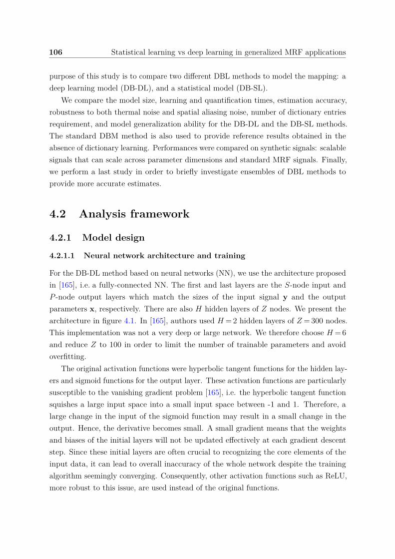
106 Statistical learning vs deep learning in generalized MRF applications
purpose of this study is to compare two different DBL methods to model the mapping: adeep learning model (DB-DL), and a statistical model (DB-SL).
We compare the model size, learning and quantification times, estimation accuracy,robustness to both thermal noise and spatial aliasing noise, number of dictionary entriesrequirement, and model generalization ability for the DB-DL and the DB-SL methods.The standard DBM method is also used to provide reference results obtained in theabsence of dictionary learning. Performances were compared on synthetic signals: scalablesignals that can scale across parameter dimensions and standard MRF signals. Finally,we perform a last study in order to briefly investigate ensembles of DBL methods toprovide more accurate estimates.
4.2 Analysis framework
4.2.1 Model design
4.2.1.1 Neural network architecture and training
For the DB-DL method based on neural networks (NN), we use the architecture proposedin [165], i.e. a fully-connected NN. The first and last layers are the S-node input andP -node output layers which match the sizes of the input signal y and the outputparameters x, respectively. There are also H hidden layers of Z nodes. We present thearchitecture in figure 4.1. In [165], authors used H = 2 hidden layers of Z = 300 nodes.This implementation was not a very deep or large network. We therefore choose H = 6and reduce Z to 100 in order to limit the number of trainable parameters and avoidoverfitting.
The original activation functions were hyperbolic tangent functions for the hidden lay-ers and sigmoid functions for the output layer. These activation functions are particularlysusceptible to the vanishing gradient problem [165], i.e. the hyperbolic tangent functionsquishes a large input space into a small input space between -1 and 1. Therefore, alarge change in the input of the sigmoid function may result in a small change in theoutput. Hence, the derivative becomes small. A small gradient means that the weightsand biases of the initial layers will not be updated effectively at each gradient descentstep. Since these initial layers are often crucial to recognizing the core elements of theinput data, it can lead to overall inaccuracy of the whole network despite the trainingalgorithm seemingly converging. Consequently, other activation functions such as ReLU,more robust to this issue, are used instead of the original functions.
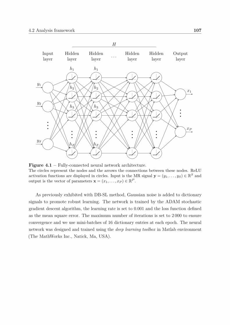
4.2 Analysis framework 107
... ... ... ... ...
...
y1
y2
yS
h1
h2
h3
hZ
h1
h2
h3
hZ
x1
xP
Inputlayer
Hiddenlayer
Hiddenlayer . . . Hidden
layerHiddenlayer
Outputlayer
H
Figure 4.1 – Fully-connected neural network architecture.The circles represent the nodes and the arrows the connections between these nodes. ReLUactivation functions are displayed in circles. Input is the MR signal y = (y1, . . . , yS) ∈ RS andoutput is the vector of parameters x = (x1, . . . , xP ) ∈ RP .
As previously exhibited with DB-SL method, Gaussian noise is added to dictionarysignals to promote robust learning. The network is trained by the ADAM stochasticgradient descent algorithm, the learning rate is set to 0.001 and the loss function definedas the mean square error. The maximum number of iterations is set to 2 000 to ensureconvergence and we use mini-batches of 16 dictionary entries at each epoch. The neuralnetwork was designed and trained using the deep learning toolbox in Matlab environment(The MathWorks Inc., Natick, Ma, USA).
108 Statistical learning vs deep learning in generalized MRF applications
4.2.1.2 Calibration model parameter set and model sizes
An increase in model size is commonly combined with an increase in the number ofdictionary entries and computational cost. However, the model must maintain a goodexpressivity to handle non-linear mappings. For example, linear and generalized linearregressions (e.g. least-square affine regression, perceptron, etc.) have a small model sizeO(SP ) but do not handle non-linear mappings1. In contrast, fully connected deep NNexhibit very high modeling power but the model size is O(HS2) (considering Z = S).This quadratic size is also observable with second order polynomial regressions thathave a model size in O(PS2). Note that nth order polynomial regressions have modelsizes in O(PSn). A reduction of the size of these models is possible by performing areduction/projection of the input signals. For example for NN, one can choose Z ≪ S toreduce model size to O(ZS). However, this reduction leads to a loss of information (i.e.reduction of explained variance). This loss is more or less important depending on thecomplexity of the input data structure.
C is the set of model calibration variables. Using the NN method, we identify twomodel calibration variables: C = Z, H. In this case, the model size is (H − 1)(Z2 +Z) + Z(S + 1) + P (Z + 1) = O(HZ2). Using the GLLiM model, we identify one modelcalibration variable: C = K and the model size is K(P + P 2 + 1 + SP + S) + S =O(KSP ) with equal diagonal covariance matrices. Note that using the original DBMmethod, C = ∅. One can roughly see the cardinal of C as an indication of model flexibility:it represents the number of parameters to be tuned for a new sequence.
4.2.2 Signals and performance evaluation
4.2.2.1 Standard MRF signal
To evaluate the proposed reconstruction methods on a standard relaxometry applicationof magnetic resonance fingerprinting (MRF) [137], we use an MRF acquisition schemebased on an inversion-recovery balanced steady state free-precession sequence to generatesynthetic MRF signals. According to [137], after an initial inversion pulse, the flip angleis a series of repeating sinusoidal curves with a period of 250 repetition times (TR)and alternating maximum flip angles (FA). In the odd periods, the FA is calculatedas FAt = 10 + 50 × sin
(2π500t
)+ rand(2), where t varies from 1 to 250 and rand(2)
is a function to generate normally distributed random numbers (mean is zero) with a1O is a mathematical notation that describes the limiting behavior of a function, here, the model
size function.
4.2 Analysis framework 109
standard deviation of 2. In the even periods, we divide the previous period’s FA by two.A 50-TR delay is added between each period. The TR pattern, between 10.5 and 14 ms, isgenerated following a procedural noise. This procedure yields pseudorandom acquisitionparameters. We consider S = 1 000 samples. FA and TR patterns as well as examplemagnitude synthetic MRF signals are shown in figure 4.6(a-c). The parameters of interest(P = 3) are the relaxation times T1 (between 200 and 3 000 ms) and T2 (between 20 and300 ms), and the off-resonance ∆f (between -200 and 200 Hz). Signals are generated usingthe simulation tool2 described in [157].
Note that compared to the vascular MRF signals used in the previous study, standardsignals are vectors of complex-valued samples. For the DBM method, the scalar productextends to complex data. However, to consider these complex samples using the twoDBL methods, signals are doubled in size and composed of the real and imaginary partsof the initial signals [167, 168].
4.2.2.2 Aliasing noise as modulated Gaussian noise
In [192], authors introduce a tool to rapidly assess the efficiency of an MRF sequence inthe presence of both normal and aliasing noise. In MRI, the acquired signal containsboth Gaussian noise ηthermal as the result of thermal contributions (section 2.2.2.4), andcorrelated aliasing noise ηaliasing due to spatial undersampling artifacts (section 2.2.2.3).According to this work, the aliasing noise can be modeled as proportional to the signal ateach sample, with a coefficient of proportionality that is taken to be zero-mean Gaussiannoise. It results that a noisy signal ynoisy is computed from an original signal y as:
ynoisy = y + ηthermal + |y| ηaliasing . (4.1)
In our experiments on aliasing artifacts, we focus on the case where aliasing noiseis dominant so that ηthermal = 0. In addition, we have empirically determined therelationship between the standard deviation σaliasing of ηaliasing and the undersamplingfactor R (validity range 1-50) as σaliasing = (3R − 2)/100. This entire procedure providestypical undersampled MRF signals, see examples in figure 4.7(d-f).
2https://bitbucket.org/asslaender/nyu_mrf_recon/src/master/
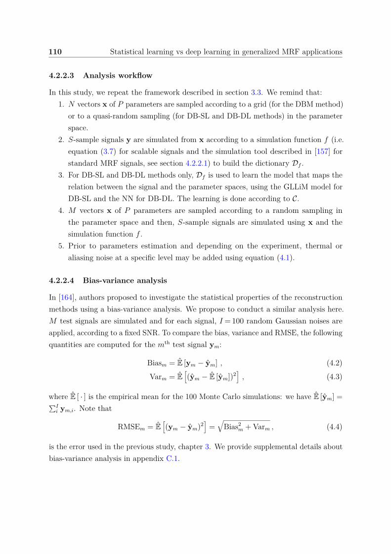
110 Statistical learning vs deep learning in generalized MRF applications
4.2.2.3 Analysis workflow
In this study, we repeat the framework described in section 3.3. We remind that:1. N vectors x of P parameters are sampled according to a grid (for the DBM method)
or to a quasi-random sampling (for DB-SL and DB-DL methods) in the parameterspace.
2. S-sample signals y are simulated from x according to a simulation function f (i.e.equation (3.7) for scalable signals and the simulation tool described in [157] forstandard MRF signals, see section 4.2.2.1) to build the dictionary Df .
3. For DB-SL and DB-DL methods only, Df is used to learn the model that maps therelation between the signal and the parameter spaces, using the GLLiM model forDB-SL and the NN for DB-DL. The learning is done according to C.
4. M vectors x of P parameters are sampled according to a random sampling inthe parameter space and then, S-sample signals are simulated using x and thesimulation function f .
5. Prior to parameters estimation and depending on the experiment, thermal oraliasing noise at a specific level may be added using equation (4.1).
4.2.2.4 Bias-variance analysis
In [164], authors proposed to investigate the statistical properties of the reconstructionmethods using a bias-variance analysis. We propose to conduct a similar analysis here.M test signals are simulated and for each signal, I = 100 random Gaussian noises areapplied, according to a fixed SNR. To compare the bias, variance and RMSE, the followingquantities are computed for the mth test signal ym:
Biasm = E [ym − ym] , (4.2)Varm = E
[(ym − E [ym])2
], (4.3)
where E [ · ] is the empirical mean for the 100 Monte Carlo simulations: we have E [ym] =∑Ii ym,i. Note that
RMSEm = E[(ym − ym)2
]=√
Bias2m + Varm , (4.4)
is the error used in the previous study, chapter 3. We provide supplemental details aboutbias-variance analysis in appendix C.1.
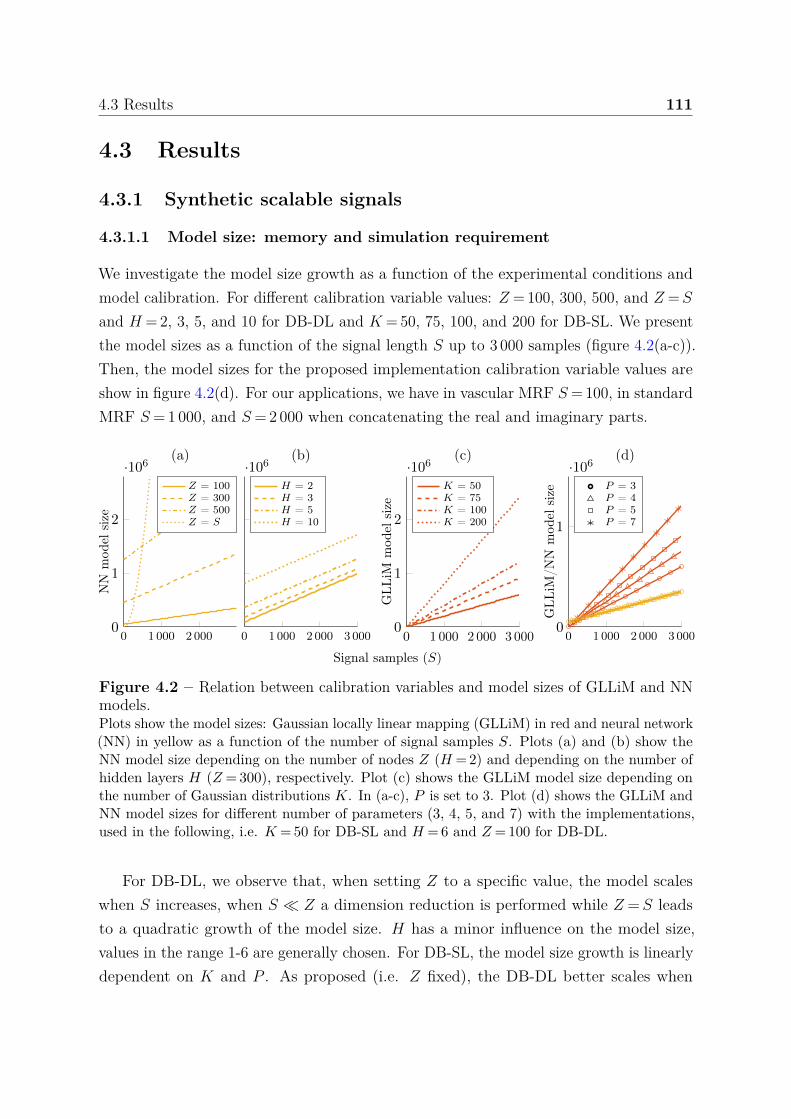
4.3 Results 111
4.3 Results
4.3.1 Synthetic scalable signals
4.3.1.1 Model size: memory and simulation requirement
We investigate the model size growth as a function of the experimental conditions andmodel calibration. For different calibration variable values: Z = 100, 300, 500, and Z = S
and H = 2, 3, 5, and 10 for DB-DL and K = 50, 75, 100, and 200 for DB-SL. We presentthe model sizes as a function of the signal length S up to 3 000 samples (figure 4.2(a-c)).Then, the model sizes for the proposed implementation calibration variable values areshow in figure 4.2(d). For our applications, we have in vascular MRF S = 100, in standardMRF S = 1 000, and S = 2 000 when concatenating the real and imaginary parts.
0 1 000 2 000 3 0000
1
·106
GLL
iM/N
Nm
odel
size
(d)
P = 3P = 4P = 5P = 7
0 1 000 2 0000
1
2
·106
NN
mod
elsi
ze
(a)
Z = 100Z = 300Z = 500Z = S
0 1 000 2 000 3 000
·106(b)
H = 2H = 3H = 5H = 10
0 1 000 2 000 3 0000
1
2
·106
Signal samples (S)
GLL
iMm
odel
size
(c)
K = 50K = 75K = 100K = 200
Figure 4.2 – Relation between calibration variables and model sizes of GLLiM and NNmodels.Plots show the model sizes: Gaussian locally linear mapping (GLLiM) in red and neural network(NN) in yellow as a function of the number of signal samples S. Plots (a) and (b) show theNN model size depending on the number of nodes Z (H = 2) and depending on the number ofhidden layers H (Z = 300), respectively. Plot (c) shows the GLLiM model size depending onthe number of Gaussian distributions K. In (a-c), P is set to 3. Plot (d) shows the GLLiM andNN model sizes for different number of parameters (3, 4, 5, and 7) with the implementations,used in the following, i.e. K = 50 for DB-SL and H = 6 and Z = 100 for DB-DL.
For DB-DL, we observe that, when setting Z to a specific value, the model scaleswhen S increases, when S ≪ Z a dimension reduction is performed while Z = S leadsto a quadratic growth of the model size. H has a minor influence on the model size,values in the range 1-6 are generally chosen. For DB-SL, the model size growth is linearlydependent on K and P . As proposed (i.e. Z fixed), the DB-DL better scales when
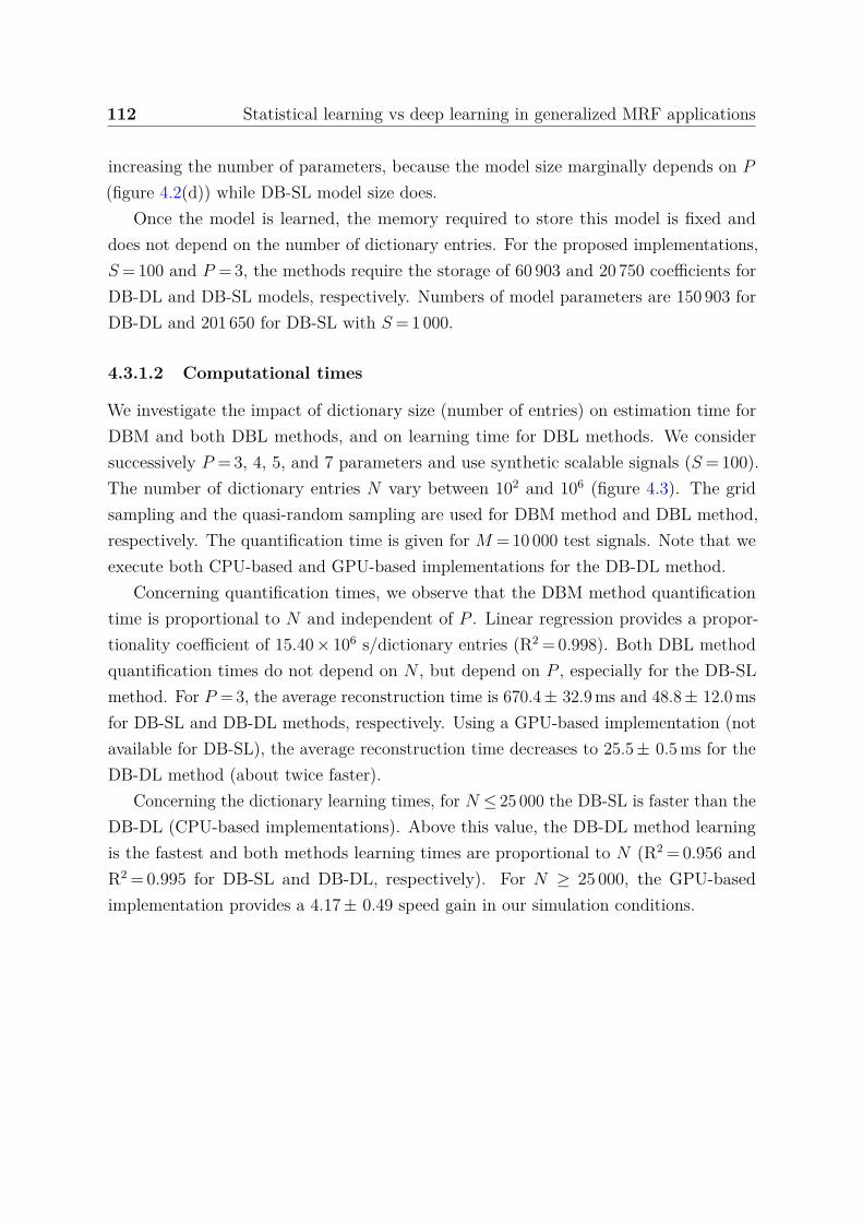
112 Statistical learning vs deep learning in generalized MRF applications
increasing the number of parameters, because the model size marginally depends on P
(figure 4.2(d)) while DB-SL model size does.Once the model is learned, the memory required to store this model is fixed and
does not depend on the number of dictionary entries. For the proposed implementations,S = 100 and P = 3, the methods require the storage of 60 903 and 20 750 coefficients forDB-DL and DB-SL models, respectively. Numbers of model parameters are 150 903 forDB-DL and 201 650 for DB-SL with S = 1 000.
4.3.1.2 Computational times
We investigate the impact of dictionary size (number of entries) on estimation time forDBM and both DBL methods, and on learning time for DBL methods. We considersuccessively P = 3, 4, 5, and 7 parameters and use synthetic scalable signals (S = 100).The number of dictionary entries N vary between 102 and 106 (figure 4.3). The gridsampling and the quasi-random sampling are used for DBM method and DBL method,respectively. The quantification time is given for M = 10 000 test signals. Note that weexecute both CPU-based and GPU-based implementations for the DB-DL method.
Concerning quantification times, we observe that the DBM method quantificationtime is proportional to N and independent of P . Linear regression provides a propor-tionality coefficient of 15.40 × 10⁶ s/dictionary entries (R2 = 0.998). Both DBL methodquantification times do not depend on N , but depend on P , especially for the DB-SLmethod. For P = 3, the average reconstruction time is 670.4 ± 32.9 ms and 48.8 ± 12.0 msfor DB-SL and DB-DL methods, respectively. Using a GPU-based implementation (notavailable for DB-SL), the average reconstruction time decreases to 25.5 ± 0.5 ms for theDB-DL method (about twice faster).
Concerning the dictionary learning times, for N ≤ 25 000 the DB-SL is faster than theDB-DL (CPU-based implementations). Above this value, the DB-DL method learningis the fastest and both methods learning times are proportional to N (R2 = 0.956 andR2 = 0.995 for DB-SL and DB-DL, respectively). For N ≥ 25 000, the GPU-basedimplementation provides a 4.17 ± 0.49 speed gain in our simulation conditions.
4.3 Results 113
102 103 104 105 10610−3
10−2
10−1
100
101
102
103
Dictionary entries (N)
Tim
e(m
in)
(b) Learning
102 103 104 105 10610−2
10−1
100
101
Dictionary entries (N)
Tim
e(s
)
(a) Estimation (M = 104 signals)
DBMDB-DLDB-SLP = 3P = 4P = 5P = 7CPUGPU
Figure 4.3 – Estimation and learning computational times for DBM, DB-SL and DB-DLmethods.Figure (a) shows S = 100-sample signal estimation times (in seconds for M = 10 000 test signals)for the tree methods, and figure (b) shows learning times (in minutes) for DB-SL and DB-DLmethods only. Different values of P are used (3, 4, 5 and 7). Computer hardware is a 32-CPUIntel Xeon Gold 6130, 2.1 GHz, 384 GB system memory with a GPU Nvidia RTX2080 Ti, 4352CUDA cores, 11 GB memory.
4.3.1.3 Impact of the dictionary size and noise on parameter estimationaccuracy
We investigate the impact of dictionary size reduction and SNR on estimate accuracy,using the same four previous conditions (on P and N) and synthetic scalable signals (seesection 3.3.1.2). For each condition, we compute the average RMSE, using M = 10 000test signals. To characterize the effect of thermal noise, two noise levels (SNR = 20 andSNR = 100) are added (figure 4.4).
As already shown in section 3.4.1.3, we observe that with the DBM method and withlow noise level (SNR = 100), the RMSE decreases as the dictionary size increases (linearrelations between log-values; R2 ≥ 0.994). While for DBL methods, the RMSE decreaseswhen increasing the number of dictionary entries and then plateaus. We observe thatRMSE are similar between the DB-SL and DB-DL methods with a slight improvementfor the DB-DL method (the mean RMSE decrease of DB-DL compared to DB-SL is8.31 ± 4.62 % including all conditions). For SNR = 20, we observe that the errors of all
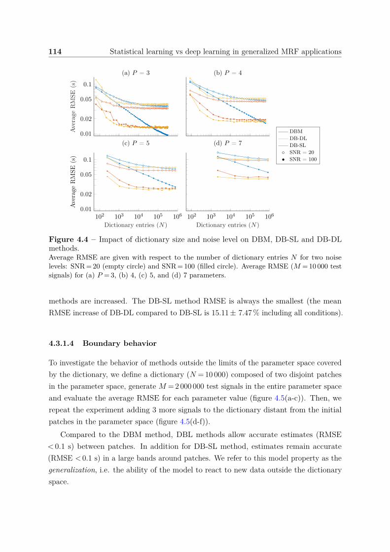
114 Statistical learning vs deep learning in generalized MRF applications
(b) P = 4
102 103 104 105 1060.01
0.02
0.05
0.1
Dictionary entries (N)
Ave
rage
RM
SE(s
)
(c) P = 5
102 103 104 105 106
Dictionary entries (N)
(d) P = 70.01
0.02
0.05
0.1
Ave
rage
RM
SE(s
)(a) P = 3
DBMDB-DLDB-SLSNR = 20SNR = 100
Figure 4.4 – Impact of dictionary size and noise level on DBM, DB-SL and DB-DLmethods.Average RMSE are given with respect to the number of dictionary entries N for two noiselevels: SNR = 20 (empty circle) and SNR = 100 (filled circle). Average RMSE (M = 10 000 testsignals) for (a) P = 3, (b) 4, (c) 5, and (d) 7 parameters.
methods are increased. The DB-SL method RMSE is always the smallest (the meanRMSE increase of DB-DL compared to DB-SL is 15.11 ± 7.47 % including all conditions).
4.3.1.4 Boundary behavior
To investigate the behavior of methods outside the limits of the parameter space coveredby the dictionary, we define a dictionary (N = 10 000) composed of two disjoint patchesin the parameter space, generate M = 2 000 000 test signals in the entire parameter spaceand evaluate the average RMSE for each parameter value (figure 4.5(a-c)). Then, werepeat the experiment adding 3 more signals to the dictionary distant from the initialpatches in the parameter space (figure 4.5(d-f)).
Compared to the DBM method, DBL methods allow accurate estimates (RMSE< 0.1 s) between patches. In addition for DB-SL method, estimates remain accurate(RMSE < 0.1 s) in a large bands around patches. We refer to this model property as thegeneralization, i.e. the ability of the model to react to new data outside the dictionaryspace.
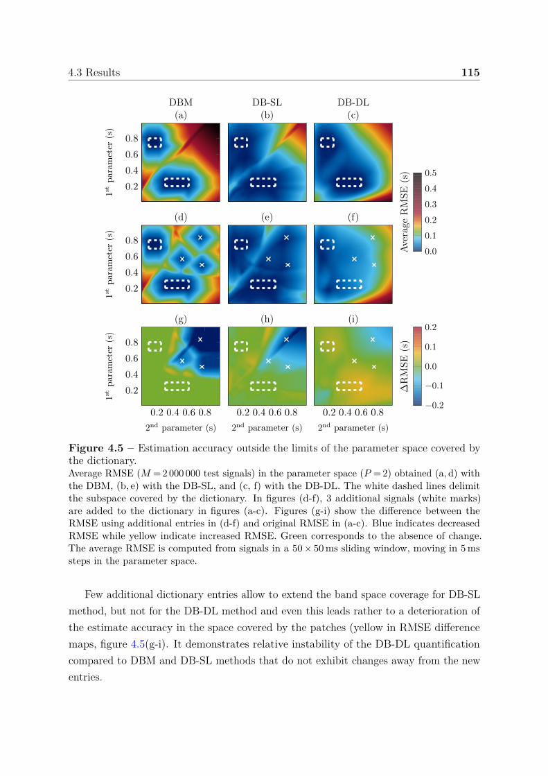
4.3 Results 115
0.2
0.4
0.6
0.8
1st
para
met
er(s
)DBM(a)
DB-SL(b)
DB-DL(c)
0.2
0.4
0.6
0.8
1st
para
met
er(s
)
(d) (e) (f)
0.0
0.1
0.2
0.3
0.4
0.5
Ave
rage
RM
SE(s
)0.2 0.4 0.6 0.8
0.2
0.4
0.6
0.8
2nd parameter (s)
1st
para
met
er(s
)
(g)
0.2 0.4 0.6 0.8
2nd parameter (s)
(h)
0.2 0.4 0.6 0.8
2nd parameter (s)
(i)
−0.2
−0.1
0.0
0.1
0.2
∆R
MSE
(s)
Figure 4.5 – Estimation accuracy outside the limits of the parameter space covered bythe dictionary.Average RMSE (M = 2 000 000 test signals) in the parameter space (P = 2) obtained (a, d) withthe DBM, (b, e) with the DB-SL, and (c, f) with the DB-DL. The white dashed lines delimitthe subspace covered by the dictionary. In figures (d-f), 3 additional signals (white marks)are added to the dictionary in figures (a-c). Figures (g-i) show the difference between theRMSE using additional entries in (d-f) and original RMSE in (a-c). Blue indicates decreasedRMSE while yellow indicate increased RMSE. Green corresponds to the absence of change.The average RMSE is computed from signals in a 50 × 50 ms sliding window, moving in 5 mssteps in the parameter space.
Few additional dictionary entries allow to extend the band space coverage for DB-SLmethod, but not for the DB-DL method and even this leads rather to a deterioration ofthe estimate accuracy in the space covered by the patches (yellow in RMSE differencemaps, figure 4.5(g-i). It demonstrates relative instability of the DB-DL quantificationcompared to DBM and DB-SL methods that do not exhibit changes away from the newentries.
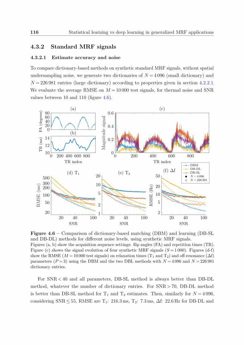
116 Statistical learning vs deep learning in generalized MRF applications
4.3.2 Standard MRF signals
4.3.2.1 Estimate accuracy and noise
To compare dictionary-based methods on synthetic standard MRF signals, without spatialundersampling noise, we generate two dictionaries of N = 4 096 (small dictionary) andN = 226 981 entries (large dictionary) according to properties given in section 4.2.2.1.We evaluate the average RMSE on M = 10 000 test signals, for thermal noise and SNRvalues between 10 and 110 (figure 4.6).
020406080
FA(d
egre
es) (a)
0 200 400 600 80010
12
14
TR index
TR
(ms)
(b)
0 200 400 600 8000
0.2
0.4
0.6
TR index
Mag
nitu
desi
gnal
(c)
20 40 10020
50
100
200300500
SNR
RM
SE(m
s)
(d) T1
20 40 1001
2
5
10
20
SNR
(e) T2
20 40 1002
5
10
20
50
SNR
RM
SE(H
z)
(f) ∆fDBMDB-DLDB-SLN = 4 096N = 226 981
Figure 4.6 – Comparison of dictionary-based matching (DBM) and learning (DB-SLand DB-DL) methods for different noise levels, using synthetic MRF signals.Figures (a, b) show the acquisition sequence settings: flip angles (FA) and repetition times (TR).Figure (c) shows the signal evolution of four synthetic MRF signals (S = 1 000). Figures (d-f)show the RMSE (M = 10 000 test signals) on relaxation times (T1 and T2) and off-resonance (∆f)parameters (P = 3) using the DBM and the two DBL methods with N = 4 096 and N = 226 981dictionary entries.
For SNR < 40 and all parameters, DB-SL method is always better than DB-DLmethod, whatever the number of dictionary entries. For SNR > 70, DB-DL methodis better than DB-SL method for T1 and T2 estimates. Then, similarly for N = 4 096,considering SNR ≤ 55, RMSE are T1: 216.3 ms, T2: 7.3 ms, ∆f: 22.6 Hz for DB-DL and
4.3 Results 117
T1: 93.6 ms, T2: 4.4 ms, ∆f: 9.0 Hz for DB-SL. For SNR > 55, RMSE become T1: 44.2 ms,T2: 2.2 ms, ∆f: 8.4 Hz for DB-DL and T1: 66.1 ms, T2: 3.4 ms, ∆f: 7.6 Hz for DB-SL.
4.3.2.2 Highly undersampled data
To investigate the estimation accuracy of dictionary-based methods with highly under-sampled data, we use the two previous dictionaries. A 4-region human brain phantom isgenerated, resolution is 128 × 128 (figures 4.7(a-b)). In each region T1 and T2 values aresampled according to a normal distribution around a central value (1 000, 1 400, 1 800 and2 200 for T1 and 60, 120, 180 and 240 for T2). An off-resonance map (∆f) is generatedby linear increase following each direction, between -200 and 200 Hz, figure 4.7(c). Thisphantom results in M = 7 622 test signals. Noise is added to test signals according toequation (4.1), with undersampling factor between 1 and 50. Examples of resultingsignals for 3 undersampling factors (8, 16 and 48) are shown in figures 4.7(d-f).
We observe that the RMSE increases significantly with the undersampling factor. ForT1, RMSE remain below 300 ms (≈ 10 %) until undersampling factors of 10 for DB-DLand 22 for DB-SL. For T2, RMSE remain below 30 ms (≈ 10 %) until undersamplingfactors of 46 for DB-DL and 38 for DB-SL. Note that the impact of the number of entriesin the dictionary is no longer visible when the aliasing noise increases.
4.3.2.3 Model variance
To investigate the statistical properties of the methods, we conduct a bias-varianceanalysis (section 4.2.2.4). The model used is the one computed using the N = 4 096dictionary entries. 100 random noises are generated according to SNR = 40 for each valueof the previous brain phantom (M = 7 622). Bias, variance and RMSE are computedaccording to equations (4.2), (4.3) and (4.4), respectively. Resulting maps are presentedin figure 4.8(a-c). Mean values for each map and those obtained with the N = 226 981dictionary entries, are given in table 4.8(d).
For T1 and T2, we observe that the DB-DL method is the less biased method with amean bias about twice smaller than the one of the DB-SL method, but exhibits largervariance. Consequently, DB-DL RMSE are higher for both T1 and T2 than DB-SL RMSE,see table 4.8(d). We observe that compared to the DBM method, DBL methods provideerrors that depend on underlying parameter maps such that we can distinguish brainstructures in error maps.
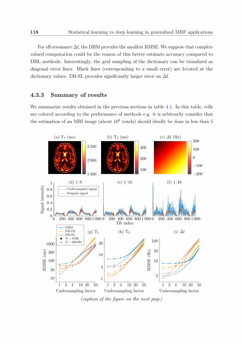
118 Statistical learning vs deep learning in generalized MRF applications
For off-resonance ∆f, the DBM provides the smallest RMSE. We suppose that complex-valued computation could be the reason of this better estimate accuracy compared toDBL methods. Interestingly, the grid sampling of the dictionary can be visualized asdiagonal error lines. Black lines (corresponding to a small error) are located at thedictionary values. DB-SL provides significantly larger error on ∆f.
4.3.3 Summary of results
We summarize results obtained in the previous sections in table 4.1. In this table, cellsare colored according to the performance of methods e.g. it is arbitrarily consider thatthe estimation of an MRI image (about 106 voxels) should ideally be done in less than 5
(a) T1 (ms)
1 500
2 000
2 500
(b) T2 (ms)
100
200
300
(c) ∆f (Hz)
−200
−100
0
100
200
0 200 400 600 800 1 0000
0.2
0.4
0.6
0.8
1
Sign
alin
tens
ity
(d) 1/8Undersampled signalOriginal signal
0 200 400 600 800 1 000TR index
(e) 1/16
0 200 400 600 800 1 000
(f) 1/48
1 2 4 10 20 5010
30
100
300
1000
Undersampling factor
RM
SE(m
s)
(g) T1
1 2 4 10 20 501
3
10
30
Undersampling factor
(h) T2
1 2 4 10 20 50
2
10
30
100
Undersampling factor
RM
SE(H
z)
(i) ∆fDBMDB-DLDB-SLN = 4 096N = 226 981
(caption of the figure on the next page)
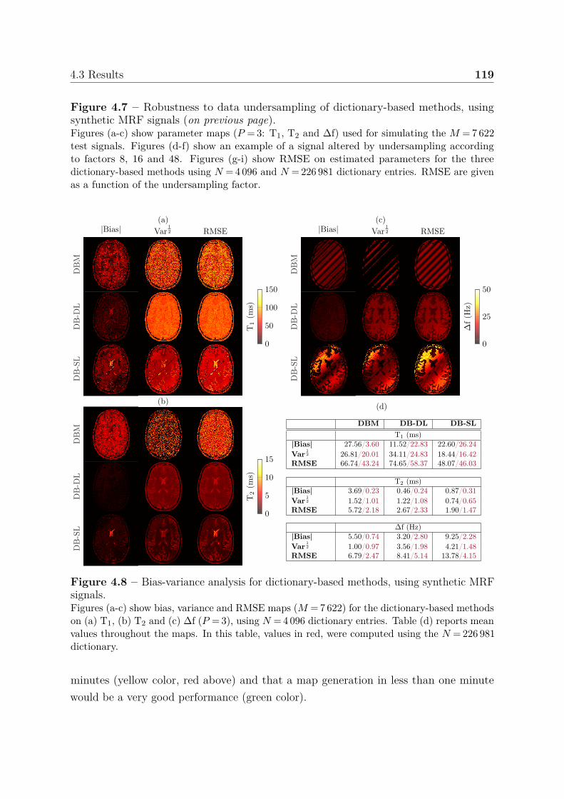
4.3 Results 119
Figure 4.7 – Robustness to data undersampling of dictionary-based methods, usingsynthetic MRF signals (on previous page).Figures (a-c) show parameter maps (P = 3: T1, T2 and ∆f) used for simulating the M = 7 622test signals. Figures (d-f) show an example of a signal altered by undersampling accordingto factors 8, 16 and 48. Figures (g-i) show RMSE on estimated parameters for the threedictionary-based methods using N = 4 096 and N = 226 981 dictionary entries. RMSE are givenas a function of the undersampling factor.
DB
-DL
0
50
100
150
T1
(ms)
DB
-SL
DB
M
|Bias|(a)
Var12 RMSE
DB
-DL
0
5
10
15
T2
(ms)
DB
-SL
DB
M
(b)
DB
-DL
0
25
50
∆f(H
z)
DB
-SL
DB
M
|Bias|(c)
Var12 RMSE
(d)
DBM DB-DL DB-SLT1 (ms)
|Bias| 27.56/3.60 11.52/22.83 22.60/26.24Var
12 26.81/20.01 34.11/24.83 18.44/16.42
RMSE 66.74/43.24 74.65/58.37 48.07/46.03
T2 (ms)|Bias| 3.69/0.23 0.46/0.24 0.87/0.31Var
12 1.52/1.01 1.22/1.08 0.74/0.65
RMSE 5.72/2.18 2.67/2.33 1.90/1.47
∆f (Hz)|Bias| 5.50/0.74 3.20/2.80 9.25/2.28Var
12 1.00/0.97 3.56/1.98 4.21/1.48
RMSE 6.79/2.47 8.41/5.14 13.78/4.15
Figure 4.8 – Bias-variance analysis for dictionary-based methods, using synthetic MRFsignals.Figures (a-c) show bias, variance and RMSE maps (M = 7 622) for the dictionary-based methodson (a) T1, (b) T2 and (c) ∆f (P = 3), using N = 4 096 dictionary entries. Table (d) reports meanvalues throughout the maps. In this table, values in red, were computed using the N = 226 981dictionary.
minutes (yellow color, red above) and that a map generation in less than one minutewould be a very good performance (green color).
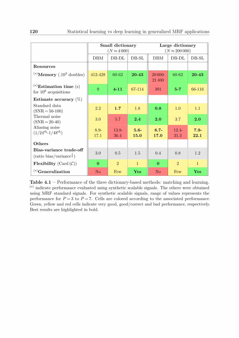
120 Statistical learning vs deep learning in generalized MRF applications
Small dictionary(N ≈ 4 000)
Large dictionary(N ≈ 200 000)
DBM DB-DL DB-SL DBM DB-DL DB-SL
Resources(∗)Memory (.103 doubles) 412-428 60-62 20-43 20 600-
21 40060-62 20-43
(∗)Estimation time (s)for 106 acquisitions 9 4-11 67-114 391 5-7 66-116
Estimate accuracy (%)Standard data(SNR = 50-100) 2.2 1.7 1.8 0.8 1.0 1.1
Thermal noise(SNR = 20-40) 3.0 5.7 2.4 2.0 3.7 2.0
Aliasing noise(1/24th-1/48th) 8.9-
17.113.8-36.4
5.6-15.0
8.7-17.0
12.4-31.3
7.9-22.1
OthersBias-variance trade-off(ratio bias/variance
12 )
3.0 0.5 1.5 0.4 0.8 1.2
Flexibility (Card (C)) 0 2 1 0 2 1(∗)Generalization No Few Yes No Few Yes
Table 4.1 – Performance of the three dictionary-based methods: matching and learning.(∗) indicate performance evaluated using synthetic scalable signals. The others were obtainedusing MRF standard signals. For synthetic scalable signals, range of values represents theperformance for P = 3 to P = 7. Cells are colored according to the associated performance.Green, yellow and red cells indicate very good, good/correct and bad performance, respectively.Best results are highlighted in bold.
4.3 Results 121
We observe that each method has its own specific domains of application. Briefly,DBM is very flexible and achieves very good performance with good noise robustness forlarge dictionary entries but requires considerable resources (time and memory). DB-DLis extremely fast but exhibits low performance with high noise levels both thermal andaliasing. DB-SL provides good estimate accuracy even in noisy conditions and has theability to preserve good accuracy outside the space covered by the dictionary. It isinteresting to note that DB-SL is the best performing method for the small dictionary.
4.3.4 Ensemble learning
To produce more accurate estimates, we propose to combine the two DBL models to getan ensemble model with better performances [193]. We investigate here two ensemblelearning approaches. The bagging learns models independently from each other in paralleland combines them following a deterministic averaging process (figures 4.9(a)). Theboosting learns them sequentially, i.e. each model depends on the previous ones (here,DB-SL then DB-DL, figure 4.9(b)). The way to combine models has to be adapted totheir types. Briefly, we can say that bagging will mainly focus at getting an ensemblemodel with less variance than its model components whereas boosting will mainly try toproduce strong models less biased than their components (even if variance can also bereduced).
For each combination, we try two strategies: a first, standard, using only estimates andas the confidence index (CI) is correlated to the RMSE, we investigate its considerationin combination in figure 4.10(a). For the bagging, first, we compute standard mean andthen, we compute a weighted mean using the CI, i.e. wDB-SL = (CImax − CI) /CImax andwDB-DL = 1 − wDB-SL, where CImax is the maximum CI value. It results that the smallerthe CI, the more weight is given to the DB-SL method and the larger the CI, the moreweight is given to the DB-DL method. For the boosting, first, we use the DB-SL estimateas the input of the DB-DL and them, we use both the estimate and CI as the inputs ofthe DB-DL in figure 4.10(b).
We observe that when computing the mean estimates from DB-SL and DB-DLestimates, the RMSE decreases so that the mean RMSE is better than both individualRMSE. In particular, whatever the SNR, the combined RMSE is always smaller than theDB-DL RMSE. Regarding the serial combination, the mean RMSE is also better thanindividual RMSE and in particular, the RMSE of the ensemble mdoel is always betterthan the DB-SL RMSE. Considering the CI does not improve much the results.
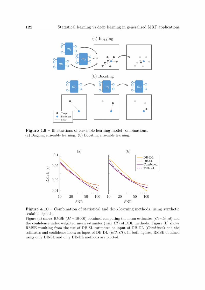
122 Statistical learning vs deep learning in generalized MRF applications
(a) Bagging
(b) Boosting
Figure 4.9 – Illustrations of ensemble learning model combinations.(a) Bagging ensemble learning. (b) Boosting ensemble learning.
10 20 50 100
0.01
0.02
0.05
0.1
SNR
RM
SE(s
)
(a)
10 20 50 100SNR
(b)
DB-DLDB-SLCombinedwith CI
Figure 4.10 – Combination of statistical and deep learning methods, using syntheticscalable signals.Figure (a) shows RMSE (M = 10 000) obtained computing the mean estimates (Combined) andthe confidence index weighted mean estimates (with CI ) of DBL methods. Figure (b) showsRMSE resulting from the use of DB-SL estimates as input of DB-DL (Combined) and theestimates and confidence index as input of DB-DL (with CI ). In both figures, RMSE obtainedusing only DB-SL and only DB-DL methods are plotted.
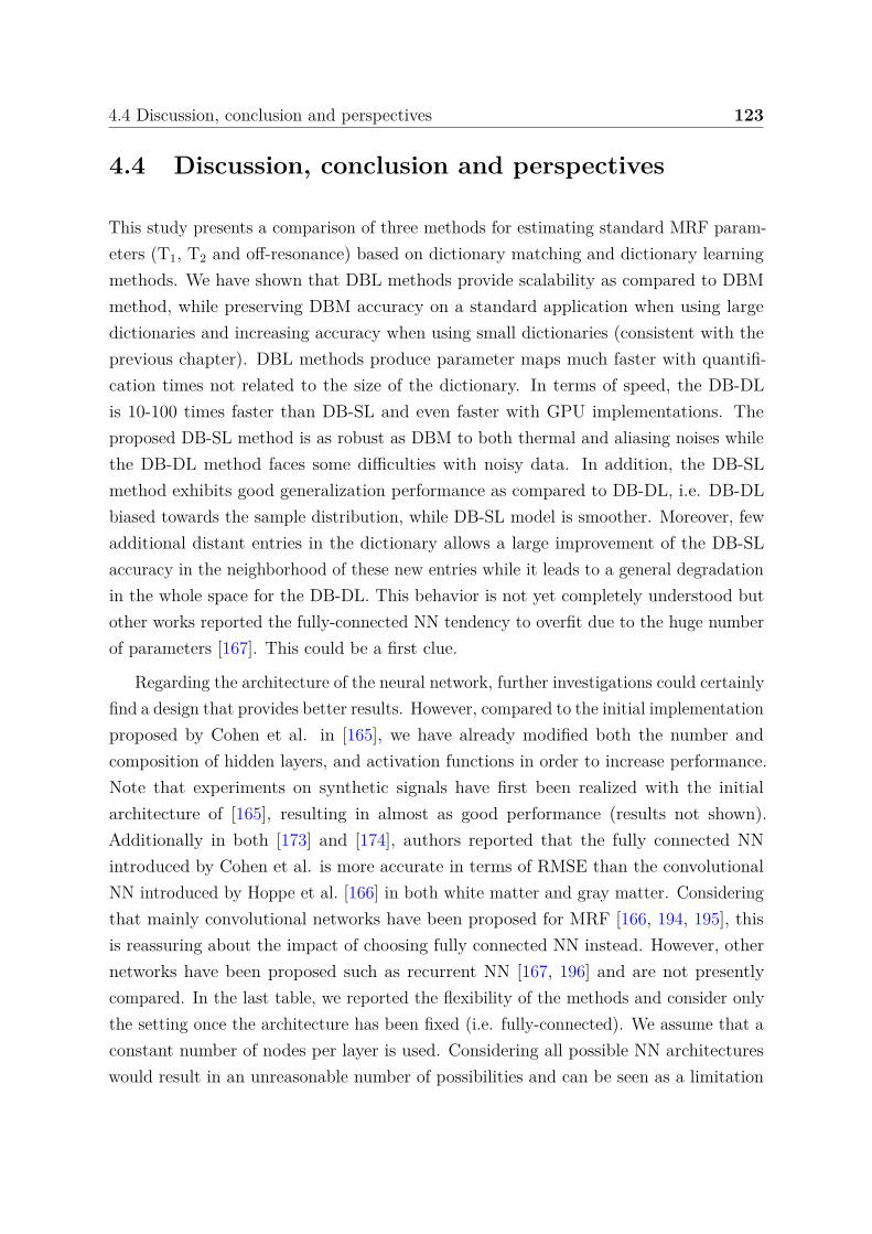
4.4 Discussion, conclusion and perspectives 123
4.4 Discussion, conclusion and perspectives
This study presents a comparison of three methods for estimating standard MRF param-eters (T1, T2 and off-resonance) based on dictionary matching and dictionary learningmethods. We have shown that DBL methods provide scalability as compared to DBMmethod, while preserving DBM accuracy on a standard application when using largedictionaries and increasing accuracy when using small dictionaries (consistent with theprevious chapter). DBL methods produce parameter maps much faster with quantifi-cation times not related to the size of the dictionary. In terms of speed, the DB-DLis 10-100 times faster than DB-SL and even faster with GPU implementations. Theproposed DB-SL method is as robust as DBM to both thermal and aliasing noises whilethe DB-DL method faces some difficulties with noisy data. In addition, the DB-SLmethod exhibits good generalization performance as compared to DB-DL, i.e. DB-DLbiased towards the sample distribution, while DB-SL model is smoother. Moreover, fewadditional distant entries in the dictionary allows a large improvement of the DB-SLaccuracy in the neighborhood of these new entries while it leads to a general degradationin the whole space for the DB-DL. This behavior is not yet completely understood butother works reported the fully-connected NN tendency to overfit due to the huge numberof parameters [167]. This could be a first clue.
Regarding the architecture of the neural network, further investigations could certainlyfind a design that provides better results. However, compared to the initial implementationproposed by Cohen et al. in [165], we have already modified both the number andcomposition of hidden layers, and activation functions in order to increase performance.Note that experiments on synthetic signals have first been realized with the initialarchitecture of [165], resulting in almost as good performance (results not shown).Additionally in both [173] and [174], authors reported that the fully connected NNintroduced by Cohen et al. is more accurate in terms of RMSE than the convolutionalNN introduced by Hoppe et al. [166] in both white matter and gray matter. Consideringthat mainly convolutional networks have been proposed for MRF [166, 194, 195], thisis reassuring about the impact of choosing fully connected NN instead. However, othernetworks have been proposed such as recurrent NN [167, 196] and are not presentlycompared. In the last table, we reported the flexibility of the methods and consider onlythe setting once the architecture has been fixed (i.e. fully-connected). We assume that aconstant number of nodes per layer is used. Considering all possible NN architectureswould result in an unreasonable number of possibilities and can be seen as a limitation
124 Statistical learning vs deep learning in generalized MRF applications
of this approach. Although we cannot claim to have used the best possible design, thetime spent in tuning the NN parameters was considerably higher than the time spenton tuning the DB-SL, which consisted only in the choice of the covariance matricesconstraints and the selection of the number of Gaussian distributions in the mixturemodel.
In this study, we extended our approach to complex-valued signals by splitting thereal and imaginary parts resulting in twice larger input signals as proposed in otherworks [167, 168]. However, such a representation could not respect the phase informationthat is captured by complex algebra [168]. In this work, authors thus introduce a newcomplex activation function for complex NN and showed that complex-valued NNsoutperform 2-channel NNs. An adaptation of GLLiM for complex-valued data, which ispossible, could improve the estimation of parameters from complex signals. Interestingly,both 2-channel and complex-valued NNs do not reach the DBM accuracy in estimatingB0 as observed in this study and in agreement with other work [168]. This may still be alimitation as compared to the initial DBM method.
An interesting point that, to the best of our knowledge, has not been discussed isthe structure of the error on maps found in the majority of DBL works, including ours,see figure 4.8. Indeed, we observe that in RMSE maps using DBL methods, most ofthe brain structures can be distinguished while it does not when using DBM. It may beinteresting to keep this in mind when interpreting the results since it means that we donot have a constant error across the estimated maps (e.g. white noise). Interestingly,using the DB-SL method, this information can be found in CI maps. We believe thatknowing the average performance of a method is very valuable, but being able to predictit on new estimates has a totally different impact. Now that we have shown that it ispossible to have access to such information, an optimization in this direction could be anopportunity for improvement.
In conclusion, this method irrefutably highlights the interest of learning methodsas compared to matching ones. This comparison of the DBL methods shows that theproposed statistical learning method outperforms the fully-connected deep learningapproach in standard MRF conditions, i.e. thermal noise and highly spatial aliasingnoise. Nevertheless, there may still be a need to improve the DB-SL implementation inorder to accelerate quantification. The real and imaginary 2-channel DB-SL method canhandle complex-valued data but cannot directly capture complete complex algebra whilesome DB-DL method can [168]. This requires an adjustment of the inverse regressionmodel, which is left as a short term future work.
Chapter 5
Murine model study of MTLE
To investigate the identification of the epileptogenic zone and associated seizure spreadingregions, we use a multi-parametric MRI analysis at 9.4 T. We examined, elaborated andcombined multiple cellular and neurovascular MRI parameters as imaging biomarkers ofthe epileptogenic and seizure propagating regions. Analyses were performed longitudinallyin an experimental model of mesial temporal lobe epilepsy (MTLE). The previous proposedquantitative DB-SL method is compared with the CEF method.
5.1 Introduction
Defining the epileptogenic zone and the anatomical boundaries of seizure spreadingnetworks in experimental or clinical focal epilepsies requires a complex clinical toolkitthat includes magnetic resonance imaging (MRI) [89, 101, 105, 107]. Novel imagingapproaches are based on the analysis of the multiple cellular and cerebrovascular dynamicsthat unfold during seizures, particularly blood-brain barrier permeability [197–199],perfusion modifications [200, 201], pathological neurovascular cell remodeling [84, 202],angiogenesis [62], and glial cells inflammation [203]. Cellular changes can translate intoT1, T2, or diffusion modifications [91–93, 100], while cerebrovascular damage can beexamined using gadolinium-based MRI [96, 204], with an extension to hemodynamicmeasurements such as cerebral blood flow or cerebral blood volume [105, 205], seedetails in section 2.1.3.4. However, no clear consensus has emerged on a single clinicallyapplicable MRI parameter that would significantly improve the identification of theepileptogenic zone and the associated seizure propagating regions.
Here, we developed a multi-parametric MRI approach based on the quantificationof four cerebrovascular (blood volume, microvessel diameter, tissue oxygen saturation

126 Murine model study of MTLE
and BBB permeability) and three cellular (T1, T2, and diffusion contrast) parameters,allowing the acquisition of data within an examination session in each animal. Using amodel of mesio-temporal lobe epilepsy (MTLE) elicited by a unilateral intra-hippocampalkainic acid (KA) injection [85, 206], we tracked the MRI modifications in the ipsilateralepileptogenic [207] and in the contralateral seizure propagating hippocampi. We mappedall MRI parameters with equal spatial resolution to obtain multiple values per image pixel.To derive an integrated information, we used standard statistical approaches (nearestneighbors, discriminant analysis, support vector machine, naive Bayes and decision tree)to classify the multi-parametric pixels, with the goal of discriminating the ipsilateralfrom the contralateral hippocampi, and comparing to sham animals.
5.2 Materials and methods
5.2.1 Animals
C57BL/6J male mice (8-10 weeks, Janvier LABS, Saint Berthevin, France), were housedin individual cages after surgery with food and water ad libitum and maintained ina 12-hour light-dark cycle (room temperature: 22 ± 1°C). All animal procedures wereperformed in accordance with the European Committee Council Directive 2010/63/EUafter validation by our local ethical committee and authorization from the French Ministryof Research (#8804-2014121714272897 v6).
5.2.2 MTLE model
A stereotaxic injection into the right dorsal hippocampus of 50 nL of a 20 mM solutionof KA (i.e. 1 nmol; Sigma, Lyon, France) was performed under general anesthesia (4 %chloral hydrate), as previously described and used by different groups [84, 85, 206, 208],while sham mice received 0.9 % NaCl. After KA injection, asymmetric clonic movementsof the forelimbs and head deviations, rotations, and periods of immobility were observedfor several hours [85]. After surgery, the mortality rate was 10.7 %. Animals thatdid not exhibit any of these signs were excluded from the study. These archetypicalbehavioural modifications lead to electrographic spontaneous seizures, as we and otherspreviously showed by using intrahippocampal recordings [84, 85, 206, 209] (see figure 5.1).Furthermore, animals that did not present hippocampus sclerosis on the anatomicalimage acquired during the MRI sessions at 4-6 weeks were excluded (see figure 5.2). Theexperimental protocol and group sizes are summarized in figure 5.3.
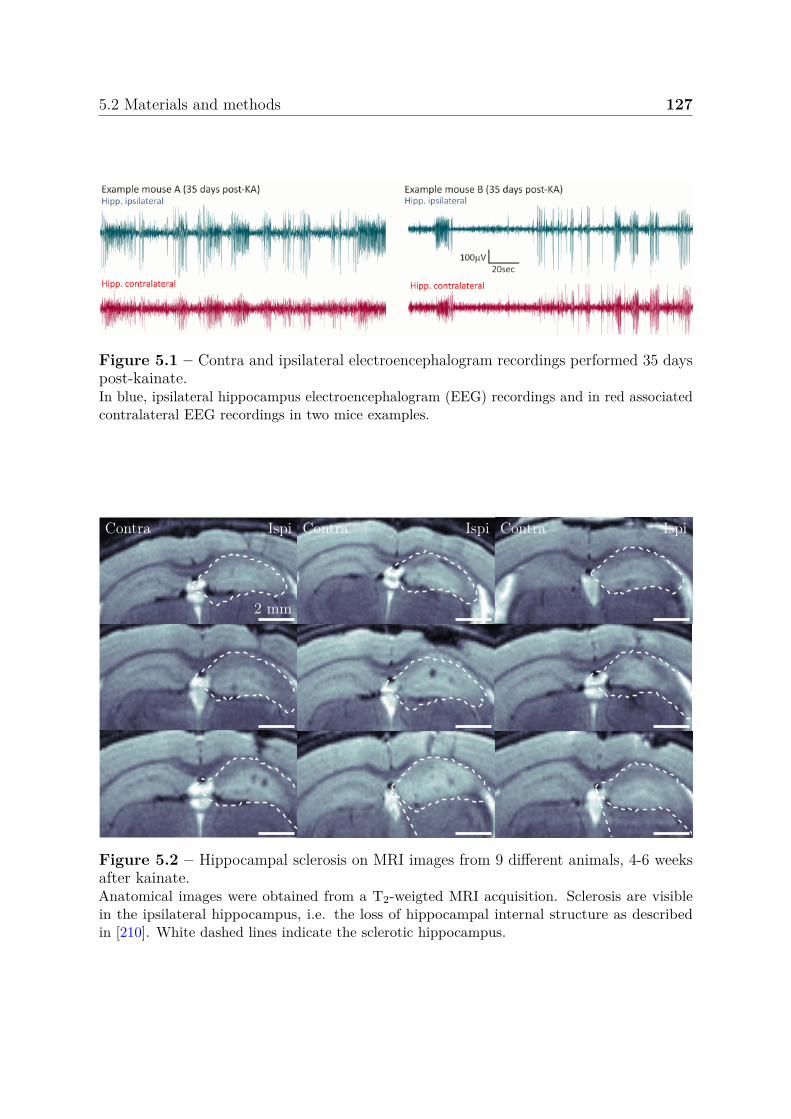
5.2 Materials and methods 127
Figure 5.1 – Contra and ipsilateral electroencephalogram recordings performed 35 dayspost-kainate.In blue, ipsilateral hippocampus electroencephalogram (EEG) recordings and in red associatedcontralateral EEG recordings in two mice examples.
Contra Ispi
2 mm
Contra Ispi Contra Ispi
Figure 5.2 – Hippocampal sclerosis on MRI images from 9 different animals, 4-6 weeksafter kainate.Anatomical images were obtained from a T2-weigted MRI acquisition. Sclerosis are visiblein the ipsilateral hippocampus, i.e. the loss of hippocampal internal structure as describedin [210]. White dashed lines indicate the sclerotic hippocampus.
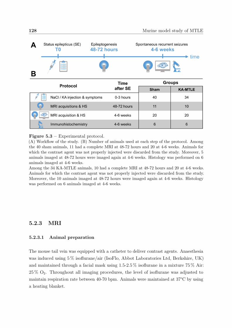
128 Murine model study of MTLE
Figure 5.3 – Experimental protocol.(A) Workflow of the study. (B) Number of animals used at each step of the protocol. Amongthe 40 sham animals, 11 had a complete MRI at 48-72 hours and 20 at 4-6 weeks. Animals forwhich the contrast agent was not properly injected were discarded from the study. Moreover, 5animals imaged at 48-72 hours were imaged again at 4-6 weeks. Histology was performed on 6animals imaged at 4-6 weeks.Among the 34 KA-MTLE animals, 10 had a complete MRI at 48-72 hours and 20 at 4-6 weeks.Animals for which the contrast agent was not properly injected were discarded from the study.Moreover, the 10 animals imaged at 48-72 hours were imaged again at 4-6 weeks. Histologywas performed on 6 animals imaged at 4-6 weeks.
5.2.3 MRI
5.2.3.1 Animal preparation
The mouse tail vein was equipped with a catheter to deliver contrast agents. Anaesthesiawas induced using 5 % isoflurane/air (IsoFlo, Abbot Laboratories Ltd, Berkshire, UK)and maintained through a facial mask using 1.5-2.5 % isoflurane in a mixture 75 % Air:25 % O2. Throughout all imaging procedures, the level of isoflurane was adjusted tomaintain respiration rate between 40-70 bpm. Animals were maintained at 37°C by usinga heating blanket.
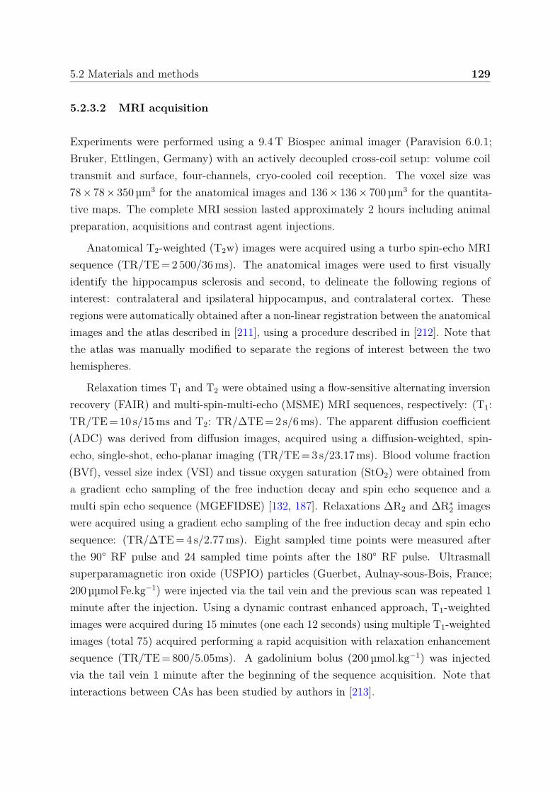
5.2 Materials and methods 129
5.2.3.2 MRI acquisition
Experiments were performed using a 9.4 T Biospec animal imager (Paravision 6.0.1;Bruker, Ettlingen, Germany) with an actively decoupled cross-coil setup: volume coiltransmit and surface, four-channels, cryo-cooled coil reception. The voxel size was78 × 78 × 350 µm3 for the anatomical images and 136 × 136 × 700 µm3 for the quantita-tive maps. The complete MRI session lasted approximately 2 hours including animalpreparation, acquisitions and contrast agent injections.
Anatomical T2-weighted (T2w) images were acquired using a turbo spin-echo MRIsequence (TR/TE = 2 500/36 ms). The anatomical images were used to first visuallyidentify the hippocampus sclerosis and second, to delineate the following regions ofinterest: contralateral and ipsilateral hippocampus, and contralateral cortex. Theseregions were automatically obtained after a non-linear registration between the anatomicalimages and the atlas described in [211], using a procedure described in [212]. Note thatthe atlas was manually modified to separate the regions of interest between the twohemispheres.
Relaxation times T1 and T2 were obtained using a flow-sensitive alternating inversionrecovery (FAIR) and multi-spin-multi-echo (MSME) MRI sequences, respectively: (T1:TR/TE = 10 s/15 ms and T2: TR/∆TE = 2 s/6 ms). The apparent diffusion coefficient(ADC) was derived from diffusion images, acquired using a diffusion-weighted, spin-echo, single-shot, echo-planar imaging (TR/TE = 3 s/23.17 ms). Blood volume fraction(BVf), vessel size index (VSI) and tissue oxygen saturation (StO2) were obtained froma gradient echo sampling of the free induction decay and spin echo sequence and amulti spin echo sequence (MGEFIDSE) [132, 187]. Relaxations ∆R2 and ∆R∗
2 imageswere acquired using a gradient echo sampling of the free induction decay and spin echosequence: (TR/∆TE = 4 s/2.77 ms). Eight sampled time points were measured afterthe 90° RF pulse and 24 sampled time points after the 180° RF pulse. Ultrasmallsuperparamagnetic iron oxide (USPIO) particles (Guerbet, Aulnay-sous-Bois, France;200 µµmol Fe.kg−1) were injected via the tail vein and the previous scan was repeated 1minute after the injection. Using a dynamic contrast enhanced approach, T1-weightedimages were acquired during 15 minutes (one each 12 seconds) using multiple T1-weightedimages (total 75) acquired performing a rapid acquisition with relaxation enhancementsequence (TR/TE = 800/5.05ms). A gadolinium bolus (200 µmol.kg−1) was injectedvia the tail vein 1 minute after the beginning of the sequence acquisition. Note thatinteractions between CAs has been studied by authors in [213].
130 Murine model study of MTLE
5.2.3.3 MRI quantification
Quantitative parameter maps were computed pixel-by-pixel using previously publishedmethods and the Medical software for Processing multi-Parametric images Pipelines tool1
in the Matlab environment (Mathworks, MA, USA), see appendix E.2. Seven parametermaps were obtained: relaxation times T1 and T2, apparent diffusion coefficient (ADC),blood volume fraction (BVf), vessel size index (VSI), tissue oxygen saturation (StO2)and BBB permeability (BBBp).
T1 and T2 maps were derived from the FAIR and MSME data respectively, usinga non-linear fitting algorithm (section 2.3.1). ADC maps were computed as the meanof the ADCs observed in each of three orthogonal directions (section 2.3.2). BVf, VSIand StO2 maps were estimated using the vascular MRF approach proposed in chapter 3.Combinations of parameters for simulation were obtained for BVf between 0.5 and 25 %,VSI between 1 and 100 µm, and StO2 between 50 and 90 %. The susceptibility differencebetween blood in the presence and absence of USPIO, was set to 0.14 × 10⁻⁶ (CGS) [214]and hematocrit was set to 0.357. Other simulation settings (i.e. magnetic field, sequenceacquisition) matched experiment conditions. Finally, after spatial Gaussian filtering(3 × 3), BBBp was estimated as the area under the curve over the 10 minutes followingthe injection (AUC600, section 2.3.4.2). In the brain, an increase of this quantity indicatesan accumulation of the gadolinium in the extravascular compartment and therefore areduction in the BBB permeability [188].
To reduce the possible contribution of biases inherent to the acquisition set-up (e.g.position of the receiver coil, dose of contrast agent), parameter maps were normalized bya region where no significant MRI changes are observed in these experimental conditions,e.g. the thalamus [211]. To allow a direct evaluation and graphical comparisons acrossread-outs, all parameter ratios were centered using the mean normalized sham ratio asreference. For each parameter and each animal, the following ratio R was calculated:
R = H
T− 1
S
S∑n=1
Hn
Sn
, (5.1)
where H and T are the mean parameter values in the hippocampus and thalamus of oneanimal, respectively. S is the number of sham mice and ∑S
n=1 Hn/Sn is the sum of theratios of hippocampus and thalamus mean parameter values for all the sham mice. Thisrepresentation of the MRI parameters constitutes the normalized MRI parameter.
1https://github.com/nifm-gin/MP3
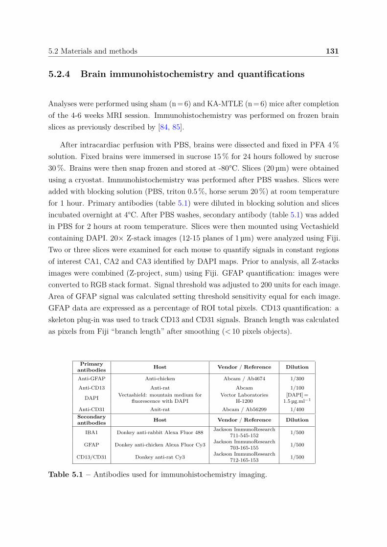
5.2 Materials and methods 131
5.2.4 Brain immunohistochemistry and quantifications
Analyses were performed using sham (n = 6) and KA-MTLE (n = 6) mice after completionof the 4-6 weeks MRI session. Immunohistochemistry was performed on frozen brainslices as previously described by [84, 85].
After intracardiac perfusion with PBS, brains were dissected and fixed in PFA 4 %solution. Fixed brains were immersed in sucrose 15 % for 24 hours followed by sucrose30 %. Brains were then snap frozen and stored at -80°C. Slices (20 µm) were obtainedusing a cryostat. Immunohistochemistry was performed after PBS washes. Slices wereadded with blocking solution (PBS, triton 0.5 %, horse serum 20 %) at room temperaturefor 1 hour. Primary antibodies (table 5.1) were diluted in blocking solution and slicesincubated overnight at 4°C. After PBS washes, secondary antibody (table 5.1) was addedin PBS for 2 hours at room temperature. Slices were then mounted using Vectashieldcontaining DAPI. 20× Z-stack images (12-15 planes of 1 µm) were analyzed using Fiji.Two or three slices were examined for each mouse to quantify signals in constant regionsof interest CA1, CA2 and CA3 identified by DAPI maps. Prior to analysis, all Z-stacksimages were combined (Z-project, sum) using Fiji. GFAP quantification: images wereconverted to RGB stack format. Signal threshold was adjusted to 200 units for each image.Area of GFAP signal was calculated setting threshold sensitivity equal for each image.GFAP data are expressed as a percentage of ROI total pixels. CD13 quantification: askeleton plug-in was used to track CD13 and CD31 signals. Branch length was calculatedas pixels from Fiji “branch length” after smoothing (< 10 pixels objects).
Primaryantibodies Host Vendor / Reference Dilution
Anti-GFAP Anti-chicken Abcam / Ab4674 1/300
Anti-CD13 Anti-rat Abcam 1/100
DAPI Vectashield: mountain medium forfluorescence with DAPI
Vector LaboratoriesH-1200
[DAPI] =1.5 µg.ml−1
Anti-CD31 Anit-rat Abcam / Ab56299 1/400Secondaryantibodies Host Vendor / Reference Dilution
IBA1 Donkey anti-rabbit Alexa Fluor 488 Jackson ImmunoResearch711-545-152 1/500
GFAP Donkey anti-chicken Alexa Fluor Cy3 Jackson ImmunoResearch703-165-155 1/500
CD13/CD31 Donkey anti-rat Cy3 Jackson ImmunoResearch712-165-153 1/500
Table 5.1 – Antibodies used for immunohistochemistry imaging.
132 Murine model study of MTLE
5.2.5 Statistical analyses and classification
5.2.5.1 Statistical analyses
Histological data were analyzed using Prism 8.3.1. Depending on normality (Shapiro-Wilk) data were analyzed using a two-tailed t-test or a non-parametric Mann-Whitney test.Results are reported as violin box with single points and indicating median, interquartileranges and min-max range (figure 5.6). Significance threshold was set at p < 0.05.
MRI data were analyzed in the Matlab environment. Data were analyzed using anon-parametric Mann-Whitney test. Results are reported as a box. On each box, thecentral mark indicates the median, and the bottom and top edges of the box indicate the25th and 75th percentiles, respectively. Whiskers extend to the most extreme data points.
5.2.5.2 Classification
We applied automatic classifications to MRI data considering 3 groups (sham, KA-MTLEcontralateral, and KA-MTLE ipsilateral). To evaluate the impact of the classificationmethod, different approaches are performed: k-nearest neighbors (kNN), linear andquadratic discriminant analysis (LDA and QDA), support vector machine (SVM), NaïveBayes (NB), and Decision Tree (DT). Each approach was evaluated using a “leave-one-out” cross-validation strategy, specifically each classification model was trained using allanimals except one. The omitted animal was then classified using the trained model. Theprocedure was repeated for all animals and the mean classification accuracy was reported.To examine whether it is more accurate to use one or several MRI parameters to classifythe experimental groups, we performed the classification procedure considering 1) eachMRI parameter individually, 2) all MRI parameters or 3) the subset of MRI parametersthat yields to the highest classification accuracy. All possible parameter combinationswere tested.
5.3 Results
5.3.1 Tracking hippocampal MRI changes post-KA and duringspontaneous seizures
Anatomical imaging performed after status epilepticus (48-72 hours post-KA) indicatedthe unilateral cortical lesion and edema corresponding to the kainate injection route(figure 5.4 A2-A4, D2 and H2).
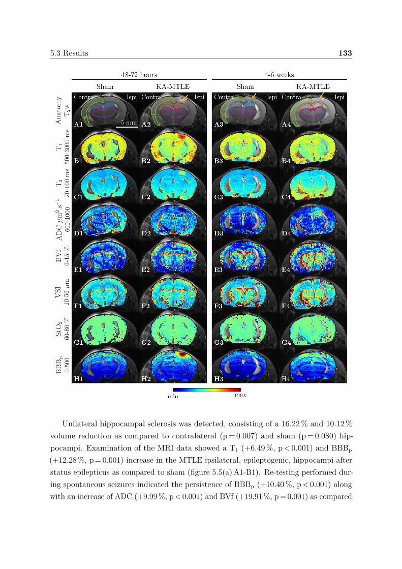
5.3 Results 133
Unilateral hippocampal sclerosis was detected, consisting of a 16.22 % and 10.12 %volume reduction as compared to contralateral (p = 0.007) and sham (p = 0.080) hip-pocampi. Examination of the MRI data showed a T1 (+6.49 %, p < 0.001) and BBBp
(+12.28 %, p = 0.001) increase in the MTLE ipsilateral, epileptogenic, hippocampi afterstatus epilepticus as compared to sham (figure 5.5(a) A1-B1). Re-testing performed dur-ing spontaneous seizures indicated the persistence of BBBp (+10.40 %, p < 0.001) alongwith an increase of ADC (+9.99 %, p < 0.001) and BVf (+19.91 %, p = 0.001) as compared
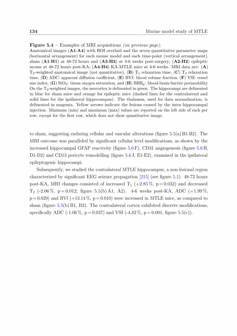
134 Murine model study of MTLE
Figure 5.4 – Examples of MRI acquisitions (on previous page).Anatomical images (A1-A4) with ROI overlaid and the seven quantitative parameter maps(horizontal arrangement) for each mouse model and each time-point (vertical arrangement).sham (A1-H1) at 48-72 hours and (A3-H3) at 4-6 weeks post-surgery; (A2-H2) epilepticmouse at 48-72 hours post-KA; (A4-H4) KA-MTLE mice at 4-6 weeks. MRI data are: (A)T2-weighted anatomical image (not quantitative), (B) T1 relaxation time, (C) T2 relaxationtime, (D) ADC: apparent diffusion coefficient, (E) BVf: blood volume fraction, (F) VSI: vesselsize index, (G) StO2: tissue oxygen saturation, and (H) BBBp: blood-brain-barrier permeability.On the T2-weighted images, the neocortex is delineated in green. The hippocampi are delineatedin blue for sham mice and orange for epileptic mice (dashed lines for the contralateral andsolid lines for the ipsilateral hippocampus). The thalamus, used for data normalization, isdelineated in magenta. Yellow arrows indicate the lesions caused by the intra hippocampalinjection. Minimum (min) and maximum (max) values are reported on the left side of each perrow, except for the first row, which does not show quantitative image.
to sham, suggesting enduring cellular and vascular alterations (figure 5.5(a) B1-B2). TheMRI outcome was paralleled by significant cellular level modifications, as shown by theincreased hippocampal GFAP reactivity (figure 5.6 F), CD31 angiogenesis (figure 5.6 H,D1-D2) and CD13 pericyte remodelling (figure 5.6 J, E1-E2), examined in the ipsilateralepileptogenic hippocampi.
Subsequently, we studied the contralateral MTLE hippocampus, a non-lesional regioncharacterized by significant EEG seizure propagation [215] (see figure 5.1). 48-72 hourspost-KA, MRI changes consisted of increased T1 (+2.85 %, p = 0.032) and decreasedT2 (-2.06 %, p = 0.012; figure 5.5(b) A1, A2). 4-6 weeks post-KA, ADC (+1.99 %,p = 0.029) and BVf (+13.14 %, p = 0.010) were increased in MTLE mice, as compared tosham (figure 5.5(b) B1, B2). The contralateral cortex exhibited discrete modifications,specifically ADC (-1.06 %, p = 0.037) and VSI (-4.82 %, p = 0.001; figure 5.5(c)).
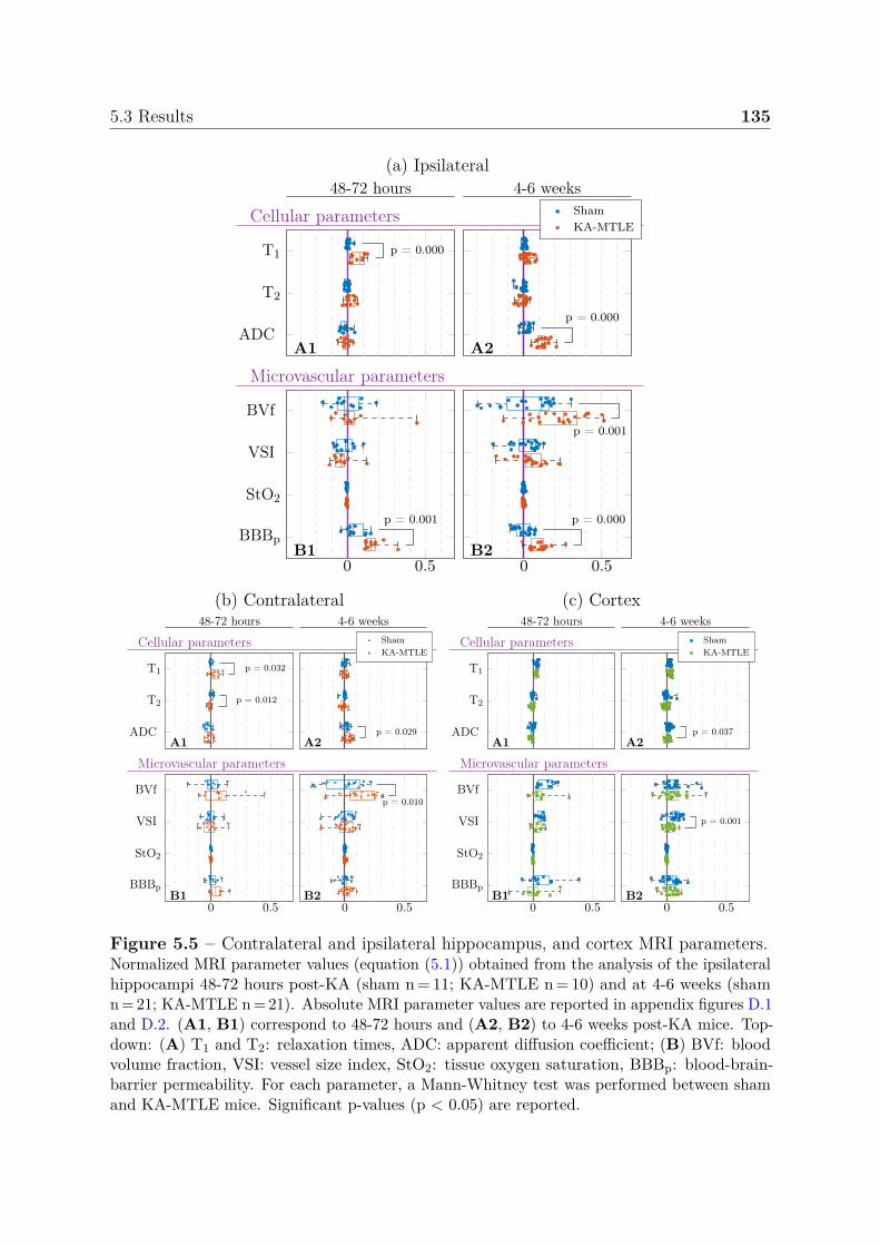
5.3 Results 135
(a) Ipsilateral48-72 hours 4-6 weeks
Cellular parameters
Microvascular parameters
T1
T2
ADC
p = 0.000
A1
BVf
VSI
StO2
BBBp
0 0.5
p = 0.001
B1
p = 0.000
A2
ShamKA-MTLE
0 0.5
p = 0.001
p = 0.000
B2
(b) Contralateral48-72 hours 4-6 weeks
Cellular parameters
Microvascular parameters
T1
T2
ADC
p = 0.032
p = 0.012
A1
BVf
VSI
StO2
BBBp
0 0.5B1
p = 0.029A2
ShamKA-MTLE
0 0.5
p = 0.010
B2
(c) Cortex48-72 hours 4-6 weeks
Cellular parameters
Microvascular parameters
T1
T2
ADCA1
BVf
VSI
StO2
BBBp
0 0.5B1
p = 0.037A2
ShamKA-MTLE
0 0.5
p = 0.001
B2
Figure 5.5 – Contralateral and ipsilateral hippocampus, and cortex MRI parameters.Normalized MRI parameter values (equation (5.1)) obtained from the analysis of the ipsilateralhippocampi 48-72 hours post-KA (sham n = 11; KA-MTLE n = 10) and at 4-6 weeks (shamn = 21; KA-MTLE n = 21). Absolute MRI parameter values are reported in appendix figures D.1and D.2. (A1, B1) correspond to 48-72 hours and (A2, B2) to 4-6 weeks post-KA mice. Top-down: (A) T1 and T2: relaxation times, ADC: apparent diffusion coefficient; (B) BVf: bloodvolume fraction, VSI: vessel size index, StO2: tissue oxygen saturation, BBBp: blood-brain-barrier permeability. For each parameter, a Mann-Whitney test was performed between shamand KA-MTLE mice. Significant p-values (p < 0.05) are reported.

136 Murine model study of MTLE
Figure 5.6 – Histological neurovascular changes in the ipsi and contralateral hippocampiduring chronic seizures.(A1, A2) DAPI and CD13 pericyte maps of the whole dorsal hippocampi (ipsi and contra-lateral) during chronic seizures (4-6 weeks). Arrowhead in A2 show gross pericyte abnormalityin the CA regions. (B1, B2) Examples of GFAP reactivity during SRS in the ipsilateral CA1hippocampus as compared to sham. (C1, C3) Examples of astrocyte morphological changesduring chronic seizures (arrowhead, ipsi and contra-lateral) as compared to sham. (D1,D2)Example of CD31 angiogenesis during chronic seizures. Arrowheads in D2 indicate large andlooping abnormal vessels. (E1, E2) Example of CD13 pericyte modification and hypertrophyduring chronic seizures (arrowheads in E2). (F, G) Quantification of sub-hippocampal GFAPfluorescence, ipsi and contralateral. (H, I) Quantification of sub-hippocampal CD31 vessellength, ipsi and contralateral. (J, K) Quantification of sub-hippocampal CD13 pericyte length,ipsi and contralateral. Depending on normality (Shapiro-Wilk) data were analyzed using atwo-tailed t-test. Panel G CA2 contra, panel H CA3 ipsi, panel I CA2 contra, panel K CA1contra that were instead analyzed using non-parametric Mann-Whitney. Data refers to n = 6mice/group, 2-3 slices/mouse. * p < 0.05, ** p < 0.01, and *** p < 0.001.
Histological analysis of the contralateral hippocampi indicated distinct cellular levelchanges, less apparent as compared to the lesional ipsilateral hippocampus (figure 5.6).In particular, CD13 pericyte (figure 5.6 K) and CD31 capillary (figure 5.6 I) lengthwas trending or significantly increased as compared to sham, suggesting angiogenesis
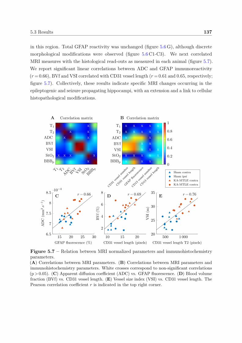
5.3 Results 137
in this region. Total GFAP reactivity was unchanged (figure 5.6 G), although discretemorphological modifications were observed (figure 5.6 C1-C3). We next correlatedMRI measures with the histological read-outs as measured in each animal (figure 5.7).We report significant linear correlations between ADC and GFAP immunoreactivity(r = 0.66), BVf and VSI correlated with CD31 vessel length (r = 0.61 and 0.65, respectively;figure 5.7). Collectively, these results indicate specific MRI changes occurring in theepileptogenic and seizure propagating hippocampi, with an extension and a link to cellularhistopathological modifications.
15 20 25 306.5
7
7.5
8
8.5·10−4
r= 0.66C
GFAP fluorescence (%)
AD
C(m
m2.s−1)
10 15 20
2
4
6
8 r= 0.69D
CD31 vessel length (pixels)
BV
f(%
)
Sham contraSham ipsiKA-MTLE contraKA-MTLE contra
500 1 00020
25
30
35 r= 0.76E
CD31 vessel length T2 (pixels)
VSI
(m)
A B
xx x
x x
x x x xx
T 1 T 2
ADCBVf
VSI StO 2
BBB p
T1
T2
ADCBVfVSIStO2
BBBp
Correlation matrix
x x x x xx x x x xx x
x xx x x
x x x x xx x x
CD31ve
ssel n
umbe
r
CD31ve
ssel len
gth
GFAP
fluorescenc
e
CD13ve
ssel n
umbe
r
CD13ve
ssel len
gth
T1
T2
ADCBVfVSI
StO2
BBBp
Correlation matrix
0
0.2
0.4
0.6
0.8
1
Figure 5.7 – Relation between MRI normalized parameters and immunohistochemistryparameters.(A) Correlations between MRI parameters. (B) Correlations between MRI parameters andimmunohistochemistry parameters. White crosses correspond to non-significant correlations(p > 0.05). (C) Apparent diffusion coefficient (ADC) vs. GFAP fluorescence. (D) Blood volumefraction (BVf) vs. CD31 vessel length. (E) Vessel size index (VSI) vs. CD31 vessel length. ThePearson correlation coefficient r is indicated in the top right corner.
138 Murine model study of MTLE
5.3.2 Multiparametric analysis for the identification of epilep-togenic and seizure-spreading hippocampi
We initially tested whether redundancy existed among all MRI parameters examined.Correlations below 0.5, except for BVf and VSI (r = 0.88; figure 5.7), ruled out inter-dependence between the MRI parameters, indicating that MRI parameter variationscan be combined without redundant information. Furthermore, the correlation levelbetween MRI parameter values and hippocampal volumes was low or not significant,indicating that quantitative MRI provides integrating data to hippocampus sclerosis(figure 5.2). We then examined the effectiveness of multiparametric analyses to separateour experimental groups. To this end, MRI data acquired from all animals underwentsix classification analyses (see section 5.2.5.2; figure 5.8 A1-A2, B1-B2). Initially, we clas-sified two experimental conditions, specifically ipsilateral MTLE and sham hippocampi,considering one MRI parameter at a time (figure 5.8 A1-A2). 48-72 hours post-KA, weobtained the highest classification accuracies using T1, T2 and BBBp (93.0 %, 81.2 % and89.2 %, respectively; MTLE: n = 10 and sham: n = 22). During spontaneous seizures (4-6weeks), the best classification was obtained using ADC, BVf and BBBp (98.3 %, 83.3 %and 89.2 %, respectively; MTLE: n = 20 and sham: n = 40). When we considered all sevenMRI parameters, the accuracy score was 92.5 % post-KA and 96.7 % during spontaneousseizures. When screening and selecting the subset of MRI parameters that provides thehighest accuracy score, we found that the combination of T1, T2, ADC and BBBp deliversan accuracy of 100 % post-KA, while the combination of ADC, BVf, VSI and BBBp
delivers an accuracy of 99.2 % during spontaneous seizures. These results were obtainedusing QDA and SVM classification methods. The mean (across parameters) standarddeviation (across classification methods) of accuracy was 2.15 ± 1.46 %, suggesting thatthe classification methods led to close results.
Next, we attempted classifying three experimental conditions, specifically MTLEipsilateral, MTLE contralateral, and sham hippocampi (figure 5.8 B1-B2). 48-72 hourspost-KA and considering one parameter at a time, the highest classification accuracieswere obtained using BBBp, T1, and T2 (74 %, 69 %, and 65.8 %, respectively). Duringspontaneous seizures, accuracies based on ADC, BBBp, BVf were 77.6 %, 63.7 %, and60 %, respectively. Combination of all MRI parameters did not improve the classificationaccuracy. However, the multiparametric approach using the combination of T2, BVf,VSI, StO2 and BBBp delivered a 90.5 % accuracy post-KA, while the combination of T1,ADC and BVf lead to an 85 % accuracy in segregating the three experimental conditions
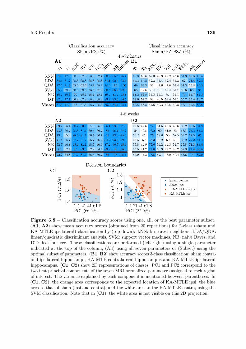
5.3 Results 139
Figure 5.8 – Classification accuracy scores using one, all, or the best parameter subset.(A1, A2) show mean accuracy scores (obtained from 20 repetitions) for 2-class (sham andKA-MTLE ipsilateral) classification by (top-down): kNN: k-nearest neighbors, LDA/QDA:linear/quadratic discriminant analysis, SVM: support vector machines, NB: naive Bayes, andDT: decision tree. These classifications are performed (left-right) using a single parameterindicated at the top of the column, (All) using all seven parameters or (Subset) using theoptimal subset of parameters. (B1, B2) show accuracy scores 3-class classification: sham contra-and ipsilateral hippocampi, KA-MTE contralateral hippocampus and KA-MTLE ipsilateralhippocampus. (C1, C2) show 2D representations of classes. PC1 and PC2 correspond to thetwo first principal components of the seven MRI normalized parameters assigned to each regionof interest. The variance explained by each component is mentioned between parentheses. In(C1, C2), the orange area corresponds to the expected location of KA-MTLE ipsi, the bluearea to that of sham (ipsi and contra), and the white area to the KA-MTLE contra, using theSVM classification. Note that in (C1), the white area is not visible on this 2D projection.
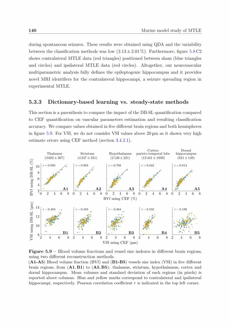
140 Murine model study of MTLE
during spontaneous seizures. These results were obtained using QDA and the variabilitybetween the classification methods was low (3.13 ± 2.01 %). Furthermore, figure 5.8 C2shows contralateral MTLE data (red triangles) positioned between sham (blue trianglesand circles) and ipsilateral MTLE data (red circles). Altogether, our neurovascularmultiparametric analysis fully defines the epileptogenic hippocampus and it providesnovel MRI identifiers for the contralateral hippocampi, a seizure spreading region inexperimental MTLE.
5.3.3 Dictionary-based learning vs. steady-state methods
This section is a parenthesis to compare the impact of the DB-SL quantification comparedto CEF quantification on vascular parameters estimation and resulting classificationaccuracy. We compare values obtained in five different brain regions and both hemispheresin figure 5.9. For VSI, we do not consider VSI values above 20 µm as it shown very highestimate errors using CEF method (section 3.4.2.1).
0 2 4 6 82
4
6
8
10 r= 0.893
A1
BV
fus
ing
DB
-SL
(%)
Thalamus(3 682± 267)
0 2 4 6 8
r= 0.903
A2
Striatum(4 247± 331)
0 2 4 6 8
r= 0.768
A3
BVf using CEF (%)
Hypothalamus(2 126± 221)
0 2 4 6 8
r= 0.842
A4
Cortex:parieto-temporal lobe
(13 441± 1039)
0 2 4 6 8
r= 0.814
A5
Dorsalhippocampus(821± 149)
2 4 6 88
10
12
14r= 0.483
B1
VSI
usin
gD
B-S
L(µ
m)
2 4 6 8
r= 0.458
B22 4 6 8
r= 0.364
B3
VSI using CEF (µm)2 4 6 8
r= 0.532
B42 4 6 8
r= 0.199
B5
Figure 5.9 – Blood volume fractions and vessel size indexes in different brain regions,using two different reconstruction methods.(A1-A5) Blood volume fraction (BVf) and (B1-B5) vessels size index (VSI) in five differentbrain regions, from (A1, B1) to (A5, B5): thalamus, striatum, hypothalamus, cortex anddorsal hippocampus. Mean volumes and standard deviation of each regions (in pixels) isreported above columns. Blue and yellow marks correspond to contralateral and ipsilateralhippocampi, respectively. Pearson correlation coefficient r is indicated in the top left corner.
5.4 Discussion, conclusion and perspectives 141
Regarding BVf estimates, we observe correlation values between 0.768 and 0.903indicating a high similarity of estimates. Regarding VSI estimates, correlation values aresmaller, between 0.199 and 0.532. These results are in agreement with section 3.4.2.1indicating low BVf estimates error for both methods but larger VSI estimates error.
Considering the classifications, we do not observe significant classification changesusing CEF method. We interpret this minor difference by the fact that this method wasapplied to only three of the seven MRI parameters and that among these parametersone is not discriminant (StO2) and the two others (BVf and VSI) are strongly correlated.Further investigations applying DBL analysis to quantify more parameters could have agreater impact.
5.4 Discussion, conclusion and perspectives
Our study effectively identifies and mathematically elaborates a suite of MRI cellularand cerebrovascular parameters over time and within a precise experimental MTLEsetting. We successfully applied a quantitative, multiparametric, MRI acquisition anddata processing pipeline to differentiate with high accuracy 1) epileptogenic hippocampifrom sham and 2) the epileptogenic from the contralateral seizure spreading region.We confirmed coherence between neurovascular MRI identifiers and specific histologicaloutputs within the same regions of interest during spontaneous seizures, and we proposethis approach for a better identification of brain regions involved in seizure spreading.Our method could be integrated in current clinical MRI pre-surgical examinations withthe goal of potentially improve mapping of the epileptic networks.
5.4.1 Multiparametric MRI to map the epileptic networks: clin-ical and experimental evidence
Our pre-clinical study indicates QDA as the most efficient method for MRI data set clas-sification. Furthermore, all multi-parametric methods outperformed the mono-parametricanalysis. Clinically, SVM was previously used to classify TLE patients by means ofT1-weighted [216] or diffusion images [217]. SVM achieved a prediction accuracy of 71 %for whole-brain and 81 % when focusing on the hemisphere ipsilateral to the hippocampalsclerosis [216]. A 69.4-77.8 % classification accuracy was also reported when using SVMto analyse the individual parameters T1, T2, ADC and fractional anisotropy in 17 TLEpatients and 19 control volunteers [218]. When pre-processing the data (e.g. using feature
142 Murine model study of MTLE
selection, dimensionality reduction) prior to the classification, the accuracy increasedto 80.6 %. A focus on the ipsilateral hemisphere (2-class analysis) further improvedaccuracies within 88.9-100 % [218]. To the best of our knowledge, our study is thefirst one applying multi-parametric MRI analysis to a pre-clinical model of MTLE. Theepileptogenic hippocampi were identified and distinguished from sham with a 98.3 %accuracy during spontaneous seizures and 100 % accuracy 48-72 hours post-KA. Whenreapplying the analysis to classify sham, seizure spreading and epileptogenic hippocampi,we maintained a high accuracy of 85 % and 90.5 % during spontaneous seizures andpost-KA, respectively (figure 5.8). These results are relevant offering a novel MRItoolkit, based on neurovascular read out, to better outline the epileptic networks withthe inclusion of propagating regions, perhaps also applicable to cases of non-lesionalepilepsies.
5.4.2 Integrating imaging and histological evidence of neurovas-cular damage in MTLE
Single analysis of specific MRI read outs have previously been described. For instance,hyperintense T2-weighted signal 1 hour to 7 days post-KA were previously reported in theMTLE model used herein [99] and in a pilocarpine-induced status epilepticus in rats [91].In the latter study, T2 values return to baseline 1 week after status epilepticus [91]. TheT1 changes observed in our study are also consistent with the T1 increase 1 to 3 daysafter pilocarpine-induced status epilepticus and the return to baseline 2 weeks after [91].At 4-6 weeks post-KA, the observed increased ADC is in line with the increased ADCobserved 7 to 84 days after KA-induced status epilepticus in rats,while ADC remainsnormal 1 to 3 days after KA [219] and 23 days after electrical stimulation [94]. In [95],normal BVf was reported 2 days after status epilepticus and a trend increase in BVf14 days after status epilepticus, although increased vessel density was reported byimmunohistochemistry [202].
Our BBB permeability findings are consistent with [97], although we here useda clinically relevant contrast agent bolus injection followed by a 10 minutes trackingacquisition in place of a long-lasting infusion. Clinically, calculating the differentialT1 relaxation pre- and post-interictally was successfully used to spatially localize theepileptic foci in patients by detecting blood-brain barrier permeability [107]. Previously,we showed histological BBB leakage by analysing parenchymal fluorescein in the ipsilateralhippocampus in this MTLE model [84], an outcome consistent with the MRI data reported
5.4 Discussion, conclusion and perspectives 143
here. Here, we report histological evidence of glio-vascular modifications that echoes theMRI data, specifically the ADC and BVf increase in the ipsilateral and contralateralhippocampi. The histological analyses of the contralateral hippocampi in MTLE micereveals subtle cellular modifications possibly associated with seizures spreading [85, 207,220]. Furthermore, some alterations were also observed by MRI in the cortex, butminor as compared to the contralateral hippocampus. In summary, contralateral seizuresspreading regions could be further investigated for (sub)cellular or molecular changesand our MRI and histological studies comfort this line of reasoning [215, 221].
5.4.3 Study limitations and conclusions
Our study has limitations. From a technical standpoint, we experienced a typical slightsignal decay from the cortex (located close the MRI coil, figure 5.4) towards the lowerpart of the brain (away from the MRI coil), which can be observed on anatomical, T2 andBBB permeability maps (figure 5.4 A1-A4, C4, H1-H4). However, these intrinsic patternswere similar in all groups, not affecting our analyses. Our investigation did not includefunctional MRI [222, 223] or MR spectroscopy (e.g. Glutamate, GABA), two importanttechnical approaches generating potentially complementary information. Furthermore,the diffusion acquisition protocol used in this work could be refined to analyze fractionalanisotropy of diffusion kurtosis. In general, our multiparametric MRI analysis could beextended to include additional imaging measures, thereby refining classification accuracy.Here, we acknowledge that EEG recordings were not performed during MRI investigationslong-term. This technical pitfall has impeded an MRI read-out classification based onquantifiable seizure activity in each mouse. By overcoming this technical challenge, we willcontinue the research initiated here. We also recognize that performing the proposed MRIprotocol may be time consuming. Upon technical optimization, exploration in each mouserequired approximately 45 minutes. This time frame could be shortened by eliminatingspecific sequences as, for example, we observed that StO2 mapping did not significantlyimprove our results. We also acknowledge that, to define the epileptogenic and seizurepropagating hippocampi we used reference data obtained from sham animals. Thisapproach raises the significant issue of availability of reference data for humans. WhileT1, T2, and diffusion data exist [224–226], reference perfusion and BBB permeabilitydata are not available. The latter represents a stumbling block, negatively impacting apre-clinical to clinical transition. Generating imaging templates for the healthy humanbrain would be significant to develop statistical approach and to obtain maps of abnormaltissues, as performed for example for tumour identification [191]. An alternative to atlases

144 Murine model study of MTLE
would searching for asymmetries in parameter maps between left and right hemispheres,as typically performed in current neuroradiology.
In summary, a multi-parametric quantitative MRI acquisition combining an optimalarray of neurovascular read-outs may improve the identification of the epileptogenicand seizures spreading regions. Further pre-clinical trials are required to validate nextapplication to specific clinical settings.
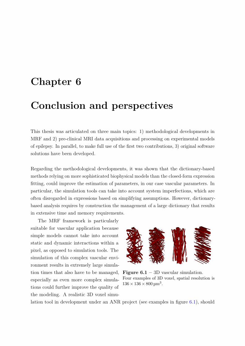
Chapter 6
Conclusion and perspectives
This thesis was articulated on three main topics: 1) methodological developments inMRF and 2) pre-clinical MRI data acquisitions and processing on experimental modelsof epilepsy. In parallel, to make full use of the first two contributions, 3) original softwaresolutions have been developed.
Regarding the methodological developments, it was shown that the dictionary-basedmethods relying on more sophisticated biophysical models than the closed-form expressionfitting, could improve the estimation of parameters, in our case vascular parameters. Inparticular, the simulation tools can take into account system imperfections, which areoften disregarded in expressions based on simplifying assumptions. However, dictionary-based analysis requires by construction the management of a large dictionary that resultsin extensive time and memory requirements.
Figure 6.1 – 3D vascular simulation.Four examples of 3D voxel, spatial resolution is136 × 136 × 800 µm3.
The MRF framework is particularlysuitable for vascular application becausesimple models cannot take into accountstatic and dynamic interactions within apixel, as opposed to simulation tools. Thesimulation of this complex vascular envi-ronment results in extremely large simula-tion times that also have to be managed,especially as even more complex simula-tions could further improve the quality ofthe modeling. A realistic 3D voxel simu-lation tool in development under an ANR project (see examples in figure 6.1), should
146 Conclusion and perspectives
provides signal highly sensitive to vascular parameters based on ex vivo angiogramimaging and optimal signal patterns [227]. The tool exhibits a single signal simulationtimes of approximately 15 minutes (about 10 seconds for current 2D tool). We canalso speculate that reducing a real vascular geometry to a few parameters would be toosimplistic and taking into account a larger number of parameters is necessary e.g. theanisotropy, tortuosity, vessel orientations, etc. One may also want to simulate signalsseveral minutes after contrast agent injections such as in dynamic contrast enhancement.In these cases, dictionary-based methods that allow a continuous representation of alarge set of parameters from a small number of dictionary entries are highly desirable tolimit simulation cost.
There has been several attempt to learn a continuous representation of the dictionary,all based on neural networks. We propose a statistical method that provides an highestimation accuracy compared to neural networks. Despite their high performance,neural network methods have some weaknesses, including difficulties in generalizingbeyond the learning dictionary and potential instability in case of new dictionary entries(section 4.3.1.4, page 114), low robustness to both thermal and aliasing high noise levels(sections 4.3.2.1 and 4.3.2.2), and a significant interpretability of the estimates obtained.Indeed, black box machine learning models, i.e. functions that are too complicated forany human to comprehend, are currently being used for high stakes decision makingsuch as in healthcare. Eventually methods are applied to explain these black box models.More complex models does not necessary mean more accurate, this is often not true,particularly when the data are structured, with a good representation in terms of naturallymeaningful features [228].
Instead of creating methods to explain black box models, creating models that areinherently interpretable/explainable is an alternative way, as chosen in this work for DB-SL method. We demonstrated that relying on our statistical method, the interpretabilityof the model has resulted in the production of a confidence index. Other possibilities havebeen explored such as, for example, the inclusion of spatial considerations to constrain themodel, which had previously been presented on hyper-spectral imaging [229]. This featureis part of the software package. Further investigations would be necessary to producean effective spatially-constrained dictionary-based learning method in MRF. Among thepossible improvements, a method for complex-valued data could be an important stepforward. The benefits of a complex-valued neural network have been shown by [168] andin particular, the benefit of the complex-valued framework over the split of the real andimaginary parts into two channels, which is the usual technique. Finally, we saw that
147
each method has its own strengths and weaknesses (table 4.1, page 120) and the specificapplication will determine the use of one or the other, or even considering combiningthem for better results.
Ensemble learning typically refers to methods that generate several models that arecombined to make a prediction, either in classification or regression problems [193]. Inthis multi-model study, we therefore considered a combination of methods that wouldimprove accuracy. The preliminary results focused on dictionary-based learning methodscombination, clearly shown the increase of estimates accuracy (section 4.3.4). One canalso combine matching and the proposed learning method. The mean and standarddeviation of the estimated posterior distribution (used in the actual framework as estimateand confidence index, respectively) could be used to compute the distance between themand those of the dictionary signals, i.e. the summary statistics of an approximate Bayesiancomputation (ABC, for more details, see [230]). This would provide a compression of thedictionary signals to two values and then avoid extensive time and memory requirements.In fact, ABC can be seen as a matching procedure, if we only consider the simulationentry that provided the minimum distance and reject others. One can also imagine usingthe entire posterior distribution and compute distance between distributions [231] tofurther improve estimate accuracy.
Related findings have been presented in several conferences: in 2018 at the annualcongress of the International Society for Magnetic Resonance in Medicine (ISMRM) [9],and in 2019 at the French national congress of life imaging [10] and at the annual congressof the French Society of Magnetic Resonance in Biology and Medicine [11]. A comparisonof the proposed and neural network approaches has been performed at the ISMRM thisyear [13] and a full paper is in revision [170].
Regarding the evaluation of epilepsy, the project was based on the use of experimentalmodels to investigate the localization of regions involved in the epilepsy network. InHumans it may be difficult to identify these regions, both the epileptic foci and regionsof epileptic seizure spread. We explored two different models of MTLE, one induced byintraperitoneal injection and the other one by intracerebral kainate injection. Resultsconcerning the first one are documented in appendix D but were not presented in thisthesis since we focused on the data corresponding to the second model (chapter 5). Infact, intraperitoneal injection model exhibits greater extent of neuronal damage but doesnot reproduce hippocampal sclerosis. Several practical issues were also addressed duringthis thesis but are not reported in this manuscript e.g. catheter installation for injection
148 Conclusion and perspectives
of contrast agents into the scanner, stabilization of physiological parameters and scalingof the protocol on mice at 9.4 T. Issues remain, in particular, the ASL acquisition ofblood flow in the absence of a dedicated labeling coil, remain. The MRI protocol couldthus be improved: it could be more complete. MRF could be further used to accelerateacquisition and/or improve accuracy on the other vascular parameters evaluated in thisstudy.
The study on MTLE model induced by intraperitoneal kainate injection, showedthat a multi-parameter approach could improve the identification of epileptic zones butalso of the regions in which the seizures spread. Since the data have been acquiredand revealed a possible discrimination of epileptic hippocampus compared to healthyhippocampus, it would be valuable to investigate methods allowing discrimination at thevoxel scale. As we have seen, depending on patient, areas within the hippocampus areinhomogeneously affected in humans (figure 2.7, page 27) The proposed approach couldthus be used to refine the localization of altered tissues. Such methods have alreadybeen used to characterize tumor tissues in rats [191] but in this pathology the cellularand vascular changes induced are substantial and cover a large region. It is thereforeobvious to localize the tumor in an image, even for unexperimented eyes. In epilepsy,these changes are small and are not detectable by eyes. An atlas of quantitative normalvalues could help detect local anomalies. Alternatively, asymmetry ratios may be used, astandard practice in radiology.
The protocol and analysis could be used with other experimental models of epilepsyto identify eventually a shared signature of MRI changes (e.g. intraperitoneal injectionmodel). One could also investigate the impact of treatment on this MRI signature andthus determine whether it would be possible to identify the regions involved in epilepsyin treated patients. As it stands, the protocol is not compatible with a routine clinicalexamination and adjustments would be necessary, mainly in reducing the acquisitiontime. Findings are currently in preparation for submission.
An effort in this work has been made to provide a tool to easily apply the analysis methods(ours and competitors’) to MRI data. Compare to standard MRF, dictionary-based learn-ing methods can easily be computed on a desktop computer even for large dictionaries.We showed that NN based methods are faster (section 4.3.1.2, page 112), speed mainly re-lying on mini-batch algorithms combined to GPU implementation. The proposed methodcould be greatly accelerated by using the same algorithms, mini-batch [232]. Currently,the algorithm could already be optimized in its current implementation for moderate

149
speed gain (e.g. parallelization of local Gaussian computation) and implementationsin other programming languages might be more suitable (e.g. in Python: GLLiM). Iactually had the opportunity to support two clinicians in the use of the tools during theirone-year research project.
We interfaced the proposed package with the medical software for processing multi-parametric images pipelines for an extended use to an audience not necessarily familiarwith programming, accepted work [185]. With open science in mind, protocols, data andcode will be shared.


Bibliography
[1] World Health Organization. Epilepsy: a public health imperative. Orga-nization, World Health, 2019. https://www.who.int/mental_health/neurology/epilepsy/report_2019/en/.
[2] Kristina Malmgren, Sallie Baxendale, and J. Helen Cross. Long-term outcomes of epilepsysurgery in adults and children. Long-Term Outcomes of Epilepsy Surgery in Adults andChildren, 7(6):1–283, 2015, DOI:10.1007/978-3-319-17783-0.
[3] Christian E. Elger and Dieter Schmidt. Modern management of epilepsy: A practicalapproach. Epilepsy and Behavior, 12(4):501–539, 2008, DOI:10.1016/j.yebeh.2008.01.003.
[4] William H Theodore and Robert S Fisher. Brain stimulation for epilepsy. The LancetNeurology, 3(2):111–118, 2004, DOI:10.1016/S1474-4422(03)00664-1.
[5] Shlomo Shinnar. The risk of seizure recurrence following a first unprovoked seizure: Aquantitative review. Neurology, 41(7):965–972, 1991, DOI:10.1212/wnl.41.7.965.
[6] Ettore Beghi, Arturo Carpio, Lars Forsgren, Dale C. Hesdorffer, Kristina Malmgren,Josemir W. Sander, Torbjorn Tomson, and W. Allen Hauser. Recommendation for a defi-nition of acute symptomatic seizure. Epilepsia, 51(4):671–675, 2010, DOI:10.1111/j.1528-1167.2009.02285.x.
[7] Soheyl Noachtar and Jan Rémi. The role of EEG in epilepsy: A critical review. Epilepsyand Behavior, 15(1):22–33, 2009, DOI:10.1016/j.yebeh.2009.02.035.
[8] Ingrid E. B. Tuxhorn, Reinhard Schulz, and Bernd Kruse. Invasive EEG in the definitionof the seizure onset zone: subdural electrodes. Handbook of Clinical Neurophysiology,3(C):97–108, 2003, DOI:10.1016/S1567-4231(03)03008-9.
[9] Fabien Boux, Florence Forbes, Julyan Arbel, and Emmanuel L. Barbier. Dictionary-freeMR fingerprinting parameter estimation via inverse regression. In Proceedings of the 26thAnnual Meeting, ISMRM, Paris, page 4259, 2016. HAL:01941630.
152 Bibliography
[10] Fabien Boux, Florence Forbes, Julyan Arbel, and Emmanuel Barbier. Dicionary learningvia regression: vascular MRI application. In 3e Congrès National d’Imagerie du Vivant(CNIV), 2019. HAL:02428647.
[11] Fabien Boux, Florence Forbes, Julyan Arbel, and Emmanuel Barbier. Estimation deparamètres IRM en grande dimension via une régression inverse. In 4e congrés de laSociété Française de Résonance Magnétique en Biologie et Médecine (SFRMBM), 2019.HAL:02428679.
[12] Aurélien Delphin. MRI Signals Simulation for Validation of a New Microvascular Charac-terization, 2019. DiVA:1355024.
[13] Fabien Boux, Florence Forbes, Julyan Arbel, Aurélien Delphin, Thomas Christen, andEmmanuel Barbier. Dictionary-based Learning in MR Fingerprinting: Statistical Learningversus Deep Learning. In International Society for Magnetic Resonance in Medicine(ISMRM), 2020., 2020. HAL:02922858.
[14] Hermann Ackermann. Cerebellar contributions to speech production and speech per-ception: psycholinguistic and neurobiological perspectives. Trends in Neurosciences,31(6):265–272, 2008, DOI:10.1016/j.tins.2008.02.011.
[15] S. Blease, M. Griffiths, and J. Bradshaw. Anatomy of the brain, 2001.https://mayfieldclinic.com/pe-anatbrain.htm.
[16] A. Dorr, J. G. Sled, and N. Kabani. Three-dimensional cerebral vasculature of the CBAmouse brain: A magnetic resonance imaging and micro computed tomography study.NeuroImage, 35(4):1409–1423, 2007, DOI:10.1016/j.neuroimage.2006.12.040.
[17] R. S. Sellers. Book Review: Comparative Anatomy and Histology: A Mouse and HumanAtlas, volume 49. Press, Academic, 2012.
[18] Julius Fridriksson, Paul Fillmore, Dazhou Guo, and Chris Rorden. Chronic Broca’s aphasiais caused by damage to Broca’s and wernicke’s areas. Cerebral Cortex, 25(12):4689–4696,2015, DOI:10.1093/cercor/bhu152.
[19] Jeffrey R. Binder. The Wernicke area. Neurology, 85(24):2170–2175, 2015,DOI:10.1212/WNL.0000000000002219.
[20] Tim Czopka, Charles Ffrench-Constant, and David A. Lyons. Individual oligodendrocyteshave only a few hours in which to generate new myelin sheaths in vivo. DevelopmentalCell, 25(6):599–609, 2013, DOI:10.1016/j.devcel.2013.05.013.
Bibliography 153
[21] Jochen Gehrmann, Yoh Matsumoto, and Georg W. Kreutzberg. Microglia: Intrin-sic immuneffector cell of the brain. Brain Research Reviews, 20(3):269–287, 1995,DOI:10.1016/0165-0173(94)00015-H.
[22] Konstantinos Meletis, Fanie Barnabé-Heider, Marie Carlén, Emma Evergren, Niko-lay Tomilin, Oleg Shupliakov, and Jonas Frisén. Spinal cord injury reveals mul-tilineage differentiation of ependymal cells. PLoS Biology, 6(7):1494–1507, 2008,DOI:10.1371/journal.pbio.0060182.
[23] J. A. Ramos-Vara and M. A. Miller. When Tissue Antigens and Antibodies Get Along:Revisiting the Technical Aspects of Immunohistochemistry-The Red, Brown, and BlueTechnique. Veterinary Pathology, 51(1):42–87, 2014, DOI:10.1177/0300985813505879.
[24] Deepa B. Rao, Peter B. Little, and Robert C. Sills. Subsite awareness in neuropathol-ogy evaluation of National Toxicology Program (NTP) studies: A review of selectneuroanatomical structures with their functional significance in rodents. ToxicologicPathology, 42(3):487–509, 2014, DOI:10.1177/0192623313501893.
[25] Samar Deb and Samar Deb. Blood Supply of Brain and Spinal Cord. Easy and In-teresting Approach to Human Neuroanatomy (Clinically Oriented), 2:228–228, 2014,DOI:10.5005/jp/books/12107_15.
[26] Frederic Lauwers, Francis Cassot, Valerie Lauwers-Cances, Prasanna Puwanarajah,and Henri Duvernoy. Morphometry of the human cerebral cortex microcirculation:General characteristics and space-related profiles. NeuroImage, 39(3):936–948, 2008,DOI:10.1016/j.neuroimage.2007.09.024.
[27] Kurt E. Schlageter, Peter Molnar, Gregory D. Lapin, and Dennis R. Groothuis. Microvesselorganization and structure in experimental brain tumors: Microvessel populations withdistinctive structural and functional properties. Microvascular Research, 58(3):312–328,1999, DOI:10.1006/mvre.1999.2188.
[28] Hartmut Vatter, Erdem Gueresir, and Volker Seifert. Blood injection subarachnoidhemorrhage rat model. 2009, DOI:10.1007/978-1-60327-185-1_22.
[29] Berislav V. Zlokovic. Neurovascular mechanisms of Alzheimer’s neurodegeneration. Trendsin Neurosciences, 28(4):202–208, 2005, DOI:10.1016/j.tins.2005.02.001.
[30] Amy J. Bastian and W. Thomas Thach. Structure and function of the cerebellum. TheCerebellum and its Disorders, 37(1):49–66, 2010, DOI:10.1017/cbo9780511666469.007.
154 Bibliography
[31] Karen K. Hirschi and Patricia A. D’Amore. Pericytes in the microvasculature. Cardio-vascular Research, 32(4):687–698, 1996, DOI:10.1016/0008-6363(96)00063-6.
[32] Annika Armulik, Guillem Genové, Maarja Mäe, Maya H. Nisancioglu, Elisabet Wallgard,Colin Niaudet, Liqun He, Jenny Norlin, Per Lindblom, Karin Strittmatter, Bengt R.Johansson, and Christer Betsholtz. Pericytes regulate the blood-brain barrier. Nature,468(7323):557–561, 2010, DOI:10.1038/nature09522.
[33] Brian T. Hawkins and Thomas P. Davis. The blood-brain barrier/neurovascular unit inhealth and disease. Pharmacological Reviews, 57(2):173–185, 2005, DOI:10.1124/pr.57.2.4.
[34] Amy R. Nelson, Melanie D. Sweeney, Abhay P. Sagare, and Berislav V. Zlokovic. Neu-rovascular dysfunction and neurodegeneration in dementia and Alzheimer’s disease.Biochimica et Biophysica Acta - Molecular Basis of Disease, 1862(5):887–900, 2016,DOI:10.1016/j.bbadis.2015.12.016.
[35] Stefanie Robel, Benedikt Berninger, and Magdalena Götz. The stem cell potential ofglia: Lessons from reactive gliosis. Nature Reviews Neuroscience, 12(2):88–104, 2011,DOI:10.1038/nrn2978.
[36] Michael V. Sofroniew and Harry V. Vinters. Astrocytes: Biology and pathology. ActaNeuropathologica, 119(1):7–35, 2010, DOI:10.1007/s00401-009-0619-8.
[37] Mark A. Anderson, Yan Ao, and Michael V. Sofroniew. Heterogeneity of reactiveastrocytes. Neuroscience Letters, 565:23–29, 2014, DOI:10.1016/j.neulet.2013.12.030.
[38] Randolph N. Christensen, Byeong Keun Ha, Fang Sun, Jacqueline C. Bresnahan,and Michael S. Beattie. Kainate induces rapid redistribution of the actin cytoskele-ton in ameboid microglia. Journal of Neuroscience Research, 84(1):170–181, 2006,DOI:10.1002/jnr.20865.
[39] Engin Gonul, Bülent Duz, Serdar Kahraman, Hakan Kayali, Ayhan Kubar, and ErdenerTimurkaynak. Early pericyte response to brain hypoxia in cats: An ultrastructural study.Microvascular Research, 64(1):116–119, 2002, DOI:10.1006/mvre.2002.2413.
[40] Paula Dore-Duffy, Cheri Owen, Roumen Balabanov, Sharon Murphy, Thomas Beaumont,and José A. Rafols. Pericyte migration from the vascular wall in response to traumaticbrain injury. Microvascular Research, 60(1):55–69, 2000, DOI:10.1006/mvre.2000.2244.
[41] Gesa Rascher, Arne Fischmann, Stephan Kröger, Frank Duffner, Ernst H. Grote, andHartwig Wolburg. Extracellular matrix and the blood-brain barrier in glioblastoma
Bibliography 155
multiforme: Spatial segregation of tenascin and agrin. Acta Neuropathologica, 104(1):85–91, 2002, DOI:10.1007/s00401-002-0524-x.
[42] Giovanni Savettieri, Italia Di Liegro, Caterina Catania, Luana Licata, Giovanna LauraPitarresi, Stefania D’Agostino, Gabriella Schiera, Viviana De Caro, Giulia Gian-dalia, Libero Italo Giannola, and Alessandro Cestelli. Neurons and ECM regulateoccludin localization in brain endothelial cells. NeuroReport, 11(5):1081–1084, 2000,DOI:10.1097/00001756-200004070-00035.
[43] Jerome Engel. A proposed diagnostic scheme for people with epileptic seizures and withepilepsy: Report of the ILAE task force on classification and terminology. Epilepsia,42(6):796–803, 2001, DOI:10.1046/j.1528-1157.2001.10401.x.
[44] Jerome Engel. ILAE classification of epilepsy syndromes. Epilepsy Research,70(SUPPL.1):5–10, 2006, DOI:10.1016/j.eplepsyres.2005.11.014.
[45] Gregory D. Cascino and Joseph I. Sirven. Adult Epilepsy. Adult Epilepsy, 367(9516):1087–1100, 2011, DOI:10.1002/9780470975039.
[46] M. J. During and D. D. Spencer. Extracellular hippocampal glutamate and sponta-neous seizure in the conscious human brain. The Lancet, 341(8861):1607–1610, 1993,DOI:10.1016/0140-6736(93)90754-5.
[47] Matthew J. During, Kathryn M. Ryder, and Dennis D. Spencer. HippocampalGABA transporter function in temporal-lobe epileps. Nature, 376(6536):174–177, 1995,DOI:10.1038/376174a0.
[48] David M. Treiman. GABAergic mechanisms in epilepsy. Epilepsia, 42(SUPPL. 3):8–12,2001, DOI:10.1046/j.1528-1157.2001.042Suppl.3008.x.
[49] Solomon L. Moshé, Emilio Perucca, Philippe Ryvlin, and Torbjörn Tomson. Epilepsy: Newadvances. The Lancet, 385(9971):884–898, 2015, DOI:10.1016/S0140-6736(14)60456-6.
[50] Marco De Curtis and Giuliano Avanzini. Interictal spikes in focal epileptogenesis. Progressin Neurobiology, 63(5):541–567, 2001, DOI:10.1016/S0301-0082(00)00026-5.
[51] C. S. Herrmann and T. Demiralp. Human EEG gamma oscillations inneuropsychiatric disorders. Clinical Neurophysiology, 116(12):2719–2733, 2005,DOI:10.1016/j.clinph.2005.07.007.
[52] J. Talairach, J. Bancaud, A. Bonis, G. Szikla, and P. Tournoux. Functional stereotaxic ex-ploration of epilepsy. Confinia neurologica, 22(1):328–331, 1962, DOI:10.1159/000104378.
156 Bibliography
[53] Greg A. Worrell, Landi Parish, Stephen D. Cranstoun, Rachel Jonas, Gordon Baltuch,and Brian Litt. High-frequency oscillations and seizure generation in neocortical epilepsy.Brain, 127(7):1496–1506, 2004, DOI:10.1093/brain/awh149.
[54] Vadym Gnatkovsky, Stefano Francione, Francesco Cardinale, Roberto Mai, Laura Tassi,Giorgio Lo Russo, and Marco De Curtis. Identification of reproducible ictal patterns basedon quantified frequency analysis of intracranial EEG signals. Epilepsia, 52(3):477–488,2011, DOI:10.1111/j.1528-1167.2010.02931.x.
[55] Shelagh J. M. Smith. EEG in the diagnosis, classification, and management of patientswith epilepsy. Neurology in Practice, 76(2):ii2—-ii7, 2005, DOI:10.1136/jnnp.2005.069245.
[56] Olivier David, Thomas Blauwblomme, Anne Sophie Job, Stéphan Chabards, Do-minique Hoffmann, Lorella Minotti, and Philippe Kahane. Imaging the seizureonset zone with stereo-electroencephalography. Brain, 134(10):2898–2911, 2011,DOI:10.1093/brain/awr238.
[57] Gary W. Mathern, Thomas L. Babb, Barbara G. Vickrey, Maria Melendez, andJames K. Pretorius. The clinical-pathogenic mechanisms of hippocampal neuronloss and surgical outcomes in temporal lobe epilepsy. Brain, 118(1):105–118, 1995,DOI:10.1093/brain/118.1.105.
[58] Ingmar Blümcke, Maria Thom, Eleonora Aronica, Dawna D. Armstrong, Fabrice Bar-tolomei, Andrea Bernasconi, Neda Bernasconi, Christian G. Bien, Fernando Cendes,Roland Coras, J. Helen Cross, Thomas S. Jacques, Philippe Kahane, Gary W. Mathern,Haijme Miyata, Solomon L. Moshé, Buge Oz, Çigdem Özkara, Emilio Perucca, SanjaySisodiya, Samuel Wiebe, and Roberto Spreafico. International consensus classification ofhippocampal sclerosis in temporal lobe epilepsy: A Task Force report from the ILAE Com-mission on Diagnostic Methods. Epilepsia, 54(7):1315–1329, 2013, DOI:10.1111/epi.12220.
[59] Orrin Devinsky, Annamaria Vezzani, Souhel Najjar, Nihal C. De Lanerolle, and Michael A.Rogawski. Glia and epilepsy: Excitability and inflammation. Trends in Neurosciences,36(3):174–184, 2013, DOI:10.1016/j.tins.2012.11.008.
[60] Jonathon Wetherington, Geidy Serrano, and Ray Dingledine. Astrocytes in the EpilepticBrain. Neuron, 58(2):168–178, 2008, DOI:10.1016/j.neuron.2008.04.002.
[61] Teresa Ravizza, Barbara Gagliardi, Francesco Noé, Karin Boer, Eleonora Aronica, andAnnamaria Vezzani. Innate and adaptive immunity during epileptogenesis and sponta-neous seizures: Evidence from experimental models and human temporal lobe epilepsy.Neurobiology of Disease, 29(1):142–160, 2008, DOI:10.1016/j.nbd.2007.08.012.
Bibliography 157
[62] Valérie Rigau, Mélanie Morin, Marie Claude Rousset, Frédéric De Bock, Aurore Le-brun, Philippe Coubes, Marie Christine Picot, Michel Baldy-Moulinier, Joël Bockaert,Arielle Crespel, and Mireille Lerner-Natoli. Angiogenesis is associated with blood-brain barrier permeability in temporal lobe epilepsy. Brain, 130(7):1942–1956, 2007,DOI:10.1093/brain/awm118.
[63] Nicola Marchi, Lilyana Angelov, Thomas Masaryk, Vincent Fazio, Tiziana Granata, NadiaHernandez, Kerri Hallene, Tammy Diglaw, Linda Franic, Imad Najm, and Damir Janigro.Seizure-promoting effect of blood-brain barrier disruption. Epilepsia, 48(4):732–742, 2007,DOI:10.1111/j.1528-1167.2007.00988.x.
[64] Nicola Marchi, Tiziana Granata, Chaitali Ghosh, and Damir Janigro. Blood-brain barrierdysfunction and epilepsy: Pathophysiologic role and therapeutic approaches. Epilepsia,53(11):1877–1886, 2012, DOI:10.1111/j.1528-1167.2012.03637.x.
[65] Arielle Crespel, Philippe Coubes, Marie Claude Rousset, Corinne Brana, Alain Rougier,Gérard Rondouin, Joël Bockaert, Michel Baldy-Moulinier, and Mireille Lerner-Natoli.Inflammatory reactions in human medial temporal lobe epilepsy with hippocampalsclerosis. Brain Research, 952(2):159–169, 2002, DOI:10.1016/S0006-8993(02)03050-0.
[66] E. A. Van Vliet, S. Da Costa Araújo, S. Redeker, R. Van Schaik, E. Aronica, and J. A.Gorter. Blood-brain barrier leakage may lead to progression of temporal lobe epilepsy.Brain, 130(2):521–534, 2007, DOI:10.1093/brain/awl318.
[67] A. Depaulis and S. Hamelin. Animal models for mesiotemporal lobe epilepsy:The end of a misunderstanding? Revue Neurologique, 171(3):217–226, 2015,DOI:10.1016/j.neurol.2015.01.558.
[68] Graham V. Goddard. Development of epileptic seizures through brain stimulation at lowintensity. Nature, 214(5092):1020–1021, 1967, DOI:10.1038/2141020a0.
[69] Kiyoshi Morimoto, Margaret Fahnestock, and Ronald J. Racine. Kindling and statusepilepticus models of epilepsy: Rewiring the brain. Progress in Neurobiology, 73(1):1–60,2004, DOI:10.1016/j.pneurobio.2004.03.009.
[70] Y. Ben-Ari and J. Lagowska. Action épileptogène induite par des injections intraamyg-daliennes d’acide kainique. Comptes rendus hebdomadaires des seances de l"Academiedes sciences. Serie D: Sciences naturelles, 287(8):813–816, 1978. PMID:103652.
[71] Waldemar A. Turski, Esper A. Cavalheiro, Michael Schwarz, Stanisław J. Czuczwar,Zdzisław Kleinrok, and Lechosław Turski. Limbic seizures produced by pilocarpine in

158 Bibliography
rats: Behavioural, electroencephalographic and neuropathological study. BehaviouralBrain Research, 9(3):315–335, 1983, DOI:10.1016/0166-4328(83)90136-5.
[72] Maxime Lévesque and Massimo Avoli. The kainic acid model of temporallobe epilepsy. Neuroscience and Biobehavioral Reviews, 37(10):2887–2899, 2013,DOI:10.1016/j.neubiorev.2013.10.011.
[73] Andrew White, Philip A. Williams, Jennifer L. Hellier, Suzanne Clark, F. Edward Dudek,and Kevin J. Staley. EEG spike activity precedes epilepsy after kainate-induced statusepilepticus. Epilepsia, 51(3):371–383, 2010, DOI:10.1111/j.1528-1167.2009.02339.x.
[74] Doodipala Samba Reddy and Ramkumar Kuruba. Experimental models of status epilepti-cus and neuronal injury for evaluation of therapeutic interventions. International Journalof Molecular Sciences, 14(9):18284–18318, 2013, DOI:10.3390/ijms140918284.
[75] Luiz E. A. M. Mello, Esper A. Cavalheiro, Aiko M. Tan, William R. Kupfer, James K.Pretorius, Thomas L. Babb, and David M. Finch. Circuit Mechanisms of Seizures in thePilocarpine Model of Chronic Epilepsy: Cell Loss and Mossy Fiber Sprouting. Epilepsia,34(6):985–995, 1993, DOI:10.1111/j.1528-1157.1993.tb02123.x.
[76] Muddanna S. Rao, Bharathi Hattiangady, Doodipala S. Reddy, and Ashok K. Shetty.Hippocampal neurodegeneration, spontaneous seizures, and mossy fiber sprouting in theF344 rat model of temporal lobe epilepsy. Journal of Neuroscience Research, 83(6):1088–1105, 2006, DOI:10.1002/jnr.20802.
[77] Paul S. Buckmaster, Guo Feng Zhang, and Ruth Yamawaki. Axon sprouting in a modelof temporal lobe epilepsy creates a predominantly excitatory feedback circuit. Journal ofNeuroscience, 22(15):6650–6658, 2002, DOI:10.1523/jneurosci.22-15-06650.2002.
[78] Robert S. Sloviter. The neurobiology of temporal lobe epilepsy: Too much infor-mation, not enough knowledge. Comptes Rendus - Biologies, 328(2):143–153, 2005,DOI:10.1016/j.crvi.2004.10.010.
[79] Marcio A. De Furtado, Glaucia K. Braga, José A. C. Oliveira, Flavio Del Vecchio,and Norberto Garcia-Cairasco. Behavioral, morphologic, and electroencephalographicevaluation of seizures induced by intrahippocampal microinjection of pilocarpine. Epilepsia,43(SUPPL. 5):37–39, 2002, DOI:10.1046/j.1528-1157.2002.043s2037.x.
[80] V. Bouilleret, V. Ridoux, A. Depaulis, C. Marescaux, A. Nehlig, and G. Le Gal La Salle.Recurrent seizures and hippocampal sclerosis following intrahippocampal kainate injectionin adult mice: Electroencephalography, histopathology and synaptic reorganization similar
Bibliography 159
to mesial temporal lobe epilepsy. Neuroscience, 89(3):717–729, 1999, DOI:10.1016/S0306-4522(98)00401-1.
[81] Y. Ben-Ari, E. Tremblay, and O. P. Ottersen. Injections of kainic acid into the amyg-daloid complex of the rat: An electrographic, clinical and histological study in relationto the pathology of epilepsy. Neuroscience, 5(3):515–528, 1980, DOI:10.1016/0306-4522(80)90049-4.
[82] C. Cepeda, T. Tanaka, D. Riche, and R. Naquet. Limbic status epilepticus: behaviourand sleep alterations after intra-amygdaloid kainic acid microinjections in Papio papiobaboons. Electroencephalography and Clinical Neurophysiology, 54(6):603–613, 1982,DOI:10.1016/0013-4694(82)90114-6.
[83] Marta Rattka, Claudia Brandt, and Wolfgang Löscher. The intrahippocampal kainatemodel of temporal lobe epilepsy revisited: Epileptogenesis, behavioral and cognitive alter-ations, pharmacological response, and hippoccampal damage in epileptic rats. EpilepsyResearch, 103(2-3):135–152, 2013, DOI:10.1016/j.eplepsyres.2012.09.015.
[84] Wendy Klement, Marine Blaquiere, Emma Zub, Frederic DeBock, Fabien Boux, EmmanuelBarbier, Etienne Audinat, Mireille Lerner-Natoli, and Nicola Marchi. A pericyte-gliascarring develops at the leaky capillaries in the hippocampus during seizure activity.Epilepsia, 60(7):1399–1411, jul 2019, DOI:10.1111/epi.16019.
[85] V. Riban, V. Bouilleret, B. T. Pham-Lê, J. M. Fritschy, C. Marescaux, and A. Depaulis.Evolution of hippocampal epileptic activity during the development of hippocampalsclerosis in a mouse model of temporal lobe epilepsy. Neuroscience, 112(1):101–111, 2002,DOI:10.1016/S0306-4522(02)00064-7.
[86] Khichar Shubhakaran and Rekha Jakhar Khichar. Neuroimaging of first-ever seizure:Contribution of MRI if CT is normal. Neurology: Clinical Practice, 4(5):372, 2014,DOI:10.1212/01.CPJ.0000455828.60011.1d.
[87] Nitin K. Sethi and Shinnar. Evidence-based guideline: Management of an unprovoked firstseizure in adults: Report of the Guideline Development Subcommittee of the AmericanAcademy of Neurology and the American Epilepsy Society. Neurology, 85(17):1525, 2015,DOI:10.1212/WNL.0000000000002093.
[88] R. A. Bronen. Epilepsy: The role of MR imaging. American Journal of Roentgenology,159(6):1165–1174, 1992, DOI:10.2214/ajr.159.6.1442376.
160 Bibliography
[89] Maarten G. Lansberg, M. W. O’Brien, A. M. Norbash, M. E. Moseley, M. Morrell, andG. W. Albers. MRI abnormalities associated with partial status epilepticus. Neurology,52(5):1021–1027, 1999, DOI:10.1212/wnl.52.5.1021.
[90] M. D. King, N. Van Bruggen, R. G. Ahier, J. E. Cremer, J. V. Hajnal, S. R. Williams, andM. Doran. Diffusion-weighted imaging of kainic acid lesions in the rat brain. MagneticResonance in Medicine, 1991, DOI:10.1002/mrm.1910200117.
[91] Man Kin Choy, King K. Cheung, David L. Thomas, David G. Gadian, Mark F. Lythgoe,and Rod C. Scott. Quantitative MRI predicts status epilepticus-induced hippocampalinjury in the lithium-pilocarpine rat model. Epilepsy Research, 88(2-3):221–230, 2010,DOI:10.1016/j.eplepsyres.2009.11.013.
[92] Yang Wang, Anthony Majors, Imad Najm, Min Xue, Youssef Comair, Michael Modic,and Thian C. Ng. Postictal alteration of sodium content and apparent diffusion coeffi-cient in epileptic rat brain induced by kainic acid. Epilepsia, 37(10):1000–1006, 1996,DOI:10.1111/j.1528-1157.1996.tb00539.x.
[93] T. Engelhorn, J. Weise, T. Hammen, I. Bluemcke, A. Hufnagel, and A. Doerfler.Early diffusion-weighted MRI predicts regional neuronal damage in generalized sta-tus epilepticus in rats treated with diazepam. Neuroscience Letters, 417(3):275–280, 2007,DOI:10.1016/j.neulet.2007.02.072.
[94] Jaak Nairismägi, Olli H. J. Gröhn, Mikko I. Kettunen, Jari Nissinen, Risto A. Kauppinen,and Asla Pitkänen. Progression of brain damage after status epilepticus and its associationwith epileptogenesis: A quantitative MRI study in a rat model of temporal lobe epilepsy.Epilepsia, 45(9):1024–1034, 2004, DOI:10.1111/j.0013-9580.2004.08904.x.
[95] Nick M. E. A. Hayward, Xavier Ekolle Ndode-Ekane, Nino Kutchiashvili, Olli Gröhn,and Asla Pitkänen. Elevated cerebral blood flow and vascular density in the amyg-dala after status epilepticus in rats. Neuroscience Letters, 484(1):39–42, 2010,DOI:10.1016/j.neulet.2010.08.013.
[96] Guy Bar-Klein, Svetlana Lublinsky, Lyn Kamintsky, Iris Noyman, Ronel Veksler, HotjensaDalipaj, Vladimir V. Senatorov, Evyatar Swissa, Dror Rosenbach, Netta Elazary, Dan Z.Milikovsky, Nadav Milk, Michael Kassirer, Yossi Rosman, Yonatan Serlin, Arik Eisenkraft,Yoash Chassidim, Yisrael Parmet, Daniela Kaufer, and Alon Friedman. Imaging blood-brain barrier dysfunction as a biomarker for epileptogenesis. Brain, 140(6):1692–1705,2017, DOI:10.1093/brain/awx073.
Bibliography 161
[97] E. A. van Vliet, W. M. Otte, J. A. Gorter, R. M. Dijkhuizen, and W. J. Wad-man. Longitudinal assessment of blood-brain barrier leakage during epileptogenesisin rats. A quantitative MRI study. Neurobiology of Disease, 63:74–84, mar 2014,DOI:10.1016/j.nbd.2013.11.019.
[98] Catherine Roch, Claire Leroy, Astrid Nehlig, and Izzie J. Namer. Magnetic resonanceimaging in the study of the lithium-pilocarpine model of temporal lobe epilepsy in adultrats. Epilepsia, 43(4):325–335, 2002, DOI:10.1046/j.1528-1157.2002.11301.x.
[99] Viviane Bouilleret, Astrid Nehlig, Christian Marescaux, and Izzie J. Namer. Magneticresonance imaging follow-up of progressive hippocampal changes in a mouse modelof mesial temporal lobe epilepsy. Epilepsia, 41(6):642–650, 2000, DOI:10.1111/j.1528-1157.2000.tb00223.x.
[100] Boris C. Bernhardt, Fatemeh Fadaie, Reinder Vos de Wael, Seok Jun Hong, MinLiu, Marie C. Guiot, David A. Rudko, Andrea Bernasconi, and Neda Bernasconi.Preferential susceptibility of limbic cortices to microstructural damage in temporallobe epilepsy: A quantitative T1 mapping study. NeuroImage, 182:294–303, 2018,DOI:10.1016/j.neuroimage.2017.06.002.
[101] Lionel Thivard, Stéphane Lehéricy, Alexandre Krainik, Claude Adam, Didier Dormont,Jacques Chiras, Michel Baulac, and Sophie Dupont. Diffusion tensor imaging in medialtemporal lobe epilepsy with hippocampal sclerosis. NeuroImage, 28(3):682–690, 2005,DOI:10.1016/j.neuroimage.2005.06.045.
[102] S. Flacke, U. Wüllner, E. Keller, F. Hamzei, and H. Urbach. Reversible changes inecho planar perfusion- and diffusion-weighted MRI in status epilepticus. Neuroradiology,42(2):92–95, 2000, DOI:10.1007/s002340050021.
[103] P. F. Fabene, P. Marzola, A. Sbarbati, and M. Bentivoglio. Magnetic resonance imaging ofchanges elicited by status epilepticus in the rat brain: Diffusion-weighted and T2-weightedimages, regional blood volume maps, and direct correlation with tissue and cell damage.NeuroImage, 18(2):375–389, 2003, DOI:10.1016/S1053-8119(02)00025-3.
[104] Ren H. Wu, Roland Bruening, Sami Noachtar, Stephan Arnold, Christian Berchtenbreiter,Peter Bartenstein, Alexander Drzezga, Klaus Tatsch, and Maximilian Reiser. MR mea-surement of regional relative cerebral blood volume in epilepsy. Journal of Magnetic Res-onance Imaging, 9(3):435–440, 1999, DOI:10.1002/(SICI)1522-2586(199903)9:3<435::AID-JMRI11>3.0.CO;2-J.
162 Bibliography
[105] Jerome Aellen, Eugenio Abela, Sarah E. Buerki, Raimund Kottke, Elisabeth Springer,Kaspar Schindler, Christian Weisstanner, Marwan El-Koussy, Gerhard Schroth, RolandWiest, Jan Gralla, and Rajeev K. Verma. Focal hemodynamic patterns of status epilepticusdetected by susceptibility weighted imaging (SWI). European Radiology, 24(11):2980–2988,2014, DOI:10.1007/s00330-014-3284-9.
[106] Xinyang Feng, Marla J. Hamberger, Hannah C. Sigmon, Jia Guo, Scott A. Small,and Frank A. Provenzano. Temporal lobe epilepsy lateralization using retro-spective cerebral blood volume MRI. NeuroImage: Clinical, 19:911–917, 2018,DOI:10.1016/j.nicl.2018.05.012.
[107] Theodor Rüber, Bastian David, Guido Lüchters, Robert D. Nass, Alon Friedman, RainerSurges, Tony Stöcker, Bernd Weber, Ralf Deichmann, Gottfried Schlaug, Elke Hattingen,and Christian E. Elger. Evidence for peri-ictal blood-brain barrier dysfunction in patientswith epilepsy. Brain, 141(10):2952–2965, 2018, DOI:10.1093/brain/awy242.
[108] A. D. Elster. Questions and Answers in MRI, 2017. http://mriquestions.com.
[109] IMAIOS. L’IRM pas à pas, cours interactif sur l’imagerie par résonance magnétique,2011. http://www.imaios.com/fr/e-Cours/e-MRI.
[110] H. H. Mitchell, T. S. Hamilton, F. R. Steggerda, and H. W. Bean. TheChemical Composition of the Adult Human Body and Its Bearing on the Bio-chemistry of Growth. Journal of Biological Chemistry, 158(3):625–637, 1945.https://www.jbc.org/content/158/3/625.full.pdf.
[111] F. Bloch. Nuclear induction. Physica, 17(3-4):272–281, 1951, DOI:10.1016/0031-8914(51)90068-7.
[112] Mark A. Brown and Richard C. Semelka. MRI: basic principles and applications. Sons,John Wiley &, 2011. ISBN:978-1-119-01305-1.
[113] Gary H Glover and John M Pauly. Projection reconstruction techniques for reduc-tion of motion effects in mri. Magnetic resonance in medicine, 28(2):275–289, 1992,DOI:10.1002/mrm.1910280209.
[114] Jesse Hamilton, Dominique Franson, and Nicole Seiberlich. Recent advances in parallelimaging for MRI. Progress in Nuclear Magnetic Resonance Spectroscopy, 101:71–95, 2017,DOI:10.1016/j.pnmrs.2017.04.002.
[115] Albert Macovski. Noise in MRI. Magnetic Resonance in Medicine, 1996,DOI:10.1002/mrm.1910360327.
Bibliography 163
[116] J. B. Johnson. Thermal agitation of electricity in conductors. Physical Review, 32(1):97–109, 1928, DOI:10.1103/PhysRev.32.97.
[117] Assaf Tal. Lecture 9: SNR, 2014. https://www.weizmann.ac.il/chemphys/assaf_tal/sites/chemphys.assaf_tal/files/uploads/lecture_9_-_snr.pdf.
[118] Adolf Fick. Ueber Diffusion. Annalen der Physik, 170(1):59–86, 1855,DOI:10.1002/andp.18551700105.
[119] E. O. Stejskal and J. E. Tanner. Spin diffusion measurements: Spin echoes in the presenceof a time-dependent field gradient. The Journal of Chemical Physics, 42(1):288–292, 1965,DOI:10.1063/1.1695690.
[120] H. C. Torrey. Bloch equations with diffusion terms. Physical Review, 104(3):563–565,1956, DOI:10.1103/PhysRev.104.563.
[121] D. Le Bihan. Molecular diffusion nuclear magnetic resonance imaging. Magnetic resonancequarterly, 7(1):1–30, 1991. PMID:2043461.
[122] Emmanuel L. Barbier, Laurent Lamalle, and Michel Décorps. Methodology of brainperfusion imaging. Journal of Magnetic Resonance Imaging, 13(4):496–520, 2001,DOI:10.1002/jmri.1073.
[123] Donald S. Williams, Donald J. Grandis, Weiguo Zhang, and Alan P. Koretsky. Magneticresonance imaging of perfusion in the isolated rat heart using spin inversion of arterial wa-ter. Magnetic Resonance in Medicine, 30(3):361–365, 1993, DOI:10.1002/mrm.1910300314.
[124] Wen Chau Wu, María Fernández-Seara, John A. Detre, Felix W. Wehrli, and JiongjiongWang. A theoretical and experimental investigation of the tagging efficiency of pseu-docontinuous arterial spin labeling. Magnetic Resonance in Medicine, 58(5):1020–1027,2007, DOI:10.1002/mrm.21403.
[125] Weiying Dai, Dairon Garcia, Cedric De Bazelaire, and David C. Alsop. Continuousflow-driven inversion for arterial spin labeling using pulsed radio frequency and gradientfields. Magnetic Resonance in Medicine, 60(6):1488–1497, 2008, DOI:10.1002/mrm.21790.
[126] Lydiane Hirschler, Clément S. Debacker, Jérôme Voiron, Sascha Köhler, Jan M. Warnking,and Emmanuel L. Barbier. Interpulse phase corrections for unbalanced pseudo-continuousarterial spin labeling at high magnetic field. Magnetic Resonance in Medicine, 79(3):1314–1324, 2018, DOI:10.1002/mrm.26767.
[127] CheMatech. P00449 – Gd-DOTA. https://www.chematech-mdt.com/produit/p00449-gd-dota/.
164 Bibliography
[128] CheMatech. P904 – USPIO. https://www.chematech-mdt.com/produit/p904-uspio/.
[129] Sagar Buch, Ying Wang, Min-Gyu Park, Pavan K Jella, Jiani Hu, YongshengChen, Kamran Shah, Yulin Ge, and E Mark Haacke. Subvoxel vascular imag-ing of the midbrain using uspio-enhanced mri. NeuroImage, 220:117106, 2020,DOI:10.1016/j.neuroimage.2020.117106.
[130] Jerrold L Boxerman, Leena M Hamberg, Bruce R Rosen, and Robert M Weisskoff. Mrcontrast due to intravascular magnetic susceptibility perturbations. Magnetic resonancein medicine, 34(4):555–566, 1995, DOI:10.1002/mrm.1910340412.
[131] Irene Troprès, Laurent Lamalle, M Peoc’h, Régine Farion, Yves Usson, Michel Décorps,and C Remy. In vivo assessment of tumoral angiogenesis. Magnetic Resonance in Medicine:An Official Journal of the International Society for Magnetic Resonance in Medicine,51(3):533–541, 2004, DOI:10.1002/mrm.20017.
[132] Irène Troprès, Stephan Grimault, Albert Vaeth, Emmanuelle Grillon, Cécile Julien,Jean François Payen, Laurent Lamalle, and Michel Décorps. Vessel size imag-ing. Magnetic Resonance in Medicine, 45(3):397–408, 2001, DOI:10.1002/1522-2594(200103)45:3<397::AID-MRM1052>3.0.CO;2-3.
[133] Thomas Christen, Pierre Bouzat, Nicolas Pannetier, Nicolas Coquery, Anaïck Moisan,Benjamin Lemasson, Sébastien Thomas, Emmanuelle Grillon, Olivier Detante, ChantalRémy, Jean François Payen, and Emmanuel Luc Barbier. Tissue oxygen saturation map-ping with magnetic resonance imaging. Journal of Cerebral Blood Flow and Metabolism,34(9):1550–1557, 2014, DOI:10.1038/jcbfm.2014.116.
[134] Thomas Christen, Benjamin Lemasson, Nicolas Pannetier, Régine Farion, ChristophSegebarth, Chantal Rémy, and Emmanuel L. Barbier. Evaluation of a quantitative bloodoxygenation level-dependent (qBOLD) approach to map local blood oxygen saturation.NMR in Biomedicine, 24(4):393–403, 2011, DOI:10.1002/nbm.1603.
[135] Fahmi Khalifa, Ahmed Soliman, Ayman El-Baz, Mohamed Abou El-Ghar, Tarek El-Diasty, Georgy Gimel’Farb, Rosemary Ouseph, and Amy C. Dwyer. Models andmethods for analyzing DCE-MRI: A review. Medical Physics, 41(12):124301, 2014,DOI:10.1118/1.4898202.
[136] Hai Ling Margaret Cheng. Improved correlation to quantitative DCE-MRI pharmacoki-netic parameters using a modified initial area under the uptake curve (mIAUC) approach.Journal of Magnetic Resonance Imaging, 30(4):864–872, 2009, DOI:10.1002/jmri.21916.
Bibliography 165
[137] Dan Ma, Vikas Gulani, Nicole Seiberlich, Kecheng Liu, Jeffrey L. Sunshine, Jeffrey L.Duerk, and Mark A. Griswold. Magnetic resonance fingerprinting. Nature, 495(7440):187–192, 2013, DOI:10.1038/nature11971.
[138] Ananya Panda, Bhairav B. Mehta, Simone Coppo, Yun Jiang, Dan Ma, NicoleSeiberlich, Mark A. Griswold, and Vikas Gulani. Magnetic resonance fingerprint-ing – An overview. Current Opinion in Biomedical Engineering, 3:56–66, 2017,DOI:10.1016/j.cobme.2017.11.001.
[139] Debra F. McGivney, Rasim Boyacıoğlu, Yun Jiang, Megan E. Poorman, Nicole Seiberlich,Vikas Gulani, Kathryn E. Keenan, Mark A. Griswold, and Dan Ma. Magnetic resonancefingerprinting review part 2: Technique and directions. Journal of Magnetic ResonanceImaging, 51(4):993–1007, 2020, DOI:10.1002/jmri.26877.
[140] Jorge J. Moré. The Levenberg-Marquardt algorithm: Implementation and theory. Nu-merical analysis, pages 105–116, 1978, DOI:10.1007/bfb0067700.
[141] Dan Ma, Eric Y. Pierre, Yun Jiang, Mark D. Schluchter, Kawin Setsompop, Vikas Gulani,and Mark A. Griswold. Music-based magnetic resonance fingerprinting to improve patientcomfort during MRI examinations. Magnetic Resonance in Medicine, 75(6):2303–2314,2016, DOI:10.1002/mrm.25818.
[142] Yun Jiang, Dan Ma, Nicole Seiberlich, Vikas Gulani, and Mark A. Griswold. MRfingerprinting using fast imaging with steady state precession (FISP) with spiral readout.Magnetic Resonance in Medicine, 74(6):1621–1631, 2015, DOI:10.1002/mrm.25559.
[143] Jakob Assländer, Steffen J. Glaser, and Jürgen Hennig. Pseudo Steady-State FreePrecession for MR-Fingerprinting. Magnetic Resonance in Medicine, 77(3):1151–1161,2017, DOI:10.1002/mrm.26202.
[144] Benedikt Rieger, Fabian Zimmer, Jascha Zapp, Sebastian Weingärtner, and Lothar R.Schad. Magnetic resonance fingerprinting using echo-planar imaging: Joint quantificationof T1 and T2 relaxation times. Magnetic Resonance in Medicine, 78(5):1724–1733, 2017,DOI:10.1002/mrm.26561.
[145] Megan E. Poorman, Michele N. Martin, Dan Ma, Debra F. McGivney, Vikas Gulani,Mark A. Griswold, and Kathryn E. Keenan. Magnetic resonance fingerprinting Part 1:Potential uses, current challenges, and recommendations. Journal of Magnetic ResonanceImaging, 51(3):675–692, 2020, DOI:10.1002/jmri.26836.
166 Bibliography
[146] Pan Su, Deng Mao, Peiying Liu, Yang Li, Marco C. Pinho, Babu G. Welch, and HanzhangLu. Multiparametric estimation of brain hemodynamics with MR fingerprinting ASL.Magnetic Resonance in Medicine, 78(5):1812–1823, 2017, DOI:10.1002/mrm.26587.
[147] T. Christen, N. A. Pannetier, W. W. Ni, D. Qiu, M. E. Moseley, N. Schuff, and G. Za-harchuk. MR vascular fingerprinting: A new approach to compute cerebral blood volume,mean vessel radius, and oxygenation maps in the human brain. NeuroImage, 89:262–270,2014, DOI:10.1016/j.neuroimage.2013.11.052.
[148] Matthias Weigel. Extended phase graphs: Dephasing, RF pulses, and echoes -Pure and simple. Journal of Magnetic Resonance Imaging, 41(2):266–295, 2015,DOI:10.1002/jmri.24619.
[149] Dong Wang, Jason Ostenson, and David S. Smith. snapMRF: GPU-accelerated magneticresonance fingerprinting dictionary generation and matching using extended phase graphs.Magnetic Resonance Imaging, 66:248–256, 2020, DOI:10.1016/j.mri.2019.11.015.
[150] Shaihan J. Malik, Rui Pedro A. G. Teixeira, and Joseph V. Hajnal. Extended phase graphformalism for systems with magnetization transfer and exchange. Magnetic Resonance inMedicine, 80(2):767–779, 2018, DOI:10.1002/mrm.27040.
[151] Martijn A. Cloos, Florian Knoll, Tiejun Zhao, Kai T. Block, Mary Bruno, Graham C.Wiggins, and Daniel K. Sodickson. Multiparametric imaging with heterogeneous radiofre-quency fields. Nature Communications, 7:12445, 2016, DOI:10.1038/ncomms12445.
[152] Nicolas Adrien Pannetier, Clément Stéphan Debacker, Franck Mauconduit, ThomasChristen, and Emmanuel Luc Barbier. A Simulation Tool for Dynamic Contrast EnhancedMRI. PLoS ONE, 8(3), 2013, DOI:10.1371/journal.pone.0057636.
[153] Philippe Pouliot, Louis Gagnon, Tina Lam, Pramod K. Avti, Chris Bowen, Michèle Des-jardins, Ashok K. Kakkar, Eric Thorin, Sava Sakadzic, David A. Boas, and Frédéric Lesage.Magnetic resonance fingerprinting based on realistic vasculature in mice. NeuroImage,149:436–445, 2017, DOI:10.1016/j.neuroimage.2016.12.060.
[154] B. Lemasson, N. Pannetier, N. Coquery, Ligia S. B. Boisserand, Nora Collomb, N. Schuff,M. Moseley, G. Zaharchuk, E. L. Barbier, and T. Christen. MR vascular fingerprinting instroke and brain tumors models. Scientific Reports, 6:37071, 2016, DOI:10.1038/srep37071.
[155] Jakob Assländer. A Perspective on MR Fingerprinting. Journal of Magnetic ResonanceImaging, pages 1–10, 2020, DOI:10.1002/jmri.27134.
Bibliography 167
[156] Debra F. McGivney, Eric Pierre, Dan Ma, Yun Jiang, Haris Saybasili, Vikas Gulani,and Mark A. Griswold. SVD compression for magnetic resonance fingerprinting inthe time domain. IEEE Transactions on Medical Imaging, 33(12):2311–2322, 2014,DOI:10.1109/TMI.2014.2337321.
[157] Jakob Assländer, Martijn A. Cloos, Florian Knoll, Daniel K. Sodickson, Jürgen Hennig,and Riccardo Lattanzi. Low rank alternating direction method of multipliers recon-struction for MR fingerprinting. Magnetic Resonance in Medicine, 79(1):83–96, 2018,DOI:10.1002/mrm.26639.
[158] Bo Zhao, Kawin Setsompop, Elfar Adalsteinsson, Borjan Gagoski, Huihui Ye, Dan Ma,Yun Jiang, P. Ellen Grant, Mark A. Griswold, and Lawrence L. Wald. Improved magneticresonance fingerprinting reconstruction with low-rank and subspace modeling. MagneticResonance in Medicine, 79(2):933–942, 2018, DOI:10.1002/mrm.26701.
[159] Gal Mazor, Lior Weizman, Assaf Tal, and Yonina C. Eldar. Low-rank magnetic resonancefingerprinting. Medical Physics, 45(9):4066–4084, 2018, DOI:10.1002/mp.13078.
[160] Mingrui Yang, Dan Ma, Yun Jiang, Jesse Hamilton, Nicole Seiberlich, Mark A. Gris-wold, and Debra McGivney. Low rank approximation methods for MR fingerprintingwith large scale dictionaries. Magnetic Resonance in Medicine, 79(4):2392–2400, 2018,DOI:10.1002/mrm.26867.
[161] Stephen F. Cauley, Kawin Setsompop, Dan Ma, Yun Jiang, Huihui Ye, Elfar Adal-steinsson, Mark A. Griswold, and Lawrence L. Wald. Fast group matching for MRfingerprinting reconstruction. Magnetic Resonance in Medicine, 74(2):523–528, 2015,DOI:10.1002/mrm.25439.
[162] Mike Davies, Gilles Puy, Pierre Vandergheynst, and Yves Wiaux. A compressed sensingframework for magnetic resonance fingerprinting. SIAM Journal on Imaging Sciences,7(4):2623–2656, 2014, DOI:10.1137/130947246.
[163] Tao Zhang, John M. Pauly, and Ives R. Levesque. Accelerating parameter mapping witha locally low rank constraint. Magnetic Resonance in Medicine, 73(2):655–661, 2015,DOI:10.1002/mrm.25161.
[164] Bo Zhao, Kawin Setsompop, Huihui Ye, Stephen F. Cauley, and Lawrence L. Wald.Maximum Likelihood Reconstruction for Magnetic Resonance Fingerprinting. IEEETransactions on Medical Imaging, 35(8):1812–1823, 2016, DOI:10.1109/TMI.2016.2531640.
168 Bibliography
[165] Ouri Cohen, Bo Zhu, and Matthew S. Rosen. MR fingerprinting Deep RecOnstruc-tion NEtwork (DRONE). Magnetic Resonance in Medicine, 80(3):885–894, 2018,DOI:10.1002/mrm.27198.
[166] Elisabeth Hoppe, Gregor Körzdörfer, Tobias Würfl, Jens Wetzl, Felix Lugauer, JosefPfeuffer, and Andreas Maier. Deep learning for magnetic resonance fingerprinting: A newapproach for predicting quantitative parameter values from time series. In Studies inHealth Technology and Informatics, volume 243, pages 202–206, 2017, DOI:10.3233/978-1-61499-808-2-202.
[167] Elisabeth Hoppe, Florian Thamm, Gregor Körzdörfer, Christopher Syben, FranziskaSchirrmacher, Mathias Nittka, Josef Pfeuffer, Heiko Meyer, and Andreas Maier. Ab-stract: Rinq fingerprinting: recurrence-informed quantile networks for magnetic resonancefingerprinting. In Informatik aktuell, page 184. Springer, 2020, DOI:10.1007/978-3-658-29267-6_38.
[168] Patrick Virtue, Stella X. Yu, and Michael Lustig. Better than real: Complex-valued neural nets for MRI fingerprinting. In Proceedings - International Confer-ence on Image Processing, ICIP, volume 2017-Septe, pages 3953–3957. IEEE, 2018,DOI:10.1109/ICIP.2017.8297024.
[169] Marco Barbieri, Leonardo Brizi, Enrico Giampieri, Francesco Solera, Gastone Castellani,Claudia Testa, and Daniel Remondini. Circumventing the Curse of Dimensionality inMagnetic Resonance Fingerprinting through a Deep Learning Approach. arXiv preprintarXiv:1811.11477, 2018. arXiv:1811.11477.
[170] Fabien Boux, Florence Forbes, Julyan Arbel, Benjamin Lemasson, and Emmanuel Barbier.Bayesian inverse regression for vascular magnetic resonance fingerprinting. HAL preprint,2020. HAL:02314026v2.
[171] Bhairav Bipin Mehta, Simone Coppo, Debra Frances McGivney, Jesse Ian Hamilton, YongChen, Yun Jiang, Dan Ma, Nicole Seiberlich, Vikas Gulani, and Mark Alan Griswold.Magnetic resonance fingerprinting: a technical review. Magnetic Resonance in Medicine,81(1):25–46, 2019, DOI:10.1002/mrm.27403.
[172] Gopal Nataraj, Jon Fredrik Nielsen, Clayton Scott, and Jeffrey A. Fessler. Dictionary-FreeMRI PERK: Parameter Estimation via Regression with Kernels. IEEE Transactions onMedical Imaging, 37(9):2103–2114, 2018, DOI:10.1109/TMI.2018.2817547.
[173] Fabian Balsiger, Amaresha Shridhar Konar, Shivaprasad Chikop, Vimal Chandran, OlivierScheidegger, Sairam Geethanath, and Mauricio Reyes. Magnetic resonance fingerprinting
Bibliography 169
reconstruction via spatiotemporal convolutional neural networks. In Lecture Notesin Computer Science (including subseries Lecture Notes in Artificial Intelligence andLecture Notes in Bioinformatics), volume 11074 LNCS, pages 39–46. Springer, 2018,DOI:10.1007/978-3-030-00129-2_5.
[174] Pingfan Song, Yonina C. Eldar, Gal Mazor, and Miguel R. D. Rodrigues. HYDRA:Hybrid deep magnetic resonance fingerprinting. Medical Physics, 46(11):4951–4969, 2019,DOI:10.1002/mp.13727.
[175] Mohammad Golbabaee, Dongdong Chen, Pedro A. Gomez, Marion I. Menzel, and Mike E.Davies. Geometry of Deep Learning for Magnetic Resonance Fingerprinting. In ICASSP,IEEE International Conference on Acoustics, Speech and Signal Processing - Proceedings,volume 2019-May, pages 7825–7829. IEEE, 2019, DOI:10.1109/ICASSP.2019.8683549.
[176] Antoine Deleforge, Florence Forbes, and Radu Horaud. High-dimensional regressionwith gaussian mixtures and partially-latent response variables. Statistics and Computing,25(5):893–911, 2015, DOI:10.1007/s11222-014-9461-5.
[177] Ker Chau Li. Sliced inverse regression for dimension reduction. Journal of the AmericanStatistical Association, 86(414):316–327, 1991, DOI:10.1080/01621459.1991.10475035.
[178] R. Dennis Cook and Liliana Forzani. Partial least squares prediction in high-dimensionalregression. Annals of Statistics, 47(2):884–908, 2019, DOI:10.1214/18-AOS1681.
[179] Hien D. Nguyen, Faicel Chamroukhi, and Florence Forbes. Approximation results regard-ing the multiple-output Gaussian gated mixture of linear experts model. Neurocomputing,366:208–214, 2019, DOI:10.1016/j.neucom.2019.08.014.
[180] Salvatore Ingrassia, Simona C. Minotti, and Giorgio Vittadini. Local Statistical Modelingvia a Cluster-Weighted Approach with Elliptical Distributions. Journal of Classification,29(3):363–401, 2012, DOI:10.1007/s00357-012-9114-3.
[181] Bruce Jay Collings and Harald Niederreiter. Random Number Generation and Quasi-Monte Carlo Methods. 88(422):699, 1993, DOI:10.2307/2290359.
[182] Art B. Owen. Randomly Permuted (t,m,s)-Nets and (t,s)-Sequences. pages 299–317,1995, DOI:10.1007/978-1-4612-2552-2_19.
[183] Paul Bratley and Bennett L. Fox. Algorithm 659: Implementing Sobol’s QuasirandomSequence Generator. ACM Transactions on Mathematical Software (TOMS), 14(1):88–100,1988, DOI:10.1145/42288.214372.
170 Bibliography
[184] J. Matousěk. On the l2-discrepancy for Anchored Boxes. Journal of Complexity, 14(4):527–556, 1998. Corpus:15895395.
[185] Clément Brossard, Olivier Montigon, Fabien Boux, Aurélien Delphin, Thomas Christen,Emmanuel Barbier, Benjamin Lemasson, and Emmanuel L. Barbier. MP3: Medicalsoftware for Processing multi-Parametric images Pipelines. 2020. HAL:02937866.
[186] M. J. Sáiz-Abajo, B. H. Mevik, V. H. Segtnan, and T. Næs. Ensemble methods and dataaugmentation by noise addition applied to the analysis of spectroscopic data. AnalyticaChimica Acta, 533(2):147–159, 2005, DOI:10.1016/j.aca.2004.10.086.
[187] Irène Troprès, Nicolas Pannetier, Sylvie Grand, Benjamin Lemasson, Anaïck Moisan,Michel Péoc’h, Chantal Rémy, and Emmanuel L. Barbier. Imaging the microvessel caliberand density: Principles and applications of microvascular MRI. Magnetic Resonance inMedicine, 73(1):325–341, 2015, DOI:10.1002/mrm.25396.
[188] Benjamin Lemasson, Thomas Christen, Raphaël Serduc, Cécile Maisin, Audrey Bouchet,Géraldine Le Duc, Chantal Rémy, and Emmanuel L. Barbier. Evaluation of the re-lationship between MR estimates of blood oxygen saturation and hypoxia: Effect ofan antiangiogenic treatment on a gliosarcoma model. Radiology, 265(3):743–752, 2012,DOI:10.1148/radiol.12112621.
[189] Hirotogu Akaike. Information Theory and an Extension of the Maximum LikelihoodPrinciple. pages 199–213, 1998, DOI:10.1007/978-1-4612-1694-0_15.
[190] Gideon Schwarz. Estimating the Dimension of a Model. The Annals of Statistics,6(2):461–464, 1978, DOI:10.1214/aos/1176344136.
[191] Alexis Arnaud, Florence Forbes, Nicolas Coquery, Nora Collomb, Benjamin Lemasson,and Emmanuel L. Barbier. Fully Automatic Lesion Localization and Characterization:Application to Brain Tumors Using Multiparametric Quantitative MRI Data. IEEE Trans-actions on Medical Imaging, 37(7):1678–1689, jul 2018, DOI:10.1109/TMI.2018.2794918.
[192] Danielle Kara, Mingdong Fan, Jesse Hamilton, Mark Griswold, Nicole Seiberlich,and Robert Brown. Parameter map error due to normal noise and aliasing arti-facts in MR fingerprinting. Magnetic Resonance in Medicine, 81(5):3108–3123, 2019,DOI:10.1002/mrm.27638.
[193] João Mendes-Moreira, Carlos Soares, Aĺipio Mário Jorge, and Jorge Freire De Sousa.Ensemble approaches for regression: A survey. 2012, DOI:10.1145/2379776.2379786.

Bibliography 171
[194] Zhenghan Fang, Yong Chen, Weili Lin, and Dinggang Shen. Quantification of relaxationtimes in MR Fingerprinting using deep learning. In Proceedings of the InternationalSociety for Magnetic Resonance in Medicine. Scientific Meeting and Exhibition, volume 25.NIH Public Access, 2017. PMID: 29681776.
[195] Zhenghan Fang, Yong Chen, Mingxia Liu, Lei Xiang, Qian Zhang, Qian Wang, Weili Lin,and Dinggang Shen. Deep Learning for Fast and Spatially Constrained Tissue Quantifica-tion from Highly Accelerated Data in Magnetic Resonance Fingerprinting. IEEE Trans-actions on Medical Imaging, 38(10):2364–2374, 2019, DOI:10.1109/TMI.2019.2899328.
[196] Ilkay Oksuz, Gastao Cruz, James Clough, Aurelien Bustin, Nicolo Fuin, Rene M.Botnar, Claudia Prieto, Andrew P. King, and Julia A. Schnabel. Magnetic reso-nance fingerprinting using recurrent neural networks. In Proceedings - InternationalSymposium on Biomedical Imaging, volume 2019-April, pages 1537–1540. IEEE, 2019,DOI:10.1109/ISBI.2019.8759502.
[197] Alon Friedman. Blood-brain barrier dysfunction, status epilepticus, seizures, andepilepsy: A puzzle of a chicken and egg? Epilepsia, 52(SUPPL. 8):19–20, oct 2011,DOI:10.1111/j.1528-1167.2011.03227.x.
[198] E. A. van Vliet, E. Aronica, and J. A. Gorter. Blood-brain barrier dysfunction, seizuresand epilepsy. 38:26–34, feb 2015, DOI:10.1016/j.semcdb.2014.10.003.
[199] Nicola Marchi, William Tierney, Andreas V. Alexopoulos, Vikram Puvenna, TizianaGranata, and Damir Janigro. The etiological role of blood-brain barrier dysfunc-tion in seizure disorders. Cardiovascular Psychiatry and Neurology, 2011, 2011,DOI:10.1155/2011/482415.
[200] Margarita Arango-Lievano, Badreddine Boussadia, Lucile Du Trieu De Terdonck, CamilleGault, Pierre Fontanaud, Chrystel Lafont, Patrice Mollard, Nicola Marchi, and FreddyJeanneteau. Topographic Reorganization of Cerebrovascular Mural Cells under SeizureConditions. Cell Reports, 23(4):1045–1059, apr 2018, DOI:10.1016/j.celrep.2018.03.110.
[201] Ofer Prager, Lyna Kamintsky, Luisa A. Hasam-Henderson, Karl Schoknecht, Vera Wuntke,Ismini Papageorgiou, Jutta Swolinsky, Valeria Muoio, Guy Bar-Klein, Udi Vazana, UweHeinemann, Alon Friedman, and Richard Kovács. Seizure-induced microvascular injuryis associated with impaired neurovascular coupling and blood–brain barrier dysfunction.Epilepsia, 60(2):322–336, feb 2019, DOI:10.1111/epi.14631.
[202] Sebastien Milesi, Badreddine Boussadia, Clement Plaud, Matthias Catteau, Marie ClaudeRousset, Frederic De Bock, Marie Schaeffer, Mireille Lerner-Natoli, Valerie Rigau, and
172 Bibliography
Nicola Marchi. Redistribution of PDGFRβ cells and NG2DsRed pericytes at the cere-brovasculature after status epilepticus. Neurobiology of Disease, 71:151–158, 2014,DOI:10.1016/j.nbd.2014.07.010.
[203] Annamaria Vezzani, Silvia Balosso, and Teresa Ravizza. Neuroinflammatory pathways astreatment targets and biomarkers in epilepsy. In Nature Reviews Neurology, volume 15,pages 459–472. Nature Publishing Group, aug 2019, DOI:10.1038/s41582-019-0217-x.
[204] Erwin A. Van Vliet, Willem M. Otte, Wytse J. Wadman, Eleonora Aronica, Gijs Kooij,Helga E. De Vries, Rick M. Dijkhuizen, and Jan A. Gorter. Blood-brain barrier leakageafter status epilepticus in rapamycin-treated rats I: Magnetic resonance imaging. Epilepsia,57(1):59–69, jan 2016, DOI:10.1111/epi.13246.
[205] Yuji Hamamoto, Daisuke Hasegawa, Shunta Mizoguchi, Yoshihiko Yu, Masae Wada,Takayuki Kuwabara, Aki Fujiwara-Igarashi, and Michio Fujita. Changes in the in-terictal and early postictal diffusion and perfusion magnetic resonance parametersin familial spontaneous epileptic cats. Epilepsy Research, 133(April):76–82, 2017,DOI:10.1016/j.eplepsyres.2017.04.015.
[206] Christophe Heinrich, Naoki Nitta, Armin Flubacher, Martin Müller, Alexander Fahrner,Matthias Kirsch, Thomas Freiman, Fumio Suzuki, Antoine Depaulis, Michael Frotscher,and Carola A. Haas. Reelin deficiency and displacement of mature neurons, but notneurogenesis, underlie the formation of granule cell dispersion in the epileptic hippocam-pus. Journal of Neuroscience, 26(17):4701–4713, 2006, DOI:10.1523/JNEUROSCI.5516-05.2006.
[207] Fabien Pernot, Christophe Heinrich, Laure Barbier, André Peinnequin, Pierre Carpentier,Franck Dhote, Valérie Baille, Claire Beaup, Antoine Depaulis, and Frédéric Dorandeu.Inflammatory changes during epileptogenesis and spontaneous seizures in a mouse model ofmesiotemporal lobe epilepsy. Epilepsia, 52(12):2315–2325, dec 2011, DOI:10.1111/j.1528-1167.2011.03273.x.
[208] Itamar Ronen and Dae Shik Kim. Principles of magnetic resonance imaging. 2008.
[209] Emma Zub, Geoffrey Canet, Rita Garbelli, Marine Blaquiere, Laura Rossini, ChiaraPastori, Madeeha Sheikh, Chris Reutelingsperger, Wendy Klement, Frederic de Bock,Etienne Audinat, Laurent Givalois, Egle Solito, and Nicola Marchi. The GR-ANXA1pathway is a pathological player and a candidate target in epilepsy. FASEB journal: official publication of the Federation of American Societies for Experimental Biology,33(12):13998–14009, 2019, DOI:10.1096/fj.201901596R.
Bibliography 173
[210] G. D. Jackson, S. F. Berkovic, J. S. Duncan, and A. Connelly. Optimizing the diagnosis ofhippocampal sclerosis using MR imaging. American Journal of Neuroradiology, 14(3):753–762, 1993. PMID:8517369.
[211] Amanpreet Badhwar, Jason P. Lerch, Edith Hamel, and John G. Sled. Impaired structuralcorrelates of memory in Alzheimer’s disease mice. NeuroImage: Clinical, 3:290–300, jan2013, DOI:10.1016/j.nicl.2013.08.017.
[212] B. B. Avants, C. L. Epstein, M. Grossman, and J. C. Gee. Symmetric diffeo-morphic image registration with cross-correlation: Evaluating automated labelingof elderly and neurodegenerative brain. Medical Image Analysis, 12(1):26–41, 2008,DOI:10.1016/j.media.2007.06.004.
[213] Marine Beaumont, Benjamin Lemasson, Régine Farion, Christoph Segebarth, ChantalRémy, and Emmanuel L Barbier. Characterization of tumor angiogenesis in rat brainusing iron-based vessel size index mri in combination with gadolinium-based dynamiccontrast-enhanced mri. Journal of Cerebral Blood Flow & Metabolism, 29(10):1714–1726,2009, DOI:10.1038/jcbfm.2009.86.
[214] Samuel Valable, Benjamin Lemasson, Régine Farion, Marine Beaumont, Christoph Sege-barth, Chantal Remy, and Emmanuel L. Barbier. Assessment of blood volume, vessel size,and the expression of angiogenic factors in two rat glioma models: A longitudinal in vivoand ex vivo study. NMR in Biomedicine, 21(10):1043–1056, 2008, DOI:10.1002/nbm.1278.
[215] Ralph Meier, Ute Häussler, Ad Aertsen, Colin Deransart, Antoine Depaulis, and UlrichEgert. Short-term changes in bilateral hippocampal coherence precede epileptiform events.NeuroImage, 38(1):138–149, 2007, DOI:10.1016/j.neuroimage.2007.07.016.
[216] Jeffrey D. Rudie, John B. Colby, and Noriko Salamon. Machine learning classificationof mesial temporal sclerosis in epilepsy patients. Epilepsy Research, 117:63–69, 2015,DOI:10.1016/j.eplepsyres.2015.09.005.
[217] John Del Gaizo, Neda Mofrad, Jens H. Jensen, David Clark, Russell Glenn, JosephHelpern, and Leonardo Bonilha. Using machine learning to classify temporal lobe epilepsybased on diffusion MRI. Brain and Behavior, 7(10):1–7, 2017, DOI:10.1002/brb3.801.
[218] Diego Cantor-Rivera, Ali R. Khan, Maged Goubran, Seyed M. Mirsattari, andTerry M. Peters. Detection of temporal lobe epilepsy using support vec-tor machines in multi-parametric quantitative MR imaging. 41:14–28, 2015,DOI:10.1016/j.compmedimag.2014.07.002.
174 Bibliography
[219] Takaaki Tokumitsu, Anthony Mancuso, Philip R. Weinstein, Michael W. Weiner, ShojiNaruse, and Andrew A. Maudsley. Metabolic and pathological effects of temporal lobeepilepsy in rat brain detected by proton spectroscopy and imaging. 744(1):57–67, 1997,DOI:10.1016/S0006-8993(96)01071-2.
[220] Dimitrula Arabadzisz, Károly Antal, Franziska Parpan, Zsuzsa Emri, and Jean MarcFritschy. Epileptogenesis and chronic seizures in a mouse model of temporal lobeepilepsy are associated with distinct EEG patterns and selective neurochemical alter-ations in the contralateral hippocampus. Experimental Neurology, 194(1):76–90, 2005,DOI:10.1016/j.expneurol.2005.01.029.
[221] Johan Pallud, Ute Häussler, Mélanie Langlois, Sophie Hamelin, Bertrand Devaux, ColinDeransart, and Antoine Depaulis. Dentate gyrus and hilus transection blocks seizurepropagation and granule cell dispersion in a mouse model for mesial temporal lobe epilepsy.Hippocampus, 21(3):334–343, 2011, DOI:10.1002/hipo.20795.
[222] Antti M. Airaksinen, Juha Pekka Niskanen, Ryan Chamberlain, Joanna K. Huttunen,Jari Nissinen, Michael Garwood, Asla Pitkänen, and Olli Gröhn. Simultaneous fMRI andlocal field potential measurements during epileptic seizures in medetomidine-sedated ratsusing RASER pulse sequence. Magnetic Resonance in Medicine, 64(4):1191–1199, 2010,DOI:10.1002/mrm.22508.
[223] Hal Blumenfeld. Functional MRI studies of animal models in epilepsy. Epilepsia,48(SUPPL. 4):18–26, sep 2007, DOI:10.1111/j.1528-1167.2007.01238.x.
[224] David Alexander Dickie, Susan D. Shenkin, Devasuda Anblagan, Juyoung Lee,Manuel Blesa Cabez, David Rodriguez, James P. Boardman, Adam Waldman, Do-minic E. Job, and Joanna M. Wardlaw. Whole brain magnetic resonance image atlases:A systematic review of existing atlases and caveats for use in population imaging. 11:1,jan 2017, DOI:10.3389/fninf.2017.00001.
[225] Khader M. Hasan, Indika S. Walimuni, Larry A. Kramer, and Ponnada A. Narayana.Human brain iron mapping using atlas-based T2 relaxometry. Magnetic Resonance inMedicine, 67(3):731–739, mar 2012, DOI:10.1002/mrm.23054.
[226] Shengwei Zhang and Konstantinos Arfanakis. Evaluation of standardized and study-specific diffusion tensor imaging templates of the adult human brain: Template character-istics, spatial normalization accuracy, and detection of small inter-group FA differences.NeuroImage, 172:40–50, may 2018, DOI:10.1016/j.neuroimage.2018.01.046.
Bibliography 175
[227] Aurélien Delphin, Fabien Boux, Clément Brossard, Jan Warnking, Benjamin Lemasson,Emmanuel Luc Barbier, and Thomas Christen. Optimizing signal patterns for mrvascular fingerprinting. In ISMRM & SMRT Virtual Conference & Exhibition, 2020.HAL:02926840.
[228] Cynthia Rudin. Stop explaining black box machine learning models for high stakesdecisions and use interpretable models instead. Nature Machine Intelligence, 1(5):206–215, 2019, DOI:10.1038/s42256-019-0048-x.
[229] Antoine Deleforge, Florence Forbes, Sileye Ba, and Radu Horaud. Hyper-spectralimage analysis with partially latent regression and spatial Markov dependen-cies. IEEE Journal on Selected Topics in Signal Processing, 9(6):1037–1048, 2015,DOI:10.1109/JSTSP.2015.2416677.
[230] Paul Fearnhead and Dennis Prangle. Constructing summary statistics for approximateBayesian computation: Semi-automatic approximate Bayesian computation. Journalof the Royal Statistical Society. Series B: Statistical Methodology, 74(3):419–474, 2012,DOI:10.1111/j.1467-9868.2011.01010.x.
[231] Bai Jiang, Tung Yu Wu, and Wing Hung Wong. Approximate Bayesian computation withKullback-Leibler divergence as data discrepancy. In International Conference on ArtificialIntelligence and Statistics, AISTATS 2018, pages 1711–1721, 2018. PMLR:84:1711-1721.
[232] Hien D. Nguyen, Florence Forbes, and Geoffrey J. McLachlan. Mini-batch learning ofexponential family finite mixture models. Statistics and Computing, 30(4):731–748, 2020,DOI:10.1007/s11222-019-09919-4.
[233] Bb Avants, Nick Tustison, and Gang Song. Advanced normalization tools (ants). Insightj, 2(365):1–35, 2009. http://stnava.github.io/ANTs/.
[234] Thibaud Crespy, Maxime Durost, Pierre Fricault, Benjamin Lemasson, Pierre Bouzat,Emmanuel L. Barbier, and Jean François Payen. Hypertonic Sodium Lactate to AlleviateFunctional Deficits Following Diffuse Traumatic Brain Injury: An Osmotic or a Lactate-Related Effect? Neurocritical Care, pages 1–9, 2020, DOI:10.1007/s12028-020-01090-3.


Appendix A
Curriculum vitae

Fabien Boux, Ph.D. student£ [email protected]
http://fabienboux.wordpress.com/
https://www.linkedin.com/in/fabien-boux-248626101/
Education2017 – 2020 $ Ph.D. Applied Mathematics in Université Grenoble Alpes, France,
supervised by Florence Forbes (Inria) & Emmanuel Barbier (Grenoble Institute of Neuro-sciences), in collaboration with Julyan Arbel (Inria).Thesis title: Statistical methods for vascular magnetic resonance fingerprinting: application toimaging the epileptic brain.
2013 – 2016 $ M.Sc. Signal and Image processing, Communication systems, and Multimedia inPhelma engineering school, Polytechnic Institute of Grenoble, France.
Employment History2017 $ Consultant engineer in Schneider Electric, Grenoble, France.
Development of continuous automatic integration tools for implementing analytics and artificialintelligence solutions in python programming.
2016 $ Engineer (6-month internship) in Clinatec biomedical research centre (CEA), Grenoble,France.Optimization of supervised machine learning algorithms to estimate movements imagined by atetraplegic patient from brain ECoG recording, using a regularized partial least squares regres-sion.
2015 $ Assistant engineer (4-month internship) in GIPSA-lab, Grenoble, France.Development of an algorithm to characterize the spatial dynamic of an epileptic seizure frombrain EEG recording, using time-frequency decomposition and independent component analysis.
Research PublicationsJournal Articles
1 Boux, F., Forbes, F., Arbel, J., Lemasson, B., & Barbier, E. (2020). Bayesian inverse regression forvascular magnetic resonance fingerprinting. Submitted to IEEE Transactions on Medical Imaging.
2 Boux, F., Forbes, F., Collomb, N., Zub, E., Lucile, M., de Bock, F., Blaquiere, M., Stupar, V., Depaulis, A.,Marchi, N., & Barbier, E. (2020). Neurovascular multiparametric MRI defines epileptogenic regions inexperimental mesiotemporal lobe epilepsy. In preparation.
3 Brossard, C., Montigon, O., Boux, F., Delphin, A., Thomas, C., Barbier, E. L., & Lemasson, B. (2020).MP3: Medical software for Processing multi-Parametric images Pipelines. Submitted to Frontiers inNeuroinformatics.
4 Klement, W., Blaquiere, M., Zub, E., Debock, F., Boux, F., Barbier, E., Audinat, E., Lerner-Natoli, M., &Marchi, N. (2019). A pericyte-glia scarring develops at the leaky capillaries in the hippocampus duringseizure activity. Epilepsia, 60(7), 1399–1411.

Conference Proceedings
1 Boux, F., Forbes, F., Arbel, J., & Barbier, E. (2020). Estimation de paramètres IRM en grande dimensionvia une régression inverse, In 4e congrés de la Société Française de Résonance Magnétique en Biologie etMédecine (SFRMBM).
2 Boux, F., Forbes, F., Arbel, J., Delphin, A., Christen, T., & Barbier, E. (2020). Dictionary-based Learningin MR Fingerprinting: Statistical Learning versus Deep Learning, In ISMRM & SMRT VirtualConference & Exhibition.
3 Delphin, A., Boux, F., Brossard, C., Warnking, J., Lemasson, B., Barbier, E. L., & Christen, T. (2020).Optimizing signal patterns for MR vascular fingerprinting, In ISMRM & SMRT Virtual Conference &Exhibition.
4 Boux, F., Forbes, F., Arbel, J., & Barbier, E. (2019). Dictionary learning via regression: vascular MRIapplication, In 3e Congrès National d’Imagerie du Vivant (CNIV).
5 Boux, F., Forbes, F., Arbel, J., & Barbier, E. (2018). Dictionary-free MR fingerprinting parameterestimation via inverse regression, In Joint annual meeting ISMRM-ESMRMB.
SkillsData science $ Pre-proccesing, vizualisation, machine learning, supervised& unsupervised learning,
classification & regression, statistical & deep learning.Coding $ Matlab, Python, R, C/C++.
MRI acquisition $ Pre-clinical 9.4T Bruker scanner, relaxometry, diffusion, perfusion: arterial spin la-belling, vascular MRI: dynamic contrast-enhanced & USPIO-enhanced.
MRI processing $ Quantitative MRI, closed-form equation fitting, simulation-based magnetic reso-nance fingerprinting: matching & learning, multi-parametric pipeline management,mask extraction, atlas registration.
Misc. $ Academic research, supervision, oral communication, typesetting and publishing.Languages $ Strong reading, writing and speaking competencies for English and French.
Miscellaneous ExperienceAwards and Achievements2020 $ Educational stipend for attending the ISMRM 28th Annual Meeting & Exhibition,
awarded by the ISMRM committee on Trainee Stipends.2018 $ Qualified for the regional finals of "Ma thèse en 180 secondes" competition, international
competition for the scientific vulgarisation open to French-speaking doctoral students from allover the world.
$ SFRMBM stipend for attending the Joint Annual Meeting ISMRM-ESMRMB 2018,awarded by the SFRMBM committee.
Certification2014 $ Certification for Animal Experimentation levels 1 and 2, certified by the University centre
for Experimental Biology.
ReferencesAvailable on Request

Appendix B
Co-supervision of a master’s studentinternship
B.1 Context
Aurélien Delphin, an engineering student at the Polytechnic Institute of Grenoble, realizedhis 6-month internship in the laboratory. At this occasion, I co-supervised him on twomissions: 1) to implement additional features to the simulation tool initially developed inthe team by Pannetier et al. [152], and 2) to investigate the deployment of the simulationtool on the university’s computing grids (CiGri).
In the remainder, we present a sample from his master’s internship report, which canbe consulted online [12]. Brackets indicate text added to the original report for clarity.
B.2 Abstract: validation of MRI simulations
This report addressed the improvement of an MR simulation tool intended to generatelarge dictionaries of signals for microvascular characterization. Two main objectiveswere at stake. The first one was to improve the quality of the simulations by allowinga more realistic and flexible geometry generation. The [field of view (FOV)] of thevoxels simulated has been made constant, and the possibility to generate vessels withnormally distributed radii was added, which opens the way to new parameters explo-ration [figure B.1]. In addition, error control options on the geometrical parameters wereimplemented to ensure the user that the result he obtains matches his requirements.This last addition yields a higher rate of fails when generating dictionaries of signals, but
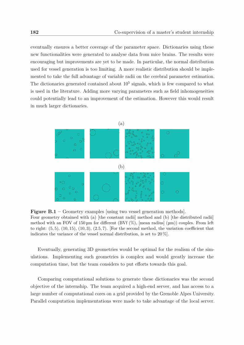
182 Co-supervision of a master’s student internship
eventually ensures a better coverage of the parameter space. Dictionaries using thesenew functionalities were generated to analyse data from mice brains. The results wereencouraging but improvements are yet to be made. In particular, the normal distributionused for vessel generation is too limiting. A more realistic distribution should be imple-mented to take the full advantage of variable radii on the cerebral parameter estimation.The dictionaries generated contained about 105 signals, which is few compared to whatis used in the literature. Adding more varying parameters such as field inhomogeneitiescould potentially lead to an improvement of the estimation. However this would resultin much larger dictionaries.
(a)
(b)
Figure B.1 – Geometry examples [using two vessel generation methods].Four geometry obtained with (a) [the constant radii] method and (b) [the distributed radii]method with an FOV of 150 µm for different (BVf (%), [mean radius] (µm)) couples. From leftto right: (5, 5), (10, 15), (10, 3), (2.5, 7). [For the second method, the variation coefficient thatindicates the variance of the vessel normal distribution, is set to 20 %].
Eventually, generating 3D geometries would be optimal for the realism of the sim-ulations. Implementing such geometries is complex and would greatly increase thecomputation time, but the team considers to put efforts towards this goal.
Comparing computational solutions to generate these dictionaries was the secondobjective of the internship. The team acquired a high-end server, and has access to alarge number of computational cores on a grid provided by the Grenoble Alpes University.Parallel computation implementations were made to take advantage of the local server.
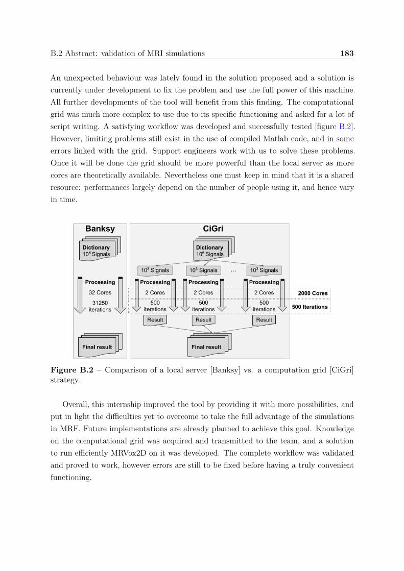
B.2 Abstract: validation of MRI simulations 183
An unexpected behaviour was lately found in the solution proposed and a solution iscurrently under development to fix the problem and use the full power of this machine.All further developments of the tool will benefit from this finding. The computationalgrid was much more complex to use due to its specific functioning and asked for a lot ofscript writing. A satisfying workflow was developed and successfully tested [figure B.2].However, limiting problems still exist in the use of compiled Matlab code, and in someerrors linked with the grid. Support engineers work with us to solve these problems.Once it will be done the grid should be more powerful than the local server as morecores are theoretically available. Nevertheless one must keep in mind that it is a sharedresource: performances largely depend on the number of people using it, and hence varyin time.
Figure B.2 – Comparison of a local server [Banksy] vs. a computation grid [CiGri]strategy.
Overall, this internship improved the tool by providing it with more possibilities, andput in light the difficulties yet to overcome to take the full advantage of the simulationsin MRF. Future implementations are already planned to achieve this goal. Knowledgeon the computational grid was acquired and transmitted to the team, and a solutionto run efficiently MRVox2D on it was developed. The complete workflow was validatedand proved to work, however errors are still to be fixed before having a truly convenientfunctioning.


Appendix C
Supplementary material - chapter 3
C.1 Bias-variance analysis
C.1.1 Frequentist analysis
The goal is to investigate the statistical properties of a proposed approach or equivalentlyof an estimator denoted by θ of a quantity of interest θ. In statistics, an estimator is afunction of the observations and is therefore random as observations are usually assumedrandom too. In practice however, the observations are only seen through a finite numberof realizations, say y1, . . . , yI .
For θ the true value of a parameter, we simulate I signals, using a given biophysicalmodel and the same parameter θ, say, for i = 1 : I, yi = f(θ) + ϵi, where ϵi is therealization of a given noise variable usually a centered Gaussian variable. From each ofthese I signals, we estimate the corresponding parameter value using the estimator θ,which leads to I values to approximate the same true θ, denoted by θi, for i = 1:I.
The bias of an estimator with respect to a target value θ is
Bias(θ) = (E[θ] − θ)
and usually appears squared as
Bias2(θ) = (E[θ] − θ)2 .
Note that it does not involve an absolute value. The bias measures the performance ofthe estimator on average. Similarly the variance of an estimator is
V ar(θ) = E[(θ − E[θ])2] .
186 Supplementary material - chapter 3
The variance measures the stability of the estimator or how much it moves around itsmean performance. The variance depends only on the estimator and is not per se ameasure of error as it does not involve the target θ. So in addition to the bias, anotherimportant quantity to measure the performance of an estimator is the Mean SquareError:
MSE(θ) = E[(θ − θ)2].
It measures the average square error made by the estimator.
An important relationship between these quantities is referred to as the bias-variancetrade-off or the bias-variance decomposition:
MSE(θ) = Bias2(θ) + V ar(θ).
In practice, the averages (E[·]) are computed empirically on a given number of yi fori = 1:I. Denoting E the empirical mean evaluated for the I simulations, and denotingθi for θ(yi), we can therefore write ;
1I
I∑i=1
|θ − θi|2 = |E[θ] − θ|2 + 1I
I∑i=1
|θi − E[θ]|2
whereE[θ] = 1
I
I∑i=1
θi.
The first two terms are measures of the deviation from the true θ while the last term is aconstant intrinsic uncertainty due to the estimator. It depends on θ only through the yi.
Note that the MSE is also the square RMSE by definition. In addition, it is commonto use normalized quantities by dividing each term in the decomposition by θ2.
Remark: Note that denomination and notation are slightly wrong in the bias-varianceanalysis of Zhao et al. [226]. What is called there the bias is in reality the so-calledMAD for mean absolute deviation and there is a typo in the variance term where thefirst θn should be θn. The square MAD is probably not too far from the square bias butthey differ due to the presence of the absolute value in the MAD. We are not aware of asimilar decomposition using the MAD instead of the bias. For the MAD, the medianshould replace the mean.
MAD(θ) = E[|θ − θ|]
C.1 Bias-variance analysis 187
whileBias(θ) = (θ − E[θ]) = E[(θ − θ)] .
C.1.2 Bayesian analysis
In the previous section, the goal was to analyze the performance of an estimator θ(Y )considering the observations Y as a random variable so that the averages are taken overthe observations, while the true θ to recover was considered as fixed. In this section, θ isassumed to be a random variable and averages are first taken with respect to θ and thenwith respect to both θ and Y .
Let p0 be the true distribution of (Y, θ) both considered as random variables. We usea capital Y to denote the random Y while a small y denotes a realization of Y . Thesame holds for θ except that the notation is the same (oops) but the context shouldbe clear...For a given y, then consider an estimator θ(y) of θ. We have the followingdecomposition:
Ep0(θ|y)[(θ(y) − θ)2] = (θ(y) − Ep0(θ|y)[θ])2 + V ar(p0(θ|y))
Let us denote by pG,D(θ|y) the posterior provided by GLLiM which is hoped to be agood approximation of the true p0(θ|y). Let also θG,D(y) be the estimate of θ providedby GLLiM, which in practice is set to the mean of the GLLiM posterior. It follows that
Ep0(θ|y)[(θG,D(y) − θ)2] = (θG,D(y) − Ep0(θ|y)[θ])2 + V ar(p0(θ|y)) . (C.1)
If we consider now that Y is random, we can take the expectation of equation (C.1)with respect to Y . It comes:
Ep0(θ,y)[(θG,D(Y ) − θ)2] = Ep0(y)[(θG,D(Y ) − Ep0(θ|Y )[θ])2] + Ep0(y)[V ar(p0(θ|Y ))] .
The expectation in the left-hand side is now with respect to the joint p0(θ, y) whilethe right-hand side was already independent of θ and just averaged over Y then. Theleft-hand side cannot be computed exactly in general but can be approximated byits empirical version using Monte Carlo simulations. Namely, consider i.i.d samples(θm, ym), m = 1 . . . M distributed according to p0. Equivalently, one can simulate θm
according to some prior p0(θ) and then ym according to the physical model p0(y|θm).From these samples, the left-hand side is approximated as
1M
M∑m=1
(θG,D(ym) − θm)2,
188 Supplementary material - chapter 3
which is the usual empirical MSE of θG,D.Doing the same for the terms in the right-hand side, we get
1M
M∑m=1
(θG,D(ym) − Ep0(θ|ym)[θ])2 + 1M
M∑m=1
V ar(p0(θ|ym)) .
Both Ep0(θ|ym)[θ] and V ar(p0(θ|ym)) in the last expression are unknown and cannot becomputed easily. It is actually the goal of methods like GLLiM to provide approximationsfor these quantities. GLLiM does so through an approximation pG,D(θ|ym) of the wholeposterior p0(θ|ym).
If as expected, for all ym, EpG,D(θ|ym)[θ] = θG,D(ym) and V ar(pG,D(θ|ym)) are respec-tively good approximations of Ep0(θ|ym)[θ] and V ar(p0(θ|ym)), meaning that pG,D(θ|ym)and p0(θ|ym) are close in terms of mean and variance, then the bias-variance decompositionabove leads to
1M
M∑m=1
(θG,D(ym) − θm)2 ≈ 1M
M∑m=1
V ar(pG,D(θ|ym)) = 1M
M∑m=1
CI2m .
Taking the square root, it comes
RMSE ≈
√√√√ 1M
M∑m=1
CI2m .
This later relationship is the one illustrated in figure 3.8, page 97. The figure showinga good relationship between both quantities indicates that the GLLiM approximationprovides good first and second posterior moments. The slight deviation from equalitywhen the SNR decreases is also consistent with the fact that the GLLiM performancemay decrease as the noise increases.
Note that in figure 3.8, for each SNR level, 100 different samples of (θm, ym), m =1 . . . M with M = 10 000 are simulated to check the above relationship.
As a conclusion the CI is a good indicator of the RMSE only if the learned GLLiMmodel is close to the true model in terms of mean and variance.
C.2 Data augmentation and noise modeling
This work has been submitted at the ISMRM congress 2020 but not accepted.
Data augmentation improves accuracy of dictionary-based learning
methods for MR Fingerprinting
Fabien Boux Florence Forbes Julyan Arbel Emmanuel L. Barbier
November 2019
Summary of Main Findings: Dictionary augmentation using Gaussian noise improves the reconstructionaccuracy of a dictionary-based learning approach by 50% without additional simulation or reconstructioncost.
Abstract
The dictionary-based learning (DBL) method, i.e the learning of a relationship between fingerprintsand parameters spaces using an inverse regression, is faster, more accurate, and requires less simulationsthan the conventional dictionary-matching method. However, the DBL method is less robust to thenoise level compared to the conventional dictionary-matching method. In this work, we investigate dataaugmentations by adding Gaussian noise to the dictionary fingerprints. We show that, at low SNR, dataaugmentation can increase estimates accuracy by more than 50%.
INTRODUCTION
To reduce simulation cost and reconstruction time, we recently proposed a dictionary-based learning (DBL)approach [1, 2], which uses a probabilistic model to learn the mapping from the dictionary fingerprint spaceto the parameters space. Interestingly, this approach also improves the accuracy on the final parameter esti-mates, compared to the standard dictionary matching method (DBM) [3]. However, compared to DBM, DBLappears to be less robust to fingerprints with low signal-to-noise ratio (SNR). To address this limitation, thiswork evaluates data augmentations by noise addition: first, we consider three data augmentation approaches,using various noise levels; second, we investigate the benefit of modeling the noise during the regression.
METHOD:
Experiments are designed as follows:
• Dictionary design: For P parameters and N entries, a matrix Xdico ∈ RN×P is sampled accordingto a quasi-random strategy in the parameter space. Then, the matrix of fingerprints Ydico ∈ RN×S issimulated according to the function:
ytoy (xtoy) =
∣∣∣∣∣N∑
i=1
sin (φif0 t) exp
(− t
xi
) ∣∣∣∣∣ ,
where xtoy = (x1, x2, . . . , xP ) ∈ RP is the parameter vector, f0 and φ ∈ RP are constants and t ∈ RS
is the sample vector. This choice of function allows the evaluation of various parameter dimensions.
• Data augmentation: The matrix Yaugmented is built from Ydico according to one of the three fol-lowing data augmentation procedure [4]:
1
1. The dictionary fingerprints Ydico is substituted by its noisy version Ynoisy1 according to SNRdico1:
Yaugmented1 = Ynoisy1.
2. Ydico is doubled in size with the noisy fingerprints Ynoisy1:
Yaugmented2 =
(Ydico
Ynoisy1
).
3. Ydico is augmented two times in size by noisy fingerprints Ynoisy1 and Ynoisy2 according toSNRdico1 and SNRdico2:
Yaugmented3 =
Ydico
Ynoisy1
Ynoisy2
.
Note that the size of Xdico is also augmented by replicating the matrix one or two times to match thelength of Yaugmented.
Noisy signals (ynoisy) were computed from y using:
ynoisy = |y + n|,where n is a Gaussian noise. The dictionary signal SNR is SNRdico.
• Model learning: A regression is performed to learn, from the dictionary, a model that handles thenon-linear relationship between Xaugmented and Yaugmented with a piece-wise linear model [2, 5].
• Estimation: The model is applied on the fingerprints y to compute the parameter estimates x.
• Performance evaluation: The parameter space Xtest is sampled and corresponding signals Ytest aresimulated and used to compute Xtest. Gaussian noise is added on test signals according to SNRtest.Then, the root-mean-squared-error (RMSE) is computed between Xtest and Xtest and averaged overdimensions. For a given SNRdico, SNRtest, and data augmentation method, the RMSE gain is the ratiobetween the RMSE obtained without and with data augmentation.
RESULTS:
Using data augmentation (1), three SNRdico (10, 60, and a random SNRdico vector between 10 and 60), andSNRtest between 3 and 100, we evaluate the RMSE gain in 4 experiment conditions (i.e. 3 and 5 parameters,2 different dictionary sizes). For all SNRdico, the data augmentation increases the robustness of the method(gain¿1) for SNRtest above 5 and below a cut-off value and deteriorates above. This cut-off depends SNRdico,SNRtest, the number of parameters and the dictionary size. Cuttoffs (mean ± standard deviation) are:73.9±16.3 for SNRdico=60, 17.3±4.1 for SNRdico=10 and 43.2±11.2 for SNRdico ∈ [10, 60]. Accuracy gainsbefore the cut-off are: 1.28±0.04, 1.22±0.05 and 1.26±0.04.
To search the optimal SNRdico for the data augmentation (1), we evaluated values of SNRdico between 10and 250 for three SNRtest (15, 30 and 45). Figure 2 represents RMSE gains for the same conditions as that ofFigure 1. As expected, gains are higher for noisy signals (low SNRtest); For high SNRdico, the gain convergesto 1. As RMSE gains depend on simulation conditions (i.e. dictionary design and SNRtest), there is nooptimal SNRdico. However, SNRdico=60 always yields RMSE gains above 1 and average RMSE gain is 1.43for the lowest SNRtest.
We compared data augmentations (1-3) with SNRdico1=60 and SNRdico2=10 (Figure 3). Data augmentations(1) and (2) provide similar results, except for large SNRtest for which the data augmentation (2) provideslarger RMSE gains. Data augmentation (3) yields higher RMSE gains for SNRtest between 5 and 15 butlower elsewhere.
To model the noise, we incorporated SNRdico as a new parameter (Xdico ∈ RN×(P+1)); for simulations,SNRdico values were randomly picked between 10 and 60. SNRtest are well evaluated only between 3 and10 (Figure 4). The combination of data augmentation (1) and noise modelling does not provide any benefit,however it reduces RMSE gains for low SNR (Figure 5).
2
DISCUSSION
Data augmentations based on noise addition reduces the RMSE on parameter estimates by more than 50%,in case of data with low SNRtest. Conversely, the accuracy on estimated parameters is decreased when usinga noisy dictionary with high SNRtest. [values here]. Learning the noise does not provide significant benefitover adding noise to the dictionary. Several assumptions can be made regarding the mechanism behind noiseaugmentation including limit the overfitting during the learning phase (similar to what has been reportedfor deep learning) and produce fingerprints more similar to test signals (e.g. no true zero points). Furtherexperiments are required to clarify these mechanisms.
CONCLUSION
Data augmentation using noise can readily be used to improve DBL reconstruction accuracy by 50% withoutadditional simulation or reconstruction cost.
References
[1] Fabien Boux, Florence Forbes, Julyan Arbel, and Emmanuel L. Barbier. Dictionary-free mr fingerprintingparameter estimation via inverse regression. In 26th Annual Meeting ISMRM, Paris, page 4259, 2018.
[2] Fabien Boux, Florence Forbes, Julyan Arbel, Benjamin Lemasson, and Emmanuel L. Barbier. In-verse regression in mr fingerprinting: reducing dictionary size while increasing parameters accuracy.Submitted to Magnetic resonance in medicine, 2019. Preprint: https://hal.archives-ouvertes.fr/hal-02314026/document.
[3] Dan Ma, Vikas Gulani, Nicole Seiberlich, Kecheng Liu, Jeffrey L Sunshine, Jeffrey L Duerk, and Mark AGriswold. Magnetic resonance fingerprinting. Nature, 495(7440):187, 2013.
[4] MJ Saiz-Abajo, B-H Mevik, VH Segtnan, and T Næs. Ensemble methods and data augmentation by noiseaddition applied to the analysis of spectroscopic data. Analytica chimica acta, 533(2):147–159, 2005.
[5] Antoine Deleforge, Florence Forbes, and Radu Horaud. High-dimensional regression with gaussian mix-tures and partially-latent response variables. Statistics and Computing, 25(5):893–911, 2015.
3
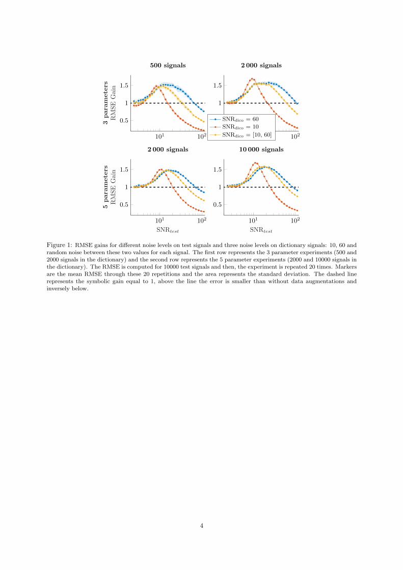
101 102
0.5
1
1.5
3para
meters
RM
SE
Gai
n
500 signals
101 102
0.5
1
1.5
2 000 signals
SNRdico = 60
SNRdico = 10
SNRdico = [10, 60]
101 102
0.5
1
1.5
SNRtest
5para
meters
RM
SE
Gai
n
2 000 signals
101 102
0.5
1
1.5
SNRtest
10 000 signals
Figure 1: RMSE gains for different noise levels on test signals and three noise levels on dictionary signals: 10, 60 andrandom noise between these two values for each signal. The first row represents the 3 parameter experiments (500 and2000 signals in the dictionary) and the second row represents the 5 parameter experiments (2000 and 10000 signals inthe dictionary). The RMSE is computed for 10000 test signals and then, the experiment is repeated 20 times. Markersare the mean RMSE through these 20 repetitions and the area represents the standard deviation. The dashed linerepresents the symbolic gain equal to 1, above the line the error is smaller than without data augmentations andinversely below.
4
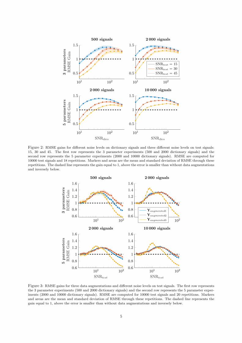
101 102
0.5
1
1.5
3para
meters
RM
SE
Gain
500 signals
101 102
0.5
1
1.5
2 000 signals
SNRtest = 15
SNRtest = 30
SNRtest = 45
101 102
0.5
1
1.5
SNRdico
5para
meters
RM
SE
Gain
2 000 signals
101 102
0.5
1
1.5
SNRdico
10 000 signals
Figure 2: RMSE gains for different noise levels on dictionary signals and three different noise levels on test signals:15, 30 and 45. The first row represents the 3 parameter experiments (500 and 2000 dictionary signals) and thesecond row represents the 5 parameter experiments (2000 and 10000 dictionary signals). RMSE are computed for10000 test signals and 18 repetitions. Markers and areas are the mean and standard deviation of RMSE through theserepetitions. The dashed line represents the gain equal to 1, above the error is smaller than without data augmentationsand inversely below.
101 1020.6
0.8
1
1.2
1.4
1.6
3para
meters
RM
SE
Gai
n
500 signals
101 1020.6
0.8
1
1.2
1.4
1.6
2 000 signals
Yaugmented1
Yaugmented2
Yaugmented3
101 1020.6
0.8
1
1.2
1.4
1.6
SNRtest
5para
meters
RM
SE
Gai
n
2 000 signals
101 1020.6
0.8
1
1.2
1.4
1.6
SNRtest
10 000 signals
Figure 3: RMSE gains for three data augmentations and different noise levels on test signals. The first row representsthe 3 parameter experiments (500 and 2000 dictionary signals) and the second row represents the 5 parameter exper-iments (2000 and 10000 dictionary signals). RMSE are computed for 10000 test signals and 20 repetitions. Markersand areas are the mean and standard deviation of RMSE through these repetitions. The dashed line represents thegain equal to 1, above the error is smaller than without data augmentations and inversely below.
5
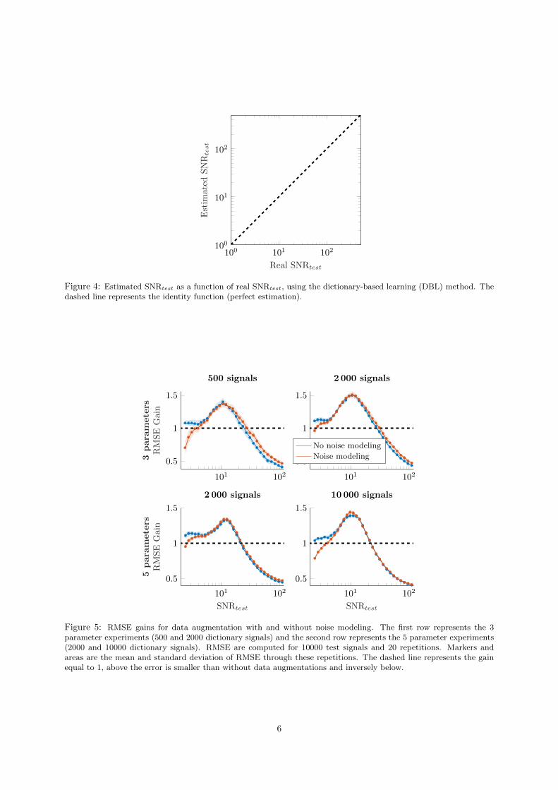
100 101 102100
101
102
Real SNRtest
Est
imat
edS
NR
test
Figure 4: Estimated SNRtest as a function of real SNRtest, using the dictionary-based learning (DBL) method. Thedashed line represents the identity function (perfect estimation).
101 102
0.5
1
1.5
3para
meters
RM
SE
Gai
n
500 signals
101 102
0.5
1
1.5
2 000 signals
No noise modeling
Noise modeling
101 102
0.5
1
1.5
SNRtest
5para
meters
RM
SE
Gai
n
2 000 signals
101 102
0.5
1
1.5
SNRtest
10 000 signals
Figure 5: RMSE gains for data augmentation with and without noise modeling. The first row represents the 3parameter experiments (500 and 2000 dictionary signals) and the second row represents the 5 parameter experiments(2000 and 10000 dictionary signals). RMSE are computed for 10000 test signals and 20 repetitions. Markers andareas are the mean and standard deviation of RMSE through these repetitions. The dashed line represents the gainequal to 1, above the error is smaller than without data augmentations and inversely below.
6
Appendix D
Supplementary material - chapter 5
During this work, we acquired MRI data on two experimental models of mesio-temporallobe epilepsy (MTLE) in mice. The status epilepticus was induced by an administrationof kainic acid, either using an intraperitoneal injection (IP model) or an intrahippocampalinjection (IH model).
We are interested in 3 regions of interest: thalamus, hippocampus and cortex. For IHmodel, we only consider the contralateral cortex because of the lesion resulting from thecannula that passed through the cortex for intrahippocampal injection. For IH model,we also distinguish the contralateral and ipsilateral hippocampus.
In figures D.1 and D.2, we present the mean value obtained in each region of interest,for the eight following MRI parameters: relaxation times T1 and T2, diffusion (ADC),blood volume fraction (BVf), vessel size index (VSI), tissue oxygen saturation (StO2),blood-brain-barrier permeability (BBBp and cerebral blood flow (CBF).
Note that the data acquired with the IH model are those presented in chapter 5.
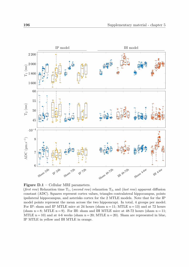
196 Supplementary material - chapter 5
IP model IH model
1 600
1 800
2 000
2 200
T1
(ms)
45
50
55
60
T2
(ms)
Sham
24hIP
24h
Sham
72hIP
72h
Sham
48-72h
IH48-
72h
Sham
4-6w
IH4-6
w6
7
8
·10−4
AD
C(µ
m.s−1)
Figure D.1 – Cellular MRI parameters.(first row) Relaxation time T1, (second row) relaxation T2, and (last row) apparent diffusionconstant (ADC). Squares represent cortex values, triangles contralateral hippocampus, pointsipsilateral hippocampus, and asterisks cortex for the 2 MTLE models. Note that for the IPmodel points represent the mean across the two hippomcapi. In total, 4 groups per model.For IP: sham and IP MTLE mice at 24 hours (sham n = 11; MTLE n = 13) and at 72 hours(sham n = 8; MTLE n = 9). For IH: sham and IH MTLE mice at 48-72 hours (sham n = 11;MTLE n = 10) and at 4-6 weeks (sham n = 20; MTLE n = 20). Sham are represented in blue,IP MTLE in yellow and IH MTLE in orange.
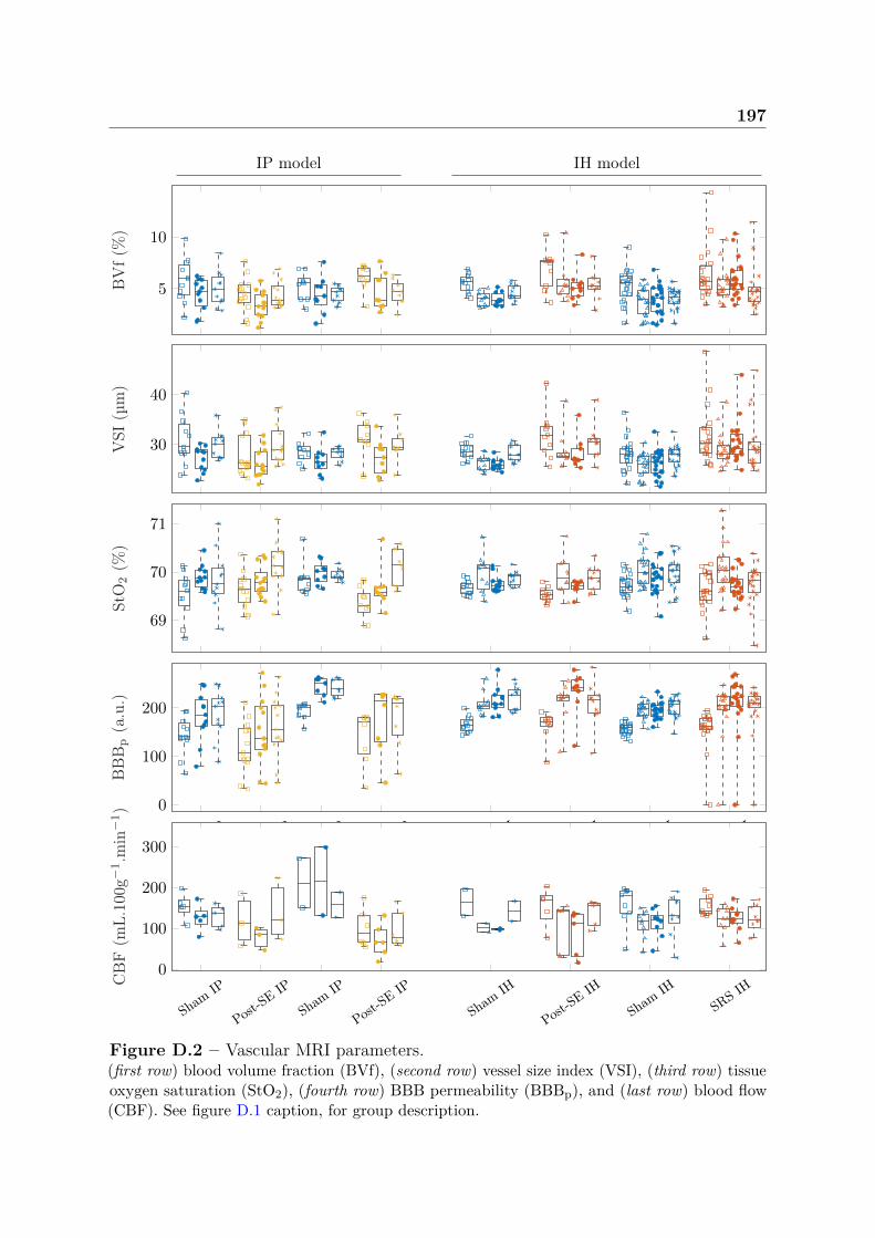
197
IP model IH model
5
10
BV
f(%
)
30
40
VSI
(µm
)
69
70
71
StO
2(%
)
Sham
IP
Post-SE
IP
Sham
IP
Post-SE
IP
Sham
IH
Post-SE
IH
Sham
IHSR
S IH
0
100
200
BB
Bp
(a.u
.)
Sham
IP
Post-SE
IP
Sham
IP
Post-SE
IP
Sham
IH
Post-SE
IH
Sham
IHSR
S IH0
100
200
300
CB
F(m
L.10
0g−1.m
in−1)
Figure D.2 – Vascular MRI parameters.(first row) blood volume fraction (BVf), (second row) vessel size index (VSI), (third row) tissueoxygen saturation (StO2), (fourth row) BBB permeability (BBBp), and (last row) blood flow(CBF). See figure D.1 caption, for group description.


Appendix E
Software
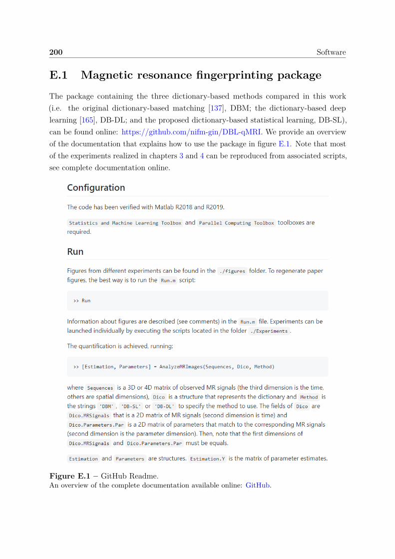
200 Software
E.1 Magnetic resonance fingerprinting package
The package containing the three dictionary-based methods compared in this work(i.e. the original dictionary-based matching [137], DBM; the dictionary-based deeplearning [165], DB-DL; and the proposed dictionary-based statistical learning, DB-SL),can be found online: https://github.com/nifm-gin/DBL-qMRI. We provide an overviewof the documentation that explains how to use the package in figure E.1. Note that mostof the experiments realized in chapters 3 and 4 can be reproduced from associated scripts,see complete documentation online.
Figure E.1 – GitHub Readme.An overview of the complete documentation available online: GitHub.
E.2 MP3: Medical software for Processing multi-Parametric images Pipelines 201
E.2 MP3: Medical software for Processing multi-Parametric images Pipelines
This section introduces an open source software to convert, display and process medicalimages [185]. This software called medical software for processing multi-parametric imagespipelines (MP3), is a collaborative development within the team initiated by BenjaminLemasson and mainly achieved by Clément Brossard. It differentiates itself from theexisting software by its ability to design complex processing pipelines and to wiselyexecute them on a large database. An MP3 pipeline can contain unlimited homemade orpre-existing processes called module, and can be carried out with a parallel executionsystem. As a viewer, MP3 allows to display up to four images together and to draw regionsof interest (ROI), see figure E.2 B. MP3 is available at https://github.com/nifm-gin/MP3.
In this project, I was one of the principal developer and beta tester. Among others,here are some of my contributions:
• Implementation of the modules of vascular magnetic resonance fingerprinting, seesection E.3.
• Implementation of a module running different scripts provided by Advanced Nor-malization Tools (ANTs) [233] to perform a co-registration of an anatomical imagewith a reference atlas image to automatically segment maps in different ROI. Thismodule is supplemented by another module allowing to compute several statisticsby ROI (e.g. mean, median, standard deviation,...).
• Design of a complete pipeline in mouse at 9.4 T, to generate maps, remove outliers,match atlas and extract summary statistics per ROI. This pipeline has beenvalidated with a rat study at 4.7 T and the atlas matching procedure for humanstudy.
I have also been involved in introducing the tool and providing support to several hospitalclinicians and biologists. In particular, I have accompanied two hospital clinicians duringtheir medical thesis project, providing support on the tool: Pierre Fricault in a pre-clinical MRI study on an experimental model of traumatic brain injury (part of the workin [234]) and Sarah Sintzel Strippoli in a clinical MRI study on brain damages afterminor traumatic brain injury.
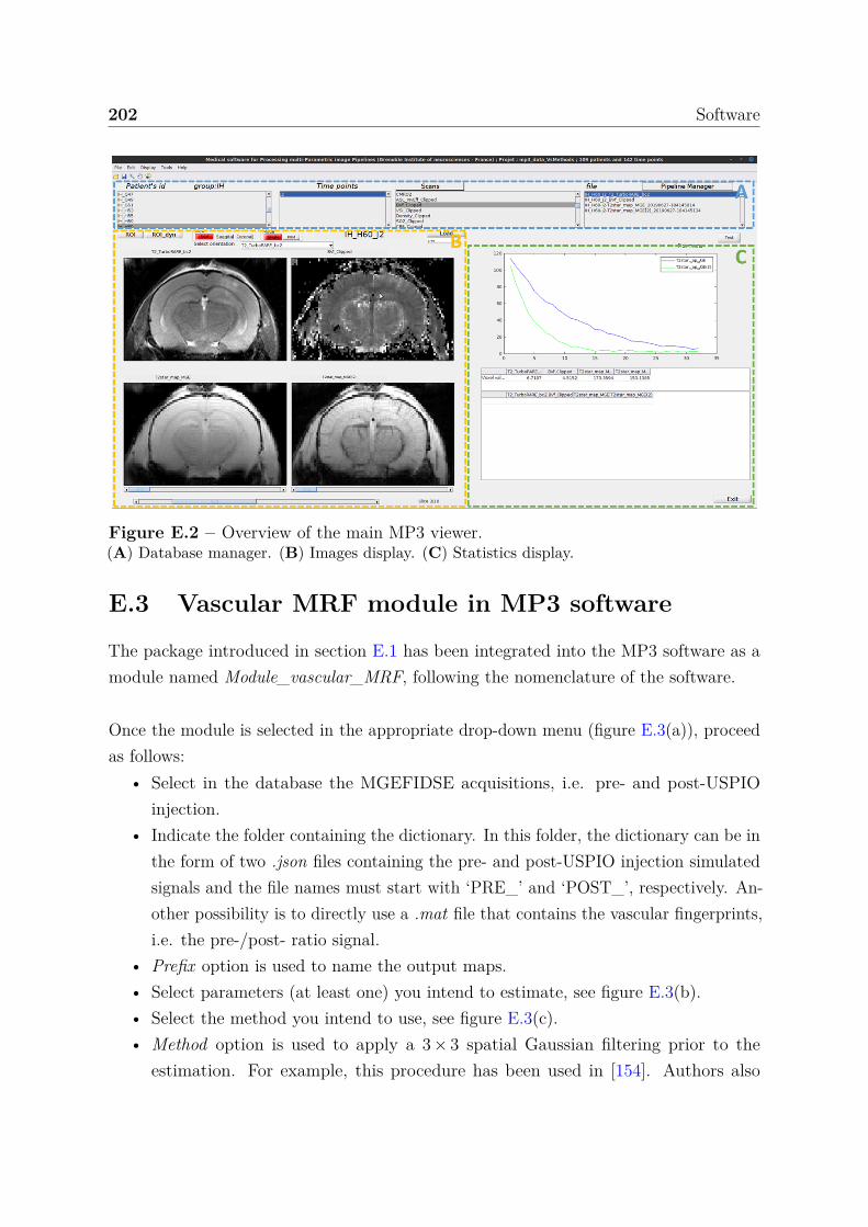
202 Software
Figure E.2 – Overview of the main MP3 viewer.(A) Database manager. (B) Images display. (C) Statistics display.
E.3 Vascular MRF module in MP3 software
The package introduced in section E.1 has been integrated into the MP3 software as amodule named Module_vascular_MRF, following the nomenclature of the software.
Once the module is selected in the appropriate drop-down menu (figure E.3(a)), proceedas follows:
• Select in the database the MGEFIDSE acquisitions, i.e. pre- and post-USPIOinjection.
• Indicate the folder containing the dictionary. In this folder, the dictionary can be inthe form of two .json files containing the pre- and post-USPIO injection simulatedsignals and the file names must start with ‘PRE_’ and ‘POST_’, respectively. An-other possibility is to directly use a .mat file that contains the vascular fingerprints,i.e. the pre-/post- ratio signal.
• Prefix option is used to name the output maps.• Select parameters (at least one) you intend to estimate, see figure E.3(b).• Select the method you intend to use, see figure E.3(c).• Method option is used to apply a 3 × 3 spatial Gaussian filtering prior to the
estimation. For example, this procedure has been used in [154]. Authors also
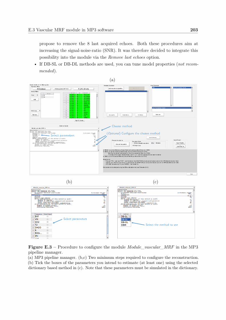
E.3 Vascular MRF module in MP3 software 203
propose to remove the 8 last acquired echoes. Both these procedures aim atincreasing the signal-noise-ratio (SNR). It was therefore decided to integrate thispossibility into the module via the Remove last echoes option.
• If DB-SL or DB-DL methods are used, you can tune model properties (not recom-mended).
(a)
(b) (c)
Figure E.3 – Procedure to configure the module Module_vascular_MRF in the MP3pipeline manager.(a) MP3 pipeline manager. (b,c) Two minimum steps required to configure the reconstruction.(b) Tick the boxes of the parameters you intend to estimate (at least one) using the selecteddictionary based method in (c). Note that these parameters must be simulated in the dictionary.
Méthodes statistiques pour l’imagerie vasculaire par résonance magnétique :application au cerveau épileptique
L’objectif de ce travail de thèse est l’exploration de l’imagerie par résonance magnétique (IRM)pour l’identification et la localisation des régions du cerveau impliquées dans l’épilepsie mésio-temporale.Précisément, les travaux visent 1) à optimiser un protocole d’IRM vasculaire sur un modèle animal d’épilepsieet 2) à concevoir une méthode de quantification de cartes IRM vasculaires basée sur la modélisation de larelation entre signaux IRM et paramètres biophysiques. Les acquisitions IRM sur un modèle expérimentalmurin d’épilepsie mésio-temporale avec sclérose de l’hippocampe ont été effectuées sur un scanner 9.4 T. Lesdonnées collectées ont permis de quantifier sept cartes IRM cellulaires et vasculaires quelques jours aprèsl’état de mal épileptique puis plus tard, lorsque les crises spontanées sont apparues. Ces paramètres ont étéemployés pour l’identification automatique des régions épileptogènes et des régions de propagation des crises.Afin d’augmenter la détection de petites variations des paramètres IRM chez les individus épileptiques, uneméthode de quantification basée sur la résonance magnétique fingerprinting est développée. Cette méthodeconsiste à identifier, parmi un ensemble de signaux simulés, le plus proche du signal IRM acquis et peutêtre vue comme un problème inverse qui présente les difficultés suivantes : le modèle direct est non-linéaireet provient d’une série d’équations sans expression analytique simple; les signaux en entrée sont de grandesdimensions; les vecteurs des paramètres en sortie sont multidimensionnels. Pour ces raisons, nous avonsutilisé une méthode de régression inverse afin d’apprendre à partir de simulation la relation entre l’espacedes paramètres et celui des signaux. Dans un domaine largement dominé par les approches d’apprentissageprofond, la méthode proposée se révèle très compétitive fournissant des résultats plus précis. De plus, laméthode permet pour la première fois de produire un indice de confiance associé à chacune des estimations.En particulier, cet indice permet de réduire l’erreur de quantification en rejetant les estimations associées àune faible confiance. Actuellement, aucun protocole clinique permettant de localiser avec précision le foyerépileptique ne fait consensus. La possibilité d’une identification non-invasive de ces régions est donc unpremier pas vers un potentiel transfert clinique.
Statistical methods for vascular magnetic resonance fingerprinting:application to the epileptic brain
The objective of this thesis is the investigation of magnetic resonance imaging (MRI) for the identificationand localization of brain regions involved in mesio-temporal lobe epilepsy (MTLE). Precisely, the workaims 1) at optimizing a vascular MRI protocol on an animal model of epilepsy and 2) at designing amethod to quantify vascular MRI maps based on the modeling of the relationship between MRI signals andbiophysical parameters. MRI acquisitions on an experimental mouse model of MTLE with hippocampalsclerosis were performed on a 9.4 T scanner. The data collected allowed the quantification of seven cellularand vascular MRI maps a few days after the epileptic condition and later when the spontaneous seizuresemerged. These parameters were used for the automatic identification of epileptogenic regions and regionsof seizure propagation. To enhance the detection of small variations in MRI parameters in epileptic subjects,a quantification method based on magnetic resonance fingerprinting has been developed. This methodconsists in identifying, among a set of simulated signals, the closest one to the acquired signal. It can beseen as an inverse problem that presents the following difficulties: the direct model is non-linear, as acomplex series of equations or simulation tools; the inputs are high-dimensional signals; and the outputis multidimensional. For these reasons, we used an appropriate inverse regression approach to learn amapping between signal and biophysical parameter spaces. In a field widely dominated by deep learningapproaches, the proposed method is very competitive and provides more accurate results. Moreover, themethod allows for the first time to produce a confidence index associated with each estimate. In particular,this index allows to reduce the quantification error by discarding estimates associated with low confidence.So far no clinical protocol emerges as a consensus to accurately localize epileptic foci. The possibility of anon-invasive identification of these regions is therefore a first step towards a potential clinical transfer.