Study of minor species in the Venus night

mesosphere

Étude des espèces mineures dans la mésosphère

nocturne de Vénus

Thèse de doctorat de l’université Paris-Saclay et Space

Research Institute IKI of Russian Academy of Sciences

École doctorale n° 127 : astronomie et astrophysique d’Ile-de-France

(AAIF)

Spécialité de doctorat: Astronomie et Astrophysique

Unité de recherche : Université Paris-Saclay, UVSQ, CNRS, LATMOS, 78280,

Guyancourt, France

Référent : Université de Versailles Saint-Quentin-en-Yvelines

Thèse présentée et soutenue à Paris-Saclay,

le 22 janvier 2021, par

Daria EVDOKIMOVA

Composition du Jury

Nathalie CARRASCO

Professeur à l’Université Paris-Saclay Présidente

Sébastien LEBONNOIS

Directeur de recherche CNRS à Sorbonne Université Rapporteur & Examinateur

Dmitrij TITOV

European Space Agency (Pays-Bas) Rapporteur & Examinateur

Alexander RODIN

Directeur de laboratoire au Moscow Institute of Physics

and Technology (Russie)

Examinateur

Nicholas SCHNEIDER

Professeur à l’Université du Colorado (Etats-Unis) Examinateur

Direction de la thèse

Franck MONTMESSIN

Directeur de Recherche CNRS à l’Université Paris-Saclay Directeur de thèse

Denis BELYAEV

Chercheur au Space Research Institute (Russie) Co-Directeur de thèse

Th

èse

de d

octo

rat

NN

T : 2

021U

PA

SP

039

2

СONTENTS

СONTENTS ............................................................................................................................................. 2

ACKNOWLEDGMENTS ........................................................................................................................ 5

PURPOSE OF THE WORK .................................................................................................................... 7

CHAPTER 1. Venus and its atmosphere ................................................................................................. 9

1.1. The Earth’s evil twin .................................................................................................................................. 10

1.2. A new view of Venus ................................................................................................................................. 11

1.3. History of observations .............................................................................................................................. 12

1.3.1. Venus space missions .......................................................................................................................... 12

1.3.2. Venus Express ..................................................................................................................................... 17

1.3.3. Future missions .................................................................................................................................... 18

1.4. The surface of Venus .................................................................................................................................. 19

1.5. The atmosphere of Venus ........................................................................................................................... 20

1.5.1. Composition ........................................................................................................................................ 20

1.5.2. Structure of the atmosphere ................................................................................................................. 21

1.5.3. The cloud layer .................................................................................................................................... 23

1.5.4. Transparency windows ........................................................................................................................ 25

1.5.5. Mesosphere and atmospheric dynamics .............................................................................................. 27

1.6. The SPICAV instrument ............................................................................................................................ 30

1.6.1. Ultraviolet channel of the SPICAV spectrometer ............................................................................... 31

1.6.2. Infrared channel of the SPICAV spectrometer .................................................................................... 34

CHAPTER 2. Sulphur dioxide and ozone in the atmosphere of Venus ................................................. 36

2.1. Overview of sulphur dioxide research ........................................................................................................ 36

2.1.1. Temporal and spatial distributions of sulphur dioxide ........................................................................ 36

2.1.2. Vertical profile of SO2 obtained by SPICAV/SOIR instrument on board Venus Express and ground

based facilities in the mesosphere ................................................................................................................. 38

2.2. Ozone in the atmosphere of Venus. ............................................................................................................ 40

2.2.1. Discovery of ozone in the atmosphere ................................................................................................ 41

2.2.2. Ozone at the top of the clouds ............................................................................................................. 41

2.3. Photochemistry: a review of atmospheric models for SO2 and O3 ............................................................. 42

CHAPTER 3. Data processing of stellar occultation spectra ................................................................. 49

3.1. The stellar occultation technique: retrieving the atmospheric composition from transmittance spectra .... 49

3.2. Calibrations and stray light correction in the raw data. .............................................................................. 51

3.2.1. Studied trace gases .............................................................................................................................. 51

3.2.2. UV Signal considerations with SPICAV ............................................................................................. 53

3.2.3. Estimation of errors in atmospheric transmission spectra. .................................................................. 54

3

3.2.4. Sources of an additional emission registered by the UV channel of SPICAV .................................... 55

3.2.4.1. Lyman-α emission ........................................................................................................................ 56

3.2.4.2. Airglow of nitric oxide ................................................................................................................. 57

3.2.4.3. Solar radiance in the stellar occultation spectra ........................................................................... 59

3.2.5. Wavelength- to-pixel registration ........................................................................................................ 59

3.2.6. Spectral inversion ................................................................................................................................ 61

3.2.6.1. Cases of positive gas detection ..................................................................................................... 62

3.2.6.2. Upper detection limits for two gases. ........................................................................................... 65

3.2.6.3. Chlorine oxide absorption band .................................................................................................... 70

3.2.7. Vertical inversion problem .................................................................................................................. 71

3.2.8. Calibration influence on the spectral inversion ................................................................................... 73

3.2.9. Stray light elimination technique ......................................................................................................... 75

3.2.9.1. Method #1..................................................................................................................................... 76

3.2.9.2. Method #2..................................................................................................................................... 76

3.2.9.3. Comparison of methods ................................................................................................................ 77

3.2.9.4. Atmospheric transmission and error bars estimation. .................................................................. 82

3.2.10. Altitude assignment ........................................................................................................................... 82

3.3. Summary .................................................................................................................................................... 84

CHAPTER 4. Sulphur dioxide ............................................................................................................... 85

4.1. CO2 and SO2 retrievals: from column abundances to profile and its variability. ....................................... 85

4.1.1. Carbon dioxide distribution in the upper mesosphere and the lower thermosphere. ........................... 86

4.1.2. SO2 in the upper mesosphere ............................................................................................................... 87

4.2. SO2 profiles: Comparison with data from previous studies. ...................................................................... 88

4.3. Variations of SO2 mixing ratio ................................................................................................................... 93

4.3.1. Short term variations ........................................................................................................................... 93

4.3.2. Long term variations of SO2 mixing ratio. .......................................................................................... 94

4.3.3. Diurnal variations of SO2 .................................................................................................................... 96

4.3.4. Geographical distribution of SO2 ........................................................................................................ 99

4.3.4.1. Local time and latitude distribution .............................................................................................. 99

4.3.4.2. Variations with a solar zenith angle .......................................................................................... 100

4.3.4.3. Establishing independence from topography ............................................................................. 100

4.4. Discussion. ............................................................................................................................................... 103

4.4.1 Rapid changes in the SO2 content....................................................................................................... 103

4.4.2. Global patterns in the SO2 behaviour ................................................................................................ 104

4.5. Summary .................................................................................................................................................. 105

CHAPTER 5. Ozone ............................................................................................................................ 106

5.1. Ozone retrievals ........................................................................................................................................ 106

5.1.1. The main feature of the ozone positive detections ............................................................................ 107

4

5.2. Ozone positive detections distribution ..................................................................................................... 108

5.2.1. Average volume mixing ratio profile of ozone for established positive detections. ......................... 108

5.2.2. Spatial variations of ozone positive detections.................................................................................. 109

5.2.3. Temporal variations of ozone based on positive detections .............................................................. 111

5.3. Detection limits of ozone ......................................................................................................................... 112

5.4. Review of possible correlations with other chemical compounds ........................................................... 114

5.5. Comparative analysis of ozone layers in Earth, Mars and Venus atmospheres. ...................................... 120

5.5.1. Ozone on the Earth ............................................................................................................................ 120

5.5.2. Ozone on Mars and Venus ................................................................................................................ 123

5.6. Summary .................................................................................................................................................. 124

CHAPTER 6. O2 (α1Δg) emission in the upper mesosphere ................................................................ 126

6.1. The infrared emissions in the night atmosphere ....................................................................................... 126

6.2. SPICAV observations of lower atmosphere thermal emission ................................................................ 127

6.3. Modelling of the night thermal emission.................................................................................................. 129

6.3.1. Direct model ...................................................................................................................................... 129

6.3.2. Inverse problem ................................................................................................................................. 131

6.4. Mapping water vapour and aerosols and uncertainties ............................................................................. 132

6.5. Map of oxygen airglow in the night mesosphere .................................................................................... 134

6.6. Summary .................................................................................................................................................. 136

CONCLUSION .................................................................................................................................... 137

PERSPECTIVES .................................................................................................................................. 139

LIST OF PUBLICATIONS ................................................................................................................. 141

LIST OF CONFERENCES .................................................................................................................. 142

ANNEX 1. Positive detections of SO2 presented individually ............................................................ 144

ANNEX 2. Positive detections of O3 presented individually............................................................... 156

ANNEX 3. Parameters of stellar occultation sessions ......................................................................... 160

ANNEX 4. Weighted mean .................................................................................................................. 166

ANNEX 5. Estimation of an impact of diffrent stray light types ......................................................... 167

ANNEX 6. Résumé de la thèse en français .......................................................................................... 170

REFERENCES ..................................................................................................................................... 180

5

ACKNOWLEDGMENTS

The work on this study has become the most fascinating and instructive experience in my professional

and personal life. And I would like to thank sincerely everyone who helped me to successfully complete

this study and my PhD thesis.

I appreciate the wise supervision of Franck Montmessin at LATMOS. I thank you for all your advices

and discussions, your support of my work and a lot of administrational assistance. Your supervision and

competence made my work in LATMOS for these years being a remarkable experience. I am very

grateful to my co-supervisor Denis Belyaev accompanying my work at the Space Research Institute of

the Russian Academy of Sciences (IKI RAS). I thank you for proposing a subject of this study for me.

Especially I appreciate that you have always been present and kind to help me with all my questions.

The joint work with my supervisors allowed me to grow up my proficiency, and it was a source of every

day motivation. I also would like to thank Emmanuel Marcq for sharing your experience with me and

for your support with administration difficulties I have faced.

The defence of the thesis, under the joint supervision, became possible thanks to the French government

BGF PhD grant 2016-2019 Vernadski, which is an honor for me. I sincerely thank the Embassy of

France in Moscow. Also, I am grateful to LATMOS and to IKI RAS for providing me the chance to

perform the PhD study under these terms, and for the additional financial support to complete the

research.

I acknowledge the work with Anna Fedorova on the infrared spectra of Venus. I thank you for providing

me a basis to perform this analysis and all your supervision and ideas during all the rough way of this

research. Furthermore, I appreciate the big contribution of Oleg Korablev, the deputy director of IKI

RAS, for organization of the joint supervision and of the defence. I would like to thank you as the PI of

SPICAV IR spectrometer for a beautiful and informative experiment. The major part of this work was

done based on the measurements of the SPICAV UV instrument, and I wish also to thank Jean Loup

Bertaux, a PI of this experiment. The clues to analysis and the work with you was very important for

me.

I would like to express my deep gratitude to all the members of the jury, Nathalie Carrasco, Sebastien

Lebonnois, Alexander Rodin, Nicholas Schneider, Dmitry Titov, who were very kind and supportive

during the organization of the defence in the complicated and stressful time of 2020-2021. I am very

grateful to my two reviewers Sebastien Lebonnois and Dmitry Titov, for taking the time for careful

examination of my manuscript. And I would like particularly to thank the president of my jury, Nathalie

Carrasco, for full cooperation, and thank you for being a member of my thesis committee and for

following steps of my work from the beginning. I am also very grateful to Franck Lefèvre for being a

member of my thesis committee and for a lot of explanations concerning the Venus general circulation

modeling.

In this work some results are compared with the IPSL Venus general circulation mode, which were

prepared by Gabriela Gilli. I am happy to have a chance to cooperate with you and I appreciate very

6

much your participation in deeper analysis of the obtained experimental results. Thank you to Lucio

Baggio and Loïc Verdier for cooperation during the study of data calibration efficiency.

This PhD project under the joint supervision was very supported by the directors of the École doctorale

N°127: astronomie et astrophysique d’Ile-de-France (AAIF), Thierry Fouchet and Jeacques Le Bourlot,

and its deputy director Alain Abergel at all the stages, and I am very grateful for this extremely valuable

support. Similarly, I appreciate the assistance of the LATMOS directors: Dr. Phillip Keckhut and Pr.

Francois Ravetta. I also thank the administration of the École doctorale, the Université Paris-Saclay and

the Université de Versailles St Quentin en Yvelines, and the administration of the doctoral school of IKI,

Angelina Shchukina and Andrey Sadovsky.

Thank you also to all my colleagues, the members of SPICAV, SPICAM and ACS teams, I have worked

with in France and in Russia. It was great to have met my colleges: Loïc Rossi, Kevin Olsen, Gaetan

Lacombe, Anni Määttänen, Aurélien Stcherbinine, Abdenour Irbah, Ashwin Braude, Margaux Vals,

Hugo Gilardy and Jean-Yves Chaufray. Furthermore, I was happy to participate in the European research

course on atmospheres, and gain a lot of the experience. And it was a great pleasure to continue working

with my colleges: Alexander Trokhimovskiy, Nikolay Ignatiev, Michail Luginin, Andrey Patrakeev,

Nikita Vyasovetsky, Yuri Dobrolensky, Vladimir Kotsov, Sergey Mantzevich, Alexander Lomakin,

Nadezhda Rotova, Marina Patzaeva, Igor Khatuntsev and Alexandra Smirnova. I appreciate your

friendship very much. I am very grateful to Sergey Khaykin for support and some Russian language in

France. I would like also to thank my dear friends Olya, Alina, Slava, Kemal, Artem, Sasha, Olya and

my family for continuous support, belief and guidance.

7

PURPOSE OF THE WORK

The structure of Venus’ atmosphere and the study of its composition have remained a challenge

for scientists: which processes of the planet’s evolution did lead to the observed atmospheric condition

crucially different from the Earth’s atmosphere. Various models based on the data up to date show that

an overall picture of the atmospheric composition and dynamics has not yet been obtained. Prior to the

Venus Express (VEX) mission (2006-2014), a detailed study of the atmosphere and minor gas

components above the clouds, where the defining processes take place, was not possible. For the first

time, the VEX experiments of solar and stellar occultations studied in detail the vertical structure of the

atmosphere on both planetary terminators and on the night side.

The SPIСAV spectrometer could observe several trace gases using its ultraviolet (UV) channel (118-

320 nm). The Venus Express mission with this instrument on board was operating for 8 years. Sensitivity

of the implemented stellar occultation method establishes the observed altitude range to 85-110 km. A

large amount of unique information has been accumulated for a detailed study of variations in

atmospheric components. Sulphur dioxide and ozone are the two atmospheric minor species which are

targets of our study in Venus mesosphere. The study of their distribution in the night mesosphere is the

goal of this work. It contributes to global understanding of the main chemical processes which are the

carbon dioxide and sulphur dioxide cycles in the Venus atmosphere.

Sulphur dioxide possesses ultraviolet absorption bands in 190-300 nm. The gas was extensively

observed by ground-based telescopes and orbiters on the day side of the planet at the level of clouds top

(~70 km) for more than 40 years on Venus. On the other hand, the SPICAV/SOIR instrument of Venus

Express mission sounded the vertical distribution of SO2 at altitudes 65-110 km on the terminator.

Variations of the dioxide content occurred to be extremely high in the dayside and twilight mesosphere.

So far, there was no data from SO2 distributions at the night-time mesosphere where photochemical and

temperature conditions differ from those at the day time. The first goal of our study is to obtain a

mesospheric distribution of sulphur dioxide at the night side of Venus. Spatial and long-term variations

are to be compared with previous dayside results.

The second scientific objective deals with the recent discovery of an ozone layer in Venus’ mesosphere

on the night side (Montmessin et al., 2011). Absorption of ozone in the Hartley band (~250 nm) was

observed by the SPICAV UV in the stellar occultation mode at altitudes 90-100 km. Just episodic bursts

of O3 mixing ratio with a few tens ppbv were detected in 2006-2010 from 29 observation sessions. That

was consistent with ozone production and destruction schemes according to reactions with oxygen and

chlorine atoms in the anti-solar point at the SSAS circulation. Such a mechanism takes place in the

Earth’s upper stratosphere. In parallel, an abundance of ozone was recently discovered at the Venusian

cloud tops near polar regions (Marcq et al., 2019) that signifies the O3 interconnection with the

atmospheric dynamics.

In the present research we have processed the whole statistics of the SPICAV UV stellar occultations in

2006-2014, that is >400 sessions. We characterize ozone distribution at altitudes 90-100 km, the region

8

corresponding to airmass transitions between two circulation mechanisms. This study of the ozone

behaviour on the night side will improve existing atmospheric models and will provide revealing the

differences between the terrestrial atmospheres.

Another process leading to ozone formation results in oxygen (α1Δg) airglow at 1.27 μm primarily

formed at about 95 km which corresponds to the altitude range of the ozone detections. Our analysis was

also supplemented by the night-time observations of the O2 emission by the infrared (IR) channel of

SPICAV.

In order to accomplish the SO2 and O3 vertical distribution study, all processed stellar occultation spectra

of SPICAV have to be cleaned and calibrated. It is important to provide the detection even at small

concentrations of these gases. The importance of calibration is revealed by the analysis of the night-time

SO2 vertical distribution when considering two different calibration approaches (Belyaev, Evdokimova

et al., 2017 vs. Evdokimova et al., 2020).

The thesis is organized in 6 Chapters.

Chapter 1 contains an overview of basic knowledge about Venus and its atmosphere.

Chapter 2 presents a result of sulphur dioxide and ozone observations in detail. The explanation of

observed data is partially presented in several photochemical models that summarize a

knowledge about chemical processes affected by the atmospheric circulation.

Chapter 3 describes the used dataset and the observation technique that was performed by SPICAV UV.

The data processing algorithm is presented in detail including a test of the experiment

sensitivity and improvements that were used.

Chapter 4 is devoted to the obtained results of SO2 content and its analysis.

Chapter 5 is devoted to the obtained results of O3 content and its analysis.

Chapter 6 considers the O2 (α1Δg) airglow at 1.27 μm as an additional source of the information about

the Venus night mesosphere. The nadir observations by SPICAV IR are used to retrieve a

nigh-side distribution of the emission intensity.

9

CHAPTER 1. Venus and its atmosphere

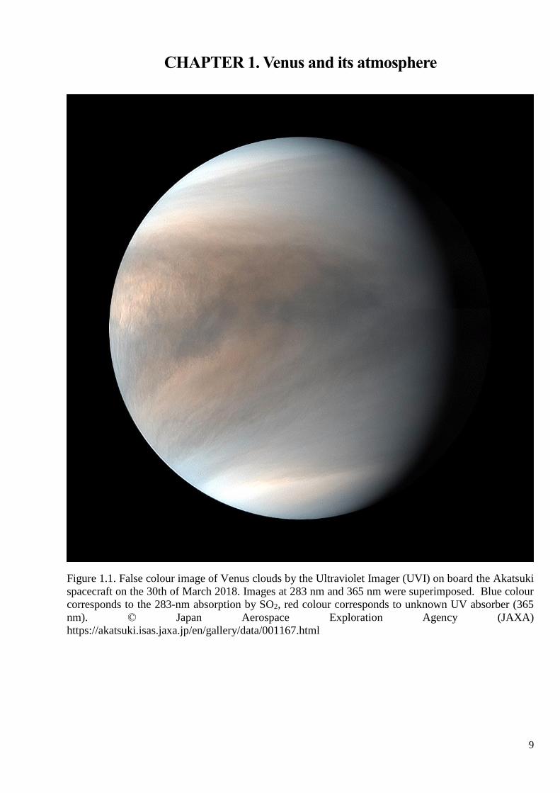
Figure 1.1. False colour image of Venus clouds by the Ultraviolet Imager (UVI) on board the Akatsuki

spacecraft on the 30th of March 2018. Images at 283 nm and 365 nm were superimposed. Blue colour

corresponds to the 283-nm absorption by SO2, red colour corresponds to unknown UV absorber (365

nm). © Japan Aerospace Exploration Agency (JAXA)

https://akatsuki.isas.jaxa.jp/en/gallery/data/001167.html

10

1.1. The Earth’s evil twin

Since ancient times the second planet from the Sun and the closest to the Earth, Venus, has been the

object of close attention. Out of the terrestrial planets, this planet is the most similar to the Earth in size

and mass. So it is often called the «sister» planet or even the «twin» of the Earth: its radius is 6052 km

and its mass is 4.87×1024 kg, that is 95% and 82% respectively of the Earth’s. In other respects, the

differences between the two planets can be significant (Colin, 1983). Moving in an almost circular orbit

around the Sun, with an eccentricity of 0.00677 and at an average distance of 0.723 astronomical units

(108 million km), Venus approaches the Earth at a minimum distance of 38 million kilometers. For

comparison, the minimum distance to Mars, the fourth planet of the terrestrial group, is one and a half

times greater. Thus, the planet makes a complete revolution around the Sun in 224.7 Earth days.

Venus is one of the two planets in the solar system with retrograde rotation. Venus’ rotation axis

inclination angle is 177°, thus, it is nearly perpendicular to the ecliptic plane. Such an axis tilt and orbital

parameters exclude a presence of seasons on the planet. In addition, Venus rotates very slowly. The

period of the planet’s revolution around its own axis is approximately 243 Earth days. However, due to

the retrograde rotation, a solar day on the planet lasts about 116.75 Earth days, and a complete revolution

around the Sun amounts to only 1.92 Venus days. This slow rotation has allowed the gravimetric surface

of Venus to maintain a spherical shape, mitigating polar compression.

Our knowledge on Venus before the beginning of the space exploration era was rather scarce. In 1610,

using the first telescope, Galileo Galilei was the first who observed a change of the visible diameter of

Venus and its phase that became a proof of the planetary movement around a single centre, i.e. the Sun

(Chruikshank, 1983). The historical discovery was made by M.V. Lomonosov on June 6, 1761 during

the planet’s transit over the solar disk. He noticed a halo of light emerging around the Venus disk when

observed at the Sun limb. The scientist correctly explained the pattern as light scattered by an atmosphere

enshrouding the planet. In his work M.V. Lomonosov concluded: «The planet Venus is surrounded by

a noble air atmosphere, such (if only not more), which is poured around our globe.» (Lomonosov, 1761,

the citation is translated to English by the author). It took more than three centuries to obtain more

detailed information about the structure of the atmosphere.

For an astronomical observer using the visible range of the spectrum, Venus appears as a slightly

yellowish bright disk without pronounced features. This is due to an opaque cloud layer having no

“holes” and hiding the surface for remote observations. At the dawn of the Venus exploration era this

peculiarity of the planet was a cause of diverging hypotheses about the conditions below the clouds, at

the surface and a possible presence of life. The high albedo of the clouds, which reflect about 80% of

the solar radiation, provides an amount of energy received by Venus from the Sun, comparable to that

of the Earth. Until the 1960s, this led some scientists to assume the planet’s climate to be similar to the

temperate climate of the Earth (Cruikshank, 1983). One can simply estimate the effective temperature

for Venus, which is 231 K (-45° C). However, the first radio astronomical observations (Mayer et al.,

1958) showed that the conditions near the surface are much more severe and not comparable to those on

Earth. The planet’s surface reaches 750 K (477º C). The reason for such a hot surface is the significant

greenhouse effect produced by the dense CO2 atmosphere.

11

A detailed study of Venus would not have been possible without the contribution made by spacecraft

reaching the lower atmosphere and surface. One of the important examples is that the pressure at the

surface reaching 90 bar was measured only when the Soviet station of Venera 7 released the first landing

on the 15th of December 1970. The space exploration of the planet started in 1962.

1.2. A new view of Venus

The era of active spacecraft exploration of Venus coincided with increased research interest in climate

change on Earth. New knowledge about the Venusian atmosphere has made this planet an example of a

world where the uncontrolled greenhouse effect has heated the airmass below clouds and the surface up

to enormous temperatures (Sagan, 1960; Rasool and De Berg, 1970). The discovery of this phenomenon

has become a catalyst for the study of such processes on Earth. Venus gives an example of the extreme

greenhouse effect in a dry carbon dioxide atmosphere. Since the two planets are similar by size and mass

the researchers need to understand which processes may become responsible for triggering an

uncontrollable greenhouse effect on Earth. Not only the impact of carbon dioxide is to be considered.

The Venus clouds, reflecting 76% of the sunlight, should protect against the surface overheating.

However, at wavelengths shorter than 2.5 μm, concentrated sulphuric acid, which dominates the

composition of aerosol particles on Venus (Sill, 1972; Young, 1973), also absorbs radiation contributing

to some extent to the greenhouse effect. That is why, researchers of the Earth’s atmosphere have paid

more attention to the chemistry of sulphur compounds. The possible impact of sulphate aerosols, both

volcanic and anthropogenic, on changes in the Earth’s global temperature was also reassessed (Hansen

et al., 1978).

Our neighbour, being an object of scientific observation of new physical and chemical processes, has

demonstrated the importance of controlling them also on Earth (Prinn, 1982). The stability of the relative

carbon dioxide content (96.5%) on Venus raised the issue of a large influence of minor gaseous

components on chemical processes in the atmosphere. Carbon dioxide is actively photodissociated, but

it less effectively restored from the produced CO and O2. Thus, this should reduce its amount. The first

CO2-atmosphere models of Mars and Venus showed the importance of catalytic cycles (Cruikshank,

1983; Krasnopolsky, 2011). In these reaction chains minor gas components are catalysts, and they

contribute to CO2 restoration without changing themselves. At the same time, the effect of such

processes on the Earth’s stratospheric ozone was studied. The observations showed a smaller amount of

O3 than a model considering only photolysis for its destruction provided (the Chapman mechanism from

Chapman, 1930). Both natural sources (products of water photolysis) and anthropogenic impacts

(combustion products from rocket fuel in the stratosphere) were considered. Halogens were already

found in the Venus atmosphere at that time (Mueller, 1968). Works of Prinn (1971) and McElroy et al.

(1973) showed the importance of chlorine compounds, namely the detected hydrogen chloride, as

catalysts. The chains of chemical reactions in the photochemical model of the Venusian atmosphere also

included oxygen compounds, which partly showed the effect of chlorine-containing substances on the

breakdown of the ozone molecule. Later on studies of catalytic chemistry of anthropogenic emissions,

especially volatile chlorine compounds (Wofsy and McElroy, 1974; Stolarski and Cicerone, 1974;

12

Molina and Rowland, 1974), demonstrated their effect on the ozone loss in the Earth’s atmosphere

(Farman et al., 1985).

With the development of exoplanet science, the existence of life on Earth started to be considered in the

context of searching for habitable worlds near other stars. A «habitable zone» criterion for the planetary

system was formulated by Kopparapu et al. (2013). This criterion defines the location of the planet in

respect to a parent star so that conditions on its surface allow the presence of liquid water. This is the

only robust criterion for the possible origin of life so far. The habitable zone also limits the runaway

greenhouse effect during the planet’s evolution, which brings the atmosphere to a state similar to that it

is on Venus now. In the context of the habitable zone near the Sun, Venus is on its inner boundary (the

orbit of Venus is 0.723 AU, while the inner boundary of the inhabited zone is 0.75 AU). However, based

on current atmospheric composition knowledge, modelling also shows that conditions on Venus in its

past did not rule out the possibility of an ocean on its surface (Way et al., 2020). If this hypothesis is

confirmed in future studies, the limits of search for life shall be extended beyond the inner boundary of

the habitable zone, into the «Venus zone», where many more planets are currently found than in the

canonical habitable zone.

1.3. History of observations

1.3.1. Venus space missions

In total, 27 spacecrafts were launched and successfully performed science experiments either around

Venus, or inside the atmosphere or on the surface: 19 from the Soviet Union, 6 from the United States

of America, one European Venus Express orbiter in 2005, and one Japanese Akatsuki station in 2010.

The first period of active exploration of Venus was led by space programs of the USSR and the USA.

At least one mission in every «astronomical window» was launched in the period from 1965 to 1985.

The USSR led the series of «Venera» and «Vega» stations which successfully landed on Venus 10 times.

On the U.S. side, several spacecraft (Mariner 2, the first interplanetary probe, Pioneer Venus and

Magellan) were sent to the planet from the sixties to the nineties. One descent probe also reached the

surface as a part of the Pioneer Venus 2 mission. Table 1.1 shows the timescale of successful missions

to Venus.

The first spacecraft, which successfully reached the orbit of Venus, was the American Mariner 2 mission

launched in 1962. Its measurements confirmed the slow retrograde rotation of the planet, high surface

temperatures and a dense cloud cover. In addition, the calculation of the spacecraft trajectory made it

possible to estimate the mass of the planet, which was not yet precisely known. In 1967, Venera 4 was

the first probe which made in situ measurements in the atmosphere of a planet other than Earth during

its descent to the surface down to 26 km. This made it possible to confirm that CO2 was the main

component of the atmosphere and that the estimated surface pressure (~100 bar) exceeded the values

expected at that time (Avduevskij et al., 1968). This pressure estimate was later confirmed by radiometric

soundings from the Mariner 5 probe. The Venera 5 and 6 stations also attempted to land on the planet

surface, but none of them were successful due to the extreme temperatures and pressures encountered

during the descent.

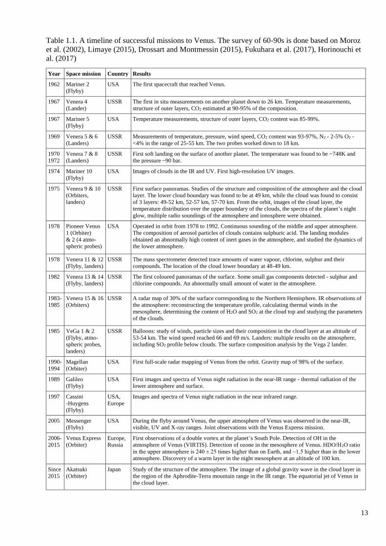
13

Table 1.1. A timeline of successful missions to Venus. The survey of 60-90s is done based on Moroz

et al. (2002), Limaye (2015), Drossart and Montmessin (2015), Fukuhara et al. (2017), Horinouchi et

al. (2017)

Year Space mission Country Results

1962 Mariner 2

(Flyby)

USA The first spacecraft that reached Venus.

1967 Venera 4

(Lander)

USSR The first in situ measurements on another planet down to 26 km. Temperature measurements,

structure of outer layers, CO2 estimated at 90-95% of the composition.

1967 Mariner 5

(Flyby)

USA Temperature measurements, structure of outer layers, CO2 content was 85-99%.

1969 Venera 5 & 6

(Landers)

USSR Measurements of temperature, pressure, wind speed, CO2 content was 93-97%, N2 - 2-5% O2 -

<4% in the range of 25-55 km. The two probes worked down to 18 km.

1970

1972

Venera 7 & 8

(Landers)

USSR First soft landing on the surface of another planet. The temperature was found to be ~748K and

the pressure ~90 bar.

1974 Mariner 10

(Flyby)

USA Images of clouds in the IR and UV. First high-resolution UV images.

1975 Venera 9 & 10

(Orbiters,

landers)

USSR First surface panoramas. Studies of the structure and composition of the atmosphere and the cloud

layer. The lower cloud boundary was found to be at 49 km, while the cloud was found to consist

of 3 layers: 49-52 km, 52-57 km, 57-70 km. From the orbit, images of the cloud layer, the

temperature distribution over the upper boundary of the clouds, the spectra of the planet’s night

glow, multiple radio soundings of the atmosphere and ionosphere were obtained.

1978 Pioneer Venus

1 (Orbiter)

& 2 (4 atmo-

spheric probes)

USA Operated in orbit from 1978 to 1992. Continuous sounding of the middle and upper atmosphere.

The composition of aerosol particles of clouds contains sulphuric acid. The landing modules

obtained an abnormally high content of inert gases in the atmosphere, and studied the dynamics of

the lower atmosphere.

1978 Venera 11 & 12

(Flyby, landers)

USSR The mass spectrometer detected trace amounts of water vapour, chlorine, sulphur and their

compounds. The location of the cloud lower boundary at 48-49 km.

1982 Venera 13 & 14

(Flyby, landers)

USSR The first coloured panoramas of the surface. Some small gas components detected - sulphur and

chlorine compounds. An abnormally small amount of water in the atmosphere.

1983-

1985

Venera 15 & 16

(Orbiters)

USSR A radar map of 30% of the surface corresponding to the Northern Hemisphere. IR observations of

the atmosphere: reconstructing the temperature profile, calculating thermal winds in the

mesosphere, determining the content of H2O and SO2 at the cloud top and studying the parameters

of the clouds.

1985 VeGa 1 & 2

(Flyby, atmo-

spheric probes,

landers)

USSR Balloons: study of winds, particle sizes and their composition in the cloud layer at an altitude of

53-54 km. The wind speed reached 66 and 69 m/s. Landers: multiple results on the atmosphere,

including SO2 profile below clouds. The surface composition analysis by the Vega 2 lander.

1990-

1994

Magellan

(Orbiter)

USA First full-scale radar mapping of Venus from the orbit. Gravity map of 98% of the surface.

1989 Galileo

(Flyby)

USA First images and spectra of Venus night radiation in the near-IR range - thermal radiation of the

lower atmosphere and surface.

1997 Cassini

-Huygens

(Flyby)

USA,

Europe

Images and spectra of Venus night radiation in the near infrared range.

2005 Messenger

(Flyby)

USA During the flyby around Venus, the upper atmosphere of Venus was observed in the near-IR,

visible, UV and X-ray ranges. Joint observations with the Venus Express mission.

2006-

2015

Venus Express

(Orbiter)

Europe,

Russia

First observations of a double vortex at the planet’s South Pole. Detection of OH in the

atmosphere of Venus (VIRTIS). Detection of ozone in the mesosphere of Venus. HDO/H2O ratio

in the upper atmosphere is 240 ± 25 times higher than on Earth, and ~1.5 higher than in the lower

atmosphere. Discovery of a warm layer in the night mesosphere at an altitude of 100 km.

Since

2015

Akatsuki

(Orbiter)

Japan Study of the structure of the atmosphere. The image of a global gravity wave in the cloud layer in

the region of the Aphrodite-Terra mountain range in the IR range. The equatorial jet of Venus in

the cloud layer.

14

The first soft landing was made in 1970 by Venera 7 on the night side of the planet. During its 23 minutes

of operations on the surface, temperature and pressure were measured, as well as the composition of the

crust using gamma spectrometry. A pressure of 90±15 bar and a temperature of 748±20 K (475±20°C)

were obtained at the surface. Venera 8 confirmed the possibility of taking photos at the surface:

illumination on Venus surface near the evening terminator turned out to be equal to the Earth twilight.

Venera 9 and 10 landers performed the first imaging of the surface. During the descent, nephelometers

studied the composition and structure of the atmosphere and of the cloud layer (see Table 1.1). Venus

was then reached by the 2 Pioneer Venus (PV) missions led by NASA. PV 1 was orbiting the planet

from 1978 to 1992 and sounding the atmosphere remotely. The concept of PV 2 contained 4 descent

probes: one large and three small modules (the North Probe, the Day Probe and the Night Probe). The

Day Probe successfully landed and transmitted data from the Venus surface for ~60 minutes (Colin,

1979). The important observations of the cloud layer structure were done during descent (Knollenberg

and Hunten, 1980). Further development of the Venera program allowed obtaining unique phenomena

of atmospheric lightning. The electrical activity was registered by the GROZA experiments on board the

Venera 11 and Venera 12 missions (Ksanfomaliti et al., 1979). The composition of cloud aerosols was

supplemented by such components as chlorine and phosphorus, although it was not possible to identify

compounds. Moreover, Venera 13 and 14 conveyed the only colour surface panoramas. The Venera 15

and 16 orbiters mapped 30% of the surface in the Northern Hemisphere.

The era of the Soviet study of Venus ended with the Vega mission, which combined explorations of

Venus and Halley’s comet. The part dedicated to Venus contained two aerostat balloons placed into the

clouds. They were tracked by the ground based NASA’s Deep Space Network, and the data of their

motion provided the wind velocities at an altitude of 53-54 km (Kremnev et al., 1987). Convective and

turbulent activities in the cloud layer and the aerosol composition were characterized in detail. The both

probes also detected lightning discharges on the night side. Vega 2 for the first time landed in a high

mountain region, where the Venusian rock was found to be a close analogue of terrestrial volcanic

material (Surkov et al., 1986). It is the only spacecraft measured the high-resolution temperature profile

down to the surface and found the anomalius behaviour below 7 km (Crisp and Titov, 1987).

NASA’s Magellan mission accomplished a topographic mapping of the surface in detail (spatial

resolution ~100 m) in the early 1990s (Saunders et al., 1992; Bindschadler, 1995). Magellan payload

included a synthetic aperture radar and an instrument for studying the gravitational field of Venus. In

September 1990, Magellan began its scientific mission, which lasted for 4 years. Radar showed more

than 1660 volcanic landforms. This number included 274 intermediate volcanoes 20-100 km in diameter

and 56 large volcanoes greater than 100 km in diameter (Saunders et al., 1992). It was found that 85%

of the planet’s surface is covered by lava flows. The surface of Venus has different tectonic features with

a variety of scales (Solomon et al., 1992). The absence of erosion has saved them in well-defined

structures. As a result, 98% of the planet’s surface was mapped (Figure 1.2), and moreover, stereo maps

of the surface were also obtained. In addition, it was concluded that the surface of Venus is geologically

young (<500 million years) because only a few impacts craters were found at the surface (Bullock et al.,

1993).

15

Figure 1.2. The topographic map of Venus produced by the Magellan mission.

In 1989 Galileo on its way to Jupiter was able to measure spectra of Venus transparency windows. After

the Magellan mission and the Galileo flyby, there was a pause in the Venus space exploration apart from

several flybys by spacecraft accomplishing a gravitational manoeuvre around Venus.

The new era of space exploration of Venus began with the launch of the European Space Agency’s

(ESA) Venus Express (VEX) mission (Svedhem et al., 2007). For ESA it was the first spacecraft to

explore Venus. Venus Express is the heir of Mars Express (MEX) and Rosetta (Chicarro et al., 2004;

Glassmeier et al., 2007). The probe was successfully launched on November 9, 2005 by a Soyuz-Fregat

rocket from Baikonur, Kazakhstan. The spacecraft reached Venus on April 11, 2006, and the scientific

mission started on May 6, 2006. The spacecraft’s orbit was highly elliptical and quasi polar. One of the

VEX goals was to investigate in detail the South Pole of the planet, which had not been explored before

by other missions because of their orbit properties. The pericenter of the VEX orbit was located at a

latitude of 80°N and an altitude of 250 km. The period of this orbit was 24 Earth hours.

In 2010, the Akatsuki scientific mission of the Japan Aerospace Exploration Agency (JAXA) was

supposed to be inserted in orbit around Venus (Nakamura et al., 2011). However, the spacecraft entered

the target orbit after the second attempt, five years later namely on December 9, 2015 (Nakamura et al.,

2014). Ultraviolet camera (UVI), long-wave infrared camera (LIR), 1-μm (IR1) and 2-μm (IR2) cameras

as well as lightning and atmospheric glow detectors are installed on board and keep operating at the time

this manuscript is being written. After one year the IR1 and IR2 cameras stopped operations in nominal

mode. Akatsuki observation in the IR identified dynamical processes occurring in lower clouds. The

influence of topography was found with the presence of a gravity wave (Fukuhara et al., 2017) in the

cloud layer near the Aphrodite-Terra mountain (Figure 1.3).

16

Figure 1.3. A-E. Brightness temperatures of the entire disk of Venus measured by the LIR camera on

board the Akatsuki spacecraft from 7 December to 11 December 2015. Solid and dashed lines correspond

to the equator and evening terminator correspondingly. The colour bar is valid only for panel A. The

temperature ranges for pictures in panels B-E are adjusted so that the mean temperatures in a circle with

a radius of 0.1 RVenus at the disk centre are constant, where RVenus is the Venus radius. F. The UV image

of cloud tops obtained by UVI at a wavelength of 283 nm (Fukuhara et al., 2017).

17

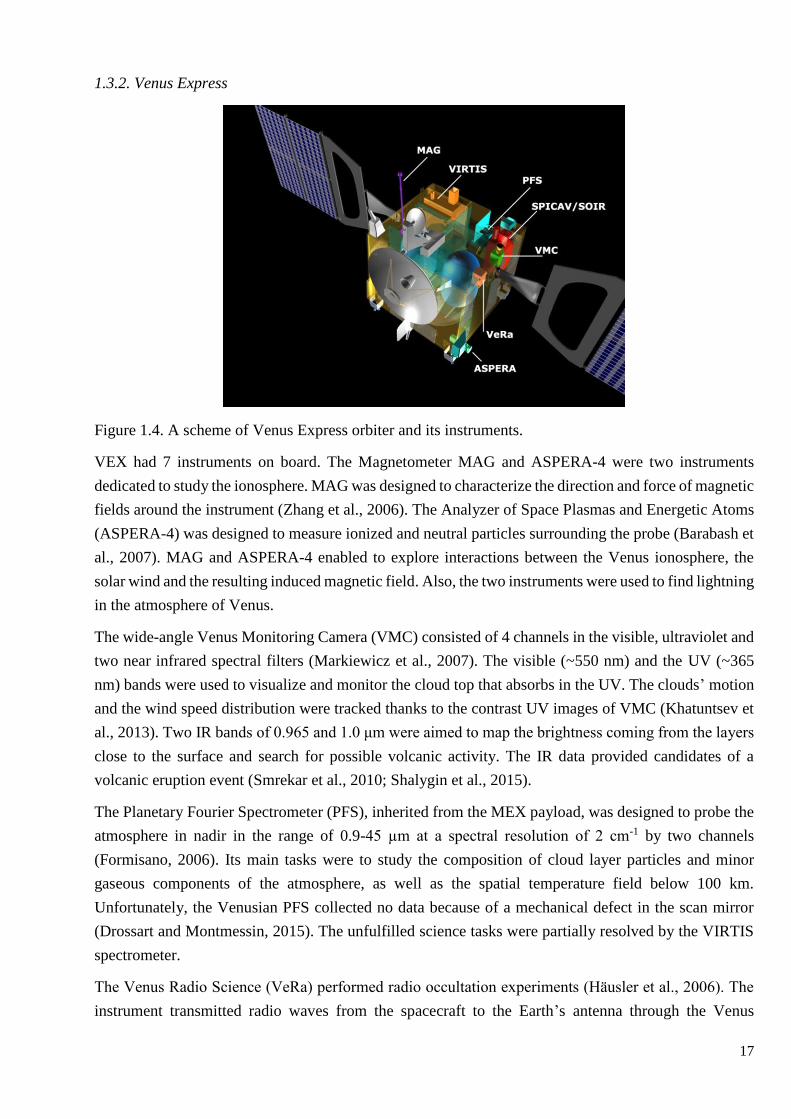
1.3.2. Venus Express

Figure 1.4. A scheme of Venus Express orbiter and its instruments.

VEX had 7 instruments on board. The Magnetometer MAG and ASPERA-4 were two instruments

dedicated to study the ionosphere. MAG was designed to characterize the direction and force of magnetic

fields around the instrument (Zhang et al., 2006). The Analyzer of Space Plasmas and Energetic Atoms

(ASPERA-4) was designed to measure ionized and neutral particles surrounding the probe (Barabash et

al., 2007). MAG and ASPERA-4 enabled to explore interactions between the Venus ionosphere, the

solar wind and the resulting induced magnetic field. Also, the two instruments were used to find lightning

in the atmosphere of Venus.

The wide-angle Venus Monitoring Camera (VMC) consisted of 4 channels in the visible, ultraviolet and

two near infrared spectral filters (Markiewicz et al., 2007). The visible (~550 nm) and the UV (~365

nm) bands were used to visualize and monitor the cloud top that absorbs in the UV. The clouds’ motion

and the wind speed distribution were tracked thanks to the contrast UV images of VMC (Khatuntsev et

al., 2013). Two IR bands of 0.965 and 1.0 μm were aimed to map the brightness coming from the layers

close to the surface and search for possible volcanic activity. The IR data provided candidates of a

volcanic eruption event (Smrekar et al., 2010; Shalygin et al., 2015).

The Planetary Fourier Spectrometer (PFS), inherited from the MEX payload, was designed to probe the

atmosphere in nadir in the range of 0.9-45 µm at a spectral resolution of 2 cm-1 by two channels

(Formisano, 2006). Its main tasks were to study the composition of cloud layer particles and minor

gaseous components of the atmosphere, as well as the spatial temperature field below 100 km.

Unfortunately, the Venusian PFS collected no data because of a mechanical defect in the scan mirror

(Drossart and Montmessin, 2015). The unfulfilled science tasks were partially resolved by the VIRTIS

spectrometer.

The Venus Radio Science (VeRa) performed radio occultation experiments (Häusler et al., 2006). The

instrument transmitted radio waves from the spacecraft to the Earth’s antenna through the Venus

18

atmosphere or after a reflection from the Venus surface. The purpose of this experiment was to analyse

the ionosphere, atmosphere and surface of Venus. It allowed retrieving vertical profiles of atmospheric

temperature and density from 40 to 100 km (Tellmann et al, 2009).

The Visible and Infrared Thermal Imaging Spectrometer (VIRTIS), which was previously designed for

Rosetta mission, consisted of three spectrometric channels (Drossart et al., 2007). VIRTIS-M in the IR

and visible operated in the 1.02-5.13 µm and 0.28-1.10 µm spectral ranges respectively, while VIRTIS-

H covered the 1.84-5.00 µm range. These two IR channels included several Venus transparency windows

to study the composition of the lower atmosphere. Emission of hydroxyl at 1.40-1.49 and 2.6-3.14 μm

was discovered (Piccioni et al., 2008).

The SPectroscopy for Investigation of Characteristics of the Atmosphere of Venus (SPICAV) has been

successfully operating for 8 years (Bertaux et al., 2007b; Vandaele et al., 2008; Korablev et al., 2012).

It consisted of the UV (118-320 nm) and the IR (0.65-1.7 μm) channels. SOIR (SOIR - Solar Occultation

in InfraRed) is an independent high-resolution spectrometer in 2.3-4.2 μm, which was part of the

SPICAV/SOIR assembly (Vandaele et al., 2008).

1.3.3. Future missions

The discoveries by the missions of the last 15 years, however, still leave unresolved questions concerning

present volcanism and geological activity on the surface, the lower atmosphere structure, the unknown

UV absorber in the clouds, the water evolution on the planet, etc. The answers require continued study

of Venus both from the Earth and by new exploratory missions to Venus, including modern atmospheric

and landing modules. Therefore, the world space agencies assume launches of new missions with a wide

range of scientific tasks.

The first in the list is the orbital mission to Venus from the Indian Space Research Organization (ISRO),

whose launch was initially scheduled for 2023 (Shaji, 2019) and recently postponed to 2025. The

planned mission named Shukrayaan-1 (translated as “Venus craft”) will be devoted to remote sensing of

the surface, the atmosphere and the ionosphere. The payload includes VIRAL and IVOLGA

spectrometers provided by Roscosmos. The VIRAL IR spectrometer is being developed at the Space

Research Institute with the participation of LATMOS. The IVOLGA heterodyne laser spectrometer for

the near-IR range is being developed at the Moscow Institute of Physics and Technology.

A post-2025 launch is planned for a new Roscosmos mission in collaboration with NASA. Venera-D or

«Venus the Long-lived» will contain a lander based on previous Vega missions with a capability to

improve results of previous descent and landing probes. The lander will include one or more long-lived

small station LLISSE (Long-Lived In-Situ Solar System Explorer) that is assumed to operate on the

surface of Venus for about 60 days (Zasova et al., 2014). It is also planned to implement a module, flying

in the clouds, with an ability to manoeuvre vertically and to explore different layers. There will be an

orbiter, for data relay, with science objectives similar to those of VEX and with a Fourier spectrometer

on board, in order to compensate the PFS loss in 2006. The planned launch date for Venera-D is 2029

or 2031.

19

One of the candidates for ESA is the new EnVision mission (Widemann et al., 2020), which is being

prepared in collaboration with NASA. In case of positive selection in 2021 the launch will be in 2032.

The objectives of this orbital mission are mapping the surface with a very high spatial resolution (1-30

m), studying its properties in the IR spectrum and studying the atmosphere.

There are six NASA missions as well that are in a designing stage, none of which has yet been selected

for launch: VERITAS, DAVINCI, VISE, SAGE, VCM, VITaL. VERITAS (Venus Emissivity, Radio

Science, InSAR, Topography, and Spectroscopy) would aim to high-resolution surface study (Smrekar

et al., 2016). The combination of IR spectroscopy in transparency windows, radar mapping and gravity

field measurements is planned to improve the knowledge about the Venus inner structure and ongoing

geological activity. DAVINCI (Deep Atmosphere Venus Investigation of Noble gases, Chemistry, and

Imaging) is a proposed atmospheric probe to Venus (Glaze et al., 2016). Venus In Situ Explorer (VISE)

and The Surface and Atmosphere Geochemical Explorer (SAGE) concepts propose to land close to a

volcano (Squyres, 2011; Esposito, 2011). The Venus Climate Mission (VCM) is a more complex

program including an orbiter, a balloon, a mini-probe, and two dropsonde observational platforms

(Grinspoon et al., 2010). Similar to VCM is the Venus Intrepid Tessera Lander (VITaL) concept, which

is considered for landing on one of the oldest parts of the Venus surface: mountainous tessera regions

(Gilmore et al., 2010).

1.4. The surface of Venus

Venus clouds hide its surface. Remote investigation of its composition is almost impossible. Landers

studied the surface which appeared to be similar to the terrestrial basalt rocks (Surkov, 1983) that are

associated with volcanic activity. Radar measurements made by Magellan revealed that the Venus

surface is rather flat, and is mainly shaped by lava plains, produced by more than 1660 volcanoes on

Venus (Saunders et al., 1992). The small number of craters implies that the Venus surface is geologically

young (<500 million years, according to Bullock et al., 1993).

Figure 1.5. Coloured panorama by Venera 14 at 13.055°S, 310.19° (Phoebe Regio).

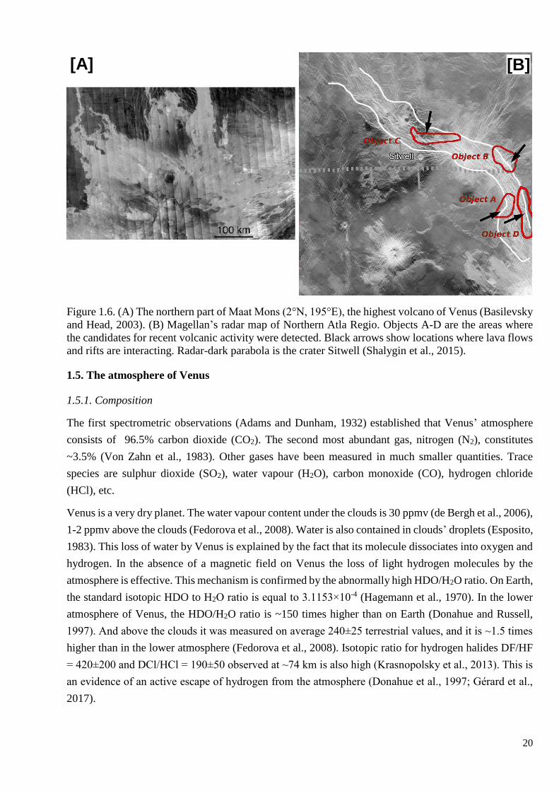
The question of active volcanism on Venus is still open. Observations of surface emissivity in the

infrared is compatible with an opinion of ongoing volcanic processes. The Venus Express mission

revealed four candidates named «hotspots» associated with increased surface emissivity possibly caused

by fresh lava flows (Smrekar et al., 2010; Shalygin et al., 2015). This activity was detected near the

highest volcano of Venus, Maat Mons, which is located in the Alta rift region. Radar shows light

solidified lava flows around the volcano itself, overlapping darker plains with wrinkled ridges.

20

Figure 1.6. (A) The northern part of Maat Mons (2°N, 195°E), the highest volcano of Venus (Basilevsky

and Head, 2003). (B) Magellan’s radar map of Northern Atla Regio. Objects A-D are the areas where

the candidates for recent volcanic activity were detected. Black arrows show locations where lava flows

and rifts are interacting. Radar-dark parabola is the crater Sitwell (Shalygin et al., 2015).

1.5. The atmosphere of Venus

1.5.1. Composition

The first spectrometric observations (Adams and Dunham, 1932) established that Venus’ atmosphere

consists of 96.5% carbon dioxide (CO2). The second most abundant gas, nitrogen (N2), constitutes

~3.5% (Von Zahn et al., 1983). Other gases have been measured in much smaller quantities. Trace

species are sulphur dioxide (SO2), water vapour (H2O), carbon monoxide (CO), hydrogen chloride

(HCl), etc.

Venus is a very dry planet. The water vapour content under the clouds is 30 ppmv (de Bergh et al., 2006),

1-2 ppmv above the clouds (Fedorova et al., 2008). Water is also contained in clouds’ droplets (Esposito,

1983). This loss of water by Venus is explained by the fact that its molecule dissociates into oxygen and

hydrogen. In the absence of a magnetic field on Venus the loss of light hydrogen molecules by the

atmosphere is effective. This mechanism is confirmed by the abnormally high HDO/H2O ratio. On Earth,

the standard isotopic HDO to H2O ratio is equal to 3.1153×10-4 (Hagemann et al., 1970). In the lower

atmosphere of Venus, the HDO/H2O ratio is ~150 times higher than on Earth (Donahue and Russell,

1997). And above the clouds it was measured on average 240±25 terrestrial values, and it is ~1.5 times

higher than in the lower atmosphere (Fedorova et al., 2008). Isotopic ratio for hydrogen halides DF/HF

= 420±200 and DCl/HCl = 190±50 observed at ~74 km is also high (Krasnopolsky et al., 2013). This is

an evidence of an active escape of hydrogen from the atmosphere (Donahue et al., 1997; Gérard et al.,

2017).

[A] [B]

21

The loss of water, even if it existed in the liquid state on the planet’s surface in the past (Way et al.,

2020), is related to the greenhouse effect. CO2 and H2O are mainly responsible for the greenhouse effect

that warms up the surface and the atmosphere. These gases effectively absorb infrared (IR) radiation

from the warm surface, making it difficult for heat to escape into space. The tiny amount of water vapour

contributes less significantly, which is the opposite in the Earth atmosphere. However, the H2O

absorption regulates the transmission of several IR transparency windows of the Venus atmosphere

(Section 1.5.4). On Venus, the cloud aerosol particles (Section 1.5.3) are very reflective making the

spherical albedo of Venus equal to 0.76. However, ~3% of solar radiation reaching the surface maintains

the enormous greenhouse effect increasing the temperature of the atmosphere by about 200 K. On Earth,

the greenhouse influence is about 35 K. The cloud layer additionally to filtering of solar radiation

contributes to atmospheric heating on Venus. The aerosols are opaque in most of the IR spectrum of the

thermal radiation from the planet’s surface.

While the difference in CO2 abundances in the atmospheres of the Earth and Venus is large, the global

inventory of CO2 on both planets is comparable. On the Earth, most of CO2 is trapped as carbonates at

the floor of oceans. If this trapped CO2 would be released in the Earth’s atmosphere, it would end up in

creating a 100 bar-thick atmosphere of CO2, that is very close to the Venus atmosphere.

1.5.2. Structure of the atmosphere

Like on Earth, several compartments can be distinguished in the atmosphere of Venus: the troposphere,

the mesosphere, the thermosphere and the exosphere. Yet, there is no evidence for a stratosphere on

Venus, reflecting the absence of an absorbing layer like the terrestrial ozone, which causes a temperature

inversion. It is seen in Figure 1.7 showing the temperature profiles on both day and night sides of the

planet.

The troposphere, covering altitudes up to 65 km, contains 99% of the entire mass of the atmosphere. The

upper part of the troposphere is characterized by active convection. Then the temperature decreases

uniformly with increasing altitude, and the atmosphere becomes neutral. The temperature gradient dT/dz

was measured to -7.7 K/km (Seiff, 1983) and it is close to the adiabatic lapse rate equal to -g/Cp. The

airmass is delivered from the near-surface to the clouds deck while sustaining adiabatic relaxation. Such

a behaviour can be traced upon descent in very deep atmospheric layers down to an altitude of ~7 km,

where the planetary boundary layer (PBL) begins. The vertical gradient measured by VeGa 2 represents

the high instability here (Linkin et al., 1986; Linkin et al., 1987). Possibly, CO2 and N2 can be

fractionated in the deep atmosphere as their properties correspond to super fluid liquids under high

temperature and pressure conditions. Then, the N2 abundance should decrease to zero near the surface

and this change of molecular mass would stabilize the lapse rate (Lebonnois and Shubert, 2017). In the

vertical structure, there is a layer around ~50 km characterized by the terrestrial normal conditions,

which is 1 bar and 293 K. Another peculiarity of the troposphere, there is no significant temperature

difference between day and night since the high-density greenhouse CO2 provides constant thermal

balance under the thick clouds. Here thermochemistry contributes significantly to chemical processes.

With an increase in temperature and a decrease in the amount of sunlight, thermochemistry becomes the

dominant process into the deep atmosphere. Vertical transport delivers constituents to the upper

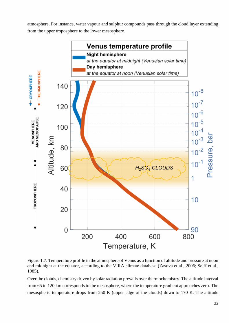
22

atmosphere. For instance, water vapour and sulphur compounds pass through the cloud layer extending

from the upper troposphere to the lower mesosphere.

Figure 1.7. Temperature profile in the atmosphere of Venus as a function of altitude and pressure at noon

and midnight at the equator, according to the VIRA climate database (Zasova et al., 2006; Seiff et al.,

1985).

Over the clouds, chemistry driven by solar radiation prevails over thermochemistry. The altitude interval

from 65 to 120 km corresponds to the mesosphere, where the temperature gradient approaches zero. The

mesospheric temperature drops from 250 K (upper edge of the clouds) down to 170 K. The altitude

23

interval between 90 and 120 km, where the temperature of the day side reaches a minimum hosts the

mesopause. On the night side, altitudes above ~100 km are occupied by the cryosphere with a further

slight temperature decrease. A warm layer by 20-40 K was detected here around 100 km from Venus

Express observations (Bertaux et al., 2007a). It is likely produced by the adiabatic heating within a

downwelling motion or, possibly, by the presence of aerosols (Bertaux et al., 2007a; Picciali et al., 2015).

The thermosphere is located above 120 km up to 200 km (Limayer et al., 2018). On the day side,

temperatures are 270-400 K. On the night side, the atmosphere is very cold, which has led scientists to

call it “cryosphere”. There, temperatures reach 100 K which is the minimum temperature encountered

on Venus. In that range the homosphere becomes the heterosphere, since the homopause on Venus was

measured at 120-132 km (Mahieux et al., 2015). So the CO2 is the dominant gas of the Venus

thermosphere up to ∼140 km and ∼155 km on the night and day sides respectively (Niemann et al. 1980;

Kasprzak et al. 1997). But at higher altitudes abundances of lighter compounds increase (Niemann et al.

1980; Seiff and Kirk, 1982).

Above 120 km, the number of particles ionized by the UV radiation, the solar wind and cosmic rays,

increases. The maximum density of the ionosphere on the daytime side is located at an altitude of 140

km. Venus does not have a magnetic field, so the particles of the solar wind interact directly with the

atmosphere, changing the characteristics of the ionosphere depending on the activity of the Sun. The

ionosphere determines the parameters of the induced magnetic field of Venus, which turns the solar wind

particles around the planet.

1.5.3. The cloud layer

The first data on the composition of aerosol particles in the cloud layer were obtained on the basis of

measurements of the brightness temperature and polarimetry (Sill, 1972; Young, 1973; Hansen et al.,

1974; Pollack et al., 1974). These measurements forced the community to discard the hypothesis of

water-dominated clouds. Knowledge about the depth and the structure of the clouds was derived from

descent probes. It is still the most valuable dataset for describing the vertical layering of Venusian clouds.

The vertical thickness of the cloud layer was measured to be more than 20 km, with particles detected

in the altitude range from 47 to 70-75 km. Three modes of aerosol particles are forming the cloud layer.

Each mode is characterized by a specific modal radius: <0.4 µm for the mode 1, 1.05 and 1.25 µm for

modes 2 and 2’ correspondingly, 3-4 µm for mode 3 (Esposito et al., 1983). The modes populate three

cloud layers, upper and lower hazes differently: the largest mode (mode 3) prevails in the lower and

middle cloud layers and the lower haze, which forms the bulk of the clouds. Mode 1 and 2 are contained

in the upper layer (50-70 km) and in the upper haze (>70 km). The lower haze was detected down to 30

km. The upper haze reaches an altitude of ~110 km.

The main component of aerosol particles in the Venusian cloud layer is an aqueous solution of sulphuric

acid (75-90%). Sulphuric acid is mainly produced from SO2 and H2O under solar light in the upper cloud

layer, considered as a photochemical “factory” (Titov et al., 2017).

SO2 + O → SO3

24

SO3 + H2O → H2SO4

SO2 and H2O are transported upward from the lower atmosphere to supply the production of sulphuric

acid. H2SO4 formation is followed by condensation. While the aerosol particles descend lower in the

cloud deck forming larger particles until they evaporate. Below clouds H2SO4 is decomposed in

thermodynamic equilibrium reactions back to SO2 and H2O to restart the cycle (Mills et al., 2007).

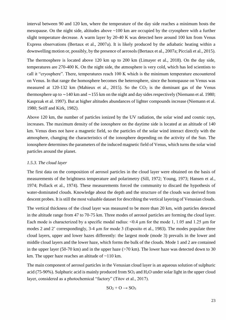
Figure 1.8. Modal partitioning of number density by the cloud particle size spectrometer on board the

Pioneer Venus Sounder probe (Knollenberg and Hunten, 1980).

The largest particles form the bulk of the clouds. However, it is controversial whether it is a separate

mode or a tale of the mode 1 and 2 distribution. Mode 3 detailed composition is still a mystery. It is also

controversial if these particles are crystallized or liquid and if the mode 3 includes some other species

additionally to H2SO4 (Knollenberg and Hunten 1980). Descend probes of Venera 13, 14 and Vega 1, 2

detected the presence of sulphur, chlorine, phosphorus and iron (Petryanov et al., 1981; Andreichikov,

1987) without specification of the substance.

Some uncertainty remains in the composition of the lightest aerosol particles. Remote observations in

the UV range have shown that the clouds contain an unknown absorber effective at λ>320 nm. It is

associated with additional substances whose composition is not fully known. Many candidates have been

proposed: sulphur (S8, S3, S4, OSSO or S2O) and chlorine (FeCl3 or SCl2) species, organic compounds,

mineral dusts or even bacteria (Mills et al., 2007; Zhang et al., 2012; Marcq et al., 2017; Carlson et al.,

2016; Frandsen et al. 2016; Krasnopolsky, 2017; Krasnopolsky, 2018; Limaye et al., 2018).

25

Numerous new results were collected by three instruments on board Venus Express mission: VMC,

VIRTIS and SPICAV. The upper boundary of the cloud layer was found to decrease from 72±1 km at

low and middle latitudes to 61-67 km in polar regions (Ignatiev et al., 2009; Cottini et al., 2015; Fedorova

et al., 2016). SPICAV IR data showed that the upper haze reaches an altitude of ∼110 km and also has

a latitudinal trend similar as that of the cloud top (Luginin et al., 2016).

1.5.4. Transparency windows

The thermal emission emitted by the hot lower atmosphere and the surface is not totally shielded by the

cloud layer and the gases. Between the strong absorption bands of CO2 there are several intervals where

clouds do not absorb and only scatter photons mostly in the forward direction. In these «transparency

windows» the IR thermal radiation escapes to outer space. This phenomenon was discovered by David

A. Allen and John W. Crawford (Allen and Crawford, 1984) at 1.74 and 2.35 µm. This discovery

provided a new tool to study atmospheric properties from the cloud layer down to the surface (Marcq et

al., 2008; Arney et al., 2014; Bézard et al., 2011; Fedorova et al., 2015). Thermal radiation of the lower

atmosphere and the surface of Venus can only be observed on the night side of the planet since on the

dayside the solar radiation is overwhelming in this spectral range.

Figure 1.9. Venus night-side spectrum measured by Galileo mission (Taylor et al., 1997).

Subsequently all transparency windows in the near infrared from 0.85 to 2.5 µm were inventoried (Crisp

et al., 1991). The windows in 0.85-1.0 µm correspond to the surface radiation and allow studying its

thermal properties and geological processes. For example, the possible volcanic activity of Venus

(Smrekar et al., 2010; Shalygin et al., 2015). Radiation of 1.1- and 1.18-μm intervals originates from the

first-scale heights, i.e. 0-15 km. The other two transparency windows at 1.28 and 1.31 μm are sensitive

to the 15-30 km altitude range (Taylor et al., 1997). At 1.51 and 1.55 μm there are two additional

26

transparency windows. They are characterized by significantly weaker intensity formed at 20-35 km, the

difference between their intensity and one of the following 1.74-window is 2 orders in magnitude

(Wilson et al., 2009). The 1.74 and 2.35 μm windows correspond to emission formation at 20-30 km and

20-45 km respectively (Taylor et al., 1997).

The transparency windows are located in a range where there are no strong absorption lines for carbon

dioxide, which dominates the atmosphere of Venus. Absorption by carbon dioxide is determined only

by far-wings of its strong absorption lines. However, the study is also sensitive to trace gases in the

lower atmosphere. The absorption bands of water overlap the transparency windows of 1.1, 1.18, 1.74,

and 2.35 μm. HCl coincides with the absorption band of water vapour at the maximum of the 1.74-μm

transparency window. The transparency window at 2.35 μm is the most sensitive to minor gaseous

constituents of the lower atmosphere where the CO, OSC, and SO2 bands are also present.

The main parameter controlling the thermal brightness is the concentration of aerosol in the observed

atmospheric column: mainly the scattering by the largest particles of the cloud layer which are found in

the lower and middle clouds. Moreover, the intensities in the transparency windows of 1.28 and 1.31

μm, which are insensitive to changes in surface properties and to absorption by trace gas components,

are modulated only by variations in the clouds.

Figure 1.10. (A) Spectra measured in five transparency windows during one observation #2941A07 by

SPICAV IR spectrometer on board Venus Express spacecraft. Coloured rectangles show factors that

modulate the thermal emission in different spectral ranges: aerosol scaterring, surface emissivity and

water vapour absorption. The orange rectangle highlights the spectral range of the mesospheric O2 (a1Δg)

airglow at 1.27 μm. (B) The geographical locations corresponding to measured spectra.

The first space measurement of the full night IR spectra of Venus was done during Galileo flyby in 1989

(Figure 1.9). The IR emission has been monitored by ground-based high-resolution spectrometers and

during the Venus Express mission. It has been shown that it can change significantly at small scales

reflecting so far unknown variability in the lower cloud layers (Figure 1.10), surface emissivity and

minor species content. The 1.28-μm window is contaminated by the mesospheric oxygen emission at

1.27 μm that needs to be separated to enable the study of the thermal emission spectrum in that range.

[A] [B]

27

1.5.5. Mesosphere and atmospheric dynamics

Figure 1.11. Diagram of the main mechanisms of matter transfer in the Venus mesosphere above the

cloud layer.

The mesosphere is a very active region where two regimes of atmospheric circulation dominate in two

different altitude ranges. A powerful zonal motion dominates in the upper cloud, but at an altitude of

~100 km atmospheric components are subject to a different global circulation regime, characterized by

a global motion going from the subsolar point to the antisolar one (Sub-Solar Anti-Solar or SSAS

circulation). A retrograde superrotation of the cloud top was obtained by tracking the cloud features

exhibited large contrast in the UV. A speed of 110 m/s was then measured. The period of rotation of

Venus is 243 terrestrial solar days while the clouds need only 4 days for a full rotation around the planet.

There are only two solid surface bodies having this type of global atmospheric circulation: Venus and

Titan, the largest satellite of Saturn in the Solar System. Mainly this effect is related (Imamura et al.,

2020) to an angular momentum transfer from the slow rotating body to the atmosphere according to the

mechanism discussed by Gierasch (1975). This superrotation has its maximum at the cloud tops,

however, it was measured down to the surface with a decreasing speed with altitude (Rossow et al.,

1980; Counselman et al., 1980; Lellouch et al., 1997)

The cloud top winds have been particularly well studied by the tracking of large-scale features

characterised by lower albedo in UV. In the first era of Venus exploration the UV contrasts monitoring

was done by Mariner 10 (Limaye and Suomi, 1981), Pioneer Venus (Rossow et al., 1980) and Galileo

28

(Peralta et al., 2007) missions. The cameras on board Venus Express (Khatuntsev et al., 2013; Patsaeva

et al., 2015; Bertaux et al., 2016) and Akatsuki (Horinouchi et al., 2018) orbiters resumed this study.

The dynamics of the deeper cloud layer was derived from the VeGa balloons (Blamont et al., 1993) and

from the continuous monitoring of Akatsuki IR cameras (Horinouchi et al., 2017).

Venus rotates very slowly and the planet’s atmosphere is in cyclostrophic balance. So the zonal winds

are directed along the equator due to a balance between the equatorward component of centrifugal force

and the meridional pressure gradient (Leovy, 1973). The cyclostrophic winds can be modelled based on

the temperature field measurements. The temperature in the Venus atmosphere (40-200 km) was

measured from orbiters (Taylor et al., 1983; Zasova et al., 2007; Limaye et al., 2017). However, the

process of such acceleration of the atmosphere is still a subject to study, as is the observed dependence

of wind speed on altitude.

The zonal super rotation in the upper layer of the clouds is supplemented by a meridional transfer of

matter to the poles in Hadley cells of each hemisphere. This meridional transport is carried out at a much

slower speed than the zonal one. The speed is lower than 10 m/s. It is assumed that the meridional

circulation is effective on Venus in transferring warm air masses to the poles and colder air masses

towards the equator (Limaye, 1985). Observations (Limaye, 2007; Peralta et al., 2007; Khatuntsev et al.,

2017) show that the Hadley cell exists between the equator and latitude about 65º. It is the region where

the top of the cloud going deeper affecting the radiative balance, a cold collar is observed (Garate-Lopez

and Lebonnois, 2018). The polar collar is a cold air belt around the polar vortex. Its temperature inside

the collar is about 30 degrees colder than outside at the same altitude (Piccioni et al., 2007) that may be

caused by an adiabatic cooling of upwelling air.

The superposition of zonal rotation and meridional advection leads to the formation of a giant vortex at

each of the poles, where air is rotating downwards with a period of 2.8 terrestrial days. The northern

polar vortex was studied by Pioneer Venus and the southern one by means of VMC and VIRTIS

instruments on board Venus Express (Piccioni et al., 2007). The vortices are similar in nature to a tropical

cyclone on Earth (Limaye et al., 2009) and have a complex structure. On average, it is the dipole

(Schofield and Diner, 1983) but the shape can be an ellipsoid to a tripodal structure (Sánchez-Lavega et

al., 2017). However, a full description of the vortex dynamics is still to be established by global

circulation models.

The wind speeds of zonal rotation decrease from 70 km to ∼85 km (Piccialli et al. 2012), but their

variation increase (Sánchez-Lavega et al., 2017). At the altitudes nearing the mesosphere boundary (110

km) the SSAS circulation dominates. SSAS transfers air masses from the subsolar to the anti-solar point,

as a result of the significant contrast between day and night temperatures in the thermosphere and the

cryosphere. Its speed reaches 100-300 m/s (Sánchez-Lavega et al., 2017). The details of atmospheric

motion in the transition from the range between zonal superrotation in the lower layers of the mesosphere

have not been established yet.

The SSAS circulation transfers different atoms and ions to the night side produced by photolysis in the

dayside. Several airglows are the products of this dynamic process as a result of the downwelling atoms

motions of airmasses leading to excited state molecular recombination in the night-time mesosphere.

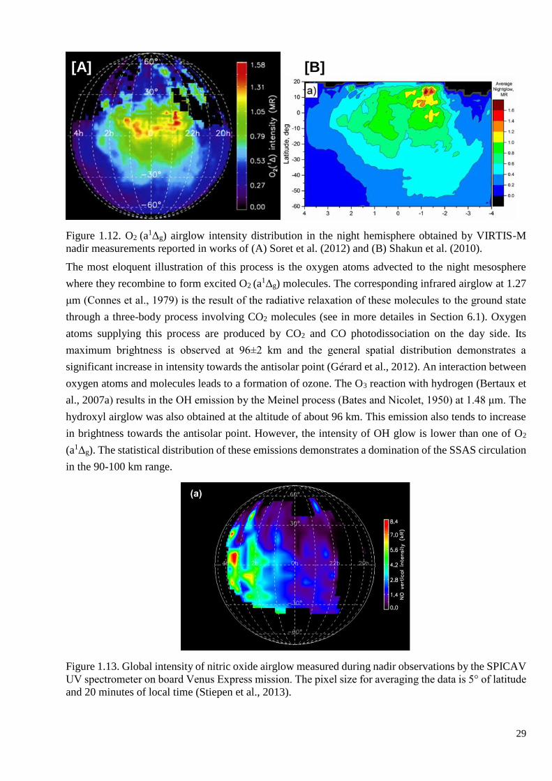
29

Figure 1.12. O2 (a1Δg) airglow intensity distribution in the night hemisphere obtained by VIRTIS-M

nadir measurements reported in works of (A) Soret et al. (2012) and (B) Shakun et al. (2010).

The most eloquent illustration of this process is the oxygen atoms advected to the night mesosphere

where they recombine to form excited O2 (a1Δg) molecules. The corresponding infrared airglow at 1.27

μm (Connes et al., 1979) is the result of the radiative relaxation of these molecules to the ground state

through a three-body process involving CO2 molecules (see in more detailes in Section 6.1). Oxygen

atoms supplying this process are produced by CO2 and CO photodissociation on the day side. Its

maximum brightness is observed at 96±2 km and the general spatial distribution demonstrates a

significant increase in intensity towards the antisolar point (Gérard et al., 2012). An interaction between

oxygen atoms and molecules leads to a formation of ozone. The O3 reaction with hydrogen (Bertaux et

al., 2007a) results in the OH emission by the Meinel process (Bates and Nicolet, 1950) at 1.48 μm. The

hydroxyl airglow was also obtained at the altitude of about 96 km. This emission also tends to increase

in brightness towards the antisolar point. However, the intensity of OH glow is lower than one of O2

(a1Δg). The statistical distribution of these emissions demonstrates a domination of the SSAS circulation

in the 90-100 km range.

Figure 1.13. Global intensity of nitric oxide airglow measured during nadir observations by the SPICAV

UV spectrometer on board Venus Express mission. The pixel size for averaging the data is 5° of latitude

and 20 minutes of local time (Stiepen et al., 2013).

[A] [B]

30

The nitrogen atoms brought by SSAS transfer are recombining with oxygen on the night side, and the

nitrogen emission in δ- and γ- bands is resulted. Its maximum intensity corresponds to the higher

altitudes of ~115 km and it completely differs from the one observed at ~95 km. Its spatial distribution

surprisingly displayed a significant shift towards the morning terminator (03:00-04:00). It results from

a joint influence of gravity wave propagation, thermal tides and large scale planetary waves (Gilli et al.,

2020) that are partially explained by the recent results of the Venus Global Climat Model (VGCM)

developed at the Institute Pierre-Simon Laplace (IPSL), further noted IPSL Venus GCM (see in more

detailes in Section 2.3).

1.6. The SPICAV instrument

Figure 1.14. Image of the SPICAV instrument without a cover (Korablev et al., 2012) without the SOIR

spectrometer.

The SPICAV/SOIR instrument was a set of three spectrometers (Bertaux et al., 2007a; Vandaele et al.,

2008; Korablev et al., 2012) that was designed by Laboratoire Atmosphères, Milieux, Observations

spatiales (LATMOS, France) in collaboration with the Space Research Institute of the Russian Academy

of Sciences (IKI, Russia), and the Royal Belgian Institute for Space Aeronomy (BIRA-IASB, Belgium).

All of them operated around Venus during the 8 years of the Venus Express mission, from April 2006

to December 2014, however, the full scientific phase of observations began on May 14, 2006.

The SPICAV part consisted of the UV (118-320 nm) and the IR (0.65-1.7 μm) channels that could

observe the atmosphere in different modes (Bertaux et al., 2007a). For the first time, three instruments

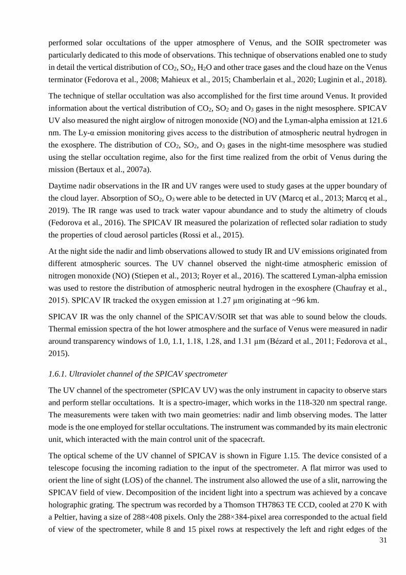
31

performed solar occultations of the upper atmosphere of Venus, and the SOIR spectrometer was

particularly dedicated to this mode of observations. This technique of observations enabled one to study

in detail the vertical distribution of CO2, SO2, H2O and other trace gases and the cloud haze on the Venus

terminator (Fedorova et al., 2008; Mahieux et al., 2015; Chamberlain et al., 2020; Luginin et al., 2018).

The technique of stellar occultation was also accomplished for the first time around Venus. It provided

information about the vertical distribution of CO2, SO2 and O3 gases in the night mesosphere. SPICAV

UV also measured the night airglow of nitrogen monoxide (NO) and the Lyman-alpha emission at 121.6

nm. The Ly-α emission monitoring gives access to the distribution of atmospheric neutral hydrogen in

the exosphere. The distribution of CO2, SO2, and O3 gases in the night-time mesosphere was studied

using the stellar occultation regime, also for the first time realized from the orbit of Venus during the

mission (Bertaux et al., 2007a).

Daytime nadir observations in the IR and UV ranges were used to study gases at the upper boundary of

the cloud layer. Absorption of SO2, O3 were able to be detected in UV (Marcq et al., 2013; Marcq et al.,

2019). The IR range was used to track water vapour abundance and to study the altimetry of clouds

(Fedorova et al., 2016). The SPICAV IR measured the polarization of reflected solar radiation to study

the properties of cloud aerosol particles (Rossi et al., 2015).

At the night side the nadir and limb observations allowed to study IR and UV emissions originated from

different atmospheric sources. The UV channel observed the night-time atmospheric emission of

nitrogen monoxide (NO) (Stiepen et al., 2013; Royer et al., 2016). The scattered Lyman-alpha emission

was used to restore the distribution of atmospheric neutral hydrogen in the exosphere (Chaufray et al.,

2015). SPICAV IR tracked the oxygen emission at 1.27 µm originating at ~96 km.

SPICAV IR was the only channel of the SPICAV/SOIR set that was able to sound below the clouds.

Thermal emission spectra of the hot lower atmosphere and the surface of Venus were measured in nadir

around transparency windows of 1.0, 1.1, 1.18, 1.28, and 1.31 µm (Bézard et al., 2011; Fedorova et al.,

2015).

1.6.1. Ultraviolet channel of the SPICAV spectrometer

The UV channel of the spectrometer (SPICAV UV) was the only instrument in capacity to observe stars

and perform stellar occultations. It is a spectro-imager, which works in the 118-320 nm spectral range.

The measurements were taken with two main geometries: nadir and limb observing modes. The latter

mode is the one employed for stellar occultations. The instrument was commanded by its main electronic

unit, which interacted with the main control unit of the spacecraft.

The optical scheme of the UV channel of SPICAV is shown in Figure 1.15. The device consisted of a

telescope focusing the incoming radiation to the input of the spectrometer. A flat mirror was used to

orient the line of sight (LOS) of the channel. The instrument also allowed the use of a slit, narrowing the

SPICAV field of view. Decomposition of the incident light into a spectrum was achieved by a concave

holographic grating. The spectrum was recorded by a Thomson TH7863 TE CCD, cooled at 270 K with

a Peltier, having a size of 288×408 pixels. Only the 288×384-pixel area corresponded to the actual field

of view of the spectrometer, while 8 and 15 pixel rows at respectively the left and right edges of the

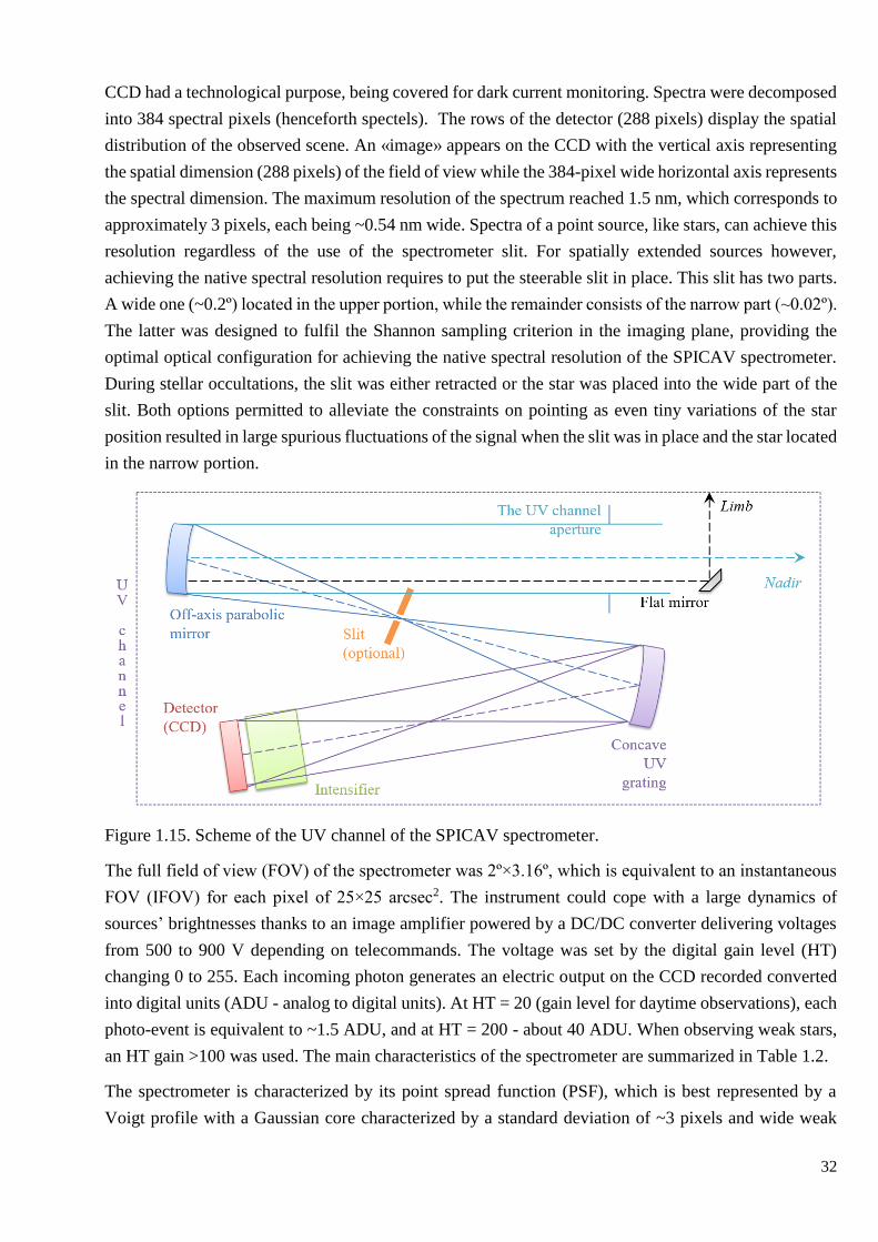
32

CCD had a technological purpose, being covered for dark current monitoring. Spectra were decomposed

into 384 spectral pixels (henceforth spectels). The rows of the detector (288 pixels) display the spatial

distribution of the observed scene. An «image» appears on the CCD with the vertical axis representing

the spatial dimension (288 pixels) of the field of view while the 384-pixel wide horizontal axis represents

the spectral dimension. The maximum resolution of the spectrum reached 1.5 nm, which corresponds to

approximately 3 pixels, each being ~0.54 nm wide. Spectra of a point source, like stars, can achieve this

resolution regardless of the use of the spectrometer slit. For spatially extended sources however,

achieving the native spectral resolution requires to put the steerable slit in place. This slit has two parts.

A wide one (~0.2º) located in the upper portion, while the remainder consists of the narrow part (~0.02º).

The latter was designed to fulfil the Shannon sampling criterion in the imaging plane, providing the

optimal optical configuration for achieving the native spectral resolution of the SPICAV spectrometer.

During stellar occultations, the slit was either retracted or the star was placed into the wide part of the

slit. Both options permitted to alleviate the constraints on pointing as even tiny variations of the star

position resulted in large spurious fluctuations of the signal when the slit was in place and the star located

in the narrow portion.

Figure 1.15. Scheme of the UV channel of the SPICAV spectrometer.

The full field of view (FOV) of the spectrometer was 2º×3.16º, which is equivalent to an instantaneous

FOV (IFOV) for each pixel of 25×25 arcsec2. The instrument could cope with a large dynamics of

sources’ brightnesses thanks to an image amplifier powered by a DC/DC converter delivering voltages

from 500 to 900 V depending on telecommands. The voltage was set by the digital gain level (HT)

changing 0 to 255. Each incoming photon generates an electric output on the CCD recorded converted

into digital units (ADU - analog to digital units). At HT = 20 (gain level for daytime observations), each

photo-event is equivalent to ~1.5 ADU, and at HT = 200 - about 40 ADU. When observing weak stars,

an HT gain >100 was used. The main characteristics of the spectrometer are summarized in Table 1.2.

The spectrometer is characterized by its point spread function (PSF), which is best represented by a

Voigt profile with a Gaussian core characterized by a standard deviation of ~3 pixels and wide weak

33

wings. The PSF of the device therefore distributes the incoming light of a point monochromatic source

within a ~20-pixel diameter disk (Figure 1.16A).

Table 1.2. Main characteristics of the SPICAV UV spectrometer.

Characteristics Value

Spectral range 118-320 nm

Number of spectral points 384

Resolution (Δλ) ~1.5 nm

Resolving power (λ/Δλ) ~150

Atmospheric absorption altitude range 85-145 km

Weight of the spectrometer 4.7 kg

Field of view(FOV) 2º×3.16º (without slit)

0.2º×0.98º (wide part of the slit)

0.02º×1.9º (narrow part of the slit)

Instantaneous field of view (IFOV) per pixel 25”×25”

To optimize telemetry, only a fraction of the full image obtained by the CCD was transmitted. In the

stellar occultation mode, it concerned the portion of the CCD where the star was focused. The selected

part of the signal was binned along the spatial axis into five contiguous bands (bins) consisting of n

detector lines. Starlight concentrated in the third, i.e. central, bin. The rest of the bins contained the wings

of the PSF, that is a small part of the stellar signal, as well as some background signal (scattered light,

atmospheric radiation at the planet’s limb, etc.). The number n of spectra (CCD rows) per bin in the

stellar occultation mode could be selected among 4, 8, 16 or 32. Then each group of lines was summed

up into one spectrum, and the resulting set of 5 spectra was transferred to the Earth (Figure 1.16B). An

example of a signal distribution over a CCD from a point source, i.e. stars, in the absence of background

illumination, is shown in Figure 1.16A.

Figure 1.16. (A) A measured image represents the spreading of starlight among several CCD rows at the

occultation #0668A05. (B) An example of 5 spectra transferred to the Earth after onboard summing

within different bins where the colors of lines correspond to bin areas highlighted in Panel A.

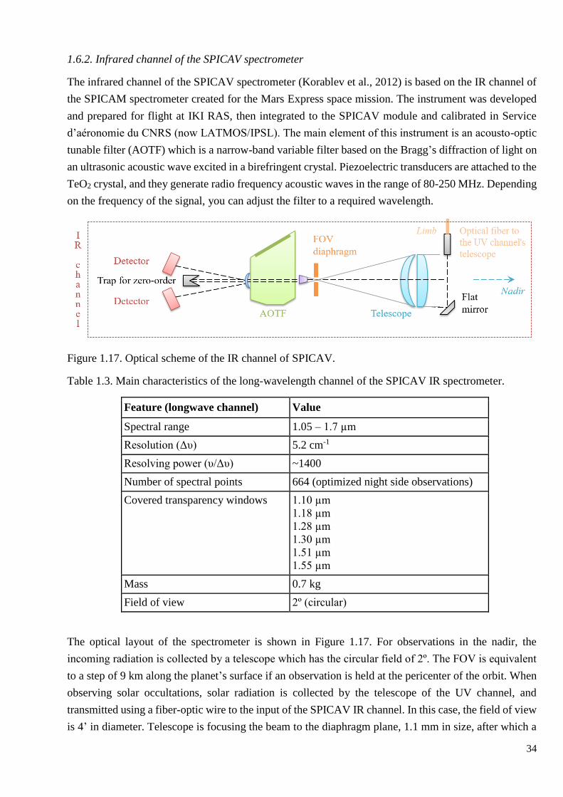
34

1.6.2. Infrared channel of the SPICAV spectrometer

The infrared channel of the SPICAV spectrometer (Korablev et al., 2012) is based on the IR channel of

the SPICAM spectrometer created for the Mars Express space mission. The instrument was developed

and prepared for flight at IKI RAS, then integrated to the SPICAV module and calibrated in Service

d’aéronomie du CNRS (now LATMOS/IPSL). The main element of this instrument is an acousto-optic

tunable filter (AOTF) which is a narrow-band variable filter based on the Bragg’s diffraction of light on

an ultrasonic acoustic wave excited in a birefringent crystal. Piezoelectric transducers are attached to the

TeO2 crystal, and they generate radio frequency acoustic waves in the range of 80-250 MHz. Depending

on the frequency of the signal, you can adjust the filter to a required wavelength.

Figure 1.17. Optical scheme of the IR channel of SPICAV.

Table 1.3. Main characteristics of the long-wavelength channel of the SPICAV IR spectrometer.

Feature (longwave channel) Value

Spectral range 1.05 – 1.7 µm

Resolution (Δυ) 5.2 cm-1

Resolving power (υ/Δυ) ~1400

Number of spectral points 664 (optimized night side observations)

Covered transparency windows 1.10 µm

1.18 µm

1.28 µm

1.30 µm

1.51 µm

1.55 µm

Mass 0.7 kg

Field of view 2º (circular)

The optical layout of the spectrometer is shown in Figure 1.17. For observations in the nadir, the

incoming radiation is collected by a telescope which has the circular field of 2º. The FOV is equivalent

to a step of 9 km along the planet’s surface if an observation is held at the pericenter of the orbit. When

observing solar occultations, solar radiation is collected by the telescope of the UV channel, and

transmitted using a fiber-optic wire to the input of the SPICAV IR channel. In this case, the field of view

is 4’ in diameter. Telescope is focusing the beam to the diaphragm plane, 1.1 mm in size, after which a

35

collimator is installed. After the AOTF filter, another lens system is installed that separates the beams

of diffracted rays with orthogonal polarization and separates the “zero” order. The separated beams fall

on two identical photodiode detectors consisting of Si and InGaAs layers. The silicon photodiode

provided recording of short-wavelength radiation (0.65-1.05 µm), and the InGaAs detector - long-

wavelength (1.05-1.7 µm). The photodetectors can be cooled using two built-in Peltier elements. In this

study only the dataset obtained in the long-wave range is considered. The particular capacities of the

instrument at these wavelengths are summarized in Table 1.3.

When observing the night side, IR radiation at each wavelength was integrated for 44.8 or 89.6 ms. Some

measurements in nadir, due to the long integration times of the signal, were carried out only for the long-

wavelength range. The recorded signal is the sum of the dark current and the photo-signal proportional

to the radiation intensity. For calibration, the dark current was measured separately at the beginning and

end of each signal integration.

36

CHAPTER 2. Sulphur dioxide and ozone in the atmosphere of

Venus

2.1. Overview of sulphur dioxide research

Sulphur compounds play a key role in the chemistry of the atmosphere of Venus. They are formed as a

result of volcanic activity on the planet and participate in the formation of clouds consisting of

concentrated H2SO4 acid droplets. Moreover, the unknown UV absorber in the upper part of the cloud

is also associated with sulphur compounds, inexplicably reducing the albedo of Venus in the UV range

(Frandsen et al., 2016; Krasnopolskiy, 2018). Sulphur dioxide is the third most abundant gas making up

0.015% of Venus’s atmosphere. Thus, any major changes in SO2 content occurring in the upper

atmosphere can be indicators of photochemical processes and dynamics on Venus. The sulphur dioxide

is destroyed by chlorine and hydroxyl radicals as well as by an effective photodissociation on the day

side. The catalytic processes are noticeable on the night side, where fluxes of atoms and molecules are

brought by the global SSAS circulation at altitudes of about ~100 km.

2.1.1. Temporal and spatial distributions of sulphur dioxide

The entire history of observations of sulphur dioxide on Venus showed significant variations in its

amount at the cloud top (~70 km) presented in Figure 2.1. SO2 gas was first detected in the cloud tops

by a ground-based ultraviolet telescope with a content of 0.02-0.5 ppm (Barker, 1979). The SO2

abundance was mainly measured at the altitude corresponding to the cloud top level on the day side, that

is about 70 km. Several instruments aboard the first spacecraft to Venus showed a global decrease of the

SO2 volume mixing ratio of (VMR) in the upper atmosphere in the 80s and 90s (Figure 2.1). During this

period some local peaks of the gas abundance were obtained. This result mainly came from ten years of

monitoring by the ultraviolet spectrometer (UVS) on board the Pioneer Venus Orbiter (PVO). The

reduction of the amount was steep at the beginning, and then it was followed by a gradual decline in the

SO2 mixing ratio. It was confirmed by several other instruments working in the UV. The International

Ultraviolet Explorer (IUE) observed Venus in 1979 (Conway et al., 1979) and 1987-1988 (Na et al.,

1990; Na et al., 1993), when the corresponding mixing ratios changed from 380±70 ppbv to 50±20 ppbv.

Lower abundance of sulphur dioxide was also obtained based on observations by the Venera-15 Fourier

spectrometer in the IR range (Moroz et al., 1990; Zasova et al., 1993). Its data originally corresponded

to 60-62 km but the value was scaled to an altitude of 70 km in order to compare with the UV

observations (Zasova et al., 1993). Rocket observations in 1988 and 1991 measured SO2 equal to 80±40

ppbv and 120±60 ppb respectively (McClintock et al., 1994). The further observations by IUE and

ground based facilities (Barker et al., 1992; Esposito et al., 1997) showed the local maximum of the SO2

content in 1991-1992. In 1995, the Hubble Space Telescope (HST) completed the first era of continuous

SO2 exploration on Venus and gave a value of 20±10 ppbv (Na et al. 1995), which was 2-5 times less

than previous measurements.

37

Figure 2.1. The timeline of sulphur dioxide observations at the cloud tops on the day side of Venus. The

references are given in the legend. The SPICAV UV observations are presented with the corresponding

variability of obtained values within 4-month intervals. The full range of obtained values is represented

by the grey area which is accompanied by a median curve (grey solid line).

This behaviour was puzzling. The sulphur compounds are rather associated with geological activity. So,

the main hypothesis to explain the observed SO2 change has considered a link with possible episodic

volcanic eruptions on Venus. It was assumed that one event would inject sulphur compounds into the

atmosphere, and the vertical transfer would distribute them over clouds. Then SO2 depleted and a

monotonic trend of its VMR was observed (Esposito, 1984).

For spatial variations sulphur dioxide was studied in the IR range (7 µm, 8 µm and 19 µm) using a

Fourier spectrometer on board the Soviet spacecraft Venera-15. The study of latitudinal distribution

revealed an increase in gas content from the equatorial zone and middle latitudes to the poles of the

planet. At a pressure level of 150 mbar (corresponding to ~ 62 km), the amount of SO2 at low latitudes

was 0.3-0.5 ppm, and 1-2 ppm in the polar regions. The same picture was observed at the level of the

cloud top (40 mbar, ~ 69 km).

SO2 monitoring on Venus was resumed in 2006, when the Venus Express spacecraft began its orbital

mission (Titov et al., 2006) with a set of three SPICAV/SOIR spectrometers on board. UV and IR

instruments covered SO2 absorption bands at 190-300 nm (for SPICAV UV) and about 4 μm (for SOIR).

In this period there were several ground-based observations by instruments in various spectral intervals:

STIS/HST (Space Telescope Imaging Spectrograph/Hubble Space Telescope), IRTF/TEXES (Infrared

Telescope Facility/Texas Echelon-Cross-Echelle Spectrograph), JCMT (James Clerk Maxwell

Telescope), ALMA (Atacama Large Millimeter/Submillimeter Array) and the CSHELL (Cryogenic

Echelle) spectrograph. STIS measures in the same spectral range as SPICAV UV while CSHELL

operates at 4.04 μm. These instruments observed the cloud top level. SPICAV UV in nadir mode and

STIS were able to perform measurements only on the day side of Venus. Solar occultations by SOIR

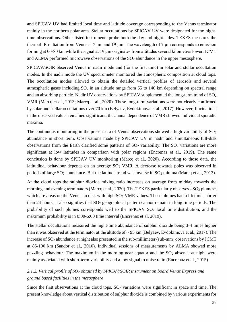
38

and SPICAV UV had limited local time and latitude coverage corresponding to the Venus terminator

mainly in the northern polar area. Stellar occultations by SPICAV UV were designated for the night-

time observations. Other listed instruments probe both the day and night sides. TEXES measures the

thermal IR radiation from Venus at 7 μm and 19 μm. The wavelength of 7 μm corresponds to emission

forming at 60-80 km while the signal at 19 μm originates from altitudes several kilometres lower. JCMT

and ALMA performed microwave observations of the SO2 abundance in the upper mesosphere.

SPICAV/SOIR observed Venus in nadir mode and (for the first time) in solar and stellar occultation

modes. In the nadir mode the UV spectrometer monitored the atmospheric composition at cloud tops.

The occultation modes allowed to obtain the detailed vertical profiles of aerosols and several

atmospheric gases including SO2 in an altitude range from 65 to 140 km depending on spectral range

and an absorbing particle. Nadir UV observations by SPICAV supplemented the long-term trend of SO2

VMR (Marcq et al., 2013; Marcq et al., 2020). These long-term variations were not clearly confirmed

by solar and stellar occultations over 70 km (Belyaev, Evdokimova et al., 2017). However, fluctuations

in the observed values remained significant; the annual dependence of VMR showed individual sporadic

maxima.

The continuous monitoring in the present era of Venus observations showed a high variability of SO2

abundance in short term. Observations made by SPICAV UV in nadir and simultaneous full-disk

observations from the Earth clarified some patterns of SO2 variability. The SO2 variations are more

significant at low latitudes in comparison with polar regions (Encrenaz et al., 2019). The same

conclusion is done by SPICAV UV monitoring (Marcq et al., 2020). According to those data, the

latitudinal behaviour depends on an average SO2 VMR. A decrease towards poles was observed in

periods of large SO2 abundance. But the latitude trend was inverse in SO2 minima (Marcq et al., 2013).

At the cloud tops the sulphur dioxide mixing ratio increases on average from midday towards the

morning and evening terminators (Marcq et al., 2020). The TEXES particularly observes «SO2 plumes»

which are areas on the Venusian disk with high SO2 VMR values. These plumes had a lifetime shorter

than 24 hours. It also signifies that SO2 geographical pattern cannot remain in long time periods. The

probability of such plumes corresponds well to the SPICAV SO2 local time distribution, and the

maximum probability is in 0:00-6:00 time interval (Encrenaz et al. 2019).

The stellar occultations measured the night-time abundance of sulphur dioxide being 3-4 times higher

than it was observed at the terminator at the altitude of ~ 95 km (Belyaev, Evdokimova et al., 2017). The

increase of SO2 abundance at night also presented in the sub-millimeter (sub-mm) observations by JCMT

at 85-100 km (Sandor et al., 2010). Individual sessions of measurements by ALMA showed more

puzzling behaviour. The maximum in the morning near equator and the SO2 absence at night were

mainly associated with short-term variability and a low signal to noise ratio (Encrenaz et al., 2015).

2.1.2. Vertical profile of SO2 obtained by SPICAV/SOIR instrument on board Venus Express and

ground based facilities in the mesosphere

Since the first observations at the cloud tops, SO2 variations were significant in space and time. The

present knowledge about vertical distribution of sulphur dioxide is combined by various experiments for

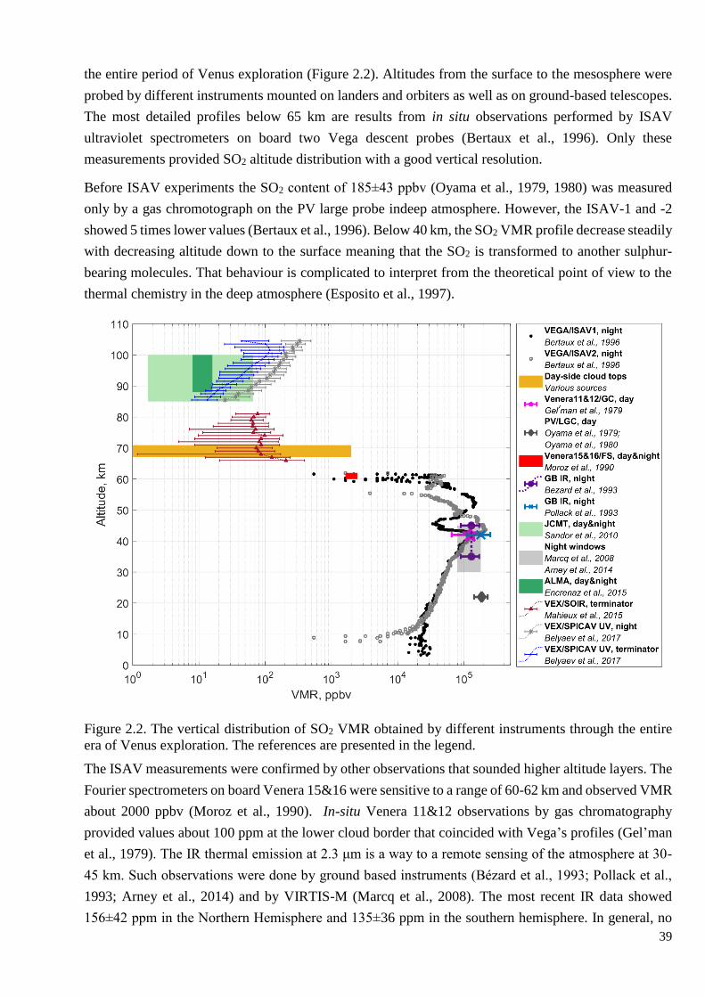
39

the entire period of Venus exploration (Figure 2.2). Altitudes from the surface to the mesosphere were

probed by different instruments mounted on landers and orbiters as well as on ground-based telescopes.

The most detailed profiles below 65 km are results from in situ observations performed by ISAV

ultraviolet spectrometers on board two Vega descent probes (Bertaux et al., 1996). Only these

measurements provided SO2 altitude distribution with a good vertical resolution.

Before ISAV experiments the SO2 content of 185±43 ppbv (Oyama et al., 1979, 1980) was measured

only by a gas chromotograph on the PV large probe indeep atmosphere. However, the ISAV-1 and -2

showed 5 times lower values (Bertaux et al., 1996). Below 40 km, the SO2 VMR profile decrease steadily

with decreasing altitude down to the surface meaning that the SO2 is transformed to another sulphur-

bearing molecules. That behaviour is complicated to interpret from the theoretical point of view to the

thermal chemistry in the deep atmosphere (Esposito et al., 1997).

Figure 2.2. The vertical distribution of SO2 VMR obtained by different instruments through the entire

era of Venus exploration. The references are presented in the legend.

The ISAV measurements were confirmed by other observations that sounded higher altitude layers. The

Fourier spectrometers on board Venera 15&16 were sensitive to a range of 60-62 km and observed VMR

about 2000 ppbv (Moroz et al., 1990). In-situ Venera 11&12 observations by gas chromatography

provided values about 100 ppm at the lower cloud border that coincided with Vega’s profiles (Gel’man

et al., 1979). The IR thermal emission at 2.3 μm is a way to a remote sensing of the atmosphere at 30-

45 km. Such observations were done by ground based instruments (Bézard et al., 1993; Pollack et al.,

1993; Arney et al., 2014) and by VIRTIS-M (Marcq et al., 2008). The most recent IR data showed

156±42 ppm in the Northern Hemisphere and 135±36 ppm in the southern hemisphere. In general, no

40

significant variations of the SO2 content below the clouds were revealed. It is in correspondence with

expecting stability of the lower atmosphere.

The gas abundance was studied over the clouds in much more detail by the SPICAV/SOIR instrument

during the period of the Venus Express mission. SO2 absorption was measured in the first UV and IR

observations of solar and stellar occultations (Figure 2.2). The altitude distribution retrieved from those

occultations demonstrates an inversion layer of the SO2 content around 85-100 km. On average, an

increase of the SO2 VMR with altitude from 8-20 ppbv at 85-90 km to 50-180 ppbv at 100 km was

observed (Belyaev et al., 2012; Belyaev, Evdokimova et al., 2017). This distribution was supplemented

by the SOIR data with a decrease of the SO2 abundance from 100-300 pbbv at 65 km to 50-100 ppbv at

80 km possessing large uncertainty values (Mahieux et al., 2015). The previous results of the stellar

occultation data revealed the SO2 VMR rising with altitude from 10-30 ppbv at 85-95 km to 100-300

ppbv at 100-105 km (Belyaev, Evdokimova et al., 2017). However, this increase is re-investigated

further in this work in the framework of the detailed calibration study.

All in all, one can see significant short-term changes in the amount of sulphur dioxide in the mesosphere

that are interpreted by different models. Discussions of the models that could be compared with our

occultation data are presented in Section 2.3 of this Chapter and in Chapter 4. The comprehensive

overview of SO2 content variations with time, altitude and latitude retrieved from experiments and

analysed by models is presented in papers of Vandaele et al. (2017a, 2017b).

2.2. Ozone in the atmosphere of Venus.

Ozone on Venus excites a great interest for researchers due to its active participation in basic atmospheric

chemical processes, as well as its bio-protective function in the terrestrial atmosphere. On the Earth the

large amount of the UV radiation is absorbed by the abundant O3 layer in the stratosphere where the

vertical temperature profile is inverted. Here the Hartley band of ozone absorption at 240-300 nm is

saturated, and the atmospheric transmission in this range is close to zero. On Venus, where the total O3

content is expected to be >103 times less than on the Earth, the Hartley band is applicable for the spectral

investigation. Before this first detection, the ozone presence was estimated by different photochemical

models (Yung and DeMore, 1999; Krasnopolsky, 2010a; Mills, 2007). However, so far, except for the

molecular O2 airglows another oxygen species was not quantified experimentally on Venus. It

constrained estimation of the ozone concentration in the atmosphere. The upper limit for the oxygen

abundance was estimated to <2 ppmv that signified extremely low amounts of the Venusian ozone

(Mills, 1998).

The discovery of ozone on Venus concluded a presence of this gas on three terrestrial planets: Earth,

Mars and Venus. Due to the Earth, with the O3 protection of the biosphere, and Mars, with an evidence

of oxygen-rich airmasses, ozone is considered in a search of possible life. It is known that such a

protection from the strong UV radiation requires a significant abundance of O3. The observed values in

the Earth atmosphere are around 300 DU (Dobson Units), where 1 DU corresponds to a column

concentration of 2.69×1016 molecules per cm2. Mars and Venus have a tiny amount of ozone compared

to the terrestrial quantity. The Martian ozone compiles <1 DU (Lefèvre et al., 2004; Lebonnois et al.,

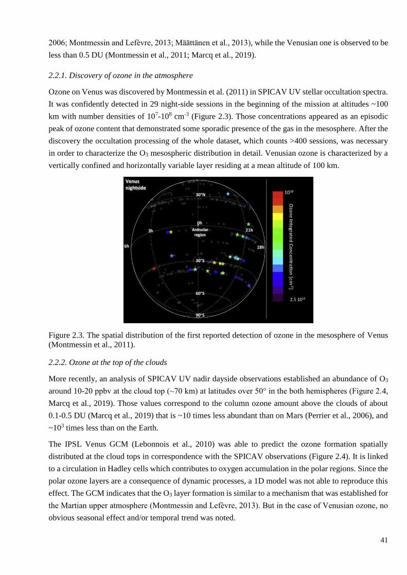
41

2006; Montmessin and Lefèvre, 2013; Määttänen et al., 2013), while the Venusian one is observed to be

less than 0.5 DU (Montmessin et al., 2011; Marcq et al., 2019).

2.2.1. Discovery of ozone in the atmosphere

Ozone on Venus was discovered by Montmessin et al. (2011) in SPICAV UV stellar occultation spectra.

It was confidently detected in 29 night-side sessions in the beginning of the mission at altitudes ~100

km with number densities of 107-108 cm-3 (Figure 2.3). Those concentrations appeared as an episodic

peak of ozone content that demonstrated some sporadic presence of the gas in the mesosphere. After the

discovery the occultation processing of the whole dataset, which counts >400 sessions, was necessary

in order to characterize the O3 mesospheric distribution in detail. Venusian ozone is characterized by a

vertically confined and horizontally variable layer residing at a mean altitude of 100 km.

Figure 2.3. The spatial distribution of the first reported detection of ozone in the mesosphere of Venus

(Montmessin et al., 2011).

2.2.2. Ozone at the top of the clouds

More recently, an analysis of SPICAV UV nadir dayside observations established an abundance of O3

around 10-20 ppbv at the cloud top (~70 km) at latitudes over 50° in the both hemispheres (Figure 2.4,

Marcq et al., 2019). Those values correspond to the column ozone amount above the clouds of about

0.1-0.5 DU (Marcq et al., 2019) that is ~10 times less abundant than on Mars (Perrier et al., 2006), and

~103 times less than on the Earth.

The IPSL Venus GCM (Lebonnois et al., 2010) was able to predict the ozone formation spatially

distributed at the cloud tops in correspondence with the SPICAV observations (Figure 2.4). It is linked

to a circulation in Hadley cells which contributes to oxygen accumulation in the polar regions. Since the

polar ozone layers are a consequence of dynamic processes, a 1D model was not able to reproduce this

effect. The GCM indicates that the O3 layer formation is similar to a mechanism that was established for

the Martian upper atmosphere (Montmessin and Lefèvre, 2013). But in the case of Venusian ozone, no

obvious seasonal effect and/or temporal trend was noted.

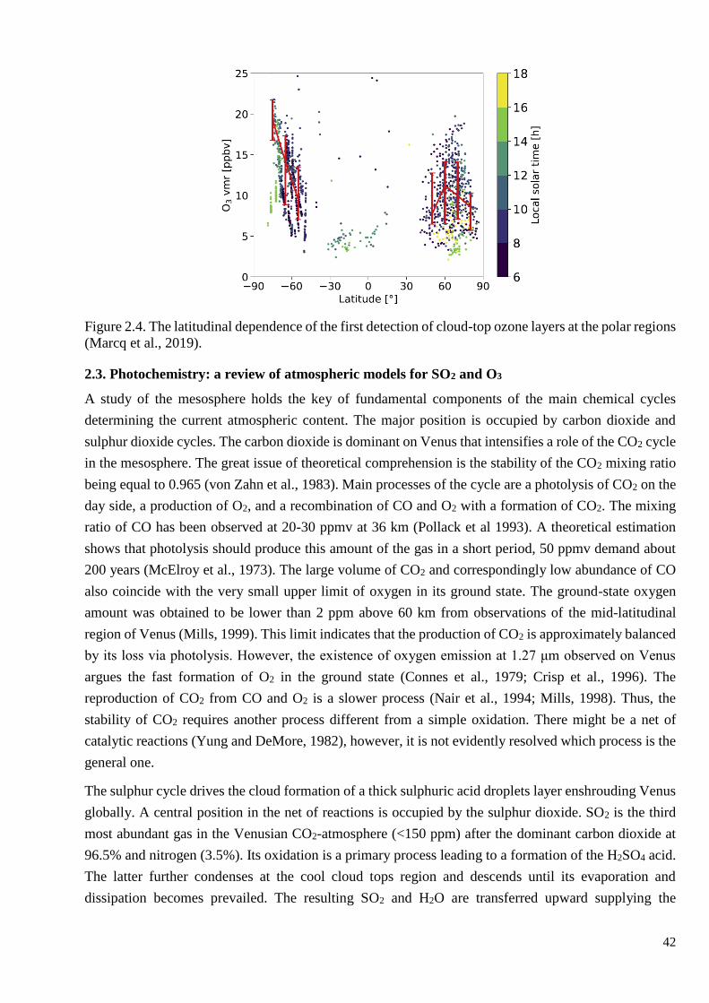
42

Figure 2.4. The latitudinal dependence of the first detection of cloud-top ozone layers at the polar regions

(Marcq et al., 2019).

2.3. Photochemistry: a review of atmospheric models for SO2 and O3

A study of the mesosphere holds the key of fundamental components of the main chemical cycles

determining the current atmospheric content. The major position is occupied by carbon dioxide and

sulphur dioxide cycles. The carbon dioxide is dominant on Venus that intensifies a role of the CO2 cycle

in the mesosphere. The great issue of theoretical comprehension is the stability of the CO2 mixing ratio

being equal to 0.965 (von Zahn et al., 1983). Main processes of the cycle are a photolysis of CO2 on the

day side, a production of O2, and a recombination of CO and O2 with a formation of CO2. The mixing

ratio of CO has been observed at 20-30 ppmv at 36 km (Pollack et al 1993). A theoretical estimation

shows that photolysis should produce this amount of the gas in a short period, 50 ppmv demand about

200 years (McElroy et al., 1973). The large volume of CO2 and correspondingly low abundance of CO

also coincide with the very small upper limit of oxygen in its ground state. The ground-state oxygen

amount was obtained to be lower than 2 ppm above 60 km from observations of the mid-latitudinal

region of Venus (Mills, 1999). This limit indicates that the production of CO2 is approximately balanced

by its loss via photolysis. However, the existence of oxygen emission at 1.27 μm observed on Venus

argues the fast formation of O2 in the ground state (Connes et al., 1979; Crisp et al., 1996). The

reproduction of CO2 from CO and O2 is a slower process (Nair et al., 1994; Mills, 1998). Thus, the

stability of CO2 requires another process different from a simple oxidation. There might be a net of

catalytic reactions (Yung and DeMore, 1982), however, it is not evidently resolved which process is the

general one.

The sulphur cycle drives the cloud formation of a thick sulphuric acid droplets layer enshrouding Venus

globally. A central position in the net of reactions is occupied by the sulphur dioxide. SO2 is the third

most abundant gas in the Venusian CO2-atmosphere (<150 ppm) after the dominant carbon dioxide at

96.5% and nitrogen (3.5%). Its oxidation is a primary process leading to a formation of the H2SO4 acid.

The latter further condenses at the cool cloud tops region and descends until its evaporation and

dissipation becomes prevailed. The resulting SO2 and H2O are transferred upward supplying the

43

mesospheric SO2 content. Sulphur acid synthesis is a prevailing process independent of the local time,

and it results in a sharp decrease of SO2 in the upper cloud layer (Figure 2.2).

Figure 2.5. The main reactions of the sulphur chemical cycle in the day and night parts of the mesosphere.

Another sink of SO2 is its photolysis occurring in the daytime atmosphere. Sulphur monoxide and pure

sulphur are formed and their oxidation is maintaining the cycle. At night a significant role of reactions

with Cl radicals and hydroxyl takes place while they are involved in the SSAS circulation. However,

those components destroy the SO2 molecule less efficiently than the photodissociation process that leads

to an increase of SO2 in the night mesosphere.

Figure 2.5 presents an overview of the most prominent processes with SO2 in the mesosphere of Venus.

However, such a simplified scheme does not resolve the following questions that rise up:

(1) A dramatic decrease of SO2 through the cloud layer that could not be explained only by the

oxidation.

(2) An inversion of SO2 volume mixing ratio at 80-100 km that was observed in occultation

experiments by SPICAV on board Venus Express,

(3) The sub-mm observations have revealed correlations between SO and SO2 contents that argue

the hypothesis of a closed cycle between the SO2 depletion and the SO oxidation, so it indicates

that another species also impacts the sulphur bulk in the mesosphere.

A simulation of photochemical processes shows which reactions are decisive in the atmosphere and

which gaseous species are establishing equilibrium in the atmospheric chemical cycles. There are two

general approaches used to model the vertical distribution of species in the Venus atmosphere. The first

one is a 1-D model neglecting a horizontal transport in the atmosphere. It is a reasonable approach to

characterize the average vertical distribution of atmospheric species. A more complex 3-D model, i.e.

general circulation model, is able to quantify in detail occurring spatial and temporal variations. So far

the required accuracy has not been achieved to explain by models the observed ozone and sulphur

dioxide distributions.

44

Table 2.1. An overview of discussed photochemical models of Venus’ atmosphere.

Model Type Diurnal cycle Altitude

range, km

Ref. SO2 O3

DAY Caltech/JPL

Photoche-

mical

Model

(KINETICS)

1-D Global average 58-110 Yung, DeMore

(1982)

A: a decrease from ~4 ppbv at 80 km

to ~2 ppbv at 90 km

B: a decrease from ~10 ppbv at 80 km

to ~6 ppbv at 90 km

C: a decrease from ~10 ppbv at 80 km

to ~8 ppbv at 90 km

A: ~25 ppbv at 100-105 km

decreasing to ~ 2.5 ppbv at 80 km

B: 20 ppbv at 95-100 km decreasing to

~6 ppbv at 80 km

C: 12 ppbv at 100-105km decreasing

to ~0.08 ppbv at 80 km

1-D Global average 58–112 Mills, Allen

(2007)

~40-50 ppbv at 80-100 km (Vandaele

aet al., 2017)

1-D Diurnal average

at 45° latitude

58–112 Zhang et al.

(2010)

Min. ~6 ppbv at 75 km

A: a decrease <2 ppbv at 100 km

B: max. at 100 km of 90 ppbv

C: max. at 100 km of 1.5 ppmv

1-D Diurnal average

at 70° latitude

58–112 Zhang et al.,

(2012)

Min. at 80 km of 30 ppbv

Max. at 97 km of 300 ppbv

Max. 20 ppbv at 100 km

A decrease to 0.2 ppbv at 80 km

Krasnopolsky

Mesosphere

model

1-D Global average 47–112 Krasnopolsky

(2012)

~25 ppbv at 85 km

~30 ppbv at 95 km

10 ppbv at 90-95 km forming an

ozone layer

IPSL Venus

GCM

3-D 0–96 Stolzenbach et

al. (2014)

Nearly constant at around 8 ppbv at

80-100km

(Vandaele et al., 2017a)

Ozone polar layers and an increase

over 80 km (Marcq et al., 2019)

IPSL Venus

GCM

3-D 0-150 Gilli et al.

(2017)

Nearly constant at around 200 ppbv at

80-100 km (Gilli, in priv. commun.)

Maximum VMR at 100 km: ~8 ppbv

(Gilli, in priv. commun.)

NIGHT Krasnopolsky

Mesosphere

model

1-D Night

mesosphere

80–130 Krasnopolsky

(2013)

100 ppbv at 80-106 km A thin layer with a maximum at 95 km

of 20-40 ppbv depending on the

assumed Cl ions flux.

45

Figure 2.6. Synthetic ozone (A) and sulphur dioxide (B) vertical distributions in the mesosphere of

Venus.

The Caltech/JPL Photochemical Model (KINETICS) was a base of several atmospheric models

considering gaseous abundances without any diurnal changes. The solar conditions differ in different

models, however, there are no simulations of the nightside atmosphere.

The first model that is considered is a work by Yung and DeMore (1982). The model estimates an

influence of three possible catalytic cycles influencing a first CO2 restoration in the atmosphere. The

OHx, NOx and ClOx cycles are considered in models A, B and C respectively. The model A considered

a high flux of H2. The model B of the nitrogen influence just slightly decreases the oxygen compounds

abundance. The chlorine cycle was preferred by the results of the model С, and model A and B demanded

correspondingly rather high values of hydrogen and nitric oxide. Thus, model C concluded the lowest

O2 and corresponding O3 abundances. It is a reasonable approach since the ClO was recently detected in

the Venus night mesosphere confirming an abundant chlorine budget (Sandor et al., 2018). However, a

lack of resulting sulphur dioxide abundance also results from the calculations.

The space exploration gave a number of data about the sulphur dioxide decrease through the cloud layer.

The simple oxidation is insufficient to explain accurately the SO2 VMR reduction in 3-orders of

magnitude from 40 km to 70 km (Vandaele et al., 2017a). Most of the models are focused on a

description of its mesospheric distribution, i.e. the SO2 gradient over ~65 km (Vandaele et al., 2017a).

[A] [B]

46

The comprehensive sulphur chemistry (Krasnopolsky, 2012; Mills and Allen, 2007; Zhang et al., 2012)

includes metastable sulphur and chlorine species, OSSO, S2O, ClSO2 and others, that extend the effective

lifetime of SO2 against oxidation to SO3 at an altitude of about 70 km. It increases the vertical transport

of SO2 compared to simplified models of sulphur chemistry (Zhang et al., 2010). These models provide

small vertical gradients for SO2 at an altitude within 75-90 km. All observational studies qualitatively

conclude that the inversion layer of SO2 VMR exists. The most significant inversion layer was modeled

by Zhang et al. (2012) considering H2SO4 and S8 bulk above 90 km. In particular, it was simulated in a

high-latitude region which SPICAV/SOIR solar occultations were observed. The ozone layer was also

obtained by this model with a present maximum at 95-105 km of 20 ppbv.

Other models, such as Krasnopolsky (2012), Mills and Allen (2007) and Stolzenbach et al. (2014), show

almost constant SO2 VMR between 80 and 95 km (Figure 2.6) that is in the range of SPICAV

observations.

The particular interest of our study is aimed at the only one 1-D chemical model of the night side, which

assumes the night airglows and the detected ozone layer (Krasnopolsky, 2010a; Krasnopolsky, 2013). It

describes how the layer thickness is determined by the chlorine radicals flux to the night side. The

nightside O3 abundances appeared to be higher than simulated ones for a diurnal average. However, a

presence of high values of the Cl flux is still questionable.

Figure 2.7. Diurnal average of O3 volume mixing ratio depending on latitude and altitude (Marcq et al.,

2019) synthesised by the IPSL Venus general circulation model, which was developed for 0-96 km

(Stolzenbach et al., 2014).

The IPSL Venus general circulation (Lebonnois et al., 2010) and photochemical (Stolzenbach et al.,

2014) models are adopted for Venus from the Earth’s (Hourdin et al., 2006) and Martian (Forget et al.,

1999) analogues. Consideration of joint dynamics and photochemistry by carbon dioxide, oxygen,

hydrogen, chlorine and sulphur compounds proved the influence of the global circulation to minor

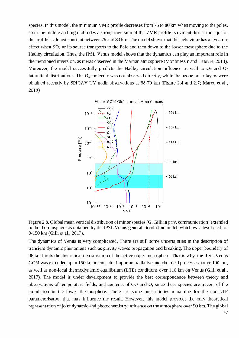
47

species. In this model, the minimum VMR profile decreases from 75 to 80 km when moving to the poles,

so in the middle and high latitudes a strong inversion of the VMR profile is evident, but at the equator

the profile is almost constant between 75 and 80 km. The model shows that this behaviour has a dynamic

effect when SO2 or its source transports to the Pole and then down to the lower mesosphere due to the

Hadley circulation. Thus, the IPSL Venus model shows that the dynamics can play an important role in

the mentioned inversion, as it was observed in the Martian atmosphere (Montmessin and Lefèvre, 2013).

Moreover, the model successfully predicts the Hadley circulation influence as well to O2 and O3

latitudinal distributions. The O2 molecule was not observed directly, while the ozone polar layers were

obtained recently by SPICAV UV nadir observations at 68-70 km (Figure 2.4 and 2.7; Marcq et al.,

2019)

Figure 2.8. Global mean vertical distribution of minor species (G. Gilli in priv. communication) extended

to the thermosphere as obtained by the IPSL Venus general circulation model, which was developed for

0-150 km (Gilli et al., 2017).

The dynamics of Venus is very complicated. There are still some uncertainties in the description of

transient dynamic phenomena such as gravity waves propagation and breaking. The upper boundary of

96 km limits the theoretical investigation of the active upper mesosphere. That is why, the IPSL Venus

GCM was extended up to 150 km to consider important radiative and chemical processes above 100 km,

as well as non-local thermodynamic equilibrium (LTE) conditions over 110 km on Venus (Gilli et al.,

2017). The model is under development to provide the best correspondence between theory and

observations of temperature fields, and contents of CO and O, since these species are tracers of the

circulation in the lower thermosphere. There are some uncertainties remaining for the non-LTE

parameterisation that may influence the result. However, this model provides the only theoretical

representation of joint dynamic and photochemistry influence on the atmosphere over 90 km. The global

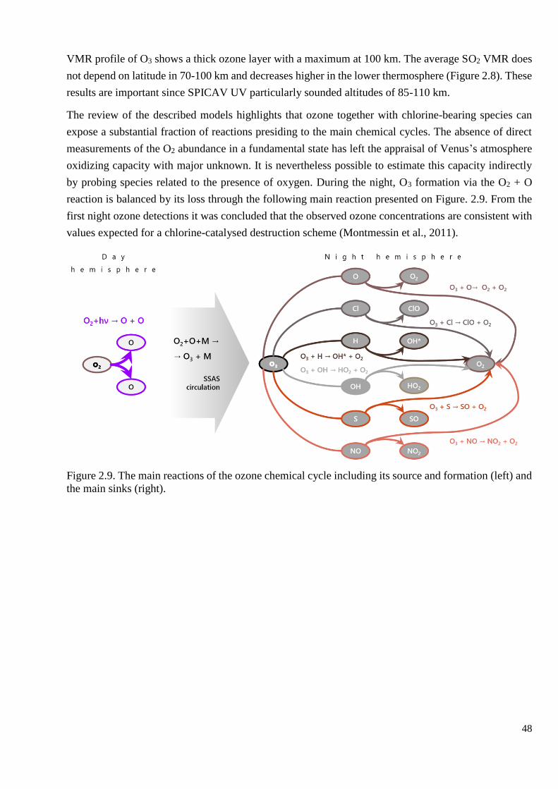
48

VMR profile of O3 shows a thick ozone layer with a maximum at 100 km. The average SO2 VMR does

not depend on latitude in 70-100 km and decreases higher in the lower thermosphere (Figure 2.8). These

results are important since SPICAV UV particularly sounded altitudes of 85-110 km.

The review of the described models highlights that ozone together with chlorine-bearing species can

expose a substantial fraction of reactions presiding to the main chemical cycles. The absence of direct

measurements of the O2 abundance in a fundamental state has left the appraisal of Venus’s atmosphere

oxidizing capacity with major unknown. It is nevertheless possible to estimate this capacity indirectly

by probing species related to the presence of oxygen. During the night, O3 formation via the O2 + O

reaction is balanced by its loss through the following main reaction presented on Figure. 2.9. From the

first night ozone detections it was concluded that the observed ozone concentrations are consistent with

values expected for a chlorine-catalysed destruction scheme (Montmessin et al., 2011).

Figure 2.9. The main reactions of the ozone chemical cycle including its source and formation (left) and

the main sinks (right).

49

CHAPTER 3. Data processing of stellar occultation spectra

3.1. The stellar occultation technique: retrieving the atmospheric composition from transmittance

spectra

Stellar occultation occurs when a star is tracked through the atmosphere of a planet while a spacecraft is

moving along its orbit. On board the spacecraft, an instrument is collecting a sequence of spectra of the

stellar light partially absorbed by the atmospheric species while the star is rising or setting behind the

planet (Figure 3.1A). It is an efficient way to study the vertical distribution of atmospheric absorbers

such as gas molecules or aerosol particles. Venus has a very dense atmosphere and very opaque clouds.

This makes the method of stellar occultation usable only for studying the atmosphere above them.

Occultations can probe up to an altitude where absorption features in the spectrum are overwhelmed by

signal noise (Figure 3.2). The line of sight (LOS) of the instrument gradually crosses layers of the

atmosphere, sensing atmospheric gases with a varying density. Absorption by the upper haze particles

is what eventually limits the depth of sounding. As a result, the UV stellar occultation technique is only

effective in the upper mesosphere and the lower thermosphere. SPICAV starts to be sensitive above 83-

85 km (pressure ~1 mbar) up to 145 km (pressure ~10-6 mbar) (Bertaux et al., 2007a) and allows one to

study the vertical structure of the planet’s night-time atmosphere. On the dayside the scattered solar light

does not allow one to observe weaker sources like stars. It should be noted that at the considered

altitudes, atmospheric refraction can be neglected due to the low gas concentrations.

Figure 3.1. (A) A sketch of the stellar occultation technique. The arrows show the LOS of the

spectrometer pointing to the star. The occultation session begins above the planet’s atmosphere (blue

arrow), then the star is tracked through the atmosphere (red arrow), and the session ends when the stellar

light is completely absorbed by the atmosphere (black arrow). (B) Two spectra of a star obtained by

SPICAV in one occultation session. The blue curve corresponds to the reference spectrum of the star

measured above the atmosphere (Sref(λ)), the red one - the stellar spectrum of the star’s radiation

attenuated by atmospheric absorption and scattering (S(λ, z)).

In space, the occultation method was originally used to scan ozone in the Earth’s atmosphere on board

satellites OAO-2 (The second Orbiting Astronomical Observatory) (Hays et al., 1972) and Copernicus

(OAO-3) (Atreya et al., 1976). In the 90-170 nm range, UV spectrometers on Voyager-1 and Voyager-

2 conducted studies of the vertical distribution of hydrogen and methane in the atmosphere of Jupiter

and then Saturn, Uranus, and their satellites (Broadfoot et al., 1977). Then, a predecessor of the Venusian

[A] [B]

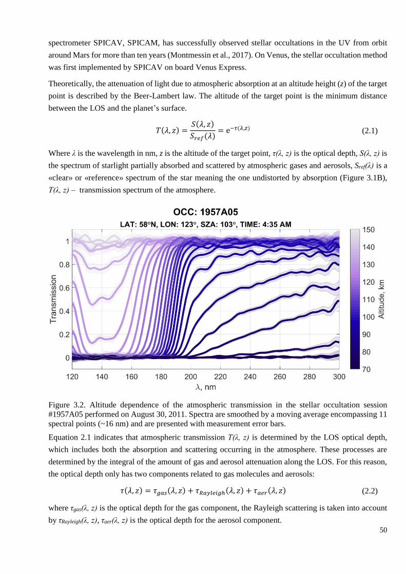
50

spectrometer SPICAV, SPICAM, has successfully observed stellar occultations in the UV from orbit

around Mars for more than ten years (Montmessin et al., 2017). On Venus, the stellar occultation method

was first implemented by SPICAV on board Venus Express.

Theoretically, the attenuation of light due to atmospheric absorption at an altitude height (z) of the target

point is described by the Beer-Lambert law. The altitude of the target point is the minimum distance

between the LOS and the planet’s surface.

𝑇(𝜆, 𝑧) =𝑆(𝜆, 𝑧)

𝑆𝑟𝑒𝑓(𝜆)= e−𝜏(𝜆,𝑧) (2.1)

Where λ is the wavelength in nm, z is the altitude of the target point, τ(λ, z) is the optical depth, S(λ, z) is

the spectrum of starlight partially absorbed and scattered by atmospheric gases and aerosols, Sref(λ) is a

«clear» or «reference» spectrum of the star meaning the one undistorted by absorption (Figure 3.1B),

Т(λ, z) – transmission spectrum of the atmosphere.

Figure 3.2. Altitude dependence of the atmospheric transmission in the stellar occultation session

#1957A05 performed on August 30, 2011. Spectra are smoothed by a moving average encompassing 11

spectral points (~16 nm) and are presented with measurement error bars.

Equation 2.1 indicates that atmospheric transmission Т(λ, z) is determined by the LOS optical depth,

which includes both the absorption and scattering occurring in the atmosphere. These processes are

determined by the integral of the amount of gas and aerosol attenuation along the LOS. For this reason,

the optical depth only has two components related to gas molecules and aerosols:

𝜏(𝜆, 𝑧) = 𝜏𝑔𝑎𝑠(𝜆, 𝑧) + 𝜏𝑅𝑎𝑦𝑙𝑒𝑖𝑔ℎ(𝜆, 𝑧) + 𝜏𝑎𝑒𝑟(𝜆, 𝑧) (2.2)

where τgas(λ, z) is the optical depth for the gas component, the Rayleigh scattering is taken into account

by τRayleigh(λ, z), τaer(λ, z) is the optical depth for the aerosol component.

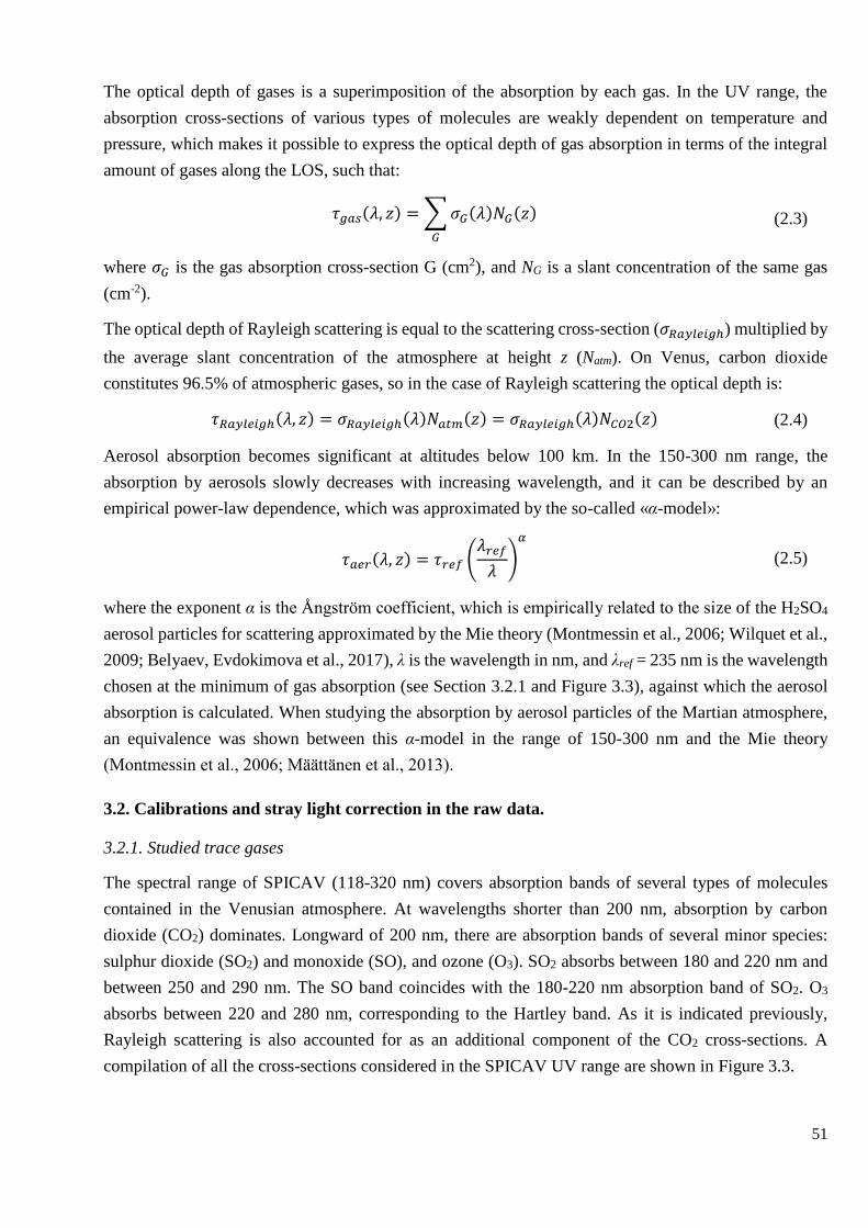
51

The optical depth of gases is a superimposition of the absorption by each gas. In the UV range, the

absorption cross-sections of various types of molecules are weakly dependent on temperature and

pressure, which makes it possible to express the optical depth of gas absorption in terms of the integral

amount of gases along the LOS, such that:

𝜏𝑔𝑎𝑠(𝜆, 𝑧) =∑𝜎𝐺(𝜆)𝑁𝐺(𝑧)

𝐺

(2.3)

where 𝜎𝐺 is the gas absorption cross-section G (cm2), and NG is a slant concentration of the same gas

(cm-2).

The optical depth of Rayleigh scattering is equal to the scattering cross-section (𝜎𝑅𝑎𝑦𝑙𝑒𝑖𝑔ℎ) multiplied by

the average slant concentration of the atmosphere at height z (Natm). On Venus, carbon dioxide

constitutes 96.5% of atmospheric gases, so in the case of Rayleigh scattering the optical depth is:

𝜏𝑅𝑎𝑦𝑙𝑒𝑖𝑔ℎ(𝜆, 𝑧) = 𝜎𝑅𝑎𝑦𝑙𝑒𝑖𝑔ℎ(𝜆)𝑁𝑎𝑡𝑚(𝑧) = 𝜎𝑅𝑎𝑦𝑙𝑒𝑖𝑔ℎ(𝜆)𝑁𝐶𝑂2(𝑧) (2.4)

Aerosol absorption becomes significant at altitudes below 100 km. In the 150-300 nm range, the

absorption by aerosols slowly decreases with increasing wavelength, and it can be described by an

empirical power-law dependence, which was approximated by the so-called «α-model»:

𝜏𝑎𝑒𝑟(𝜆, 𝑧) = 𝜏𝑟𝑒𝑓 (𝜆𝑟𝑒𝑓

𝜆)

𝛼

(2.5)

where the exponent α is the Ångström coefficient, which is empirically related to the size of the H2SO4

aerosol particles for scattering approximated by the Mie theory (Montmessin et al., 2006; Wilquet et al.,

2009; Belyaev, Evdokimova et al., 2017), λ is the wavelength in nm, and λref = 235 nm is the wavelength

chosen at the minimum of gas absorption (see Section 3.2.1 and Figure 3.3), against which the aerosol

absorption is calculated. When studying the absorption by aerosol particles of the Martian atmosphere,

an equivalence was shown between this α-model in the range of 150-300 nm and the Mie theory

(Montmessin et al., 2006; Määttänen et al., 2013).

3.2. Calibrations and stray light correction in the raw data.

3.2.1. Studied trace gases

The spectral range of SPICAV (118-320 nm) covers absorption bands of several types of molecules

contained in the Venusian atmosphere. At wavelengths shorter than 200 nm, absorption by carbon

dioxide (CO2) dominates. Longward of 200 nm, there are absorption bands of several minor species:

sulphur dioxide (SO2) and monoxide (SO), and ozone (O3). SO2 absorbs between 180 and 220 nm and

between 250 and 290 nm. The SO band coincides with the 180-220 nm absorption band of SO2. O3

absorbs between 220 and 280 nm, corresponding to the Hartley band. As it is indicated previously,

Rayleigh scattering is also accounted for as an additional component of the CO2 cross-sections. A

compilation of all the cross-sections considered in the SPICAV UV range are shown in Figure 3.3.

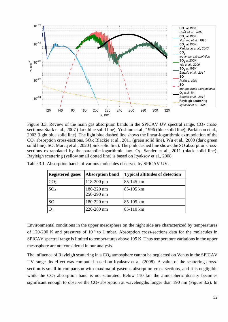
52

Figure 3.3. Review of the main gas absorption bands in the SPICAV UV spectral range. CO2 cross-

sections: Stark et al., 2007 (dark blue solid line), Yoshino et al., 1996 (blue solid line), Parkinson et al.,

2003 (light blue solid line). The light blue dashed line shows the linear-logarithmic extrapolation of the

CO2 absorption cross-sections. SO2: Blackie et al., 2011 (green solid line), Wu et al., 2000 (dark green

solid line). SO: Marcq et al., 2020 (pink solid line). The pink dashed line shows the SO absorption cross-

sections extrapolated by the parabolic-logarithmic law. O3: Sander et al., 2011 (black solid line).

Rayleigh scattering (yellow small dotted line) is based on Ityaksov et al., 2008.

Table 3.1. Absorption bands of various molecules observed by SPICAV UV.

Registered gases Absorption band Typical altitudes of detection

CO2 118-200 pm 85-145 km

SO2 180-220 nm

250-290 nm

85-105 km

SO 180-220 nm 85-105 km

O3 220-280 nm 85-110 km

Environmental conditions in the upper mesosphere on the night side are characterized by temperatures

of 120-200 K and pressures of 10-4 to 1 mbar. Absorption cross-sections data for the molecules in

SPICAV spectral range is limited to temperatures above 195 K. Thus temperature variations in the upper

mesosphere are not considered in our analysis.

The influence of Rayleigh scattering in a CO2 atmosphere cannot be neglected on Venus in the SPICAV

UV range. Its effect was computed based on Ityaksov et al. (2008). A value of the scattering cross-

section is small in comparison with maxima of gaseous absorption cross-sections, and it is negligible

while the CO2 absorption band is not saturated. Below 110 km the atmospheric density becomes

significant enough to observe the CO2 absorption at wavelengths longer than 190 nm (Figure 3.2). In

53

this spectral range the Raleigh scattering and CO2 cross-sections are comparable, so the scattering mainly

contributes to the atmospheric transmission below 110 km.

SO2 absorption cross-sections are combined from Wu et al. (2000) and from the high-resolution

measurements of Blackie et al. (2011). There is a lack of databases for SO. For this reason, we use data

from Marcq et al. (2020), which used the data of Phillips (1981) in the range of 190–230 nm. These

values were extrapolated to the rest of the range by a parabolic dependence on a logarithmic scale (Marcq

et al., 2019):

log10(𝜎[𝑐𝑚−2]) = − (

𝜆 − 200.132 𝑛𝑚

20.961)2

− 16.780 (2.6)

Unlike Marcq et al. (2020) we extrapolate the cross-sections in this way for the entire SPICAV range,

without fixing the constant value in the long-wave part of the range.

Ozone absorption is based on Sander et al. (2011), where the cross-sections for O3 in the 196–343 nm

band were obtained at a temperature of 218 K.

3.2.2. UV Signal considerations with SPICAV

Venus Express orbited around Venus from 2006 to December 2014. During a stellar occultation the

SPICAV FOV is pointed to the star. The vertical step in one observation session varies from 1 to 8 km,

depending on viewing geometry. A typical occultation lasts 30 minutes, during which a reference stellar

spectrum is collected based on the average of the stellar spectra collected above 200 km. Observations

cover all latitudes of the night side from 18:00 to 06:00.

Typical SPICAV data, like the one used in this work, is a sequence of observations where each

acquisition consists of five individual UV spectra (corresponding to the five bins mentioned earlier. A

raw (so-called Level 0) spectrum is a 408-spectel vector on values in ADU, where only 384 spectels

contain an actual signal. Level 1 data are obtained after removing pixel dark current, also known as DC,

whose pattern across the detector was estimated from dedicated technological observations (see next

paragraphs). Level 1 also includes a correction for readout systematic, and cosmic ray outbreaks that

contaminate nearby pixels. Also, to minimize bias in weak signals, pixel readout includes a fixed offset

that is accounted for as well as other instrument artefacts.

The CCD of the SPICAV UV channel is characterized by an average DC of about 10-20 ADU per second

while pixel dynamics is limited to 4095 ADU (12-bit conversion). DC increases with temperature at a

rate specific to each pixel. However, this non-uniformity pattern of the DC is stable and has been

monitored throughout the mission. Special observation sessions carried out at HT = 0, preventing any

photo-event to reach the CCD, allowed one to collect only the dark signal (sum of DC and offset). Then,

a DC non-uniformity (DCNU) model for the entire detector could be inferred by fitting the recorded

dark signal with a linear law, such as:

𝐷𝐶𝑁𝑈𝑖𝑗 = 𝑆𝑑𝑎𝑟𝑘 𝑖 ∙ 𝑎𝑖𝑗 + 𝑏𝑖𝑗 (2.7)

54

Where 𝐷𝐶𝑁𝑈𝑖𝑗 is the sum of dark and offset signals in a pixel of coordinates i (row) and j (column),

𝑆𝑑𝑎𝑟𝑘 𝑖 is the signal collected by the masked pixels at the edge on the same row of the detector, and (a,b)

are the linear coefficients established for each pixel during the technological observation at HT=0.

A weak (~6 ADU) readout systematic with a 14-pixel period affects the spectra, especially for very low

signals. The line-by-line readout of the SPICAV CCD generates a correlated variation in the phase of

the periodic readout pattern. Several techniques have been developed to correct for this readout

systematic by the engineering team that are based on identifying the phase and amplitude of this spurious

periodic signal that can be then removed from spectra and permit a better exploitation of low-signal

spectra.

Also, the recorded signal was sometimes distorted by cosmic rays hitting the detectors, creating

temporarily «warm» pixels easily discernible from the rest of the detector as they usually constitute an

isolated event affecting only the adjacent pixels. It is to be noted that with the branding strategy used to

cope with the telemetry constraints, such an event is smoothed out by the line binning, yet remains an

identifiable feature that is easy to spot and correct.

The influence of the spectrometer PSF and the detector flat field on the spectra was not corrected in the

Level 1 data used to create transmittance. Flat field has no impact in the context of spectra created by

the ratio of two signals, like the transmittance. The PSF consideration was sequentially handled in the

forward model used to fit the collected transmittances.

With regard to the ancillary information, Level 0 data carry a set of geometrical parameters at the

tangential point, which is defined as the point along the LOS closest to the surface, computed at the

centre of each bin of the detector, that is for 5 different points along the slit. This information is

dependent on how well we know the pointing of the instrument A great advantage of stellar occultation

is that the observation geometry can be accurately determined without knowing the exact pointing of the

main axis of the instrument. Indeed, one has to only consider the optical path between the target star,

whose celestial coordinates are known with outstanding precision, and the body of the spacecraft whose

position around Venus is given by the Venus Express ephemerides which is likewise extremely well

constrained. This is this information that we retain for our retrievals and in particular to produce altitude-

dependent concentrations of gases and aerosols.

3.2.3. Estimation of errors in atmospheric transmission spectra.

The SPICAV UV channel detector is characterized by linear charge coupling, therefore, for the signal-

to-noise ratio (SNR), this is the formula

𝑆𝑁𝑅 =𝑆

𝜎=

𝑆𝑆𝑃𝐼𝐶𝐴𝑉𝐺

√(𝑆𝑆𝑃𝐼𝐶𝐴𝑉𝐺 + (𝑆𝐷𝐶 + 𝑆𝑂𝐹𝐹) 𝑔⁄ + 𝜎𝑆𝐸2 )

(2.8)

where SSPICAV is the number of ADU corresponding to the detected UV radiation, SDC and SOFF are the

signals from the dark current and the offset current, and 𝜎𝑆𝐸2 is the variation for electronic noise. By

55

multiplying the signal by the gain G of the detector which is set by the digital equivalent of HT, the

number of photons entering the detector is calculated. To estimate the error of the dark current, the signal

is multiplied by g, since dark current electrons are subject to Poisson statistics. The g coefficient was

determined from a set of purely stellar observations.

The standard measured signal corresponds on average to a level of 2000 ADU signal. DC is on average

20/400 ADU when the Peltier cooler is on/off, and the amplitude of readout systematic was estimated

around 6 ADU. The gain g changes from 0.3 to 12 ADU/photo-event. The estimation of the average

signal-to-noise ratio (SNR) gives a value of 50. According to this formula, each pixel can be assigned a

corresponding 1-σ uncertainty, which includes all the known sources of noise affecting the measurement.

3.2.4. Sources of an additional emission registered by the UV channel of SPICAV

The SPICAV spectral range is sensitive not only to the stellar radiation. Its range of 118-320 nm allows

observing several types of UV radiation coming from various sources such as atmospheric nitric oxide

(SNO) emission, the Lyman-α hydrogen line at 121.6 nm (SLy-α), and the scattered light from the Sun

(SSUN). Thus, the measured signal (SSPICAV) is the addition of several signals, where all the

aforementioned emissions are considered as «stray» light (SSTRL) since contaminating the signal of

interest, that of the star (Equation 2.9).

𝑆𝑆𝑃𝐼𝐶𝐴𝑉 = 𝑆𝑆𝑇𝐴𝑅 + (𝑆𝑁𝑂 + 𝑆𝐿𝑦−𝛼 + 𝑆𝑆𝑈𝑁) = 𝑆𝑆𝑇𝐴𝑅 + (𝑆𝑆𝑇𝑅𝐿) (2.9)

Figure 3.4. Several components of the signal obtained in the occultation session #2721A05: (1) the

spectrum of a star (purple) with atmospheric absorption lines at 98 km whose intensity is divided by two

to better visualize the signal from other weaker UV radiation source, (2) the NO (pink), (3) Lyman-α

(cyan), (4) the Sun scattered light (yellow). The NO emission obtained in 90-110 km, the Lyman-α and

solar spectra are averaged over 200 km. More detailes of the the Lyman-α and solar signal extraction

can be found in Annex 5, for more detailes of the nitric oxide emission extraction see Section 3.2.9.

This «stray» light component depends on the observation geometry and on the FOV size determined by

the presence or absence of the slit. While the spectrum of a star, which is a point source, does not change

56

due to the presence of a slit, the spectral resolution and shape of the spectrum of extended sources

emission is convolved by the angular aperture and is therefore slit-width dependent. Also, the light of

the star is almost completely collected in the central bin and in the corresponding spectrum, and the PSF

scatters just a few percent of it into the other 4 bins. In the absence of the slit, which is the most recurrent

configuration of the stellar occultation mode, the radiation of extended sources is integrated over the

entire field of view of the spectrometer, and can be thus a major contamination for the target star.

3.2.4.1. Lyman-α emission

Figure 3.5. Observations of the night hydrogen corona on Venus from the limb scans by the UV channel

of the SPICAV Venus Express spectrometer for observations #2000, #2001, #2002, #2003. The result is

taken from the work of J.-Y. Chaufray et al. (2015).

Lyman-α emission is the result of the resonant scattering of sunlight by hydrogen atoms present in the

planet’s exosphere and interplanetary space. The emission serves as a source of information about the

hydrogen content in the exosphere of planets and about its temperature. The first Venusian Lyman-α

emission was studied during a flyby of the Venera-4 and Mariner-5 spacecraft (Barth et al., 1967; Kurt

et al., 1968). SPICAV UV observations showed that the intensity of the Lyman-α line changes with

decreasing altitude and increasing atmospheric density (Chaufray et al., 2015), as well as depending on

the geometry of observations. The registered glow is a superposition of radiation scattered by atoms of

interplanetary and Venusian hydrogen. Also, when moving into deeper atmosphere layers (below 2000

km), the altitude dependence of emission begins to show absorption by cold H atoms, which reduces the

intensity of Lyman-α (Figure 3.5).

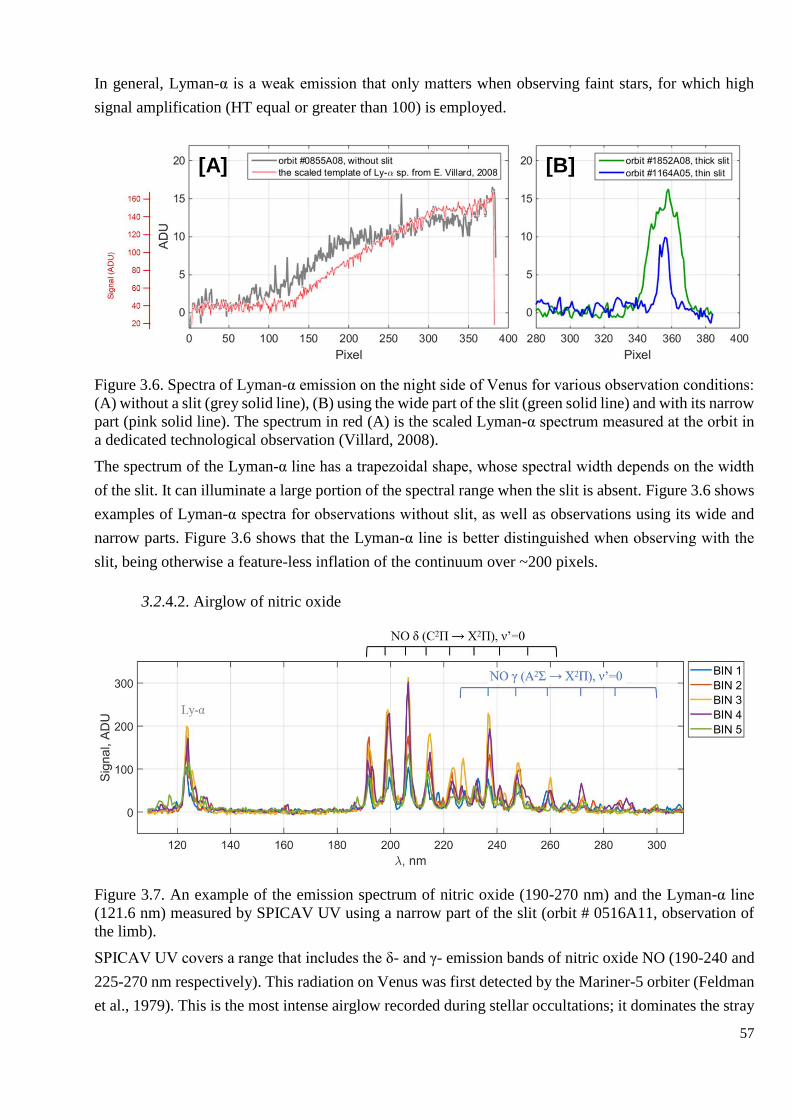
57

In general, Lyman-α is a weak emission that only matters when observing faint stars, for which high

signal amplification (HT equal or greater than 100) is employed.

Figure 3.6. Spectra of Lyman-α emission on the night side of Venus for various observation conditions:

(A) without a slit (grey solid line), (B) using the wide part of the slit (green solid line) and with its narrow

part (pink solid line). The spectrum in red (A) is the scaled Lyman-α spectrum measured at the orbit in

a dedicated technological observation (Villard, 2008).

The spectrum of the Lyman-α line has a trapezoidal shape, whose spectral width depends on the width

of the slit. It can illuminate a large portion of the spectral range when the slit is absent. Figure 3.6 shows

examples of Lyman-α spectra for observations without slit, as well as observations using its wide and

narrow parts. Figure 3.6 shows that the Lyman-α line is better distinguished when observing with the

slit, being otherwise a feature-less inflation of the continuum over ~200 pixels.

3.2.4.2. Airglow of nitric oxide

Figure 3.7. An example of the emission spectrum of nitric oxide (190-270 nm) and the Lyman-α line

(121.6 nm) measured by SPICAV UV using a narrow part of the slit (orbit # 0516A11, observation of

the limb).

SPICAV UV covers a range that includes the δ- and γ- emission bands of nitric oxide NO (190-240 and

225-270 nm respectively). This radiation on Venus was first detected by the Mariner-5 orbiter (Feldman

et al., 1979). This is the most intense airglow recorded during stellar occultations; it dominates the stray

[A] [B]

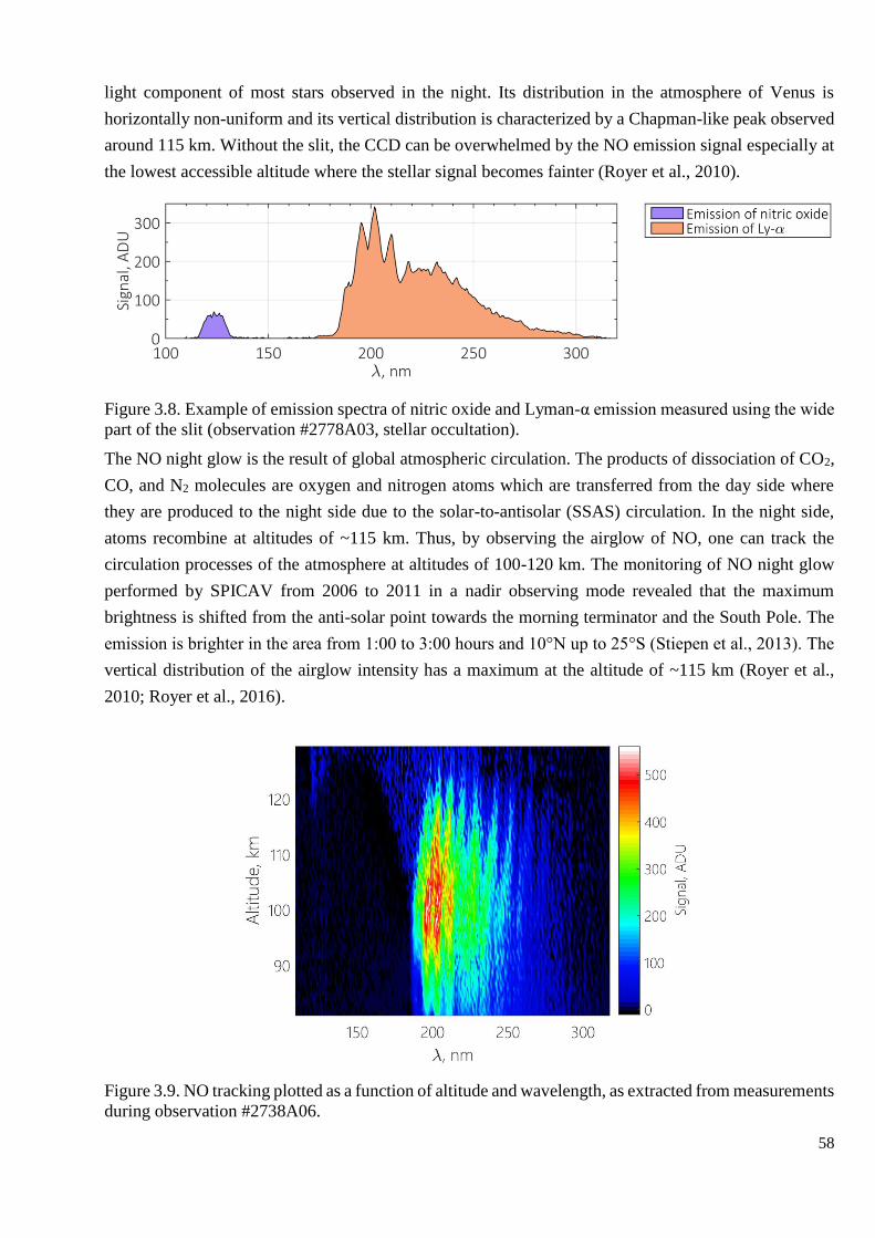
58

light component of most stars observed in the night. Its distribution in the atmosphere of Venus is

horizontally non-uniform and its vertical distribution is characterized by a Chapman-like peak observed

around 115 km. Without the slit, the CCD can be overwhelmed by the NO emission signal especially at

the lowest accessible altitude where the stellar signal becomes fainter (Royer et al., 2010).

Figure 3.8. Example of emission spectra of nitric oxide and Lyman-α emission measured using the wide

part of the slit (observation #2778A03, stellar occultation).

The NO night glow is the result of global atmospheric circulation. The products of dissociation of CO2,

CO, and N2 molecules are oxygen and nitrogen atoms which are transferred from the day side where

they are produced to the night side due to the solar-to-antisolar (SSAS) circulation. In the night side,

atoms recombine at altitudes of ~115 km. Thus, by observing the airglow of NO, one can track the

circulation processes of the atmosphere at altitudes of 100-120 km. The monitoring of NO night glow

performed by SPICAV from 2006 to 2011 in a nadir observing mode revealed that the maximum

brightness is shifted from the anti-solar point towards the morning terminator and the South Pole. The

emission is brighter in the area from 1:00 to 3:00 hours and 10°N up to 25°S (Stiepen et al., 2013). The

vertical distribution of the airglow intensity has a maximum at the altitude of ~115 km (Royer et al.,

2010; Royer et al., 2016).

Figure 3.9. NO tracking plotted as a function of altitude and wavelength, as extracted from measurements

during observation #2738A06.

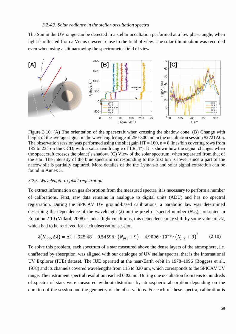
59

3.2.4.3. Solar radiance in the stellar occultation spectra

The Sun in the UV range can be detected in a stellar occultation performed at a low phase angle, when

light is reflected from a Venus crescent close to the field of view. The solar illumination was recorded

even when using a slit narrowing the spectrometer field of view.

Figure 3.10. (A) The orientation of the spacecraft when crossing the shadow cone. (B) Change with

height of the average signal in the wavelength range of 250-300 nm in the occultation session #2721A05.

The observation session was performed using the slit (gain HT = 160, n = 8 lines/bin covering rows from

185 to 225 on the CCD, with a solar zenith angle of 136.4°). It is shown how the signal changes when

the spacecraft crosses the planet’s shadow. (C) View of the solar spectrum, when separated from that of

the star. The intensity of the blue spectrum corresponding to the first bin is lower since a part of the

narrow slit is partially captured. More detailes of the the Lyman-α and solar signal extraction can be

found in Annex 5.

3.2.5. Wavelength-to-pixel registration

To extract information on gas absorption from the measured spectra, it is necessary to perform a number

of calibrations. First, raw data remains in analogue to digital units (ADU) and has no spectral

registration. During the SPICAV UV ground-based calibrations, a parabolic law was determined

describing the dependence of the wavelength (λ) on the pixel or spectel number (Npix), presented in

Equation 2.10 (Villard, 2008). Under flight conditions, this dependence may shift by some value of Δλ,

which had to be retrieved for each observation session.

𝜆(𝑁𝑝𝑖𝑥 , Δ𝜆) = Δ𝜆 + 325.48 − 0.54596 ∙ (𝑁𝑝𝑖𝑥 + 9) − 4.9096 ∙ 10−6 ∙ (𝑁𝑝𝑖𝑥 + 9)

2 (2.10)

To solve this problem, each spectrum of a star measured above the dense layers of the atmosphere, i.e.

unaffected by absorption, was aligned with our catalogue of UV stellar spectra, that is the International

UV Explorer (IUE) dataset. The IUE operated at the near-Earth orbit in 1978–1996 (Boggess et al.,

1978) and its channels covered wavelengths from 115 to 320 nm, which corresponds to the SPICAV UV

range. The instrument spectral resolution reached 0.02 nm. During one occultation from tens to hundreds

of spectra of stars were measured without distortion by atmospheric absorption depending on the

duration of the session and the geometry of the observations. For each of these spectra, calibration is

[A] [B] [C]

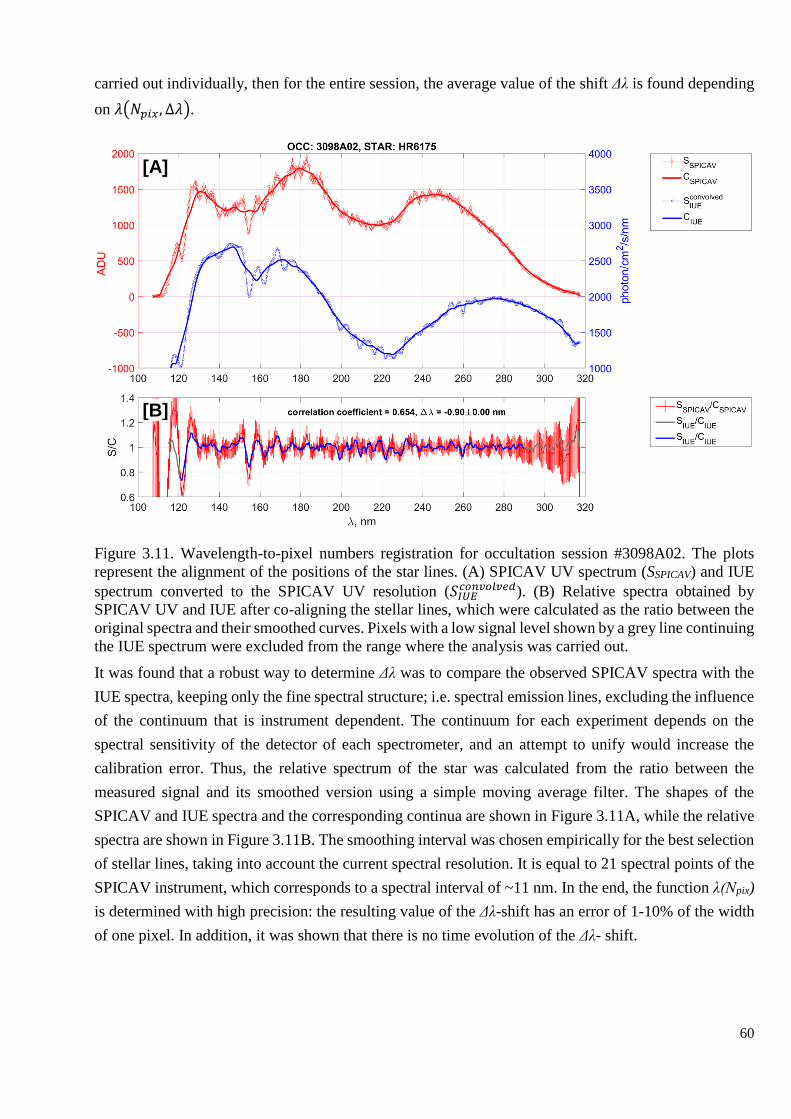
60

carried out individually, then for the entire session, the average value of the shift Δλ is found depending

on 𝜆(𝑁𝑝𝑖𝑥 , Δ𝜆).

Figure 3.11. Wavelength-to-pixel numbers registration for occultation session #3098A02. The plots

represent the alignment of the positions of the star lines. (A) SPICAV UV spectrum (SSPICAV) and IUE

spectrum converted to the SPICAV UV resolution (𝑆𝐼𝑈𝐸𝑐𝑜𝑛𝑣𝑜𝑙𝑣𝑒𝑑). (B) Relative spectra obtained by

SPICAV UV and IUE after co-aligning the stellar lines, which were calculated as the ratio between the

original spectra and their smoothed curves. Pixels with a low signal level shown by a grey line continuing

the IUE spectrum were excluded from the range where the analysis was carried out.

It was found that a robust way to determine Δλ was to compare the observed SPICAV spectra with the

IUE spectra, keeping only the fine spectral structure; i.e. spectral emission lines, excluding the influence

of the continuum that is instrument dependent. The continuum for each experiment depends on the

spectral sensitivity of the detector of each spectrometer, and an attempt to unify would increase the

calibration error. Thus, the relative spectrum of the star was calculated from the ratio between the

measured signal and its smoothed version using a simple moving average filter. The shapes of the

SPICAV and IUE spectra and the corresponding continua are shown in Figure 3.11A, while the relative

spectra are shown in Figure 3.11B. The smoothing interval was chosen empirically for the best selection

of stellar lines, taking into account the current spectral resolution. It is equal to 21 spectral points of the

SPICAV instrument, which corresponds to a spectral interval of ~11 nm. In the end, the function λ(Npix)

is determined with high precision: the resulting value of the Δλ-shift has an error of 1-10% of the width

of one pixel. In addition, it was shown that there is no time evolution of the Δλ- shift.

[A]

[B]

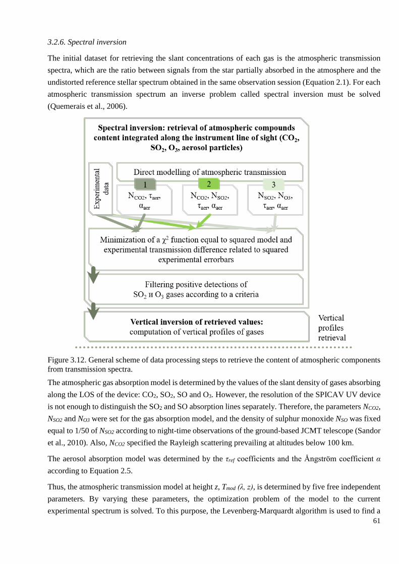
61

3.2.6. Spectral inversion

The initial dataset for retrieving the slant concentrations of each gas is the atmospheric transmission

spectra, which are the ratio between signals from the star partially absorbed in the atmosphere and the

undistorted reference stellar spectrum obtained in the same observation session (Equation 2.1). For each

atmospheric transmission spectrum an inverse problem called spectral inversion must be solved

(Quemerais et al., 2006).

Figure 3.12. General scheme of data processing steps to retrieve the content of atmospheric components

from transmission spectra.

The atmospheric gas absorption model is determined by the values of the slant density of gases absorbing

along the LOS of the device: CO2, SO2, SO and O3. However, the resolution of the SPICAV UV device

is not enough to distinguish the SO2 and SO absorption lines separately. Therefore, the parameters NCO2,

NSO2 and NO3 were set for the gas absorption model, and the density of sulphur monoxide NSO was fixed

equal to 1/50 of NSO2 according to night-time observations of the ground-based JCMT telescope (Sandor

et al., 2010). Also, NCO2 specified the Rayleigh scattering prevailing at altitudes below 100 km.

The aerosol absorption model was determined by the τref coefficients and the Ångström coefficient α

according to Equation 2.5.

Thus, the atmospheric transmission model at height z, Tmod (λ, z), is determined by five free independent

parameters. By varying these parameters, the optimization problem of the model to the current

experimental spectrum is solved. To this purpose, the Levenberg-Marquardt algorithm is used to find a

62

minimum of the reduced χ2 function. The latter is normalized by the number of free parameters (number

of independent spectral points minus the number of retrieved parameters).

𝜒2(𝑁𝐶𝑂2, 𝑁𝑆𝑂2, 𝑁𝑂3, 𝜏𝑟𝑒𝑓, 𝛼) = ∑[(𝑇𝑒𝑥𝑝(𝜆𝑖) − 𝑇𝑚𝑜𝑑(𝜆𝑖 , 𝑁𝐶𝑂2, 𝑁𝑆𝑂2, 𝑁𝑂3, 𝜏𝑟𝑒𝑓, 𝛼))

𝛿𝑒𝑥𝑝(𝜆𝑖)]

2

/𝑁𝑓𝑟𝑒𝑒 (2.11)

Nfree – number of free parameters, δexp(λi) – experimental transmission uncertainty Texp(λi).

SPICAV PSF effect weighted by the flat field are needed to compute the model transmittance Tmod that

is calculated as follows ([BIN] - consideration of the summing of signal within one bin)

𝑇𝑚𝑜𝑑(𝑁𝐶𝑂2, 𝑁𝑆𝑂2, 𝑁𝑂3, 𝜏𝑟𝑒𝑓, 𝛼) = [𝐵𝐼𝑁][𝐹𝐹][𝑃𝑆𝐹](𝑇𝑡ℎ𝑒𝑜𝑟(𝑁𝐶𝑂2, 𝑁𝑆𝑂2, 𝑁𝑂3, 𝜏𝑟𝑒𝑓, 𝛼) ∙ 𝑆𝑟𝑒𝑓)

𝑆𝑟𝑒𝑓 (2.12)

where Ttheory is described by Equation 2.2.

Optimization of the Equation 2.12 is performed by the Levenberg-Marquardt algorithm. It also allows

to estimate a converge parameters covariance as a reverse Hessian matrix (H) equal to

𝑑𝑖𝑎𝑔(𝜎2) = 𝐶 = [𝐻]−1 = (𝐽𝑇𝐽)−1 (2.13)

where J is a Jacobian of the χ-function (Press et al., 2007). The standard errors of estimating parameters

of the atmospheric absorption and scattering are the diagonal elements of the covariance C.

3.2.6.1. Cases of positive gas detection

It has been found that the densities of minor gases such as sulphur dioxide and ozone are subject to brutal

changes, and sometimes their concentrations are below the detection limit. The detection limit is directly

related to the error of experimental data which varies with observing sessions and which mostly depends

on the brightness of the observed star. However, the determination of a reliable detection limit is a needed

task for characterizing the atmospheric composition in the various layers probed by the instrument. The

general scheme for retrieving gas abundances from the atmospheric transmission spectra is shown in

Figure 3.12.

First, it is necessary to establish a criterion for detecting small gas components. The spectral inversion

problem is solved in three successive steps with every step adding a new species whose influence on the

fit can then be precisely monitored.

In the first step, only the slant density of CO2 is fitted, while absorption by sulphur oxides and ozone is

not taken into account. Simultaneously the aerosol opacity parameters τref and α are also kept free.

In the second step, the slant density of SO2 tied to that of SO is added to CO2 and aerosols as free

parameters, but ozone remains excluded from the fit.

In the last step, the O3 absorption in the Hartley band is added to the algorithm. At the same time NCO2

is fixed to the value that provides the best fit for the first and second steps. This approach is justified,

since there is no overlap between the absorption bands of O3 and CO2 at 150-300 nm, and it gives us the

63

opportunity to reduce the number of free parameters. The aerosol parameters at the third step were also

retrieved.

For each step, a minimum value of the reduced χ2 is obtained and stored. The resulting three values are

compared with each other. Positive detection of any trace gas in the observed layer (i.e. in one spectrum)

is established if χ2 decreases significantly compared to the model in Step 1, which assumes only CO2

and aerosol absorptions. A detection criterion was then established empirically:

𝛿𝜒2 =𝜒2(𝑆𝑂2 𝑜𝑟 𝑎𝑛𝑑⁄ 𝑂3, 𝐶𝑂2)

𝜒2(𝐶𝑂2)< 0.95 (2.14)

An example of a positive identification of SO2 absorption at an altitude of 87 km is shown in Figure

3.13A where the relative decrease in χ2 is 0.74. Here, the best fit is reached when considering the

residuals at wavelengths of SO2 absorption bands (Figure 3.13B).

Figure 3.13. Example of positive detection of SO2 absorption at the altitude of 87.3 km in the stellar

occultation session #0103A07 (August 2, 2006; at latitude 3.9°S and longitude 241.9°; local time 23.37

hours). (A) Measured transmission spectrum TEXP with corresponding error bars (black solid line);

aerosol continuum Taer (black dashed line), the model atmospheric transmission for carbon dioxide

absorption TCO2 only (blue solid line) and for joint carbon dioxide and sulphur dioxide absorption

TCO2,SO2 (red solid line). The model spectra are convolved taking into account the spectrometer point

spread function ([PSF]) and detector flat field ([FF]), see Equation 2.12. (B) Residuals of two different

models related to experimental errors. The solid blue line corresponds to the CO2 absorption model. The

solid red line corresponds to a model that takes into account the atmospheric absorption of CO2 and SO2.

Dotted black lines indicate the level of error bars.

Data processing algorithms used in previous and accompanying works of SPICAV UV (Montmessin et

al., 2011, Marcq et al., 2019, 2020) use a similar strategy. However, criteria chosen to conclude on a

64

positive detection were different. In the paper of Montmessin et al. (2011) the firm detection of ozone

in stellar occultations was concluded when the O3 absorption band is very pronounced: 𝛿𝜒20112 ≤ 0.5 or

5-σ significance. In the recent reanalysis of SPICAV UV nadir observations (Marcq et al., 2019, 2020)

O3 and SO2 detections within the significance interval of 3σ corresponded to 𝛿𝜒20192 ≤

1

5.5≈ 0.18.

However, there is a difference in spectral filtration considered in those papers and in our work. In present

analysis any high-pass filter is not used, in contrast to a moving-average filter with the 8-nm window in

Montmessin et al. (2011) and a special selection of spectral points in Marcq et al. (2019, 2020). These

techniques lead to an increase of χ2 values meaning an underestimation of computed data errors, and to

the decrease of δχ2. For example, δχ2 is 2 times lower if the moving-average filter with 8-nm window is

applied to the spectrum presented in Figure 3.13A. As well, 𝛿𝜒20112 ≤ 0.5 is fulfilled when the current

δχ2 is lower than 0.85. However, the SPICAV UV stellar occultation measurements are heterogeneous

in terms of noise level, and it is difficult to choose one particular approach for smoothing outliers and

noise fluctuations for the whole dataset. In order to unify the detection criterion, it was decided not to

apply smoothing techniques to the resulting transmission spectra. In general, the resulting values of

reduced χ2 for any set of fitting parameters are in the range of 0.55-2.5. It means that an underestimation

and overestimation of data errors are both possible, forcing conclusions based on δχ2 rather than χ2. It

was concluded that a 5% decrease of reduced χ2 corresponds to the detection with a significance of 1σ.

Figure 3.14. A case of positive O3 detection at an altitude of 100.36 km in the stellar occultation session

#0348A17, that is the same as reported in Montmessin et al., 2011 (April 4, 2007; at latitude 4.1°S and

longitude 245.3°; local time 1.57 hours). (A) Measured transmission spectrum TEXP with corresponding

errors (black solid line); the model atmospheric transmission for carbon dioxide absorption TCO2 (red

solid line) and TCO2, O3 (green solid line). B and C: Residual distribution histograms for two models. (B)

The residuals of the TCO2 model and the optimal normal distribution for the given histogram. (C)

Residuals of the TCO2,O3 model, and the optimal normal distribution for the given histogram.

Overall, SPICAV data have revealed that O3 is far less abundant than SO2 in the Venusian mesosphere.

Moreover, data are more uncertain in the range of the Hartley band due to the overlapping emission band

65

of NO. To avoid false positive detections, the positive detection criterion for SO2 needs to be narrowed.

In addition to the χ2 reduction, we have analysed a histogram representing the distribution of the

transmission residuals within the Hartley absorption band. A proof of the goodness of fit is given when

the Gaussian is symmetric about zero. If the histogram fulfils this requirement without considering O3

absorption, we can conclude that O3 is absent from the analysed spectrum. Conversely, an offset of the

Gaussian maximum could potentially reveal an unaccounted absorption due to O3. In that case, the final

Gaussian distribution after adding O3 to the retrieval was also checked against symmetry about zero. To

filter out noisy spectra hiding a weak O3 absorption, we considered only spectra when the standard

deviation of residual histograms is lower than 0.05.

3.2.6.2. Upper detection limits for two gases.

Figure 3.15. Statistics of the χ2 value for SO2 (A) and O3 (B) detections.

Both SO2 and O3 appear highly variable in time yet some observations do not lead to a firm detection.

A deeper analysis of the χ2 function can help us to address the problem of estimating correctly a detection

limit. It was mentioned above that the positive detections correspond to at least 5% reduction of χ2 value

after a certain trace gas has been added to the fit. In most cases a χ2 reduction of >10% is observed for

SO2 (Figure 3.15A). The opposite proportion is obtained for the ozone retrievals (Figure 3.15B). It means

that the experiment reaches a detection limit for ozone that needs to be quantified.

SPICAV observed stars with various brightness and in different stray light configurations that defined a

noise of atmospheric transmission spectra. It leads to changing detection limits that are unique for each

spectrum. A simple approach was used to determine them for each gaseous compound. The limit is

considered to be linked to the 1-σ uncertainty of the spectral data, which can be associated to a value for

the slant density. The σ value is determined as standard deviation computed for a ration of an

experimental spectrum and a corresponding best-fit model. The spectral range for σ computation is

limited to spectral bands of minor species, thus, the interval of 210-280 nm is considered. Due to this

limitation the uncertainties related to lower spectral signals were not taken under consideration.

Detection limit slant density is assumed to provide a 1-σ absorption quantity in a maximum of studying

trace gas band. It is estimated around a maximum of the absorption band that correspond to 245-265 nm

[A] [B]

66

for O3. The interval of 190-210 nm is used for SO2 detection attempts since this absorption band is the

strongest for SO2 in the SPICAV UV spectral range. The algorithm solves the spectral inversion problem

for one gas. If one neglects the convolution by the instrumental PSF for this problem, the transmission

is computed by exp (−𝜎𝑔𝑎𝑠 𝑁𝑔𝑎𝑠) where σgas are gaseous cross-sections. However, The PSF convolution

should be considered in the analysis since the experimental transmission spectra are not deconvolved.

Therefore, for detection limit estimation the transmission is calculated as a ratio between two synthetic

spectra (Equation 2.15) when only one considers the studying gas. The atmospheric transmission model

is supplemented by the SO2 absorption when the O3 detection limit is estimated.

𝑇𝑔𝑎𝑠(𝑁𝐶𝑂2, 𝑁𝑆𝑂2, 𝑁𝑂3, 𝜏𝑟𝑒𝑓, 𝛼) =𝑇𝑚𝑜𝑑(𝑁𝐶𝑂2, 𝑁𝑔𝑎𝑠, 𝜏𝑟𝑒𝑓 , 𝛼)

𝑇𝑚𝑜𝑑(𝑁𝐶𝑂2, 𝜏𝑟𝑒𝑓, 𝛼) (2.15)

Figure 3.16. A and C: Atmospheric transmission spectra of occultations #1563A03 (August 1, 2010; at

latitude 24.4°N and longitude 107°; local time 2.07 hours) and #1438A06 (March 29, 2010; at latitude

3.1°S and longitude 46.6°; local time 2.29 hours) within altitude range of 83-110 km. Grey curves with

error bars are the experimental data. The red tones curves are the synthetic transmission spectra assuming

the absorption by CO2 and SO2. The green curves are the model also including the ozone absorption.

The experimental spectra are shown with best fit models. (B) The estimated detection limits presented

by blue triangles, and ozone slant densities successfully retrieved (the green circle for #1563A03 and

the green star for #1438A06).

An example of our analysis is presented in Figure 3.16 for two occultation sessions (#1563A03 and

#1438A06) characterized by different signal fluctuation levels. There are positive detections of ozone at

altitudes of 109 and 99 km respectively in #1563A03 and #1438A06, where O3 absorption band is clearly

[A] [B] [C]

67

distinguishable in those of transmissions. Figure 3.17A represents the evaluated 1-σ uncertainty for each

spectrum. The detection limits for O3 for these two cases vary by a factor of two. However, for each

observation the 1-σ value is nearly constant over most of the probed altitude range, and equivalently for

the corresponding upper limit on slant density. When this detection limit on slant density quantity is

divided by the CO2 slant density obtained at the same altitude, then the 1-σ uncertainty in terms of VMR

can be derived. Considering that the 1-σ uncertainty on the slant density is constant with altitude, then

the corresponding 1-σ uncertainty on the VMR necessarily decreases with decreasing altitude as the CO2

slant density increases (see Figure 3.17C).

Figure 3.17. (A) 1-σ value variation with altitude found for orbits #1563A03 (August 1, 2010; at latitude

24.4°N and longitude 107°; local time 2.07 hours) and #1438A06 (March 29, 2010; at latitude 3.1°S and

longitude 46.6°; local time 2.29 hours). (B) Estimated detection limits are presented by blue triangles,

while filled circles and stars indicate successfully retrieved O3 slant densities (the black circle for

#1563A03 and the black star for #1438A06). (C) 1-σ uncertainty as well as detection values obtained

for O3 VMR corresponding to the slant densities presented in B.

This algorithm is applied to every available observation made by SPICAV UV in order to compute the

detection limits for O3 and SO2. The orbits with at least one positive detection are combined to estimate

the general characteristics of the stellar occultation experiment by SPICAV.

Within the altitude range of 90-110 km the mean detection limit is estimated to be equal to 3.3±0.1×1015

cm-2 (Figure 3.18). It is shown that the detected O3 concentrations are in general just 1-3 times larger

than the estimated limit. However, the values over 103 km should be considered with caution even if

some observations were performed with a low noise level permitting not false positive detections of slant

densities lower than the mean detection limit. Less than 15% of the spectra led to O3 detection.

The SO2 detection limit is about two times higher than the one retrieved for O3. In the 90-110 km range

it is 5.8±0.2×1015 cm-2 (Figure 3.19). This difference in detection limit can be explained by the difference

in cross-sections between the two gases. The detection limit is reached at an altitude of about 100 km

while below the majority of the detections are significantly higher than corresponding detection limits.

These detections constitute the SO2 layer that can be found in the 83-100 km altitude range.

[A] [B] [C]

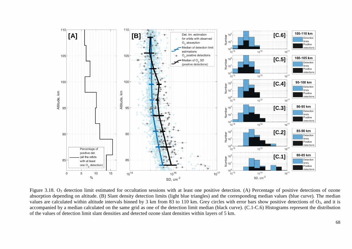
68

Figure 3.18. O3 detection limit estimated for occultation sessions with at least one positive detection. (A) Percentage of positive detections of ozone

absorption depending on altitude. (B) Slant density detection limits (light blue triangles) and the corresponding median values (blue curve). The median

values are calculated within altitude intervals binned by 3 km from 83 to 110 km. Grey circles with error bars show positive detections of O3, and it is

accompanied by a median calculated on the same grid as one of the detection limit median (black curve). (C.1-C.6) Histograms represent the distribution

of the values of detection limit slant densities and detected ozone slant densities within layers of 5 km.

[A] [B] [C.6]

[C.5]

[C.4]

[C.3]

[C.2]

[C.1]

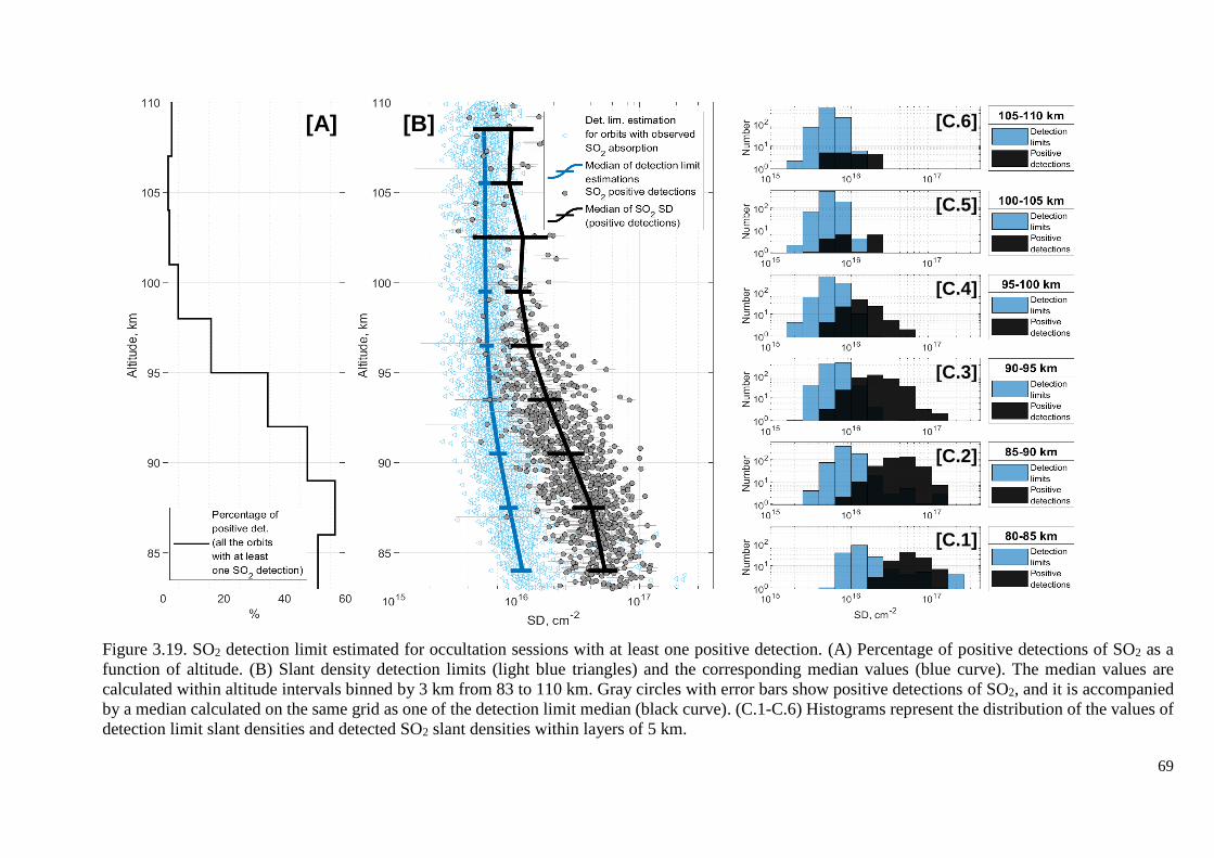
69

Figure 3.19. SO2 detection limit estimated for occultation sessions with at least one positive detection. (A) Percentage of positive detections of SO2 as a

function of altitude. (B) Slant density detection limits (light blue triangles) and the corresponding median values (blue curve). The median values are

calculated within altitude intervals binned by 3 km from 83 to 110 km. Gray circles with error bars show positive detections of SO2, and it is accompanied

by a median calculated on the same grid as one of the detection limit median (black curve). (C.1-C.6) Histograms represent the distribution of the values of

detection limit slant densities and detected SO2 slant densities within layers of 5 km.

[A] [B] [C.6]

[C.5]

[C.4]

[C.3]

[C.2]

[C.1]

70

3.2.6.3. Chlorine oxide absorption band

Figure 3.20. Ozone and chlorine oxide absorption cross-sections in the range 200-320 nm. Absorption

cross-sections for chlorine oxide are taken from Simon et al. (1990), and they were measured at 300K.

In addition to SO2, SO and O3, the range of the SPICAV UV spectrometer also covered the absorption

band of the chlorine oxide (ClO) molecule. This gas absorbs the UV radiation in the 240-300 nm

wavelength range, which overlaps the O3 Hartley band (Figure 3.20). However, the ClO absorbance is

twice weaker than that of O3.

Such overlapping of ClO and O3 absorption bands results in a strong correlation (exceeding 0.7) between

their slant densities if they are used simultaneously as free parameters in the numerical spectral inversion

problem. At the same time chlorine compounds should destroy the ozone molecules, so their anti-

correlation is expected from a chemical point of view. Thus, the retrieval of ClO slant density is always

performed after fixing O3 abundance. However, the attempts to discriminate ClO absorption using stellar

occultations were not successful.

A detection limit for ClO estimated with SPICAV spectra turned out to be on average 3-4 times higher

than the one for ozone. With an average detection limit for O3 is 3.3×1015 cm-2, the average detection

limit for ClO is estimated at 1016 cm-2. In terms of mixing ratio, it corresponds to ~30 ppbv at 85-90 km

and ~300 ppbv above 105 km. These values are determined mainly by the lower ClO absorbance. In

some observations a noise increase is observed at wavelengths longer than 280-300 nm, where the

sensitivity of the detector is lower. This also influences the ClO detection limit.

The estimated detection limit is at least 10 times higher than the recent ClO detection at 85 km in the

nightside mesosphere. The detection was made using the sub-millimetre ground based JCMT at λ~0.85

mm in 2010. The chlorine oxide abundance was measured in quantities of 3.7±0.9 and 1.5±0.5 ppbv in

October and November 2010 respectively (Sandor et al., 2018). Such a ClO absorption level

unfortunately would not be distinguishable in the SPICAV UV spectra. The experimental data was

71

examined for a presence of larger values, but the consideration of ClO in the atmospheric transmission

model did not improve χ2 more than 0.5%.

3.2.7. Vertical inversion problem

The previous formulas establish a relationship between transmission values and linear gas

concentrations. To compute the volume concentration, an algorithm called the «onion-peeling» method

(Figure 3.21) is implemented. The slant value is an integral of volume densities along the LOS through

the atmosphere. To compute it numerically, the atmosphere is assumed as consisting of spherically

symmetric homogeneous layers. Inside each layer, the value of the gas volume concentration ng (cm-3)

is assumed constant. Then the slant concentration Ng is equal to the sum over all layers of the products

of the volume concentration (𝑛𝑗𝑔

) by the path of the LOS of the device inside the layer (Δli). Taking into

account the error ε(z), Ng is:

𝑁𝑔(𝑧) = ∑ 𝑛𝑖𝑔Δ𝑙𝑖 + 휀(𝑧)

∞

𝑧𝑖=𝑧

(2.16)

Figure 3.21. Scheme of dividing the atmosphere into spherically symmetric layers when performing

vertical inversion by the «onion-peeling» method.

In matrix form, the slant concentration profile is expressed from the volume profile through the Abel

matrix [A]

𝑁 = [𝐴] ∙ 𝐷 + 휀 (2.17)

whose elements are equal to the LOS path in the layer j, which is characterized by the height of the target

point zj, when observing the height zi, and zmax j and zmin j are the maximum and minimum heights of layer

j, and RVenus is the radius of Venus.

𝐴𝑖𝑗 = 2(√(𝑧𝑚𝑎𝑥 𝑗 + 𝑅𝑉𝑒𝑛𝑢𝑠)2− (𝑧𝑖 + 𝑅𝑉𝑒𝑛𝑢𝑠)2 + √(𝑧𝑚𝑖𝑛 𝑗 + 𝑅𝑉𝑒𝑛𝑢𝑠)

2− (𝑧𝑖 + 𝑅𝑉𝑒𝑛𝑢𝑠)2) (2.18)

72

Then the volume density profile is

𝐷 = [𝐾] ∙ 𝑁 (2.19)

[𝐾] = ([𝐴]𝑇[𝐶𝑁]−1[𝐴])−1 ∙ ([𝐴]𝑇[𝐶𝑁]

−1) (2.20)

where [CN] is the covariance matrix for the slant density profile, i.e. a diagonal matrix. The elements of

its diagonal are the squared errors of the concentration values. The covariance matrix of the volume

concentration, in this case, is equal to:

[𝐶𝐷] = [𝐾][𝐶𝑁][𝐾]𝑇 = ([𝐴]𝑇[𝐶𝑁]

−1[𝐴])−1 (2.21)

In practice, there is an altitude limit above which the instrument is no longer sensitive and is unable to

characterize the mass of gases lying above this limit. Therefore, the presented formula is modified to

include this unknown part in the Abel matrix operand where it is represented by an additional parameter

ACh - the Chapman factor (Sekera, 1968).

𝐴𝑖𝑗 𝑚𝑎𝑥 = 𝐴𝐶ℎ = √2𝜋(𝑧𝑚𝑎𝑥 + 𝑅𝑉𝑒𝑛𝑢𝑠)𝐻 (2.22)

𝐻 =𝑅𝑇

𝜇𝐺 (2.23)

where RVenus is the radius of Venus, H is the scale height of the outer atmosphere, R is the universal gas

constant, T is the assumed temperature, μ is the molar mass of the atmosphere, G is the gravitational

constant at the altitude zmax.

The inversion problem is ill-posed, that means the unstable solution. So the direct computation of the

Equation 2.19 in most cases would increase noise or biases of the slant density profile. The smoothness

of the result requires a modification of the basic inverse problem to make it pseudo-inverse. The

Tikhonov regularization method is one of the instruments (Tikhonov and Arsenin, 1977; Twomey, 1977)

and it is used in the analysis (Quemerais et al., 2006). Following this method, [K] becomes

[𝐾] = ([𝐴]𝑇[𝐶𝑁]−1[𝐴] + 𝜆𝑠[𝐿]

𝑇[𝐿])−1 ∙ ([𝐴]𝑇[𝐶𝑁]−1) (2.24)

[𝐿] =1

ℎ2

(

−110

1−21

01−2

⋯000

………

000

⋮ ⋱ ⋮000

………

000

⋯−210

1−21

01−1)

(2.25)

The additional parameter of λS[L]T[L] is responsible for the regularisation. The matrix [L] represents an

operator of the second derivative with the h as a difference of altitude of the layers. The smoothness of

the method is defined by the λS. A large value of this coefficient leads to the vertical resolution

degradation since more neighbour layers are involved to derive a local density at the particular altitude.

Determination of the correct regularization parameter is puzzling. The analysis of this question was done

for the stellar occultations on Mars by Quemerais et al. (2006). It is proposed to tie a value of λS(z) ~

1/σD(z)2 where σD(z) is an estimated error of the local density at altitude z. This assumption allows the

release of an iteration scheme for the density profile retrieval. The first iteration is an inversion of a slant

73

density profile by Equation 2.19 and an estimation of σD(z) based on Equation 2.21. Then a

corresponding value of λS(z) = λ0/σD(z)2 is computed to perform the next iteration by the regulazing

scheme of Equation 2.19 with the operator in Equation 2.24. It was obtained that the scheme converges

in less than 10 iterations. In the current analysis 5 iterations perform a good converging of the problem.

3.2.8. Calibration influence on the spectral inversion

The accuracy of the results obtained for determining the gas concentration in a stellar occultation

experiment can be significantly affected by systematic errors appearing during the calibration step of the

raw data. The uncertainties under consideration are mainly related to two aspects:

1. Wavelength-to-pixel registration;

2. Stray light estimation.

Transmission spectra can be modelled by the Beer-Lambert law whose parameters are wavelength-

dependent. An accurate wavelength-to-pixel registration is therefore a prerequisite to the fitting process.

The wavelength shift Δλ is estimated for every observation can be a source of both underestimation and

overestimation of the obtained concentrations. For example, consider the error in the retrieved Δλ shift

equal to the width of one pixel, 0.54 nm, and investigate the effect on the resulting values of the slant

density of CO2 for observation #1269A03. So, the error of the final slant density of carbon dioxide

reaches 20% for the deeper layers of the mesosphere (Figure 3.22). As a side note, gas concentration is

traditionally normalized by the CO2 concentration to produce volume mixing ratios (VMR). Therefore,

such metrics will inevitably be impacted on both parts of the ratio and amplify the adverse effect of a

shift estimation error.

Figure 3.22. The difference in the percentage of slant CO2 concentration values at different altitudes

obtained from the same observation #1269A03 using two different wavelength-to-pixel assignments.

The ratio is calculated relative to the CO2 profile obtained from spectra calibrated using the accurate

stellar line alignment. (A) Negative offset for one pixel wide (-0.54 nm) is applied to the «reference»

calibration. (B) A positive offset of one-pixel width (0.54 nm) is applied.

The wavelength calibration based on aligning with the stellar catalogue was preferred over another

algorithm for wavelength calibration which is based on the alignment of the CO2 absorption band

position (Figure 3.23) in the atmospheric transmission spectra. This has been described in details in

Quemerais et al. (2006) for the atmosphere of Mars at altitudes where pressure is comparable to the

Venus upper mesosphere. The shape of the CO2 absorption band in the range of 120–170 nm is observed

74

by SPICAV UV at altitudes from 120 to 140 km. At lower altitudes, increased CO2 density ends up in

the band saturation, which makes the application of such wavelength calibration method useless.

The Venus Express spacecraft had a very elongated elliptical orbit around the planet. The difference in

altitude between the exposures of each spectrum was determined by the distance of the spacecraft from

the target point. This altitude step could reach 8 km and only 3-4 spectra per observation session can be

used for the wavelength to pixel allignment based on the CO2 absorption band. This statistical limitation

provides an inaccuracy in determining Δλ comparable to the width of one pixel, which could significantly

distort the resulting vertical profiles of the studying gases, as it is shown above. On the contrary, in the

other approach from tens to hundreds of measurements were used to perform the calibration, and then

the obtained Δλ values were averaged. It reduced the uncertainty in determining the wavelength by at

least 10 times to values of 1-10% of the pixel width. As well, the possible Δλ change with altitude was

examined and it was found that for a particular orbit Δλ remains stable with altitude.

Figure 3.23. Wavelength-to-pixel assignment obtained for observation session #3098A02. (A)

Transmission spectrum (black solid line) with corresponding error bars measured by SPICAV UV

(TSPICAV) at an altitude of 133.43 km which demonstrates the shape of the CO2 absorption band. The

synthesized spectrum (green solid line) of the CO2 absorption (TCO2) for the appropriate wavelength

calibration.

The error in retrieved gas concentrations along the LOS was also affected by the accuracy of the stray

light estimation. Systematic errors in the retrieved profiles of atmospheric components, caused by

overestimation or underestimation of the transmission when extracting the illumination, can be

significant. They are comparable to the effect of wavelength-to-pixel assignment error. One assumes

that the stray light is on average overestimated by 0.5%, which corresponds to an underestimation of the

atmospheric transmission. Then three different spectral ranges that define the absorption of each of the

three test gases are considered:

1. CO2 absorption band;

2. emission range of NO, which coincides with the absorption band of SO2;

3. and the Hartley absorption band of O3.

75

In Figure 3.24 the estimated deviations from a nominal value are shown. The slant density of СО2 does

not change significantly for altitudes where the absorption band of СО2 is unsaturated (Figure 3.24A).

However, the deviation from the original profile is almost 100% when the relative values of trace gases

SO2 and O3 are considered (Figure 3.24B and 3.26C).

Figure 3.24. Effect of underestimating transmission level on the resulting profiles of CO2 slant density

(A) and mixing ratios (VMR) of SO2 (B) and O3 (C) as a function of altitude.

This study demonstrates the importance of accurate separation the atmospheric transmission and

emission spectra. Various studies have suggested two different approaches for removing stray light.

These two approaches are based on the imaging capabilities of the SPICAV spectrometer since the

targeted stellar signal and the UV emission one are distributed differently on the detector. The methods

separately described by Royer et al. (2010), Piccialli et al. (2015) and Belyaev, Evdokimova et al. (2017)

was analysed in detail to determine the most efficient algorithm.

3.2.9. Stray light elimination technique

A package of five spectra corresponding to the five bins (Figure 1.16, Section 1.6.1), which are recorded

during one exposure of the detector, are summed from the superposition of the star image and the

additional illumination spread over the CCD. The star is a point source and its image at every wavelength

on the detector is determined by the instrumental PSF function. The stray light is scattered similarly over

all the detector; however, its extended nature makes its signal distribution over the detector being more

homogeneous than the stellar one. The superposition of all signals for each bin (SiSPICAV) can be

represented as follows:

𝑆𝑖𝑆𝑃𝐼𝐶𝐴𝑉(𝜆) = 𝛼𝑖𝑆

𝑟𝑒𝑓(𝜆)𝑇(𝜆) + 𝑆𝑖𝑆𝑇𝑅𝐿(𝜆), 𝑖 = 1…5 (2.26)

where 𝑆𝑖𝑆𝑇𝑅𝐿 is the component describing the part of the stray light that fell into the i bin, αi is the fraction

by the PSF in this bin, Sref is the spectrum of the star multiplied by the atmospheric transmission (T).

Nominally, the star is focused on the central or 3rd bin, and 90% of its signal is contained there. Extended

sources illuminate the entire CCD and they are also characterized by a slower temporal variability in

comparison with the evolution of the stellar signal. These two factors were used in two algorithms to

76

separate the stray light in the stellar occultation data. Both methods make it possible to subtract the

emission spectrum from the spectra of stars based on the signal in non-central bins that contains the

wings of the PSF distribution of the star image. However, their accuracy was examined considering the

differences between these algorithms. Further on in this research these methods will conventionally

reffered as «Method #1» and «Method #2», implying respectively the method described in Royer et al.

(2010) and Picciali et al. (2015), and the method presented in Belyaev, Evdokimova et al. (2017).

3.2.9.1. Method #1

The first method reviewed was presented in Royer et al. (2010) and in Picciali et al. (2015) in more

detail. The algorithm assumes that the stray light spectrum in the third bin (S3STRL) is a linear combination

of the scattered light spectra in other, non-central bins (SiSTRL, i≠3).

𝑆3𝑆𝑇𝑅𝐿(𝜆) = ∑ 𝑘𝑖𝑆𝑖

𝑆𝑇𝑅𝐿(𝜆)

𝑖=1,2,4,5

(2.27)

Accurate determination of the linear coefficients ki is the key to the correct subtraction of the emission

signal from the transmission spectra. They can be reliably estimated at altitudes where the atmosphere

becomes completely opaque for a star radiation. Usually, altitudes below 60 km are considered. For

these spectra, the resulting coefficients best describe the Equation 2.27, thus correspond to the minimum

of the following function χ2:

𝜒2 (𝑘1, 𝑘2, 𝑘4, 𝑘5) = ∑ ∑(𝑆3𝑆𝑇𝑅𝐿(𝜆) − ∑𝑘𝑖𝑆𝑖

𝑆𝑇𝑅𝐿(𝜆)

𝜎𝑆𝑇𝑅𝐿(𝜆))

2

𝜆

𝑧=60 𝑘𝑚

𝑧=−200 𝑘𝑚

(2.28)

where σSTRL (λ) - errors of experimental data measured below 60 km.

The resulting values are then used in the stellar occultation region (85-140 km) to determine the

atmospheric transmission spectra using the following formula, taking into account that the fraction of

the PSF distributed to the outer bins constitute only a few percent.

𝑇(𝜆, 𝑧) =𝑆3𝑆𝑃𝐼𝐶𝐴𝑉(𝜆, 𝑧) − ∑𝑘𝑖𝑆𝑖

𝑆𝑃𝐼𝐶𝐴𝑉(𝜆, 𝑧)

𝑆𝑟𝑒𝑓(𝜆) (2.29)

3.2.9.2. Method #2

The second method also aims to determine the fraction of stray light contained in the central (3rd)

spectrum. It was mentioned above that this bin usually collects about 90% of the stellar signal, and the

1st and 5th bins correspond to only 1-3% (Figure 1.16, Section 1.6.1). Therefore, it is possible to calculate

the template stray light spectrum (𝑆𝑡𝑒𝑚𝑝𝑙𝑎𝑡𝑒𝑆𝑇𝑅𝐿 ) by averaging the spectra of the 1st and 5th bins.

𝑆𝑡𝑒𝑚𝑝𝑙𝑎𝑡𝑒𝑆𝑇𝑅𝐿 (𝜆) =

1

2(𝑆1

𝑆𝑃𝐼𝐶𝐴𝑉(𝜆) + 𝑆5𝑆𝑃𝐼𝐶𝐴𝑉(𝜆)) (2.30)

This template can be included in the spectral inversion problem for each measurement within the studied

altitude range. Then the χ2-function describing the approximation of experimental spectra by the model

77

(Equation 2.31) will depend on the additional free parameter k which scales the intensity of the template

spectrum in order to avoid an overestimation of the atmospheric transmission model:

𝜒2 (𝑘, 𝑁𝑔, 𝜏𝛼) =∑(𝑆3𝑆𝑃𝐶𝐴𝑉(𝜆) − [𝑇𝑀𝑂𝐷𝐸𝐿(𝜆, 𝑁𝑔, 𝜏𝛼) + 𝑘 ∙ 𝑆𝑡𝑒𝑚𝑝𝑙𝑎𝑡𝑒

𝑆𝑇𝑅𝐿 (𝜆)]

𝜎(𝜆))

2

𝜆

(2.31)

where σ(λ) is the 𝑆3𝑆𝑃𝐶𝐴𝑉(𝜆) spectrum error.

TMODEL is an atmospheric transmission model, which depends on the following parameters: slant gaseous

concentration Ng and aerosol optical thickness (τα) along the LOS. In this case, the atmospheric

transmission spectrum is calculated by the formula:

𝑇(𝜆, 𝑧) =𝑆3𝑆𝑃𝐼𝐶𝐴𝑉(𝜆, 𝑧) − 𝑘 ∙ 𝑆𝑡𝑒𝑚𝑝𝑙𝑎𝑡𝑒

𝑆𝑇𝑅𝐿 (𝜆, 𝑧)

𝑆𝑟𝑒𝑓(𝜆) (2.32)

3.2.9.3. Comparison of methods

Both methods determine the stray light pattern and thus show similar results. Each orbit, when the

SPICAV UV spectrometer has successfully observed stellar transmission, was processed by two ways

to study their accuracy. An example of correct processing by both algorithms is shown in Figure 3.25,

where in the initial data contains a strong illumination from the atmospheric NO airglow at wavelengths

of 200-250 nm. This signal significantly distorts the transmission values.

Atmospheric transmission decreases from 1 to 0 as the instrument’s LOS moves down into denser layers

of the atmosphere. The CO2 absorption band quickly saturates and the atmospheric transmittance goes

to zero below 120 km at wavelengths shorter than 150 nm. At altitudes above 115 km and wavelengths

longward of 180 nm, absorption by small gaseous components and aerosols is negligible, and the

spectrum remains equal to 1.

Considering this altitude dependence, the resulting atmospheric transmission spectra were studied in

three different spectral intervals of the SPICAV UV range corresponding to absorption bands of three

studied molecules:

(1) the absorption band of CO2 (130-150 nm),

(2) one of the SO2 band (200-230 nm),

(3) one of the O3 band (250-270 nm).

In Section 3.2.8 the impact on concentration retrievals from a transmission uncertainty was explored for

the same spectral ranges. The considered absorption band of SO2 is particularly interesting since it

corresponds to the peak of the nitric oxide emission.

78

Figure 3.25. Altitude dependence of the transmission spectra for orbit #3071A02. (A) Raw data; (B) data

processed by method 1; (C) data processed by Method #2, and (D) the difference between the results of

applying each method. The latter demonstrates an insufficient evaluation of NO emission by Method #2.

[A]

[B]

[C]

[D]

79

The results of applying both methods are compared in the following way. For each resulting atmospheric

transmission spectrum, three values are calculated averaging over each spectral interval. A set of mean

transmission altitude profiles is obtained. The uncertainties in each of the two methods cause some

statistical dispersion around the expected transmittance: 0 (Figure 3.26.1A and 3.26.2A) or 1 (Figure

3.27.1A and 3.27.2A; Figs 3.28.1A and 3.28.2A). In most cases, both methods lead to nearly the same

results. After applying each of the methods, we will consider the general statistics on the average

transmission values for each spectral interval and the corresponding altitude range. The transmission in

the 130-150 nm range is zero below 120 km, and it is equal to one in the 200-230 nm and 250-270 nm

ranges above 115 km. The uncertainties of the two methods cause some statistical dispersion around the

expected values, i.e. zero or one.

As a result, for each investigated spectral range, we obtain a pair of statistical distributions of the average

transmission, which can be conveniently expressed in terms of probability density functions (PDF). In

the case of the most effective application of the method, the obtained distributions must strictly

correspond to the PDF of the normal distribution. Therefore, for each histogram, the parameters µ (mean)

and σ (standard deviation) were calculated, corresponding to the optimal Gaussian distribution curve

(Table 3.2).

Table 3.2. Distribution parameters.

Method #1 Method #2

CO2 absorption band

(Figure 3.26 1B and 2B)

µ0 = (69.5 ± 0.2) e-05

σ0 = 0.0020 ± 3.1e-06

µ0 = (8.2 ± 0.7) e-05

σ0 = 0.0021 ± 1.1e-05

µ1 = 0.0049 ± 2.2e-05

σ1 = 0.0106 ±1.7e-05

µ1 = 0.0054 ± 1.4e-05

σ1 = 0.0095 ±1.5e-05

NO emission band

(Figure 3.27 1B and 2B)

µ0 = 0.9989 ± 0.0003

σ0 = 0.0087 ± 0.0002

µ0 = 1.0009 ± 0.0003

σ0 = 0.0085 ± 0.0002

O3 absorption band

(Figure 3.28 1B and 2B)

µ0 = 0.9823 ± 0.0005

σ0 = 0.0156 ± 0.0003

µ0 = 0.9829 ± 0.0006

σ0 = 0.0180 ± 0.0004

The CO2 absorption band range (Figure 3.26) is most conveniently used to evaluate the effectiveness of

methods. Carbon dioxide in the mesosphere partially or completely absorbs UV light at the wavelengths

of its absorption band, which ultimately leads to a transmission of zero. Thus, any deviations seen on

the histograms are solely due to method errors (Figure 3.26 1A and 2A). It is seen that the usual Gaussian

function does not correspond to the obtained distribution. For the best description of the data obtained,

it was necessary to use a bimodal normal distribution. Bimodality is most evident in the statistical

distribution of the results of Method #2 (Figure 3.26 2B). Thus, the modes of the obtained distribution

are characterized by µ0 ≅ 0 and µ1 = 0.0054. The results of Method #1 are also better described with

the addition of the second mode to the normal distribution with respect to 0, but the bimodality is much

less pronounced and is used only to describe the tail of the distribution (Figure 3.26 1B).

80

Figure 3.26. 1A and 2A. Transmission profiles obtained by Method #1 and Method #2, respectively,

averaged over the CO2 absorption band range (130-150 nm). Distributions of these values are plotted

within 120–140 km. The points that are used to build histograms correspond to the selected areas of the

transmission profiles. 1B and 2B. Histograms are plotted in terms of the probability density function

(PDF) for each sample. The black dashed line shows the Gaussian model that describes each distribution

in the best way and that is characterized by the parameters presented in Table 3.2.

In the intervals corresponding to the maximum of NO emission (Figure 3.27) and the ozone absorption

band (Figure 3.28), the obtained statistical distributions are in good agreement with the Gaussian law.

The range 200-230 nm is characterized by an average transmittance µ0 close to 1, which fully

corresponds to expectations (Figure 3.27 1B and 2B). The resulting bias is covered by this experimental

uncertainty. Transmittance deviations from 1 can also be associated with variations in atmospheric

absorbers in addition to inaccurate estimates of the illumination component.

81

Figure 3.27. 1A and 2A. The transmission profiles obtained by Method #1 and Method #2, respectively,

averaged in the range of the maximum emission of NO (200-230 nm) and the absorption band of SO2.

Distributions of these values are plotted within 85–115 km. The points that are used to build histograms

correspond to the selected areas of the transmission profiles. 1B and 2B. Histograms are plotted in terms

of the probability density function for each sample. The black dashed line shows the best Gaussian model

that describes each distribution and is characterized by the parameters in Table 3.2.

For the Hartley absorption band, Method #2 also demonstrates the deviation of the resulting transmission

distribution from normal (Figure 3.28). It should also be noted that the values of µ0 for both methods in

this spectral range are slightly less than 1. This may be due to the noisiness of the atmospheric

transmission spectra, which increases in this range due to (1) a decrease in the star signal, (2) an increase

in the backlight signal, or (3) the presence of ignored illumination in the reference spectrum of the star.

However, these inaccuracies are the same for both methods and do not affect their results.

82

Figure 3.28. 1A and 2A. Transmission profiles obtained by Method #1 and Method #2, respectively,

averaged over the O3 absorption band range (250-270 nm). Distributions of these values are plotted

within 85–115 km. The points that are used to build histograms correspond to the selected areas of the

transmission profiles. 1B and 2B. Histograms are plotted in terms of the probability density function for

each sample. The black dashed line shows the Gaussian model that best describes each distribution,

which is characterized by the parameters presented in Table 3.2.

3.2.9.4. Atmospheric transmission and error bars estimation.

For the current task, Method #1 is the best. It is chosen in a calibration phase of the signal. However,

each spectrum was evaluated for residual illumination in the region of the spectrum where full absorption

of incoming star light is achieved. Thus, in this region the mean value should be 0.

Atmospheric transmission spectra are evaluated by Equation 2.29. The resulting error bars of a particular

transmission are defined by uncertainties of the initial stellar spectrum, the reference stellar spectrum

and a stray light composite error. The stray light error bars include the uncertainties of obtained 4 spectra

in non-central bins and an error of k-coefficients estimated by the Levenberg-Marquardt optimisation

algorithm.

3.2.10. Altitude assignment

Raw data transmitted to Earth also require calculation of geometric parameters of observation. Knowing

the exact time of each measurement and the coordinates and orientation of the spacecraft in space, all

necessary parameters are calculated. For observations in tangential geometry such parameters are, first

83

of all, the parameters of the target point: altitude, its geographical coordinates (latitude and longitude),

local time, solar-zenith angle. Also parameters of the spacecraft position, as the distance from the planet,

phase angle between the observer and the sun, etc. All these values have already been calculated for

each spectrum package used in this work. Detailed information about them can be found on the official

ESA archive.

Figure 3.29. Scheme of a star focus shift in stellar occultation mode with respect to the center of the 3rd

bin on the CCD. Its influence on determining altitude of the target point.

For the solar occultation mode and when observing spread emission sources on the planet’s limb, all

parameters for the device’s LOS and target point are calculated relative to the LOS corresponding to the

centre of each of the 5 bins on the matrix. The 5 respective spectra in these observations averages a

signal of the entire FOV of one bin. However, the situation is different in stellar occultation mode. A

point source as a star has a precise localization in the spectrometer FOV. Thus, all geometrical

parameters of the target point are unambiguously linked to the LOS directed to a star. From 4 to 32 rows

of pixels are summed up in each bin on the matrix in this mode. The star is focused on the third bin, but

not necessarily to its centre, which is observed in the resulting spectra packets. Thus, the difference in

target point altitude (dz in Figure 3.29) computed to the LOS from the centre of the 3rd bin and the LOS

directed to the star may differ by 5 km or more. Parameters are very different depending on a position

of the device in the planet’s orbit. The observations in the pericenter have the smallest FOV on the planet

limb, but are made with a large step between spectra. When the spacecraft is distant, its FOV increases,

but it becomes possible to scan the planet’s limb in more detail. However, the spacecraft is moving away

from the planet, the possible difference in parameters assignment increases if the star focus is shifted

from the centre of the bin. Therefore, in the stellar occultation mode, the geometric parameters are

supplemented with the values calculated with respect to the LOS directed to the point source. These are

the parameters used in this analysis.

84

3.3. Summary

The stellar occultation experiment is a powerful technique to measure the detailed vertical distributions

of gases and aerosols in the night-time mesosphere of Venus. The SPICAV UV spectrometer (118-320

nm) was able to identify and quantify the absorption of CO2, SO2 and O3 molecules in the range covered

by SPICAV.

Stellar spectra obtained by SPICAV were processed in two steps. In a first step, the raw dataset was

calibrated using an updated calibration protocol, which minimizes impacts of systematic errors. The

protocol features in particular:

‒ An improved pixel-to-wavelength assignment based on aligning stellar spectra measured by

SPICAV with a reference taken from the IUE observations, whereas it used to be aligned with

CO2 spectral features between 110 and 160 nm.

‒ An efficient way to eliminate «stray light» from observed spectra. This removal relies on an

algorithm where the stray light pattern is estimated based on a linear combination of the spectra

collected from those matrix lines where no stellar signal is observed.

This updated calibration allowed the regeneration of the full SPICAV dataset of atmospheric

transmission spectra.

The second step concerns the spectral inversion problem, which has been developed to find optimal

parameters needed to fit calibrated atmospheric transmissions with a forward model including detailed

spectroscopy of all target gases, as well as a representative instrumental function. Slant density of the

trace gases (SO2 and O3) integrated along the LOS is sometimes too small to produce a firm detection

by SPICAV UV. For this reason, a specific approach was developed to establish detection limits for O3

and SO2. On average, these limits are found to be

‒ NSO2 = 5.8±0.2 1015 cm-2;

‒ NO3 = 3.3±0.1 10 15 cm-2.

A ClO absorption band is also present in the spectral range covered by the SPICAV UV channel.

However, attempts to detect it proved unsuccessful. The detection limit of ClO is 3-4 times higher than

the one for ozone, that is on the order of 1016 cm-2.

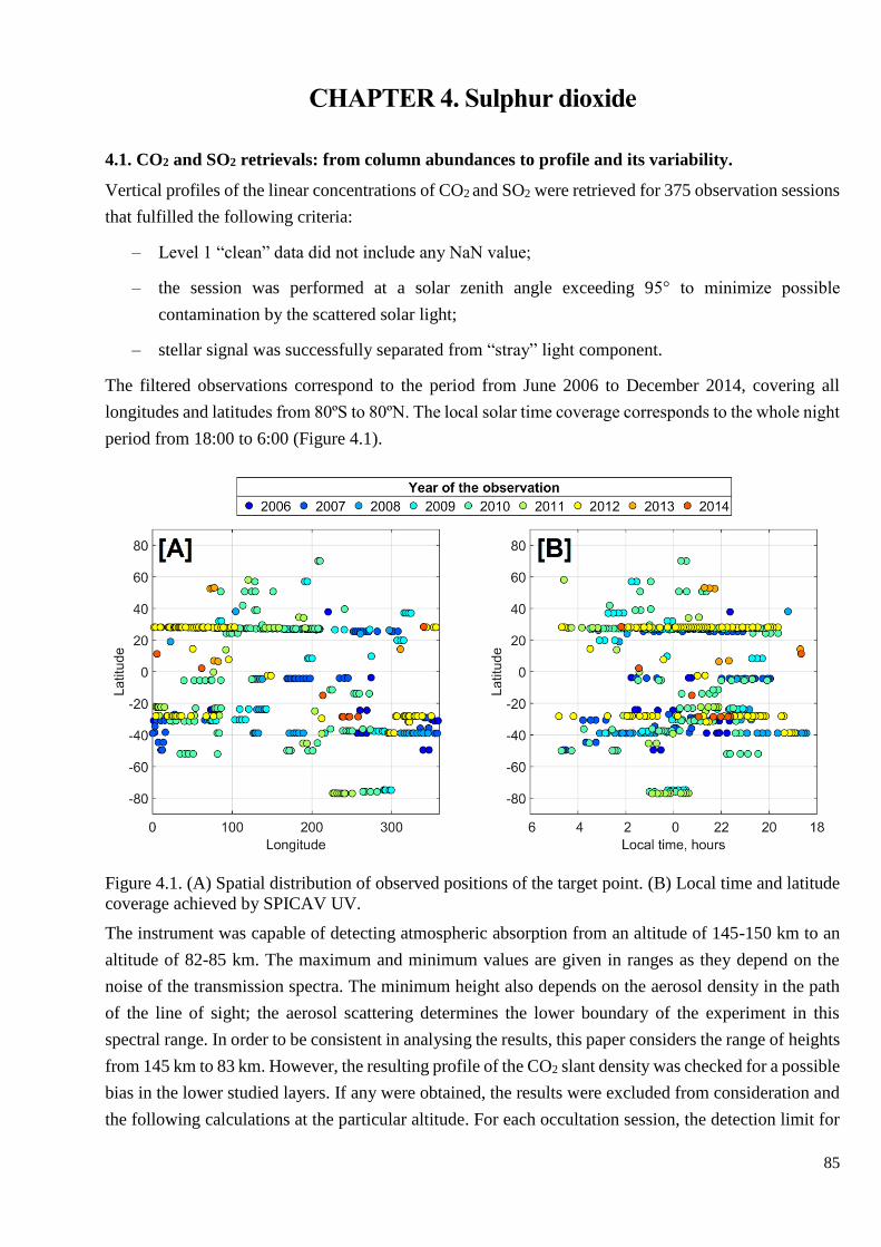
85

CHAPTER 4. Sulphur dioxide

4.1. CO2 and SO2 retrievals: from column abundances to profile and its variability.

Vertical profiles of the linear concentrations of CO2 and SO2 were retrieved for 375 observation sessions

that fulfilled the following criteria:

‒ Level 1 “clean” data did not include any NaN value;

‒ the session was performed at a solar zenith angle exceeding 95° to minimize possible

contamination by the scattered solar light;

‒ stellar signal was successfully separated from “stray” light component.

The filtered observations correspond to the period from June 2006 to December 2014, covering all

longitudes and latitudes from 80ºS to 80ºN. The local solar time coverage corresponds to the whole night

period from 18:00 to 6:00 (Figure 4.1).

Figure 4.1. (A) Spatial distribution of observed positions of the target point. (B) Local time and latitude

coverage achieved by SPICAV UV.

The instrument was capable of detecting atmospheric absorption from an altitude of 145-150 km to an

altitude of 82-85 km. The maximum and minimum values are given in ranges as they depend on the

noise of the transmission spectra. The minimum height also depends on the aerosol density in the path

of the line of sight; the aerosol scattering determines the lower boundary of the experiment in this

spectral range. In order to be consistent in analysing the results, this paper considers the range of heights

from 145 km to 83 km. However, the resulting profile of the CO2 slant density was checked for a possible

bias in the lower studied layers. If any were obtained, the results were excluded from consideration and

the following calculations at the particular altitude. For each occultation session, the detection limit for

86

sulphur dioxide was also calculated in the range up to 110 km. In Annex 1 there are the obtained profiles

of the linear concentrations of CO2 and SO2 and the SO2 detection limit if the gas is not detected for each

individual session (Figure A1.1)

Vertical profiles of the volume concentrations of CO2 and SO2 were sequentially retrieved by the «onion-

peeling» algorithm. In stellar occultations by SPICAV UV, the values are obtained with height steps

from ~1 km to ~8 km, which are inversely proportional to the distance of the spacecraft to the target

point. For sparse profiles containing just a few points the inverse problem of volume concentration

computation is calculated directly. When achieving a good altitude coverage, the “onion-peeling”

method is implemented with the Tikhonov’s regularization. However, the SO2 local densities are

retrieved with the regularization if the gas was detected in more than 4 spectra of a particular

observational session.

4.1.1. Carbon dioxide distribution in the upper mesosphere and the lower thermosphere.

Figure 4.2. Individual profiles of the CO2 local density accompanied by the median values estimated per

1 km. The median profile (wine red curve) is shown with the standard deviation within each layer. The

dotted line corresponds to the VIRA database (Zasova et al., 2006; Seiff, 1985).

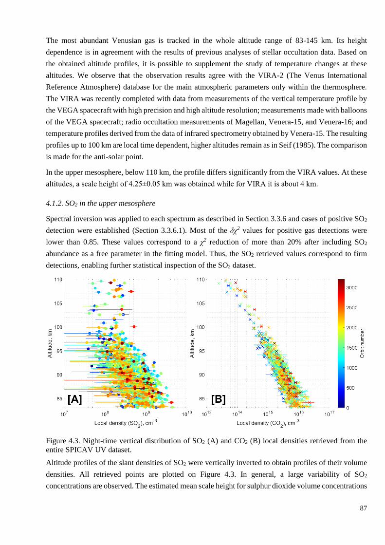
87

The most abundant Venusian gas is tracked in the whole altitude range of 83-145 km. Its height

dependence is in agreement with the results of previous analyses of stellar occultation data. Based on

the obtained altitude profiles, it is possible to supplement the study of temperature changes at these

altitudes. We observe that the observation results agree with the VIRA-2 (The Venus International

Reference Atmosphere) database for the main atmospheric parameters only within the thermosphere.

The VIRA was recently completed with data from measurements of the vertical temperature profile by

the VEGA spacecraft with high precision and high altitude resolution; measurements made with balloons

of the VEGA spacecraft; radio occultation measurements of Magellan, Venera-15, and Venera-16; and

temperature profiles derived from the data of infrared spectrometry obtained by Venera-15. The resulting

profiles up to 100 km are local time dependent, higher altitudes remain as in Seif (1985). The comparison

is made for the anti-solar point.

In the upper mesosphere, below 110 km, the profile differs significantly from the VIRA values. At these

altitudes, a scale height of 4.25±0.05 km was obtained while for VIRA it is about 4 km.

4.1.2. SO2 in the upper mesosphere

Spectral inversion was applied to each spectrum as described in Section 3.3.6 and cases of positive SO2

detection were established (Section 3.3.6.1). Most of the δχ2 values for positive gas detections were

lower than 0.85. These values correspond to a χ2 reduction of more than 20% after including SO2

abundance as a free parameter in the fitting model. Thus, the SO2 retrieved values correspond to firm

detections, enabling further statistical inspection of the SO2 dataset.

Figure 4.3. Night-time vertical distribution of SO2 (A) and CO2 (B) local densities retrieved from the

entire SPICAV UV dataset.

Altitude profiles of the slant densities of SO2 were vertically inverted to obtain profiles of their volume

densities. All retrieved points are plotted on Figure 4.3. In general, a large variability of SO2

concentrations are observed. The estimated mean scale height for sulphur dioxide volume concentrations

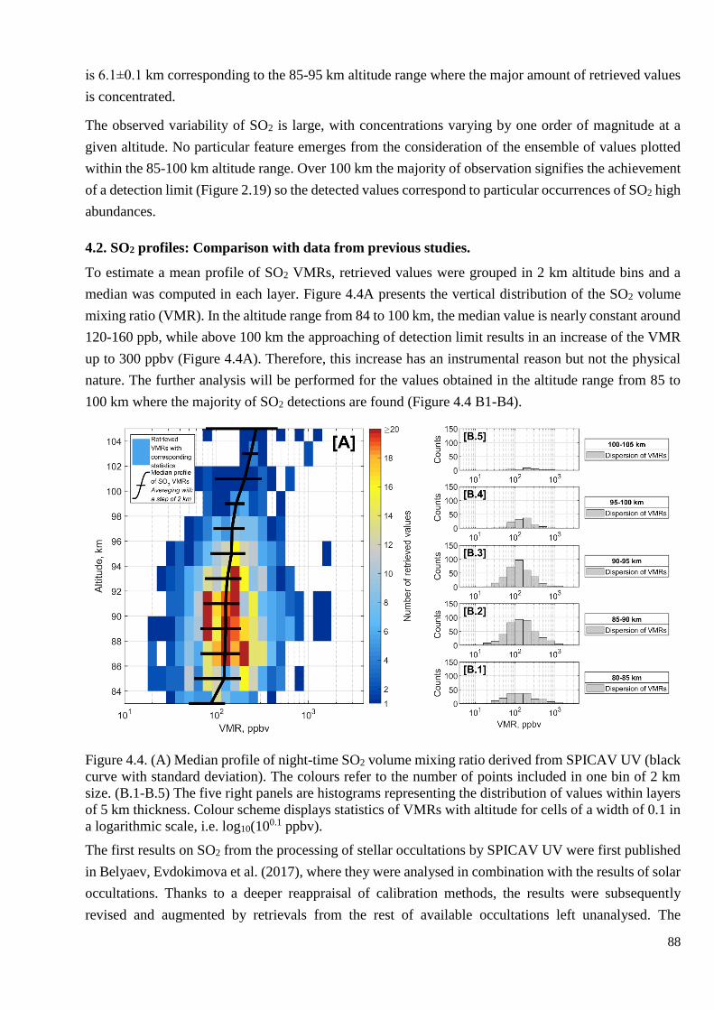
88

is 6.1±0.1 km corresponding to the 85-95 km altitude range where the major amount of retrieved values

is concentrated.

The observed variability of SO2 is large, with concentrations varying by one order of magnitude at a

given altitude. No particular feature emerges from the consideration of the ensemble of values plotted

within the 85-100 km altitude range. Over 100 km the majority of observation signifies the achievement

of a detection limit (Figure 2.19) so the detected values correspond to particular occurrences of SO2 high

abundances.

4.2. SO2 profiles: Comparison with data from previous studies.

To estimate a mean profile of SO2 VMRs, retrieved values were grouped in 2 km altitude bins and a

median was computed in each layer. Figure 4.4A presents the vertical distribution of the SO2 volume

mixing ratio (VMR). In the altitude range from 84 to 100 km, the median value is nearly constant around

120-160 ppb, while above 100 km the approaching of detection limit results in an increase of the VMR

up to 300 ppbv (Figure 4.4A). Therefore, this increase has an instrumental reason but not the physical

nature. The further analysis will be performed for the values obtained in the altitude range from 85 to

100 km where the majority of SO2 detections are found (Figure 4.4 B1-B4).

Figure 4.4. (A) Median profile of night-time SO2 volume mixing ratio derived from SPICAV UV (black

curve with standard deviation). The colours refer to the number of points included in one bin of 2 km

size. (B.1-B.5) The five right panels are histograms representing the distribution of values within layers

of 5 km thickness. Colour scheme displays statistics of VMRs with altitude for cells of a width of 0.1 in

a logarithmic scale, i.e. log10(100.1 ppbv).

The first results on SO2 from the processing of stellar occultations by SPICAV UV were first published

in Belyaev, Evdokimova et al. (2017), where they were analysed in combination with the results of solar

occultations. Thanks to a deeper reappraisal of calibration methods, the results were subsequently

revised and augmented by retrievals from the rest of available occultations left unanalysed. The

89

reanalysis led to the suppression of the previously reported SO2 VMR increase with altitude (Belyaev,

Evdokimova et al., 2017), where values were found to increase from 20±10 ppbv at 85-95 km to 200±100

ppbv at 100-105 km (Figure 4.3; Individual profiles for each session are presented in Annex 2, Figure

A1.2). In particular, retrieved CO2 abundances revealed themselves to be very sensitive to wavelength

calibration (Evdokimova et al., 2020), which eventually affected SO2 VMR determination, especially

below 115 km, where CO2 absorption saturates.

Figure 4.5. The overview of mean vertical profiles of SO2. The black dashed curve is the current work,

the blue one was obtained by Belyaev, Evdokimova et al. (2017) which did not include calibration

improvements.

There are two factors that caused the differences in the obtained values (Figure 4.5). Previously, the

analysis used the altitude assignment following the solar occultation scheme, i.e. the parameters were

considered based on the LOS from the centre of the 3rd bin. That resulted in shifted altitudes of the slant

density profiles of both species. In general, the spectral inversion problem does not depend on altitude

itself. However, the altitude determination is crucial for the vertical inversion computing local densities

of both species.

The second factor is a combination of two calibration methods investigated in Chapter 2. However, the

study of Belyaev, Evdokimova et al. (2017) also used a wavelength to pixel assignment based on stellar

lines. However, the 3 parameters of parabolic law were fitted instead of as in the current approach. The

limitation of a free parameters number is a necessary measure. The stellar lines are more pronounced in

the short-wavelength range that is limiting the accuracy of the second order parameter determination.

Thus, the difference of the wavelengths at the edge of the CO2 absorption band is about one-pixel width,

which is significant as it was displayed before (Section 3.2.8). The stray light elimination has changed

as well, however, it was concluded that it mainly impacted the statistics of good detections.

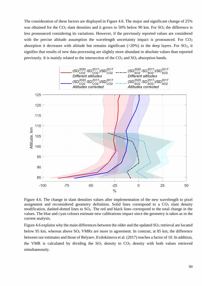
90

The consideration of these factors are displayed in Figure 4.6. The major and significant change of 25%

was obtained for the CO2 slant densities and it grows to 50% below 90 km. For SO2 the difference is

less pronounced considering its variations. However, if the previously reported values are considered

with the precise altitude assumption the wavelength uncertainty impact is pronounced. For CO2

absorption it decreases with altitude but remains significant (>20%) in the deep layers. For SO2, it

signifies that results of new data processing are slightly more abundant in absolute values than reported

previously. It is mainly related to the intersection of the CO2 and SO2 absorption bands.

Figure 4.6. The change in slant densities values after implementation of the new wavelength to pixel

assignment and reconsidered geometry definition. Solid lines correspond to a CO2 slant density

modification, dashed-dotted lines to SO2. The red and black lines correspond to the total change in the

values. The blue and cyan colours estimate new calibrations impact since the geometry is taken as in the

current analysis.

Figure 4.6 explains why the main differences between the older and the updated SO2 retrieval are located

below 95 km, whereas above SO2 VMRs are more in agreement. In contrast, at 85 km, the difference

between our estimates and those of Belyaev, Evdokimova et al. (2017) reaches a factor of 10. In addition,

the VMR is calculated by dividing the SO2 density to CO2 density with both values retrieved

simultaneously.

91

The obtained altitude profile of the SO2 VMR is the only such detailed scan obtained over clouds in

these altitude ranges on the night side. However, two ground based facilities were also able to detect

SO2 absorption at similar altitude ranges of the night and day sides. They are the James Clerk Maxwell

Telescope (JCMT) in several campaigns in 2004-2008 and the Atacama Large Millimeter/submillimeter

Array (ALMA) in 2011 (Sandor et al., 2010; Encrenaz et al., 2015). Both worked in the sub-millimeter

range. JCMT measured simultaneously two lines 346.652 and 346.524 GHz, and ALMA measured

346.652 GHz (~0.86 mm). These observations gave a result within 85-100 km and 88-100 km

respectively and they are compared with the SPICAV UV results.

On average, VMR is found to remain around 135±21 ppbv in the 85-100 km altitude range. This value

is at >2 times higher than the maximum VMR of 66±2 ppbv at 85-100 km reported by JCMT in Sandor

et al. (2010). A smaller value, 12±4 ppbv in the 88-100 km range was reported by Encrenaz et al. (2015)

using ALMA observations. Sandor et al. (2010) also showed that the SO2 abundance in the 85-100 km

range is much larger than in the 80-85 km range, suggesting the presence of a strong sink of SO2 below

85 km.

Figure 4.7. Overview of the SO2 vertical distributions obtained by different instruments above the

clouds. Curve styles and colours are given in the legend box. Vertical median profile of the SO2 VMR

obtained in this work (black triangles) is binned by 3 km. All the occultation results are presented with

a dispersion of ±1 σ.

Solar occultation by SPICAV UV provided the altitude profiles of SO2 VMR at the evening and morning

terminators at 85-105 km that completed the night side data coverage by local time. SO2 abundance

obtained in the SPICAV UV solar occultation increases significantly in the altitude range of 85-100 km

in comparison to the night observations. On average, measured SO2 volume mixing ratio changes with

altitude from 8-20 ppbv at 85-90 km to 50-180 ppbv at 100 km (Belyaev, Evdokimova et al., 2017).

92

However, in the latitude distribution, observed locations are concentrated in the north polar region while

the stellar occultations mainly observed mid-latitudes. So it may be suggested that the processes on poles

slightly differ from those in mid-latitudes. However, further study is needed to clarify the differences

between mean profiles of terminator and night side. The consideration of overall profile revealed by

ALMA observations (Encrenaz et al., 2015) are lower than the minimal values obtained at terminator.

The both considered ground based facilities report a high variability of SO2 VMR in the observed

regions. In different observations JCMT measurements reported variations of more than two orders of

magnitude. Moreover, in some sessions the gas was not detected that corresponds to its abundance in

particular case being lower than 2 ppb.

Sub-mm signal emanates from the superimposition of the thermal emission coming from different

altitudes. UV’s observations are probably less sensitive to temperature uncertainties compared to the

thermal IR, however, the temperature sensitivity in the UV was not studied. However, such a strong

difference between occultations and sub-millimetre (sub-mm) measurements could be partially related

to the temperature uncertainties which is a critical parameter of sub-mm data retrieval.

Below 83-85 km the atmosphere becomes too opaque for UV stellar occultation. The most of

measurements of occultations in UV was supported by the IR spectrometer SOIR (Mahieux et al., 2015)

on board Venus Express. It explored the altitude range from 65 to 85 km. Similar to SPICAV UV

occultations the vertical resolution of its observations is rather detailed. Since SOIR exclusively

performed in solar occultation mode by design, it allows one to examine also the terminator regions in

65-85 km. The solar occultation data obtained by SOIR benefits from simultaneous temperatures and

SO2 abundances measurements. The IR spectra concluded the SO2 abundance in the 65-85 km range

(Mahieux et al., 2015) with a minimum of 60 ppbv detected at 70-80 km. However, the observations are

followed by significant uncertainties, that are on average ~ 80%.

In theoretical description there is a lack of models particularly designed for the night atmosphere. The

only one mesospheric model was developed by Krasnopolsky (2010, 2013). In this model the lower

boundary is 80 km, where the SO2 abundant is set. The estimated altitude profile remains stable and

equal to 100 km. This result is in good correspondence with the average profile obtained in this study.

The diurnal averaged 1-D models by Zhang et al (2010), Zhang et al (2012) aimed to reproduce the

minimum of SO2 VMR at 70-80 km in mid-latitudinal and polar regions and Krasnopolsky (2012) are

also considered. From these models the result presented in Zhang et al (2012) is in correspondence with

both SPICAV UV stellar occultation and SOIR IR solar occultation results. The model represents the

diurnal average of SO2 at 75°N latitude. However, the processes in this altitude range (80-100 km)

require a 3-D model which would be able to reproduce a complex dynamic of the region.

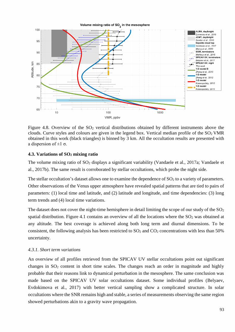
93

Figure 4.8. Overview of the SO2 vertical distributions obtained by different instruments above the

clouds. Curve styles and colours are given in the legend box. Vertical median profile of the SO2 VMR

obtained in this work (black triangles) is binned by 3 km. All the occultation results are presented with

a dispersion of ±1 σ.

4.3. Variations of SO2 mixing ratio

The volume mixing ratio of SO2 displays a significant variability (Vandaele et al., 2017a; Vandaele et

al., 2017b). The same result is corroborated by stellar occultations, which probe the night side.

The stellar occultation’s dataset allows one to examine the dependence of SO2 to a variety of parameters.

Other observations of the Venus upper atmosphere have revealed spatial patterns that are tied to pairs of

parameters: (1) local time and latitude, and (2) latitude and longitude, and time dependencies: (3) long

term trends and (4) local time variations.

The dataset does not cover the night-time hemisphere in detail limiting the scope of our study of the SO2

spatial distribution. Figure 4.1 contains an overview of all the locations where the SO2 was obtained at

any altitude. The best coverage is achieved along both long term and diurnal dimensions. To be

consistent, the following analysis has been restricted to SO2 and CO2 concentrations with less than 50%

uncertainty.

4.3.1. Short term variations

An overview of all profiles retrieved from the SPICAV UV stellar occultations point out significant

changes in SO2 content in short time scales. The changes reach an order in magnitude and highly

probable that their reasons link to dynamical perturbation in the mesosphere. The same conclusion was

made based on the SPICAV UV solar occultations dataset. Some individual profiles (Belyaev,

Evdokimova et al., 2017) with better vertical sampling show a complicated structure. In solar

occultations where the SNR remains high and stable, a series of measurements observing the same region

showed perturbations akin to a gravity wave propagation.

94

The four sets of sequential observations made at the same latitude and at similar local time were

considered. These sets also represent detected profiles of SO2 instead of individual detections. They

definitely reveal these turbulence effects. The gravity wave propagation may be expected as a plausible

cause for explaining similar features in particular profiles. Moreover, the wave structure is probably

detected in occultation #1683A03, while 48h before (occultation #1681A05) this pattern was not

detected. Our observations are inferior to solar observations in terms of resolution in height and noise

level. Therefore, for other sets of profiles, such disturbances can only be presumed.

Figure 4.9. Stellar occultations that are sequential in time obtaining retrieved SO2 volume density

profiles with a small vertical step. The observations of one set were made at one latitude and at similar

local times. More geographical parameters are presented in Annex 3.

4.3.2. Long term variations of SO2 mixing ratio.

Long-term variations were considered based on the retrieved SO2 content (Figure 4.10 A1 and A2). We

analysed annual variations of SO2 abundance grouping the values by 4 months’ intervals and deriving a

weighted mean (Equation A4.3 in Annex 4) for each interval. Short (<4-month) term variations are found

to be larger than the long-term variations. One can however distinguish two periods of higher VMR

values, before 2010 and after that, with a minimum located around 2010. A decrease to the end of the

mission (2014) can be also seen (Figure 4.10 A2).

The previously reported SO2 evolution at 90-95 km near the terminators showed several periods of VMR

increases accompanied by sharp decreases. However, a steady reduction during the entire mission period

was not reported (Figure 4.11).

95

Figure 4.10. A1 and A2: Weighted-mean SO2 VMR evolution with time for two altitude ranges: (1) 85-

90 km and (2) 90-95 km. The data are binned by 4 months. Red and white squares include ≥5 and <5

individual points respectively. Standard deviation from the mean of the bin is indicated by the black

vertical bar. The B panels represent the number of individual points for one bin. Black dashed lines in

the histograms correspond to the level of 5 points.

Figure 4.11. Long-term evolution of SO2 VMR within 90-95 km corresponds to a pressure level of ~ 0.1

mbar in a comparison with the values of a same altitude range retrieved at the terminator from solar

occultation spectra by SPICAV (Belyaev, Evdokimova et al., 2017).

96

The other long-term trend of SO2 is based on SPICAV UV nadir observations. In this geometry, the

instrument observes the vertically-integrated column density of SO2 over the cloud tops (~ 70 km). In

this set of observations, the SO2 short-term variations were also significant (as represented by the yellow

area on Figure 4.12). However, the median curve calculated on the full set of data shows a decrease of

SO2 VMR toward the end of the mission (Marcq et al., 2020) which is confirmed by UV observations

by STIS/HTS (Jessup et al., 2015) and IR observations by the TEXES instrument (Encrenaz et al., 2012;

Encrenaz et al., 2016). The 85-90 km range is the lower robust one provided by stellar occultations. In

general, the similarities in behaviour of trends at different altitudes are not obtained. The night

observations on average do not follow a specific pattern, and there are not pronounced maxima or

minima as observed on the day side. Moreover, the stellar occultation data do not have enough coverage

to confirm or deny the behaviour around the second local minimum observed in 2014 in nadir.

Figure 4.12. Long-term evolution of SO2 VMR within 85-90 km compared with daytime values derived

from nadir monitoring and converted into a mixing ratio at an altitude of ~70 km (cloud top) from

SPICAV UV spectra (Marcq et al., 2020). Also shown are the TEXES IR observations of Encrenaz et

al., 2012; Encrenaz et al. (2016) and the HST/STIS UV observations of Jessup et al. (2015).

4.3.3. Diurnal variations of SO2

The whole dataset was explored to identify any hint of a diurnal variability in SO2 VMR. The data was

split by 30 minutes’ intervals. The weighted mean (Equation A4.3 in Annex 4) was calculated within

each bin. We selected two 5-km thick layers where retrieved values are more numerous (see Figure 4.4

B.2- 4.3 B.3). The analysis considers the number of points constituting the average values in each bin

which are represented by histograms below the distribution (Figure 4.13 B.1-4.12 B.2). There is a slight

VMR increase from 02:00 AM toward the evening terminator in the 90-95 km range: from 90±40 ppbv

at 2h to 115±25 ppbv at 20h (Figure 4.13 A.2). On the other hand, we do not observe any monotonous

change in the 85-90 km range (Figure 4.13 A.1) in frames of the statistical dispersion.

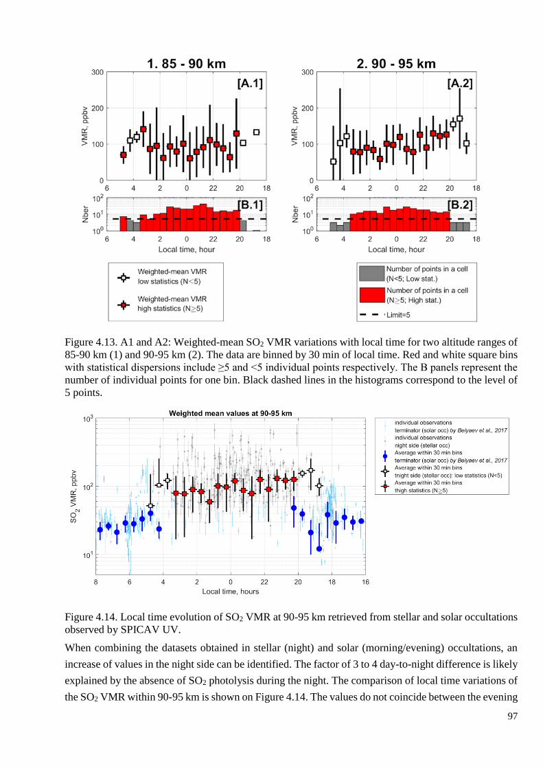
97

Figure 4.13. A1 and A2: Weighted-mean SO2 VMR variations with local time for two altitude ranges of

85-90 km (1) and 90-95 km (2). The data are binned by 30 min of local time. Red and white square bins

with statistical dispersions include ≥5 and <5 individual points respectively. The B panels represent the

number of individual points for one bin. Black dashed lines in the histograms correspond to the level of

5 points.

Figure 4.14. Local time evolution of SO2 VMR at 90-95 km retrieved from stellar and solar occultations

observed by SPICAV UV.

When combining the datasets obtained in stellar (night) and solar (morning/evening) occultations, an

increase of values in the night side can be identified. The factor of 3 to 4 day-to-night difference is likely

explained by the absence of SO2 photolysis during the night. The comparison of local time variations of

the SO2 VMR within 90-95 km is shown on Figure 4.14. The values do not coincide between the evening

98

and the morning regions. Nevertheless, points at 4:30-5:00 and at 18:30-19:00 correspond to the

expected decrease of SO2 VMR. Nevertheless, the data coverage of stellar occultation is poor around

4:00-6:00 and 18:00-20:00 due to increase of solar light contamination of spectra as is presented in

Figure 4.14 B.1-B.2 and it is preventing the firm conclusion about the divergence of results of stellar

and solar occultations. Moreover, solar occultations were mainly restricted to the latitudes poleward

80°N.

Figure 4.15. (A) Local time evolution of SO2 VMR depending on the altitude. The values are grouped

and averaged within a bin of 1h and 2 km. The bins combined with more or 5 values are considered. (B)

Corresponding number of points in a bin.

The studied altitude region of the upper mesosphere corresponds to the place of transition between two

global circulation regimes. The first is a fast zonal rotation below 70 km and the second is the SSAS.

Our dataset is too sparse to provide a detailed distribution of SO2 with local time, latitudes and altitudes,

but it is however possible to track the altitude versus local time dependence. To this end, we mapped

data over a grid of ½ h increment in time and 2 km increment in altitude. For each bin, a weighted-mean

value was calculated (Figure 4.15A). Below 88 km, SO2 is distributed rather fuzzily and any local time

dependence is not concluded. The pattern is changing between 88 and 96 km. There is a constant

decrease of VMR from evening terminator to 2H00 at night where a minimum is observed. The

maximum values are observed between 20H00 and 22H00 at night and the minimum values are observed

around 2H00 at night. Moreover, the values are growing with altitude keeping the same pattern.

Such behaviour is puzzling. It should be noted that a similar asymmetry was recently deduced from a

study of the Venusian atmospheric circulation in the 90-110 km range based on tracking the oxygen

emission features (Gorinov et al., 2018). Velocities of two opposite flows in zonal directions from

evening and morning terminators towards midnight reach zero values around 22H30±00H30. This

asymmetry in the zonal flow should affect the chemical species involved in the SO2 photochemistry,

such as chlorinated species and oxygen atoms.

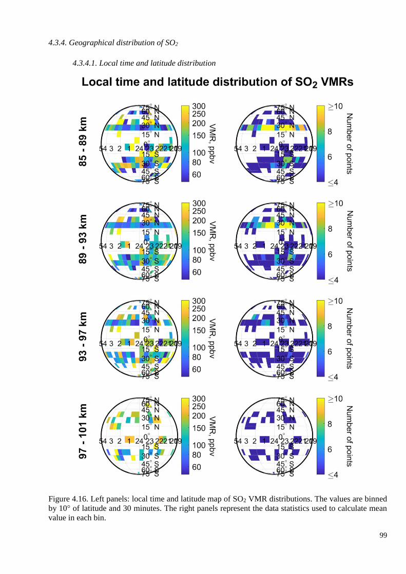
99

4.3.4. Geographical distribution of SO2

4.3.4.1. Local time and latitude distribution

Figure 4.16. Left panels: local time and latitude map of SO2 VMR distributions. The values are binned

by 10° of latitude and 30 minutes. The right panels represent the data statistics used to calculate mean

value in each bin.

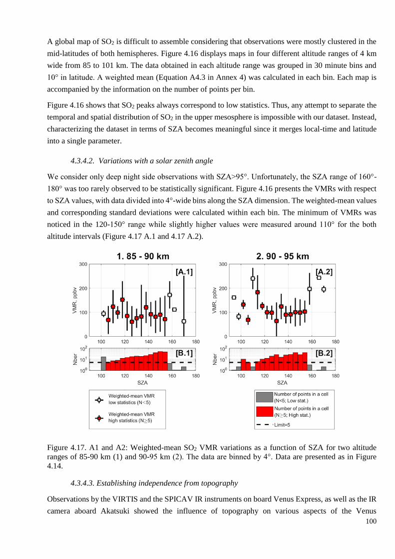
100

A global map of SO2 is difficult to assemble considering that observations were mostly clustered in the

mid-latitudes of both hemispheres. Figure 4.16 displays maps in four different altitude ranges of 4 km

wide from 85 to 101 km. The data obtained in each altitude range was grouped in 30 minute bins and

10° in latitude. A weighted mean (Equation A4.3 in Annex 4) was calculated in each bin. Each map is

accompanied by the information on the number of points per bin.

Figure 4.16 shows that SO2 peaks always correspond to low statistics. Thus, any attempt to separate the

temporal and spatial distribution of SO2 in the upper mesosphere is impossible with our dataset. Instead,

characterizing the dataset in terms of SZA becomes meaningful since it merges local-time and latitude

into a single parameter.

4.3.4.2. Variations with a solar zenith angle

We consider only deep night side observations with SZA>95°. Unfortunately, the SZA range of 160°-

180° was too rarely observed to be statistically significant. Figure 4.16 presents the VMRs with respect

to SZA values, with data divided into 4°-wide bins along the SZA dimension. The weighted-mean values

and corresponding standard deviations were calculated within each bin. The minimum of VMRs was

noticed in the 120-150° range while slightly higher values were measured around 110° for the both

altitude intervals (Figure 4.17 A.1 and 4.17 A.2).

Figure 4.17. A1 and A2: Weighted-mean SO2 VMR variations as a function of SZA for two altitude

ranges of 85-90 km (1) and 90-95 km (2). The data are binned by 4°. Data are presented as in Figure

4.14.

4.3.4.3. Establishing independence from topography

Observations by the VIRTIS and the SPICAV IR instruments on board Venus Express, as well as the IR

camera aboard Akatsuki showed the influence of topography on various aspects of the Venus

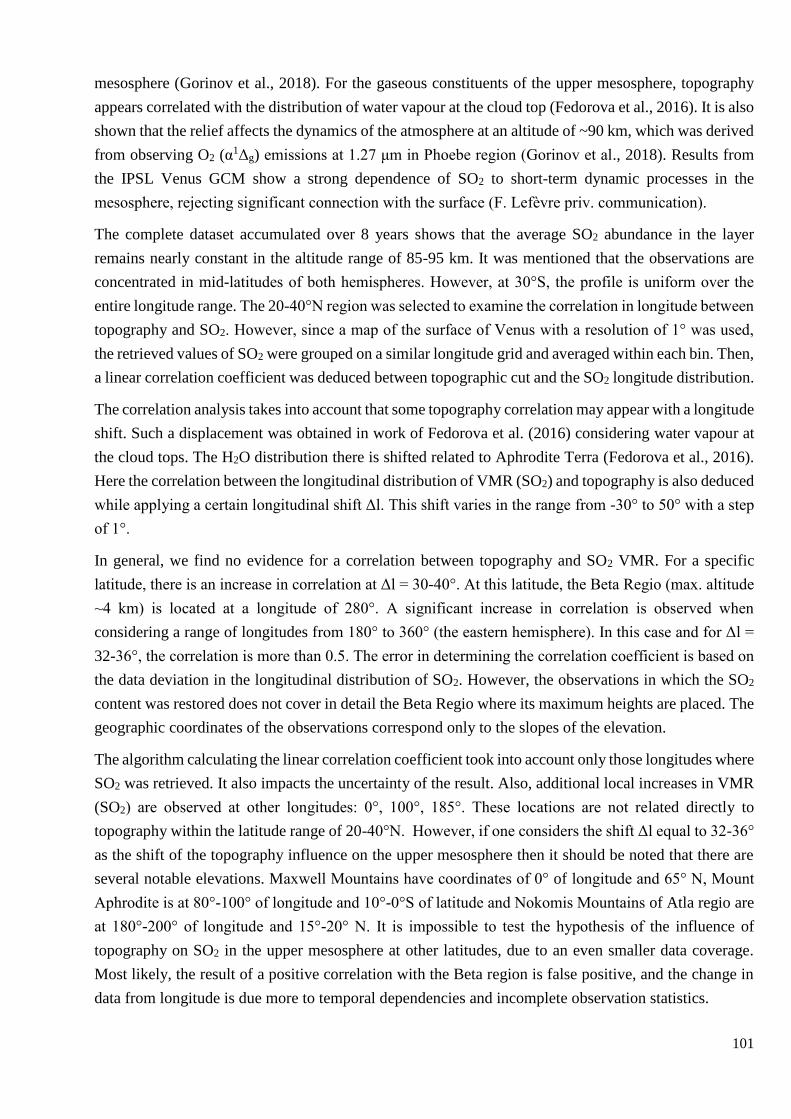
101

mesosphere (Gorinov et al., 2018). For the gaseous constituents of the upper mesosphere, topography

appears correlated with the distribution of water vapour at the cloud top (Fedorova et al., 2016). It is also

shown that the relief affects the dynamics of the atmosphere at an altitude of ~90 km, which was derived

from observing O2 (α1Δg) emissions at 1.27 μm in Phoebe region (Gorinov et al., 2018). Results from

the IPSL Venus GCM show a strong dependence of SO2 to short-term dynamic processes in the

mesosphere, rejecting significant connection with the surface (F. Lefèvre priv. communication).

The complete dataset accumulated over 8 years shows that the average SO2 abundance in the layer

remains nearly constant in the altitude range of 85-95 km. It was mentioned that the observations are

concentrated in mid-latitudes of both hemispheres. However, at 30°S, the profile is uniform over the

entire longitude range. The 20-40°N region was selected to examine the correlation in longitude between

topography and SO2. However, since a map of the surface of Venus with a resolution of 1° was used,

the retrieved values of SO2 were grouped on a similar longitude grid and averaged within each bin. Then,

a linear correlation coefficient was deduced between topographic cut and the SO2 longitude distribution.

The correlation analysis takes into account that some topography correlation may appear with a longitude

shift. Such a displacement was obtained in work of Fedorova et al. (2016) considering water vapour at

the cloud tops. The H2O distribution there is shifted related to Aphrodite Terra (Fedorova et al., 2016).

Here the correlation between the longitudinal distribution of VMR (SO2) and topography is also deduced

while applying a certain longitudinal shift Δl. This shift varies in the range from -30° to 50° with a step

of 1°.

In general, we find no evidence for a correlation between topography and SO2 VMR. For a specific

latitude, there is an increase in correlation at Δl = 30-40°. At this latitude, the Beta Regio (max. altitude

~4 km) is located at a longitude of 280°. A significant increase in correlation is observed when

considering a range of longitudes from 180° to 360° (the eastern hemisphere). In this case and for Δl =

32-36°, the correlation is more than 0.5. The error in determining the correlation coefficient is based on

the data deviation in the longitudinal distribution of SO2. However, the observations in which the SO2

content was restored does not cover in detail the Beta Regio where its maximum heights are placed. The

geographic coordinates of the observations correspond only to the slopes of the elevation.

The algorithm calculating the linear correlation coefficient took into account only those longitudes where

SO2 was retrieved. It also impacts the uncertainty of the result. Also, additional local increases in VMR

(SO2) are observed at other longitudes: 0°, 100°, 185°. These locations are not related directly to

topography within the latitude range of 20-40°N. However, if one considers the shift Δl equal to 32-36°

as the shift of the topography influence on the upper mesosphere then it should be noted that there are

several notable elevations. Maxwell Mountains have coordinates of 0° of longitude and 65° N, Mount

Aphrodite is at 80°-100° of longitude and 10°-0°S of latitude and Nokomis Mountains of Atla regio are

at 180°-200° of longitude and 15°-20° N. It is impossible to test the hypothesis of the influence of

topography on SO2 in the upper mesosphere at other latitudes, due to an even smaller data coverage.

Most likely, the result of a positive correlation with the Beta region is false positive, and the change in

data from longitude is due more to temporal dependencies and incomplete observation statistics.

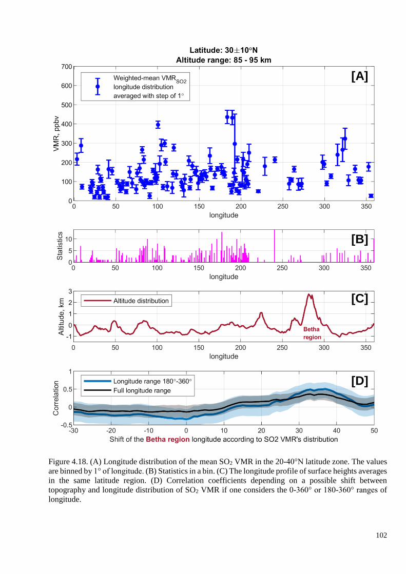
102

Figure 4.18. (A) Longitude distribution of the mean SO2 VMR in the 20-40°N latitude zone. The values

are binned by 1° of longitude. (B) Statistics in a bin. (C) The longitude profile of surface heights averages

in the same latitude region. (D) Correlation coefficients depending on a possible shift between

topography and longitude distribution of SO2 VMR if one considers the 0-360° or 180-360° ranges of

longitude.

[A]

[B]

[C]

[D]

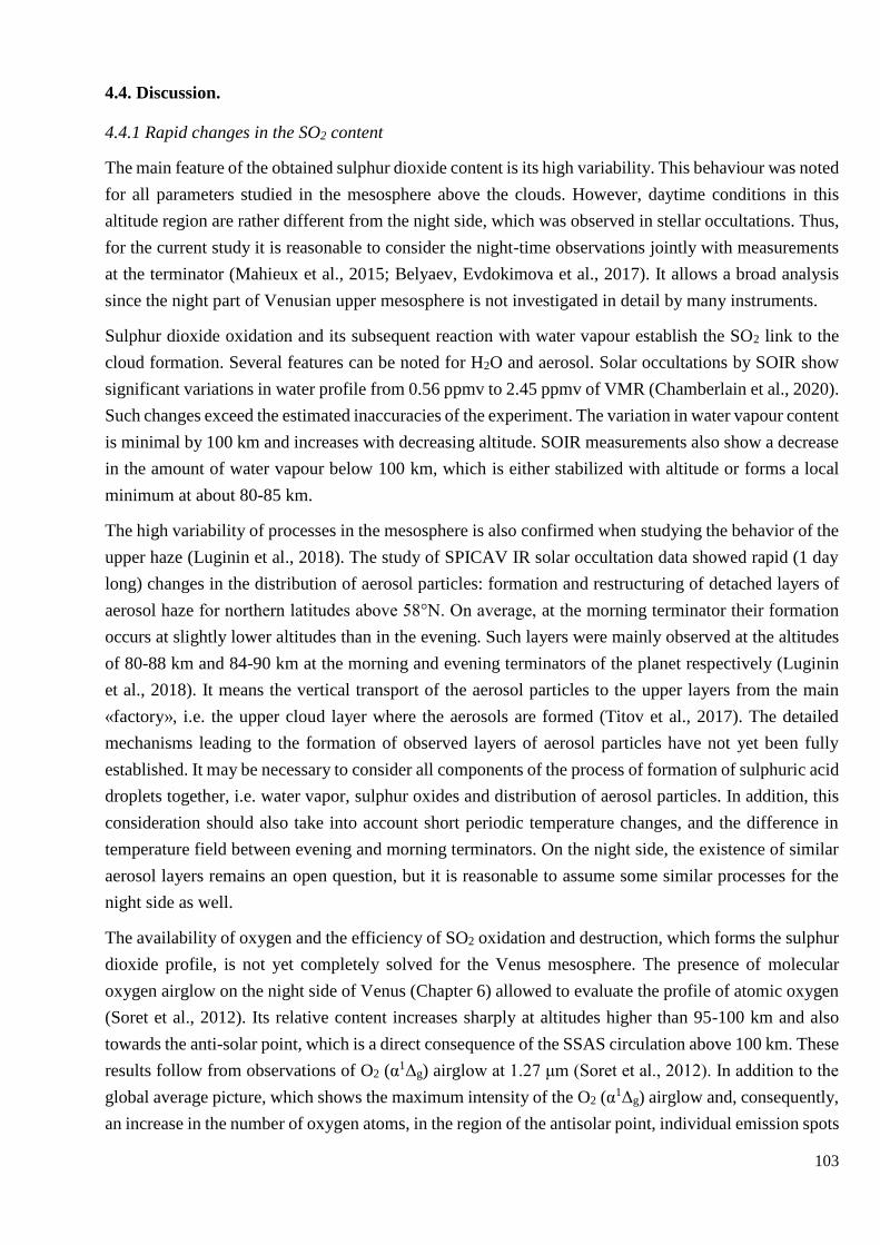
103

4.4. Discussion.

4.4.1 Rapid changes in the SO2 content

The main feature of the obtained sulphur dioxide content is its high variability. This behaviour was noted

for all parameters studied in the mesosphere above the clouds. However, daytime conditions in this

altitude region are rather different from the night side, which was observed in stellar occultations. Thus,

for the current study it is reasonable to consider the night-time observations jointly with measurements

at the terminator (Mahieux et al., 2015; Belyaev, Evdokimova et al., 2017). It allows a broad analysis

since the night part of Venusian upper mesosphere is not investigated in detail by many instruments.

Sulphur dioxide oxidation and its subsequent reaction with water vapour establish the SO2 link to the

cloud formation. Several features can be noted for H2O and aerosol. Solar occultations by SOIR show

significant variations in water profile from 0.56 ppmv to 2.45 ppmv of VMR (Chamberlain et al., 2020).

Such changes exceed the estimated inaccuracies of the experiment. The variation in water vapour content

is minimal by 100 km and increases with decreasing altitude. SOIR measurements also show a decrease

in the amount of water vapour below 100 km, which is either stabilized with altitude or forms a local

minimum at about 80-85 km.

The high variability of processes in the mesosphere is also confirmed when studying the behavior of the

upper haze (Luginin et al., 2018). The study of SPICAV IR solar occultation data showed rapid (1 day

long) changes in the distribution of aerosol particles: formation and restructuring of detached layers of

aerosol haze for northern latitudes above 58°N. On average, at the morning terminator their formation

occurs at slightly lower altitudes than in the evening. Such layers were mainly observed at the altitudes

of 80-88 km and 84-90 km at the morning and evening terminators of the planet respectively (Luginin

et al., 2018). It means the vertical transport of the aerosol particles to the upper layers from the main

«factory», i.e. the upper cloud layer where the aerosols are formed (Titov et al., 2017). The detailed

mechanisms leading to the formation of observed layers of aerosol particles have not yet been fully

established. It may be necessary to consider all components of the process of formation of sulphuric acid

droplets together, i.e. water vapor, sulphur oxides and distribution of aerosol particles. In addition, this

consideration should also take into account short periodic temperature changes, and the difference in

temperature field between evening and morning terminators. On the night side, the existence of similar

aerosol layers remains an open question, but it is reasonable to assume some similar processes for the

night side as well.

The availability of oxygen and the efficiency of SO2 oxidation and destruction, which forms the sulphur

dioxide profile, is not yet completely solved for the Venus mesosphere. The presence of molecular

oxygen airglow on the night side of Venus (Chapter 6) allowed to evaluate the profile of atomic oxygen

(Soret et al., 2012). Its relative content increases sharply at altitudes higher than 95-100 km and also

towards the anti-solar point, which is a direct consequence of the SSAS circulation above 100 km. These

results follow from observations of O2 (α1Δg) airglow at 1.27 μm (Soret et al., 2012). In addition to the

global average picture, which shows the maximum intensity of the O2 (α1Δg) airglow and, consequently,

an increase in the number of oxygen atoms, in the region of the antisolar point, individual emission spots

104

rapidly change over time (Soret et al., 2014). The dependence of the mean profile of atomic oxygen

explains the significant reduction of sulphur dioxide in photochemical models above 100 km. Moreover,

the photochemical models assume an additional source of sulphur in the upper mesosphere, such as S8

to correctly describe the increase in relative sulphur dioxide content theoretically (Zhang et al., 2012).

However, one-dimensional models are significantly limited when considering a dynamically active

region such as the upper mesosphere. They cannot reproduce the short-term effects of perturbations in

processes of the vertical or horizontal airmass transport.

4.4.2. Global patterns in the SO2 behaviour

First of all, it is necessary to consider the global temporal variation in sulphur dioxide content.

Observations at the cloud tops level indicate a global downward trend over 40 years of observations.

However, it is impossible to trace a picture of the time dependence in the period 1995-2006 (Figure 2.1,

Chapter 2), when no data was obtained. Nevertheless, the time dependence during the both epochs of

observations is a consecutive decrease of SO2 content accompanied by several maxima. This behaviour

was associated with possible injections of sulphur compounds into the lower atmosphere of Venus as a

result of volcanic eruptions, passive degassing and pyroclastic phenomena on the surface (Esposito et

al., 1984). The subsequent vertical transport of matter should distribute volcanic gases into the upper

atmosphere, which forms a local increase of SO2 content on the time scale. In the case of possible

explosive eruptions, the transport of matter to the upper layers can be directly caused by this

phenomenon, as shown by the simulation of possible Venusian activity (Airey et al., 2015). The

observation of surface temperature showed a hot spot, i.e. a possible candidate for a volcanic eruption

in June 2008 (Shalygin et al., 2015). The discussion about the Venus activity is not closed yet, and at

the moment the only conclusion is that the set of observations considered in this work has not shown

clear evidence of sulphur dioxide injections into the upper mesosphere above 85 km. In contrast to the

observations at an altitude of 70 km on the day side, the long-term variations on the night side do not

show significant long-term temporal variations. Moreover, all observations of solar and stellar

occultations are consistent in such a conclusion. It should be noted, however, that nadir observations

(Marcq et al., 2013; Marcq et al., 2020) provide a much more detailed statistical coverage of time and

space than the occultation mode. The reason for the difference in global trends at different altitudes is

not completely understood. It migt be related to the difference in the observed areas, since the terminator

zone is also different from the day side. Besides it is possible that dynamic processes smooth out the

effect of short-term increases in the amount of sulphur dioxide for higher altitudes.

In general, an increase of sulphur dioxide content was obtained on the night side, in comparison with

terminators of the planet, at an altitude of 85-95 km. And the difference become more significant in the

lower observed altitudes. However, it is difficult to determine a certain dependence on local time based

on current data. Averaging over the entire period of observation shows a slight increase in content

towards the evening terminator. Such behaviour is puzzling. It should be noticed that a similar

asymmetry was recently deduced from a study of the Venusian atmospheric circulation in the 90-110

km range based on tracking the oxygen emission features (Gorinov et al., 2018). It was shown that

velocities of two opposite zonal flows coming from evening and morning terminators towards midnight

105

reach zero values around 22.5±0.5 PM. This asymmetry in the zonal transport would affect chemical

species involved in SO2 photochemistry, such as chlorine species and oxygen atoms.

The dependence of sulphur dioxide on local solar time was only investigated using JCMT sub-mm

observations (Sandor et al., 2010). In absolute values, the results of this work and JCMT observations

are not consistent, however, they qualitatively confirm the increase in relative content on the night side.

Accumulation of sulphur dioxide occurs due to the exclusion of photolysis from the chain of

photochemical processes, which allows the rapid regeneration of SO2 from sulphur monoxide.

4.5. Summary

Vertical profiles of the linear concentrations of CO2 and SO2 were retrieved from 375 observations in

2006-2014. The mean scale heights for these gases were computed, and they are equal to 5.25±0.05 km

and 6.1±0.1 km respectively.

Based on the obtained CO2 and SO2 local density profiles, the volume mixing ratio of SO2 was

calculated. On average it remains around 135±21 ppbv in the range of 85-100 km. It is a correction of

the previously reported result by Belyaev, Evdokimova et al. (2017). The reason for such correction was

analysed. It is concluded that the used calibration methods mainly impact the CO2 local density values.

This also impacts the mixing ratios of trace gases.

Short-term variations of sulphur dioxide prevailed in the upper mesosphere. The difference in obtained

values of the SO2 VMR reaches one order in magnitude. On a long-term scale an annual trend is not

observed. The local time coverage allows the study SO2 changes in the interval from 19:00H to 5:00H

of the local time. There is a possible diurnal asymmetry in relation to midnight. It is noted that the SO2

VMR may be increasing from 2:00H to the evening terminator at an altitude range of 93-97 km. No

statistically significant conclusion about the longitudinal distribution of SO2 or possible correlation with

surface topography could be drawn from the dataset available.

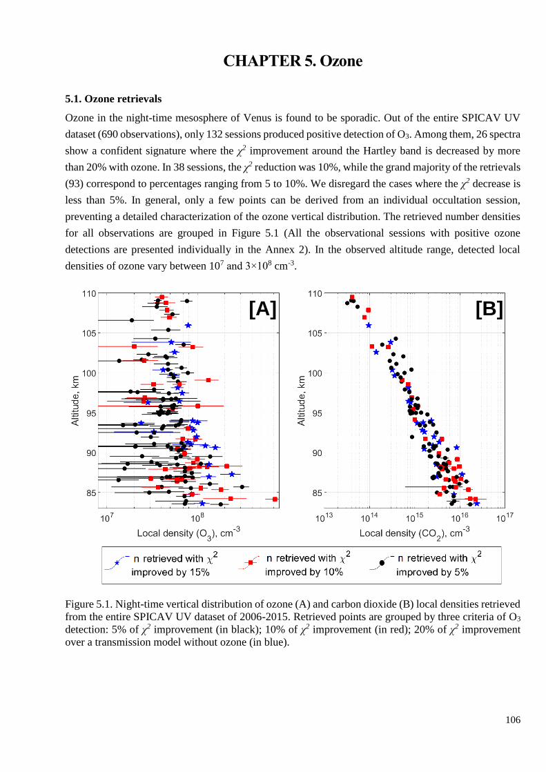
106

CHAPTER 5. Ozone

5.1. Ozone retrievals

Ozone in the night-time mesosphere of Venus is found to be sporadic. Out of the entire SPICAV UV

dataset (690 observations), only 132 sessions produced positive detection of O3. Among them, 26 spectra

show a confident signature where the χ2 improvement around the Hartley band is decreased by more

than 20% with ozone. In 38 sessions, the χ2 reduction was 10%, while the grand majority of the retrievals

(93) correspond to percentages ranging from 5 to 10%. We disregard the cases where the χ2 decrease is

less than 5%. In general, only a few points can be derived from an individual occultation session,

preventing a detailed characterization of the ozone vertical distribution. The retrieved number densities

for all observations are grouped in Figure 5.1 (All the observational sessions with positive ozone

detections are presented individually in the Annex 2). In the observed altitude range, detected local

densities of ozone vary between 107 and 3×108 cm-3.

Figure 5.1. Night-time vertical distribution of ozone (A) and carbon dioxide (B) local densities retrieved

from the entire SPICAV UV dataset of 2006-2015. Retrieved points are grouped by three criteria of O3

detection: 5% of χ2 improvement (in black); 10% of χ2 improvement (in red); 20% of χ2 improvement

over a transmission model without ozone (in blue).

[A] [B]

107

5.1.1. The main feature of the ozone positive detections

The majority of O3 positive detections based on the chosen criteria is characterized by a single detection

per profile. Assuming that the observations are done with a vertical step of 1-8 km, a single O3

occurrence is localized within an altitude interval which should be less than 10 km.

Analysing observations with finer vertical stepping indicates that ozone detection is usually surrounded

by non-detections (Figure 5.2A and 5.2B). It allows one to conclude that the experiment is only sensitive

to peak ozone abundances which are close to the detection limit, while the ozone occurrences themselves

are highly variable. Different observations also show an altitude shift of ozone peak within the observing

range of 85-110 km. Detections do not allow deriving information on the details of the ozone

distribution. Measured peaks only indicate how variable in altitude the peaks are.

Figure 5.2. Two examples of occultation sessions made with a different vertical step of ~1 km (A) and

~5 km (B). The occultation session #0600A10: December 11, 2007; at latitude 25.5°N and longitude

307.5°; local time 1.26 hours. The occultation session #0603A13: December 15, 2007; at latitude

29.0°S and longitude 346.7°; local time 23.29 hours.

However, there are also some evident detections isolated in the profile, suggesting the ozone layer is 1

km or less thick. In Fig. 5.3 there is an example of such detection where the ozone feature is also visible

in spectra, but the nearby altitudes are free from ozone absorption. This observation corresponds to no

stray light conditions.

[A] [B]

108

Figure 5.3. (A) An example of occultation session made with a vertical step of ~1 km and revealing

strictly localized ozone detection. The occultation session #1260A03: October 2, 2009; at latitude

26.9°N and longitude 197.8°; local time 0.23 hours. (B) A transmission spectrum with error bars (black

solid line) measured at 91.3 km that corresponds to ozone detection and the best atmospheric

transmission models: one neglects ozone absorption (red solid line) and the other includes ozone

absorption (green solid line).

The consideration of individual slant densities profiles suggests ozone exhibits very thin layers, perhaps

because ozone is produced out of an oxygen layer that is already thin and that further recombination

constrains ozone to be even thinner.

5.2. Ozone positive detections distribution

5.2.1. Average volume mixing ratio profile of ozone for established positive detections.

When all the positive detections observed for the whole altitude range, the mean volume mixing ratio of

ozone seems to continuously increase with altitude. The mean profile goes from 10 ppbv at 85 km to

600 ppbv at 108 km. The histograms (Figure 5.4 B1-5.4 B6) represent the dispersion of retrieved values

within a 5-km layer.

It should be noted that the detection limit in relative quantities also increases with altitude, but there are

no reliable VMR values of ozone exceeding 100 ppbv observed below 95 km.

[A]

[B]

109

Figure 5.4. (A) Vertical median profile of the night-time ozone volume mixing ratio derived from

SPICAV UV (the black curve with standard deviation). The color bar indicates the number of points

within one bin of 5 km size. B.1-B.6. The right six panels are histograms of values within the layers of

5 km thickness to represent the stability of the median VMR profile. The statistics is calculated for each

layer by binning the values with a step of 0.1 in a logarithmic scale, i.e. log10(100.1 ppbv).

5.2.2. Spatial variations of ozone positive detections

The detected values were split by 5 km from 83 to 108 km to estimate the spatial distribution of the

ozone bursts. All the individual detections are presented in Figure 5.5 within four studied layers. There

is no evident pattern of ozone distribution in space at night.

In general, it is expected that the behaviour of ozone is related to the SSAS circulation at altitudes around

~100 km. The SSAS transfers oxygen atoms to the night side, where they recombine, producing the

molecular oxygen (a1Δg) emission (Gerard et al., 2009) and leading to the formation of the O3 molecule.

The O2 airglow brightness increases towards the antisolar point and its vertical distribution demonstrates

a maximum at 96±2 km. SSAS also transfers OH and Cl radicals that are likely involved in t destroying

O3 (Yung and DeMore, 1999; Krasnopolsky, 2013) and make the ozone horizontal distribution not as

uniform as O2, actually concentrating the sink region of O3 around the antisolar region where O2

emission is observed to be more intense. This should reduce the ozone amount towards midnight at the

equator within the same layer.

Occultations concentrate in the mid-latitudes, while the polar and equatorial regions, including the

antisolar point (24h), were observed rarely (Figure 4.1). However, conclusion about the space

110

distribution of ozone requires consideration of locations where this gas was not detected, which is

discussed in Section 5.3.

Figure 5.5. Local time and latitude distribution of observed locations where ozone was detected.

Altitudes are binned into 5 km intervals between 83 and 103 km. The colour bar represents the ozone

mixing ratios at a given location.

Detections found in the mid-northern latitudes (20-40°N) allow a deeper inspection of the ozone

dependence to local time (Figure 5.5). Here, the increase of the gas content with altitude is more

pronounced around midnight where minimal ozone VMRs below 93 km have been obtained. On the

other hand, at higher altitudes there is not any pattern (Figure 5.6). Furthermore, high VMRs prevail

towards the evening terminator within 83-93 km.

111

Figure 5.6. Local time variability of the ozone volume mixing ratio (ppbv) retrieved at the latitude zone

of 30±10°N where the biggest number of observations was obtained. Various colors represent different

altitude bins of 5 km thickness.

5.2.3. Temporal variations of ozone based on positive detections

Figure 5.7. Long-term variability of the ozone volume mixing ratio (ppbv) retrieved at the latitude zone

of 30±10°N. Various colors represent different altitude bins of 5 km thickness.

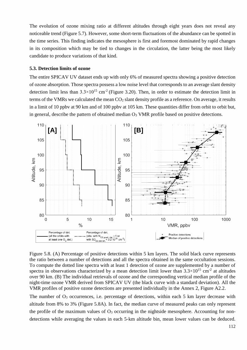
112

The evolution of ozone mixing ratio at different altitudes through eight years does not reveal any

noticeable trend (Figure 5.7). However, some short-term fluctuations of the abundance can be spotted in

the time series. This finding indicates the mesosphere is first and foremost dominated by rapid changes

in its composition which may be tied to changes in the circulation, the latter being the most likely

candidate to produce variations of that kind.

5.3. Detection limits of ozone

The entire SPICAV UV dataset ends up with only 6% of measured spectra showing a positive detection

of ozone absorption. Those spectra possess a low noise level that corresponds to an average slant density

detection limit less than 3.3×1015 cm-2 (Figure 3.20). Then, in order to estimate the detection limit in

terms of the VMRs we calculated the mean CO2 slant density profile as a reference. On average, it results

in a limit of 10 ppbv at 90 km and of 100 ppbv at 105 km. These quantities differ from orbit to orbit but,

in general, describe the pattern of obtained median O3 VMR profile based on positive detections.

Figure 5.8. (A) Percentage of positive detections within 5 km layers. The solid black curve represents

the ratio between a number of detections and all the spectra obtained in the same occultation sessions.

To compute the dotted line spectra with at least 1 detection of ozone are supplemented by a number of

spectra in observations characterized by a mean detection limit lower than 3.3×1015 cm-2 at altitudes

over 90 km. (B) The individual retrievals of ozone and the corresponding vertical median profile of the

night-time ozone VMR derived from SPICAV UV (the black curve with a standard deviation). All the

VMR profiles of positive ozone detections are presented individually in the Annex 2, Figure A2.2.

The number of O3 occurrences, i.e. percentage of detections, within each 5 km layer decrease with

altitude from 8% to 3% (Figure 5.8A). In fact, the median curve of measured peaks can only represent

the profile of the maximum values of O3 occurring in the nightside mesosphere. Accounting for non-

detections while averaging the values in each 5‐km altitude bin, mean lower values can be deduced.

[A] [B]

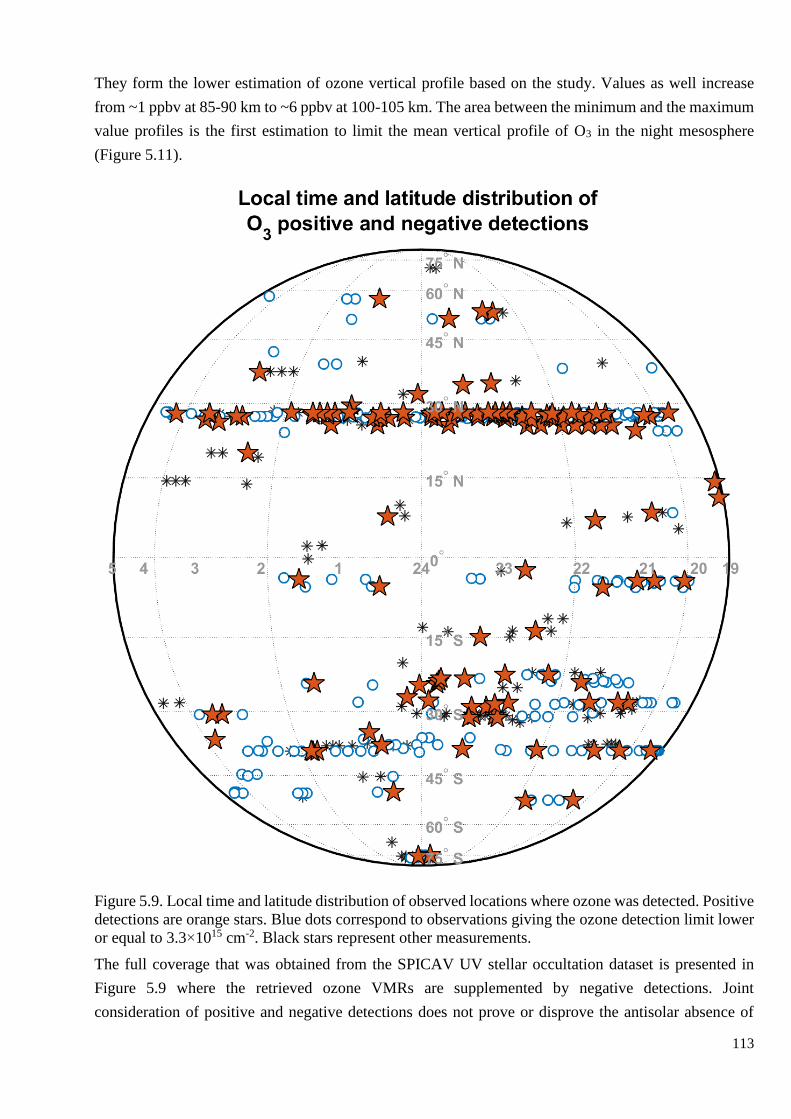
113

They form the lower estimation of ozone vertical profile based on the study. Values as well increase

from ~1 ppbv at 85-90 km to ~6 ppbv at 100-105 km. The area between the minimum and the maximum

value profiles is the first estimation to limit the mean vertical profile of O3 in the night mesosphere

(Figure 5.11).

Figure 5.9. Local time and latitude distribution of observed locations where ozone was detected. Positive

detections are orange stars. Blue dots correspond to observations giving the ozone detection limit lower

or equal to 3.3×1015 cm-2. Black stars represent other measurements.

The full coverage that was obtained from the SPICAV UV stellar occultation dataset is presented in

Figure 5.9 where the retrieved ozone VMRs are supplemented by negative detections. Joint

consideration of positive and negative detections does not prove or disprove the antisolar absence of

114

ozone. The coverage near the equator is anyway insufficient to allow any conclusion. Also, it is almost

impossible to identify a global local time or latitude pattern of O3 detection. However, an examination

of a percentage of positive detections at 20-40°N revealed a similar value for each hour from 3:00 to

21:00 accompanied by a high number of measurements (Figure 5.10). The presence of this curious local

time dependence (Figure 5.10) may be considered as a basis for future closer research, but for the

existing dataset, we can only note the obtained changes. Small statistics impede the formulation of

confident conclusions about any possible patterns.

Figure 5.10. (A) Percentage of positive detections in every hour in the latitude range of 20-40°N. The

ratio is computed based on spectra from observational sessions providing at least 1 detection of ozone

or the mean detection limit lower than 3.3×1015 cm-2 at altitudes over 90 km. (B) The number of such

spectra in every hour is shown by the dark red curve.

5.4. Review of possible correlations with other chemical compounds

The production of ozone is maintained in the upper atmosphere of Venus by the SSAS circulation at

~100 km (Yung and DeMore, 1999; Krasnopolsky, 2013). The main tracers of these dynamic processes

are airglows by oxygen (a1Δg), nitric oxide (NO) and hydroxyl (OH). The infrared oxygen airglow first

observed by Connes et al. (1979) at 1.27 μm is a result of radiative relaxation of the O2 (a1Δg) metastable

molecules to the ground state through the three-body process. Oxygen atoms supplying this process are

produced by the CO2 and CO photodissociation on the day side and then transferred to the night

atmosphere.

The line at 1.27 μm is the strongest emission of O2 and it has now been well documented on Venus. Its

maximum brightness is observed at 96±2 km and the general spatial distribution demonstrates a

significant increase in intensity towards the antisolar point (Gerard et al., 2012). It was observed with

the same result by the VIRTIS (Soret et al., 2012) and SPICAV IR (Evdokimova et al., 2019b) nadir

monitoring of the night side. Moreover, the O2 emission study allowed to reconstruct the oxygen atoms

distribution in the night mesosphere with a peak of O atom density (~2 1011 cm-3) at 100 km. It is then

followed by a sharp reduction deeper into the atmosphere down to negligible values at 85 km (Soret et

al., 2012). The O3 formation is regulated by the recombination of oxygen atoms and molecules that may

in principle suggest that there is a strong correlation in space between ozone and molecular oxygen.

[A]

[B]

115

One of the possible sinks for O3 is a reaction with hydrogen (Bertaux et al., 2007a). Partially it involves

the Meinel process resulting in the OH emission (Bates and Nicolet, 1950). In comparison with oxygen

IR airglow both emissions observed by the VIRTIS instrument showed similarities in the spatial

distribution (Gerard et al., 2012), i.e. an increase towards the antisolar point. The hydroxyl emission

intensity is weaker compared to the one from oxygen but appears at the same altitude range with the

maximum at 95.3±3 km (Piccioni et al., 2008). In contradiction with the hypothesis of an ozone spatial

pattern following the oxygen (a1Δg) airglow behaviour, the presence of hydroxyl radicals should reduce

the O3 amount around midnight at the equator in the same altitude range as the OH and O2 nightglows.

There are also species carried by the SSAS circulation, like chlorine bearing molecules which have been

observed repeatedly on Venus. Chlorine atoms are expected to play a role in the oxygen chemical cycle

at these altitudes at night (Bertaux et al., 2007a). It was suggested that chlorine radicals are the main

factor in the destruction of ozone (Montmessin et al., 2011) since they form a continuous SSAS flux

when originated from the day-side photolysis of HCl (Yung and DeMore, 1999). A sign of such a

mechanism are the molecules of ClO and HCl.

The observations of HCl by different instruments have provided rather contradictory results. SOIR

measurements only at the terminator concluded an exponential increase of HCl VMR between 78 and

98 km. The VMR observed rising from ~40 ppbv to ~600 ppbv (Mahieux et al., 2015). This trend was

similar in equatorial and polar regions and any significant difference between evening and morning

values were obtained. The ground based observations by JCMT (Sandor et al., 2012; Sandor et al., 2017)

and CSHELL (Krasnopolsky, 2010b) agree in HCl content around 400 ppbv below 80 km. JCMT was

measuring subsolar and anti-solar profiles of hydrogen chloride in 70-100 km. Contrary to SOIR, the

result of observations was a sharp decrease of HCl abundance above 85 km. The local time dependency

was not inferred (Sandor et al., 2017), but month-scale changes were obtained. Some changes in the long

term were also shown by SOIR monitoring. This instrument has accumulated a much larger dataset than

ground observations. And its results demonstrate as well a large short-term variability (Mahieux et al.,

2015). A big contradiction of noon and midnight and terminator data in HCl altitude behaviour is not

explained. From the chemical models point of view, HCl is considered as chlorine reservoir of upper

mesosphere (Yung and DeMore, 1982; Krasnopolsky 2010, 2012; Zhang et al., 2012), but none of

theoretical predictions describe well neither the big increase of HCl nor its sharp decrease over 80 km.

A layer of chlorine oxide over 85 km was detected on the night side by Sandor et al. (2018). Two

detections show the gas abundance of 3.7±0.9 and 1.5±0.5 ppb that is at least 4 times bigger than in the

Earth polar region possessing the ozone hole. For the terrestrial stratosphere the prevailing mechanism

of ozone destruction corresponds to ClOx catalysis (Brasseur and Solomon, 1986). So, in the presence

of O and ClO the following net process should occur:

ClO + O → Cl + O2

O + O2 + M → O3 + M

Cl + O3 → ClO + O2

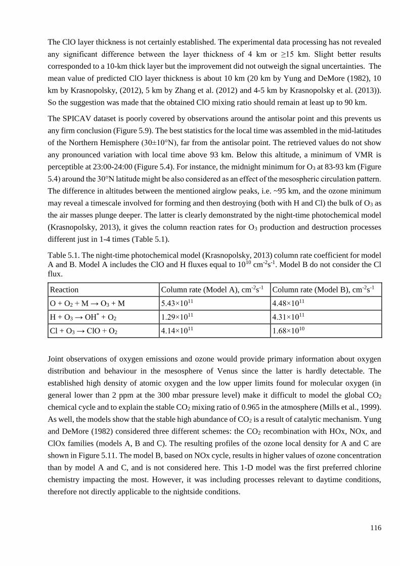
116

The ClO layer thickness is not certainly established. The experimental data processing has not revealed

any significant difference between the layer thickness of 4 km or ≥15 km. Slight better results

corresponded to a 10-km thick layer but the improvement did not outweigh the signal uncertainties. The

mean value of predicted ClO layer thickness is about 10 km (20 km by Yung and DeMore (1982), 10

km by Krasnopolsky, (2012), 5 km by Zhang et al. (2012) and 4-5 km by Krasnopolsky et al. (2013)).

So the suggestion was made that the obtained ClO mixing ratio should remain at least up to 90 km.

The SPICAV dataset is poorly covered by observations around the antisolar point and this prevents us

any firm conclusion (Figure 5.9). The best statistics for the local time was assembled in the mid-latitudes

of the Northern Hemisphere (30±10°N), far from the antisolar point. The retrieved values do not show

any pronounced variation with local time above 93 km. Below this altitude, a minimum of VMR is

perceptible at 23:00-24:00 (Figure 5.4). For instance, the midnight minimum for O3 at 83-93 km (Figure

5.4) around the 30°N latitude might be also considered as an effect of the mesospheric circulation pattern.

The difference in altitudes between the mentioned airglow peaks, i.e. ~95 km, and the ozone minimum

may reveal a timescale involved for forming and then destroying (both with H and Cl) the bulk of O3 as

the air masses plunge deeper. The latter is clearly demonstrated by the night-time photochemical model

(Krasnopolsky, 2013), it gives the column reaction rates for O3 production and destruction processes

different just in 1-4 times (Table 5.1).

Table 5.1. The night-time photochemical model (Krasnopolsky, 2013) column rate coefficient for model

A and B. Model A includes the ClO and H fluxes equal to 1010 cm-2s-1. Model B do not consider the Cl

flux.

Reaction Column rate (Model A), cm-2s-1 Column rate (Model B), cm-2s-1

O + O2 + M → O3 + M 5.43×1011 4.48×1011

H + O3 → OH* + O2 1.29×1011 4.31×1011

Cl + O3 → ClO + O2 4.14×1011 1.68×1010

Joint observations of oxygen emissions and ozone would provide primary information about oxygen

distribution and behaviour in the mesosphere of Venus since the latter is hardly detectable. The

established high density of atomic oxygen and the low upper limits found for molecular oxygen (in

general lower than 2 ppm at the 300 mbar pressure level) make it difficult to model the global CO2

chemical cycle and to explain the stable CO2 mixing ratio of 0.965 in the atmosphere (Mills et al., 1999).

As well, the models show that the stable high abundance of CO2 is a result of catalytic mechanism. Yung

and DeMore (1982) considered three different schemes: the CO2 recombination with HOx, NOx, and

ClOx families (models A, B and C). The resulting profiles of the ozone local density for A and C are

shown in Figure 5.11. The model B, based on NOx cycle, results in higher values of ozone concentration

than by model A and C, and is not considered here. This 1-D model was the first preferred chlorine

chemistry impacting the most. However, it was including processes relevant to daytime conditions,

therefore not directly applicable to the nightside conditions.

117

A night-time 1-D model (Krasnopolsky, 2013) designed specifically for the night-time mesosphere,

however, predicts larger values than those positively detected with SPICAV. The model concludes that

the most efficient processes leading to ozone destruction are ClOx and HOx cycles. The NOx species

influence much less: the column reaction rate is at least 4 times smaller. The predictions are presented

in Figure 5.11 with conditions of different chlorine radicals flux and the remaining odd-hydrogen flux.

A large Cl flux forms a thin layer peaking at 94 km of altitude that has never been observed, yet predicts

values comparable to the obtained ozone below 100 km.

Figure 5.11. Altitude profileof O3 local density obtained from positive detections by SPICAV UV (black

triangles). The median is calculated within 3-km bin layers from 83 to 110 km. Grey triangles correspond

to the lower estimation of ozone abundance estimated by multiplying the median local density and a

percentage of positive detections during the entire mission. Solid violet and yellow lines correspond to

1-D photochemical models by Yung and DeMore (1982). The model A does not consider the ClOx

chemistry but it is characterized by high H2 abundance. In contrast, the model C represents the major

catalytic cycle driven by the chlorine chemistry. Dashed lines represent the 1-D night-side model by

Krasnopolsky (2013) characterized by the same flux of hydrogen and different by chlorine chemistry

consideration.

Model C by Young and DeMore (1982) assuming chlorine cycle predicts smaller values for O3. An O3

decrease down to 85 km is reaching a O3 lower estimation. However, the positive detections by SPICAV

UV represent maximum values of ozone distribution at each altitude, and the mean O3 abundance is

expected to be smaller. So this hypothesis likely coincides with the profile produced by the model C.

However, it is evident that the considered models predict the thinner ozone layer than the one observed

by SPICAV UV while ozone absorption was detected even above 100 km in the SPICAV UV stellar

occultation data.

The discovery of ozone at the cloud top (~70 km) in the polar regions (Marcq et al., 2019) indicates an

influence of the global dynamics on the distribution of atmospheric species. Marcq et al. (2019) obtained

O3 VMRs around ~10 ppbv in the both southern and northern hemispheres. It should be noted, that the

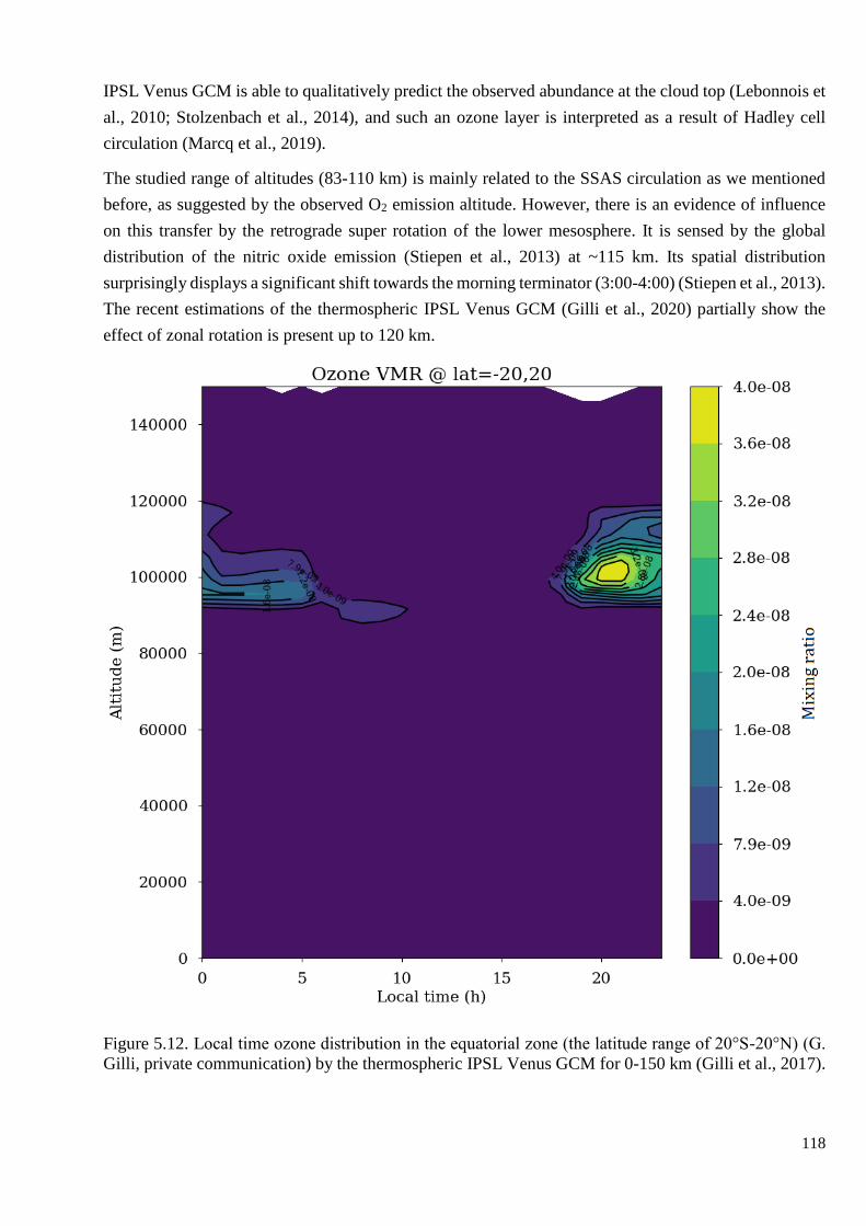
118

IPSL Venus GCM is able to qualitatively predict the observed abundance at the cloud top (Lebonnois et

al., 2010; Stolzenbach et al., 2014), and such an ozone layer is interpreted as a result of Hadley cell

circulation (Marcq et al., 2019).

The studied range of altitudes (83-110 km) is mainly related to the SSAS circulation as we mentioned

before, as suggested by the observed O2 emission altitude. However, there is an evidence of influence

on this transfer by the retrograde super rotation of the lower mesosphere. It is sensed by the global

distribution of the nitric oxide emission (Stiepen et al., 2013) at ~115 km. Its spatial distribution

surprisingly displays a significant shift towards the morning terminator (3:00-4:00) (Stiepen et al., 2013).

The recent estimations of the thermospheric IPSL Venus GCM (Gilli et al., 2020) partially show the

effect of zonal rotation is present up to 120 km.

Figure 5.12. Local time ozone distribution in the equatorial zone (the latitude range of 20°S-20°N) (G.

Gilli, private communication) by the thermospheric IPSL Venus GCM for 0-150 km (Gilli et al., 2017).

119

Figure 5.13. Local time and latitude distribution of O3 at 100 km (G. Gilli, private communication) by

the thermospheric IPSL Venus GCM for 0-150 km (Gilli et al., 2017).

Ozone’s link to the dynamic has not been precisely described by theory considering the low number of

observations of O3. The thermospheric GCM made the first attempt to provide the ozone spatial

distribution above 96 km. The results clearly show a stable ozone layer on the night side at altitudes of

90-110 km (Figure 5.12). The layer is localized in the equatorial zone. This pattern is different from the

upper clouds O3 layer found in the polar areas by both the model and observations. This reflects the

theoretical link between ozone production and SSAS circulation at an altitude of 100 km. However, the

theoretical maximum of ozone content is shifted towards the evening terminator, an opposite situation

in comparison with other dynamical markers (O2 and NO emissions, CO content) tending to concentrate

around the antisolar point or closer to the morning terminator. About ten positive ozone detections in

the 98-103 km layer at a latitude of 30°N show slight growth towards the evening, but it is not enough

to establish that observations confirm what the model predicts.

120

The maximum VMR of 40 ppbv is predicted to be inside the local time interval of 20:00-22:00 (Figure

5.12 and 5.13). This value is generally consistent with the established upper and lower estimates of ozone

content at altitudes of 85-110 km. Ozone destruction is not evidenced by data at altitudes below 90 km.

Also, the increase in ozone VMR with altitude in 85-105 km is qualitatively consistent between our

observations and the model. It is not possible to track the behaviour of this gas above 105-110 km from

SPICAV UV, so it is not possible to confirm the gradient of ozone depletion above 110 km from our

data set.

The model predicts two maxima of O3 concentration at 20°S and 20°N (Figure 5.13). The O3 was not

detected exactly at these latitudes. There is the best achieved coverage at a latitude of 30°N, and the

SPICAV values were studied depending on local time. At this parallel the model obtained a local

minimum of ozone VMR in the night atmosphere at around 01:00 at 100 km. Similar behaviour, with a

minimum of around 23:00-24:00, was observed by SPICAV UV at altitudes below 93 kilometres. For

altitudes of 100 km, it is not possible to assess the dependence on local time

At the antisolar point, the model also predicts lower values associated with a higher concentration of

chemically active compounds contributing to the attenuation of the ozone layer. This is indirectly

confirmed by the experiment. In general, there is no contradiction between the simulated distribution of

ozone and night observations at altitudes of 85-110 km in a qualitative comparison. A rigorous

quantitative analysis based on the existing dataset is not correct.

The ozone vertical distribution is an additional instrument to investigate this complex region and to

improve chemical and circulation models of the Venus atmosphere.

5.5. Comparative analysis of ozone layers in Earth, Mars and Venus atmospheres.

Among the terrestrial planets, Venus is the third one where ozone was discovered. This gas is associated

with fundamental processes in the atmospheres in a way that is specific to each of terrestrial planets.

5.5.1. Ozone on the Earth

For the Earth, ozone plays an important role in atmospheric chemistry. One can distinguish two ozone

layers: in the troposphere and in the stratosphere. In the troposphere O3 is produced by polluting

technogenic gases, such as nitrogen oxides and volatile organic compounds (VOCs), and tropospheric

ozone may contribute to global warming (Mohnen et al., 2012).

The presence of the stratospheric ozone is a result of the evolution of life on the Earth. In the past, O3

was filtering out the life-threatening UV radiation, allowing the biosphere formation into its current state

(Holland, 1995). The atmosphere has been loaded with oxygen that led to the ozone production.

At present, the Earth possesses the most abundant ozone layer, among all the terrestrial planets. Its

maximal concentration takes place at an altitude of ~20 km that corresponds to a pressure of ~30 mbar.

In the stratosphere, the molecular Hartley band effectively absorbs the solar radiation at 250 nm that

causes a warm layer around altitudes of 30-50 km (Figure 5.14). To compare, such a temperature

inversion stratospheric ozone is not observed in the atmospheres of Venus and Mars. This radiative

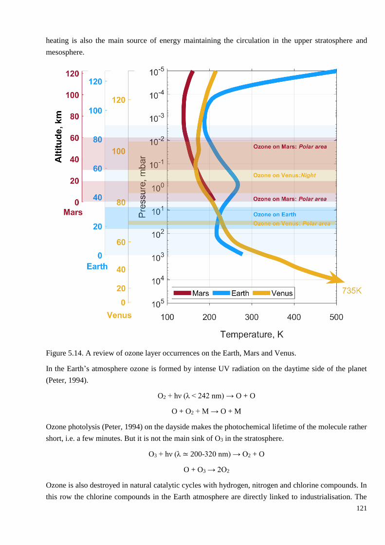
121

heating is also the main source of energy maintaining the circulation in the upper stratosphere and

mesosphere.

Figure 5.14. A review of ozone layer occurrences on the Earth, Mars and Venus.

In the Earth’s atmosphere ozone is formed by intense UV radiation on the daytime side of the planet

(Peter, 1994).

O2 + hν (λ < 242 nm) → O + O

O + O2 + M → O + M

Ozone photolysis (Peter, 1994) on the dayside makes the photochemical lifetime of the molecule rather

short, i.e. a few minutes. But it is not the main sink of O3 in the stratosphere.

O3 + hν (λ ≃ 200-320 nm) → O2 + O

O + O3 → 2O2

Ozone is also destroyed in natural catalytic cycles with hydrogen, nitrogen and chlorine compounds. In

this row the chlorine compounds in the Earth atmosphere are directly linked to industrialisation. The

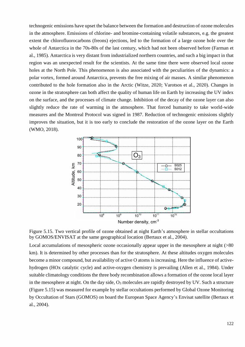
122

technogenic emissions have upset the balance between the formation and destruction of ozone molecules

in the atmosphere. Emissions of chlorine- and bromine-containing volatile substances, e.g. the greatest

extent the chlorofluorocarbons (freons) ejections, led to the formation of a large ozone hole over the

whole of Antarctica in the 70s-80s of the last century, which had not been observed before (Farman et

al., 1985). Antarctica is very distant from industrialized northern countries, and such a big impact in that

region was an unexpected result for the scientists. At the same time there were observed local ozone

holes at the North Pole. This phenomenon is also associated with the peculiarities of the dynamics: a

polar vortex, formed around Antarctica, prevents the free mixing of air masses. A similar phenomenon

contributed to the hole formation also in the Arctic (Witze, 2020; Varotsos et al., 2020). Changes in

ozone in the stratosphere can both affect the quality of human life on Earth by increasing the UV index

on the surface, and the processes of climate change. Inhibition of the decay of the ozone layer can also

slightly reduce the rate of warming in the atmosphere. That forced humanity to take world-wide

measures and the Montreal Protocol was signed in 1987. Reduction of technogenic emissions slightly

improves the situation, but it is too early to conclude the restoration of the ozone layer on the Earth

(WMO, 2018).

Figure 5.15. Two vertical profile of ozone obtained at night Earth’s atmosphere in stellar occultations

by GOMOS/ENVISAT at the same geographical location (Bertaux et al., 2004).

Local accumulations of mesospheric ozone occasionally appear upper in the mesosphere at night (>80

km). It is determined by other processes than for the stratosphere. At these altitudes oxygen molecules

become a minor compound, but availability of active O atoms is increasing. Here the influence of active-

hydrogen (HOx catalytic cycle) and active-oxygen chemistry is prevailing (Allen et al., 1984). Under

suitable climatology conditions the three body recombination allows a formation of the ozone local layer

in the mesosphere at night. On the day side, O3 molecules are rapidly destroyed by UV. Such a structure

(Figure 5.15) was measured for example by stellar occultations performed by Global Ozone Monitoring

by Occultation of Stars (GOMOS) on board the European Space Agency’s Envisat satellite (Bertaux et

al., 2004).

123

5.5.2. Ozone on Mars and Venus

In the oxygen-depleted CO2-atmospheres of Venus and Mars, there is no stable ozone layer completely

covering the planet. Local ozone layers are formed in the atmospheres of both planets as a result of

dynamic processes with appropriate temperature conditions. In contrast to the Earth’s stratosphere, the

gas is accumulated on Mars and Venus where the solar radiation is weaker or absent, but the main process

for its production is the same three body recombination between oxygen atoms and molecules.

Ozone decay processes in the atmosphere of Mars are directly related to the HOx cycle. The products of

water dissociation which are mainly H atoms drive the ozone depletion while the mixing ratio is high. It

is the most efficient catalytic cycle on Mars where the amount of water vapour is greater than that of

other compounds destructing O3. There are three different ozone layers in water-depleted areas: in the

boundary layer at the winter pole, at low and mid-latitudes at night in 30-60 km and during the southern

polar night at at 40-60 km. The polar near-surface ozone layer is the result of dehydration of the

atmosphere when water condenses into the polar cap. On the night side, where ozone is not destroyed

by UV radiation, it is collected at water-depleted altitudes. Seasonality of O3 distribution is traced, and

ozone formation is associated with a significant decrease in water content during the cold aphelion

period. When the planet is at perihelion, layers over 20 km do not form at all. The ozone layer during

the southern polar night is the result of global transport. The oxygen-rich air masses are transferred from

the sunlit southern latitudes and northern hemisphere to the south pole.

Figure 5.16. (A) Ozone layer formed over the south pole on Mars during the polar night (Montmessin

and Lefèvre, 2013) and (B) the ozone detected in the atmosphere of Venus (mesospheric distribution

from the current work and the polar ozone from Marcq et al. (2019).

A precise analysis of ozone variations was made possible due to joint consideration of SPICAM UV and

IR instruments (Lebonnois et al., 2006) and the full 3-D general circulation model for Mars (Lefèvre et

al., 2004). At the moment SPICAM dataset provides one of the widest coverage of ozone profiles on

Mars (Montmessin et al., 2017). The study of ozone in the Martian atmosphere is an example of fruitful

[A] [B]

124

cross-analysis between the GCM model and experimental data, that provides promising perspectives for

Venus exploration (Lefèvre et al., 2004; Lebonnois et al., 2006; Montmessin and Lefèvre, 2013).

A relationship with dynamics can be found in the ozone accumulation in the atmosphere of Venus. There

is a similarity between Venus and Mars in terms of ozone layer formation. On Mars, it specifically

concerns Southern wintertime polar O3 layer located at ~70 km. Its presence is due to the transfer of

oxygen-rich air masses transported by the Hadley cell from the Equator. The absence of solar radiation

in the south polar region allows ozone there at an altitude that corresponds to a maximum of

recombination. Strangely, a symmetrical layer could be found in the north pole wintertime atmosphere.

This asymmetry can be explained by the H atoms carried from the summertime equatorial hemisphere

created by enhanced water vapour photolysis as the regions there are known to host a higher hygropause

level and expose more water to sunlight.

The O3 content in the upper mesosphere of Venus is mainly controlled by a chemical cycle of chlorine-

containing elements (Yung and DeMore, 1982; Krasnopolsky, 2013), which makes it more comparable

to the Earth’s stratospheric ozone. On Venus as on Mars the O3 chemistry is also driven by global

circulation processes transferring oxygen-rich air masses. The local dynamics of atmospheric

perturbations in contrast affects the other oxygen compounds (for example, O2 (α1Δg) emission) and

probably the ozone behaviour as well.

On three planets, the study of the ozone layer is in different stages. On Earth, the chemical processes

that regulate the ozone content have been sufficiently studied, they are given great importance in

connection with the problem of global warming. Monitoring this gas is a daily vital task. A good result

for Mars, achieved, among other things, thanks to a detailed study of the ozone content, was the creation

of a 3D model of the general chemistry and circulation of the atmosphere, which made it possible to get

a fairly complete picture of its state. Venus has the smallest amount of ozone among three planets. It

rather obstructed the investigation of its variability and distribution in the atmosphere and the detection

of ozone on the planet is very recent (Montmessin et al., 2011; Marcq et al., 2019). Moreover, one of

the achievements of the Venus study is the correspondence between observations and modeling to the

detection of ozone layers in polar regions at an altitude of ~ 70 km (Lebonnois, 2010; Marcq et al.,

2019). However, the theoretical description of atmospheric processes above the clouds remains to be

completed. The carried out and further ozone observations are one of the components to a gradual

solution of this complex task.

5.6. Summary

Ozone in the night atmosphere of Venus was monitored for 8 years. The accurate analysis of SPICAV

UV capabilities indicates that the obtained ozone values do not significantly exceed the detection limit.

It is concluded that the positive detections of ozone correspond to peak concentrations that can be found

in the upper mesosphere.

Low amounts of mesospheric ozone were obtained. The percentage of positive detections is about 6%.

On average, for the positive detections, the local concentrations decrease with altitude from 108 cm-3 at

85 km to 107 cm-3 at 110 km. In general, ozone is expected to constitute VMR from 1-2 ppbv to 10-30

125

ppbv at altitudes of 85-95 km. At 95-105 km O3 VMR increases, the estimation provides a value within

an interval from 3-6 ppbv to 50-120 ppbv. The maximum values are the positive detection results.

Ozone positive detections are sporadic. The obtained VMR values change significantly in time and

space. Majority of the detections are localized in a latitude zone of 30°N±10°due to the best coverage

by observations. A decrease towards midnight from the terminators can be noted only below 93 km. The

other patterns were not concluded.

126

CHAPTER 6. O2 (α1Δg) emission in the upper mesosphere

6.1. The infrared emissions in the night atmosphere

Study of the night-time composition and dynamics of Venus mesosphere derived from the UV spectra

can be supplemented by infrared observations. The primary IR source is the thermal emission of the hot

Venus surface and deep atmosphere in spectral transparency windows. An additional signal, which can

be observed on Venus, concerns the contribution of spontaneous emissions originating from the upper

layers of the atmosphere, namely airglows (Taylor et al., 1997). One of those sources is the O2 (α1Δg)

emission at 1.27 μm produced near 95 km corresponding to the altitude range of ozone detection. O2

(α1Δg) and O3 are both products of the same processes occurring in the upper mesosphere of Venus.

The origin of this bright O2 (α1Δg) airglow on the night side is a direct consequence of the SSAS

circulation. As explained in Section 1.5, the O2 (α1Δg) emission originates from the recombination of

oxygen atoms in a three-body chemical reaction involving CO2 (see §1.5), such that:

2O + CO2 → O2* + CO2

where the excited O2* molecule is formed. It is followed by further relaxation and an emitting light at

1.27 µm. The radiative lifetime of O2 (α1Δg) state is ~4300 s (Miller et al., 2001).

O2* (α1Δg) → O2 (X

3Σg-) + hν

Also, O2 (α1Δg) may be quenched by collisions with CO2.

O2* + CO2 → O2 + CO2

However, it is not a dominant process above 90 km. Approximately 80% of excited O2 (α1Δg) molecules

emits photons at altitudes where the airglow is observed to be maximum (Gérard et al., 2007).

The reaction producing the 1.27-µm emission constitutes the major mechanism removing oxygen atoms

in the mesosphere. On average, the maximum of emission is located near the anti-solar point, as could

be expected from the SSAS-led mechanism. In parallel, O2 airglow spots can be observed intermittently

everywhere in the night-side hemisphere (Soret et al., 2014). These spots can last more than 75 minutes

that permits tracking atmospheric dynamics at an altitude of ~95 km. These features imply that the SSAS

is perturbed by transient effects (Soret et al., 2014), and cannot simply be represented by a direct flow

from the subsolar to the anti-solar point, but by a more hectic flow showing short-term variability.

Further analysis even suggests that the influence of the topography can be identified in the airglow

dataset despite the high altitude of the emission (Gorinov et al., 2018).

The O2 (α1Δg) airglow was initially identified using ground-based observations (Connes et al., 1979).

The bright emission line is located at a wavelength of 1.27 µm which also coincides with the

transparency window at 1.28 μm. For this reason, monitoring Venus’ emission around the 1.28-µm

spectral interval can potentially allow one to track variations in the lower cloud layer while exploring

the upper mesosphere.

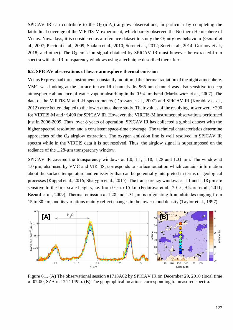
127

SPICAV IR can contribute to the O2 (α1Δg) airglow observations, in particular by completing the

latitudinal coverage of the VIRTIS-M experiment, which barely observed the Northern Hemisphere of

Venus. Nowadays, it is considered as a reference dataset to study the O2 airglow behaviour (Gérard et

al., 2007; Piccioni et al., 2009; Shakun et al., 2010; Soret et al., 2012; Soret et al., 2014; Gorinov et al.,

2018; and other). The O2 emission signal obtained by SPICAV IR must however be extracted from

spectra with the IR transparency windows using a technique described thereafter.

6.2. SPICAV observations of lower atmosphere thermal emission

Venus Express had three instruments constantly monitored the thermal radiation of the night atmosphere.

VMC was looking at the surface in two IR channels. Its 965-nm channel was also sensitive to deep

atmospheric abundance of water vapour absorbing in the 0.94-μm band (Markiewicz et al., 2007). The

data of the VIRTIS-M and -H spectrometers (Drossart et al., 2007) and SPICAV IR (Korablev et al.,

2012) were better adapted to the lower atmosphere study. Their values of the resolving power were ~200

for VIRTIS-M and ~1400 for SPICAV IR. However, the VIRTIS-M instrument observations performed

just in 2006-2009. Thus, over 8 years of operation, SPICAV IR has collected a global dataset with the

higher spectral resolution and a consistent space-time coverage. The technical characteristics determine

approaches of the O2 airglow extraction. The oxygen emission line is well resolved in SPICAV IR

spectra while in the VIRTIS data it is not resolved. Thus, the airglow signal is superimposed on the

radiance of the 1.28-µm transparency window.

SPICAV IR covered the transparency windows at 1.0, 1.1, 1.18, 1.28 and 1.31 µm. The window at

1.0 µm, also used by VMC and VIRTIS, corresponds to surface radiation which contains information

about the surface temperature and emissivity that can be potentially interpreted in terms of geological

processes (Kappel et al., 2016; Shalygin et al., 2015). The transparency windows at 1.1 and 1.18 μm are

sensitive to the first scale heights, i.e. from 0-5 to 15 km (Fedorova et al., 2015; Bézard et al., 2011;

Bézard et al., 2009). Thermal emission at 1.28 and 1.31 μm is originating from altitudes ranging from

15 to 30 km, and its variations mainly reflect changes in the lower cloud density (Taylor et al., 1997).

Figure 6.1. (A) The observational session #1713A02 by SPICAV IR on December 29, 2010 (local time

of 02:00, SZA in 124°-149°). (B) The geographical locations corresponding to measured spectra.

[A] [B]

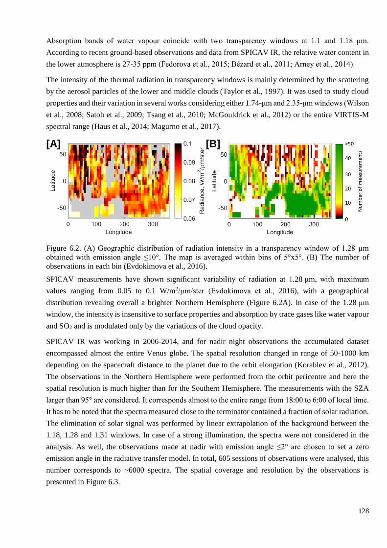
128

Absorption bands of water vapour coincide with two transparency windows at 1.1 and 1.18 μm.

According to recent ground-based observations and data from SPICAV IR, the relative water content in

the lower atmosphere is 27-35 ppm (Fedorova et al., 2015; Bézard et al., 2011; Arney et al., 2014).

The intensity of the thermal radiation in transparency windows is mainly determined by the scattering

by the aerosol particles of the lower and middle clouds (Taylor et al., 1997). It was used to study cloud

properties and their variation in several works considering either 1.74-μm and 2.35-μm windows (Wilson

et al., 2008; Satoh et al., 2009; Tsang et al., 2010; McGouldrick et al., 2012) or the entire VIRTIS-M

spectral range (Haus et al., 2014; Magurno et al., 2017).

Figure 6.2. (A) Geographic distribution of radiation intensity in a transparency window of 1.28 µm

obtained with emission angle ≤10°. The map is averaged within bins of 5°х5°. (B) The number of

observations in each bin (Evdokimova et al., 2016).

SPICAV measurements have shown significant variability of radiation at 1.28 μm, with maximum

values ranging from 0.05 to 0.1 W/m2/µm/ster (Evdokimova et al., 2016), with a geographical

distribution revealing overall a brighter Northern Hemisphere (Figure 6.2A). In case of the 1.28 μm

window, the intensity is insensitive to surface properties and absorption by trace gases like water vapour

and SO2 and is modulated only by the variations of the cloud opacity.

SPICAV IR was working in 2006-2014, and for nadir night observations the accumulated dataset

encompassed almost the entire Venus globe. The spatial resolution changed in range of 50-1000 km

depending on the spacecraft distance to the planet due to the orbit elongation (Korablev et al., 2012).

The observations in the Northern Hemisphere were performed from the orbit pericentre and here the

spatial resolution is much higher than for the Southern Hemisphere. The measurements with the SZA

larger than 95° are considered. It corresponds almost to the entire range from 18:00 to 6:00 of local time.

It has to be noted that the spectra measured close to the terminator contained a fraction of solar radiation.

The elimination of solar signal was performed by linear extrapolation of the background between the

1.18, 1.28 and 1.31 windows. In case of a strong illumination, the spectra were not considered in the

analysis. As well, the observations made at nadir with emission angle ≤2° are chosen to set a zero

emission angle in the radiative transfer model. In total, 605 sessions of observations were analysed, this

number corresponds to ~6000 spectra. The spatial coverage and resolution by the observations is

presented in Figure 6.3.

[B] [A]

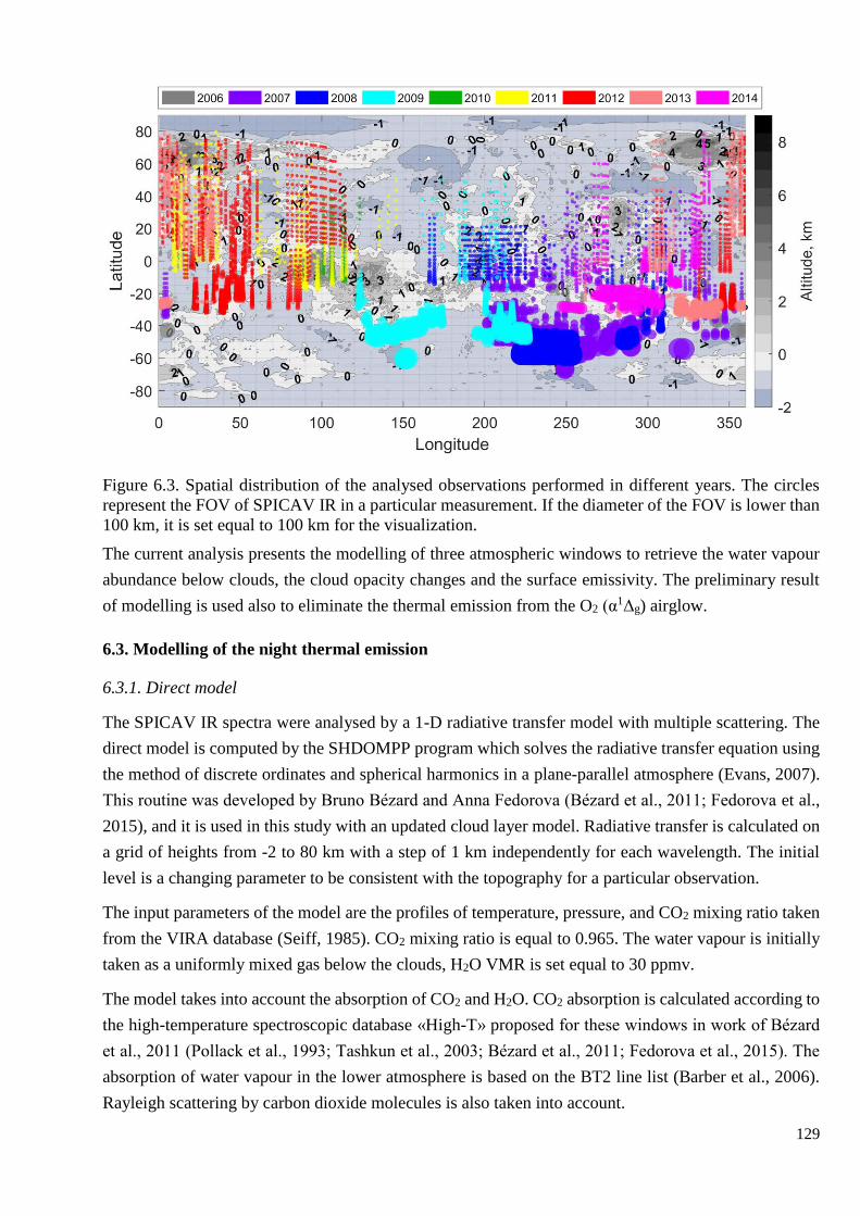
129

Figure 6.3. Spatial distribution of the analysed observations performed in different years. The circles

represent the FOV of SPICAV IR in a particular measurement. If the diameter of the FOV is lower than

100 km, it is set equal to 100 km for the visualization.

The current analysis presents the modelling of three atmospheric windows to retrieve the water vapour

abundance below clouds, the cloud opacity changes and the surface emissivity. The preliminary result

of modelling is used also to eliminate the thermal emission from the O2 (α1Δg) airglow.

6.3. Modelling of the night thermal emission

6.3.1. Direct model

The SPICAV IR spectra were analysed by a 1-D radiative transfer model with multiple scattering. The

direct model is computed by the SHDOMPP program which solves the radiative transfer equation using

the method of discrete ordinates and spherical harmonics in a plane-parallel atmosphere (Evans, 2007).

This routine was developed by Bruno Bézard and Anna Fedorova (Bézard et al., 2011; Fedorova et al.,

2015), and it is used in this study with an updated cloud layer model. Radiative transfer is calculated on

a grid of heights from -2 to 80 km with a step of 1 km independently for each wavelength. The initial

level is a changing parameter to be consistent with the topography for a particular observation.

The input parameters of the model are the profiles of temperature, pressure, and CO2 mixing ratio taken

from the VIRA database (Seiff, 1985). CO2 mixing ratio is equal to 0.965. The water vapour is initially

taken as a uniformly mixed gas below the clouds, H2O VMR is set equal to 30 ppmv.

The model takes into account the absorption of CO2 and H2O. CO2 absorption is calculated according to

the high-temperature spectroscopic database «High-T» proposed for these windows in work of Bézard

et al., 2011 (Pollack et al., 1993; Tashkun et al., 2003; Bézard et al., 2011; Fedorova et al., 2015). The

absorption of water vapour in the lower atmosphere is based on the BT2 line list (Barber et al., 2006).

Rayleigh scattering by carbon dioxide molecules is also taken into account.

130

The gaseous, specifically CO2, absorption in the IR is more complex to handle at the high temperature

and pressure conditions of the Venusian atmosphere. The observations showed that it is necessary to

consider the CO2 continuum, i.e. the superposition of very distant wings of strong permitted CO2 bands

and the possible collision-induced transitions with this molecule. Its possible values were limited to the

1.28-μm and 1.18-μm windows in the ranges of (0.30-0.78)×10-9 cm-1amagat-2 and (0.29-0.66)×10-9 cm-

1amagat-2 respectively, as described in the work of Fedorova et al. (2015). For the defined ranges, the

continuum level was empirically chosen equal to 0.75×10-9 cm-1amagat-2 and 0.38×10-9 cm-1amagat-2 for

transparency windows of 1.28 and 1.18 μm respectively. For 1.1-μm transparency window continuum

is taken also equal to 0.38×10-9 cm-1amagat-2.

Figure 6.4. Vertical distribution of aerosol particles in the cloud layer with mode separation based on

Haus et al. (2016).

The scattering in the cloud layer is computed according to the Mie theory. The chosen cloud model is

an update in comparison with the previous study of Fedorova et al. (2015). Here it is considered the

work of Haus et al. (2016) assumes spherical-shaped aerosol particles composed of 75%-H2SO4 water

solution. The density profiles of aerosol (Figure 6.4) are computed by the Equation 6.1 with parameters

set in Table 6.1.

𝑁(𝑧) =

{

𝑁0(𝑧𝑏) 𝑒𝑥𝑝 (−

(𝑧 − (𝑧𝑏 + 𝑧𝑐)

𝐻𝑢𝑝 ) , 𝑧 > (𝑧𝑏 + 𝑧𝑐)

𝑁0(𝑧𝑏), (𝑧𝑏 + 𝑧𝑐) ≥ 𝑧 ≥ 𝑧𝑏

𝑁0(𝑧𝑏) 𝑒𝑥𝑝 (−(𝑧𝑏 − 𝑧)

𝐻𝑙𝑜 ) , 𝑧 < 𝑧𝑏

(6.1)

The aerosol particles sizes of four modes are assumed to be distributed according to log-normal law. The

modal radii are 0.3, 1.0, 1.4, 3.65 μm for modes 1, 2, 2’ and 3 respectively. The dispersions of modal

sizes’ distributions are 1.56, 1.29, 1.23, 1.28 (Pollack et al., 1993). Refractive index of H2SO4-acid

solution was taken from Palmer and Williams (1975). It was estimated (Evdokimova et al., 2016) that

131

the main impact on the 1.28-μm intensity comes from aerosol particles belonging to the Modes 2 and 3

that compose the middle and the lower cloud layers.

Table 6.1. Parameters of the aerosol distribution in the cloud layer from Haus et al. (2016).

Mode 1 2 2’ 3

Lower base of peak altitude zb, km 49.0 65.0 49.0 49.0

Layer thickness of constant peak particle

number zc, km

16.0 1.0 11.0 8.0

Upper scale height Hup, km 3.5 3.5 1.0 1.0

Lower scale height Hlo, km 1.0 3.0 0.1 0.5

Particle number density N0 at zb, cm−3 193.5 100 50 14

The radiative transfer model spectral step is 0.1 cm-1. A convolution is carried out later to simulate the

AOTF function of the spectrometer (Korablev et al., 2012) and to be consistent with the spectral

resolution of SPICAV IR.

6.3.2. Inverse problem

The model set up to handle the experimental data requires a determination of three parameters:

(1) a scaling parameter applied to mode 2 and 3 particles’ distribution in the lower cloud layer (SF

in Equation 6.2);

(2) the water vapour VMR in the lower atmosphere of Venus (VMRH2O in Equation 6.2),

(3) the value of the surface emissivity for the 1.1-µm window (EMIS in Equation 6.2).

The inversion problem for the spectra obtained SPICAV IR were analysed using a look-up table. It

represents the calculated radiation intensity for parameter values in the intervals: 70-240% for the scaling

factor of aerosol concentration with a step of 5%, 2-50 ppm for the H2O VMR with a step of 2 ppm and

70% -95% for surface emissivity with a step of 5%. Surface temperature changes due to topography are

accounted for, and the radiation was modelled for various initial heights. Their values were set in the

range from -2 to 9 km with a step of 1 km. Continuum values remained fixed for all calculations. The

implication of Haus et all., model allowed to successfully describe the variation of 1.28-µm window

intensity by varying the Mode 2 and 3 densities.

Parameters that provided the minimum value of χ2 between the modelled radiance Rmod and the

experimental one Rexp were considered as the solution. The computation of χ2 value excludes the spectral

range of 1.26-1.277 μm (blue interval in Figure 6.5A) where the IR thermal spectra is overlapped by the

oxygen emission line at 1.27 µm (Figure 6.5B). The surface height in the observing location is z0, it

determines the initial level for the radiative transfer computation.

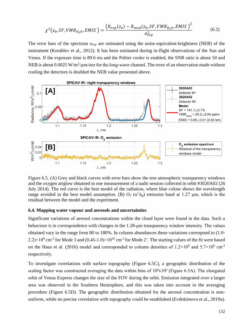
132

𝜒2(𝑧0, 𝑆𝐹, 𝑉𝑀𝑅𝐻2𝑂 , 𝐸𝑀𝐼𝑆 ) =(𝑅𝑒𝑥𝑝(𝑧0) − 𝑅𝑚𝑜𝑑(𝑧0, 𝑆𝐹, 𝑉𝑀𝑅𝐻2𝑂 , 𝐸𝑀𝐼𝑆 )

2

𝜎𝑒𝑥𝑝2 (6.2)

The error bars of the spectrum σexp are estimated using the noise-equivalent-brightness (NEB) of the

instrument (Korablev et al., 2012). It has been estimated during in-flight observations of the Sun and

Venus. If the exposure time is 89.6 ms and the Peltier cooler is enabled, the SNR ratio is about 50 and

NEB is about 0.0025 W/m2/µm/ster for the long-wave channel. The error of an observation made without

cooling the detectors is doubled the NEB value presented above.

Figure 6.5. (A) Grey and black curves with error bars show the tree atmospheric transparency windows

and the oxygen airglow obtained in one measurement of a nadir session collected in orbit #3020A02 (26

July 2014). The red curve is the best model of the radiation, where blue colour shows the wavelength

range avoided in the best model assumption. (B) O2 (α1Δg) emission band at 1.27 μm, which is the

residual between the model and the experiment.

6.4. Mapping water vapour and aerosols and uncertainties

Significant variations of aerosol concentrations within the cloud layer were found in the data. Such a

behaviour is in correspondence with changes in the 1.28-μm transparency window intensity. The values

obtained vary in the range from 80 to 180%. In column abundances these variations correspond to (1.0-

2.2)×109 cm-2 for Mode 3 and (0.45-1.0)×1010 cm-2 for Mode 2’. The starting values of the fit were based

on the Haus et al. (2016) model and corresponded to column densities of 1.2×109 and 5.7×109 cm-2

respectively.

To investigate correlations with surface topography (Figure 6.5C), a geographic distribution of the

scaling factor was constructed averaging the data within bins of 10ºx10º (Figure 6.5A). The elongated

orbit of Venus Express changes the size of the FOV during the orbit. Emission integrated over a larger

area was observed in the Southern Hemisphere, and this was taken into account in the averaging

procedure (Figure 6.5D). The geographic distribution obtained for the aerosol concentration is non-

uniform, while no precise correlation with topography could be established (Evdokimova et al., 2019a).

[A]

[B]

133

In the lower atmosphere the water vapour content was observed by SPICAV IR to be quite stable at

25±3 ppmv, and this value is slightly lower than the obtained by previous observers (Bézard et al., 2011;

Fedorova et al., 2015). The best correspondence was obtained with a value of 26±7 ppmv derived from

ground based observations of the 1.18-μm window (Arney et al., 2014). In agreement with previous

studies, the zonal averaging of H2O VMR does not show any prominent latitudinal trend. A possible link

with topography (Figure 6.4B) was however noted. The latter could be consolidated by minimizing the

data processing uncertainties considered below.

Figure 6.6. Scaling factor for concentration profiles of modes 2 and 3 aerosol particles (A) and water

vapour volume mixing ratio (B) averaged by a geographical grid of 10ºx10º. (C) Planetary surface map

from Magellan (Saunders et al., 1990). (D) Statistics of observations in each bin.

The parameters retrieved for the lower cloud layer and water vapour below 15 km are affected by the

model uncertainties. The accuracy of the radiative transfer computations in the hot dense atmosphere of

Venus depends on:

(1) the profiles of temperature, pressure and CO2 concentration;

(2) the model of aerosol particles and their distributions within the cloud layer;

(3) the accuracy of high-temperature databases for the spectroscopic parameters associated with the

vibrational-rotational transitions of the CO2 molecule and the actual models of line wings suitable

for the conditions of the hot dense lower atmosphere of Venus.

[A] [B]

[C] [D]

134

It is expected that the first source of inaccuracy is not expected to play a major role. The second and

third items have similar influence. The composition of cloud particles remains subject to large

uncertainty. The existing models of the cloud layers are based only on the in situ observations that were

made by atmospheric probes which might be a good proxy for the entire cloud system. The primary

constituent of the clouds is the concentrated H2SO4 acid water solution. However, the some in situ

observations have argued that other chemical species might be doped in the aerosols of Mode 3 (Titov

et al., 2017). Lastly, some observations as well show variations in the concentration of the acid solution

(Arney et al., 2014) which may then violate our hypothesis #2. In polar regions where the cloud tops

altitude is decreasing the model should also include some corrections. Therefore, while our assumptions

on the scattering properties in the clouds appear in a good agreement with observed changes of IR

radiance, some significant uncertainties remain.

Hypothesis #3 is related to the gaseous absorption at high temperatures. The high density and high

temperatures of the lower atmosphere profoundly affect the absorption behaviour of atmospheric gases,

especially CO2. The CO2 continuum absorption is not computed theoretically, and could only be

retrieved based on actual Venus thermal spectra. Its appearance has no distinct features, yet a good

scattering estimation of the IR inside the clouds greatly depends on representing it correctly. The

obtained ranges are too loose to constrain the continuum and provide a good estimate necessary to

conduct a qualitative analysis of the lower cloud density. This is why the continuum is fixed in our

analysis since the elevation does not change significantly on Venus to alter this absorption. Areas of

high mountains should however be considered more cautiously. An underestimation of the continuum

probably explains the strong correlation between topography and the retrieved water vapour amount

around the Aphrodita Tera area (Figure 6.6B: latitudes of 10°S-20°N and longitudes of 80-110°), but

this aspect was not studied in details. Current spectroscopy should be improved by laboratory study,

which would then favourably impact the analysis of the IR emission.

Further analysis of SPICAV is therefore possible. Our current analysis considers only the nadir

observations really perpendicular to the surface. However, other observations performed at different

angles are yet to be processed, but would require to allow the radiative transfer model handling these

geometries.

6.5. Map of oxygen airglow in the night mesosphere

This preliminary modelling of the radiative transfer was sufficient to separate the O2 (α1Δg) emission

from thermal emission spectra. The remaining uncertainties in the radiative transfer do not impede our

ability to perform this separation thanks to the high resolution of the IR channel of the SPICAV

spectrometer. To be more consistent the model is computed for the 1.05-1.3 μm interval instead of

focusing on the 1.28-μm window. The O2 emission may vary significantly during the monitoring while

different locations are scanned. For instance, during the orbit #1713A02 the airglow is rather bright at

the beginning of measurements, but at the end (Figure 6.7).

135

Figure 6.7. (A) The O2 (α1Δg) emission obtained during the observational session #1713A02 by SPICAV

IR (December 29, 2010; local time of 02:00; SZA in 124°-149°). (B) The geographical locations

corresponding to measured spectra.

In total, more than 600 observations were analysed based on the aforementioned procedure of O2

emission separation. It allowed us to corroborate and complete the VIRTIS-M study of latitudinal

distribution of the airglow’s intensity in the nightside. The VIRTIS-M monitoring stopped in 2010 and

covered mainly the night Southern Hemisphere of Venus (Gerard et al., 2009; Shakun et al., 2010; Soret

et al., 2012). The SPICAV was operational until the end of 2014. SPICAV dataset finally allowed the

reconstruction of the full mean distribution of airglow brightness (Figure 6.8). Each spectrum was

integrated to compute the absolute intensity.

Figure 6.8. (A) Average map of oxygen airglow brightness obtained by nadir measurements of SPICAV

IR (Evdokimova et al., 2019b) on the night side. The observations are grouped by a grid of 30 min in

local time and 4° in latitude. (B) The corresponding statistics of observations.

An intensity maximum of 2 MR was found exactly at the antisolar point. The emission pattern is fairly

symmetrical about the equator, yet shows some tendency to be slightly shifted towards the morning

terminator. The brightness is decreasing significantly after 23:00 towards the evening terminator. These

results are in agreement with the analysis of VIRTIS data (Shakun et al., 2010; Soret et al., 2012), yet

suggest a slightly higher intensity.

[A] [B]

[A] [B]

136

The map obtained by SPICAV does not reveal any latitudinal shift of the brightest O2 emission area.

The VIRTIS-M provided in contras a slight shift (~10°) to the north. The reason for this difference with

the VIRTIS-M result is unclear. It may be the result of different statistics used. Also the lower resolution

of VIRTIS does not allow the robust separation of O2 emission from IR windows as is the case for

SPICAV IR. The fixed ratio between intensity of 1.18-μm and 1.28-μm windows is set for the O2 airglow

elimination (Shakun et al., 2010). However, the VIRTIS nadir pattern was confirmed by the its limb

observations, whose spectra are free from IR emission. The difference between SPICAV IR and VIRTIS-

M patter is a question requiring deeper analysis. But results of both experiments concur with the idea

that SSAS circulation is the main mechanism explaining the O2 (α1Δg) airglow.

6.6. Summary

Nadir observations by SPICAV IR provided information for studying the lower atmosphere and clouds,

and O2 (α1Δg) airglow. Our analysis of the SPICAV IR dataset allowed to separate the emission signal

from thermal spectra. It represents a significant contribution to the study of the O2 (α1Δg) airglow, since

the whole night hemisphere is covered in details. The simultaneous VIRTIS-M observations correspond

mainly to the Southern Hemisphere. Statistically the maximum of the emission distribution on the night

side is located near the antisolar point where the intensity reaches 2MR. This result mainly corresponds

to previously reported conclusions.

137

CONCLUSION

This work is the first analysis of the complete dataset obtained by the SPICAV UV channel operated in

the mode of stellar occultation on board the Venus Express orbiter. The goal is to study two trace gases,

sulphur dioxide and ozone, in the night mesosphere of Venus. The atmospheric transmission spectra in

the range of 118-320 nm, measured at different local times and geographic coordinates, have been

analysed.

This goal is achieved thanks to the deep inspection of the data processing algorithms implemented for

the whole statistics of stellar occultations. It includes an uncertainty estimation related to following the

calibrations of the atmospheric transmission spectra: (1) a wavelength to pixel assignment, and (2)

subtracting a portion of emitting atmospheric light which contaminates the analysed transmissions. The

wavelength displacement along a pixel number may result in either underestimation or overestimation

of retrieved concentrations. For instance, an uncertainty of one-pixel width corresponding to 0.54 nm

leads to the retrieved CO2 slant density change of 20% in the lower mesosphere (85–100 km), as it was

estimated. The best accuracy is proved for a method of the pixel-to-wavelength assignment based on the

spectral features of measured stars. The method compares star spectra measured by SPICAV with

reference ones taken from the well-resolved IUE data. As a result, the higher accuracy was achieved

versus the previous approach, based on the wavelength alignment by only CO2 absorption bands at λ <

200 nm. Thus, the developed algorithm reduces the uncertainty of the wavelength to pixel assignment

at least by 10 times, and it was estimated to be 1–10% of the width of the pixel.

The second important uncertainty is related to different kinds of atmospheric emissions and stellar

radiation in the UV registered by the spectrometer. Those emissions were considered jointly as a stray

light, which overlaps a star spectrum making an atmospheric transmission overestimated. There are two

different techniques developed for the elimination of such a stray light. In the present work we

statistically tested and established the best of two methods to separate the UV emission signal from the

incoming stellar light. To apply both methods, we used imaging capabilities of the instrument, where

the stray light pattern was determined as a linear combination of spectra registered within edge bins

according to the star focus position on the matrix. An algorithm, selected as the most valid, was accepted

to calibrate the entire SPICAV dataset. The resulting transmission spectra were used for the spectral

inversion problem to retrieve gaseous and aerosols vertical profiles for further investigations.

Thus, the preliminary data preparation finally allowed retrieving sulphur dioxide and ozone contents at

altitudes of 85-100 km. The following statements can be concluded:

1. The median volume mixing ratio of SO2 remains around 135±21 ppbv in the range of 85-100

km. In comparison to the previous study (Belyaev, Evdokimova et al., 2017) a significant correction of

SO2 VMR was obtained. It is strongly related to the calibration method that enhanced the CO2

concentration values and, therefore, the mixing ratios of trace gases.

2. Variations of sulphur dioxide content were investigated based on 375 observational sessions. The

short-term variations reach one-two orders of magnitude, i.e. from ~50 to ~500 ppbv. In detail, the local

138

time dependence was studied for the interval from 19:00H to 5:00H. A possible diurnal asymmetry

relative to midnight is highlighted. The relative sulphur dioxide content may be increasing from 2:00H

to the evening terminator at an altitude range of 93-97 km.

3. For the first time, ozone abundance was monitored for 8 years and could be detected in 132

observations. Ozone occurrences are always close to the detection limit, which implies that SPICAV

could only probe the peak abundance with no information on the details of the layering. In general, ozone

is only detected once when observed during an occultation sequence.

4. The detected ozone concentrations between 85 and 110 km vary from 107 to 108 cm-3, and

detections comprise is about 6% of the entire SPICAV observations. On average, O3 detections

correspond to the range of VMR from 1 to 30 ppbv at altitudes of 85-95 km and from 6 to 120 ppbv at

95-105 km.

5. Ozone positive detections are sporadic. Individual observations show significant changes in

VMR in time and in space. Temporal variations were studied in detail in a latitude zone of 30°N±10°

where the best coverage was achieved. The local time distribution of ozone content suggests a possible

dependence with altitude: below 93 km a decrease towards midnight from the terminators is observed.

This minimum flattens higher up in the mesosphere. The pattern is presented only for the 30°N-latitude

zone where the observation statistics is dominant. The long-term variations, in turn, does not reveal any

significant trends.

139

PERSPECTIVES

Spectroscopy is currently the most accessible tool to investigate the properties of space objects. It also

concerns the study of the atmosphere of Venus, especially above the clouds. Any result of long-term

monitoring of the Venusian atmosphere is always a unique set of data, the detailed analysis of which

exceeds the potential of terrestrial observations, in the overwhelming majority of cases. For 8 years, the

SPIСAV spectrometer was accumulating a volume of atmospheric transmission and emission spectra of

the lower atmosphere, of the daytime atmosphere at the cloud top level, of the evening and morning

mesosphere and thermosphere and, for the first time, of the upper atmosphere in the planet’s night-time.

My work presents a preliminary analysis of the whole set of the IR spectra of Venus’s night-time thermal

radiation and the complete analysis of the UV spectra for studying the planet’s night-time upper

mesosphere. The results of this analysis are very promising as a basis for future investigations of Venus

and the formulation of scenarios for future experiments.

Sulphur dioxide and ozone are key components of the chemical cycles in the atmosphere of the Earth’s

sister. Many observations of sulphur dioxide have been obtained for the entire history of the Venus

exploration. This resulted in a great number of publications, but despite this, some results are still a

subject of hot discussions. One such question is a reason for the annual variations in SO2. At different

heights, the trends obtained do not quite coincide between each other. Whether it results from a

consequence of active dynamics in the upper mesosphere - this is a question for further more in-depth

studies.

One of the tasks for researchers of the atmosphere of Venus is to build a global model of its chemistry

and circulation, which will describe both transient processes at the surface and active dynamics, and

changeable photochemistry above the clouds. For the upper mesosphere on the night side, detailed

experimental data on the atmospheric temperature and composition will serve as a basis for validating

theoretical calculations. The dataset retrieved in this work is the only detailed measurements of the

vertical distributions of sulphur dioxide, carbon dioxide and ozone in the night-time mesosphere and

thermosphere.

Ozone was first detected in the atmosphere of Venus using the SPIСAV UV spectrometer. Analysis of

data for 8 years of observations shows that we do not observe any steady O3 layer at heights of 85-110

km. However, the registered bursts of ozone content leave the question unresolved: how the processes

of formation and destruction of this gas are balanced on the night side of Venus. The processes that

regulate the decay of ozone in the Earth’s stratosphere and in the mesosphere of Venus are reactions

with chlorine-containing components. However, on Venus, neither the global distribution of this

molecule nor the substances that break it down have been finally established. This makes it difficult to

obtain a model description for the observed altitude range, which is a subject to significant changes due

to transient dynamic phenomena. The existing one-dimensional model of the night-time mesosphere

(Krasnopolsky, 2013), for example, tends to overestimate the amount of ozone.

140

Of course, my work provides data for its subsequent discussion and development. It completely

systematizes the methodology for processing spectral data. However, the atmosphere of Venus

represents a very different environment from its terrestrial twin. Its atmosphere below the clouds is a

dense incandescent gas. On the contrary, very cold temperatures are observed above the clouds. Taking

these conditions into account is important for the UV spectroscopy of the cold night-time mesosphere

and thermosphere, as well as for the IR spectroscopy of the night-time thermal radiation of Venus.

Several studies of the atmosphere below clouds have shown that the databases on absorption lines of the

carbon dioxide molecule should be supplemented by transitions that are possible only under extreme

conditions. In the further analysis of new data obtained by UV spectrometers, especially of high spectral

resolution, additional laboratory experiments can also be useful. Recently, it was shown how the

absorption of carbon dioxide changes when the temperature drops below 200K. Venot et al. (2018)

traced these changes in detail to wavelengths shorter than 180 nm at the lowest temperatures of 150 and

170 K. On the night side, lower temperatures are observed in the cryosphere. Usually, the progress of

future missions implies an increase in the accuracy of the experiment, which also means a higher

observation boundary, where the temperature decreases. Moreover, for the majority of minor gas

components, there are no data on the temperature dependences of their UV absorption cross-sections in

the literature so far. Such research, for example, can have a positive impact on the study of the cold

atmosphere of Mars.

At the end of this work, I would like to express my confidence that the Venus Express and Akatsuki

missions have revived the interest of the scientific community to Venus. Moreover, these studies were

accompanied by a very controversial, but disturbing all of humanity, scientific report on the discovery

of indirect evidence of a possible life existence in the atmosphere of Venus (Greaves et al., 2020;

Encrenaz et al., 2020; Snellen et al., 2020). It convinces me that this will contribute to an active study

both of the data: already received by the various instruments and of future observations. The new

missions, which are slated to launch in the next decade, hold a great potential to unravel the mysteries

of our space neighbour.

141

LIST OF PUBLICATIONS

The SO2 night vertical profiles obtained by the author were published in the following works:

Belyaev, D.A., Evdokimova, D.G., Montmessin, F., Bertaux, J.-L., Korablev, O.I., Fedorova, A.A.,

Marcq, E., Soret, L., & Luginin, M.S. (2017). Night time distribution of SO2 content in Venus’ upper

mesosphere. Icarus, 294, pp. 58-71.

Vandaele, A. C., Korablev, O., Belyaev, D., Chamberlain, S., Evdokimova, D., Encrenaz, Th., Esposito,

L., Jessup, K. L., Lefèvre, F., Limaye, S., Mahieux, A., Marcq, E., Mills, F. P., Montmessin, F.,

Parkinson, C. D., Roberta, S., Roman, T., Sandor, B., Stolzenbach, A., Wilson, C., & Wilqueta, V.

(2017). Sulfur dioxide in the Venus atmosphere: I. Vertical distribution and variability. Icarus, 295, pp.

16-33.

Vandaele, A. C., Korablev, O., Belyaev, D., Chamberlain, S., Evdokimova, D., Encrenaz, Th., Esposito,

L., Jessup, K. L., Lefèvre, F., Limaye, S., Mahieux, A., Marcq, E., Mills, F. P., Montmessin, F.,

Parkinson, C. D., Roberta, S., Roman, T., Sandor, B., Stolzenbach, A., Wilson, C., & Wilqueta, V.

(2017). Sulfur dioxide in the Venus Atmosphere: II. Spatial and temporal variability. Icarus, 295, 1-15.

Pinto, J. P., Li, J., Mills, F. P., Marcq, E., Evdokimova, D., Belyaev, D., & Yung, Y. L. (2021) Sulfur

monoxide dimer chemistry as a possible source of polysulfur in the upper atmosphere of Venus. Nature

Communications, 12, 175.

The study of the accuracy of the calibration methods performed by the author is published in the

following work:

Evdokimova, D., Belyaev, D., Montmessin, F., Bertaux, J. L., & Korablev, O. (2020). Improved

calibrations of the stellar occultation data accumulated by the SPICAV UV onboard Venus Express.

Planetary and Space Science, 184, 104868.

The study of O3 and SO2 night content performed by the author were published in the following work:

Evdokimova, D., Belyaev, D., Montmessin, F., Korablev, O., Bertaux, J.‐L., Verdier, L., Lefèvre, F., &

Marcq, E. (2021). The spatial and temporal distribution of nighttime ozone and sulfur dioxide in the

Venus mesosphere as deduced from SPICAV UV stellar occultations. Journal of Geophysical Research:

Planets, 126, e2020JE006625.

142

LIST OF CONFERENCES

Evdokimova D.G., Belyaev D.A., Luginin M.S., Fedorova A.A., Korablev O.I., Montmessin F., Marcq

E., Bertaux J.-L. Variations in SO2 content in the mesosphere on the night side of Venus. The 13th All-

Russian Open Conference "Modern Problems of Earth Remote Sensing from Space", Moscow, IKI RAS,

November 16-20, 2015. (Abstract is in Russian)

Evdokimova D.G., Fedorova A.A., Belyaev D.A. Study of the cloud layer of Venus according to the

data of night observations of SPICAV IR on board Venus Express in 2006-2014. XIII Conference of

Junior Scientists "Fundamental and Applied Space Research", IKI RAS, April 13-15, 2016, Moscow.

(Abstract is in Russian)

Evdokimova D., Fedorova A., Belyaev D., Korablev O., Bertaux J. L. «Studying of cloud variations

using night observations data of SPICAV IR in 2006-2014» Abstracts. The Seventh Moscow Solar

System Symposium, October 10-14, 2016, IKI RAS, Moscow.

Evdokimova D., Montmessin F., Belyaev D., Fedorova A. «Remote sensing of the Venus night

atmosphere by SPICAV onboard the Venus Express orbiter» Abstracts. Conférence Elbereth 2016,

November 21-25, 2016, IAP, Paris.

Evdokimova, D.G., Fedorova, A.A., Belyaev, D.A. Influence of Venus cloud layer parameters on the

intensity of the night transparency window at 1.28 μm according to the SPICAV IR observations in

2006-2014. XIV Conference of Junior Scientists "Fundamental and Applied Space Research", IKI RAS,

April 12-14, 2017, Moscow. (Abstract is in Russian)

Evdokimova, D., Baggio, L., Montmessin, F., Belyaev, D., Bertaux, J. -L. A new method to analyze UV

stellar occultation data. European Planetary Science Congress 2017, 17–22 September 2017, Riga. EPSC

Abstracts Vol. 11, EPSC2017-962-1, 2017.

Evdokimova, D.G., Fedorova, A.A., Belyaev, D.A., Korablev, O.I., Marcq, E. Venus cloud parameters

modulating the 1.28-µm nightside window emission observed by SPICAV IR/VEX. The Eighth Moscow

Solar System Symposium, 9-13 October 2017, IKI RAS, Moscow. 8MS3-PS-02. Pp 199-

200.

Evdokimova D., Montmessin F., Belyaev D., Fedorova A., Baggio L., Marcq E. Studying the aerosol

and gaseous composition of the night-side Venus atmosphere with SPICAV on Venus Express.

Conférence Elbereth 2017, 22-24 November 2017, IAP, Paris. P. 8.

Evdokimova D., Montmessin F., Belyaev D., Fedorova A., Baggio L., Marcq E., Korablev O.I. Methods

for studying gases and aerosols of the night atmosphere and clouds of Venus based on observations of

the SPICAV spectrometer. XV Conference of Junior Scientists "Fundamental and Applied Space

Research", IKI RAS, April 11-13, 2018, Moscow. (Abstract is in Russian) Pp. 30-

31.

143

Evdokimova, D., Baggio, L., Montmessin, F., Belyaev, D., Bertaux, J. -L. Retrieval the gaseous

composition of Venus night-side mesosphere with SPICAV UV onboard Venus Express, European

Geosciences Union General Assembly 2018, 8–13 April 2018, Vienna, Austria. P. EGU2018-16084

Evdokimova, D.G., Fedorova, A.A., Belyaev, D.A., Korablev, O.I., Marcq, E., Bertaux, J.-L. Variations

of the lower cloud layer and H2O in the deep atmosphere of Venus from the night windows observations

by SPICAV-IR/VEX. The Ninth Moscow Solar System Symposium, October 9-12, 2018, IKI RAS,

Moscow. 9MS3-VN-01. Pp 62-63.

Evdokimova, D.G., Baggio, L., Montmessin, F., Belyaev, D.A., Bertaux, J.-L. Improved retrieval of

gaseous concentration profiles in Venus mesosphere using SPICAV-UV/VEX stellar occultation data.

The Ninth Moscow Solar System Symposium, October 9-12, 2018, IKI RAS, Moscow. 9MS3-PS-34.

Pp 287-288.

Evdokimova D. Investigation of NO emission from the data of observations of limbs and stellar

occultations SPICAV-UV/VEX. School-seminar "Atmospheres of planets: From the terrestrial planets

to exoplanets", March 25-27, 2019, Polar Geophysical Institute, Apatity.

Evdokimova, D.G., Belyaev D.A., Montmessin F., Venot O. Analysis of the temperature dependence of

the molecular absorption cross-sections of CO2 in the UV spectral range from 120 to 190 nm. XVI

Conference of Junior Scientists "Fundamental and Applied Space Research", IKI RAS, April 15-17,

2019, Moscow. (Abstract is in Russian) Pp. 43-44.

Evdokimova D., Fedorova A., Korablev O., Marcq E., Bertaux J.-L. Variations of lower clouds and

water vapor amount in deep Venus atmosphere based on night windows observations by the SPICAV-

IR/Venus-Express. International Venus Conference 2019, May 31 - June 3, 2019, Niseko, Hokkaido,

Japan. 09-6 IVC2019-0112. P. 123.

Evdokimova, D., Montmessin, F., Belyaev, D., Bertaux, J. -L. First global extraction of mesospheric

Venusian O3 and SO2 concentrations from the entire SPICAV-UV/VEX stellar occultations dataset.

EPSC-DPS Joint Meeting 2019. September 15-20, 2019, Geneva, Switzerland, EPSC-DPS2019-1469

Evdokimova, D.G., Fedorova, A.A., Korablev, O.I., Belyaev, D.A., Bertaux J.-L. (2019) Monitoring of

the atmospheric oxygen airglow on the night side of Venus according to the dataset of SPICAV IR of

the Venus Express spacecraft. (in Russian). The 17th All-Russian Open Conference "Modern Problems

of Earth Remote Sensing from Space", Moscow, IKI RAS, 2019. DOI: 10.21046/17DZZconf-2019a

Evdokimova, D.G., Belyaev, D.A., Montmessin, F., Korablev, O.I., Bertaux, J.-L., Verdier, L., Lefevre,

F., Marcq, E. (2019) Observations of ozone and sulfur dioxide in the night atmosphere of Venus at 85-

105 km by SPICAV UV/Venus Express. (in Russian). The 18th All-Russian Open Conference "Modern

Problems of Earth Remote Sensing from Space", Moscow, IKI RAS, 2020. XVIII.P.525

144

ANNEX 1. Positive detections of SO2 presented individually

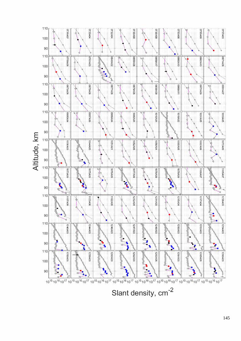
145

146

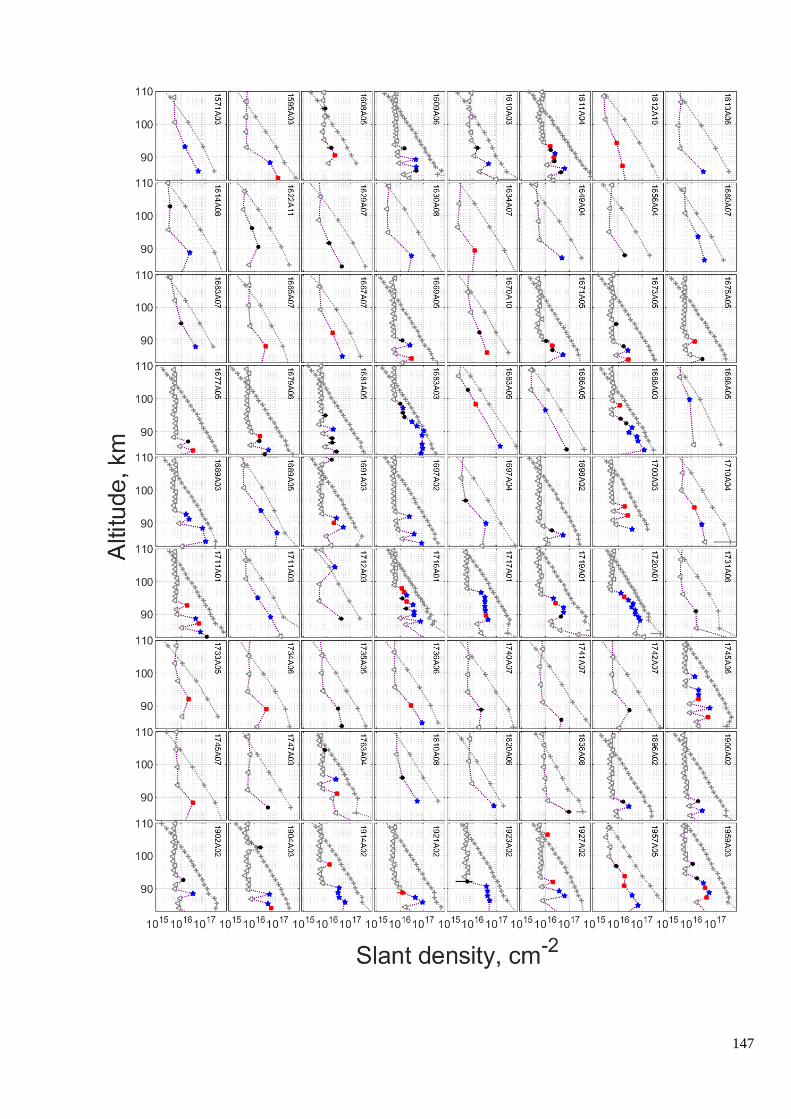
147

148

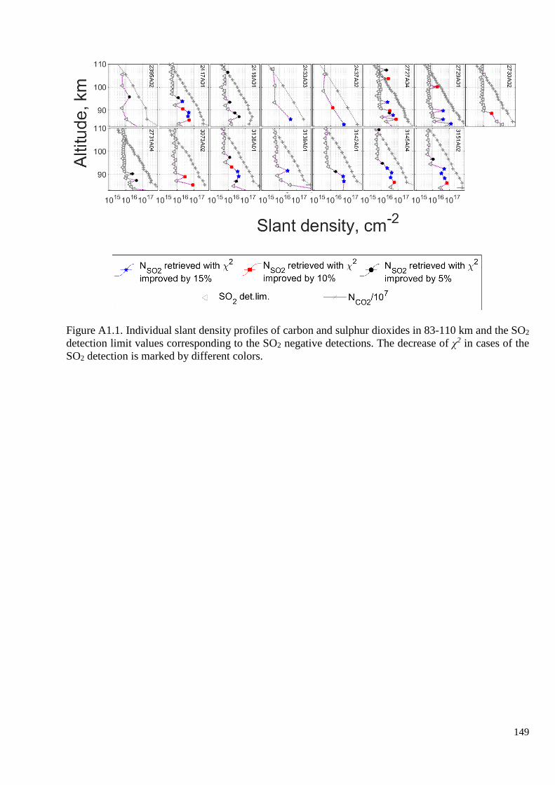
149

Figure A1.1. Individual slant density profiles of carbon and sulphur dioxides in 83-110 km and the SO2

detection limit values corresponding to the SO2 negative detections. The decrease of χ2 in cases of the

SO2 detection is marked by different colors.

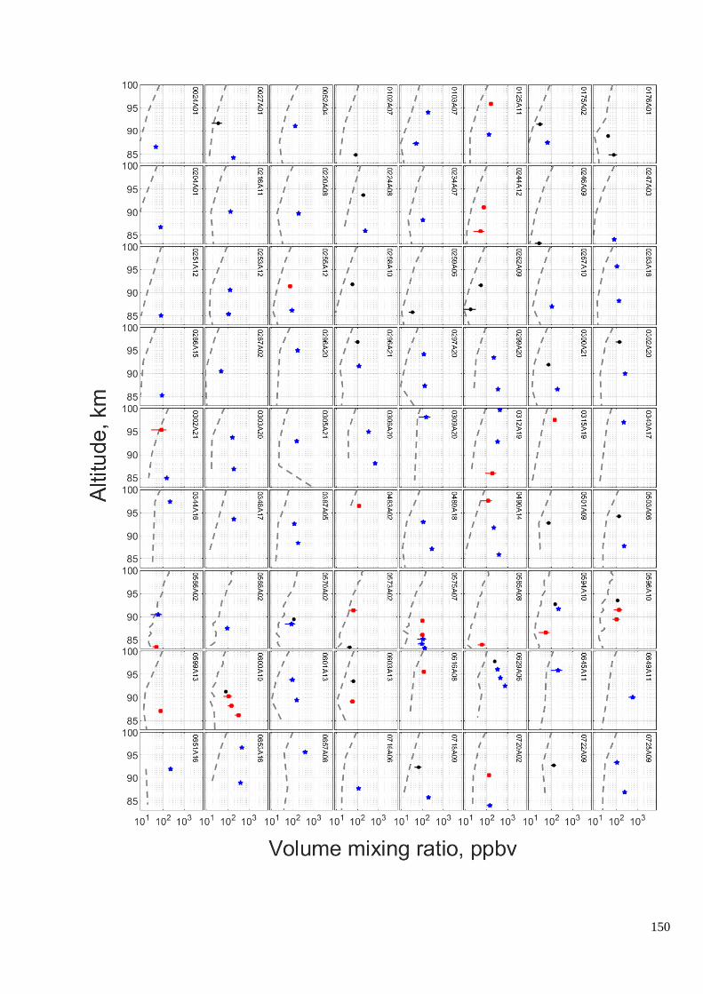
150

151

152

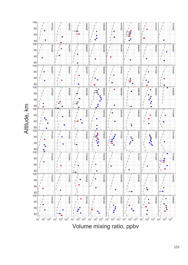
153

154

155

Figure A1.2 Individual volume mixing ratio profiles of sulphur dioxide in 83-100 km and the estimated

SO2 detection limit in terms of VMR (dashed curves). The decrease of χ2 in cases of the SO2 detection

is marked by different colours.

156

ANNEX 2. Positive detections of O3 presented individually

157

Figure A2.1. Positive detections of O3 and slant density profiles of CO2 in 83-110 km. The O3 detection

limits correspond to negative detections. The decrease of χ2 in cases of the SO2 detection is marked by

different colors.

158

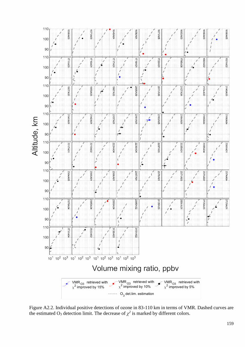
159

Figure A2.2. Individual positive detections of ozone in 83-110 km in terms of VMR. Dashed curves are

the estimated O3 detection limit. The decrease of χ2 is marked by different colors.

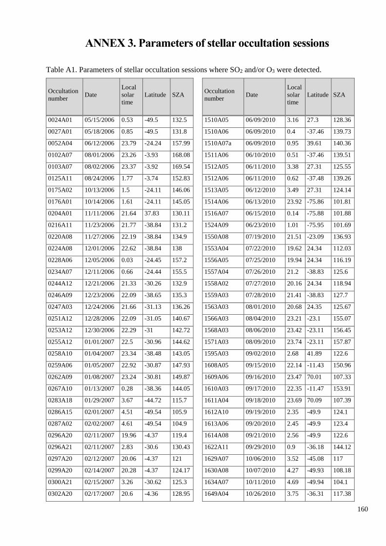
160

ANNEX 3. Parameters of stellar occultation sessions

Table A1. Parameters of stellar occultation sessions where SO2 and/or O3 were detected.

Occultation

number Date

Local

solar

time

Latitude SZA

Occultation

number Date

Local

solar

time

Latitude SZA

0024A01 05/15/2006 0.53 -49.5 132.5 1510A05 06/09/2010 3.16 27.3 128.36

0027A01 05/18/2006 0.85 -49.5 131.8 1510A06 06/09/2010 0.4 -37.46 139.73

0052A04 06/12/2006 23.79 -24.24 157.99 1510A07a 06/09/2010 0.95 39.61 140.36

0102A07 08/01/2006 23.26 -3.93 168.08 1511A06 06/10/2010 0.51 -37.46 139.51

0103A07 08/02/2006 23.37 -3.92 169.54 1512A05 06/11/2010 3.38 27.31 125.55

0125A11 08/24/2006 1.77 -3.74 152.83 1512A06 06/11/2010 0.62 -37.48 139.26

0175A02 10/13/2006 1.5 -24.11 146.06 1513A05 06/12/2010 3.49 27.31 124.14

0176A01 10/14/2006 1.61 -24.11 145.05 1514A06 06/13/2010 23.92 -75.86 101.81

0204A01 11/11/2006 21.64 37.83 130.11 1516A07 06/15/2010 0.14 -75.88 101.88

0216A11 11/23/2006 21.77 -38.84 131.2 1524A09 06/23/2010 1.01 -75.95 101.69

0220A08 11/27/2006 22.19 -38.84 134.9 1550A08 07/19/2010 21.51 -23.09 136.93

0224A08 12/01/2006 22.62 -38.84 138 1553A04 07/22/2010 19.62 24.34 112.03

0228A06 12/05/2006 0.03 -24.45 157.2 1556A05 07/25/2010 19.94 24.34 116.19

0234A07 12/11/2006 0.66 -24.44 155.5 1557A04 07/26/2010 21.2 -38.83 125.6

0244A12 12/21/2006 21.33 -30.26 132.9 1558A02 07/27/2010 20.16 24.34 118.94

0246A09 12/23/2006 22.09 -38.65 135.3 1559A03 07/28/2010 21.41 -38.83 127.7

0247A03 12/24/2006 21.66 -31.13 136.26 1563A03 08/01/2010 20.68 24.35 125.67

0251A12 12/28/2006 22.09 -31.05 140.67 1566A03 08/04/2010 23.21 -23.1 155.07

0253A12 12/30/2006 22.29 -31 142.72 1568A03 08/06/2010 23.42 -23.11 156.45

0255A12 01/01/2007 22.5 -30.96 144.62 1571A03 08/09/2010 23.74 -23.11 157.87

0258A10 01/04/2007 23.34 -38.48 143.05 1595A03 09/02/2010 2.68 41.89 122.6

0259A06 01/05/2007 22.92 -30.87 147.93 1608A05 09/15/2010 22.14 -11.43 150.96

0262A09 01/08/2007 23.24 -30.81 149.87 1609A06 09/16/2010 23.47 70.01 107.33

0267A10 01/13/2007 0.28 -38.36 144.05 1610A03 09/17/2010 22.35 -11.47 153.91

0283A18 01/29/2007 3.67 -44.72 115.7 1611A04 09/18/2010 23.69 70.09 107.39

0286A15 02/01/2007 4.51 -49.54 105.9 1612A10 09/19/2010 2.35 -49.9 124.1

0287A02 02/02/2007 4.61 -49.54 104.9 1613A06 09/20/2010 2.45 -49.9 123.4

0296A20 02/11/2007 19.96 -4.37 119.4 1614A08 09/21/2010 2.56 -49.9 122.6

0296A21 02/11/2007 2.83 -30.6 130.43 1622A11 09/29/2010 0.9 -36.18 144.12

0297A20 02/12/2007 20.06 -4.37 121 1629A07 10/06/2010 3.52 -45.08 117

0299A20 02/14/2007 20.28 -4.37 124.17 1630A08 10/07/2010 4.27 -49.93 108.18

0300A21 02/15/2007 3.26 -30.62 125.3 1634A07 10/11/2010 4.69 -49.94 104.1

0302A20 02/17/2007 20.6 -4.36 128.95 1649A04 10/26/2010 3.75 -36.31 117.38

161

0302A21 02/17/2007 3.47 -30.63 122.65 1656A04 11/02/2010 20.46 -51.93 112.4

0303A20 02/18/2007 20.7 -4.33 130.53 1660A07 11/06/2010 20.89 -51.93 115.41

0305A21 02/20/2007 3.79 -30.64 118.61 1663A07 11/09/2010 21.21 -51.93 117.53

0306A20 02/21/2007 21.03 -4.33 135.3 1665A07 11/11/2010 23.14 -31 146.77

0309A20 02/24/2007 21.35 -4.32 140.1 1667A07 11/13/2010 21.64 -51.93 120.1

0312A19 02/27/2007 21.67 -4.3 144.9 1669A05 11/15/2010 20.16 27.51 118.47

0315A19 03/02/2007 21.99 -4.28 149.67 1670A10 11/16/2010 23.67 -31.04 148.35

0340A17 03/27/2007 0.7 -4.11 168.08 1671A05 11/17/2010 20.37 27.51 121.25

0344A16 03/31/2007 1.13 -4.09 162.03 1673A05 11/19/2010 20.58 27.51 124.01

0348A17 04/04/2007 1.57 -4.06 155.73 1675A05 11/21/2010 20.8 27.5 126.73

0387A05 05/13/2007 0.2 -26.96 150.53 1677A05 11/23/2010 21.01 27.49 129.41

0483A02 08/17/2007 23.25 -35.82 145.26 1679A06 11/25/2010 21.22 27.49 132.05

0489A18 08/23/2007 23.88 -35.74 146.87 1681A05 11/27/2010 21.43 27.48 134.64

0490A14 08/24/2007 23.99 -35.75 146.91 1683A03 11/29/2010 21.65 27.48 137.18

0501A09 09/04/2007 1.79 -39.01 136 1683A05 11/29/2010 22.63 50.72 127.5

0503A06 09/06/2007 2 -39 134.3 1686A05 12/02/2010 20.71 -4.81 130.33

0562A03 11/03/2007 21.11 25.44 131.82 1688A03 12/04/2010 22.18 27.47 143.17

0564A02 11/05/2007 21.33 25.44 134.55 1688A05 12/04/2010 0.52 -5.37 169.6

0566A02 11/07/2007 21.54 25.44 137.24 1689A03 12/05/2010 22.29 27.47 144.29

0568A02 11/09/2007 21.76 25.44 139.85 1689A05 12/05/2010 0.63 -5.37 168.31

0570A02 11/11/2007 21.97 25.43 142.39 1691A03 12/07/2010 22.5 27.47 146.42

0573A02 11/14/2007 22.3 25.43 146.02 1697A02 12/13/2010 23.15 27.46 151.77

0575A07 11/16/2007 22.51 25.42 148.26 1697A04 12/13/2010 1.48 -5.43 156.55

0585A08 11/26/2007 23.62 25.51 156.3 1698A02 12/14/2010 23.25 27.46 152.43

0594A10 12/05/2007 0.61 25.52 155.48 1700A03 12/16/2010 23.47 27.46 153.6

0596A10 12/07/2007 0.83 25.53 154.2 1710A04 12/26/2010 1.38 38.87 139

0599A13 12/11/2007 22.85 -29.07 144.3 1711A01 12/27/2010 0.68 27.49 153.22

0600A10 12/11/2007 1.26 25.54 150.75 1711A03 12/27/2010 1 29.58 149.4

0601A13 12/13/2007 23.07 -29.05 145.63 1712A03 12/28/2010 1.6 38.87 137.6

0603A13 12/15/2007 23.29 -29.03 146.74 1716A01a 01/01/2011 22.94 34.43 144.7

0616A08 12/28/2007 0.79 -34.53 141.55 1717A01 01/02/2011 1.34 27.51 148.59

0629A06 01/10/2008 2.27 18.98 142.41 1719A01 01/04/2011 1.56 27.52 146.57

0645A11 01/26/2008 19.65 -38.85 108.6 1720A01a 01/05/2011 23.38 34.01 147.22

0649A11 01/30/2008 20.07 -38.85 113.5 1731A06 01/16/2011 0.03 -39.16 138.33

0651A16 02/01/2008 20.29 -38.85 115.9 1733A05 01/18/2011 23.37 -76.84 100.5

0653A16 02/03/2008 20.5 -38.85 118.3 1734A06 01/19/2011 23.48 -76.86 100.56

0657A08 02/07/2008 20.93 -38.84 122.9 1735A05 01/20/2011 23.59 -76.87 100.6

0716A06 04/06/2008 0.76 -38.89 142.27 1736A06 01/21/2011 23.7 -76.89 100.67

0718A09 04/08/2008 0.97 -38.9 141.36 1740A07 01/25/2011 0.14 -76.93 100.8

0720A02 04/10/2008 1.19 -38.89 140.23 1741A07 01/26/2011 0.25 -76.94 100.8

162

0722A09 04/12/2008 1.39 -38.9 138.96 1742A07 01/27/2011 0.35 -76.95 100.8

0725A09 04/15/2008 1.71 -38.88 136.7 1744A07 01/29/2011 0.57 -76.97 100.78

0726A02 04/16/2008 1.82 -38.88 135.9 1745A06 01/30/2011 4.42 27.61 111.95

0729A04 04/19/2008 2.14 -38.89 133.24 1745A07 01/30/2011 0.68 -76.98 100.74

0732A04 04/22/2008 2.45 -38.89 130.34 1747A03 02/01/2011 0.9 -77 100.67

0735A09 04/25/2008 2.77 -38.88 127.23 1763A04 02/16/2011 20.44 -27.78 121.28

0738A09 04/28/2008 3.09 -38.9 123.97 1795A06 03/20/2011 23.9 -27.71 153.5

0753A06 05/13/2008 20.72 -4.61 130.75 1810A08 04/05/2011 1.44 -0.27 158.38

0755A09 05/15/2008 20.93 -4.61 133.91 1816A06 04/10/2011 2.1 -27.72 140.61

0757A03 05/17/2008 21.15 -4.61 137.13 1820A06 04/15/2011 2.38 13.84 140.99

0759A06 05/19/2008 21.36 -4.61 140.31 1838A08 05/03/2011 22.66 -24.93 150.5

0761A03 05/21/2008 21.58 -4.61 143.5 1896A02 06/30/2011 20.53 27.74 123.16

0840A02 08/08/2008 3.15 26.21 128.87 1900A02 07/04/2011 20.95 27.73 128.58

0855A08 08/23/2008 19.21 38.07 105.3 1902A02 07/06/2011 21.17 27.72 131.23

0859A17 08/27/2008 18.55 -38.87 95.5 1904A03 07/08/2011 21.38 27.72 133.83

0860A10 08/28/2008 18.65 -38.87 96.8 1914A02 07/18/2011 22.45 27.7 145.7

0862A10 08/30/2008 18.87 -38.87 99.4 1921A02 07/25/2011 23.21 27.7 151.9

0871A08 09/08/2008 20.83 -23.94 127.85 1923A02 07/27/2011 23.42 27.7 153.1

0873A08 09/10/2008 21.05 -23.93 130.65 1927A02 07/31/2011 23.86 27.7 154.5

0875A08 09/12/2008 21.26 -23.93 133.42 1957A03 08/30/2011 3.17 27.81 128.06

0877A08 09/14/2008 21.47 -23.92 136.13 1957A05 08/30/2011 4.59 58.1 103.15

0879A08 09/16/2008 21.69 -23.92 138.78 1959A03 09/01/2011 3.39 27.82 125.27

0938A09 11/14/2008 1.94 24.01 141.11 1960A03 09/02/2011 0.72 -45.31 131.31

0968A11 12/14/2008 20.76 -30.46 125.7 1963A03 09/05/2011 3.83 27.83 119.61

0972A09 12/18/2008 21.18 -30.45 130.57 1963A04 09/05/2011 1.04 -45.36 130.32

0991A07 01/06/2009 23.21 -30.42 147.63 1967A03 09/09/2011 4.27 27.84 113.85

0995A04 01/10/2009 23.64 -30.4 148.95 2004A08 10/16/2011 22.13 -22.36 144.78

0997A06 01/12/2009 23.85 -30.41 149.14 2005A09 10/17/2011 22.23 -22.37 146.03

0999A04 01/14/2009 0.07 -30.39 149.06 2006A10 10/18/2011 22.34 -22.37 147.22

1006A04 01/21/2009 20.29 8.41 124.12 2008A10 10/20/2011 22.55 -22.38 149.53

1010A04 01/25/2009 20.72 8.4 130.56 2011A06 10/23/2011 22.86 -22.39 152.68

1019A02 02/03/2009 22.32 26.48 145.45 2109A01 01/29/2012 22.53 -31.75 142.44

1020A02 02/04/2009 22.43 26.49 146.56 2110A05 01/30/2012 22.64 -31.75 143.19

1031A05 02/15/2009 1.54 57.02 122.31 2119A02 02/08/2012 20.49 27.94 122.5

1033A05 02/17/2009 1.76 57.01 121.5 2121A04 02/10/2012 20.7 27.94 125.22

1044A05 02/28/2009 1.04 26.55 151.79 2123A03 02/12/2012 20.91 27.93 127.9

1051A01 03/07/2009 0.27 9.76 171.75 2125A01 02/14/2012 21.12 27.93 130.54

1052A05 03/08/2009 0.23 -37.62 139.66 2127A04 02/16/2012 21.33 27.93 133.13

1056A04 03/12/2009 0.66 -37.66 138.79 2134A02 02/23/2012 22.08 27.92 141.71

1060A05 03/16/2009 1.09 -37.68 137.1 2138A01 02/27/2012 22.51 27.91 146.1

163

1062A08 03/18/2009 1.31 -37.68 135.99 2140A03 02/29/2012 22.73 27.91 148.03

1066A06 03/22/2009 3.45 26.65 124.85 2141A01 03/01/2012 22.83 27.91 148.94

1072A09 03/28/2009 2.46 19.85 139.85 2142A01 03/02/2012 22.94 27.91 149.8

1073A09 03/29/2009 2.09 37.19 134.34 2143A01 03/03/2012 23.05 27.91 150.6

1075A09 03/31/2009 2.31 37.15 132.37 2154A04 03/14/2012 0.25 27.92 154.2

1076A09 04/01/2009 2.89 19.82 134.06 2157A01 03/17/2012 0.57 27.93 153.2

1077A09 04/02/2009 2.52 37.07 130.31 2160A04 03/20/2012 0.9 27.94 151.5

1078A09 04/03/2009 3.1 19.82 131.12 2161A01 03/21/2012 1.01 27.94 150.74

1079A09 04/04/2009 2.74 37.02 128.17 2163A05 03/23/2012 1.23 27.95 149.1

1100A07 04/25/2009 21.32 -23.65 134.33 2164A01 03/24/2012 1.34 27.95 148.17

1105A07 04/30/2009 0.05 31.97 147.66 2165A04 03/25/2012 1.46 27.95 147.2

1107A09 05/02/2009 0.27 32.04 147.23 2166A04 03/26/2012 1.57 27.96 146.17

1108A08 05/03/2009 22.17 -23.64 144.67 2205A02 05/04/2012 19.39 -28.16 107.51

1123A06 05/18/2009 23.76 -23.64 157.48 2206A01 05/05/2012 19.5 -28.16 108.93

1162A05 06/26/2009 2.85 -38.85 126.8 2212A01 05/11/2012 20.15 -28.14 117.51

1214A03 08/17/2009 22.97 -30.84 146.01 2213A01 05/12/2012 20.26 -28.14 118.91

1215A04 08/18/2009 23.07 -30.85 146.57 2214A01 05/13/2012 20.37 -28.13 120.3

1217A04 08/20/2009 23.29 -30.85 147.53 2216A02 05/15/2012 20.58 -28.13 123.08

1238A03 09/09/2009 21.84 26.9 139.91 2217A01 05/16/2012 20.69 -28.13 124.44

1240A03 09/12/2009 22.06 26.89 142.33 2219A02 05/18/2012 20.91 -28.12 127.16

1244A03 09/16/2009 22.49 26.89 146.84 2222A01 05/21/2012 21.23 -28.12 131.14

1246A03 09/18/2009 22.71 26.89 148.89 2224A04 05/23/2012 21.45 -28.11 133.73

1247A03 09/19/2009 22.82 26.89 149.82 2228A01 05/27/2012 21.89 -28.1 138.7

1248A03 09/20/2009 22.92 26.89 150.71 2236A04 06/04/2012 22.75 -28.07 147.29

1250A03 09/22/2009 23.14 26.89 152.32 2246A01 06/13/2012 23.83 -28.04 153.2

1252A03 09/24/2009 23.36 26.89 153.69 2254A01 06/21/2012 0.69 -28.03 152

1254A03 09/26/2009 23.58 26.9 154.7 2256A04 06/23/2012 0.9 -28.03 150.89

1256A03 09/28/2009 23.8 26.9 155.3 2258A02 06/25/2012 1.11 -28.03 149.5

1258A03 09/30/2009 0.02 26.91 155.5 2259A01 06/26/2012 1.22 -28.03 148.7

1260A03 10/02/2009 0.23 26.91 155.35 2261A04 06/28/2012 1.42 -28.03 147.01

1262A03 10/04/2009 0.45 26.91 154.77 2264A04 07/01/2012 1.74 -28.04 144.2

1263A05 10/05/2009 0.56 26.92 154.33 2265A04 07/02/2012 1.84 -28.04 143.17

1264A03 10/06/2009 0.67 26.92 153.8 2274A01 07/11/2012 2.76 -28.07 132.96

1265A05 10/07/2009 0.78 26.92 153.2 2279A08 07/17/2012 3.49 14.45 125.42

1266A03 10/08/2009 0.89 26.93 152.51 2287A03 07/25/2012 22.68 -2.39 160.3

1268A03 10/10/2009 1.11 26.93 150.92 2288A01 07/25/2012 4.19 -28.14 115.08

1286A08 10/28/2009 23.48 -74.84 102.6 2294A02 07/31/2012 4.8 -28.17 107.08

1287A07 10/29/2009 23.59 -74.85 102.67 2335A01 09/10/2012 19.64 28.11 111.3

1289A07 10/31/2009 23.81 -74.87 102.79 2337A01 09/12/2012 19.85 28.1 114.1

1291A07 11/02/2009 0.03 -74.89 102.86 2338A03 09/13/2012 19.95 28.1 115.5

164

1293A07 11/04/2009 0.24 -74.9 102.9 2339A02 09/14/2012 20.06 28.1 116.89

1322A06 12/03/2009 21.11 -23.35 131.62 2343A01 09/18/2012 20.48 28.09 122.4

1327A03 12/08/2009 21.64 -23.35 138.42 2345A04 09/20/2012 20.7 28.09 125.1

1385A08 02/04/2010 22.29 -13.79 152.31 2349A02 09/24/2012 21.12 28.08 130.44

1387A10 02/06/2010 22.5 -13.82 155.13 2353A01 09/29/2012 21.55 28.08 135.6

1390A03 02/09/2010 22.81 -13.86 159.2 2355A04 10/01/2012 21.76 28.07 138.06

1398A03 02/17/2010 23.66 -13.9 167.55 2357A04 10/03/2012 21.98 28.07 140.46

1413A04 03/04/2010 2.57 -36.63 130.31 2361A01 10/07/2012 22.41 28.07 144.91

1422A06 03/13/2010 20.09 -5.55 121.3 2363A01 10/09/2012 22.62 28.06 146.96

1424A09 03/15/2010 21.39 -31.29 132.37 2364A05 10/10/2012 22.73 28.06 147.9

1431A06 03/22/2010 21.05 -5.55 135.53 2365A01 10/11/2012 22.84 28.06 148.8

1433A07 03/24/2010 22.35 -31.28 141.4 2366A01 10/12/2012 22.95 28.06 149.67

1436A06 03/27/2010 21.58 -5.55 143.42 2367A04 10/13/2012 23.05 28.06 150.44

1438A06 03/29/2010 22.88 -31.29 145.13 2368A04 10/14/2012 23.16 28.06 151.2

1440A06 03/31/2010 22.01 -5.55 149.69 2369A01 10/15/2012 23.27 28.06 151.82

1442A06 04/02/2010 23.31 -31.31 147.13 2370A01 10/16/2012 23.38 28.06 152.4

1444A04 04/04/2010 20.01 27.27 116.63 2371A03 10/17/2012 23.49 28.06 152.9

1444A06 04/04/2010 21.78 -52.05 120.7 2372A02 10/18/2012 23.6 28.06 153.4

1446A03 04/06/2010 20.22 27.27 119.43 2373A02 10/19/2012 23.71 28.06 153.7

1448A02 04/08/2010 20.44 27.26 122.22 2374A04 10/20/2012 23.81 28.06 154

1450A02 04/10/2010 20.65 27.26 124.97 2375A01 10/21/2012 23.92 28.06 154.1

1458A07 04/18/2010 21.49 27.2 135.47 2378A04 10/24/2012 0.25 28.07 154

1460A08 04/20/2010 22.81 50.72 128.37 2385A04 10/31/2012 1.02 28.08 150.58

1462A06 04/22/2010 21.91 27.19 140.48 2387A02 11/02/2012 1.24 28.08 148.9

1464A06 04/24/2010 22.13 27.19 142.85 2392A01 11/07/2012 1.8 28.1 143.81

1466A08 04/26/2010 23.46 50.72 130.5 2393A04 11/08/2012 1.91 28.1 142.69

1468A06 04/28/2010 22.56 27.18 147.23 2395A01 11/10/2012 2.13 28.11 140.3

1469A08 04/29/2010 23.78 50.72 131.1 2395A02 11/10/2012 0.42 7.72 171.89

1470A06 04/30/2010 22.77 27.18 149.2 2417A01 12/02/2012 4.57 28.17 109.95

1472A07 05/02/2010 22.99 27.18 150.94 2418A01 12/03/2012 4.67 28.17 108.5

1474A07 05/04/2010 23.21 27.18 152.45 2433A03 12/18/2012 18.94 -38.75 100.1

1475A09 05/05/2010 0.96 57.02 123.94 2435A03 12/20/2012 19.15 -38.75 102.7

1476A07 05/06/2010 23.42 27.18 153.7 2437A02 12/22/2012 19.37 -38.75 105.2

1480A08 05/10/2010 23.86 27.19 155.1 2554A01 04/18/2013 18.7 14.22 99.97

1482A08 05/12/2010 0.08 27.19 155.2 2726A03 10/07/2013 21.69 6.92 144.1

1484A07 05/14/2010 1.4 50.72 128.6 2727A04 10/08/2013 22.28 52.51 120.91

1490A07 05/20/2010 0.96 27.21 151.82 2729A01 10/10/2013 22.5 52.8 121.59

1492A07 05/22/2010 1.18 27.22 150.17 2730A02 10/11/2013 22.11 6.44 150.22

1498A08 05/28/2010 1.84 27.24 143.95 2731A04 10/12/2013 22.71 53.08 122.15

1501A05 05/31/2010 2.17 27.26 140.33 2922A02 04/21/2014 18.66 11.27 99.5

165

1502A05 06/01/2010 2.28 27.26 139.06 3073A02 09/13/2014 2.19 28.38 139.49

1503A05 06/02/2010 2.39 27.27 137.77 3097A03 10/05/2014 1.45 2.19 158.2

1504A04 06/03/2010 2.5 27.27 136.47 3138A01 11/13/2014 21.62 -28.51 135.7

1504A05 06/03/2010 23.75 -37.35 139.97 3138A03 11/13/2014 23.24 -14.96 161.41

1506A04 06/05/2010 2.72 27.28 133.83 3139A01 11/14/2014 21.72 -28.51 136.86

1507A05 06/06/2010 2.83 27.29 132.47 3142A01 11/16/2014 22.03 -28.5 140.2

1507A06 06/06/2010 0.07 -37.41 140.1 3145A04 11/19/2014 22.34 -28.49 143.39

1508A05 06/07/2010 2.94 27.29 131.13 3151A02 11/25/2014 22.95 -28.47 148.7

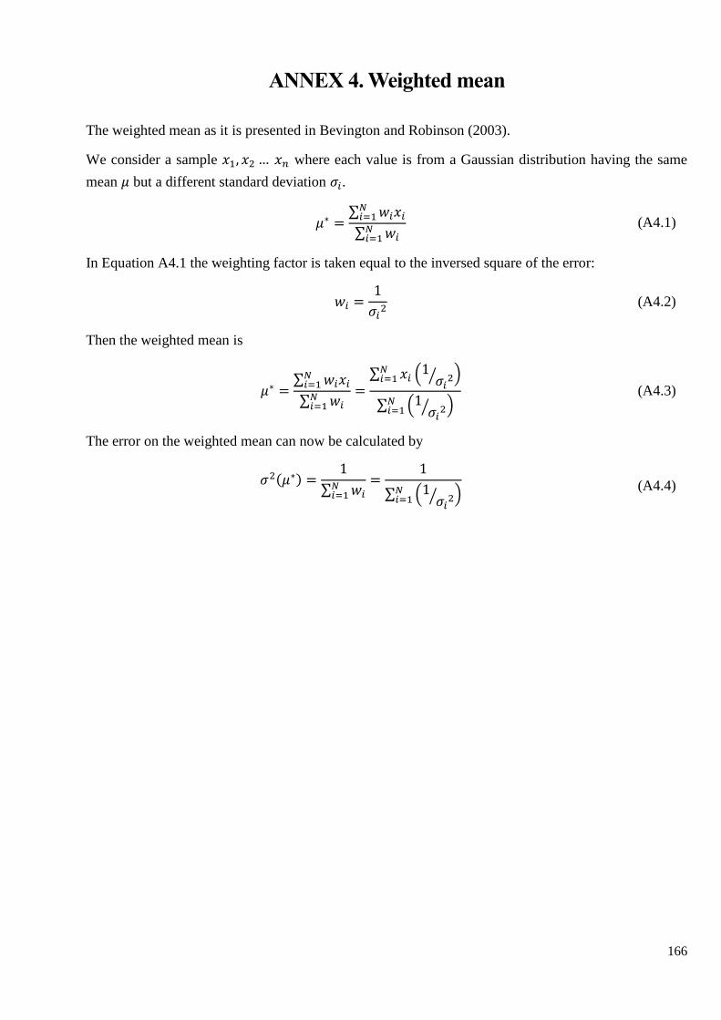
166

ANNEX 4. Weighted mean

The weighted mean as it is presented in Bevington and Robinson (2003).

We consider a sample 𝑥1, 𝑥2… 𝑥𝑛 where each value is from a Gaussian distribution having the same

mean 𝜇 but a different standard deviation 𝜎𝑖.

𝜇∗ =∑ 𝑤𝑖𝑥𝑖𝑁𝑖=1

∑ 𝑤𝑖𝑁𝑖=1

(A4.1)

In Equation A4.1 the weighting factor is taken equal to the inversed square of the error:

𝑤𝑖 =1

𝜎𝑖2 (A4.2)

Then the weighted mean is

𝜇∗ =∑ 𝑤𝑖𝑥𝑖𝑁𝑖=1

∑ 𝑤𝑖𝑁𝑖=1

=∑ 𝑥𝑖 (

1𝜎𝑖2⁄ )𝑁

𝑖=1

∑ (1 𝜎𝑖2⁄ )𝑁

𝑖=1

(A4.3)

The error on the weighted mean can now be calculated by

𝜎2(𝜇∗) =1

∑ 𝑤𝑖𝑁𝑖=1

=1

∑ (1 𝜎𝑖2⁄ )𝑁

𝑖=1

(A4.4)

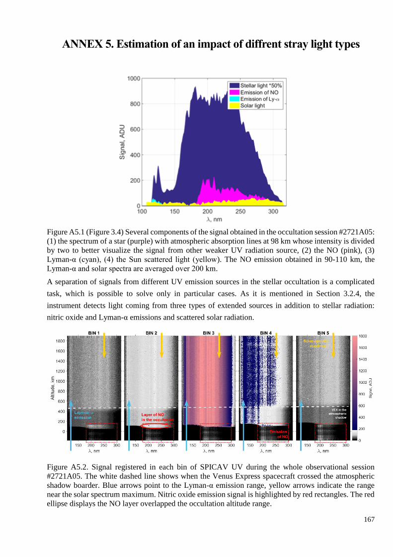
167

ANNEX 5. Estimation of an impact of diffrent stray light types

Figure A5.1 (Figure 3.4) Several components of the signal obtained in the occultation session #2721A05:

(1) the spectrum of a star (purple) with atmospheric absorption lines at 98 km whose intensity is divided

by two to better visualize the signal from other weaker UV radiation source, (2) the NO (pink), (3)

Lyman-α (cyan), (4) the Sun scattered light (yellow). The NO emission obtained in 90-110 km, the

Lyman-α and solar spectra are averaged over 200 km.

A separation of signals from different UV emission sources in the stellar occultation is a complicated

task, which is possible to solve only in particular cases. As it is mentioned in Section 3.2.4, the

instrument detects light coming from three types of extended sources in addition to stellar radiation:

nitric oxide and Lyman-α emissions and scattered solar radiation.

Figure A5.2. Signal registered in each bin of SPICAV UV during the whole observational session

#2721A05. The white dashed line shows when the Venus Express spacecraft crossed the atmospheric

shadow boarder. Blue arrows point to the Lyman-α emission range, yellow arrows indicate the range

near the solar spectrum maximum. Nitric oxide emission signal is highlighted by red rectangles. The red

ellipse displays the NO layer overlapped the occultation altitude range.

168

In this section, we consider the observational session #2721A05, which was dedicated specially for stray

light sources’ identification, and it was done with the applied spectrometer slit. Spectra of stray light

measured without the slit are not isolated in particular spectral ranges. In such a case more complex

techniques are needed, for example, a deconvolution by method Richardson-Lucy (Lucy, 1974).

However, there would be no straightforward technique (as it is presented in this section) to distinguish

between different sources.

Elimination of the nitric oxide emission spectra is discussed in details in Section 3.2.9. It was applied

accordingly for this observation when the instrument moved into the atmospheric shadow, where the

solar contamination disappears from the recording data. The difference between the stellar signal

measured before and after VEX crossing of the shadow would provide the solar signal. The mean solar

spectrum is estimated as

𝑆𝑆𝑈𝑁 =∑( ∑ 𝑆𝑖𝑆𝑃𝐼𝐶𝐴𝑉(𝑧)

𝑧=800 𝑘𝑚

𝑧=600 𝑘𝑚

− ∑ 𝑆𝑖𝑆𝑃𝐼𝐶𝐴𝑉(𝑧)

𝑧=400 𝑘𝑚

𝑧=200 𝑘𝑚

)

5

𝑖=1

(A5.1)

The UV Lyman-α radiation is very weak, however it is also distinguishable. The emission changes very

slowly with altitude decrease until a level where the CO2 absorption around 121.6 nm becomes

significant. In the observation #2721A05 this spectral shape is clear because of a high value of the raw

signal intensification (HT=160 from the 0-255 range). One can simulate how the stellar signal without

atmospheric absorption is spread along the CCD rows by the instrument PSF. After this simulation, the

additional signal resting around 121.6 nm will correspond to the Lyman-α spectrum (Franck Montmessin

and Jean-Loup Bertaux, in priv. commun.). Equation A5.2 represents the iterative algorithm to extract

the Lyman-α spectrum. As this glow evolves very slowly in space, its spectrum recorded by the 3rd bin

is determined as an average one, extracted from non-central bins. Since the original spectrum contains

the Lyman- α contamination, the iterative algorithm is required:

Iteration #0: 𝑆0 = 𝑆3𝑆𝑃𝐼𝐶𝐴𝑉

𝑆𝑖=1,2,4,5 = [𝐵𝐼𝑁][𝑃𝑆𝐹] 𝑆0

𝑆𝐿𝑦−𝛼 = 𝑆𝑖𝑆𝑃𝐼𝐶𝐴𝑉 − 𝑆𝑖̅̅ ̅̅ ̅̅ ̅̅ ̅̅ ̅̅ ̅̅ ̅, 𝑖 = 1,2,4,5

𝑆3𝑆𝑃𝐼𝐶𝐴𝑉 = 𝑆3

𝑆𝑃𝐼𝐶𝐴𝑉 − 𝑆𝐿𝑦−𝛼

Iteration #1: 𝑆1 = 𝑆3𝑆𝑃𝐼𝐶𝐴𝑉 …

(A5.2)

While the CO2 absorption turns the stellar signal to zero, the shape of the Lyman-α spectrum can be

extracted directly (Figure A5.3). This method is applicable only if the stellar light strongly dominates in

the 3rd bin. This criterion is not satisfied in the occultation altitude range where the nitric oxide emission

is present. As a possible solution there is a linear extrapolation of the signal from higher altitudes to the

range where emission of NO is observed.

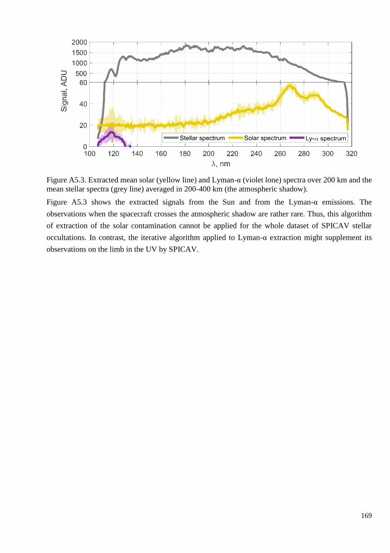
169

Figure A5.3. Extracted mean solar (yellow line) and Lyman-α (violet lone) spectra over 200 km and the

mean stellar spectra (grey line) averaged in 200-400 km (the atmospheric shadow).

Figure A5.3 shows the extracted signals from the Sun and from the Lyman-α emissions. The

observations when the spacecraft crosses the atmospheric shadow are rather rare. Thus, this algorithm

of extraction of the solar contamination cannot be applied for the whole dataset of SPICAV stellar

occultations. In contrast, the iterative algorithm applied to Lyman-α extraction might supplement its

observations on the limb in the UV by SPICAV.

170

ANNEX 6. Résumé de la thèse en français

Les objectifs de la thèse

La structure de l’atmosphère de Vénus et l’étude de sa composition sont restées depuis longtemps un

défi pour la communauté scientifique: quels processus de l’évolution de la planète ont conduit aux

conditions atmosphériques observées, et qui sont si différentes de l’atmosphère terrestre. Divers modèles

basés sur les données disponibles démontrent qu’une compréhension globale de la composition et de la

dynamique de l’atmosphère n’a toujours pas été obtenue. Avant la mission Venus Express (VEX) (2006-

2014), une étude détaillée de l’atmosphère et des composants gazeux trace au-dessus des nuages, où se

déroulent les processus déterminants, n’avait jamais été réalisée. Pour la première fois, des occultations

solaires et stellaires réalisées par VEX ont permis d’étudier en détail la structure verticale de

l’atmosphère aux deux terminateurs de la planète.

Le spectromètre SPIСAV a pu observer pendant 8 ans plusieurs gaz à l’état en utilisant son canal UV

(118-320 nm). La méthode d’occultation stellaire a permis d’observer les altitudes allant de 85 à 110

km. Une grande quantité d’informations a été accumulée, aboutissant à une étude détaillée des variations

des composants atmosphériques. Le dioxyde de soufre et l’ozone sont les deux espèces atmosphériques

mineures qui font l’objet de cette étude dans la mésosphère de Vénus, avec un accent particulier sur leur

distribution dans la mésosphère de nuit.

Le dioxyde de soufre possède des bandes d’absorption ultraviolette entre 190 et 300 nm. Ce gaz a été

abondamment observé par les télescopes terrestres et les orbiteurs du côté jour de Vénus au niveau du

sommet des nuages (~70 km) pendant plus de 40 ans. D’autre part, l’instrument SPICAV/SOIR de la

mission Venus Express a exploré la distribution verticale du SO2 à des altitudes de 65-110 km au niveau

du terminateur. Les variations de la teneur en SO2 sont extrêmement élevées dans la mésosphère du jour

et du crépusculaire. Jusqu’à présent, on ne disposait d’aucune donnée sur les distributions de SO2 dans

la mésosphère de nuit où les conditions photochimiques et les températures diffèrent considérablement

de celles rencontrées de jour. Le premier objectif de cette étude fut d’obtenir la distribution

mésosphérique du dioxyde de soufre côté nuit. Les variations spatiales et à long terme ont été comparées

aux résultats précédents.

Le deuxième objectif scientifique concerne la découverte d’une couche d’ozone dans la mésosphère de

Vénus (Montmessin et al., 2011). L’absorption de l’ozone dans la bande de Hartley (~250 nm) a été

observée par SPICAV-UV en occultation stellaire à des altitudes de 90-100 km. Des détections éparses

d’O3 avec un rapport de mélange de quelques dizaines de ppbv ont été relevées de 2006 à 2010 sur 29

observations. Ces résultats étaient cohérents avec un cycle de production et de destruction de l’ozone

associé aux réactions entre les atomes d’oxygène et de chlore au niveau du point antisolaire où là de la

très haute atmosphère (>90 km) converge et est aussi connue sous le nom de circulation SubSolaire-à-

Anti-Solaire (SSAS), et faisant écho à un mécanisme bien connu dans la haute stratosphère de la Terre.

En parallèle, une couche d’ozone a été récemment découverte au sommet des nuages vénusiens près des

régions polaires (Marcq et al., 2019), ce qui illustre la connexion de l’ozone avec la dynamique

171

atmosphérique. Dans ma recherche, l’ensemble des statistiques des occultations stellaires de SPICAV-

UV en 2006-2014 a été traité, soit plus de 400 séquences de mesures. J’ai ainsi pu caractériser la

distribution de l’ozone à des altitudes 90-100 km, dans la région correspondant au changement de

circulation des masses d’air. Cette étude du comportement de l’ozone du côté de la nuit est supposée

aider à améliorer les modèles photochimiques existants pour l’atmosphère de Vénus et révéler les

différences entre les atmosphères des planètes telluriques.

Le processus conduisant à la formation de l’ozone est aussi le responsable d’une émission aéronomique

de l’oxygène (α1Δg) à 1.27 μm principalement formée à 95 km où les détections d’ozone ont été faites.

Pour cette raison, j’ai complété mon analyse avec les observations de l’émission de O2 par le canal IR

de SPICAV réalisées côté nuit.

Avant de pouvoir étudier la distribution verticale de SO2 et O3, les spectres d’occultation stellaire de

SPICAV ont dû faire l’objet d’une étape de préparation approfondie pour les corriger d’effets

instrumentaux et les calibrer précisément en longueur d’onde. Cette étape a été fondamentale en vue

d’assurer une détection à de très faibles concentrations des gaz recherchés. L’importance de la

calibration a pu être révélée au travers de l’analyse de la distribution verticale du SO2 en s’appuyant sur

deux approches de calibration différentes (Belyaev, Evdokimova et al., 2017 vs. Evdokimova et al.,

2020).

Chapitre 1. Venus et son atmosphère

Dans ce chapitre est présenté un aperçu des connaissances élémentaires sur Vénus et son atmosphère.

Les premières observations spectrométriques réalisées dans les années 1930 ont permis d’établir que

l’atmosphère très dense (pression de 90 atm à la surface) de Vénus est constituée à 96.5 % de dioxyde

de carbone (CO2). Le deuxième gaz le plus abondant est l’azote, les autres gaz étant des constituants

mineurs: dioxyde de soufre (SO2), vapeur d’eau (H2O), etc. CO2 et H2O sont les principaux déclencheurs

de l’effet de serre qui réchauffe l’atmosphère et porte la surface à plus de 477°C. Ces molécules

absorbent efficacement le rayonnement infrarouge de la surface, et réémettent beaucoup moins en

comparaison vers l’espace. La couche nuageuse à 47-70 km, qui est opaque sur la majeure partie du

spectre, y contribue également. La formation de particules d’aérosol qui composent ces nuages est le

processus chimique le plus important se produisant dans la mésosphère de Vénus, et s’appuie sur le cycle

chimique des composés soufrés de l’atmosphère de la planète. Il est également probable que la source

du soufre dans l’atmosphère soit liée à l’activité volcanique. Le principal composant des particules

d’aérosols de la couche nuageuse de Vénus est une solution aqueuse d’acide sulfurique (à la

concentration de 75-90%), dont le SO2 est la source principale.

Comme pour l’atmosphère terrestre, on peut distinguer plusieurs couches dans l’atmosphère de Vénus.

La mésosphère, qui englobe la couche nuageuse supérieure (>65 km) et s’étend jusqu’à 120 km, est

probablement la région la plus active en termes de dynamique et de chimie. Ici, la nature de la circulation

atmosphérique change. La couche nuageuse est dominée par un fort transport zonal de matière (super-

rotation), où les vitesses de vent atteignent 100 km/s (4 jours) à 70 km. À ~100 km, les molécules et les

atomes des composants atmosphériques sont soumis à la circulation SSAS.

172

Bien que l’existence de l’atmosphère de Vénus ait été suggérée il y a plus de deux cent cinquante ans,

les principales découvertes sur sa structure, sa composition et sa dynamique ont dû attendre le les

premiers véhicules spatiaux. L’exploration récente de Vénus a débuté en 2006 (15 ans après la dernière

mission), avec le lancement de la sonde Venus Express par l’Agence spatiale européenne, suivie de la

mission Akatsuki de la JAXA. Venus Express a fonctionné jusqu’à la fin de 2014, mais l’analyse des

résultats se poursuit encore aujourd’hui. Parmi les découvertes, citons la première observation d’un

double vortex au pôle sud de la planète, la détection de OH et O3 dans l’atmosphère de Vénus, un rapport

D/H anormalement élevé, par rapport à la Terre, dans la haute atmosphère. Pour la première fois, des

expériences d’occultationéclipse ont été menées depuis l’orbite de la planète, ce qui a permis une étude

détaillée de la structure verticale de la mésosphère.

Le spectromètre SPICAV (Spectroscopie pour l’étude des caractéristiques de l’atmosphère de Vénus)

de la sonde Venus Express a été utilisé avec succès pendant huit ans d’exploitation de la sonde en orbite

(Bertaux et al., 2007b). Il se composait des canaux UV (118-320 nm) et IR (0,65-1,7 μm). Les canaux

UV et IR de l’instrument ont permis d’observer l’atmosphère dans différents modes incluant le nadir, la

visée au limbe de la planète, et les occultations solaires et stellaires. Des spectres à haute résolution en

longueur d’onde ont permis l’étude du rayonnement thermique de la basse atmosphère et de la surface,

ainsi que l’émission de l’oxygène à 1.27 μm à 95 km d’altitude dans le domaine du proche infrarouge

ont été mesurés par le canal du spectromètre IR au nadir du côté nuit. Les occultations solaires de la

haute atmosphère de Vénus ont été observées pour la première fois dans deux bandes spectrales, ainsi

que par le spectromètre SOIR (Solar Occultation in InfraRed). La première utilisation des occultations

stellaires, a permis d’étudier la distribution des gaz CO2, SO2 et O3 dans la mésosphère de nuit.

Chapitre 2. Le dioxyde de soufre et l’ozone dans l’atmosphère de Vénus

Ce chapitre présente en détail les résultats passés sur l’observation de SO2 et O3. L’interprétation de ces

données observées est sommairement présentée sur la base de modèles photochimiques qui ont abouti

à notre connaissance des processus chimiques affectés et leur lien avec la circulation atmosphérique.

SO2 et O3 sont deux composants principaux des cycles chimiques de la mésosphère de Vénus: le cycle

de CO2 et des SOx.

Les composés soufrés jouent un rôle clé dans la chimie de l’atmosphère de Vénus. SO2 est le troisième

gaz le plus abondant dans l’atmosphère de Vénus et sa présence conduit à la formation des nuages

composées de gouttelettes H2SO4. Ainsi, des variations significatives de SO2 au-dessus des nuages

peuvent influencer les processus photochimiques et la dynamique de l’ensemble et de la couche

nuageuse.

L’une des questions restées en suspens concerne la cause exacte des variations du dioxyde de soufre

observées au-dessus des nuages. Des augmentations et des diminutions de SO2 dans la couche supérieure

des nuages supérieurs (~70 km) et au-dessus ont été rapportées depuis des décennies. On impute ce

comportement à l’activité géologique qui est une source de soufre dans l’atmosphère, mais aucune

preuve n’a encore été apportée.

173

Une autre question en suspens, liée cette fois à la couche nuageuse, est l’origine de la substance

inconnue qui réduit considérablement l’albédo de Vénus dans le domaine de l’ UV. Celle-ci pourrait

également être liée aux composés soufrés (Frandsen et al., 2016; Krasnopolsky, 2018).

Avant la mission Venus Express, la distribution du SO2 au-dessus de 70 km n’avait jamais été mesurée.

Cependant, les occultations solaires ont montré qu’en moyenne, son contenu relatif diminue avec

l’altitude et atteint un minimum à ~85 km pour ensuite augmenter. Cette dépendance à l’altitude est

difficile à expliquer. Les modèles qui peuvent reproduire cette inversion nécessitent la présence d’autres

composés de soufre au-dessus de ~85 km. Ces composés n’ont pas été observés expérimentalement. En

outre, toutes les expériences présentent des variabilités significatives sur des échelles de temps courtes

(quelques jours).

L’oxydation est un processus chimique important de la mésosphère de Vénus. Le pourcentage de

dioxyde de carbone est élevé sur Vénus, donc le processus de sa récupération après photodissociation

du côté jour est efficace. Cela indique une grande efficacité des cycles catalytiques dans la mésosphère.

Il s’agit de réactions avec le chlore et les radicaux hydroxyles principalement. Un autre produit chimique

fortement dépendant de ces processus est l’ozone. La teneur en oxygène moléculaire, qui n’a jamais été

mesurée directement, est estimée faible, <2 ppmv. L’ozone sur Vénus a été découvert par Montmessin

et al. (2011) dans les spectres UV des occultations stellaires de SPICAV. Il a été détecté côté nuit lors

de 29 sessions à ~100 km d’altitude au début de la mission, avec une concentration moléculaire de 107-

108 cm-3 ~10,000 inférieure à celle de l’atmosphère terrestre.

La production d’ozone et l’émission de l’oxygène sont le résultat de la recombinaison des atomes

d’oxygène. Les atomes sont produits par photodissociation côté jour et sont ramenés côté nuit par la

dynamique de la haute mésosphère et de la thermosphère où ils se recombinent. Plus récemment,

l’analyse des observations UV SPICAV au nadir côté jour a permis d’établir une teneur en O3 d’environ

10-20 ppbv dans les nuages supérieurs (~70 km) à des latitudes supérieures à 50° dans les deux

hémisphères (Marcq et al., 2019). Un modèle de circulation planétaire tenant compte de la photochimie

a permis d’interpréter ce résultat (Lebonnois et al., 2010).

Chapitre 3. Le traitement des données des spectres d’occultation stellaire

Dans ce chapitre, on décrit le jeu de données utilisé et la technique d’observation employée par SPICAV

UV. L’algorithme de traitement des données est présenté en détail, y compris un test de la sensibilité et

les améliorations qui ont été effectuées.

La méthode de l’occultation stellaire est effectuée quand le spectre d’une étoile est mesuré lorsque le

satellite se déplace le long de son orbite. Le rayonnement d’une étoile est absorbé par l’atmosphère

lorsque cette étoile se lève et se couche derrière la planète. Vénus ayant une atmosphère opaque en raison

de ses épais nuages, cette méthode n’est applicable que pour la partie située au-dessus des nuages de

l’atmosphère. La limite supérieure de la méthode est imposée par l’altitude à laquelle les bandes

d’absorption du spectre sont comparable au bruit de fond. Par conséquent, la méthode d’occultation

stellaire est efficace à des altitudes supérieures à 85 km et seulement côté nuit. En effet, au côté jour, le

rayonnement du Soleil masque celui de l’étoile sur une grande partie du spectre. Cependant, c’est l’outil

174

le plus efficace pour étudier la structure verticale de l’atmosphère nocturne de la planète. Pour

reconstruire les distributions verticales de gaz, des problèmes d’inversion spectrale et d’inversion

verticale doivent être résolus, et la précision de la solution dépend de la qualité des étalonnages initiales

des données. Dans ce travail, une analyse détaillée des méthodes d’étalonnage a été réalisée, et à la suite

de cette analyse, les algorithmes les plus efficaces ont été sélectionnés.

Les incertitudes considérées sont principalement liées à deux aspects de l’étalonnage : (1) l’attribution

d’une longueur d’onde à un pixel, et (2) la lumière d’émission UV contaminant les spectres de

transmission analysés.

Une attribution erronée de la longueur d’onde à un pixel peut entraîner une sous-estimation ou une

surestimation des concentrations récupérées. Par exemple, une incertitude d’une largeur d’un pixel

correspondant à 0.54 nm entraîne un changement de densité colonne de CO2 de 20 % à 85-100 km. On

a testé une nouvelle méthode d’attribution pixel-longueur d’onde calée sur les raies spectrales stellaires.

Les spectres des étoiles mesurées par SPICAV ont été comparés avec des spectres de référence tirés des

données de l’International Ultraviolet Explorer. L’approche précédente était basée sur l’alignement des

longueurs d’onde par la bande d’absorption du CO2 à λ<200 nm. L’attribution de la longueur d’onde à

partir de la bande d’absorption du CO2 à 120-170 nm est limitée par une augmentation rapide de

l’épaisseur optique de la mésosphère. Nominalement cela ne permet que de mesurer 3-4 spectres avec

la bande de CO2 non saturée lors d’une session d’occultation. En revanche, des centaines de spectres

d’étoiles, mesurés hors atmosphère avant (ou après) chaque occultation, ont été utilisés pour les

calibrations en longueur d’onde. Par conséquent, la précision est au moins 10 fois supérieure à celle de

l’approche précédente, et elle a été estimée à 1-10% de la largeur du pixel.

La sous-estimation possible des abondances des gaz et des aérosols est aussi un effet des différents types

d’émission de lumière dans l’UV enregistrés par SPICAV. Le signal mesuré se compose de la lumière

provenant de l’étoile, de l’émission d’oxyde d’azote (NO) enregistrée avec un maximum à 115 km (160-

240 nm), de l’émission d’hydrogène diffusée dans la bande Lyman-alpha (121.6 nm), et de la lumière

dispersée du Soleil (200-320 nm). Ces émissions ont longtemps été considérées comme une lumière

parasite, qui se superpose au spectre de l’étoile et génère une sous-estimation de la transmission

atmosphérique. Deux méthodes ont été envisagées afin de séparer la composante d’émission du NO et

la lumière de l’étoile. Les spectres obtenus par SPICAV UV ont été traités par les deux méthodes et les

transmissions résultantes ont été comparées pour établir la manière la plus efficace d’extraire la

composante d’émission totale.

Les deux méthodes sont basées sur les capacités d’imagerie de l’instrument. Simultanément,

l’instrument mesure cinq spectres correspondant aux signaux provenant de différentes altitudes de

l’atmosphère. En principe, le troisième spectre ou spectre central contient le signal stellaire. Dans ce

spectre, le modèle de lumière parasite a été déterminé comme une combinaison linéaire d’autres spectres

enregistrés. Dans le premier algorithme, les coefficients définissants la combinaison linéaire sont

calculés au niveau de l’ombre atmosphérique et ils restent fixes pour toute la gamme d’altitude

d’occultation. La seconde approche considère le modèle de lumière parasite inclus dans une équation

d’inversion spectrale avec un paramètre libre proportionnel au modèle de NO . Ce paramètre est récupéré

175

pour chaque spectre séparément. L’analyse des profils de transmission à différentes longueurs d’onde

montre que la première méthode est plus efficace pour soustraire la composante d’émission de la

composante stellaire en raison de l’atténuation causée par les aérosols. L’analyse statistique de

l’ensemble d’ensemble de données de SPICAV permet de conclure que la composante d’émission est

estimée plus précisément avec la première méthode. Par conséquent, les erreurs causées par le NO sur

les profils verticaux de CO2 et d’autres composés atmosphériques ont pu être diminués. Cet algorithme

est celui qui a été utilisé pour calibrer l’ensemble de données de SPICAV.

La deuxième étape concerne le problème de l’inversion spectrale, qui a été développé pour trouver les

densités de gaz optimales qui permettent de reproduire les spectres sur la base de leurs sections efficaces.

La densité colonne des gaz (SO2 et O3) intégrée le long de la ligne de visée peut être trop faible pour être

détectable par SPICAV UV. Pour cette raison, des limites de détection pour O3 et SO2 ont été établies.

En moyenne, ces limites sont NSO2 = 5.8±0.2 1015 cm-2 pour SO2 et NO3 = 3.3±0.1 1015 cm-2 pour O3.

Une bande d’absorption ClO est également présente dans le domaine spectral couvert par le canal UV

de SPICAV. Cependant, les tentatives pour la détecter se sont avérées infructueuses. La limite de

détection de ClO est 3-4 fois plus élevée que celle de l’ozone, qui est ~1016 cm-2.

Chapitre 4. Le dioxyde de soufre

Ce chapitre est consacré aux résultats obtenus sur la teneur en SO2 et à son analyse.

Les profils verticaux des densités colonne de CO2 et de SO2 ont été extraits de 375 observations réalisées

entre 2006 et 2014. Les hauteurs d’échelle moyennes pour ces gaz ont été calculées, et elles sont égales

à 5.25±0.05 km et 6.1±0.1 km respectivement.

Le rapport de mélange volumique du SO2 a été calculé sur la base des obtenus de densité locale du CO2

et du SO2 obtenus après inversion verticale. En moyenne, il est autour de 135±21 ppbv dans entre 85 et

100 km, ce qui constitue une modification des résultats précédemment rapportés par Belyaev,

Evdokimova et al. (2017) où une augmentation de la valeur avec l’altitude avait été obtenue. Cette

évolution a été causée par l’amélioration des techniques d’étalonnage et qui a impacté l’inversion

spectrale des densités colonne de gaz. .

Le profil vertical résultant a été comparé avec les résultats d’autres observations et des modèles actuels

de la mésosphère de Vénus. Les observations sub-mm réalisées par des télescopes terrestres sont les

seules à avoir observé la même heure locale sur Vénus que SPICAV. Cependant, les résultats SPICAV

ont révélé des valeurs beaucoup plus élevées (Figure A6.1). La raison de cette différence n’a pas été

précisément établie. Une cause possible est que le signal sub-mm émane de la superposition de

l’émission thermique provenant de différentes altitudes. alors que les observations dans l’UV sont moins

sensibles aux incertitudes sur la température que l’IR thermique. Cependant, la sensibilité exacte à la

température dans l’UV reste à être.

La Figure A6.1 montre également une différence entre les résultats d’occultation mesurés au terminateur

et du côté nuit. Cependant, les occultations solaires observaient principalement la région polaire nord

tandis que les occultations stellaires observaient principalement les latitudes moyennes.

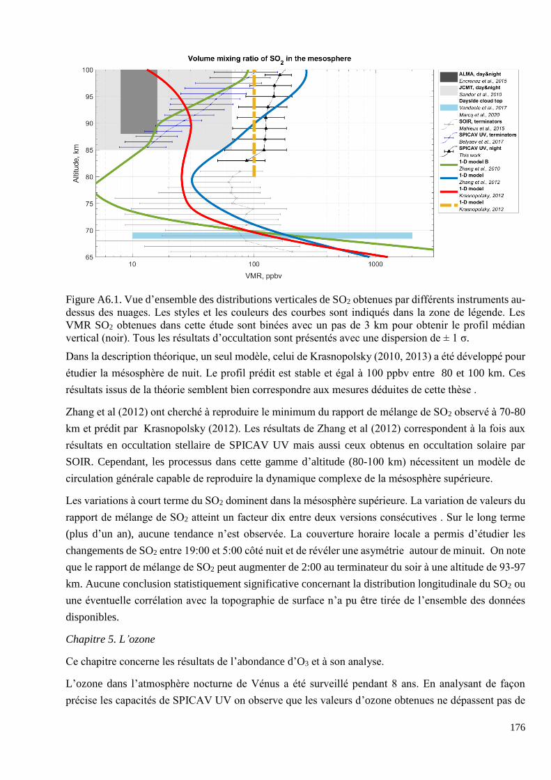
176

Figure A6.1. Vue d’ensemble des distributions verticales de SO2 obtenues par différents instruments au-

dessus des nuages. Les styles et les couleurs des courbes sont indiqués dans la zone de légende. Les

VMR SO2 obtenues dans cette étude sont binées avec un pas de 3 km pour obtenir le profil médian

vertical (noir). Tous les résultats d’occultation sont présentés avec une dispersion de ± 1 σ.

Dans la description théorique, un seul modèle, celui de Krasnopolsky (2010, 2013) a été développé pour

étudier la mésosphère de nuit. Le profil prédit est stable et égal à 100 ppbv entre 80 et 100 km. Ces

résultats issus de la théorie semblent bien correspondre aux mesures déduites de cette thèse .

Zhang et al (2012) ont cherché à reproduire le minimum du rapport de mélange de SO2 observé à 70-80

km et prédit par Krasnopolsky (2012). Les résultats de Zhang et al (2012) correspondent à la fois aux

résultats en occultation stellaire de SPICAV UV mais aussi ceux obtenus en occultation solaire par

SOIR. Cependant, les processus dans cette gamme d’altitude (80-100 km) nécessitent un modèle de

circulation générale capable de reproduire la dynamique complexe de la mésosphère supérieure.

Les variations à court terme du SO2 dominent dans la mésosphère supérieure. La variation de valeurs du

rapport de mélange de SO2 atteint un facteur dix entre deux versions consécutives . Sur le long terme

(plus d’un an), aucune tendance n’est observée. La couverture horaire locale a permis d’étudier les

changements de SO2 entre 19:00 et 5:00 côté nuit et de révéler une asymétrie autour de minuit. On note

que le rapport de mélange de SO2 peut augmenter de 2:00 au terminateur du soir à une altitude de 93-97

km. Aucune conclusion statistiquement significative concernant la distribution longitudinale du SO2 ou

une éventuelle corrélation avec la topographie de surface n’a pu être tirée de l’ensemble des données

disponibles.

Chapitre 5. L’ozone

Ce chapitre concerne les résultats de l’abondance d’O3 et à son analyse.

L’ozone dans l’atmosphère nocturne de Vénus a été surveillé pendant 8 ans. En analysant de façon

précise les capacités de SPICAV UV on observe que les valeurs d’ozone obtenues ne dépassent pas de

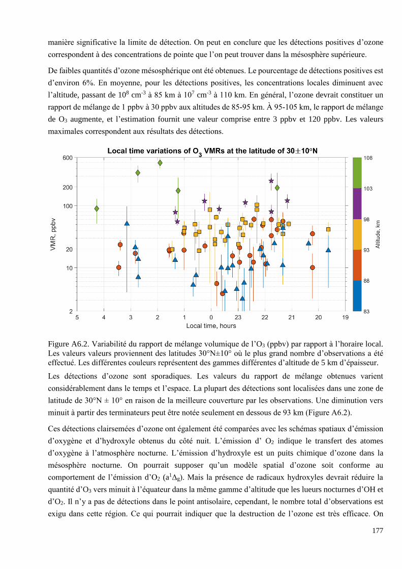
177

manière significative la limite de détection. On peut en conclure que les détections positives d’ozone

correspondent à des concentrations de pointe que l’on peut trouver dans la mésosphère supérieure.

De faibles quantités d’ozone mésosphérique ont été obtenues. Le pourcentage de détections positives est

d’environ 6%. En moyenne, pour les détections positives, les concentrations locales diminuent avec

l’altitude, passant de 108 cm-3 à 85 km à 107 cm-3 à 110 km. En général, l’ozone devrait constituer un

rapport de mélange de 1 ppbv à 30 ppbv aux altitudes de 85-95 km. À 95-105 km, le rapport de mélange

de O3 augmente, et l’estimation fournit une valeur comprise entre 3 ppbv et 120 ppbv. Les valeurs

maximales correspondent aux résultats des détections.

Figure A6.2. Variabilité du rapport de mélange volumique de l’O3 (ppbv) par rapport à l’horaire local.

Les valeurs valeurs proviennent des latitudes 30°N±10° où le plus grand nombre d’observations a été

effectué. Les différentes couleurs représentent des gammes différentes d’altitude de 5 km d’épaisseur.

Les détections d’ozone sont sporadiques. Les valeurs du rapport de mélange obtenues varient

considérablement dans le temps et l’espace. La plupart des détections sont localisées dans une zone de

latitude de 30°N ± 10° en raison de la meilleure couverture par les observations. Une diminution vers

minuit à partir des terminateurs peut être notée seulement en dessous de 93 km (Figure A6.2).

Ces détections clairsemées d’ozone ont également été comparées avec les schémas spatiaux d’émission

d’oxygène et d’hydroxyle obtenus du côté nuit. L’émission d’ O2 indique le transfert des atomes

d’oxygène à l’atmosphère nocturne. L’émission d’hydroxyle est un puits chimique d’ozone dans la

mésosphère nocturne. On pourrait supposer qu’un modèle spatial d’ozone soit conforme au

comportement de l’émission d’O2 (a1Δg). Mais la présence de radicaux hydroxyles devrait réduire la

quantité d’O3 vers minuit à l’équateur dans la même gamme d’altitude que les lueurs nocturnes d’OH et

d’O2. Il n’y a pas de détections dans le point antisolaire, cependant, le nombre total d’observations est

exigu dans cette région. Ce qui pourrait indiquer que la destruction de l’ozone est très efficace. On

178

s’attend également à ce que les atomes de chlore jouent un rôle important dans le cycle chimique de

l’oxygène à ces altitudes la nuit (Bertaux et al., 2007a; Montmessin et al., 2011). Le signe d’un tel

mécanisme sont les molécules de ClO (Sandor et al., 2018) observées dans la mésosphère nocturne et

de HCl observées au terminateur (Mahieux et al., 2015; Sandor et al., 2012; Sandor et al., 2017;

Krasnopolsky, 2010).

Le GCM thermosphérique a fait la première tentative de reproduire la distribution spatiale de l’ozone

au-dessus de 96 km. Les résultats montrent clairement une couche d’ozone stable du côté nuit à des

altitudes de 90-110 km, localisée dans la zone équatoriale. L’abondance de l’ozone est conforme à notre

estimation à 85-110 km. Le maximum théorique de la distribution spatiale de l’ozone s’est décalé vers

20:00-22:00, ce qui est difficile à confirmer par nos données. Cependant, à une latitude de 30°N, le

modèle a obtenu un minimum local de l’ozone VMR dans l’atmosphère nocturne vers 01:00 à 100 km.

Un comportement similaire, avec un minimum vers 23:00-24:00, a été observé par SPICAV UV à des

altitudes inférieures à 93 kilomètres. Au point antisolaire, le modèle prévoit également des valeurs plus

faibles associées à une concentration plus élevée de composés chimiquement actifs contribuant à

l’atténuation de la couche d’ozone. Ceci est indirectement confirmé par l’expérience. En général, il n’y

a pas de contradiction entre la distribution simulée de l’ozone et les observations nocturnes à des altitudes

de 85-110 km dans une comparaison qualitative.

Chapitre 6. L’émission d’O2 (α1Δg) dans la mésosphère supérieure

Ce chapitre considère la lueur atmosphérique nocturne (airglow) de O2 (α1Δg) à 1.27 μm comme une

source supplémentaire d’informations sur la physique de la mésosphère nocturne de Vénus. Les

observations au nadir par SPICAV IR sont utilisées pour récupérer une distribution de l’intensité de

l’émission du côté de la nuit.

En plus de l’étude de l’ozone, il est possible d’observer un autre produit de recombinaison des atomes

d’oxygène, qui est l’airglow O2 (α1Δg) à 1,27 mm. Cette émission apparaît en relaxation des molécules

O2* excitées formées. La luminosité maximale est observée à ~95 km; par conséquent cet airglow met

en évidence des processus dynamiques qui se produisent dans la mésosphère supérieure.

Les observations au nadir par SPICAV IR ont fourni des spectres qui correspondent à l’émission

thermique de la basse atmosphère et des nuages, et à l’airglow O2 (α1Δg). Ces spectres ont été réalisés à

haute résolution : le pouvoir de résolution de SPICAV IR est de ~1400. Notre analyse du jeu de données

IR SPICAV a permis de séparer le signal d’émission des spectres thermiques. Cette séparation est

obtenue par une modélisation minutieuse de l’émission thermique de Vénus. Les spectres IR de SPICAV

ont été analysés par un modèle de transfert radiatif 1D avec diffusion multiple. Le modèle direct est

calculé par le programme SHDOMPP qui résout l’équation de transfert radiatif en utilisant la méthode

des ordonnées discrètes et des harmoniques sphériques dans une atmosphère plane-parallèle (Evans,

2007). Cette routine a été développée par Bruno Bézard et Anna Fedorova (Bézard et al., 2011 ; Fedorova

et al., 2015), et elle a été utilisée dans cette étude avec un modèle de couche nuageuse actualisé par Haus

et al. (2016). Les résidus du modèle correspondent alors au spectre d’émission de l’oxygène.

179

Au total, plus de 600 observations en 2006-2014 ont été analysées sur la base de la procédure de

séparation des émissions d’O2. Cette analyse est significative pour l’étude de l’airglow O2 (α1Δg),

puisque tout l’hémisphère nocturne est couvert en détail On a permis de corroborer et d’étendre l’étude

VIRTIS-M de la distribution latitudinale de l’intensité de cette émission dans l’hémisphère nocturne. Le

fonctionnement de VIRTIS-M s’est arrêté en 2010 et ces observations couvraient principalement

l’hémisphère sud nocturne de Vénus (Gerard et al., 2009; Shakun et al., 2010; Soret et al., 2012).

Dans cette étude, un maximum d’intensité de 2 MR a été trouvé précisément au point antisolaire. Le

modèle d’émission est assez symétrique autour de l’équateur, mais montre une certaine tendance à être

légèrement décalé vers le terminateur du matin. La luminosité diminue de manière significative après

23:00 vers le terminateur du soir. Ces résultats concordent avec l’analyse des données de VIRTIS

(Shakun et al., 2010; Soret et al., 2012), mais suggèrent une intensité légèrement supérieure.

180

REFERENCES

Adams, W. S., & Dunham Jr, T. (1932). Absorption bands in the infra-red spectrum of Venus.

Publications of the Astronomical Society of the Pacific, 44, 243-245.

Airey, M. W., Mather, T. A., Pyle, D. M., Glaze, L. S., Ghail, R. C., & Wilson, C. F. (2015). Explosive

volcanic activity on Venus: The roles of volatile contribution, degassing, and external environment.

Planetary and Space Science, 113-114, 33–48. DOI: 10.1016/j.pss.2015.01.009

Allen, D. A., & Crawford, J. W. (1984). Cloud structure on the dark side of Venus. Nature, 307(5948),

222-224.

Allen, M., Lunine, J. I., & Yung, Y. L. (1984). The vertical distribution of ozone in the mesosphere and

lower thermosphere. Journal of Geophysical Research: Atmospheres, 89(D3), 4841-4872.

Andreichikov, B. M. (1987). Chemical composition and structure of Venus clouds from results of X-ray

radiometric experiments made with the Vega 1 and Vega 2 automatic interplanetary stations.

Kosmicheskie Issledovaniia, 25, 737-743.

Arney, G., Meadows, V., Crisp, D., Schmidt, S. J., Bailey, J., & Robinson, T. (2014). Spatially resolved

measurements of H2O, HCl, CO, OCS, SO2, cloud opacity, and acid concentration in the Venus

near‐infrared spectral windows. Journal of Geophysical Research: Planets, 119(8), 1860-1891.

Atreya, S. K., Donahue, T. M., Sharp, W. E., Wasser, B., Drake, J. F., & Riegler, G. R. (1976). Ultraviolet

stellar occultation measurement of the H 2 and O 2 densities near 100 km in the earth’s atmosphere.

Geophysical Research Letters, 3(10), 607-610.

Avduevsky, V. S., Marov, M. Y., & Rozhdestvensky, M. K. (1968). Model of the Atmosphere of the

Planet Venus Based on Results of Measurements made by the Soviet Automatic Interplanetary

Station Venera 4. Journal of the Atmospheric Sciences, 25(4), 537–545.

Barabash, S., Sauvaud, J. A., Gunell, H., Andersson, H., Grigoriev, A., Brinkfeldt, K., ... & Baumjohann,

W. (2007). The analyser of space plasmas and energetic atoms (ASPERA-4) for the Venus Express

mission. Planetary and Space Science, 55(12), 1772-1792.

Barber, R. J., Tennyson, J., Harris, G. J., & Tolchenov, R. N. (2006). A high-accuracy computed water

line list. Monthly Notices of the Royal Astronomical Society, 368(3), 1087-1094.

Barker, E. S. (1979). Detection of SO2 in the UV spectrum of Venus. Geophysical Research Letters,

6(2), 117-120.

Barker, E. S., Stern, S. A., & Na, C. Y. (1992). Venus SO2 Abundance: 1991 Groundbased and IUE

Measurements. In Bulletin of the American Astronomical Society, 24, p. 996.

Barth, C. A., Pearce, J. B., Kelly, K. K., Wallace, L., & Fastie, W. G. (1967). Ultraviolet emissions

observed near Venus from Mariner V. Science, 158(3809), 1675-1678.

181

Basilevsky, A. T., & Head, J. W. (2003). The surface of Venus. Reports on Progress in Physics, 66(10),

1699.

Bates, D. R., & Nicolet, M. (1950). The photochemistry of atmospheric water vapor. Journal of

Geophysical Research, 55(3), 301-327.

Belyaev, D. A., Montmessin, F., Bertaux, J. L., Mahieux, A., Fedorova, A. A., Korablev, O. I., ... &

Zhang, X. (2012). Vertical profiling of SO2 and SO above Venus’ clouds by SPICAV/SOIR solar

occultations. Icarus, 217(2), 740-751.

Belyaev, D. A., Evdokimova, D. G., Montmessin, F., Bertaux, J. L., Korablev, O. I., Fedorova, A. A., ...

& Luginin, M. S. (2017). Night side distribution of SO2 content in Venus’ upper mesosphere.

Icarus, 294, 58-71.

Bertaux, J. L., Widemann, T., Hauchecorne, A., Moroz, V. I., & Ekonomov, A. P. (1996). VEGA 1 and

VEGA 2 entry probes: An investigation of local UV absorption (220–400 nm) in the atmosphere of

Venus (SO2 aerosols, cloud structure). Journal of Geophysical Research: Planets, 101(E5), 12709-

12745.

Bertaux, J. L., Hauchecorne, A., Dalaudier, F., Cot, C., Kyrölä, E., Fussen, D., ... & d’Andon, O. F.

(2004). First results on GOMOS/Envisat. Advances in Space Research, 33(7), 1029-1035.

Bertaux, J. L., Vandaele, A. C., Korablev, O., Villard, E., Fedorova, A., Fussen, D., ... & Muller, C.

(2007a). A warm layer in Venus’ cryosphere and high-altitude measurements of HF, HCl, H 2 O

and HDO. Nature, 450(7170), 646-649.

Bertaux, J. L., Nevejans, D., Korablev, O., Villard, E., Quémerais, E., Neefs, E., ... & Hauchecorne, A.

(2007b). SPICAV on Venus Express: Three spectrometers to study the global structure and

composition of the Venus atmosphere. Planetary and Space Science, 55(12), 1673-1700.

Bertaux, J. L., Khatuntsev, I. V., Hauchecorne, A., Markiewicz, W. J., Marcq, E., Lebonnois, S., ... &

Fedorova, A. (2016). Influence of Venus topography on the zonal wind and UV albedo at cloud top

level: The role of stationary gravity waves. Journal of Geophysical Research: Planets, 121(6),

1087-1101.

Bevington, P. R., & Robinson, K. D. (2003). Data reduction and error analysis for the physical sciences,

3rd ed., by Bevington, P. R., & Robinson, K. D. Boston, MA: McGraw-Hill, ISBN 0-07-247227-

8.

Bézard, B., De Bergh, C., Fegley, B., Maillard, J. P., Crisp, D., Owen, T., ... & Grinspoon, D. (1993).

The abundance of sulfur dioxide below the clouds of Venus. Geophysical research letters, 20(15),

1587-1590.

Bézard, B., Fedorova, A., Bertaux, J. L., Rodin, A., & Korablev, O. (2011). The 1.10-and 1.18-μm

nightside windows of Venus observed by SPICAV-IR aboard Venus Express. Icarus, 216(1), 173-

183. DOI: 10.1016/j.icarus.2011.08.025

182

Bindschadler, D. L. (1995). Magellan: A new view of Venus’ geology and geophysics. Reviews of

Geophysics, 33(S1), 459-467.

Blackie, D., Blackwell‐Whitehead, R., Stark, G., Pickering, J. C., Smith, P. L., Rufus, J., & Thorne, A.

P. (2011). High‐resolution photoabsorption cross‐section measurements of SO2 at 198 K from 213

to 325 nm. Journal of Geophysical Research: Planets, 116(E3).

Blamont, J., Boloh, L., Kerzhanovich, V., Kogan, L., Kurgansky, M., Linkin, V., ... & Hildebrand, C.

(1993). Balloons on planet Venus: final results. Advances in Space Research, 13(2), 145-152.

Boggess, A., Carr, F. A., Evans, D. C., Fischel, D., Freeman, H. R., Fuechsel, C. F., ... & Pyle, E. J.

(1978). The IUE spacecraft and instrumentation. Nature, 275(5679), 372-377.

Bougher, S. W., Alexander, M. J., & Mayr, H. G. (1997). Upper atmosphere dynamics: Global

circulation and gravity waves, in Venus II: Geology, Geophysics, Atmosphere, and Solar Wind

Environment, (Ed.) Bougher, S. W., Hunten, D. M., & Phillips, R. J., pp 259-292, The University

of Arizona Press, Tucson.

Brasseur, G. P., & Solomon, S. (2006). Aeronomy of the middle atmosphere: Chemistry and physics of

the stratosphere and mesosphere (Vol. 32). Springer Science & Business Media.

Broadfoot, A. L., Sandel, B. R., Shemansky, D. E., Atreya, S. K., Donahue, T. M., Moos, H. W., ... &

McConnell, J. C. (1977). Ultraviolet spectrometer experiment for the Voyager mission. Space

Science Reviews, 21(2), 183-205.

Bullock, M. A., Grinspoon, D. H., & Head III, J. W. (1993). Venus resurfacing rates: Constraints

provided by 3‐D Monte Carlo simulations. Geophysical research letters, 20(19), 2147-2150.

Carlson, R.W., Piccioni, G., Filacchione, G., Yung, Y.L., & Gao, P. (2016). Venus’s ultraviolet absorber:

cyclo-octal (S8) and polymeric sulfur (Sx) and their latitudinal behavior. International Venus

Conference, Oxford, UK, p.27 (abstract).

Chamberlain, S., Mahieux, A., Robert, S., Piccialli, A., Trompet, L., Vandaele, A. C., & Wilquet, V.

(2020). SOIR/VEx observations of water vapor at the terminator in the Venus mesosphere. Icarus,

113819.

Chapman, S. (1930). A theory of upper-atmospheric ozone. Mem. Roy. Meteor., 3, 103-125.

Chaufray, J. Y., Bertaux, J. L., Quémerais, E., Leblanc, F., & Sulis, S. (2015). Observations of the

nightside venusian hydrogen corona with SPICAV/VEX. Icarus, 262, 1-8.

Chaufray, J. Y., Bertaux, J. L., Quémerais, E., Villard, E., & Leblanc, F. (2012). Hydrogen density in

the dayside venusian exosphere derived from Lyman-α observations by SPICAV on Venus Express.

Icarus, 217(2), 767-778.

Chicarro, A., Martin, P., & Trautner, R. (2004). The Mars Express mission: an overview. In Mars

Express: The Scientific Payload, 1240, 3-13.

Colin, L. (1979). Encounter with Venus. Science, 203(4382), 743-745.

183

Colin, L. (1983). Basic facts about Venus. In Venus, (Ed.) Hunten, D. M., Colin, L., Donahue, T. M., &

Moroz, V. I., pp. 10-26, The University of Arizona Press, Tucson.

Connes, P., Noxon, J. F., Traub, W. A., & Carleton, N. P. (1979). O2 (1Δ) emission in the day and night

airglow of Venus. The Astrophysical Journal, 233, L29-L32.

Conway, R. R., McCoy, R. P., Barth, C. A., & Lane, A. L. (1979). IUE detection of sulfur dioxide in the

atmosphere of Venus. Geophysical Research Letters, 6(7), 629-631.

Cottini, V., Ignatiev, N. I., Piccioni, G., & Drossart, P. (2015). Water vapor near Venus cloud tops from

VIRTIS-H/Venus express observations 2006–2011. Planetary and Space Science, 113, 219-225.

Counselman, C. C., Gourevitch, S. A., King, R. W., Loriot, G. B., & Ginsberg, E. S. (1980). Zonal and

meridional circulation of the lower atmosphere of Venus determined by radio interferometry.

Journal of Geophysical Research: Space Physics, 85(A13), 8026-8030.

Crisp, D., McMuldroch, S., Stephens, S. K., Sinton, W. M., Ragent, B., Hodapp, K. W., Probst, R.G.,

Doyle, L.R. Allen, D.A., & Elias, J. (1991). Ground-based near-infrared imaging observations of

Venus during the Galileo encounter. Science, 253(5027), 1538-1541.

Crisp, D., Meadows, V. S., Bézard, B., De Bergh, C., Maillard, J. P., & Mills, F. P. (1996). Ground‐

based near‐infrared observations of the Venus nightside: 1.27‐μm O2 (a 1Δ g) airglow from the

upper atmosphere. Journal of Geophysical Research: Planets, 101(E2), 4577-4593.

Crisp, D., & Titov, D. (1997) The thermal balance of the Venus atmosphere, in Venus II: Geology,

Geophysics, Atmosphere, and Solar Wind Environment, (Ed.) Bougher, S. W., Hunten, D. M., &

Phillips, R. J., pp 353-384, The University of Arizona Press, Tucson.

Cruikshank, D. P., (1983). The development of studies of Venus. In Venus, (Ed.) Hunten, D. M., Colin,

L., Donahue, T. M., & Moroz, V. I., pp. 1–9, The University of Arizona Press, Tucson.

de Bergh, C., Moroz, V. I., Taylor, F. W., Crisp, D., Bézard, B., & Zasova, L. V. (2006). Composition

of the atmosphere of Venus below the clouds. Planetary and Space Science, 54, 1389– 1397.

Donahue, T. M., D. H. Grinspoon, R. E. Hartle, and R. R. Hodges Jr. (1997), Ion/neutral escape of

hydrogen and deuterium: Evolution of water, in Venus II: Geology, Geophysics, Atmosphere, and

Solar Wind Environment, (Ed.) Bougher, S. W., Hunten, D. M., & Phillips, R. J., pp 385–415, The

University of Arizona Press, Tucson.

Donahue, T.M., & Russell, C.T., 1997. The Venus atmosphere and ionosphere and their interaction with

the solar wind: An overview, in Venus II: Geology, Geophysics, Atmosphere, and Solar Wind

Environment, (Ed.) Bougher, S. W., Hunten, D. M., & Phillips, R. J., pp 3–32, University of Arizona

Press, Tucson.

Drossart, P., Piccioni, G., Adriani, A., Angrilli, F., Arnold, G., Baines, K. H., ... & Blanco, A. (2007).

Scientific goals for the observation of Venus by VIRTIS on ESA/Venus Express mission. Planetary

and Space Science, 55(12), 1653-1672.

184

Drossart, P., & Montmessin, F. (2015). The legacy of Venus Express: highlights from the first European

planetary mission to Venus. The Astronomy and Astrophysics Review, 23(1), 5.

Encrenaz, T., Greathouse, T. K., Roe, H., Richter, M., Lacy, J., Bézard, B., ... & Widemann, T. (2012).

HDO and SO2 thermal mapping on Venus: evidence for strong SO2 variability. Astronomy &

Astrophysics, 543, A153.

Encrenaz, T., Moreno, R., Moullet, A., Lellouch, E., & Fouchet, T. (2015). Submillimeter mapping of

mesospheric minor species on Venus with ALMA. Planetary and Space Science, 113, 275-291.

Encrenaz, T., Greathouse, T. K., Richter, M. J., DeWitt, C., Widemann, T., Bézard, B., ... & Sagawa, H.

(2016). HDO and SO2 thermal mapping on Venus-III. Short-term and long-term variations between

2012 and 2016. Astronomy & Astrophysics, 595, A74.

Encrenaz, T., Greathouse, T. K., Marcq, E., Sagawa, H., Widemann, T., Bézard, B., ... & Lee, Y. J.

(2019). HDO and SO2 thermal mapping on Venus-IV. Statistical analysis of the SO2 plumes.

Astronomy & Astrophysics, 623, A70.

Encrenaz, T., Greathouse, T. K., Marcq, E., Widemann, T., Bézard, B., Fouchet, T., ... & Sousa-Silva,

C. (2020). A stringent upper limit of the PH3 abundance at the cloud top of Venus. Astronomy &

Astrophysics, 643, L5.

Esposito, L. W., Knollenberg, R. G., Marov, M. Y. A., Toon, O. B., & Turco, R. (1983). The clouds and

hazes of Venus, in Venus, (Ed.) Hunten, D. M., Colin, L., Donahue, T. M., & Moroz, V. I., pp. 484-

564, The University of Arizona Press, Tucson.

Esposito, L. W. (1984). Sulfur dioxide: Episodic injection shows evidence for active Venus volcanism.

Science, 223(4640), 1072-1074.

Esposito, L. W., Bertaux, J. L., Krasnopolsky, V., Moroz, V. I., & Zasova, L. V. (1997). Chemistry of

lower atmosphere and clouds, in Venus II: Geology, Geophysics, Atmosphere, and Solar Wind

Environment, (Ed.) Bougher, S. W., Hunten, D. M., & Phillips, R. J., pp 415-458, University of

Arizona Press, Tucson.

Esposito, L.W. (2011). SAGE New Frontiers mission to Venus, in 42nd Lunar and Planetary Science

Conference, Abstract #1519

Evans, K. F. (2007). SHDOMPPDA: A radiative transfer model for cloudy sky data assimilation. Journal

of the atmospheric sciences, 64(11), 3854-3864.

Evdokimova, D., Fedorova, A., Belyaev, D., Korablev O., Bertaux J. L. (2016). Studying of cloud

variations using night observations data of SPICAV IR in 2006-2014. Abstracts. The Seventh

Moscow Solar System Symposium, October 10-14, 2016, IKI, Moscow

Evdokimova, D., Fedorova, A., Korable, O., Marcq, E., & Bertaux, J.-L. (2019a). Variations of lower

clouds and water vapor amount in deep Venus atmosphere based on night windows observations by

the SPICAV-IR/Venus-Express. International Venus Conference 2019, May 31-June 3, 2019,

Niseko, Hokkaido, Japan. 09-6 IVC2019-0112. P. 123.

185

Evdokimova, D.G., Fedorova, A.A., Korablev, O.I., Belyaev, D.A., Bertaux J.-L. (2019b) Monitoring of

the atmospheric oxygen airglow on the night side of Venus according to the dataset of SPICAV IR

of the Venus Express spacecraft. (in Russian). Materials of the 17th All-Russian Open Conference

«Modern Problems of Earth Remote Sensing from Space», Moscow, IKI RAS, 2019. DOI:

10.21046/17DZZconf-2019a

Evdokimova, D., Belyaev, D., Montmessin, F., Bertaux, J. L., & Korablev, O. (2020). Improved

calibrations of the stellar occultation data accumulated by the SPICAV UV onboard Venus Express.

Planetary and Space Science, 184, 104868.

Farman, J. C., Gardiner, B. G., & Shanklin, J. D. (1985). Large losses of total ozone in Antarctica reveal

seasonal ClOx/NOx interaction. Nature, 315(6016), 207-210.

Fedorova, A., Bézard, B., Bertaux, J. L., Korablev, O., & Wilson, C. (2015). The CO2 continuum

absorption in the 1.10-and 1.18-μm windows on Venus from Maxwell Montes transits by SPICAV

IR onboard Venus express. Planetary and Space Science, 113, 66-77. DOI:

10.1016/j.pss.2014.08.010

Fedorova, A., Marcq, E., Luginin, M., Korablev, O., Bertaux, J. L., & Montmessin, F. (2016). Variations

of water vapor and cloud top altitude in the Venus’ mesosphere from SPICAV/VEx observations.

Icarus, 275, 143-162.

Feldman, P. D., Moos, H. W., Clarke, J. T., & Lane, A. L. (1979). Identification of the UV nightglow

from Venus. Nature, 279(5710), 221-222.

Forget, F., Hourdin, F., Fournier, R., Hourdin, C., Talagrand, O., Collins, M., ... & Huot, J. P. (1999).

Improved general circulation models of the Martian atmosphere from the surface to above 80 km.

Journal of Geophysical Research: Planets, 104(E10), 24155-24175.

Formisano, V., Angrilli, F., Arnold, G., Atreya, S., Baines, K. H., Bellucci, G., ... & Colangeli, L. (2006).

The planetary fourier spectrometer (PFS) onboard the European Venus Express mission. Planetary

and Space Science, 54(13-14), 1298-1314.

Frandsen, B. N., Wennberg, P. O., & Kjaergaard, H. G. (2016). Identification of OSSO as a near‐UV

absorber in the Venusian atmosphere. Geophysical Research Letters, 43(21), 11-146.

Fukuhara, T., Futaguchi, M., Hashimoto, G. L., Horinouchi, T., Imamura, T., Iwagaimi, N., ... & Sato,

M. (2017). Large stationary gravity wave in the atmosphere of Venus. Nature Geoscience, 10(2),

85-88.

Garate-Lopez, I., & Lebonnois, S. (2018). Latitudinal variation of clouds’ structure responsible for

Venus’ cold collar. Icarus, 314, 1-11.

Gérard, J. C., Saglam, A., Piccioni, G., Drossart, P., Cox, C., Erard, S., ... & Sánchez‐Lavega, A. (2008).

Distribution of the O2 infrared nightglow observed with VIRTIS on board Venus Express.

Geophysical research letters, 35(2).

186

Gérard, J. C., Saglam, A., Piccioni, G., Drossart, P., Montmessin, F., & Bertaux, J. L. (2009). Atomic

oxygen distribution in the Venus mesosphere from observations of O2 infrared airglow by VIRTIS-

Venus Express. Icarus, 199(2), 264-272.

Gérard, J. C., Soret, L., Piccioni, G., & Drossart, P. (2012). Spatial correlation of OH Meinel and O2

infrared atmospheric nightglow emissions observed with VIRTIS-M on board Venus Express.

Icarus, 217(2), 813-817.

Gérard, J. C., Bougher, S. W., López-Valverde, M. A., Pätzold, M., Drossart, P., & Piccioni, G. (2017).

Aeronomy of the Venus upper atmosphere. Space Science Reviews, 212(3-4), 1617-1683.

Gierasch, P. (1975). Meridional circulation and the maintenance of the Venus atmospheric rotation.

Journal of the Atmospheric Sciences, 32, 1038-1044.

Gilli, G., Lebonnois, S., González-Galindo, F., López-Valverde, M. A., Stolzenbach, A., Lefèvre, F., ...

& Lott, F. (2017). Thermal structure of the upper atmosphere of Venus simulated by a ground-to-

thermosphere GCM. Icarus, 281, 55-72. Hourdin, F., Musat, I., Bony, S., Braconnot, P., Codron,

F., Dufresne, J. L., ... & Krinner, G. (2006). The LMDZ4 general circulation model: climate

performance and sensitivity to parametrized physics with emphasis on tropical convection. Climate

Dynamics, 27(7-8), 787-813.

Gilli G., Navarro T., Lebonnois S, Quirino D, Silva V, Lefèvre F, and Schubert G. (2020). Venus upper

atmosphere revealed by a GCM: Temperature, CO, O2 and O distribution in the puzzling transition

region. EPSC Abstracts (14), EPSC2020-353, 2020, updated on 05 Oct 2020. Europlanet Science

Congress 2020.

Gilmore, M.S., Glaze, L.S., Baker, C.L., Tahu, G.J. Adams, M., Karpati, G., & Amato, M.J. (2010).

Venus Intrepid Tessera Lander: Mission Concept Study Report to the NRC Decadal Survey Inner

Planets Panel. http://www.lpi.usra.edu/vexag/reports/VITaL_FINAL_040809.pdf

Glassmeier, K. H., Boehnhardt, H., Koschny, D., Kührt, E., & Richter, I. (2007). The Rosetta mission:

flying towards the origin of the solar system. Space Science Reviews, 128(1-4), 1-21.

Glaze, L.S. et al. (DAVINCI the DAVINCI Science Team) (2016). Deep atmosphere investigation of

noble gases, chemistry, and imaging, in 47th Lunar and Plan. Sci. Conf., Abstract #1560

Gorinov, D. A., Khatuntsev, I. V., Zasova, L. V., Turin, A. V., & Piccioni, G. (2018). Circulation of

Venusian Atmosphere at 90–110 km Based on Apparent Motions of the O2 1.27 μm Nightglow

From VIRTIS‐M (Venus Express) Data. Geophysical Research Letters, 45(5), 2554-2562.

Greaves, J. S., Richards, A. M., Bains, W., Rimmer, P. B., Sagawa, H., Clements, D. L., ... & Drabek-

Maunder, E. (2020). Phosphine gas in the cloud decks of Venus. Nature Astronomy, 1-10.

Grinspoon, D., Pavlov, A., Adams, M. (2010). Venus Climate Mission (VCM).

http://www.lpi.usra.edu/vexag/reports/VCM_report_FINAL.pdf

Hagemann, R., Nief, G., & Roth, E. (1970). Absolute isotopic scale for deuterium analysis in natural

waters: Absolute D/H ratio of SMOW. Tellus, 22, 712– 715.

187

Hansen, J. E., & Hovenier, J. (1974). Interpretation of the polarization of Venus. Journal of the

Atmospheric Sciences, 31(4), 1137-1160.

Hansen, J. E., Wang, W. C., & Lacis, A. A. (1978). Mount Agung eruption provides test of a global

climatic perturbation. Science, 199(4333), 1065-1068.

Hays, P. B., Roble, R. G., & Shah, A. N. (1972). Terrestrial atmospheric composition from stellar

occultations. Science, 176(4036), 793-794.

Haus, R., Kappel, D., & Arnold, G. (2014). Atmospheric thermal structure and cloud features in the

southern hemisphere of Venus as retrieved from VIRTIS/VEX radiation measurements. Icarus, 232,

232–248. DOI: 10.1016/j.icarus.2014.01.020

Haus, R., Kappel, D., Tellmann, S., Arnold, G., Piccioni, G., Drossart, P., & Häusler, B. (2016).

Radiative energy balance of Venus based on improved models of the middle and lower atmosphere.

Icarus, 272, 178-205.

Häusler, B., Pätzold, M., Tyler, G. L., Simpson, R. A., Bird, M. K., Dehant, V., ... & Selle, J. (2006).

Radio science investigations by VeRa onboard the Venus Express spacecraft. Planetary and Space

Science, 54(13-14), 1315-1335.

Holland, H. D. (1995). Atmospheric oxygen and the biosphere. In Linking Species & Ecosystems (pp.

127-136). Springer, Boston, MA.

Horinouchi, T., Murakami, S. Y., Satoh, T., Peralta, J., Ogohara, K., Kouyama, T., ... & Nakamura, M.

(2017). Equatorial jet in the lower to middle cloud layer of Venus revealed by Akatsuki. Nature

geoscience, 10(9), 646-651.

Horinouchi, T., Kouyama, T., Lee, Y. J., Murakami, S. Y., Ogohara, K., Takagi, M., ... & Yamada, M.

(2018). Mean winds at the cloud top of Venus obtained from two-wavelength UV imaging by

Akatsuki. Earth, Planets and Space, 70(1), 1-19.

Ignatiev, N. I., Titov, D. V., Piccioni, G., Drossart, P., Markiewicz, W. J., Cottini, V., ... & Manoel, N.

(2009). Altimetry of the Venus cloud tops from the Venus Express observations. Journal of

Geophysical Research: Planets, 114(E9).

Imamura, T., Mitchell, J., Lebonnois, S. Kaspi, Y., Showman, A. P., & Korablev, O. (2020).

Superrotation in Planetary Atmospheres. Space Science Reviews, 216, 87. DOI: 10.1007/s11214-

020-00703-9

Ityaksov, D., Linnartz, H., & Ubachs, W. (2008). Deep-UV absorption and Rayleigh scattering of carbon

dioxide. Chemical Physics Letters, 462(1-3), 31-34.

Jessup, K. L., Marcq, E., Mills, F., Mahieux, A., Limaye, S., Wilson, C., ... & Vandaele, A. C. (2015).

Coordinated hubble space telescope and Venus express observations of Venus’ upper cloud deck.

Icarus, 258, 309-336.

Kasprzak, W. T., Keating, G. M., Hsu, N. C., Stewart, A. I. F., Colwell, W. B., & Bougher, S. W. (1997).

Solar activity behavior of the thermosphere, in Venus II: Geology, Geophysics, Atmosphere, and

188

Solar Wind Environment, (Ed.) Bougher, S. W., Hunten, D. M., & Phillips, R. J., pp 225-257, The

University of Arizona Press, Tucson.

Khatuntsev, I. V., Patsaeva, M. V., Titov, D. V., Ignatiev, N. I., Turin, A. V., Limaye, S. S., ... & Moissl,

R. (2013). Cloud level winds from the Venus Express Monitoring Camera imaging. Icarus, 226(1),

140-158.

Khatuntsev, I. V., Patsaeva, M. V., Titov, D. V., Ignatiev, N. I., Turin, A. V., Fedorova, A. A., &

Markiewicz, W. J. (2017). Winds in the middle cloud deck from the near‐IR imaging by the Venus

Monitoring Camera onboard Venus Express. Journal of Geophysical Research: Planets, 122(11),

2312-2327.

Knollenberg, R. G., & Hunten, D. M. (1980). The microphysics of the clouds of Venus: Results of the

Pioneer Venus particle size spectrometer experiment. Journal of Geophysical Research: Space

Physics, 85(A13), 8039-8058.

Kopparapu, R. K., Ramirez, R., Kasting, J. F., Eymet, V., Robinson, T. D., Mahadevan, S., ... &

Deshpande, R. (2013). Habitable zones around main-sequence stars: new estimates. The

Astrophysical Journal, 765(2), 131.

Korablev, O., Fedorova, A., Bertaux, J. L., Stepanov, A. V., Kiselev, A., Kalinnikov, Y. K., ... & Sarago,

V. (2012). SPICAV IR acousto-optic spectrometer experiment on Venus Express. Planetary and

Space Science, 65(1), 38-57.

Krasnopolsky, V. A. (2010a). Venus night airglow: Ground-based detection of OH, observations of O2

emissions, and photochemical model. Icarus, 207(1), 17-27.

Krasnopolsky, V. A. (2010b). Spatially-resolved high-resolution spectroscopy of Venus 1. Variations of

CO2, CO, HF, and HCl at the cloud tops. Icarus, 208(2), 539-547.

Krasnopolsky, V. A. (2011). Atmospheric chemistry on Venus, Earth, and Mars: Main features and

comparison. Planetary and Space Science, 59(10), 952-964.

Krasnopolsky, V. A. (2012). A photochemical model for the Venus atmosphere at 47–112 km. Icarus,

218(1), 230-246.

Krasnopolsky, V. A. (2013). Nighttime photochemical model and night airglow on Venus. Planetary

and Space Science, 85, 78-88.

Krasnopolsky, V. A., Belyaev, D. A., Gordon, I. E., Li, G., & Rothman, L. S. (2013). Observations of

D/H ratios in H2O, HCl, and HF on Venus and new DCl and DF line strengths. Icarus, 224(1), 57-

65.

Krasnopolsky, V. A. (2017). On the iron chloride aerosol in the clouds of Venus. Icarus, 286, 134-137.

Krasnopolsky, V. A. (2018). Disulfur dioxide and its near-UV absorption in the photochemical model of

Venus atmosphere. Icarus, 299, 294-299.

189

Kremnev, R. S., Linkin, V. M., Lipatov, A. N., Pichkadze, K. M., Shurupov, A. A., Terterashvili, A. V.,

... & Preston, R. A. (1986). VEGA balloon system and instrumentation. Science, 231(4744), 1408-

1411.

Ksanfomaliti, L. V., Vasilchikov, N. M., Ganpantserova, O. F., Petrova, E. V., Suvorov, A. P., Filippov,

G. F., ... & Iabrova, L. V. (1979). Electrical discharges in the atmosphere of Venus. Soviet

Astronomy Letters, 5, 122-126.

Kurt, V. G., Dostovalow, S. B., & Sheffer, E. K. (1968). The Venus far ultraviolet observations with

Venera 4. Journal of the Atmospheric Sciences, 25(4), 668-671.

Lebonnois, S., Quémerais, E., Montmessin, F., Lefèvre, F., Perrier, S., Bertaux, J. L., & Forget, F. (2006).

Vertical distribution of ozone on Mars as measured by SPICAM/Mars Express using stellar

occultations. Journal of Geophysical Research: Planets, 111(E9).

Lebonnois, S., Hourdin, F., Eymet, V., Crespin, A., Fournier, R., & Forget, F. (2010). Superrotation of

Venus’ atmosphere analyzed with a full general circulation model. Journal of Geophysical

Research: Planets, 115(E6).

Lebonnois, S., & Schubert, G. (2017). The deep atmosphere of Venus and the possible role of density-

driven separation of CO 2 and N 2. Nature Geoscience, 10(7), 473-477.

Lefèvre, F., Lebonnois, S., Montmessin, F., & Forget, F. (2004). Three-dimensional modeling of ozone

on Mars. Journal of Geophysical Research: Planets, 109(E7).

Lellouch, E., Clancy, T., Crisp, D., Kliore, A. J., Titov, D., & Bougher, S. W. (1997). Monitoring of

mesospheric structure and dynamics, in Venus II: Geology, Geophysics, Atmosphere, and Solar

Wind Environment, (Ed.) Bougher, S. W., Hunten, D. M., & Phillips, R. J., pp 295-324, The

University of Arizona Press, Tucson.

Leovy, C. B. (1973). Rotation of the upper atmosphere of Venus. Journal of the Atmospheric Sciences,

30(6), 1218-1220.

Limaye, S. S., & Suomi, V. E. (1981). Cloud motions on Venus: Global structure and organization.

Journal of the Atmospheric Sciences, 38(6), 1220-1235.

Limaye, S. S. (1985). Venus atmospheric circulation: Observations and implications of the thermal

structure. Advances in Space Research, 5(9), 51-62.

Limaye, S. S. (2007). Venus atmospheric circulation: Known and unknown. Journal of Geophysical

Research: Planets, 112(E4).

Limaye, S. S., Kossin, J. P., Rozoff, C., Piccioni, G., Titov, D. V., & Markiewicz, W. J. (2009). Vortex

circulation on Venus: Dynamical similarities with terrestrial hurricanes. Geophysical Research

Letters, 36(4).

Limaye S.S. (2015) Mercury and Venus: Significant Results from MESSENGER and Venus Express

Missions, in Inner Solar System. (Eds.) Badescu V., Zacny K. Springer, Cham. DOI: 10.1007/978-

3-319-19569-8_2

190

Limaye, S. S., Lebonnois, S., Mahieux, A., Pätzold, M., Bougher, S., Bruinsma, S., Chamberlaind, S.,

Clancy T.R., Gérard, J.-C., Gilli, G., … & Zasova, L. (2017). The thermal structure of the Venus

atmosphere: Intercomparison of Venus Express and ground based observations of vertical

temperature and density profiles. Icarus, 294, 124-155.

Limaye, S. S., Mogul, R., Smith, D. J., Ansari, A. H., Słowik, G. P., & Vaishampayan, P. (2018). Venus’

spectral signatures and the potential for life in the clouds. Astrobiology, 18(9), 1181-1198.

Linkin, V. M., Blamont, J., Lipatov, A. N., Deviatkin, S. I., D’yachkov, A. V., Ignatova, S. P., ... &

Terterashvili, A. V. (1986). Vertical thermal structure in the Venus atmosphere from provisional

Vega 2 temperature and pressure data. Sov. Astron. Lett., 12, 40-42.

Linkin, V. M., Blamont, J., Deviatkin, S. I., Ignatova, S. P. & Kerzhanovich, V. V. (1987). Thermal

structure of the Venus atmosphere according to measurements with the Vega-2 lander.

Kosmicheskie Issledovaniia, 25, 659-672.

Lomonosov, M.V. (1761). The Appearance of Venus On The Sun, Observed At The St. Petersburg

Imperial Academy Of Sciences On May 26, 1761. St. Petersburg, St. Petersburg Imperial Academy

of Sciences (in Russian).

Luginin, M., Fedorova, A., Belyaev, D., Montmessin, F., Wilquet, V., Korablev, O., ... & Vandaele, A.

C. (2016). Aerosol properties in the upper haze of Venus from SPICAV IR data. Icarus, 277, 154-

170.

Luginin, M., Fedorova, A., Belyaev, D., Montmessin, F., Korablev, O., & Bertaux, J. L. (2018). Scale

heights and detached haze layers in the mesosphere of Venus from SPICAV IR data. Icarus, 311,

87-104.

Määttänen, A., Listowski, C., Montmessin, F., Maltagliati, L., Reberac, A., Joly, L., & Bertaux, J. L.

(2013). A complete climatology of the aerosol vertical distribution on Mars from MEx/SPICAM

UV solar occultations. Icarus, 223(2), 892-941.

Magurno, D., Maestri, T., Grassi, D., Piccioni, G., & Sindoni, G. (2017). Retrieval of Venus’ cloud

parameters from VIRTIS nightside spectra in the latitude band 25°-55° N. Planetary and Space

Science, 144, 16-31.

Mahieux, A., Vandaele, A. C., Robert, S., Wilquet, V., Drummond, R., Chamberlain, S., ... & Bertaux,

J. L. (2015). Venus mesospheric sulfur dioxide measurement retrieved from SOIR on board Venus

Express. Planetary and Space Science, 113, 193-204.

Markiewicz, W. J., Titov, D. V., Ignatiev, N., Keller, H. U., Crisp, D., Limaye, S. S., ... & Watanabe, S.

(2007). Venus monitoring camera for Venus Express. Planetary and Space Science, 55(12), 1701-

1711.

Marcq, E., Bézard, B., Drossart, P., Piccioni, G., Reess, J. M., & Henry, F. (2008). A latitudinal survey

of CO, OCS, H2O, and SO2 in the lower atmosphere of Venus: Spectroscopic studies using VIRTIS‐

H. Journal of Geophysical Research: Planets, 113(E5), E00B07. DOI:10.1029/2008JE003074

191

Marcq, E., Bertaux, J. L., Montmessin, F., & Belyaev, D. (2013). Variations of sulphur dioxide at the

cloud top of Venus’s dynamic atmosphere. Nature geoscience, 6(1), 25-28.

Marcq, E., Mills, F. P., Parkinson, C. D., & Vandaele, A. C. (2018). Composition and chemistry of the

neutral atmosphere of Venus. Space Science Reviews, 214(1), 10.

Marcq, E., Baggio, L., Lefèvre, F., Stolzenbach, A., Montmessin, F., Belyaev, D., ... & Bertaux, J. L.

(2019). Discovery of cloud top ozone on Venus. Icarus, 319, 491-498.

Marcq, E., Jessup, K. L., Baggio, L., Encrenaz, T., Lee, Y. J., Montmessin, F., ... & Bertaux, J. L. (2020).

Climatology of SO2 and UV absorber at Venus’ cloud top from SPICAV-UV nadir dataset. Icarus,

335, 113368.

Mayer, C. H., McCullough, T. P., Sloanaker, R. M. (1958). Observations of Venus at 3.15-cm wave

length. The Astrophysical Journal, 127, 1.

McClintock, W. E., Barth, C. A., & Kohnert, R. A. (1994). Sulfur dioxide in the atmosphere of Venus:

I. Sounding rocket observations. Icarus, 112(2), 382-388.

McElroy, M. B., Dak Sze, N., & Ling Yung, Y. (1973). Photochemistry of the Venus atmosphere.

Journal of the Atmospheric Sciences, 30(7), 1437-1447.

McGouldrick, K., Momary, T. W., Baines, K. H., & Grinspoon, D. H. (2012). Quantification of middle

and lower cloud variability and mesoscale dynamics from Venus Express/VIRTIS observations at

1.74 μm. Icarus, 217(2), 615-628.

Miller, H. C., McCord, J. E., Choy, J., & Hager, G. D. (2001). Measurement of the radiative lifetime of

O2(a1Δg) using cavity ring down spectroscopy. Journal of Quantitative Spectroscopy and Radiative

Transfer, 69(3), 305–325. DOI: 10.1016/s0022-4073(00)00086-8

Mills, F. P. (1998). I. Observations and photochemical modeling of the Venus middle atmosphere. II.

Thermal infrared spectroscopy of Europa and Callisto (Doctoral dissertation, California Institute of

Technology).

Mills, F. P. (1999). A spectroscopic search for molecular oxygen in the Venus middle atmosphere.

Journal of Geophysical Research: Planets, 104(E12), 30757-30763.

Mills, F. P., & Allen, M. (2007). A review of selected issues concerning the chemistry in Venus’ middle

atmosphere. Planetary and Space Science, 55(12), 1729-1740.

Mohnen, V. A., Goldstein, W., & Wang, W. C. (1993). Tropospheric ozone and climate change. Air &

Waste, 43(10), 1332-1334.

Molina, M. J., & Rowland, F. S. (1974). Stratospheric sink for chlorofluoromethanes: chlorine atom-

catalysed destruction of ozone. Nature, 249(5460), 810-812.

Montmessin, F., Quémerais, E., Bertaux, J. L., Korablev, O., Rannou, P., & Lebonnois, S. (2006). Stellar

occultations at UV wavelengths by the SPICAM instrument: Retrieval and analysis of Martian haze

profiles. Journal of Geophysical Research: Planets, 111(E9).

192

Montmessin, F., Bertaux, J. L., Lefèvre, F., Marcq, E., Belyaev, D., Gérard, J. C., ... & Vandaele, A. C.

(2011). A layer of ozone detected in the nightside upper atmosphere of Venus. Icarus, 216(1), 82-

85.

Montmessin, F., & Lefèvre, F. (2013). Transport-driven formation of a polar ozone layer on Mars. Nature

geoscience, 6(11), 930-933.

Montmessin, F., Korablev, O., Lefèvre, F., Bertaux, J. L., Fedorova, A., Trokhimovskiy, A., ... &

Willame, Y. (2017). SPICAM on Mars Express: a 10 year in-depth survey of the Martian

atmosphere. Icarus, 297, 195-216.

Moroz, V. I., Spaenkuch, D., Titov, D. V., Schaefer, K., Dyachkov, A. V., Dohler, W., ... &

Nopirakowski, J. (1990). Water vapor and sulfur dioxide abundances at the Venus cloud tops from

the Venera-15 infrared spectrometry data. Advances in space research, 10(5), 77-81.

Moroz, V. I., Huntress, W. T., & Shevalev, I. L. (2002). Planetary missions of the 20th century. Cosmic

Research, 40(5), 419-445.

Mueller, R. F. (1968). Sources of HCl and HF in the atmosphere of Venus. Nature, 220(5162), 55-57.

Na, C. Y., Esposito, L. W., & Skinner, T. E. (1990). International ultraviolet explorer observation of

Venus SO2 and SO. Journal of Geophysical Research: Atmospheres, 95(D6), 7485-7491.

Na, C. & Barker, Edwin & Stern, S. (1993). Observations of Venus SO2 in 1993. 25. 1096.

Na, C. Y., & Esposito, L. W. (1995). UV observation of Venus with HST. In DPS, 27, pp. 07-01).

Nair, H., Allen, M., Anbar, A. D., Yung, Y. L., & Clancy, R. T. (1994). A photochemical model of the

Martian atmosphere. Icarus, 111(1), 124-150.

Nakamura, M., Imamura, T., Ishii, N., Abe, T., Satoh, T., Suzuki, M., ... & Taguchi, M. (2011). Overview

of venus orbiter, Akatsuki. Earth, planets and space, 63(5), 443-457.

Nakamura, M., Kawakatsu, Y., Hirose, C., Imamura, T., Ishii, N., Abe, T., ... & Fukuhara, T. (2014).

Return to Venus of the Japanese Venus climate orbiter AKATSUKI. Acta Astronautica, 93, 384-

389.

Niemann, H. B., Kasprzak, W. T., Hedin, A. E., Hunten, D. M., & Spencer, N. W. (1980). Mass

spectrometric measurements of the neutral gas composition of the thermosphere and exosphere of

Venus. Journal of Geophysical Research: Space Physics, 85(A13), 7817-7827.

Palmer, K. F., & Williams, D. (1975). Optical constants of sulfuric acid; application to the clouds of

Venus? Applied Optics, 14(1), 208-219.

Parkinson, W. H., Rufus, J., & Yoshino, K. (2003). Absolute absorption cross section measurements of

CO2 in the wavelength region 163–200 nm and the temperature dependence. Chemical Physics,

290(2-3), 251-256.

193

Patsaeva, M. V., Khatuntsev, I. V., Patsaev, D. V., Titov, D. V., Ignatiev, N. I., Markiewicz, W. J., &

Rodin, A. V. (2015). The relationship between mesoscale circulation and cloud morphology at the

upper cloud level of Venus from VMC/Venus Express. Planetary and Space Science, 113, 100-108.

Peter, T. (1994). The stratospheric ozone layer — an overview. Environmental pollution, 83(1-2), 69-

79.

Peralta, J., Hueso, R., & Sánchez-Lavega, A. (2007). A reanalysis of Venus winds at two cloud levels

from Galileo SSI images. Icarus, 190(2), 469-477.

Petryanov, I.V., Andreychikov, B.M., Korchuganov, B.N., Ovsyankin, E.I., Ogorodnikov, B.I.,

Skitovich, V.I., & Khristianov, V.K. (1981). Iron in the Venus clouds. Dokl. AN SSSR 260, 834.

Piccialli, A., Tellmann, S., Titov, D. V., Limaye, S. S., Khatuntsev, I. V., Pätzold, M., & Häusler, B.

(2012). Dynamical properties of the Venus mesosphere from the radio-occultation experiment VeRa

onboard Venus Express. Icarus, 217(2), 669-681.

Piccialli, A., Montmessin, F., Belyaev, D., Mahieux, A., Fedorova, A., Marcq, E., ... & Korablev, O.

(2015). Thermal structure of Venus nightside upper atmosphere measured by stellar occultations

with SPICAV/Venus Express. Planetary and Space Science, 113, 321-335.

Piccioni, G., Drossart, P., Sanchez-Lavega, A., Hueso, R., Taylor, F. W., Wilson, C. F., ... & Lebonnois,

S. (2007). South-polar features on Venus similar to those near the north pole. Nature, 450(7170),

637-640.

Piccioni, G., Drossart, P., Zasova, L., Migliorini, A., Gérard, J. C., Mills, F. P., ... & Cottini, V. (2008).

First detection of hydroxyl in the atmosphere of Venus. Astronomy & Astrophysics, 483(3), L29-

L33.

Phillips, L. F. (1981). Absolute absorption cross sections for SO between 190 and 235 nm. The Journal

of Physical Chemistry, 85(26), 3994-4000.

Pollack, J. B., Erickson, E. F., Witteborn, F. C., Chackerian Jr, C., Summers, A. L., Van Camp, W., ...

& Caroff, L. J. (1974). Aircraft observations of Venus’ near-infrared reflection spectrum:

Implications for cloud composition. Icarus, 23(1), 8-26.

Pollack, J. B., Dalton, J. B., Grinspoon, D., Wattson, R. B., Freedman, R., Crisp, D., ... & Ma, Q. (1993).

Near-infrared light from Venus’ nightside: A spectroscopic analysis. Icarus, 103(1), 1-42.

Press, W. H., Teukolsky, S. A., Vetterling, W. T., & Flannery, B. P. (2007). Numerical recipes 3rd

edition: The art of scientific computing. Cambridge University Press.

Prinn, R. G. (1971). Photochemistry of HCl and other minor constituents in the atmosphere of Venus.

Journal of the Atmospheric Sciences, 28(6), 1058-1068.

Prinn, R. G. (1982). Origin and evolution of planetary atmospheres: an introduction to the problem.

Planetary and Space Science, 30(8), 741-753.

194

Quémerais, E., Bertaux, J. L., Korablev, O., Dimarellis, E., Cot, C., Sandel, B. R., & Fussen, D. (2006).

Stellar occultations observed by SPICAM on Mars Express. Journal of Geophysical Research:

Planets, 111(E9).

Rasool, S. I., & de Bergh, C. (1970). The runaway greenhouse and the accumulation of CO2 in the Venus

atmosphere. Nature, 226(5250), 1037-1039.

Rossi, L., Marcq, E., Montmessin, F., Fedorova, A., Stam, D., Bertaux, J. L., & Korablev, O. (2015).

Preliminary study of Venus cloud layers with polarimetric data from SPICAV/VEx. Planetary and

Space Science, 113, 159-168.

Rossow, W. B., Del Genio, A. D., Limaye, S. S., Travis, L. D., & Stone, P. H. (1980). Cloud morphology

and motions from Pioneer Venus images. Journal of Geophysical Research: Space Physics,

85(A13), 8107-8128.

Royer, E., Montmessin, F., & Bertaux, J. L. (2010). NO emissions as observed by SPICAV during stellar

occultations. Planetary and Space Science, 58(10), 1314-1326.

Royer, E. M., Montmessin, F., & Marcq, E. (2016). Variability of the nitric oxide nightglow at Venus

during solar minimum. Journal of Geophysical Research: Planets, 121(5), 846-853.

Sagan, C. (1960). The Surface Temperature of Venus. The Astronomical Journal, 65, 352-353.

Sánchez-Lavega, A., Lebonnois, S., Imamura, T., Read, P., & Luz, D. (2017). The atmospheric dynamics

of Venus. Space Science Reviews, 212(3-4), 1541-1616.

Sandor, B. J., Clancy, R. T., Moriarty-Schieven, G., & Mills, F. P. (2010). Sulfur chemistry in the Venus

mesosphere from SO2 and SO microwave spectra. Icarus, 208(1), 49-60.

Sander, S.P., Abbatt, J., Barker, J.R., Burkholder, J.B., Friedl, R.R., Golden, D.M., Huie, R.E., Kolb,

C.E., Kurylo, M.J., Moortgat, G.K., Orkin, V.L., Wine, P.H. (2011). Chemical Kinetics and

Photochemical Data for Use in Atmospheric Studies, Evaluation number 17. Technical Report. Jet

Propulsion Laboratory.

Sandor, B. J., & Clancy, R. T. (2012). Observations of HCl altitude dependence and temporal variation

in the 70–100 km mesosphere of Venus. Icarus, 220(2), 618-626.

Sandor, B. J., & Clancy, R. T. (2017). Diurnal observations of HCl altitude variation in the 70–100 km

mesosphere of Venus. Icarus, 290, 156-161.

Sandor, B. J., & Clancy, R. T. (2018). First measurements of ClO in the Venus atmosphere–altitude

dependence and temporal variation. Icarus, 313, 15-24.

Satoh, T., Imamura, T., Hashimoto, G. L., Iwagami, N., Mitsuyama, K., Sorahana, S., ... & Piccioni, G.

(2009). Cloud structure in Venus middle‐to‐lower atmosphere as inferred from VEX/VIRTIS 1.74

μm data. Journal of Geophysical Research: Planets, 114(E9).

195

Saunders, R. S., Spear, A. J., Allin, P. C., Austin, R. S., Berman, A. L., Chandlee, R. C., ... & Gunn, J.

M. (1992). Magellan mission summary. Journal of Geophysical Research: Planets, 97(E8), 13067-

13090.

Schofield, J., Diner, D. (1983). Rotation of Venus's polar dipole. Nature, 305, 116-119. DOI:

10.1038/305116a0

Seiff, A., & Kirk, D. B. (1982). Structure of the Venus mesosphere and lower thermosphere from

measurements during entry of the Pioneer Venus probes. Icarus, 49(1), 49-70.

Seiff, A., Schofield, J. T., Kliore, A. J., Taylor, F. W., Limaye, S. S., Revercomb, H. E., ... & Marov, M.

Y. (1985). Models of the structure of the atmosphere of Venus from the surface to 100 kilometers

altitude. Advances in Space Research, 5(11), 3-58.

Sekera, Z. (1968). Chapman Function for an Atmosphere with a Constant Temperature Gradient.

Geophysical Journal International, 15(1-2), 137-145.

Shaji, N. ISRO Venus Orbiter Mission (2019). https://www.lpi.usra.edu/vexag/meetings/archive/vexag-

17/presentations/Nigar.pdf

Shakun, A. V., Zasova, L. V., Piccioni, G., Drossart, P., & Migliorini, A. (2010). Investigation of oxygen

O2 (a1Δg) emission on the nightside of Venus: Nadir data of the VIRTIS-M experiment of the

Venus Express mission. Cosmic Research, 48(3), 232-239.

Shalygin, E. V., Markiewicz, W. J., Basilevsky, A. T., Titov, D. V., Ignatiev, N. I., & Head, J. W. (2015).

Active volcanism on Venus in the Ganiki Chasma rift zone. Geophysical Research Letters, 42(12),

4762-4769.

Sill, G. T. (1972). Sulfuric acid in the Venus clouds. Communications of the Lunar and Planetary

Laboratory 9, 191-198.

Simon, F. G., Schneider, W., Moortgat, G. K., & Burrows, J. P. (1990). A study of the ClO absorption

cross-section between 240 and 310 nm and the kinetics of the self-reaction at 300 K. Journal of

Photochemistry and Photobiology A: Chemistry, 55(1), 1-23.

Smrekar, S. E., Stofan, E. R., Mueller, N., Treiman, A., Elkins-Tanton, L., Helbert, J., ... & Drossart, P.

(2010). Recent hotspot volcanism on Venus from VIRTIS emissivity data. Science, 328(5978), 605-

608.

Smrekar, S.E., Hensley, S., Dyar, M.D., Helbert, J. (the VERITAS Science Team), (2016). VERITAS

(Venus Emissivity, Radio science, InSAR, Topography And Spectroscopy): a proposed Discovery

mission, in 47th Lunar and Plan. Sci. Conf., Abstract #2439.

Snellen, I. A. G., Guzman-Ramirez, L., Hogerheijde, M. R., Hygate, A. P. S., & van der Tak, F. F. S.

(2020). Re-analysis of the 267-GHz ALMA observations of Venus: No statistically significant

detection of phosphine. Astronomy & Astrophysics. ArXiv preprint arXiv:2010.09761.

196

Solomon, S. C., Smrekar, S. E., Bindschadler, D. L., Grimm, R. E., Kaula, W. M., McGill, G. E., ... &

Stofan, E. R. (1992). Venus tectonics: An overview of Magellan observations. Journal of

Geophysical Research: Planets, 97(E8), 13199-13255.

Soret, L., Gérard, J. C., Montmessin, F., Piccioni, G., Drossart, P., & Bertaux, J. L. (2012). Atomic

oxygen on the Venus nightside: Global distribution deduced from airglow mapping. Icarus, 217(2),

849-855.

Soret, L., Gérard, J. C., Piccioni, G., & Drossart, P. (2014). Time variations of O2 (a1Δ) nightglow spots

on the Venus nightside and dynamics of the upper mesosphere. Icarus, 237, 306-314.

Squyres, S. (2011). Vision and Voyages for Planetary Science in the Decade 2013–2022 (National

Academy of Sciences, Washington, DC, 2011). https://www.nap.edu/catalog/13117/vision-and-

voyages-for-planetaryscience-in-the-decade-2013-2022

Stark, G., Yoshino, K., Smith, P. L., & Ito, K. (2007). Photoabsorption cross section measurements of

CO2 between 106.1 and 118.7 nm at 295 and 195 K. Journal of Quantitative Spectroscopy and

Radiative Transfer, 103(1), 67-73.

Stiepen, A., Gérard, J. C., Dumont, M., Cox, C., & Bertaux, J. L. (2013). Venus nitric oxide nightglow

mapping from SPICAV nadir observations. Icarus, 226(1), 428-436.

Stolarski, R. S., & Cicerone, R. J. (1974). Stratospheric chlorine: a possible sink for ozone. Canadian

journal of Chemistry, 52(8), 1610-1615.

Stolzenbach, A., Lefèvre, F., Lebonnois, S., Määttänen, A., & Bekki, S. (2014). Three-dimensional

modelling of Venus photochemistry. In: Proceedings of the EGU General Assembly. Vienna,

Austria.

Surkov, Y. A. (1983). Studies of Venus rocks by Veneras 8, 9, and 10, in Venus, (Ed.) Hunten, D. M.,

Colin, L., Donahue, T. M., & Moroz, V. I., pp. 154-158, The University of Arizona Press, Tucson.

Surkov, Y. A., Moskalyova, L. P., Kharyukova, V. P., Dudin, A. D., Smirnov, G. G., & Zaitseva, S. Y.

(1986). Venus rock composition at the Vega 2 landing site. Journal of Geophysical Research: Solid

Earth, 91(B13), E215-E218.

Svedhem, H., Titov, D. V., McCoy, D., Lebreton, J. P., Barabash, S., Bertaux, J. L., ... & Markiewicz,

W. J. (2007). Venus Express—the first European mission to Venus. Planetary and Space Science,

55(12), 1636-1652.

Tsang, C. C., Wilson, C. F., Barstow, J. K., Irwin, P. G., Taylor, F. W., McGouldrick, K., ... & Svedhem,

H. (2010). Correlations between cloud thickness and sub‐cloud water abundance on

Venus. Geophysical research letters, 37(2).

Tashkun, S. A., Perevalov, V. I., Teffo, J. L., Bykov, A. D., & Lavrentieva, N. N. (2003). CDSD-1000,

the high-temperature carbon dioxide spectroscopic databank. Journal of Quantitative Spectroscopy

and Radiative Transfer, 82(1-4), 165-196.

197

Taylor, F. W., Hunten, D. M., & Ksanfomaliti, L. V. (1983). The thermal balance of the middle and

upper atmosphere of Venus. In Venus, (Ed.) Hunten, D. M., Colin, L., Donahue, T. M., & Moroz,

V. I., pp. 650-680, The University of Arizona Press, Tucson.

Taylor, F. W., Crisp, D., & Bézard, B. (1997). Near-infrared sounding of the lower atmosphere of Venus,

in Venus II: Geology, Geophysics, Atmosphere, and Solar Wind Environment, (Ed.) Bougher, S.

W., Hunten, D. M., & Phillips, R. J., pp 325-351, The University of Arizona Press, Tucson.

Tellmann, S., Pätzold, M., Häusler, B., Bird, M. K., & Tyler, G. L. (2009). Structure of the Venus neutral

atmosphere as observed by the Radio Science experiment VeRa on Venus Express. Journal of

Geophysical Research: Planets, 114(E9).

Tikhonov, A. N., and V. Y. Arsenin (1977), Solutions of Ill-Posed Problems, V. H. Winston,

Washington, D. C.

Titov, D. V., Svedhem, H., Koschny, D., Hoofs, R., Barabash, S., Bertaux, J. L., ... & Markiewicz, W.

J. (2006). Venus Express science planning. Planetary and Space Science, 54(13-14), 1279-1297.

Titov, D. V., Ignatiev, N. I., McGouldrick, K., Wilquet, V., & Wilson, C. F. (2018). Clouds and hazes

of Venus. Space Science Reviews, 214(8), 126.

Twomey, S. (1977), Some aspects of the inversion problem in remote sensing, in Inversion Methods in

Atmospheric Remote Sounding, pp. 41– 65, NASA Langley Res. Cent., Hampton, Va.

Vandaele, A. C., De Mazière, M., Drummond, R., Mahieux, A., Neefs, E., Wilquet, V., ... & Bertaux, J.

L. (2008). Composition of the Venus mesosphere measured by Solar Occultation at Infrared on

board Venus Express. Journal of Geophysical Research: Planets, 113(E5).

Vandaele, A. C., Korablev, O., Belyaev, D., Chamberlain, S., Evdokimova, D., Encrenaz, T., ... &

Mahieux, A. (2017a). Sulfur dioxide in the Venus atmosphere: I. Vertical distribution and

variability. Icarus, 295, 16-33.

Vandaele, A. C., Korablev, O., Belyaev, D., Chamberlain, S., Evdokimova, D., Encrenaz, T., ... &

Mahieux, A. (2017b). Sulfur dioxide in the Venus Atmosphere: II. Spatial and temporal variability.

Icarus, 295, 1-15.

Varotsos, C. A., Efstathiou, M. N., & Christodoulakis, J. (2020). The lesson learned from the

unprecedented ozone hole in the Arctic in 2020; A novel nowcasting tool for such extreme events.

Journal of Atmospheric and Solar-Terrestrial Physics, 105330.

Villard, E., 2008. L’instrument SPICAV d’etude de l’atmosphère de Venus sur la mission Venus

Express: caractérisation instrumentale et observations en vol. PhD Thesis. Université Versailles

Saint-Quentin-En-Yvelines.

Von Zahn, U., Kumar, S., Niemann, H., & Prinn, R. (1983). Composition of the Venus atmosphere, in

Venus, (Ed.) Hunten, D. M., Colin, L., Donahue, T. M., & Moroz, V. I., pp. 299-430, The University

of Arizona Press, Tucson.

198

Way, M. J., & Del Genio, A. D. (2020). Venusian Habitable Climate Scenarios: Modeling Venus

Through Time and Applications to Slowly Rotating Venus‐Like Exoplanets. Journal of Geophysical

Research: Planets, 125(5), e2019JE006276.

Widemann, T., Ghail, R. C., Wilson, C. F., & Titov, D. V. (2020). EnVision: Europe’s Proposed Mission

to Venus. LPICo, 2195, 3024.

Wilson, C. F., Guerlet, S., Irwin, P. G. J., Tsang, C. C. C., Taylor, F. W., Carlson, R. W., ... & Piccioni,

G. (2008). Evidence for anomalous cloud particles at the poles of Venus. Journal of Geophysical

Research: Planets, 113(E9).

Wilson, C. F., Tsang, C. C. C., Irwin, P. G. J., Taylor, F. W., Bézard, B., Erard, S., ... & Holmes, R. C.

(2009). Analysis of thermal emission from the nightside of Venus at 1.51 and 1.55 μm. Icarus,

201(2), 814-817.

Witze A. (2020). Rare ozone hole opens over Arctic - and it’s big. Nature 580, 18-19 DOI:

10.1038/d41586-020-00904-w

Wofsy, S. C., & McElroy, M. B. (1974). HO x, NO x, and ClO x: Their role in atmospheric

photochemistry. Canadian Journal of Chemistry, 52(8), 1582-1591.

Wu, C. R., Yang, B. W., Chen, F. Z., Judge, D. L., Caldwell, J., & Trafton, L. M. (2000). Measurements

of high-, room-, and low-temperature photoabsorption cross sections of SO2 in the 2080-to 2950-Å

region, with application to Io. Icarus, 145(1), 289-296.

Yoshino, K., Esmond, J. R., Sun, Y., Parkinson, W. H., Ito, K., & Matsui, T. (1996). Absorption cross

section measurements of carbon dioxide in the wavelength region 118.7–175.5 nm and the

temperature dependence. Journal of Quantitative Spectroscopy and Radiative Transfer, 55(1), 53-

60.

Young, A. T. (1973). Are the clouds of Venus sulfuric acid? Icarus, 18(4), 564-582.

Yung, Y. L., & DeMore, W. B. (1982). Photochemistry of the stratosphere of Venus: Implications for

atmospheric evolution. Icarus, 51(2), 199-247.

Yung, Y.L., & DeMore, W.B. (1999). Photochemistry of Planetary Atmospheres. p. 306. Oxford

University Press.

Zasova, L. V., Moroz, V. I., Esposito, L. W., & Na, C. Y. (1993). SO2 in the middle atmosphere of

Venus: IR measurements from Venera-15 and comparison to UV data. Icarus, 105(1), 92-109.

Zasova, L. V., Moroz, V. I., Linkin, V. M., Khatuntsev, I. V., & Maiorov, B. S. (2006). Structure of the

Venusian atmosphere from surface up to 100 km. Cosmic Research, 44(4), 364-383.

Zasova, L. V., Ignatiev, N., Khatuntsev, I., & Linkin, V. (2007). Structure of the Venus atmosphere.

Planetary and Space Science, 55(12), 1712-1728.

Zasova, L., Ignatiev, N.I., Gerasimov, M.V. (2014). Future Venus exploration: mission Venera-D, in

45th Lunar and Planetary Science Conference, Abstract #6037.

199

Zhang, T. L., Baumjohann, W., Delva, M., Auster, H. U., Balogh, A., Russell, C. T., ... & Lammer, H.

(2006). Magnetic field investigation of the Venus plasma environment: Expected new results from

Venus Express. Planetary and Space Science, 54(13-14), 1336-1343.

Zhang, X., Liang, M. C., Montmessin, F., Bertaux, J. L., Parkinson, C., & Yung, Y. L. (2010). Photolysis

of sulphuric acid as the source of sulphur oxides in the mesosphere of Venus. Nature Geoscience,

3(12), 834-837.

Zhang, X., Liang, M. C., Mills, F. P., Belyaev, D. A., & Yung, Y. L. (2012). Sulfur chemistry in the

middle atmosphere of Venus. Icarus, 217(2), 714-739.

Maison du doctorat de l’Université Paris-Saclay

2ème étage aile ouest, Ecole normale supérieure Paris-Saclay

4 avenue des Sciences,

91190 Gif sur Yvette, France

Titre : Étude des espèces mineures dans la mésosphère nocturne de Vénus

Mots clés : COMPOSITION, SPECTROSCOPIE, ATMOSPHERE

Résumé : Les processus chimiques de l’atmosphère dense de CO2 de Vénus sont contrôlés par des gaz à traces tels que SO2, O3, H2O, CO,

etc. Parmi ces composants atmosphériques, un groupe de composés soufrés et oxygènés occupe une place centrale.

L’objectif de cette thèse concerne l’étude du dioxyde de soufre et de l’ozone présents du côté nuit de la haute mésosphère de Vénus entre

85 et 110 km d’altitude. La chimie et la dynamique sont très actives dans cette région et le cycle chimique du soufre dans cette région

conduit à la formation de l’épaisse couche nuageuse entre 47 et 70 km d’altitude tout autour de la planète. En outre, on n’a pas encore

déterminé exactement quelles interactions chimiques étaient responsables de l’équilibre sur le long terme du CO2. Une réelle difficulté

subsiste en effet quant à notre capacité à évaluer la capacité d’oxydation de l’atmosphère vénusienne, du fait de l’absence de mesures

directes de la quantité d’oxygène moléculaire. Cependant, des estimations indirectes de l’O2 peuvent être faites sur la base des dérivés de

cette molécule, dont l’un en particulier est l’ozone. On s’attend à ce que l’ozone soit impliqué dans des réactions avec des espèces

principalement chlorées très présentes sur Vénus.

Mon travail de recherche est basé sur les données obtenues par le canal UV du spectromètre SPICAV (SPectroscopy for the Investigation

of the Characteristics of the Atmosphere of Venus) à bord de l’orbiteur Venus Express qui a opéré entre 2006 et 2014. SPICAV est un

instrument particulièrement bien adapté à la mesure de CO2, SO2 et O3 du côté nuit de l’atmosphère de Vénus au-dessus de la couche

nuageuse. Mon étude comprend également une ré-évaluation détaillée de la précision des méthodes de traitement des données spectrales

employées jusqu’alors pour déterminer les distributions verticales de la concentrations de gaz dans l’atmosphère. Il s’agit principalement

d’une séparation entre la lumière d’une étoile utilisée pour la mesure et celle d’émissions UV provenant de différentes sources, que l’on

considère comme parasitant l’interprétation des données obtenues lors des occultations stellaires. Une influence très forte de la calibration

en longueur d’onde a pu être mise en évidence, et a abouti à une modification de la technique de calibration se basant sur la comparaison

de la position des raies stellaires avec une base de données de référence. Ainsi, cela a permis d’établir des profils de SO2 de 85 km à 100

km principalement localisés dans les latitudes moyennes. Ces profils suggèrent que SO2 est uniformément mélangé dans cette gamme

d’altitude et qu’il est soumis à une variabilité forte sur de faibles échelles de temps. Cependant, une faible augmentation a été constatée

entre le matin et le soir dans les zones du terminateur vénusien et à une altitude de 90-95 km. Enfin, après la découverte de la couche

d’ozone sur Vénus faite par Montmessin et al. (2011), la présence de l’ozone a pu être confirmée dans plus de 100 séances d’occultation.

L’étude actuelle montre également que les valeurs d’ozone détecté correspondent à ses valeurs maximales plutôt qu’à l’épaisse couche

stable que l’on trouve près du sommet des nuages. Ces résultats représentent la première base de données sur la distribution verticale

détaillée de la teneur en SO2 et O3 dans la mésosphère supérieure du côté nuit, ce qui ouvre de nouvelles perspective pour la compréhension

théorique des processus se produisant dans l’atmosphère de Vénus.

Title : Study of minor species in the Venus night mesosphere

Keywords : COMPOSITION, SPECTROSCOPY, ATMOSPHERE

Abstract : Chemical processes of the dense CO2-atmosphere of Venus are determined by trace gases such as SO2, O3, H2O, CO, etc. Among

these atmospheric components, a group of sulphur and oxygen compounds occupies a central position. The objective of this thesis is a

study of sulphur dioxide and ozone at the night side of Venus’ upper mesosphere that is related to altitudes from 85 to 110 km. Chemistry

and dynamics of this altitude range is very active. The sulphuric chemical cycle in the mesosphere leads to a formation of the thick cloud

deck at 47-70 km globally enshrouding the planet. Furthermore, it has not yet been determined exactly which chemical interactions are

responsible for stabilizing the equilibrium in the chemical cycles of the atmosphere, and maintaining a high mixing ratio of CO2. The difficulty

of evaluating the oxidizing capacity of the atmosphere, due to the lack of direct measurements of the amount of molecular oxygen, is one

reason for this. However, indirect O2 estimations can be made based on derivatives of this molecule, and one of them is ozone. This gas is

involved in reactions with species, probably mainly chlorinated compounds, leading to the general chemical cycles.

The research is based on the data obtained from the first stellar occultation experiment released for Venus. It was performed by the UV

channel of the SPICAV (SPectroscopy for the Investigation of the Characteristics of the Atmosphere of Venus) spectrometer on board Venus

Express orbiter working in 2006-2014. This is a powerful instrument to measure absorption of CO2, SO2 and O3 at the night side of Venus’

atmosphere above the cloud layer. This study also includes a detailed assessment of the accuracy of the spectral data processing methods

used to retrieve vertical atmospheric gas concentration distributions. Mainly it concerns a separation of a stellar light from UV emission

signal originated from different spread sources, which is a parasitic light for the stellar occultation data investigation. A significant influence

of a calibration assignment of wavelength to a digital pixel number was obtained. The required accuracy was achieved by a determination

of stellar lines position for a large set of stars’ spectra measuring in each observational session. Thus, it allowed to establish a profile of the

SO2 content from 85 km to 100 km mainly devoted to mid-latitudinal range. On average, it shows a stable mixing ratio with altitude. For

this gas, a prevailed short-period variability has been confirmed. However, a weak possible increase of SO2 abundance with local time from

the morning to the evening terminator at 90-95 km is noticed. After the discovery of the ozone layer on Venus made by Montmessin et al.

(2011), the ozone content was confirmed in more than 100 occultation sessions. The current study also shows that the detected ozone

values correspond to its maximum values rather than to the thick stable layer. These results are the first detailed vertical distribution of the

SO2 and O3 content in the upper mesosphere on the night side, which opens up new possibilities for the theoretical description of processes

occurring in the atmosphere of Venus.